Environ Fluid MechDOI 10.1007/s10652-014-9369-9

ORIGINAL ARTICLE

Non-Newtonian power-law gravity currents propagatingin confining boundaries

Sandro Longo · Vittorio Di Federico · Luca Chiapponi

Received: 26 November 2013 / Accepted: 17 June 2014© Springer Science+Business Media Dordrecht 2014

Abstract The propagation of viscous, thin gravity currents of non-Newtonian liquids in hor-izontal and inclined channels with semicircular and triangular cross-sections is investigatedtheoretically and experimentally. The liquid rheology is described by a power-law modelwith flow behaviour index n, and the volume released in the channel is taken to be propor-tional to tα , where t is time and α is a non-negative constant. Some results are generalised topower-law cross-sections. These conditions are representative of environmental flows, suchas lava or mud discharges, in a variety of conditions. Theoretical solutions are obtained inself-similar form for horizontal channels, and with the method of characteristics for inclinedchannels. The position of the current front is found to be a function of the current volume,the liquid rheology, and the channel inclination and geometry. The triangular cross-sectionis associated with the fastest or slowest propagation rate depending on whether α < αc orα > αc. For horizontal channels, αc = n/(n+1) < 1, whereas for inclined channels, αc = 1,irrespective of the value of n. Experiments were conducted with Newtonian and power-lawliquids by independently measuring the rheological parameters and releasing currents withconstant volume (α = 0) or constant volume flux (α = 1) in right triangular and semicircularchannels. The experimental results validate the model for horizontal channels and inclinedchannels with α = 0. For tests in inclined channels with α = 1, the propagation rate of thecurrent front tended to lower values than predicted, and different flow regimes were observed,i.e., uniform flow with normal depth or instabilities resembling roll waves at an early stageof development. The theoretical solution accurately describes current propagation with timebefore the transition to longer roll waves. An uncertainty analysis reveals that the rheologicalparameters are the main source of uncertainty in the experiments and that the model is most

S. Longo (B) · L. ChiapponiDipartimento di Ingegneria Civile, Ambiente Territorio e Architettura (DICATeA), Università di Parma,Parco Area delle Scienze, 181/A, 43124 Parma, Italye-mail: sandro.longo@unipr.it

V. Di FedericoDipartimento di Ingegneria Civile, Chimica, Ambientale e dei Materiali (DICAM), Università di Bologna,Viale Risorgimento, 2, 40136 Bologna, Italy

123

Environ Fluid Mech

sensitive to their variation. This behaviour supports the use of carefully designed laboratoryexperiments as rheometric tests.

Keywords Gravity current · Similarity solution · Non-Newtonian · Power-law · Channelshape · Laboratory experiments

1 Introduction

Gravity currents occur in several natural phenomena (e.g., mud flows and lava flows) andmanufacturing processes (e.g., coating processes and mould filling) and are characterisedby a large variety of physical conditions and approximations, as discussed in the reviews ofSimpson [1], Huppert [2], and Ungarish [3]. Models of gravity currents of Newtonian fluids,in which buoyancy and viscous or inertial forces are balanced, have been successfully testedin experiments by Huppert [4] and Didden and Maxworthy [5]. However, fluids exhibitingpurely Newtonian behaviour are an exception to the rule that most fluids in the environ-ment, in biology, and in industrial processes behave as non-Newtonian fluids. Experimentalevidence from both field and laboratory studies demonstrates that some magmas behave asnon-Newtonian fluids at sub-liquidus temperatures due to gas bubbles and the presence ofcrystals [6]. Numerous factors influence the propagation of magma flows, such as thermaleffects that cause an increase in the apparent viscosity eventually inducing a crustal layerat the surface, accompanied by an increase in the flow resistance. However, the early stageof lava eruption is not affected by these factors and can be confidently modelled within thesimplified framework of the present model [7]. Mudflows in surface and submarine settingsalso exhibit complex rheological behaviour when treated with a single phase approach; for areview, see Ugarelli and Di Federico [8]. Although the fluid rheology in these environmentalflows is often best described by a yield stress model, the relatively simple Ostwald-de Waelepower-law approximation is appropriate for describing the behaviour of fresh magma, finesediment-water mixtures, and mine tailings in the limit that the yield stress tends to zero [9–11]. Gravity current models of power-law fluids have been developed by, among others, Pascal[12], Gratton et al. [13], and Di Federico et al. [14] and experimentally tested by Chowdhuryand Testik [15], Sayag and Worster [16], and Longo et al. [17]. In some analyses, the esti-mation of fluid parameters relies on the measurement of the slumping of a constant volumeof power-law fluid on a horizontal base [18]. The inference of non-Newtonian rheologicalparameters by experiments with gravity currents is extensively analysed in [17]. Jacobsonand Testik [19] experimentally investigated the entrainment of ambient water into constantvolume release gravity currents of power-law fluid. In many cases, the flow of gravity cur-rents is confined by channels [20,21], as in lava flows [7] and mud dynamics [22]. The shapeof the boundaries influences the velocity of the front and significantly modifies the overalldynamics of the current. The goals of the present study are to develop solutions for gravitycurrents of power-law liquids flowing in confined channels and to test them experimentally.In Sect. 2, governing equations are derived for the cases of flow in a horizontal channel andflow in an inclined rectilinear channel, caused by the release of a volume of liquid varying astα . Two subsections present self-similar solutions (horizontal case) and solutions using themethod of characteristics (inclined case) for semicircular and triangular channels. A thirdsubsection generalises some results to channels described by a power function. In Sects. 3and 4, theoretical results are compared with laboratory experiments conducted at constantvolume or constant volume flux with shear-thinning, Newtonian, and shear-thickening (onlyin a single test) fluids in three different channels. Section 3 describes the experimental setting

123

Environ Fluid Mech

and procedures, and Sect. 4 discusses the experimental results and presents an uncertaintyanalysis. A set of conclusions in Sect. 5 closes the paper.

2 Formulation

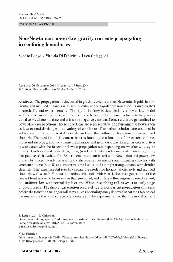
Consider a non-Newtonian liquid with rheology parameterised by an Ostwald-de Waelepower-law relating the shear stress and the shear rate τ = μ̃γ̇ |γ̇ |n−1, where τ is the shearstress, μ̃ the consistency index, n the fluid behaviour index, and γ̇ the shear rate. A liquid ofuniform density, ρ, is injected into a rectilinear channel of fixed cross-section inclined at anangle β with the horizontal, and moves in an ambient fluid of negligible mass density (due tothe large density difference between the current and the ambient fluid). The channel geometryis shown in Fig. 1, with the x, y, and z orthogonal axes oriented along the channel axis, acrossthe channel, and normal to the slope, respectively. The cross-section of the channel, with aboundary described by the function d(y), is partly occupied by the current, which has a topwidth of 2W (x, t) and a height h(x, t) that is invariant in the span-wise direction. We assumethat buoyancy and viscous forces are balanced with negligible inertial effects and that themotion is quasi-stationary and can be described by continuity and momentum balance withnull acceleration. Assuming that the streamlines are parallel to the bottom of the channel andneglecting the effects of surface tension, the pressure in the liquid is hydrostatic and givenby

p = p0 + ρg(h − z) cosβ, (1)

where p0 is the atmospheric pressure at the free surface and g is the gravitational acceleration.We also assume that the extent of the flow, xN (t), is much larger than both h and W . Hence,the motion is taken to be unidimensional along the x-axis and is described by a single velocitycomponent u(x, y, z, t). Under these hypotheses, the Stokes equation reduces to

− ∂p

∂x+ ρ fx + ∂τyx

∂y+ ∂τzx

∂z= 0, (2)

where ρ fx is the volume force in the x-direction and τyx , τzx are the shear stresses. We alsoconsider wide cross-sections with h � W , allowing one to neglect ∂τyx/∂y with respectto ∂τzx/∂z. Under this hypothesis, substitution of the expression for the shear stress of apower-law fluid into Eq. (2) yields

∂

∂z

[(

∂u

∂z

)n]

= −S, (3)

Fig. 1 A sketch of the current in the x–z and y– z planes

123

Environ Fluid Mech

where the assumption ∂u/∂z > 0 holds and the source term S, dependent on the channelinclination angle β, is given by

S = −ρg

μ̃

∂h

∂x(β = 0), S = ρg

μ̃sin β (β �= 0). (4)

Equation (4) indicates that for a horizontal channel, the motion is induced by the slopeof the free surface, while for an inclined channel, it is assumed that the current is locally inequilibrium, with gravity acting proportionally to the slope. The latter condition also requiresthat tan β � ∂h/∂x and excludes the possibility that the effect of the free-surface slope iscomparable with that of the channel slope. The dynamic boundary condition at the free surfacerequires the continuity of the shear stress in the liquid and in the ambient fluid, which can beapproximated by zero. The no-slip condition holds at the fixed boundary. Hence, Eq. (3) canbe integrated by imposing

u|z=d = 0,∂u

∂z

∣

∣

∣

∣

z=h= 0, (5)

such that we obtain

u(x, y, z, t) = S1/n n

n + 1

[

(h − d)(n+1)/n − (h − z)(n+1)/n]

. (6)

The local continuity equation for a one-dimensional current is

∂A

∂t+ ∂Q

∂x= 0, (7)

where A is the cross-sectional area occupied by the liquid, given in the symmetric case by

A(x, t) = 2

W (x,t)∫

0

[h(x, t)− d(y)] dy, (8)

and Q is the downstream volume flux obtained by integrating the velocity over the cross-sectional area. Substituting Eq. (8) into Eq. (7) yields

2W∂h

∂t+ ∂Q

∂x= 0. (9)

The global continuity equation yields

xN (t)∫

0

A dx = qtα, (10)

where q > 0 and α ≥ 0 are constants and qtα is the volume of liquid released. The caseα = 0 corresponds to instantaneous injection of a constant volume and α = 1 correspondsto constant volume flux. At the front end of the current, the boundary condition of vanishingheight

h [xN (t), t] = 0 (11)

completes the mathematical statement of the problem for horizontal channels. However,Eq. (11) cannot be satisfied for inclined channels as the order of the differential equation islower due to the assumptions made in Eq. (4). For the inclined case this produces a profileending abruptly at the head of the current, as noted by Huppert [23].

123

Environ Fluid Mech

2.1 Semicircular cross-section

For a semicircular cross-section of radius r , the boundary is given by d = r − (r2 − y2)1/2

and the current half-width by W = (2rh)1/2[1 − (1/2)h/r ]1/2. Assuming that the currentis thin compared to the radius, i.e., h � r , it follows that the approximations d ≈ y2/(2r),W ≈ (2rh)1/2, and A ≈ 4/3(2rh3)1/2 hold. The relative error in the approximation of thewidth is O (h/r); for h/r = 0.1 and h/r = 0.5 the relative error is equal to 2.6 and 15.5 %,respectively. By integrating Eq. (6), the volume flux is obtained as

Q(x, t) = 2

W (x,t)∫

0

dy

h(x,t)∫

d(y)

udz = h5/2+1/n√r S1/n Kc(n), (12)

where

Kc(n) =√

2π Γ (2 + 1/n)

Γ (7/2 + 1/n), (13)

where Kc(n) is a numerical factor andΓ (·) is the gamma function. Substituting the expressionfor the cross-sectional area into Eq. (10) yields

4

3

√2r

xN (t)∫

0

h3/2dx = qtα. (14)

2.1.1 The case β = 0 for a semicircular cross-section

For a horizontal channel with inclination angle β = 0, Eq. (9) yields

h1/2 ∂h

∂t−

√2

4Kc

(

ρg

μ̃

)1/n∂

∂x

(

h5/2+1/n∣

∣

∣

∣

∂h

∂x

∣

∣

∣

∣

1/n−1∂h

∂x

)

= 0. (15)

Introducing the length and time scales

x∗ =(

q√r

)2n/(2α+5n) (μ̃

ρg

)2α/(2α+5n)

, (16)

t∗ =(

q√r

)−2/(2α+5n) (μ̃

ρg

)5/(2α+5n)

, (17)

Equations (15) and (14) become

H1/2 ∂H

∂T−

√2

4Kc

∂

∂X

(

H5/2+1/n∣

∣

∣

∣

∂H

∂X

∣

∣

∣

∣

1/n−1∂H

∂X

)

= 0, (18)

X N (T )∫

0

H3/2 dX = 3√

2

8T α, (19)

respectively, and the boundary condition (11) is given by

H [X N (T ), T ] = 0, (20)

123

Environ Fluid Mech

where H = h/x∗, X = x/x∗ and T = t/t∗ are nondimensional variables. The similaritysolution of Eqs. (18) and (19) is expressed in terms of the similarity variable

η =(

2√

2

Kc

)n/(n+1)

XT −F1c , F1c = 2α(n + 2)+ 3n

5n + 7(21)

and the solution form

H(X, T ) = η(n+1)/(n+2)N T F2cψ(ζ ), ζ = η

ηN, F2c = F1c(n + 1)− n

n + 2, (22)

where ηN is the value of η at the current edge X N , and the shape function, ψ , is the solutionof the nonlinear ordinary differential equation

(

ψ5/2+1/n∣

∣ψ ′∣∣

1/n−1ψ ′)′ − F2cψ

3/2 + F1cζψ1/2ψ ′ = 0, ψ(1) = 0, (23)

in which the prime indicates d/dζ . The value of ηN is obtained from Eq. (19), which trans-forms into

ηN =⎡

⎣

4√

2

3

(

Kc√

2

4

)n/(n+1) 1∫

0

ψ3/2dζ

⎤

⎦

−F3c

, F3c = 2(n + 2)

5n + 7. (24)

In Eqs. (21)–(24), the factors F1c, F2c, and F3c take different values depending on thefluid rheology. For α = 0, Eqs. (23) and (24) admit the following analytical solutions:

ψ =(

n + 2

n + 1

)1/(n+2) (2F1c

3

)n/(n+2)

(1 − ζ n+1)1/(n+2), (25)

ηN =(

3√

2

8

)F3c(

2√

2

Kc

)

nF3cn+1 (

n + 1

n + 2

)

3F3c2(n+2)

(

3

2F1c

)

3nF3c2(n+2)

×⎡

⎣

Γ[

1 + 11+n + 3

2(2+n)

]

Γ(

1 + 11+n

)

Γ[

1 + 32(2+n)

]

⎤

⎦

F3c

, (26)

which, for n = 1, are equivalent to the expressions given by Takagi and Huppert [20]. Forα �= 0, Eq. (23) must be integrated numerically. To do so, a second boundary condition isobtained by generating an asymptotic solution near the current front in terms of a powerseries [4], to yield

ψ ′(ζ → 1) = −a0b(1 − ζ )b−1, a0 =(

2F1c

3b1/n

)nb

, b = 1

n + 2. (27)

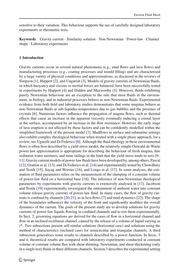
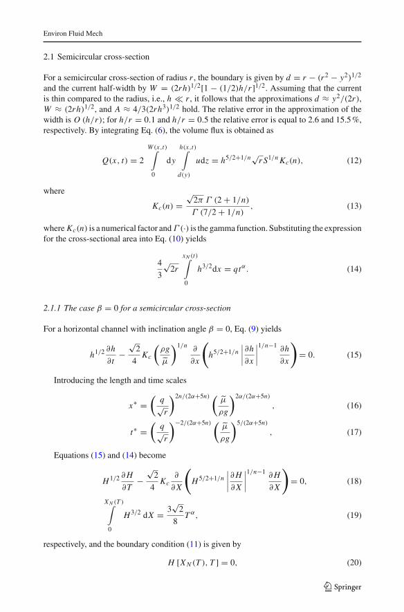
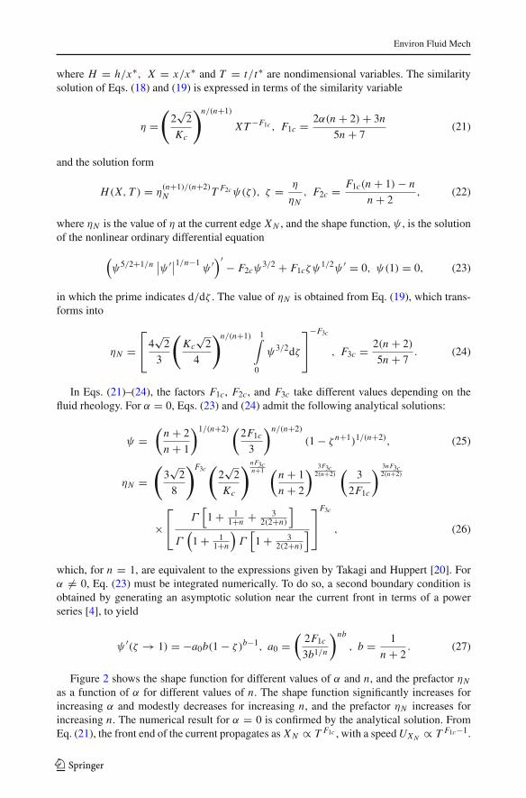
Figure 2 shows the shape function for different values of α and n, and the prefactor ηN

as a function of α for different values of n. The shape function significantly increases forincreasing α and modestly decreases for increasing n, and the prefactor ηN increases forincreasing n. The numerical result for α = 0 is confirmed by the analytical solution. FromEq. (21), the front end of the current propagates as X N ∝ T F1c , with a speed UX N ∝ T F1c−1.

123

Environ Fluid Mech

Fig. 2 Left panel shape functions for semicircular horizontal channel sections for n = 0.5 (dashed line),n = 1.0 (solid line), and n = 1.5 (dotted line). The thick dotted line represents the analytical solution forn = 1.0. Right panel the prefactor ηN as a function of α for n = 0.5 (dashed line), n = 1.0 (solid line), andn = 1.5 (dotted line). For n = 1.0 and α = 0 the analytical solution ηN = 2.9021 is reproduced

2.1.2 The case β > 0 for a semicircular cross-section

For an inclined channel with β > 0, Eq. (9) becomes

∂h

∂t+ Kc

√2

4

(

ρg

μ̃

)1/n(5n + 2)

2n(sin β)1/n h1+1/n ∂h

∂x= 0, (28)

where the factor Kc is given by Eq. (13). The dimensionless form of Eq. (28) is

∂H

∂T+ Kc

√2

4

(5n + 2)

2n(sin β)1/n H1+1/n ∂H

∂X= 0, (29)

while Eq. (19) is unchanged. The function H is constant along the characteristics given by

dX

dT= gc(n)H

1+1/n, gc(n) = Kc√

2

4

(5n + 2)

2n(sin β)1/n (30)

and admits the solutionH = g−n/(n+1)

c Xn/(n+1)T −n/(n+1). (31)

Eq. (31) represents a profile abruptly ending at X N , which can be smoothed by includingsurface tension [23]. The condition X N = 0 for T = 0, implicit in Eq. (31), can be changedto X N > 0 for T = 0 by introducing a time shift equivalent to a virtual origin; this is a localeffect without significant consequences for the current profile in the asymptotic regime. Notethat no further boundary conditions are required. Upon substitution of Eq. (31), the constraintrepresented by Eq. (19) gives the length of the current as

X N =(

3√

2

8

)2(n+1)5n+2

g3n

5n+2c

[

5n + 2

2(n + 1)

]2(n+1)5n+2

T2α(n+1)+3n

5n+2 (32)

with the front end advancing with a speed UX N ∝ T 2(α−1)(n+1)/(5n+2). The current accel-erates (decelerates) for α > 1 (α < 1). For α = 0 and n = 1, the expressions given indimensional form by Takagi and Huppert [20] are recovered.

For α = 1, the volume flux, Q, is constant with Q ≡ q , the maximum height of thecurrent at X = X N is equal to

HX N =[

2(n + 1)

3nKc(sin β)1/n

]−2n/(5n+2)

, (33)

123

Environ Fluid Mech

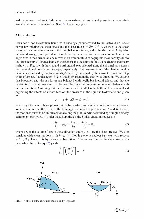
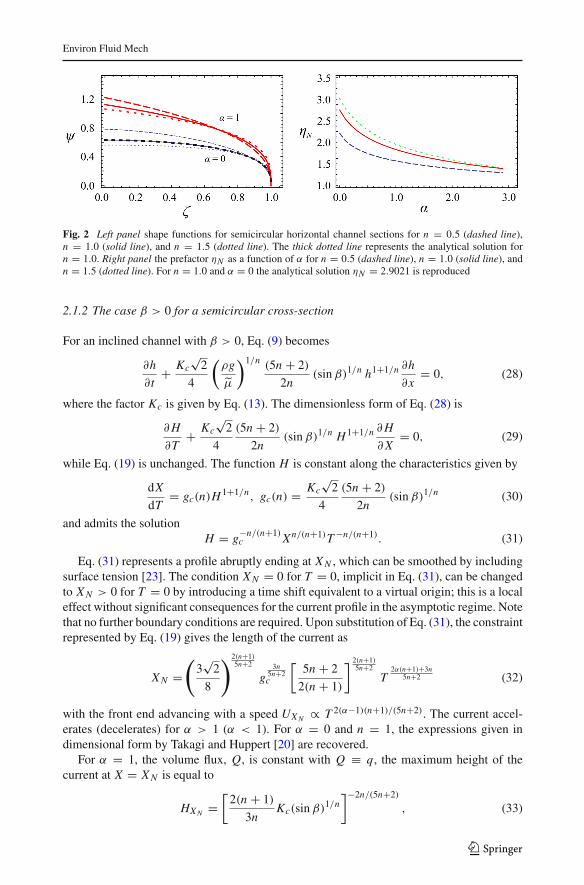
Fig. 3 The nondimensionalprofile of the gravity current in asemicircular inclined channel(bold line) with α = 1.0,n = 1.0, and Fr = 0.11. Thedashed line is the normal depthand the dash-dotted line is thecritical depth

and the front end advances with a constant speed. The depth predicted by Eq. (33) may becompared with the normal and critical depths of the channel for the same volume flux. Thenormal depth is derived by balancing the gravitational force and tangential stress such that

hn =[

μ̃1/n Q√r Kc(ρg sin β)1/n

]2n/(5n+2)

, (34)

yielding, in nondimensional form,

Hn = [

Kc(sin β)1/n]−2n/(5n+2). (35)

The critical depth, where energy is at a minimum for a given volume flux, is equal to

hc =(

27χQ2

64gr

)1/4

, (36)

where χ is the Coriolis coefficient.A comparison between the maximum depth at the current front calculated with the present

model, as given by Eq. (33), and the normal depth yields HX N > Hn, HX N = Hn , orHX N < Hn , depending on whether n > 2, n = 2, or n < 2.

The global Reynolds and Froude numbers of the current are computed for inclined channels(β > 0) and constant volume flux (α = 1) as

Re = 8ρU 2n

μ̃

[√2rhn

2Un

]n

, Fr = Un√

2ghn cosβ3χ

, (37)

where Un is the normal velocity. Figure 3 shows the nondimensional profile of the currentfor n = 1.0 and Fr = 0.11. Similar results are obtained for other values of n (but are notshown here).

2.2 Triangular cross-section

The velocity distribution for laminar flow in a V-shaped cross-section with vertex angle 2θcannot be computed by assuming ∂τzx/∂z � ∂τyx/∂y in the Stokes equation (2) for generalvalues of θ , but only for 2θ � 90◦. For Newtonian liquids, Takagi and Huppert [20] adopteda coordinate transformation and found a solution for the velocity field in terms of an infinitesummation of orthogonal cosine functions, deriving by integration an expression for thevolume flux in the form

Q ≈ 0.137m3

1 + m2 h4S, (38)

123

Environ Fluid Mech

where m = tan θ and S is the source term defined by Eq. (4). For a power-law liquid, asimilar approach cannot be followed due to nonlinearity. Hence we resort to an empiricalapproach and employ the experimental results of Burger et al. [11]. They investigated theflow of various non-Newtonian liquids in open channels of different cross-sectional shapesand expressed the relationship between the Fanning friction factor, f , and the generalisedReynolds number, ReH , in fully developed laminar flow through the use of a shape factorcoefficient (the theoretical formulation given by Muzychka and Edge [24] yields similarresults). For a power-law liquid flowing in a right triangular section with 2θ = 90◦, theirexperiments yielded

f = 14.6/ReH , (39)

with

f = 2gR sin β

U 2 , ReH = 8ρU 2

μ̃

(

R

2U

)n

, (40)

where U = Q/A and R is the hydraulic radius. Hence, by substituting the expressions givenfor f and ReH in Eq. (40) into Eq. (39) we obtain

Q = Kt (n,m)h(3n+1)/n S1/n, Kt (n,m) = 2(3−2n)/n m(2n+1)/n

(1 + m2)(n+1)/(2n)

(

1

14.6

)1/n

, (41)

where Kt (n,m) is a coefficient incorporating the shape of the cross-section and the fluidrheology. For n = 1, Kt is approximately equal to the value 0.137 given in Eq. (38). Eq. (41)is thus strictly valid only for 2θ = 90◦. For other values of the vertex angle, 2θ , a factor solelydependent on channel shape and with a numerical value different from 14.6 will appear in theexpression for the friction factor given by Eq. (39); this numerical factor must be determinedwith independent experiments similar to those of Burger et al. [11]. This will, in turn, changethe numerical value of the coefficient Kt (n,m) given by Eq. (41), but not its dependence onm and n. Hence. in the following theoretical derivations Kt (n,m) is assumed to be known,regardless of its actual value.

2.2.1 The case β = 0 for a triangular cross-section

For a horizontal channel (β = 0), substituting Eq. (41) into Eq. (9) with W = mh yields

h∂h

∂t− Kt

2m

(

ρg

μ̃

)1/n∂

∂x

(

h(3n+1)/n∣

∣

∣

∣

∂h

∂x

∣

∣

∣

∣

1/n−1∂h

∂x

)

= 0, (42)

while Eq. (10) becomes

m

xN (t)∫

0

h2dx = qtα, (43)

because A = mh2 and the boundary condition given by Eq. (11) holds. Introducing the lengthand time scales

x∗ =( q

m

)n/(α+3n)(

μ̃

ρg

)α/(α+3n)

, (44)

t∗ =( q

m

)−1/(α+3n)(

μ̃

ρg

)3/(α+3n)

, (45)

123

Environ Fluid Mech

Equations (42) and (43) become, in dimensionless form,

H∂H

∂T− Kt

2m

∂

∂X

(

H (3n+1)/n∣

∣

∣

∣

∂H

∂X

∣

∣

∣

∣

1/n−1∂H

∂X

)

= 0, (46)

X N (T )∫

0

H2dX = T α, (47)

and the boundary condition is again given by Eq. (20). The similarity variable and the solutionform of the problem described by Eqs. (46) and (47), with Eq. (20), are given by

η =(

2m

Kt

)n/(n+1)

XT −F1t , F1t = α(n + 2)+ 2n

3n + 4, (48)

H(X, T ) = η(n+1)/(n+2)N T F2tψ(ζ ), ζ = η

ηN, F2t = α(n + 1)+ n

3n + 4, (49)

where the shape function, ψ , is obtained by solving the differential equation

(

ψ(3n+1)/n∣

∣ψ ′∣∣

1/n−1ψ ′)′ − F2tψ

2 + F1tζψψ′ = 0, ψ(1) = 0, (50)

and the prefactor is given by

ηN =⎡

⎣

(

Kt

2m

)n/(n+1) 1∫

0

ψ2dζ

⎤

⎦

−F3t

, F3t = n + 2

3n + 4. (51)

In Eqs. (48)–(51), the factors F1t , F2t , and F3t depend solely on fluid rheology. For α = 0,a closed form solution is derived as

ψ =(

n

3n + 4

)n/(n+2) (n + 2

n + 1

)1/(n+2)(

1 − ζ n+1)1/(n+2), (52)

ηN =(

2m

Kt

)nF3t/(n+1) (3n + 4

n

)2nF3t/(n+2) (n + 1

n + 2

)2F3t/(n+2)

×[

2 F1

(

1

1 + n,− 2

2 + n,

2 + n

1 + n, 1

)]−F3t

, (53)

where 2 F1 is the hypergeometric function. For the case n = 1, Eq. (53) is equivalent tothe solution reported in dimensional form by [20]. For α �= 0, the numerical integration ofEq. (50) requires a second boundary condition near the current front, obtained similarly toEq. (27) as

ψ ′(ζ → 1) = −a0b(1 − ζ )b−1, a0 =(

nF1t b(n−1)/n

b(3n + 2)− 1

)nb

, b = 1

n + 2. (54)

Numerical values of the shape function and the prefactor ηN for different values of α andn are similar to the semicircular case. The front end of the current propagates as X N ∝ T F1t

and advances with a speed UX N ∝ T F1t −1.

123

Environ Fluid Mech

2.2.2 The case β > 0 for a triangular cross-section

In an inclined triangular channel with β > 0, Eq. (9) becomes

∂h

∂t+ Kt

2m

(

ρg

μ̃

)1/n(3n + 1)

n(sin β)1/n h(n+1)/n ∂h

∂x= 0, (55)

and Eq. (43) is unchanged. In nondimensional form, Eq. (55) is

∂H

∂T+ Kt

2m

(3n + 1)

n(sin β)1/n H (n+1)/n ∂H

∂X= 0, (56)

while Eq. (20) still holds. The solution is obtained with the method of characteristics as

H = g−n/(n+1)t Xn/(n+1)T −n/(n+1), gt = Kt

2m

(3n + 1)

n(sin β)1/n , (57)

and the length of the current is given by

X N =(

3n + 1

n + 1

)(n+1)/(3n+1)

g2n/(3n+1)t T

α(n+1)+2n3n+1 , (58)

with the front end advancing with a speed UX N ∝ T (α−1)(n+1)/(3n+1). For α = 1 (constantvolume flux), the maximum height of the current at X = X N is equal to

HX N =(

n + 1

2n

Kt

msin β1/n

)−n/(3n+1)

, (59)

and the front end advances with constant speed. For α = 0 and n = 1, the solution givenby Takagi and Huppert [20] is recovered. The normal depth is given in dimensional andnondimensional form by

hn =[

μ̃1/n Q

Kt (ρg sin β)1/n

]n/(3n+1)

, Hn =[

Kt

m(sin β)1/n

]−n/(3n+1)

, (60)

and the critical depth is

hc =(

2χQ2

gm2

)1/5

. (61)

The Reynolds and Froude numbers of the current are computed for constant volume flux(α = 1) as

Re = 8ρU 2n

μ̃

[

mhn

4Un(1 + m2)

]n

, Fr = Un√

2ghn cosβ2χ

. (62)

Hence, HX N > Hn, HX N = Hn , or HX N < Hn depending on whether n < 1, n = 1, orn > 1.

2.3 A generalisation for power-law channels

The previous results can be suitably generalised upon describing the cross-section with ageneral power-law relationship d = a |y/a|k , where a is a length scale and k is a prescribedconstant: k = 1, k = 2, and k → ∞ correspond to triangular, semicircular, and infinitelywide rectangular sections, respectively. For k > 1, the current depth is much smaller than itswidth and ∂τzx/∂z � ∂τyx/∂y, as earlier hypothesised for semicircular sections. By using

123

Environ Fluid Mech

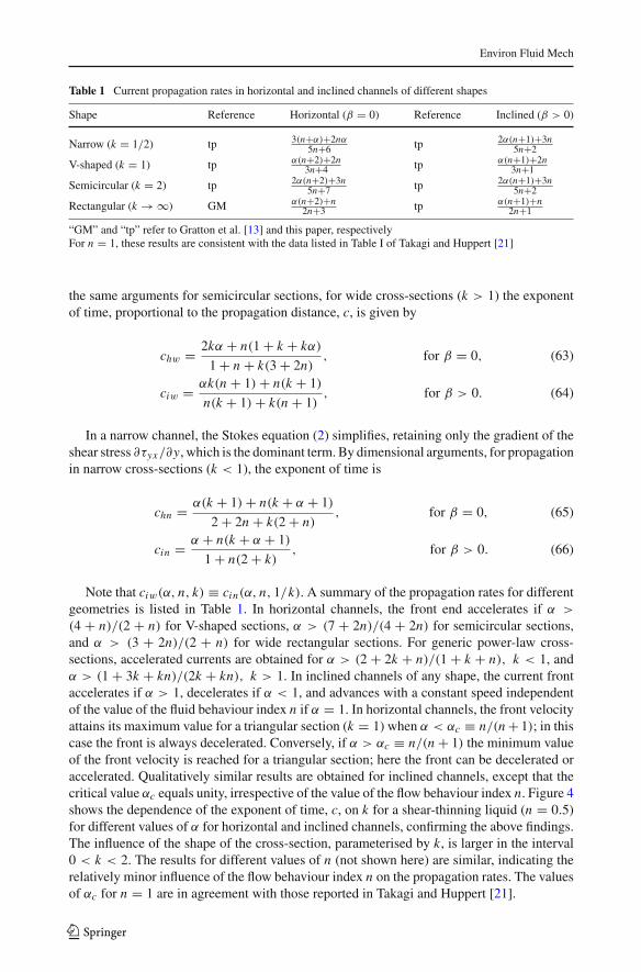
Table 1 Current propagation rates in horizontal and inclined channels of different shapes

Shape Reference Horizontal (β = 0) Reference Inclined (β > 0)

Narrow (k = 1/2) tp 3(n+α)+2nα5n+6 tp 2α(n+1)+3n

5n+2

V-shaped (k = 1) tp α(n+2)+2n3n+4 tp α(n+1)+2n

3n+1

Semicircular (k = 2) tp 2α(n+2)+3n5n+7 tp 2α(n+1)+3n

5n+2

Rectangular (k → ∞) GM α(n+2)+n2n+3 tp α(n+1)+n

2n+1

“GM” and “tp” refer to Gratton et al. [13] and this paper, respectivelyFor n = 1, these results are consistent with the data listed in Table I of Takagi and Huppert [21]

the same arguments for semicircular sections, for wide cross-sections (k > 1) the exponentof time, proportional to the propagation distance, c, is given by

chw = 2kα + n(1 + k + kα)

1 + n + k(3 + 2n), for β = 0, (63)

ciw = αk(n + 1)+ n(k + 1)

n(k + 1)+ k(n + 1), for β > 0. (64)

In a narrow channel, the Stokes equation (2) simplifies, retaining only the gradient of theshear stress ∂τyx/∂y, which is the dominant term. By dimensional arguments, for propagationin narrow cross-sections (k < 1), the exponent of time is

chn = α(k + 1)+ n(k + α + 1)

2 + 2n + k(2 + n), for β = 0, (65)

cin = α + n(k + α + 1)

1 + n(2 + k), for β > 0. (66)

Note that ciw(α, n, k) ≡ cin(α, n, 1/k). A summary of the propagation rates for differentgeometries is listed in Table 1. In horizontal channels, the front end accelerates if α >

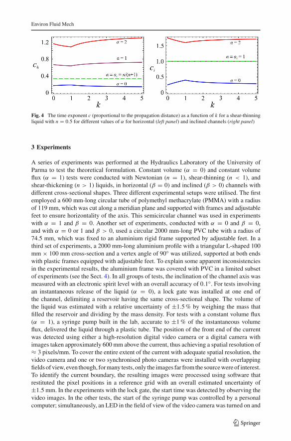
(4 + n)/(2 + n) for V-shaped sections, α > (7 + 2n)/(4 + 2n) for semicircular sections,and α > (3 + 2n)/(2 + n) for wide rectangular sections. For generic power-law cross-sections, accelerated currents are obtained for α > (2 + 2k + n)/(1 + k + n), k < 1, andα > (1 + 3k + kn)/(2k + kn), k > 1. In inclined channels of any shape, the current frontaccelerates if α > 1, decelerates if α < 1, and advances with a constant speed independentof the value of the fluid behaviour index n if α = 1. In horizontal channels, the front velocityattains its maximum value for a triangular section (k = 1) when α < αc ≡ n/(n + 1); in thiscase the front is always decelerated. Conversely, if α > αc ≡ n/(n + 1) the minimum valueof the front velocity is reached for a triangular section; here the front can be decelerated oraccelerated. Qualitatively similar results are obtained for inclined channels, except that thecritical value αc equals unity, irrespective of the value of the flow behaviour index n. Figure 4shows the dependence of the exponent of time, c, on k for a shear-thinning liquid (n = 0.5)for different values of α for horizontal and inclined channels, confirming the above findings.The influence of the shape of the cross-section, parameterised by k, is larger in the interval0 < k < 2. The results for different values of n (not shown here) are similar, indicating therelatively minor influence of the flow behaviour index n on the propagation rates. The valuesof αc for n = 1 are in agreement with those reported in Takagi and Huppert [21].

123

Environ Fluid Mech

Fig. 4 The time exponent c (proportional to the propagation distance) as a function of k for a shear-thinningliquid with n = 0.5 for different values of α for horizontal (left panel) and inclined channels (right panel)

3 Experiments

A series of experiments was performed at the Hydraulics Laboratory of the University ofParma to test the theoretical formulation. Constant volume (α = 0) and constant volumeflux (α = 1) tests were conducted with Newtonian (n = 1), shear-thinning (n < 1), andshear-thickening (n > 1) liquids, in horizontal (β = 0) and inclined (β > 0) channels withdifferent cross-sectional shapes. Three different experimental setups were utilised. The firstemployed a 600 mm-long circular tube of polymethyl methacrylate (PMMA) with a radiusof 119 mm, which was cut along a meridian plane and supported with frames and adjustablefeet to ensure horizontality of the axis. This semicircular channel was used in experimentswith α = 1 and β = 0. Another set of experiments, conducted with α = 0 and β = 0,and with α = 0 or 1 and β > 0, used a circular 2000 mm-long PVC tube with a radius of74.5 mm, which was fixed to an aluminium rigid frame supported by adjustable feet. In athird set of experiments, a 2000 mm-long aluminium profile with a triangular L-shaped 100mm × 100 mm cross-section and a vertex angle of 90◦ was utilized, supported at both endswith plastic frames equipped with adjustable feet. To explain some apparent inconsistenciesin the experimental results, the aluminium frame was covered with PVC in a limited subsetof experiments (see the Sect. 4). In all groups of tests, the inclination of the channel axis wasmeasured with an electronic spirit level with an overall accuracy of 0.1◦. For tests involvingan instantaneous release of the liquid (α = 0), a lock gate was installed at one end ofthe channel, delimiting a reservoir having the same cross-sectional shape. The volume ofthe liquid was estimated with a relative uncertainty of ±1.5 % by weighing the mass thatfilled the reservoir and dividing by the mass density. For tests with a constant volume flux(α = 1), a syringe pump built in the lab, accurate to ±1 % of the instantaneous volumeflux, delivered the liquid through a plastic tube. The position of the front end of the currentwas detected using either a high-resolution digital video camera or a digital camera withimages taken approximately 600 mm above the current, thus achieving a spatial resolution of≈ 3 pixels/mm. To cover the entire extent of the current with adequate spatial resolution, thevideo camera and one or two synchronised photo cameras were installed with overlappingfields of view, even though, for many tests, only the images far from the source were of interest.To identify the current boundary, the resulting images were processed using software thatrestituted the pixel positions in a reference grid with an overall estimated uncertainty of±1.5 mm. In the experiments with the lock gate, the start time was detected by observing thevideo images. In the other tests, the start of the syringe pump was controlled by a personalcomputer; simultaneously, an LED in the field of view of the video camera was turned on and

123

Environ Fluid Mech

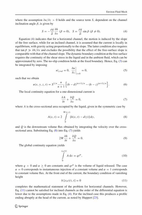
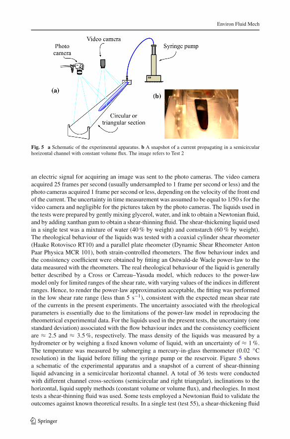
Fig. 5 a Schematic of the experimental apparatus. b A snapshot of a current propagating in a semicircularhorizontal channel with constant volume flux. The image refers to Test 2

an electric signal for acquiring an image was sent to the photo cameras. The video cameraacquired 25 frames per second (usually undersampled to 1 frame per second or less) and thephoto cameras acquired 1 frame per second or less, depending on the velocity of the front endof the current. The uncertainty in time measurement was assumed to be equal to 1/50 s for thevideo camera and negligible for the pictures taken by the photo cameras. The liquids used inthe tests were prepared by gently mixing glycerol, water, and ink to obtain a Newtonian fluid,and by adding xanthan gum to obtain a shear-thinning fluid. The shear-thickening liquid usedin a single test was a mixture of water (40 % by weight) and cornstarch (60 % by weight).The rheological behaviour of the liquids was tested with a coaxial cylinder shear rheometer(Haake Rotovisco RT10) and a parallel plate rheometer (Dynamic Shear Rheometer AntonPaar Physica MCR 101), both strain-controlled rheometers. The flow behaviour index andthe consistency coefficient were obtained by fitting an Ostwald-de Waele power-law to thedata measured with the rheometers. The real rheological behaviour of the liquid is generallybetter described by a Cross or Carreau–Yasuda model, which reduces to the power-lawmodel only for limited ranges of the shear rate, with varying values of the indices in differentranges. Hence, to render the power-law approximation acceptable, the fitting was performedin the low shear rate range (less than 5 s−1), consistent with the expected mean shear rateof the currents in the present experiments. The uncertainty associated with the rheologicalparameters is essentially due to the limitations of the power-law model in reproducing therheometrical experimental data. For the liquids used in the present tests, the uncertainty (onestandard deviation) associated with the flow behaviour index and the consistency coefficientare ≈ 2.5 and ≈ 3.5 %, respectively. The mass density of the liquids was measured by ahydrometer or by weighing a fixed known volume of liquid, with an uncertainty of ≈ 1 %.The temperature was measured by submerging a mercury-in-glass thermometer (0.02 ◦Cresolution) in the liquid before filling the syringe pump or the reservoir. Figure 5 showsa schematic of the experimental apparatus and a snapshot of a current of shear-thinningliquid advancing in a semicircular horizontal channel. A total of 36 tests were conductedwith different channel cross-sections (semicircular and right triangular), inclinations to thehorizontal, liquid supply methods (constant volume or volume flux), and rheologies. In mosttests a shear-thinning fluid was used. Some tests employed a Newtonian fluid to validate theoutcomes against known theoretical results. In a single test (test 55), a shear-thickening fluid

123

Environ Fluid Mech

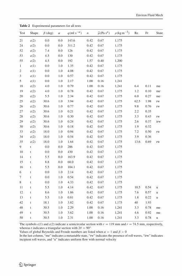
was utilised. The experimental parameters are reported in Table 2, including: test number;channel inclination; type of test (α = 0 or 1 for constant volume or volume flux); injectedvolume or volume flux; flow behaviour index and consistency coefficient; fluid density; globalReynolds and Froude numbers for tests conducted with constant volume flux (α = 1) in aninclined channel (β > 0); and the state of the current.

We note that the highest observed value of the Reynolds number is Re = 60; this ensuresthat the Stokes flow approximation is correct, because the gradual transition from laminarto fully turbulent flow is expected to begin for Re > 500. In only two tests (25 and 42),the equivalent uniform flow in the channel is supercritical with a Froude number greaterthan unity (or, equivalently, with a normal depth less than the critical depth) and with themaximum height of the predicted profile smaller than the normal and critical depths. For thetests with Fr < 1, the maximum height of the predicted profile is between the critical depthand the normal depth. A time shift equivalent to a virtual origin was introduced to interpretthe experimental data for the inclined channel and the constant volume subcase (α = 0) forthe horizontal channel. In the latter case, the correction was needed to account for the finitesize of the reservoir and the finite time needed to open the gate.

4 Discussion

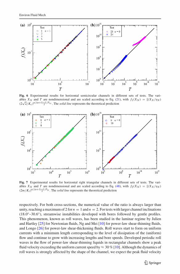
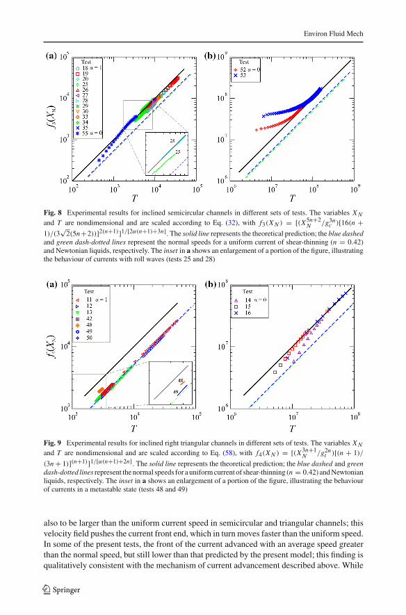
The scaled, nondimensional results for current front position as a function of time are depictedin Fig. 6 for horizontal channels with semicircular cross-sections, and in Fig. 7 for horizontalchannels with right triangular cross-sections. Figures 8 and 9 show the corresponding resultsfor inclined channels. Each Figure is split into two panels (a) and (b), each covering a differentrange of abscissa and ordinate values. The different factors used for the scaling of X N inthe four Figures are expressed as fi (X N ), i = 1, 2, 3, 4. Figures 8 and 9, valid for inclinedchannels, depict two additional reference lines representing the normal speed of uniformcurrents of shear-thinning (n = 0.42) and Newtonian liquids. The inset in panel (a) of eachFigure represents an enlargement of a portion of the panel.

For horizontal channels, the experimental results (symbols) are in good agreement withthe theoretical predictions (solid lines) for constant volume flux (α = 1) and constant volume(α = 0). In the latter case, only the late time evolution of the current is consistent with thetheory, while at early times the time exponent for the front end position differs from thesimilarity solution. This is because the current, after the slumping phase, is initially in aninertial-buoyancy regime, where buoyancy forces are balanced by inertia. The transition to aviscous-buoyancy regime takes longer for constant volume (α = 0) than for constant volumeflux (α = 1) currents, as also noted by Sayag and Worster [16] for an axisymmetric geometry.For inclined channels, good agreement with the theory at late times was again observed intests with α = 0. In tests with α = 1, the speed of the front was generally lower than thetheoretical prediction, and different flow regimes were observed. In some tests conducted intriangular channels with small inclinations (up to 8.6◦), the flow was stable, but the front ofthe current advanced with a constant speed lower than UX N predicted by Eq. (58) and equalto the mean velocity Un in a channel with normal depth. The latter is significantly lower thanthe former, as shown by their ratio, which is given for semicircular and triangular channels by

UX N

Un= (2 + 5n) [2(n + 1)]−2(n+1)/(2+5n) (3n)−3n/(2+5n) (67)

UX N

Un= (1 + 3n)(n + 1)−(n+1)/(1+3n)(2n)−2n/(1+3n), (68)

123

Environ Fluid Mech

Table 2 Experimental parameters for all tests

Test Shape β (deg) α q(ml s−α) n μ̃(Pa sn ) ρ(kg m−3) Re Fr State

21 c(2) 0.0 0.0 143.6 0.42 0.67 1,175

24 c(2) 0.0 0.0 311.2 0.42 0.67 1,175

52 c(2) 7.4 0.0 126 0.42 0.67 1,175

53 c(2) 4.5 0.0 130 0.42 0.67 1,175

55 c(2) 4.5 0.0 192 1.57 0.40 1,200

1 c(1) 0.0 1.0 1.35 0.42 0.67 1,175

2 c(1) 0.0 1.0 4.08 0.42 0.67 1,175

3 c(1) 0.0 1.0 0.57 0.42 0.67 1,175

5 c(1) 0.0 1.0 2.17 1.00 0.16 1,241

18 c(2) 4.0 1.0 0.79 1.00 0.16 1,241 6.4 0.11 me

19 c(2) 4.0 1.0 0.78 0.42 0.67 1,175 1.2 0.10 me

20 c(2) 5.5 1.0 2.34 0.42 0.67 1,175 6.0 0.27 me

25 c(2) 30.6 1.0 3.94 0.42 0.67 1,175 62.5 1.98 rw

26 c(2) 30.6 1.0 0.77 0.42 0.67 1,175 9.8 0.76 rw

27 c(2) 30.6 1.0 0.21 0.42 0.67 1,175 2.2 0.35

28 c(2) 30.6 1.0 0.30 0.42 0.67 1,175 3.3 0.43 rw

29 c(2) 30.6 1.0 0.24 0.42 0.67 1,175 2.6 0.37 irw

30 c(2) 30.6 1.0 0.18 0.42 0.67 1,175 1.9 0.32

33 c(2) 18.0 1.0 0.94 0.42 0.67 1,175 7.2 0.50 rw

34 c(2) 18.0 1.0 0.54 0.42 0.67 1,175 3.9 0.36

35 c(2) 18.0 1.0 1.64 0.42 0.67 1,175 13.6 0.69 rw

9 t 0.0 0.0 286 0.42 0.67 1,175

10 t 0.0 0.0 430 0.42 0.67 1,175

14 t 5.5 0.0 163.9 0.42 0.67 1,175

15 t 8.8 0.0 68.0 0.42 0.67 1,175

16 t 5.5 0.0 104.1 0.42 0.67 1,175

6 t 0.0 1.0 2.14 0.42 0.67 1,175

7 t 0.0 1.0 0.54 0.42 0.67 1,175

8 t 0.0 1.0 4.33 0.42 0.67 1,175

11 t 5.5 1.0 4.14 0.42 0.67 1,175 10.5 0.54 u

12 t 8.6 1.0 1.86 0.42 0.67 1,175 7.6 0.57 u

13 t 5.5 1.0 0.81 0.42 0.67 1,175 1.8 0.22 u

42 t 18.1 1.0 3.82 0.42 0.67 1,175 40 1.93

48 t 30.5 1.0 2.29 1.00 0.16 1,241 3.3 0.78 me

49 t 30.5 1.0 3.62 1.00 0.16 1,241 4.6 0.92 me

50 t 30.5 1.0 2.31 1.00 0.16 1,241 3.3 0.78 u

The symbols c(1) and c(2) indicate a semicircular section with r = 119 mm and r = 74.5 mm, respectively,whereas t indicates a triangular section with 2θ = 90◦Values of global Reynolds and Froude numbers are listed when α = 1 and β > 0In the last column, “me” indicates a metastable state, “rw” indicates the presence of roll waves, “irw” indicatesincipient roll waves, and “u” indicates uniform flow with normal velocity

123

Environ Fluid Mech

Fig. 6 Experimental results for horizontal semicircular channels in different sets of tests. The vari-ables X N and T are nondimensional and are scaled according to Eq. (21), with f1(X N ) = [(X N /ηN )

(2√

2/Kc)n/(n+1)]1/F1c . The solid line represents the theoretical prediction

Fig. 7 Experimental results for horizontal right triangular channels in different sets of tests. The vari-ables X N and T are nondimensional and are scaled according to Eq. (48), with f2(X N ) = [(X N /ηN )

(2m/Kt )n/(n+1)]1/F1t . The solid line represents the theoretical prediction

respectively. For both cross-sections, the numerical value of the ratio is always larger thanunity, reaching a maximum of 2 for n = 1 and n = 2. For tests with larger channel inclinations(18.0◦–30.6◦), streamwise instabilities developed with bores followed by gentle profiles.This phenomenon, known as roll waves, has been studied in the laminar regime by Julienand Hartley [25] for Newtonian fluids, Ng and Mei [10] for power-law shear-thinning fluids,and Longo [26] for power-law shear-thickening fluids. Roll waves start to form on uniformcurrents with a minimum length corresponding to the level of dissipation of the (uniform)flow and continue to grow with increasing lengths and bore speeds. Developed periodic rollwaves in the flow of power-law shear-thinning liquids in rectangular channels show a peakfluid velocity exceeding the uniform current speed by ≈ 30 % [10]. Although the dynamics ofroll waves is strongly affected by the shape of the channel, we expect the peak fluid velocity

123

Environ Fluid Mech

Fig. 8 Experimental results for inclined semicircular channels in different sets of tests. The variables X Nand T are nondimensional and are scaled according to Eq. (32), with f3(X N ) = [(X5n+2

N /g3nc )[16(n +

1)/(3√

2(5n+2))]2(n+1)]1/[2α(n+1)+3n]. The solid line represents the theoretical prediction; the blue dashedand green dash-dotted lines represent the normal speeds for a uniform current of shear-thinning (n = 0.42)and Newtonian liquids, respectively. The inset in a shows an enlargement of a portion of the figure, illustratingthe behaviour of currents with roll waves (tests 25 and 28)

Fig. 9 Experimental results for inclined right triangular channels in different sets of tests. The variables X Nand T are nondimensional and are scaled according to Eq. (58), with f4(X N ) = [(X3n+1

N /g2nt )[(n + 1)/

(3n + 1)](n+1)]1/[α(n+1)+2n]. The solid line represents the theoretical prediction; the blue dashed and greendash-dotted lines represent the normal speeds for a uniform current of shear-thinning (n = 0.42) and Newtonianliquids, respectively. The inset in a shows an enlargement of a portion of the figure, illustrating the behaviourof currents in a metastable state (tests 48 and 49)

also to be larger than the uniform current speed in semicircular and triangular channels; thisvelocity field pushes the current front end, which in turn moves faster than the uniform speed.In some of the present tests, the front of the current advanced with an average speed greaterthan the normal speed, but still lower than that predicted by the present model; this finding isqualitatively consistent with the mechanism of current advancement described above. While

123

Environ Fluid Mech

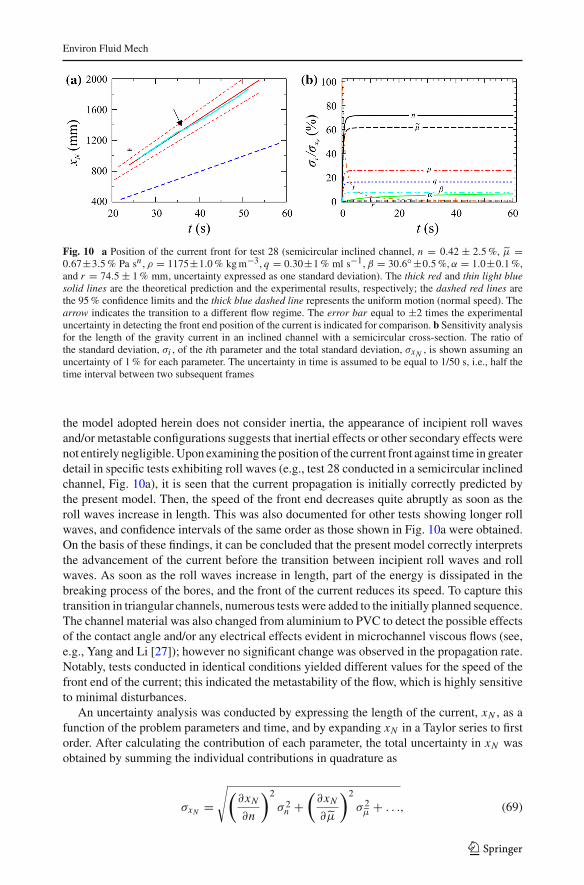
Fig. 10 a Position of the current front for test 28 (semicircular inclined channel, n = 0.42 ± 2.5 %, μ̃ =0.67±3.5 % Pa sn , ρ = 1175±1.0 % kg m−3, q = 0.30±1 % ml s−1, β = 30.6◦ ±0.5 %, α = 1.0±0.1 %,and r = 74.5 ± 1 % mm, uncertainty expressed as one standard deviation). The thick red and thin light bluesolid lines are the theoretical prediction and the experimental results, respectively; the dashed red lines arethe 95 % confidence limits and the thick blue dashed line represents the uniform motion (normal speed). Thearrow indicates the transition to a different flow regime. The error bar equal to ±2 times the experimentaluncertainty in detecting the front end position of the current is indicated for comparison. b Sensitivity analysisfor the length of the gravity current in an inclined channel with a semicircular cross-section. The ratio ofthe standard deviation, σi , of the ith parameter and the total standard deviation, σxN , is shown assuming anuncertainty of 1 % for each parameter. The uncertainty in time is assumed to be equal to 1/50 s, i.e., half thetime interval between two subsequent frames

the model adopted herein does not consider inertia, the appearance of incipient roll wavesand/or metastable configurations suggests that inertial effects or other secondary effects werenot entirely negligible. Upon examining the position of the current front against time in greaterdetail in specific tests exhibiting roll waves (e.g., test 28 conducted in a semicircular inclinedchannel, Fig. 10a), it is seen that the current propagation is initially correctly predicted bythe present model. Then, the speed of the front end decreases quite abruptly as soon as theroll waves increase in length. This was also documented for other tests showing longer rollwaves, and confidence intervals of the same order as those shown in Fig. 10a were obtained.On the basis of these findings, it can be concluded that the present model correctly interpretsthe advancement of the current before the transition between incipient roll waves and rollwaves. As soon as the roll waves increase in length, part of the energy is dissipated in thebreaking process of the bores, and the front of the current reduces its speed. To capture thistransition in triangular channels, numerous tests were added to the initially planned sequence.The channel material was also changed from aluminium to PVC to detect the possible effectsof the contact angle and/or any electrical effects evident in microchannel viscous flows (see,e.g., Yang and Li [27]); however no significant change was observed in the propagation rate.Notably, tests conducted in identical conditions yielded different values for the speed of thefront end of the current; this indicated the metastability of the flow, which is highly sensitiveto minimal disturbances.

An uncertainty analysis was conducted by expressing the length of the current, xN , as afunction of the problem parameters and time, and by expanding xN in a Taylor series to firstorder. After calculating the contribution of each parameter, the total uncertainty in xN wasobtained by summing the individual contributions in quadrature as

σxN =√

(

∂xN

∂n

)2

σ 2n +

(

∂xN

∂μ̃

)2

σ 2μ̃ + . . ., (69)

123

Environ Fluid Mech

where the symbols σi denote the standard deviation, which is assumed to be an estimateof the uncertainty. Figure 10b depicts the sensitivity of the model to the uncertainty in theparameters as the ratio between the standard deviation associated with each parameter and thetotal standard deviation, assuming a fixed uncertainty of 1 % for each parameter. The highestratio is associated with the rheological parameters n and μ̃, accounting for more than 80 %of the total standard deviation of xN . This is because in the present tests, the uncertainties inn and μ̃ are by far the most relevant - all the other sources of uncertainty are almost trivial.

5 Conclusions

We investigated the flow of laminar gravity currents of power-law liquids in horizontal andinclined channels having different cross-sectional shapes, namely semicircular and right tri-angular, theoretically and experimentally. The theoretical solutions are self-similar or basedon the method of characteristics, and allow the evaluation of the position of the currentfront and the thickness of its profile, extending the Newtonian results of Takagy and Hup-pert [20,21]. Laboratory experiments were conducted with liquids of different rheologies insemicircular and triangular channels. The main conclusions of our work are:

– The position of the current front depends on (i) the volume parameter α, (ii) the liquidrheology, and (iii) the channel inclination and shape of the cross-section. The latterfactor influences the mass balance equation and modulates the downstream evolution ofthe current. Critical values of α are determined for horizontal channels as a function ofbehaviour index n as αc = n/(n + 1), and for inclined channels as αc = 1, irrespectiveof cross-section geometry. For triangular cross-sections, a maximum (minimum) valueof the rate of spreading is attained for α < αc (α > αc).

– The position of the current front obtained experimentally is generally in good agreementwith theory. For tests in inclined channels with α = 1, a variety of flow regimes typicalof open-channel flows were observed at the end of the tests: uniform flow with normaldepth, incipient roll waves, roll waves, metastable conditions. The final propagation rateof the current front was overpredicted by the model, while the presence of roll wavessuggested the influence of inertia or other secondary effects. Upon examining the rateof propagation of the current over time, it was discovered that the theoretical solutionaccurately describes the phenomenon before the transition between incipient roll wavesand roll waves. As these require a sufficient channel length to develop, the final fateof the currents analysed in the present tests is not known. However, on the basis ofour experimental results, we infer that the profile predicted for inclined channels in thepresent model is a limiting profile of the current and marks the transition to a differentflow regime.

– The rheology of complex liquids is usually of concern in laminar flow models becauseit is often not adequately known or described. This is confirmed by the present study,where the rheological parameters are shown to be the main source of uncertainty. Thisbehaviour supports the use of carefully designed laboratory experiments as rheometrictests.

– The results obtained may prove useful in analysing the joint influence of rheology, chan-nel shape, and volume growth rate in environmental flows, such as turbidity currents,avalanches, and pyroclastic flows of non-Newtonian fluids characterised by negligibleyield stress.

123

Environ Fluid Mech

Acknowledgments Support from Università di Bologna RFO (Ricerca Fondamentale Orientata) 2011 and2012 is gratefully acknowledged.

References

1. Simpson JE (1982) Gravity currents in the laboratory, atmosphere, and ocean. Ann Rev Fluid Mech14:213–234

2. Huppert HE (1986) The intrusion of fluid mechanics into geology. J Fluid Mech 173:557–5983. Ungarish M (2010) An introduction to gravity currents and intrusions. CRC Press, Boca Raton4. Huppert HE (1982) The propagation of two-dimensional and axisymmetric viscous gravity currents over

a rigid horizontal surface. J Fluid Mech 121:43–585. Didden N, Maxworthy T (1982) The viscous spreading of plane and axisymmetric gravity currents. J

Fluid Mech 121:27–426. Pinkerton H, Sparks RSJ (1978) Field measurements of the rheology of lava. Nature 276:383–3857. Takagi D, Huppert HE (2010) Initial advance of long lava flows in open channels. J Volcanol Geotherm

Res 195:121–1268. Ugarelli R, Di Federico V (2007) Transition from supercritical to subcritical regime in free surface flow

of yield stress fluids. Geophys Res Lett 34:L214029. Sonder I, Zimanowski B, Buttner R (2006) Non-Newtonian viscosity of basaltic magma. Geophys Res

Lett 33:L0230310. Ng C-O, Mei CG (2004) Roll waves on a shallow layer of mud modelled as a power-law fluid. J Fluid

Mech 263:151–18311. Burger J, Haldenwang R, Alderman N (2010) Friction factor—Reynolds number relationship for laminar

flow of non-Newtonian fluids in open channels of different cross-sectional shapes. Chem Eng Sci 85:3549–3556

12. Pascal JP (1991) Gravity flow of a non-Newtonian fluid sheet on an inclined plane. Int J Eng Sci29(10):1307–1313

13. Gratton J, Minotti F, Mahajan SM (1999) Theory of creeping gravity currents of a non-Newtonian liquid.Phys Rev E 60(6):6960–6967

14. Di Federico V, Malavasi S, Cintoli S (2006) Viscous spreading of non-Newtonian gravity currents on aplane. Meccanica 41:207–217

15. Chowdhury MR, Testik FY (2012) Viscous propagation of two-dimensional non-Newtonian gravity cur-rents. Fluid Dyn Res 44:045502

16. Sayag R, Worster MG (2013) Axisymmetric gravity currents of power-law fluids over a rigid horizontalsurface. J Fluid Mech 716(R5):1–11

17. Longo S, Di Federico V, Archetti R, Chiapponi L, Ciriello V, Ungarish M (2013) On the axisymmetricspreading of non-Newtonian power-law gravity currents of time-dependent volume: an experimental andtheoretical investigation focused on the inference of rheological parameters. J Non-Newton Fluid Mech201:69–79

18. Piau MP, Debiane K (2005) Consistometers rheometry of power-law viscous fluids. J Non-Newton FluidMech 127:213–224

19. Jacobson MR, Testik FY (2014) Turbulent entrainment into fluid mud gravity currents. Fluid MechEnviron. doi:10.1007/s10652-014-9344-5

20. Takagi D, Huppert HE (2007) The effect of confining boundaries on viscous gravity currents. J FluidMech 577:495–505

21. Takagi D, Huppert HE (2008) Viscous gravity currents inside confining channels and fractures. PhysFluids 20:023104

22. Mei CC, Yuhi M (2001) Slow flow of a Bingham fluid in a shallow channel of finite width. J Fluid Mech431:135–159

23. Huppert HE (1982) Flow and instability of a viscous current down a slope. Nature 300:427–42924. Muzychka YS, Edge J (2008) Laminar non-Newtonian fluid flow in noncircular ducts and microchannels.

J Fluid Eng—ASME 130:111201–11120725. Julien PY, Hartley DM (1986) Formation of roll waves in laminar sheet flow. J Hydraul Res 24:1–1726. Longo S (2011) Roll waves on a shallow layer of a dilatant fluid. Eur J Mech B 30:57–6727. Yang C, Li D (1998) Analysis of electrokinetic effects on the liquid flow in rectangular microchannels.

Colloid Surf A 143:339–353

123