Embed Size (px)
Citation preview
Node Coarsening Calculi for Program Slicing
Mark Harman, Sebastian Danicic, Rob Hierons John Howroyd,
Brunel University, Mike Laurence Uxbridge, Middlesex, Goldsmiths College,
University of London, New Cross,
London SE 14 6NW, UK. Tel: +44 (0)20 79 19 7856 Fax: +44 (0)20 7919 7853
UB8 3PH, UK. Tel: +44 (0)1895 274 000 Fax: +44 (0) 1895 25 1 686
[email protected] [email protected]
Keywords: slicing, slice precision, node merging
Abstract
Several approaches to reverse and re-engineering are based upon program slicing. Unfortunately, for large systems, such as those which typically form the subject of reverse engineering activities, the space and time requirements of slicing can be a barrier to successful application.
Faced with this problem, several authors have found it helpful to merge Control Flow Graph (CFG) nodes, thereby improving the space and time requirements of standard slicing algorithms. The node-merging process essentially creates a ‘coarser’ version of the original CFG.
This paper introduces a theory for defining Control Flow Graph node coarsening calculi. The theory formalizes properties of interest, when coarsening is used as a precur- sor to program slicing. The theory is illustrated with a case study of a coarsening calculus, which is proved to have the desired properties of sharpness and consistency.
1 Introduction
Program slicing [26, 171 is a source code analysis.technique which extracts parts of the source code associated with cer- tain computations defined by a ‘slicing criterion’.
Slicing has been used to assist several reverse and re- engineering activities. For example, Beck and Eichmann use slicing at both statement and module level to extract functionality from Ada programs [2]; Canfora at al. [6] used slicing as a part of the RE2 reverse and re-engineering project; Cimitile et al. [7] showed how slicing (together with other techniques) can be used to identify reuse candi- dates.
Chris Fox Kings College,
University of London, Strand,
London, WC2R 2LS, UK. Tel: +44 (0)20 7848 2694 Fax: +44 (0)20 7848 285 1 [email protected]
Slicing has also been applied to problem areas, closely related to reverse engineering, such as program compre- hension [8], software maintenance [3, I I ] and testing [4, 13, 161. Tip [24] and Binkley and Gallagher [5] pro- vide detailed surveys of slicing.
Other dependence-based analyses have been applied to reverse engineering, for example chopping [ 181, tucking [20] and the RECAST method [IO]. The theoretical frame- work presented in the present paper is defined for slic- ing, but could easily be extended to apply to these related dependence-based analysis techniques.
When constructing program slices, it is sometimes help- ful to increase slice-construction speed at the expense of precision, by merging program nodes. This may be partic- ularly important where slicing is applied to reverse engi- neering and re-engineering, where the subject program un- der analysis may be subject to several ‘change phases’ or where the systems to be analyzed are prohibitively large.
Recently, several authors have found that the space and time requirements of slicing large systems make the appli- cation of standard algorithms problematic [9, 22, 11. This difficultly can be ameliorated by applying these standard techniques to an abstracted program. The abstraction is achieved by merging together nodes of the program’s con- trol flow graph (CFG), upon which the standard techniques for slice construction [26, 171 are based. This node merging introduces imprecision but reduces space and time com- plexity.
This paper provides a theory to underpin the process of node coarsening. The theory allows precise statements to be made concerning the correctness and efficacy of node coarsening. The theory allows for formal analysis of the trade off between precision and space and time complexity.’
1095-1350/01 /$10.00 0 2001 IEEE 25
Two important coarsening calculus properties are for- mally defined:
Consistency, which captures the safety concern that slices of coarsened programs are guaranteed to be cor- rect;
0 Sharpness, which captures the property that a set of coarsening inference rules is as precise as the abstrac- tion will allow.
The theory is illustrated with a case study which intro- duces a coarsening calculus, R-coarsening, for a simple in- traprocedural language. The theory also allows coarsening at the interprocedural level, where a procedure makes a nat- ural choice for converting to a single node. The intraproce- dural example of R-coarsening presented in Section 3 has been chosen because it illustrates the issues of consistency, sharpness and minimality in a comparatively straightfor- ward manner.
For ease of exposition, only end slicing [I91 will be considered, but the results presented can be generalized to cover other forms of slicing. Hereinafter, the terms ‘slice’ and ‘end slice’ will be used interchangeably. In end-slicing, the slicing criterion is simply a set of variables, V.
Definition 1.1 (End Slicing) An end slice of a program p , constructed with respect to a slicing criterion V, is any program which can be con- structed from p by deleting nodes of the Control Flow Graph (CFG) of p in such a way that the effect of p upon all variables in V is preserved.
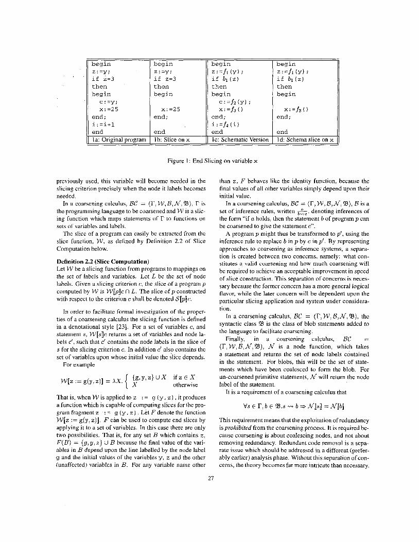
An end slice s, of a program p , constructed with respect to a slicing criterion V , has two properties; one syntactic and the other semantic. The syntactic property is that s is constructed from p by removing nodes from the Control Flow Graph of p . The semantic property is that s has the same effect a s p on all variables in V. A slice thus preserves a projection of the original program’s syntax and semantics [14]. An example program and one of its end slices are given in the Figures l a and lb.
Slicing algorithms [26, 171 are traditionally insensitive to changes i n , a program’s arithmetic and boolean expres- sions which have no effect upon sets of referenced vari- ables. Therefore, it will be convenient to abstract away from the precise details of concrete program syntax, to an abstract syntax in which expressions are denoted by the sets of variables they reference.
In this paper, this is achieved using program schemas [27, 211. A program schema has the same syntactic struc- ture as a program up to expressions. In the schema, expres- sions are replaced by the application of some uninterpreted function or predicate symbol to a set of actual parame- ters. The actual parameters are the referenced variables of the expression which this abstraction replaces. Thus, in a
schema, all that is ‘known’ about an expression is its set of referenced variables.
A single schema denotes an equivalence class of many programs, each of which is equivalent up to referenced variables of expressions. An interpretation of a schema is a program obtained from the schema by replacing each func- tion and predicate symbol with a real (fully interpreted) function or predicate. For example, the schema corre- sponding to the program in Figure l a is given in Figure IC and its slice constructed for {x} (at the schema level) is given in Figure Id.
In order to coalesce nodes together, a new syntactic con- struct, the blob, will be added to the language. Syntacti- cally, a blob will be a form of statement, denoting a sub- graph which has been collapsed onto a single node, the blob, which contains sufficient information to approximate the information denoted by the original subgraph.
The rest of this paper is organised as follows. Section 2 introduces a theory of coarsening, which is illustrated in section 3 with an instance of a coarsening calculus called R-coarsening. Section 4 contains a proof that R-coarsening is both consistent and sharp with respect to the definitions in Section 2. This illustrates the way in which the theory introduced in section 2 allows for formal and rigorous cer- tification of approaches to coarsening. Section 5 describes the relationship between coarsening and other work on co- alescing nodes of program graphs. Section 6 concludes.
2 A Theory of Coarsening A coarsening calculus, BC, is a quintuple, ( r , W , B , N , % ) . Each of the elements of a coarsen- ing calculus are described in more detail below. First, a notation is introduced to describe the process of coarsening.
Definition 2.1 (Coarsens to) Let R be an inference rule, axiom or set of rules and axioms of a coarsening calculus. s -+R b denotes the fact that the blob b can be inferred from the statement s using R.
When the inference rule set is clear from the context, the reflexive, transitive closure of a relation +R, will be denoted by +.
It will be helpful to label each node with a unique vari- able, which will be called a ‘node label’. The variable is a new variable introduced solely to signify the inclusion of the corresponding node in the slice. Since there is a one- to-one correspondence between the nodes of the CFG on the one hand and the union of the set of predicates and arithmetic expressions on the other, it will be possible to achieve this node labelling by including an additional refer- enced variable U , in the expression or predicate associated with each node n. Provided that each U , is unique and not
26
begin z : = y ; i f z=3 t hen begin
c : =y; x:=25
end ; i : =i+l end 1 a: Original program
begin z : =y; if z=3 t hen begin
x : =25 end :
end 1 b: Slice on x
begin
i f bl (z) t hen begin
z:=f1 ( U ) ;
c:=f2(y); x : = f 3 0
end ; i : = f d ( i )
end IC: Schematic Version
Figure 1 : End Slicing on variable x
previously used, this variable will become needed in the slicing criterion precisely when the node it labels becomes needed.
In a coarsening calculus, BC = (r, W , BIN, B), r is the programming language to be coarsened and W is a slic- ing function which maps statements of r to functions on sets of variables and labels.
The slice of a program can easily be extracted from the slice function, W , as defined by Definition 2.2 of Slice Computation below.
Definition 2.2 (Slice Computation) Let W be a slicing function from programs to mappings on the set of labels and variables. Let L be the set of node labels. Given a slicing criterion c, the slice of a program p computed by W is W b ] c n L. The slice of p constructed with respect to the criterion c shall be denoted Sl[p]c.
In order to facilitate formal investigation of the proper- ties of a coarsening calculus the slicing function is defined in a denotational style [23]. For a set of variables c, and statement s, W[s]c returns a set of variables and node la- bels c’, such that c‘ contains the node labels in the slice of s for the slicing criterion c. In addition c’ also contains the set of variables upon whose initial value the slice depends.
For example
That is, when W is applied to z : = g ( y , z ) , it produces a function which is capable of computing slices for the pro- gram fragment i : = g ( y , z ) . Let F denote the function W [ z := g(y, z)]. F can be used to compute end slices by applying it to a set of variables. In this case there are only two possibilities. That is, for any set B which contains z , F ( B ) = (9, y, z } U B because the final value of the vari- ables in B depend upon the line labelled by the node label g and the initial values of the variables y, z and the other (unaffected) variables in B. For any variable name other
begin
i f bl (z) t hen begin
z:=f1 (Y) ;
x : = f 3 0 end :
end Id: Schema slice on x
than z , F behaves like the identity function, because the final values of all other variables simply depend upon their initial value.
In a coarsening calculus, BC = (r, W , B, NI B), B is a set of inference rules, written &, denoting inferences of the form “if a holds, then the statement b of program p can be coarsened to give the statement c”.
A program p might thus be transformed to p’ , using the inference rule to replace b in p by c in p’. By representing approaches to coarsening as inference systems, a separa- tion is created between two concerns, namely: what con- stitutes a valid coarsening and how much coarsening will be required to achieve an acceptable improvement in speed of slice construction. This separation of concerns is neces- sary because the former concern has a more general logical flavor, while the later concern will be dependent upon the particular slicing application and system under considera- tion.
In a coarsening calculus, BC = (I?, W , B, NI %), the syntactic class 23 is the class of blob statements added to the language to facilitate coarsening.
Finally, in a coarsening calculus, BC = ( ~ , W , B , N , % ) , JV is a node function, which takes a statement and returns the set of node labels contained in the statement. For blobs, this will be the set of state- ments which have been coalesced to form the blob. For un-coarsened primitive statements, n/ will return the node label of the statement.
It is a requirement of a coarsening calculus that
b’s E I?, b E ‘23.s b + = A@]
This requirement means that the exploitation of redundancy is prohibited from the coarsening process. It is required be- cause coarsening is about coalescing nodes, and not about removing redundancy. Redundant code removal is a sepa- rate issue which should be addressed in a different (prefer- ably earlier) analysis phase. Without this separation of con- cerns, the theory becomes far more intricate than necessary.
27
It will be helpful to define a semantic ordering, C on slicing functions. f1 E f2 if slices produced by f1 are always subsets of slices produced by f2.
Definition 2.3 (Semantic Ordering) Let f1 and f2 be two functions on sets of variables and node labels. f1 precedes fi, written fi f2, iff Vc.f i (c) f 2 ( 4
It will also be useful to speak of strict semantic ordering, E, which is defined in the obvious way:
f i C f2 i f f f i E f2 A ~ ( f 2 E f i )
Definition 2.4 (Consistency) Let BC = (I’, W , B,N, ‘13) be a coarsening calculus. BC is consistent iff Vp E r , p ‘ E ’13.p ~ r ) p’ + Wl[plI E W W ] .
In a consistent coarsening calculus it is impossible for a slice of a coarsened program to be smaller than the slice of the original program. This is important, because coarsen- ing clearly cannot cause slices to get smaller. Were it to do so, the coarsening rules may not be safe and could not be considered consistent with the definition of slicing captured by W .
Consistency merely guarantees that all slices constructed from a coarsened version of a program will be valid. How- ever, a coarsening calculus could satisfy this requirement by being excessively conservative. In the most conservative case, the algorithm would simply return the entire program as the slice, regardless of the slicing criterion. Such overly conservative approaches will render the calculus safe but useless.
To address this issue of the ‘level of conservativeness’ of approximati,on in coarsening, two other properties of a coarsening calculus are defined: minimality and sharpness.
Definition 2.5 (Minimality) Let P S be the powerset of a set S. Let BC = (I’, W , B, n/, %) be a coarsening calculus. BC is minimal iff VS E I?, b E !€IS .US b + VC E P(v U L).Wl[s]c - n/nsn = wpjC - NIs].
If a coarsening calculus is minimal then the slices con- structed from blobs will be equivalent to those which would have been constructed by computing the slice, s of the orig- inal program, p and then adding to s all nodes which are in the blobs that contain nodes from s.
Minimality is a highly desirable property of a coarsen- ing calculus, because it ensures that the only imprecision introduced by coarsening is embodied by the blobs them- selves, and that the act of combining several nodes has no impact upon the data and control flow passing through the coarsened region of the CFG.
Using a non-minimal coarsening calculus the act of coarsening several nodes into a single blob may cause the
data and control information of the coarsened region to be less precise than that of the original un-coarsened version. This may impact upon the slice computation of the entire program, as this imprecise information flows from the blob to the surrounding context. For such a non-minimal coars- ening calculus, the effect of ‘zooming in’ to analyze a blob in more detail may result in a refinement of the slice of the surrounding code. By contrast a minimal calculus will pro- vide the guarantee that zooming in on some chosen blob will only affect the slice of the blob, leaving the context in which the blob is located unchanged.
Desirable though minimality is, it remains a rather strong requirement upon a coarsening calculus, because it seems inevitable that, for many coarsening calculi, some of the available precision will be lost when nodes are combined to form a blob.
A related concept, sharpness, is therefore introduced. In- tuitively, sharpness captures the property that a coarsening rule is ‘as minimal as it can be’ at the level of abstraction imposed by the syntax and semantics of the coarsening con- struct. If a coarsening calculus is not sharp then it is, in ef- fect, needlessly imprecise, throwing away data and control information that could have been represented.
To illustrate sharpness, suppose two statements s1 and s2 appear in a sequence SI; s2, and that the sequence is to be merged to a single node n with defined and referenced variables which attempt to capture the information in the un-coarsened sequence. At first sight it may seem reason- able that the referenced variables of the blob should be the union of the referenced variables of its two constituents. This would yield a safe blob, but not a sharp one. For ex- ample, variables which are defined but not referenced in s1 need not be referenced in the blob of SI; s2. To include them is safe, but it leads to unnecessary loss of precision.
Definition 2.6 (Sharpness) Let BC = (r, W , B,N, ‘13) be a coarsening calculus. B is sharp iff Vs E r,b E 23.s +-+ b + 13’ E B.Wl[s] 5 ~ i b q E wpi.
Sharpness demands that no better blob can be found which would allow the coarsening calculus to be consis- tent. Thus the coarsening rule produces the best blob avail- able within the constraints imposed by the structure of ’23 and the slicing function W .
For a coarsening calculus to be useful it should be con- sistent and sharp. Minimality is also a desirable property. However, minimal coarsening calculi may require a large computational overhead to compute the blob and its asso- ciated data and control information. As the whole idea of coarsening is to compute blobs quickly, allowing precision to be traded for speed, it is unlikely that minimal coarsen- ing calculi, though of theoretical interest, will be of practi- cal use unless their blobs can be computed speedily.
28
3 Case Study: R-Coarsening
In this section a particular example of coarsening, called R-coarsening, is introduced in order to illustrate the ap- plication of the coarsening theory introduced in the previ- ous section. Although introduced primarily for exposition purposes, the R-coarsening calculus is consistent and sharp and thus may form the basis for a practical and useful ap- proach to coarsening.
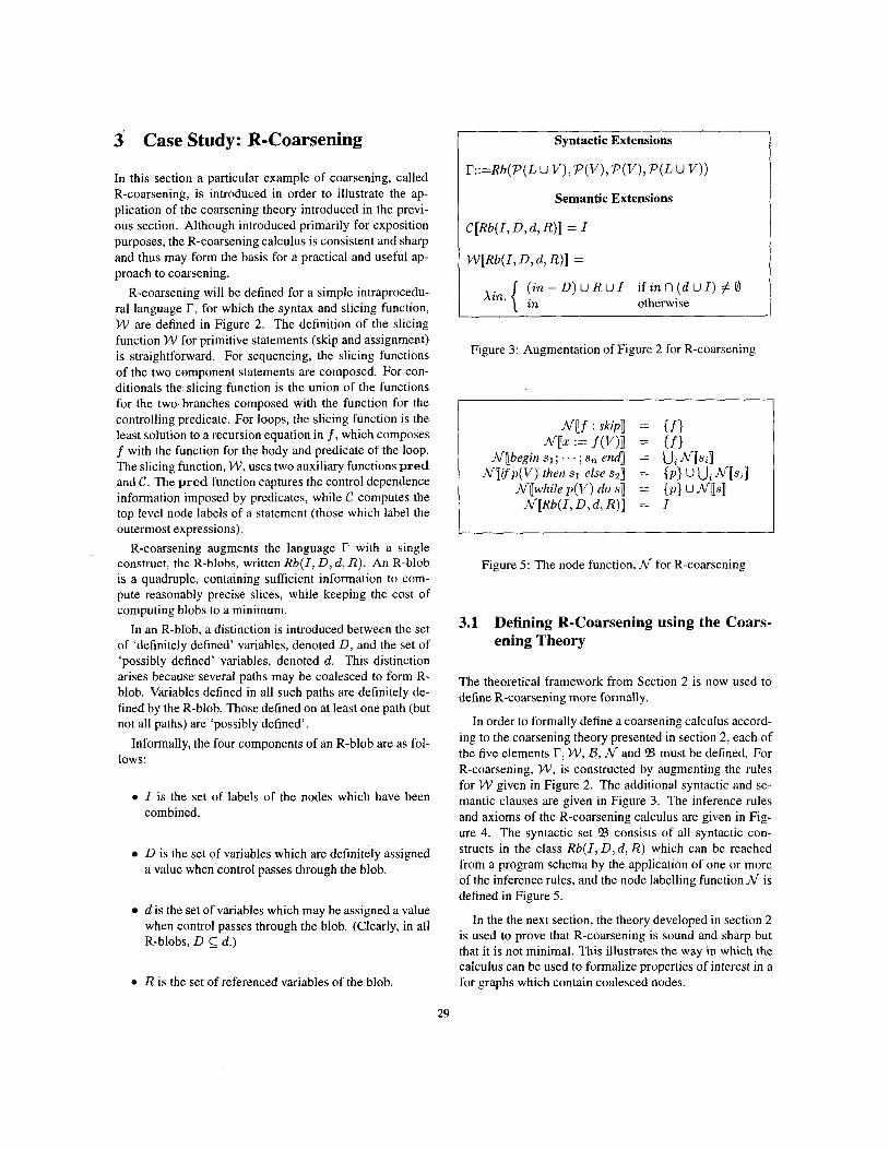
R-coarsening will be defined for a simple intraprocedu- ral language r, for which the syntax and slicing function, W are defined in Figure 2. The definition of the slicing function W for primitive statements (skip and assignment) is straightforward. For sequencing, the slicing functions of the two component statements are composed. For con- ditionals the slicing function is the union of the functions for the two branches composed with the function for the controlling predicate. For loops, the slicing function is the least solution to a recursion equation in f , which composes f with the function for the body and predicate of the loop. The slicing function, W , uses two auxiliary functions pred and C. The pred function captures the control dependence information imposed by predicates, while C computes the top level node labels of a statement (those which label the outermost expressions).
R-coarsening augments the language r with a single construct, the R-blobs, written Rb(1, D, d, R). An R-blob is a quadruple, containing sufficient information to com- pute reasonably precise slices, while keeping the cost of computing blobs to a minimum.
In an R-blob, a distinction is introduced between the set of 'definitely defined' variables, denoted D, and the set of 'possibly defined' variables, denoted d. This distinction arises because several paths may be coalesced to form R- blob. Variables defined in all such paths are definitely de- fined by the R-blob. Those defined on at least one path (but not all paths) are 'possibly defined'.
Informally, the four components of an R-blob are as fol- lows:
0 I is the set of labels of the nodes which have been combined.
D is the set of variables which are definitely assigned a value when control passes through the blob.
d is the set of variables which may be assigned a value when control passes through the blob. (Clearly, in all R-blobs, D d.)
0 R is the set of referenced variables of the blob.
Syntactic Extensions
r::=Rb(P(LU V ) , P ( V ) , P ( V ) , P ( L U V ) )
Semantic Extensions
CI[Rb(I, D, d , R)] = I
WI[Rb(I , D, d, R)] =
(in - D) U R U l if inn ( d U I) # 0 Xin. in otherwise {
Figure 3: Augmentation of Figure 2 for R-coarsening
I
Figure 5: The node function, N for R-coarsening
3.1 Defining R-Coarsening using the Coars- ening Theory
The theoretical framework from Section 2 is now used to define R-coarsening more formally.
In order to formally define a coarsening calculus accord- ing to the coarsening theory presented in section 2, each of the five elements r, W , .U, N and 93 must be defined. For R-coarsening, W , is constructed by augmenting the rules for W given in Figure 2. The additional syntactic and se- mantic clauses are given in Figure 3. The inference rules and axioms of the R-coarsening calculus are given in Fig- ure 4. The syntactic set 23 consists of all syntactic con- structs in the class Rb(I , D , d , R) which can be reached from a program schema by the application of one or more of the inference rules, and the node labelling function N is defined in Figure 5.
In the the next section, the theory developed in section 2 is used to prove that R-coarsening is sound and sharp but that it is not minimal. This illustrates the way in which the calculus can be used to formalize properties of interest in a for graphs which contain coalesced nodes.
29
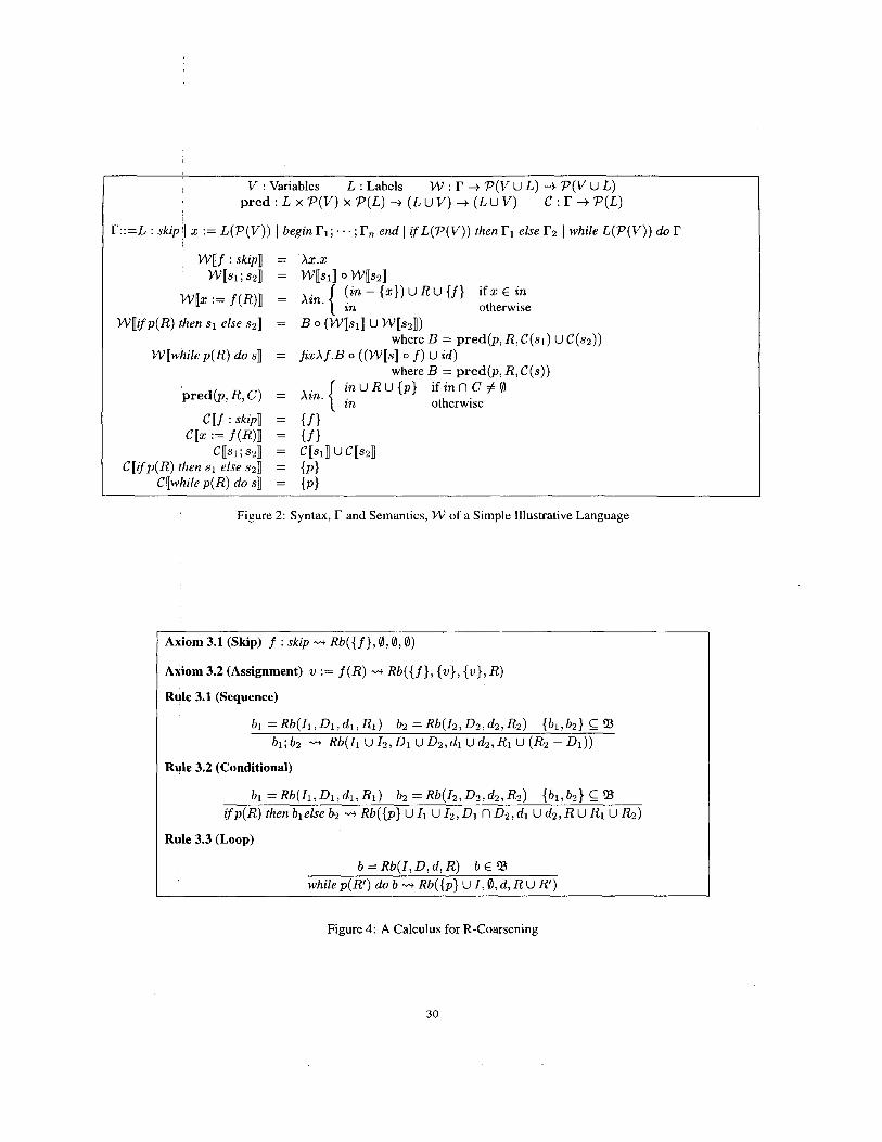
V : Variables L : Labels pred : L x P ( V ) x P ( L ) + ( L U V ) + ( L U V )
W : r + P(V U L ) -+ P(V U L ) C : r + P ( L )
r::=L : skip ' 1 x := L(P(V) ) I begin rl; . . . ; rn end I i fL(P(V/ ) ) then rl else r2 I while L(P(V) ) do I?
W[while p ( R ) do s]
= Xx.x = wnsln 0 w1s2n
= B 0 (w[sln U w[S2n)
(in - {x}) U R U {f} if x E an { in otherwise = Xin.
where B = pred(p, R, C(s1) U C(s2))
where B = pred(p, R,C(s)) = fiXXf.B 0 ( (W[s] 0 f ) U id)
i n u R U { p } i f i n n C f 0 { in otherwise = Xin.
= {f) = {f}
= {PI = {PI
= cisli U cis2]
Figure 2: Syntax, r and Semantics, W of a Simple Illustrative Language
Axiom 3.1 (Skip) f : skip * R b ( { f } , 8,8,8)
Axiom 3.2 (Assignment) w := f(R) * R b ( { f } , {U}, {w}, R)
Rule 3.1 (Sequence)
b i = R b ( I i , D i , d i , R i ) b2 = R b ( I 2 , D 2 , 4 , & ) { b i , b 2 } G 23 b l ; b 2 4 R b ( l i U I 2 , D i U 0 2 , d i U d 2 , R i U ( R 2 - D i ) )
Rule 3.2 (Conditional)
Rule 3.3 (Loop)
b = Rb(1, D, d, R) b E 23 Rb({p} U I , 0, d, R U R') while p(R') do b
Figure 4: A Calculus for R-Coarsening
30
4 Theoretical Properties of R- coarsening
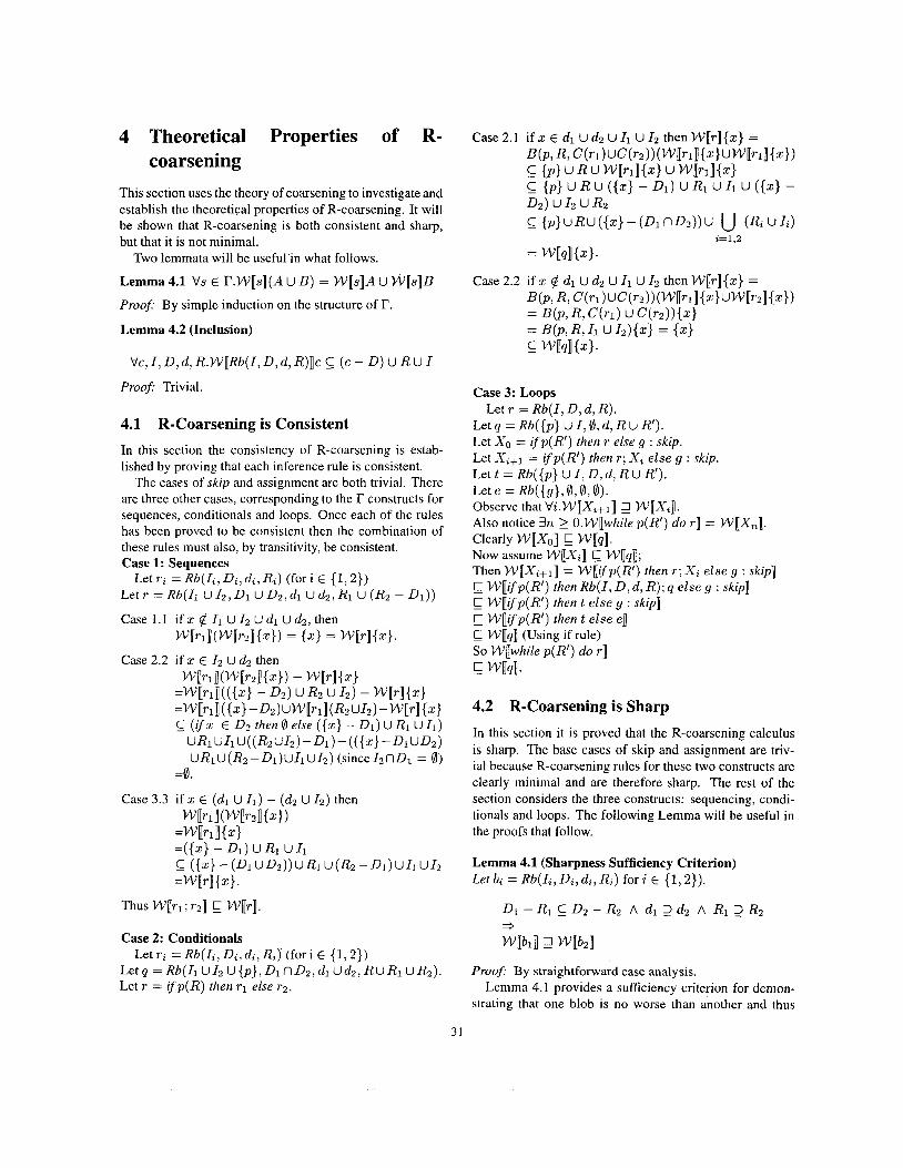
This section uses the theory of coarsening to investigate and establish the theoretical properties of R-coarsening. It will be shown that R-coarsening is both consistent and sharp, but that it is not minimal.
Lemma 4.1 Vs E F.Wl[s](A U B ) = W [ s ] A U W[s]B
Proof: By simple induction on the structure of r. Lemma 4.2 (Inclusion)
Two lemmata will be useful’in what follows.
V c , I , D,d,R.WI[Rb(I,D,d,R)]c 5 ( C - D ) U RUI
Proof: Trivial.
4.1 R-Coarsening is Consistent In this section the consistency of R-coarsening is estab- lished by proving that each inference rule is consistent.
The cases of skip and assignment are both trivial. There are three other cases, corresponding to the r constructs for sequences, conditionals and loops. Once each of the rules has been proved to be consistent then the combination of these rules must also, by transitivity, be consistent. Case 1: Sequences
Let T = Rb(l1 U 1 2 , D1 U D2, dl U dz, R1 U (R2 - 0 1 ) )
Let7-i =Rb(Ii ,Di ,di ,Ri) (fori E {1,2})
Case 3: Loops
Let q = Rb({p} U I , 0 , d, R U R‘). Let X , = ifp(R’) then r else g : skip. Let Xi+l = ifp(R’) then r ; X i else g : skip. Let t = Rb({p} U I , D , d, R U R’). Let e = Rb({g}, 0,0,0). Observe that V’i.WIXi+l] WIXi]l . Also notice 3n >_ O.W[while p(R’) do r ] = W [ X n ] . Clearly W [ [ X o ] g Wuq]. Now assume W[Xi] g W[q]; Then W[[Xi+,] = W[[ifp(R’) rhen r ; X i else g : skip] 5 W[ifp(R’) then Rb(I, D , d , R); q else g : skip1 g W[ifp(R’) then t else g : skip] E W[[ifp(R’) rhen t else e] & W[q] (Using if rule) So Wuwhile p(R’) do T ]
Let r = Rb(I , D , d, R).
c wuqn.
4.2 R-Coarsening is Sharp In this section it is proved that the R-coarsening calculus is sharp. The base cases of skip and assignment are triv- ial because R-coarsening rules for these two constructs are clearly minimal and are therefore sharp. The rest of the section considers the three constructs: sequencing, condi- tionals and loops. The following Lemma will be useful in the proofs that follow.
Lemma 4.1 (Sharpness Sufficiency Criterion) Let bi = Rb(Ii, Di, di, Ri) fo r i E {1,2}).
Thus W[[rl; 7-21 _C Wir]. D1 - R1 C 0 2 - R2 A dl 2 d2 A R1 2 R2 * Case 2: Conditionals wubln 2 wub21
Letr i =Rb(l i ,Di ,di ,Ri)’(for i E {1,2}) Let q = Rb(11 U I2 U { p } , D1 n D2, dl U d2 , R U R1 U R2). Let r = ifp(R) then 7-1 else 7-2.
Proof: By straightforward case analysis. Lemma 4.1 provides a sufficiency criterion for demon-
strating that one blob is no worse than another and thus
31
,
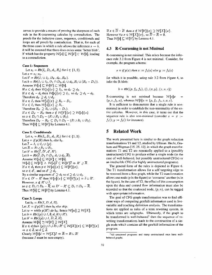
serves to provide a means of proving the sharpness of each rule in the R-coarsening calculus by contradiction. The proofs for the inductive cases, sequence, conditionals and loops are all proofs by contradiction. That is, for each of
If z E E - 3 then z $ W[b’]{z) 2 _W[X]{z}. H0weverVz.z E W [ X ] { z } , so D - R = 0. Thus W[b] F W[b‘] by Lemma 4.1.
the three cases in which a rule allows the inference s y.) b, it will be assumed that there does exists some ‘better blob’, 4.3 R-Coarsening is not Minimal b’ which has the property W[s] to a contradiction.
Case 1: Sequences
L e t s = s l ; s2. ,
Let b = Rb(Il U 12, D1 n D2, dl U d2, R1 U (R2 - D l ) ) . Assume W[s] W[b’] c W[b].
W[b’] c W[b], leading
Lets i =Rb(I , ,D, ,d , ,R,) fori E {1,2}.
Let b‘ Rb(I1 U 1 2 , Dbf, dbf , Rbt).
If 2 E d2 then W [ s ] { z } 2 12, SO db t 2 d2. If z E d l - d2 then W [ s ] { x } 2 I1 , SO dbi 2 d l - d2. Therefore dbt 2 d l U d2.
If z E I2 then W [ s ] { z } 2 R2 - D1. I f z E Il thenW[s]{z} 2 R1. Therefore Rbl 2 R1 U (R2 - 0 1 ) .
S O X E D1 n D 2 - (RURi UR2). If z E Dbi - then z $ w[b’]{x} 2 w[S]{z}
Therefore Dbt - Rb, C D1 n 0 2 - ( R U RI U R2). Thus W[b] C W[b’] by Lemma 4.1.
Case 2: Conditionals
Let s = ifp(R) then bl else 132.
L e t I = I l u I 2 ~ { p } . LetZ = R U RI U Rz. Let b’ = Rb(?, D‘, d’, R’). Let b = Rb(7, D1 n D 2 , d l U d2 , R) . Assume W[s] c W[b‘] c W[b]. w~s j 5. wpq A w p j ~ E wpq? + RI 2 3. I f z E dl thenp E W [ s ] { z } C W[b’]{x}, sox E d’, andsod’ 2 d l . By a similar argument d’ 2 d2 so d 2 dl U d2.
If z E D’ - R’ then W[s]{z} C W[b’]{x} = 7 U R’. However, z $ R’ U 7, SO z E D~ n~~ - R, SO D‘ - R’ c D~ n D~ - R . Thus W[b] W([b’] by Lemma 4.1.
Let s, = Rb(l,, D,, d,, R,) fo r i E {1,2}.
Case 3: Loops
Let X = ifp( R’) then bo else skip. Let w = whilep(R’) do bo; hence W [ w ] 7 W [ X ] . Let b = Rb({p} U I , 0, d , R U R’). Let b’ = Rb( {p} U I , o,& B). Assume W[b] ZI W[b’] 7 W [ X ] . I f ~ ~ d t h e n { p } u I u R u R ‘ ~ W [ X ] { z } CW[b’]{x} + x ~ & s o d c d . Clearly W[b]I = W [ X ] I + a = R U R’ (because I must be non-empty).
Let bo = Rb(I , D, d , R).
R-coarsening is not minimal. This arises because the infer- ence rule 3.2 from Figure 4 is not minimal. Consider, for example, the program schema:
s = ifp(z) then z := f 2 ( a ) else y := f3(c)
for which it is possible, using rule 3.2 from Figure 4, to infer the R-blob:
R-coarsening is not minimal because W [ s ] x =
It is sufficient to demonstrate that a single rule is non- minimal in order to establish the non-minimality of the en- tire calculus. However, in this case, it turns out that the sequence rule is also non-minimal (consider s = z := f l ( ) ; y := f 2 ( ) for instance).
{ p , z , f 2 , ai, whereas wpnz = {P, f2 , f3, z, a ,
5 Related Work
The work presented here is similar to the graph reduction transformations T1 and T2, studied by Ullman, Hecht, Gra- ham and Wegman [15, 25, 121, in which the graph transfor- mations T1 and T2 are repeatedly applied to a (possibly unstructured) CFG to produce either a single node (in the case of well-behaved, but possibly unstructured CFGs) or an irreducible CFG (for highly unstructured programs).
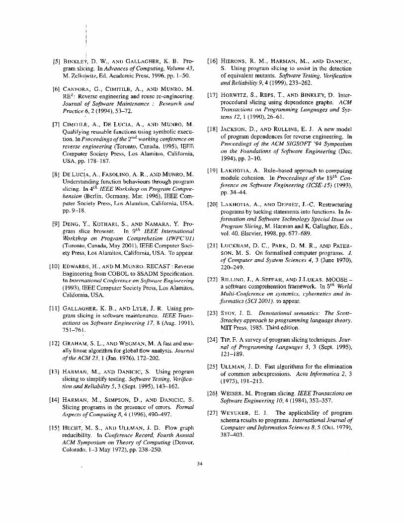
The general form of the rules is depicted in Figure 6. The T1 transformation allows for a self targeting edge to be removed from a flow graph, while the T2 transformation allows one node (p in the figure) to ‘consume’ another (n in the figure). In the case of T2, the effect of this consumption upon the data and control flow information must also be recorded so that the coalesced node, ( p , n) , can be tagged with appropriate information.
The goal of CFG graph transformation was to find effi- cient ways of computing genkill information used in live- variable and reaching definition analysis. The transforma- tions are applied as rules of a term rewriting system, in which terms are subgraphs. Ultimately, if the graph to be transformed is well-behaved’ then the sequence of re- writing transformations leads to the construction of a sin- gle node which contains all the genkill information of the program.
‘All structured programs and many unstructured ones have well- behaved graphs.
32
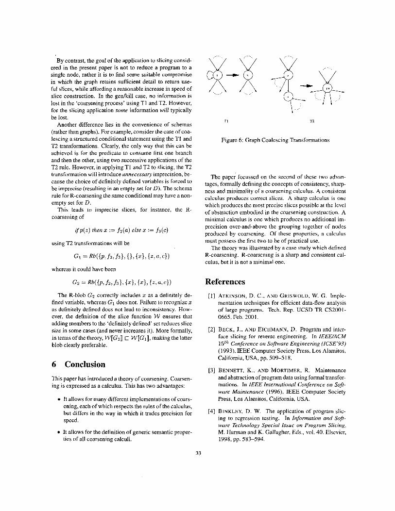
By contrast, the goal of the application to slicing consid- ered in the present paper is not to reduce a program to a single node, rather it is to find some suitable compromise in which the graph retains sufficient detail to return use- ful slices, while affording a reasonable increase in speed of slice construction. In the genkill case, no information is lost in the ‘coarsening process’ using T1 and T2. However, for the slicing application some information will typically be lost.
Another difference lies in the convenience of schemas (rather than graphs). For example, consider the case of coa- lescing a structured conditional statement using the T1 and T2 transformations. Clearly, the only way that this can be achieved is for the predicate to consume first one branch and then the ottier, using two successive applications of the T2 rule. However, in applying T1 and T2 to slicing, the T2 transformation will introduce unnecessary imprecision, be- cause the choice of definitely defined variables is forced to be imprecise (resulting in an empty set for D). The schema rule for R-coarsening the same conditional may have a non- empty set for D.
This leads to imprecise slices, for instance, the R- coarsening of
i f p ( z ) then 2 := f ~ ( a ) else 2 := f s ( c )
using T2 transformations will be
whereas it could have been
G2 = W { P , f 2 , f 3 1 , (51, (21, { z , a , cl> The R-blob G2 correctly includes 2 as a definitely de-
fined variable, whereas G1 does not. Failure to recognize 3:
as definitely defined does not lead to inconsistency. How- ever, the definition of the slice function W ensures that adding members to the ‘definitely defined’ set reduces slice size in some cases (and never increases it). More formally, in terms of the theory, W([G2JJ c W([GlIJ, making the latter blob clearly preferable.
6 Conclusion This paper has introduced a theory of coarsening. Coarsen- ing is expressed as a calculus. This has two advantages:
0 It allows for many different implementations of coars- ening, each of which respects the rules of the calculus, but differs in the way in which it trades precision for speed.
0 It allows for the definition of generic semantic proper- ties of all coarsening calculi.
TI T2
Figure 6: Graph Coalescing Transformations
The paper focussed on the second of these two advan- tages, formally defining the concepts of consistency, sharp- ness and minimality of a coarsening calculus. A consistent calculus produces correct slices. A sharp calculus is one which produces the most precise slices possible at the level of abstraction embodied in the coarsening construction. A minimal calculus is one which produces no additional im- precision over-and-above the grouping together of nodes produced by coarsening. Of these properties, a calculus must possess the first two to be of practical use.
The theory was illustrated by a case study which defined R-coarsening. R-coarsening is a sharp and consistent cal- culus, but it is not a minimal one.
References [ I ] ATKINSON, D. c . , A N D GRISWOLD, w. G . Imple-
mentation techniques for efficient data-flow analysis of large programs. Tech. Rep. UCSD TR CS2001- 0665, Feb. 2001.
[2] BECK, J., A N D EICHMANN, D. Program and inter- face slicing for reverse engineering. In IEEE/ACM Isth Conference on Sofrware Engineering (ICSE’93) (1993), IEEE Computer Society Press, Los Alamitos, California, USA, pp. 509-5 18.
[3] BENNETT, K., AND MORTIMER, R. Maintenance and abstraction of program data using formal transfor- mations. In IEEE International Conference on Soft- ware Maintenance (1996), IEEE Computer Society Press, Los Alamitos, California, USA.
[4] BINKLEY, D. W. The application of program slic- ing to regression testing. In Information and Soft- ware Technology Special Issue on Program Slicing, M. Harman and K. Gallagher, Eds., vol. 40. Elsevier, 1998, pp. 583-594.
33
[SI BINKLEt, D. W., AND GALLAGHER, K. B. Pro- gram slicing. In Advances of Computing, Volume 43, M. Zelkowitz, Ed. Academic Press, 1996, pp. 1-50.
[6] CANFORA, G., CIMITILE, A., AND MUNRO, M. RE2 : Reverse engineering and reuse re-engineering . Journal of Software Maintenance : Research and Practice 6, 2 (1994), 53-72.
[7] CIMITILE, A., DE LUCIA, A., AND MUNRO, M. Qualifying reusable functions using symbolic execu- tion. In Proceedings of the 2nd working conference on reverse engineering (Toronto, Canada, 1995), IEEE Computer Society Press, Los Alamitos, California, USA, pp. 178-187.
[SI DE LUCIA, A., FASOLINO, A. R., A N D MUNRO, M. Understanding function behaviours through program slicing. In 4th IEEE Workshop on Program Compre- hension (Berlin, Germany, Mar. 1996), IEEE Com- puter Society Press, Los Alamitos, California, USA, pp. 9-18.
[9] DENG, Y., KOTHARI, s., A N D NAMARA, Y. Pro- gram slice browser. In gth IEEE International Workshop on Program Comprehesion (IWPC'OI) (Toronto, Canada, May 2001), IEEE Computer Soci- ety Press, Los Alamitos, California, USA. To appear.
[ lo] EDWARDS, H., A N D M.MUNRO. RECAST : Reverse Engineering from COBOL to SSADM Specification. In International Conference on Software Engineering (1993), IEEE Computer Society Press, Los Alamitos, California, USA.
[ l l ] GALLAGHER, K. B., AND LYLE, J. R. Using pro- gram slicing in software maintenance. IEEE Trans- actions on Sofiware Engineering 17, 8 (Aug. 1991), 75 1-76 1.
[12] GRAHAM, S. L., A N D WEGMAN, M. Afastandusu- ally linear algorithm for global flow analysis. Journal of the ACM 23, 1 (Jan. 1976), 172-202.
[13] HARMAN, M., AND DANICIC, S. Using program slicing to simplify testing. Software Testing, Verijica- tion and Reliability 5, 3 (Sept. 1995), 143-162.
[14] HARMAN, M., SIMPSON, D., A N D DANICIC, s. Slicing programs in the presence of errors. Formal Aspects of Computing 8 , 4 (1996), 490-497.
[15] HECHT, M. S . , AND ULLMAN, J. D. Flow graph reducibility. In Conference Record, Fourth Annual ACM Symposium on Theory of Computing (Denver, Colorado, 1-3 May 1972), pp. 238-250.
[16] HIERONS, R. M., HARMAN, M., AND DANICIC, S. Using program slicing to assist in the detection of equivalent mutants. Software Testing, Verification and Reliability 9 , 4 (1999), 233-262.
[17] HORWITZ, s., REPS, T., AND BINKLEY, D. Inter- procedural slicing using dependence graphs. ACM Transactions on Programming Languages and Sys- tems 12, 1 (1990), 26-61.
[18] JACKSON, D., AND ROLLINS, E. J. A new model of program dependences for reverse engineering. In Proceedings of the ACM SIGSOFT '94 Symposium on the Foundations of Software Engineering (Dec. 1994), pp. 2-10.
[I91 LAKHOTIA, A. Rule-based approach to computing module cohesion. In Proceedings of the 15th Con- ference on Software Engineering (ICSE-15) (1993), pp. 3 4 4 4 .
[20] LAKHOTIA, A., AND DEPREZ, J.-C. Restructuring programs by tucking statements into functions. In In- formation and Software Technology Special Issue on Program Slicing, M. Harman and K. Gallagher, Eds., vol. 40. Elsevier, 1998, pp. 677-689.
[21] LUCKHAM, D. C., PARK, D. M. R., AND PATER- SON, M. S . On formalised computer programs. J. of Computer and System Sciences 4, 3 (June 1970), 220-249.
[22] RILLING, J., A.SEFFAH, A N D J.LUKAS. MOOSE - a software comprehension framework. In 5th World Multi-Conference on systemics, cybernetics and in- formatics (SCI 2001). to appear.
[23] STOY, J. E. Denotational semantics: The Scott- Strachey approach to programming language theory. MIT Press, 1985. Third edition.
[24] TIP, F. A survey of program slicing techniques. Jour- nal of Programming Languages 3, 3 (Sept. 1995), 121-189.
[25] ULLMAN, J. D. Fast algorithms for the elimination of common subexpressions. Acta Informatica 2, 3 (1973), 191-213.
[26] WEISER, M. Program slicing. IEEE Transactions on Software Engineering 10,4 (1984), 352-357.
[27] WEYUKER, E. J. The applicability of program schema results to programs. International Journal of Computer and Information Sciences 8,5 (Oct. 1979), 387-403.
34


