Nineteen Dubious Ways to Compute the Exponential of a Matrix

SIAM REVIEWVol. 20, No. 4, October 1978

) Society for Industrial and Applied Mathematics

0036-1445/78/2004-0031 $01.00/0

NINETEEN DUBIOUS WAYS TO COMPUTETHE EXPONENTIAL OF A MATRIX*

CLEVE MOLER" AND CHARLES VAN LOANS

Abstract. In principle, the exponential of a matrix could be computed in many ways. Methods involvingapproximation theory, differential equations, the matrix eigenvalues, and the matrix characteristic poly-nomial have been proposed. In practice, consideration of computational stability and efficiency indicatesthat some of the methods are preferable to others, but that none are completely satisfactory.

1. Introduction. Mathematical models of many physical, biological, andeconomic processes involve systems of linear, constant coefficient ordinary differentialequations

(t)=Ax(t).

Here A is a given, fixed, real or complex n-by-n matrix. A solution vector x(t) issought which satisfies an initial condition

x(0)=x0.

In control theory, A is known as the state companion matrix and x(t) is the systemresponse.

In principle, the solution is given by x(t)=etAxo where e ta can be formallydefined by the convergent power series

t2A2tAe =I+tA+ +....

2!

The effective computation of this matrix function is the main topic of this survey.We will primarily be concerned with matrices whose order n is less than a few

hundred, so that all the elements can be stored in the main memory of a contemporarycomputer. Our discussion will be less germane to the type of large, sparse matriceswhich occur in the method of lines for partial differential equations.

Dozens of methods for computing e ta can be obtained from more or less classicalresults in analysis, approximation theory, and matrix theory. Some of the methodshave been proposed as specific algorithms, while others are based on less constructivecharacterizations. Our bibliography concentrates on recent papers with strongalgorithmic content, although we have included a fair number of references whichpossess historical or theoretical interest.

In this survey we try to describe all the methods that appear to be practical,classify them into five broad categories, and assess their relative effectiveness. Actu-ally, each of the "methods" when completely implemented might lead to manydifferent computer programs which differ in various details. Moreover, these detailsmight have more influence on the actual performance than our gross assessmentindicates. Thus, our comments may not directly apply to particular subroutines.

In assessing the effectiveness of various algorithms we will be concerned with thefollowing attributes, listed in decreasing order of importance" generality, reliability,

* Received by the editors July 23, 1976, and in revised form March 19, 1977.t Department of Mathematics, University of New Mexico, Albuquerque, New Mexico 87106. This

work was partially supported by NSF Grant MCS76-03052.$ Department of Computer Science, Cornell University, Ithaca, New York 14850. This work was

partially supported by NSF Grant MCS76-08686.

801

Dow

nloa

ded

01/3

1/18

to 1

28.2

10.1

07.2

6. R

edis

trib

utio

n su

bjec

t to

SIA

M li

cens

e or

cop

yrig

ht; s

ee h

ttp://

ww

w.s

iam

.org

/jour

nals

/ojs

a.ph

p

802 CLEVE MOLER AND CHARLES VAN LOAN

stability, accuracy, efficiency, storage requirements, ease of use, and simplicity. Wewould consider an algorithm completely satisfactory if it could be used as the basis fora general purpose subroutine which meets the standards of quality software nowavailable for linear algebraic equations, matrix eigenvalues, and initial value problemsfor nonlinear ordinary differential equations. By these standards, none of thealgorithms we know of are completely satisfactory, although some are much betterthan others.

Generality means that the method is applicable to wide classes of matrices. Forexample, a method which works only on matrices with distinct eigenvalues will not behighly regarded.

When defining terms like reliability, stability and accuracy, it is important todistinguish between the inherent sensitivity of the underlying problem and the errorproperties of a particular algorithm for solving that problem. Trying to find the inverseof a nearly singular matrix, for example, is an inherently sensitive problem. Suchproblems-are said to be poorly posed or badly conditioned. No algorithm working withfinite precision arithmetic can be expected to obtain a computed inverse that is notcontaminated by large errors.

An algorithm is said to be.reliable if it gives some warning whenever it introducesexcessive errors. For example, Gaussian elimination without some form of pivoting isan unreliable algorithm for inverting a matrix. Roundoff errors can be magnified bylarge multipliers to the point where they can make the computed result completelyerroneous, but there is no indication of the difficulty.

An algorithm is stable if it does not introduce any more sensitivity to perturbationthan is inherent in the underlying problem. A stable algorithm produces an answerwhich is exact for a problem close to the given one. A method can be stable and stillnot produce accurate results if small changes in the data cause large changes in theanswer. A method can be unstable and still be reliable if the instability can bedetected. For example, Gaussian elimination with either partial or complete pivotingmust be regarded as a mildly unstable algorithm because there is a possibility that thematrix elements will grow during the elimination and the resulting roundott errors willnot be small when compared with the original data. In practice, however, such growthis rare and can be detected.

The accuracy of an algorithm refers primarily to the error introduced by truncat-ing infinite series or terminating iterations. It is one component, but not the onlycomponent, of the accuracy of the computed answer. Often, using more computertime will increase accuracy provided the method is stable. For example, the accuracyof an iterative method for solving a system of equations can be controlled by changingthe number of iterations.

Efficiency is measured by the amount of computer time required to solve aparticular problem. There are several problems to distinguish. For example, comput-ing only eA is different from computing e tA for several values of t. Methods which usesome decomposition of A (independent of t) might be more efficient for the secondproblem. Other methods may be more efficient for computing etaxo for one or severalvalues of t. We are primarily concerned with the order of magnitude of the workinvolved. In matrix eigenvalue computation, for example, a method which requiredO(n4) time would be considered grossly inefficient because the usual methods requireonly O(rt 3).

In estimating the time required by matrix computations it is traditional to esti-mate the number of multiplications and then employ some factor to account for theother operations. We suggest making this slightly more precise by defining a basic

Dow

nloa

ded

01/3

1/18

to 1

28.2

10.1

07.2

6. R

edis

trib

utio

n su

bjec

t to

SIA

M li

cens

e or

cop

yrig

ht; s

ee h

ttp://

ww

w.s

iam

.org

/jour

nals

/ojs

a.ph

p

THE EXPONENTIAL OF A MATRIX 803

floating point operation, or "flop", to be the time required for a particular computersystem to execute the FORTRAN statement

A(I, J)= A(I, J)+ T*A(I, K).

This involves one floating point multiplication, one floating point addition, a fewsubscript and index calculations, and a few storage references. We can then say, forexample, that Gaussian elimination requires n3/3 flops to solve an n-by-n linearsystem Ax b.

The eigenvalues of A play a fundamental role in the study of e tA even thoughthey may not be involved in a specific algorithm. For example, if all the eigenvalues liein the open left half plane, then etAo as to. This property is often called"stability" but we will reserve the use of this term for describing numerical propertiesof algorithms.

Several particular classes of matrices lead to special algorithms. If A is symmetric,then methods based on eigenvalue decompositions are particularly effective. If theoriginal problem involves a single, nth order differential equation which has beenrewritten as a system of first order equations in the standard way, then A is a

companion matrix and other special algorithms are appropriate.The inherent difficulty of finding effective algorithms for the matrix exponential is

based in part on the following dilemma. Attempts to exploit the special properties ofthe differential equation lead naturally to the eigenvalues A and eigenvectors v of Aand to the representation

x(t)= E aii=1

However, it is not always possible to express x(t) in this way. If there are confluenteigenvalues, then the coefficients ai in the linear combination may have to be poly-nomials in t. In practical computation with inexact data and inexact arithmetic, thegray area where the eigenvalues are nearly confluent leads to loss of accuracy. On theother hand, algorithms which avoid use of the eigenvalues tend to require consider-ably more computer time for any particular problem. They may also be adverselyeffected by roundoff error in problems where the matrix tA has large elements.

These difficulties can be illustrated by a simple 2-by-2 example,

The exponential of this matrix is

tA

A=0 tz

e At et1At

et

Of course, when A =/x, this representation must be replaced by

tA [ ext atet]kO e

There is no serious difficulty when A and tx are exactly equal, or even when theirdifference can be considered negligible. The degeneracy can be detected and theresulting special form of the solution invoked. The difficulty comes when A -/x is small

Dow

nloa

ded

01/3

1/18

to 1

28.2

10.1

07.2

6. R

edis

trib

utio

n su

bjec

t to

SIA

M li

cens

e or

cop

yrig

ht; s

ee h

ttp://

ww

w.s

iam

.org

/jour

nals

/ojs

a.ph

p


but not negligible. Then, if the divided difference

e at e

A-is computed in the most obvious way, a result with a large relative error is produced.When multiplied by a, the final computed answer may be very inaccurate. Of course,for this example, the formula for the off-diagonal element can be written in other wayswhich are more stable. However, when the same type of difficulty occurs in nontrian-gular problems, or in problems that are larger than 2-by-2, its detection and cure is byno means easy.

The example also illustrates another property of e ta which must be faced by anysuccessful algorithm. As increases, the elements of e ta may grow before they decay.If A and are both negative and a is fairly large, the graph in Fig. 1 is typical.

FIG. 1. The "hump".

Several algorithms make direct or indirect use of the identity

ea (eSa/")".The difficulty occurs when s/m is under the hump but s is beyond it, for then

Unfortunately, the roundoff errors in the mth power of a matrix, say B’, are usuallysmall relative to IIBII" rather than IIB’II. Consequently, any algorithm which tries topass over the hump by repeated multiplications is in difficulty.

Finally, the example illustrates the special nature of symmetric matrices. A issymmetric if and only if a 0, and then the difficulties with multiple eigenvalues andthe hump both disappear. We will find later that multiple eigenvalue and humpproblems do not exist when A is a normal matrix.

It is convenient to review some conventions and definitions at this time. Unlessotherwise stated, all matrices are n-by-n. If A (aij) we have the notions of transpose,A’= (aji), and conjugate transpose, A*= (ai--.). The following types of matrices have

Dow

nloa

ded

01/3

1/18

to 1

28.2

10.1

07.2

6. R

edis

trib

utio

n su

bjec

t to

SIA

M li

cens

e or

cop

yrig

ht; s

ee h

ttp://

ww

w.s

iam

.org

/jour

nals

/ojs

a.ph

p


an important role to play:

A symmetricoAT A,A HermitianoA* A,A normal A*A AA*,O orthogonal 0TO I,O unitary Q*O I,T triangular- tii O, > j,D diagonal- dii O,

Because of the convenience of unitary invariance, we shall work exclusively withthe 2-norm:

ix 121 Ilnll max Ilnxll.i= Ilxll

However, all our results apply with minor modification when other norms are used.The condition of an invertible matrix A is denoted by cond (A) where

Should A be singular, we adopt the convention that it has infinite condition. Thecommutator of two matrices B and C is [B, C] BC-CB.

Two matrix decompositions are of importance. The Schur decomposition statesthat for any matrix A, there exists a unitary 0 and a triangular T, such that

O*AO T.

If T (ti), then the eigenvalues of A are h,""",The Jordan canonical form decomposition states that there exists an invertible P

such that

P-AP=Zwhere is a direct sum, J ]1", , of Jordan blocks

/i

0

Ji

0

(mi-by-mi).

The Ai are eigenvalues of A. If any of the mi are greater than 1, A is said to bedefective. This means that A does not have a full set of n linearly independenteigenvectors. A is derogatory if there is more than one Jordan block associated with agiven eigenvalue.

2. The sensitivity of the problem. It is important to know how sensitive a quantityis before its computation is attempted. For the problem under consideration we areinterested in the relative perturbation

Ile’(a+)_e’AIIb(t) ile,ll

In the following three theorems we summarize some upper bounds for &(t) which arederived in Van Loan [32].

Dow

nloa

ded

01/3

1/18

to 1

28.2

10.1

07.2

6. R

edis

trib

utio

n su

bjec

t to

SIA

M li

cens

e or

cop

yrig

ht; s

ee h

ttp://

ww

w.s

iam

.org

/jour

nals

/ojs

a.ph

p


THEOREM 1. If Ce (A) max {Re (h)[A an eigenvalue of A} and (A) max {tz ]/xan eigenvalue of (A* + A)/2}, then

$(t)<=t[[E[[exp[u(a)-a(a)+l]E[]]t (t<=O).

The scalar/x(A) is the "log norm" of A (associated with the 2-norm) and has manyinteresting properties [35]-[42t. In particular, t (A ) >- a (A ).

THEOREM 2. IfA PIP- is the Jordan decomposition of A and m is the dimen-sion of the largest Jordan block in J, then

4(t) <- tlIE[IM(I)2 e t,<,)llEII, (t _>- 0),

where

Mj(t)= m cond (P) maxOj<--m--1

THEOREM 3. IrA Q(D +N)Q* is the Schur decomposition ofA with D diagonaland N strictly upper triangular (nij 0, _-> ), then

(t)<= tl[EllMs(tf e Ms(’)llEIIt (t -->_0),

where

n-1

Ms(t)= E ([[Nllt)k/k !.k=0

As a corollary to any of these theorems one can show that if A is normal, then

(t) tllEII e I111’.

This shows that the perturbation bounds on b(t) for normal matrices are as small ascan be expected. Furthermore, when A is normal, I[eSAIl= IleSA/"[l" for all positiveintegers m implying that the "hump" phenomenon does not exist. These observationslead us to conclude that the eA problem is "well conditioned" when A is normal.

It is rather more difficult to characterize those A for which e tA is very sensitive tochanges in A. The bound in Theorem 2 suggests that this might be the case when Ahas a poorly conditioned eigensystem as measured by cond (P). This is related to alarge Ms(t) in Theorem 3 or a positive/z (A)-a(A) in Theorem 1. It is unclear whatthe precise connection is between these situations and the hump phenomena wedescribed in the Introduction.

Some progress can be made in understanding the sensitivity of e tA by defining the"matrix exponential condition number" u(A, t):

u(A, t)= IIll=max, e e dstie’all"

A discussion of u(A, t) can be found in [32]. One can show that there exists aperturbation E such that

[IEI[u(A t).O(t)[

This indicates that if u(A, t) is large, small changes in A can induce relatively largechanges in etA. It is easy to verify that

u(A, t) >= tllm[I,

Dow

nloa

ded

01/3

1/18

to 1

28.2

10.1

07.2

6. R

edis

trib

utio

n su

bjec

t to

SIA

M li

cens

e or

cop

yrig

ht; s

ee h

ttp://

ww

w.s

iam

.org

/jour

nals

/ojs

a.ph

p


with equality if and only if A is normal. When A is not normal, u(A, t)can grow like ahigh degree polynomial in t.

3. Series methods. The common theme of what we call series methods is thedirect application to matrices of standard approximation techniques for the scalarfunction e t. In these methods, neither the order of the matrix nor its eigenvalues play adirect role in the actual computations.

METI-IOI 1. TAYLOR SERIES. The definitionAe =I+A+A2/2!+

is, of course, the basis for an algorithm. If we momentarily ignore efficiency, we cansimply sum the series until adding another term does not alter the numbers stored inthe computer. That is, if

k

Tt,(A)= Y Ai/j!i=0

and fl [Tk (A)] is the matrix of floating point numbers obtained by computing Tk (A) infloating point arithmetic, then we find K so that fl TK (A)] fl TK+I(A)]. We thentake T(A) as our approximation to e a.

Such an algorithm is known to be unsatisfactory even in the scalar case [4] andour main reason for mentioning it is to set a clear lower bound on possible per-formance. To illustrate the most serious shortcoming, we implemented this algorithmon the IBM 370 using "short" arithmetic, which corresponds to a relative accuracy of16-5 0.95 10-6. We input

-49 24]A-64 31

and obtained the output

a [-22.25880-1.432766]e-61.49931 -3.4742803"

A total of K 59 terms were required to obtain convergence. There are several waysof obtaining the correct e a for this example. The simplest is to be told how theexample was constructed in the first place. We have

1 3 -1 0 1 -1

and so

-1 11 eJ[ 4]017][2 3]=[2 34][0 e

-1

which, to 6 decimal places is,

a [-0.735759el-1.471518

0.551819]1.103638_1"

The computed approximation even has the wrong sign in two components.Of course, this example was constructed to make the method look bad. But it is

important to understand the source of the error. By looking at intermediate results inthe calculation we find that the two matrices A16/16! and A17/17! have elements

Dow

nloa

ded

01/3

1/18

to 1

28.2

10.1

07.2

6. R

edis

trib

utio

n su

bjec

t to

SIA

M li

cens

e or

cop

yrig

ht; s

ee h

ttp://

ww

w.s

iam

.org

/jour

nals

/ojs

a.ph

p


between 106 and 107 in magnitude but of opposite signs. Because we are using arelative accuracy of only 10-5 the elements of these intermediate results haveabsolute errors larger than the final result. So, we have an extreme example of"catastrophic cancellation" in floating point arithmetic. It should beemphasized thatthe difficulty is not the truncation of the series, but the truncation of the arithmetic. Ifwe had used "long" arithmetic which does not require significantly more time butwhich involves 16 digits of accuracy, then we would have obtained a result accurate toabout nine decimal places.

Concern over where to truncate the series is important if efficiency is beingconsidered. The example above required 59 terms giving Method 1 low marks in thisconnection. Among several papers concerning the truncation error of Taylor series,the paper by Liou [52] is frequently cited. If 6 is some prescribed error tolerance, Liousuggests choosing K large enough so that

( [IA[lg+l )( 1 )IIZ(A)--emll<---- (gt 1-11AII/(K + 2)<-a.

Moreover, when e ta is desired for several different values of t, say 1,..., m, hesuggests an error checking procedure which involves choosing L from the sameinequality with A replaced by mA and then comparing [TK(A)]"Xo with TL(mA)xo.In related papers Everling [50] has sharpened the truncation error bound imple-mented by Liou, and Bickhart [46] has considered relative instead of absolute error.Unfortunately, all these approaches ignore the effects of roundoff error and so mustfail in actual computation with certain matrices.

METHOD 2. PADI APPROXIMATION. The (p, q) Pad6 approximation to eA isdefined by

R,q(A [D,(A)]-1N,q (A),where

and

N,q(A)=(P+q-J)!P!

i=o(p+q)!j!(p-j)!A

D,q(A)=(P+q-J)!q!

i=o(p+q)!j!(q-])!

Nonsingularity of D,q(A) is assured if p and q are large enough or if the eigenvalues ofA are negative. Zakian [76] and Wragg and Davies [75] consider the advantages ofvarious representations of these rational approximations (e.g. partial fraction,continued fraction) as well as the choice of p and q to obtain prescribed accuracy.

Again, roundoff error makes Pad6 approximations unreliable. For large q,Dqq(A) approaches the series for e -A/2 whereas Nq,(A) tends to the series for e A/2.Hence, cancellation error can prevent the accurate determination of these matrices.Similar comments apply to general (p, q) approximants. In addition to the cancellationproblem, the denominator matrix D,q (A) may be very poorly conditioned with respectto inversion. This is particularly true when A has widely spread eigenvalues. To seethis again consider the (q, q) Pad6 approximants. It is not hard to show that for largeenough q, we have

cond [Dqq(A )] cond (e -A/2) >= e (Ota--Otn)/2

where Cl 2" Of are the real parts of the eigenvalues of A.

Dow

nloa

ded

01/3

1/18

to 1

28.2

10.1

07.2

6. R

edis

trib

utio

n su

bjec

t to

SIA

M li

cens

e or

cop

yrig

ht; s

ee h

ttp://

ww

w.s

iam

.org

/jour

nals

/ojs

a.ph

p


When the diagonal Pad6 approximants Rqq(A) were computed for the sameexample used with the Taylor series and with the same single precision arithmetic, itwas found that the most accurate was good to only three decimal places. This occurredwith q 10 and cond [Dqq(A)] was greater than 104. All other values of q gave lessaccurate results.

Pad6 approximants can be used if IIAII is not too large. In this case, there areseveral reasons why the diagonal approximants (p q) are preferred over the offdiagonal approximants (p q). Suppose p < q. About qn 3 flops are required to evalu-ate epq(A), an approximation which has order p + q. However, the same amount ofwork is needed to compute Rqq(A) and this approximation has order 2q >p +q. Asimilar argument can be applied to the superdiagonal approximants (p > q).

There are other reasons for favoring the diagonal Pad6 approximants. If all theeigenvalues of A are in the left half plane, then the computed approximants with p > qtend to have larger rounding errors due to cancellation while the computed approxi-mants with p <q tend to have larger rounding errors due to badly conditioneddenominator matrices Dtq(A).

There are certain applications where the determination of p and q is based on thebehavior of

lim Rq(tA ).

If all the eigenvalues of A are in the open left half plane, then eta* 0 as t* oe and thesame is true for Rpq(tA)when q > p. On the other hand, the Pad6 approximants withq <p, including q 0, which is the Taylor series, are unbounded for large t. Thediagonal approximants are bounded as t*

METHOD 3. SCALING AND SQUARING. The roundoff error difficulties and thecomputing costs of the Taylor and Pad6 approximants increases as tlA[ increases, oras the spread of the eigenvalues of A increases. Both of these difficulties can becontrolled by exploiting a fundamental property unique to the exponential function:

The idea is to choose m to be a power of two for which ea/ can be reliably andefficiently computed, and then to form the matrix (ca/m) by repeated squaring. Onecommonly used criterion for choosing m is to make it the smallest power of two forwhich Ilnll/m N 1. With this restriction, ea/ can be satisfactorily computed by eitherTaylor or Pad6 approximants. When properly implemented, the resulting algorithm isone of the most effective we know.

This approach has been suggested by many authors and we will not try toattribute it to any one of them. Among those who have provided some error analysisor suggested some refinements are Ward [72], Kammler [97], Kallstrom [116],Scraton [67], and Shah [56], [57].

If the exponential of the scaled matrix e a/2’ is to be approximated by Rqq(A/2i),then we have two parameters, q and ], to choose. In Appendix 1 we show that ifIlnll N 2i-a then

[Rqq(a/zi)]z ewhere

(q!)((2q)!(2q + 1)!)"

Dow

nloa

ded

01/3

1/18

to 1

28.2

10.1

07.2

6. R

edis

trib

utio

n su

bjec

t to

SIA

M li

cens

e or

cop

yrig

ht; s

ee h

ttp://

ww

w.s

iam

.org

/jour

nals

/ojs

a.ph

p


This "inverse error analysis" can be used to determine q and f in a number of ways.For example, if e is any error tolerance, we can choose among the many (q,/’) pairs forwhich the above inequality implies

Since [R,q(A/2i)]2’ requires about (q+/’+1/2)n 3 flops to evaluate, it is sensible tochoose the pair for which q +] is minimum. The table below specifies these "opti-mum" pairs for various values of e and [JAIl. By way of comparison, we have includedthe corresponding optimum (k,/’) pairs associated with the approximant [Tk(A/2i)]2.These pairs were determined from Corollary 1 in Appendix .1, and from the fact thatabout (k +/’- 1)n 3 flops are required to evaluate [Tk(A/2i)] 2’.

TABLEOptimum scaling and squaring parameters with diagonal Pad and Taylor series

approximation.

10-2

10

101

10

10

-3

(1,0)(1,0)

(1,0)(3,0)

(2,1)(5,1)

(2,5)(4,5)

(2,8)(4,8)

(2,11)(5,11)

10-6

(1,0)(2, 1)

(2,0)(4, O)

(3,1)(7, 1)

(3,8)(5,9)

(3,11)(7, 11)

-9

(2,0)(3,1)

(3,0)(4,2)

(4, 1)(6,3)

(4,5)(8,5)

(4,8)(7,9)

(4,11)(6, 13)

10-12

(3,0)(4, 1)

(4, 0)(4,4)

(5,1)(8,3)

(5,11)(8,13)

10-15

(3,0)(5,1)

(4, 0)(5,4)

(6, 1)(7,5)

(6,5)(9, 7)

(6,8)(10, 10)

(6,11)(8, 14)

To read the table, for a given e and ]IA]] the top ordered pair gives the optimum (q, j)associated with [R,q(A/2J)]’ while the bottom ordered pair specifies the most efficientchoice of (k,/’) associated with [Tk(A/2i)]2.

On the basis of the table we find that Pad6 approximants are generally moreefficient than Taylor approximants. When []All is small, the Pad6 approximant requiresabout one half as much work for the same accuracy. As ]JAIl grows, this advantagedecreases because of the larger amount of scaling needed.

Relative error bounds can be derived from the above results. Noting fromAppendix 1 that AE EA, we have

[][R,q(A/2i)]Z’- eA[I [lea(er-I)ll

--< IIEII e"ml--< ellAll e "’".A similar bound can be derived for the Taylor approximants.

Dow

nloa

ded

01/3

1/18

to 1

28.2

10.1

07.2

6. R

edis

trib

utio

n su

bjec

t to

SIA

M li

cens

e or

cop

yrig

ht; s

ee h

ttp://

ww

w.s

iam

.org

/jour

nals

/ojs

a.ph

p


The analysis and our table does not take roundoff error into account, althoughthis is the method’s weakest point. In general, the computed square of a matrix R canbe severely affected by arithmetic cancellation since the rounding errors are smallwhen compared to [IRII2 but not necessarily small when compared to IIR211. Suchcancellation can only happen when cond (R) is large because R-1R2= R implies

cond (R) => IIR :1---"The matrices which are repeatedly squared in this method can be badly conditioned.However, this does not necessarily imply that severe cancellation actually takes place.Moreover, it is possible that cancellation occurs only in problems which involve a largehump. We regard it as an open question to analyze the roundoff error of the repeatedsquaring of eA/" and to relate the analysis to a realistic assessment of the sensitivityof eA.

In his implementation of scaling and squaring Ward [72] is aware of the possi-bility of cancellation. He computes an a posteriori bound for the error, including theeffects of both truncation and roundoff. This is certainly preferable to no errorestimate at all, but it is not completely satisfactory. A large error estimate could be theresult of any of three distinct difficulties:

(i) The error estimate is a severe overestimate of the true error, which isactually small. The algorithm is stable but the estimate is too pessimistic.

(ii) The true error is large because of cancellation in going over the hump, butthe problem is not sensitive. The algorithm is unstable and another algorithmmight produce a more accurate answer.

(iii) The underlying problem is inherently sensitive. No algorithm can beexpected to produce a more accurate result.

Unfortunately, it is currently very difficult to distinguish among these three situations.METHOD 4. CHEBYSHEV RATIONAL APPROXIMATION. Let Cqq(X) be the ratio of

two polynomials each of degree q and consider maxo__<x<oo ICqq(X)-e-X]. For variousvalues of q, Cody, Meinardus, and Varga [62] have determined the coefficients of theparticular cqq which minimizes this maximum. Their results can be directly translatedinto bounds for IlCqq (A)- call when A is Hermitian with eigenvalues on the negativereal axis. The authors are interested in such matrices because of an application topartial differential equations. Their approach is particularly effective for the sparsematrices which occur in such applications.

For non-Hermitian (non-normal) A, it is hard to determine how well cqq(A)approximates e A. If A has an eigenvalue A off the negative real axis, it is possible forcqq(A) to be a poor approximation to e. This would imply that cqq(A) is a poorapproximation to ea since

lieA (A)II le x (A)l.These remarks prompt us to emphasize an important facet about approximation

of the matrix exponential, namely, there is more to approximating ea than justapproximating e at the eigenvalues of A. It is easy to illustrate this with Pad6approximation. Suppose

0 6 0 0

!o60 00 0

Dow

nloa

ded

01/3

1/18

to 1

28.2

10.1

07.2

6. R

edis

trib

utio

n su

bjec

t to

SIA

M li

cens

e or

cop

yrig

ht; s

ee h

ttp://

ww

w.s

iam

.org

/jour

nals

/ojs

a.ph

p


Since all of the eigenvalues of A are zero, Rl1(2") is a perfect approximation to ethe eigenvalues. However,

Rll(A)

1 6 18 54-1 6 180 1 6’0 0 1

whereas

and thus,

A

1 6 18 360 1 6 180 0 1 6

10 0 0

lie a R ll(A)II 18.

These discrepancies arise from the fact that A is not normal. The example illustratesthat non-normality exerts a subtle influence upon the methods of this section eventhough the eigensystem, per se, is not explicitly involved in any of the algorithms.

4. Ordinary differential equation methods. Since e tA and etAxo are solutions toordinary differential equations, it is natural to consider methods based on numericalintegration. Very sophisticated and powerful methods for the numerical solution ofgeneral nonlinear differential equations have been developed in recent years. Allworthwhile codes have automatic step size control and some of them automaticallyvary the order of approximation as well. Methods based on single step formulas,multistep formulas, and implicit multistep formulas each have certain advantages.When used to compute e tA all these methods are easy to use and they require verylittle additional programming or other thought. The primary disadvantage is a rela-tively high cost in computer time.

The o.d.e, programs are designed to solve a single system

f(x, t), x(0) x0,

tAand to obtain the solution at many values of t. With f(x, t)= Ax the kth column of ecan be obtained by setting x0 to the kth column of the identity matrix. All the methodsinvolve a sequence of values 0 to, tl," , ti with either fixed or variable step sizehi--ti+l--ti. They all produce vectors xi which approximate x(ti).

METHOD 5. GENERAL PURPOSE O.D.E. SOLVER. Most computer center librariescontain programs for solving initial value problems in ordinary differential equations.Very few libraries contain programs that compute e tA Until the latter programs aremore readily available, undoubtedly the easiest and, from the programmer’s point ofview, the quickest way to compute a matrix exponential is to call upon a generalpurpose o.d.e, solver. This is obviously an expensive luxury since the o.d.e, routinedoes not take advantage of the linear, constant coefficient nature of our specialproblem.

We have run a very small experiment in which we have used three recentlydeveloped o.d.e, solvers to compute the exponentials of about a dozen matrices andhave measured the amount of work required. The programs are:

(1) RKF45. Written by Shampine and Watts [108], this program uses theFehlberg formulas of the Runge-Kutta type. Six function evaluations are required per

Dow

nloa

ded

01/3

1/18

to 1

28.2

10.1

07.2

6. R

edis

trib

utio

n su

bjec

t to

SIA

M li

cens

e or

cop

yrig

ht; s

ee h

ttp://

ww

w.s

iam

.org

/jour

nals

/ojs

a.ph

p


step. The resulting formula is fifth order with automatic step size control. (See also[4].)

(2) DE/STEP. Written by Shampine and Gordon [107], this program uses vari-able order, variable step Adams predictor-corrector formulas. Two function evalua-tions are required per step.

(3) IMPSUB. Written by Starner [109], this program is a modification of Gear’sDIFSUB [106] and is based on implicit backward differentiation formulas intendedfor stiff differential equations. Starner’s modifications add the ability to solve"infinitely stiff" problems in which the derivatives of some of the variables may bemissing. Two function evaluations are usually required per step but three or four mayoccasionally be used.

For RKF45 the output points are primarily determined by the step size selectionin the program. For the other two routines, the output is produced at user specifiedpoints by interpolation. For an n-by-n matrix A, the cost of one function evaluation isa matrix-vector multiplication or n 2 flops. The number of evaluations is determined bythe length of the integration interval and the accuracy requested.

The relative performance of the three programs depends fairly strongly on theparticular matrix. RKF45 often requires the most function evaluations, especiallywhen high accuracy is sought, because its order is fixed. But it may well require theleast actual computer time at modest accuracies because of its low overhead.DE/STEP indicates when it thinks a problem is stiff. If it doesn’t give this indication, itusually requires the fewest function evaluations. If it does, IMPSUB may requirefewer.

The following table gives the results for one particular matrix which we arbitrarilydeclare to be a "typical" nonstiff problem. The matrix is of order 3, with eigenvaluesA 3, 3, 6; the matrix is defective. We used three different local error tolerances andintegrated over [0, 1]. The average number of function evaluations for the three

2starting vectors is given in the table. These can be regarded as typical coefficients of nfor the single vector problem or of n 3 for the full matrix exponential; IBM 370 longarithmetic was used.

TABLE 2Work as a function of subroutine and local error tolerance.

10-6 10

-9 lO-12

RKF45 217 832 3268

DE/STEP 118 160 211

IMPSUB 173 202 1510

Although people concerned with the competition between various o.d.e, solversmight be interested in the details of this table, we caution that it is the result of onlyone experiment. Our main reason for presenting it is to support our contention thatthe use of any such routine must be regarded as very inefficient. The scaling andsquaring method of 3 and some of the matrix decomposition methods of 6 requireon the order of 10 to 20 n 3 flops and they obtain higher accuracies than those obtainedwith 200 n 3 or more flops for the o.d.e, solvers.

Dow

nloa

ded

01/3

1/18

to 1

28.2

10.1

07.2

6. R

edis

trib

utio

n su

bjec

t to

SIA

M li

cens

e or

cop

yrig

ht; s

ee h

ttp://

ww

w.s

iam

.org

/jour

nals

/ojs

a.ph

p


This excessive cost is due to the fact that the programs are not taking advantageof the linear, constant coefficient nature of the differential equation. They mustrepeatedly call for the multiplication of various vectors by the matrix A because, as faras they know, the matrix may have changed since the last multiplication.

We now consider the various methods which result from specializing generalo.d.e, methods to handle our specific problem.

METHOD 6. SINGLE STEP O.D.E. METHODS. Two of the classical techniques for thesolution of differential equations are the fourth order Taylor and Runge-Kuttamethods with fixed step size. For our particular equation they become

(4:he)Xi+l I + hA +. +-,A4 x T4(hA )x

and

Xj+I Xj q- kl +k2 +k3 +k4,where kl=hAxi, k2=hA(xi+1/2kl), k3=hA(xi+1/2k2), and kn=hA(xi+k3). A littlemanipulation reveals that in this case, the two methods would produce identicalresults were it not for roundoff error. As long as the step size is fixed, the matrixT4(hA) need be computed just once and then xi+l can be obtained from xi with justone matrix-vector multiplication. The standard Runge-Kutta method would require 4such multiplications per step.

Let us consider x(t) for one particular value of t, say 1. If h 1/m, then

x (1) x (mh) x,,, T4(hA )]x0.Consequently, there is a close connection between this method and Method 3 whichinvolved scaling and squaring [54], [60]. The scaled matrix is hA and its exponential isapproximated by T4(hA). However, even if m is a power of 2, [T4(hA)]m is usually notobtained by repeated squaring. The methods have roughly the same roundoff errorproperties and so there seem to be no important advantages for Runge-Kutta withfixed step size.

Let us now consider the possibility of varying the step size. A simple algorithmmight be based on a variable step Taylor method. In such a method, two ap-proximations to Xi+l would be computed and their difference used to choose the stepsize. Specifically, let e be some prescribed local relative error tolerance and define Xi+land x/*+x by

X]+ Ts(hiA )xi,

* T4(hiA)xi.Xi+l

One way of determining hi is to require

II/;/1- x/*/ 111- II/ll.

Notice that we are using a 5th order formula to compute the approximation, and a 4thorder formula to control step size.

At first glance, this method appears to be considerably less efficient than one withfixed step size because the matrices T4(hiA) and Ts(hiA) cannot be precomputed.Each step requires 5 n 2 flops. However, in those problems which involve large"humps" as described in 1, a smaller step is needed at the beginning of thecomputation than at the end. If the step size changes by a factor of more than 5, thevariable step method will require less work.

Dow

nloa

ded

01/3

1/18

to 1

28.2

10.1

07.2

6. R

edis

trib

utio

n su

bjec

t to

SIA

M li

cens

e or

cop

yrig

ht; s

ee h

ttp://

ww

w.s

iam

.org

/jour

nals

/ojs

a.ph

p


The method does provide some insight into the costs of more sophisticatedintegrators. Since

Xi.l--X.l =hiA55!

we see that the required step size is given approximately by

hi--lllAlljThe work required to integrate over some fixed interval is proportional to the inverseof the average step size. So, if we decrease the tolerance e from, say 10- to 10-, thenthe work is increased by a factor of (10s)/s which is about 4. This is typical of any fithorder error estimateasking for 3 more figures roughly quadruples the work.

METHOD 7. MULTISTEP O.D.E. SOLVER. As af as we know, the possibility ofspecializing multistep methods, such as those based on the Adams formulas, to linear,constant coecient problems has not been explored in detail. Such a method wouldnot be equivalent to scaling and squaring because the approximate solution at a giventime is defined in terms of approximate solutions at several previous times. The actualalgorithm would depend upon how the starting vectors are obtained, and how the stepsize and order are determined. It is conceivable that such an algorithm might beeffective, particularly for problems which involve a single vector, output at manyvalues of t, large n, and a hump.

The problems associated with roundoff error have not been of as much concern todesigners of differential equation solvers as they have been to designers of matrixalgebra algorithms since the accuracy requested of o.d.e, solvers is typically less thanfull machine precision. We do not know what eect rounding errors would have in aproblem with a large hump.. olomi! melhos. Let the characteristic polynomial of A be

c(z)=det(zI-A)=z- cz.From the Cayley-Hamilton theorem c(A) 0 and hence

A col +cA +. + c,_A-.

It follows that any power of A can be expressed in terms of I, A, , A"-"

A E &A.=0

This implies that e is a polynomial in A with analytic coecients in t:

tA tkAk k n-1

=o k -. kiAik=0

i=0 k =0

n-1-- E ai(t)A i.

Dow

nloa

ded

01/3

1/18

to 1

28.2

10.1

07.2

6. R

edis

trib

utio

n su

bjec

t to

SIA

M li

cens

e or

cop

yrig

ht; s

ee h

ttp://

ww

w.s

iam

.org

/jour

nals

/ojs

a.ph

p


The methods of this section involve this kind of exploitation of the characteristicpolynomial.

METHOD 8. CAYLFY--HAMILTON. Once the characteristic polynomial is known,the coefficients /3k. which define the analytic functions aj(t)=Y.gkjtk/k! can begenerated as follows: , (k < n)

cj (k n)Cok-l,n-1 (k > n, j O)Cjk-l,n-1 -1- jk-l,j-1 (k > n, j > 0).

One difficulty is that these recursive formulas for the/3ki are very prone to roundofferror. This can be seen in the 1-by-1 case. If A=(a) then /3k0=a k and ao(t)=Y (at)k/k! is simply the Taylor series for e "t. Thus, our criticisms of Method 1 apply.In fact, if at =-6, no partial sum of the series for e at will have any significant digitswhen IBM 370 short arithmetic is used.

Another difficulty is the requirement that the characteristic polynomial must beknown. If A1,..., An are the eigenvalues of A, then c(z)could be computed fromc(z)=l-I1 (z-Ai). Although the eigenvalues could be stably computed, it is unclearwhether the resulting ci would be acceptable. Other methods for computing c(z) arediscussed in Wilkinson [14]. It turns out that methods based upon repeated powers ofA and methods based upon formulas for the ci in terms of various symmetric functionsare unstable in the presence of roundoff error and expensive to implement. Tech-niques based upon similarity transformations break down when A is nearly deroga-tory. We shall have more to say about these difficulties in connection with Methods 12and 13.

In Method 8 we attempted to expand e tA in terms of the matrices/, A, , AIf {A0,’’’, An-a} is some other set of matrices which span the same subspace, thenthere exist analytic functions/3i(t) such that

tAn-1_, ti(t)Ai./=0

The convenience of this formula depends upon how easily the Ai and/3i(t) can begenerated. If the eigenvalues A 1, , An of A are known, we have the following threemethods.

METHOD 9. LAGRANGE INTERPOLATION.

tA 1 (A --hkI)’=o

eX"k=lII (/] --/k)

METHOD 10. NEWTON INTERPOLATION.

j-1

e tA eltI + [A 1, /]] H (A]=2 k=l

The divided differences [A 1,’", Aj] depend on and are defined recursively by

[ 1, /2] (e’- eX’)/(A-A2),Dow

nloa

ded

01/3

1/18

to 1

28.2

10.1

07.2

6. R

edis

trib

utio

n su

bjec

t to

SIA

M li

cens

e or

cop

yrig

ht; s

ee h

ttp://

ww

w.s

iam

.org

/jour

nals

/ojs

a.ph

p


We refer to MacDuffee [9] for a discussion of these formulae in the confluenteigenvalue case.

METHOD 11. VANDERMONDE. There are other methods for computing thematrices

r (A AkI)Aj = (_)

which were required in Method 9. One of these involves the Vandermonde matrix

If uik is the (j, k)entry of V-a, then

Ai ’ikAk=l

and

tA

1=1

When A has repeated eigenvalues, the appropriate confluent Vandermonde matrix isinvolved. Closed expressions for the uik are available and Vidysager [92] has proposedtheir use.

Methods 9, 10, and 11 suffer on several accounts. They are O(n4) algorithmsmaking them prohibitively expensive except for small n. If the spanning matricesA0,’’ ", An-a are saved, then storage is n 3 which is an order of magnitude greaterthan the amount of storage required by any "nonpolynomial" method. Furthermore,even though the formulas which define Methods 9, 10, and 11 have special form in theconfluent case, we do not have a satisfactory situation. The "gray" area of nearconfluence poses difficult problems which are best discussed in the next section ondecomposition techniques.

The next two methods of this section do not require the eigenvalues of A and thusappear to be free of the problems associated with confluence. However, equallyformidable difficulties attend these algorithms.

METHOD 12. INVERSE LAPLACE TRANSFORMS. If .[e tA] is the Laplace transformof the matrix exponential, then

.P[etal (sI A -1.

The entries of this matrix are rational functions of s. In fact,

n-k-1

(sI A)-1= s-------Ak,,,=o c(s)

where c(s)= det (sI-A)= s"-Y"-a kk=0CkS and fork=l,...,n"

C.-k -trace (Ak-IA)/ k, Ak =Ak-lA--Cn-kI (Ao I).

Dow

nloa

ded

01/3

1/18

to 1

28.2

10.1

07.2

6. R

edis

trib

utio

n su

bjec

t to

SIA

M li

cens

e or

cop

yrig

ht; s

ee h

ttp://

ww

w.s

iam

.org

/jour

nals

/ojs

a.ph

p


These recursions were derived by Leverrier and Faddeeva [3] and can be used toevaluate e tA.

n--1tA n-ke -l[s -/c(s)]A.

k=0

The inverse transforms -I[sn-k-1/C(S)] can be expressed as a power series in t. Liou[102] suggests evaluating these series using various recursions involving the ck. Wesuppress the details of this procedure because of its similarity to Method 8. There areother ways Laplace transforms can be used to evaluate e ’A [78], [80], [88], [89], [93].By and large, these techniques have the same drawbacks as Methods 8-11. They areO(n4) for general matrices and may be seriously effected by roundoff error.

MF:rHOD 13. COMPANION MATRIX. We now discuss techniques which involve thecomputation of e c where C is a companion matrix:

0 1 0 00 0 1\ 0

0 Cn-

Companion matrices have some interesting properties which various authors havetried to exploit"

(i) C is sparse.n--1 k(ii) The characteristic polynomial of C is c(z)= z -F.k=O CkZ

(iii) If V is the Vandermonde matrix of eigenvalues of C (see Method 11), thenV-CV is in Jordan form. (Confluent Vandermonde matrices are involved inthe multiple eigenvalue case.)

(iv) If A is not derogatory, then it is similar to a companion matrix; otherwise it issimilar to a direct sum of companion matrices.

Because C is sparse, small powers of C cost considerably less than the usual n 3

flops. Consequently, one could implement Method 3 (scaling and squaring) with areduced amount of work.

Since the characteristic polynomial of C is known, one can apply Method 8 orvarious other techniques which involve recursions with the Ck. However, this is notgenerally advisable in view of the catastrophic cancellation that can occur.

As we mentioned during our discussion of Method 11, the closed expression forV-1 is extremely sensitive. Because V- is so poorly conditioned, exploitation ofproperty (iii) will generally yield a poor estimate of e A.

If A YCY-1, then from the series definition of the matrix exponential it is easyto verify that

A Ce =Ye Y-.

Hence, property (iv) leads us to an algorithm for computing the exponential of ageneral matrix. Although the reduction of A to companion form is a rational process,the algorithm for accomplishing this are extremely unstable and should be avoided[141.

We mention that if the original differential equation is actually a single nth orderequation written as a system of first order equations, then the matrix is already incompanion form. Consequently, the unstable reduction is not necessary. This is theonly situation in which companion matrix methods should be considered.

Dow

nloa

ded

01/3

1/18

to 1

28.2

10.1

07.2

6. R

edis

trib

utio

n su

bjec

t to

SIA

M li

cens

e or

cop

yrig

ht; s

ee h

ttp://

ww

w.s

iam

.org

/jour

nals

/ojs

a.ph

p


We conclude this section with an interesting aside on computing en whereH (hij) is lower Hessenberg (hij 0, > + 1). Notice that companion matrices arelower Hessenberg. Our interest in computing en stems from the fact that any realmatrix A is orthogonally similar to a lower Hessenberg matrix. Hence, if

A OHO.T, (TO Lthen

A Te =QenQ

Unlike the reduction to companion form, this factorization can be stably computedusing the EISPACK routine ORTHES [113].

Now, let fk denote the kth column of en. It is easy to verify that

Hf 2 hikfi (k >- 2),i=k-1

by equating the kth columns in the matrix identity Hen= enH. If none of thesuperdiagonal entries hk-l,k are zero, then once f. is known, the other fk followimmediately from

1 [Hfk-- hikfi].fk-l=hk-a.k i=k

cSimilar recursive procedures have been suggested in connection with computing e[104]. Since f, equals x(1) where x(t) solves Hx 2, x(0)= (0,. , 0, 1), it could befound using one of the o.d.e, methods in the previous section.

There are ways to recover in the above algorithm should any of the hk-l,k bezero. However, numerically the problem is when we have a small, but non-negligiblehk-l,k. In this case rounding errors involving a factor of 1/hk_l,k will occur precludingthe possibility of an accurate computation of e H.

In summary, methods for computing ea which involve the reduction of A tocompanion or Hessenberg form are not attractive. However, there are other matrix

Afactorizations which can be more satisfactorily exploited in the course of evaluating eand these will be discussed in the next section.

6. Matrix decomposition methods. The methods which are likely to be mostefficient for problems involving large matrices and repeated evaluation of e ta arethose which are based on factorizations or decompositions of the matrix A. If Ahappens to be symmetric, then all these methods reduce to a simple very effectivealgorithm.

All the matrix decompositions are based on similarity transformations of the form

A SBS-.As we have mentioned, the power series definition of e tA implies

e ’A S etBs-1.The idea is to find an S for which e tB is easy to compute. The difficulty is that S may beclose to singular which means that cond (S) is large.

METHOD 14. EIGENVECTORS. The naive approach is to take S to be the matrixwhose columns are eigenvectors of A, that is, $ V where

V---[/)11"""

Dow

nloa

ded

01/3

1/18

to 1

28.2

10.1

07.2

6. R

edis

trib

utio

n su

bjec

t to

SIA

M li

cens

e or

cop

yrig

ht; s

ee h

ttp://

ww

w.s

iam

.org

/jour

nals

/ojs

a.ph

p

820 CLFVF MOLER AND CHARLES VAN LOAN

and

Avi ,ivi, j 1, , n.

These n equations can be written

AV= VD.

where D diag (A 1, , ,n). The exponential of D is trivial to compute assuming wehave a satisfactory method for computing the exponential of a scalar"

tD Alt Ante =diage ,...,e ).

Since V is nonsingular we have e tA= VetDV-1.In terms of the differential equation 2 Ax, the same eigenvector approach takes

the following form. The initial condition is a combination of the eigenvectors,

x(0)= E v,

and the solution x(t) is given by

x(t) E oq eX’tvi.

Of course, the coefficients a. are obtained by solving a set of linear equationsVa x(O).

The difficulty with this approach is not confluent eigenvalues per se. For example,the method works very well when A is the identity matrix, which has an eigenvalue ofthe highest possible multiplicity. It also works well for any other symmetric matrixbecause the eigenvectors can be chosen orthogonal. If reliable subroutines such asTRED2 and TQL2 in EISPACK [113] are used, then the computed vi will beorthogonal to the full accuracy of the computer and the resulting algorithm for e ’A hasall the attributes we desire--except that it is limited to symmetric matrices.

The theoretical difficulty occurs when A does not have a complete set of linearlyindependent eigenvectors and is thus defective. In this case there is no invertiblematrix of eigenvectors V and the algorithm breaks down. An example of a defectivematrix is

A defective matrix has confluent eigenvalues but a matrix which has confluent eigen-values need not be defective.

In practice, difficulties occur when A is "nearly" defective. One way to make thisprecise is to use the condition number, cond (V)= Ilvllllv- ll, of the matrix of eigen-vectors. If A is nearly (exactly) defective, then cond (V) is large (infinite). Any errorsin A, including roundoff errors in its computation and roundoff errors from theeigenvalue computation, may be magnified in the final result by cond(V).Consequently, when cond (V) is large, the computed e tA will most likely be inac-curate. For example, if

0 1-s

Dow

nloa

ded

01/3

1/18

to 1

28.2

10.1

07.2

6. R

edis

trib

utio

n su

bjec

t to

SIA

M li

cens

e or

cop

yrig

ht; s

ee h

ttp://

ww

w.s

iam

.org

/jour

nals

/ojs

a.ph

p


then

1 -1]V=0 2e

D diag (1 +e, l-e),

and

If e 10-5 and IBM 370 short floating point arithmetic is used to compute theexponential from the formula eA= veDv-1, we obtain

2.718307 2.750000]0 2.718254J"

Since the exact exponential to six decimals is

2.718309 2.718282]0 2.718255_1’

we see that the computed exponential has errors of order 105 times the machineprecision as conjectured.

One might feel that for this example ea might be particularly sensitive toperturbations in A. However, when we apply Theorem 3 in 2 to this example, wefind

+)_ eAl[ 41IEI[ e 211rllileal]

independent of e. Certainly, ea is not overly sensitive to changes in A and so Method14 must be regarded as unstable.

Before we proceed to the next method it is interesting to note the connectionbetween the use of eigenvectors and Method 9, Lagrange interpolation. When theeigenvalues are distinct the eigenvector approach can be expressed

tA V diag (e")V-= e,’viyLi=1

where y/r is the flh row of V-1. The Lagrange formula is

tA E e’btAi,

where

Ai fi (Ak=l (li lk

Because these two expressions hold for all t, the individual terms in the sum must bethe same and so

A vy.

Dow

nloa

ded

01/3

1/18

to 1

28.2

10.1

07.2

6. R

edis

trib

utio

n su

bjec

t to

SIA

M li

cens

e or

cop

yrig

ht; s

ee h

ttp://

ww

w.s

iam

.org

/jour

nals

/ojs

a.ph

p


This indicates that the Aj are, in fact, rank one matrices obtained from the eigen-vectors. Thus, the O(n4) work involved in the computation of the Aj is totallyunnecessary.

METHOD 15. TRIANGULAR SYSTEMS OF EIGENVECTORS. An improvement inboth the efficiency and the reliability of the conventional eigenvector approach can beobtained when the eigenvectors are computed by the OR algorithm [14]. Assumetemporarily that although A is not symmetric, all its eigenvalues happen to be real.The idea is to use EISPACK subroutines ORTHES and HQR2 to compute theeigenvalues and eigenvectors [113]. These subroutines produce an orthogonal matrixO and a triangular matrix T so that

QTAQ= T.

Since Q-l= Q, this is a similarity transformation and the desired eigenvalues occuron the diagonal of T. HQR2 next attempts to find the eigenvectors of T. This results ina matrix R and a diagonal matrix D, which is simply the diagonal part of T, so that

TR RD.

Finally, the eigenvectors of A are obtained by a simple matrix multiplication V QR.The key observation is that R is upper triangular. In other words, the

ORTHES/HQR2 path in EISPACK computes the matrix of eigenvectors by firstcomputing its "QR" factorization. HQR2 can be easily modified to remove the finalmultiplication of Q and R. The availability of these two matrices has two advantages.First, the time required to find V-1 or to solve systems involving V is reduced.However, since this is a small fraction of the total time required, the improvement inefficiency is not very significant. A more important advantage is that cond (V)=cond (R) (in the 2-norm) and that the estimation of cond (R) can be done reliably andefficiently.

The effect of admitting complex eigenvalues is that R is not quite triangular, buthas 2-by-2 blocks on its diagonal for each complex conjugate pair. Such a matrix iscalled quasi-triangular and we avoid complex arithmetic with minor inconvenience.

In summary, we suspect the following algorithm to be reliable:(1) Given A, use ORTHES and a modified HQR2 to find orthogonal Q, diagonal

D, and quasi-triangular R so that

AQR QRD.

(2) Given Xo, compute yo by solving

Ryo OXo.Also estimate cond (R) and hence the accuracy of y0.

(3) If cond (R) is too large, indicate that this algorithm cannot solve the problemand exit.

(4) Given t, compute x(t) by

x(t)= Ve’yo.(If we want to compute the full exponential, then in Step 2 we solve RY 07" for Yand then use e ta= Ve’Y in Step 4.) It is important to note that the first three stepsare independent of t, and that the fourth step, which requires relatively little work, canbe repeated for many values of t.

We know there are examples where the exit is taken in Step 3 even though theunderlying problem is not poorly conditioned implying that the algorithm is unstable.

Dow

nloa

ded

01/3

1/18

to 1

28.2

10.1

07.2

6. R

edis

trib

utio

n su

bjec

t to

SIA

M li

cens

e or

cop

yrig

ht; s

ee h

ttp://

ww

w.s

iam

.org

/jour

nals

/ojs

a.ph

p


Nevertheless, the algorithm is reliable insofar as cond (R) enables us to assess theerrors in the computed solution when that solution is found. It would be interesting tocode this algorithm and compare it with Ward’s scaling and squaring program forMethod 3. In addition to comparing timings, the crucial question would be how oftenthe exit in Step 3 is taken and how often Ward’s program returns an unacceptablylarge error bound.

METHOD 16. JORDAN CANONICAL FORM. In principle, the problem posed bydefective eigensystems can be solved by resorting to the Jordan canonical form (JCF).if

is the JCF of A, then

A P[J.. O)Jk]p-1

ta tjk ]p-1e =P[e ’’’03e

The exponentials of the Jordan blocks Ji can be given in closed form. For example, if

then

hi 1 0 0

’i 10 hi0 0 hiA

1 t2/2! t3/3!

ea’ e, 0 1 t2/20 0 10 0 0 1

The difficulty is that the JCF cannot be computed using floating point arithmetic.A single rounding error may cause some multiple eigenvalue to become distinct orvice versa altering the entire structure of J and P. A related fact is that there is no apriori bound on cond (P). For further discussion of the difficulties of computing theJCF, see the papers by Golub and Wilkinson [110] and Kgstrom and Ruhe [111].

METHOD 17. SCHUR. The Schur decomposition

A QTQT

with orthogonal Q and triangular T exists if A has real eigenvalues. If A has complexeigenvalues, then it is necessary to allow 2-by-2 blocks on the diagonal of T or tomake Q and T complex (and replace Qr with Q*). The Schur decomposition can becomputed reliably and quite efficiently by ORTHES and a short-ended version ofHQR2. The required modifications are discussed in the EISPACK guide [113].

Once the Schur decomposition is available,

e,A Q e,TO T.The only delicate part is the computation of etr where T is a triangular or quasi-triangular matrix. Note that the eigenvectors of A are not required.

Computing functions or triangular matrices is the subject of a recent paper byParlett [112]. If T is upper triangular with diagonal elements A1,..., An, then it is

Aclear that e a" is upper triangular with diagonal elements el, e -. Parlett showshow to compute the off-diagonal elements of e ’T recursively from divided differencesof the e x’. The example in 1 illustrates the 2-by-2 case.

Dow

nloa

ded

01/3

1/18

to 1

28.2

10.1

07.2

6. R

edis

trib

utio

n su

bjec

t to

SIA

M li

cens

e or

cop

yrig

ht; s

ee h

ttp://

ww

w.s

iam

.org

/jour

nals

/ojs

a.ph

p


Again, the difficulty is magnification of roundoff error caused by nearly confluenteigenvalues hi. As a step towards handling this problem, Parlett describes a general-ization of his algorithm applicable to block upper triangular matrices. The diagonalblocks are determined by clusters of nearby eigenvalues. The confluence problems donot disappear, but they are confined to the diagonal blocks where special techniquescan be applied.

METHOD 18. BLOCK DIAGONAL. All methods which involve decompositions ofthe form

A SBS-1

involve two conflicting objectives:(1) Make B close to diagonal so that e t is easy to compute.(2) Make S well conditioned so that errors are not magnified.

The Jordan canonical form places all the emphasis on the first objective, while theSchur decomposition places most of the emphasis on the second. (We would regardthe decomposition with S I and B A as placing even more emphasis on the secondobjective.)

The block diagonal method is a compromise between these two extremes. Theidea is to use a nonorthogonal, but well conditioned, S to produce a B which istriangular and block diagonal as illistrated in Fig. 2.

B

FIG. 2. Triangular block diagonal form.

Each block in B involves a cluster of nearly confluent eigenvalues. The number ineach cluster (the size of each block) is to be made as small as possible while maintain-ing some prescribed upper bound for cond (S), such as cond (S)< 100. The choice ofthe bound 100 implies roughly that at most 2 significant decimal figures will be lostbecause of rounding errors when e tA is obtained from e tB via e tA S etBS-1. A largerbound would mean the loss of more figures while a smaller bound would mean morecomputer time--both for the factorization itself and for the evaluation of e tB.

In practice, we would expect almost all the blocks to be 1-by-1 or 2-by-2 and theresulting computation of e tn to be very fast. The bound on cond (S) will mean that it isoccasionally necessary to have larger blocks in B, but it will insure against excessiveloss of accuracy from confluent eigenvalues.

Dow

nloa

ded

01/3

1/18

to 1

28.2

10.1

07.2

6. R

edis

trib

utio

n su

bjec

t to

SIA

M li

cens

e or

cop

yrig

ht; s

ee h

ttp://

ww

w.s

iam

.org

/jour

nals

/ojs

a.ph

p


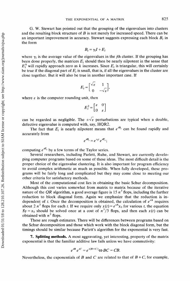
G. W. Stewart has pointed out that the grouping of the eigenvalues into clustersand the resulting block structure of B is not merely for increased speed. There can bean important improvement in accuracy. Stewart suggests expressing each block Bi inthe form

Bj TJ + Ej

where ,j is the average value of the eigenvalues in the flh cluster. If the grouping hasbeen done properly, the matrices E should then be nearly nilpotent in the sense that

Ek will rapidly approach zero as k increases. Since E is triangular, this will certainlybe true if the diagonal part of Ei is small, that is, if all the eigenvalues in the cluster areclose together. But it will also be true in another important case. If

E=0

where e is the computer rounding unit, then

can be regarded as negligible. The +x/-e perturbations are typical when a double,defective eigenvalue is computed with, say, HQR2.

The fact that E. is nearly nilpotent means that e tBj can be found rapidly andaccurately from

etBj e/ etE

computing etEJ by a few terms of the Taylor series.Several researchers, including Parlett, Ruhe, and Stewart, are currently develo-

ping computer programs based on some of these ideas. The most difficult detail is theproper choice of the eigenvalue clustering. It is also important for program efficiencyto avoid complex arithmetic as much as possible. When fully developed, these pro-grams will be fairly long and complicated but they may come close to meeting ourother criteria for satisfactory methods.

Most of the computational cost lies in obtaining the basic Schur decomposition.Although this cost varies somewhat from matrix to matrix because of the iterativenature of the OR algorithm, a good average figure is 15 n 3 flops, including the furtherreduction to block diagonal form. Again we emphasize that the reduction is in-dependent of t. Once the decomposition is obtained, the calculation of e tA requiresabout 2 n 3 flops for each t. If we require only x(t)= etAxo for various t, the equationSy =x0 should be solved once at a cost of n3/3 flops, and then each x(t) can beobtained with n 2 flops.

These are rough estimates. There will be differences between programs based onthe Schur decomposition and those which work with the block diagonal form, but thetimings should be similar because Parlett’s algorithm for the exponential is very fast.

7. Splitting methods. A most aggravating, yet interesting, property of the matrixexponential is that the familiar additive law fails unless we have commutivity"

tB tC t(B +C)<e e e BC CB.

Nevertheless, the exponentials of B and C are related to that of B + C, for example,

Dow

nloa

ded

01/3

1/18

to 1

28.2

10.1

07.2

6. R

edis

trib

utio

n su

bjec

t to

SIA

M li

cens

e or

cop

yrig

ht; s

ee h

ttp://

ww

w.s

iam

.org

/jour

nals

/ojs

a.ph

p


by the Trotter product formula [30]"

B+ ee lim (e B/m C/m)m.

METHOD 19. SPLITTING. Our colleagues M. Gunzburger and D. Gottleib sug-gested that the Trotter result be used to approximate eA by splitting A into B + C andthen using the approximation

A B/m C/m)m.e (e e

This approach to computing eA is of potential interest when the exponentials of B andC can be accurately and efficiently computed. For example, if B (A +A7")/2 andC (A-AT) then en and ec can be effectively computed by the methods of 5.For this choice we show in Appendix 2 that

I[[AT, A]II g(A)(7.1) lie a (e B/" ec/) e4m

where/z (A) is the log norm of A as defined in 2. In the following algorithm, thisinequality is used to determine the parameter m.

(a) Set B (A +A T)/2 and C (A A v)/2. Compute the factorization BQ diag(/zi)O T (oTo=I) using TRED2 and TQL2 [113]. Variations ofthese programs can be used to compute the factorization C UDUT whereuTu I and D is the direct sum of zero matrices and real 2-by-2 blocks ofthe form

a

corresponding to eigenvalues +/-ia.

(b) Determine rn =2 such that the upper bound in (7.1) is less than some

prescribed tolerance. Recall that tz(A) is the most positive eigenvalue of Band that this quantity is known as a result of step (a).

(c) Compute X=Q diag(e’’/")O T and Y= UeO/mUT. In the latter compu-tation, one uses the fact that

[ 0 a/ore] [ cos(a/m) sin(a/m))1exp-a/rn -sin (a/m) cos (a/rn

(d) Compute the approximation, (XY)z, to eA by repeated squaring.If we assume 5 n 3 flops for each of the eigenvalue decompositions in (a), then the

overall process outlined above requires about (13 +j)n 3 flops. It is difficult to assessthe relative efficiency of this splitting method because it depends strongly on thescalars IlIA , a]ll and tz (a) and these quantities have not arisen in connection with anyof our previous eighteen methods. On the basis of truncation error bounds, however,it would seem that this technique would be much less efficient than Method 3 (scalingand squaring) unless (a) were negative and Ilia , a][I much less than Ila[I.

Accuracy depends on the rounding errors which arise in (d) as a result of therepeated squaring. The remarks about repeated squaring in Method 3 apply also here"

Athere may be severe cancellation but whether or not this only occurs in sensitive eproblems is unknown.

Dow

nloa

ded

01/3

1/18

to 1

28.2

10.1

07.2

6. R

edis

trib

utio

n su

bjec

t to

SIA

M li

cens

e or

cop

yrig

ht; s

ee h

ttp://

ww

w.s

iam

.org

/jour

nals

/ojs

a.ph

p


For a general splitting A B + C, we can determine rn from the inequality

(7.2) lie a (e B/" e c/’)’ll <= [lIB,c]ll e iiBil+ltcll2m

which we establish in Appendix 2.To illustrate, suppose A has companion form

I-0 1\ 0... 0

iA--1Cn-1

If

and C e,,c 7- where c

and

0

(Co,’", c,-1) and e[= (0, 0, , 0, 1), then

nl [B]kleB/mk=0 k!

e c"-l/m- 1 Te C/m I+ enCCn-1

Notice that the computation of these scaled exponentials require only O(n 2) flops.Since IIBII 1, IIfII Ilcl], and II[B, fill--< 211c11, (7.2) becomes

e 1+11"11c11Ilea_(e/’,eC/,,),ll"m

The parameter m can be determined from this inequality.

8. Conclusions. A section called "conclusions" must deal with the obvious ques-tion: Which method is best? Answering that question is very risky. We don’t knowenough about the sensitivity of the original problem, or about the detailed per-formance of careful implementations of various methods to make any firmconclusions. Furthermore, by the time this paper appears in the open literature, anygiven conclusion might well have to be modified.

We have considered five general classes of methods. What we have called poly-nomial methods are not really in the competition for "best". Some of them require thecharacteristic polynomial and so are appropriate only for certain special problems andothers have the same stability difficulties as matrix decomposition methods but aremuch less efficient. The approaches we have outlined under splitting methods arelargely speculative and untried and probably only of interest in special settings. Thisleaves three classes in the running.

The only generally competitive series method is Method 3, scaling and squaring.Ward’s program implementing this method is certainly among the best currentlyavailable. The program may fail, but at least it tells you when it does. We don’t knowyet whether or not such failures usually result from the inherent sensitivity of the

Dow

nloa

ded

01/3

1/18

to 1

28.2

10.1

07.2

6. R

edis

trib

utio

n su

bjec

t to

SIA

M li

cens

e or

cop

yrig

ht; s

ee h

ttp://

ww

w.s

iam

.org

/jour

nals

/ojs

a.ph

p


Aproblem or from the instability of the algorithm. The method basically computes efor a single matrix A. To compute e ta for p arbitrary values of requires about p timesas much work. The amount of work is O(n3), even for the vector problem etaxo. Thecoefficient of n 3 increases as []a[[ increases.

Specializations of o.d.e, methods for the ea problem have not yet been im-plemented. The best method would appear to involve a variable order, variable stepdifference scheme. We suspect it would be stable and reliable but expensive. Its bestshowing on efficiency would be for the vector problem etAxo with many values ofsince the amount of work is only O(n2). It would also work quite well for vectorproblems involving a large sparse A since no "nonsparse" approximation to theexponential would be explicitly required.

The best programs using matrix decomposition methods are just now beingwritten. They start with the Schur decomposition and include some sort of eigenvalueclustering. There are variants which involve further reduction to a block form. In allcases the initial decomposition costs O(n 3) steps and is independent of andAfter that, the work involved in using the decomposition to compute etAxo fordifferent and x0 is only a small multiple of n 2.

Thus, we see perhaps three or four candidates for "best" method. The choice willdepend upon the details of implementation and upon the particular problem beingsolved.

Appendix 1. Inverse error analysis of Pad6 matrix approximation.LEPTA 1. If Ilnll < X, then log (I +H) exists and

[llog (I + n)[I <=1-Iln[----"

Proof. If IIn[I < a then log (I +H)= Ek=l (--1)k+l(Hk/k) and so

IIlog (I +n)ll -< E Ilnllk <- Ilnl[ E Iln[I [lUllk=a k k=O 1-

LEMMA 2. If IIAII 1/2 and p >0, then IIDo.(A)-lll<-(q +p)/p.Proof. From the definition of D,q (A) in 3, D(A) I +F where

Using the fact that

F=(P+q-J)!q! (-A)i

/=1 (p -t- q)!(q --j)!

(P + q -J)!q <[ql(p+q)!(q-f)!--

we find

IIFII <-- [pq ]i_ q

il + q lln <-p+q

IlAIl(e 1) <-p+q

and so I[Opq(A)-lll II(I + F)-all-<- 1/(1 -IIFII) <- (q + p)/p.LMMA 3. / Ilel[<_--1/2, q <-p, and p >- 1, then Rpq(A)= ea+v where

[IFII 81JAIl "+’+ (p +q)!(p +q + 1)!"

Dow

nloa

ded

01/3

1/18

to 1

28.2

10.1

07.2

6. R

edis

trib

utio

n su

bjec

t to

SIA

M li

cens

e or

cop

yrig

ht; s

ee h

ttp://

ww

w.s

iam

.org

/jour

nals

/ojs

a.ph

p


Proofi From the remainder theorem for Pad6 approximants [71],

Rp. (A) eA(-1) f01 )q(p+q)-.n’+q+lD,q(A)-1 e(-’)au’(1-u du,

and so e-aRpq(A)= I +H where

H (-1)"+1(p+ Io )qq)-----.A+"+aD,,(A)-1 e-"au(1 u du.

By taking norms, using Lemma 2, and noting that (p + q)/p es N 4 we obtain

1 p+q f01=(p+q)lA[+q+l e (1- )*P

4[[A[[++l Pq(p + q)l (p + q + 1)"

With the assumption ][A][ it is possible to show that for all admissable p and q,]]H]] and so from Lemma 1,

[log (t +)< <8A"+"+’ Pq1 -]]H]]= (p + q)(p + q + 1)"

Setting F log (I + H), we see that e-aR,,(A) I +H ev. The lemma now followsbecause A and F commute implying R,q(A) ea ef e a+v.

LEMMA 4, If [Ia[I 1/2 then R,q(a) ea+v where

(p + q)!(p + q + 1)!"

Pro@ The case p _-> q, p _-> 1 is covered by Lemma 1. If p + q 0, then F -A andthe above inequality holds. Finally, consider the case q > p, q-> 1. From Lemma 3,Rq,(-A) e-A+F where F satisfies the above bound. The lemma now follows because

II-FII IIFII and R,q(A)= [Rqp(-A)]-1 [e-A+F]-1 eA-F

THEOREM A.1. If IlAII/2 < 1/2, then [Roq(A/2i)]z a+Ee where

IIEll <8 P <--P!q!

Ilnll- (p + q)!(p + q + 1)!- (p + q)!(p + q + 1)!"

Proof. From Lemma 4, R,q(A/2i) ea+F where

pq!(p +q)!(p +q + 1)!"

The theorem follows by noting that if E 2iF, then

2

[Rpq(--)] A+E

COROLLARY 1./f IIAl[/2; N1/2, then [Tk(A/2i)]2’= eA+ where

()k 1 ()’- 1IIEII < 8 _<IIAII k + 1- k + 1

Dow

nloa

ded

01/3

1/18

to 1

28.2

10.1

07.2

6. R

edis

trib

utio

n su

bjec

t to

SIA

M li

cens

e or

cop

yrig

ht; s

ee h

ttp://

ww

w.s

iam

.org

/jour

nals

/ojs

a.ph

p


COROLLARY 2. If IIA[I/2 <- 1/2, then [Rqq(A/2i)]2’= ea+E, where

()2q (q!)2 ()2q--3 (q I)2IIEII__< 8 -<

[Imll (2q)!(2q + 1)!- (2q)!(2q + 1)!"

Appendix 2. Accuracy of splitting techniques. In this appendix we derive theinequalities (7.1) and (7.2). We assume throughout that A is an n-by-n matrix andthat

A =B+C.

It is convenient to define the matrices

Sm eA/m,and

Tm eS/m e C/m

where m is a positive integer. Our goal is to bound ]]Sm -Tmml]. To this end we shallhave to exploit the following properties of the log norm/x (A) defined in 2"

(i) ]]etAll < e tz(a)t (t >--_ O)

(ii) /x (A) =< IIA(iii) /x (B + C) -</x (B) + IIcII,

These and other results concerning log norms are discussed in references [35]-[42].LEMMA 1. If 19 _-->max {/x (A),/z(B)+/x (C)} then

Proof. Following Reed and Simon [11] we have

m-1

S:- T= E S(S.- Tm)T-1-k.k=O

Using log norm property (i)it is easy to show that both IlSmll and IlTmll are boundedabove by e/m and thus

m--1

[Is:- T:II E IlSmllllSm- TmIIIITII m-l-kk=O

m-1

llSm-Tmll E e ek=0

from which the lemma immediately follows.In Lemmas 2 and 3 we shall make use of the notation

t=t

F(t) =F(tl)-f(to),t=

where F(t) is a matrix whose entries are functions of t.LEMMA 2.

Tm Sm ffoetB/m[e(1-t)A/m, Xc] em

Ok/m O(m-l-k)/m

tC/m dt.

Dow

nloa

ded

01/3

1/18

to 1

28.2

10.1

07.2

6. R

edis

trib

utio

n su

bjec

t to

SIA

M li

cens

e or

cop

yrig

ht; s

ee h

ttp://

ww

w.s

iam

.org

/jour

nals

/ojs

a.ph

p


Proof. We have Tm- Sm e ‘/m e (1-t)A/m e,C/m it=t=o and thus

Io1{ d (1-t)A/m tC/m}Tm Sm -d7 [ett/m e e dt.

The lemma follows since

d tB/m (1-t)A/m tC/m-[e e e ]=e ’n/m[ e {l-OA/m 1CI em

tCl

LEMMA 3. IfX and Y are matrices then

II[e x, Y]II e"X)ll[x, Y]II.

Proof. We have [e x, Y]=etXyetl-t)xlt=,= and thus

Io’ d ,Xye -t)x]} dt.[e x, y]= {_7[e (1

Since d/dt[etXye (1-’)x] etX[x, Y] e(1-x we get

II[e x, g]ll--< Io Ile’Xllll[x’ g]l[lle (1-t)xll dt

-< ]I[X, Y][[ Io e "(X)te (x)(1-t) dt

from which the lemma immediately follows.THEOREM A.2./f 19 >_--max {Ix(A), Ix(B)+ Ix(C)}, then

1IIs T[I el[[B, Ell[.

Proof. If 0 =< =< 1 then an application of Lemma 3 with X- (1 t)A/m andY =- C/m yields

]lie (1-t)a/m, C/m ][[ <- et(A)(1-t)/m[[[(1 --t)A/m, C/m ]ll

-<-e (1-‘)/m(1 -t)ll[B, Clll.m

By coupling this inequality with Lemma 2 we can bound ]]T- Stall"

IlTm-Stall<= fro [le’/mllll[e(1-’a/" C/mllllle’c/mll dt

<-- IO eu’(B)t/m e(R)(1-t)/m(lm’t)ll[B’ C]ll e "(c)’/m dt

1 eO/m II[B, C]ll---- :2-2 m

The theorem follows by combining this result with Lemma 1.COROLLARY 1. IfB =(A +A*)/2 and C=(A-A*)/2 then

1IIs TII 7 e"a)ll[A*, A 111.z4m

Dow

nloa

ded

01/3

1/18

to 1

28.2

10.1

07.2

6. R

edis

trib

utio

n su

bjec

t to

SIA

M li

cens

e or

cop

yrig

ht; s

ee h

ttp://

ww

w.s

iam

.org

/jour

nals

/ojs

a.ph

p


Proof. Since tz (A) tx (B) and tz (C) 0, we can set 19 =/x (A). The corollary isestablished by noting that [B, C] 1/2[A*, A].

COROLLARY 2.

IIs.

Proof. max {x (A), tz (B)+ tx (C)} =<Acknowledgments. We have greatly profited from the comments and suggestions

of so many people that it is impossible to mention them all. However, we areparticularly obliged to B. N. Parlett and G. W. Stewart for their very perceptiveremarks and to G. H. Golub for encouraging us to write this paper. We are obliged toProfessor Paul Federbush of the University of Michigan for helping us with theanalysis in Appendix 2. Finally, we would like to thank the referees for theirnumerous and most helpful comments.

REFERENCES

Background.[1] R. BELLMAN, Introduction to Matrix Analysis, McGraw-Hill, New York, 1969.[2] C. DAVIS, Explicit functional calculus, J. Linear Algebra Appl., 6 (1973), pp. 193-199.[3] V. N. FADDEEVA, Computational Methods ofLinear Algebra, Dover Publications, New York, 1959.[4] G. E. FORSYTHE, M. A. MALCOLM AND C. B. MOLER, Computer Methods for Mathematical

Computations, Prentice-Hall, Englewood Cliffs, NJ, 1977.[5] J. S. FRAME, Matrix ]’unctions and applications, part II: Functions of matrices, IEEE Spectrum,

(April, 1964), pp. 102-108.[6] ., Matrix functions and applications, part IV: Matrix functions and constituent matrices, Ibid.,

(June, 1964), pp. 123-131.[7] ., Matrix functions and applications, part V: Similarity reductions by rational or orthogonal

matrices, Ibid., (July, 1964), pp. 103-116.[8.] F. R. GANTMACHER, The Theory of Matrices, Vols. and II, Chelsea Publishing Co., New York,

1959.[9] C. C. MACDUFrEE, The Theory of Matrices, Chelsea, New York, 1956.

[10] L. MIRSKY, An Introduction to Linear Algebra, Oxford University Press, London, 1955.[11] M. REED AND B. SIMON, Functional Analysis, Academic Press, New York, 1972.[12] R. F. RINEHART, The equivalence of definitions of a matrix function, Amer. Math. Monthly, 62

(1955), pp. 395-414.[13] P. C. ROSENBLOOM, Bounds on ]:unctions of matrices, Ibid., 74 (1967), pp. 920-926.[14] J. H. WILKINSON, The Algebraic Eigenvalue Problem, Oxford University Press, Oxford, 1965.

Properties and representations.[15] T. M. APOSTOL, Some explicit formulas ]’or the matrix exponential, Amer. Math. Monthly, 76 (1969),

pp. 284-292.[16] R. W. ATHERTON AND A. E. DE GANCE, On the evaluation of the derivative of the matrix

exponential [unction, IEEE Trans. Automatic Control, AC-20 (1975), pp. 707-708.[17] A. BRADSHAW, The eigenstructure of sample data systems with confluent eigenvalues, Internat. J.

Systems Sci., 5 (1974), pp. 607-613.[18] R. BELLMAN, Perturbation Techniques in Mathematics, Physics, and Engineering, Holt, Rinehart,

and Winston, New York, 1964.[19] J. C. CAVENDISH, On the norm of a matrix exponential, this Review, 17 (1975), pp. 174-175.[20] C. G. CULLEN, Remarks on computing e at, IEEE Trans. Automatic Control, AC-16 (1971), pp.

94-95.[21] F. FER, Resolution de l’equation matricelle dU/dt pUpar produit infini d’exponentielles, Acad. Roy.

Belg. Bull. CI. Sci., 44 (1958), pp. 819-829.[22] E. P. FULMER, Computation of the matrix exponential, Amer. Math. Monthly, 82 (1975), pp.

156-159.

Dow

nloa

ded

01/3

1/18

to 1

28.2

10.1

07.2

6. R

edis

trib

utio

n su

bjec

t to

SIA

M li

cens

e or

cop

yrig

ht; s

ee h

ttp://

ww

w.s

iam

.org

/jour

nals

/ojs

a.ph

p


[23] B. KA,GSTROM, Bounds and perturbation bounds ]’or the matrix exponential, BIT, 17 (1977), pp.39-57.

[24] T. KATO, Perturbation Theory for Linear Operators, Chap. 9, Springer-Verlag, New York, 1966.[25] R. B. KIRCHNER, An explicit formula ior e at, Amer. Math. Monthly, 74 (1967), pp. 1200-1204.[26] H. O. KREISS, Ober Matrizen die beschriinkte Halbgruppen erzeuge, Math. Scand., 7 (1959), pp.

71-80.[27] D. L. POWERS, On the eigenstructure of the matrix exponential, Internat. J. Systems Sci., 7 (1976), pp.

723-725.[28] E. J. PUTZER, Avoiding the Jordan canonical ’orm in the discussion o]: linear systems with constant

coefficients, Amer. Math. Monthly, 73 (1966), pp. 2-7.[29] N. M. RICE, More explicit ]ormulas ]:or the exponential matrix, Queen’s Mathematical Reprints no.

1970-21, Queen’s University, Kingston, Ontario, 1970.[30] H. F. TROTTER, Product otsemigroups oloperators, Proc. Amer. Math. Soc., 10 (1959), pp. 545-551.[31 C. F. VAN LOAN, A study o]" the matrix exponential, Numerical Analysis Report no. 7, Department of

Mathematics, University of Manchester, Manchester, England, 1975.[32] , The sensitivity o]" the matrix exponential, SIAM J. Numer. Anal., 14 (1977), pp. 971-981.[33] G. H. WEISS AND A. A. MARADUDIN, The Baker-Hausdorff formula and a problem in crystal

physics, J. Math. and Phys., 3 (1962), pp. 771-777.[34] A. D. ZIEBUR, On determining the structure of A by analyzing e at, this Review, 12 (1970), pp.

98-102.

Log norms and stability.[35] W. A. COPPEL, Stability and Asymptotic Behavior o] Differential Equations, D. C. Heath, Boston,

1965.[36] G. DAHLQUIST, Stability and error bounds in the numerical integration o] ordinary differential

equations, Transactions of the Royal Institute of Technology, no. 130, Stockholm, Sweden, 1959.

[37] C. A. DESOER AND H. HANEDA, The measure o] a matrix as a tool to analyze computer algorithms

]or circuit analysis, IEEE Trans. Circuit Theory, CT-19 (1972), pp. 480-486.[38] E. DEUTSCH, On matrix norms and logarithmic norms, Numer. Math., 24 (1975), pp. 49-51.[39] C. V. PAO, Logarithmic derivatives o] a square matrix, J. Linear Algebra Appl., 6 (1973), pp.

159-164.[40] , A further remark on the logarithmic derivatives oi a square matrix, Ibid., 7 (1973), pp.

275-278.[41] T. STROM, Minimization of norms and logarithmic norms by diagonal similarities, Computing, 10

(1972), pp. 1-9.[42] , On logarithmic derivatives, SIAM J. Numer. Anal., 12 (1975), pp. 741-753.

Survey articles.[43] M. HEALEY, Study o" methods o]" computing transition matrices, Proc. IEEE, 120 (1973), pp.

905-912.[44] C. B. MOLER, Difficulties in computing the exponential o] a matrix, Proceedings of the Second

USA-Japan Computer Conference, A.F.I.P.S., Montvale, NJ, 1975, pp. 79-82.

Truncated Taylor series.[45] L. Y. BAHAR AND m. K. SINHA, Matrix exponential approach to dynamic response, Computers and

Structures, 5 (1975), pp. 159-165.[46] T. A. BICKART, Matrix exponential: Approximation by truncated power series, Proc. IEEE, 56 (1968),

pp. 372-373.[47] G. J. BIERMAN, Power series evaluation of transition and covariance matrices, IEEE Trans. Auto-

matic Control, AC-17 (1972), pp. 228-231.[48] D. A. CALAHAN, Numerical solution of linear systems with widely separated time constants, Proc.

IEEE, 55 (1967), pp. 2016-2017.[49] K. C. DALY, Evaluating the matrix exponential, Electron. Lett., 8 (1972), p. 390.

[50] W. EVERLING, On the evaluation of eat by power series, Proc. IEEE, 55 (1967), p. 413.

[51] D. A. GALL, The solution o1 linear constant coefficient ordinary differential equations with APL,Comput. Methods Mechanics and Engrg., (1972), pp. 189-196.

[52] M. L. LIOU, A novel method o]: evaluating transient response, Proc. IEEE, 54 (1966), pp. 20-23.

[53] J. B. MANKIN AND J. C. HUNG, On roundoff errors in computation ol transition matrices, Reprints of

the Joint Automatic Control Conference, pp. 60-64, University of Colorado, Boulder, CO, 1969.

Dow

nloa

ded

01/3

1/18

to 1

28.2

10.1

07.2

6. R

edis

trib

utio

n su

bjec

t to

SIA

M li

cens

e or

cop

yrig

ht; s

ee h

ttp://

ww

w.s

iam

.org

/jour

nals

/ojs

a.ph

p


[54] E. J. MASTASCUSA, A relation between Liou’s method and fourth order Runge-Kutta method ]’orevaluation of transient response, Proc. IEEE, 57 (1969), pp. 803-804.

[55] J. B. PLANT, On the computation of transient matrices for time invariant systems, Ibid., 56 (1968), pp.1397-1398.

[56] M. M. SHAH, On the evaluation of e At, Cambridge Report CUED/B-Control TRS, Cambridge,England, 1971.

[57] ., Analysis o]: roundoffand truncation errors in the computation o1 transition matrices, CambridgeReport CUED/B-Control TR12, Cambridge, England, 1971.

[58] C. J. STANDISH, Truncated Taylor series approximation to the state transition matrix of a continuous

parameter Markov chain, J. Linear Algebra Appl., 12 (1975), pp. 179-183.[59] D. E. WHITNEY, Propogated error bounds for numerical solution of transient response, Proc. IEEE, 54

(1966), pp. 1084-1085.[60]. More similarities between Runge-Kutta and matrix exponential methods for evaluating

transient response, Ibid., 57 (1969), pp. 2053-2054.

Rational approximation.[61] J. L. BLUE AND H. K. GUMMEL, Rational approximations to the matrix exponential for systems of stiff

differential equations, J. Computational Phys., 5 (1970), pp. 70-83.[62] W. J. COPY, G. MEINARDUS AND R. S. VARGA, Chebyshev rational approximation to exp f-x) in

[0, +] and applications to heat conduction problems, J. Approximation Theory, 2 (1969), pp.50-65.

[63] W. FAIR AND Y. LUKE, Pad approximations to the operator exponential, Numer. Math., 14 (1970),pp. 379-382.

[64] S. P. NORSETT, C-polynomials for rational approximation to the exponential function, Ibid., 25(1975), pp. 39-56.

[65] E. B. SAFF, On the degree of best rational approximation to the exponential function, J. ApproximationTheory, 9 (1973), pp. 97-101.

[66] E. B. SAFE AND R. S. VARGA, On the zeros and poles of Pad approximants to exp (z), Numer.Math., 25 (1975), pp. 1-14.

[67] R. E. SCRATON, Comment on rational approximants to the matrix exponential, Electron. Lett., 7(1971 ), pp. 260-261.

[68] J. L. SIEMIENIUCIq, Properties of certain rational approximations to e -, BIT, 16 (1976), pp. 172-191.[69] G. SIEMIENIUCH AND I. GLADWELL, On time discretizations ]’or linear time dependent partial

differential equations, Numerical Analysis Report no. 5, Department of Mathematics, University ofManchester, Manchester, England, 1974.

[70] D. M. TRUJILLO, The direct numerical integration of linear matrix differential equations using Padapproximations, Internat. J. for Numer. Methods Engrg., 9 (1975), pp. 259-270.

[71] R. S. VARGA, On higher order stable implicit methods ]or solving parabolic partial differentialequations, J. Math. Phys., 40 (1961), pp. 220-231.

[72] R. C. WARD, Numerical computation of the matrix exponential with accuracy estimate, SIAM J.Numer. Anal., 14 (1977), pp. 600-610.

[73] A. WRAGG AND C. DAVIES, Evaluation of the matrix exponential, Electron. Lett., 9 (1973), pp.525-526.

[74] , Computation of the exponential of a matrix I: Theoretical considerations, J. Inst. Math. Appl.,11 (1973), pp. 369-375.

[75] , Computation of the exponential of a matrix II: Practical considerations, Ibid., 15 (1975), pp.273-278.

[76] V. ZAKIAN, Rational approximants to the matrix exponential, Electron. Lett., 6 (1970), pp. 814-815.[77] V. ZAKIAN AND R. E. SCRATON, Comments on rational approximations to the matrix exponential,

Ibid., 7 (1971), pp. 260-262.

Polynomial methods.[78] G. J. BIERMAN, Finite series solutions for the transition matrix and covariance of a time-invariant

system, IEEE Trans. Automatic Control, AC-16 (1971), pp. 173-175.[79] J. A. BOEHM AND J. A. THURMAN, An algorithm for generating constituent matrices, IEEE Trans.

Circuit Theory, CT-18 (1971), pp. 178-179.[80] C. F. CHEN AND R. R. PARKER, Generalization of Heaviside’s expansion technique to transition

matrix evaluation, IEEE Trans. Educ., E-9 (1966), pp. 209-212.[81] W. C. DAVIDON, Exponential Function of a 2-by-2 Matrix, Hewlett-Packard HP65 Library Pro-

gram.

Dow

nloa

ded

01/3

1/18

to 1

28.2

10.1

07.2

6. R

edis

trib

utio

n su

bjec

t to

SIA

M li

cens

e or

cop

yrig

ht; s

ee h

ttp://

ww

w.s

iam

.org

/jour

nals

/ojs

a.ph

p


[82] S. DEARDS, On the evaluation ofexp (tA), Matrix Tensor Quart., 23 (1973), pp. 141-142.[83] S. GANAPATHY AND R. S. RAO, Transient response evaluation from the state transition matrix, Proc.

IEEE, 57 (1969), pp. 347-349.[84] I. C. GOKNAR, On the evaluation of constituent matrices, Internat. J. Systems Sci., 5 (1974), pp.

213-218.[85] I. I. KOLODNER, On exp (tA) with A satisfying a polynomial, J. Math. Anal. Appl., 52 (1975), pp.

514-524.[86] Y. L. Kuo AND M. L. LIOU, Comments on "A novel method ofevaluating e At in closed form", IEEE

Trans. Automatic Control, AC-16 (1971), p. 521.[87] E. J. MASTASCUSA, A method of calculating e At based on the Cayley-Hamilton theorem, Proc.

IEEE, 57 (1969), pp. 1328-1329.[88] K. R. RAO AND N. AHMED, Heaviside expansion of transition matrices, ibid., 56 (1968), pp.

884-886.[89], Evaluation of transition matrices, IEEE Trans. Automatic Control, AC-14 (1969), pp.

779-780.[90] B. RoY, A. K. MANDAL, D. RoY CHOUDHURY, A. K. CHOUDHURY, On the evaluation of the

state transition matrix, Proc. IEEE, 57 (1969), pp. 234-235.[91] M. N. S. SWAMY, On a formula for evaluating e At when the eigenvalues are not necessarily distinct,

Matrix Tensor Quart., 23 (1972), pp. 67-72.[92] M. VIDYSAGER, A novel method of evaluating e in closed form, IEEE Trans. Automatic Control,

AC-15 (1970), pp. 600-601.[93] V. ZAKIAN, Solution of homogeneous ordinary linear differential equations by numerical inversion of

Laplace transforms, Electron. Lett., 7 (1971), pp. 546-548.

Companion matrix methods.[94] A. K. CHOUDHURY, ET AL., Oft the evaluation ofeAt, Proc. IEEE, 56 (1968), pp. 1110-1111.[95] L. FALCIDIENO AND A. LUViNSON, A numerical approach to computing the companion matrix

exponential, CSELT Rapporti technici, No. 4, 1975, pp. 69-71.[96] C. J. HARRIS, Evaluation of matrix polynomials in the state companion matrix of linear time invariant

systems, Internat. J. Systems Sci., 4 (1973), pp. 301-307.[97] D. W. KAMMLER, Numerical evaluation of exp (At) when A is a companion matrix, unpublished

manuscript, University of Southern Illinois, Carbondale, IL, 1976.[98] I. KAUFMAN, Evaluation of an analytical function of a companion matrix with distinct eigenvalues,

Proc. IEEE, 57 (1969), pp. 1180-1181.[99] ., A note on the "Evaluation of an analytical function of a companion matrix with distinct

eigenvalues", Ibid., 57 (1969), pp. 2083-2084.[100] I. KAUFMAN AND P. H. ROE, On systems described by a companion matrix, IEEE Trans. Automatic

Control, AC-15 (1970), pp. 692-693.101] I. KAUFMAN, H. MANN AND J. VLACH, A fast procedure for the analysis of linear time invariant

networks, IEEE Trans. Circuit Theory, CT-18 (1971), pp. 739-741.[102] M. L. Lou, Evaluation of the transition matrix, Proc. IEEE, 55 (1967), pp. 228-229.[103] A. K. MANDAL, ET AL., Numerical computation method for the evaluation of the transition matrix,

Ibid., 116 (1969), pp. 500-502.[104] W. E. THOMSON, Evaluation of transient response, Ibid., 54 (1966), p. 1584.

Ordinary differential equations.105] B. L. EHLE AND J. D. LAWSON, Generalized Runge-Kutta processes for stiff initial value problems, J.

Inst. Math. Appl., 16 (1975), pp. 11-21.[106] C. W. GEAR, Numerical Initial Value Problems in Ordinary Differential Equations, Prentice-Hall,

Englewood Cliffs, NJ, 1971.[107] L. F. SHAMPINE AND M. K. GORDON, Computer Solution of Ordinary Differential EquationsThe

Initial Value Problem, W. H. Freeman and Co., San Francisco, 1975.[108] L. F. SHAMPINE AND H. A. WATTS, Practical solution of ordinary differential equations by Runge-

Kutta methods, Sandia Lab Report SAND 76-0585 Albuquerque, NM, 1976.109] J. STARNER, Numerical solution of implicit differential-algebraic equations, Ph.D. Thesis, University

of New Mexico, Albuquerque, NM, 1976.

Matrix decomposition methods.[110] G. H. GOLUB AND J. H. WILKINSON, Ill-conditioned eigensystems and the computation of the

Jordan canonical form, this Review, 18 (1976), pp. 578-619.

Dow

nloa

ded

01/3

1/18

to 1

28.2

10.1

07.2

6. R

edis

trib

utio

n su

bjec

t to

SIA

M li

cens

e or

cop

yrig

ht; s

ee h

ttp://

ww

w.s

iam

.org

/jour

nals

/ojs

a.ph

p


111] B. KAGSTROM AND A. RUHE, An algorithm for numerical computation of the Jordan normalform ofa complex matrix, Report UMINF 51.74, Department of Information Processing, University ofUmea, Umea, Sweden, 1974. To appear in Trans. Math. Softwave.

[112] B. N. PARLETT, A recurrence among the elements offunctions of triangular matrices, Linear AlgebraAppl., 14 (1976), pp. 117-121.

[113] B. T. SMITH, J. M. BOYLE, J. J. DONGARRA, B. S. GARBOW, Y. IKEBE, V. C. KLEMA, C. B.MOLER, Matrix Eigensystem Routines: EISPACK Guide, 2nd ed., Lecture Notes in ComputerScience 6, Springer-Verlag, New York, 1976.

Integrals involving e At

[114] E. S. ARMSTRONG AND A. K. CAGLAYAN, An algorithm for the weighting matrices in thesampled-data optimal linear regulator problem, NASA Technical Note, TN D-8372, 1976.

[115] J. JOHNSON AND C. L. PHILLIPS, An algorithm ]:or the computation of the integral of the statetransition matrix, IEEE Trans. Automatic Control, AC-16 (1971), pp. 204-205.

116] C. KALLSTROM, Computing exp (A) and exp (As)ds, Report 7309, Division of Automatic Control,Lund Institute of Technology, Lund, Sweden, 1973.

117] A. H. LEVIS, Some computational aspects of the matrix exponential, IEEE Trans. Automatic Control,AC-14 (1969), pp. 410-411.

[118] C. F. VAN LOAN, Computing integrals involving the matrix exponential, Cornell Computer ScienceReport TR 76-270, 1976.

Selected applications.[119] F. H. BRANIN, Computer methods of network analysis, Proc. IEEE, 55 (1967), pp. 1787-1801.[120] R. BROCKETT, Finite Dimensional Linear Systems, John Wiley, New York, 1970.[121] K. F. HANSEN, B. V. KOEN AND W. W. LITTLE, Stable numerical solutions of the reactor kinetics

equations, Nuclear Sci. Engrg., 22 (1965), pp. 51-59.[122] J. A. W. DA NOBREGA, A new solution ofthe point kinetics equations, Ibid., 46 (1971), pp. 366-375.

Dow

nloa

ded

01/3

1/18

to 1

28.2

10.1

07.2

6. R

edis

trib

utio

n su

bjec

t to

SIA

M li

cens

e or

cop

yrig

ht; s

ee h

ttp://

ww

w.s

iam

.org

/jour

nals

/ojs

a.ph

p

Documents

Nineteen Dubious Ways to Compute the Exponential of a Matrix