Embed Size (px)
Citation preview

New Models for Pseudo Self-Similar Tra�c
Stephan Robert� Jean-Yves Le Boudec y
July 3, 1996
Abstract
After measurements on a lan at Bellcore, it is known that data tra�c is extremely variable on time
scales ranging from milliseconds to days. The tra�c behaves quite di�erently to what has been assumed
until now; tra�c sources were generally characterized by short term dependences but characteristics
of the measured tra�c have shown that it is long term dependent. Therefore, new models (such as
Fractional Brownian motion, arima processes and Chaotic maps) have been applied. Although they
are not easily tractable, one big advantage of these models is that they give a good description of the
tra�c using few parameters. In this paper, we describe a Markov chain emulating self-similarity which is
quite easy to manipulate and depends only on two parameters (plus the number of states in the Markov
chain). An advantage of using it is that it is possible to re-use the well-known analytical queuing theory
techniques developed in the past in order to evaluate network performance. The tests performed on the
model are the following: Hurst parameter (by the variances method) and the so-called \visual" test. A
method of �tting the model to measured data is also given. In addition, considerations about pseudo
long range dependences are exposed.
1 Introduction
Recent studies of high quality tra�c measurements have revealed that tra�c behaves quite di�erently to
what has been assumed until now. It has been observed that a large number of tra�c sources produces
a self-similar [1, 2] behavior over large time scales. Imagine a cluster composed of smaller clusters which
look almost identical to the entire cluster, but scaled down by some factor. Each of these smaller clusters
is again composed of smaller ones, and those of even smaller ones again. We can identify without di�culty,
di�erent generations of cluster on cluster; this is what we call self-similarity. Here, in the case of tra�c
behavior, self-similarity indicates that the behavior of a process is very similar (in a distributional sense).
Mathematically, this concept is associated to the limit concept and therefore it will require some care.
For time-series, the concept of \self-similarity" indicates a form of invariance with respect to changes of
�University of California at Berkeley, Department of EECS, CA 94720, USAySwiss Fereral Institute of Technology (EPFL), Laboratoire des r�eseaux de communication, CH-1015 Lausanne, Switzerland
1

time-scales. Positive correlations, for example, are present at each time-scale, which is not the case for
classical models. On the contrary, aggregated tra�c become less bursty when the interval time grows. To
summarize, a self-similar process can be sketched in the time direction by a factor a and in amplitude by
r: y(t) = rx(t=a) where y(t) is the rescaled random function and x(t) the original random function. For
ordinary Brownian motion, we need to scale the amplitude byp2 when time is scaled by a factor of 2.
Scaling amplitudes by other factors, such as 1 or 2, changes the statistical properties of the graphs. This
Brownian motion is restrictive, therefore Mandelbrot introduced the fractional Brownian motion where it
is possible to arbitrarily scale the vertical axis by a factor between 1 and 2. For small factors (' 1), the
graph appears rougher than the Brownian motion and for large factor (' 2), the Brownian motion appears
much smoother. For Brownian motion, this factor is set to 0.5. This factor is usually written as H and
often called the Hurst exponent. Hurst [1] was an hydrologist who did some work on scaling properties of
river uctuation. The range for the exponent is from 0, corresponding to very rough random fractal curves,
to 1 corresponding to rather smooth looking random fractals. In fact, there exists a direct relation between
H and the fractal dimension of the graph of a random fractal [3]. Ordinary Brownian motion is a process
X(t) with Gaussian increments and var(X(t2) �X(t1)) / jt2 � t1j2H where H = 1=2. The generalization
of parameters 0 < H < 1 is called fractional Brownian motion. If X(t)�X(t0) and ([X(rt)�X[t0])=(rH)
are statistically undistinguable (they have the same �nite dimensional joint distribution functions for any
t0 and r > 0), we say that they are statistically self-similar with parameter H. In this case, if X(t0) = 0
for t0 = 0, X(t) and X(rt)=rH are statistically undistinguable. Then, if X(t) is accelerated by a factor r:
X(rt), it is rescaled by dividing the amplitudes by rH .
2 New model
2.1 Considerations on pseudo long-range dependences
Mathematically [4], the di�erence between short-range and long-range dependencies is clear: for a short-
range dependent process.
� P1�=0 cov(Xt;Xt+� ) is convergent
� spectrum at 0 is �nite
� var(X(m)) is for large m asymptotically of the form varXm
� the averaged process X(m)k tends to second order pure noise as m!1
and for a long-range dependent process:
2

� P1�=0 cov(Xt;Xt+� ) is divergent
� spectrum at 0 is singular
� var(X(m)) is for large m asymptotically of the form m��
� the averaged process X(m)k don't tend to second order pure noise as m!1
There is another category: the processes that have long-range dependences of index �, but do not have
a degenerate correlation structure as m!1.
All stationary autoregressive-moving average processes of �nite order, all �nite Markov chains (including
semi-Markov processes) are included in the �rst category. In the second category, we have the fractional
Brownian motion [5], arima processes [6]and chaotic maps [7] which have long-range dependences. How-
ever, if we look at this de�nition, we see that a process having \long term dependences", but which is limited
is considered as a short term dependences process. We see for example that Ethernet measurements have
long term dependences, at least over 4 or 5 orders of magnitude. In other words, if we represent the number
of Ethernet packets arriving in a time-interval of 1 s, then the statistics of the number of packets looks the
same for 10 s, 100 s, 1000 s, 10000 s and is distinctively di�erent from a pure noise. However in the order
of days, researchers at Bellcore have observed a stabilization of the index of dispersion [8] indicating a lack
of self-similarity. So, according to the de�nition, a short term dependences process would be su�cient to
model lan tra�c. The di�erence with other processes (Poisson, on-off, ...) is striking and they should
be categorized di�erently. Therefore, we propose to name them: pseudo long-range dependent processes.
Another problem which arises is the length of the measurements: no variable can be measured during an
in�nite amount of time. Especially in the networking world (in dimensioning purposes) where the tra�c is
increasing day after day at an uncontrollable rate. A pseudo long-range dependent process is able to model
(as well as an (exactly) long-range dependent process) aggregated tra�c over several time-scales. In fact,
this de�nition of long term dependences processes comes historically from the importance of self-similar
processes which are able to give an elegant explanation to an empirical law (Hurst e�ect). In practice,
we have always a �nite set of data and asymptotic conditions are never met. We propose here to model
lan tra�c with Markov chains. As we will see in section 2.2, the auto-covariance function is a sum of
exponentials. So we approximate a hyperbolic decaying auto-covariance function by a sum of exponentials.
One myth is that it is too complicated because of the number of parameters to manage [6]. In this paper,
we give an example where it is su�cient to consider only three parameters and there are surely other
solutions to resolve this problem. Because of this di�culty, Markovian models have not been considered
yet.
2.2 Suggested process
In this paper, we investigate the use of a simple, discrete time Markov modulated model for representing
self-similar data tra�c. We consider the process of cell arrivals on a slotted link; callXt the random variable
3
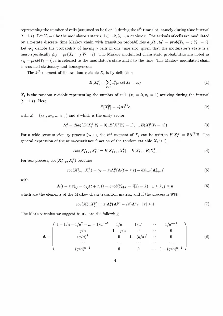
representing the number of cells (assumed to be 0 or 1) during the tth time slot, namely during time interval
[t�1; t). Let Yt = i be the modulator's state i, i 2 1; 2; 3; :::; n at time t. The arrivals of cells are modulated
by a n-state discrete time Markov chain with transition probabilities aij(t1; t2) = prob(Yt2 = jjYt1 = i).
Let �ij denote the probability of having j cells in one time slot, given that the modulator's state is i;
more speci�cally �ij = pr(Xt = jjYt = i). The Markov modulated chain state probabilities are noted as
�it = prob(Yt = i), i is referred to the modulator's state and t to the time. The Markov modulated chain
is assumed stationary and homogeneous.
The kth moment of the random variable Xt is by de�nition
E[Xkt ] =
Xi�1
xki prob(Xt = xi) (1)
Xt is the random variable representing the number of cells (x0 = 0; x1 = 1) arriving during the interval
[t� 1; t). Here
E[Xkt ] = ~�t�
(k)t ~e (2)
with ~�t = (�1t ; �2t ; :::; �nt) and ~e which is the unity vector.
�kt = diag(E(Xk
t jYt = 0); E(Xkt jYt = 1); :::; E(Xk
t jYt = n)) (3)
For a wide sense stationary process (wss), the kth moment of Xt can be written E[Xkt ] = ~��(k)~e. The
general expression of the auto-covariance function of the random variable Xt is [9]
cov(Xst+� ;X
kt ) = E[Xs
t+� ;Xkt ]�E[Xs
t+� ]E[Xkt ] (4)
For our process, cov(Xst+� ;X
kt ) becomes
cov(Xst+� ; X
kt ) = � = ~�t�
kt (A(t+ �; t)� ~e~�t+� )�
st+�~e (5)
with
A(t+ �; t)ij = akj(t+ �; t) = prob(Yt+� = jjYt = k) 1 � k; j � n (6)
which are the elements of the Markov chain transition matrix, and if the process is wss
cov(Xs� ;X
k0 ) = ~�t�
kt (A
j� j � ~e~�)�s~e j� j � 1 (7)
The Markov chains we suggest to use are the following
A =
0BBBBBBB@
1� 1=a � 1=a2 � :::� 1=an�1 1=a 1=a2 � � � 1=an�1
q=a 1� q=a 0 � � � 0
(q=a)2 0 1� (q=a)2 � � � 0
� � � � � � � � � � � � � � �(q=a)n�1 0 0 � � � 1� (q=a)n�1
1CCCCCCCA
(8)
4

� =
0BBBBBBB@
1 0 0 � � � 0
0 0 0 � � � 0
0 0 0 � � � 0
� � � � � � � � � � � � � � �0 0 0 � � � 0
1CCCCCCCA
(9)
So, the Markov chain has only 3 parameters: a; q plus the number of states in the Markov chain n.
2.3 Foundations of the model
To build our model, we have considered a theory which was developed approximately 20 years ago by
Courtois, the theory of decomposability. Courtois's analysis [10] is based on the important observation
that large computing systems can e�ectively be regarded as nearly completely decomposable systems.
Systems are arranged in a hierarchy of components and subcomponents with strong interactions within
components at the same level and lower interactions between other components. Near decomposability has
been observed in other domains than computing: in economics, in biology, genetics, social sciences. The
pioneers in this domain are Simon and Ando who studied several study-cases in economics and in physics
[11]. What they stated is that aggregation of variables in a nearly decomposable system must separate the
analysis of the short term and long term dynamics. They proved two major theorems. The �rst says that
a nearly-decomposable system can be analyzed by a completely decomposable system if the intergroup
dependences are su�ciently weak compared to intra-group ones. The second theorem says that even in
the long term, the results obtained in the short term will remain approximately valid in the long term, as
far as the relative behavior of the variables of the same group is concerned. In our study, the problem is
the inverse: we postulate that the LAN tra�c is composed of di�erent time-scales.
The Markov chain we propose to analyze here is in fact decomposable at several levels. In a �rst step,
the development is done for only one level of decomposability. The development deviates from those of
Simon, Ando and Courtois. As seen before, the Markov chain to study is characterized (section 2.2) by its
transition matrix (n � n) A and its state probabilities ~� (~�t+1 = ~�tA), A is nearly decomposable. Let A�
be completely decomposable, then A� is composed of squared sub-matrices placed on the diagonal:
A� =
0BBBBB@
A�1 � � � 0 0
0 A�2 � � � 0
0 � � � � � � 0
0 0 � � � A�N
1CCCCCA
(10)
The remaining elements are equal to zero. A�IJ is a sub-matrix of A at the intersection of the Ith set
of rows and the Jth set of columns and aiJ jJ the element at the intersection of the ith row and the jth
column of AIJ . To A� is associated a new ~��: ~��t+1 = ~��
tA�. We have adopted the following notation:
5

~�� is a horizontal vector the same size as A�II ; I = 1; :::; N . For simpli�cation AII = Ai; i = 1; :::; N and
is a square matrix n(i) � n(i) withPN
i=1 n(i) = n. Each sub-matrix of A�i has its own set of eigenvalues
��(iI). For conviniance, we suppose they are ordered: ��(1I) = 1 > ��(2I) � ::: � ��(n(I)I); I = 1; :::; N .
��(1I) = 1 because the matrix is stochastic [12]. With the matrix A, the situation is di�erent because only
one eigenvalue (�(11)) is equal to 1. We assume the eigenvalues are ordered as well.
Suppose now A is diagonalizable, so
A = P�1DP (11)
P is the passage matrix and D can be written
D =Xi
�iPi =
n(I)Xi=1
NXI=1
�(lI)PI(l) (12)
with Pl = projector (i.e. pij = 0 8i; j 6= l, pll = 1). So
A = P�1P1(1)P+NX
I=2
�(1I)P�1PI(1)P +
NXI=1
n(I)Xi=2
�(iI)P�1PI(i)P (13)
�(iI)P�1PI(i)P can be replaced by Z(iI) (zkl(iI) are the elements of Z(iI)). The properties of Z(iI) are
given in [10].
Similarly for A�, we have
A� = P�1P1(1)P +NXI=2
��(1I)P�1PI(1)P +
NXI=1
n(I)Xi=2
��(iI)P�1PI(i)P (14)
Here we will give the �rst theorem of Simon and Ando [11] without demonstration:
Theorem 1 For an arbitrary positive number &, there exists a number �& such that for � � �& ,
maxk;l
jzkl(iI)� z�kl(iI)j < & (15)
with 2 � i � n(I); 1 � I � N; 1 � k; l � n
Let us now focus our attention on the implication of this theorem. The discussion is intuitive but very
important in this context. The time behavior of �t and the comparison with the time behavior of ��t is
at the center of the debate. Due to the eigenvalues' ordinance, the �rst terms of 14 will not imply a big
variation in the short term (t < T2), because the �(1I) I = 1; :::; N are close to unity. Thus, for t < T1, the
predominantly varying term of A is the last one, so �t and ��t evolve similarly. For T1 < t < T2, the time
behaviors of �t and ��t are de�ned by the last terms of A and A� respectively. A similar equilibrium is
being reached within each subsystem of A and A�. For T2 < t < T3, the preponderantly varying term of A
is the second one. For t > T3, the �rst term of A dominates all the others. A global equilibrium is attained
6
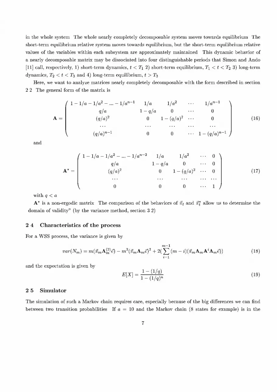
in the whole system. The whole nearly completely decomposable system moves towards equilibrium. The
short-term equilibrium relative system moves towards equilibrium, but the short-term equilibrium relative
values of the variables within each subsystem are approximately maintained. This dynamic behavior of
a nearly decomposable matrix may be dissociated into four distinguishable periods that Simon and Ando
[11] call, respectively, 1) short-term dynamics, t < T1 2) short-term equilibrium, T1 < t < T2 3) long-term
dynamics, T2 < t < T3 and 4) long-term equilibrium, t > T3.
Here, we want to analyze matrices nearly completely decomposable with the form described in section
2.2. The general form of the matrix is
A =
0BBBBBBB@
1� 1=a � 1=a2 � :::� 1=an�1 1=a 1=a2 � � � 1=an�1
q=a 1� q=a 0 � � � 0
(q=a)2 0 1� (q=a)2 � � � 0
� � � � � � � � � � � � � � �(q=a)n�1 0 0 � � � 1� (q=a)n�1
1CCCCCCCA
(16)
and
A� =
0BBBBBBB@
1� 1=a� 1=a2 � :::� 1=an�2 1=a 1=a2 � � � 0
q=a 1� q=a 0 � � � 0
(q=a)2 0 1� (q=a)2 � � � 0
� � � � � � � � � � � � � � �0 0 0 � � � 1
1CCCCCCCA
(17)
with q < a.
A� is a non-ergodic matrix. The comparison of the behaviors of ~�t and ~��t allow us to determine the
\domain of validity" (by the variance method, section 3.2).
2.4 Characteristics of the process
For a WSS process, the variance is given by
var(Nm) = m(~�m�(2)m ~e)�m2(~�m�m~e)
2 + 2(m�1Xi=1
(m� i)(~�m�mAi�m~e)) (18)
and the expectation is given by
E[X] =1� (1=q)
1� (1=q)n(19)
2.5 Simulator
The simulation of such a Markov chain requires care, especially because of the big di�erences we can �nd
between two transition probabilities. If a = 10 and the Markov chain (8 states for example) is in the
7

�rst state, a12 = 10�1 but a18 = 10�7. The ratio between the two extreme transition probabilities is in
the order of 106. If this Markov chain is simulated with classical methods, the random number generator
must be very good. If the transitions probabilities ratio is bigger, no random number generator is able
to generate tra�c according to the Markov chain. Therefore, we used an iterative method. Suppose for
example that a = 10 and that the Markov chain is in the �rst state, then a number between 0 and 1
is generated with a reliable random number generator [13]. If the next number is less than 1=a = 1=10,
the next state is not 2 but between 3 and n. The procedure continues until the random number is more
than 1=a or until the last state is reached. To resume, the probability of being in the next step in the
state i knowing that we are in the �rst state is prob(Yt+1 = ijYt = 1) = (1=a)i�1 with i = 2; 3; � � � ; nand the probability of staying in the �rst state is given by prob(Yt+1 = 1jYt = 1) = 1 �Pn
i=2(1=a)i�1.
So, we are not limited by the number of states in the Markov chain. We have seen how it is possible to
change the state if we are in the �rst state but if we are in another state, the transition probability ratios
can be very high too. If we take the preceeding example, in the eighth state, the transition probability
prob(Yt+1 = 1jYt = 8) = (q=a)8 = 4:3 � 10�9 and prob(Yt+1 = 8jYt = 8) = 1 � 4:3 � 10�9. The problem of
big di�erences between transition probabilities remains. One technique would be to use the method used
for the state in having a threshold for example, but instead of that, we used another, more e�cient and
quicker method. We don't chose at each slot if we remain or not in the same state but we calculate how
long we stay in the present state. The time we stay in the same state is geometrically distributed. The
probabilities of staying in the same state are near 1, therefore, it is useful to test the generated distribution.
This was tested for parameters varying from 0.5 to 1 � 0:5�8. For each parameter, 10000 samples have
been generated and the maximal error found between the expectation of the distribution and the mean of
the simulations is 2:3%. The modulator changes state according to the iterative method seen before and
when the modulator is in a state, the sojourn time is found with the random number generator. So, at
each iteration, the modulator changes state.
3 Tests of self-similarity
3.1 Visual test
Self-similarity is bounded with the concept of statistical invariance over timescales. So the easiest test
to detect self-similarity is to trace measured tra�c (like in [8]) or simulated tra�c over timescales. This
method is in fact very rough because it is di�cult for example, to visually quantify the degree of similarity
between scales. Figure 1 shows that as observed in real tra�c, we see similitudes over timescales. What
is very di�erent between our model and the ON-OFF source is the absence of a natural length of burst
in the �rst case as in the second. At each timescale, we observe bursty periods separated by less bursty
subperiods like in the measured LAN tra�c [14, 6]. In contrast, the classical sources behave very di�erently
because the correlation is present in general only at one timescale. Even through the tra�c could be very
8

0 10 0
1 10 0
2 10 0
3 10 0
4 10 0
5 10 0
6 10 0
0 10 0 2 10 3 4 10 3 6 10 3 8 10 3 1 10 4
Num
ber
of p
acke
ts/T
ime
Uni
t
Time [slot] Time Unit = 10 slots
0 10 0
1 10 1
2 10 1
3 10 1
4 10 1
5 10 1
0 10 0 2 10 4 4 10 4 6 10 4 8 10 4 1 10 5
Num
ber
of p
acke
ts/T
ime
Uni
t
Time [slot] Time Unit = 100 slots
0 10 0
5 10 1
1 10 2
1.5 10 2
2 10 2
0 10 0 2 10 5 4 10 5 6 10 5 8 10 5 1 10 6
Nu
mb
er
of
pa
cke
ts/T
ime
Un
it
Time [slot] Time Unit = 1000 slots
0 10 0
2 10 2
4 10 2
6 10 2
8 10 2
1 10 3
1.2 10 3
0 10 0 2 10 6 4 10 6 6 10 6 8 10 6 1 10 7
Num
ber
of p
acke
ts /
Tim
e U
nit
Time [slot] Time Unit=10000 slots
Figure 1: 5-state Markov chain time evolution on 4 di�erent timescales, Hl = 0:78
9

10-6
10-5
10-4
10-3
10-2
10-1
100
100 101 102 103 104 105 106
H_l = 0.5 (Poisson)3 states5 states7 states
varia
nces
m
Figure 2: a = 10, q = 0.9, number of states = n = 3/5/7
bursty at low timescales, it is not su�cient to reproduce real characteristics of measured tra�c because of
the lack of burstiness at higher scales [14].
3.2 Method of the variances to test the self-similarity of the process
The problem we are trying to solve in this Section is to test the self-similarity and to measure the Hurst
parameter H. In a �rst step, we want to examine second order stationary processes with autocovariance
function cov(Xt;Xt+� ) with cov(Xt;Xt) = var(Xt). By de�nition [4], a process having only one Hurst
parameter H to describe it is called exactly second-order self-similar. The process Xt and the averaged
processes X(m)t have identical correlational structures. With the Markov chains we will analyse, we are not
exactly in this case because all �nite Markov chains have a limit. Therefore, we propose to use the name
of \local" Hurst Hl parameter instead of Hurst parameter for our Markov chains. The Markov chains we
examine have pseudo long-range dependences.
� If cov(X(m)t ;X
(m)t+� ) = cov(Xt;Xt+� ) for � � 0 and var(X(m)) = �2m�� for all m = 1; 2; 3; ::: the
process X is called (exactly) second-order self-similar with self-similarity parameter H = 1��=2 [6].
� If cov(X(m)t ;X
(m)t+� ) = Cov(Xt; Xt+� ) as � !1 and var(X(m)) = �2m�� for m!1, the process X
is called (asymptotically) second-order self-similar.
Notice that 0 < � < 2 but here we are interested in the range 0 < � < 1. The case � = 1 gives second-
order pure noise with var(X(m)) = var(X)=m. All �nite Markov processes behave in this way when
m!1. 0 < � < 1 indicates positive correlation through time-scales. To estimate the Hurst parameter of
a second order self-similar process, it is su�cient to estimate � which is given by the slope of the diagram
log10(var(X(m))=�2) against log10(m). The estimated slope � gives an estimate of H : H = 1 � �=2.
Note that other methods are available to estimate H: R/S statistics proposed by Mandelbrot [15] and
periodograms [6]. In our context, we estimate the local Hurst parameter Hl. In Figures 2, 3 and 4, the
variance-time plot is given for a Markov chain having the structure described in 2.3. In addition, a line
indicates the slope of �1 (Hurst=0:5). According to the Figures, we see that the local Hurst parameter
10

10-6
10-5
10-4
10-3
10-2
10-1
100
100 101 102 103 104 105 106
H_l = 0.5 (Poisson)3 states5 states7 states
varia
nces
m
Figure 3: a = 5, q = 0.9, number of states = n = 3/5/7
10-6
10-5
10-4
10-3
10-2
10-1
100
100 101 102 103 104 105 106
H_l = 0.5 (Poisson)3 states5 states7 states
varia
nces
m
Figure 4: a = 10, q = 2, number of states = n = 3/5/7
11

varies with the number of states of the Markov chain. Note that the expectation varies also with the
number of states of the process. Here we introduce the \domain of validity" which is the domain where
Hl 6= 0:5, which is very appearent for the 3 and 5 state processes in Figures 2, 3 and 4.
4 Fitting
Based on measurements, a lot of �tting procedures have been proposed in the literature (see for example
[16], [17]). Ours is based on the Markov chain described in (section 2.2). Here, we �t only two parameters:
mean and Hurst parameter (plus the number of states in the Markov chain). As seen in (section 2.4),
E[X] equals (1� (1=q))=(1� (1=q)n). For a given E[X], it is quite easy to �nd q iteratively (algorithm 1).
With the method described, it is possible to �nd the domain where the process is self-similar. This domain
can be enlarged by increasing the number of states in the Markov chain, a is used to adjust the slope � in
order to have the desired Hurst parameter. a is found iteratively with the Newton-Raphson method and
�̂ is estimated with least squares.
Algorithm 1
Initialisation
Input of E[X ]
q = qinit = qold
repeat
E[X ]found = (1� 1=q)=(1� (1=q)n)
if (E[X ]found > E[X ]) then
qold = q
q = q=2
else
q = (qold � q)=2
until (E[X ]�E[X ]found < �)
end
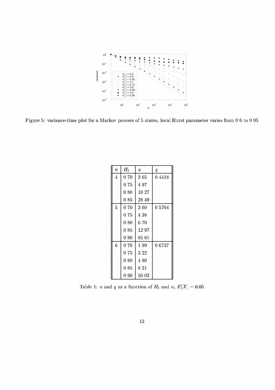
The validity domain (where Hl 6= 0:5) is determined by the method described in (section 2.3). Notice in
�gure 5 that the domain where the local Hurst parameter is 6= 0:5 becomes larger when Hl ! 1. In other
words, the Markov chain needs more states for self-similarity having a low local Hurst parameter than a
high one. The knee is very apparent, see for example at the curve where Hl = 0:8. For higher local Hurst
parameters, the knee is no more apparent because more computational time would be required to represent
it. For extreme values of local Hurst parameter (Hl = 0:9; 0:95), the variance-time curve becomes a little
bit wavy. Table 1 shows us some values found with the algorithm.
12
10-5
10-4
10-3
10-2
10-1
100
101 102 103 104 105
H_l = 0.5H_l = 0.6H_l = 0.65H_l = 0.7H_l = 0.75H_l = 0.8H_l = 0.85H_l = 0.9H_l = 0.95
varia
nces
m
Figure 5: variance-time plot for a Markov process of 5 states, local Hurst parameter varies from 0.6 to 0.95
n Hl a q
4 0.70 2.65 0.4418
0.75 4.97
0.80 10.27
0.85 28.49
5 0.70 2.60 0.5764
0.75 4.38
0.80 6.70
0.85 12.97
0.90 85.61
6 0.70 1.99 0.6737
0.75 3.22
0.80 4.80
0.85 8.21
0.90 50.02
Table 1: a and q as a function of Hl and n, E[X] = 0:05
13
5 Conclusions
In this paper, we have described a Markov chain emulating self-similarity which is quite easy to manipulate
and depends only on three. The tests performed on the model are the following: Hurst parameter (by the
variances method) and the so-called \visual" test. A method of �tting the model to measured data was
also given.
6 Acknowledgments
This work is supported by the Swiss PTT Telecom.
References
[1] H. E. Hurst, R. P. Black, and Y. M. Sinaika, \Long Term Storage in Reservoirs. An Experimental
Study," Constable, 1965.
[2] B. Mandelbrot and J. V. Ness, \Fractional Brownian Motions, Frational Noises and Applications,"
SIAM Review, vol. 10, October 1968.
[3] H.-O. Peitgen, H. Jurgens, and D. Saupe, Chaos and Fractals. New Frontiers of Science. Springer-
Verlag, 1992.
[4] D. R. Cox, \Long-range dependance: A review," Statistics: An Appraisal, 1984.
[5] I. Norros, \Studies on a model for connectionless tra�c, based on fractional Brownian motion," Tech.
Rep. TD(92)041, COST 242, 1992.
[6] W. Leland, M. Taqqu, W. Willinger, and D. Wilson, \On the Self-Similar Nature of Ethernet Tra�c
(Extended Version)," IEEE/ACM Transactions on Networking, vol. 2, February 1994.
[7] A. Erramilli, \Chaotic maps as models of packet tra�c," in ITC 14, The Fundamental Role of Tele-
tra�c in the Evolution of Telecommunications Networks (J. Labetoulle and J. Roberts, eds.), (Antibes
Juan-Les-Pins, France), Elsevier Science Publishers B.V. (North-Holland), June 6-10 1994.
[8] W. Leland and D. Wilson, \High Time{Resolution Measurement and Analysis of LAN Tra�c: Impli-
cations for LAN Interconnection," in IEEE Infocom, (Bal Harbor, FL), April 1991.
[9] A. Papoulis, Probability, Random Variables, and Stochastic Processes. Mc Graw Hill, 1984.
[10] P. J. Courtois, Decomposability. ACM Monograph Series, 1977.
[11] H. Simon and A. Ando, \Aggregation of variables in dynamic systems," Econometrica, no. 29, 1961.
14

[12] S. Friedberg, A. Insel, and L. Spence, Linear Algebra. Illinois State University: Prentice-Hall, 1989.
[13] P. L'Ecuyer, \E�cient and Portable Combined Random Number Generators," Communications of
the ACM, vol. 31, pp. 742{774, June 1988.
[14] S. Robert and J.-Y. LeBoudec, \Can self-similar tra�c be modelled by Markovian processes ?,"
in 1996 International Zurich Seminar on Digital Communications, IZS'96, (ETH-Zentrum, Zurich,
Switzerland), February 19-23 1996.
[15] B. Mandelbrot, \Robust R/S analysis of long run serial correlation," in Proc. 42nd Session ISI,
pp. 69{99, 1979.
[16] R. Gusella, \A Measurement Study of Diskless Workstation Tra�c on an Ethernet," IEEE Transac-
tions on Communications, vol. 38, September 1990.
[17] R. Gr�unenfelder and S. Robert, \Wich Arrival Law Parameters Are Decisive for Queuing System Per-
formance ?," in ITC 14, The Fundamental Role of Teletra�c in the Evolution of Telecommunications
Networks (J. Labetoulle and J. Roberts, eds.), (Antibes Juan-Les-Pins, France), pp. 377{386, Elsevier
Science Publishers B.V. (North-Holland), June 6-10, 1994.
15


