IJMMS 2003:1, 27–63PII. S016117120301233X

http://ijmms.hindawi.com© Hindawi Publishing Corp.

MULTILOCAL INVARIANTS FOR THE CLASSICAL GROUPS

PAUL F. DHOOGHE

Received 11 March 2001

Multilocal higher-order invariants, which are higher-order invariants defined atdistinct points of representation space, for the classical groups are derived in asystematic way. The basic invariants for the classical groups are the well-knownpolynomial or rational invariants as derived from the Capelli identities. Higher-order invariants are then constructed from the former ones by means of totalderivatives. At each order, it appears that the invariants obtained in this way do notgenerate all invariants. The necessary additional invariants are constructed fromthe invariant polynomials on the Lie algebra of the Lie transformation groups.

2000 Mathematics Subject Classification: 53A20, 53A55, 57S25.

1. Introduction. The study of invariants stands in contrast with the more

structural approaches in differential geometry as, for example, formulated in

the books of Kobayashi and Nomizu [13]. One of the main reasons for this is

that within this structural approach, invariants appear with a precise geometri-

cal meaning inherited from the structure. When not considered in this context,

invariants are, by definition, members of invariant rings of functions which, if

certain regularity conditions are imposed, are nothing else but rings generated

by a set of defining coordinates of the orbits of the group action on a given

manifold. Moreover, when considered as member of the coordinate ring of the

orbits, subspaces of a jet bundle, a constant function is not necessarily an

absolute invariant. The function may depend on the coordinates with respect

to which the partial derivatives are calculated and hence is not necessarily

invariant under general reparameterization. For this reason the distinction is

made between relative and absolute invariants [26]. But, in geometry, we are,

in particular, interested in invariants of a certain weight, which then determine

invariant symmetric covariant tensorfields, which are coordinate independent

quantities.

We start with a good reason to undertake the study of invariants. Con-

sider the following well-known problem: “Given the action of a group G on

a manifold M and two sets of points in M , when does an element exist in Gwhich transforms the first set into the second one?” This is the classical prob-

lem of invariants. We prefer to tackle the question in a more general form.

Consider two sets of points in M and/or tangent vectors and/or higher-order

tangent vectors at a distinct points. Say �1 = {ξi, . . . ,X|ξj , . . . ,YY . . .Y |ξk , . . .}

28 PAUL F. DHOOGHE

and �2 = {ηi, . . . ,X|ηj , . . . ,YY . . .Y |ηk , . . .}. The question then is when does there

exist an element g ∈ G such that g(�1) = �2 and what are the general crite-

ria? The problem, though interesting in itself, appears in problems related to

the existence of invariant kernels [7] and partial differential equations and, in

particular, is raised among others in computer vision [3, 16, 20, 24] and in

numerical algorithms related to symmetry [18].

One way to answer this type of question is to study invariants for the ex-

tended action of G on higher-order tangent vectors located at distinct points

of the manifold. Such invariants will be called multilocal differential invariants

because they are defined at distinct points of the manifold and also depend

on the higher-order differential structure of curves in M through the distinct

points. The natural setting for these problems seems to be multispace and

multijet space. Such invariants appear under different names in the literature,

in particular, as semidifferential invariants [24] and as joint invariants [19].

In this paper, we restrict attention to the local problem and to invariants

which are typically curve invariants. This implies that the invariants are meant

to be evaluated locally along curves. The development of the same ideas to

submanifolds is not considered here. Nonetheless, it turns out that the invari-

ants yielding the key information are tensors on jet bundles and hence, the

results are suitable for generalization to the theory of submanifolds.

For each of the groups, we start with “point invariants,” namely, invariant

functions defined on the zero-order jet space over the manifold. For the linear

transformation groups on Rn, these invariants are derived from the Capelli

identities and are found in the classical literature on the subject [9, 25]. The

point invariants are, as one expects, orbit invariants on multispace, which is an

r -fold product of the representation space with itself. Invariants, depending

on higher-order tangent vectors, are then defined on appropriate jet bundles

over these products.

The simplest example is given by the standard action of SO(3) on V = E3.

Let �2 = V1×V2 be the multispace. With x as variable on the first factor and

y as variable on the second, the functions �(x,x), �(x,y), and �(y,y) are

the well-known invariants of this action. � stands for the Euclidean quadratic

form on V . The rank of multispace equals 2, which is the smallest number

of factors needed for the orbits to have maximal dimension. Taking the first-

order jet bundle over the first factor gives the space J1V1×V2. The invariants,

together with their total derivatives, yield the set {�(x,x), �(x,y), �(y,y),�(x,x), �(x,y)}. The set thus obtained is not maximal, one lacks an invariant

function in order to have a complete set. The missing function is the well-

known Euclidean metric function on the first-order jet bundle, namely �(x, x).There are several ways to derive this function. (1) Because the action is linear

and extends linearly to the tangent space, we may reapply the Capelli identities

to the variables (x,y,x). (2) We may construct the space J1V1 × V2 × J1V3

equipped with the variablesx, x,y , z, z. The total derivative with respect to the

MULTILOCAL INVARIANTS FOR THE CLASSICAL GROUPS 29

third factor of the invariant �(x,z) yields �(x, z). The equivariant embedding

: J1V1×V2 → J1V1×V2×J1V3 given by z = x, z = x then yields the desired

invariant namely ∗�(x, z). (3) Because the orbits of SO(3) are diffeomorphic

to the group, they carry the invariant metric determined by the translation of

the Killing form on the orbits. An invariant Riemannian metric on �2 is found

by means of the construction of an invariant bundle transversal to the orbits.

The metric results from the Killing form on the orbits and the choice of an

Euclidean metric in the transversal bundle which is taken orthogonal to the

orbits. Consider the generating vector fields

Z1 = x1∂x2−x2∂x1+y1∂y2−y2∂y1 ,

Z2 = x1∂x3−x3∂x1+y1∂y3−y3∂y1 ,

Z3 = x3∂x2−x2∂x3+y3∂y2−y2∂y3

(1.1)

and the invariant transversal vector fields

Z4 = x1∂x1+x2∂x2+x3∂x3 , Z5 =y1∂y1+y2∂y2+y3∂y3 ,

Z4 =−y1∂x1−y2∂x2−y3∂x3+x1∂y1+x2∂y2+x3∂y3 .(1.2)

Defining these vector fields as orthonormal determines an invariant metric.

This metric, taken at the invariant subspace y = 0, restricted to the tangent

bundle of the first component of the multispace �2, and considered as function

on J1V , is given by φ = (x21 +x2

2 +x23)[(x1)2+ (x1)2+ (x1)2]. Because (x2

1 +x2

2+x23) is invariant, we find the extra invariant �(x, x). In this paper, we show

that this happens at each level for all the classical groups. The same approach

is then applied.

The results of the present paper can be summarized as follows. On the first-

order bundle, we find, besides the zero-order invariants and their first-order

prolongations, an additional set of functionally independent invariants which,

together with the former ones, generate the sheaf of invariant functions. We

show that, if formulated properly, these additional invariants are related to the

invariant polynomes on the Lie algebra of the transformation group. Hence,

they are symmetric tensors on the orbits of the group in the zero-order jet

bundle. In this sense, they relate directly to the geometry of the orbits of the

group in zero-order space. The same procedure then repeats at each order. The

dimension of the space upon which the group acts is crucial at each step. For

each of the groups, we follow the same procedure and present some aspects

of the geometry involved.

The following transformation groups are treated: (1) the Euclidean group,

Eucl(n); (2) the similarity group, Sim(n); (3) the symplectic group, Sym(n);(4) the volume-preserving group, Vol(n); (5) the affine group, Aff(n); (6) the

projective group, Pl(n); and (7) the conformal group, CO(1)(n). In each case,

we only consider the standard action.

30 PAUL F. DHOOGHE

For each of the groups from (1) to (5), we examine the action of their linear

part and construct the invariant sheaf. Then, by means of a homogenization

procedure, the sheaf of invariants for the transitive groups is found. Remark

that the following groups are semisimple: SO(n), O(n), Sp(n), Sl(n), Pl(n),and CO(1)(n). Furthermore, the results for CO(n) are derived from SO(n) and

those for Gl(n) from Sl(n) by projectivization of a set of generators of the

invariant sheaf.

In the first section, we review the basic results on invariants for the classical

linear groups such as given in the classical book of Weyl on the subject [25] or

more recently by Fulton and Harris [9]. The subsequent sections then treat the

higher-order multilocal invariants for the different groups. The Capelli con-

struction of the invariants is a well-debated subject, and we refer to the liter-

ature [12, 23]. A different approach has been given by Olver [17, 19], and Fels

[8] in terms of moving coframes. The construction of the invariant metric in

multispace, which we use here, is very close to this approach, although for the

point invariants, we use the classical theorems.

Besides the relative invariants, which depend on the parameterization of the

curves, we have to find a parameterization which is invariant under the induced

action of the group. Such parameters are called G-invariant parameters [16].

Clearly, the construction of such parameters is not unique; there are several

types of possible parameters. For example, the parameter may be determined

by the integral of the kth root of an invariant function of weight k, determined

on the jet bundle. But we may also determine a parameter by means of the

normalization of the prolonged curve with respect to an invariant symmetric

tensor field on the jet bundle. For example, in the Euclidean case, there exists a

tensor field which lives on the zero-order jet bundle determining the Euclidean

arc length, but, for example, in the case of a curve in one projective space, we

will show that the Schwarzian derivative, which determines a projective pa-

rameter, is nothing but a normalization with respect to the Killing form on the

orbit of the projective group in the second-order jet bundle. As said in former

paragraphs, we will not go into a systematic examination of the existence of

such invariant parameters but will give examples of such parameters.

The general setting for this paper is the C∞-category of manifolds and func-

tions. Restriction to polynomials or rational functions would be more advisable

in most cases, but, for our interest, the distinction is not very important. The

language of sheaf theory is used, which makes the formulation easier and more

elegant, but, as the reader will notice, we could also do without it at this stage.

The sheafs here are sheafs of germs of C∞-real valued functions, which are

fine sheafs, and their global analysis is outside the scope of this paper. For the

Lie groups and their algebras used in this paper, we refer to Helgason [11].

2. Elements of the classical theory. Let V be the standard representation

space of Gl(n) and G a subgroup of Gl(n). Let (ei) be a basis on V ; we denote

MULTILOCAL INVARIANTS FOR THE CLASSICAL GROUPS 31

by (ξi) the corresponding coordinates and use ξ = (ξi) to indicate a point in V .

Classical invariant theory aims at constructing all polynomials P(ξ1,ξ2, . . . ,ξm)in m variables on V which are invariant under the action of G.

It is indicated to define these polynomials on the product space �r =∏rα=1Vα,

where each Vα is a copy of V . The action of the groupG on �r is the product ac-

tion. Invariant polynomes or invariant functions inm variables are polynomes

or functions on �r , depending on m factors, with r ≥m.

Results on the invariants for the classical linear subgroups of Gl(n) are

consequences of the identities of Capelli [9, 25]. We summarize the results in

the form of a theorem.

Theorem 2.1 [9]. (1) The only polynomial invariants for Gl(n) and CO(n)are the constants.

(2) Polynomial invariants P(ξ1,ξ2, . . . ,ξm) for Sl(n) can be written as polyno-

mials in the determinants |ξα1ξα2 ···ξαn |, 1≤α1 <α2 < ···<αn ≤m.

(3) Polynomial invariants P(ξ1,ξ2, . . . ,ξm) for Sp(n) (resp.,O(n)) can be writ-

ten as polynomials in the functions �(ξα,ξβ), 1≤α< β≤m, (resp., 1≤α≤α≤m), with � the quadratic form which determines the standard action of Sp(n)(resp., O(n)) on V .

(4) Polynomial invariants P(ξ1,ξ2, . . . ,ξm) for SO(n) can be written as poly-

nomials in the functions �(ξα,ξβ) and |ξα1ξα2 ···ξαn |, with 1≤α≤ β≤m and

1≤α1 <α2 < ···<αn ≤m.

From this theorem, we easily derive rational invariants in m variables for

CO(n) and Gl(n). The following theorems state the results.

Theorem 2.2. All rational functions in |ξα1ξα2 ···ξαn |/|ξβ1ξβ2 ···ξβn |,with 1 ≤ α1 < α2 < ··· < αn ≤ m and 1 ≤ β1 < β2 < ··· < βn ≤ m, are in-

variants for the standard action of Gl(n) on V .

Theorem 2.3. All rational functions inQ(ξα1 ,ξα2)Q(ξβ1 ,ξβ2), with 1≤α1 ≤α2 ≤m and 1 ≤ β1 ≤ β2 ≤m, are invariants for the standard action of CO(n)on V .

The projective group Pl(n) � Gl(n+ 1)/± eλ Id and the conformal group

CO(1)(n) do not act linearly on V and hence need a different treatment.

First, consider the projective group. Let ξα1 ,ξα2 , . . . ,ξαm be m variables on

V and ξk an extra variable on V . We then define∣∣ξα1ξα2 ···ξαn ;ξk∣∣= ∣∣(ξα1−ξk

)(ξα2−ξk

)···(ξαn−ξk)∣∣. (2.1)

Theorem 2.4. All rational functions in

Π∣∣ξα1ξα2 ···ξαn ;ξk

∣∣/Π∣∣ξβ1ξβ2 ···ξβn ;ξk∣∣ (2.2)

with 1 ≤ α1 < α2 < ··· < αn ≤m and 1 ≤ β1 < β2 < ··· < βn ≤m, where the

products are taken such that for each αr the number of factors containing the

32 PAUL F. DHOOGHE

variable ξαr in the nominator equals the number of factors containing ξαr in

the denominator, are invariant for the standard action of Pl(n) on V .

Proof. The above expression is clearly invariant for translations and the

action of the general linear group. For this, we first remark that, because they

are invariant under translations, we may put ξk = 0. Invariance under the spe-

cial projective transformations ξj = ξj/1+aiξi is easily checked, which proves

the proposition.

The group of conformal transformations CO(1)(n) is the first prolongation

of the group CO(n) [10, 22]. The group is generated by the elements of the

similarity group Sim(n) and the inversions on the n sphere. As transforma-

tion on V , the conformal group is generated by the similarity group Sim(n),together with the special conformal transformations [1]

ξj = ξj−cj�(ξ,ξ)

fξ, (2.3)

with fξ = 1−2�(c,ξ)+�(c,c)�(ξ,ξ), c ∈ V .

Theorem 2.5. Let (ξαi) bem variables on V and d the distance function de-

fined by the quadratic form �. All rational functions in Πd(ξαiξαj )/Πd(ξβiξβj ),with 1≤αi < αj ≤m and 1≤ βi < βj ≤m and where the product is taken such

that for each αr the degree of the variable ξαr in the nominator equals the de-

gree of this variable in the denominator, are invariant for the standard action

of CO(1)(n) on V .

Proof. The expressions in the theorem are clearly invariant for the action

of the translations and the group CO(n). We only have to prove invariance for

the action of the special transformations (2.3). The proof then follows from

the application of the following lemma to the above functions.

Lemma 2.6 [1]. Let ξ1, ξ2 be two points in V . Then,

d(ξ1, ξ2

)= d(ξ1,ξ2)

fξ1fξ2

. (2.4)

3. Multispace. Let V be as before and �=∏rα=1Vα, the product of r copies

of V . � is called multispace constructed upon V . We denote by (ξiα) the co-

ordinates on the αth copy in the product and call Vα the α-layer of �. The

projection ρα : �→ Vα is the mapping onto the αth component. The identifi-

cation of V with a specific layer is called the layer mapping, which is given by

iα : V → Vα, and the image projection π is defined as the superposition of the

different layers upon V . In other words, π is the r -valued mapping defined by

the set of r functions (ρα) of � followed by the natural identification of each

layer with V . Remark that πoiα = Id for each α.

MULTILOCAL INVARIANTS FOR THE CLASSICAL GROUPS 33

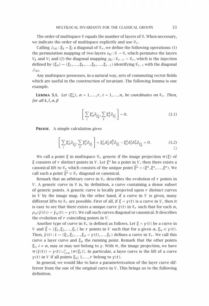
The order of multispace � equals the number of layers of �. When necessary,

we indicate the order of multispace explicitly and use �r .

Calling�kl : ξk = ξl a diagonal of �r , we define the following operations: (1)

the permutation mapping of two layers skl : �→ �, which permutes the layers

Vk and Vl and (2) the diagonal mapping kl : �r−1 → �r , which is the injection

defined by (ξα)� (ξ1, . . . ,ξk, . . . ,ξk, . . . ,ξr−1) identifying �r−1 with the diagonal

�kl.

Any multispace possesses, in a natural way, sets of commuting vector fields

which are useful in the construction of invariant. The following lemma is one

example.

Lemma 3.1. Let (ξiα), α = 1, . . . ,r , i = 1, . . . ,n, be coordinates on �r . Then,

for all k,l,α,β

[∑iξiα∂ξiβ ,

∑γξkγ∂ξlγ

]= 0. (3.1)

Proof. A simple calculation gives

[∑iξiα∂ξiβ ,

∑γξkγ∂ξlγ

]= ξiαδikδβγ∂ξlγ −ξkγδ

ilδγα∂ξiβ = 0. (3.2)

We call a point ξ in multispace �r generic if the image projection π(ξ) of

ξ consists of r distinct points in V . Let ξo be a point in V , then there exists a

canonical lift to �r which consists of the unique point ξo = (ξo,ξo, . . . ,ξo). We

call such a point ξo ∈ �r diagonal or canonical.

Remark that an arbitrary curve in �r describes the evolution of r points in

V . A generic curve in � is, by definition, a curve containing a dense subset

of generic points. A generic curve is locally projected upon r distinct curves

in V by the image map. On the other hand, if a curve in V is given, many

different lifts to �r are possible. First of all, if ξ = γ(t) is a curve in V , then it

is easy to see that there exists a unique curve γ(t) in �r such that for each α,

ρα(γ(t))= γα(t)= γ(t). We call such curves diagonal or canonical. It describes

the evolution of r coinciding points in V .

Another type of curve in �r is defined as follows. Let ξ = γ(t) be a curve in

V and ξ = {ξ1,ξ2, . . . ,ξr} be r points in V such that for a given α, ξα ∈ γ(t).Then, γ(t) : t � (ξ1,ξ2, . . . ,ξα = γ(t), . . . ,ξr ) defines a curve in �r . We call this

curve a layer curve and ξα the running point. Remark that the other points

ξi, i ≠ α, may or may not belong to γ. With π , the image projection, we have

π(γ(t)) = γ(t)∪ri≠α {π(ξi)}. In particular, a layer curve is the lift of a curve

γ(t) in V if all points ξα; 1, . . . ,r belong to γ(t).In general, we would like to have a parameterization of the layer curve dif-

ferent from the one of the original curve in V . This brings us to the following

definition.

34 PAUL F. DHOOGHE

Definition 3.2. Let γ(t) be a curve in V and (ξi) a set of r points in V , all

belonging to γ(t). Then, an α-layer curve γ, associated with γ(t), is a curve

γ(t) : t � (ξ1,ξ2, . . . ,ξα = γ(φ(t)), . . . ,ξr ), where φ is a reparameterization of

γ.

The condition that γ is a layer curve associated with γ(t) in the αth layer

can be reformulated as Imρα(γ)= Im(γ) and ρβ(γ)= ξβ for β≠α.

The construction of a general lifting of a curve is, in fact, a kind of superpo-

sition of r layer curves. Hence, we have the following definition.

Definition 3.3. Let γ(t) be a curve in V . Then, γ(t) in � is a lift of γ(t) if

the image of the image projection of γ(t) equals the image of γ(t).

Let (ξiα) be the coordinates on Vα and ξi = γi(t) a curve in V . A lifted curve

on � is given by

ξiα = γiα = iα(γ(φα(t)

)), (3.3)

where φ is a reparameterization in the domain of the curve γ. We remark that

parameterization may differ from layer to layer. Hence the lift, as a parameter-

ized curve, is not unique; indeed, we accept the freedom to move the distinct

points with a different speed along the curve. Hence, keeping the r −1 points

ξβ, with β ≠ α for a given α, fixed and ξα as the running point determines a

layer curve associated with γ(t).

4. Jets of curves in multispace. Consider the set of germs of curves in Vand denote this space by C(V). Recall that germ equivalence of two curves is

defined as γ1(t)∼to γ2(t) if and only if both curves coincide on a neighborhood

of to. The set of germs is the sheaf of germ equivalent curves on R with values

in V .

Jet equivalence is then introduced as an equivalence on C(V). Let γ1(t) and

γ2(t) be the representatives of two germs in C(V), both are k jet equivalent

if their derivatives up to order k coincide at t. This equivalence clearly does

not depend upon the choice of the representatives. We generally indicate a

germ by a representative and the k jet of a curve germ by jkt (γ). It is assumed

that the germ is taken at the point t. The set of k jets of germs of curves in Vis the space Jk(R,V). The set of infinite jets J(RV), is defined as the inverse

limit of the sequence (Jk(R,V))k. This space admits a ring of C∞-functions

�(J(R,V)), defined by the direct limit of the sets {�(Jk(R,V))} with respect

to the projections πk : J(R,V)→ Jk(R,V). In the sequel, we consider each set

�(Jk(R,V)) as a natural subset of �(J(R,V)). A section σ : R → J(R,V) is

called integrable if σ equals the jet of a curve at each of its source points.

Let α : Jk(R,V)→R be the source map defined as jkt γ � t. The fibre α−1(0)is a bundle over the target space V . We call this bundle Jk(V). This bundle is

equipped with the projection map β : Jk(V)→ V by jk0(γ)� γ(0). We denote

MULTILOCAL INVARIANTS FOR THE CLASSICAL GROUPS 35

elements in Jk(V) by jk(γ). The bundle of infinite jets is denoted by J(V).Again, we call a curve σ :R→ J(V) integrable if it is the infinite jet of a curve

in V at each of the points of β(σ(t)).Let ∂t be the derivative operator on R; the total lift of this operator, ∂ht ,

as an operator on �(J(R,V)), is given by ∂tf (σ(t)) = (∂ht f )(σ(t)) for f in

�(J(R,V)) and σ integrable section: σ :R→ J(R,V).Let X ∈�(V) be a vector field with flow φt . Because φt is a local diffeomor-

phism on V , composition with curve mappings defines the prolonged action

of the local diffeomorphism on the jet space Jk(V). Let γ(s) be a curve, then

φt(γ(s)) is the composition with the local diffeomorphism for a fixed t and

the action on Jk(V) is given by φ(k)∗t jkγ = jk(φ(γ)). This determines what is

called the complete lift X(k), generator of φ(k), on Jk(V). The following propo-

sition, which is well known in jet bundle theory [5, 14, 15], gives a constructive

definition.

Definition 4.1. Let X be a vector field on V . Then, the complete lift X(k)

is the unique vector field on Jk(V) satisfying the conditions (1) [∂ht ,X(k)] = 0

and (2) β∗X(k) =X.

The above definitions extend in a natural way to multijet space. Let γ(t) be

a curve in V and γα(t) an α-layer curve corresponding to γ(t) in �r . The 1 jet

of γα(t) defines a curve in V1×V2×···×J1Vα×···×Vr .

This operation is also defined on general curves γ in �r . The jet extension is

applied to theαth component of the curve. It means that we consider the curve

as a layer curve keeping all other components fixed. Moreover, we may extend

each component γα to a specific jet order kα. This brings us to products of jet

bundles over V , which is a bundle over the base manifold �r . This space takes

the form of the product

�(k1,...,kr )(�r)= r∏

α=1

JkαVα (4.1)

and is called multijet space. Points in this space are multijets of curves in V .

The component JkαVα is the α-layer jet bundle.

Let γ(t) be a curve in �r , and let p be a generic point on γ(t). A multijet of

γ(t) at p defines, via the image projection, r points together with tangents up

to a given order of the curve γ(t) at each of the points.

The bundle �(k1,...,kr )(�r ) is a subbundle of Jk(�r ), where k=max{k1, . . . ,kr},but the jet bundle operations are defined on each layer jet bundle. A section

σ of �(k1,...,kr )(�r ) can be written as σ = (σα). The section is integrable if and

only if each σα is integrable. Each layer carries a total derivative operator,

which we denote by Tα. Let p = (σ1(to), . . . ,σr (to)), we then have Tαf(p) =(∂tσ∗α f)(σ1(to), . . . ,σα−1(to),to,σα+1(to), . . . ,σr (to)), where f is any function

on multijet space.

36 PAUL F. DHOOGHE

The complete lift of a vector field on �r on a jet bundle over a specific

layer Jkα(Vα) is defined as in Definition 4.1 where the total derivative is Tα.

Let (ξ(lα)iα ) be the natural coordinates on �(k1,...,kr )(�r ) and X =Aiα∂ξiα a vector

field on �r , then

X =∑T(lα)α Aiα∂ξ(lα)iα

(4.2)

is the total lift of the vector field.

The operations which have been determined on multispaces extend to mul-

tijet spaces. Call JkαVα the jet bundle over the αth layer.

(1) Let the jet bundles over the layers Vk and Vl be of same order. The per-

mutation mapping ιkl : �(�)r → �(�)r is a mapping which permutes the two

layers together with their jet bundles JmVk and JmVl.(2) A diagonal in multijet space �kl is defined as follows. Let JmkVk and

JmlVl be two jet bundles over different layers in �(�)r . Suppose thatmk ≤ml.

Then, the diagonal subspace is given by �kl : JmkVk = JmkVl. At �kl, the mk

jets over both components are identified. A diagonal mapping is an injection

kl : �(�)r−1→ �(�)r with image �kl.

5. Group actions on multispace. LetG be a Lie group acting on V , the action

being given by τ :G×V → V as (g,ξ)� g·ξ. The induced action on �r is given

by τ : (g,(ξα))� (g ·ξ1,g ·ξ2, . . . ,g ·ξr ). Any function P(ξ1,ξ2, . . . ,ξm), m≤ r ,

is invariant for the action of G if and only if P(ξ1,ξ2, . . . ,ξm) is constant on the

orbits of G in �r . We easily verify the following proposition.

Proposition 5.1. The maps π , jkl, and skl are equivariant.

Let g be the Lie algebra ofG and (ea), a= 1, . . . ,dimg, a basis. The vector field

κ : ea�Xa =Dτ(ea)|e, with e the identity inG, is a fundamental (or generating)

vector field. Given the action of G on �r , we define the singular subset ΣG ={ξ ∈ �r | rk{Xa} < dimg}, where Xa is a complete set of fundamental vector

fields. The regular subset is the complement �= �r \Σ. The sheaf of germs of

C∞ invariant functions on �, �(�), is called the invariant sheaf.

Let M be a manifold and � = {f1,f2, . . . ,fk} a set of C∞-functions; the set

� is called functionally independent at p ∈M if the associated k-form ω� =df 1∧df 2∧···∧dfk is different from zero at p [20]. The conditions for a set

of functions to be functionally independent on a manifold are those of implicit

function theorem asserting the existence of a local submanifold at p, whose

tangent space is the kernel of the set of one forms {df i}. The rank k of �

equals the codimension of the submanifold.

Because the invariant sheaf is determined by its sections, we only need to

give at each point a complete functionally independent set of germs of invari-

ant C∞-functions. Such a set will be called a set of generators. We agree not

to mention the passage from functions to germs. To simplify notation, we do

MULTILOCAL INVARIANTS FOR THE CLASSICAL GROUPS 37

not mention the base points of the germs either and will give a minimal set of

functions needed in the construction of a maximal functionally independent

set of sections of the sheaf at each point in the domain of the sheaf. Such a set

of generators will be called complete.

Let Xa be a fundamental vector field, then f ∈ �(�) → Xa(f) = 0, for all

a. The converse is not always true. It follows that, on a regular subset �, the

rank of the sheaf of germs of C∞-invariant functions equals the codimension

of the level surface of any set of generators.

Consider the projective equivariant system

�1 = Vπ2

1←����������������������������������������������������������� �2π3

2←����������������������������������������������������������� �3←� ··· ←� �r−1πrr−1←�������������������������������������������������������������������������������������������������������� �r . (5.1)

Let r ⊂ �r be an orbit ofG, thenπrr−1r is an orbit in �r−1. Hence, dimr−1 ≤dimr . The orbit dimension is a nondecreasing function on the orbits. Let �

be the set of maximal orbits. We then define the order of stabilization of the

action of G in the limiting system defined by �r , for r large enough, as the

rank k such that for all l > 0 : dimk+l = dimk, for orbits in �.

Remark 5.2. (1) Let k be the order of stabilization ofG in �r . Then, as a con-

sequence of the dimensional requirements, we have rk�(�k+1)= rk�(�k)+n(n= dim(V)).

(2) Let P(ξ1,ξ2, . . . ,ξm) be a generator in �(�k). Then,

P ′(ξ1,ξ2, . . . ,ξm+1

)= sm,m+1P(ξ1,ξ2, . . . ,ξm

)(5.2)

is a generator in �(�m+1) which does not belong to �(�m).

The product action of a Lie groupG on � prolongs in a natural manner to any

multijet bundle �(�). Using the natural prolongation of one-parameter local

diffeomorphisms on the target space to the jet bundles, we find the prolonga-

tion of fundamental vector fields of a group action. Let Xa be a fundamental

vector field on V ; with respect to the coordinates we set

Xa =∑iAia∂xi . (5.3)

The corresponding fundamental vector field on �r becomes

Xa =∑α

∑iAia,α∂ξiα , (5.4)

where Aia,α = Aia(xi = ξiα). The prolongation of the fundamental vector field

onto the multijet bundle �(k1,...,kr )(�r )=∏α JkαVα is obtained from (4.2).

38 PAUL F. DHOOGHE

6. The first-order transformations groups

6.1. The linear subgroups of Gl(n)

6.1.1. Invariants for O(n). Let e = (ei), i = 1, . . . ,n, be an orthonormal ba-

sis, (ξi) the corresponding coordinates on V , and � the Euclidean quadratic

form on V .

Zero-order invariants. Let ξ = (ξ1,ξ2, . . . ,ξr ) ∈ �r , with �r = V1×V2×···×Vr . From Theorem 2.1, we know that each polynomial in the r(r +1)/2forms �(ξα,ξβ) is invariant. Let � be the subset in �r such that each ξ ∈� is

a linear independent set of points in En.

The following properties are elementary. We present them without proof.

Proposition 6.1. (1) The set � = {�(ξα,ξβ) | α ≤ β, ξα,ξβ ∈ ξ, ξ ∈�} is

functionally independent.

(2) The order of stabilization equals r = n− 1. Moreover, if r = n− 1, the

polynomial invariants for SO(n) coincide with those for O(n) as a consequence

of Theorem 2.1.

(3) Let Γ be a level set of � in �n−1. Then, Γ is an orbit of SO(n).

It follows that the subset � in �n−1 is foliated by orbits of SO(n), and the

leaves are the level surfaces of �. Let �(�) be the sheaf generated by � in

�n−1.

Remark 6.2. Because �r is the zero-order level in jet space, a curve γ(t) in

� is lying in an orbit if and only if the invariant sheaf �(�) restricted to γ is

constant.

Let ξ = {ξ1, . . . ,ξn−1} be a set of n−1 points in V . The isotropy group at

ξn−1 is the group SO(n−1), and, by recursion, the isotropy group leaving kpoints fixed, say {ξn−k,ξn−k+1, . . . ,ξn−1}, is the group SO(n−k) [2]. From this,

it follows that, if γ(t) is a nowhere constant layer curve such that the invariant

sheaf restricted to γ(t) is constant, the image of γ(t) is locally the image of

an orbit of SO(2).Finally, remark that, if the symmetry of the r points is taken into account,

it is indicated to construct the quotient space �/�, where � is the symmetry

group of �r . The set �/� is parameterized by

0< �(ξ1,ξ1

)≤ �(ξ2,ξ2

)≤ ··· ≤ �(ξr ,ξr

). (6.1)

First-order invariants. In order to construct first-order invariants, we

consider multijet space

�(1,...,1)(�r)= J1V1×J1V2×···×J1Vr , (6.2)

MULTILOCAL INVARIANTS FOR THE CLASSICAL GROUPS 39

which is a bundle over �r with mapπ : �(1,...,1)(�r )→ �r . We denote by ((ξα, ξα))the coordinates on �(1,...,1)(�r ). The action of SO(n) extends in a natural way to

�(1,...,1)(�r ) as (g,(ξα, ξα))� (g ·ξα,g · ξα). Let �(1,1,...,1) be the regular subset

of �(1,...,1)(�r ).The total derivative operators in the different layers Tα,α= 1, . . . ,r commute

with the product action of SO(n). Then, if φ is an invariant function on �r ,

each function Tαφ is invariant. Tαφ is the α-layer first-order prolongation of

φ. Let �′ =�(1,...,1)∩π−1�. We construct the invariant sheaf �(1)(�′) as the

sheaf generated by the elements of

(1)� = {�(ξα,ξβ),Tγ�(ξα,ξβ

) |α≤ β, ξα,ξβ ∈ ξ, ξ ∈�}, (6.3)

where α,β, and γ = 1, . . . ,r , restricted to �′.We remark that �(1)(�′) is generated by the n(n−1)/2 forms �(ξα,ξβ)

and the (n−1)(n−1) forms �(ξα,ξβ). The forms �(ξα,ξβ) are linear in the

variables (ξα), and because the points ξβ are linear independent, we find the

following proposition.

Proposition 6.3. The rank of the sheaf �(1)(�′) equals (n−1)(3n−2)/2.

Remark that the dimension of the orbits equals n(n−1)/2 and is constant

on �, while � has dimension n(n−1).Let � be a level surface of the invariant sheaf �(1)(�′). Then, � is foliated

by orbits of SO(n). As a consequence of former Proposition 6.3, the codimen-

sion of the orbits in � equals n− 1. This implies that we need n− 1 extra

independent generators to construct the complete invariant sheaf.

In order to derive n−1 extra invariants, we construct an invariant normal

bundle N(�), as subbundle of T�. This bundle is a vector bundle whose sec-

tions are transversal to the leaves and which is invariant as a subbundle under

the action of SO(n).The fundamental vector fields on �n−1 for SO(n) are given by

{Xa; a= 1, . . . ,

n(n−1)2

}={Xij =

n−1∑α=1

ξiα∂ξjα−ξjα∂ξiα ; i < j, i,j = 1, . . . ,n

}.

(6.4)

Proposition 6.4. The following set of n(n−1)/2 vector fields commute

with the fundamental vector fields Xa on �r :

Yα =∑iξiα∂ξiα , Yα,β =

∑iξiα∂ξiβ−ξ

iβ∂ξiα . (6.5)

Denote this set by Ya, a = 1, . . . ,n(n−1)/2. A simple calculation, together

with Lemma 3.1, shows the following proposition.

Proposition 6.5. The set of vector fields Za = (X1,X2, . . . ,Y1,Y2, . . .), with

a= 1, . . . ,n(n−1), is linear independent at each point on �.

40 PAUL F. DHOOGHE

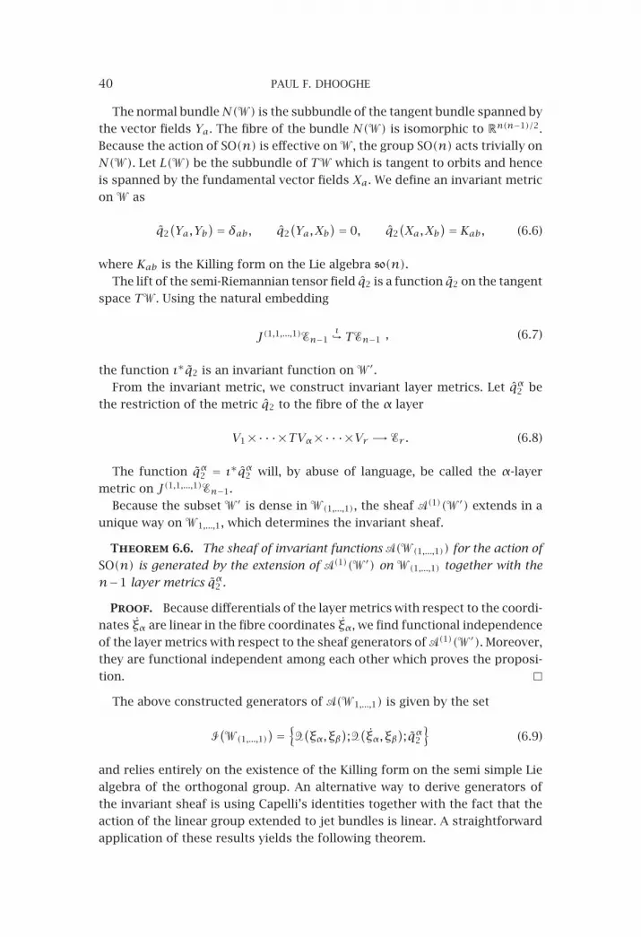
The normal bundleN(�) is the subbundle of the tangent bundle spanned by

the vector fields Ya. The fibre of the bundle N(�) is isomorphic to Rn(n−1)/2.

Because the action of SO(n) is effective on �, the group SO(n) acts trivially on

N(�). Let L(�) be the subbundle of T� which is tangent to orbits and hence

is spanned by the fundamental vector fields Xa. We define an invariant metric

on � as

q2(Ya,Yb

)= δab, q2(Ya,Xb

)= 0, q2(Xa,Xb

)=Kab, (6.6)

where Kab is the Killing form on the Lie algebra so(n).The lift of the semi-Riemannian tensor field q2 is a function q2 on the tangent

space T�. Using the natural embedding

J(1,1,...,1)�n−1ı↩ T�n−1 , (6.7)

the function ı∗q2 is an invariant function on �′.From the invariant metric, we construct invariant layer metrics. Let qα2 be

the restriction of the metric q2 to the fibre of the α layer

V1×···×TVα×···×Vr �→ �r . (6.8)

The function qα2 = ı∗qα2 will, by abuse of language, be called the α-layer

metric on J(1,1,...,1)�n−1.

Because the subset �′ is dense in �(1,...,1), the sheaf �(1)(�′) extends in a

unique way on �1,...,1, which determines the invariant sheaf.

Theorem 6.6. The sheaf of invariant functions �(�(1,...,1)) for the action of

SO(n) is generated by the extension of �(1)(�′) on �(1,...,1) together with the

n−1 layer metrics qα2 .

Proof. Because differentials of the layer metrics with respect to the coordi-

nates ξα are linear in the fibre coordinates ξα, we find functional independence

of the layer metrics with respect to the sheaf generators of �(1)(�′). Moreover,

they are functional independent among each other which proves the proposi-

tion.

The above constructed generators of �(�1,...,1) is given by the set

(�(1,...,1)

)= {�(ξα,ξβ);�(ξα,ξβ); qα2 } (6.9)

and relies entirely on the existence of the Killing form on the semi simple Lie

algebra of the orthogonal group. An alternative way to derive generators of

the invariant sheaf is using Capelli’s identities together with the fact that the

action of the linear group extended to jet bundles is linear. A straightforward

application of these results yields the following theorem.

MULTILOCAL INVARIANTS FOR THE CLASSICAL GROUPS 41

Theorem 6.7. The invariant sheaf �(�(1,...,1)) is generated by the following

set of functionally independent functions:

�(�(1,...,1)

)= {�(ξα,ξβ);�(ξα,ξβ);�(ξα, ξα)}. (6.10)

Remark that J(1,1,...,1)�n−1 contains a lot of redundant information. A large

part of the invariant sheaf �(�(1,...,1)) can be retrieved from a smaller part of

the sheaf. The following proposition is a direct consequence of the prolonged

group action of SO(n).

Proposition 6.8. The subspace = {ξβ = 0, β= 2,3, . . . ,n−1, ξ1 ≠ 0} is an

invariant subspace in J(1,1,...,1)�n−1.

The extension of the invariant sheaf �(�(1,...,1)) on the subspace is an

invariant sheaf, say �( ). With the canonical embedding

κ : J(1,0,...,0)�n−1 ↩ J(1,1,...,1)�n−1 , (6.11)

where κ identifies J(1,0,...,0)�n−1 with , the pullback κ∗�( ) is the invariant

sheaf on π−1(�)\{ξ1 = 0}. π is the projection J(1,0,...,0)�n−1→ �n−1. The sheaf

κ∗�( ) has a maximal rank.

Let � be the diagonal in J(1,0,...,0)�n−1 defined by ξn−2 = ξn−1 and

: J(1,0,...,0)�n−2 �→ J(1,0,...,0)�n−1 (6.12)

the diagonal embedding with image �.

The invariant sheaf �(�(1,...,0)) then equals ∗κ∗�( ). The following the-

orem is an immediate consequence of our construction. Denote by �1 the

regular subset �(1,0,...,0).

Theorem 6.9. The following sets are equivalent sets of generators of the

invariant sheaf �(�1):

(�1)= {�(ξα,ξβ);�(ξ1,ξβ

); q1

2

},

�(�1)= {�(ξα,ξβ);�(ξ1,ξβ

);�(ξ1, ξ1

)},

(6.13)

with α,β= 1, . . . ,n−1.

The above results generalize to the first-order jets over several layers. We

formulate this in Theorem 6.10.

Let

�(1,...,1,0,...,0)�n−l−1 = J1V1×···×J1Vl︸ ︷︷ ︸l time

×Vl+1×···×Vn−l−1, (6.14)

where 1≤ l < n−1 and �(l) =�(1,...,1,0,...,0) is the regular subset.

42 PAUL F. DHOOGHE

Theorem 6.10. The following sets are equivalent sets of generators of the

invariant sheaf:

(l)(�(l))= {�(ξα,ξβ);�(ξσ ,ξβ); qσ2 },

�(l)(�(l))= {�(ξα,ξβ);�(ξσ ,ξβ);�(ξσ , ξσ )}, (6.15)

with α,β= 1, . . . ,n−l−1 and σ = 1, . . . , l.

Remark 6.11. The expression �(ξα, ξα) is a tensor field on the α layer for

each α and determines the well-known Euclidean arc length parameter along

each layer curve.

Higher-order invariants. Before formulating the general case, we con-

sider in detail the one-layer case and work by induction on the order. Let for

1≤ l < n−1

�(l,0,...,0)�n−l−1 = JlV1×V2×···×Vn−l−1, (6.16)

and let �l =�(l,0,...,0) be the regular subset. The following theorem is a con-

sequence of the identities of Capelli and the linear action of the prolonged

action.

Theorem 6.12. Let k,r = 1, . . . , l, α,β= 1, . . . ,n−l−1. The set

�l(�l)= {�(ξα,ξβ);�(ξ(k)1 ,ξ(r)1

);�(ξ(k)1 ,ξβ

)}(6.17)

generates the invariant sheaf on �l.

It is easily verified that the set is functionally independent and invariant. The

cardinal number of the set equals (n−l−1)(n−l)/2+l(l+1)/2+l(n−l−1)=n(n−1)/2. The dimension of �(l,0,...,0)�n−l−1 equals n(n−1). Hence, we find

on �l

dim�(l,0,...,0)�n−l−1 = dim+rank �l(�l), (6.18)

where �l(�l) is the sheaf generated by l(�l).Consider the space �(l+1,0,...,0)�n−l−1 = Jl+1V1×V2×···×Vn−l−1 and projec-

tion π : �(l+1,0,...,0)�n−l−1→ �(l,0,...,0)�n−l−1.

Let �′ =�l+1∩π−1�l. The prolonged sheaf is generated by

(1)l (�′)={

�(ξα,ξβ

);�(ξ(k)1 ,ξβ

);�(ξ(k)1 ,ξ(r)1

)}, (6.19)

where k= 1, . . . , l+1, r = 1, . . . , l, α,β= 1, . . . ,n−l−1.

MULTILOCAL INVARIANTS FOR THE CLASSICAL GROUPS 43

The rank of (1)l (�′) equals n(n−1)/2+(n−l−1)+l=n(n−1)/2+n−1.

Using the unique extension of the sheaf on �l+1, we find that one generator is

missing for the construction of the invariant sheaf on �l+1. For the construc-

tion of the extra generator, we follow the same procedure as in the first-order

case. Because the group action of SO(n) extends linearly to the jet bundle, the

same construction for the invariant transversal bundle can be applied at each

order. From the invariant Killing metric on the orbits and an invariant metric

in the normal bundle, we construct a layer metric on the first layer of multijet

space �(l+1,0,...,0)�n−l−1. The construction is analogous to the constructions in

Propositions 6.4 and 6.5.

Restriction of this metric to the tangent space to the jet bundle over the first

layer gives us a layer metric. This metric lifts as a function on �l+1 denoted

by q12. We then have the following theorem.

Theorem 6.13. The invariant sheaf �l+1(�l+1) is generated by the set

(1)l(�l+1

), (6.20)

together with a layer metric q12 .

The construction is summarized in the following diagram:

�(l,0,...,0)�n−l−1 T1�(l,0,...,0)�n−l−1π

�(l+1,0,...,0)�n−l−2

�(l+1,0,...,0)�n−l−1

ρı

(6.21)

Here, T1�(l,0,...,0)�n−l−1 denotes the tangent bundle to the jet bundle over

the first layer. is the diagonal embedding with image ξr−1 = ξr , ı the natural

embedding, and ρ and π the bundle projections.

Corollary 6.14. The following two sets are equivalent sets of generators:

�l+1(�l+1

)= {�(ξα,ξβ);�(ξ(k)1 ,ξ(r)1

);�(ξ(k)1 ,ξβ

)},

l+1(�l+1

)= {�(ξα,ξβ);�(ξ(k)1 ,ξβ);�(ξ(k)1 ,ξ(r)1

), q1

2

},

(6.22)

for k,r = 1, . . . , l+1, α,β= 1, . . . ,n−l.Top-order invariants. The above construction works as long as n− l−

1 > 1. Then, l = n−2 determines what we call the top order. Proceeding as

above, we have the following diagram:

Jn−2V TJn−2Vπ

Jn−1V

ρı

(6.23)

44 PAUL F. DHOOGHE

Notice that dimJn−2V equals n(n− 1). Let �n−2 be the subset on which

the fundamental vector fields are linear independent. The sheaf �n−2(�n−2)is constructed the same way as before. Again, prolongation of the sheaf to

Jn−1V does not generate the invariant sheaf. An additional generator is con-

structed from the Killing form on the involutive distribution spanned by the

fundamental vector fields, together with a metric in a normal invariant distri-

bution spanned by a set of normal vector fields Ya as before. This determines

an invariant metric q2 on �n−2. Let �n−1 be the open set in Jn−1V on which

the fundamental vector fields are linear independent. Let �(�)n−1 be the in-

variant sheaf generated in this way. The following theorem shows that we are

really dealing with the top invariants.

Theorem 6.15. Let �(�n−1) be the invariant sheaf as defined above. Then,

the invariant sheaf on �n+l−1 is generated by the lth prolongation of �(�)n−1

for l > 0.

The theorem is a consequence of the dimensions of the jet spaces involved.

Remark there is no restriction here because multispace contains only one layer.

6.1.2. Invariants for CO(n). The connected component of the identity of

the group CO(n) is generated by SO(n), together with the dilatations dλ : ξ�eλξ with λ∈R. Let � ⊂ �n−1 be the subset of all sets of n−1 linear indepen-

dent vectors in V , and �(�) the quotient space of � by the action of dλ.

Zero-order invariants. Each invariant for SO(n) as formulated in

Proposition 6.1, which is defined on �n−1, is a homogeneous monomial of

degree two. For each �(ξα,ξβ), we have d∗λ�(ξα,ξβ) = e−2λ�(ξα,ξβ). Conse-

quently,

� ={�(ξ1,ξ2

): �(ξ1,ξ3

): ··· : �

(ξn−1,ξn−1

)}(6.24)

is a set of functionally independent functions on �(�) which are invariant

under the action of CO(n).

Higher-order invariants. The set of dilatations as subgroup of Gl(n)lifts linearly to any order in the jet bundle. The quotient space of the regular

subset �(l,0,...,0) in �(l,0,...,0)(�n−l−1) by the action of dλ is the projectivization

�(�(l,0,...,0)) of �(l,0,...,0).

Hence, the projectivization of the set

l(�l)= {�(ξα,ξβ);�(ξ(k)1 ,ξ(r)1

);�(ξ(k)1 ,ξβ

)}(6.25)

is a set of generators of the invariant sheaf for CO(n). The same method de-

termines generators for the top-order invariants. Their order equals n−1. We

omit their derivation.

MULTILOCAL INVARIANTS FOR THE CLASSICAL GROUPS 45

Remark 6.16. The invariant �(ξ1, ξ1)/�(ξ1,ξ1) is an invariant tensorfield

on the first layer determining an invariant parameterization along first-layer

curves.

Remark 6.17. Dimension n= 2 is exceptional. The sheaf of zero-order in-

variants is the constant sheaf. The group acts prehomogeneously on V , and

the origin is the singular part. Because J1V � V1×V2, a set of generators, is

given by

(�)={

�(ξ,ξ) : �(ξ,ξ)

: �(ξ, ξ)}, (6.26)

with �= J1V \{π−1(0)}, which generate the top-order invariants. Because the

group CO(2) is Abelian, the geometric structure is locally flat.

6.1.3. Invariants for Sp(n). Let � be the skew-symmetric form on V deter-

mining the symplectic structure, and e a basis of V . The dimension of V is even

and equals 2n. Recall that the dimension of the group equals n(2n+1).

Zero-order invariants. Let ξ = (ξ1, . . . ,ξr ) ∈ �r . We know by Theorem

2.1 that the polynomials �(ξα,ξβ), with α < β, are invariant under the action

of Sp(n). Let �⊂ �r be the subset of all r linear independent points in V . We

then have the following lemma.

Lemma 6.18. The set � = {�(ξα,ξβ) |α< β, ξα,ξβ ∈ ξ, ξ ∈�} is function-

ally independent.

Corollary 6.19. The stabilization order for Sp(n) equals r = 2n.

The level surfaces of � are submanifolds of constant dimension and, con-

sequently, are disjoint unions of orbits. The generated sheaf is invariant and

has rankn(2n−1). Each orbit is a pseudo-Riemannian manifold which inherits

its geometric structure from the semi simple group Sp(n).

Higher-order invariants. We show how to construct first-order invari-

ants; then, higher-order invariants are derived by repeating the construction

the way it has been done for the orthogonal group.

Consider the following jet bundle π : �(1,0,...,0)(�r ) → �r , with r = 2n, and

construct the prolongation of � on �′ = π−1(�)∩�(1,0,...,0), with �(1,0,...,0)

the regular subset of �(1,0,...,0)(�r ). Then,

(1)(�′)= {�(ξα,ξβ), α < β; �

(ξ1,ξγ

), γ ≠ 1

}. (6.27)

Proposition 6.20. The set (1)(�′) is functionally independent.

We extend the set (1)(�′) on �(1,0,...,0). We easily find that, on �(1,0,...,0),

the subset of �(1,0,...,0)(�r ), we lack one generator. In order to construct an

additional invariant, we need to construct an invariant normal bundle over the

orbits in π−1(�).

46 PAUL F. DHOOGHE

The fundamental vector fields on � are given by

Xij =∑α

[ξiα∂ξjα−ξ

n+jα ∂ξn+iα

],

Xin+j =∑α

12

[ξiα∂ξn+jα

+ξjα∂ξn+iα

],

Xn+ij =∑α

12

[ξn+iα ∂

ξjα+ξn+jα ∂ξiα

].

(6.28)

Define the following vector fields on

� : Yαβ =∑i

[ξiα∂ξiβ−ξ

in+β∂ξin+α

],

Yαn+β =∑i

12

[ξin+β∂ξiα−ξiα∂ξin+β

],

Yn+αβ =∑i

12

[ξiβ∂ξin+α−ξ

iα∂ξin+β

].

(6.29)

Proposition 6.21. The vector fields

Xij, Xn+ij , Xin+j, Y

αβ , Y

n+αβ , Yαn+β (6.30)

are linear independent on �.

Let q2 be the pseudo-Riemannian metric which, in the level sets, is given

by the Killing form on the Lie algebra sp(n) and, in the normal space, by an

Euclidean metric. The restriction of this metric to the tangent space of the first

layer defines the layer metric q12. The lift of this metric, q1

2, as a function on

�(1,0,...,0)(�), is an invariant function which is functionally independent from

the set (6.27).

We are now able to formulate the following theorem on the regular subset

�1 =�(1,0,...,0).

Theorem 6.22. The following sets are equivalent sets of generators of the

invariant sheaf �(�1):

(�1)= {�(ξα,ξβ), α < β; �

(ξ1,ξβ

), β≠ 1; q1

2

},

�(�1)= {�(ξα,ξβ), α < β; �

(ξ1,ξβ

)}.

(6.31)

Consider the equivariant diagonal embedding defined by the diagonal ξ2n =ξ2n−1

: �(1,0,...,0)(�2n−1

)↩ �(1,0,...,0)

(�2n). (6.32)

The pullback ∗(�1) determines a set of generators on the regular sub-

set. Because the action of Sp(n) is linear, the same construction applies to all

MULTILOCAL INVARIANTS FOR THE CLASSICAL GROUPS 47

higher-order spaces �(l,0,...,0)(�2(n−l)). The top-order invariants are found for

l=n−1.

Remark 6.23. Each invariant �(ξ1,ξβ), for any β, determines an invari-

ant parameters along first-layer curves. In case of the top order, the invariant

�(ξ1,ξ1) is a good candidate.

6.1.4. Invariants for Sl(n)

Zero-order invariants. Let V be of dimension n, and consider the stan-

dard action of Sl(n) on V . The key invariant for Sl(n) is the determinant

|ξ1, . . . ,ξn|.The following lemma shows that the order of stabilization equals n in mul-

tispace �r .

Lemma 6.24. Let r < n, and an orbit of maximal dimension in �r . Then,

dim<n2−1. (6.33)

Proof. The proof follows from dim�r ≤ n(n− 1) for n > 1 and r < n.

The regular subset � of �n is defined by the set of points ξ = (ξ1, . . . ,ξn)which is linear independent. Let �(�) be the invariant sheaf generated by � ={|ξ1, . . . ,ξn|}. All orbits in � are of maximal dimension. Let Γ be a connected

component of a level set of �, then Γ is an orbit of Sl(n) and hence is a

connected pseudo-Riemannian manifold.

First-order invariants. Let �(1,0,...,0) be the regular subset in �1,0,...,0�n.

Consider the projectionπ : �1,0,...,0�n→ �n, and let �′ =π−1(�)∩�(1,...,1). The

prolongation of (�) to �′ is given by (1)(�′)= {|ξ1, . . . ,ξn|,|ξ1,ξ2, . . . ,ξn|}.Let �(1)(�′) be the sheaf generated by (1)(�′). We easily find that

dim�(1,0,...,0)�n−dimSl(n)−rk �(1)(�′)=n−1, (6.34)

which implies that we are missing n−1 generators.

Supplementing the set of fundamental vector fields with the vector field

Y =∑α∑i ξiα∂ξiα determines a complete parallelization of �. Remark that the

vector field Y satisfies [Xa,Y] = 0 and hence is invariant under the action of

Sl(n).Let Za = {X1,X2, . . . ,Xn2−1,Y}, and set Za =Aαia ∂ξiα . We define the one forms

ωa = Baαidξiα, where B = (Baαi) is the inverse matrix of A = (Aαia ). Using the

chosen basis for the Lie algebra determines the canonical one form

ω : T� �→ sl (n)⊕R. (6.35)

In particular, for any layer curve γ(t) in � with running point in the first

layer, we findω(γ(t))∈ sl (n)⊕R. Remark that γ(t) is a point in �′ for fixed t.

48 PAUL F. DHOOGHE

We determine (ξ1, . . . ,ξn, ξ1) as coordinates on �(1,0,...,0)(�n). Let q2,q3, . . . ,qnbe a base for the invariant polynomes on sl (n). The invariant polynomes on

sl (n) extend in a trivial manner to sl (n)⊕R. Let �1 =�(1,0,...,0). The functions

q1j(ξ1, . . . ,ξn, ξ1

)= (ω(ξ1))∗qj(ξ1, . . . ,ξn

)(6.36)

are functionally independent invariants on �1, for j = 2, . . . ,n.

Proposition 6.25. The following sets are equivalent sets of generators of

the invariant sheaf �(�1):

(�1)= {∣∣ξ1, . . . ,ξn

∣∣,∣∣ξ1, . . . ,ξn∣∣, q1

2, . . . , q1n

},

�(�1)= {∣∣ξ1,ξ2, . . . ,ξn

∣∣,∣∣ξ1,ξ1,ξ3, . . . ,ξn∣∣,∣∣ξ1,ξ2,ξ1, . . . ,ξn

∣∣, . . . ,∣∣ξ1,ξ2,ξ3, . . . ,ξ1

∣∣}.(6.37)

Higher-order invariants. Consider the space �(l,0,...,0)�n−l = JlV1×V2×···×Vn−l. Using Capelli’s results, we find a generating set on the regular subset

�l of �(l,0,...,0)�n−l, namely,

�(�l)= {∣∣∣ξ1,ξ

(1)1 , . . . ,ξ(l)1 ,ξ2, . . . ,ξn−l

∣∣∣}. (6.38)

Let �(1) be the prolongation on �l+1, the regular subset of �(l+1,0,...,0)�n−l.The dimension of �(1) equals 2. Then, dimensional arguments show that we

lack n−1 generators to produce the invariant sheaf on the regular subset in

�(l+1,0,...,0)�n−l. Again as before, we construct extra generators by means of the

canonical one form on �(l,0,...,0)�n−l with values in sl (n)⊕R and a base for

the invariant polynomials on sl (n). Restriction to the first layer considered as

functions gives us the set {q12, q

13, . . . , q1

n}.Proposition 6.26. The following sets are equivalent sets of generators of

the invariant sheaf �(�(1)l ):

(

�(1)l

)={∣∣∣ξ1,ξ

(1)1 , . . . ,ξ(l)1 ,ξ2, . . . ,ξn−l

∣∣∣,∣∣∣ξ1, . . . ,ξ(l−1)1 ,ξ(l+1),ξ2, . . . ,ξn−l

∣∣∣, q12, . . . , q

1n

},

�(

�(1)l

)={∣∣∣ξ1,ξ

(1)1 , . . . ,ξ(l)1 ,ξ2, . . . ,ξn−l

∣∣∣,∣∣∣ξ1,ξ(1)1 , . . . , ξ(k), . . . ,ξ(l+1),ξ2, . . . ,ξn−l

∣∣∣, . . . ,∣∣∣ξ1,ξ(1)1 , . . . ,ξ(l+1)

1 ,ξ2, . . . , ξk, . . . ,ξn−l∣∣∣, . . .},

(6.39)

where x means the omission of the element x.

MULTILOCAL INVARIANTS FOR THE CLASSICAL GROUPS 49

Remark 6.27. On �(1,0,...,0)�n−1, the invariant function |ξ1,ξ1, . . . ,ξn−1| is

covariant of weight 1 under the action of the reparameterization group, while,

on �(l,0,...,0)�n−l, we have |ξ1, ξ1, . . . ,ξ(l)1 ,ξ1, . . . ,ξn−l| as invariant function of

weight l!.

The top-order invariants. Let l=n−1, and consider the space Jn−1Vequipped with the coordinates (ξ,ξ(1), . . . ,ξ(n−1)). The generator given by

Capelli is the determinant ∆ = |ξ,ξ(1), . . . ,ξ(n−1)| on the regular subset �n−1,

which is the subset where this determinant is nonzero. The level surfaces are

the orbits of Sl(n). Supplementing the set of fundamental vector fields with the

vector field Y =∑n−1k=0 ξ(k)i∂ξ(k)i determines a complete parallelisation of �n−1.

Let ξ = (ξ,ξ(1), . . . ,ξ(n)) be a point in �n. The canonical one form ω takes

values in sl (n)⊕R and pulls back the ad-invariant monomials qi, i = 2, . . . ,n,

by

qi(ξ)=ω(ξ, ξ(1), . . . , ξn−1

)(ξ,ξ(1), . . . ,ξn−1

). (6.40)

Theorem 6.28. The following sets of invariant generators are equivalent:

(�n)= {∆,∆, q2, . . . , qn

},

�(�n)= {∆,∆,∣∣∣ξ, . . . , ξ(k), . . . ,ξ(n)∣∣∣; k= 0, . . . ,n

},

(6.41)

where x means the omission of the element x.

Remark 6.29. The invariant function |ξ1, ξ1, . . . ,ξ(n−1)1 | is of weight (n−1)!

while |ξ1, . . . ,ξ(n)1 | is of weight n! under the action of reparameterizations.

6.1.5. Invariants for Gl(n). The connected component of the identity of

the general linear group is generated by Sl(n), together with the dilatations

dλ : ξ � eλξ with λ ∈ R. Let � ⊂ �n be the subset of all sets of n linear

independent vectors in V . The general linear group acts prehomogeneously on

�. Because the open orbit has maximal, the stabilization order of Gl(n) equals

n. Hence, the zero-order invariant sheaf is constant.

Higher-order invariants. The set of dilatations as subgroup of Gl(n)lifts linearly to any order in the jet bundle. From this, we find that the quotient

space of the regular subset

�(l+1,0,...,0) ⊂ �(l+1,0,...,0)(�n−l) (6.42)

by the action of dλ is the projectivization �(�(l+1,0,...,0)) of �(l+1,0,...,0). The

projectivization of the sets formulated in Proposition 6.26 gives two equiv-

alent sets of generators of the invariant sheaf for Gl(n). The same method

determines generators for the top-order invariants. Their order equals n. We

omit their derivation.

50 PAUL F. DHOOGHE

Remark 6.30. The function∣∣∣ξ1, . . . ,ξ(l+1)1 ,ξ2, . . . ,ξn−l

∣∣∣∣∣∣ξ1, ξ1, . . . ,ξ(l)1 ,ξ1, . . . ,ξn−l

∣∣∣ , (6.43)

which is of weight l+1, determines an invariant parameter on �(l+1,0,...,0).

6.2. The transitive transformation groups. We start with the Euclidean

case and then indicate how the same constructions are applied to the other

transitive groups. The central key in the construction is the introduction of

an extra layer in a multispace and the homogenization of the invariants with

respect to the zero-order coordinates in order to make them invariant under

translations.

6.2.1. Invariants for the Euclidean transformation group. The orientation

preserving Euclidean group is generated by SO(n), together with the trans-

lations. Let dimV = n, and consider sets ξ = {ξ1, . . . ,ξn} of n points in Vsuch that the sets � = {ξ1 − ξn,ξ2 − ξn, . . . ,ξ1 − ξn} are linear independent.

Let ηα = ξα−ξn for α= 1, . . . ,n−1. We define the following multispaces:

�n−1 =n−1∏α=1

Vα, �n =n∏α=1

Vα. (6.44)

The space �n is equipped with the coordinates ξ = (ξiα), and �n−1 with

η = (ηiα). We define the projection ρ : �n → �n−1 given by ηα = ξα − ξn for

α = 1, . . . ,n− 1. Let � be the regular subset in �; we define = ρ−1� as

subset of �n.

Proposition 6.31. The set of generating vector fields of the Euclidean group

on �n is linear independent at each point of .

Proof. Let Xa be the generating vector fields on �. The matrix of the com-

ponents in terms of the coordinates is (Aiaα), which takes the form(Id Id ··· Id

A1 A2 ··· An

), (6.45)

where each Aα is the matrix of the fundamental rotation vector fields in the

layer Vα. The proof follows from a rearrangement of the matrix such that(0 0 ··· Id

A1−An A2−An ··· An

). (6.46)

Zero-order invariants. Using the results for the orthogonal group on

�, we find that the set = ρ∗� is functionally independent. � is the set

given by Proposition 6.1. Let �( ) be the sheaf generated by �. Because the

level surfaces of � are orbits of SO(n), the inverse image of an orbit of SO(n)

MULTILOCAL INVARIANTS FOR THE CLASSICAL GROUPS 51

in � by ρ is an orbit of Eucl(n) and a level surface of . Hence, the regular

subset is foliated by orbits of Eucl(n).

Higher-order invariants. Consider the first order and let n ≥ 2. We

construct the projection ρ : �(1,0,...,0)(�n)→ �(1,0,...,0)(�n−1), which is given by

ηα = ξα−ξn, η1 = ξ1. Using the notations of Theorem 6.10 and defining 1 =ρ−1�1, we find that the sets ρ∗(�1) and ρ∗�(�1) are equivalent generators

of the invariant sheaf �( 1).The same construction extends to all orders, with l ≤ n−2, using the pro-

jections ρ : �(l,0,...,0)(�n−l)→ �(l,0,...,0)(�n−l−1), which are given by ηα = ξα−ξn,

η(l)1 = ξ(l)1 . In each case, it suffices to construct the pullback of the invariant

generators on the regular subsets for SO(n).

Remark 6.32. The invariant quadratic forms �(ξα, ξα) determine the Eucli-

dean arc length parameter along layer curves at any order.

Top-order invariants. Consider next the case l = n−1. For the space

�(l,0)(�2), we have the invariant sheaf �( ), with the regular subset of the jet

space. Construction of the first layer prolongation yields �(1)( (1)), with (1)

the inverse image of . Consider next the diagonal embedding : J(n−1)V →J(n−1)V × V , which is equivariant. The pullback of the set of generators of

�(1)( (1)) by generates the invariant sheaf on the regular subset in J(n−1)V .

We omit the construction.

6.2.2. Invariants for the similarity transformation group. The similarity

group is generated by CO(n), together with the translations. We use the same

methods as for the Euclidean group. At zero order, we consider sets ξ ={ξ1, . . . ,ξn} of n points in V such that the sets � = {ξ1−ξn,ξ2−ξn, . . . ,ξn−1−ξn} are linear independent. Let ηα = ξα−ξn for α= 1, . . . ,n−1. The projection

ρ of �n−1 =∏n−1α=1Vα to �n =

∏nα=1Vα pulls back the generators (6.24). For the

higher-order invariants, the same procedure applied to the set (6.25) gives the

desired results. We omit the details.

Remark 6.33. The invariants �(ξα, ξα)/�(ξα−ξβ,ξα−ξβ), for β≠α, deter-

mine invariant parameters along layer curves except for the top order where

only one layer is available.

6.2.3. Invariants for the symplectic transformation group. The homoge-

nization construction in this case is identical with the one used for the Eu-

clidean group. We omit their construction.

6.2.4. Invariants for the volume-preserving transformation group. The

volume-preserving group is generated by Sl(n), together with the translations.

Via the map ρ : �n+1 → �n as ηα = ξα−ξn+1, the pullback of the sets of in-

variants given in Proposition 6.25 determines a set of invariant generators on

ρ(−1)�. For the higher-order invariants, we follow the same construction us-

ing the generators formulated in Proposition 6.26. To construct the top-order

52 PAUL F. DHOOGHE

invariants, consider the jet bundle JnV ×V and the sheaf of invariants un-

der the action of Sl(n). Let �(�) be this sheaf. Construct the prolongation

�(1)(�(1)) with �(1) =π(−1)�. The pullback along the following maps yields

the desired result: Jn+1V→ Jn+1V ×V κ→ Jn+1V , where is the diagonal em-

bedding and κ the homogenization map η = ξ1−ξ2. Homogenization of the

invariant parameters for the Sl(n) action yield invariant parameters. The same

remains true at the top order.

6.2.5. Invariants for the affine transformation group. At the zero order,

we take multispace �n+1 of rank n+ 1. Let ρ : �n+1 → �n be the projection

map defined by ηα = ξα−ξn+1, and consider the preimage of �⊂ �n. Because

� is an orbit of Gl(n), we find that ρ−1� is an orbit of the affine group. The

invariant sheaf is consequently the constant sheaf.

Consider the projection ρ : �(l+1,0,...,0)(�n−l+1) → �(l+1,0,...,0)(�n−l). The in-

variants for Gl(n) are pulled back upon the former bundle via ρ. Then, ho-

mogenization with respect to the zero-order coordinates produces invariants

with respect to the affine group. We omit their derivation. The same proce-

dure applies to the top-order terms. The same remarks are valid for invariant

parameters.

7. The second-order transformation groups

7.1. The projective group

7.1.1. Zero-order invariants. Recall that Pl(n)= Gl(n+1)/±eλ · Idn. Then,

dimPl(n) = n(n+2). If n is odd, we find Pl(n) = Sl(n+1), while, in case nis even, we find Pl(n) = Sl(n+1)/± Id. By direct verification, we find that the

stabilization order in �r equals n+2.

Proposition 7.1. Let ∆(k1, . . . ,kn+1)= |ξk1−ξkn+1 , . . . ,ξkn−ξkn+1 |.(a) The sets ∆(k1, . . . ,kn+1)= 0 are invariant sets.

(b) The singular subset Σ⊂ �n+2 is defined by

∏k1<k2<···<kn+1

∆(k1, . . . ,kn+1

)= 0. (7.1)

Proof. The set∆(k1, . . . ,kn+1)= 0 is invariant under translations; hence, by

means of a translation, we choose ξn+1 = 0. Using the transformation formula

ξi = bijξj

1+ciξi =1fξbijξ

j, (7.2)

we find

∣∣ξk1 , . . . , ξkn∣∣= 1

fξk1

··· 1fξkn

|b|n∣∣ξk1 ,ξk2 , . . . ,ξkn∣∣, (7.3)

MULTILOCAL INVARIANTS FOR THE CLASSICAL GROUPS 53

which proves statement (a). To prove (b), we remark that the set of fundamental

vector fields drops rank at ξ if and only if ξ ∈ Σ.

Proposition 7.2. The regular subset �= �n+2 \Σ is an orbit of Pl(n).

Proof. At each point of �, the set of fundamental vector fields span the

tangent space. The singular subset Σ is closed in �n+1; hence, � is an open

subset. On the other hand, it is not hard to prove that, given two points ξ1 and

ξ2 in �, there exists an element in g ∈ Pl(n) such that ξ2 = g · ξ1. It suffices

to show that the point (δi1,δi2, . . . ,δin,

∑nk=1δ

ik,0) can be transformed into any

(ξ1, . . . ,ξn,ξn+1,0). Using the transformation (7.2), we find that

ξin+1 =∑nk=1a

ik

1+∑nk=1 ck, ξik =

aik1+ck (7.4)

for k= 1, . . . ,n.

Rewriting this system as

aik = ξik(1+ck

),

n∑k=1

(ξik−ξin+1

)ck = ξi−

n∑k=1

ξik, (7.5)

we find that the determinant of this system is different from zero on �, and

hence, the system yields an unique solution.

Corollary 7.3. The sheaf of invariants on the zero-order level �⊂ �n+2 is

constant.

Because the subset � is an orbit of the projective group, it inherits all the

properties of the group. The set of fundamental vector fields {Xa} has rank

n(n+ 2) on �. Again, we define Xa = Aαia ∂ξiα . Let B = (Baαi) be the inverse

matrix of A= (Aαia ). The one form

ω= Baαidξiα⊗ea, (7.6)

where (ea) is a basis for the Lie algebra pl (n), determines an isomorphism

ω : Tp�→ pl (n) for each p ∈�.

As a consequence, the n canonical ad-invariant forms {q2, . . .qn+1} on pl (n)define the invariant symmetric tensors

Φi = Tr[(adω)i

], (7.7)

for i= 2, . . . ,n+1. The form Φ2 defines a pseudo-Riemannian metric on �.

7.1.2. Higher-order invariants. Consider the space �(1,0,...,0)�n+2 = J1V1×V2×···×Vn+2 and the canonical identification j : �(1,0,...,0)�n+2 → TV1×V2×···×Vn+2. Let Φ1

i be the restrictions of the tensors Φi to the fibre of π : TV1×V2×···×Vn+2→ V1×V2×···×Vn+2. The functions j∗Φ1

i are invariant genera-

tors. The subset �(1,0,...,0) =π−1�\Σ1, where Σ1 =⋃{|ξ1,ξk1 ,ξk2 , . . . ,ξkn | = 0},

is the regular subset for the prolonged action on �(1,0,...,0)�n+2.

54 PAUL F. DHOOGHE

Theorem 7.4. (1) The set (�(1,0,...,0)) = {j∗Φ1i } generates the invariant

sheaf on �(1,0,...,0).

(2) The regular subset �(1,0,...,0) is foliated by orbits of Pl(n).

The construction applies to all higher orders.

Lemma 7.5. The singular subset in �(l,0,...,0)�n−l+3 is given by

Σl =⋃

1≤k1<k2<···<kn−l+1

{∣∣∣ξ(1)1 , . . . ,ξ(l)1 ξk1 , . . . ,ξkn−l+1

∣∣∣= 0}. (7.8)

Let j : �(l,0,...,0)�n−l+3 → T 1�(l−1,0,...,0)�n−l+3 be the natural embedding. T 1

means the tangent bundle over the first layer. The set of ad-invariant symmetric

tensors lift as functions to T 1�(l−1,0,...,0)�n−l+3. Let Φi, i = 2, . . . ,n+1 be these

functions. We then have the following theorem.

Theorem 7.6. Let �(l,0,...,0) be the regular subset of �(l,0,...,0)�n−l+3. The in-

variant sheaf on �(l,0,...,0) is generated by (�(l,0,...,0))= {j∗Φi, i= 1, . . . ,n+1}.The top-order invariants are obtained for l=n+2. Remark that, in this case,

the tangent space to the first layer coincides with the tangent bundle of the

jet bundle. The lifts of the ad-invariant forms are nothing else but their lifts

to the tangent bundle of the group.

Remark 7.7. In each case, the function j∗Φ2 determines a semi-Riemannian

metric on the appropriate jet bundle over the first layer. Normalization of a

layer curve with running point in the first layer fixes a projective invariant

parameter on the curve. In case n = 1, this parameter is determined by the

Schwarzian derivative as will be shown in (7.14).

We present some results in low dimensions.

Projective transformations on E1 [6]. Consider the action of Sl(2) on

E ≡ E1 =R. Let (∂x,x∂x,x2∂x) be fundamental fields on E.

(1) Consider �3 = Ex×Ey×Ez. The fundamental vector fields on �3 are

X1 = ∂x+∂y+∂z, X2 = x∂x+y∂y+z∂z, X3 = x2∂x+y2∂y+z2∂z.(7.9)

The singular subset is given by vanishing of the Vandermonden determinant

Σ : (y−x)(z−x)(z−y)= 0. Consider a regular layer curve γ(t) with running

point y(t) and lying in the regular subset � = �3 ⊂ Σ. Then, the norm of the

tangent taken with respect to the layer metric g is given by

g(γ′, γ′

)= 2(y−x)2(y ′)2(z−x)2(z−y)2 , (7.10)

from which it follows that the curve is always lying outside the null cone of

the metric.

MULTILOCAL INVARIANTS FOR THE CLASSICAL GROUPS 55

(2) Consider �(�2)= Ex×J1Ey . The fundamental vector fields are

X1 = ∂x+∂y, X2 = x∂x+y∂y+y ′∂y′ , X3 = x2∂x+y2∂y+2yy ′∂y′ .(7.11)

The singular subset is given by Σ = (y −x)2y ′ = 0. Again, we consider a

regular layer curve γ(t) with running point y(t) lying outside Σ. Then,

g(γ′, γ′

)= 2

[2y ′

y−x −y ′′

y ′

]2

, (7.12)

with g the layer metric. This curve is either lying outside the null cone or on

the null cone of the metric.

(3) Finally, consider �(�1)= J3Ex . The fundamental vector fields are now

X1 = ∂x, X2 = x∂x+x′∂x′ +x′′∂x′′ ,X3 = x2∂x+2xx′∂x+2

((x′)2+xx′′)∂x′′ , (7.13)

and singular subset Σ : (x′)3 = 0. Consider a regular curve γ(t) in Ex . Then,

g(γ′, γ′

)=−4

x′′′x′− 3

2

(x′′

x′

)2, (7.14)

which lies inside or outside the null cone of the metric. The last invariant equals

minus 4 the well-known Schwarzian derivative in projective geometry [21, 26].

Notice that any regular curve in E is in the regular subset of the projective

action.

Remark 7.8. In each of the cases, we have a parameter along the curve such

that g(γ′, γ′)= constant which determines a projective invariant parameter.

Projective transformations on E2. In this section, we study the pro-

jective motion of points in E ≡ E2 =R2. Let x = (x1,x2) be the standard coor-

dinates on E.

The one-parameter groups generated by the standard basis vectors in Pl(2)define through the action on E the set of fundamental vector fields on E given

by

X1 = x2

(∑ixi∂i

), X2 =−x1

(∑ixi∂i

), X3 = x2∂1,

X4 =−2x1∂1−x2∂2, X5 =−x1∂1+x2∂2,

X6 = ∂1, X7 = x1∂2, X8 = ∂2.

(7.15)

56 PAUL F. DHOOGHE

The invariant polynomials on the Lie algebra are given by the coefficients of

the polynomial in λ

det

d b af −d+e ch g −e

−λ Id3

= 0. (7.16)

This yields the quadratic form

q2 = d2−de+e2+bf +ah+cg (7.17)

and the cubic form

q3 = de(d−e)+e(bf −ah)+d(ah−cg)+bch+afg. (7.18)

The Killing form equals 12 times q2 as follows from a direct calculation.

The prehomogeneous spaces on which Pl(2) acts and which are used as

reference spaces are (1) �4 = Ex×Ey×Eu×Ev , (2) �(1,0,0)(�3)= J1Ex×Ey×Eu,

(3) �(2,0)(�2)= J2Ex×Ey , (4) �(1,1)(�2)= J1Ex×J1Ey , and (5) �3(�1)= J3Ex .

From the quadratic and the cubic forms constructed for the prehomoge-

neous spaces, we are able to derive invariant generators on appropriate mul-

tijet spaces using the equivariant lifting procedure given in the chapter on jet

bundles.

(1) �(1,0,0,0)(�4). Taking the one jets of layer curves in �4 with running point

in the x layer, we find the space �(1,0,0,0)(�4). Let π : �(1,0,0,0)(�4)→ �4 be the

projection. The set Σ : |xyu| · |xyv| · |xuv| · |yuv| = 0 in �4 is the singular

locus. Let q2|x and q3|x be the restrictions to the x layer of the quadratic

and cubic form on �4. These forms are not defined at Σ. Let � be the set in

�(1,0,0,0)(�4)\π−1(Σ). The lift of both forms are the desired generators.

(2) �(2,0,0)(�3). Taking the one jets of layer curves in �(1,0,0)(�3) with run-

ning point in the x layer, we find the space �(2,0,0)(�3). Let π : �(2,0,0)(�3) →�(1,0,0)(�3) be the canonical projection. The singular subset Σ in �(1,0,0)(�3)is given by |xyu|2|x′(u−x)||x′(y−x)| = 0. The quadratic and cubic forms

restricted to the x layer and lifted onto � = �(2,0,0)(�3)\π−1(Σ) generate the

invariant sheaf on �.

(3) �(1,1,0)(�3). The set of one jets of layer curves in �(1,0,0)(�3) with running

point in the y layer defines the space �(1,1,0)(�3). Denote by π : �(1,1,0)(�3)→�(1,0,0)(�3) the canonical projection. The quadratic and cubic forms defined

outside the singular subset Σ : |xyu|2|x′(u−x)||x′(y−x)| = 0 and restricted

to the y layer are invariant. Their lifts onto the set � = �(1,1,0)(�3)\π−1(Σ)define a set of generating functions of the invariant sheaf on �.

(4) �(3,0)(�2). Consider the prehomogeneous space �(2,0)(�2). The one jets

of the layer curves with running point in the x layer defines multijet space

�(3,0)(�2). The singular subset of this last space is given by Σ : |x′x′′|3|x′(y−x)| = 0. The quadratic and cubic forms on the regular part and restricted to

MULTILOCAL INVARIANTS FOR THE CLASSICAL GROUPS 57

the x layer are invariant forms. Their lifts on �= �(3,0)(�2)\π−1(Σ), where πis the projection �(3,0)(�2)→ �(2,0)(�2) and generate the invariant sheaf on �.

(5) �(2,1)(�2). The set of one jets of layer curves with running point in the

x layer in the multijet space �(1,1)(�2) defines the space �(2,1)(�2). The singu-

lar subset � in �(1,1)(�2) is given by Σ : |x′(y −x)|2|y ′(x−y)|2 = 0. Define

�= �(2,1)(�2)\π−1(�), with π the projection �(2,1)(�2)→ �(1,1)(�2). The qua-

dratic and the cubic form restricted to the x layer lifted onto � are generating

functions of the invariant sheaf on �.

(6) �4(�1). Consider the one jets of curves in �3(�1). The singular subset of

�3(�1) is given by Σ : |x′x′′|4 = 0. Let π be the projection �4(�1) → �3(�1).The quadratic and the cubic form lifted onto � = �4(�1)\π−1(Σ) determine

the generating functions of the invariant sheaf over �.

7.2. The conformal group

7.2.1. Zero-order invariants. We start with a classical result on the group

of conformal transformations.

Lemma 7.9 [1]. The group CO(1)(n) is isomorphic to O+(1,n+1).

Here, O+(1,n+1) is the subgroup of O(1,n+1) which preserves the null

cone orientation in Minkowski space E(1,n+1). � is the quadratic form with

signature (−,+, . . . ,+). We will identify the Lie algebra of the conformal group

with the Lie algebra o(1,n+1).Using the isomorphism, we proceed as in the orthogonal case. Choose sets

of n+1 points in E1,n+1 and construct multispace n+2 =∏n+2α=1E

(1,n+1)α . Let

(ziα) : i = 0, . . . ,n+1 and α = 1, . . . ,n+1 be coordinates on this space. Let �′

be the regular subset in consisting of linear independent sets of points in

E1,n+1. The future null cone at the origin �(zα,zα)= 0 in each layer is invariant

for the action of O+(1,n+1). Moreover, the group sends future-oriented null

lines through the origin into future-oriented null lines through the origin in

each layer space. We are interested in the set of invariants under the action of

O+(1,n+1) on then+1 product ofn-spheres representing the future-oriented

null lines. The null cones are given by (z0α)2 =

∑i(ziα)2. Let �+ =∏n+1

α=1 �+α be

the set of all null lines in this product. Choosing the polar point (zn+1α = 1,

ziα = 0), i≠n+1 in each layer, we find by stereographic projection the (n+1)-fold product of vector spaces Vα. Multispace is given by �n+1 =

∏n+1α=1Vα. Let

ξiα be the coordinates on �n+1 and � the Euclidean form on each layer. The

embedding of �n+1 is given by [1, 4]

σ :(ξα) � �→ (1,

2ξ1α

�(ξα,ξα

)+1,

2ξ2α

�(ξα,ξα

)+1, . . . ,

2ξnα�(ξα,ξα

)+1,

�(ξα,ξα

)−1�(ξα,ξα

)+1

).

(7.19)

The image is the (n+1)-fold product of punctured n dimensional spheres.

We will denote the image also by σ . Let P be the plane containing these spheres

58 PAUL F. DHOOGHE

which is given by z0α = 1, α= 1, . . . ,n+1. A short calculation gives

σ∗�(zα,zβ

)=−2�(ξα−ξβ,ξα−ξβ

)(�(ξα,ξα

)+1)(

�(ξβ,ξβ

)+1) . (7.20)

Hence, we find that all expressions of the form

�(zα,zβ

)�(zγ,zδ

)/�(zα,zγ

)�(zβ,zδ

)(7.21)

are invariants defined on �+. Set qα,β = �(ξα−ξβ,ξα−ξβ). But, then, the func-

tions qα,βqγ,δ/qα,γqβ,δ are invariant on �n+1. Functionally independent sets

are defined by recurrence. Let, for α< β,

Φα,β,δ = qα,δqβ,(β+1)

qβ,δqα,(β+1), (7.22)

and define, for β > 3,

Φβ ={Φα,β,δ,Φ−1

α,β,δ;α,δ= (1,2),(2,3), . . . ,(β−2,β−1),(β−1,1)},

�β+1 = �β∪Φβ,(7.23)

where �β stands for the regular subset of the product of the β first factors.

Let r denote the number of factors in �r . We then have following results:

(1) r = 3. The only invariants are constants;

(2) r = 4. Let

Q1 = q1,2q3,4

q1,3q2,4, Q2 = q1,2q3,4

q1,4q2,3. (7.24)

The set �4 = {Q1,Q2,Q−11 ,Q−1

2 } is a set of invariant generators;

(3) r = 5. Define

Q3 = q1,2q4,5

q4,2q1,5, Q4 = q2,3q4,5

q4,3q2,5, Q5 = q3,1q4,5

q4,1q3,5. (7.25)

The set �5 = {Qi,Q−1i ; i= 1, . . . ,5} is a set of invariant generators.

Proposition 7.10. Provided r ≥ 3, the number of generators in the set �r

equals r(r −3)/2.

Proof. The number of functions in the set Φα equals α− 1. Hence, the

number of functions in �n+1 equals∑r−2i=2 i, which proves the proposition.

Using the results for the orthogonal group O+(1,n+1), we find that �n+1

is foliated by orbits of maximal dimension which are level surfaces of the

invariant set �r .

7.2.2. Higher-order invariants. In casen= 2, the conformal group acts pre-

homogeneously on the space �3. Let �1 be the regular subset of �(1,0,0)�3, and

MULTILOCAL INVARIANTS FOR THE CLASSICAL GROUPS 59

ω the canonical one form on � with values in the Lie algebra co(1)(2). Define

Φ1 = Tr(ad(ω)2

), Φ2 = Tr

(ad(ω)4

); (7.26)

then, the set

(�1)= {Φ1

1, Φ12,(Φ1

1

)(−1),(Φ1

2

)(−1)}, (7.27)

where Φ11, Φ1

2 are the functions which are the lifts of the restriction of the

symmetric tensors Φ1 and Φ2 to the tangent space to the first layer, is a set of

invariant generators.

Remark 7.11. The symmetric tensor Φ1 determines an invariant parameter

along each curve in �⊂ �3.

Let n > 2. In this case, the regular subset of multispace �n+1 is foliated by

orbits of CO(1)(n). In order to construct all invariants, we need the following

construction.

Let �′ be the regular subset in multispace =∏n+1α=1E(1,n+1) and let (ziα),

with i = 0,1, . . . ,n+1 and α = 1, . . . ,n+1, be the standard coordinates. The

following set of vector fields are fundamental fields for the action of O+(1,n+1):

Xij =n+1∑α=1

[ziα∂zjα−z

jα∂ziα], i < j, i, j = 1, . . . ,n+1, (7.28)

which are the rotations and

Xi = 2n+1∑α=1

[ziα∂z0

α+z0

α∂ziα], i= 1, . . . ,n+1, (7.29)

which are the boosts.

Remark that the generators of the group action on �n+1 are found by pro-

jection of the generators Xij and Xi along the generators of the null cones

taken over σ . The projection along the generators of the null cone may be

seen as the projection along the z0α-axis followed by a radial projection on the

tangent planes to the n spheres. The generators Xij for i,j = 1, . . . ,n are the

usual rotations in the layers of �n+1. The generators Xn+1,i for i= 1, . . . ,n are

the translations. The generators Xi for i = 1, . . . ,n are the special conformal

transformations and Xn+1 are the dilatations. The generators Xij are lying in

the plane P and are tangent to σ .

Now, consider the fundamental vector fields over the subspace �+ at the sec-

tion z0α = 1 defined by σ . The vector fieldsXij are tangent toσ by construction.

We will construct the projection of the fields Xi. Denote the projection by π .

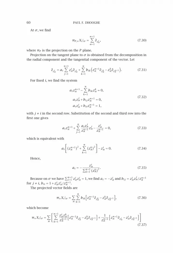
60 PAUL F. DHOOGHE

At σ , we find

πP,∗Xi|σ =n+1∑α=1

∂ziα , (7.30)

where πP is the projection on the P plane.

Projection on the tangent plane to σ is obtained from the decomposition in

the radial component and the tangential component of the vector. Let

∂ziα = ain+1∑j=1

ziα∂ziα+n∑k=1

bik(zn+1α ∂zkα−zkα∂zn+1

α

). (7.31)

For fixed i, we find the system

aizn+1α −

n∑k=1

bikzkα = 0,

aizjα+bijzn+1

α = 0,

aiziα+biizn+1α = 1,

(7.32)

with j ≠ i in the second row. Substitution of the second and third row into the

first one gives

aizn+1α +

n∑j=1

aizjα

zn+1α

zjα− ziαzn+1α

= 0, (7.33)

which is equivalent with

ai

[(zn+1α)2+ n∑

k=1

(zkα)2]−ziα = 0. (7.34)

Hence,

ai =− ziα∑n+1k=1

(zkα)2 . (7.35)

Because on σ we have∑n+1i=1 ziαziα = 1, we find ai =−ziα and bij = ziαzjα/zn+1

α

for j ≠ i, bii = 1+ziαziα/zn+1α .

The projected vector fields are

π∗Xi|σ =∑α

n∑k=1

bik[zn+1α ∂zkα−zkα∂zn+1

α

], (7.36)

which become

π∗Xi|σ =∑α

[n+1∑k=1

ziαzkαzn+1α

[zn+1α ∂zkα−zkα∂zn+1

α

]+ 1

zn+1α

[zn+1α ∂ziα−ziα∂zn+1

α

]](7.37)

MULTILOCAL INVARIANTS FOR THE CLASSICAL GROUPS 61

or

π∗Xi|σ =∑α

[∂ziα−2

ziαzn+1α

∂zn+1α+n+1∑k=1

ziαzkα∂zkα

]. (7.38)

But the following set of vector fields commute with the fundamental fields

and are transversal to the orbits in �′:

Yα =n+1∑i=0

ziα∂ziα , α= 1, . . . ,n+1,

Yα,β =n+1∑i=0

[ziα∂ziβ−z

iβ∂ziα], α < β, α,β= 1, . . . ,n+1.

(7.39)

Define the fields

Yαβ = 1�(zα,zβ

)[Yαβ+Yα−Yβ], (7.40)

which are equal to

Yαβ = 1�(zα,zβ

) n+1∑i=0

(ziα−ziβ

)(∂ziβ+∂ziα

). (7.41)

Proposition 7.12. The following invariant vector fields, taken over σ , are

tangent to σ

Yαβγ = Yαβ+ Yβγ+ Yγα. (7.42)

Proof. It suffices to check that Yαβγ annihilate the forms∑n+1i=0 ziαziα over

the sets∑n+1i=0 ziαziα = 0.

The former vector fields equal

Yαβγ =n+1∑i=1

[(1φαβ

+ 1φγα

)ziα−

ziβφαβ

− ziγφγα

]∂ziα

+n+1∑i=1

[(1φβγ

+ 1φαβ

)ziβ−

ziγφβγ

− ziαφαβ

]∂ziβ

+n+1∑i=1

[(1φγα

+ 1φβγ

)ziγ−

ziαφγα

− ziβφβγ

]∂ziγ .

(7.43)

We omit the proof of following proposition.

Proposition 7.13. The set Yαβ(β+1), with α < β < n if α = 1 and α < β <n+1 otherwise, span an invariant normal bundle to the orbits of CO(1)(n) in σ .

The existence of these vector fields allows the construction of an invariant

metric on σ . We proceed as in the orthogonal case and require the normal

62 PAUL F. DHOOGHE

bundle to be orthogonal to the orbits. In the normal bundle, we introduce the

Euclidean metric with respect to the above constructed vector fields, and, in

the orbits, we use the Killing form K of the Lie algebra co(1)(n) with respect to

the fundamental vector fields. Let q2 be this metric, and q2 the corresponding

function in the tangent space.

Consider the space �(1,0,...,0)�n+1 = J1V1×V2×···×Vn+1.

Taking the prolongation of (1)(�) on π(−1)� =�′, we, as a consequence

of the definition of the set (1)(�), find

dim(1)(�′)= (n+1)(n−2)

2+n+1= n

2+n−42

. (7.44)

But, then, because dim�(1,0,...,0)�n+1 =n(n+2), we find that the codimension

of the orbits in the level surfaces of the sheaf generated by (1)(�′) equals one.

The extra invariant generator is given by the layer metric q12, which is nothing

but the restriction of the metric q2 to the first-layer tangent bundle.

This brings us to the following theorem.

Theorem 7.14. Let � be the regular subset of �(1,0,...,0)�n+1; the invariant

sheaf is generated by � = �n+1∪(1)�n+1∪{q1

2}.The same procedure applies to the higher-order cases because the group

O+(1,n+1) extends linearly on the jet bundles over the base manifold which

allows to construct the transversal vector fields Yαβγ in exactly the same way,

and only the embedding changes. Let σ : �n+1 ↩ n+1. Then,

�(l,0,...,0)σ : �(l,0,··· ,0)�n+1 ↩ �(l,0,...,0) n+1 (7.45)

is the natural jet bundle embedding.

References

[1] A. F. Beardon, The Geometry of Discrete Groups, Graduate Texts in Mathematics,vol. 91, Springer-Verlag, New York, 1983.

[2] H. Boerner, Representation of Groups with Special Consideration for the Needs ofModern Physics, North-Holland Publishing, Amsterdam, 1963.

[3] M. H. Brill, E. B. Barrett, and P. M. Payton, Projective invariants for curves intwo and three dimensions, Geometric Invariance in Computer Vision (J. L.Mundy and A. Zisserman, eds.), Artificial Intelligence, MIT Press, Mas-sachusetts, 1992, pp. 193–214.

[4] H. S. M Coxeter, The representation of conformal space on a quadric, Ann. ofMath. 37 (1936), 416–426.

[5] P. F. Dhooghe, Contact transformations, contact algebras and lifts on a jet bundle,Ann. Mat. Pura Appl. (4) 131 (1982), 291–309.

[6] , On projective invariants of curves, Results Math. 27 (1995), no. 3-4, 237–243.

[7] , Multi local invariants on real unit balls, Math. J. Okayama Univ. 41 (1999),149–179.

[8] M. Fels and P. J. Olver, Moving coframes. I. A practical algorithm, Acta Appl. Math.51 (1998), no. 2, 161–213.

MULTILOCAL INVARIANTS FOR THE CLASSICAL GROUPS 63

[9] W. Fulton and J. Harris, Representation Theory, Graduate Texts in Mathematics,vol. 129, Springer-Verlag, New York, 1991.

[10] V. W. Guillemin and S. Sternberg, An algebraic model of transitive differentialgeometry, Bull. Amer. Math. Soc. 70 (1964), 16–47.

[11] S. Helgason, Differential Geometry, Lie Groups, and Symmetric Spaces, Pure andApplied Mathematics, vol. 80, Academic Press, New York, 1978.

[12] R. Howe, Remarks on classical invariant theory, Trans. Amer. Math. Soc. 313(1989), no. 2, 539–570.

[13] S. Kobayashi and K. Nomizu, Foundations of Differential Geometry. Vol I, Inter-science Publishers, New York, 1963.

[14] I. S. Krasil’shchik, V. V. Lychagin, and A. M. Vinogradov, Geometry of Jet Spacesand Nonlinear Partial Differential Equations, Advanced Studies in Contem-porary Mathematics, vol. 1, Gordon and Breach Science Publishers, NewYork, 1986.

[15] P. J. Olver, Applications of Lie Groups to Differential Equations, Graduate Texts inMathematics, vol. 107, Springer-Verlag, New York, 1993.

[16] , Differential invariants, Acta Appl. Math. 41 (1995), no. 1–3, 271–284.[17] , Moving frames and joint differential invariants, Regul. Chaotic Dyn. 4

(1999), no. 4, 3–18.[18] , Geometric foundations of numerical algorithms and symmetry, Appl. Al-

gebra Engrg. Comm. Comput. 11 (2001), no. 5, 417–436.[19] , Joint invariant signatures, Found. Comput. Math. 1 (2001), no. 1, 3–67.[20] P. J. Olver, G. Sapiro, and A. Tannenbaum, Differential invariant signatures and

flows in computer vision: a symmetry group approach, Geometry DrivenDiffusion in Computer Vision (B. M. ter Haar Romeny, ed.), Kluwer Aca-demic Publishers, Dordrecht, 1994.

[21] T. Sasaki, Projective differential geometry and linear homogeneous differentialequations, preprint, 1989.

[22] S. Sternberg, Lectures on Differential Geometry, Prentice-Hall, New Jersey, 1965.[23] T. Umeda, The Capelli identities, a century after, Selected Papers on Harmonic

Analysis, Groups, and Invariants, Amer. Math. Soc. Transl. Ser. 2, vol. 183,American Mathematical Society, Rhode Island, 1998, pp. 51–78.

[24] L. J. Van Gool, T. Moons, E. Pauwels, and A. Oosterlinck, Semi-differential invari-ants, Geometric Invariance in Computer Vision (J. L. Mundy and A. Zisser-man, eds.), Artificial Intelligence, MIT Press, Massachusetts, 1992, pp. 157–192.

[25] H. Weyl, The Classical Groups, Princeton University Press, New Jersey, 1946.[26] E. Wilczynski, Projective Differential Geometry of Curves and Ruled Surfaces,

Teubner, Leibzig, 1906.

Paul F. Dhooghe: Department of Mathematics, Center for Pure and Applied Differen-tial Geometry, KULeuven, Celestijnenlaan 200 B, 3001 Leuven, Belgium

E-mail address: Paul.Dhooghe@wis.kuleuven.ac.be

Mathematical Problems in Engineering

Special Issue on

Space Dynamics

Call for Papers

Space dynamics is a very general title that can accommodatea long list of activities. This kind of research started withthe study of the motion of the stars and the planets backto the origin of astronomy, and nowadays it has a largelist of topics. It is possible to make a division in two maincategories: astronomy and astrodynamics. By astronomy, wecan relate topics that deal with the motion of the planets,natural satellites, comets, and so forth. Many importanttopics of research nowadays are related to those subjects.By astrodynamics, we mean topics related to spaceflightdynamics.

It means topics where a satellite, a rocket, or any kind ofman-made object is travelling in space governed by the grav-itational forces of celestial bodies and/or forces generated bypropulsion systems that are available in those objects. Manytopics are related to orbit determination, propagation, andorbital maneuvers related to those spacecrafts. Several othertopics that are related to this subject are numerical methods,nonlinear dynamics, chaos, and control.

The main objective of this Special Issue is to publishtopics that are under study in one of those lines. The ideais to get the most recent researches and published them ina very short time, so we can give a step in order to helpscientists and engineers that work in this field to be awareof actual research. All the published papers have to be peerreviewed, but in a fast and accurate way so that the topics arenot outdated by the large speed that the information flowsnowadays.

Before submission authors should carefully read over thejournal’s Author Guidelines, which are located at http://www.hindawi.com/journals/mpe/guidelines.html. Prospective au-thors should submit an electronic copy of their completemanuscript through the journal Manuscript Tracking Sy-stem at http://mts.hindawi.com/ according to the followingtimetable:

Manuscript Due July 1, 2009

First Round of Reviews October 1, 2009

Publication Date January 1, 2010

Lead Guest Editor

Antonio F. Bertachini A. Prado, Instituto Nacional dePesquisas Espaciais (INPE), São José dos Campos,12227-010 São Paulo, Brazil; prado@dem.inpe.br

Guest Editors

Maria Cecilia Zanardi, São Paulo State University(UNESP), Guaratinguetá, 12516-410 São Paulo, Brazil;cecilia@feg.unesp.br

Tadashi Yokoyama, Universidade Estadual Paulista(UNESP), Rio Claro, 13506-900 São Paulo, Brazil;tadashi@rc.unesp.br

Silvia Maria Giuliatti Winter, São Paulo State University(UNESP), Guaratinguetá, 12516-410 São Paulo, Brazil;silvia@feg.unesp.br

Hindawi Publishing Corporationhttp://www.hindawi.com