Embed Size (px)
Citation preview

Universita degli Studi di Pisa
Dipartimento di InformaticaDottorato di Ricerca in Informatica
Ph.D. Thesis
Multidimensional Network Analysis
Michele Coscia
Supervisor
Fosca Giannotti
Supervisor
Dino Pedreschi
May 9, 2012

Abstract
This thesis is focused on the study of multidimensional networks. A multidimensional network isa network in which among the nodes there may be multiple different qualitative and quantitativerelations. Traditionally, complex network analysis has focused on networks with only one kind ofrelation. Even with this constraint, monodimensional networks posed many analytic challenges,being representations of ubiquitous complex systems in nature. However, it is a matter of commonexperience that the constraint of considering only one single relation at a time limits the set ofreal world phenomena that can be represented with complex networks. When multiple differentrelations act at the same time, traditional complex network analysis cannot provide suitable an-alytic tools. To provide the suitable tools for this scenario is exactly the aim of this thesis: thecreation and study of a Multidimensional Network Analysis, to extend the toolbox of complexnetwork analysis and grasp the complexity of real world phenomena. The urgency and need for amultidimensional network analysis is here presented, along with an empirical proof of the ubiquityof this multifaceted reality in different complex networks, and some related works that in the lasttwo years were proposed in this novel setting, yet to be systematically defined. Then, we tackle thefoundations of the multidimensional setting at different levels, both by looking at the basic exten-sions of the known model and by developing novel algorithms and frameworks for well-understoodand useful problems, such as community discovery (our main case study), temporal analysis, linkprediction and more. We conclude this thesis with two real world scenarios: a monodimensionalstudy of international trade, that may be improved with our proposed multidimensional analysis;and the analysis of literature and bibliography in the field of classical archaeology, used to showhow natural and useful the choice of a multidimensional network analysis strategy is in a problemtraditionally tackled with different techniques.

4

To my family: my parents for their exceptional support of all my needs, and my sister being waysmarter and professional than I will ever dream.
εαν µη ελπηται ανελπιστoν oυκ εξευρησει, ανεξερευνητoν εoν και απoρoν.


Acknowledgments
The most important role in this thesis, for which I really need to be grateful beyond what I canexpress, is the one played by my supervisors. Fosca Giannotti and Dino Pedreschi are really afundamental part of my professional career and probably all the opportunities I was able to obtainare due to their hard work.
I also need to thank the professional guiding figures of Ricardo Hausmann and Cesar A. Hidalgo,two incredibly enthusiastic and professional researchers who, even if they do not have any formalrole in this thesis, have accompanied me through more than half of my period as graduate studentand they are offering me the possibility of having a real impact on the world, far greater thanthe one I could dream before. Also Albert-Laszlo Barabasi gave me great opportunities anda great scientific environment to live in. A profound gratitude goes also to the reviewers of thisthesis, Hannu Toivonen, Yong-Yeol Ahn, Paolo Ferragina and Maria Simi, whose comments greatlyimproved the quality of the work I’m presenting.
Among all my co-authors, the prominent figure who deserves the biggest acknowledgment is forsure Michele Berlingerio, having taught me everything I know about being a good researcher andan efficient computer scientist, losing in the process probably more time, energy and patience thanhe expected. A big thank also to Maximilian Schich, because I do believe that 90% of what I knowabout complex networks is probably due to him. I cannot stress enough also how important was towork together with Anna Monreale and Ruggero Pensa, two of the people who worked harder thanone can believe, and also responsible for the preparation that lead me into starting the PhD. AlsoSalvo Rinzivillo was the most funny and enjoyable co-author ever, able to “make me christian”, ashe would say. And finally, of course, a big thank to Amedeo Cappelli.
There is an incredible amount of other people with whom I do not have a formal collaboration,nevertheless their impact of this thesis is far from negligible. They are too many, and a data miningapproach is needed to cluster them into geographically separated groups. This consideration givesalso the idea how ridiculous is for me to take the entire credit as sole author of this thesis, thatis basically a collaborative melting pot of an incredible hive-mind: I should rather take the blamefor all the errors and misunderstanding I put in it.
Pisa is the place where my career is born. Therefore I should start thanking Alessio Orlandi(for that coding summer, for Lucca Comics and for Zurich), Diego Pennacchioli (who got plentyof unrequested updates about this thesis), Roberto Trasarti (I hope he remembers the fun we hadin our complex network class in Lucca), Filippo Volpini, Giulio Rossetti and Riccardo Guidotti(my beloved trio of undergraduates), Lorenzo Gabrielli (the most precise person I know), MircoNanni (a fellow cinephile), Chiara Renso (she always brings loads of stuff to eat and to drink fromher missions) and Chiara Falchi (I probably owe her way more than a month of dinners). I willprobably be killed by all the people I did not mentioned, they are that many, but it’s better tostop here.
I spent an important period of my life at the Harvard Kennedy School, and I hope to continueto stay there for a long time. I then thank Catalina Prieto and Jennifer Gala, being the solutionto all my problems involving the US. Stephen Kosack keeps demonstrating how a great guy is, andI am looking forward to see what our thousands of projects will became. A big thank also to JuanJimenez, Muhammed Yildirim, Isabel Meirelles and Alex Simoes (an MIT intruder!) for the workwith the Product Space. Finally a thanks also to Juan Pablo Chauvin and Jasmina Beganovic, fortheir appreciation of my t-shirts and the quotes on my whiteboard.

Finally, for the group in Northeastern University, the first thought goes to Sune Lehmann, forthe great talks we had. And then I think about Yong-Yeol Ahn, with the hope and promise thatwe will be able to actually make real the collaboration we were planning. I also need to apologizeto Nicholas Blumm, Dashun Wang and Chaoming Song for all the times I stole part of their deskor their chairs. And again, for all the people not mentioned here, the thesis is long enough withscientific blabbering, but if it would contain all the friendship you gifted to me, it would explodeexponentially.
Damiano Ceccarelli for sure deserves a special thanks, being my only non-scientific co-author.But, more importantly, being the voice of the reason for basically everything else. Silvia Tomaninis probably my main motivator, constantly increasing the threshold of what should I do to beather, but she will keep anyway to end up as a winner. I won’t give up, by the way. I did notforget Gabriele Pastore, Francesca Aversa and all the guys from the forum, even if in these yearsI probably gave them less attention than I should. A big special thank also to Eleonora Grasso:our relationship was the cornerstone of three years of my life and one of the few things that keptme sane in the darkest hours of a PhD student (and there are many of those). I wish the very bestfor your future.
The last final “Thank you”, the special one, to my family: my parents and my sister. You aresimply perfect in understanding, supporting and correcting me in every occasion. I wish the worldwould be an easier place, where work does not bring you far from home, because being that farfrom where my heart is, I just feel lost.
And then there is you, Clara. The biggest, beautiful and exciting bet I have in my future. Ihave put everything on it.

Contents
1 Introduction 15
I Setting the Stage 19
2 Network Analysis 21
2.1 The Graph Representation . . . . . . . . . . . . . . . . . . . . . . . . . . . . . . . . 21
2.2 Statistical Properties . . . . . . . . . . . . . . . . . . . . . . . . . . . . . . . . . . . 22
2.3 Community Discovery . . . . . . . . . . . . . . . . . . . . . . . . . . . . . . . . . . 25
2.3.1 Problem Features . . . . . . . . . . . . . . . . . . . . . . . . . . . . . . . . . 26
2.3.2 The Definition-based classification . . . . . . . . . . . . . . . . . . . . . . . 28
2.3.3 Feature Distance . . . . . . . . . . . . . . . . . . . . . . . . . . . . . . . . . 31
2.3.4 Internal Density . . . . . . . . . . . . . . . . . . . . . . . . . . . . . . . . . 36
2.3.5 Bridge Detection . . . . . . . . . . . . . . . . . . . . . . . . . . . . . . . . . 42
2.3.6 Diffusion . . . . . . . . . . . . . . . . . . . . . . . . . . . . . . . . . . . . . 45
2.3.7 Closeness . . . . . . . . . . . . . . . . . . . . . . . . . . . . . . . . . . . . . 49
2.3.8 Structure Definition . . . . . . . . . . . . . . . . . . . . . . . . . . . . . . . 50
2.3.9 Link Clustering . . . . . . . . . . . . . . . . . . . . . . . . . . . . . . . . . . 53
2.3.10 No Definition . . . . . . . . . . . . . . . . . . . . . . . . . . . . . . . . . . . 54
2.3.11 Empirical Test . . . . . . . . . . . . . . . . . . . . . . . . . . . . . . . . . . 56
2.3.12 Alternative Classifications . . . . . . . . . . . . . . . . . . . . . . . . . . . . 58
2.4 Generators . . . . . . . . . . . . . . . . . . . . . . . . . . . . . . . . . . . . . . . . 59
2.4.1 Descriptive Models . . . . . . . . . . . . . . . . . . . . . . . . . . . . . . . . 60
2.4.2 Generative Models . . . . . . . . . . . . . . . . . . . . . . . . . . . . . . . . 62
2.5 Link Analysis . . . . . . . . . . . . . . . . . . . . . . . . . . . . . . . . . . . . . . . 63
2.6 Information Propagation . . . . . . . . . . . . . . . . . . . . . . . . . . . . . . . . . 64
2.7 Graph Mining . . . . . . . . . . . . . . . . . . . . . . . . . . . . . . . . . . . . . . . 66
2.8 Privacy . . . . . . . . . . . . . . . . . . . . . . . . . . . . . . . . . . . . . . . . . . 67
3 Multidimensional Network: Model Definition 69
4 Related Work 71
4.1 Layered Networks . . . . . . . . . . . . . . . . . . . . . . . . . . . . . . . . . . . . . 71
4.2 Hypergraphs . . . . . . . . . . . . . . . . . . . . . . . . . . . . . . . . . . . . . . . 74
4.3 Multidimensional Networks . . . . . . . . . . . . . . . . . . . . . . . . . . . . . . . 75
4.3.1 Multidimensional Community Discovery . . . . . . . . . . . . . . . . . . . . 75
4.3.2 Multidimensional Link Prediction . . . . . . . . . . . . . . . . . . . . . . . . 76
4.3.3 Signed Networks . . . . . . . . . . . . . . . . . . . . . . . . . . . . . . . . . 76
4.4 Tensor Decomposition . . . . . . . . . . . . . . . . . . . . . . . . . . . . . . . . . . 77

6 CHAPTER 0. CONTENTS
5 Real World Multidimensional Networks 795.1 Facebook . . . . . . . . . . . . . . . . . . . . . . . . . . . . . . . . . . . . . . . . . 795.2 Supermarket . . . . . . . . . . . . . . . . . . . . . . . . . . . . . . . . . . . . . . . 805.3 Flickr . . . . . . . . . . . . . . . . . . . . . . . . . . . . . . . . . . . . . . . . . . . 825.4 DBLP . . . . . . . . . . . . . . . . . . . . . . . . . . . . . . . . . . . . . . . . . . . 825.5 Querylog . . . . . . . . . . . . . . . . . . . . . . . . . . . . . . . . . . . . . . . . . . 845.6 GTD . . . . . . . . . . . . . . . . . . . . . . . . . . . . . . . . . . . . . . . . . . . . 845.7 IMDb . . . . . . . . . . . . . . . . . . . . . . . . . . . . . . . . . . . . . . . . . . . 845.8 Classical Archaeology . . . . . . . . . . . . . . . . . . . . . . . . . . . . . . . . . . 85
II Multidimensional Network Analysis 87
6 Extension of Classical Measures 896.1 Degree Related Measures . . . . . . . . . . . . . . . . . . . . . . . . . . . . . . . . 896.2 Shortest Path Related Measures . . . . . . . . . . . . . . . . . . . . . . . . . . . . 91
7 Novel Measures 957.1 Dimension Relevance . . . . . . . . . . . . . . . . . . . . . . . . . . . . . . . . . . . 95
7.1.1 Neighbors . . . . . . . . . . . . . . . . . . . . . . . . . . . . . . . . . . . . . 977.1.2 Dimension Relevance . . . . . . . . . . . . . . . . . . . . . . . . . . . . . . . 987.1.3 Finding and Characterizing Hubs . . . . . . . . . . . . . . . . . . . . . . . . 100
7.2 Dimension Correlation . . . . . . . . . . . . . . . . . . . . . . . . . . . . . . . . . . 1087.2.1 Finding Eras in Evolving networks . . . . . . . . . . . . . . . . . . . . . . . 1087.2.2 Experiments . . . . . . . . . . . . . . . . . . . . . . . . . . . . . . . . . . . 1117.2.3 Turning points and link prediction . . . . . . . . . . . . . . . . . . . . . . . 120
7.3 Dimension Connectivity . . . . . . . . . . . . . . . . . . . . . . . . . . . . . . . . . 124
8 Advanced Analysis 1298.1 Multidimensional Community Discovery . . . . . . . . . . . . . . . . . . . . . . . . 129
8.1.1 Finding and characterizing multidimensional communities . . . . . . . . . . 1308.1.2 Experiments . . . . . . . . . . . . . . . . . . . . . . . . . . . . . . . . . . . 136
8.2 Multidimensional Network Models . . . . . . . . . . . . . . . . . . . . . . . . . . . 1418.3 Multidimensional Link Prediction . . . . . . . . . . . . . . . . . . . . . . . . . . . . 1458.4 Multidimensional Shortest Path . . . . . . . . . . . . . . . . . . . . . . . . . . . . . 146
III Novel Insights for Network Analysis 153
9 The Product Space 1559.1 Economic Complexity . . . . . . . . . . . . . . . . . . . . . . . . . . . . . . . . . . 1559.2 How and Why Economic Complexity? . . . . . . . . . . . . . . . . . . . . . . . . . 1569.3 Product Space Creation . . . . . . . . . . . . . . . . . . . . . . . . . . . . . . . . . 1599.4 A Novel Product Categorization . . . . . . . . . . . . . . . . . . . . . . . . . . . . 1609.5 Applications . . . . . . . . . . . . . . . . . . . . . . . . . . . . . . . . . . . . . . . . 161
10 Study of Subject Themes in Classical Archaeology 16310.1 Previous Work . . . . . . . . . . . . . . . . . . . . . . . . . . . . . . . . . . . . . . 16410.2 Method . . . . . . . . . . . . . . . . . . . . . . . . . . . . . . . . . . . . . . . . . . 164
10.2.1 Data Preparation . . . . . . . . . . . . . . . . . . . . . . . . . . . . . . . . . 16610.2.2 Finding Overlapping Communities . . . . . . . . . . . . . . . . . . . . . . . 16610.2.3 Lift Significance . . . . . . . . . . . . . . . . . . . . . . . . . . . . . . . . . 16810.2.4 Era Discovery . . . . . . . . . . . . . . . . . . . . . . . . . . . . . . . . . . . 16810.2.5 Snapshot Connections . . . . . . . . . . . . . . . . . . . . . . . . . . . . . . 169
10.3 Global Exploration . . . . . . . . . . . . . . . . . . . . . . . . . . . . . . . . . . . . 170

0.0. CONTENTS 7
10.4 Meso Level Exploration . . . . . . . . . . . . . . . . . . . . . . . . . . . . . . . . . 17110.4.1 Co-Occurrence plus Lift-Significance . . . . . . . . . . . . . . . . . . . . . . 17110.4.2 Ego-Networks vs. Communities . . . . . . . . . . . . . . . . . . . . . . . . . 174
10.5 Conclusion . . . . . . . . . . . . . . . . . . . . . . . . . . . . . . . . . . . . . . . . 176
11 Conclusion and Future Works 177

8 CHAPTER 0. CONTENTS
List of Figures
2.1 Different degrees of complexity in the graph representation. . . . . . . . . . . . . . 222.2 A network toy example. . . . . . . . . . . . . . . . . . . . . . . . . . . . . . . . . . 232.3 Different community features. . . . . . . . . . . . . . . . . . . . . . . . . . . . . . . 272.4 An example of a graph that can be partitioned with a notion of “distance” between
its nodes. . . . . . . . . . . . . . . . . . . . . . . . . . . . . . . . . . . . . . . . . . 322.5 An example of the MDL principle for matrices: the matrix on the left is exactly the
same matrix as the one on the right, but reordered in order to describe it simply. . 352.6 An example of a graph which can be partitioned with a notion of internal density
between its nodes. . . . . . . . . . . . . . . . . . . . . . . . . . . . . . . . . . . . . 372.7 A dendrogram result for the modularity maximization algorithm, with a plot of
resulting modularity values given the partition. . . . . . . . . . . . . . . . . . . . . 392.8 An example of a graph that can be partitioned by identifying a “bridge”. . . . . . 422.9 An intuitive example of the bridge detection approach. In this graph the edge width
is proportional to the edge betweenness value. Wider edges are more likely to be abridge between communities. . . . . . . . . . . . . . . . . . . . . . . . . . . . . . . 43
2.10 An example of graph partitioned with a diffusion process. . . . . . . . . . . . . . . 452.11 Possible steps of a label propagation-based community discoverer. . . . . . . . . . . 462.12 The GuruMine data structures: the action table and the influence graphs. . . . . . 472.13 An example of a graph which can be partitioned by considering the relative distance,
in terms of number of edges, among its vertices. . . . . . . . . . . . . . . . . . . . . 492.14 The overlapping community structure detected by a clique-percolation approach. . 512.15 A multidimensional network. Solid, dashed and tick lines represent edges in three
different dimensions. . . . . . . . . . . . . . . . . . . . . . . . . . . . . . . . . . . . 552.16 Three graphs generated with the small-world model: (a) p = 0; (b) p = 1
4 ; (c) p = 1. 61
4.1 An example of layered network (a) and the process of a cascade failure involvingthe two different layers (b, c and d). In (a) the attacked grey node and its whitedependent disappear, with all the edges attached to them, generating (b). Then,the cascade is triggered: the white nodes connected to the disappeared node losetheir connections because they cannot sustain them anymore (b→c) and the samehappens for the grey nodes (c→d). . . . . . . . . . . . . . . . . . . . . . . . . . . . 72
5.1 The friendship dimension in Facebook network. . . . . . . . . . . . . . . . . . . . . 805.2 Small extracts of the three real multidimensional networks. . . . . . . . . . . . . . 82
6.1 A toy example. The solid line is dimension 1, the dashed line is dimension 2. . . . 906.2 Cumulative distributions of degree per dimension and global degree for Querylog,
Flickr and DBLP-Y. . . . . . . . . . . . . . . . . . . . . . . . . . . . . . . . . . . . 90
7.1 Example of different multidimensional hubs. . . . . . . . . . . . . . . . . . . . . . . 967.2 Toy example and computed measures. Lines: solid = dim 1, dashed = dim 2, dotted
= dim 3, dash-dotted = dim 4. . . . . . . . . . . . . . . . . . . . . . . . . . . . . . 997.3 The metrics computed on the three networks (color image). . . . . . . . . . . . . . 104
10 CHAPTER 0. LIST OF FIGURES
7.4 The overlap ratio between monodimensional and multidimensional hubs . . . . . . 1057.5 Some of the multidimensional hubs extracted . . . . . . . . . . . . . . . . . . . . . 1057.6 The Dimension Correlation computed only between subsequent snapshots (a,c,e)
and the corresponding dissimilarities computed on it (b,d,f). We recall that valuesfor the Random and Preferential attachment models are reported but not visible, asthey are constant on the 0 line. . . . . . . . . . . . . . . . . . . . . . . . . . . . . . 112
7.7 The Node and Edge Correlation computed among all the snapshots. . . . . . . . . 1137.8 Eras on both edge and node evolutions in DBLP . . . . . . . . . . . . . . . . . . . 1147.9 Eras in IMDb edge evolution . . . . . . . . . . . . . . . . . . . . . . . . . . . . . . 1157.10 Eras in IMDb node evolution . . . . . . . . . . . . . . . . . . . . . . . . . . . . . . 1167.11 Eras on both edge and node evolutions in GTD . . . . . . . . . . . . . . . . . . . . 1217.12 Forecasting eras on dissimilarities via autoregressive models . . . . . . . . . . . . . 1237.13 The Node and Edge Correlation in our networks. . . . . . . . . . . . . . . . . . . . 126
8.1 Three examples of multidimensional communities . . . . . . . . . . . . . . . . . . . 1308.2 Run through example for three instances of MCD Solver varying the φ parameter. 1358.3 The running times of STEP2 and STEP3 on our networks (color image). . . . . . . 1368.4 The cumulative distributions for γ and ρ in (from left to right): GTD, DBLP-C,
DBLP-Y and IMDb datasets. . . . . . . . . . . . . . . . . . . . . . . . . . . . . . . 1378.5 A few interesting communities found, with their γ or ρ. . . . . . . . . . . . . . . . 1408.6 QueryLog (left column) and DBLP-Y (right) original Dimension Relevance distri-
butions. . . . . . . . . . . . . . . . . . . . . . . . . . . . . . . . . . . . . . . . . . . 1418.7 Random: QueryLog (left column) and DBLP-Y (right) . . . . . . . . . . . . . . . . 1428.8 Preferential attachment: QueryLog (left column) and DBLP-Y (right column) . . . 1438.9 Shuffle: QueryLog (left column) and DBLP-Y (right column) . . . . . . . . . . . . 1448.10 Jaccard: QueryLog (left column) and DBLP-Y (column) . . . . . . . . . . . . . . . 1458.11 Performances of multidimensional link predictors. . . . . . . . . . . . . . . . . . . . 1478.12 A toy example for the multidimensional shortest path with cost modifiers problem. 149
9.1 The Product Space. . . . . . . . . . . . . . . . . . . . . . . . . . . . . . . . . . . . 1609.2 Community quality for five different ways of grouping products. . . . . . . . . . . . 1619.3 Contributions to the R square regression over the GDP growth of several different
indicators. . . . . . . . . . . . . . . . . . . . . . . . . . . . . . . . . . . . . . . . . . 162
10.1 Data model sketch for Archaologische Bibliographie, including the fat-tail distribtionfor classification co-occurrence in publications (upper left, see [232] for detail), andan indication of dataset growth from 1956 to 2011 (upper right). . . . . . . . . . . 164
10.2 Data preparation, analysis, and visualization pipeline as described in Sections 10.2.1to 10.2.3, including (a) the one-mode multidimensional projection from publication-classification or author-classification to classification co-occurrence, (b) the creationand visualization of rule-mined directed lift significance link weights in addition toregular co-occurrence weights, and (c) the creation and visualization of the multidi-mensional link community network, using Vespignani-filtering and Hierarchical LinkClustering. . . . . . . . . . . . . . . . . . . . . . . . . . . . . . . . . . . . . . . . . 165
10.3 (a) Relative number of nodes and edges size for different filtering thresholds. (b)Partition density values for each dendrogram cut threshold for each decade. Highervalues means denser partition, i.e. a better community division. . . . . . . . . . . . 167
10.4 Era structure dendrogram of classification cooccurrence in publications of ArchaologischeBibliographie according to [40] and Section 7.2. Eras are colored in the tree, whileour arbitrary decades are highlighted in the x-axis labels. . . . . . . . . . . . . . . 169
10.5 Communities belonging to various temporal snapshots are connected using a dedi-cated algorithm, revealing interesting merges and splits over time. . . . . . . . . . 169
10.6 Links in the community overlap network corresponding to subject themes, locations,and periods are distributed in a very different way. . . . . . . . . . . . . . . . . . . 170

0.0. LIST OF FIGURES 11
10.7 Both classification co-occurrence in publications as well as authors evolve over time,fleshing out structure that emerges early on in the process. . . . . . . . . . . . . . 172
10.8 Classification co-occurrence (≥ 4) in publications with lift-significance (≥ 0.056) forthe branch Plastic Art and Sculpture. . . . . . . . . . . . . . . . . . . . . . . . . . 173
10.9 Classification co-occurrence evolution clearly shows that initially highly significant,i.e. dark links become less significant and wider as they accumulate literature. . . 174
10.10Mutual self-definition of Names Portraits. . . . . . . . . . . . . . . . . . . . . . . . 17410.11Combining global and meso-level exploration by zooming into overlapping commu-
nities containing a given classification - here Paestum - reveals its meaning even tothe uneducated eye, improving significantly over simple ego-networks (see 10.4.2). . 175

12 CHAPTER 0. LIST OF FIGURES
List of Tables
2.1 Resume of the main notation used in this section. . . . . . . . . . . . . . . . . . . . 272.2 Resume of the community discovery methods. . . . . . . . . . . . . . . . . . . . . . 292.3 The evaluation measures for the communities extracted with different approaches. 57
5.1 Main statistics about Facebook and Supermarket networks, and their dimensions. . 815.2 Summary of the datasets extracted from Flickr, DBLP and Querylog. Column 1
specifies the dataset; Column 2 the dimension into account; Columns 3 and 4 thenumber of nodes and edges; Column 5 the average degree; Column 6 the densitycomputed as number of edges out of number of total possible edges in all the dimensions 83
7.1 Relationship between mono and multidimensional hubbiness of a node . . . . . . . 1037.2 Era labels on both DBLP edges and nodes . . . . . . . . . . . . . . . . . . . . . . . 1177.3 Era labels on both IMDb edges and nodes . . . . . . . . . . . . . . . . . . . . . . . 1197.4 Era labels on both GTD edges and nodes . . . . . . . . . . . . . . . . . . . . . . . 1227.5 Dimension Connectivity, HRC, LRC, OCN and OCP of our networks. . . . . . . . 126
8.1 Number of communities found (|C|) and modularity (Q) for each combination ofnetwork and parameters. . . . . . . . . . . . . . . . . . . . . . . . . . . . . . . . . . 137
9.1 The five most and least complex products according to PCI. . . . . . . . . . . . . 158

14 CHAPTER 0. LIST OF TABLES

Chapter 1
Introduction
A complex network is a model used to represent complex interacting phenomena such as socialinteractions among human beings, biological reactions in organisms and technological systems. Aninteraction takes places when there is some sort of information or physical exchange between twoactors, for example in a social network when two individuals establish a friendship or enmity linkbetween each other. To analyze the properties and understand the behavior of these phenomenathrough this model in different settings is a scientific field gaining a lot of attention in the lastdecade. Countless different problems have been tackled and an impressive number of good solu-tions, algorithms and descriptions of reality, has been proposed. A very brief, and incomplete, listincludes the following main topics:
� Community discovery, i.e. the decomposition of a complex network in its modular structure[78, 94];
� Link prediction, i.e. the prediction of the new relations that we will observe given the currentstate of the network (or the discovery of possible missing connections due to incomplete data)[74, 207];
� Flow analysis, i.e. the analysis of the structural properties of networks unveiled by differentrandom walk strategies over the edges of the graph;
� Cascade events, i.e. the investigation over the dynamics of epidemic events changing thestate of nodes through their connections [111];
� Graph motifs mining, i.e. the discovery of regularities in the connection patterns of the nodesin the network [268].
By exploiting the tools developed in the investigation of these topics, and usually combiningthem with each other or other analytic tools, complex network analysis has been used to tacklemany specific problems. For example, link prediction algorithms can be used to predict whethera user will trust the information provided by another user in a recommendation system [170]; orflow analysis is used for web page ranking in the popular Google search engine [208].
How can we explain this amount of interest by the scientific community? First of all, complexnetworks are by definition complex systems. A complex system is a system composed of differentparts that expresses at the global level properties that are not present in any single part takenalone. Their importance is derived by different factors. First, they are ubiquitous: complexsystems are present in many different scientific fields such as biology (the brain), ecology (the Earthclimate), engineering (telecommunication structures) and many more. Second, to understand whatoriginates their global properties is non trivial and can lead to important scientific results, such asdeeper understanding of how the human brain works or a prediction of the evolution of the Earth’secosystem.
16 CHAPTER 1. INTRODUCTION
This makes complex network analysis a suitable test field for many different approaches andtheories. In fact, crucial advancements in this field have been carried on by different professionalfigures: computer scientists, mathematicians, physicists, but also sociologists, economists andhumanities scholars. Complex network analysis is a melting pot of different disciplines, wheredifferent backgrounds can find a common vocabulary and primitives, making this novel field atruly new branch of science for the next years. Thus, we have a further reason for explaining thesuccess of complex networks: their ubiquity in modeling such different phenomena.
The clash of many different areas of expertise has lead complex network analysis to be appliedto many and different problems. Novel problems and settings have been explored in recent yearswith this model. Clearly, to be useful a model has to represent the features of real world phenomenain a simple way, but without losing too many details in the process. Therefore, from the originalsimple graph, many extensions have been proposed: weighted, dynamic, asymmetric relations arenow fundamental building bricks of any study aiming to unveil novel insights about the interactingphenomena in the real world. However, these extensions do not address a critical feature, presentin many interacting phenomena. In fact, weighted or directed relations do not help us when weare dealing with phenomena characterized by multiple different kinds of interactions.
We are not the only researchers that raised this issue. We will see that some intuitions aboutthe intrinsic multifaceted nature of the real world are already present in literature. But it is notnecessary to perform experiments or to deeply study obscure data to understand that multipledifferent relations interact with each other everyday everywhere. Let us consider the case of asocial network. At the present day, a person can establish a social relation with hundreds ofdifferent people. Are all these people “friends”? Is it possible to organize all these relationshipsin the same class? Of course not: we have relatives, sentimental relationships, work mates andseveral different reasons, and degrees, to call the people we know “friends” or “acquaintances”.
To be just a little more formal, it is well known that complex systems show their complexityin their multifaceted dynamics. There are several different competing forces acting either inde-pendently or in a complex interaction, either in equilibrium or in disequilibrium. As for complexnetworks, the interplay among different relations cannot be expressed with the traditional singlerelational models. In particular, the simple graph, a simplified representation used in the latteryears, is not enough for this increase in complexity.
In this shift of setting and representation, also the traditional complex network analysis needs toevolve and embrace the new complexity it is supposed to explain. If reality is multifaceted, or as wename it in this thesis “multidimensional”, then also network analysis should be multidimensional.Here we introduce the term “dimension” to indicate a particular edge type in a complex network.It is not an equivalent of the term “relations”. While each different relation is a dimension of anetwork, a dimension may also be a quality of the same relation, such as the different discretepoints in time when the relation was present. We will address this distinction more formally inthe thesis.
Just as non-linear and non-equilibrium systems needs a new paradigm for statistics, called su-perstatistics, multidimensional networks need new models (multigraphs, data tensors, and so on)and tools (multidimensional community discovery, multilink prediction, shortest path in multi-graphs with cost modifiers, just to name some of them). This is exactly the aim of this thesis: thecreation and study of a Multidimensional Network Analysis, to extend the known metaphors ofcomplex network analysis and grasp the complexity of real world phenomena.
In this thesis we want to accomplish several objectives. First, we want to advocate the urgencyand need for a multidimensional network analysis. We present an empirical proof of the ubiquityof this multifaceted reality in different complex networks. We are able to create multidimensionalrepresentations of many different interacting phenomena. We want also to let emerge the fact thatthese multidimensional representations are indeed more accurate than a simple monodimensionalmodel, and/or can lead to better insights about the phenomenon being represented. The need fora multidimensional network analysis is also witnessed by many other researchers, and we providea collection of their early works in this novel analytic setting. We also point out that theseapplications are indeed useful and advanced, but a common analytic ground, needed to fullyunderstand and develop novel insights, is yet to be defined.
17
The preliminary steps in the definition and creation of this common ground are exactly thesecond main objective of this thesis. We want to tackle this problem at two different levels. Westart by looking at the basic extensions of the known model: what is the new meaning of thedegree in the multidimensional network analysis? What does happen to the scale free structurein a multirelational environment? What is the new relation between the degree and the numberof neighbors for a node? How does multidimensionality influence the clustering coefficient or thecentrality measures?
We then move our attention to the development of novel algorithms and frameworks for well-understood and useful traditional problems in complex network analysis. For example, we areinterested in multidimensional community discovery, that we take as the main case study of thisthesis, and therefore tackled with special attention. Traditionally, in community discovery theproblem definition is to find a graph partition, clustering together densely connected sets of nodes.If we translate this problem definition in multidimensional terms, we want to find sets of nodesmultidimensionally densely connected. But what does “multidimensionally dense” mean here?Does it mean that all the different relations need to be expressed for each couple of nodes? Orthat is it necessary that at least one relation is expressed at a time for each couple, and it is onlyrequired that different relations connect different couples? This ambiguity will be tackled down inthis thesis.
Another example is link prediction. Link prediction has a straightforward problem definition:to rank not observed edges, i.e. couples of nodes, according to how likely they are to appear inthe future (or how likely they are not present due to missing data). If we have multiple relationsin our network, a new dimension appears. We are not supposed to identify just a couple of nodesthat have in between them an unexpected missing link, but we need also to decide in whichparticular relation, or set of relations. Is it sufficient to simply apply a traditional link predictorto each relation in an independent fashion? Or is it true that actually the different dimensions areinfluencing each other, and then a completely new framework has to be defined?
As a last example, we want to consider how to include known analysis frameworks into mul-tidimensional network analysis. In fact, we are interested in how a dynamic framework can beincluded into a multidimensional formulation. If we consider time as source of dimensions, i.e. arelation established in 2012 is a dimension and the same relation in 2011 is another dimension,then with the primitives of multidimensional networks we can perform temporal analysis. Thisdistinction unveils a characteristic of multidimensionality: it is possible to define two differentclasses of dimensions, the explicit and the implicit dimensions. We will explain the difference lateron in the thesis.
We conclude this thesis with a third objective: an example of how useful multidimensionalnetwork analysis can be when applied to analytic real world scenarios. We chose two of them.In the first scenario, we present a network analysis approach to international economics, namelythe creation and the analysis of the Product Space, i.e. a network map of products connected ifthey are frequently co-exported by the same countries. From this analysis, an impressive amountof useful knowledge can be extracted, leading to predictions of new products exported by thecountries and even their future economic growth. The aim of this first scenario is to indicate whereare the parts in which multidimensional network analysis is able to provide analytic improvementsover the monodimensional analysis performed. Our second scenario is the analysis of literature andbibliography in the field of classical archaeology. In this scenario we show how natural and usefulthe choice of a multidimensional network analysis strategy is in a problem traditionally tackledwith different techniques.
This thesis is organized as follows. Each of the aforementioned objectives constitutes a mainpart of the thesis. The first part, Setting the Stage, is devoted to the presentation of the urgencyand need for a multidimensional network analysis. We firstly present some aspects of traditionalcomplex network analysis in Chapter 2. Particular attention is devoted to the case of communitydiscovery in Section 2.3, with an extensive study of the state of the art in the field. We will thenbriefly define in a formal way our model for multidimensional networks in Chapter 3. In Chapter 4we explore the literature regarding multidimensional network analysis. In Chapter 5 we concludeour exploration about the need of a multidimensional network analysis by presenting many real

18 CHAPTER 1. INTRODUCTION
world examples of multidimensional networks, that will be analyzed in the following part of thethesis.
The second part, Multidimensional Network Analysis, is the core of this thesis. Here we tackleour second and main objective: the exploration of the various building bricks of multidimensional-ity in complex networks. We start from the bottom, by creating a simple extension mechanism totranslate the most basics network measures into multidimensional basics in Chapter 6. We thentake a step further in Chapter 7 by defining a collection of novel measures that acquire a meaningonly in the multidimensional setting, and are trivially solved in the monodimensional case. Finally,we conclude our main section by proposing also some more advanced analysis in Chapter 8. InSection 8.1 we propose novel evaluation measures and a framework for the discovery of multidi-mensional communities. The other advanced analysis we consider, with a lower resolution, aregenerative models for multidimensional networks (Section 8.2), multidimensional link prediction(Section 8.3) and the problem of finding the shortest path in a multigraph with cost modifiers(Section 8.4).
The third part, that concludes this thesis, deals with the real world analytical examples wechose: the Product Space creation (Chapter 9) and the analysis of the co-classification network inclassical archaeology, in Chapter 10.
Chapter 11 concludes the thesis, by presenting the future research directions opened by thisstudy.
The three parts of this thesis are based on peer reviewed papers published in internationalconferences. From the first part, the state of the art of complex network and the main definition ofthe multidimensional netowrk model are inherited from [37]. In the same paper, we introduced alsothe basic extension to the complex network model (Chapter 6) and the Dimension Connectivitymeasures (Section 7.3). Dimension Relevance measures (Section 7.1) and multidimensional networknull models (Section 8.2) are introduced and studied in [42]. Dimension Correlation and themapping of temporal analysis with multidimensional networks (Section 7.2) are published in [41,40, 43]. The community discovery problem in multidimensional complex networks (Section 2.3 forthe review and Section 8.1 for the actual algorithm) has been tackled in [78, 36, 39]. The ProductSpace analysis (Chapter 9) has been published as a book with Harvard University and MIT [128].Finally, the analysis of publications in Classical Archeology (Chapter 10) has been presented toscholars both from art history and computer science [233].

Part I
Setting the Stage

Chapter 2
Network Analysis
In this chapter we present the basic notions of complex network theory. We will start by explaininghow a network is represented with a graph, what variants can be defined for this basic representationand what are the basic statistical properties of graphs. We then present in each section one ofthe main sub branches of complex network analysis in computer science. We start with the maincase study of this thesis, namely the community discovery in complex network, with an extensivereview of the field. We provide a novel classification of community discovery algorithms, with theaim of presenting where in this branch multidimensional networks can play an important role (andwhere multidimensionality is already taken into account). The other subsections are shorter anddo not provide an exhaustive classification and literature review, outside the scope of this thesis.These sub branches are: network models, link analysis and information propagation. We providefor completeness also a brief overview of problems not directly tackled in the thesis, such as graphmining and privacy concerns in social networks. Where not otherwise specified, we use as basicreferences the review works presented in [195] and [66], which provide a more complete collectionof literature references.
2.1 The Graph Representation
A graph is a mathematical structure used to model pairwise relations between entities from acertain collection. A network is a set of entities with connections among them. The entities aremodeled as nodes. Nodes are also called vertices: in this thesis we will use the terms “node” and“vertex” interchangeably as synonyms, while the term “entity” is used to indicate what a nodein the graph represents in the real world. The interactions between nodes are represented by theedges.
A set of nodes joined by edges, as depicted in Figure 2.1(a), is only the simplest type ofnetwork; there are many ways in which networks may be more complex than this. We can add toour representation additional information. Here we present a list of them, taking the example of aclassical social network:
� We can add (multiple) labels both to vertices and to edges. Thus, there may be more thanone different type of vertex in a network, or more than one different type of edge. For examplenodes in a social network can be men or women, or they may have different nationalities,while edges may represent friendship, but they could also represent enmity. An example oflabeled graph is depicted in Figure 2.1(b).
� We can add a variety of properties, numerical or otherwise, associated with vertices and edges,thus specifying some attributes. In our social network setting, people can have different agesor incomes, and edges can be weighted by the geographical proximity or by how well twopeople know each other.
22 CHAPTER 2. NETWORK ANALYSIS
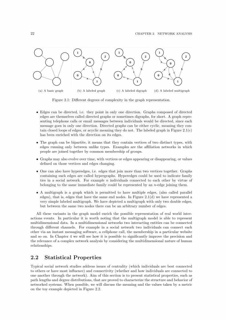
(a) A basic graph (b) A labeled graph (c) A labeled digraph (d) A labeled multigraph
Figure 2.1: Different degrees of complexity in the graph representation.
� Edges can be directed, i.e. they point in only one direction. Graphs composed of directededges are themselves called directed graphs or sometimes digraphs, for short. A graph repre-senting telephone calls or email messages between individuals would be directed, since eachmessage goes in only one direction. Directed graphs can be either cyclic, meaning they con-tain closed loops of edges, or acyclic meaning they do not. The labeled graph in Figure 2.1(c)has been enriched with the direction on its edges.
� The graph can be bipartite, it means that they contain vertices of two distinct types, withedges running only between unlike types. Examples are the affiliation networks in whichpeople are joined together by common membership of groups.
� Graphs may also evolve over time, with vertices or edges appearing or disappearing, or valuesdefined on those vertices and edges changing.
� One can also have hyperedges, i.e. edges that join more than two vertices together. Graphscontaining such edges are called hypergraphs. Hyperedges could be used to indicate familyties in a social network. For example n individuals connected to each other by virtue ofbelonging to the same immediate family could be represented by an n-edge joining them.
� A multigraph is a graph which is permitted to have multiple edges, (also called paralleledges), that is, edges that have the same end nodes. In Figure 2.1(d) we have represented avery simple labeled multigraph. We have depicted a multigraph with only two double edges,but between the same two nodes there can be an arbitrary number of edges.
All these variants in the graph model enrich the possible representation of real world inter-actions events. In particular it is worth noting that the multigraph model is able to representmultidimensional data. In a multidimensional networks two interacting entities can be connectedthrough different channels. For example in a social network two individuals can connect eachother via an instant messaging software, a cellphone call, the membership in a particular websiteand so on. In Chapter 4 we will see how it is possible to significantly improve the precision andthe relevance of a complex network analysis by considering the multidimensional nature of humanrelationships.
2.2 Statistical Properties
Typical social network studies address issues of centrality (which individuals are best connectedto others or have most influence) and connectivity (whether and how individuals are connected toone another through the network). Aim of this section is to present statistical properties, such aspath lengths and degree distributions, that are proved to characterize the structure and behavior ofnetworked systems. When possible, we will discuss the meaning and the values taken by a metricon the toy example depicted in Figure 2.2.
2.2. STATISTICAL PROPERTIES 23
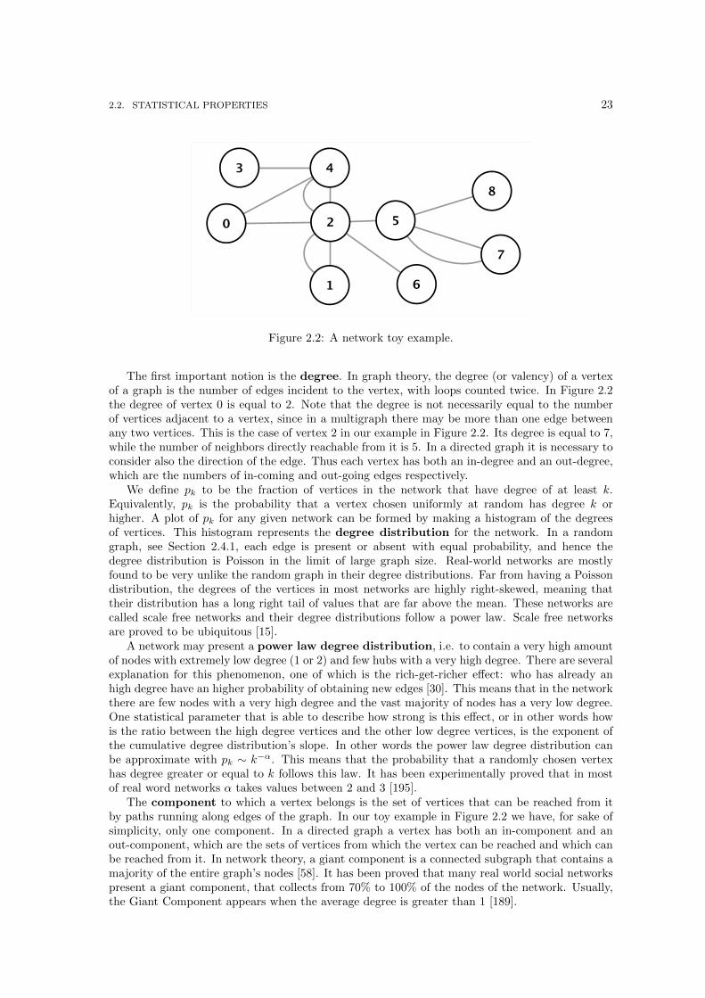
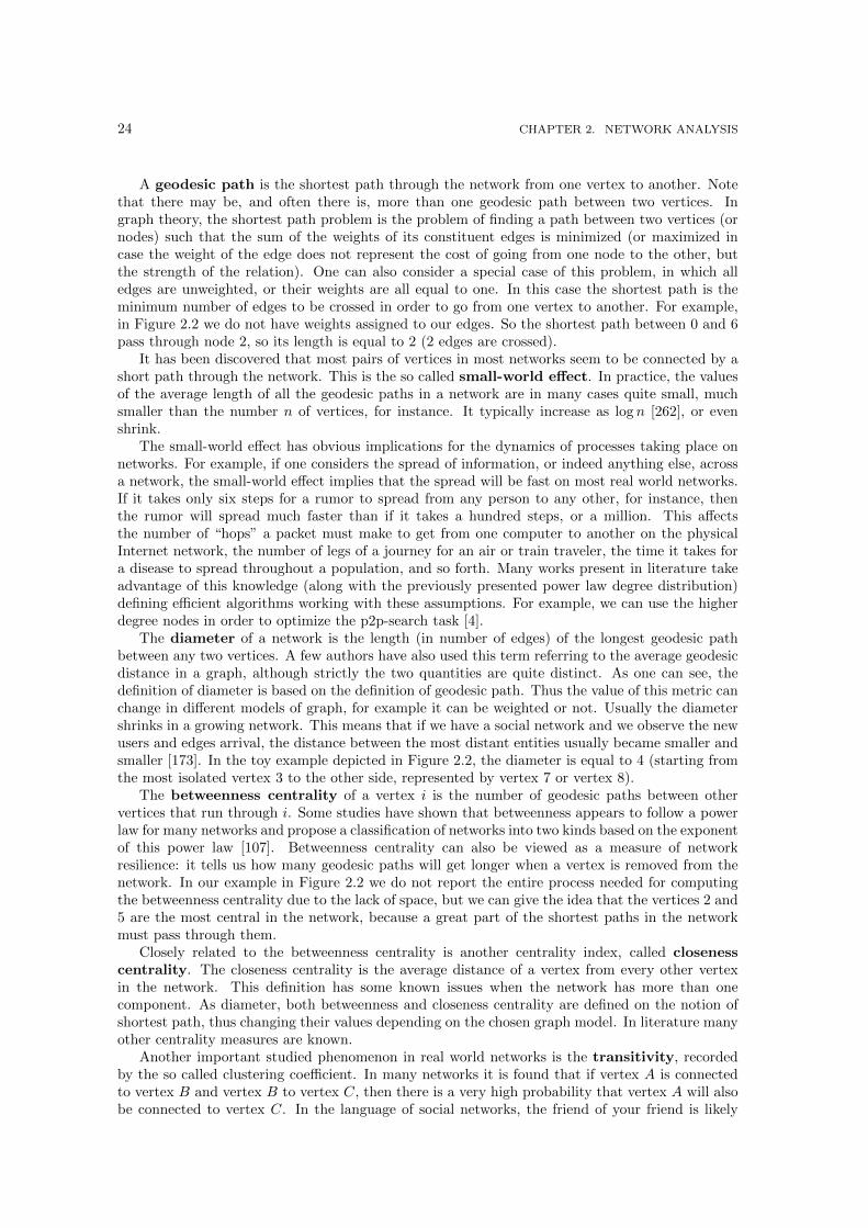
Figure 2.2: A network toy example.
The first important notion is the degree. In graph theory, the degree (or valency) of a vertexof a graph is the number of edges incident to the vertex, with loops counted twice. In Figure 2.2the degree of vertex 0 is equal to 2. Note that the degree is not necessarily equal to the numberof vertices adjacent to a vertex, since in a multigraph there may be more than one edge betweenany two vertices. This is the case of vertex 2 in our example in Figure 2.2. Its degree is equal to 7,while the number of neighbors directly reachable from it is 5. In a directed graph it is necessary toconsider also the direction of the edge. Thus each vertex has both an in-degree and an out-degree,which are the numbers of in-coming and out-going edges respectively.
We define pk to be the fraction of vertices in the network that have degree of at least k.Equivalently, pk is the probability that a vertex chosen uniformly at random has degree k orhigher. A plot of pk for any given network can be formed by making a histogram of the degreesof vertices. This histogram represents the degree distribution for the network. In a randomgraph, see Section 2.4.1, each edge is present or absent with equal probability, and hence thedegree distribution is Poisson in the limit of large graph size. Real-world networks are mostlyfound to be very unlike the random graph in their degree distributions. Far from having a Poissondistribution, the degrees of the vertices in most networks are highly right-skewed, meaning thattheir distribution has a long right tail of values that are far above the mean. These networks arecalled scale free networks and their degree distributions follow a power law. Scale free networksare proved to be ubiquitous [15].
A network may present a power law degree distribution, i.e. to contain a very high amountof nodes with extremely low degree (1 or 2) and few hubs with a very high degree. There are severalexplanation for this phenomenon, one of which is the rich-get-richer effect: who has already anhigh degree have an higher probability of obtaining new edges [30]. This means that in the networkthere are few nodes with a very high degree and the vast majority of nodes has a very low degree.One statistical parameter that is able to describe how strong is this effect, or in other words howis the ratio between the high degree vertices and the other low degree vertices, is the exponent ofthe cumulative degree distribution’s slope. In other words the power law degree distribution canbe approximate with pk ∼ k−α. This means that the probability that a randomly chosen vertexhas degree greater or equal to k follows this law. It has been experimentally proved that in mostof real word networks α takes values between 2 and 3 [195].
The component to which a vertex belongs is the set of vertices that can be reached from itby paths running along edges of the graph. In our toy example in Figure 2.2 we have, for sake ofsimplicity, only one component. In a directed graph a vertex has both an in-component and anout-component, which are the sets of vertices from which the vertex can be reached and which canbe reached from it. In network theory, a giant component is a connected subgraph that contains amajority of the entire graph’s nodes [58]. It has been proved that many real world social networkspresent a giant component, that collects from 70% to 100% of the nodes of the network. Usually,the Giant Component appears when the average degree is greater than 1 [189].
24 CHAPTER 2. NETWORK ANALYSIS
A geodesic path is the shortest path through the network from one vertex to another. Notethat there may be, and often there is, more than one geodesic path between two vertices. Ingraph theory, the shortest path problem is the problem of finding a path between two vertices (ornodes) such that the sum of the weights of its constituent edges is minimized (or maximized incase the weight of the edge does not represent the cost of going from one node to the other, butthe strength of the relation). One can also consider a special case of this problem, in which alledges are unweighted, or their weights are all equal to one. In this case the shortest path is theminimum number of edges to be crossed in order to go from one vertex to another. For example,in Figure 2.2 we do not have weights assigned to our edges. So the shortest path between 0 and 6pass through node 2, so its length is equal to 2 (2 edges are crossed).
It has been discovered that most pairs of vertices in most networks seem to be connected by ashort path through the network. This is the so called small-world effect. In practice, the valuesof the average length of all the geodesic paths in a network are in many cases quite small, muchsmaller than the number n of vertices, for instance. It typically increase as log n [262], or evenshrink.
The small-world effect has obvious implications for the dynamics of processes taking place onnetworks. For example, if one considers the spread of information, or indeed anything else, acrossa network, the small-world effect implies that the spread will be fast on most real world networks.If it takes only six steps for a rumor to spread from any person to any other, for instance, thenthe rumor will spread much faster than if it takes a hundred steps, or a million. This affectsthe number of “hops” a packet must make to get from one computer to another on the physicalInternet network, the number of legs of a journey for an air or train traveler, the time it takes fora disease to spread throughout a population, and so forth. Many works present in literature takeadvantage of this knowledge (along with the previously presented power law degree distribution)defining efficient algorithms working with these assumptions. For example, we can use the higherdegree nodes in order to optimize the p2p-search task [4].
The diameter of a network is the length (in number of edges) of the longest geodesic pathbetween any two vertices. A few authors have also used this term referring to the average geodesicdistance in a graph, although strictly the two quantities are quite distinct. As one can see, thedefinition of diameter is based on the definition of geodesic path. Thus the value of this metric canchange in different models of graph, for example it can be weighted or not. Usually the diametershrinks in a growing network. This means that if we have a social network and we observe the newusers and edges arrival, the distance between the most distant entities usually became smaller andsmaller [173]. In the toy example depicted in Figure 2.2, the diameter is equal to 4 (starting fromthe most isolated vertex 3 to the other side, represented by vertex 7 or vertex 8).
The betweenness centrality of a vertex i is the number of geodesic paths between othervertices that run through i. Some studies have shown that betweenness appears to follow a powerlaw for many networks and propose a classification of networks into two kinds based on the exponentof this power law [107]. Betweenness centrality can also be viewed as a measure of networkresilience: it tells us how many geodesic paths will get longer when a vertex is removed from thenetwork. In our example in Figure 2.2 we do not report the entire process needed for computingthe betweenness centrality due to the lack of space, but we can give the idea that the vertices 2 and5 are the most central in the network, because a great part of the shortest paths in the networkmust pass through them.
Closely related to the betweenness centrality is another centrality index, called closenesscentrality. The closeness centrality is the average distance of a vertex from every other vertexin the network. This definition has some known issues when the network has more than onecomponent. As diameter, both betweenness and closeness centrality are defined on the notion ofshortest path, thus changing their values depending on the chosen graph model. In literature manyother centrality measures are known.
Another important studied phenomenon in real world networks is the transitivity, recordedby the so called clustering coefficient. In many networks it is found that if vertex A is connectedto vertex B and vertex B to vertex C, then there is a very high probability that vertex A will alsobe connected to vertex C. In the language of social networks, the friend of your friend is likely
2.3. COMMUNITY DISCOVERY 25
also to be your friend. In terms of network topology, transitivity means the presence of an highnumber of triangles in the network, i.e. sets of three vertices each of which is connected to each ofthe others.
The transitivity property play a crucial role in another studied aspect of complex networks:the community structure, i.e. groups of vertices that have an high density of edges within themand a lower density of edges between groups. In social networks it is straightforward to verifythat people do organize themselves into (overlapping) groups along lines of interest, occupation,age, and so forth. This division can be detected in the communities of a network that representstheir interactions [190]. Other examples can be citation networks, in which authors would divideinto groups representing particular areas of research interest [266]; or in the World Wide Web thecommunity structure might reflect the subject matter of pages.
The detection of this particular structure inside complex networks is one of the most interestingand explored fields of research. We present in Chapter 2.3 some of the most important communitydetection algorithms, along with their strong points and the open problems. As we will see, alsoin this research track we are far from getting a definitive answer to the problem of identifyingcommunities in a network. The definition itself of community in a network is controversial, andthis stimulated further research.
2.3 Community Discovery
One critical feature of complex networks, which has been widely studied in the literature sinceits early stages of analysis, is the possibility of identifying groups and communities within thestructure of many phenomena represented by this model. Community detection is important formany reasons, such as node classification which entails homogeneous groups, group leaders orcrucial group connectors. A “Community” is usually considered to be a set of entities whereeach entity is closer to the other entities within the community than to the entities outside it.Communities are groups of entities that probably share common properties and/or play similarroles within the interacting phenomenon that is being represented. Communities may correspondto groups of pages of the World Wide Web dealing with related topics [92], to functional modulessuch as cycles and pathways in metabolic networks [123, 209], to groups of related individuals insocial networks [106] and so on.
Community discovery is very similar to the clustering problem, i.e. it is a traditional datamining task. In data mining, clustering is an unsupervised learning task, which aims to assign largesets of data into homogeneous groups (clusters). In fact, community discovery can be viewed as adata mining analysis on graphs: an unsupervised classification of its nodes. In addition, communitydiscovery is the most studied data mining application on social networks. Other applications, suchas graph mining [268], are in an early phase of their development. Instead community discoveryhas achieved a more advanced development with contributions from different fields such as physics.
Nevertheless, this is only part of the community discovery problem. In classical data miningclustering, we have data that is not in a relational form. Thus, in this general form, the factthat the entities are nodes connected to each other through edges has not been explored much.Therefore, the concept of spatial proximity needs to be mapped between entities (i.e. vertices) ingraph representation.
The traditional and most accepted definition of proximity in a network is based on the topologyof its edges. In this case the definition of community is formulated according to the differencesin the densities of links in different parts of the network. Many networks have been found to benon-homogeneous, consisting not of an undifferentiated mass of vertices, but of distinct groups.Within these groups there are many edges between vertices, but between groups there are feweredges. The aim of a community detection algorithm is, in this case, to divide the vertices of anetwork into some number k of groups, while maximizing the number of edges inside these groupsand minimizing the number of edges established between vertices in different groups. These groupsare the desired communities of the network.
This definition is no longer suitable due to the increasing complexity of network representations
26 CHAPTER 2. NETWORK ANALYSIS
and of the novel analytical settings, such as the information propagation or multidimensionalnetwork analysis. For example, in a temporal evolving setting, two entities can be considered closeto each other if they share a common action profile even if they are not directly connected. Thuseach novel approach to community discovery has had to face this problem and has developed itsown definition of community for its own solution. The underlying definition of community is thecriterion that we use to classify community discovery algorithms.
In addition to the variety of different definitions of community, communities have a numberof interesting features. These features can be a hierarchical or overlapping configuration of thegroups inside the network. Or else the graph can include directed edges, thus giving importance tothis direction when considering the relations between entities. The communities can be dynamic,i.e. evolving over time, or multidimensional, i.e. there could be multiple relations and sets ofindividuals that behave as isolated entities in each relation of the network, thus forming a densecommunity when considering all the possible relations at the same time. Or they can interactinside all relations, and still the result is a densely connected community, but with a differentconfiguration. We tackle this problem, the ambiguity of the concept of “multidimensional density”,in Section 8.1.
As a result this extreme richness of definitions and features has lead to the publication ofan impressive number of excellent solutions to the community discovery problem. It is thereforenot surprising that there are a number of review papers describing all these methods, such as [94].However, existing reviews tend to analyze the different techniques from a very technical perspective.They do not consider organizing the algorithms according to their definition of community, whichare many and different as acknowledged also by other papers, such as [200], in which authors say“[all the methods] require us to know what we are looking for in advance before we can decide whatto measure”, in which “know what we are looking for” clearly means define what a community is.To use a metaphor, existing reviews talk about bricks and mortar but not about the architecturalstyle. Further, no one considered the problem of community discovery in a multidimensionalperspective.
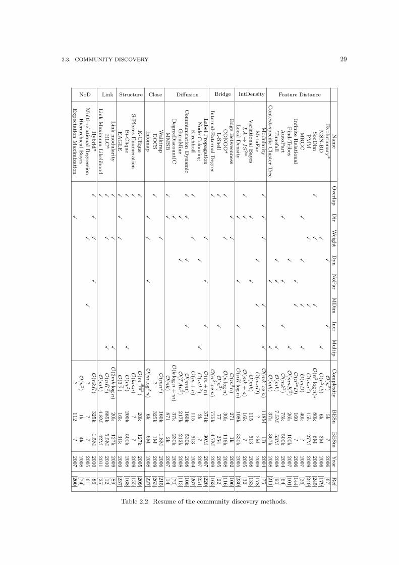
We have thus chosen to cluster the community discovery algorithms by considering their defi-nition of what is a community, which depends on what kinds of groups they aim to extract fromthe network. For each algorithm we record the characteristics of the output of the method, thushighlighting which sets of features the reviewed algorithm is suitable or not suitable for. We alsoconsider some general frameworks that provide both a community discovery approach and a gen-eral technique. These are applicable to other graph partitioning algorithms by adding new featuresto these other methods.
We now explain the classification of algorithms based on community definitions. Firstly, wereport in Table 2.1 the general notation used in this section. Sometimes we need an additional nota-tion to better explain what an algorithm exactly does. We introduce this additional notation whenneeded and the scope of the additional notation is limited to the paragraph of one particular algo-rithm. Then, before presenting the classification, we make explicit what are the problem featureswe consider more important for community discovery, including, of course, multidimensionality.
2.3.1 Problem Features
There are many features to be considered in the complex task of detecting communities in graphstructures. In this section we present some of the features an analyst may be interested in fordiscovery network communities. We use them to evaluate the reviewed algorithms in Table 2.2and also to motivate our classification.
Table 2.2 records the main properties of a community discovery algorithm. These properties canbe grouped into two classes. The first class considers the features of the problem representation,the second the characteristics of the approach.
Within the first class of features we group together all the possible variants in the representationof the original real world phenomenon. The most important features we consider are:
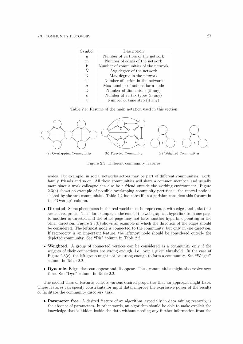
� Overlapping. In some real world networks, communities can share one or more common
2.3. COMMUNITY DISCOVERY 27
Symbol Descriptionn Number of vertices of the networkm Number of edges of the networkk Number of communities of the networkK Avg degree of the networkK Max degree in the networkT Number of action in the networkA Max number of actions for a nodeD Number of dimensions (if any)c Number of vertex types (if any)t Number of time step (if any)
Table 2.1: Resume of the main notation used in this section.
(a) Overlapping Communities (b) Directed Community (c) Weighted Communities
Figure 2.3: Different community features.
nodes. For example, in social networks actors may be part of different communities: work,family, friends and so on. All these communities will share a common member, and usuallymore since a work colleague can also be a friend outside the working environment. Figure2.3(a) shows an example of possible overlapping community partitions: the central node isshared by the two communities. Table 2.2 indicates if an algorithm considers this feature inthe “Overlap” column.
� Directed. Some phenomena in the real world must be represented with edges and links thatare not reciprocal. This, for example, is the case of the web graph: a hyperlink from one pageto another is directed and the other page may not have another hyperlink pointing in theother direction. Figure 2.3(b) shows an example in which the direction of the edges shouldbe considered. The leftmost node is connected to the community, but only in one direction.If reciprocity is an important feature, the leftmost node should be considered outside thedepicted community. See “Dir” column in Table 2.2.
� Weighted. A group of connected vertices can be considered as a community only if theweights of their connections are strong enough, i.e. over a given threshold. In the case ofFigure 2.3(c), the left group might not be strong enough to form a community. See “Weight”column in Table 2.2.
� Dynamic. Edges that can appear and disappear. Thus, communities might also evolve overtime. See “Dyn” column in Table 2.2.
The second class of features collects various desired properties that an approach might have.These features can specify constraints for input data, improve the expressive power of the resultsor facilitate the community discovery task.
� Parameter free. A desired feature of an algorithm, especially in data mining research, isthe absence of parameters. In other words, an algorithm should be able to make explicit theknowledge that is hidden inside the data without needing any further information from the
28 CHAPTER 2. NETWORK ANALYSIS
analyst regarding the data or the problem (for instance the number of communities). See“NoPar” column in Table 2.2.
� Multidimensional input. This is the most important feature in the economy of thisthesis. As we already know, multidimensionality in networks is an emerging topic [244,170, 37]. When dealing with multiple dimensions, the notion of community changes. Theconcept of multidimensionality is used (with various names: multi-relational, multiplex, andso on) by some approaches as a feature of the input considered by the approach, as wealso discussed in Chapter 4. This is the reason why multidimensionality is considered afeature of the input. However, in our opinion, multidimensionality feature should not beplaced here, since what we want to extract are truly multidimensional communities. Sofar, no approach in the community discovery literature is able to do that, and this is thereason why the multidimensionality feature is “misplaced”. We explore the idea of returningmultidimensional communities in Section 8.1. See “MDim” column in Table 2.2.
� Incremental. Another desired feature of an algorithm is its ability to provide an outputwithout an exhaustive search of the entire input. An incremental approach to the communitydiscovery is to classify a node in one community by looking only at its neighborhood, or theset of nodes two hops away. Alternatively newcomers are put in one of the previously definedcommunities without starting the community detection process from the beginning. See“Incr” column in Table 2.2.
� Multipartite input. Many community discovery approaches work even if the network hasthe particular form of a multipartite graph. The multipartite graph, however, is not entirely afeature of the input that we might want to consider for the output. Many algorithms often usea (usually) bipartite projection of a classical graph in order to apply efficient computations.As in the case of multidimensionality, this is the reason for including the multipartite inputas a feature of the approach and not of the output. See “Multip” column in Table 2.2.
There is one more “meta feature” that we consider. This is the possibility of applying theconsidered approach to another community discovery technique by adding new features to the“guest method”. This meta feature will be highlighted with an asterisk next to the algorithm’sname.
Table 2.2 also has a “Complexity” column that gives the time complexity of the methods pre-sented. The two “BES” columns give the Biggest Experiment Size, in terms of nodes (“BESn”) andedges (“BESm”), that are included in the original paper reviewed. Note that the Complexity andBES columns often offer an evaluation of the actual values, since the original work did not providean explicit and clear analysis of the complexity or their experimental setting. A question markindicates where evaluating the complexity would not be straightforward, or where no experimentaldetails are provided.
2.3.2 The Definition-based classification
We now review community detection approaches. We group together the algorithms in eight classessharing the same definition of what a community is, i.e. the same conditions satisfied by a groupof entities that allow them to be clustered together in a community. This classification should helpto get a higher level view of the universe of graph clustering algorithms, by uncovering a practicaland reasoned point of view for those analysts seeking to obtain precise results in their analyticalproblems. The proposed categories are the following:
� Feature Distance. Here we collect all the community discovery approaches that start fromthe assumption that a community is composed of entities which ubiquitously share a veryprecise set of features, with similar values (i.e. defining a distance measure on their features,the entities are all close to each other). A common feature can be an edge or any attributelinked to the entity (in our problem definition: the action). Usually, these approaches propose
2.3. COMMUNITY DISCOVERY 29N
am
eO
verla
pD
irW
eight
Dyn
NoP
ar
MD
imIn
crM
ultip
Com
plex
ityB
ES
nB
ES
mY
ear
Ref
Feature Distance
Evolu
tion
ary
*X
XO
(n2)
5k
?2006
[67]
MS
N-B
DX
XO
(n2ck
)6k
3M
2006
[179]
SocD
imX
XX
O(n
2lo
gn
)∗80k
6M
2009
[245]
PM
MX
XO
(mn2)
15k
27M
2009
[249]
MR
GC
XX
XX
O(mD
)40k
?2007
[26]
Infi
nite
Rela
tion
al
XX
O(n
2cD
)160
?2006
[144]
Fin
d-T
ribes
XX
O(mnK
2)
26k
100k
2007
[101]
Au
toP
art
XX
XO
(mk2)
75k
500k
2004
[64]
Tim
efall
XX
XO
(mk)
7.5
M53M
2008
[90]
Contex
t-specifi
cC
luster
Tree
XX
O(mk)
37k
367k
2008
[211]
IntDensity
Mod
ula
rityX
XX
XX
XO
(mk
logn
)118M
1B
2004
[75]
Meta
Fac
XX
O(mnD
)?
2M
2009
[178]
Varia
tion
al
Bayes
XX
O(mk)
115
613
2008
[133]
LA→IS2*
XX
O(mk
+n
)16k
?2005
[32]
Loca
lD
ensity
XX
XO
(nK
logn
)108k
330k
2005
[230]
Bridge
Ed
ge
Betw
eenn
essX
XO
(m2n
)271
1k
2002
[106]
CO
NG
O*
XX
O(n
logn
)30k
116k
2008
[116]
L-S
hell
XX
O(n
3)
77
254
2005
[22]
Intern
al-E
xtern
al
Deg
reeX
O(n
2lo
gn
)775k
4.7
M2009
[163]
Diffusion
Lab
elP
rop
agatio
nX
XX
O(m
+n
)374k
30M
2007
[220]
Nod
eC
olo
urin
gX
XO
(ntk
2)
2k
?2007
[251]
Kirch
hoff
XX
O(m
+n
)115
613
2004
[267]
Com
mu
nica
tion
Dyn
am
icX
XX
XO
(mnt)
160k
530k
2008
[108]
Gu
ruM
ine
XX
O(TAn2)
217k
212k
2008
[113]
Deg
reeDisco
untIC
XO
(klo
gn
+m
)37k
230k
2009
[70]
MM
SB
XX
O(nk)
871
2k
2007
[14]
Close
Walk
trap
XO
(mn2)
160k
1.8
M2006
[215]
DO
CS
X?
325k
1M
2009
[263]
Info
map
XX
XO
(mlo
g2n
)6k
6M
2008
[227]
Structure
K-C
liqu
eX
O(m
lnm
10
)20k
127k
2005
[209]
S-P
lexes
Enu
mera
tion
XO
(kmn
)?
?2009
[155]
Bi-C
liqu
eX
XO
(m2)
200k
500k
2008
[168]
EA
GL
EX
XX
O(3n3
)16k
31k
2009
[237]
Link
Lin
km
od
ula
rityX
XX
O(2mk
logn
)20k
127k
2009
[89]
HL
C*
XX
XO
(nK
2)
885k
5.5
M2010
[12]
Lin
kM
axim
um
Lik
elihood
XO
(mk)
4.8
M42M
2011
[25]
NoD
Hyb
rid*
XX
XX
O(nkK
)325k
1.5
M2010
[86]
Mu
lti-relatio
nal
Reg
ression
XX
??
?2005
[61]
Hiera
rchica
lB
ayes
O(n
2)
1k
4k
2008
[74]
Exp
ectatio
nM
axim
izatio
nX
?112
?2007
[200]
Table 2.2: Resume of the community discovery methods.

30 CHAPTER 2. NETWORK ANALYSIS
this community definition in order to apply classical data mining clustering techniques, suchas the Minimum Description Length principle [223, 121].
� Internal Density. In this group we consider the most important articles that define com-munity discovery as a process driven by directly detecting the denser areas of the network.
� Bridge Detection. This section includes the community discovery approaches based on theconcept that communities are dense parts of the graph among which there are very few edgesthat can break the network down into pieces if they are removed. These edges are “bridges”and the components of the network resulting from their removal are the desired communities.
� Diffusion. Here we include all the approaches to the community discovery task that rely onthe idea that communities are groups of nodes that can be influenced by the diffusion of acertain properties or information inside the network. In addition, the community definitioncan be narrowed down to the groups that are only influenced by the very same set of diffusionsources.
� Closeness. A community can also be defined as a group of entities that can reach each of itsown community companions with very few hops on the edges of the graph, while the entitiesoutside the community are significantly farther apart.
� Structure. Another approach to community discovery is to define the community exactly asa very precise and almost immutable structure of edges. Often these structures are definedas a combination of smaller network motifs. The algorithms following this approach definesome kinds of structures and then try to find them efficiently inside the graph.
� Link Clustering. This class can be viewed as a projection of the community discoveryproblem. Instead of clustering the nodes of a network, these approaches state that it is therelation that belongs to a community, not the node. Therefore they cluster the edges of thenetwork and thus the nodes belong to the set of communities of their edges.
� No Definition. There are a number of community discovery frameworks which do nothave a basic definition of the characteristic of the community they want to explore. Insteadthey define various operations and algorithms to combine the results of various communitydiscovery approaches and then use the target method community definition for their results.Alternatively, they let the analyst define his / her own notion of community and search forit in the graph.
In each section we clarify which features in a particular community discovery category of theones presented in the previous section are derived naturally, and which features are naturallydifficult to achieve. We are not formally building an axiomatic approach, such as the one builtin [150] for spatial clustering. Instead, we are using the features presented and an experimentalsetting to make the rationale and the properties of each category in this classification more explicit.The experiments made to support this point are presented after the classification in this section.
Where possible, we also provide a simple graphical example of the definition considered. Thisexample provides a graphical intuition of the main properties of the given classification, in termsof the strong and weak points in particular community features.
The aim of this section is to focus on the most recent approaches and on the more generaldefinitions of community. We are not focusing on historical approaches. Some examples of classicalclustering algorithms that have not been extensively reviewed are the Kernighan-Lin algorithm[146] or the classical spectral bisection approach [217]. Thus, for a historical point of view of thecommunity discovery problem, please refer to other review papers.
There is a sort of overlap for some community definitions. For example a definition of internaldensity may also include communities with sparse external links, i.e. bridges. We see in theInternal Density category that in this definition a key concept is modularity [75]. Modularityis a quality function which considers both the internal density of a community and the absence
2.3. COMMUNITY DISCOVERY 31
of edges between communities. Thus methods based on modularity could be clustered in bothcategories. However, the underlying definition of modularity focuses on the internal density, whichis the reason for the proposed classification. To give another example, a diffusion approach maydetect the same communities whose members can reach each other with just a few hops. Howeverthis is not always the case: the diffusion approach may also find communities with an arbitrarydistance between its members.
Many approaches in the literature do not explicitly define the communities they want to detector, worse, they generically claim that their aim is to find dense modules of the network. This isnot a problem for us, since the underlying community definition can be inferred from a high-levelunderstanding of the approach described in the original paper. One cannot expect researchers tobe able to categorize their method before an established categorization has been accepted.
In order to gain stronger evidence of the differences between the proposed categories, considerFigures 2.4, 2.6, 2.8, 2.10, 2.13 and 2.14. These figures depict the simplest typical communities thathave been identified from the definitions of Feature Distance, Internal Density, Bride Detection,Diffusion, Closeness and Structure Definition, respectively. As can be seen, there are a number ofdifferences between these examples. The Bridge Detection example (Figure 2.8) is a random graph,thus with no community structure defined for the algorithms in the Internal Density category. TheDiffusion example (Figure 2.10) is also a random graph, however although the diffusion processidentifies two communities, no clear bridges can be detected.
The overlap is due to the fact that many algorithms work with some general “background”meta definition of community. Further, many algorithms may present common strategies in theexploration of the search space or in evaluating the quality of their partition in order to refine it.Consider for example [161] and [222]. In these two papers there is a thorough theoretical studyconcerning modularity and its most general form. In [161], for example, the authors were able toderive modularity as a random walk exploration strategy, thus highlighting its overlap with thealgorithms clustered here in the “Closeness” category.
Evaluating the overlap and the relationships between the most important community discoveryapproaches is not simple, and is outside the scope of this section. Here we focus on the connectionbetween an algorithm and its particular definition of community. Thus we can create our usefulhigh-level classification to connect the needs of particular analyses (i.e. the community definitions)to the tools available in the literature. To study how to derive one algorithm in terms of another,thus creating a graph of algorithms and not a classification, is an interesting open issue we leavefor future research.
2.3.3 Feature Distance
In this category we review the community discovery methods that define a community accordingto this meta definition:
Meta Definition 1 (Feature Community) A feature community in a complex network is a setof entities that share a precise set of features (including the edge as a feature). Defining a distancemeasure based on the values of the features, the entities inside a community are very close to eachother, more than the entities outside the community.
This meta definition operates according to the following meta procedure:
Meta Procedure 1 Given a set of entities and their attributes (which may be relations, actionsor properties), represent them as a vector of values according to these attributes and thus operatea matrix/spatial clustering on the resulting structure.
Using this definition the task of finding communities is very similar to the classical clusteringproblem in data mining. In data mining, clustering is an unsupervised learning task. The aim ofa clustering algorithm is to assign a large set of data into groups (clusters) so that the data in thesame clusters are more similar to each other than any other data in any other cluster. Similarity
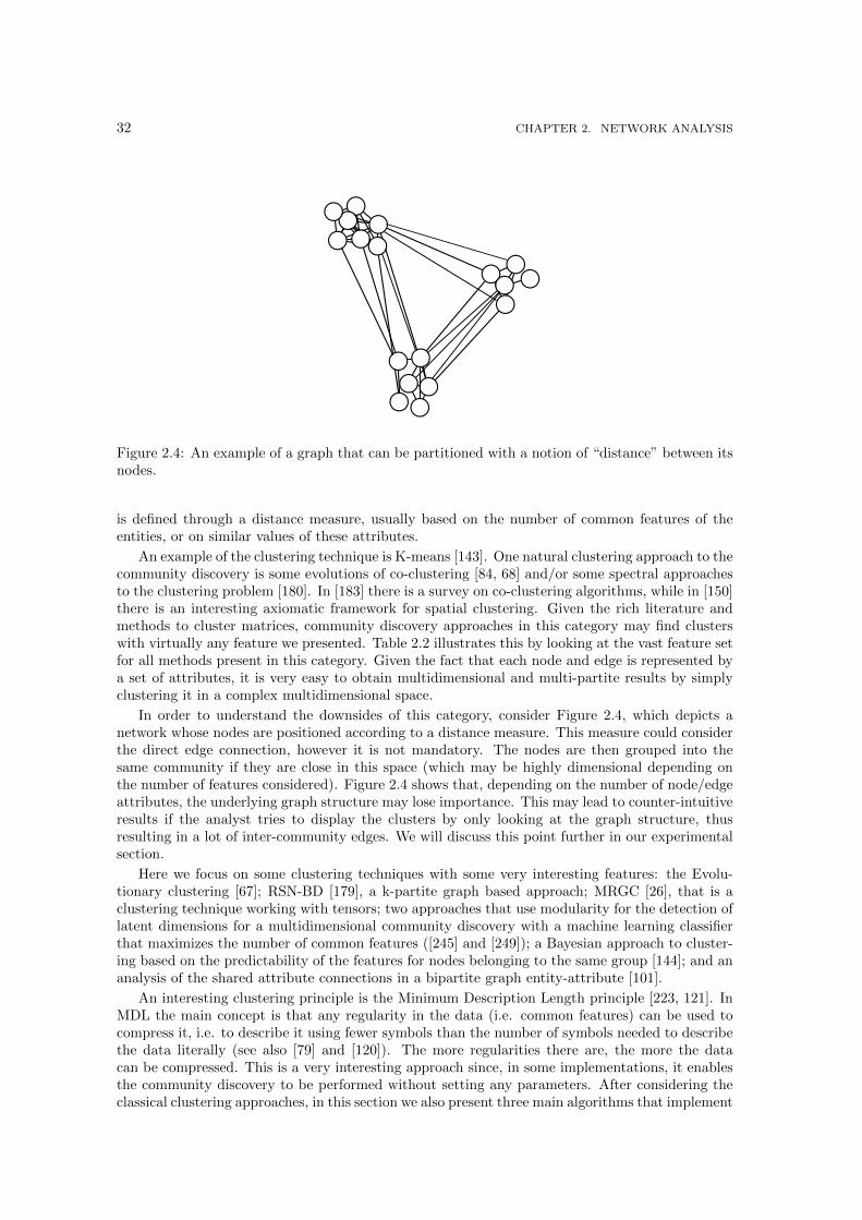
32 CHAPTER 2. NETWORK ANALYSIS
Figure 2.4: An example of a graph that can be partitioned with a notion of “distance” between itsnodes.
is defined through a distance measure, usually based on the number of common features of theentities, or on similar values of these attributes.
An example of the clustering technique is K-means [143]. One natural clustering approach to thecommunity discovery is some evolutions of co-clustering [84, 68] and/or some spectral approachesto the clustering problem [180]. In [183] there is a survey on co-clustering algorithms, while in [150]there is an interesting axiomatic framework for spatial clustering. Given the rich literature andmethods to cluster matrices, community discovery approaches in this category may find clusterswith virtually any feature we presented. Table 2.2 illustrates this by looking at the vast feature setfor all methods present in this category. Given the fact that each node and edge is represented bya set of attributes, it is very easy to obtain multidimensional and multi-partite results by simplyclustering it in a complex multidimensional space.
In order to understand the downsides of this category, consider Figure 2.4, which depicts anetwork whose nodes are positioned according to a distance measure. This measure could considerthe direct edge connection, however it is not mandatory. The nodes are then grouped into thesame community if they are close in this space (which may be highly dimensional depending onthe number of features considered). Figure 2.4 shows that, depending on the number of node/edgeattributes, the underlying graph structure may lose importance. This may lead to counter-intuitiveresults if the analyst tries to display the clusters by only looking at the graph structure, thusresulting in a lot of inter-community edges. We will discuss this point further in our experimentalsection.
Here we focus on some clustering techniques with some very interesting features: the Evolu-tionary clustering [67]; RSN-BD [179], a k-partite graph based approach; MRGC [26], that is aclustering technique working with tensors; two approaches that use modularity for the detection oflatent dimensions for a multidimensional community discovery with a machine learning classifierthat maximizes the number of common features ([245] and [249]); a Bayesian approach to cluster-ing based on the predictability of the features for nodes belonging to the same group [144]; and ananalysis of the shared attribute connections in a bipartite graph entity-attribute [101].
An interesting clustering principle is the Minimum Description Length principle [223, 121]. InMDL the main concept is that any regularity in the data (i.e. common features) can be used tocompress it, i.e. to describe it using fewer symbols than the number of symbols needed to describethe data literally (see also [79] and [120]). The more regularities there are, the more the datacan be compressed. This is a very interesting approach since, in some implementations, it enablesthe community discovery to be performed without setting any parameters. After considering theclassical clustering approaches, in this section we also present three main algorithms that implement
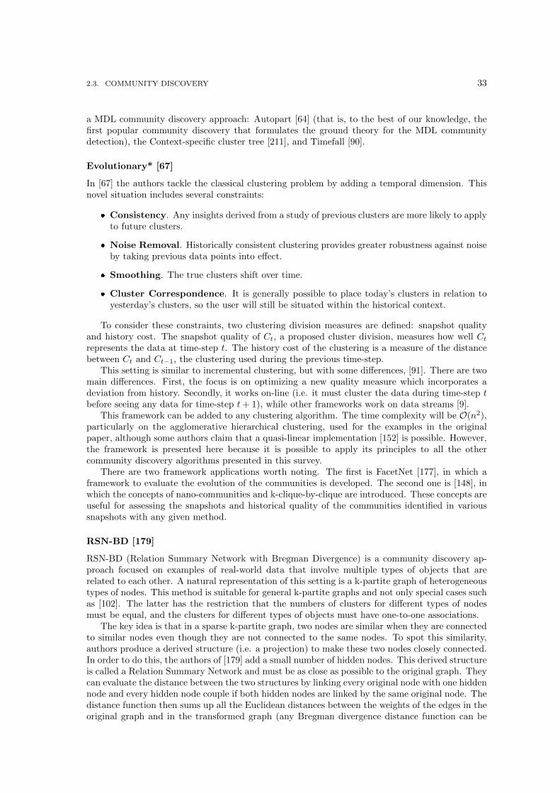
2.3. COMMUNITY DISCOVERY 33
a MDL community discovery approach: Autopart [64] (that is, to the best of our knowledge, thefirst popular community discovery that formulates the ground theory for the MDL communitydetection), the Context-specific cluster tree [211], and Timefall [90].
Evolutionary* [67]
In [67] the authors tackle the classical clustering problem by adding a temporal dimension. Thisnovel situation includes several constraints:
� Consistency. Any insights derived from a study of previous clusters are more likely to applyto future clusters.
� Noise Removal. Historically consistent clustering provides greater robustness against noiseby taking previous data points into effect.
� Smoothing. The true clusters shift over time.
� Cluster Correspondence. It is generally possible to place today’s clusters in relation toyesterday’s clusters, so the user will still be situated within the historical context.
To consider these constraints, two clustering division measures are defined: snapshot qualityand history cost. The snapshot quality of Ct, a proposed cluster division, measures how well Ctrepresents the data at time-step t. The history cost of the clustering is a measure of the distancebetween Ct and Ct−1, the clustering used during the previous time-step.
This setting is similar to incremental clustering, but with some differences, [91]. There are twomain differences. First, the focus is on optimizing a new quality measure which incorporates adeviation from history. Secondly, it works on-line (i.e. it must cluster the data during time-step tbefore seeing any data for time-step t+ 1), while other frameworks work on data streams [9].
This framework can be added to any clustering algorithm. The time complexity will be O(n2),particularly on the agglomerative hierarchical clustering, used for the examples in the originalpaper, although some authors claim that a quasi-linear implementation [152] is possible. However,the framework is presented here because it is possible to apply its principles to all the othercommunity discovery algorithms presented in this survey.
There are two framework applications worth noting. The first is FacetNet [177], in which aframework to evaluate the evolution of the communities is developed. The second one is [148], inwhich the concepts of nano-communities and k-clique-by-clique are introduced. These concepts areuseful for assessing the snapshots and historical quality of the communities identified in varioussnapshots with any given method.
RSN-BD [179]
RSN-BD (Relation Summary Network with Bregman Divergence) is a community discovery ap-proach focused on examples of real-world data that involve multiple types of objects that arerelated to each other. A natural representation of this setting is a k-partite graph of heterogeneoustypes of nodes. This method is suitable for general k-partite graphs and not only special cases suchas [102]. The latter has the restriction that the numbers of clusters for different types of nodesmust be equal, and the clusters for different types of objects must have one-to-one associations.
The key idea is that in a sparse k-partite graph, two nodes are similar when they are connectedto similar nodes even though they are not connected to the same nodes. To spot this similarity,authors produce a derived structure (i.e. a projection) to make these two nodes closely connected.In order to do this, the authors of [179] add a small number of hidden nodes. This derived structureis called a Relation Summary Network and must be as close as possible to the original graph. Theycan evaluate the distance between the two structures by linking every original node with one hiddennode and every hidden node couple if both hidden nodes are linked by the same original node. Thedistance function then sums up all the Euclidean distances between the weights of the edges in theoriginal graph and in the transformed graph (any Bregman divergence distance function can be

34 CHAPTER 2. NETWORK ANALYSIS
used). A Bregman divergence defines a class of distance measures for which neither the triangleinequality, nor symmetry, is respected, and these measures are defined for matrices, functions anddistributions [28]. The total complexity of the algorithm, as discussed by the authors, is O(n2ck).
MRGC [26]
In this model, each relation between a given set of entity classes is represented as a multidimensionaltensor (or data cube) over an appropriate domain, with the dimensions associated with the variousentity classes. In addition, each cell in the tensor encodes the relation between a particular set ofentities and can either take real values, i.e., the relation has a single attribute, or itself is a vectorof attributes.
The general idea is that each node and each relation is a collection of attributes. All theseattributes are a dimension of the relational space. MRGC (Multi-way Relation Graphs Clustering),basically tries to find a solution on one dimension at a time. It finds the optimal clustering withrespect to each dimension by keeping every other intermediate result on the other dimensions fixed(thus its time complexity is given by the number of relations times the number of dimensions,i.e. O(mD)). It then evaluates the solutions and keeps recalculating over all dimensions until itconverges. Although defined for relation graphs, this model can be also used for identify communitystructures in social networks.
MRGC operates in a multi-way clustering setting where the objective is to map the set of entitiesin a (smaller) set of clusters by using a set of clustering functions (i.e. it is a general frameworkin which previous co-clustering approaches, such as [72], can be viewed as special cases). Thecrucial mechanism in this problem is how to evaluate the quality of the multi-way clustering inorder to get to the convergence. In this case, the authors propose to measure it in terms of theapproximation error or the expected Bregman distortion [27] between the original tensor and theapproximate tensor built after applying the clustering function.
SocDim [245]
One basic (Markov) assumption in community discovery is frequently that the label of a node isonly dependent on the labels of all its neighbors. SocDim tries to go beyond this assumption bybuilding a classifier which not only considers the connectivity of a node, but assigns additionalinformation to its connection i.e. a description of a likely affiliation between social actors. Thisinformation is called latent social dimensions and the resulting framework is based on relationallearning.
In order to do this, two steps are performed by SocDim. Firstly, it extracts latent socialdimensions based on network connectivity. It uses modularity in order to find in the structure ofthe network the dimensions in which the nodes are placed (following the homophily theory whichstates that actors sharing certain properties tend to form groups [185]). This can usually be donein O(n2 log n). This step may be replaced if there is already knowledge of the social dimensions.Secondly, it constructs a discriminative classifier (one-vs-rest linear [248] or structural [254] SVM):the extracted social dimensions are considered as normal features (including other possible sources)in the classical supervised learning task. It is then possible to use the predicted labels of theclassifier to reconstruct the community organization of the entities. This is a multidimensionalcommunity discovery because the classifier will determine which dimensions are relevant to aclass label. This work is the basis of a further evolution [246] that has an edge-centric view ofcommunities (similar to the methods classified in the Link Clustering category)
PMM [249]
This work was originally presented in [247] and then evolved in [249]. It presents a variation of themodularity approach on a multidimensional setting. The goal of the PMM (Principal modularityMaximization) algorithm is: given a lot of different dimensions, find a concise representation ofthem (the authors call this step “Structural Feature Extraction”, computing modularity with the
2.3. COMMUNITY DISCOVERY 35
(a) The original matrix (b) Reordered matrix
Figure 2.5: An example of the MDL principle for matrices: the matrix on the left is exactly thesame matrix as the one on the right, but reordered in order to describe it simply.
Lanczos method. The latter is an algorithm to find eigenvalues and eigenvectors of a square matrix[109], of complexity O(mn2)) and then detect the correlations between these representations (inthe “Cross-Dimension Integration”, using a generalized canonical correlation analysis [147]).
After this step, the authors obtain lower-dimensional embedding, which captures the principalpattern across all the dimensions of the network. They can then perform k-means [143] on thisembedding to find out the discrete community assignment.
Infinite Relational [144]
Suppose there are one or more relations (i.e. edges) involving one or more types (i.e. nodes). Thegoal of the Infinite Relational Model is to partition each type into clusters (i.e. communities),where a good set of partitions allows relationships between entities to be predicted by their clusterassignments. The authors’ goal is to organize the entities into clusters that relate to each other inpredictable ways, by simultaneously clustering the entities and the relations.
Formally, suppose that the observed data are m relations involving n types. Let Ri be theith relation, T j be the jth type, and zj be a vector of cluster assignments for T j . The taskis to infer the cluster assignments, and the ultimate interest lies in the posterior distributionP (z1, ..., zn | R1, ..., Rm).
To enable the IRM to discover the number of clusters in type T , the authors use a prior [214]that assigns some probability mass to all possible partitions of the type. Inferences can be madeusing Markov chain Monte Carlo methods to sample from the posterior on cluster assignments.This method has a very high time complexity (O(n2cD)).
Find-Tribes [101]
Find-Tribes was not explicitly developed for community discovery purposes. However, the tech-nique can still be used to identify some kind of community. It uses a particular definition of acommunity, according to which the entities in a group tend to behave in the same way.
As input, the authors require a bipartite graph G = (R ∪ A,E) of entities R and attributesA. The entities should connect to several attributes. The aim of the algorithm is to return thosegroups sharing “unusual” combinations of attributes. This restriction can be easily generalized inorder to also obtain the “usual” groups as outputs.
The strategy for the desired task revolves around the development of a good definition of“unusual”. For an entity group to be considered anomalous, the shared attributes themselves neednot be unusual, but their particular configuration should be. A projected non-bipartite graphH ′(R,F ) is built, then for each edge a score cij (the number of attributes in the shared sequence,the number of time steps of overlap, a probabilistic Markov chain of attributes and so on) iscomputed, measuring how significant or unusual its sequence of shared attributes is. In the enda threshold d is chosen and all edges fij removed for which cij < d are removed. The connectedcomponents of H ′ are the desired tribes and the overall complexity is O(mnK2).
36 CHAPTER 2. NETWORK ANALYSIS
AutoPart [64]
Autopart is the basic formulation of the MDL approach to the community discovery problem.There is a binary matrix that represents associations between the n nodes of the graph (and theirattributes). An example of a possible adjacency matrix is shown in Figure 2.5(a).
The main idea is to reorder the adjacency matrix so that similar nodes, i.e. nodes that areconnected to the same set of nodes, are grouped with each other. The adjacency matrix shouldthen consist of homogeneous rectangular/square blocks of a high (low) density, representing thefact that certain node groups have more (less) connections with other groups (right hand sideof Figure 2.5(b)), which can be encoded with a great compression of the data. The aim of thealgorithm is to identify the best grouping that minimizes the cost (compression) function [210].
A trade-off point must therefore be identified that indicates the best number of groups k. Theauthors solved this problem using a two-step iterative process: first, they find a good node groupingG for a given number of node groups k that minimize entropy; and second, they search for thenumber of node groups k by splitting the previously identified groups and verifying if there is apossible gain in the total encoding cost function, at a total time complexity of O(mk2).
Context-specific Cluster Tree [211]
In this variant of the MDL approach, a binary ns × nd matrix represents a bipartite graph withns source nodes and nd destination nodes. The aim is to automatically construct a recursivecommunity structure of a large bipartite graph at multiple levels, namely, a Context-specific ClusterTree (CCT). The resulting CCT can identify relevant context-specific clusters. The main idea isto subdivide the adjacency matrix into tiles, or “contexts”, with a possible reordering of rowsand columns, and to compress them, either as-is (if they are homogeneous enough) or by furthersubdividing.
The entire graph is considered as a whole community. If the best representation of the con-sidered (sub)graph is the random graph, by testing its possible compression with a total encodingcost function, then the community cannot be split into two sub-communities. In fact, by definitionthe random graph has no community structure at all. Otherwise, the graph is split and the algo-rithm is reapplied recursively. Each edge is visited once for each subdivision (thus the complexity isO(mk)). The result is a tree of communities in which the bottom levels are a context specializationof the generic communities at the top of the tree.
This idea of recursive clustering is also applied to streaming setting [10, 240], although witha number of parameters. This is a hierarchical evolution of the existing flat method described in[68].
Timefall [90]
Timefall is an MDL approach that can be described as a parameter-free network evolution tracking.Given n time-stamped events each related to several of m items, it simultaneously finds (a) thecommunities, that is, item-groups (e.g., research topics and/or research communities) and (b) adescription of how the communities evolve over time (e.g., appear, disappear, split, merge), and(c) a selection of the appropriate cut-points in time when existing community structures changeabruptly.
The adjacency matrix representing the graph is split according to the row timestamps. Columnsare then clustered with a Cross Association algorithm [68], which is the basis of the MDL commu-nity discovery algorithms. The MDL principle is used again to connect the column clusters of thematrices across the split rows: if two column clusters can be encoded together with a low encodingcost then they are connected, ignoring time points with little or no changes. The time complexityis equal to O(mk).
2.3.4 Internal Density
For this group of approaches, the underlying meta definition is:
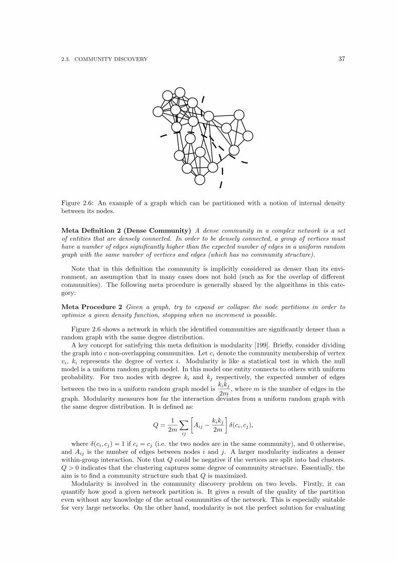
2.3. COMMUNITY DISCOVERY 37
Figure 2.6: An example of a graph which can be partitioned with a notion of internal densitybetween its nodes.
Meta Definition 2 (Dense Community) A dense community in a complex network is a setof entities that are densely connected. In order to be densely connected, a group of vertices musthave a number of edges significantly higher than the expected number of edges in a uniform randomgraph with the same number of vertices and edges (which has no community structure).
Note that in this definition the community is implicitly considered as denser than its envi-ronment, an assumption that in many cases does not hold (such as for the overlap of differentcommunities). The following meta procedure is generally shared by the algorithms in this cate-gory:
Meta Procedure 2 Given a graph, try to expand or collapse the node partitions in order tooptimize a given density function, stopping when no increment is possible.
Figure 2.6 shows a network in which the identified communities are significantly denser than arandom graph with the same degree distribution.
A key concept for satisfying this meta definition is modularity [199]. Briefly, consider dividingthe graph into c non-overlapping communities. Let ci denote the community membership of vertexvi, ki represents the degree of vertex i. Modularity is like a statistical test in which the nullmodel is a uniform random graph model. In this model one entity connects to others with uniformprobability. For two nodes with degree ki and kj respectively, the expected number of edges
between the two in a uniform random graph model iskikj2m
, where m is the number of edges in the
graph. Modularity measures how far the interaction deviates from a uniform random graph withthe same degree distribution. It is defined as:
Q =1
2m
∑ij
[Aij −
kikj2m
]δ(ci, cj),
where δ(ci, cj) = 1 if ci = cj (i.e. the two nodes are in the same community), and 0 otherwise,and Aij is the number of edges between nodes i and j. A larger modularity indicates a denserwithin-group interaction. Note that Q could be negative if the vertices are split into bad clusters.Q > 0 indicates that the clustering captures some degree of community structure. Essentially, theaim is to find a community structure such that Q is maximized.
Modularity is involved in the community discovery problem on two levels. Firstly, it canquantify how good a given network partition is. It gives a result of the quality of the partitioneven without any knowledge of the actual communities of the network. This is especially suitablefor very large networks. On the other hand, modularity is not the perfect solution for evaluating
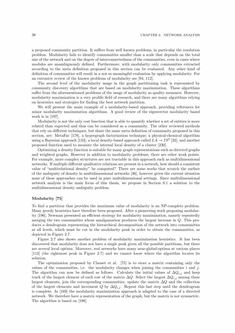
38 CHAPTER 2. NETWORK ANALYSIS
a proposed community partition. It suffers from well known problems, in particular the resolutionproblem. Modularity fails to identify communities smaller than a scale that depends on the totalsize of the network and on the degree of interconnectedness of the communities, even in cases wheremodules are unambiguously defined. Furthermore, with modularity only communities extractedaccording to the meta definition proposed in this section can be evaluated. Any other kind ofdefinition of communities will result in a not so meaningful evaluation by applying modularity. Foran extensive review of the known problems of modularity see [94, 112].
The second level of the modularity usage in the graph partitioning task is represented bycommunity discovery algorithms that are based on modularity maximization. These algorithmssuffer from the aforementioned problems of the usage of modularity as quality measures. However,modularity maximization is a very prolific field of research, and there are many algorithms relyingon heuristics and strategies for finding the best network partition.
We will present the main example of a modularity-based approach, providing references forminor modularity maximization algorithms. A good review of the eigenvector modularity basedwork is in [197].
Modularity is not the only cost function that is able to quantify whether a set of entities is morerelated than expected and thus can be considered as a community. The other reviewed methodsthat rely on different techniques, but share the same meta definition of community proposed in thissection, are: MetaFac [178], a hypergraph factorization technique; a physical-chemical algorithmusing a Bayesian approach [133]; a local density-based approach called LA→ IS2 [32]; and anotherproposed function used to measure the internal local density of a cluster [230].
Optimizing a density function is suitable for many graph representations such as directed graphsand weighted graphs. However in addition to modularity problems, there are other weak points.For example, more complex structures are not tractable in this approach such as multidimensionalnetworks. If multiple different qualitative relations are present in a network, how should a consistentvalue of “multirelational density” be computed? There are some works that scratch the surfaceof the ambiguity of density in multidimensional networks [36], however given the current situationnone of these approaches can be used in pure multidimensional settings. Since multidimensionalnetwork analysis is the main focus of this thesis, we propose in Section 8.1 a solution to themultidimensional density ambiguity problem.
Modularity [75]
To find a partition that provides the maximum value of modularity is an NP-complete problem.Many greedy heuristics have therefore been proposed. After a pioneering work proposing modular-ity [196], Newman presented an efficient strategy for modularity maximization, namely repeatedlymerging the two communities whose amalgamation produces the largest increase in Q. This pro-duces a dendrogram representing the hierarchical decomposition of the network into communitiesat all levels, which must be cut in the modularity peak in order to obtain the communities, asdepicted in Figure 2.7.
Figure 2.7 also shows another problem of modularity maximization heuristics. It has beendiscovered that modularity does not have a single peak given all the possible partitions, but thereare several local optima. Moreover, real networks have many near-global-optima at various places[112] (the rightmost peak in Figure 2.7) and we cannot know where the algorithm locates itssolution.
The optimization proposed by Clauset et al. [75] is to store a matrix containing only thevalues of the communities, i.e. the modularity changes when joining the communities i and j.The algorithm can now be defined as follows. Calculate the initial values of ∆Qi,j and keeptrack of the largest element of each row of the matrix ∆Q. Select the largest ∆Qi,j among theselargest elements, join the corresponding communities, update the matrix ∆Q and the collectionof the largest elements and increment Q by ∆Qi,j . Repeat this last step until the dendrogramis complete. In [169] the modularity maximization approach is adapted to the case of a directednetwork. We therefore have a matrix representation of the graph, but the matrix is not symmetric.The algorithm is based on [198].
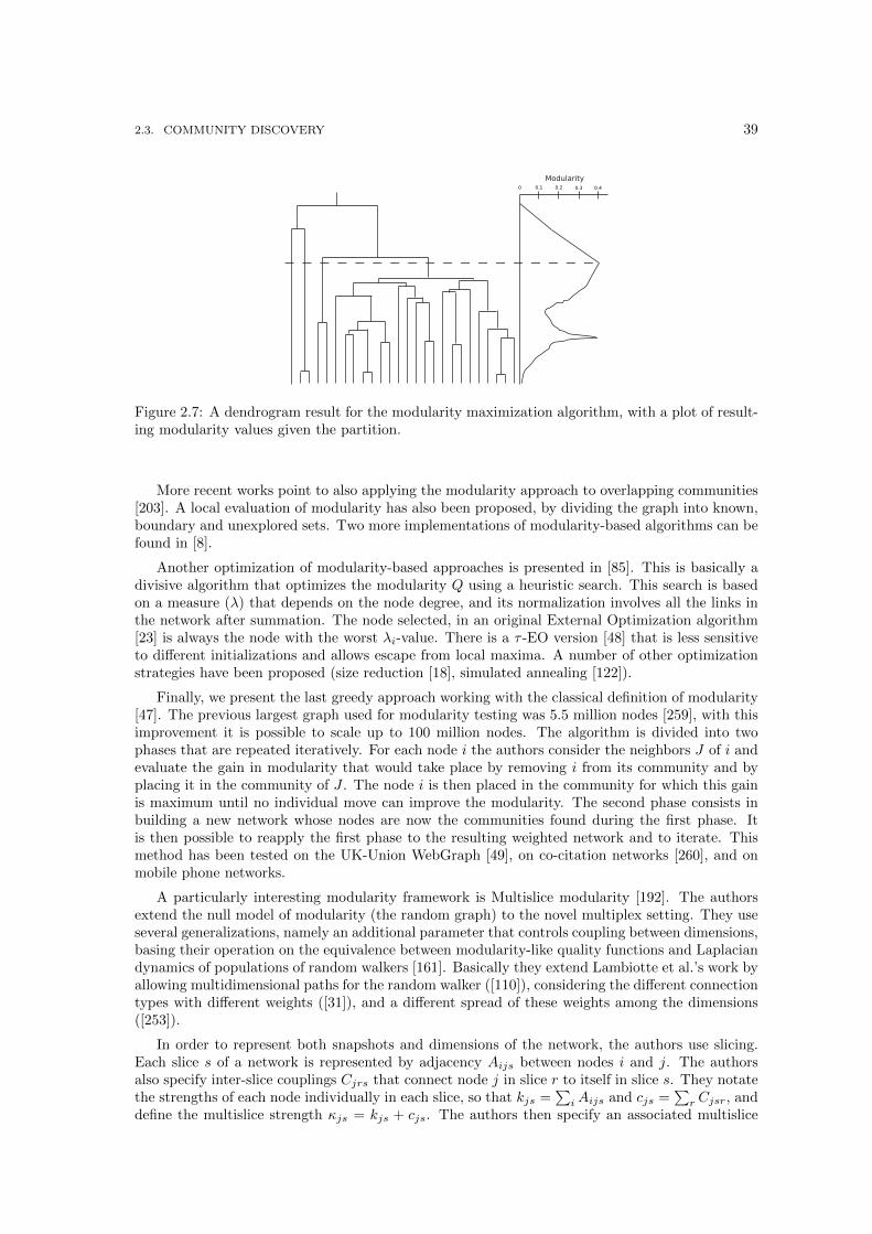
2.3. COMMUNITY DISCOVERY 39
Modularity0 0.1 0.2 0.3 0.4
Figure 2.7: A dendrogram result for the modularity maximization algorithm, with a plot of result-ing modularity values given the partition.
More recent works point to also applying the modularity approach to overlapping communities[203]. A local evaluation of modularity has also been proposed, by dividing the graph into known,boundary and unexplored sets. Two more implementations of modularity-based algorithms can befound in [8].
Another optimization of modularity-based approaches is presented in [85]. This is basically adivisive algorithm that optimizes the modularity Q using a heuristic search. This search is basedon a measure (λ) that depends on the node degree, and its normalization involves all the links inthe network after summation. The node selected, in an original External Optimization algorithm[23] is always the node with the worst λi-value. There is a τ -EO version [48] that is less sensitiveto different initializations and allows escape from local maxima. A number of other optimizationstrategies have been proposed (size reduction [18], simulated annealing [122]).
Finally, we present the last greedy approach working with the classical definition of modularity[47]. The previous largest graph used for modularity testing was 5.5 million nodes [259], with thisimprovement it is possible to scale up to 100 million nodes. The algorithm is divided into twophases that are repeated iteratively. For each node i the authors consider the neighbors J of i andevaluate the gain in modularity that would take place by removing i from its community and byplacing it in the community of J . The node i is then placed in the community for which this gainis maximum until no individual move can improve the modularity. The second phase consists inbuilding a new network whose nodes are now the communities found during the first phase. Itis then possible to reapply the first phase to the resulting weighted network and to iterate. Thismethod has been tested on the UK-Union WebGraph [49], on co-citation networks [260], and onmobile phone networks.
A particularly interesting modularity framework is Multislice modularity [192]. The authorsextend the null model of modularity (the random graph) to the novel multiplex setting. They useseveral generalizations, namely an additional parameter that controls coupling between dimensions,basing their operation on the equivalence between modularity-like quality functions and Laplaciandynamics of populations of random walkers [161]. Basically they extend Lambiotte et al.’s work byallowing multidimensional paths for the random walker ([110]), considering the different connectiontypes with different weights ([31]), and a different spread of these weights among the dimensions([253]).
In order to represent both snapshots and dimensions of the network, the authors use slicing.Each slice s of a network is represented by adjacency Aijs between nodes i and j. The authorsalso specify inter-slice couplings Cjrs that connect node j in slice r to itself in slice s. They notatethe strengths of each node individually in each slice, so that kjs =
∑iAijs and cjs =
∑r Cjsr, and
define the multislice strength κjs = kjs + cjs. The authors then specify an associated multislice
40 CHAPTER 2. NETWORK ANALYSIS
null model. The resulting multislice extended definition of modularity is the following:
Q =1
2µ
∑ijsr
{(Aijs − γs
kiskjs2ms
δsr
)+ δijCjsr
}δ(cis, cjr).
In this extension γs is the resolution parameter, that may or may not be different for each slice.If γs = 1 for any s, then this formula degenerates on the usual interpretation of modularity asa count of the total weight of intra-slice edges minus the weight expected at random. Otherwiseinter-slice coupling Cjsr is considered. Cjsr takes values from 0 to ∞. If Cjsr = 0 we degenerateagain in the usual modularity definition. Otherwise the quality-optimizing partitions force thecommunity assignment of a node to remain the same across all slices in which that node appears.In addition the multislice quality is reduced to that of an adjacency matrix summed over thecontributions from the individual slices with a null model that respects the degree distributions ofthe individual contributions. The generality of this framework also enables different weights to beincluded across the Cjsr couplings. After defining the new quality function, the algorithm neededto extract communities can be one of many modularity-based algorithms.
In Table 2.2 we merged all modularity approaches on the single “Modularity” row. One caveatis that, depending on the implementation, not all the features may be returned (for example onlyMultislice implementation is able to consider multidimensionality).
MetaFac [178]
In this paper the concept of metagraph is introduced. The metagraph is a relational hypergraphto represent multi-relational and multi-dimensional social data. In practice, there are entitieswhich connect to different kinds of objects in different ways (e.g.in a social media through tagging,commenting or publishing a photo, video or text). The aim is to discover a latent communitystructure in the metagraph, for example the common context of user actions in social medianetworks. In other words the authors are interested in clusters of people who interact with eachother in a coherent manner. In this model, a set of entities of the same type is called a facet. Aninteraction between two or more facets is called a relation.
The idea of the authors is to use an M -way hyperedge to represent the interactions of M facets:each facet as a vertex and each relation as a hyperedge on a hypergraph. A metagraph definesa particular structure of interactions between facets (groups of entities of the same type), notbetween facet elements (the entities themselves). In order to do so, the metagraph is defined as aset of data tensors. A tensor is an array with N dimensions. This is a mathematical and computerscience definition of tensors, for the notion of tensor in physics and engineering see [193]. For anextensive review of tensors, tensor decomposition and their applications and tools see [153] (in thiswork some examples are also provided of possible applications of tensor decompositions: signalprocessing [166], numerical linear algebra [165] and, closer to our area of interest, data mining[241, 242], graph analysis tasks [21, 1] and recommendation systems [71]).
Given the metagraph and its defined data tensors, the authors apply a tensor decompositionand factorization operation, which is a very hard task with a number of known issues. To the bestof our knowledge, only recently have some memory and time efficient techniques been developed,such as [154]. In the metagraph approach the tensor decomposition can also be viewed as a dynamicanalysis, when the sets of tensors are temporally annotated and the resulting core tensor refers toa specific time-step t. This is called metagraph factorization (for time evolving data). Finally, theMF problem can be stated in terms of optimization, i.e. minimizing a given cost function, thusobtaining facet communities (for a time complexity of O(mnD)).
Variational Bayes [133]
In the Variational Bayes framework, a complex network is modeled as a physical system, and thenthe problem of assigning each node to a module (inferring the hidden membership vector) in thenetwork is tackled by solving the disorder-averaged partition function of a spin-glass.
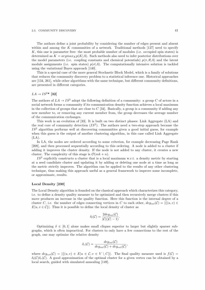
2.3. COMMUNITY DISCOVERY 41
The authors define a joint probability by considering the number of edges present and absentwithin and among the K communities of a network. Traditional methods [127] need to specifyK, this one is parameter free: the most probable number of modules (i.e. occupied spin states) isdetermined as K = argmaxKp(K|A). Such methods also need to infer posterior distributions overthe model parameters (i.e. coupling constants and chemical potentials) p(π, θ|A) and the latentmodule assignments (i.e. spin states) p(σ|A). The computationally intensive solution is tackledusing the variational Bayes approach [140].
This is a special case of the more general Stochastic Block Model, which is a family of solutionsthat reduces the community discovery problem to a statistical inference one. Historical approachesare [134, 261], while other algorithms with the same technique, but different community definitions,are presented in different categories.
LA→ IS2* [32]
The authors of LA→ IS2 adopt the following definition of a community: a group C of actors in asocial network forms a community if its communication density function achieves a local maximumin the collection of groups that are close to C [34]. Basically, a group is a community if adding anynew member to, or removing any current member from, the group decreases the average numberof the communication exchanges.
This work is an evolution of [33]. It is built on two distinct phases: Link Aggregate (LA) andthe real core of community detection (IS2). The authors need a two-step approach because theIS2 algorithm performs well at discovering communities given a good initial guess, for examplewhen this guess is the output of another clustering algorithm, in this case called Link Aggregate(LA).
In LA, the nodes are ordered according to some criterion, for example decreasing Page Rank[208], and then processed sequentially according to this ordering. A node is added to a cluster ifadding it improves the cluster density. If the node is not added to any cluster, it creates a newcluster. The complexity of this stage is O(mk + n).
IS2 explicitly constructs a cluster that is a local maximum w.r.t. a density metric by startingat a seed candidate cluster and updating it by adding or deleting one node at a time as long asthe metric strictly improves. The algorithm can be applied to the results of any other clusteringtechnique, thus making this approach useful as a general framework to improve some incomplete,or approximate, results.
Local Density [230]
The Local Density algorithm is founded on the classical approach which characterizes this category,i.e. to define a density quality measure to be optimized and then recursively merge clusters if thismove produces an increase in the quality function. Here this function is the internal degree of acluster C, i.e. the number of edges connecting vertices in C to each other, degint(C) = |{(u, v) ∈E|u, v ∈ C}|. Thus it is possible to define the local density of cluster as
δl(C) =2degint(C)|C|(|C| − 1)
.
Optimizing δ ∈ [0, 1] alone makes small cliques superior to larger but slightly sparser sub-graphs, which is often impractical. For clusters to only have a few connections to the rest of thegraph, one may optimize the relative density
δr(C) =degint(C)
degint(C) + degext(C),
where degext(C) = |{(u, v) ∈ E|u ∈ C, v ∈ V \ C}|. The final quality measure used is f(C) =δl(C)δr(C). A good approximation of the optimal cluster for a given vertex can be obtained by alocal search, guided with simulated annealing [149].
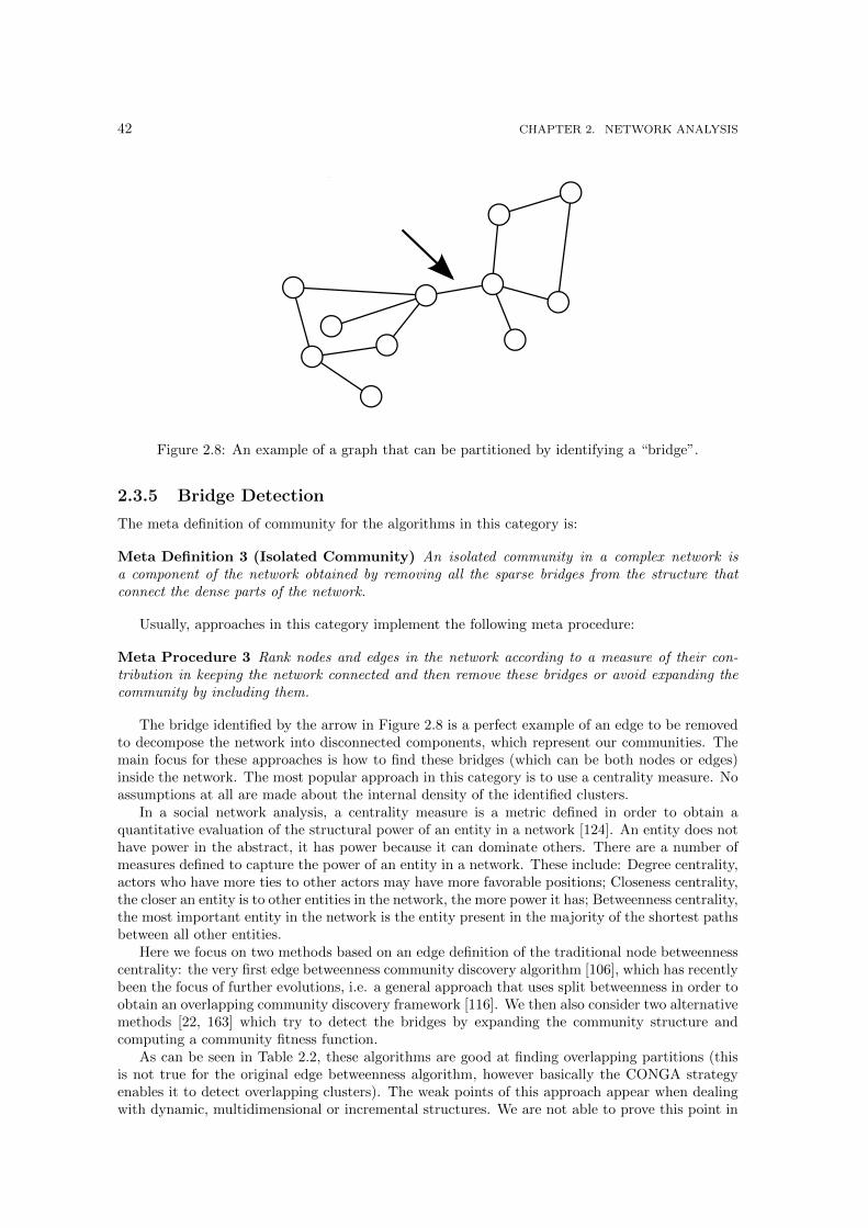
42 CHAPTER 2. NETWORK ANALYSIS
Figure 2.8: An example of a graph that can be partitioned by identifying a “bridge”.
2.3.5 Bridge Detection
The meta definition of community for the algorithms in this category is:
Meta Definition 3 (Isolated Community) An isolated community in a complex network isa component of the network obtained by removing all the sparse bridges from the structure thatconnect the dense parts of the network.
Usually, approaches in this category implement the following meta procedure:
Meta Procedure 3 Rank nodes and edges in the network according to a measure of their con-tribution in keeping the network connected and then remove these bridges or avoid expanding thecommunity by including them.
The bridge identified by the arrow in Figure 2.8 is a perfect example of an edge to be removedto decompose the network into disconnected components, which represent our communities. Themain focus for these approaches is how to find these bridges (which can be both nodes or edges)inside the network. The most popular approach in this category is to use a centrality measure. Noassumptions at all are made about the internal density of the identified clusters.
In a social network analysis, a centrality measure is a metric defined in order to obtain aquantitative evaluation of the structural power of an entity in a network [124]. An entity does nothave power in the abstract, it has power because it can dominate others. There are a number ofmeasures defined to capture the power of an entity in a network. These include: Degree centrality,actors who have more ties to other actors may have more favorable positions; Closeness centrality,the closer an entity is to other entities in the network, the more power it has; Betweenness centrality,the most important entity in the network is the entity present in the majority of the shortest pathsbetween all other entities.
Here we focus on two methods based on an edge definition of the traditional node betweennesscentrality: the very first edge betweenness community discovery algorithm [106], which has recentlybeen the focus of further evolutions, i.e. a general approach that uses split betweenness in order toobtain an overlapping community discovery framework [116]. We then also consider two alternativemethods [22, 163] which try to detect the bridges by expanding the community structure andcomputing a community fitness function.
As can be seen in Table 2.2, these algorithms are good at finding overlapping partitions (thisis not true for the original edge betweenness algorithm, however basically the CONGA strategyenables it to detect overlapping clusters). The weak points of this approach appear when dealingwith dynamic, multidimensional or incremental structures. We are not able to prove this point in
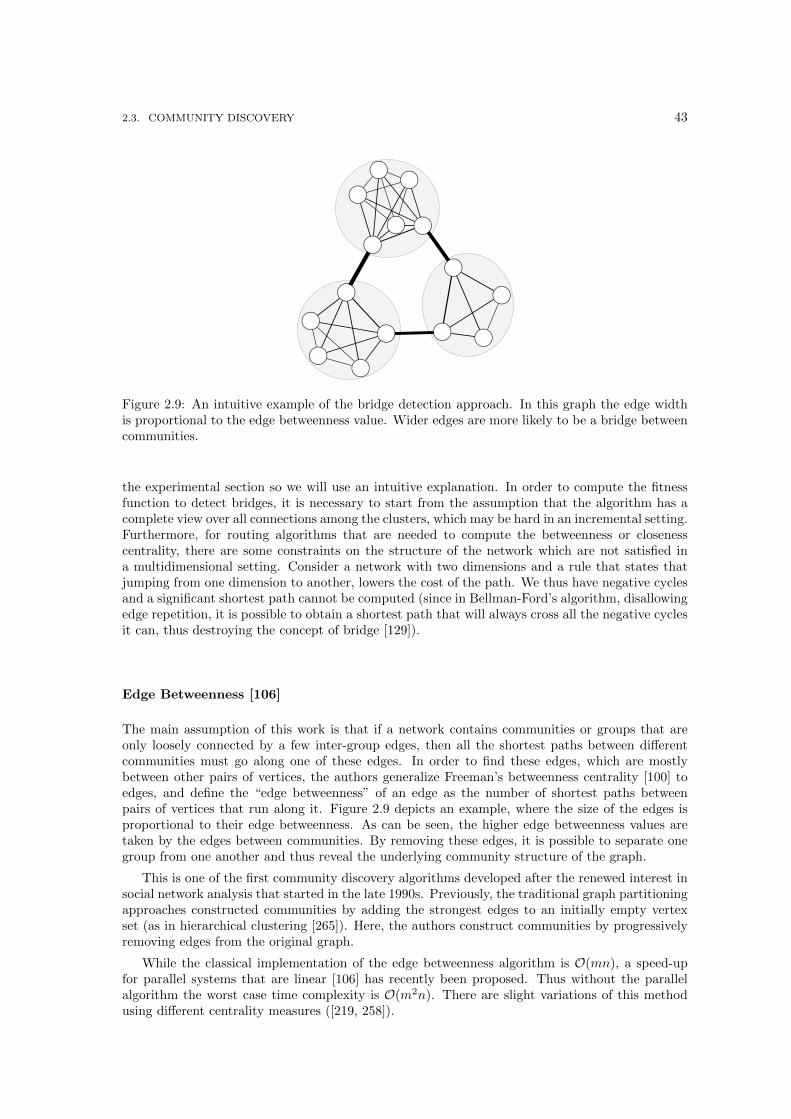
2.3. COMMUNITY DISCOVERY 43
Figure 2.9: An intuitive example of the bridge detection approach. In this graph the edge widthis proportional to the edge betweenness value. Wider edges are more likely to be a bridge betweencommunities.
the experimental section so we will use an intuitive explanation. In order to compute the fitnessfunction to detect bridges, it is necessary to start from the assumption that the algorithm has acomplete view over all connections among the clusters, which may be hard in an incremental setting.Furthermore, for routing algorithms that are needed to compute the betweenness or closenesscentrality, there are some constraints on the structure of the network which are not satisfied ina multidimensional setting. Consider a network with two dimensions and a rule that states thatjumping from one dimension to another, lowers the cost of the path. We thus have negative cyclesand a significant shortest path cannot be computed (since in Bellman-Ford’s algorithm, disallowingedge repetition, it is possible to obtain a shortest path that will always cross all the negative cyclesit can, thus destroying the concept of bridge [129]).
Edge Betweenness [106]
The main assumption of this work is that if a network contains communities or groups that areonly loosely connected by a few inter-group edges, then all the shortest paths between differentcommunities must go along one of these edges. In order to find these edges, which are mostlybetween other pairs of vertices, the authors generalize Freeman’s betweenness centrality [100] toedges, and define the “edge betweenness” of an edge as the number of shortest paths betweenpairs of vertices that run along it. Figure 2.9 depicts an example, where the size of the edges isproportional to their edge betweenness. As can be seen, the higher edge betweenness values aretaken by the edges between communities. By removing these edges, it is possible to separate onegroup from one another and thus reveal the underlying community structure of the graph.
This is one of the first community discovery algorithms developed after the renewed interest insocial network analysis that started in the late 1990s. Previously, the traditional graph partitioningapproaches constructed communities by adding the strongest edges to an initially empty vertexset (as in hierarchical clustering [265]). Here, the authors construct communities by progressivelyremoving edges from the original graph.
While the classical implementation of the edge betweenness algorithm is O(mn), a speed-upfor parallel systems that are linear [106] has recently been proposed. Thus without the parallelalgorithm the worst case time complexity is O(m2n). There are slight variations of this methodusing different centrality measures ([219, 258]).

44 CHAPTER 2. NETWORK ANALYSIS
CONGA [116]
CONGA (Cluster-Overlap Newman Girvan Algorithm) is based on the well-known edge between-ness community discovery algorithm [106]. It adds the ability to split vertices between communities,based on the new concept of “split betweenness”.
The split betweenness [115] of a vertex v is the number of shortest paths that would passbetween the two parts of v if it was split. There are many ways to split a vertex into two, the bestsplit is the one that maximizes the split betweenness. Basically, with the following split operation,any disjoint community discovery algorithm can be applied and returns overlapping partitions([117]):
1. Calculate edge betweenness of edges and split betweenness of vertices.
2. Remove edge with maximum edge betweenness or split vertex with maximum split between-ness, if greater.
3. Recalculate edge betweenness and split betweenness.
4. Repeat from step 2 until no edges remain.
Given a relaxed assumption on the edge betweenness computation, the total time complexityof CONGA is O(n log n).
L-Shell [22]
In L-Shell algorithm, the idea is to expand a community as much as it can, stopping the expansionwhenever the network structure does not allow any further expansion, i.e. the bridges are reached.
The key concept is the l−shell, a group of l vertices whose aim is to grow and occupy an entirecommunity while two quantities are computed: the emerging degree and total emerging degree.The emerging degree of a vertex is defined as the number of edges that connect that vertex tovertices that the l− shell has not already visited as it expanded from the previous (l− 1), (l− 2),... −shells. The total emerging degree Kj of an l − shell is thus the sum of the emerging degreesof all vertices on the leading edge of the lshell.
For a starting vertex j the algorithm starts an l − shell, l = 0, at vertex j (add j to the listof community members) and computes the total emerging degree of the shell. Then it spreads thel− shell, l = 1, it adds the neighbors of j to the list, and computes the new total emerging degree.Now it can compute the change in the emerging degree of the shell. If the total emerging degree isincreased less than a given threshold α, then a community has been found. Otherwise it increasesthe size of the shell (posing l = l + 1) until α is crossed or the entire connected component isadded to the community list. As can be seen, for each node we have a quadratic problem, i.e. thetime complexity is O(n3). The assumption is that a community is a structure in which the totalemerging degree cannot be significantly increased, i.e. the vertices at the border of the communityhave few edges outside it and these edges are the bridges among different communities.
Internal-External Degree [163]
An approach close to l − shell starts from the similar basic assumption that communities areessentially local structures, involving the nodes belonging to the modules themselves plus at mostan extended neighborhood of them. The fitness chosen here is the total internal degree of nodeson the sum of internal and external degrees to the power of a positive real-valued parameter (α).Given a fitness function, the fitness of a node A with respect to sub-graph G, fG, is defined asthe variation of the fitness of sub-graph G with and without node A. The process of calculatingthe fitness of the nodes and them joining them together in a community stops when the nodesexamined in the neighborhood of G all have negative fitness, i.e. their external edges are all bridges,after a total time complexity of O(n2 log n).
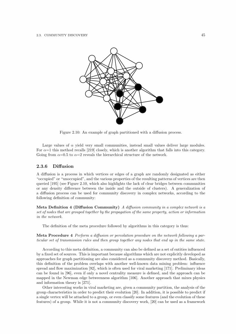
2.3. COMMUNITY DISCOVERY 45
Figure 2.10: An example of graph partitioned with a diffusion process.
Large values of α yield very small communities, instead small values deliver large modules.For α=1 this method recalls [219] closely, which is another algorithm that falls into this category.Going from α=0.5 to α=2 reveals the hierarchical structure of the network.
2.3.6 Diffusion
A diffusion is a process in which vertices or edges of a graph are randomly designated as either“occupied” or “unoccupied”, and the various properties of the resulting patterns of vertices are thenqueried [195] (see Figure 2.10, which also highlights the lack of clear bridges between communitiesor any density difference between the inside and the outside of clusters). A generalization ofa diffusion process can be used for community discovery in complex networks, according to thefollowing definition of community:
Meta Definition 4 (Diffusion Community) A diffusion community in a complex network is aset of nodes that are grouped together by the propagation of the same property, action or informationin the network.
The definition of the meta procedure followed by algorithms in this category is thus:
Meta Procedure 4 Perform a diffusion or percolation procedure on the network following a par-ticular set of transmission rules and then group together any nodes that end up in the same state.
According to this meta definition, a community can also be defined as a set of entities influencedby a fixed set of sources. This is important because algorithms which are not explicitly developed asapproaches for graph partitioning are also considered as a community discovery method. Basically,this definition of the problem overlaps with another well-known data mining problem: influencespread and flow maximization [92], which is often used for viral marketing [171]. Preliminary ideascan be found in [96], even if only a novel centrality measure is defined, and the approach can bemapped in the Newman edge betweenness algorithm [106]. Another approach that mixes physicsand information theory is [271].
Other interesting works in viral marketing are, given a community partition, the analysis of thegroup characteristics in order to predict their evolution [20]. In addition, it is possible to predict ifa single vertex will be attached to a group, or even classify some features (and the evolution of thesefeatures) of a group. While it is not a community discovery work, [20] can be used as a framework
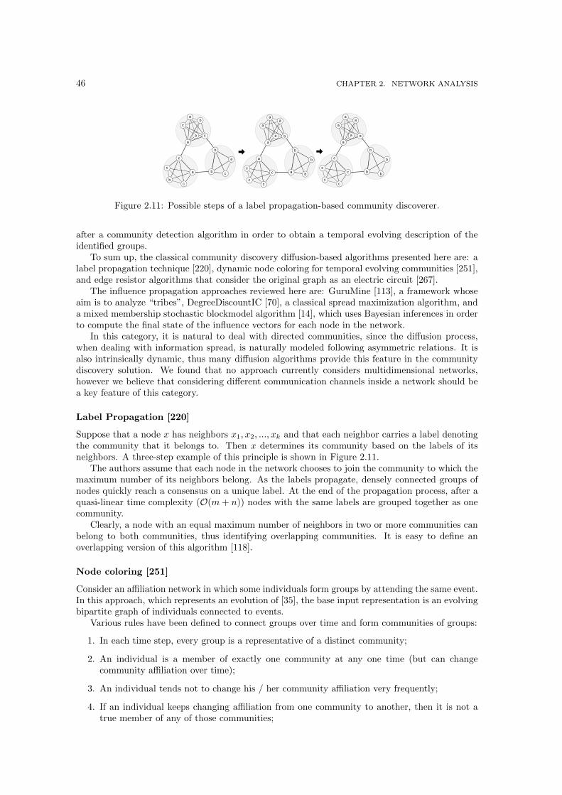
46 CHAPTER 2. NETWORK ANALYSIS
D
F
ED
D
D
D
D F
F
F
D
F
E
E
E
D
F
D
D
E
D
F
F
F
F
D
E
E
E
D
D
D
D
D D
F
F
F
F
F
E
E
EE
Figure 2.11: Possible steps of a label propagation-based community discoverer.
after a community detection algorithm in order to obtain a temporal evolving description of theidentified groups.
To sum up, the classical community discovery diffusion-based algorithms presented here are: alabel propagation technique [220], dynamic node coloring for temporal evolving communities [251],and edge resistor algorithms that consider the original graph as an electric circuit [267].
The influence propagation approaches reviewed here are: GuruMine [113], a framework whoseaim is to analyze “tribes”, DegreeDiscountIC [70], a classical spread maximization algorithm, anda mixed membership stochastic blockmodel algorithm [14], which uses Bayesian inferences in orderto compute the final state of the influence vectors for each node in the network.
In this category, it is natural to deal with directed communities, since the diffusion process,when dealing with information spread, is naturally modeled following asymmetric relations. It isalso intrinsically dynamic, thus many diffusion algorithms provide this feature in the communitydiscovery solution. We found that no approach currently considers multidimensional networks,however we believe that considering different communication channels inside a network should bea key feature of this category.
Label Propagation [220]
Suppose that a node x has neighbors x1, x2, ..., xk and that each neighbor carries a label denotingthe community that it belongs to. Then x determines its community based on the labels of itsneighbors. A three-step example of this principle is shown in Figure 2.11.
The authors assume that each node in the network chooses to join the community to which themaximum number of its neighbors belong. As the labels propagate, densely connected groups ofnodes quickly reach a consensus on a unique label. At the end of the propagation process, after aquasi-linear time complexity (O(m+ n)) nodes with the same labels are grouped together as onecommunity.
Clearly, a node with an equal maximum number of neighbors in two or more communities canbelong to both communities, thus identifying overlapping communities. It is easy to define anoverlapping version of this algorithm [118].
Node coloring [251]
Consider an affiliation network in which some individuals form groups by attending the same event.In this approach, which represents an evolution of [35], the base input representation is an evolvingbipartite graph of individuals connected to events.
Various rules have been defined to connect groups over time and form communities of groups:
1. In each time step, every group is a representative of a distinct community;
2. An individual is a member of exactly one community at any one time (but can changecommunity affiliation over time);
3. An individual tends not to change his / her community affiliation very frequently;
4. If an individual keeps changing affiliation from one community to another, then it is not atrue member of any of those communities;

2.3. COMMUNITY DISCOVERY 47
User Action TimeU1 β 12U5 β 14U1 α 15U2 β 15U3 β 16U4 β 17U2 α 18U4 α 19U3 α 19
(a) Action Table
�
�
� �
8�
8�
8�
8�
(b) Action α
�
�
�
�
�
�
8�
8�
8�
8�
8�
(c) Action β
Figure 2.12: The GuruMine data structures: the action table and the influence graphs.
5. An individual is frequently present in the group representing the community with which he/ she is affiliated.
The authors define the community interpretation of a graph G as a function f : V → N.Each individual belongs to exactly one community in each time-step, and each group representsexactly one community. Thus, although the affiliation can change over time, this is a disjointcommunity detection algorithm, not an overlapping one. To measure the quality of a communityinterpretation, the authors use costs (whenever an individual changes color, or it connects to groupswith different colors, and so on) to penalize violations of Rules 3 and 5. The optimization problemis then to find the valid community interpretation by minimizing the total cost resulting from theindividual edges, group edges and color usage. The authors present an exhaustive global optimumalgorithm with exponential time complexity (the algorithm with dynamic programming tries allpossible colorings of the graph) and then some heuristics, ending up with a final complexity ofO(ntk2). In [250] the authors present another set of heuristics and optimizations.
Kirchhoff [267]
In this paper, the basic idea is to imagine each edge as a resistor with the same resistance. Itis then possible to connect a virtual “battery” between chosen vertices so that they have fixedvoltages. Having made these assumptions the graph can be viewed as an electric circuit with acurrent flowing through each edge (resistor). By solving Kirchhoff’s equations, the authors obtainthe voltage value of each node. The authors claim that, from a node’s voltage value they are ableto judge whether it belongs to one community or another. This approach is very efficient, sincethe complexity is O(m+ n).
A further expansion [17] applies a walk-based approach in order to unveil the hidden hierarchicalstructure of the network and identify good choices for the seed poles. The authors then apply avery similar implementation of this method using a Kirchhoff matrix.
GuruMine [113]
The aim of GuruMine is to investigate how influence (for performing certain actions) propagatesfrom users to their network friends, potentially recursively, thus identifying a group of users thatbehave homogeneously (i.e. a tribe, or a community). For instance, Table 2.12(a) shows a possibleaction table with two actions, α and β, and five users. Figures 2.12(b) and 2.12(c) representthe influence graphs of these two actions. U1 can be considered as a tribe leader in both cases.However, for action α, U1 cannot be considered a leader if the threshold regarding the minimumnumber of influenced users is equal to 4.
Since the set of influenced users is the same, we have a “tribe leader”, meaning the user leadsa fixed set of users (tribe) w.r.t. a set of actions, which can be considered a community. Thegeneral goal is similar to recent works such as [6, 175, 145]. However, here the input includes notjust a graph (which is not edge-weighted) but also an action table which plays a central role in thedefinition of leaders. This action table contains a triple (u; t; a) indicating that user u performed
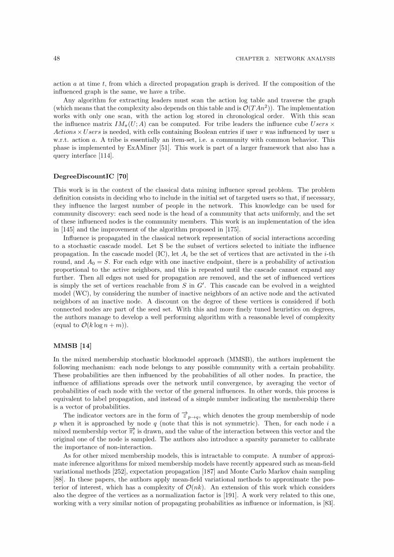
48 CHAPTER 2. NETWORK ANALYSIS
action a at time t, from which a directed propagation graph is derived. If the composition of theinfluenced graph is the same, we have a tribe.
Any algorithm for extracting leaders must scan the action log table and traverse the graph(which means that the complexity also depends on this table and isO(TAn2)). The implementationworks with only one scan, with the action log stored in chronological order. With this scanthe influence matrix IMπ(U ;A) can be computed. For tribe leaders the influence cube Users ×Actions×Users is needed, with cells containing Boolean entries if user v was influenced by user uw.r.t. action a. A tribe is essentially an item-set, i.e. a community with common behavior. Thisphase is implemented by ExAMiner [51]. This work is part of a larger framework that also has aquery interface [114].
DegreeDiscountIC [70]
This work is in the context of the classical data mining influence spread problem. The problemdefinition consists in deciding who to include in the initial set of targeted users so that, if necessary,they influence the largest number of people in the network. This knowledge can be used forcommunity discovery: each seed node is the head of a community that acts uniformly, and the setof these influenced nodes is the community members. This work is an implementation of the ideain [145] and the improvement of the algorithm proposed in [175].
Influence is propagated in the classical network representation of social interactions accordingto a stochastic cascade model. Let S be the subset of vertices selected to initiate the influencepropagation. In the cascade model (IC), let Ai be the set of vertices that are activated in the i-thround, and A0 = S. For each edge with one inactive endpoint, there is a probability of activationproportional to the active neighbors, and this is repeated until the cascade cannot expand anyfurther. Then all edges not used for propagation are removed, and the set of influenced verticesis simply the set of vertices reachable from S in G′. This cascade can be evolved in a weightedmodel (WC), by considering the number of inactive neighbors of an active node and the activatedneighbors of an inactive node. A discount on the degree of these vertices is considered if bothconnected nodes are part of the seed set. With this and more finely tuned heuristics on degrees,the authors manage to develop a well performing algorithm with a reasonable level of complexity(equal to O(k log n+m)).
MMSB [14]
In the mixed membership stochastic blockmodel approach (MMSB), the authors implement thefollowing mechanism: each node belongs to any possible community with a certain probability.These probabilities are then influenced by the probabilities of all other nodes. In practice, theinfluence of affiliations spreads over the network until convergence, by averaging the vector ofprobabilities of each node with the vector of the general influences. In other words, this process isequivalent to label propagation, and instead of a simple number indicating the membership thereis a vector of probabilities.
The indicator vectors are in the form of −→z p→q, which denotes the group membership of nodep when it is approached by node q (note that this is not symmetric). Then, for each node i amixed membership vector −→πi is drawn, and the value of the interaction between this vector and theoriginal one of the node is sampled. The authors also introduce a sparsity parameter to calibratethe importance of non-interaction.
As for other mixed membership models, this is intractable to compute. A number of approxi-mate inference algorithms for mixed membership models have recently appeared such as mean-fieldvariational methods [252], expectation propagation [187] and Monte Carlo Markov chain sampling[88]. In these papers, the authors apply mean-field variational methods to approximate the pos-terior of interest, which has a complexity of O(nk). An extension of this work which considersalso the degree of the vertices as a normalization factor is [191]. A work very related to this one,working with a very similar notion of propagating probabilities as influence or information, is [83].
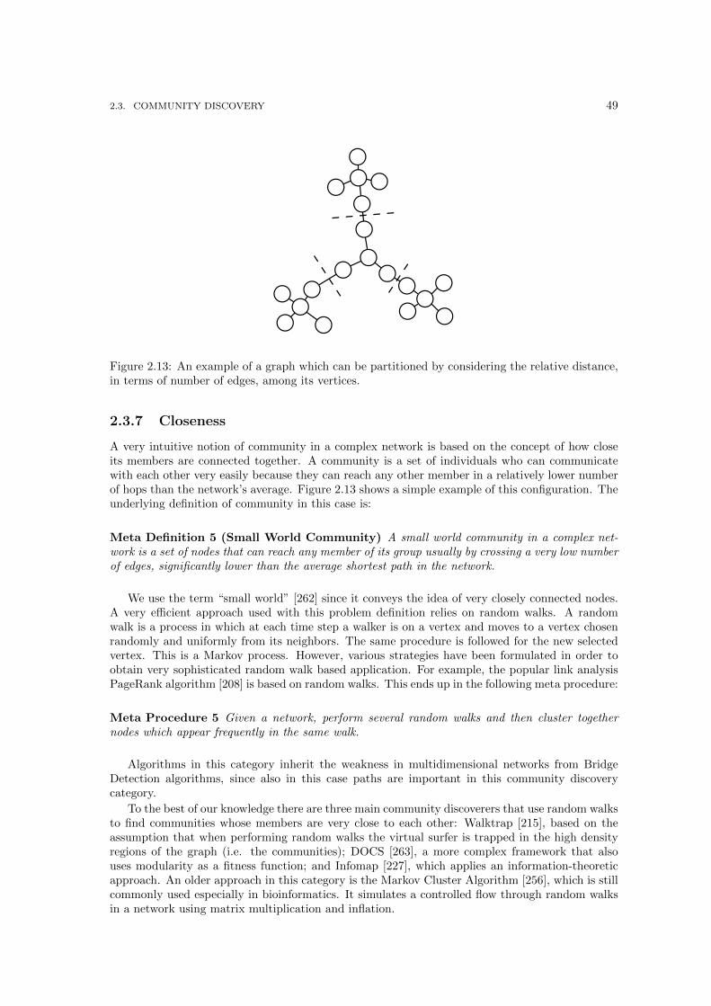
2.3. COMMUNITY DISCOVERY 49
Figure 2.13: An example of a graph which can be partitioned by considering the relative distance,in terms of number of edges, among its vertices.
2.3.7 Closeness
A very intuitive notion of community in a complex network is based on the concept of how closeits members are connected together. A community is a set of individuals who can communicatewith each other very easily because they can reach any other member in a relatively lower numberof hops than the network’s average. Figure 2.13 shows a simple example of this configuration. Theunderlying definition of community in this case is:
Meta Definition 5 (Small World Community) A small world community in a complex net-work is a set of nodes that can reach any member of its group usually by crossing a very low numberof edges, significantly lower than the average shortest path in the network.
We use the term “small world” [262] since it conveys the idea of very closely connected nodes.A very efficient approach used with this problem definition relies on random walks. A randomwalk is a process in which at each time step a walker is on a vertex and moves to a vertex chosenrandomly and uniformly from its neighbors. The same procedure is followed for the new selectedvertex. This is a Markov process. However, various strategies have been formulated in order toobtain very sophisticated random walk based application. For example, the popular link analysisPageRank algorithm [208] is based on random walks. This ends up in the following meta procedure:
Meta Procedure 5 Given a network, perform several random walks and then cluster togethernodes which appear frequently in the same walk.
Algorithms in this category inherit the weakness in multidimensional networks from BridgeDetection algorithms, since also in this case paths are important in this community discoverycategory.
To the best of our knowledge there are three main community discoverers that use random walksto find communities whose members are very close to each other: Walktrap [215], based on theassumption that when performing random walks the virtual surfer is trapped in the high densityregions of the graph (i.e. the communities); DOCS [263], a more complex framework that alsouses modularity as a fitness function; and Infomap [227], which applies an information-theoreticapproach. An older approach in this category is the Markov Cluster Algorithm [256], which is stillcommonly used especially in bioinformatics. It simulates a controlled flow through random walksin a network using matrix multiplication and inflation.

50 CHAPTER 2. NETWORK ANALYSIS
Walktrap [215]
The Walktrap approach is based on the following intuition: random walks are able to unveil thereal distance among nodes by frequently exploring nodes in the same community. The key problemis the definition of the distance function between any two vertices, computed from the informationgiven by random walks in the graph. High values of this measure mean that the two vertices i andj “see” the network in a very similar way, thus they belong to the same community. Therefore,this distance must be large if the two vertices are in different communities, and small otherwise.In the original paper this distance is defined as:
rij =
√√√√ n∑k=1
(P tik − P tjk)2
d(k)
where P tik is the probability to go from i to j in t steps and d(k) is the degree of vertex k.A critical parameter is the length t of the random walks: it must be sufficiently long to gather
enough information regarding the topology of the graph. However it must not be too long becausewhen the length of a random walk starting at vertex i tends towards infinity, the probability ofbeing on a vertex j only depends on the degree of vertex j (and not on the starting vertex i).
Similar random walk approaches are [97, 270]. However they are less efficient compared to theaverage complexity of Walktrap, which is at the worst case O(mn2).
DOCS [263]
This method is based on a spectral partition and random walk expansion, and is an extensionof [264]. The general idea is to obtain an initial guess in a first step regarding the communitystructure, and then collapse or expand these communities according to the hints given by therandom walks among them.
The first step is to coarsen the original graph into a series of higher level graphs. This is guidedby modularity maximization. In the lazy random walk stage, vertices are labeled as contributing ornon contributing vertices depending on whether or not they can be moved to another cluster andprovide an increase in modularity. They are also sorted in a descending order by their contributingvalues. The target communities can then be extracted.
Infomap [227]
The Infomap algorithm is one of the most accurate community discovery methods [162]. It is basedon a combination of information-theoretic techniques and random walks. The authors explore thegraph structure with a number of random walks of a given length and with a given probability ofjumping to a random node. This approach is equivalent to the random surfer of the PageRankalgorithm [208].
Intuitively, the random walkers are trapped in a community and exit from it very rarely. Eachwalk is described as a sequence of steps inside a community followed by a jump. By using uniquenames for communities and reusing a short code for nodes inside the community, this descriptioncan be highly compressed, in the same way as re-using street names (nodes) inside different cities(communities). The renaming is done by assigning a Huffman coding to the nodes of the network.The best network partition will result in the shortest description for all the walks.
2.3.8 Structure Definition
A number of works tackle community discovery with a very strong assumption: to be called acommunity, a group of vertices must follow a very strict structural property. In other words, theyuse the following meta definition of community:
Meta Definition 6 (Structure Community) A structure community in a complex network isa set of nodes with a precise number of edges between them, distributed in a very precise topology
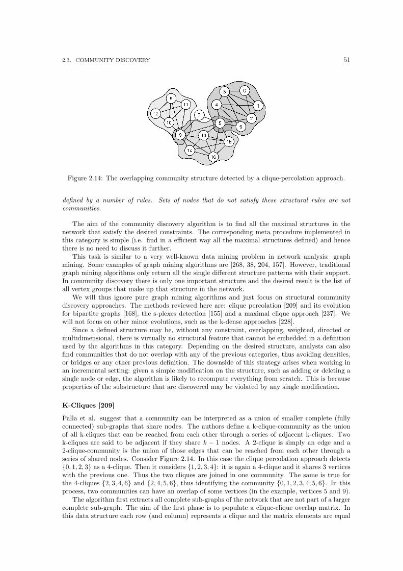
2.3. COMMUNITY DISCOVERY 51
Figure 2.14: The overlapping community structure detected by a clique-percolation approach.
defined by a number of rules. Sets of nodes that do not satisfy these structural rules are notcommunities.
The aim of the community discovery algorithm is to find all the maximal structures in thenetwork that satisfy the desired constraints. The corresponding meta procedure implemented inthis category is simple (i.e. find in a efficient way all the maximal structures defined) and hencethere is no need to discuss it further.
This task is similar to a very well-known data mining problem in network analysis: graphmining. Some examples of graph mining algorithms are [268, 38, 204, 157]. However, traditionalgraph mining algorithms only return all the single different structure patterns with their support.In community discovery there is only one important structure and the desired result is the list ofall vertex groups that make up that structure in the network.
We will thus ignore pure graph mining algorithms and just focus on structural communitydiscovery approaches. The methods reviewed here are: clique percolation [209] and its evolutionfor bipartite graphs [168], the s-plexes detection [155] and a maximal clique approach [237]. Wewill not focus on other minor evolutions, such as the k-dense approaches [228].
Since a defined structure may be, without any constraint, overlapping, weighted, directed ormultidimensional, there is virtually no structural feature that cannot be embedded in a definitionused by the algorithms in this category. Depending on the desired structure, analysts can alsofind communities that do not overlap with any of the previous categories, thus avoiding densities,or bridges or any other previous definition. The downside of this strategy arises when working inan incremental setting: given a simple modification on the structure, such as adding or deleting asingle node or edge, the algorithm is likely to recompute everything from scratch. This is becauseproperties of the substructure that are discovered may be violated by any single modification.
K-Cliques [209]
Palla et al. suggest that a community can be interpreted as a union of smaller complete (fullyconnected) sub-graphs that share nodes. The authors define a k-clique-community as the unionof all k-cliques that can be reached from each other through a series of adjacent k-cliques. Twok-cliques are said to be adjacent if they share k − 1 nodes. A 2-clique is simply an edge and a2-clique-community is the union of those edges that can be reached from each other through aseries of shared nodes. Consider Figure 2.14. In this case the clique percolation approach detects{0, 1, 2, 3} as a 4-clique. Then it considers {1, 2, 3, 4}: it is again a 4-clique and it shares 3 verticeswith the previous one. Thus the two cliques are joined in one community. The same is true forthe 4-cliques {2, 3, 4, 6} and {2, 4, 5, 6}, thus identifying the community {0, 1, 2, 3, 4, 5, 6}. In thisprocess, two communities can have an overlap of some vertices (in the example, vertices 5 and 9).
The algorithm first extracts all complete sub-graphs of the network that are not part of a largercomplete sub-graph. The aim of the first phase is to populate a clique-clique overlap matrix. Inthis data structure each row (and column) represents a clique and the matrix elements are equal
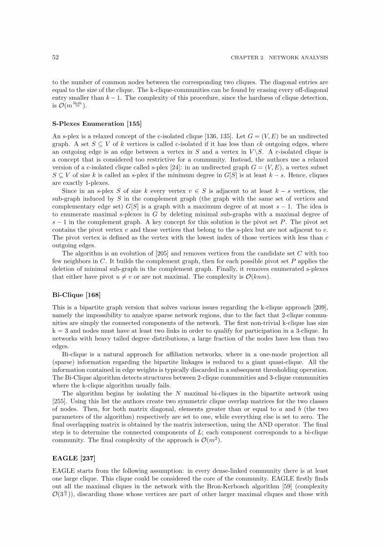
52 CHAPTER 2. NETWORK ANALYSIS
to the number of common nodes between the corresponding two cliques. The diagonal entries areequal to the size of the clique. The k-clique-communities can be found by erasing every off-diagonalentry smaller than k− 1. The complexity of this procedure, since the hardness of clique detection,is O(m
lnm10 ).
S-Plexes Enumeration [155]
An s-plex is a relaxed concept of the c-isolated clique [136, 135]. Let G = (V,E) be an undirectedgraph. A set S ⊆ V of k vertices is called c-isolated if it has less than ck outgoing edges, wherean outgoing edge is an edge between a vertex in S and a vertex in V \S. A c-isolated clique isa concept that is considered too restrictive for a community. Instead, the authors use a relaxedversion of a c-isolated clique called s-plex [24]: in an undirected graph G = (V,E), a vertex subsetS ⊆ V of size k is called an s-plex if the minimum degree in G[S] is at least k − s. Hence, cliquesare exactly 1-plexes.
Since in an s-plex S of size k every vertex v ∈ S is adjacent to at least k − s vertices, thesub-graph induced by S in the complement graph (the graph with the same set of vertices andcomplementary edge set) G[S] is a graph with a maximum degree of at most s − 1. The idea isto enumerate maximal s-plexes in G by deleting minimal sub-graphs with a maximal degree ofs − 1 in the complement graph. A key concept for this solution is the pivot set P . The pivot setcontains the pivot vertex v and those vertices that belong to the s-plex but are not adjacent to v.The pivot vertex is defined as the vertex with the lowest index of those vertices with less than coutgoing edges.
The algorithm is an evolution of [205] and removes vertices from the candidate set C with toofew neighbors in C. It builds the complement graph, then for each possible pivot set P applies thedeletion of minimal sub-graph in the complement graph. Finally, it removes enumerated s-plexesthat either have pivot u 6= v or are not maximal. The complexity is O(knm).
Bi-Clique [168]
This is a bipartite graph version that solves various issues regarding the k-clique approach [209],namely the impossibility to analyze sparse network regions, due to the fact that 2-clique commu-nities are simply the connected components of the network. The first non-trivial k-clique has sizek = 3 and nodes must have at least two links in order to qualify for participation in a 3-clique. Innetworks with heavy tailed degree distributions, a large fraction of the nodes have less than twoedges.
Bi-clique is a natural approach for affiliation networks, where in a one-mode projection all(sparse) information regarding the bipartite linkages is reduced to a giant quasi-clique. All theinformation contained in edge weights is typically discarded in a subsequent thresholding operation.The Bi-Clique algorithm detects structures between 2-clique communities and 3-clique communitieswhere the k-clique algorithm usually fails.
The algorithm begins by isolating the N maximal bi-cliques in the bipartite network using[255]. Using this list the authors create two symmetric clique overlap matrices for the two classesof nodes. Then, for both matrix diagonal, elements greater than or equal to a and b (the twoparameters of the algorithm) respectively are set to one, while everything else is set to zero. Thefinal overlapping matrix is obtained by the matrix intersection, using the AND operator. The finalstep is to determine the connected components of L; each component corresponds to a bi-cliquecommunity. The final complexity of the approach is O(m2).
EAGLE [237]
EAGLE starts from the following assumption: in every dense-linked community there is at leastone large clique. This clique could be considered the core of the community. EAGLE firstly findsout all the maximal cliques in the network with the Bron-Kerbosch algorithm [59] (complexityO(3
n3 )), discarding those whose vertices are part of other larger maximal cliques and those with

2.3. COMMUNITY DISCOVERY 53
less than k vertices. EAGLE then calculates the similarity between each pair of communities. Itthen selects the pair of communities with the maximum similarity, incorporating them into a newcommunity and calculating the similarity between the new community and other communities. Thesimilarity measure is the modularity [75]. This calculation is repeated until only one communityremains, thus completing the dendrogram.
The second stage is to cut the dendrogram. Any cut through the dendrogram produces a coverof the network. To determine the place of the cut, a measurement is required to judge the qualityof a cover, computed with a given variant of modularity.
2.3.9 Link Clustering
Some recent approaches have been based on the idea that a community is not a partition of networknodes, but a partition of the links. In other words, it is the relationship between two entities thatbelongs to a particular environment and the entities belong to all the communities of their edges(or a subset of them).
The meta procedure in this class is:
Meta Procedure 6 We are given a set of relations M between a set of entities N. We clustertogether relations that are similar, i.e. established between the same set of entities, and we thenconnect each entity n to the communities its relations belong to.
The underlying meta definition of community is:
Meta Definition 7 (Link Community) A link community in a complex network is a set ofnodes that share a number of relations clustered together since they belong to a particular relationalenvironment.
This approach implies an overlapping partition, since a node belongs to all the communities of itslinks, and only in rare occasions do all the links belong to a single community. We provide evidencefor this point in the experimental section, by looking at the average number of communities a nodebelongs to, according to algorithms in this category. One feature that is ignored by this communitydefinition is the direction of a relation, since an undirected link belongs to a single community.There is no way to attach a relationship from u to v to a community and a relationship from v tou to another community, since they both belong to the same relational environment.
The basic approach to the link clustering problem is to define a projection graph in which thenodes represent the links of the original graph and the definition of a proximity value in order tounderstand how close two edges of the network are. In both cases the critical point is to measurethe relations between the edges. A classical clustering algorithm can then be applied.
The methods reviewed here reflect both approaches. The first [89] defines the projection graphwith a random walk measure for the proximity of the projected edges, then uses modularity tocompute the modules of the network. The second one [12] is a general framework in which it ispossible to define any distance measure for the nodes (such as the Jaccard index) and then applya classical hierarchical clustering technique based on this distance definition. Finally we presentalso a bayesian approach to this problem [25].
Link modularity [89]
In this work, by defining communities as a partition of the links rather than the set of nodes, theauthors interpret the usual modularity Q in terms of a random walker moving on the nodes. Theyfurther define two walking strategies: a link-link and a link-node-link random walk. They projectthe adjacency matrix onto a bipartite incidence matrix. The elements Biα of this n ×m matrixare equal to 1 if link α is related to node i, and 0 otherwise.
The incidence matrix is then projected onto a line graph: a link is added between two nodesin this projected graph if these two nodes have at least one node of the other type in common inthe original incidence bipartite graph. Modularity is then computed on this line graph. The totalcomplexity of creating the line graph and computing modularity is O(2mk log n).

54 CHAPTER 2. NETWORK ANALYSIS
Hierarchical Link Clustering HLC* [12]
In this approach, the authors start from the assumption that whereas nodes belong to multiplegroups (individuals have families, co-workers and friends), links often exist for one dominant reason(two people are in the same family, work together or have common interests) and therefore theycluster them. They define a link similarity measure as the Jaccard coefficient. This measure iscomputed on the sets of neighbors of each edge sharing one node (i.e. only adjacent edges). Theformula used is:
S(eik, ejk) =|n+(i) ∩ n+(j)||n+(i) ∪ n+(j)|
where eik is an edge between nodes i and k and n+(i) is the set of neighbors of node i. Theapproach can be used with an arbitrary similarity function for the edges. Furthermore, althoughweights and multipartite structures are not considered with this formula, the authors claim thatit is possible to extend the approach in order to obtain such features.
The authors then build a dendrogram with a classical hierarchical clustering approach usingthe defined similarity measure, with a time complexity of O(nK2). In the dendrogram each leafis a link from the original network and branches represent link communities. In the hierarchicalstructure identified, links occupy unique communities whereas nodes naturally occupy multiplecommunities, owing to their links. Thus the extracted network structure is both hierarchical andoverlapping. The dendrogram is then cut by optimizing the partition density objective function[93].
Link Maximum Likelihood [25]
In this work the general idea of a link clustering is combined with multidimensional networks:the idea is that communities arise when there are different types of edges, i.e. dimensions, in anetwork. Basically the approach is to generate a model for the observed network with a givenpartition of edges into link communities and then testing these communities with a maximumlikelihood approach. The generation and test is very similar to the technique implemented in theExpectation Maximization [200] presented in the following category, but in this case is applied onedges instead of applying it on nodes.
2.3.10 No Definition
There are a number of frameworks for community discovery that use a very trivial definition ofcommunity or have no definition at all. These methods often assume that there are some desirablefeatures for communities that are not provided by many algorithms. They define preprocessingand/or postprocessing operations and then apply them to a number of other different knownmethods which do not extract communities with the desired features. In this way they improvethe results.
Basically, the meta definition adopted is:
Meta Definition 8 (Community) Communities in a complex network are sets which present anumber of particular features regardless of why their nodes are grouped together.
Of course, the meta procedures and features of these approaches depend on both the pre/postprocessand the “hosted” method. The works presenting a proper definition of a community are, for in-stance, the evolutionary clustering [67] or the CONGA algorithm [116], which have already beenoutlined in this section. Given that we have presented their desired common features for the setsin the form of an independent community definition, we have not included these methods in thiscategory.
Instead we focus on four methods: the first is a hybrid framework combining Bayesian andnon-Bayesian approaches [86], the second relies on a custom definition of community given bythe analyst and then performs a multidimensional community discovery, by identifying the noisyrelations inside the network [61], the third one is a bayesian hierarchical approach [74], finally thelast one is based on an expectation maximization principle [200].
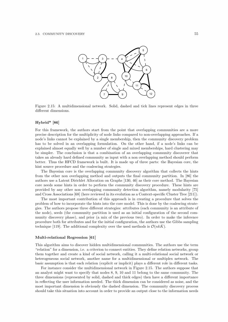
2.3. COMMUNITY DISCOVERY 55
��
��
��
����
�
� � �
�
Figure 2.15: A multidimensional network. Solid, dashed and tick lines represent edges in threedifferent dimensions.
Hybrid* [86]
For this framework, the authors start from the point that overlapping communities are a moreprecise description for the multiplicity of node links compared to non-overlapping approaches. If anode’s links cannot be explained by a single membership, then the community discovery problemhas to be solved in an overlapping formulation. On the other hand, if a node’s links can beexplained almost equally well by a number of single and mixed memberships, hard clustering maybe simpler. The conclusion is that a combination of an overlapping community discoverer thattakes an already hard defined community as input with a non overlapping method should performbetter. Thus the HFCD framework is built. It is made up of three parts: the Bayesian core, thehint source procedure and the coalescing strategies.
The Bayesian core is the overlapping community discovery algorithm that collects the hintsfrom the other non overlapping method and outputs the final community partition. In [86] theauthors use a Latent Dirichlet Allocation on Graphs [130, 46] as their core method. The Bayesiancore needs some hints in order to perform the community discovery procedure. These hints areprovided by any other non overlapping community detection algorithm, namely modularity [75]and Cross Associations [68] (here reviewed in its evolution as a Context-specific Cluster Tree [211]).
The most important contribution of this approach is in creating a procedure that solves theproblem of how to incorporate the hints into the core model. This is done by the coalescing strate-gies. The authors propose three different strategies: attributes (each community is an attribute ofthe node), seeds (the community partition is used as an initial configuration of the second com-munity discovery phase), and prior (a mix of the previous two). In order to make the inferenceprocedure both for attributes and for the initial configuration, the authors use the Gibbs samplingtechnique [119]. The additional complexity over the used methods is O(nkK).
Multi-relational Regression [61]
This algorithm aims to discover hidden multidimensional communities. The authors use the term“relation” for a dimension, i.e. a criterion to connect entities. They define relation networks, groupthem together and create a kind of social network, calling it a multi-relational social network orheterogeneous social network, another name for a multidimensional or multiplex network. Thebasic assumption is that each relation (explicit or implicit) plays a different role in different tasks.
For instance consider the multidimensional network in Figure 2.15. The authors suppose thatan analyst might want to specify that nodes 8, 9, 10 and 11 belong to the same community. Thethree dimensions (represented by solid, dashed and thick edges) then have a different importancein reflecting the user information needed. The thick dimension can be considered as noise, and themost important dimension is obviously the dashed dimension. The community discovery processshould take this situation into account in order to provide an output close to the information needs

56 CHAPTER 2. NETWORK ANALYSIS
of the user.
The authors thus represent each relation with a weighted matrix. Each element in the matrixreflects the relation strength between the two corresponding entities. This matrix is then mineddepending on a user example (or information need): the user submits a query defining the desiredcommunity structure. From this structure, the algorithm reconstructs the possible hidden relation,combining the single relation graphs with linear techniques, and then performs the communitydiscovery on the resulting hidden graph.
The hidden relation is tackled as a prediction problem: once the combination coefficients ofthe desired entities and the desired relations are computed, the hidden relation strength betweenany object pair can be predicted. This is a regression problem that can be solved with a numberof techniques [45]. For a discussion of the issues in this solution based on unconstrained linearregression see [126]. The exact regression used is the Ridge Regression.
Hierarchical Bayes [74]
In this work authors start from the assumption that many real world networks present a hiddenhierarchical organization able to explain some of the basic properties of the structure. By recon-structing this latent organization, they are able to group together nodes which are part of the samefunctional module of the network. It is evident that there is no traditional definition of communityat all, and also the authors acknowledge that to reconstruct the hidden dendrogram is a task whichgoes beyond the simple clustering.
Basically, authors generate and sample a set of dendrograms, which are able to generate arandom network with similar features to the observed network, with a Monte Carlo algorithm.The sampling is driven by the maximum likelihood, i.e. the dendrograms are extracted accordingto how well they can reproduce the observed features. By varying the pr parameter, the probabilityto join two vertices in the dendrogram, authors can tune the dendrogram generation in order tofit different properties of the network. Finally, the set of dendrograms is merged into a singleconsensus dendrogram, which is the best overall representation of the observed network. Althoughtheir technique presents an exponential time complexity at the worst case, authors found that inaverage their complexity should not exceed O(n2).
Expectation Maximization [200]
This work acknowledges the basic problem in the community discovery literature, i.e. it is neededfirstly to define what a community is and only after it is possible to implement an algorithmicprocedure able to create a partition of the network which reflect the best community divisionaccording to the starting definition. However, the problem is that sometimes it is hard to definea priori what a community is in a particular network, and failing to do so may end up in findingnot significant results. The proposed method is instead able to adapt its definition of communityto the most likely present in the data, which may be anyone of the presented classification in thispaper.
Basically the authors consider the group membership of each node as an unknown feature. Theythen define for each vertex i the probability that a (directed) link from a particular vertex in group rconnects to vertex i as ηri. Finally, πr is the probability of belonging to group r. Both ηri and πr areunknown and depend on each other. With an iterative, self-consistent approach that evaluates bothsimultaneously, two characteristic equations which define the expectation maximization algorithmare derived, and the problem can be then solved.
2.3.11 Empirical Test
In this section we briefly present an empirical evaluation of some of the presented algorithms. Theaim is to strengthen the intuition regarding the desired features which each category is either ableto present naturally or has difficulties with.
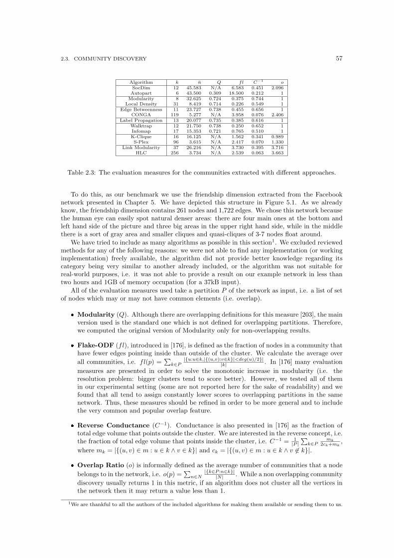
2.3. COMMUNITY DISCOVERY 57
Algorithm k n Q fl C−1 oSocDim 12 45.583 N/A 6.583 0.451 2.096
Autopart 6 43.500 0.309 18.500 0.212 1Modularity 8 32.625 0.724 0.375 0.744 1
Local Density 31 8.419 0.714 0.226 0.549 1Edge Betweenness 11 23.727 0.738 0.455 0.656 1
CONGA 119 5.277 N/A 3.958 0.076 2.406Label Propagation 13 20.077 0.735 0.385 0.616 1
Walktrap 12 21.750 0.738 0.250 0.652 1Infomap 17 15.353 0.721 0.765 0.510 1K-Clique 16 16.125 N/A 1.562 0.341 0.989S-Plex 96 3.615 N/A 2.417 0.070 1.330
Link Modularity 37 26.216 N/A 3.730 0.395 3.716HLC 256 3.734 N/A 2.539 0.063 3.663
Table 2.3: The evaluation measures for the communities extracted with different approaches.
To do this, as our benchmark we use the friendship dimension extracted from the Facebooknetwork presented in Chapter 5. We have depicted this structure in Figure 5.1. As we alreadyknow, the friendship dimension contains 261 nodes and 1,722 edges. We chose this network becausethe human eye can easily spot natural denser areas: there are four main ones at the bottom andleft hand side of the picture and three big areas in the upper right hand side, while in the middlethere is a sort of gray area and smaller cliques and quasi-cliques of 3-7 nodes float around.
We have tried to include as many algorithms as possible in this section1. We excluded reviewedmethods for any of the following reasons: we were not able to find any implementation (or workingimplementation) freely available, the algorithm did not provide better knowledge regarding itscategory being very similar to another already included, or the algorithm was not suitable forreal-world purposes, i.e. it was not able to provide a result on our example network in less thantwo hours and 1GB of memory occupation (for a 37kB input).
All of the evaluation measures used take a partition P of the network as input, i.e. a list of setof nodes which may or may not have common elements (i.e. overlap).
� Modularity (Q). Although there are overlapping definitions for this measure [203], the mainversion used is the standard one which is not defined for overlapping partitions. Therefore,we computed the original version of Modularity only for non-overlapping results.
� Flake-ODF (fl), introduced in [176], is defined as the fraction of nodes in a community thathave fewer edges pointing inside than outside of the cluster. We calculate the average over
all communities, i.e. fl(p) =∑k∈P
|{u:u∈k,|{(u,v):v∈k}|<deg(u)/2}||k| . In [176] many evaluation
measures are presented in order to solve the monotonic increase in modularity (i.e. theresolution problem: bigger clusters tend to score better). However, we tested all of themin our experimental setting (some are not reported here for the sake of readability) and wefound that all tend to assign constantly lower scores to overlapping partitions in the samenetwork. Thus, these measures should be refined in order to be more general and to includethe very common and popular overlap feature.
� Reverse Conductance (C−1). Conductance is also presented in [176] as the fraction oftotal edge volume that points outside the cluster. We are interested in the reverse concept, i.e.the fraction of total edge volume that points inside the cluster, i.e. C−1 = 1
|P |∑k∈P
mk2ck+mk
,
where mk = |{(u, v) ∈ m : u ∈ k ∧ v ∈ k}| and ck = |{(u, v) ∈ m : u ∈ k ∧ v 6∈ k}|.
� Overlap Ratio (o) is informally defined as the average number of communities that a node
belongs to in the network, i.e. o(p) =∑n∈N
|{k∈P :n∈k}||N | . While a non overlapping community
discovery usually returns 1 in this metric, if an algorithm does not cluster all the vertices inthe network then it may return a value less than 1.
1We are thankful to all the authors of the included algorithms for making them available or sending them to us.
58 CHAPTER 2. NETWORK ANALYSIS
We report the final results in Table 2.3, in which we have one row per algorithm and one column permeasure. We added some simple statistics about the partitions, such as the number of communitiesand average number of nodes per community. For the measures, in Table 2.3 we use the samenotation used in this section to present them.
We are now able to provide an additional reason for our classification by analyzing the presentedresults.
SocDim and Autopart belong to the Feature Distance category. As discussed previously, in thiscategory we have a method with basically any feature (for example, SocDim is multidimensionaland overlapping, while Autopart is parameter free and allows directed edges). The downside is thecounter intuitive partition according to the graph topology. It is easy to see, in fact, how poorlyAutopart scores in the Modularity test (Q). However, since we did not compute Modularity forthe overlapping SocDim partition, we also used the Flake-ODF measure (fl). In this case too,both SocDim and Autopart got higher values, i.e. it is more frequent that a node has moreedges pointing outside the cluster than pointing in. Overlap partitions usually have the lowestperformance according to Flake-ODF, and to Conductance, since nodes in the overlap zone aredensely connected to two or more clusters. However Autopart is not an overlapping method andSocDim turned out to be the worst of the other overlapping algorithms according to this evaluation.
For the Internal Density category we tested Modularity and Local Density algorithms. Theiredge volume inside the community (Reverse Conductance C−1) is high. For Modularity edgevolume was the highest score, while Local Density scored well, although it did not come secondfor implementation reasons (the algorithm returns some communities with only one vertex whichobviously contributes with zero to the sum).
As stated in the paragraph regarding the bridge detection community discovery, no assumptionsabout the density of the clusters are made. Thus these algorithms may have a high score on theinverse conductance (Edge Betweenness), or may not (CONGA).
Unfortunately our set of algorithms for the Diffusion category is very narrow and no conclusionscan be drawn. Instead, Closeness algorithms Walktrap and Infomap highlight their independencefrom a simple density definition: Walktrap favors a few bigger (and denser) communities, whileInfomap focuses on smaller and lower level sparser ones.
There is one clear downside to the Structure definition category: the K-Clique algorithm hasan overlap ratio o less than one, since its structure definition is very strict and many nodes cannotsatisfy it, ending up in no community.
Finally, algorithms in the Link Community category gave a very high overlap score (o). Thisproves that clustering edges is a natural and automatic way to get highly overlapping partitions.
2.3.12 Alternative Classifications
Over the last decade, several reviews of community discovery methods have been published. Wewould consider the most important to be [201, 66, 82, 95, 216, 231].
Fortunato and Castellano [95], hugely extended by Fortunato in [94], have published the mostrecent and probably the most comprehensive review on the community discovery problem. Totackle the problem they consider various definitions of community (local, global and vertex simi-larity), features of communities for extraction, and different categories. The number of algorithmsand references they considered is impressive. We believe that a new review of this topic is neededbecause the authors analyze the main techniques of each method for community detection, howeverthey do not build an organization of community definitions (while acknowledging that differentones exist). Their work does not include some more advanced features and definitions of commu-nity found in the literature, such as multidimensionality or an influence spread formulation of theproblem.
Porter et al. [216] and Schaeffer [231] have also recently reviewed community discovery methods.In [231] they also introduced the problem of a comprehensive meta definition of community in agraph. Again, however, although they begin to provide different definitions of community, they donot create a classification of the community discovery algorithm based on such a community.
2.4. GENERATORS 59
In Newman’s pioneering work [201] we can find an organization of historical approaches tocommunity discovery in complex networks following their traditional fields of application. Newmanpresents the most important classical approaches in computer science and sociology, enumeratingalgorithms such as spectral bisection [217] or hierarchical clustering [235]. He then reviews newphysical approaches to the community discovery problem, including the known edge betweenness[106] and modularity [199]. His paper is very useful for a historical perspective, however it recordsfew works and obviously does not take into account all the algorithms and categories of methodsthat have been developed since it was published.
Chakrabarti and Faloutsos [66] give a complete survey of many aspects of graph mining. Oneimportant chapter discusses community detection concepts, techniques and tools. The authorsintroduce the basic concepts of the classical notion of community structure based on edge density,along with other key concepts such as transitivity, edge betweenness and resilience. However, thissurvey is not explicitly devoted to the community discovery problem. It describes existing methodsbut does not investigate the possibility of different definitions of community or of a more complexanalysis.
Danon et al. [82] test an impressive number of different community discovery algorithms. Theycompare the time complexity and performances of the methods considered. Furthermore, theydefine a heuristic to evaluate the results of each algorithm and also compare their performance.However, they focus more on a practical comparison of the methods, rather than a true clas-sification, both in terms of a community definition and in the feature considered for the inputnetwork.
Various authors have also proposed a benchmark graph, which would be useful to test commu-nity discovery algorithms [164].
As we have seen, community discovery is a very complex task involving an incredible amountof techniques and desired features. To define and predict what will be the most important featuresin the future is an open question. As witnessed by this thesis and by many other publications[246, 36, 192, 25, 61] there is a growing interest in multidimensionality, perceived as a feature thatis part of the solution and not only as an input to be preprocessed. In other words, we wantnot only to consider multidimensionality as an input, but also to extract truly multidimensionalcommunities. But how to define what exactly a “multidimensional community” is? Are all thegroups of nodes with dense multidimensional connections equal? We address these questions inthe following section.
2.4 Generators
In this section we present the most common and basics generators of synthetic graphs. The generalaim of the network modeling is to capture essential properties behind real-world phenomena,with simple assumptions over the mechanisms generating them (just like the rich-get-richer effectexplanation for generating power law degree distributions). With these generators it is also possibleto obtain a network respecting some of the properties of real world ones, presented in Section 2.2.The two different aims can cluster network generators into two different main categories: descriptiveand generative models.
As we see, in the descriptive category generally each model focuses onto one or few essentialproperties of real world complex networks, trying to unveil knowledge about how that propertycame to life. None of these models has the aim of respecting all the properties of all the possiblevariants of real world networks. In the generative category, the models are more focused onproviding as output data more similar to the actual networks, but the creation of a syntheticnetwork that is able to represent all the rich semantic of real world data is still an open problem.
We now provide more details about each category in the two following subsections. Please notethat an orthogonal categorization, namely one that divides models into static and dynamic, canbe applied to models belonging either to the descriptive or to the generative one.
60 CHAPTER 2. NETWORK ANALYSIS
2.4.1 Descriptive Models
Solomonoff and Rapoport [239] and independently Erdos and Renyi [87] proposed the followingextremely simple model of a network. Take some number n of vertices and connect each pair (ornot) with probability p (or 1− p). A slight variation of the same model is the following: consider
all possible node pairs (that are n(n−1)2 ), then choose randomly m node pairs. An equivalent
definition: list all graphs with exactly n nodes and m edges and choose one randomly.The random graph is the mathematically most well-studied and understood model. The ran-
dom graph, while illuminating, is inadequate to describe some important properties of real-worldnetworks. In fact, in a random graph all edges are equally probable and appear independently.This assumption is not true in almost all the networks in real world.
The structure of the random graph dramatically change by considering different values of thep and/or m parameter. The usual regime of interest is p ∼ 1
n (m ∼ n), when n is large. Whenp > 1
n the average degree z is greater than one and in the network there is a transition phase. Agiant component, see Section 2.2, appears and the expected diameter of the network is equal tolognlog z [195].
However in almost all other respects, the properties of the random graph do not match thoseof networks in the real world. It has a low clustering coefficient: the probability of connection oftwo vertices is p regardless whether they have a common neighbor or not [262]. As a consequence,a random graph does not show a community structure. The model also has a Poisson degreedistribution, quite unlike the power law degree distributions present in real world networks.
Random graphs can be extended in a variety of ways to make them more realistic. The propertyof real graphs that is simplest to incorporate is the property of non-Poisson degree distributions,which leads us to the so-called configuration model [189]. In order to obtain a graph with theconfiguration model, we specify a degree distribution pk, such that pk is the fraction of vertices inthe network having degree k or higher. We choose a degree sequence, which is a set of n valuesof the degrees ki of vertices i = 1...n, from this distribution. We can think of this as giving eachvertex i in our graph ki “stubs” or “spokes” sticking out of it, which are the ends of edges-to-be.Then we choose pairs of stubs at random from the network and connect them together. In order toobtain a real power law degree distribution, one needs only to specify the correct degree sequence.
With this model is possible to generate scale free networks, although we do not know howthis distribution has been generated. We know that the probability of attaching a new edge to avertex is proportional to the vertex actual number of “stubs”, but this is not sufficient in orderto understand the power law degree distribution in real world networks. Further, the clusteringcoefficient of this model is still very low.
It is possible to define slight variants of the configuration model, that take into account alsoother characteristics such as the direction of the edges, the degree correlations or anticorrelationsand the high clustering coefficient. An important class of these models are the so called exponentialrandom graphs or Markov graphs [98]. In Markov graphs the presence or absence of an edgebetween two vertices in the graph is correlated only with those edges that share one of the sametwo vertices. Edge pairs that are disjoint (have no vertices in common) are uncorrelated. Thismodel has a tendency to condense, i.e. it creates regions of the graph that are essentially completecliques. Networks in the real world, however, do not seem to have this sort of “clumpy” transitivity:regions of cliquishness contributing heavily to the clustering coefficient, separated by other regionswith few triangles.
However, all these variants share the common problem that are defined in order to captureone single real world network property. In order to obtain a greater accuracy, different graphgeneration criteria are needed.
Networks may have a geographical component attached to them; i.e. the vertices of the networkhave positions in space. In many cases it is reasonable to assume that geographical proximity willplay a role in deciding which vertices are connected to which others. The small-world model [262]starts from this idea by positing a network built on a low-dimensional regular lattice and thenadding or moving edges to create a low density of “shortcuts” that join remote parts of the latticeto one another.
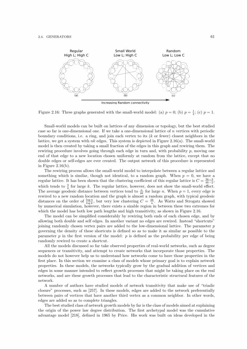
2.4. GENERATORS 61
(a) (b) (c)
RegularHigh L; High C
Small WorldLow L; High C
RandomLow L; Low C
Increasing Random connectivity
Figure 2.16: Three graphs generated with the small-world model: (a) p = 0; (b) p = 14 ; (c) p = 1.
Small-world models can be built on lattices of any dimension or topology, but the best studiedcase so far is one-dimensional one. If we take a one-dimensional lattice of n vertices with periodicboundary conditions, i.e. a ring, and join each vertex to its (k or fewer) closest neighbors in thelattice, we get a system with nk edges. This system is depicted in Figure 2.16(a). The small-worldmodel is then created by taking a small fraction of the edges in this graph and rewiring them. Therewiring procedure involves going through each edge in turn and, with probability p, moving oneend of that edge to a new location chosen uniformly at random from the lattice, except that nodouble edges or self-edges are ever created. The output network of this procedure is representedin Figure 2.16(b).
The rewiring process allows the small-world model to interpolate between a regular lattice andsomething which is similar, though not identical, to a random graph. When p = 0, we have aregular lattice. It has been shown that the clustering coefficient of this regular lattice is C = 3k−3
4k−2 ,
which tends to 34 for large k. The regular lattice, however, does not show the small-world effect.
The average geodesic distance between vertices tend to n4k for large n. When p = 1, every edge is
rewired to a new random location and the graph is almost a random graph, with typical geodesicdistances on the order of logn
log k , but very low clustering C = 2kn . As Watts and Strogatz showed
by numerical simulation, however, there exists a sizable region in between these two extremes forwhich the model has both low path lengths and high transitivity, as shown in Figure 2.16.
The model can be simplified considerably by rewiring both ends of each chosen edge, and byallowing both double and self edges. In another variant no edges are rewired. Instead “shortcuts”joining randomly chosen vertex pairs are added to the low-dimensional lattice. The parameter pgoverning the density of these shortcuts is defined so as to make it as similar as possible to theparameter p in the first version of the model: p is defined as the probability per edge of beingrandomly rewired to create a shortcut.
All the models discussed so far take observed properties of real-world networks, such as degreesequences or transitivity, and attempt to create networks that incorporate those properties. Themodels do not however help us to understand how networks come to have those properties in thefirst place. In this section we examine a class of models whose primary goal is to explain networkproperties. In these models, the networks typically grow by the gradual addition of vertices andedges in some manner intended to reflect growth processes that might be taking place on the realnetworks, and are these growth processes that lead to the characteristic structural features of thenetwork.
A number of authors have studied models of network transitivity that make use of “triadicclosure” processes, such as [257]. In these models, edges are added to the network preferentiallybetween pairs of vertices that have another third vertex as a common neighbor. In other words,edges are added so as to complete triangles.
The best studied class of network growth models by far is the class of models aimed at explainingthe origin of the power law degree distribution. The first archetypal model was the cumulativeadvantage model [218], defined in 1965 by Price. His work was built on ideas developed in the
62 CHAPTER 2. NETWORK ANALYSIS
1950s by Herbert Simon, who showed that power laws arise when “the rich get richer”, when theamount you get goes up with the amount you already have. Price appears to have been the firstto discuss cumulative advantage specifically in the context of networks, and in particular in thecontext of the network of citations between papers. His idea was that the rate at which a papergets new citations should be proportional to the number that it already has.
This idea is now widely accepted as the probable explanation for the power-law degree distribu-tion observed not only in citation networks but in a wide variety of other networks too, includingthe World Wide Web, collaboration networks, and so on. The idea of cumulative advantage is atthe basis of the preferential attachment model [30] of Barabasi and Albert. In this model we havevertices that are added to the network with degree m, which is never changed thereafter. Theother end of each edge is then being attached to another vertex with probability proportional tothe degree of that end vertex. There are many different variants of this model that are definedin order to capture some differences in the event to be represented: for example this undirectedgraph can be considered directed when one needs to model the structure of the World Wide Web.However, all these variants do not alter the basic properties of this model.
The preferential attachment model is able to create networks with a power law degree distribu-tion. In particular, its power law exponent α is fixed to 3, that is a good approximation for mostreal world networks [50].
There are other interesting properties of the model that has been studied so far. Some of themhighlight issues of inaccuracy in the real world network representation of this model. First, themodel has two important types of correlations. There is a correlation between the age of verticesand their degrees, with older vertices having higher mean degree. In other words the earliestvertices added have substantially higher expected degree than those added later, and the overallpower-law degree distribution of the whole graph is a result primarily of the influence of theseearliest vertices. This correlation between degree and age has been used to argue against themodel as a model of the World Wide Web: it has been shown, using actual Web data, that thereis no such correlation in the real Web [3]. The second correlation has been discovered between thedegrees of adjacent vertices.
2.4.2 Generative Models
The study of temporal evolving networks has given new life blood also to a related problem: thedefinition of novel generator tools of synthetic complex networks, a well-known problem in literatureeven in the first years of graph theory, as presented in the previous section [30]. However, as wepresented, the preferential attachment model focuses more on a description about how we obtaina power law degree distribution, rather than on the generation of a synthetic real world complexnetwork. This step is tackled by models clustered in this category, and it relies mainly on makingsome hypothesis about what kind of microscopic node behavior would reproduce the observedmacroscopic network structure.
Recently, it has been proposed a new way of looking at the evolution models. In this newapproach the model does not try to represent the characteristics of the network as a whole, insteadthe focus is devoted to the microscopic level, i.e. what is interesting is the behavior of every nodetaken individually. The focus is to study the individual node arrival and edge creation processesthat collectively lead to macroscopic properties of networks. Instead of only focusing on the globalnetwork structure and then hypothesizing about what kind of microscopic node behavior wouldreproduce the observed macroscopic network structure, works of this kind focus directly on themicroscopic node behavior per se.
The main work in this class is based on the maximum-likelihood estimation (MLE) principle[172], that can be applied to compare a family of parameterized models in terms of their likelihoodof generating the observed data, and as a result, pick the “best” model (and parameters) to explainthe data. To apply the likelihood principle, authors consider the following setting: they evolve thenetwork edge by edge and for every edge that arrives into the network they measure the networkslikelihood that the particular edge endpoints would be chosen under some model. The productof these likelihoods over all edges will give the likelihood of the model. The mechanism of node
2.5. LINK ANALYSIS 63
and edge arrivals considered are a given node and edge arrival process and the edge destinationselection process. This microscopic evolution approach can outperform the preferential attachmentin generating synthetic networks that are a better representation of the real world networks.
However, also in this case it is important to notice that these generators are defined only fora monodimensional dynamic setting. No consideration of the different dimensions in which a linkcan appear are represented in the model.
2.5 Link Analysis
Link analysis refers to a complex of techniques that explicitly consider the links when buildingpredictive or descriptive models of the linked data. Commonly addressed link mining tasks includeobject ranking, collective classification, entity resolution and link prediction. The main referencepresent in literature about link analysis methods is [103].
Perhaps the most well known link analysis task is that of link-based object ranking (LBR),which is a primary focus of the link analysis community. The objective of LBR is to exploit thelink structure of a graph to order or prioritize the set of objects within the graph. Much of thisresearch focuses on graphs with a single object type and a single link type.
In the context of web information retrieval, the PageRank [208] and HITS [151] algorithms arethe most notable approaches to LBR. PageRank models web surfing as a random walk wherethe surfer randomly selects and follows links and occasionally jumps to a new web page to startanother traversal of the link structure. The rank of a given web page in this context is thefraction of time that the random web surfer would spend at the page if the random process wereiterated ad infinitum. This can be determined by computing the steady-state distribution of therandom process. HITS implements a slightly more complex process, modeling the web as beingcomposed of two types of web pages: hubs and authorities. Hubs are web pages that link to manyauthoritative pages. Authorities are web pages that are linked by many hubs. Each page in theweb is assigned hub and authority scores. These scores are computed by an iterative algorithmthat updates the scores of a page based on the scores of pages in its immediate neighborhood. Thisapproach bears a relation to PageRank with two separate random walks, one with hub transitionsand one with authority transitions, on a corresponding bipartite graph of hubs and authorities.The hub and authority scores are the steady-state distributions of the respective random processes.While PageRank is currently used in real world applications, there are no information, to the bestof our knowledge, about real world scalable implementation of HITS.
In the domain of social network analysis, LBR is a core analysis task, i.e. finding the mostimportant (central) vertices inside the network. They range in complexity from local measures suchas degree centrality, which is simply the vertex degree, to global measures such as eigenvector/powercentrality, which use spectral methods to characterize the importance of individuals based on theirconnectedness to other important individuals [103].
Ranking objects in dynamic graphs that capture event data such as email, telephone calls,or publications introduces new challenges. In contrast to ranking methods for static settings thatproduce a single rank, the goal is to track the changes in object rank over time as new events unfold.Static ranking methods can be applied to aggregated event data over various time intervals, butthis aggregation removes the time ordering of events, and the sparse link structure over a giventime interval limits the utility of the resulting ranks.
In the link-based object classification (LBC) problem, a data graph G = (O,L) is composedof a set objects O connected to each other via a set of links L. The task is to label the members ofO from a finite set of categorical values. The discerning feature of LBC that makes it different fromtraditional classification is that, in many cases, the labels of related objects tend to be correlated.The challenge is to design algorithms for collective classification that exploit such correlations andjointly infer the categorical values associated with the objects in the graph. In addition to themachine learning community [181], the computer vision and natural language communities havealso studied the LBC problem [159], thus highlighting the truly interdisciplinary nature of thesefields of research.
64 CHAPTER 2. NETWORK ANALYSIS
The final object-centric task is entity resolution, which involves identifying the set of objectsin a domain. The goal of entity resolution is to determine which references in the data referto the same real-world entity. Examples of this problem arise in databases [141] (deduplication,data integration), natural language processing [44] (co-reference resolution, object consolidation),personal information management, and other fields. Entity resolution has been viewed as a pair-wise resolution problem, where each pair of references is independently resolved as being co-referentor otherwise, depending on the similarity of their attributes. Recently, there has been significantinterest in the use of links for improved entity resolution. The central idea is to consider, in additionto the attributes of the references to be resolved, the other references to which these are linked.These links may be, for example, co-author links between author references in bibliographic data,hierarchical links between spatial references in geo-spatial data, or co-occurrence links betweenname references in natural language documents. However, while these approaches consider linksfor entity resolution, only the attributes of linked references are considered and different resolutiondecisions are still taken independently. In contrast, collective entity resolution approaches havealso been proposed in databases [141], where one resolution decision affects another if they arelinked.
Link prediction is an edge-oriented task and it is defined as the problem of predicting theexistence of a link between two entities, based on attributes of the objects and other observed links.Examples include predicting links among actors in social networks, such as predicting friendships;predicting the participation of actors in events, such as email, telephone calls and co-authorship;and so on. This problem is often viewed as a simple binary classification problem: for any twopotentially linked objects oi and oj , predict whether lij is 1 or 0. One approach is to make thisprediction entirely based on structural properties of the network. Liben-Nowell and Kleinberg [207]present a survey of predictors based on different graph proximity measures. Other approaches makeuse of attribute information for link prediction. Just as in the community discovery research track,also in this case there are very recent works that use a tensor-based approach for link prediction [1].A latter class of approaches is composed by systems of probabilistic inference about the links. Thisallows them to capture the correlations among the links. They can also be used for other tasks,such as link-based classification. Ideally this makes for more accurate predictions. However, model-based probabilistic approaches have a computational price: exact inference is generally intractable,so approximate inference techniques are necessary.
In this brief resume of the link analysis state of the art, we have described each link mining taskin isolation. More generally, component link mining algorithms may be part of a larger knowledgediscovery process [103]. As we move from one domain to another, the processing requirementswill change, but the need to compose the algorithms in a unified process will remain. Ideally,as we move from data conditioning to more complex inference tasks, we would like to propagateuncertainty throughout the process. One approach that solves this problem, in theory, is to definea full probabilistic model. However, this approach is not always desirable or feasible. Moreover,many link analysis algorithms are defined in a static environment. But when considering the overallknowledge discovery process, it is important to keep in mind that many aspects of the process areintrinsically defined in an evolving setting.
2.6 Information Propagation
One of the most important event that we can represent with a network is the contagion model.Many researcher have worked defining different possible contagion dynamics that can take place ina network. The general model states that given a node n in state A, then all its neighbors directlyconnected with an edge to n have an increased probability of turning into state A. The differentdynamics through this change of state may happen are modeled in different ways. We report forexample the SIR/SIS model and the threshold models in social sciences.
We now focus on a particular type of contagion in complex networks, i.e. when what is spreadingon a network is not a disease, but information. This particular problem definition, to understandthe dynamics of the information propagation in a social network, is a problem particularly popular
2.6. INFORMATION PROPAGATION 65
in the data mining literature. We consider a social network in which users can view the actionperformed by their neighbors. Aim of the information propagation works is to investigate howinfluence (for performing certain actions) propagates from users to their network friends, poten-tially recursively, thus identifying a group of users that behaves homogeneously (i.e. a tribe, or acommunity). These works can be focused basically on two aspects of the information propagation:the temporal dimension intrinsically contained in the flow of information and the causes of theinformation propagation.
The works of the first class are focused on the topic and the general characteristic of the in-formation propagation in different environments. Basically their aim is to answer the followingquestions: why certain topics are spread faster than others? What is the distribution of the tempo-ral intervals among the “hops” that the information passes through? In this class can be clusteredworks like applications of graph mining [66] and temporally annotated sequences [105] techniquesthat aim to discover frequent patterns (both in graphs and in sequences that represents flows ofcommunication) and then obtain a rich description of the information propagation process. An-other work analyzes the efficiency of a recommendation system, trying to define a model of theuser behavior [171]. The authors identify the recommendation system as a complex interactionof cascade behavior: one user influences, and is influenced by, a set of neighbors. Then they firstanalyze the probability of purchasing as one gets more and more recommendations. Next, theymeasure recommendation effectiveness as two people exchange more and more recommendations.Lastly, they observe the recommendation network from the perspective of the sender of the recom-mendation. The aim is to answer to the question: does a node that makes more recommendationsalso influence more purchases? Then authors present a model which characterizes product cate-gories for which recommendations are more likely to be accepted. They use a regression of theproduct attributes to correlate them with recommendation success.
In the second class the focus is moved from the information propagation to the actors of thisevent. Aim is to identify in a social network the characteristics and the attribute that make a usera sort of power user, i.e. a leader in the information propagation. Here the focus is to answer theseother questions: why certain discussions are passed over while others stop in two hops? Whatare the characteristics of the nodes that pass the information? The aim can be summarized asleader detection. An example of this kind of works can be represented by [113]. In this work,a node u can be defined as a leader if u performed a and within a chosen time bound after uperformed a, a sufficient number of other users performed a. Furthermore these other users mustbe reachable from u thus capturing the role social ties may have played. A stronger notion ofleadership might be based on requiring that w.r.t. each of a class of actions of interest, the set ofinfluenced users must be the same: this will identify a tribe leader, meaning the user leads a fixedset of users (tribe) w.r.t. a set of actions. This variants can be viewed as an alternative definition ofcommunity discovery, as explored in Section 2.3. In some works the input includes just the networkrepresentation (which is not edge-weighted) [145], in other works this is enriched with an actiontable which plays a central role in the definition of leaders [113]. Another work that is included inthis class aims to represent the information spread as an heat diffusion process [182]. In this wayit is possible to model not only the spread of positive opinions about a specific product (or fact),but also the negative influence. Once modeled the information spread, it is possible to apply amarketing candidate selection that identify the characteristics of the user inside the network thatcan maximize the positive heat diffusion.
Both these classes of works are intrinsically focused on the temporal evolution of their data.In order to register the information spread and/or to identify leaders from a set of timestampedactions, the temporal analysis is a mandatory step. However, in literature the impression is that ourknowledge about this phenomenon is still far from complete. Further, very little has been done inanother crucial part of the information propagation analysis. It is a matter of common experience,in fact, that the form, the content, the lasting and all the characteristics of an information exchangeare dramatically different when we communicate through different media. A phone call is differentfrom an email, from a paper letter, from a chat via an instant messaging software. Thus, it iscrucial to record this information and include it in the data representation. And this considerationholds also for contagion models: a virus can be airborne, waterborne or spread through different
66 CHAPTER 2. NETWORK ANALYSIS
media, and the underlying topology of the airborne networks are dramatically different from thewaterborne ones. But the works focused on the multidimensional information spread are, to thebest of our knowledge, very few.
2.7 Graph Mining
Given a complex network as a basic structure, traditionally a graph with labels attached bothto vertices and to edges, aim of a graph mining algorithm is to find in this structure frequentsubgraphs. An interesting and complete survey on graph mining tools and techniques can befound in [66]. Here we refer to the narrower definition of graph mining, namely the discovery offrequent patterns in the simple graph structure, i.e. nodes with the same labels connected by edgeswith the same label. More broadly, graph mining aims to find patterns of all kinds including, butnot limited to, path lengths, communities, time evolution patterns, etc.
A subgraph p is said to be frequent in a graph database g if its support σ∧(p, g) is greaterthan or equal to a given threshold [268]. There are different definitions of support, depending onthe specific format of data input. However, the definition of support should have three properties:anti-monotone, easy to compute and intuitive [56]. An anti-monotone support definition meansthat if a set cannot pass the frequency test, being found not frequent, all of its super-set will fail thesame test as well. In our case this means that if a subgraph does not pass the threshold test thennone of its extension will never pass the threshold test, thus dramatically narrowing the searchspace. It should be easy to compute because an NP-hard support definition is a clear source ofinefficiency. Finally, an intuitive support definition is necessary to understand clearly what thegraph miner is actually computing.
The problem of frequent pattern discovery in graph databases can be split in two very differ-ent scenarios, namely the graph-transaction and the large single-graph setting [137]. In graph-transaction setting the graph database to be mined is a set of relatively small graphs, and the taskof the mining process is to find frequently recurring graphs in this graph database. In single-graphsetting the input of the mining system is one single graph with large number of nodes, and thetask is to find frequent recurring subgraphs of the single input graph.
Thus in the graph-transaction setting the support of a subgraph is defined as the number ofthe graphs in the input database that contains at least one occurrence of the starting subgraph.The number of actual occurrences in the graph database is not considered. It is easy to notethat the frequency is anti-monotone: when we extend our subgraph some of the structures in thedatabase that contained the smallest subgraph may be no longer counted into the support of thenew pattern. The kernel of frequent subgraph mining is the subgraph isomorphism test, i.e. themechanism that allow to verify if two graphs are different instances of the same structure. Lots ofwell-known pair-wise isomorphism testing algorithms were developed.
These algorithms can be roughly divided by looking at their strategies in exploring the graphstructure: they can implement a breadth first search [202] (quick, but expensive in terms ofmemory) or a depth first search [268] (slower, but requires a small amount of memory). Theneach algorithm uses some heuristics to further cut the search space. One of the most importantalgorithms is gSpan [268], that represents the basic kernel also for techniques in other settings,such as link prediction. gSpan has introduced two concepts: the DFS lexicographic order andthe minimum DFS code, that form a canonical labeling system to support DFS search. Whenexploring a graph with a depth-first approach, there might be different alternatives. The DFSlexicographic order is a technique to assign an order to all these alternatives, from the “smallest”to the “largest”. The minimum DFS code of p is the representation of the smallest depth-firstexploration of p. For any p there is one and only one minimum DFS code. Therefore we can solvethe graph isomorphism test (i.e. decide if two graphs are the same structure) by confronting theminimum DFS code of two different graph patterns.
By exploiting the DFS lexicographic order, gSpan discovers all the frequent subgraphs withoutcandidate generation and false positives pruning, needed, for example, in an Apriori approach. Itcombines the growing and checking of frequent subgraphs into one procedure, thus accelerating
2.8. PRIVACY 67
the mining process. Currently some researchers are still looking for better heuristics in order toachieve faster implementations of a graph miner [16].
In the single-graph setting the frequency, or the number of occurrence, of a subgraph is nota good support function. This definition of support have the problem that it is not anti-monotone[56]; thus it cannot be used effectively in pattern mining, as anti-monotonicity is required to prunethe search space. Anti-monotone support definitions currently accepted in literature are based oncomputing maximum independent sets in overlap graphs, or the minimum image based support.The second one is defined as follows, given a subgraph p that appears in our single input graphg, its support σ∧(p, g) is defined as follows: σ∧(p, g) = minv∈Vp |{ϕi(v) : ϕi is an occurrence of pin g}|, where v is a vertex in the set Vp of vertices inside the pattern p [56]. Unfortunately thissupport definition is highly counter-intuitive.
Lately, it has been developed a further evolution in the single graph mining setting. In thisevolution the labels attached to the edges represent the time step in which the edge has beencreated. From this setting it is possible to derive graph-evolution rules from frequent patterns [38].In this work authors can provide not only frequent patterns with an absolute timestamp on theedges, but patterns in which the edges are labeled with a relative timestamp.
2.8 Privacy
Digital traces of human social interactions can now be found in a wide variety of on-line settings,and this has made them rich sources of data for large-scale studies of social networks. While anumber of these on-line data sources are based on publicly crawlable blogging and social networkingsites, where users have explicitly chosen to publish their links to others, many of the most promisingopportunities for the study of social networks are emerging from data on domains where usershave strong expectations of privacy, including e-mail and messaging networks, as well as the linkstructure of closed (i.e. members-only) on-line communities.
In designing studies of such systems, one needs to set up the data to protect the privacy ofindividual users while preserving the global network properties. This is typically done throughanonymization, a simple procedure in which each individual’s “name” (e.g., e-mail address, phonenumber, or actual name) is replaced by a random user ID, but the connections between the (nowanonymized) people, encoding who spoke together on the phone, who corresponded with whom,or who instant-messaged whom, are revealed. The motivation behind anonymizing is roughly asfollows: while the social network labeled with actual names is sensitive and cannot be released,there may be considerable value in allowing researchers to study its structure.
But anonymous social network data almost never exists in the absence of outside context, andan adversary can potentially combine this knowledge with the observed structure to begin com-promising privacy, de-anonymizing nodes and even learning the edge relations between explicitlynamed (de-anonymized) individuals in the system. Moreover, such an adversary may in fact be auser (or set of users) of the system that is being anonymized.
In literature there are some papers focused on defining the type of attacks to the privacy ofthe users represented in a social network, such as [19], [194] and [206]. In short, these attacks areactive (walk-based and cut-based) and passive attacks.
The structure of the active attack is roughly as follows. Before the anonymized graph isproduced, the attacker creates k new user accounts (for a small parameter k), and it links themtogether to create a subgraph H. It then uses these accounts to create links (e.g. by sendingmessages or creating address book entries) to nodes in {w1, ..., wb}, and potentially other nodesas well. Now, when the anonymized copy of G is released, this subgraph H will be still present.The attacker finds the copy of H that it planted in G, and from this it locates w1, ..., wb. Havingidentified the true location of these targeted users in G, the attacker can then determine all theedges among them, thereby compromising privacy.
The passive attack is based on the observation that most nodes in real social network dataalready belong to a small uniquely identifiable subgraph. Hence, if a user u is able to colludewith a coalition of k − 1 friends after the release of the network, he or she will be able to identify

68 CHAPTER 2. NETWORK ANALYSIS
additional nodes that are connected to this coalition, and thereby learn the edge relations amongthem.
The results of the attack survey in literature is that one cannot rely on anonymization toensure individual privacy in social network data, in the presence of parties who may be tryingto compromise this privacy. Still are missing some mathematically rigorous implementations ofsystem that can ensure some robust countermeasures to one or more of these attacks.
Chapter 3
Multidimensional Network: ModelDefinition
In this chapter we briefly provide a formal definition of the concept of Multidimensional Network.We use this model for the remainder of the thesis.
The term network refers to the informal concept describing a structure composed of a set ofelements and connections or interactions between them. In a real world network the entities maybe connected by relations of different nature: for example, two persons may be linked because theyare friends, colleagues, relatives or because they communicate to each other by phone, email, andso on. A network where a pair of entities may be linked by different kinds of links, having morethan one connection between the two entites, is called a multidimensional network. We considereach possible type of relation between two entities a particular dimension of the network.
Often, the graph is used to model a network with its properties. In the graph model, theentities are represented by nodes while a relation is modeled by a (directed or undirected) edge.In the case of a multidimensional setting a convenient way to model a network is hence a labeledmultigraph. Intuitively, a labeled multigraph is a graph where both nodes and edges are labeledand where there can exist two or more edges between two nodes. Just any regular labeled graph,also labeled multigraph may be directed and undirected, thus we allow edges to be both directedand undirected, when the analytic aim requires it. However, in our context we do not considernode labels, thus we adopt a particular version of multigraph where only the edges are labeled.The model that we use in the remainder of the paper is hence the edge-labeled multigraph. Wereserve the possibility of using in this thesis, where specified, multigraphs with labels attached alsoto nodes, or any other extension of the basic model here presented, to be more general. Formally,such a graph is denoted by a triple G = (V,E,D) where:
� V is a set of nodes
� D is a set of labels representing our dimensions
� E is a set of labeled edges, i.e., it is a set of triple of the form (u, v, d) where u, v ∈ V arenodes and d ∈ D is a label.
We assume that given a pair of nodes u, v ∈ V and a label d ∈ D it may exist only one edge(u, v, d). Moreover, as before reported, we are working with an directed graph, therefore the edges(u, v, d) and (v, u, d) are considered distinct, except when otherwise specified.
Thus, given |D| = m each pair of nodes in G can be connected by at most m possible edges.In fact, it is useless to connect with two distinct edges in the same dimension, as they representthe same relation. When needed, however, we can allow weights to handle the particular situationwhere two or more relations of the same type are expressed in the data. Therefore, in those casesthe edges are no more triplets, but quadruplets (u, v, d, w), where w is any real number representingthe weight of the relation between nodes u, v ∈ V and labeled with d ∈ D.

70 CHAPTER 3. MULTIDIMENSIONAL NETWORK: MODEL DEFINITION
In the following, we denote by P(D) the power set of the label collection D and by G the setof graphs of the form G = (V,E,D).
When we use edge-labeled multigraphs to model a multidimensional network, the set of nodesrepresents the set of entities or actors in the networks, the edges represent the interactions andrelations between them and the edge labels describe the nature of the relations, i.e., the dimensionsof the network. Given the strong correlation between labels and dimensions, in the following weuse the term dimension in order to indicate label. Moreover, we denote by χE the characteristicfunction of E, which equals to 1 if a given edge (u, v, d) belongs to E, 0 otherwise. We also saythat a node belongs to or appears in a given dimension d if it has at least one edge labeled withd. So, we define an operator dim(v, d) : V ×D → {0, 1} which equals to 1 if the node v appearsin dimension d, 0 otherwise. Given a node v ∈ V , nv is the number of dimensions in which vappears, i.e. nv = | {d ∈ D s.t. dim(v, d) = 1} | =
∑d∈D dim(v, d). Similarly, given a pair of
nodes u, v ∈ V , nuv is the number of dimensions which label the edges between u and v, i.e.,nuv = | {d ∈ D s.t. χE(u, v, d) = 1} | =
∑d∈D χE(u, v, d).
Chapter 4
Related Work
In this chapter we present a subset of the state of the art of complex network analysis. In par-ticular, here we focus on the study and analysis of networks with multiple kind of interactions inthe broadest sense possible. We want to cluster all alternative models developed to express thecomplex interplay of multiple relations in the real world. We want to understand what are thecommon features of all these different models with our chosen idea of multidimensional network,also highlighting if and for which cases a mapping of these models cannot be done. We are able todivide the current examples in roughly three categories.
The first category is a collection of papers devoted to the analysis of layered (or interdependent)networks, and it is presented in Section 4.1. A second category is a mapping between tripartitenetworks and hypergraphs, in Section 4.2. In Section 4.3 we present those publications related tothe first examples of multidimensional network analysis that are closest to our chosen model, that isthe third category we can define. Finally, we take a look to the techniques of tensor decompositionin Section 4.4: in this case we are not dealing with an alternative model for multirelational networks,but to a toolbox that can be used in the presented frameworks.
4.1 Layered Networks
A layered network is a collection of different networks, the layers, whose nodes are interdependentto each other. In practice, nodes from one layer of the network depend or control nodes in adifferent layer. In the chosen representation, these dependencies are additional edges connectingthe different layers. This structure, in between the network layers, is called “meso structure”. Apreliminary study about layered networks was presented in [158]. More recently, layered networkswere used to study the interdependence of several real world infrastructure networks in [60] and[212], two works that also explore several statistical properties of these structures, there calledinterdependent networks, such as cascade failures and percolation.
In [60] the general concept of layered network is reduced for simplicity to a network with onlytwo layers, but without loss of generality. The authors consider two networks, A and B, with thesame number of nodes, N . The functioning of node Ai (i = 1, 2, ..., N), in network A, depends onthe ability of node Bi, in network B, to supply a critical resource, and vice versa. An exampleof this two-layers network is depicted in Figure 4.1a. This model was developed particularly torepresent the real world fact that diverse infrastructures such as water supply, transportation, fueland power stations are coupled together. Aim of [60] is to show that, owing to this coupling,interdependent networks are extremely sensitive to random failure, such that a random removal ofa small fraction of nodes from one network can produce an iterative cascade of failures in severalinterdependent networks.
In the model, if node Ai stops functioning owing to attack or failure, node Bi stops function-ing. Similarly, if node Bi stops functioning then node Ai stops functioning. The cascade failuregenerated by this process is depicted in Figures 4.1b, c and d. Authors denote such a dependence
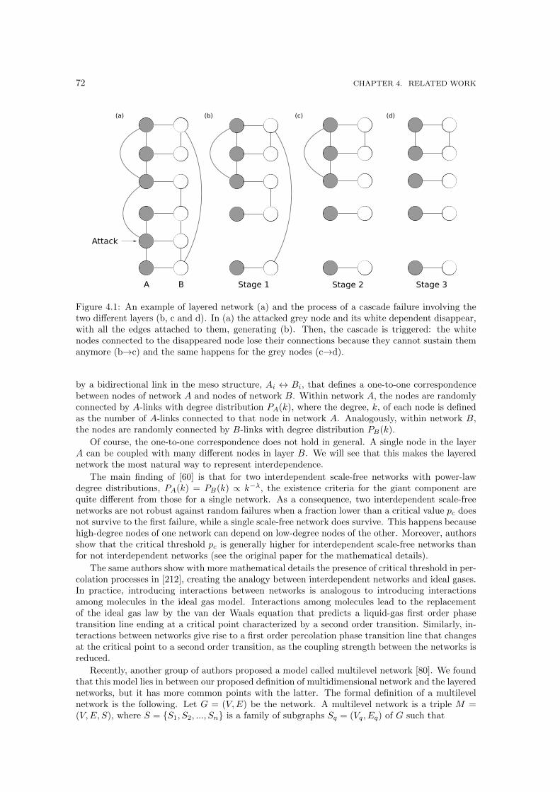
72 CHAPTER 4. RELATED WORK
A B Stage 1 Stage 3Stage 2
Attack
(a) (d)(c)(b)
Figure 4.1: An example of layered network (a) and the process of a cascade failure involving thetwo different layers (b, c and d). In (a) the attacked grey node and its white dependent disappear,with all the edges attached to them, generating (b). Then, the cascade is triggered: the whitenodes connected to the disappeared node lose their connections because they cannot sustain themanymore (b→c) and the same happens for the grey nodes (c→d).
by a bidirectional link in the meso structure, Ai ↔ Bi, that defines a one-to-one correspondencebetween nodes of network A and nodes of network B. Within network A, the nodes are randomlyconnected by A-links with degree distribution PA(k), where the degree, k, of each node is definedas the number of A-links connected to that node in network A. Analogously, within network B,the nodes are randomly connected by B-links with degree distribution PB(k).
Of course, the one-to-one correspondence does not hold in general. A single node in the layerA can be coupled with many different nodes in layer B. We will see that this makes the layerednetwork the most natural way to represent interdependence.
The main finding of [60] is that for two interdependent scale-free networks with power-lawdegree distributions, PA(k) = PB(k) ∝ k−λ, the existence criteria for the giant component arequite different from those for a single network. As a consequence, two interdependent scale-freenetworks are not robust against random failures when a fraction lower than a critical value pc doesnot survive to the first failure, while a single scale-free network does survive. This happens becausehigh-degree nodes of one network can depend on low-degree nodes of the other. Moreover, authorsshow that the critical threshold pc is generally higher for interdependent scale-free networks thanfor not interdependent networks (see the original paper for the mathematical details).
The same authors show with more mathematical details the presence of critical threshold in per-colation processes in [212], creating the analogy between interdependent networks and ideal gases.In practice, introducing interactions between networks is analogous to introducing interactionsamong molecules in the ideal gas model. Interactions among molecules lead to the replacementof the ideal gas law by the van der Waals equation that predicts a liquid-gas first order phasetransition line ending at a critical point characterized by a second order transition. Similarly, in-teractions between networks give rise to a first order percolation phase transition line that changesat the critical point to a second order transition, as the coupling strength between the networks isreduced.
Recently, another group of authors proposed a model called multilevel network [80]. We foundthat this model lies in between our proposed definition of multidimensional network and the layerednetworks, but it has more common points with the latter. The formal definition of a multilevelnetwork is the following. Let G = (V,E) be the network. A multilevel network is a triple M =(V,E, S), where S = {S1, S2, ..., Sn} is a family of subgraphs Sq = (Vq, Eq) of G such that
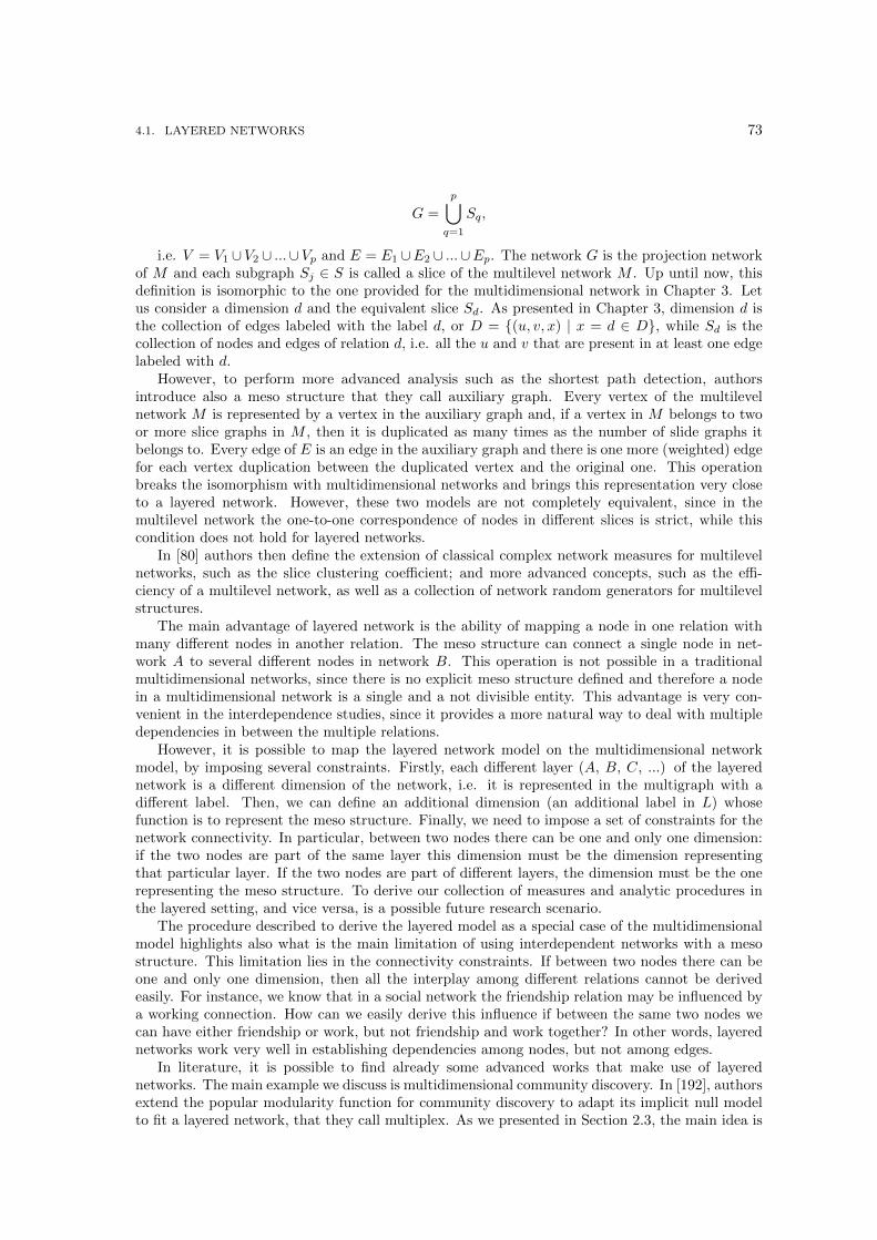
4.1. LAYERED NETWORKS 73
G =
p⋃q=1
Sq,
i.e. V = V1 ∪ V2 ∪ ...∪ Vp and E = E1 ∪E2 ∪ ...∪Ep. The network G is the projection networkof M and each subgraph Sj ∈ S is called a slice of the multilevel network M . Up until now, thisdefinition is isomorphic to the one provided for the multidimensional network in Chapter 3. Letus consider a dimension d and the equivalent slice Sd. As presented in Chapter 3, dimension d isthe collection of edges labeled with the label d, or D = {(u, v, x) | x = d ∈ D}, while Sd is thecollection of nodes and edges of relation d, i.e. all the u and v that are present in at least one edgelabeled with d.
However, to perform more advanced analysis such as the shortest path detection, authorsintroduce also a meso structure that they call auxiliary graph. Every vertex of the multilevelnetwork M is represented by a vertex in the auxiliary graph and, if a vertex in M belongs to twoor more slice graphs in M , then it is duplicated as many times as the number of slide graphs itbelongs to. Every edge of E is an edge in the auxiliary graph and there is one more (weighted) edgefor each vertex duplication between the duplicated vertex and the original one. This operationbreaks the isomorphism with multidimensional networks and brings this representation very closeto a layered network. However, these two models are not completely equivalent, since in themultilevel network the one-to-one correspondence of nodes in different slices is strict, while thiscondition does not hold for layered networks.
In [80] authors then define the extension of classical complex network measures for multilevelnetworks, such as the slice clustering coefficient; and more advanced concepts, such as the effi-ciency of a multilevel network, as well as a collection of network random generators for multilevelstructures.
The main advantage of layered network is the ability of mapping a node in one relation withmany different nodes in another relation. The meso structure can connect a single node in net-work A to several different nodes in network B. This operation is not possible in a traditionalmultidimensional networks, since there is no explicit meso structure defined and therefore a nodein a multidimensional network is a single and a not divisible entity. This advantage is very con-venient in the interdependence studies, since it provides a more natural way to deal with multipledependencies in between the multiple relations.
However, it is possible to map the layered network model on the multidimensional networkmodel, by imposing several constraints. Firstly, each different layer (A, B, C, ...) of the layerednetwork is a different dimension of the network, i.e. it is represented in the multigraph with adifferent label. Then, we can define an additional dimension (an additional label in L) whosefunction is to represent the meso structure. Finally, we need to impose a set of constraints for thenetwork connectivity. In particular, between two nodes there can be one and only one dimension:if the two nodes are part of the same layer this dimension must be the dimension representingthat particular layer. If the two nodes are part of different layers, the dimension must be the onerepresenting the meso structure. To derive our collection of measures and analytic procedures inthe layered setting, and vice versa, is a possible future research scenario.
The procedure described to derive the layered model as a special case of the multidimensionalmodel highlights also what is the main limitation of using interdependent networks with a mesostructure. This limitation lies in the connectivity constraints. If between two nodes there can beone and only one dimension, then all the interplay among different relations cannot be derivedeasily. For instance, we know that in a social network the friendship relation may be influenced bya working connection. How can we easily derive this influence if between the same two nodes wecan have either friendship or work, but not friendship and work together? In other words, layerednetworks work very well in establishing dependencies among nodes, but not among edges.
In literature, it is possible to find already some advanced works that make use of layerednetworks. The main example we discuss is multidimensional community discovery. In [192], authorsextend the popular modularity function for community discovery to adapt its implicit null modelto fit a layered network, that they call multiplex. As we presented in Section 2.3, the main idea is
74 CHAPTER 4. RELATED WORK
to represent each layer (that can be a snapshot, as well as a different relation) with a slice. Eachslice s of a network is represented by adjacency Aijs between nodes i and j. The authors alsospecify the meso structure, that they call “inter-slice couplings”, as Cjrs that connect node j inslice r to itself in slice s. They notate the strengths of each node individually in each slice, so thatkjs =
∑iAijs and cjs =
∑r Cjsr, and define the multislice strength κjs = kjs + cjs. The authors
then specify an associated multislice null model. They then derive a resulting multislice extendeddefinition of modularity, that we reported in Section 2.3.4.
4.2 Hypergraphs
A hypergraph is a generalization of a regular graph in the sense that an edge can connect multiplevertices. Thus, unlike in a regular graph where an edge connects two vertices, in a hypergraph ahyperedge is a collection of an arbitrary number of vertices. These vertices can be of the same ordifferent types, and hyperedges can vary in the number of vertices they connect.
In [272], the authors represent the network as tripartite graphs consisting of three different typesof vertices. The edges represent three-way hyperedges that each connect exactly three vertices.
This representation corresponds to the case of a tripartite hypergraph G = (V,H) which canbe defined as a pair of sets V and H, that satisfy the following conditions: firstly, the set V ={V1 ∪ V2 ∪ V3|Vi ∩ Vj = ∅} is formed by the union of three disjoint sets of vertices. Secondly, theset H ⊂ {(v1 ∈ V1, v2 ∈ V2, v3 ∈ V3)} of hyperedges is a set of triangles connecting elements ofthese three sets.
The case study of the paper involved modeling folksonomies with hypergraphs. In practice,they have three sets of entities: users, content and tags. Each hyperedge connects an user and apiece of content with a tag, used by the user to annotate the content. Also in this case, there existsa mapping between this representation and the multidimensional networks. This mapping consistsin projecting one set of entities as dimensions and recreating a regular bipartite multigraph. Ifwe project over tags, we get a bipartite graph that connects users to content. Each user can usemultiple tags to annotate the same piece of content, and this lead to multidimensionality. In otherwords, the tag “temples” or “Rome” are two different dimensions. If the set of tags is very big,this procedure is not feasible, making the projected graph crowded with too many dimensions.
In [272] the authors provide a collection of useful metrics on tripartite hypergraphs, makingthis model very robust for basic analysis. This is the second most important advantage of thismodel, the first being explained before as a very natural way to model tripartite interactionsin folksonomies. Along with the extension of the classical node degree, authors provide also anedge degree, namely the number of hyperedges a couple of vertices is part of. Authors test thedistribution of both these definitions of degree in real world networks extracted from Flickr andCiteULike. The vertex degree is, as common in social networks, a fat-tailed distribution, andalso the edge degree distributions are right skewed. Authors also adapt the clustering coefficientto this setting, via what they call hyperedge density Dh(k), and the vertex to vertex distance, ameasure needed to develop algorithms to navigate into the hypergraph structure. Finally, they alsodefine a vertex similarity measure that is used for a preliminary community discovery algorithmon hypergraphs.
In a previous work [104], the authors investigate the theory of random tripartite hypergraphswith given degree distributions. An extension of the configuration model for traditional complexnetworks is provided. Then, a theoretical framework in which analytical properties of these randomgraphs are investigated is provided. In particular, authors analyze the conditions that allow thecreation of giant components in tripartite hypergraphs, along with classical percolation events inthese complex structures. Other research groups has devoted some attention also to this model[81].
Thanks to the work of these authors, tripartite hypergraphs and their properties are now wellunderstood. However, this model is tailored on folksonomies and on a very particular class ofphenomena, namely all the phenomena that involves complex interactions among three class ofentities. This scenario is far from universal. If we are interested in a phenomenon that involves

4.3. MULTIDIMENSIONAL NETWORKS 75
only users interacting with each other through different media, then this model is no more suitablebecause it is too complex: one would need to add at least one hypothetical class of entities besidesusers and media themselves, that in multidimensional networks are represented naturally withnodes and edge types.
We continue to use multidimensional community discovery as the main test case for the applica-tions of the models presented in this chapter. One of the main examples of hypergraph analysis isrepresented by Metafac [178]. Also in this case, we will present more details in Section 2.3. In thiswork, the authors use relational hypergraphs to represent multi-relational and multi-dimensionalsocial data. Instead of using tripartite hypergraphs, authors use a more general model composedby M -way hyperedges to represent the interactions of M facets (groups of entities of the same type,i.e. users, contents, tags...). The metagraph is defined as a set of data tensors. Then tensor decom-position and factorization operations are defined in order to unveil the community organizationamong facets.
4.3 Multidimensional Networks
In this section we focus on the part of the literature that uses multigraphs to model networkwith multiple kind of interactions, i.e. the model proposed and studied in this thesis. In subsection 4.3.1 we present the examples of multidimensional community discovery, i.e. detecting themodular structure of a network in which multiple relations are expressed at the same time. Anotherinteresting problem is the prediction of multidimensional links. In Section 4.3.2 we briefly presentone recent approach for this problem. We found that researchers in this field focus particularlyon signed networks, or networks in which the multiple relations can be classified in “positive” and“negative” relations. We analyze those publications in Section 4.3.3.
It is important to note that the term “multidimensional”, that we use here to describe theparticular representation we are interested in, is far from universally accepted. The terminologyreferring to networks with multiple different relations has not reached a consensus yet, even amongthose researchers that are actually using the same model to tackle the problem of multiple inter-actions. Moreover, different scientists from different fields used similar terminologies for differentmodels and different names for the same model. Thus, what we call “multidimensional” is oftenreferred as multiplex, multislice, multirelational, multifaceted and this list is far from complete.However, the analysis we present in this section can be mapped entirely with the labeled multigraphwe use as representation of multidimensional networks.
4.3.1 Multidimensional Community Discovery
To find densely connected modules in a complex multidimensional network is not an easy problem.We will see in Section 8.1 that the concept of “multidimensional density” is intrinsically ambiguous.Nevertheless, there are two important research tracks on this topic (also in this case, more detailswill be provided in Section 2.3).
The first one is represented by a collection of papers that investigate the possibility of extract-ing the latent social dimensions from real world networks [245, 246]. The dimensions are extractedusing a classifier which not only considers the connectivity of a node, but assigns additional infor-mation to its connection i.e. a description of a likely affiliation between social actors. The basicassumption is borrowed from the concept of homophily, which states that actors sharing certainproperties tend to form groups [185].
The second one [61] aims to discover hidden multidimensional communities. The authors startfrom the basic assumption that each relation (explicit or implicit) plays a different role in differenttasks. Therefore they allow an analyst to specify custom community definitions. Then, all thedimensions have a different importance according to the community definition (some are important,some others are noise). All the relations are then weighted accordingly to how they reflect thecommunity definition using a regression model. Finally, the communities are extracted.
76 CHAPTER 4. RELATED WORK
4.3.2 Multidimensional Link Prediction
Given a pair of nodes in an evolving network, the literature on monodimensional network analysisdefines link prediction as the problem of estimating the likelihood that an edge will form betweentwo nodes [207]; we have discussed this problem in Section 2.5. In multidimensional networks thistranslates in estimating the likelihood that an edge will appear between two nodes in a specificdimension. In practice an additional degree of freedom is added to the classical definition.
A preliminary work [226] explores how useful a set of simple multidimensional measures canbe if added to well-known link predictors. Authors show that using the established link predictorsand adding a correction for multidimensionality and temporal evolution is sufficient to get slightlyimproved performances, even if the need of a truly multidimensional link predictor is proved. Wewill analyze more deeply this case in Section 8.3.
But multidimensional link prediction is obtaining an increasing attention in literature, andnovel algorithms are being proposed. One of the main examples is [243]. The goal is to system-atically define the relations between entities encoded in different paths using the metastructureof these paths, that authors call the “meta paths”. For example, in the real world we have au-thors publishing papers in different venues. If two authors published two different papers in thesame venue, we may have the chain “Jim-P5-SIGMOD-P6-Mike”. This chain is translated in ameta-path “author-paper-venue-paper-author”. Then, several measures are proposed to quantifythe meta path-based relations, each of which quantifies the relation in a different way. In otherwords “paper-venue-paper” is simply a dimension that may connect two authors. This relationand several different other relations are studied in the paper. In our case, the relation is definedas co-venue publication (we will see in Chapter 5 that this dimension definition is used for theDBLP Conference multidimensional network). Authors then use a supervised learning frameworkto learn the best weights associated with each topological feature.
4.3.3 Signed Networks
A sub-problem in link prediction for multidimensional networks considers some specific propertiesof the dimensions. For example, each relation in a multidimensional network can be tagged as“positive” or “negative”. Our main reference for this particular branch of research is [244], butother research groups share part of both methodology and problem definition with this work, suchas [170].
In [244] six dimensions are extracted from the actions of tens of thousands players of a massivemultiplayer online game. These six dimensions are either positive (friendship, trade, commu-nication) or negative (attack, enmity, bounty). Then statistical properties, such as dimensioninteractions or degree distributions, are studied, highlighting the fact that truly different dynamicsare working behind the curtain to shape the evolution of these relations.
Then, authors focus on the structural balance problem, particularly on the triangle, a verybasic network structure. When we have positive and negative links, there are four possible differenttriangle configurations. The edges can be all positive, all negative, two positive and one negativeand vice versa. Social balance theory, in its strong form [63], claims that there are “balanced”triads, where the links are all positive or there are two negative links (i.e. one element is enemyof both two allies) and “unbalanced” triads, where the links are all negative or there are twopositive links (one element is allied with two enemies). Unbalanced triads are sources of stress andtherefore tend to be avoided by agents when they update their personal relationships. In fact, theauthors are able to prove that balanced triads are heavily over represented in the network, whileunbalanced triads are very rare.
These results are confirmed by [170]. In this case the data sources are different, namely a trustnetwork in which users connect with each other by deciding if a particular user is trustworthyor not, a social network that allows to create “enemy” links, and the register of Wikipedia votes(positive or negative) expressed by the community for the promotion of users to administrationtasks. In all these different kinds of networks, all with positive and negative relations, the socialbalance proves to be one of the main features in order to increase the link predictor performances.
4.4. TENSOR DECOMPOSITION 77
4.4 Tensor Decomposition
In this section we briefly provide an overview of mathematical tensors. Also, tensors are nota general model for multidimensional networks. Multidimensional networks, and hypergraphs,can be represented with tensors, but tensors are just the tool in which different models could beimplemented. However, tensors are used for several other purposes and their usefulness is notbounded to their contribution to multidimensional network analysis. Our main reference is [153].
A tensor is a multidimensional array. More formally, an N -way or Nth-order tensor is anelement of the tensor product of N vector spaces, each of which has its own coordinate system.The order of a tensor is the number of dimensions, also known as ways or modes. Scalars are tensorsof order zero. A vector is a tensor of order one. A matrix is a tensor of order two. Tensors withorder three or higher are called higher-order tensors. Of course, if a network can be representedwith a two-order tensor (a matrix), then we can represent a multidimensional network with a threeorder tensor.
Some basic operations on tensors are defined such as the extraction of fibers and slices. A fiberis defined by fixing every index but one. Slices are two-dimensional sections of a tensor, definedby fixing all but two indexes. Other operations are defined, such as matricization (transforming atensor into a matrix) and tensor multiplication. We are particularly interested in tensor decom-position, since many real world problems can be expressed in a tensor form and then solved bytensor decomposition.
Several different decomposition strategies and applications has been studied since decades. Werecall the CANDECOMP (canonical decomposition) by Carroll and Chang [62] and PARAFAC(parallel factors) by Harshman [125]. One of the most popular strategies is actually the combinationof the two, the CANDECOMP/PARAFAC (CP). Very briefly, the CP decomposition factorizes atensor into a sum of component rank-one tensors. In a computer science perspective, the mainproblem is that there is no finite algorithm for determining the rank of a tensor. Consequently,the first issue that arises in computing a CP decomposition is how to choose the number ofrank-one components. Most procedures fit multiple CP decompositions with different numbersof components until one is “good”. Only recently some memory efficient and low time complexityframeworks has been proposed [154]. In this last work, and in [1], some examples of applicationsof tensor decomposition to complex network analysis have been provided.

78 CHAPTER 4. RELATED WORK
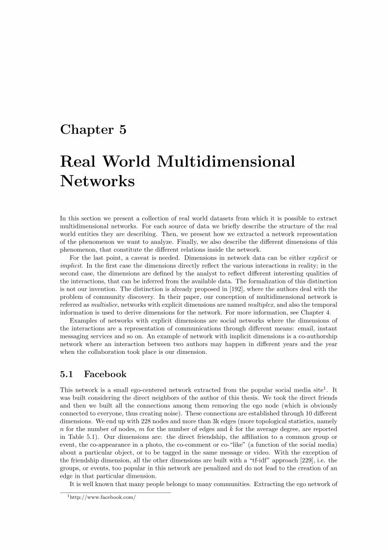
Chapter 5
Real World MultidimensionalNetworks
In this section we present a collection of real world datasets from which it is possible to extractmultidimensional networks. For each source of data we briefly describe the structure of the realworld entities they are describing. Then, we present how we extracted a network representationof the phenomenon we want to analyze. Finally, we also describe the different dimensions of thisphenomenon, that constitute the different relations inside the network.
For the last point, a caveat is needed. Dimensions in network data can be either explicit orimplicit. In the first case the dimensions directly reflect the various interactions in reality; in thesecond case, the dimensions are defined by the analyst to reflect different interesting qualities ofthe interactions, that can be inferred from the available data. The formalization of this distinctionis not our invention. The distinction is already proposed in [192], where the authors deal with theproblem of community discovery. In their paper, our conception of multidimensional network isreferred as multislice, networks with explicit dimensions are named multiplex, and also the temporalinformation is used to derive dimensions for the network. For more information, see Chapter 4.
Examples of networks with explicit dimensions are social networks where the dimensions ofthe interactions are a representation of communications through different means: email, instantmessaging services and so on. An example of network with implicit dimensions is a co-authorshipnetwork where an interaction between two authors may happen in different years and the yearwhen the collaboration took place is our dimension.
5.1 Facebook
This network is a small ego-centered network extracted from the popular social media site1. Itwas built considering the direct neighbors of the author of this thesis. We took the direct friendsand then we built all the connections among them removing the ego node (which is obviouslyconnected to everyone, thus creating noise). These connections are established through 10 differentdimensions. We end up with 228 nodes and more than 3k edges (more topological statistics, namelyn for the number of nodes, m for the number of edges and k for the average degree, are reportedin Table 5.1). Our dimensions are: the direct friendship, the affiliation to a common group orevent, the co-appearance in a photo, the co-comment or co-“like” (a function of the social media)about a particular object, or to be tagged in the same message or video. With the exception ofthe friendship dimension, all the other dimensions are built with a “tf-idf” approach [229], i.e. thegroups, or events, too popular in this network are penalized and do not lead to the creation of anedge in that particular dimension.
It is well known that many people belongs to many communities. Extracting the ego network of
1http://www.facebook.com/
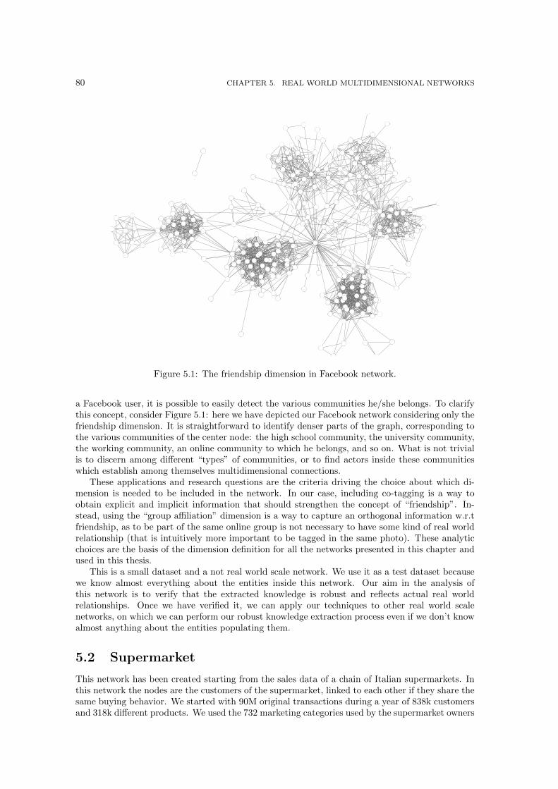
80 CHAPTER 5. REAL WORLD MULTIDIMENSIONAL NETWORKS
Figure 5.1: The friendship dimension in Facebook network.
a Facebook user, it is possible to easily detect the various communities he/she belongs. To clarifythis concept, consider Figure 5.1: here we have depicted our Facebook network considering only thefriendship dimension. It is straightforward to identify denser parts of the graph, corresponding tothe various communities of the center node: the high school community, the university community,the working community, an online community to which he belongs, and so on. What is not trivialis to discern among different “types” of communities, or to find actors inside these communitieswhich establish among themselves multidimensional connections.
These applications and research questions are the criteria driving the choice about which di-mension is needed to be included in the network. In our case, including co-tagging is a way toobtain explicit and implicit information that should strengthen the concept of “friendship”. In-stead, using the “group affiliation” dimension is a way to capture an orthogonal information w.r.tfriendship, as to be part of the same online group is not necessary to have some kind of real worldrelationship (that is intuitively more important to be tagged in the same photo). These analyticchoices are the basis of the dimension definition for all the networks presented in this chapter andused in this thesis.
This is a small dataset and a not real world scale network. We use it as a test dataset becausewe know almost everything about the entities inside this network. Our aim in the analysis ofthis network is to verify that the extracted knowledge is robust and reflects actual real worldrelationships. Once we have verified it, we can apply our techniques to other real world scalenetworks, on which we can perform our robust knowledge extraction process even if we don’t knowalmost anything about the entities populating them.
5.2 Supermarket
This network has been created starting from the sales data of a chain of Italian supermarkets. Inthis network the nodes are the customers of the supermarket, linked to each other if they share thesame buying behavior. We started with 90M original transactions during a year of 838k customersand 318k different products. We used the 732 marketing categories used by the supermarket owners
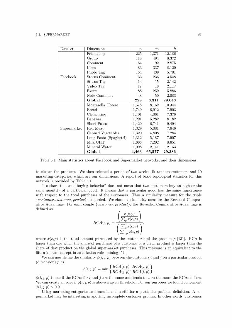
5.2. SUPERMARKET 81
Dataset Dimension n m k
Friendship 225 1,371 12.186Group 118 494 8.372Comment 64 92 2.875Likes 83 337 8.120Photo Tag 154 439 5.701Status Comment 133 236 3.548Status Tag 14 15 2.142Video Tag 17 18 2.117Event 88 259 5.886Note Comment 48 50 2.083Global 228 3,311 29.043
Supermarket
Mozzarella Cheese 1,578 8,162 10.344Bread 1,749 6,912 7.903Clementine 1,101 4,061 7.376Bananas 1,291 5,282 8.182Short Pasta 1,420 6,741 9.494Red Meat 1,329 5,081 7.646Canned Vegetables 1,320 4,808 7.284Long Pasta (Spaghetti) 1,312 5,187 7.907Milk UHT 1,665 7,202 8.651Mineral Water 1,998 12,141 12.153Global 4,463 65,577 29.386
Table 5.1: Main statistics about Facebook and Supermarket networks, and their dimensions.
to cluster the products. We then selected a period of two weeks, 4k random customers and 10marketing categories, which are our dimensions. A report of basic topological statistics for thisnetwork is provided by Table 5.1.
“To share the same buying behavior” does not mean that two customers buy an high or thesame quantity of a particular good. It means that a particular good has the same importancewith respect to the total purchases of the customers. Thus a similarity measure for the triple{customer, customer, product} is needed. We chose as similarity measure the Revealed Compar-ative Advantage. For each couple {customer, product}, the Revealed Comparative Advantage isdefined as
RCA(c, p) =
(x(c, p)∑p x(c, p)
)( ∑
c x(c, p)∑c,p x(c, p)
) ,where x(c, p) is the total amount purchased by the customer c of the product p [131]. RCA islarger than one when the share of purchases of a customer of a given product is larger than theshare of that product on the global supermarket purchases. This measure is an equivalent to thelift, a known concept in association rules mining [54].
We can now define the similarity φ(i, j, p) between the customers i and j on a particular product(dimension) p as
φ(i, j, p) = min
{RCA(i, p)
RCA(j, p),RCA(j, p)
RCA(i, p)
}.
φ(i, j, p) is one if the RCAs for i and j are the same and tends to zero the more the RCAs differs.We can create an edge if φ(i, j, p) is above a given threshold. For our purposes we found convenientφ(i, j, p) > 0.9.
Using marketing categories as dimensions is useful for a particular problem definition. A su-permarket may be interesting in spotting incomplete customer profiles. In other words, customers
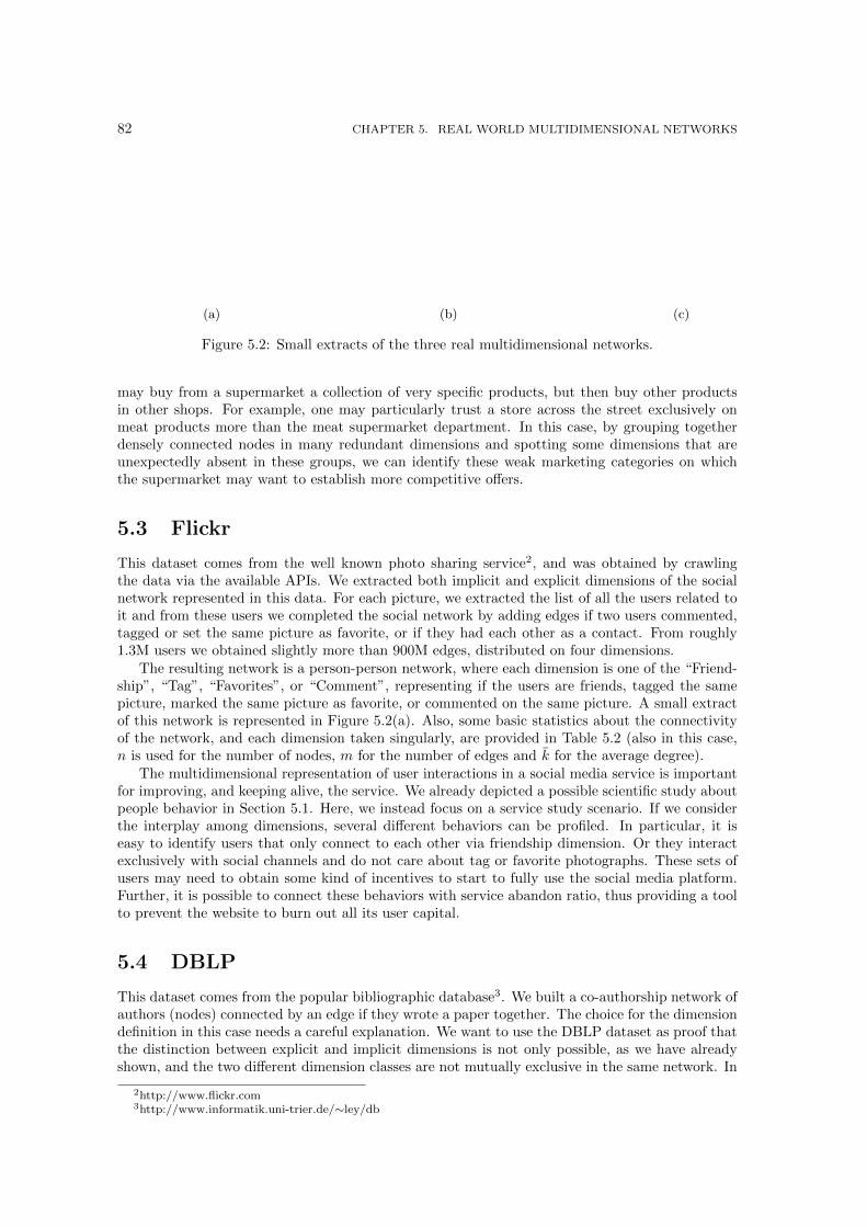
82 CHAPTER 5. REAL WORLD MULTIDIMENSIONAL NETWORKS
(a) (b) (c)
Figure 5.2: Small extracts of the three real multidimensional networks.
may buy from a supermarket a collection of very specific products, but then buy other productsin other shops. For example, one may particularly trust a store across the street exclusively onmeat products more than the meat supermarket department. In this case, by grouping togetherdensely connected nodes in many redundant dimensions and spotting some dimensions that areunexpectedly absent in these groups, we can identify these weak marketing categories on whichthe supermarket may want to establish more competitive offers.
5.3 Flickr
This dataset comes from the well known photo sharing service2, and was obtained by crawlingthe data via the available APIs. We extracted both implicit and explicit dimensions of the socialnetwork represented in this data. For each picture, we extracted the list of all the users related toit and from these users we completed the social network by adding edges if two users commented,tagged or set the same picture as favorite, or if they had each other as a contact. From roughly1.3M users we obtained slightly more than 900M edges, distributed on four dimensions.
The resulting network is a person-person network, where each dimension is one of the “Friend-ship”, “Tag”, “Favorites”, or “Comment”, representing if the users are friends, tagged the samepicture, marked the same picture as favorite, or commented on the same picture. A small extractof this network is represented in Figure 5.2(a). Also, some basic statistics about the connectivityof the network, and each dimension taken singularly, are provided in Table 5.2 (also in this case,n is used for the number of nodes, m for the number of edges and k for the average degree).
The multidimensional representation of user interactions in a social media service is importantfor improving, and keeping alive, the service. We already depicted a possible scientific study aboutpeople behavior in Section 5.1. Here, we instead focus on a service study scenario. If we considerthe interplay among dimensions, several different behaviors can be profiled. In particular, it iseasy to identify users that only connect to each other via friendship dimension. Or they interactexclusively with social channels and do not care about tag or favorite photographs. These sets ofusers may need to obtain some kind of incentives to start to fully use the social media platform.Further, it is possible to connect these behaviors with service abandon ratio, thus providing a toolto prevent the website to burn out all its user capital.
5.4 DBLP
This dataset comes from the popular bibliographic database3. We built a co-authorship network ofauthors (nodes) connected by an edge if they wrote a paper together. The choice for the dimensiondefinition in this case needs a careful explanation. We want to use the DBLP dataset as proof thatthe distinction between explicit and implicit dimensions is not only possible, as we have alreadyshown, and the two different dimension classes are not mutually exclusive in the same network. In
2http://www.flickr.com3http://www.informatik.uni-trier.de/∼ley/db
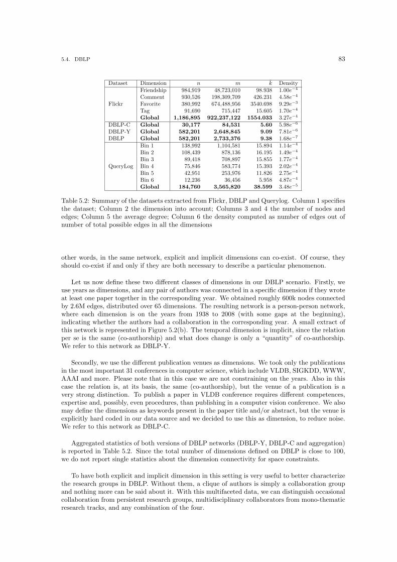
5.4. DBLP 83
Dataset Dimension n m k Density
Flickr
Friendship 984,919 48,723,010 98.938 1.00e−4
Comment 930,526 198,309,709 426.231 4.58e−4
Favorite 380,992 674,488,956 3540.698 9.29e−3
Tag 91,690 715,447 15.605 1.70e−4
Global 1,186,895 922,237,122 1554.033 3.27e−4
DBLP-C Global 30,177 84,531 5.60 5.98e−6
DBLP-Y Global 582,201 2,648,845 9.09 7.81e−6
DBLP Global 582,201 2,733,376 9.38 1.68e−7
QueryLog
Bin 1 138,992 1,104,581 15.894 1.14e−4
Bin 2 108,439 878,136 16.195 1.49e−4
Bin 3 89,418 708,897 15.855 1.77e−4
Bin 4 75,846 583,774 15.393 2.02e−4
Bin 5 42,951 253,976 11.826 2.75e−4
Bin 6 12,236 36,456 5.958 4.87e−4
Global 184,760 3,565,820 38.599 3.48e−5
Table 5.2: Summary of the datasets extracted from Flickr, DBLP and Querylog. Column 1 specifiesthe dataset; Column 2 the dimension into account; Columns 3 and 4 the number of nodes andedges; Column 5 the average degree; Column 6 the density computed as number of edges out ofnumber of total possible edges in all the dimensions
other words, in the same network, explicit and implicit dimensions can co-exist. Of course, theyshould co-exist if and only if they are both necessary to describe a particular phenomenon.
Let us now define these two different classes of dimensions in our DBLP scenario. Firstly, weuse years as dimensions, and any pair of authors was connected in a specific dimension if they wroteat least one paper together in the corresponding year. We obtained roughly 600k nodes connectedby 2.6M edges, distributed over 65 dimensions. The resulting network is a person-person network,where each dimension is on the years from 1938 to 2008 (with some gaps at the beginning),indicating whether the authors had a collaboration in the corresponding year. A small extract ofthis network is represented in Figure 5.2(b). The temporal dimension is implicit, since the relationper se is the same (co-authorship) and what does change is only a “quantity” of co-authorship.We refer to this network as DBLP-Y.
Secondly, we use the different publication venues as dimensions. We took only the publicationsin the most important 31 conferences in computer science, which include VLDB, SIGKDD, WWW,AAAI and more. Please note that in this case we are not constraining on the years. Also in thiscase the relation is, at its basis, the same (co-authorship), but the venue of a publication is avery strong distinction. To publish a paper in VLDB conference requires different competences,expertise and, possibly, even procedures, than publishing in a computer vision conference. We alsomay define the dimensions as keywords present in the paper title and/or abstract, but the venue isexplicitly hard coded in our data source and we decided to use this as dimension, to reduce noise.We refer to this network as DBLP-C.
Aggregated statistics of both versions of DBLP networks (DBLP-Y, DBLP-C and aggregation)is reported in Table 5.2. Since the total number of dimensions defined on DBLP is close to 100,we do not report single statistics about the dimension connectivity for space constraints.
To have both explicit and implicit dimension in this setting is very useful to better characterizethe research groups in DBLP. Without them, a clique of authors is simply a collaboration groupand nothing more can be said about it. With this multifaceted data, we can distinguish occasionalcollaboration from persistent research groups, multidisciplinary collaborators from mono-thematicresearch tracks, and any combination of the four.
84 CHAPTER 5. REAL WORLD MULTIDIMENSIONAL NETWORKS
5.5 Querylog
This network was constructed from a query-log of approximately 20 millions web-search queriessubmitted by 650,000 users over a period of time4, and was described in [213]. Each record of thisdataset stores an anonymous user ID, the query terms, the date and hour of the query, the rankposition of the result visited by the user on each record and the host portion of the URL of thevisited result. From this dataset, we extracted a word-word network of query terms, consisting ofroughly 200k words (nodes), after removing stop-words.
We connected two words if they appeared together in a query, producing roughly 2M edges.Dimensions are defined as the rank positions of the results, grouped into six almost equi-populatedbins: “Bin1” for rank 1, “Bin2” for ranks 2-3, “Bin3” for ranks 4-6, “Bin4” for ranks 7-10, “Bin5”for ranks 11-58, “Bin6” for ranks 59-500. Hence two words appeared together in a query for whichthe user clicked on a resulting url ranked #4 will produce a link in dimension “Bin3” between thetwo words. The result is a word-word network, for which we give a small extract in Figure 5.2(c).
The Querylog network is different from what we have seen until now because its nodes are notpeople and the definition of its implicit dimension may seem obscure. However, it is tailored ona particular problem definition. Aim of this network definition is to provide a field where to testthe performances of the search engine ranking system. The simple link distribution among thedimensions is already an interesting measure of the search engine performances: the more linksappear exclusively in dimension “Bin1” the better. But since we are in a network, we are notinterested in a single word query but in the complex interaction between query terms. Therefore,to find terms surrounded mainly by dimensions “Bin4”, “Bin5” and “Bin6” raises an alert aboutthe way the search engine is operating for those particular ambiguous terms.
5.6 GTD
From this database of global terrorism5, we created a group-group graph for the years 1969-2008,where each node represents a terrorist group or organization, and two groups are connected if theyparticipated in a terrorist attack to the same country (note that the two groups only attacked thesame country, but they do not need to have collaborated to the attack in order to be connected).We then considered each year as temporal snapshot, generating 40 snapshots. As for DBLP, thesnapshots are non-cumulative, and we ended up with 2,279 nodes and 31,843 total edges.
This network is useful to characterize the history of global terrorism. An important observation,considering implicit dimensions defined with a quantitative logic, is that we can define an dimensionorder (just like in the DBLP-Y network). The year as dimension is an unambiguous quantity.Therefore, it is natural to order the dimension “2006” before dimension “2007” and after dimension“2005”. By studying the relationships between consecutive dimensions, it is possible to extractuniform periods, and to characterize them using the nodes (the groups active in those years), thelength of the period itself (the edge dimensions) and the hot areas (by checking the edge creationcriterion).
5.7 IMDb
From the Internet Movie Database6, we created a collaboration graph for the years 1899-2010,where each node represents a person who took part in the realization of a movie (directors, cast,song writers, and so on), and two persons are connected if they participated to the realizationof the same movie. We considered each year as temporal snapshot, i.e. an implicit dimension,generating 112 of them. As for DBLP-Y, the temporal snapshots are non-cumulative, for a totalnumber of 57,457 nodes and 13,047,319 edges.
4http://www.gregsadetsky.com/aol-data5http://www.start.umd.edu/gtd6http://www.imdb.com

5.8. CLASSICAL ARCHAEOLOGY 85
This network has been used mainly together with both DBLP-Y and GTD networks. IMDbnetwork shares with DBLP-Y network its general scenario: it is a structure that we use to in-vestigate mainly co-authorship. This is simply an alternative setting in which collaboration takesplace. The application we are interested in is shared with GTD network: we are mainly interestedin analyze a very long collaboration history. IMDb data is very rich since the beginning of movieindustry. Starting from the year 1900, the data is very reliable and the quantity is enough to applycomplex network and data mining analysis. The data quality and the wide temporal window (morethan a century) makes IMDb a unique data source.
5.8 Classical Archaeology
Lastly, we present the dataset we will use in the third part of this thesis to show a real worldcomplex scenario for multidimensional network analysis. We will provide more details about thisdata source in Chapter 10.
We made use of Archaologische Bibliographie, i.e. a bibliographic database that collects andclassifies literature in classical archaeology since 1956 [234]. Analyzing the state of 2007, oursource data includes about 370,000 classified publications authored by circa 88,000 archaeologiststhat are connected to about 45,000 classification criteria, via 670,000 classification links. Theclassification criteria themselves are manually grouped into different categories: subject themes,locations, periods, persons and objects.
Firstly we generate a classification co-occurrence network from the classification link betweenpublications and classification criteria. In this case we already have a multidimensional net-work with implicit dimensions, since we use the year of the publication as dimension for theco-classification link.
However, this is not the only structure we extract from this data source. After performing anoverlapping community discovery on this structure, we are able to group together classificationcriteria into groups. Since each classification criterion may be part of more than one group (forinstance, the classification “Paestum” is part of 12 communities), we are able to draw a linkbetween two different groups, weighted accordingly to the number of shared classifications. Thiscommunity network is not only weighted, it is also multidimensional. The classification criteria,as stated before, are clustered into categories. Each one of this categories defines then a link type,i.e. a dimension, in this structure.
We will see in Chapter 10 how these two structures can be analyzed and used to solve somecritical problem typical of classical archaeology, namely the difficulty of finding related works for anauthors and of navigating through literature. These problems have nothing to do, apparently, withcomplex network theory in general and multidimensional networks in particular, but the techniquesand measures defined in this thesis play a crucial role in their solutions.

86 CHAPTER 5. REAL WORLD MULTIDIMENSIONAL NETWORKS
Part II
Multidimensional NetworkAnalysis

Chapter 6
Extension of Classical Measures
In this chapter we discuss the most straightforward and basic changes in the playing field of complexnetwork analysis when allowing multidimensionality. This chapter is mainly focused on verifyingwhat happens to the degree and to the shortest path, and their derivable measures, allowingmultiple kinds of edges. Besides describing how the analytical measures defined on standardgraphs can be extended to cope with multiple dimensions, we also define new aggregate functionsinduced by some local or global measures.
In general, in order to adapt the classical measures to the multidimensional setting we need toextend the domain of each function in order to specify the set of dimensions for which they arecalculated. Intuitively, when a measure considers a specific set of dimensions, a filter is applied onthe multigraph to produce a view of it considering only that specific set, and then the measure iscalculated over this view. In the following, we redefine some of the classical measures on graphsand networks, using the presented approach. After this set of measures, in Chapter 7 we presentthe new measures we introduce in the multidimensional setting, that are meaningful only in thisscenario.
The general notation is the following, and it is consistent with the notation used in Chapter 3.V is the set of nodes of the network, E is the set of edges, D is the set of all dimensions of thenetwork and, when needed, D′ indicates a subset of D.
6.1 Degree Related Measures
We start by considering what happens to the degree in a multidimensional network. We use thissection also to provide the general operation for the extension of traditional measures into thenovel setting. In order to cope with the multidimensional setting, we have to define the degree ofa node w.r.t a single dimension, w.r.t a set of dimensions and we need also to analyze the averagedegree of a node within the network. To this end we have to redefine the domain of the classicaldegree function by including also the dimensions. This operation is standard and general and, aswe will see, it also holds for more complex traditional measures such as the closeness centrality.
Definition 1 (Degree) Let v ∈ V be a node of a network G. The function Degree : V ×P(D)→N defined as
Degree(v,D′) = |{(u, v, d) ∈ E s.t. u ∈ V ∧ d ∈ D′}|
computes the number of edges between v and any other node labeled with one of the dimensions inD′. �
As it can be done for most of the measures that we present further, for this measure we canconsider two particular cases: when D′ = D we have the degree of the node v within the wholenetwork, while when the set of dimensions D′ contains only one dimension d we have the degree ofv in the dimension d, which is the classical degree of a node in a monodimensional network. This
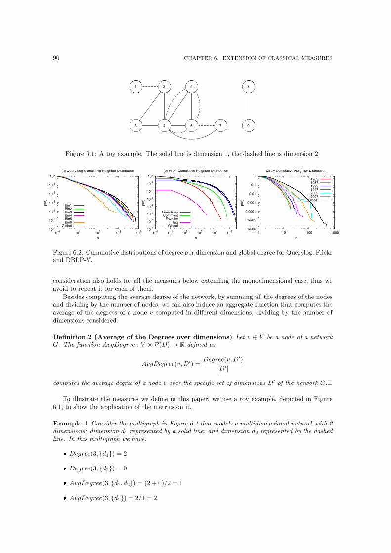
90 CHAPTER 6. EXTENSION OF CLASSICAL MEASURES
Figure 6.1: A toy example. The solid line is dimension 1, the dashed line is dimension 2.
10-6
10-5
10-4
10-3
10-2
10-1
100
100
101
102
103
104
p(n
)
n
(a) Query Log Cumulative Neighbor Distribution
Bin1Bin2Bin3Bin4Bin5Bin6
Global10
-7
10-6
10-5
10-4
10-3
10-2
10-1
100
100
101
102
103
104
105
p(n
)
n
(e) Flickr Cumulative Neighbor Distribution
FriendshipComment
FavoriteTag
Global 1e-06
1e-05
0.0001
0.001
0.01
0.1
1
1 10 100 1000
p(n
)n
DBLP Cumulative Neighbor Distribution
198219871992199720022007
Global
Figure 6.2: Cumulative distributions of degree per dimension and global degree for Querylog, Flickrand DBLP-Y.
consideration also holds for all the measures below extending the monodimensional case, thus weavoid to repeat it for each of them.
Besides computing the average degree of the network, by summing all the degrees of the nodesand dividing by the number of nodes, we can also induce an aggregate function that computes theaverage of the degrees of a node v computed in different dimensions, dividing by the number ofdimensions considered.
Definition 2 (Average of the Degrees over dimensions) Let v ∈ V be a node of a networkG. The function AvgDegree : V × P(D)→ R defined as
AvgDegree(v,D′) =Degree(v,D′)
|D′|
computes the average degree of a node v over the specific set of dimensions D′ of the network G.�
To illustrate the measures we define in this paper, we use a toy example, depicted in Figure6.1, to show the application of the metrics on it.
Example 1 Consider the multigraph in Figure 6.1 that models a multidimensional network with 2dimensions: dimension d1 represented by a solid line, and dimension d2 represented by the dashedline. In this multigraph we have:
� Degree(3, {d1}) = 2
� Degree(3, {d2}) = 0
� AvgDegree(3, {d1, d2}) = (2 + 0)/2 = 1
� AvgDegree(3, {d1}) = 2/1 = 2

6.2. SHORTEST PATH RELATED MEASURES 91
In Figure 6.2 we show that with this function it is possible to identify dimensions that aregood representatives of the global degree distribution of the network, thus allowing tasks suchas focused sampling or (lossy) compression of the graph. Consider the case of Flickr network(Figure 6.2b): “Comment” dimension shows a very similar exponential cutoff of the general degreedistribution, but it has almost an order of magnitude less edges. Also consider “Tag” dimensionfor Flickr or “Bin 6” dimension for Querylog (Figure 6.2a). What is happening is that even insidea multidimensional network that does not present a power law degree distribution, since both thegeneral degree distribution in Querylog and Flickr present a very strong exponential cutoff, therecan be scale free dimensions, where the cutoff is evidently weaker.
Traditionally in complex network studies, degree distributions and average degree are theo-retically linked with the study of the connected components of the network, focusing particularlyon the preconditions for observing a giant component. We are not tackling the problem from atheoretical point of view, but we just provide some useful tools to derive an easily computableway to better understand the topology of the network. In the following we compute the numberof connected components of a multidimensional network, including also a set of dimensions intoaccount.
Definition 3 (Connected Components) The function CC : G ×P(D)→ N, called ConnectedComponents, computes the number of connected component of a graph considering only the edgeslabeled with dimensions included in a given set D′. It counts the number of the maximal set ofnodes that can be reached through paths only using the edges belonging to any d ∈ D′. �
Definition 4 (Average of the Connected Components over Dimensions) The function AvgCC :G × P(D)→ R, called Average of the Connected Components over Dimensions, is defined as
AvgCC(G,D′) =
∑d∈D′ CC(v, {d})
|D′|
and computes the average of the number of connected components over the specific set of dimensionsD′ of a given network G. �
Example 2 Considering the multidimensional network of the Figure 6.1:
� if we consider only the dimension d1 we have 3 components, as we can consider node 1 as acomponent composed by only one node
� if we consider only the dimension d2 we have 5 components, as we can consider nodes 3, 8and 9 as above
� if we consider all the dimensions of the network we have 2 components
� the connected component average of the network are (3 + 5)/2 = 4
6.2 Shortest Path Related Measures
As done for the degree, the classical shortest path definition has to be revisited in order to dealwith the multidimensional setting, by extending the domain with a set of dimensions.
Definition 5 (Shortest Path) Let u, v ∈ V be two nodes of a network G. The function ShortestPath :V ×V ×P(D)→ N computes the length of the shortest path (in terms of number of edges) betweenu and v, where the edges are labeled with dimensions in D′. �
As in the classical definition, if are no paths between two nodes then the distance betweenthem is ∞. We also define the Average Shortest Path and the Average of the Shortest Paths overdimensions, which are two aggregate functions.

92 CHAPTER 6. EXTENSION OF CLASSICAL MEASURES
Definition 6 (Average Shortest Path) The function ShortestPathAVG : P(D) → R is de-fined as
ShortestPathAVG(D′) =
∑∀p∈SPD′
Length(p)
|SPD′ |where:
� SPD′ denotes the set of shortest paths having only edges labeled with dimensions belonging toD′, between node v and any node u reachable from it.
� Length(p) denotes the length of the shortest path p in terms of number of edges.
It computes the average shortest path considering only the set of dimensions D′. �
Definition 7 (Average of the Shortest Paths over dimensions) Let u, v ∈ V be two nodesof a network G such that v is reachable from u. The function AvgShortestPath : V ×V ×P(D)→ Rdefined as
AvgShortestPath(u, v,D′) =∑d∈D′ ShortestPath(u,v,{d})
|D′|
computes the average of the lengths of the shortest paths between two nodes u and v over the specificset of dimensions D′ of the network G. �
An interesting analysis that can be done when taking the dimensions into account in thedefinition of the shortest path is to verify the heterogeneity of the shortest path, i.e. verifying howmany dimensions are traversed by a given shortest path. To this end, we define a function thatcomputes the heterogeneity of a path.
Definition 8 (Path Heterogeneity) Let P be a path between two nodes of a multidimensionalnetwork, i.e. a sequence of labeled edges. The Path Heterogeneity function computes the ratio ofdimensions in P with respect to the dimensions in the whole network, i.e. PathHeterogeneity =|{d | ∃(u, v, d) ∈ P}|
|D|�
Given a set of paths it is possible to compute aggregate functions of the path heterogeneitymeasure, such as the average, the maximum and the minimum. In a multidimensional network, itis interesting to apply this measure on the set of the shortest paths: considering a transportationnetwork, this would translate in knowing how many different trains, or tickets, a persons has totake to get to the destination. A possible variant of this is to count the number of “changes”of dimensions: even though the number of different crossed dimensions can be only two, it mayhappen that in order to go from one node to another one in the network, the shortest path is asequence of d1−d2−d1− ...−d2, which, in the transportation network, would mean to change trainat every station. An interesting problem would be to modify Dijkstra algorithm for computing theshortest path [77] to include also the change of edge label (i.e. dimension) as additional cost of theshortest path. We investigate more deeply this problem in Section 8.4.
Example 3 Continuing with the example of Figure 6.1 we have:
� the ShortestPath(1, 7, {d1, d2}) = 3 and its Heterogeneity is equal to 1, as this shortest pathcontains 2 edges of the dimension d2 and 1 edge of the dimension d1.
� ShortestPath(1, 7, {d1}) =∞
� ShortestPath(6, 7, {d1, d2}) = 1
� ShortestPath(6, 7, {d1}) = 2
� ShortestPath(6, 7, {d2}) = 1

6.2. SHORTEST PATH RELATED MEASURES 93
� AvgShortestPath(6, 7, {d1, d2}) = 1.5
� ShortestPathAVG({d1, d2}) = 1.6
The concept of shortest path has been used in complex networks to derive a collection ofcentrality measures, such as the closeness and the betweenness centrality. We now take a lookwhat does change for these two measures with a multidimensional formulation of the shortestpath.
The closeness centrality describes a particular kind of “importance” of a node within a network,in terms of distance of it from all the other nodes. In the standard definition this measure is onlydefined on nodes. As done for the above measures, we modify the definition introducing thedimensions. Please note that there are several different definitions of closeness centrality (suchas the random-walk or the information centrality). The underlying logic needed to extend allthe variants in the multidimensional case is fairly similar to the one presented here, and this isthe reason why we present only this closeness version. In practice, what is needed is to selectonly the edges belonging to the set D of dimensions we are interested in, collapse them into amonodimensional view and apply the standard definition.
Definition 9 (Closeness Centrality) Let v ∈ V be a node of a network G. The functionCloseness : V × P(D)→ [0, 1] is defined as
Closeness(v,D′) =|V |∑
u∈V ShortestPath(v, u,D′)
where V denotes the set of nodes reachable from v by a path, excluding v itself. �
Moreover, we define an aggregate function that computes the average of the closeness centralitycomputed over different dimensions.
Definition 10 (Average of the Closeness Centralities over Dimensions) Let v ∈ V a nodeof a network G. The function AvgCloseness : V × P(D)→ [0, 1] defined as
AvgCloseness(v,D′) =
∑d∈D′ Closeness(v, {d})
|D′|
computes the average of the closeness centralities of a node v over the specific set of dimensionsD′ of the network G. �
Please note that in this measure we explicitly indicate the set Dv, as it is not meaningful toconsider the closeness in dimensions where the node does not appear.
Example 4 In the multidimensional network of the Figure 6.1:
� if we consider the entire dimension set and the node 7 we have six nodes reachable with atotal number of 11 edges: Closeness(7, {d1, d2}) = 6/11 = 0.54
� if we consider only the dimension d1 and the node 7 we have Closeness(7, {d1}) = 5/9 = 0.55
� if we consider only the dimension d2 and the node 7 we have Closeness(7, {d2}) = 3/5 = 0.6
� the average of the closeness on the all the dimensions of the node 7 is AvgCloseness(7, {d1, d2}) =(0.55 + 0.6)/2 = 0.57
While the closeness centrality takes into account the distance between a node and all the othernodes in a network, the betweenness centrality considers the number of shortest paths passingthrough a node, thus emphasizing the analysis of the resilience of the network to the removal ofimportant nodes. Also in this case, we would like to include a set of dimensions into account, hencewe modify the standard definitions, introducing the followings.

94 CHAPTER 6. EXTENSION OF CLASSICAL MEASURES
Definition 11 (Betweenness Centrality) Let v ∈ V be a node of a network G. The functionBetweenness : V × P(D)→ [0, 1] defined as
Betweenness(v,D′) =
∑s,t∈V SPsvt(D
′)
SPst(D′)
where:
� SPsvt(D′) denotes the number of shortest path between the nodes s and t passing through v,
only considering edges belonging to the set of dimensions D′
� SPst(D′) denotes the number of shortest path between the nodes s and t, considering only
considering edges belonging to the set of dimensions D′. �
We can also define an aggregate function that computes the average of the betweenness cen-tralities computed on different dimensions.
Definition 12 (Average of the Betweenness Centralities over Dimensions) Let v ∈ V bea node of a network G. The function AvgBetweenness : V × P(D)→ [0, 1] defined as
AvgBetweenness(v,D′) =
∑d∈D′ Betweenness(v, {d})
|D′|
computes the average of the betweenness centralities of a node v computed over the specific set ofdimensions D′ of the network G. �
Finally, the last measure influenced by the novel definition of the shortest path is the diameter.The classical definition of the diameter is the length of the longest shortest path between any pairof nodes in the network. Having re-defined the notion of “shortest path” we can define the conceptof diameter in terms of it.
Definition 13 (Diameter) The function Diameter : G × P(D)→ N computes the length of thelongest shortest path of a network G considering only edges labeled with dimension belonging to aspecific set D′. �
Clearly, on the diameter it is possible to define aggregate functions as for the shortest path. Itis also interesting to measure the difference between the diameter computed considering a givenset of dimensions and the diameter of the whole network.
Example 5 On Figure 6.1:
� Diameter(G,D) = 3
� Diameter(G, {d1}) = 2
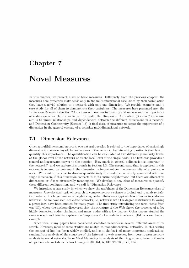
Chapter 7
Novel Measures
In this chapter, we present a set of basic measures. Differently from the previous chapter, themeasures here presented make sense only in the multidimensional case, since by their formulationthey have a trivial solution in a network with only one dimension. We provide examples and acase study for all of them to demonstrate their usefulness. The measures here presented are: theDimension Relevance (Section 7.1), a class of measures to quantify and understand the importanceof a dimension for the connectivity of a node; the Dimension Correlation (Section 7.2), whoseaim is to unveil relationships and dependencies between the different dimensions in a network;and Dimension Connectivity (Section 7.3), a final class of measures to assess the importance of adimension in the general ecology of a complex multidimensional network.
7.1 Dimension Relevance
Given a multidimensional network, one natural question is related to the importance of each singledimension in the economy of the connections of the network. An interesting question is then how toquantify this importance. The quantification can be calculated at two different granularity levels:at the global level of the network or at the local level of the single node. The first case provides ageneral and aggregate answer to the question “How much in general a dimension is important inthe network?” and we explore this branch in Section 7.3. The second case, that is explored in thissection, is focused on how much the dimension is important for the connectivity of a particularnode. We want to be able to discern quantitatively if a node is exclusively connected with onesingle dimension, if this dimension connects it to its entire neighborhood but there are alternativedimensions or if it is structurally meaningless. We develop a new class of measures to quantifythese different configurations and we call it “Dimension Relevance”.
We introduce a case study in which we show the usefulness of the Dimension Relevance class ofmeasures. One classical topic of research in complex network science is to find and to analyze hubs,i.e. nodes with a large number of neighboring nodes. Hubs are a typical class of nodes in scale-freenetworks. As we have seen, scale-free networks, i.e. networks with the degree distribution followinga power law, have been studied for many years. The first study introducing the term “scale-free”was [30], where the authors discovered that the structure of the Web shows the presence of a fewhighly connected nodes, the hubs, and many nodes with a low degree. Other papers studied thesame concept and tried to capture the “importance” of a node in a network: [151] is a well knownexample.
Since then, many papers have considered scale-free networks in several different areas of re-search. However, most of these studies are related to monodimensional networks. In this settingthe concept of hub has been widely studied, and is at the basis of many important applications,ranging from analysis of the structure of the Internet to web searches, from peer-to-peer networkanalysis to social networks, from Viral Marketing to analysis of the Blogosphere, from outbreaksof epidemics to metabolic network analysis [30, 151, 5, 139, 99, 238, 171, 184].
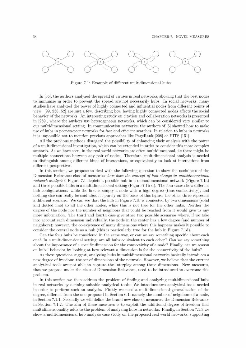
96 CHAPTER 7. NOVEL MEASURES
Figure 7.1: Example of different multidimensional hubs.
In [65], the authors analyzed the spread of viruses in real networks, showing that the best nodesto immunize in order to prevent the spread are not necessarily hubs. In social networks, manystudies have analyzed the power of highly connected and influential nodes from different points ofview: [99, 238, 52] are just a few, describing how having highly connected nodes affects the socialbehavior of the networks. An interesting study on citation and collaboration networks is presentedin [269], where the authors use heterogeneous networks, which can be considered very similar toour multidimensional setting. In communication networks, the authors of [5] showed how to makeuse of hubs in peer-to-peer networks for fast and efficient searches. In relation to hubs in networksit is impossible not to mention previous approaches like PageRank [208] or HITS [151].
All the previous methods disregard the possibility of enhancing their analysis with the powerof a multidimensional investigation, which can be extended in order to consider this more complexscenario. As we have seen, in the real world networks are often multidimesional, i.e there might bemultiple connections between any pair of nodes. Therefore, multidimensional analysis is neededto distinguish among different kinds of interactions, or equivalently to look at interactions fromdifferent perspectives.
In this section, we propose to deal with the following question to show the usefulness of theDimension Relevance class of measures: how does the concept of hub change in multidimensionalnetwork analysis? Figure 7.1 depicts a possible hub in a monodimensional network (Figure 7.1a)and three possible hubs in a multidimensional setting (Figure 7.1b-d). The four cases show differenthub configurations: while the first is simply a node with a high degree (thus connectivity), andnothing else can really be said about it purely on the basis of this figure, the other three representa different scenario. We can see that the hub in Figure 7.1b is connected by two dimensions (solidand dotted line) to all the other nodes, while this is not true for the other hubs. Neither thedegree of the node nor the number of neighbors that could be reached from it would give us anymore information. The third and fourth case give other two possible scenarios where, if we takeinto account each dimension individually, the node in the center has a low degree (and number ofneighbors); however, the co-existence of many dimensions where this happens makes it possible toconsider the central node as a hub (this is particularly true for the hub in Figure 7.1d).
Can the four hubs be considered in the same way, or can we say something specific about eachone? In a multidimensional setting, are all hubs equivalent to each other? Can we say somethingabout the importance of a specific dimension for the connectivity of a node? Finally, can we reasonon hubs’ behavior by looking at how relevant a dimension is for the connectivity of the hubs?
As these questions suggest, analyzing hubs in multidimensional networks basically introduces anew degree of freedom: the set of dimensions of the network. However, we believe that the currentanalytical tools are not able to capture the interplay among these dimensions. New measures,that we propose under the class of Dimension Relevance, need to be introduced to overcome thisproblem.
In this section we then address the problem of finding and analyzing multidimensional hubsin real networks by defining suitable analytical tools. We introduce two analytical tools neededin order to perform such an analysis. Firstly we need a multidimensional generalization of thedegree, different from the one proposed in Section 6.1, namely the number of neighbors of a node,in Section 7.1.1. Secondly we will define the brand new class of measures, the Dimension Relevancein Section 7.1.2. The aim of these measures is to exploit the additional degree of freedom thatmultidimensionality adds to the problem of analyzing hubs in networks. Finally, in Section 7.1.3 weshow a multidimensional hub analysis case study on the proposed real world networks, supporting

7.1. DIMENSION RELEVANCE 97
the meaningfulness of the problem introduced, the effectiveness of the measures defined, and a fewpractical applications intended to demonstrate the power of our approach.
The most important insights of this section are: (1) we show that multidimensional hubsexist, and can be found and analyzed using our introduced measures of interplay of the differentdimensions; (2) we show that the characterization of multidimensional hubs highlights interestinganalytical properties, and (3) thanks to our measures, we discover and quantify the importance ofevery single dimension with respect to the others, generally unknown a priori.
7.1.1 Neighbors
Now, we define the Neighbors class of measures, needed for the creation of the analytical ground ofthe Dimension Relevance measures. Neighbors is an extension of the degree in the multidimensionalsetting. We also give its interpretation and we show a toy example illustrating its behavior for afew nodes.
In classical graph theory the Degree of a node refers to the connections of a node in a network:it is defined, in fact, as the number of edges adjacent to a node. In a simple graph, each edge is thesole connection to an adjacent node. In multidimensional networks the degree of a node (i.e., thenumber of the connections of that node in a network) and the number of nodes adjacent to it areno longer related, since there may be more than one edge between any two nodes. For instance, inFigure 7.1, all nodes have four neighbors, but they have a very different degree, especially in everysingle dimension.
In order to capture this difference, we define a measure concerning the neighbors of a node.
Definition 14 (Neighbors) Let v ∈ V and D′ ⊆ D be a node and a set of dimensions of anetwork G = (V,E,D), respectively. The function Neighbors : V × P(d)→ N is defined as
Neighbors(v,D′) = |NeighborSet(v,D′)|
where NeighborSet(v,D′) = {u ∈ V | ∃(u, v, d) ∈ E ∧ d ∈ D′}. This function computes thenumber of all the nodes directly reachable from node v by edges labeled with dimensions belongingto D′. �
Note that, in the monodimensional case, the value of this measure corresponds to the degree.It is easy to see that Neighbors(v,D′) ≤ Degree(v), but we can also easily say something about
the ratio Neighbors(v,D′)Degree(v) . When the number of neighbors is small, but each one is connected by
many edges to v, we have low values for this ratio, which means that the set of dimensions issomehow redundant with respect to the connectivity of that node. This is the case of node 2 in thetoy example illustrated in Figure 6.1. On the opposite extreme, the two measures coincide, andthis ratio is equal to 1, which means that each dimension in which v has a neighbor is necessary(and not redundant) for the connectivity of that node: removing any of these dimensions woulddisconnect (directly) that node from some of its neighbors. This is the case of node 5 in Figure7.2.
We also define a variant of the Neighbors function, which takes into account only the adjacentnodes that are connected by edges belonging exclusively to a given set of dimensions.
Definition 15 (NeighborsXOR) Let v ∈ V and D′ ⊆ D be a node and a set of dimensions of anetwork G = (V,E,D), respectively. The function NeighborsXOR : V × P(D)→ N is defined as
NeighborsXOR(v,D′) = |{u ∈ V | ∃d ∈ D′ : (u, v, d) ∈ E ∧ @d′ /∈ D′ : (u, v, d′) ∈ E}|
It computes the number of neighboring nodes connected by edges belonging exclusively to dimensionsin D′. �

98 CHAPTER 7. NOVEL MEASURES
7.1.2 Dimension Relevance
As already mentioned, while performing hub analysis it is important to understand how importanta particular dimension is over the others for the connectivity of a node, i.e. what happens to theconnectivity of the node if we remove that dimension. In order to answer these questions, we definethe new concept of Dimension Relevance. Also in this case, we refer to the toy example in Figure7.2 for its intuition and interpretation.
Definition 16 (Dimension Relevance) Let v ∈ V and d ∈ D be a node and a dimension of anetwork G = (V,E,D), respectively. The function DimRelevance : V ×D → [0, 1] is defined as
DimRelevance(v, d) =Neighbors(v, d)
Neighbors(v,D)
and computes the ratio between the neighbors of a node v connected by edges labeled with a specificdimension d and the total number of its neighbors. �
Clearly, the above function can be defined taking into account a set of dimensions instead of asingle dimension. In other words, we can generalize Definition 16 as follows:
Definition 17 (Dimension Relevance) Let v ∈ V and D′ ⊆ D be a node and a set of dimen-sions of a network G = (V,E,D), respectively. The function DimRelevance : V × P(D) → [0, 1]is defined as
DimRelevance(v,D′) =Neighbors(v,D′)
Neighbors(v,D)and computes the ratio between the neighbors of a node v connected by edges belonging to a specificset of dimensions in D′ and the total number of its neighbors. �
Note that, the case of a single dimension (Definition 16) is a particular case of that in Definition17, where the set of dimensions D contains only the dimension d. In the remaining of the paperwe define the others measures considering a set of dimensions.
However, in a multidimensional setting, this measure may still not cover important informationabout the connectivity of a node. Figure 7.1 shows three nodes (a, b and c) with a high dimensionrelevance for the dimension represented by a solid line. In the first two cases the dimension relevanceis equal to one, but the complete set of connections they present is different: if we remove the solidline dimension the node a will be completely disconnected while the node b can still reach all itsneighbors. To capture these possible different cases we introduce a variant of this metric.
Definition 18 (Dimension Relevance XOR) Let v ∈ V and D′ ⊆ D be a node and a set ofdimensions of a network G = (V,E,D), respectively.The function DimRelevanceXOR : V × P(D)→ [0, 1] defined as
DimRelevanceXOR(v,D′) =NeighborsXOR(v,D′)
Neighbors(v,D)
computes the fraction of neighbors directly reachable from node v following edges belonging only todimensions D. �
We can easily calculate the above metric in the examples in Figure 7.1. For the node a thereis no difference with the Dimension Relevance (Definition 17): all its neighbors are only reachableby solid edges. In node b we have the opposite situation: all its neighbors are reachable by solidedges, but we always have an alternative edge. So the Dimension Relevance XOR of the solid linedimension is equal to zero.In the following, we want to capture the intuitive intermediate value, i.e. the number of neighborsreachable through a dimension, taking into account all the possible alternatives.
Definition 19 (Weighted Dimension Relevance)Let v ∈ V and D′ ⊆ D be a node and a set of dimensions of a network G = (V,E,D), respectively.The function DimRelevanceW : V × P(D) → [0, 1], called Weighted Dimension Relevance, isdefined as
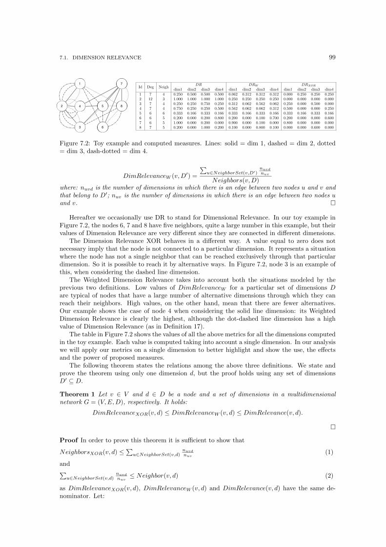
7.1. DIMENSION RELEVANCE 99
Id Deg NeighDR DRW DRXOR
dim1 dim2 dim3 dim4 dim1 dim2 dim3 dim4 dim1 dim2 dim3 dim41 7 4 0.250 0.500 0.500 0.500 0.062 0.312 0.312 0.312 0.000 0.250 0.250 0.2502 12 3 1.000 1.000 1.000 1.000 0.250 0.250 0.250 0.250 0.000 0.000 0.000 0.0003 7 4 0.250 0.250 0.750 0.250 0.312 0.062 0.562 0.062 0.250 0.000 0.500 0.0004 7 4 0.750 0.250 0.250 0.500 0.562 0.062 0.062 0.312 0.500 0.000 0.000 0.2505 6 6 0.333 0.166 0.333 0.166 0.333 0.166 0.333 0.166 0.333 0.166 0.333 0.1666 6 5 0.200 0.000 0.200 0.800 0.200 0.000 0.100 0.700 0.200 0.000 0.000 0.6007 6 5 1.000 0.000 0.200 0.000 0.900 0.000 0.100 0.000 0.800 0.000 0.000 0.0008 7 5 0.200 0.000 1.000 0.200 0.100 0.000 0.800 0.100 0.000 0.000 0.600 0.000
Figure 7.2: Toy example and computed measures. Lines: solid = dim 1, dashed = dim 2, dotted= dim 3, dash-dotted = dim 4.
DimRelevanceW (v,D′) =
∑u∈NeighborSet(v,D′)
nuvdnuv
Neighbors(v,D)where: nuvd is the number of dimensions in which there is an edge between two nodes u and v andthat belong to D′; nuv is the number of dimensions in which there is an edge between two nodes uand v. �
Hereafter we occasionally use DR to stand for Dimensional Relevance. In our toy example inFigure 7.2, the nodes 6, 7 and 8 have five neighbors, quite a large number in this example, but theirvalues of Dimension Relevance are very different since they are connected in different dimensions.
The Dimension Relevance XOR behaves in a different way. A value equal to zero does notnecessary imply that the node is not connected to a particular dimension. It represents a situationwhere the node has not a single neighbor that can be reached exclusively through that particulardimension. So it is possible to reach it by alternative ways. In Figure 7.2, node 3 is an example ofthis, when considering the dashed line dimension.
The Weighted Dimension Relevance takes into account both the situations modeled by theprevious two definitions. Low values of DimRelevanceW for a particular set of dimensions Dare typical of nodes that have a large number of alternative dimensions through which they canreach their neighbors. High values, on the other hand, mean that there are fewer alternatives.Our example shows the case of node 4 when considering the solid line dimension: its WeightedDimension Relevance is clearly the highest, although the dot-dashed line dimension has a highvalue of Dimension Relevance (as in Definition 17).
The table in Figure 7.2 shows the values of all the above metrics for all the dimensions computedin the toy example. Each value is computed taking into account a single dimension. In our analysiswe will apply our metrics on a single dimension to better highlight and show the use, the effectsand the power of proposed measures.
The following theorem states the relations among the above three definitions. We state andprove the theorem using only one dimension d, but the proof holds using any set of dimensionsD′ ⊆ D.
Theorem 1 Let v ∈ V and d ∈ D be a node and a set of dimensions in a multidimensionalnetwork G = (V,E,D), respectively. It holds:
DimRelevanceXOR(v, d) ≤ DimRelevanceW (v, d) ≤ DimRelevance(v, d).
�
Proof In order to prove this theorem it is sufficient to show that
NeighborsXOR(v, d) ≤∑u∈NeighborSet(v,d)
nuvdnuv
(1)
and∑u∈NeighborSet(v,d)
nuvdnuv≤ Neighbor(v, d) (2)
as DimRelevanceXOR(v, d), DimRelevanceW (v, d) and DimRelevance(v, d) have the same de-nominator. Let:
100 CHAPTER 7. NOVEL MEASURES
A = NeighborsXOR(v, d)B =
∑u∈NeighborSet(v,d)
nuvdnuv
C = Neighbors(v, d).
First of all, we prove the inequality (1). If node v is connected to a neighbor u only by edges labeledwith dimension d then in both A and B, u contributes with 1; if they are connected only by edgeslabeled with dimensions different than d then in both the formulas, A and B, u contributes with0; lastly, if they are connected by some edges labeled with dimension in d and some edges labeledwith dimensions different than d then in A the node u contributes with a value equal to 0 while inB it contributes with a value greater than 0. Thus, we have that A ≤ B.
Now, we prove the inequality (2). If node v is connected to a neighbor u only labeled withdimension d then in both the formula B and C it contributes with 1; if they are connected onlyby edges labeled with dimensions different than d then in A and B u contributes with 0; lastly, ifthey are connected by some edges labeled with dimensions different than d and some edges labeledwith dimension d then in B the node u contributes with a value equal to nuvd
nuv< 1 while in C it
contributes with 1. Thus, we have that B ≤ C. �
7.1.3 Finding and Characterizing Hubs
Many interesting network analytic concepts, both at the global and at the local level, such asconnectivity, centrality, diameter, etc., developed for standard, monodimensional networks, comeunder a different light when seen in the multidimensional setting. At the global level, for example,the connectivity of the whole network changes if we see a single dimension as a separate network,with respect to the network formed by all the edges in the entire set of dimensions. Also at thelocal level, it is possible to analyze many other examples. One such example is the concept ofa hub, i.e., a node with a very high degree, substantially higher than the average degree of allnodes. When considering a multidimensional network, such simple concept becomes subtler andmultifaceted: first, the definition of a multidimensional hub is parametric with respect to a setof dimensions and secondly, the relevance of a node depends on the interplay among the differentdimensions and their impact on the connectivity of the node. Here, a multidimensional hub isa node with high connectivity in the sub-network obtained by considering only the edges fromsome specified dimensions (we give a formal definition later in this section). As evidence of howsubtle the characterization of a multidimensional hub is, we found in all our real-world networksthat the population of hubs obtained while neglecting the dimensions, differs substantially fromthat of hubs obtained taking dimensions into account (see Table 7.1 and its discussion later in thissection): some (sometimes many) monodimensional hubs are not multidimensional hubs, and viceversa (we provide later on further analysis of this phenomenon). In this section we use mainly theQuerylog, Flickr and DBLP-Y networks presented in Chapter 5.
This led us to conclude that analyzing hubs in multidimensional networks is not a trivialextension of the standard case. In other words, it requires techniques and measures of nodeconnectivity across different dimensions, able to highlight the interplay among (sets of) dimensionsand their impact on node connectivity. Therefore, the problem that we dealt with in this papercan be defined as follows:
Definition 20 (Problem Definition) Given a large multidimensional network, find and char-acterize the multidimensional hubs.
Measuring the Hubbiness
We now formally define the concept of multidimensional hub and a possible characterization for it.
Definition 21 (Multidimensional Hub) Let v be a node and D the set of dimensions in a mul-tidimensional network. Given a threshold δ the node v is a multidimensional hub iff Neighbors(v,D) ≥δ.
7.1. DIMENSION RELEVANCE 101
In general, the threshold δ depends on the specific network, although there are empirical rules inthe literature to determine it (one example is the classical 80-20 rule [221]). This is why hereafterwe omit this threshold, saying only that a hub is a node with a high number of neighbors.
At this point, one question arises: can we give a formal characterization of multidimensionalhubs? The set of measures to assess the relevance of a dimension for a given node allows tocharacterize some kinds of hubs. In particular, by combining the two following notions of mul-tidimensional hub and relevance of a dimension for a node we are able to identify, within a setof multidimensional hubs, those for which a specific dimension d is relevant (Definition 22) orirrelevant (Definition 23).
Definition 22 (D-supported Hub) Let v ∈ V and D′ ⊆ D be a node and a set of dimensionsof a network G = (V,E,D), respectively. The node v is D-supported if v is a multidimensional hubwith respect to the set of network dimensions D and R(v,D′) ≥ ε, with R ∈ {DR, DRXOR, DRW }
Definition 23 (D-unsupported Hub) Let v ∈ V and D′ ⊆ D be a node and a set of dimensionsof a network G = (V,E,D), respectively. The node v is D-unsupported if v is a multidimensionalhub with respect to a set of dimensions D and R(v,D′) < ε, with R ∈ {DR, DRXOR, DRW }
As one can see, the difference between the two resides only in the direction of the inequality.They are equivalently “powerful” nodes of the network, as they are hubs thus very highly connected,but they have a totally opposed connection patterns w.r.t the dimensions of the network. We chooseto use the term nemesis to address them, and we use this term hereafter to refer to hubs that playthe opposite role of other ones (fixing D′, if v1 is a D-supported Hub for the set of dimensions D′
and v2 is a D-unsupported Hub for the same set of dimensions, then v1 and v2 are the nemesisof each other). An interesting future work is to have a multidimensional definition for “date”and “party” hubs [7], and to study the relationship between this four classes (i.e. are date hubssignificantly more represented in the D-unsupported class for the entire set of dimensions D? Arethe classes completely orthogonal?).
There are two caveats in the above definitions. First, the definitions are generic for any setof dimensions D′, where D′ might even contain only a single dimension. When analyzing realnetworks, a specific target of analysis might be to find the set of d-supported hubs for one singlespecific dimension d.
Second, the choice among the various DRs allows to find D-supported (D-unsupported) hubswith very different multidimensional characteristics. The choice is ad-hoc, and only depends onthe analysis that one might want to perform, hence there is no better choice among the others. Forexample, by choosing the DRXOR, and looking for the d-unsupported hubs for a specific dimensiond, we are looking for hubs that would be hubs even without the connections provided by dimensiond.
Note that the above characterization in a network whose set of dimensions D would containonly a single dimension d, would not make any sense, for the following reasons: (1) all the valuesfor the DRs would be 1, making the distinction between D-supported and D-unsupported vain, and(2) there would be no distinction among the three DRs, making thus the characterization leadingto only one possible type of hubs, which is, obviously, the traditional concept of monodimensionalhub.
Given all the above, building a multidimensional analysis aimed at extracting and characterizinga multidimensional hub is relatively easy: the analyst defines the desired analysis, translates it interms of a filter on the values of Dimension Relevance and then selects, among the nodes withhigh number of neighbors, the ones satisfying the filter, leading to D-supported or D-unsupportedhubs, according to the most appropriate choice of DR and parameters.
Example 6 (Airline Network) Without looking at the complete structure of the multidimen-sional network of airlines (each airline company taken as a dimension), we selected two Europeanmultidimensional hubs (≥ 100 connected cities): Dublin and Madrid. We found that the Ryanairairline has a DR of 0.54 for Dublin and 0.27 for Madrid, while it has a DRXOR of 0.31 for theformer, and 0.09 for the latter. This means that, while the Ryanair’s importance seems to be

102 CHAPTER 7. NOVEL MEASURES
double for Dublin w.r.t Madrid in terms of connected cities, its importance as sole connection ismore than triple. Dublin is then a Ryanair-supported hub, according to both DR and DRXOR.
Computing the Dimension Relevance
The complexity required to compute the Dimension Relevance measure set is low. The procedurewe used is the following. First, we are considering an undirected network, thus the edge set E is asequence of triplets (u, v, d), where each element is a numerical is for nodes and dimensions, andu < v, i.e. the numerical id of the first node is always lower than the second node (no self loopsallowed).
We then sort |E|, with a sub-quadratic complexity of O(|E| log |E|). All the Dimension Rel-evance variants can be now computed by a simple scan of the sorted edge list, with complexityO(|E|), that is dominated by the sorting complexity (in case the edge list is already sorted, tocalculate the Dimension relevance is linear). When cycling over the edge list, the following cri-teria are used to update the values of the Dimension Relevance measures. When we found thefirst triple (u, v, d), we increase by one the Neighbors(u,D) and Neighbors(v,D) values. For eachtriple (u, v, d), we also update the Neighbors(u, d) and Neighbors(v, d) values, needed for the plainDimension Relevance, and the nuvd and nuv values, needed for the Weighted Dimension Relevance.We then update NeighborsXOR(u, d) and NeighborsXOR(v, d), needed for the Dimension Rele-vance XOR, if and only if the triple (u, v, d) is the only one connecting nodes u and v (and we avethis information since all the triplets involving directly u and v are clustered together, due to thesorting).
We now want to answer the following:
Q1. Are the presented multidimensional measures able to make important latent knowledgeemerge from the data?
Q2. Would it be possible to extract (part of) this knowledge with non-multidimensional techniqueswith the same degree of complexity?
Q3. What kind of knowledge would the measures make emerge on null models?
We now provide an answer for Q1 and Q2. Q3 is a particular case, requiring the definition ofmultidimensional null models and/or generators for complex networks. Since this is an interestingproblem per se, we address its solution in a following section (Section 8.2). For clarity, we reporthere the main findings: more sophisticated multidimensional network generators are able to betterrepresent the complex dynamics of the distribution of the Dimension Relevance class of measures.However, significant differences still emerge between the most advanced null models and the realworld networks, proving that Dimension Relevance measures are able to unveil complex dynamicsat the local level that are not fully understandable with assumptions at the global level (we referin particular to the comparison of DR distributions from the original networks in Figures 7.3(a-i)and from the null models in Figures 8.7, 8.8, 8.9 and 8.10).
Q1: Multidimensional Measures on Real Networks
Here, we want to study the power of our multidimensional tools in letting latent knowledge emergefrom the data. Figures 6.2(a)-(c) show, for the three datasets, the cumulative neighbor distribu-tions in log-log scale. Consider the curve corresponding to the global network, i.e. the distributionof neighbors computed over all the dimensions. The DBLP-Y network shows a behavior similar tothe “the rich gets richer”, with very different cut-offs, while the other networks behave differently.The figures show that the behavior of this measure resembles the one of the degree in the monodi-mensional setting, even without being completely similar. To support this, in Figure 6.2(a)-(c) wereport also the cumulative neighbor distribution per dimension (which, in turn, is the degree perdimension) of the three networks, and we compare them with the global neighbors distribution.For DBLP-Y, we chose only six representative dimensions out of the original 65.
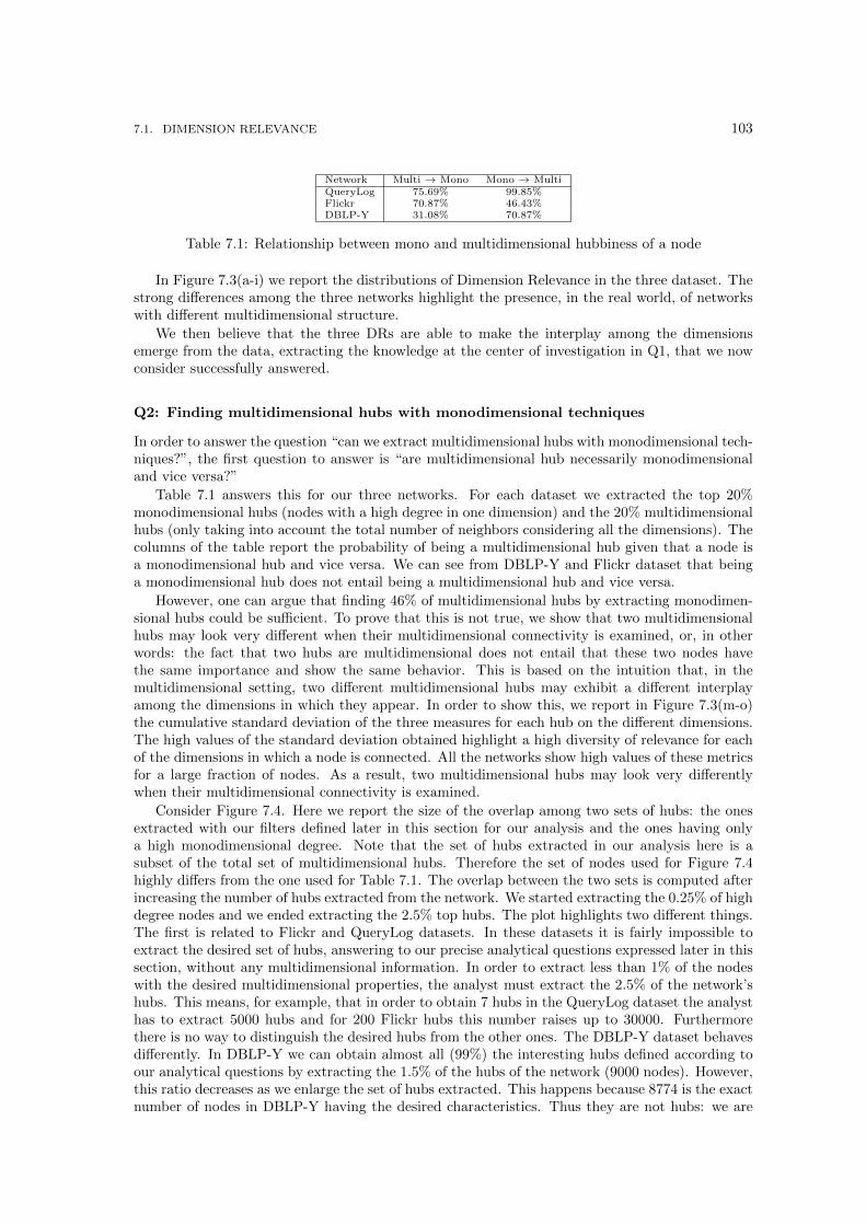
7.1. DIMENSION RELEVANCE 103
Network Multi → Mono Mono → MultiQueryLog 75.69% 99.85%Flickr 70.87% 46.43%DBLP-Y 31.08% 70.87%
Table 7.1: Relationship between mono and multidimensional hubbiness of a node
In Figure 7.3(a-i) we report the distributions of Dimension Relevance in the three dataset. Thestrong differences among the three networks highlight the presence, in the real world, of networkswith different multidimensional structure.
We then believe that the three DRs are able to make the interplay among the dimensionsemerge from the data, extracting the knowledge at the center of investigation in Q1, that we nowconsider successfully answered.
Q2: Finding multidimensional hubs with monodimensional techniques
In order to answer the question “can we extract multidimensional hubs with monodimensional tech-niques?”, the first question to answer is “are multidimensional hub necessarily monodimensionaland vice versa?”
Table 7.1 answers this for our three networks. For each dataset we extracted the top 20%monodimensional hubs (nodes with a high degree in one dimension) and the 20% multidimensionalhubs (only taking into account the total number of neighbors considering all the dimensions). Thecolumns of the table report the probability of being a multidimensional hub given that a node isa monodimensional hub and vice versa. We can see from DBLP-Y and Flickr dataset that beinga monodimensional hub does not entail being a multidimensional hub and vice versa.
However, one can argue that finding 46% of multidimensional hubs by extracting monodimen-sional hubs could be sufficient. To prove that this is not true, we show that two multidimensionalhubs may look very different when their multidimensional connectivity is examined, or, in otherwords: the fact that two hubs are multidimensional does not entail that these two nodes havethe same importance and show the same behavior. This is based on the intuition that, in themultidimensional setting, two different multidimensional hubs may exhibit a different interplayamong the dimensions in which they appear. In order to show this, we report in Figure 7.3(m-o)the cumulative standard deviation of the three measures for each hub on the different dimensions.The high values of the standard deviation obtained highlight a high diversity of relevance for eachof the dimensions in which a node is connected. All the networks show high values of these metricsfor a large fraction of nodes. As a result, two multidimensional hubs may look very differentlywhen their multidimensional connectivity is examined.
Consider Figure 7.4. Here we report the size of the overlap among two sets of hubs: the onesextracted with our filters defined later in this section for our analysis and the ones having onlya high monodimensional degree. Note that the set of hubs extracted in our analysis here is asubset of the total set of multidimensional hubs. Therefore the set of nodes used for Figure 7.4highly differs from the one used for Table 7.1. The overlap between the two sets is computed afterincreasing the number of hubs extracted from the network. We started extracting the 0.25% of highdegree nodes and we ended extracting the 2.5% top hubs. The plot highlights two different things.The first is related to Flickr and QueryLog datasets. In these datasets it is fairly impossible toextract the desired set of hubs, answering to our precise analytical questions expressed later in thissection, without any multidimensional information. In order to extract less than 1% of the nodeswith the desired multidimensional properties, the analyst must extract the 2.5% of the network’shubs. This means, for example, that in order to obtain 7 hubs in the QueryLog dataset the analysthas to extract 5000 hubs and for 200 Flickr hubs this number raises up to 30000. Furthermorethere is no way to distinguish the desired hubs from the other ones. The DBLP-Y dataset behavesdifferently. In DBLP-Y we can obtain almost all (99%) the interesting hubs defined according toour analytical questions by extracting the 1.5% of the hubs of the network (9000 nodes). However,this ratio decreases as we enlarge the set of hubs extracted. This happens because 8774 is the exactnumber of nodes in DBLP-Y having the desired characteristics. Thus they are not hubs: we are
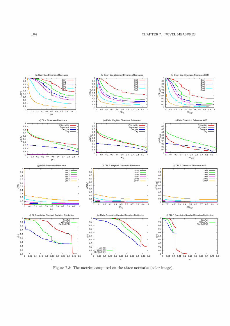
104 CHAPTER 7. NOVEL MEASURES
0
0.1
0.2
0.3
0.4
0.5
0.6
0.7
0.8
0.9
1
0 0.1 0.2 0.3 0.4 0.5 0.6 0.7 0.8 0.9 1
p(D
R)
DR
(a) Query Log Dimension Relevance
Bin1Bin2Bin3Bin4Bin5Bin6
0
0.1
0.2
0.3
0.4
0.5
0.6
0.7
0.8
0.9
1
0 0.1 0.2 0.3 0.4 0.5 0.6 0.7 0.8 0.9 1
p(D
RW
)
DRW
(b) Query Log Weighted Dimension Relevance
Bin1Bin2Bin3Bin4Bin5Bin6
0
0.1
0.2
0.3
0.4
0.5
0.6
0.7
0.8
0.9
1
0 0.1 0.2 0.3 0.4 0.5 0.6 0.7 0.8 0.9 1
p(D
RX
OR
)
DRXOR
(c) Query Log Dimension Relevance XOR
Bin1Bin2Bin3Bin4Bin5Bin6
0
0.1
0.2
0.3
0.4
0.5
0.6
0.7
0.8
0.9
1
0 0.1 0.2 0.3 0.4 0.5 0.6 0.7 0.8 0.9 1
p(D
R)
DR
(d) Flickr Dimension Relevance
FriendshipComment
FavoriteTag
0
0.1
0.2
0.3
0.4
0.5
0.6
0.7
0.8
0.9
1
0 0.1 0.2 0.3 0.4 0.5 0.6 0.7 0.8 0.9 1
p(D
RW
)
DRW
(e) Flickr Weighted Dimension Relevance
FriendshipComment
FavoriteTag
0
0.1
0.2
0.3
0.4
0.5
0.6
0.7
0.8
0.9
1
0 0.1 0.2 0.3 0.4 0.5 0.6 0.7 0.8 0.9 1
p(D
RX
OR
)DRXOR
(f) Flickr Dimension Relevance XOR
FriendshipComment
FavoriteTag
0
0.1
0.2
0.3
0.4
0.5
0.6
0.7
0.8
0.9
1
0 0.1 0.2 0.3 0.4 0.5 0.6 0.7 0.8 0.9 1
p(D
R)
DR
(g) DBLP Dimension Relevance
198219871992199720022007
0
0.1
0.2
0.3
0.4
0.5
0.6
0.7
0.8
0.9
1
0 0.1 0.2 0.3 0.4 0.5 0.6 0.7 0.8 0.9 1
p(D
RW
)
DRW
(h) DBLP Weighted Dimension Relevance
198219871992199720022007
0
0.1
0.2
0.3
0.4
0.5
0.6
0.7
0.8
0.9
1
0 0.1 0.2 0.3 0.4 0.5 0.6 0.7 0.8 0.9 1
p(D
RX
OR
)
DRXOR
(i) DBLP Dimension Relevance XOR
198219871992199720022007
0.1
0.2
0.3
0.4
0.5
0.6
0.7
0.8
0.9
1
0 0.05 0.1 0.15 0.2 0.25 0.3 0.35 0.4 0.45 0.5
p(σ
)
σ
(j) QL Cumulative Standard Deviation Distribution
DimRelWDimRel
DimRelXOR
0
0.1
0.2
0.3
0.4
0.5
0.6
0.7
0.8
0.9
1
0 0.05 0.1 0.15 0.2 0.25 0.3 0.35 0.4 0.45 0.5
p(σ
)
σ
(k) Flickr Cumulative Standard Deviation Distribution
DimRelWDimRel
DimRelXOR 0
0.1
0.2
0.3
0.4
0.5
0.6
0.7
0.8
0.9
1
0 0.05 0.1 0.15 0.2 0.25 0.3 0.35 0.4 0.45 0.5
p(σ
)
σ
(l) DBLP Cumulative Standard Deviation Distribution
DimRelWDimRel
DimRelXOR
Figure 7.3: The metrics computed on the three networks (color image).
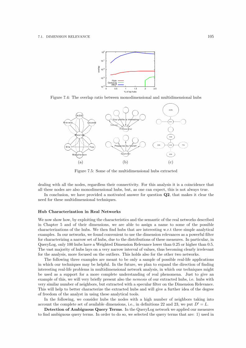
7.1. DIMENSION RELEVANCE 105
10-4
10-3
10-2
10-1
100
0 0.5 1 1.5 2 2.5
ove
rla
p
% of top hubs
FlickrQueryLog
DBLP
Figure 7.4: The overlap ratio between monodimensional and multidimensional hubs
(a) (b) (c)
Figure 7.5: Some of the multidimensional hubs extracted
dealing with all the nodes, regardless their connectivity. For this analysis it is a coincidence thatall these nodes are also monodimensional hubs, but, as one can expect, this is not always true.
In conclusion, we have provided a motivated answer for question Q2, that makes it clear theneed for these multidimensional techniques.
Hub Characterization in Real Networks
We now show how, by exploiting the characteristics and the semantic of the real networks describedin Chapter 5 and of their dimensions, we are able to assign a name to some of the possiblecharacterizations of the hubs. We then find hubs that are interesting w.r.t three simple analyticalexamples. In our networks, we found convenient to use the dimension relevances as a powerful filterfor characterizing a narrow set of hubs, due to the distributions of these measures. In particular, inQueryLog, only 100 hubs have a Weighted Dimension Relevance lower than 0.25 or higher than 0.5.The vast majority of hubs lays on a very narrow interval of values, thus becoming clearly irrelevantfor the analysis, more focused on the outliers. This holds also for the other two networks.
The following three examples are meant to be only a sample of possible real-life applicationsin which our techniques may be helpful. In the future, we plan to expand the direction of findinginteresting real-life problems in multidimensional network analysis, in which our techniques mightbe used as a support for a more complete understanding of real phenomena. Just to give anexample of this, we will very briefly present also the nemesis of our extracted hubs, i.e. hubs withvery similar number of neighbors, but extracted with a specular filter on the Dimension Relevance.This will help to better characterize the extracted hubs and will give a further idea of the degreeof freedom of the analyst in using these analytical tools.
In the following, we consider hubs the nodes with a high number of neighbors taking intoaccount the complete set of available dimensions, i.e., in definitions 22 and 23, we put D′ = L.
Detection of Ambiguous Query Terms. In the QueryLog network we applied our measuresto find ambiguous query terms. In order to do so, we selected the query terms that are: 1) used in
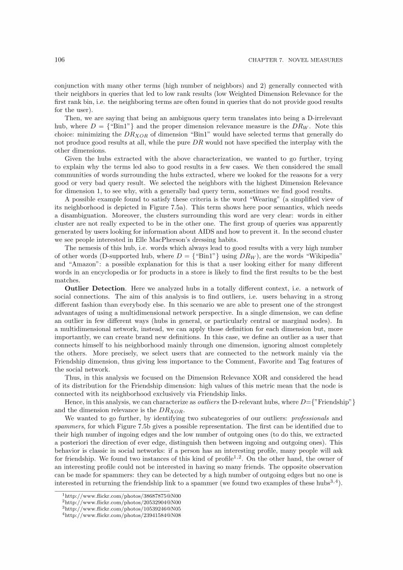
106 CHAPTER 7. NOVEL MEASURES
conjunction with many other terms (high number of neighbors) and 2) generally connected withtheir neighbors in queries that led to low rank results (low Weighted Dimension Relevance for thefirst rank bin, i.e. the neighboring terms are often found in queries that do not provide good resultsfor the user).
Then, we are saying that being an ambiguous query term translates into being a D-irrelevanthub, where D = {“Bin1”} and the proper dimension relevance measure is the DRW . Note thischoice: minimizing the DRXOR of dimension “Bin1” would have selected terms that generally donot produce good results at all, while the pure DR would not have specified the interplay with theother dimensions.
Given the hubs extracted with the above characterization, we wanted to go further, tryingto explain why the terms led also to good results in a few cases. We then considered the smallcommunities of words surrounding the hubs extracted, where we looked for the reasons for a verygood or very bad query result. We selected the neighbors with the highest Dimension Relevancefor dimension 1, to see why, with a generally bad query term, sometimes we find good results.
A possible example found to satisfy these criteria is the word “Wearing” (a simplified view ofits neighborhood is depicted in Figure 7.5a). This term shows here poor semantics, which needsa disambiguation. Moreover, the clusters surrounding this word are very clear: words in eithercluster are not really expected to be in the other one. The first group of queries was apparentlygenerated by users looking for information about AIDS and how to prevent it. In the second clusterwe see people interested in Elle MacPherson’s dressing habits.
The nemesis of this hub, i.e. words which always lead to good results with a very high numberof other words (D-supported hub, where D = {“Bin1”} using DRW ), are the words “Wikipedia”and “Amazon”: a possible explanation for this is that a user looking either for many differentwords in an encyclopedia or for products in a store is likely to find the first results to be the bestmatches.
Outlier Detection. Here we analyzed hubs in a totally different context, i.e. a network ofsocial connections. The aim of this analysis is to find outliers, i.e. users behaving in a strongdifferent fashion than everybody else. In this scenario we are able to present one of the strongestadvantages of using a multidimensional network perspective. In a single dimension, we can definean outlier in few different ways (hubs in general, or particularly central or marginal nodes). Ina multidimensional network, instead, we can apply those definition for each dimension but, moreimportantly, we can create brand new definitions. In this case, we define an outlier as a user thatconnects himself to his neighborhood mainly through one dimension, ignoring almost completelythe others. More precisely, we select users that are connected to the network mainly via theFriendship dimension, thus giving less importance to the Comment, Favorite and Tag features ofthe social network.
Thus, in this analysis we focused on the Dimension Relevance XOR and considered the headof its distribution for the Friendship dimension: high values of this metric mean that the node isconnected with its neighborhood exclusively via Friendship links.
Hence, in this analysis, we can characterize as outliers the D-relevant hubs, whereD={”Friendship”}and the dimension relevance is the DRXOR.
We wanted to go further, by identifying two subcategories of our outliers: professionals andspammers, for which Figure 7.5b gives a possible representation. The first can be identified due totheir high number of ingoing edges and the low number of outgoing ones (to do this, we extracteda posteriori the direction of ever edge, distinguish then between ingoing and outgoing ones). Thisbehavior is classic in social networks: if a person has an interesting profile, many people will askfor friendship. We found two instances of this kind of profile1,2. On the other hand, the owner ofan interesting profile could not be interested in having so many friends. The opposite observationcan be made for spammers: they can be detected by a high number of outgoing edges but no one isinterested in returning the friendship link to a spammer (we found two examples of these hubs3,4).
1http://www.flickr.com/photos/38687875@N002http://www.flickr.com/photos/20532904@N003http://www.flickr.com/photos/10539246@N054http://www.flickr.com/photos/23941584@N08

7.1. DIMENSION RELEVANCE 107
As nemesis (D-unsupported hubs, where D={ ”Friendship”} and using DRXOR), we foundthree profiles5,6,7. All these profile presented, at the time of the download of the network, avery high number of neighbors and no one exclusively through the Friendship dimension: at themoment of writing this paper, all the profiles are closed. Therefore, the nemesis of both spammersand professionals are the quitters (and this is really interesting in the perspective of the serviceproviders).
Analyzing Temporal Behaviors. In this section, we go beyond the theory presented so far.Consider definitions 22 and 23. It is clear that real networks might express rich semantic, andthat even powerful tools and characterizations as defined so far could not cover the complete set ofanalysis that one might want to perform. In this perspective, we want to show how, by substitutingthe usage of the DRs in the two mentioned definitions with any of the possible aggregates computedon their values, it is possible to expand the class of phenomena that can be studied with our tools.
In this context, an interesting application of our approach is to analyze the temporal behaviorof multidimensional hubs on evolving networks. In this section we show the results obtained onDBLP-Y, whose dimensions are the years of publications. The specific object of our analysis isto find authors of scientific papers who tend to change the authors with whom they collaboratepossibly every year. Note that we are not focusing on just new collaborations, but we want alsoto see the old ones to disappear. In order to do so, we found hubs v maximizing the number ofdimensions d for which DRXOR(v, d) > 0 (maximizing this value means maximizing the numberof years in which the author had collaborations that took place only in a specific year and not inothers).
In this scenario then, we call then dynamic researchers the D-relevant hubs v, where D = L(where L contains all the years) and, instead of the any of the simple DRs, we maximize |{d :DRXOR(v, d) > 0}|.
Figure 7.5c reports two representations of hubs extracted in this way: the hubs behaving as H1and the ones behaving as H2. To be more precise, a deeper classification among them might beperformed by looking also at the standard deviation of the DRXOR computed in all the dimensions.The example H2 in the right of that Figure, in fact, represents a hub minimizing the standarddeviation. H1 hubs are collaborators in high effort publications such as books (such as Maxine D.Brown or Steffen Schulze-Kremer); while H2 hubs are authors who tend work with many differentpeople, rarely keeping these collaborations alive, such as Ming Xu or Jakob Nielsen.
Finally, if we minimize the DRXOR(v, d) we find the nemesis of these hubs. The list of thesehubs includes many relevant names in Computer Science: Allan Borodin, Richard M. Karp, RobertEndre Tarjan, Godfried T. Toussaint, and Jeffrey D. Ullman fall in this category.
To conclude the analysis in this section we would like to sum up our final remarks.
We applied our scalable methodology to large real networks and showed that such hubs do existand they can be found and studied by using our measures of interplay of the different dimensions.Moreover, our measures allow to discover and quantify the importance of every single dimensionabove the others.
Many other questions on multidimensional network hubs remain unanswered, and call for fur-ther research; we mention two such lines briefly here.
First, we did not consider, in our approach, the possible structure or semantics of the specificset of dimensions under analysis: each different dimension is a distinct categorical value, and usedas such in the multidimensional measures; however, such dimension values can be meaningfullysorted (as, e.g., in the QueryLog network, where dimensions are associated to quality levels) ormay have a temporal or spatial semantics (as, e.g., in the DBLP-Y network, where dimensions areassociated to years). How can our measures be extended to fully exploit this additional structure?
Second, it would be interesting to devise a generalized query framework for the discoveryand analysis of hubs in multidimensional networks, based on the proposed measures, capableof supporting the analyst in expressing the desired queries (e.g., top-k hubs according to some
5http://www.flickr.com/photos/21700048@N046http://www.flickr.com/photos/22045276@N007http://www.flickr.com/photos/53654438@N00
108 CHAPTER 7. NOVEL MEASURES
specified hubbiness and relevance constraints), in finding appropriate parameters and thresholdsfor the involved measures on the basis of the available network data.
7.2 Dimension Correlation
In this section we present a second class of measures that makes sense only in multidimensionalnetworks. An interesting question in multidimensional networks involves the investigation whethera couple or a set of different relations is actually influencing or not each other. In a social network,being friends is probably a strong prerequisite to the communication relation, i.e. sending eachother messages. To be able to quantify this “correlation” is our aim. Naturally, this class ofmeasure is called “Dimension Correlation”. We firstly provide a general formulation for this classof measures. Then, we are interested in providing a scenario in which Dimension Correlationmeasures show their analytic usefulness. We chose to avoid social network analysis in its puresense by using a very particular definition of dimension for our networks. In fact, what we analyzeis the temporal evolution of several different evolving networks. In this way, we are able to showthat Dimension Correlation, and multidimensional network analysis in general, is able to includein its scope also temporal analysis. In particular, Dimension Correlation is a key element to detectperiods in network evolution via a hierarchical clustering technique.
Dimension Correlation class of measures is composed by the following two definitions of corre-lation. Intuitively, they give an idea of how redundant are two dimensions, if we can expect twonodes to be connected by a given dimension when they are found to be connected by a specific one,and so on. They are based on the Jaccard coefficient, computed between two (sets of) dimensionsusing in the first case the sets of nodes (Node Correlation) and in the second case the sets ofconnected couples (Edge Correlation).
Definition 24 (Node Correlation) Let d1, d2 ∈ D be two dimensions of a network G = (V,E,D).The Node Correlation is the function ρnode : D ×D → [0, 1] defined as
ρnode(d1, d2) =|Vd1 ∩ Vd2 ||Vd1 ∪ Vd2 |
where Vd1 and Vd2 denote the nodes belonging to dimensions d1 and d2, respectively. It computesthe ratio of nodes belonging to both the dimensions over the total number of nodes belonging to atleast one of them. �
Definition 25 (Edge Correlation) Let d1, d2 ∈ D be two dimensions of a network G = (V,E,D).The Edge Correlation is the function ρedge : D ×D → [0, 1] defined as
ρedge(d1, d2) =|Ed1 ∩ Ed2 ||Ed1 ∪ Ed2 |
where Ed1 and Ed2 denote the edges belonging to dimensions d1 and d2, respectively. It computesthe ratio of edges belonging to both the dimensions over the total number of edges belonging to atleast one of them. �
We now present one of the possible applications of these two measures, namely the detectionof eras in evolving networks.
7.2.1 Finding Eras in Evolving networks
We are given an evolving network G, whose evolution is described by a temporally ordered sequenceof temporal snapshots T = {t1, t2, . . . , tn}, where ti represents the i-th snapshot. Without any lossof generality, G is represented by a multidimensional network, whose dimensions represent each onea single snapshot. T can be either defined on the sets of nodes, i.e. each snapshot ti is represented
7.2. DIMENSION CORRELATION 109
by the set of nodes involved, or on the sets of edges, i.e. each snapshot is represented by the set ofedges in it.
Based on a distance function f : (ti, ti+1)→]−∞,+∞[, we want to find a hierarchical clusteringon T , returning clusters Ci = {tj , . . . , tj+k}, with j ≥ 1, and 0 ≤ k ≤ n− j.
Each cluster represents then an era of evolution. Due to the global evolution of real-life net-works, we do allow alterations of the structure of the network among snapshots of the same cluster,as long as they follow a constant trend. As soon as this trend changes, we want to set the corre-sponding snapshot as the first of a new era, i.e. a turning point. The stronger is the change, thehigher should be the dissimilarity of that snapshot with the previous one. The definition of thedissimilarity function should reflect this intuition.
We then want to assign to each cluster Ci a set of labels describing the represented era. Thisstep adds a semantic dimension to our framework.
To provide a solution to the general problem presented we need to: (a) define and compute adissimilarity measure on the temporal snapshots; (b) merge the snapshots into clusters; (c) assignsemantics to the clusters based on frequent labels.
(A) Dissimilarity. To perform clustering, the first step is to define a measure of dissimilarityamong elements that we want to cluster. As stated before, we use the Dimension Correlation classof measures between each snapshot of the network. In a generic network, we can easily apply boththe Node and the Edge Correlation, where each dimension corresponds to a temporal snapshot ofthe network. The coefficient would then tell us how each snapshot is correlated to the previousone, helping in detecting turning points along the evolution. As we show later in the paper,clustering temporal snapshots actually corresponds to perform a segmentation of the sequenceof the snapshots, thus we are interested only in computing the Dimension Correlation for everypair of consecutive snapshots. Note that the Dimension Correlation could be computed betweenany pair of dimensions, thus corresponding also to non-consecutive snapshots. We are, however,not interested in a two-dimensional clustering of its values, which would lead to eras formed bypotentially non-consecutive years; rather we want to perform monodimensional clustering of thetemporal evolution of the Dimension Correlation. In the following section we also show how, forthe networks we use, this intuition is also supported by the values of the Dimension Correlation:every snapshot is more correlated with its precedent and consecutive ones, than with any otherelse, justifying eras formed by consecutive snapshots.
Many real-life networks are characterized by a global evolutionary trend, then if we plot theDimension Correlation for each snapshot, either the Node or the Edge definition, we shall seea global trend, characterized by an almost constant slope of the Dimension Correlation plot,alternated by (moderate to high) changes of this slope. An immediate way to define startingpoint of new eras is to detect the snapshots corresponding to these changes. This could be doneby computing the second derivative of the Dimension Correlation and finding values different fromzero. However, the Dimension Correlation is continuous but not derivable exactly in the points weneed. To overcome this problem, we consider an approximation of the second derivative definedas follows. We take triples of consecutive years, and trace the segment that has, as endpoints, theDimension Correlation computed for the first and the third snapshot. If the middle point is distantfrom the segment, the corresponding snapshot should be considered as the start of a new era. TheEuclidean distance between the middle point and the segment also gives us a quantitative analysisof how important is the change: the higher the distance, the stronger the change.
Formally, given a temporal snapshot tj , we define the following measure:
sN (tj) =|cN (tj)− (m× j)− q|√
(1 + (m2))
where m =cN (tj−1)−cN (tj+1)
tj−1−tj+1, q = (−(j + 1)×m) + cN (tj+1), and cN (tk) = |Nk−1∩Nk|
|Nk−1∪Nk| is the Node
Correlation.
Defining sE , which is the counterpart computed on the set of edges, requires to consider cEinstead of cN , where cE is the Edge Correlation.
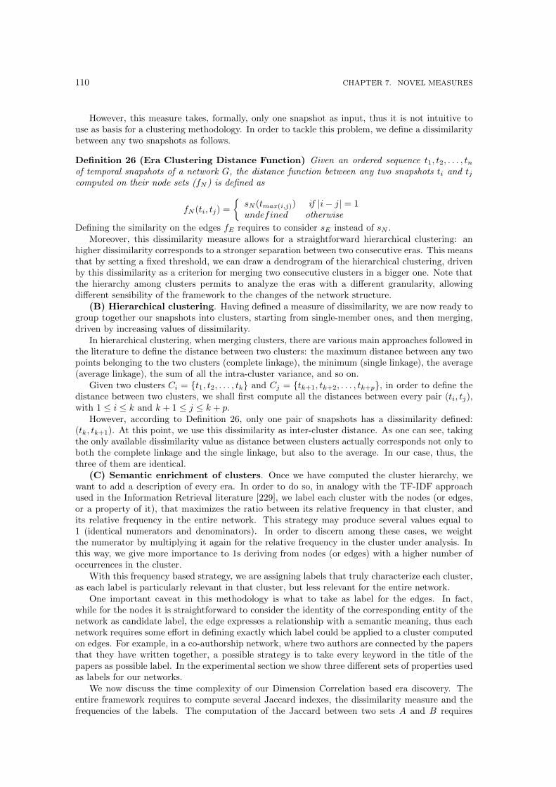
110 CHAPTER 7. NOVEL MEASURES
However, this measure takes, formally, only one snapshot as input, thus it is not intuitive touse as basis for a clustering methodology. In order to tackle this problem, we define a dissimilaritybetween any two snapshots as follows.
Definition 26 (Era Clustering Distance Function) Given an ordered sequence t1, t2, . . . , tnof temporal snapshots of a network G, the distance function between any two snapshots ti and tjcomputed on their node sets (fN ) is defined as
fN (ti, tj) =
{sN (tmax(i,j)) if |i− j| = 1undefined otherwise
Defining the similarity on the edges fE requires to consider sE instead of sN .Moreover, this dissimilarity measure allows for a straightforward hierarchical clustering: an
higher dissimilarity corresponds to a stronger separation between two consecutive eras. This meansthat by setting a fixed threshold, we can draw a dendrogram of the hierarchical clustering, drivenby this dissimilarity as a criterion for merging two consecutive clusters in a bigger one. Note thatthe hierarchy among clusters permits to analyze the eras with a different granularity, allowingdifferent sensibility of the framework to the changes of the network structure.
(B) Hierarchical clustering. Having defined a measure of dissimilarity, we are now ready togroup together our snapshots into clusters, starting from single-member ones, and then merging,driven by increasing values of dissimilarity.
In hierarchical clustering, when merging clusters, there are various main approaches followed inthe literature to define the distance between two clusters: the maximum distance between any twopoints belonging to the two clusters (complete linkage), the minimum (single linkage), the average(average linkage), the sum of all the intra-cluster variance, and so on.
Given two clusters Ci = {t1, t2, . . . , tk} and Cj = {tk+1, tk+2, . . . , tk+p}, in order to define thedistance between two clusters, we shall first compute all the distances between every pair (ti, tj),with 1 ≤ i ≤ k and k + 1 ≤ j ≤ k + p.
However, according to Definition 26, only one pair of snapshots has a dissimilarity defined:(tk, tk+1). At this point, we use this dissimilarity as inter-cluster distance. As one can see, takingthe only available dissimilarity value as distance between clusters actually corresponds not only toboth the complete linkage and the single linkage, but also to the average. In our case, thus, thethree of them are identical.
(C) Semantic enrichment of clusters. Once we have computed the cluster hierarchy, wewant to add a description of every era. In order to do so, in analogy with the TF-IDF approachused in the Information Retrieval literature [229], we label each cluster with the nodes (or edges,or a property of it), that maximizes the ratio between its relative frequency in that cluster, andits relative frequency in the entire network. This strategy may produce several values equal to1 (identical numerators and denominators). In order to discern among these cases, we weightthe numerator by multiplying it again for the relative frequency in the cluster under analysis. Inthis way, we give more importance to 1s deriving from nodes (or edges) with a higher number ofoccurrences in the cluster.
With this frequency based strategy, we are assigning labels that truly characterize each cluster,as each label is particularly relevant in that cluster, but less relevant for the entire network.
One important caveat in this methodology is what to take as label for the edges. In fact,while for the nodes it is straightforward to consider the identity of the corresponding entity of thenetwork as candidate label, the edge expresses a relationship with a semantic meaning, thus eachnetwork requires some effort in defining exactly which label could be applied to a cluster computedon edges. For example, in a co-authorship network, where two authors are connected by the papersthat they have written together, a possible strategy is to take every keyword in the title of thepapers as possible label. In the experimental section we show three different sets of properties usedas labels for our networks.
We now discuss the time complexity of our Dimension Correlation based era discovery. Theentire framework requires to compute several Jaccard indexes, the dissimilarity measure and thefrequencies of the labels. The computation of the Jaccard between two sets A and B requires
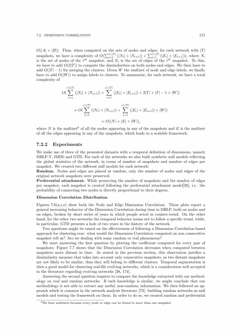
7.2. DIMENSION CORRELATION 111
O(|A| + |B|). Thus, when computed on the sets of nodes and edges, for each network with |T |snapshots, we have a complexity of O(
∑i<|T |i=1 (|Ni|+ |Ni+1|) +
∑i<|T |i=1 (|Ei|+ |Ei+1|)), where Ni
is the set of nodes of the ith snapshot, and Ei is the set of edges of the ith snapshot. To this,we have to add O(2|T |) to compute the dissimilarities on both nodes and edges. We then have toadd O(|T | − 1) for merging the clusters. Given W the multiset of node and edge labels, we finallyhave to add O(|W |) to assign labels to clusters. To summarize, for each network, we have a totalcomplexity of
O(
i<|T |∑i=1
(|Ni|+ |Ni+1|) +
i<|T |∑i=1
(|Ei|+ |Ei+1|) + 2|T |+ |T | − 1 + |W |)
= O(
i<|T |∑i=1
(|Ni|+ |Ni+1|) +
i<|T |∑i=1
(|Ei|+ |Ei+1|) + |W |)
= O(|N |+ |E|+ |W |),
where N is the multiset8 of all the nodes appearing in any of the snapshots and E is the multisetof all the edges appearing in any of the snapshots, which leads to a scalable framework.
7.2.2 Experiments
We make use of three of the presented datasets with a temporal definition of dimensions, namelyDBLP-Y, IMDb and GTD. For each of the networks we also built synthetic null models reflectingthe global statistics of the network, in terms of number of snapshots and number of edges persnapshot. We created two different null models for each network:Random. Nodes and edges are placed at random, only the number of nodes and edges of theoriginal network snapshots were preserved.Preferential attachment. While preserving the number of snapshots and the number of edgesper snapshot, each snapshot is created following the preferential attachment model[30], i.e. theprobability of connecting two nodes is directly proportional to their degrees.
Dimension Correlation Distribution
Figures 7.6(a,c,e) show both the Node and Edge Dimension Correlation. These plots report ageneral increasing behavior of the Dimension Correlation during time in DBLP, both on nodes andon edges, broken by short series of years in which people acted in counter-trend. On the otherhand, for the other two networks the temporal behavior seems not to follow a specific trend, while,in particular, GTD presents a hole of two years in the history of the network.
Two questions might be raised on the effectiveness of following a Dimension Correlation-basedapproach for clustering eras: what would the Dimension Correlation computed on non consecutivesnapshot tell us? Are we dealing with some random or real phenomena?
We start answering the first question by plotting the coefficient computed for every pair ofsnapshots: Figure 7.7 shows that the Dimension Correlation decreases when computed betweensnapshots more distant in time. As stated in the previous section, this observation justifies adissimilarity measure that takes into account only consecutive snapshots, as two distant snapshotsare not likely to be similar, thus they will belong to different clusters. Temporal segmentation isthen a good model for clustering real-life evolving networks, which is a consideration well acceptedin the literature regarding evolving networks [38, 174].
Answering the second question requires to compare the knowledge extracted with our method-ology on real and random networks. If such knowledge is similar, we might conclude that ourmethodology is not able to extract any useful, non-random, information. We then followed an ap-proach which is common in the network analysis literature [73]: building random networks as nullmodels and testing the framework on them. In order to do so, we created random and preferential
8We have multisets because every node or edge can be found in more than one snapshot
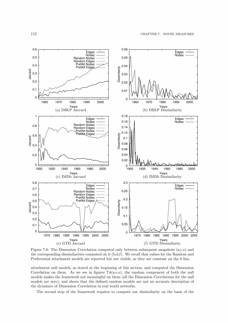
112 CHAPTER 7. NOVEL MEASURES
0
0.1
0.2
0.3
0.4
0.5
0.6
1960 1970 1980 1990 2000
Ja
cca
rd
Years
EdgesNodes
Random NodesRandom Edges
PrefAtt NodesPrefAtt Edges
0
0.01
0.02
0.03
0.04
0.05
0.06
1960 1970 1980 1990 2000
Dis
sim
ilarity
Years
EdgesNodes
(a) DBLP Jaccard (b) DBLP Dissimilarity
0
0.2
0.4
0.6
0.8
1
1900 1920 1940 1960 1980 2000
Ja
cca
rd
Years
EdgesNodes
Random NodesRandom Edges
PrefAtt NodesPrefAtt Edges
0
0.02
0.04
0.06
0.08
0.1
0.12
0.14
0.16
0.18
1900 1920 1940 1960 1980 2000
Dis
sim
ilarity
Years
EdgesNodes
(c) IMDb Jaccard (d) IMDb Dissimilarity
0
0.1
0.2
0.3
0.4
0.5
0.6
0.7
0.8
1975 1980 1985 1990 1995 2000 2005
Ja
cca
rd
Years
EdgesNodes
Random NodesRandom Edges
PrefAtt NodesPrefAtt Edges
0
0.05
0.1
0.15
0.2
0.25
0.3
1975 1980 1985 1990 1995 2000 2005
Dis
sim
ilarity
Years
EdgesNodes
(e) GTD Jaccard (f) GTD Dissimilarity
Figure 7.6: The Dimension Correlation computed only between subsequent snapshots (a,c,e) andthe corresponding dissimilarities computed on it (b,d,f). We recall that values for the Random andPreferential attachment models are reported but not visible, as they are constant on the 0 line.
attachment null models, as stated at the beginning of this section, and computed the DimensionCorrelation on them. As we see in figures 7.6(a,c,e), the random component of both the nullmodels makes the framework not meaningful on them (all the Dimension Correlations for the nullmodels are zero), and shows that the defined random models are not an accurate description ofthe dynamics of Dimension Correlation in real world networks.
The second step of the framework requires to compute our dissimilarity on the basis of the
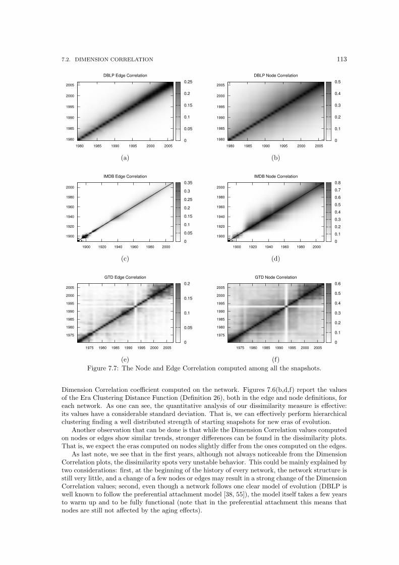
7.2. DIMENSION CORRELATION 113
DBLP Edge Correlation
1980 1985 1990 1995 2000 2005
1980
1985
1990
1995
2000
2005
0
0.05
0.1
0.15
0.2
0.25
DBLP Node Correlation
1980 1985 1990 1995 2000 2005
1980
1985
1990
1995
2000
2005
0
0.1
0.2
0.3
0.4
0.5
(a) (b)
IMDB Edge Correlation
1900 1920 1940 1960 1980 2000
1900
1920
1940
1960
1980
2000
0
0.05
0.1
0.15
0.2
0.25
0.3
0.35
IMDB Node Correlation
1900 1920 1940 1960 1980 2000
1900
1920
1940
1960
1980
2000
0
0.1
0.2
0.3
0.4
0.5
0.6
0.7
0.8
(c) (d)
GTD Edge Correlation
1975 1980 1985 1990 1995 2000 2005
1975
1980
1985
1990
1995
2000
2005
0
0.05
0.1
0.15
0.2
GTD Node Correlation
1975 1980 1985 1990 1995 2000 2005
1975
1980
1985
1990
1995
2000
2005
0
0.1
0.2
0.3
0.4
0.5
0.6
(e) (f)
Figure 7.7: The Node and Edge Correlation computed among all the snapshots.
Dimension Correlation coefficient computed on the network. Figures 7.6(b,d,f) report the valuesof the Era Clustering Distance Function (Definition 26), both in the edge and node definitions, foreach network. As one can see, the quantitative analysis of our dissimilarity measure is effective:its values have a considerable standard deviation. That is, we can effectively perform hierarchicalclustering finding a well distributed strength of starting snapshots for new eras of evolution.
Another observation that can be done is that while the Dimension Correlation values computedon nodes or edges show similar trends, stronger differences can be found in the dissimilarity plots.That is, we expect the eras computed on nodes slightly differ from the ones computed on the edges.
As last note, we see that in the first years, although not always noticeable from the DimensionCorrelation plots, the dissimilarity spots very unstable behavior. This could be mainly explained bytwo considerations: first, at the beginning of the history of every network, the network structure isstill very little, and a change of a few nodes or edges may result in a strong change of the DimensionCorrelation values; second, even though a network follows one clear model of evolution (DBLP iswell known to follow the preferential attachment model [38, 55]), the model itself takes a few yearsto warm up and to be fully functional (note that in the preferential attachment this means thatnodes are still not affected by the aging effects).

114 CHAPTER 7. NOVEL MEASURES
1956
1957
1958
1959
1960
1961
1962
1963
1964
1965
1966
1967
1968
1969
1970
1971
1972
1973
1974
1975
1976
1977
1978
1979
1980
1981
1982
1983
1984
1985
1986
1987
1988
1989
1990
1991
1992
1993
1994
1995
1996
1997
1998
1999
2000
2001
2002
2003
2004
2005
2006
Years
(a) Edge eras
1956
1957
1958
1959
1960
1961
1962
1963
1964
1965
1966
1967
1968
1969
1970
1971
1972
1973
1974
1975
1976
1977
1978
1979
1980
1981
1982
1983
1984
1985
1986
1987
1988
1989
1990
1991
1992
1993
1994
1995
1996
1997
1998
1999
2000
2001
2002
2003
2004
2005
2006
Years
(b) Node eras
Figure 7.8: Eras on both edge and node evolutions in DBLP
We then started to compute the clusters on the sequences of temporal snapshots. We startedfrom clusters containing only one year and then, driven by the dissimilarity values computed in
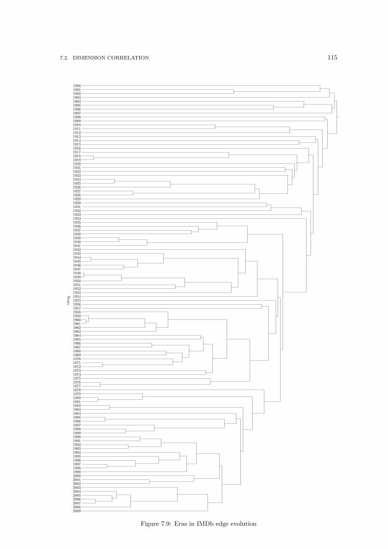
7.2. DIMENSION CORRELATION 115
19001901190219031904190519061907190819091910191119121913191419151916191719181919192019211922192319241925192619271928192919301931193219331934193519361937193819391940194119421943194419451946194719481949195019511952195319541955195619571958195919601961196219631964196519661967196819691970197119721973197419751976197719781979198019811982198319841985198619871988198919901991199219931994199519961997199819992000200120022003200420052006200720082009
Years
Figure 7.9: Eras in IMDb edge evolution
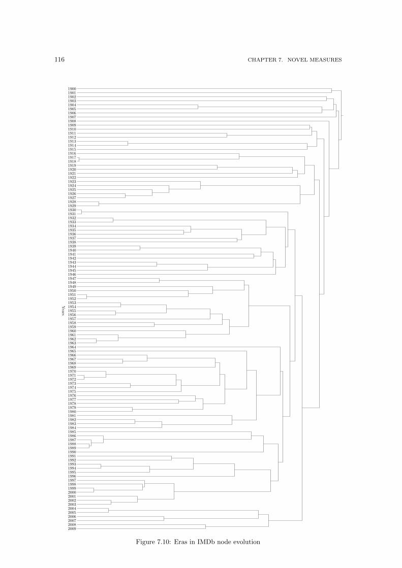
116 CHAPTER 7. NOVEL MEASURES
19001901190219031904190519061907190819091910191119121913191419151916191719181919192019211922192319241925192619271928192919301931193219331934193519361937193819391940194119421943194419451946194719481949195019511952195319541955195619571958195919601961196219631964196519661967196819691970197119721973197419751976197719781979198019811982198319841985198619871988198919901991199219931994199519961997199819992000200120022003200420052006200720082009
Years
Figure 7.10: Eras in IMDb node evolution
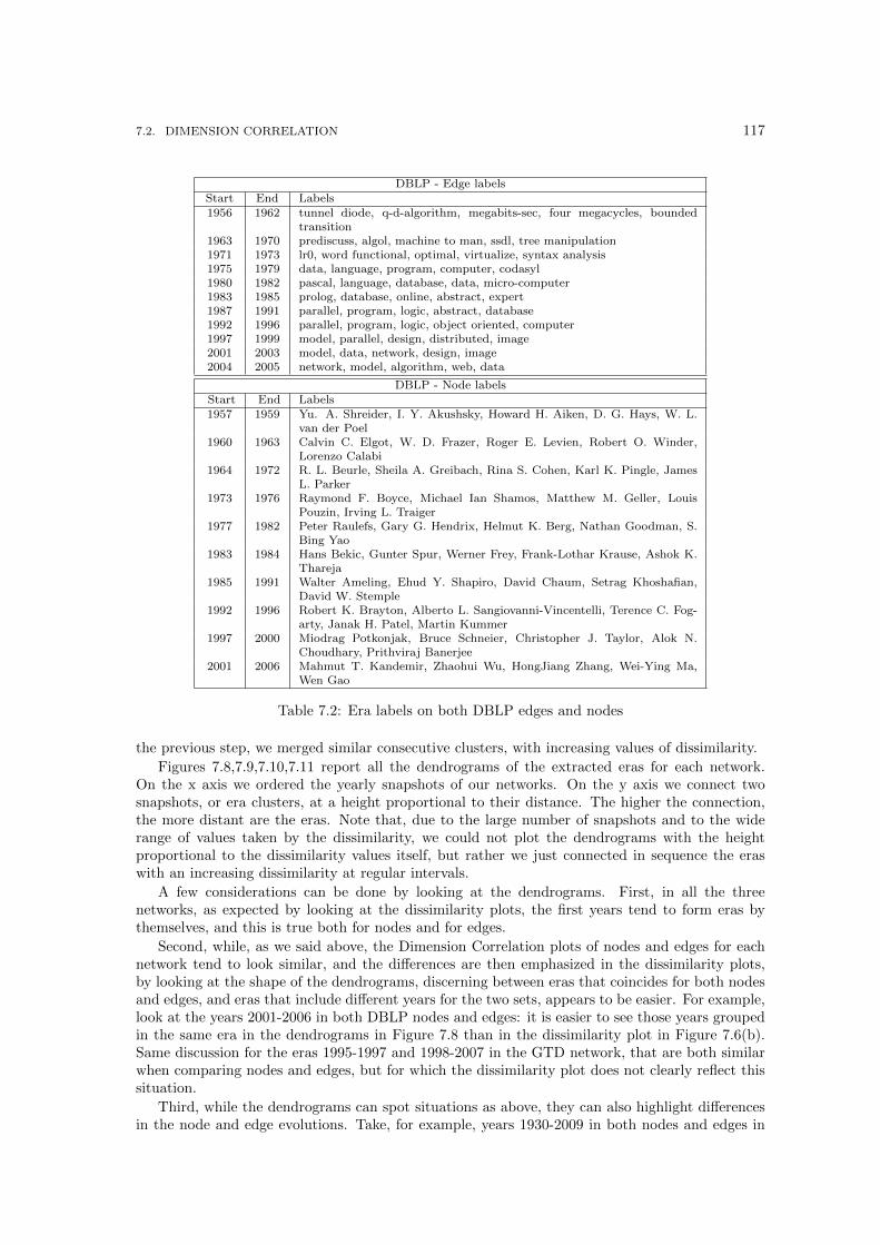
7.2. DIMENSION CORRELATION 117
DBLP - Edge labelsStart End Labels1956 1962 tunnel diode, q-d-algorithm, megabits-sec, four megacycles, bounded
transition1963 1970 prediscuss, algol, machine to man, ssdl, tree manipulation1971 1973 lr0, word functional, optimal, virtualize, syntax analysis1975 1979 data, language, program, computer, codasyl1980 1982 pascal, language, database, data, micro-computer1983 1985 prolog, database, online, abstract, expert1987 1991 parallel, program, logic, abstract, database1992 1996 parallel, program, logic, object oriented, computer1997 1999 model, parallel, design, distributed, image2001 2003 model, data, network, design, image2004 2005 network, model, algorithm, web, data
DBLP - Node labelsStart End Labels1957 1959 Yu. A. Shreider, I. Y. Akushsky, Howard H. Aiken, D. G. Hays, W. L.
van der Poel1960 1963 Calvin C. Elgot, W. D. Frazer, Roger E. Levien, Robert O. Winder,
Lorenzo Calabi1964 1972 R. L. Beurle, Sheila A. Greibach, Rina S. Cohen, Karl K. Pingle, James
L. Parker1973 1976 Raymond F. Boyce, Michael Ian Shamos, Matthew M. Geller, Louis
Pouzin, Irving L. Traiger1977 1982 Peter Raulefs, Gary G. Hendrix, Helmut K. Berg, Nathan Goodman, S.
Bing Yao1983 1984 Hans Bekic, Gunter Spur, Werner Frey, Frank-Lothar Krause, Ashok K.
Thareja1985 1991 Walter Ameling, Ehud Y. Shapiro, David Chaum, Setrag Khoshafian,
David W. Stemple1992 1996 Robert K. Brayton, Alberto L. Sangiovanni-Vincentelli, Terence C. Fog-
arty, Janak H. Patel, Martin Kummer1997 2000 Miodrag Potkonjak, Bruce Schneier, Christopher J. Taylor, Alok N.
Choudhary, Prithviraj Banerjee2001 2006 Mahmut T. Kandemir, Zhaohui Wu, HongJiang Zhang, Wei-Ying Ma,
Wen Gao
Table 7.2: Era labels on both DBLP edges and nodes
the previous step, we merged similar consecutive clusters, with increasing values of dissimilarity.
Figures 7.8,7.9,7.10,7.11 report all the dendrograms of the extracted eras for each network.On the x axis we ordered the yearly snapshots of our networks. On the y axis we connect twosnapshots, or era clusters, at a height proportional to their distance. The higher the connection,the more distant are the eras. Note that, due to the large number of snapshots and to the widerange of values taken by the dissimilarity, we could not plot the dendrograms with the heightproportional to the dissimilarity values itself, but rather we just connected in sequence the eraswith an increasing dissimilarity at regular intervals.
A few considerations can be done by looking at the dendrograms. First, in all the threenetworks, as expected by looking at the dissimilarity plots, the first years tend to form eras bythemselves, and this is true both for nodes and for edges.
Second, while, as we said above, the Dimension Correlation plots of nodes and edges for eachnetwork tend to look similar, and the differences are then emphasized in the dissimilarity plots,by looking at the shape of the dendrograms, discerning between eras that coincides for both nodesand edges, and eras that include different years for the two sets, appears to be easier. For example,look at the years 2001-2006 in both DBLP nodes and edges: it is easier to see those years groupedin the same era in the dendrograms in Figure 7.8 than in the dissimilarity plot in Figure 7.6(b).Same discussion for the eras 1995-1997 and 1998-2007 in the GTD network, that are both similarwhen comparing nodes and edges, but for which the dissimilarity plot does not clearly reflect thissituation.
Third, while the dendrograms can spot situations as above, they can also highlight differencesin the node and edge evolutions. Take, for example, years 1930-2009 in both nodes and edges in

118 CHAPTER 7. NOVEL MEASURES
IMDb, as reported in Figure 7.9 and 7.10. This era presents very different sub-eras when lookingat nodes or edges, and this is because of the different importance, given during time, to new nodesor new edges over old ones.
As last step in our framework, we computed the labels for each cluster obtained. We recall thatfor each cluster Ci we assign the set of the k labels maximizing the ratio between their frequencyin Ci and their frequency in the entire network. Tables 7.2, 7.3 and 7.4 report a few of the mostcharacterizing labels for some of the eras of each network. Due to the impressive number of totaleras and labels, we could not report all the labels for all the eras, but instead we chose, for eachnetwork a selection of interesting eras (covering the entire network history), and a selection of themost representative labels for them. The DBLP keywords were pre-processed using the Porter’sstemming algorithm [224].
We chose some relatively small eras in order to cover approximately the entire time span ofthe dataset. The start and end years of an era were selected where the inclusion of the following,or preceding, year would have caused the merging of two eras resulting in a selected period ofmany years not strongly correlated each other, according to the dendrogram. Verifying the labelsof the extracted eras provides two benefits: it is useful to evaluate our results, as we refer to fieldsin which there is a ground truth about periods, and may lead to novel points of view about thehistory of our data sources.
For DBLP, we present the labels for the node and edge eras in Table 7.2. It is possible tospot some interesting eras, such as the ALGOL era from 1963 (the year of one major revisionof ALGOL609) to 1970. In the 70s many popular programming languages were developed, suchas C (developed from 1969 to 197310), Prolog (which was born in 1972 from a project aimednot at producing a programming language but at processing natural languages [76]) and Pascal(standardized in 198311, and this might explain also its era from 1980 to 1982).
Interesting enough, from 2004 we are witnessing a brand new era, made of networks and theincreasing complexity of web technologies. Node era labels for DBLP let emerge some other keyresearch results: we can recognize the huge work made by David Chaum (1985-1991) in the field ofcryptography, the basis of the electronic currency system, culminating in 1990 with the foundationof his electronic cash company; another example is Raymond F. Boyce, a key researcher for thedevelopment of SQL [69], died in 1974.
For IMDb, we present the era labels in Table 7.3. It is possible to perform an analysis attwo different granularity levels. At a high level, one may notice that the keywords for periodsbefore 1975 are very specific and referring to precise concepts in movie history (such as the soundsynchronized to record, referring to the very first movies with sound, or heimatfilm, such as “Lassiecome home”), while after 1975 keywords are simpler and less specific (love, death, murder, blood).This is due to the fact that the keywords are user-assigned, thus very old movies are only watched(and tagged) by a niche of expert cinephiles, while the mass tags recent blockbusters. Note alsothat the vast majority of IMDb users are Western and particularly American, thus the keywordsare heavily unbalanced on Hollywood and European industry, disgreaging other filmographies suchas Japan, Hong Kong and the prolific Bollywood. At a lower level of granularity, our technique isable to spot actual eras or sub-eras of movie history, such as the “pre code” era (from 1930, theyear in which the Motion Picture Production Code was written, to 1933, when the code becomeeffectively enforced12).
In IMDb node eras we see the most prolific people in movie industry. Especially in latteryears, counter-intuitively, instead of finding movie stars, which are involved in leading roles in bigproductions (thus it is impossible for them to participate to more than 4-5 movies a year), we seeactors that are prolific in minor roles, or producers (Andreas Schmid, producer from 2004 of movieslike “The Punisher”, “Lord of war” and “Perfume: The Story of a Murderer”, before stopping hiscareer in 200713), directors (Peter Elfelt, very well known for many experimental documentary
9http://www.masswerk.at/algol60/report.htm10http://cm.bell-labs.com/cm/cs/who/dmr/chist.html11ISO 7185, http://www.pascal-central.com/iso7185.html12Mick LaSalle, “Complicated Women: Sex and Power in Pre-Code Hollywood”13http://www.imdb.com/name/nm1209077/
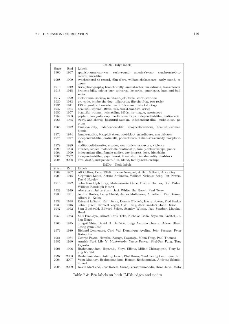
7.2. DIMENSION CORRELATION 119
IMDb - Edge labelsStart End Labels1900 1907 spanish-american-war, early-sound, america’s-cup, synchronized-to-
record, trick-film1908 1909 synchronized-to-record, film-d’art, william-shakespeare, early-sound, te-
deum1910 1912 trick-photography, broncho-billy, animal-actor, melodrama, law-enforcer1913 1915 broncho-billy, mister-jarr, universal-ike-series, americana, ham-and-bud-
series1917 1929 melodrama, society, mutt-and-jeff, fable, world-war-one1930 1933 pre-code, bimbo-the-dog, talkartoon, flip-the-frog, two-reeler1935 1941 1930s, gunfire, b-movie, beautiful-woman, stock-footage1942 1954 beautiful-woman, 1940s, usa, world-war-two, series1956 1957 beautiful-woman, heimatfilm, 1950s, mr-magoo, sportscope1958 1963 peplum, loopy-de-loop, modern-madcaps, independent-film, nudie-cutie1964 1965 swifty-and-shorty, beautiful-woman, independent-film, nudie-cutie, pe-
plum1966 1972 female-nudity, independent-film, spaghetti-western, beautiful-woman,
hippie1973 1974 female-nudity, blaxploitation, hoot-kloot, grindhouse, martial-arts1975 1977 independent-film, erotic-70s, poliziottesco, italian-sex-comedy, naziploita-
tion1979 1989 nudity, cult-favorite, murder, electronic-music-score, violence1990 1993 murder, sequel, male-female-relationship, family-relationships, police1994 1999 independent-film, female-nudity, gay-interest, love, friendship2000 2002 independent-film, gay-interest, friendship, female-nudity, flashback2004 2008 love, death, independent-film, blood, family-relationships
IMDb - Node labelsStart End Labels1902 1907 Alf Collins, Peter Elfelt, Lucien Nonguet, Arthur Gilbert, Alice Guy1909 1915 Siegmund Lubin, Arturo Ambrosio, William Nicholas Selig, Pat Powers,
David Horsley1916 1922 John Randolph Bray, Matsunosuke Onoe, Burton Holmes, Bud Fisher,
William Randolph Hearst1923 1929 Abe Stern, Julius Stern, Jack White, Hal Roach, Paul Terry1930 1931 Arthur Hurley, Leroy Shield, James Mulhauser, Amadee J. Van Beuren,
Albert H. Kelley1932 1938 Edward LeSaint, Earl Dwire, Dennis O’Keefe, Harry Bowen, Fred Parker1939 1946 John Tyrrell, Emmett Vogan, Cyril Ring, Jack Gardner, John Dilson1947 1952 Sam Buchwald, Edward Selzer, Stanley Wilson, Izzy Sparber, Marshall
Reed1953 1963 Milt Franklyn, Ahmet Tarik Teke, Nicholas Balla, Seymour Kneitel, Ju-
lian Biggs1966 1975 Sung-il Shin, David H. DePatie, Luigi Antonio Guerra, Adoor Bhasi,
Jeong-geun Jeon1976 1980 Richard Lemieuvre, Cyril Val, Dominique Aveline, John Seeman, Peter
Katadotis1981 1984 George Payne, Herschel Savage, Ilayaraja, Mona Fong, Paul Thomas1985 1990 Amrish Puri, Lily Y. Monteverde, Yunus Parvez, Shui-Fan Fung, Tony
Fajardo1991 1996 Brahmanandam, Ilayaraja, Floyd Elliott, Milind Chitragupth, Tony Le-
ung Ka Fai1997 2003 Brahmanandam, Johnny Lever, Phil Hawn, Yiu-Cheung Lai, Simon Lui2004 2007 Venu Madhav, Brahmanandam, Himesh Reshammiya, Andreas Schmid,
Suneel2008 2009 Kevin MacLeod, Jose Rosete, Suraaj Venjarammoodu, Brian Jerin, Moby
Table 7.3: Era labels on both IMDb edges and nodes
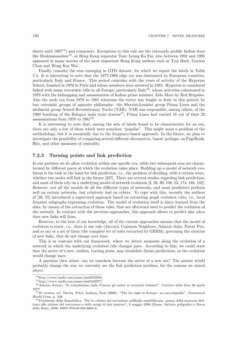
120 CHAPTER 7. NOVEL MEASURES
shorts until 190714) and composers. Exceptions to this rule are the extremely prolific Indian starslike Brahmanandam15, or Hong Kong superstar Tony Leung Ka Fai, who between 1991 and 1995appeared in many movies of the most important Hong Kong authors such as Tsui Hark, GordonChan and Wong Kar Wai.
Finally, consider the eras emerging in GTD dataset, for which we report the labels in Table7.4. It is interesting to note that the 1977-1983 edge era was dominated by European countries,particularly Italy and France. This period coincides with the years of activity of the HyperionSchool, founded in 1976 in Paris and whose members were arrested in 1983. Hyperion is consideredlinked with many terroristic cells in all Europe, particularly Italy16, whose activities culminated in1978 with the kidnapping and assassination of Italian prime minister Aldo Moro by Red Brigades.Also the node era from 1978 to 1981 witnesses the terror war fought in Italy in this period, bytwo extremist groups of opposite philosophy: the Marxist-Leninist group Prima Linea and theneofascist group Armed Revolutionary Nuclei (NAR). NAR was responsible, among others, of the1980 bombing of the Bologna main train station17; Prima Linea had carried 18 out of their 23assassinations from 1978 to 198118.
It is interesting to note that, among the sets of labels found to be characteristic for an era,there are only a few of them which were somehow “popular”. This might seem a problem of themethodology, but it is essentially due to the frequency-based approach. In the future, we plan toinvestigate the possibility of comparing several different alternatives, based, perhaps, on PageRank,Hits, and other measures of centrality.
7.2.3 Turning points and link prediction
In our problem we do allow evolution within one specific era, while two subsequent eras are charac-terized by different paces at which the evolution takes place. Building up a model of network evo-lution is the task at the basis for link prediction, i.e., the problem of deciding, with a certain score,whether two nodes will link in the future [207]. There are several studies regarding link prediction,and most of them rely on a underlying model of network evolution [2, 29, 30, 138, 53, 174, 188, 142].However, not all the models fit all the different types of networks, and most predictors performwell on certain networks, but relatively bad on others. To cope with this, recently the authorsof [38, 55] introduced a supervised approach based on extracting graph evolution rules, i.e., localfrequent subgraphs expressing evolution. The model of evolution itself is there learned from thedata, by means of the extraction of those rules, that are afterward used to predict the evolution ofthe network. In contrast with the previous approaches, this approach allows to predict also whenthen new links will form.
However, to the best of our knowledge, all of the current approaches assume that the model ofevolution is static, i.e., there is one rule (Jaccard, Common Neighbors, Adamic-Adar, Forest Fire,and so on) or a set of them (the complete set of rules extracted by GERM), governing the creationof new links, that do not change over time.
This is in contrast with our framework, where we detect moments along the evolution of anetwork in which the underlying evolution rule changes pace. According to this, we could statethat the arrive of a new, sudden, turning point, may invalidate future predictions, as the evolutionwould change pace.
A question then arises: can we somehow forecast the arrive of a new era? The answer wouldprobably change the way we currently see the link prediction problem, for the reasons we statedabove.
14http://www.imdb.com/name/nm0253298/15http://www.imdb.com/name/nm0103977/16Antonio Ferrari, “In teleselezione dalla Francia gli ordini ai terroristi italiani?”, Corriere della Sera 26 aprile
19791785 victims, ref. Davies, Peter, Jackson, Paul (2008). “The far right in Europe: an encyclopedia”. Greenwood
World Press, p. 23818Presidenza della Repubblica, “Per le vittime del terrorismo nellItalia repubblicana: giorno della memoria ded-
icato alle vittime del terrorismo e delle stragi di tale matrice”, 9 maggio 2008 (Rome: Istituto poligrafico e Zeccadello Stato, 2008, ISBN 978-88-240-2868-4)
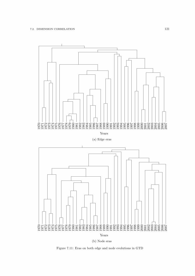
7.2. DIMENSION CORRELATION 121
197
019
71197
219
73
1974
1975
1976
1977
197
8197
919
8019
8119
8219
8319
8419
8519
8619
8719
8819
8919
9019
9119
92
1993
1994
1995
1996
1997
1998
1999
2000
2001
2002
2003
2004
2005
2006
2007
Years
(a) Edge eras
1970
1971
1972
197
319
74197
519
7619
77197
819
7919
80198
119
8219
8319
8419
8519
8619
8719
8819
8919
9019
9119
9219
9319
9419
9519
9619
97199
819
9920
0020
0120
0220
0320
0420
0520
0620
07
Years
(b) Node eras
Figure 7.11: Eras on both edge and node evolutions in GTD

122 CHAPTER 7. NOVEL MEASURES
GTD - Edge labelsStart End Labels1971 1975 United States, Northern Ireland, West Germany (FRG), France, Ar-
gentina1977 1983 Italy, France, Spain, El Salvador, Guatemala1984 1988 Lebanon, Colombia, Sri Lanka, France, Peru1989 1991 India, Colombia, Israel, Myanmar, Lebanon1992 1994 India, Bangladesh, Germany, West Bank and Gaza Strip, Venezuela1995 1997 India, Bangladesh, Pakistan, Indonesia, Colombia1998 1999 Greece, India, Timor-Leste, Northern Ireland, Kosovo2000 2002 India, West Bank and Gaza Strip, Israel, Russia, Macedonia2003 2005 Iraq, India, West Bank and Gaza Strip, Saudi Arabia, Pakistan2006 2007 Iraq, India, Pakistan, Nigeria, Sudan
GTD - Node labelsStart End Labels1971 1975 Black September, National Front for the Liberation of Cuba
(FLNC), Weatherman, Secret Cuban Government, National IntegrationFront(FIN)
1976 1977 Communist Combat Unit, Armed Communist Struggle, Baader-MeinhofGroup, Black Order, Che Guevara Brigade
1978 1981 Armenian Secret Army for the Liberation of Armenia, Armed Revolu-tionary Nuclei (NAR), Right-Wing Extremists, Spanish Basque Battalion(BBE), Prima Linea
1982 1987 Armenian Secret Army for the Liberation of Armenia, Abu Nidal Organi-zation (ANO), Anti-terrorist Liberation Group (GAL), M-19 (Movementof April 19), Action Directe
1989 1991 Moslem Janbaz Force, Bhinderanwale Tiger Force of Khalistan (BTHK),Popular Militia (Colombia), Kurdish Dissidents, Death to Bazuqueros
1992 1993 Khasi Students Union, Jharkhand Tribal Forces, Revolutionary SecurityApparatus, Allah’s Tigers, Ikhwan-ul-Muslimeen
1995 1997 Kuki tribesmen, Jammu and Kashmir Islamic Front, Harkat ul Ansar,Tamil Nadu Liberation Arm, Al Faran
1998 2000 Communist Party of India Marxist-Leninist, Vishwa Hindu Parishad(VHP), Individual, Shiv Sena, Mazdoor Kisan Sangram Samiti (MKSS)
2002 2005 Al-Mansoorian, Kuki Revolutionary Army (KRA), Jaish-e-Mohammad(JeM), Rashtriya Swayamsevak Sangh, Tawhid and Jihad
Table 7.4: Era labels on both GTD edges and nodes
In this section we would like to pose the basis for future work in which we want to solve thelink prediction problem taking eras into account. In this section, instead, we try to answer twodifferent questions: do the temporal series formed by our dissimilarities follow any pattern? Isthere a way to forecast the subsequent values of the dissimilarities? We will not actually predicteras and formally evaluate the preediction, we rather focus on posing the basis for an era predictionframework.
In the rest of this section we address the above questions, by means of statistical analysis oftime series, and, in particular, by means of autoregressive models.
Time series analysis by autoregressive models
An autoregressive model (AR) is a type of random process often used to forecast future values oftime series representing natural and social phenomena. The notation AR(p) refers to the autore-gressive model of order p, defined as
Xt = c+
p∑i=1
ϕiXt−i + εt
where ϕ1, . . . , ϕp are the parameters of the model, c is a constant and εt is white noise. Manyauthors omit the constant for simplicity.
We refer to [57] for a complete introduction to time series analysis, and how to perform predic-tion on them based on autoregressive models. We used the tseries package under the R statistical
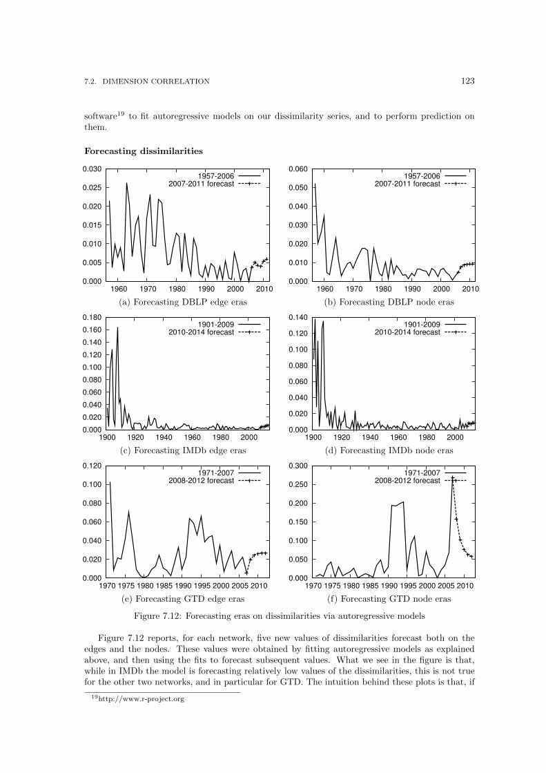
7.2. DIMENSION CORRELATION 123
software19 to fit autoregressive models on our dissimilarity series, and to perform prediction onthem.
Forecasting dissimilarities
0.000
0.005
0.010
0.015
0.020
0.025
0.030
1960 1970 1980 1990 2000 2010
1957-2006
2007-2011 forecast
0.000
0.010
0.020
0.030
0.040
0.050
0.060
1960 1970 1980 1990 2000 2010
1957-2006
2007-2011 forecast
(a) Forecasting DBLP edge eras (b) Forecasting DBLP node eras
0.000
0.020
0.040
0.060
0.080
0.100
0.120
0.140
0.160
0.180
1900 1920 1940 1960 1980 2000
1901-2009
2010-2014 forecast
0.000
0.020
0.040
0.060
0.080
0.100
0.120
0.140
1900 1920 1940 1960 1980 2000
1901-2009
2010-2014 forecast
(c) Forecasting IMDb edge eras (d) Forecasting IMDb node eras
0.000
0.020
0.040
0.060
0.080
0.100
0.120
1970 1975 1980 1985 1990 1995 2000 2005 2010
1971-2007
2008-2012 forecast
0.000
0.050
0.100
0.150
0.200
0.250
0.300
1970 1975 1980 1985 1990 1995 2000 2005 2010
1971-2007
2008-2012 forecast
(e) Forecasting GTD edge eras (f) Forecasting GTD node eras
Figure 7.12: Forecasting eras on dissimilarities via autoregressive models
Figure 7.12 reports, for each network, five new values of dissimilarities forecast both on theedges and the nodes. These values were obtained by fitting autoregressive models as explainedabove, and then using the fits to forecast subsequent values. What we see in the figure is that,while in IMDb the model is forecasting relatively low values of the dissimilarities, this is not truefor the other two networks, and in particular for GTD. The intuition behind these plots is that, if
19http://www.r-project.org

124 CHAPTER 7. NOVEL MEASURES
the forecast values are low, we are not expecting a sudden change of era in the near future, i.e., alink predictor trained on the past evolution of the network, may perform well for the near future.On the other hand, in networks where the forecast values are high, as in GTD - particularly forthe nodes - we do expect a new, well distinct, era in the next few years, with this meaning thatthe results of a link predictor based on the previous history of the network may be not accurate,due to the expected change of evolution pace.
The above might suggest a new way of looking at the link prediction problem, where the basicrules of evolution are supported by a certain confidence in the prediction given also by our temporalanalysis of the network evolution. In the future, we plan to investigate the possibility of buildingsuch solution for the link prediction problem, based on our clustering framework.
7.3 Dimension Connectivity
We introduce now a small set of measures that analyze the dimension connectivity of the networkdimensions, firstly from the point of view of single nodes and then with a higher-level detail.
We start considering two new concepts regarding the nodes of multidimensional networks: High-est Redundancy Connections (HRC) and Lowest Redundancy Connection (LRC) nodes. They arederived from the combination of the functions Degree and Neighbors. Intuitively, these measuresdescribe the structure around a given node in terms of edge density: if the node is a LRC thisstructure is sparse, while if the node is HRC it is dense and redundant.
Definition 27 (LRC) A node v ∈ V is said to be at Lowest Redundancy Connection (LRC) ifeach of its neighbors is reachable via only one dimension, i.e.,
Degree(v,D) = Neighbors(v,D).
�
Definition 28 (HRC) A node v ∈ V is called Highest Redundancy Connections (HRC) if eachof its neighbors is reachable via all the dimensions in the network, i.e.,
∀u ∈ NeighborSet(v,D) : ∀d ∈ D (u, v, d) ∈ E. �
Note that if a node v is HRC we have
Degree(v,D) = Neighbors(v,D)× |D|.
Example 7 In Figure 6.1 we have several LRC nodes: 1, 2, 3, 7, 8 and 9. Some of them appearin both dimensions (2 and 7), while other nodes appear in only one dimension (1, 3, 8 and 9). Onthe other hand we have only one HRC node: node number 5 is connected via both the dimensionswith each of its neighbors. �
Another interesting quantitative property of multidimensional networks to study is the percent-age of nodes or edges contained in a specific dimension or that belong only to that dimension. Tothis end we also introduce: the Dimension Connectivity and the Exclusive Dimension Connectivityon both the sets of nodes and edges.
Definition 29 (Node Dimension Connectivity) Let d ∈ D be a dimension of a network G =(V,E,D). The function NDC : D → [0, 1] defined as
NDC(d) = |{u∈V |∃v∈V :(u,v,d)∈E}||V |
computes the ratio of nodes of the network that belong to the dimension d. �
Definition 30 (Edge Dimension Connectivity) Let d ∈ D be a dimension of a network G =(V,E,D). The function EDC : D → [0, 1] defined as
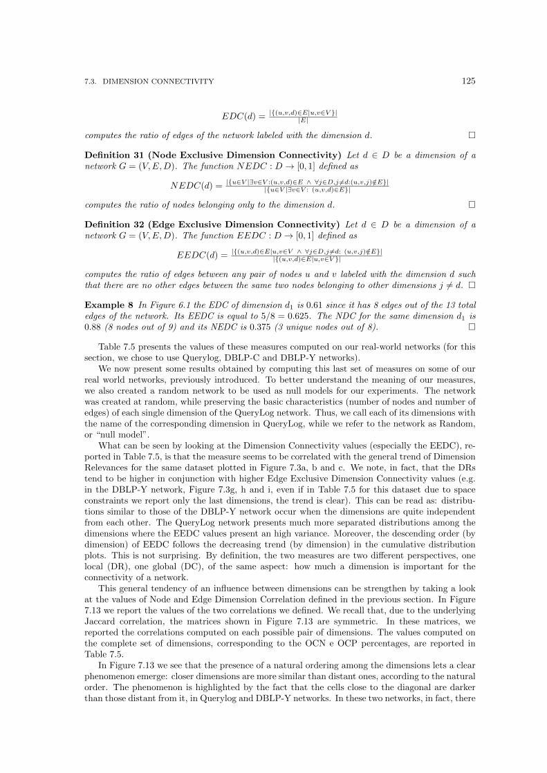
7.3. DIMENSION CONNECTIVITY 125
EDC(d) = |{(u,v,d)∈E|u,v∈V }||E|
computes the ratio of edges of the network labeled with the dimension d. �
Definition 31 (Node Exclusive Dimension Connectivity) Let d ∈ D be a dimension of anetwork G = (V,E,D). The function NEDC : D → [0, 1] defined as
NEDC(d) = |{u∈V |∃v∈V :(u,v,d)∈E ∧ ∀j∈D,j 6=d:(u,v,j)/∈E}||{u∈V |∃v∈V : (u,v,d)∈E}|
computes the ratio of nodes belonging only to the dimension d. �
Definition 32 (Edge Exclusive Dimension Connectivity) Let d ∈ D be a dimension of anetwork G = (V,E,D). The function EEDC : D → [0, 1] defined as
EEDC(d) = |{(u,v,d)∈E|u,v∈V ∧ ∀j∈D,j 6=d: (u,v,j)/∈E}||{(u,v,d)∈E|u,v∈V }|
computes the ratio of edges between any pair of nodes u and v labeled with the dimension d suchthat there are no other edges between the same two nodes belonging to other dimensions j 6= d. �
Example 8 In Figure 6.1 the EDC of dimension d1 is 0.61 since it has 8 edges out of the 13 totaledges of the network. Its EEDC is equal to 5/8 = 0.625. The NDC for the same dimension d1 is0.88 (8 nodes out of 9) and its NEDC is 0.375 (3 unique nodes out of 8). �
Table 7.5 presents the values of these measures computed on our real-world networks (for thissection, we chose to use Querylog, DBLP-C and DBLP-Y networks).
We now present some results obtained by computing this last set of measures on some of ourreal world networks, previously introduced. To better understand the meaning of our measures,we also created a random network to be used as null models for our experiments. The networkwas created at random, while preserving the basic characteristics (number of nodes and number ofedges) of each single dimension of the QueryLog network. Thus, we call each of its dimensions withthe name of the corresponding dimension in QueryLog, while we refer to the network as Random,or “null model”.
What can be seen by looking at the Dimension Connectivity values (especially the EEDC), re-ported in Table 7.5, is that the measure seems to be correlated with the general trend of DimensionRelevances for the same dataset plotted in Figure 7.3a, b and c. We note, in fact, that the DRstend to be higher in conjunction with higher Edge Exclusive Dimension Connectivity values (e.g.in the DBLP-Y network, Figure 7.3g, h and i, even if in Table 7.5 for this dataset due to spaceconstraints we report only the last dimensions, the trend is clear). This can be read as: distribu-tions similar to those of the DBLP-Y network occur when the dimensions are quite independentfrom each other. The QueryLog network presents much more separated distributions among thedimensions where the EEDC values present an high variance. Moreover, the descending order (bydimension) of EEDC follows the decreasing trend (by dimension) in the cumulative distributionplots. This is not surprising. By definition, the two measures are two different perspectives, onelocal (DR), one global (DC), of the same aspect: how much a dimension is important for theconnectivity of a network.
This general tendency of an influence between dimensions can be strengthen by taking a lookat the values of Node and Edge Dimension Correlation defined in the previous section. In Figure7.13 we report the values of the two correlations we defined. We recall that, due to the underlyingJaccard correlation, the matrices shown in Figure 7.13 are symmetric. In these matrices, wereported the correlations computed on each possible pair of dimensions. The values computed onthe complete set of dimensions, corresponding to the OCN e OCP percentages, are reported inTable 7.5.
In Figure 7.13 we see that the presence of a natural ordering among the dimensions lets a clearphenomenon emerge: closer dimensions are more similar than distant ones, according to the naturalorder. The phenomenon is highlighted by the fact that the cells close to the diagonal are darkerthan those distant from it, in Querylog and DBLP-Y networks. In these two networks, in fact, there
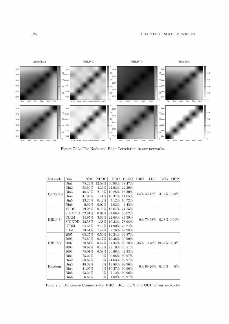
126 CHAPTER 7. NOVEL MEASURES
QueryLog DBLP-C DBLP-Y Random
Bin1
Bin2
Bin3
Bin4
Bin5
Bin6
Bin1 Bin2 Bin3 Bin4 Bin5 Bin6
0
0.2
0.4
0.6
0.8
1N
od
e J
acca
rd
VLDB
ICDM
CIKM
SIGKDD
SIGMOD
SDM
VLDB ICDM CIKM SIGKDD SIGMOD SDM
0
0.2
0.4
0.6
0.8
1
No
de
Ja
cca
rd
2005
2006
2007
2008
2009
2005 2006 2007 2008 2009
0
0.2
0.4
0.6
0.8
1
No
de
Ja
cca
rd
Bin1
Bin2
Bin3
Bin4
Bin5
Bin6
Bin1 Bin2 Bin3 Bin4 Bin5 Bin6
0
0.2
0.4
0.6
0.8
1
No
de
Ja
cca
rd
Bin1
Bin2
Bin3
Bin4
Bin5
Bin6
Bin1 Bin2 Bin3 Bin4 Bin5 Bin6 0
0.2
0.4
0.6
0.8
1
Ed
ge
Ja
cca
rd
VLDB
ICDM
CIKM
SIGKDD
SIGMOD
SDM
VLDB ICDM CIKM SIGKDD SIGMOD SDM
0
0.2
0.4
0.6
0.8
1
Ed
ge
Ja
cca
rd
2005
2006
2007
2008
2009
2005 2006 2007 2008 2009 0
0.2
0.4
0.6
0.8
1
Ed
ge
Ja
cca
rd
Bin1
Bin2
Bin3
Bin4
Bin5
Bin6
Bin1 Bin2 Bin3 Bin4 Bin5 Bin6 0
0.2
0.4
0.6
0.8
1
Ed
ge
Ja
cca
rd
Figure 7.13: The Node and Edge Correlation in our networks.
Network Dim NDC NEDC EDC EEDC HRC LRC OCN OCP
QueryLog
Bin1 75.22% 12.58% 30.98% 38.47%
0.04% 42.47% 3.14% 0.78%
Bin2 58.69% 4.39% 24.63% 22.39%Bin3 48.39% 2.19% 19.88% 16.30%Bin4 41.05% 1.41% 16.37% 14.05%Bin5 23.24% 0.42% 7.12% 10.72%Bin6 6.62% 0.02% 1.02% 4.45%
DBLP-C
VLDB 19.28% 0.75% 16.67% 74.75%
0% 79.58% 0.18% 0.01%
SIGMOD 22.81% 0.97% 21.66% 80.02%CIKM 34.95% 3.86% 22.68% 84.59%SIGKDD 22.58% 1.38% 16.33% 78.68%ICDM 24.38% 2.45% 14.90% 76.24%SDM 13.51% 1.44% 7.76% 68.28%
DBLP-Y
2005 65.35% 0.50% 16.24% 36.87%
0.35% 9.78% 19.42% 2.83%2006 74.69% 0.47% 19.36% 30.90%2007 78.81% 0.47% 21.34% 29.78%2008 78.62% 0.48% 22.10% 33.51%2009 75.01% 0.58% 20.96% 42.33%
Random
Bin1 75.22% 0% 30.98% 99.97%
0% 99.26% 0.43% 0%
Bin2 58.69% 0% 24.63% 99.97%Bin3 48.39% 0% 19.88% 99.96%Bin4 41.05% 0% 16.37% 99.96%Bin5 23.24% 0% 7.12% 99.96%Bin6 6.62% 0% 1.02% 99.97%
Table 7.5: Dimension Connectivity, HRC, LRC, OCN and OCP of our networks.

7.3. DIMENSION CONNECTIVITY 127
is a natural order of the years and the bins, used as dimensions. This is not true for DBLP-C: itis not possible to establish a natural ordering among conferences, thus the corresponding matricesin the second column of Figure 7.13 do not have any apparent order like the ones referring toDBLP-Y and Querylog networks.
Consider now the matrices related to the Random network. Due to the random generation,the natural ordering of the dimensions disappears, while, in this case, the size of the dimensionsdoes the difference. Please note that we cannot draw any conclusion from the node correlationsfor the Random network. They are quite high due to an implementation issue: when generatinga dimension for the random network we chose the node set by extracting at random a subset ofnodes of the same size of the corresponding Querylog dimension. In this way, the correlation wasunfairly increased. Among all the node set generating procedure, we found the one implemented tobe the less biased. In any case, the general idea is that more nodes and edges in a dimension implymore correlation with the other ones, by pure chance. The number of possible edges is very large,thus it is difficult to create, using a random generator, the same edges in two different dimensions,dramatically lowering then the Edge Correlation values (which appears almost white in the lastcolumn of Figure 7.13) and bringing close to 100% the EEDC values (NEDC values are all equalto zero due to the artifact of choosing the random node ids from the same set).
This is true also considering HRC and OCP values of our networks, reported in Table 7.5.The null model does not present any node with these properties, while instead it has the highestnumber of LRC nodes. This is again an effect of the above mentioned properties: too manyedge combinations lead the edges of a random network to appear only in one dimension. On theother hand, in DBLP-Y we have some authors publishing each year with all their collaborators(HRC column) or at least one time each year (OCN column). These two events are quite rare inthe random null model. Some networks may present also situations even more extreme than therandom null model: it is the case of DBLP-C in which only 12 authors have published in all thesix considered conferences (OCN column), and only two pairs have collaborated at least once in allthe conferences (OCP column). But this is natural, since publishing in all of these top conferencesis very difficult.
Again, these considerations support the thesis that our multidimensional measures are cap-turing real, and not random, phenomena, that constitute meaningful knowledge mined in themultidimensional networks analyzed.

128 CHAPTER 7. NOVEL MEASURES
Chapter 8
Advanced Analysis
In this chapter we present some classical problem definitions, traditionally tackled in complexnetwork science. We plan to investigate how multidimensionality affects these problem definitionsand we propose some solutions, extensions, new methodologies and approaches to take advantage ofthe additional degree of freedom allowed by this novel setting. The main focus of this chapter willbe on community discovery, in Section 2.3. The reason of the choice is due to the incredible amountof literature on this subject, the difficulty of the problem per se and the vast application scenarioof community discovery algorithms. Therefore, the community discovery case study is the core ofthis chapter and of this thesis: firstly we provide a vast analysis of its state of the art and secondlywe propose a solution to the problem of finding and characterizing multidimensional communities,solving the multidimensional density ambiguity. In the rest of the chapter, we tackle other classicalproblems in complex network analysis with a multidimensional perspective: in Section 8.2 wedefine null models and multidimensional network generators, in Section 8.3 we define the problemof multidimensional link prediction and we analyze how a truly multidimensional algorithm isneeded to solve it, finally in Section 8.4 we define the problem of finding the shortest path ina multidimensional network with cost modifiers, we propose a greedy solution and we give theinsights for future works in the defined field.
8.1 Multidimensional Community Discovery
As we have seen in Section 2.3, in community discovery the connections among the nodes of anetwork are posed at the center of investigation, since they play a key role in the study of thenetwork structure, evolution, and behavior. The simplified monodimensional perspective used sofar is not suitable to describe the dynamics of communities in the real world, where this perspectiveis not always enough to model all the available information, especially if the actors are users, withtheir multiple preferences, their multifaceted behaviors, and their complex interactions. With theaim of better representing these dynamics, in this section we introduce the problem of detectingmultidimensional communities of actors in complex networks. As we have stated before, the conceptof multidimensional community has to be defined, and we introduce two new measures aimed atanalyzing the multidimensional properties of the communities discovered. We then present aframework for finding and characterizing multidimensional communities and we show the resultsobtained by applying such framework on real-world networks, giving a few examples of interestingmultidimensional communities found in different scenarios: co-authorship, movie collaborationsand terrorist attacks.
Our main contribution is then: we introduce and formally define the problem of multidimen-sional community discovery; we introduce two measures for characterizing the communities found;we build up a framework for solving the introduced problem by means of a conjunction of existingtechniques and our newly introduced concepts; we perform a case study on real networks, showinga few resulting communities, along with their characterization.
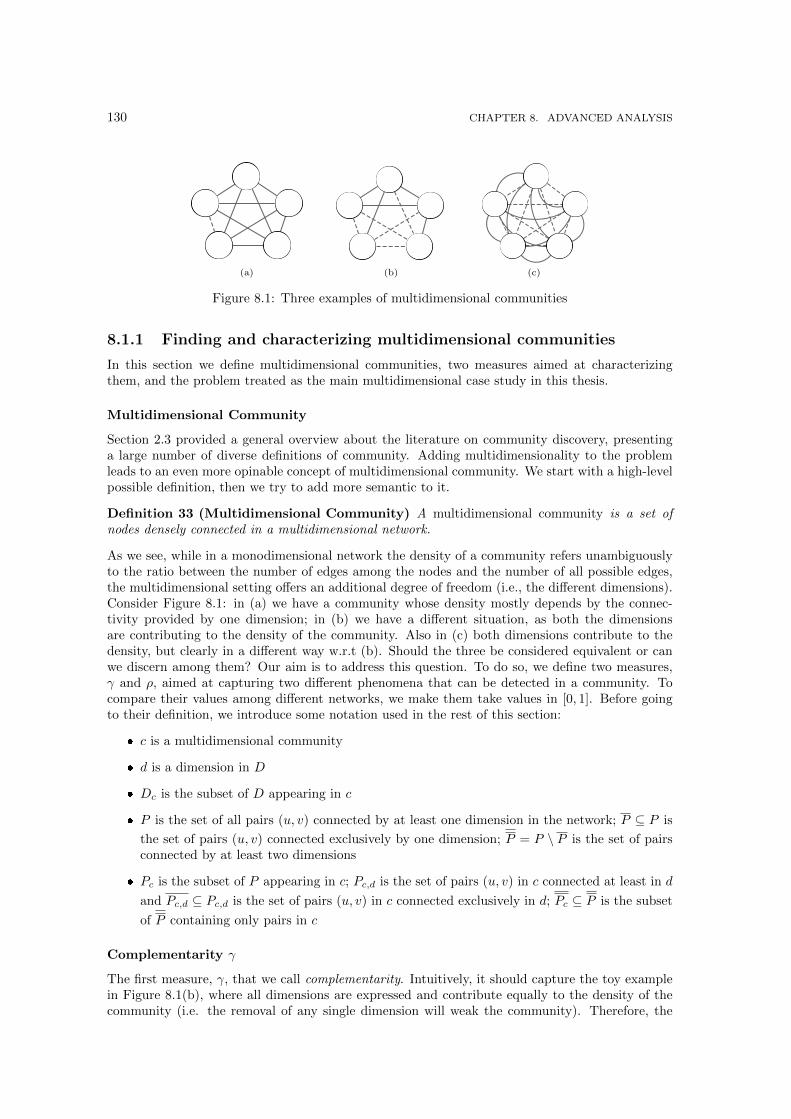
130 CHAPTER 8. ADVANCED ANALYSIS
(a) (b) (c)
Figure 8.1: Three examples of multidimensional communities
8.1.1 Finding and characterizing multidimensional communities
In this section we define multidimensional communities, two measures aimed at characterizingthem, and the problem treated as the main multidimensional case study in this thesis.
Multidimensional Community
Section 2.3 provided a general overview about the literature on community discovery, presentinga large number of diverse definitions of community. Adding multidimensionality to the problemleads to an even more opinable concept of multidimensional community. We start with a high-levelpossible definition, then we try to add more semantic to it.
Definition 33 (Multidimensional Community) A multidimensional community is a set ofnodes densely connected in a multidimensional network.
As we see, while in a monodimensional network the density of a community refers unambiguouslyto the ratio between the number of edges among the nodes and the number of all possible edges,the multidimensional setting offers an additional degree of freedom (i.e., the different dimensions).Consider Figure 8.1: in (a) we have a community whose density mostly depends by the connec-tivity provided by one dimension; in (b) we have a different situation, as both the dimensionsare contributing to the density of the community. Also in (c) both dimensions contribute to thedensity, but clearly in a different way w.r.t (b). Should the three be considered equivalent or canwe discern among them? Our aim is to address this question. To do so, we define two measures,γ and ρ, aimed at capturing two different phenomena that can be detected in a community. Tocompare their values among different networks, we make them take values in [0, 1]. Before goingto their definition, we introduce some notation used in the rest of this section:
� c is a multidimensional community
� d is a dimension in D
� Dc is the subset of D appearing in c
� P is the set of all pairs (u, v) connected by at least one dimension in the network; P ⊆ P is
the set of pairs (u, v) connected exclusively by one dimension; P = P \ P is the set of pairsconnected by at least two dimensions
� Pc is the subset of P appearing in c; Pc,d is the set of pairs (u, v) in c connected at least in d
and Pc,d ⊆ Pc,d is the set of pairs (u, v) in c connected exclusively in d; Pc ⊆ P is the subset
of P containing only pairs in c
Complementarity γ
The first measure, γ, that we call complementarity. Intuitively, it should capture the toy examplein Figure 8.1(b), where all dimensions are expressed and contribute equally to the density of thecommunity (i.e. the removal of any single dimension will weak the community). Therefore, the

8.1. MULTIDIMENSIONAL COMMUNITY DISCOVERY 131
operational definition of a multidimensional community with γ = 1 is “A community where theremoval of any dimension from the network disconnects an equal number of node couples”.
We now formally define the concept of complementarity. Following its operational definition,we state that it is composed by the conjunction of three concepts:
� Variety Vc: how many different dimensions are detectable among the community c taken asoverall;
� Exclusivity Ec: how many pairs of nodes are connected exclusively by one dimension amongthe ones present in c;
� Homogeneity Hc: how uniform is the distribution of the number of edges per dimension inc.
We want this measure to be higher when each of the above is high: from the operational definitionof γ, variety captures the “removal of any dimension from the network” part; exclusivity capturesthe “disconnects” part; finally homogeneity captures the “equal number of node couples” part. InFigure 8.1(b) if we remove either the solid or the dashed edges we will disconnect an equal numberof node couples (namely five), while this does not hold for both Figure 8.1(a) and Figure 8.1(c).
A natural way to achieve this is to aggregate them by their product1:
γc = Vc × Ec ×Hc. (8.1)
We now have to define the three concepts. Variety can be computed by
Vc =|Dc| − 1
|D| − 1(8.2)
as the number of dimensions expressed with the community c over the total number of dimensionswithin the network. The two negative terms serve as corrections to make Variety take values in[0, 1]. Note that Variety defined as above would be undefined when |D| = 1, but this would meanhaving a monodimensional network, then the use of γ would be meaningless.
Exclusivity can be computed as the ratio between the number of exclusive connections withinthe community and the total number of connected pairs in c:
Ec =
∑d∈D |Pc,d||Pc|
. (8.3)
This term is equal to zero when there are no exclusive connections, i.e. every pair of nodes in c isconnected by at least two dimensions, while it is equal to one when every pair in c is connected byonly one dimension. The formula is not defined for |Pc| = 0, which happens only for communitiesof only one node, for which it has no sense to compute γ.
Finally, we have to define Homogeneity. We want this term to be equal to one when the edgeswithin the community are uniformly distributed among the dimensions represented in c. Thesimplest way to measure this is to look at the standard deviation of the distribution of the edgesin c on the dimensions. We define:
σc =
√∑d∈D (|Pc,d| − avgc)2
|D|(8.4)
where avgc is the mean of the distribution, as the standard deviation of the number of edges perdimension in c, and:
σmaxc =
√(max(|Pc,d|)− 1)
2
2(8.5)
1Although this is not the only possible choice, it is the simplest one.

132 CHAPTER 8. ADVANCED ANALYSIS
where max(|Pc,d|) is the number of edges belonging to the dimension more represented in c (basi-cally we want to achieve the maximum possible standard deviation). Then, we can define Homo-geneity as:
Hc = 1− σcσmaxc
(8.6)
where we subtract the right term from 1, to make Hc equal to one when the right term is zero, i.e.when the edges are uniformly distributed among the different dimensions.
If we could have the complete set of communities of a network, we could make a more preciseestimation of σmaxc :
σmaxc =
√(max(|Pc,d|)−min(|Pc,d|))2
2(8.7)
where min(|Pc,d|) is the number of edges belonging to dimension d in community c where d and care picked to minimize the number of edges appearing in c labeled with dimension d (i.e. there isno d or c generating a lower |Pc,d|).
If all the communities presents the same dimensions represented with the same number of edges,i.e. all |Pc,d| are equal to the same number, the two normalization coefficients σmaxc would be equalto zero, making the right term of Equation 8.3 undefined. In this case, being the denominator anupper bound, also the numerator would be equal to zero. But this is the ideal topology of a networkwhere the Homogeneity is maximum since all the edges are uniformly distributed, and then we canhandle this exceptional case, without lack of generality, by defining Hc as:
Hc =
{1 if σc = 0
1− σcσmaxc
otherwise (8.8)
Example 9 (Multidimensional communities and γ) Consider Figure 8.1. We see three dif-ferent multidimensional communities, each of them with different multidimensional structures: in(a), the standard deviation of the number of edges per dimension is the maximum possible, henceHc = 0, thus γ = 0; in (b), every term of the complementarity is equal to one, thus γ = 1; in (c),the exclusivity is zero, as every pair is connected by two dimensions, hence γ = 0.
Redundancy ρ
The second measure we define is called redundancy, and it captures the phenomenon for which a setof nodes that constitute a community in a dimension tend to constitute a community also in otherdimensions. We can see this measure as a simple indicator of the redundancy of the connections:the more dimensions connect each pair of nodes within a community, the higher the redundancywill be.
We can then define the redundancy ρ by counting how many pairs have redundant connections,normalizing by the theoretical maximum:
ρc =∑
(u,v)∈Pc
|{d : (u, v, d) ∈ E}||D| × |Pc|
(8.9)
With the help of Figure 8.1 we see how ρ takes values in [0, 1]: in 8.1(b), each pair of nodes
is connected in only one dimension, then |Pc| = 0 and the numerator is equal to zero; in 8.1(c),all the node pairs are connected in all the dimensions of D, which is equivalent to the numberof connected pairs |Pc| multiplied by the number of network dimensions |D| (the denominator),making ρ = 1. We see that ρ is undefined for communities formed by one single node, where|Pc| = 0 and then the denominator is equal to zero. For this type of communities, however, theredundancy measure is not meaningful, thus we can ignore this case.
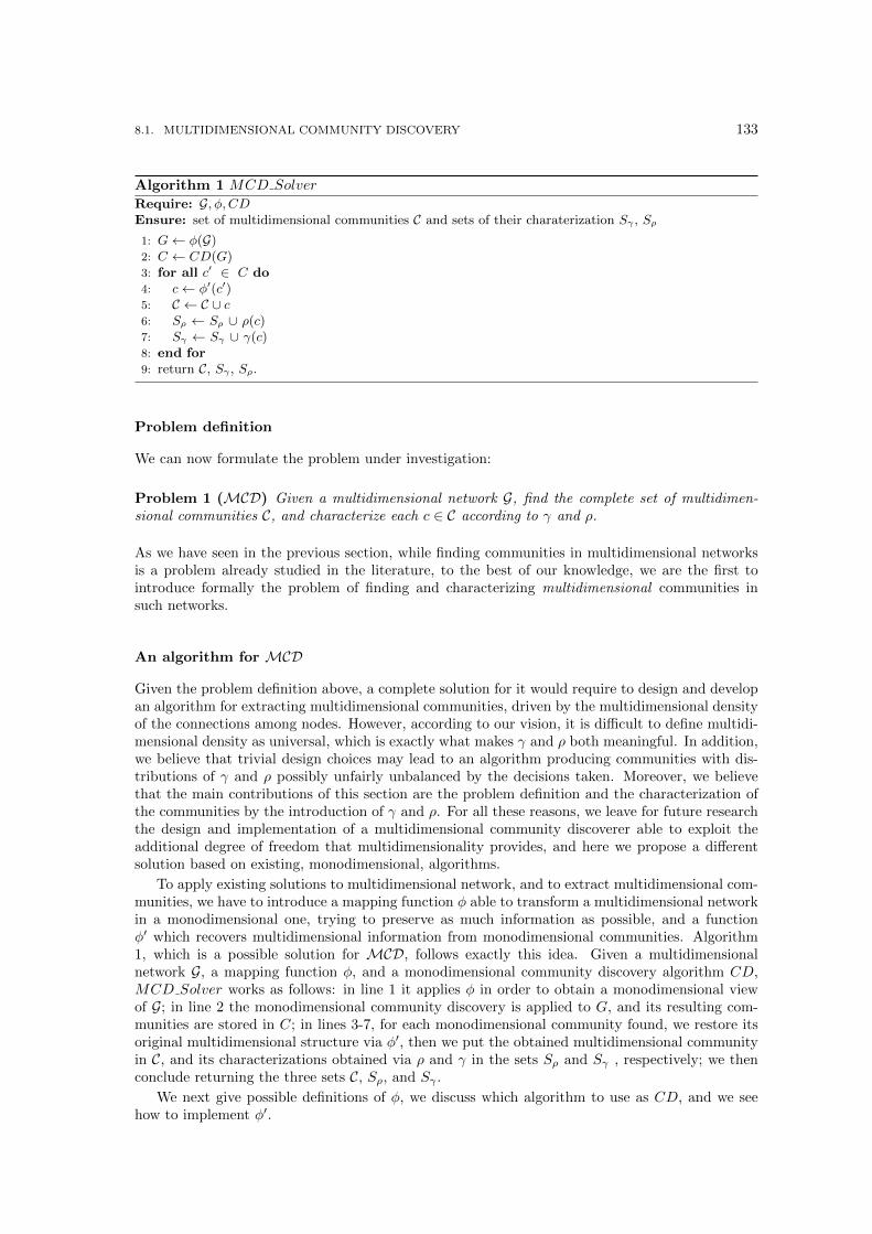
8.1. MULTIDIMENSIONAL COMMUNITY DISCOVERY 133
Algorithm 1 MCD Solver
Require: G, φ, CDEnsure: set of multidimensional communities C and sets of their charaterization Sγ , Sρ
1: G← φ(G)2: C ← CD(G)3: for all c′ ∈ C do4: c← φ′(c′)5: C ← C ∪ c6: Sρ ← Sρ ∪ ρ(c)7: Sγ ← Sγ ∪ γ(c)8: end for9: return C, Sγ , Sρ.
Problem definition
We can now formulate the problem under investigation:
Problem 1 (MCD) Given a multidimensional network G, find the complete set of multidimen-sional communities C, and characterize each c ∈ C according to γ and ρ.
As we have seen in the previous section, while finding communities in multidimensional networksis a problem already studied in the literature, to the best of our knowledge, we are the first tointroduce formally the problem of finding and characterizing multidimensional communities insuch networks.
An algorithm for MCD
Given the problem definition above, a complete solution for it would require to design and developan algorithm for extracting multidimensional communities, driven by the multidimensional densityof the connections among nodes. However, according to our vision, it is difficult to define multidi-mensional density as universal, which is exactly what makes γ and ρ both meaningful. In addition,we believe that trivial design choices may lead to an algorithm producing communities with dis-tributions of γ and ρ possibly unfairly unbalanced by the decisions taken. Moreover, we believethat the main contributions of this section are the problem definition and the characterization ofthe communities by the introduction of γ and ρ. For all these reasons, we leave for future researchthe design and implementation of a multidimensional community discoverer able to exploit theadditional degree of freedom that multidimensionality provides, and here we propose a differentsolution based on existing, monodimensional, algorithms.
To apply existing solutions to multidimensional network, and to extract multidimensional com-munities, we have to introduce a mapping function φ able to transform a multidimensional networkin a monodimensional one, trying to preserve as much information as possible, and a functionφ′ which recovers multidimensional information from monodimensional communities. Algorithm1, which is a possible solution for MCD, follows exactly this idea. Given a multidimensionalnetwork G, a mapping function φ, and a monodimensional community discovery algorithm CD,MCD Solver works as follows: in line 1 it applies φ in order to obtain a monodimensional viewof G; in line 2 the monodimensional community discovery is applied to G, and its resulting com-munities are stored in C; in lines 3-7, for each monodimensional community found, we restore itsoriginal multidimensional structure via φ′, then we put the obtained multidimensional communityin C, and its characterizations obtained via ρ and γ in the sets Sρ and Sγ , respectively; we thenconclude returning the three sets C, Sρ, and Sγ .
We next give possible definitions of φ, we discuss which algorithm to use as CD, and we seehow to implement φ′.
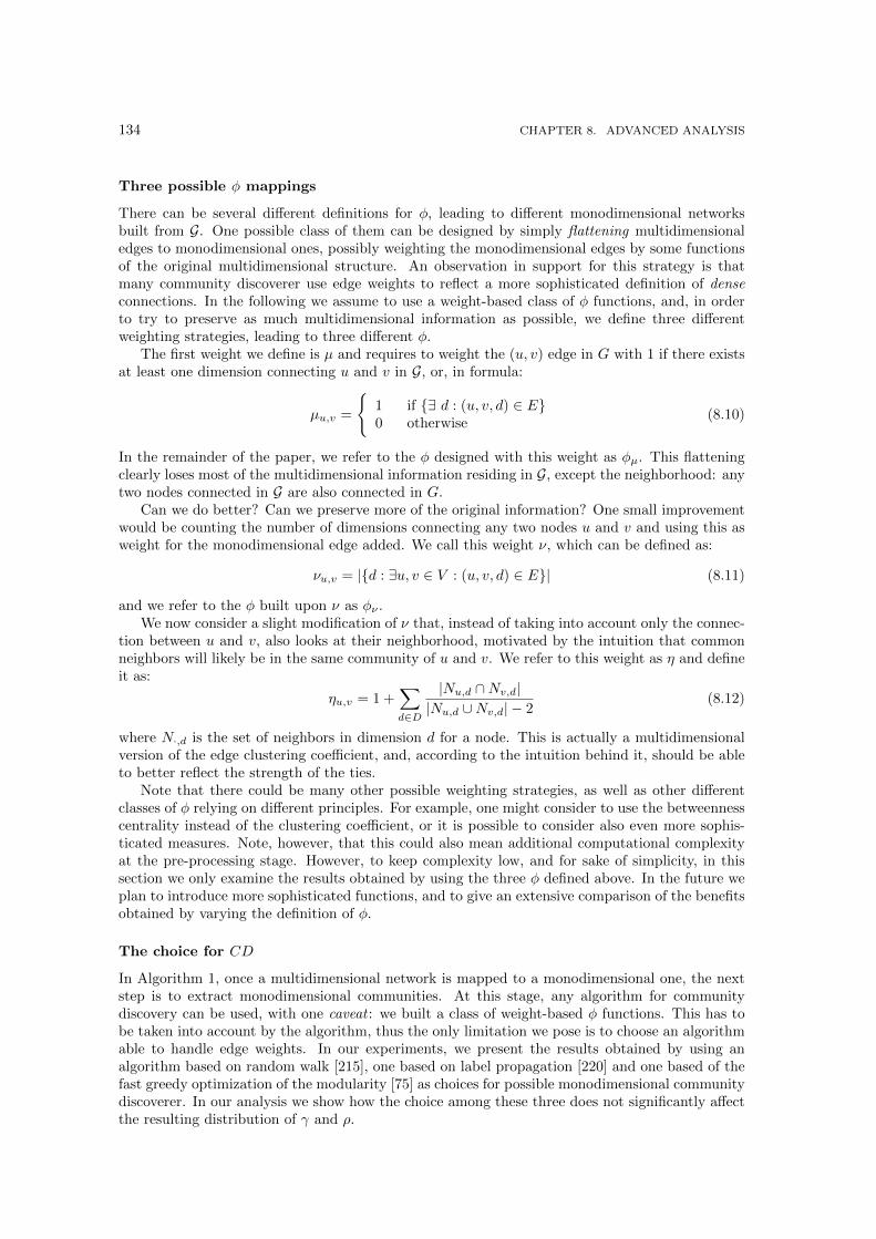
134 CHAPTER 8. ADVANCED ANALYSIS
Three possible φ mappings
There can be several different definitions for φ, leading to different monodimensional networksbuilt from G. One possible class of them can be designed by simply flattening multidimensionaledges to monodimensional ones, possibly weighting the monodimensional edges by some functionsof the original multidimensional structure. An observation in support for this strategy is thatmany community discoverer use edge weights to reflect a more sophisticated definition of denseconnections. In the following we assume to use a weight-based class of φ functions, and, in orderto try to preserve as much multidimensional information as possible, we define three differentweighting strategies, leading to three different φ.
The first weight we define is µ and requires to weight the (u, v) edge in G with 1 if there existsat least one dimension connecting u and v in G, or, in formula:
µu,v =
{1 if {∃ d : (u, v, d) ∈ E}0 otherwise
(8.10)
In the remainder of the paper, we refer to the φ designed with this weight as φµ. This flatteningclearly loses most of the multidimensional information residing in G, except the neighborhood: anytwo nodes connected in G are also connected in G.
Can we do better? Can we preserve more of the original information? One small improvementwould be counting the number of dimensions connecting any two nodes u and v and using this asweight for the monodimensional edge added. We call this weight ν, which can be defined as:
νu,v = |{d : ∃u, v ∈ V : (u, v, d) ∈ E}| (8.11)
and we refer to the φ built upon ν as φν .We now consider a slight modification of ν that, instead of taking into account only the connec-
tion between u and v, also looks at their neighborhood, motivated by the intuition that commonneighbors will likely be in the same community of u and v. We refer to this weight as η and defineit as:
ηu,v = 1 +∑d∈D
|Nu,d ∩Nv,d||Nu,d ∪Nv,d| − 2
(8.12)
where N·,d is the set of neighbors in dimension d for a node. This is actually a multidimensionalversion of the edge clustering coefficient, and, according to the intuition behind it, should be ableto better reflect the strength of the ties.
Note that there could be many other possible weighting strategies, as well as other differentclasses of φ relying on different principles. For example, one might consider to use the betweennesscentrality instead of the clustering coefficient, or it is possible to consider also even more sophis-ticated measures. Note, however, that this could also mean additional computational complexityat the pre-processing stage. However, to keep complexity low, and for sake of simplicity, in thissection we only examine the results obtained by using the three φ defined above. In the future weplan to introduce more sophisticated functions, and to give an extensive comparison of the benefitsobtained by varying the definition of φ.
The choice for CD
In Algorithm 1, once a multidimensional network is mapped to a monodimensional one, the nextstep is to extract monodimensional communities. At this stage, any algorithm for communitydiscovery can be used, with one caveat : we built a class of weight-based φ functions. This has tobe taken into account by the algorithm, thus the only limitation we pose is to choose an algorithmable to handle edge weights. In our experiments, we present the results obtained by using analgorithm based on random walk [215], one based on label propagation [220] and one based of thefast greedy optimization of the modularity [75] as choices for possible monodimensional communitydiscoverer. In our analysis we show how the choice among these three does not significantly affectthe resulting distribution of γ and ρ.
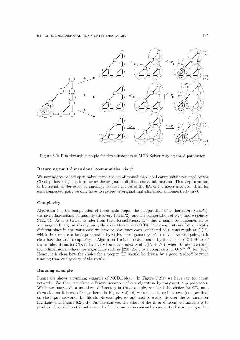
8.1. MULTIDIMENSIONAL COMMUNITY DISCOVERY 135
φµ
φν
φη
CD
CD
CD
φ', γ, ρ
φ', γ, ρ
φ', γ, ρ
11
11
1
11
111
1 1
11
11
11
11
11
1 11
1
3
3 3
3
1.5
1.5
1.83
1.83
1.331.76
γ = 0ρ = 1
γ = 0ρ = 0
γ = 0ρ = 0
γ = 0ρ = 1
γ = 0ρ = 1
γ = 1ρ = 0
γ = 1ρ = 0
γ = .69ρ = .14
Figure 8.2: Run through example for three instances of MCD Solver varying the φ parameter.
Returning multidimensional communities via φ′
We now address a last open point: given the set of monodimensional communities returned by theCD step, how to get back restoring the original multidimensional information. This step turns outto be trivial, as, for every community, we have the set of the IDs of the nodes involved: then, foreach connected pair, we only have to restore its original multidimensional connectivity in G.
Complexity
Algorithm 1 is the composition of three main steps: the computation of φ (hereafter, STEP1),the monodimensional community discovery (STEP2), and the computation of φ′, γ and ρ (jointly,STEP3). As it is trivial to infer from their formulations, φ, γ and ρ might be implemented byscanning each edge in E only once, therefore their cost is O(E). The computation of φ′ is slightlydifferent since in the worst case we have to scan once each connected pair, thus requiring O(P),which, in turns, can be approximated by O(E), since generally |N | >> |L|. At this point, it isclear how the total complexity of Algorithm 1 might be dominated by the choice of CD. State ofthe art algorithms for CD, in fact, vary from a complexity of O(|E|+ |N |) (where E here is a set ofmonodimensional edges) for algorithms such as [220, 267], to a complexity of O(3|N |/3) for [163].Hence, it is clear how the choice for a proper CD should be driven by a good tradeoff betweenrunning time and quality of the results.
Running example
Figure 8.2 shows a running example of MCD Solver. In Figure 8.2(a) we have our toy inputnetwork. We then run three different instances of our algorithm by varying the φ parameter.While we imagined to use three different φ in this example, we fixed the choice for CD, as adiscussion on it is out of scope here. In Figure 8.2(b-d) we see the three instances (one per line)on the input network. In this simple example, we assumed to easily discover the communitieshighlighted in Figure 8.2(c-d). As one can see, the effect of the three different φ functions is toproduce three different input networks for the monodimensional community discovery algorithm
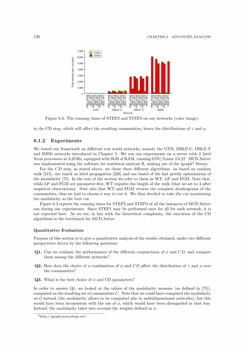
136 CHAPTER 8. ADVANCED ANALYSIS
0
1,000
2,000
3,000
4,000
5,000
6,000
7,000
PH
I1−
FG
MP
HI1
−L
PP
HI1
−W
TP
HI2
−F
GM
PH
I2−
LP
PH
I2−
WT
PH
I3−
FG
MP
HI3
−L
PP
HI3
−W
T
PH
I1−
FG
MP
HI1
−L
PP
HI1
−W
TP
HI2
−F
GM
PH
I2−
LP
PH
I2−
WT
PH
I3−
FG
MP
HI3
−L
PP
HI3
−W
T
PH
I1−
FG
MP
HI1
−L
PP
HI1
−W
TP
HI2
−F
GM
PH
I2−
LP
PH
I2−
WT
PH
I3−
FG
MP
HI3
−L
PP
HI3
−W
T
PH
I1−
FG
MP
HI1
−L
PP
HI1
−W
TP
HI2
−F
GM
PH
I2−
LP
PH
I2−
WT
PH
I3−
FG
MP
HI3
−L
PP
HI3
−W
T
To
tal
run
nin
g t
ime
(sec
ond
s)
Network
GTD DBLP−C DBLP−Y IMDb
STEP3
STEP2
Figure 8.3: The running times of STEP2 and STEP3 on our networks (color image).
in the CD step, which will affect the resulting communities, hence the distributions of γ and ρ.
8.1.2 Experiments
We tested our framework on different real world networks, namely the GTD, DBLP-C, DBLP-Yand IMDb networks introduced in Chapter 5. We ran our experiments on a server with 2 IntelXeon processors at 3.2GHz, equipped with 8GB of RAM, running GNU/Linux 2.6.27. MCD Solverwas implemented using the software for statistical analysis R, making use of the igraph2 library.
For the CD step, as stated above, we chose three different algorithms: on based on randomwalk [215], one based on label propagation [220] and one based of the fast greedy optimization ofthe modularity [75]. In the rest of the section we refer to them as WT, LP and FGM. Note that,while LP and FGM are parameter-free, WT requires the length of the walk (that we set to 4 afterempirical observations). Note also that WT and FGM returns the complete dendrograms of thecommunities, thus we had to choose a way to cut it. We then decided to take the cut maximizingthe modularity as the best cut.
Figure 8.3 reports the running times for STEP2 and STEP3 of all the instances of MCD Solverran during our experiments. Since STEP1 may be performed once for all for each network, it isnot reported here. As we see, in line with the theoretical complexity, the execution of the CDalgorithms is the bottleneck for MCD Solver.
Quantitative Evaluation
Purpose of this section is to give a quantitative analysis of the results obtained, under two differentperspectives driven by the following questions:
Q1. Can we evaluate the performances of the different conjunctions of φ and CD, and comparethem among the different networks?
Q2. How does the choice of a combination of φ and CD affect the distribution of γ and ρ overthe communities?
Q3. What is the best choice of φ and CD parameters?
In order to answer Q1, we looked at the values of the modularity measure (as defined in [75]),computed on the resulting set of communities C. Note that we could have computed the modularityon C instead (the modularity allows to be computed also in multidimensional networks), but thiswould have been inconsistent with the use of φ, which would have been disregarded in that way.Instead, the modularity takes into account the weights defined in φ.
2http://igraph.sourceforge.net/
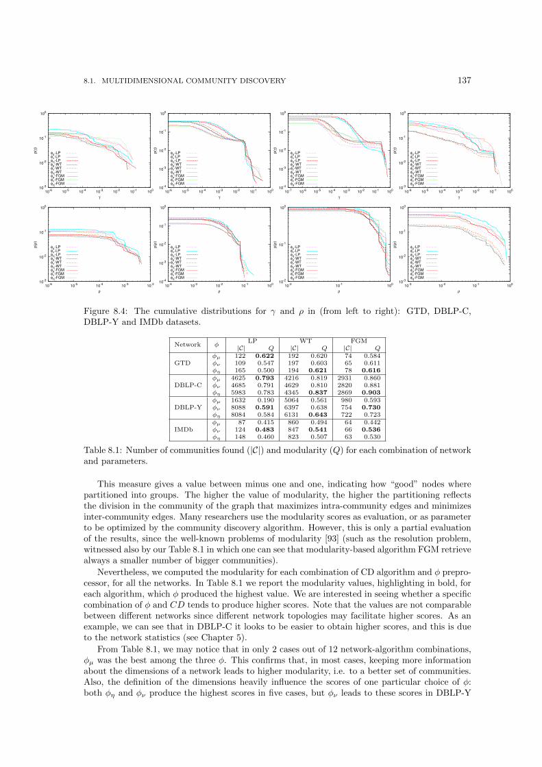
8.1. MULTIDIMENSIONAL COMMUNITY DISCOVERY 137
10-3
10-2
10-1
100
10-6
10-5
10-4
10-3
10-2
10-1
100
p(γ
)
γ
φµ-LPφν-LPφη-LPφµ-WTφν-WTφη-WTφµ-FGMφν-FGMφη-FGM
10-4
10-3
10-2
10-1
100
10-6
10-5
10-4
10-3
10-2
10-1
100
p(γ
)
γ
φµ-LPφν-LPφη-LPφµ-WTφν-WTφη-WTφµ-FGMφν-FGMφη-FGM
10-4
10-3
10-2
10-1
100
10-7
10-6
10-5
10-4
10-3
10-2
10-1
100
p(γ
)
γ
φµ-LPφν-LPφη-LPφµ-WTφν-WTφη-WTφµ-FGMφν-FGMφη-FGM
10-3
10-2
10-1
100
10-6
10-5
10-4
10-3
10-2
10-1
100
p(γ
)
γ
φµ-LPφν-LPφη-LPφµ-WTφν-WTφη-WTφµ-FGMφν-FGMφη-FGM
10-3
10-2
10-1
100
10-6
10-5
10-4
10-3
10-2
p(ρ
)
ρ
φµ-LPφν-LPφη-LPφµ-WTφν-WTφη-WTφµ-FGMφν-FGMφη-FGM
10-4
10-3
10-2
10-1
100
10-4
10-3
10-2
10-1
100
p(ρ
)
ρ
φµ-LPφν-LPφη-LPφµ-WTφν-WTφη-WTφµ-FGMφν-FGMφη-FGM
10-2
10-1
100
10-2
10-1
100
p(ρ
)
ρ
φµ-LPφν-LPφη-LPφµ-WTφν-WTφη-WTφµ-FGMφν-FGMφη-FGM
10-3
10-2
10-1
100
10-3
10-2
10-1
100
p(ρ
)
ρ
φµ-LPφν-LPφη-LPφµ-WTφν-WTφη-WTφµ-FGMφν-FGMφη-FGM
Figure 8.4: The cumulative distributions for γ and ρ in (from left to right): GTD, DBLP-C,DBLP-Y and IMDb datasets.
Network φLP WT FGM
|C| Q |C| Q |C| Q
GTDφµ 122 0.622 192 0.620 74 0.584φν 109 0.547 197 0.603 65 0.611φη 165 0.500 194 0.621 78 0.616
DBLP-Cφµ 4625 0.793 4216 0.819 2931 0.860φν 4685 0.791 4629 0.810 2820 0.881φη 5983 0.783 4345 0.837 2869 0.903
DBLP-Yφµ 1632 0.190 5064 0.561 980 0.593φν 8088 0.591 6397 0.638 754 0.730φη 8084 0.584 6131 0.643 722 0.723
IMDbφµ 87 0.415 860 0.494 64 0.442φν 124 0.483 847 0.541 66 0.536φη 148 0.460 823 0.507 63 0.530
Table 8.1: Number of communities found (|C|) and modularity (Q) for each combination of networkand parameters.
This measure gives a value between minus one and one, indicating how “good” nodes wherepartitioned into groups. The higher the value of modularity, the higher the partitioning reflectsthe division in the community of the graph that maximizes intra-community edges and minimizesinter-community edges. Many researchers use the modularity scores as evaluation, or as parameterto be optimized by the community discovery algorithm. However, this is only a partial evaluationof the results, since the well-known problems of modularity [93] (such as the resolution problem,witnessed also by our Table 8.1 in which one can see that modularity-based algorithm FGM retrievealways a smaller number of bigger communities).
Nevertheless, we computed the modularity for each combination of CD algorithm and φ prepro-cessor, for all the networks. In Table 8.1 we report the modularity values, highlighting in bold, foreach algorithm, which φ produced the highest value. We are interested in seeing whether a specificcombination of φ and CD tends to produce higher scores. Note that the values are not comparablebetween different networks since different network topologies may facilitate higher scores. As anexample, we can see that in DBLP-C it looks to be easier to obtain higher scores, and this is dueto the network statistics (see Chapter 5).
From Table 8.1, we may notice that in only 2 cases out of 12 network-algorithm combinations,φµ was the best among the three φ. This confirms that, in most cases, keeping more informationabout the dimensions of a network leads to higher modularity, i.e. to a better set of communities.Also, the definition of the dimensions heavily influence the scores of one particular choice of φ:both φη and φν produce the highest scores in five cases, but φν leads to these scores in DBLP-Y
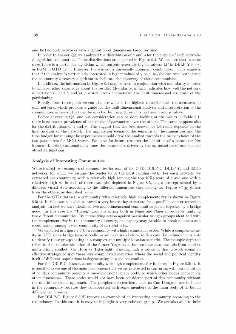
138 CHAPTER 8. ADVANCED ANALYSIS
and IMDb, both networks with a definition of dimensions based on time.In order to answer Q2, we analyzed the distribution of γ and ρ for the output of each network-
φ-algorithm combination. These distributions are depicted in Figure 8.4. We can see that in somecases there is a particular algorithm which outputs generally higher values: LP in DBLP-Y for γ,or FGM in GTD for γ. However, there is not a universally dominant combination. This suggeststhat if the analyst is particularly interested in higher values of γ or ρ, he/she can tune both φ andthe community discovery algorithm to facilitate the discovery of those communities.
In addition, the information in Figure 8.4 may be used in conjunction with modularity in orderto achieve richer knowledge about the results. Modularity, in fact, indicates how well the networkis partitioned, and γ and/or ρ distributions characterize the multidimensional structure of thepartitioning.
Finally, from these plots we can also see what is the highest value for both the measures, ineach network, which provides a guide for the multidimensional analysis and interpretation of thecommunities achieved, that can be selected by using thresholds on their γ and ρ values.
Before answering Q3, one last consideration can be done looking at the values in Table 8.1:there is no strong prevalence of one choice of parameters over the others. The same happens alsofor the distributions of γ and ρ. This suggest that the best answer for Q3 really depends on thefinal analysis of the network: the application scenario, the semantic of the dimensions and thetime budget for running the experiments should drive the analyst towards the proper choice of thetwo parameters for MCD Solver. We leave for future research the definition of a parameter-freeframework able to automatically tune the parameters driven by the optimization of user-definedobjective functions.
Analysis of Interesting Communities
We extracted two examples of communities for each of the GTD, DBLP-C, DBLP-Y, and IMDbnetworks, for which we assume the reader to be the most familiar with. For each network, weextracted one community with a relatively high (among the top 10%) score of γ and one with arelatively high ρ. In each of these examples depicted in Figure 8.5, edges are represented by adifferent visual style according to the different dimensions they belong to. Figure 8.5(g) differsfrom the others, as described below.
For the GTD dataset, a community with relatively high complementarity is shown in Figure8.5(a). In this case γ is able to unveil a very interesting structure for a possible counter-terrorismanalysis. In fact we have identified two monodimensional communities joined together by a bridgenode. In this case the “Tuareg” group is acting both in Niger and Nigeria, probably unifyingtwo different communities. By intensifying action against particular bridges groups identified withthe complementarity in the community discovery, one agency may be able to break alliances andcoordination among a vast community of terrorist cells.
We depicted in Figure 8.5(b) a community with high redundancy score. While a complementar-ity in GTD spots bridge terrorist cells, as we have seen before, in this case the redundancy is ableto identify those groups acting in a complex and multiple location scenario. The example depictedrefers to the complex situation of the former Yugoslavia, but we have also example from anothermulti ethnic conflict: the Hutu vs Tutsi fight. Finding high ρ values in this network seems aneffective strategy to spot these very complicated scenarios, where the social and political identityitself of different populations is degenerating in a violent conflict.
For the DBLP-C dataset, a community with high complementarity is shown in Figure 8.5(c). Itis possible to see one of the main phenomena that we are interested in capturing with our definitionof γ: this community presents a one-dimensional main body, to which other nodes connect viaother dimensions. These nodes would not have been considered part of this community withoutthe multidimensional approach. The peripheral researchers, such as Cao Dongwei, are includedin the community because they collaborated with some members of the main body of it, but indifferent conferences.
For DBLP-C, Figure 8.5(d) reports an example of an interesting community according to theredundancy. In this case it is easy to highlight a very cohesive group. We are also able to infer
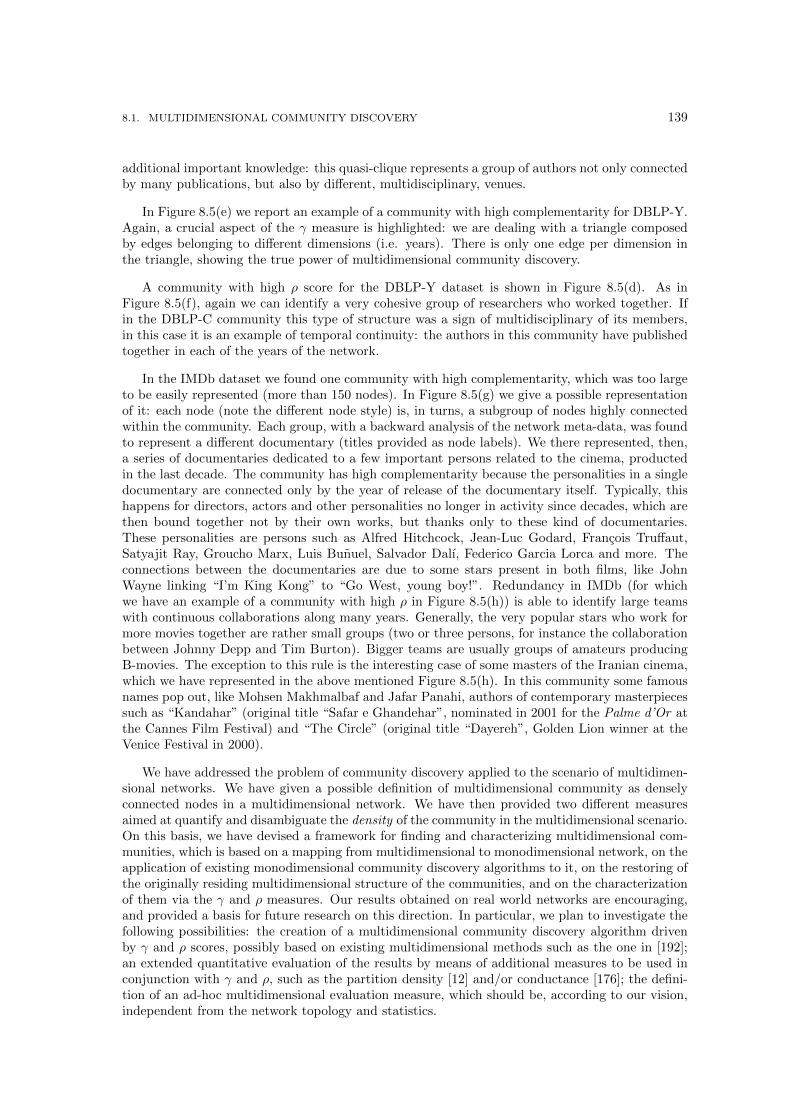
8.1. MULTIDIMENSIONAL COMMUNITY DISCOVERY 139
additional important knowledge: this quasi-clique represents a group of authors not only connectedby many publications, but also by different, multidisciplinary, venues.
In Figure 8.5(e) we report an example of a community with high complementarity for DBLP-Y.Again, a crucial aspect of the γ measure is highlighted: we are dealing with a triangle composedby edges belonging to different dimensions (i.e. years). There is only one edge per dimension inthe triangle, showing the true power of multidimensional community discovery.
A community with high ρ score for the DBLP-Y dataset is shown in Figure 8.5(d). As inFigure 8.5(f), again we can identify a very cohesive group of researchers who worked together. Ifin the DBLP-C community this type of structure was a sign of multidisciplinary of its members,in this case it is an example of temporal continuity: the authors in this community have publishedtogether in each of the years of the network.
In the IMDb dataset we found one community with high complementarity, which was too largeto be easily represented (more than 150 nodes). In Figure 8.5(g) we give a possible representationof it: each node (note the different node style) is, in turns, a subgroup of nodes highly connectedwithin the community. Each group, with a backward analysis of the network meta-data, was foundto represent a different documentary (titles provided as node labels). We there represented, then,a series of documentaries dedicated to a few important persons related to the cinema, productedin the last decade. The community has high complementarity because the personalities in a singledocumentary are connected only by the year of release of the documentary itself. Typically, thishappens for directors, actors and other personalities no longer in activity since decades, which arethen bound together not by their own works, but thanks only to these kind of documentaries.These personalities are persons such as Alfred Hitchcock, Jean-Luc Godard, Francois Truffaut,Satyajit Ray, Groucho Marx, Luis Bunuel, Salvador Dalı, Federico Garcia Lorca and more. Theconnections between the documentaries are due to some stars present in both films, like JohnWayne linking “I’m King Kong” to “Go West, young boy!”. Redundancy in IMDb (for whichwe have an example of a community with high ρ in Figure 8.5(h)) is able to identify large teamswith continuous collaborations along many years. Generally, the very popular stars who work formore movies together are rather small groups (two or three persons, for instance the collaborationbetween Johnny Depp and Tim Burton). Bigger teams are usually groups of amateurs producingB-movies. The exception to this rule is the interesting case of some masters of the Iranian cinema,which we have represented in the above mentioned Figure 8.5(h). In this community some famousnames pop out, like Mohsen Makhmalbaf and Jafar Panahi, authors of contemporary masterpiecessuch as “Kandahar” (original title “Safar e Ghandehar”, nominated in 2001 for the Palme d’Or atthe Cannes Film Festival) and “The Circle” (original title “Dayereh”, Golden Lion winner at theVenice Festival in 2000).
We have addressed the problem of community discovery applied to the scenario of multidimen-sional networks. We have given a possible definition of multidimensional community as denselyconnected nodes in a multidimensional network. We have then provided two different measuresaimed at quantify and disambiguate the density of the community in the multidimensional scenario.On this basis, we have devised a framework for finding and characterizing multidimensional com-munities, which is based on a mapping from multidimensional to monodimensional network, on theapplication of existing monodimensional community discovery algorithms to it, on the restoring ofthe originally residing multidimensional structure of the communities, and on the characterizationof them via the γ and ρ measures. Our results obtained on real world networks are encouraging,and provided a basis for future research on this direction. In particular, we plan to investigate thefollowing possibilities: the creation of a multidimensional community discovery algorithm drivenby γ and ρ scores, possibly based on existing multidimensional methods such as the one in [192];an extended quantitative evaluation of the results by means of additional measures to be used inconjunction with γ and ρ, such as the partition density [12] and/or conductance [176]; the defini-tion of an ad-hoc multidimensional evaluation measure, which should be, according to our vision,independent from the network topology and statistics.
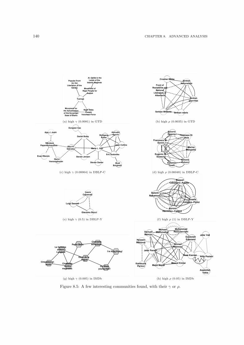
140 CHAPTER 8. ADVANCED ANALYSIS
Movement of
Niger People for
Justice
Niger Delta
People
Volunteer Force
Al−Qaida in the
Lands of the
Islamic Maghreb
Tuaregs
Movement for
the Actualization
of the Sovereign
State of Biafra
Popular Front
for the
Liberation of the
Sahara
Croatian Militia
Serbian
guerrillas
Front of
Resistance and
National
Liberation of
Albanians
Serbian rebels
Serbian
Nationalists
Serbian Militants
(a) high γ (0.0081) in GTD (b) high ρ (0.0035) in GTD
John Collins
Amrudin Agovic Wolfgang
Ketter Daniel Boley
Brett Borghetti
Eric SodomkaSteven Jensen
Steven Damer
Ajay J. Joshi
Nikolaos Papanikolopoulos
Paul R. Schrater Maria L. Gini
Dongwei Cao
Harini Veeraraghavan
Evan Ribnick
Simona Colucci
Azzurra Ragone
Marina Mongiello
Eufemia Tinelli
Francesco M. Donini
Eugenio Di Sciascio
Tommaso Di Noia
(c) high γ (0.00064) in DBLP-C (d) high ρ (0.06048) in DBLP-C
Laura Carnevali
Giacomo Bucci
Luigi Sassoli
Aurora Hermoso−Carazo
Josefa Linares−Pérez
Raquel Caballero−Aguila
Seiichi Nakamori
(e) high γ (0.5) in DBLP-Y (f) high ρ (1) in DBLP-Y
Cineastes en acciò Cineastas
contra magnates
I’m King Kong!
Cinerama adventure
Deux de la Vague
Pepìn BelloLe fantome
d’Henri Langlois
Go West, young man!
Reza Kianian
Jafar Vali
Atila Pesiani
Asadollah Yekta
Ezzatolah Entezami Hossein
Mahjoub
Majid MajidiKambuzia
Partovi
Dariush Mehrjui
Mohammad Reza Darvishi
Masud Kimiai
Mohsen Makhmalbaf
Ahmad Pezhman
Jafar Panahi
(g) high γ (0.005) in IMDb (h) high ρ (0.05) in IMDb
Figure 8.5: A few interesting communities found, with their γ or ρ.
8.2. MULTIDIMENSIONAL NETWORK MODELS 141
00.10.20.30.40.50.60.70.80.9
1
0 0.1 0.2 0.3 0.4 0.5 0.6 0.7 0.8 0.9 1
p(D
R)
DR
Bin1Bin2Bin3Bin4Bin5Bin6
0
0.1
0.2
0.3
0.4
0.5
0.6
0.7
0.8
0.9
1
0 0.1 0.2 0.3 0.4 0.5 0.6 0.7 0.8 0.9 1
p(D
R)
DR
198219871992199720022007
00.10.20.30.40.50.60.70.80.9
1
0 0.1 0.2 0.3 0.4 0.5 0.6 0.7 0.8 0.9 1
p(D
RW
)
DRW
Bin1Bin2Bin3Bin4Bin5Bin6
0
0.1
0.2
0.3
0.4
0.5
0.6
0.7
0.8
0.9
1
0 0.1 0.2 0.3 0.4 0.5 0.6 0.7 0.8 0.9 1
p(D
RW
)
DRW
198219871992199720022007
00.10.20.30.40.50.60.70.80.9
1
0 0.1 0.2 0.3 0.4 0.5 0.6 0.7 0.8 0.9 1
p(D
RX
OR
)
DRXOR
Bin1Bin2Bin3Bin4Bin5Bin6
0
0.1
0.2
0.3
0.4
0.5
0.6
0.7
0.8
0.9
1
0 0.1 0.2 0.3 0.4 0.5 0.6 0.7 0.8 0.9 1
p(D
RX
OR
)
DRXOR
198219871992199720022007
Figure 8.6: QueryLog (left column) and DBLP-Y (right) original Dimension Relevance distribu-tions.
8.2 Multidimensional Network Models
As briefly introduced in Section 7.1, one very important aspect in complex network theory isrepresented by the study of network null models. To understand the dynamics that regulates thecreation and the evolution of links in complex networks is a crucial aspect, because it gives usthe power to better understand and predict future behavior. Many network models have beendeveloped for classical monodimensional networks. They date back to the random graph [239, 87],until more recent approaches, as reviewed in Section 2.4. As we have pointed out in many sectionsof this thesis, even in this case there is little or no study about multidimensional network generators.The aim of this section is to provide some basic network generators and to verify if they are ableto grasp some of the crucial characteristics of real world multidimensional networks.
We built four different multidimensional network generators, each with different characteristics,starting from a simple random generator, towards a generator that tries to preserve a globalproperty of the original network that we might see as correlated with our measures, namely the EdgeDimension Correlation 7.2, being intuitively the most important measure to represent dimensioninterplay. For each model, we present its characteristics and the evaluation of the DimensionRelevances (Section 7.1) on the QueryLog and the DBLP-Y networks, because we choose to verifyhow much of the local dimension interplay, i.e. the distribution of the DRs, is preserved fromthe original network. We recall that the Dimension Relevance class of measures quantifies theimportance of each single dimension in the economy of the connections of the network, using anode centric perspective. For each node, it quantifies how much each dimension is important in theeconomy of its connections. The distribution of the DRs gives a picture about how the importanceof the dimensions is distributed on the network.
For clarity, we report the original Dimension Relevance distributions for Querylog and DBLP-Ynetworks in Figure 8.6, originally plotted in Figure 7.3(a-c) and 7.3(g-i) respectively, allowing aneasier comparison.
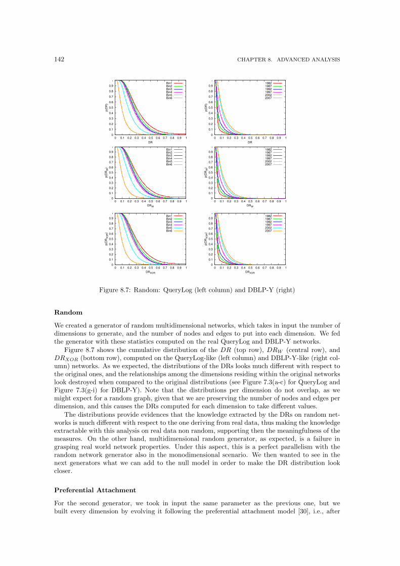
142 CHAPTER 8. ADVANCED ANALYSIS
0
0.1
0.2
0.3
0.4
0.5
0.6
0.7
0.8
0.9
1
0 0.1 0.2 0.3 0.4 0.5 0.6 0.7 0.8 0.9 1
p(D
R)
DR
Bin1Bin2Bin3Bin4Bin5Bin6
0
0.1
0.2
0.3
0.4
0.5
0.6
0.7
0.8
0.9
1
0 0.1 0.2 0.3 0.4 0.5 0.6 0.7 0.8 0.9 1
p(D
R)
DR
198219871992199720022007
0
0.1
0.2
0.3
0.4
0.5
0.6
0.7
0.8
0.9
1
0 0.1 0.2 0.3 0.4 0.5 0.6 0.7 0.8 0.9 1
p(D
RW
)
DRW
Bin1Bin2Bin3Bin4Bin5Bin6
0
0.1
0.2
0.3
0.4
0.5
0.6
0.7
0.8
0.9
1
0 0.1 0.2 0.3 0.4 0.5 0.6 0.7 0.8 0.9 1p(D
RW
)DRW
198219871992199720022007
0
0.1
0.2
0.3
0.4
0.5
0.6
0.7
0.8
0.9
1
0 0.1 0.2 0.3 0.4 0.5 0.6 0.7 0.8 0.9 1
p(D
RX
OR
)
DRXOR
Bin1Bin2Bin3Bin4Bin5Bin6
0
0.1
0.2
0.3
0.4
0.5
0.6
0.7
0.8
0.9
1
0 0.1 0.2 0.3 0.4 0.5 0.6 0.7 0.8 0.9 1
p(D
RX
OR
)
DRXOR
198219871992199720022007
Figure 8.7: Random: QueryLog (left column) and DBLP-Y (right)
Random
We created a generator of random multidimensional networks, which takes in input the number ofdimensions to generate, and the number of nodes and edges to put into each dimension. We fedthe generator with these statistics computed on the real QueryLog and DBLP-Y networks.
Figure 8.7 shows the cumulative distribution of the DR (top row), DRW (central row), andDRXOR (bottom row), computed on the QueryLog-like (left column) and DBLP-Y-like (right col-umn) networks. As we expected, the distributions of the DRs looks much different with respect tothe original ones, and the relationships among the dimensions residing within the original networkslook destroyed when compared to the original distributions (see Figure 7.3(a-c) for QueryLog andFigure 7.3(g-i) for DBLP-Y). Note that the distributions per dimension do not overlap, as wemight expect for a random graph, given that we are preserving the number of nodes and edges perdimension, and this causes the DRs computed for each dimension to take different values.
The distributions provide evidences that the knowledge extracted by the DRs on random net-works is much different with respect to the one deriving from real data, thus making the knowledgeextractable with this analysis on real data non random, supporting then the meaningfulness of themeasures. On the other hand, multidimensional random generator, as expected, is a failure ingrasping real world network properties. Under this aspect, this is a perfect parallelism with therandom network generator also in the monodimensional scenario. We then wanted to see in thenext generators what we can add to the null model in order to make the DR distribution lookcloser.
Preferential Attachment
For the second generator, we took in input the same parameter as the previous one, but webuilt every dimension by evolving it following the preferential attachment model [30], i.e., after
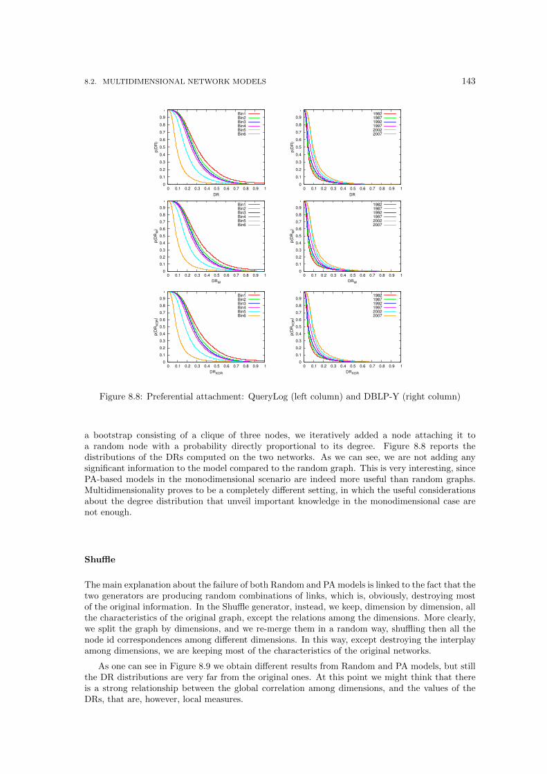
8.2. MULTIDIMENSIONAL NETWORK MODELS 143
0
0.1
0.2
0.3
0.4
0.5
0.6
0.7
0.8
0.9
1
0 0.1 0.2 0.3 0.4 0.5 0.6 0.7 0.8 0.9 1
p(D
R)
DR
Bin1Bin2Bin3Bin4Bin5Bin6
0
0.1
0.2
0.3
0.4
0.5
0.6
0.7
0.8
0.9
1
0 0.1 0.2 0.3 0.4 0.5 0.6 0.7 0.8 0.9 1
p(D
R)
DR
198219871992199720022007
0
0.1
0.2
0.3
0.4
0.5
0.6
0.7
0.8
0.9
1
0 0.1 0.2 0.3 0.4 0.5 0.6 0.7 0.8 0.9 1
p(D
RW
)
DRW
Bin1Bin2Bin3Bin4Bin5Bin6
0
0.1
0.2
0.3
0.4
0.5
0.6
0.7
0.8
0.9
1
0 0.1 0.2 0.3 0.4 0.5 0.6 0.7 0.8 0.9 1
p(D
RW
)
DRW
198219871992199720022007
0
0.1
0.2
0.3
0.4
0.5
0.6
0.7
0.8
0.9
1
0 0.1 0.2 0.3 0.4 0.5 0.6 0.7 0.8 0.9 1
p(D
RX
OR
)
DRXOR
Bin1Bin2Bin3Bin4Bin5Bin6
0
0.1
0.2
0.3
0.4
0.5
0.6
0.7
0.8
0.9
1
0 0.1 0.2 0.3 0.4 0.5 0.6 0.7 0.8 0.9 1
p(D
RX
OR
)
DRXOR
198219871992199720022007
Figure 8.8: Preferential attachment: QueryLog (left column) and DBLP-Y (right column)
a bootstrap consisting of a clique of three nodes, we iteratively added a node attaching it toa random node with a probability directly proportional to its degree. Figure 8.8 reports thedistributions of the DRs computed on the two networks. As we can see, we are not adding anysignificant information to the model compared to the random graph. This is very interesting, sincePA-based models in the monodimensional scenario are indeed more useful than random graphs.Multidimensionality proves to be a completely different setting, in which the useful considerationsabout the degree distribution that unveil important knowledge in the monodimensional case arenot enough.
Shuffle
The main explanation about the failure of both Random and PA models is linked to the fact that thetwo generators are producing random combinations of links, which is, obviously, destroying mostof the original information. In the Shuffle generator, instead, we keep, dimension by dimension, allthe characteristics of the original graph, except the relations among the dimensions. More clearly,we split the graph by dimensions, and we re-merge them in a random way, shuffling then all thenode id correspondences among different dimensions. In this way, except destroying the interplayamong dimensions, we are keeping most of the characteristics of the original networks.
As one can see in Figure 8.9 we obtain different results from Random and PA models, but stillthe DR distributions are very far from the original ones. At this point we might think that thereis a strong relationship between the global correlation among dimensions, and the values of theDRs, that are, however, local measures.
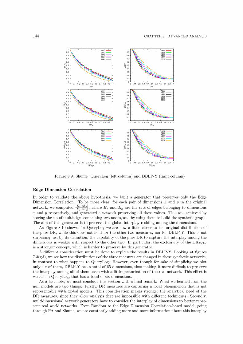
144 CHAPTER 8. ADVANCED ANALYSIS
0
0.1
0.2
0.3
0.4
0.5
0.6
0.7
0.8
0.9
1
0 0.1 0.2 0.3 0.4 0.5 0.6 0.7 0.8 0.9 1
p(D
R)
DR
Bin1Bin2Bin3Bin4Bin5Bin6
0
0.1
0.2
0.3
0.4
0.5
0.6
0.7
0.8
0.9
1
0 0.1 0.2 0.3 0.4 0.5 0.6 0.7 0.8 0.9 1
p(D
R)
DR
198219871992199720022007
0
0.1
0.2
0.3
0.4
0.5
0.6
0.7
0.8
0.9
1
0 0.1 0.2 0.3 0.4 0.5 0.6 0.7 0.8 0.9 1
p(D
RW
)
DRW
Bin1Bin2Bin3Bin4Bin5Bin6
0
0.1
0.2
0.3
0.4
0.5
0.6
0.7
0.8
0.9
1
0 0.1 0.2 0.3 0.4 0.5 0.6 0.7 0.8 0.9 1p(D
RW
)DRW
198219871992199720022007
0
0.1
0.2
0.3
0.4
0.5
0.6
0.7
0.8
0.9
1
0 0.1 0.2 0.3 0.4 0.5 0.6 0.7 0.8 0.9 1
p(D
RX
OR
)
DRXOR
Bin1Bin2Bin3Bin4Bin5Bin6
0
0.1
0.2
0.3
0.4
0.5
0.6
0.7
0.8
0.9
1
0 0.1 0.2 0.3 0.4 0.5 0.6 0.7 0.8 0.9 1
p(D
RX
OR
)
DRXOR
198219871992199720022007
Figure 8.9: Shuffle: QueryLog (left column) and DBLP-Y (right column)
Edge Dimension Correlation
In order to validate the above hypothesis, we built a generator that preserves only the EdgeDimension Correlation. To be more clear, for each pair of dimensions x and y in the original
network, we computed|Ex∩Ey||Ex∪Ey| , where Ex and Ey are the sets of edges belonging to dimensions
x and y respectively, and generated a network preserving all these values. This was achieved bystoring the set of multiedges connecting two nodes, and by using them to build the synthetic graph.The aim of this generator is to preserve the global interplay residing among the dimensions.
As Figure 8.10 shows, for QueryLog we are now a little closer to the original distribution ofthe pure DR, while this does not hold for the other two measures, nor for DBLP-Y. This is notsurprising, as, by its definition, the capability of the pure DR to capture the interplay among thedimensions is weaker with respect to the other two. In particular, the exclusivity of the DRXOR
is a stronger concept, which is harder to preserve by this generator.A different consideration must be done to explain the results in DBLP-Y. Looking at figures
7.3(g-i), we see how the distributions of the three measures are changed in these synthetic networks,in contrast to what happens to QueryLog. However, even though for sake of simplicity we plotonly six of them, DBLP-Y has a total of 65 dimensions, thus making it more difficult to preservethe interplay among all of them, even with a little perturbation of the real network. This effect isweaker in QueryLog, that has a total of six dimensions.
As a last note, we must conclude this section with a final remark. What we learned from thenull models are two things. Firstly, DR measures are capturing a local phenomenon that is notrepresentable with global models. This consideration makes stronger the analytical need of theDR measures, since they allow analysis that are impossible with different techniques. Secondly,multidimensional network generators have to consider the interplay of dimensions to better repre-sent real world networks. From Random to the Edge Dimension Correlation-based model, goingthrough PA and Shuffle, we are constantly adding more and more information about this interplay
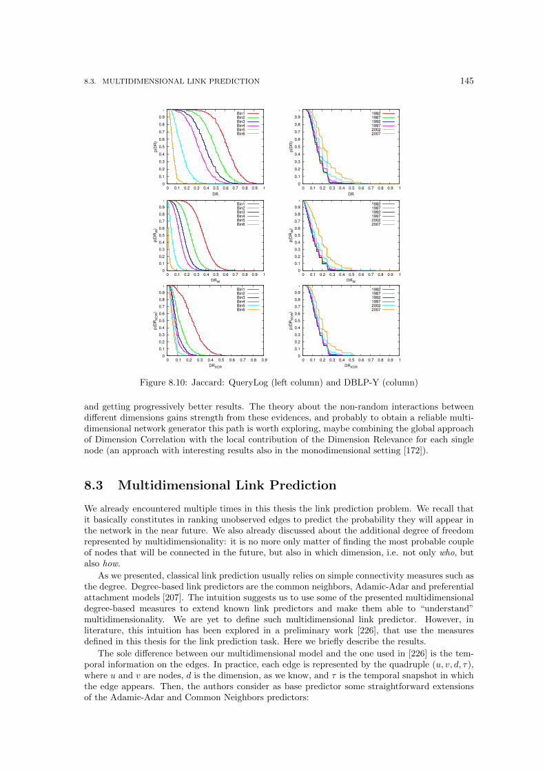
8.3. MULTIDIMENSIONAL LINK PREDICTION 145
0
0.1
0.2
0.3
0.4
0.5
0.6
0.7
0.8
0.9
1
0 0.1 0.2 0.3 0.4 0.5 0.6 0.7 0.8 0.9 1
p(D
R)
DR
Bin1Bin2Bin3Bin4Bin5Bin6
0
0.1
0.2
0.3
0.4
0.5
0.6
0.7
0.8
0.9
1
0 0.1 0.2 0.3 0.4 0.5 0.6 0.7 0.8 0.9 1
p(D
R)
DR
198219871992199720022007
0
0.1
0.2
0.3
0.4
0.5
0.6
0.7
0.8
0.9
1
0 0.1 0.2 0.3 0.4 0.5 0.6 0.7 0.8 0.9 1
p(D
RW
)
DRW
Bin1Bin2Bin3Bin4Bin5Bin6
0
0.1
0.2
0.3
0.4
0.5
0.6
0.7
0.8
0.9
1
0 0.1 0.2 0.3 0.4 0.5 0.6 0.7 0.8 0.9 1
p(D
RW
)
DRW
198219871992199720022007
0
0.1
0.2
0.3
0.4
0.5
0.6
0.7
0.8
0.9
1
0 0.1 0.2 0.3 0.4 0.5 0.6 0.7 0.8 0.9
p(D
RX
OR
)
DRXOR
Bin1Bin2Bin3Bin4Bin5Bin6
0
0.1
0.2
0.3
0.4
0.5
0.6
0.7
0.8
0.9
1
0 0.1 0.2 0.3 0.4 0.5 0.6 0.7 0.8 0.9 1
p(D
RX
OR
)
DRXOR
198219871992199720022007
Figure 8.10: Jaccard: QueryLog (left column) and DBLP-Y (column)
and getting progressively better results. The theory about the non-random interactions betweendifferent dimensions gains strength from these evidences, and probably to obtain a reliable multi-dimensional network generator this path is worth exploring, maybe combining the global approachof Dimension Correlation with the local contribution of the Dimension Relevance for each singlenode (an approach with interesting results also in the monodimensional setting [172]).
8.3 Multidimensional Link Prediction
We already encountered multiple times in this thesis the link prediction problem. We recall thatit basically constitutes in ranking unobserved edges to predict the probability they will appear inthe network in the near future. We also already discussed about the additional degree of freedomrepresented by multidimensionality: it is no more only matter of finding the most probable coupleof nodes that will be connected in the future, but also in which dimension, i.e. not only who, butalso how.
As we presented, classical link prediction usually relies on simple connectivity measures such asthe degree. Degree-based link predictors are the common neighbors, Adamic-Adar and preferentialattachment models [207]. The intuition suggests us to use some of the presented multidimensionaldegree-based measures to extend known link predictors and make them able to “understand”multidimensionality. We are yet to define such multidimensional link predictor. However, inliterature, this intuition has been explored in a preliminary work [226], that use the measuresdefined in this thesis for the link prediction task. Here we briefly describe the results.
The sole difference between our multidimensional model and the one used in [226] is the tem-poral information on the edges. In practice, each edge is represented by the quadruple (u, v, d, τ),where u and v are nodes, d is the dimension, as we know, and τ is the temporal snapshot in whichthe edge appears. Then, the authors consider as base predictor some straightforward extensionsof the Adamic-Adar and Common Neighbors predictors:
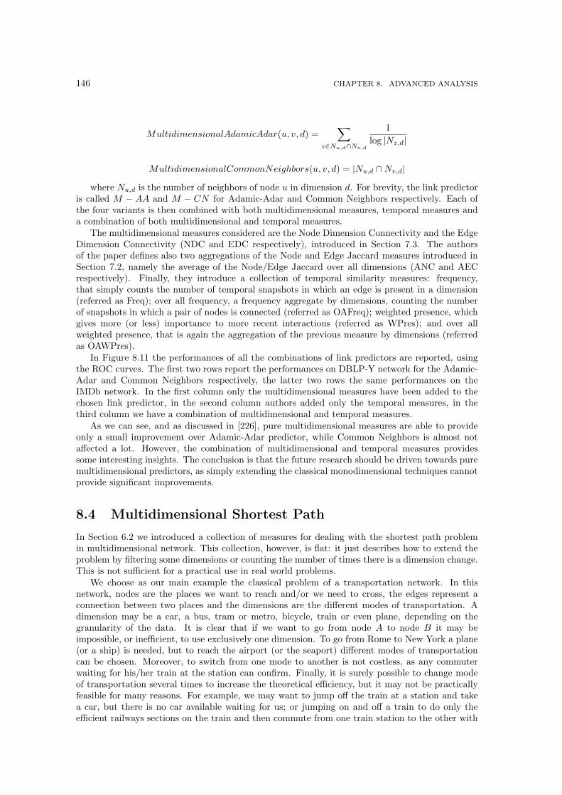
146 CHAPTER 8. ADVANCED ANALYSIS
MultidimensionalAdamicAdar(u, v, d) =∑
z∈Nu,d∩Nv,d
1
log |Nz,d|
MultidimensionalCommonNeighbors(u, v, d) = |Nu,d ∩Nv,d|
where Nu,d is the number of neighbors of node u in dimension d. For brevity, the link predictoris called M − AA and M − CN for Adamic-Adar and Common Neighbors respectively. Each ofthe four variants is then combined with both multidimensional measures, temporal measures anda combination of both multidimensional and temporal measures.
The multidimensional measures considered are the Node Dimension Connectivity and the EdgeDimension Connectivity (NDC and EDC respectively), introduced in Section 7.3. The authorsof the paper defines also two aggregations of the Node and Edge Jaccard measures introduced inSection 7.2, namely the average of the Node/Edge Jaccard over all dimensions (ANC and AECrespectively). Finally, they introduce a collection of temporal similarity measures: frequency,that simply counts the number of temporal snapshots in which an edge is present in a dimension(referred as Freq); over all frequency, a frequency aggregate by dimensions, counting the numberof snapshots in which a pair of nodes is connected (referred as OAFreq); weighted presence, whichgives more (or less) importance to more recent interactions (referred as WPres); and over allweighted presence, that is again the aggregation of the previous measure by dimensions (referredas OAWPres).
In Figure 8.11 the performances of all the combinations of link predictors are reported, usingthe ROC curves. The first two rows report the performances on DBLP-Y network for the Adamic-Adar and Common Neighbors respectively, the latter two rows the same performances on theIMDb network. In the first column only the multidimensional measures have been added to thechosen link predictor, in the second column authors added only the temporal measures, in thethird column we have a combination of multidimensional and temporal measures.
As we can see, and as discussed in [226], pure multidimensional measures are able to provideonly a small improvement over Adamic-Adar predictor, while Common Neighbors is almost notaffected a lot. However, the combination of multidimensional and temporal measures providessome interesting insights. The conclusion is that the future research should be driven towards puremultidimensional predictors, as simply extending the classical monodimensional techniques cannotprovide significant improvements.
8.4 Multidimensional Shortest Path
In Section 6.2 we introduced a collection of measures for dealing with the shortest path problemin multidimensional network. This collection, however, is flat: it just describes how to extend theproblem by filtering some dimensions or counting the number of times there is a dimension change.This is not sufficient for a practical use in real world problems.
We choose as our main example the classical problem of a transportation network. In thisnetwork, nodes are the places we want to reach and/or we need to cross, the edges represent aconnection between two places and the dimensions are the different modes of transportation. Adimension may be a car, a bus, tram or metro, bicycle, train or even plane, depending on thegranularity of the data. It is clear that if we want to go from node A to node B it may beimpossible, or inefficient, to use exclusively one dimension. To go from Rome to New York a plane(or a ship) is needed, but to reach the airport (or the seaport) different modes of transportationcan be chosen. Moreover, to switch from one mode to another is not costless, as any commuterwaiting for his/her train at the station can confirm. Finally, it is surely possible to change modeof transportation several times to increase the theoretical efficiency, but it may not be practicallyfeasible for many reasons. For example, we may want to jump off the train at a station and takea car, but there is no car available waiting for us; or jumping on and off a train to do only theefficient railways sections on the train and then commute from one train station to the other with
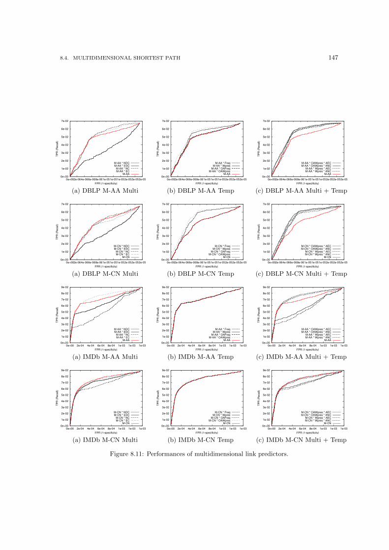
8.4. MULTIDIMENSIONAL SHORTEST PATH 147
0e+00
1e-02
2e-02
3e-02
4e-02
5e-02
6e-02
7e-02
0e+002e-064e-066e-068e-061e-051e-051e-052e-052e-052e-05
TP
R (
Re
ca
ll)
FPR (1-specificity)
M-AA * NDCM-AA * EDC
M-AA * NCM-AA * EC
M-AA0e+00
1e-02
2e-02
3e-02
4e-02
5e-02
6e-02
7e-02
0e+002e-064e-066e-068e-061e-051e-051e-052e-052e-052e-05
TP
R (
Re
ca
ll)
FPR (1-specificity)
M-AA * FreqM-AA * Wpres
M-AA * OAFreqM-AA * OAWpres
M-AA0e+00
1e-02
2e-02
3e-02
4e-02
5e-02
6e-02
7e-02
0e+002e-064e-066e-068e-061e-051e-051e-052e-052e-052e-05
TP
R (
Re
ca
ll)
FPR (1-specificity)
M-AA * OAWpres * AECM-AA * OAWpres * ANC
M-AA * Wpres * AECM-AA * Wpres * ANC
M-AA
(a) DBLP M-AA Multi (b) DBLP M-AA Temp (c) DBLP M-AA Multi + Temp
0e+00
1e-02
2e-02
3e-02
4e-02
5e-02
6e-02
7e-02
0e+002e-064e-066e-068e-061e-051e-051e-052e-052e-052e-05
TP
R (
Re
ca
ll)
FPR (1-specificity)
M-CN * NDCM-CN * EDC
M-CN * NCM-CN * EC
M-CN0e+00
1e-02
2e-02
3e-02
4e-02
5e-02
6e-02
7e-02
0e+002e-064e-066e-068e-061e-051e-051e-052e-052e-052e-05
TP
R (
Re
ca
ll)
FPR (1-specificity)
M-CN * FreqM-CN * Wpres
M-CN * OAFreqM-CN * OAWpres
M-CN0e+00
1e-02
2e-02
3e-02
4e-02
5e-02
6e-02
7e-02
0e+002e-064e-066e-068e-061e-051e-051e-052e-052e-052e-05
TP
R (
Re
ca
ll)
FPR (1-specificity)
M-CN * OAWpres * AECM-CN * OAWpres * ANC
M-CN * Wpres * AECM-CN * Wpres * ANC
M-CN
(a) DBLP M-CN Multi (b) DBLP M-CN Temp (c) DBLP M-CN Multi + Temp
0e+00
1e-02
2e-02
3e-02
4e-02
5e-02
6e-02
7e-02
8e-02
9e-02
0e+00 2e-04 4e-04 6e-04 8e-04 1e-03 1e-03 1e-03
TP
R (
Re
ca
ll)
FPR (1-specificity)
M-AA * NDCM-AA * EDC
M-AA * NCM-AA * EC
M-AA0e+00
1e-02
2e-02
3e-02
4e-02
5e-02
6e-02
7e-02
8e-02
9e-02
0e+00 2e-04 4e-04 6e-04 8e-04 1e-03 1e-03 1e-03
TP
R (
Re
ca
ll)
FPR (1-specificity)
M-AA * FreqM-AA * Wpres
M-AA * OAFreqM-AA * OAWpres
M-AA0e+00
1e-02
2e-02
3e-02
4e-02
5e-02
6e-02
7e-02
8e-02
9e-02
0e+00 2e-04 4e-04 6e-04 8e-04 1e-03 1e-03 1e-03
TP
R (
Re
ca
ll)
FPR (1-specificity)
M-AA * OAWpres * AECM-AA * OAWpres * ANC
M-AA * Wpres * AECM-AA * Wpres * ANC
M-AA
(a) IMDb M-AA Multi (b) IMDb M-AA Temp (c) IMDb M-AA Multi + Temp
0e+00
1e-02
2e-02
3e-02
4e-02
5e-02
6e-02
7e-02
8e-02
9e-02
0e+00 2e-04 4e-04 6e-04 8e-04 1e-03 1e-03 1e-03
TP
R (
Re
ca
ll)
FPR (1-specificity)
M-CN * NDCM-CN * EDC
M-CN * NCM-CN * EC
M-CN0e+00
1e-02
2e-02
3e-02
4e-02
5e-02
6e-02
7e-02
8e-02
9e-02
0e+00 2e-04 4e-04 6e-04 8e-04 1e-03 1e-03 1e-03
TP
R (
Re
ca
ll)
FPR (1-specificity)
M-CN * FreqM-CN * Wpres
M-CN * OAFreqM-CN * OAWpres
M-CN0e+00
1e-02
2e-02
3e-02
4e-02
5e-02
6e-02
7e-02
8e-02
9e-02
0e+00 2e-04 4e-04 6e-04 8e-04 1e-03 1e-03 1e-03
TP
R (
Re
ca
ll)
FPR (1-specificity)
M-CN * OAWpres * AECM-CN * OAWpres * ANC
M-CN * Wpres * AECM-CN * Wpres * ANC
M-CN
(a) IMDb M-CN Multi (b) IMDb M-CN Temp (c) IMDb M-CN Multi + Temp
Figure 8.11: Performances of multidimensional link predictors.
148 CHAPTER 8. ADVANCED ANALYSIS
more efficient modes of transportation is probably not efficient, as staying quiet in the same trainfor the entire trip is less costly in practice.
All these scenarios lead to more complex tools for a practical computation of shortest pathsin multidimensional network. More precisely, here we define the problem of finding the shortestpath in a multidimensional network with cost modifiers. To tackle this problem we need to in-troduce some modifications to our model. Of course, our multidimensional network has to beweighted, because otherwise the model loses importance for real world scenarios. Then we willuse the classical definition of a simple path in a network, i.e. a sequence P = (e0, e1, ..., en−1) =((v0, v1, d0, w0), (v1, v2, d1, w1), ..., (vn−1, vn, dn−1, wn−1)); where v0 ∈ V is the source node, vn ∈ Vis the destination node, ek ∈ E and n is the path length. We recall that in a simple path there isno vertex vi and no edge ek crossed more than once.
Usually, the cost of a path is given by the sum of all the weights of the edges crossed, orC(P ) =
∑n−1i=0 wi. We introduce the concept of a path constraint : a boolean check that, given
a path, can return true or false, i.e. A(P ) → {T |F}. Finally, a cost modifier m is a couple(A, φ), where A is a path constraint and φ : R → R is a function such that if A(P ) = T , thenC(P ) = φ(C(P )). M is defined as a collection of m. It is important to note that M has an internalorder, that can be freely defined. Without an order, it is impossible to calculate the final cost ofa path P . Let us assume we have two cost modifiers m′ and m′′ and path P satisfies both A′ andA′′. Without an order we cannot say if the final cost is φ′(φ′′(C(P ))) or φ′′(φ′(C(P ))), and giventhat φ′ may be + and φ′′ may be ×, this will lead to two different results.
We are now able to define the shortest path in a multidimensional network with cost modifiersproblem as follows:
Definition 34 (Multidimensional Shortest Path with Cost Modifiers) Given two nodes v1
and vn in a multidimensional network and a set M of cost modifiers, find the path P : v1 → vnfrom the source node v1 and the destination node vn such that Φ(C(P )) is minimal, where Φ is theordered application of all φi ∈M for which Ai(P ) = T .
We do not have a complete solution for this problem, as the research in this direction is inits early stages. We do have, however, a preliminary framework and a proposed implementedalgorithm, MSPCM (Multidimensional Shortest Path with Cost Modifiers), that still needs a moreprincipled formulation and rigorous experimental test. We record here what are the foundationsand the intuitions constituting the basis of MSPCM.
There is a collection of shortest path algorithms in literature. The most popular in literatureare Dijkstra, Bellman-Ford and Floyd-Warshall algorithms [13]. However, these algorithms are notsuitable for our scenario, since they cannot handle cost modifiers. A naive solution would be to usea particular algorithm, for example Dijkstra algorithm and for each new edge to check Φ(C(P )).This is not possible, since shortest path algorithms need to satisfy the Bellman equation. In termsof our problem, the Bellman equation is reduced to the following lemma: if Pst is a shortest pathfrom s to t and it contains node j, then the sub-path from s to j is the shortest path between sand j. But an hypothetical cost modifier involving an additional node j′ may be less costly forgoing from s to t, even if j′ is not required to go from s to j because that particular cost modifieris not triggered.
Consider the graph in Figure 8.12. Obviously, without cost modifiers, the shortest path fromnode 0 to node 2 passes through node 3. But suppose that our set M contains two cost modifiers.The first modifier subtracts 3 from C(P ) if we cross two times in a row an edge in the red dimension.The second modifier adds 4 to C(P ) if we cross two times in a row an edge in the gray dimension.What happens now is that the shortest path from node 0 to node 2 crosses node 1 before node 3.But node 1 is not necessary for the shortest path from node 0 to node 3. Therefore the fundamentallemma presented before is not satisfied and no classical algorithm can be used to obtain an exactsolution to Problem 34.
Currently, the only algorithm able to solve our problem with an optimal solution is the bruteforce algorithm, i.e. to calculate all shortest paths and then choose the path with the lowest costafter applying all cost modifiers. Of course, this is not what we are interested in, since the brute

8.4. MULTIDIMENSIONAL SHORTEST PATH 149
2
3
2
3
n o d e 3
n o d e 0
n o d e 1
n o d e 2
Figure 8.12: A toy example for the multidimensional shortest path with cost modifiers problem.
Algorithm 2 Flattening(G,M)
Require: multidimensional network G = (V,E, L), list of cost modifiers MEnsure: simple weighted graph G′
1: E′ ← ∅2: G′ ← (V,E′)3: for all {(u, v) | ∃(u, v, d) ∈ E ∧ d ∈ D}. do4: c← H(Fuv,M)5: e′ ← (u, v, c)6: E′ ← E′ ∪ e′7: end for8: return G′
force algorithm will scale as O(2n), where n is the number of nodes of the network. The problemis reduced to find an efficient way to find a reasonably short path in a reasonable computing time.
The solution here proposed is a multi-step process. In practice, our algorithm will be composedby three phases:
1. Flattening preprocessing, in which we reduce the multidimensional network and the costmodifier set M into a simple flat structure G′;
2. Shortest path detection, that uses a classical algorithm and G′ as input to get an intermediateresult P ′st for each source s and destination d;
3. Path reconstruction, in which we transform each optimal path P ′st for G′ into a greedyshortest path Pst for the original network.
Flattening preprocessing. This is the most important step of our algorithm. The generalidea is to create some function F (G,M) = G′ able to reduce the original problem into a simplifiedversion that can be handled by the current state-of-the-art algorithms. Of course, the most accurateis G′ in describing (G,M), the closest to optimal the results will be. The algorithm we chose isformalized in Algorithm 2. Some additional notation is needed.
The key concept here is the H(Fuv,M) function. This functions takes as input a set of nodesand edges Fuv, a set of cost modifies M and returns a single edge connecting u and v with anestimation of its average cost. Fuv may be simply an arbitrary set of nodes and edges containingnodes u and v, however it is useful to define it as the neighborhood of u and v. The idea is todefine a range and then collect into Fuv all nodes and edges distant from u or v at most the sizeof the range. The intuition of breaking down the complex shortest path problem into smallersections of the network is also at the basis of the fastest implementation of the Newman-Girvancommunity discovery algorithm based on the concept of “split betweenness” [106] (see also Section
150 CHAPTER 8. ADVANCED ANALYSIS
2.3). Into this small range, a smaller portion of the network is analyzed. The lowest cost amongall the shortest paths crossing entirely this network portion and containing the edge (u, v) is thenreturned by the H function.
In practice, Algorithm 2 cycles over all the connected couples of G, regardless the dimensionsinvolved, estimates the cost for passing through this connection applying H(Fuv,M) on a givenset Fuv and adds to a result graph G′ an edge e′ weighted accordingly to the estimate.
Shortest path detection. This step is trivial. Given a simple weighted graph G′ we simplyapply a chosen shortest path algorithm and we get P ′st for each source s and target t we areinterested in. Any shortest path algorithm present in literature can be applied, since in G′ thelemma derived from the Bellman equation holds.
Path reconstruction. The last step in conceptually simple. Given a path P ′st, optimal in G′,we want to reconstruct the actual path Pst in our original multidimensional network. Technically,also this step may pose several algorithmic challenges. However, we make use of a classical empiricalresult of complex network analysis that holds generally for a fairly big amount of different complexnetworks. This result states that usually the shortest path between any two vertices in a complexnetwork does not include an high number of edges. To be precise, this is the small-world property,derived from an intuition of Stanley Milgram [186] later quantified: the average length in termsof edges of the shortest path in a complex network is proportional to, and usually lower than, thelogarithm of the number of nodes of the network itself [195]. Since the number of edges to beconsidered is small, at this step we apply a brute force solution for the path P ′st by checking allthe possible combinations of edges in all possible dimensions from s to t and then we return theone that minimizes Φ(C(Pst)).
We do not provide an extensive complexity evaluation, but we find that, using Floyd-Washallalgorithm for the second step of our algorithm, the time complexity can be approximated toO(mn|M | log n) if we want to find the entire collection of shortest path in the network. The Floyd-Washall algorithm forces us to compute all shortest paths instead only one separately, but for thisproperty it needs to run the preprocessing stage only once. Dijkstra algorithm is more efficientfor computing all shortest paths from a single root node, but for each root node the preprocessingstage needs to be run again. Also, the range for the approximation should be taken into accountin the complexity. However, since for heuristic reasons we rarely will use a range higher than 6,its weight in the complexity is negligible.
We now want to test how efficient our heuristic is on real world data. We calculated all theshortest paths on a multidimensional network using our algorithm MSPCM and the brute forcealgorithm, that always retrieve the optimal solution. Both algorithms are implemented in Java.We will not use the networks presented in Chapter 5 since they are too big for the brute forcealgorithm: even the toy network from Facebook with less than 300 nodes takes too long. Weinstead used a simplified version of the MBTA transportation in Boston, using only the dimensionof the subway and reducing the nodes only to the stations where it is possible to change the line(ending up with 27 nodes). On the other hand, when tested on DBLP-C and DBLP-Y networks,MSPCM was able to end its computation in orders of minutes.
One last caveat is needed. It has been observed that the best results in general are obtainedwith a range value between 4 and 6. However, in these cases the path shorter than the rangevalues were far from optimal. This is a natural consequence of the example depicted in Figure 8.12and described in the text: using a range of 4 the gain from the cost modifiers related to the reddimension is triggered, making those two edges very convenient in G′, but then when moved to Gthe paths are not optimal. We found convenient, then, to make two consecutive runs of MSPCM,the first one with the optimal range and the second one with range equal to 1. For each path wethen choose the solution with the lower cost. With this strategy, we firstly identify long paths andthen we obtain the short paths with the second run.
The brute force algorithm found the average cost of all the paths in our MBTA representationto be equal to 17.73. MSPCM was able to find an average value of 19.57. Among the pathsreturned by MSPCM, 65.16% were also present in the brute force solution, i.e. almost two pathsout of three were actually the optimal path. The biggest gain comes from confronting the runningtimes. The brute force algorithm took 155 seconds to calculate all the paths on the 27 nodes

8.4. MULTIDIMENSIONAL SHORTEST PATH 151
network, while MSPCM took 7.24 seconds. This means that with MSPCM we can expect to find65% optimal paths with running time 20 times lower, and this gain grows for bigger networks,given the exponential nature of the brute force solution.

152 CHAPTER 8. ADVANCED ANALYSIS

Part III
Novel Insights for NetworkAnalysis


Chapter 9
The Product Space
In this chapter we present the creation and the analysis of the Product Space. The ProductSpace is a tool created with complex network analysis techniques that has been used to obtainan improved knowledge about the mechanics of international trade. We see how this is achievedusing monodimensional network analysis, being only one kind of interaction included in the mainstructure of the Product Space. However, from the creation of the dataset itself to each analyticalstep, we are able to detect where multidimensionality could be useful to better grasp the real worldcomplexity of international trade, leading to novel results.
We firstly introduce the concept of Economic Complexity, that is the fundamental buildingblock of the Product Space. Then, we show why and how Economic Complexity is a very usefultool able to better explain the country-level trade dynamics of the real world. We then explainhow to use Economic Complexity indicators to create the Product Space. Finally, we present onepossible analysis done with the Product Space, namely a new product classification based not on atop-down interpretation of what the world should look like according to an analyst or a particularphilosophy, but based on how product arrange themselves according to the capabilities needed toproduce them. For each of these steps, our aim is to make evident where multidimensional networkanalysis can be applied.
The work of this chapter is mainly based on [128]. The original work introducing the ProductSpace concept is [131].
9.1 Economic Complexity
One way of describing the economic world is to say that products are made with machines, rawmaterials and labor. Another perspective is that products are made with knowledge. The truevalue of a tube of toothpaste is that it manifests knowledge about the chemicals that facilitatebrushing, and that kill the germs that cause bad breath, cavities and gum disease.
Markets allow us to access the vast amounts of knowledge that are scattered among the peopleof the world, that is concentrated in all the different products. Products are vehicles for knowledge,but embedding knowledge in products requires people who possess a working understanding of thatknowledge. Most of us can be ignorant about how to synthesize sodium fluoride because we canrely on the few people who know how to create this atomic cocktail, and who together with theircolleagues at the toothpaste factory, can deposit it into a product that we can use. The divisionof labor is what allows us to access a quantity of knowledge that none of us would be able to holdindividually.
We can distinguish between two kinds of knowledge: explicit and tacit. Explicit knowledgecan be transferred easily by reading a text or listening to a conversation. If all knowledge hadthis characteristic, the world would be very different. Countries would catch up very quickly tofrontier technologies, and the income differences across the world would be much smaller thanwhat we see today. The problem is that crucial parts of knowledge are tacit and therefore hard to
156 CHAPTER 9. THE PRODUCT SPACE
embed in people: they require a costly and time-consuming effort. Because it is hard to transfer,tacit knowledge is what constrains the process of growth and development. Ultimately, differencesin prosperity are related to the amount of tacit knowledge that societies hold. In allocatingproductive knowledge to individuals, it is important that the chunks each person gets be internallycoherent so that he or she can perform a certain function. We refer to these modularized chunksof embedded knowledge as capabilities. Some of these capabilities have been modularized at thelevel of individuals, while others have been grouped into organizations and even into networks oforganizations. Most products require more knowledge than can be mastered by any individual.Hence, those products require that individuals with different capabilities interact. Larger amountsof knowhow are modularized in organizations, and networks of organizations, as organizational orcollective capabilities.
Ultimately, the complexity of an economy is related to the multiplicity of useful knowledgeembedded in it. Economic complexity, therefore, is expressed in the composition of a country’sproductive output and reflects the structures that emerge to hold and combine knowledge. In-creased economic complexity is necessary for a society to be able to hold and use a larger amountof productive knowledge, and we can measure it from the mix of products that countries are ableto make.
9.2 How and Why Economic Complexity?
Now that we have the intuition and informal description of what Economic Complexity is, wedefine it formally. The primary input of the Product Space is represented by the internationalworld trade. It can be formalized with a four dimensional tensor Mccpy: for each country c1 wehave the exported quantity of each product p to the country c2 in year y. To obtain the formaldefinition of the Economic Complexity Index, we reduce the number of dimension by projectingover destination countries and years. What we are interested in is the relations between countriesand the products they export.
When associating countries to products it is important to take into account the size of theexport volume of countries and that of the world trade of products. This is because, even forthe same product, we expect the volume of exports of a large country like China, to be largerthan the volume of exports of a small country like Uruguay. By the same token, we expect theexport volume of products that represent a large fraction of world trade, such as cars or footwear,to represent a larger share of a country’s exports than products that account for a small fractionof world trade, like cotton seed oil or potato flour. To make countries and products comparablewe use Balassa’s definition of Revealed Comparative Advantage or RCA. Balassa’s definition saysthat a country has Revealed Comparative Advantage in a product if it exports more than its “fair”share, that is, a share that is equal to the share of total world trade that the product represents.For example, in 2008, with exports of $42 billion, soybeans represented 0.35% of world trade. Ofthis total, Brazil exported nearly $11 billion, and since Brazil’s total exports for that year were$140 billion, soybeans accounted for 7.8% of Brazil’s exports. This represents around 21 timesBrazil’s “fair share” of soybean exports (7.8% divided by 0.35%), so we can say that Brazil hasrevealed comparative advantage in soybeans.
Formally, if Xcp represents the exports of country c in product p, we can express the RevealedComparative Advantage that country c has in product p as:
RCAcp =
Xcp∑cXcp∑pXcp∑c,pXcp
.
We use this measure to construct a matrix that connects each country to the products thatit makes. The entries in the matrix are 1 if country exports product with Revealed ComparativeAdvantage larger than 1, and 0 otherwise. Formally we define this as the matrix Mcp, where:
9.2. HOW AND WHY ECONOMIC COMPLEXITY? 157
Mcp =
{1 if RCAcp ≥ 1;
0 otherwise
We also smooth changes in export volumes induced by the price fluctuation of commodities byusing a modified definition of RCA in which the denominator is averaged over the previous threeyears.
Mcp is then a matrix that is 1 if country c produces with profit product p, and 0 otherwise. Wecan measure diversity and ubiquity simply by summing over the rows or columns of that matrix.The Diversity kc,0 of a country c is related to the number of products that a country is connectedto. This is equal to the number of links that this country has in the country-product bipartitenetwork represented by the matrix Mcp. The Ubiquity kp,0 of a product p is related to the numberof countries that a product is connected to. This is equal to the number of links that this producthas in the aforementioned bipartite network.
Formally, we define kc,0 =∑pMcp and kp,0 =
∑cMcp. To generate a more accurate measure
of the number of capabilities available in a country, or required by a product, we need to correctthe information that diversity and ubiquity carry by using each one to correct the other. Forcountries, this requires us to calculate the average ubiquity of the products that it exports, theaverage diversity of the countries that make those products and so forth. For products, this requiresus to calculate the average diversity of the countries that make them and the average ubiquity ofthe other products that these countries make. This can be expressed by the recursion:
kc,N =1
kc,0
∑p
Mcpkp,N−1
kp,N =1
kp,0
∑c
Mcpkc,N−1.
We the insert kp,N−1 into kc,N obtaining:
kc,N =1
kc,0
∑p
Mcp1
kp,0
∑c′
Mc′pkc′,N−2
kc,N =∑c′
Mc′pkc′,N−2
∑McpMc′p
kc,0kp,0
and rewrite this as:
kc,N =∑c′
Mcc′kc′,N−2,
where:
Mcc′ =∑p
McpMc′p
kc,0kp,0.
We note in the last formulation kc,N is satisfied when kc,N = kc,N−2 = 1. This is the eigenvectorof which is associated with the largest eigenvalue. Since this eigenvector is a vector of ones, it is notinformative. We look, instead, for the eigenvector associated with the second largest eigenvalue.This is the eigenvector that captures the largest amount of variance in the system and is ourmeasure of economic complexity. Hence, we define the Economic Complexity Index (ECI) as:
ECI =~K− < ~K >
σ( ~K),
where ~K is the eigenvector of Mcc′ associated to the second largest eigenvalue, < ~K > is itsaverage and σ( ~K) its standard deviation. Analogously, we define a Product Complexity Index
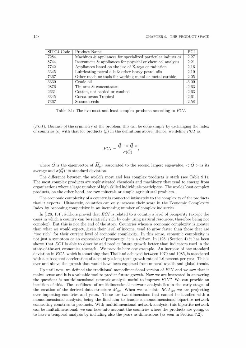
158 CHAPTER 9. THE PRODUCT SPACE
SITC4 Code Product Name PCI7284 Machines & appliances for specialized particular industries 2.278744 Instrument & appliances for physical or chemical analysis 2.217742 Appliances based on the use of X-rays or radiation 2.163345 Lubricating petrol oils & other heavy petrol oils 2.107367 Other machine tools for working metal or metal carbide 2.053330 Crude oil -3.002876 Tin ores & concentrates -2.632631 Cotton, not carded or combed -2.633345 Cocoa beans Tropical -2.617367 Sesame seeds -2.58
Table 9.1: The five most and least complex products according to PCI.
(PCI). Because of the symmetry of the problem, this can be done simply by exchanging the indexof countries (c) with that for products (p) in the definitions above. Hence, we define PCI as:
PCI =~Q− < ~Q >
σ( ~Q),
where ~Q is the eigenvector of Mpp′ associated to the second largest eigenvalue, < ~Q > is its
average and σ( ~Q) its standard deviation.
The difference between the world’s most and less complex products is stark (see Table 9.1).The most complex products are sophisticated chemicals and machinery that tend to emerge fromorganizations where a large number of high skilled individuals participate. The worlds least complexproducts, on the other hand, are raw minerals or simple agricultural products.
The economic complexity of a country is connected intimately to the complexity of the productsthat it exports. Ultimately, countries can only increase their score in the Economic ComplexityIndex by becoming competitive in an increasing number of complex industries.
In [128, 131], authors proved that ECI is related to a country’s level of prosperity (except thecases in which a country can be relatively rich by only using natural resources, therefore being notcomplex). But this is not the end of the story. Countries whose a economic complexity is greaterthan what we would expect, given their level of income, tend to grow faster than those that are“too rich” for their current level of economic complexity. In this sense, economic complexity isnot just a symptom or an expression of prosperity: it is a driver. In [128] (Section 4) it has beenshown that ECI is able to describe and predict future growth better than indicators used in thestate-of-the-art economics research. We provide here one example. An increase of one standarddeviation in ECI, which is something that Thailand achieved between 1970 and 1985, is associatedwith a subsequent acceleration of a country’s long-term growth rate of 1.6 percent per year. This isover and above the growth that would have been expected from mineral wealth and global trends.
Up until now, we defined the traditional monodimensional version of ECI and we saw that itmakes sense and it is a valuable tool to predict future growth. Now we are interested in answeringthe question: is multidimensional network analysis useful to improve ECI? We can provide anintuition of this. The usefulness of multidimensional network analysis lies in the early stages ofthe creation of the derived data structure Mcp. When we calculate RCAcp, we are projectingover importing countries and years. These are two dimensions that cannot be handled with amonodimensional analysis, being the final aim to handle a monodimensional bipartite networkconnecting countries to products. With multidimensional network analysis, this bipartite networkcan be multidimensional: we can take into account the countries where the products are going, orto have a temporal analysis by including also the years as dimensions (as seen in Section 7.2).
9.3. PRODUCT SPACE CREATION 159
9.3 Product Space Creation
In the previous section we saw that ECI is a good describing tool for the world trade economicdynamics. What is important is if we are able also to understand how ECI evolves, that will enableus to have a deeper knowledge about these dynamics. Specifically, questions like the followings canbe answered: how do societies increase the amount of productive knowledge embedded in them?What limits the speed of this process? And why does it happen in some places but not in others?
The complexity of a country’s economy reflects the amount of productive knowledge it contains.This knowledge is costly to acquire and transfer, and is modularized into chunks we call capabilities.Capabilities are difficult to accumulate because doing so creates a complicated chicken and eggproblem. On the one hand, countries cannot create products that require capabilities they do nothave. On the other hand, there are scant incentives to accumulate capabilities in places wherethe industries that demand them do not exist. New capabilities will be more easily accumulatedif they can be combined with others that already exist. Countries are more likely to move intoproducts that make use of the capabilities that are already available. We are then interested inmeasuring the similarity in the capability requirements of different products.
Our basic assumption is that the probability that a pair of products is co-exported carries infor-mation about how similar these products are. Our measure is based on the conditional probabilitythat a country that exports product p will also export product p′. Since conditional probabilitiesare not symmetric we take the minimum of the probability of exporting product p, given p′ andthe reverse, to make the measure symmetric and more stringent. Formally, for a pair of goods pand p′ we define proximity as:
φpp′ =
∑cMcpMcp′
max{kp,0, kp′,0}.
As results, we obtain a squared matrix of product proximities. Obviously, this one-modeprojection is very dense and may contain links that are not significant (the co-export probabilitymay be non zero, but very small). To create the final Product Space we employ the followingfurther strategies.
First, we want the visualization of the Product Space to be a connected network. By this,we mean avoiding islands of isolated products. The second criteria is that we want the ProductSpace to be relatively sparse. This is achieved by fixing the average number of links per node asnot larger than 5 and results in a representation that can summarize the structure of the ProductSpace using the strongest 1% of the links.
To make sure the visualization of the product space is connected, we calculate the maximumspanning tree (MST) of the proximity matrix. MST is the set of links that connects all thenodes in the network using a minimum number of connections and the maximum possible sumof proximities. We calculated the MST using Kruskal’s algorithm [156]. Basically the algorithmsorts the values of the proximity matrix in descending order and then includes links in the MST ifand only if they connect an isolated product or two trees without creating a cycle. By definition,the MST includes all products, but the number of links is the minimum requested to have a singleconnected component.
The second step is to add the strongest connections that were not selected for the MST. Inthis visualization we included the top 1,006 connections satisfying our criterion. By definition aspanning tree for 774 nodes contains 773 edges. With the additional 1,006 connections we end upwith 1,779 edges and an average degree of nearly 4.6.
After selecting the links using the above mentioned criteria we build a visualization using aForce-Directed layout algorithm in Figure 9.1.
We care about the structure of the product space because it affects the ability of countries tomove into new products. Products that are tightly connected share most of the requisite capabili-ties. If this is the case, then countries that already have what it takes to make one product will findit relatively easy to move to the next ones. A highly connected product space, therefore, makesthe problem of growing the complexity of an economy easier. Conversely, a sparsely connectedproduct space makes it harder.
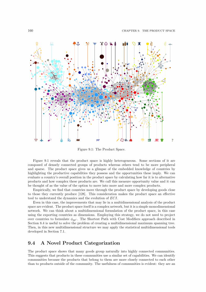
160 CHAPTER 9. THE PRODUCT SPACE
Figure 9.1: The Product Space.
Figure 9.1 reveals that the product space is highly heterogeneous. Some sections of it arecomposed of densely connected groups of products whereas others tend to be more peripheraland sparse. The product space gives us a glimpse of the embedded knowledge of countries byhighlighting the productive capabilities they possess and the opportunities these imply. We canevaluate a country’s overall position in the product space by calculating how far it is to alternativeproducts and how complex these products are. We call this measure opportunity value and it canbe thought of as the value of the option to move into more and more complex products.
Empirically, we find that countries move through the product space by developing goods closeto those they currently produce [128]. This consideration makes the product space an effectivetool to understand the dynamics and the evolution of ECI.
Even in this case, the improvements that may lie in a multidimensional analysis of the productspace are evident. The product space itself is a complex network, but it is a simple monodimensionalnetwork. We can think about a multidimensional formulation of the product space, in this caseusing the exporting countries as dimensions. Employing this strategy, we do not need to projectover countries to formulate φpp′ . The Shortest Path with Cost Modifiers approach described inSection 8.4 is useful to solve the problem of creating a multidimensional maximum spanning tree.Then, in this new multidimensional structure we may apply the statistical multidimensional toolsdeveloped in Section 7.1.
9.4 A Novel Product Categorization
The product space shows that many goods group naturally into highly connected communities.This suggests that products in these communities use a similar set of capabilities. We can identifycommunities because the products that belong to them are more closely connected to each otherthan to products outside of the community. The usefulness of communities is evident: they are an
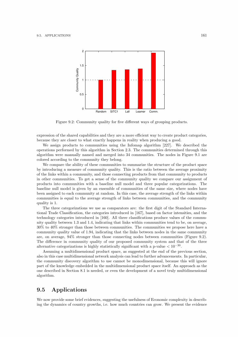
9.5. APPLICATIONS 161
0
0.5
1
1.5
2
Random SITC1 Lall Leamer Comm.
Co
mm
unity Q
ua
lity
Figure 9.2: Community quality for five different ways of grouping products.
expression of the shared capabilities and they are a more efficient way to create product categories,because they are closer to what exactly happens in reality when producing a good.
We assign products to communities using the Infomap algorithm [227]. We described theoperations performed by this algorithm in Section 2.3. The communities determined through thisalgorithm were manually named and merged into 34 communities. The nodes in Figure 9.1 arecolored according to the community they belong.
We compare the ability of these communities to summarize the structure of the product spaceby introducing a measure of community quality. This is the ratio between the average proximityof the links within a community, and those connecting products from that community to productsin other communities. To get a sense of the community quality we compare our assignment ofproducts into communities with a baseline null model and three popular categorizations. Thebaseline null model is given by an ensemble of communities of the same size, where nodes havebeen assigned to each community at random. In this case, the average strength of the links withincommunities is equal to the average strength of links between communities, and the communityquality is 1.
The three categorizations we use as comparators are: the first digit of the Standard Interna-tional Trade Classification, the categories introduced in [167], based on factor intensities, and thetechnology categories introduced in [160]. All three classifications produce values of the commu-nity quality between 1.3 and 1.4, indicating that links within communities tend to be, on average,30% to 40% stronger than those between communities. The communities we propose here have acommunity quality value of 1.94, indicating that the links between nodes in the same communityare, on average, 94% stronger than those connecting nodes between communities (Figure 9.2).The difference in community quality of our proposed community system and that of the threealternative categorizations is highly statistically significant with a p-value < 10−30.
Assuming a multidimensional product space, as suggested at the end of the previous section,also in this case multidimensional network analysis can lead to further advancements. In particular,the community discovery algorithm to use cannot be monodimensional, because this will ignorepart of the knowledge embedded in the multidimensional product space itself. An approach as theone described in Section 8.1 is needed, or even the development of a novel truly multidimensionalalgorithm.
9.5 Applications
We now provide some brief evidences, suggesting the usefulness of Economic complexity in describ-ing the dynamics of country growths, i.e. how much countries can grow. We present the evidence
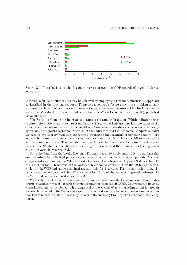
162 CHAPTER 9. THE PRODUCT SPACE
Econom Compl
WEF Combined
Corruption
Govt. Effect
Stability
Rule of Law
Regu Quality
Voice Acc
0 2 4 6 8 10 12 14 16
Contribution to R2
6 Years
12 Years
Figure 9.3: Contributions to the R square regression over the GDP growth of several differentindicators.
collected so far, but better results may be achieved by employing a new multidimensional approachas described in the previous sections. To predict a country’s future growth is a problem alreadyaddressed in the economics literature. Some of the most respected measures of institutional qualityare the six Worldwide Governance Indicators from the World Economic Forum (WEF), publishedbiennially since 1996.
The Economic Complexity Index aims to capture the same information. Which indicator bettercaptures information that is more relevant for growth is an empirical question. Here we compare thecontribution to economic growth of the Worldwide Governance Indicators and economic complexityby estimating a growth regression where all of the indicators and the Economic Complexity Indexare used as explanatory variables. As controls we include the logarithm of per capita income, theincrease in natural resource exports during the period and the initial share of GDP represented bynatural resource exports. The contribution of each variable is estimated by taking the differencebetween the R2 obtained for the regression using all variables and that obtained for the regressionwhere the variable was removed.
Since the data from the World Economic Forum are available only since 1996, we perform thisexercise using the 1996-2008 period as a whole and as two consecutive 6-year periods. We alsocompare with each individual WGI and with the six of them together. Figure 9.3 shows that theECI accounts for 13.6 percent of the variance in economic growth during the 1996-2008 period,while the six WEF indicators combined account only for 5 percent. For the estimation using thetwo six year periods, we find that ECI accounts for 15.2% of the variance in growth, whereas thesix WEF indicators combined account for 3%.
We conclude that as far as future economic growth is concerned, the Economic Complexity Indexcaptures significantly more growth-relevant information than the six World Governance Indicators,either individually or combined. This suggests that the aspects of governance important for growthare weakly reflected in the WGIs and appear to be more strongly reflected in the economic activitiesthat thrive in each country. These may be more effectively captured by the Economic ComplexityIndex.

Chapter 10
Study of Subject Themes inClassical Archaeology
In this section we tackle a general analytical problem to demonstrate the usefulness of multidi-mensional network analysis in a real world scenario that does not necessarily involves the use ofcomplex network analysis to be solved. If multidimensional networks are able to help in this casestudy, and are used to unveil novel analytical insights, we can reasonably conclude that the prac-tical application of the framework created in the second part of this thesis is indeed useful. Thescenario in which we want to operate is the study of subject themes in classical archaeology.
In classical archaeology, or the arts and humanities in general, citation indices are of limited useand literature is still not fully available in digital form. Researchers still rely more on traditionalsubject classification as other fields do. A major pain point in exploring the respective classi-fied literature is that scholars are usually limited to relatively simple user interfaces, where theycan search or query for simple lists of literature associated to sets of classifications, or hop backand forth between classifications and publications while browsing the results. In the meantimethe complex ecology of classification criteria related to each other remains opaque. Combiningcomplex network analysis and data mining techniques in this paper, we offer a solution to thisproblem, enabling the exploration of a subject classification system, both on a meso as well as on aglobal level. Beyond standard user interface functionality, we are able to create a browsable set ofvisualizations, with which the interested scholar can explore neighboring sub-fields as well as thestructure of the discipline as a whole, in a way that is more up to date and contextually superior toany written text book, as the big picture emerges algorithmically from an abundance of data thatis accumulated by many actors. The tools we are developing make great use of complex networksand, in particular, of multidimensional networks. As our example we use Archaologische Bibli-ographie, i.e. a bibliographic database that collects and classifies literature in classical archaeologysince 1956 [234]. Analyzing the state of 2007, our source data includes about 370.000 classifiedpublications by circa 88.000 authors that are connected to about 45.000 classification criteria, via670.000 classification links. Figure 10.1 shows a data model sketch of the database, including twoadditional link types which we construct within our analysis. First we generate and analyze a clas-sification co-occurrence network from the classification link between publications and classificationcriteria. Second we abstract further by shortcutting from classifications to persons, resulting inan alternative perspective on classification cooccurrence in authors. Both derived structures aremultidimensional networks, in which the dimensions represent different temporal snapshots.
That our problem is not trivial becomes evident by looking at the density of the classificationco-occurrence network across publications. Its giant connected component includes about 29.000classification criteria and over 200,000 co-occurrence links, with an average diameter of 2.7. Simplenode-link diagrams of cooccurrence therefore are of limited use on a meso-level, resulting in atotally useless hairball on the global level [232]. This chapter is organized as follows: Section 10.1indicates previous work. Section 10.2 details our analytical framework. Sections 10.3 and 10.4
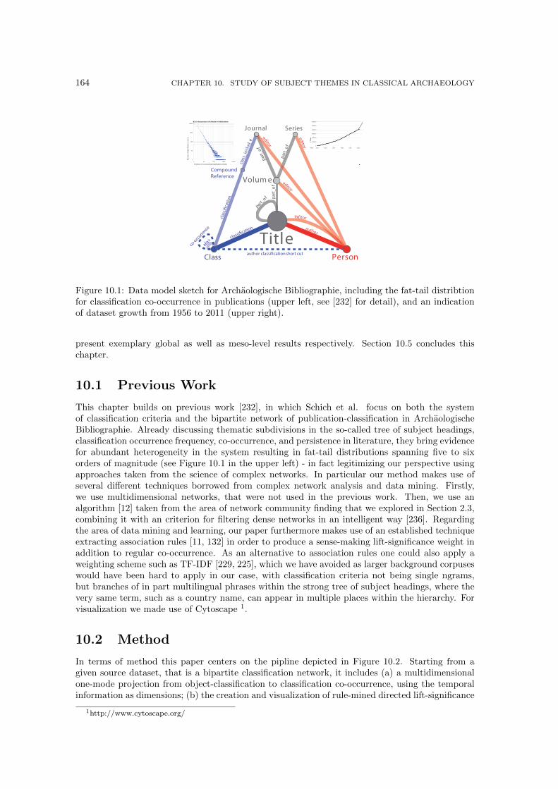
164 CHAPTER 10. STUDY OF SUBJECT THEMES IN CLASSICAL ARCHAEOLOGY
clas
si
cati
on
clas
s_in
clu
de
par
t_o
f
par
t_o
f
editor
pa
rt_
of
editor
author
editor
ed
itor
part_of
classi cation
alias
Compound
ReferenceVolume
Journal
Person
Title
Series
Classauthor classi cation short cut
co-o
ccurre
nce
0
10000 0
20000 0
30000 0
40000 0
50000 0
60000 0
1956 1966 1976 1986 1996 2006
# T
itle
s
Years
1
10
100
1000
10000
1 10 100 1000 10000
Num
ber
of cla
ssific
ation c
rite
ria
Number of co-occurring classification criteria
d) Co-Occurrence of Criteria in Publications
Figure 10.1: Data model sketch for Archaologische Bibliographie, including the fat-tail distribtionfor classification co-occurrence in publications (upper left, see [232] for detail), and an indicationof dataset growth from 1956 to 2011 (upper right).
present exemplary global as well as meso-level results respectively. Section 10.5 concludes thischapter.
10.1 Previous Work
This chapter builds on previous work [232], in which Schich et al. focus on both the systemof classification criteria and the bipartite network of publication-classification in ArchaologischeBibliographie. Already discussing thematic subdivisions in the so-called tree of subject headings,classification occurrence frequency, co-occurrence, and persistence in literature, they bring evidencefor abundant heterogeneity in the system resulting in fat-tail distributions spanning five to sixorders of magnitude (see Figure 10.1 in the upper left) - in fact legitimizing our perspective usingapproaches taken from the science of complex networks. In particular our method makes use ofseveral different techniques borrowed from complex network analysis and data mining. Firstly,we use multidimensional networks, that were not used in the previous work. Then, we use analgorithm [12] taken from the area of network community finding that we explored in Section 2.3,combining it with an criterion for filtering dense networks in an intelligent way [236]. Regardingthe area of data mining and learning, our paper furthermore makes use of an established techniqueextracting association rules [11, 132] in order to produce a sense-making lift-significance weight inaddition to regular co-occurrence. As an alternative to association rules one could also apply aweighting scheme such as TF-IDF [229, 225], which we have avoided as larger background corpuseswould have been hard to apply in our case, with classification criteria not being single ngrams,but branches of in part multilingual phrases within the strong tree of subject headings, where thevery same term, such as a country name, can appear in multiple places within the hierarchy. Forvisualization we made use of Cytoscape 1.
10.2 Method
In terms of method this paper centers on the pipline depicted in Figure 10.2. Starting from agiven source dataset, that is a bipartite classification network, it includes (a) a multidimensionalone-mode projection from object-classification to classification co-occurrence, using the temporalinformation as dimensions; (b) the creation and visualization of rule-mined directed lift-significance
1http://www.cytoscape.org/
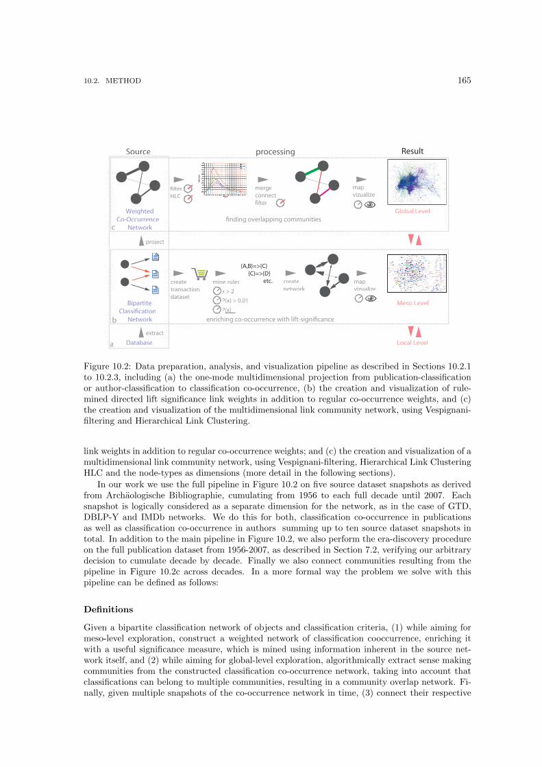
10.2. METHOD 165
processing
Weighted
Co-Occurrence
Network
Source Result
Bipartite
Classi cation
Network
Database
Global Level
Meso Level
Local Level
lter
HLC
merge
connect
lter
map
vizualizecreate
transaction
dataset
mine rules
x > 2
P(x) > 0.01
P(x)
create
network
extract
project
{A,B}=>{C}
{C}=>{D}
etc.
map
vizualize
enriching co-occurrence with lift-signi"cance
"nding overlapping communities
a
b
c
Figure 10.2: Data preparation, analysis, and visualization pipeline as described in Sections 10.2.1to 10.2.3, including (a) the one-mode multidimensional projection from publication-classificationor author-classification to classification co-occurrence, (b) the creation and visualization of rule-mined directed lift significance link weights in addition to regular co-occurrence weights, and (c)the creation and visualization of the multidimensional link community network, using Vespignani-filtering and Hierarchical Link Clustering.
link weights in addition to regular co-occurrence weights; and (c) the creation and visualization of amultidimensional link community network, using Vespignani-filtering, Hierarchical Link ClusteringHLC and the node-types as dimensions (more detail in the following sections).
In our work we use the full pipeline in Figure 10.2 on five source dataset snapshots as derivedfrom Archaologische Bibliographie, cumulating from 1956 to each full decade until 2007. Eachsnapshot is logically considered as a separate dimension for the network, as in the case of GTD,DBLP-Y and IMDb networks. We do this for both, classification co-occurrence in publicationsas well as classification co-occurrence in authors summing up to ten source dataset snapshots intotal. In addition to the main pipeline in Figure 10.2, we also perform the era-discovery procedureon the full publication dataset from 1956-2007, as described in Section 7.2, verifying our arbitrarydecision to cumulate decade by decade. Finally we also connect communities resulting from thepipeline in Figure 10.2c across decades. In a more formal way the problem we solve with thispipeline can be defined as follows:
Definitions
Given a bipartite classification network of objects and classification criteria, (1) while aiming formeso-level exploration, construct a weighted network of classification cooccurrence, enriching itwith a useful significance measure, which is mined using information inherent in the source net-work itself, and (2) while aiming for global-level exploration, algorithmically extract sense makingcommunities from the constructed classification co-occurrence network, taking into account thatclassifications can belong to multiple communities, resulting in a community overlap network. Fi-nally, given multiple snapshots of the co-occurrence network in time, (3) connect their respective
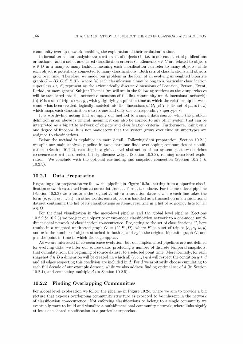
166 CHAPTER 10. STUDY OF SUBJECT THEMES IN CLASSICAL ARCHAEOLOGY
community overlap network, enabling the exploration of their evolution in time.In formal terms, our analysis starts with a set of objects O - i.e. in our case a set of publications
or authors - and a set of associated classification criteria C. Elements c ∈ C are related to objectso ∈ O in a many-to-many fashion, meaning each classification can refer to many objects, whileeach object is potentially connected to many classifications. Both sets of classifications and objectsgrow over time. Therefore, we model our problem in the form of an evolving unweighted bipartitegraph G = {O,C, S,E, T}, where (a) each classification c may belong to a particular classificationsuperclass s ∈ S, representing the axiomatically discrete dimensions of Location, Person, Event,Period, or more general Subject Themes (we will see in the following sections as these superclasseswill be translated into the network dimensions of the link community multidimensional network);(b) E is a set of triples (o, c, y), with y signifying a point in time at which the relationship betweenc and o has been created, logically modeled into the dimensions of G; (c) T is the set of pairs (c, s)which maps each classification c to its one and only one corresponding supertype s.
It is worthwhile noting that we apply our method to a single data source, while the problemdefinition given above is general, meaning it can also be applied to any other system that can beinterpreted as a bipartite network of objects and classification criteria. Furthermore, losing onlyone degree of freedom, it is not mandatory that the system grows over time or supertypes areassigned to classifications.
Below the method is explained in more detail. Following data preparation (Section 10.2.1)we split our main analysis pipeline in two: part one finds overlapping communities of classifi-cations (Section 10.2.2), resulting in a global level abstraction of our system; part two enrichesco-occurrence with a directed lift-significance weight (Section 10.2.3), refining meso-level explo-ration. We conclude with the optional era-finding and snapshot connection (Section 10.2.4 &10.2.5).
10.2.1 Data Preparation
Regarding data preparation we follow the pipeline in Figure 10.2a, starting from a bipartite classi-fication network extracted from a source database, as formalized above. For the meso-level pipeline(Section 10.2.3) we transform the edgeset E into a transaction dataset where each line takes theform (o, y, c1, c2, ..., cn). In other words, each object o is handled as a transaction in a transactionaldataset containing the list of its classifications as items, resulting in a list of adjecency lists for allo ∈ O.
For the final visualization in the meso-level pipeline and the global level pipeline (Sections10.2.2 & 10.2.3) we project our bipartite or two-mode classification network to a one-mode multi-dimensional network of classification co-occurrence. Projecting to the set of classifications C, hereresults in a weighted undirected graph G′ = (C,E′, D), where E′ is a set of triples (c1, c2, w, y)and w is the number of objects attached to both c1 and c2 in the original bipartite graph G, andy is the point in time in which the edge appear.
As we are interested in co-occurrence evolution, but our implemented pipelines are not definedfor evolving data, we filter our source data, producing a number of discrete temporal snapshots,that cumulate from the beginning of source dataset to a selected point time. More formally, for eachsnapshot d ∈ D a dimension will be created, in which all (c, o, y) ∈ d will respect the condition y ≤ dand all edges respecting this condition are included in d. For d we arbitrarily choose cumulating toeach full decade of our example dataset, while we also address finding optimal set of d (in Section10.2.4), and connecting multiple d (in Section 10.2.5).
10.2.2 Finding Overlapping Communities
For global level exploration we follow the pipeline in Figure 10.2c, where we aim to provide a bigpicture that exposes overlapping community structure as expected to be inherent in the networkof classification co-occurrence. Not enforcing classifications to belong to a single community weeventually want to build and visualize a multidimensional community network, where links signifyat least one shared classification in a particular superclass.
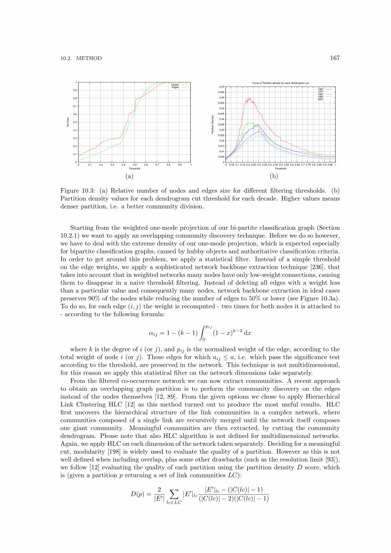
10.2. METHOD 167
0
0.1
0.2
0.3
0.4
0.5
0.6
0.7
0.8
0.9
1
0 0.1 0.2 0.3 0.4 0.5 0.6 0.7 0.8 0.9 1
Rel S
ize
Threshold
NodesEdges
0
0.005
0.01
0.015
0.02
0.025
0.03
0.035
0.04
0.045
0.05
0.055
0.06
0.065
0.07
0 0.05 0.1 0.15 0.2 0.25 0.3 0.35 0.4 0.45 0.5 0.55 0.6 0.65 0.7 0.75 0.8 0.85 0.9 0.95 1
Part
itio
n D
ensity
Threshold
Curve of Partition density for each dendrogram cut
19671977198719972007
(a) (b)
Figure 10.3: (a) Relative number of nodes and edges size for different filtering thresholds. (b)Partition density values for each dendrogram cut threshold for each decade. Higher values meansdenser partition, i.e. a better community division.
Starting from the weighted one-mode projection of our bi-partite classification graph (Section10.2.1) we want to apply an overlapping community discovery technique. Before we do so however,we have to deal with the extreme density of our one-mode projection, which is expected especiallyfor bipartite classification graphs, caused by hubby objects and authoritative classification criteria.In order to get around this problem, we apply a statistical filter. Instead of a simple thresholdon the edge weights, we apply a sophisticated network backbone extraction technique [236], thattakes into account that in weighted networks many nodes have only low-weight connections, causingthem to disappear in a naive threshold filtering. Instead of deleting all edges with a weight lessthan a particular value and consequently many nodes, network backbone extraction in ideal casespreserves 90% of the nodes while reducing the number of edges to 50% or lower (see Figure 10.3a).To do so, for each edge (i, j) the weight is recomputed - two times for both nodes it is attached to- according to the following formula:
αij = 1− (k − 1)
∫ pij
0
(1− x)k−2 dx
where k is the degree of i (or j), and pij is the normalized weight of the edge, according to thetotal weight of node i (or j). Those edges for which aij ≤ a, i.e. which pass the significance testaccording to the threshold, are preserved in the network. This technique is not multidimensional,for this reason we apply this statistical filter on the network dimensions take separately.
From the filtered co-occurrence network we can now extract communities. A recent approachto obtain an overlapping graph partition is to perform the community discovery on the edgesinstead of the nodes themselves [12, 89]. From the given options we chose to apply HierarchicalLink Clustering HLC [12] as this method turned out to produce the most useful results. HLCfirst uncovers the hierarchical structure of the link communities in a complex network, wherecommunities composed of a single link are recursively merged until the network itself composesone giant community. Meaningful communities are then extracted, by cutting the communitydendrogram. Please note that also HLC algorithm is not defined for multidimensional networks.Again, we apply HLC on each dimension of the network taken separately. Deciding for a meaningfulcut, modularity [198] is widely used to evaluate the quality of a partition. However as this is notwell defined when including overlap, plus some other drawbacks (such as the resolution limit [93]),we follow [12] evaluating the quality of each partition using the partition density D score, whichis (given a partition p returning a set of link communities LC):
D(p) =2
|E′|∑lc∈LC
|E′|lc|E′|lc − (|C(lc)| − 1)
(|C(lc)| − 2)(|C(lc)| − 1)
168 CHAPTER 10. STUDY OF SUBJECT THEMES IN CLASSICAL ARCHAEOLOGY
where |E′| is the total number of edges in the dimension, and |C(lc)| and |E′|lc are the numbersof nodes and edges in lc in the dimension respectively. The higher D(p), the better the partitionp identifies well divided clusters in the network.
Figure 10.3b reports the evolution of the partition density for all possible dendrogram cuts inour co-occurrence network in publications for each decade (i.e. our dimensions d ∈ D). For eachdimension, choosing the given optimal partition p, we now obtain a set of overlapping communitiesLC, allowing us to produce the desired global level picture of our classification network. In orderto do so, we collapse each lc ∈ LC into a single node, connecting the nodes of this network withlinks, whose weight is proportional to the number of nodes shared by the two communities. Aseach node and edge has a complex internal structure derived from the weight of the classificationsupertypes of all c ∈ lc, we can further enrich both nodes and edges in the representation of theresulting community overlap network, by representing the nodes with pie diagrams and splittingthe edges in different dimensions according to the inherent superclass frequency. As the communityoverlap network is again very dense, and we aim for a text-book-style global picture we apply thebackbone filter again.
10.2.3 Lift Significance
For meso-level exploration we follow the pipeline in figure 10.2b. Here we aim to visualize oursimple weighted co-occurrence network of classifications c ∈ C with a more sophisticated directedsignificance measure. In order to do so, we perform association rule mining [11] over our transactiondataset (as introduced in Section 10.2.1), mining for frequent rules of co-classifications. Minimumsupport and confidence thresholds may be tuned depending on the phenomenon one is interested tohighlight. As a result we obtain a set R of rules in the form P (C)⇒ c, where P (C) is the set of allsubsets of C, excluding ∅. Using this result, we are able to build our significance network in whichthe nodes are the classifications C, and the edges are triples (c1, c2, w(c1, c2)), where w(c1, c2), i.e.the significance of the relationship between c1 and c2 is defined as follows
w(c1, c2) =∑
∀r∈R.c1∈P (C)∧c=c2
supp(P (C) ∪ c)supp(P (C))× supp(c)
where P (C) is the set of classifications in the left side of rule r, c is the classification in the rightside of the rule r, and supp(x) is the support of the set x of classifications inside the transactionaldataset. In other words, w is the sum of the lift of all rules involving c1 as one of the antecedentsof the rule, and c2 is the consequence. The lift measure as such is not directed, but since we arefiltering rules according to their confidence, which is directed, it follows that w(c1, c2) 6= w(c2, c1),resulting in a directed network. This means a situation may (and does) occur, in which c1 is verysignificant in pointing to c2, while c2 is not so significantly pointing to c1 (see Section 10.4.1).
10.2.4 Era Discovery
Neither the global- nor meso-level pipelines above take into account time. To study evolutiontherefore, it is necessary to discretize the evolving source network into temporal dimensions onwhich the pipelines can be applied separately - raising the question: how to choose the rightsnapshot size?
Looking for eras, i.e. periods of regular and predictable network evolution, we apply a method[40] (see Section 7.2) that calculates the Node and Edge Dimension Correlation between all con-secutive observations of the network, resulting in the ability to define a distance measure betweengroups of observations. We refer mainly to Section 7.2 of this thesis for more details about theprocedure.
Using this distance measure, computed on all adjacent observations, a dendrogram is built,grouping together consecutive observations, presenting regular evolution separated from abruptchanges in trend. Figure 10.4 depicts the respective dendrogram for classification co-occurrence in
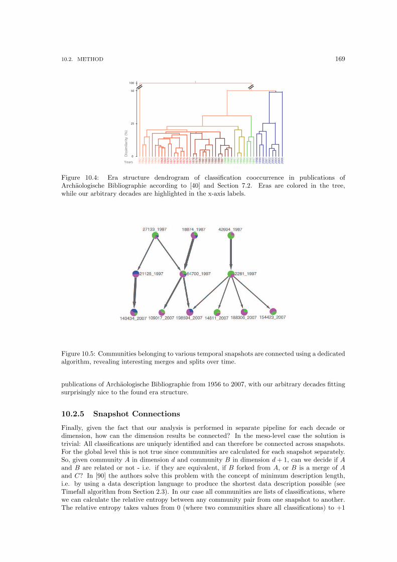
10.2. METHOD 169
1961
1962
1963
1964
1965
1966
1967
1968
1969
1970
1971
1972
1973
1974
1975
1976
1977
1978
1979
1980
1981
1982
1983
1984
1985
1986
1987
1988
1989
1990
1991
1992
1993
1994
1995
1996
1997
1998
1999
2000
2001
2002
2003
2004
2005
2006
0
25
50
Dis
sim
ilari
ty(%
)
Years
50
75
100
Figure 10.4: Era structure dendrogram of classification cooccurrence in publications ofArchaologische Bibliographie according to [40] and Section 7.2. Eras are colored in the tree,while our arbitrary decades are highlighted in the x-axis labels.
Figure 10.5: Communities belonging to various temporal snapshots are connected using a dedicatedalgorithm, revealing interesting merges and splits over time.
publications of Archaologische Bibliographie from 1956 to 2007, with our arbitrary decades fittingsurprisingly nice to the found era structure.
10.2.5 Snapshot Connections
Finally, given the fact that our analysis is performed in separate pipeline for each decade ordimension, how can the dimension results be connected? In the meso-level case the solution istrivial: All classifications are uniquely identified and can therefore be connected across snapshots.For the global level this is not true since communities are calculated for each snapshot separately.So, given community A in dimension d and community B in dimension d + 1, can we decide if Aand B are related or not - i.e. if they are equivalent, if B forked from A, or B is a merge of Aand C? In [90] the authors solve this problem with the concept of minimum description length,i.e. by using a data description language to produce the shortest data description possible (seeTimefall algorithm from Section 2.3). In our case all communities are lists of classifications, wherewe can calculate the relative entropy between any community pair from one snapshot to another.The relative entropy takes values from 0 (where two communities share all classifications) to +1
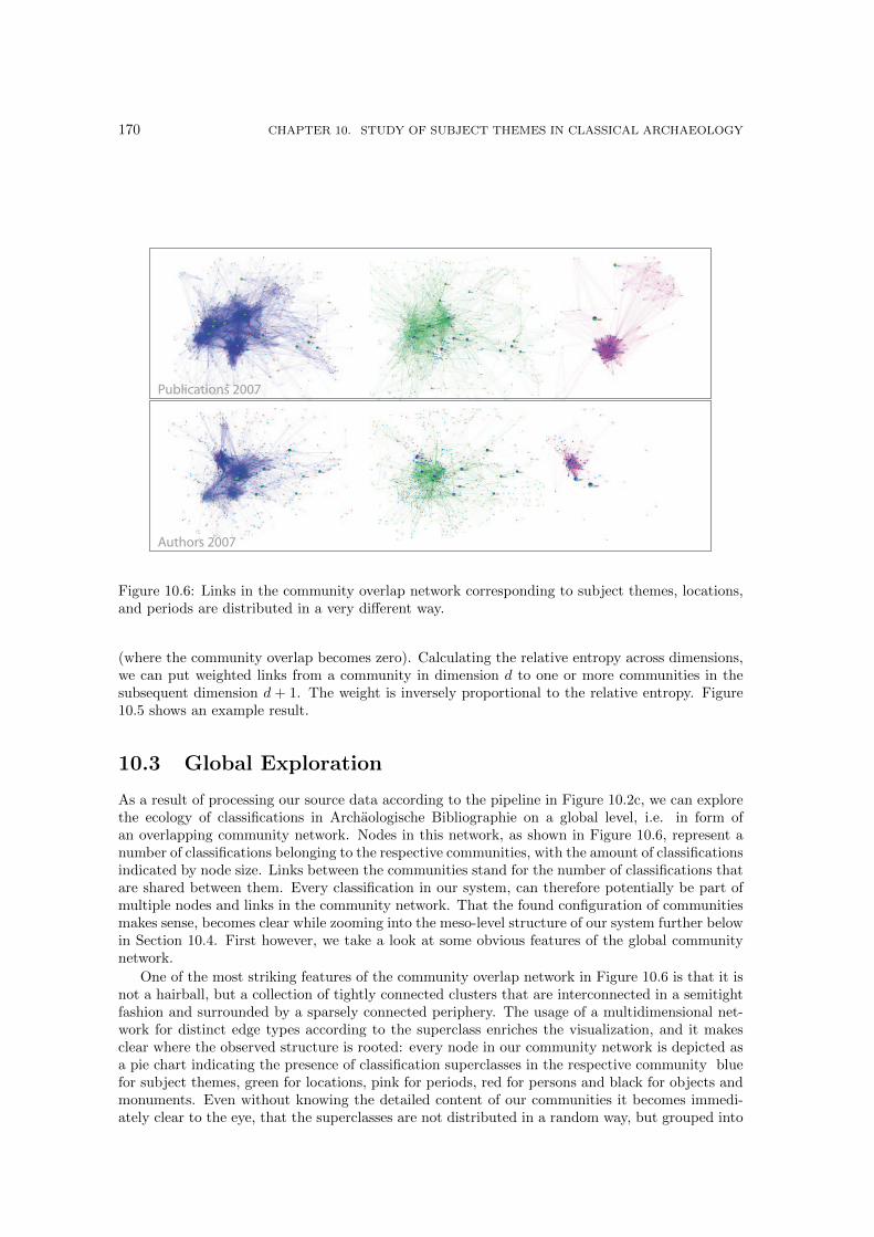
170 CHAPTER 10. STUDY OF SUBJECT THEMES IN CLASSICAL ARCHAEOLOGY
Publications 2007
Authors 2007
Figure 10.6: Links in the community overlap network corresponding to subject themes, locations,and periods are distributed in a very different way.
(where the community overlap becomes zero). Calculating the relative entropy across dimensions,we can put weighted links from a community in dimension d to one or more communities in thesubsequent dimension d + 1. The weight is inversely proportional to the relative entropy. Figure10.5 shows an example result.
10.3 Global Exploration
As a result of processing our source data according to the pipeline in Figure 10.2c, we can explorethe ecology of classifications in Archaologische Bibliographie on a global level, i.e. in form ofan overlapping community network. Nodes in this network, as shown in Figure 10.6, represent anumber of classifications belonging to the respective communities, with the amount of classificationsindicated by node size. Links between the communities stand for the number of classifications thatare shared between them. Every classification in our system, can therefore potentially be part ofmultiple nodes and links in the community network. That the found configuration of communitiesmakes sense, becomes clear while zooming into the meso-level structure of our system further belowin Section 10.4. First however, we take a look at some obvious features of the global communitynetwork.
One of the most striking features of the community overlap network in Figure 10.6 is that it isnot a hairball, but a collection of tightly connected clusters that are interconnected in a semitightfashion and surrounded by a sparsely connected periphery. The usage of a multidimensional net-work for distinct edge types according to the superclass enriches the visualization, and it makesclear where the observed structure is rooted: every node in our community network is depicted asa pie chart indicating the presence of classification superclasses in the respective community bluefor subject themes, green for locations, pink for periods, red for persons and black for objects andmonuments. Even without knowing the detailed content of our communities it becomes immedi-ately clear to the eye, that the superclasses are not distributed in a random way, but grouped into
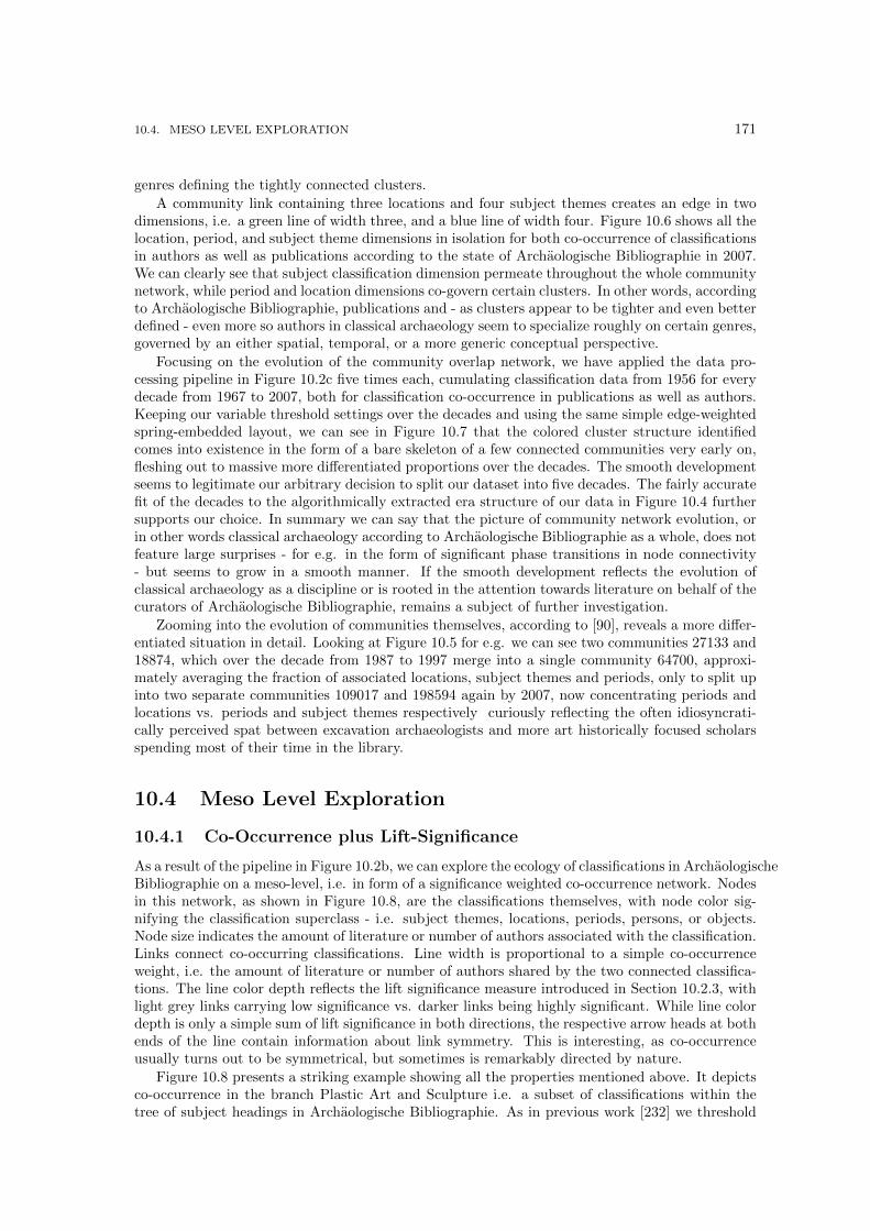
10.4. MESO LEVEL EXPLORATION 171
genres defining the tightly connected clusters.
A community link containing three locations and four subject themes creates an edge in twodimensions, i.e. a green line of width three, and a blue line of width four. Figure 10.6 shows all thelocation, period, and subject theme dimensions in isolation for both co-occurrence of classificationsin authors as well as publications according to the state of Archaologische Bibliographie in 2007.We can clearly see that subject classification dimension permeate throughout the whole communitynetwork, while period and location dimensions co-govern certain clusters. In other words, accordingto Archaologische Bibliographie, publications and - as clusters appear to be tighter and even betterdefined - even more so authors in classical archaeology seem to specialize roughly on certain genres,governed by an either spatial, temporal, or a more generic conceptual perspective.
Focusing on the evolution of the community overlap network, we have applied the data pro-cessing pipeline in Figure 10.2c five times each, cumulating classification data from 1956 for everydecade from 1967 to 2007, both for classification co-occurrence in publications as well as authors.Keeping our variable threshold settings over the decades and using the same simple edge-weightedspring-embedded layout, we can see in Figure 10.7 that the colored cluster structure identifiedcomes into existence in the form of a bare skeleton of a few connected communities very early on,fleshing out to massive more differentiated proportions over the decades. The smooth developmentseems to legitimate our arbitrary decision to split our dataset into five decades. The fairly accuratefit of the decades to the algorithmically extracted era structure of our data in Figure 10.4 furthersupports our choice. In summary we can say that the picture of community network evolution, orin other words classical archaeology according to Archaologische Bibliographie as a whole, does notfeature large surprises - for e.g. in the form of significant phase transitions in node connectivity- but seems to grow in a smooth manner. If the smooth development reflects the evolution ofclassical archaeology as a discipline or is rooted in the attention towards literature on behalf of thecurators of Archaologische Bibliographie, remains a subject of further investigation.
Zooming into the evolution of communities themselves, according to [90], reveals a more differ-entiated situation in detail. Looking at Figure 10.5 for e.g. we can see two communities 27133 and18874, which over the decade from 1987 to 1997 merge into a single community 64700, approxi-mately averaging the fraction of associated locations, subject themes and periods, only to split upinto two separate communities 109017 and 198594 again by 2007, now concentrating periods andlocations vs. periods and subject themes respectively curiously reflecting the often idiosyncrati-cally perceived spat between excavation archaeologists and more art historically focused scholarsspending most of their time in the library.
10.4 Meso Level Exploration
10.4.1 Co-Occurrence plus Lift-Significance
As a result of the pipeline in Figure 10.2b, we can explore the ecology of classifications in ArchaologischeBibliographie on a meso-level, i.e. in form of a significance weighted co-occurrence network. Nodesin this network, as shown in Figure 10.8, are the classifications themselves, with node color sig-nifying the classification superclass - i.e. subject themes, locations, periods, persons, or objects.Node size indicates the amount of literature or number of authors associated with the classification.Links connect co-occurring classifications. Line width is proportional to a simple co-occurrenceweight, i.e. the amount of literature or number of authors shared by the two connected classifica-tions. The line color depth reflects the lift significance measure introduced in Section 10.2.3, withlight grey links carrying low significance vs. darker links being highly significant. While line colordepth is only a simple sum of lift significance in both directions, the respective arrow heads at bothends of the line contain information about link symmetry. This is interesting, as co-occurrenceusually turns out to be symmetrical, but sometimes is remarkably directed by nature.
Figure 10.8 presents a striking example showing all the properties mentioned above. It depictsco-occurrence in the branch Plastic Art and Sculpture i.e. a subset of classifications within thetree of subject headings in Archaologische Bibliographie. As in previous work [232] we threshold
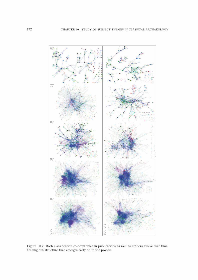
172 CHAPTER 10. STUDY OF SUBJECT THEMES IN CLASSICAL ARCHAEOLOGY
67
77
87
97
07
pu
b
au
tho
rs
Figure 10.7: Both classification co-occurrence in publications as well as authors evolve over time,fleshing out structure that emerges early on in the process.
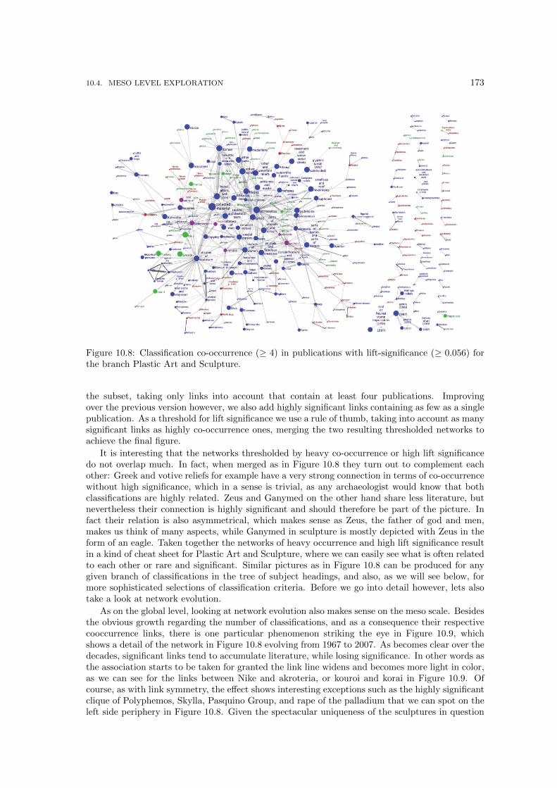
10.4. MESO LEVEL EXPLORATION 173
Figure 10.8: Classification co-occurrence (≥ 4) in publications with lift-significance (≥ 0.056) forthe branch Plastic Art and Sculpture.
the subset, taking only links into account that contain at least four publications. Improvingover the previous version however, we also add highly significant links containing as few as a singlepublication. As a threshold for lift significance we use a rule of thumb, taking into account as manysignificant links as highly co-occurrence ones, merging the two resulting thresholded networks toachieve the final figure.
It is interesting that the networks thresholded by heavy co-occurrence or high lift significancedo not overlap much. In fact, when merged as in Figure 10.8 they turn out to complement eachother: Greek and votive reliefs for example have a very strong connection in terms of co-occurrencewithout high significance, which in a sense is trivial, as any archaeologist would know that bothclassifications are highly related. Zeus and Ganymed on the other hand share less literature, butnevertheless their connection is highly significant and should therefore be part of the picture. Infact their relation is also asymmetrical, which makes sense as Zeus, the father of god and men,makes us think of many aspects, while Ganymed in sculpture is mostly depicted with Zeus in theform of an eagle. Taken together the networks of heavy occurrence and high lift significance resultin a kind of cheat sheet for Plastic Art and Sculpture, where we can easily see what is often relatedto each other or rare and significant. Similar pictures as in Figure 10.8 can be produced for anygiven branch of classifications in the tree of subject headings, and also, as we will see below, formore sophisticated selections of classification criteria. Before we go into detail however, lets alsotake a look at network evolution.
As on the global level, looking at network evolution also makes sense on the meso scale. Besidesthe obvious growth regarding the number of classifications, and as a consequence their respectivecooccurrence links, there is one particular phenomenon striking the eye in Figure 10.9, whichshows a detail of the network in Figure 10.8 evolving from 1967 to 2007. As becomes clear over thedecades, significant links tend to accumulate literature, while losing significance. In other words asthe association starts to be taken for granted the link line widens and becomes more light in color,as we can see for the links between Nike and akroteria, or kouroi and korai in Figure 10.9. Ofcourse, as with link symmetry, the effect shows interesting exceptions such as the highly significantclique of Polyphemos, Skylla, Pasquino Group, and rape of the palladium that we can spot on theleft side periphery in Figure 10.8. Given the spectacular uniqueness of the sculptures in question
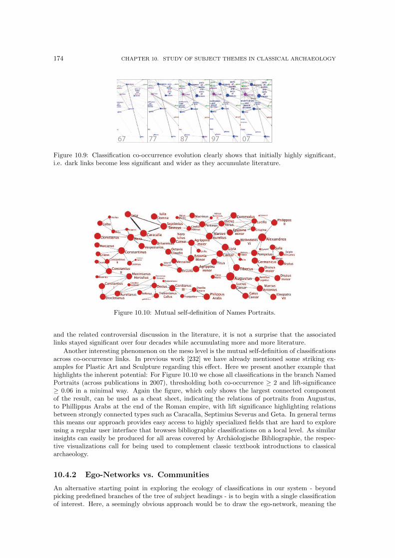
174 CHAPTER 10. STUDY OF SUBJECT THEMES IN CLASSICAL ARCHAEOLOGY
Figure 10.9: Classification co-occurrence evolution clearly shows that initially highly significant,i.e. dark links become less significant and wider as they accumulate literature.
Figure 10.10: Mutual self-definition of Names Portraits.
and the related controversial discussion in the literature, it is not a surprise that the associatedlinks stayed significant over four decades while accumulating more and more literature.
Another interesting phenomenon on the meso level is the mutual self-definition of classificationsacross co-occurrence links. In previous work [232] we have already mentioned some striking ex-amples for Plastic Art and Sculpture regarding this effect. Here we present another example thathighlights the inherent potential: For Figure 10.10 we chose all classifications in the branch NamedPortraits (across publications in 2007), thresholding both co-occurrence ≥ 2 and lift-significance≥ 0.06 in a minimal way. Again the figure, which only shows the largest connected componentof the result, can be used as a cheat sheet, indicating the relations of portraits from Augustus,to Phillippus Arabs at the end of the Roman empire, with lift significance highlighting relationsbetween strongly connected types such as Caracalla, Septimius Severus and Geta. In general termsthis means our approach provides easy access to highly specialized fields that are hard to exploreusing a regular user interface that browses bibliographic classifications on a local level. As similarinsights can easily be produced for all areas covered by Archaologische Bibliographie, the respec-tive visualizations call for being used to complement classic textbook introductions to classicalarchaeology.
10.4.2 Ego-Networks vs. Communities
An alternative starting point in exploring the ecology of classifications in our system - beyondpicking predefined branches of the tree of subject headings - is to begin with a single classificationof interest. Here, a seemingly obvious approach would be to draw the ego-network, meaning the
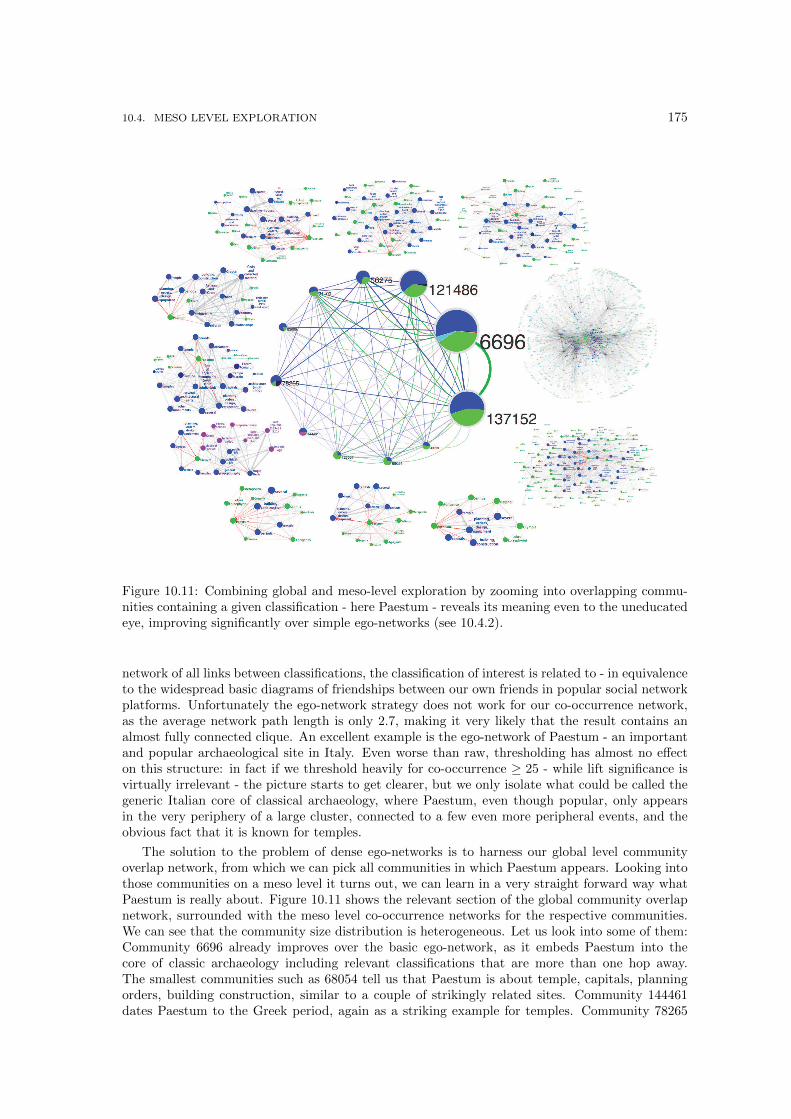
10.4. MESO LEVEL EXPLORATION 175
Figure 10.11: Combining global and meso-level exploration by zooming into overlapping commu-nities containing a given classification - here Paestum - reveals its meaning even to the uneducatedeye, improving significantly over simple ego-networks (see 10.4.2).
network of all links between classifications, the classification of interest is related to - in equivalenceto the widespread basic diagrams of friendships between our own friends in popular social networkplatforms. Unfortunately the ego-network strategy does not work for our co-occurrence network,as the average network path length is only 2.7, making it very likely that the result contains analmost fully connected clique. An excellent example is the ego-network of Paestum - an importantand popular archaeological site in Italy. Even worse than raw, thresholding has almost no effecton this structure: in fact if we threshold heavily for co-occurrence ≥ 25 - while lift significance isvirtually irrelevant - the picture starts to get clearer, but we only isolate what could be called thegeneric Italian core of classical archaeology, where Paestum, even though popular, only appearsin the very periphery of a large cluster, connected to a few even more peripheral events, and theobvious fact that it is known for temples.
The solution to the problem of dense ego-networks is to harness our global level communityoverlap network, from which we can pick all communities in which Paestum appears. Looking intothose communities on a meso level it turns out, we can learn in a very straight forward way whatPaestum is really about. Figure 10.11 shows the relevant section of the global community overlapnetwork, surrounded with the meso level co-occurrence networks for the respective communities.We can see that the community size distribution is heterogeneous. Let us look into some of them:Community 6696 already improves over the basic ego-network, as it embeds Paestum into thecore of classic archaeology including relevant classifications that are more than one hop away.The smallest communities such as 68054 tell us that Paestum is about temple, capitals, planningorders, building construction, similar to a couple of strikingly related sites. Community 144461dates Paestum to the Greek period, again as a striking example for temples. Community 78265
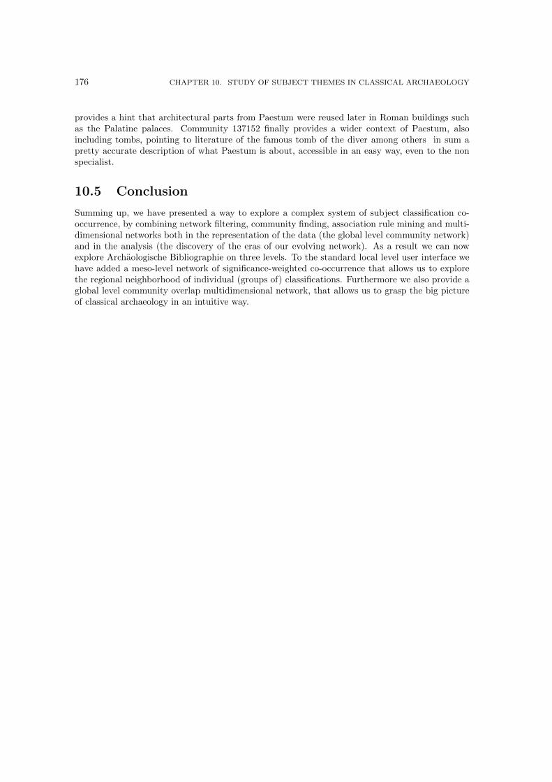
176 CHAPTER 10. STUDY OF SUBJECT THEMES IN CLASSICAL ARCHAEOLOGY
provides a hint that architectural parts from Paestum were reused later in Roman buildings suchas the Palatine palaces. Community 137152 finally provides a wider context of Paestum, alsoincluding tombs, pointing to literature of the famous tomb of the diver among others in sum apretty accurate description of what Paestum is about, accessible in an easy way, even to the nonspecialist.
10.5 Conclusion
Summing up, we have presented a way to explore a complex system of subject classification co-occurrence, by combining network filtering, community finding, association rule mining and multi-dimensional networks both in the representation of the data (the global level community network)and in the analysis (the discovery of the eras of our evolving network). As a result we can nowexplore Archaologische Bibliographie on three levels. To the standard local level user interface wehave added a meso-level network of significance-weighted co-occurrence that allows us to explorethe regional neighborhood of individual (groups of) classifications. Furthermore we also provide aglobal level community overlap multidimensional network, that allows us to grasp the big pictureof classical archaeology in an intuitive way.
Chapter 11
Conclusion and Future Works
In this thesis, we have introduced multidimensional network analysis, a novel framework for theanalysis of complex networks where the interactions between entities can be labelled with differenttypes, or observed from different dimensions. We organized the presentation of multidimensionalnetwork analysis in three parts.
Firstly, we defined what a multidimensional network is; what are the alternative representationsand the works that different authors already presented in the literature; and where it is possibleto find multidimensional networks in the real world. Secondly, we presented our contribution tomultidimensional network analysis, expressed by extending the network measures defined for simplegraphs; proposing novel measures meaningful only in the multidimensional setting; and developingmore complex analytical solutions to advanced network problems, with particular attention to ourmain case study: the community discovery. Finally, we defined two different real world problemsnot necessarily related to network theory: the analysis of international trade and the problem ofexploring literature in classical archaeology. In the first case we show how it is possible to introducemultidimensional network analysis to enrich a problem tackled with monodimensional networks;in the second scenario we show how we can develop a solution to a general problem by usingmultidimensional network analysis.
The future research directions of this thesis can be mainly divided in two tracks. The firsttrack has been proposed in the related work section. There are several different models trying tograsp the complex setting of multiple different relations and interactions in a complex network.To study the relationships between layered interdependent networks, tripartite hypergraphs andmultidimensional networks is an important future development. A second track of research is openfrom the second part of this thesis. For example, in the multidimensional community discoverysection, a method for characterizing multidimensional communities has been proposed. But thealgorithm described to extract them is an adaptation of a classical monodimensional communitydiscoverer. To develop a truly multidimensional community discovery algorithm, able to takeadvantage of the proposed characterization of communities is still an open problem. And thisstatement holds true for the other analysis, both for the multidimensional measures and the otherproblems, proposed in this thesis.
Multidimensional link prediction has been proved to be a more complex problem that cannotbe tackled with a simple combination of known techniques and multidimensional score modifiers.A technique that combines multidimensional network analysis and the real world properties of thedifferent dimensions creating the multidimensional structure is needed. For example, a mobilitynetwork with different modes of transportation provides different working mechanism than theones of a multirelational social network.
Also the contribution for the multidimensional shortest path problem is here represented morein the formalization of the problem posed by the introduction of cost modifiers than in its solution.More research on heuristics, optimization strategies and experiments is needed.
Of course, this big and novel analytical section has one main end: to be able to better rep-resent, and to provide better tools for the analysis of, real world interacting phenomena. The

178 CHAPTER 11. CONCLUSION AND FUTURE WORKS
underlying meta-objective is to grasp complex interactions from real world and to translate theminto knowledge. An example is provided in the third part of the thesis and it is our mission tomake clear that this is just one of the many instances of what can be done with multidimensionalnetworks. The final end is to populate the scientific world with better tools, and we believe thatmultidimensional networks should be part of the workbench of any complex system scientist. Manyother case studies of multidimensional networks can be identified.

Bibliography
[1] Evrim Acar, Daniel M. Dunlavy, and Tamara G. Kolda. Link prediction on evolving datausing matrix and tensor factorizations. In LDMTA’09: Proceeding of the ICDM’09 Work-shop on Large Scale Data Mining Theory and Applications, pages 262–269. IEEE ComputerSociety Press, December 2009.
[2] Lada Adamic and Eytan Adar. Friends and neighbors on the web. Social Networks, (25):230,2001.
[3] Lada A. Adamic and Bernardo A. Huberman. Power-law distribution of the world wide web.Science, 287(5461):2115a–, 2000.
[4] Lada A. Adamic, Rajan M. Lukose, and Bernardo A. Huberman. Local search in unstructurednetworks. Handbook of Graphs and Networks, pages 295–317, 2003.
[5] Lada A. Adamic, Rajan M. Lukose, Amit R. Puniyani, and Bernardo A. Huberman. Searchin power-law networks. CoRR, cs.NI/0103016, 2001.
[6] Nitin Agarwal, Huan Liu, Lei Tang, and Philip S. Yu. Identifying the influential bloggers ina community. In WSDM ’08: Proceedings of the international conference on Web search andweb data mining, pages 207–218, New York, NY, USA, 2008. ACM.
[7] Sumeet Agarwal, Charlotte M. Deane, Mason A. Porter, and Nick S. Jones. Revisiting dateand party hubs: Novel approaches to role assignment in protein interaction networks. PLoSComput Biol, 6(6):e1000817, 06 2010.
[8] Agarwal, G. and Kempe, D. Modularity-maximizing graph communities via mathematicalprogramming. Eur. Phys. J. B, 66(3):409–418, 2008.
[9] Charu C. Aggarwal, Jiawei Han, Jianyong Wang, and Philip S. Yu. A framework for clusteringevolving data streams. In VLDB ’2003: Proceedings of the 29th international conference onVery large data bases, pages 81–92. VLDB Endowment, 2003.
[10] Charu C. Aggarwal, Jiawei Han, Jianyong Wang, Philip S. Yu, T. J. Watson, and Resch Ctr.A framework for projected clustering of high dimensional data streams. In Proc. of VLDB,pages 852–863, 2004.
[11] Rakesh Agrawal, Tomasz Imielinski, and Arun Swami. Mining association rules betweensets of items in large databases. In SIGMOD ’93: Proceedings of the 1993 ACM SIGMODinternational conference on Management of data, pages 207–216, New York, NY, USA, 1993.ACM.
[12] Yong-Yeol Ahn, James P. Bagrow, and Sune Lehmann. Link communities reveal multi-scalecomplexity in networks. Nature, (466):761–764, 2010.
[13] Ravindra K. Ahuja, Thomas L. Magnanti, and James B. Orlin. Network Flows: Theory,Algorithms, and Applications. Prentice Hall, 1 edition, February 1993.

180 BIBLIOGRAPHY
[14] Edoardo M. Airoldi, David M. Blei, Stephen E. Fienberg, and Eric P. Xing. Mixed member-ship stochastic blockmodels. JOURNAL OF MACHINE LEARNING RESEARCH, 9:1981,2007.
[15] Reka Albert and Albert-Laszlo Barabasi. Statistical mechanics of complex networks. Rev.Mod. Phys., 74(1):47–97, January 2002.
[16] Andres Gago Alonso, Jose E. Medina-Pagola, Jesus Ariel Carrasco-Ochoa, and Jose Fran-cisco Martınez Trinidad. Mining frequent connected subgraphs reducing the number of can-didates. In ECML/PKDD (1), pages 365–376, 2008.
[17] Nelson Augusto Alves. Unveiling community structures in weighted networks. PhysicalReview E, 76:036101, 2007.
[18] A. Arenas, J. Duch, A. Fernandez, and S. Gomez. Size reduction of complex networkspreserving modularity. New Journal of Physics, 9:176, 2007.
[19] Lars Backstrom, Cynthia Dwork, and Jon Kleinberg. Wherefore art thou r3579x?:anonymized social networks, hidden patterns, and structural steganography. In WWW ’07:Proceedings of the 16th international conference on World Wide Web, pages 181–190, NewYork, NY, USA, 2007. ACM.
[20] Lars Backstrom, Dan Huttenlocher, Jon Kleinberg, and Xiangyang Lan. Group formationin large social networks: membership, growth, and evolution. In KDD ’06: Proceedings ofthe 12th ACM SIGKDD international conference on Knowledge discovery and data mining,pages 44–54, New York, NY, USA, 2006. ACM.
[21] B.W. Bader, R.A. Harshman, and T.G. Kolda. Temporal analysis of semantic graphs usingasalsan. ICDM, pages 33 –42, oct. 2007.
[22] Jim Bagrow and Erik Bollt. A local method for detecting communities. Physical Review E,72:046108, 2005.
[23] Per Bak and Kim Sneppen. Punctuated equilibrium and criticality in a simple model ofevolution. Phys. Rev. Lett., 71(24):4083–4086, Dec 1993.
[24] B. Balasundaram, S. Butenko, I.V. Hicks, and S. Sachdeva. Clique relaxations in socialnetwork analysis: The maximum k-plex problem. In Operations Research, 2009.
[25] B. Ball, B. Karrer, and M. E. J. Newman. An efficient and principled method for detectingcommunities in networks. ArXiv e-prints, April 2011.
[26] Arindam Banerjee, Sugato Basu, and Srujana Merugu. Multi-way clustering on relationgraphs. In SDM. SIAM, 2007.
[27] Arindam Banerjee, Inderjit Dhillon, Joydeep Ghosh, Srujana Merugu, and Dharmendra S.Modha. A generalized maximum entropy approach to bregman co-clustering and matrixapproximation. In In KDD, pages 509–514, 2004.
[28] Arindam Banerjee, Srujana Merugu, Inderjit Dhillon, and Joydeep Ghosh. Clustering withbregman divergences. In Journal of Machine Learning Research, pages 234–245, 2004.
[29] A. L. Barabasi, H. Jeong, Z. Neda, E. Ravasz, A. Schubert, and T. Vicsek. Evolution of thesocial network of scientific collaborations. PHYSICA A, 311:3, 2002.
[30] Albert-Laszlo Barabasi and Reka Albert. Emergence of scaling in random networks. Science,286(5439):509–512, October 1999.
[31] M. J. Barber. Modularity and community detection in bipartite networks. arXiv,76(6):066102–+, December 2007.
BIBLIOGRAPHY 181
[32] Jeffrey Baumes, Mark Goldberg, and Malik Magdon-ismail. Efficient identification of over-lapping communities. In In IEEE International Conference on Intelligence and SecurityInformatics (ISI, pages 27–36, 2005.
[33] Jeffrey Baumes, Mark K. Goldberg, Mukkai S. Krishnamoorthy, Malik Magdon-Ismail, andNathan Preston. Finding communities by clustering a graph into overlapping subgraphs. InIADIS AC, pages 97–104, 2005.
[34] Jeffrey Baumes, Mark K. Goldberg, Malik Magdon-Ismail, and William A. Wallace. Discov-ering hidden groups in communication networks. In ISI, pages 378–389, 2004.
[35] Tanya Y. Berger-Wolf and Jared Saia. A framework for analysis of dynamic social networks.In KDD ’06: Proceedings of the 12th ACM SIGKDD international conference on Knowledgediscovery and data mining, pages 523–528, New York, NY, USA, 2006. ACM.
[36] M. Berlingerio, M. Coscia, and F. Giannotti. Finding and characterizing communities inmultidimensional networks. In ASONAM. IEEE, 2011.
[37] M. Berlingerio, M. Coscia, F. Giannotti, A. Monreale, and D. Pedreschi. Foundations ofmultidimensional network analysis. In ASONAM. IEEE, 2011.
[38] Michele Berlingerio, Francesco Bonchi, Bjorn Bringmann, and Aristides Gionis. Mining graphevolution rules. In ECML/PKDD (1), pages 115–130, 2009.
[39] Michele Berlingerio, Michele Coscia, and Fosca Giannotti. Finding redundant and comple-mentary communities in multidimensional networks. In CIKM, pages 2181–2184, 2011.
[40] Michele Berlingerio, Michele Coscia, Fosca Giannotti, Anna Monreale, and Dino Pedreschi.As time goes by: Discovering eras in evolving social networks. In PAKDD (1), pages 81–90,2010.
[41] Michele Berlingerio, Michele Coscia, Fosca Giannotti, Anna Monreale, and Dino Pedreschi.Towards discovery of eras in social networks. In ICDE - M3SN, 2010.
[42] Michele Berlingerio, Michele Coscia, Fosca Giannotti, Anna Monreale, and Dino Pedreschi.The pursuit of hubbiness: Analysis of hubs in large multidimensional networks. Journal ofComputational Science, 2(3):223 – 237, 2011.
[43] Michele Berlingerio, Michele Coscia, Fosca Giannotti, Anna Monreale, and Dino Pedreschi.Evolving networks: Eras and turning points. In IDA DyNak Journal, pages 81–90, To appear.
[44] Indrajit Bhattacharya and Lise Getoor. A latent dirichlet model for unsupervised entityresolution. In SDM, 2006.
[45] Ake Bjorck. Numerical methods for least squares problems. SIAM, 1996.
[46] David M. Blei, Andrew Y. Ng, and Michael I. Jordan. Latent dirichlet allocation. J. Mach.Learn. Res., 3:993–1022, 2003.
[47] Vincent D. Blondel, Jean-Loup Guillaume, Renaud Lambiotte, and Etienne Lefebvre. Fastunfolding of communities in large networks. J.STAT.MECH., page P10008, 2008.
[48] Stefan Boettcher and Allon G. Percus. Optimization with extremal dynamics. Phys. Rev.Lett., 86(23):5211–5214, Jun 2001.
[49] Paolo Boldi, Massimo Santini, and Sebastiano Vigna. A large time-aware web graph. SIGIRForum, 42(2):33–38, 2008.
[50] Bela Bollobas, Oliver Riordan, Joel Spencer, and Gabor Tusnady. The degree sequence of ascale-free random graph process. Random Struct. Algorithms, 18(3):279–290, 2001.

182 BIBLIOGRAPHY
[51] Francesco Bonchi, Fosca Giannotti, Alessio Mazzanti, and Dino Pedreschi. Examiner: Op-timized level-wise frequent pattern mining with monotone constraints. Data Mining, IEEEInternational Conference on, 0:11, 2003.
[52] Karsten M. Borgwardt, Hans-Peter Kriegel, and Peter Wackersreuther. Pattern mining infrequent dynamic subgraphs. In ICDM, pages 818–822. IEEE Computer Society, 2006.
[53] S. Brin and L. Page. The anatomy of a large-scale hypertextual web search engine. InProceedings of the 7th International Conference on World Wide Web, 1998.
[54] Sergey Brin, Rajeev Motwani, Jeffrey D. Ullman, and Shalom Tsur. Dynamic itemset count-ing and implication rules for market basket data. In SIGMOD ’97, pages 255–264, New York,NY, USA, 1997. ACM.
[55] Bjorn Bringmann, Michele Berlingerio, Francesco Bonchi, and Aristides Gionis. Learning andpredicting the evolution of social networks. IEEE Intelligent Systems, 25(4):26–35, 2010.
[56] Bjorn Bringmann and Siegfried Nijssen. What is frequent in a single graph? In PAKDD,pages 858–863, 2008.
[57] Peter J. Brockwell and Richard A. Davis. Introduction to Time Series and Forecasting.Springer, 2nd edition, March 2002.
[58] Andrei Broder, Ravi Kumar, Farzin Maghoul, Prabhakar Raghavan, Sridhar Rajagopalan,Raymie Stata, Andrew Tomkins, and Janet Wiener. Graph structure in the web. Comput.Netw., 33(1-6):309–320, 2000.
[59] Coen Bron and Joep Kerbosch. Algorithm 457: finding all cliques of an undirected graph.Commun. ACM, 16(9):575–577, 1973.
[60] Sergey V. Buldyrev, Roni Parshani, Gerald Paul, H. Eugene Stanley, and Shlomo Havlin.Catastrophic cascade of failures in interdependent networks. Nature, 464(7291):1025–1028,April 2010.
[61] Deng Cai, Zheng Shao, Xiaofei He, Xifeng Yan, and Jiawei Han. Community mining frommulti-relational networks. In Proceedings of the 2005 European Conference on Principles andPractice of Knowledge Discovery in Databases (PKDD’05), Porto, Portugal, 2005.
[62] J. Carroll and Jih J. Chang. Analysis of individual differences in multidimensional scalingvia an n-way generalization of ‘Eckart-Young’ decomposition. Psychometrika, 35(3):283–319,September 1970.
[63] D. Cartwright and F. Harary. Structural balance: a generalization of Heider’s theory. Psy-chological Review, 63(5):277–93, 1956.
[64] Deepayan Chakrabarti. Autopart: parameter-free graph partitioning and outlier detection.In PKDD ’04: Proceedings of the 8th European Conference on Principles and Practice ofKnowledge Discovery in Databases, pages 112–124, New York, NY, USA, 2004. Springer-Verlag New York, Inc.
[65] Deepayan Chakrabarti, Yang Wang 0008, Chenxi Wang, Jure Leskovec, and Christos Falout-sos. Epidemic thresholds in real networks. ACM Trans. Inf. Syst. Secur., 10(4), 2008.
[66] Deepayan Chakrabarti and Christos Faloutsos. Graph mining: Laws, generators, and algo-rithms. ACM Comput. Surv., 38(1):2, 2006.
[67] Deepayan Chakrabarti, Ravi Kumar, and Andrew Tomkins. Evolutionary clustering. InKDD ’06: Proceedings of the 12th ACM SIGKDD international conference on Knowledgediscovery and data mining, pages 554–560, New York, NY, USA, 2006. ACM.
BIBLIOGRAPHY 183
[68] Deepayan Chakrabarti, Spiros Papadimitriou, Dharmendra S. Modha, and Christos Falout-sos. Fully automatic cross-associations. In KDD ’04: Proceedings of the tenth ACM SIGKDDinternational conference on Knowledge discovery and data mining, pages 79–88, New York,NY, USA, 2004. ACM.
[69] Donald D. Chamberlin and Raymond F. Boyce. Sequel: A structured english query language.In Randall Rustin, editor, SIGMOD Workshop, Vol. 1, pages 249–264. ACM, 1974.
[70] Wei Chen, Yajun Wang, and Siyu Yang. Efficient influence maximization in social networks.In KDD ’09: Proceedings of the 15th ACM SIGKDD international conference on Knowledgediscovery and data mining, pages 199–208, New York, NY, USA, 2009. ACM.
[71] Yun Chi, Shenghuo Zhu, Yihong Gong, and Yi Zhang. Probabilistic polyadic factorizationand its application to personalized recommendation. In CIKM ’08: Proceeding of the 17thACM conference on Information and knowledge management, pages 941–950, New York, NY,USA, 2008. ACM.
[72] Hyuk Cho, Inderjit S. Dhillon, Yuqiang Guan, and Suvrit Sra. Minimum sum-squared residueco-clustering of gene expression data. In SDM, 2004.
[73] Aaron Clauset, Cristopher Moore, and M. E. J. Newman. Structural inference of hierarchiesin networks. CoRR, abs/physics/0610051, 2006.
[74] Aaron Clauset, Cristopher Moore, and M EJ Newman. Hierarchical structure and the pre-diction of missing links in networks. Nature, 453(7191):98–101, 2008.
[75] Aaron Clauset, M. E. J. Newman, and Cristopher Moore. Finding community structure invery large networks. Physical Review E, 70:066111, 2004.
[76] Alain Colmerauer and Philippe Roussel. The birth of Prolog. In The second ACM SIGPLANconference on History of programming languages, pages 37–52. ACM Press, 1993.
[77] Thomas H. Cormen, Charles E. Leiserson, Ronald L. Rivest, and Clifford Stein. Introductionto Algorithms. The MIT Press, September 2001.
[78] Michele Coscia, Fosca Giannotti, and Dino Pedreschi. A classification for community dis-covery methods in complex networks. Statistical Analysis and Data Mining, 4(5):512–546,2011.
[79] Thomas M. Cover and Joy A. Thomas. Elements of Information Theory. Wiley-Interscience,August 1991.
[80] Regino Criado, Julio Flores, Alejandro Garca del Amo, Jess Gmez-Gardees, and MiguelRomance. A mathematical model for networks with structures in the mesoscale. CoRR,abs/1012.3252, 2010. informal publication.
[81] Regino Criado, Miguel Romance, and M. Vela-Prez. Hyperstructures, a new approach tocomplex systems. I. J. Bifurcation and Chaos, 20(3):877–883, 2010.
[82] Leon Danon, Albert D. Guilera, Jordi Duch, and Alex Arenas. Comparing commu-nity structure identification. Journal of Statistical Mechanics: Theory and Experiment,2005(9):P09008–09008, September 2005.
[83] A. Decelle, F. Krzakala, C. Moore, and L. Zdeborova. Phase transition in the detection ofmodules in sparse networks. ArXiv e-prints, February 2011.
[84] Inderjit S. Dhillon, Subramanyam Mallela, and Dharmendra S. Modha. Information-theoreticco-clustering. In KDD ’03: Proceedings of the ninth ACM SIGKDD international conferenceon Knowledge discovery and data mining, pages 89–98, New York, NY, USA, 2003. ACM.

184 BIBLIOGRAPHY
[85] Jordi Duch and Alex Arenas. Community detection in complex networks using extremaloptimization. Physical Review E, 72(2):027104+, Aug 2005.
[86] Tina Eliassi-Rad, Keith Henderson, Sprios Papadimitriou, and Christos Faloutsos. A hybridcommunity discovery framework for complex networks. In SIAM Conference on Data Mining,2010.
[87] P. Erdos and A. Renyi. On random graphs, i. Publicationes Mathematicae (Debrecen),6:290–297, 1959.
[88] Elena A. Erosheva and Stephen E. Fienberg. Bayesian mixed membership models for softclustering and classification. In Classification - The ubiquitous challenge. Springer BerlinHeidelberg, 2005.
[89] T. S. Evans and R. Lambiotte. Line graphs, link partitions and overlapping communities.Physical Review E, 80:016105, 2009.
[90] Jure Ferlez, Christos Faloutsos, Jure Leskovec, Dunja Mladenic, and Marko Grobelnik. Mon-itoring network evolution using mdl. Data Engineering, International Conference on, 0:1328–1330, 2008.
[91] Douglas H. Fisher. Knowledge acquisition via incremental conceptual clustering. Mach.Learn., 2(2):139–172, September 1987.
[92] Gary William Flake, Steve Lawrence, C. Lee Giles, and Frans M. Coetzee. Self-organizationand identification of web communities. IEEE Computer, 35:66–71, 2002.
[93] S. Fortunato and M. Barthelemy. Resolution limit in community detection. Proceedings ofthe National Academy of Science, 104:36–41, January 2007.
[94] Santo Fortunato. Community detection in graphs. Physics Reports, 486(3-5):75 – 174, 2010.
[95] Santo Fortunato and Claudio Castellano. Community structure in graphs. In Encyclopediaof Complexity and Systems Science, pages 1141–1163. 2009.
[96] Santo Fortunato, Vito Latora, and Massimo Marchiori. Method to find community structuresbased on information centrality. Physical review. E, Statistical, nonlinear, and soft matterphysics, 70(5 Pt 2), November 2004.
[97] Francois Fouss, Alain Pirotte, and Marco Saerens. A novel way of computing similaritiesbetween nodes of a graph, with application to collaborative recommendation. In WI ’05:Proceedings of the The 2005 IEEE/WIC/ACM International Conference on Web Intelligence(WI’05), pages 550–556, Washington, DC, USA, 2005. IEEE Computer Society.
[98] Ove Frank and David Strauss. Markov graphs. Journal of the American Statistical Associa-tion, 81(395):832–842, 1986.
[99] D. W. Franks, J. Noble, P. Kaufmann, and S. Stagl. Extremism propagation in social net-works with hubs. Adaptive Behavior - Animals, Animats, Software Agents, Robots, AdaptiveSystems, 16(4):264–274, 2008.
[100] Linton C. Freeman. A set of measures of centrality based on betweenness. Sociometry,40(1):35–41, March 1977.
[101] Lisa Friedland and David Jensen. Finding tribes: identifying close-knit individuals fromemployment patterns. In KDD ’07: Proceedings of the 13th ACM SIGKDD internationalconference on Knowledge discovery and data mining, pages 290–299, New York, NY, USA,2007. ACM.
BIBLIOGRAPHY 185
[102] Bin Gao, Tie-Yan Liu, Xin Zheng, Qian-Sheng Cheng, and Wei-Ying Ma. Consistent bipartitegraph co-partitioning for star-structured high-order heterogeneous data co-clustering. InKDD ’05: Proceedings of the eleventh ACM SIGKDD international conference on Knowledgediscovery in data mining, pages 41–50, New York, NY, USA, 2005. ACM.
[103] Lise Getoor and Christopher P. Diehl. Link mining: a survey. SIGKDD Explor. Newsl.,7(2):3–12, 2005.
[104] Gourab Ghoshal, Vinko Zlatic, Guido Caldarelli, and M. Newman. Random hypergraphsand their applications. Physical Review E, 79(6):066118+, June 2009.
[105] Fosca Giannotti, Mirco Nanni, and Dino Pedreschi. Efficient mining of temporally annotatedsequences. In Joydeep Ghosh, Diane Lambert, David B. Skillicorn, and Jaideep Srivastava,editors, SDM. SIAM, 2006.
[106] Michelle Girvan and M. E. J. Newman. Community structure in social and biological net-works. PROC.NATL.ACAD.SCI.USA, 99:7821, 2002.
[107] K. I. Goh, E. OH, H. Jeong, B. Kahng, and D. Kim. Classification of scale-free networks.PROC.NATL.ACAD.SCI.USA, 99:12583, 2002.
[108] Mark Goldberg, Stephen Kelley, Malik Magdon-Ismail, Konstantin Mertsalov, andWilliam A. Wallace. Communication dynamics of blog networks. In The 2nd SNA-KDDWorkshop ’08 (SNA-KDD’08), August 2008.
[109] G. H. Golub and C. F. Van Loan. Matrix computations. Baltimore, MD, USA, 1989.
[110] S. Gomez, P. Jensen, and A. Arenas. Analysis of community structure in networks of corre-lated data. ArXiv e-prints, December 2008.
[111] Manuel Gomez-Rodriguez, Jure Leskovec, and Andreas Krause. Inferring networks of diffu-sion and influence. In KDD, pages 1019–1028, 2010.
[112] Benjamin H. Good, Yves A. de Montjoye, and Aaron Clauset. Performance of modularitymaximization in practical contexts. Physical Review E, 81(4):046106+, April 2010.
[113] Amit Goyal, Francesco Bonchi, and Laks V.S. Lakshmanan. Discovering leaders from com-munity actions. In CIKM ’08: Proceeding of the 17th ACM conference on Information andknowledge management, pages 499–508, New York, NY, USA, 2008. ACM.
[114] Amit Goyal, Byung-Won On, Francesco Bonchi, and Laks V. S. Lakshmanan. Gurumine: Apattern mining system for discovering leaders and tribes. Data Engineering, InternationalConference on, 0:1471–1474, 2009.
[115] Steve Gregory. An algorithm to find overlapping community structure in networks. In Pro-ceedings of the 11th European Conference on Principles and Practice of Knowledge Discoveryin Databases (PKDD 2007), pages 91–102. Springer-Verlag, September 2007.
[116] Steve Gregory. A fast algorithm to find overlapping communities in networks. In ECMLPKDD ’08: Proceedings of the 2008 European Conference on Machine Learning and Knowl-edge Discovery in Databases - Part I, pages 408–423, Berlin, Heidelberg, 2008. Springer-Verlag.
[117] Steve Gregory. Finding overlapping communities using disjoint community detection algo-rithms. In Complex Networks: CompleNet 2009, pages 47–61. Springer-Verlag, May 2009.
[118] Steve Gregory. Finding overlapping communities in networks by label propagation. NewJournal of Physics, 12(10):103018, 2010.

186 BIBLIOGRAPHY
[119] Tom Griffiths. Gibbs sampling in the generative model of latent dirichlet allocation. Technicalreport, Stanford University, 2002.
[120] Peter Grunwald. A tutorial introduction to the minimum description length principle. CoRR,math.ST/0406077, 2004.
[121] Peter D. Grunwald. The Minimum Description Length Principle, volume 1 of MIT PressBooks. The MIT Press, 2007.
[122] Roger Guimera and Luis A. Amaral. Cartography of complex networks: modules and uni-versal roles. Journal of Statistical Mechanics: Theory and Experiment, 2005(02), February2005.
[123] Roger Guimera and Luis A. Nunes Amaral. Functional cartography of complex metabolicnetworks. Nature, 433(7028):895–900, 2005.
[124] R. A. Hanneman and M. Riddle. Introduction to social network methods. 2005.
[125] R. A. Harshman. Foundations of the PARAFAC procedure: Models and conditions for an”explanatory” multi-modal factor analysis. UCLA Working Papers in Phonetics, 16(1):84,1970.
[126] T. Hastie, R. Tibshirani, and J. H. Friedman. The elements of statistical learning. Springer,2003.
[127] M. B. Hastings. Community detection as an inference problem. Physical Review E (Statistical,Nonlinear, and Soft Matter Physics), 74(3):035102, 2006.
[128] Ricardo Hausmann, Cesar Hidalgo, Sebastian Bustos, Michele Coscia, Sara Chung, JuanJimenez, Alexander Simoes, and Muhammed Yildirim. The Atlas of Economic Complexity.Harvard / MIT, 2011.
[129] George T. Heineman, Gary Pollice, and Stanley Selkow. Algorithms in a nutshell (chapter6). In O’Reilly Media, 2008.
[130] Keith Henderson and Tina Eliassi-Rad. Applying latent dirichlet allocation to group dis-covery in large graphs. In SAC ’09: Proceedings of the 2009 ACM symposium on AppliedComputing, pages 1456–1461, New York, NY, USA, 2009. ACM.
[131] C. A. Hidalgo, B. Klinger, A.-L. Barabasi, and R. Hausmann. The Product Space Conditionsthe Development of Nations. Science, 317(5837):482–487, 2007.
[132] Jochen Hipp, Ulrich Guntzer, and Gholamreza Nakhaeizadeh. Algorithms for associationrule mining – a general survey and comparison. SIGKDD Explor. Newsl., 2(1):58–64, June2000.
[133] Jake M. Hofman and Chris H. Wiggins. A bayesian approach to network modularity. PhysicalReview Letters, 100:258701, 2008.
[134] P. W. Holland, K. B. Laskey, and S. Leinhardt. Stochastic blockmodels: Some first steps.Social Networks, 5:109–137, 1983.
[135] Hiro Ito and Kazuo Iwama. Enumeration of isolated cliques and pseudo-cliques. In ACMTransactions on Algorithms, 2008.
[136] Hiro Ito, Kazuo Iwama, and Tsuyoshi Osumi. Linear-time enumeration of isolated cliques.In ESA, pages 119–130, 2005.
[137] Gabor Ivancsy, Renata Ivancsy, and Istvan Vajk. Graph mining-based image indexing. InProc. of the 5th International Symposium of Hungarian Researchers on Computational In-telligence, pages 313–323, Budapest, Hungary, 2004.
BIBLIOGRAPHY 187
[138] G Jeh and J Widom. Simrank: a measure of structural-context similarity. In in KDD ’02:Proceedings of the eighth ACM SIGKDD international. ACM Press, 2002.
[139] H. Jeong, B. Tombor, R. Albert, Z. N. Oltvai, and A. L. Barabasi. The large-scale organiza-tion of metabolic networks. Nature, 407(6804):651–654, 2000.
[140] Michael I. Jordan, Zoubin Ghahramani, Tommi S. Jaakkola, and Lawrence K. Saul. Anintroduction to variational methods for graphical models. Mach. Learn., 37(2):183–233,November 1999.
[141] Dmitri V. Kalashnikov and Sharad Mehrotra. Domain-independent data cleaning via analysisof entity-relationship graph. ACM Trans. Database Syst., 31(2):716–767, June 2006.
[142] Leo Katz. A new status index derived from sociometric analysis. Psychometrika, (18):39–43,1953.
[143] L. Kaufman and P. J. Rousseeuw. Finding groups in data: An introduction to cluster analysis.John Wiley, 1990.
[144] Charles Kemp, Joshua B. Tenenbaum, Thomas L. Griffiths, Takeshi Yamada, and NaonoriUeda. Learning systems of concepts with an infinite relational model. In AAAI’06: Proceed-ings of the 21st national conference on Artificial intelligence, pages 381–388. AAAI Press,2006.
[145] David Kempe, Jon Kleinberg, and Eva Tardos. Maximizing the spread of influence through asocial network. In KDD ’03: Proceedings of the ninth ACM SIGKDD international conferenceon Knowledge discovery and data mining, pages 137–146. ACM, 2003.
[146] B. W. Kernighan and S. Lin. An efficient heuristic procedure for partitioning graphs. TheBell system technical journal, 49(1):291–307, 1970.
[147] J.R. Kettenring. Canonical analysis of several sets of variables. Biometrika, 58(3):433–451,1971.
[148] Min-Soo Kim and Jiawei Han. A particle-and-density based evolutionary clustering methodfor dynamic networks. Proc. VLDB Endow., 2(1):622–633, 2009.
[149] S. Kirkpatrick, C. D. Gelatt, and M. P. Vecchi. Optimization by simulated annealing. Science,Number 4598, 220, 4598:671–680, 1983.
[150] J. Kleinberg. An impossibility theorem for clustering. In S. Becker, S. Thrun, and K. Ober-mayer, editors, Advances in Neural Information Processing Systems, pages 446–453. MITPress, 2002.
[151] Jon M. Kleinberg. Authoritative sources in a hyperlinked environment. J. ACM, 46(5):604–632, 1999.
[152] Hisashi Koga, Tetsuo Ishibashi, and Toshinori Watanabe. Fast agglomerative hierarchicalclustering algorithm using locality-sensitive hashing. Knowl. Inf. Syst., 12(1):25–53, 2007.
[153] Tamara G. Kolda and Brett W. Bader. Tensor decompositions and applications. SIAMReview, 51(3):455–500, September 2009.
[154] Tamara G. Kolda and Jimeng Sun. Scalable tensor decompositions for multi-aspect datamining. In ICDM 2008: Proceedings of the 8th IEEE International Conference on DataMining, pages 363–372, December 2008.
[155] Christian Komusiewicz, Falk Huffner, Hannes Moser, and Rolf Niedermeier. Isolation con-cepts for efficiently enumerating dense subgraphs. Theor. Comput. Sci., 410(38-40):3640–3654, 2009.

188 BIBLIOGRAPHY
[156] Joseph B. Kruskal. On the shortest spanning subtree of a graph and the traveling salesmanproblem. Proceedings of the American Mathematical Society, 7(1):48–50, February 1956.
[157] Michihiro Kuramochi and George Karypis. Finding frequent patterns in a large sparse graph*.Data Min. Knowl. Discov., 11(3):243–271, 2005.
[158] Maciej Kurant and Patrick Thiran. Layered complex networks. Physical Review Letters,96(13):138701+, April 2006.
[159] John D. Lafferty, Andrew McCallum, and Fernando C. N. Pereira. Conditional random fields:Probabilistic models for segmenting and labeling sequence data. In ICML ’01: Proceedings ofthe Eighteenth International Conference on Machine Learning, pages 282–289, San Francisco,CA, USA, 2001. Morgan Kaufmann Publishers Inc.
[160] S. Lall. The technological structure and performance of developing country manufacturedexports, 1985-1998. Queen Elizabeth House Working Paper #44, 2000.
[161] R. Lambiotte, J. -. Delvenne, and M. Barahona. Laplacian Dynamics and Multiscale ModularStructure in Networks. ArXiv e-prints, December 2008.
[162] A. Lancichinetti and S. Fortunato. Community detection algorithms: A comparative analysis.Physical Review E, 80(5):056117–+, November 2009.
[163] Andrea Lancichinetti, Santo Fortunato, and Janos Kertesz. Detecting the overlapping andhierarchical community structure of complex networks. New Journal of Physics, 11:033015,2009.
[164] Andrea Lancichinetti, Santo Fortunato, and Filippo Radicchi. Benchmark graphs for testingcommunity detection algorithms. Physical Review E, 78:046110, 2008.
[165] Amy Nicole Langville and William J. Stewart. Testing the nearest kronecker product pre-conditioner on markov chains and stochastic automata networks. INFORMS Journal onComputing, 16(3):300–315, 2004.
[166] Lieven De Lathauwer and Alexandre de Baynast. Blind deconvolution of ds-cdma signalsby means of decomposition in rank-(1, l, l) terms. IEEE Transactions on Signal Processing,56(4):1562–1571, 2008.
[167] E. E. Leamer. Sources of comparative advantage: Theory and evidence. The MIT Press,1984.
[168] Sune Lehmann, Martin Schwartz, and Lars Kai Hansen. Bi-clique communities. PHYS.REV.,78:016108, 2008.
[169] E. A. Leicht and M. E. J. Newman. Community structure in directed networks. PhysicalReview Letters, 100:118703, 2008.
[170] J. Leskovec, D. Huttenlocher, and J. Kleinberg. Predicting positive and negative links inonline social networks. In WWW, pages 641–650. ACM, 2010.
[171] Jure Leskovec, Lada A. Adamic, and Bernardo A. Huberman. The dynamics of viral mar-keting. ACM Transactions on the Web, 1:1, 2007.
[172] Jure Leskovec, Lars Backstrom, Ravi Kumar, and Andrew Tomkins. Microscopic evolution ofsocial networks. In KDD ’08: Proceeding of the 14th ACM SIGKDD international conferenceon Knowledge discovery and data mining, pages 462–470. ACM, 2008.
[173] Jure Leskovec, Jon Kleinberg, and Christos Faloutsos. Graph evolution: Densification andshrinking diameters. ACM Trans. Knowl. Discov. Data, 1(1):2, 2007.
BIBLIOGRAPHY 189
[174] Jure Leskovec, Jon M. Kleinberg, and Christos Faloutsos. Graphs over time: densificationlaws, shrinking diameters and possible explanations. In KDD, pages 177–187, 2005.
[175] Jure Leskovec, Andreas Krause, Carlos Guestrin, Christos Faloutsos, Jeanne VanBriesen, andNatalie Glance. Cost-effective outbreak detection in networks. In KDD ’07: Proceedings ofthe 13th ACM SIGKDD international conference on Knowledge discovery and data mining,pages 420–429. ACM, 2007.
[176] Jure Leskovec, Kevin J. Lang, and Michael Mahoney. Empirical comparison of algorithms fornetwork community detection. In Proceedings of the 19th international conference on Worldwide web, WWW ’10, pages 631–640, New York, NY, USA, 2010. ACM.
[177] Yu-Ru Lin, Yun Chi, Shenghuo Zhu, Hari Sundaram, and Belle L. Tseng. Facetnet: aframework for analyzing communities and their evolutions in dynamic networks. In WWW’08: Proceeding of the 17th international conference on World Wide Web, pages 685–694,New York, NY, USA, 2008. ACM.
[178] Yu-Ru Lin, Jimeng Sun, Paul Castro, Ravi Konuru, Hari Sundaram, and Aisling Kelliher.Metafac: community discovery via relational hypergraph factorization. In KDD ’09: Pro-ceedings of the 15th ACM SIGKDD international conference on Knowledge discovery anddata mining, pages 527–536, New York, NY, USA, 2009. ACM.
[179] Bo Long, Xiaoyun Wu, Zhongfei (Mark) Zhang, and Philip S. Yu. Unsupervised learningon k-partite graphs. In KDD ’06: Proceedings of the 12th ACM SIGKDD internationalconference on Knowledge discovery and data mining, pages 317–326, New York, NY, USA,2006. ACM.
[180] Bo Long, Zhongfei (Mark) Zhang, Xiaoyun Wu, and Philip S. Yu. Spectral clustering formulti-type relational data. In ICML ’06: Proceedings of the 23rd international conferenceon Machine learning, pages 585–592, New York, NY, USA, 2006. ACM.
[181] Qing Lu and Lise Getoor. Link-based classification. In Tom Fawcett, Nina Mishra, TomFawcett, and Nina Mishra, editors, ICML, pages 496–503. AAAI Press, 2003.
[182] Hao Ma, Haixuan Yang, Michael R. Lyu, and Irwin King. Mining social networks using heatdiffusion processes for marketing candidates selection. In CIKM, pages 233–242, 2008.
[183] Sara C. Madeira and Arlindo L. Oliveira. Biclustering algorithms for biological data analysis:A survey. IEEE/ACM Transactions on Computational Biology and Bioinformatics, 1(1):24–45, 2004.
[184] Arun S. Maiya and Tanya Y. Berger-Wolf. Online sampling of high centrality individualsin social networks. In Mohammed Javeed Zaki, Jeffrey Xu Yu, B. Ravindran, and VikramPudi, editors, PAKDD (1), volume 6118 of Lecture Notes in Computer Science, pages 91–98.Springer, 2010.
[185] Miller Mcpherson, Lynn S. Lovin, and James M. Cook. Birds of a feather: Homophily insocial networks. Annual Review of Sociology, 27(1):415–444, 2001.
[186] Stanley Milgram. The small world problem. Psychology Today, 2:60–67, 1967.
[187] Thomas Minka and John Lafferty. Expectation-propagation for the generative aspect model.In In Proceedings of the 18th Conference on Uncertainty in Artificial Intelligence, pages352–359. Morgan Kaufmann, 2002.
[188] Michael Mitzenmacher. A brief history of lognormal and power law distributions. InternetMathematics, (1):2004.

190 BIBLIOGRAPHY
[189] Michael Molloy and Bruce A. Reed. A critical point for random graphs with a given degreesequence. Random Struct. Algorithms, 6(2/3):161–180, 1995.
[190] J Moody. Race, school integration, and friendship segregation in america. Am J Soc,107(3):679–716, 2001.
[191] M. Mørup and L. K. Hansen. Learning latent structure in complex networks. Workshop onAnalyzing Networks and Learning with Graphs, 2009.
[192] P. J. Mucha, T. Richardson, K. Macon, M. A. Porter, and J.-P. Onnela. Community Structurein Time-Dependent, Multiscale, and Multiplex Networks. Science, 328:876–878, November2010.
[193] M. N. L. Narasimhan. Principles of continuum mechanics. John Wiley and Sons, New York,1993.
[194] Arvind Narayanan and Vitaly Shmatikov. How to break anonymity of the netflix prizedataset. CoRR, abs/cs/0610105, 2006.
[195] M. E. J. Newman. The structure and function of complex networks. SIAM Review, 45(2):167–256, 2003.
[196] M. E. J. Newman. Fast algorithm for detecting community structure in networks. PhysicalReview E, 69:066133, 2004.
[197] M. E. J. Newman. Finding community structure in networks using the eigenvectors of ma-trices. Physical Review E, 74:036104, 2006.
[198] M. E. J. Newman. Modularity and community structure in networks. PROC. NATL. ACAD.SCI. USA, 103:8577, 2006.
[199] M. E. J. Newman and M. Girvan. Finding and evaluating community structure in networks.Physical Review E, 69:026113, 2004.
[200] M. E. J. Newman and E. A. Leicht. Mixture models and exploratory analysis in networks.Proceedings of the National Academy of Science, 104:9564–9569, June 2007.
[201] M.E.J. Newman. Detecting community structure in networks. Eur. Phys. J. B, 38(2):321–330, mar 2004.
[202] Phu Chien Nguyen, Takashi Washio, Kouzou Ohara, and Hiroshi Motoda. Using a hash-based method for apriori-based graph mining. In PKDD ’04: Proceedings of the 8th EuropeanConference on Principles and Practice of Knowledge Discovery in Databases, pages 349–361,New York, NY, USA, 2004. Springer-Verlag New York, Inc.
[203] V. Nicosia, G. Mangioni, V. Carchiolo, and M. Malgeri. Extending the definition of mod-ularity to directed graphs with overlapping communities. J.STAT.MECH., page P03024,2009.
[204] Siegfried Nijssen and Joost N. Kok. A quickstart in frequent structure mining can make adifference. In KDD ’04: Proceedings of the tenth ACM SIGKDD international conference onKnowledge discovery and data mining, pages 647–652, New York, NY, USA, 2004. ACM.
[205] Naomi Nishimura, Prabhakar Ragde, and Dimitrios M. Thilikos. Fast fixed-parametertractable algorithms for nontrivial generalizations of vertex cover. Discrete Appl. Math.,152(1-3):229–245, 2005.
[206] Jasmine Novak, Prabhakar Raghavan, and Andrew Tomkins. Anti-aliasing on the web. InWWW, pages 30–39, 2004.
BIBLIOGRAPHY 191
[207] David L. Nowell and Jon Kleinberg. The link-prediction problem for social networks. Journalof the American Society for Information Science and Technology, 58(7):1019–1031, 2007.
[208] L. Page, S. Brin, R. Motwani, and T. Winograd. The pagerank citation ranking: Bringingorder to the web. Technical report, 1998.
[209] Gergely Palla, Imre Derenyi, Illes Farkas, and Tamas Vicsek. Uncovering the overlappingcommunity structure of complex networks in nature and society. Nature, 435:814, 2005.
[210] Spiros Papadimitriou, Aristides Gionis, Panayiotis Tsaparas, Risto A. Visnen, Heikki Man-nila, and Christos Faloutsos. Parameter-free spatial data mining using mdl. Data Mining,IEEE International Conference on, 0:346–353, 2005.
[211] Spiros Papadimitriou, Jimeng Sun, Christos Faloutsos, and Philip S. Yu. Hierarchical,parameter-free community discovery. In ECML PKDD ’08: Proceedings of the Europeanconference on Machine Learning and Knowledge Discovery in Databases - Part II, pages170–187, Berlin, Heidelberg, 2008. Springer-Verlag.
[212] Roni Parshani, Sergey V. Buldyrev, and Shlomo Havlin. Interdependent networks: Reducingthe coupling strength leads to a change from a first to second order percolation transition.Physical Review Letters, 105(4):048701+, July 2010.
[213] Greg Pass, Abdur Chowdhury, and Cayley Torgeson. A picture of search. In Xiaohua Jia,editor, Infoscale, volume 152 of ACM International Conference Proceeding Series, page 1.ACM, 2006.
[214] J. Pitman. Combinatorial Stochastic Processes. Lecture Notes in Mathematics, Vol. 1875,Picard, Jean (Ed.), 2006.
[215] Pascal Pons and Matthieu Latapy. Computing communities in large networks using randomwalks. In ISCIS 2005, volume 3733, chapter 31, pages 284–293. Springer, Berlin, Heidelberg,2005.
[216] Mason A. Porter, Jukka-Pekka Onnela, and Peter J. Mucha. Communities in networks.NOTICES OF THE AMERICAN MATHEMATICAL SOCIETY, 56:1082, 2009.
[217] Alex Pothen, Horst D. Simon, and Kan-Pu Liou. Partitioning sparse matrices with eigen-vectors of graphs. SIAM J. Matrix Anal. Appl., 11(3):430–452, 1990.
[218] D. J. de S. Price. Networks of scientific papers. Science, 149(3683):510–515, July 1965.
[219] F. Radicchi, C. Castellano, F. Cecconi, V. Loreto, and D. Parisi. Defining and identifyingcommunities in networks. Proceedings of the National Academy of Sciences of the UnitedStates of America, 101(9):2658–2663, March 2004.
[220] Usha Nandini Raghavan, Reka Albert, and Soundar Kumara. Near linear time algorithm todetect community structures in large-scale networks. Physical Review E, 76:036106, 2007.
[221] W. J. Reed. The pareto, zipf and other power laws. Economics Letters, 74(1):15–19, 2001.
[222] J. Reichardt and S. Bornholdt. Statistical mechanics of community detection. 74(1):016110–+, July 2006.
[223] J Rissanen. Modelling by the shortest data description. Automatica, 14:465–471, 1978.
[224] Stephen E. Robertson, C. J. van Rijsbergen, and Martin F. Porter. Probabilistic models ofindexing and searching. In SIGIR, pages 35–56, 1980.
[225] Thomas Roelleke and Jun Wang. TF-IDF uncovered: a study of theories and probabilities. InSIGIR ’08: Proceedings of the 31st annual international ACM SIGIR conference on Researchand development in information retrieval, pages 435–442, New York, NY, USA, 2008. ACM.

192 BIBLIOGRAPHY
[226] Giulio Rossetti, Michele Berlingerio, and Fosca Giannotti. Scalable link prediction on mul-tidimensional networks via structural analysis. In ICDM Workshop, 2011.
[227] M. Rosvall and C. T. Bergstrom. Maps of random walks on complex networks reveal com-munity structure. Proceedings of the National Academy of Science, 105:1118–1123, January2008.
[228] Kazumi Saito and Takeshi Yamada. Extracting communities from complex networks by thek-dense method. In ICDMW ’06: Proceedings of the Sixth IEEE International Conferenceon Data Mining - Workshops, pages 300–304, Washington, DC, USA, 2006. IEEE ComputerSociety.
[229] Gerard Salton and Chris Buckley. Term weighting approaches in automatic text retrieval.Technical report, Ithaca, NY, USA, 1987.
[230] Satu Elisa Schaeffer. Stochastic local clustering for massive graphs. In Proceedings of theNinth Pacific-Asia Conference on Knowledge Discovery and Data Mining (PAKDD-05), vol-ume 3518 of Lecture Notes in Computer Science, pages 354–360. Springer-Verlag GmbH,2005.
[231] Satu Elisa Schaeffer. Graph clustering. Computer Science Review, 1(1):27 – 64, 2007.
[232] M. Schich, C. Hidalgo, S. Lehmann, and J. Park. The network of subject co-popularity inclassical archaeology. Bolletino di Archeologia On-line, 2009.
[233] Maximilian Schich and Michele Coscia. Exploring co-occurrence on a meso and global levelusing network analysis and rule mining. Proceedings of the ninth workshop on mining andLearning with Graphs MLG 11, 2011.
[234] Martina Schwarz et al. Archaologische bibliographie. online-database. Munich: Biering &Brinkmann, 1956-2011.
[235] John P. Scott. Social Network Analysis: A Handbook. SAGE Publications, 2000.
[236] M. Angeles Serrano, Marian Boguna, and Alessandro Vespignani. Extracting the multiscalebackbone of complex weighted networks. Proceedings of the National Academy of Sciences,106(16):6483–6488, 2009.
[237] Huawei Shen, Xueqi Cheng, Kai Cai, and Mao-Bin Hu. Detect overlapping and hierarchicalcommunity structure in networks. PHYSICA A, 388:1706, 2009.
[238] X. Shi, B. Tseng, and L.A. Adamic. Looking at the Blogosphere Topology through DifferentLenses. In ICWSM 2007, volume 1001, page 48109, 2007.
[239] Ray Solomonoff and Anatol Rapoport. Connectivity of random nets. Bulletin of MathematicalBiology, 13(2):107–117, June 1951.
[240] Jimeng Sun, Christos Faloutsos, Spiros Papadimitriou, and Philip S. Yu. Graphscope:parameter-free mining of large time-evolving graphs. In KDD ’07: Proceedings of the 13thACM SIGKDD international conference on Knowledge discovery and data mining, pages687–696, New York, NY, USA, 2007. ACM.
[241] Jimeng Sun, S. Papadimitriou, and P.S. Yu. Window-based tensor analysis on high-dimensional and multi-aspect streams. pages 1076 –1080, dec. 2006.
[242] Jimeng Sun, Dacheng Tao, and Christos Faloutsos. Beyond streams and graphs: dynamictensor analysis. In KDD ’06: Proceedings of the 12th ACM SIGKDD international conferenceon Knowledge discovery and data mining, pages 374–383, New York, NY, USA, 2006. ACM.
BIBLIOGRAPHY 193
[243] Yizhou Sun, Rick Barber, Manish Gupta, Charu C. Aggarwal, and Jiawei Han. Co-authorrelationship prediction in heterogeneous bibliographic networks. In ASONAM, pages 121–128, 2011.
[244] Michael Szell, Renaud Lambiotte, and Stefan Thurner. Multirelational organization of large-scale social networks in an online world. Proceedings of the National Academy of Sciences,107(31):13636–13641, August 2010.
[245] Lei Tang and Huan Liu. Relational learning via latent social dimensions. In KDD ’09:Proceedings of the 15th ACM SIGKDD international conference on Knowledge discovery anddata mining, pages 817–826, New York, NY, USA, 2009. ACM.
[246] Lei Tang and Huan Liu. Scalable learning of collective behavior based on sparse socialdimensions. In CIKM ’09: Proceeding of the 18th ACM conference on Information andknowledge management, pages 1107–1116, New York, NY, USA, 2009. ACM.
[247] Lei Tang and Huan Liu. Uncovering cross-dimension group structures in multi-dimensionalnetworks. In SDM workshop on Analysis of Dynamic Networks, 2009.
[248] Lei Tang, Suju Rajan, and Vijay K. Narayanan. Large scale multi-label classification viametalabeler. In WWW ’09: Proceedings of the 18th international conference on World wideweb, pages 211–220, New York, NY, USA, 2009. ACM.
[249] Lei Tang, Xufei Wang, and Huan Liu. Uncovering groups via heterogeneous interactionanalysis. In ICDM. IEEE, 2009.
[250] Chayant Tantipathananandh and Tanya Berger-Wolf. Constant-factor approximation algo-rithms for identifying dynamic communities. In KDD ’09: Proceedings of the 15th ACMSIGKDD international conference on Knowledge discovery and data mining, pages 827–836,New York, NY, USA, 2009. ACM.
[251] Chayant Tantipathananandh, Tanya Berger-Wolf, and David Kempe. A framework for com-munity identification in dynamic social networks. In KDD ’07: Proceedings of the 13th ACMSIGKDD international conference on Knowledge discovery and data mining, pages 717–726,New York, NY, USA, 2007. ACM.
[252] Y. W. Teh, D. Newman, and M. Welling. A collapsed variational Bayesian inference algo-rithm for latent Dirichlet allocation. In Advances in Neural Information Processing Systems,volume 19, 2007.
[253] V. A. Traag and J. Bruggeman. Community detection in networks with positive and negativelinks. arXiv, 80(3):036115–+, September 2009.
[254] Ioannis Tsochantaridis, Thomas Hofmann, Thorsten Joachims, and Yasemin Altun. Supportvector machine learning for interdependent and structured output spaces. In ICML, 2004.
[255] Takeaki Uno, Masashi Kiyomi, and Hiroki Arimura. Lcm ver.3: collaboration of array,bitmap and prefix tree for frequent itemset mining. In OSDM ’05: Proceedings of the 1stinternational workshop on open source data mining, pages 77–86, New York, NY, USA, 2005.ACM.
[256] S. M. van Dongen. Graph Clustering by Flow Simulation. PhD thesis, University of Utrecht,The Netherlands, 2000.
[257] Alexei Vazquez, Marian Boguna, Yamir Moreno, Romualdo Pastor-Satorras, and AlessandroVespignani. Topology and correlations in structured scale-free networks. Physical Review E,67:046111, 2003.

194 BIBLIOGRAPHY
[258] I. Vragovic and E. Louis. Network community structure and loop coefficient method. Phys.Rev. E, 74(1):016105, Jul 2006.
[259] Ken Wakita and Toshiyuki Tsurumi. Finding community structure in mega-scale social net-works: [extended abstract]. In WWW ’07: Proceedings of the 16th international conferenceon World Wide Web, pages 1275–1276, New York, NY, USA, 2007. ACM.
[260] Matthew L. Wallace, Yves Gingras, and Russell Duhon. A new approach for detectingscientific specialties from raw cocitation networks. J. Am. Soc. Inf. Sci. Technol., 60(2):240–246, 2009.
[261] Y. J. Wang and G. Y. Wong. Stochastic blockmodels for directed graphs. Journal of AmericanStatistical Associ- ation, 82:8–19, 1987.
[262] Duncan J. Watts and Steve H. Strogatz. Collective dynamics of small-world networks. Nature,393(6684):440–442, June 1998.
[263] Fang Wei, Weining Qian, Chen Wang, and Aoying Zhou. Detecting overlapping communitystructures in networks. World Wide Web, 12(2):235–261, 2009.
[264] Fang Wei, Chen Wang, Li Ma, and Aoying Zhou. Detecting overlapping community struc-tures in networks with global partition and local expansion. Progress in WWW Researchand Development, 2008.
[265] Douglas R White, Frank Harary, Michael Sobel, and Mark Becker. The cohesiveness of blocksin social networks: Node connectivity and conditional density. Sociological Methodology, 2001.
[266] Howard D. White, Barry Wellman, and Nancy Nazer. Does citation reflect social structure?:longitudinal evidence from the ”globenet” interdisciplinary research group. J. Am. Soc. Inf.Sci. Technol., 55(2):111–126, 2004.
[267] F. Wu and B. A. Huberman. Finding communities in linear time: a physics approach.The European Physical Journal B - Condensed Matter and Complex Systems, 38(2):331–338,2004.
[268] Xifeng Yan and Jiawei Han. gspan: Graph-based substructure pattern mining. ICDM ’02,pages 721–. IEEE, 2002.
[269] Ding Zhou, Sergey A. Orshanskiy, Hongyuan Zha, and C. Lee Giles. Co-ranking authors anddocuments in a heterogeneous network. In ICDM, pages 739–744. IEEE Computer Society,2007.
[270] Haijun Zhou and Reinhard Lipowsky. Network brownian motion: A new method to measurevertex-vertex proximity and to identify communities and subcommunities. In InternationalConference on Computational Science, pages 1062–1069, 2004.
[271] Etay Ziv, Manuel Middendorf, and Chris H. Wiggins. Information-theoretic approach tonetwork modularity. Phys. Rev. E, 71(4):046117, Apr 2005.
[272] Vinko Zlatic, Gourab Ghoshal, and Guido Caldarelli. Hypergraph topological quantities fortagged social networks. CoRR, abs/0905.0976, 2009.


