mth 102 course title: elementary mathematics ii - National

NATIONAL OPEN UNIVERSITY OF NIGERIA

SCHOOL OF SCIENCE AND TECHNOLOGY

COURSE CODE: MTH 102

COURSE TITLE: ELEMENTARY MATHEMATICS II





COURSE GUIDE

Course Developer/Writers Dr. Peter Ogedebe .

and

Ester Omonayin

Base University, Abuja

Content Editor Dr. Babatunde Disu

And

Babatunde J. Osho.

Department of Mathematics,

National Open University of Nigeria

Course Coordinators Dr. Babatunde Disu

And

Babatunde J. Osho.




Headquarters

14/16 Ahmadu Bello Way

Victoria Island

Lagos

Published in 2015 by the National Open University of Nigeria, 14/16 Ahmadu Bello Way, Victoria Island,

Lagos, Nigeria

© National Open University of Nigeria 2015

This publication is made available in Open Access under the Attribution-ShareAlike4.0 (CC-BY-SA 4.0)

license (http://creativecommons.org/licenses/by-sa/4.0/). By using the content of this publication, the

users accept to be bound by the terms of use of the National Open University of Nigeria Open Educational

Resources Repository: http://www.oer.nou.edu.ng

The designations employed and the presentation of material throughout this publication do not imply the

expression of any opinion whatsoever on the part of National Open University of Nigeria concerning the

legal status of any country, territory, city or area or of its authorities, or concerning the delimitation of its

frontiers or boundaries. The ideas and opinions expressed in this publication are those of the authors; they

are not necessarily those of National Open University of Nigeria and do not commit the Organization.

How to Reuse and Attribute this content

Under this license, any user of this textbook or the textbook contents herein must provide proper

attribution as follows: “First produced by the National Open University of Nigeria” and include the NOUN

Logo and the cover of the publication.

If you use this course material as a bibliographic reference, then you should cite it as follows: “Course code: Course Title, National Open University of Nigeria, 2014 at http://www.nou.edu.ng/index.htm#

http://www.oer.nou.edu.ng/

http://www.nou.edu.ng/index.htm

If you redistribute this textbook in a print format, in whole or part, then you must include on every physical page the following attribution: "Download for free at the National Open University of Nigeria Open Educational Resources Repository at http://www.nou.edu.ng/index.htm#).

If you electronically redistribute part of this textbook, in whole or part, then you must retain in every digital format page view (including but not limited to EPUB, PDF, and HTML) the following attribution: "Download for free, National Open University of Nigeria Open Educational Resources Repository athttp://www.nou.edu.ng/index.htm#)



Course Guide

Course Code: MTH 102

Course Title: ELEMENTARY MATHEMATICS II

Introduction

MTH 102 - Elemetary Mathematics II is designed to teach you how differential and integral calculus could be used in solving problems in the contemporary business, technological and scientific world. Therefore, the course is structured to expose you to the skills required in other to attain a level of proficiency in Science, technology and Engineering Professions .

What you will learn in this Course

You will be taught the basis of mathematics required in solving s c i e n t i f i c problems.

Course Aim

There are ten study units in the course and each unit has its objectives. You

should read the objectives of each unit and bear them in mind as you go

through the unit. In addition to the objectives of each unit, the overall aims

of this course include:

(i) To introduce you to the words and concepts in Elementary mathematics

(ii) To familiarize you with the peculiar characteristics in Elementary mathematics.

(iii) To expose you to the need for and the demands of mathematics in

the Science world.

(iv) To prepare you for the contemporary Science world.

Course Objectives

The objectives of this course are:

To inculcate appropriate mathematical skills required in

Science and Engineering.

Educate learners on how to use mathematical Techniques in solving real life problems.

Educate the learners on how to integrate mathematical models in Sciences and Engineering.

Working through this Course

{ You have to work through all the study units in the course. There are two modules and ten study units in all.

Course Materials

Major components of the course are:

1. Course Guide

2. Study Units

3. Textbooks

4. CDs

5. Assignments File

6. Presentation Schedule

Study Units

The breakdown of the three modules and eight study units are as follows:

MODULE ONE:

UNIT 1: FUNCTION AND GRAPHS

UNIT 2: LIMITS

UNIT 3: IDEA OF CONTINUITY

MODULE TWO:

UNIT 1: THE DERIVATIVE AS LIMIT OF RATE OF CHANGE

UNIT 2: DIFFERENTIATION TECHNIQUES

UNIT 3:: INTEGRATION

MODULE THREE:

UNIT 1: DEFINITE INTEGRALS

(Application to areas under curve and Volumes of solids)

UNIT 2: VOLUME OF SOLIDS OF REVOLUTION BY DEFINATE INTEGRAL

Recommended Texts

* { Seymour, L.S. (1964). Outline Series: Theory and Problems of Set Theory and

related topics, pp. 1 – 133.

* Sunday, O.I. (1998). Introduction to Real Analysis (Real-valued functions of a

real variable, Vol. 1)

* Pure Mathematics for Advanced Level By B.D Bunday H Mulholland1970.

* Introduction to Mathematical Economics By Edward T. Dowling.

* Mathematics and Quantitative Methods for Business and

Economics. By Stephen P. Shao. 1976.

* Mathematics for Commerce & Economics By Qazi Zameeruddin &

V.K. Khanne 1995.

* Engineering Mathematics By K. A Stroad.

* Business Mathematics and Information Technology. ACCA STUDY MANUAL By. Foulks Lynch.

* Introduction to Mathematical Economics SCHAUM‟S Out lines

Assignment File

{ In this file, you will find all the details of the work you must submit to your tutor

for marking. The marks you obtain from these assignments will count towards the final

mark you obtain for this course. Further information on assignments will be found in

the Assignment File itself and later in this Course Guide in the section on assessment.

Presentation Schedule

The Presentation Schedule included in your course materials gives you the important

dates for the completion of tutor-marked assignments and attending tutorials.

Remember, you are required to submit all your assignments by the due date. You

should guard against falling behind in your work.

Assessment

Your assessment will be based on tutor-marked assignments (TMAs) and a final

examination which you will write at the end of the course.

}

Exercises TMAS

{ Every unit contains at least one or two assignments. You are advised to work

through all the assignments and submit them for assessment. Your tutor will

assess the assignments and select four which will constitute the 30% of your final

grade. The tutor-marked assignments may be presented to you in a separate

file. Just know that for every unit there are some tutor-marked assignments for

you. It is important you do them and submit for assessment. }

Final Examination and Grading

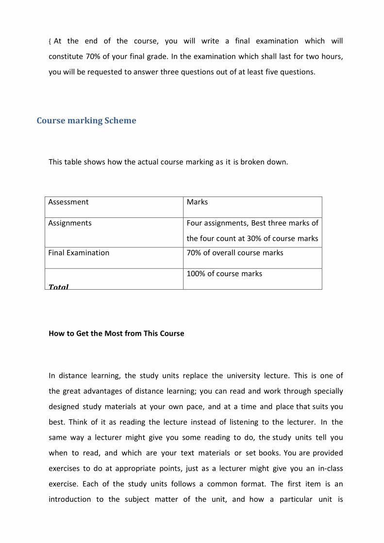
{ At the end of the course, you will write a final examination which will

constitute 70% of your final grade. In the examination which shall last for two hours,

you will be requested to answer three questions out of at least five questions.

Course marking Scheme

This table shows how the actual course marking as it is broken down.

Assessment Marks

Assignments Four assignments, Best three marks of

the four count at 30% of course marks

Final Examination 70% of overall course marks

Total

100% of course marks

How to Get the Most from This Course

In distance learning, the study units replace the university lecture. This is one of

the great advantages of distance learning; you can read and work through specially

designed study materials at your own pace, and at a time and place that suits you

best. Think of it as reading the lecture instead of listening to the lecturer. In the

same way a lecturer might give you some reading to do, the study units tell you

when to read, and which are your text materials or set books. You are provided

exercises to do at appropriate points, just as a lecturer might give you an in-class

exercise. Each of the study units follows a common format. The first item is an

introduction to the subject matter of the unit, and how a particular unit is

integrated with the other units and the course as a whole. Next to this is a set

of learning objectives. These objectives let you know what you should be able to

do by the time you have completed the unit. These learning objectives are meant to

guide your study. The moment a unit is finished, you must go back and check

whether you have achieved the objectives. If this is made a habit, then you will

significantly improve your chances of passing the course. The main body of the unit

guides you through the required reading from other sources. This will usually be

either from your set books or from a Reading section. The following is a practical

strategy for working through the course. If you run into any trouble, telephone your

tutor. Remember that your tutor’s job is to help you. When you need assistance,

do not hesitate to call and ask your tutor to provide it.

In addition do the following:

1. Read this Course Guide thoroughly, it is your first assignment.

2. Organise a Study Schedule. Design a Course Overview ‟ to guide you through

the Course”. Note the time you are expected to spend on each unit and how the

assignments relate to the units. Important information, e.g. details of your tutorials,

and the date of the first day of the Semester is available from the study centre. You

need to gather all the information into one place, such as your diary or a wall

calendar. Whatever method you choose to use, you should decide on and write in

your own dates and schedule of work for each unit.

3. Once you have created your own study schedule, do everything to stay

faithful to it. The major reason that students fail is that they get behind with their

course work. If you get into difficulties with your schedule, please, let your tutor

know before it is too late for help.

4. Turn to Unit 1, and read the introduction and the objectives for the unit.

5. Assemble the study materials. You will need your set books and the unit you are

studying at any point in time.

6. Work through the unit. As you work through the unit, you will know what sources to

consult for further information.

7. Keep in touch with your study centre. Up-to-date course information will be

continuously available there.

8. Well before the relevant due dates (about 4 weeks before due dates), keep in mind

that you will learn a lot by doing the assignment carefully. They have been

designed to help you meet the objectives of the course and, therefore, will help you

pass the examination. Submit all assignments not later than the due date.

9. Review the objectives for each study unit to confirm that you have achieved them.

If you feel unsure about any of the objectives, review the study materials or consult

your tutor.

10. When you are confident that you have achieved a unit’s objectives, you can start

on the next unit. Proceed unit by unit through the course and try to pace your study so

that you keep yourself on schedule.

11. When you have submitted an assignment to your tutor for marking, do not wait

for its return before starting on the next unit. Keep to your schedule. When the

Assignment is returned, pay particular attention to your tutor’s comments, both on

the tutor-marked assignment form and also the written comments on the ordinary

assignments.

12. After completing the last unit, review the course and prepare yourself for the

final examination. Check that you have achieved the unit objectives (listed at the

beginning of each unit) and the course objectives (listed in the Course Guide).

Tutors and Tutorials

The dates, times and locations of these tutorials will be made available to you,

together with the name, telephone number and the address of your tutor. Each

assignment will be marked by your tutor. Pay close attention to the comments

your tutor might make on your assignments as these will help in your progress. Make

sure that assignments reach your tutor on or before the due date.

Your tutorials are important therefore try not to skip any. It is an opportunity to meet

your tutor and your fellow students. It is also an opportunity to get the help of

your tutor and discuss any difficulties encountered on your reading. Summary

This course would train you on the concept of multimedia, production and

utilization of it.

Wish you the best of luck as you read through this course





COURSE MATERIAL

Course Developer/Writers Dr. Peter Ogedebe .

and

Ester Omonayin

Base University, Abuja

Content Editor Dr. Babatunde Disu

And

Babatunde J. Osho.



Course Coordinators Dr. Babatunde Disu

And

Babatunde J. Osho.



MODULE ONE:

UNIT 1: FUNCTION AND GRAPHS

Content:

1.1 Introduction

1.2 Objectives

1.3 Functions

1.4 Function Notation

1.5 Graphs of function

1.6 Combination of function

1.7 Inverse Notation and Exercises

1.8 Conclusion and summary

1.9 References.

1.1 Introduction.

In everyday life, many quantities depend on one or more changing variable. For

example:

a) Speed of a moving car or object depend on distance travelled and time taken

b) The voltage of electrical devices depends on current and resistance.

c) The volume of given mass of gas depends on the pressure at room temperature

(I.e. temperature remain constant)

A function is a phenomenon that relates how one variable or quantity depends on the other

variables or quantities.

For instance, in ohm’s law V I, mathematically V=IR where R is constant of proportionality.

If I increase, so does the voltage V. If I decrease, so does the voltage. Hence, from this, we

can say voltage is a function of current.

1.2 Objectives

In this module, you will cover the following topics:

Function(Definition of function)

Function Notation

Graphs of Function

Combinations of Functions

Inverse Function.

1.3 Function.

Definition of a function

A function is a relationship between two variables such that, to each value of the

independent variable there is exactly one corresponding value of the dependent variable.

The domain of the function is the set of all values of the independent variable for which the

function is defined. The range of the function is the set of all values taken on by the

dependent variable.

OR

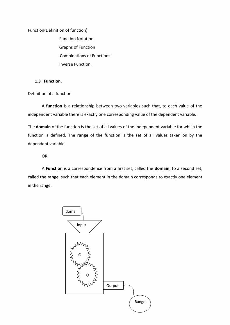
A Function is a correspondence from a first set, called the domain, to a second set,

called the range, such that each element in the domain corresponds to exactly one element

in the range.

input

domai

n

Output

Range

In fig.1, notice that you can think of a function as a machine that inputs values of the

independent variable and inputs values of the dependent variable.

Although function can be described by various means such as table, graphs and

diagrams, they are most often specified by formulas or equation.

For instance, the equation describes y as a function of . For this

function, is the independent variable and y is the dependent variable.

Example 1

Deciding whether relation are functions.

Which of the equation below define y as a function of x?

a) b)

c) d)

Solution

To decide whether an equation defines a function, it is helpful to isolate the dependent

variable on the left side.

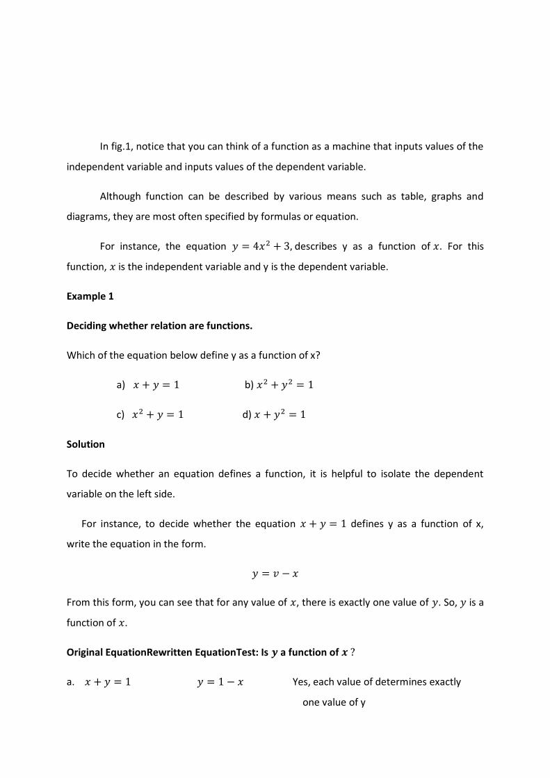
For instance, to decide whether the equation defines y as a function of x,

write the equation in the form.

From this form, you can see that for any value of , there is exactly one value of . So, is a

function of .

Original EquationRewritten EquationTest: Is a function of

a. Yes, each value of determines exactly

one value of y

b. No, some values of x determine two values of .

c. Yes, each value of x determine exactly one

value of y.

d. No, some value of x determine two values

of y.

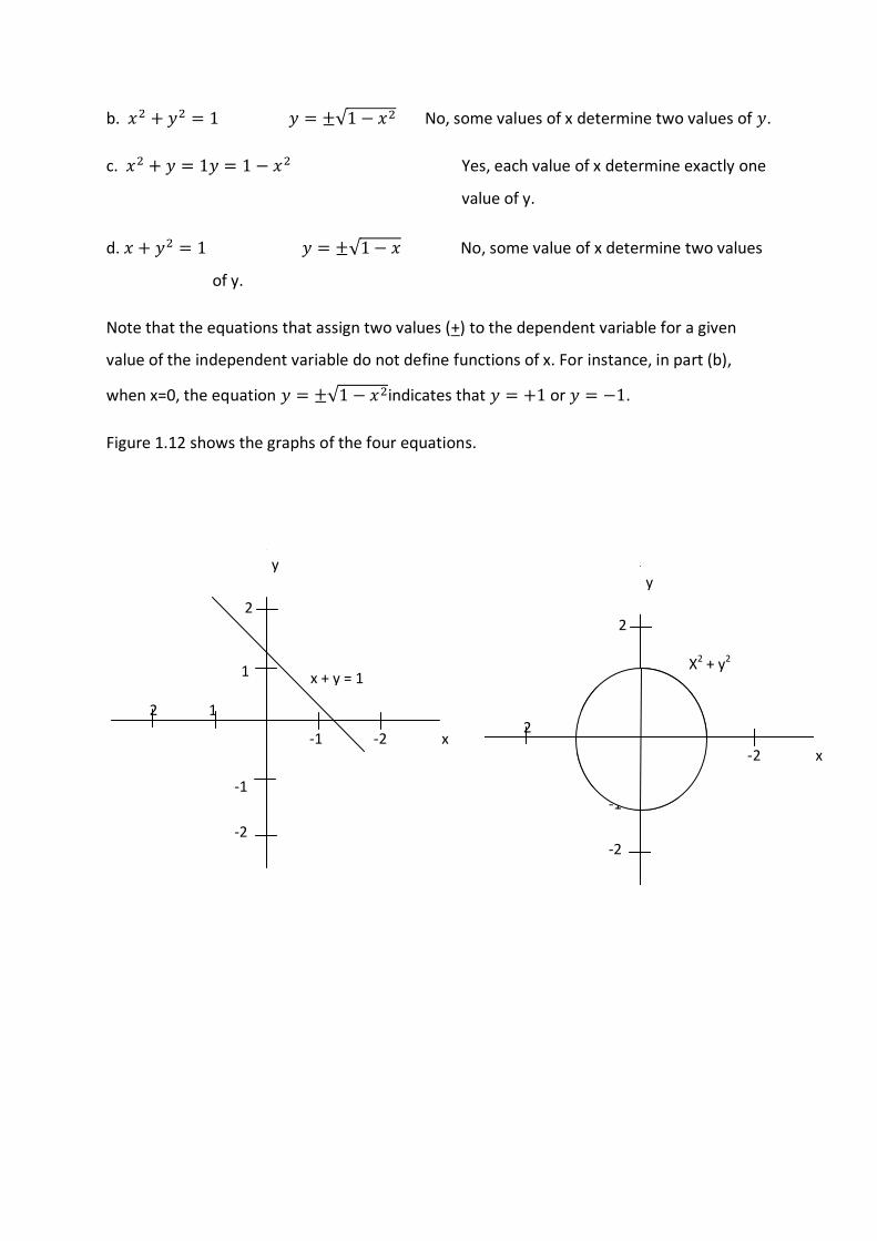
Note that the equations that assign two values (+) to the dependent variable for a given

value of the independent variable do not define functions of x. For instance, in part (b),

when x=0, the equation indicates that or .

Figure 1.12 shows the graphs of the four equations.

2

1

-1

-2

2 1

-1 -2 x

y

2

1

-1

-2

2 1

-1 -2 x

y

2

1

-1

-2

2 1

-1 -2 x

y

x + y = 1 X2 + y2

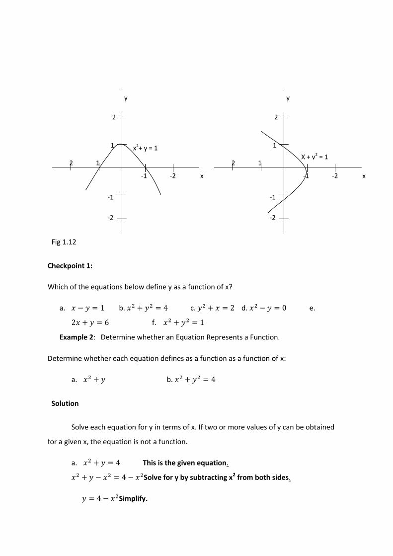
Fig 1.12

Checkpoint 1:

Which of the equations below define y as a function of x?

a. b. c. d. e.

f.

Example 2: Determine whether an Equation Represents a Function.

Determine whether each equation defines as a function as a function of x:

a. b.

Solution

Solve each equation for y in terms of x. If two or more values of y can be obtained

for a given x, the equation is not a function.

a. This is the given equation.

Solve for y by subtracting x2 from both sides.

Simplify.

2

1

-1

-2

2 1

-1 -2 x

y

2

1

-1

-2

2 1

-1 -2 x

y

x2+ y = 1 X + y2 = 1

From this last equation we can see that for each value of x, there is one and only one value

of y. For example, if x=1, then . The equation defines y as a function of x.

b. This is the given equation.

Isolate y2 by subtracting x2 from both sides.

Simplify.

Apply the square root properly: if u2=d then

Then + in this last equation shows that for certain values of x (all values between -2 and 2),

there are two values of y. For example, if x=1, then = . For this reason,

the equation does not define y as a function of x.

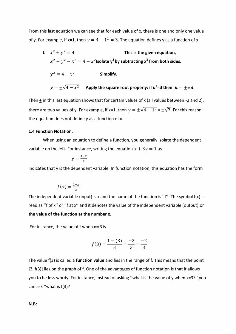
1.4 Function Notation.

When using an equation to define a function, you generally isolate the dependent

variable on the left. For instance, writing the equation as

indicates that y is the dependent variable. In function notation, this equation has the form

The independent variable (input) is x and the name of the function is ‘’f’’. The symbol f(x) is

read as ‘’f of x’’ or ‘’f at x’’ and it denotes the value of the independent variable (output) or

the value of the function at the number x.

For instance, the value of f when x 3 is

The value f(3) is called a function value and lies in the range of f. This means that the point

[3, f(3)] lies on the graph of f. One of the advantages of function notation is that it allows

you to be less wordy. For instance, instead of asking ‘’what is the value of y when x=3?’’ you

can ask ‘’what is f(3)?

N.B:

Study Tip: the notation f(x) does not mean ‘’f times x’’. The notation describes the value of

the function at x.

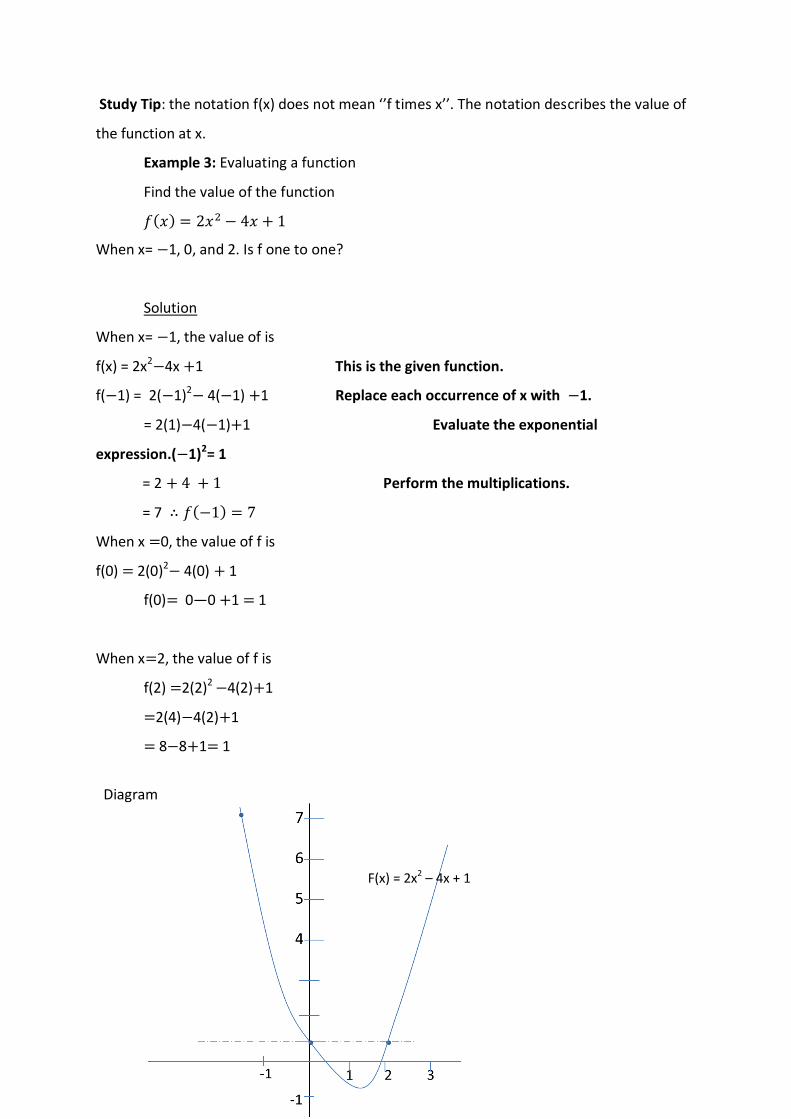
Example 3: Evaluating a function

Find the value of the function

When x= 1, 0, and 2. Is f one to one?

Solution

When x= 1, the value of is

f(x) = 2x2 4x 1 This is the given function.

f( 1) = 2( 1)2 4( 1) 1 Replace each occurrence of x with 1.

= 2(1) 4( 1) 1 Evaluate the exponential

expression.( 1)2= 1

= 2 Perform the multiplications.

= 7

When x 0, the value of f is

f(0) 2(0)2 4(0) 1

f(0) 0—0 1 1

When x 2, the value of f is

f(2) 2(2)2 4(2) 1

2(4) 4(2) 1

8 8 1 1

Diagram

F(x) = 2x2 – 4x + 1

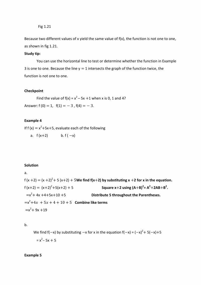
Fig 1.21

Because two different values of x yield the same value of f(x), the function is not one to one,

as shown in fig 1.21.

Study tip:

You can use the horizontal line to test or determine whether the function in Example

3 is one to one. Because the line y 1 intersects the graph of the function twice, the

function is not one to one.

Checkpoint

Find the value of f(x) = x2 – 5x 1 when x is 0, 1 and 4?

Answer: f (0) 1, f(1) , f(4) .

Example 4

If f (x) x2 5x 5, evaluate each of the following

a. f (x 2) b. f ( x)

Solution

a.

f (x 2) (x 2)2 5 (x 2) We find f(x 2) by substituting x 2 for x in the equation.

f (x 2) (x 2)2 5(x 2) 5 Square x 2 using (A B)2= A2 2AB B2.

x2 4x 4 5x 10 5 Distribute 5 throughout the Parentheses.

x2 Combine like terms

x2 9x 19

b.

We find f( x) by substituting x for x in the equation f( x) = ( x)2 5( x) 5

= x2– 5x 5

Example 5

Let f(x) = x2 – 4x 7, find

a. f(x+ x) b. f(x+ x)-f(x)

x

Solution

a. To evaluate f(x+ x), substitute x+ x as x as shown in each set of parentheses

as follows.

f(x+ x) (x+ x)2 4(x+ x)

x2 2x x ( x)2 4x 4 x 7

b. Using the result of part (a), you can write the following.

f(x+ x)-f(x)

x

[(x+ x)2 4(x+ x) (x2 – 4x 7)]

x

[x2 2x x ( x)2 4x 4 x 7 x2 4x 7]

x

2x x ( x)2 4 x

x

2x x – 4 as x 0

Checkpoint:

1. If , and find

a. b.

2. If , evaluate each of the following

a. b. c.

1.5 Graphs of Functions

The graph of a function is the graph of its ordered pairs. For example, the graph of f(x) = 3x

is the set of points (x, y) in the rectangular coordinates system satisfying y = 3x.

When the graph of a function is sketched, the standard convention is to let the

horizontal axis represents the independent variable. When this convention is used, the test

described in Example 1 has vertical line test.

This test states that if every vertical line intersects the graph of an equation at most

once, then the equation defines y as a function of x. For instance, in figure 1.12, the graph in

parts (a) and (c) pass the vertical line test but those in parts (b) and (d) do not

The domain of a function may be described explicitly or it may be implied by an

equation used to define the function. For example, the function given by y = 1/(x2 ) has an

implied domain that consists of real x except x = 2. These two values (x2 – 4) excluded

from the domain because division by zero is undefined.

Another type of implied domain is that used to avoid even roots of negative number,

as indicated in example below.

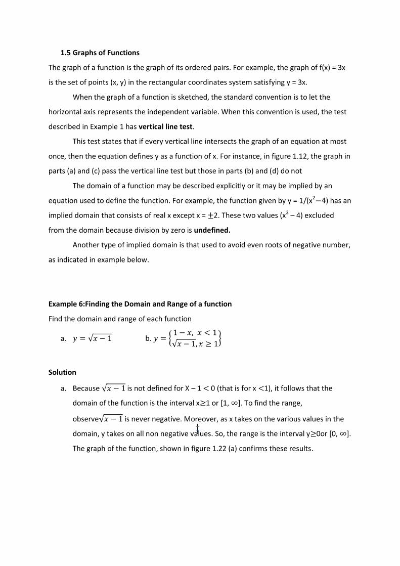
Example 6:Finding the Domain and Range of a function

Find the domain and range of each function

a. b.

Solution

a. Because is not defined for X – 1 0 (that is for x 1), it follows that the

domain of the function is the interval x 1 or [1, ]. To find the range,

observe is never negative. Moreover, as x takes on the various values in the

domain, y takes on all non negative values. So, the range is the interval y 0or [0, ].

The graph of the function, shown in figure 1.22 (a) confirms these results.

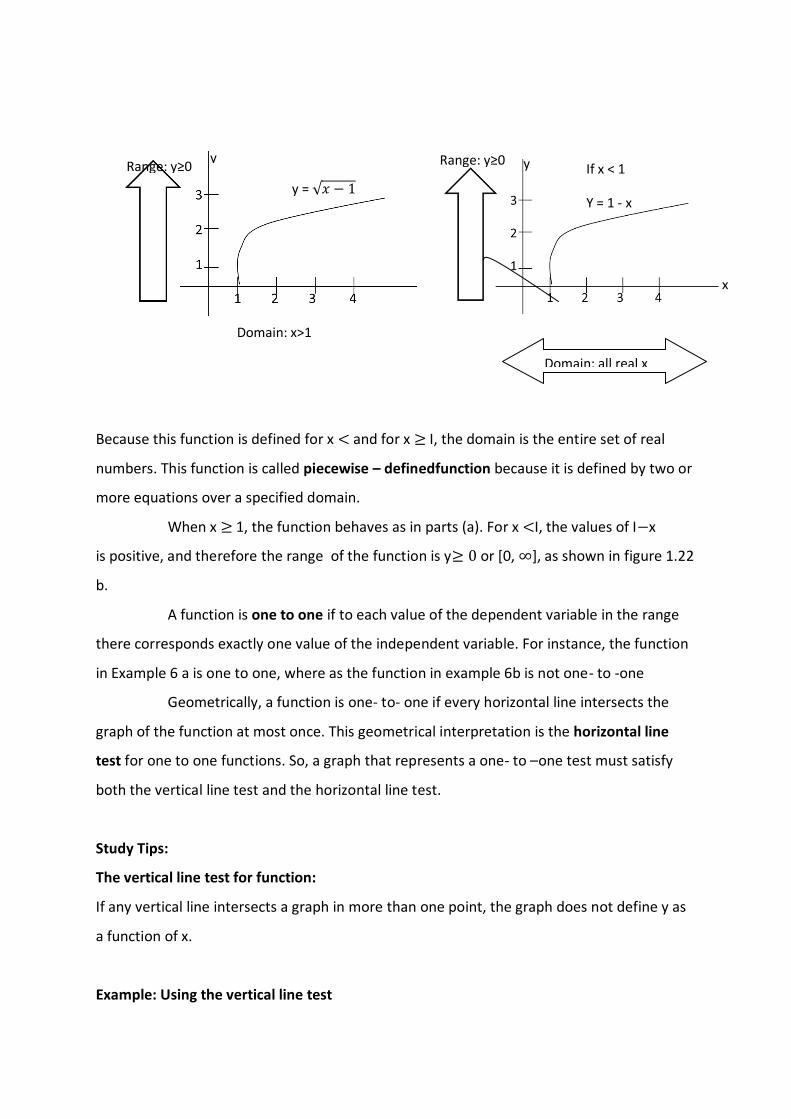
Because this function is defined for x and for x I, the domain is the entire set of real

numbers. This function is called piecewise – definedfunction because it is defined by two or

more equations over a specified domain.

When x 1, the function behaves as in parts (a). For x I, the values of I x

is positive, and therefore the range of the function is y or [0, ], as shown in figure 1.22

b.

A function is one to one if to each value of the dependent variable in the range

there corresponds exactly one value of the independent variable. For instance, the function

in Example 6 a is one to one, where as the function in example 6b is not one- to -one

Geometrically, a function is one- to- one if every horizontal line intersects the

graph of the function at most once. This geometrical interpretation is the horizontal line

test for one to one functions. So, a graph that represents a one- to –one test must satisfy

both the vertical line test and the horizontal line test.

Study Tips:

The vertical line test for function:

If any vertical line intersects a graph in more than one point, the graph does not define y as

a function of x.

Example: Using the vertical line test

Range: y≥0

y =

y Range: y≥0 y

x

If x < 1

Y = 1 - x

Domain: all real x

Domain: x>1

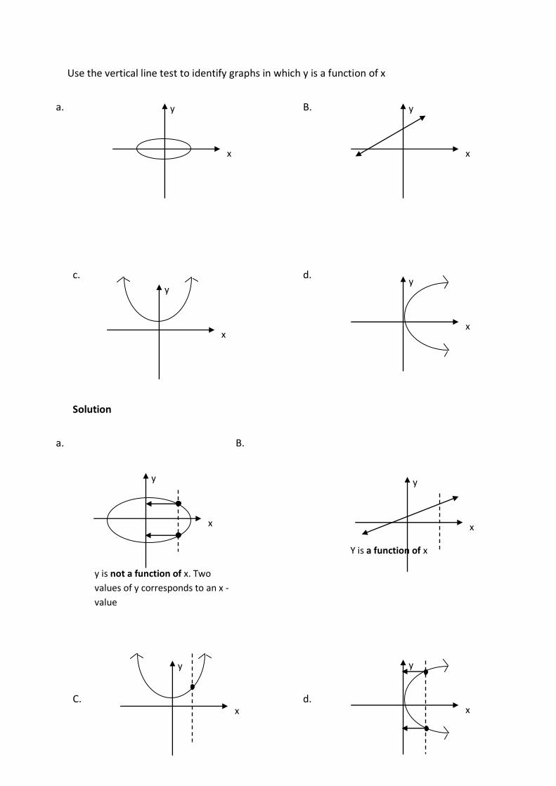
Use the vertical line test to identify graphs in which y is a function of x

a. B.

c. d.

Solution

a. B.

C. d.

x

y

x

y

x

y

x

y

x

y

x

y

x

y

x

y

y is not a function of x. Two

values of y corresponds to an x -

value

Y is a function of x

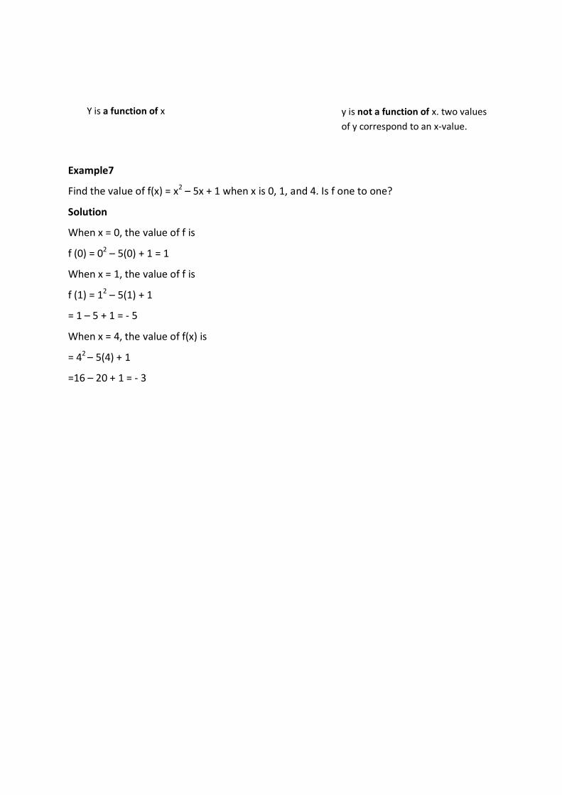
Example7

Find the value of f(x) = x2 – 5x + 1 when x is 0, 1, and 4. Is f one to one?

Solution

When x = 0, the value of f is

f (0) = 02 – 5(0) + 1 = 1

When x = 1, the value of f is

f (1) = 12 – 5(1) + 1

= 1 – 5 + 1 = - 5

When x = 4, the value of f(x) is

= 42 – 5(4) + 1

=16 – 20 + 1 = - 3

Y is a function of x y is not a function of x. two values

of y correspond to an x-value.

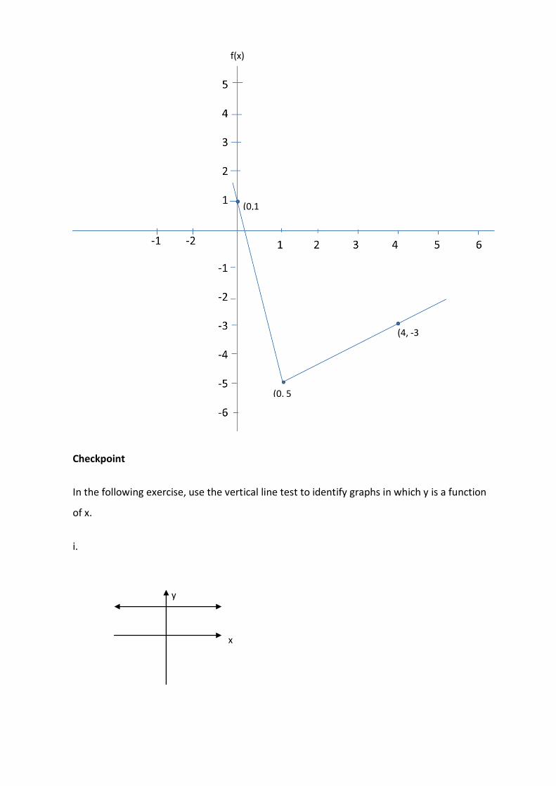
Checkpoint

In the following exercise, use the vertical line test to identify graphs in which y is a function

of x.

i.

x

y

f(x)

(0,1

(0, 5

(4, -3

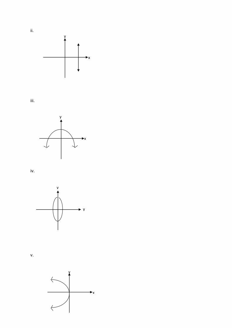
ii.

iii.

iv.

v.

y

x

y

x

y

x

y

y

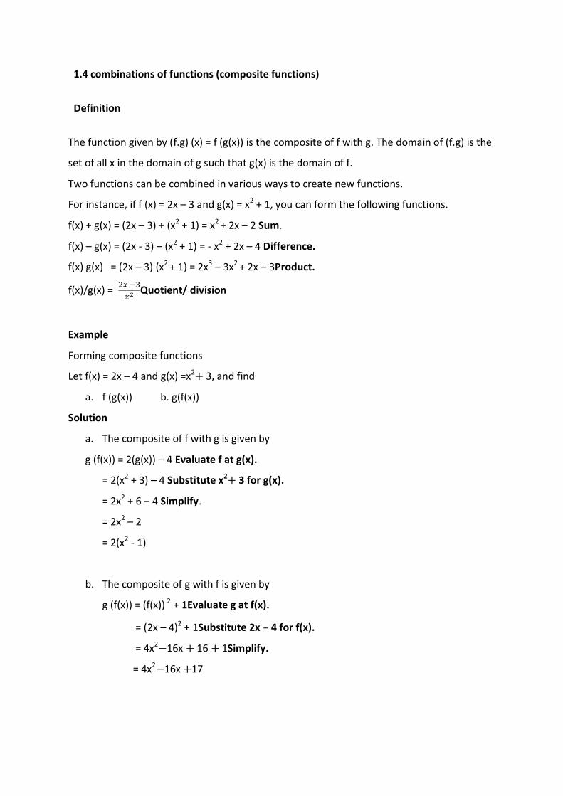
1.4 combinations of functions (composite functions)

Definition

The function given by (f.g) (x) = f (g(x)) is the composite of f with g. The domain of (f.g) is the

set of all x in the domain of g such that g(x) is the domain of f.

Two functions can be combined in various ways to create new functions.

For instance, if f (x) = 2x – 3 and g(x) = x2 + 1, you can form the following functions.

f(x) + g(x) = (2x – 3) + (x2 + 1) = x2 + 2x – 2 Sum.

f(x) – g(x) = (2x - 3) – (x2 + 1) = - x2 + 2x – 4 Difference.

f(x) g(x) = (2x – 3) (x2 + 1) = 2x3 – 3x2 + 2x – 3Product.

f(x)/g(x) =

Quotient/ division

Example

Forming composite functions

Let f(x) = 2x – 4 and g(x) =x2 3, and find

a. f (g(x)) b. g(f(x))

Solution

a. The composite of f with g is given by

g (f(x)) = 2(g(x)) – 4 Evaluate f at g(x).

= 2(x2 + 3) – 4 Substitute x2 3 for g(x).

= 2x2 + 6 – 4 Simplify.

= 2x2 – 2

= 2(x2 - 1)

b. The composite of g with f is given by

g (f(x)) = (f(x)) 2 + 1Evaluate g at f(x).

= (2x – 4)2 + 1Substitute 2x – 4 for f(x).

= 4x2 16x 16 1Simplify.

= 4x2 16x 17

Checkpoint

Let f(x) = 2x 1 and g(x) = x2 2, and find

a) f (g(x)). b) g (f(x)).

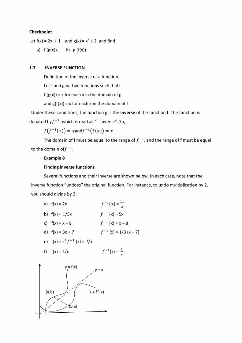
1.7 INVERSE FUNCTION

Definition of the inverse of a function.

Let f and g be two functions such that:

f (g(x)) = x for each x in the domain of g

and g(f(x)) = x for each x in the domain of f

Under these conditions, the function g is the inverse of the function f. The function is

donated by , which is read as “f- inverse”. So,

and

The domain of f must be equal to the range of , and the range of f must be equal

to the domain of .

Example 8

Finding inverse functions

Several functions and their inverse are shown below. In each case, note that the

inverse function “undoes” the original function. For instance, to undo multiplication by 2,

you should divide by 2.

a) f(x) = 2x ) =

b) f(x) = /5x (x) = 5x

c) f(x) = x + 8 (x) = x – 8

d) f(x) = 3x + 7 (x) = 1/3 (x + 7)

e) f(x) = x3 (x) =

f) f(x) = 1/x (x) =

(a,b)

y = f(x) y = x

Y = f-1(x)

(b,a)

The graphs of f and f-1 are mirror images of each other (with respect to the line y = x), as in

figure 1.23

Checkpoint

Informally find the inverse function of each function

a. f(x) = 1/5x b. f (x) = 3x + 2

Example 9: Finding the inverse function

Find the inverse function of f(x) = .

Solution

Begin by substituting f(x) with y. Then interchange x and y and solve for y.

Write original function.

Replace f(x) with y.

Interchange x and y.

Squaring each side.

Add 3 to each side.

y Divide each side by 2.

So, the inverse function has the form

Using x as the independent variable, you can write

as x 0.

In the figure 1.24, note that the domain of coincides with the range of f.

Diagram

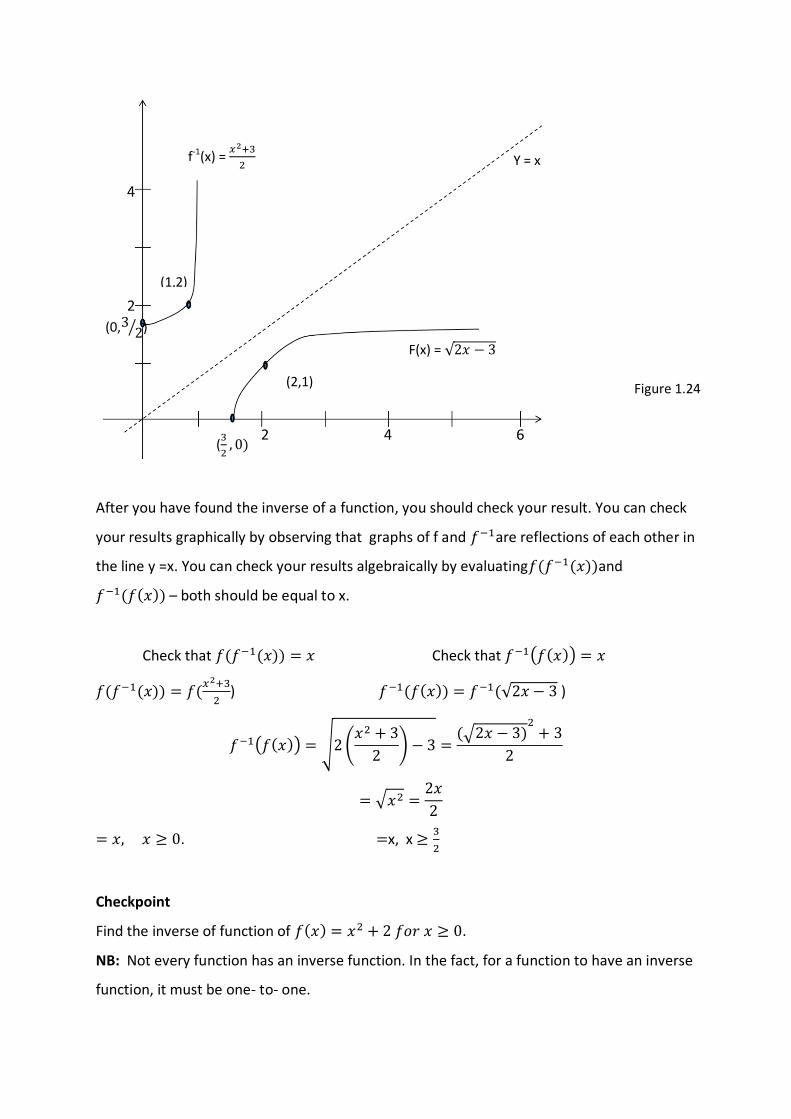
After you have found the inverse of a function, you should check your result. You can check

your results graphically by observing that graphs of f and are reflections of each other in

the line y =x. You can check your results algebraically by evaluating and

– both should be equal to x.

Check that Check that

) )

. x, x

Checkpoint

Find the inverse of function of .

NB: Not every function has an inverse function. In the fact, for a function to have an inverse

function, it must be one- to- one.

f-1(x) =

(

(1,2)

(0, )

(2,1)

(

Y = x

F(x) =

Figure 1.24

Example 10

A function that has no inverse function.

Show that the function f(x) = x2 – 1 has no inverse function. (Assume that the domain of f is

the set of all real numbers)

Solution

Begin by sketching the graph of f, as shown in figure 1.25 Note that

f (x) = x2 – 1

f (2) = 22 – 1 = 3

And

f( 2) = ( 2)2 1 = 3

So, f does not pass the horizontal line test, which implies that if is not one- to- one and

therefore has no inverse function. The same conclusion can be obtained by trying to find the

inverse of f algebraically.

f (x) = x2 – 1 Write original function.

y = x2 – 1 Replace f(x) with y

x = y2 – 1 Interchange x and y

x + 1 = y2

Add 1 to each side

= y Take square root of each side

The last equation does not define y as a function of x, and so f has no inverse function

F (x) = x2 – 1 write original function.

Y = x2 – 1 Replace f(x) with y

X = y2 – 1 Interchange x and y

X + 1 = y2

Add1 to each side

+ Take square root of each side

The last equation does not define y as a function of x, and so f has no inverse function

y

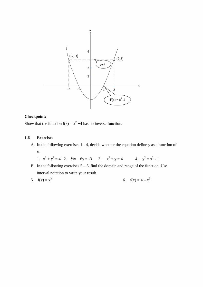
Checkpoint:

Show that the function f(x) = x2 +4 has no inverse function.

1.6 Exercises

A. In the following exercises 1 - 4, decide whether the equation define y as a function of

x.

1. x2 + y

2 = 4 2. ½x – 6y = -3 3. x

2 + y = 4 4. y

2 = x

2 - 1

B. In the following exercises 5 – 6, find the domain and range of the function. Use

interval notation to write your result.

5. f(x) = x3 6. f(x) = 4 – x

2

y

(-2, 3) (2,3)

y=3

F(x) = x2-1

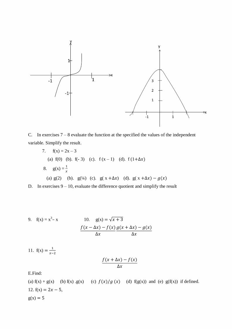
C. In exercises 7 – 8 evaluate the function at the specified the values of the independent

variable. Simplify the result.

7. f(x) = 2x – 3

(a) f(0) (b). f(- 3) (c). f (x – 1) (d). f (1

8. g(x) =

(a) g(2) (b). g(¼) (c). g( x ) (d). g( x

D. In exercises 9 – 10, evaluate the difference quotient and simplify the result

9. f(x) = x3– x 10. g(x)

11. f(x)

E.Find:

(a) f(x) + g(x) (b) f(x) .g(x) (c) (d) f(g(x)) and (e) g(f(x)) if defined.

12. f(x) ,

g(x)

y y

x

x

13. f(x) ,

g(x)

F.

14. Given that f(x) = and g (x) = x2 - 1, find the composite functions:

a. f(g(1)) b. g(f(1)) c. g(f(0)) d. f(g( e. f(g(x)) f. g(f(x))

G. In exercises 15 – 16, show that f and g are inverse functions by showing that f(g(x)) = x

and g (f(x)) = x. Then sketch the graphs of f and g on the same coordinate axes .

15. f(x) g(x)

16. f(x) g(x) , x 9

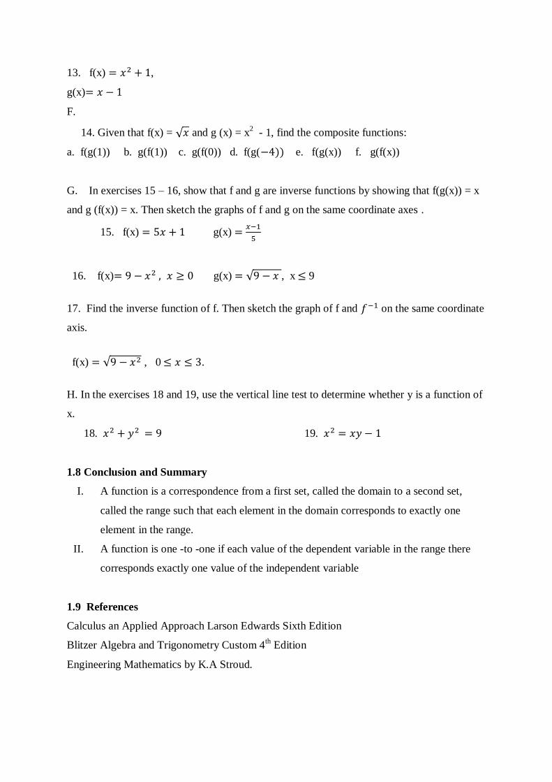
17. Find the inverse function of f. Then sketch the graph of f and on the same coordinate

axis.

f(x) , 0 .

H. In the exercises 18 and 19, use the vertical line test to determine whether y is a function of

x.

18. 19.

1.8 Conclusion and Summary

I. A function is a correspondence from a first set, called the domain to a second set,

called the range such that each element in the domain corresponds to exactly one

element in the range.

II. A function is one -to -one if each value of the dependent variable in the range there

corresponds exactly one value of the independent variable

1.9 References

Calculus an Applied Approach Larson Edwards Sixth Edition

Blitzer Algebra and Trigonometry Custom 4th Edition

Engineering Mathematics by K.A Stroud.

MODULE 2: LIMITS.

Contents:

2.1 Introduction

2.2 Objectives

2.3 Limit (Definition)

2.4 Properties of Limit

2.5 The Limit of a Polynomial Function

2.6 Techniques for Evaluating Limits

2.7 Exercises

2.8 Summary

2.9 References.

2.1 Introduction:

In everyday language, one always refers to limit one’s endurance, speed limit of a car, a wrestler’s weight limit or stretching a spring to its limit. These phrases all suggest that a limit is a bound, which on some instances may not be reached but on other instance may be reached or exceeded.

Hooke’s law is a perfect illustration of limit which states provided an elastic limit of a spring is not exceeded; the extension (e) is directly proportional to the tension or force acting on it. That is a spring has a limit of extension when a load is suspended on it. If it exceeds the boundary, it will reach a point of plasticity or break without returning to its initial position.

Limit is a concept/Fundamental to Calculus.

2.2 Objectives:

In this Module, you will cover the following topics:

2.3 Limits (Definition)

2.4 Properties of Limits



2.1 Definition of Limit of a Function:

If becomes arbitrarily close to a single number L as approaches c from either side, , then which is read as “the limit of as approaches c is L”

2.2 Properties of Limit:

Many times, the limit of as approaches c is simply .Whenever the limit of as approaches c is .The limit can be evaluated by direct substitution.

Properties of Limits:

Let b and c be real numbers, and let n be a positive integer.

i. = b ii. = c iii.

n = c iv.

n = n In the property IV, if n is even, then c must be positive.

By combining the properties of limits with the rules for operating with limits shown below, you can find limits for a wide variety of algebraic function.

Operations with limits:

Let b and c be real numbers let n be a positive integer, and let f and g be functions with the following limits.

= L and = k

I. Scalar multiple: = b L . II. Sum or Difference: = L k. III. Product: = L . k. IV. Quotient: = L/k provided that k 0.

V. Power: n = Ln

VI. Radical: =

In property VI, if n is even, then L must be positive.

Example 1: Find the limit:

2+1)

Solution.

Using direct substitution by substituting 1 for x

2+1) = 12 1 = 2

Example 2:

Find the limit:

a. f(x) =

b. f(x) =

c.

Solution

a.

=

Factorizing the numerator by the difference of two square [

].

= 1 + 1 = 2 Substituting 1 for x.

Therefore,

b.

=

=

= 0 Substituting 1 for x.

Therefore,

does not exist.

c.

= 1

2.3 The limit of a polynomial function

If p is a polynomial function and c is any real number, then

Example 3

Finding the limit of a polynomial function

Find the limit:

Solution:

=

+ Applying property II.

= Use direct substitution.

4 + 4 – 3 = 5 Simplify.

= 5

Note: Example 3 show or state that the limit of polynomial can be evaluated by direct

substitution.

Check point:

1. Find the limit:

a. f(x) =

b. f(x) =

c.

2. Find the limit :

2.4 Techniques for Evaluating Limits.

There are several techniques for calculating limits and these are based on the

following important theorem. Basically, the theorem states that “if two functions agree at all

but a single point c, then they have identical limit behavior at x = c.

The Replacement Theorem/Technique

Let c be a real number and f(x) = g(x) for all x c. if the limit of g(x) exists as x→c, then the

limit of f(x) also exists and

To apply the Replacement Theorem, you can use a result from algebra which states that for a

polynomial function p, p(c) = 0 if and only if (x-c) is a factor of p(x).

Example 4

Finding the limit of a function

Find the limit:

Solution

Note that the numerator and the denominator are zero when x=1

.For the numerator

= =0 the denominator

.

This implies or means that x - 1 is a factor of both and you can divide out this like factor

using division of polynomial.

= (x

2 + x +1)(x -1)

=

=

factor numerator.

=

Divide out factor.

= , x 1 Simplify.

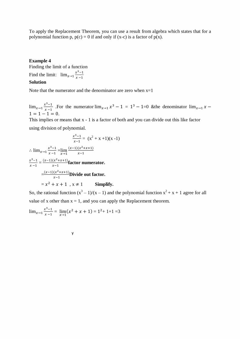
So, the rational function (x3 – 1)/(x – 1) and the polynomial function x

2 + x + 1 agree for all

value of x other than x = 1, and you can apply the Replacement theorem.

=

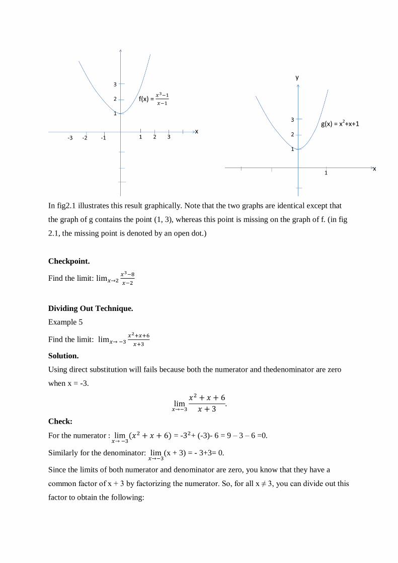
= + 1+1 =3

f(x) =

y

x

y

x

g(x) = x2+x+1

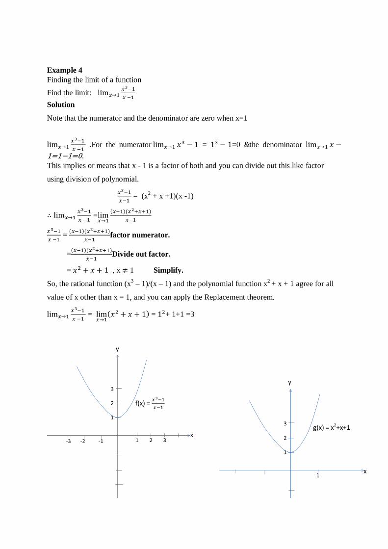
In fig2.1 illustrates this result graphically. Note that the two graphs are identical except that

the graph of g contains the point (1, 3), whereas this point is missing on the graph of f. (in fig

2.1, the missing point is denoted by an open dot.)

Checkpoint.

Find the limit:

Dividing Out Technique.

Example 5

Find the limit:

Solution.

Using direct substitution will fails because both the numerator and thedenominator are zero

when x = -3.

Check:

For the numerator

= - + (-3)- 6 = 9 – 3 – 6 =0.

Similarly for the denominator:

(x + 3) = - 3+3= 0.

Since the limits of both numerator and denominator are zero, you know that they have a

common factor of x + 3 by factorizing the numerator. So, for all x ≠ 3, you can divide out this

factor to obtain the following:

=

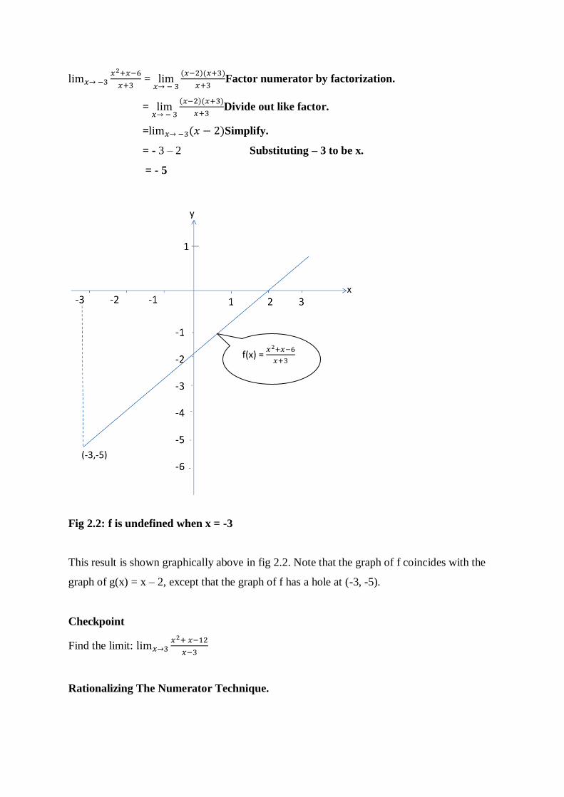
Factor numerator by factorization.

=

Divide out like factor.

= Simplify.

= - 3 – 2 Substituting – 3 to be x.

= - 5

y

x

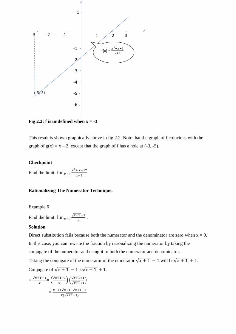
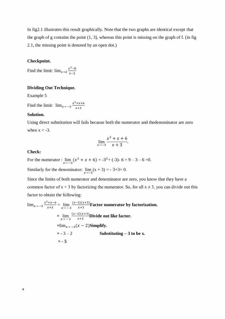
Fig 2.2: f is undefined when x = -3

This result is shown graphically above in fig 2.2. Note that the graph of f coincides with the

graph of g(x) = x – 2, except that the graph of f has a hole at (-3, -5).

Checkpoint

Find the limit:

Rationalizing The Numerator Technique.

Example 6

Find the limit:

.

Solution

Direct substitution fails because both the numerator and the denominator are zero when x = 0.

In this case, you can rewrite the fraction by rationalizing the numerator by taking the

conjugate of the numerator and using it to both the numerator and denominator.

Taking the conjugate of the numerator of the numerator will be .

Conjugate of is .

=

=

(-3,-5)

f(x) =

=

=

=

, x

Now, using the replacement theorem, you can evaluate the limit as follows:

=

=

=

=

= ½

Checkpoint

Find the limit:

.

One Sided Limit

One way in which a limit fails to exist is when a function approachesa different value from

the left of c than it approaches from right of c. This type of behaviour can be described more

concisely with the concept of a one-sided limit.

Limit from the left.

Limit from the right.

The first of these two limits is read as “the limit of f(x) as x approaches c from the left is L”.

The second is read as “limitf(x) as x approaches c from the right is L”.

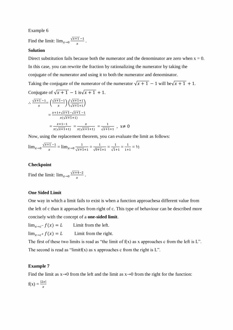
Example 7

Find the limit as x 0 from the left and the limit as x 0 from the right for the function:

f(x) =

Solution

Fig 2.3

f(x) =

y

x

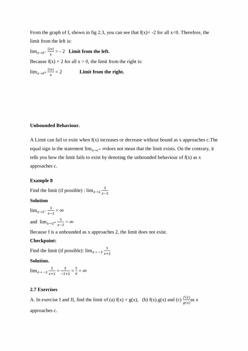
From the graph of f, shown in fig 2.3, you can see that f(x)= -2 for all x<0. Therefore, the

limit from the left is:

= - 2 Limit from the left.

Because f(x) = 2 for all x > 0, the limit from the right is:

= 2 Limit from the right.

Unbounded Behaviour.

A Limit can fail to exist when f(x) increases or decrease without bound as x approaches c.The

equal sign in the statement does not mean that the limit exists. On the contrary, it

tells you how the limit fails to exist by denoting the unbounded behaviour of f(x) as x

approaches c.

Example 8

Find the limit (if possible) :

Solution

=

and

=

Because f is a unbounded as x approaches 2, the limit does not exist.

Checkpoint:

Find the limit (if possible):

Solution.

=

=

=

2.7 Exercises

A. In exercise I and II, find the limit of (a) f(x) + g(x), (b) f(x).g(x) and (c)

as x

approaches c.

I. II.

B. In exercise III – XVI, find the limit:

III. IV.

V. VI.

VII. IX. X.

XI.

XII.

XIII.

XIV.

XV.

XVI.

In the following exercise XVII – XXX, find the limit (if it exists):

XVII.

XVIII.

XIX.

XX.

XXI.

XXII.

XXIII.

XXIV.

XXV.

XXVI.

XXVII. , where f(x) =

XXVIII.

XXIX.

XXX.

2.8 Summary.

I. If f(x) becomes arbitrary close to a single number L as x approach c from either side, then

= L which is as the limit of f(x) as x approaches c is L.

II. If p is a polynomial function and c is any real number, then

2.9References:

I. Engineering Mathematics by K. A Stroud.

II. Blitzer Algebra and Trigonometry Custom 4th Edition.

III. Calculus An Applied Approach Larson Edwards Sixth Edition.

MODULE ONE

UNIT 2: LIMITS.

Contents:

2.1 Introduction

2.2 Objectives

2.3 Limit (Definition)

2.4 Properties of Limit



2.7 Exercises

2.8 Summary

2.9 References.

2.1 Introduction:

In everyday language, one always refers to limit one’s endurance, speed limit of a car, a wrestler’s weight limit or stretching a spring to its limit. These phrases all suggest that a limit is a bound, which on some instances may not be reached but on other instance may be reached or exceeded.

Hooke’s law is a perfect illustration of limit which states provided an elastic limit of a spring is not exceeded; the extension (e) is directly proportional to the tension or force acting on it. That is a spring has a limit of extension when a load is suspended on it. If it exceeds the boundary, it will reach a point of plasticity or break without returning to its initial position.

Limit is a concept/Fundamental to Calculus.

2.2 Objectives:

In this Module, you will cover the following topics:

2.3 Limits (Definition)

2.4 Properties of Limits



2.1 Definition of Limit of a Function:

If becomes arbitrarily close to a single number L as approaches c from either side, , then which is read as “the limit of as approaches c is L”

2.2 Properties of Limit:

Many times, the limit of as approaches c is simply .Whenever the limit of as approaches c is .The limit can be evaluated by direct substitution.

Properties of Limits:

Let b and c be real numbers, and let n be a positive integer.

v. = b vi. = c vii.

n = c viii.

n = n In the property IV, if n is even, then c must be positive.

By combining the properties of limits with the rules for operating with limits shown below, you can find limits for a wide variety of algebraic function.

Operations with limits:

Let b and c be real numbers let n be a positive integer, and let f and g be functions with the following limits.

= L and = k

V. Scalar multiple: = b L . VI. Sum or Difference: = L k. VII. Product: = L . k. VIII. Quotient: = L/k provided that k 0.

V. Power: n = Ln

VI. Radical: =

In property VI, if n is even, then L must be positive.

Example 1: Find the limit:

2+1)

Solution.

Using direct substitution by substituting 1 for x

2+1) = 12 1 = 2

Example 2:

Find the limit:

a. f(x) =

b. f(x) =

c.

Solution

a.

=

Factorizing the numerator by the difference of two square [

].

= 1 + 1 = 2 Substituting 1 for x.

Therefore,

b.

=

=

= 0 Substituting 1 for x.

Therefore,

does not exist.

c.

= 1

2.3 The limit of a polynomial function

If p is a polynomial function and c is any real number, then

Example 3

Finding the limit of a polynomial function

Find the limit:

Solution:

=

+ Applying property II.

= Use direct substitution.

4 + 4 – 3 = 5 Simplify.

= 5

Note: Example 3 show or state that the limit of polynomial can be evaluated by direct

substitution.

Check point:

3. Find the limit:

b. f(x) =

b. f(x) =

c.

4. Find the limit :

2.4 Techniques for Evaluating Limits.

There are several techniques for calculating limits and these are based on the

following important theorem. Basically, the theorem states that “if two functions agree at all

but a single point c, then they have identical limit behavior at x = c.

The Replacement Theorem/Technique

Let c be a real number and f(x) = g(x) for all x c. if the limit of g(x) exists as x→c, then the

limit of f(x) also exists and

To apply the Replacement Theorem, you can use a result from algebra which states that for a

polynomial function p, p(c) = 0 if and only if (x-c) is a factor of p(x).

Example 4

Finding the limit of a function

Find the limit:

Solution

Note that the numerator and the denominator are zero when x=1

.For the numerator

= =0 the denominator

.

This implies or means that x - 1 is a factor of both and you can divide out this like factor

using division of polynomial.

= (x

2 + x +1)(x -1)

=

=

factor numerator.

=

Divide out factor.

= , x 1 Simplify.

So, the rational function (x3 – 1)/(x – 1) and the polynomial function x

2 + x + 1 agree for all

value of x other than x = 1, and you can apply the Replacement theorem.

=

= + 1+1 =3

y

In fig2.1 illustrates this result graphically. Note that the two graphs are identical except that

the graph of g contains the point (1, 3), whereas this point is missing on the graph of f. (in fig

2.1, the missing point is denoted by an open dot.)

Checkpoint.

Find the limit:

Dividing Out Technique.

Example 5

Find the limit:

Solution.

Using direct substitution will fails because both the numerator and thedenominator are zero

when x = -3.

Check:

For the numerator

= - + (-3)- 6 = 9 – 3 – 6 =0.

Similarly for the denominator:

(x + 3) = - 3+3= 0.

Since the limits of both numerator and denominator are zero, you know that they have a

common factor of x + 3 by factorizing the numerator. So, for all x ≠ 3, you can divide out this

factor to obtain the following:

f(x) =

x

y

x

g(x) = x2+x+1

=

Factor numerator by factorization.

=

Divide out like factor.

= Simplify.

= - 3 – 2 Substituting – 3 to be x.

= - 5

Fig 2.2: f is undefined when x = -3

This result is shown graphically above in fig 2.2. Note that the graph of f coincides with the

graph of g(x) = x – 2, except that the graph of f has a hole at (-3, -5).

Checkpoint

Find the limit:

Rationalizing The Numerator Technique.

(-3,-5)

y

x

f(x) =

Example 6

Find the limit:

.

Solution

Direct substitution fails because both the numerator and the denominator are zero when x = 0.

In this case, you can rewrite the fraction by rationalizing the numerator by taking the

conjugate of the numerator and using it to both the numerator and denominator.

Taking the conjugate of the numerator of the numerator will be .

Conjugate of is .

=

=

=

=

=

, x

Now, using the replacement theorem, you can evaluate the limit as follows:

=

=

=

=

= ½

Checkpoint

Find the limit:

.

One Sided Limit

One way in which a limit fails to exist is when a function approachesa different value from

the left of c than it approaches from right of c. This type of behaviour can be described more

concisely with the concept of a one-sided limit.

Limit from the left.

Limit from the right.

The first of these two limits is read as “the limit of f(x) as x approaches c from the left is L”.

The second is read as “limitf(x) as x approaches c from the right is L”.

Example 7

Find the limit as x 0 from the left and the limit as x 0 from the right for the function:

f(x) =

Solution

Fig 2.3

From the graph of f, shown in fig 2.3, you can see that f(x)= -2 for all x<0. Therefore, the

limit from the left is:

= - 2 Limit from the left.

Because f(x) = 2 for all x > 0, the limit from the right is:

= 2 Limit from the right.

Unbounded Behaviour.

A Limit can fail to exist when f(x) increases or decrease without bound as x approaches c.The

equal sign in the statement does not mean that the limit exists. On the contrary, it

tells you how the limit fails to exist by denoting the unbounded behaviour of f(x) as x

approaches c.

Example 8

Find the limit (if possible) :

Solution

=

and

=

Because f is a unbounded as x approaches 2, the limit does not exist.

Checkpoint:

f(x) =

y

x

Find the limit (if possible):

Solution.

=

=

=

2.7 Exercises

A. In exercise I and II, find the limit of (a) f(x) + g(x), (b) f(x).g(x) and (c)

as x

approaches c.

I. II.

B. In exercise III – XVI, find the limit:

III. IV.

V. VI.

VII. IX. X.

XI.

XII.

XIII.

XIV.

XV.

XVI.

In the following exercise XVII – XXX, find the limit (if it exists):

XVII.

XVIII.

XIX.

XX.

XXI.

XXII.

XXIII.

XXIV.

XXV.

XXVI.

XXVII. , where f(x) =

XXVIII.

XXIX.

XXX.

2.8 Summary.

I. If f(x) becomes arbitrary close to a single number L as x approach c from either side, then

= L which is as the limit of f(x) as x approaches c is L.

II. If p is a polynomial function and c is any real number, then

2.9References:

I. Engineering Mathematics by K. A Stroud.

II. Blitzer Algebra and Trigonometry Custom 4th Edition.

III. Calculus An Applied Approach Larson Edwards Sixth Edition.

MODULE ONE

UNIT 3: IDEA OF CONTINUITY

3.1 Introduction

3.2 Objective

3.3 Definition of Continuity

3.4 Continuity of Polynomial and Rational Functions

3.5 Exercises

3.6 References

3.1 Introduction:

In mathematics, continuity means rigorous formulation of the intuitive concept of

function that varies with no abrupt breaks or jumps.

Continuity of a function is expressed some times by saying if the X values are closed

together, then the y value of the function will also be close.

3.2 Objective

In this module, you will cover the following topics

3.3 Definition of Continuity

3.4 Continuity of Polynomial and Rational functions

3.5 Continuity on a closed interval

3.3 Idea of Continuity

3.3.1 Definition of Continuity

Let c be a number in the interval (a, b), and let f be a function whose domain

contains the interval (a, b). The function f is continuous at the point cif the following

conditions are true:

i. F(c) is defined

ii. exists

iii. = f(c)

If f is continuous at every point in the interval (a, b), then it is continuous on an open

interval (a, b).

N:B

Roughly, we can say that a function is said to be continuous on an interval if its graph

on the interval can be traced using a pencil and paper without lifting the pencil from

the paper (i.e. the graph of f is unbroken at c, and there are no holes, jumps, or gaps

or to say that a function is continuous at x=c when there is no interruption in the

graph of f at c.

Specifically, when direct substitution can be used to evaluate the limit of a function

at c, then the function is continuous at c.The two types of functions that have this

property are polynomial functions and rational functions.

3.4 Continuity of polynomial and Rational Functions.

i. A polynomial function is continuous at every real number.

iiA rational function is continuous at every number in its domain.

Determining continuity of a polynomial function

Example 1

Discuss the continuity of each function

a. f(x) = x2 – 2x +3 b. f(x) = x3 – x

Solution

Each of these functions is a polynomial function. So, each is continuous on the entire real

line.

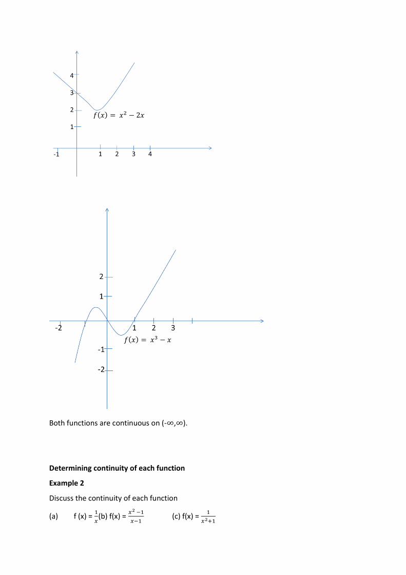
Both functions are continuous on (- , ).

Determining continuity of each function

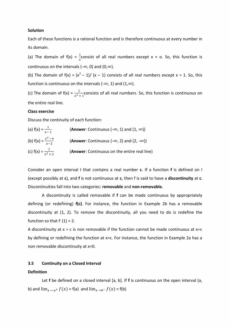
Example 2

Discuss the continuity of each function

(a) f (x) =

(b) f(x) =

(c) f(x) =

Solution

Each of these functions is a rational function and is therefore continuous at every number in

its domain.

(a) The domain of f(x) =

consist of all real numbers except x = o. So, this function is

continuous on the intervals (- , 0) and (0, ).

(b) The domain of f(x) = (x2 – 1)/ (x – 1) consists of all real numbers except x = 1. So, this

function is continuous on the intervals (- , 1) and (1, ).

(c) The domain of f(x) =

consists of all real numbers. So, this function is continuous on

the entire real line.

Class exercise

Discuss the continuity of each function:

(a) f(x) =

(Answer: Continuous (- , 1) and (1, ))

(b) f(x) =

(Answer: Continuous (- , 2) and (2, - ))

(c) f(x) =

(Answer: Continuous on the entire real line)

Consider an open interval I that contains a real number c. If a function f is defined on I

(except possibly at c), and f is not continuous at c, then f is said to have a discontinuity at c.

Discontinuities fall into two categories: removable and non-removable.

A discontinuity is called removable if f can be made continuous by appropriately

defining (or redefining) f(c). For instance, the function in Example 2b has a removable

discontinuity at (1, 2). To remove the discontinuity, all you need to do is redefine the

function so that F (1) = 2.

A discontinuity at x = c is non removable if the function cannot be made continuous at x=c

by defining or redefining the function at x=c. For instance, the function in Example 2a has a

non removable discontinuity at x=0.

3.5 Continuity on a Closed Interval

Definition

Let f be defined on a closed interval [a, b]. If f is continuous on the open interval (a,

b) and = f(a) and = f(b)

Then f is continuous on the closed interval [a, b]. Moreover, f is continuous from

the right at a andcontinuous from the left at b.

Similar definitions can be made to cover continuity on intervals of the form (a, b] and [a,b),

or on infinite intervals. For example the function

f(x) = is continuous on the infinite interval [0, ).

Examining Continuity at an End point

Example 3

Discuss the continuity of f(x) =

Solution

Notice that the domain of f is the set (- , 3].

Moreover, f is continuous from the left at x = 3 because:

=

= 0

= f(3)

For all x<3, the function f satisfies the three conditions foe continuity. So, you can conclude

that f is continuous on the interval (- , 3].

Working Tip

When working with radical functions of the form f(x) = , remember that the

domain of f coincides with the solution of g (x) 0.

Examining Continuity on a closed interval.

Example 4:

Discuss the continuity of

Solution

The polynomial functions 5 – x and X2 – 1 are continuous on the intervals [- 1, 2) and (2, 3],

respectively. So, to conclude that g is continuous on the entire interval [-1, 3], you need only

check the behavior of g when x =2. You can do this by taking the one – sided limit when x=2.

= = 3 limit from the left

and

= = 3 limit from the right

Because these two limits are equal

= g(2) = 3.

So, g is continuous at x = 2 and consequently, it is continuous on the entire interval [-1, 3]

3.6 Exercises

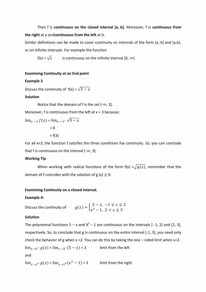
A. In exercise i to iii, determine whether the function is continuous on the entire real line.

Explain your reasoning.

i. f(x) = 5x3 – x2 +2 ii. f(x) =

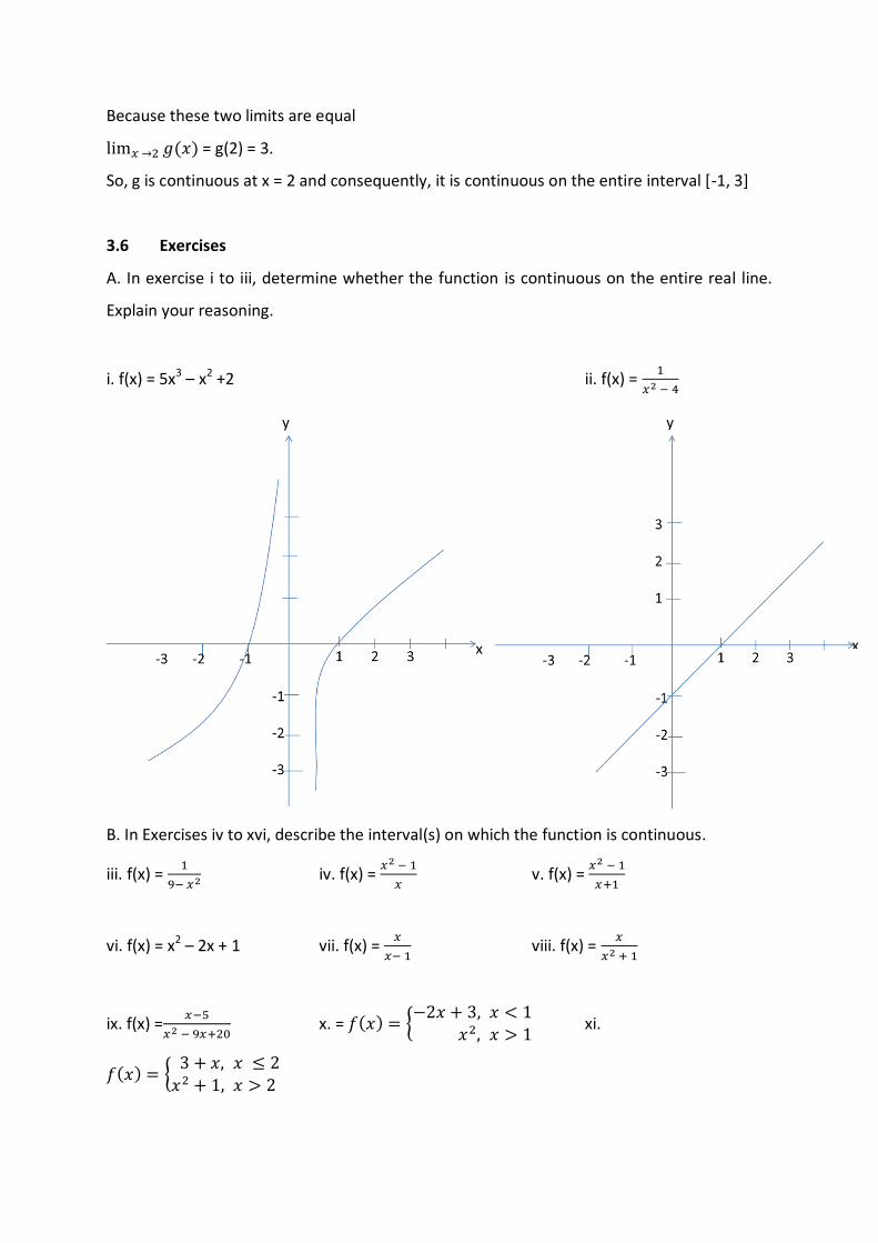
B. In Exercises iv to xvi, describe the interval(s) on which the function is continuous.

iii. f(x) =

iv. f(x) =

v. f(x) =

vi. f(x) = x2 – 2x + 1 vii. f(x) =

viii. f(x) =

ix. f(x) =

x. =

xi.

y

x x

y

xii.

xiii.

xvi.

3.7 Summary

i. A function is said to be continuous if and only if it is continuous at every point of its

domain.

ii. Continuity can be defined in terms of limits by saying that f(x) is continuous at x(0) of its

domain if and only if, for values of x in its domain

3.8 References

i. Blitzer Algebra and Trigonometry Custom 4th Edition

ii. Calculus: An Applied Approach. Larson Edwards Sixth Edition

iii. Engineering Mathematics by K.A Stroud.

MODULE TWO

UNIT 1: THE DERIVATIVE AS LIMIT OF RATE OF CHANGE

Contents

4.1 Introduction

4.2 Objective

4.3 Differentiation

4.4 Derivative for Power of xn

4.5 Differentiation of Polynomials

4.6 Standard derivative

4.7 Exercises

4.8 Summary

4.9 References

4.1 Introduction

The derivative of a function of a real variable measures the sensitivity to change of a

quantity (a function value or dependent variable) which is determined by another quantity

(the independent variable).

Derivatives are fundamental tools of calculus. The derivative of a function of a single

variable at a chosen input value is the slope of the tangent line to the graph of the function at

that point. This means that it describe the best linear approximation of the function near that

input value. For this reason, the derivative is often described as the “instantaneous rate of

change”, the ratio of the instantaneous change in the dependent variable to that of the

independent variable.

Differentiation is the action of computing a derivative.

4.2 Objective

In this module, you will cover the following topics:

4.3 Differentiation (First Principle)

4.4 Derivative for Power of xn

4.5 Differentiation of Polynomials

4.6 Standard derivative

4.3 Differentiation

Before introducing differentiation, it is always good to study gradient at point on a curve

since it is the basis of differentiation. The process of finding a derivative is called

differentiation.

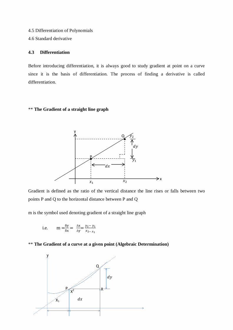
** The Gradient of a straight line graph

Gradient is defined as the ratio of the vertical distance the line rises or falls between two

points P and Q to the horizontal distance between P and Q

m is the symbol used denoting gradient of a straight line graph

i.e. m =

=

=

** The Gradient of a curve at a given point (Algebraic Determination)

Q

P

y

x

y

P

Q

X2 R

X1

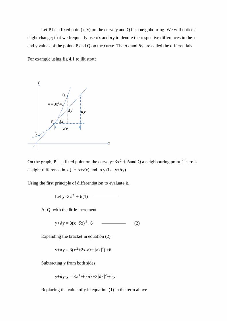
Let P be a fixed point(x, y) on the curve y and Q be a neighbouring. We will notice a

slight change; that we frequently use x and y to denote the respective differences in the x

and y values of the points P and Q on the curve. The x and y are called the differentials.

For example using fig 4.1 to illustrate

On the graph, P is a fixed point on the curve y= and Q a neighbouring point. There is

a slight difference in x (i.e. x+ x) and in y (i.e. y+ y)

Using the first principle of differentiation to evaluate it.

Let y= (1)

At Q: with the little increment

y+ y = 3(x+ x) 2

+6 (2)

Expanding the bracket in equation (2)

y+ y = 3( +2x- x+ 2) +6

Subtracting y from both sides

y+ y-y = 3 +6x x+3 2+6-y

Replacing the value of y in equation (1) in the term above

6

y

Q

P

y = 3x2+6

x

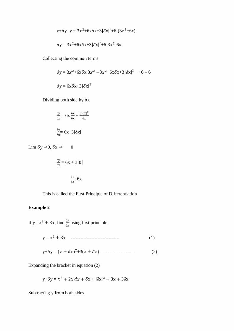
y+ y- y = 3 +6x x+3 2+6-(3 +6x)

y = 3 +6x x+3 2+6-3 -6x

Collecting the common terms

y = 3 +6x x 3 3 +6x x+3 2 +6 – 6

y = 6x x+3 2

Dividing both side by x

= 6x

+

= 6x+3

Lim y 0, x 0

= 6x + 3

=6x

This is called the First Principle of Differentiation

Example 2

If y = , find

using first principle

y = ------------------------------- (1)

y+ y = +3( ---------------------- (2)

Expanding the bracket in equation (2)

y+ y = x +

Subtracting y from both sides

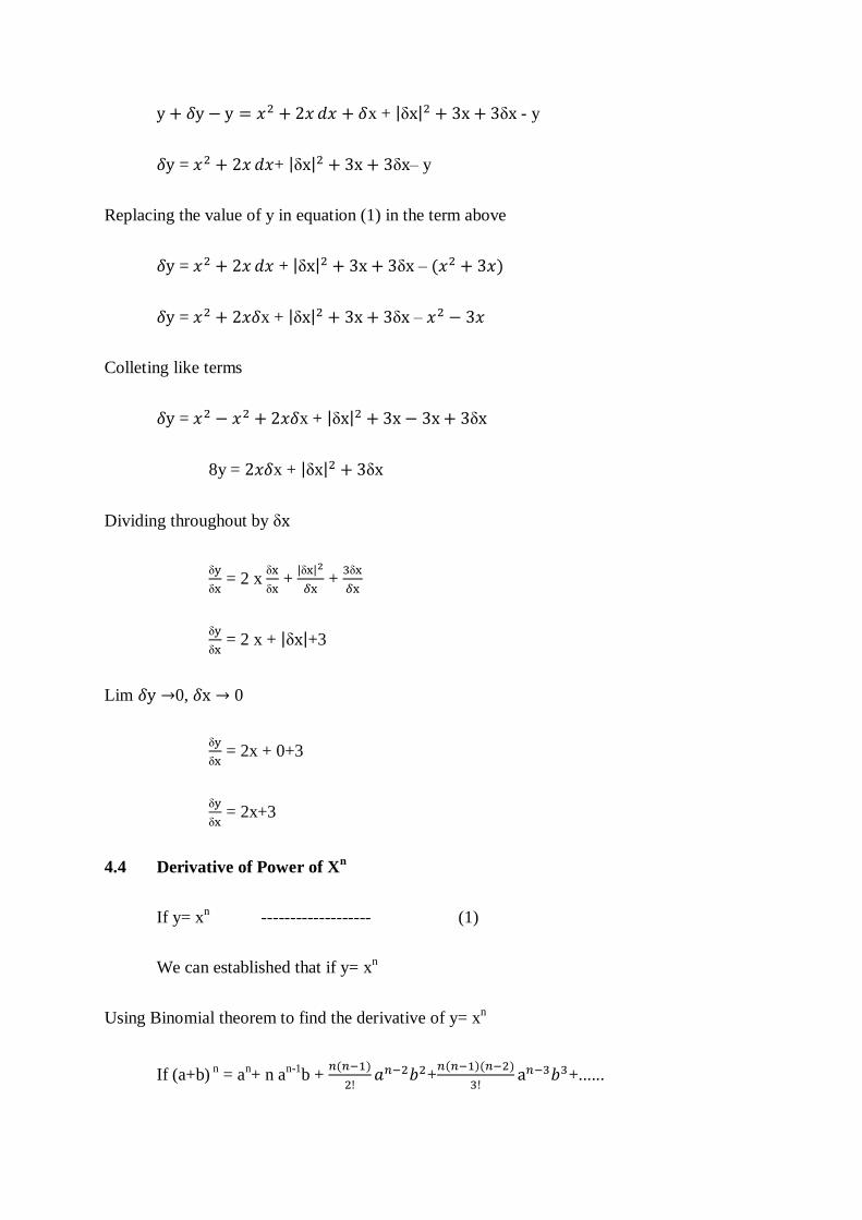
x + - y

= + – y

Replacing the value of y in equation (1) in the term above

= + –

= x + –

Colleting like terms

= x +

8y = x +

Dividing throughout by

= 2 x

+

+

= 2 x + +3

Lim 0, 0

= 2x + 0+3

= 2x+3

4.4 Derivative of Power of Xn

If y= xn ------------------- (1)

We can established that if y= xn

Using Binomial theorem to find the derivative of y= xn

If (a+b) n = a

n+ n a

n-1b +

+

+......

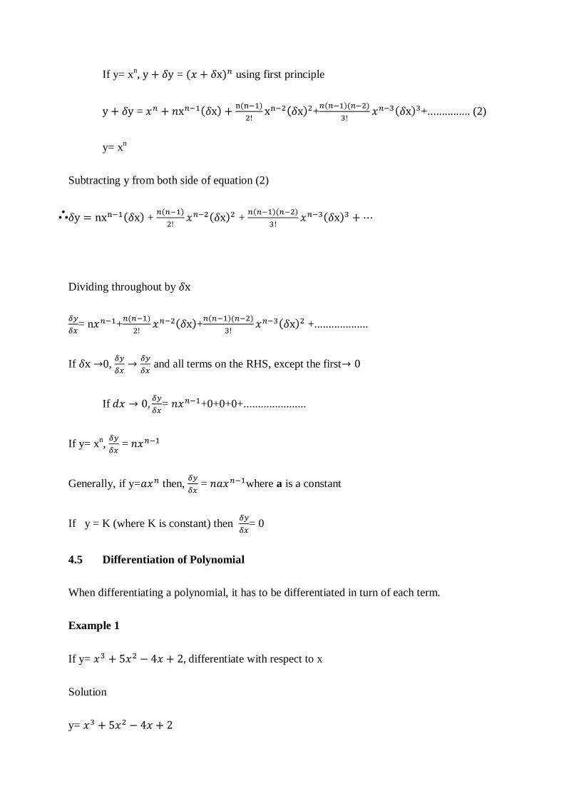
If y= xn, = using first principle

=

+

+............... (2)

y= xn

Subtracting y from both side of equation (2)

+

+

Dividing throughout by

= n +

+

+...................

If 0,

and all terms on the RHS, except the first

If

= +0+0+0+......................

If y= xn,

=

Generally, if y= then,

= where a is a constant

If y = K (where K is constant) then

= 0

4.5 Differentiation of Polynomial

When differentiating a polynomial, it has to be differentiated in turn of each term.

Example 1

If y= differentiate with respect to x

Solution

y=

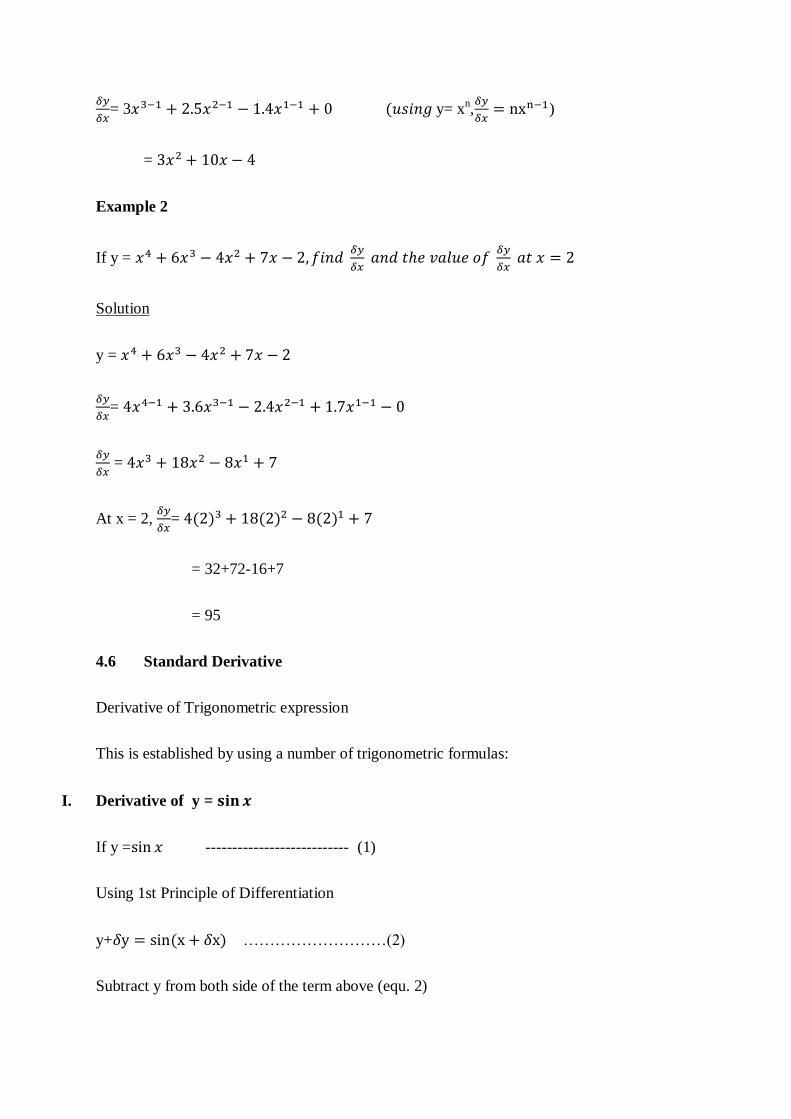
= 3 y= x

n,

)

=

Example 2

If y =

Solution

y =

=

=

At x = 2,

=

= 32+72-16+7

= 95

4.6 Standard Derivative

Derivative of Trigonometric expression

This is established by using a number of trigonometric formulas:

I. Derivative of y =

If y = --------------------------- (1)

Using 1st Principle of Differentiation

y+ ………………………(2)

Subtract y from both side of the term above (equ. 2)

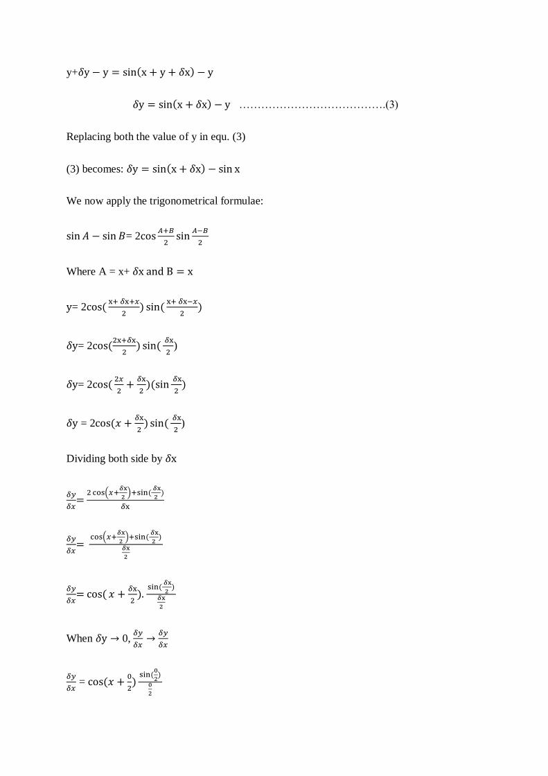
y+

………………………………….(3)

Replacing both the value of y in equ. (3)

(3) becomes:

We now apply the trigonometrical formulae:

= 2

Where A = x+

= 2

= 2

)

= 2

= 2

)

Dividing both side by

=

=

=

.

When 0,

=

=

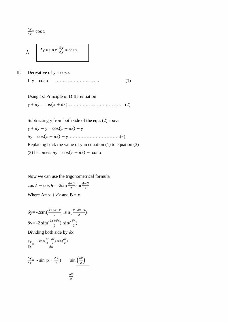
II. Derivative of y =

If y = ……………………….. (1)

Using 1st Principle of Differentiation

y + = ……………………………… (2)

Subtracting y from both side of the equ. (2) above

y + =

= …………………………….(3)

Replacing back the value of y in equation (1) to equation (3)

(3) becomes: =

Now we can use the trigonometrical formula

= -2

Where A= and B = x

= -2

= -2

Dividing both side by

=

= - sin (x +

) sin

If y =

=

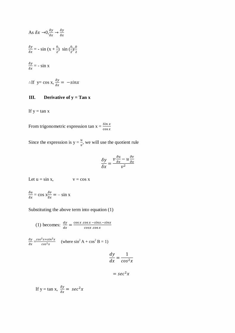
As 0,

= - sin (x +

) sin (

)/

= - sin x

If y= cos x,

III. Derivative of y = Tan x

If y = tan x

From trigonometric expression tan x =

Since the expression is y =

, we will use the quotient rule

Let u = sin x, v = cos x

= cos x

– sin x

Substituting the above term into equation (1)

(1) becomes:

=

(where sin

2 A + cos

2 B = 1)

If y = tan x,

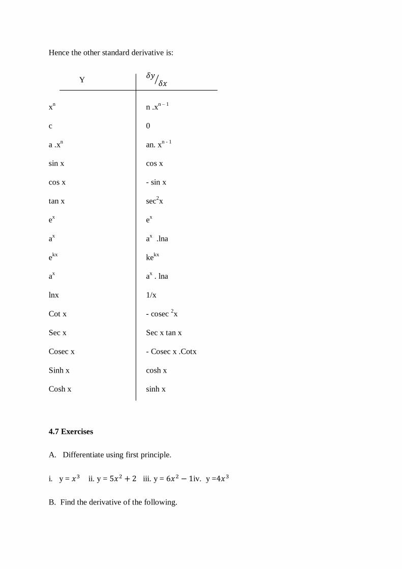
Hence the other standard derivative is:

Y

xn

n .xn – 1

c 0

a .xn

an. xn - 1

sin x cos x

cos x - sin x

tan x sec2x

ex

ex

ax a

x .lna

ekx

kekx

ax

ax . lna

lnx 1/x

Cot x - cosec 2x

Sec x Sec x tan x

Cosec x - Cosec x .Cotx

Sinh x cosh x

Cosh x sinh x

4.7 Exercises

A. Differentiate using first principle.

i. y = ii. y = iii. y = iv. y =

B. Find the derivative of the following.

i. y =6x3 +4x

2- 7x +2 ii. y= 15x

3 – 6x

2 +10 iii. y= 10x

5 +7x

3 +2x

4.8 Summary

i. Differentiation is the action of computing a derivative. The derivate of a function f(x) of a

variable x is a measure of the rate at which the changes with respect to the change of the

variable.

ii. Derivate of powers of x

a) y = c (constant),

= 0

b) y = xn,

= nx

n – 1c) y = ax

n ,

iii. Gradient of a straight line graph (m) =

iv. Differentiation of polynomial means differentiating each term in turn

4.9 References

1. Additional Mathematics by Godman and J.F Talbert

2. Calculus An Applied Approach Larson Edwards Sixth Edition

3. Blitzer Algebra and Trigonometry Custom 4th Edition

4. Engineering Mathematics by K.A Stroud.

MODULE TWO

UNIT 2: DIFFERENTIATION TECHNIQUES

Contents

5.1 Introduction

5.2 Objective

5.3 Differentiation of products of functions (Product Rule)

5.4 differentiation of a quotient of two function (Quotient Rule)

5.5 Function of a function (Composite Function)

5.6 Implicit Function

5.7 Exercises

5.8 Summary

5.9 Reference

5.1 Introduction

This shows the useful formulas in showing that the derivative is linear. Here we will learn the

quotient rule, product, function of a function and implicit function

5.2 Objective:

In this module, you will cover the following subtopics

5.3 Differentiation of products of functions (product rule)

5.4 differentiation of a quotient of two function (quotient rule)

5.5 Function of a function (composite function)

5.6 Implicit function

5.3: Differentiation of Products of Functions (Product Rule)

Let y = uv, where u and v are functions of x

If x x, u u+ u, v v + ∂v and as a result,y y+ y.

The above expression shows that an increment ∂x in x will turn produce increments ∂u in u

and also producing a change ∂v in v and a change ∂y in y.

Using first principle:

If y = uv. . . . . . . . . . . . . . . . . . . . . . . . . .(1)

Therefore, y+ y= (u+ u)(v+ v). . . . . . . (2)

Expanding the left hand side in equation (2) gives:

y + y = uv+u v+v u+ u. v . . . . . . . . . (3)

Subtracting y = uv in equation (3) gives

y + y – y=uv+u v+v u+ u. v-y

y=uv+u v +v u + u. v-y

y=uv+u v+v u+ u. v-uv (where y=uv)

y=u v+v u+ u. v

Divide throughout by x

u. v . . . . . . . . . . . . . . . (4)

Limit if

(NB tends to turns to )

Therefore, (4) now gives:

Product Rule:

If y=uv

Example 1

Differentiate with respect to x: y= x3 sinx

y = x3

sinx

Let u= x3 and v = sin x

= 3x

2

= x (

Example 2

Differentiate (3x-2)( ) with respect to x

(3x-2)( )

Let u=3x-2

v=

= 2x,

= 3

= (3x-2) 2x+(

=6

=6

=9x2

-4x+9

Example 3

Differentiate with respect to x

y =

y =

Let u= and v =ex

=

=

=

=

Example 4

Differentiate y=

y =

Let u= and v =

= 2x

Let u=2x – 5 and y = ( as in function of a function (composite function) as

will be explained in module 3.3)

=

=

= x

=2 4 2x

Simplify as far as possible by collecting common terms and leaving the result in factors

= 2x

=2x

Example 5

Differentiate y=

y =

Let u= and v =

=9

=2x

=

Collecting the common terms and leaving the result in factors

]

= 6

(15

Checkpoints

Differentiate the following with respect to x

1. y = (

2. y =x(

3. y =

4. y =4

5. y =3

Solution

1. y = (

Let u= ( and v =

Using the formula:

=(

=

=x(

2. y =x(

u =x, and v =

(

= 6x( . x + (

=6 +

= (6 +

3. y =

Let u= , v=sin x

=

=

4. y =4

u =4

= 4

=4

5. y =3

u =3

Therefore,

3

3

Differentiation of a quotient of two function (Quotient Rule)

Let y =

where u and v are functions of x.

An increment and a

change

If x x+

Using the first principle

If y =

. . . . . . . . . . . . . . . . . . .(1)

Then

. . . . . . . . .(2)

Subtract y from both side of the term in equation (2) above

Simplify by collecting like terms.

becomes

. . . . . . . . . . . . . . . . . . .(4)

Then equation (4) is the quotient rule of differentiation

Example 1

1.

Solution

=

Simplifying the numerator

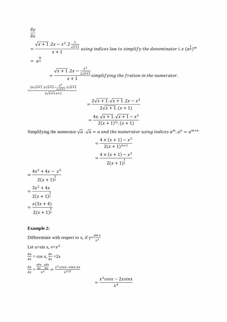
Example 2:

Differentiate with respect to x, if y=

Let u=sin x, v=

= cos x,

=2x

=

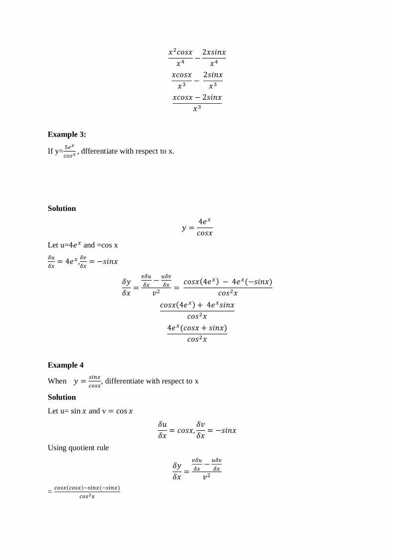
Example 3:

If y=

dfferentiate with respect to x.

Solution

Let u= and =cos x

,

Example 4

When

, differentiate with respect to x

Solution

Let u= and v

Using quotient rule

=

=

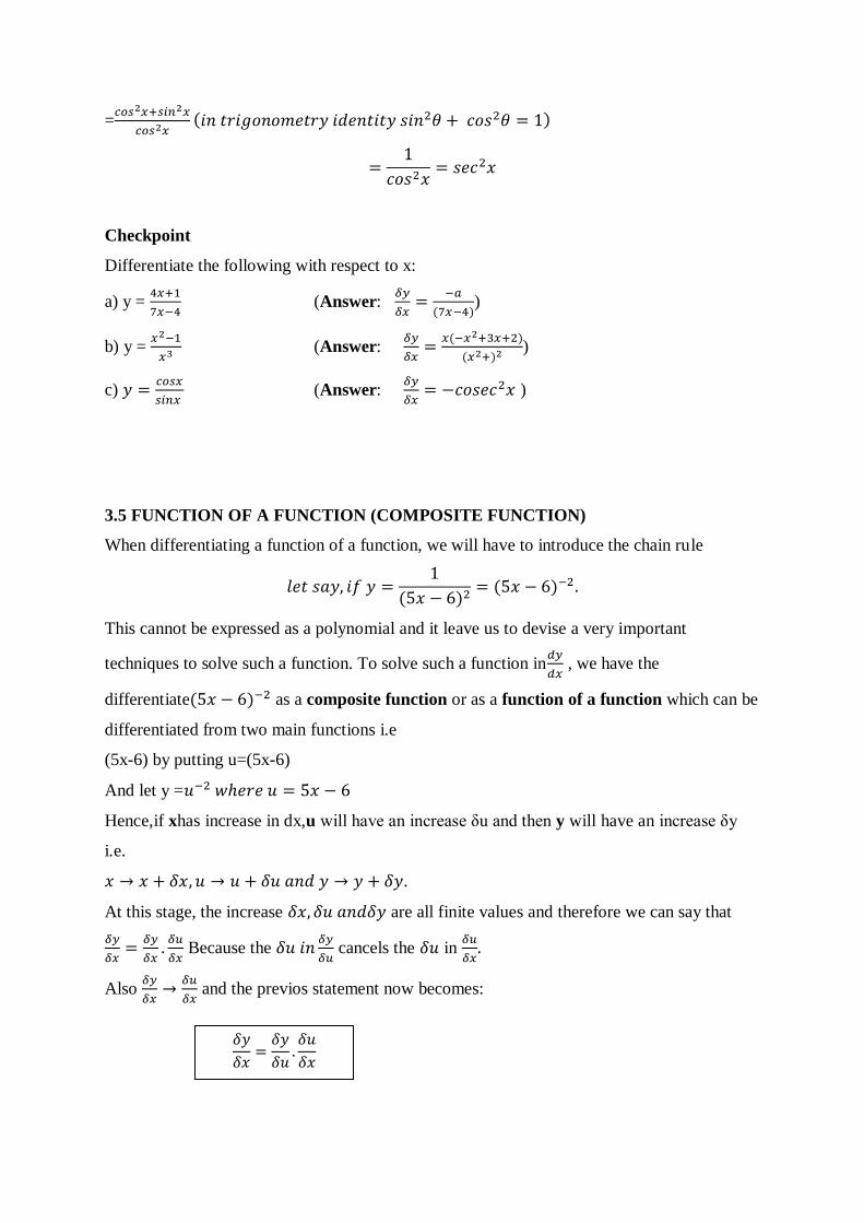
Checkpoint

Differentiate the following with respect to x:

a) y =

(Answer:

)

b) y =

(Answer:

)

c)

(Answer:

)

3.5 FUNCTION OF A FUNCTION (COMPOSITE FUNCTION)

When differentiating a function of a function, we will have to introduce the chain rule

This cannot be expressed as a polynomial and it leave us to devise a very important

techniques to solve such a function. To solve such a function in

, we have the

differentiate as a composite function or as a function of a function which can be

differentiated from two main functions i.e

(5x-6) by putting u=(5x-6)

And let y =

Hence,if xhas increase in dx,u will have an increase u and then y will have an increase y

i.e.

.

At this stage, the increase are all finite values and therefore we can say that

Because the

cancels the in

Also

and the previos statement now becomes:

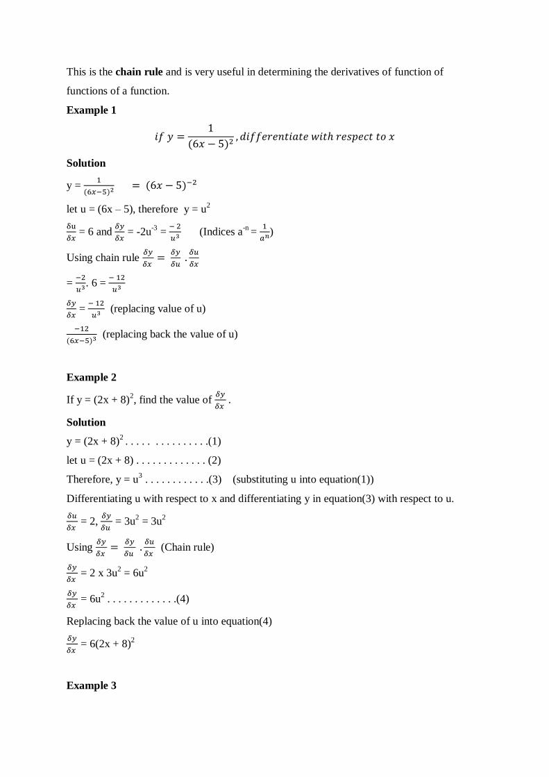
This is the chain rule and is very useful in determining the derivatives of function of

functions of a function.

Example 1

Solution

y =

let u = (6x – 5), therefore y = u2

= 6 and

= -2u

-3 =

(Indices a-n

=

)

Using chain rule

=

. 6 =

=

(replacing value of u)

(replacing back the value of u)

Example 2

If y = (2x + 8)2, find the value of

Solution

y = (2x + 8)2 . . . . . . . . . . . . . . .(1)

let u = (2x + 8) . . . . . . . . . . . . . (2)

Therefore, y = u3 . . . . . . . . . . . .(3) (substituting u into equation(1))

Differentiating u with respect to x and differentiating y in equation(3) with respect to u.

= 2,

= 3u

2 = 3u

2

Using

(Chain rule)

= 2 x 3u

2 = 6u

2

= 6u

2 . . . . . . . . . . . . .(4)

Replacing back the value of u into equation(4)

= 6(2x + 8)

2

Example 3

If y = sin(5x – 6), determine

Solution

y = sin(5x – 6)

let u = (5x – 6), therefore, y = sin u

= 5,

= cos u

= 5cos u

= 5 cos(5x – 6)

Example 4

Determine

when y = tan(3x + 2).

Solution

Y tan(3x + 2)

Let u = 3x = 2, therefore, y = tan u

= 3 and

= sec

2u

= 3sec2u

= 3sec2(3x =2)

Checkpoint


i. y = (2x + 5)3 [Answer: 6(2x + 5)

2]

ii. ii. y = [Answer:

]

iii. y = sin(4x + 3) [Answer: 4cos(4x + 3)]

Exercises


i. y = (2x + 5)3 ii. y = iii. y = sin(4x + 3)

5.6 IMPLICIT FUNCTIONS

When functions that are differentiated which in the form y= x3 + 5x -3 are called an explicit

function of x. i.e. y is stated directly in terms of x.

A relationship in which x and y is more involved may not be possible to separate y

completely on the left hand side.

For example xy + cosy = 5, in this case, y is called an implicit functionof x, because a

relationship of the form y = f(x) is implied in the given equation.

Steps for Differentiating Implicit function

When differentiating implicit function, it is important to determine the derivate y with respect

to x and while doing so, it is the derivative of the function. It is very important to multiply the

differential function of y by the derivative of the function. It is very important to also notice

that derivative of constant number is zero.

Example 1

If 2x2 + 3y

2 = 16, find

Solution

2x2+3y

2 =16

Differentiating the above term with respect to x

4x + 6y = 0

Subtracting L. H. S. from R. H. S. by 4x

4x + 6y – 4x = 0 - 4x

6y = -4x

Making subject of the formula by divding both side by 6y

=

=

Example 2

If 2x2+ 3y

2 - 4x – 3y + 6 = 0, find and

at x = 3, and y = 2

Solution

2x2+ 3y

2 - 4x – 3y + 6 = 0

Differentiating the above expression with respect to x,

4x + 6y

– 4 - 3

+ 0 = 0

Collecting like terms

6y

– 3

+ 4x – 4 = 0

6y

– 3

= 4 – 4x

=

=

at (x, y) = (3, 2);

=

=

=

[Substituting the values of x and y into values of

]

To calculate

, since

, we have to differentiate

once to get

.

Then

=

Using quotient rule to differentiate since the function is the form

Let u = 4 – 4x and v = 6y – 3,

= -4,

= 6

Hence,

=

=

Therefore,

=

Therefore, at (x, y) = (3, 2) and

=

Substituting the above terms into

,

=

=

=

=

=

=

=

=

=

=

Example 3

Find

, if x

3 + y

3 = 2xy

Solution

x3 + y

3 = 2xy

Differentiating with respect to y, we have to treat 2xy as product of the function.

= 3x2 + 3y

2

= 2y + 2x

Collecting like terms (i.e. common terms)

3y2

– 2x

= 2y – 3x

2

(3y

2 – 2x) = 2y – 3x

2

=

[dividing the both sides by 3y

2 – 2x)

Example 4

Find the equation of the tangent(s) where x = 2on the curve x2+y

2= 2x +y =6.

Solution

Differentiating the expression with respect to x

2x + 2y – 2 + = 0

2y + =

- (collecting like term and common term)

=

Substituting the value of x=2 in the original equation of the curve, we find:

= 6

= 6

= 0

= 0

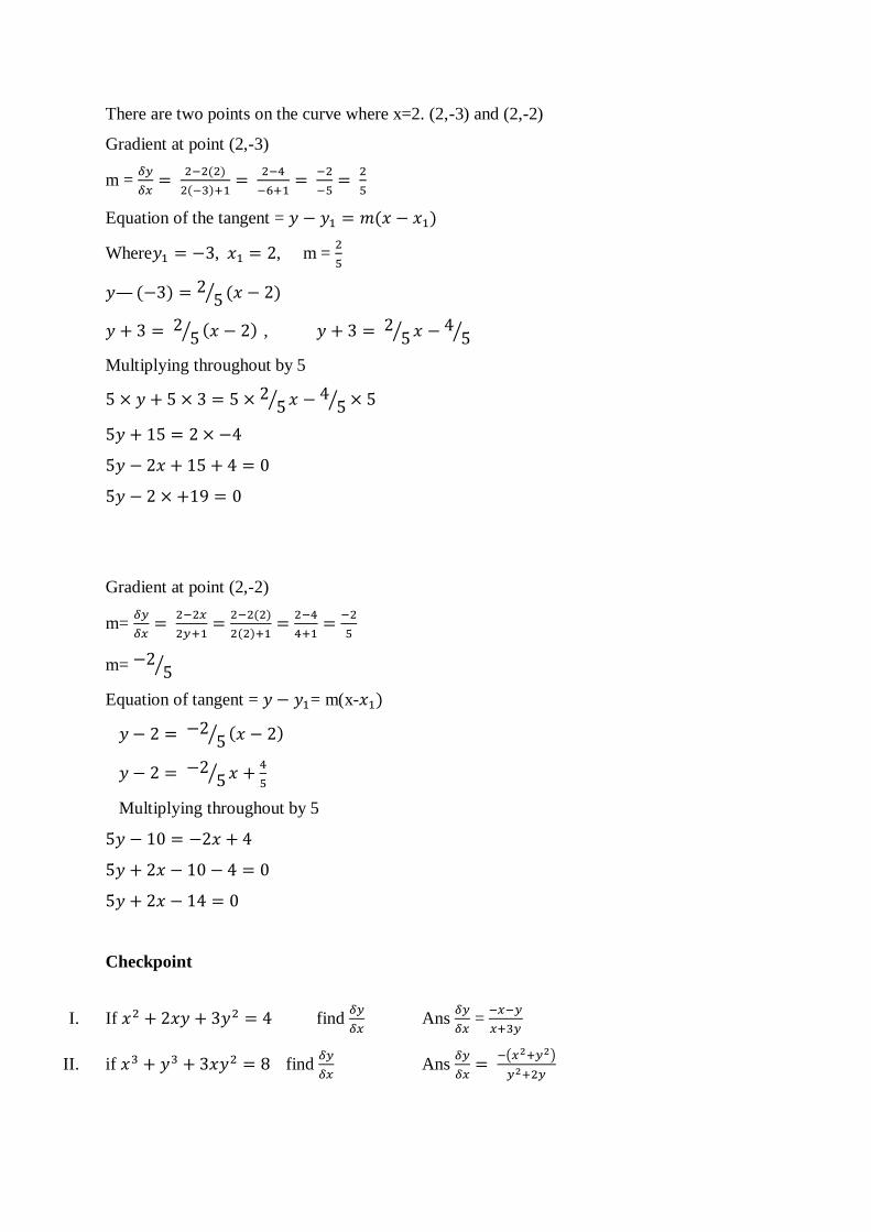
There are two points on the curve where x=2. (2,-3) and (2,-2)

Gradient at point (2,-3)

m =

Equation of the tangent =

Where , , m =

,

Multiplying throughout by 5

Gradient at point (2,-2)

m=

m=

Equation of tangent = = m(x-

Multiplying throughout by 5

Checkpoint

I. If find

Ans

=

II. if find

Ans

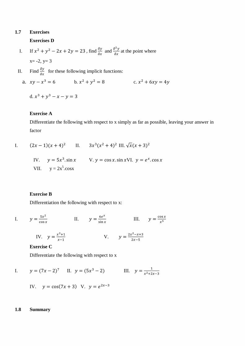
1.7 Exercises

Exercises D

I. If find

and

at the point where

x= -2, y= 3

II. Find

for these following implicit functions:

a. b. c.

d.

Exercise A

Differentiate the following with respect to x simply as far as possible, leaving your answer in

factor

I. II. III.

IV. V. VI.

VII. y = 2x5.cosx

Exercise B

Differentiation the following with respect to x:

I.

II.

III.

IV.

V.

Exercise C

Differentiate the following with respect to x

I. II. III.

IV. V.

1.8 Summary

I. If

,

=

II. If ,

References

I. Additional Mathematics by Godman and J.F Talbert

II. Calculus And Applied Approach Larson Edward Sixth Edition

III. Blitzer algebra and trigonometry Custom 4th

edition

IV. Engineering Mathematics by K.A Stroud

MODULE TWO

UNIT 3: INTEGRATION

Contents

6.1 Introduction

6.2 Objective

6.3 Integration

6.4 Notations for Integration

6.5 Methods of Integration

6.6 Exercise

6.7 Summary

6.8 References

6.1Introduction

Integration is a way of adding slices to find the whole. Integration can be used to find

areas, volumes, central points and many useful things. Integration is like filling a tank from a

tap. The input (before integration) is the flow rate from the tap. Integrating the flow (adding

up all the little bits of water) gives us the volume of the water in the tank.

Hence the processes of integration are used in many applications.

(1) The Petronas Tower in Kuala Lumpur, experience high forces due to winds.

Integration was used to design the building for its strength

(2) It is used in finding areas under curve surfaces, centre of mass – displacement and

velocity, fluid flow, modelling the behaviour of object under stress (e.g. Car engine

block, piston, curvature beam of houses, bridges e.t.c)

6.2 Objective:

In this module, the student will learn the following topics and its application:

6.3 Integration

6.4 Notation of Integration

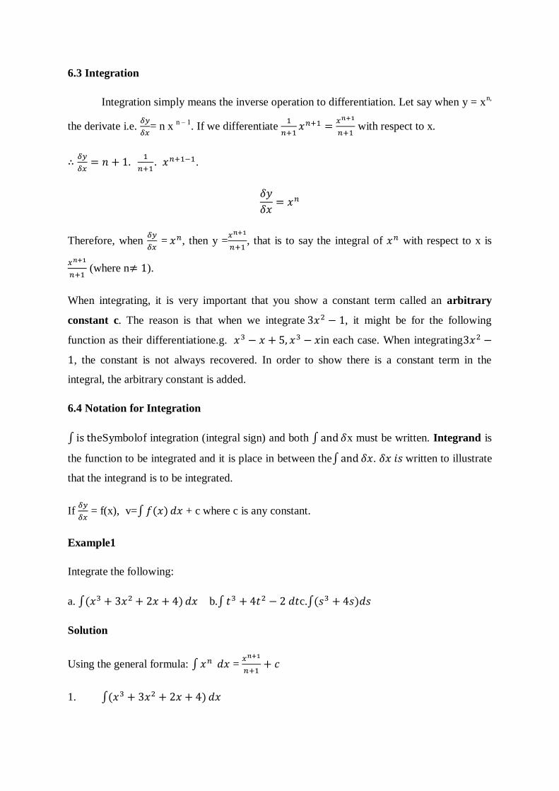
6.3 Integration

Integration simply means the inverse operation to differentiation. Let say when y = xn,

the derivate i.e.

= n x

n – 1. If we differentiate

with respect to x.

.

Therefore, when

= , then y =

, that is to say the integral of with respect to x is

(where n ).

When integrating, it is very important that you show a constant term called an arbitrary

constant c. The reason is that when we integrate , it might be for the following

function as their differentiatione.g. in each case. When integrating

, the constant is not always recovered. In order to show there is a constant term in the

integral, the arbitrary constant is added.

6.4 Notation for Integration

Symbolof integration (integral sign) and both x must be written. Integrand is

the function to be integrated and it is place in between the . written to illustrate

that the integrand is to be integrated.

If

= f(x), v= + c where c is any constant.

Example1

Integrate the following:

a. b. c.

Solution

Using the general formula: =

1.

=

+

+

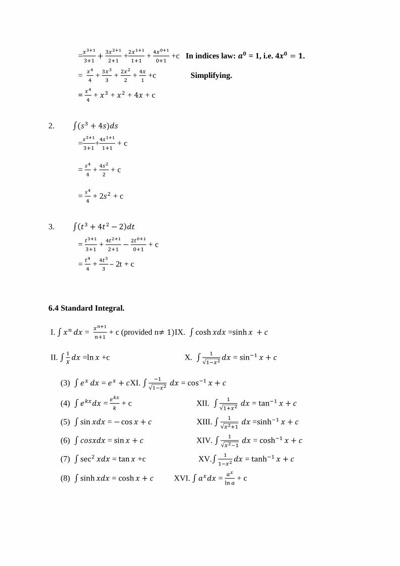
+c In indices law: = 1, i.e. 4 .

=

+

+

+

+c Simplifying.

=

+ + + + c

2.

=

+

+ c

=

+

+ c

=

+ 2 + c

3.

=

+

+ c

=

+

– 2t + c

6.4 Standard Integral.

I. =

+ c (provided n IX. =

II.

= +c X.

=

(3) = XI.

=

(4) =

+ c XII.

=

(5) = XIII.

=

(6) = XIV.

=

(7) = +c XV.

=

(8) = XVI. =

+ c

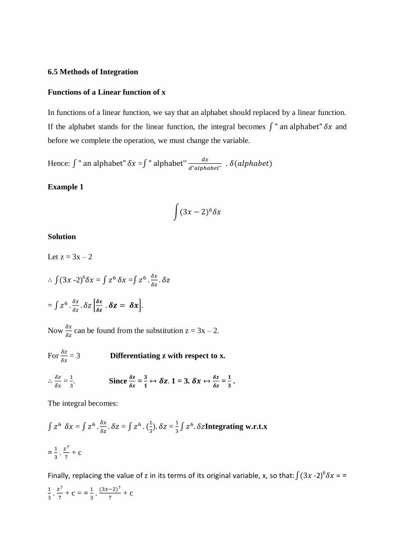
6.5 Methods of Integration

Functions of a Linear function of x

In functions of a linear function, we say that an alphabet should replaced by a linear function.

If the alphabet stands for the linear function, the integral becomes and

before we complete the operation, we must change the variable.

Hence: = ”

.

Example 1

Solution

Let z = 3x – 2

-2)6 = =

=

.

Now

can be found from the substitution z = 3x – 2.

For

= 3 Differentiating z with respect to x.

=

. Since

=

1 = 3.

=

.

The integral becomes:

=

=

=

Integrating w.r.t.x

=

.

+ c

Finally, replacing the value of z in its terms of its original variable, x, so that: -2)6 = =

.

+ c = =

.

+ c

=

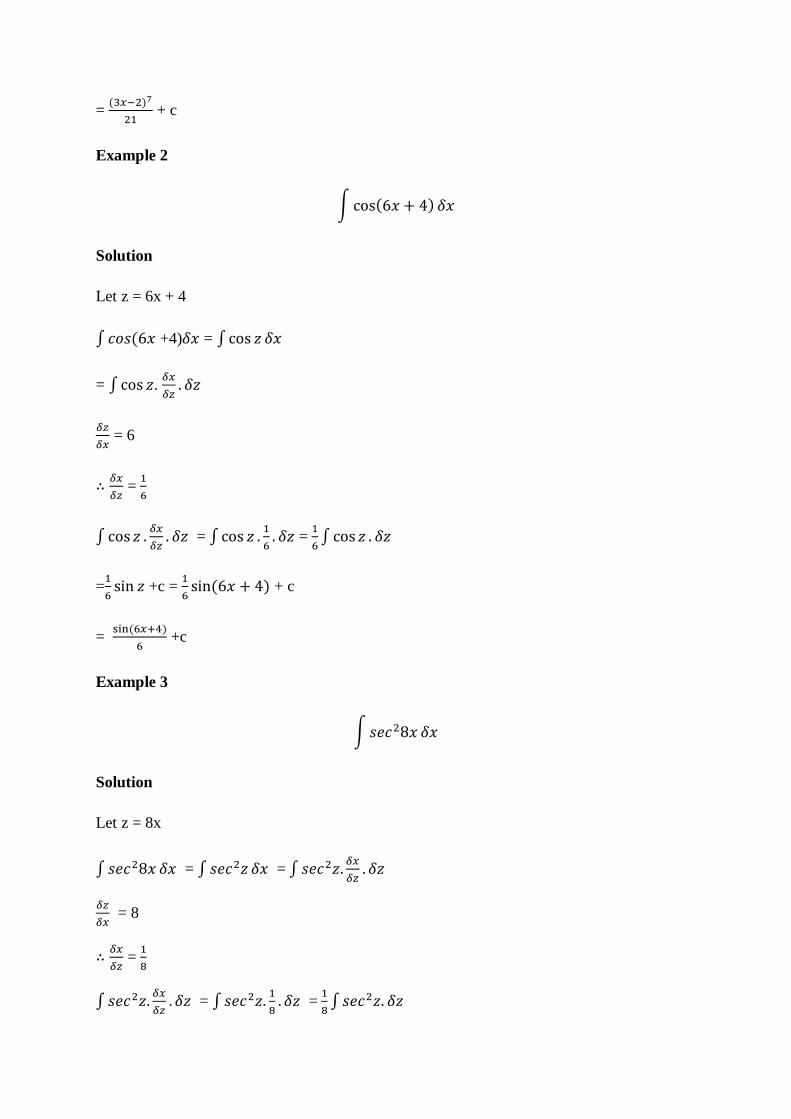
+ c

Example 2

Solution

Let z = 6x + 4

+4) =

= .

= 6

=

=

=

=

+c =

+ c

=

+c

Example 3

Solution

Let z = 8x

= =

= 8

=

=

=

=

+ c =

+ c =

Integrals of the form

and

Integral in the form

is any in which the numerator is the derivative of the denominator.

It is of the kind

= +c .

Example 1

Let us consider the integral

We notice that when we differentiate the denominator, we will have the expression in the

numerator.

Let z = 5x 6

= 2x – 5

= (2x – 5) Making subject of the formula.

= (2x – 5) .............................................. (1)

The given integral can be rewritten in terms of z.

=

Substituting equation (1) into the above term

=

=

. Where

=

.

=

= + c

Replacing back the value of z.

+ c = + c

Example 2

Integrate

Solution

Let z =

= , = ( )

=

. =

=

= + c

= + c

Example 3

Solution

= .

Note:When differentiating the denominator it gives 2x 4. Looking at the

numerator, collecting common terms give 2(2x 4).

= 2

Placing the constant number before the integral sign.

Let z =

= 2x – 4, = (2x – 4)

= 2

= 2

= 2

= 2 + c

= 2 + c

Example 4

Solution

From trigonometric function =

=

where

Substituting as

.

=

=

Let z =

= , =

=

=

=

= + c

= + c

Integration of Product (Integration by parts).

If u and v are functions of x, then we known that

= u

v

. Integrating both side

with respect to x. We noticed on the left, we get back to the function from which we started.

uv =

. +

.

Rearranging the terms, we have:

. = uv

. Clearing the common factors.

= uv .

Example1

Solution

Let u = , v = . Since is not in the list of standard integrals.

=

, =

.

=

Integrating it

=

v =

Omitting integration constant because of evaluation in the middle.

Using = uv .

=

=

=

Simplifying

= .

=

=

+ c Integrating =

+ c .

=

+ c Collecting common terms.

Example 2

.

Solution.

Using = uv .

Let u = , v =

=

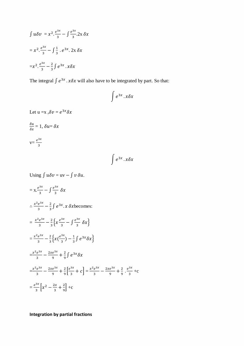
.2x

=

2x

=

The integral will also have to be integrated by part. So that:

Let u =x , =

= 1, =

v=

Using = uv .

= x.

becomes:

=

=

=

=

=

+c

=

+c

Integration by partial fractions

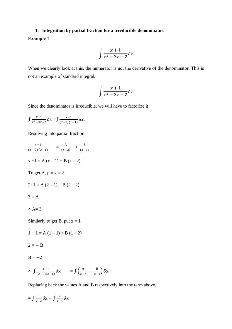
1. Integration by partial fraction for a irreducible denominator.

Example 1

When we clearly look at this, the numerator is not the derivative of the denominator. This is

not an example of standard integral.

Since the denominator is irreducible, we will have to factorize it

=

.

Resolving into partial fraction

=

+

x +1 = A (x – 1) + B (x – 2)

To get A, put x = 2

2+1 = A (2 – 1) + B (2 – 2)

3 = A

A= 3

Similarly to get B, put x = 1

1 + 1 = A (1 – 1) + B (1 – 2)

2 = B

B = 2

x =

x

Replacing back the values A and B respectively into the term above.

=

x

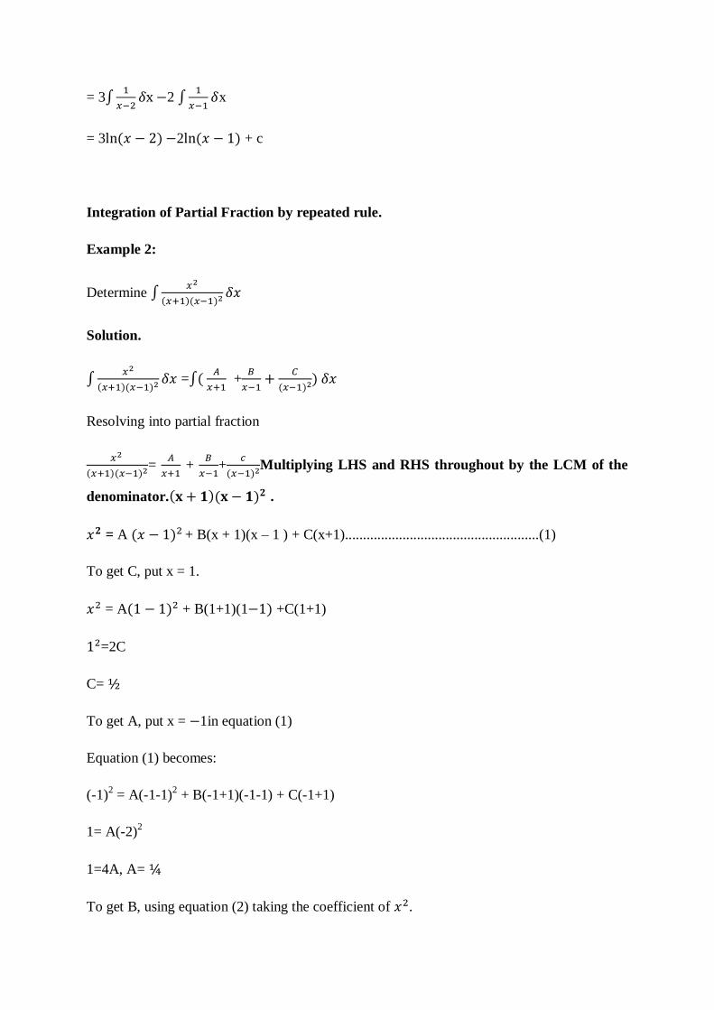
= 3

2

x

= 3 2 + c

Integration of Partial Fraction by repeated rule.

Example 2:

Determine

Solution.

=

+

Resolving into partial fraction

=

+

+

Multiplying LHS and RHS throughout by the LCM of the

denominator. .

= A + B(x + 1)(x – 1 ) + C(x+1)......................................................(1)

To get C, put x = 1.

= A + B(1+1)(1 +C(1+1)

=2C

C=

To get A, put x = 1in equation (1)

Equation (1) becomes:

(-1)2 = A(-1-1)

2 + B(-1+1)(-1-1) + C(-1+1)

1= A(-2)2

1=4A, A=

To get B, using equation (2) taking the coefficient of .

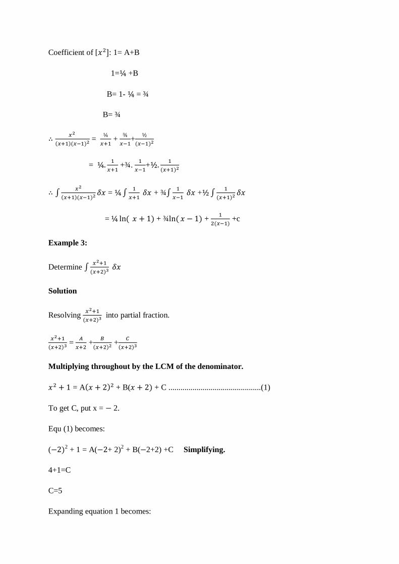
Coefficient of [ : 1= A+B

1= +B

B= 1- = ¾

B= ¾

=

+

+

=

+¾.

+

=

+ ¾

+

= + ¾ +

+c

Example 3:

Determine

Solution

Resolving

into partial fraction.

=

+

+

Multiplying throughout by the LCM of the denominator.

= A + B( + C ..............................................(1)

To get C, put x = 2.

Equ (1) becomes:

( 2 + 1 = A( + 2)

2 + B( 2+2) +C Simplifying.

4+1=C

C=5

Expanding equation 1 becomes:

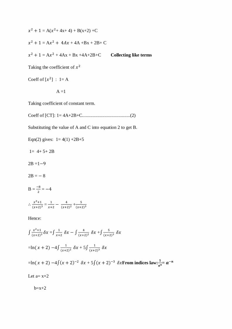
= A( + 4x+ 4) + B(x+2) +C

= A + 4A +Bx + 2B+ C

= A + 4Ax + Bx +4A+2B+C Collecting like terms

Taking the coefficient of

Coeff of [ ] : 1= A

A =1

Taking coefficient of constant term.

Coeff of [CT]: 1= 4A+2B+C.........................................(2)

Substituting the value of A and C into equation 2 to get B.

Eqn(2) gives: 1= 4(1) +2B+5

1= 4+ 5+ 2B

2B =1

2B = 8

B =

=

=

+

Hence:

=

+

= 4

+ 5

= 4 + 5 From indices law:

=

Let a= x+2

b=x+2

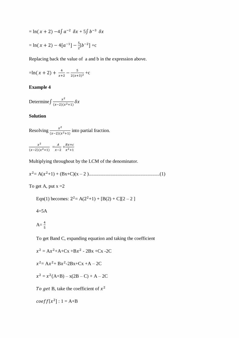
= 4 + 5

=

[ +c

Replacing back the value of a and b in the expression above.

=

+c

Example 4

Determine

Solution

Resolving

into partial fraction.

=

+

Multiplying throughout by the LCM of the denominator.

= A( +1) + (Bx+C)(x – 2 )...........................................................(1)

To get A, put x =2

Eqn(1) becomes: = A( +1) + [B(2) + C][2 – 2 ]

4=5A

A=

To get Band C, expanding equation and taking the coefficient

= A +A+Cx +B - 2Bx +Cx -2C

= A + B -2Bx+Cx +A – 2C

= A+B) – x(2B – C) + A – 2C

B, take the coefficient of

[ : 1 = A+B

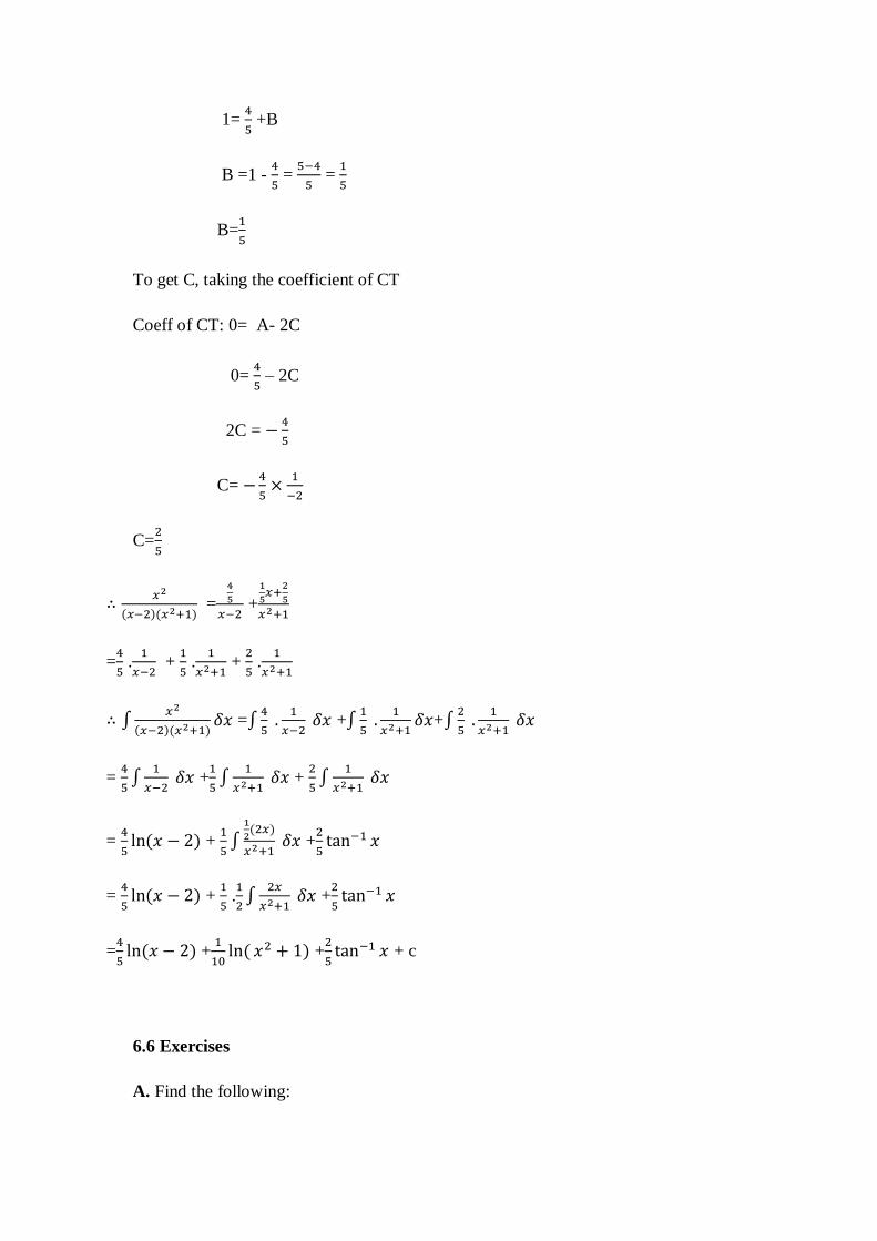
1=

+B

B =1 -

=

=

B=

To get C, taking the coefficient of CT

Coeff of CT: 0= A- 2C

0=

– 2C

2C =

C=

C=

=

+

=

.

+

.

+

.

=

+

+

=

+

+

=

+

+

=

+

.

+

=

+

+

+ c

6.6 Exercises

A. Find the following:

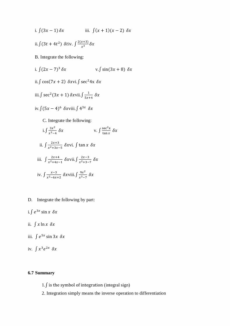
i. iii.

ii. iv.

B. Integrate the following:

i. v.

ii. vi.

iii. vii.

iv. viii.

C. Integrate the following:

i.

v.

ii.

vi.

iii.

vii.

iv.

viii.

D. Integrate the following by part:

i.

ii.

iii.

iv.

6.7 Summary

1. (integral sign)

2. Integration simply means the inverse operation to differentiation

3. =

+ C {provided n 1}

4.

5.

= +c .

6.8 References

1. Calculus An Applied Approach Larson Edwards Sixth Edition

2. Blitzer Algebra and Trigonometry Custom 4th Edition

3. Engineering Mathematics by K.A Stroud 5th Edition

4. Additional Mathematics by Godman, and J.F Talbert.

MODULE 8:

VOLUME OF SOLIDS OF REVOLUTION BY DEFINATE INTEGRAL

Contents.

8.1 Introduction

8.2 Objectives.

8.3 Volume of Solids of revolution.

8.4 The Volume of Sphere

8.5 The Volume of a Spherical Segment

8.6 The Volume of a cone

8.7 Exercise

8.8 Summary

8.9 References.

8.1 Introduction:

Volume of solids of revolution by definite integrals deals with volume of solid such as cone,

cylinder, sphere used in construction of mega structure in beams of houses, sky scrapper,

for bridges to be able to withstand load and stress.

8.2 Objectives:

In this module, students are expected to know how to use definite integral in calculating

volume of solids such as sphere, cylinder, cone etc.

8.3 Volume of Solids of Revolution

A solid figure generated by revolving a given curve around an axis of revolution is called the

solid of revolution.

The volume generated by the region of the coordinate plane bounded by the segment of the

curve y=f(x) between x=a, y=b and the x- axis, revolving around the x-axis, is shown in the

figure 1 below:

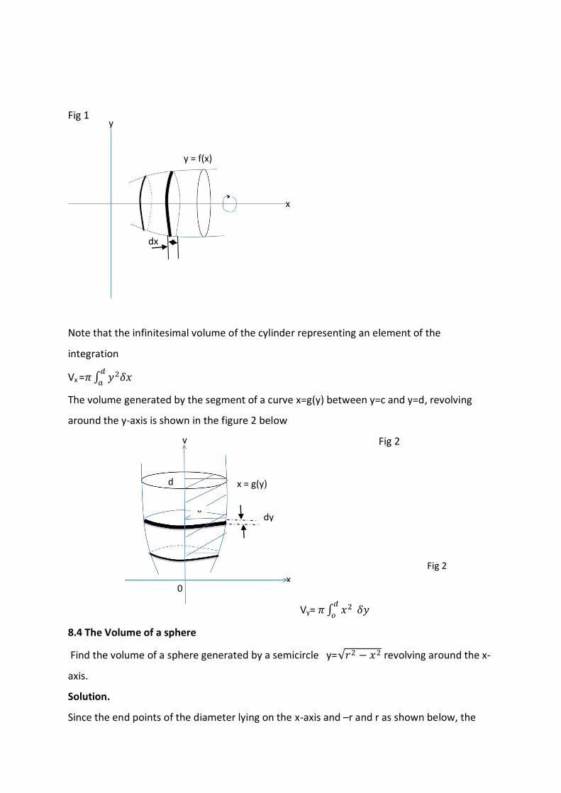
Fig 1

Note that the infinitesimal volume of the cylinder representing an element of the

integration

Vx =

The volume generated by the segment of a curve x=g(y) between y=c and y=d, revolving

around the y-axis is shown in the figure 2 below

Fig 2

Vy=

8.4 The Volume of a sphere

Find the volume of a sphere generated by a semicircle y= revolving around the x-

axis.

Solution.

Since the end points of the diameter lying on the x-axis and –r and r as shown below, the

y

x

y = f(x)

dx

y

d

x

x = g(y)

dy

0 x

Fig 2

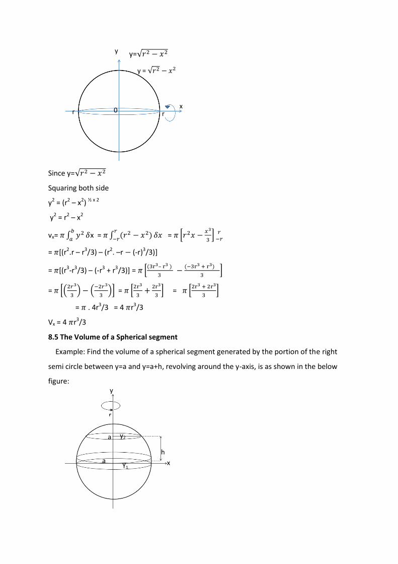
y=

Since y=

Squaring both side

y2 = (r2 – x2) ½ x 2

y2 = r2 – x2

vx=

x =

=

= [(r2.r – r3/3) – (r2. –r (-r)3/3)]

= [(r3-r3/3) – (-r3 + r3/3)] = –

=

=

=

= . 4r3/3 = 4 r3/3

Vx = 4 r3/3

8.5 The Volume of a Spherical segment

Example: Find the volume of a spherical segment generated by the portion of the right

semi circle between y=a and y=a+h, revolving around the y-axis, is as shown in the below

figure:

y

x r

y =

r 0

y

r

a y2

h

Y1 a x

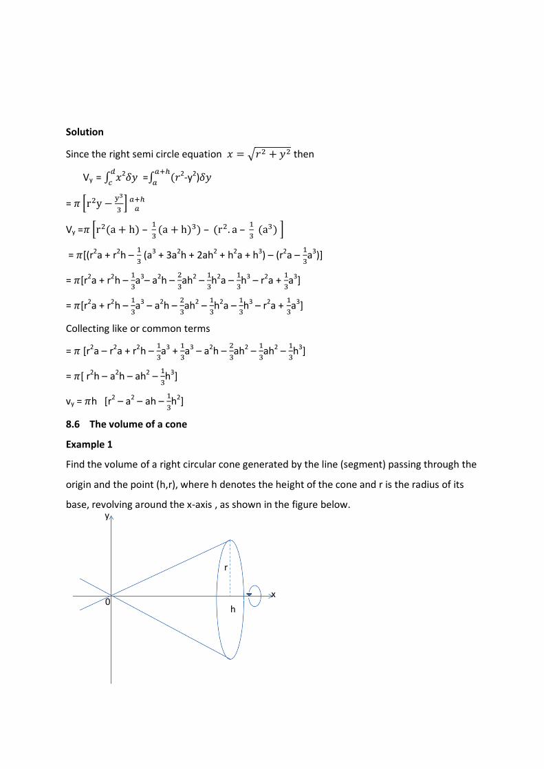
Solution

Since the right semi circle equation then

Vy =

2 =

2-y2)

=

Vy = –

– –

= [(r2a + r2h –

(a3 + 3a2h + 2ah2 + h2a + h3) – (r2a –

a3)]

= [r2a + r2h –

a3– a2h –

ah2 –

h2a –

h3 – r2a +

a3]

= [r2a + r2h –

a3 – a2h –

ah2 –

h2a –

h3 – r2a +

a3]

Collecting like or common terms

= [r2a – r2a + r2h –

a3 +

a3 – a2h –

ah2 –

ah2 –

h3]

= [ r2h – a2h – ah2 –

h3]

vy = h [r2 – a2 – ah –

h2]

8.6 The volume of a cone

Example 1

Find the volume of a right circular cone generated by the line (segment) passing through the

origin and the point (h,r), where h denotes the height of the cone and r is the radius of its

base, revolving around the x-axis , as shown in the figure below.

0

r

h

x 0

y

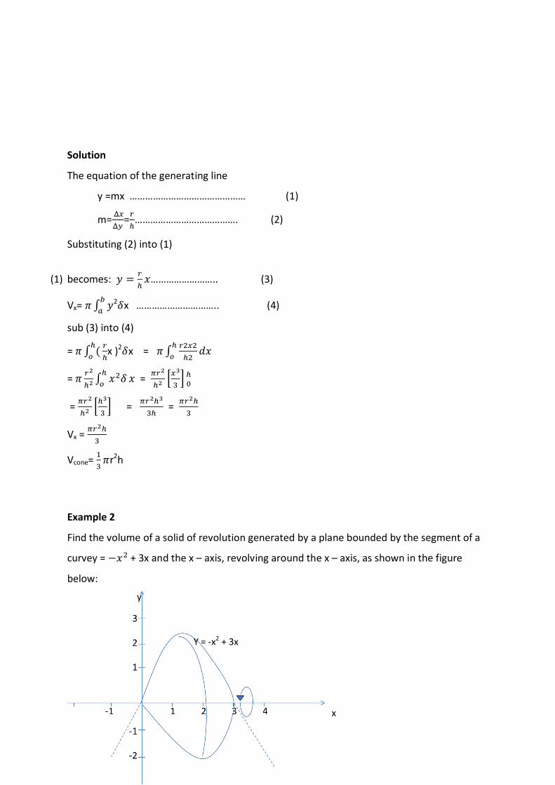
Solution

The equation of the generating line

y =mx ……………………………………… (1)

m=

=

…………………………………. (2)

Substituting (2) into (1)

(1) becomes:

…………………….. (3)

Vx=

2 x ………………………….. (4)

sub (3) into (4)

=

x )2 x =

=

=

=

=

=

Vx =

Vcone=

r2h

Example 2

Find the volume of a solid of revolution generated by a plane bounded by the segment of a

curvey = + 3x and the x – axis, revolving around the x – axis, as shown in the figure

below:

y

x

Y = -x2 + 3x

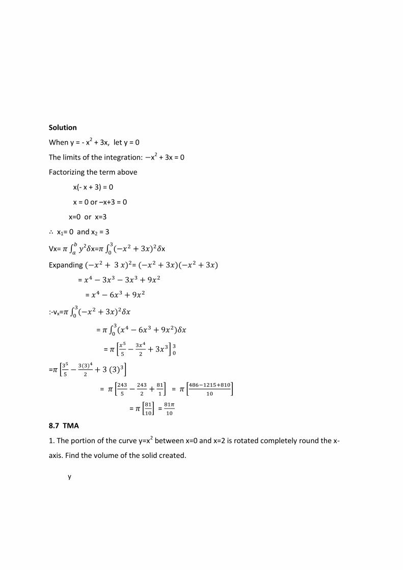
Solution

When y = - x2 + 3x, let y = 0

The limits of the integration: x2 + 3x = 0

Factorizing the term above

x(- x + 3) = 0

x = 0 or –x+3 = 0

x=0 or x=3

x1= 0 and x2 = 3

Vx=

2 x=

x

Expanding =

=

=

:-vx=

=

=

=

=

=

=

=

8.7 TMA

1. The portion of the curve y=x2 between x=0 and x=2 is rotated completely round the x-

axis. Find the volume of the solid created.

y

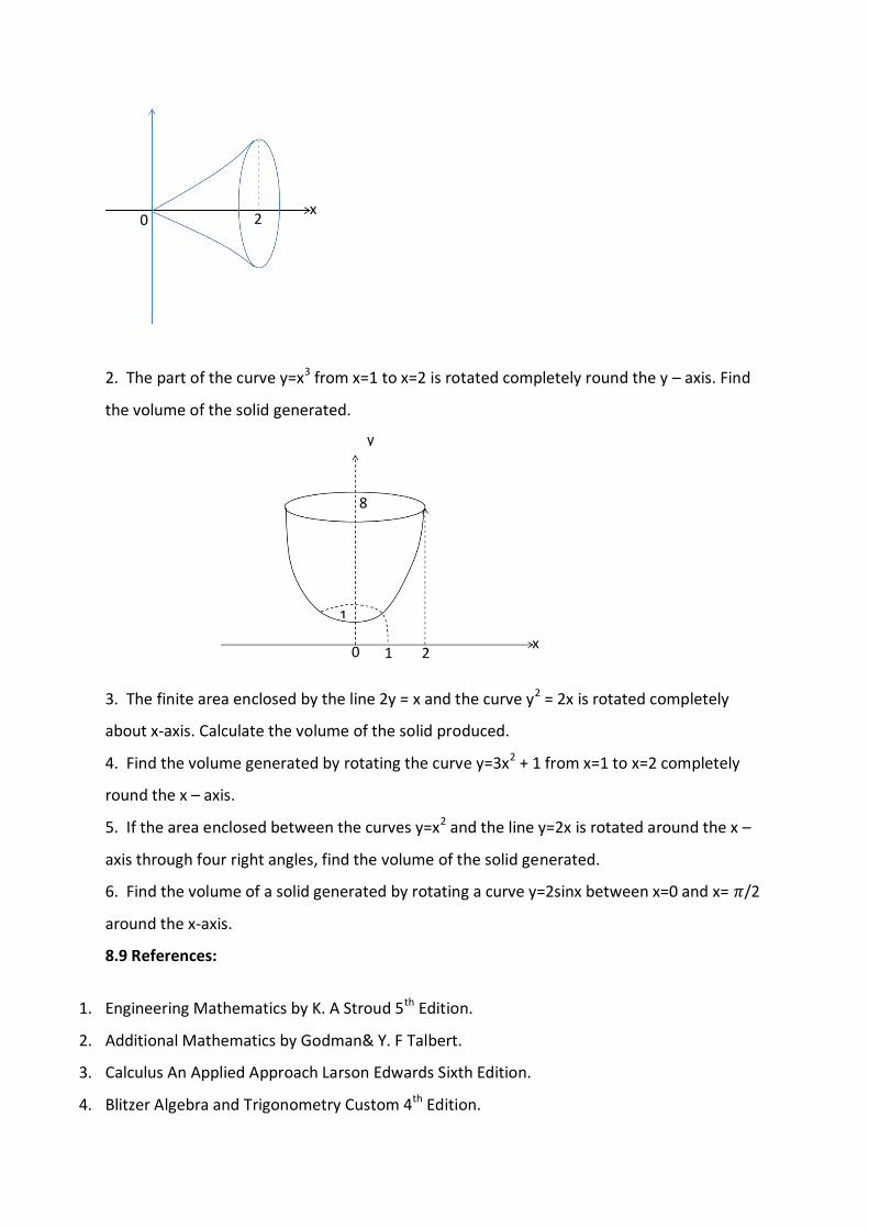
2. The part of the curve y=x3 from x=1 to x=2 is rotated completely round the y – axis. Find

the volume of the solid generated.

3. The finite area enclosed by the line 2y = x and the curve y2 = 2x is rotated completely

about x-axis. Calculate the volume of the solid produced.

4. Find the volume generated by rotating the curve y=3x2 + 1 from x=1 to x=2 completely

round the x – axis.

5. If the area enclosed between the curves y=x2 and the line y=2x is rotated around the x –

axis through four right angles, find the volume of the solid generated.

6. Find the volume of a solid generated by rotating a curve y=2sinx between x=0 and x= /2

around the x-axis.

8.9 References:

1. Engineering Mathematics by K. A Stroud 5th Edition.

2. Additional Mathematics by Godman& Y. F Talbert.

3. Calculus An Applied Approach Larson Edwards Sixth Edition.

4. Blitzer Algebra and Trigonometry Custom 4th Edition.

2 0 x

y

8

1

x 0 1 2

Documents

mth 102 course title: elementary mathematics ii - National