Embed Size (px)
Citation preview
arX
iv:c
ond-
mat
/070
1208
v2 [
cond
-mat
.mtr
l-sc
i] 2
0 Fe
b 20
07
Morphological stability of electromigration-driven vacancy islands
Frank Haußer,1, ∗ Philipp Kuhn,2, † Joachim Krug,2, ‡ and Axel Voigt1, 3, §
1Crystal Growth Group, Research Center caesar, Ludwig-Erhard-Allee 2, 53175 Bonn, Germany2Institut fur Theoretische Physik, Universitat zu Koln, Zulpicher Strasse 77, 50937 Koln, Germany
3Institut fur Wissenschaftliches Rechnen, Technische Universitat Dresden, Zellescher Weg 12-14, 01062 Dresden
(Dated: August 13, 2013)
The electromigration-induced shape evolution of two-dimensional vacancy islands on a crystalsurface is studied using a continuum approach. We consider the regime where mass transport isrestricted to terrace diffusion in the interior of the island. In the limit of fast attachment/detachmentkinetics a circle translating at constant velocity is a stationary solution of the problem. In contrastto earlier work [O. Pierre-Louis and T.L. Einstein, Phys. Rev. B 62, 13697 (2000)] we showthat the circular solution remains linearly stable for arbitrarily large driving forces. The numericalsolution of the full nonlinear problem nevertheless reveals a fingering instability at the trailing endof the island, which develops from finite amplitude perturbations and eventually leads to pinch-off.Relaxing the condition of instantaneous attachment/detachment kinetics, we obtain non-circularelongated stationary shapes in an analytic approximation which compares favorably to the fullnumerical solution.
PACS numbers: 05.45.-a, 68.65.-k, 66.30.Qa, 68.35.Fx
I. INTRODUCTION
Much of the diversity of natural shapes in the inan-imate world is the result of morphological instabilities.The paradigmatic example is the Mullins-Sekerka insta-bility, in which a spherical solid nucleus in an undercooledmelt forms lobes and petals which eventually develop intoa delicate dendritic pattern [1], and its two-dimensionalanalogs that can be observed in the growth of islandson crystal surfaces [2]. These systems share the com-mon mathematical structure of moving boundary valueproblems, in which an interface evolves in response tothe gradient of some continuous field defined in the spa-tial domains that it separates. In the context of two-dimensional crystal surfaces, the interfaces are atomicheight steps separating different terraces, and their mo-tion is governed by the attachment and detachment ofthe adsorbed atoms (adatoms) [3, 4, 5].
A rich variety of two-dimensional morphological in-stabilities has been observed on the surfaces of current-carrying crystals, where an electromigration force inducesa directed motion of adatoms [6, 7]. The microscopic ori-gin of this force is a combination of momentum transferfrom the conduction electrons (the ’wind force’) and adirect effect of the local electric field [8]. On stepped sur-faces vicinal to Si(111), electromigration has been foundto cause step bunching [9], step meandering [10], stepbending [11] and step pairing [12] instabilities. In addi-tion, single layer adatom islands on silicon surfaces havebeen seen to drift under the influence of electromigration
∗Electronic address: [email protected]†Electronic address: [email protected]‡Electronic address: [email protected]§Electronic address: [email protected]
[13, 14].In the present paper we focus on the morphological
stability of single layer vacancy islands driven by elec-tromigration. We build on the work of Pierre-Louisand Einstein (PLE) [15], who introduced a class of con-tinuum models for island electromigration. The dif-ferent models are distinguished according to the domi-nant mechanism of mass transport, which can be due toperiphery diffusion (PD) along the edge of the island,terrace diffusion (TD), or two-dimensional evaporation-condensation (EC), i.e. attachment-detachment, kinet-ics. In the PD regime the dynamics of the island edgeis local, while in the TD and EC regimes it is coupledto the adatom concentration on the terrace. In the TD(EC) regime diffusion is slow (fast) compared to the at-tachment/detachment processes, as reflected in the mag-nitude of the kinetic lengths
d± = D/k± (1)
defined as the ratio of the surface diffusion constant D tothe rates of adatom attachment to a step from the lower(k+) or upper (k−) terrace, respectively. The two ratesgenerally differ, because step edge barriers suppressingattachment across descending steps are ubiquitous onmany surfaces, leading to k+ > k− [2].
As a common feature of the models of PLE, the elec-tromigration force is taken to be of constant directionand magnitude everywhere, which implies in particularthat it is not affected by the presence and the shape ofthe island. This is motivated by the fact that the islandconstitutes a small perturbation in the morphology of thecrystal, which is not expected to substantially change thedistribution of the electrical current in the bulk. Detailedatomistic calculations do in fact show that the electromi-gration force is modified in the vicinity of a step [16, 17],which may also be incorporated into a continuum model[18], but this is a higher order effect that can be ne-
2
glected on the present level of description. The situationis completely different for electromigration-driven macro-scopic voids in metallic thin films, which can be modeledusing a closely related two-dimensional continuum ap-proach [19, 20, 21, 22, 23, 24, 25]. Since the void inter-rupts the current flow, the effect of the void shape on thecurrent distribution is an essential part of the analysis.In the following we refer to this problem as void migra-
tion, to be distinguished from island migration under aconstant force.
Apart from the work of PLE, analytical results con-cerning the morphological stability of electromigration-driven two-dimensional shapes have been obtained onlyin the PD regime. In the absence of crystal anisotropy thebasic solution is then a circle moving at constant veloc-ity [19]. In the case of island electromigration the circlebecomes linearly unstable at a critical radius or criticaldriving force [20]. Beyond the linear instability station-ary shapes that are elongated in the current directionappear [26, 27]. Remarkably, the stability scenario forvoid migration is completely different. Voids are linearlystable at any size [20, 21], but they become nonlinearlyunstable beyond a finite threshold perturbation strength,which decreases with increasing radius or driving force[22, 24]. Unstable voids break up into smaller circularvoids, and non-circular stationary shapes do not exist[25]. The increasing sensitivity to finite amplitude per-turbations can be linked to the increasing non-normalityof the linear eigenvalue problem, which leads to transientgrowth of linear perturbations [22]. This route to nonlin-ear instability has been previously described for linearlystable hydrodynamic flows [28, 29, 30], and it will befurther discussed below in Section IV.
VF
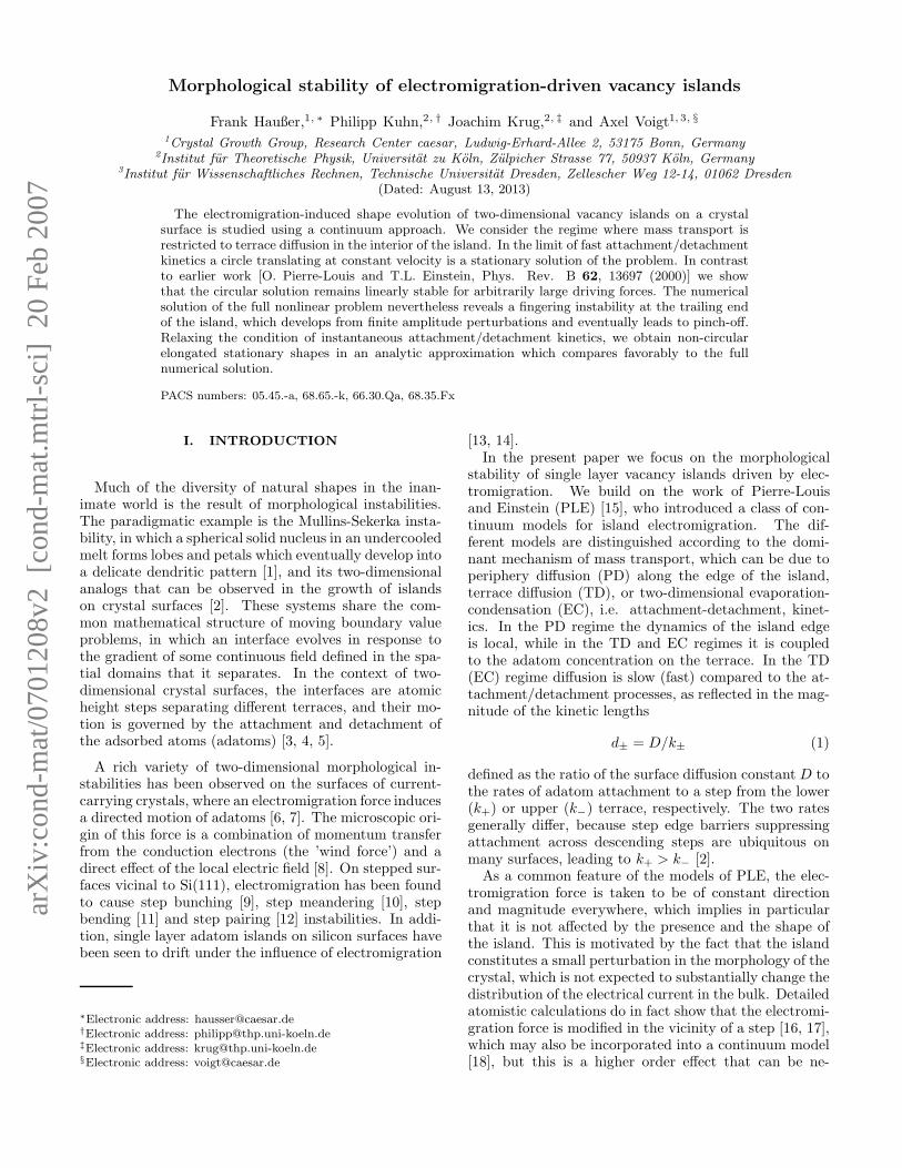
FIG. 1: Schematic of the interior model. Adatoms detachfrom the inner boundary of the vacancy island and diffusesubject to the electromigration force F directed to the right.As a consequence, the entire island drifts to the left at speedV .
In the present paper we focus on the “interior model”introduced by PLE. Referring to Fig. 1, we consider asingle vacancy island which is isolated from the surround-ing upper terrace by a strong step edge barrier that pre-vents adatoms from entering across the descending step(k− = 0, d− = ∞). Diffusive motion of vacancy islandsmediated by internal terrace diffusion has been observedexperimentally on the Ag(110) surface [31]. The math-
ematically equivalent process of internal diffusion of va-
cancies also plays an important role in the motion ofadatom islands [32]. We will use the terminology ap-propriate for adatom diffusion inside a vacancy islandthroughout the paper.
The mathematical description of the interior modelleads to a moving boundary value problem on a finitedomain, which we formulate in the next section. A keyingredient of our analytic work is a separation ansatz forthe adatom concentration, which allows us to determinestationary island shapes and investigate their linear sta-bility in a simpler and more transparent way than in pre-vious work [15]. The analytic approach is complementedby numerical simulations of the full nonlinear and non-local dynamics. Specifically, in Section III we computenon-circular stationary island shapes perturbatively inthe parameter δ = d+/R0, where R0 is the radius ofthe circle which solves the stationary problem in the TDlimit (d+ = 0). Section IV is devoted to the linear sta-bility analysis of the circular solution for d+ = 0. Inagreement with PLE, we find that the eigenvalues of thelinearized problem depend only on the ratio z = R0/ξ,where
ξ =kBT
F(2)
is the characteristic length scale associated with the elec-tromigration force F . However, in contrast to PLE, whoargued (on the basis of a less extensive analysis) that thecircle becomes unstable for z > 0.1, we show that it infact remains linearly stable for all values of z. Simula-tions of the full nonlinear evolution in Section V neverthe-less reveal an instability under finite amplitude perturba-tions, in which a finger develops at the trailing end of theisland and eventually leads to a pinch-off. In Section VIwe summarize our results and discuss their significance inthe broader context of morphological stability in movingboundary value problems.
II. MODEL
Since we assume that the mass transport on the surfaceis dominated by terrace diffusion, the main dynamicalquantity of interest is the adatom concentration c(x, y, t)on the terrace. By mass conservation its time evolutionis governed by
∂tc + ∇ ·~j = 0 (3)
~j = −D∇c +D
ξxc, (4)
where the current ~j takes into account the contributionsfrom diffusion and electromigration. Since we assume theforce to be constant, electromigration appears as a driftin the direction of the electric current, denoted by theunit vector x.
The coupling to the periphery of the island is givenby the boundary conditions at the step edge. Let the
3
subscripts +, − denote quantities at the lower and up-per terrace, respectively, ~n the normal pointing from theupper to the lower terrace, and v the normal velocity ofthe island boundary. The fluxes
j± := ∓( ~j± · ~n − c±v) (5)
from the lower (+) and the upper (−) terrace, respec-tively, towards the step are then assumed to be propor-tional to the deviation from equilibrium [5], i.e.,
j± = k±(c± − ceq), (6)
with k+, k− denoting the attachment rates from thelower and upper terrace, respectively. Here the equi-librium density ceq is given by the linearized Gibbs-Thomson relation
ceq = c0eq(1 + Γκ), Γ = a2γ/kBT, (7)
where γ denotes the (isotropic) step stiffness, a the latticeconstant, and κ the curvature of the terrace boundary.The validity of (7) requires the capillary length Γ to besmall compared to the radius of curvature of the islandboundary. Defining the kinetic lengths by (1), we notethat in the terrace diffusion limit (TD), where the at-tachment/detachment becomes instantaneous (k± → ∞,d± → 0), the boundary conditions (6) reduce to
c = ceq. (8)
Finally, by mass conservation, the normal velocity v ofthe boundary is
v = a2(j+ + j−). (9)
We neglect periphery diffusion, since we are concernedhere with the kinetic regime where terrace diffusion is thedominant mass transport mechanism. For the interiormodel k− = 0, which implies j− = 0, and (8) applies onthe interior (lower) terrace in the TD limit.
In the following, it is assumed that the electric cur-rent is in the x-direction, i.e. x = (1, 0). Moreover,for analytic calculations the quasistatic approximation isfrequently used, which amounts to setting ∂tc = 0 in thediffusion equation (3), which then reduces to
∆c − ξ−1∂xc = 0 (10)
and omitting the term proportional to v in (5), whicharises from the sweeping of adatoms by the moving step.For our purposes, the general solution of (10) is mostconveniently expressed in polar coordinates. To arriveat a suitable representation, we first eliminate the driftterm breaking the rotational symmetry of (10) via theansatz
c(x, y) = exp(x
2ξ)f(
x
2ξ,
y
2ξ),
which leads to the Helmholtz equation ∆f = f . Sepa-ration of the latter equation yields a harmonic angular
dependence and a modified Bessel function of imaginaryargument In for the radial part. The general solution of(10) is then a superposition of the form
c(r, θ) = exp( r2ξ
cos θ)f(r, θ), (11)
f(r, θ) =
∞∑
n=−∞
cnIn( r2ξ
) exp(inθ), (12)
where the unknown coefficients cn are to be determinedby the boundary conditions (6).
We further note that, in the quasistatic approximation,the total area A of the island is strictly conserved by thedynamics. For the interior model one computes
d
dtA =
∫
∂Ω
v ds = −a2
∫
∂Ω
~j+ · ~n ds
= −a2
∫
Ω
∇ ·~j+ dA = 0,
using the divergence theorem, where Ω denotes the in-terior domain and ∂Ω its boundary. The last integralvanishes in the quasistatic approximation. This meansthat the mass exchange between the island boundary (thebulk) and the adatom concentration inside is always bal-anced. In this sense the diffusion field merely mediatesthe mass transport from one part of the boundary toanother.
III. STEADY STATES
For the interior model in the TD limit (d+ = 0, d− =∞), circular islands are steady states. More precisely, anisland with radius R0, constant adatom concentration
c = c0 = c0eq(1 − Γ
R0
)
and drifting with constant velocity
~V = −D
ξ
a2c0
1 − a2c0
x (13)
is a solution of (3)-(9); the factor (1 − a2c0)−1 is a cor-
rection to the quasistatic approximation, which requiresa2c0 ≪ 1. However, if the attachment is not instanta-neous (d+ > 0), the circle is no longer stationary. As wasshown in [15], an expansion of the interior model to sec-ond order in z = R0/ξ leads to noncircular steady statesbeing elongated perpendicular to the field direction.
In the following we will investigate the existence ofsteady states in the regime where z ∼ 1. To this end, weexpand the interior model in the small parameter
δ = d+/R0
and look for first order perturbations of the steady state,i.e.
R(θ) = R0 + ρ(θ) + O(δ2),
c(r, θ) = c0 + c1 + O(δ2).
4
Applying the quasistatic approximation, this leads to thefollowing linear system for c1 and ρ:
∆c1 − ξ−1∂xc1 = 0, (14)
c1 − d+ξ−1c0 cos θ = c0eq
Γ
R20
(ρ + ρ′′), (15)
0 = ∂tρ = −(v1 − ~V · ~n)
= a2D(c1
ξx · ~n0 −∇c1 · ~n0
)
, (16)
where ~n0 = (− cos θ, sin θ) is the normal of the circularsteady state.
With the ansatz (11) for c1, the steady state condition(16) is equivalent to
0 = ∂rf − 12ξ
f cos θ.
Next, using (12) and property (A2) of the Bessel func-tions In leads to the following simple recursion relationfor the coefficients cn:
cn−1In−1 + cn+1In+1 = cn
(
In−1 + In+1
)
, (17)
where we have used the notation Im = Im(R0/2ξ). Fora solution that is symmetric under reflection at the x-axis (field direction) we have cn = c−n, which togetherwith (17) implies that cn ≡ c0. Therefore any symmetricsolution of (14),(16) is of the form
c1(r, θ) = c0 exp( r2ξ
cos θ)
∞∑
n=−∞
In( r2ξ
) exp(inθ)
= c0 exp( rξ
cos θ),
where in the second identity we have used (A4). Nowthe boundary condition (15) is used to fix the constantc0 as follows: First note that (15) describes a driven har-monic oscillator in ”time” θ, with the left hand side beingthe driving force. Next recall that a 2π periodic solutionρ(θ) of this oscillator exists provided the driving force is2π-periodic with vanishing n = 1 Fourier mode, wherethe latter condition means that the oscillator is not inresonance with the driving force. Using the Fourier ex-pansion of c1 (see (A4)) this determines the constant c0
to be
c0 = d+
c0eq(1 − Γ
R0
)
2ξI1(z), z =
R0
ξ.
Thus, the steady state adatom concentration is given by
c1(r, θ) = d+
c0eq(1 − Γ
R0
)
2ξI1(z)exp( r
ξcos θ).
Finally, the symmetric steady state shape (ρ(θ) = ρ(−θ))is obtained as the solution of the ordinary differentialequation (15) as:
ρ(θ) = ρ0(z) +∑
n≥2
ρn(z) cosnθ
= R0δz(R0
Γ− 1)
I1(z)
(
12I0(z) +
∞∑
n≥2
In(z)
1 − n2cosnθ
)
. (18)
The relative perturbation ρ/R0 is expressed as a functionof the dimensionless parameters δ = d+/R0, z = R0/ξand Γ/R0, which characterize the deviation from the TDlimit, the strength of the electromigration force and thecapillary effects, respectively.
δ = 0.001
δ = 0.002
δ = 0.005
δ = 0.010
z = 1
z = 2
z = 3
z = 5
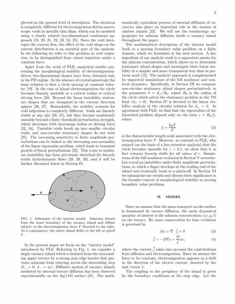
FIG. 2: First order perturbations of the circular steady state.Left: Steady state shape for different values of δ = d+/R0 ≪ 1with fixed z = R0/ξ = 5 and Γ/R0 = 0.05. Right: Differentvalues of z with fixed δz = 0.05. In both cases the perturbedshape R0 +ρ−ρ0 is depicted, i.e. the dilation mode has beensubtracted.
The constant term ρ0 in (18) describes a uniform di-lation of the circle. Since Γ/R0 ≪ 1, ρ0 > 0, whileρn≥2 < 0. In particular, the leading order deformationwith n = 2 corresponds to an elongation perpendicular tothe drift direction. This is illustrated in Fig. 2, where thedilation mode has been subtracted. Moreover, with in-creasing electromigration force (increasing z), the shapesstart to become concave on the trailing side (recall thatthe islands are moving to the left).
As has been pointed out above in Section II, the full(nonlinear) evolution is area conserving in the quasistaticlimit. Since the dilation mode ρ0 is of the same order asthe elongation mode ρ2, this property is generally vio-lated by the first order perturbation in δ. This suggeststhat the perturbative regime may be restricted to rathersmall elongations. To obtain the steady states of thefull nonlinear model, numerical simulations of the time-dependent equations (3)-(9) have been performed. Anadaptive finite element method is used, where the freeboundary problem is discretized semi-implicitly using anoperator splitting approach and two independent numer-ical grids for the adatom density c and for the islandboundary, respectively. For the boundary evolution, afront tracking method is applied, for details see [33].
Starting with a circular shape, the void elongates untilit reaches a steady state. A typical example of the timeevolution is depicted in Fig. 3. Here the parameters areδ = 0.1, z = 5, which, as will be seen below, is alreadyfar away from the perturbative regime. We do not ob-serve any concave parts at the back side of the void asopposed to the perturbative steady state, see Fig. 2. This
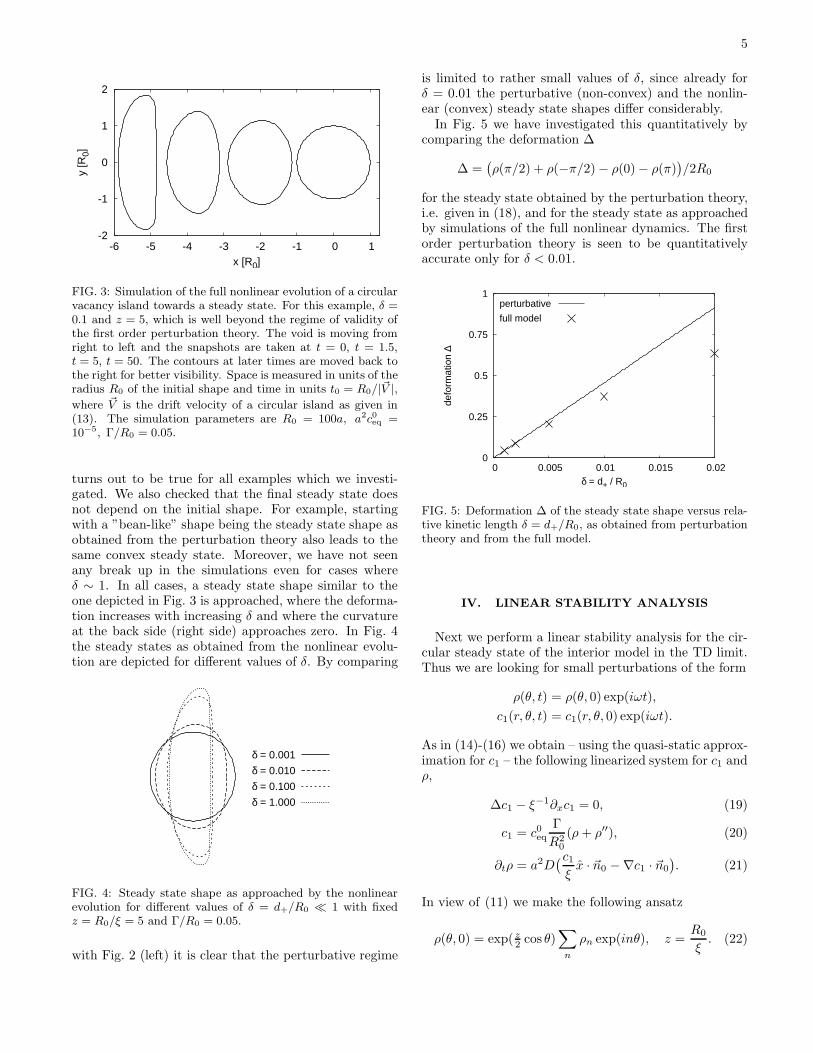
5
-2
-1
0
1
2
-6 -5 -4 -3 -2 -1 0 1
y [R
0]
x [R0]
FIG. 3: Simulation of the full nonlinear evolution of a circularvacancy island towards a steady state. For this example, δ =0.1 and z = 5, which is well beyond the regime of validity ofthe first order perturbation theory. The void is moving fromright to left and the snapshots are taken at t = 0, t = 1.5,t = 5, t = 50. The contours at later times are moved back tothe right for better visibility. Space is measured in units of theradius R0 of the initial shape and time in units t0 = R0/|~V |,
where ~V is the drift velocity of a circular island as given in(13). The simulation parameters are R0 = 100a, a2c0
eq =10−5, Γ/R0 = 0.05.
turns out to be true for all examples which we investi-gated. We also checked that the final steady state doesnot depend on the initial shape. For example, startingwith a ”bean-like” shape being the steady state shape asobtained from the perturbation theory also leads to thesame convex steady state. Moreover, we have not seenany break up in the simulations even for cases whereδ ∼ 1. In all cases, a steady state shape similar to theone depicted in Fig. 3 is approached, where the deforma-tion increases with increasing δ and where the curvatureat the back side (right side) approaches zero. In Fig. 4the steady states as obtained from the nonlinear evolu-tion are depicted for different values of δ. By comparing
δ = 0.001
δ = 0.010
δ = 0.100
δ = 1.000
FIG. 4: Steady state shape as approached by the nonlinearevolution for different values of δ = d+/R0 ≪ 1 with fixedz = R0/ξ = 5 and Γ/R0 = 0.05.
with Fig. 2 (left) it is clear that the perturbative regime
is limited to rather small values of δ, since already forδ = 0.01 the perturbative (non-convex) and the nonlin-ear (convex) steady state shapes differ considerably.
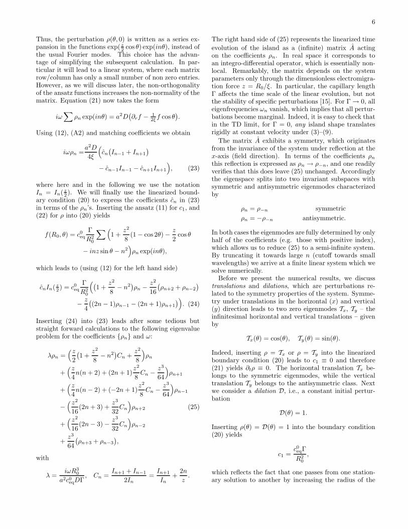
In Fig. 5 we have investigated this quantitatively bycomparing the deformation ∆
∆ =(
ρ(π/2) + ρ(−π/2) − ρ(0) − ρ(π))
/2R0
for the steady state obtained by the perturbation theory,i.e. given in (18), and for the steady state as approachedby simulations of the full nonlinear dynamics. The firstorder perturbation theory is seen to be quantitativelyaccurate only for δ < 0.01.
0
0.25
0.5
0.75
1
0 0.005 0.01 0.015 0.02
defo
rmat
ion
∆
δ = d+ / R0
perturbative
full model
FIG. 5: Deformation ∆ of the steady state shape versus rela-tive kinetic length δ = d+/R0, as obtained from perturbationtheory and from the full model.
IV. LINEAR STABILITY ANALYSIS
Next we perform a linear stability analysis for the cir-cular steady state of the interior model in the TD limit.Thus we are looking for small perturbations of the form
ρ(θ, t) = ρ(θ, 0) exp(iωt),
c1(r, θ, t) = c1(r, θ, 0) exp(iωt).
As in (14)-(16) we obtain – using the quasi-static approx-imation for c1 – the following linearized system for c1 andρ,
∆c1 − ξ−1∂xc1 = 0, (19)
c1 = c0eq
Γ
R20
(ρ + ρ′′), (20)
∂tρ = a2D(c1
ξx · ~n0 −∇c1 · ~n0
)
. (21)
In view of (11) we make the following ansatz
ρ(θ, 0) = exp( z2
cos θ)∑
n
ρn exp(inθ), z =R0
ξ. (22)
6
Thus, the perturbation ρ(θ, 0) is written as a series ex-pansion in the functions exp(z
2cos θ) exp(inθ), instead of
the usual Fourier modes. This choice has the advan-tage of simplifying the subsequent calculation. In par-ticular it will lead to a linear system, where each matrixrow/column has only a small number of non zero entries.However, as we will discuss later, the non-orthogonalityof the ansatz functions increases the non-normality of thematrix. Equation (21) now takes the form
iω∑
ρn exp(inθ) = a2D(
∂rf − 12ξ
f cos θ)
.
Using (12), (A2) and matching coefficients we obtain
iωρn =a2D
4ξ
(
cn
(
In−1 + In+1
)
− cn−1In−1 − cn+1In+1
)
, (23)
where here and in the following we use the notationIn = In( z
2). We will finally use the linearized bound-
ary condition (20) to express the coefficients cn in (23)in terms of the ρn’s. Inserting the ansatz (11) for c1, and(22) for ρ into (20) yields
f(R0, θ) = c0eq
Γ
R20
∑
(
1 +z2
8(1 − cos 2θ) − z
2cos θ
− inz sin θ − n2)
ρn exp(inθ),
which leads to (using (12) for the left hand side)
cnIn( z2) = c0
eq
Γ
R20
(
(
1 +z2
8− n2
)
ρn − z2
16
(
ρn+2 + ρn−2
)
− z
4
(
(2n − 1)ρn−1 − (2n + 1)ρn+1
)
)
. (24)
Inserting (24) into (23) leads after some tedious butstraight forward calculations to the following eigenvalueproblem for the coefficients ρn and ω:
λρn =(z
2
(
1 +z2
8− n2
)
Cn +z2
8
)
ρn
+(z
4n(n + 2) + (2n + 1)
z2
8Cn − z3
64
)
ρn+1
+(z
4n(n − 2) + (−2n + 1)
z2
8Cn − z3
64
)
ρn−1
−(z2
16(2n + 3) +
z3
32Cn
)
ρn+2 (25)
+(z2
16(2n − 3) − z3
32Cn
)
ρn−2
+z3
64
(
ρn+3 + ρn−3
)
,
with
λ =iωR3
0
a2c0eqDΓ
, Cn =In+1 + In−1
2In
=In+1
In
+2n
z.
The right hand side of (25) represents the linearized time
evolution of the island as a (infinite) matrix A actingon the coefficients ρn. In real space it corresponds toan integro-differential operator, which is essentially non-local. Remarkably, the matrix depends on the systemparameters only through the dimensionless electromigra-tion force z = R0/ξ. In particular, the capillary lengthΓ affects the time scale of the linear evolution, but notthe stability of specific perturbations [15]. For Γ → 0, alleigenfrequencies ωn vanish, which implies that all pertur-bations become marginal. Indeed, it is easy to check thatin the TD limit, for Γ = 0, any island shape translatesrigidly at constant velocity under (3)–(9).
The matrix A exhibits a symmetry, which originatesfrom the invariance of the system under reflection at thex-axis (field direction). In terms of the coefficients ρn
this reflection is expressed as ρn → ρ−n, and one readilyverifies that this does leave (25) unchanged. Accordinglythe eigenspace splits into two invariant subspaces withsymmetric and antisymmetric eigenmodes characterizedby
ρn = ρ−n symmetric
ρn = −ρ−n antisymmetric.
In both cases the eigenmodes are fully determined by onlyhalf of the coefficients (e.g. those with positive index),which allows us to reduce (25) to a semi-infinite system.By truncating it towards large n (cutoff towards smallwavelengths) we arrive at a finite linear system which wesolve numerically.
Before we present the numerical results, we discusstranslations and dilations, which are perturbations re-lated to the symmetry properties of the system. Symme-try under translations in the horizontal (x) and vertical(y) direction leads to two zero eigenmodes Tx, Ty – theinfinitesimal horizontal and vertical translations – givenby
Tx(θ) = cos(θ), Ty(θ) = sin(θ).
Indeed, inserting ρ = Tx or ρ = Ty into the linearizedboundary condition (20) leads to c1 ≡ 0 and therefore(21) yields ∂tρ ≡ 0. The horizontal translation Tx be-longs to the symmetric eigenmodes, while the verticaltranslation Ty belongs to the antisymmetric class. Nextwe consider a dilation D, i.e., a constant initial pertur-bation
D(θ) = 1.
Inserting ρ(θ) = D(θ) = 1 into the boundary condition(20) yields
c1 =c0eqΓ
R20
,
which reflects the fact that one passes from one station-ary solution to another by increasing the radius of the
7
island and the concentration inside the island by a con-stant value. However, a dilation is not a zero eigenmode:Since we consider perturbations of a circular steady state,which has a steady state drift velocity depending on theradius, two circles with different radius are drifting apart.This leads to a linear increase of the perturbation. From(21), an initial perturbation ρ(θ, 0) = 1 has to grow ac-cording to
∂tρ =a2c0
eqΓD
R20ξ
cos(θ) =a2c0
eqΓD
R20ξ
Tx(θ).
In that sense a dilation D generates a translation, and Dis a generalized eigenmode with eigenvalue zero accordingto A2D ∼ ATx = 0. Thus (restricting to the symmetriccase) the eigenvalue zero is two-fold degenerate, and has
one (proper) eigenvector. Therefore the matrix A can notbe diagonalized completely but contains a 2 × 2 Jordanblock corresponding to the invariant subspace spanned byD and Tx. Apart from that, the dilation doesn’t play arole, because the time evolution preserves the area and wecan therefore always restrict ourselves to perturbationswhich do not contain dilations.
-120
-100
-80
-60
-40
-20
0
0 5 10 15 20 25 30
eige
nval
ues
λ
z = R0/ξ
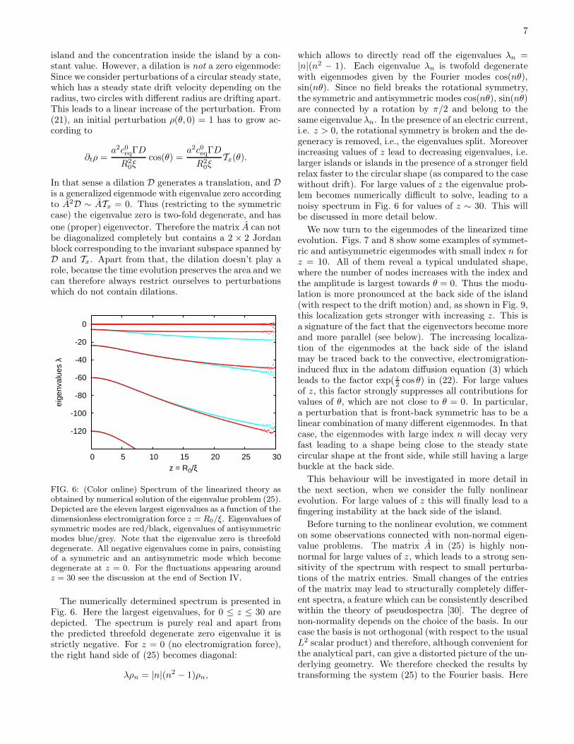
FIG. 6: (Color online) Spectrum of the linearized theory asobtained by numerical solution of the eigenvalue problem (25).Depicted are the eleven largest eigenvalues as a function of thedimensionless electromigration force z = R0/ξ. Eigenvalues ofsymmetric modes are red/black, eigenvalues of antisymmetricmodes blue/grey. Note that the eigenvalue zero is threefolddegenerate. All negative eigenvalues come in pairs, consistingof a symmetric and an antisymmetric mode which becomedegenerate at z = 0. For the fluctuations appearing aroundz = 30 see the discussion at the end of Section IV.
The numerically determined spectrum is presented inFig. 6. Here the largest eigenvalues, for 0 ≤ z ≤ 30 aredepicted. The spectrum is purely real and apart fromthe predicted threefold degenerate zero eigenvalue it isstrictly negative. For z = 0 (no electromigration force),the right hand side of (25) becomes diagonal:
λρn = |n|(n2 − 1)ρn,
which allows to directly read off the eigenvalues λn =|n|(n2 − 1). Each eigenvalue λn is twofold degeneratewith eigenmodes given by the Fourier modes cos(nθ),sin(nθ). Since no field breaks the rotational symmetry,the symmetric and antisymmetric modes cos(nθ), sin(nθ)are connected by a rotation by π/2 and belong to thesame eigenvalue λn. In the presence of an electric current,i.e. z > 0, the rotational symmetry is broken and the de-generacy is removed, i.e., the eigenvalues split. Moreoverincreasing values of z lead to decreasing eigenvalues, i.e.larger islands or islands in the presence of a stronger fieldrelax faster to the circular shape (as compared to the casewithout drift). For large values of z the eigenvalue prob-lem becomes numerically difficult to solve, leading to anoisy spectrum in Fig. 6 for values of z ∼ 30. This willbe discussed in more detail below.
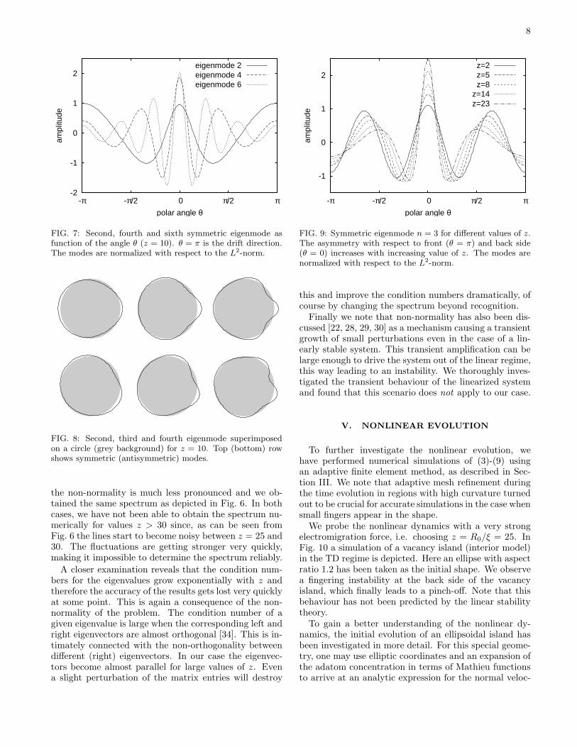
We now turn to the eigenmodes of the linearized timeevolution. Figs. 7 and 8 show some examples of symmet-ric and antisymmetric eigenmodes with small index n forz = 10. All of them reveal a typical undulated shape,where the number of nodes increases with the index andthe amplitude is largest towards θ = 0. Thus the modu-lation is more pronounced at the back side of the island(with respect to the drift motion) and, as shown in Fig. 9,this localization gets stronger with increasing z. This isa signature of the fact that the eigenvectors become moreand more parallel (see below). The increasing localiza-tion of the eigenmodes at the back side of the islandmay be traced back to the convective, electromigration-induced flux in the adatom diffusion equation (3) whichleads to the factor exp( z
2cos θ) in (22). For large values
of z, this factor strongly suppresses all contributions forvalues of θ, which are not close to θ = 0. In particular,a perturbation that is front-back symmetric has to be alinear combination of many different eigenmodes. In thatcase, the eigenmodes with large index n will decay veryfast leading to a shape being close to the steady statecircular shape at the front side, while still having a largebuckle at the back side.
This behaviour will be investigated in more detail inthe next section, when we consider the fully nonlinearevolution. For large values of z this will finally lead to afingering instability at the back side of the island.
Before turning to the nonlinear evolution, we commenton some observations connected with non-normal eigen-value problems. The matrix A in (25) is highly non-normal for large values of z, which leads to a strong sen-sitivity of the spectrum with respect to small perturba-tions of the matrix entries. Small changes of the entriesof the matrix may lead to structurally completely differ-ent spectra, a feature which can be consistently describedwithin the theory of pseudospectra [30]. The degree ofnon-normality depends on the choice of the basis. In ourcase the basis is not orthogonal (with respect to the usualL2 scalar product) and therefore, although convenient forthe analytical part, can give a distorted picture of the un-derlying geometry. We therefore checked the results bytransforming the system (25) to the Fourier basis. Here
8
2
1
0
-1
-2ππ/2 0-π/2-π
ampl
itude
polar angle θ
eigenmode 2eigenmode 4eigenmode 6
FIG. 7: Second, fourth and sixth symmetric eigenmode asfunction of the angle θ (z = 10). θ = π is the drift direction.The modes are normalized with respect to the L2-norm.
FIG. 8: Second, third and fourth eigenmode superimposedon a circle (grey background) for z = 10. Top (bottom) rowshows symmetric (antisymmetric) modes.
the non-normality is much less pronounced and we ob-tained the same spectrum as depicted in Fig. 6. In bothcases, we have not been able to obtain the spectrum nu-merically for values z > 30 since, as can be seen fromFig. 6 the lines start to become noisy between z = 25 and30. The fluctuations are getting stronger very quickly,making it impossible to determine the spectrum reliably.
A closer examination reveals that the condition num-bers for the eigenvalues grow exponentially with z andtherefore the accuracy of the results gets lost very quicklyat some point. This is again a consequence of the non-normality of the problem. The condition number of agiven eigenvalue is large when the corresponding left andright eigenvectors are almost orthogonal [34]. This is in-timately connected with the non-orthogonality betweendifferent (right) eigenvectors. In our case the eigenvec-tors become almost parallel for large values of z. Evena slight perturbation of the matrix entries will destroy
2
1
0
-1
ππ/2 0-π/2-π
ampl
itude
polar angle θ
z=2z=5z=8
z=14z=23
FIG. 9: Symmetric eigenmode n = 3 for different values of z.The asymmetry with respect to front (θ = π) and back side(θ = 0) increases with increasing value of z. The modes arenormalized with respect to the L2-norm.
this and improve the condition numbers dramatically, ofcourse by changing the spectrum beyond recognition.
Finally we note that non-normality has also been dis-cussed [22, 28, 29, 30] as a mechanism causing a transientgrowth of small perturbations even in the case of a lin-early stable system. This transient amplification can belarge enough to drive the system out of the linear regime,this way leading to an instability. We thoroughly inves-tigated the transient behaviour of the linearized systemand found that this scenario does not apply to our case.
V. NONLINEAR EVOLUTION
To further investigate the nonlinear evolution, wehave performed numerical simulations of (3)-(9) usingan adaptive finite element method, as described in Sec-tion III. We note that adaptive mesh refinement duringthe time evolution in regions with high curvature turnedout to be crucial for accurate simulations in the case whensmall fingers appear in the shape.
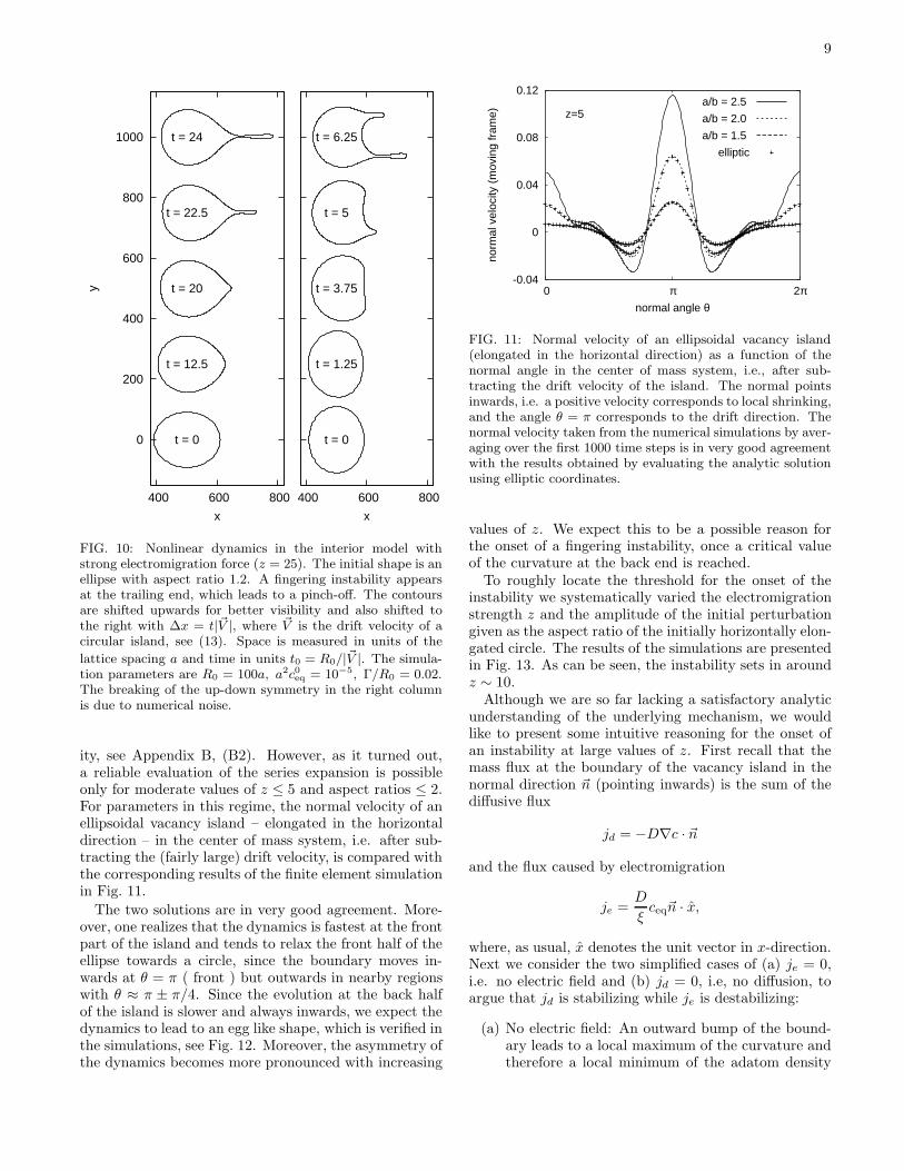
We probe the nonlinear dynamics with a very strongelectromigration force, i.e. choosing z = R0/ξ = 25. InFig. 10 a simulation of a vacancy island (interior model)in the TD regime is depicted. Here an ellipse with aspectratio 1.2 has been taken as the initial shape. We observea fingering instability at the back side of the vacancyisland, which finally leads to a pinch-off. Note that thisbehaviour has not been predicted by the linear stabilitytheory.
To gain a better understanding of the nonlinear dy-namics, the initial evolution of an ellipsoidal island hasbeen investigated in more detail. For this special geome-try, one may use elliptic coordinates and an expansion ofthe adatom concentration in terms of Mathieu functionsto arrive at an analytic expression for the normal veloc-
9
0
200
400
600
800
1000
400 600 800
y
x
t = 0
t = 12.5
t = 20
t = 22.5
t = 24
0
200
400
600
800
1000
400 600 800
x
t = 0
t = 1.25
t = 3.75
t = 5
t = 6.25
FIG. 10: Nonlinear dynamics in the interior model withstrong electromigration force (z = 25). The initial shape is anellipse with aspect ratio 1.2. A fingering instability appearsat the trailing end, which leads to a pinch-off. The contoursare shifted upwards for better visibility and also shifted tothe right with ∆x = t|~V |, where ~V is the drift velocity of acircular island, see (13). Space is measured in units of the
lattice spacing a and time in units t0 = R0/|~V |. The simula-tion parameters are R0 = 100a, a2c0
eq = 10−5, Γ/R0 = 0.02.The breaking of the up-down symmetry in the right columnis due to numerical noise.
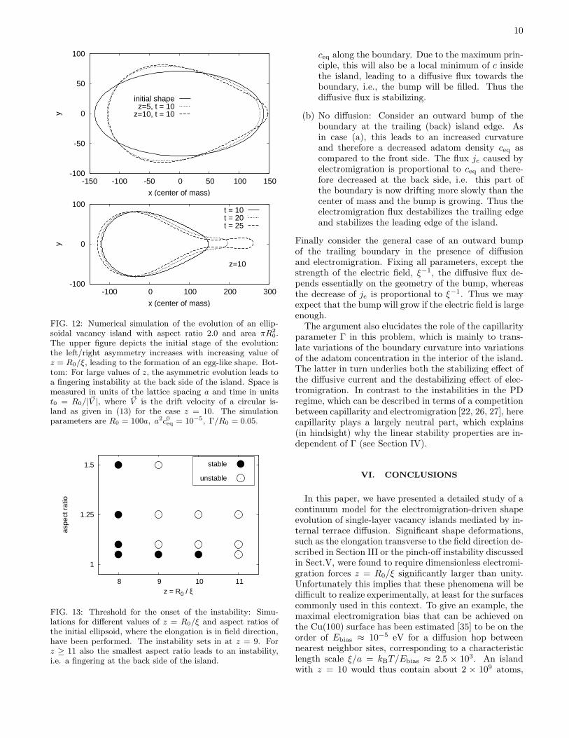
ity, see Appendix B, (B2). However, as it turned out,a reliable evaluation of the series expansion is possibleonly for moderate values of z ≤ 5 and aspect ratios ≤ 2.For parameters in this regime, the normal velocity of anellipsoidal vacancy island – elongated in the horizontaldirection – in the center of mass system, i.e. after sub-tracting the (fairly large) drift velocity, is compared withthe corresponding results of the finite element simulationin Fig. 11.
The two solutions are in very good agreement. More-over, one realizes that the dynamics is fastest at the frontpart of the island and tends to relax the front half of theellipse towards a circle, since the boundary moves in-wards at θ = π ( front ) but outwards in nearby regionswith θ ≈ π ± π/4. Since the evolution at the back halfof the island is slower and always inwards, we expect thedynamics to lead to an egg like shape, which is verified inthe simulations, see Fig. 12. Moreover, the asymmetry ofthe dynamics becomes more pronounced with increasing
-0.04
0
0.04
0.08
0.12
2ππ 0
norm
al v
eloc
ity (
mov
ing
fram
e)
normal angle θ
z=5a/b = 2.5
a/b = 2.0
a/b = 1.5
elliptic
FIG. 11: Normal velocity of an ellipsoidal vacancy island(elongated in the horizontal direction) as a function of thenormal angle in the center of mass system, i.e., after sub-tracting the drift velocity of the island. The normal pointsinwards, i.e. a positive velocity corresponds to local shrinking,and the angle θ = π corresponds to the drift direction. Thenormal velocity taken from the numerical simulations by aver-aging over the first 1000 time steps is in very good agreementwith the results obtained by evaluating the analytic solutionusing elliptic coordinates.
values of z. We expect this to be a possible reason forthe onset of a fingering instability, once a critical valueof the curvature at the back end is reached.
To roughly locate the threshold for the onset of theinstability we systematically varied the electromigrationstrength z and the amplitude of the initial perturbationgiven as the aspect ratio of the initially horizontally elon-gated circle. The results of the simulations are presentedin Fig. 13. As can be seen, the instability sets in aroundz ∼ 10.
Although we are so far lacking a satisfactory analyticunderstanding of the underlying mechanism, we wouldlike to present some intuitive reasoning for the onset ofan instability at large values of z. First recall that themass flux at the boundary of the vacancy island in thenormal direction ~n (pointing inwards) is the sum of thediffusive flux
jd = −D∇c · ~n
and the flux caused by electromigration
je =D
ξceq~n · x,
where, as usual, x denotes the unit vector in x-direction.Next we consider the two simplified cases of (a) je = 0,i.e. no electric field and (b) jd = 0, i.e, no diffusion, toargue that jd is stabilizing while je is destabilizing:
(a) No electric field: An outward bump of the bound-ary leads to a local maximum of the curvature andtherefore a local minimum of the adatom density
10
-100
-50
0
50
100
-150 -100 -50 0 50 100 150
y
x (center of mass)
initial shapez=5, t = 10
z=10, t = 10
-100
0
100
-100 0 100 200 300
y
x (center of mass)
z=10
t = 10t = 20t = 25
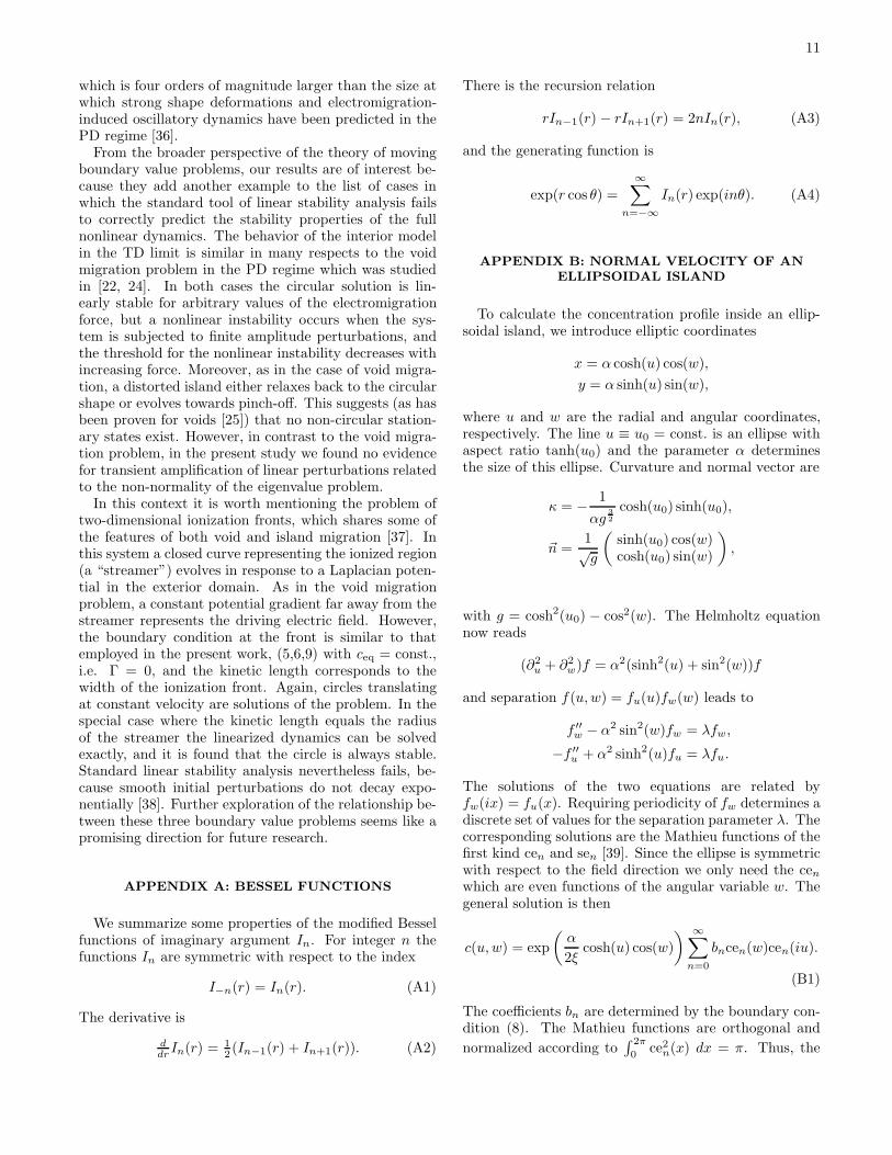
FIG. 12: Numerical simulation of the evolution of an ellip-soidal vacancy island with aspect ratio 2.0 and area πR2
0.The upper figure depicts the initial stage of the evolution:the left/right asymmetry increases with increasing value ofz = R0/ξ, leading to the formation of an egg-like shape. Bot-tom: For large values of z, the asymmetric evolution leads toa fingering instability at the back side of the island. Space ismeasured in units of the lattice spacing a and time in unitst0 = R0/|~V |, where ~V is the drift velocity of a circular is-land as given in (13) for the case z = 10. The simulationparameters are R0 = 100a, a2c0
eq = 10−5, Γ/R0 = 0.05.
1
1.25
1.5
8 9 10 11
aspe
ct r
atio
z = R0 / ξ
stable
unstable
FIG. 13: Threshold for the onset of the instability: Simu-lations for different values of z = R0/ξ and aspect ratios ofthe initial ellipsoid, where the elongation is in field direction,have been performed. The instability sets in at z = 9. Forz ≥ 11 also the smallest aspect ratio leads to an instability,i.e. a fingering at the back side of the island.
ceq along the boundary. Due to the maximum prin-ciple, this will also be a local minimum of c insidethe island, leading to a diffusive flux towards theboundary, i.e., the bump will be filled. Thus thediffusive flux is stabilizing.
(b) No diffusion: Consider an outward bump of theboundary at the trailing (back) island edge. Asin case (a), this leads to an increased curvatureand therefore a decreased adatom density ceq ascompared to the front side. The flux je caused byelectromigration is proportional to ceq and there-fore decreased at the back side, i.e. this part ofthe boundary is now drifting more slowly than thecenter of mass and the bump is growing. Thus theelectromigration flux destabilizes the trailing edgeand stabilizes the leading edge of the island.
Finally consider the general case of an outward bumpof the trailing boundary in the presence of diffusionand electromigration. Fixing all parameters, except thestrength of the electric field, ξ−1, the diffusive flux de-pends essentially on the geometry of the bump, whereasthe decrease of je is proportional to ξ−1. Thus we mayexpect that the bump will grow if the electric field is largeenough.
The argument also elucidates the role of the capillarityparameter Γ in this problem, which is mainly to trans-late variations of the boundary curvature into variationsof the adatom concentration in the interior of the island.The latter in turn underlies both the stabilizing effect ofthe diffusive current and the destabilizing effect of elec-tromigration. In contrast to the instabilities in the PDregime, which can be described in terms of a competitionbetween capillarity and electromigration [22, 26, 27], herecapillarity plays a largely neutral part, which explains(in hindsight) why the linear stability properties are in-dependent of Γ (see Section IV).
VI. CONCLUSIONS
In this paper, we have presented a detailed study of acontinuum model for the electromigration-driven shapeevolution of single-layer vacancy islands mediated by in-ternal terrace diffusion. Significant shape deformations,such as the elongation transverse to the field direction de-scribed in Section III or the pinch-off instability discussedin Sect.V, were found to require dimensionless electromi-gration forces z = R0/ξ significantly larger than unity.Unfortunately this implies that these phenomena will bedifficult to realize experimentally, at least for the surfacescommonly used in this context. To give an example, themaximal electromigration bias that can be achieved onthe Cu(100) surface has been estimated [35] to be on theorder of Ebias ≈ 10−5 eV for a diffusion hop betweennearest neighbor sites, corresponding to a characteristiclength scale ξ/a = kBT/Ebias ≈ 2.5 × 10³. An islandwith z = 10 would thus contain about 2 × 10⁹ atoms,
11
which is four orders of magnitude larger than the size atwhich strong shape deformations and electromigration-induced oscillatory dynamics have been predicted in thePD regime [36].
From the broader perspective of the theory of movingboundary value problems, our results are of interest be-cause they add another example to the list of cases inwhich the standard tool of linear stability analysis failsto correctly predict the stability properties of the fullnonlinear dynamics. The behavior of the interior modelin the TD limit is similar in many respects to the voidmigration problem in the PD regime which was studiedin [22, 24]. In both cases the circular solution is lin-early stable for arbitrary values of the electromigrationforce, but a nonlinear instability occurs when the sys-tem is subjected to finite amplitude perturbations, andthe threshold for the nonlinear instability decreases withincreasing force. Moreover, as in the case of void migra-tion, a distorted island either relaxes back to the circularshape or evolves towards pinch-off. This suggests (as hasbeen proven for voids [25]) that no non-circular station-ary states exist. However, in contrast to the void migra-tion problem, in the present study we found no evidencefor transient amplification of linear perturbations relatedto the non-normality of the eigenvalue problem.
In this context it is worth mentioning the problem oftwo-dimensional ionization fronts, which shares some ofthe features of both void and island migration [37]. Inthis system a closed curve representing the ionized region(a “streamer”) evolves in response to a Laplacian poten-tial in the exterior domain. As in the void migrationproblem, a constant potential gradient far away from thestreamer represents the driving electric field. However,the boundary condition at the front is similar to thatemployed in the present work, (5,6,9) with ceq = const.,i.e. Γ = 0, and the kinetic length corresponds to thewidth of the ionization front. Again, circles translatingat constant velocity are solutions of the problem. In thespecial case where the kinetic length equals the radiusof the streamer the linearized dynamics can be solvedexactly, and it is found that the circle is always stable.Standard linear stability analysis nevertheless fails, be-cause smooth initial perturbations do not decay expo-nentially [38]. Further exploration of the relationship be-tween these three boundary value problems seems like apromising direction for future research.
APPENDIX A: BESSEL FUNCTIONS
We summarize some properties of the modified Besselfunctions of imaginary argument In. For integer n thefunctions In are symmetric with respect to the index
I−n(r) = In(r). (A1)
The derivative is
ddr
In(r) = 12(In−1(r) + In+1(r)). (A2)
There is the recursion relation
rIn−1(r) − rIn+1(r) = 2nIn(r), (A3)
and the generating function is
exp(r cos θ) =
∞∑
n=−∞
In(r) exp(inθ). (A4)
APPENDIX B: NORMAL VELOCITY OF AN
ELLIPSOIDAL ISLAND
To calculate the concentration profile inside an ellip-soidal island, we introduce elliptic coordinates
x = α cosh(u) cos(w),
y = α sinh(u) sin(w),
where u and w are the radial and angular coordinates,respectively. The line u ≡ u0 = const. is an ellipse withaspect ratio tanh(u0) and the parameter α determinesthe size of this ellipse. Curvature and normal vector are
κ = − 1
αg3
2
cosh(u0) sinh(u0),
~n =1√g
(
sinh(u0) cos(w)cosh(u0) sin(w)
)
,
with g = cosh2(u0) − cos2(w). The Helmholtz equationnow reads
(∂2u + ∂2
w)f = α2(sinh2(u) + sin2(w))f
and separation f(u, w) = fu(u)fw(w) leads to
f ′′w − α2 sin2(w)fw = λfw,
−f ′′u + α2 sinh2(u)fu = λfu.
The solutions of the two equations are related byfw(ix) = fu(x). Requiring periodicity of fw determines adiscrete set of values for the separation parameter λ. Thecorresponding solutions are the Mathieu functions of thefirst kind cen and sen [39]. Since the ellipse is symmetricwith respect to the field direction we only need the cen
which are even functions of the angular variable w. Thegeneral solution is then
c(u, w) = exp
(
α
2ξcosh(u) cos(w)
) ∞∑
n=0
bncen(w)cen(iu).
(B1)
The coefficients bn are determined by the boundary con-dition (8). The Mathieu functions are orthogonal and
normalized according to∫ 2π
0ce2
n(x) dx = π. Thus, the
12
bn can be found in a way similar to Fourier coefficientsvia the integrals
bn =c0eq
πcen(iu0)
∫ 2π
0
cen(w) exp
(
− α
2ξcosh(u0) cos(w)
)
×
× (1 − Γκ) dw.
These integrals are solved numerically. Finally, using thegeneral solution (B1) to calculate the flux to the bound-ary, the normal velocity v of the island edge is obtainedas
v =a2D√
gexp
(
α
2ξcosh(u0) cos(w)
)
∑
bncen(w)×
×(
1
αIm(ce′n(iu0)) +
1
ξsinh(u0) cos(w)cen(iu0)
)
.
(B2)
ACKNOWLEDGMENTS
We are grateful to Ute Ebert, Yan Fyodorov, OlivierPierre-Louis, Vakhtang Putkaradze and Gerhard Wolffor instructive discussions and helpful suggestions. Thiswork was supported by DFG within project KR 1123/1-2and within SPP 1253.
[1] P. Pelce, New Visions on Form and Growth (Oxford Uni-versity Press, New York, 2004).
[2] T. Michely and J. Krug, Islands, Mounds and Atoms
(Springer, Berlin, 2004).[3] H. C. Jeong and E. D. Williams, Surf. Sci. Rep. 34, 171
(1999).[4] O. Pierre-Louis, C.R.Phys. 6, 11 (2005).[5] J. Krug, in Multiscale modeling of epitaxial growth, edited
by A. Voigt (Birkhauser, Basel, 2005), pp. 69–95.[6] K. Yagi, H. Minoda, and M. Degawa, Surf. Sci. Repts.
43, 45 (2001).[7] H. Minoda, J. Phys.-Cond. Matter 15, S3255 (2003).[8] R. S. Sorbello, in Solid State Physics Vol.51, edited by
H. Ehrenreich and F. Spaepen (Academic, New York,1998), p. 159.
[9] A. V. Latyshev, A. Aseev, A. B. Krasilnikov, andS. Stenin, Surf. Sci. 213, 157 (1989).
[10] M. Degawa, H. Nishimura, Y. Tanishiro, H. Minoda, andK. Yagi, Jpn. J. Appl. Phys. 38, L308 (1999).
[11] K. Thurmer, D.-J. Liu, E. D. Williams, and J. D. Weeks,Phys. Rev. Lett. 83, 5531 (1999).
[12] O. Pierre-Louis and J.-J. Metois, Phys. Rev. Lett. 93,165901 (2004).
[13] J.-J. Metois, J. C. Heyraud, and A. Pimpinelli, Surf. Sci.420, 250 (1999).
[14] A. Saul, J.-J. Metois, and A. Ranguis, Phys. Rev. B 65,075409 (2002).
[15] O. Pierre-Louis and T. L. Einstein, Phys. Rev. B 62,13697 (2000).
[16] P. J. Rous, Phys. Rev. B 59, 7719 (1999).[17] P. J. Rous and D. N. Bly, Phys. Rev. B 62, 8478 (2000).[18] O. Pierre-Louis, Phys. Rev. Lett. 96, 135901 (2006).[19] P. S. Ho, J. Appl. Phys. 41, 64 (1970).[20] W. Wang, Z. Suo, and T.-H. Hao, J. Appl. Phys. 79,
2394 (1996).[21] M. Mahadevan and R. M. Bradley, J. Appl. Phys. 79,
6840 (1996).[22] M. Schimschak and J. Krug, Phys. Rev. Lett. 80, 1674
(1998).[23] M. R. Gungor and D. Maroudas, J. Appl. Phys. 85, 2233
(1999).[24] M. Schimschak and J. Krug, J. Appl. Phys. 87, 695
(2000).[25] L. J. Cummings, G. Richardson, and M. Ben Amar, Eur.
J. Appl. Math. 12, 97 (2001).[26] P. Kuhn and J. Krug, in Multiscale modeling of epitaxial
growth, edited by A. Voigt (Birkhauser, Basel, 2005), pp.159–173.
[27] P. Kuhn, J. Krug, F. Haußer, and A. Voigt, Phys. Rev.Lett. 94, 166105 (2005).
[28] L. N. Trefethen, A. E. Trefethen, S. C. Reddy, and T. A.Driscoll, Science 261, 578 (1993).
[29] S. Grossmann, Rev. Mod. Phys. 72, 603 (2000).[30] L. N. Trefethen and M. Embree, Spectra and Pseudospec-
tra: The Behavior of Nonnormal Matrices and Operators
(Princeton University Press, 2005).[31] K. Morgenstern, E. Laegsgaard, and F. Besenbacher,
Phys. Rev. Lett. 86, 5739 (2001).[32] J. Heinonen, I. Koponen, J. Merikoski, and T. Ala-
Nissila, Phys. Rev. Lett. 82, 2733 (1999).[33] E. Bansch, F. Haußer, O. Lakkis, B. Li, and A. Voigt, J.
Comput. Phys. 194, 409 (2004).[34] A. Quarteroni, R. Saccoo, and F. Saleri, Numerical Math-
ematics (Springer, New York, 2000).[35] H. Mehl, O. Biham, O. Millo, and M. Karimi, Phys. Rev.
B 74, 4975 (2000).[36] M. Rusanen, P. Kuhn, and J. Krug, Phys. Rev. B 74,
245423 (2006).[37] B. Meulenbroek, U. Ebert, and L. Schafer, Phys. Rev.
Lett. 95, 195004 (2005).[38] U. Ebert, B. Meulenbroek, and L. Schafer,
nlin.PS/0606048 (2006).[39] I. S. Gradshteyn and I. M. Ryzhik, Table of Integrals,
Series, and Products (Academic Press, San Diego, 2000),sixth ed.


