QATAR UNIVERSITY

COLLEGE OF ENGINEERING

ASSESSMENT OF TURBULENCE MODELS FOR HYDROFRACTURING SLURRY

TRANSPORT SIMULATION IN HORIZONTAL PERFORATED PIPE

BY

MOHAMED KHAIRY MOHAMED YOUSSEF

A Thesis Submitted to

the College of Engineering

in Partial Fulfillment of the Requirements for the Degree of

Masters of Science in Mechanical Engineering

June 2020

© 2020. Mohamed Youssef. All Rights Reserved.

ii

COMMITTEE PAGE

The members of the Committee approve the Thesis of

Mohamed Youssef defended on 19/08/2020.

Dr. Saud Ghani

Thesis/Dissertation Supervisor

Approved:

Khalid Kamal Naji, Dean, College of Engineering

iii

ABSTRACT

YOUSSEF, MOHAMED, K., Masters : June : 2020,

Masters of Science in Mechanical Engineering

Title: Assessment of Turbulence Models for Hydraulic Fracturing Slurry Transport

Simulation in Horizontal Perforated Pipe.

Supervisor of Thesis: Saud, A., Ghani.

Hydraulic fracture is a well stimulation process that involves injecting

pressurized liquid at high velocity to initiate and propagate a fracture in the deep rock

formations through which hydrocarbons are extracted [1]. Typically, the pressurized

liquid, or the fracking liquid, is water mixed with sand. The water creates the fracture

and the sand maintains the void open. Hydraulic fracture stimulation is a standard

completion process for modern unconventional gas reservoirs. Proppant transport

through the wellbore is a major consideration when a horizontal well is fractured.

CFD simulation is utilized to understand the hydrofracturing process. This

study is characterizing different turbulence models that can capture the hydraulic

fracturing process. Selection of a suitable CFD turbulence model is carried through

investigating slurry flow in a horizontal pipe and employing various turbulence

models. The CFD results obtained from a Standard k-ε, Renormalization Group

(RNG) k-ε and Reynold-Stress-Model (RSM) were assessed. The (RNG) k-ε model

deemed the best turbulence model when capturing the slurry flow behavior.

In a laboratory experiment, particle image velocimetry (PIV) was used to non-

intrusively measure the transportation of sand slurry flow in a horizontal see through

pipeline with perforated holes. The investigation reports the results of the slurry flow

iv

patterns, the slurry flow pressure drop, the concentration profile and velocity

distribution at the perforated holes.

The experimental results supported the validity of the (RNG) k-ε model in

obtaining reliable predictions of the slurry flow. A linear relationship between the

surly velocity and the sand solid phase velocity was established.

Keywords: Horizontal well stimulation, Hydraulic fracturing; Slurry transport; CFD,

Turbulence models.

v

DEDICATION

I dedicate this work to Dr. Saud Ghani and my professors in the mechanical

engineering department for their faithful support and guidance during the completion

of this thesis.

vi

ACKNOWLEDGMENTS

First and foremost, I would like to praise God Almighty and thank him for

giving me this opportunity to be among distinguished professors and outstanding

students and complete my academic thesis for postgraduate studies from Qatar

University.

I would like to express the deepest appreciation to my advising Dr. Saud

Ghani for his support, guidance, valuable comments, encouragement, and positive

attitude during the execution of the thesis. My appreciation also extends to my

colleague Eng. Ahmed Osama and Eng. Suliman who helped me in performing the

experimental works.

Finally, I am highly indebted to my mother, father, and siblings, who

supported me spiritually through my life and sustain a positive atmosphere in which

to do science.

vii

TABLE OF CONTENTS

DEDICATION ............................................................................................................... v

ACKNOWLEDGMENTS ............................................................................................ vi

LIST OF TABLES ......................................................................................................... x

LIST OF FIGURES ...................................................................................................... xi

ABBREVIATIONS AND ACRONYMS ................................................................... xiv

Chapter 1: Introduction .................................................................................................. 1

1.1 Introduction on hydrofracturing treatment ........................................................... 1

1.2 Background of fracturing ..................................................................................... 2

1.3 General procedures for successful stimulation treatment .................................... 4

1.4 Scope and aims of the work ................................................................................. 5

1.5 Research Objectives ............................................................................................. 6

Chapter 2: Literature review .......................................................................................... 7

2.1 Introduction on slurry flow .................................................................................. 7

2.2 Rheology of the slurry .......................................................................................... 8

2.2.1 Newton’s Law of viscosity ............................................................................ 8

2.2.2 Slurry density ............................................................................................... 10

2.3 Fluid Flow Regimes ........................................................................................... 12

2.3.1 Transitional velocities .................................................................................. 14

2.3.2 Laminar and turbulent models ..................................................................... 15

viii

2.3.3 Calculation of critical deposition velocities ................................................ 17

2.4 Previous work on slurry flow: ............................................................................ 20

2.5 Conclusion of literature review .......................................................................... 25

Chapter 3: material and methods ................................................................................. 27

3.1 Experiential setup: .............................................................................................. 28

3.1.1 Velocity measurement using particle image velocimetry (PIV) ................. 30

3.1.2 The slurry system design of the experiment ................................................ 32

3.1.3 The challenges of slurry experiment: .......................................................... 33

3.2 Numerical simulation ......................................................................................... 33

3.2.1. Mathematical models .................................................................................. 34

Chapter 4: Results and discussion................................................................................ 41

4.1 Selecting a suitable turbulence closure .............................................................. 41

4.1.1 Pressure gradient verification: ..................................................................... 41

4.1.2 Solid concentration verification: ................................................................. 44

4.2 The framework of the numerical model for the slurry flow in a horizontal

perforated pipe.......................................................................................................... 48

4.2.1 Grid independent test: .................................................................................. 48

4.2.2 Geometry model and meshing ..................................................................... 50

4.2.3 Numerical equations selection for this thesis. ............................................. 51

4.2.4 Model validation: ......................................................................................... 51

ix

4.3 Comprehensive simulation results and discussion: ............................................ 57

4.3.1 Pressure gradient.......................................................................................... 57

4.3.2 Particle concentration: ................................................................................. 60

4.3.3 Velocity distribution: ................................................................................... 64

Chapter 5: Conclusion.................................................................................................. 69

REFERENCES ............................................................................................................ 72

Appendix A .................................................................................................................. 82

Appendix A: Durand’s limiting settling velocity graph ........................................... 82

Appendix B .................................................................................................................. 83

Appendix B: Modified Durand’s limiting settling velocity graph. .......................... 83

Appendix C .................................................................................................................. 84

Appendix C: Operating characteristics at 50 Hz, 2 poles. ....................................... 84

Appendix C: Hydraulic performance table .............................................................. 84

Appendix D .................................................................................................................. 85

Appendix D: Technical specification of digital sanitary pressure gauge. ................ 85

x

LIST OF TABLES

Table 1. An overview of previous academic research on slurry flow ......................... 22

Table 2. Skudarnov et al. and Newitt geometry and boundary conditions [62] .......... 42

Table 3. Statistical comparison of mean slurry pressure gradient between Standard k-

ε, RSM, and RNG in accordance with Skudarnov et al. (2001) .................................. 44

Table 4. Gillis and Shook geometry and boundary conditions [69] ............................ 45

Table 5. Statistical comparison of concentration profile between RSM and RNG ..... 48

Table 6. Geometry and boundary conditions of the numerical and the experimental

work of the thesis. ........................................................................................................ 52

xi

LIST OF FIGURES

Figure 1. Hydrofracturing in horizontal well [5, 6]. ...................................................... 2

Figure 2. Permeability in millidarcy verse the mean propant diameter in inch [4] ....... 5

Figure 3. Couette flow for defining viscosity [24]. ....................................................... 9

Figure 4. comparatively harsh method to find the slurry is settling or non-settling [27]

...................................................................................................................................... 13

Figure 5. Pressure drop vs the mean flow velocity at different flow regimes of

heterogenous slurries [26]. ........................................................................................... 14

Figure 6. Turbulent and laminar flow [23]. ................................................................. 16

Figure 7. Types of the flow according to the Reynolds number .................................. 17

Figure 8. Flowchart of the thesis approach. ................................................................. 27

Figure 9. Schematic setup of slurry flow system. ........................................................ 28

Figure 10. The apparatus of the slurry flow experiment. ............................................ 29

Figure 11. DL 125 xylem submersible pump. ............................................................. 30

Figure 12. Digital slurry pressure gauge. ..................................................................... 30

Figure 13. Typical 2-D PIV setup [71]. ....................................................................... 31

Figure 14. Auto sieve shaker. ...................................................................................... 32

Figure 15. 2D and 3D meshed geometry of Skudarnov and Newitt experiment. ........ 43

Figure 16. Comparisons of the numerical solution with the experimental data from

Skudarnov et al. (2001) and Newitt et al. (1955) in fully developed turbulent flow (ρ=

998.2 kg/m3, d= 0.0221 m, dp= 0.099 mm). Silica sand–water slurry, ρ = 2381 kg/m3,

concentration= 20% [62]. ............................................................................................ 44

Figure 17. 2D and 3D meshed geometry of Gillis and Shook experiment .................. 46

Figure 18. Comparison between RSM model and experimental data of concentration

xii

profile for different slurry volumetric concentration at mixture velocity of 3.1 m/s

[69]. .............................................................................................................................. 47

Figure 19. Comparison between RNG model and experimental data of concentration

profile for different slurry volumetric concentration at mixture velocity of 3.1 m/s

[69]. .............................................................................................................................. 48

Figure 20. Grid independent test of the slurry flow in horizontal pipe with 2 m long

and 50.8 mm internal diameter. ................................................................................... 49

Figure 21. 2D geometry of the thesis experimental work ............................................ 50

Figure 22. 2D and 3D meshed geometry of the thesis experimental work .................. 51

Figure 23. Contour plot of particle concentration in horizontal pipe with inlet

boundary. ..................................................................................................................... 54

Figure 24. Velocity vector of the slurry system experiment using PIV (At boundary

condition of 150 Kpa). ................................................................................................. 54

Figure 25. Velocity vector of the simulated slurry system using ANSYS-fluent (at

boundary condition of 150 Kpa). ................................................................................. 55

Figure 26. normalized velocity profile of slurry flow in the inner pipe at 1 m from the

inlet. ............................................................................................................................. 56

Figure 27. velocity profile of slurry flow in the inner pipe at a boundary condition of

150 Kpa. ....................................................................................................................... 57

Figure 28. Simulation result of average pressure drops for different flow velocities at

the perforated holes outlet. ........................................................................................... 58

Figure 29. Logarithm of pressure drops along the horizontal axis of the inner pipe

with different slurry velocities. .................................................................................... 59

Figure 30. Comparison between the pressure drop of slurry, sand and water flow at

xiii

three different concentrations (5%, 10%, and 15%) with a constant inlet velocity of 6

m/s. ............................................................................................................................... 60

Figure 31. Volumetric sand concentration profile across vertical center line of 1.7

meter from the pipe inlet at different mixture velocities. ............................................ 61

Figure 32. Volumetric concentration average at the four perforated holes of 5% slurry

volume fraction with different velocities. .................................................................... 62

Figure 33. Concentration profile of three different sand volume fractions at slurry

inlet velocity of 6 m/s. ................................................................................................. 63

Figure 34: Standard deviation of concentration profile of different sand volume

fractions at 6 m/s. ......................................................................................................... 64

Figure 35. Contour plot of velocity distribution of the outlet perforated holes: a) Y+ b)

Y- at boundary inlet condition of 2 m/s. ...................................................................... 65

Figure 36. Contour plot of velocity distribution of the outlet perforated holes: a) Y+ b)

Y- at boundary inlet condition of 4 m/s. ...................................................................... 65

Figure 37. Contour plot of velocity distribution of the outlet perforated holes: a) Y+ b)

Y- at boundary inlet condition of 5 m/s. ...................................................................... 66

Figure 38. Contour plot of velocity distribution of the outlet perforated holes: a) Y+ b)

Y- at boundary inlet condition of 6 m/s. ...................................................................... 66

Figure 39. Contour plot of velocity distribution of the outlet perforated holes: a) Y+ b)

Y- at boundary inlet condition of 7 m/s. ...................................................................... 67

Figure 40. Correlation between the inlet velocity and the average velocities at the

outlet perforated holes for the slurry system................................................................ 67

Figure 41. Correlation between the slurry inlet velocity and the pressure at the outlet

perforated holes for the slurry system. ......................................................................... 68

xiv

ABBREVIATIONS AND ACRONYMS

RNG Renormalization Group �̿�𝒔 stress-strain tensors of the

solid phase

RSM Reynold-Stress-Model �⃗� Gravitational acceleration

PIV particle image velocimetry 𝐾𝑓𝑠 inter-phase drag force

coefficient

EIA

energy information

administration �⃗�𝑙𝑖𝑓𝑡 lift force

D horizontal pipe diameter 𝐶𝑣𝑚 virtual mass coefficient

𝒗 Slurry velocity 𝜇𝑞 Shear viscosity of phase q

CFD Computational Fluid Dynamics 𝜆𝑞 bulk viscosity of phase q

𝜶𝒒 volume fractions of phase q 𝐼 ̿ identity tensor

𝜶𝒇 Volume fraction of fluid k Turbulence kinetic energy

𝜶𝒔 Volume fraction of solid 휀 turbulence dissipation rate

V space occupied by each phase 𝑢𝑖 velocity component in

corresponding direction

𝝆�̇� effective density of the slurry

flow 𝐺𝑘

generation of turbulence

kinetic energy due to the mean

velocity gradients

𝝆𝒒 physical density of phase q 𝐺𝑏 generation of turbulence

kinetic energy due to

buoyancy.

𝒗𝒒⃗⃗ ⃗⃗⃗ velocity vector of phase q 𝜎𝑘

turbulent Prandtl numbers

for k

xv

�⃗⃗⃗�𝒇 velocity vector of fluid 𝜎𝜀 turbulent Prandtl numbers

for 휀

�⃗⃗⃗�𝒔 velocity vector of solid 𝜎𝑘, 𝜎𝜀,

𝐶1𝜀,

𝐶2𝜀,

𝐶3𝜀,

𝐶𝜇, 𝜂0,

𝛽

Adjustable constants of

turbulence model in which

they have been arrived by

numerous iterations of data

fitting for a wide range of

turbulent flows.

𝛁𝑷 static pressure gradient

𝛁𝑷𝒔 solid pressure gradient

𝛁. �̿� viscous forces

�̿�𝒇 stress-strain tensors of the fluid

phase

1

CHAPTER 1: INTRODUCTION

1.1 Introduction on hydrofracturing treatment

Hydraulic fracturing has played a significant role in increasing the production

of oil and gas wells [1-2]. According to the energy information administration (EIA),

69% of all oil and natural gas wells drilled in the United States are hydraulically

fractured [3]. It is of potential importance in various oil and gas companies in Qatar

such as Total Company. After the well is drilled, the hydrocarbon is derived to the

wellbore through existing flow channels in several ways such as natural or artificial

fluid displacement, fluid expansion, capillary expulsion, gravity drainage, and

compaction of sediments and rocks. Multiple techniques can be applied independently

or simultaneously to displace the oil and gas to the wellbore. Wells production rate

could be commercially insufficient due to two main reasons. Namely, low formation

permeability, which prevents the hydrocarbons to drain into the wellbore at a

sufficiently high rate, or wellbore damage sustained during the drilling process [4].

In hydraulic fracturing, fluid is injected until the pressure of the fluid

overcomes the inherent stresses of the rock or is greater than the forces holding the

rock together. Eventually, the rock splits apart, forming a fracture [5]. In order to hold

the fracture open, fracturing fluid or the slurry flow must be pumped into the fracture

rapidly to allow the propping agent (sand) carried by the fluid to enter the fracture and

hold the walls of the fracture apart (Figure 1). Hence, fracture crack expands around

the wellbore and new and larger flow channels are created out into the undamaged

portions of the reservoir and may also connect the preexisting natural fractures and

micro-fractures (fissures) to the wellbore. if the propping agent is not used, the

fracture walls can heal or close [7-9].

2

Figure 1. Hydrofracturing in horizontal well [5, 6].

1.2 Background of fracturing

The essential idea of fracturing almost started in 1857, when Preston Barmore

used gunpowder in the well to fracture the rock and increase the gas flow production

[10-11]. In 1866, US patent was issued by Edward Robert who developed an

invention with the title of “Improvement In Method of Increasing Capacity of Oil-

Wells” in which the wellbore is filled with water to dampen the explosion and prevent

any debris blowing back up the hole and amplify its effects. He also developed a

nitro-glycerine ‘torpedo’, replacing the gunpowder that had previously been used [12-

13]. In the 1940s, Floyd Farris of Stanolind Oil studied the relation between observed

well performance and treatment pressure “formation breakdown” during fracturing by

acidizing, injecting water, and filling with cement [14-15]. After 1950, well

3

stimulation with high explosive gunpowder became less common because the oil

industry found that commercial fracturing treatments could achieve the same results.

Whereas, the use of explosives was limited by the severe risks associated with

handling unstable materials [4].

The first attempts to hydrofrac a well was performed in the Klepper gas well,

Hugoton gas field in 1947. This well was completed and produced gas from four

limestone horizons between 2340 and 2580 ft. The treatment of the well was done

using a centrifugal pump for mixing the gasoline-base napalm gel fracturing fluid,

then the fluid was injected with a high-pressure positive-displacement pump into the

wellbore. However, the production rate of gas from these zones did not significantly

improve and it was considered as an unsuccessful attempt to stimulate the well

[4][16].

In 1949, Hydrofrac process was introduced more widely to the industry in a

paper by Clark of the Stanolind Oil and Gas Company. Clark stated that the process

consists of two steps:

1- Injecting a high-pressure viscous liquid containing a propping agent such as sand

in order to fracture the formation.

2- Changing the viscosity of the liquid from high to low so that the liquid will flow

back out of the well and not stay in place and plug the crack which it has formed.

One of the requirements must be met with considering these two steps is the

hydraulic fluid should carry in suspension a propping agent such as sand so that once

a fracture is formed, the sand will prevent the fracture from closing off and the

fracture will remain to serve as a flow channel for gas and oil. Secondly, the ideal

fluid should be an oily one rather than a water-based fluid, to avoid decreasing the

permeability of the formation to oil or gas. However, he predicted that future work

4

with this process may indicate that it is more economical to use a water base for the

hydraulic fracturing fluids than the more expensive gasoline and crude oil base fluids,

particularly in formations not appreciably contaminated with argillaceous materials

[17].

After the mid of 19th century, the technology and knowledge of fracturing

have developed with time. Halliburton started to use treatments composed of injecting

small volumes of fluid (200-400 gal) mixed with sand (0.5 lb/gal), injected at rates

from 2 to 4 bbl/min. While operators experimented with a higher injection rate, larger

production was observed. Progressively, the job sizes and the injection rates began to

increase. In late 1952, the treatment of wells became more cost-effective and efficient

and the treatment trend curve has risen steadily since then on average of 1.1 lb/gal for

sand/fluid ratio [4].

1.3 General procedures for successful stimulation treatment

The variables that affect the stimulation process, could impose some

limitations on the operating procedures for example the volume of proppant and the

pumping flow rate during the hydrofracturing treatment may be limited due to the

wellbore dimensions which can cause excessive pressure-drop at high proppant

concentration and high flow rates [9]. Review of past hydraulic fracture treatments

indicates that insufficient volume of proppant and incorrect selection of proppant can

cause the failure of stimulation treatment while in the case of successful treatment the

following common procedures must be observed [4]:

(1) The fracturing fluid is mainly water base, (2) Spacers is used to help reduce

proppant concentration and, thus, reduce the possibility of a screen-out, (3) reducing

pumping rates near the end of the treatment to enhance proppant packing and fracture

conductivity, (4) using proppant agents having chemical stability, high strength, and

5

high permeability retention under loading.

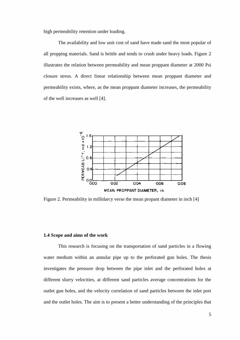
The availability and low unit cost of sand have made sand the most popular of

all propping materials. Sand is brittle and tends to crush under heavy loads. Figure 2

illustrates the relation between permeability and mean proppant diameter at 2000 Psi

closure stress. A direct linear relationship between mean proppant diameter and

permeability exists, where, as the mean proppant diameter increases, the permeability

of the well increases as well [4].

Figure 2. Permeability in millidarcy verse the mean propant diameter in inch [4]

1.4 Scope and aims of the work

This research is focusing on the transportation of sand particles in a flowing

water medium within an annular pipe up to the perforated gun holes. The thesis

investigates the pressure drop between the pipe inlet and the perforated holes at

different slurry velocities, at different sand particles average concentrations for the

outlet gun holes, and the velocity correlation of sand particles between the inlet port

and the outlet holes. The aim is to present a better understanding of the principles that

6

affect the design of slurry systems in horizontal pipelines.

This research presents previous relevant experimental and numerical

investigations on slurry flows. Hence, introducing the experimental setup and the

numerical methods used. Characterization of the CFD turbulence models and the

validation of the selected turbulence model is discussed. The results are presented in

terms of the pressure gradient, particle concentration and velocity distribution off the

gun holes.

1.5 Research Objectives

The overall goals of this thesis are:

1. Characterizing turbulence models that can capture the hydraulic fracturing slurry

flow behavior in a horizontal pipe.

2. Investigating the pressure drop between the pipe inlet and perforated holes at

different slurry velocities.

3. Investigating the sand average concentrations of the different outlet perforated

holes at different slurry velocities.

4. Investigating the velocity correlation of sand particles between the inlet and the

outlet holes.

Accordingly, achieving these overall goals require fulfillment of three sub-

objectives:

1. Characterizing the process of hydrofracturing treatment, identifying the fluid and

proppant agent which have been used in this process over the years, and analyzing

the challenges and difficulties in the hydrofracturing process.

2. Classifying the slurry rheology and flow regimes.

3. Investigating the previous works in literature which studied and contributed to the

field of slurry flow in horizontal well experimentally and numerically.

7

CHAPTER 2: LITERATURE REVIEW

2.1 Introduction on slurry flow

A semi-liquid mixture of solid particles with a carrier liquid is known as

Slurry. Overall, sand is useful to easily prop open the fractures in shallow formations.

It is because sand doesn’t cost much per pound as compared to other proppant i.e.

silica sand, ceramic proppants, and resin-coated sand (RCS). While, the solid particles

are merely just sand. Similarly, there are various kinds of liquid carriers. However,

water is the practical liquid that is used in the thesis unless otherwise stated. These

slurries can also be called conveying or hydraulic transport, if they are used for the

transportation of some material that is suspended in water [18].

To understand the whole slurry flow process, it is essential to have an accurate

prediction of slurry flow characteristics. The characterization of the slurry flow

regime is useful in developing and validating empirical and numerical multiphase

models. In industry, it is very important to define the type of slurry flow regimes for

designing, optimization, and controlling processes involving slurry flow. In spite of

the large area of application, a complete description of the flow based only on

differential equations is not possible, due to the complexity of two-phase flow

systems. Many researchers studied over the years the effect of solid particle

concentrations, pressure drop, and velocity distribution along with other flow

parameters to understand the flow regime governing mechanisms [9, 19]. Generally,

the attempt to solve the slurry flow regimes problems could be approached by begins

from experimental data and simplifies know correlations for some parameters by

dimensional analysis. The second method is using numerical methods to solve the

basic equation of motion with mathematical assumptions for different terms.

Computational Fluid Dynamics (CFD) is a computer-based numerical analysis system

8

[20]. This sophisticated CFD develops and adopts suitable mathematical models in

order to provide a tool for the analysis of complex solid-liquid slurry flow problems.

With lower cost and great ease, CFD helps researchers to conduct detailed numerical

analysis of the complex flow regime. CFD provides information within the

computational domain, extensively regarding the variation locally made, of the flow

parameters [19]. This chapter describes slurry rheology and its associated

characteristics, flow regimes, and previous experimental and numerical studies related

to the slurry flow in a horizontal pipeline.

2.2 Rheology of the slurry

Rheology is one of the most important characteristics associated with slurries.

It can be defined as the study of the behavior of materials related to their flow, for

both fluids and solids. This definition can easily be applied to complex

microstructural substances which may include mud, suspensions, slurries, and sludge.

Trying to understand the rheology related to slurries is very basic and necessary in

order to properly design and engineer slurry systems [21, 22]. The same rheology is as

well, a property that is dynamically concerned with the microstructure that is the basis

of the slurry. It is henceforth, easily affected by different attributes e.g. the shape,

density, mass fraction, and size of the solid suspended particles. A similar effect is

imparted by the viscosity and density of the carrier liquid. Therefore, this section will

give an outline to all the basic qualities of slurry flows. It will also explain the key

physical properties of slurries. Accurate engineering and efficient designing are

dependent on these properties.

2.2.1 Newton’s Law of viscosity

Viscosity is that one rheological attributes which has a lot of significance

when it comes to liquids. Simultaneously, viscosity can be known as the quantity that

9

shows any fluid’s ability to resist flow. It is imparted with friction forces in between

the particles prevents them from moving in conjunction to one and another. The

idealized situation used to describe viscosity is Couette flow. It is the phenomenon

that involves the trapping of a fluid in between a horizontal plate simultaneously

moving at a constant speed V0 and a stationary plate horizontally, across the surface

of the liquid. In turn, the topmost layer of the liquid will start moving parallelly to the

moving plate, this will take place at the exact speed as the moving plate (V = V0).

Therefore, every layer of the liquid will start to move slower as compared to the layer

on the top of it because of the frictional forces that are resisting the relative motion.

Furthermore, the fluid will start to exert a force opposite to the direction of its motion,

on the moving top plate. Therefore, a force externally, will be required in order to

move the top plate [23]. The Couette flow is exemplified in figure 3.

Figure 3. Couette flow for defining viscosity [24].

The external force of friction F will be proportional to speed Vo as well as the

area A of the plates, and at the same time, inversely being proportional to their

separation. It is shown in the equation (1).

10

𝐹 = 𝜇𝐴𝜕𝑉

𝜕𝑦

Where:

𝜇: Fluid dynamics viscosity.

A: surface area

𝑉0: moving plate speed

Y: Separation of the plates on the y-axis

A fluid having a viscosity that is not dependent on the stress is known as a

Newtonian fluid (kept after the great name of Isaac Newton); he showed the viscous

forces with the usage of the differential equation (2). For a Newtonian fluid, the shear

stress at a surface element parallel to a flat plate at the point y is given by:

𝜏 = 𝜇𝜕𝑉

𝜕𝑦

Where:

𝑉: The flow velocity along the boundary;

y: The height above the boundary.

Pa·s is the SI unit for viscosity. However, viscosity can be also presented in

centipoises, (cP). Similarly, the shear stress comes in direct proportion to the velocity

gradient (the shear rate), for Newtonian fluids. In Addition, shear stress will be given

off as zero if velocity gradient is also zero.

2.2.2 Slurry density

Density of slurry is influenced by, the concentration of solid particles, the

density of the carrier liquid and density of the solid particles. For the concentration of

the solid particles, moreover, the value is often shown in percent by weight. The only

reason to it is convenience; when the calculation is done for the pipeline throughout

… (1)

… (2)

11

tonnages. Despite that, slurry properties in pipeline flow are influenced greatly by the

volume of solids. Similarly, density of slurry using solid percent by weight can be

defined easily by the following equation (3) [25].

𝜌𝑚 =100

𝑐𝑤𝜌𝑠+ 100 − 𝑐𝑤

𝜌𝑙

Where

𝜌𝑚= density of slurry (kg/m3)

𝑐𝑤 = concentration of solids by weight in the slurry (%)

𝜌𝑠 = density of the solids (kg/m3)

𝜌𝑙 = density of liquid without solids (kg/m3).

The concentration of solids by volume, CV, is expressed in percent by the

following equation (4) [25]:

𝐶𝑉 =𝐶𝑤𝜌𝑚𝜌𝑠

=100

𝐶𝑤𝜌𝑠

𝐶𝑤𝜌𝑠+100 − 𝐶𝑤

𝜌𝑙

The concentration by weight of solids, CW, is conversely expressed, in percent by

the equation (5) [25].

𝐶𝑊 =𝐶𝑣𝜌𝑠𝜌𝑚

=

𝐶𝑣𝜌𝑠

𝐶𝑣𝜌𝑠 + (100 − 𝐶𝑣)

Slurry density is measurable directly by using online measurements or in

laboratory testing. However, when settling slurries are being measured, care is

required for the assurance of keeping the larger particles from settling out before the

… (3)

… (4)

… (5)

12

measurement is done. Similarly, flow rates have to be suitably increased to assure

appropriate suspension of the particles in the case of online measuring. It is possibly

better to sometimes, make measurements of the fluid and particle densities in order to

provide a definition of the density of the slurry with a provided concentration. In

contrast to it, slurry density is usable as a measure of concentration [26].

2.3 Fluid Flow Regimes

In general slurry flow regimes can be classified into four principal regimes in

horizontal pipe according to the solid concentration profile; homogeneous,

heterogeneous, stationary bed and moving bed. When systems of slurries are being

designed, possibly the most influential part that requires prior determination is the

behavior of settlement that is being imparted the slurry. So, slurries are, further

divided into two types, in practice, basing on the settlement of particles inside the

carrier liquid in the given flow conditions. Solid particles normally settle in all sorts

of carrier liquid when provided with enough time. Similarly, all the methods for

gravity separation are centered on the same fact. So, when applied practically, it is

very crucial to know the behavior of the solid particles when the sole objective is the

transportation of the solid particles by the use of hydraulic conveying, i.e. slurry

pumping [26].

In settling or heterogeneous slurries, the particles do not get suspended

properly in the carrier liquid. Instead, simply transport with the liquid. Contrary to

this, they become suspended by turbulence at high velocities. With heterogeneous

slurries, it is necessary to take care to prevent plugging of pipelines, so that keeping

the velocities of the pipelines higher than the critical settling velocity is possible, that

comes with the particles. A Heterogeneous slurry is usually water based and comes

with a huge quantity of solid particles that are greater than 100 μm in size. At the

13

same time, a lesser content of solids that are smaller than 40 μm (fines) means that the

fine particles and water (carrier fluid) is somewhat same as water. Non-settling or

homogeneous slurries are those which have solid particles being in a suspended state

in the carrier liquid in a continuous phase. The homogeneous slurries have features

that may or may not vary significantly from different basic Newtonian liquids or

water. The finer particles henceforth, make an increment in the viscosity of fluid [26].

In general, settling slurries are more complex and have a significant effect on pump

performance, as a result, many practical applications tend to use non-settling slurry.

Figure 4. comparatively harsh method to find the slurry is settling or non-settling [27]

Whether the slurries are non-settling or settling, is decided by the specific

gravity and the particle size of solid particles. Therefore, a raw determination can be

estimated between non-settling and settling behavior using a chart given in the Figure

14

4 [27]. This is a comparatively harsh method and therefore, should be treated as such.

Moreover, it only considers the specific gravity and the average particle size of the

solid, however it is to be noted that slurry concentration also effects on the settling

behavior of solids.

2.3.1 Transitional velocities

Slurry flow in a horizontal pipe can be classified with solid phase

concentration into four distinct flow regimes; Stationary bed, moving bed, asymmetric

flow and symmetric flow (Figure 5). The Pressure drop per meter of pipe are on the

plot against the mean flow velocity. So, the pressure drop behavior of every flow

regime differs greatly.

Figure 5. Pressure drop vs the mean flow velocity at different flow regimes of

heterogenous slurries [26].

15

As the heterogeneous slurry velocity decreases, the solids-concentration

gradient increases until either a stationary or a slowly moving particle bed appears

along the pipe bottom. That the lowest pressure drop is achieved at transitional

velocity of which a particle bed forms, is defined as the critical velocity, deposition

velocity or limiting velocity (V3) and represents the lower pump rate limit for

minimum particle settling. A further decrease in slurry velocity increases pressure

loss, as indicated by the characteristic upward hook of slurry curve, and may also

cause pipe plugging. The motion of solid particles starts in the upper pipe as the speed

of the slurry exceeds the moving bed, where gravity causes asymmetrical suspension

configuration of forces and segregation is always present. At extremely high velocity,

fine particle sized, and or small density differences between solids and liquid, a

symmetrical suspension is formed in which the solid are uniformly distributed

through the liquid. Later, hydraulic fracturing slurries are shown to exhibit this

heterogeneous response.

2.3.2 Laminar and turbulent models

In respect with driving forces, fluid flow is categorized into two different types;

laminar flow and turbulent flow (Figure 6) [28]. Laminar Flow: A fluid flows through

a smooth path with no disruption between its infinitesimal parallel layers. It is quite

compatible to examine laminar flow both numerically and experimentally. On the

other hand, turbulent flow is a type of fluid flow that is unsteady, enormously

irregular in space and time, three-dimensional, rotational, dissipative (in terms of

energy), and diffusive (transport phenomenon) at high Reynolds numbers. Due to

those divergences in turbulent flow, extremely small-scale fluctuations emerge in

velocity, pressure, and temperature. Thus, requires rigorous effort during

experimental and numerical examinations [29].

16

Figure 6. Turbulent and laminar flow [23].

Earlier, it was difficult to perceive the type of fluid flow numerically. Irish

scientist Osborne Reynolds (1883) discovered the dimensionless number that predicts

fluid flow based on static and dynamic properties such as density, velocity, length,

and dynamic viscosity [28]:

Re = (inertial force) / (viscous force)

= ρVL

μ

Where ρ (kg/m3) is the density of the fluid, V (m/s2) is the characteristic

velocity of the flow, L (m) is the characteristic length scale of flow, and μ (Pa*s) is

the dynamic viscosity of the fluid. Figure 7 explains the type of the flow based on his

Reynolds number.

… (6)

17

Figure 7. Types of the flow according to the Reynolds number

2.3.3 Calculation of critical deposition velocities

That velocities in which the lowest pressure drops achieved is at flow

transforming from moving bed to asymmetric flow is called the critical deposition

velocities (VD). Also, this transition point has different names as critical velocity or

limiting velocity. The initial equation for the determination of the V3 (or VD)

transitional velocity is given in 1952 by Condolios and Durand [30], it is shown in the

equation (6):

𝑉𝐷 = 𝐹𝐿√2𝑔𝐷𝑖[𝜌𝑠 − 𝜌𝐿)/𝜌𝐿]

The Durand factor is shown mostly in a graph of single of thin-graded

particles. Simultaneously, basing on the work done by Durand (1953), the original

graph, is normally thought of to be a bit conservative for a lot of slurries that include a

mix of particles of various sizes. But, it is still used, e.g. Weir, which is a supplier of

pumps that specializes in slurry pumps [31]. Furthermore, the Durand’s limiting

settling velocity parameter diagram for narrow graded particles is also given in

… (7)

18

appendix A [32]. Moreover, Weir consider narrow particle size distribution as one

where the ratio of particles sizes, does not exceed approximately 2:1 expressed as

testing screen apertures, for about 90 % by weight of the total solids.

Therefore, several other correlations were proposed as an experimental factor,

each of which attempted for the improvement in the pioneering work given by

Durand. The reviews of different correlations are accessible in literature, for example

by Turing et al. (1987) and Carleton & Cheng (1974) [33]. A modified Durand’s

limiting settling velocity parameter diagram, suitable for a more widely graded

particle sizes, later used by Weir (Anon, 2009) is shown in the Appendix B [32].

In 1991, Schiller and Herbich proposed the equation (7) to calculate the

Durand factor:

𝐹𝐿 = {(1.3 × 𝐶𝑣0.125)[1 − exp(−6.9 × 𝑑50)]}

Where:

𝐶𝑣: volumetric concentration in percent

𝑑50: Average diameter of solid particles (mm)

In 1970, Wasp and Aude, later created an equation that was modified, the

basis of it was laid on the equation given by Durand and Condolios (equation 6),

known as Wasp’s equation. There was an included ratio between the inner diameter of

the pipe and the solid particle diameter. Therefore, the equation also comprises of a

modified Durand factor, 𝐹𝐿′. Wasp’s equation is given in equation (8).

𝑉𝐷 = 𝐹𝐿′√2𝑔𝐷𝑖[𝜌𝑠 − 𝜌𝐿)/𝜌𝐿] (

𝑑50𝐷𝑖)1/6

… (8)

… (9)

19

Where:

𝐹𝐿′ = 3.399 × 𝐶𝑉

0.2156

The results for critical deposition velocity, coming from Wasp’s equation are

naturally lower than those given off by original Durand formula. Later in 2006,

Wilson et al. use a comparable term, it was based on the work done by Wilson’s

earlier in the 1970’s, the velocity at limit of stationary deposition. This can be called a

flow speed, in the base of which there is a formation of a stationary bed inside the

pipe. After that, they paralleled this with the critical deposition velocity by Durand.

Contrary to this, the comparison is not completely accurate. So, the critical deposition

velocity shows a flow speed that has a moving bed forming below it, in Durand’s

model. As mentioned earlier, there is a noticeable difference between a stationary bed

and a moving bed [34].

Wilson et al. (2006) concluded that the velocity is concentration dependent at

the extent of stationary deposition, that have low values at likewise concentrations

which simultaneously rise to the highest value at an intermediate concentration value,

soon after this, dropping off again at concentrations that are much higher. They made

use of a force balance analysis for the development of a model to predict, at the extent

of stationary deposition, the velocities, and specifically for the highest velocity

(denoted VSM). The problem that arose with the model is, it requires too much values

that are not accessible for a process engineer when considering the basic engineering

timing of a project. Moreover, it needs a lot of values that are solely published as

graphs. This makes the usage weighty, as there are needs when the sizing has to be

done for hundreds of different pumps and pipelines.

… (10)

20

2.4 Previous work on slurry flow:

Researchers investigated numerically and experimentally, the solid-liquid

slurry flow through both vertical and horizontal pipelines. For a better understanding

of the slurry flow process, the researchers developed general numerical models for the

description of the characteristics regarding various flow parameters which includes,

concentration distributions, pressure drops, deposition velocity distributions.

Using a diffusion model, initial studies of O’Brien (1933), and Rouse (1937)

were able to predict the concentration distribution inside a gravity based open channel

slurry flow that contained extremely low solid volumetric concentration [34-36].

Following this, other researchers Shook and Daniel (1965) Karabelas (1977), Shook

et al. (1968), Gillies et al. (1991), Roco and Shook (1983), Gillies and Shook (1994),

Seshadri et al. (1982), Roco and Shook (1984), Gillies et al. (1999), Gillies and Shook

(2000) have studied the effects of solid concentration distributions in slurry flow in

relation to various flow parameters [37-46]. Many researchers scrutinized the slurry

flow process, focusing on the prediction of flow velocity distribution. Some of the

contributions in this area involve the work of Wasp al. (1970), Gillies et al. (1991),

Doron et al.(1987), Sundqvist et al. (1996), Ghanta and Purohit (1999), Mishra et

al.(1998), Wilson et al. (2002) [40,47-52]. Various studies formulated predictions of

the pressure drop in a slurry flow process. Similarly, in this area, these were the

noteworthy contributors: Masayuki Toda et. al (1972), experimentally investigated the

pressure drop in a pipe bend for the solid-fluid slurry flow [53]. Later, Turian and

Yuan (1977) formed a pressure drop correlation for the flow of slurries in pipelines in

consideration with a stationary bed, heterogeneous flow, saltation flow, and

homogeneous flow regime [54]. Moreover, P. Doron et. al (1987) also developed a

two layer model for the prediction of pressure drop of a slurry flow of coarse particles

21

and that too, through horizontal pipelines [48]. Later, Geldart and Ling (1990), Doron

and Barnea (1995), Gillis et. al (1991), A. Mukhtar et. al (1995), J. Bellus et. al (2002)

Turian et. al (1998), devised different models of the slurry flow through pipes [40, 55-

59]. They predicted the pressure drop in relation to various flow parameters that

included, concentration distribution, granular pressure effects, velocity distributions,

energy effects and turbulence kinetics.

Table 1 presents an overview of the work that has been carried in the field of

annular slurry flow (sand and water) in a horizontal pipeline either using Ansys-fluent

software or performing practical lab-scale experiments or both. Where, CFD

simulations helped to minimize assumptions by using the physics-based Navier–

Stokes equations to model the hydrodynamics of the flow system. Also, table-1 shows

the different parameters used in each study such as the multiphase and viscous model,

the diameter of the horizontal pipe (D), the slurry velocity (𝑣), the solid particle

diameter (ds), the solid particle density (𝜌), and the volumetric concentration (Cv%) of

the slurry flow.

22

Table 1. An overview of previous academic research on slurry flow

Reference Multiphase model Viscous model D (mm) ds (mm) 𝝆 (Kg/m3) 𝒗 (m/s) Cv %

(Gillies & Shook,

1994) [42] 53.2 0.18 2650 3.1 14, 29, 45

(Matousek, 2001)

[60] 150

0.12, 0.37,

1.85 2-10 12 - 43

(Kaushal & Tomita,

2002) [61] 105

0.38, 0.91,

1.28, 1.80,

2.55, 7.39

2 4.0, 8.2, 13.5,

18.6

2.75 12.2, 19.1, 25.8

3.5 12.2, 18.6, 26.0

(Ling, Skudarnov,

Lin, & Ebadian,

2003)

[62]

Algebraic slip

mixture (ASM)

RNG k–ε

turbulent 22.1 0.11 2381 & 4223 1-3 10, 20

(Hernández, Blanco,

& Rojas-Solórzano,

2008) [63]

Eulerian

multiphase

RNG k–ε

turbulent 22.1 0.30 2390 3 5

(Kaushal, Thinglas,

Tomita, Kuchii, &

Tsukamoto, 2012)

[64]

Eulerian

multiphase Standard k– ε 54.9 0.125 1-5 0-5

23

Reference Multiphase model Viscous model D (mm) ds (mm) 𝜌 (Kg/m3) 𝑣 (m/s) Cv %

(Vlask, Kysela, &

Chara, 2012)

[65]

36 6 2540, 2560 1.0-5.5 2.7, 2.9, 6.1, 6.5,

9.7, 10.4

(Nabil, El-Sawaf, &

El-Nahhas, 2013)

[66]

Eulerian

multiphase Standard k– ε 26.8 0.2, 0.7, 1.4 2650 0.5- 5.0 10-30

(Gopaliya & D.R.,

2016)

[67]

Eulerian

multiphase

RNG k-ε

turbulence 263

0.165 2650 3.5 9.95, 18.4, 26.8,

33.8

0.29 2650 4.0, 4.7 16, 25, 34

0.55 2650 3.9, 4.4 15, 25, 30

(Ofei & Ismail, 2016)

[68]

Eulerian

multiphase Standard k– ε 103 0.09-0.27 2650 5.4 10-40

(Sultan, Rahmana,

Zendehboudia,

Talimi, & Kelessidis,

2018) (Skudarnov,

Lin, & Ebadian,

2004)

[69, 70]

Eulerian

multiphase

Reynolds Stress

Model (RSM) 23 0.14

(2490 &

4200) 1.3-2.3 15

(Sultan, Rahmana,

Zendehboudia,

Talimi, & Kelessidis,

2018)

[69]

Eulerian

multiphase

Reynolds Stress

Model (RSM) 26

0.165 2650 3.5 9.95, 18.4, 26.8,

33.8

0.29 2650 4.0,4.7 16, 25, 34

0.55 2650 3.9 15, 25, 30

24

Reference Multiphase model Viscous model D (mm) ds (mm) 𝜌 (Kg/m3) 𝑣 (m/s) Cv %

(Ahmed & Mohanty,

2018)

[20]

Eulerian

multiphase

RNG k-ε

turbulence 54.9 0.125 2470 2, 5 30, 40

25

2.5 Conclusion of literature review

Overall, investigations of two-phase slurry flow through pipelines aim to

develop general solutions based on available experimental data for solid volumetric or

mass concentration profiles, pressure gradients and slurry velocity profiles. Various

studies scrutinized the flow of Newtonian fluids in annuli to develop empirical and

analytical models. However, the novelty of this research work is demonstrated on the

presentation of the hydrofracturing fluid pressure issuing off the perforating gun

holes, as the fluid pressure is expected to be lower at the outlet holes according to

Bernoulli theory. It is evident through the literature review that none of the previous

studies investigated or analyzed the slurry flow at the outlet perforated holes, yet

many thorough studies have investigated the different parameters of the slurry system

in horizontal pipes.

Also, it is noticeable that none of the previous studies have used Particle

Image velocimetry (PIV) in which it has a high ability to measure the instantaneous

velocity of the particles and diagnose the slurry flow by using non-instructive leaser.

Hence, the PIV technology will be utilized in the experimental work of this thesis for

a better understanding of the whole slurry flow process.

Furthermore, it is observed that most of the fracturing fluid is using sand

particles due to its availability and low unit cost as explained in chapter 1.

Consequently, the sand particle will be used as the proppant agent in the research.

Generally, most of the numerical studies in table-1 used Eulerian and RNG k-ε

turbulent for the multiphase and viscous model, respectively in which it indicates the

effectiveness of these two models in solving the slurry flow system and its parameters

such as pressure drop, solid concentration profiles, and deposition velocity.

Finally, it is observed that the studied slurry velocities range from 1 to 10 m/s,

26

the particle volumetric concentration ranges from 2.7% to 40%, the particle diameter

ranges from 0.09 mm to 7.39 mm, and the diameter of the horizontal pipe ranges

between 23 mm to 263 mm. These limitations will be taken into consideration in the

designing of the slurry flow system in chapter 3.

27

CHAPTER 3: MATERIAL AND METHODS

This chapter is divided into two main sections; the experimental setup and the

numerical simulation. Each part presents the material and methods which have been

used to analyze the slurry flow in a horizontal perforated pipeline. Figure 8 presents

the flowchart of the thesis approach. Where, selecting a suitable turbulence model

between (k-휀, RNG, RSM) is carried through comparing the results against published

experimental data. The selected turbulence closure in modeling the slurry flow in a

perforated pipe is validated through conducting an experiment in a lab-scale.

Throughout the experiment, various issues have occurred (which will be mentioned

later), yet some results have been achieved.

Figure 8. Flowchart of the thesis approach.

28

3.1 Experiential setup:

A closed loop pipe system, with a test section of clear acrylic pipe, is used to

experimentally investigate the slurry flow parameters. The experiment utilized a

slurry composed of one size particle dry sand of density of 1442 Kg/m3 mechanically

mixed with water. From an open tank, the slurry was pumped throughout the circuit

using a centrifugal pump, Xylem DL-125. A variable frequency speed drive was used

to control slurry flow rate. A digital pressure gauge, ASHCROFT 2030 sanitary gauge

model, was used to measure the system slurry pressure. The detailed specifications of

the pump and the pressure gauge are presented in appendix C and D, respectively.

Figure 9. Schematic setup of slurry flow system.

Figures 9 and 10 present the components of the experimental setup used in this

study. Component (1) is the DL 125 xylem centrifugal pump with a maximum flow

rate of 67.2 GPM and maximum pressure of 152 kPa (Figure 11). Component (2) is

29

the mixing tank of a capacity of 14.3 gallons, where the sand and water are

continuously mechanically mixed. Component (3) is the internal acrylic pipe of

dimensions of 2 inches in diameter, 3mm thickness, and 2m long. Component (4) is

the outlet gun holes of the internal pipe; four holes are drilled symmetrically with a

diameter of 5 mm. Component (5) is the return line of the external pipe with a

diameter of 12 mm, where the slurry flow is returned to the mixing tank (2).

Component (6) is the Particle image velocimetry (PIV) system which is connected to

a computer to non-intrusively record and measure the velocity and visualize the

movement of sand particles through the internal perforated gun holes (4). Component

(7) is a digital slurry pressure gauge connected to the external pipe near the perforated

holes to measure the pressure with an accuracy of 0.25% (Figure 12). Component (8)

is the variable frequency drive (VFD); used for adjusting the flow rate and the

pressure of the centrifugal pump (1) as required.

Figure 10. The apparatus of the slurry flow experiment.

Return line Internal holes

location

Internal pipe Digital pressure

gauge

30

Figure 11. DL 125 xylem submersible pump.

Figure 12. Digital slurry pressure gauge.

3.1.1 Velocity measurement using particle image velocimetry (PIV)

Particle image velocimetry (PIV) is an experimental tool to non intrusively

obtain the velocity of a whole flow field. PIV is based on detecting the light scattered

from the sand as tracer particles contained in the slurry flow. It captures two

consecutive images of the sand seeded flow field. Cross correlation of the two images

is used to estimate the displacement of each group of sand particles, and from the

knowledge of the time between the frames, a corresponding velocity is obtained. The

31

sand particles are illuminated at two different time instants by means of a double

pulsed laser sheet. The laser used is Dantec Dynamics DualPower 200-15, which is a

twin cavity Nd:YAG laser. Wavelength is 532 nm, and the pulse duration is 4 ns.

Maximum laser power is 1200 mJ. For processing the acquired images and the results,

DynamicStudio software is used. The camera used is a CCD camera, which is the

FlowSense EO 4M from Dantec Dynamics, with a resolution of 2048 × 2048 pixels.

In order to obtain the velocity field, a set of 50 double frame images were acquired at

a triggering frequency of 7.4 Hz, which spans a period of 6.75 seconds. The time

between the light pulses, which is also the time between the two frames of a double

frame image, was 1000 𝜇𝑠𝑒𝑐. Each double frame image resulted in a velocity field.

Hence, 50 velocity fields were obtained and averaged to obtain the final flow filed

velocity. The interrogation window size was 32 × 32 pixels with a 50% overlap in

both the horizontal and vertical directions, which resulted in a map of 127 × 127

vectors map (Figure 13) [71].

Figure 13. Typical 2-D PIV setup [71].

32

3.1.2 The slurry system design of the experiment

The design of the slurry system experimental set up was based on several

factors such as the internal pipe diameter and the particles size of the dry sand. In his

experimental study of a slurry system, Gopaliya (2016) reported that the pressure

gradient of slurry flow in a horizontal pipeline, of an internal diameter D, becomes

almost constant after a length of 25-30D downstream [67]. To ensure a fully

developed flow, the gun holes of the internal pipe were drilled at about 33D of the

internal pipe length. The internal perforation holes were drilled about 1.7m

downstream of the pipe inlet. The diameter of the internal pipe perforation holes was

drilled based on the range of the most commercial perforating gun punch holes which

were in (0.23 in to 0.72 in) range [72]. The lowest reported mean value of sand

particle diameter in well stimulation was about 500 microns [4]. Using an auto sieve

shaker (Figure 14), in this experiment, the dry sand particles were sieved to limit the

range of sand particle size between 425 microns and 600 microns [73].

Figure 14. Auto sieve shaker.

33

3.1.3 The challenges of slurry experiment:

Finding a suitable pump for the slurry system was the most challenging part of

the experimental work due to their unavailability in Qatar Market and their high cost

in the international market. Moreover, the selected pump from Italy failed two times

due to a malfunction in the seal system as a result, few results have been achieved,

and they were not sufficient to build facts or to establish a full conclusion. Also, the

process of manufacturing the pipe, and assembling the parts from different places

were a big challenge to make the slurry system. Finally, the laboratory space was not

enough to make a larger model with a larger pump, so the space element was also a

factor in the system designing. Therefore, the focus was on simulation in order to

compensate for the major shortfall in practical experience. However, some results

were extracted from the experiment which supports the simulation process and proves

its validity.

3.2 Numerical simulation

Computational Fluid Dynamics (CFD) techniques were used to study slurry

flow in a horizontal pipeline. CFD is based on solving the relevant equations of

motion by numerical methods. Recent improvements in numerical procedures, in

meshing schemes and in computational power made it possible to consider large and

complicated simulations.

ANSYS- Fluent is used as a simulation tool in many industrial applications

due to its physical modeling capabilities to model flows, turbulence, reactions and

heat transfer. FLUENT software was tested using experimental data of various

research and proved its ability to perform detailed simulations and generate matching

results when using appropriate methods and high-quality mesh [74]. This study used

the commercially available CFD software ANSYS-Fluent to perform the numerical

34

simulations of the slurry flow in a horizontal pipe. Assigning appropriated boundary

conditions, all governing equations of slurry flow were solved in a Cartesian

coordinate system.

3.2.1. Mathematical models

Selection of an appropriate viscous model is foremost important in the CFD

analysis of slurry flows. The selection depends mainly on the flow Reynold number

and the range of volume fraction (α) of the flow solid phase. Since Reynold number,

considered in this study, is higher than 500,000, the type of the flow is considered as

turbulent.

In the literature review section, most of the studies used Eulerian model to

simulate several types of slurry flow through different pipe diameters. For each phase,

the Eulerian model solves the momentum equations in a segregated method. Ansys

Fluent algorithm solves the total pressure of multiphase for a wide range of flows due

to the shared pressure of the multiphase flow and volume fraction equations.

Additionally, solving the implemented phase coupled (SIMPLE) in an implicit

manner rather than explicit, offers a robust solution to the multiphase system.

In this research, granular version of the Eulerian model with implicit

calculations was adopted for calculating the different parameters of the slurry flow.

The Granular version is capable of capturing the effect of friction and collisions

between the sand particles which is an important phenomenon in higher concentration

slurry flows of different particle sizes. Granular viscosity and frictional viscosity were

modeled using Syamlal-Orbien and Schaeffe model respectively [75]. Drag and lift

coefficients in the phase interaction were calculated based on the equations of

Schiller-Naumann and Moroga [75].

35

3.2.1.1 Mixture theory approach

The description of Eulerian multiphase flow is account for dispersed-

continuous phase interaction in which it incorporates with the concept of phasic

volume fractions, denoted by (𝛼𝑞). Volume fractions represents dispersed phase

dissolved in each continuous phase, and the laws of conservation of mass and

momentum are satisfied by each phase individually. The mixture theory approach can

be used for the derivation of the conservation equations. The volume of phase q.

Where, q is either solid (s) or fluid (f), 𝑣𝑞, is defined by [75]

𝑣𝑞 = ∫𝛼𝑞𝑑𝑣.

𝑉

Where

∑𝛼𝑞 = 1

𝑛

𝑞=1

The effective density of slurry flow (𝜌�̇�) is

𝜌�̇� = 𝛼𝑞𝜌𝑞

Where, 𝜌𝑞 is the physical density of phase. The volume fraction equation is solved

through implicit time discretization.

3.2.1.2 The continuity equation

𝜕

𝜕𝑡(𝛼𝑞𝜌𝑞) + ∇. (𝛼𝑞𝜌𝑞𝑣𝑞⃗⃗⃗⃗⃗) = 0

Where, 𝑣𝑞⃗⃗⃗⃗⃗ is the velocity vector of phase q.

… (11)

… (12)

… (13)

… (14)

36

3.2.1.3 The momentum balance for fluid phase:

𝜕

𝜕𝑡(𝛼𝑓𝜌𝑓�⃗�𝑓) + ∇. (𝛼𝑓𝜌𝑓�⃗�𝑓𝑣𝑓)

= −𝛼𝑓∇𝑃 + ∇. 𝜏�̿� + 𝛼𝑓𝜌𝑓�⃗� + 𝐾𝑠𝑓(�⃗�𝑠 − �⃗�𝑓) + �⃗�𝑙𝑖𝑓𝑡,𝑓

+ 𝐶𝑣𝑚𝛼𝑓𝜌𝑓(�⃗�𝑠. ∇�⃗�𝑠 − �⃗�𝑓∇�⃗�𝑓)

3.2.1.4 The momentum balance for solid phase:

𝜕

𝜕𝑡(𝛼𝑠𝜌𝑠�⃗�𝑠) + ∇. (𝛼𝑠𝜌𝑠�⃗�𝑠�⃗�𝑠)

= −𝛼𝑠∇𝑃𝑠 + ∇. 𝜏�̿� + 𝛼𝑠𝜌𝑠�⃗� + 𝐾𝑓𝑠(�⃗�𝑓 − �⃗�𝑠) + �⃗�𝑙𝑖𝑓𝑡,𝑠

+ 𝐶𝑣𝑚𝛼𝑠𝜌𝑓(�⃗�𝑓 . ∇�⃗�𝑓 − �⃗�𝑠∇�⃗�𝑠)

Where;

∇𝑃: is the static pressure gradient.

∇𝑃𝑠: is the solid pressure gradient or the inertial force due to particle interactions.

∇. 𝜏̿: is viscous forces, where 𝜏�̿� and 𝜏�̿� are the stress-strain tensors for fluid and solid,

respectively.

𝜌𝑠�⃗� 𝑎𝑛𝑑 𝜌𝑙�⃗�: are body forces, where 𝜌 is the density and �⃗� is acceleration due to

gravity.

𝐾𝑓𝑠 𝑎𝑛𝑑 𝐾𝑠𝑓 : are inter-phase drag force coefficient caused by the velocity difference

between the velocity of fluid �⃗�𝑓 and solid �⃗�𝑠 phases.

�⃗�𝑙𝑖𝑓𝑡: is the lift force.

𝐶𝑣𝑚𝛼𝑠𝜌𝑓(�⃗�𝑓 . ∇�⃗�𝑓 − �⃗�𝑠∇�⃗�𝑠): is the virtual mass force. Since in most of the multiphase

applications, the effective particle radius is very small as compared to the velocity

… (15)

… (16)

37

scale, virtual mass effects can be observed predominantly only at relatively high

efflux concentrations. It is therefore, a value of 0.5 (default value) is adopted for 𝐶𝑣𝑚

in the present study [75]:

𝜏̿ is expressed as follow [75]:

𝜏̿ = 𝛼𝑞𝜇𝑞(∇�⃗⃗�𝑞 + ∇�⃗⃗�𝑞𝑇) + 𝛼𝑞(𝜆𝑞 −

2

3𝜇𝑞)∇. �⃗⃗�𝑞𝐼 ̿

Where;

𝐼 ̿indicates identity tensor 𝜆𝑞 represents bulk viscosity of the solid

𝜇𝑞 and 𝜆𝑞 are the shear and bulk viscosity of phase q,

3.2.1.5 Turbulent Models

Turbulence models are classified according to the applied governing equations

(Reynolds-averaged Navier-Stokes or Large Eddy Simulation equations). Within

these broader categories, turbulence models are further broken down by the number of

additional transport equations which must be solved in order to compute the model

contributions. The most common turbulence model is the k-ε model. However, there

are many other models in this caption. The k-ε model is called a family of models.

Specialized versions were developed for various specific flow configurations. Some

of the more common variants include the RNG k-ε models [76].

3.2.1.5.1 Standard k-ε Model

The standard k-epsilon (k-ε) turbulence model is used to simulated mean flow

characteristics for turbulent flow conditions. The turbulence models implemented in

this thesis belong to the class of two equations k-epsilon models. The original impetus

for the k-ε model was to improve the mixing-length model, as well as to find an

alternative to algebraically prescribing turbulent length scales in moderate to high

… (17)

38

complexity flows. The model assumes that the ratio between Reynolds stress and

mean rate of deformations is the same in all directions. The turbulence closure is

achieved using two transport PDEs for the turbulence kinetic energy k and turbulence

dissipation ε scalars [75, 76]:

For turbulent kinetic energy k:

𝜕(𝜌𝐾)

𝜕𝑡+ 𝜕(𝜌𝑘𝑢𝑖)

𝜕𝑥𝑖=𝜕

𝜕𝑥𝑗 [(𝜇 +

𝜇𝑡𝜎𝑘) 𝜕𝐾

𝜕𝑥𝑗] + 𝐺𝑘 + 𝐺𝑏 − 𝜌휀

For dissipation 휀:

𝜕(𝜌휀)

𝜕𝑡+ 𝜕(𝜌휀𝑢𝑖)

𝜕𝑥𝑖=𝜕

𝜕𝑥𝑗 [(𝜇 +

𝜇𝑡𝜎휀) 𝜕휀

𝜕𝑥𝑗] + 𝐶1𝜀

휀

𝑘(𝐺𝑘 + 𝐶3𝜀𝐺𝑏) − 𝐶2𝜀𝜌

휀2

𝑘

Where,

𝑢𝑖 represents velocity component in corresponding direction

𝐺𝑘 represents the generation of turbulence kinetic energy due to the mean velocity

gradients.

𝐺𝑏 is the generation of turbulence kinetic energy due to buoyancy.

𝜎𝑘 and 𝜎𝜀 are the turbulent Prandtl numbers for k and 휀 , respectively.

The turbulent or eddy viscosity 𝜇𝑡 is represented in terms of two turbulence

variables, the turbulence kinetic energy k and its rate of dissipation (휀):

𝑢𝑡 = 𝜌𝐶𝜇𝑘2

휀

… (18)

… (19)

… (20)

39

Equations (18, 19, and 20) consist of some adjustable constants (𝜎𝑘, 𝜎𝜀, 𝐶1𝜀, 𝐶2𝜀,

𝐶𝜇). The values of these constants have been arrived at by numerous iterations of data

fitting for a wide range of turbulent flows. These are as follows:

𝜎𝑘 = 1.00, 𝜎𝜀=1.30, 𝐶𝜇=0.09

𝐶1𝜀= 1.44, 𝐶2𝜀= 1.92

3.2.1.5.2 RNG k-ε Model

The RNG-based k-휀 turbulence model is derived from the Navier-Stokes

instantaneous equations, using a mathematical technique called “renormalization

group” (RNG) methods. RNG theory provides an analytically derived differential

correlation for turbulent Prandtl numbers that accounts for low Reynolds number

effects. while the standard k- ε model uses constant values. The main difference

between the RNG model and standard k-ε model lies in the additional term in the ε

equation that improves the accuracy for rapidly strained flows, given by [75,76]:

𝑅𝜀 =𝐶𝜇𝜌𝜂

3(1 −𝜂𝜂0)

1 + 𝛽𝜂3휀2

𝑘

Where 𝜂 = 𝑆𝑘/휀 , 𝜂0 = 4.38 , 𝛽 = 0.012. The constant parameters used indifferent

equations are taken as 𝐶1𝜀 = 1.42 , 𝐶2𝜀 = 1.68 , 𝐶3𝜀 = 1.2 , 𝜎𝑘 = 1.0 , 𝜎𝜀 = 1.3

3.2.1.5.3 Reynolds Stress Equation Model

Reynolds stress equation model (RSM), also known as second-order or

second-moment closure model is the nearly most complex classical turbulence model.

The exact transport equation for the Reynolds Stress Model (RSM) is [75]:

… (21)

40

𝜕

𝜕𝑡(𝜌𝑢𝑖

′𝑢𝑗′̅̅ ̅̅ ̅̅ )

⏟ 𝑙𝑜𝑐𝑎𝑙 𝑡𝑖𝑚𝑒 𝑑𝑒𝑟𝑖𝑣𝑎𝑡𝑖𝑣𝑒

+ 𝜕

𝜕𝑥𝑘(𝜌𝑢𝑘𝑢𝑖

′𝑢𝑗′̅̅ ̅̅ ̅̅ )

⏟ 𝐶𝑖𝑗=𝑐𝑜𝑛𝑣𝑒𝑐𝑡𝑖𝑜𝑛

= −𝜕

𝜕𝑥𝑘[𝜌𝑢𝑖′𝑢𝑗′𝑢𝑘

′̅̅ ̅̅ ̅̅ ̅̅ ̅ + 𝜌′(𝛿𝑘𝑗𝑢𝑖′ + 𝛿𝑖𝑘𝑢𝑗′̅̅ ̅̅ ̅̅ ̅̅ ̅̅ ̅̅ ̅̅ ̅̅ ̅̅ ̅̅ ̅)]⏟

+

𝐷𝑇,𝑖𝑗=𝑇𝑢𝑟𝑏𝑙𝑒𝑛𝑡 𝑑𝑖𝑓𝑓𝑢𝑠𝑖𝑜𝑛

𝜕

𝜕𝑥𝑘[ 𝜇

𝜕

𝜕𝑥𝑘(𝑢𝑖′𝑢𝑗′̅̅ ̅̅ ̅̅ )]

⏟ 𝐷𝐿,𝑖𝑗=𝑀𝑜𝑙𝑒𝑐𝑢𝑙𝑎𝑟 𝑑𝑖𝑓𝑓𝑢𝑠𝑖𝑜𝑛

− 𝜌(𝑢𝑖′𝑢𝑘′̅̅ ̅̅ ̅̅𝜕𝑢𝑗

𝜕𝑥𝑘+ 𝑢𝑗′𝑢𝑘

′̅̅ ̅̅ ̅̅𝜕𝑢𝑖𝜕𝑥𝑘

)⏟

𝑃𝑖,𝑗=𝑆𝑡𝑟𝑒𝑠𝑠 𝑃𝑟𝑜𝑑𝑢𝑐𝑡𝑖𝑜𝑛

− 𝜌𝛽(𝑔𝑖𝑢𝑗′𝜃̅̅̅̅̅ + 𝑔𝑗𝑢𝑖′𝜃̅̅̅̅̅)⏟ 𝐺𝑖𝑗= 𝐵𝑢𝑜𝑦𝑎𝑛𝑐𝑦 𝑝𝑟𝑜𝑑𝑢𝑐𝑡𝑖𝑜𝑛

+ 𝑝 (𝜕𝑢𝑖

′

𝜕𝑥𝑗+𝜕𝑢𝑗

′

𝜕𝑥𝑖)

⏟ 𝜑𝑖𝑗= 𝑃𝑟𝑒𝑠𝑠𝑢𝑟𝑒 𝑠𝑡𝑟𝑎𝑖𝑛

− 2𝜇𝜕𝑢𝑙

′

𝜕𝑥𝑘

𝜕𝑢𝑗′

𝜕𝑥𝑘⏟ 𝜖𝑖𝑗= 𝐷𝑖𝑠𝑠𝑖𝑝𝑎𝑡𝑖𝑜𝑛

− 2𝜌Ω𝑘( 𝑢𝑗′𝑢𝑚′̅̅ ̅̅ ̅̅ ̅𝜖𝑖𝑘𝑚 + 𝑢𝑖′𝑢𝑚′̅̅ ̅̅ ̅̅ ̅𝜖𝑗𝑘𝑚)⏟ 𝐹𝑖𝑗= 𝑃𝑟𝑜𝑑𝑢𝑐𝑡𝑖𝑜𝑛 𝑏𝑦 𝑠𝑦𝑠𝑡𝑒𝑚 𝑅𝑜𝑡𝑎𝑡𝑖𝑜𝑛

The various terms in these exact equations, 𝐶𝑖𝑗,𝐷𝐿,𝑖𝑗, 𝑃𝑖𝑗,and 𝐹𝑖𝑗 do not require

any modeling. However, 𝐷𝑇,𝑖𝑗, 𝐺𝑖𝑗, 𝜑𝑖𝑗, and 휀𝑖𝑗 need to be modeled to close the

equations.

… (22)

41

CHAPTER 4: RESULTS AND DISCUSSION

In this chapter, selecting a suitable turbulence model for this study will be

carried through comparing the numerical results of the pressure gradient and the solid

concentration profile for a slurry flow in a horizontal pipe against several published

experimental studies using three different turbulent models (Standard k-휀, RNG k-휀,

and RSM). Hence, the best matching turbulent closure model with the published

experimental data is selected for further simulation of the slurry flow of a perforated

pipe. In the second part of the research, the result acquired from the laboratory

experiment of a slurry flow in a horizontal perforated pipe are utilized to support the

validity of the selected turbulence model.

4.1 Selecting a suitable turbulence closure

4.1.1 Pressure gradient verification:

The mean slurry pressure gradient is an important parameter in slurry

transportation and pipeline design. Skudarnov et al. (2001) and Newitt et al. (1955)

[77, 78] conducted laboratory scale experiments of slurry flow of different sand-water

mixtures in horizontal pipe of 1.4 m long and an internal diameter of 0.0221 m [62].

Their experimental data, as reported by Ling et al. (2003), were compared with the

numerical results generated from the three Ansys-Fluent turbulence models.

The Eulerian multiphase with standard k-ε turbulence model was used to

simulate the slurry flow where the secondary phase (sand particles) was modeled as

spherical granular particles. The three models were set up with the following

boundary conditions; a volume concentration of solids in the slurry of 20%, a solid

density of 2381 kg/m3, a mean diameter of the sand particles of 0.099 mm, and a

slurry flow mean velocity range of 1 to 3 m/s. The geometry and the boundary

conditions, as reported by Skudarnov et al. (2001) and Newitt et al. (1955), are shown

42

in Table 2.

Table 2. Skudarnov et al. and Newitt geometry and boundary conditions [62]

Parameter value Parameter Value

Pipe length 1.4 m Silica sand

density 2381 Kg/m3

Pipe diameter 0.0221 m Mean particle

diameter 0.099 mm

Slurry type Water + Silica

sand

Solid volumetric

concentration 20%

Water density 998.2 kg/m3 Mean slurry

velocity 1–3 m/s

The structured mesh of Skudarnov et al. (2001) and Newitt et al. (1955) model

was generated using Ansys-Fluent mesher. In 2003, Ling et al. assessed the

Skudarnov and Newitt slurry model and found that the level of tolerance of the grid

system was acceptable when using about 184,000 cells [62]. Therefore, this study

considered a 1.2 million cells model to ensure a satisfactory solution for the slurry

flow. The maximum face size of the grid did not exceed 0.001 m and the minimum

face size was set to 0.00021 m. The average quality of the model mesh was 81%

(Figure 15).

43

Figure 15. 2D and 3D meshed geometry of Skudarnov and Newitt experiment.

As shown in figure 16, the slurry mean velocity obtained from the

experimental data and the numerical results of the three models was higher than the

critical deposition velocity. Table 3 summarizes the percentage difference of the mean

slurry pressure gradient obtained by the three numerical models at 20% volumetric

concentration. Among the three numerical models, the difference between the

numerical results of the standard k-휀 and the experimental data was the highest in

comparison to the numerical results of the RNG and RSM models. It is evident that

the RSM and RNG model results yielded the lowest average root mean square (RSM)

percentage difference in comparison to Skudarnov’s experimental data. An error of

about 5%, specifically at the lower slurry mean velocity, could be critical when

calculating the pressure drop in different applications [79, 80]. Hence, the standard k-

휀 numerical model was eliminated. The RSM and the RNG k- ε numerical models

concentration analysis of different slurry volumetric concentrations were assessed.

44

Figure 16. Comparisons of the numerical solution with the experimental data from

Skudarnov et al. (2001) and Newitt et al. (1955) in fully developed turbulent flow (ρ=

998.2 kg/m3, d= 0.0221 m, dp= 0.099 mm). Silica sand–water slurry, ρ = 2381 kg/m3,

concentration= 20% [62].

Table 3. Statistical comparison of mean slurry pressure gradient between Standard k-

ε, RSM, and RNG in accordance with Skudarnov et al. (2001)

Volumetric

concentration

Root mean square (%)

Standard RSM RNG

20% 6.55 2.72 0.70

4.1.2 Solid concentration verification:

The local solid concentration profile of a water-sand slurry in a horizontal pipe

is calculated using the numerical Reynolds stress model (RSM) and RNG k- ε model.

The Eulerian model was used for calculating the parameters of the multiphase flow.

For selecting a best matching model, results of the RSM and the RNG k- ε model

were compared with the experimental data published by Gillis and Shook (1994) [42,

0

1000

2000

3000

4000

5000

1 1.5 2 2.5 3

Mea

n S

lurr

y P

ress

ure

Gra

dia

nt

(Pa

/m)

Mean Slurry Velocity (m/s)

Standard model

RSM model

RNG model

Skudarnov et al. (2001)

Newitt et al. (1955)

45

69]. Table 4 summarizes the geometry and the boundary conditions of Gillis and

Shook experiment

Table 4. Gillis and Shook geometry and boundary conditions [69]

Parameter value Parameter Value

Pipe length 2.7 m Silica density 2650 Kg/m3

Pipe diameter 53.2 mm Mean particle

diameter 0.18 mm

Slurry type Water + Silica wall material Aluminum

Water density 982 Kg/m3 Wall roughness 0.2mm

Water viscosity 0.001003

Kg/m.s

Solid volumetric

concentration 14%, 29%, 45%

Slurry velocity 3.1 m/s

The structured mesh system of Gillis and Shook (1994) model is generated

using the Ansys-Fluent mesher. Refinement mesh with 100 edge sizing was used to

enhance the meshing quality near the walls in addition to fixing the generated

maximum face sizing to 0.005 m. The average quality of the mesh was 83% and the

number of elements was about 2.6 million (Figure 17).

46

Figure 17. 2D and 3D meshed geometry of Gillis and Shook experiment

Using three different slurry volumetric concentrations of 14%, 29%, 45%,

figure 18 and figure 19 show a comparison of concentration profiles obtained from

Gillis and Shook (1994) experimental data and the simulation results of the RSM and

RNG turbulence models. Generally, the simulated radial concentration values

deviated from experimental data as sand concentration increased. In particular, near

the walls in the lower half of the pipe cross-section. This deviation is attributed to the

abrasive rounding of the large size sand particles from repeated system circulation

during the experiment. This is resulting in significant generation of finer sand

particles distributed uniformly within the pipe. This would have led to a possible

increase in carrier density. The simulations were carried at a mixture velocity of 3.1

m/s.

Table 5 depicts the root mean square (RMS) of the percentage difference

between Gillis and Shook experimental data and the simulation results. It is clear that

the results obtained off the RNG k- ε model agreed better than their RSM model

counterparts for the three different slurry volumetric concentrations of 14%, 29%,

45%. This result infers that the RNG K- ε model is more suited model for the slurry

47

flow analysis. Therefore, in this paper, the RNG k- ε numerical model is selected to

simulate the slurry flow.

Figure 18. Comparison between RSM model and experimental data of concentration

profile for different slurry volumetric concentration at mixture velocity of 3.1 m/s

[69].

-1

-0.8

-0.6

-0.4

-0.2

0

0.2

0.4

0.6

0.8

1

0 0.2 0.4 0.6

Dim

ensi

on

less

ver

tica

l cen

terl

ine,

Y/R

Volumetric Cocentration of Sand

Experiment (14%VolConcentration)Experiment (29%VolConcentration)Experiment (45%VolConcentration)RSM (14% VolConcentration)

RSM (29% VolConcentration)

RSM (45% VolConcentration)

48

Figure 19. Comparison between RNG model and experimental data of concentration

profile for different slurry volumetric concentration at mixture velocity of 3.1 m/s

[69].

Table 5. Statistical comparison of concentration profile between RSM and RNG

Volumetric

concentration

Root mean square (%)

RSM RNG

14% 9.76 7.95

29% 6.17 4.20

45% 6.60 4.37

4.2 The framework of the numerical model for the slurry flow in a horizontal

perforated pipe

4.2.1 Grid independent test:

A CFD meshed model must be assessed using an appropriate grid

-1

-0.8

-0.6

-0.4

-0.2

0

0.2

0.4

0.6

0.8

1

0 0.1 0.2 0.3 0.4 0.5 0.6

Dim

ensi

on

less

ver

tica

l cen

terl

ine,

Y/R

Volumetric concnetration of Sand

RNG (14% VolConcentration)

RNG (29% VolConcnetration)

RNG (45% Volconcentration)

Experiment (14%Vol concnetration)

Experiment (29%Vol concentration)

experiment (45%Vol concentration)

49

independence method. Otherwise, the numerical results must be vigorously compared

to their experimental counterpart to ensure an acceptable level of accuracy. Grid

independence is performed by varying the model mesh size from coarser to finer

while monitoring the output results of each meshed model. When the acquired

numerical results are not affected by increasing the model mesh size, then the model

is selected to perform the final solution. Figure 20 shows that the pressure drop

variation of two-phase (sand and water) flow in horizontal pipe of 2 m long and 50.8

mm internal diameter are not significant after using 0.008m face element size and

66780 meshed elements. Hence, the mesh face sizing of the inner tube should be less

than 0.008m.

Figure 20. Grid independent test of the slurry flow in horizontal pipe with 2 m long

and 50.8 mm internal diameter.

21000

21200

21400

21600

21800

22000

22200

22400

22600

22800

23000

23200

00.0020.0040.0060.0080.010.0120.0140.0160.0180.02

Pre

ssu

re d

rop

(P

a)

Face element size (m)

50

4.2.2 Geometry model and meshing

The three-dimensional (3D) horizontal pipe geometry was modeled using

ANSYS 18.0 Workbench Design Modeler. The dimensions of the geometry were

designed according to the slurry system of the experimental work as explained in

method section. Where, the horizontal internal pipeline was of 2 m long, 50.8 mm

internal diameter. Four symmetrical perforated holes of 5 mm diameter were punched

about 1.7 m of its length) (Figure 21).

Figure 21. 2D geometry of the thesis experimental work

The grid-independent test yielded a face element less than 0.008 m with 66780

elements. To increase the quality of the model mesh, the mesh count was increased to

2.43 million elements with a maximum face size of 0.002m. Additionally, 90

divisions of edge sizing were applied to the internal pipe. Furthermore, meshing of the

four perforated holes was enhanced by using a face size of 0.0003 m (figure 22).

Y+ Z+

Z- Y-

51

Figure 22. 2D and 3D meshed geometry of the thesis experimental work

4.2.3 Numerical equations selection for this thesis.

The Eulerian model, which considers the continuous liquid phase and the

dispersed solid phase as an interpenetrating continuum, is used to model the slurry

flow. The Eulerian model is suited for high volume fractions of the dispersed phase

which is averaged over each control volume.

The RNG k-ε model is an enhanced model of the standard k- ε model. The

model proved its efficacy and accuracy as it has been extensively used for simulation

of various processes. This study characterized the RNG k-ε model to be the best

suited model for slurry flow simulations. Hence, in this study, the turbulence flow

calculations were modeled using the RNG k-ε model with a scalable wall function.

Granular viscosity and frictional viscosity were modeled using Syamlal-Orbien and

Schaeffe, respectively. Drag and lift coefficients in the phase interaction were

calculated based on the equations of Schiller-Naumann and Moroga [73].

4.2.4 Model validation:

For further assessing the RNG k-ε numerical model, a three-dimensional CFD

numerical model was developed mimicking a laboratory scale experimental setup.

52

Hence, the numerical model results were compared to the experimental results. As

presented in Table 6, an acrylic pipe of 2 m long, internal pipe diameter of 50.8 mm

and wall roughness of 0.002mm was punched with four perforated gun holes each of

5mm in diameter. Dry sand of mean particle diameter of 500 µm and density of 𝜌𝑠 =

1442 kg/m3 was mixed with water with a particle volume fraction of Cv = 0.05. The

inlet mixture pressure was set to 150 kPa and the outlet mixture pressure for the outlet

zone is defined as atmospheric pressure.

Table 6. Geometry and boundary conditions of the numerical and the experimental

work of the thesis.

Parameter Value Parameter Value

Pipe length 2.0 m Mean particle

diameter 500 μm

Pipe diameter 50.8 mm Wall material Acrylic pipe

Diameter of perforated

holes 5.0 mm Wall roughness [81] 0.002 mm

Slurry type Water +

sand

Solid volumetric

concentration 5%

Water density 998.2

Kg/m3

Inlet mixture pressure

gauge 150 kPa

Water viscosity 0.001003

Kg/m.s

Outlet mixture

pressure gauge

Atmospheric

pressure

Sand density 1442 Kg/m3

53

The result of the RNG k-ε numerical model shows that the sand particles

precipitated in close proximity to the inlet boundary after 1.5 seconds (Figure 23).

This behavior of sand precipitation agreed with the result obtained from the PIV

experiment, as the sand was deposited near the inlet of the pipe. The PIV results did

not detect any quantities of sand issuing out of the perforated holes (figure 24). Figure

24 and figure 25 show the velocity vectors of the experimental and the numerical

results of the slurry flow at 150 kPa. The experimental and numerical results exhibited

a fairly flat velocity distribution across the inner pipe section. The velocity of the fluid

in contact with the inner pipe wall was almost zero and increases further away from

the wall towards the pipe center. The velocity value near the perforated holes was

significantly higher than other locations complying with Bernoulli’s theory. Due to

the drastic reduction in the radius of the flow path at the perforated holes, vortices

were formed downstream of the perforated holes as depicted in figures 24 and 25.

Qualitatively, the fluid pressure was low at the high velocity areas in full agreement

of the Bernoulli theory.

54

Figure 23. Contour plot of particle concentration in horizontal pipe with inlet

boundary.

Figure 24. Velocity vector of the slurry system experiment using PIV (At boundary

condition of 150 Kpa).

Internal

holes

55

Figure 25. Velocity vector of the simulated slurry system using ANSYS-fluent (at

boundary condition of 150 Kpa).

The normalized velocity profile of the slurry flow, obtained experimentally

and numerically, is presented in figure 26. The results of the RNG k-ε numerical

model and the PIV experimental data exhibited almost asymmetrical distribution with

maxima depicted at the center of the pipe annuli. The experimental velocity values

were lower than the simulation results at the bottom section of the pipe. This anomaly

aroused due to the complex geometry of the double pipe experimental set up and the

reflection of the PIV laser sheet of the acrylic lower pipe boundaries. The laser sheet

reflection off the annulus, the void between the inner pipe and the outer pipe, impeded

the camera ability to capture the fluid velocity of the inner pipe without a reflection

glare. As a result, the experimental velocity measurements, conducted using the PIV

system, showed some irregularity at the lower section of the double pipe setup. As

illustrated in figure 26, the difference between the experimental and numerical

normalized velocity values was less than 5% at the upper section of the pipe (zone 1)

and almost 10% near the upper inner wall (zone 2). The normalized velocity profile

was further used for validation of the RNG k-ε numerical model simulation results.

56

Figure 26. normalized velocity profile of slurry flow in the inner pipe at 1 m from the

inlet.

The RNG k-ε model simulation at boundary conditions of 150kPa yielded a

maximum mixture velocity of about 0.45 m/s. As depicted in figure 27, the acquired

velocity values indicated that the slurry flow is in the range of the settling velocity of

suspended solid particles. Hence, further comprehensive numerical simulations were

performed with an increased pressure and velocity. While the experimental method

was not used further due to the acrylic pipe cannot withstand more pressure than this

limit.

-1

-0.8

-0.6

-0.4

-0.2

0

0.2

0.4

0.6

0.8

1

0 0.1 0.2 0.3 0.4 0.5 0.6 0.7 0.8 0.9 1 1.1

Y/R

normalized velocity (u/u0)

Experiment RNG

pipe center

inner pipe

outer pipe

Zone 1

Zone 2

57

Figure 27. velocity profile of slurry flow in the inner pipe at a boundary condition of

150 Kpa.

4.3 Comprehensive simulation results and discussion:

This This section shows the effect of varying the slurry velocity on the slurry

pressure drop and concentration profile. The velocity profiles of sand particles are

shown at the four perforated gun holes located on the Cartesian (Y+, Y-, Z+, Z-). As

depicted in figure 21, each letter indicates the Cartesian location of the gun hole on

the inner pipe. Y+ hole is located at the upper slot and it is opposite to the Y- gun

hole. Similarly, the location of the Z+ and Z- holes located opposite at the centerline.

4.3.1 Pressure gradient

Figure 28 depicts the change in pressure gradient of the slurry components

across various slurry velocity. When increasing the slurry velocity, the term of

difference in pressure between the perforated holes and the inlet pressure, located 1.7

m away, increases in agreement with previous research [62]. In figure 28, it can be

observed that the pressure drop increased rapidly after the slurry velocity exceeded 4

-1

-0.8

-0.6

-0.4

-0.2

0

0.2

0.4

0.6

0.8

1

0 0.1 0.2 0.3 0.4 0.5

Y/R

velocity profile of sand particle (m/s)

RNG model

58

m/s. The graph also captured the difference in the pressure drop profile for the

mixture water phase, sand phase and the slurry. Ignoring the variation of the pressure

drop between the phases may lead to many challenges during to hydrofracturing

process. The four perforated gun holes have similar pressure drop with a variance less

than 0.012%. This small difference in pressure drop was most noticeable between the

gun holes located at (Y+) and (Y-).

Figure 28. Simulation result of average pressure drops for different flow velocities at

the perforated holes outlet.

0

2000

4000

6000

8000

10000

12000

14000

16000

18000

20000

0 1 2 3 4 5 6 7 8

∆P

/m (

KP

a/m

)

Velocity (m/s)

Slurry

Water

sand

59

Figure 29. Logarithm of pressure drops along the horizontal axis of the inner pipe

with different slurry velocities.

Figure 29 shows the pressure drop along the length of the pipe at different

slurry velocities. It is clear that the logarithmic differential pressure increased

gradually along the length of the pipe. At a distance of 1.7 meter along the pipe

length, the slurry log(∆P) value increased significantly, due to the presence of the

perforated gun holes. The log(∆P) value pattern was similar for the other velocities of

the slurry.

As illustrated in figure 30, the higher the solid particle volume fraction in the

liquid phase, the greater the differential pressure due to the momentum interaction

between the liquid and the solid particles. This increased friction is attributed to the

increased interactions between particles-walls, particles-liquid, and particles-particles.

At 6 m/s of mixture flow, the sand particles were fully suspended. As a result, the

pressure drop of the four perforated holes (Y+, Y-, Z+, Z-) slightly vary for both sand

and water phases. The pressure drop across the four gun holes was almost the same

-0.5

0

0.5

1

1.5

2

2.5

3

3.5

0 0.2 0.4 0.6 0.8 1 1.2 1.4 1.6 1.8

Log(

∆P

) K

Pa

Distance from inlet (m)

7 m/s

6 m/s

5 m/s

4 m/s

2 m/s

60

for the slurry flow. Additionally, it was possible to calculate the pressure drop

separately for the water and solid phase, since Eulerian equation calculates each phase

in a segregated method. Whereas, it is obvious that the pressure drop of sand and

water flow is much less than the actual pressure drop of the slurry.

Figure 30. Comparison between the pressure drop of slurry, sand and water flow at

three different concentrations (5%, 10%, and 15%) with a constant inlet velocity of 6

m/s.

4.3.2 Particle concentration:

This section shows the particle concentration profile in the radial direction at

the horizontal pipe centerline for various slurry flow rates and different volume

fraction of sand particles.

Figure 31 shows the concentration profile at 1.7 m from the pipe inlet for 5%

volume fraction of sand particles for 5 different velocities. The results demonstrate a

0

2000

4000

6000

8000

10000

12000

14000

16000

0 5 10 15 20

∆P

/L(K

pa/

1.7

m)

Sand Concnetration %

Slurry

Water

Sand

61

broad spectrum of fluid turbulence effects on particle suspension. At low flow

velocity of 2 m/s, the sand particles tend to form a moving bed layer at the bottom of

the pipe. It is noticeable that the variance between sand volumetric concentration at

the bottom and the top of the pipe decreases as the slurry flow rate increases. This

behavior agreed with several previous studies [69], where at high flow velocities, the

solid particles will be suspended by turbulence as illustrated earlier in chapter 2.

Figure 31. Volumetric sand concentration profile across vertical center line of 1.7

meter from the pipe inlet at different mixture velocities.

Figure 32 illustrates the difference in sand average concentration between the

four perforated gun holes at different velocities of 5% slurry volume fraction. It is

obvious that there is a high consistency in concentration profile for the slurry velocity

at 6 and 7 m/s. At low flow velocities corresponding to low flow rates, the

-1.5

-1

-0.5

0

0.5

1

1.5

0 0.02 0.04 0.06 0.08 0.1 0.12 0.14 0.16

Y/R

volumetric concenteration of sand

2 m/s

4 m/s

5 m/s

6 m/s

7 m/s

62

gravitational force effect dominated the sand particles dynamic behavior. A flow of

low velocity allows for the settling of sand particles at the perforated holes. Thus,

increasing the possibility of screen-out and eventually blocking the gun holes during

the well stimulation process. The standard-deviation of the volumetric concentration

of sand particles between the four holes becomes less than 1% after the slurry velocity

exceeds 6 m/s, while at a slurry velocity of 2 m/s, the standard deviation was about

3.7%.

Figure 32. Volumetric concentration average at the four perforated holes of 5% slurry

volume fraction with different velocities.

Figure 33 depicts the concentration profiles of three different sand volume

fractions of 5%, 10%, and 15%, at slurry inlet velocity of 6 m/s. Although the slurry

velocity is higher than the settling velocity of slurry flow at 5% concentration, the

sand particles tend to become less consistent along the radial direction as the

volumetric concentration increases. The interaction of the sand particles and the pipe

0

0.02

0.04

0.06

0.08

0.1

0.12

0 1 2 3 4 5 6 7 8

con

cen

trat

ion

ave

rage

Velocity (m/s)

Y-

Z+

Y+

Z-

63

internal wall increases at higher volumetric concentration. Figure 34, shows the

standard deviation of the three-phase fractions for the four perforated holes at a

mixture flow rate of 6m/s. At the lowest sand volume fraction of 5%, the

concentration difference between the holes was less than 1% and reaching about 2%

in the other volume fraction of 10% and 15%. The standard-deviation of particle

concentration decreased at mixture of 15% volume fraction. This phenomenon was

observed by Ofei and Ismaile (2016), where they emphasized that a large increase of

sand concentration may lead to an increase of the sand particles bonding. Hence,

suspending the particle concentration in almost the entire pipe [68].

Figure 33. Concentration profile of three different sand volume fractions at slurry

inlet velocity of 6 m/s.

-1.50

-1.00

-0.50

0.00

0.50

1.00

1.50

0.00 0.05 0.10 0.15 0.20 0.25

Rad

ial p

osi

tio

n (

Y/R

)

Volumetric sand concentration

Cv= 5%

Cv= 10%

Cv= 15%

64

Figure 34: Standard deviation of concentration profile of different sand volume

fractions at 6 m/s.

4.3.3 Velocity distribution:

Figures 35 to 39 show the velocity contours of the sand solid particles at Y+

and Y- of the perforated holes at five different inlet flow velocity. For the five cases,

the difference of the maximum velocity of solid particles between Y+ and Y- of the

perforated holes did not exceed 0.95 m/s. The velocity contours showed very near

symmetric profile at the perforated holes with maxima depicted at the center of the

holes. Where, the flow is constricted into the vena contracta region (the midsection of

the hole). While, the velocity near the sharp edge of the holes is almost zero. This

because the fluid cannot make sharp 90O turns easily, especially at high velocity, in

addition to the swirling turbulent eddies generated at the edges of the perforated holes.

This result is supported by previous study [82]. Figure 40 depicts the linear

relationship between the slurry velocity and the sand particle velocity calculated at the

outlet of the perforated gun holes. The correlation of sand particles velocity at the

inlet and the outlet is equal 30.731. That means that the maximum outlet velocity of

the 5 mm diameter gun hole is about 30 times higher than the slurry inlet velocity.

0

0.5

1

1.5

2

2.5

0 5 10 15 20St

and

ard

-dev

iati

on

%

Inlet particle volume fraction (%)

6 m/s

65

Figure 35. Contour plot of velocity distribution of the outlet perforated holes: a) Y+ b)

Y- at boundary inlet condition of 2 m/s.

Figure 36. Contour plot of velocity distribution of the outlet perforated holes: a) Y+ b)

Y- at boundary inlet condition of 4 m/s.

(a)

(b) (a)

(b)

66

Figure 37. Contour plot of velocity distribution of the outlet perforated holes: a) Y+ b)

Y- at boundary inlet condition of 5 m/s.

Figure 38. Contour plot of velocity distribution of the outlet perforated holes: a) Y+ b)

Y- at boundary inlet condition of 6 m/s.

(a) (b)

(a) (b)

67

Figure 39. Contour plot of velocity distribution of the outlet perforated holes: a) Y+ b)

Y- at boundary inlet condition of 7 m/s.

Figure 40. Correlation between the inlet velocity and the average velocities at the

outlet perforated holes for the slurry system.

Figure 41 illustrates the correlation between the slurry inlet velocity and the

pressure calculated at the outlet perforated holes. Where, an empirical equation of

second order non-linear relationship is generated. The empirical equation could be

y = 30.731xR² = 1

0

50

100

150

200

250

1 3 5 7 9

aver

age

slu

rry v

elo

citi

es a

t th

e o

utl

et p

erfo

rate

d

ho

les

(m/s

)

Slurry Velocity at the inlet boundary condition (m/s)

(a) (b)

68

used to calculate the hydrofracturing pressure of the slurry flow at the perforated

holes outlet while, taking into account the geometry and the boundary condition under

which this simulation was made. Furthermore, it is imperative to indicate that the

pressure variance between the four perforated holes is not significant, however, the

sand particle concentration variance between the perforated holes is critical as

explained in figure 32. The generated hydrofracturing pressure is in agreement with

similar research [83].

Figure 41. Correlation between the slurry inlet velocity and the pressure at the outlet

perforated holes for the slurry system.

y = 432.34x2 + 163.14x - 277.39R² = 1

0

5000

10000

15000

20000

25000

0 1 2 3 4 5 6 7 8

Pre

ssu

re (

KP

a)

Slurry velocity (m/s)

69

CHAPTER 5: CONCLUSION

During the process of well stimulation, hydraulic fracturing occurs when the

pressure of the fluid injected into a formation is sufficient to generate forces exceed

the tensile strength of the rock. Failure of the rock allows fractures to propagate along

the path of least resistance. To design a successful hydraulic fracturing treatment for

horizontal wells, accurate information on the transport properties of slurry in a

horizontal pipe is vital. This paper presented a comprehensive numerical and

experimental study of hydrofracturing slurry flow in a horizontal pipe. The results

acquired from a laboratory scale experiment was used to assess the CFD numerical

results. Through numerical and experimental investigation, the RNG k- ε turbulence

closure model is characterized to be the more suited model to use in slurry flows

simulation in horizontal pipes over the standard k- ε and RSM models. Using three

different volumetric sand concentrations and five different slurry inlet velocities, the

RNG k- ε model successfully captured the flow behavior of flow phases. For further

analysis, the RNG k- ε model was used to analyze the turbulent slurry flow in the

perforated pipe. The commercial CFD ANSYS-Fluent software was used to

numerically solve and analyze the two-phase (sand-water) slurry flow through a 50.8

mm diameter horizontal pipe with different perforated holes. Using the RNG k- ε

model, a simulation was carried for a slurry flow velocity range of 2-7 m/s with 5%

efflux concentration and one sand particles size of 500 µm of a density of 1442

kg/m3. More simulations were carried using three efflux concentrations of 5%, 10%,

and 15% at a slurry inlet velocity of 6 m/s. The novelty of this paper lies on

presention of the relationship between the slurry flow velocity at the inlet and the

average slurry flow at the outlet of the perforated gun holes in a horizontal pipe. The

results of the thesis are concluded in the following points:

70

1- Inaccurate predictions of frictional pressure losses and settling conditions for

the transportation of drilling fluids in the annuli can lead to a number of costly

drilling problems such as screen-out and pumping flow rate.

2- Water and sand slurry flow are the most popular fracturing fluid through the

history due to their availability and low unit cost.

3- The analysis of pressure drop and solid concentration at the outlet perforated

holes enhanced the selection of slurry and mixture velocity during the

operation.

4- Literature Review showed the novelty of this thesis, as none of the researchers

have studied nor analyzed the slurry flow at the outlet perforated holes in a

horizontal pipe.

5- The (RNG) k-ε model deemed to be the best matching turbulence model in

capturing the slurry flow behavior. The RNG k- ε model obtained results were

in agreement with the experimental results better than the RSM or standard k-

ε model counterparts. This result infers that the RNG K- ε model is a more

suited model for the slurry flow analysis.

6- The numerical results showed that the pressure drop of the perforated gun

holes increases rapidly after the slurry velocity exceeds 4 m/s.

7- During hydrofracturing process, a slurry high flow rate is required to mitigate

against screen out or blocking of the gun holes.

8- A linear relationship between the surly velocity and the sand solid phase

velocity was established. The correlation of sand particles velocity at the inlet

and the outlet is equal 30.731.

71

9- An empirical equation of a nonlinear relationship between the hydrofracturing

pressure at the perforated holes outlet and the slurry inlet velocity was

established.

For future work, improvements in the current thesis can be concluded in the

following points:

Performing the slurry flow experiment with higher velocities and larger lab-

scale.

Testing different diameters of sand particles with a wider range of

concentrations.

Develop an empirical model that can calculate the slurry flow pressure drops

at the outlet perforated holes.

Investigate different diameters of perforated holes at different concentrations.

72

REFERENCES

[1] Osiptsov, A. A. (2017). Fluid Mechanics of Hydraulic Fracturing: a Review.

Journal of Petroleum Science and Engineering, 513-535.

[2] Speight, J. G. (2017). Chapter Five - Hydraulic Fracturing. In Deep Shale Oil and

Gas (pp. 209-260). Laramie: CD&W Inc.

[3] Troy Cook, J. P. (2018, January 30). Hydraulically fractured horizontal wells

account for most new oil and natural gas wells. Retrieved from U.S. Energy

Information Administration:

https://www.eia.gov/todayinenergy/detail.php?id=34732#

[4] Chilingarian, G., Jr, J. R., & Kumar, S. (2008). Chapter 4 Fracturing. In G.

Chilingarian, J. R. Jr, & S. Kumar, Surface Operations in Petroleum

Production, II (pp. 101-159). Elsevier.

[5] Chen, X., Li, Y., Zhao, J., Xu, W., & Fu, D. (2018). Numerical investigation for

simultaneous growth of hydraulic fractures in multiple horizontal wells.

Journal of Natural Gas Science and Engineering, 44-52.

[6] Leggett, M. (2011, Jul 16). Hydraulic fracturing and shale gas. Retrieved from

earthtimes: http://www.earthtimes.org/encyclopaedia/environmental-

issues/hydraulic-fracturing-shale-gas/

[7] Eftekharia, B., Mardera, M., & Patzekb, T. W. (2018). Field data provide

estimates of effective permeability, fracture spacing, well drainage area and

incremental production in gas shales. Journal of Natural Gas Science and

Engineering, 141-151.

73

[8] Suri, Y., Islam, S. Z., & Hossain, M. (2019). A new CFD approach for proppant

transport in unconventional hydraulic fractures. Journal of Natural Gas

Science and Engineering.

[9] Gong, Y., Mehana, M., El-Monier, I., & Viswanathan, H. (2020). Proppant

placement in complex fracture geometries: A computational fluid dynamics

study. Journal of Natural Gas Science and Engineering, 103295.

[10] Lawn, C., & Gluyas, J. (2018). Novel energy sources and carbon sinks

underground. Journal of Power and Energy, 3-5.

[11] Lash, G. G., & Lash, E. P. (2014). Early History of the Natural Gas Industry.

AAPG Annual Convention and Exhibition. Fredonia.

[12] Morton, M. Q. (2013). Unlocking the Earth - A Short History of Hydraulic

Fracturing. Vol. 10, No. 6 .

[13] ROBERTS, E. A. (1866). NEW YORK Patent No. 59936.

[14] Campos, de, V. P., Labat, G. A., Sansone, E., Gouvea, D., & Silva, G. F. (2018).

Development of Sodium Hydroxide-Activated Metakaolin with Nanocarbon

Materials as Synthetic Ceramic Proppants. Materials Science Forum, vol. 912

(pp. 251-256). Trans Tech Publications.

[15] Montgomery, C. T., & Smith, M. B. (2010). Hydraulic Fracturing: History of an

Enduring Technology. Journal of Petroleum Technology, 26-40.

[16] Hydraulic Fracturing: History of an Enduring Technology. (2010). Journal of

Petroleum Technology, 26 - 40.

[17] Clark, J. B. (1949). A HYDRAULIC PROCESS FOR INCREASING THE

PRODUCTIVITY OF WELLS . Journal of Petroleum Technology, 1-8.

74

[18] Holditch, S. A. (2006). Chapter 8 - Hydraulic Fracturing. In L. W. Lake,

Petroleum Engineering Handbook (pp. 323-366). Holditch: Society of

Petroleum Engineers.

[19] Rahmaniana, M., & Kantzas, A. (2018). Stochastic generation of virtual porous

media using a pseudo-crystallization approach. Journal of Natural Gas

Science and Engineering, 204-217.

[20] Ahmed, S. U., & Mohanty, S. (2018). Numerical Analysis of Slurry Flow

Characteristics through Horizontal Pipeline using CFD. International

Research Journal of Engineering and Technology, 1348-1354.

[21] Shah, S. (1993). Rheological Characterization of Hydraulic Fracturing Slurries.

Society of Petroleum Engineers, 123-130.

[22] Bohloli, B., & Pater, C. d. (2006). Experimental study on hydraulic fracturing of

soft rocks: Influence of fluid rheology and confining stress. Journal of

Petroleum Science and Engineering, 1-12.

[23] Munson, B. R., Young, D. F., & Okiishi, T. H. (2002). Fundamentals of Fluid

Mechanics. New York: John Wiley & Sons.

[24] Anon. (2010). Centrifugal Pump Handbook. Sulzer Pumps Ltd.

[25] Wasp, E. J., Kenny, J. P., & Gandhi, R. L. (1977). Solid-Liquid Flow – Slurry

Pipeline Transport. Series on Bulk Materials Handling Vol. 1. Clausthal:

Trans Tech Publications.

[26] Abulnaga, B. (2002). Slurry systems handbook. New York: McGraw-Hill

Handbooks.

75

[27] Bootle, M. J. (2002). Selection and Sizing of Slurry Pumps. In Mineral

Processing Plant Design, Practice, and Control. (pp. 1373-1402). Colorado:

Society of Mining Engineers.

[28] Reynolds, O. (1883). An experimental investigation of the circumstances which

determine whether the motion of water shall be direct or sinuous, and of the

law of resistance in parallel channels. Philosophical Transactions of the Royal

Society, 935-982.

[29] Bird, R., Stewart, W., & Lightfoot, E. (2002). Transport Phenomena”, Second

edition. London: John Wiley.

[30] Durand, R., & Condolios, E. (1952). Experimental investigation of the transport

of solids in. Paper presented at the Deuxieme Journée de l’hydraulique.

Societé Hydrotechnique de France.

[31] Anon. (2009). Slurry Pump Handbook, 5th edition. Weir Slurry Group, Inc.

[32] Grzina, A. T., Roudnev, A., & Burgess, K. E. (2002). SLURRY PUMPING

MANUAL. WARMAN INTERNATIONAL LTD and EnviroTech

Pumpsystems.

[33] Carleton, A. J., & Cheng, D. C.-H. (1974). Design velocities for hydraulic

conveying of settling suspensions. Proceedings of Hydrotransport 3, the third

international conference on the hydraulic transport of solids in pipes, (pp. 57-

74). Colorado.

[34] Wilson, K. C., Addie, G. R., Sellgren, A., & Clift, R. (2006). Slurry Transport

Using Centrifugal Pumps, 3rd edition. New York: Springer Science+Business

Media Inc.

76

[35] O’Brien, M. (1933). Review of the theory of turbulent flow and its relations to

sediment transport. Transaction of the American Geophysical Union, 487-491.

[36] Rouse, H. (1937). Modern conceptions of the mechanics of fluid turbulence.

Transactions of ASCE, 463-505.

[37] Shook, C., & Daniel, S. (1965). Flow of suspensions of solids in pipeline: I. Flow

with a stable stationary deposit. The Canadian Journal of Chemical

Engineering, 56-72.

[38] Karabelas, A. (1977). Vertical distribution of dilute suspensions in turbulent pipe

flow. AIChE Journal, 426-434.

[39] Shook, C., Daniel, S., Scott, J., & Holgate, J. (1968). Flow of suspensions in

pipelines. The Canadian Journal of Chemical Engineering, 238-244.

[40] Gillies, R., Shook, C., & Wilson, K. (1991). An improved two layer model for

horizontal slurry pipeline flow. The Canadian Journal of Chemical

Engineering, 173–178.

[41] Roco, M., & Shook, C. (1983). Modeling of slurry flow: The effect of particle

size. The Canadian Journal of Chemical Engineering, 494–503.

[42] Gillies, R. G., & Shook, C. A. (1994). CONCENTRATION DISTRIBUTIONS

OF SAND SLURRIES IN HORIZONTAL PIPE FLOW. Particulate Science

and Technology: An International Journal, 45-69.

[43] Seshadri, V., Malhotra, R., & Sundar, K. (1982). Concentration and size

distribution of solids in a slurry pipeline. In: Proc. 11th Nat. Conference on

Fluid mechanics and fluid power. Hyderabad.: B.H.E.L.

77

[44] Roco, M., & Shook, C. (1984). Computational methods for coal slurry pipeline

with heterogeneous size distribution. Powder Technology, 159-176.

[45] Gillies, R., Hill, K., Mckibben, M., & Shook, C. (1999). Solids transport by

laminar Newtonian flows. Powder Technology, 269-277.

[46] Gillies, R., & Shook, C. (2000). Modeling high concentration settling slurry

flows. The Canadian Journal of Chemical Engineering, 709-716.

[47] Wasp, E., Aude, T., Kenny, J., Seiter, R., & Jacques, R. (1970). Deposition

velocities, transition velocities and spatial distribution of solids in slurry

pipelines. the 1st International British Hydromechanics Research Association

Hydraulic Transport of Solids in Pipes Conference (pp. 53-76). Coventry:

BHRA Fluid Engineering.

[48] Doron, P., Granica, D., & Barnea, D. (1987). Slurry flow in horizontal pipes—

experimental and modeling. International Journal of Multiphase Flow, 535-

547.

[49] Sundqvist, A., Sellgren, A., & Addie, G. (1996). Slurry pipeline friction losses

for coarse and high density products. Powder Technology, 19-28.

[50] Ghanta, K., & Purohit, N. (1999). Pressure drop prediction in hydraulic transport

of bi-dispersed particles of coal and copper ore in pipeline. The Canadian

Journal of Chemical Engineering, 127-131.

[51] Mishra, R., Singh, S., & Seshadri, V. (1998). Improved model for prediction of

pressure drop and velocity field in multisized particulate slurry flow through

horizontal pipes. Powder Handling and Processing Journal, 279-289.

78

[52] Wilson, K., Clift, R., & Sellgren, A. (2002). Operating points for pipelines

carrying concentrated heterogeneous slurries. Powder Technology, 19-24.

[53] Toda, M., Shimazaki, K., & Maeda, S. (1972). Hydraulic conveying of solids

through pipe bends. Journal of Chemical Engineering of Japan, 4-13.

[54] Turian, R. M., & Yuan, T. F. (1977). Flow of slurries in pipelines. AIChE

Journal, 232-243.

[55] Geldart, D., & Ling, S. J. (1990). ense phase conveying of fine coal at high total

pressures. Powder Technology, 243-252.

[56] Doron, P., & Barnea, D. (1995). Pressure drop and limit deposit velocity for

solid-liquid flow in pipes. Chemical engineering science, 1595-1604.

[57] Mukhtar, A., Singh, S. N., & & Seshadri, V. (1995). Pressure drop in a long

radius 90° horizontal bend for the flow of multisized heterogeneous slurries.

International journal of multiphase flow, 329-334.

[58] Turian, R. M., Ma, T. W., Hsu, F. L., & Sung, D. J. (1998). Flow of concentrated

non-Newtonian slurries: 1. Friction losses in laminar, turbulent and transition

flow through straight pipe. International journal of Multiphase flow, 225-242.

[59] Bellas, J., Chaer, I., & Tassou, S. A. (2002). Heat transfer and pressure drop of

ice slurries in plate heat exchangers. Applied Thermal Engineering, 721-732.

[60] Matousek, V. (2001). Pressure drops and flow patterns in sand-mixture pipes.

Experimental Thermal and Fluid Science, 693-702.

[61] Kaushal, D., & Tomita, Y. (2002). Solids concentration profiles and pressure

drop in pipeline flow of multisized particulate slurries. International Journal

of Multiphase Flow, 1697-1717.

79

[62] Ling, J., Skudarnov, P., Lin, C., & Ebadian, M. (2003). Numerical investigations

of liquid–solid slurry flows in a fully developed turbulent flow region.

International Journal of Heat and Fluid Flow, 389-398.

[63] Hernández, F. H., Blanco, A. J., & Rojas-Solórzano, L. (2008). CFD

MODELING OF SLURRY FLOWS IN HORIZONTAL PIPES. 8th

Symposium on Applications in Computational Fluid Dynamics . Jacksonville:

ASME.

[64] Kaushal, D., Thinglas, T., Tomita, Y., Kuchii, S., & Tsukamoto, H. (2012). CFD

modeling for pipeline flow of fine particles at high concentration.

International Journal of Multiphase Flow, 85-100.

[65] Vlask, P., Kysela, B., & Chara, Z. (2012). FLOW STRUCTURE OF COARSE-

GRAINED SLURRY IN A HORIZONTAL PIPE. Journal of Hydrology and

Hydromechanics, 115-124.

[66] Nabil, T., El-Sawaf, I., & El-Nahhas, K. (2013). COMPUTATIONAL FLUID

DYNAMICS SIMULATION OF THE SOLIDLIQUID SLURRY FLOW IN

A PIPELINE. International Water Technology Conference, (pp. 5-7). Istanbul.

[67] Gopaliya, M. K., & D.R., K. (2016). Modeling of sand-water slurry flow through

horizontal pipe using CFD. Journal of Hydrology and Hydromechanics, 261-

271.

[68] Ofei, T. N., & Ismail, A. Y. (2016). Eulerian-Eulerian Simulation of Particle-

Liquid Slurry Flow in Horizontal Pipe. Journal of Petroleum Engineering, 10.

80

[69] Sultan, R. A., Rahmana, M. A., Zendehboudia, S., Talimi, V., & Kelessidis, V.

C. (2018). Sensitivity analysis of a CFD model for simulating slurry flow

through pipline. Journal of Nature Science and Sustainable Technology.

[70] Skudarnov, P. V., Lin, C. X., & Ebadian, M. A. (2004). Double-Species Slurry

Flow in a Horizontal Pipeline. Journal of Fluids Engineering, 125-131.

[71] Aroussi, A., Abdul Ghani, S., and Rice, E., "PIV Measurement and Numerical

Simulation of Airflow Field in a Road Vehicle HVAC Cowl Box," SAE

Technical Paper 2001-01-0294, 2001, https://doi.org/10.4271/2001-01-0294.

[72] Hansen, B. (2013, March 05). Casing Perforating Overview. Retrieved from

Devon Energy Corporation:

https://www.epa.gov/sites/production/files/documents/casingperforatedovervie

w.pdf

[73] Huang, Z., Guo, B., Shaibu, R., (2020). Lab-Supported Hypothesis and

Mathematical Modeling of Crack Development in the Fluid-Soaking Process

of Multi-Fractured Horizontal Wells in Shale Gas Reservoirs, Energies,

volume 13, https://doi.org/10.3390/en13051035.

[74] Ghani, S., Gamaledin, S. M. A., Bakochristou, F., El-Bialy, E., Mohamed, M.

M., Elsawi, R. M. E., (2018), Numerical and wind tunnel investigation of Hot

Air Recirculation across Liquefied Natural Gas Air Cooled Heat Exchangers,

Journal of Wind Engineering and Industrial Aerodynamics, Volume 172,

Pages 409-422, ISSN 0167-6105, DOI 10.1016/j.jweia.2017.11.026.

[75] ANSYS. (2009, 01 23). ANSYS FLUENT 12.0 Theory Guide. Retrieved from

ANSYS:

https://www.afs.enea.it/project/neptunius/docs/fluent/html/th/main_pre.htm

81

[76] Rodriguez, S. (2019). Applied Computational fluid Dynamics and Turbulence

Modeling. Albuquerque: Sandia National Laboratories.

[77] Skudarnov, P.V., Kang, H.J., Lin, C.X., Ebadian, M.A., Gibbons, P.W., Erian,

F.F., Rinker, M., (2001), Experimental Investigation of Single- and Double-

Species Slurry Transportation in a Horizontal Pipeline. Proc. ANS 9th

International Topical Meeting on Robotics and Remote Systems, Seattle, WA.

[78] Newitt, D.M., Richardson, J.F., Abbot, M., Turtle, R.B., (1955), Hydraulic

conveying of solids in horizontal pipes. Transactions of the Institute of

Chemical Engineers 33, 93–113.

[79] Energy. (1998). In F. Government, Code of Federal Regulations (pp. 200-499).

Washington: The office of the Federal Register National Archives and

Records Administration.

[80] Maxwell, S. E., & D, D. H. (2004). Designing Experiments and Analyzing Data:

A Model Comparison Perspective. New York: Tayler & Francis Group.

[81] Darby, R. (2001). Chemical Engineering Fluid Mechanics. New York: Marcel

Dekker.

[82] Çengel, Y. A., & Cimbala, J. M. (2006). FLOW IN PIPES. In Y. A. Çengel, & J.

M. Cimbala, FLUID MECHANICS - FUNDAMENTALS AND

APPLICATIONS (pp. 321-398). New York: McGraw-Hill.

[83] Zhang, J., & Yin, S. (2017). Fracture gradient prediction: an overview and an

improved method. Petroleum Science, 720-730

82

Appendix A

Appendix A: Durand’s limiting settling velocity graph

83

Appendix B

Appendix B: Modified Durand’s limiting settling velocity graph.

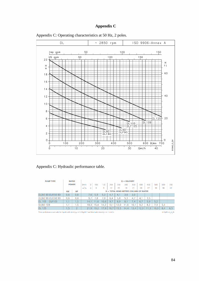
84

Appendix C

Appendix C: Operating characteristics at 50 Hz, 2 poles.

Appendix C: Hydraulic performance table.

85

Appendix D

Appendix D: Technical specification of digital sanitary pressure gauge.