Modular Termination of Basic Narrowing⋆

Marıa Alpuente, Santiago Escobar, and Jose Iborra

Universidad Politecnica de Valencia, Spain.{alpuente,sescobar,jiborra}@dsic.upv.es

Abstract. Basic narrowing is a restricted form of narrowing which con-strains narrowing steps to a set of non-blocked (or basic) positions. Basicnarrowing has a number of important applications including equationalunification in canonical theories. Another application is analyzing ter-mination of narrowing by checking the termination of basic narrowing,as done in pioneering work by Hullot. In this work, we study the modu-larity of termination of basic narrowing in hierarchical combinations ofTRSs, including a generalization of proper extensions with shared sub-system. This provides new algorithmic criteria to prove termination ofbasic narrowing.

1 Introduction

Narrowing [11] is a generalization of term rewriting that allows free variablesin terms (as in logic programming) and replaces pattern matching with syntac-tic unification. Narrowing was originally introduced as a mechanism for solvingequational unification problems [15], hence termination results for narrowinghave been traditionally achieved as a by–product of addressing the decidabil-ity of equational unification. Basic narrowing [15] is a refinement of narrowingwhich restricts narrowing steps to a set of non-blocked (or basic) positions, and isstill complete for equational unification in canonical TRSs. Termination of basicnarrowing was first studied by Hullot in [15], where a faulty termination resultfor narrowing was enunciated, namely the termination of all narrowing deriva-tions in canonical theories when all basic narrowing derivations issuing fromthe right–hand sides (rhs’s) of the rules terminate. This result was implicitlycorrected in [16], downgrading it to the more limited result of basic narrowingtermination (instead of ordinary narrowing) under the basic narrowing termi-nation requirement for the rhs’s of the rules. The missing condition to recovernarrowing termination in [15] is to require that the TRS satisfies Rety’s maximalcommutation condition for narrowing sequences [23], as we proved1 in [1]. Fromthis result, we also distilled in [1] a syntactic characterization of TRSs where

⋆ This work has been partially supported by the EU (FEDER) and Spanish MECproject TIN2007-68093-C02-02, Integrated Action Hispano-Alemana A2006-0007,the UPV grant 3249 PAID0607 and the UPV grant FPI-UPV 2006-01.

1 We also explicitly dropped in [1] the superfluous requirement of canonicity fromHullot’s termination result, as cognoscenti tacitly do.

termination of basic narrowing implies termination of narrowing, namely right-linear TRSs that are either left-linear or regular and where narrowing computes2

only normalized substitutions.The main motivation for this paper is proving termination of narrowing via

termination of basic narrowing. We present several criteria for modular ter-mination of basic narrowing in hierarchical combinations of TRSs, includinggeneralized proper extensions with shared subsystem. By adopting the divide-and-conquer principle, this allows us to prove (basic) narrowing termination ina modular way, thus extending the class of TRSs for which termination of basicnarrowing (and hence termination of narrowing) can be proved. We assume astandard notion of modularity, where a property ϕ of TRSs is called modular if,whenever R1 and R2 satisfy ϕ, then their combination R1 ∪ R2 also satisfiesϕ. Our modularity results for basic narrowing rely on a commutation result forbasic narrowing sequences that has not been identified in the related literaturebefore.

In [21], a modularity result for decidability of unification (via termination ofnarrowing) in canonical TRSs is given. However, this result does not imply themodularity of narrowing termination for a particular class of TRSs but ratherthe possibility to define a terminating, modular narrowing procedure. Namely,the result in [21] is as follows: given a canonical TRS R such that narrowing ter-minates for R1 and R2 and R↓⊆ R1↓R2↓ (i.e. normalization with R = R1∪R2

can be obtained by first normalizing with R1 followed by a normalization withR2), then there is a terminating and complete, modular narrowing strategy forR. Any complete strategy can be used within the modular procedure given in[21], including the basic narrowing strategy. As far as we know this is the onlyprevious modularity result in the literature that concerns the modular termina-tion of basic narrowing.

After some preliminaries in Section 2, we study commutation properties ofbasic narrowing derivations in Section 3. Section 4 recalls some standard notionsfor modularity of rewriting and presents our main modularity results for thetermination of basic narrowing. In order to prove in Section 4.5 that termina-tion of basic narrowing is modular for proper extensions [22], we first prove anintermediate result: in Section 4.4 we prove that basic narrowing terminationis modular for a restriction of proper extensions called nice extensions [22]. InSection 5 we generalize our results and prove modularity for a wider class ofTRSs called relaxed proper extensions. We conclude in Section 6. Proofs of allresults in this paper are included in [?].

2 Preliminaries

In this section, we briefly recall the essential notions and terminology of termrewriting [8, 20, 24].

V denotes a countably infinite set of variables, and Σ denotes a set of func-tion symbols, or signature, each of which has a fixed associated arity. Terms are

2 This includes some popular classes of TRSs, including linear constructor systems

4

viewed as labelled trees in the usual way, where T (Σ,V) and T (Σ) denote thenon-ground term algebra and the ground algebra built on Σ ∪V and Σ, respec-tively. Positions are defined as sequences of positive natural numbers used toaddress subterms of a term, with ǫ as the root (or top) position (i.e., the emptysequence). Concatenation of positions p and q is denoted by p.q, and p < q is theusual prefix ordering. Two positions p, q are disjoint, denoted by p ‖ q, if neitherp < q, p > q, nor p = q. Given S ⊆ Σ ∪ V , PosS(t) denotes the set of positionsof a term t that are rooted by function symbols or variables in S. Pos{f}(t) withf ∈ Σ ∪ V will be simply denoted by Posf (t), and PosΣ∪V(t) will be simplydenoted by Pos(t). t|p is the subterm at the position p of t. t[s]p is the term twith the subterm at the position p replaced with term s. By Var(s), we denotethe set of variables occurring in the syntactic object s. By x, we denote a tupleof pairwise distinct variables. A fresh variable is a variable that appears nowhereelse. A linear term is one where every variable occurs only once.

A substitution σ is a mapping from the set of variables V into the set of termsT (Σ,V), with a finite domain D(σ) and image I(σ). A substitution is repre-sented as {x1/t1, . . . , xn/tn} for variables x1, . . . , xn and terms t1, . . . , tn. Theapplication of substitution θ to term t is denoted by tθ, using postfix notation.Composition of substitutions is denoted by juxtaposition, i.e., the substitutionσθ denotes (θ ◦σ). We write θ|Var(s) to denote the restriction of the substitutionθ to the set of variables in s; by abuse of notation, we often simply write θ|s.Given a term t, θ = ν [t] iff θ|Var(t) = ν|Var(t), that is, ∀x ∈ Var(t), xθ = xν. Asubstitution θ is more general than σ, denoted by θ ≤ σ, if there is a substitutionγ such that θγ = σ. A unifier of terms s and t is a substitution ϑ such thatsϑ = tϑ. The most general unifier of terms s and t, denoted by mgu(s, t), is aunifier θ such that for any other unifier θ′, θ ≤ θ′.

A term rewriting system (TRS) R is a pair (Σ, R), where R is a finite set ofrewrite rules of the form l → r such that l, r ∈ T (Σ,V), l 6∈ V , and Var(r) ⊆Var(l). We will often write just R or (Σ, R) instead of R = (Σ, R). Givena TRS R = (Σ, R), the signature Σ is often partitioned into two disjoint setsΣ = C ⊎ D, where D = {f | f(t1, . . . , tn) → r ∈ R} and C = Σ \ D. Symbolsin C are called constructors, and symbols in D are called defined functions. Theelements of T (C,V) are called constructor terms. We let Def(R) denote the setof defined symbols in R. A rewrite step is the application of a rewrite rule toan expression. A term s ∈ T (Σ,V) rewrites to a term t ∈ T (Σ,V), denoted by

sp→R t, if there exist p ∈ PosΣ(s), l → r ∈ R, and substitution σ such that

s|p = lσ and t = s[rσ]p. When no confusion can arise, we omit the subscriptin →R . We also omit the reduced position p when it is not relevant. A terms is a normal form w.r.t. the relation →R (or simply a normal form), if thereis no term t such that s →R t. A term is a reducible expression or redex if itis an instance of the left hand side of a rule in R. A term s is a head normalform if there are no terms t, t′s.t. s →∗

R t′ǫ→R t. A TRS R is (→)-terminating

(also called strongly normalizing or noetherian) if there are no infinite reductionsequences t1 →R t2 →R . . ..

5

Narrowing is a symbolic computation mechanism that generalizes rewritingby replacing pattern matching with syntactic unification. Many redundancies inthe narrowing algorithm can be eliminated by restricting narrowing steps to adistinguished set of basic positions, which was proposed by Hullot in [15].

2.1 Basic Narrowing

Basic narrowing is the restriction of narrowing introduced by Hullot [15] whichis essentially based on forbidding narrowing steps on terms brought in by in-stantiation. We use the definition of basic narrowing given in [14], where theexpression to be narrowed is split into a skeleton t and an environment part θ,i.e., 〈t, θ〉. The environment part keeps track of the accumulated substitutionso that, at each step, substitutions are composed in the environment part, butare not applied to the expression in the skeleton part, as opposed to ordinarynarrowing. For TRS R, l → r << R denotes that l → r is a fresh variant of arule in R, i.e., all the variables are fresh.

Definition 1 (Basic narrowing). [14] Given a term s ∈ T (Σ,V) and a sub-

stitution σ, a basic narrowing step for 〈s, σ〉 is defined by 〈s, σ〉b;p,R,θ 〈t, σ′〉

if there exist p ∈ PosΣ(s), l → r << R, and substitution θ such that θ =mgu(s|pσ, l), t = (s[r]p), and σ′ = σθ.

Along a basic narrowing derivation, the set of basic occurrences of 〈t, θ〉is PosΣ(t), and the non–basic occurrences are PosΣ(tθ) − PosΣ(t). When p

is not relevant, we simply denote the basic narrowing relation byb;R,θ. By

abuse of notation, we often relax the skeleton-environment notation for basic

narrowing steps, i.e., 〈s, σ〉b;R,θ 〈t, σ′〉, and use the more compact notation

sσb;R,θ tσθ instead; but then suitable track of the basic positions along the

narrowing sequences is implicitly done.

We say that R is (b;)-terminating when every basic narrowing derivation

issuing from any term terminates. All modular termination results in this paperare based on the following termination result for basic narrowing. It is essentiallyHullot’s basic narrowing termination result, where we have explicitly droppedthe superfluous requirement of canonicity [1].

Theorem 1 (Termination of Basic Narrowing). [15, 1] Let R be a TRS.If for every l → r ∈ R, all basic narrowing derivations issuing from r terminate,

then R is (b;)-terminating.

In the literature, this condition has been approximated by requiring that everyrhs of a rewrite rule is a variable, in [15], or a constructor term, in [21]. Thisapproximation has been generalized in [1] by requiring the rhs’s to be a rigidnormal form (rnf), i.e., unnarrowable.

6

3 A Commutation result for basic narrowing derivations

The commutation properties of ordinary narrowing were extensively studied byRety in [23]. We analyze here those of basic narrowing, in Rety’s style. First letus recall the notion of antecedent of a position in a rewriting sequence [23].

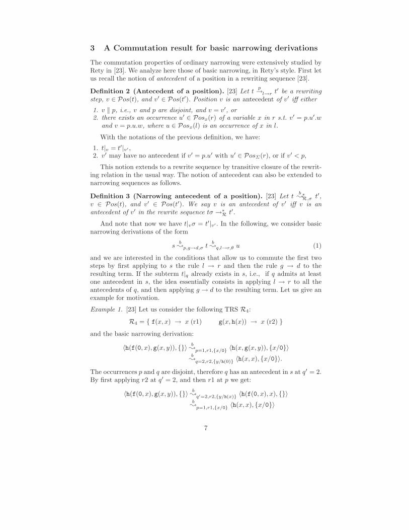
Definition 2 (Antecedent of a position). [23] Let tp→l→r t′ be a rewriting

step, v ∈ Pos(t), and v′ ∈ Pos(t′). Position v is an antecedent of v′ iff either

1. v ‖ p, i.e., v and p are disjoint, and v = v′, or2. there exists an occurrence u′ ∈ Posx(r) of a variable x in r s.t. v′ = p.u′.w

and v = p.u.w, where u ∈ Posx(l) is an occurrence of x in l.

With the notations of the previous definition, we have:

1. t|v = t′|v′ ,2. v′ may have no antecedent if v′ = p.u′ with u′ ∈ PosΣ(r), or if v′ < p,

This notion extends to a rewrite sequence by transitive closure of the rewrit-ing relation in the usual way. The notion of antecedent can also be extended tonarrowing sequences as follows.

Definition 3 (Narrowing antecedent of a position). [23] Let tb;

∗R,σ t′,

v ∈ Pos(t), and v′ ∈ Pos(t′). We say v is an antecedent of v′ iff v is anantecedent of v′ in the rewrite sequence tσ →∗

R t′.

And note that now we have t|vσ = t′|v′ . In the following, we consider basicnarrowing derivations of the form

sb;p,g→d,σ t

b;q,l→r,θ u (1)

and we are interested in the conditions that allow us to commute the first twosteps by first applying to s the rule l → r and then the rule g → d to theresulting term. If the subterm t|q already exists in s, i.e., if q admits at leastone antecedent in s, the idea essentially consists in applying l → r to all theantecedents of q, and then applying g → d to the resulting term. Let us give anexample for motivation.

Example 1. [23] Let us consider the following TRS R4:

R4 = { f(x, x) → x (r1) g(x, h(x)) → x (r2) }

and the basic narrowing derivation:

〈h(f(0, x), g(x, y)), {}〉b;p=1,r1,{x/0} 〈h(x, g(x, y)), {x/0}〉b;q=2,r2,{y/h(0)} 〈h(x, x), {x/0}〉.

The occurrences p and q are disjoint, therefore q has an antecedent in s at q′ = 2.By first applying r2 at q′ = 2, and then r1 at p we get:

〈h(f(0, x), g(x, y)), {}〉b;q′=2,r2,{y/h(x)} 〈h(f(0, x), x), {}〉b;p=1,r1,{x/0} 〈h(x, x), {x/0}〉

7

The following result establishes that in a basic narrowing derivation, theantecedent of a position is always in the skeleton part, and case 2 of Definition2 cannot happen.

Lemma 1. Given a basic narrowing derivation tb;p,l→r,σ t′

b;q′,g→d,θ u, if

q ∈ Pos(t) is an antecedent of q′, then q and p are necessarily disjoint, q′ is inthe skeleton, and q = q′.

Proof. Suppose that q and p are not disjoint, then we are in case 2 of Definition 2,and q′ = p.u′.w for some u ∈ Posx(r). But this means q′ is in the environment,and hence the narrowing derivation is not basic, which contradicts the initialassumption. ⊓⊔

Now we show that basic narrowing steps can be commuted under certainconditions. This result is the basis for the modularity results of Section 5.

Proposition 1 (Commutation of Basic Narrowing). Let R be a TRS and

〈s, θ〉b;p,g→d,σ1

〈s[d]p, θσ1〉b;q,l→r,σ2

〈s[d]p[r]q , θσ1σ2〉 (2)

be a sequence of two basic narrowing steps s.t. q admits an antecedent in s. Then(2) can be commuted to the following equivalent basic narrowing derivation:

〈s, θ〉b;q,l→r,σ3

〈s[r]q, θσ3〉b;p,g→d,σ4

〈s[r]q [d]p, θσ3σ4〉 (3)

where σ1σ2 = σ3σ4[s].

In order to provide the proof, we need the auxiliary notion of substitutionmerge [23].

Definition 4 (Unifiable Substitutions). [23] We say that two substitutionsσ and θ are unifiable iff there exists a substitution µ s.t. σµ = θµ. The mostgeneral instance σ∩θ = ση = θη of σ and θ is called the merge of σ and θ. Notethat the merge is commutative, i.e., σ ∩ θ = θ ∩ σ.

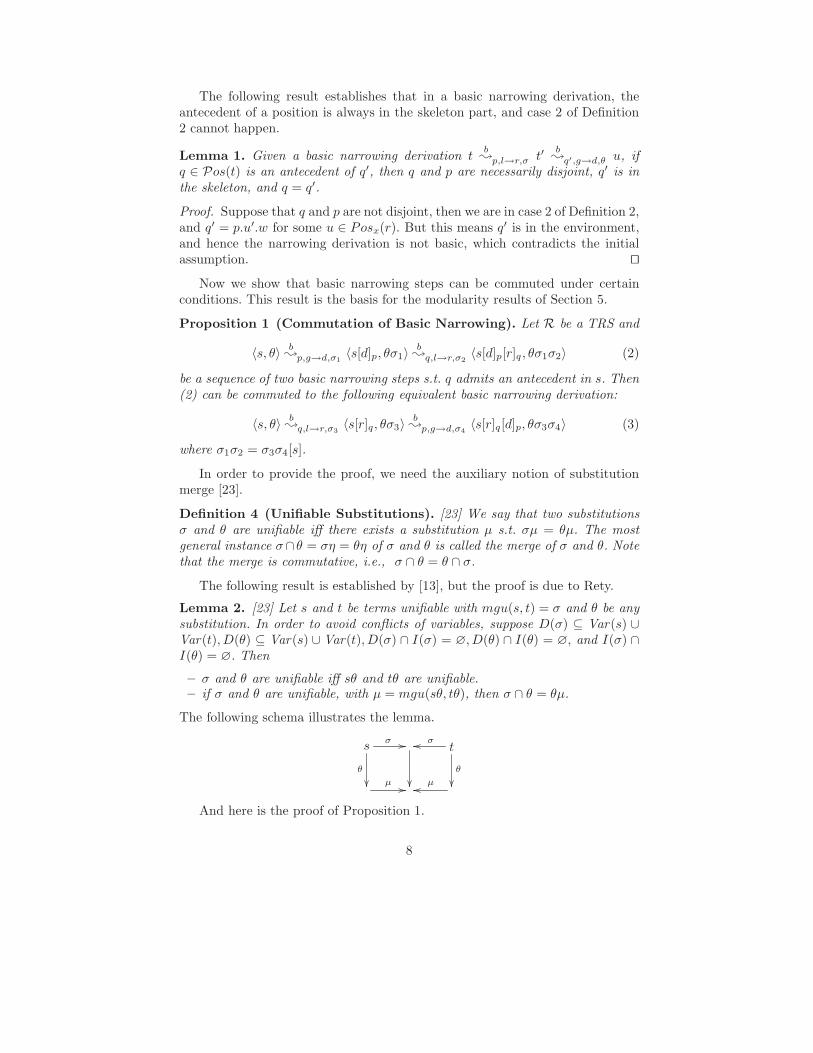
The following result is established by [13], but the proof is due to Rety.

Lemma 2. [23] Let s and t be terms unifiable with mgu(s, t) = σ and θ be anysubstitution. In order to avoid conflicts of variables, suppose D(σ) ⊆ Var(s) ∪Var(t), D(θ) ⊆ Var(s) ∪ Var(t), D(σ) ∩ I(σ) = ∅, D(θ) ∩ I(θ) = ∅, and I(σ) ∩I(θ) = ∅. Then

– σ and θ are unifiable iff sθ and tθ are unifiable.– if σ and θ are unifiable, with µ = mgu(sθ, tθ), then σ ∩ θ = θµ.

The following schema illustrates the lemma.

sσ

θ

tσ

θ

µ µ

And here is the proof of Proposition 1.

8

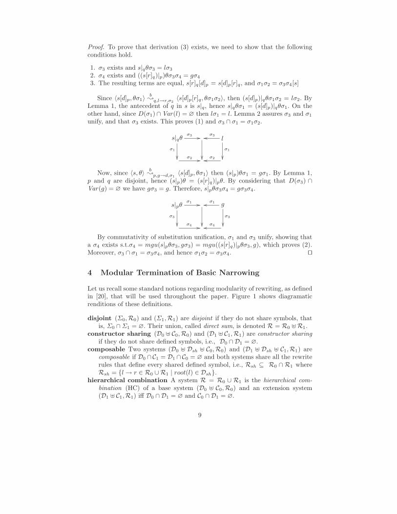
Proof. To prove that derivation (3) exists, we need to show that the followingconditions hold.

1. σ3 exists and s|qθσ3 = lσ3

2. σ4 exists and ((s[r]q)|p)θσ3σ4 = gσ4

3. The resulting terms are equal, s[r]q[d]p = s[d]p[r]q, and σ1σ2 = σ3σ4[s]

Since 〈s[d]p, θσ1〉b;q,l→r,σ2

〈s[d]p[r]q, θσ1σ2〉, then (s[d]p)|qθσ1σ2 = lσ2. ByLemma 1, the antecedent of q in s is s|q, hence s|qθσ1 = (s[d]p)|qθσ1. On theother hand, since D(σ1) ∩Var(l) = ∅ then lσ1 = l. Lemma 2 assures σ3 and σ1

unify, and that σ3 exists. This proves (1) and σ3 ∩ σ1 = σ1σ2.

s|qθσ3

σ1

lσ3

σ1

σ2 σ2

Now, since 〈s, θ〉b;p,g→d,σ1

〈s[d]p, θσ1〉 then (s|p)θσ1 = gσ1. By Lemma 1,p and q are disjoint, hence (s|p)θ = (s[r]q)|pθ. By considering that D(σ3) ∩Var(g) = ∅ we have gσ3 = g. Therefore, s|pθσ3σ4 = gσ3σ4.

s|pθσ1

σ3

gσ1

σ3

σ4 σ4

By commutativity of substitution unification, σ1 and σ3 unify, showing thata σ4 exists s.t.σ4 = mgu(s|pθσ3, gσ3) = mgu((s[r]q)|pθσ3, g), which proves (2).Moreover, σ3 ∩ σ1 = σ3σ4, and hence σ1σ2 = σ3σ4. ⊓⊔

4 Modular Termination of Basic Narrowing

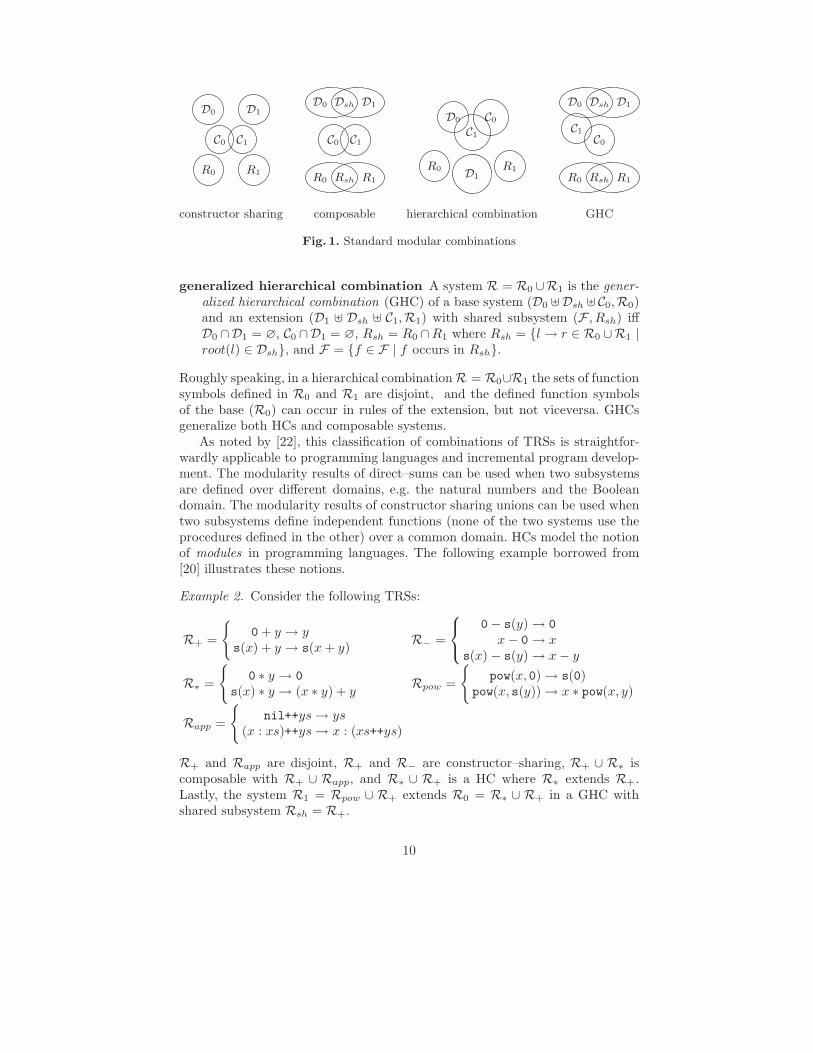
Let us recall some standard notions regarding modularity of rewriting, as definedin [20], that will be used throughout the paper. Figure 1 shows diagramaticrenditions of these definitions.

disjoint (Σ0,R0) and (Σ1,R1) are disjoint if they do not share symbols, thatis, Σ0 ∩ Σ1 = ∅. Their union, called direct sum, is denoted R = R0 ⊎R1.

constructor sharing (D0 ⊎ C0,R0) and (D1 ⊎ C1,R1) are constructor sharingif they do not share defined symbols, i.e., D0 ∩D1 = ∅.

composable Two systems (D0 ⊎ Dsh ⊎ C0,R0) and (D1 ⊎ Dsh ⊎ C1,R1) arecomposable if D0 ∩C1 = D1 ∩C0 = ∅ and both systems share all the rewriterules that define every shared defined symbol, i.e., Rsh ⊆ R0 ∩ R1 whereRsh = {l → r ∈ R0 ∪R1 | root(l) ∈ Dsh}.

hierarchical combination A system R = R0 ∪ R1 is the hierarchical com-bination (HC) of a base system (D0 ⊎ C0,R0) and an extension system(D1 ⊎ C1,R1) iff D0 ∩ D1 = ∅ and C0 ∩ D1 = ∅.

9

D0 D1

R0 R1

C0 C1

Dsh

Rsh

D0 D1

R0 R1

C0 C1

D0 C0

C1

D1

R0 R1

Dsh

Rsh

D0 D1

R0 R1

C0

C1

constructor sharing composable hierarchical combination GHC

Fig. 1. Standard modular combinations

generalized hierarchical combination A system R = R0 ∪R1 is the gener-alized hierarchical combination (GHC) of a base system (D0 ⊎Dsh ⊎ C0,R0)and an extension (D1 ⊎ Dsh ⊎ C1,R1) with shared subsystem (F , Rsh) iffD0 ∩D1 = ∅, C0 ∩D1 = ∅, Rsh = R0 ∩R1 where Rsh = {l → r ∈ R0 ∪R1 |root(l) ∈ Dsh}, and F = {f ∈ F | f occurs in Rsh}.

Roughly speaking, in a hierarchical combination R = R0∪R1 the sets of functionsymbols defined in R0 and R1 are disjoint, and the defined function symbolsof the base (R0) can occur in rules of the extension, but not viceversa. GHCsgeneralize both HCs and composable systems.

As noted by [22], this classification of combinations of TRSs is straightfor-wardly applicable to programming languages and incremental program develop-ment. The modularity results of direct–sums can be used when two subsystemsare defined over different domains, e.g. the natural numbers and the Booleandomain. The modularity results of constructor sharing unions can be used whentwo subsystems define independent functions (none of the two systems use theprocedures defined in the other) over a common domain. HCs model the notionof modules in programming languages. The following example borrowed from[20] illustrates these notions.

Example 2. Consider the following TRSs:

R+ =

{

0 + y → ys(x) + y → s(x + y)

R− =

0− s(y) → 0

x − 0 → xs(x) − s(y) → x − y

R∗ =

{

0 ∗ y → 0

s(x) ∗ y → (x ∗ y) + yRpow =

{

pow(x, 0) → s(0)pow(x, s(y)) → x ∗ pow(x, y)

Rapp =

{

nil++ys → ys(x : xs)++ys → x : (xs++ys)

R+ and Rapp are disjoint, R+ and R− are constructor–sharing, R+ ∪ R∗ iscomposable with R+ ∪ Rapp, and R∗ ∪ R+ is a HC where R∗ extends R+.Lastly, the system R1 = Rpow ∪ R+ extends R0 = R∗ ∪ R+ in a GHC withshared subsystem Rsh = R+.

10

Note that constructor sharing systems generalize disjoint unions, and arethemselves generalized by both composable and HCs. Finally, these last twonotions are subsumed by GHCs.

4.1 Cε-termination

The notion of Cε-termination is used in the literature for proving termination ofrewriting in a modular way [20]. The technique is essentially based on findingsufficient conditions for the modularity of the more restrictive Cε-terminationproperty.

Definition 5 (Cε termination). [20] A TRS R is called Cε-terminating if thecollapsing extended TRS R ⊎ Cε, where Cε = {Cons(x, y) → x, Cons(x, y) → y},is terminating, where Cons is a fresh symbol not occurring in the signature ofR.

This definition can be lifted in the obvious way to (basic) narrowing termina-tion of R ⊎ Cε, which we call Cε-termination of Basic Narrowing. The followingconsequence of Theorem 1 is interesting.

Proposition 2 (Cε-termination of Basic Narrowing). Let R be a

(b;)-terminating TRS. Then, the TRS R ⊎ Cε is also (

b;)-terminating.

Proof. Immediate by Theorem 1 because the rhs’s of the rules Cε satisfy thetermination condition for basic narrowing derivations of Theorem 1. ⊓⊔

In contrast, the corresponding property does not generally hold for (→)-termination,but only for termination of innermost rewriting (see [20]).

4.2 Constructor–sharing and composable unions

The following result is a direct consequence of Theorem 1.

Theorem 2 (Modularity of Constructor–Sharing Unions). Terminationof basic narrowing is modular for constructor–sharing systems.

Proof. Let R = R0∪R1 be a constructor-sharing union of two (b;)-terminating

TRSs. We need to prove that any basic narrowing derivation issuing from everyright hand side in R terminates. But this is easy, because every derivation stem-ming from the right hand side of a rule of R0 only use rules from R0 (there is no

redex w.r.t. R1), and then are finite by hypothesis since R0 is (b;)-terminating.

The same argument applies to the right hand sides of the rules of R1. By The-orem 1, the conclusion follows. ⊓⊔

This implies modularity for disjoint unions too, as in the following well-knownexample.

11

Example 3 (Toyama). Let us consider Toyama’s example [25]:

R0 : f(0, 1, x) → f(x, x, x) R1 : g(x, y) → x g(x, y) → y

Basic narrowing trivially terminates on each system, since every rhs is clearlyunnarrowable. By Theorem 2, it also terminates for R0 ∪R1.

It is well known that Toyama’s example is not (→)-terminating. However,

it is innermost terminating. This shows that (b;)-termination does not entail

(→)-termination, which suggests that the modularity requirements for (b;)-

termination are less restrictive than those of (→)-termination. Actually, the

modularity properties of (b;)-termination are comparable to those of innermost

(→)-termination (see e.g. [20]). The next theorem extends the modularity of

(b;)-termination to composable systems.

Theorem 3 (Modularity of Composable Unions). Termination of basicnarrowing is a modular property of composable systems.

Proof. Let R = R0 ∪ R1 be the union of two composable, (b;)-terminating

TRSs. We can partition the rules in R in the following disjoint sets:

Rsh = R0 ∩R1

R′0 = R0 \ R0

R′1 = R1 \ R0

Basic narrowing derivations issuing from the right hand sides of the rules inR′

0 or R′1 terminate by an argument analog to the one used in the proof of

Proposition 2. It is easy to see that derivations issuing from the right handsides of Rsh are terminating too, since they include no redex w.r.t. either R′

0 orR′

1, and basic narrowing does never reduce any redex occurring ar a non–basicposition (i.e. in the environment part of the tuple). By Theorem 1, the conclusionfollows. ⊓⊔

In Section 4.5 we further extend this result up to generalized proper exten-sions (GPE) [22], a fairly general restriction of HCs. To achieve this result, weproceed as follows. First we prove in Section 4.4 the modularity for generalizednice extensions (GNE) [22], a restriction of GPEs. Then, we apply a result from[22] that relates GPEs to GNEs, which delivers the desired result.

In the remaining of this section we make use of the following notion.

Definition 6 (Dependency Relation DR). [22] For a TRS (D ⊎ C,R) thedependency relation DR is the smallest preorder satisfying the condition f DR gwhenever there is a rewrite rule f(s1, . . . , sm) → r ∈ R and g(t1, . . . , tn) is asubterm of r, with g ∈ D.

We often omit R from DR when it is clear from the context. We say that asymbol f ∈ D depends on a symbol g ∈ D if f D g. Intuitively, f D g if theevaluation of f involves a call to g after one or more rewrite steps.

12

Dsh

Rsh

6D

6D

D0 D1

R0 R1

C0C1

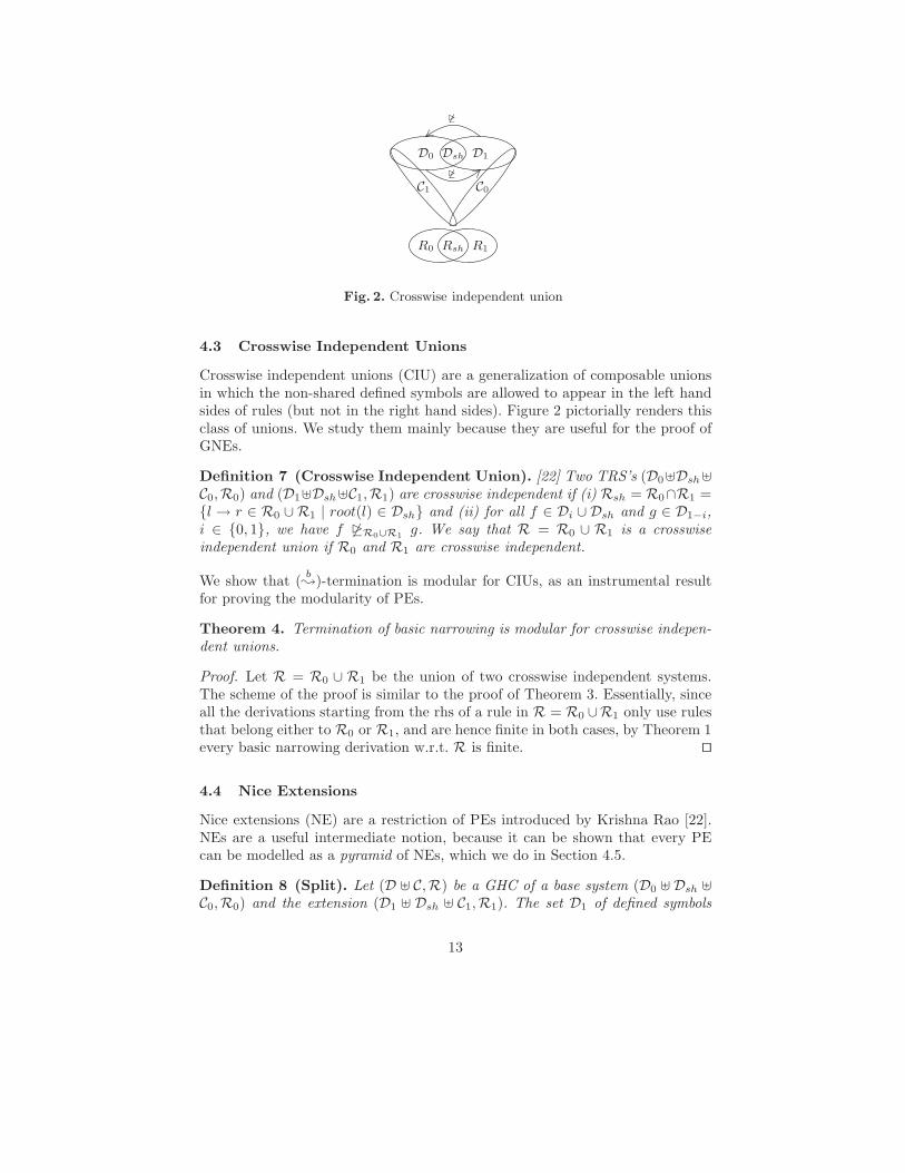
Fig. 2. Crosswise independent union

4.3 Crosswise Independent Unions

Crosswise independent unions (CIU) are a generalization of composable unionsin which the non-shared defined symbols are allowed to appear in the left handsides of rules (but not in the right hand sides). Figure 2 pictorially renders thisclass of unions. We study them mainly because they are useful for the proof ofGNEs.

Definition 7 (Crosswise Independent Union). [22] Two TRS’s (D0⊎Dsh⊎C0,R0) and (D1⊎Dsh⊎C1,R1) are crosswise independent if (i) Rsh = R0∩R1 ={l → r ∈ R0 ∪ R1 | root(l) ∈ Dsh} and (ii) for all f ∈ Di ∪ Dsh and g ∈ D1−i,i ∈ {0, 1}, we have f 6DR0∪R1

g. We say that R = R0 ∪ R1 is a crosswiseindependent union if R0 and R1 are crosswise independent.

We show that (b;)-termination is modular for CIUs, as an instrumental result

for proving the modularity of PEs.

Theorem 4. Termination of basic narrowing is modular for crosswise indepen-dent unions.

Proof. Let R = R0 ∪ R1 be the union of two crosswise independent systems.The scheme of the proof is similar to the proof of Theorem 3. Essentially, sinceall the derivations starting from the rhs of a rule in R = R0 ∪R1 only use rulesthat belong either to R0 or R1, and are hence finite in both cases, by Theorem 1every basic narrowing derivation w.r.t. R is finite. ⊓⊔

4.4 Nice Extensions

Nice extensions (NE) are a restriction of PEs introduced by Krishna Rao [22].NEs are a useful intermediate notion, because it can be shown that every PEcan be modelled as a pyramid of NEs, which we do in Section 4.5.

Definition 8 (Split). Let (D ⊎ C,R) be a GHC of a base system (D0 ⊎ Dsh ⊎C0,R0) and the extension (D1 ⊎ Dsh ⊎ C1,R1). The set D1 of defined symbols

13

of R1 is split in two sets D01 and D1

1 where D01 contains all the symbols that

depend on function symbols from R0, i.e., D01 = {f ∈ D1 | ∃g ∈ D0, f DR g}

and D11 = D1 \ D0

1. We can then split R1 in two subsystems R01 and R1

1 asR0

1 = {l → r ∈ R1 | root(l) ∈ D01} and R1

1 = {l → r ∈ R1 | root(l) ∈ D11}.

Definition 9 (Generalized Nice Extension). [22] Let R = R0 ∪ R1 be theGHC of the extension (D1⊎Dsh⊎C1,R1) over the base (D0⊎Dsh⊎C0,R0). R1 isa generalized nice extension (GNE) of R0 if, for every rewrite rule l → r ∈ R1,and for every subterm s of r such that root(s) ∈ D0

1, s contains no functionsymbol of D0 ∪ D0

1 strictly below its root.

Figure 4.5 shows a diagramatic rendition of NEs, and an example can befound in Example 4 later.

We identify a special set SR0∪R1of terms that represent the right hand sides

of rules of the TRSs that can be obtained as GNEs. This allows us to provethat basic narrowing w.r.t. R = R0 ∪ R1 terminates only if it terminates forthe terms in SR0∪R1

. Let us introduce the standard notion of context here. Acontext is a term C with zero or more ‘holes’, i.e., the fresh constant symbol 2.If C is a context and t a list of terms, C[t] denotes the result of replacing theholes in C by the terms in t.

Definition 10 (SR0∪R1terms). Let (D ⊎ C,R) be the union of a base system

(D0⊎Dsh⊎C0,R0) and a GNE (D1⊎Dsh⊎C1,R1). Define the sets D01, D

11, R

01 and

R11 as in Definition 8. Let CC01 be the set of contexts of (C ∪D0 ∪Dsh ∪D1

1). Wedefine SR0∪R1

as the set of all terms of the form C[s1, . . . , sn], where C ∈ CC01

and the following conditions hold:

1. for all i ∈ {1 · · ·n}, root(si) ∈ D01, and

2. si contains no function symbol of D0 ∪D01 strictly below its root.

By definition, SR0∪R1terms have the property that no R0

1 reduction step is

possible within the context C. Also, the set SR0∪R1is closed under

b;R0∪R1

ifR1 is a GNE of R0.

The reader can check that the right hand sides of the rules in a GNE fulfill

the conditions above. In order to prove the (b;)-termination of a system, by

Theorem 1 it suffices to prove that derivations starting from the right handsides of the rules are finite. We prove in Section 5 the more general result thatderivations starting from SR0∪R1

terms are finite.

Corollary 1. Let R1 be a GNE over R0. Every basic narrowing derivation inR0 ∪R1 starting from a term of SR0∪R1

terminates.

Now we can easily generalize this result to any term by applying Theorem 1.

Corollary 2. Termination of basic narrowing is modular for generalized niceextensions.

14

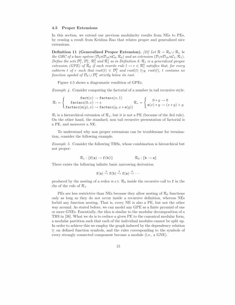
4.5 Proper Extensions

In this section, we extend our previous modularity results from NEs to PEs,by reusing a result from Krishna Rao that relates proper and generalized niceextensions.

Definition 11 (Generalized Proper Extension). [22] Let R = R0 ∪R1 bethe GHC of a base system (D0⊎Dsh⊎C0,R0) and an extension (D1⊎Dsh⊎C1,R1).Define the sets D0

1, D11, R

01 and R1

1 as in Definition 8. R1 is a generalized properextension (GPE) of R0 if each rewrite rule l → r ∈ R0

1 satisfies that, for everysubterm t of r such that root(t) ∈ D0

1 and root(t) DR root(l), t contains nofunction symbol of D0 ∪D0

1 strictly below its root.

Figure 4.5 shows a diagramatic rendition of GPEs.

Example 4. Consider computing the factorial of a number in tail recursive style.

R! =

{

fact(x) → factacc(x, 1)factacc(0, x) → x

factacc(s(y), x) → factacc(y, x ∗ s(y))R∗ =

{

0 ∗ y → 0

s(x) ∗ y → (x ∗ y) + y

R! is a hierarchical extension of R∗, but it is not a PE (because of the 3rd rule).On the other hand, the standard, non tail recursive presentation of factorial isa PE, and moreover a NE.

To understand why non proper extensions can be troublesome for termina-tion, consider the following example.

Example 5. Consider the following TRSs, whose combination is hierarchical butnot proper:

R1 : {f(a) → f(b)} R0 : {b → a}

There exists the following infinite basic narrowing derivation

f(a)b; f(b)

b; f(a)

b; · · ·

produced by the nesting of a redex w.r.t. R0 inside the recursive call to f in therhs of the rule of R1.

PEs are less restrictive than NEs because they allow nesting of R0 functionsonly as long as they do not occur inside a recursive definition, whereas NEsforbid any function nesting. That is, every NE is also a PE, but not the otherway around. As stated before, we can model any GPE as a finite pyramid of oneor more GNEs. Essentially, the idea is similar to the modular decomposition of aTRS in [26]. What we do is to reduce a given PE to the canonical modular form,a modular partition such that each of the individual modules cannot be split up.In order to achieve this we employ the graph induced by the dependency relationD on defined function symbols, and the rules corresponding to the symbols ofevery strongly connected component become a module (i.e., a GNE).

15

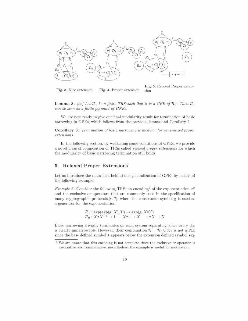
C0D0

C1

D1D0

1 D1

1

R0R1

l → C[f(t)]

6D

6D

6⊆ ∈ ⊆

Fig. 3. Nice extension

C0D0

C1

D1D0

1 D1

1

R0R1

l → C[f(t)]

6D

6D

∈

D

⊆

Fig. 4. Proper extension

C0D0

C1

D1D0

1 D1

1

R0R1

l → C[f(t)|{z}

]

6D

6D

∈

D

⊆

¬¬¬ rs−rnf

Fig. 5. Relaxed Proper exten-sion

Lemma 3. [22] Let R1 be a finite TRS such that it is a GPE of R0. Then R1

can be seen as a finite pyramid of GNEs.

We are now ready to give our final modularity result for termination of basicnarrowing in GPEs, which follows from the previous lemma and Corollary 2.

Corollary 3. Termination of basic narrowing is modular for generalized properextensions.

In the following section, by weakening some conditions of GPEs, we providea novel class of composition of TRSs called relaxed proper extensions for whichthe modularity of basic narrowing termination still holds.

5 Relaxed Proper Extensions

Let us introduce the main idea behind our generalization of GPEs by means ofthe following example.

Example 6. Consider the following TRS, an encoding3 of the exponentiation xy

and the exclusive or operators that are commonly used in the specification ofmany cryptographic protocols [6, 7], where the constructor symbol g is used asa generator for the exponentiation.

R1 : exp(exp(g, X), Y ) → exp(g, X*Y )R0 : X*X−1 → 1 X*1 → X 1*X → X

Basic narrowing trivially terminates on each system separately, since every rhsis clearly unnarrowable. However, their combination R = R0 ∪R1 is not a PE,since the base defined symbol * appears below the extension defined symbol exp

3 We are aware that this encoding is not complete since the exclusive or operator isassociative and commutative; nevertheless, the example is useful for motivation.

16

in a recursive call. It is easy to see that basic narrowing indeed terminates inR, because the outer function symbol exp in the recursive invocation occurringin the right hand side of the rule of R1 is blocked forever. The following novelnotion of relaxed proper extension (RPE) captures this idea.

We introduce the notion of root-stable rigid normal form, which lifts to nar-rowing the standard concept of head normal form. By abuse of notation, weapply this notion, with no change, to basic narrowing.

Definition 12 (Root-Stable Rigid Normal Form). [1] A term s is a root-stable rigid normal form (rs−rnf) w.r.t. R if either s is a variable or there are

no substitutions θ and θ′ and terms s′ and s′′ s.t. sθ>ǫ→∗

R s′b;ǫ,R,θ′ s′′.

Definition 13 (Generalized Relaxed Proper Extension). Let (D⊎C,R) bea GHC of a base system (D0⊎Dsh⊎C0,R0) and the extension (D1⊎Dsh⊎C1,R1).Define the sets D0

1, D11, R0

1 and R11 as in Definition 8. R1 is a generalized

relaxed proper extension (GRPE) of R0 if every rule in R01 satisfies the following

condition:

(H1) for each subterm t of r such that (a) root(t) ∈ D01, (b) t is not a rs−rnf,

and (c) root(t) DR root(l), t does not contain a function symbol of D0 ∪D01

strictly below its root.

Figure 4.5 shows a diagramatic rendition of GRPEs, and the reader can checkthat the TRS of Example 6 is indeed a GRPE. In the following, we show that

(b;)-termination is modular for RPEs by showing first its modularity for GRNEs,

and then establishing a relation between GRPEs an GRNEs. The reasoning issimilar to the one followed in Section 4.5.

Definition 14 (Generalized Relaxed Nice Extension). Let (D⊎C,R) be aGHC of a base system (D0⊎Dsh ⊎C0,R0) and an extension (D1⊎Dsh ⊎C1,R1).Define the sets D0

1, D11, R0

1 and R11 as in Definition 8. R1 is a generalized

relaxed nice extension (GRNE) of R0 if it is a GRPE, and for every rewriterule l → r ∈ R1 the following condition holds:

(N1) for each subterm t of r such that t is not a rs−rnf and root(t) ∈ D01, t

contains no function symbol of D0 ∪ D01 strictly below its root.

We can extend SR0∪R1to precisely capture the right hand sides of GRNEs.

Definition 15 (Srs−rnf

R0∪R1Terms). Let (D ⊎ C,R) be a GRNE of a base system

(D0⊎Dsh⊎C0,R0) and an extension (D1⊎Dsh⊎C1,R1). Define the sets D01, D

11,

R01 and R1

1 as in Definition 8. We define Srs−rnf

R0∪R1as the set of all terms of the

form C[s1, . . . , sn], where C is a context in (D∪C) and the following conditionshold:

1. no reduction is possible in R01 at a position within the context C,

2. for all i ∈ {1 · · ·n}, root(si) ∈ D01, si is not a rs−rnf, and

17

3. si contains no function symbol of D0 ∪D01 strictly below its root.

Note that SR0∪R1⊆ Srs−rnf

R0∪R1. The set Srs−rnf

R0∪R1also enjoys the property of

being closed underb;R0∪R1

in a GRNE.

Lemma 4. If t ∈ Srs−rnf

R0∪R1and t

b;R0∪R1,θ t′, then t′ ∈ Srs−rnf

R0∪R1.

Proof. We consider the cases tb;R0,θ t′ and or t

b;R1,θ t′ separately.

For the first case, by definition t = C[s1, . . . , sn], and let l → r ∈ R1 be therule applied in the reduction step. We consider further two cases depending onwhether root(l) is in D0

1 or not.

(a) root(l) 6∈ D01. That is, root(l) ∈ (D1

1 ∪ Dsh). There are two subcases.(1) The reduction took place in C. By definition, no D0

1 symbol occurs inr, hence t′ is of the form C′[t1, . . . , tm], where C′ ∈ CC01, root(ti) ∈ D0

1 andeach ti is a subterm of some sj . The lemma holds.(2) The reduction took place in a proper subterm of some si and t′ is of theform C[s1, . . . , s

′j, . . . , sn]. As in case (1), since no D0

1 symbol occurs in r,the lemma holds.

(b) root(l) ∈ D01. Therefore, the reduction happened at the root of some si, and r

is a term in Srs−rnf

R0∪R1, r = C′[u1, . . . , um]. t′ is of the form C[s1, . . . , si−1, r, si+1, . . . , sn] =

C′′[s1, . . . , si−1, u1, . . . , um, si+1, . . . , sn], where C′′ is the context resultingof joining C and C′.

Next, we consider the closedness for R0. By definition t = C[s1, . . . , sn], and letl → r ∈ R0 be the rule applied in the reduction step. The reduction takes placein C, and since no symbol in D1 occurs in r. By definition we have that t′ is ofthe form C′[t1, . . . , tm] where C′ ∈ CC01, root(ti) ∈ D0

1 and each ti is a subtermof some sj . The result follows. ⊓⊔

The rest of this section is devoted to extending Corollary 1 to the set Srs−rnf

R0∪R1.

First, let us recall some general results on quasi–commutation of abstract rela-tions.

Definition 16 (Abstract Reduction System). An abstract reduction system(ARS) is a structure A = (A, {→α| α ∈ I}) consisting of a set A and a set ofbinary relations →α on A, indexed by a set I. We write (A,→1,→2) instead of(A, {→α| α ∈ {1, 2}}).

Definition 17 (Quasi-commutation). [5] Let →0 and →1 be two relations ona set S. The relation →1 quasi-commutes over →0 if, for all s, u, t ∈ S s.t. s →0

u →1 t, there exists v ∈ S s.t. s →1 v →∗01 t, where →∗

01 is the transitive-reflexiveclosure of →0 ∪ →1.

Theorem 5. [5] If the relations →0 and →1 in the ARS(S, →0, →1) arestrongly normalizing and →1 quasi-commutes over →0, the relation →0 ∪ →1 isstrongly normalizing too.

18

We now define an ARS with skeleton–environment pairs as elements, wherethe skeletons come from the set Srs−rnf

R0∪R1of terms, and the relationships →0 and

→1 of the ARS are restrictions of basic narrowing.

Definition 18. Let R = R0∪R1 be a generalized relaxed nice combination. Wedefine the ARS A(R0,R1) = (Srs−rnf

R0∪R1×Subst,→0,→1), where the relations →0

and →1 are defined as follows. Let s = C[s0, . . . , sn] be a term in Srs−rnf

R0∪R1. Then

1. 〈C[s0, . . . , sn], σ〉 →0 〈C′[s0, . . . , sn], θσ〉 if 〈C[s0, . . . , sn], σ〉b;

R0∪R1

1,θ

〈C′[s0, . . . , sn], σθ〉 is a basic narrowing step given within the context C2. 〈C[s0, . . . , sn], σ〉 →1 〈C[s0, . . . , si−1, s

′i, si+1, . . . , sn], θσ〉 if 〈C[s0, . . . , sn], σ〉

b;R1,θ 〈C[s0, . . . , si−1, s

′i, si+1, . . . , sn], θσ〉 is a basic narrowing step given at

a subterm si, with i ∈ {0, . . . , n}.

The relation →1 ∪ →0 is exactly the basic narrowing relation over Srs−rnf

R0∪R1.

In the following we establish that both →0 and →1 are terminating relations.

Lemma 5. Given the ARS A(R0,R1) of Definition 18, the relations →0 and

→1 are terminating if R0 and R1 are (b;)-terminating.

Proof. The relation →1 is a subrelation ofb;R1

, and hence terminating.Now consider the subsystem R′1

1 = R11∪R

′. It can be shown that R0 and R′11

are crosswise independent and hence their union is terminating by Theorem 4.From the definition of A, it can be seen that →0 is actually a restriction of thissystem to the terms in Srs−rnf

R0∪R1, and therefore termination of →0 follows. ⊓⊔

We are now in a position to prove the quasi-commutation of the relation →1

over the relation →0 in the ARS A(R0,R1). The proof of this result relies onProposition 1.

Theorem 6. Given the ARS A(R0,R1) of Definition 18, the relation →1 quasi-commutes over the relation →0.

Proof. We have to show that

∀s, u, t ∈ Srs−rnf

R0∪R1s.t. s

p→0 u

q→1 t, ∃v ∈ Srs−rnf

R0∪R1, p′ ∈ PosΣ(s) s.t. s

p′

→1 v →∗01 t(4)

where, by abuse of notation, p, q and p′ refer to positions that are in the skeletonpart of the tuples denoted by s, u, t and v.

As →0⊆→01 and →1⊆→01, we can equivalently see these as →01 derivations.Since →01 is a basic narrowing relation, we can use Proposition 1 to prove theresult. We only need to show that q admits an antecedent in s. It is easy to seethat this is satisfied, because →0 cannot create new →1 redexes, which meansthat redex u|q was already there in s|q. On the other hand, since no redex can bepropagated by basic narrowing, p and q must be disjoint. Applying Proposition1, we have:

∀s, u, t ∈ Srs−rnf

R0∪R1s.t. s

p→01 u

q→01 t, ∃v ∈ Srs−rnf

R0∪R1s.t. s

q→01 v

p→01 t (5)

19

from which we observe that (1) p′ = q, (2) t is reached in a single →0 step, and(3) the step s →01 t is indeed given in →1, which suffices to prove the result. ⊓⊔

Then, as a straightforward consequence of Theorem 5 and Theorem 6, wederive the relaxed version of Corollary 1.

Corollary 4. Let R1 be a GRNE over R0. Every basic narrowing derivation inR0 ∪R1 starting from a term of Srs−rnf

R0∪R1terminates.

By Theorem 1, we obtain the desired modularity result for basic narrowing inour generalization of GNEs.

Corollary 5. Termination of basic narrowing is modular for generalized relaxednice extensions.

We now study the connection between GRNEs and GRPEs, and extend theresults and proofs from [22] extending them to our generalized relaxed niceextensions.

Lemma 6. Let R1 be a finite TRS such that it is a GRPE of R0. R1 can beseen as a finite pyramid of GRNEs.

In order to prove this Lemma, we need first two auxiliary definitions.

Definition 19 (Equivalence Relation ≈ and Partial Order ⊐). [22] Let(D⊎C,R) be a generalized hierarchical combination of a base system (D0⊎Dsh⊎C0,R0) and the extension (D1⊎Dsh⊎C1,R1). Define the sets D0

1, D11, R

01 and R1

1

as in Definition 8. We define an equivalence relation ≈R from the dependencyrelation DR , where the equivalence class containing f is denoted by [f ]R , and apartial ordering ⊐R on the set of equivalence classes:

– f ≈R g iff f DR g and g DR f , where f, g ∈ D01.

– [f ]R ⊐R [g]R iff f DR g and g 6DR f .

Since the signature of any TRS is a countable set, the equivalence relation≈ partitions D0

1 into a countable set E of equivalence classes. If we can assumethat the ordering ⊐ is noetherian, then it can be extended to a well-ordering oftype λ, where λ is a countable ordinal.

Definition 20. [22] Let (D⊎C,R) be a GHC of a base system (D0⊎Dsh⊎C0,R0)and the extension (D1 ⊎ Dsh ⊎ C1,R1). Define the sets D0

1, D11, R

01 and R1

1 asin Definition 8. For any ordinal α we denote the α-th element in the above well-ordering by Eα (if α > λ then Eα = ∅). We define the TRS Xα = {l → r ∈R1 | root(l) ∈ Dsh ∪D1

1 ∪Eα}, and the combined system Sα = R0 ∪ (⋃

β<α Xβ).So S0 is R0 and Sk for k > λ is R0 ∪R1.

Theorem 7. Let (D ⊎ C,R) be a GHC of a base system (D0 ⊎ Dsh ⊎ C0,R0)and the extension (D1 ⊎ Dsh ⊎ C1,R1). Define the sets D0

1, D11, R

01 and R1

1 asin Definition 8. If the relation ⊐R is noetherian, then Xα is a GRNE of Sα forevery ordinal α, where Sα and Xα are defined as in Definition 20.

20

Proof. For every α, we have that Sα and Xα form a GHC. We have to showthat (N1) holds in Xα. That is, for every l → r ∈ Xα, if s is a subterm of r s.t.root(s) ∈ Eα and some subterm of s contains a defined symbol depending onDef(Sα)−Def(Xα), then s must be a rs−rnf. Since root(s) ∈ Eα, it follows thatroot(l) ∈ Eα and, by definition, root(l) ∈ D0

1 and root(s) ≈ root(l). Thereforeroot(s) D root(l). Now, since R1 is a GRPE, the following holds by (H1): if ucontains a defined symbol depending on D0, then u must be a rs−rnf. Finally,since Def(Sα) − Def(Xα) ⊂ D0 ∪ D0

1 , Xα is a GRNE of Sα. ⊓⊔

And now we can prove Lemma 6.

Proof. By Theorem 7, if we can assume that the relation ⊐R0∪R1is noetherian.

⊓⊔

Finally, we are able to establish the most general result of the paper, whichfollows directly from Corollary 5 and Lemma 6.

Corollary 6. Termination of basic narrowing is modular for generalized relaxedproper extensions.

6 Conclusions

The completeness and termination properties of basic narrowing have been stud-ied previously in landmark work [15, 23, 19]. Recently we have contributed to thestudy of narrowing termination based on the termination of basic narrowing in[1]. In this paper, we improve our characterization of basic narrowing termi-nation by proving modular termination in several hierarchical combinations ofTRSs, including generalized proper extensions with shared subsystem.

Our main motivation for this work is proving termination of narrowing [15, 1].Narrowing has received much attention due to the different applications, suchas automated proofs of termination [4], execution of multiparadigm program-ming languages [12, 17], symbolic reachability [18], verification of cryptographicprotocols [9], equational unification [15], equational constraint solving [2, 3], andmodel checking [10], among others. Termination of narrowing is, therefore, ofmuch interest to these applications.

References

1. M. Alpuente, S. Escobar, and J. Iborra. Termination of Narrowing revisited. The-oretical Computer Science, 2008, to appear.

2. M. Alpuente, M. Falaschi, M. Gabbrielli, and G. Levi. The semantics of equationallogic programming as an instance of CLP. In K. R. Apt, J. W. de Bakker, and J. J.M. M. Rutten, editors, Logic Programming Languages: Constraints, Functions andObjects, pages 49–81. The MIT Press, Cambridge, Mass., 1993.

3. M. Alpuente, M. Falaschi, and G. Levi. Incremental Constraint Satisfaction forEquational Logic Programming. Theoretical Computer Science, 142(1):27–57, 1995.

21

4. Thomas Arts and Jurgen Giesl. Termination of term rewriting using dependencypairs. Theor. Comput. Sci., 236(1-2):133–178, 2000.

5. L Bachmair and N Dershowitz. Commutation, transformation, and termination.Proc. of the 8th Int’l Conf. on Automated Deduction:5-20, Jan 1986.

6. H. Comon-Lundh. Intruder Theories (Ongoing Work). In Proc. FoSSaCS 2004,pages 1–4. Springer LNCS 2987, 2004.

7. V. Cortier, S. Delaune, and P. Lafourcade. A Survey of Algebraic Properties usedin Cryptographic Protocols. Journal of Computer Security, 14(1):1–43, 2006.

8. Nachum Dershowitz and Jean-Pierre Jouannaud. Rewrite systems. In J. vanLeeuwen, editor, Handbook of Theoretical Computer Science, volume B: FormalMethods and Semantics, chapter 6, pages 244–320. Elsevier Science, 1990.

9. S. Escobar, C. Meadows, and J. Meseguer. A Rewriting-Based Inference System forthe NRL Protocol Analyzer and its Meta-Logical Properties. Theoretical ComputerScience, 367(1-2):162–202, 2006.

10. Santiago Escobar and Jose Meseguer. Symbolic model checking of infinite-statesystems using narrowing. In Proc. RTA 2007, pages 153–168. Springer LNCS4533, 2007.

11. M. Fay. First-Order Unification in an Equational Theory. In Fourth Int’l Conf. onAutomated Deduction, pages 161–167, 1979.

12. M. Hanus. The Integration of Functions into Logic Programming: From Theory toPractice. Journal of Logic Programming, 19&20:583–628, 1994.

13. A. Herold. Some basic notions of first-order unification theory. Technical ReportSR-83-15, SEKI report, 1983.

14. S. Holldobler. Foundations of Equational Logic Programming, volume 353 of Lec-ture Notes in Artificial Intelligence. Springer-Verlag, Berlin, 1989.

15. J.-M. Hullot. Canonical Forms and Unification. In Proceedings of the 5th In-ternational Conference on Automated Deduction, volume 87 of Lecture Notes inComputer Science, pages 318–334, Berlin, 1980. Springer-Verlag.

16. J.-M. Hullot. Compilation de Formes Canoniques dans les Theories quationelles.These de Doctorat de Troisieme Cycle. PhD thesis, Universite de Paris Sud, Orsay(France), 1981.

17. J. Meseguer. Multiparadigm logic programming. In H. Kirchner and G. Levi,editors, Algebraic and Logic Programming, Proceedings of the Third InternationalConference (ALP’92), volume 632 of Lecture Notes in Computer Science, pages158–200, Berlin, 1992. Springer-Verlag.

18. Jose Meseguer and Prasanna Thati. Symbolic reachability analysis using narrowingand its application to verification of cryptographic protocols. Higher-Order andSymbolic Computation, 20(1-2):123–160, 2007.

19. A. Middeldorp and E. Hamoen. Completeness Results for Basic Narrowing. Journalof Applicable Algebra in Engineering, Communication and Computing, 5:313–353,1994.

20. E. Ohlebusch. Advanced Topics in Term Rewriting. Springer-Verlag, 2002.21. C. Prehofer. On Modularity in Term Rewriting and Narrowing. In CCL’94, volume

845 of Lecture Notes in Computer Science, pages 253–268. Springer, 1994.22. M.R.K. Krishna Rao. Modular proofs for completeness of hierarchical term rewrit-

ing systems. Theoretical Computer Science, Jan 1995.23. Pierre Rety. Improving Basic Narrowing Techniques. In RTA. LNCS 256, 1987.24. TeReSe, editor. Term Rewriting Systems. Cambridge University Press, Cambridge,

UK, 2003.25. Yoshihito Toyama. Counterexamples to termination for the direct sum of term

rewriting systems. Inf. Process. Lett., 25(3):141–143, 1987.

22

26. Xavier Urbain. Modular & incremental automated termination proofs. Int. J.Approx. Reasoning, 32(4):315–355, 2004.

23