Modelling stream–aquifer seepage in an alluvial aquifer: an improved loosing-stream package for MODFLOW

Modelling stream–aquifer seepage in an alluvial aquifer:

an improved loosing-stream package for MODFLOW

Yassin Z. Osman, Michael P. Bruen*

Centre for Water Resources Research, Department of Civil Engineering, University College Dublin, Earlsfort Terrace, Dublin 2, Ireland

Received 28 June 2000; revised 25 January 2002; accepted 15 March 2002

Abstract

Seepage from a stream, which partially penetrates an unconfined alluvial aquifer, is studied for the case when the water table

falls below the streambed level. Inadequacies are identified in current modelling approaches to this situation. A simple and

improved method of incorporating such seepage into groundwater models is presented. This considers the effect on seepage

flow of suction in the unsaturated part of the aquifer below a disconnected stream and allows for the variation of seepage with

water table fluctuations. The suggested technique is incorporated into the saturated code MODFLOW and is tested by

comparing its predictions with those of a widely used variably saturated model, SWMS_2D simulating water flow and solute

transport in two-dimensional variably saturated media. Comparisons are made of both seepage flows and local mounding of the

water table. The suggested technique compares very well with the results of variably saturated model simulations. Most

currently used approaches are shown to underestimate the seepage and associated local water table mounding, sometimes

substantially. The proposed method is simple, easy to implement and requires only a small amount of additional data about the

aquifer hydraulic properties. q 2002 Elsevier Science B.V. All rights reserved.

Keywords: Stream; River; Aquifer; Seepage; Model; Simulating water flow and solute transport in two-dimensional variably saturated media;

MODFLOW

1. Introduction

It is important to be able to quantify water

exchanges between streams and aquifers. Some

practical applications include (1) investigating the

effects of aquifer drawdown or mine dewatering on

nearby rivers and streams, (2) tracing of contaminants

from stream to aquifer or vice versa, (3) estimation of

irrigation canal losses, (4) estimation of groundwater

recharge from rivers, (5) estimation of the base flow in

streams.

Three different types of flow are involved: free

surface flow in the stream, saturated groundwater flow

in the aquifer and unsaturated flow in the vadose zone.

If there is a clay or silt ‘clogging’ or ‘impeding’ layer

in the bed of the stream with hydraulic properties

different from the aquifer then this further complicates

the modelling problem.

This paper studies the exchange of water between a

stream, which partially penetrates an alluvial aquifer,

with particular emphasis on the case in which the bed

and banks are clogged. The analysis shows that the

flow between stream and aquifer cannot be deter-

mined accurately unless the effects of the suction head

beneath the clogging layer are taken into account.

0022-1694/02/$ - see front matter q 2002 Elsevier Science B.V. All rights reserved.

PII: S0 02 2 -1 69 4 (0 2) 00 0 67 -7

Journal of Hydrology 264 (2002) 69–86

www.elsevier.com/locate/jhydrol

* Corresponding author.

E-mail address: [email protected] (M.P. Bruen).

http://www.elsevier.com/locate/jhydrol

Such an approach has been developed here and

successfully incorporated into the widely used

groundwater flow model, MODFLOW. The technique

is new, simple to implement, and gives results much

closer to those of complex variably saturated codes,

such as simulating water flow and solute transport in

two-dimensional variably saturated media

(SWMS_2D), than previously used simple methods.

The paper is organised as follows: First, a brief

theoretical background of stream–aquifer interaction

for the cases of fully and partially penetrating clogged

stream is given. Second, a review of previous

investigations suggests deficiencies in how the

phenomenon has been modelled up to now. Third,

the improved technique for predicting a stream–

aquifer seepage is explained. Fourth, the improved

technique is tested by comparing its results to those

from the variably saturated flow model, SWMS_2D,

and the conventional model MODFLOW. The tests

are conducted on a representative stream–aquifer

flow system for selected cases thought to serve the

subject of the paper. Fifth, comparison results are

discussed and assessed. Finally conclusions reached

by the paper are given.

2. Theoretical background

A stream can either fully or partially penetrate an

unconfined aquifer. A stream fully penetrates if its bed

is at or below the lower boundary of the aquifer. The

stream partially penetrates when its bed is above the

lower boundary. There is a major difference in the

flow system behaviour between rivers having a

clogging layer on their bed and banks and those

devoid of it (Spalding and Khaleel, 1991). Clogging

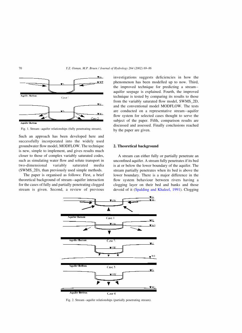
Fig. 2. Stream–aquifer relationships (partially penetrating stream).

Fig. 1. Stream–aquifer relationships (fully penetrating stream).

Y.Z. Osman, M.P. Bruen / Journal of Hydrology 264 (2002) 69–8670

layers on beds and banks of rivers consist of fine-

grained clay or silt soils or biologically degraded

organic matter. They usually have lower permeability

than the underlying aquifer. This paper concentrates

on modelling steady exchange flows for streams

whose bed and banks are clogged (Brockway and

Bloomsburg, 1968).

When a stream fully penetrates an unconfined

aquifer there are two cases to be considered, Fig. 1. In

the first case, called a connected gaining stream, the

groundwater table is higher than the water level in the

stream and water flows from the aquifer to the stream.

In the second case, called a connected losing stream,

the water table is below the stream water level and

water flows from the stream into the aquifer. In both

cases, the flow is predominantly through a saturated

medium. When the stream partially penetrates the

unconfined aquifer four cases can be distinguished,

Fig. 2. The first two cases are the same as in Fig. 1 for

the fully penetrating stream. Cases 3 and 4 occur when

the water table in the unconfined aquifer falls below

the streambed level and there is no longer a direct

connection of saturated medium between aquifer and

stream. The water table is said to disconnect from the

stream base. Case 3, called a disconnected stream with

shallow water table, is when the water table is not far

below the streambed and can affect the flow from the

stream. Case 4, called a disconnected stream with

deep water table, is when the water table falls far

below the streambed and any further drop does not

affect the flow rate from the stream, Zaslavsky (1964,

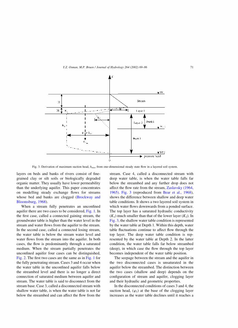
1965). Fig. 3 (reproduced from Bear et al., 1968),

shows the difference between shallow and deep water

table conditions. It shows a two layered soil system in

which water flows downwards from a ponded surface.

The top layer has a saturated hydraulic conductivity

(K1) much smaller than that of the lower layer (K2). In

Fig. 3, the shallow water table condition is represented

by the water table at Depth 1. Within this depth, water

table fluctuations continue to affect flow through the

top layer. The deep water table condition is rep-

resented by the water table at Depth 2. In the latter

condition, the water table falls far below streambed

(deep), in which case the flow through the top layer

becomes independent of the water table position.

The seepage between the stream and the aquifer in

the two disconnected cases is unsaturated in the

aquifer below the streambed. The distinction between

the two cases (shallow and deep) depends on the

configuration of stream and aquifer, clogging layer

and their hydraulic and geometric properties.

In the disconnected conditions of cases 3 and 4, the

suction head, (w1) at the base of the clogging layer

increases as the water table declines until it reaches a

Fig. 3. Derivation of maximum suction head, hmis, from one-dimensional steady state flow in a layered soil system.

Y.Z. Osman, M.P. Bruen / Journal of Hydrology 264 (2002) 69–86 71

maximum value (w2), and does not change any further

even if the water table declines further. The flow from

stream to aquifer increases with the increase in suction

head and reaches a corresponding maximum. The

clogging layer in most cases remains saturated since it

has a high air entry value. Other factors that affect the

flow to/from aquifer are the heterogeneity of the

aquifer, e.g. aquifer stratification, aquifer anisotropy,

the properties and thickness of the clogging layer, the

changing stream water levels, and the lateral boundary

condition of the flow domain. Some of these factors

are considered later in this paper.

So, to accurately model the seepage in stream–

aquifer flow system, a combined saturated–unsatu-

rated flow model is required. (e.g. UNSAT2,

SWMS_2D, VS2D, SWATRE, HYDRUS2, etc.); or

at least a kind of model that can take account of any

suction head, due to unsaturated conditions, prevail-

ing below the streambed. (e.g. see Bouwer, 1969;

Rovey, 1975).

3. Previous investigations

Much research has already been directed at

quantifying stream–aquifer fluxes. The methods,

which are well known, can be divided mainly into

(i) model construction and (ii) field measurement

methods. The models can be deterministic or

stochastic. Field measurement methods include

measuring stream seepage with a seepage meter at

small scales and water balance (inflow/outflow)

methods. This paper considers only deterministic

modelling methods as implemented in widely used

computer codes, such as MODFLOW (McDonald and

Harbaugh, 1996).

3.1. Stream–aquifer seepage as modelled in

MODFLOW

In the MODFLOW stream package (McDonald

and Harbaugh, 1996), a stream is considered to be

divided into sections, each linked to a cell in the

underlying aquifer model. The stream water level is

assumed to be the same throughout the section and

constant during a stress period. Thus, the effect of

water loss on the stream water levels is not taken into

account. When the aquifer head is above the bed of the

channel the seepage is assumed proportional to the

difference in hydraulic heads between stream and

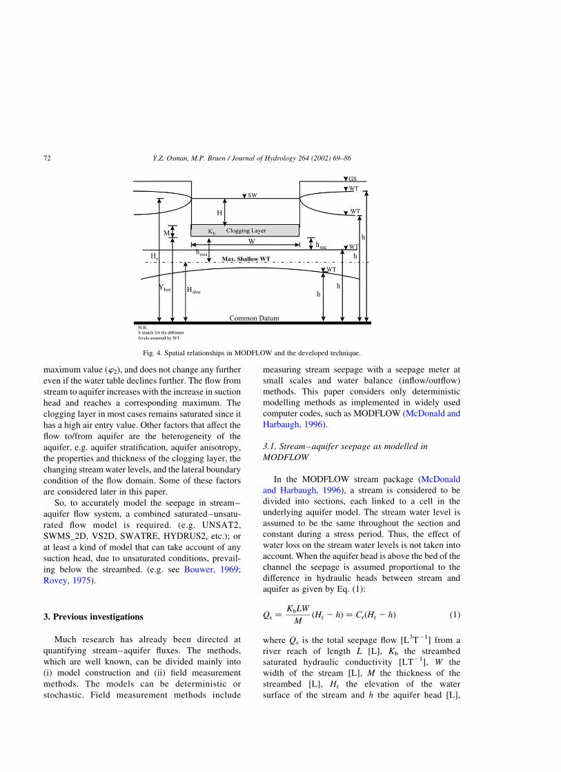
aquifer as given by Eq. (1):

Qs ¼KbLW

MðHr 2 hÞ ¼ CrðHr 2 hÞ ð1Þ

where Qs is the total seepage flow [L3T21] from a

river reach of length L [L], Kb the streambed

saturated hydraulic conductivity [LT21], W the

width of the stream [L], M the thickness of the

streambed [L], Hr the elevation of the water

surface of the stream and h the aquifer head [L],

Fig. 4. Spatial relationships in MODFLOW and the developed technique.


see Figs. 4 and 5. Note Cr ¼ KbLW=M is called

the streambed conductance [L2T21].

Once the aquifer head drops below the riverbed

level however, the dependence of the flow on the

aquifer head is assumed to disappear and the flow is

assumed proportional to the stream stage alone, i.e.

Qs ¼ CrðHr 2 YbotÞ ð2Þ

where Ybot is the elevation of the streambed [L].

It is implicitly assumed that there is sufficient water

in the stream to supply the flow without affecting

water levels. For a constant Hr, Eq. (2) will give a

constant seepage flow regardless of the position of the

water table in the aquifer. In the original release of

MODFLOW, it is stated that, in Eq. (2), the aquifer

bottom can be replaced by the depth at which seepage

becomes constant. However, no means for determin-

ing this depth is given and it is recommended that it

can be determined by calibration with data.

3.2. Other models of stream–aquifer interaction

3.2.1. Rovey’s model

Rovey (1975) developed a saturated three-dimen-

sional finite difference groundwater model to simulate

a flow system domain which includes seepage

between stream and aquifer. She used an expression

based on Darcy’s law to calculate stream losses in the

case of a disconnected stream, h , Ybot :

Qs ¼ CrðHr 2 Ybot 2 haÞ ð3Þ

where ha is the air entry (bubbling pressure) head of

the clogging layer [L].

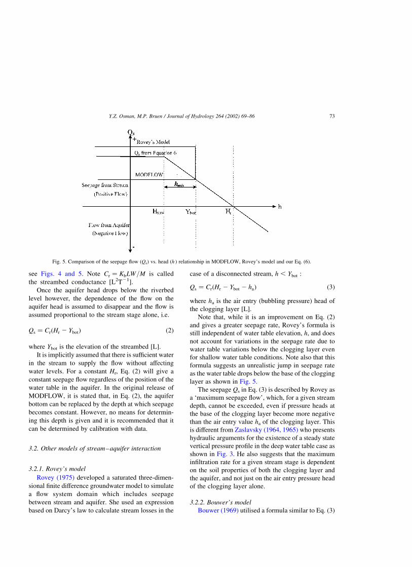
Note that, while it is an improvement on Eq. (2)

and gives a greater seepage rate, Rovey’s formula is

still independent of water table elevation, h, and does

not account for variations in the seepage rate due to

water table variations below the clogging layer even

for shallow water table conditions. Note also that this

formula suggests an unrealistic jump in seepage rate

as the water table drops below the base of the clogging

layer as shown in Fig. 5.

The seepage Qs in Eq. (3) is described by Rovey as

a ‘maximum seepage flow’, which, for a given stream

depth, cannot be exceeded, even if pressure heads at

the base of the clogging layer become more negative

than the air entry value ha of the clogging layer. This

is different from Zaslavsky (1964, 1965) who presents

hydraulic arguments for the existence of a steady state

vertical pressure profile in the deep water table case as

shown in Fig. 3. He also suggests that the maximum

infiltration rate for a given stream stage is dependent

on the soil properties of both the clogging layer and

the aquifer, and not just on the air entry pressure head

of the clogging layer alone.

3.2.2. Bouwer’s model

Bouwer (1969) utilised a formula similar to Eq. (3)

Fig. 5. Comparison of the seepage flow (Qs) vs. head (h ) relationship in MODFLOW, Rovey’s model and our Eq. (6).


to compute stream losses in the case of disconnection.

However, instead of using the air entry value of the

clogging layer to designate the maximum seepage

flux, he used a more representative average suction

head in the underlying aquifer to replace the air entry

value in the clogging layer. The formula he used to

calculate the maximum seepage flow, also written in

terms of previously defined parameters is

Qs ¼ CrðHr 2 Ybot 2 hcrÞ ð4Þ

where hcr is the critical pressure head calculated as in

Eq. (5).

Bouwer (1969) uses the expression ‘critical

pressure head’ to describe the term hcr. It is, in effect,

a measure of the thickness of a fictitious capillary

fringe that would be found in a hydrostatic moisture

profile above the water table in the aquifer material

that one is considering. He defined this critical

pressure head as

hcr ¼ðww

0

KðwÞ

Ks

dw ð5Þ

where KðwÞ is the aquifer unsaturated hydraulic

conductivity function, [LT21]; Ks the aquifer satu-

rated hydraulic conductivity, [LT21]; and ww is the

pressure head at which moisture content and hydraulic

conductivity essentially become irreducible (Bouwer,

1969) [L].

Laboratory studies by Bouwer (1964) indicate that

Eq. (4) provides a viable method for computing

maximum steady state seepage of surface water across

a ‘restricting layer’, similar to the clogging layer

considered in stream–aquifer studies, when the stream

lies well above the capillary fringe of the water table

below it. When the stream falls within the capillary

fringe, Bouwer (1964) suggested that Eq. (4) can still

be used for calculating seepage from the stream with

the term hcr replaced by the depth to the water table

from the bottom of the stream. Therefore, Bouwer’s

(1969) method suggests that the maximum seepage

from the stream is determined by the critical pressure

hcr, which in turn depends on the aquifer material

hydraulic properties alone. He did not discuss the

roles of the clogging layer properties and stream stage

in this value of hcr. According to Bouwer (1969) the

value of the critical pressure in an aquifer should be

the same in all cases regardless of the clogging layer

material or stream stage. Consequently, for a given

stream stage, the maximum stream seepage should be

attained at the same water table depth in the aquifer.

Therefore, while Bouwer’s (1969) model is an

improvement over Rovey’s (1975) in considering

the variations of seepage within the shallow water

table, it does not take into consideration the roles of

stream stage and clogging layer properties in

determining the water table depth at which maximum

seepage first occurs. Hence it will result in erroneous

estimation of the maximum seepage flux.

3.2.3. Dillon and Liggett’s model

Dillon and Liggett (1983) modelled the flow

between an ephemeral stream and an unconfined

aquifer with a disconnected water table. They

simulated the negative pressure head, which they

termed ‘the changeover head’ and put it into a Green–

Ampt (Green and Ampt, 1911) algorithm for deter-

mining the delay time between incipient stream

infiltration and subsequent recharge of the water

table. However, as in the previous cases the model

uses a constant suction head, and cannot respond to

fluctuations of a shallow water table. Also, they did

not show how to calculate this suction head.

Although the earlier models are improvements

over conventional ones, two of them are incapable of

estimating variable seepage in shallow water table

conditions, and produce a constant maximum seepage

the moment disconnection takes place, while the third

one ignores factors other than aquifer properties in

estimating the maximum suction head beneath a

clogging layer.

4. Suggested improvement for loosing-streams in

MODFLOW

Currently used simple models of stream aquifer

interaction are not completely satisfactory. In theory,

an unsaturated–saturated model could always be used

in such cases, but since most groundwater flow

modelling is done with saturated-only models, a

more practical solution is to develop a model which

addresses the deficiencies of existing approaches and

yet can be implemented in the widely used saturated-

only codes. Thus the technique suggested here is

based on the theoretical mechanism of stream–

aquifer seepage described earlier. It builds on the


earlier techniques of Bouwer (1969), Rovey

(1975) and Dillon and Liggett (1983), by assum-

ing that when there is a clogging layer seepage

through this clogging layer is at all times

represented by a fully saturated one-dimensional

steady state flow equation. However, it differs

from Rovey’s (1975) scheme in that seepage flow

during disconnection can vary with water table

elevation over a wider range, and that the

maximum seepage flow does not depend on the

clogging layer alone. It also differs from Bouwer’s

(1969) scheme in that the maximum suction head

does not depend on aquifer properties alone. The

suggested technique estimates the suction head at

the base of the clogging layer (hsuc) similar to

Bouwer’s (1969) as depth to water table from

stream bottom when the water table is still within

a shallow depth. However, the maximum seepage

and its corresponding water table level are

determined by evaluating the maximum suction

at stream bottom for a particular set of stream

stage, clogging layer and aquifer geometrical and

material properties, altogether. In other words the

important feature of this technique is the deter-

mination of the limiting shallow water table

elevation (Hshw) for a given stream stage and

clogging layer and aquifer configuration. Once

Hshw is determined, the seepage flow can be

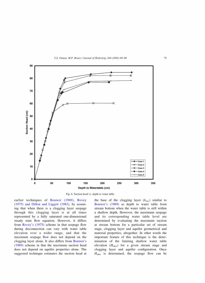
Fig. 6. Suction head vs. depth to water table.


calculated from:

Qs ¼

CrðHr 2 hÞ for h . Ybot

CrðHr 2 Ybot þ hsucÞ for Hshw , h # Ybot

CrðHr 2 HshwÞ for h # Hshw

8>><>>:

ð6Þ

where hsuc is the suction head [L] at the base of

clogging layer, approximated by Ybot 2 h; Hshw the

limiting shallow water table elevation [L],

approximated by Ybot 2 hmis; with hmis as the

maximum suction head [L] at the base of clogging

layer for a given set of stream stage and clogging

layer and aquifer materials and configurations.

Cr ¼ KbLW=M; is the streambed conductance,

where, L is the length [L] of the reach, W its

width [L], and Kb is the saturated hydraulic

conductivity of the bed material [LT21] and M

[L] its thickness.

The proposed relationship is shown in Figs. 4–6.

Fig. 4 defines the parameters in Eq. (6). Fig. 5 shows

the variation of the seepage flow with hydraulic head

in the aquifer for the proposed technique. When the

water table drops below the streambed, the seepage

flow continues to respond linearly to the water table

position until it falls below the shallow WT elevation

limit (Hshw), after which it remains constant. Thus, the

essential difference between this and MODFLOW

method is that the range of water table elevations at

which the seepage remains proportional to water table

elevation is extended downwards. Also, the lower

limit for shallow water table conditions can vary

depending on the material of the aquifer and clogging

layer, and the elevations of the water table and stream.

The part of the curve between the points correspond-

ing to h ¼ Ybot and h ¼ Hshw is the additional seepage

flow resulting from the suction at the base of the

clogging layer which is mainly missed by the current

MODFLOW method. However, the manuals for early

versions of MODFLOW did suggest that the stream

bottom could be replaced by the depth at which

seepage becomes constant. Fig. 6 relates suction head

at the base of the clogging layer (hsuc), obtained with

the variably saturated code SWMS_2D, to depth to

water table (below clogging layer) for some specific

test combinations of clogging layer and aquifer

properties. These are the same combinations used in

Section 5 to test the proposed improved method and

are described in more detail in that section. Fig. 6

emphasises clearly that depth to water table is

proportional to suction head and hence it is an

extremely important parameter in estimating seepage

from a losing stream and should not be ignored. Fig. 6

also shows that the maximum suction head attained in

any case, and consequently the depth to shallow water

table, is a function of the set of stream stage and

clogging layer and aquifer geometry and properties.

An important conclusion from Fig. 6 is that, under

steady state one-dimensional flow across a clogging

layer, similar to Bouwer’s (1969), the suction head at

the base of clogging layer can be replaced by the

depth to water table below the clogging layer base

when the water table is shallow, i.e. hsuc < Ybot 2 h:To use the proposed method, hmis or Hshw must first

be determined. Estimates of hmis are based on the

theory of one-dimensional steady state flow in a

layered soil derived by Zaslavsky (1964, 1965). Fig. 3

is reproduced from the latter reference to explain the

relationship between downward flux (flow through

unit area), qsmax; [LT21] across a clogging layer and

the unsaturated hydraulic conductivity in the aquifer.

In one-dimensional steady state downward flow in

a two layered system of soil in which the upper layer

has a saturated hydraulic conductivity (K1) much less

than the lower one (K2), the deep water table condition

in the lower layer is attained when the unsaturated

downward flux through the lower layer becomes

equivalent to the unsaturated hydraulic conductivity

of its soil. In other words, the deep water table

condition is established when the vertical hydraulic

gradient in the lower layer becomes unity. At this

point the maximum seepage flux, qsmax; [LT21] occurs,

so that

qsmax¼ K2ðhmisÞ ð7Þ

where K2( ) is the unsaturated hydraulic conductivity

of the aquifer and is a function of suction head. Here

we represent K2 with van Genuchten’s (1980)

equation which expresses the unsaturated hydraulic

conductivity, K, and moisture content, uw, as func-

tions of pressure head w:

uwðwÞ ¼ ur þus 2 ur

½1 þ lawln�mð8aÞ


KðwÞ ¼ KsSe1=2 1 2 1 2 Se

1=m� �h i2

ð8bÞ

with

Se ¼uw 2 ur

us 2 ur

ð8cÞ

where us is the saturated moisture content, dimension-

less; ur the residual moisture content, dimensionless;

a a parameter in the soil retention function, [L]; n an

exponent in the soil retention function ðn . 1Þ;dimensionless; m ¼ 1 2 1=n; dimensionless; and Ks

is the soil saturated hydraulic conductivity, [LT21].

Since the flow is steady, this unsaturated flux

through the aquifer, qs [LT21], given by Eq. (7), must

equal the saturated flux through the clogging layer,

which will also be at its maximum. This is given by

Eq. (6) with hsuc ¼ hmis as

qsmax¼

Kb

MðHr 2 Ybot þ hmisÞ ð9Þ

qsmaxcan be found by combining Eqs. (7) and (9),

solving for hmis

K2ðhmisÞ ¼Kb

MðHr 2 Ybot þ hmisÞ ð10Þ

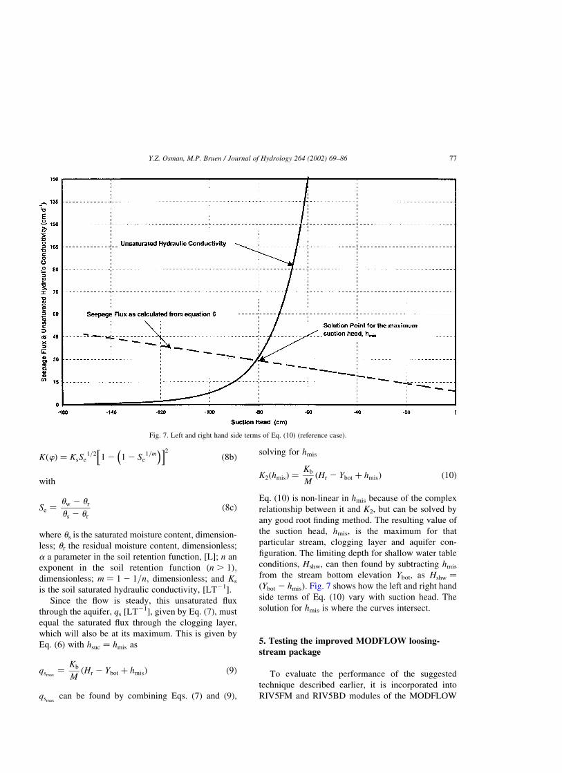
Eq. (10) is non-linear in hmis because of the complex

relationship between it and K2, but can be solved by

any good root finding method. The resulting value of

the suction head, hmis, is the maximum for that

particular stream, clogging layer and aquifer con-

figuration. The limiting depth for shallow water table

conditions, Hshw, can then found by subtracting hmis

from the stream bottom elevation Ybot, as Hshw ¼

ðYbot 2 hmisÞ: Fig. 7 shows how the left and right hand

side terms of Eq. (10) vary with suction head. The

solution for hmis is where the curves intersect.

5. Testing the improved MODFLOW loosing-

stream package

To evaluate the performance of the suggested

technique described earlier, it is incorporated into

RIV5FM and RIV5BD modules of the MODFLOW

Fig. 7. Left and right hand side terms of Eq. (10) (reference case).


River Package. Some modifications were also made to

the main program and other modules to read in the

unsaturated hydraulic properties for the aquifer plus

the saturated hydraulic conductivity of the clogging

layer. The new version of MODFLOW that contains

these modifications is called MOBFLOW and it is

tested by comparing its results with those from a

variably saturated flow model and the original MOD-

FLOW.

The test consists of (i) selecting the variably

saturated and saturated models, (ii) forming an

appropriate simulation test domain, (iii) conducting

and analysing the steady state simulations and (iv)

comparing the results from the three simulators.

The code SWMS_2D by Simunek et al. (1994) is

used here for the variably saturated numerical test. It

uses a Galerkin linear finite element formulation to

solve a two-dimensional form of Richards’ equation,

for water flow with a sink term, coupled with a

convection–dispersion equation for solute transport.

The hydraulic properties of the unsaturated soil are

represented by the model of Vogel and Cislerova

(1988), which under certain conditions becomes the

van Genuchten (1980) model. The flow and transport

can occur in a vertical plane, horizontal plane, or in a

three-dimensional region exhibiting radial symmetry

about a vertical axis. Verifications of the code by

comparison with field data or the output of other

variably saturated codes, e.g. UNSAT2, SWATRE are

well documented in its manual and are not discussed

here. Some minor modifications have been made to

the code to suit the present problem. The widely used

MODFLOW code (McDonald and Harbaugh, 1996) is

used here in the saturated numerical test as an

example for the conventional saturated codes.

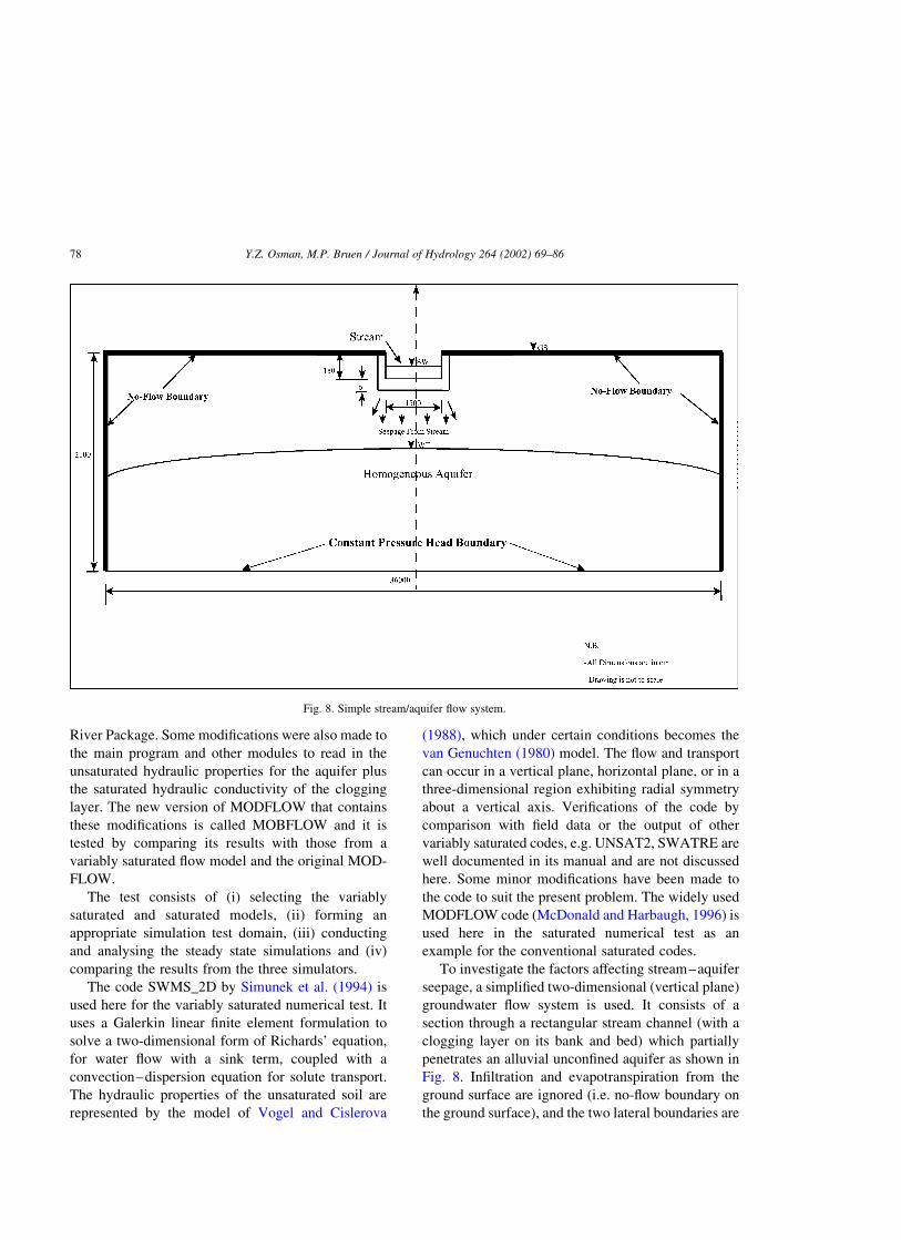
To investigate the factors affecting stream–aquifer

seepage, a simplified two-dimensional (vertical plane)

groundwater flow system is used. It consists of a

section through a rectangular stream channel (with a

clogging layer on its bank and bed) which partially

penetrates an alluvial unconfined aquifer as shown in

Fig. 8. Infiltration and evapotranspiration from the

ground surface are ignored (i.e. no-flow boundary on

the ground surface), and the two lateral boundaries are

Fig. 8. Simple stream/aquifer flow system.


taken either as no-flow or fixed head boundaries.

When the lateral boundaries are no-flow boundaries,

the only exchange of water within the model domain

is through the streambed and banks, and through the

bottom boundary of the domain where water can drain

to or rise from the lower part of the aquifer. The

dimensions of the flow domain are typical of Irish

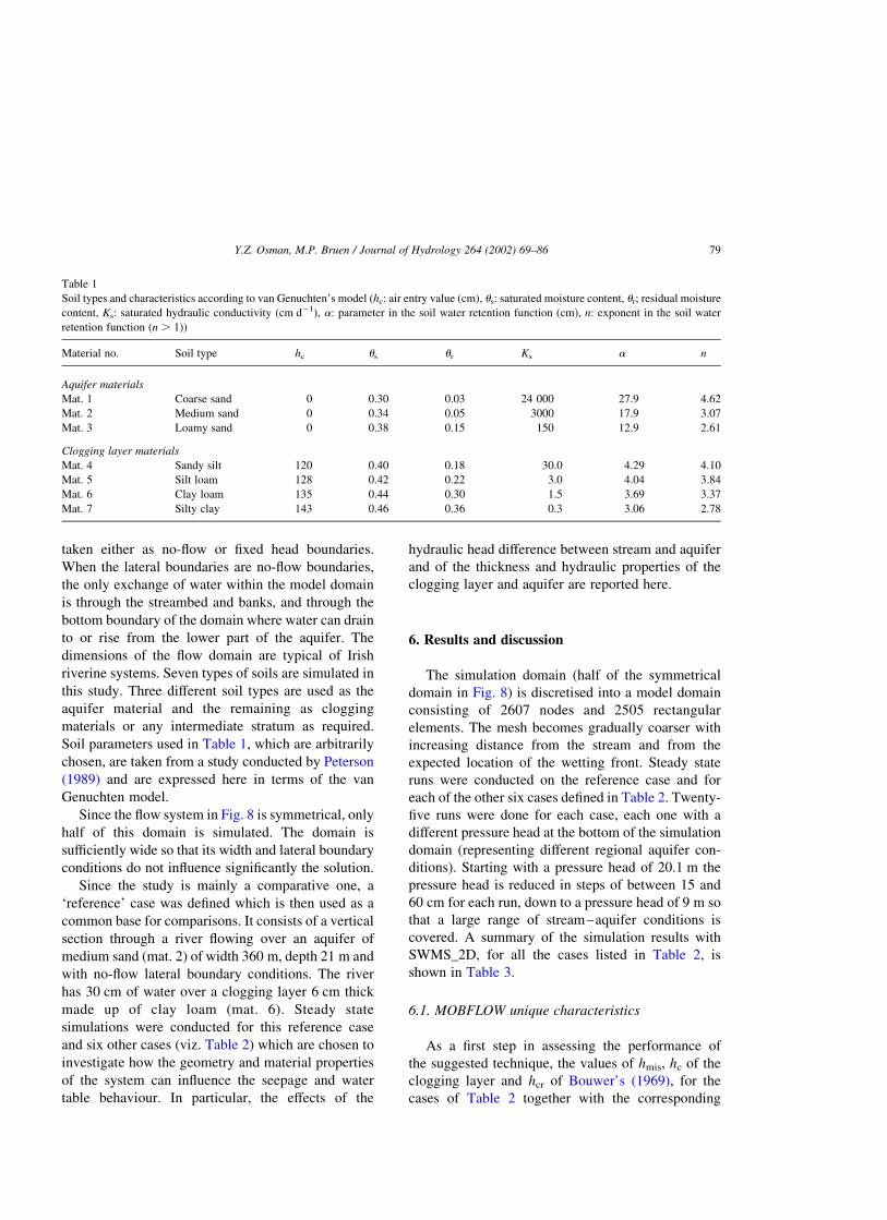
riverine systems. Seven types of soils are simulated in

this study. Three different soil types are used as the

aquifer material and the remaining as clogging

materials or any intermediate stratum as required.

Soil parameters used in Table 1, which are arbitrarily

chosen, are taken from a study conducted by Peterson

(1989) and are expressed here in terms of the van

Genuchten model.

Since the flow system in Fig. 8 is symmetrical, only

half of this domain is simulated. The domain is

sufficiently wide so that its width and lateral boundary

conditions do not influence significantly the solution.

Since the study is mainly a comparative one, a

‘reference’ case was defined which is then used as a

common base for comparisons. It consists of a vertical

section through a river flowing over an aquifer of

medium sand (mat. 2) of width 360 m, depth 21 m and

with no-flow lateral boundary conditions. The river

has 30 cm of water over a clogging layer 6 cm thick

made up of clay loam (mat. 6). Steady state

simulations were conducted for this reference case

and six other cases (viz. Table 2) which are chosen to

investigate how the geometry and material properties

of the system can influence the seepage and water

table behaviour. In particular, the effects of the

hydraulic head difference between stream and aquifer

and of the thickness and hydraulic properties of the

clogging layer and aquifer are reported here.

6. Results and discussion

The simulation domain (half of the symmetrical

domain in Fig. 8) is discretised into a model domain

consisting of 2607 nodes and 2505 rectangular

elements. The mesh becomes gradually coarser with

increasing distance from the stream and from the

expected location of the wetting front. Steady state

runs were conducted on the reference case and for

each of the other six cases defined in Table 2. Twenty-

five runs were done for each case, each one with a

different pressure head at the bottom of the simulation

domain (representing different regional aquifer con-

ditions). Starting with a pressure head of 20.1 m the

pressure head is reduced in steps of between 15 and

60 cm for each run, down to a pressure head of 9 m so

that a large range of stream–aquifer conditions is

covered. A summary of the simulation results with

SWMS_2D, for all the cases listed in Table 2, is

shown in Table 3.

6.1. MOBFLOW unique characteristics

As a first step in assessing the performance of

the suggested technique, the values of hmis, hc of the

clogging layer and hcr of Bouwer’s (1969), for the

cases of Table 2 together with the corresponding

Table 1

Soil types and characteristics according to van Genuchten’s model (hc: air entry value (cm), us: saturated moisture content, ur; residual moisture

content, Ks: saturated hydraulic conductivity (cm d21), a: parameter in the soil water retention function (cm), n: exponent in the soil water

retention function (n . 1))

Material no. Soil type hc us ur Ks a n

Aquifer materials

Mat. 1 Coarse sand 0 0.30 0.03 24 000 27.9 4.62

Mat. 2 Medium sand 0 0.34 0.05 3000 17.9 3.07

Mat. 3 Loamy sand 0 0.38 0.15 150 12.9 2.61

Clogging layer materials

Mat. 4 Sandy silt 120 0.40 0.18 30.0 4.29 4.10

Mat. 5 Silt loam 128 0.42 0.22 3.0 4.04 3.84

Mat. 6 Clay loam 135 0.44 0.30 1.5 3.69 3.37

Mat. 7 Silty clay 143 0.46 0.36 0.3 3.06 2.78


maximum seepage flux for each case were

computed from the formulae of Rovey (1975),

Bouwer (1969), and Eq. (6). The computed values

are compared with the estimates given by

SWMS_2D in Table 4 which confirms that hmis

neither depend on the clogging layer properties

alone nor on the aquifer properties alone. It is a

function of the whole stream–aquifer configur-

ation. It is different from Bouwer’s (1969) hcr,

since it has different values for the same aquifer

as in cases 1, 5, 8, and 14. The maximum flux

computed by the four models is also different.

While Rovey’s (1975) method overestimates the

maximum flux, Bouwer’s (1969) method seriously

underestimates the maximum flux. The technique

suggested in this paper gives a maximum flux

much closer to SWMS-2D.

6.2. Results from SWMS_2D

Fig. 9 shows the variation of steady state seepage

flows as the water table varies for the reference

simulation. As expected, seepage varies linearly with

decrease in water table until it reaches a maximum

and remains constant at this value irrespective of any

further drop in water table level. Three distinct points

on the curve should be noted. The first is the

‘hydrostatic condition’ point, which is the point at

which the stream and aquifer heads are equal, and it

separates cases 1 and 2 of Fig. 2. The second is the

‘incipient disconnection’ point, which is the point at

which the water table in the aquifer disconnects from

the stream, i.e. there is no longer a saturated

connection with the stream bottom. This point

separates cases 2 and 3 in Fig. 2. The third, is the

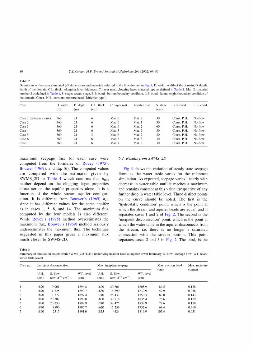
Table 2

Definitions of the cases simulated (all dimensions and materials referred to the flow domain in Fig. 8; D. width: width of the domain, D. depth:

depth of the domain, C.L. thick.: clogging layer thickness, C. layer mat.: clogging layer material type as defined in Table 1, Mat. 2: material

number 2 as defined in Table 1, S. stage: stream stage, B.B. cond.: bottom boundary condition, L.B. cond.: lateral (right) boundary condition of

the domain, Const. P.H.: constant pressure head (Dirichlet type))

Case D. width

(m)

D. depth

(m)

C.L. thick

(cm)

C. layer mat. Aquifer mat. S. stage

(cm)

B.B. cond. L.B. cond.

Case 1 (reference case) 360 21 6 Mat. 6 Mat. 2 30 Const. P.H. No-flow

Case 2 360 21 6 Mat. 6 Mat. 1 30 Const. P.H. No-flow






Table 3

Summary of simulation results from SWMS_2D (U.H.: underlying head or head at aquifer lower boundary, S. flow: seepage flow, WT. level:

water table level)

Case no. Incipient disconnection Max. incipient seepage Max. suction head

(cm)

Max. moisture

content

U.H.

(cm)

S. flow

(cm3 d21 cm21)

WT. level

(cm)

U.H.

(cm)

S. flow

(cm3 d21 cm21)

WT. level

(cm)

1 1890 10 961 1894.8 1800 20 801 1808.9 84.5 0.138

2 1890 11 725 1890.7 1830 16 899 1830.9 59.9 0.058

3 1890 17 577 1897.4 1740 26 433 1750.3 82.0 0.143

4 1890 20 387 1899.0 1800 39 718 1835.4 76.6 0.159

5 1890 20 250 1898.9 1740 38 475 1839.9 77.6 0.158

6 1830 8890 1906.7 1620 15 259 1752.6 64.4 0.310

7 1890 2315 1891.0 1815 4424 1816.9 107.4 0.051


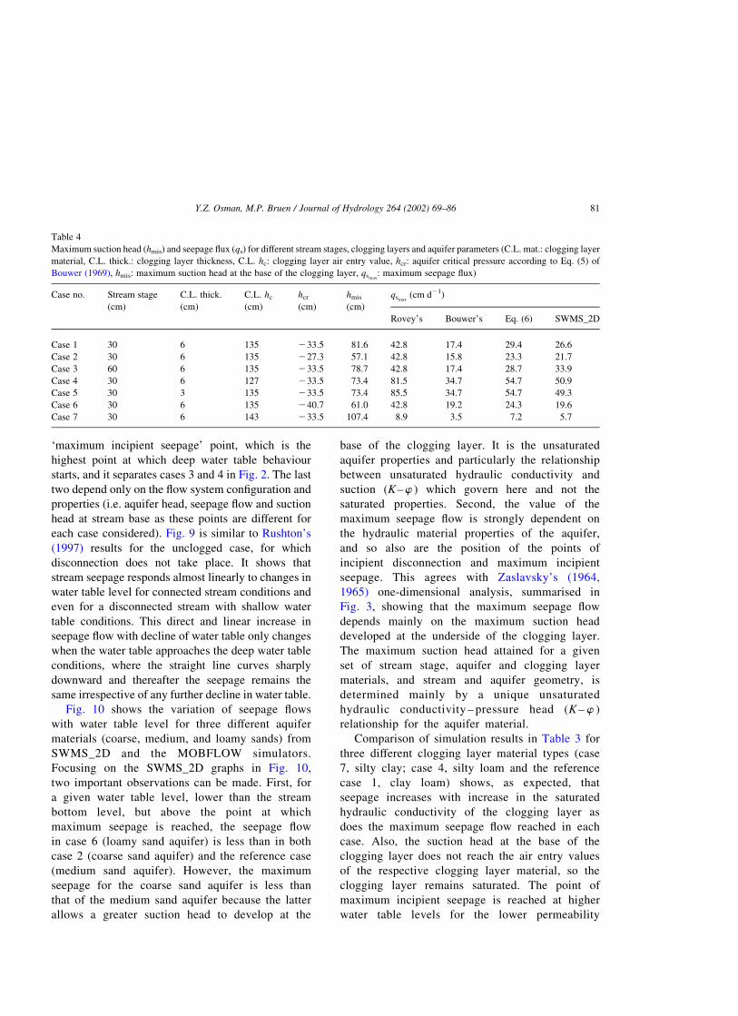
‘maximum incipient seepage’ point, which is the

highest point at which deep water table behaviour

starts, and it separates cases 3 and 4 in Fig. 2. The last

two depend only on the flow system configuration and

properties (i.e. aquifer head, seepage flow and suction

head at stream base as these points are different for

each case considered). Fig. 9 is similar to Rushton’s

(1997) results for the unclogged case, for which

disconnection does not take place. It shows that

stream seepage responds almost linearly to changes in

water table level for connected stream conditions and

even for a disconnected stream with shallow water

table conditions. This direct and linear increase in

seepage flow with decline of water table only changes

when the water table approaches the deep water table

conditions, where the straight line curves sharply

downward and thereafter the seepage remains the

same irrespective of any further decline in water table.

Fig. 10 shows the variation of seepage flows

with water table level for three different aquifer

materials (coarse, medium, and loamy sands) from

SWMS_2D and the MOBFLOW simulators.

Focusing on the SWMS_2D graphs in Fig. 10,

two important observations can be made. First, for

a given water table level, lower than the stream

bottom level, but above the point at which

maximum seepage is reached, the seepage flow

in case 6 (loamy sand aquifer) is less than in both

case 2 (coarse sand aquifer) and the reference case

(medium sand aquifer). However, the maximum

seepage for the coarse sand aquifer is less than

that of the medium sand aquifer because the latter

allows a greater suction head to develop at the

base of the clogging layer. It is the unsaturated

aquifer properties and particularly the relationship

between unsaturated hydraulic conductivity and

suction (K–w ) which govern here and not the

saturated properties. Second, the value of the

maximum seepage flow is strongly dependent on

the hydraulic material properties of the aquifer,

and so also are the position of the points of

incipient disconnection and maximum incipient

seepage. This agrees with Zaslavsky’s (1964,

1965) one-dimensional analysis, summarised in

Fig. 3, showing that the maximum seepage flow

depends mainly on the maximum suction head

developed at the underside of the clogging layer.

The maximum suction head attained for a given

set of stream stage, aquifer and clogging layer

materials, and stream and aquifer geometry, is

determined mainly by a unique unsaturated

hydraulic conductivity – pressure head (K –w )

relationship for the aquifer material.

Comparison of simulation results in Table 3 for

three different clogging layer material types (case

7, silty clay; case 4, silty loam and the reference

case 1, clay loam) shows, as expected, that

seepage increases with increase in the saturated

hydraulic conductivity of the clogging layer as

does the maximum seepage flow reached in each

case. Also, the suction head at the base of the

clogging layer does not reach the air entry values

of the respective clogging layer material, so the

clogging layer remains saturated. The point of

maximum incipient seepage is reached at higher

water table levels for the lower permeability

Table 4

Maximum suction head (hmis) and seepage flux (qs) for different stream stages, clogging layers and aquifer parameters (C.L. mat.: clogging layer

material, C.L. thick.: clogging layer thickness, C.L. hc: clogging layer air entry value, hcr: aquifer critical pressure according to Eq. (5) of

Bouwer (1969), hmis: maximum suction head at the base of the clogging layer, qsmax: maximum seepage flux)

Case no. Stream stage

(cm)

C.L. thick.

(cm)

C.L. hc

(cm)

hcr

(cm)

hmis

(cm)

qsmax(cm d21)

Rovey’s Bouwer’s Eq. (6) SWMS_2D

Case 1 30 6 135 233.5 81.6 42.8 17.4 29.4 26.6

Case 2 30 6 135 227.3 57.1 42.8 15.8 23.3 21.7

Case 3 60 6 135 233.5 78.7 42.8 17.4 28.7 33.9

Case 4 30 6 127 233.5 73.4 81.5 34.7 54.7 50.9

Case 5 30 3 135 233.5 73.4 85.5 34.7 54.7 49.3

Case 6 30 6 135 240.7 61.0 42.8 19.2 24.3 19.6

Case 7 30 6 143 233.5 107.4 8.9 3.5 7.2 5.7


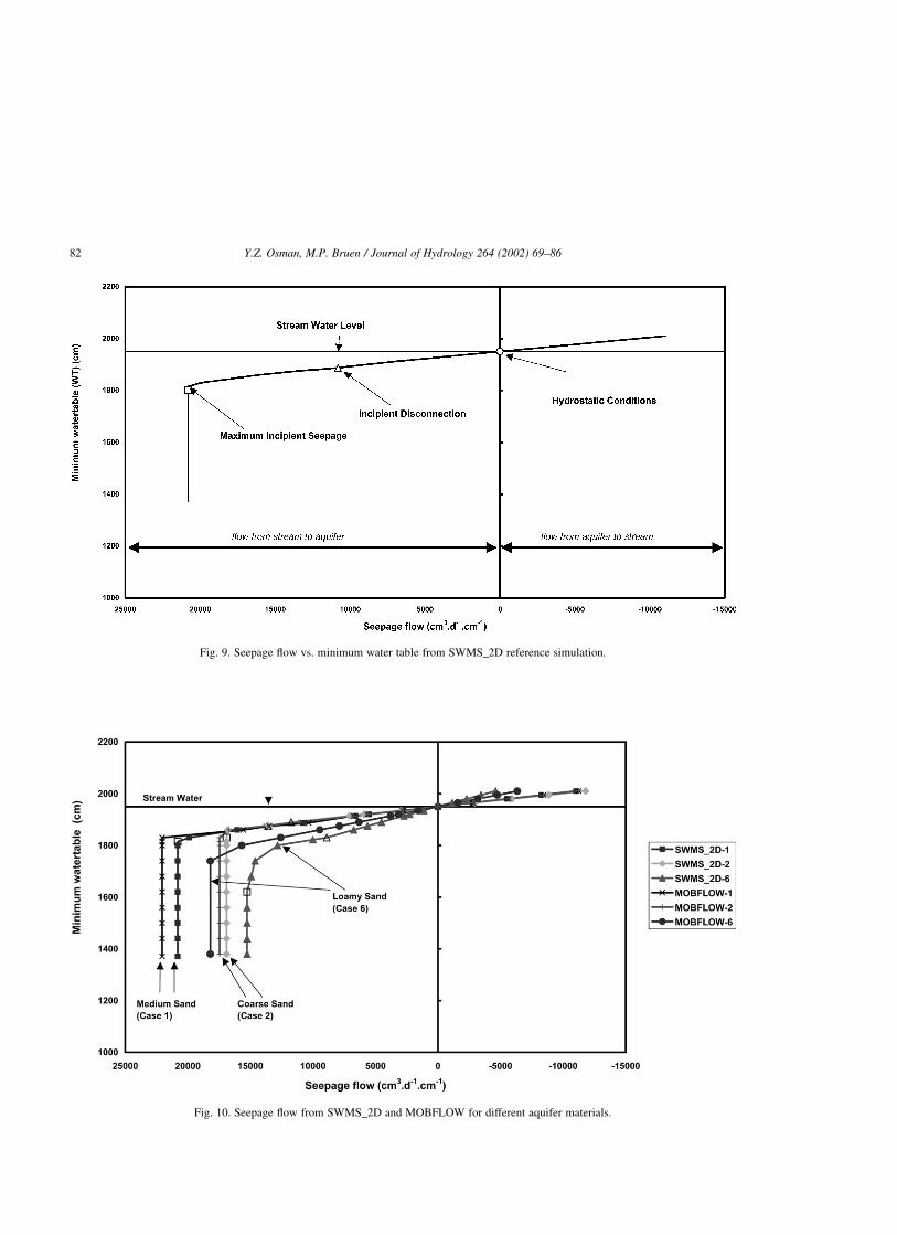
Fig. 9. Seepage flow vs. minimum water table from SWMS_2D reference simulation.

Fig. 10. Seepage flow from SWMS_2D and MOBFLOW for different aquifer materials.


clogging layers than for the higher ones. This is

also expected since seepage is restricted more by a

lower permeability material than a higher per-

meability one, which means less ‘mounding’ of

the water table. Thus, the water table under the

stream responds more closely to changes in

aquifer head for the lower permeability clogging

layer case than for the higher permeability one.

Similarly, comparison of results in Table 3 for

cases with different clogging layer thickness,

namely, case 5 (clogging layer is 3 cm thick)

and the reference case (clogging layer is 6 cm

thick) shows that seepage flow is inversely

proportional to the thickness of clogging layer

and maximum incipient seepage conditions are

reached at relatively higher water table levels for

thicker clogging layers than for thinner ones.

Nevertheless, for both cases, the suction heads at

the base of the clogging layer are still lower than

the air entry value of the clogging layer. This

indicates that clogging layers tend to remain

saturated, even when they are thin. The relatively

higher suction heads at the base of the thinner

clogging layer explains the deeper depths reached

by water table before deep water table conditions

occur.

6.3. Comparison between SWMS_2D and

MODFLOW

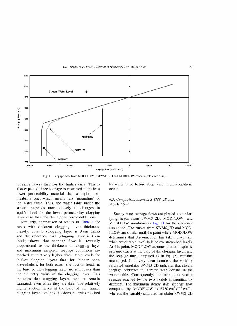
Steady state seepage flows are plotted vs. under-

lying heads from SWMS_2D, MODFLOW, and

MOBFLOW simulators in Fig. 11 for the reference

simulation. The curves from SWMS_2D and MOD-

FLOW are similar until the point where MODFLOW

determines that disconnection has taken place (i.e.

when water table level falls below streambed level).

At this point, MODFLOW assumes that atmospheric

pressure exists at the base of the clogging layer, and

the seepage rate, computed as in Eq. (2), remains

unchanged. In a very clear contrast, the variably

saturated simulator SWMS_2D indicates that stream

seepage continues to increase with decline in the

water table. Consequently, the maximum stream

seepage reached by the two models is significantly

different. The maximum steady state seepage flow

computed by MODFLOW is 6750 cm3 d21 cm21,

whereas the variably saturated simulator SWMS_2D

Fig. 11. Seepage flow from MODFLOW, SMWMS_2D and MOBFLOW models (reference case).


computes it as 20 801 cm3 d21 cm21. Note that the

MODFLOW estimate is less than one-third of that

estimated by the variably saturated code, so the

difference is substantial.

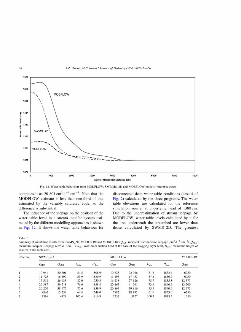
The influence of the seepage on the position of the

water table level in a stream–aquifer system esti-

mated by the different modelling approaches is shown

in Fig. 12. It shows the water table behaviour for

disconnected deep water table conditions (case 4 of

Fig. 2) calculated by the three programs. The water

table elevations are calculated for the reference

simulation aquifer at underlying head of 1380 cm.

Due to the underestimation of stream seepage by

MODFLOW, water table levels calculated by it for

the area underneath the streambed are lower than

those calculated by SWMS_2D. The greatest

Fig. 12. Water table behaviour from MODFLOW, SMWMS_2D and MOBFLOW models (reference case).

Table 5

Summary of simulation results from SWMS_2D, MODFLOW and MOBFLOW (QIDS: incipient disconnection seepage (cm3 d21 cm21), QMIS:

maximum incipient seepage (cm3 d21 cm21), hmis: maximum suction head at the base of the clogging layer (cm), Hshw: maximum height of

shallow water table (cm))

Case no. SWMS_2D MOBFLOW MODFLOW

QIDS QMIS hmis Hshw QIDS QMIS hmis Hshw QMIS

1 10 961 20 801 84.5 1808.9 10 825 22 046 81.6 1832.4 6750

2 11 725 16 899 59.9 1830.9 11 195 17 453 57.1 1856.9 6750

3 17 568 26 433 82.0 1750.3 16 238 27 126 78.7 1835.3 12 375

4 20 387 39 718 76.6 1838.4 20 863 41 041 73.4 1840.6 13 500

5 20 250 38 475 77.6 1839.9 20 863 39 916 73.4 1840.6 12 375

6 8890 15 259 64.4 1749.0 7882 18 192 61.0 1853.0 6750

7 2316 4424 107.4 1816.9 2232 5127 100.7 1813.3 1350


disparities occur directly under the streambed and

decrease and vanish towards the ends of the flow

domain. This is clearly attributed to the greater

incoming seepage from the stream in this area.

It is worth mentioning that MODFLOW would

yield equal and constant maximum seepage flows for

different aquifer materials for a given stream stage,

clogging layer material and thickness and domain

geometry since they would be calculated from Eq. (2),

and this is obviously unrealistic.

6.4. Comparison of SWM_2D, MODFLOW and

MOBFLOW

The newly proposed code MOBFLOW and the

original MODFLOW are compared to the variably

saturated code SWMS_2D. The comparative simu-

lation results of the three codes are shown in Table 5

and in the accompanying figures. Steady state seepage

flow is plotted vs. aquifer water table estimated by

SWMS_2D, MODFLOW, and MOBFLOW in Fig. 11

for the reference simulation case. The seepage flow

from MOBFLOW matches very well with that of

SWMS_2D in all stages and is an improvement over

MODFLOW. The main difference is that, MOB-

FLOW takes account of suction heads at the base of

the clogging layer when the water table drops below

the streambed level and continues to respond to water

table changes until deep water table conditions are

reached. The maximum seepage flow computed by

MOBFLOW is 22 050 cm3 d21 cm21 with a maxi-

mum suction head of 81.6 cm, whereas the actual value

computed by SWMS_2D is 20 801 cm3 d21 cm21 with

a maximum suction head of 84.3 cm. The corresponding

MODFLOW value, 6750 cm3 d21 cm21, seriously

underestimates the maximum seepage. The relatively

small, 6%, overestimation by MOBFLOW of the

maximum incipient seepage, which could be due to

the approximations used in representing the soil

properties and evaluating the suction head, is definitely

better than the 67.5% underestimation by MODFLOW.

Therefore, the improvement achieved by the proposed

method is valuable, and may be especially important

when the groundwater model is calibrated when the

stream and aquifer are connected and used when the

systems are disconnected.

Fig. 12 shows the water table behaviour obtained

by the three models for the reference simulation case

at aquifer head of 1380 cm. The MOBFLOW water

table curve is close to that of SWMS_2D, especially

directly below the stream. The MODFLOW curve is

quite different and shows much less mounding. There

is a slight overestimation by MOBFLOW compared

with SWMS_2D, which could be explained by the

approximations used in determining hmis. Again, the

improvement here is a direct result of accounting for

suction head effects. All the three methods yield

almost the same water table level at distance away

from the stream.

The test for the effect of aquifer material is

conducted here to assess the performance of the

proposed code, MOBFLOW, on predicting seepage

flow for the three different aquifer materials already

discussed. The three aquifers give different seepage

flow-head curves for both connected and disconnected

conditions, including different points of maximum

incipient seepage attained in each case, see Fig. 10.

This is in stark contrast to MODFLOW’s expected

estimates based on Eq. (2). Thus, the proposed

MOBFLOW is capable of accounting for different

aquifer materials especially during disconnection.

7. Conclusions

This paper assesses the main factors influencing

stream–aquifer seepage for a loosing-stream with a

clogged layer using a variably saturated flow code

with the purpose of producing a simple technique to

improve the current status of modelling stream–

aquifer seepage in conventional saturated models.

Simple numerical approaches for modelling

stream–aquifer interactions through clogging layers

have been reviewed and the differences between them

have been evaluated. The most commonly used

technique tends to underestimate stream losses

because it ignores suction heads below the clogging

layer.

Aquifer material properties strongly affect seepage

flow rates in all stages of stream–aquifer relation-

ships. These effects become very obvious when the

stream disconnects from the aquifer. Therefore,

seepage from a disconnected stream cannot be

determined correctly unless the unsaturated hydraulic

properties of the aquifer and clogging layer, and the

stream water level are known.


Previously used saturated flow approaches

seriously underestimate stream losses, hydraulic

heads and water table levels for disconnected

conditions. It is the inability of the conventional

saturated codes to accurately estimate the stream

losses that is the major cause of disparities between

SWMS_2D and MODFLOW in estimating seepage

flows and water levels.

The improved MODFLOW code, MOBFLOW,

gives stream seepage and water table levels that match

very well with those from the variably saturated flow

code SWMS_2D. Therefore, it could be used in

simulating stream–aquifer systems, especially when

the stream disconnects from its adjacent aquifer.

Acknowledgments

The authors would like to thank Dr Jirka Simunek

of the US Salinity Laboratory for providing the

SWMS_2D code. The constructive criticisms and

comments made by Prof. Ken Rushton, Birmingham

University, and the anonymous reviewers are highly

appreciated by the authors. Finally, the first author

would like to acknowledge the financial support he

received from the Centre for Water Resources

Research, UCD, during his PhD course.

References

Bear, J., Zaslavsky, D., Irmay, S., 1968. Physical Principles of

Water Percolation and Seepage, UNESCO, Paris.

Bouwer, H., 1964. Unsaturated flow in groundwater hydraulics.

Am. Soc. Civ. Engr, J. Hydrauls Div. 90 (HY5), 121–144.

Bouwer, H., 1969. In: Chow, V.T., (Ed.), Theory of Seepage from

Open Channels, Advances in Hydroscience, vol. 5. Academic

Press, New York, pp. 121–172.

Brockway, C.E., Bloomsburg, G.L., 1968. Movement of water from

canals to groundwater table. Water Resources Research

Institute, University of Idaho, Research Technical Completion

Report, Project A-009-IDA.

Dillon, P.J., Liggett, J.A., 1983. An ephemeral stream–aquifer

interaction model. Water Resour. Res. 19 (3), 621–626.

van Genuchten, M.Th., 1980. A closed-form equation for predicting

the hydraulic conductivity of unsaturated soils. Soil Sci. Soc.

Am. J. 44, 892–898.

Green, W.H., Ampt, C.A., 1911. Studies on soil physics 1. Flow of

air and water through soils. J. Agric. Sci. 4, 1–24..

McDonald, M.G., Harbaugh, A.W., 1983, 1984, 1988, 1996. A

modular three-dimensional finite difference groundwater model.

United States Geological Survey, Openfile Report No. 6.

Peterson, D.M., 1989. Variably saturated flow between streams and

aquifers. PhD Dissertation, New Mexico Institute of Mining and

Technology, Socorro, New Mexico.

Rovey, C.E.K., 1975. Numerical Model of Flow in Stream Aquifer

System, Hydrology Paper No. 74, Colorado State University,

Fort Collins, Colorado.

Rushton, K.R., 1997. Recharge of Phreatic Aquifers in (Semi-) Arid

Areas, IAH Publication No. 19, chapter 4, pp. 215–277.

Simunek, J., Vogel, T., van Genuchten, M.Th., 1994. The

SWMS_2D code for simulating water flow and solute transport

in two-dimensional variably saturated media, version 1.21.

Research Report No. 132. US Salinity Laboratory, Agricultural

Research Service, US Department of Agriculture, Riverside,

California.

Spalding, C.P., Khaleel, R., 1991. An evaluation of analytical

solutions to estimate drawdowns and stream depletions by

wells. Water Resour. Res. 27 (4), 597–609.

Vogel, T., Cislerova, M., 1988. On the reliability of unsaturated

hydraulic conductivity calculated from the moisture retention

curve. Transp. Porous Media 3, 1–15.

Zaslavsky, D., 1964. Saturated and unsaturated flow in unstable

porous medium. Soil Sci. 98 (5), 317–321.

Zaslavsky, D., 1965. The significant of water head measurements in

porous material. RILEM Symposium on Transfer of Water in

Porous Media, Paris (Bull. RILEM, no. 29, December 1965, pp.

55–59).


Documents

Modelling stream–aquifer seepage in an alluvial aquifer: an improved loosing-stream package for MODFLOW