AlmaLaurea Working Papers – ISSN 2239-9453

ALMALAUREA WORKING PAPERS no. 56

November 2012

Modelling Job Satisfaction in AlmaLaurea Surveys

by

Stefania Capecchi, Maria Iannario, Domenico Piccolo

Department of Theory and Methods of Human and Social Sciences

Statistical Sciences Unit, University of Naples Federico II

This paper can be downloaded at: AlmaLaurea Working Papers series http://www2.almalaurea.it/universita/pubblicazioni/wp/index.shtml

Also available at: REsearch Papers in Economics (RePEC)

The AlmaLaurea working paper series is designed to make available to a wide readership selected works

by AlmaLaurea staff or by outside, generally available in English or Italian. The series focuses on the study

of the relationship between educational systems, society and economy, the quality of educational process,

the demand and supply of education, the human capital accumulation, the structure and working of the

labour markets, the assessment of educational policies.

Comments on this series are welcome and should be sent to pubblicazioni@almalaurea.it.

AlmaLaurea is a public consortium of Italian universities which, with the support of the Ministry of

Education, meets the information needs of graduates, universities and the business community.

AlmaLaurea has been set up in 1994 following an initiative of the Statistical Observatory of the University

of Bologna. It supplies reliable and timely data on the effectiveness and efficiency of the higher education

system to member universities’ governing bodies, assessment units and committees responsible for

teaching activities and career guidance.

AlmaLaurea:

facilitates and improves the hiring of young graduates in the labour markets both at the national

and international level;

simplifies companies' search for personnel, reducing the gap between the demand for and supply

of qualified labour (www.almalaurea.it/en/aziende/);

makes available online more than 1.5 million curricula (in Italian and English) of graduates,

including those with a pluriannual work experience (www.almalaurea.it/en/);

ensures the optimization of human resources utilization through a steady updating of data on the

careers of students holding a degree (www.almalaurea.it/en/lau/).

Each year AlmaLaurea plans two main conferences (www.almalaurea.it/en/informa/news) in which the

results of the annual surveys on Graduates’ Employment Conditions and Graduates’ Profile are presented.

________________________________________________________________________________________

AlmaLaurea Inter-University Consortium | viale Masini 36 | 40126 Bologna (Italy)

Website: www.almalaurea.it | E-mail: pubblicazioni@almalaurea.it

______________________________________________________________________________________

The opinions expressed in the papers issued in this series do not necessarily reflect the position of

AlmaLaurea

© AlmaLaurea 2012

Applications for permission to reproduce or translate all or part of this material should be made to: AlmaLaurea Inter-University Consortium email: pubblicazioni@almalaurea.it | fax +39 051 6088988 | phone +39 051 6088919

1

Modelling Job Satisfaction in AlmaLaurea Surveys

by

Stefania Capecchi, Maria Iannario, Domenico Piccolo*

Abstract

A statistical approach for modelling job satisfaction stemming from the surveys on graduates’ employment conditions

collected by AlmaLaurea is presented. Graduates have been interviewed about their employment conditions 1, 3 and 5

years after the time of degree. The focus of the survey is to assess the capacity of labour demand and labour market to

exploit the human capital created by universities and, reciprocally, the ability of universities to meet society's

requirements and needs (i.e. their external effectiveness and efficiency). Specifically, we compare different models

implemented for the ordinal rating to the question: “How satisfied are you with your job?”. We establish differences in

the estimated patterns of global job satisfaction and its components, but also emphasize the possibility to use an

innovative approach (CUB models) to allow for control the effects of feeling and uncertainty in the response process.

Keywords: Job satisfaction, Graduates’ employment conditions, Ordinal data modelling, CUB models

1. Introduction

Investigated by different disciplines such as Psychology, Sociology, Economics and Management

sciences, several studies have examined which worker characteristics and organization features lead

or are related to job satisfaction (Spector 1997). Although this topic has been mainly motivated by

psychological studies, especially in the field of industrial-organizational psychology and in the so

called goal-setting theory, the current literature about job satisfaction has been spread in a wide

range of research fields (Spector 1985).

These analyses were initially motivated by positive link with worker productivity and economic

impact. Since the early Seventies (Vroom et al. 1971), various models have been implemented in

order to detect leadership and decision-making abilities and attitudes: job satisfaction is revealed to

be a major determinant of labour market dynamics such as productivity, mobility, unionism, etc.

(Freeman 1978). In addition, job satisfaction may be considered both an explicative variable of job

performance and mobility and a dependent variable on psychological as well objective

circumstances.

Recently, the interest has moved towards the relevance that this component can have on individuals

overall life well-being (Blanchflower and Oswald 2004; Bakhshi et al. 2008; Kapteyn et al. 2009).

Thus, job satisfaction is considered as an attitudinal variable and it is used in connection or apart

from the usual economic variables like income and wealth because it is considered a part of the

* Department of Theory and Methods of Human and Social Sciences Statistical Sciences Unit, University of Naples

Federico II.

e-mail: {stefania.capecchi, maria.iannario, domenico.piccolo}@unina.it

2

economic development of a country. Moreover, although job satisfaction consistently seems a factor

of job performance, it cannot be considered only related to economic incentives which, in some

cases, act as counterproductive (Pugno and Depedri 2009).

A definition of job satisfaction frequently quoted explains job satisfaction as an emotional state

through a behavioural variable: “(...) a pleasurable or positive emotional state resulting from the

appraisal of one’s job or job experiences” (Locke 1976).

Another definition is the following: “Job satisfaction is simply how people feel about their jobs and

different aspects of their jobs. It is the extent to which people like (satisfaction) or dislike

(dissatisfaction) their jobs” (Spector 1997).

The main problem in analyzing job satisfaction is associated with the collection of adequate data

related to the phenomenon. Job satisfaction and, more generally, individual attitudes cannot be

directly observed, but are usually obtained from subjective survey questions, as for instance: “How

satisfied are you with your work?”

Generally, questions used to quantify individuals’ satisfaction measure an underlying continuous

variable through a rating scale. The responses indicate the degree of agreement with each statement,

with higher scores reflecting a higher degree. In the survey used for the present study, respondents

were asked to answer questions referring to their level of satisfaction on different items about

overall work, intrinsic aspects of work and aspects related to job environment. A 10-point response

on a Likert scale was used (1=very dissatisfied, 10=very satisfied). Consequently, the variables

resulting from the questionnaire are ordered categorical (i.e., ordinal) variables.

However, psychological factors may induce respondents to refrain from using certain values of the

rating scale and to concentrate towards others as in “response contraction bias” (Poulton 1989), but

they can also exceed to rate the maximum value or concentrate the answer to one focal modality

generating the so-called “shelter effect” (Iannario 2012a). Also, when dealing with such subjective

variables, some problems (e.g. “cognitive dissonance”) can arise and affect the meaningfulness of

the data (Bertrand and Mullainathan 2001). A related issue concerns the so-called “scale

heterogeneity problem” generated by the circumstance that each subject adopts a personal metric

for expressing a judgment, which is only a subset of the proposed scale on the questionnaire. This

behaviour is well recognized in educational surveys (as PISA, for instance: Buckley 2009) and is

derived by both psychological and cultural differences in the response style. Thus, researchers may

distinguish: acquiescence and disacquiescence response style (the tendency to agree or disagree,

respectively, with the items), extreme response style (the tendency to choose endpoints of the

scale), and noncontingent response style (the tendency to generate a careless or totally random

choice of the response modality). These issues have been investigated both from a methodological

point of view and also for their statistical and interpretative consequences (Rossi et al. 2005; Fiebig

et al. 2009). They are also present in job satisfaction surveys and we will discuss them in the

following sections.

In addition, it has been advocated that respondents will be prone to select the answer adopting a

“satisficing” behaviour (Simon 1957), by choosing an adequate answer that may not be the optimal

one, in the attempt to minimize the burden of the question (Krosnick 1991).

Moreover, other aspects related to surveys as the amount of time devoted to the answer, the use of

limited set of information, partial understanding of the item, lack of self-confidence, laziness,

apathy (Krosnick 1991) can influence the response.

Neglecting these aspects implies adding an underlying noise in the model and, from a statistical

point of view, these omissions increase bias and reduce efficiency of the estimates.

Generally, the question used to investigate job satisfaction in surveys can be referred to the overall

job satisfaction, or use a range of specific items regarding individual facets related to work, like

pay, promotion, co-workers, education/job mismatch and job security, to study different aspects that

3

can influence the global on-the-job satisfaction. As a matter of fact, job satisfaction depends on the

balance between work-role inputs - such as education, working time, effort - and work-role outputs

- wages, fringe benefits, status, working conditions, intrinsic aspects of the job. If work-role outputs

(‘pleasures’) increase with respect to work-role inputs (‘pains’), then job satisfaction will increase

(Sousa-Poza and Sousa-Poza 2000).

Moreover, in recent job design and occupation health literature, job satisfaction is often detected

regarding work stress issues. One of the most widely used theory, known as demand-control model

(Karasek 1997) implies workplace stress as a function of job pressure, in terms of quantitative job

demands, and of worker's control over his own responsibilities.

Other theorists (e.g. Rose 2005) have viewed job satisfaction as a bi-dimensional concept consisting

of intrinsic and extrinsic satisfaction dimensions (two latent components). Intrinsic sources of

satisfaction depend on the individual characteristics of the person, such as the ability to use

initiatives, relations with supervisors, or the work that the person actually performs; these are

symbolic or qualitative facets of the job. Extrinsic sources of satisfaction are situational and depend

on the environment, such as pay, promotion, or job security; these sources are financial and other

material rewards or advantages of a job. Both extrinsic and intrinsic job facets should be

represented, as equally as possible, in a composite measure of overall job satisfaction.

All features may be accounted for a class of statistical models where the response is explicitly

modelled as the combination of two latent components, related to the individual feeling towards the

item and to the uncertainty in the response process, respectively. Such approach has been

successfully experimented with job satisfaction data in the context of the national Survey of the

Household Income and Wealth (SHIW), promoted by the Bank of Italy (Gambacorta and Iannario

2012). Indeed, in the present work we exploit this class of models to investigate several aspects of

job satisfaction as expressed by a large data set of students after 5 years they got the university

degree (available from AlmaLaurea surveys).

The paper is organized as follows: in the next section we briefly mention the data collection process

and the relevant variables we will use. In section 3 we perform some exploratory analysis to

introduce the main characteristics of the response variable. Then, in section 4 we set the notation

and the main interpretation of the class of proposed models. Then, in section 5 we investigate this

methodology with reference to respondents’ covariates. In section 6, global job satisfaction and its

components are analyzed and section 7 is devoted to the investigation of selected clusters. In section

8, the effect of income and typology of occupation is checked whereas family background on job

satisfaction are studied in section 9. Groups and disciplines characterizing the degree are explored

in section 10 whereas the relationship between final score and job satisfaction is investigated in

section 11. Sections 12 and 13 consider the role of variables related to time, that is age at degree

and time spent at university. The phenomenon known as “scale usage heterogeneity” is examined in

section 14 and an example of an omnibus statistical model is presented in section 15. Some possible

profiles of respondents are presented for interpretative and predictive objectives in section 16. Some

concluding remarks end the work.

2. Data collection and selected variables

The data set analyzed in this study stems from the archive of AlmaLaurea surveys, which now

cover almost all graduates at 64 Italian universities and accounts for about 78% of the whole

population of Italian graduates. Specifically, we are concerned with several components of job

satisfaction which are collected during the 2010 wave and include several subjects’ covariates,

which hopefully may be interpreted as predictors of the responses.

4

The survey concerns with graduates ante-riforma, which changed the scheduling of Italian

university degree from a single (4, 5 or 6 years) to a two-step curriculum (3+2 years). More

specifically, data set consists of graduates of 2005 interviewed within the period May-August 2010

and who are working after 5 years from the degree. This analysis refers to 59% of all Italian

graduates in the same period.

Indeed, AlmaLaurea data set is a “panel” of responses available for most subjects after 1, 3, 5 years

after they received a university degree. However, our analysis concerns only graduates who have a

job after 5 years of their degree and accepted to answer.

Thus, after a preliminary screening to validate the collected questionnaires for internal consistency,

data set consists of a matrix of 17,387 rows (subjects) and 55 columns (variables). In some cases,

there are missing values and although statistical techniques are available for this purpose we will

avoid imputation techniques in this study. More precisely, the possible presence of missing values

is tackled in the following manner: we consider the joint relationship among the interested variables

only if they are complete, and thus we will exploit in turn all available data which are pairwise

complete or complete as necessary.

Job satisfaction has been investigated by asking graduates to answer a global question (coded as

a18) and fourteen components (a19_01…a19_14) of satisfaction related to several aspects: 1.

Security of the job 2. Coherence with studies 3. Acquisition of professionalism 4. Prestige 5.

Correspondence with cultural interests 6. Social utility 7. Independence or autonomy in the job 8.

Involvement in the decisional processes 9. Flexibility of time 10. Availability of free time 11.

Workplace 12. Relationships with co-workers 13. Expectation of future gains 14. Perspectives of

career.

All responses to the personal evaluation of job satisfaction and its components are expressed on a

Likert scale (without wording) ranging from 1 to 10, where 1 means “extremely unsatisfied” and 10

means “extremely satisfied”. These responses may be related to subjects’ covariates and data about

family and career information available from the general archive of AlmaLaurea graduates.

The main purpose of this work is to examine the response pattern and study the relationships among

job satisfaction and the other available covariates like regions of the university, characteristics of

the study career, previous job experience, time spent abroad, and so on.

3. Exploratory analysis of job satisfaction

First of all, we present a synthetic analysis of the responses given to the 15 questions concerning job

satisfaction and we limit the presentation to few results which have to be considered as preliminary

to the modelling strategy, which is the main objective of this work (all analysis have been

performed by using the R statistical environment). Respondents are mainly women (59.7%) and we

check in several cases if difference of gender affects the responses.

In Table 1 we list the average of job satisfaction responses, the ranking of the 14 components of the

satisfaction with respect to the average and the correlation of each component with the global

response. The number of missing data is also shown.

It turns out that the items “Relationships with co-workers” and “Independence or autonomy in the

job” achieve the highest scores whereas “Availability of free time”, “Expectation of future gains”

and “Perspectives of career” achieve the lowest. We notice that the number of missing values tends

progressively to increase according to the list of items in the questionnaire: this signal may suggest

some tiredness in respondents when they have to answer a long list of similar questions. In future

surveys, it may be convenient to rotate the list of the 14 components in order to cancel the

positional effect of the responses. In any case, the high value of missing data for the “Relationships

issue with co-workers” is mainly ascribable to the responses of single workers.

5

Since the global satisfaction is the final result of an evaluation composed by many facets we

compute the correlation among the global satisfaction and each of the 14 components; thus, the last

columns of Table 1 displays the Bravais-Pearson measure (the Spearman correlation coefficient

gives similar results in this case). It turns out that the strongest relationship of global satisfaction is

with “Correspondence with cultural interests” and “Coherence with studies”, followed by

“Acquisition of professionalism”, “Prestige” and “Involvement in the decisional processes”. At the

opposite, we find “Relationships with co-workers”, “Workplace”, and “Availability of free time”.

Thus, we register that the global evaluation of job satisfaction is mainly due to the personal

achievement of an expected position in relation to studies, career and competences. The fact that the

“Relationships with co-workers” is the highest item in the ranking of the averages and the lowest in

the correlation with global satisfaction should not be considered as a contradiction: respondents feel

that the human relationships with colleagues are mostly related to friendship and common life, but

this does not affect too much the final evaluation of the job they perform.

Table 1. Average of global satisfaction and its components

Items Missing Average Rank Corr

Global job satisfaction 5 7.5698 === ===

1. Security of the job 5 6.7374 11 0.312

2. Coherence with studies 3 6.9222 10 0.452

3. Acquisition of professionalism 14 7.6635 3 0.371

4. Prestige 20 7.1008 8 0.365

5. Correspondence with cultural interests 4 7.2712 7 0.540

6. Social utility 37 7.3679 6 0.220

7. Independence or autonomy in the job 12 7.8294 2 0.329

8. Involvement in the decisional processes 15 7.5449 4 0.351

9. Flexibility of time 14 7.0598 9 0.258

10. Availability of free time 10 6.1901 14 0.192

11. Workplace 63 7.4625 5 0.178

12. Relationships with co-workers 581 8.0250 1 0.049

13. Expectation of future gains 117 6.5260 13 0.210

14. Perspectives of career 139 6.5660 12 0.179

A principal component analysis (PCA) on the correlation matrix of these 14 variables has been

carried out to investigate possible relationships among them, and we just report here the main

findings. The relevant eigenvalues are the first four (globally, they account for 53% of the total

variability) and may be interpreted as follows:

- A first latent component is related to “size effect” since it is an average response of the

scores of all components. It accounts for 26% of the total variability.

- A second component is a contrast of coherence of studies and professionalism against

expectation of future gains and career. It accounts for 11% of the total variability.

- A third component is a contrast of personal and subjective interests (coherence with studies,

professionalism, prestige, cultural interests) against environmental and objective facts

(independence and autonomy, involvement in decisions, flexibility and availability of time,

workplace and relationships with co-workers). It accounts for 9% of the total variability.

6

- A fourth component is a contrast of relationship with co-workers against the security of job.

It accounts for 8% of the total variability.

These results show that a large individual component is relevant for explaining the responses, that

people use a similar metric on the ordinal scale (some respondents reduce the nominal Likert scale

to a limited subset, as documented in section 14) and that the main contrasts are between personal

evaluation and environmental facts related to job. An important effect is played by the relationship

with co-workers which can be considered both the result of a subjective reaction towards the job

environment and an objective evaluation of the place where the worker acts.

Although a correct modelling analysis should take the ordinal nature of responses into account, we

do a crude regression estimation to gain some idea about the predictive ability of the 14 components

for explaining the global job satisfaction. The main results may be briefly summarized as follows:

- All components significantly contribute to explain global job satisfaction except “flexibility

to time”. If we drop it from the model, both R2=0.576 and parameter estimates do not

change.

- The first three principal components are useful for explaining the response (the fourth is not

significant) with R2=0.554, but the first component accounts by itself for an R

2=0.537.

Thus, according to this coarse analysis, the “size effect” of the response is the main source of

variability in the evaluation of job satisfaction.

Figure 1. Bar plots of the global satisfaction and its components

For more accurate modelling purposes, it may be relevant to examine how the shape of the response

distributions appears: this is shown in Figure 1 by means of the corresponding bar plots of the

global satisfaction and the 14 components. The circles on the abscissa denote the average scores of

7

each item and confirm that this location index is a poor synthesis of these phenomena: in fact, the

average may be close even if the behaviour in the responses is very different (compare “Security of

the job” and “Prestige”, for instance). Most of respondents denote high level of satisfaction to all

aspects of the job although some differences among the distributions are present. Thus, in some

instances, there are few small scores and modal values generally range between 7 and 8. In addition,

the “extreme response style” is clear with reference to modalities 9 and 10; more precisely, we

register a “coupled effect” in the second, third, sixth, seventh, eighth, ninth and tenth bar plots, and

also in some others with minor emphasis. This circumstance suggests a transformation of the

modalities as we will discuss in section 6.

Finally, in a few cases, subgroups of respondents select the minimum value of the scale as it

happens for “Security of the job”, “Coherence with studies”, “Social utility”, “Flexibility of time”

and “Perspectives of career”: this fact manifests that a number of graduates is seriously dissatisfied

and discouraged of the current job situation and this is caused by several aspects of their job.

Then, Table 2 shows how the average responses to job satisfaction and its components are different

with respect to Gender. More precisely, we find an average satisfaction which is greater for women

than for men for items related to “Coherence with studies”, “Correspondence with cultural

interests”, “Social utility”, “Availability of free time”, “Workplace” and “Relationships with co-

workers”. Indeed, such differences are limited and only for “Social utility” and “Availability of free

time” may be considered as relevant. On the other side, the average scores of “Security of the job”,

“Prestige”, “Flexibility of time”, “Expectation of future gains” and “perspectives of career” strongly

favour men.

Table 2. Average of global satisfaction and its components by gender

Items Women Men Difference(W-M)

Global job satisfaction 7.5379 7.6171 -0.0792

1. Security of the job 6.6043 6.9348 -0.3305

2. Coherence with studies 6.9268 6.9153 0.0115

3. Acquisition of professionalism 7.6441 7.6924 -0.0482

4. Prestige 6.9858 7.2713 -0.2854

5. Correspondence with cultural interests 7.3018 7.2260 0.0758

6. Social utility 7.5186 7.1441 0.3745

7. Independence or autonomy in the job 7.7442 7.9558 -0.2116

8. Involvement in the decisional processes 7.4612 7.6691 -0.2079

9. Flexibility of time 6.8955 7.3035 -0.4079

10. Availability of free time 6.3246 5.9906 0.3341

11. Workplace 7.4770 7.4411 0.0358

12. Relationships with co-workers 8.0272 8.0216 0.0056

13. Expectation of future gains 6.3206 6.8300 -0.5094

14. Perspectives of career 6.3673 6.8610 -0.4936

4. A mixture model for job satisfaction

The most popular models used for modelling ordered categorical response variables are defined by

introducing a link function with the cumulative probabilities, generally the logit or probit function

(Agresti 2012). Although models for ordinal data received some attention in the 1960s and 1970s

8

(e.g. Snell 1964; Bock and Jones 1968), a stronger focus on the ordinal case was inspired by

Zavonia and McElvey (1975), McCullagh (1980) for Generalized Linear Models and Goodman

(1979) for loglinear modelling (which are related to odds ratios, a natural measure for ordinal

variables).

In recent years, considerable progress in methodological development for the analysis of categorical

ordinal response data has been made (Agresti 2010; Tutz 2012). The need to go over the mean

response model, the effect of cut points (they are usually nuisance parameters, difficult to be

interpreted), the identical effect of predictors for each cumulative probability and the odds ratios for

describing effects of explanatory variables on the response variable encouraged the study of

different approaches. Thus, several studies in this area aim at analyzing the differences of

performance and motivations between standard and new approaches (Gambacorta and Iannario,

2012). Specifically, we will use the class of CUB models for interpreting the behaviour of

respondents when faced with multiple ordinal choices to express a personal evaluation of job

satisfaction.

This class of models stems from the awareness that two latent components move the psychological

process of selection among discrete ordered alternatives: attractiveness towards the item and

uncertainty in the response (Piccolo 2003; D’Elia and Piccolo 2005). Both components of models

express the stochastic mechanism in term of feeling, which is an internal/personal perception of the

subject towards the item, and uncertainty, which mainly pertains to the modality of the final choice.

Further discussion and motivations are listed in Iannario and Piccolo (2012).

We should notice that the latent variables are conceptually necessary in order to specify the nature

of the mixture components, but the inferential procedures are not based upon the knowledge (or

estimation) of cut-points. Thus, when a CUB model turns out to be adequate in fitting data, it is

usually more parsimonious with respect to models derived by the Generalized Linear Model

approach.

Formally, to introduce CUB models, we denote the Uniform and shifted Binomial random variable

distributions defined on the support {1,2, . . . ,m}, for given m>3 categories, as Ur and br(ξ),

respectively. Then, we interpret opinions expressed by means of ratings (r1, r2, . . . , rn )′ as

realizations of a discrete random variable R whose probability mass distribution is the mixture:

Pr(R = r) = π br(ξ) + (1−π) Ur ; r = 1,2, . . . ,m.

This random variable is well defined for all parameters belonging to the parametric space which is

the left open unit square, that is:

Ω(π,ξ) = {(π,ξ) : 0 <π≤ 1; 0 ≤ξ≤ 1}.

Such a random variable has been proved identifiable for m> 3 (Iannario 2010).

It is immediate to relate parameters (π,ξ) to uncertainty and feeling components, respectively.

Indeed, each respondent acts with a propensity to adhere to a thoughtful or to a completely

uncertain choice, and these propensities are measured by π and 1−π, respectively.

As a consequence, (1−π) is a measure of uncertainty, which is different from accidental variability

(that is, randomness). Uncertainty is not induced by sampling selection, measurement errors and

limited knowledge. In our setting, uncertainty is explicitly modelled whereas randomness is

generated by the sampling paradigm. In addition, it is possible to show that the parameter π is

strictly related to the heterogeneity of data by means of a formal relationship with Gini index

(Iannario 2009b, 2012b).

9

Instead, in a rating survey, (1−ξ) may be interpreted as a measure of adhesion to the proposed

choice. The exact meaning of ξ changes with the specific empirical contexts since ξ is related to the

predominance of “unfavourable” responses (that is, lower than the midrange). Thus, according to

the problem we are discussing about, the ξ parameter has been considered as degree of perception,

measure of closeness, assessment of proficiency, level of satisfaction, rating of concern, index of

selectiveness, pain threshold, personal confidence, subjective probability, and so on.

High values of the responses usually imply high consideration towards the object. Then, in

evaluation studies (ratings), the quantity 1−ξ increases with agreement towards the item; on the

contrary, in ranking analyses (a survey where people are asked to give an ordered arrangement of a

list of objects) the parameter ξ increases with the expressed preference (since a low rank implies a

preferred item).

There is a one-to-one correspondence among CUB probability distributions and parameters, and

thus we may represent each CUB model as a point with coordinates (π,ξ) in the unit square. In this

way, CUB models visualization becomes immediate and it adds value to experimental results based

on ordinal data.

From an operational point of view, we may assess and summarize expressed ratings as a collection

of points in the parametric space and test for the possible effect of covariates, when space, time and

circumstances are modified. In some circumstances (preference or exclusion of extreme values,

improper wording, laziness effect, and so on), by introducing a dummy variable to the standard

CUB model we are able to catch also a shelter effect related to a single modality R=c (Iannario

2012a).

The estimation procedure of CUB model parameters is obtained by Maximum Likelihood

exploiting the EM algorithm, as proposed in Piccolo (2006). We refer to Iannario and Piccolo

(2009) for getting detailed information and a free released R program for these computations. Here,

we limit ourselves to present the main results when CUB models are applied to job satisfaction

responses of AlmaLaurea data set.

5. Introducing subjects’ covariates in CUB models

The previous mixture distribution allows to be generalized in several directions and one of the more

relevant for our analysis concerns the introduction of subjects’ covariates. In such a way, by means

of formal tests, we are able to check if the personal characteristics of the respondents are significant

for explaining feeling and uncertainty, respectively.

More precisely, a CUB models with covariates is defined if we assume that uncertainty and feeling

parameters are functions of subjects’ covariates by means a formal link. Generally, a very

convenient formulation for the link is the logistic function:

i=1,2,...,n,

where yi and wi are the covariates of the i-th subject, suitable to characterize (πi,ξi), respectively.

In this context, it is interesting to observe that CUB models with covariates are able to fit also

bimodal (multimodal) data when dichotomous (polytomous) covariates explain a different

behaviour of the respondents in a significant measure. Thus, the introduction of covariates in a CUB

models (if statistically significant) improve both fitting and interpretation of ordinal data.

In fact, if we wish to evaluate ceteris paribus the impact of a covariate x on uncertainty or on

feeling it is sufficient to consider the partial derivatives of (1-πi) or (1-ξi), respectively, with respect

10

to x. After some calculus, it is immediate to infer that ceteris paribus variations of uncertainty or

feeling are strictly related to the opposite of the sign of the corresponding parameters βj or γj ,

respectively. This property will be often exploited in the following sections.

The inferential aspects of such generalizations have been discussed by Piccolo (2006) whereas the

quoted program in R (introduced for the estimation of CUB models without covariates) allows also

for the estimation and validation of these further extensions.

We will report the main results we obtained from the estimation of CUB models, without and with

covariates, by selecting some examples which we consider relevant for our study. Many other

solutions and combinations of covariates may be pursued and several results may be further

investigated by disaggregation (with respect to universities or other clusters). In a sense, the

discussion and the comments that follow are prototypes of the kind of analysis that may be

implemented within the framework of CUB models when a very rich data set is available.

For simplifying the study, we will present only models for global satisfaction and for aggregated

data; when a covariate may be interpreted as a cluster (as regions, for instance) we fit separated

CUB models for each cluster whereas in presence of subgroup characterized by dichotomous or

continuous covariate (as gender, income, for instance), if such a variable is significant, it has been

introduced as an explicative one for uncertainty and/or feeling, respectively. Then, we consider how

these components vary as functions of the selected covariates in the parametric space.

In any case, we will display the results in a visual format since these presentations are by far more

effective than formulas and long tables of estimated models. In any case, we comment only on

statistical models whose parameters are statistically significant (as an instance, an omnibus CUB

model will be presented in section 15). More specifically, the discussion will be focussed on the

main visual display which consists of points in the parametric space conditioned to given values of

covariates. In this perspective, we examine how feeling and uncertainty modify as function of the

selected covariates.

6. Modelling job satisfaction and its components

A preliminary decision concerns the possibility to transform the original Likert scale anchored to 10

modalities by collapsing the extreme ratings (R=9 and R=10) into a single category: this

assumption considers the two final scores as the expression of a great satisfaction, which is difficult

to distinguish. This choice is also supported by the previous empirical analysis both for global job

satisfaction and related components. In fact, respondents choose the final two values as they are

substantially the same top evaluation; a sharper distinction between them is merely the result of the

subjective aptitude towards the extremes values of the scale.

This exploratory analysis is also confirmed by a more refined investigation by using statistical

models for ordinal data. Thus, we fit a CUB model to global job satisfaction measure both by letting

m=10 and m=9, respectively. Then, we repeat such fitting exercise by including in both cases a

“shelter effect” in the extreme modalities (R=10 and R=9, respectively).

The plots of observed and fitted distributions are shown in Figures 2 and 3, respectively. In the

following representations we also report the normalized index of dissimilarity among observed and

fitted distributions: it measures the proportion of subjects to move from a modality to another for

getting a perfect fit.

The introduction of a component for explaining the shelter effect in the extreme modality is an

effective solution since it reduces dissimilarity indexes from 0.1181 to 0.0846 (when m=10) and

from 0.0481 to 0.0237 (when m=9), respectively. Moreover, when we use a modified scaling with

m=9 categories (instead of m=10) the reduction is more important since the dissimilarity index

lowers from 0.1181 to 0.0481 (in the first case) and from 0.0481 to 0.0237 (in the second case).

11

Figure 2. CUB models of Global satisfaction without and with shelter effect at R=10 (given m=10)

Figure 3. CUB models of Global satisfaction without and with shelter effect at R=9 (given m=9)

12

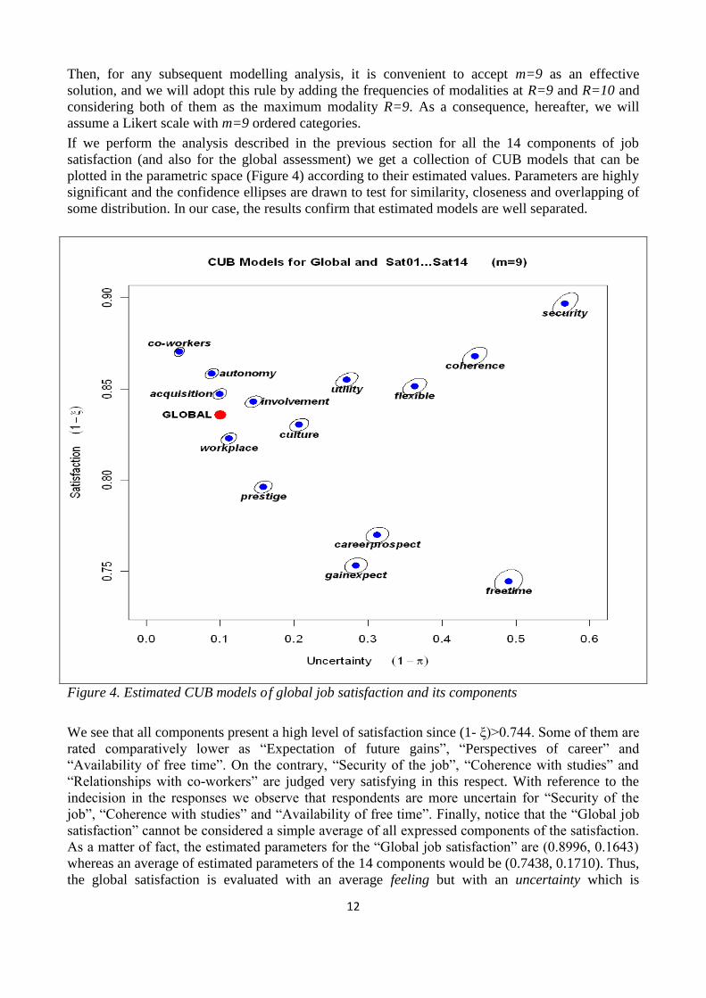
Then, for any subsequent modelling analysis, it is convenient to accept m=9 as an effective

solution, and we will adopt this rule by adding the frequencies of modalities at R=9 and R=10 and

considering both of them as the maximum modality R=9. As a consequence, hereafter, we will

assume a Likert scale with m=9 ordered categories.

If we perform the analysis described in the previous section for all the 14 components of job

satisfaction (and also for the global assessment) we get a collection of CUB models that can be

plotted in the parametric space (Figure 4) according to their estimated values. Parameters are highly

significant and the confidence ellipses are drawn to test for similarity, closeness and overlapping of

some distribution. In our case, the results confirm that estimated models are well separated.

Figure 4. Estimated CUB models o f global job satisfaction and its components

We see that all components present a high level of satisfaction since (1- ξ)>0.744. Some of them are

rated comparatively lower as “Expectation of future gains”, “Perspectives of career” and

“Availability of free time”. On the contrary, “Security of the job”, “Coherence with studies” and

“Relationships with co-workers” are judged very satisfying in this respect. With reference to the

indecision in the responses we observe that respondents are more uncertain for “Security of the

job”, “Coherence with studies” and “Availability of free time”. Finally, notice that the “Global job

satisfaction” cannot be considered a simple average of all expressed components of the satisfaction.

As a matter of fact, the estimated parameters for the “Global job satisfaction” are (0.8996, 0.1643)

whereas an average of estimated parameters of the 14 components would be (0.7438, 0.1710). Thus,

the global satisfaction is evaluated with an average feeling but with an uncertainty which is

13

substantially smaller than a simple average of the 14 components. This result is consistent with the

common findings that general assessments are obtained as mean values of several components with

a large convergence among respondents.

At this point, we wonder if Gender is a relevant covariate for explaining some differences in the

responses. It turns out that women are more uncertain in the response but there are no significant

differences as far as we are concerned with the feeling: so we conclude that the global satisfaction

as a whole may not be considered different between the genders.

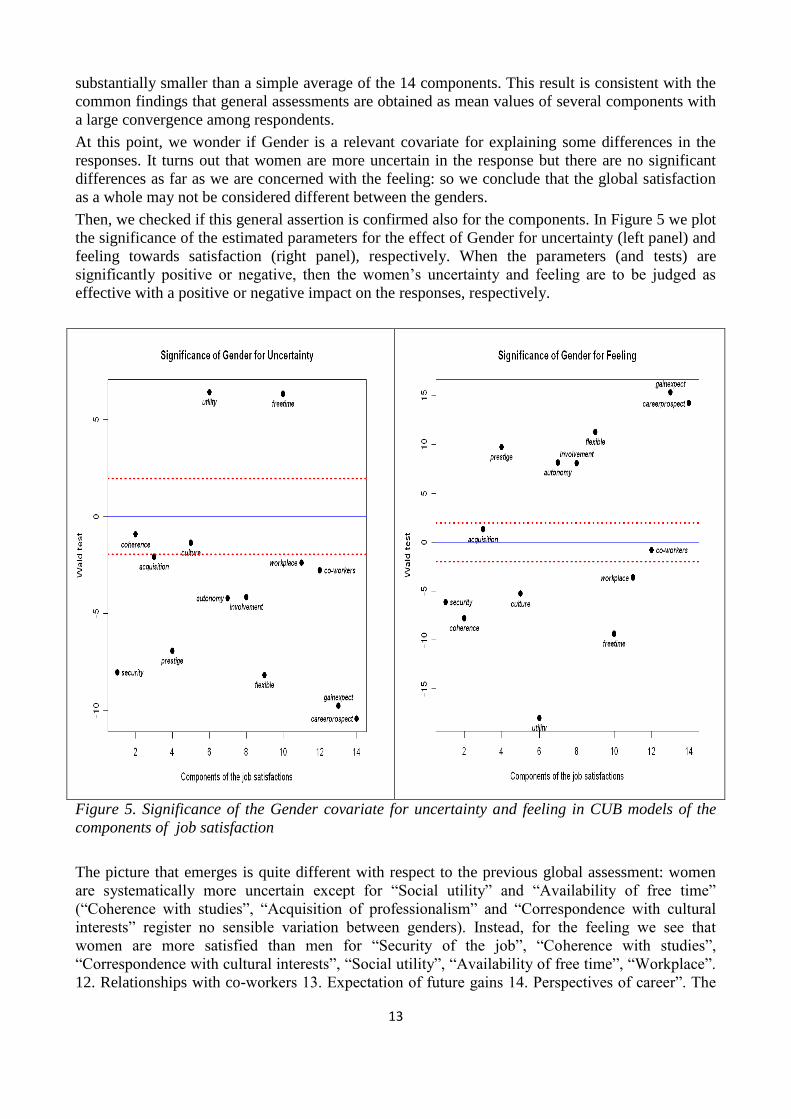
Then, we checked if this general assertion is confirmed also for the components. In Figure 5 we plot

the significance of the estimated parameters for the effect of Gender for uncertainty (left panel) and

feeling towards satisfaction (right panel), respectively. When the parameters (and tests) are

significantly positive or negative, then the women’s uncertainty and feeling are to be judged as

effective with a positive or negative impact on the responses, respectively.

Figure 5. Significance of the Gender covariate for uncertainty and feeling in CUB models of the

components of job satisfaction

The picture that emerges is quite different with respect to the previous global assessment: women

are systematically more uncertain except for “Social utility” and “Availability of free time”

(“Coherence with studies”, “Acquisition of professionalism” and “Correspondence with cultural

interests” register no sensible variation between genders). Instead, for the feeling we see that

women are more satisfied than men for “Security of the job”, “Coherence with studies”,

“Correspondence with cultural interests”, “Social utility”, “Availability of free time”, “Workplace”.

12. Relationships with co-workers 13. Expectation of future gains 14. Perspectives of career”. The

14

opposite happens with the other components except for “Acquisition of professionalism” and

“Relationships with co-workers”, where we register no significance between genders.

If we compare these results with the exploratory considerations we obtained from Table 2, it should

be evident that the average scores mask significant effects and an accurate modelling study deserves

more interest. Briefly, for almost all the components of job satisfaction there is a marked difference

ascribed to the Gender of the respondents and this has an homogeneous effect on the feeling

(causing a general more dissatisfaction for men) and also for describing uncertainty.

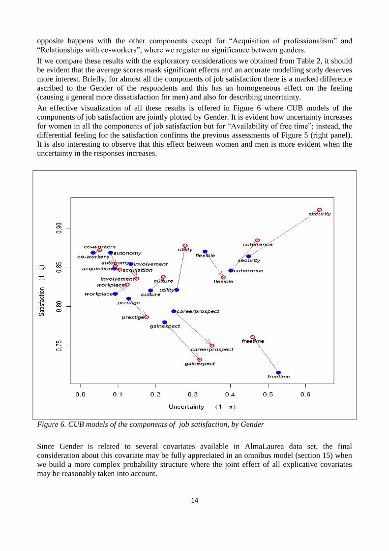
An effective visualization of all these results is offered in Figure 6 where CUB models of the

components of job satisfaction are jointly plotted by Gender. It is evident how uncertainty increases

for women in all the components of job satisfaction but for “Availability of free time”; instead, the

differential feeling for the satisfaction confirms the previous assessments of Figure 5 (right panel).

It is also interesting to observe that this effect between women and men is more evident when the

uncertainty in the responses increases.

Figure 6. CUB models of the components of job satisfaction, by Gender

Since Gender is related to several covariates available in AlmaLaurea data set, the final

consideration about this covariate may be fully appreciated in an omnibus model (section 15) when

we build a more complex probability structure where the joint effect of all explicative covariates

may be reasonably taken into account.

15

7. Modelling job satisfaction for selected clusters

In this section, we apply the same analysis to subgroups defined by geographical variables,

economic sectors and typology of the occupation of the respondents. In a sense, all these clusters

may be defined as “environmental” variables.

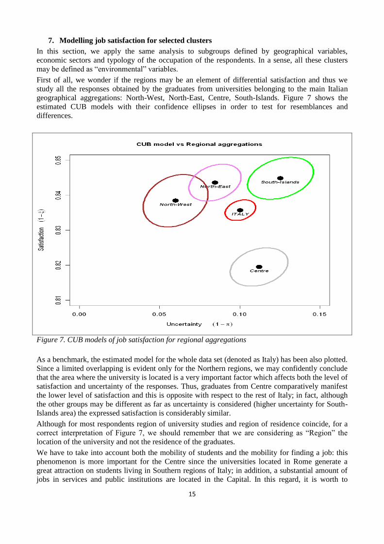
First of all, we wonder if the regions may be an element of differential satisfaction and thus we

study all the responses obtained by the graduates from universities belonging to the main Italian

geographical aggregations: North-West, North-East, Centre, South-Islands. Figure 7 shows the

estimated CUB models with their confidence ellipses in order to test for resemblances and

differences.

Figure 7. CUB models of job satisfaction for regional aggregations

As a benchmark, the estimated model for the whole data set (denoted as Italy) has been also plotted.

Since a limited overlapping is evident only for the Northern regions, we may confidently conclude

that the area where the university is located is a very important factor which affects both the level of

satisfaction and uncertainty of the responses. Thus, graduates from Centre comparatively manifest

the lower level of satisfaction and this is opposite with respect to the rest of Italy; in fact, although

the other groups may be different as far as uncertainty is considered (higher uncertainty for South-

Islands area) the expressed satisfaction is considerably similar.

Although for most respondents region of university studies and region of residence coincide, for a

correct interpretation of Figure 7, we should remember that we are considering as “Region” the

location of the university and not the residence of the graduates.

We have to take into account both the mobility of students and the mobility for finding a job: this

phenomenon is more important for the Centre since the universities located in Rome generate a

great attraction on students living in Southern regions of Italy; in addition, a substantial amount of

jobs in services and public institutions are located in the Capital. In this regard, it is worth to

16

remember that AlmaLaurea data set include 61% of the graduates of universities of Centre and

University of Rome “La Sapienza” represents 26% of Centre graduates. If we consider the

respondents who work after 5 years, graduates from University of Rome “La Sapienza” are 47% of

Centre. Thus, it seems evident that results of this geographical area mostly refer to “La Sapienza”.

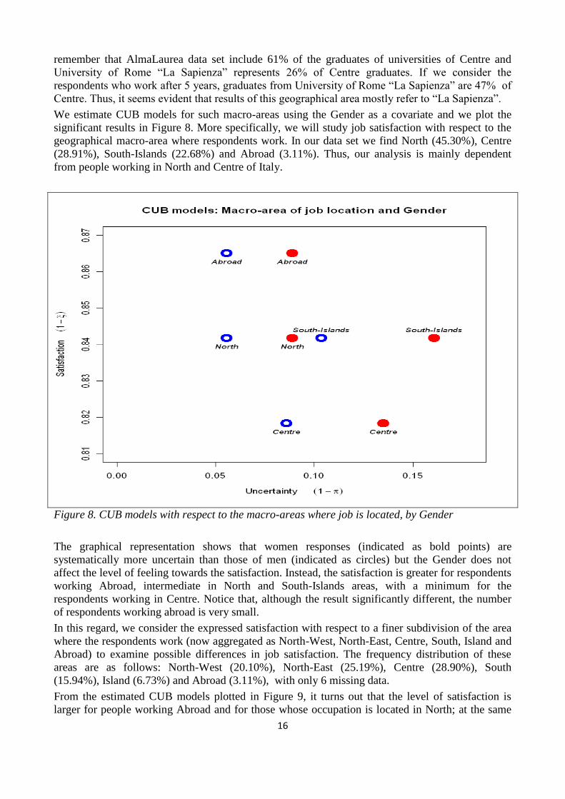
We estimate CUB models for such macro-areas using the Gender as a covariate and we plot the

significant results in Figure 8. More specifically, we will study job satisfaction with respect to the

geographical macro-area where respondents work. In our data set we find North (45.30%), Centre

(28.91%), South-Islands (22.68%) and Abroad (3.11%). Thus, our analysis is mainly dependent

from people working in North and Centre of Italy.

Figure 8. CUB models with respect to the macro-areas where job is located, by Gender

The graphical representation shows that women responses (indicated as bold points) are

systematically more uncertain than those of men (indicated as circles) but the Gender does not

affect the level of feeling towards the satisfaction. Instead, the satisfaction is greater for respondents

working Abroad, intermediate in North and South-Islands areas, with a minimum for the

respondents working in Centre. Notice that, although the result significantly different, the number

of respondents working abroad is very small.

In this regard, we consider the expressed satisfaction with respect to a finer subdivision of the area

where the respondents work (now aggregated as North-West, North-East, Centre, South, Island and

Abroad) to examine possible differences in job satisfaction. The frequency distribution of these

areas are as follows: North-West (20.10%), North-East (25.19%), Centre (28.90%), South

(15.94%), Island (6.73%) and Abroad (3.11%), with only 6 missing data.

From the estimated CUB models plotted in Figure 9, it turns out that the level of satisfaction is

larger for people working Abroad and for those whose occupation is located in North; at the same

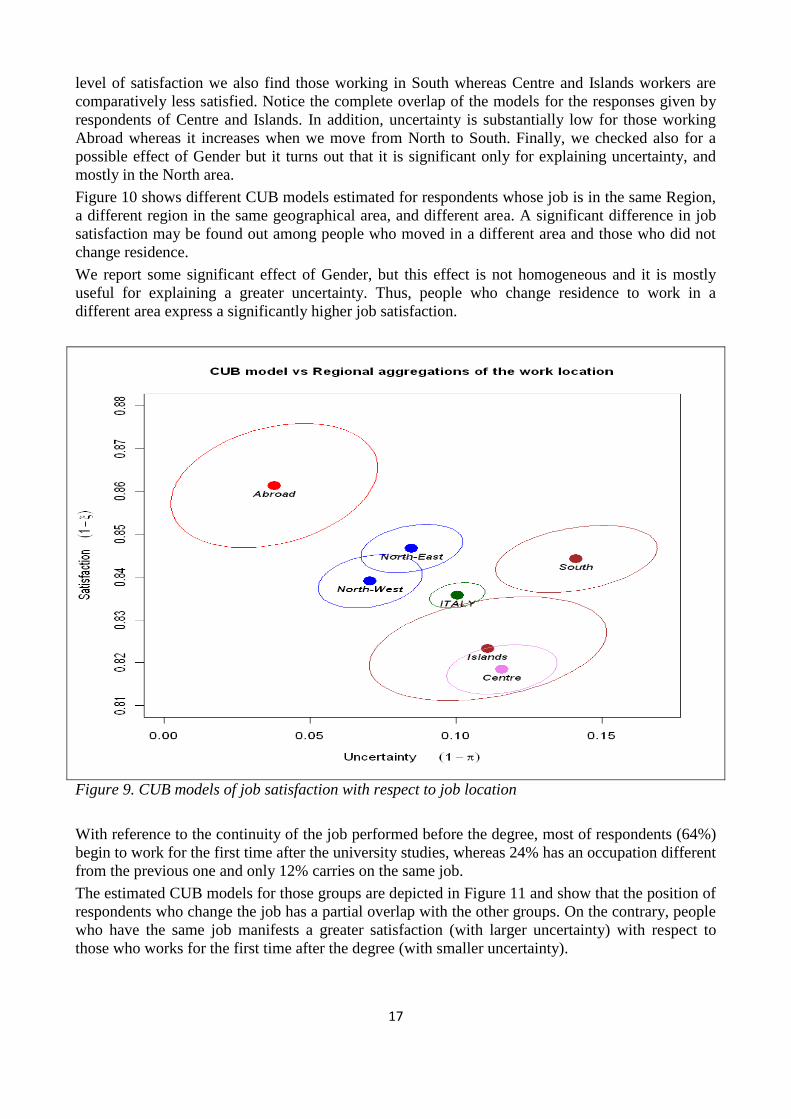
17

level of satisfaction we also find those working in South whereas Centre and Islands workers are

comparatively less satisfied. Notice the complete overlap of the models for the responses given by

respondents of Centre and Islands. In addition, uncertainty is substantially low for those working

Abroad whereas it increases when we move from North to South. Finally, we checked also for a

possible effect of Gender but it turns out that it is significant only for explaining uncertainty, and

mostly in the North area.

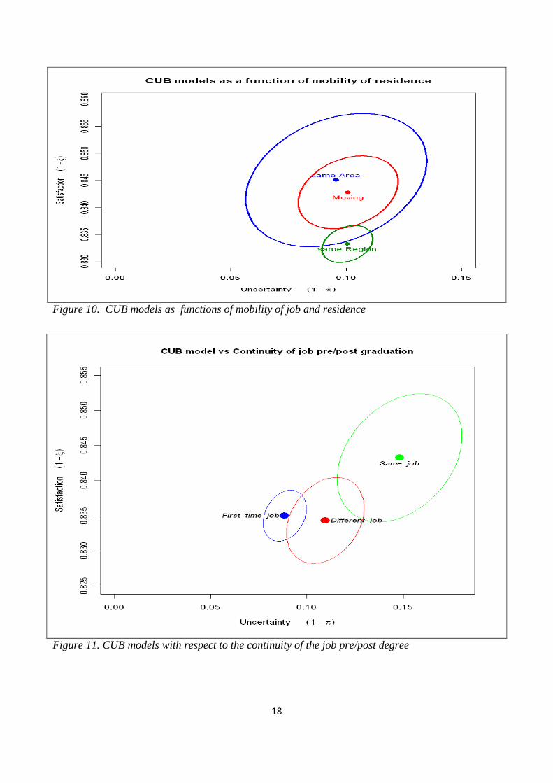
Figure 10 shows different CUB models estimated for respondents whose job is in the same Region,

a different region in the same geographical area, and different area. A significant difference in job

satisfaction may be found out among people who moved in a different area and those who did not

change residence.

We report some significant effect of Gender, but this effect is not homogeneous and it is mostly

useful for explaining a greater uncertainty. Thus, people who change residence to work in a

different area express a significantly higher job satisfaction.

Figure 9. CUB models of job satisfaction with respect to job location

With reference to the continuity of the job performed before the degree, most of respondents (64%)

begin to work for the first time after the university studies, whereas 24% has an occupation different

from the previous one and only 12% carries on the same job.

The estimated CUB models for those groups are depicted in Figure 11 and show that the position of

respondents who change the job has a partial overlap with the other groups. On the contrary, people

who have the same job manifests a greater satisfaction (with larger uncertainty) with respect to

those who works for the first time after the degree (with smaller uncertainty).

18

Figure 10. CUB models as functions of mobility of job and residence

Figure 11. CUB models with respect to the continuity of the job pre/post degree

19

These results may be consistently accepted if we observe that people who enter the job market the

first time are generally young. Thus, they accept an occupation that does not completely meet

expectations of gains, perspectives of career or coherence with the university studies.

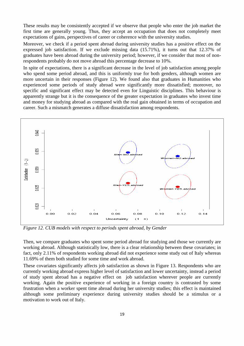
Moreover, we check if a period spent abroad during university studies has a positive effect on the

expressed job satisfaction. If we exclude missing data (15.71%), it turns out that 12.37% of

graduates have been abroad during the university period; however, if we consider that most of non-

respondents probably do not move abroad this percentage decrease to 10%.

In spite of expectations, there is a significant decrease in the level of job satisfaction among people

who spend some period abroad, and this is uniformly true for both genders, although women are

more uncertain in their responses (Figure 12). We found also that graduates in Humanities who

experienced some periods of study abroad were significantly more dissatisfied; moreover, no

specific and significant effect may be detected even for Linguistic disciplines. This behaviour is

apparently strange but it is the consequence of the greater expectation in graduates who invest time

and money for studying abroad as compared with the real gain obtained in terms of occupation and

career. Such a mismatch generates a diffuse dissatisfaction among respondents.

Figure 12. CUB models with respect to periods spent abroad, by Gender

Then, we compare graduates who spent some period abroad for studying and those we currently are

working abroad. Although statistically low, there is a clear relationship between these covariates; in

fact, only 2.11% of respondents working abroad did not experience some study out of Italy whereas

11.69% of them both studied for some time and work abroad.

These covariates significantly affects job satisfaction as shown in Figure 13. Respondents who are

currently working abroad express higher level of satisfaction and lower uncertainty, instead a period

of study spent abroad has a negative effect on job satisfaction wherever people are currently

working. Again the positive experience of working in a foreign country is contrasted by some

frustration when a worker spent time abroad during her university studies; this effect is maintained

although some preliminary experience during university studies should be a stimulus or a

motivation to work out of Italy.

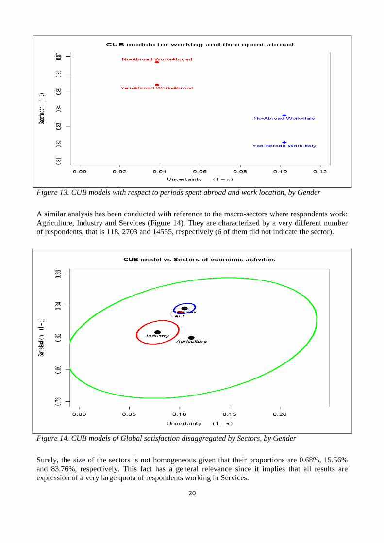
20

Figure 13. CUB models with respect to periods spent abroad and work location, by Gender

A similar analysis has been conducted with reference to the macro-sectors where respondents work:

Agriculture, Industry and Services (Figure 14). They are characterized by a very different number

of respondents, that is 118, 2703 and 14555, respectively (6 of them did not indicate the sector).

Figure 14. CUB models of Global satisfaction disaggregated by Sectors, by Gender

Surely, the size of the sectors is not homogeneous given that their proportions are 0.68%, 15.56%

and 83.76%, respectively. This fact has a general relevance since it implies that all results are

expression of a very large quota of respondents working in Services.

21

If we fit different CUB models for job satisfaction in these sectors, it turns out that this variable has

a different impact on the expression of a satisfaction mostly for Industry and Services: people

working in Services are a bit more satisfied and even more resolute in the responses. Given the

limited sample size of respondents working in Agriculture, we cannot ascertain a significant

difference of this sector with respect to the others as confirmed by a comparison of correspondent

confidence ellipses.

Finally, we report that in a more disaggregated analysis (here not reported for brevity), the Gender

is not a relevant covariate for Agriculture. Instead, it is significant as a covariate of the uncertainty

in Services whereas it affects both feeling and uncertainty in Industry.

8. The effects of income and typology of work

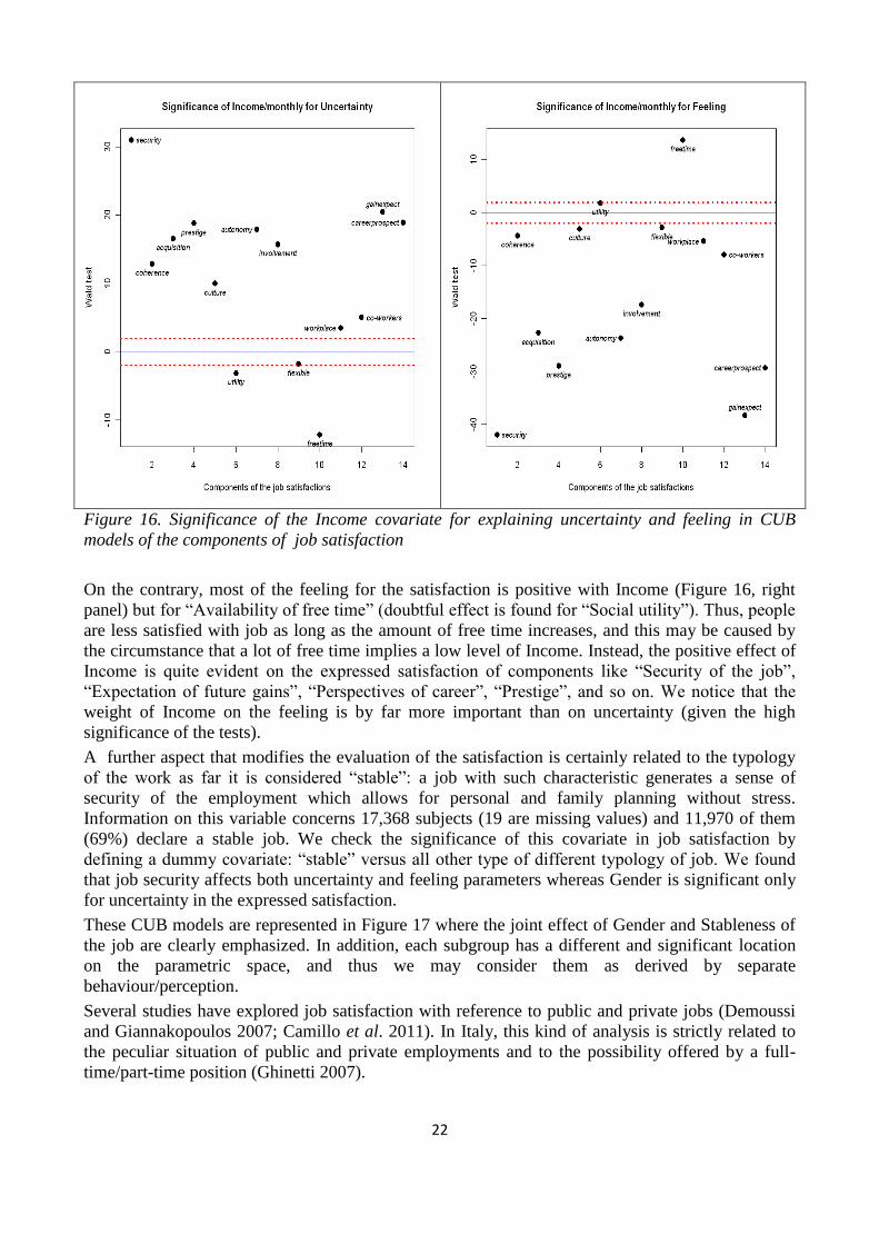
The effect of Income on the expressed satisfaction is confirmed with a positive relationship between

monthly income and feeling of the respondents, as shown in Figure 15 (left panel); in this regard,

for the global satisfaction, the effect of Gender is only to increase uncertainty as it is evident in the

parametric representation of Figure 15 (right panel). Then, the Income positively affects job

satisfaction for both genders but women are more uncertain in expressing their evaluation. A

cautionary note should be added since missing values in the income declaration are high. In fact,

this analysis is implemented on 16,590 respondents; thus, since 4.58% of the full data set is

removed, some selection bias should be considered if non-respondents have a systematically

higher/lower Income than the others.

Figure 15. Effect of Income and Gender on Global Satisfaction

We underline how the global effect diversifies when we consider the different components of job

satisfaction. In these CUB models, a logarithmic transformation and a deviation from the average of

the Income have been considered to improve convergence of the estimation algorithm.

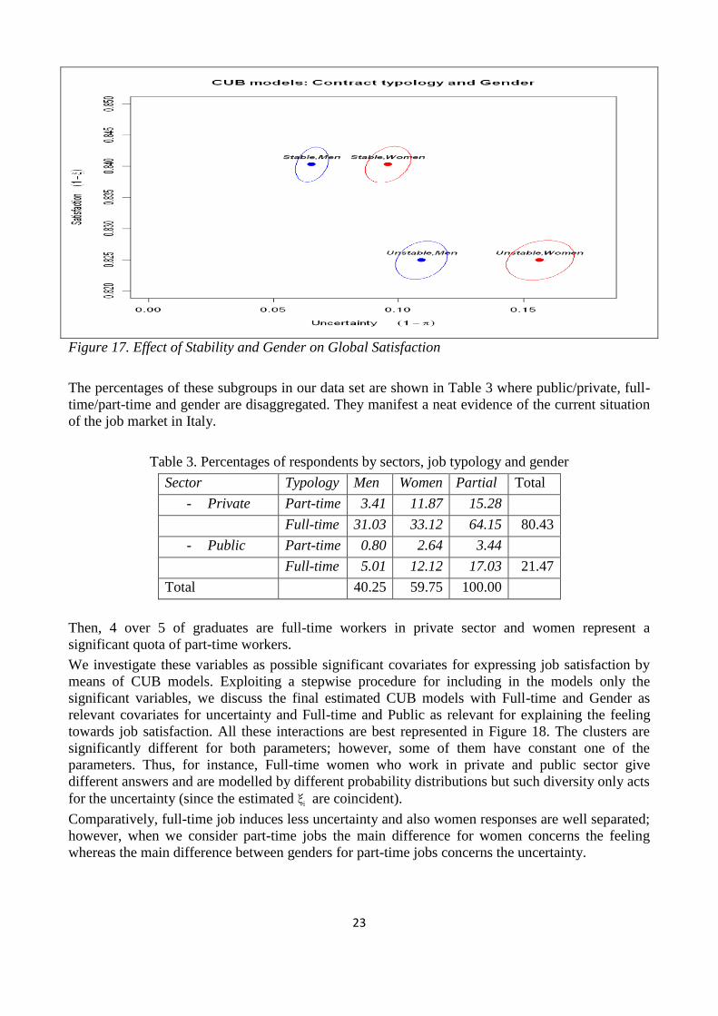
Figure 16 (left panel) shows that uncertainty in the responses generally lowers with an increasing

Income but for “Social utility” and “Availability of free time” (no effect for “Flexibility of time”).

22

Figure 16. Significance of the Income covariate for explaining uncertainty and feeling in CUB

models of the components of job satisfaction

On the contrary, most of the feeling for the satisfaction is positive with Income (Figure 16, right

panel) but for “Availability of free time” (doubtful effect is found for “Social utility”). Thus, people

are less satisfied with job as long as the amount of free time increases, and this may be caused by

the circumstance that a lot of free time implies a low level of Income. Instead, the positive effect of

Income is quite evident on the expressed satisfaction of components like “Security of the job”,

“Expectation of future gains”, “Perspectives of career”, “Prestige”, and so on. We notice that the

weight of Income on the feeling is by far more important than on uncertainty (given the high

significance of the tests).

A further aspect that modifies the evaluation of the satisfaction is certainly related to the typology

of the work as far it is considered “stable”: a job with such characteristic generates a sense of

security of the employment which allows for personal and family planning without stress.

Information on this variable concerns 17,368 subjects (19 are missing values) and 11,970 of them

(69%) declare a stable job. We check the significance of this covariate in job satisfaction by

defining a dummy covariate: “stable” versus all other type of different typology of job. We found

that job security affects both uncertainty and feeling parameters whereas Gender is significant only

for uncertainty in the expressed satisfaction.

These CUB models are represented in Figure 17 where the joint effect of Gender and Stableness of

the job are clearly emphasized. In addition, each subgroup has a different and significant location

on the parametric space, and thus we may consider them as derived by separate

behaviour/perception.

Several studies have explored job satisfaction with reference to public and private jobs (Demoussi

and Giannakopoulos 2007; Camillo et al. 2011). In Italy, this kind of analysis is strictly related to

the peculiar situation of public and private employments and to the possibility offered by a full-

time/part-time position (Ghinetti 2007).

23

Figure 17. Effect of Stability and Gender on Global Satisfaction

The percentages of these subgroups in our data set are shown in Table 3 where public/private, full-

time/part-time and gender are disaggregated. They manifest a neat evidence of the current situation

of the job market in Italy.

Table 3. Percentages of respondents by sectors, job typology and gender

Sector Typology Men Women Partial Total

- Private Part-time 3.41 11.87 15.28

Full-time 31.03 33.12 64.15 80.43

- Public Part-time 0.80 2.64 3.44

Full-time 5.01 12.12 17.03 21.47

Total 40.25 59.75 100.00

Then, 4 over 5 of graduates are full-time workers in private sector and women represent a

significant quota of part-time workers.

We investigate these variables as possible significant covariates for expressing job satisfaction by

means of CUB models. Exploiting a stepwise procedure for including in the models only the

significant variables, we discuss the final estimated CUB models with Full-time and Gender as

relevant covariates for uncertainty and Full-time and Public as relevant for explaining the feeling

towards job satisfaction. All these interactions are best represented in Figure 18. The clusters are

significantly different for both parameters; however, some of them have constant one of the

parameters. Thus, for instance, Full-time women who work in private and public sector give

different answers and are modelled by different probability distributions but such diversity only acts

for the uncertainty (since the estimated ξi are coincident).

Comparatively, full-time job induces less uncertainty and also women responses are well separated;

however, when we consider part-time jobs the main difference for women concerns the feeling

whereas the main difference between genders for part-time jobs concerns the uncertainty.

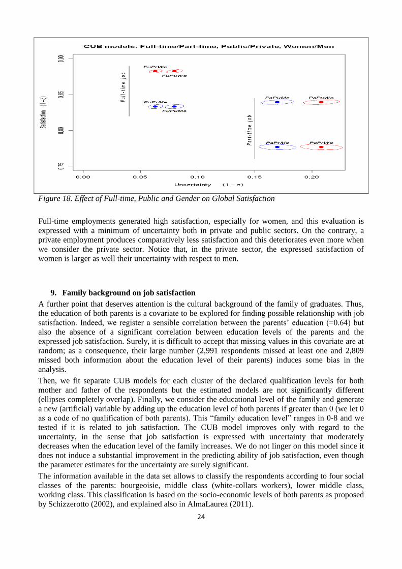
24

Figure 18. Effect of Full-time, Public and Gender on Global Satisfaction

Full-time employments generated high satisfaction, especially for women, and this evaluation is

expressed with a minimum of uncertainty both in private and public sectors. On the contrary, a

private employment produces comparatively less satisfaction and this deteriorates even more when

we consider the private sector. Notice that, in the private sector, the expressed satisfaction of

women is larger as well their uncertainty with respect to men.

9. Family background on job satisfaction

A further point that deserves attention is the cultural background of the family of graduates. Thus,

the education of both parents is a covariate to be explored for finding possible relationship with job

satisfaction. Indeed, we register a sensible correlation between the parents’ education (=0.64) but

also the absence of a significant correlation between education levels of the parents and the

expressed job satisfaction. Surely, it is difficult to accept that missing values in this covariate are at

random; as a consequence, their large number (2,991 respondents missed at least one and 2,809

missed both information about the education level of their parents) induces some bias in the

analysis.

Then, we fit separate CUB models for each cluster of the declared qualification levels for both

mother and father of the respondents but the estimated models are not significantly different

(ellipses completely overlap). Finally, we consider the educational level of the family and generate

a new (artificial) variable by adding up the education level of both parents if greater than 0 (we let 0

as a code of no qualification of both parents). This “family education level” ranges in 0-8 and we

tested if it is related to job satisfaction. The CUB model improves only with regard to the

uncertainty, in the sense that job satisfaction is expressed with uncertainty that moderately

decreases when the education level of the family increases. We do not linger on this model since it

does not induce a substantial improvement in the predicting ability of job satisfaction, even though

the parameter estimates for the uncertainty are surely significant.

The information available in the data set allows to classify the respondents according to four social

classes of the parents: bourgeoisie, middle class (white-collars workers), lower middle class,

working class. This classification is based on the socio-economic levels of both parents as proposed

by Schizzerotto (2002), and explained also in AlmaLaurea (2011).

25

The percentage of missing data is very high: respondents to this item are only 82% of the data set

and thus some selection bias should be seriously considered. Among the respondents, there is an

almost homogeneity among the class with the following percentages: bourgeoisie (25.12%), middle

class (33.31%), lower middle class (21.02%), working class (20.55%), with no large difference

between genders.

First of all, we register a different Age at degree among classes and Gender and this is very regular

as confirmed by Table 4. As expected, Age at degree increases regularly when the social conditions

deteriorate and this effect is systematically worse for men.

Table 4. Averages of Age at degree (years) by Social classes of parents and Gender

Classes Men Women Total

Bourgeoisie 27.235 26.645 26.609

Middle class 27.497 26.691 27.021

Lower middle class 28.092 27.328 27.607

Working class 28.314 27.328 27.706

Total 27.696 26.958 27.257

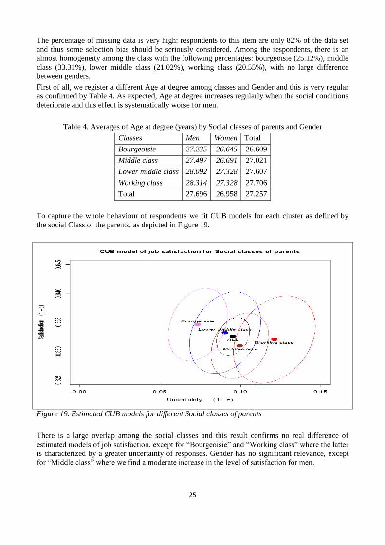
To capture the whole behaviour of respondents we fit CUB models for each cluster as defined by

the social Class of the parents, as depicted in Figure 19.

Figure 19. Estimated CUB models for different Social classes of parents

There is a large overlap among the social classes and this result confirms no real difference of

estimated models of job satisfaction, except for “Bourgeoisie” and “Working class” where the latter

is characterized by a greater uncertainty of responses. Gender has no significant relevance, except

for “Middle class” where we find a moderate increase in the level of satisfaction for men.

26

10. Job satisfaction for groups and disciplines of university degree

A relevant feature of the University system is the main difference among two groups (Human and

Social versus Technical and Scientific Sciences) and several disciplines which characterizes the

degree in some extent. Thus, it should be important to detect if there is some significant effect of

these aspects on the expressed satisfaction.

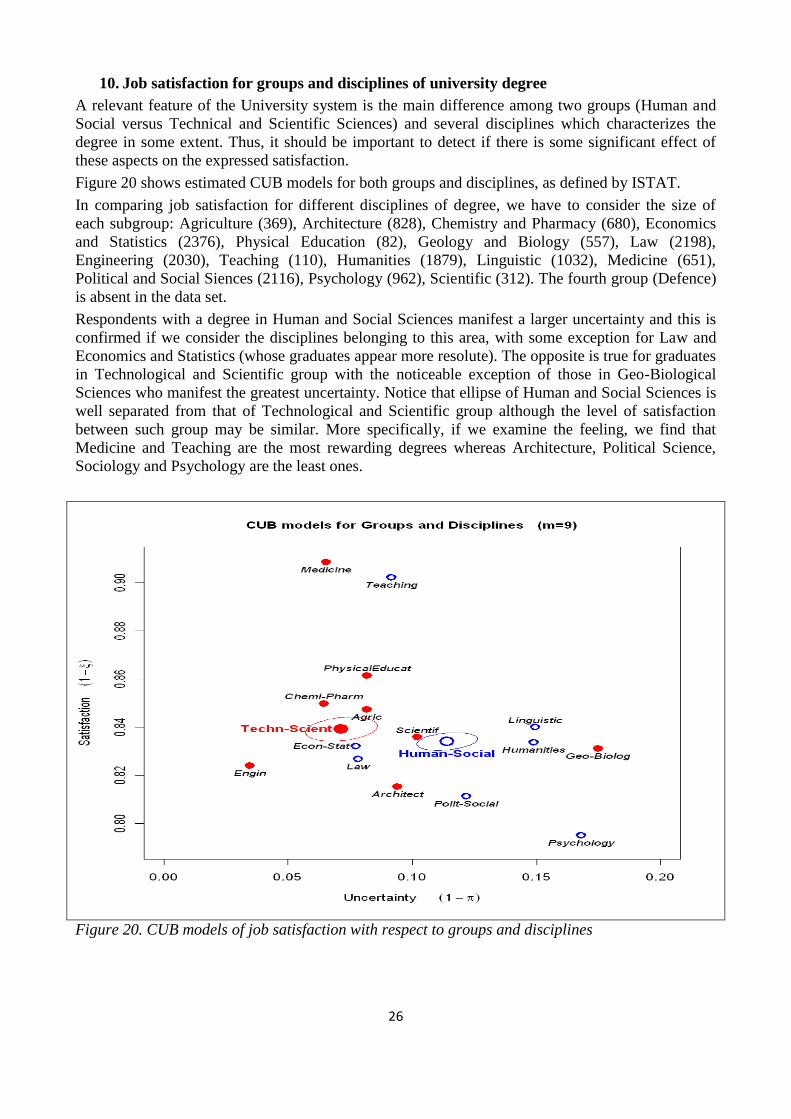
Figure 20 shows estimated CUB models for both groups and disciplines, as defined by ISTAT.

In comparing job satisfaction for different disciplines of degree, we have to consider the size of

each subgroup: Agriculture (369), Architecture (828), Chemistry and Pharmacy (680), Economics

and Statistics (2376), Physical Education (82), Geology and Biology (557), Law (2198),

Engineering (2030), Teaching (110), Humanities (1879), Linguistic (1032), Medicine (651),

Political and Social Siences (2116), Psychology (962), Scientific (312). The fourth group (Defence)

is absent in the data set.

Respondents with a degree in Human and Social Sciences manifest a larger uncertainty and this is

confirmed if we consider the disciplines belonging to this area, with some exception for Law and

Economics and Statistics (whose graduates appear more resolute). The opposite is true for graduates

in Technological and Scientific group with the noticeable exception of those in Geo-Biological

Sciences who manifest the greatest uncertainty. Notice that ellipse of Human and Social Sciences is

well separated from that of Technological and Scientific group although the level of satisfaction

between such group may be similar. More specifically, if we examine the feeling, we find that

Medicine and Teaching are the most rewarding degrees whereas Architecture, Political Science,

Sociology and Psychology are the least ones.

Figure 20. CUB models of job satisfaction with respect to groups and disciplines

27

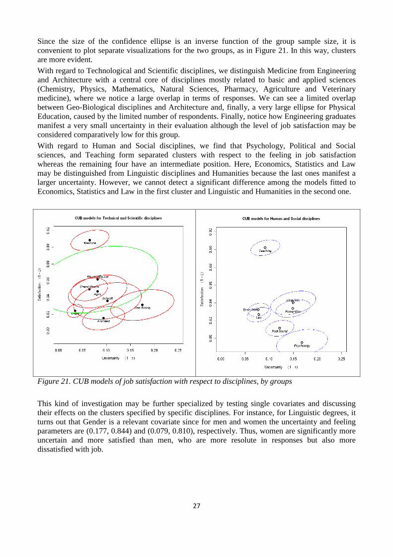
Since the size of the confidence ellipse is an inverse function of the group sample size, it is

convenient to plot separate visualizations for the two groups, as in Figure 21. In this way, clusters

are more evident.

With regard to Technological and Scientific disciplines, we distinguish Medicine from Engineering

and Architecture with a central core of disciplines mostly related to basic and applied sciences

(Chemistry, Physics, Mathematics, Natural Sciences, Pharmacy, Agriculture and Veterinary

medicine), where we notice a large overlap in terms of responses. We can see a limited overlap

between Geo-Biological disciplines and Architecture and, finally, a very large ellipse for Physical

Education, caused by the limited number of respondents. Finally, notice how Engineering graduates

manifest a very small uncertainty in their evaluation although the level of job satisfaction may be

considered comparatively low for this group.

With regard to Human and Social disciplines, we find that Psychology, Political and Social

sciences, and Teaching form separated clusters with respect to the feeling in job satisfaction

whereas the remaining four have an intermediate position. Here, Economics, Statistics and Law

may be distinguished from Linguistic disciplines and Humanities because the last ones manifest a

larger uncertainty. However, we cannot detect a significant difference among the models fitted to

Economics, Statistics and Law in the first cluster and Linguistic and Humanities in the second one.

Figure 21. CUB models of job satisfaction with respect to disciplines, by groups

This kind of investigation may be further specialized by testing single covariates and discussing

their effects on the clusters specified by specific disciplines. For instance, for Linguistic degrees, it

turns out that Gender is a relevant covariate since for men and women the uncertainty and feeling

parameters are (0.177, 0.844) and (0.079, 0.810), respectively. Thus, women are significantly more

uncertain and more satisfied than men, who are more resolute in responses but also more

dissatisfied with job.

28

11. Final score of university degree and job satisfaction

The current literature registers atypical correlation between the final score received at the end of

university education and the expressed job satisfaction: generally, one expects that clever students

would find better jobs, which are also more adequate to their aspirations, and thus they should be

more satisfied than the average. However, the empirical evidence seems to offer no (or very weak)

relationship between these variables. Thus, we deepen these aspects within the framework of CUB

models and the results will confirm the added value and the interpretative usefulness of this

approach to discover unusual effects.

First of all, an exploratory research has been conducted to check if the expressed satisfaction is

related to the final score of the university degree (maximum is 110 or 110 with first-class honours).

The reported scores have been codified by converting them to integer numbers from 66 up to 110.

In addition, we associated the numeric value of 112 with graduates with honours (instead of 113, as

proposed in other AlmaLaurea studies) to avoid to attribute a too heavy weight to the extreme class,

which is indeed very frequent in this data set (1 over 5 graduates receive a degree with honours).

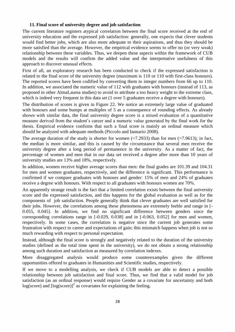
The distribution of scores is given in Figure 22. We notice an extremely large value of graduated

with honours and some bumps at multiples of 5 as a consequence of rounding effects. As already

shown with similar data, the final university degree score is a mixed evaluation of a quantitative

measure derived from the student’s career and a numeric value generated by the final work for the

thesis. Empirical evidence confirms that such a final score is mainly an ordinal measure which

should be analyzed with adequate methods (Piccolo and Iannario 2008).

The average duration of the study is shorter for women (=7.2933) than for men (=7.9613); in fact,

the median is more similar, and this is caused by the circumstance that several men receive the

university degree after a long period of permanence in the university. As a matter of fact, the

percentage of women and men that in our data set received a degree after more than 10 years of

university studies are 13% and 18%, respectively.

In addition, women receive higher average scores than men: the final grades are 101.39 and 104.31

for men and women graduates, respectively, and the difference is significant. This performance is

confirmed if we compare graduates with honours and gender: 15% of men and 24% of graduates

receive a degree with honours. With respect to all graduates with honours women are 70%.

An apparently strange result is the fact that a limited correlation exists between the final university

score and the expressed satisfaction, and this happens for the global evaluation as well as for the

components of job satisfaction. People generally think that clever graduates are well satisfied for

their jobs. However, the correlations among these phenomena are extremely feeble and range in [-

0.055, 0.045]. In addition, we find no significant difference between genders since the

corresponding correlations range in [-0.029, 0.038] and in [-0.063, 0.052] for men and women,

respectively. In some cases, the correlation is negative since the current job generates some

frustration with respect to career and expectations of gain; this mismatch happens when job is not so

much rewarding with respect to personal expectation.

Instead, although the final score is strongly and negatively related to the duration of the university

studies (defined as the total time spent in the university), we do not obtain a strong relationship

among such duration and satisfaction as measured by correlation indexes.

More disaggregated analysis would produce some counterexamples given the different

opportunities offered to graduates in Humanities and Scientific studies, respectively.

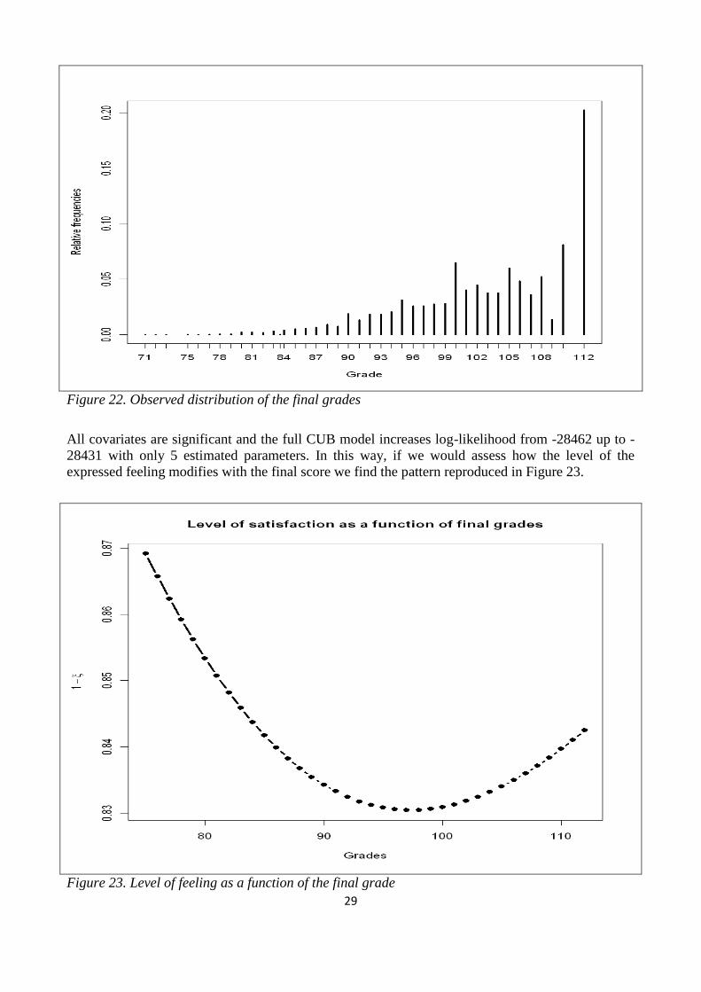
If we move to a modelling analysis, we check if CUB models are able to detect a possible

relationship between job satisfaction and final score. Thus, we find that a valid model for job

satisfaction (as an ordinal response) would require Gender as a covariate for uncertainty and both

log(score) and [log(score)]2 as covariates for explaining the feeling.

29

Figure 22. Observed distribution of the final grades

All covariates are significant and the full CUB model increases log-likelihood from -28462 up to -

28431 with only 5 estimated parameters. In this way, if we would assess how the level of the

expressed feeling modifies with the final score we find the pattern reproduced in Figure 23.

Figure 23. Level of feeling as a function of the final grade

30

It shows that job satisfaction is high in the extremes of the scale for scores (and this explain why a

linear correlation index is almost zero) as a consequence of two opposite circumstances:

- People receiving low scores are generally older and end the university training with some

difficulties due to personal, family and environmental problems. Thus, when they get a

degree, are already in the labour market and such a result may improve their career: as a

consequence, they manifest a greater satisfaction in the job.

- People receiving very high scores are generally quite clever in their professional ability,

look for jobs adequate to their competence and thus they express a larger satisfaction.

It is interesting to conclude that scores around 97/110 produces ceteris paribus the minimum job

satisfaction. In addition, the estimated relationship is asymmetric and thus very high grades do not

generate a corresponding increase in the job satisfaction.

This relationship may be searched and tested also for the components of the job satisfaction.

Finally, we notice that this case study is an empirical evidence of the ability of CUB models to

detect and measure unusual relationships in a case where standard methods failed to ascertain a

sensible link among variables.

12. Age at degree and job satisfaction

The effect of Age on job satisfaction involves at least two different aspects of time (although they

are strongly related): the first is the age of the respondent when he/she takes a degree; the second is

the permanence at university until he/she gets the degree. In this section, we explore the first of

them.

The Age of a graduate when he/she takes the degree is a continuous variable and it is interesting to

see how the job satisfaction is possibly affected by or related to its value.

Figure 24. Kernel histograms and box plots of the Age at degree, by Gender

31

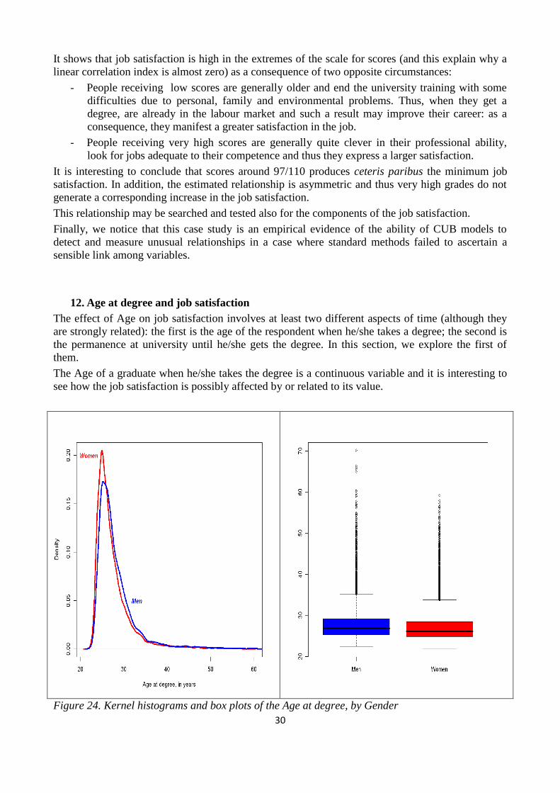
In our data set, Age at degree ranges between 21.839 and 70.169 years and both kernel histogram

and boxplot show that most of the distribution is concentrated between 22 and 35 years (indeed,

there are 94.77% of graduates). These exploratory tools are presented in Figure 24 with respect to

Gender and confirm that women get a degree in a shorter time than men.

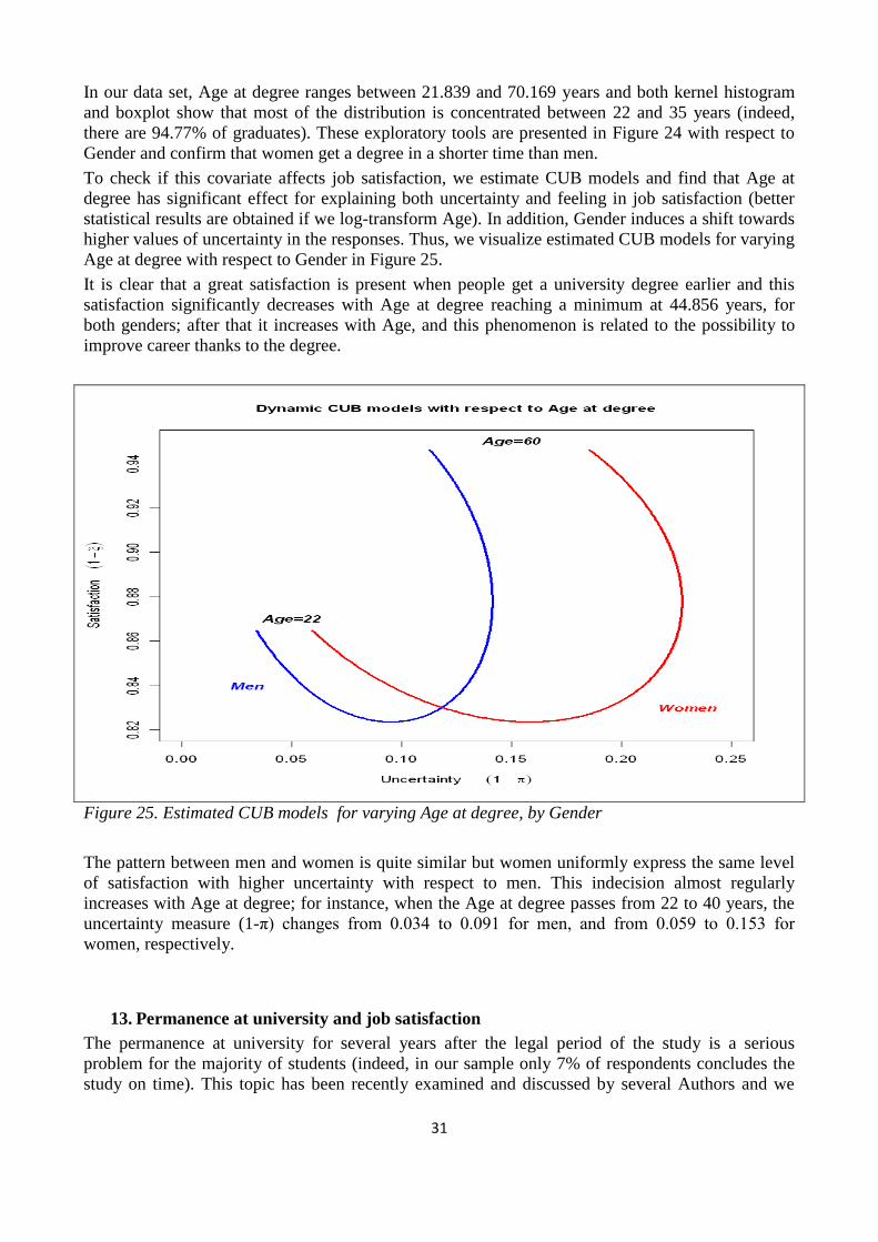
To check if this covariate affects job satisfaction, we estimate CUB models and find that Age at

degree has significant effect for explaining both uncertainty and feeling in job satisfaction (better

statistical results are obtained if we log-transform Age). In addition, Gender induces a shift towards

higher values of uncertainty in the responses. Thus, we visualize estimated CUB models for varying

Age at degree with respect to Gender in Figure 25.

It is clear that a great satisfaction is present when people get a university degree earlier and this

satisfaction significantly decreases with Age at degree reaching a minimum at 44.856 years, for

both genders; after that it increases with Age, and this phenomenon is related to the possibility to

improve career thanks to the degree.

Figure 25. Estimated CUB models for varying Age at degree, by Gender

The pattern between men and women is quite similar but women uniformly express the same level

of satisfaction with higher uncertainty with respect to men. This indecision almost regularly

increases with Age at degree; for instance, when the Age at degree passes from 22 to 40 years, the

uncertainty measure (1-π) changes from 0.034 to 0.091 for men, and from 0.059 to 0.153 for

women, respectively.

13. Permanence at university and job satisfaction

The permanence at university for several years after the legal period of the study is a serious

problem for the majority of students (indeed, in our sample only 7% of respondents concludes the

study on time). This topic has been recently examined and discussed by several Authors and we

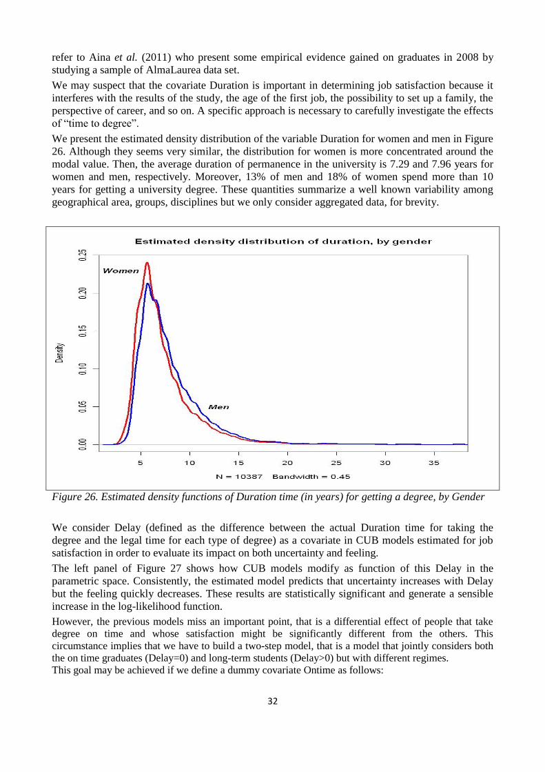
32

refer to Aina et al. (2011) who present some empirical evidence gained on graduates in 2008 by

studying a sample of AlmaLaurea data set.

We may suspect that the covariate Duration is important in determining job satisfaction because it

interferes with the results of the study, the age of the first job, the possibility to set up a family, the

perspective of career, and so on. A specific approach is necessary to carefully investigate the effects

of “time to degree”.

We present the estimated density distribution of the variable Duration for women and men in Figure

26. Although they seems very similar, the distribution for women is more concentrated around the

modal value. Then, the average duration of permanence in the university is 7.29 and 7.96 years for

women and men, respectively. Moreover, 13% of men and 18% of women spend more than 10

years for getting a university degree. These quantities summarize a well known variability among

geographical area, groups, disciplines but we only consider aggregated data, for brevity.

Figure 26. Estimated density functions of Duration time (in years) for getting a degree, by Gender

We consider Delay (defined as the difference between the actual Duration time for taking the

degree and the legal time for each type of degree) as a covariate in CUB models estimated for job

satisfaction in order to evaluate its impact on both uncertainty and feeling.

The left panel of Figure 27 shows how CUB models modify as function of this Delay in the

parametric space. Consistently, the estimated model predicts that uncertainty increases with Delay

but the feeling quickly decreases. These results are statistically significant and generate a sensible

increase in the log-likelihood function.

However, the previous models miss an important point, that is a differential effect of people that take

degree on time and whose satisfaction might be significantly different from the others. This

circumstance implies that we have to build a two-step model, that is a model that jointly considers both

the on time graduates (Delay=0) and long-term students (Delay>0) but with different regimes.

This goal may be achieved if we define a dummy covariate Ontime as follows:

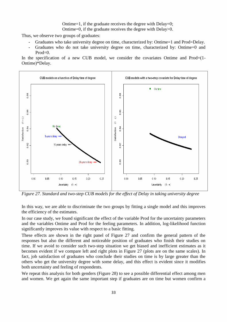
33

Ontime=1, if the graduate receives the degree with Delay=0;

Ontime=0, if the graduate receives the degree with Delay>0.

Thus, we observe two groups of graduates:

- Graduates who take university degree on time, characterized by: Ontime=1 and Prod=Delay.

- Graduates who do not take university degree on time, characterized by: Ontime=0 and

Prod=0.

In the specification of a new CUB model, we consider the covariates Ontime and Prod=(1-

Ontime)*Delay.

Figure 27. Standard and two-step CUB models for the effect of Delay in taking university degree

In this way, we are able to discriminate the two groups by fitting a single model and this improves

the efficiency of the estimates.

In our case study, we found significant the effect of the variable Prod for the uncertainty parameters

and the variables Ontime and Prod for the feeling parameters. In addition, log-likelihood function

significantly improves its value with respect to a basic fitting.

These effects are shown in the right panel of Figure 27 and confirm the general pattern of the

responses but also the different and noticeable position of graduates who finish their studies on

time. If we avoid to consider such two-step situation we get biased and inefficient estimates as it

becomes evident if we compare left and right plots in Figure 27 (plots are on the same scales). In

fact, job satisfaction of graduates who conclude their studies on time is by large greater than the

others who get the university degree with some delay, and this effect is evident since it modifies

both uncertainty and feeling of respondents.

We repeat this analysis for both genders (Figure 28) to see a possible differential effect among men

and women. We get again the same important step if graduates are on time but women confirm a

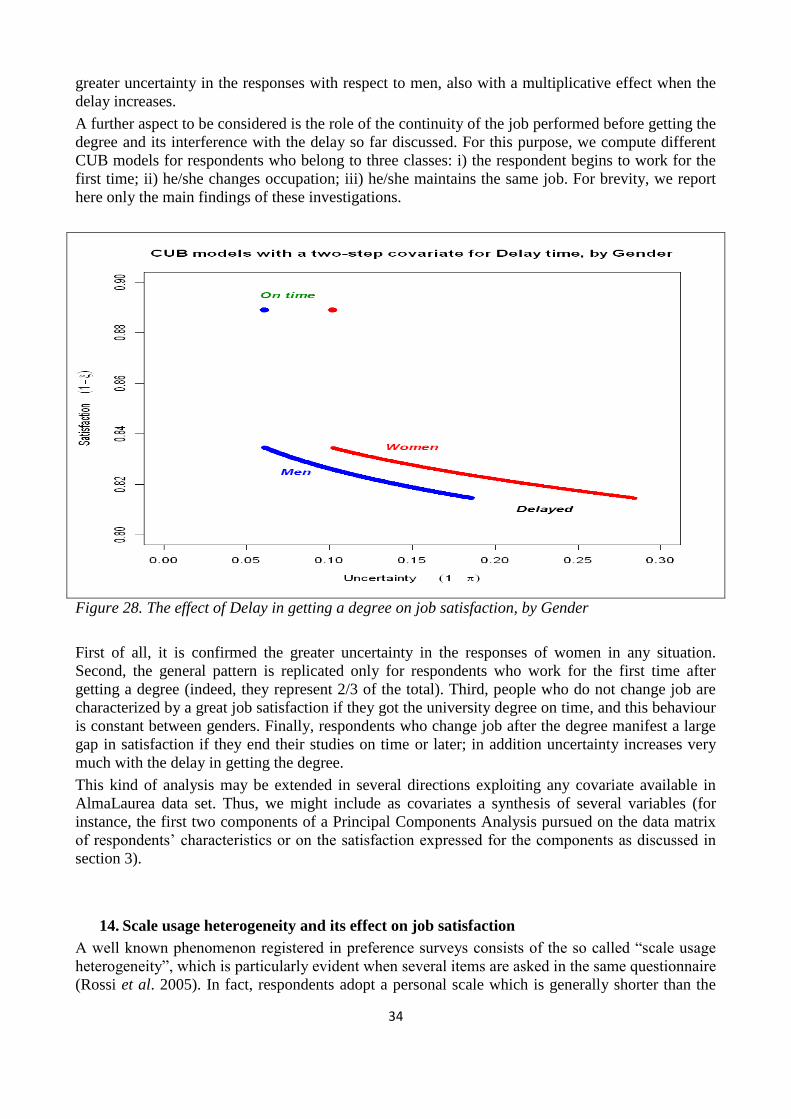
34

greater uncertainty in the responses with respect to men, also with a multiplicative effect when the

delay increases.

A further aspect to be considered is the role of the continuity of the job performed before getting the

degree and its interference with the delay so far discussed. For this purpose, we compute different

CUB models for respondents who belong to three classes: i) the respondent begins to work for the

first time; ii) he/she changes occupation; iii) he/she maintains the same job. For brevity, we report

here only the main findings of these investigations.

Figure 28. The effect of Delay in getting a degree on job satisfaction, by Gender

First of all, it is confirmed the greater uncertainty in the responses of women in any situation.

Second, the general pattern is replicated only for respondents who work for the first time after

getting a degree (indeed, they represent 2/3 of the total). Third, people who do not change job are

characterized by a great job satisfaction if they got the university degree on time, and this behaviour

is constant between genders. Finally, respondents who change job after the degree manifest a large

gap in satisfaction if they end their studies on time or later; in addition uncertainty increases very

much with the delay in getting the degree.

This kind of analysis may be extended in several directions exploiting any covariate available in

AlmaLaurea data set. Thus, we might include as covariates a synthesis of several variables (for

instance, the first two components of a Principal Components Analysis pursued on the data matrix

of respondents’ characteristics or on the satisfaction expressed for the components as discussed in

section 3).

14. Scale usage heterogeneity and its effect on job satisfaction

A well known phenomenon registered in preference surveys consists of the so called “scale usage

heterogeneity”, which is particularly evident when several items are asked in the same questionnaire

(Rossi et al. 2005). In fact, respondents adopt a personal scale which is generally shorter than the

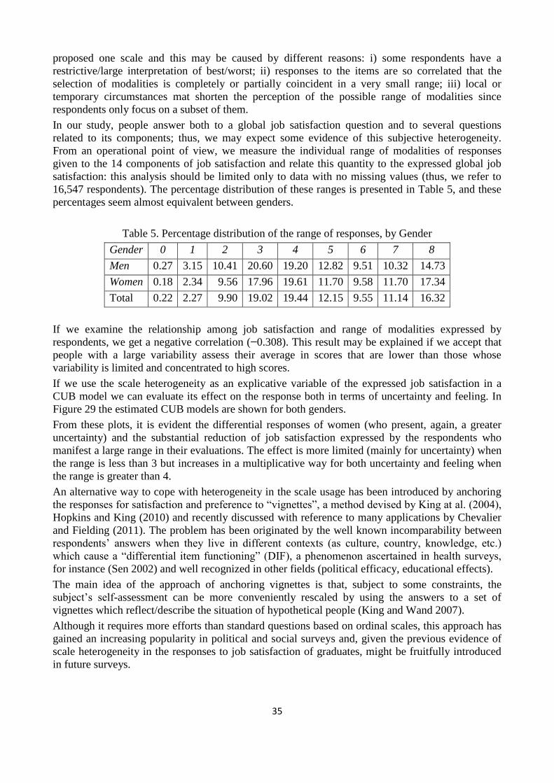
35

proposed one scale and this may be caused by different reasons: i) some respondents have a

restrictive/large interpretation of best/worst; ii) responses to the items are so correlated that the

selection of modalities is completely or partially coincident in a very small range; iii) local or

temporary circumstances mat shorten the perception of the possible range of modalities since

respondents only focus on a subset of them.

In our study, people answer both to a global job satisfaction question and to several questions

related to its components; thus, we may expect some evidence of this subjective heterogeneity.

From an operational point of view, we measure the individual range of modalities of responses

given to the 14 components of job satisfaction and relate this quantity to the expressed global job

satisfaction: this analysis should be limited only to data with no missing values (thus, we refer to

16,547 respondents). The percentage distribution of these ranges is presented in Table 5, and these

percentages seem almost equivalent between genders.

Table 5. Percentage distribution of the range of responses, by Gender

Gender 0 1 2 3 4 5 6 7 8

Men 0.27 3.15 10.41 20.60 19.20 12.82 9.51 10.32 14.73

Women 0.18 2.34 9.56 17.96 19.61 11.70 9.58 11.70 17.34

Total 0.22 2.27 9.90 19.02 19.44 12.15 9.55 11.14 16.32

If we examine the relationship among job satisfaction and range of modalities expressed by

respondents, we get a negative correlation (−0.308). This result may be explained if we accept that

people with a large variability assess their average in scores that are lower than those whose

variability is limited and concentrated to high scores.

If we use the scale heterogeneity as an explicative variable of the expressed job satisfaction in a

CUB model we can evaluate its effect on the response both in terms of uncertainty and feeling. In

Figure 29 the estimated CUB models are shown for both genders.

From these plots, it is evident the differential responses of women (who present, again, a greater

uncertainty) and the substantial reduction of job satisfaction expressed by the respondents who

manifest a large range in their evaluations. The effect is more limited (mainly for uncertainty) when

the range is less than 3 but increases in a multiplicative way for both uncertainty and feeling when

the range is greater than 4.

An alternative way to cope with heterogeneity in the scale usage has been introduced by anchoring

the responses for satisfaction and preference to “vignettes”, a method devised by King at al. (2004),

Hopkins and King (2010) and recently discussed with reference to many applications by Chevalier

and Fielding (2011). The problem has been originated by the well known incomparability between

respondents’ answers when they live in different contexts (as culture, country, knowledge, etc.)

which cause a “differential item functioning” (DIF), a phenomenon ascertained in health surveys,

for instance (Sen 2002) and well recognized in other fields (political efficacy, educational effects).

The main idea of the approach of anchoring vignettes is that, subject to some constraints, the

subject’s self-assessment can be more conveniently rescaled by using the answers to a set of

vignettes which reflect/describe the situation of hypothetical people (King and Wand 2007).

Although it requires more efforts than standard questions based on ordinal scales, this approach has

gained an increasing popularity in political and social surveys and, given the previous evidence of

scale heterogeneity in the responses to job satisfaction of graduates, might be fruitfully introduced

in future surveys.

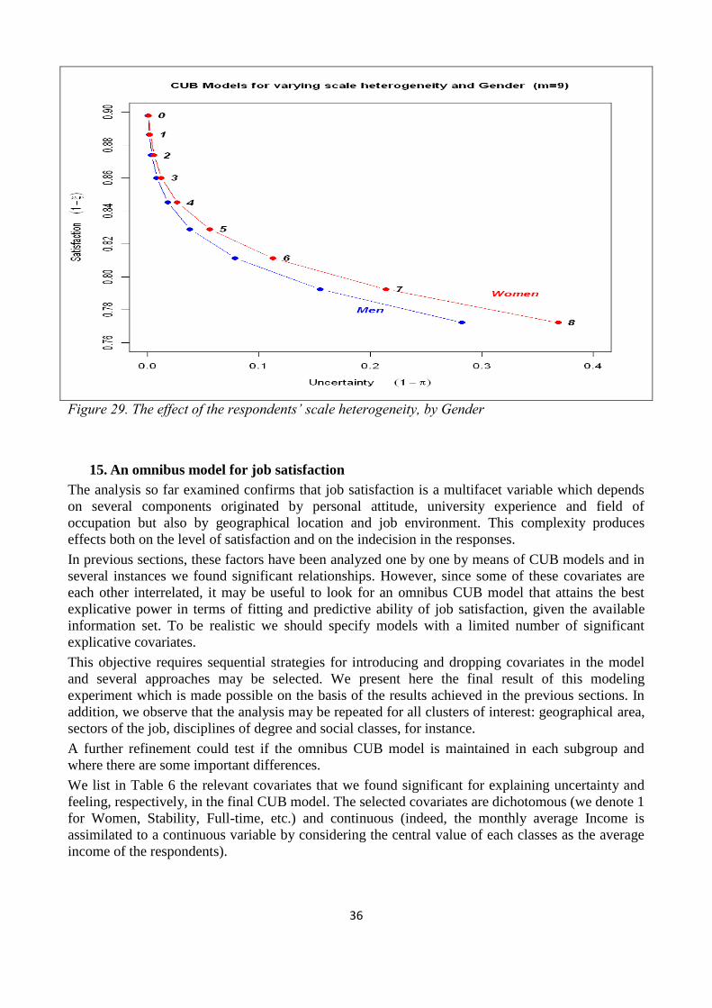
36

Figure 29. The effect of the respondents’ scale heterogeneity, by Gender

15. An omnibus model for job satisfaction

The analysis so far examined confirms that job satisfaction is a multifacet variable which depends

on several components originated by personal attitude, university experience and field of

occupation but also by geographical location and job environment. This complexity produces

effects both on the level of satisfaction and on the indecision in the responses.

In previous sections, these factors have been analyzed one by one by means of CUB models and in

several instances we found significant relationships. However, since some of these covariates are

each other interrelated, it may be useful to look for an omnibus CUB model that attains the best

explicative power in terms of fitting and predictive ability of job satisfaction, given the available

information set. To be realistic we should specify models with a limited number of significant

explicative covariates.

This objective requires sequential strategies for introducing and dropping covariates in the model

and several approaches may be selected. We present here the final result of this modeling

experiment which is made possible on the basis of the results achieved in the previous sections. In

addition, we observe that the analysis may be repeated for all clusters of interest: geographical area,

sectors of the job, disciplines of degree and social classes, for instance.

A further refinement could test if the omnibus CUB model is maintained in each subgroup and

where there are some important differences.

We list in Table 6 the relevant covariates that we found significant for explaining uncertainty and

feeling, respectively, in the final CUB model. The selected covariates are dichotomous (we denote 1

for Women, Stability, Full-time, etc.) and continuous (indeed, the monthly average Income is

assimilated to a continuous variable by considering the central value of each classes as the average

income of the respondents).

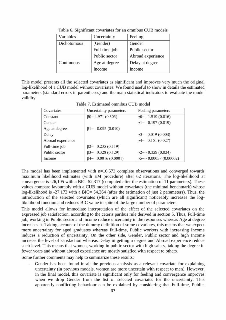
37

Table 6. Significant covariates for an omnibus CUB models

Variables Uncertainty Feeling

Dichotomous (Gender)

Full-time job

Public sector

Gender

Public sector

Abroad experience

Continuous Age at degree

Income

Delay at degree

Income

This model presents all the selected covariates as significant and improves very much the original

log-likelihood of a CUB model without covariates. We found useful to show in details the estimated

parameters (standard errors in parentheses) and the main statistical indicators to evaluate the model

validity.

Table 7. Estimated omnibus CUB model

Covariates Uncertainty parameters Feeling parameters

Constant

Gender

Age at degree

Delay

Abroad experience

Full-time job

Public sector

Income

β0= 4.971 (0.303)

β1= - 0.095 (0.010)

β2= 0.235 (0.119)

β3= 0.328 (0.129)

β4= 0.0016 (0.0001)

γ0= - 1.519 (0.016)

γ1= - 0.197 (0.019)

γ3= 0.019 (0.003)

γ4= 0.151 (0.027)

γ2= - 0.329 (0.024)

γ5= - 0.00057 (0.00002)

The model has been implemented with n=16,573 complete observations and converged towards

maximum likelihood estimates (with EM procedure) after 62 iterations. The log-likelihood at

convergence is -26,105 with a BIC=52,317 (computed after the estimation of 11 parameters). These

values compare favourably with a CUB model without covariates (the minimal benchmark) whose

log-likelihood is -27,173 with a BIC= 54,364 (after the estimation of just 2 parameters). Thus, the

introduction of the selected covariates (which are all significant) noticeably increases the log-

likelihood function and reduces BIC value in spite of the large number of parameters.

This model allows for immediate interpretation of the effect of the selected covariates on the

expressed job satisfaction, according to the ceteris paribus rule derived in section 5. Thus, Full-time

job, working in Public sector and Income reduce uncertainty in the responses whereas Age at degree

increases it. Taking account of the dummy definition of some covariates, this means that we expect

more uncertainty for aged graduates whereas Full-time, Public workers with increasing Income

induces a reduction of uncertainty. On the other side, Gender, Public sector and high Income

increase the level of satisfaction whereas Delay in getting a degree and Abroad experience reduce

such level. This means that women, working in public sector with high salary, taking the degree in

fewer years and without abroad experience are mostly satisfied with respect to others.

Some further comments may help to summarize these results:

- Gender has been found in all the previous analysis as a relevant covariate for explaining

uncertainty (in previous models, women are more uncertain with respect to men). However,

in the final model, this covariate is significant only for feeling and convergence improves

when we drop Gender from the list of selected covariates for the uncertainty. This

apparently conflicting behaviour can be explained by considering that Full-time, Public,

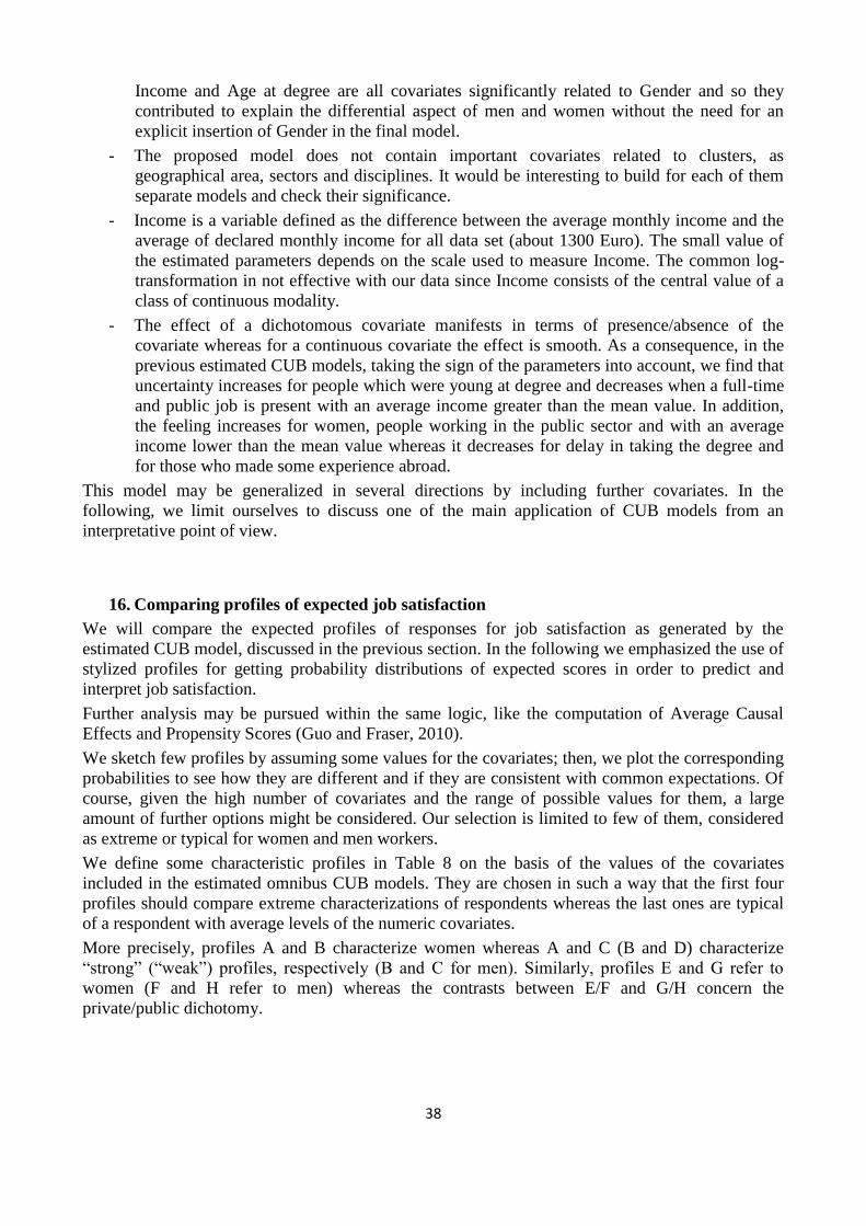
38

Income and Age at degree are all covariates significantly related to Gender and so they

contributed to explain the differential aspect of men and women without the need for an

explicit insertion of Gender in the final model.

- The proposed model does not contain important covariates related to clusters, as

geographical area, sectors and disciplines. It would be interesting to build for each of them

separate models and check their significance.

- Income is a variable defined as the difference between the average monthly income and the

average of declared monthly income for all data set (about 1300 Euro). The small value of

the estimated parameters depends on the scale used to measure Income. The common log-

transformation in not effective with our data since Income consists of the central value of a

class of continuous modality.

- The effect of a dichotomous covariate manifests in terms of presence/absence of the

covariate whereas for a continuous covariate the effect is smooth. As a consequence, in the

previous estimated CUB models, taking the sign of the parameters into account, we find that

uncertainty increases for people which were young at degree and decreases when a full-time

and public job is present with an average income greater than the mean value. In addition,

the feeling increases for women, people working in the public sector and with an average

income lower than the mean value whereas it decreases for delay in taking the degree and

for those who made some experience abroad.

This model may be generalized in several directions by including further covariates. In the

following, we limit ourselves to discuss one of the main application of CUB models from an

interpretative point of view.

16. Comparing profiles of expected job satisfaction

We will compare the expected profiles of responses for job satisfaction as generated by the

estimated CUB model, discussed in the previous section. In the following we emphasized the use of

stylized profiles for getting probability distributions of expected scores in order to predict and

interpret job satisfaction.

Further analysis may be pursued within the same logic, like the computation of Average Causal

Effects and Propensity Scores (Guo and Fraser, 2010).

We sketch few profiles by assuming some values for the covariates; then, we plot the corresponding

probabilities to see how they are different and if they are consistent with common expectations. Of

course, given the high number of covariates and the range of possible values for them, a large

amount of further options might be considered. Our selection is limited to few of them, considered

as extreme or typical for women and men workers.

We define some characteristic profiles in Table 8 on the basis of the values of the covariates

included in the estimated omnibus CUB models. They are chosen in such a way that the first four

profiles should compare extreme characterizations of respondents whereas the last ones are typical

of a respondent with average levels of the numeric covariates.

More precisely, profiles A and B characterize women whereas A and C (B and D) characterize

“strong” (“weak”) profiles, respectively (B and C for men). Similarly, profiles E and G refer to

women (F and H refer to men) whereas the contrasts between E/F and G/H concern the

private/public dichotomy.

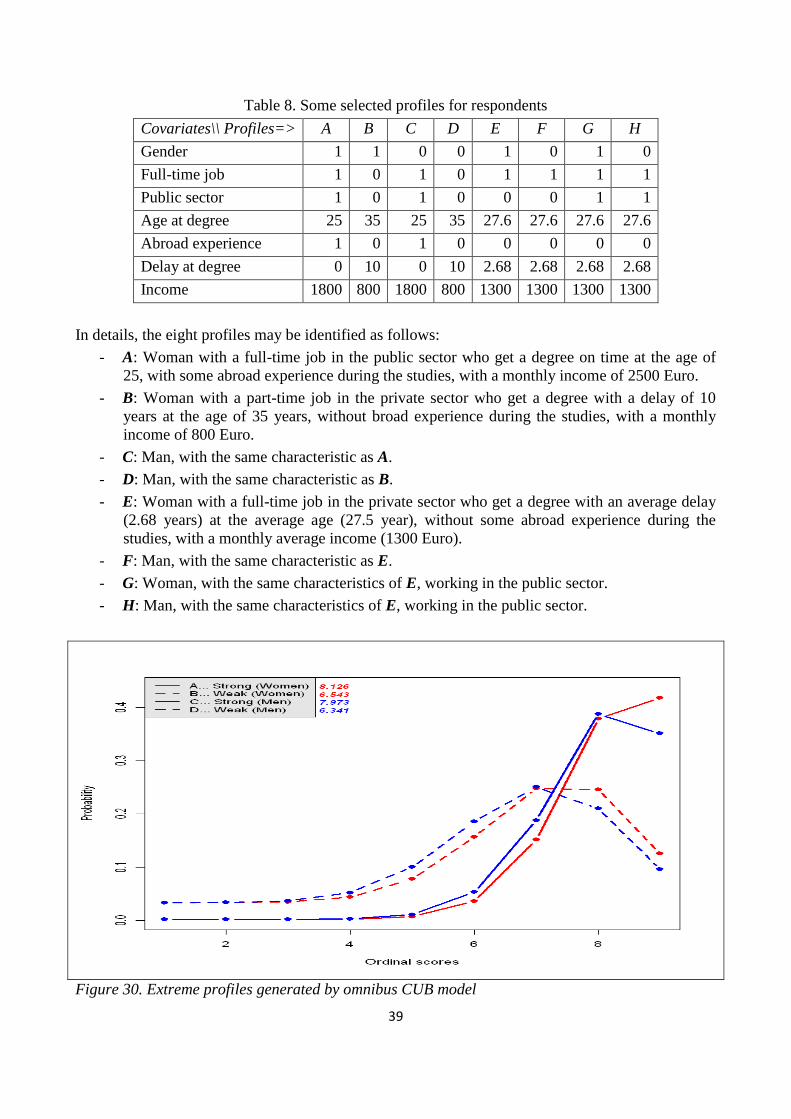
39

Table 8. Some selected profiles for respondents

Covariates\\ Profiles=> A B C D E F G H

Gender 1 1 0 0 1 0 1 0

Full-time job 1 0 1 0 1 1 1 1

Public sector 1 0 1 0 0 0 1 1

Age at degree 25 35 25 35 27.6 27.6 27.6 27.6

Abroad experience 1 0 1 0 0 0 0 0

Delay at degree 0 10 0 10 2.68 2.68 2.68 2.68

Income 1800 800 1800 800 1300 1300 1300 1300

In details, the eight profiles may be identified as follows:

- A: Woman with a full-time job in the public sector who get a degree on time at the age of

25, with some abroad experience during the studies, with a monthly income of 2500 Euro.

- B: Woman with a part-time job in the private sector who get a degree with a delay of 10

years at the age of 35 years, without broad experience during the studies, with a monthly

income of 800 Euro.

- C: Man, with the same characteristic as A.

- D: Man, with the same characteristic as B.

- E: Woman with a full-time job in the private sector who get a degree with an average delay

(2.68 years) at the average age (27.5 year), without some abroad experience during the

studies, with a monthly average income (1300 Euro).

- F: Man, with the same characteristic as E.

- G: Woman, with the same characteristics of E, working in the public sector.

- H: Man, with the same characteristics of E, working in the public sector.

Figure 30. Extreme profiles generated by omnibus CUB model

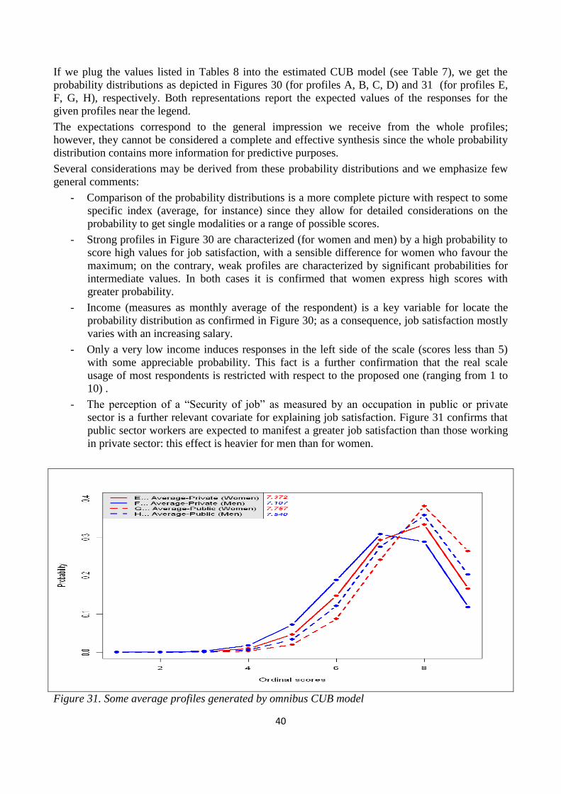
40

If we plug the values listed in Tables 8 into the estimated CUB model (see Table 7), we get the

probability distributions as depicted in Figures 30 (for profiles A, B, C, D) and 31 (for profiles E,

F, G, H), respectively. Both representations report the expected values of the responses for the

given profiles near the legend.

The expectations correspond to the general impression we receive from the whole profiles;

however, they cannot be considered a complete and effective synthesis since the whole probability

distribution contains more information for predictive purposes.

Several considerations may be derived from these probability distributions and we emphasize few

general comments:

- Comparison of the probability distributions is a more complete picture with respect to some

specific index (average, for instance) since they allow for detailed considerations on the

probability to get single modalities or a range of possible scores.

- Strong profiles in Figure 30 are characterized (for women and men) by a high probability to

score high values for job satisfaction, with a sensible difference for women who favour the

maximum; on the contrary, weak profiles are characterized by significant probabilities for

intermediate values. In both cases it is confirmed that women express high scores with

greater probability.

- Income (measures as monthly average of the respondent) is a key variable for locate the

probability distribution as confirmed in Figure 30; as a consequence, job satisfaction mostly

varies with an increasing salary.

- Only a very low income induces responses in the left side of the scale (scores less than 5)

with some appreciable probability. This fact is a further confirmation that the real scale

usage of most respondents is restricted with respect to the proposed one (ranging from 1 to

10) .

- The perception of a “Security of job” as measured by an occupation in public or private

sector is a further relevant covariate for explaining job satisfaction. Figure 31 confirms that

public sector workers are expected to manifest a greater job satisfaction than those working

in private sector: this effect is heavier for men than for women.

Figure 31. Some average profiles generated by omnibus CUB model

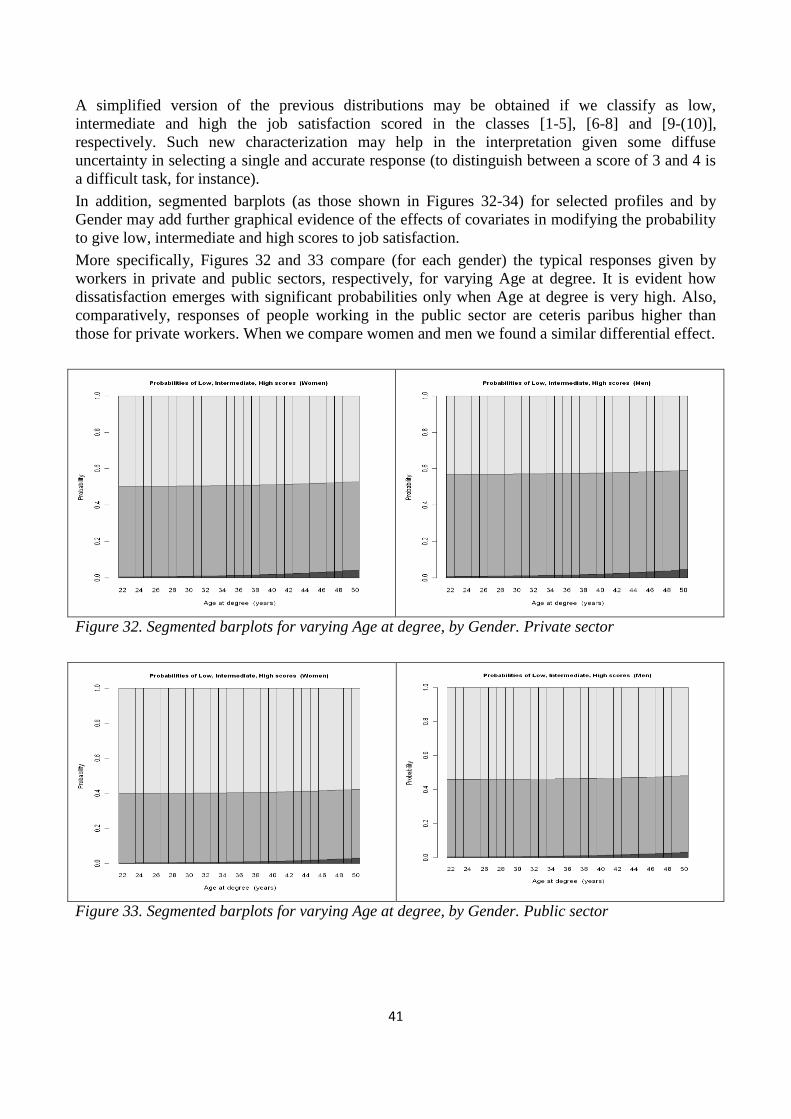
41

A simplified version of the previous distributions may be obtained if we classify as low,

intermediate and high the job satisfaction scored in the classes [1-5], [6-8] and [9-(10)],

respectively. Such new characterization may help in the interpretation given some diffuse

uncertainty in selecting a single and accurate response (to distinguish between a score of 3 and 4 is

a difficult task, for instance).

In addition, segmented barplots (as those shown in Figures 32-34) for selected profiles and by

Gender may add further graphical evidence of the effects of covariates in modifying the probability

to give low, intermediate and high scores to job satisfaction.

More specifically, Figures 32 and 33 compare (for each gender) the typical responses given by

workers in private and public sectors, respectively, for varying Age at degree. It is evident how

dissatisfaction emerges with significant probabilities only when Age at degree is very high. Also,

comparatively, responses of people working in the public sector are ceteris paribus higher than

those for private workers. When we compare women and men we found a similar differential effect.

Figure 32. Segmented barplots for varying Age at degree, by Gender. Private sector

Figure 33. Segmented barplots for varying Age at degree, by Gender. Public sector

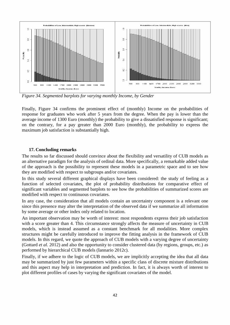
42

Figure 34. Segmented barplots for varying monthly Income, by Gender

Finally, Figure 34 confirms the prominent effect of (monthly) Income on the probabilities of

response for graduates who work after 5 years from the degree. When the pay is lower than the

average income of 1300 Euro (monthly) the probability to give a dissatisfied response is significant;

on the contrary, for a pay greater than 2000 Euro (monthly), the probability to express the

maximum job satisfaction is substantially high.

17. Concluding remarks

The results so far discussed should convince about the flexibility and versatility of CUB models as

an alternative paradigm for the analysis of ordinal data. More specifically, a remarkable added value

of the approach is the possibility to represent these models in a parametric space and to see how

they are modified with respect to subgroups and/or covariates.

In this study several different graphical displays have been considered: the study of feeling as a

function of selected covariates, the plot of probability distributions for comparative effect of

significant variables and segmented barplots to see how the probabilities of summarized scores are

modified with respect to continuous covariates.

In any case, the consideration that all models contain an uncertainty component is a relevant one

since this presence may alter the interpretation of the observed data if we summarize all information

by some average or other index only related to location.

An important observation may be worth of interest: most respondents express their job satisfaction

with a score greater than 4. This circumstance strongly affects the measure of uncertainty in CUB

models, which is instead assumed as a constant benchmark for all modalities. More complex

structures might be carefully introduced to improve the fitting analysis in the framework of CUB

models. In this regard, we quote the approach of CUB models with a varying degree of uncertainty

(Gottard et al. 2012) and also the opportunity to consider clustered data (by regions, groups, etc.) as

performed by hierarchical CUB models (Iannario 2012c).

Finally, if we adhere to the logic of CUB models, we are implicitly accepting the idea that all data

may be summarized by just few parameters within a specific class of discrete mixture distributions

and this aspect may help in interpretation and prediction. In fact, it is always worth of interest to

plot different profiles of cases by varying the significant covariates of the model.

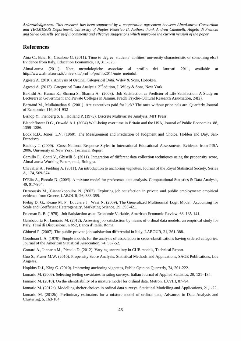
43

Acknowledgments. This research has been supported by a cooperation agreement between AlmaLaurea Consortium

and TEOMESUS Department, University of Naples Federico II. Authors thank Andrea Cammelli, Angelo di Francia

and Silvia Ghiselli for useful comments and effective suggestions which improved the current version of the paper.

References

Aina C., Baici E., Casalone G. (2011). Time to degree: students’ abilities, university characteristic or something else?

Evidence from Italy, Education Economics, 19, 311-325.

AlmaLaurea (2011). Note metodologiche associate al profilo dei laureati 2011, available at

http://www.almalaurea.it/universita/profilo/profilo2011/note_metodol.

Agresti A. (2010). Analysis of Ordinal Categorical Data. Wiley & Sons, Hoboken.

Agresti A. (2012). Categorical Data Analysis. 2nd

edition, J. Wiley & Sons, New York.

Bakhshi A., Kumar K., Sharma S., Sharma A. (2008). Job Satisfaction as Predictor of Life Satisfaction: A Study on

Lecturers in Government and Private Colleges in Jammu. Prachi Psycho-Cultural Research Association, 24(2).

Bertrand M., Mullainathan S. (2001). Are executives paid for luck? The ones without principals are. Quarterly Journal

of Economics 116, 901-932

Bishop Y., Fienberg S. E., Holland P. (1975). Discrete Multivariate Analysis. MIT Press.

Blanchflower D.G., Oswald A.J. (2004) Well-being over time in Britain and the USA, Journal of Public Economics. 88,

1359–1386.

Bock R.D., Jones, L.V. (1968). The Measurement and Prediction of Judgment and Choice. Holden and Day, San-

Francisco.

Buckley J. (2009). Cross-National Response Styles in International Educational Assessments: Evidence from PISA

2006, University of New York, Technical Report.

Camillo F., Conti V., Ghiselli S. (2011). Integration of different data collection techniques using the propensity score,

AlmaLaurea Working Papers, no.4, Bologna.

Chevalier A., Fielding A. (2011). An introduction to anchoring vignettes, Journal of the Royal Statistical Society, Series

A, 174, 569-574.

D’Elia A., Piccolo D. (2005). A mixture model for preference data analysis. Computational Statistics & Data Analysis,

49, 917-934.

Demoussis M., Giannakopoulos N. (2007). Exploring job satisfaction in private and public employment: empirical

evidence from Greece, LABOUR, 26, 333-359.

Fiebig D. G., Keane M. P., Louviere J., Wasi N. (2009). The Generalized Multinomial Logit Model: Accounting for

Scale and Coefficient Heterogeneity, Marketing Science, 29, 393-421.

Freeman R. B. (1978). Job Satisfaction as an Economic Variable, American Economic Review, 68, 135-141.

Gambacorta R., Iannario M. (2012). Assessing job satisfaction by means of ordinal data models: an empirical study for

Italy, Temi di Discussione, n.852, Banca d’Italia, Roma.

Ghinetti P. (2007). The public-provate job satisfaction differential in Italy, LABOUR, 21, 361-388.

Goodman L.A. (1979). Simple models for the analysis of association in cross-classifications having ordered categories.

Journal of the American Statistical Association, 74, 537-52.

Gottard A., Iannario M., Piccolo D. (2012). Varying uncertainty in CUB models, Technical Report.

Guo S., Fraser M.W. (2010). Propensity Score Analysis. Statistical Methods and Applications, SAGE Publications, Los

Angeles.

Hopkins D.J., King G. (2010). Improving anchoring vignettes, Public Opinion Quarterly, 74, 201-222.

Iannario M. (2009). Selecting feeling covariates in rating surveys. Italian Journal of Applied Statistics, 20, 121–134.

Iannario M. (2010). On the identifiability of a mixture model for ordinal data, Metron, LXVIII, 87–94.

Iannario M. (2012a). Modelling shelter choices in ordinal data surveys. Statistical Modelling and Applications, 21,1-22.

Iannario M. (2012b). Preliminary estimators for a mixture model of ordinal data, Advances in Data Analysis and

Clustering, 6, 163-184.

44

Iannario M. (2012c). Hierarchical CUB Models for Ordinal Variables, Communications in Statistics - Theory and

Methods, 41, 3110-3125.

Iannario M., Piccolo D. (2009). A package in R for CUB models inference, Version 2.0, available at

http://www.dipstat.unina.it/CUBmodels/

Kapteyn A., Smith J.P., Van Soest A.H. (2009). Comparing Life Satisfaction, RAND Working Paper WR-623-1

Karasek R. (1997). Demand & control model: A social, emotional, and physiological approach to stress risk and active

behavior development. Encyclopedia of Occupational Health and Safety, Volume II (4th Ed.). Geneva: International

Labor Office.

King G., Murray C., Salomon J., Tandon A. (2004). Enhancing the validity and cross-cultural comparability of

measurement in survey research, American Political Science Review, 98, 191-205.

King G., Wand J. (2007). Comparing incomparable survey responses: Evaluating and selecting anchoring vignettes,

Political Analysis, 15, 46-66.

Krosnick J.A. (1991). Response Strategies for coping with the cognitive demands of attitude measures in surveys.

Applied Cognitive Psychology, 5, 213-236.

Locke E. (1976), The nature and causes of job satisfaction. In M.D. Dunnette, ed., Handbook of Industrial and

Organizational Psychology, Rand McNally, pp.1297-1349.

McCullagh P. (1980). Regression models for ordinal data. Journal of the Royal Statistical Society, B. 42, 109-142.

McLachlan G., Peel G.J. (2000). Finite mixture models, J. Wiley, New York.

Piccolo D. (2003). On the moments of a mixture of uniform and shifted binomial random variables, Quaderni di

Statistica, 5, 85-104.

Piccolo D. (2006). Observed information matrix for MUB models, Quaderni di Statistica, 8, 33-78.

Piccolo D., Iannario M. (2008). Qualitative and quantitative models for ordinal data analysis, Proceedings of MTISD

2008 Conference, University of Salento, Lecce, 140-143.

Poulton E.C. (1989). Bias in Quantifying Judgments. Lawrence Erlbaum, Hillsdale, NJ.

Pugno M., Depedri S. (2009). Job performance and job satisfaction an integrated survey, Discussion Paper, n.4,

Dipartimento di Economia, Università di Trento.

Rose M. (2005). Job Satisfaction in Britain: Coping with Complexity, British Journal of Industrial Relations, 43, 455-

467.

Rossi P. E., Allenby G. M., McCulloch R. (2005). Overcoming Scale Usage Heterogeneity, in P. E. Rossi et al. (eds.),

Bayesian Statistics in Marketing, John Wiley & Sons, N.Y., pp.237-252.

Schizzerotto A. editor (2002). Vite ineguali. Disuguaglianze e corsi di vita nell’Italia contemporanea. Il Mulino,

Bologna.

Sen A. (2002). Health: perception versus observation, British Medical Journal, 324, 860-861.

Simon H. A. (1957). Models of man, social and rational: Mathematical essays on rational human behavior. Wiley, New

York.

Souza-Poza A., Souza-Poza A. A. (2000). Well-being at work: a cross-national analysis of the levels and determinants

of job satisfaction, The Journal of Socio-Economics, 29, 517-538.

Snell F.J. (1964). A scaling procedure for ordered categorical data. Biometrics, 20, 592-607.

Spector P. E. (1997). Job satisfaction: Application, assessment, causes, and consequences. SAGE Publications, Los

Angeles.

Spector P.E. (1985). Measurement of human service staff satisfaction: Development of the Job Satisfaction Survey,

American Journal of Community Psychology, 1985, 13, 6, 693-713.

Vroom V.H., Deci E.L. (1971). The Stability of Post-Decision Dissonance: A Follow-Up Study of the Job Attitudes of

Business School Graduates, Organizational Behavior and Human Performance, 6, 36-49.

Tutz G. (2012). Regression for Categorical Data, Cambridge University Press, Cambridge.

Zavonia R., McElvey W. (1975). A statistical model for the analysis of ordinal level dependent variables, Journal of

Mathematical Sociology, 4, 103–120.