Modelling the onset of shear boundary layers in fibrous

composite reinforcements by second gradient theory

Manuel Ferretti, Angela Madeo*, Francesco dell’Isola and Philippe Boisse

Abstract. It has been known since the pioneering works by Piola, Cosserat, Mindlin, Toupin, Erin-gen, Green, Rivlin and Germain that many micro-structural effects in mechanical systems canbe still modeled by means of continuum theories. When needed, the displacement field must becomplemented by additional kinematical descriptors, called sometimes microstructural fields. Inthis paper, a technologically important class of fibrous composite reinforcements is considered andtheir mechanical behavior is described at finite strains by means of a second gradient, hyperelastic,orthotropic continuum theory which is obtained as the limit case of a micromorphic theory. Fol-lowing Mindlin and Eringen, we consider a micromorphic continuum theory based on an enrichedkinematics constituted by the displacement field u and a second order tensor field ψ describingmicroscopic deformations. The governing equations in weak form are used to perform numericalsimulations in which a bias extension test is reproduced. We show that second gradient energyterms allow for an effective prediction of the onset of internal shear boundary layers which aretransition zones between two different shear deformation modes. The existence of these boundarylayers cannot be described by a simple first gradient model and its features are related to secondgradient material coefficients. The obtained numerical results, together with the available experi-mental evidences, allow us to estimate the order of magnitude of the introduced second gradientcoefficients by inverse approach. This justifies the need of a novel measurement campaign aimedto estimate the value of the introduced second gradient parameters for a wide class of fibrousmaterials.

1. Introduction

In the engineering effort of designing new materials, a constant demand is directed towards the searchfor better performances and new functionalities. A class of materials which is gaining more and moreattention is that of so-called complex materials, e.g. materials exhibiting different mechanical responsesat different scales due to different scales of heterogeneity. Indeed, the overall mechanical behavior ofsuch materials is macroscopically influenced by the underlying microstructure especially in presenceof particular loading and/or boundary conditions. Therefore, understanding the mechanics of meso-and micro-structured materials is becoming a major issue in engineering.

Such materials may exhibit superior mechanical properties with respect to more commonly usedengineering materials, also providing some advantages as easy formability processes. We focus in thispaper on a class of engineering materials which are known as woven fibrous composite reinforcements.These materials are constituted by woven tows which are themselves made up of thousand of fibers.Different weaving schemes can be used giving rise to different types of composite reinforcements (seeFig.1), but in each of considered case one can assume that sharp changes in mechanical properties

The authors thank INSA-Lyon for the financial support assigned to the project BQR 2013-0054 “Materiaux Meso etMicro-Heterogenes: Optimisation par Modeles de Second Gradient et Applications en Ingenierie”.

hal-0

0838

662,

ver

sion

1 -

26 J

un 2

013

2 Manuel Ferretti, Angela Madeo*, Francesco dell’Isola and Philippe Boisse

Plain Weave Twill Satin

Figure 1. Schemes of weaving for fibrous composite reinforcements.

may occur inside the unit cell. Indeed, for the considered materials, the tensile stiffness of tows canbe considered to be of many order of magnitudes higher than the shear stiffness related to anglevariations between yarns. The hierarchical heterogeneity of composite reinforcements is illustrated inFig. 2, in which three different scales can be recognized: the macroscopic scale (left), the mesoscopicscale (center) and the microscopic scale (right).

All materials are actually heterogeneous if one considers sufficiently small scales, but the wovencomposites reinforcements show their heterogeneity at scales which are significant from an engineeringpoint of view. It is also clear that woven materials also macroscopically show strong anisotropy, sincetheir mechanical response significantly varies if the load is applied in the direction of the fibers orin some other direction. As it will be better pointed out in the following, the introduced continuummodel for composite reinforcements belongs to the class of initially orthotropic continua, i.e. continuawhich have two privileged directions in their undeformed configuration.

The fibrous composite preforms can be shaped and their final shape is maintained by injectionand curing of a thermoset resin or by the use of a thermoplastic polymer. The final composite materialcommonly used in aerospace engineering is hence constituted by the fibrous composite reinforcementand the organic matrix. We are interested in this paper only in describing the mechanical behavior ofthe fibrous composite reinforcements since this knowledge is fundamental for the process of formabilityof the final composite. Following [13, 14] we find convenient to model the quoted fibrous reinforcementsas continuous media. This hypothesis can be considered to be realistic if no relative displacementbetween superimposed fibers occurs. In other words, we are assuming that two superimposed fiberscan rotate around their contact point, while no slipping takes place. This hypothesis is generallyverified during experimental analyses, even at finite strains. In fact, when straight lines are drawn onthe textile reinforcement, these lines become curved after forming but they remain continuous (see e.g.[10]). As it will be better pointed out in the remainder of this paper, the anisotropy of the consideredreinforcements will be taken into account by introducing suitable hyperelastic, orthotropic constitutivelaws which are able to characterize the behavior of considered materials also at large strains.

Nevertheless, a first gradient continuum orthotropic model is not able to take into accountall the possible effects that the microstructure of considered materials have on their macroscopicdeformation. More precisely, some particular loading conditions, associated to particular types ofboundary conditions may cause some microstructure-related deformation modes which are not fullytaken into account in first gradient continuum theories. This is the case, for example, when observingsome regions inside the materials in which high gradients of deformation occur, concentrated in thoserelatively narrow regions which we will call boundary layers.

Actually, the onset of shear boundary layers can be observed in some experimental tests which areused to characterize the mechanical properties of fibrous composite reinforcements. Indeed, internalboundary layers do arise in the so-called bias extension test, the phenomenology of which we duly

hal-0

0838

662,

ver

sion

1 -

26 J

un 2

013

Second gradient modelling of composite reinforcements 3

Figure 2. The different scales of textile composite reinforcements.

describe in section 4. One way to deal with the description of such boundary layers, while remainingin the framework of a macroscopic theory, is to consider so-called “generalized continuum theories”.Such generalized theories allow for the introduction of a class of internal actions which is wider thanthe one which is accounted for by classical first gradient Cauchy continuum theory. These more generalcontact actions excite additional deformation modes which can be seen to be directly related with theproperties of the microstructure of considered materials.

Indeed, it has been known since the pioneering works by Piola [67], Cosserat [15], Midlin [57],Toupin [86], Eringen [29], Green and Rivlin [37] and Germain [35, 36] that many microstructure-related effects in mechanical systems can be still modeled by means of continuum theories. It is knownsince then that, when needed, the placement function must be complemented by additional kinemat-ical descriptors, called sometimes micro-structural fields. More recently, these generalized continuumtheories have been widely developed to describe the mechanical behavior of many complex systems,such as e.g. porous media [53, 80, 78, 22], capillary fluids [12, 16, 17, 20, 18], exotic media obtainedby homogenization of heterogeneous media [3, 81, 66]. Interesting applications on wave propagationin such generalized media has also gained attention in the recent years for the possible application ofthis kind of materials to passive control of vibrations and stealth technology (see e.g. [24, 54, 68, 76]).

In this paper, the class of fibrous composite preforms described before is considered and theirmacroscopic mechanical behavior (i.e. at a scale relatively larger than the yarn) is described by meansof a second gradient, hyperelastic continuum theory. The quoted hyperelastic, second gradient theoryis obtained as the limit case of a micromorphic theory, following what done in [7, 57] for the linear-elastic case. The governing equations in weak form are used as a basis for the formulation of suitablenumerical codes, which allow to perform simulations reproducing the so-called bias extension test.We show that second gradient energy terms allow for an effective prediction of the onset of internalshear boundary layers which can be defined as those transition zones between two different regionsexhibiting different shear deformation modes. The existence and thickness of these boundary layerscannot be described by a first gradient model and its overall features are related to the particularsecond gradient model introduced in this paper. The obtained numerical results seem to be in agood agreement with the already available experimental evidence and fully justify the need of a novelmeasurement campaign.

2. Micromorphic media and second gradient continua

We describe the deformation of the considered continuum by introducing a Lagrangian configurationBL ⊂ R

3 and a suitably regular kinematical field χ(X, t) which associates to any material pointX ∈ BL its current position x at time t. The image of the function χ gives, at any instant t thecurrent shape of the body BE(t): this time-varying domain is usually referred to as the Eulerianconfiguration of the medium and, indeed, it represents the system during its deformation. Since wewill use it in the following, we also introduce the displacement field u(X, t) := χ(X, t) − X, the

hal-0

0838

662,

ver

sion

1 -

26 J

un 2

013

4 Manuel Ferretti, Angela Madeo*, Francesco dell’Isola and Philippe Boisse

tensor F := ∇χ and the Right Cauchy-Green deformation tensor1 C := FT · F. The kinematics

of the continuum is then enriched by adding a second order tensor field ψ(X, t) which accounts fordeformations associated to the microstructure of the continuum. Indeed, as it was explained e. g.by Mindlin [57] and Cosserat [15], the addition of supplementary kinematical fields can be of helpto describe the deformation of the microstructure of the considered material independently of itsaverage continuum deformation. If, on the one hand, Cosserat’s models are able to complement theclassical continuum deformations with extra rotations of considered microstructure, on the other hand,micromorphic models of the type considered in this paper also allow to consider micro-stretches andmicro-shear deformations. In particular, the introduced micromorphic tensor ψ(X, t) allows to accountfor all these microscopic deformation in a very general fashion. If some constraints are introduced onthe tensor ψ, the micromorphic model can then be particularized so as to obtain Cosserat or secondgradient models as limit cases. In what follows, the current state of the considered medium is, ingeneral, identified by 12 independent kinematical fields: 3 components of the displacement field and9 components of the micro-deformation field. Such a theory of a continuum with microstructure hasbeen derived in [57] for the linear-elastic case and re-proposed e.g. in [30, 31, 32, 33] for the case ofnon-linear elasticity. For the sake of clearness, using similar notations to [57] and [7], we introducethe following kinematical quantities which are all functions of the basic kinematical fields introducedbefore

εij = (Cij − δij) /2, the macro-strain,

γij = εij − ψij , the relative(micro/macro) deformation, (1)

κijk = ψij,k, the gradient of micro-deformation,

where clearly Cij and ψij represent the components of the second order tensorsC and ψ respectively. Ifone, for example, imposes the relative deformation to be zero (i.e. ψij → εij), then κijk → εij,k and onerecovers the standard second gradient theory presented in [35, 36]. As it will be more clearly explainedin the following, the external actions which can be introduced in the framework of a micromorphiccontinuum theory are more easily understandable than those intervening in second gradient theoriessince they have a more direct physical meaning. Since second gradient theory can be readily obtainedas limit case of the micromorphic theory, one can then derive the second gradient contact actions interms of the micromorphic ones following the procedure used in [7]. We present in the following theweak formulation of a constrained micromorphic theory which will actually give rise to a particularsecond gradient theory. This constrained micromorphic theory is the one which we directly implementin the numerical simulations presented in this paper.

2.1. Equations in weak form for a constrained micromorphic continuum

We assume that we can write the power of internal actions as the first variation of a suitable actionfunctional A as follows

P int = δA = δ

ˆ

BL

[

W (εij , γij , κijk) +

n∑

α=1

λα fα(εij , γij , κijk)

]

dX, (2)

where W and f are real scalar-valued functions of the introduced deformation measures and, in par-ticular, W (εij , γij , κijk) is the bulk micromorphic strain energy density, λα are Lagrange multipliersand fα are particular constraints the particular form of which will be better specified later on. Asit will be better explained in the sequel, this expression of the power of internal forces is the onewhich is necessary to describe a micromorphic continuum which is subjected to the n constraintsfα(εij , γij , κijk) = 0.

1Here in the sequel a central dot indicates simple contraction between tensors of order greater than zero. For exampleif A and B are second order tensors of components Aij and Bjh respectively, then (A ·B)ih := AijBjh, where Einstein

notation of sum over repeated indeces is used.

hal-0

0838

662,

ver

sion

1 -

26 J

un 2

013

Second gradient modelling of composite reinforcements 5

Considering that the independent kinematical fields appearing in (2) are indeed εij , ψij and κijk,it can be recovered that the power of internal actions can be rewritten by computing the first variationof the action functional as

P int = δA =

ˆ

BL

(

∂W

∂εij+

n∑

α=1

λα∂fα∂εij

)

δεij +

(

∂W

∂ψij

+

n∑

α=1

λα∂fα∂ψij

)

δψij

(3)

+

(

∂W

∂κijk+

n∑

α=1

λα∂fα∂κijk

)

δκijk +

n∑

α=1

fαδλα,

where from now on we drop the symbol dX inside the integral sign and we adopt the Einstein notationof sum over repeated indices if no confusion can arise.

As for the expression of the power of external forces, we assume that they take the followinggeneral form (see also [57, 7])

Pext =

ˆ

BL

bexti δui +

ˆ

BL

Φextij δψij +

ˆ

∂BL

texti δui +

ˆ

∂BL

T extij δψij (4)

where bexti are volume forces, Φij are so called double forces per unit volume, texti are forces perunit area and T ext

ij are double forces per unit area. The physical meaning of aforementioned external

actions is immediate: bexti and texti work on the displacement of the centroid of each RepresentativeElementary Volume, while Φext

ij and T extij work on micro-deformations inside the considered REV. If

one forces ψij → εij , i.e. imposes the constraint ψij − εij = 0, then a more complicated form of thecontact actions than those appearing in (4) can be derived by integration by parts. In this way, it ispossible to recover the standard form for external actions of second gradient materials which workon displacement and on the normal derivatives of displacement (see e.g. [35, 51, 79, 52, 19, 21, 25]).Considering the surface power densities texti δui and T

extij δψij appearing in expression (4) for the power

of external actions, one can imagine to act on the boundary of considered body both by assigning theforces and/or double forces (natural boundary conditions) or by assigning the displacements and/ormicro-deformation (kinematical boundary conditions).

The mechanical governing equations in weak form can be directly expressed by imposing thevalidity of the principle of virtual powers

P int = Pext, (5)

where P int and Pext are respectively given in Eq. (3) and (4). We explicitly remark that, giventhe considered expression of the principle of virtual powers, we are assuming that the consideredphenomena are sufficiently slow to neglect inertia. We do not explicitly write here the correspondingstrong form of balance equations since we will directly implement a particularization of the weak form(5) in the finite element code used to perform numerical simulations.

3. Hyperelastic orthotropic model with micromorphic correction

In this section we specify the constitutive equations for the strain energy density W (εij , γij , κijk)which we use to model the mechanical behavior of some fibrous composite reinforcements in the finitestrain regime. We will equivalently use the deformation measure C = 2ε + I instead of ε to specifythe form for the energy, i.e. W (εij , γij , κijk) = W (Cij , γij , κijk). In particular, we will assume that

W (Cij , γij , κijk) =WI(Cij) +WII(κijk). (6)

In this formula WI is the first gradient strain energy and WII is the energy associated to the macro-inhomogeneity of micro-deformation. We do not explicitly consider a coupling energy depending on γij ,but some coupling effects will be accounted for by introducing particular constraints fα(εij , γij , κijk) =0 in the power of internal actions by using Lagrange multipliers, as specified in Eq.(2).

hal-0

0838

662,

ver

sion

1 -

26 J

un 2

013

6 Manuel Ferretti, Angela Madeo*, Francesco dell’Isola and Philippe Boisse

3.1. Representation theorem for hyperelastic orthotropic materials

Various hyperelastic constitutive equations for an isotropic strain energy density W iso(C) have beenproposed in the literature which are suitable to describe the mechanical behavior of isotropic materialseven at finite strains (see e.g. [61, 84]). Generalized constitutive laws are also available for linear elasticisotropic second gradient media (see [23]). These constitutive equations for isotropic materials areclassically derived starting from a well-known representation theorem for the strain energy potentialwhich states that only three independent scalar invariants of the Cauchy-Green tensor C are sufficientto correctly represent the functional dependence ofW iso onC. In other words, for an isotropic material,it is sufficient to consider that W iso(C) =W (i1, i2, i3), where i1, i2, i3 are the three scalar invariantsof C classically defined as

i1 = tr(C), i2 = tr(

det(C) C−T)

, i3 = det(C).

These three invariants respectively describe local deformations associated to changes of length, changesof area and changes of volume: superposition of these three deformation modes are sufficient to repro-duce the global deformation of an isotropic medium. Constitutive equations for transversely isotropicmaterials are also well assessed in the literature (see e.g. [44, 8, 9, 62, 13, 45]) and their derivationrelies on the classical representation theorem according to which five independent invariants of thetensor C are needed to characterize the behavior of such materials: W tran(C) =W (i1, i2, i3, i4, i5). Ifone denotes by m1 the unitary vector along the preferred direction inside the transversely isotropicmaterial in its reference (Lagrangian) configuration, then the two additional invariants appearing inthe representation of W tran are defined as

i4 = m1 ·C ·m1, i5 = m1 ·C2 ·m1.

These two invariants respectively describe local stretch in the direction of the preferential directionm1 and changes of angles mixed to changes of length.

As far as orthotropic materials are considered, clear and exploitable constitutive hyperelasticequations are harder to be found in the literature. Plenty of authors try to generalize the representa-tion theorems valid for isotropic and transversely isotropic media, but often there is apparently notagreement between the different versions proposed for such a theorem. The more diffused version of therepresentation theorem for the strain energy potential for orthotropic media states that seven invari-ants can be used to write the functional dependence of the strain energy density (see e.g. [43, 82, 62]).More precisely, denoting by m1 and m2 two orthogonal unitary vectors along the preferred directionsin the considered orthotropic material, the functional dependence of the orthotropic energy on C canbe expressed in the form W orth = W (i1, i2, i3, i4, i5, i6, i7), where the additional two invariants aredefined as

i6 = m2 ·C ·m2, i7 = m2 ·C2 ·m2,

Nevertheless, it can be proved that, indeed, only six independent scalar invariants are sufficient tocompletely describe the behavior of an orthotropic material (see the elegant proof given in [69]), sothat, even if it is effectively possible to write the strain energy as function of seven scalar invariants,it must be kept in mind that not all of them are truly independent functions of C. In particular,following [69], one can think to introduce the following set of six invariants to represent the functionaldependence of W on C:

iO := {i1, i4, i6, i8, i9, i10} ,where all the invariants not previously defined are given by

i8 = m1 ·C ·m2, i9 = m1 ·C ·m3, i10 = m2 ·C ·m3,

where m3 := m1 ∧m2. All the invariants belonging to the set iO correspond to simple deformationmodes. In particular, in addition to the invariants already discussed before, one can remark that i6represents stretching in the direction m2, while i8, i9 and i10 represent changes of angles between the

hal-0

0838

662,

ver

sion

1 -

26 J

un 2

013

Second gradient modelling of composite reinforcements 7

directions (m1,m2), (m1,m3) and (m2,m3) respectively. It can be shown (see [69]) that all previouslyintroduced invariants can be written as functions of the six invariants in iO as

i2 = i4i6 + (i4 + i6) (i1 − (i4 + i6))− i28 − i29 − i210,

i3 =(

i4i6 − i28)

(i1 − (i4 + i6)) + 2 i8i9i10 − i6i29 − i4i

210,

i5 = i24 + i28 + i29, i7 = i26 + i28 + i210.

The fact of correctly identifying the maximum number of scalar invariants which are all independentfunctions of C is of fundamental importance when one wants to write the constitutive hyperelastic lawsstarting from the considered strain energy potential. Indeed, a hyperelastic energy is, by construction,differentiable with respect to the strain tensor C and, considered that all the invariants in iO areindependent functions of C, one can obtain the second Piola-Kirchhoff stress tensor for orthotropicmaterials as

S :=∂W orth

∂ε= 2

∂W orth

∂C= 2

∑

k∈iO

∂W orth

∂ik

∂ik∂C

, (7)

W orth(C) :=W (i1, i4, i6, i8, i9, i10) (8)

In [69] it is also explicitly proved that a strain energy W (i1, i2, i3, i4, i5, i6, i7) which is function ofthe seven classical invariants can also be obtained starting from the strain energy W orth definedin (8). If we consider the functional dependence of W orth on the six invariants in iO given in (8)we must take into account the results found in [69] where it is proven that W (i1, i4, i6, i8, i9, i10) =W (i1, i4, i6, |i8| , |i9| , |i10| , sgn(i8i9i10)). Using this expression for the energy and replacing it in (7),then it is possible to prove that the constitutive law for the second Piola Kirchhoff stress tensor isgiven by

S = 2∂W

∂i1I+ 2

∂W

∂i4m1 ⊗m1 + 2

∂W

∂i6m2 ⊗m2 + sgn(i8)

∂W

∂|i8|(m1 ⊗m2 +m2 ⊗m1)

(9)

+sgn(i9)∂W

∂|i9|(m1 ⊗m3 +m3 ⊗m1) + sgn(i10)

∂W

∂|i10|(m2 ⊗m3 +m3 ⊗m2).

This orthotropic constitutive law can be used to model the macroscopic behavior at finite strains of3D interlocks of fibrous composite reinforcements. Fully reliable models which are able to describethe mechanical behavior of 3D composite preforms are not completely developed up to now bothfor the interlock reinforcements (see e.g. [14]) and for the complete composite (reinforcements plusorganic matrix) (see e.g. [26]). For this reason, the mechanical characterization of such materials isnowadays a major scientific and technological issue. The mechanical behavior of composite preformswith rigid organic matrix (see e.g. [26, 65, 55, 56]) is quite different from the behavior of the sole fibrousreinforcements (see e.g. [14]). In [14] a hyperelastic approach is presented which allows to capture themain features of 3D interlocks at finite strain. On the other hand, in [14] it is also underlined thatCauchy continuum theory may not be sufficient to model a class of complex contact interactions whichare related to local stiffness of the yarns and which macroscopically affect the overall deformationof interlocks. Such microstructure-related contact interactions may be taken into account by usinggeneralized continuum theories, such as higher order or micromorphic theories. In this paper we willlimit ourselves to the application of a hyperelastic, orthotropic, second gradient model to the caseof thin fibrous composite reinforcements at finite strains, for which the third direction can easily bethought to have negligible effect on the overall behavior of the material.

3.2. Phenomenological choice of the potential W I for thin sheets of fibrous composite reinforcements

Explicit expressions for the strain energy potential W orth as function of the invariants iO which aresuitable to describe the real behavior of orthotropic elastic materials are difficult to be found in

hal-0

0838

662,

ver

sion

1 -

26 J

un 2

013

8 Manuel Ferretti, Angela Madeo*, Francesco dell’Isola and Philippe Boisse

the literature. Certain constitutive models are for instance presented in [44], where some polyconvexenergies for orthotropic materials are proposed to describe the deformation of rubbers in uniaxialtests. Explicit anisotropic hyperelastic potentials for soft biological tissues are also proposed in [42]and reconsidered in [77, 6] in which their polyconvex approximations are derived. Other examples ofpolyconvex energies for anisotropic solids are given in [85].

Polyconvex energies are energies automatically satisfying the Legendre-Hadamard (L-H) ellip-ticity condition which, in turns, guarantees material stability of considered potentials. Reliable con-stitutive models for the description of the real behavior of fibrous composite reinforcements at finitestrains are even more difficult to be found in the literature and can be for instance recovered in [2, 13].In the present paper, we will introduce a first gradient anisotropic hyperelastic potential of the typeproposed in [13, 14] to model the overall behavior of considered fibrous materials and we will add asecond gradient term to account for the onset of some boundary layers which are observed experi-mentally but which cannot be described by means of a first gradient theory. We do not attempt inthis paper to test L-H ellipticity of the chosen first gradient potential WI(Cij), our major concernbeing that one of recovering the experimental deformed shape of some particular fibrous compositepreforms. We are nevertheless aware that the used first gradient potential might not be L-H ellipticon some precise directions along which one could hence obtain material instability. We postpone theseinvestigations to subsequent works in which we will also put in evidence how the addition of somesecond gradient terms in the energy potential can indeed guarantee mathematical existence of thesolution.

To the sake of consistency, we recall here some steps which have been followed to derive theconstitutive hyperelastic expression for the potential WI (C) proposed in [13, 14]. We recall that thetwo privileged directions in the reference (or Lagrangian) configuration are identified by means of twovectorsm1 and m2 which are assumed to be orthogonal and to have unitary length. For the consideredfibrous composite reinforcements the two privileged directions clearly coincide with the fiber directionsm1 and m2 (called warp and weft) in the undeformed configuration. For the case studied in this paper,we focus on the modeling of specimens of fibrous composite reinforcements which are very thin in thedirection m3 = m1 ∧m2 and we will treat the case of thick composite reinforcements in subsequentworks. The fact of considering very thin sheets of fibrous composite preforms allows us to assumethat the strain energy potential is constant with respect to the invariants i9 and i10, so that thecalculation to get the stress tensor S starting from (7) results to be simplified since the last twoterms are automatically vanishing. We hence propose the following additive decomposition whichseparately accounts for the potential associated to isotropic deformation, to elongation of fibers in thetwo privileged directions (warp and weft) and to the variation of the shear angle among two fibersrespectively

WI (C) =WNH(C) +W 1elong (C) +W 2

elong (C) +Wshear (C) . (10)

The isotropic energy potential WNH can be assumed to take the classical Neo-Hooke form

WNH(i1, i4, i6, i8, i9, i10) = µ [(i1 − 3)− ln (i3(i1, i4, i6, i8, i9, i10))] ,

where the explicit expression of i3 as function of the other invariants is given in the previous subsection.We remark that, in the case studied in the following, the isotropic deformations can be considered tobe very small compared to the anisotropic ones, so that the stiffness coefficient µ will be consideredto be very small with respect to the anisotropic material constants. As for the anisotropic energiesappearing in (10), we now specify their explicit dependence on the invariants i4, i6 and i8 followingwhat done in [14]. To do so, we first introduce the three scalar functions

I1elong(i4) = ln(√i4)

, I2elong(i6) = ln(√i6)

, Ishear(i4, i6, i8) =i8√i4i6

,

which clearly represent elongation measures in the two principal directions of fibers and variation of theangle between fibers. It can be checked that the function Ishear is indeed related to the angle variationφ from the reference angle between the fibers by the formula Ishear = sin(φ) (see e.g.[13, 14]). Wethen recall the explicit form of the three introduced potentials which has been shown to be suitable

hal-0

0838

662,

ver

sion

1 -

26 J

un 2

013

Second gradient modelling of composite reinforcements 9

for describing physically reasonable material behavior for thin fibrous composite reinforcements (see[13, 14]):

W 1elong (i1) =

12K

0elong

(

I1elong

)2

if I1elong ≤ I0elong

12K

1elong

(

I1elong − I0elong

)2

+ 12K

0elongI

1elongI

0elong if I1elong > I0elong,

W 2elong (i2) =

12K

0elong

(

I2elong

)2

if I2elong ≤ I0elong

12K

1elong

(

I2elong − I0elong

)2

+ 12K

0elongI

2elongI

0elong if I2elong > I0elong,

(11)

Wshear (i4, i6, |i8|) ={

K12shear (|Ishear|)

2if |Ishear| ≤ I0shear

K21shear (1− |Ishear|)−p

+W 0shear if |Ishear| > I0shear.

In the three proposed potentials one can notice the existence of threshold values of the three introducedscalar functions, namely I0elong for I1elong and I2elong and I0shear for Ishear . The threshold value for the

elongation strain measures I0elong is due to the fact that, for small stretch of the fibers, the weftand warp yarns are undulated due to weaving. When the fibers are completely stretched, they startshowing their complete tension stiffness which can indeed reach extremely high values if one considerse.g. carbon fibers. Also for the shear deformation measure a threshold value is identified (related tolateral contact between the yarns due to shearing) which discriminates between two different behaviors.

As already explained in detail, the first gradient energy given by Eqs. (10), (11) has been in-troduced on a phenomenological basis. The strong non-linearities and some loss of regularity of suchenergy make the well-posedness of elastic problems related to it difficult to prove. Actually, (see [60])some new mathematical results seem to be needed in order to regularize the considered form of theenergy potential. In the literature, these regularization has been proposed by the use of judiciousnumerical techniques: in [38, 39] the functional space where looking for solutions is constrained bysuitably choosing the mesh for employed finite elements. This is done in [38, 39] in conformity withthe indications given by the models developed e.g. in [82]. Another possible method for regularizinghill-posed problems, as the one which seems to be confronted here, is to introduce an ad hoc regu-larizing parameters involving higher order derivatives or fictitious additional kinematical parameters.However, until a physical interpretation for such parameters is not reached, one cannot consider thatthe ill-posedness is removed: indeed, as it is obvious, there is not a unique limit of the solution whenthese parameters vanish. An elegant example of successful regularization, obtained by introducingin the mathematical modeling some physically relevant corrections, is given e.g. in [46] where someimportant dissipation phenomena in strain softening are accounted for by means of suitably chosenregularizing parameters. It has to be remarked that the first remedy proposed by [38, 39] determinesthe correct limit to be obtained when regularizing parameters vanish. In the subsequent subsectionwe propose a first attempt to find a regularized energy which is based on the physical concept oflonger range mechanical interactions among non-adjacent unit cells of considered fibrous compositereinforcements. A validation of the regularized model proposed in the present paper is obtained bycomparing the numerical results presented here with those obtained in [38, 39].

Mathematically speaking, micromorphic models produce boundary problems for partial differen-tial equations which are “singular perturbations” of the boundary problems obtained in the frameworkof first gradient models. Therefore, the type of PDEs may change when micromorphic constitutiveparameters tend to zero and, as a consequence, it could be lost the possibility of describing the onsetof boundary layers. Also relevant are the phenomena of loss of stability, buckling and post-bucklingphenomena which may occur in considered structures: while refraining here to attempt to model e.g.the wrinkling occurring in bias test for very high imposed displacements, we want to mention that,by using methods similar to those presented in [48, 49, 50], also this modeling challenge may beconfronted.

hal-0

0838

662,

ver

sion

1 -

26 J

un 2

013

10 Manuel Ferretti, Angela Madeo*, Francesco dell’Isola and Philippe Boisse

3.3. Some physical considerations leading to regularized micromorphic strain energy potentials

In woven reinforcements for composite materials, when the external loads are applied only at theterminal extremities of the yarns, a unit cell is deformed because of its interaction with the closestones. The basic assumption about these interactions which leads to first gradient homogenized continuais that they are negligible when the two considered cells are not the closest adjacent ones. However,simple mechanical considerations can be heuristically developed: i) for low loads, friction among yarnsintroduces perfect constraints at the contact points between them and, in a first approximation2, theseconstraints are internal pivots which do not interrupt continuity of single yarns, ii) the actions whichare deforming one unit cell are transmitted to closer cells via these internal pivots. Therefore, jumpsin elongation and in shear deformation are not allowed as it can be seen from microscopic balanceconsiderations. More detailed models considering friction between yarns can be obtained by followinge.g. the methods used in [58]

We postpone to further investigations the quantitative analysis needed to identify the macroscopicconstitutive parameters which we are going to introduce in terms of the microscopic properties of yarns.Suitable multi-scale methods as the one introduced in [59] may be generalized to be applied to thepresent case. Moreover, the description of the considered system at the microscopic scale may takeadvantage of some of the results proposed in [5, 41, 83, 70, 71, 72, 73, 74]. Indeed, we content ourselveshere with the introduction of three phenomenological parameters controlling the thickness of the shearand elongation boundary layers and the value of the introduced deformation gradients.

The micromorphic hyperelastic model which we propose in this paper is based on a phenomeno-logical approach: the addition of the micromorphic terms in the strain energy density as specified inEq. (6) allows us to describe the existence of some regions inside the material in which high gradientsof deformation occur (see also [1, 87] for the use of gradient theories to model strain localization). Theonset of such boundary layers is completely accounted for by the proposed generalized hyperelasticmodel and will be illustrated by numerical simulations which will be subsequently compared withexperimental results.

At this point, we can finally introduce the constitutive form of the micromorphic strain energydensities which will be used to describe the onset of some boundary layers which are actually ob-served in experimental tests on the described thin specimens of fibrous composite reinforcements. Inparticular, we assume that the micromorphic term appearing in Eq.(6) takes the particular form

WII(κ) =1

2α1

(

m1i κijkm

2j

) (

m1p κpqkm

2q

)

+

(12)

+1

2α2

(

m1i κijkm

1j

) (

m1p κpqkm

1q

)

+1

2α3

(

m2i κijkm

2j

) (

m2p κpqkm

2q

)

where we denoted by m1i and m2

j the components of the vectors m1 and m2 respectively. We can then

rewrite the action functional defined in (2) as

A =

ˆ

BL

(

WI(ε) +WII(κ) +

3∑

α=1

λα fα(γ)

)

,

where we set n = 3 for the number of introduced constraints which we now suppose to depend onlyon the relative deformation γ. With the considered expressions of the strain energy densities WI (ε)and WII(κ) and with the considered constraints, one can recover the particularization of the power

2When yarns experience a relative displacement of the contact points the macroscopic modeling may become verydifficult to be obtained from microscopic considerations: an eventual attempt should be based on the methods used in[74, 75].

hal-0

0838

662,

ver

sion

1 -

26 J

un 2

013

Second gradient modelling of composite reinforcements 11

of internal forces given in (3) which reads

P int = δA =

ˆ

BL

((

∂WI

∂εij+

3∑

α=1

λα∂fα∂γhk

∂γhk∂εij

)

δεij

)

+

ˆ

BL

(

3∑

α=1

λα∂fα∂γhk

∂γhk∂ψij

δψij +∂WII

∂κijkδκijk +

3∑

α=1

fαδλα.

)

We now choose the following particular form for the constraints fα(γ)

f1(γ) = m1 ·(

γ +I

2

)

·m2, f2(γ) = m1 ·(

γ +I

2

)

·m1, f3(γ) = m2 ·(

γ +I

2

)

·m2.

In other words, recalling the definition of γ given in (1), we are imposing that particular projections ofthe micro-deformation tensor ψ on directionsm1 andm2 actually tend to angle variations between thedirections m1 and m2 and to macroscopic stretches in these two privileged directions. Other possibletypes of constraints could be included in the proposed micromorphic model which, for example, imposeinextensibility of yarns so giving rise to so-called micropolar continua (see e.g. [29, 64, 28, 4, 27]). Thisis not the case here, since we suppose that the yarns are very stiff in elongation, but still deformable.More particularly and as it will be better seen in the following, f1 imposes constraints on the variationof shear angle, while f2 and f3 impose constraints on the elongations in the two preferred directionsm1 and m2. Recalling definition (1) for γ, and that the vectors m1 and m2 are constant vectors, itis possible to verify that the power of internal forces can be finally written as

P int =

ˆ

BL

(

∂WI

∂εij+ λ1m

1i m

2j + λ2m

1i m

1j + λ3m

2i m

2j

)

δεij

−ˆ

BL

(

λ1m1i m

2j + λ2m

1i m

1j + λ3m

2i m

2j

)

δψij (13)

+

ˆ

BL

(

∂WII

∂κijkδκijk +

3∑

α=1

fαδλα

)

.

It can be checked that, imposing the principle of virtual powers P int = Pext, where P int and Pext arerespectively given by equations (13) and (4), and considering arbitrary variations δλi one explicitlygets the constraints

f1(γ) = 0, f2(γ) = 0, f3(γ) = 0.

We explicitly remark that, recalling definitions (1), the constraints fα = 0 actually relates the micro-deformation to the macroscopic deformation as follows

f1(γ) = m1 ·(

γ +I

2

)

·m2 =1

2m1 · (C− 2ψ) ·m2 =

1

2

(

i8 − ψ1)

= 0,

f2(γ) = m1 ·(

γ +I

2

)

·m1 =1

2m1 · (C− 2ψ) ·m1 =

1

2

(

i4 − ψ2)

= 0, (14)

f3(γ) =1

2m2 ·

(

γ +I

2

)

·m2 =1

2m2 · (C− 2ψ) ·m2 =

1

2

(

i6 − ψ3)

= 0

where we set ψ1 := 2m1 · ψ ·m2, ψ2 := 2m1 · ψ · m1, ψ

3 := 2m2 · ψ · m2. If we now consider theconstitutive expression for WII given in Eq. (12), recalling that m1 and m2 are constant vectors and

hal-0

0838

662,

ver

sion

1 -

26 J

un 2

013

12 Manuel Ferretti, Angela Madeo*, Francesco dell’Isola and Philippe Boisse

that κijk = ψij,k, equation (13) reduces to

P int =

ˆ

BL

(

∂WI

∂εij+ λ1m

1i m

2j + λ2m

1i m

1j + λ3m

2i m

2j

)

δεij

−ˆ

BL

(

λ1m1i m

2j + λ2m

1i m

1j + λ3m

2i m

2j

)

δψij

+

ˆ

BL

(α1

2m1

i m2jψ

1,k +

α2

2m1

i m1jψ

2,k +

α3

2m2

i m2jψ

3,k

)

δψij,k ,

together with the constraints ψ1 = i8, ψ2 = i4, ψ

3 = i6. Recalling that m1 and m2 are constantvectors, we can write

m1i m

2j δψij = δ(m1

i m2j ψij) =

1

2δψ1,

m1i m

2j δψij,k = δ

(

m1i m

2j ψij,k

)

= δ(

m1i m

2j ψij

)

,k=

1

2δ(ψ1

,k),

and analogously

m1i m

1j δψij =

1

2δψ2, m2

i m2j δψij =

1

2δψ3

m1i m

1j δψij,k =

1

2δ(ψ2

,k), m2i m

2j δψij,k =

1

2δ(ψ3

,k)

so that the power of internal forces, written in terms of the strain tensor C, finally simplifies into

P int =

ˆ

BL

(

∂WI

∂Cij

+ λ1m1i m

2j + λ2m

1i m

1j + λ3m

2i m

2j

)

δCij

(15)

−ˆ

BL

3∑

i=1

λi δψi +

ˆ

BL

3∑

i=1

αi ψi,k δ(ψ

i,k),

where we set λi := λ/2 and αi := α/4. As for the power of external forces given in Eq. (4), we neglect

body actions setting bexti = 0 and Φextij = 0, and we also set T ext

ij = 2βext1 m1

i m2j + 2βext

2 m1i m

1j +

2βext3 m2

i m2j , so that the principle of virtual powers P int = Pext finally implies

ˆ

BL

(

∂WI

∂Cij

+ λ1m1i m

2j + λ2m

1i m

1j + λ3m

2i m

2j

)

δCij ,

(16)

−ˆ

BL

3∑

i=1

λiδψi +

ˆ

BL

3∑

i=1

αi ψi,k δ(ψ

i,k) =

ˆ

∂BL

texti δui +

ˆ

∂BL

3∑

i=1

βexti δψi,

together with the constraints ψ1 = i8, ψ2 = i4 and ψ3 = i6. We remark that the considered expression

for the external double forces, actually allows to consider external actions which expend power on shearangle variations and on fiber elongation. In this way, one has the possibility to act on the boundary ofconsidered material assigning force or displacement, shear double force or shear angle variation andalso elongation double force or fiber elongation.

We finally want to explicitly remark that Eq. (16) actually represents a very particular case ofsecond gradient theory. In fact, using the constraints ψ1 = i8, ψ

2 = i4 and ψ3 = i6 one gets

hal-0

0838

662,

ver

sion

1 -

26 J

un 2

013

Second gradient modelling of composite reinforcements 13

δψ1 = δi8 = m1i m

2j δCij , δψ2 = δi4 = m1

i m1j δCij , δψ3 = δi6 = m2

i m2j δCij ,

δ(ψ1,k) = δ(i8),k = m1

i m2j δCij,k, δ(ψ

2,k) = δ(i4),k = m1

i m1j δCij,k, δ(ψ

3,k) = δ(i6),k = m2

i m2j δCij,k

so that Eq. (16) is also equivalent toˆ

BL

[

∂WI

∂Cij

δCij +(

α1

(

m1pm

2q Cpq,k

)

m1i m

2j + α2

(

m1pm

1q Cpq,k

)

m1i m

1j + α3

(

m2pm

2q Cpq,k

)

m2i m

2j

)

δCij,k

]

=

ˆ

∂BL

texti δui +

ˆ

∂BL

(

βext1 m1

i m2j + βext

2 m1i m

1j + βext

3 m2i m

2j

)

δCij (17)

We have hence explicitly recovered a special second gradient theory starting from the proposed con-strained micromorphic model. Nevertheless, in our numerical simulations, instead of using the secondgradient weak form (17), we use the constrained micromorphic one (16). The advantage of using themicromorphic approach instead of directly using a second gradient theory is that the boundary condi-tions which can be imposed are, in the present case, more easily understandable from a physical pointof view. In particular, we remark that, for example, under the constraints ψ1 = i8, the fact of imposingψ1 = 0 on the boundary means that we are imposing zero variation of the angle between the fibers.Analogously, under the constraints ψ2 = i4 and ψ3 = i6, imposing ψ2 = 1 and ψ3 = 1 is equivalentto prevent elongation in the preferred directions m1 and m2. We therefore end up with a model inwhich it is possible to impose, at the boundary of considered system, both the displacement field andthe deformation fields measuring variation of the angle between fibers and elongations along the twopreferred directions. The generalized theory proposed in this paper becomes essential for describingdeformation patterns in which high gradients of deformation occur in relatively narrow regions of thematerial. This is the case for the deformation patterns which will be described in the next section.

4. Phenomenology of the bias extension test

The bias extension test is a mechanical test which is very well known in the field of composite materialsmanufacturing (see e.g. [11, 40, 63]). It is widely used to characterize the mechanical behavior of woven-fabric fibrous composite preforms undergoing large shear deformations. Such fibrous materials haveattracted significant attention from both industry and academia, due to their high specific strengthand stiffness as well as their excellent formability characteristics. These materials are widely beingused in the aerospace industry since they provide a suitable compromise between high mechanicalperformances, light weight and easy shaping. The bias extension test is performed on rectangularsamples of woven composite reinforcements, with the height (in the loading direction) relatively greater(at least twice) than the width, and the yarns initially oriented at ± 45-degrees with respect to theloading direction. The specimen is clamped at two ends, one of which is maintained fixed and thesecond one is displaced of a given amount. The relative displacement of the two ends of the specimenprovokes angle variations between the warp and weft: the creation of three different regions A, Band C, in which the shear angle between fibers remains almost constant after deformation, can bedetected (see Fig. 3). In particular, the fibers in regions C remain undeformed, i.e. the angle betweenfibers remains at 45° also after deformation. On the other hand, the angle between fibers becomesmuch smaller than 45° in regions A and B, but it keeps almost constant in each of them. The maincharacteristics of the bias extension test are summarized in Fig. 3 in which both the undeformed anddeformed shapes of the considered specimen are depicted. The specimen is clamped at its two endsusing specific tools which impose the following boundary conditions:

• vanishing displacement at the bottom of the specimen,• assigned displacement at the top of the specimen

hal-0

0838

662,

ver

sion

1 -

26 J

un 2

013

14 Manuel Ferretti, Angela Madeo*, Francesco dell’Isola and Philippe Boisse

A

A

BB

BB

BB

BB

C

CC

C

L0L0

La

w0

Clamp Area

Clamp Area

Clamp AreaClamp Area

d

1

Figure 3. Simplified description of the deformation pattern in the bias extension test.

Figure 4. Boundary layers between two regions at constant shear (left) and curva-ture of the free boundary (right).

• fixed angle between the fibers (45°) at both the top and the bottom of the specimen.• vanishing elongation of the fibers at both the top and the bottom of the specimen.

It is clear that the third type of boundary condition which imposes that the angle between fibers cannotvary during deformation of the specimen is a boundary condition which, at the level of a macro model,imposes deformation and not displacement. The same is for the fourth type of boundary conditionsblocking elongation of fibers. Boundary conditions of this type cannot be accounted for in a first

hal-0

0838

662,

ver

sion

1 -

26 J

un 2

013

Second gradient modelling of composite reinforcements 15

gradient theory, while they can be naturally included in a second gradient one, as duly explained inthe previous section.

Moreover, the deformation scheme described in Fig. 3 does not take into account some specificityof the deformations which are actually observed during a bias extension test. In particular, the followingtwo experimental evidences are not included in the scheme presented in the quoted figure:

• the presence of transition layers between two adjacent zones with constant shear deformation• the more or less pronounced curvature of the free boundaries of the specimen.

Indeed, both these evidences can be observed in almost any bias extension test on woven compositepreforms, as it is shown in Fig. 4.

Figure 5. Contour of shear angle in a bias-extension test obtained from the opticalmeasurement software Icasoft (INSA-Lyon).

A set of bias tests run on specimens under identical circumstances have produced some suggestiveresults which were gathered in a picture of [11] which we reproduce here in Fig. 5. In this figure thecontour of the shear angle variation between yarns is depicted as the result of some optical measure-ments conducted at INSA-Lyon. Unfortunately, the yarns constituting the considered reinforcementshave a very high extensional rigidity and, as a consequence, the tickness of the corresponding elonga-tion boundary layers is relatively smaller. Hence, in order to obtain similar results for the elongationboundary layers, suitably targeted measurement campaigns should be conceived.

The principle of virtual powers for constrained micromorphic media formulated in Eq. (16) allowsfor the description of the onset of thin boundary layers in which high gradients of shear deformationoccur and which allow for a gradual transition from one value of the shear angle to the other one.The onset of these boundary layers cannot be accounted for by a first gradient theory, while it can bedescribed by adding a dependence of the energy density on gradients of the shear deformation. Cur-vature effects will be also pointed out in the results obtained in the performed numerical simulationsand which will be shown in the next section.

5. Numerical simulations

We now propose to apply the introduced second gradient model to perform numerical simulations ofthe bias extension test which take into account the onset of shear boundary layers. We consider arectangular specimen of 100 mm of width of and 300 mm of height in the undeformed configuration.The fibers are at ±45° with respect to the direction of the height of the specimen in the undeformedconfiguration. To perform the numerical simulations we choose a fixed orthonormal basis such that,

hal-0

0838

662,

ver

sion

1 -

26 J

un 2

013

16 Manuel Ferretti, Angela Madeo*, Francesco dell’Isola and Philippe Boisse

Table 1. Constitutive first gradient coefficients used in the numerical simulations.

K0elong K1

elong I0elong K12

shear K21shear p W 0

shear I0shear

[MPa] [MPa] [−] [MPa] [MPa] [MPa] [−]

37.85 816.33 1.45×10−2 0.07575 1.69×10−4 3.69 -1.69×10−4 4.20×10−3

the components of the two structural vectors introduced before are m1 =(√

2/2,√2/2, 0

)Tand

m2 =(√

2/2,−√2/2, 0

)Tand we impose at the top of the specimen a vertical displacement d = 55mm.

Clearly, also the deformation tensor C and all its introduced invariants can be accordingly writtenin the chosen basis. We summarize in Tab. 1 the values of the first gradient constitutive parametersappearing in the orthotropic hyperelastic potential (11) which are used to perform the numericalsimulations presented in this section. These values have been proposed in [14] as the result of specificmeasurement campaigns.

5.1. First gradient limit solution

As discussed in detail by [38, 39], first gradient energies, in which the physical phenomena governingthe onset of boundary layers are neglected, actually produce mesh-dependent numerical simulations.To remedy to this circumstance, [82] suggested some techniques whose numerical counterpart has beendeveloped in [38, 39] for considered case: following the ideas there exposed we could get numericalsimulations in which boundary layers reduce to lines and deformation measures are subjected tojumps. We show the result of one of these numerical simulations in Fig. 6. This picture represents the

Figure 6. Shear angle variation φ for an imposed displacement d = 55mm obtainedwith the first gradient theory. The lateral bar indicates the values of φ in degrees.

shear deformation field which is the correct limit to which regularized models must converge whenhigher gradient parameters tend to zero. In particular, figure 6 shows the shear angle variation φwhich is obtained as solution of the first gradient equilibrium problem resulting from (16) by setting

α1 = α2 = α3 = 0 and βext1 = βext

2 = βext3 = 0. The boundary conditions which have been used to

solve the first gradient equilibrium problem are

• Vanishing displacement on the left surface: δui = 0, i = {1, 2},• Assigned displacement on the right surface: δu1 = 55mm, δu2 = 0,• Unloaded lateral (top and bottom) surfaces (i.e. texti = 0, i = {1, 2}).

hal-0

0838

662,

ver

sion

1 -

26 J

un 2

013

Second gradient modelling of composite reinforcements 17

As it can be seen, the three zones A, B and C defined in Fig. 3 can be identified in the solutionshown in Fig. 6: the red zones (corresponding to zones C) are such that no angle variation occurswith respect to the reference configuration (φ = 0). On the other hand, the green and the blue zonesrespectively correspond to regions B and A and are such that two different constant angle variations(φB ≈ φA/2 6= 0) with respect to the reference configuration occur. The first gradient solution is suchthat a sharp interface between each pair of the three shear regions can be observed.

5.2. Second gradient solution and the onset of boundary layers

For what concerns the solution which we have obtained by means of the introduced second gradientmodel, we start by heuristically choose the values of the second gradient parameters by using aninverse method based on physical observations. However, further investigations are needed to establisha theoretical relationship between the microscopic structure of considered reinforcements and themacroscopic parameters here introduced: it is indeed well known (see e.g. [12, 16, 17, 34]) that thesecond gradient parameters are intrinsically related to a characteristic length Lc which is, in turn,associated to the micro-structural properties of considered materials. It is also known that manyidentification methods have been introduced to relate the macroscopic second gradient parameter tothe microscopic properties of the considered medium. Some of these methods are presented in [3, 81].Calling Lc the measured thickness of the shear boundary layer highlighted in Fig. 4, we tune the valueof the second gradient parameters αi, i = {1, 2, 3} in our numerical simulations until we obtain aboundary layer having the same thickness Lc. In particular, for a characteristic length Lc ≈ 2 cm,we obtain, by inverse approach, the following values of the shear and elongation second gradientparameters respectively

α1 = 3× 10−5MPa m2, α2 = α3 = 9× 10−3 MPa m2.

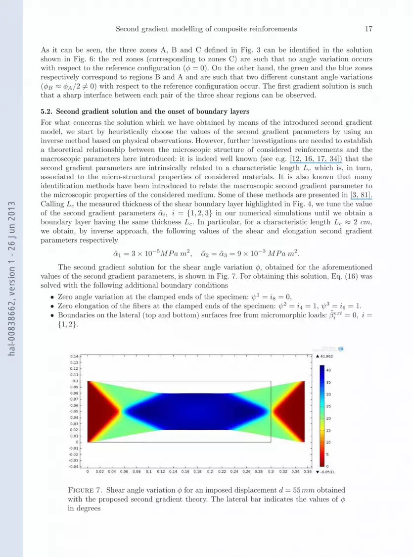
The second gradient solution for the shear angle variation φ, obtained for the aforementionedvalues of the second gradient parameters, is shown in Fig. 7. For obtaining this solution, Eq. (16) wassolved with the following additional boundary conditions

• Zero angle variation at the clamped ends of the specimen: ψ1 = i8 = 0,• Zero elongation of the fibers at the clamped ends of the specimen: ψ2 = i4 = 1, ψ3 = i6 = 1.• Boundaries on the lateral (top and bottom) surfaces free from micromorphic loads: βext

i = 0, i ={1, 2}.

Figure 7. Shear angle variation φ for an imposed displacement d = 55mm obtainedwith the proposed second gradient theory. The lateral bar indicates the values of φin degrees

hal-0

0838

662,

ver

sion

1 -

26 J

un 2

013

18 Manuel Ferretti, Angela Madeo*, Francesco dell’Isola and Philippe Boisse

It can be noticed that in the second gradient solution shown in Fig. 7 the transition zones betweendifferent shear regions are regularized and shear boundary layers can be clearly observed, as well asa curvature of the free boundaries on the two free sides. It can be immediately remarked how thesolution shown in Fig. 7 is, at least qualitatively, very close to the experimental picture shown inFig.5.

We show in Fig. 8 the first and second gradient solutions for the shear angle variation along thesections I and II. It can be clearly seen that, along section I, the first gradient solution (dashed line)

s1

s2

I

II

s1

φ

I

Lc

s2

φ

II

Figure 8. Definition of the sections I and II (top) and shear angle variation φ forthe two sections I and II both for first gradient (dashed line) and second gradient(continuous line).

produces a sharp variation of the shear angle across the two regions C and B. On the other hand, thesecond gradient solution (continuous line) clearly regularizes the transition between the zone at zerovariation of the shear angle and the adjacent zone. The same arrives in section II, which spans on thewhole specimen, in which the transition zones are clearly regularized by the second gradient solution.

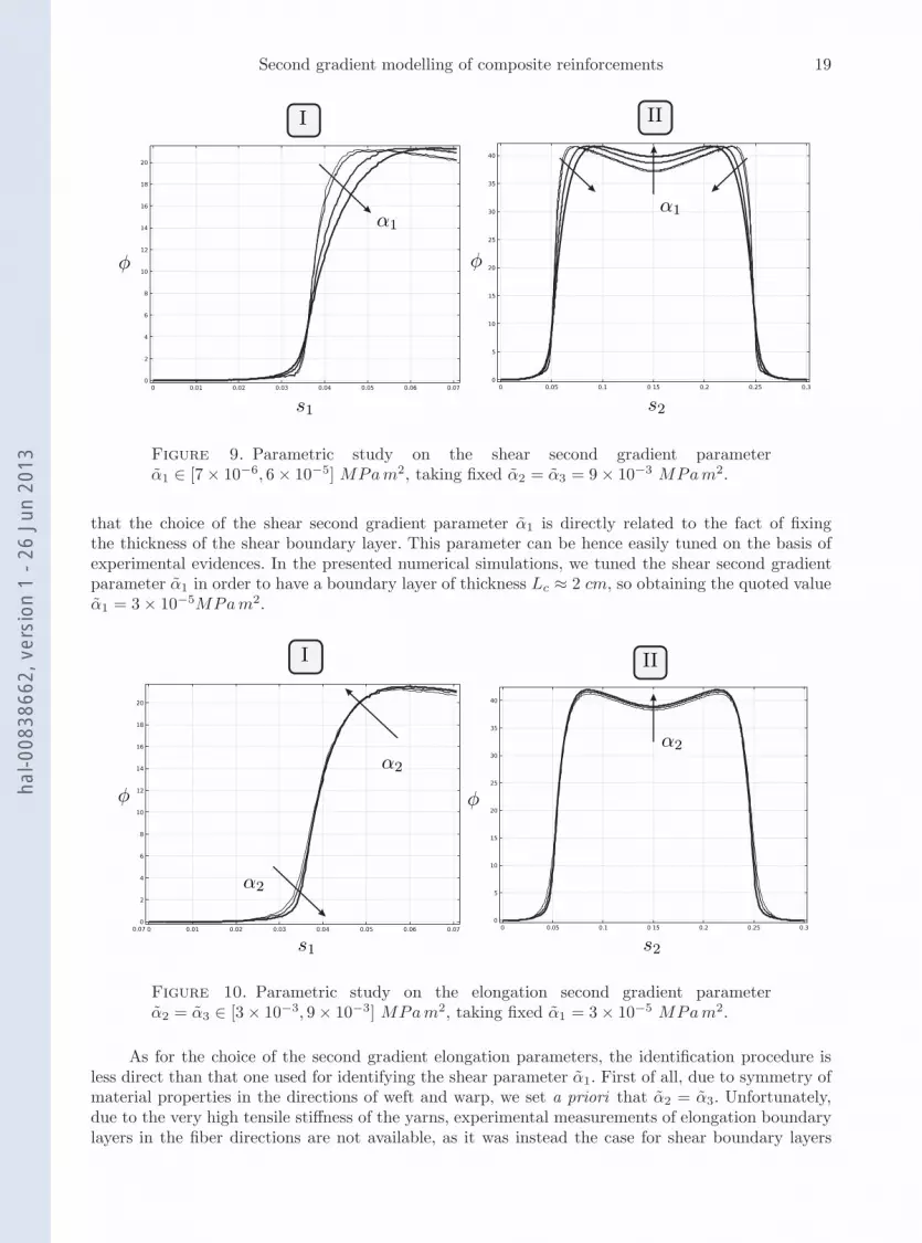
In Fig. (9) we show the effect of the variation of the shear second gradient parameter α1 onthe solution for the shear angle variation φ along the sections I and II respectively. It can be seenthat the effect of increasing the shear second gradient parameter actually lower the value of the shearangle variation so producing more regular transitions from the two regions at different constant shear.This clearly results in an increasing of the characteristic size of the shear boundary layer. It can bealso noticed that the value of φ increases with α1 in the center of the specimen. We can conclude

hal-0

0838

662,

ver

sion

1 -

26 J

un 2

013

Second gradient modelling of composite reinforcements 19

s1

φ

I

α1

s2

φ

II

α1

Figure 9. Parametric study on the shear second gradient parameterα1 ∈ [7× 10−6, 6× 10−5] MPam2, taking fixed α2 = α3 = 9× 10−3 MPam2.

that the choice of the shear second gradient parameter α1 is directly related to the fact of fixingthe thickness of the shear boundary layer. This parameter can be hence easily tuned on the basis ofexperimental evidences. In the presented numerical simulations, we tuned the shear second gradientparameter α1 in order to have a boundary layer of thickness Lc ≈ 2 cm, so obtaining the quoted valueα1 = 3× 10−5MPam2.

s1

φ

I

α2

α2

s2

φ

II

α2

Figure 10. Parametric study on the elongation second gradient parameterα2 = α3 ∈ [3× 10−3, 9× 10−3] MPam2, taking fixed α1 = 3× 10−5 MPam2.

As for the choice of the second gradient elongation parameters, the identification procedure isless direct than that one used for identifying the shear parameter α1. First of all, due to symmetry ofmaterial properties in the directions of weft and warp, we set a priori that α2 = α3. Unfortunately,due to the very high tensile stiffness of the yarns, experimental measurements of elongation boundarylayers in the fiber directions are not available, as it was instead the case for shear boundary layers

hal-0

0838

662,

ver

sion

1 -

26 J

un 2

013

20 Manuel Ferretti, Angela Madeo*, Francesco dell’Isola and Philippe Boisse

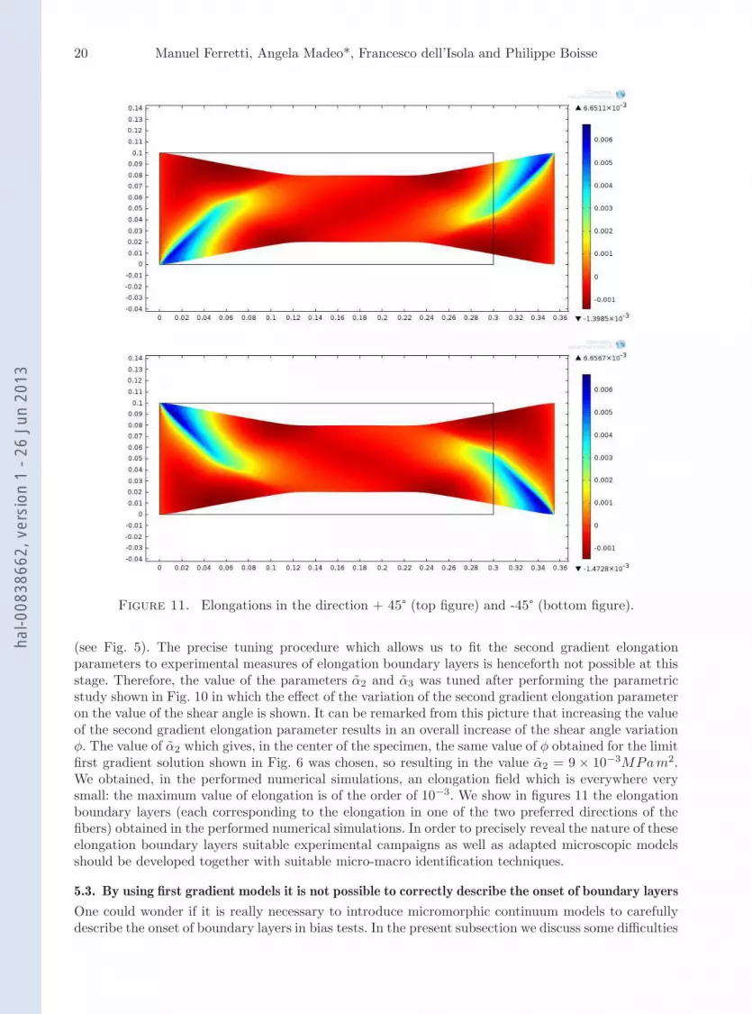
Figure 11. Elongations in the direction + 45° (top figure) and -45° (bottom figure).

(see Fig. 5). The precise tuning procedure which allows us to fit the second gradient elongationparameters to experimental measures of elongation boundary layers is henceforth not possible at thisstage. Therefore, the value of the parameters α2 and α3 was tuned after performing the parametricstudy shown in Fig. 10 in which the effect of the variation of the second gradient elongation parameteron the value of the shear angle is shown. It can be remarked from this picture that increasing the valueof the second gradient elongation parameter results in an overall increase of the shear angle variationφ. The value of α2 which gives, in the center of the specimen, the same value of φ obtained for the limitfirst gradient solution shown in Fig. 6 was chosen, so resulting in the value α2 = 9 × 10−3MPam2.We obtained, in the performed numerical simulations, an elongation field which is everywhere verysmall: the maximum value of elongation is of the order of 10−3. We show in figures 11 the elongationboundary layers (each corresponding to the elongation in one of the two preferred directions of thefibers) obtained in the performed numerical simulations. In order to precisely reveal the nature of theseelongation boundary layers suitable experimental campaigns as well as adapted microscopic modelsshould be developed together with suitable micro-macro identification techniques.

5.3. By using first gradient models it is not possible to correctly describe the onset of boundary layers

One could wonder if it is really necessary to introduce micromorphic continuum models to carefullydescribe the onset of boundary layers in bias tests. In the present subsection we discuss some difficulties

hal-0

0838

662,

ver

sion

1 -

26 J

un 2

013

Second gradient modelling of composite reinforcements 21

which arise if one tries to use the methods discussed in section 5.1. Actually, as shown by Fig. 12,although it is indeed possible to describe the onset of some boundary layers still remaining in theframework of first gradient models, it seems very unlikely that with those methods one can catch allexperimental features which are present in bias extension tests. In the numerical simulations leadingto Fig. 12 one can see formation of boundary layers where high gradients of shear and elongation areconcentrated even if this simulation is conducted in the framework of first gradient theory. However,the solution is qualitatively and quantitatively different from the first gradient sharp solution shownin Fig. 6 so that realistic quantitative values for shear deformations cannot be obtained from it.Moreover, if one evaluates the reaction force on the fixed clamped end in the last considered case,

Figure 12. Shear angle variation φ for an imposed displacement d = 55mm obtainedwith the first gradient theory and for an arbitrary mesh. The lateral bar indicates thevalues of φ in degrees

it can be checked that its value exceeds of a big amount the reaction force which is expected. Moreparticularly, the force evaluated for the limit first gradient solution depicted in Fig. 6 is of the order of5 N which is a sensible force for the bias extension test. On the other hand, if one evaluates the force forthe case depicted in Fig. 12, this force exceeds from 10 to 100 times the 5 N obtained in the limit sharpfirst gradient solution, depending on the choice of the mesh. This means that the mesh dependence ofthe first gradient solution is even more evident when analyzing force than when analyzing deformation.Such a problem on the value of calculated force is not present when considering the second gradientsolution shown in Fig. 7. This point allows us to conclude that, using first gradient models, it is notpossible to correctly describe the onset of boundary layers and that the reaction forces at clampedends are definitely overestimated as soon as one gets far from the limit first gradient solution shownin Fig. 6.

6. Conclusions

In this paper a constrained micromorphic theory is introduced which includes, as a particular case, asecond gradient model. Particular orthotropic, hyperelastic, constitutive laws are introduced in orderto account for the anisotropy of fibrous composite reinforcements undergoing large deformations. Theobtained theoretical framework is used to model the mechanical behavior of such fibrous compositematerials during the so-called bias extension test.

The first and second gradient solutions are compared showing that the proposed second gradientmodel is actually able to describe the onset of shear boundary layers which regularize the first gradientsharp transition between two zones at different levels of shear. Moreover, differently from what happens

hal-0

0838

662,

ver

sion

1 -

26 J

un 2

013

22 Manuel Ferretti, Angela Madeo*, Francesco dell’Isola and Philippe Boisse

for the first gradient model, the proposed second gradient theory also allows to describe the curvatureof the free boundaries of the specimen.

In order to identify the values of introduced second gradient parameters we proceed by inverseapproach, performing numerical simulations which correctly fits the experimental data. More partic-ularly, we choose the values of second gradient parameters in order to fit at best the characteristiclength of the shear boundary layer which is observed is bias test experiments.

Therefore, the results obtained in this paper allow us to estimate the order of magnitude of thesecond gradient parameters to be used for the considered fibrous materials. These results are promisingand justify the need of novel experimental campaigns in order to estimates such gradient parametersfor a wider class of composite preforms.

References

[1] Aifantis E.C., 1992. On the role of gradients in the localization of deformation and fracture. InternationalJournal of Engineering Science 30:10, 1279-1299

[2] Aimene Y., Vidal-Salle E., Hagege B., Sidoroff F., Boisse P., 2010. A hyperelastic approach for compositereinforcement large deformation analysis. J. Compos. Mater., 44:1, 5-26

[3] Alibert J.-J., Seppecher P., Dell’Isola F., 2003. Truss modular beams with deformation energy dependingon higher displacement gradients. Math. Mech. Solids 8:1, 51-73

[4] Altenbach H., Eremeyev V.A., Lebedev L.P., Rendon L.A. (2010). Acceleration waves and ellipticity inthermoelastic micropolar media Archive of Applied Mechanics 80 (3), 217-227

[5] Atai, A.A., Steigmann, D.J. (1997). On the nonlinear mechanics of discrete networks Archive of AppliedMechanics, 67:5, 303-319

[6] Balzani D., Neff P., Schroder J., Holzapfel G.A., (2006). A polyconvex framework for soft biological tissues,Adjustment to experimental data. Int. J. Solids Struct., 43, 6052-6070

[7] Bleustein J.L., 1967. A note on the boundary conditions of Toupin’s strain gradient-theory. Int. J. SolidsStructures, 3, 1053-1057.

[8] Boehler, J.P., 1987. Introduction to the invariant formulation of anisotropic constitutive equations. In:Boehler, J.P. (Ed.), Applications of Tensor Functions in Solid Mechanics CISM Course No. 292. Springer-Verlag.

[9] Boehler JP. Lois de comportement anisotrope des milieux continus. J Mec 1978;17:153-70

[10] Boisse P., Cherouat A., Gelin J.C., Sabhi H., 1995. Experimental Study and Finite Element SimulationOf Glass Fiber Fabric Shaping Process. Polymer Composites 16:1, 83-95

[11] Cao J., Akkerman R., Boisse P., Chen J., et al., 2008. Characterization of mechanical behavior of wovenfabrics: experimental methods and benchmark results. Compos. Part A: Appl. Sci. Manuf. 39, 1037-53.

[12] Casal P., 1972. La theorie du second gradient et la capillarite. C.R. Acad. Sci. Paris, Ser. A 274, 1571-1574

[13] Charmetant A., Vidal-Salle E., Boisse P. (2011). Hyperelastic modelling for mesoscopic analyses of com-posite reinforcements. Composites Science and Technology, 71,1623-1631

[14] Charmetant A., Orliac J.G.,Vidal-Salle E., Boisse P. (2012). Hyperelastic model for large deformationanalyses of 3D interlock composite preforms. Composites Science and Technology, 72, 1352-1360

[15] Cosserat E., Cosserat F., 1909. Theorie de Corps deformables. Librairie Scientifique A. Hermann et fils,Paris

[16] deGennes, P.G., 1981. Some effects of long range forces on interfacial phenomena. J. Phys. Lett. 42,L377–L37

[17] dell’Isola F., Gouin H., Seppecher P., 1995. Radius and surface tension of microscopic bubbles by secondgradient theory. C.R. Acad. Sci. II, Mec. 320, 211-216

[18] dell’Isola F., Rotoli G., 1995. Validity of Laplace formula and dependence of surface tension on curvaturein second gradient fluids. Mechanics Research Communications, 22, 485-490

[19] dell’Isola F., Seppecher P., 1995. The relationship between edge contact forces, double force and interstitialworking allowed by the principle of virtual power, C.R. Acad. Sci. II, Mec. Phys. Chim. Astron. 321, 303-308

hal-0

0838

662,

ver

sion

1 -

26 J

un 2

013

Second gradient modelling of composite reinforcements 23

[20] dell’Isola F., Gouin H., Rotoli G., 1996. Nucleation of Spherical shell-like interfaces by second gradienttheory: numerical simulations, Eur. J. Mech. B, Fluids 15:4, 545-568

[21] dell’Isola F., Seppecher P., 1997. Edge contact forces and quasi-balanced power, Meccanica 32, 33-52

[22] dell’Isola F., Guarascio M., Hutter K., 2000. A variational approach for the deformation of a saturatedporous solid. A second-gradient theory extending Terzaghi’s effective stress principle. Archive of AppliedMechanics. 70, 323-337.

[23] dell’Isola F., Sciarra G., and Vidoli S., 2009. Generalized Hooke’s law for isotropic second gradient mate-rials, Proc. R. Soc. Lond. A 465, 2177–2196.

[24] dell’Isola F., Madeo A., Placidi L., 2012. Linear plane wave propagation and normal transmission and re-flection at discontinuity surfaces in second gradient 3D Continua. Zeitschrift fur Angewandte Mathematikund Mechanik (ZAMM), 92:1, 52-71

[25] dell’Isola F., Seppecher P., Madeo A., 2012. How contact interactions may depend on the shape of Cauchycuts in N-th gradient continua: approach “a la D’Alembert”. ZAMP, 63:6, 1119-1141

[26] Dumont J.P., Ladeveze P., Poss M., Remond Y., 1987. Damage mechanics for 3-D composites Compositestructures, 8:2, 119-141

[27] Eremeyev V. A., Lebedev L. P., Altenbach H. (2013). Foundations of micropolar mechanics. Springer,Heidelberg.

[28] Eremeyev V.A., 2005. Acceleration waves in micropolar elastic media. Doklady Physics 50:4, 204-206

[29] Eringen A. C., 2001. Microcontinuum field theories. Springer-Verlag, New York.

[30] Eringen A.C., Suhubi, E.S. 1964. Nonlinear theory of simple microelastic solids: I. Int. J. Eng. Sci., 2,189-203.

[31] Eringen A. C., Suhubi, E. S. 1964. Nonlinear theory of simple microelastic solids: II. Int. J. Eng. Sci., 2,389-404.

[32] Forest, S., Sievert, R. 2006. Nonlinear microstrain theories. Int. J. Solids Struct., 43, 7224-7245.

[33] Forest S. 2009. Micromorphic Approach for Gradient Elasticity, Viscoplasticity, and Damage. Journal ofEngineering Mechanics, 135:3, 117-131.

[34] Forest S., Aifantis E.C., 2010. Some links between recent gradient thermo-elasto-plasticity theories andthe thermomechanics of generalized continua. Int. J. Solids. Struct. 47:(25-26), 3367-3376

[35] Germain, P., 1973. La methode des puissances virtuelles en mecanique des milieux continus. Premierepartie. Theorie du second gradient. J. Mecanique 12, 235-274.

[36] Germain, P., 1973. The method of virtual power in continuum mechanics. Part 2: Microstructure. SIAMJ. Appl. Math. 25, 556-575

[37] Green A.E., Rivlin R.S., 1964. Multipolar continuum mechanics. Archive for Rational Mechanics andAnalysis, 17: 2, 113-147

[38] Hamila N., Boisse P., 2013. Tension locking in finite-element analyses of textile composite reinforcementdeformation. Comptes Rendus Mecanique, 341:6, 508-519.

[39] Hamila N., Boisse P., 2013. Locking in simulation of composite reinforcement deforma-tions. Analysis and treatment. Composites Part A: Applied Science and Manufacturing, DOI:http://dx.doi.org/10.1016/j.compositesa.2013.06.001

[40] Harrison P., Clifford M.J., Long A.C. 2004. Shear characterisation of viscous woven textile composites: acomparison between picture frame and bias extension experiments. Composites Science and Technology,64, 1453-1465

[41] Haseganu, E.M., Steigmann, D.J. (1996). Equilibrium analysis of finitely deformed elastic networks. Com-putational Mechanics, 17:6, 359-373

[42] Holzapfel, G.A., Gasser, T.C., Ogden, R.W., 2000. A new constitutive framework for arterial wall me-chanics and a comparative study of material models. Journal of Elasticity 61, 1-48.

[43] Holzapfel, G.A., 2000. Nonlinear Solid Mechanics, Wiley.

[44] Itskov M., Aksel N., 2004. A class of orthotropic and transversely isotropic hyperelastic constitutivemodels based on a polyconvex strain energy function. Int. J. Solids Struct., 41, 3833–3848

[45] Itskov M. 2000. On the theory of fourth-order tensors and their applications in computational mechanics.Comput Methods Appl. Mech. Eng., 189:2, 419-38

hal-0

0838

662,

ver

sion

1 -

26 J

un 2

013

24 Manuel Ferretti, Angela Madeo*, Francesco dell’Isola and Philippe Boisse

[46] Lasry D., Belytschko T., 1988. Localization limiters in transient problems. Int. J. Solids Struct., 24: 6,581-597.

[47] Lee W., Padvoiskis J., Cao J., de Luycker E., Boisse P., Morestin F., Chen J., Sherwood J., 2008. Bias-extension of woven composite fabrics. Int J Mater Form Suppl 1:895-898

[48] Luongo A. (1991). On the amplitude modulation and localization phenomena in interactive bucklingproblems. International Journal of Solids and Structures 27:15, 1943-1954

[49] Luongo A. (2001). Mode localization in dynamics and buckling of linear imperfect continuous structures.Nonlinear Dynamics 25:1, 133-156

[50] Luongo A., D’Egidio A. (2005). Bifurcation equations through multiple-scales analysis for a continuousmodel of a planar beam. Nonlinear Dynamics 41:1, 171-190

[51] Madeo A., George D., Lekszycki T., Nieremberger M., Remond Y., 2012. A second gradient contin-uum model accounting for some effects of micro-structure on reconstructed bone remodelling. CRASMecanique, 340:8, 575-589

[52] A. Madeo, F. dell’Isola, N. Ianiro and G. Sciarra, 2008. A Variational Deduction of Second GradientPoroelasticity II: an Application to the Consolidation Problem. Journal of Mechanics of Materials andStructures, 3:4, 607-625

[53] Madeo A., dell’Isola F., Ianiro N., SciarraG., 2008. A variational deduction of second gradient poroelas-ticity II: An application to the consolidation problem, J. Mech. Mater. Struct. 3:4, 607-625

[54] Madeo A., Djeran-Maigre I., Rosi G., Silvani C., 2012. The Effect of Fluid Streams in Porous Mediaon Acoustic Compression Wave Propagation, Transmission and Reflection. Continuum Mechanics andThermodynamics, DOI: 007/s00161-012-0236-y

[55] Makradi A., Ahzi S., Garmestani H., Li D.S., Remond Y., 2010. Statistical continuum theory for theeffective conductivity of fiber filled polymer composites: Effect of orientation distribution and aspect ratioA Mikdam. Composites Science and Technology 70 :3, 510-517

[56] Mikdam A., Makradi A., Ahzi S., Garmestani H., Li D.S., Remond Y., 2009. Effective conductivityin isotropic heterogeneous media using a strong-contrast statistical continuum theory. Journal of theMechanics and Physics of Solids 57:1, 76-86

[57] Mindlin R.D. , 1964. Micro-structure in linear elasticity. Archs ration. Mech. Analysis 51-78

[58] Nadler, B., Steigmann, D.J. (2003). A model for frictional slip in woven fabrics. Comptes Rendus -Mecanique, 331 (12), pp. 797-804

[59] Nadler, B., Papadopoulos, P., Steigmann, D.J. (2006). Multiscale constitutive modeling and numericalsimulation of fabric material. International Journal of Solids and Structures, 43 (2), pp. 206-221

[60] Neff P., private communication.

[61] Ogden R.W. Non-linear elastic deformations. New York: Wiley and Sons; 1984.

[62] Ogden R.W., 2003. Nonlinear Elasticity, Anisotropy, Material Stability and Residual stresses in SoftTissue. CISM Courses and Lectures Series 441, 65-108

[63] Peng X., Guo Z., Du T., Yu W.R., 2013. A Simple Anisotropic Hyperelastic ConstitutiveModel for Textile Fabrics with Application to Forming Simulation. Composites: Part B, DOI:http://dx.doi.org/10.1016/j.compositesb.2013.04.014

[64] Pietraszkiewicz W., Eremeyev V.A., 2009. On natural strain measures of the non-linear micropolar con-tinuum. International Journal of Solids and Structures 46:3, 774-787

[65] Oshmyan V.G., Patlazhan S.A., Remond Y., 2006. Principles of structural-mechanical modeling of poly-mers and composites. Polymer Science Series A 48:9, 1004-1013

[66] Pideri C., Seppecher P., 1997. A second gradient material resulting from the homogenization of an het-erogeneous linear elastic medium. Contin. Mech. Thermodyn. 9:5, 241-257

[67] Piola G., 1846. Memoria intorno alle equazioni fondamentali del movimento di corpi qualsivogliono con-siderati secondo la naturale loro forma e costituzione. Modena, Tipi del R.D. Camera

[68] Placidi L., Rosi G., Giorgio. I., Madeo A., 2013. Reflection and transmission of plane waves at surfacescarrying material properties and embedded in second gradient materials. Mathematics and Mechanics ofSolids, DOI: 10.1177/1081286512474016.

[69] Raoult A., 2009. Symmetry groups in nonlinear elasticity: An exercise in vintage mathematics. Commu-nications on Pure and Applied Analysis 8:1, 435-456

hal-0

0838

662,

ver

sion

1 -

26 J

un 2

013

Second gradient modelling of composite reinforcements 25

[70] Rinaldi A., Krajcinovic K., Peralta P., Lai Y.-C., (2008). Modeling Polycrystalline Microstructures WithLattice Models: A Quantitative Approach. Mech. Mater., 40, 17-36

[71] Rinaldi A. (2009). A rational model for 2D Disordered Lattices Under Uniaxial Loading. Int. J. DamageMech., 18, 233-57

[72] Rinaldi A., Lai Y.C., (2007), Damage Theory Of 2D Disordered Lattices: Energetics And Physical Foun-dations Of Damage Parameter. Int. J. Plasticity, 23, 1796-1825

[73] Rinaldi A. (2011). Statistical model with two order parameters for ductile and soft fiber bundles innanoscience and biomaterials. Phys Rev E , 83(4-2) 046126

[74] Rinaldi A. (2013). Bottom-up modeling of damage in heterogeneous quasi-brittle solids. Continuum Me-chanics and Thermodynamics, 25, Issue 2-4, 359-373

[75] Rinaldi A., Krajcinovic D., Mastilovic S., (2007). Statistical Damage Mechanics and Extreme Value The-ory. Int. J. Damage Mech, 16:1, 57-76

[76] Rosi G., Madeo A., Guyader J.-L., 2013. Switch between fast and slow Biot compression waves inducedby second gradient microstructur at material discontinuity surfaces in porous media. Int. J. Solids Struct.,50:10, 1721-1746

[77] Schroder J., Balzani D., Neff P., 2005. A variational approach for materially stable anisotropic hyperelas-ticity. Int. J. Solids Struct., 42, 4352-4371

[78] Sciarra G., dell’Isola F., Coussy O., 2007. Second gradient poromechanics, Int. J. Solids Struct, 44:20,6607-6629

[79] Sciarra G., dell’Isola F., Ianiro N., Madeo A., 2008. A Variational Deduction of Second Gradient Poroe-lasticity I: General Theory. Journal of Mechanics of Materials and Structures, 3:3, 507-526

[80] Sciarra G., dell’Isola F., Ianiro N., Madeo A., 2008. A Variational Deduction of Second Gradient Poroe-lasticity I: General Theory, Journal of Mechanics of Materials and Structures 3:3 507-526

[81] Seppecher P., Alibert J.-J., dell’Isola F., 2011. Linear elastic trusses leading to continua with exoticmechanical interactions. Journal of Physics: Conference Series, 319

[82] Spencer A.J.M., Constitutive theory for strongly anisotropic solids, in Continuum Theory of Fibre- Rein-forced Composites, CISM International Centre for Mechanical Sciences Courses and Lecture Notes, 282,Spencer A.J. M. Ed., Springer, 1984.

[83] Steigmann, D.J. (1992). Equilibrium of prestressed networks. IMA Journal of Applied Mathematics (In-stitute of Mathematics and Its Applications), 48:2, 195-215

[84] Steigmann, D.J. (2002). Invariants of the stretch tensors and their application to finite elasticity theory.Mathematics and Mechanics of Solids, 7:4, 393-404

[85] Steigmann, D.J. (2003). Frame-invariant polyconvex strain-energy functions for some anisotropic solidsMathematics and Mechanics of Solids, 8:5, 497-506

[86] Toupin R. 1964. Theories of elasticity with couples-stress. Arch. Rational Mech and Anal., 17, 85-112

[87] Triantafyllidis N., Aifantis E.C.A., 1986. Gradient approach to localization of deformation, I. Hyperelasticmaterials. J. Elast. 16:3, 225-237

Manuel FerrettiLaMCoS, Universite de Lyon, INSA-CNRS, France & DICEAA, Universita dell’Aquila, Italy20 avenue Albert Einstein, 69621, Villeurbanne cedex, Francee-mail: manuel.ferretti@insa-lyon.fr

Angela Madeo*LGCIE, Universite de Lyon, INSA,20 avenue Albert Einstein, 69621, Villeurbanne cedex, France& International research center M&MoCS, Universita dell’Aquila, Italy*: Corresponding authore-mail: angela.madeo@insa-lyon.fr

Francesco dell’IsolaDISG, Universita di Roma ”La Sapienza”, Italy & International research center M&MoCS, Universita dell’Aquila,Italye-mail: francesco.dellisola@uniroma1.it

hal-0

0838

662,

ver

sion

1 -

26 J

un 2

013

26 Manuel Ferretti, Angela Madeo*, Francesco dell’Isola and Philippe Boisse

Philippe BoisseLaMCoS, Universite de Lyon, INSA-CNRS, France20 avenue Albert Einstein, 69621, Villeurbanne cedex, Francee-mail: philippe.boisse@insa-lyon.fr

hal-0

0838

662,

ver

sion

1 -

26 J

un 2

013