lable at ScienceDirect

Journal of Environmental Radioactivity 136 (2014) 41e55

Contents lists avai

Journal of Environmental Radioactivity

journal homepage: www.elsevier .com/locate/ jenvrad

Modeling the fallout from stabilized nuclear clouds using the HYSPLITatmospheric dispersion model

G.D. Rolph a,*, F. Ngan a,b, R.R. Draxler a

aNOAA Air Resources Laboratory (ARL), NCWCP R/ARL, 5830 University Research Court, College Park, MD 20740, USAbCooperative Institute for Climate and Satellites, University of Maryland, College Park, MD, USA

a r t i c l e i n f o

Article history:Received 21 February 2014Received in revised form6 May 2014Accepted 7 May 2014Available online

Keywords:HYSPLITDispersion modelingNuclear falloutDeposition

* Corresponding author. Tel.: þ1 301 683 1376.E-mail address: glenn.rolph@noaa.gov (G.D. Rolph

http://dx.doi.org/10.1016/j.jenvrad.2014.05.0060265-931X/Published by Elsevier Ltd. This is an open

a b s t r a c t

The Hybrid Single Particle Lagrangian Integrated Trajectory (HYSPLIT) model, developed by the NationalOceanic and Atmospheric Administration’s Air Resources Laboratory, has been configured to simulate thedispersion and deposition of nuclear materials from a surface-based nuclear detonation using publiclyavailable information on nuclear explosions. Much of the information was obtained from “The Effects ofNuclear Weapons” by Glasstone and Dolan (1977). The model was evaluated against the measurementsof nuclear fallout from six nuclear tests conducted between 1951 and 1957 at the Nevada Test Site usingthe global NCEP/NCAR Reanalysis Project (NNRP) and the Weather Research and Forecasting (WRF)meteorological data as input. The model was able to reproduce the general direction and depositionpatterns using the coarse NNRP data with Figure of Merit in Space (FMS e the percent overlap betweenpredicted and measured deposition patterns) scores in excess of 50% for four of six simulations for thesmallest dose rate contour, with FMS scores declining for higher dose rate contours. When WRF mete-orological data were used the FMS scores were 5e20% higher in five of the six simulations, especially atthe higher dose rate contours. The one WRF simulation where the scores declined slightly (10e30%) wasalso the best scoring simulation when using the NNRP data. When compared with measurements of doserate and time of arrival from the Town Data Base (Thompson et al., 1994), similar results were found withthe WRF simulations providing better results for four of six simulations. The overall result was that thedifferent plume simulations using WRF data had more consistent performance than the plume simu-lations using NNRP data fields.

Published by Elsevier Ltd. This is an open access article under the CC BY-NC-ND license (http://creativecommons.org/licenses/by-nc-nd/3.0/).

1. Introduction

The National Oceanic and Atmospheric Administration’s (NOAA)Air Resources Laboratory (ARL) has its origins in providing meteo-rological support to other Federal agencies during the Cold War’snuclear arms race. In 1948, a predecessor of ARL, the U.S. WeatherBureau created a Special Projects Section (SPS), inWashington, D.C.,to bridge the gap between the meteorological expertise of theWeather Bureau and the research needs of other agencies related tonuclear weapons testing and development. As the arms raceaccelerated, a need arose to determine where clandestine nucleartests were conducted using measurements of nuclear falloutaround theworld. The SPSwas involved in determining the locationof the first Soviet nuclear test (Machta, 1992) conducted in 1949using backward trajectory analysis from interceptions of

).

access article under the CC BY-NC

radioactive debris measured by Air Weather Service B-29 weatherreconnaissance aircraft. As this collaboration progressed, it becameclear that the development of more complex atmospheric transportmodels was needed to predict the long-range transport anddeposition of nuclear materials from the many tests being con-ducted around the world, and over the next several decades ARLmaintained a continued interest in the transport, dispersion, anddeposition of nuclear materials (Draxler, 1982; Ferber and Heffter,1961, 1976; Heffter, 1969, 1980; Hoecker and Machta, 1990;Machta and List, 1956; Machta et al., 1962; Machta and Heffter,1986; Telegadas et al., 1978, 1979; Telegadas and List, 1964; Listet al., 1961).

With an increase in the concern for future terrorist incidentssince the September 11, 2001, attack on the World Trade Center inNew York City and the Pentagon in Washington, D.C., and thepossibility that terrorists could acquire nuclear materials anddevelop an Improvised Nuclear Device (IND), ARL expanded itscapabilities for responding to exercises and incidents involving thedetonation of a nuclear device and made them available to the

-ND license (http://creativecommons.org/licenses/by-nc-nd/3.0/).

G.D. Rolph et al. / Journal of Environmental Radioactivity 136 (2014) 41e5542

civilian forecasters of the U.S. National Weather Service in supportof their local clients.

A number of models have been used to simulate the explosionand fallout from a nuclear weapon with varying degrees ofcomplexity. For example, the HotSpot Gaussian plume model(Homann and Aluzzi, 2013) developed by the U.S. Department ofEnergy is designed to provide a quick response to field personnel onthe radiation effects from the atmospheric release of radioactivematerials and is designed for short-range (less than 10 km), andshort-term (less than a few hours) predictions. A special purposeprogram is included in HotSpot to model the effects of a surface-burst nuclear weapon; however the model assumes a constantwind direction and speed and does not take into account the effectsof terrain on the wind flow.

A much more sophisticated model is the Hazard Prediction &Assessment Capability (HPAC) model developed by the DefenseThreat Reduction Agency (DTRA, 2001; Chang et al., 2005). HPAC,which is a composed of a hazard source definition module, atransport module, and an effects module, uses the Second-orderClosure Integrated PUFF (SCIPUFF) dispersion model to quicklypredict the hazards from nuclear, biological, chemical, and radio-logical weapons and facilities. The second-order turbulence closuretheory employed by SCIPUIFF provides a unique advantage overother models in that it can also produce a probabilistic estimate ofthe uncertainty in the concentration results due to atmosphericdispersion. HPAC can input real-time observed wind speed anddirection at a single location or use 3-dimensional gridded windand temperature fields to calculate the pollutant transport. HPACuses the Nuclear Weapon (NWPN) module to calculate the initialstabilized nuclear cloud prior to modeling the dispersion anddeposition by SCIPUFF.

Recently, the Norwegian Meteorological Institute (Bartnicki andSaltbones, 2008) modified the Severe Nuclear Accident Program(SNAP) model to not only predict the dispersion of radioactivedebris following a nuclear accident, but also from a nuclear ex-plosion. The model assumes two types of stabilized cloud shapes; acylinder and a mushroom shape. Particle sizes range from 2 to200 mm in ten discrete size ranges and an activity distribution thatassumes 10% of the activity is in each category. They found that theresults were not sensitive to different initial nuclear cloud shapes,however there were considerable differences in the plumes forvarious nuclear yields due to transport at different levels in theatmosphere.

Finally, one of the most advanced nuclear fallout models is theDefense Land Fallout Interpretive Code (DELFIC, Norment, 1979a,1979b), which was originally developed in 1968 by the DefenseAtomic Support Agency and has been subsequently revised by themilitary, government laboratories, and private organizations.DELFIC includes a dynamic, one-dimensional cloud rise modulethat explicitly calculates the growth of the nuclear cloud based onthe yield of the weapon, the soil type, the height of burst, the at-mospheric profile, the particle size distribution, etc. DELFIC isintended for use in the research of local nuclear fallout predictionand to be the standard against which simpler models are compared.DELFIC computes the downwind spread of nuclear material basedon the assumed particle fall velocities and turbulence in thedownwind direction from the calculated cloud rise module.

One of the atmospheric dispersion models developed by ARL inthe late 1970’s, and the primary model in use by NOAA today, is theHybrid Single Particle Lagrangian Integrated Trajectory (HYSPLIT)(Draxler, 1999; Draxler and Hess, 1997, 1998) model. This modeloriginally used surface weather observations and upper-airsoundings as its source of meteorology until gridded meteorolog-ical model forecast data became routinely available from the U.S.National Weather Service in the late 1980’s. Today, HYSPLIT serves

as the operational dispersion model for the National WeatherService providing routine forecasts of smoke fromwild fires (Rolphet al., 2009; Stein et al., 2009), windblown dust (Draxler et al.,2010), volcanic ash (Stunder et al., 2007), and atmosphericdispersion products for chemical and nuclear accidents (Draxlerand Rolph, 2012).

The focus of the research presented here will be to model thedispersion, deposition, and decay of nuclear debris that followedthe detonation of six relatively small (<50 kT) nuclear devices inthe 1950’s in Nevada using the HYSPLIT model and to calculate theradioactive dose rates from the local fallout using a new moduledeveloped for calculating doses in HYSPLIT. The resulting dose ratepatterns will then be compared to the measured dose rate patternsfrom each of the six Nevada nuclear tests. The goal is to parame-terize the HYSPLIT model using information currently available inthe literature about the nuclear source term so that it can be runquickly to give a realistic estimate of the magnitude and pattern ofdeposition from small nuclear devices. Therefore, HYSPLIT will notbe used to model the initial nuclear cloud growth, but will assumethat the nuclear cloud has stabilized before proceeding with thetransport and deposition calculations. In addition, the model willbe run with global- and local-scale gridded meteorological data todetermine if increasing the horizontal and vertical resolution of themeteorological data will result in improved predictions of nuclearfallout.

2. Dispersion model experimental design

2.1. HYSPLIT model

The Hybrid Single-Particle Lagrangian Integrated Trajectory(HYSPLIT) model is a Lagrangian particle and puff model that isused by air quality researchers and forecasters to model thetransport of pollutants using 3-dimensional gridded meteorolog-ical fields. In a recent publication (Moroz et al., 2010), the modelwas used to reconstruct the 137Cs deposition from nuclear tests inthe Marshall Islands, the Nevada Test Site, and the SemipalatinskTest Site of the former Soviet Union. HYSPLIT was configured with alog-normal particle distribution and each particle size bin wasassigned a fraction of the total 137Cs activity. The resulting 137Csmodeled deposition patterns were then compared to the observedpatterns from each nuclear test. The study suggested that givenadequate spatial and temporal meteorological data, HYSPLIT can beused to determinewhere andwhen nuclear material was depositedwith relatively good degree of accuracy. They also found that whenno measurements are available, HYSPLIT can be used to determineif fallout might have occurred at a given location and also someindication of the magnitude of the deposition.

In this application, we expand on the work of Moroz et al. (2010)and configure the model with several particle size and activitydistributions obtained from various published sources, andcompute dose rate contours for several nuclear tests at the NevadaTest Site in Nevada, USA.

2.2. Stabilized nuclear cloud

To model the nuclear fallout quickly it is necessary to establishthe characteristics of the nuclear cloud just after stabilizationinstead of calculating the complex evolution of the cloud beginningat the time of detonation. Stabilization occurs after the temperatureof the nuclear cloud is equalized with the ambient temperature inthe surrounding air. At this point entrainment of outside air ceasesand the vertical growth of the cloud stops. Nuclear particles havebeen formed directly by the fission reaction, the condensation ofvaporized material lofted from the surface, and the vaporized

G.D. Rolph et al. / Journal of Environmental Radioactivity 136 (2014) 41e55 43

components of the device itself. These particles settle out of theatmosphere at the particle’s fall velocity, which is based on the size,shape, and density of the particle. In the HYSPLIT calculations, allparticles are assumed to be spherical and have a density of 2.5 g/cm3 (Glasstone and Dolan, 1977) assuming that the bulk of theradioactive material is attached to soil particles.

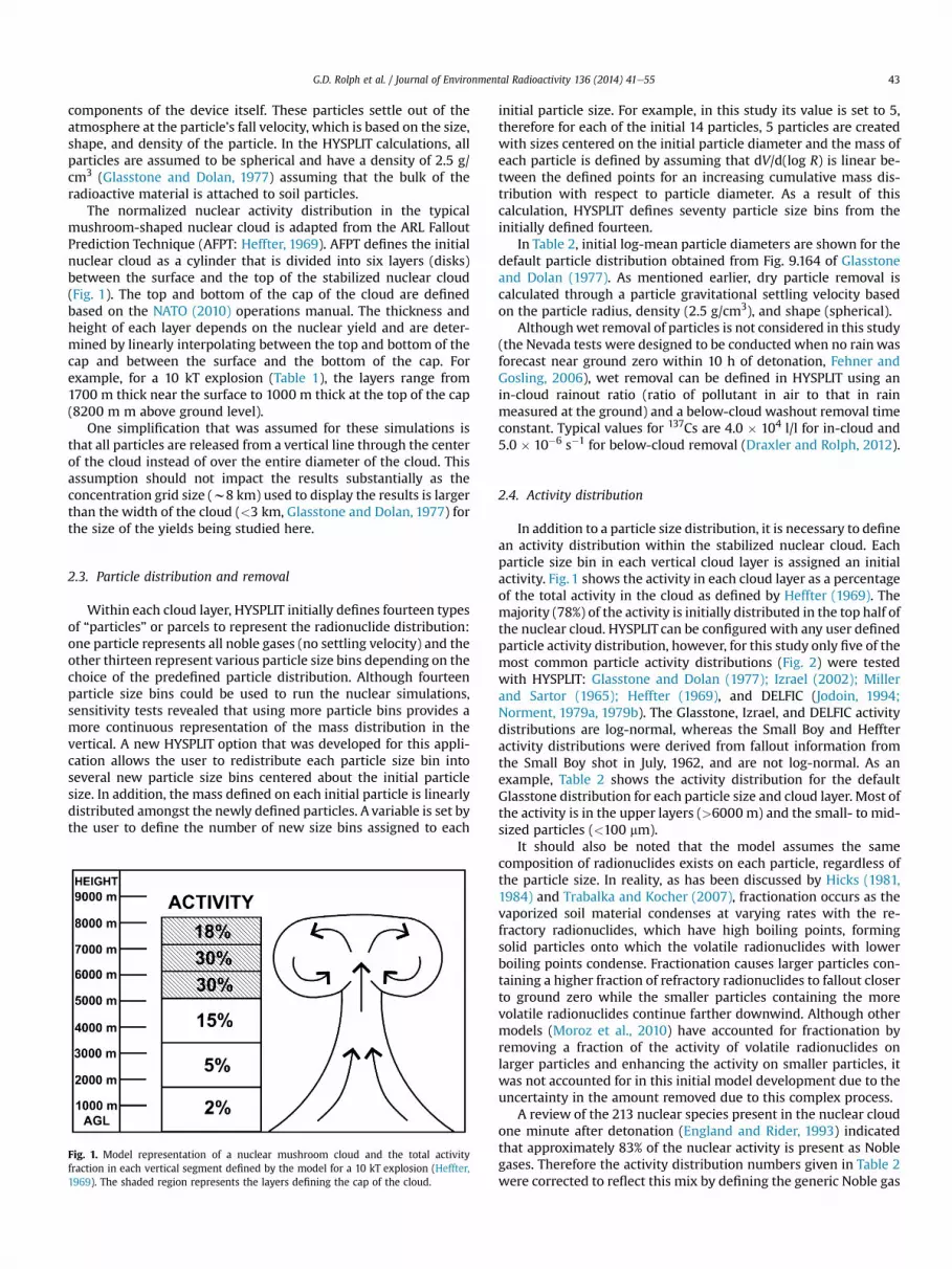
The normalized nuclear activity distribution in the typicalmushroom-shaped nuclear cloud is adapted from the ARL FalloutPrediction Technique (AFPT: Heffter, 1969). AFPT defines the initialnuclear cloud as a cylinder that is divided into six layers (disks)between the surface and the top of the stabilized nuclear cloud(Fig. 1). The top and bottom of the cap of the cloud are definedbased on the NATO (2010) operations manual. The thickness andheight of each layer depends on the nuclear yield and are deter-mined by linearly interpolating between the top and bottom of thecap and between the surface and the bottom of the cap. Forexample, for a 10 kT explosion (Table 1), the layers range from1700 m thick near the surface to 1000 m thick at the top of the cap(8200 m m above ground level).

One simplification that was assumed for these simulations isthat all particles are released from a vertical line through the centerof the cloud instead of over the entire diameter of the cloud. Thisassumption should not impact the results substantially as theconcentration grid size (w8 km) used to display the results is largerthan the width of the cloud (<3 km, Glasstone and Dolan, 1977) forthe size of the yields being studied here.

2.3. Particle distribution and removal

Within each cloud layer, HYSPLIT initially defines fourteen typesof “particles” or parcels to represent the radionuclide distribution:one particle represents all noble gases (no settling velocity) and theother thirteen represent various particle size bins depending on thechoice of the predefined particle distribution. Although fourteenparticle size bins could be used to run the nuclear simulations,sensitivity tests revealed that using more particle bins provides amore continuous representation of the mass distribution in thevertical. A new HYSPLIT option that was developed for this appli-cation allows the user to redistribute each particle size bin intoseveral new particle size bins centered about the initial particlesize. In addition, the mass defined on each initial particle is linearlydistributed amongst the newly defined particles. A variable is set bythe user to define the number of new size bins assigned to each

Fig. 1. Model representation of a nuclear mushroom cloud and the total activityfraction in each vertical segment defined by the model for a 10 kT explosion (Heffter,1969). The shaded region represents the layers defining the cap of the cloud.

initial particle size. For example, in this study its value is set to 5,therefore for each of the initial 14 particles, 5 particles are createdwith sizes centered on the initial particle diameter and the mass ofeach particle is defined by assuming that dV/d(log R) is linear be-tween the defined points for an increasing cumulative mass dis-tribution with respect to particle diameter. As a result of thiscalculation, HYSPLIT defines seventy particle size bins from theinitially defined fourteen.

In Table 2, initial log-mean particle diameters are shown for thedefault particle distribution obtained from Fig. 9.164 of Glasstoneand Dolan (1977). As mentioned earlier, dry particle removal iscalculated through a particle gravitational settling velocity basedon the particle radius, density (2.5 g/cm3), and shape (spherical).

Althoughwet removal of particles is not considered in this study(the Nevada tests were designed to be conducted when no rainwasforecast near ground zero within 10 h of detonation, Fehner andGosling, 2006), wet removal can be defined in HYSPLIT using anin-cloud rainout ratio (ratio of pollutant in air to that in rainmeasured at the ground) and a below-cloud washout removal timeconstant. Typical values for 137Cs are 4.0 � 104 l/l for in-cloud and5.0 � 10�6 s�1 for below-cloud removal (Draxler and Rolph, 2012).

2.4. Activity distribution

In addition to a particle size distribution, it is necessary to definean activity distribution within the stabilized nuclear cloud. Eachparticle size bin in each vertical cloud layer is assigned an initialactivity. Fig. 1 shows the activity in each cloud layer as a percentageof the total activity in the cloud as defined by Heffter (1969). Themajority (78%) of the activity is initially distributed in the top half ofthe nuclear cloud. HYSPLIT can be configured with any user definedparticle activity distribution, however, for this study only five of themost common particle activity distributions (Fig. 2) were testedwith HYSPLIT: Glasstone and Dolan (1977); Izrael (2002); Millerand Sartor (1965); Heffter (1969), and DELFIC (Jodoin, 1994;Norment, 1979a, 1979b). The Glasstone, Izrael, and DELFIC activitydistributions are log-normal, whereas the Small Boy and Heffteractivity distributions were derived from fallout information fromthe Small Boy shot in July, 1962, and are not log-normal. As anexample, Table 2 shows the activity distribution for the defaultGlasstone distribution for each particle size and cloud layer. Most ofthe activity is in the upper layers (>6000 m) and the small- to mid-sized particles (<100 mm).

It should also be noted that the model assumes the samecomposition of radionuclides exists on each particle, regardless ofthe particle size. In reality, as has been discussed by Hicks (1981,1984) and Trabalka and Kocher (2007), fractionation occurs as thevaporized soil material condenses at varying rates with the re-fractory radionuclides, which have high boiling points, formingsolid particles onto which the volatile radionuclides with lowerboiling points condense. Fractionation causes larger particles con-taining a higher fraction of refractory radionuclides to fallout closerto ground zero while the smaller particles containing the morevolatile radionuclides continue farther downwind. Although othermodels (Moroz et al., 2010) have accounted for fractionation byremoving a fraction of the activity of volatile radionuclides onlarger particles and enhancing the activity on smaller particles, itwas not accounted for in this initial model development due to theuncertainty in the amount removed due to this complex process.

A review of the 213 nuclear species present in the nuclear cloudone minute after detonation (England and Rider, 1993) indicatedthat approximately 83% of the nuclear activity is present as Noblegases. Therefore the activity distribution numbers given in Table 2were corrected to reflect this mix by defining the generic Noble gas

Table 1Model cloud layer heights (meters above ground level) based on nuclear yield in kilotons (kT).

Yield (kT) �2.5 �7.5 �12.5 �17.5 �22.5 �27.5 �32.5 �37.5 �42.5 �45.0

Level 7 3700 6300 8200 9700 10800 11200 11600 11900 12200 12500Level 6 3132 5434 7166 8532 9532 9900 10232 10500 10766 11000Level 5 2566 4567 6130 7366 8266 8600 8866 9100 9333 9500Level 4 2000 3700 5100 6200 7000 7300 7500 7700 7900 8000Level 3 1334 2466 3400 4132 4666 4866 5000 5132 5266 5332Level 2 667 1233 1700 2066 2333 2433 2500 2566 2633 2666Level 1 0 0 0 0 0 0 0 0 0 0

Table 2Initial log-mean particle diameter (mm) and percentage of nuclear activity by cloud layer and particle size for the Glasstone particle distribution. The total activity sums to 100%.

Diameter (mm) 500 350 275 225 187.5 162.5 137.5 112.5 87.5 70 57.5 45 20

Height (m) P1 P2 P3 P4 P5 P6 P7 P8 P9 P10 P11 P12 P13 Total

8200 0.175 0.525 0.525 0.875 0.700 1.050 1.400 2.100 3.150 1.750 1.750 1.400 2.100 17.57166 0.300 0.900 0.900 1.500 1.200 1.800 2.400 3.600 5.400 3.000 3.000 2.400 3.600 306130 0.300 0.900 0.900 1.500 1.200 1.800 2.400 3.600 5.400 3.000 3.000 2.400 3.600 305100 0.150 0.450 0.450 0.750 0.600 0.900 1.200 1.800 2.700 1.500 1.500 1.200 1.800 153400 0.050 0.150 0.150 0.250 0.200 0.300 0.400 0.600 0.900 0.500 0.500 0.400 0.600 51700 0.250 0.075 0.075 0.125 0.100 0.150 0.200 0.300 0.450 0.250 0.250 0.200 0.300 2.5Total 1 3 3 5 4 6 8 12 18 10 10 8 12 100

G.D. Rolph et al. / Journal of Environmental Radioactivity 136 (2014) 41e5544

“particle” (Pgas) with 83% of the activity and proportionallyreducing the other particle activity values.

HYSPLIT uses an emissions text file to define the initial activitydistribution for each particle size in each layer in units of activityper hour. The model assumes a 1 min emission for the nuclearexplosion simulation (the initial emission values in activity perminute are multiplied by 60 to obtain activity per hour).

The default HYSPLIT nuclear explosion simulation is initiallyconfigured with 9000 particles distributed over the 70 particle sizebins. However, after HYSPLIT calculates the number of particlesneeded to represent the source term through the six vertical layers,approximately 54,000 three-dimensional particles are required. Inaddition, the HYSPLIT nuclear simulation is performed assuming aunit source emission; the yield of theweapon is not defined prior tocomputing the transport and deposition except in terms of definingthe top of the cloud (Table 1). The model produces the dilution anddeposition factors between the ground and 100 m AGL at varioustimes downwind in terms of a unit emission on eight grids

Fig. 2. Particle activity distributions used by the model: Glasstone, Izrael, Small Boy,Heffter, and DELFIC.

(Table 3), which are used to compute various doses at a later step.This allows the user to modify the dose calculations, say with otherdose conversion factors or breathing rates, without having to rerunthe model.

2.5. Fission yield

Prior to being able to compute doses, it is necessary to computethe radionuclide yield for various fission reactions, a step that onlyneeds to be performed once. The calculation is based upon the yieldper 100 fissions as taken from England and Rider (1993), which hasbeen digitally tabulated and available from http://ie.lbl.gov/fission.html. Radionuclide inventories were computed using the rate of1.45�1023 fissions per kT (Glasstone and Dolan, 1977). The result isa table (not shown) of the activity for a one kT detonation in Bec-querels (Bq) for 213 radionuclides with one column each for 235Uand 239Pu for high-energy (blast) and thermal (reactor) fissions,respectively. Other columns have been added to the table forradionuclide half-lives and the external dose rate conversion fac-tors for cloud- and ground-shine as obtained from Eckerman andLeggett (1996). Although most nuclear weapons test were notpure 235U and had some of their beta activity from activationproducts (Hicks, 1981; Glasstone and Dolan, 1977), for this simu-lation, only the high-energy 235U activities were considered.

Table 3Concentration (dilution) and deposition model defined grid details.

Type Grid resolution(deg. latitude)

Grid area(deg. latitude)

Interval(hr)

Duration(hr)

GRID1 Dilution 0.02 10 � 10 1 12GRID2 Dilution 0.08 30 � 60 1 24GRID3 Deposition 0.02 10 � 10 1 12GRID4 Deposition 0.08 30 � 60 1 24GRID5 Dilution &

Deposition0.02 10 � 10 1 12

GRID6 Dilution &Deposition

0.08 30 � 60 1 24

GRID7 Deposition 0.02 10 � 10 24 24GRID8 Deposition 0.08 30 � 60 24 24

G.D. Rolph et al. / Journal of Environmental Radioactivity 136 (2014) 41e55 45

2.6. Dose rate calculations

As previously mentioned, the resulting HYSPLIT output filescontain the dilution and deposition factors at various times down-wind in termsof a unit source emission. In order toproduce adose ordose rate, a post-processing program converts these fields to a dosebymultiplying the actual yield (in kT) by thefission reaction (235U or239Pu) activity. The activity for each radionuclide is decayed from thedetonation time to each concentration averaging period using thehalf-life of each species defined in the activity file. The speciesdependent dose rate is then computed using the Eckerman andLeggett (1996) dose conversion factors from the air concentration(for cloud-shine & inhalation doses) and deposition (for ground-shine dose). The cloud- and ground-shine dose conversion factorsdo not include any contribution from the ingrowth of daughterproducts in the environment, although the inhalation dose con-version factors do account for the contribution from ingrowth in thebody after inhalation. The final dose is integrated over all species. Atimedelaymayalso be specified to increase the decay time, allowingthe user to compare results withmeasurements that may apply to aparticular time after detonation. The user has the option to displaythe following maps: particle animation; Total Effective DoseEquivalent (TEDE); 4-day dose from deposition; cloud-shine due toimmersion in the plume, inhalation & ground-shine doses or doserates; 24 h dose from deposition; dose rate from ground-shine after6 h; and decayed concentration & deposition.

2.7. Meteorological input data

The availability of three-dimensional gridded meteorologicaldata to run HYSPLIT is limited during the 1950’s and 1960’s. For thisstudy, themodelwas initially run usingmeteorological data from theglobalNCEP/NCARReanalysis Project (NNRP; Kalnayet al.,1996). TheNNRP data were created from a joint venture between the NOAANational Centers for Environmental Prediction (NCEP) and the Na-tional Center for Atmospheric Research (NCAR) with the goal ofproducing an archive of meteorological data from 1948 onwardsusing a consistent suite of data assimilation andatmosphericmodels.

The NNRP data, originally in GRIB format, have been convertedto a HYSPLIT compatible form and are available to other HYSPLITusers as monthly files (http://www.ready.noaa.gov/archives.php).The data are on a 2.5� global latitudeelongitude grid with a tem-poral resolution of 6 h and are on 17 pressure levels between1000 hPa and 10 hPa. Given that the spatial and temporal resolu-tions of the NNRP data are rather coarse, HYSPLITmodel results willalso be compared with simulations using higher resolution mete-orology (12 km) from theWeather Research and Forecasting (WRF)model in Section 5 to mimic the resolution of the regional forecastmodels used in operations today.

3. Nevada nuclear tests used in study

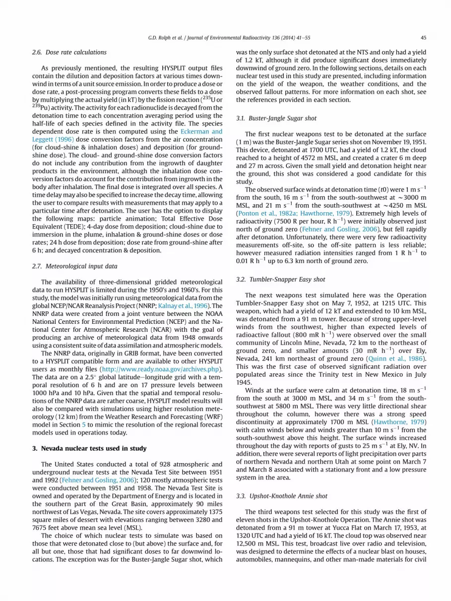
The United States conducted a total of 928 atmospheric andunderground nuclear tests at the Nevada Test Site between 1951and 1992 (Fehner and Gosling, 2006); 120mostly atmospheric testswere conducted between 1951 and 1958. The Nevada Test Site isowned and operated by the Department of Energy and is located inthe southern part of the Great Basin, approximately 90 milesnorthwest of Las Vegas, Nevada. The site covers approximately 1375square miles of dessert with elevations ranging between 3280 and7675 feet above mean sea level (MSL).

The choice of which nuclear tests to simulate was based onthose that were detonated close to (but above) the surface and, forall but one, those that had significant doses to far downwind lo-cations. The exception was for the Buster-Jangle Sugar shot, which

was the only surface shot detonated at the NTS and only had a yieldof 1.2 kT, although it did produce significant doses immediatelydownwind of ground zero. In the following sections, details on eachnuclear test used in this study are presented, including informationon the yield of the weapon, the weather conditions, and theobserved fallout patterns. For more information on each shot, seethe references provided in each section.

3.1. Buster-Jangle Sugar shot

The first nuclear weapons test to be detonated at the surface(1m)was the Buster-Jangle Sugar series shot on November 19,1951.This device, detonated at 1700 UTC, had a yield of 1.2 kT, the cloudreached to a height of 4572 m MSL, and created a crater 6 m deepand 27 m across. Given the small yield and detonation height nearthe ground, this shot was considered a good candidate for thisstudy.

The observed surfacewinds at detonation time (t0) were 1m s�1

from the south, 16 m s�1 from the south-southwest at w3000 mMSL, and 21 m s�1 from the south-southwest at w4250 m MSL(Ponton et al., 1982a; Hawthorne, 1979). Extremely high levels ofradioactivity (7500 R per hour, R h�1) were initially observed justnorth of ground zero (Fehner and Gosling, 2006), but fell rapidlyafter detonation. Unfortunately, there were very few radioactivitymeasurements off-site, so the off-site pattern is less reliable;however measured radiation intensities ranged from 1 R h�1 to0.01 R h�1 up to 6.3 km north of ground zero.

3.2. Tumbler-Snapper Easy shot

The next weapons test simulated here was the OperationTumbler-Snapper Easy shot on May 7, 1952, at 1215 UTC. Thisweapon, which had a yield of 12 kT and extended to 10 km MSL,was detonated from a 91 m tower. Because of strong upper-levelwinds from the southwest, higher than expected levels ofradioactive fallout (800 mR h�1) were observed over the smallcommunity of Lincoln Mine, Nevada, 72 km to the northeast ofground zero, and smaller amounts (30 mR h�1) over Ely,Nevada, 241 km northeast of ground zero (Quinn et al., 1986).This was the first case of observed significant radiation overpopulated areas since the Trinity test in New Mexico in July1945.

Winds at the surface were calm at detonation time, 18 m s�1

from the south at 3000 m MSL, and 34 m s�1 from the south-southwest at 5800 m MSL. There was very little directional shearthroughout the column, however there was a strong speeddiscontinuity at approximately 1700 m MSL (Hawthorne, 1979)with calm winds below and winds greater than 10 m s�1 from thesouth-southwest above this height. The surface winds increasedthroughout the day with reports of gusts to 25 m s�1 at Ely, NV. Inaddition, there were several reports of light precipitation over partsof northern Nevada and northern Utah at some point on March 7and March 8 associated with a stationary front and a low pressuresystem in the area.

3.3. Upshot-Knothole Annie shot

The third weapons test selected for this study was the first ofeleven shots in the Upshot-Knothole Operation. The Annie shot wasdetonated from a 91 m tower at Yucca Flat on March 17, 1953, at1320 UTC and had a yield of 16 kT. The cloud top was observed near12,500 m MSL. This test, broadcast live over radio and television,was designed to determine the effects of a nuclear blast on houses,automobiles, mannequins, and other man-made materials for civil

G.D. Rolph et al. / Journal of Environmental Radioactivity 136 (2014) 41e5546

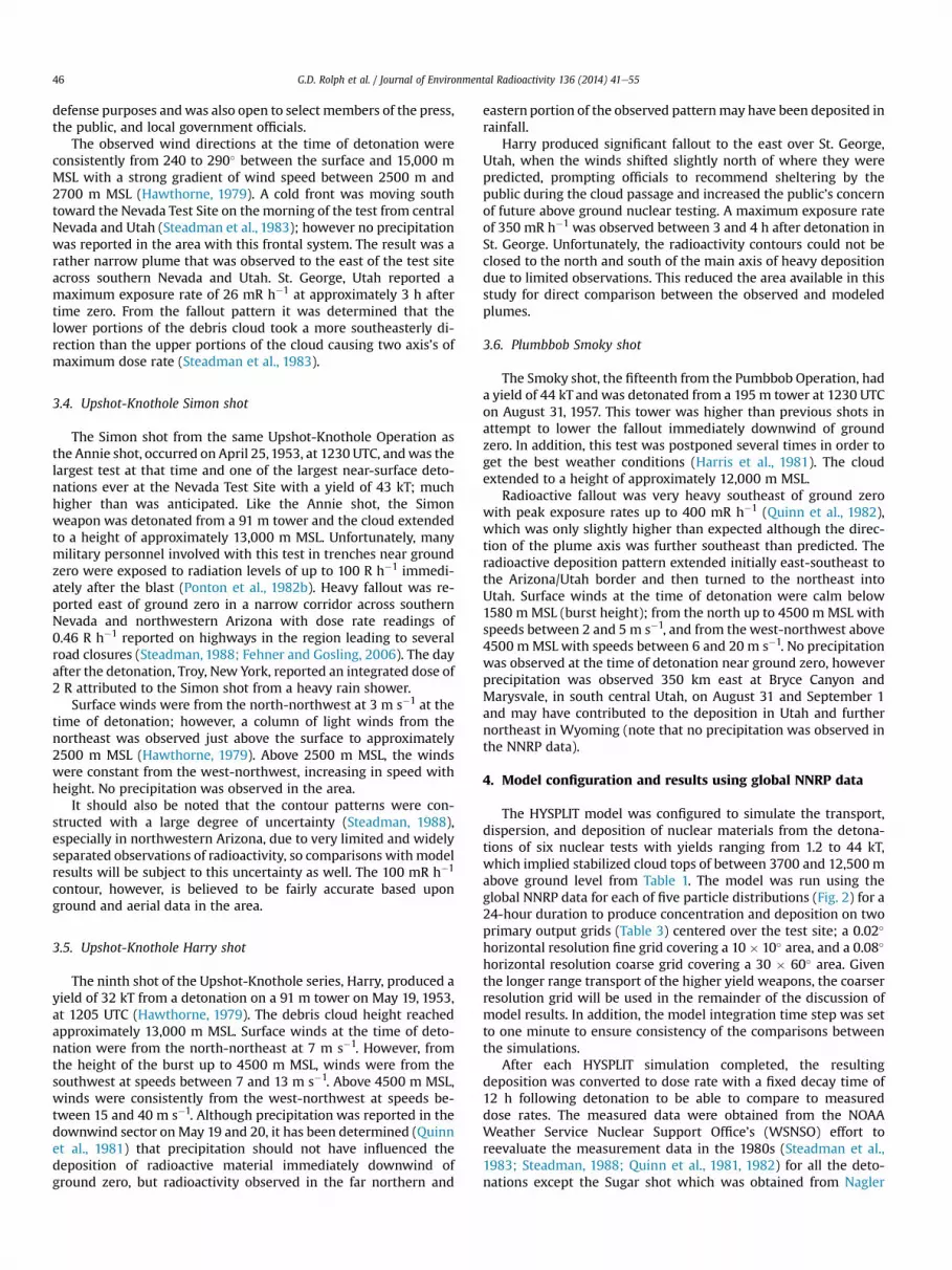
defense purposes andwas also open to select members of the press,the public, and local government officials.

The observed wind directions at the time of detonation wereconsistently from 240 to 290� between the surface and 15,000 mMSL with a strong gradient of wind speed between 2500 m and2700 m MSL (Hawthorne, 1979). A cold front was moving southtoward the Nevada Test Site on the morning of the test from centralNevada and Utah (Steadman et al., 1983); however no precipitationwas reported in the area with this frontal system. The result was arather narrow plume that was observed to the east of the test siteacross southern Nevada and Utah. St. George, Utah reported amaximum exposure rate of 26 mR h�1 at approximately 3 h aftertime zero. From the fallout pattern it was determined that thelower portions of the debris cloud took a more southeasterly di-rection than the upper portions of the cloud causing two axis’s ofmaximum dose rate (Steadman et al., 1983).

3.4. Upshot-Knothole Simon shot

The Simon shot from the same Upshot-Knothole Operation asthe Annie shot, occurred on April 25,1953, at 1230 UTC, andwas thelargest test at that time and one of the largest near-surface deto-nations ever at the Nevada Test Site with a yield of 43 kT; muchhigher than was anticipated. Like the Annie shot, the Simonweapon was detonated from a 91 m tower and the cloud extendedto a height of approximately 13,000 m MSL. Unfortunately, manymilitary personnel involved with this test in trenches near groundzero were exposed to radiation levels of up to 100 R h�1 immedi-ately after the blast (Ponton et al., 1982b). Heavy fallout was re-ported east of ground zero in a narrow corridor across southernNevada and northwestern Arizona with dose rate readings of0.46 R h�1 reported on highways in the region leading to severalroad closures (Steadman, 1988; Fehner and Gosling, 2006). The dayafter the detonation, Troy, New York, reported an integrated dose of2 R attributed to the Simon shot from a heavy rain shower.

Surface winds were from the north-northwest at 3 m s�1 at thetime of detonation; however, a column of light winds from thenortheast was observed just above the surface to approximately2500 m MSL (Hawthorne, 1979). Above 2500 m MSL, the windswere constant from the west-northwest, increasing in speed withheight. No precipitation was observed in the area.

It should also be noted that the contour patterns were con-structed with a large degree of uncertainty (Steadman, 1988),especially in northwestern Arizona, due to very limited and widelyseparated observations of radioactivity, so comparisons withmodelresults will be subject to this uncertainty as well. The 100 mR h�1

contour, however, is believed to be fairly accurate based uponground and aerial data in the area.

3.5. Upshot-Knothole Harry shot

The ninth shot of the Upshot-Knothole series, Harry, produced ayield of 32 kT from a detonation on a 91 m tower on May 19, 1953,at 1205 UTC (Hawthorne, 1979). The debris cloud height reachedapproximately 13,000 m MSL. Surface winds at the time of deto-nation were from the north-northeast at 7 m s�1. However, fromthe height of the burst up to 4500 m MSL, winds were from thesouthwest at speeds between 7 and 13 m s�1. Above 4500 m MSL,winds were consistently from the west-northwest at speeds be-tween 15 and 40 m s�1. Although precipitation was reported in thedownwind sector on May 19 and 20, it has been determined (Quinnet al., 1981) that precipitation should not have influenced thedeposition of radioactive material immediately downwind ofground zero, but radioactivity observed in the far northern and

eastern portion of the observed patternmay have been deposited inrainfall.

Harry produced significant fallout to the east over St. George,Utah, when the winds shifted slightly north of where they werepredicted, prompting officials to recommend sheltering by thepublic during the cloud passage and increased the public’s concernof future above ground nuclear testing. A maximum exposure rateof 350 mR h�1 was observed between 3 and 4 h after detonation inSt. George. Unfortunately, the radioactivity contours could not beclosed to the north and south of the main axis of heavy depositiondue to limited observations. This reduced the area available in thisstudy for direct comparison between the observed and modeledplumes.

3.6. Plumbbob Smoky shot

The Smoky shot, the fifteenth from the Pumbbob Operation, hada yield of 44 kT and was detonated from a 195 m tower at 1230 UTCon August 31, 1957. This tower was higher than previous shots inattempt to lower the fallout immediately downwind of groundzero. In addition, this test was postponed several times in order toget the best weather conditions (Harris et al., 1981). The cloudextended to a height of approximately 12,000 m MSL.

Radioactive fallout was very heavy southeast of ground zerowith peak exposure rates up to 400 mR h�1 (Quinn et al., 1982),which was only slightly higher than expected although the direc-tion of the plume axis was further southeast than predicted. Theradioactive deposition pattern extended initially east-southeast tothe Arizona/Utah border and then turned to the northeast intoUtah. Surface winds at the time of detonation were calm below1580 mMSL (burst height); from the north up to 4500 m MSL withspeeds between 2 and 5 m s�1, and from the west-northwest above4500 mMSL with speeds between 6 and 20 m s�1. No precipitationwas observed at the time of detonation near ground zero, howeverprecipitation was observed 350 km east at Bryce Canyon andMarysvale, in south central Utah, on August 31 and September 1and may have contributed to the deposition in Utah and furthernortheast in Wyoming (note that no precipitation was observed inthe NNRP data).

4. Model configuration and results using global NNRP data

The HYSPLIT model was configured to simulate the transport,dispersion, and deposition of nuclear materials from the detona-tions of six nuclear tests with yields ranging from 1.2 to 44 kT,which implied stabilized cloud tops of between 3700 and 12,500 mabove ground level from Table 1. The model was run using theglobal NNRP data for each of five particle distributions (Fig. 2) for a24-hour duration to produce concentration and deposition on twoprimary output grids (Table 3) centered over the test site; a 0.02�

horizontal resolution fine grid covering a 10 � 10� area, and a 0.08�

horizontal resolution coarse grid covering a 30 � 60� area. Giventhe longer range transport of the higher yield weapons, the coarserresolution grid will be used in the remainder of the discussion ofmodel results. In addition, the model integration time step was setto one minute to ensure consistency of the comparisons betweenthe simulations.

After each HYSPLIT simulation completed, the resultingdeposition was converted to dose rate with a fixed decay time of12 h following detonation to be able to compare to measureddose rates. The measured data were obtained from the NOAAWeather Service Nuclear Support Office’s (WSNSO) effort toreevaluate the measurement data in the 1980s (Steadman et al.,1983; Steadman, 1988; Quinn et al., 1981, 1982) for all the deto-nations except the Sugar shot which was obtained from Nagler

G.D. Rolph et al. / Journal of Environmental Radioactivity 136 (2014) 41e55 47

and Telegadas (1956). The contoured plumes from each of the sixshots were digitized and converted to standard vector format sothat statistical results (Figure of Merit in Space, FMS) could becalculated based on the percent of overlap between the observedand modeled plumes. Unfortunately, some of the observedplumes are very complex and do not always intersect the sourcelocation or extend in all directions downwind due to the un-availability of measurements. In order to be able to provide aquantitative estimate of the overlap, only the portion of theobserved plume (dose contours) that had two defined edges wasconsidered in this evaluation.

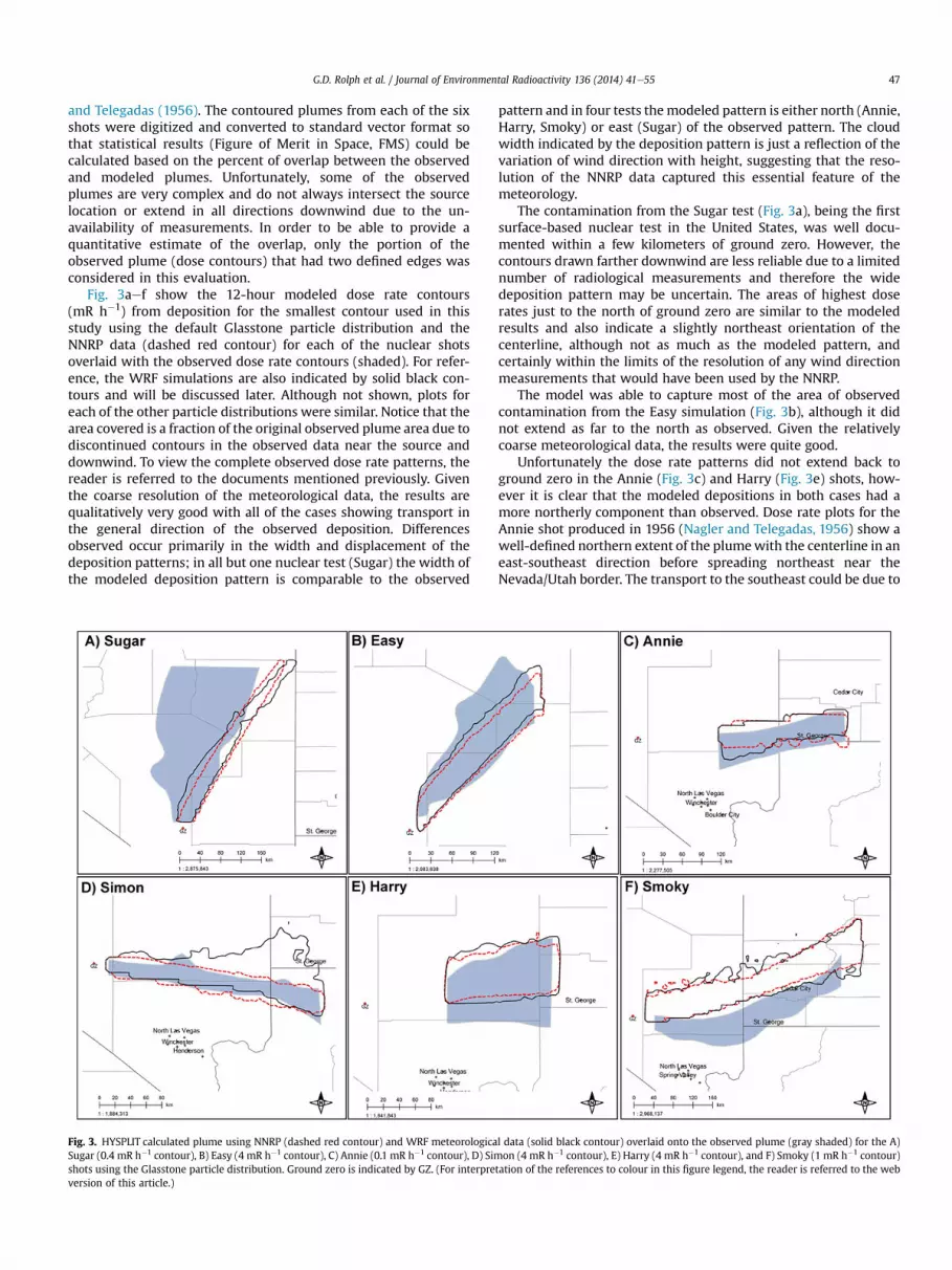
Fig. 3aef show the 12-hour modeled dose rate contours(mR h�1) from deposition for the smallest contour used in thisstudy using the default Glasstone particle distribution and theNNRP data (dashed red contour) for each of the nuclear shotsoverlaid with the observed dose rate contours (shaded). For refer-ence, the WRF simulations are also indicated by solid black con-tours and will be discussed later. Although not shown, plots foreach of the other particle distributions were similar. Notice that thearea covered is a fraction of the original observed plume area due todiscontinued contours in the observed data near the source anddownwind. To view the complete observed dose rate patterns, thereader is referred to the documents mentioned previously. Giventhe coarse resolution of the meteorological data, the results arequalitatively very good with all of the cases showing transport inthe general direction of the observed deposition. Differencesobserved occur primarily in the width and displacement of thedeposition patterns; in all but one nuclear test (Sugar) the width ofthe modeled deposition pattern is comparable to the observed

Fig. 3. HYSPLIT calculated plume using NNRP (dashed red contour) and WRF meteorologicaSugar (0.4 mR h�1 contour), B) Easy (4 mR h�1 contour), C) Annie (0.1 mR h�1 contour), D) Simshots using the Glasstone particle distribution. Ground zero is indicated by GZ. (For interpreversion of this article.)

pattern and in four tests themodeled pattern is either north (Annie,Harry, Smoky) or east (Sugar) of the observed pattern. The cloudwidth indicated by the deposition pattern is just a reflection of thevariation of wind direction with height, suggesting that the reso-lution of the NNRP data captured this essential feature of themeteorology.

The contamination from the Sugar test (Fig. 3a), being the firstsurface-based nuclear test in the United States, was well docu-mented within a few kilometers of ground zero. However, thecontours drawn farther downwind are less reliable due to a limitednumber of radiological measurements and therefore the widedeposition pattern may be uncertain. The areas of highest doserates just to the north of ground zero are similar to the modeledresults and also indicate a slightly northeast orientation of thecenterline, although not as much as the modeled pattern, andcertainly within the limits of the resolution of any wind directionmeasurements that would have been used by the NNRP.

The model was able to capture most of the area of observedcontamination from the Easy simulation (Fig. 3b), although it didnot extend as far to the north as observed. Given the relativelycoarse meteorological data, the results were quite good.

Unfortunately the dose rate patterns did not extend back toground zero in the Annie (Fig. 3c) and Harry (Fig. 3e) shots, how-ever it is clear that the modeled depositions in both cases had amore northerly component than observed. Dose rate plots for theAnnie shot produced in 1956 (Nagler and Telegadas, 1956) show awell-defined northern extent of the plumewith the centerline in aneast-southeast direction before spreading northeast near theNevada/Utah border. The transport to the southeast could be due to

l data (solid black contour) overlaid onto the observed plume (gray shaded) for the A)on (4 mR h�1 contour), E) Harry (4 mR h�1 contour), and F) Smoky (1 mR h�1 contour)

tation of the references to colour in this figure legend, the reader is referred to the web

G.D. Rolph et al. / Journal of Environmental Radioactivity 136 (2014) 41e5548

the lighter observed winds in the lower layers from southwest tonorthwest that the NNRP data did not capture. The modeledpattern for Harry may have been shifted slightly north of theobserved pattern due to less flow from the west-northwest thanwas observed at mid-levels above 5000 m.

Finally, the modeled deposition pattern of the Smoky simulation(Fig. 3f), although very similar in size and shape, completely missedthe area of observed deposition by passing to the north. Theobserved pattern had a very sharp northern extent with the bulk ofthe deposition extending east-southeast before curving to thenortheast near the Nevada/Utah border. As mentioned earlier, theobserved plume was actually farther southeast than predicted atthe time of detonation. The meteorological situation was rathercomplex with a low pressure area over southwestern Utah and anupper-level trough passing through the region, which contributedto the strong flow from the west-northwest throughout the col-umn. The NNRP data had mostly westerly flow at mid-levels andlight and variable winds below 3000 m. Similar results wererecently found by Schofield (2012) in that HYSPLIT, HPAC and theWeather Research & Forecasting with Chemistry (WRF-CHEM)

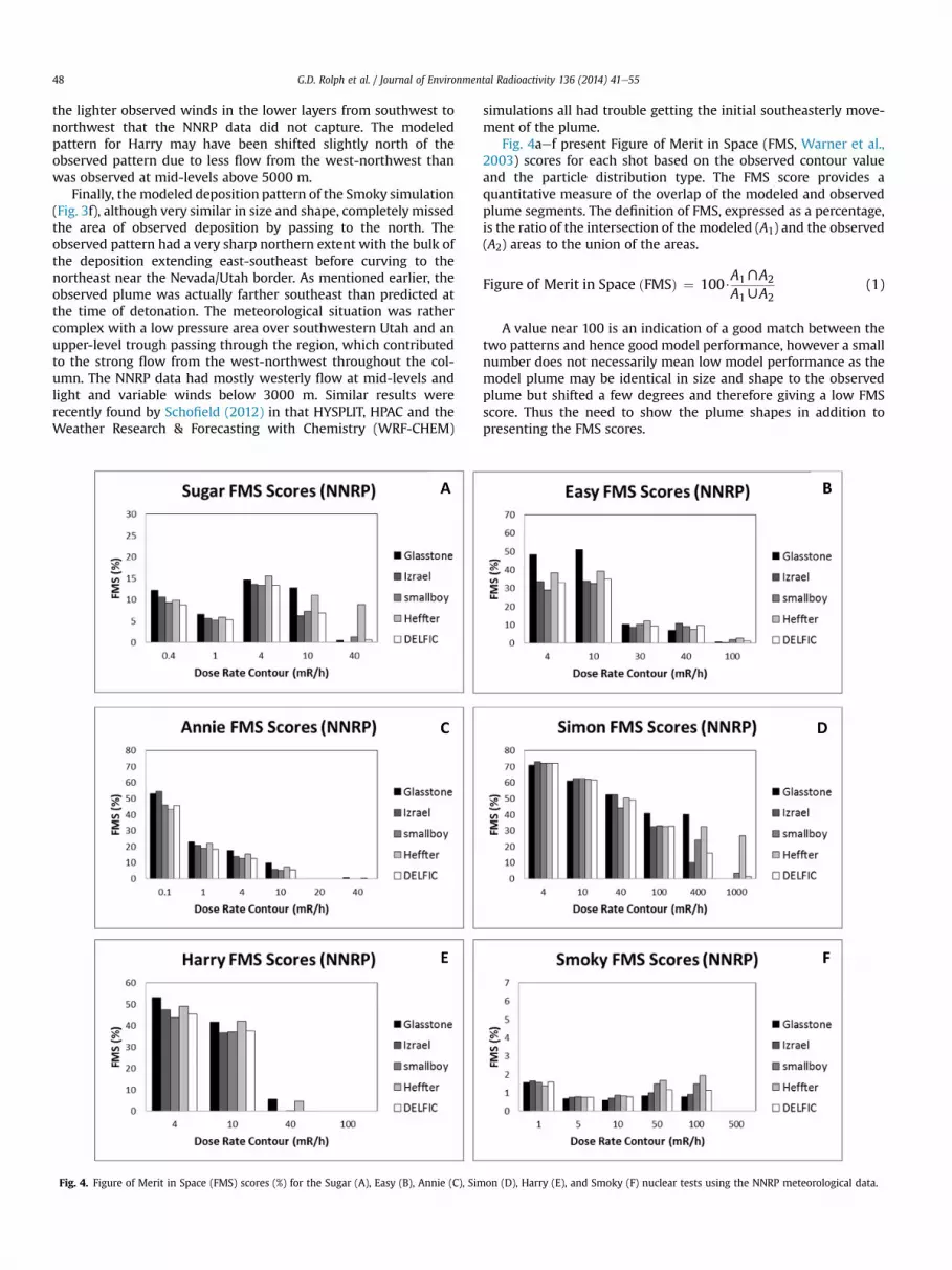
Fig. 4. Figure of Merit in Space (FMS) scores (%) for the Sugar (A), Easy (B), Annie (C), Sim

simulations all had trouble getting the initial southeasterly move-ment of the plume.

Fig. 4aef present Figure of Merit in Space (FMS, Warner et al.,2003) scores for each shot based on the observed contour valueand the particle distribution type. The FMS score provides aquantitative measure of the overlap of the modeled and observedplume segments. The definition of FMS, expressed as a percentage,is the ratio of the intersection of the modeled (A1) and the observed(A2) areas to the union of the areas.

Figure of Merit in Space ðFMSÞ ¼ 100$A1XA2

A1WA2(1)

A value near 100 is an indication of a good match between thetwo patterns and hence good model performance, however a smallnumber does not necessarily mean low model performance as themodel plume may be identical in size and shape to the observedplume but shifted a few degrees and therefore giving a low FMSscore. Thus the need to show the plume shapes in addition topresenting the FMS scores.

on (D), Harry (E), and Smoky (F) nuclear tests using the NNRP meteorological data.

G.D. Rolph et al. / Journal of Environmental Radioactivity 136 (2014) 41e55 49

In general, FMS scores decrease with increasing dose rate con-tours with the exception of the Sugar (Fig. 4a) and Smoky (Fig. 4f)shots which had very little overlap overall. The decreasing scorewith increasing dose rate is to be expected given the smallerfootprint of the highest dose rate contours. In regard to the particledistribution type, the FMS scores are very similar for all distributiontypes, especially at the lower dose rate contours. However, theGlasstone distribution tends to have the highest FMS score per doserate contour for all but the Smoky shot (Fig. 4f), which producedvery low FMS scores at all contour levels and all distribution typesdue to the modeled plumes being north of the observed plumeswith little overlap. The Glasstone particle/activity distribution isquite different from the others in that it has the least activity in thesmallest and largest particle sizes. The highest FMS scores wereobtained from the Simon shot (Fig. 4d) with FMS scores above 70%at the lowest dose rate contour; a result of the very good overlapbetween modeled and observed dose rate contours.

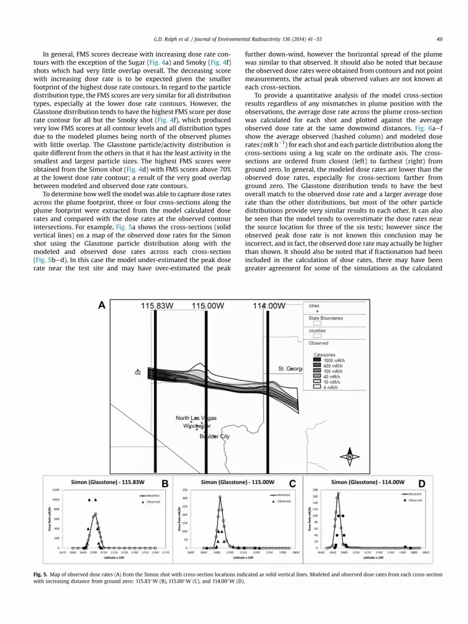
To determine howwell the model was able to capture dose ratesacross the plume footprint, three or four cross-sections along theplume footprint were extracted from the model calculated doserates and compared with the dose rates at the observed contourintersections. For example, Fig. 5a shows the cross-sections (solidvertical lines) on a map of the observed dose rates for the Simonshot using the Glasstone particle distribution along with themodeled and observed dose rates across each cross-section(Fig. 5bed). In this case the model under-estimated the peak doserate near the test site and may have over-estimated the peak

Fig. 5. Map of observed dose rates (A) from the Simon shot with cross-section locations indwith increasing distance from ground zero: 115.83�W (B), 115.00�W (C), and 114.00�W (D)

further down-wind, however the horizontal spread of the plumewas similar to that observed. It should also be noted that becausethe observed dose rates were obtained from contours and not pointmeasurements, the actual peak observed values are not known ateach cross-section.

To provide a quantitative analysis of the model cross-sectionresults regardless of any mismatches in plume position with theobservations, the average dose rate across the plume cross-sectionwas calculated for each shot and plotted against the averageobserved dose rate at the same downwind distances. Fig. 6aefshow the average observed (hashed column) and modeled doserates (mR h�1) for each shot and each particle distribution along thecross-sections using a log scale on the ordinate axis. The cross-sections are ordered from closest (left) to farthest (right) fromground zero. In general, the modeled dose rates are lower than theobserved dose rates, especially for cross-sections farther fromground zero. The Glasstone distribution tends to have the bestoverall match to the observed dose rate and a larger average doserate than the other distributions, but most of the other particledistributions provide very similar results to each other. It can alsobe seen that the model tends to overestimate the dose rates nearthe source location for three of the six tests; however since theobserved peak dose rate is not known this conclusion may beincorrect, and in fact, the observed dose rate may actually be higherthan shown. It should also be noted that if fractionation had beenincluded in the calculation of dose rates, there may have beengreater agreement for some of the simulations as the calculated

icated as solid vertical lines. Modeled and observed dose rates from each cross-section.

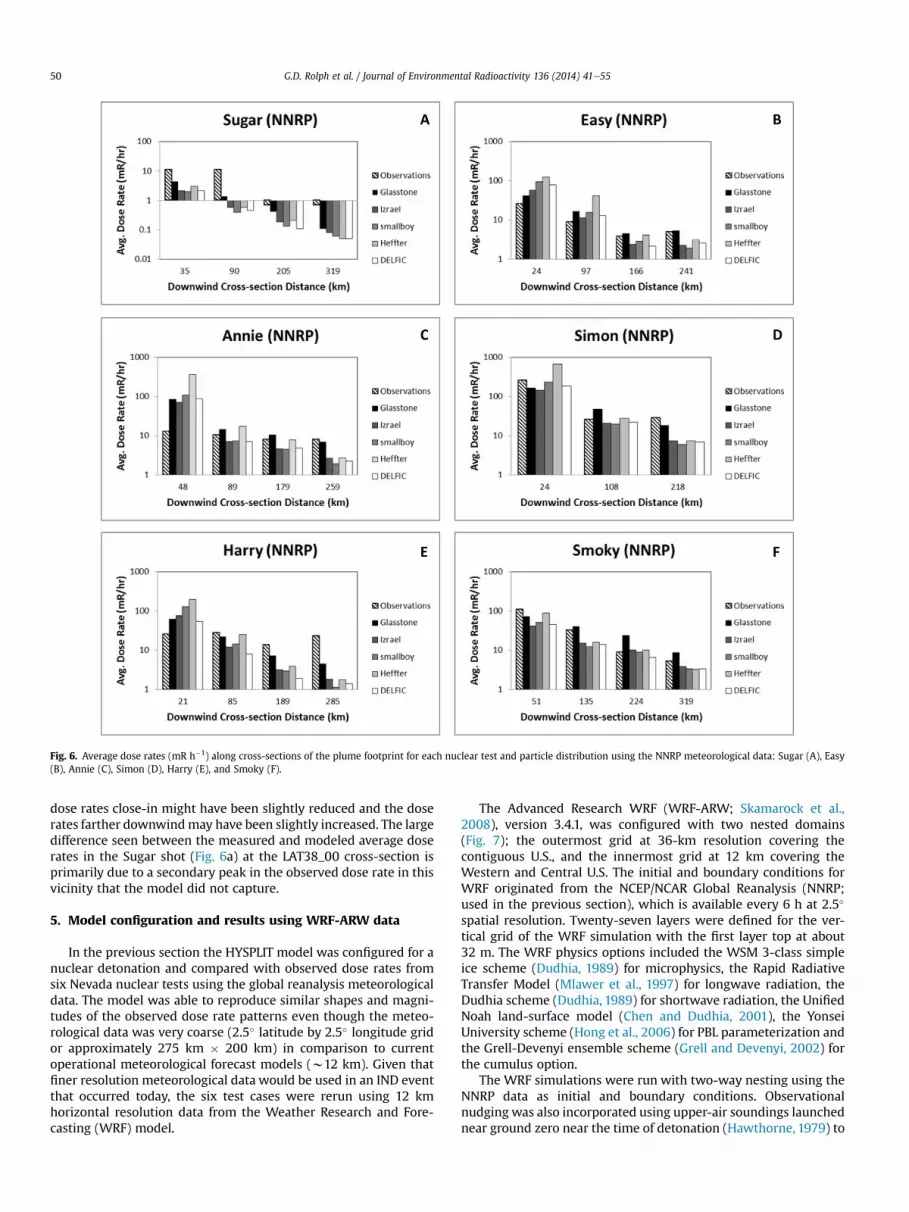
Fig. 6. Average dose rates (mR h�1) along cross-sections of the plume footprint for each nuclear test and particle distribution using the NNRP meteorological data: Sugar (A), Easy(B), Annie (C), Simon (D), Harry (E), and Smoky (F).

G.D. Rolph et al. / Journal of Environmental Radioactivity 136 (2014) 41e5550

dose rates close-in might have been slightly reduced and the doserates farther downwindmay have been slightly increased. The largedifference seen between the measured and modeled average doserates in the Sugar shot (Fig. 6a) at the LAT38_00 cross-section isprimarily due to a secondary peak in the observed dose rate in thisvicinity that the model did not capture.

5. Model configuration and results using WRF-ARW data

In the previous section the HYSPLIT model was configured for anuclear detonation and compared with observed dose rates fromsix Nevada nuclear tests using the global reanalysis meteorologicaldata. The model was able to reproduce similar shapes and magni-tudes of the observed dose rate patterns even though the meteo-rological data was very coarse (2.5� latitude by 2.5� longitude gridor approximately 275 km � 200 km) in comparison to currentoperational meteorological forecast models (w12 km). Given thatfiner resolution meteorological data would be used in an IND eventthat occurred today, the six test cases were rerun using 12 kmhorizontal resolution data from the Weather Research and Fore-casting (WRF) model.

The Advanced Research WRF (WRF-ARW; Skamarock et al.,2008), version 3.4.1, was configured with two nested domains(Fig. 7); the outermost grid at 36-km resolution covering thecontiguous U.S., and the innermost grid at 12 km covering theWestern and Central U.S. The initial and boundary conditions forWRF originated from the NCEP/NCAR Global Reanalysis (NNRP;used in the previous section), which is available every 6 h at 2.5�

spatial resolution. Twenty-seven layers were defined for the ver-tical grid of the WRF simulation with the first layer top at about32 m. The WRF physics options included the WSM 3-class simpleice scheme (Dudhia, 1989) for microphysics, the Rapid RadiativeTransfer Model (Mlawer et al., 1997) for longwave radiation, theDudhia scheme (Dudhia, 1989) for shortwave radiation, the UnifiedNoah land-surface model (Chen and Dudhia, 2001), the YonseiUniversity scheme (Hong et al., 2006) for PBL parameterization andthe Grell-Devenyi ensemble scheme (Grell and Devenyi, 2002) forthe cumulus option.

The WRF simulations were run with two-way nesting using theNNRP data as initial and boundary conditions. Observationalnudging was also incorporated using upper-air soundings launchednear ground zero near the time of detonation (Hawthorne, 1979) to

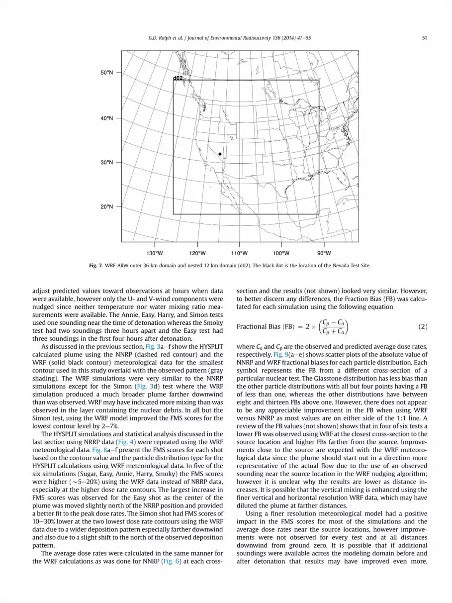
Fig. 7. WRF-ARW outer 36 km domain and nested 12 km domain (d02). The black dot is the location of the Nevada Test Site.

G.D. Rolph et al. / Journal of Environmental Radioactivity 136 (2014) 41e55 51

adjust predicted values toward observations at hours when datawere available, however only the U- and V-wind components werenudged since neither temperature nor water mixing ratio mea-surements were available. The Annie, Easy, Harry, and Simon testsused one sounding near the time of detonation whereas the Smokytest had two soundings three hours apart and the Easy test hadthree soundings in the first four hours after detonation.

As discussed in the previous section, Fig. 3aef show the HYSPLITcalculated plume using the NNRP (dashed red contour) and theWRF (solid black contour) meteorological data for the smallestcontour used in this study overlaid with the observed pattern (grayshading). The WRF simulations were very similar to the NNRPsimulations except for the Simon (Fig. 3d) test where the WRFsimulation produced a much broader plume farther downwindthanwas observed. WRFmay have indicated moremixing thanwasobserved in the layer containing the nuclear debris. In all but theSimon test, using the WRF model improved the FMS scores for thelowest contour level by 2e7%.

The HYSPLIT simulations and statistical analysis discussed in thelast section using NRRP data (Fig. 4) were repeated using the WRFmeteorological data. Fig. 8aef present the FMS scores for each shotbased on the contour value and the particle distribution type for theHYSPLIT calculations using WRF meteorological data. In five of thesix simulations (Sugar, Easy, Annie, Harry, Smoky) the FMS scoreswere higher (w5e20%) using the WRF data instead of NRRP data,especially at the higher dose rate contours. The largest increase inFMS scores was observed for the Easy shot as the center of theplumewasmoved slightly north of the NRRP position and provideda better fit to the peak dose rates. The Simon shot had FMS scores of10e30% lower at the two lowest dose rate contours using the WRFdata due to awider deposition pattern especially farther downwindand also due to a slight shift to the north of the observed depositionpattern.

The average dose rates were calculated in the same manner forthe WRF calculations as was done for NNRP (Fig. 6) at each cross-

section and the results (not shown) looked very similar. However,to better discern any differences, the Fraction Bias (FB) was calcu-lated for each simulation using the following equation

Fractional Bias ðFBÞ ¼ 2��Cp � CoCp þ Co

�(2)

where Co and Cp are the observed and predicted average dose rates,respectively. Fig. 9(aee) shows scatter plots of the absolute value ofNNRP andWRF fractional biases for each particle distribution. Eachsymbol represents the FB from a different cross-section of aparticular nuclear test. The Glasstone distribution has less bias thanthe other particle distributions with all but four points having a FBof less than one, whereas the other distributions have betweeneight and thirteen FBs above one. However, there does not appearto be any appreciable improvement in the FB when using WRFversus NNRP as most values are on either side of the 1:1 line. Areview of the FB values (not shown) shows that in four of six tests alower FBwas observed usingWRF at the closest cross-section to thesource location and higher FBs farther from the source. Improve-ments close to the source are expected with the WRF meteoro-logical data since the plume should start out in a direction morerepresentative of the actual flow due to the use of an observedsounding near the source location in the WRF nudging algorithm;however it is unclear why the results are lower as distance in-creases. It is possible that the vertical mixing is enhanced using thefiner vertical and horizontal resolution WRF data, which may havediluted the plume at farther distances.

Using a finer resolution meteorological model had a positiveimpact in the FMS scores for most of the simulations and theaverage dose rates near the source locations, however improve-ments were not observed for every test and at all distancesdownwind from ground zero. It is possible that if additionalsoundings were available across the modeling domain before andafter detonation that results may have improved even more,

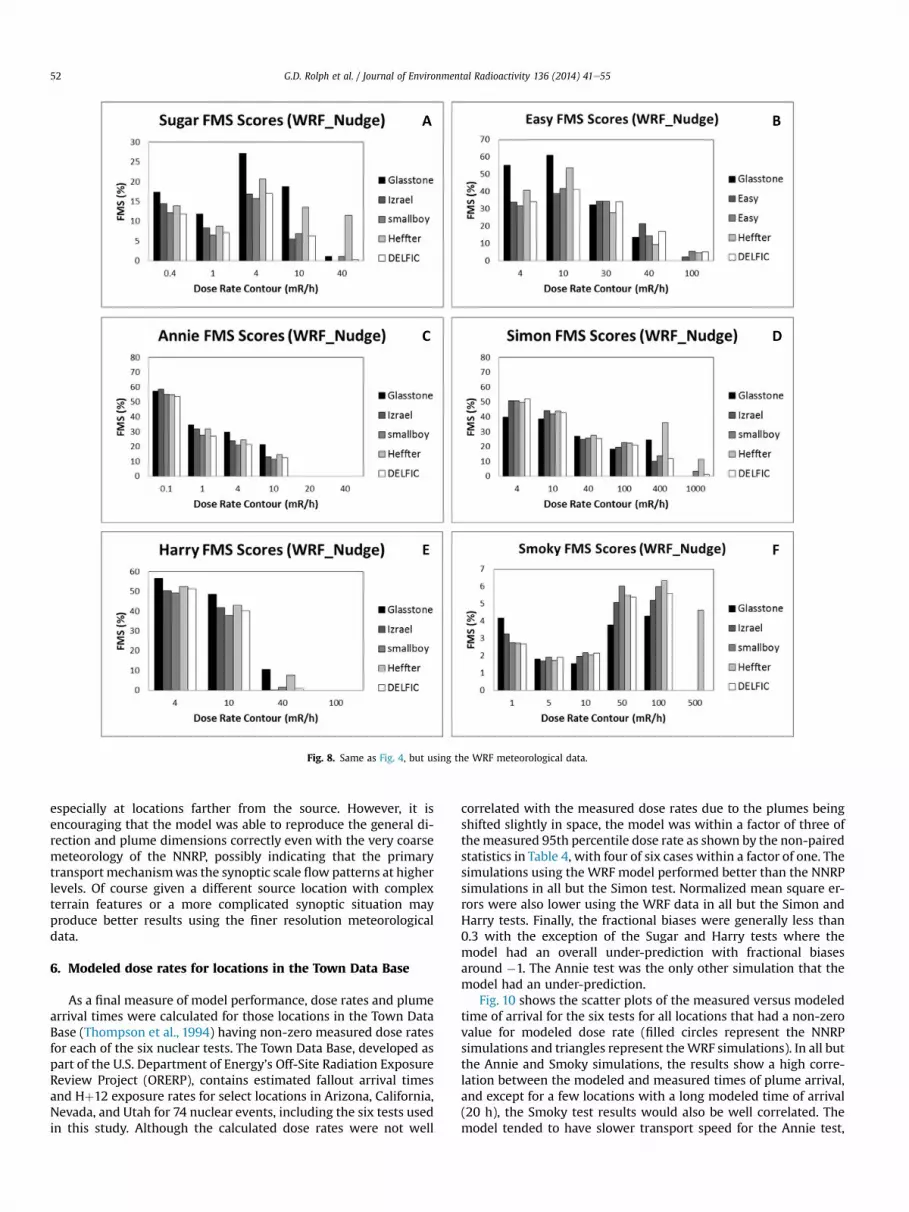
Fig. 8. Same as Fig. 4, but using the WRF meteorological data.

G.D. Rolph et al. / Journal of Environmental Radioactivity 136 (2014) 41e5552

especially at locations farther from the source. However, it isencouraging that the model was able to reproduce the general di-rection and plume dimensions correctly even with the very coarsemeteorology of the NNRP, possibly indicating that the primarytransport mechanismwas the synoptic scale flow patterns at higherlevels. Of course given a different source location with complexterrain features or a more complicated synoptic situation mayproduce better results using the finer resolution meteorologicaldata.

6. Modeled dose rates for locations in the Town Data Base

As a final measure of model performance, dose rates and plumearrival times were calculated for those locations in the Town DataBase (Thompson et al., 1994) having non-zero measured dose ratesfor each of the six nuclear tests. The Town Data Base, developed aspart of the U.S. Department of Energy’s Off-Site Radiation ExposureReview Project (ORERP), contains estimated fallout arrival timesand Hþ12 exposure rates for select locations in Arizona, California,Nevada, and Utah for 74 nuclear events, including the six tests usedin this study. Although the calculated dose rates were not well

correlated with the measured dose rates due to the plumes beingshifted slightly in space, the model was within a factor of three ofthemeasured 95th percentile dose rate as shown by the non-pairedstatistics in Table 4, with four of six cases within a factor of one. Thesimulations using the WRF model performed better than the NNRPsimulations in all but the Simon test. Normalized mean square er-rors were also lower using the WRF data in all but the Simon andHarry tests. Finally, the fractional biases were generally less than0.3 with the exception of the Sugar and Harry tests where themodel had an overall under-prediction with fractional biasesaround �1. The Annie test was the only other simulation that themodel had an under-prediction.

Fig. 10 shows the scatter plots of the measured versus modeledtime of arrival for the six tests for all locations that had a non-zerovalue for modeled dose rate (filled circles represent the NNRPsimulations and triangles represent theWRF simulations). In all butthe Annie and Smoky simulations, the results show a high corre-lation between the modeled and measured times of plume arrival,and except for a few locations with a long modeled time of arrival(20 h), the Smoky test results would also be well correlated. Themodel tended to have slower transport speed for the Annie test,

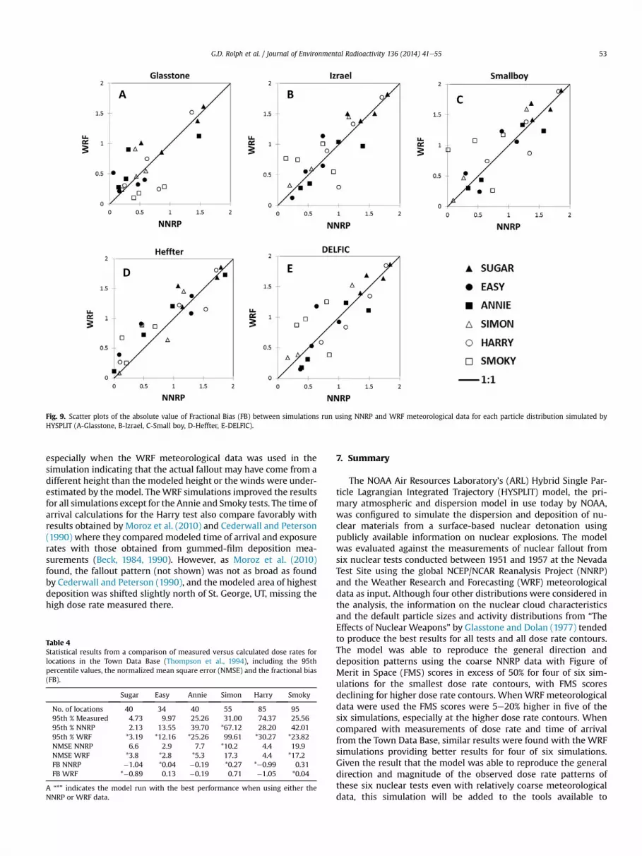
Fig. 9. Scatter plots of the absolute value of Fractional Bias (FB) between simulations run using NNRP and WRF meteorological data for each particle distribution simulated byHYSPLIT (A-Glasstone, B-Izrael, C-Small boy, D-Heffter, E-DELFIC).

G.D. Rolph et al. / Journal of Environmental Radioactivity 136 (2014) 41e55 53

especially when the WRF meteorological data was used in thesimulation indicating that the actual fallout may have come from adifferent height than the modeled height or the winds were under-estimated by the model. TheWRF simulations improved the resultsfor all simulations except for the Annie and Smoky tests. The time ofarrival calculations for the Harry test also compare favorably withresults obtained by Moroz et al. (2010) and Cederwall and Peterson(1990) where they compared modeled time of arrival and exposurerates with those obtained from gummed-film deposition mea-surements (Beck, 1984, 1990). However, as Moroz et al. (2010)found, the fallout pattern (not shown) was not as broad as foundby Cederwall and Peterson (1990), and the modeled area of highestdeposition was shifted slightly north of St. George, UT, missing thehigh dose rate measured there.

Table 4Statistical results from a comparison of measured versus calculated dose rates forlocations in the Town Data Base (Thompson et al., 1994), including the 95thpercentile values, the normalized mean square error (NMSE) and the fractional bias(FB).

Sugar Easy Annie Simon Harry Smoky

No. of locations 40 34 40 55 85 9595th % Measured 4.73 9.97 25.26 31.00 74.37 25.5695th % NNRP 2.13 13.55 39.70 *67.12 28.20 42.0195th % WRF *3.19 *12.16 *25.26 99.61 *30.27 *23.82NMSE NNRP 6.6 2.9 7.7 *10.2 4.4 19.9NMSE WRF *3.8 *2.8 *5.3 17.3 4.4 *17.2FB NNRP �1.04 *0.04 �0.19 *0.27 *e0.99 0.31FB WRF *�0.89 0.13 �0.19 0.71 �1.05 *0.04

A “*” indicates the model run with the best performance when using either theNNRP or WRF data.

7. Summary

The NOAA Air Resources Laboratory’s (ARL) Hybrid Single Par-ticle Lagrangian Integrated Trajectory (HYSPLIT) model, the pri-mary atmospheric and dispersion model in use today by NOAA,was configured to simulate the dispersion and deposition of nu-clear materials from a surface-based nuclear detonation usingpublicly available information on nuclear explosions. The modelwas evaluated against the measurements of nuclear fallout fromsix nuclear tests conducted between 1951 and 1957 at the NevadaTest Site using the global NCEP/NCAR Reanalysis Project (NNRP)and the Weather Research and Forecasting (WRF) meteorologicaldata as input. Although four other distributions were considered inthe analysis, the information on the nuclear cloud characteristicsand the default particle sizes and activity distributions from “TheEffects of Nuclear Weapons” by Glasstone and Dolan (1977) tendedto produce the best results for all tests and all dose rate contours.The model was able to reproduce the general direction anddeposition patterns using the coarse NNRP data with Figure ofMerit in Space (FMS) scores in excess of 50% for four of six sim-ulations for the smallest dose rate contours, with FMS scoresdeclining for higher dose rate contours. When WRF meteorologicaldata were used the FMS scores were 5e20% higher in five of thesix simulations, especially at the higher dose rate contours. Whencompared with measurements of dose rate and time of arrivalfrom the Town Data Base, similar results were found with the WRFsimulations providing better results for four of six simulations.Given the result that the model was able to reproduce the generaldirection and magnitude of the observed dose rate patterns ofthese six nuclear tests even with relatively coarse meteorologicaldata, this simulation will be added to the tools available to

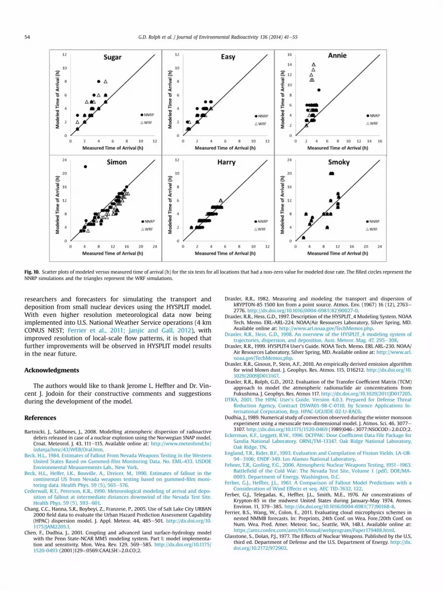
Fig. 10. Scatter plots of modeled versus measured time of arrival (h) for the six tests for all locations that had a non-zero value for modeled dose rate. The filled circles represent theNNRP simulations and the triangles represent the WRF simulations.

G.D. Rolph et al. / Journal of Environmental Radioactivity 136 (2014) 41e5554

researchers and forecasters for simulating the transport anddeposition from small nuclear devices using the HYSPLIT model.With even higher resolution meteorological data now beingimplemented into U.S. National Weather Service operations (4 kmCONUS NEST; Ferrier et al., 2011; Janjic and Gall, 2012), withimproved resolution of local-scale flow patterns, it is hoped thatfurther improvements will be observed in HYSPLIT model resultsin the near future.

Acknowledgments

The authors would like to thank Jerome L. Heffter and Dr. Vin-cent J. Jodoin for their constructive comments and suggestionsduring the development of the model.

References

Bartnicki, J., Saltbones, J., 2008. Modelling atmospheric dispersion of radioactivedebris released in case of a nuclear explosion using the Norwegian SNAP model.Croat. Meteorol. J. 43, 111e115. Available online at: http://www.meteohmd.hr/izdanja/hmc/43/WEB/Oral.htm.

Beck, H.L., 1984. Estimates of Fallout From Nevada Weapons Testing in the WesternUnited States Based on Gummed-film Monitoring Data. No. EML-433. USDOEEnvironmental Measurements Lab., New York.

Beck, H.L., Helfer, I.K., Bouville, A., Dreicer, M., 1990. Estimates of fallout in thecontinental US from Nevada weapons testing based on gummed-film moni-toring data. Health Phys. 59 (5), 565e576.

Cederwall, R.T., Peterson, K.R., 1990. Meteorological modeling of arrival and depo-sition of fallout at intermediate distances downwind of the Nevada Test Site.Health Phys. 59 (5), 593e601.

Chang, C.C., Hanna, S.R., Boybeyi, Z., Franzese, P., 2005. Use of Salt Lake City URBAN2000 field data to evaluate the Urban Hazard Prediction Assessment Capability(HPAC) dispersion model. J. Appl. Meteor. 44, 485e501. http://dx.doi.org/10.1175/JAM2205.1.

Chen, F., Dudhia, J., 2001. Coupling and advanced land surface-hydrology modelwith the Penn State-NCAR MM5 modeling system. Part I: model implementa-tion and sensitivity. Mon. Wea. Rev. 129, 569e585. http://dx.doi.org/10.1175/1520-0493 (2001)129<0569:CAALSH>2.0.CO;2.

Draxler, R.R., 1982. Measuring and modeling the transport and dispersion ofkRYPTON-85 1500 km from a point source. Atmos. Env. (1967) 16 (12), 2763e2776. http://dx.doi.org/10.1016/0004-6981(82)90027-0.

Draxler, R.R., Hess, G.D., 1997. Description of the HYSPLIT_4 Modeling System. NOAATech. Memo. ERL-ARL-224. NOAA/Air Resources Laboratory, Silver Spring, MD.Available online at: http://www.arl.noaa.gov/TechMemos.php.

Draxler, R.R., Hess, G.D., 1998. An overview of the HYSPLIT_4 modeling system oftrajectories, dispersion, and deposition. Aust. Meteor. Mag. 47, 295e308.

Draxler, R.R., 1999. HYSPLIT4 User’s Guide. NOAA Tech. Memo. ERL ARL-230. NOAA/Air Resources Laboratory, Silver Spring, MD. Available online at: http://www.arl.noaa.gov/TechMemos.php.

Draxler, R.R., Ginoux, P., Stein, A.F., 2010. An empirically derived emission algorithmfor wind blown dust. J. Geophys. Res. Atmos. 115, D16212. http://dx.doi.org/10.1029/2009JD013167.

Draxler, R.R., Rolph, G.D., 2012. Evaluation of the Transfer Coefficient Matrix (TCM)approach to model the atmospheric radionuclide air concentrations fromFukushima. J. Geophys. Res. Atmos 117. http://dx.doi.org/10.1029/2011JD017205.

DTRA, 2001. The HPAC User’s Guide, Version 4.0.3. Prepared for Defense ThreatReduction Agency, Contract DSWA01-98-C-0110, by Science Applications In-ternational Corporation, Rep. HPAC-UGUIDE-02-U-RAC0.

Dudhia, J.,1989. Numerical study of convection observed during thewintermonsoonexperiment using a mesoscale two-dimensional model. J. Atmos. Sci. 46, 3077e3107. http://dx.doi.org/10.1175/1520-0469 (1989)046<3077:NSOCOD>2.0.CO;2.

Eckerman, K.F., Leggett, R.W., 1996. DCFPAK: Dose Coefficient Data File Package forSandia National Laboratory. ORNL/TM-13347. Oak Ridge National Laboratory,Oak Ridge, TN.

England, T.R., Rider, B.F., 1993. Evaluation and Compilation of Fission Yields. LA-UR-94e3106; ENDF-349. Los Alamos National Laboratory.

Fehner, T.R., Gosling, F.G., 2006. Atmospheric Nuclear Weapons Testing, 1951e1963.Battlefield of the Cold War: The Nevada Test Site, Volume 1 (pdf). DOE/MA-0003. Department of Energy, Washington, D.C.

Ferber, G.J., Heffter, J.L., 1961. A Comparison of Fallout Model Predictions with aConsideration of Wind Effects et seq. AEC TID-7632, 122.

Ferber, G.J., Telegadas, K., Heffter, J.L., Smith, M.E., 1976. Air concentrations ofKrypton-85 in the midwest United States during January-May 1974. Atmos.Environ. 11, 379e385. http://dx.doi.org/10.1016/0004-6981(77)90168-8.

Ferrier, B.S., Wang, W., Colon, E., 2011. Evaluating cloud microphysics schemes innested NMMB forecasts. In: Preprints, 24th Conf. on Wea. Fore./20th Conf. onNum. Wea. Pred. Amer. Meteor. Soc., Seattle, WA, 14B.1. Available online at:https://ams.confex.com/ams/91Annual/webprogram/Paper179488.html.

Glasstone, S., Dolan, P.J., 1977. The Effects of Nuclear Weapons. Published by the U.S,third ed. Department of Defense and the U.S. Department of Energy. http://dx.doi.org/10.2172/972902.

G.D. Rolph et al. / Journal of Environmental Radioactivity 136 (2014) 41e55 55

Grell, G.A., Devenyi, D., 2002. A generalized approach to parameterizing convectioncombining ensemble and data assimilation techniques. Geophys Res. Lett. 29,1693. http://dx.doi.org/10.1029/2002GL015311.

Harris, P.S., Lowery, C., Nelson, A.G., Obermiller, S., Ozeroff, W.J., Weary, E., 1981. ShotSMOKY, A Test of the PLUMBBOB Series (DNA 6004F). Defense Nuclear Agency.

Continental U.S. Tests (DNA 1251-1-FX). In: Hawthorne, H.A. (Ed.), 1979. Compila-tion of Local Fallout Data from Test Detonations 1945e1962 Extracted fromDASA 1251, vol. I. Defense Nuclear Agency.

Heffter, J.L., 1969. ARL Fallout Prediction Technique. ESSA Tech. Memo. ERLTM-ARL13. NOAA/Air Resources Laboratory, Silver Spring, MD. Available online at:http://www.arl.noaa.gov/TechMemos.php.

Heffter, J.L., 1980. Air Resources Laboratories Atmospheric Transport and DispersionModel (ARL-ATAD). NOAA Tech. Memo. ERL ARL 81. NOAA/Air Resources Lab-oratory, Silver Spring, MD. Available online at: http://www.arl.noaa.gov/TechMemos.php.

Hicks, H.G., 1981. Results of Calculations of External Radiation Exposure Rates fromFallout and the Related Radionuclide Composition. UCRL-53152, parts 1e8,1981. Lawrence Livermore National Laboratory, Livermore, CA.

Hicks, H.G., 1984. Results of Calculations of External Gamma Radiation ExposureRates From Local Fallout and the Related Radionuclide Compositions of SelectedU.S. Pacific Events. Lawrence Livermore National Laboratory, Livermore, CA.UCRL-53505.

Hoecker, W.H., Machta, L., 1990. Meteorological modeling of radioiodine transportand deposition within the continental United States. Health Phys. 59 (5), 603e617.

Homann, S.G., Aluzzi, F., 2013. HotSpot Health Physics Codes: Version 3.0 User’sGuide. LLNL-SM-636474. National Atmospheric Release Advisory Center, Liv-ermore, CA.

Hong, S.Y., Noh, Y., Dudhia, J., 2006. A new vertical diffusion package with anexplicit treatment of entrainment processes. Mon. Wea. Rev. 134, 2318e2341.http://dx.doi.org/10.1175/MWR3199.1.

Izrael, Y.A., 2002. Radioactive Fallout after Nuclear Explosions and Accidents,Radioactivity in the Environment Series. Elsevier Science, Amsterdam, p. 3.

Janjic, Z., Gall, R.L., 2012. Scientific Documentation of the NCEP NonhydrostaticMultiscale Model on the B Grid (NMMB). Part 1 Dynamics. NCAR Technical NoteNCAR/TN-489þSTR. http://dx.doi.org/10.5065/D6WH2MZX.

Jodoin, V.J., 1994. Nuclear Cloud Rise and Growth. AD B007 607. Air Force Institute ofTechnology, Wright-Patterson AFB, OH.

Kalnay, E., Kanamitsu, M., Kistler, R., Collins, W., Deaven, D., Gandin, L., Iredell, M.,Saha, S., White, G., Woollen, J., Zhu, Y., Chelliah, M., Ebisuzaki, W., Higgins, W.,Janowiak, J., Mo, K.C., Ropelewski, C., Wang, J., Leetmaa, A., Reynolds, R.,Jenne, R., Joseph, D., 1996. The NCEP/NCAR 40-year reanalysis project. Bull. Am.Meteor. Soc. 77, 437e470. http://dx.doi.org/10.1175/1520-0477 (1996)077<0437:TNYRP>2.0.CO;2.

List, R.J., Machta, L., Telegadas, K., 1961. Fallout from the 1961 soviet test series.Weatherwise 14 (6), 219e223. http://dx.doi.org/10.1080/00431672.1961.9930027.

Machta, L., List, R.J., 1956. World-wide travel of atomic debris. Science (UnitedStates) 124.

Machta, L., List, R.J., Telegadas, K., 1962. A survey of radioactive fallout from nucleartests. J. Geophys. Res. 67 (4), 1389e1400. http://dx.doi.org/10.1029/JZ067i004p01389.

Machta, L., Heffter, J.L., 1986. Chernobyl: the meteorological viewpoint. Environ-ment (USA) 28 (7).

Machta, L., 1992. Finding the site of the first Soviet nuclear test in 1949. Bull. Amer.Meteor. Soc. 73, 1797e1806. http://dx.doi.org/10.1175/1520-0477 (1992)073<1797:FTSOTF>2.0.CO;2.

Miller, C.F., Sartor, J.D., 1965. Small Boy shot fallout research program. In:Klement Jr., A.W. (Ed.), Radioactive Fallout from Nuclear Weapons Tests. U.S.Atomic Energy Commission, Germantown, MD, pp. 44e71.

Mlawer, E.J., Taubman, S.J., Brown, P.D., Iacono, M.J., Clough, S.A., 1997. Radiativetransfer for inhomogeneous atmosphere: RTTM, a validated correlated-k modelfor the longwave. J. Geophys. Res. 102, 16663e16682. http://dx.doi.org/10.1029/97JD00237.

Moroz, B.E., Beck, H.L., Bouville, A., Simon, S.L., 2010. Predictions of dispersion anddeposition of fallout from nuclear testing using the NOAA-HYSPLIT meteoro-logical model. Health Phys. 99 (2), 252e269. http://dx.doi.org/10.1097/HP.0b013e3181b43697.

Nagler, K.M., Telegadas, K., 1956. The Distribution of Significant Fallout From NevadaTests. Prepared for the Albuquerque Operations Office of the U.S.. Atomic En-ergy Commission. U.S. Weather Bureau, Washington, D.C.

NATO, 2010. Warning and Reporting and Hazard Prediction of Chemical, Biological,Radiological and Nuclear Incidents (Operators Manual). NATO/PfP UNCLASSI-FIED, ATP e 45 (D). http://www.assistdocs.com/search/document_details.cfm?ident_number¼97673.

Norment, H.G., 1979a. DELFIC: Department of Defense Fallout Prediction System,vol. I. Fundamentals. ADA 088e367.

Norment, H.G., 1979b. DELFIC: Department of Defense Fallout Prediction System,vol. II. User’s Manual. ADA 088e512.

Ponton, J., Rohrer, S., Maag, C., Massie, J., 1982a. Shots SUGAR and UNCLE, the FinalTests of the BUSTER-JANGLE Series (DNA 6025F). Defense Nuclear Agency.

Ponton, J., Shepanek, R., Massie, J., Rohrer, S., Maag, C., 1982b. Operation Upshot-Knothole, 1953 (DNA 6014F). JRB Associates, Inc., McLean, VA.

Quinn, V.E., Urban, V.D., Kennedy, N.C., 1981. Analysis of Operation Upshot-Knothole9 (HARRY) Radiological and Meteorological Data. NVO-233. National Oceanicand Atmospheric Administration, Weather Service Nuclear Support Office, LasVegas, Nevada.

Quinn, V.E., Kennedy, N.C., Urban, V.D., 1982. Analysis of Operation Plumbbob Nu-clear Test SMOKY Radiological and Meteorological Data. NVO-249. NationalOceanic and Atmospheric Administration, Weather Service Nuclear SupportOffice, Las Vegas, Nevada.

Quinn, V.E., Urban, V.D., Kennedy, N.C., 1986. Analysis of Operation Tumbler-Snapper Nuclear Test EASY Radiological and Meteorological Data. NVO-297.National Oceanic and Atmospheric Administration, Weather Service NuclearSupport Office, Las Vegas, Nevada.

Rolph, G.D., Draxler, R.R., Stein, A.F., Taylor, A., Ruminski, M.G., Kondragunta, S.,Zeng, J., Huang, H., Manikan, G., McQueen, J.T., Davidson, P.M., 2009. Descriptionand verification of the NOAA smoke forecasting system: the 2007 fire season.Weather Forecast. 24, 361e378. http://dx.doi.org/10.1175/2008WAF2222165.1.

Schofield, J.C., 2012. Mapping Nuclear Fallout Using the Weather Research & Fore-casting (WRF) Model (No. AFIT/CWMD/ENP/12-S01). Air Force Inst. of Tech..Graduate School of Engineering and Management, Wright-Patterson AFB, OH.

Skamarock, W.C., Klemp, J.B., Dudhia, J., Gill, D.O., Barker, D.M., Huang, X., Wang, W.,Powers, J.G., 2008. A Description of the Advanced Research WRF Version 3.NCAR Tech Note NCAR/TN-475þSTR.

Steadman, C.R., Kennedy, N.C., Quinn, V.E., 1983. Analysis of Upshot-Knothole 1(ANNIE) Radiological and Meteorological Data. NVO-254. National Oceanic andAtmospheric Administration, Weather Service Nuclear Support Office, LasVegas, Nevada.

Steadman, C.R., 1988. Analysis of Upshot-Knothole Nuclear Test SIMON Radiologicaland Meteorological Data. NVO-315. National Oceanic and AtmosphericAdministration, Weather Service Nuclear Support Office, Las Vegas, Nevada.

Stein, A.F., Rolph, G.D., Draxler, R.R., Stunder, B., 2009. Verification of the NOAAsmoke forecasting system: model sensitivity to the injection height. WeatherForecast. 24, 379e394. http://dx.doi.org/10.1175/2008WAF2222166.1.

Stunder, B.J.B., Heffter, J.L., Draxler, R.R., 2007. Airborne volcanic ash forecast areareliability. Weather Forecast. 22, 1132e1139. http://dx.doi.org/10.1175/WAF1042.1.

Telegadas, K., List, R.J., 1964. Global history of the 1958 nuclear debris and itsmeteorological implications. J. Geophys. Res. 69 (22), 4741e4753. http://dx.doi.org/10.1029/JZ069i022p04741.

Telegadas, K., Ferber, G.J., Heffter, J.L., Draxler, R.R., 1978. Calculated and observedseasonal and annual Kr-85 concentrations at 30e150 km from a point source.Atmos. Environ. 12, 1769e1775. http://dx.doi.org/10.1016/0004-6981(78)90325-6.

Telegadas, K., 1979. Estimation of maximum credible atmospheric radioactivityconcentrations and dose rates from nuclear tests. Atmos. Environ. 13, 327e334.http://dx.doi.org/10.1016/0004-6981(79)90176-8.

Thompson, C.B., McArthur, R.D., Hutchinson, S.W., 1994. Development of the TownData Base: Estimates of Exposure Rates and Times of Fallout Arrival Near theNevada Test Site. Report DOE/NV-374, U.S.. Department of Energy, NevadaOperations Office, Las Vegas.

Trabalka, J.R., Kocher, D.C., 2007. Bounding Analysis of Effects of Fractionation ofRadionuclides in Fallout on Estimation of Doses to Atomic Veterans. DTRA-TR-07e15. SENES Oak Ridge, Inc., Oak Ridge, TN, and Defense Threat ReductionAgency, Fort Belvoir, VA.

Warner, S., Platt, N., Heagy, J.F., 2003. User-oriented two-dimensional measure ofeffectiveness for the evaluation of transport and dispersion models. J. Appl.Meteor. 43, 58e73. http://dx.doi.org/10.1175/1520-0450 (2004)043<0058:UTMOEF>2.0.CO;2.