materials

Review

Modeling Stone Columns

Jorge Castro

Department of Ground Engineering and Materials Science, University of Cantabria, Avda. de los Castros s/n,39005 Santander, Spain; castrogj@unican.es; Tel.: +34-942-201813

Received: 4 May 2017; Accepted: 7 July 2017; Published: 11 July 2017

Abstract: This paper reviews the main modeling techniques for stone columns, both ordinary stonecolumns and geosynthetic-encased stone columns. The paper tries to encompass the more recentadvances and recommendations in the topic. Regarding the geometrical model, the main optionsare the “unit cell”, longitudinal gravel trenches in plane strain conditions, cylindrical rings ofgravel in axial symmetry conditions, equivalent homogeneous soil with improved properties andthree-dimensional models, either a full three-dimensional model or just a three-dimensional row orslice of columns. Some guidelines for obtaining these simplified geometrical models are providedand the particular case of groups of columns under footings is also analyzed. For the latter case,there is a column critical length that is around twice the footing width for non-encased columns in ahomogeneous soft soil. In the literature, the column critical length is sometimes given as a functionof the column length, which leads to some disparities in its value. Here it is shown that the columncritical length mainly depends on the footing dimensions. Some other features related with columnmodeling are also briefly presented, such as the influence of column installation. Finally, someguidance and recommendations are provided on parameter selection for the study of stone columns.

Keywords: stone columns; encased stone columns; geosynthetic; numerical modeling; critical length;parameter selection

1. Introduction

Ground improvement using stone columns, also known as granular piles or aggregate piers,is one of the most popular techniques to improve soft soils for the foundation of embankments orstructures. These are vertical boreholes in the ground, filled upwards with gravel compacted by meansof a vibrator.

The idea of improving soft soils for foundation purposes using granular inclusions is relativelyold. It is documented [1] that in 1839 in Bayonne (France), the French colonel Burbach used for thefirst time sand piles as deep foundations instead of the classical wood piles that rapidly degrade withfluctuations of the ground water level. However, it was not until the 50 s of the last century when stonecolumns started to be used. The ground improvement technique started as an extension of traditionalvibro-compaction (deep compaction) to non-granular soils, whose low permeability and cohesion donot allow for a quick rearranging of soil particles in a denser configuration.

Stone columns act mainly as inclusions with a higher stiffness, shear strength and permeabilitythan the natural soil. Consequently, they improve the following aspects:

• The bearing capacity• The stability of embankments and natural slopes• Final settlement• Degree of consolidation• Liquefaction potential

Materials 2017, 10, 782; doi:10.3390/ma10070782 www.mdpi.com/journal/materials

Materials 2017, 10, 782 2 of 23

The reduction of the liquefaction potential is beyond the scope of the present paper. Please referto [2,3] for further information on that topic. The present paper focuses on the other four improvements,particularly, the settlement reduction. The modeling strategy for stone columns should be chosendepending on which of the previous improvements is to be analyzed.

In extremely soft soils, stone columns are not suitable because their continuity, stability, geometricshape, etc. cannot be guaranteed. The undrained shear strength (cu) of natural soft soil is generallyused as the limiting parameter for stone column feasibility. A limiting value around 5–15 kPa [4] maybe adopted. To improve the lateral confinement of stone columns in those extremely soft soils, encasingthe columns with geotextiles or other geosynthetics, such as geogrids, has proven to be a successfultechnique in recent times (e.g., [5]). Rigid or semi-rigid inclusions (e.g., adding lime or cement) isanother common alternative (e.g., [6,7]). Han [8] summarizes different ground column technologies.

Ground improvement using stone columns, either ordinary or encased stone columns, requires aconsiderable amount of columns or, at least, a group of columns. This implies a complex modelingprocess of the real geometry. This paper provides some guidelines for obtaining these simplifiedgeometrical models. Some other features related with column modeling are also briefly presented,such as the critical length of the column and the influence of column installation. Additionally, someguidance and recommendations are provided on parameter selection to study stone columns. Here,the word “modeling” is understood in a broad sense, covering geometrical, mechanical, geotechnicaland installation features of stone columns.

The increase in computer power and the availability of finite element codes makes numericalanalyses very appealing in geotechnical design. They usually lead to more detailed studies butrequire a clear conception of the modeling techniques. Ground improvement techniques, such asstone columns, are more and more popular due to the increasing occupation of natural soft soils andenvironmental concerns [9,10]. Within these current trends, the review of the modeling techniquesfor stone columns seems interesting and useful. Besides, in some instances, there is some confusionabout geometrical models and their application. For example, the results for an isolated columnunder concentrated load just on top of the column cannot be directly extrapolated for a large group ofcolumns under distributed uniform load.

2. Geometrical Models

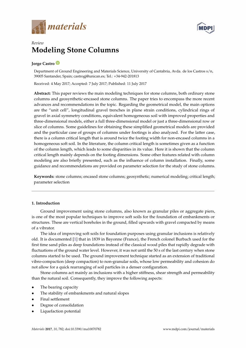
To simplify the real geometry of the problem that usually involves a considerable amount ofcolumns (e.g., Figure 1a) and to be able to deal with the problem, the following simplified geometricalmodels are usually adopted:

• “Unit cell” in axial symmetry (Figure 1b). Only one column and its corresponding surroundingsoil are studied. It may be useful to study just a horizontal slice of the unit cell, rather than thewhole length.

• Longitudinal gravel trenches (Figure 1c). The stone columns are transformed into longitudinalgravel trenches to study the problem in plane strain conditions.

• Cylindrical rings of gravel (Figure 1d). The columns are transformed into cylindrical rings ofgravel to study the problem in axial symmetry.

• Homogenization or equivalent homogeneous soil (Figure 1e). The columns and the surroundingsoil are transformed into a homogeneous soil with equivalent improved properties.

• Three-dimensional (3D) model of a row or slice of columns (Figure 1f).• Geometrical models for small groups of stone columns.• “Unit cell” with constant lateral pressure (triaxial conditions).• Isolated column.

Materials 2017, 10, 782 3 of 23

Materials 2017, 10, 782 3 of 23

(a) (b) (c)

(d) (e) (f)

Figure 1. Main geometrical models for stone column studies: (a) Full 3D model; (b) Unit cell; (c) Longitudinal gravel trenches; (d) Cylindrical gravel rings; (e) Equivalent homogenous soil; (f) 3D slice of columns.

The two latter cases, namely “unit cell” under triaxial conditions and isolated column, do not usually appear in real problems, but they have been used for laboratory tests (e.g., [11–13]). The case of an isolated column is widely used for field tests (usually plate load tests) for the sake of simplicity (e.g., [14]).

As a simple introductory comparison between the different geometrical models, Table 1 summarizes the suitability of some of these models to study the improvements achieved with a stone column treatment for the foundation of an embankment.

Table 1. Suitability of simplified geometrical models to study different features of a stone column treatment for the foundation of an embankment.

Geometrical Model Final Settlement Consolidation Stability Unit cell *** *** -

Gravel trenches ** ** ** Homogenization ** * *

3D slice *** *** *** *** Completely suitable, ** Moderately suitable, * Slightly suitable, - Not suitable.

All the geometrical models listed above are valid for non-encased stone columns. However, for encased stone columns, there is not yet any satisfactory way to convert the cylindrical encasement (geosynthetic) that surrounds the column for the cases of longitudinal gravel trenches and cylindrical rings of gravel.

3. Unit Cell

The unit cell model is the most widely used for theoretical analyses and it is reviewed in detail, for example, in [15]. The basis for the simplified model is the usage of a great number of columns, uniformly distributed in a wide area under a uniform load. This is the case, for example, in the central part of an embankment on soft ground improved with stone columns. In these situations, the behavior of all the columns is the same and then, it is enough to study the behavior of just one column with the corresponding surrounding soil (tributary area). Due to symmetry conditions, at the external lateral boundary of the unit cell, only vertical displacements and only vertical water seepage are allowed.

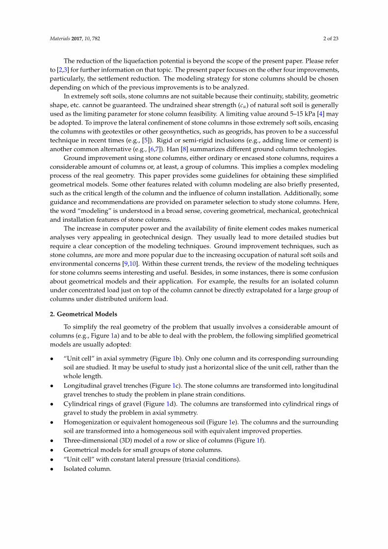
Stone columns are generally uniformly distributed in triangular or square grids. Thus, the tributary area of natural soil for each column is a hexagon or a square, respectively. To allow for axial symmetry conditions, the tributary area is transformed into a circle (cylinder) of the same (cross-sectional) area. Therefore, the diameter of the unit cell is equal to = 1.05 − 1.13 for triangular and square grids, respectively, where is the centre-to-centre distance between columns (Figure 2). Figure 3 shows the unit cell model with axial symmetry that can be studied in two dimensions.

Figure 1. Main geometrical models for stone column studies: (a) Full 3D model; (b) Unit cell; (c)Longitudinal gravel trenches; (d) Cylindrical gravel rings; (e) Equivalent homogenous soil; (f) 3D sliceof columns.

The two latter cases, namely “unit cell” under triaxial conditions and isolated column, do notusually appear in real problems, but they have been used for laboratory tests (e.g., [11–13]). The caseof an isolated column is widely used for field tests (usually plate load tests) for the sake of simplicity(e.g., [14]).

As a simple introductory comparison between the different geometrical models, Table 1summarizes the suitability of some of these models to study the improvements achieved with astone column treatment for the foundation of an embankment.

Table 1. Suitability of simplified geometrical models to study different features of a stone columntreatment for the foundation of an embankment.

Geometrical Model Final Settlement Consolidation Stability

Unit cell *** *** -Gravel trenches ** ** **

Homogenization ** * *3D slice *** *** ***

*** Completely suitable, ** Moderately suitable, * Slightly suitable, - Not suitable.

All the geometrical models listed above are valid for non-encased stone columns. However,for encased stone columns, there is not yet any satisfactory way to convert the cylindrical encasement(geosynthetic) that surrounds the column for the cases of longitudinal gravel trenches and cylindricalrings of gravel.

3. Unit Cell

The unit cell model is the most widely used for theoretical analyses and it is reviewed in detail,for example, in [15]. The basis for the simplified model is the usage of a great number of columns,uniformly distributed in a wide area under a uniform load. This is the case, for example, in the centralpart of an embankment on soft ground improved with stone columns. In these situations, the behaviorof all the columns is the same and then, it is enough to study the behavior of just one column with thecorresponding surrounding soil (tributary area). Due to symmetry conditions, at the external lateralboundary of the unit cell, only vertical displacements and only vertical water seepage are allowed.

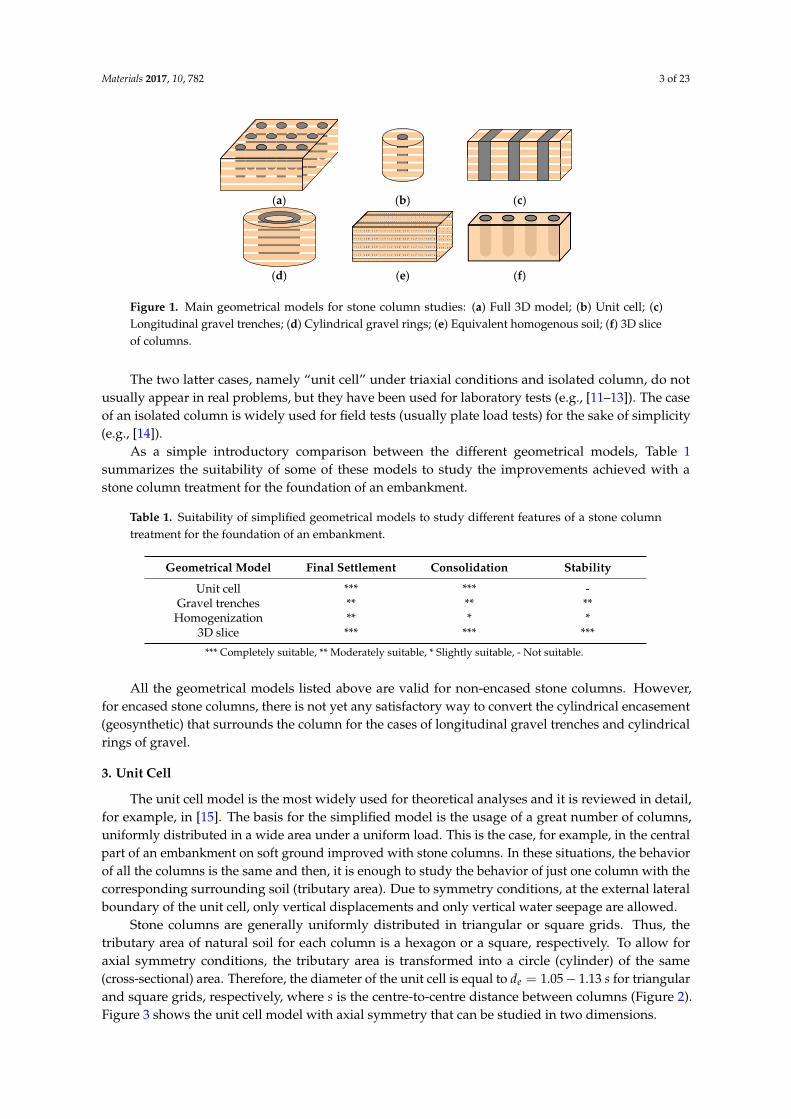
Stone columns are generally uniformly distributed in triangular or square grids. Thus, thetributary area of natural soil for each column is a hexagon or a square, respectively. To allow foraxial symmetry conditions, the tributary area is transformed into a circle (cylinder) of the same(cross-sectional) area. Therefore, the diameter of the unit cell is equal to de = 1.05− 1.13 s for triangularand square grids, respectively, where s is the centre-to-centre distance between columns (Figure 2).Figure 3 shows the unit cell model with axial symmetry that can be studied in two dimensions.

Materials 2017, 10, 782 4 of 23

Materials 2017, 10, 782 4 of 23

Figure 2. Simplification of the unit cell to axial symmetry conditions.

Figure 3. Unit cell model for analytical solutions.

The unit cell model is used for most of the existing analytical solutions (e.g., [16,17]). In the analytical solutions, there is usually a further simplifying assumption for the geometry, which is to assume that the behavior of each horizontal slice is independent, i.e., the shear stresses are neglected. Numerical analyses [17,18] show that shear stresses are usually negligible for distributed loads. Balaam and Booker [19] is a notable exception to the simplifying assumption of neglecting shear stresses because they study the total length of the unit cell as a whole. Nevertheless, the solution requires numerical integration, which makes the solution complex for practical purposes.

Most analytical solutions focus on the settlement reduction caused by stone columns (e.g., [16,17,19]), but stone columns also act as vertical drains and, therefore, they dissipate excess pore pressures. The consolidation process may be studied independently from the settlement analysis using solutions for vertical drains [20,21]. Han and Ye [22] and Castro and Sagaseta [23] showed that the consolidation process around stone columns is slightly different because of the distribution of vertical stresses between soft soil and stone columns and they proposed specific analytical solutions to study the consolidation process around stone columns. Very recently, Pulko and Logar [24] have developed a fully coupled solution for the consolidation process assuming the soil as a poroelastic medium and the stone column as an elastoplastic material. The solution is very accurate but requires numerical inversion of the Laplace transform.

Extending analytical solutions for ordinary stone columns to encased stone columns is quite straightforward (e.g., [25]). Equilibrium and compatibility conditions of the geosynthetic encasement are those of a thin-walled tube, or better said, those of a flexible membrane because the encasement does not usually support compressive stresses. The internal and external pressures are here denoted as

re rc s rc

re

s

Figure 2. Simplification of the unit cell to axial symmetry conditions.

Materials 2017, 10, 782 4 of 23

Figure 2. Simplification of the unit cell to axial symmetry conditions.

Figure 3. Unit cell model for analytical solutions.

The unit cell model is used for most of the existing analytical solutions (e.g., [16,17]). In the analytical solutions, there is usually a further simplifying assumption for the geometry, which is to assume that the behavior of each horizontal slice is independent, i.e., the shear stresses are neglected. Numerical analyses [17,18] show that shear stresses are usually negligible for distributed loads. Balaam and Booker [19] is a notable exception to the simplifying assumption of neglecting shear stresses because they study the total length of the unit cell as a whole. Nevertheless, the solution requires numerical integration, which makes the solution complex for practical purposes.

Most analytical solutions focus on the settlement reduction caused by stone columns (e.g., [16,17,19]), but stone columns also act as vertical drains and, therefore, they dissipate excess pore pressures. The consolidation process may be studied independently from the settlement analysis using solutions for vertical drains [20,21]. Han and Ye [22] and Castro and Sagaseta [23] showed that the consolidation process around stone columns is slightly different because of the distribution of vertical stresses between soft soil and stone columns and they proposed specific analytical solutions to study the consolidation process around stone columns. Very recently, Pulko and Logar [24] have developed a fully coupled solution for the consolidation process assuming the soil as a poroelastic medium and the stone column as an elastoplastic material. The solution is very accurate but requires numerical inversion of the Laplace transform.

Extending analytical solutions for ordinary stone columns to encased stone columns is quite straightforward (e.g., [25]). Equilibrium and compatibility conditions of the geosynthetic encasement are those of a thin-walled tube, or better said, those of a flexible membrane because the encasement does not usually support compressive stresses. The internal and external pressures are here denoted as

re rc s rc

re

s

Figure 3. Unit cell model for analytical solutions.

The unit cell model is used for most of the existing analytical solutions (e.g., [16,17]). In theanalytical solutions, there is usually a further simplifying assumption for the geometry, which is toassume that the behavior of each horizontal slice is independent, i.e., the shear stresses are neglected.Numerical analyses [17,18] show that shear stresses are usually negligible for distributed loads. Balaamand Booker [19] is a notable exception to the simplifying assumption of neglecting shear stressesbecause they study the total length of the unit cell as a whole. Nevertheless, the solution requiresnumerical integration, which makes the solution complex for practical purposes.

Most analytical solutions focus on the settlement reduction caused by stone columns(e.g., [16,17,19]), but stone columns also act as vertical drains and, therefore, they dissipate excess porepressures. The consolidation process may be studied independently from the settlement analysis usingsolutions for vertical drains [20,21]. Han and Ye [22] and Castro and Sagaseta [23] showed that theconsolidation process around stone columns is slightly different because of the distribution of verticalstresses between soft soil and stone columns and they proposed specific analytical solutions to studythe consolidation process around stone columns. Very recently, Pulko and Logar [24] have developeda fully coupled solution for the consolidation process assuming the soil as a poroelastic medium andthe stone column as an elastoplastic material. The solution is very accurate but requires numericalinversion of the Laplace transform.

Extending analytical solutions for ordinary stone columns to encased stone columns is quitestraightforward (e.g., [25]). Equilibrium and compatibility conditions of the geosynthetic encasementare those of a thin-walled tube, or better said, those of a flexible membrane because the encasementdoes not usually support compressive stresses. The internal and external pressures are here denoted

Materials 2017, 10, 782 5 of 23

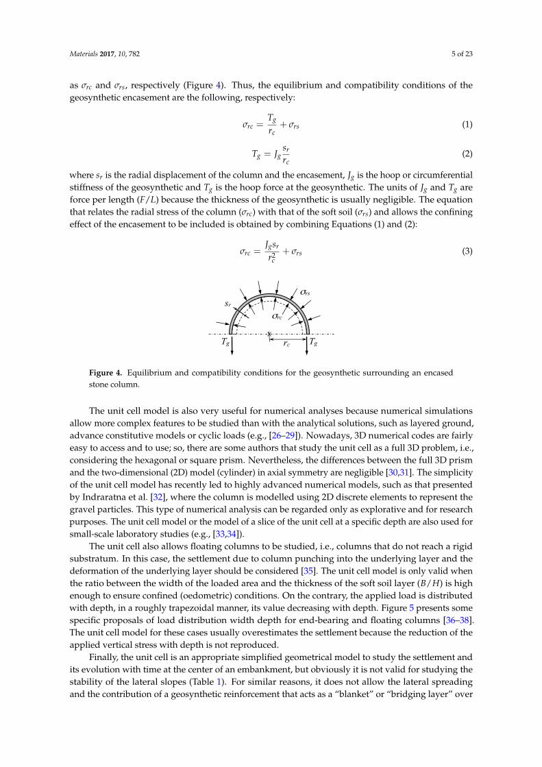
as σrc and σrs, respectively (Figure 4). Thus, the equilibrium and compatibility conditions of thegeosynthetic encasement are the following, respectively:

σrc =Tg

rc+ σrs (1)

Tg = Jgsr

rc(2)

where sr is the radial displacement of the column and the encasement, Jg is the hoop or circumferentialstiffness of the geosynthetic and Tg is the hoop force at the geosynthetic. The units of Jg and Tg areforce per length (F/L) because the thickness of the geosynthetic is usually negligible. The equationthat relates the radial stress of the column (σrc) with that of the soft soil (σrs) and allows the confiningeffect of the encasement to be included is obtained by combining Equations (1) and (2):

σrc =Jgsr

r2c

+ σrs (3)

Materials 2017, 10, 782 5 of 23

and , respectively (Figure 4). Thus, the equilibrium and compatibility conditions of the geosynthetic encasement are the following, respectively: = + (1)

= (2)

where is the radial displacement of the column and the encasement, is the hoop or circumferential stiffness of the geosynthetic and is the hoop force at the geosynthetic. The units of

and are force per length (F/L) because the thickness of the geosynthetic is usually negligible. The equation that relates the radial stress of the column ( ) with that of the soft soil ( ) and allows the confining effect of the encasement to be included is obtained by combining Equations (1) and (2): = + (3)

Figure 4. Equilibrium and compatibility conditions for the geosynthetic surrounding an encased stone column.

The unit cell model is also very useful for numerical analyses because numerical simulations allow more complex features to be studied than with the analytical solutions, such as layered ground, advance constitutive models or cyclic loads (e.g., [26–29]). Nowadays, 3D numerical codes are fairly easy to access and to use; so, there are some authors that study the unit cell as a full 3D problem, i.e., considering the hexagonal or square prism. Nevertheless, the differences between the full 3D prism and the two-dimensional (2D) model (cylinder) in axial symmetry are negligible [30,31]. The simplicity of the unit cell model has recently led to highly advanced numerical models, such as that presented by Indraratna et al. [32], where the column is modelled using 2D discrete elements to represent the gravel particles. This type of numerical analysis can be regarded only as explorative and for research purposes. The unit cell model or the model of a slice of the unit cell at a specific depth are also used for small-scale laboratory studies (e.g., [33,34]).

The unit cell also allows floating columns to be studied, i.e., columns that do not reach a rigid substratum. In this case, the settlement due to column punching into the underlying layer and the deformation of the underlying layer should be considered [35]. The unit cell model is only valid when the ratio between the width of the loaded area and the thickness of the soft soil layer ( / ) is high enough to ensure confined (oedometric) conditions. On the contrary, the applied load is distributed with depth, in a roughly trapezoidal manner, its value decreasing with depth. Figure 5 presents some specific proposals of load distribution width depth for end-bearing and floating columns [36–38]. The unit cell model for these cases usually overestimates the settlement because the reduction of the applied vertical stress with depth is not reproduced.

Finally, the unit cell is an appropriate simplified geometrical model to study the settlement and its evolution with time at the center of an embankment, but obviously it is not valid for studying the stability of the lateral slopes (Table 1). For similar reasons, it does not allow the lateral spreading and the contribution of a geosynthetic reinforcement that acts as a “blanket” or “bridging layer” over the columns and soft soil foundation (geosynthetic reinforced and column supported embankments,

rc Tg Tg

rs

rc

sr

Figure 4. Equilibrium and compatibility conditions for the geosynthetic surrounding an encasedstone column.

The unit cell model is also very useful for numerical analyses because numerical simulationsallow more complex features to be studied than with the analytical solutions, such as layered ground,advance constitutive models or cyclic loads (e.g., [26–29]). Nowadays, 3D numerical codes are fairlyeasy to access and to use; so, there are some authors that study the unit cell as a full 3D problem, i.e.,considering the hexagonal or square prism. Nevertheless, the differences between the full 3D prismand the two-dimensional (2D) model (cylinder) in axial symmetry are negligible [30,31]. The simplicityof the unit cell model has recently led to highly advanced numerical models, such as that presentedby Indraratna et al. [32], where the column is modelled using 2D discrete elements to represent thegravel particles. This type of numerical analysis can be regarded only as explorative and for researchpurposes. The unit cell model or the model of a slice of the unit cell at a specific depth are also used forsmall-scale laboratory studies (e.g., [33,34]).

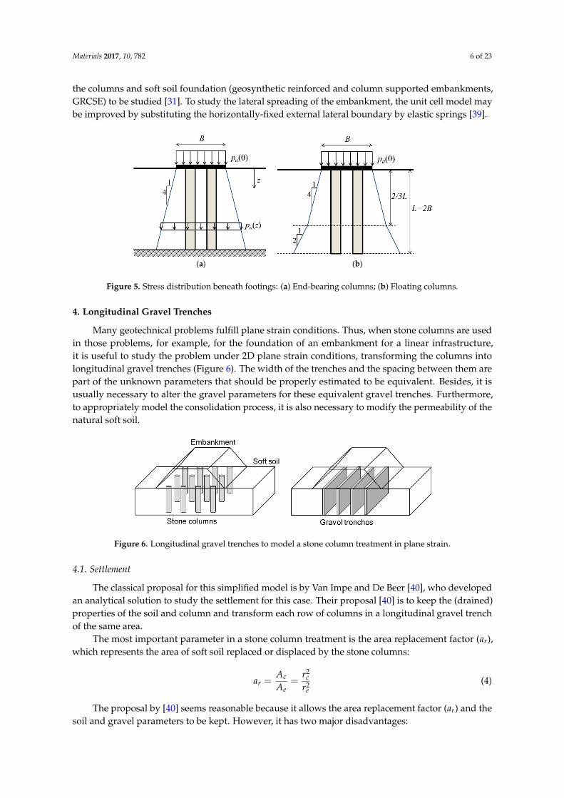
The unit cell also allows floating columns to be studied, i.e., columns that do not reach a rigidsubstratum. In this case, the settlement due to column punching into the underlying layer and thedeformation of the underlying layer should be considered [35]. The unit cell model is only valid whenthe ratio between the width of the loaded area and the thickness of the soft soil layer (B/H) is highenough to ensure confined (oedometric) conditions. On the contrary, the applied load is distributedwith depth, in a roughly trapezoidal manner, its value decreasing with depth. Figure 5 presents somespecific proposals of load distribution width depth for end-bearing and floating columns [36–38].The unit cell model for these cases usually overestimates the settlement because the reduction of theapplied vertical stress with depth is not reproduced.

Finally, the unit cell is an appropriate simplified geometrical model to study the settlement andits evolution with time at the center of an embankment, but obviously it is not valid for studying thestability of the lateral slopes (Table 1). For similar reasons, it does not allow the lateral spreadingand the contribution of a geosynthetic reinforcement that acts as a “blanket” or “bridging layer” over

Materials 2017, 10, 782 6 of 23

the columns and soft soil foundation (geosynthetic reinforced and column supported embankments,GRCSE) to be studied [31]. To study the lateral spreading of the embankment, the unit cell model maybe improved by substituting the horizontally-fixed external lateral boundary by elastic springs [39].

Materials 2017, 10, 782 6 of 23

GRCSE) to be studied [31]. To study the lateral spreading of the embankment, the unit cell model may be improved by substituting the horizontally-fixed external lateral boundary by elastic springs [39].

(a) (b)

Figure 5. Stress distribution beneath footings: (a) End-bearing columns; (b) Floating columns.

4. Longitudinal Gravel Trenches

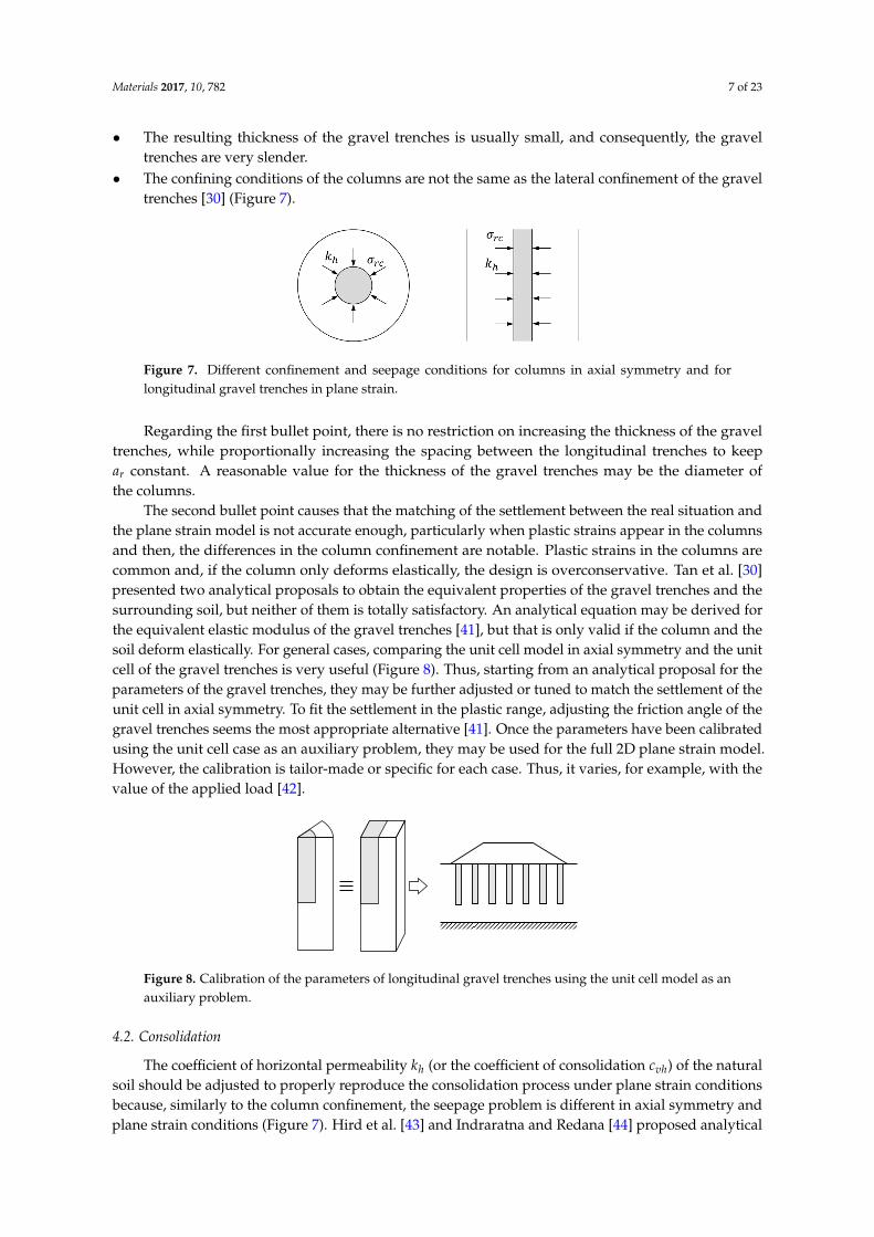
Many geotechnical problems fulfill plane strain conditions. Thus, when stone columns are used in those problems, for example, for the foundation of an embankment for a linear infrastructure, it is useful to study the problem under 2D plane strain conditions, transforming the columns into longitudinal gravel trenches (Figure 6). The width of the trenches and the spacing between them are part of the unknown parameters that should be properly estimated to be equivalent. Besides, it is usually necessary to alter the gravel parameters for these equivalent gravel trenches. Furthermore, to appropriately model the consolidation process, it is also necessary to modify the permeability of the natural soft soil.

Figure 6. Longitudinal gravel trenches to model a stone column treatment in plane strain.

4.1. Settlement

The classical proposal for this simplified model is by Van Impe and De Beer [40], who developed an analytical solution to study the settlement for this case. Their proposal [40] is to keep the (drained) properties of the soil and column and transform each row of columns in a longitudinal gravel trench of the same area.

The most important parameter in a stone column treatment is the area replacement factor ( ), which represents the area of soft soil replaced or displaced by the stone columns: = = (4)

The proposal by [40] seems reasonable because it allows the area replacement factor ( ) and the soil and gravel parameters to be kept. However, it has two major disadvantages:

Figure 5. Stress distribution beneath footings: (a) End-bearing columns; (b) Floating columns.

4. Longitudinal Gravel Trenches

Many geotechnical problems fulfill plane strain conditions. Thus, when stone columns are usedin those problems, for example, for the foundation of an embankment for a linear infrastructure,it is useful to study the problem under 2D plane strain conditions, transforming the columns intolongitudinal gravel trenches (Figure 6). The width of the trenches and the spacing between them arepart of the unknown parameters that should be properly estimated to be equivalent. Besides, it isusually necessary to alter the gravel parameters for these equivalent gravel trenches. Furthermore,to appropriately model the consolidation process, it is also necessary to modify the permeability of thenatural soft soil.

Materials 2017, 10, 782 6 of 23

GRCSE) to be studied [31]. To study the lateral spreading of the embankment, the unit cell model may be improved by substituting the horizontally-fixed external lateral boundary by elastic springs [39].

(a) (b)

Figure 5. Stress distribution beneath footings: (a) End-bearing columns; (b) Floating columns.

4. Longitudinal Gravel Trenches

Many geotechnical problems fulfill plane strain conditions. Thus, when stone columns are used in those problems, for example, for the foundation of an embankment for a linear infrastructure, it is useful to study the problem under 2D plane strain conditions, transforming the columns into longitudinal gravel trenches (Figure 6). The width of the trenches and the spacing between them are part of the unknown parameters that should be properly estimated to be equivalent. Besides, it is usually necessary to alter the gravel parameters for these equivalent gravel trenches. Furthermore, to appropriately model the consolidation process, it is also necessary to modify the permeability of the natural soft soil.

Figure 6. Longitudinal gravel trenches to model a stone column treatment in plane strain.

4.1. Settlement

The classical proposal for this simplified model is by Van Impe and De Beer [40], who developed an analytical solution to study the settlement for this case. Their proposal [40] is to keep the (drained) properties of the soil and column and transform each row of columns in a longitudinal gravel trench of the same area.

The most important parameter in a stone column treatment is the area replacement factor ( ), which represents the area of soft soil replaced or displaced by the stone columns: = = (4)

The proposal by [40] seems reasonable because it allows the area replacement factor ( ) and the soil and gravel parameters to be kept. However, it has two major disadvantages:

Figure 6. Longitudinal gravel trenches to model a stone column treatment in plane strain.

4.1. Settlement

The classical proposal for this simplified model is by Van Impe and De Beer [40], who developedan analytical solution to study the settlement for this case. Their proposal [40] is to keep the (drained)properties of the soil and column and transform each row of columns in a longitudinal gravel trenchof the same area.

The most important parameter in a stone column treatment is the area replacement factor (ar),which represents the area of soft soil replaced or displaced by the stone columns:

ar =Ac

Ae=

r2c

r2e

(4)

The proposal by [40] seems reasonable because it allows the area replacement factor (ar) and thesoil and gravel parameters to be kept. However, it has two major disadvantages:

Materials 2017, 10, 782 7 of 23

• The resulting thickness of the gravel trenches is usually small, and consequently, the graveltrenches are very slender.

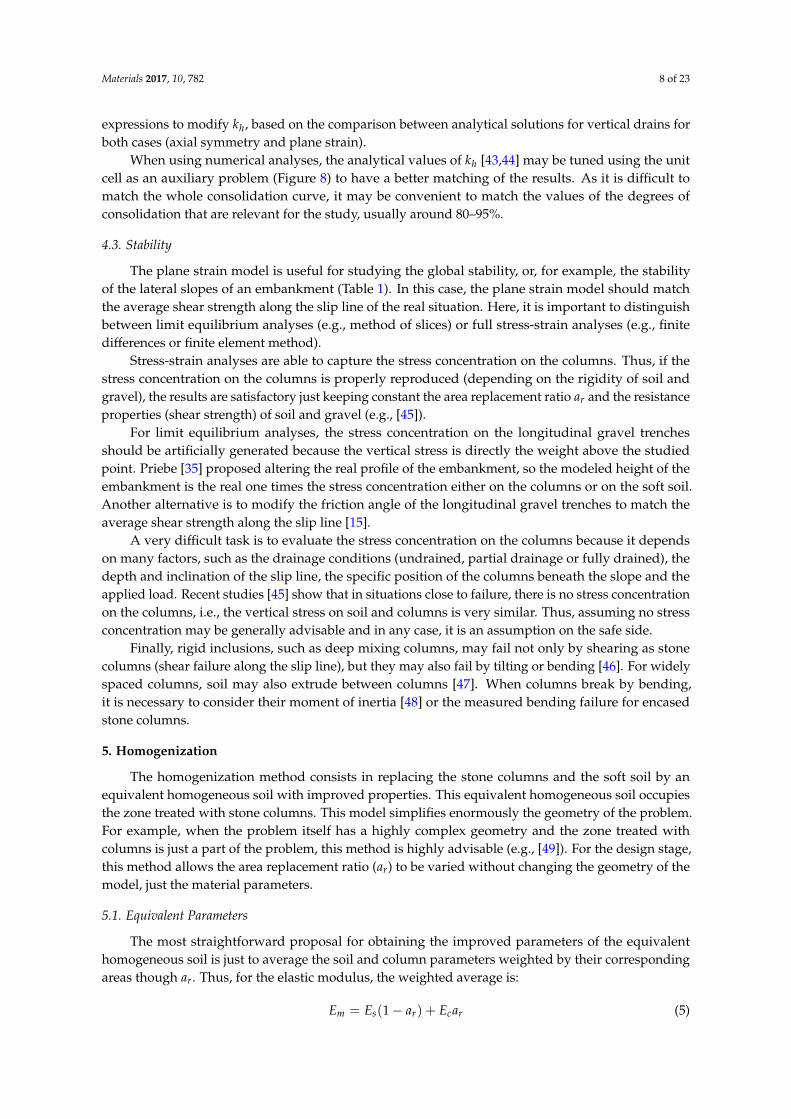
• The confining conditions of the columns are not the same as the lateral confinement of the graveltrenches [30] (Figure 7).

Materials 2017, 10, 782 7 of 23

The resulting thickness of the gravel trenches is usually small, and consequently, the gravel trenches are very slender.

The confining conditions of the columns are not the same as the lateral confinement of the gravel trenches [30] (Figure 7).

Figure 7. Different confinement and seepage conditions for columns in axial symmetry and for longitudinal gravel trenches in plane strain.

Regarding the first bullet point, there is no restriction on increasing the thickness of the gravel trenches, while proportionally increasing the spacing between the longitudinal trenches to keep constant. A reasonable value for the thickness of the gravel trenches may be the diameter of the columns.

The second bullet point causes that the matching of the settlement between the real situation and the plane strain model is not accurate enough, particularly when plastic strains appear in the columns and then, the differences in the column confinement are notable. Plastic strains in the columns are common and, if the column only deforms elastically, the design is overconservative. Tan et al. [30] presented two analytical proposals to obtain the equivalent properties of the gravel trenches and the surrounding soil, but neither of them is totally satisfactory. An analytical equation may be derived for the equivalent elastic modulus of the gravel trenches [41], but that is only valid if the column and the soil deform elastically. For general cases, comparing the unit cell model in axial symmetry and the unit cell of the gravel trenches is very useful (Figure 8). Thus, starting from an analytical proposal for the parameters of the gravel trenches, they may be further adjusted or tuned to match the settlement of the unit cell in axial symmetry. To fit the settlement in the plastic range, adjusting the friction angle of the gravel trenches seems the most appropriate alternative [41]. Once the parameters have been calibrated using the unit cell case as an auxiliary problem, they may be used for the full 2D plane strain model. However, the calibration is tailor-made or specific for each case. Thus, it varies, for example, with the value of the applied load [42].

Figure 8. Calibration of the parameters of longitudinal gravel trenches using the unit cell model as an auxiliary problem.

4.2. Consolidation

The coefficient of horizontal permeability (or the coefficient of consolidation ) of the natural soil should be adjusted to properly reproduce the consolidation process under plane strain conditions because, similarly to the column confinement, the seepage problem is different in axial symmetry and plane strain conditions (Figure 7). Hird et al. [43] and Indraratna and Redana [44]

Figure 7. Different confinement and seepage conditions for columns in axial symmetry and forlongitudinal gravel trenches in plane strain.

Regarding the first bullet point, there is no restriction on increasing the thickness of the graveltrenches, while proportionally increasing the spacing between the longitudinal trenches to keepar constant. A reasonable value for the thickness of the gravel trenches may be the diameter ofthe columns.

The second bullet point causes that the matching of the settlement between the real situation andthe plane strain model is not accurate enough, particularly when plastic strains appear in the columnsand then, the differences in the column confinement are notable. Plastic strains in the columns arecommon and, if the column only deforms elastically, the design is overconservative. Tan et al. [30]presented two analytical proposals to obtain the equivalent properties of the gravel trenches and thesurrounding soil, but neither of them is totally satisfactory. An analytical equation may be derived forthe equivalent elastic modulus of the gravel trenches [41], but that is only valid if the column and thesoil deform elastically. For general cases, comparing the unit cell model in axial symmetry and the unitcell of the gravel trenches is very useful (Figure 8). Thus, starting from an analytical proposal for theparameters of the gravel trenches, they may be further adjusted or tuned to match the settlement of theunit cell in axial symmetry. To fit the settlement in the plastic range, adjusting the friction angle of thegravel trenches seems the most appropriate alternative [41]. Once the parameters have been calibratedusing the unit cell case as an auxiliary problem, they may be used for the full 2D plane strain model.However, the calibration is tailor-made or specific for each case. Thus, it varies, for example, with thevalue of the applied load [42].

Materials 2017, 10, 782 7 of 23

The resulting thickness of the gravel trenches is usually small, and consequently, the gravel trenches are very slender.

The confining conditions of the columns are not the same as the lateral confinement of the gravel trenches [30] (Figure 7).

Figure 7. Different confinement and seepage conditions for columns in axial symmetry and for longitudinal gravel trenches in plane strain.

Regarding the first bullet point, there is no restriction on increasing the thickness of the gravel trenches, while proportionally increasing the spacing between the longitudinal trenches to keep constant. A reasonable value for the thickness of the gravel trenches may be the diameter of the columns.

The second bullet point causes that the matching of the settlement between the real situation and the plane strain model is not accurate enough, particularly when plastic strains appear in the columns and then, the differences in the column confinement are notable. Plastic strains in the columns are common and, if the column only deforms elastically, the design is overconservative. Tan et al. [30] presented two analytical proposals to obtain the equivalent properties of the gravel trenches and the surrounding soil, but neither of them is totally satisfactory. An analytical equation may be derived for the equivalent elastic modulus of the gravel trenches [41], but that is only valid if the column and the soil deform elastically. For general cases, comparing the unit cell model in axial symmetry and the unit cell of the gravel trenches is very useful (Figure 8). Thus, starting from an analytical proposal for the parameters of the gravel trenches, they may be further adjusted or tuned to match the settlement of the unit cell in axial symmetry. To fit the settlement in the plastic range, adjusting the friction angle of the gravel trenches seems the most appropriate alternative [41]. Once the parameters have been calibrated using the unit cell case as an auxiliary problem, they may be used for the full 2D plane strain model. However, the calibration is tailor-made or specific for each case. Thus, it varies, for example, with the value of the applied load [42].

Figure 8. Calibration of the parameters of longitudinal gravel trenches using the unit cell model as an auxiliary problem.

4.2. Consolidation

The coefficient of horizontal permeability (or the coefficient of consolidation ) of the natural soil should be adjusted to properly reproduce the consolidation process under plane strain conditions because, similarly to the column confinement, the seepage problem is different in axial symmetry and plane strain conditions (Figure 7). Hird et al. [43] and Indraratna and Redana [44]

Figure 8. Calibration of the parameters of longitudinal gravel trenches using the unit cell model as anauxiliary problem.

4.2. Consolidation

The coefficient of horizontal permeability kh (or the coefficient of consolidation cvh) of the naturalsoil should be adjusted to properly reproduce the consolidation process under plane strain conditionsbecause, similarly to the column confinement, the seepage problem is different in axial symmetry andplane strain conditions (Figure 7). Hird et al. [43] and Indraratna and Redana [44] proposed analytical

Materials 2017, 10, 782 8 of 23

expressions to modify kh, based on the comparison between analytical solutions for vertical drains forboth cases (axial symmetry and plane strain).

When using numerical analyses, the analytical values of kh [43,44] may be tuned using the unitcell as an auxiliary problem (Figure 8) to have a better matching of the results. As it is difficult tomatch the whole consolidation curve, it may be convenient to match the values of the degrees ofconsolidation that are relevant for the study, usually around 80–95%.

4.3. Stability

The plane strain model is useful for studying the global stability, or, for example, the stabilityof the lateral slopes of an embankment (Table 1). In this case, the plane strain model should matchthe average shear strength along the slip line of the real situation. Here, it is important to distinguishbetween limit equilibrium analyses (e.g., method of slices) or full stress-strain analyses (e.g., finitedifferences or finite element method).

Stress-strain analyses are able to capture the stress concentration on the columns. Thus, if thestress concentration on the columns is properly reproduced (depending on the rigidity of soil andgravel), the results are satisfactory just keeping constant the area replacement ratio ar and the resistanceproperties (shear strength) of soil and gravel (e.g., [45]).

For limit equilibrium analyses, the stress concentration on the longitudinal gravel trenchesshould be artificially generated because the vertical stress is directly the weight above the studiedpoint. Priebe [35] proposed altering the real profile of the embankment, so the modeled height of theembankment is the real one times the stress concentration either on the columns or on the soft soil.Another alternative is to modify the friction angle of the longitudinal gravel trenches to match theaverage shear strength along the slip line [15].

A very difficult task is to evaluate the stress concentration on the columns because it dependson many factors, such as the drainage conditions (undrained, partial drainage or fully drained), thedepth and inclination of the slip line, the specific position of the columns beneath the slope and theapplied load. Recent studies [45] show that in situations close to failure, there is no stress concentrationon the columns, i.e., the vertical stress on soil and columns is very similar. Thus, assuming no stressconcentration may be generally advisable and in any case, it is an assumption on the safe side.

Finally, rigid inclusions, such as deep mixing columns, may fail not only by shearing as stonecolumns (shear failure along the slip line), but they may also fail by tilting or bending [46]. For widelyspaced columns, soil may also extrude between columns [47]. When columns break by bending,it is necessary to consider their moment of inertia [48] or the measured bending failure for encasedstone columns.

5. Homogenization

The homogenization method consists in replacing the stone columns and the soft soil by anequivalent homogeneous soil with improved properties. This equivalent homogeneous soil occupiesthe zone treated with stone columns. This model simplifies enormously the geometry of the problem.For example, when the problem itself has a highly complex geometry and the zone treated withcolumns is just a part of the problem, this method is highly advisable (e.g., [49]). For the design stage,this method allows the area replacement ratio (ar) to be varied without changing the geometry of themodel, just the material parameters.

5.1. Equivalent Parameters

The most straightforward proposal for obtaining the improved parameters of the equivalenthomogeneous soil is just to average the soil and column parameters weighted by their correspondingareas though ar. Thus, for the elastic modulus, the weighted average is:

Em = Es(1− ar) + Ecar (5)

Materials 2017, 10, 782 9 of 23

However, this can only be regarded as a first approximation. A more detailed analysis showsthat the equivalent homogenous soil should be anisotropic by nature to account for the columnorientation [50]. Some authors (e.g., [51–53]) use theories for periodic media to propose analyticaltransformations from the columns and the soft soil (heterogeneous periodic composite material atthe microscale) to a homogeneous equivalent soil (homogenous material at a macroscale). They use amacroscopic strength criterion of the anisotropic homogeneous equivalent soil to evaluate the bearingcapacity. The practical application of these techniques is complex and they are only valid for sufficientlysmall values of the scale factor, i.e., the ratio between the micro and macroscales, for example, the ratiobetween the column spacing and the characteristic size of the whole problem to be studied.

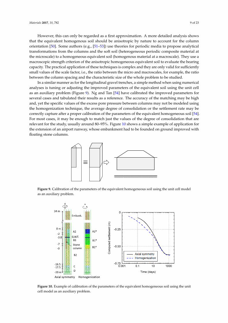
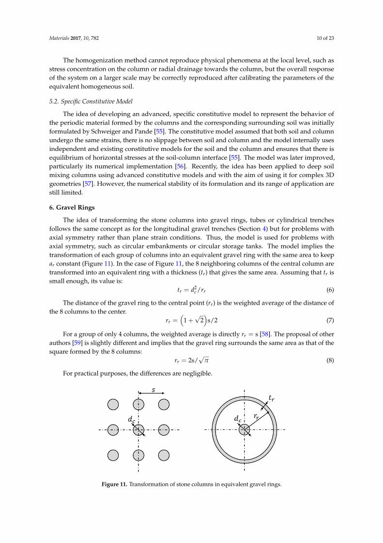
In a similar manner as for the longitudinal gravel trenches, a simple method when using numericalanalyses is tuning or adjusting the improved parameters of the equivalent soil using the unit cellas an auxiliary problem (Figure 9). Ng and Tan [54] have calibrated the improved parameters forseveral cases and tabulated their results as a reference. The accuracy of the matching may be highand, yet the specific values of the excess pore pressure between columns may not be modeled usingthe homogenization technique, the average degree of consolidation or the settlement rate may becorrectly capture after a proper calibration of the parameters of the equivalent homogeneous soil [54].For most cases, it may be enough to match just the values of the degree of consolidation that arerelevant for the study, usually around 80–95%. Figure 10 shows a simple example of application forthe extension of an airport runway, whose embankment had to be founded on ground improved withfloating stone columns.

Materials 2017, 10, 782 9 of 23

orientation [50]. Some authors (e.g., [51–53]) use theories for periodic media to propose analytical transformations from the columns and the soft soil (heterogeneous periodic composite material at the microscale) to a homogeneous equivalent soil (homogenous material at a macroscale). They use a macroscopic strength criterion of the anisotropic homogeneous equivalent soil to evaluate the bearing capacity. The practical application of these techniques is complex and they are only valid for sufficiently small values of the scale factor, i.e., the ratio between the micro and macroscales, for example, the ratio between the column spacing and the characteristic size of the whole problem to be studied.

In a similar manner as for the longitudinal gravel trenches, a simple method when using numerical analyses is tuning or adjusting the improved parameters of the equivalent soil using the unit cell as an auxiliary problem (Figure 9). Ng and Tan [54] have calibrated the improved parameters for several cases and tabulated their results as a reference. The accuracy of the matching may be high and, yet the specific values of the excess pore pressure between columns may not be modeled using the homogenization technique, the average degree of consolidation or the settlement rate may be correctly capture after a proper calibration of the parameters of the equivalent homogeneous soil [54]. For most cases, it may be enough to match just the values of the degree of consolidation that are relevant for the study, usually around 80–95%. Figure 10 shows a simple example of application for the extension of an airport runway, whose embankment had to be founded on ground improved with floating stone columns.

Figure 9. Calibration of the parameters of the equivalent homogeneous soil using the unit cell model as an auxiliary problem.

Figure 10. Example of calibration of the parameters of the equivalent homogeneous soil using the unit cell model as an auxiliary problem.

The homogenization method cannot reproduce physical phenomena at the local level, such as stress concentration on the column or radial drainage towards the column, but the overall response

Figure 9. Calibration of the parameters of the equivalent homogeneous soil using the unit cell modelas an auxiliary problem.

Materials 2017, 10, 782 9 of 23

orientation [50]. Some authors (e.g., [51–53]) use theories for periodic media to propose analytical transformations from the columns and the soft soil (heterogeneous periodic composite material at the microscale) to a homogeneous equivalent soil (homogenous material at a macroscale). They use a macroscopic strength criterion of the anisotropic homogeneous equivalent soil to evaluate the bearing capacity. The practical application of these techniques is complex and they are only valid for sufficiently small values of the scale factor, i.e., the ratio between the micro and macroscales, for example, the ratio between the column spacing and the characteristic size of the whole problem to be studied.

In a similar manner as for the longitudinal gravel trenches, a simple method when using numerical analyses is tuning or adjusting the improved parameters of the equivalent soil using the unit cell as an auxiliary problem (Figure 9). Ng and Tan [54] have calibrated the improved parameters for several cases and tabulated their results as a reference. The accuracy of the matching may be high and, yet the specific values of the excess pore pressure between columns may not be modeled using the homogenization technique, the average degree of consolidation or the settlement rate may be correctly capture after a proper calibration of the parameters of the equivalent homogeneous soil [54]. For most cases, it may be enough to match just the values of the degree of consolidation that are relevant for the study, usually around 80–95%. Figure 10 shows a simple example of application for the extension of an airport runway, whose embankment had to be founded on ground improved with floating stone columns.

Figure 9. Calibration of the parameters of the equivalent homogeneous soil using the unit cell model as an auxiliary problem.

Figure 10. Example of calibration of the parameters of the equivalent homogeneous soil using the unit cell model as an auxiliary problem.

The homogenization method cannot reproduce physical phenomena at the local level, such as stress concentration on the column or radial drainage towards the column, but the overall response

Figure 10. Example of calibration of the parameters of the equivalent homogeneous soil using the unitcell model as an auxiliary problem.

Materials 2017, 10, 782 10 of 23

The homogenization method cannot reproduce physical phenomena at the local level, such asstress concentration on the column or radial drainage towards the column, but the overall responseof the system on a larger scale may be correctly reproduced after calibrating the parameters of theequivalent homogeneous soil.

5.2. Specific Constitutive Model

The idea of developing an advanced, specific constitutive model to represent the behavior ofthe periodic material formed by the columns and the corresponding surrounding soil was initiallyformulated by Schweiger and Pande [55]. The constitutive model assumed that both soil and columnundergo the same strains, there is no slippage between soil and column and the model internally usesindependent and existing constitutive models for the soil and the column and ensures that there isequilibrium of horizontal stresses at the soil-column interface [55]. The model was later improved,particularly its numerical implementation [56]. Recently, the idea has been applied to deep soilmixing columns using advanced constitutive models and with the aim of using it for complex 3Dgeometries [57]. However, the numerical stability of its formulation and its range of application arestill limited.

6. Gravel Rings

The idea of transforming the stone columns into gravel rings, tubes or cylindrical trenchesfollows the same concept as for the longitudinal gravel trenches (Section 4) but for problems withaxial symmetry rather than plane strain conditions. Thus, the model is used for problems withaxial symmetry, such as circular embankments or circular storage tanks. The model implies thetransformation of each group of columns into an equivalent gravel ring with the same area to keepar constant (Figure 11). In the case of Figure 11, the 8 neighboring columns of the central column aretransformed into an equivalent ring with a thickness (tr) that gives the same area. Assuming that tr issmall enough, its value is:

tr = d2c /rr (6)

The distance of the gravel ring to the central point (rr) is the weighted average of the distance ofthe 8 columns to the center.

rr =(

1 +√

2)

s/2 (7)

For a group of only 4 columns, the weighted average is directly rr = s [58]. The proposal of otherauthors [59] is slightly different and implies that the gravel ring surrounds the same area as that of thesquare formed by the 8 columns:

rr = 2s/√

π (8)

For practical purposes, the differences are negligible.

Materials 2017, 10, 782 10 of 23

of the system on a larger scale may be correctly reproduced after calibrating the parameters of the equivalent homogeneous soil.

5.2. Specific Constitutive Model

The idea of developing an advanced, specific constitutive model to represent the behavior of the periodic material formed by the columns and the corresponding surrounding soil was initially formulated by Schweiger and Pande [55]. The constitutive model assumed that both soil and column undergo the same strains, there is no slippage between soil and column and the model internally uses independent and existing constitutive models for the soil and the column and ensures that there is equilibrium of horizontal stresses at the soil-column interface [55]. The model was later improved, particularly its numerical implementation [56]. Recently, the idea has been applied to deep soil mixing columns using advanced constitutive models and with the aim of using it for complex 3D geometries [57]. However, the numerical stability of its formulation and its range of application are still limited.

6. Gravel Rings

The idea of transforming the stone columns into gravel rings, tubes or cylindrical trenches follows the same concept as for the longitudinal gravel trenches (Section 4) but for problems with axial symmetry rather than plane strain conditions. Thus, the model is used for problems with axial symmetry, such as circular embankments or circular storage tanks. The model implies the transformation of each group of columns into an equivalent gravel ring with the same area to keep

constant (Figure 11). In the case of Figure 11, the 8 neighboring columns of the central column are transformed into an equivalent ring with a thickness ( ) that gives the same area. Assuming that is small enough, its value is: = / (6)

The distance of the gravel ring to the central point ( ) is the weighted average of the distance of the 8 columns to the center. = 1 + √2 s/2 (7)

For a group of only 4 columns, the weighted average is directly = s [58]. The proposal of other authors [59] is slightly different and implies that the gravel ring surrounds the same area as that of the square formed by the 8 columns: = 2s/√ (8)

For practical purposes, the differences are negligible.

Figure 11. Transformation of stone columns in equivalent gravel rings.

Figure 11. Transformation of stone columns in equivalent gravel rings.

Materials 2017, 10, 782 11 of 23

Mitchel and Huber [58] seem to be the first authors to use this model. They used it in combinationwith the finite element method to study a field case (the foundation of a water treatment plant).Contrary to the model of the longitudinal gravel trenches, here the confining conditions of the gravelrings seem to be somehow similar to those of the stone columns and it is enough to maintain the valuesof ar and of the drained properties of the soil and the columns to obtain satisfactory results [60,61].As for the longitudinal gravel trenches, there is not yet any satisfactory way to convert the cylindricalencasement (geosynthetic) that surrounds the columns for this case.

7. Three-Dimensional Slice of Columns

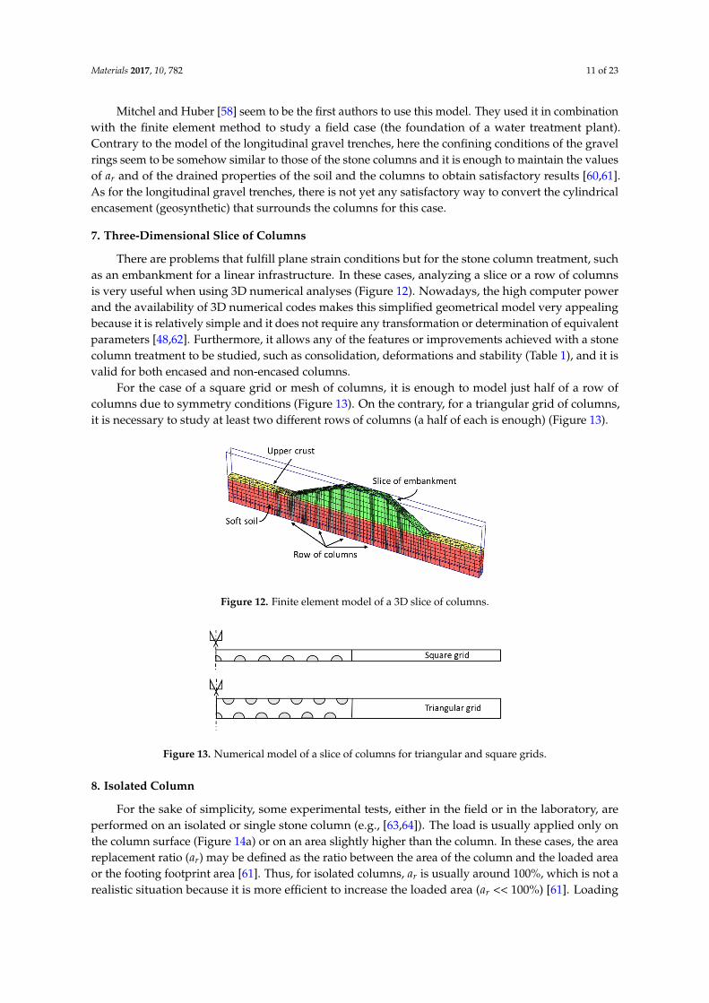
There are problems that fulfill plane strain conditions but for the stone column treatment, suchas an embankment for a linear infrastructure. In these cases, analyzing a slice or a row of columnsis very useful when using 3D numerical analyses (Figure 12). Nowadays, the high computer powerand the availability of 3D numerical codes makes this simplified geometrical model very appealingbecause it is relatively simple and it does not require any transformation or determination of equivalentparameters [48,62]. Furthermore, it allows any of the features or improvements achieved with a stonecolumn treatment to be studied, such as consolidation, deformations and stability (Table 1), and it isvalid for both encased and non-encased columns.

For the case of a square grid or mesh of columns, it is enough to model just half of a row ofcolumns due to symmetry conditions (Figure 13). On the contrary, for a triangular grid of columns,it is necessary to study at least two different rows of columns (a half of each is enough) (Figure 13).

Materials 2017, 10, 782 11 of 23

Mitchel and Huber [58] seem to be the first authors to use this model. They used it in combination with the finite element method to study a field case (the foundation of a water treatment plant). Contrary to the model of the longitudinal gravel trenches, here the confining conditions of the gravel rings seem to be somehow similar to those of the stone columns and it is enough to maintain the values of and of the drained properties of the soil and the columns to obtain satisfactory results [60,61]. As for the longitudinal gravel trenches, there is not yet any satisfactory way to convert the cylindrical encasement (geosynthetic) that surrounds the columns for this case.

7. Three-Dimensional Slice of Columns

There are problems that fulfill plane strain conditions but for the stone column treatment, such as an embankment for a linear infrastructure. In these cases, analyzing a slice or a row of columns is very useful when using 3D numerical analyses (Figure 12). Nowadays, the high computer power and the availability of 3D numerical codes makes this simplified geometrical model very appealing because it is relatively simple and it does not require any transformation or determination of equivalent parameters [48,62]. Furthermore, it allows any of the features or improvements achieved with a stone column treatment to be studied, such as consolidation, deformations and stability (Table 1), and it is valid for both encased and non-encased columns.

For the case of a square grid or mesh of columns, it is enough to model just half of a row of columns due to symmetry conditions (Figure 13). On the contrary, for a triangular grid of columns, it is necessary to study at least two different rows of columns (a half of each is enough) (Figure 13).

Figure 12. Finite element model of a 3D slice of columns.

Figure 13. Numerical model of a slice of columns for triangular and square grids.

8. Isolated Column

For the sake of simplicity, some experimental tests, either in the field or in the laboratory, are performed on an isolated or single stone column (e.g., [63,64]). The load is usually applied only on the column surface (Figure 14a) or on an area slightly higher than the column. In these cases, the area replacement ratio ( ) may be defined as the ratio between the area of the column and the loaded area or the footing footprint area [61]. Thus, for isolated columns, is usually around 100%, which is not a realistic situation because it is more efficient to increase the loaded area ( << 100%) [61].

Figure 12. Finite element model of a 3D slice of columns.

Materials 2017, 10, 782 11 of 23

Mitchel and Huber [58] seem to be the first authors to use this model. They used it in combination with the finite element method to study a field case (the foundation of a water treatment plant). Contrary to the model of the longitudinal gravel trenches, here the confining conditions of the gravel rings seem to be somehow similar to those of the stone columns and it is enough to maintain the values of and of the drained properties of the soil and the columns to obtain satisfactory results [60,61]. As for the longitudinal gravel trenches, there is not yet any satisfactory way to convert the cylindrical encasement (geosynthetic) that surrounds the columns for this case.

7. Three-Dimensional Slice of Columns

There are problems that fulfill plane strain conditions but for the stone column treatment, such as an embankment for a linear infrastructure. In these cases, analyzing a slice or a row of columns is very useful when using 3D numerical analyses (Figure 12). Nowadays, the high computer power and the availability of 3D numerical codes makes this simplified geometrical model very appealing because it is relatively simple and it does not require any transformation or determination of equivalent parameters [48,62]. Furthermore, it allows any of the features or improvements achieved with a stone column treatment to be studied, such as consolidation, deformations and stability (Table 1), and it is valid for both encased and non-encased columns.

For the case of a square grid or mesh of columns, it is enough to model just half of a row of columns due to symmetry conditions (Figure 13). On the contrary, for a triangular grid of columns, it is necessary to study at least two different rows of columns (a half of each is enough) (Figure 13).

Figure 12. Finite element model of a 3D slice of columns.

Figure 13. Numerical model of a slice of columns for triangular and square grids.

8. Isolated Column

For the sake of simplicity, some experimental tests, either in the field or in the laboratory, are performed on an isolated or single stone column (e.g., [63,64]). The load is usually applied only on the column surface (Figure 14a) or on an area slightly higher than the column. In these cases, the area replacement ratio ( ) may be defined as the ratio between the area of the column and the loaded area or the footing footprint area [61]. Thus, for isolated columns, is usually around 100%, which is not a realistic situation because it is more efficient to increase the loaded area ( << 100%) [61].

Figure 13. Numerical model of a slice of columns for triangular and square grids.

8. Isolated Column

For the sake of simplicity, some experimental tests, either in the field or in the laboratory, areperformed on an isolated or single stone column (e.g., [63,64]). The load is usually applied only onthe column surface (Figure 14a) or on an area slightly higher than the column. In these cases, the areareplacement ratio (ar) may be defined as the ratio between the area of the column and the loaded areaor the footing footprint area [61]. Thus, for isolated columns, ar is usually around 100%, which is not arealistic situation because it is more efficient to increase the loaded area (ar << 100%) [61]. Loading

Materials 2017, 10, 782 12 of 23

the surroundings of the columns is beneficial because it increases the horizontal stresses at the lateralboundaries of the columns and increases their confinement.

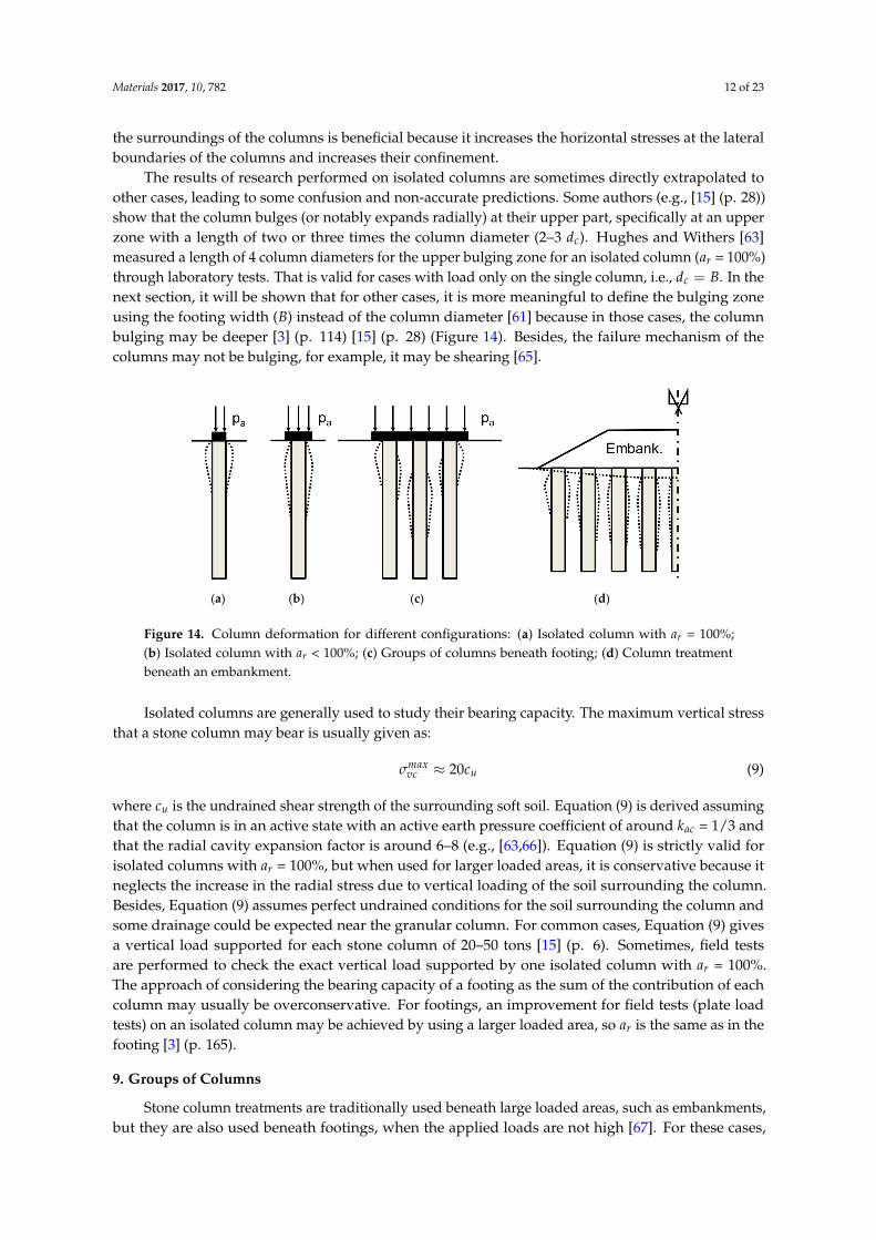
The results of research performed on isolated columns are sometimes directly extrapolated toother cases, leading to some confusion and non-accurate predictions. Some authors (e.g., [15] (p. 28))show that the column bulges (or notably expands radially) at their upper part, specifically at an upperzone with a length of two or three times the column diameter (2–3 dc). Hughes and Withers [63]measured a length of 4 column diameters for the upper bulging zone for an isolated column (ar = 100%)through laboratory tests. That is valid for cases with load only on the single column, i.e., dc = B. In thenext section, it will be shown that for other cases, it is more meaningful to define the bulging zoneusing the footing width (B) instead of the column diameter [61] because in those cases, the columnbulging may be deeper [3] (p. 114) [15] (p. 28) (Figure 14). Besides, the failure mechanism of thecolumns may not be bulging, for example, it may be shearing [65].

Materials 2017, 10, 782 12 of 23

Loading the surroundings of the columns is beneficial because it increases the horizontal stresses at the lateral boundaries of the columns and increases their confinement.

The results of research performed on isolated columns are sometimes directly extrapolated to other cases, leading to some confusion and non-accurate predictions. Some authors (e.g., [15] (p. 28)) show that the column bulges (or notably expands radially) at their upper part, specifically at an upper zone with a length of two or three times the column diameter (2–3 ). Hughes and Withers [63] measured a length of 4 column diameters for the upper bulging zone for an isolated column ( = 100%) through laboratory tests. That is valid for cases with load only on the single column, i.e., = . In the next section, it will be shown that for other cases, it is more meaningful to define the bulging zone using the footing width ( ) instead of the column diameter [61] because in those cases, the column bulging may be deeper [3] (p. 114) [15] (p. 28) (Figure 14). Besides, the failure mechanism of the columns may not be bulging, for example, it may be shearing [65].

(a) (b) (c) (d)

Figure 14. Column deformation for different configurations: (a) Isolated column with = 100%; (b) Isolated column with < 100%; (c) Groups of columns beneath footing; (d) Column treatment beneath an embankment.

Isolated columns are generally used to study their bearing capacity. The maximum vertical stress that a stone column may bear is usually given as: 20 (9)

where is the undrained shear strength of the surrounding soft soil. Equation (9) is derived assuming that the column is in an active state with an active earth pressure coefficient of around = 1/3 and that the radial cavity expansion factor is around 6–8 (e.g., [63,66]). Equation (9) is strictly valid for isolated columns with = 100%, but when used for larger loaded areas, it is conservative because it neglects the increase in the radial stress due to vertical loading of the soil surrounding the column. Besides, Equation (9) assumes perfect undrained conditions for the soil surrounding the column and some drainage could be expected near the granular column. For common cases, Equation (9) gives a vertical load supported for each stone column of 20–50 tons [15] (p. 6). Sometimes, field tests are performed to check the exact vertical load supported by one isolated column with = 100%. The approach of considering the bearing capacity of a footing as the sum of the contribution of each column may usually be overconservative. For footings, an improvement for field tests (plate load tests) on an isolated column may be achieved by using a larger loaded area, so is the same as in the footing [3] (p. 165).

9. Groups of Columns

Stone column treatments are traditionally used beneath large loaded areas, such as embankments, but they are also used beneath footings, when the applied loads are not high [67]. For these cases, the homogenization technique is valid [68]. Besides, the plane strain model using gravel trenches

Figure 14. Column deformation for different configurations: (a) Isolated column with ar = 100%;(b) Isolated column with ar < 100%; (c) Groups of columns beneath footing; (d) Column treatmentbeneath an embankment.

Isolated columns are generally used to study their bearing capacity. The maximum vertical stressthat a stone column may bear is usually given as:

σmaxvc ≈ 20cu (9)

where cu is the undrained shear strength of the surrounding soft soil. Equation (9) is derived assumingthat the column is in an active state with an active earth pressure coefficient of around kac = 1/3 andthat the radial cavity expansion factor is around 6–8 (e.g., [63,66]). Equation (9) is strictly valid forisolated columns with ar = 100%, but when used for larger loaded areas, it is conservative because itneglects the increase in the radial stress due to vertical loading of the soil surrounding the column.Besides, Equation (9) assumes perfect undrained conditions for the soil surrounding the column andsome drainage could be expected near the granular column. For common cases, Equation (9) givesa vertical load supported for each stone column of 20–50 tons [15] (p. 6). Sometimes, field testsare performed to check the exact vertical load supported by one isolated column with ar = 100%.The approach of considering the bearing capacity of a footing as the sum of the contribution of eachcolumn may usually be overconservative. For footings, an improvement for field tests (plate loadtests) on an isolated column may be achieved by using a larger loaded area, so ar is the same as in thefooting [3] (p. 165).

9. Groups of Columns

Stone column treatments are traditionally used beneath large loaded areas, such as embankments,but they are also used beneath footings, when the applied loads are not high [67]. For these cases,

Materials 2017, 10, 782 13 of 23

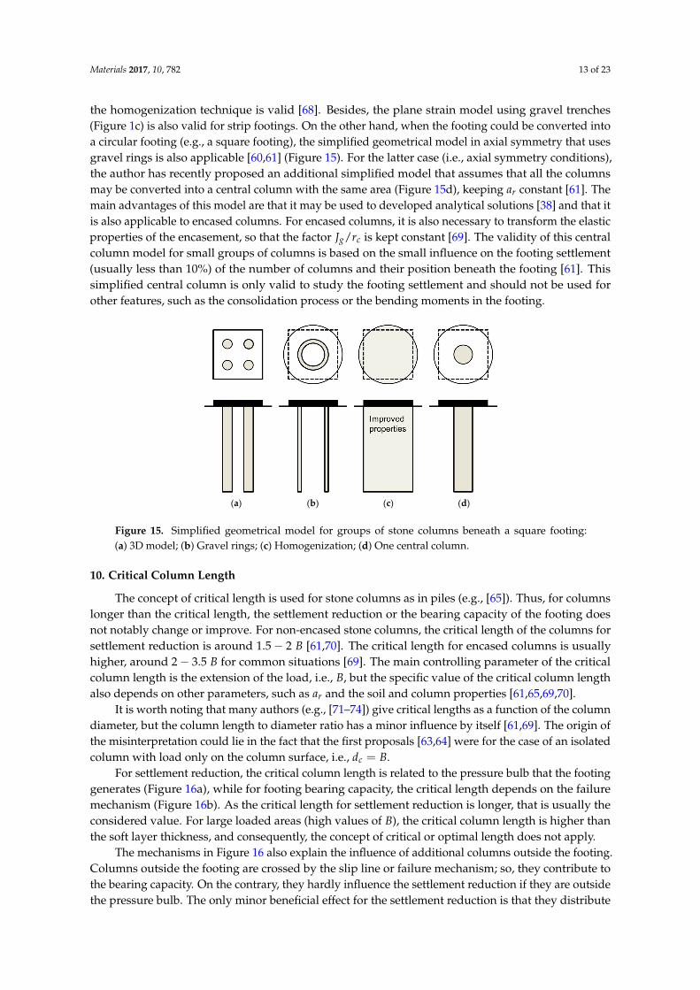
the homogenization technique is valid [68]. Besides, the plane strain model using gravel trenches(Figure 1c) is also valid for strip footings. On the other hand, when the footing could be converted intoa circular footing (e.g., a square footing), the simplified geometrical model in axial symmetry that usesgravel rings is also applicable [60,61] (Figure 15). For the latter case (i.e., axial symmetry conditions),the author has recently proposed an additional simplified model that assumes that all the columnsmay be converted into a central column with the same area (Figure 15d), keeping ar constant [61]. Themain advantages of this model are that it may be used to developed analytical solutions [38] and that itis also applicable to encased columns. For encased columns, it is also necessary to transform the elasticproperties of the encasement, so that the factor Jg/rc is kept constant [69]. The validity of this centralcolumn model for small groups of columns is based on the small influence on the footing settlement(usually less than 10%) of the number of columns and their position beneath the footing [61]. Thissimplified central column is only valid to study the footing settlement and should not be used forother features, such as the consolidation process or the bending moments in the footing.

Materials 2017, 10, 782 13 of 23

(Figure 1c) is also valid for strip footings. On the other hand, when the footing could be converted into a circular footing (e.g., a square footing), the simplified geometrical model in axial symmetry that uses gravel rings is also applicable [60,61] (Figure 15). For the latter case (i.e., axial symmetry conditions), the author has recently proposed an additional simplified model that assumes that all the columns may be converted into a central column with the same area (Figure 15d), keeping constant [61]. The main advantages of this model are that it may be used to developed analytical solutions [38] and that it is also applicable to encased columns. For encased columns, it is also necessary to transform the elastic properties of the encasement, so that the factor ⁄ is kept constant [69]. The validity of this central column model for small groups of columns is based on the small influence on the footing settlement (usually less than 10%) of the number of columns and their position beneath the footing [61]. This simplified central column is only valid to study the footing settlement and should not be used for other features, such as the consolidation process or the bending moments in the footing.

(a) (b) (c) (d)

Figure 15. Simplified geometrical model for groups of stone columns beneath a square footing: (a) 3D model; (b) Gravel rings; (c) Homogenization; (d) One central column.

10. Critical Column Length

The concept of critical length is used for stone columns as in piles (e.g., [65]). Thus, for columns longer than the critical length, the settlement reduction or the bearing capacity of the footing does not notably change or improve. For non-encased stone columns, the critical length of the columns for settlement reduction is around 1.5 − 2 [61,70]. The critical length for encased columns is usually higher, around 2 − 3.5 for common situations [69]. The main controlling parameter of the critical column length is the extension of the load, i.e., , but the specific value of the critical column length also depends on other parameters, such as and the soil and column properties [61,65,69,70].

It is worth noting that many authors (e.g., [71–74]) give critical lengths as a function of the column diameter, but the column length to diameter ratio has a minor influence by itself [61,69]. The origin of the misinterpretation could lie in the fact that the first proposals [63,64] were for the case of an isolated column with load only on the column surface, i.e., = .

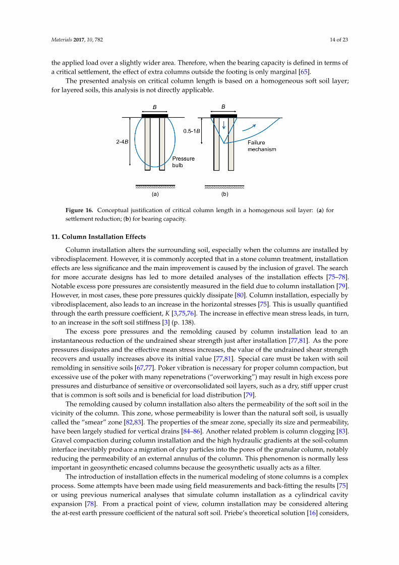
For settlement reduction, the critical column length is related to the pressure bulb that the footing generates (Figure 16a), while for footing bearing capacity, the critical length depends on the failure mechanism (Figure 16b). As the critical length for settlement reduction is longer, that is usually the considered value. For large loaded areas (high values of ), the critical column length is higher than the soft layer thickness, and consequently, the concept of critical or optimal length does not apply.

The mechanisms in Figure 16 also explain the influence of additional columns outside the footing. Columns outside the footing are crossed by the slip line or failure mechanism; so, they contribute to the bearing capacity. On the contrary, they hardly influence the settlement reduction if

Figure 15. Simplified geometrical model for groups of stone columns beneath a square footing:(a) 3D model; (b) Gravel rings; (c) Homogenization; (d) One central column.

10. Critical Column Length

The concept of critical length is used for stone columns as in piles (e.g., [65]). Thus, for columnslonger than the critical length, the settlement reduction or the bearing capacity of the footing doesnot notably change or improve. For non-encased stone columns, the critical length of the columns forsettlement reduction is around 1.5− 2 B [61,70]. The critical length for encased columns is usuallyhigher, around 2− 3.5 B for common situations [69]. The main controlling parameter of the criticalcolumn length is the extension of the load, i.e., B, but the specific value of the critical column lengthalso depends on other parameters, such as ar and the soil and column properties [61,65,69,70].

It is worth noting that many authors (e.g., [71–74]) give critical lengths as a function of the columndiameter, but the column length to diameter ratio has a minor influence by itself [61,69]. The origin ofthe misinterpretation could lie in the fact that the first proposals [63,64] were for the case of an isolatedcolumn with load only on the column surface, i.e., dc = B.

For settlement reduction, the critical column length is related to the pressure bulb that the footinggenerates (Figure 16a), while for footing bearing capacity, the critical length depends on the failuremechanism (Figure 16b). As the critical length for settlement reduction is longer, that is usually theconsidered value. For large loaded areas (high values of B), the critical column length is higher thanthe soft layer thickness, and consequently, the concept of critical or optimal length does not apply.

The mechanisms in Figure 16 also explain the influence of additional columns outside the footing.Columns outside the footing are crossed by the slip line or failure mechanism; so, they contribute tothe bearing capacity. On the contrary, they hardly influence the settlement reduction if they are outsidethe pressure bulb. The only minor beneficial effect for the settlement reduction is that they distribute

Materials 2017, 10, 782 14 of 23

the applied load over a slightly wider area. Therefore, when the bearing capacity is defined in terms ofa critical settlement, the effect of extra columns outside the footing is only marginal [65].

The presented analysis on critical column length is based on a homogeneous soft soil layer;for layered soils, this analysis is not directly applicable.

Materials 2017, 10, 782 14 of 23

they are outside the pressure bulb. The only minor beneficial effect for the settlement reduction is that they distribute the applied load over a slightly wider area. Therefore, when the bearing capacity is defined in terms of a critical settlement, the effect of extra columns outside the footing is only marginal [65].

The presented analysis on critical column length is based on a homogeneous soft soil layer; for layered soils, this analysis is not directly applicable.

Figure 16. Conceptual justification of critical column length in a homogenous soil layer: (a) for settlement reduction; (b) for bearing capacity.

11. Column Installation Effects

Column installation alters the surrounding soil, especially when the columns are installed by vibrodisplacement. However, it is commonly accepted that in a stone column treatment, installation effects are less significance and the main improvement is caused by the inclusion of gravel. The search for more accurate designs has led to more detailed analyses of the installation effects [75–78]. Notable excess pore pressures are consistently measured in the field due to column installation [79]. However, in most cases, these pore pressures quickly dissipate [80]. Column installation, especially by vibrodisplacement, also leads to an increase in the horizontal stresses [75]. This is usually quantified through the earth pressure coefficient, [3,75,76]. The increase in effective mean stress leads, in turn, to an increase in the soft soil stiffness [3] (p. 138).

The excess pore pressures and the remolding caused by column installation lead to an instantaneous reduction of the undrained shear strength just after installation [77,81]. As the pore pressures dissipates and the effective mean stress increases, the value of the undrained shear strength recovers and usually increases above its initial value [77,81]. Special care must be taken with soil remolding in sensitive soils [67,77]. Poker vibration is necessary for proper column compaction, but excessive use of the poker with many repenetrations (“overworking”) may result in high excess pore pressures and disturbance of sensitive or overconsolidated soil layers, such as a dry, stiff upper crust that is common is soft soils and is beneficial for load distribution [79].

The remolding caused by column installation also alters the permeability of the soft soil in the vicinity of the column. This zone, whose permeability is lower than the natural soft soil, is usually called the “smear” zone [82,83]. The properties of the smear zone, specially its size and permeability, have been largely studied for vertical drains [84–86]. Another related problem is column clogging [83]. Gravel compaction during column installation and the high hydraulic gradients at the soil-column interface inevitably produce a migration of clay particles into the pores of the granular column, notably reducing the permeability of an external annulus of the column. This phenomenon is normally less important in geosynthetic encased columns because the geosynthetic usually acts as a filter.

The introduction of installation effects in the numerical modeling of stone columns is a complex process. Some attempts have been made using field measurements and back-fitting the results [75]

Figure 16. Conceptual justification of critical column length in a homogenous soil layer: (a) forsettlement reduction; (b) for bearing capacity.

11. Column Installation Effects

Column installation alters the surrounding soil, especially when the columns are installed byvibrodisplacement. However, it is commonly accepted that in a stone column treatment, installationeffects are less significance and the main improvement is caused by the inclusion of gravel. The searchfor more accurate designs has led to more detailed analyses of the installation effects [75–78].Notable excess pore pressures are consistently measured in the field due to column installation [79].However, in most cases, these pore pressures quickly dissipate [80]. Column installation, especially byvibrodisplacement, also leads to an increase in the horizontal stresses [75]. This is usually quantifiedthrough the earth pressure coefficient, K [3,75,76]. The increase in effective mean stress leads, in turn,to an increase in the soft soil stiffness [3] (p. 138).

The excess pore pressures and the remolding caused by column installation lead to aninstantaneous reduction of the undrained shear strength just after installation [77,81]. As the porepressures dissipates and the effective mean stress increases, the value of the undrained shear strengthrecovers and usually increases above its initial value [77,81]. Special care must be taken with soilremolding in sensitive soils [67,77]. Poker vibration is necessary for proper column compaction, butexcessive use of the poker with many repenetrations (“overworking”) may result in high excess porepressures and disturbance of sensitive or overconsolidated soil layers, such as a dry, stiff upper crustthat is common is soft soils and is beneficial for load distribution [79].

The remolding caused by column installation also alters the permeability of the soft soil in thevicinity of the column. This zone, whose permeability is lower than the natural soft soil, is usuallycalled the “smear” zone [82,83]. The properties of the smear zone, specially its size and permeability,have been largely studied for vertical drains [84–86]. Another related problem is column clogging [83].Gravel compaction during column installation and the high hydraulic gradients at the soil-columninterface inevitably produce a migration of clay particles into the pores of the granular column, notablyreducing the permeability of an external annulus of the column. This phenomenon is normally lessimportant in geosynthetic encased columns because the geosynthetic usually acts as a filter.

The introduction of installation effects in the numerical modeling of stone columns is a complexprocess. Some attempts have been made using field measurements and back-fitting the results [75]or using previous numerical analyses that simulate column installation as a cylindrical cavityexpansion [78]. From a practical point of view, column installation may be considered alteringthe at-rest earth pressure coefficient of the natural soft soil. Priebe’s theoretical solution [16] considers,

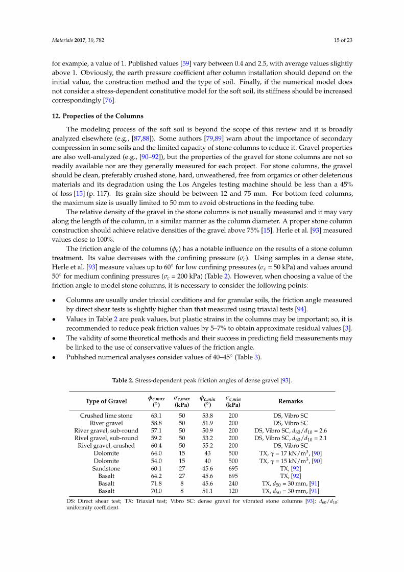
Materials 2017, 10, 782 15 of 23

for example, a value of 1. Published values [59] vary between 0.4 and 2.5, with average values slightlyabove 1. Obviously, the earth pressure coefficient after column installation should depend on theinitial value, the construction method and the type of soil. Finally, if the numerical model doesnot consider a stress-dependent constitutive model for the soft soil, its stiffness should be increasedcorrespondingly [76].

12. Properties of the Columns

The modeling process of the soft soil is beyond the scope of this review and it is broadlyanalyzed elsewhere (e.g., [87,88]). Some authors [79,89] warn about the importance of secondarycompression in some soils and the limited capacity of stone columns to reduce it. Gravel propertiesare also well-analyzed (e.g., [90–92]), but the properties of the gravel for stone columns are not soreadily available nor are they generally measured for each project. For stone columns, the gravelshould be clean, preferably crushed stone, hard, unweathered, free from organics or other deleteriousmaterials and its degradation using the Los Angeles testing machine should be less than a 45%of loss [15] (p. 117). Its grain size should be between 12 and 75 mm. For bottom feed columns,the maximum size is usually limited to 50 mm to avoid obstructions in the feeding tube.

The relative density of the gravel in the stone columns is not usually measured and it may varyalong the length of the column, in a similar manner as the column diameter. A proper stone columnconstruction should achieve relative densities of the gravel above 75% [15]. Herle et al. [93] measuredvalues close to 100%.

The friction angle of the columns (φc) has a notable influence on the results of a stone columntreatment. Its value decreases with the confining pressure (σc). Using samples in a dense state,Herle et al. [93] measure values up to 60◦ for low confining pressures (σc = 50 kPa) and values around50◦ for medium confining pressures (σc = 200 kPa) (Table 2). However, when choosing a value of thefriction angle to model stone columns, it is necessary to consider the following points:

• Columns are usually under triaxial conditions and for granular soils, the friction angle measuredby direct shear tests is slightly higher than that measured using triaxial tests [94].

• Values in Table 2 are peak values, but plastic strains in the columns may be important; so, it isrecommended to reduce peak friction values by 5–7% to obtain approximate residual values [3].

• The validity of some theoretical methods and their success in predicting field measurements maybe linked to the use of conservative values of the friction angle.

• Published numerical analyses consider values of 40–45◦ (Table 3).

Table 2. Stress-dependent peak friction angles of dense gravel [93].

Type of Gravel φc,max(◦)

σc,max(kPa)

φc,min(◦)

σc,min(kPa) Remarks

Crushed lime stone 63.1 50 53.8 200 DS, Vibro SCRiver gravel 58.8 50 51.9 200 DS, Vibro SC

River gravel, sub-round 57.1 50 50.9 200 DS, Vibro SC, d60/d10 = 2.6Rivel gravel, sub-round 59.2 50 53.2 200 DS, Vibro SC, d60/d10 = 2.1

Rivel gravel, crushed 60.4 50 55.2 200 DS, Vibro SCDolomite 64.0 15 43 500 TX, γ = 17 kN/m3, [90]Dolomite 54.0 15 40 500 TX, γ = 15 kN/m3, [90]Sandstone 60.1 27 45.6 695 TX, [92]

Basalt 64.2 27 45.6 695 TX, [92]Basalt 71.8 8 45.6 240 TX, d50 = 30 mm, [91]Basalt 70.0 8 51.1 120 TX, d50 = 30 mm, [91]

DS: Direct shear test; TX: Triaxial test; Vibro SC: dense gravel for vibrated stone columns [93]; d60/d10:uniformity coefficient.

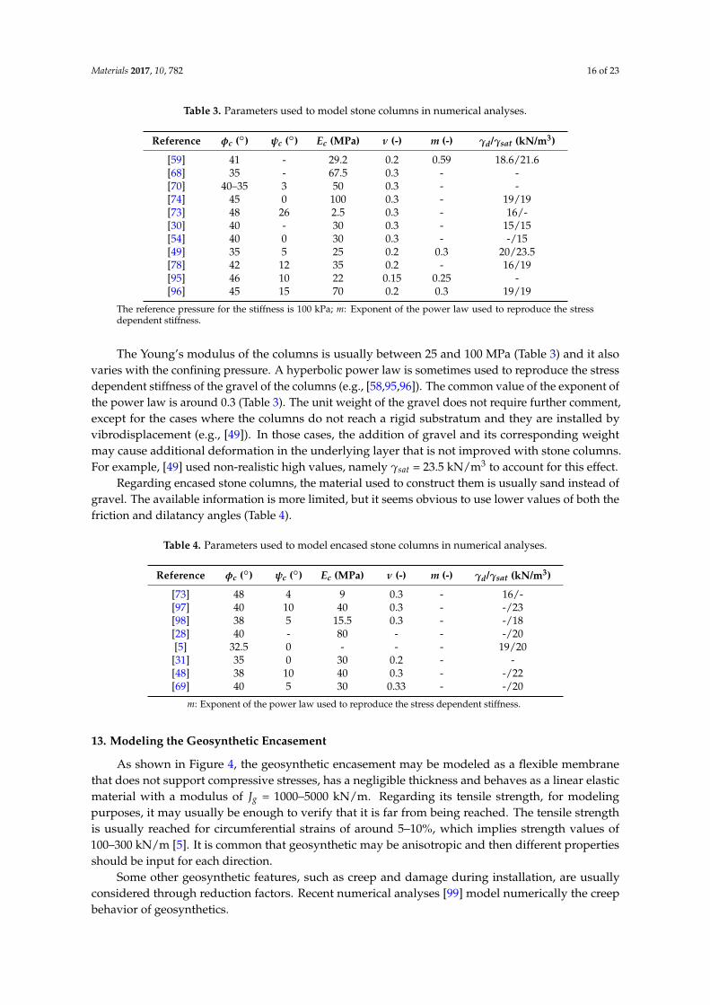
Materials 2017, 10, 782 16 of 23

Table 3. Parameters used to model stone columns in numerical analyses.

Reference φc (◦) ψc (◦) Ec (MPa) ν (-) m (-) γd/γsat (kN/m3)

[59] 41 - 29.2 0.2 0.59 18.6/21.6[68] 35 - 67.5 0.3 - -[70] 40–35 3 50 0.3 - -[74] 45 0 100 0.3 - 19/19[73] 48 26 2.5 0.3 - 16/-[30] 40 - 30 0.3 - 15/15[54] 40 0 30 0.3 - -/15[49] 35 5 25 0.2 0.3 20/23.5[78] 42 12 35 0.2 - 16/19[95] 46 10 22 0.15 0.25 -[96] 45 15 70 0.2 0.3 19/19

The reference pressure for the stiffness is 100 kPa; m: Exponent of the power law used to reproduce the stressdependent stiffness.

The Young’s modulus of the columns is usually between 25 and 100 MPa (Table 3) and it alsovaries with the confining pressure. A hyperbolic power law is sometimes used to reproduce the stressdependent stiffness of the gravel of the columns (e.g., [58,95,96]). The common value of the exponent ofthe power law is around 0.3 (Table 3). The unit weight of the gravel does not require further comment,except for the cases where the columns do not reach a rigid substratum and they are installed byvibrodisplacement (e.g., [49]). In those cases, the addition of gravel and its corresponding weightmay cause additional deformation in the underlying layer that is not improved with stone columns.For example, [49] used non-realistic high values, namely γsat = 23.5 kN/m3 to account for this effect.

Regarding encased stone columns, the material used to construct them is usually sand instead ofgravel. The available information is more limited, but it seems obvious to use lower values of both thefriction and dilatancy angles (Table 4).

Table 4. Parameters used to model encased stone columns in numerical analyses.

Reference φc (◦) ψc (◦) Ec (MPa) ν (-) m (-) γd/γsat (kN/m3)

[73] 48 4 9 0.3 - 16/-[97] 40 10 40 0.3 - -/23[98] 38 5 15.5 0.3 - -/18[28] 40 - 80 - - -/20[5] 32.5 0 - - - 19/20

[31] 35 0 30 0.2 - -[48] 38 10 40 0.3 - -/22[69] 40 5 30 0.33 - -/20

m: Exponent of the power law used to reproduce the stress dependent stiffness.

13. Modeling the Geosynthetic Encasement

As shown in Figure 4, the geosynthetic encasement may be modeled as a flexible membranethat does not support compressive stresses, has a negligible thickness and behaves as a linear elasticmaterial with a modulus of Jg = 1000–5000 kN/m. Regarding its tensile strength, for modelingpurposes, it may usually be enough to verify that it is far from being reached. The tensile strengthis usually reached for circumferential strains of around 5–10%, which implies strength values of100–300 kN/m [5]. It is common that geosynthetic may be anisotropic and then different propertiesshould be input for each direction.

Some other geosynthetic features, such as creep and damage during installation, are usuallyconsidered through reduction factors. Recent numerical analyses [99] model numerically the creepbehavior of geosynthetics.

Materials 2017, 10, 782 17 of 23

In those numerical analyses where the geosynthetic is modeled as a continuum element of smallthickness, it is necessary to ensure that it does not support compressive stresses, and hence, bendingmoments. Its Young’s modulus should be Jg divided by its thickness.

Little attention is usually paid to the Poisson’s ratio of the geosynthetic (νg), but it may haveimportant consequences on the results [100]. When the encasement is modeled as a membrane, it iscommon to study the two directions of the geosynthetic independently, without interaction betweenthem (Equation (3)). That means νg = 0.

On the other hand, when the geosynthetic is modeled as a continuum element, it is necessaryto specify a value for νg. In some cases (e.g., [31]), a common value of 0.3 is input. That impliesthat, although the geosynthetic that surrounds the columns does not support compressive stressesin the vertical direction, it compresses vertically (vertical strains) and then, that vertical compressionleads to a radial expansion of the geosynthetic (horizontal or circumferential strains) due to Poisson’seffect. Thus, the geosynthetic encasement decreases its lateral confinement to the column due to thisradial expansion. Common geosynthetics for column encasement are woven geotextiles. For wovengeotextiles, the two directions work nearly independently; so, it seems logical to use values of thePoisson’s ratio close to 0. Soderman and Giroud [101] propose values of νg = 0.1 for woven geotextilesand νg = 0.35 for non-woven geotextiles.

14. Conclusions

This paper reviews the main modeling techniques for stone columns, both ordinary ornon-encased stone columns, and geosynthetic-encased stone columns. The paper tries to encompassthe more recent advances and recommendations in the topic.

There exist several simplified geometrical models. The suitability of each of them depends onthe type of process to be studied, e.g., bearing capacity or settlement, and the type of analyses, e.g.,analytical or numerical in 2D or 3D. For numerical analyses of a problem that fulfils plane strainconditions but for the stone column treatment, such as an embankment for a linear infrastructure,the simplified geometrical model of a three-dimensional slice of columns is recommended becauseit does not require any transformation of the problem parameters. For more simplified models forthe stone column treatment, such as gravel trenches or homogenization, calibrating or tuning theparameters using the unit cell as an auxiliary problem is recommended. The model of an isolatedcolumn with load just on top of it may be useful for field tests, but it is not a common situationin real cases because loading the soil that surrounds the column is beneficial. The behavior of anisolated column is different from that of a column within a large group under distributed load. Thosedifferences should be considered when extrapolating results.

For groups of columns, the critical column length depends mainly on the loading area.For non-encased columns, its value is around twice the footing width and for encased columnsis slightly higher.

Some guidance is provided to consider installation effects and to model the column and thegeosynthetic encasement. Column installation usually increases the horizontal stresses and that isoften accounted for using a high value of the earth pressure coefficient, typically around 1. On the otherhand, the relevance of the Poisson’s ratio of the geosynthetic is taken into account and an appropriatevalue for a woven geotextile could be close to 0, i.e., the two directions work nearly independently.

Finally, laboratory tests are not commonly performed to characterize stone column propertiesand some column parameters published in the literature are tabulated as a reference.

Acknowledgments: The author thanks all the institutions that have allowed him to work on stone columnsand all the people that have collaborated in the research on stone columns. The author thanks the SpanishSociety for Soil Mechanics and Geotechnical Engineering (SEMSIG) for the invitation to give a lecture onstone columns in the 10th National Symposium on Geotechnical Engineering, held in A Coruña in October2016. The present paper is based on that lecture and the corresponding conference paper [102] (In Spanish).The author acknowledges the funding received through the following projects: “Improvement of soft soilswith stone columns for foundation of embankments. Analysis of the process and design criteria” for

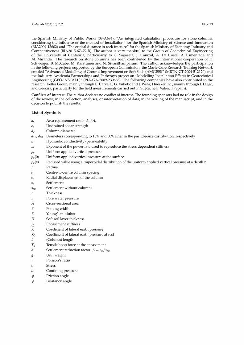
Materials 2017, 10, 782 18 of 23

the Spanish Ministry of Public Works (03-A634), “An integrated calculation procedure for stone columns,considering the influence of the method of installation” for the Spanish Ministry of Science and Innovation(BIA2009-13602) and “The critical distance in rock fracture” for the Spanish Ministry of Economy, Industry andCompetitiveness (BIA2015-67479-R). The author is very thankful to the Group of Geotechnical Engineeringof the University of Cantabria, particularly to C. Sagaseta, J. Cañizal, A. Da Costa, A. Cimentada andM. Miranda. The research on stone columns has been contributed by the international cooperation of H.Schweiger, B. McCabe, M. Karstunen and N. Sivasithamparam. The author acknowledges the participationin the following projects supported by the European Commission: the Marie Cure Research Training Networkentitled “Advanced Modelling of Ground Improvement on Soft Soils (AMGISS)” (MRTN-CT-2004-512120) andthe Industry-Academia Partnerships and Pathways project on “Modelling Installation Effects in GeotechnicalEngineering (GEO-INSTALL)” (PIA-GA-2009-230638). The following companies have also contributed to theresearch: Keller Group, mainly through E. Carvajal, G. Vukotic and J. Wehr; Huesker Inc., mainly through I. Diego;and Geocisa, particularly for the field measurements carried out in Sueca, near Valencia (Spain).

Conflicts of Interest: The author declares no conflict of interest. The founding sponsors had no role in the designof the review; in the collection, analyses, or interpretation of data; in the writing of the manuscript, and in thedecision to publish the results.

List of Symbols

ar Area replacement ratio: Ac/Ae

cu Undrained shear strengthdc Column diameterd10, d60 Diameters corresponding to 10% and 60% finer in the particle-size distribution, respectivelyk Hydraulic conductivity/permeabilitym Exponent of the power law used to reproduce the stress dependent stiffnesspa Uniform applied vertical pressurepa(0) Uniform applied vertical pressure at the surfacepa(z) Reduced value using a trapezoidal distribution of the uniform applied vertical pressure at a depth zr Radiuss Centre-to-centre column spacingsr Radial displacement of the columnsz Settlementsz0 Settlement without columnst Thicknessu Pore water pressureA Cross-sectional areaB Footing widthE Young’s modulusH Soft soil layer thicknessJg Encasement stiffnessK Coefficient of lateral earth pressureK0 Coefficient of lateral earth pressure at restL (Column) lengthTg Tensile hoop force at the encasementb Settlement reduction factor: β = sz/sz0

g Unit weightν Poisson’s ratioσ Stressσc Confining pressureϕ Friction angleψ Dilatancy angle

Materials 2017, 10, 782 19 of 23

Subscripts

c, s, g, e column, soil, encasement or geosynthetic, loaded area or unit celld drym equivalent homogeneous soilmax maximum valuemin minimum valuer equivalent gravel ringr, θ, z Cylindrical coordinatessat Saturatedx, y, z Cartesian coordinates¯ (upper bar) average value along the radius

Abbreviations

DS Direct shear testG.W.T. Ground water tableSC Stone columnTX Triaxial test

References

1. Dhouib, A.; Magnan, J.-P.; Guilloux, A. Procédés D’amélioration des Sols: Historique, Méthodes de Reconnaissance,Applications et Données Économiques; ASEP-GI; Presses de l’ENPC/LCPC: Paris, France, 2004; Volume 2,pp. 577–598. (In French)

2. Seed, H.B.; Booker, J.R. Stabilization of potentially liquefiable sand deposits. J. Geotech. Eng. ASCE 1977, 103,757–768.

3. Kirsch, K.; Kirsch, F. Ground Improvement by Deep Vibratory Methods; Spon Press: London, UK, 2010.4. Wehr, J. The undrained cohesion of the soil as criterion for the column installation with a depth vibrator.

In International Symposium on Vibratory Pile Driving and Deep Soil VIBRATORY Compaction, TRANSVIB 2006,Paris; Laboratoire Central des Ponts et Chaussées: Paris, France, 2006.

5. Alexiew, D.; Raithel, M. Geotextile-Encased Columns: Case Studies over Twenty Years. In Embankmentswith Special Reference to Consolidation and Other Physical Methods; Butterworth-Heinemann: Oxford, UK, 2015;pp. 451–477.

6. Simon, B. General Report S5: Rigid Inclusions and Stone Columns. In Proceedings of the ISSMGE-TC 211International Symposium on Ground Improvement (IS-GI), Brussels, Belgium, 30 May–1 June 2012; VolumeI, pp. 127–168.

7. Golait, Y.S.; Padade, A.H. Analytical and experimental studies on cemented stone columns for soft clayground improvement. Int. J. Geomech. 2017, 17, 04016100. [CrossRef]

8. Han, J. Recent research and development of ground column technologies. Proc. ICE-Ground Improv. 2015,168, 246–264. [CrossRef]

9. Serridge, C.J. Achieving sustainability in vibro stone column techniques. Proc. ICE-Eng. Sust. 2005, 158,211–222. [CrossRef]

10. Egan, D.; Slocombe, B.C. Demonstrating environmental benefits of ground improvement. Proc. ICE-GroundImprov. 2010, 163, 63–69. [CrossRef]

11. Sivakumar, V.; McKelvey, D.; Graham, J.; Hughes, D. Triaxial tests on model sand columns in clay.Can. Geotech. J. 2004, 41, 299–312. [CrossRef]

12. Najjar, S.S.; Skeini, H. Triaxial response of clays reinforced with granular columns. Proc. ICE-Ground Improv.2015, 168, 265–281. [CrossRef]

13. Hong, Y.-S.; Wu, C.-S.; Yu, Y.-S. Model tests on geotextile-encased granular columns under 1-g and undrainedconditions. Geotext. Geomembr. 2016, 44, 13–27. [CrossRef]

14. Stuedlein, A.W.; Holtz, R.D. Analysis of Footing Load Tests on Aggregate Pier Reinforced Clay. J. Geotech.Geoenviron. Eng. ASCE 2012, 138, 1091–1103. [CrossRef]

Materials 2017, 10, 782 20 of 23

15. Barksdale, R.D.; Bachus, R.C. Design and Construction of Stone Columns; Report FHWA/RD-83/026; NationalTechnical Information Service: Springfield, VA, USA, 1983.

16. Priebe, H.J. Design of vibro replacement. Ground Eng. 1995, 28, 31–37.17. Pulko, B.; Majes, B.; Logar, J. Geosynthetic-encased stone columns: Analytical calculation model. Geotext.

Geomembr. 2011, 29, 29–39. [CrossRef]18. Castro, J.; Sagaseta, C. Consolidation and deformation around stone columns: Numerical evaluation of

analytical solutions. Comput. Geotech. 2011, 38, 354–362. [CrossRef]19. Balaam, N.P.; Booker, J.R. Effect of stone column yield on settlement of rigid foundations in stabilized clay.

Int. J. Numer. Anal. Methods Geomech. 1985, 9, 331–351. [CrossRef]20. Barron, R.A. Consolidation of fine-grained soils by drain wells. Trans. ASCE 1948, 113, 718–742.21. Hansbo, S. Consolidation of fine-grained soils by prefabricated drains. In Proceedings of the 10th

International Conference Soil Mechanics and Foundation Engineering, Stockholm, Sweden, 15–19 June 1981;Volume 3, pp. 677–682.

22. Han, J.; Ye, S.L. Simplified method of consolidation rate of stone column reinforced foundation. J. Geotech.Geoenviron. Eng. ASCE 2001, 127, 597–603. [CrossRef]

23. Castro, J.; Sagaseta, C. Consolidation around stone columns. Influence of column deformation. Int. J. Numer.Anal. Methods Geomech. 2009, 33, 851–877. [CrossRef]

24. Pulko, B.; Logar, J. Fully coupled solution for the consolidation of poroelastic soil around elastoplastic stonecolumn. Acta Geotech. 2016. [CrossRef]

25. Castro, J.; Sagaseta, C. Influence of elastic strains during plastic deformation of encased stone columns.Geotext. Geomembr. 2013, 37, 45–53. [CrossRef]

26. Lo, S.R.; Zhang, R.; Mak, J. Geosynthetic-encased stone columns in soft clay: A numerical study. Geotext.Geomembr. 2010, 28, 292–302. [CrossRef]

27. Hosseinpour, I.; Riccio, M.; Almeida, M.S.S. Numerical evaluation of a granular column reinforced bygeosynthetics using encasement and laminated disks. Geotext. Geomembr. 2014, 42, 363–373. [CrossRef]

28. Hosseinpour, I.; Almeida, M.S.S.; Riccio, M. Full-scale load test and finite-element analysis of soft groundimproved by geotextile-encased granular columns. Geosynth. Int. 2015, 22, 428–438. [CrossRef]

29. Basack, S.; Indraratna, B.; Rujikiatkamjorn, C. Modelling the performance of stone column reinforced softground under static and cyclic loads. J. Geotech. Geoenviron. Eng. ASCE 2016, 142, 04015067. [CrossRef]

30. Tan, S.A.; Tjahyono, S.; Oo, K.K. Simplified plane-strain modeling of stone-column reinforced ground.J. Geotech. Geoenviron. Eng. ASCE 2008, 134, 185–194. [CrossRef]

31. Khabbazian, M.; Kaliakin, V.N.; Meehan, C.L. Column Supported Embankments with Geosynthetic EncasedColumns: Validity of the Unit Cell Concept. Geotech. Geol. Eng. 2015, 33, 425–442. [CrossRef]

32. Indraratna, B.; Ngo, N.T.; Rujikiatkamjorn, C.; Sloan, S.W. Coupled discrete element–finite difference methodfor analysing the load-deformation behaviour of a single stone column in soft soil. Comput. Geotech. 2015, 63,267–278. [CrossRef]

33. Cimentada, A.; da Costa, A.; Cañizal, J.; Sagaseta, C. Laboratory study on radial consolidation anddeformation in clay reinforced with stone columns. Can. Geotech. J. 2011, 48, 36–52. [CrossRef]

34. Miranda, M.; Da Costa, A.; Castro, J.; Sagaseta, C. Influence of geotextile encasement on the behaviour ofstone columns: Laboratory study. Geotext. Geomembr. 2017, 45, 14–22. [CrossRef]

35. Priebe, H.J. Design of vibro replacement. Ground Eng. 2005, 38, 25–27.36. Sehn, A.L.; Blackburn, J.T. Predicting performance of aggregate piers. In Proceedings of the 23rd Central

Pennsylvania Geotechnical Conference, Hershey, PA, USA, 28–30 May 2008.37. Stuedlein, A.W.; Holtz, R.D. Displacement of Spread Footings on Aggregate Pier Reinforced Clay. J. Geotech.

Geoenviron. Eng. 2014, 140, 36–45. [CrossRef]38. Castro, J. An analytical solution for the settlement of stone columns beneath rigid footings. Acta Geotech.

2016, 11, 309–324. [CrossRef]39. Yu, Y.; Bathurst, R.J.; Damians, I.P. Modified unit cell approach for modelling geosynthetic-reinforced

column-supported embankments. Geotext. Geomembr. 2016, 44, 332–343. [CrossRef]40. Van Impe, W.; De Beer, E. Improvement of settlement behaviour of soft layers by means of Stone columns.

In Proceedings of the 8th European Conference on Soil Mechanics and Foundation Engineering, Helsinki,Finland, 23–26 May 1983; Volume 1, pp. 309–312.

Materials 2017, 10, 782 21 of 23

41. Castro, J.; Sagaseta, C. Discussion of “Simplified plane-strain modeling of stone-column reinforced ground”.J. Geotech. Geoenviron. Eng. ASCE 2010, 136, 892–894. [CrossRef]

42. Weber, T.M.; Springman, S.M.; Gäb, M.; Racansky, V.; Schweiger, H.F. Numerical modelling of stone columnsin soft clay under an embankment. In Geotechnics of Soft Soils—Focus on Ground Improvement; Taylor & Francis:London, UK, 2009; pp. 305–311.

43. Hird, C.C.; Pyrah, I.C.; Russell, D. Finite element modelling of vertical drains beneath embankments on softground. Géotechnique 1992, 42, 499–511. [CrossRef]

44. Indraratna, B.; Redana, I.W. Plane-strain modeling of smear effects associated with vertical drains. J. Geotech.Geoenviron. Eng. ASCE 1997, 123, 474–478. [CrossRef]

45. Zhang, Z.; Han, J.; Ye, G. Numerical investigation on factors for deep-seated slope stability of stonecolumn-supported embankments over soft clay. Eng. Geol. 2014, 168, 104–113. [CrossRef]

46. Kitazume, M.; Okano, K.; Miyajima, S. Centrifuge model tests on failure envelope of column type deepmixing method improved ground. Soils Found. 2000, 40, 43–55. [CrossRef]

47. Navin, M.P.; Filz, G.M. Reliability of Deep Mixing Method Columns for Embankment Support. In GeoCongress2006; ASCE: Atlanta, GA, USA, 2006.

48. Chen, J.-F.; Li, L.-Y.; Xue, J.-F.; Feng, S.-Z. Failure mechanism of geosynthetic-encased stone columns in softsoils under embankment. Geotext. Geomembr. 2015, 43, 424–431. [CrossRef]

49. Adam, D.; Schweiger, H.F.; Markiewicz, R.; Knabe, T. Euro 2008 Stadium Klagenfurt–Prediction, Monitoringand back calculation of settlement behavior. In Proceedings of the From Research to Design in EuropeanPractice, Bratislava, Slovak Republic, 2–4 June 2010.

50. Hassen, G.; de Buhan, P.; Abdelkrim, M. Finite element implementation of a homogenized constitutive lawfor stone column-reinforced foundation soils, with application to the design of structures. Comput. Geotech.2010, 37, 40–49. [CrossRef]

51. Gueguin, M.; Hassen, G.; de Buhan, P. Stability analysis of homogenized stone column reinforced foundationsusing a numerical yield design approach. Comput. Geotech. 2015, 64, 10–19. [CrossRef]

52. Hassen, G.; Gueguin, M.; de Buhan, P. A homogenization approach for assessing the yield strength propertiesof stone column reinforced soils. Eur. J Mech. A/Solids 2013, 37, 266–280. [CrossRef]

53. Gueguin, M.; Hassen, G.; de Buhan, P. Numerical assessment of the macroscopic strength criterion ofreinforced soils using semidefinite programming. Int. J. Numer. Methods Eng. 2014, 99, 522–541. [CrossRef]

54. Ng, K.S.; Tan, S.A. Simplified homogenization method in stone column designs. Soils Found. 2015, 55,154–165. [CrossRef]

55. Schweiger, H.F.; Pande, G.N. Numerical analysis of stone column supported foundations. Comput. Geotech.1986, 2, 347–372. [CrossRef]

56. Lee, J.S.; Pande, G.N. Analysis of stone-column reinforced foundations. Int. J. Numer. Anal. Methods Geomech.1998, 22, 1001–1020. [CrossRef]

57. Becker, P.; Karstunen, M. Volume averaging technique in numerical modelling of floating deep mixedcolumns in soft soils. In Installation Effects in Geotechnical Engineering; CRC Press: Boca Raton, FL, USA, 2013;pp. 198–204.

58. Mitchell, J.K.; Huber, T.R. Performance of a stone column foundation. J. Geotech. Eng. ASCE 1985, 111,205–223. [CrossRef]

59. Elshazly, H.; Elkasabgy, M.; Elleboudy, A. Effect of Inter-Column Spacing on Soil Stresses due toVibro-Installed Stone Columns: Interesting Findings. Geotech. Geol. Eng. 2008, 26, 225–236. [CrossRef]

60. Ng, K.S. Numerical Study of Floating Stone Columns. Ph.D. Thesis, National University of Singapore,Singapore, 2013.

61. Castro, J. Numerical modelling of stone columns beneath a rigid footing. Comput. Geotech. 2014, 60, 77–87.[CrossRef]

62. Kirsch, F.; Sondermann, W. Field measurements and numerical analysis of the stress distribution belowstone column supported embankments and their stability. In Proceedings of the International Workshop onGeotechnics of Soft Soils-Theory and Practice, Noordwijkerhout, The Netherlands, 17–19 September 2003.

63. Hughes, J.M.O.; Withers, N.J. Reinforcing of soft soils with stone columns. Ground Eng. 1974, 7, 42–49.[CrossRef]

64. Hughes, J.M.O.; Withers, N.J.; Greenwood, D.A. A field trial of the reinforcing effect a stone column in soil.Géotechnique 1975, 25, 31–44. [CrossRef]

Materials 2017, 10, 782 22 of 23

65. Wood, D.M.; Hu, W.; Nash, D.F.T. Group effects in stone column foundations: Model tests. Géotechnique 2000,50, 689–698. [CrossRef]

66. Mitchell, J.K. Soil improvement: State-of-the-art report. In Proceedings of the 10th International Conferenceon Soil Mechanics and Foundation Engineering, Stockholm, Sweden, 15–19 June 1981; Volume 4, pp. 509–565.

67. Watts, K.S.; Johnson, D.; Wood, L.A.; Saadi, A. An instrumented trial of vibro ground treatment supportingstrip foundations in a variable fill. Géotechnique 2000, 50, 699–708. [CrossRef]

68. Schweiger, H.F. Finite Element Analysis of Stone Column Reinforced Foundations. Ph.D. Thesis, TU Graz,Graz, Austria, 1989.

69. Castro, J. Groups of encased stone columns: Influence of column length and arrangement. Geotext. Geomembr.2017, 45, 68–80. [CrossRef]

70. Wehr, J. Stone columns—Single columns and group behaviour. In Proceedings of the 5th InternationalConference on Ground Improvement Technologies, Kuala Lumpur, Malaysia, 22–23 March 2004; pp. 329–340.

71. Babu, M.R.D.; Nayak, S.; Shivashankar, R. A critical review of construction, analysis and behaviour of stonecolumns. Geotech. Geol. Eng. 2013, 31, 1–22. [CrossRef]

72. Black, J.A.; Sivakumar, V.; Bell, A. The settlement performance of stone column foundations. Géotechnique2011, 61, 909–922. [CrossRef]

73. Malarvizhi, S.N.; Ilamparuthi, K. Comparative study on the behaviour of encased stone column andconventional stone column. Soils Found. 2007, 47, 873–885. [CrossRef]

74. Ali, K.; Shahu, J.T.; Sharma, K.G. Model tests on geosynthetic-reinforced stone columns: A comparativestudy. Geosynth. Int. 2012, 19, 433–451. [CrossRef]

75. Kirsch, F. Vibro stone column installation and its effect on ground improvement. In Numerical Modelling ofConstruction Processes in Geotechnical Engineering for Urban Environment; Taylor & Francis: London, UK, 2006;pp. 115–124.

76. Guetif, Z.; Bouassida, M.; Debats, J.M. Improved soft clay characteristics due to stone column installation.Comput. Geotech. 2007, 34, 104–111. [CrossRef]

77. Castro, J.; Karstunen, M. Numerical simulations of stone column installation. Can. Geotech. J. 2010, 47,1127–1138. [CrossRef]

78. Castro, J.; Karstunen, M.; Sivasithamparam, N. Influence of stone column installation on settlement reduction.Comput. Geotech. 2014, 59, 87–97. [CrossRef]

79. McCabe, B.A.; Nimmons, G.J.; Egan, D. A review of field performance of stone columns in soft soils.Proc. ICE-Geotech. Eng. 2009, 162, 323–334. [CrossRef]

80. Castro, J.; Sagaseta, C. Pore pressure during stone column installation. Proc. ICE-Ground Improv. 2012, 165,97–109. [CrossRef]

81. Aboshi, H.; Ichimoto, E.; Enoki, M.; Harada, K. The “Compozer”—A method to improve characteristics ofsoft clays by inclusion of large diameter sand columns. In Proceedings of the International Conference onSoil Reinforcement: Reinforced Earth and Other Techniques, Paris, France, 20–22 March 1979; Volume 1,pp. 211–216.

82. Weber, T.M.; Plötze, M.; Laue, J.; Peschke, G.; Springman, S.M. Smear zone indentification and soil propertiesaround stone columns constructed in-flight in centrifuge model tests. Géotechnique 2010, 60, 197–206.[CrossRef]

83. Indraratna, B.; Basack, S.; Rujikiatkamjorn, C. Numerical solution to stone column reinforced soft groundconsidering arching, clogging and smear effects. J. Geotech. Geoenv. Eng. ASCE 2013, 139, 377–394. [CrossRef]

84. Bergado, D.T.; Asakami, H.; Alfaro, M.C.; Balasubramaniam, A.S. Smear effects of vertical drains on softBangkok clay. J. Geotech. Eng. ASCE 1991, 117, 1509–1530. [CrossRef]

85. Indraratna, B.; Redana, I.W. Laboratory determination of smear zone due to vertical drain installation.J. Geotech. Geoenv. Eng. ASCE 1998, 124, 180–184. [CrossRef]

86. Rujikiatkamjorn, C.; Indraratna, B. Design procedure for vertical drains considering a linear variation oflateral permeability within the smear zone. Can. Geotech. J. 2009, 46, 270–280. [CrossRef]

87. Wood, D.M. Soil Behaviour and Critical State Soil Mechanics; Cambridge University Press: Cambridge, UK,1990; p. 462.

88. Brand, E.W.; Brenner, R.P. Soft Clay Engineeering; Elsevier: Amsterdam, The Netherlands, 1981; p. 779.89. Pugh, R.S. Settlement of floor slabs on stone columns in very soft clays. Proc. ICE-Geotech. Eng. 2017, 170,

16–26. [CrossRef]

Materials 2017, 10, 782 23 of 23

90. Raymond, G.P.; Davies, J.R. Triaxial tests on dolomite railroad ballast. J. Geotech. Eng. ASCE 1978, 104,737–751.

91. Indraratna, B.; Ionescu, D.; Christie, H.D. Shear behavior of railway ballast based on large-scale triaxial tests.J. Geotech. Geoenviron. Eng. ASCE 1998, 124, 439–449. [CrossRef]

92. Charles, J.; Watts, K. The influence of confining pressure on the shear strength of compacted rockfill.Géotechnique 1980, 30, 353–367. [CrossRef]

93. Herle, I.; Wehr, J.; Arnold, M. Influence of pressure level and relative density on friction angle of gravel invibrated stone column. In Pfahl-Symposium 2007; Mitteilung des Instituts für Grundbau und Bodenmechanik,TU Braunschweig: Braunschweig, Germany, 2007; pp. 81–93.

94. Rowe, P.W. The relation between the shear strength of sands in triaxial compression, plane strain and directshear. Géotechnique 1969, 19, 75–86. [CrossRef]

95. Castro, J.; Cimentada, A.; da Costa, A.; Cañizal, J.; Sagaseta, C. Consolidation and deformation around stonecolumns: Comparison of theoretical and laboratory results. Comput. Geotech. 2013, 49, 326–337. [CrossRef]

96. Killeen, M.; McCabe, B.A. Settlement performance of pad footings on soft clay supported by stone columns:A numerical study. Soils Found. 2014, 54, 760–776. [CrossRef]

97. Yoo, C. Performance of geosynthetic-encased stone columns in embankment construction: Numericalinvestigation. J. Geotech. Geoenviron. Eng. ASCE 2010, 136, 1148–1160. [CrossRef]

98. Almeida, M.S.S.; Hosseinpour, I.; Riccio, M. Performance of a geosynthetic-encased column (GEC) in softground: Numerical and analytical studies. Geosynth. Int. 2013, 20, 252–262. [CrossRef]

99. Liu, K.-W.; Rowe, R.K.; Su, Q.; Liu, B.; Yang, Z. Long-term reinforcement strains for column supportedembankments with viscous reinforcement by FEM. Geotext. Geomembranes 2017, 45, 307–319. [CrossRef]

100. Castro, J. Discussion of “Column Supported Embankments with Geosynthetic Encased Columns: Validity ofthe Unit Cell Concept”. Geotech. Geol. Eng. 2016, 34, 419–420. [CrossRef]

101. Soderman, K.L.; Giroud, J.P. Relationships between uniaxial and biaxial stresses and strains in geosynthetics.Geosynth. Int. 1995, 2, 495–504. [CrossRef]

102. Castro, J.; Sagaseta, C.; Cañizal, J.; Da Costa, A. Modelización de columnas de grava. In Proceedings of the10◦ Simposio Nacional de Ingeniería Geotécnica, La Coruña, Spain, 19–21 October 2016; Sociedad Españolade Mecánica del Suelo e Ingeniería Geotécnica: Madrid, Spain, 2016; Volume II, pp. 567–588. (In Spanish)

© 2017 by the author. Licensee MDPI, Basel, Switzerland. This article is an open accessarticle distributed under the terms and conditions of the Creative Commons Attribution(CC BY) license (http://creativecommons.org/licenses/by/4.0/).