arX

iv:0

712.

0806

v1 [

cond

-mat

.dis

-nn]

5 D

ec 2

007

Modeling disorder in graphene

Vitor M. PereiraDepartment of Physics, Boston University, 590 Commonwealth Avenue, Boston, MA 02215, USA∗

J. M. B. Lopes dos SantosCFP and Departamento de Fısica, Faculdade de Ciencias Universidade de Porto, 4169-007 Porto, Portugal

A. H. Castro NetoDepartment of Physics, Boston University, 590 Commonwealth Avenue, Boston, MA 02215, USA

(Dated: February 2, 2008)

We present a study of different models of local disorder in graphene. Our focus is on the maineffects that vacancies — random, compensated and uncompensated —, local impurities and sub-stitutional impurities bring into the electronic structure of graphene. By exploring these types ofdisorder and their connections, we show that they introduce dramatic changes in the low energyspectrum of graphene, viz. localized zero modes, strong resonances, gap and pseudogap behavior,and non-dispersive midgap zero modes.

PACS numbers: 71.23.-k,81.05.Uw,71.55.-i

Graphene is poised to become a new paradigm in solidstate physics and materials science, owing to its truly bi-dimensional character and a host of rich and unexpectedphenomena1,2,3. These have cascaded into the literaturein the wake of the seminal experiments that presenteda relatively easy route towards the isolation of graphenecrystals4.

Carbon is a very interesting element, on account of itschemical versatility: it can form more compounds thanany other element5. Its valence orbitals are known to hy-bridize in many different forms like sp1, sp2, sp3, andothers. As a consequence, carbon can exist in manystable allotropic forms, characterized by the differentrelative orientions of the carbon atoms. Carbon bindsthrough covalence, and leads to the strongest chemicalbonds found in nature. Common to the most interestingforms of carbon is the so-called graphene sheet, a singleplane of sp2 carbon organized in an honeycomb lattice(Fig. 1(a)). Graphite, for instance, is made of stack-ings of graphene planes, nanotubes from rolled graphenesheets, and fullerenes are wrapped graphene. Yet, formany years, it was believed that graphene itself wouldbe thermodynamically unstable. This presumption hasbeen overturned by a series of remarkable experimentsin which truly bi-dimensional (one atom thick) sheets ofgraphene have been isolated and characterized4. Thismeans that studies of the 2D (Dirac) electron gas cannow be performed on a truly 2D crystal, as opposed tothe traditional measurements made at interfaces as inMOSFET and other structures6.

The crystalline simplicity of graphene — a plane ofsp2 hybridized carbon atoms arranged in a honeycomblattice — is deceiving. The characteristics of the hon-eycomb lattice make graphene a half-filled system witha density of states (DOS) that vanishes linearly at theneutrality point, and an effective, low energy quasiparti-cle spectrum characterized by a dispersion which is linearin momentum7 close to the Fermi energy. These two fea-

tures underlie the unconventional electronic propertiesof this material, whose quasiparticles behave as Diracmassless chiral electrons8. Consequently, many phenom-ena of the realm of quantum electrodynamics (QED)find a practical realization in this solid state material.They include: the minimum conductivity when the car-rier density tends to zero9; the new half-integer quantumHall effect, measurable up to room temperature9; Kleintunneling10; strong overcritical positron-like resonancesin the Coulomb scattering cross-section analogous to su-percritical nuclei in QED11,12; the zitterbewegung in con-fined structures13; anomalous Andreev reflections14,15;negative refraction16 in p-n junctions.

Arguably, the most interesting and promising proper-ties from the technological point of view are its great crys-talline quality, high mobility and resilience to very highcurrent densities1; the ability to tune the carrier densitythrough a gate voltage4; the absence of backscattering17

and the fact that graphene exhibits both spin and valleydegrees of freedom which might be harnessed in envis-aged spintronic18,19 or valleytronic devices20.

Disorder, ever present in graphene owing to its exposedsurface and the substrates, is the central concern of thispaper. In particular, we focus on the effects of vacan-cies and random impurities in the electronic structureof bulk graphene. The models examined below applyto situations in which Carbon atoms are extracted fromthe graphene plane (e.g. through irradiation21), in whichadatoms and/or adsorbed species attach to the grapheneplane22, or in which some carbon atoms are chemicallysubstituted for other elements. They are, therefore, mod-els of local disorder. We do not consider explicitly othersources of disorder like rough edges or ripples23, or thedramatic effects of Coulomb impurities, which have beendiscussed elsewhere11,24. In this article we expand thediscussion of vacancies initiated in Ref. 25, using thesame techniques, and discuss the consequences of localdisorder originally presented in Ref. 26. Numerically we

2

(a) (b)

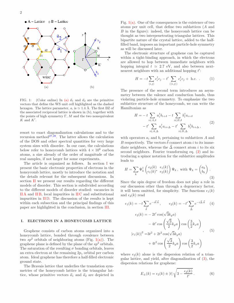
FIG. 1: (Color online) In (a) ~a1 and ~a2 are the primitivevectors that define the WS unit cell highlighted as the dashedhexagon. The lattice parameter, a, is ≃ 1.4 A. The first BZ ofthe associated reciprocal lattice is shown in (b), together withthe points of high symmetry Γ, M and the two nonequivalentK and K′.

resort to exact diagonalization calculations and to therecursion method27,28. The latter allows the calculationof the DOS and other spectral quantities for very largesystem sizes with disorder. In our case, the calculationsbelow refer to honeycomb lattices with 4 × 106 carbonatoms, a size already of the order of magnitude of thereal samples, if not larger for some experiments.

The article is organized as follows. In section I wepresent the basic electronic properties of electrons in thehoneycomb lattice, mostly to introduce the notation andthe details relevant for the subsequent discussions. Insection II we present our results regarding the differentmodels of disorder. This section is subdivided accordingto the different models of disorder studied: vacancies inII A and II B, local impurities in II C and substitutionalimpurities in II D. The discussion of the results is keptwithin each subsection and the principal findings of thispaper are highlighted in the conclusion, in section III.

I. ELECTRONS IN A HONEYCOMB LATTICE

Graphene consists of carbon atoms organized into ahoneycomb lattice, bonded through covalence betweentwo sp2 orbitals of neighboring atoms (Fig. 1(a)). Thegraphene plane is defined by the plane of the sp2 orbitals.The saturation of the resulting σ bonding orbitals, leavesan extra electron at the remaining 2pz orbital per carbonatom. Ideal graphene has therefore a half-filled electronicground state.

The Bravais lattice that underlies the translation sym-metries of the honeycomb lattice is the triangular lat-tice, whose primitive vectors ~a1 and ~a2 are depicted in

Fig. 1(a). One of the consequences is the existence of twoatoms per unit cell, that define two sublattices (A andB in the figure): indeed, the honeycomb lattice can bethought as two interpenetrating triangular lattices. Thisbipartite nature of the crystal lattice, added to the half-filled band, imposes an important particle-hole symmetryas will be discussed later.

The electronic structure of graphene can be capturedwithin a tight-binding approach, in which the electronsare allowed to hop between immediate neighbors withhopping integral t ≃ 2.7 eV, and also between next-nearest neighbors with an additional hopping t′:

H = −t∑

〈i,j〉

c†icj − t′∑

〈〈i,j〉〉

c†i cj + h.c. . (1)

The presence of the second term introduces an asym-metry between the valence and conduction bands, thusviolating particle-hole symmetry. To emphasize the twosublattice structure of the honeycomb, we can write theHamiltonian as

H = − t∑

i∈A,δ

a†ibi+δ − t∑

i∈B,δ

b†iai+δ

− t′∑

i∈A,∆

a†iai+∆ − t′∑

i∈B,∆

b†ibi+∆ ,(2)

with operators ai and bi pertaining to sublattices A and

B respectively. The vectors ~δ connect atom i to its imme-

diate neighbors, whereas the ~∆ connect atom i to its sixsecond neighbors. Fourier transforming eq. (2) and in-troducing a spinor notation for the sublattice amplitudesleads to

H =∑

k

Ψ†k

(

ǫ2(k) ǫ1(k)ǫ1(k)

∗ ǫ2(k)

)

Ψk , with Ψk =

(

ak

bk

)

.

(3)Since the spin degree of freedom does not play a role inour discussion other than through a degeneracy factor,it will been omitted, for simplicity. The functions ǫ1(k)and ǫ2(k) read

ǫ1(k) = −t∑

~δ

e−i~δ.~k , ǫ2(k) = −t′∑

~∆

e−i~∆.~k (4)

ǫ2(k) = − 2t′ cos(√

3kya)

− 4t′ cos

(√3

2kya

)

cos

(

3

2kxa

)

|ǫ1(k)|2 =3t2 + 2t2 cos(√

3kya)

+ 4t2 cos

(√3

2kya

)

cos

(

3

2kxa

)

, (5)

where ǫ2(k) alone is the dispersion relation of a trian-gular lattice, and yield, after diagonalization of (3), thedispersion relations for graphene:

E±(k) = ǫ2(k) ± |t|√

3 − ǫ2(k)

t′. (6)

3

(a) (b)

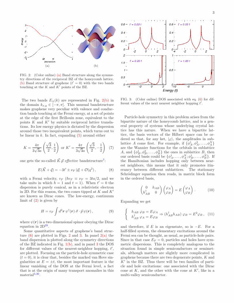
FIG. 2: (Color online) (a) Band structure along the symme-try directions of the reciprocal BZ of the honeycomb lattice.(b) Band structure of graphene (t′ = 0) with the two bandstouching at the K and K′ points of the BZ.

The two bands E±(k) are represented in Fig. 2(b) inthe domain kx,y ∈ [−π, π]. This unusual bandstructuremakes graphene very peculiar with valence and conduc-tion bands touching at the Fermi energy, at a set of pointsat the edge of the first Brillouin zone, equivalent to thepoints K and K ′ by suitable reciprocal lattice transla-tions. Its low energy physics is dictated by the dispersionaround those two inequivalent points, which turns out tobe linear in k. In fact, expanding (5) around either

K =4π

3√

3a

(√3

2,1

2

)

or K ′ =4π

3√

3a

(√3

2,−1

2

)

(7)

one gets the so-called ~K.~p effective bandstructure7:

E( ~K + ~q) = −3t′ ± νF |~q| + O(q2) , (8)

with a Fermi velocity, vF (~vF ≡ νF = 3ta/2, and wetake units in which ~ = 1 and t = 1). When t′ = 0 thedispersion is purely conical, as in a relativistic electronin 2D. For this reason, the two cones tipped at K and K ′

are known as Dirac cones. The low-energy, continuumlimit of (2) is given by

H = vF

∫

d2r ψ†(r) ~σ · ~p ψ(r) , (9)

where ψ(r) is a two dimensional spinor obeying the Diracequation in 2D29.

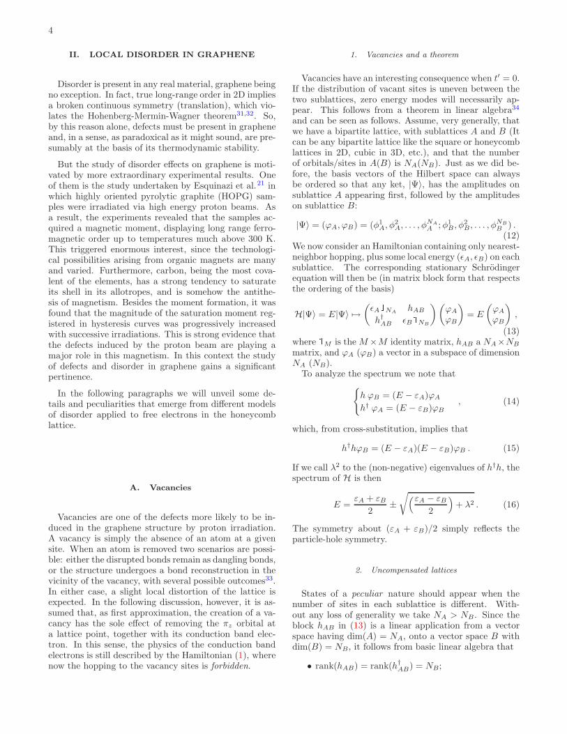
Some quantitative aspects of graphene’s band struc-ture (6) are plotted in Figs. 2 and 3. In panel 2(a) theband dispersion is plotted along the symmetry directionsof the BZ indicated in Fig. 1(b), and in panel 3 the DOSfor different values of the nearest-neighbor hopping, t′,are plotted. Focusing on the particle-hole symmetric case(t = 0), it is clear that, besides the marked van Hove sin-gularities at E = ±t, the most important feature is thelinear vanishing of the DOS at the Fermi level, a factthat is at the origin of many transport anomalies in thismaterial3,30.

FIG. 3: (Color online) DOS associated with eq. (6) for dif-ferent values of the next nearest neighbor hopping t′.

Particle-hole symmetry in this problem arises from thebipartite nature of the honeycomb lattice, and is a gen-eral property of systems whose underlying crystal lat-tice has this nature. When we have a bipartite lat-tice, the basis vectors of the Hilbert space can be or-dered so that, for any ket, |ϕ〉, the amplitudes in sub-lattice A come first. For example, if {φ1

A, φ2A, . . . , φ

NA }

are the Wannier functions for the orbitals in sublatticeA, and {φ1

B , φ2B, . . . , φ

NB } the ones in sublattice B, then

our ordered basis could be {φ1A, . . . , φ

NA ;φ1

B, . . . , φNB }. If

the Hamiltonian includes hopping only between near-est neighbors, this means that it only promotes itin-erancy between different sublattices. The stationarySchrodinger equation then reads, in matrix block formin the ordered basis,

(

0 hAB

h†AB 0

)(

ϕA

ϕB

)

= E

(

ϕA

ϕB

)

. (10)

Expanding we get

{

hAB ϕB = EϕA

h†AB ϕA = EϕB⇒ (h†ABhAB) ϕB = E2ϕB , (11)

and therefore, if E is an eigenstate, so is −E. For ahalf-filled system, the elementary excitations around theFermi sea can be thought, as usual, as particle-hole pairs.Since in that case EF = 0, particles and holes have sym-metric dispersions. This is completely analogous to thesituation found in simple semiconductors or semimet-als, although matters are slightly more complicated ingraphene because there are two degenerate points, K andK ′ in the BZ. Thus there will be two families of parti-cle and hole excitations: one associated with the Diraccone at K, and the other with the cone at K ′, like in amulti-valley semiconductor.

4

II. LOCAL DISORDER IN GRAPHENE

Disorder is present in any real material, graphene beingno exception. In fact, true long-range order in 2D impliesa broken continuous symmetry (translation), which vio-lates the Hohenberg-Mermin-Wagner theorem31,32. So,by this reason alone, defects must be present in grapheneand, in a sense, as paradoxical as it might sound, are pre-sumably at the basis of its thermodynamic stability.

But the study of disorder effects on graphene is moti-vated by more extraordinary experimental results. Oneof them is the study undertaken by Esquinazi et al.21 inwhich highly oriented pyrolytic graphite (HOPG) sam-ples were irradiated via high energy proton beams. Asa result, the experiments revealed that the samples ac-quired a magnetic moment, displaying long range ferro-magnetic order up to temperatures much above 300 K.This triggered enormous interest, since the technologi-cal possibilities arising from organic magnets are manyand varied. Furthermore, carbon, being the most cova-lent of the elements, has a strong tendency to saturateits shell in its allotropes, and is somehow the antithe-sis of magnetism. Besides the moment formation, it wasfound that the magnitude of the saturation moment reg-istered in hysteresis curves was progressively increasedwith successive irradiations. This is strong evidence thatthe defects induced by the proton beam are playing amajor role in this magnetism. In this context the studyof defects and disorder in graphene gains a significantpertinence.

In the following paragraphs we will unveil some de-tails and peculiarities that emerge from different modelsof disorder applied to free electrons in the honeycomblattice.

A. Vacancies

Vacancies are one of the defects more likely to be in-duced in the graphene structure by proton irradiation.A vacancy is simply the absence of an atom at a givensite. When an atom is removed two scenarios are possi-ble: either the disrupted bonds remain as dangling bonds,or the structure undergoes a bond reconstruction in thevicinity of the vacancy, with several possible outcomes33.In either case, a slight local distortion of the lattice isexpected. In the following discussion, however, it is as-sumed that, as first approximation, the creation of a va-cancy has the sole effect of removing the πz orbital ata lattice point, together with its conduction band elec-tron. In this sense, the physics of the conduction bandelectrons is still described by the Hamiltonian (1), wherenow the hopping to the vacancy sites is forbidden.

1. Vacancies and a theorem

Vacancies have an interesting consequence when t′ = 0.If the distribution of vacant sites is uneven between thetwo sublattices, zero energy modes will necessarily ap-pear. This follows from a theorem in linear algebra34

and can be seen as follows. Assume, very generally, thatwe have a bipartite lattice, with sublattices A and B (Itcan be any bipartite lattice like the square or honeycomblattices in 2D, cubic in 3D, etc.), and that the numberof orbitals/sites in A(B) is NA(NB). Just as we did be-fore, the basis vectors of the Hilbert space can alwaysbe ordered so that any ket, |Ψ〉, has the amplitudes onsublattice A appearing first, followed by the amplitudeson sublattice B:

|Ψ〉 = (ϕA, ϕB) = (φ1A, φ

2A, . . . , φ

NA

A ;φ1B , φ

2B, . . . , φ

NB

B ) .(12)

We now consider an Hamiltonian containing only nearest-neighbor hopping, plus some local energy (ǫA, ǫB) on eachsublattice. The corresponding stationary Schrodingerequation will then be (in matrix block form that respectsthe ordering of the basis)

H|Ψ〉 = E|Ψ〉 7→(

ǫA1NAhAB

h†AB ǫB1NB

)(

ϕA

ϕB

)

= E

(

ϕA

ϕB

)

,

(13)where 1M is the M×M identity matrix, hAB a NA×NB

matrix, and ϕA (ϕB) a vector in a subspace of dimensionNA (NB).

To analyze the spectrum we note that

{

h ϕB = (E − εA)ϕA

h† ϕA = (E − εB)ϕB, (14)

which, from cross-substitution, implies that

h†hϕB = (E − εA)(E − εB)ϕB . (15)

If we call λ2 to the (non-negative) eigenvalues of h†h, thespectrum of H is then

E =εA + εB

2±√

(εA − εB

2

)

+ λ2 . (16)

The symmetry about (εA + εB)/2 simply reflects theparticle-hole symmetry.

2. Uncompensated lattices

States of a peculiar nature should appear when thenumber of sites in each sublattice is different. With-out any loss of generality we take NA > NB. Since theblock hAB in (13) is a linear application from a vectorspace having dim(A) = NA, onto a vector space B withdim(B) = NB, it follows from basic linear algebra that

• rank(hAB) = rank(h†AB) = NB;

5

• hAB ϕB = 0 has no solutions other than the trivialone;

• h†AB ϕA = 0 has non-trivial solutions that we callϕ0

A.

From the rank-nullity theorem,

rank(h†AB) + nullity(h†AB) = NA , (17)

and hence the null space of h†AB has dimension:

nullity(h†AB) = NA −NB. Consequently, there are statesof the form

|Ψ0〉 = (ϕ0A; 0)

in which ϕ0A satisfies h†AB ϕ

0A = 0, that are eigenstates of

H with eigenvalue εA:

H|Ψ0〉 = E|Ψ〉 ⇔{

h 0 = (εA − εA)ϕA

h† ϕ0A = (εA − εB)0

. (18)

Furthermore, since nullity(h†AB) = NA −NB implies theexistence ofNA−NB linearly independent ϕ0

A, this eigen-state has a degeneracy of NA−NB. It should be stressedthat a state of the form (ϕA; 0) has only amplitude inthe A sublattice. Therefore, we conclude that, wheneverthe two sublattices are not balanced with respect to theirnumber of atoms, there will appear NA −NB states withenergy EA, all linearly independent and localized onlyon the majority sublattice. In addition, one can modifysublattice B in any way (remove more sites, for instance)that these zero modes will remain totally undisturbed.

We remark that in the above the details of the hoppingmatrix hAB were not specified and need not be. The re-sult holds in general, provided that the hopping inducestransitions between different sublattice only, and that thediagonal energies are constant (diagonal disorder is ex-cluded).

3. Zero modes

The case with εA = εB = 0 is of obvious relevancefor us, since our model for pristine graphene does notinclude any local potentials. In this situation, the aboveresults imply that introducing a vacancy in an otherwiseperfect lattice, immediately creates a zero energy mode.Now this is important because those states are createdprecisely at the Fermi level, and have this peculiar topo-logical localization determining that they should live injust one of the lattices.

Even more interestingly, it is possible to obtain theexact analytical wavefunction associated with the zeromode induced by a single vacancy in a honeycomb lat-tice. This was done by the authors and collaborators inRef. 25, and will not be repeated here. We only mentionthat the wavefunction can be constructed by an appro-priate matching of the zero modes of two semi-infinite

(a) (b)

(c) (d)

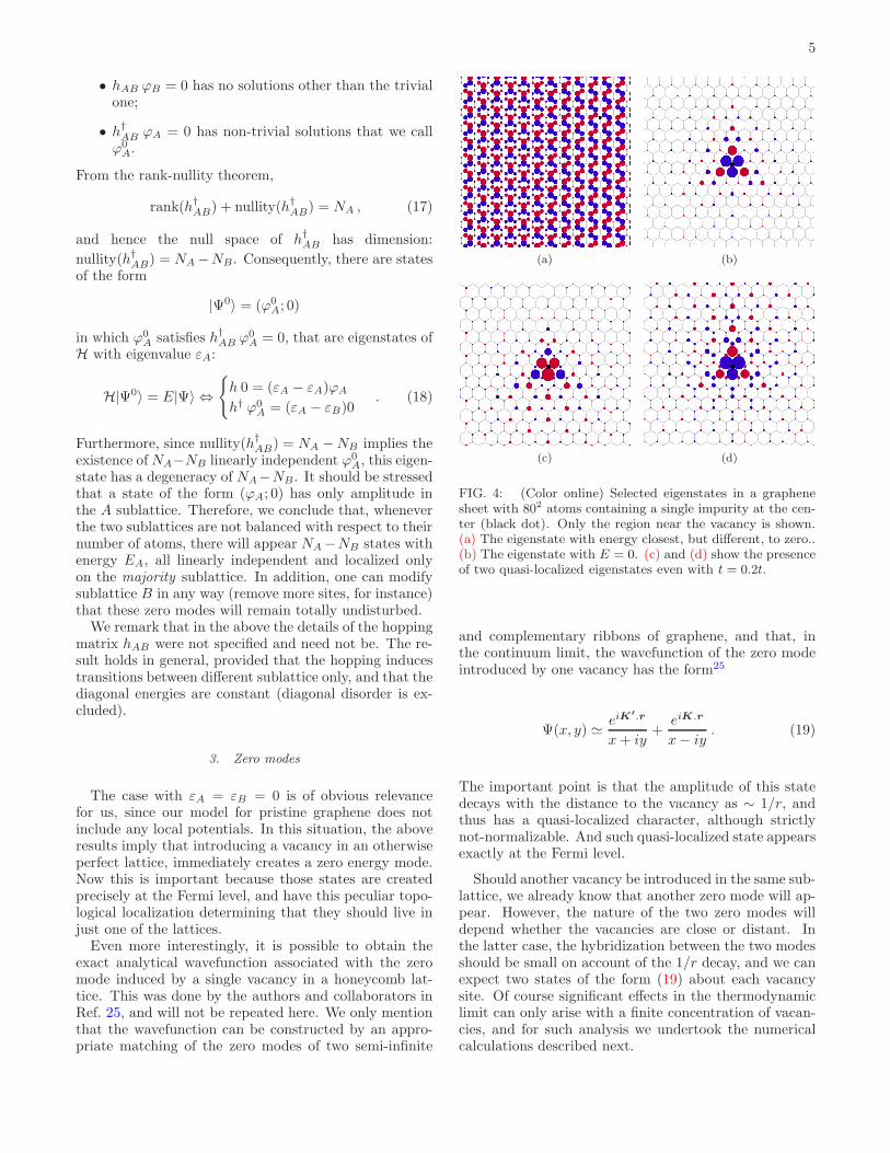
FIG. 4: (Color online) Selected eigenstates in a graphenesheet with 802 atoms containing a single impurity at the cen-ter (black dot). Only the region near the vacancy is shown.(a) The eigenstate with energy closest, but different, to zero..(b) The eigenstate with E = 0. (c) and (d) show the presenceof two quasi-localized eigenstates even with t = 0.2t.

and complementary ribbons of graphene, and that, inthe continuum limit, the wavefunction of the zero modeintroduced by one vacancy has the form25

Ψ(x, y) ≃ eiK′.r

x+ iy+

eiK.r

x− iy. (19)

The important point is that the amplitude of this statedecays with the distance to the vacancy as ∼ 1/r, andthus has a quasi-localized character, although strictlynot-normalizable. And such quasi-localized state appearsexactly at the Fermi level.

Should another vacancy be introduced in the same sub-lattice, we already know that another zero mode will ap-pear. However, the nature of the two zero modes willdepend whether the vacancies are close or distant. Inthe latter case, the hybridization between the two modesshould be small on account of the 1/r decay, and we canexpect two states of the form (19) about each vacancysite. Of course significant effects in the thermodynamiclimit can only arise with a finite concentration of vacan-cies, and for such analysis we undertook the numericalcalculations described next.

6

4. Numerical Results – Single Vacancy

The first calculation is the numerical verification of theexact analytical result for the localized state in (19). Forthat, we consider the tight-binding Hamiltonian (1) andcalculate numerically, via exact diagonalization, the fullspectrum and eigenstates in the presence of a single va-cancy. For some typical results we turn our attention toFig. 4. There we plot a real-space representation of someselected wavefunctions. This has been done by drawinga circle at each lattice site, whose radius is proportionalto the wavefunction amplitude at that site, and whosecolor (red/blue) reflects the sign (+/-) of the amplitudeat each site. Thus bigger circles mean higher amplitudes.In the first panel, 4(a), we are showing the eigenstatewith lowest, yet non-zero, absolute energy. It is visiblethat the wavefunction associated with such state spreadsuniformly across the totality of the system. like a planewave. In the second panel, 4(b), we draw the wavefunc-tion of the state E = 0, that corresponds to (19). Thestate is clearly decaying as the distance to the central va-cancy increases. In addition, the state exhibits the full C3

point symmetry about the vacant site, just as expected.This picture provides a snapshot of the lattice version25

of (19). Since only one vacancy was introduced, the stateshown in Fig. 4(b) is the only zero mode present.

When particle-hole symmetry is disturbed by a non-zero t′, we still find states having this quasi-localized na-ture, where the wavefunction amplitude is still quite con-centrated about the vacancy. Two examples are shownin panels 4(b) and 4(c). They are two eigenstates withneighboring energy calculated for the same system. Animportant difference occurs here, in that, unlike thecase t′ = 0 where only one localized state appears, theparticle-hole asymmetric case opens the possibility formore than one of such states.

This fact can be seen more transparently through theinverse participation ratio (IPR) of the eigenstates. Withsuch purpose in mind, the IPR

P(En) =∑

i

|Ψn(ri)|4

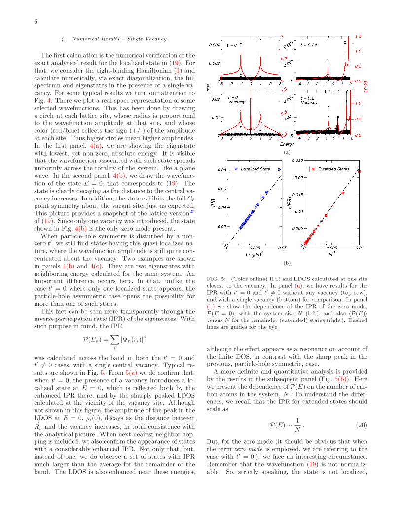
was calculated across the band in both the t′ = 0 andt′ 6= 0 cases, with a single central vacancy. Typical re-sults are shown in Fig. 5. From 5(a) we do confirm that,when t′ = 0, the presence of a vacancy introduces a lo-calized state at E = 0, which is reflected both by theenhanced IPR there, and by the sharply peaked LDOScalculated at the vicinity of the vacancy site. Althoughnot shown in this figure, the amplitude of the peak in theLDOS at E = 0, ρi(0), decays as the distance between~Ri and the vacancy increases, in total consistence withthe analytical picture. When next-nearest neighbor hop-ping is included, we also confirm the appearance of stateswith a considerably enhanced IPR. Not only that, but,instead of one, we do observe a set of states with IPRmuch larger than the average for the remainder of theband. The LDOS is also enhanced near these energies,

(a)

(b)

FIG. 5: (Color online) IPR and LDOS calculated at one siteclosest to the vacancy. In panel (a), we have results for theIPR with t′ = 0 and t′ 6= 0 without any vacancy (top row),and with a single vacancy (bottom) for comparison. In panel(b) we show the dependence of the IPR of the zero mode,P(E = 0), with the system size N (left), and also 〈P(E)〉versus N for the remainder (extended) states (right). Dashedlines are guides for the eye.

although the effect appears as a resonance on account ofthe finite DOS, in contrast with the sharp peak in theprevious, particle-hole symmetric, case.

A more definite and quantitative analysis is providedby the results in the subsequent panel (Fig. 5(b)). Herewe present the dependence of P(E) on the number of car-bon atoms in the system, N . To understand the differ-ences, we recall that the IPR for extended states shouldscale as

P(E) ∼ 1

N. (20)

But, for the zero mode (it should be obvious that whenthe term zero mode is employed, we are referring to thecase with t′ = 0.), we face an interesting circumstance.Remember that the wavefunction (19) is not normaliz-able. So, strictly speaking, the state is not localized,

7

and hence the designation quasi-localized that we haveadopted above. The consequence of this is that the nor-malization constant for Ψ(x, y) depends on the systemsize:

N∑

i

|Ψ(x, y)|2 ∼ log(√N) ∼ log(N) . (21)

This, in turn has an effect on the IPR because P(E) isdefined in terms of normalized wavefunctions:

P(0) =1

log(N)2

N∑

i

|Ψ(x, y)|4 ∼ 1

log(N)2. (22)

This scaling of the IPR with N is precisely the one ob-tained numerically in Fig. 5(b) (left) for the zero mode,and is just another way of confirming the 1/r decay ofthis wavefunction.

5. Numerical Results – Finite Concentration of Vacancies

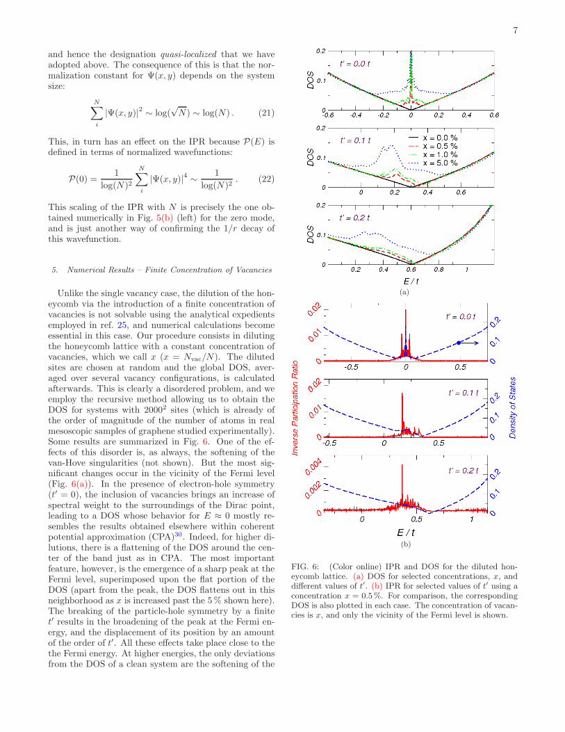
Unlike the single vacancy case, the dilution of the hon-eycomb via the introduction of a finite concentration ofvacancies is not solvable using the analytical expedientsemployed in ref. 25, and numerical calculations becomeessential in this case. Our procedure consists in dilutingthe honeycomb lattice with a constant concentration ofvacancies, which we call x (x = Nvac/N). The dilutedsites are chosen at random and the global DOS, aver-aged over several vacancy configurations, is calculatedafterwards. This is clearly a disordered problem, and weemploy the recursive method allowing us to obtain theDOS for systems with 20002 sites (which is already ofthe order of magnitude of the number of atoms in realmesoscopic samples of graphene studied experimentally).Some results are summarized in Fig. 6. One of the ef-fects of this disorder is, as always, the softening of thevan-Hove singularities (not shown). But the most sig-nificant changes occur in the vicinity of the Fermi level(Fig. 6(a)). In the presence of electron-hole symmetry(t′ = 0), the inclusion of vacancies brings an increase ofspectral weight to the surroundings of the Dirac point,leading to a DOS whose behavior for E ≈ 0 mostly re-sembles the results obtained elsewhere within coherentpotential approximation (CPA)30. Indeed, for higher di-lutions, there is a flattening of the DOS around the cen-ter of the band just as in CPA. The most importantfeature, however, is the emergence of a sharp peak at theFermi level, superimposed upon the flat portion of theDOS (apart from the peak, the DOS flattens out in thisneighborhood as x is increased past the 5 % shown here).The breaking of the particle-hole symmetry by a finitet′ results in the broadening of the peak at the Fermi en-ergy, and the displacement of its position by an amountof the order of t′. All these effects take place close to thethe Fermi energy. At higher energies, the only deviationsfrom the DOS of a clean system are the softening of the

(a)

(b)

FIG. 6: (Color online) IPR and DOS for the diluted hon-eycomb lattice. (a) DOS for selected concentrations, x, anddifferent values of t′. (b) IPR for selected values of t′ using aconcentration x = 0.5 %. For comparison, the correspondingDOS is also plotted in each case. The concentration of vacan-cies is x, and only the vicinity of the Fermi level is shown.

8

van Hove singularities and the development of Lifshitztails (not shown) at the band edge, both induced by theincreasing disorder caused by the random dilution. Theonset of this high energy regime, where the profile of theDOS is essentially unperturbed by the presence of va-

cancies, is determined by ǫ ≈ vF/l, with l ∼ n−1/2

imp beingessentially the average distance between impurities.

To address the degree of localization for the states nearthe Fermi level, the IPR was calculated again, via exactdiagonalization on smaller systems. Results for differentvalues of t′ are shown in Fig. 6(b) for random dilution at0.5 %. One observes, first, that Pm ∼ 3/N for all energiesbut the Fermi level neighborhood, as expected for statesextended up to the length scale of the system sizes usedin the numerics. Secondly, the IPR becomes significantexactly in the same energy range where the DOS exhibitsthe vacancy-induced anomalies discussed above. Clearly,the farther the system is driven from the particle-holesymmetric case, the weaker the localization effect, as il-lustrated by the results obtained with t′ = 0.2 t. To thisrespect, it is worth mentioning that the magnitude of thestrongest peaks in Pm at t′ = 0 and t′ = 0.1 t is equal tothe magnitude of the IPR calculated above for a singleimpurity problem. Such behavior indicates the existenceof quasi-localized states at the center of the resonance,induced by the presence of the vacancies. For higher dop-ing strengths, the enhancement of Pm is weaker in theregions where the DOS becomes flat. This explains thequalitative agreement between our results and the onesobtained within CPA in that region, since CPA does notaccount for localization effects.

In summary, in this section, we saw that a single va-cancy introduces a quasi-localized zero mode. Its pres-ence is ensured by the uncompensation between the num-ber of orbitals in the two sublattices, and a theorem fromlinear algebra. The presence of this mode translates inthe appearance of a peak in the LDOS near the vacancy,and in an enhanced IPR for this state. When we go fromone to a macroscopic number of vacancies, we saw thatboth the peak and the enhancement of the IPR persistin the global DOS at EF .

B. Selective Dilution

It is important to recall that the results of the previoussection pertain to lattices that were randomly diluted.During such process, we expect the number of vacanciesin sublattice A to be equal to the number of vacanciesin sublattice B, on average. Strictly speaking, since ouroriginal lattices are always chosen with NA = NB, thefluctuations on the degree of uncompensation, NA −NB,should scale as 1/

√N thus vanishing in the thermody-

namic limit. Because of this, in principle, we would ex-pect the lattices used above to be reasonably compen-sated. But the theorem in § II A 1 only guarantees thepresence of zero modes when the lattice is uncompen-sated. It turns out that, notwithstanding our utilization

(a)

(b)

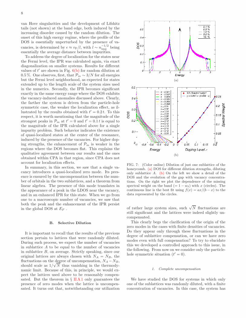
FIG. 7: (Color online) Dilution of just one sublattice of thehoneycomb. (a) DOS for different dilution strengths, dilutingonly sublattice A. (b) On the left we show a detail of theDOS and the evolution of the gap with vacancy concentra-tions. On the right we plot the dependence of the missingspectral weight on the band (= 1 − wδ) with x (circles). Thecontinuous line is the best fit using f(x) = ax/(b − x) to thedata represented by the circles.

of rather large system sizes, such√N fluctuations are

still significant and the lattices were indeed slightly un-compensated.

This clearly begs the clarification of the origin of thezero modes in the cases with finite densities of vacancies.Do they appear only through these fluctuations in thedegree of sublattice compensation, or can we have zeromodes even with full compensation? To try to elucidatethis we developed a controlled approach to this issue, inthe following. From now on we consider only the particle-hole symmetric situation (t′ = 0).

1. Complete uncompensation

We have studied the DOS for systems in which onlyone of the sublattices was randomly diluted, with a finiteconcentration of vacancies. In this case, the system has

9

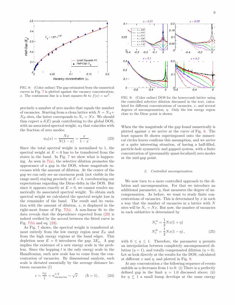
FIG. 8: (Color online) The gap estimated from the numericalcurves in Fig. 7 is plotted against the vacancy concentration,x. The continuous line is a least squares fit to f(x) = axb.

precisely a number of zero modes that equals the numberof vacancies. Starting from a clean lattice withN = NA+NB sites, the latter corresponds to Nv = Nx. We shouldthus expect a δ(E) peak contributing to the global DOS,with an associated spectral weight, wδ that coincides withthe fraction of zero modes:

wδ(x) =Nx

N(1 − x)=

x

1 − x. (23)

Since the total spectral weight is normalized to 1, thespectral weight at E = 0 has to be transferred from thestates in the band. In Fig. 7 we show what is happen-ing. As seen in 7(a), the selective dilution promotes theappearance of a gap in the DOS, whose magnitude in-creases with the amount of dilution. At the center of thegap we can only see an enormous peak (not visible in therange used) staying precisely at E = 0, corroborating ourexpectations regarding the Dirac-delta in the DOS. Butsince it appears exactly at E = 0, we cannot resolve nu-merically its associated spectral weight. To obtain suchspectral weight we calculated the spectral weight loss inthe remainder of the band. The result and its varia-tion with the amount of dilution, x, is displayed in theright-most frame of Fig. 7(b). A non-linear fit to thedata reveals that the dependence expected from (23) isindeed verified by the accord between the fitted curve inFig. 7(b) and eq. (23).

As Fig. 7 shows, the spectral weight is transferred al-most entirely from the low energy region near EF andfrom the high energy regions at the band edges. Thisdepletion near E = 0 introduces the gap, 2Eg. A gapimplies the existence of a new energy scale in the prob-lem. Since the hopping t is the only energy scale in theHamiltonian, such new scale has to come from the con-centration of vacancies. By dimensional analysis, suchscale is dictated essentially by the average distance be-tween vacancies (l)

ǫ ∼ vF

l∼ n

1/2

vacancies ∼√x (~ = 1) . (24)

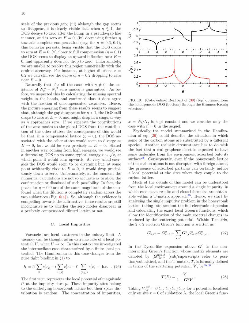
FIG. 9: (Color online) DOS for the honeycomb lattice usingthe controlled selective dilution discussed in the text, calcu-lated for different concentrations of vacancies, x, and severaldegrees of uncompensation, η. Only the low energy regionclose to the Dirac point is shown.

When the the magnitude of the gap found numerically isplotted against x we arrive at the curve of Fig. 8. Theleast squares fit shown superimposed onto the numeri-cal circles leaves confirms this assumption, and we arriveat a quite interesting situation, of having a half-filled,particle-hole symmetric and gapped system, with a finiteconcentration of (presumably quasi-localized) zero modesat the mid-gap point.

2. Controlled uncompensation

We now turn to a more controlled approach to the di-lution and uncompensation. For that we introduce anadditional parameter, η, that measures the degree of un-compensation. As before, we want to study finite con-centrations of vacancies. This is determined by x in sucha way that the number of vacancies in a lattice with Nsites will be Nv = Nx. But now, the number of vacanciesin each sublattice is determined by

NAv =

1

2Nx(1 + η)

NBv =

1

2Nx(1 − η) , (25)

with 0 ≤ η ≤ 1. Therefore, the parameter η permitsan interpolation between completely uncompensated di-lution (η = 1), and totally compensated dilution (η = 0).Let us look directly at the results for the DOS, calculatedat different x and η, and plotted in Fig. 9.

At any concentration x the following sequence of eventsunfolds as η decreases from 1 to 0: (i) There is a perfectlydefined gap in the limit η = 1.0 discussed above; (ii)for η . 1 a small hump develops at the same energy

10

scale of the previous gap; (iii) although the gap seemsto disappear, it is clearly visible that when η . 1, theDOS decays to zero after the hump in a pseudo-gap likemanner, and is zero at E = 0; (iv) decreasing further ηtowards complete compensation (say, for η = 0.6, 0.4),this behavior persists, being visible that the DOS dropsto zero at E = 0; (v) closer to full compensation (η = 0.1)the DOS seems to display an upward inflection near E =0, and apparently does not drop to zero. Unfortunately,we are unable to resolve this region numerically with thedesired accuracy. For instance, at higher dilutions x =0.2 we can still see the curve of η = 0.2 dropping to zeronear E = 0.

Naturally that, for all the cases with η 6= 0, the ex-istence of NA

v − NBv zero modes is guaranteed. As be-

fore, we inspected this by calculating the missing spectralweight in the bands, and confirmed that it does agreewith the fraction of uncompensated vacancies. Hence,the picture emerging from these results seems to suggestthat, although the gap disappears for η < 1, the DOS stilldrops to zero at E = 0, and might drop in a singular wayas η approaches zero. If we separate the contributionsof the zero modes to the global DOS from the contribu-tion of the other states, the consequence of this wouldbe that, in a compensated lattice (η = 0), the DOS as-sociated with the other states would seem to diverge asE → 0, but would be zero precisely at E = 0. Statedin another way, coming from high energies, we would seea decreasing DOS up to some typical energy ǫ ∼ √

x, atwhich point it would turn upwards. At very small ener-gies the DOS would seem to be diverging but, at somepoint arbitrarily close to E = 0, it would drop precipi-tously down to zero. Unfortunately, at the moment thenumerical calculations are not so accurate as to allow theconfirmation or dismissal of such possibility. In fact, thepeaks for η = 0.0 are of the same magnitude of the onesfound when the dilution is completely random across thetwo sublattices (Fig. 6(a)). So, although the evidence iscompelling towards the affirmative, these results are stillinconclusive as to whether the zero modes disappear ina perfectly compensated diluted lattice or not.

C. Local Impurities

Vacancies are local scatterers in the unitary limit. Avacancy can be thought as an extreme case of a local po-tential, U , when U → ∞. In this context we investigatedthe intermediate case characterized by a finite local po-tential. The Hamiltonian in this case changes from thepure tight binding in (1) to

H = U∑

p

c†pcp − t∑

〈i,j〉

c†icj − t′∑

〈〈i,j〉〉

c†i cj + h.c. . (26)

The first term represents the local potential of magnitudeU at the impurity sites p. These impurity sites belongto the underlying honeycomb lattice but their space dis-tribution is random. The concentration of impurities,

FIG. 10: (Color online) Real part of (30) (top) obtained fromthe homogeneous DOS (bottom) through the Kramers-Kronigrelations.

x = Ni/N , is kept constant and we consider only thecase with t′ = 0 in the sequel.

Physically the model summarized in the Hamilto-nian of eq. (26) could describe the situation in whichsome of the carbon atoms are substituted by a differentspecies. Another realistic circumstance has to do withthe fact that a real graphene sheet is expected to havesome molecules from the environment adsorbed onto itssurface22. Consequently, even if the honeycomb latticeof the carbon atoms is not disrupted with foreign atoms,the presence of adsorbed particles can certainly inducea local potential at the sites where they couple to thecarbon lattice.

Much of the details of this model can be understoodfrom the local environment around a single impurity, inwhich case exact results and closed formulas are obtain-able within a T-matrix approach35. Hence, we start byanalyzing the single impurity problem in the honeycomblattice, taking into account the full electronic dispersionand calculating the exact local Green’s functions, whichallow the identification of the main spectral changes in-troduced by the scattering potential. Within T-matrix,the 2 × 2 electron Green’s function is written as

Gr,r′ = G0r,r′ +

∑

s,s′

G0r,sTs,s′G

0s′,r′ . (27)

In the Dyson-like expansion above G0 is the non-

interacting Green’s function whose matrix elements are

denoted by [G0]α,βr,r′ (sub/superscripts refer to posi-

tion/sublattice), and the T-matrix, T , is formally definedin terms of the scattering potential, V , by35,36

T (E) =V

1 − G0V. (28)

Taking Vαβ

r,r′ = Uδr,r′δr,0δα,βδα,0 for a potential localizedonly on site r = 0 of sublattice A, the local Green’s func-

11

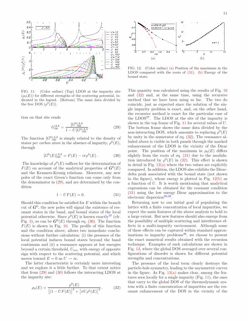
FIG. 11: (Color online) (Top) LDOS at the impurity site(ρ0(E)) for different strengths of the scattering potential, in-dicated in the legend. (Bottom) The same data divided bythe free DOS (ρ0(E)).

tion on that site reads

GAA00 =

[G0]AA00

1 − U [G0]AA00

. (29)

The function [G0]AA00 is simply related to the density of

states per carbon atom in the absence of impurity, ρ0(E),through

[G0(E)]AA00 = F (E) − iπρ0(E) . (30)

The knowledge of ρ0(E) suffices for the determination ofF (E) on account of the analytical properties of G

0(E)and the Kramers-Kronig relations. Moreover, any newpoles of the exact Green’s function can come only fromthe denominator in (29), and are determined by the con-dition

1 − UF (E) = 0 . (31)

Should this condition be satisfied for E within the branchcut of G

0, the new poles will signal the existence of res-onant states in the band, and bound states of the localpotential otherwise. Since ρ0(E) is known exactly37 (cfr.Fig. 3), so can be G

0(E) through eq. (30). The functionF (E) is shown in Fig. 10. The profile of this functionand the condition above, allows two immediate conclu-sions without further calculation: (i) the presence of thelocal potential induces bound states beyond the bandcontinuum and (ii) a resonance appears at low energiesbeyond a certain threshold, Ures, with energy of oppositesign with respect to the scattering potential, and whichmoves toward E = 0 as U → ∞.

The latter characteristic is certainly more interestingand we explore it a little further. To that extent noticethat from (29) and (30) follows the interacting LDOS atthe impurity site:

ρ0(E) =ρ0(E)

[

(1 − UF (E)]2

+[

πUρ0(E)]2. (32)

(a) (b)

FIG. 12: (Color online) (a) Position of the maximum in theLDOS compared with the roots of (31). (b) Energy of thebound state.

This quantity was calculated using the results of Fig. 10and (32) and, at the same time, using the recursivemethod that we have been using so far. The two docoincide, just as expected since the solution of the sin-gle impurity problem is exact, and, on the other hand,the recursive method is exact for the particular case ofthe LDOS27. The LDOS at the site of the impurity isshown in the top frame of Fig. 11 for several values of U .The bottom frame shows the same data divided by thenon-interacting DOS, which amounts to replacing ρ0(E)by unity in the numerator of eq. (32). The resonance al-luded above is visible in both panels through the markedenhancement of the LDOS in the vicinity of the Diracpoint. The position of the maximum in ρ0(E) differsslightly from the roots of eq. (31) due to the modula-tion introduced by ρ0(E) in (32). This effect is shownin detail in Fig. 12(a) where the two values are explicitlycompared. In addition, the LDOS also exhibits the Dirac-delta peak associated with the bound state (not shownin the figure), whose energy is plotted in Fig. 12(b) asa function of U . It is worth mentioning that analyticalexpressions can be obtained for the resonant condition(31) using the low energy Dirac approximation to theelectronic dispersion30,38.

Returning now to our initial goal of populating thelattice with a finite concentration of local impurities, weexpect the main features of the above analysis to hold toa large extent. But new features should also emerge fromthe possibility of multiple scattering and interference ef-fects in a multi-impurity environment. Although someof these effects can be captured within standard approx-imations to impurity problems36, we choose to presentthe exact numerical results obtained with the recursiontechnique. Examples of such calculations are shown inFig. 13, where the global DOS averaged over several con-figurations of disorder is shown for different potentialstrengths and concentrations.

The presence of the local term clearly destroys theparticle-hole symmetry, leading to the asymmetric curvesin the figure. As Fig. 13(a) makes clear, among the fea-tures seen locally for a single impurity (Fig. 11), the onesthat carry to the global DOS of the thermodynamic sys-tem with a finite concentration of impurities are the res-onant enhancement of the DOS in the vicinity of the

12

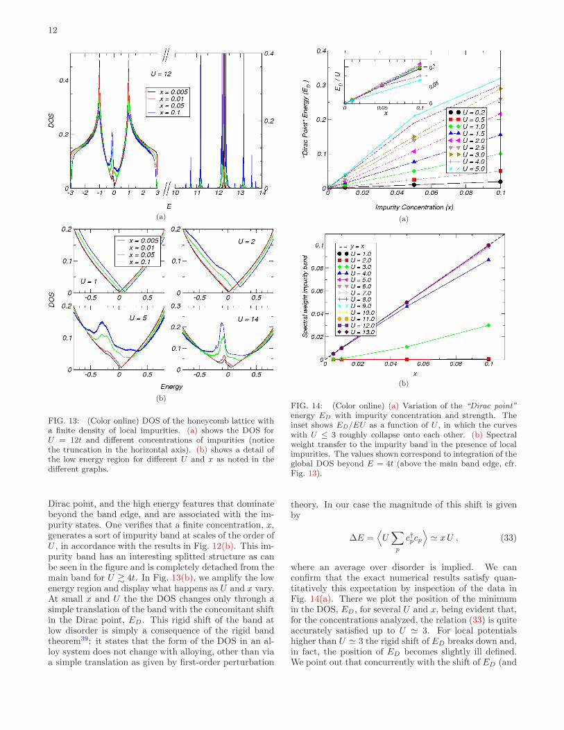
(a)

(b)

FIG. 13: (Color online) DOS of the honeycomb lattice witha finite density of local impurities. (a) shows the DOS forU = 12t and different concentrations of impurities (noticethe truncation in the horizontal axis). (b) shows a detail ofthe low energy region for different U and x as noted in thedifferent graphs.

Dirac point, and the high energy features that dominatebeyond the band edge, and are associated with the im-purity states. One verifies that a finite concentration, x,generates a sort of impurity band at scales of the order ofU , in accordance with the results in Fig. 12(b). This im-purity band has an interesting splitted structure as canbe seen in the figure and is completely detached from themain band for U & 4t. In Fig. 13(b), we amplify the lowenergy region and display what happens as U and x vary.At small x and U the the DOS changes only through asimple translation of the band with the concomitant shiftin the Dirac point, ED. This rigid shift of the band atlow disorder is simply a consequence of the rigid bandtheorem39: it states that the form of the DOS in an al-loy system does not change with alloying, other than viaa simple translation as given by first-order perturbation

(a)

(b)

FIG. 14: (Color online) (a) Variation of the “Dirac point”

energy ED with impurity concentration and strength. Theinset shows ED/EU as a function of U , in which the curveswith U ≤ 3 roughly collapse onto each other. (b) Spectralweight transfer to the impurity band in the presence of localimpurities. The values shown correspond to integration of theglobal DOS beyond E = 4t (above the main band edge, cfr.Fig. 13).

theory. In our case the magnitude of this shift is givenby

∆E =⟨

U∑

p

c†pcp

⟩

≃ xU , (33)

where an average over disorder is implied. We canconfirm that the exact numerical results satisfy quan-titatively this expectation by inspection of the data inFig. 14(a). There we plot the position of the minimumin the DOS, ED, for several U and x, being evident that,for the concentrations analyzed, the relation (33) is quiteaccurately satisfied up to U ≃ 3. For local potentialshigher than U ≃ 3 the rigid shift of ED breaks down and,in fact, the position of ED becomes slightly ill defined.We point out that concurrently with the shift of ED (and

13

the band), there is a marked increase in the DOS at ED,unlike the single impurity case (cfr. Fig. 11). This, again,is expected and appears already in approximate methodslike the CPA approximation30. Nonetheless, whereas ED

shifts linearly for moderate potential strengths, the po-sition of the resonance does not vary significantly withconcentration, and is only enhanced with an increasingnumber of impurities (Fig. 13(b)).

Another noteworthy aspect of this model has to dowith the impurity band that emerges at high energies.Besides the effects just described, a change in the con-centration of impurities implies a concomitant redistribu-tion of spectral weight between the main band and theimpurity band. This is plainly shown in Fig. 14(b) whichdisplays the spectral weight in the impurity band againstthe concentration of impurities. This spectral weight iscalculated by integrating the DOS in the region [4t,∞[.As the figure shows, for U & 5t the spectral weight ofthe impurity band saturates at the value x, signaling thedetachment of the impurity states from the main band.For those cases the spectral weight coincides with theconcentration x. It certainly had to be so because withincreasing U the impurity band drifts to higher energies,eventually disappearing from the problem in the unitarylimit. As discussed previously in section II A, the spec-tral weight of the main band is decreased by precisely x,in the presence of a concentration of vacancies of x. Thisis totally consistent with the fact that the local impu-rity interpolates between the clean case and the vacancylimit.

Finally, is also clear how the vacancy limit (U → ∞)emerges from the data in Fig. 13 as the resonance ap-proaches E = 0 and becomes more sharply defined. Atthe same time, the impurity band is displaced towardhigher and higher energies, eventually projecting out ofthe problem in the vacancy limit.

D. Non-Diagonal Impurities

Another effect expected with the inclusion of a sub-stitutional impurity in the graphene lattice is the modi-fication of the hoppings between the new atom and theneighboring carbons. This happens because the host andsubstituting atoms have different radii, because the na-ture of the orbitals involved in the conduction band isdifferent, or, most likely, a combination of both. Custom-ary impurities in carbon allotropes are nitrogen, workingas a donor, and boron, working as an acceptor40. In fact,the selective inclusion of nitrogen and/or boron impuri-ties in carbon nanotubes is a current practice in the hopeto tune the nanotubes’ electronic response41,42,43.

In general the study of a perturbation in the hoppingis much less studied in problems with impurities than thecase of diagonal, on-site, perturbations. In the contextof our investigations, the perturbation in the hoppingcan, again, be interpreted as an interpolation betweena vacancy and an impurity. To be more precise, let us

(a)

(b)

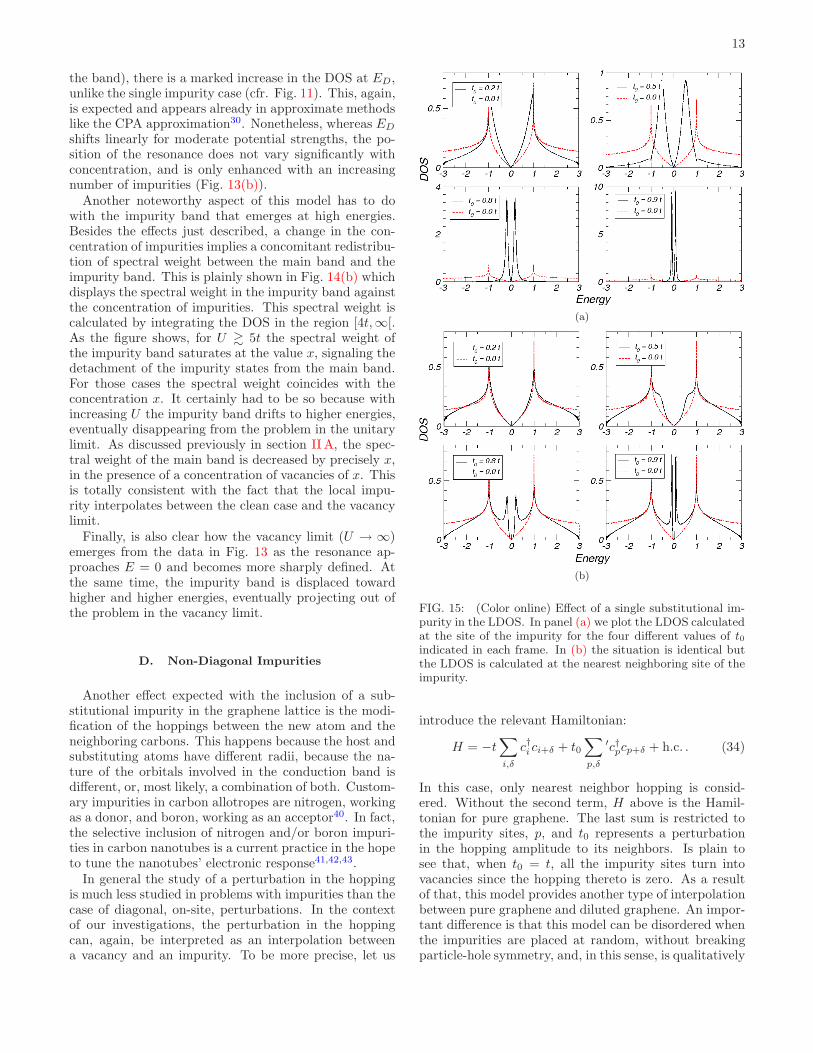
FIG. 15: (Color online) Effect of a single substitutional im-purity in the LDOS. In panel (a) we plot the LDOS calculatedat the site of the impurity for the four different values of t0indicated in each frame. In (b) the situation is identical butthe LDOS is calculated at the nearest neighboring site of theimpurity.

introduce the relevant Hamiltonian:

H = −t∑

i,δ

c†i ci+δ + t0∑

p,δ

′c†pcp+δ + h.c. . (34)

In this case, only nearest neighbor hopping is consid-ered. Without the second term, H above is the Hamil-tonian for pure graphene. The last sum is restricted tothe impurity sites, p, and t0 represents a perturbationin the hopping amplitude to its neighbors. Is plain tosee that, when t0 = t, all the impurity sites turn intovacancies since the hopping thereto is zero. As a resultof that, this model provides another type of interpolationbetween pure graphene and diluted graphene. An impor-tant difference is that this model can be disordered whenthe impurities are placed at random, without breakingparticle-hole symmetry, and, in this sense, is qualitatively

14

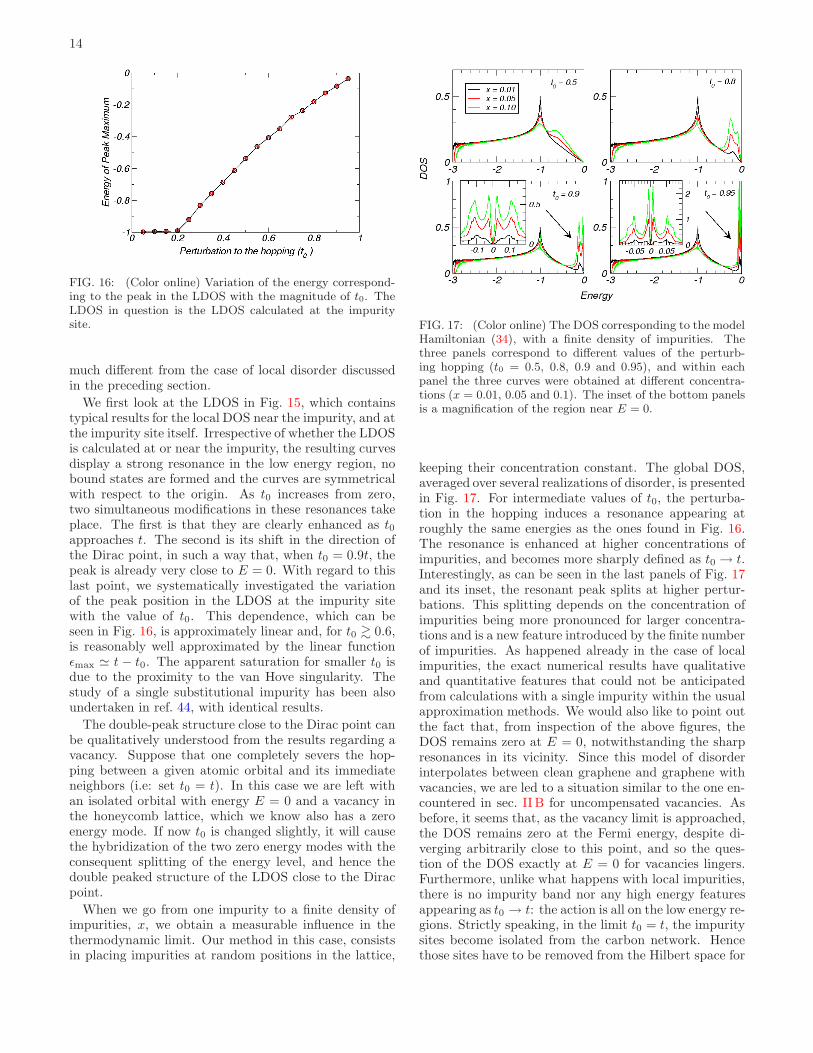
FIG. 16: (Color online) Variation of the energy correspond-ing to the peak in the LDOS with the magnitude of t0. TheLDOS in question is the LDOS calculated at the impuritysite.

much different from the case of local disorder discussedin the preceding section.

We first look at the LDOS in Fig. 15, which containstypical results for the local DOS near the impurity, and atthe impurity site itself. Irrespective of whether the LDOSis calculated at or near the impurity, the resulting curvesdisplay a strong resonance in the low energy region, nobound states are formed and the curves are symmetricalwith respect to the origin. As t0 increases from zero,two simultaneous modifications in these resonances takeplace. The first is that they are clearly enhanced as t0approaches t. The second is its shift in the direction ofthe Dirac point, in such a way that, when t0 = 0.9t, thepeak is already very close to E = 0. With regard to thislast point, we systematically investigated the variationof the peak position in the LDOS at the impurity sitewith the value of t0. This dependence, which can beseen in Fig. 16, is approximately linear and, for t0 & 0.6,is reasonably well approximated by the linear functionǫmax ≃ t − t0. The apparent saturation for smaller t0 isdue to the proximity to the van Hove singularity. Thestudy of a single substitutional impurity has been alsoundertaken in ref. 44, with identical results.

The double-peak structure close to the Dirac point canbe qualitatively understood from the results regarding avacancy. Suppose that one completely severs the hop-ping between a given atomic orbital and its immediateneighbors (i.e: set t0 = t). In this case we are left withan isolated orbital with energy E = 0 and a vacancy inthe honeycomb lattice, which we know also has a zeroenergy mode. If now t0 is changed slightly, it will causethe hybridization of the two zero energy modes with theconsequent splitting of the energy level, and hence thedouble peaked structure of the LDOS close to the Diracpoint.

When we go from one impurity to a finite density ofimpurities, x, we obtain a measurable influence in thethermodynamic limit. Our method in this case, consistsin placing impurities at random positions in the lattice,

FIG. 17: (Color online) The DOS corresponding to the modelHamiltonian (34), with a finite density of impurities. Thethree panels correspond to different values of the perturb-ing hopping (t0 = 0.5, 0.8, 0.9 and 0.95), and within eachpanel the three curves were obtained at different concentra-tions (x = 0.01, 0.05 and 0.1). The inset of the bottom panelsis a magnification of the region near E = 0.

keeping their concentration constant. The global DOS,averaged over several realizations of disorder, is presentedin Fig. 17. For intermediate values of t0, the perturba-tion in the hopping induces a resonance appearing atroughly the same energies as the ones found in Fig. 16.The resonance is enhanced at higher concentrations ofimpurities, and becomes more sharply defined as t0 → t.Interestingly, as can be seen in the last panels of Fig. 17and its inset, the resonant peak splits at higher pertur-bations. This splitting depends on the concentration ofimpurities being more pronounced for larger concentra-tions and is a new feature introduced by the finite numberof impurities. As happened already in the case of localimpurities, the exact numerical results have qualitativeand quantitative features that could not be anticipatedfrom calculations with a single impurity within the usualapproximation methods. We would also like to point outthe fact that, from inspection of the above figures, theDOS remains zero at E = 0, notwithstanding the sharpresonances in its vicinity. Since this model of disorderinterpolates between clean graphene and graphene withvacancies, we are led to a situation similar to the one en-countered in sec. II B for uncompensated vacancies. Asbefore, it seems that, as the vacancy limit is approached,the DOS remains zero at the Fermi energy, despite di-verging arbitrarily close to this point, and so the ques-tion of the DOS exactly at E = 0 for vacancies lingers.Furthermore, unlike what happens with local impurities,there is no impurity band nor any high energy featuresappearing as t0 → t: the action is all on the low energy re-gions. Strictly speaking, in the limit t0 = t, the impuritysites become isolated from the carbon network. Hencethose sites have to be removed from the Hilbert space for

15

a meaningful physical description of the vacancy case asthe limit t0 → t (for local impurities the removal of theimpurity sites is akin to the drift of the impurity bandto infinity, carrying the spectral weight associated withthe number of the impurities, which projects out of theproblem).

Before closing, just a comment on the physical originof this perturbation. In effect, the presence of a substi-tutional impurity like N or B will introduce, simultane-ously, a perturbation in the hopping, and in the localenergy. However, it is more or less clear from the discus-sions in the previous section that the clearest resonancesnear EF occur when the local potential, U , is moderateor high, which is not the case for boron or nitrogen sub-stituents. Hence, the perturbation in the hopping shouldperhaps be more significant in dictating the changes inthe low-energy electronic structure in the real physicalsystem.

III. CONCLUSIONS

In this paper we have studied the influence of localdisorder in the electronic structure of graphene, withinthe tight-binding approximation of eq. (1). We focusedon vacancies in an otherwise perfect graphene plane andthe not so extreme cases of local (diagonal) impuritiesand substitutional (non-diagonal, or both) impurities. Inall cases we saw that disorder brings dramatic alterationsof the spectrum in the vicinity of the Fermi level. Thisis highly significant since many of the peculiar physicalproperties of graphene stem from the vanishing of theDOS at the Dirac point.

In the case of vacancies, the DOS features a strong di-vergence at and close to E = 0, which is associated withthe formation of quasi-localized states decaying as ∼ 1/raround the vacancies, which remain even in the presenceof next-nearest neighbor hopping. Rather interesting isthe particular case of lattices with uncompensated va-cancies, in which case we found the appearance of a gapat low energies proportional to the concentration x, andthe coexistence of localized zero modes in the middle ofthis gap. For the extreme limit of dilution among sitesof a given sublattice only, we showed that the gap is ro-bust, and that a macroscopic number of quasi-localizedzero modes dominates the spectral density in the middleof the gap. Moreover, these zero modes are strictly non-dispersive as imposed by symmetry, and give a contribu-tion x δ(E) to the gapped DOS. This is very interesting,in particular if one reasons in terms of magnetic insta-bilities and formation of local magnetic moments. Such

states might be at the origin of local magnetic moments,which would explain the magnetism seen experimentallyin the irradiation experiments21.

We showed how the vacancy case emerges as the lim-iting case of a local impurity. In this case the exact cal-culation with a single impurity problem was presented,taking into account the full dispersion of the honeycomblattice. The results of approximate methods such as CPAwere subsequently compared with the exact numericalsolution of the problem with finite concentrations of im-purities, and we identified the values of the parametersfor which these approximations qualitatively break down.The discussion of non-diagonal impurities provided yetanother alternative view of the interpolation betweenclean graphene and vacancies, with relevance for systemswith dopants that replace the host carbon atoms in thehoneycomb lattice. One important aspect of the resultswith a finite concentration of these impurities regards thesplitting of the low energy peaks (insets of Fig; 17), whichis not captured at a single particle level. The effect hasto do with situations in which substitutional impuritiesappear close to each other, causing interference and hy-bridization effects that lead to the re-splitting of the lowenergy resonances.

Finally, the results provided for the DOS and LDOSare directly testable in real-life samples through scanningtunneling spectroscopy techniques and, moreover, the ef-fects on the global DOS should reflect themselves in theelectric transport. For example, one might be able todistinguish whether the main effect of a substitutionalimpurity occurs through the modification of the hoppingto its neighbors, or through the introduction of a localpotential.

Note added — The results described here have beenoriginally presented in reference 26 during 2006. Whilepreparing this manuscript we became aware of thepreprint 45 with some overlapping results regarding localimpurities.

IV. ACKNOWLEDGMENTS

We acknowledge many motivating and fruitfull discus-sions with N. M. R. Peres and F. Guinea. V. M. Pereirais supported by Fundacao para a Ciencia e a Tecnolo-gia via SFRH/BPD/27182/2006. V. M. Pereira andJ. M. B. Lopes dos Santos further acknowledge POCI2010 via the grant PTDC/FIS/64404/2006. A. H. Cas-tro Neto was supported through the NSF grant DMR-0343790.

∗ The work reported here has been undertaken during a timeat which V.M.P was simultaneously affiliated with CFPand Departamento de Fısica, Faculdade de Ciencias Uni-

versidade de Porto, 4169-007 Porto, Portugal.1 A.K.Geim and K. Novoselov, Nature Materials 6, 183

(2007).

16

2 A. H. Castro Neto, F. Guinea, and N. M. R. Peres, PhysicsWorld 19:11, 33 (2006).

3 A. H. Castro Neto, F. Guinea, N. M. R. Peres, K. S.Novoselov, and A. K. Geim, arXiv:0709.1163 (2007).

4 K. S. Novoselov, A. K. Geim, S. V. Morozov, D. Jiang,Y. Zhang, S. V. Dubonos, I. V. Grigorieva, and A. A.Firsov, Science 306, 666 (2004).

5 R. Chang, Chemistry (McGraw Hill, Inc., 1991), 4th ed.6 K. S. Novoselov, D. Jiang, F. Schedin, T. J. Booth, V. V.

Khotkevich, S. V. Morozov, and A. K. Geim, Proc. Natl.Acad. Sci. USA 102, 10453 (2005).

7 P. R. Wallace, Phys. Rev. Lett. 71, 622 (1949).8 G. W. Semenof, Phys. Rev. Lett. 53, 2449 (1984).9 K. S. Novoselov, A. K. Geim, S. V. Morozov, D. Jiang,

M. I. Katsnelson, I. V. Grigorieva, S. V. Dubonos, andA. A. Firsov, Nature 438, 197 (2005).

10 M. I. Katsnelson and K. S. Novoselov, Solid State Com-mun. 143, 3 (2007).

11 V. M. Pereira, J. Nilsson, and A. H. Castro Neto, Phys.Rev. Lett. 99, 166802 (2007).

12 A. V. Shytov, M. I. Katsnelson, and L. S. Levitov,arXiv:0708.0837 (2007).

13 N. M. R. Peres, A. H. Castro Neto, and F. Guinea, Phys.Rev. B 73, 241403 (2006).

14 F. Miao, S. Wijeratne, Y. Zhang, U. C. Coskun, W. Bao,and C. N. Lau, Science 317, 1530 (2007).

15 C. Beenakker, A. Akhmerov, P. Recher, and J. Tworzydlo,arXiv:0710.1309 (2007).

16 V. V. Cheianov, V. Fal’ko, and B. L. Altshuler, Science315, 1252 (2007).

17 T. Ando and T. Nakanishi, J. Phys. Soc. Jpn. 67, 1704(1998).

18 C. L. Kane and E. J. Mele, Phys. Rev. Lett. 95, 226801(2005).

19 S. Cho, Y.-F. Chen, and M. S. Fuhrer, arXiv:0706.1597(2007).

20 A. Rycerz, J. Tworzydlo, and C. W. J. Beenakker, NaturePhysics 3, 172 (2007).

21 P. Esquinazi, D. Spemann, R. Hhne, A. Setzer, K.-H. Han,and T. Butz, Phys. Rev. Lett. 91, 227201 (2003).

22 F. Schedin, A. K. Geim, S. V. Morozov, D. Jiang, E. H.Hill, P. Blake, and K. S. Novoselov, Nature Materials 6,652 (2007).

23 J. C. Meyer, A. K. Geim, M. I. Katsnelson, K. S.Novoselov, T. J. Booth, and S. Roth, Nature 446, 60(2007).

24 C. H. Lewenkopf, E. R. Mucciolo, and A. H. C. Neto,arXiv:0711.3202 (2007).

25 V. M. Pereira, F. Guinea, J. M. B. L. dos Santos, N. M. R.Peres, and A. H. Castro Neto, Phys. Rev. Lett. 96, 036801(2006).

26 V. M. Pereira, Ph.D. thesis, Universidade do Porto, Porto–Portugal (2006).

27 R. Haydock, V. Heine, and M. J. Kelly, J. Phys. C: SolidState Physics 5, 2845 (1972).

28 R. Haydock, V. Heine, and M. J. Kelly, J. Phys. C: Solid

State Physics 8, 2591 (1975).29 J. Gonzalez, F. Guinea, and M. A. H. Vozmediano, Phys.

Rev. Lett. 69, 172 (1992).30 N. M. R. Peres, F. Guinea, and A. H. Castro Neto, Phys.

Rev. B 73, 125411 (2005).31 N. D. Mermin and H. Wagner, Phys. Rev. Lett. 17, 1133

(1966).32 P. C. Hohenberg, Phys. Rev. 158, 383 (1967).33 F. Ding, Phys. Rev. B 72, 245409 (2005).34 P. W. Brouwer, E. Racine, A. Furusaki, Y. Hatsugai,

Y. Morita, and C. Mudry, Phys. Rev. B 66, 14204 (2002).35 R. J. Elliot, J. A. Krumhansl, and P. L. Leath, Rev. Mod.

Phys. 46, 465 (1974).36 S. Doniach and E. H. Sondheimer, Green’s Functions for

Solid State Physicists (Imperial College Press, 1999).37 T. Hanisch, B. Kleine, A. Ritzl, and E. Mueller-Hartmann,

Annalen der Physik 507, 303 (1995).38 Y. Skrypnyk and V. Loktev, Phys. Rev. B 73, 241402(R)

(2006).39 C. Kittel, Quantum Theory of Solids (John Wiley & Sons,

New York, 1963).40 W. Kaiser and W. L. Bond, Phys. Rev. 115, 857 (1959).41 J. R. Droppa, C. T. M. Ribeiro, A. R. Zanatta, M. C. dos

Santos, and F. Alvarez, Phys. Rev. B 69, 045405 (2004).42 S. Ciraci, S. Dag, T. Yildirim, O. Gulseren, and R. T.

Senger, J. Phys. C: Solid State Physics 16, R901 (2004).43 A. H. Nevidomskyy, G. Csnyi, and M. C. Payne, Phys.

Rev. Lett. 91, 105502 (2003).44 N. M. R. Peres, F. D. Klironomos, S.-W. Tsai, J. R. Santos,

J. M. B. L. dos Santos, and A. H. Castro Neto, Europhys.Lett. 80, 67007 (2007).

45 S. Wu, L. Jing, Q. Li, Q. W. Shi, J. Chen, X. Wang, andJ. Yang, arXiv:0711.1018 (2007).

BZ Brillouin zone

CPA coherent potential approximation

DOS density of states

HOPG highly oriented pyrolytic graphite

IPR inverse participation ratio

LDOS local density of states

MOSFET metal-oxide-semiconductor field effecttransistor

QED quantum electrodynamics

QHE quantum Hall effect

STM scanning tunneling microscopy

WS Wigner-Seitz