Model-based Offline Imitation Learning withNon-expert Data

Jeongwon ParkUCLA

Lin YangUCLA

Abstract

Although Behavioral Cloning (BC) in theory suffers compounding errors, its scal-ability and simplicity still makes it an attractive imitation learning algorithm. Incontrast, imitation approaches with adversarial training typically does not sharethe same problem, but necessitates interactions with the environment. Meanwhile,most imitation learning methods only utilises optimal datasets, which could besignificantly more expensive to obtain than its suboptimal counterpart. A ques-tion that arises is, can we utilise the suboptimal dataset in a principled manner,which otherwise would have been idle? We propose a scalable model-based of-fline imitation learning algorithmic framework that leverages datasets collected byboth suboptimal and optimal policies, and show that its worst case suboptimalitybecomes linear in the time horizon with respect to the expert samples. We empiri-cally validate our theoretical results and show that the proposed method alwaysoutperforms BC in the low data regime on simulated continuous control domains.

1 Introduction

Imitation Learning(IL) refers to the setting where a policy does not have access to the ground truthreward function but instead has expert demonstrations. It has shown to be an efficient approach topolicy optimization that has been extensively tested on real world applications[14, 12]. Most previousworks on IL focuses on settings where it has limited access to expert demonstrations, where thegeneral strategies include i) BC[26, 12] when no environment interactions are allowed ii) InteractiveIL with an expert[39] iii) Adversarial IL[9, 5, 4], by minimizing some form of divergence betweenthe expert and learner’s state action distribution. In this paper, we consider an entirely offline settingas in i).

In many practical real world cases, we make the realistic assumption that the set of loggeddatasets is pyramidal[25]: there are an enormous number of bad trajectories, many mediocretrajectories, a few good trajectories, etc. It follows that when imitation learning algorithms only makeusage of the optimal trajectories, it disregards the information stored in the suboptimal trajectories.How best is it then, to utilise those suboptimal trajectories? While there were some works thatattempts to learn from suboptimal demonstrations[30, 3, 26, 27], there were limited works thatfocuses on the complete offline setting.

As in i), offline reinforcement learning (RL)[22] is a setting where the agent only has ac-cess to a fixed dataset of experience, and where interactions with the environment are not permitted.It is a setting of great interest when considering applications where deploying suboptimal policiesmight be costly, for example in healthcare and self-driving[12]. Although it is fair to assume thatsuch settings has accumulated a vast amount of behavior dataset over the years, be it optimal orsuboptimal, offline RL entails the additional assumption of the availability of a reward function, orthat such experiences are labeled with rewards. Here, we consider a slightly different setting, wherewe replace the necessity of reward labels with that of a modest amount of expert demonstrations.

Preprint. Under review.

arX

iv:2

206.

0552

1v1

[cs

.LG

] 1

1 Ju

n 20

22

That is, the setting where the behavior dataset does not include any reward labels, but instead iscomposed of both suboptimal and (a lot less)optimal trajectories. Our motivations are akin to that ofinverse RL[16, 11, 4], and we consider its offline analogue where reward functions are difficult toengineer[11] but it is relatively easier to provide expert demonstrations instead.

We also formulate connections with imitation learning and offline RL and present an imita-tion learning algorithm where, by utilising suboptimal demonstrations, its performance is lessdependent on the amount of optimal demonstrations. We approach this problem by utilising alearned model trained on the behavior dataset. Previously, imitation learning with offline modelestimation[40] has not been studied thoroughly, as in the infinite state action space regime, a modeltrained with limited and narrow coverage datasets, such as those that are exclusively comprised ofexpert demonstrations, is almost guaranteed empirically to be too incorrect for reliable usage[35, 18].We then argue that, if we cannot do substantially better with respect to the algorithm, why don’t wechange the setting itself ? Namely, we change it to the one presented in the paragraph above, andutilise suboptimal data that is potentially idle. From this stems our motivation; in such instances, canwe statistically and empirically demonstrate that, by solely interacting with an estimated transitionfrom such idle data, that we can do better than BC?

Under whats hopefully a promising setting, our primary contribution is a general algorith-mic framework for offline imitation where a policy is trained adversarially with a discriminator in anestimated model, which is trained a priori. We first demonstrate its statistical benefits over behavioralcloning, and its practical instantiation that outperforms BC on all our evaluations. Indeed, offlineestimation and usage of a model comes with its own set of difficulties[23, 18, 24], as the model onlyhas access to data with limited support and cannot improve its accuracy using additional experience.It is also well known that a policy optimizing in such a model could learn to exploit where it isinaccurate, which degrades the evaluated performance[24, 23]. We provide justifiable remedies thatare motivated by recent works in model based offline RL[18, 23, 17], where our algorithm alsoestimates and penalizes model uncertainty.

2 Preliminaries

We consider a γ discounted infinite horizon Markov Decision Process (MDP)M = (S,A, T, r, d0, γ)where S and A denotes the state and action space respectively, T (s′|s, a) the transition dynamics,r(s, a) the reward function, d0(s) the initial state distribution, and γ ∈ (0, 1) the discount factor. Wedenote the policy π(a|s) as a state conditional action distribution, and dπT (s) as the state distributioninduced by π in the dynamics T , where pπT as its state action analogue. We denote Tt, Tl ∈ T, as thetrue dynamics and the learned dynamics, respectively in the set of transitions T

We denote the expert policy as π∗, the learner policy as π, and the behavior policy as πµ.In the imitation learning setting, the goal is to find a policy π ∈ Π that minimizes the difference inexpected discounted sum of rewards with that of the expert policy V π

∗ − V π, where we considerV π∗

to be fixed. In our analysis, Π and T are discrete sets of policies and transitions respectively andwe assume a realizable setting for the policy, where Π is rich enough for π∗ ∈ Π.

We follow the conventions in [34], where for any two policies π, π and dynamics T , T we define adiscriminating function fT,Tπ,π :

fT,Tπ,π = argmaxf :||f ||∞≤1

Es∼dπT [f(s)]− Es∼dπT

[f(s)]

and the set of discriminating functions: F = {fT,Tπ,π : π, π ∈ Π , T ∈ T, π 6= π}

Note that each f ∈ F defines an Integral Probability Metric (IPM) of the Total Variation(TV) distance for the two distributions. We also define the data coverage of pπ

µ

Tt(s, a), C :=

supπ∈Π,s∈S,a∈AνπTl

(s,a)

pπµ

Tt(s,a)

, where νπTl(s, a) denotes an admissible state action density by any π ∈ Π

in the transition Tl, and, pπµ

Tt(s, a) denotes the state action distribution of the behavior policy. Unless

otherwise stated, we assume C is bounded. We define the model training loss taken with respect to thebehavior distribution, εT = Es,a∼pπµ (s,a)[||Tt(s′|a, s)− Tl(s′|a, s)||1], and the expected distance of

2

any two policies π, π′

where the expectation is taken with respect to the state vistation distribution ofπ as επ,π′ = Es∼dπ [||π(a|s)−π′(a|s)||1]. For simplicity, we assume the existence of an optimizationoracle for all optimization problems that follow. We also assume that pπT (s, a) is computable when πand T is given. Note that in general we can get arbitrarily close to the true distribution by sacrificingmore compute.Data Assumption In our work we assume access to a finite collection of M optimal state actionpairs and N suboptimal state action pairs that are generated by the expert and the behavior pol-icy respectively, when rolling out their policy on the true dynamics, i.e {s∗i a∗i }i=1..M ∼ pπ

∗

Tt,

{sµi aµi }i=1..N ∼ pπ

µ

Tt. Although we focus on instances where N >> M , our work is not restricted

on that setting.

3 Existing Algorithms

BC One of the more traditional approaches to imitation learning, behavioral cloning[12] trainsa function approximator to replicate the expert under the state distribution induced by the expert.A well known result is that the worst case expected suboptimality for any BC learner scalesquadratically in the time horizon with respect to the training error[19, 14]. We further elucidate bypresenting a general bound for the difference in expected returns for any two policies π and π.

Lemma 1:V π − V π ≤ 1

(1− γ)2επ,π

Proof and further details in Appendix. When π and π are π∗ and πBC respectively, the bound reducesto the well studied error bounds of behavioral cloning under the infinite horizon setting[19]. Thedifficulty here is that behavioral cloning does not directly minimize the difference in state visitationdensities, εdπ,π := ||dπTt(s) − d

πTt

(s)||1, between the learner and the expert. As a result, the errorfrom επ,π is summed over all timesteps when it propagates to εdπ,π , which is also known as covariateshift in the literature[14]. Furthermore, εdπ,π is also summed over all timesteps when it propagates toεV := V π − V π .

εdπ,π ≤ O(1

1− γεπ,π) εV ≤ O(

1

1− γεdπ,π )

In other words, the error’s compounding nature can be attributed to the inability to minimize εdπ,πdirectly. We can then deduce that if there were indeed a measure of minimizing εdπ,π , we wouldobtain a O( 1

1−γ ) factor improvement in εV .

Adversarial Imitation As shown previously, one gets an unfavorable guarantee on BC when επ,πis large, which generally occurs when M is small. We also showed that one can reduce the expectedworst case error by a factor of 1

1−γ when the difference in the state marginals are directly minimized.In this section we point out the successes in recent adversarial IL methods[9, 5, 4, 33, 32] and remindthat its success over behavioral cloning, particularly in the low-data regime, can simply be attributedto its access to more information. While seemingly an obvious statement, the imitation learning liter-ature seems to have overlooked this notion[6, 19]. Precisely, this additional information comes by theform of Tt, which grants them the ability to minimize εdπ,π directly. This is in contrast to the hypothe-sis presented in [6], where they assign credit to particular differences in formulations of loss functions.

Information theoretically, when the algorithm has access to a true model of its MDP, i.eknowledge of Tt, it can compute dπTt(s). Subsequently, a rather straightforward routine to computeand minimize εdπ,π is a min-max optimization procedure.

Theorem 2: Let

π = argminπ∈Π

maxf∈F

1

M

M∑m=1

f(s∗, a∗)− Es,a∼pπTt (s,a)[f(s, a)]

Then with probability at least 1− δ,

V π∗− V π ≤ 2

1− γεs

3

where εs =

√ln(|F |δ )

M . Proof and further details in Appendix.[34]

Quite simplistically, π in the algorithm above is directly minimizing ||pπ∗Tt (s, a) − pπTt(s, a)||TV ,albeit in its approximated form. As a result, there is only one stage of error propagation from thepolicy’s objective to εV . Note that the algorithm shares the same essential qualities of most adversarialIL methods[9, 5, 4], in that additional data are generated via interactions, after which min-maxoptimization procedure follows. Essentially, the reduction of dependency on M comes at the cost ofthe assumption of a known Tt, as opposed to the BC setting, where the algorithm only has accessto a limited, and usually expensive, samples of expert data. We can then deduce that BC withoutany new information is a fundamentally limited setting, especially in the low data regime. Therecently constructed lower bound on BC constitutes confirmatory evidence of this statement, wherethe lower bound also scales quadratic in the horizon[20]. However note that such online samplesare typically considered expensive and even the most sophisticated algorithms specified for sampleefficiency[38, 29] generally requires orders of magnitude more number of interactions than M .

4 Model-based Offline Imitation Learning

In previous sections we briefly analysed the properties of BC and adversarial IL methods. Weconcluded that the latter comes with better theoretical guarantees, albeit at the cost of interacting withthe environment, or access to a true model. However, BC is still widely used due to its simplicityand scalability[41]. An immediate question that arises is whether existing and tested methods as theones discussed can be repurposed for sample efficient learning in a complete offline setting, whileconserving the generality and scalability of BC.

4.1 Algorithm 1

We first begin with a simple extension of Theorem 2, namely how its bound differs when therollouts from the learner is generated from a learned model Tl instead of Tt. In both Algorithm 1and Algorithm 2, a model Tl is trained at initialization from samples s, a ∼ pπ

µ

Tt. Observing that

the expectation in the objective of π is taken over pπTl(s, a) instead of pπTt(s, a), we then obtain thefollowing sample complexity of this modified algorithm.

Theorem 3: Let

π = argminπ∈Π

maxf∈F

1

M

M∑m=1

f(s∗, a∗)− Es,a∼pπTl (s,a)[f(s, a)]

Then with probability at least 1− δ,

V π∗− V π ≤ 1

1− γ(2εs +

1

1− γ2CεT )

where εs =

√ln(|F |δ )

M . Proof and further details in Appendix.As in section 3, εs is the sampling error that has a

√1/M dependency on the number of expert

samples. It is precisely the term that we aim to reduce the suboptimality’s dependence on. εTdenotes the training loss of the model. C is the importance weight which serves as a bias correctionterm. Given a model Tl, it accounts for the distributional shift that occurs between the trainingand evaluation stage, since the distribution in which Tl was trained on, pπ

µ

Tt(s, a), differs from the

distributions on which it is evaluated. If our assumption on the bounded C holds, both of the errorterms are guaranteed to converge to 0 in the limit of infinite samples. However its scaling factorO( 1

(1−γ)2 ) implies the coverage of the behavior dataset plays an essential role in algorithm 1’sperformance, more so than the expert dataset size.

Note that Algorithm 1’s error, unlike that of BC, incur no dependence on επ∗,π, and only has aO( 1

1−γ ) dependency on M , albeit at the cost of introducing a model error term CεT . Intuitively, we’shift’ the quadratic dependency on M obtained in behavioral cloning to the model training loss εT inAlgorithm 1. Why would this be favorable? Consider the definition of the error term. As an empirical

4

risk minimization (ERM) objective, standard learning theoretical bounds shows that εT is inverselyrelated to the number of s, a pairs from pπ

µ

Tt(s, a), However, note that the algorithm is agnostic as to

what policy πµ(a|s) is. In other words, pπµ

Tt(s, a) is the distribution that is obtained by any behavior

policy, including suboptimal policies. When considering instances where it is much more easierto obtain suboptimal data, our analysis implies that provided sufficient coverage of pπ

µ

Tt(s, a), such

cases do not need as much samples from the expert, since we are ’reallocating’ the data dependencefrom that of the expert to that of any policy.

4.2 Algorithm 2

Perhaps in a more practical setting, we might want a scalable alternative loss function that can easilybe added to the BC framework along with the statistical benefits. In other words, we search foran algorithm that has similar properties to Algorithm 1, in the sense that the dependency on M isreduced, but can be easily integrated with a BC loss, in the following form:

loss(π) = επ∗,π + lossauxillary

This is motivated by the fact that relying solely on f for policy optimization might not be ideal whengiven a finite dataset, where it is easy to overfit to the discriminator[5, 4]. We are able to achieve thisby modifying the discriminator function. Algorithm 1 focuses on the setting where f takes in bothstates and actions as inputs. In this subsection, we study its variant, Algorithm 2, where f instead onlydiscriminates on the state space, while the learner π also directly minimizes a behavioral cloning loss1M

∑Mm=1||π∗(a|s∗)− π(a|s∗)||1, such that its final objective becomes a two-way trade off problem

loss(π) =1

M

M∑m=1

||π∗(a|s∗)− π(a|s∗)||1−Es∼dπTl [f(s)]

where f = argmaxf∈F1M

∑Mm=1 f(s∗) − Es∼dπTl [f(s)]. We then again bound the algorithm’s

suboptimality using terms of interest.

Theorem 4: Let

π = argminπ∈Π

maxf∈F

1

M

M∑m=1

f(s∗)− Es∼dπTl [f(s)] +1

M

M∑m=1

||π∗(a|s∗)− π(a|s∗)||1

Then with probability at least 1− δ,

V π∗− V π ≤ 1

1− γ(2εs +

1

1− γ2CεT + επ)

where εs =

√ln(|F |δ )

M and επ =

√ln( 1

δ )

M . Proof and further details in Appendix.As in Algorithm 1, both εT and εs approaches 0 in the limit of infinite samples from thebehavior distribution pπ

µ

Ttwith high probability. The third term is the sampling error of

1M

∑Mm=1||π∗(a|s∗) − π(a|s∗)||1 from the true expectation επ∗,π, which also approaches 0 as

M →∞. Thus the derived bound indeed becomes a valid sample complexity of Algorithm 2. As inAlgorithm 1, the dependence on M is linear in the time horizon, at the cost of introducing the modelerror CεT .

In the previous section we discussed that the error in the conditional action distributionεπ∗,π of two policies π∗ and π adds linearly each consecutive timestep over the time horizonwhen it propagates to ||dπ∗Tt (s) − dπTt(s)||1, and a tighter bound over V π

∗ − V π necessitates thedirect minimization of the error in state densities. A rather simplistic view of Algorithm 2 isthat it is minimizing its upper bound (approximated by samples) under its IPM form, επ∗,π =

||dπ∗Tt (s)−dπTt(s)||1≤ ||dπ∗

Tt(s)−dπTl(s)||1+ 1

1−γCεT∼= 1

M

∑Mm=1 f(s∗)−Es∼dπTl [f(s)]+ 1

1−γCεT

(further details in Appendix), where the bound all consists of terms of minimization. From thisperspective we can attribute Algorithm 2’s sample efficiency over BC by its ability to minimizeεdπ,π (almost) directly, which mitigates covariate shift. We also argue that despite the fact that ouranalysis focuses on a linear loss function for the discriminator f , a practical algorithm we propose

5

is quite general. We do not injure its essence by say, using a different loss function. Rather quitesimplistically, its crux is as follows; first train a model, after which, at each iteration, a discriminatorand a policy is trained adversarially with {s∗i }i=1..M ∼ dπ

∗

Ttand {si}i=1..M ∼ dπTl , where M could

be arbitrarily large since we have access to Tl. In addition, π has an additional behavioral cloningloss term to minimize. Full algorithm is detailed in Algorithm 2 in Appendix.

4.3 The C term and its repercussions

Recall the second term from Theorem 4, 11−γ 2CεT . When training Tl with ERM, the training loss

minimized is εT = Es,a∼pπµTt (s,a)[||Tt(s′|a, s) − Tl(s′|a, s)||1]. where the training distribution is

limited only to pπµ

Tt(s, a). However when we bound the difference of the witness functions f induced

by the the model error(detail in Appendix)

Es∼dπTt (s)[f(s)]− Es∼dπTl (s)[f(s)] ≤ fmax1

1− γEs,a∼pπTl (s,a)[||Tt(s′|a, s)− Tl(s′|a, s)||1]

we observe a different distribution pπTl(s, a) at the expectation instead of pπµ

Tt(s, a), i.e a different

train and test set for Tl. A conventional approach to such case is introducing a concentrationcoefficient C that is assumed to be bounded uniformly for all π ∈ Π, s, a ∈ S,A, such thatEs,a∼pπTl (s,a)[||Tt(s′|a, s)− Tl(s′|a, s)||1] ≤ CεT , ensuring the convergence properties during finitesample analysis, a form of insurance against any distribution shift if you will. Such simple algebraictrick, however, neglects what potentially is a ’make or break’ in an offline learning algorithm in apractical setting[22, 18, 23]. It has been empirically observed[22] that a combination of infinitestate-action space and function approximation likely causes divergence while training, due tothe policy exploiting the errors in the model, which is expected to be large with such bias in thedistributions.

As alluded before, our analysis elucidates this notion, as C compounds at a quadratic rate,which means for very large C, the second error term from Theorem 4 will dominate the other termsand the bound will become very loose in the worst case. By its definition, this occurs when anyπ ∈ Π admits s, a such that pπTl(s, a) is large but pπ

µ

Tt(s, a) is small, for all s, a ∈ S,A. As a result,

the worst case bound becomes uncontrollably large when any rollouts from Tl diverges too muchfrom the behavior dataset.

What happens then if our assumption on C doesn’t hold? This implies that the previous worst caseerror becomes unbounded. A simple algebraic modification in the proof, however resolves this issue,albeit at a cost of losing our convergence guarantees. But first we define a new term U , that attemptsto capture an intuitive notion of uncertainty[25] induced by the error in the learned model. We defineU(π) := |Es,a∼pπTl (s,a)[||Tt(s′|a, s)− Tl(s′|a, s)||1]− Es,a∼pπµTt (s,a)[||Tt(s′|a, s)− Tl(s′|a, s)||1]|,the difference in the model error induced by π when evaluated at pπTl(s, a) and pπ

µ

Tt(s, a). From its

definition, we can observe that supπ∈Π U(π) determines a property related to the global accuracy ofTl. We then utilize this term to bypass the unboundedness of C in Theorem 2.

Corollary 2: Algorithm 2 returns a policy π such that

V π∗≤ V π +

1

1− γ2εs +

1

(1− γ)2(2εT + U(π) + U(π∗)) +

1

1− γεπ∗,π

In words, the suboptimality increases when either π or π∗ visits states that incur larger model errorthan εT . Given that Tl attempts to minimize εT , we can expect that it is relatively more accurateon s, a ∼ pπ

µ

Tt(s, a). Consequently, U(π) and U(π∗) is small when π and π∗ doesn’t erroneously

lead to states that incur large model error. However, note that U(π∗) is an uncontrollable term, andsignifies a fundamental property of the provided dataset. Therefore any attempt to ensure the error isbounded should be realized by controlling U(π).

In practical settings, to avoid degenerate solutions caused by the potentially unboundedmodel bias, we instead want to solve the optimization problem of the following form,

minimizeπ∈Π

maxf∈F

1

M

M∑m=1

f(s∗)− Es∼dπTl [f(s)] +1

M

M∑m=1

||π∗(a|s∗)− π(a|s∗)||1

6

s.t.U(π) ≤ cwhere c is some sufficiently small constant. An immediate question is then how best do we ensure asufficiently small U(π)? By its definition, we know U(π) will be small when the learner π visits statesthat the model is relatively more accurate in. Certainly, we cannot formulate this as a Lagrangian todirectly minimize U(π), as no such oracle exists. In section 5, we provide some practical remedieswhich proves to be essential to Algorithm 2’s practical performance.

5 Practical Implementation and Experiments

Up to this point our theoretical results indicates that in the offline imitation learning setting, using alearned model from suboptimal datasets reduces the dependence on the number of expert samples,provided that the algorithm can control its degree of distributional shift(bounded C). Given that theresults were based on certain idealizations and assumptions, can we still empirically validate thisclaim?

Uncertainty Penalization In section 4 we discussed how the sample complexity of Algorithm 1 and2 crucially depends on the uncertainty of Tl in the states induced by π and π∗. Instead of relying on theassumption on C, we decompose the model’s uncertainty into U(π) and U(π∗), and argue that whileU(π∗) is a fundamental property of the dataset, we can attempt to control the value of U(π). In ourexperiments, we utilise uncertainty quantification techniques[18, 23, 17, 22] to estimate and controlU(π). Following works in the model based offline reinforcement learning literature[24], we train Tlas an ensemble of K probabilistic neural networks that each outputs a mean and a covariance matrixΣ to estimate the transition from the behavior dataset, and use the discrepancies in their predictions toestimate uncertainty. While there are a myriad of possible techniques for this endeavor, for our mainevaluations we use the one presented in [18] and observe that it is sufficient to obtain good results.Specifically, we define the state-action wise estimated uncertainty U(s, a) := maxKi=1||Σi(s, a)||and the uncertainty penalized discriminator fu(s, a) = f(s, a)− λU(s, a) where the objective of thepolicy then becomes(with our previously defined f )

loss(π) =1

M

M∑m=1

||π∗(a|s∗)− π(a|s∗)||1−Es∼dπTl [fu(s)]

In our experiments we attempt to answer the following questions: i) In the offline setting,does Algorithm 2 outperform BC in the low data regime? ii) Is Algorithm 2 competitive withAdversarial IL methods that are trained online? iii) To what extent does U(π) affect the algorithm’sperformance and can we validate that we can indeed control U(π) with the proposed methods? Weanswer the above questions with standard benchmark tasks from OpenAi gym[2] with the Mujoco[28]simulator. We collect both expert and behavior datasets using SAC[8]. All behavior datasets arecollected for 1M time steps, after which the collection terminates. We then evaluate our algorithmalong with BC and Adversarial IL from section 3. We implement our own Adversarial IL algorithmand practice fair comparison by training it on an identical codebase and hyperparameters(where theyapply) as on Algorithm 2, except that it uses a true model Tt to sample rollouts instead. BC alsoshares the same policy architecture with Adversarial IL and Algorithm 2.

We first highlight several factors that are expected to affect the magnitude of U(π). They include:1) Dataset Size: The number of state action pairs used to train the model2) Dataset Coverage: The degree of exploration or the number of policies used to collect the data.3) Uncertainty Penalization: This requires uncertainty quantification techniques.4) Starting State: As alluded before, the starting state of rollouts directly affects the model’suncertainty.

Note that 1) and 2) are both determined prior running the algorithm. Assuming that 1) and2) are known, we can use this prior to determine the degree of 3). In order to evaluate the severity of2), we collect two different behavior datasets to train the model. Dataset pπ

µ

w is collected by a slowlearning policy that upon termination, obtains medium level performance, or approximately half thereturns of the π∗. We deliberately induce slow learning so that the best performing policy in pπ

µ

w isstill suboptimal. Dataset pπ

µ

n is collected entirely by a random policy. Note that in the evaluated

7

BC Adversarial IL Algorithm2_w Algorithm2_nHopper-v2 1 Expert Traj 0.15 ± 0.16 0.83 ± 0.13 0.83 ± 0.11 0.52 ± 0.13

3 Expert Traj 0.14 ± 0.18 0.95 ± 0.03 0.78 ± 0.11 0.55 ± 0.2110 Expert Traj 0.56 ± 0.25 1.02 ± 0.06 0.95 ± 0.13 0.61 ± 0.1030 Expert Traj 0.91 ± 0.06 0.94 ± 0.09 0.95 ± 0.02 0.84 ± 0.04

HalfCheetah-v2 1 Expert Traj 0.21 ± 0.33 0.72 ± 0.23 0.42 ± 0.08 0.33 ± 0.043 Expert Traj 0.55 ± 0.21 0.93 ± 0.04 0.72 ± 0.11 0.31 ± 0.1210 Expert Traj 0.57 ± 0.12 1.13 ± 0.04 0.78 ± 0.18 0.52 ± 0.0430 Expert Traj 0.83 ± 0.10 0.95 ± 0.02 0.93 ± 0.11 0.78 ± 0.11

Walker2d-v2 1 Expert Traj 0.09 ± 0.12 0.74 ± 0.22 0.66 ± 0.20 0.32 ± 0.143 Expert Traj 0.10 ± 0.16 0.82 ± 0.09 0.73 ± 0.22 0.78 ± 0.1110 Expert Traj 0.37 ± 0.42 0.91 ± 0.12 0.98 ± 0.03 0.89 ± 0.0530 Expert Traj 0.92 ± 0.34 0.97 ± 0.13 0.98 ± 0.09 0.94 ± 0.05

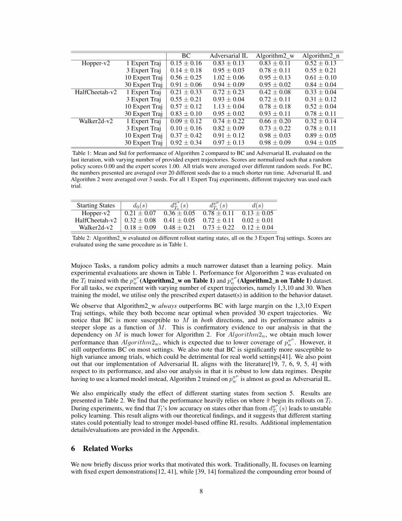
Table 1: Mean and Std for performance of Algorithm 2 compared to BC and Adversarial IL evaluated on thelast iteration, with varying number of provided expert trajectories. Scores are normalized such that a randompolicy scores 0.00 and the expert scores 1.00. All trials were averaged over different random seeds. For BC,the numbers presented are averaged over 20 different seeds due to a much shorter run time. Adversarial IL andAlgorithm 2 were averaged over 3 seeds. For all 1 Expert Traj experiments, different trajectory was used eachtrial.

Starting States d0(s) dπ∗

Tt(s) dπ

µ

Tt(s) d(s)

Hopper-v2 0.21 ± 0.07 0.36 ± 0.05 0.78 ± 0.11 0.13 ± 0.05HalfCheetah-v2 0.32 ± 0.08 0.41 ± 0.05 0.72 ± 0.11 0.02 ± 0.01

Walker2d-v2 0.18 ± 0.09 0.48 ± 0.21 0.73 ± 0.22 0.12 ± 0.04

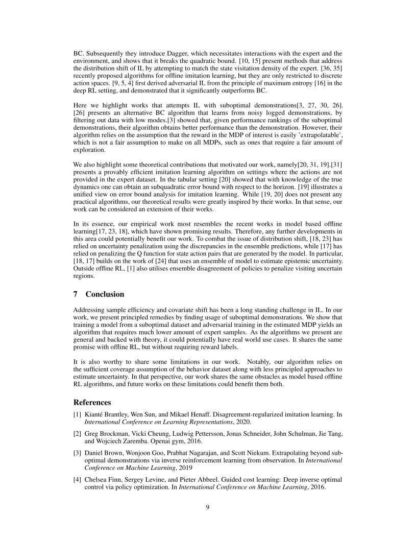
Table 2: Algorithm2_w evaluated on different rollout starting states, all on the 3 Expert Traj settings. Scores areevaluated using the same procedure as in Table 1.

Mujoco Tasks, a random policy admits a much narrower dataset than a learning policy. Mainexperimental evaluations are shown in Table 1. Performance for Algororithm 2 was evaluated onthe Tl trained with the pπ

µ

w (Algorithm2_w on Table 1) and pπµ

n (Algorithm2_n on Table 1) dataset.For all tasks, we experiment with varying number of expert trajectories, namely 1,3,10 and 30. Whentraining the model, we utilise only the prescribed expert dataset(s) in addition to the behavior dataset.

We observe that Algorithm2_w always outperforms BC with large margin on the 1,3,10 ExpertTraj settings, while they both become near optimal when provided 30 expert trajectories. Wenotice that BC is more susceptible to M in both directions, and its performance admits asteeper slope as a function of M . This is confirmatory evidence to our analysis in that thedependency on M is much lower for Algorithm 2. For Algorithm2n, we obtain much lowerperformance than Algorithm2w, which is expected due to lower coverage of pπ

µ

n . However, itstill outperforms BC on most settings. We also note that BC is significantly more susceptible tohigh variance among trials, which could be detrimental for real world settings[41]. We also pointout that our implementation of Adversarial IL aligns with the literature[19, 7, 6, 9, 5, 4] withrespect to its performance, and also our analysis in that it is robust to low data regimes. Despitehaving to use a learned model instead, Algorithm 2 trained on pπ

µ

w is almost as good as Adversarial IL.

We also empirically study the effect of different starting states from section 5. Results arepresented in Table 2. We find that the performance heavily relies on where π begin its rollouts on Tl.During experiments, we find that Tl’s low accuracy on states other than from dπ

µ

Tt(s) leads to unstable

policy learning. This result aligns with our theoretical findings, and it suggests that different startingstates could potentially lead to stronger model-based offline RL results. Additional implementationdetails/evaluations are provided in the Appendix.

6 Related Works

We now briefly discuss prior works that motivated this work. Traditionally, IL focuses on learningwith fixed expert demonstrations[12, 41], while [39, 14] formalized the compounding error bound of

8

BC. Subsequently they introduce Dagger, which necessitates interactions with the expert and theenvironment, and shows that it breaks the quadratic bound. [10, 15] present methods that addressthe distribution shift of IL by attempting to match the state visitation density of the expert. [36, 35]recently proposed algorithms for offline imitation learning, but they are only restricted to discreteaction spaces. [9, 5, 4] first derived adversarial IL from the principle of maximum entropy [16] in thedeep RL setting, and demonstrated that it significantly outperforms BC.

Here we highlight works that attempts IL with suboptimal demonstrations[3, 27, 30, 26].[26] presents an alternative BC algorithm that learns from noisy logged demonstrations, byfiltering out data with low modes.[3] showed that, given performance rankings of the suboptimaldemonstrations, their algorithm obtains better performance than the demonstration. However, theiralgorithm relies on the assumption that the reward in the MDP of interest is easily ’extrapolatable’,which is not a fair assumption to make on all MDPs, such as ones that require a fair amount ofexploration.

We also highlight some theoretical contributions that motivated our work, namely[20, 31, 19].[31]presents a provably efficient imitation learning algorithm on settings where the actions are notprovided in the expert dataset. In the tabular setting [20] showed that with knowledge of the truedynamics one can obtain an subquadratic error bound with respect to the horizon. [19] illustrates aunified view on error bound analysis for imitation learning. While [19, 20] does not present anypractical algorithms, our theoretical results were greatly inspired by their works. In that sense, ourwork can be considered an extension of their works.

In its essence, our empirical work most resembles the recent works in model based offlinelearning[17, 23, 18], which have shown promising results. Therefore, any further developments inthis area could potentially benefit our work. To combat the issue of distribution shift, [18, 23] hasrelied on uncertainty penalization using the discrepancies in the ensemble predictions, while [17] hasrelied on penalizing the Q function for state action pairs that are generated by the model. In particular,[18, 17] builds on the work of [24] that uses an ensemble of model to estimate epistemic uncertainty.Outside offline RL, [1] also utilises ensemble disagreement of policies to penalize visiting uncertainregions.

7 Conclusion

Addressing sample efficiency and covariate shift has been a long standing challenge in IL. In ourwork, we present principled remedies by finding usage of suboptimal demonstrations. We show thattraining a model from a suboptimal dataset and adversarial training in the estimated MDP yields analgorithm that requires much lower amount of expert samples. As the algorithms we present aregeneral and backed with theory, it could potentially have real world use cases. It shares the samepromise with offline RL, but without requiring reward labels.

It is also worthy to share some limitations in our work. Notably, our algorithm relies onthe sufficient coverage assumption of the behavior dataset along with less principled approaches toestimate uncertainty. In that perspective, our work shares the same obstacles as model based offlineRL algorithms, and future works on these limitations could benefit them both.

References[1] Kianté Brantley, Wen Sun, and Mikael Henaff. Disagreement-regularized imitation learning. In

International Conference on Learning Representations, 2020.

[2] Greg Brockman, Vicki Cheung, Ludwig Pettersson, Jonas Schneider, John Schulman, Jie Tang,and Wojciech Zaremba. Openai gym, 2016.

[3] Daniel Brown, Wonjoon Goo, Prabhat Nagarajan, and Scott Niekum. Extrapolating beyond sub-optimal demonstrations via inverse reinforcement learning from observation. In InternationalConference on Machine Learning, 2019

[4] Chelsea Finn, Sergey Levine, and Pieter Abbeel. Guided cost learning: Deep inverse optimalcontrol via policy optimization. In International Conference on Machine Learning, 2016.

9

[5] Justin Fu, Katie Luo, and Sergey Levine. Learning robust rewards with adversarial inversereinforce- ment learning. International Conference on Learning Representations, 2018

[6] Seyed Kamyar Seyed Ghasemipour, Richard Zemel, and Shixiang Gu. A divergence minimizationperspective on imitation learning methods. Conference on Robot Learning, 2019

[7] Liyiming Ke, Sanjiban Choudhury, Matt Barnes, Wen Sun, Gilwoo Lee, and Siddhartha Srinivasa.Imitation Learning as f-Divergence Minimization In arXiv:1905.12888, 2019

[8] Tuomas Haarnoja, Aurick Zhou, Pieter Abbeel, and Sergey Levine. Soft actor-critic: Off-policy maximum entropy deep reinforcement learning with a stochastic actor. In InternationalConference on Machine Learning, 2018a.

[9] Jonathan Ho and Stefano Ermon. Generative adversarial imitation learning. In Advances inNeural Information Processing Systems, 2016.

[10] Fangchen Liu, Zhan Ling, Tongzhou Mu, and Hao Su. State alignment-based imitation learning.International Conference on Learning Representations, 2020.

[11] Andrew Y Ng, Stuart J Russell, et al. Algorithms for inverse reinforcement learning. In Interna-tional Conference on Machine Learning, 2000.

[12] Dean A Pomerleau. Efficient training of artificial neural networks for autonomous navigation.Neural computation, 1991.

[13] Siddharth Reddy, Anca D Dragan, and Sergey Levine. Sqil: imitation learning via regularizedbehavioral cloning. International Conference on Learning Representations, 2020.

[14] Stéphane Ross and Drew Bagnell. Efficient reductions for imitation learning. In InternationalConference on Artificial Intelligence and Statistics, 2010.

[15] Yannick Schroecker and Charles L Isbell. State aware imitation learning. In Advances in NeuralInformation Processing Systems, 2017

[16] Brian D Ziebart, Andrew L Maas, J Andrew Bagnell, and Anind K Dey. Maximum entropyinverse reinforcement learning. In AAAI Conference on Artificial Intelligence, 2008.

[17] Tianhe Yu, Aviral Kumar, Rafael Rafailov, Aravind Rajeswaran, Sergey Levine, andChelsea Finn. COMBO: Conservative offline model-based policy optimization. arXiv preprintarXiv:2102.08363, 2021.

[18] Tianhe Yu, Garrett Thomas, Lantao Yu, Stefano Ermon, James Zou, Sergey Levine, ChelseaFinn, and Tengyu Ma. MOPO: Model-based offline policy optimization. arXiv preprintarXiv:2005.13239, 2020

[19] Tian Xu, Ziniu Li, and Yang Yu. Error bounds of imitating policies and environments. Advancesin Neural Information Processing Systems, 33, 2020.

[20] Nived Rajaraman, Lin F Yang, Jiantao Jiao, and Kannan Ramachandran. Toward the fundamentallimits of imitation learning. Advances in Neural Information Processing Systems, 2020

[21] Yao Liu, Adith Swaminathan, Alekh Agarwal, and Emma Brunskill. Provably good batchreinforce- ment learning without great exploration. arXiv preprint arXiv:2007.08202, 2020.

[22] Sergey Levine, Aviral Kumar, George Tucker, and Justin Fu. Offline reinforcement learning:Tuto- rial, review, and perspectives on open problems. arXiv preprint arXiv:2005.01643, 2020.

[23] Rahul Kidambi, Aravind Rajeswaran, Praneeth Netrapalli, and Thorsten Joachims. MOReL:Model- based offline reinforcement learning. arXiv preprint arXiv:2005.05951, 2020.

[24] Michael Janner, Justin Fu, Marvin Zhang, and Sergey Levine. When to trust your model:Model-based policy optimization. In Advances in Neural Information Processing Systems, pages12498–12509, 2019.

10

[25] Jacob Buckman, Carles Gelada, and Marc G Bellemare. The importance of pessimism in fixed-dataset policy optimization. arXiv preprint arXiv:2009.06799, 2020.

[26] Fumihiro Sasaki, Ryota Yamashina. Behavioral Cloning from Noisy Demonstrations. In Inter-national Conference on Learning Representations, 2021

[27] Yueh-Hua Wu, Nontawat Charoenphakdee, Han Bao, Voot Tangkaratt, and Masashi Sugiyama.Im- itation learning from imperfect demonstration. arXiv preprint arXiv:1901.09387, 2019.

[28] Emanuel Todorov, Tom Erez, and Yuval Tassa. Mujoco: A physics engine for model-basedcontrol. In 2012 IEEE/RSJ International Conference on Intelligent Robots and Systems, pp.5026–5033. IEEE, 2012.

[29] Fumihiro Sasaki, Tetsuya Yohira, and Atsuo Kawaguchi. Sample efficient imitation learning forcontinuous control. In International Conference on Learning Representations, 2018.

[30] Daniel H Grollman and Aude G Billard. Robot learning from failed demonstrations. Interna-tional Journal of Social Robotics, 4(4):331–342, 2012.

[31] WenSun, AnirudhVemula, ByronBoots,and JAndrewBagnell. Provablyefficient imitation learn-ing from observation alone. In International Conference of Machine Learning, 2019.

[32] Ian Goodfellow, Jean Pouget-Abadie, Mehdi Mirza, Bing Xu, David Warde-Farley, SherjilOzair, Aaron Courville, and Yoshua Bengio. Generative adversarial nets. In Advances in neuralinformation processing systems,pages 2672–2680, 2014.

[33] Umar Syed and Robert E Schapire. A game-theoretic approach to apprenticeship learning. InAdvances in neural information processing systems, 2008.

[34] Alekh Agarwal Nan Jiang Sham M. Kakade Wen Sun. Reinforcement Learning: Theory andAlgorithms, 2020

[35] Daniel Jarrett, Ioana Bica, Mihaela van der Schaar. Strictly Batch Imitation Learning by Energy-based Distribution Matching, In Advances in neural information processing systems, 2020

[36] Alex J. Chan and Mihaela van der Schaar. Scalable Bayesian Inverse Reinforcement Learning,International Conference of Learning Representations 2021

[37] Ilya Kostrikov, Ofir Nachum, Jonathan Tompson. Imitation Learning Via Off-Policy DistributionMatching. International Conference of Learning Representations 2020

[38] Robert Dadashi, Léonard Hussenot, Matthieu Geist, Olivier Pietquin. Primal Wassertein Imita-tion Learning. International Conference of Learning Representations 2021

[39] Stéphane Ross Geoffrey J. Gordon J. Andrew Bagnell. A Reduction of Imitation Learning andStructured Prediction to No-Regret Online Learning. In AISTATS, 2011

[40] Peter Englert; Alexandros Paraschos; Jan Peters; Marc Peter Deisenroth. Model-based imitationlearning by probabilistic trajectory matching. 2013 IEEE International Conference on Roboticsand Automation

[41] Felipe Codevilla, Eder Santana, Antonio M. López, Adrien Gaidon. Exploring the Limitationsof Behavior Cloning for Autonomous Driving. In arXiv:1904.08980

[42] John Schulman, Filip Wolski, Prafulla Dhariwal, Alec Radford, and Oleg Klimov. Proximalpolicy optimization algorithms. arXiv preprint arXiv:1707.06347, 2017.

[43] Alekh Agarwal, Sham Kakade, Akshay Krishnamurthy, and Wen Sun. Flambe: Structuralcomplexity and representa- tion learning of low rank mdps. NeurIPS, 2020b.

11

Checklist

The checklist follows the references. Please read the checklist guidelines carefully for information onhow to answer these questions. For each question, change the default [TODO] to [Yes] , [No] , or[N/A] . You are strongly encouraged to include a justification to your answer, either by referencingthe appropriate section of your paper or providing a brief inline description. For example:

• Did you include the license to the code and datasets? [Yes] See Section 2.

• Did you include the license to the code and datasets? [No] The code and the data areproprietary.

• Did you include the license to the code and datasets? [N/A]

Please do not modify the questions and only use the provided macros for your answers. Note that theChecklist section does not count towards the page limit. In your paper, please delete this instructionsblock and only keep the Checklist section heading above along with the questions/answers below.

1. For all authors...

(a) Do the main claims made in the abstract and introduction accurately reflect the paper’scontributions and scope? [Yes]

(b) Did you describe the limitations of your work? [Yes] see conclusion(c) Did you discuss any potential negative societal impacts of your work? [N/A] no

forseeable negative impact(d) Have you read the ethics review guidelines and ensured that your paper conforms to

them? [Yes]

2. If you are including theoretical results...

(a) Did you state the full set of assumptions of all theoretical results? [Yes] See preliminar-ies

(b) Did you include complete proofs of all theoretical results? [Yes] in appendix

3. If you ran experiments...

(a) Did you include the code, data, and instructions needed to reproduce the main experi-mental results (either in the supplemental material or as a URL)? [No] code will soonbe released after cleanup

(b) Did you specify all the training details (e.g., data splits, hyperparameters, how theywere chosen)? [Yes] in appendix

(c) Did you report error bars (e.g., with respect to the random seed after running experi-ments multiple times)? [Yes] see Table 1, Table 2 in section 5

(d) Did you include the total amount of compute and the type of resources used (e.g., typeof GPUs, internal cluster, or cloud provider)? [No] all experiments were run on cpus,as it doesn’t need heavy compute

4. If you are using existing assets (e.g., code, data, models) or curating/releasing new assets...

(a) If your work uses existing assets, did you cite the creators? [N/A](b) Did you mention the license of the assets? [N/A](c) Did you include any new assets either in the supplemental material or as a URL? [N/A]

(d) Did you discuss whether and how consent was obtained from people whose data you’reusing/curating? [N/A]

(e) Did you discuss whether the data you are using/curating contains personally identifiableinformation or offensive content? [N/A]

5. If you used crowdsourcing or conducted research with human subjects...

(a) Did you include the full text of instructions given to participants and screenshots, ifapplicable? [N/A]

(b) Did you describe any potential participant risks, with links to Institutional ReviewBoard (IRB) approvals, if applicable? [N/A]

12

(c) Did you include the estimated hourly wage paid to participants and the total amountspent on participant compensation? [N/A]

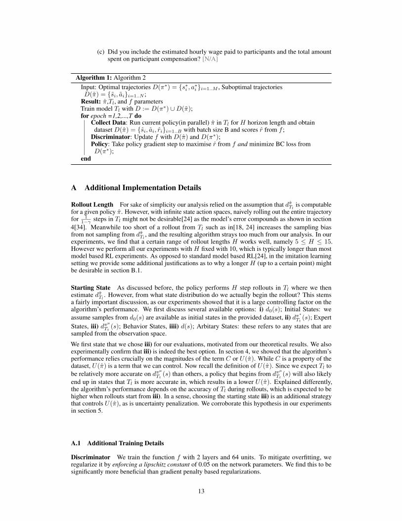
Algorithm 1: Algorithm 2Input: Optimal trajectories D(π∗) = {s∗i , a∗i }i=1..M , Suboptimal trajectoriesD(π) = {si, ai}i=1..N ;

Result: π,Tl, and f parametersTrain model Tl with D := D(π∗) ∪D(π);for epoch =1,2,...,T do

Collect Data: Run current policy(in parallel) π in Tl for H horizon length and obtaindataset D(π) = {si, ai, ri}i=1..B with batch size B and scores r from f ;

Discriminator: Update f with D(π) and D(π∗);Policy: Take policy gradient step to maximise r from f and minimize BC loss fromD(π∗);

end

A Additional Implementation Details

Rollout Length For sake of simplicity our analysis relied on the assumption that dπTl is computablefor a given policy π. However, with infinite state action spaces, naively rolling out the entire trajectoryfor 1

1−γ steps in Tl might not be desirable[24] as the model’s error compounds as shown in section4[34]. Meanwhile too short of a rollout from Tl such as in[18, 24] increases the sampling biasfrom not sampling from dπTl , and the resulting algorithm strays too much from our analysis. In ourexperiments, we find that a certain range of rollout lengths H works well, namely 5 ≤ H ≤ 15.However we perform all our experiments with H fixed with 10, which is typically longer than mostmodel based RL experiments. As opposed to standard model based RL[24], in the imitation learningsetting we provide some additional justifications as to why a longer H (up to a certain point) mightbe desirable in section B.1.

Starting State As discussed before, the policy performs H step rollouts in Tl where we thenestimate dπTl . However, from what state distribution do we actually begin the rollout? This stemsa fairly important discussion, as our experiments showed that it is a large controlling factor on thealgorithm’s performance. We first discuss several available options: i) d0(s); Initial States: weassume samples from d0(s) are available as initial states in the provided dataset, ii) dπ

∗

Tt(s); Expert

States, iii) dπµ

Tt(s); Behavior States, iiii) d(s); Arbitary States: these refers to any states that are

sampled from the observation space.

We first state that we chose iii) for our evaluations, motivated from our theoretical results. We alsoexperimentally confirm that iii) is indeed the best option. In section 4, we showed that the algorithm’sperformance relies crucially on the magnitudes of the term C or U(π). While C is a property of thedataset, U(π) is a term that we can control. Now recall the definition of U(π). Since we expect Tl tobe relatively more accurate on dπ

µ

Tt(s) than others, a policy that begins from dπ

µ

Tt(s) will also likely

end up in states that Tl is more accurate in, which results in a lower U(π). Explained differently,the algorithm’s performance depends on the accuracy of Tl during rollouts, which is expected to behigher when rollouts start from iii). In a sense, choosing the starting state iii) is an additional strategythat controls U(π), as is uncertainty penalization. We corroborate this hypothesis in our experimentsin section 5.

A.1 Additional Training Details

Discriminator We train the function f with 2 layers and 64 units. To mitigate overfitting, weregularize it by enforcing a lipschitz constant of 0.05 on the network parameters. We find this to besignificantly more beneficial than gradient penalty based regularizations.

13

Model We train the model as similar to [18, 24], where we train an ensemble of 7 neural networksand predict with a random sample from the ensemble predictions.

Policy We optimize the policy with PPO[42]. Although we can in principle backpropagate throughtime in Tl, we believed policy gradients would be a better choice since we can get a gradient arbitarilyclose to the true gradient by simply sacrificing more compute. For all our experiments, we collect5000 samples in parallel for a horizon length of 10, which results in 50000 total samples per epoch.

B Proofs

Proof of Lemma 1(Performance Difference of Two Policies): This is a simple application ofthe performance difference lemma[34] of any two policies π, π. Let Rmax ≤ 1/2, thenit follows that Qmax ≤ 1

2(1−γ) , where Qπ(s, a) := Eπ,Tt [∑∞t=0 γ

tr(s, a)] and Qπ(s, π) :=

Ea∼π,π,Tt [∑∞t=0 γ

tr(s, a)], where only the first action is averaged over π. Then it follows that

V π − V π

=1

1− γEs∼dπTt [−Q

π(s, π(s)) +Qπ(s, π(s))]

≤ Qmax1

1− γEs∼dπTt [||π − π||1]

≤ 1

(1− γ)2Es∼dπTt [||π − π||1]

We refer readers to Section E, Theorem 21 in [43] for detailed proofs on maximum likelihood(MLE)guarantees on Es∼dπTt [||π − π||1], such that the bound becomes a valid sample complexity after aMLE training procedure.

Proof of Theorem 2: The proof can be found in [34], but we also present here for com-pleteness. It is a direct application of a uniform convergence argument for all f ∈ F . For Theorem2 and 3, we define f slightly differently from its definition presented in section 2, namely f takesboth s, a as inputs. We then define f := argmaxf∈F

1M

∑Mm=1 f(s∗, a∗) − Es∼pπTt [f(s, a)] and

f := argmaxf∈F Es∼pπ∗Tt [f(s, a)]− Es∼pπTt [f(s, a)].

Then it follows that for all π ∈ Π, maxf∈F (Es,a∼pπ∗Tt [f(s, a)] − Es,a∼pπTt [f(s, a)]) =

maxf :||f ||∞≤1(Es,a∼pπ∗Tt [f(s, a)]− Es∼pπTt [f(s, a)]) = ||pπ∗Tt (s, a)− pπTt(s, a)||1

Also, let Rmax ≤ 1. It is then straightforward to see that

V π∗− V π

≤ 1

1− γ|||pπ

∗

Tt (s, a)− pπTt(s, a)||1

We now bound the distance of the state-action visitation densities,

||pπ∗

Tt (s, a)− pπTt(s, a)||1

= Es,a∼pπ∗Tt [f(s, a)]− Es∼pπTt [f(s, a)]

≤ 1

M

M∑m=1

f(s∗, a∗)− Es,a∼pπTt [f(s, a)] + εs

≤ 1

M

M∑m=1

f(s∗, a∗)− Es,a∼pπTt [f(s, a)] + εs

14

≤ 1

M

M∑m=1

f(s∗, a∗)− Es,a∼pπ∗Tt [f(s, a)] + εs

≤ 2εs

UtilisingV π∗− V π

≤ 1

1− γ||pπ

∗

Tt (s, a)− pπTt(s, a)||1

we conclude our proof. The first and last inequality is from Hoeffding’s inequality taken union boundfor all f ∈ F , where with probability at least 1− δ , |Es∼pπ∗Tt (s,a)[f(s, a)]− 1

M

∑Mm=1 f(s∗, a∗)|≤

2

√ln(|F |δ )

M ,∀f ∈ F , εs := 2

√ln(|F |δ )

M , and the third inequality is from the optimality of π.

Proof of Theorem 3: The proof is an adaptation of Theorem 2 in the case where the ex-pectation over pπ

∗

Ttis replaced with pπ

∗

Tl, then with the same definitions as in the proof of Theorem

2,||pπ

∗

Tt (s, a)− pπTt(s, a)||1= Es,a∼pπ∗Tt [f(s, a)]− Es,a∼pπTt [f(s, a)]

≤ 1

M

M∑m=1

f(s∗, a∗)− Es,a∼pπTt [f(s, a)] + εs

≤ 1

M

M∑m=1

f(s∗, a∗)− Es,a∼pπTl [f(s, a)] + εs +C

1− γεT

≤ 1

M

M∑m=1

f(s∗, a∗)− Es,a∼pπ∗Tl[f(s, a)] + εs +

C

1− γεT

≤ 1

M

M∑m=1

f(s∗, a∗)− Es,a∼pπ∗Tt [f(s, a)] + εs +2C

1− γεT

≤ 1

M

M∑m=1

f(s∗, a∗)− Es,a∼pπ∗Tt [f(s, a)] + εs

≤ 2εs +2C

1− γεT

The third inequality is from the optimality of π. For the second and fourth inequality we use lemma 6presented below to bound ||dπTt(s)− d

πTl

(s)||1≤ 11−γ εT . Consequently, using

V π∗− V π

≤ 1

1− γ||pπ

∗

Tt (s, a)− pπTt(s, a)||1

we conclude our proof

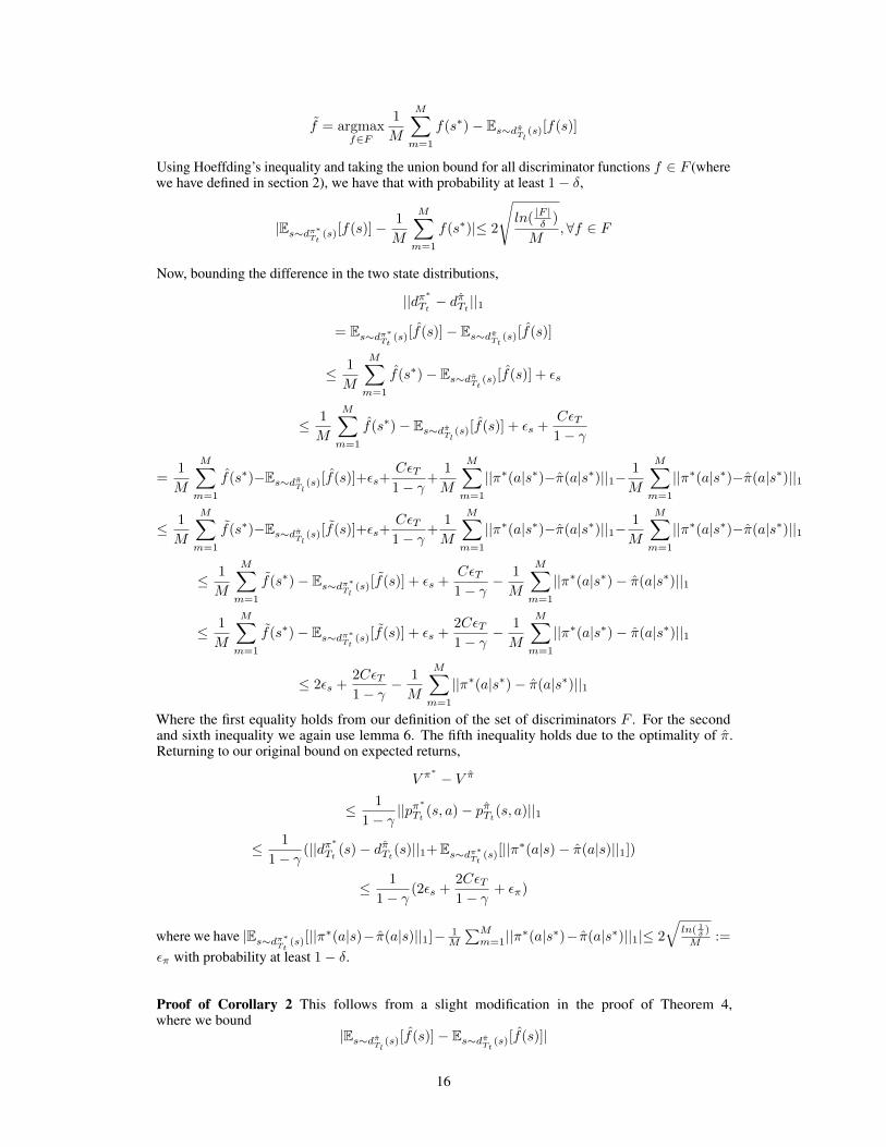
Proof of Theorem 4:

We can decompose the state action distribution distance by the following,

||pπ∗

Tt (s, a)− pπTt(s, a)||1

≤ ||dπ∗

Tt (s)− dπTt(s)||1+Es∼dπ∗Tt (s)[||π∗(a|s)− π(a|s)||1]

Definef = argmax

f∈FEs∼dπ∗Tt (s)[f(s)]− Es∼dπTt (s)[f(s)]

15

f = argmaxf∈F

1

M

M∑m=1

f(s∗)− Es∼dπTl (s)[f(s)]

Using Hoeffding’s inequality and taking the union bound for all discriminator functions f ∈ F (wherewe have defined in section 2), we have that with probability at least 1− δ,

|Es∼dπ∗Tt (s)[f(s)]− 1

M

M∑m=1

f(s∗)|≤ 2

√ln( |F |δ )

M,∀f ∈ F

Now, bounding the difference in the two state distributions,

||dπ∗

Tt − dπTt ||1

= Es∼dπ∗Tt (s)[f(s)]− Es∼dπTt (s)[f(s)]

≤ 1

M

M∑m=1

f(s∗)− Es∼dπTt (s)[f(s)] + εs

≤ 1

M

M∑m=1

f(s∗)− Es∼dπTl (s)[f(s)] + εs +CεT1− γ

=1

M

M∑m=1

f(s∗)−Es∼dπTl (s)[f(s)]+εs+CεT1− γ

+1

M

M∑m=1

||π∗(a|s∗)−π(a|s∗)||1−1

M

M∑m=1

||π∗(a|s∗)−π(a|s∗)||1

≤ 1

M

M∑m=1

f(s∗)−Es∼dπTl (s)[f(s)]+εs+CεT1− γ

+1

M

M∑m=1

||π∗(a|s∗)−π(a|s∗)||1−1

M

M∑m=1

||π∗(a|s∗)−π(a|s∗)||1

≤ 1

M

M∑m=1

f(s∗)− Es∼dπ∗Tl (s)[f(s)] + εs +CεT1− γ

− 1

M

M∑m=1

||π∗(a|s∗)− π(a|s∗)||1

≤ 1

M

M∑m=1

f(s∗)− Es∼dπ∗Tt (s)[f(s)] + εs +2CεT1− γ

− 1

M

M∑m=1

||π∗(a|s∗)− π(a|s∗)||1

≤ 2εs +2CεT1− γ

− 1

M

M∑m=1

||π∗(a|s∗)− π(a|s∗)||1

Where the first equality holds from our definition of the set of discriminators F . For the secondand sixth inequality we again use lemma 6. The fifth inequality holds due to the optimality of π.Returning to our original bound on expected returns,

V π∗− V π

≤ 1

1− γ||pπ

∗

Tt (s, a)− pπTt(s, a)||1

≤ 1

1− γ(||dπ

∗

Tt (s)− dπTt(s)||1+Es∼dπ∗Tt (s)[||π∗(a|s)− π(a|s)||1])

≤ 1

1− γ(2εs +

2CεT1− γ

+ επ)

where we have |Es∼dπ∗Tt (s)[||π∗(a|s)− π(a|s)||1]− 1M

∑Mm=1||π∗(a|s∗)− π(a|s∗)||1|≤ 2

√ln( 1

δ )

M :=

επ with probability at least 1− δ.

Proof of Corollary 2 This follows from a slight modification in the proof of Theorem 4,where we bound

|Es∼dπTl (s)[f(s)]− Es∼dπTt (s)[f(s)]|

16

≤ 1

1− γEdπTl [||Tt(s

′|s, a)− Tl(s′|s, a)||1] ≤ 1

1− γ(εT + U(π))

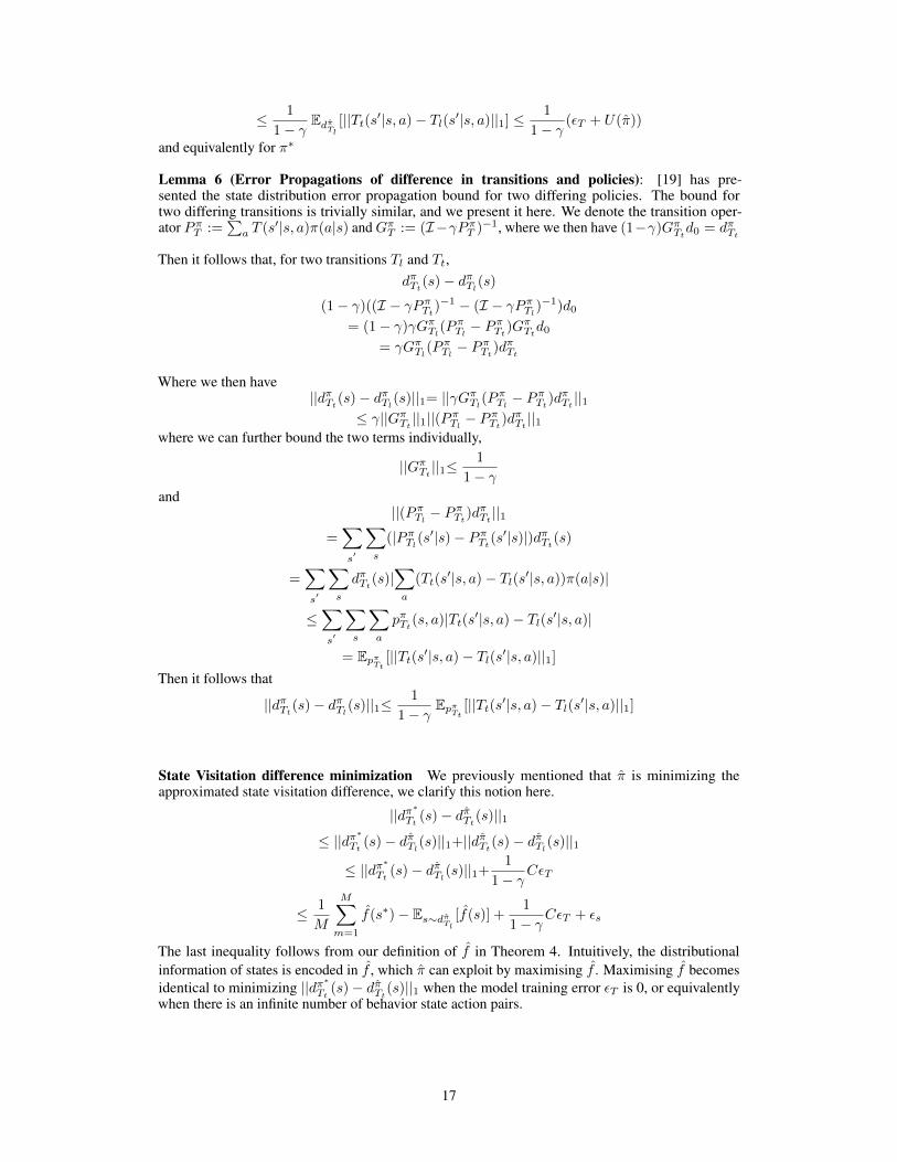
and equivalently for π∗

Lemma 6 (Error Propagations of difference in transitions and policies): [19] has pre-sented the state distribution error propagation bound for two differing policies. The bound fortwo differing transitions is trivially similar, and we present it here. We denote the transition oper-ator PπT :=

∑a T (s′|s, a)π(a|s) andGπT := (I−γPπT )−1, where we then have (1−γ)GπTtd0 = dπTt

Then it follows that, for two transitions Tl and Tt,dπTt(s)− d

πTl

(s)

(1− γ)((I − γPπTt)−1 − (I − γPπTl)

−1)d0

= (1− γ)γGπTl(PπTl− PπTt)G

πTtd0

= γGπTl(PπTl− PπTt)d

πTt

Where we then have||dπTt(s)− d

πTl

(s)||1= ||γGπTl(PπTl− PπTt)d

πTt ||1

≤ γ||GπTt ||1||(PπTl− PπTt)d

πTt ||1

where we can further bound the two terms individually,

||GπTt ||1≤1

1− γand

||(PπTl − PπTt)d

πTt ||1

=∑s′

∑s

(|PπTl(s′|s)− PπTt(s

′|s)|)dπTt(s)

=∑s′

∑s

dπTt(s)|∑a

(Tt(s′|s, a)− Tl(s′|s, a))π(a|s)|

≤∑s′

∑s

∑a

pπTt(s, a)|Tt(s′|s, a)− Tl(s′|s, a)|

= EpπTt [||Tt(s′|s, a)− Tl(s′|s, a)||1]

Then it follows that

||dπTt(s)− dπTl

(s)||1≤1

1− γEpπTt [||Tt(s

′|s, a)− Tl(s′|s, a)||1]

State Visitation difference minimization We previously mentioned that π is minimizing theapproximated state visitation difference, we clarify this notion here.

||dπ∗

Tt (s)− dπTt(s)||1≤ ||dπ

∗

Tt (s)− dπTl(s)||1+||dπTt(s)− dπTl

(s)||1

≤ ||dπ∗

Tt (s)− dπTl(s)||1+1

1− γCεT

≤ 1

M

M∑m=1

f(s∗)− Es∼dπTl [f(s)] +1

1− γCεT + εs

The last inequality follows from our definition of f in Theorem 4. Intuitively, the distributionalinformation of states is encoded in f , which π can exploit by maximising f . Maximising f becomesidentical to minimizing ||dπ∗Tt (s)− dπTt(s)||1 when the model training error εT is 0, or equivalentlywhen there is an infinite number of behavior state action pairs.

17

B.1 Recovery

In this subsection we comment on a direct consequence of our choice in the starting state, namelythe recovery behavior of our algorithm, which solidifies our intuition on its empirical success overbehavioral cloning. Imitation Learning also concerns the problem of mitigating covariate shift, whichoccurs when the learner deviates from the expert’s state distribution dπ

∗

Ttduring the evaluation stage.

Naive BC methods does not prepare the policy to recover to dπ∗

Ttin such instances. We argue that our

model based approach acts to resolve this issue.

We define vkπ as an unique recovery variable for every policy π in an MDP of interest.

vkπ := ||dπ∗

Tt − (PπTt)kν||

where PπT is the transposed transition matrix∑a∈A T (s′|a, s)π(a|s) induced by π in the dynamics

T , and ν(s) denotes the density of any admissible states by π ∈ Π. Under the assumption ofirreducibility and aperiodicity of of PπTt , (PπTt)

kν(s) will converge to its stationary distributiondπTt(s) as k → ∞. Intuitively, the finiteness of k allows vkπ to represent the ability of π to ’direct’itself to dπ

∗

Tt(s) in under k transitions, starting from any admissible state s ∼ ν(s). A policy that is

sufficiently trained to minimize this objective could endow π the ability to recover from any arbitraryadmissible state back to the expert distribution in finitely many steps. It then follows that we canbound vkπ with certain terms of interest.

Proposition 1vkπ ≤ ||dπ

∗

Tt (s)− (PπTl)kdπ

µ

(s)||+kεT +√

2 logC

Where εT = maxi=1..k Es,a∼pπµ (s,a)[||Tt(si+1|ai, si) − Tl(si+1|ai, si)||1]. The first two terms ofthis bound are approximately the minimization variables in Algorithm 2. While we do not directlyminimize C, we attempt to control a related variable U(π) to ensure C does not get too large.

Proof of Proposition 1:

||dπ∗

Tt − (PπTt)kν||1

= ||dπ∗

Tt − (PπTl)kdπ

µ

+ (PπTl)kdπ

µ

− (PπTt)kdπ

µ

+ (PπTt)kdπ

µ

− (PπTt)kν||1

≤ ||dπ∗

Tt − (PπTl)kdπ

µ

||1+||(PπTl)kdπ

µ

− (PπTt)kdπ

µ

||1+||(PπTt)kdπ

µ

− (PπTt)kν||1

≤ ||dπ∗

Tt − (PπTl)kdπ

µ

||1+kεT + ||(PπTt)k||1||dπ

µ

− ν||1

≤ ||dπ∗

Tt − (PπTl)kdπ

µ

||1+kεT +√

2 logC

In the second inequality, we bound the k step induced state divergence from two different transitionTl and Tt ||(PπTl)

kdπµ − (PπTt)

kdπµ || using the second inequality follows from applying lemma

B.2 from [24]. Also note that ||(PπTt)k||1= 1 as PπTt is a left-stochastic matrix. The last inequality

follows from Pinsker’s inequality and the definition of C. We also point out a trade-off between kand π’s recovery property. As k decreases it is quite possible that π fails to learn to direct itself todπ∗

Ttfrom any s ∼ ν(s), especially if the MDP of interest has a large state space. However, increasing

k loosens the bound for any non-zero εT . This may explain the range of horizon H that we foundworks well, as explained in section A.

Recall from section A that π begin its rollouts from dπµ

Tt(s). We then provide a consequen-

tial argument that arises from proposition 1; if dπµ

Tt(s) sufficiently represents the state space that is

generated by a learner π from making a mistake, or equivalently when C is bounded, then givena sufficiently accurate Tl, our practical instatiation of Algorithm 2 trains π to direct itself back todπ∗

Tt(s) in k transitions.

18

B.2 Reduction to offline RL

In this section we study the setting where we are given additional information, namely i) when the truereward function is given and ii) when its empirical samples are given corresponding to the behaviordataset. Given the true reward function or labels, the problem then reduces to offline RL. In i, thepolicy π generates rollouts in the learned dynamics Tl with the true reward function r : S ×A 7→ R,after which π maximises its collected reward in this fake environment. In ii, the setting is identicalto i except that its reward function r : S × A 7→ R is an empirical risk minimizing function ofreward labels obtained from the behavior dataset {si, ai, rsi,ai}i=1..N ∼ pπ

µ

Tt. This is in contrast to

the imitation learning setting where we don’t have access to either rsi,ai or r. Despite the simpleanalysis, it is insightful to compare how the bound compares to the previous setting under the sameassumptions, since we can observe what differs when the true reward is replaced with a discriminatorfunction f .

Theorem 5(When True Reward Function is Given(i)): Let

π = argmaxπ∈Π

Es,a∼pπTl (s,a)[r(s, a)]

ThenV π∗≤ V π +

2CεT(1− γ)2

An almost identical proof is used for ii, where we take into account the approximation error for thereward function, εr := Es,a∼pπµTt [|r(s, a)− r(s, a)|], so we just state the proof for ii.

Corollary 4(When Only Reward Labels are Given(ii)): Let

π = argmaxπ∈Π

Es,a∼pπTl (s,a)[r(s, a)]

ThenV π∗≤ V π +

2CεT(1− γ)2

+2Cεr1− γ

Proof of Theorem 5/Corollary 4

(1− γ)(V π∗− V π) = Epπ∗Tt (s,a)[r(s, a)]− EpπTt (s,a)[r(s, a)]

≤ Epπ∗Tt (s,a)[r(s, a)]− EpπTl (s,a)[r(s, a)] +CεT1− γ

+ Cεr

≤ Epπ∗Tt (s,a)[r(s, a)]− Epπ∗Tl (s,a)[r(s, a)] +CεT1− γ

+ Cεr

≤ Epπ∗Tt (s,a)[r(s, a)]− Epπ∗Tt (s,a)[r(s, a)] +2CεT1− γ

+ 2Cεr =2CεT1− γ

+ 2Cεr

Compared to Theorem 3, given a true reward function, we are able to purge the high probabilityerror term εs. As in the imitation learning setting, Note that for both i and ii the suboptimality is stilldependent on the concentrability coefficient. Analogous to Theorem 3 and 4, for ii the dependenceon εT significantly outweighs that of the reward function approximation error εr, which signifies theimportance of an accurate model and data coverage over the reward function.

C Additional Experiments

In section 5 we saw that Algorithm 2 outperforms BC on all domains. In this section we providesome additional empirical analysis that serves to answer the following questions;

i) Compared to BC, does Algorithm 2 mitigate compounding errors?ii) Compared to BC, does the policy trained with Algorithm 2 admit the recovery behavior outlinedin section B.1?iii) How does Algorithm 2 perform when the model is trained solely from expert demonstrations?

19

In order to evaluate i), we use a separate model Tl that is trained solely from expert demonstrationsdπ∗

Tt(s), and estimate its uncertainty when both π and πBC perform rollouts in Tl. π and πBC is

the output policy of Algorithm 2 and behavioral cloning, respectively. Both π and πBC begin theirrollouts in Tl from the same sampled state s∗ ∼ dπ

∗

Tt(s)(where Tl admits low uncertainty), and by

quantifying its rise throughout the rollout, we estimate which policy becomes more divergent fromdπ∗

Tt(s). (recall Tl only encountered dπ

∗

Tt(s) while training). In particular, we estimate both Tl’s

aleatoric and epistemic uncertainty by measuring

Ut(st, at;Tl) := α maxi=1..k

||Σi(s, a)||−β logP (s′pred|st, at)

logP (s′pred|s, a) is Tl’s estimated log-probability of the next state generated by Tl, Σi(s, a) is thecovariance matrix predicted by each member of the ensemble Tl, and α and β are appropriate scalingterms. t indexes the timesteps elapsed after beginning the rollouts.

Similarly, we evaluate ii) by letting both both π and πBC begin their rollouts from thesame sampled state from dπ

µ

Tt(s), i.e s ∼ dπ

µ

Tt(s). Indeed, Tl was not trained on dπ

µ

Tt(s) so it will

admit high Ut on s at t = 1. However we predict that a policy that admits recovery behaviorwill learn to direct itself back towards dπ

∗

Tt(s) regardless of the starting state, which would in turn

correlate with a decreasing Ut along t.

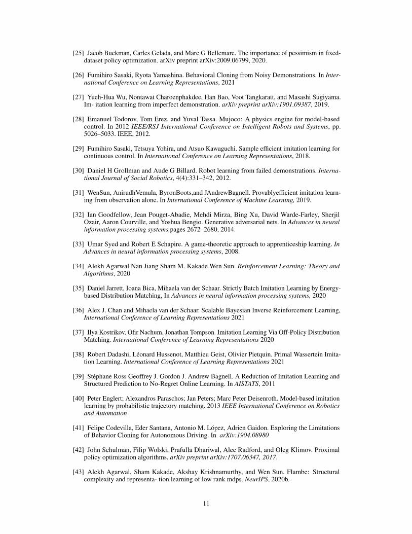
We provide confirmatory evidence of this hypothesis in figure 1 where we’ve outlined re-sults for evaluating i) and ii). Recall that π and πBC generates rollouts in Tl. For each chart thex-axis represents the elapsed timestep t during the rollout after initial sampling, and the y-axisrepresents the uncertainty Ut as measured by Tl. The lines for π and πBC are denoted by Algorithm2and BC respectively. As the lines deviate more from the x-axis, the evaluated policy is visiting moreuncertain states, which implies increased divergence from dπ

∗

Tt(s), and vice versa.

For i), the results are presented in the first two charts. Note that the BC agent admits amuch more divergent behavior than Algorithm 2 when they both begin s ∼ dπ

∗

Tt(s). The third and

fourth charts outline the evaluation results for ii). As opposed to i), both BC and Algorithm 2 beginsits rollouts from a state sampled from dπ

µ

Tt(s). As a result, the initial uncertainty measured by Tl is

greater than in i). We observe that in ii) πBC diverges even more so than in i) but π succeeds invisiting states that obtain gradually lower uncertainty. This result provides evidence to π’s recoverybehavior. We also remind the readers that as Tl becomes more accurate, this comparison wouldcorrelate greater with the true divergence behavior in Tt.

Expert Only So far, we’ve only discussed circumstances where we assume access to a behaviordataset sampled from dπ

µ

Tt(s), while being agnostic to its optimality. While it is indeed a practical

setting, we also want to evaluate Algorithm 2 when we are provided only expert demonstrations.In such setting, we can still apply results Theorem 4 without loss of its generality, but as a resultsome of its terms will depend on different distributions and we cannot guarantee a linear dependenceon the M . Namely, εT would instead depend on the number of expert demonstrations, and C :=

supπ∈Π,s∈S,a∈AνπTl

(s,a)

pπ∗Tt

(s,a), where they both scale in O( 1

(1−γ)2 ).

Observing the newly defined C, we suspect the algorithm’s performance would depend on thelearner’s ability to generate states that is covered by pπ

∗

Tt(s, a). However, recall that Algorithm 2

minimizes the estimated uncertainty of Tl, which is trained with samples s∗, a∗ ∼ pπ∗Tt (s, a). In otherwords, Tl admits less uncertainty on pπ

∗

Tt(s, a). One could then argue that in such case, by minimizing

Tl’s uncertainty, π could learn to match its visitation density with pπ∗

Tt(s, a). Additionally, as

alluded in section A, the function f could capture distributional information of states that π can utilise.

We evaluate this intuition and present its results on Table 3, where the scores are presentedin the column labeled Algorithm2expert. Indeed, we see that even if Tl is trained solely with expertsamples, Algorithm 2 outperforms BC. In the paragraph above, we attibute this to providing thelearner with more information that naive BC algorithms fails to utilise. This implies that usage of aestimated model in imitation learning in general could be beneficial.

20

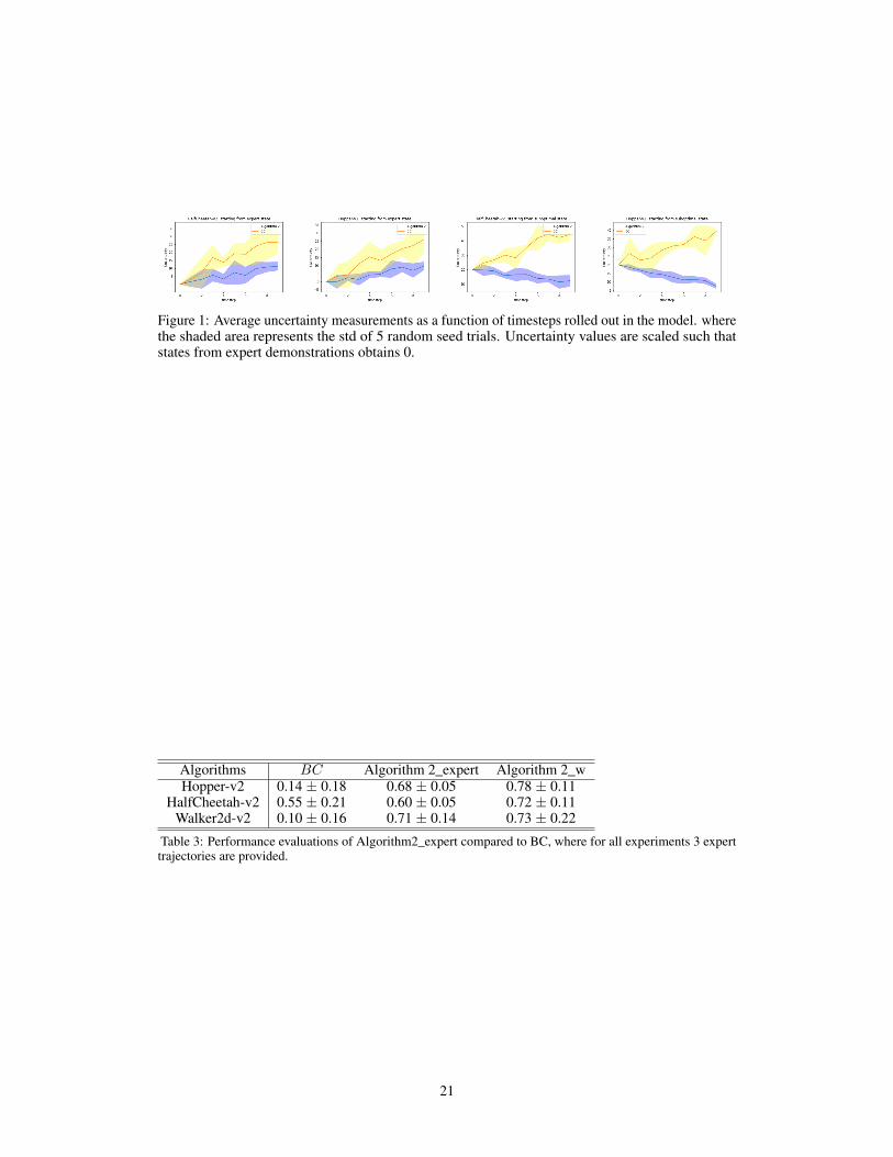
Figure 1: Average uncertainty measurements as a function of timesteps rolled out in the model. wherethe shaded area represents the std of 5 random seed trials. Uncertainty values are scaled such thatstates from expert demonstrations obtains 0.

Algorithms BC Algorithm 2_expert Algorithm 2_wHopper-v2 0.14 ± 0.18 0.68 ± 0.05 0.78 ± 0.11

HalfCheetah-v2 0.55 ± 0.21 0.60 ± 0.05 0.72 ± 0.11Walker2d-v2 0.10 ± 0.16 0.71 ± 0.14 0.73 ± 0.22

Table 3: Performance evaluations of Algorithm2_expert compared to BC, where for all experiments 3 experttrajectories are provided.

21