Mixed Exponentially Weighted Moving Average-Cumulative Sum Charts for Process Monitoring

Research Article

(wileyonlinelibrary.com) DOI: 10.1002/qre.1385 Published online 29 February 2012 in Wiley Online Library

Mixed Exponentially Weighted MovingAverage–Cumulative Sum Charts forProcess MonitoringNasir Abbas,a*† Muhammad Riaza,b and Ronald J. M. M. Doesc

The control chart is a very popular tool of statistical process control. It is used to determine the existence of special causevariation to remove it so that the process may be brought in statistical control. Shewhart-type control charts are sensitivefor large disturbances in the process, whereas cumulative sum (CUSUM)–type and exponentially weighted moving average(EWMA)–type control charts are intended to spot small and moderate disturbances. In this article, we proposed a mixedEWMA–CUSUM control chart for detecting a shift in the process mean and evaluated its average run lengths. Comparisonsof the proposed control chart were made with some representative control charts including the classical CUSUM, classicalEWMA, fast initial response CUSUM, fast initial response EWMA, adaptive CUSUM with EWMA-based shift estimator,weighted CUSUM and runs rules–based CUSUM and EWMA. The comparisons revealed that mixing the two charts makesthe proposed scheme even more sensitive to the small shifts in the process mean than the other schemes designed fordetecting small shifts. Copyright © 2012 John Wiley & Sons, Ltd.

Keywords: average run length (ARL); control charts; cumulative sum; exponentially weighted moving average; statistical process control

1. Introduction

Variations in a process are classified into two distinct parts called common and special cause variations. In the presence ofcommon cause variation only, the process is said to be statistically in control, but once the process includes both commonand special cause variations, it is deemed out of control. Statistical process control (SPC) is the application of the statistical tools

to distinguish between common and special cause variations (cf. Montgomery1). The most important of those statistical tools iscontrol chart. Cumulative sum (CUSUM) charts by Page2 and exponentially weighted moving average (EWMA) charts by Roberts3

are the two most commonly used types of control charts for detecting the smaller and moderate shifts in the process, whereasShewhart-type charts are good at detecting larger shifts.

An effective measure used for comparing the performance of the control charts is the average run length (ARL). If we define arandom variable RL equal to the number of samples until the first out of control signal occurs, then the probability distribution of thisrandom variable RL is known as the run length distribution. The average of this distribution is the ARL. The in-control ARL of a controlchart is denoted by ARL0, whereas out-of-control ARL is denoted by ARL1.

Lucas4 proposed the use of a combined Shewhart–CUSUM quality control scheme in which the CUSUM limits help in detecting thesmaller shifts whereas the Shewhart limits increase the sensitivity of the chart for the larger shifts. Similarly, the use of the combinedShewhart–EWMA scheme was recommended by Lucas and Saccucci5 to make the EWMA chart more sensitive for the larger shifts.Another alternative was presented by Jiang et al.6 to use the adaptive CUSUM procedure with EWMA-based shift estimators in whicha range of shifts is targeted and the reference value of the CUSUM is updated using the EWMA estimate.

In this article, we propose the use of a mixed EWMA–CUSUM control chart with the motivation to further enhance the sensitivity ofthe control chart structure, particularly for the shifts of smaller magnitude in the process.

The organization of the rest of the article is as follows. In the next section, we present the basic design structure of CUSUM- andEWMA-type control charts. The details regarding the design structure of the proposed scheme are provided in Section 3. Section 4consists of the comparison of the proposed scheme with its counterparts. An illustrative example of the proposed scheme ispresented in Section 5, and finally, Section 6 summarizes the findings of this article.

aDepartment of Statistics, Quaid-i-Azam University Islamabad, Islamabad, PakistanbDepartment of Mathematics and Statistics, King Fahad University of Petroleum and Minerals, Dhahran, 31261, Saudi ArabiacDepartment of Quantitative Economics, IBIS UvA, University of Amsterdam, Plantage Muidergracht 12, 1018 TV, Amsterdam, The Netherlands*Correspondence to: Nasir Abbas, Department of Statistics, Quaid-i-Azam University Islamabad, Islamabad, Pakistan.†E-mail: [email protected]

Copyright © 2012 John Wiley & Sons, Ltd. Qual. Reliab. Engng. Int. 2013, 29 345–356

345

N. ABBAS, M. RIAZ AND R. J. M. M. DOES

346

2. Classical CUSUM and EWMA charts

Shewhart-type control charts use only the current observation or sample to monitor the process. In this section, we consider controlcharts that also use previous observations along with the current observation. These mainly include CUSUM and EWMA schemes, andwe provide here the details regarding their usual design structures (also known as classical CUSUM and EWMA control charts).

2.1. Classical CUSUM control charts

The CUSUM chart was originally introduced by Page2 and is suited to detect small and sustained shifts in a process. These chartsmeasure a cumulative deviation from the mean or a target value. The two versions of the CUSUM chart, used to evaluate anout of control condition, are the V-mask CUSUM and the tabular CUSUM. The V-mask procedure, which is not very commonin use, normalizes the deviations from the mean and plots these deviations. As long as these deviations are plotted aroundthe target value, the process is said to be in control, otherwise out of control. The tabular method of evaluating a CUSUM chartis commonly used and is similar to a Shewhart-type control chart. In this method, we plot a function of the subgroup averageagainst the control limits, which are set according to a prefixed ARL0 value. Execution of the tabular CUSUM scheme forcontrolling the location parameter of the process is performed using two statistics called C+ and C�, which are defined as

Cþi ¼ max 0; Xi � m0ð Þ � k þ Cþ

i�1

� �C�i ¼ max 0;� Xi � m0ð Þ � k þ Cþ

i�1

� � (1)

where Xi denotes the ith observation (e.g. the sample mean of sample i), m0 is the target mean, and k is the reference value,which is usually chosen equal to half of the shift (in standard units) to be detected. The quantities C+ and C� are known asupper and lower CUSUM statistics, respectively, which are initially set to zero. These two statistics are plotted against the con-trol limit h. As long as the values of Cþ

i and C�i are plotted inside the control limit h, the process is said to be in control, other-

wise out of control. If the statistic Cþi is plotted above h, the process mean is said to be shifted above the target value, and if

the statistic C�i is plotted above h, the process is said to be shifted below the target value. The quantities k and h are the

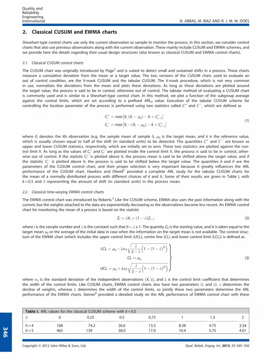
parameters of the CUSUM control chart, and their proper selection is very important because it greatly influences the ARLperformance of the CUSUM chart. Hawkins and Olwell7 provided a complete ARL study for the tabular CUSUM charts forthe mean of a normally distributed process with different choices of k and h. Some of their results are given in Table I, withk= 0.5 and d representing the amount of shift (in standard units) in the process mean.

2.2. Classical time-varying EWMA control charts

The EWMA control chart was introduced by Roberts.3 Like the CUSUM scheme, EWMA also uses the past information along with thecurrent, but the weights attached to the data are exponentially decreasing as the observations become less recent. An EWMA controlchart for monitoring the mean of a process is based on the statistic

Zi ¼ lXi þ 1� lð ÞZi�1 (2)

where i is the sample number and l is the constant such that 0< l⩽ 1. The quantity Z0 is the starting value, and it is taken equal to thetarget mean m0 or the average of the initial data in case when the information on the target mean is not available. The control struc-ture of the EWMA chart (which includes the upper control limit (UCL), centre line (CL) and lower control limit (LCL)) is defined as

LCL ¼ m0 � LsX

ffiffiffiffiffiffiffiffiffiffiffiffiffiffiffiffiffiffiffiffiffiffiffiffiffiffiffiffiffiffiffiffiffiffiffiffiffiffiffiffiffiffiffil

2� l1� 1� lð Þ2i

� �r

CL ¼ m0

UCL ¼ m0 þ LsX

ffiffiffiffiffiffiffiffiffiffiffiffiffiffiffiffiffiffiffiffiffiffiffiffiffiffiffiffiffiffiffiffiffiffiffiffiffiffiffiffiffiffiffil

2� l1� 1� lð Þ2i

� �r g (3)

where sX is the standard deviation of the independent observations Xi ′ s� �

, and L is the control limit coefficient that determinesthe width of the control limits. Like CUSUM charts, EWMA control charts also have two parameters (l and L). l determines thedecline of weights, whereas L determines the width of the control limits, so jointly these two parameters determine the ARLperformance of the EWMA charts. Steiner8 provided a detailed study on the ARL performance of EWMA control chart with these

Table I. ARL values for the classical CUSUM scheme with k=0.5

d 0 0.25 0.5 0.75 1 1.5 2

h=4 168 74.2 26.6 13.3 8.38 4.75 3.34h=5 465 139 38.0 17.0 10.4 5.75 4.01



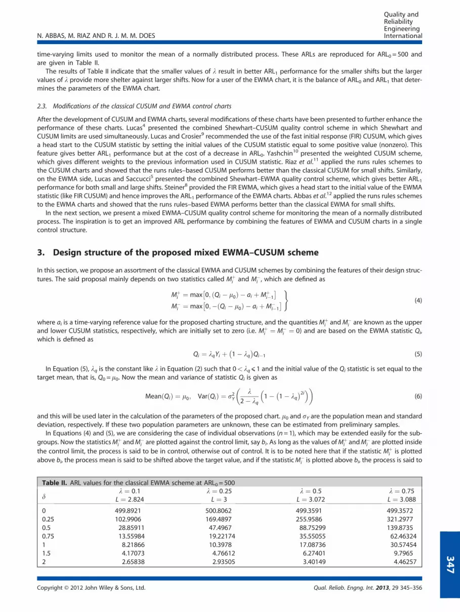
time-varying limits used to monitor the mean of a normally distributed process. These ARLs are reproduced for ARL0 = 500 andare given in Table II.

The results of Table II indicate that the smaller values of l result in better ARL1 performance for the smaller shifts but the largervalues of l provide more shelter against larger shifts. Now for a user of the EWMA chart, it is the balance of ARL0 and ARL1 that deter-mines the parameters of the EWMA chart.

2.3. Modifications of the classical CUSUM and EWMA control charts

After the development of CUSUM and EWMA charts, several modifications of these charts have been presented to further enhance theperformance of these charts. Lucas4 presented the combined Shewhart–CUSUM quality control scheme in which Shewhart andCUSUM limits are used simultaneously. Lucas and Crosier9 recommended the use of the fast initial response (FIR) CUSUM, which givesa head start to the CUSUM statistic by setting the initial values of the CUSUM statistic equal to some positive value (nonzero). Thisfeature gives better ARL1 performance but at the cost of a decrease in ARL0. Yashchin

10 presented the weighted CUSUM scheme,which gives different weights to the previous information used in CUSUM statistic. Riaz et al.11 applied the runs rules schemes tothe CUSUM charts and showed that the runs rules–based CUSUM performs better than the classical CUSUM for small shifts. Similarly,on the EWMA side, Lucas and Saccucci5 presented the combined Shewhart–EWMA quality control scheme, which gives better ARL1performance for both small and large shifts. Steiner8 provided the FIR EWMA, which gives a head start to the initial value of the EWMAstatistic (like FIR CUSUM) and hence improves the ARL1 performance of the EWMA charts. Abbas et al.12 applied the runs rules schemesto the EWMA charts and showed that the runs rules–based EWMA performs better than the classical EWMA for small shifts.

In the next section, we present a mixed EWMA–CUSUM quality control scheme for monitoring the mean of a normally distributedprocess. The inspiration is to get an improved ARL performance by combining the features of EWMA and CUSUM charts in a singlecontrol structure.

3. Design structure of the proposed mixed EWMA–CUSUM scheme

In this section, we propose an assortment of the classical EWMA and CUSUM schemes by combining the features of their design struc-tures. The said proposal mainly depends on two statistics called Mþ

i and M�i , which are defined as

Mþi ¼ max 0; Qi � m0ð Þ � ai þMþ

i�1

� �M�

i ¼ max 0;� Qi � m0ð Þ � ai þM�i�1

� �)

(4)

where ai is a time-varying reference value for the proposed charting structure, and the quantitiesMþi andM�

i are known as the upperand lower CUSUM statistics, respectively, which are initially set to zero (i.e. Mþ

i ¼ M�i ¼ 0) and are based on the EWMA statistic Qi,

which is defined as

Qi ¼ lqYi þ 1� lq� �

Qi�1 (5)

In Equation (5), lq is the constant like l in Equation (2) such that 0< lq⩽ 1 and the initial value of the Qi statistic is set equal to thetarget mean, that is, Q0 =m0. Now the mean and variance of statistic Qi is given as

Mean Qið Þ ¼ m0; Var Qið Þ ¼ s2Yl

2� lq1� 1� lq

� �2i� � (6)

and this will be used later in the calculation of the parameters of the proposed chart. m0 and sY are the population mean and standarddeviation, respectively. If these two population parameters are unknown, these can be estimated from preliminary samples.

In Equations (4) and (5), we are considering the case of individual observations (n= 1), which may be extended easily for the sub-groups. Now the statisticsMþ

i andM�i are plotted against the control limit, say bi. As long as the values ofMþ

i andM�i are plotted inside

the control limit, the process is said to be in control, otherwise out of control. It is to be noted here that if the statistic Mþi is plotted

above bi, the process mean is said to be shifted above the target value, and if the statisticM�i is plotted above bi, the process is said to

Table II. ARL values for the classical EWMA scheme at ARL0 = 500

dl ¼ 0:1L ¼ 2:824

l ¼ 0:25L ¼ 3

l ¼ 0:5L ¼ 3:072

l ¼ 0:75L ¼ 3:088

0 499.8921 500.8062 499.3591 499.35720.25 102.9906 169.4897 255.9586 321.29770.5 28.85911 47.4967 88.75299 139.87350.75 13.55984 19.22174 35.55055 62.463241 8.21866 10.3978 17.08736 30.574541.5 4.17073 4.76612 6.27401 9.79652 2.65838 2.93505 3.40149 4.46257


347


348

be shifted below the target value. The control limit bi is selected according to a prefixed ARL0. A large value of the prefixed ARL0 willgive a larger value of bi and vice versa. The two quantities ai and bi are defined as

ai ¼ a�ffiffiffiffiffiffiffiffiffiffiffiffiffiffiffiVar Qið Þp ¼ a�sY

ffiffiffiffiffiffiffiffiffiffiffiffiffiffiffiffiffiffiffiffiffiffiffiffiffiffiffiffiffiffiffiffiffiffiffiffiffiffiffiffiffiffiffiffiffiffiffiffil

2� lq1� 1� lq

� �2i� �s

bi ¼ b�ffiffiffiffiffiffiffiffiffiffiffiffiffiffiffiVar Qið Þp ¼ b�sY

ffiffiffiffiffiffiffiffiffiffiffiffiffiffiffiffiffiffiffiffiffiffiffiffiffiffiffiffiffiffiffiffiffiffiffiffiffiffiffiffiffiffiffiffiffiffiffiffil

2� lq1� 1� lq

� �2i� �s g (7)

where a* and b* are the constants like k and h, respectively, in the classical set up for the CUSUM. The time-varying reference values aiand bi are due to the variance of the EWMA statistic in Equation (6). For a fixed value of a*, we can select the value of b* from thetables (that are given later in this section) that fix the ARL0 at our desired level. In general, ai is chosen equal to half of the shift(in units of the standard deviation of Qi). Hence, we choose a* = 0.5 because it makes the CUSUM structure more sensitive to the smalland moderate shifts (cf. Montgomery1), to which memory charts actually target.

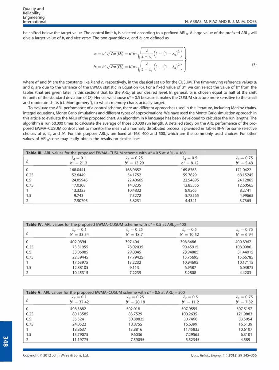
To evaluate the ARL performance of a control scheme, there are different approaches used in the literature, including Markov chains,integral equations, Monte Carlo simulations and different types of approximations. We have used the Monte Carlo simulation approach inthis article to evaluate the ARLs of the proposed chart. An algorithm in R language has been developed to calculate the run lengths. Thealgorithm is run 50,000 times to calculate the average of those 50,000 run length. A detailed study on the ARL performance of the pro-posed EWMA–CUSUM control chart to monitor the mean of a normally distributed process is provided in Tables III–V for some selectivechoices of d, lq and b*. For this purpose ARL0s are fixed at 168, 400 and 500, which are the commonly used choices. For othervalues of ARL0s one may easily obtain the results on similar lines.

Table III. ARL values for the proposed EWMA–CUSUM scheme with a* = 0.5 at ARL0 = 168

dlq ¼ 0:1b� ¼ 21:3

lq ¼ 0:25b� ¼ 13:29

lq ¼ 0:5b� ¼ 8:12

lq ¼ 0:75b� ¼ 5:48

0 168.0441 168.0652 169.8763 171.04220.25 52.6449 54.1752 59.7829 68.152450.5 24.85945 22.40665 22.54895 24.128650.75 17.0208 14.0235 12.85555 12.605651 13.3323 10.4832 8.9565 8.27411.5 9.743 7.3272 5.78565 4.996652 7.90705 5.8231 4.4341 3.7365

Table IV. ARL values for the proposed EWMA–CUSUM scheme with a* = 0.5 at ARL0 = 400

dlq ¼ 0:1

b� ¼ 33:54lq ¼ 0:25b� ¼ 18:7

lq ¼ 0:5b� ¼ 10:52

lq ¼ 0:75b� ¼ 6:94

0 402.0894 397.404 398.6486 400.89620.25 73.31955 78.02035 90.45915 108.00860.5 33.06085 29.0845 28.94885 31.440150.75 22.39445 17.79425 15.75695 15.667851 17.63975 13.2232 10.94695 10.171151.5 12.88105 9.113 6.9587 6.038752 10.45315 7.2235 5.2808 4.4203

Table V. ARL values for the proposed EWMA–CUSUM scheme with a* = 0.5 at ARL0 = 500

dlq ¼ 0:1

b� ¼ 37:42lq ¼ 0:25b� ¼ 20:18

lq ¼ 0:5b� ¼ 11:2

lq ¼ 0:75b� ¼ 7:32

0 498.3882 502.018 507.9555 507.51520.25 80.13585 83.7529 100.2635 121.98830.5 35.524 30.88825 30.7466 33.50540.75 24.0522 18.8755 16.6399 16.51391 18.8637 13.8816 11.45835 10.61071.5 13.79075 9.6036 7.29565 6.31012 11.19775 7.59055 5.52345 4.589



The relative standard errors for the results provided in Tables III–V are also calculated and found to be less than 1.2%. Moreover, wehave also replicated the ARL results of the classical CUSUM and the classical EWMA using our simulation algorithm and found almostsimilar results as by Hawkins and Olwell7 and Lucas and Saccucci,5 respectively, ensuring the validity of the simulation algorithmused.

The main findings about our proposed EWMA–CUSUM quality control scheme for monitoring the mean of a normally distributedprocess are given as follows:

1. Mixing the EWMA and CUSUM schemes really boosts the ARL performance of the resulting combination of the two chartsespecially for small and moderate shifts in the process (cf. Tables III–V).

2. For detecting small shifts in the process, the performance of the proposed scheme is better with smaller values of lq and viceversa (cf. Tables III–V).

3. The proposed scheme is ARL unbiased, that is, for a fixed value of ARL0, the ARL1 decreases with a decrease in the value of d andvice versa (cf. Tables III–V).

4. For a fixed value of d, the ARL1 of the proposed scheme decreases with a decrease in ARL0 (cf. Tables III–V).5. For a fixed value of ARL0, the control limit coefficient b* decreases with the increase in lq (cf. Tables III–V).

4. Comparisons

In this section, we present a comprehensive comparison of the proposed mixed EWMA–CUSUM scheme with some existing represen-tative EWMA and CUSUM control charts available in the literature. The performance of the control chart is compared in terms of ARL.The set of the schemes considered for the comparison consist of the classical CUSUM, the classical EWMA, the FIR CUSUM, the FIREWMA, the adaptive CUSUM with EWMA-based shift estimator, the weighted CUSUM and the runs rules–based CUSUM and EWMA.The ARLs of these charts are given in Tables I, II and VI–XIII.

4.1. Proposed versus classical CUSUM: The ARL values for the classical CUSUM control scheme proposed by Page2 are given in Table I.Comparison of the classical CUSUM with the proposed schemes reveals that the proposed scheme is performing really good for all thevalues of lq, particularly for the smaller values of lq. We can see that, for all the values of lq, the proposed scheme has better ARLperformance for small shifts, that is, d< 1, as compared with the classical CUSUM (cf. Table I versus Table III).

4.2. Proposed versus classical time-varying EWMA: The ARL values for the classical EWMA with time-varying limits, given by Steiner,8

are provided in Table II. Comparing the classical EWMAwith the proposed scheme, we observed that the proposed scheme have betterARL1 performance for small shifts, that is, d< 0.75, with its respective values of lq (cf. Table II versus Table V).

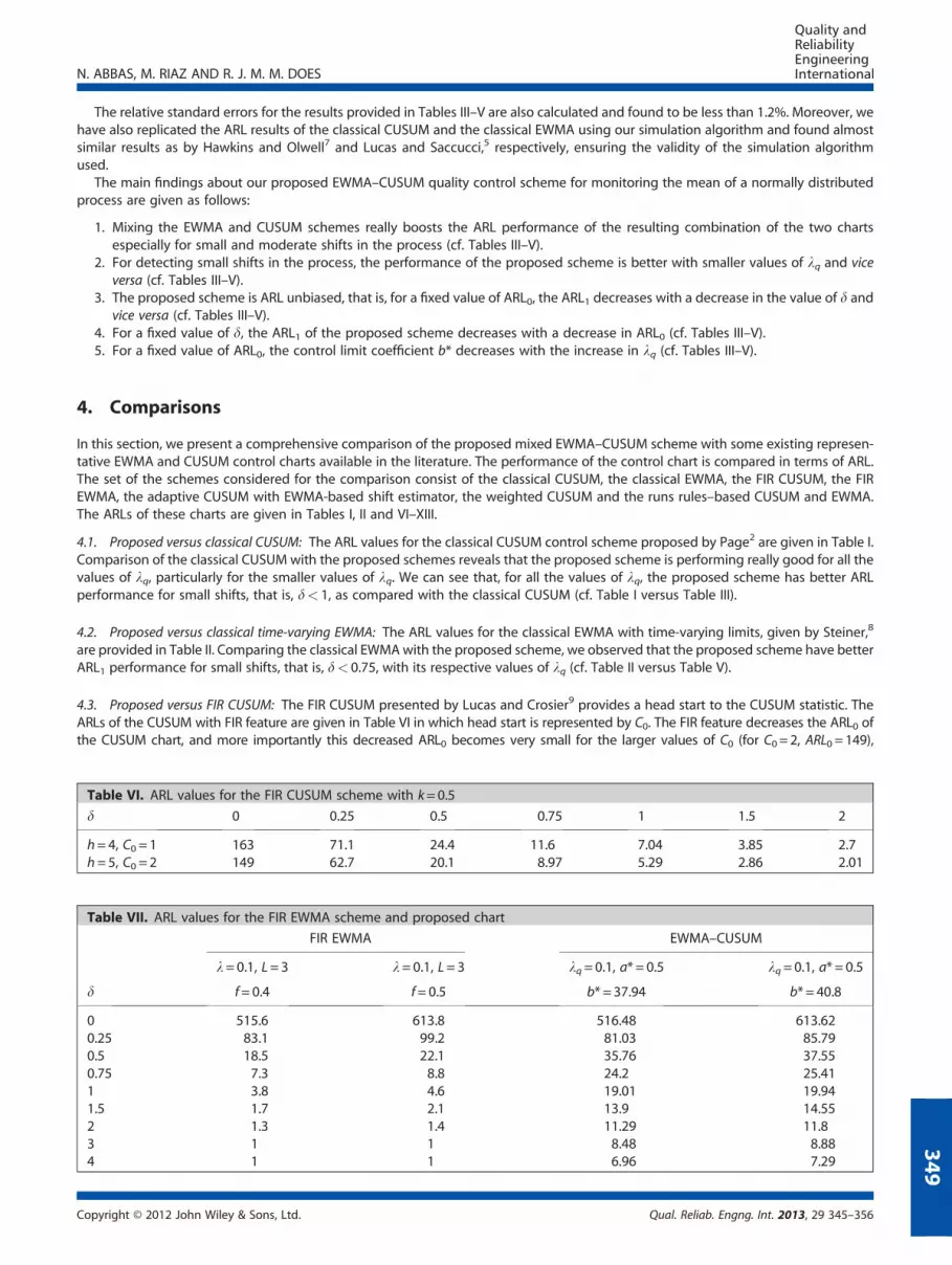
4.3. Proposed versus FIR CUSUM: The FIR CUSUM presented by Lucas and Crosier9 provides a head start to the CUSUM statistic. TheARLs of the CUSUM with FIR feature are given in Table VI in which head start is represented by C0. The FIR feature decreases the ARL0 ofthe CUSUM chart, and more importantly this decreased ARL0 becomes very small for the larger values of C0 (for C0 = 2, ARL0 = 149),

Table VI. ARL values for the FIR CUSUM scheme with k=0.5

d 0 0.25 0.5 0.75 1 1.5 2

h= 4, C0 = 1 163 71.1 24.4 11.6 7.04 3.85 2.7h= 5, C0 = 2 149 62.7 20.1 8.97 5.29 2.86 2.01

Table VII. ARL values for the FIR EWMA scheme and proposed chart

d

FIR EWMA EWMA–CUSUM

l= 0.1, L= 3 l= 0.1, L= 3 lq=0.1, a* = 0.5 lq=0.1, a* = 0.5

f= 0.4 f= 0.5 b* = 37.94 b* = 40.8

0 515.6 613.8 516.48 613.620.25 83.1 99.2 81.03 85.790.5 18.5 22.1 35.76 37.550.75 7.3 8.8 24.2 25.411 3.8 4.6 19.01 19.941.5 1.7 2.1 13.9 14.552 1.3 1.4 11.29 11.83 1 1 8.48 8.884 1 1 6.96 7.29


349

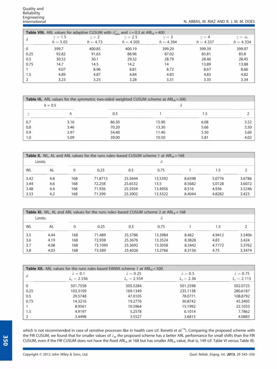
Table VIII. ARL values for adaptive CUSUM with dþmin and l= 0.3 at ARL0 = 400

dg ¼ 1:5h ¼ 5:05

g ¼ 2h ¼ 4:73

g ¼ 2:5h ¼ 4:505

g ¼ 3h ¼ 4:394

g ¼ 4h ¼ 4:337

g ¼ 1h ¼ 4:334

0 399.7 400.85 400.19 399.29 399.39 399.970.25 92.82 91.65 88.96 87.02 85.81 85.80.5 30.52 30.1 29.32 28.79 28.46 28.450.75 14.7 14.5 14.2 14 13.89 13.881 9.07 8.96 8.81 8.72 8.67 8.661.5 4.89 4.87 4.84 4.83 4.83 4.822 3.23 3.25 3.28 3.31 3.35 3.34

Table IX. ARL values for the symmetric two-sided weighted CUSUM scheme at ARL0 = 500

k = 0.5 d

g h 0.5 1 1.5 2

0.7 3.16 86.30 15.90 6.08 3.520.8 3.46 70.20 13.30 5.66 3.500.9 3.97 54.40 11.40 5.50 3.601.0 5.09 39.00 10.50 5.81 4.02

Table X. WL, AL and ARL values for the runs rules–based CUSUM scheme 1 at ARL0 = 168

Limits d

WL AL 0 0.25 0.5 0.75 1 1.5 2

3.42 4.8 168 71.8715 25.5644 13.5392 8.6598 5.0776 3.67863.44 4.6 168 72.258 25.6532 13.5 8.5682 5.0128 3.60723.48 4.4 168 71.936 25.5934 13.4956 8.516 4.936 3.52463.53 4.2 168 71.399 25.3002 13.3322 8.4044 4.8282 3.423

Table XI. WL, AL and ARL values for the runs rules–based CUSUM scheme 2 at ARL0 = 168

Limits d

WL AL 0 0.25 0.5 0.75 1 1.5 2

3.5 4.44 168 71.489 25.3786 13.3984 8.462 4.9412 3.54063.6 4.19 168 72.938 25.3676 13.3524 8.3828 4.83 3.4243.7 4.08 168 73.1095 25.3692 13.3058 8.3442 4.7772 3.37623.8 4.03 168 73.589 25.4026 13.2766 8.3156 4.75 3.3474

Table XII. ARL values for the runs rules based EWMA scheme 1 at ARL0 = 500

dl ¼ 0:1

Ls ¼ 2:556l ¼ 0:25Ls ¼ 2:554

l ¼ 0:5Ls ¼ 2:36

l ¼ 0:75Ls ¼ 2:115

0 501.7558 505.5284 501.2598 502.07250.25 103.3109 169.1349 235.1138 280.61870.5 29.5748 47.0105 78.0771 108.87920.75 14.3216 19.2776 30.8742 45.34051 8.9561 10.5964 15.1992 22.10331.5 4.9197 5.2578 6.1014 7.78622 3.4498 3.5527 3.6815 4.0883


350

which is not recommended in case of sensitive processes like in health care (cf. Bonetti et al.13). Comparing the proposed scheme withthe FIR CUSUM, we found that for smaller values of lq, the proposed scheme has a better ARL performance for small shifts than the FIRCUSUM, even if the FIR CUSUM does not have the fixed ARL0 at 168 but has smaller ARL0 value, that is, 149 (cf. Table VI versus Table III).


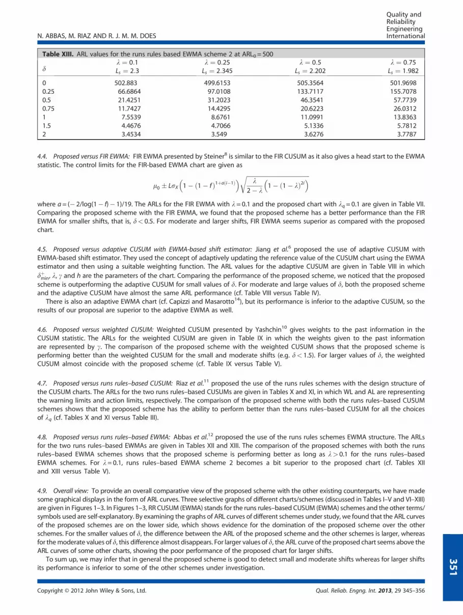
Table XIII. ARL values for the runs rules based EWMA scheme 2 at ARL0 = 500

dl ¼ 0:1Ls ¼ 2:3

l ¼ 0:25Ls ¼ 2:345

l ¼ 0:5Ls ¼ 2:202

l ¼ 0:75Ls ¼ 1:982

0 502.883 499.6153 505.3564 501.96980.25 66.6864 97.0108 133.7117 155.70780.5 21.4251 31.2023 46.3541 57.77390.75 11.7427 14.4295 20.6223 26.03121 7.5539 8.6761 11.0991 13.83631.5 4.4676 4.7066 5.1336 5.78122 3.4534 3.549 3.6276 3.7787


351

4.4. Proposed versus FIR EWMA: FIR EWMA presented by Steiner8 is similar to the FIR CUSUM as it also gives a head start to the EWMAstatistic. The control limits for the FIR-based EWMA chart are given as

m0 � LsX 1� 1� fð Þ1þa i�1ð Þ� � ffiffiffiffiffiffiffiffiffiffiffiffiffiffiffiffiffiffiffiffiffiffiffiffiffiffiffiffiffiffiffiffiffiffiffiffiffiffiffiffiffiffiffi

l2� l

1� 1� lð Þ2i� �r

where a= (� 2/log(1� f)� 1)/19. The ARLs for the FIR EWMA with l= 0.1 and the proposed chart with lq= 0.1 are given in Table VII.Comparing the proposed scheme with the FIR EWMA, we found that the proposed scheme has a better performance than the FIREWMA for smaller shifts, that is, d< 0.5. For moderate and larger shifts, FIR EWMA seems superior as compared with the proposedchart.

4.5. Proposed versus adaptive CUSUM with EWMA-based shift estimator: Jiang et al.6 proposed the use of adaptive CUSUM withEWMA-based shift estimator. They used the concept of adaptively updating the reference value of the CUSUM chart using the EWMAestimator and then using a suitable weighting function. The ARL values for the adaptive CUSUM are given in Table VIII in whichdþmin, l, g and h are the parameters of the chart. Comparing the performance of the proposed scheme, we noticed that the proposedscheme is outperforming the adaptive CUSUM for small values of d. For moderate and large values of d, both the proposed schemeand the adaptive CUSUM have almost the same ARL performance (cf. Table VIII versus Table IV).

There is also an adaptive EWMA chart (cf. Capizzi and Masarotto14), but its performance is inferior to the adaptive CUSUM, so theresults of our proposal are superior to the adaptive EWMA as well.

4.6. Proposed versus weighted CUSUM: Weighted CUSUM presented by Yashchin10 gives weights to the past information in theCUSUM statistic. The ARLs for the weighted CUSUM are given in Table IX in which the weights given to the past informationare represented by g. The comparison of the proposed scheme with the weighted CUSUM shows that the proposed scheme isperforming better than the weighted CUSUM for the small and moderate shifts (e.g. d< 1.5). For larger values of d, the weightedCUSUM almost coincide with the proposed scheme (cf. Table IX versus Table V).

4.7. Proposed versus runs rules–based CUSUM: Riaz et al.11 proposed the use of the runs rules schemes with the design structure ofthe CUSUM charts. The ARLs for the two runs rules–based CUSUMs are given in Tables X and XI, in which WL and AL are representingthe warning limits and action limits, respectively. The comparison of the proposed scheme with both the runs rules–based CUSUMschemes shows that the proposed scheme has the ability to perform better than the runs rules–based CUSUM for all the choicesof lq (cf. Tables X and XI versus Table III).

4.8. Proposed versus runs rules–based EWMA: Abbas et al.12 proposed the use of the runs rules schemes EWMA structure. The ARLsfor the two runs rules–based EWMAs are given in Tables XII and XIII. The comparison of the proposed schemes with both the runsrules–based EWMA schemes shows that the proposed scheme is performing better as long as l> 0.1 for the runs rules–basedEWMA schemes. For l= 0.1, runs rules–based EWMA scheme 2 becomes a bit superior to the proposed chart (cf. Tables XIIand XIII versus Table V).

4.9. Overall view: To provide an overall comparative view of the proposed scheme with the other existing counterparts, we have madesome graphical displays in the form of ARL curves. Three selective graphs of different charts/schemes (discussed in Tables I–V and VI–XIII)are given in Figures 1–3. In Figures 1–3, RR CUSUM (EWMA) stands for the runs rules–based CUSUM (EWMA) schemes and the other terms/symbols used are self-explanatory. By examining the graphs of ARL curves of different schemes under study, we found that the ARL curvesof the proposed schemes are on the lower side, which shows evidence for the domination of the proposed scheme over the otherschemes. For the smaller values of d, the difference between the ARL of the proposed scheme and the other schemes is larger, whereasfor themoderate values of d, this difference almost disappears. For larger values of d, the ARL curve of the proposed chart seems above theARL curves of some other charts, showing the poor performance of the proposed chart for larger shifts.

To sum up, we may infer that in general the proposed scheme is good to detect small and moderate shifts whereas for larger shiftsits performance is inferior to some of the other schemes under investigation.


0

10

20

30

40

50

60

70

80

0.25 0.5 0.75 1 1.5 2

AR

Ls

Proposed (λ=0.5) Classical CUSUM (k=0.5, h=4)FIR CUSUM (Co=1) RR CUSUM I (WL=3.53, AL=4.2)RR CUSUM II (WL=3.5, AL=4.44)

Figure 1. ARL curves for the proposed scheme, the classical CUSUM, the FIR CUSUM and the runs rules–based CUSUMs at ARL0 = 168

0

10

20

30

40

50

60

70

80

90

100

0.25 0.5 0.75 1 1.5 2

AR

Ls

Proposed (λ=0.1) Proposed (λ=0.5) Adaptive CUSUM (γ=2.5)

Figure 2. ARL curves for the proposed scheme and adaptive CUSUM at ARL0 = 400

0

10

20

30

40

50

60

70

80

90

100

0.5 1 1.5 2

AR

Ls

Proposed (λ=0.5) Classical EWMA (λ=0.5) Weighted CUSUM (γ=0.9)

RR EWMA I (λ=0.5) RR EWMA II (λ=0.5)

Figure 3. ARL curves for the proposed scheme, the classical EWMA, the FIR EWMA, the runs rules–based EWMA and the weighted CUSUM at ARL0 = 500


352

5. Illustrative example

Besides exploring the statistical properties of a method, it is always good to provide its application on some data for illustration pur-poses. Authors generally provide these types of examples using real or simulated data sets, for example, Lucas and Crosier,9 Khoo,15

Antzoulakos and Rakitzis16 and Riaz et al.11 Following this inspiration, we present here an illustrative example to show how the


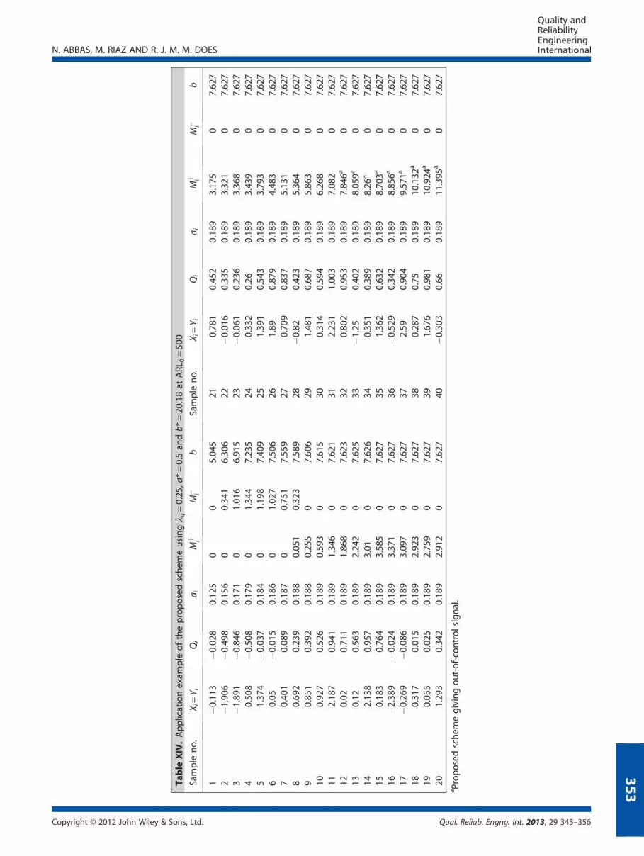
Table

XIV.Applicationexam

ple

oftheproposedschem

eusingl q

=0.25

,a*=0.5an

db*

=20

.18at

ARL

0=50

0

Sample

no.

X i=Y i

Qi

a iM

þ iM

� ib

Sample

no.

X i=Y i

Qi

a iM

þ iM

� ib

1�0

.113

�0.028

0.12

50

05.04

521

0.78

10.45

20.18

93.17

50

7.62

72

�1.906

�0.498

0.15

60

0.34

16.30

622

�0.016

0.33

50.18

93.32

10

7.62

73

�1.891

�0.846

0.17

10

1.01

66.91

523

�0.061

0.23

60.18

93.36

80

7.62

74

0.50

8�0

.508

0.17

90

1.34

47.23

524

0.33

20.26

0.18

93.43

90

7.62

75

1.37

4�0

.037

0.18

40

1.19

87.40

925

1.39

10.54

30.18

93.79

30

7.62

76

0.05

�0.015

0.18

60

1.02

77.50

626

1.89

0.87

90.18

94.48

30

7.62

77

0.40

10.08

90.18

70

0.75

17.55

927

0.70

90.83

70.18

95.13

10

7.62

78

0.69

20.23

90.18

80.05

10.32

37.58

928

�0.82

0.42

30.18

95.36

40

7.62

79

0.85

10.39

20.18

80.25

50

7.60

629

1.48

10.68

70.18

95.86

30

7.62

710

0.92

70.52

60.18

90.59

30

7.61

530

0.31

40.59

40.18

96.26

80

7.62

711

2.18

70.94

10.18

91.34

60

7.62

131

2.23

11.00

30.18

97.08

20

7.62

712

0.02

0.71

10.18

91.86

80

7.62

332

0.80

20.95

30.18

97.84

6a0

7.62

713

0.12

0.56

30.18

92.24

20

7.62

533

�1.25

0.40

20.18

98.05

9a0

7.62

714

2.13

80.95

70.18

93.01

07.62

634

0.35

10.38

90.18

98.26

a0

7.62

715

0.18

30.76

40.18

93.58

50

7.62

735

1.36

20.63

20.18

98.70

3a0

7.62

716

�2.389

�0.024

0.18

93.37

10

7.62

736

�0.529

0.34

20.18

98.85

6a0

7.62

717

�0.269

�0.086

0.18

93.09

70

7.62

737

2.59

0.90

40.18

99.57

1a0

7.62

718

0.31

70.01

50.18

92.92

30

7.62

738

0.28

70.75

0.18

910

.132

a0

7.62

719

0.05

50.02

50.18

92.75

90

7.62

739

1.67

60.98

10.18

910

.924

a0

7.62

720

1.29

30.34

20.18

92.91

20

7.62

740

�0.303

0.66

0.18

911

.395

a0

7.62

7aProposedschem

egivingout-of-controlsignal.



353


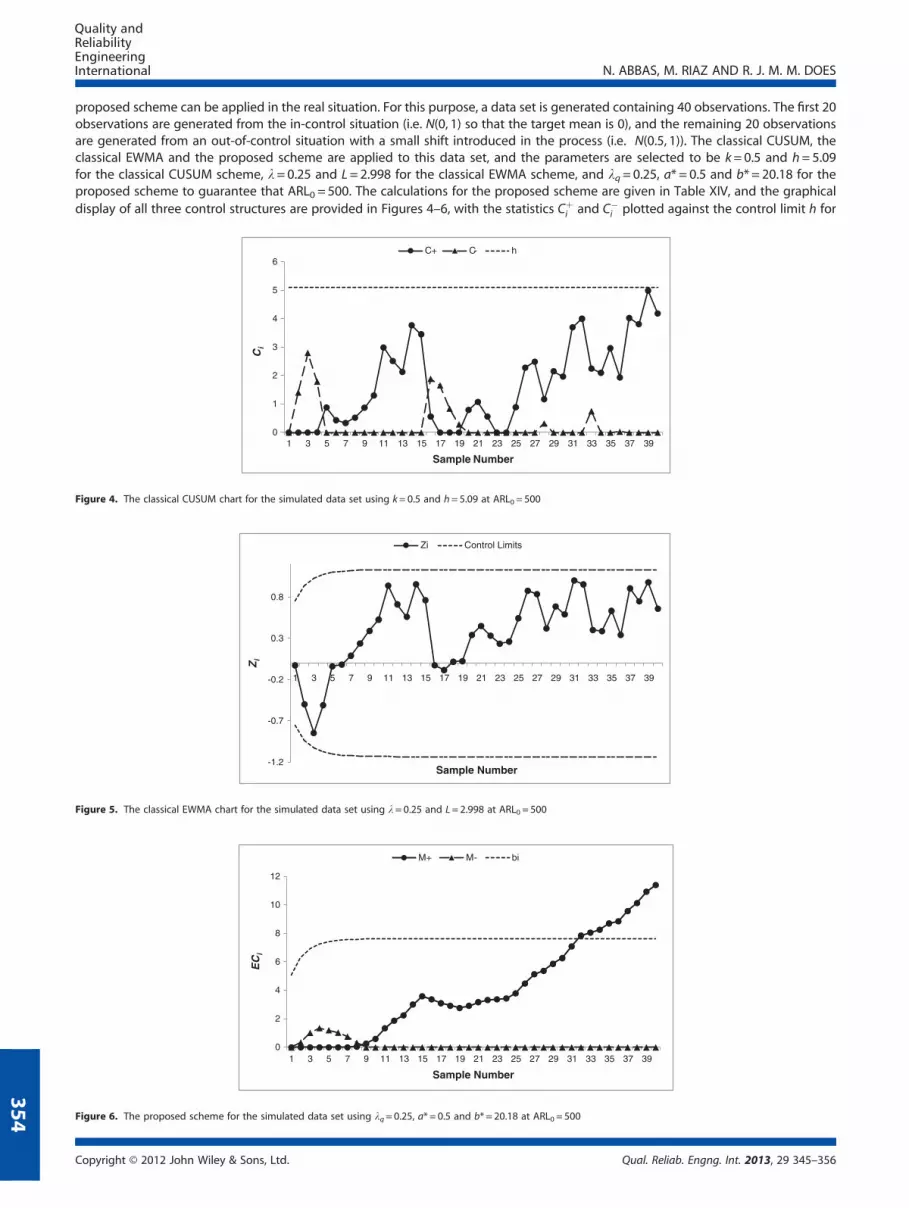
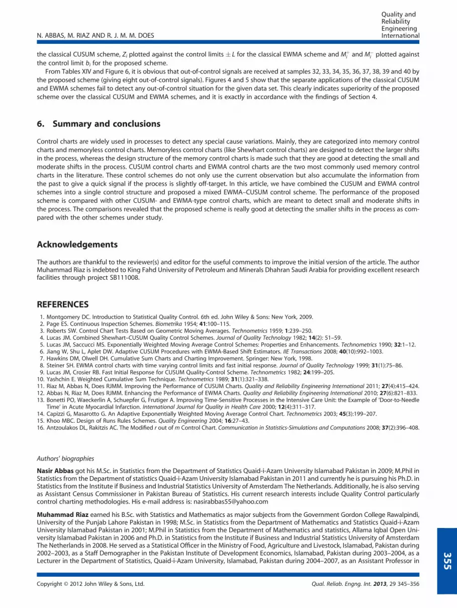
354

proposed scheme can be applied in the real situation. For this purpose, a data set is generated containing 40 observations. The first 20observations are generated from the in-control situation (i.e. N(0, 1) so that the target mean is 0), and the remaining 20 observationsare generated from an out-of-control situation with a small shift introduced in the process (i.e. N(0.5, 1)). The classical CUSUM, theclassical EWMA and the proposed scheme are applied to this data set, and the parameters are selected to be k= 0.5 and h= 5.09for the classical CUSUM scheme, l= 0.25 and L= 2.998 for the classical EWMA scheme, and lq=0.25, a* = 0.5 and b* = 20.18 for theproposed scheme to guarantee that ARL0 = 500. The calculations for the proposed scheme are given in Table XIV, and the graphicaldisplay of all three control structures are provided in Figures 4–6, with the statistics Cþ

i and C�i plotted against the control limit h for

0

1

2

3

4

5

6

1 3 5 7 9 11 13 15 17 19 21 23 25 27 29 31 33 35 37 39

Ci

Sample Number

C+ C- h

Figure 4. The classical CUSUM chart for the simulated data set using k= 0.5 and h= 5.09 at ARL0 = 500

-1.2

-0.7

-0.2

0.3

0.8

1 3 5 7 9 11 13 15 17 19 21 23 25 27 29 31 33 35 37 39

Zi

Sample Number

Zi Control Limits

Figure 5. The classical EWMA chart for the simulated data set using l= 0.25 and L= 2.998 at ARL0 = 500

0

2

4

6

8

10

12

1 3 5 7 9 11 13 15 17 19 21 23 25 27 29 31 33 35 37 39

EC

i

Sample Number

M+ M- bi

Figure 6. The proposed scheme for the simulated data set using lq= 0.25, a* = 0.5 and b* = 20.18 at ARL0 = 500



the classical CUSUM scheme, Zi plotted against the control limits � L for the classical EWMA scheme and Mþi and M�

i plotted againstthe control limit bi for the proposed scheme.

From Tables XIV and Figure 6, it is obvious that out-of-control signals are received at samples 32, 33, 34, 35, 36, 37, 38, 39 and 40 bythe proposed scheme (giving eight out-of-control signals). Figures 4 and 5 show that the separate applications of the classical CUSUMand EWMA schemes fail to detect any out-of-control situation for the given data set. This clearly indicates superiority of the proposedscheme over the classical CUSUM and EWMA schemes, and it is exactly in accordance with the findings of Section 4.

6. Summary and conclusions

Control charts are widely used in processes to detect any special cause variations. Mainly, they are categorized into memory controlcharts and memoryless control charts. Memoryless control charts (like Shewhart control charts) are designed to detect the larger shiftsin the process, whereas the design structure of the memory control charts is made such that they are good at detecting the small andmoderate shifts in the process. CUSUM control charts and EWMA control charts are the two most commonly used memory controlcharts in the literature. These control schemes do not only use the current observation but also accumulate the information fromthe past to give a quick signal if the process is slightly off-target. In this article, we have combined the CUSUM and EWMA controlschemes into a single control structure and proposed a mixed EWMA–CUSUM control scheme. The performance of the proposedscheme is compared with other CUSUM- and EWMA-type control charts, which are meant to detect small and moderate shifts inthe process. The comparisons revealed that the proposed scheme is really good at detecting the smaller shifts in the process as com-pared with the other schemes under study.

Acknowledgements

The authors are thankful to the reviewer(s) and editor for the useful comments to improve the initial version of the article. The authorMuhammad Riaz is indebted to King Fahd University of Petroleum and Minerals Dhahran Saudi Arabia for providing excellent researchfacilities through project SB111008.

REFERENCES1. Montgomery DC. Introduction to Statistical Quality Control. 6th ed. John Wiley & Sons: New York, 2009.2. Page ES. Continuous Inspection Schemes. Biometrika 1954; 41:100–115.3. Roberts SW. Control Chart Tests Based on Geometric Moving Averages. Technometrics 1959; 1:239–250.4. Lucas JM. Combined Shewhart–CUSUM Quality Control Schemes. Journal of Quality Technology 1982; 14(2): 51–59.5. Lucas JM, Saccucci MS. Exponentially Weighted Moving Average Control Schemes: Properties and Enhancements. Technometrics 1990; 32:1–12.6. Jiang W, Shu L, Aplet DW. Adaptive CUSUM Procedures with EWMA-Based Shift Estimators. IIE Transactions 2008; 40(10):992–1003.7. Hawkins DM, Olwell DH. Cumulative Sum Charts and Charting Improvement. Springer: New York, 1998.8. Steiner SH. EWMA control charts with time varying control limits and fast initial response. Journal of Quality Technology 1999; 31(1):75–86.9. Lucas JM, Crosier RB. Fast Initial Response for CUSUM Quality-Control Scheme. Technometrics 1982; 24:199–205.10. Yashchin E. Weighted Cumulative Sum Technique. Technometrics 1989; 31(1):321–338.11. Riaz M, Abbas N, Does RJMM. Improving the Performance of CUSUM Charts. Quality and Reliability Engineering International 2011; 27(4):415–424.12. Abbas N, Riaz M, Does RJMM. Enhancing the Performance of EWMA Charts. Quality and Reliability Engineering International 2010; 27(6):821–833.13. Bonetti PO, Waeckerlin A, Schuepfer G, Frutiger A. Improving Time-Sensitive Processes in the Intensive Care Unit: the Example of ‘Door-to-Needle

Time’ in Acute Myocardial Infarction. International Journal for Quality in Health Care 2000; 12(4):311–317.14. Capizzi G, Masarotto G. An Adaptive Exponentially Weighted Moving Average Control Chart. Technometrics 2003; 45(3):199–207.15. Khoo MBC. Design of Runs Rules Schemes. Quality Engineering 2004; 16:27–43.16. Antzoulakos DL, Rakitzis AC. The Modified r out of m Control Chart. Communication in Statistics-Simulations and Computations 2008; 37(2):396–408.

355

Authors' biographies

Nasir Abbas got his M.Sc. in Statistics from the Department of Statistics Quaid-i-Azam University Islamabad Pakistan in 2009; M.Phil inStatistics from the Department of statistics Quaid-i-Azam University Islamabad Pakistan in 2011 and currently he is pursuing his Ph.D. inStatistics from the Institute if Business and Industrial Statistics University of Amsterdam The Netherlands. Additionally, he is also servingas Assistant Census Commissioner in Pakistan Bureau of Statistics. His current research interests include Quality Control particularlycontrol charting methodologies. His e-mail address is: [email protected]

Muhammad Riaz earned his B.Sc. with Statistics and Mathematics as major subjects from the Government Gordon College Rawalpindi,University of the Punjab Lahore Pakistan in 1998; M.Sc. in Statistics from the Department of Mathematics and Statistics Quaid-i-AzamUniversity Islamabad Pakistan in 2001; M.Phil in Statistics from the Department of Mathematics and statistics, Allama Iqbal Open Uni-versity Islamabad Pakistan in 2006 and Ph.D. in Statistics from the Institute if Business and Industrial Statistics University of AmsterdamThe Netherlands in 2008. He served as a Statistical Officer in the Ministry of Food, Agriculture and Livestock, Islamabad, Pakistan during2002–2003, as a Staff Demographer in the Pakistan Institute of Development Economics, Islamabad, Pakistan during 2003–2004, as aLecturer in the Department of Statistics, Quaid-i-Azam University, Islamabad, Pakistan during 2004–2007, as an Assistant Professor in



356

the Department of Statistics, Quaid-i-Azam University, Islamabad, Pakistan during 2007–2010. He is serving as an Assistant Professor inthe Department of Mathematics and Statistics, King Fahad University of Petroleum and Minerals, Dhahran 31261, Saudi Arabia from2010-Present. His current research interests include Statistical Process Control, Non-Parametric techniques and Experimental Designs.His e-mail contacts are: [email protected]

Ronald J.M.M. Does graduated (PhD 1982) in mathematical statistics from the University of Leiden. Currently, he is professor of indus-trial statistics at the University of Amsterdam, managing director of the Institute for Business and Industrial Statistics and director ofthe Graduate School of Executive Programmes at the Amsterdam Business School. His research activities are the design of controlcharts for nonstandard situations, the methodology of Lean Six Sigma and healthcare engineering.


Documents

Mixed Exponentially Weighted Moving Average-Cumulative Sum Charts for Process Monitoring