Min-plus System Theory

Applied to Communication Networks

Jean-Yves Le Boudec and Patrick Thiran

LCA - ISC

School of Computer and Communication Sciences

EPFL

CH-1015 Lausanne

Switzerland

Abstract

Network Calculus is a set of recent developments, which provide a deep insight into

flow problems encountered in networking. It can be viewed as the system theory that

applies to computer networks. Contrary to traditional system theory, it relies on max-

plus and min-plus algebra. In this paper, we show how a simple but important fixed-

point theorem (residuation theorem in min-plus algebra) can be successfully applied

to a number of problems in networking, such as window flow control, multimedia

smoothing, and bounds on loss rates.

1 Introduction

Network calculus is a theory of (mainly determinstic) queuing systems found in computer

networks. The foundation of network calculus lies in the mathematical theory of dioids, and

in particular, the Min-Plus dioid (also called Min-Plus algebra). With network calculus,

we are able to understand some fundamental properties of integrated services networks, of

window flow control, of scheduling and of buffer or delay dimensioning.

The main difference between network calculus, which can be regarded as the system theory

that applies to computer networks, and traditional system theory, as the one which was so

successfully applied to design electronic circuits, is the algebra under which operations take

place: addition becomes now computation of the minimum, multiplication becomes addition.

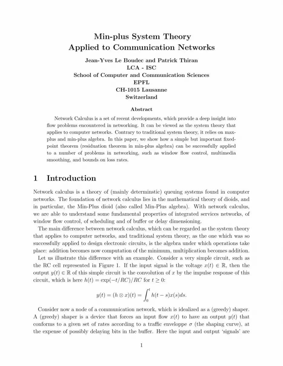
Let us illustrate this difference with an example. Consider a very simple circuit, such as

the RC cell represented in Figure 1. If the input signal is the voltage x(t) ∈ R, then the

output y(t) ∈ R of this simple circuit is the convolution of x by the impulse response of this

circuit, which is here h(t) = exp(−t/RC)/RC for t ≥ 0:

y(t) = (h ⊗ x)(t) =

∫ t

0

h(t − s)x(s)ds.

Consider now a node of a communication network, which is idealized as a (greedy) shaper.

A (greedy) shaper is a device that forces an input flow x(t) to have an output y(t) that

conforms to a given set of rates according to a traffic enveloppe σ (the shaping curve), at

the expense of possibly delaying bits in the buffer. Here the input and output ‘signals’ are

1

cumulative flows, defined as the number of bits seen on the data flow in time interval [0, t].

These functions are non-decreasing with time t. We will denote by G the set of non-negative

wide-sense increasing functions and by F denote the set of wide-sense increasing functions

(or sequences) such that f(t) = 0 for t < 0. Parameter t can be continuous or discrete. We

will see in this paper that x and y are linked by the relation

y(t) = (σ ⊗ x)(t) = infs:0≤s≤t

{σ(t − s) + x(s)} . (1.1)

This relation defines the min-plus convolution between σ and x.

[�W� \�W�

σ

� �

��

&

5

\�W�[�W�

(a)

(b)

Figure 1: Traditional system theory for an elementary circuit (top) and min-plus system

theory for a shaper (bottom).

We first review the basic concepts of network calculus, namely the way we characterize

the ‘signals’ (i.e. the flows) via arrival curves (Section 2) and the ‘system’ (e.g., the network

node) via a service curve (Section 3). These tools will enable us to derive some deterministic

performance bounds on quantities such delays and backlogs (Section 4), which are defined

as follows, for a lossless system with input flow x(t) and output flow y(t):

Definition 1.1 (Backlog and Delay). The backlog at time t is x(t) − y(t), the virtual

delay at time t is

d(t) = inf {τ ≥ 0 : x(t) ≤ y(t + τ)} .

2

The backlog is the amount of bits that are held inside the system; if the system is a

single buffer, it is the queue length. In contrast, if the system is more complex, then the

backlog is the number of bits “in transit”, assuming that we can observe input and output

simultaneously. The virtual delay at time t is the delay that would be experienced by a bit

arriving at time t if all bits received before it are served before it. If we plot x(t) and y(t)

versus t, the backlog is the vertical deviation between these two curves. The virtual delay is

the horizontal deviation.

The second part of the paper (Sections 5 and 6) is a systematic method for modeling a

number of situations arising in communication networks (lossless greedy shaping, window

flow control, video smoothing, upper bound on loss rates, packetizing variable length pack-

ets), as sets of inequalities using min-plus operators. We will find the maximal solution of

these systems of inequalities using a central result of min-plus algebra which describes the

maximal solution of these systems of inequalities using the concept of closure of an operator

[3] (Theorem 7.1 in Section 7). It is equivalent to the description of a system by a set of

ordinary differential equations in traditional system theory.

The interested reader is also referred to the pioneering work of Cruz [8], Chang[5], Agrawal

and Rajan[1], as well as to [6, 10].

2 Arrival curves

To provide guarantees to data flows requires some specific support in the network; as a

counterpart, the traffic sent by sources needs to be limited. This is done by using the

concept of arrival curve, defined below.

Definition 2.1 (Arrival Curve). Given a wide-sense increasing function α defined for

t ≥ 0 (namely α ∈ F), we say that a flow x is constrained by α if and only if for all s ≤ t:

x(t) − x(s) ≤ α(t − s).

Note that this is equivalent to imposing that for all t ≥ 0

x(t) ≤ inf0≤s≤t

{α(t − s) + x(s)} = (α ⊗ x)(t) (2.2)

The simplest arrival curve is α(t) = Rt. Then the constraint means that, on any time

window of width τ , the number of bits for the flow is limited by Rτ . We say in that case

that the flow is peak rate limited. This occurs if we know that the flow is arriving on a link

whose physical bit rate is limited by R bits/sec. A flow where the only constraint is a limit

on the peak rate is often (improperly) called a “constant bit rate” (CBR) flow.

More generally, because of their relationship with leaky buckets, we will often use affine

arrival curves γr,b, defined by: γr,b(t) = rt + b for t > 0 and 0 otherwise. Having γr,b as an

arrival curve allows a source to send b bits at once, but not more than r bits/s over the long

run. Parameters b and r are called the burst tolerance (in units of data) and the rate (in

3

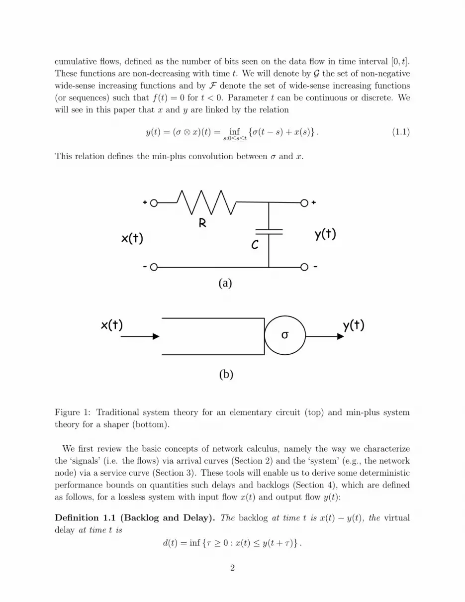
units of data per time unit). The Integrated services framework of the Internet (Intserv)

uses arrival curves, such as

α(t) = min{M + pt, rt + b} = γp,M(t) ∧ γr,b(t)

where M is interpreted as the maximum packet size, p as the peak rate, b as the burst

tolerance, and r as the sustainable rate Figure 2. Notation ∧ stands for minimum or infimum.

In Intserv jargon, the 4-uple (p, M, r, b) is also called a T-SPEC (traffic specification). ATM

uses similar curves.

T

R

t

P

r

M

b dmax

β(t)

α(t)

wmax

Figure 2: Arrival curve α for ATM VBR and for Intserv flows, rate-latency service curve β

and vertical and horizontal devaitions between both curves.

One can always replace an arrival curve α by its sub-additive closure, which is defined as

α = inf{δ0, α, α ⊗ α, . . . , α(n), . . .}

where α(n) = α ⊗ . . . ⊗ α (n times) and δ0 is the “impulse” function defined by δ0(t) = ∞

for t > 0 and δ0(0) = 0. One can show indeed that x ≤ x ⊗ α if and only if x ≤ x ⊗ α. If

α(0) = 0 and α is sub-additive (meaning that for all s, t ≥ 0, α(s + t) ≤ α(s) + α(t)), then

α = α. As an example, one can check that γr,b = γr,b.

Finally, it is possible to compute from measurements of a given flow x(t) its minimal arrival

curve, which is (x ⊘ x)(t) where ⊘ denotes the min-plus deconvolution operator defined by

(x ⊘ σ)(t) = supu≥0

{x(t + u) − σ(u)} , (2.3)

for a given function σ ∈ F . Note that if x, σ ∈ F , then (x⊗σ) ∈ F but in general (x⊘σ) /∈ F

(it belongs to G). One can check however that (x ⊘ x) ∈ F . Let us also mention that the

name deconvolution is justified by the fact that for any x, y, z ∈ F , x ≤ y ⊗ z if and only if

x ⊘ z ≤ y.

3 Service curves

We have seen that one first principle in integrated services networks is to put arrival curve

constraints on flows. In order to provide reservations, network nodes in return need to offer

4

some guarantees to flows. This is done by packet schedulers. The details of packet scheduling

are abstracted using the concept of service curve, which we introduce in this section.

Definition 3.1 (Service Curve). Consider a system S and a flow through S with input

and ouptut function x and y. We say that S offers to the flow a service curve β if and only

if for all t ≥ 0, there exists some t0 ≥ 0, with t0 ≤ t, such that

y(t) − x(t0) ≥ β(t − t0).

Again, we can recast this definition as

y(t) ≥ inf0≤s≤t

{β(t − s) + x(s)} = (β ⊗ x)(t) (3.4)

Let us consider a few examples. A simple one is a GPS (Generalized Processor Sharing)

node which, by offering a service curve β(t) = Rt, guarantees that each flow is served at

least at rate R bits/s during a busy period.

A second example is a guaranteed delay node. Here the only information we have about

the network node is that the maximum delay for the bits of a given flow x is bounded by

some fixed value T , and that the bits of the flow are served in first in, first out order. This is

used with a family of schedulers called “earliest deadline first” (EDF), and can be translated

as y(t) ≥ x(t − T ) for all t ≥ T . Using the “impulse” function δT defined by δT (t) = 0 if

0 ≤ t ≤ T and δT (t) = +∞ if t > T , we have that (x⊗ δT )(t) = x(t−T ). We have therefore

shown that a guaranteed delay node offers a service curve β = δT .

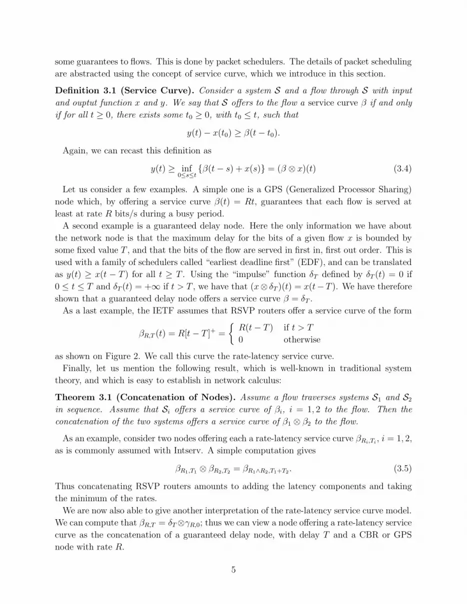
As a last example, the IETF assumes that RSVP routers offer a service curve of the form

βR,T (t) = R[t − T ]+ =

{

R(t − T ) if t > T

0 otherwise

as shown on Figure 2. We call this curve the rate-latency service curve.

Finally, let us mention the following result, which is well-known in traditional system

theory, and which is easy to establish in network calculus:

Theorem 3.1 (Concatenation of Nodes). Assume a flow traverses systems S1 and S2

in sequence. Assume that Si offers a service curve of βi, i = 1, 2 to the flow. Then the

concatenation of the two systems offers a service curve of β1 ⊗ β2 to the flow.

As an example, consider two nodes offering each a rate-latency service curve βRi,Ti, i = 1, 2,

as is commonly assumed with Intserv. A simple computation gives

βR1,T1⊗ βR2,T2

= βR1∧R2,T1+T2. (3.5)

Thus concatenating RSVP routers amounts to adding the latency components and taking

the minimum of the rates.

We are now also able to give another interpretation of the rate-latency service curve model.

We can compute that βR,T = δT ⊗γR,0; thus we can view a node offering a rate-latency service

curve as the concatenation of a guaranteed delay node, with delay T and a CBR or GPS

node with rate R.

5

4 Three basic bounds

In this section we see the main simple network calculus results. They are all bounds for

lossless systems with service guarantees [1]. The proofs are straightforward applications of

the definitions of service and arrival curves.

The first theorem says that the backlog is bounded by the vertical deviation between the

arrival and service curves:

Theorem 4.1 (Backlog Bound). Assume a flow, constrained by arrival curve α, traverses

a system that offers a service curve β. The backlog x(t) − y(t) for all t satisfies:

x(t) − y(t) ≤ sups≥0

{α(s) − β(s)}

We now use the concept of horizontal deviation. Call ∆(s) = inf {τ ≥ 0 : α(s) ≤ β(s + τ)}.

From Definition 1.1, ∆(s) is the virtual delay for a hypothetical system which would have α

as input and β as output, assuming that such a system exists. Let h(α, β) be the supremum

of all values of ∆(s). The second theorem gives a bound on delay for the general case.

Theorem 4.2 (Delay Bound). Assume a flow, constrained by arrival curve α, traverses

a system that offers a service curve of β. The virtual delay d(t) for all t satisfies: d(t) ≤

h(α, β).

Theorem 4.3 (Output Flow). Assume a flow, constrained by arrival curve α, traverses a

system that offers a service curve of β. The output flow is constrained by the arrival curve

α∗ = α ⊘ β.

As a first application of the previous results, consider a VBR flow, defined by TSPEC

(M, p, r, b) (hence α(t) = {M + pt} ∧ {rt + b}) and served in one node which guarantees

a service curve equal to the rate-latency function β(t) = R[t − T ]+. This example is the

standard model used in Intserv (Figure 2). Let us apply Theorems 4.1 and 4.2. Assume that

R ≥ r namely the reserved rate is as large as the sustainable rate of the flow. The buffer

required for the flow is bounded by

wmax = b + r max

(

b − M

p − r, T

)

The maximum delay for the flow is bounded by

dmax =M + b−M

p−r(p − R)+

R+ T.

As a second application, let us show how these bounds, combined with Theorem 3.1, allow

us to understand a phenomenon known in the Insterv community as “Pay Bursts Only

Once”. Consider the concatenation of two nodes offering each a rate-latency service curve

6

βRi,Ti, i = 1, 2, as is commonly assumed with Intserv. Assume the fresh input is constrained

by γr,b. Assume that r < R1 and r < R2. We are interested in the delay bound, which we

know is a worst case. Let us compare the results obtained by applying Theorem 4.2 (i) to

the network service curve (3.5), resulting in a delay bound D0; (ii) iteratively to every node,

resulting in two individual bounds D1 and D2.

(i) The delay bound D0 can be computed by application of Theorem 4.2:

D0 =b

R1 ∧ R2

+ T1 + T2.

(ii) Now apply the second method. A bound on the delay at node 1 is (Theorem 4.2):

D1 = b/R1+T1. The output of the first node is constrained by by α∗(t) = b+rt+rT1, because

of Theorem 4.3. A bound on the delay at the second buffer is therefore D2 = (b+rT1)/R2+T2.

Consequently,

D1 + D2 =b

R1+

b + rT1

R2+ T1 + T2

It is easy to see that D0 < D1 + D2. In other words, the bounds obtained by considering

the global service curve are better than the bounds obtained by considering every buffer in

isolation.

5 Some deterministic flow problems in networking

We now describe a few examples of situations arising in the networking context, which we

will model as min-plus systems in the next section.

Example 1: Greedy lossless traffic shaper

We call policer with curve σ a device that counts the bits arriving on an input flow and

decides which bits conform with an arrival curve of σ. We call shaper, with shaping curve

σ, a bit processing device that forces its output to have σ as arrival curve. We call greedy

shaper a shaper which delays the input bits in a buffer, whenever sending a bit would violate

the constraint σ, but outputs them as soon as possible.

With ATM and sometimes with IP (Diffserv and Intserv), traffic sent over one connection,

or flow, is policed at the network boundary. Policing is performed in order to guarantee that

users do not send more than specified by the contract of the connection. Policing devices

inside the network are normally buffered, they are thus shapers. Shaping is also often needed

because the output of a buffer normally does not conform any more with the traffic contract

specified at the input.

If a(t) denotes the input flow, and if σ denotes the shaping curve (since it is an arrival

curve, we can always assume that σ is sub-additive with σ(0) = 0, as explained in Section 2),

7

the output x(t) of the shaper is therefore such that

x(t) ≤ a(t)

x(t) − x(s) ≤ σ(t − s)

for all 0 ≤ s ≤ t. The shaper is greedy if x is the maximal solution of this set of inequalities.

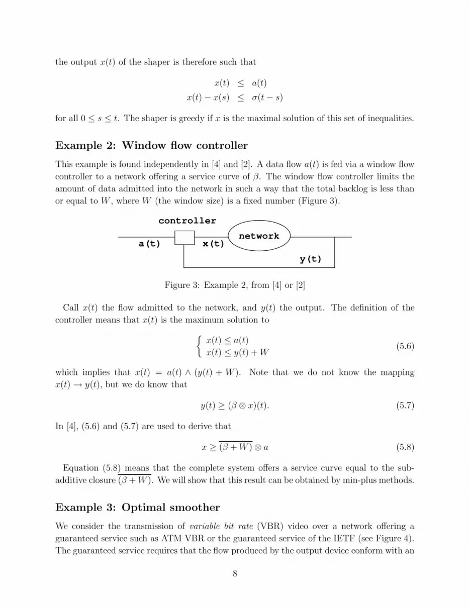
Example 2: Window flow controller

This example is found independently in [4] and [2]. A data flow a(t) is fed via a window flow

controller to a network offering a service curve of β. The window flow controller limits the

amount of data admitted into the network in such a way that the total backlog is less than

or equal to W , where W (the window size) is a fixed number (Figure 3).

a(t) x(t)

y(t)

network

controller

Figure 3: Example 2, from [4] or [2]

Call x(t) the flow admitted to the network, and y(t) the output. The definition of the

controller means that x(t) is the maximum solution to

{

x(t) ≤ a(t)

x(t) ≤ y(t) + W(5.6)

which implies that x(t) = a(t) ∧ (y(t) + W ). Note that we do not know the mapping

x(t) → y(t), but we do know that

y(t) ≥ (β ⊗ x)(t). (5.7)

In [4], (5.6) and (5.7) are used to derive that

x ≥ (β + W ) ⊗ a (5.8)

Equation (5.8) means that the complete system offers a service curve equal to the sub-

additive closure (β + W ). We will show that this result can be obtained by min-plus methods.

Example 3: Optimal smoother

We consider the transmission of variable bit rate (VBR) video over a network offering a

guaranteed service such as ATM VBR or the guaranteed service of the IETF (see Figure 4).

The guaranteed service requires that the flow produced by the output device conform with an

8

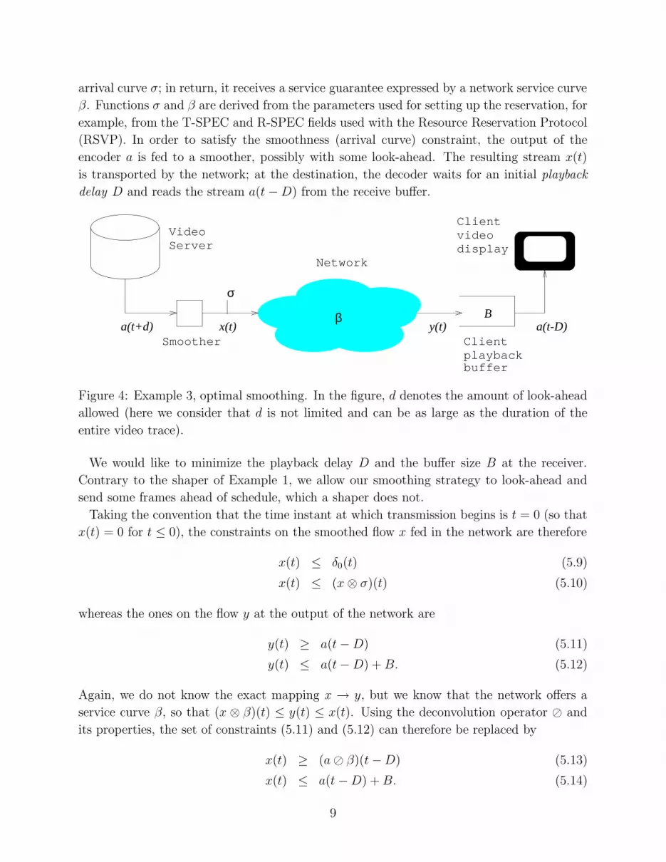
arrival curve σ; in return, it receives a service guarantee expressed by a network service curve

β. Functions σ and β are derived from the parameters used for setting up the reservation, for

example, from the T-SPEC and R-SPEC fields used with the Resource Reservation Protocol

(RSVP). In order to satisfy the smoothness (arrival curve) constraint, the output of the

encoder a is fed to a smoother, possibly with some look-ahead. The resulting stream x(t)

is transported by the network; at the destination, the decoder waits for an initial playback

delay D and reads the stream a(t − D) from the receive buffer.

a(t+d) y(t) a(t-D)x(t)β

displayvideo Client

Network

Client

buffer

σ

Smootherplayback

B

VideoServer

Figure 4: Example 3, optimal smoothing. In the figure, d denotes the amount of look-ahead

allowed (here we consider that d is not limited and can be as large as the duration of the

entire video trace).

We would like to minimize the playback delay D and the buffer size B at the receiver.

Contrary to the shaper of Example 1, we allow our smoothing strategy to look-ahead and

send some frames ahead of schedule, which a shaper does not.

Taking the convention that the time instant at which transmission begins is t = 0 (so that

x(t) = 0 for t ≤ 0), the constraints on the smoothed flow x fed in the network are therefore

x(t) ≤ δ0(t) (5.9)

x(t) ≤ (x ⊗ σ)(t) (5.10)

whereas the ones on the flow y at the output of the network are

y(t) ≥ a(t − D) (5.11)

y(t) ≤ a(t − D) + B. (5.12)

Again, we do not know the exact mapping x → y, but we know that the network offers a

service curve β, so that (x ⊗ β)(t) ≤ y(t) ≤ x(t). Using the deconvolution operator ⊘ and

its properties, the set of constraints (5.11) and (5.12) can therefore be replaced by

x(t) ≥ (a ⊘ β)(t − D) (5.13)

x(t) ≤ a(t − D) + B. (5.14)

9

We will compute the smallest values of D and B that guarantee a lossless smoothing, and pro-

pose one smoothing strategy (which is not unique: others are proposed in [11, 12], achieving

the same optimal values of D and B).

Example 4: Losses in a shaper with finite buffer

We reconsider Example 1, but now we suppose that the buffer is not large enough to avoid

losses for all possible input traffic, and we would like to compute the amount of data lost

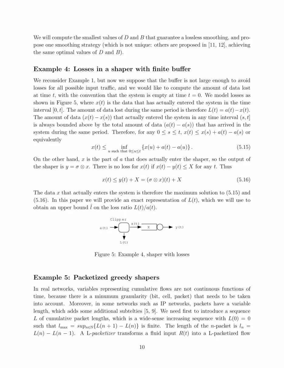
at time t, with the convention that the system is empty at time t = 0. We model losses as

shown in Figure 5, where x(t) is the data that has actually entered the system in the time

interval [0, t]. The amount of data lost during the same period is therefore L(t) = a(t)−x(t).

The amount of data (x(t)− x(s)) that actually entered the system in any time interval (s, t]

is always bounded above by the total amount of data (a(t) − a(s)) that has arrived in the

system during the same period. Therefore, for any 0 ≤ s ≤ t, x(t) ≤ x(s) + a(t) − a(s) or

equivalently

x(t) ≤ infu such that 0≤u≤t

{x(u) + a(t) − a(u)} . (5.15)

On the other hand, x is the part of a that does actually enter the shaper, so the output of

the shaper is y = σ ⊗ x. There is no loss for x(t) if x(t) − y(t) ≤ X for any t. Thus

x(t) ≤ y(t) + X = (σ ⊗ x)(t) + X (5.16)

The data x that actually enters the system is therefore the maximum solution to (5.15) and

(5.16). In this paper we will provide an exact representation of L(t), which we will use to

obtain an upper bound l̂ on the loss ratio L(t)/a(t).

Clipp er

a(t)

L(t)

x(t)X y(t)

Figure 5: Example 4, shaper with losses

Example 5: Packetized greedy shapers

In real networks, variables representing cumulative flows are not continuous functions of

time, because there is a minumum granularity (bit, cell, packet) that needs to be taken

into account. Moreover, in some networks such as IP networks, packets have a variable

length, which adds some additional subtelties [5, 9]. We need first to introduce a sequence

L of cumulative packet lengths, which is a wide-sense increasing sequence with L(0) = 0

such that lmax = supn∈N{L(n + 1) − L(n)} is finite. The length of the n-packet is ln =

L(n) − L(n − 1). A L-packetizer transforms a fluid input R(t) into a L-packetized flow

10

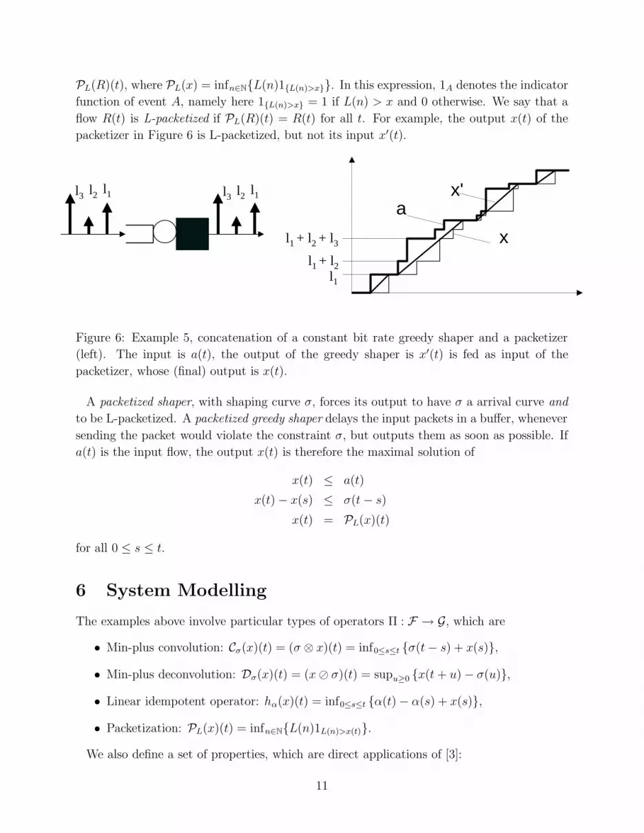
PL(R)(t), where PL(x) = infn∈N{L(n)1{L(n)>x}}. In this expression, 1A denotes the indicator

function of event A, namely here 1{L(n)>x} = 1 if L(n) > x and 0 otherwise. We say that a

flow R(t) is L-packetized if PL(R)(t) = R(t) for all t. For example, the output x(t) of the

packetizer in Figure 6 is L-packetized, but not its input x′(t).

x'

l1 + l2 + l3

l1 + l2l1

l1l2l3 l1l2l3

a

x

Figure 6: Example 5, concatenation of a constant bit rate greedy shaper and a packetizer

(left). The input is a(t), the output of the greedy shaper is x′(t) is fed as input of the

packetizer, whose (final) output is x(t).

A packetized shaper, with shaping curve σ, forces its output to have σ a arrival curve and

to be L-packetized. A packetized greedy shaper delays the input packets in a buffer, whenever

sending the packet would violate the constraint σ, but outputs them as soon as possible. If

a(t) is the input flow, the output x(t) is therefore the maximal solution of

x(t) ≤ a(t)

x(t) − x(s) ≤ σ(t − s)

x(t) = PL(x)(t)

for all 0 ≤ s ≤ t.

6 System Modelling

The examples above involve particular types of operators Π : F → G, which are

• Min-plus convolution: Cσ(x)(t) = (σ ⊗ x)(t) = inf0≤s≤t {σ(t − s) + x(s)},

• Min-plus deconvolution: Dσ(x)(t) = (x ⊘ σ)(t) = supu≥0 {x(t + u) − σ(u)},

• Linear idempotent operator: hα(x)(t) = inf0≤s≤t {α(t) − α(s) + x(s)},

• Packetization: PL(x)(t) = infn∈N{L(n)1L(n)>x(t)}.

We also define a set of properties, which are direct applications of [3]:

11

• Π is isotone if x(t) ≤ y(t) for all t always implies Π(x)(t) ≤ Π(y)(t) for all t. One can

check that all four operators Cσ,Dσ, hα,PL are isotone.

• Π is causal if for all t, Π(x)(t) depends only on x(s) for 0 ≤ s ≤ t. Cσ, hα, PL are

causal, but not Dσ.

• Π is upper-semi-continuous if for any decreasing sequence of trajectories (xi(t)) we

have inf i Π(xi) = Π(inf i xi). Cσ, hα, PL are upper semi-continuous, but not Dσ.

• Π is shift-invariant if y(t) = Π(x)(t) for all t and x′(t) = x(t + s) for some s implies

that for all t Π(x′)(t) = y(t + s). Cσ and Dσ are shift-invariant, but not hα nor PL.

• Π is min-plus linear if it is upper-semi-continuous and Π(x + K) = Π(x) + K for all

constant K. Cσ, hα are min-plus linear, but not Dσ nor PL.

We recast now the five examples using these operators.

Example 1: Greedy shaper. Its output is the maximum solution to

x ≤ a ∧ Cσ(x). (6.17)

Example 2: Window flow controller. Define Π as the operator that maps x(t) to y(t).

From Equation (5.6), we derive that x(t) is the maximum solution to

x ≤ a ∧ (Π(x) + W ) (6.18)

The operator Π can be assumed to be isotone, causal and upper-semi-continuous, but not

necessarily linear. However, we know that Π ≥ Cβ . We will exploit this formulation in

Section 7.

Example 3: Optimal smoother. Constraints (5.9) to (5.14) can be recast as

x(t) ≤ δ0(t) ∧ Cσ(x)(t) ∧ {a(t − D) + B} (6.19)

x(t) ≥ Dβ(a)(t − D) (6.20)

Example 4: Losses in a shaper with finite buffer. All operators are linear. We

know that x ≤ a. Combining this relation with (5.15) and (5.16), we derive that x is the

maximum solution to

x ≤ a ∧ ha(x) ∧ (σ ⊗ x + X). (6.21)

Example 5: Greedy packetized shaper. Its output of the function x ∈ F which (i) is

L-packetized and (ii) is the maximal solution of

x ≤ a ∧ Cσ(x) ∧ PL(x). (6.22)

12

7 Space Method

In this paper we apply Theorem 4.70, item 6 [3] to the problems formulated in the previous

section.

Theorem 7.1. Let Π be an operator F → G, and assume it is isotone and upper-semi-

continuous. For any fixed function a ∈ F , the problem

x ≤ Π(x) ∧ a (7.23)

has one maximum solution, given by

x = Π(a) = inf{

a, Π(a), Π[Π(a)], . . . , Π(n)(a), . . .}

.

The theorem is proven in [3], though with some amount of notation, using the fixed point

method. It can also easily be proven directly as follows. Consider the sequence of decreasing

sequences defined by x0 = a and xn+1 = Π(xn)∧xn, n ∈ N. Then x∗ = infn∈N xn is a solution

of (7.23) because Π is upper-semi-continuous. One easily check that xn = inf0≤m≤n{Πm(a)},

so that x∗ = Π(a). Conversely, if x is a solution, then x ≤ xn for all n because Π is isotone

and thus x ≤ x∗. We call the application of this theorem the space method, because it is

based on an iteration on complete trajectories x(t).

Let us first apply the theorem to Example 1. The maximal solution of (6.17) is

x = Cσ(a) = (σ ⊗ a) = σ ⊗ a = σ ⊗ a,

the latter equality resulting from the sub-additivity of σ. An immediate consequence of this

result is that a greedy shaper offers to the incoming flow a service curve equal to σ. The

input-output characterization of greedy shapers x = σ ⊗ a is however much stronger than

the service curve property, since we have here an equality instead of a lower bound.

Let us next apply the theorem to Example 2. We know now that (6.18) has one maximum

solution and that it is given by

x = (Π + W )(a).

Now from (5.7) we have Π(x) + W ≥ β ⊗ x + K. One easily shows that x ≥ (β + W ) ⊗ a

which is Equation (5.8).

The maximal solution of (6.19) and (6.20) in Example 3, which is

x(t) = Cσ(δ0(t) ∧ {a(t − D) + B}) = σ(t) ∧ {(σ ⊗ a)(t − D) + B} (7.24)

is guaranteed to exist if and only if it always verifies (6.20), which yields that

supt

{(a ⊘ β)(t − D) − σ(t)} ≤ 0

supt

{(a ⊘ β)(t− D) − (σ ⊗ a)(t − D)} ≤ B.

13

Working out these inequalities, we find that the smallest playback delay and buffer size are

D = inf {s ≥ 0 : (a ⊘ (β ⊗ σ))(−s) ≤ 0}

B = ((a ⊘ a) ⊘ (β ⊗ σ))(0).

These optimal values are achieved by a smoothing strategy implemented at the sender side,

given by (7.24).

From Theorem 7.1, the maximal solution of (6.21) in Example 4 is x = ha ∧ CσX(a),

which after some manipulations (see [10]) can be recast as

x = ha[CσX](a).

The amount of lost data in the interval [0, t] is

L(t) = a(t)−x(t) = supk≥0

{

sup0≤s2k≤...≤s2≤s1≤t

{

k∑

i=1

[a(s2i−1) − a(s2i) − σ(s2i−1 − s2i)]

}

− kX

}

.

As an application of this representation of L(t), we show how to retrieve the bound on the

loss rate obtained by Chuang and Chang [7], when we have an arrival curve α for the input

flow a. Define

l̂(t) = 1 − inf0<s≤t

σ(s) + X

α(s). (7.25)

Then for any 0 ≤ u < v ≤ t, since a(v) − a(u) ≤ α(v − u) by definition of an arrival curve,

1 − l̂(t) = inf0<s≤t

σ(s) + X

α(s)≤

σ(v − u) + X

α(v − u)≤

σ(v − u) + X

a(v) − a(u).

Therefore, for any 0 ≤ u ≤ v ≤ t,

a(v) − a(u) − σ(v − u) − X ≤ l̂(t) · [a(v) − a(u)].

For any integer n ≥ 1, and any sequence {sk}1≤k≤2n, with 0 ≤ s2n ≤ . . . ≤ s1 ≤ t, setting

v = s2i−1 and u = s2i in the previous equation, and summing over i, we obtainn

∑

i=1

[a(s2i−1) − a(s2i) − σ(s2i−1 − s2i) − X] ≤ l̂(t) ·

n∑

i=1

[a(s2i−1) − a(s2i)] ,

from which we deduce that

L(t) ≤ supn∈N

{

sup0≤s2n≤...≤s1≤t

{

n∑

i=1

[a(s2i−1) − a(s2i) − σ(s2i−1 − s2i) − X]

}}

≤ l̂(t) · a(t),

which shows that l̂(t) ≥ l(t) = L(t)/a(t). To have a bound independent of time t, we take

the sup over all t of (7.25):

l̂ = supt≥0

l̂(t) = 1 − inft>0

σ(t) + X

α(t).

Finally, the maximal solution of (6.22) in Example 5 is, after similar manipulations as

those made in Example 4,

x = PL ∧ Cσ(a) = PL[Cσ](a).

One checks that x is L-packetized, and is thus the output of the packetized greedy shaper.

14

8 Conclusion

Network calculus belongs to what is sometimes called topical (or exotic) algebras, a set

of mathematical results, often with high description complexity, but offering deep insights

into man-made systems such as communication networks. This paper has underlined the

importance of a simple fixed point residuation theorem in the networking context.

References

[1] R. Agrawal, R. L. Cruz, C. Okino and R. Rajan, ‘Performance Bounds for Flow Control

Protocols’, IEEE Trans. on Networking, vol 7(3), pp 310–323, June 1999.

[2] R. Aggrawal and R. Rajan. ‘Performance bounds for guaranteed and adaptive services’,

Technical report RC 20649, IBM, December 1996.

[3] F. Baccelli, G. Cohen, G. J. Olsder and J.-P. Quadrat. Synchronization and Linearity,

An Algebra for Discrete Event Systems, John Wiley and Sons, August 1992.

[4] C.S. Chang. ‘A filtering theory for deterministic traffic regulation’, in Proceedings Info-

com’97, Kobe, Japan, April 1997.

[5] C.S. Chang, Performance Guarantees in Communication Networks, Springer-Verlag,

New York, 2000.

[6] C.S. Chang, R. L. Cruz, J. Y. Le Boudec, P. Thiran ‘A Min-Plus System Theory for

Constrained Traffic Regulation and Dynamic Service Guarantees’, IEEE/ACM Trans-

actions on Networking, 2002 (to appear).

[7] C.-M. Chuang and J.-F. Chang, ‘Deterministic Loss Ratio Quality of Service Guarantees

for High Speed Networks’, IEEE Com. Letters, vol. 4, pp. 236–238, July 2000.

[8] R. L. Cruz, ‘Quality of service guarantees in virtual circuit switched networks’, IEEE

Journal on Selected Areas in Communication, pp. 1048–1056, August 1995.

[9] J. Y. Le Boudec, ‘Some properties of variable length packet shapers’ Proceedings of

ACM Sigmetrics 2001, Boston, June 2001.

[10] J. Y. Le Boudec and P. Thiran, Network Calculus: A Theory of Deterministic Queuing

Systems for the Internet, Springer-Verlag, vol. LCNS 2050, New York, 2001.

[11] J. Y. Le Boudec and O. Verscheure, ‘Optimal Smoothing for Guaranteed Service’

IEEE/ACM Transactions on Networking, Vol. 8, pp. 689–696, Dec 2000.

[12] P. Thiran, J.-Y. Le Boudec and F. Worm, ‘Network calculus applied to optimal multi-

media smoothing’, Proc of Infocom 2001, April 2001.

15