Min max generalization for deterministic batch mode reinforcement learning: relaxation schemes

MIN MAX GENERALIZATION FOR TWO-STAGE DETERMINISTIC BATCHMODE REINFORCEMENT LEARNING: RELAXATION SCHEMES

R. FONTENEAU†, D. ERNST†, B. BOIGELOT†, AND Q. LOUVEAUX†

Abstract. We study the min max optimization problem introduced in [22] for computing policies for batchmode reinforcement learning in a deterministic setting. First, we show that this problem is NP-hard. In the two-stage case, we provide two relaxation schemes. The first relaxation scheme works by dropping some constraints inorder to obtain a problem that is solvable in polynomial time. The second relaxation scheme, based on a Lagrangianrelaxation where all constraints are dualized, leads to a conic quadratic programming problem. We also theoreticallyprove and empirically illustrate that both relaxation schemes provide better results than those given in [22].

Key words. Reinforcement Learning, Min Max Generalization, Non-convex Optimization, ComputationalComplexity

AMS subject classifications. 60J05 Discrete-time Markov processes on general state spaces

1. Introduction. Research in Reinforcement Learning (RL) [48] aims at designing com-putational agents able to learn by themselves how to interact with their environment to max-imize a numerical reward signal. The techniques developed in this field have appealed re-searchers trying to solve sequential decision making problems in many fields such as Finance[26], Medicine [34, 35] or Engineering [42]. Since the end of the nineties, several researchershave focused on the resolution of a subproblem of RL: computing a high-performance policywhen the only information available on the environment is contained in a batch collection oftrajectories of the agent [10, 17, 28, 38, 42, 19]. This subfield of RL is known as “batch modeRL”.

Batch mode RL (BMRL) algorithms are challenged when dealing with large or continu-ous state spaces. Indeed, in such cases they have to generalize the information contained ina generally sparse sample of trajectories. The dominant approach for generalizing this infor-mation is to combine BMRL algorithms with function approximators [6, 28, 17, 11]. Usually,these approximators generalize the information contained in the sample to areas poorly cov-ered by the sample by implicitly assuming that the properties of the system in those areasare similar to the properties of the system in the nearby areas well covered by the sample.This in turn often leads to low performance guarantees on the inferred policy when large statespace areas are poorly covered by the sample. This can be explained by the fact that whencomputing the performance guarantees of these policies, one needs to take into account thatthey may actually drive the system into the poorly visited areas to which the generalizationstrategy associates a favorable environment behavior, while the environment may actually beparticularly adversarial in those areas. This is corroborated by theoretical results which showthat the performance guarantees of the policies inferred by these algorithms degrade with thesample dispersion where, loosely speaking, the dispersion can be seen as the radius of thelargest non-visited state space area.

To overcome this problem, [22] propose a min max-type strategy for generalizing indeterministic, Lipschitz continuous environments with continuous state spaces, finite actionspaces, and finite time-horizon. The min max approach works by determining a sequenceof actions that maximizes the worst return that could possibly be obtained considering anysystem compatible with the sample of trajectories, and a weak prior knowledge given in theform of upper bounds on the Lipschitz constants related to the environment (dynamics, reward

†Department of Electrical Engineering and Computer Science, University of Liege, Belgium

1

arX

iv:1

202.

5298

v2 [

cs.S

Y]

30

Oct

201

2

2 R. Fonteneau, D. Ernst, B. Boigelot, Q. Louveaux

function). However, they show that finding an exact solution of the min max problem is farfrom trivial, even after reformulating the problem so as to avoid the search in the space ofall compatible functions. To circumvent these difficulties, they propose to replace, inside thismin max problem, the search for the worst environment given a sequence of actions by anexpression that lower-bounds the worst possible return which leads to their so called CGRLalgorithm (the acronym stands for “Cautious approach to Generalization in ReinforcementLearning”). This lower bound is derived from their previous work [20, 21] and has a tightnessthat depends on the sample dispersion. However, in some configurations where areas of thethe state space are not well covered by the sample of trajectories, the CGRL bound turns tobe very conservative.

In this paper, we propose to further investigate the min max generalization optimizationproblem that was initially proposed in [22]. We first show that this optimization problemis NP-hard. We then focus on the two-stage case, which is still NP-hard. Since it seemshopeless to exactly solve the problem, we propose two relaxation schemes that preserve thenature of the min max generalization problem by targetting policies leading to high perfor-mance guarantees. The first relaxation scheme works by dropping some constraints in orderto obtain a problem that is solvable in polynomial time. This results into a well known con-figuration called the trust-region subproblem [13]. The second relaxation scheme, based on aLagrangian relaxation where all constraints are dualized, can be solved using conic quadraticprogramming in polynomial time. We prove that both relaxation schemes always providebounds that are greater or equal to the CGRL bound. We also show that these bounds aretight in a sense that they converge towards the actual return when the sample dispersion con-verges towards zero, and that the sequences of actions that maximize these bounds convergetowards optimal ones.

The paper is organized as follows:

• in Section 2, we give a short summary of the literature related to this work,• Section 3 formalizes the min max generalization problem in a Lipschitz continuous,

deterministic BMRL context,• in Section 4, we focus on the particular two-stage case, for which we prove that it

can be decoupled into two independent problems corresponding respectively to thefirst stage and the second stage (Theorem 4.2):

– the first stage problem leads to a trivial optimization problem that can be solvedin closed-form (Corollary 4.3),

– we prove in Section 4.2 that the second stage problem is NP-hard (Corollary4.7), which consequently proves the NP-hardness of the general min max gen-eralization problem (Theorem 4.8),

• we then describe in Section 5 the two relaxation schemes that we propose for thesecond stage problem:

– the trust-region relaxation scheme (Section 5.1),– the Lagrangian relaxation scheme (Section 5.2), which is shown to be a conic-

quadratic problem (Theorem 5.4),• we prove in Section 5.3.1 that the first relaxation scheme gives better results than

CGRL (Theorem 5.9),• we show in Section 5.3.2 that the second relaxation scheme povides better results

than the first relaxation scheme (Theorem 5.13), and consequently better results thanCGRL (Theorem 5.14),

• we analyze in Section 5.4 the asymptotic behavior of the relaxation schemes as afunction of the sample dispersion:

– we show that the the bounds provided by the relaxtion schemes converge to-

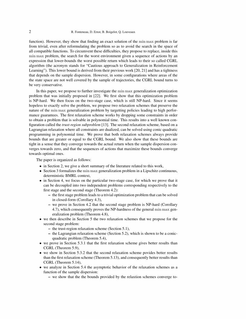
Min Max Generalization for Two-stage Deterministic Batch Mode RL: Relaxation Schemes 3

General problem

Two-stage problem

1st stage 2nd stage

Closed-form NP-hard

Relaxation schemes for the 2nd stage

decoupled

Trust-regionbetter than [22]

Lagrangian relaxationbetter than Trust-region

thus better than [22]

Convergencewhen the sample

dispersiongoes to 0

NP-hard

FIG. 1.1. Main results of the paper.

wards the actual return when the sample dispersion decreases towards zero(Theorem 5.17),

– we show that the sequences of actions maximizing such bounds converge to-wards optimal sequences of actions when the sample dispersion decreases to-wards zero (Theorem 5.20),

• Section 6 illustrates the relaxation schemes on an academic benchmark,• Section 7 concludes.

We provide in Figure 1.1 an illustration of the roadmap of the main results of this paper.

2. Related Work. Several works have already been built upon min max paradigms forcomputing policies in a RL setting. In stochastic frameworks, min max approaches are oftensuccessful for deriving robust solutions with respect to uncertainties in the (parametric) repre-sentation of the probability distributions associated with the environment [16]. In the contextwhere several agents interact with each other in the same environment, min max approachesappear to be efficient strategies for designing policies that maximize one agent’s reward giventhe worst adversarial behavior of the other agents. [29, 43]. They have also received someattention for solving partially observable Markov decision processes [30, 27].

The min max approach towards generalization, originally introduced in [22], implicitlyrelies on a methodology for computing lower bounds on the worst possible return (consid-ering any compatible environment) in a deterministic setting with a mostly unknown actualenvironment. In this respect, it is related to other approaches that aim at computing perfor-mance guarantees on the returns of inferred policies [33, 41, 39].

Other fields of research have proposed min max-type strategies for computing controlpolicies. This includes Robust Control theory [24] with H∞ methods [2], but also ModelPredictive Control (MPC) theory - where usually the environment is supposed to be fullyknown [12, 18] - for which min max approaches have been used to determine an optimalsequence of actions with respect to the “worst case” disturbance sequence occurring [44, 4].Finally, there is a broad stream of works in the field of Stochastic Programming [7] that


have addressed the problem of safely planning under uncertainties, mainly known as “robuststochastic programming” or “risk-averse stochastic programming” [15, 45, 46, 36]. In thisfield, the two-stage case has also been particularly well-studied [23, 14].

3. Problem Formalization. We first formalize the BMRL setting in Section 3.1, andwe state the min max generalization problem in Section 3.2.

3.1. Batch Mode Reinforcement Learning. We consider a deterministic discrete-timesystem whose dynamics over T stages is described by a time-invariant equation

xt+1 = f (xt, ut) t = 0, . . . , T − 1,

where for all t, the state xt is an element of the state space X ⊂ Rd where Rd denotesthe d−dimensional Euclidean space and ut is an element of the finite (discrete) action spaceU =

{u(1), . . . , u(m)

}that we abusively identify with {1, . . . ,m}. T ∈ N \ {0} is referred

to as the (finite) optimization horizon. An instantaneous reward

rt = ρ (xt, ut) ∈ R

is associated with the action ut taken while being in state xt. For a given initial state x0 ∈ Xand for every sequence of actions (u0, . . . , uT−1) ∈ UT , the cumulated reward over T stages(also named T−stage return) is defined as follows:

DEFINITION 3.1 (T−stage Return).

∀ (u0, . . . , uT−1) ∈ UT , J(u0,...,uT−1)T ,

T−1∑t=0

ρ (xt, ut) ,

where

xt+1 = f (xt, ut) , ∀t ∈ {0, . . . , T − 1} .

An optimal sequence of actions is a sequence that leads to the maximization of the T−stagereturn:

DEFINITION 3.2 (Optimal T−stage Return).

J∗T , max(u0,...,uT−1)∈UT

J(u0,...,uT−1)T .

We further make the following assumptions that characterize the batch mode setting:1. The system dynamics f and the reward function ρ are unknown;2. For each action u ∈ U , a set of n(u) ∈ N one-step system transitions

F (u) ={(x(u),k, r(u),k, y(u),k

)}n(u)

k=1

is known where each one-step transition is such that:

y(u),k = f(x(u),k, u

)and r(u),k = ρ

(x(u),k, u

).

3. We assume that every set F (u) contains at least one element:

∀u ∈ U , n(u) > 0 .


In the following, we denote by F the collection of all system transitions:

F = F (1) ∪ . . . ∪ F (m)

Under those assumptions, batch mode reinforcement learning (BMRL) techniques proposeto infer from the sample of one-step system transitions F a high-performance sequence ofactions, i.e. a sequence of actions

(u∗0, . . . , u

∗T−1

)∈ UT such that J

(u∗0 ,...,u∗T−1)

T is as closeas possible to J∗T .

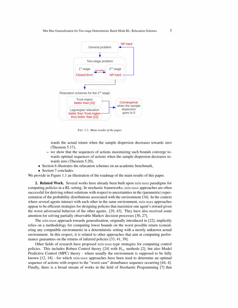
3.2. Min max Generalization under Lipschitz Continuity Assumptions. In this sec-tion, we state the min max generalization problem that we study in this paper. The formal-ization was originally proposed in [22].

We first assume that the system dynamics f and the reward function ρ are assumed to beLipschitz continuous. There exist finite constants Lf , Lρ ∈ R such that:

∀(x, x′) ∈ X 2,∀u ∈ U , ‖f (x, u)− f (x′, u)‖ ≤ Lf ‖x− x′‖ ,|ρ (x, u)− ρ (x′, u)| ≤ Lρ ‖x− x′‖ ,

where ‖.‖ denotes the Euclidean norm over the space X . We also assume that two constantsLf and Lρ satisfying the above-written inequalities are known.

For a given sequence of actions, one can define the worst possible return that can be ob-tained by any system whose dynamics f ′ and ρ′ would satisfy the Lipschitz inequalities andthat would coincide with the values of the functions f and ρ given by the sample of systemtransitions F . As shown in [22], this worst possible return can be computed by solving afinite-dimensional optimization problem over X T−1 × RT . Intuitively, solving such an op-timization problem amounts in determining a most pessimistic trajectory of the system thatis still compliant with the sample of data and the Lipschitz continuity assumptions. Morespecifically, for a given sequence of actions (u0, . . . , uT−1) ∈ UT , some given constants Lfand Lρ, a given initial state x0 ∈ X and a given sample of transitions F , this optimizationproblem writes:

(PT (F , Lf , Lρ, x0, u0, . . . , uT−1)) :

minr0 . . . rT−1 ∈ Rx0 . . . xT−1 ∈ X

T−1∑t=0

rt,

subject to∣∣∣rt − r(ut),kt∣∣∣2 ≤ L2ρ

∥∥∥xt − x(ut),kt∥∥∥2 ,∀(t, kt) ∈ {0, . . . , T − 1} ×

{1, . . . , n(ut)

},∥∥∥xt+1 − y(ut),kt

∥∥∥2 ≤ L2f

∥∥∥xt − x(ut),kt∥∥∥2,∀(t, kt) ∈ {0, . . . , T − 1} ×

{1, . . . , n(ut)

},

|rt − rt′ |2 ≤ L2ρ ‖xt − xt′‖2 ,∀t, t′ ∈ {0, . . . , T − 1|ut = ut′} ,

‖xt+1 − xt′+1‖2 ≤ L2f ‖xt − xt′‖2 ,∀t, t′ ∈ {0, . . . , T − 2|ut = ut′} ,

x0 = x0 .

Note that, throughout the paper, optimization variables will be written in bold.The min max approach to generalization aims at identifying which sequence of actions

maximizes its worst possible return, that is which sequence of actions leads to the highestvalue of (PT (F , Lf , Lρ, x0, u0, . . . , uT−1)).


We focus in this paper on the design of resolution schemes for solving the program(PT (F , Lf , Lρ, x0, u0, . . . , uT−1)). These schemes can afterwards be used for solving themin max problem through exhaustive search over the set of all sequences of actions.

Later in this paper, we will also analyze the computational complexity of this min maxgeneralization problem. When carrying out this analysis, we will assume that all the data ofthe problem (i.e., T,F , Lf , Lρ, x0, u0, . . . , uT−1) are given in the form of rational numbers.

4. The Two-stage Case. In this section, we restrict ourselves to the case where thetime horizon contains only two steps, i.e. T = 2, which is an important particular caseof(PT (F , Lf , Lρ, x0, u0, . . . , uT−1)

). Many works in optimal sequential decision making

have considered the two-stage case [23, 14], which relates to many applications, such as forinstance medical applications where one wants to infer “safe” clinical decision rules frombatch collections of clinical data [1, 31, 32, 49].

In Section 4.1, we show that this problem can be decoupled into two subproblems. Whilethe first subproblem is straightforward to solve, we prove in Section 4.2 that the second oneis NP-hard, which proves that the two-stage problem as well as the generalized T−stageproblem (PT (F , Lf , Lρ, x0, u0, . . . , uT−1)) are also NP-hard.

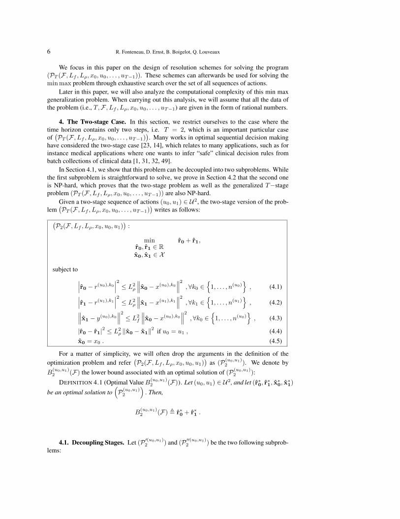
Given a two-stage sequence of actions (u0, u1) ∈ U2, the two-stage version of the prob-lem

(PT (F , Lf , Lρ, x0, u0, . . . , uT−1)

)writes as follows:(

P2(F , Lf , Lρ, x0, u0, u1))

:

minr0, r1 ∈ Rx0, x1 ∈ X

r0 + r1,

subject to∣∣∣r0 − r(u0),k0∣∣∣2 ≤ L2

ρ

∥∥∥x0 − x(u0),k0∥∥∥2 ,∀k0 ∈ {1, . . . , n(u0)

}, (4.1)∣∣∣r1 − r(u1),k1

∣∣∣2 ≤ L2ρ

∥∥∥x1 − x(u1),k1∥∥∥2 ,∀k1 ∈ {1, . . . , n(u1)

}, (4.2)∥∥∥x1 − y(u0),k0

∥∥∥2 ≤ L2f

∥∥∥x0 − x(u0),k0∥∥∥2 ,∀k0 ∈ {1, . . . , n(u0)

}, (4.3)

|r0 − r1|2 ≤ L2ρ ‖x0 − x1‖2 if u0 = u1 , (4.4)

x0 = x0 . (4.5)

For a matter of simplicity, we will often drop the arguments in the definition of theoptimization problem and refer

(P2(F , Lf , Lρ, x0, u0, u1)

)as (P(u0,u1)

2 ). We denote byB

(u0,u1)2 (F) the lower bound associated with an optimal solution of (P(u0,u1)

2 ):

DEFINITION 4.1 (Optimal ValueB(u0,u1)2 (F)). Let (u0, u1) ∈ U2, and let (r∗0, r

∗1, x∗0, x∗1)

be an optimal solution to(P(u0,u1)2

). Then,

B(u0,u1)2 (F) , r∗0 + r∗1 .

4.1. Decoupling Stages. Let (P ′(u0,u1)2 ) and (P ′′(u0,u1)

2 ) be the two following subprob-lems:

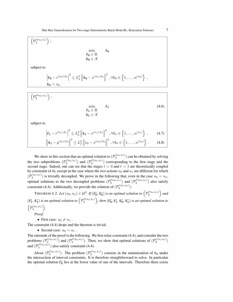
Min Max Generalization for Two-stage Deterministic Batch Mode RL: Relaxation Schemes 7(P ′(u0,u1)2

):

minr0 ∈ Rx0 ∈ X

r0

subject to ∣∣∣r0 − r(u0),k0∣∣∣2 ≤ L2

ρ

∥∥∥x0 − x(u0),k0∥∥∥2 ,∀k0 ∈ {1, . . . , n(u0)

},

x0 = x0 .

(P ′′(u0,u1)2

):

minr1 ∈ Rx1 ∈ X

r1 (4.6)

subject to ∣∣∣r1 − r(u1),k1∣∣∣2 ≤ L2

ρ

∥∥∥x1 − x(u1),k1∥∥∥2 ,∀k1 ∈

{1, . . . , n(u1)

}, (4.7)∥∥∥x1 − y(u0),k0

∥∥∥2 ≤ L2f

∥∥∥x0 − x(u0),k0∥∥∥2 ,∀k0 ∈ {1, . . . , n(u0)

}. (4.8)

We show in this section that an optimal solution to (P(u0,u1)2 ) can be obtained by solving

the two subproblems (P ′(u0,u1)2 ) and (P ′′(u0,u1)

2 ) corresponding to the first stage and thesecond stage. Indeed, one can see that the stages t = 0 and t = 1 are theoretically coupledby constraint (4.4), except in the case where the two actions u0 and u1 are different for which(P(u0,u1)

2 ) is trivially decoupled. We prove in the following that, even in the case u0 = u1,optimal solutions to the two decoupled problems (P ′(u0,u1)

2 ) and (P ′′(u0,u1)2 ) also satisfy

constraint (4.4). Additionally, we provide the solution of (P ′(u0,u1)2 ).

THEOREM 4.2. Let (u0, u1) ∈ U2. If (r∗0, x∗0) is an optimal solution to

(P ′(u0,u1)2

)and

(r∗1, x∗1) is an optimal solution to

(P ′′(u0,u1)2

), then (r∗0, r

∗1, x∗0, x∗1) is an optimal solution to(

P(u0,u1)2

).

Proof.• First case: u0 6= u1 .

The constraint (4.4) drops and the theorem is trivial.• Second case: u0 = u1 .

The rationale of the proof is the following. We first relax constraint (4.4), and consider the twoproblems (P ′(u0,u1)

2 ) and (P ′′(u0,u1)2 ). Then, we show that optimal solutions of (P ′(u0,u1)

2 )

and (P ′′(u0,u1)2 ) also satisfy constraint (4.4).

About (P ′(u0,u1)2 ). The problem (P ′(u0,u1)

2 ) consists in the minimization of r0 underthe intersection of interval constraints. It is therefore straightforward to solve. In particularthe optimal solution r∗0 lies at the lower value of one of the intervals. Therefore there exists

8 R. Fonteneau, D. Ernst, B. Boigelot, Q. Louveaux(x(u0),k

∗0 , r(u0),k

∗0 , y(u0),k

∗0

)∈ F (u0) such that

r∗0 = r(u0),k∗0 − Lρ

∥∥∥x0 − x(u0),k∗0

∥∥∥ . (4.9)

Furthermore r∗0 must belong to all intervals. We therefore have that

r∗0 ≥ r(u0),k0 − Lρ∥∥∥x0 − x(u0),k0

∥∥∥ , ∀k0 ∈{

1, . . . , n(u0)}. (4.10)

In other words,

r∗0 = maxk0∈{1,...,n(u0)}

r(u0),k0 − Lρ∥∥∥x0 − x(u0),k0

∥∥∥ .About (P ′′(u0,u1)

2 ). Again we observe that it is the minimization of r1 under the inter-section of interval constraints as well. The sizes of the intervals are however not fixed butdetermined by the variable x1. If we denote the optimal solution of (P ′′(u0,u1)

2 ) by r∗1 andx∗1, we know that r∗1 also lies at the lower value of one of the intervals. Hence there exists(x(u),k

∗1 , r(u),k

∗1 , y(u),k

∗1

)∈ F (u) such that

r∗1 = r(u),k∗1 − Lρ

∥∥∥x∗1 − x(u),k∗1∥∥∥ . (4.11)

Furthermore r∗1 must belong to all intervals. We therefore have that

r∗1 ≥ r(u),k1 − Lρ∥∥∥x∗1 − x(u),k1∥∥∥ , ∀k1 ∈

{1, . . . , n(u)

}. (4.12)

We now discuss two cases depending on the sign of r∗0 − r∗1.

− If r∗0 − r∗1 ≥ 0Using (4.9) and (4.12) with index k∗0 , we have

r∗0 − r∗1 ≤ Lρ(∥∥∥x∗1 − x(u),k∗0∥∥∥− ∥∥∥x0 − x(u),k∗0∥∥∥) (4.13)

Since r∗0 − r∗1 ≥ 0, we therefore have

|r∗0 − r∗1| ≤ Lρ(∥∥∥x∗1 − x(u),k∗0∥∥∥− ∥∥∥x0 − x(u),k∗0∥∥∥) . (4.14)

Using the triangle inequality we can write∥∥∥x∗1 − x(u),k∗0∥∥∥ ≤ ‖x∗1 − x0‖+∥∥∥x0 − x(u),k∗0∥∥∥ . (4.15)

Replacing (4.15) in (4.14) we obtain

|r∗1 − r∗0| ≤ Lρ ‖x∗1 − x0‖

which shows that r∗0 and r∗1 satisfy constraint (4.4).

− If r∗0 − r∗1 < 0Using (4.11) and (4.10) with index k∗1 , we have

r∗1 − r∗0 ≤ Lρ(∥∥∥x0 − x(u),k∗1∥∥∥− ∥∥∥x∗1 − x(u),k∗1∥∥∥)


and since r∗0 − r∗1 < 0,

|r∗1 − r∗0| ≤ Lρ(∥∥∥x0 − x(u),k∗1∥∥∥− ∥∥∥x∗1 − x(u),k∗1∥∥∥) . (4.16)

Using the triangle inequality we can write∥∥∥x0 − x(u),k∗1∥∥∥ ≤ ‖x0 − x∗1‖+∥∥∥x∗1 − x(u),k∗1∥∥∥ . (4.17)

Replacing (4.17) in (4.16) yields

|r∗1 − r∗0| ≤ Lρ ‖x0 − x∗1‖ ,

which again shows that r∗0 and r∗1 satisfy constraint (4.4).In both cases r∗0− r∗1 ≥ 0 and r∗0− r∗1 < 0, we have shown that constraint (4.4) is satisfied.

In the following of the paper, we focus on the two subproblems (P ′(u0,u1)2 ) and (P ′′(u0,u1)

2 )

rather than on (P(u0,u1)2 ). From the proof of Theorem 4.2 given above, we can directly obtain

the solution of (P ′(u0,u1)2 ):

COROLLARY 4.3. The solution of the problem (P ′(u0,u1)2 ) is

r∗0 = maxk0∈{1,...,n(u0)}

r(u0),k0 − Lρ∥∥∥x0 − x(u0),k0

∥∥∥ .4.2. Complexity of (P ′′(u0,u1)

2 ). The problem (P ′(u0,u1)2 ) being solved, we now fo-

cus in this section on the resolution of (P ′′(u0,u1)2 ). In particular, we show that it is NP-

hard, even in the particular case where there is only one element in the sample F (u1) ={(x(u1),1, r(u1),1, y(u1),1

)}. In this particular case, the problem (P ′′(u0,u1)

2 ) amounts to max-imizing of the distance

∥∥x1 − x(u1),1∥∥ under an intersection of balls as we show in the fol-

lowing lemma.LEMMA 4.4. If the cardinality of F (u1) is equal to 1:

F (u1) ={(x(u1),1, r(u1),1, y(u1),1

)},

then the optimal solution to(P ′′(u0,u1)2

)satisfies

r∗1 = r(u1),1 − Lρ∥∥∥x∗1 − x(u1),1

∥∥∥where x∗1 maximizes

∥∥x1 − x(u1),1∥∥ subject to∥∥∥x1 − y(u0),k0

∥∥∥2 ≤ L2f

∥∥∥x0 − x(u0),k0∥∥∥2 , ∀

(x(u0),k0 , r(u0),k0 , y(u0),k0

)∈ F (u0) .

Proof. The unique constraint concerning r1 is an interval. Therefore r∗1 takes the value ofthe lower bound of the interval. In order to obtain the lowest such value, the right-hand-sideof (4.7) must be maximized under the other constraints.

Note that if the cardinality n(u0) ofF (u0) is also equal to 1, then (P(u0,u1)2 ) can be solved

exactly, as we will later show in Corollary 5.3. But, in the general case where n(u0) > 1, this


problem of maximizing a distance under a set of ball-constraints is NP-hard as we now prove.To do it, we introduce the MNBC (for “Max Norm with Ball Constraints”) decision problem:

DEFINITION 4.5 (MNBC Decision Problem). Given x(0) ∈ Qd, yi ∈ Qd, γi ∈ Q, i ∈{1, . . . , I}, C ∈ Q, the MNBC problem is to determine whether there exists x ∈ Rd such that∥∥∥x− x(0)∥∥∥2 ≥ Cand ∥∥x− yi∥∥2 ≤ γi , ∀i ∈ {1, . . . , I} .

LEMMA 4.6. MNBC is NP-hard.Proof. To prove it, we will do a reduction from the {0, 1}−programming feasibility

problem [40]. More precisely, we consider in this proof the {0, 2}−programming feasibilityproblem, which is equivalent. The problem is, given p ∈ N, A ∈ Zp×d, b ∈ Zp to findwhether there exists x ∈ {0, 2}d that satisfies Ax ≤ b. This problem is known to be NP-hardand we now provide a polynomial reduction to MNBC.

The dimension d is kept the same in both problems. The first step is to define a set ofconstraints for MNBC such that the only potential feasible solutions are exactly x ∈ {0, 2}d.We define

x(0) , (1, . . . , 1)

and

C , d.

For i = 1, . . . , d, we define

y2i ,(y2i1 , . . . , y

2id

)with y2ii , 0 and y2ij , 1 for all j 6= i and γi , d+ 3.Similarly for i = 1, . . . , d, we define

y2i+1 , (y2i+11 , . . . , y2i+1

d )

with y2i+1i , 2 and y2i+1

j , 1 for all j 6= i and γi , d+ 3.

Claim{x ∈ Rd | ‖x− x(0)‖2 ≥ d

}∩

(2d+1⋂i=2

{x ∈ Rd | ‖x− yi‖2 ≤ γi

})= {0, 2}d

It is readily verified that any x ∈ {0, 2}d belongs to the 2d+ 1 above sets.Consider x ∈ Rd that belongs to the 2d + 1 above sets. Consider an index k ∈ {1, . . . , d}.Using the constraints defining the sets, we can in particular write

‖(x1, . . . , xk−1, xk, xk+1, . . . , xd)− (1, . . . , 1)‖2 ≥ d‖(x1, . . . , xk−1, xk, xk+1, . . . , xd)− (1, . . . , 1, 0, 1, . . . , 1)‖2 ≤ d+ 3

‖(x1, . . . , xk−1, xk, xk+1, . . . , xd)− (1, . . . , 1, 2, 1, . . . , 1)‖2 ≤ d+ 3


that we can write algebraically∑j 6=k

(xj − 1)2 + (xk − 1)2 ≥ d (4.18)

∑j 6=k

(xj − 1)2 + x2k ≤ d+ 3 (4.19)

∑j 6=k

(xj − 1)2 + (xk − 2)2 ≤ d+ 3. (4.20)

By computing (4.19)− (4.18) and (4.20)− (4.18), we obtain xk ≤ 2 and xk ≥ 0 respectively.This implies that

d∑k=1

(xk − 1)2 ≤ d

and the equality is obtained if and only if we have that xk ∈ {0, 2} for all k which proves theclaim.

It remains to prove that we can encode any linear inequality through a ball constraint. Con-sider an inequality of the type

∑dj=1 ajxj ≤ b. We assume that a 6= 0 and that b is even and

therefore that there exists no x ∈ {0, 2}d such that aTx = b+ 1. We want to show that thereexists y ∈ Qd and γ ∈ Q such that{

x ∈ {0, 2}d | aTx ≤ b}

={x ∈ {0, 2}d | ‖x− y‖2 ≤ γ

}. (4.21)

Let y ∈ Rd be the intersection point of the hyperplane aTx = b+1 and the line (1 · · · 1)T +λ(a1 · · · ad)T , λ ∈ R. Let r be defined as follows:

r =

d2√√√√ d∑

j=1

a2j + 1

.We claim that choosing γ , r2 and y , y − ra allows us to obtain (4.21). To prove it,we need to show that x ∈ {0, 2}d belongs to the ball if and only if it satisfies the constraintaTx ≤ b. Let x ∈ {0, 2}d. There are two cases to consider:

• Suppose first that aT x ≥ b+ 2.Since y is the closest point to y that satisfies aT y = b + 1, it also implies that any point xsuch that aTx > b+ 1 is such that ‖x− y‖2 > r2 proving that:

x /∈{x ∈ Rd | ‖x− y‖2 ≤ r2

}.

• Suppose now that aT x ≤ b and in particular that aT x = b − k with k ∈ N (seeFigure 4.1).

Let y ∈ Rd be the intersection point of the hyperplane aTx = b−k and the line (1 · · · 1)T +λ(a1 · · · ad)T , λ ∈ R. Since

((1 · · · 1)T , y, x

)form a right triangle with the right angle in y

and since ‖(1 · · · 1)T − x‖2 ≤ d, we have

‖y − x‖2 ≤ d. (4.22)

By definition of y, we have:

‖y − y‖ = r ,


FIG. 4.1. The case when aT x ≤ b.

and by definition of y and y, we have:

‖y − y‖ ≥ 1√∑dj=1 a

2j

.

Since y, y and y belong to the same line, we have

‖y − y‖ ≤ r − 1√∑dj=1 a

2j

. (4.23)

As (y, y, x) form a right triangle with the right angle in y, we have that

‖x− y‖2 = ‖y − y‖2 + ‖x− y‖2

≤

r − 1√∑dj=1 a

2j

2

+ d using (4.22), (4.23)

= r2 − 2r√∑dj=1 a

2j

+1∑dj=1 a

2j

+ d.

Since by definition, r ≥ d2

√∑dj=1 a

2j + 1, we can write

‖x− y‖2 ≤ r2 − d− 2√∑dj=1 a

2j

+1∑dj=1 a

2j

+ d

= r2 − 1∑dj=1 a

2j

≤ r2.

This proves that the chosen ball{x ∈ Rd | ‖x− y‖2 ≤ r2

}includes the same points from

{0, 2}d as the linear inequality aTx ≤ b.


The encoding length of all data is furthermore polynomial in the encoding length of theinitial inequalities. This completes the reduction and proves the NP-hardness of MNBC.

Note that the NP-hardness of MNBC is independent from the choice of the norm usedover the state space X . The two results follow:

COROLLARY 4.7.(P ′′(u0,u1)2

)is NP-hard.

THEOREM 4.8. The two-stage problem(P(u0,u1)2

)and the generalized T−stage prob-

lem (PT (F , Lf , Lρ, x0, u0, . . . , uT−1)) are NP-hard.

5. Relaxation Schemes for the Two-stage Case. The two-stage case with only oneelement in the set F (u1) was proven to be NP-hard in the previous section (except if the car-dinality of n(u0) of F (u0) is also equal to 1, in this case (P(u0,u1)

2 ) is solvable in polynomialtime as we will see later in Corollary 5.3). It is therefore unlikely that one can design analgorithm that optimally solves the general two-stage case in polynomial time (unless P =NP). The aim of the min max optimization problem is to obtain a sequence of actions thathas a performance guarantee. Therefore solving the optimization problem approximately orobtaining an upper bound would be irrelevant. Instead we want to propose some relaxationschemes that are computationally more tractable, and that are still leading to lower bounds onthe actual return of the sequences of actions.

The first relaxation scheme works by dropping some constraints in order to obtain aproblem that is solvable in polynomial time. We show that this scheme provides bounds thatare greater or equal to the CGRL bound introduced in [22]. The second relaxation scheme isbased on a Lagrangian relaxation where all constraints are dualized. Solving the Lagrangiandual is shown to be a conic-quadratic problem that can be solved in polynomial time usinginterior-point methods. We also prove that this relaxation scheme always gives better boundsthan the first relaxation scheme mentioned above, and consequently, better bounds than [22].We also prove that the bounds computed from these relaxation schemes converge towards theactual return of the sequence (u0, u1) when the sample dispersion converges towards zero.As a consequence, the sequences of actions that maximize those bounds also become optimalwhen the dispersion decreases towards zero.

From the previous section, we know that the two-stage problem (P(u0,u1)2 ) can be de-

coupled into two subproblems (P ′(u0,u1)2 ) and (P ′′(u0,u1)

2 ), where (P ′(u0,u1)2 ) can be solved

straightforwardly (cf Theorem 4.2). We therefore only focus on relaxing the subproblem(P ′′(u0,u1)

2 ):

(P ′′(u0,u1)2

): minr1 ∈ Rx1 ∈ X

r1

subject to∣∣∣r1 − r(u1),k1

∣∣∣2 ≤ L2ρ

∥∥∥x1 − x(u1),k1∥∥∥2 ∀k1 ∈ {1, . . . , n(u1)

}(5.1)∥∥∥x1 − y(u0),k0

∥∥∥2 ≤ L2f

∥∥∥x0 − x(u0),k0∥∥∥2 ∀k0 ∈

{1, . . . , n(u0)

}(5.2)

5.1. The Trust-region Subproblem Relaxation Scheme. An easy way to obtain a re-laxation from an optimization problem is to drop some constraints. We therefore suggest todrop all constraints (5.1) but one, indexed by k1. Similarly we drop all constraints (5.2) butone, indexed by k0. The following problem is therefore a relaxation of (P ′′(u0,u1)

2 ):

14 R. Fonteneau, D. Ernst, B. Boigelot, Q. Louveaux(P ′′(u0,u1)TR (k0, k1)

):

minr1 ∈ Rx1 ∈ X

r1

subject to ∣∣∣r1 − r(u1),k1∣∣∣2 ≤ L2

ρ

∥∥∥x1 − x(u1),k1∥∥∥2 , (5.3)∥∥∥x1 − y(u0),k0

∥∥∥2 ≤ L2f

∥∥∥x0 − x(u0),k0∥∥∥2 . (5.4)

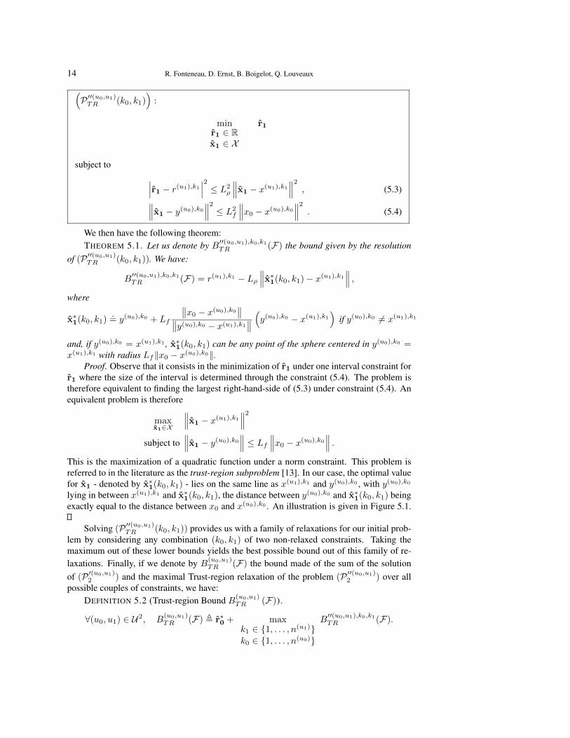
We then have the following theorem:THEOREM 5.1. Let us denote by B′′(u0,u1),k0,k1

TR (F) the bound given by the resolutionof (P ′′(u0,u1)

TR (k0, k1)). We have:

B′′(u0,u1),k0,k1TR (F) = r(u1),k1 − Lρ

∥∥∥x∗1(k0, k1)− x(u1),k1∥∥∥ ,

where

x∗1(k0, k1).= y(u0),k0 + Lf

∥∥x0 − x(u0),k0∥∥∥∥y(u0),k0 − x(u1),k1∥∥ (y(u0),k0 − x(u1),k1

)if y(u0),k0 6= x(u1),k1

and, if y(u0),k0 = x(u1),k1 , x∗1(k0, k1) can be any point of the sphere centered in y(u0),k0 =x(u1),k1 with radius Lf‖x0 − x(u0),k0‖.

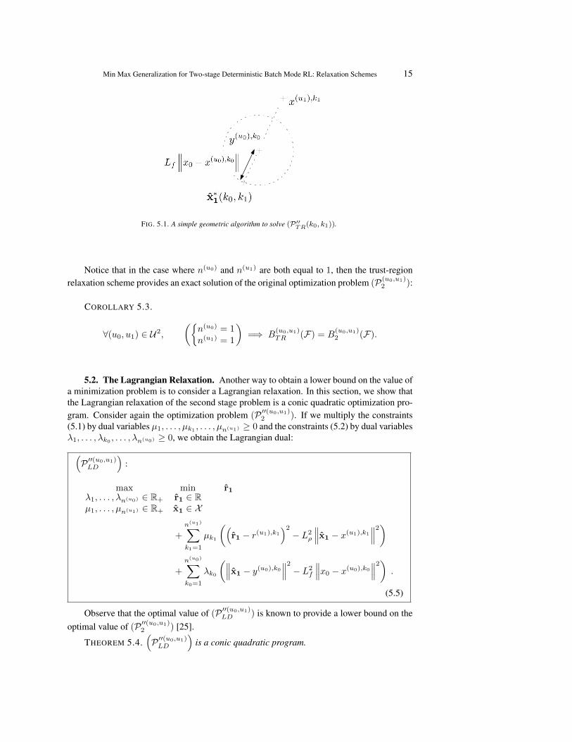
Proof. Observe that it consists in the minimization of r1 under one interval constraint forr1 where the size of the interval is determined through the constraint (5.4). The problem istherefore equivalent to finding the largest right-hand-side of (5.3) under constraint (5.4). Anequivalent problem is therefore

maxx1∈X

∥∥∥x1 − x(u1),k1∥∥∥2

subject to∥∥∥x1 − y(u0),k0

∥∥∥ ≤ Lf ∥∥∥x0 − x(u0),k0∥∥∥ .

This is the maximization of a quadratic function under a norm constraint. This problem isreferred to in the literature as the trust-region subproblem [13]. In our case, the optimal valuefor x1 - denoted by x∗1(k0, k1) - lies on the same line as x(u1),k1 and y(u0),k0 , with y(u0),k0

lying in between x(u1),k1 and x∗1(k0, k1), the distance between y(u0),k0 and x∗1(k0, k1) beingexactly equal to the distance between x0 and x(u0),k0 . An illustration is given in Figure 5.1.

Solving (P ′′(u0,u1)TR (k0, k1)) provides us with a family of relaxations for our initial prob-

lem by considering any combination (k0, k1) of two non-relaxed constraints. Taking themaximum out of these lower bounds yields the best possible bound out of this family of re-laxations. Finally, if we denote by B(u0,u1)

TR (F) the bound made of the sum of the solutionof (P ′(u0,u1)

2 ) and the maximal Trust-region relaxation of the problem (P ′′(u0,u1)2 ) over all

possible couples of constraints, we have:DEFINITION 5.2 (Trust-region Bound B(u0,u1)

TR (F)).

∀(u0, u1) ∈ U2, B(u0,u1)TR (F) , r∗0 + max

k1 ∈ {1, . . . , n(u1)}k0 ∈ {1, . . . , n(u0)}

B′′(u0,u1),k0,k1TR (F).


FIG. 5.1. A simple geometric algorithm to solve (P ′′TR(k0, k1)).

Notice that in the case where n(u0) and n(u1) are both equal to 1, then the trust-regionrelaxation scheme provides an exact solution of the original optimization problem (P(u0,u1)

2 ):

COROLLARY 5.3.

∀(u0, u1) ∈ U2,

({n(u0) = 1n(u1) = 1

)=⇒ B

(u0,u1)TR (F) = B

(u0,u1)2 (F).

5.2. The Lagrangian Relaxation. Another way to obtain a lower bound on the value ofa minimization problem is to consider a Lagrangian relaxation. In this section, we show thatthe Lagrangian relaxation of the second stage problem is a conic quadratic optimization pro-gram. Consider again the optimization problem (P ′′(u0,u1)

2 ). If we multiply the constraints(5.1) by dual variables µ1, . . . , µk1 , . . . , µn(u1) ≥ 0 and the constraints (5.2) by dual variablesλ1, . . . , λk0 , . . . , λn(u0) ≥ 0, we obtain the Lagrangian dual:(P ′′(u0,u1)LD

):

maxλ1, . . . , λn(u0) ∈ R+

µ1, . . . , µn(u1) ∈ R+

minr1 ∈ Rx1 ∈ X

r1

+

n(u1)∑k1=1

µk1

((r1 − r(u1),k1

)2− L2

ρ

∥∥∥x1 − x(u1),k1∥∥∥2)

+

n(u0)∑k0=1

λk0

(∥∥∥x1 − y(u0),k0∥∥∥2 − L2

f

∥∥∥x0 − x(u0),k0∥∥∥2) .

(5.5)

Observe that the optimal value of (P ′′(u0,u1)LD ) is known to provide a lower bound on the

optimal value of (P ′′(u0,u1)2 ) [25].

THEOREM 5.4.(P ′′(u0,u1)LD

)is a conic quadratic program.


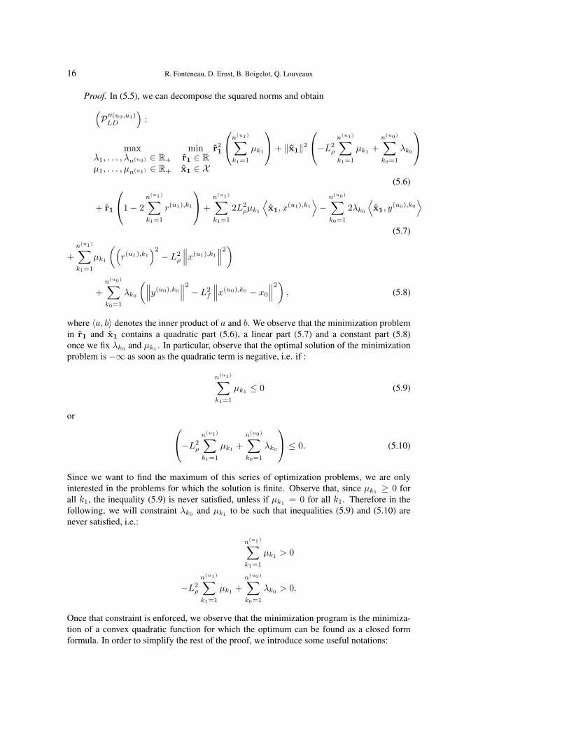
Proof. In (5.5), we can decompose the squared norms and obtain(P ′′(u0,u1)LD

):

maxλ1, . . . , λn(u0) ∈ R+

µ1, . . . , µn(u1) ∈ R+

minr1 ∈ Rx1 ∈ X

r21

n(u1)∑k1=1

µk1

+ ‖x1‖2−L2

ρ

n(u1)∑k1=1

µk1 +

n(u0)∑k0=1

λk0

(5.6)

+ r1

1− 2

n(u1)∑k1=1

r(u1),k1

+

n(u1)∑k1=1

2L2ρµk1

⟨x1, x

(u1),k1⟩−n(u0)∑k0=1

2λk0

⟨x1, y

(u0),k0⟩

(5.7)

+

n(u1)∑k1=1

µk1

((r(u1),k1

)2− L2

ρ

∥∥∥x(u1),k1∥∥∥2)

+

n(u0)∑k0=1

λk0

(∥∥∥y(u0),k0∥∥∥2 − L2

f

∥∥∥x(u0),k0 − x0∥∥∥2) , (5.8)

where 〈a, b〉 denotes the inner product of a and b. We observe that the minimization problemin r1 and x1 contains a quadratic part (5.6), a linear part (5.7) and a constant part (5.8)once we fix λk0 and µk1 . In particular, observe that the optimal solution of the minimizationproblem is −∞ as soon as the quadratic term is negative, i.e. if :

n(u1)∑k1=1

µk1 ≤ 0 (5.9)

or −L2ρ

n(u1)∑k1=1

µk1 +

n(u0)∑k0=1

λk0

≤ 0. (5.10)

Since we want to find the maximum of this series of optimization problems, we are onlyinterested in the problems for which the solution is finite. Observe that, since µk1 ≥ 0 forall k1, the inequality (5.9) is never satisfied, unless if µk1 = 0 for all k1. Therefore in thefollowing, we will constraint λk0 and µk1 to be such that inequalities (5.9) and (5.10) arenever satisfied, i.e.:

n(u1)∑k1=1

µk1 > 0

−L2ρ

n(u1)∑k1=1

µk1 +

n(u0)∑k0=1

λk0 > 0.

Once that constraint is enforced, we observe that the minimization program is the minimiza-tion of a convex quadratic function for which the optimum can be found as a closed formformula. In order to simplify the rest of the proof, we introduce some useful notations:


DEFINITION 5.5 (Additional Notations).

M ,n(u1)∑k1=1

µk1 , L ,n(u0)∑k0=1

λk0 ,

X ,(x(u1),1 · · ·x(u1),n

(u1))

, Y ,(y(u0),1 · · · y(u0),n

(u0)),

λ ,(λ1 . . . λn(u0)

)T, µ ,

(µ1 . . . µn(u1)

)T, r ,

(r(1) . . . r(n

(u1)))T

,

∀p ∈ N0, Ip is an identity matrix of size p.

The quadratic form coming from (5.6), (5.7) and (5.8) can be written in the form

zTQz + lT z + c

with

z ,

(x1

r1

)∈ Rd+1, Q ,

( (−ML2

ρ + L)Id

M

), l ,

(2L2

ρXµ− 2Y λ1− 2rTµ

)

and the constant term is given by (5.8). The minimum of a convex quadratic form zTQz +lT z + c is known to take the value − 1

4 lTQ−1l+ c. In our case, the inverse of the matrix Q is

trivial to compute and we obtain finally that (P ′′(u0,u1)LD ) can be written as

(P ′′(u0,u1)LD

): maxλ∈Rn(u0)

+ ,µ∈Rn(u1)

+

−‖L2ρXµ− Y λ‖2

−ML2ρ + L

−(1− 2rTµ

)24M

(5.11)

+

n(u0)∑k0=1

λk0

(∥∥∥y(u0),k0∥∥∥2 − L2

f

∥∥∥x(u0),k0 − x0∥∥∥2)

+

n(u1)∑k1=1

µk1

((r(u1),k1

)2− L2

ρ

∥∥∥x(u1),k1∥∥∥2)

subject to M > 0

L > ML2ρ

The optimization problem (5.11) is in variables λ1, . . . , λn(u0) and µ1, . . . , µn(u1) . Ob-serve that, with our notation, M and L are linear functions of the variables. The objectivefunction contains linear terms in λ1, . . . , λn(u0) and µ1, . . . , µn(u1) as well as a fractional-quadratic function ([5]), i.e. the quotient of a concave quadratic function with a linear func-tion. The constraint is linear. This type of problem is known as a rotated quadratic conicproblem and can be formulated as a conic quadratic optimization problem ([5]) that can besolved in polynomial time using interior point methods [5, 37, 9].


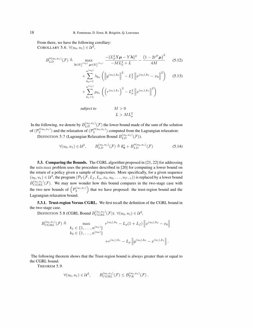
From there, we have the following corollary:COROLLARY 5.6. ∀(u0, u1) ∈ U2,

B′′(u0,u1)LD (F) , max

λ∈Rn(u0)

+ ,µ∈Rn(u1)

+


−ML2ρ + L

−(1− 2rTµ

)24M

(5.12)

+

n(u0)∑k0=1

λk0

(∥∥∥y(u0),k0∥∥∥2 − L2

f

∥∥∥x(u0),k0 − x0∥∥∥2) (5.13)

+

n(u1)∑k1=1

µk1

((r(u1),k1

)2− L2

ρ

∥∥∥x(u1),k1∥∥∥2)

subject to M > 0

L > ML2ρ

In the following, we denote by B(u0,u1)LD (F) the lower bound made of the sum of the solution

of (P ′(u0,u1)2 ) and the relaxation of (P ′′(u0,u1)

2 ) computed from the Lagrangian relaxation:DEFINITION 5.7 (Lagrangian Relaxation Bound B(u0,u1)

LD (F)).

∀(u0, u1) ∈ U2, B(u0,u1)LD (F) , r∗0 +B

′′(u0,u1)LD (F) (5.14)

5.3. Comparing the Bounds. The CGRL algorithm proposed in [21, 22] for addressingthe min max problem uses the procedure described in [20] for computing a lower bound onthe return of a policy given a sample of trajectories. More specifically, for a given sequence(u0, u1) ∈ U2, the program (PT (F , Lf , Lρ, x0, u0, . . . , uT−1)) is replaced by a lower boundB

(u0,u1)CGRL (F). We may now wonder how this bound compares in the two-stage case with

the two new bounds of(P(u0,u1)2

)that we have proposed: the trust-region bound and the

Lagrangian relaxation bound.

5.3.1. Trust-region Versus CGRL. We first recall the definition of the CGRL bound inthe two-stage case.

DEFINITION 5.8 (CGRL Bound B(u0,u1)CGRL (F)). ∀(u0, u1) ∈ U2,

B(u0,u1)CGRL (F) , max

k1 ∈ {1, . . . , n(u1)}k0 ∈ {1, . . . , n(u0)}

r(u0),k0 − Lρ(1 + Lf )∥∥∥x(u0),k0 − x0

∥∥∥+r(u1),k1 − Lρ

∥∥∥y(u0),k0 − x(u1),k1∥∥∥ .

The following theorem shows that the Trust-region bound is always greater than or equal tothe CGRL bound.

THEOREM 5.9.

∀(u0, u1) ∈ U2, B(u0,u1)CGRL (F) ≤ B(u0,u1)

TR (F) .


Proof. Let k∗0 ∈{

1, . . . , n(u0)}

and k∗1 ∈{

1, . . . , n(u1)}

be such that

B(u0,u1)CGRL (F) = r(u0),k

∗0 − Lρ(1 + Lf )

∥∥∥x(u0),k∗0 − x0

∥∥∥+ r(u1),k∗1 − Lρ

∥∥∥y(u0),k∗0 − x(u1),k

∗1

∥∥∥ .Now, let us consider the solution B′′(u0,u1),k

∗0 ,k∗1

TR (F) of the problem (P ′′(u0,u1)TR (k∗0 , k

∗1)), and

let us denote byB(u0,u1),k∗0 ,k∗1 the bound obtained if, in the definition of the value of r∗0 given

in Corollary 4.3, we fix the value of k′0 to k∗0 instead of maximizing over all possible k′0:

B(u0,u1),k∗0 ,k∗1 = r(u0),k

∗0 − Lρ

∥∥∥x0 − x(u0),k∗0

∥∥∥+B′′(u0,u1),k

∗0 ,k∗1

TR (F)

Since r(u0),k∗0 −Lρ

∥∥x0 − x(u0),k∗0

∥∥ is smaller or equal to the solution r∗0 of (P ′(u0,u1)2 ), one

has:

B(u0,u1),k

∗0 ,k∗1

TR (F) ≥ B(u0,u1),k∗0 ,k∗1 . (5.15)

Now, observe that:

B(u0,u1),k∗0 ,k∗1 −B(u0,u1)

CGRL (F) = LρLf

∥∥∥x(u0),k∗0 − x0

∥∥∥+ Lρ

∥∥∥y(u0),k∗0 − x(u1),k

∗1

∥∥∥− Lρ

∥∥∥x∗1(k∗0 , k∗1)− x(u1),k

∗1

∥∥∥ . (5.16)

By construction, x∗1(k∗0 , k∗1) lies on the same line as y(u0),k

∗0 and x(u1),k

∗1 (see Figure 5.1).

Furthermore∥∥∥x∗1(k∗0 , k∗1)− x(u1),k

∗1

∥∥∥ =∥∥∥x∗1(k∗0 , k

∗1)− y(u0),k

∗0

∥∥∥+∥∥∥y(u0),k

∗0 − x(u1),k

∗1

∥∥∥ . (5.17)

Using (5.17) in (5.16) yields

B(u0,u1),k∗0 ,k∗1 −B(u0,u1),k

∗0 ,k∗1

CGRL (F) = LρLf

∥∥∥x(u0),k∗0 − x0

∥∥∥+Lρ

(∥∥∥y(u0),k∗0 − x(u1),k

∗1

∥∥∥− ∥∥∥x∗1(k∗0 , k∗1)− y(u0),k

∗0

∥∥∥− ∥∥∥y(u0),k∗0 − x(u1),k

∗1

∥∥∥)= Lρ

(Lf

∥∥∥x(u0),k∗0 − x0

∥∥∥− ∥∥∥x∗1(k∗0 , k∗1)− y(u0),k

∗0

∥∥∥) . (5.18)

By construction, Equation (5.18) is equal to 0 (see Figure 5.1), which proves the equality ofthe two bounds:

B(u0,u1),k∗0 ,k∗1 = B

(u0,u1)CGRL (F) . (5.19)

The final result is given by combining Equations (5.15) and (5.19).From the proof, one can observe that the gap between the CGRL bound and the Trust-

region bound is only due to the resolution of (P ′(u0,u1)2 ). Note that in the case where k∗0 also

belongs to the set arg maxk0∈{1,...,n(u0)}

r(u0),k0 − Lρ∥∥x(u0),k0 − x0

∥∥, then the bounds are equal.

The two corollaries follow:COROLLARY 5.10. Let (u0, u1) ∈ U2. Let k∗0 ∈

{1, . . . , n(u0)

}and k∗1 ∈

{1, . . . , n(u1)

}be such that:

B(u0,u1)CGRL (F) = r(u0),k

∗0 − Lρ(1 + Lf )

∥∥∥x(u0),k∗0 − x0

∥∥∥+ r(u1),k∗1 − Lρ

∥∥∥y(u0),k∗0 − x(u1),k

∗1

∥∥∥ .


Then,(k∗0 ∈ arg max

k0∈{1,...,n(u0)}r(u0),k0 − Lρ

∥∥∥x(u0),k0 − x0∥∥∥) =⇒ B

(u0,u1)CGRL (F) = B

(u0,u1)TR (F) .

COROLLARY 5.11.

∀(u0, u1) ∈ U2,(n(u0) = 1

)=⇒ B

(u0,u1)CGRL (F) = B

(u0,u1)TR (F) .

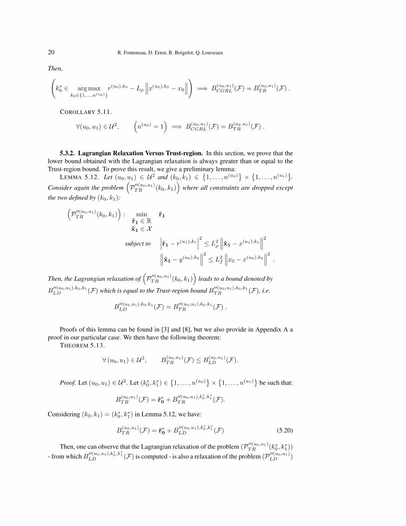
5.3.2. Lagrangian Relaxation Versus Trust-region. In this section, we prove that thelower bound obtained with the Lagrangian relaxation is always greater than or equal to theTrust-region bound. To prove this result, we give a preliminary lemma:

LEMMA 5.12. Let (u0, u1) ∈ U2 and (k0, k1) ∈{

1, . . . , n(u0)}×{

1, . . . , n(u1)}

.

Consider again the problem(P ′′(u0,u1)TR (k0, k1)

)where all constraints are dropped except

the two defined by (k0, k1):(P ′′(u0,u1)TR (k0, k1)

): min

r1 ∈ Rx1 ∈ X

r1

subject to∣∣∣r1 − r(u1),k1

∣∣∣2 ≤ L2ρ

∥∥∥x1 − x(u1),k1∥∥∥2∥∥∥x1 − y(u0),k0

∥∥∥2 ≤ L2f

∥∥∥x0 − x(u0),k0∥∥∥2 .

Then, the Lagrangian relaxation of(P ′′(u0,u1)TR (k0, k1)

)leads to a bound denoted by

B′′(u0,u1),k0,k1LD (F) which is equal to the Trust-region bound B′′(u0,u1),k0,k1

TR (F), i.e.

B′′(u0,u1),k0,k1LD (F) = B

′′(u0,u1),k0,k1TR (F) .

Proofs of this lemma can be found in [3] and [8], but we also provide in Appendix A aproof in our particular case. We then have the following theorem:

THEOREM 5.13.

∀ (u0, u1) ∈ U2, B(u0,u1)TR (F) ≤ B(u0,u1)

LD (F).

Proof. Let (u0, u1) ∈ U2. Let (k∗0 , k∗1) ∈

{1, . . . , n(u0)

}×{

1, . . . , n(u1)}

be such that:

B(u0,u1)TR (F) = r∗0 +B

′′(u0,u1),k∗0 ,k∗1

TR (F).

Considering (k0, k1) = (k∗0 , k∗1) in Lemma 5.12, we have:

B(u0,u1)TR (F) = r∗0 +B

′′(u0,u1),k∗0 ,k∗1

LD (F) (5.20)

Then, one can observe that the Lagrangian relaxation of the problem (P ′′(u0,u1)TR (k∗0 , k

∗1))

- from whichB′′(u0,u1),k∗0 ,k∗1

LD (F) is computed - is also a relaxation of the problem (P ′′(u0,u1)LD )


for which all the dual variables corresponding to constraints that are not related with the sys-tem transitions

(x(u0),k

∗0 , r(u0),k

∗0 , y(u0),k

∗0

)and

(x(u1),k

∗1 , r(u1),k

∗1 , y(u1),k

∗1

)would be forced

to zero, i.e.

B′′(u0,u1),k

∗0 ,k∗1

LD (F) = maxλ∈Rn(u0)

+ ,µ∈Rn(u1)

+


−ML2ρ + L

−(1− 2rTµ

)24M

+

n(u0)∑k0=1

λk0

(∥∥∥y(u0),k0∥∥∥2 − L2

f

∥∥∥x(u0),k0 − x0∥∥∥2)

+

n(u1)∑k1=1

µk1

((r(u1),k1

)2− L2

ρ

∥∥∥x(u1),k1∥∥∥2)

subject to M > 0 ,

L > ML2ρ ,

λk0 = 0 if k0 6= k∗0 ,∀k0 ∈{

1, . . . , n(u0)},

µk1 = 0 if k1 6= k∗1 ,∀k1 ∈{

1, . . . , n(u1)}.

We therefore have:

B′′(u0,u1),k

∗0 ,k∗1

LD (F) ≤ B′′(u0,u1)LD (F) . (5.21)

By definition of the Lagrangian relaxation bound B(u0,u1)LD (F), we have:

B(u0,u1)LD (F) = r∗0 +B

′′(u0,u1)LD (F) (5.22)

Equations (5.20), (5.21) and (5.22) finally give:

B(u0,u1)TR (F ′) = B

(u0,u1)LD (F) .

5.3.3. Bounds Inequalities: Summary. We summarize in the following theorem all theresults that were obtained in the previous sections.

THEOREM 5.14. ∀ (u0, u1) ∈ U2,

B(u0,u1)CGRL (F) ≤ B(u0,u1)

TR (F) ≤ B(u0,u1)LD (F) ≤ B(u0,u1)

2 (F) ≤ J (u0,u1)2 .

Proof. Let (u0, u1) ∈ U2. The inequality

B(u0,u1)CGRL (F) ≤ B(u0,u1)

TR (F) ≤ B(u0,u1)LD (F) (5.23)

is a straightforward consequence of Theorems 5.9 and 5.13. The inequality

B(u0,u1)LD (F) ≤ B(u0,u1)

2 (F) (5.24)

is a property of the Lagrangian relaxation, and the inequality

B(u0,u1)2 (F) ≤ J (u0,u1)

2

is derived from the formalization of the min max generalization problem introduced in [22].


5.4. Convergence Properties. We finally propose to analyze the convergence of thebounds, as well as the sequences of actions that lead to the maximization of the bounds, whenthe sample dispersion decreases towards zero. We assume in this section that the state spaceX is bounded:

∃CX > 0 : ∀(x, x′) ∈ X 2, ‖x− x′‖ ≤ CX .

Let us now introduce the sample dispersion:DEFINITION 5.15 (Sample Dispersion). Since X is bounded, one has:

∃ α > 0 : ∀u ∈ U , supx∈X

mink∈{1,...,n(u)}

∥∥∥x(u),k − x∥∥∥ ≤ α . (5.25)

The smallest α which satisfies equation (5.25) is named the sample dispersion and is denotedby α∗(F). Intuitively, the sample dispersion α∗(F) can be seen as the radius of the largestnon-visited state space area.

5.4.1. Bounds. We analyze in this subsection the tightness of the Trust-region and theLagrangian relaxation lower bounds as a function of the sample dispersion.

LEMMA 5.16.∃ C > 0 : ∀(u0, u1) ∈ U2,∀B(u0,u1)(F) ∈

{B

(u0,u1)CGRL (F), B

(u0,u1)TR (F), B

(u0,u1)LD (F)

},

J(u0,u1)2 −B(u0,u1)(F) ≤ Cα∗(F).

Proof. The proof for the case where B(u0,u1)(F) = B(u0,u1)CGRL (F) is given in [21]. Ac-

cording to Theorem 5.14, one has:

∀ (u0, u1) ∈ U2, B(u0,u1)CGRL (F) ≤ B(u0,u1)

TR (F) ≤ B(u0,u1)LD (F) ≤ J (u0,u1)

2 ,

which ends the proof.We therefore have the following theorem:THEOREM 5.17.

∀(u0, u1) ∈ U2,∀B(u0,u1)(F) ∈{B

(u0,u1)CGRL (F), B

(u0,u1)TR (F), B

(u0,u1)LD (F)

},

limα∗(F)→0

J(u0,u1)2 −B(u0,u1)(F) = 0 .

5.4.2. Bound-optimal Sequences of Actions. In the following, we denote byB(∗)CGRL (F)

(resp. B(∗)TR (F) and B(∗)

LD (F) ) the maximal CGRL bound (resp. the maximal Trust-regionbound and maximal Lagrangian relaxation bound) over the set of all possible sequences ofactions, i.e.,

DEFINITION 5.18 (Maximal Bounds).

B(∗)CGRL (F) , max

(u0,u1)∈U2B

(u0,u1)CGRL (F) ,

B(∗)TR (F) , max

(u0,u1)∈U2B

(u0,u1)TR (F) ,

B(∗)LD (F) , max

(u0,u1)∈U2B

(u0,u1)LD (F) .


We also denote by (u0, u1)CGRLF (resp. (u0, u1)

TRF and (u0, u1)

LDF ) three sequences of

actions that maximize the bounds:DEFINITION 5.19 (Bound-optimal Sequences of Actions).

(u0, u1)CGRLF ∈

{(u0, u1) ∈ U2|B(u0,u1)

CGRL (F) = B(∗)CGRL (F)

}(u0, u1)

TRF ∈

{(u0, u1) ∈ U2|B(u0,u1)

TR (F) = B(∗)TR (F)

}(u0, u1)

LDF ∈

{(u0, u1) ∈ U2|B(u0,u1)

LD (F) = B(∗)LD (F)

}We finally give in this section a last theorem that shows the convergence of the sequences

of actions (u0, u1)CGRLF , (u0, u1)

TRF and (u0, u1)

LDF towards optimal sequences of actions

- i.e. sequences of actions that lead to an optimal return J∗2 - when the sample dispersionα∗(F) decreases towards zero.

THEOREM 5.20. Let J∗ be the set of optimal two-stage sequences of actions:

J∗2 ,{

(u0, u1) ∈ U2|J (u0,u1)2 = J∗2

},

and let us suppose that J∗2 6= U2 (if J∗2 = U2, the search for an optimal sequence of actionsis indeed trivial). We define

ε , min(u0,u1)∈U2\J∗2

{J∗2 − J

(u0,u1)2

}.

Then, ∀ (u0, u1)F ∈{

(u0, u1)CGRLF , (u0, u1)

TRF , (u0, u1)

LDF

},(

Cα∗(F) < ε)

=⇒ (u0, u1)F ∈ J∗2 . (5.26)

Proof. Let us prove the theorem by contradiction. Let us assume that Cα∗(F) < ε. LetB(u0,u1)(F) ∈

{B

(u0,u1)CGRL (F), B

(u0,u1)TR (F), B

(u0,u1)LD (F)

}, and let (u0, u1)F be a sequence

such that

(u0, u1)F ∈ arg max(u0,u1)∈U2

B(u0,u1)(F)

and let us assume that (u0, u1)F is not optimal. This implies that

J(u0,u1)F2 ≤ J∗2 − ε .

Now, let us consider a sequence (u∗0, u∗1) ∈ J∗2. Then

J(u∗0 ,u

∗1)

2 = J∗2 .

The lower bound B(u∗0 ,u∗1)(F) satisfies the relationship

J∗2 −B(u∗0 ,u∗1)(F) ≤ Cα∗(F).

Knowing that Cα∗(F) < ε, we have

B(u∗0 ,u∗1)(F) > J∗2 − ε.


Since

J(u0,u1)F2 ≥ B(u0,u1)F (F),

we have

B(u∗0 ,u∗1)(F) > B(u0,u1)F (F)

which contradicts the fact that (u0, u1)F belongs to the set arg max(u0,u1)∈U2

B(u0,u1)(F). This ends

the proof.

5.4.3. Remark. It is important to notice that the tightness of the bounds resulting fromthe relaxation schemes proposed in this paper does not depend explicitly on the sample dis-persion (which suffers from the curse of dimensionality), but depends rather on the initialstate for which the sequence of actions is computed and on the local concentration of samplesaround the actual (unknown) trajectories of the system. Therefore, this may lead to caseswhere the bounds are tight for some specific initial states, even if the sample does not coverevery area of the state space well enough.

6. Experimental Results. We provide some experimental results to illustrate the theo-retical properties of the CGRL, Trust-region and Lagrangian relaxation bounds given below.We compare the tightness of the bounds, as well as the performances of the bound-optimalsequences of actions, on an academic benchmark.

6.1. Benchmark. We consider a linear benchmark whose dynamics is defined as fol-lows :

∀(x, u) ∈ X × U , f(x, u) = x+ 3.1416× u× 1d,

where 1d ∈ Rd denotes a d−dimensional vector for which each component is equal to 1. Thereward function is defined as follows:

∀(x, u) ∈ X × U , ρ(x, u) =

d∑i=1

x(i) ,

where x(i) denotes the i−th component of x. The state space X is included in Rd andthe finite action space is equal to U = {0, 0.1}. The system dynamics f is 1−Lipschitzcontinuous and the reward function is

√d−Lipschitz continuous. The initial state of the

system is set to

x0 = 0.5772× 1d .

The dimension d of the state space is set to d = 2. In all our experiments, the computationof the Lagrangian relaxations, which requires to solve a conic-quadratic program, are doneusing SeDuMi [47].

6.2. Protocol and Results.

6.2.1. Typical Run. For different cardinalities ci = 2i2, i = 1, . . . , 15, we generate asample of transitions Fci using a grid over [0, 1]d × U , as follows: ∀u ∈ U ,

F (u)ci =

{([i1i

;i2i

], u, ρ

([i1i

;i2i

], u

), f

([i1i

;i2i

], u

)) ∣∣∣∣(i1, i2) ∈ {1, . . . , i}2}


FIG. 6.1. Bounds B(∗)CGRL (Fci ), B(∗)

TR (Fci ) and B(∗)LD (Fci ) computed from all samples of transitions

Fci i ∈ {1, . . . , 15} of cardinality ci = 2i2.

FIG. 6.2. Returns of the sequences (u0, u1)CGRLFci

, (u0, u1)TRFci

and (u0, u1)LDFci

computed from all samples

of transitions Fci i ∈ {1, . . . , 15} of cardinality ci = 2i2.

and

Fci = F (0)ci ∪ F

(.1)ci


We report in Figure 6.1 the values of the maximal CGRL bound B(∗)CGRL (Fci), the maximal

Trust-region bound B(∗)TR (Fci) and the maximal Lagrangian relaxation bound B(∗)

LD (Fci) asa function of the cardinality ci of the samples of transitions Fci . We also report in Figure

6.2 the returns J(u0,u1)

CGRLFci

2 , J(u0,u1)

TRFci

2 and J(u0,u1)

LDFci

2 of the bound-optimal sequences ofactions (u0, u1)

CGRLFci

, (u0, u1)TRFci

and (u0, u1)LDFci

.

As expected, we observe that the bound computed with the Lagrangian relaxation isalways greater or equal to the Trust-region bound, which is also greater or equal to the CGRLbound as predicted by Theorem 5.14. On the other hand, no difference were observed interms of return of the bound-optimal sequences of actions.

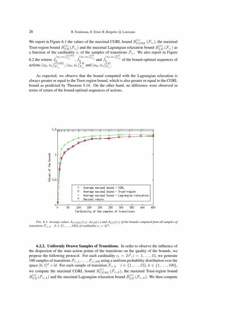
FIG. 6.3. Average values ACGRL(ci), ATR(ci) and ALD(ci) of the bounds computed from all samples oftransitions Fci,k k ∈ {1, . . . , 100} of cardinality ci = 2i2.

6.2.2. Uniformly Drawn Samples of Transitions. In order to observe the influence ofthe dispersion of the state-action points of the transitions on the quality of the bounds, wepropose the following protocol. For each cardinality ci = 2i2, i = 1, . . . , 15, we generate100 samples of transitionsFci,1, . . . ,Fci,100 using a uniform probability distribution over thespace [0, 1]d × U . For each sample of transition Fci,k i ∈ {1, . . . , 15}, k ∈ {1, . . . , 100},we compute the maximal CGRL bound B

(∗)CGRL (Fci,k), the maximal Trust-region bound

B(∗)TR (Fci,k) and the maximal Lagrangian relaxation bound B(∗)

LD (Fci,k). We then compute


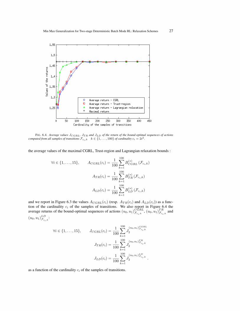
FIG. 6.4. Average values JCGRL, JTR and JLD of the return of the bound-optimal sequences of actionscomputed from all samples of transitions Fci,k k ∈ {1, . . . , 100} of cardinality ci = 2i2.

the average values of the maximal CGRL, Trust-region and Lagrangian relaxation bounds :

∀i ∈ {1, . . . , 15}, ACGRL(ci) =1

100

100∑k=1

B(∗)CGRL (Fci,k)

ATR(ci) =1

100

100∑k=1

B(∗)TR (Fci,k)

ALD(ci) =1

100

100∑k=1

B(∗)LD (Fci,k)

and we report in Figure 6.3 the values ACGRL(ci) (resp. ATR(ci) and ALD(ci)) as a func-tion of the cardinality ci of the samples of transitions. We also report in Figure 6.4 theaverage returns of the bound-optimal sequences of actions (u0, u1)

CGRLFci,k

, (u0, u1)TRFci,k

and

(u0, u1)LDFci,k

:

∀i ∈ {1, . . . , 15}, JCGRL(ci) =1

100

100∑k=1

J(u0,u1)

CGRLFci,k

2

JTR(ci) =1

100

100∑k=1

J(u0,u1)

TRFci,k

2

JLD(ci) =1

100

100∑k=1

J(u0,u1)

LDFci,k

2 .

as a function of the cardinality ci of the samples of transitions.


We observe that, on average, the Lagrangian relaxation bound is much tighter that theTrust-region and the CGRL bounds. The CGRL bound and the Trust-region bound remainvery close on average, which illustrates, in a sense, Corollary 5.10. Moreover, we also observethat the bound-optimal sequences of actions (u0, u1)

LDFci,k

better perform on average.

7. Conclusions. We have considered in this paper the problem of computing min maxpolicies for deterministic, Lipschitz continuous batch mode reinforcement learning. First,we have shown that this min max problem is NP-hard. Afterwards, we have proposed for thetwo-stage case two relaxation schemes. Both have been extensively studied and, in particular,they have been shown to perform better than the CGRL algorithm that has been introducedearlier to address this min-max generalization problem.

A natural extension of this work would be to investigate how the proposed relaxationschemes could be extended to the T -stage (T ≥ 3) framework. Lipschitz continuity as-sumptions are common in a batch mode reinforcement learning setting, but one could imag-ine developing min max strategies in other types of environments that are not necessarilyLipschitzian, or even not continuous. Additionnaly, it would also be interesting to extendthe resolution schemes proposed in this paper to problems with very large/continuous actionspaces.

Acknowledgements. Raphael Fonteneau is a Post-doctoral fellow of the FRS-FNRS(Funds for Scientific Research). This paper presents research results of the Belgian NetworkDYSCO (Dynamical Systems, Control and Optimization) funded by the Interuniversity At-traction Poles Programme, initiated by the Belgian State, Science Policy Office. The authorsthank Yurii Nesterov for pointing out the idea of using Lagrangian relaxation. The scientificresponsibility rests with its authors.

Appendix A. Proof of Lemma 5.12.Proof. For conciseness, we denote

(x(u0),k0 , r(u0),k0 , y(u0),k0

)( resp.(

x(u1),k1 , r(u1),k1 , y(u1),k1)) by

(x0, r0, y0

)(resp.

(x1, r1, y1

)), and λ1 (resp. µ1) by λ

(resp. µ). We assume that x0 6= x0 and x1 6= y0 otherwise the problem is trivial.• Trust-region solution.

According to Definition 5.2, we have:

B′′(u0,u1),k0,k1TR (F) = r1 − Lρ

∥∥x∗1(k0, k1)− x1∥∥ ,

where

x∗1(k0, k1) = y0 + Lf

∥∥x0 − x0∥∥‖y0 − x1‖

(y0 − x1

),

which writes

B′′(u0,u1),k0,k1TR (F) = r1 − Lρ

∥∥∥∥∥y0 + Lf

∥∥x0 − x0∥∥‖y0 − x1‖

(y0 − x1

)− x1

∥∥∥∥∥ ,= r1 − Lρ

∥∥y0 − x1∥∥(1 + Lf

∥∥x0 − x0∥∥‖y0 − x1‖

)= r1 − Lρ

∥∥y0 − x1∥∥− LρLf ∥∥x0 − x0∥∥• Lagrangian relaxation based solution.


According to Equation (5.11), we can write:

B′′(u0,u1),k0,k1LD (F) = max

λ∈R+,µ∈R+

−∥∥L2

ρx1µ− y0λ

∥∥2−µL2

ρ + λ−(1− 2r1µ

)24µ

+λ(∥∥y0∥∥2 − L2

f

∥∥x0 − x0∥∥2) + µ((r1)2 − L2

ρ

∥∥x1∥∥2)subject to

µ > 0

λ > µL2ρ

We denote by L(λ, µ) the quantity:

L(λ, µ) =−∥∥L2

ρx1µ− y0λ

∥∥2−µL2

ρ + λ−(1− 2r1µ

)24µ

+ λ(∥∥y0∥∥2 − L2

f

∥∥x0 − x0∥∥2)+µ((r1)2 − L2

ρ

∥∥x1∥∥2)Let λ and µ be such that λ > µL2

ρ. Since the Trust-region solution to (P ′′(u0,u1)TR (k0, k1)) is

optimal, and by property of the Lagrangian relaxation [25], one has:

L(λ, µ) ≤ B′′(u0,u1),k0,k1TR (F) . (A.1)

In order to prove the lemma, it is therefore sufficient to determine two values λ0 and µ0 suchthat the inequality (A.1) is an equality. By differentiating L(λ, µ), we obtain, after a longcalculation (that we omit here):

∂L(λ,µ)∂λ = 0

∂L(λ,µ)∂µ = 0

λ > µL2ρ

=⇒

{λ =

Lρ2Lf‖x0−x0‖ ,

µ = 12Lρ(‖y0−x1‖+Lf‖x0−x0‖) .

We denote by λ0 and µ0 the following values for the dual variables:

λ0 ,Lρ

2Lf ‖x0 − x0‖,

µ0 ,1

2Lρ (‖y0 − x1‖+ Lf ‖x0 − x0‖).

We have:

µ0 =1

2Lρ (‖y0 − x1‖+ Lf ‖x0 − x0‖)> 0

λ0µ0

= L2ρ

(1 +

∥∥y0 − x1∥∥Lf ‖x0 − x0‖

)> L2

ρ .


In the following, we denote(

1 +‖y0−x1‖Lf‖x0−x0‖

)byK. We now give the expression ofL(λ0, µ0)

using only µ0 and K:

L(λ0, µ0) = −L4ρµ

20

∥∥x1 −Ky0∥∥2µ0L2

ρ(−1 +K)− 1

4µ0+ r1 −

(r1)2µ0

+µ0KL2ρ

(∥∥y0∥∥2 − L2f

∥∥x0 − x0∥∥2)+ µ0

((r1)2 − L2

ρ

∥∥x1∥∥2)= −

L2ρµ0

∥∥x1 −Ky0∥∥2K − 1

− 1

4µ0+ r1

+L2ρµ0K

(∥∥y0∥∥2 − L2f

∥∥x0 − x0∥∥2)− L2ρµ0

∥∥x1∥∥2 .Using the fact that x1 −Ky0 = x1 − y0 − (K − 1)y0, we can write:

L(λ0, µ0) = −L2ρµ0

K − 1

(∥∥x1 − y0∥∥2 + (K − 1)2∥∥y0∥∥2 − 2(K − 1)(x1 − y0)T y0

)− 1

4µ0+ r1 + L2

ρµ0K(∥∥y0∥∥2 − L2

f

∥∥x0 − x0∥∥2)− L2ρ

∥∥x1∥∥2and

L(λ0, µ0) = −L2ρµ0

K − 1

∥∥x1 − y0∥∥2 − L2ρµ0(K − 1)

∥∥y0∥∥2 + 2L2ρµ0(x1 − y0)T y0

− 1

4µ0+ r1 + L2

ρµ0K(∥∥y0∥∥2 − L2

f

∥∥x0 − x0∥∥2)− L2ρ

∥∥x1∥∥2 .From there,

L(λ0, µ0) = −L2ρµ0

K − 1

∥∥x1 − y0∥∥2 +∥∥y0∥∥2 (−L2

ρµ0(K − 1)− 2L2ρµ0 + L2

ρµ0K)

−2L2ρµ0(x1)T y0 − 1

4µ0+ r1 + L2

ρµ0K(−L2

f

∥∥x0 − x0∥∥2)− L2ρ

∥∥x1∥∥2and, since

(−L2

ρµ0(K − 1)− 2L2ρµ0 + L2

ρµ0K)

= −L2ρµ0, we have that

L(λ0, µ0) = −L2ρµ0

K − 1

∥∥x1 − y0∥∥2 − L2ρµ0

∥∥y0∥∥2 − 2L2ρµ0(x1)T y0

− 1

4µ0+ r1 + L2

ρµ0K(−L2

f

∥∥x0 − x0∥∥2)− L2ρ

∥∥x1∥∥2and

L(λ0, µ0) = −L2ρµ0

K − 1

∥∥x1 − y0∥∥2 − L2ρµ0

(∥∥y0∥∥2 +∥∥x1∥∥2 − 2(x1)T y0

)− 1

4µ0+ r1 + L2

ρµ0K(−L2

f

∥∥x0 − x0∥∥2) .


Since(∥∥y0∥∥2 +

∥∥x1∥∥2 − 2(x1)T y0)

=∥∥x1 − y0∥∥2, we have:

L(λ0, µ0) = −L2ρµ0

K − 1

∥∥x1 − y0∥∥2 − L2ρµ0

∥∥x1 − y0∥∥2− 1

4µ0+ r1 + L2

ρµ0K(−L2

f

∥∥x0 − x0∥∥2)= −L2

ρµ0

∥∥x1 − y0∥∥2 K

K − 1

− 1

4µ0+ r1 + L2

ρµ0K(−L2

f

∥∥x0 − x0∥∥2)= −KL2

ρµ0

(∥∥x1 − y0∥∥2K − 1

+ L2f

∥∥x0 − x0∥∥2)− 1

4µ0+ r1 .

Since K ,

(1 +

‖y0−x1‖Lf‖x0−x0‖

), we have:

L(λ0, µ0) = −

(1 +

∥∥y0 − x1∥∥Lf ‖x0 − x0‖

)L2ρµ0

∥∥x1 − y0∥∥2(1 + ‖y0−x1‖

Lf‖x0−x0‖

)− 1

+ L2f

∥∥x0 − x0∥∥2

− 1

4µ0+ r1

= −L2ρµ0

(Lf∥∥x0 − x0∥∥+

∥∥y0 − x1∥∥)Lf ‖x0 − x0‖

(Lf∥∥x0 − x0∥∥∥∥x1 − y0∥∥2‖x1 − y0‖

+ L2f

∥∥x0 − x0∥∥2)

− 1

4µ0+ r1

= − L2ρµ0

(Lf∥∥x0 − x0∥∥+

∥∥y0 − x1∥∥) (∥∥x1 − y0∥∥+ Lf∥∥x0 − x0∥∥)− 1

4µ0+ r1 .

Since µ0 = 12Lρ(‖y0−x1‖+Lf‖x0−x0‖) , we finally obtain:

L(λ0, µ0) = −Lρ2

(∥∥y0 − x1∥∥+ Lf∥∥x0 − x0∥∥)− Lρ

2

(∥∥y0 − x1∥∥+ Lf∥∥x0 − x0∥∥)+ r1

= r1 − Lρ∥∥y0 − x1∥∥− LρLf ∥∥x0 − x0∥∥

= B′′(u0,u1),k0,k1TR (F) ,

which ends the proof.

REFERENCES

[1] A. BANERJEE AND A.A. TSIATIS, Adaptive two-stage designs in phase ii clinical trials, Statistics inmedicine, 25 (2006), pp. 3382–3395.

[2] T. BASAR AND P. BERNHARD, H∞-optimal control and related minimax design problems: a dynamic gameapproach, vol. 5, Birkhauser, 1995.

[3] A. BECK AND Y.C. ELDAR, Strong duality in nonconvex quadratic optimization with two quadratic con-straints, SIAM Journal on Optimization, 17 (2007), pp. 844–860.

[4] A. BEMPORAD AND M. MORARI, Robust model predictive control: A survey, Robustness in Identificationand Control, 245 (1999), pp. 207–226.

[5] A. BEN-TAL AND A.S. NEMIROVSKI, Lectures on Modern Convex Optimization, Siam, 2001.[6] D.P. BERTSEKAS AND J.N. TSITSIKLIS, Neuro-Dynamic Programming, Athena Scientific, 1996.


[7] J.R. BIRGE AND F. LOUVEAUX, Introduction to Stochastic Programming, Springer Verlag, 1997.[8] JF BONNANS, J.C. GILBERT, C. LEMARECHAL, AND C. SAGASTIZABAL, Numerical optimization, theo-

retical and numerical aspects, 2006.[9] S.P. BOYD AND L. VANDENBERGHE, Convex Optimization, Cambridge Univ Pr, 2004.

[10] S.J. BRADTKE AND A.G. BARTO, Linear least-squares algorithms for temporal difference learning, Ma-chine Learning, 22 (1996), pp. 33–57.

[11] L. BUSONIU, R. BABUSKA, B. DE SCHUTTER, AND D. ERNST, Reinforcement Learning and DynamicProgramming using Function Approximators, Taylor & Francis CRC Press, 2010.

[12] E.F. CAMACHO AND C. BORDONS, Model Predictive Control, Springer, 2004.[13] A.R. CONN, N.I.M. GOULD, AND P.L. TOINT, Trust-region Methods, vol. 1, Society for Industrial Mathe-

matics, 2000.[14] K. DARBY-DOWMAN, S. BARKER, E. AUDSLEY, AND D. PARSONS, A two-stage stochastic programming

with recourse model for determining robust planting plans in horticulture, Journal of the OperationalResearch Society, (2000), pp. 83–89.

[15] B. DEFOURNY, D. ERNST, AND L. WEHENKEL, Risk-aware decision making and dynamic programming,Selected for oral presentation at the NIPS-08 Workshop on Model Uncertainty and Risk in ReinforcementLearning, Whistler, Canada, (2008).

[16] E. DELAGE AND S. MANNOR, Percentile optimization for Markov decision processes with parameter uncer-tainty, Operations Research, 58 (2010), pp. 203–213.

[17] D. ERNST, P. GEURTS, AND L. WEHENKEL, Tree-based batch mode reinforcement learning, Journal ofMachine Learning Research, 6 (2005), pp. 503–556.

[18] D. ERNST, M. GLAVIC, F. CAPITANESCU, AND L. WEHENKEL, Reinforcement learning versus modelpredictive control: a comparison on a power system problem, IEEE Transactions on Systems, Man,and Cybernetics - Part B: Cybernetics, 39 (2009), pp. 517–529.

[19] R. FONTENEAU, Contributions to Batch Mode Reinforcement Learning, PhD thesis, University of Liege,2011.

[20] R. FONTENEAU, S. MURPHY, L. WEHENKEL, AND D. ERNST, Inferring bounds on the performance of acontrol policy from a sample of trajectories, in Proceedings of the 2009 IEEE Symposium on AdaptiveDynamic Programming and Reinforcement Learning (IEEE ADPRL 09), Nashville, TN, USA, 2009.

[21] R. FONTENEAU, S.A. MURPHY, L. WEHENKEL, AND D. ERNST, A cautious approach to generalization inreinforcement learning, in Proceedings of the Second International Conference on Agents and ArtificialIntelligence (ICAART 2010), Valencia, Spain, 2010.

[22] R. FONTENEAU, S. A. MURPHY, L. WEHENKEL, AND D. ERNST, Towards min max generalization in re-inforcement learning, in Agents and Artificial Intelligence: International Conference, ICAART 2010,Valencia, Spain, January 2010, Revised Selected Papers. Series: Communications in Computer and In-formation Science (CCIS), vol. 129, Springer, Heidelberg, 2011, pp. 61–77.

[23] K. FRAUENDORFER, Stochastic Two-stage Programming, Springer, 1992.[24] L.P. HANSEN AND T.J. SARGENT, Robust Control and Model Uncertainty, American Economic Review,

(2001), pp. 60–66.[25] J.B. HIRIART-URRUTY AND C. LEMARECHAL, Convex Analysis and Minimization Algorithms: Fundamen-

tals, vol. 305, Springer-Verlag, 1996.[26] J.E. INGERSOLL, Theory of Financial Decision Making, Rowman and Littlefield Publishers, Inc., 1987.[27] S. KOENIG, Minimax real-time heuristic search, Artificial Intelligence, 129 (2001), pp. 165–197.[28] M.G. LAGOUDAKIS AND R. PARR, Least-squares policy iteration, Jounal of Machine Learning Research, 4

(2003), pp. 1107–1149.[29] M. L. LITTMAN, Markov games as a framework for multi-agent reinforcement learning, in Proceedings of

the Eleventh International Conference on Machine Learning (ICML 1994), New Brunswick, NJ, USA,1994.

[30] , A tutorial on partially observable markov decision processes, Journal of Mathematical Psychology,53 (2009), pp. 119 – 125. Special Issue: Dynamic Decision Making.

[31] Y. LOKHNYGINA AND A.A. TSIATIS, Optimal two-stage group-sequential designs, Journal of StatisticalPlanning and Inference, 138 (2008), pp. 489–499.

[32] J.K. LUNCEFORD, M. DAVIDIAN, AND A.A. TSIATIS, Estimation of survival distributions of treatmentpolicies in two-stage randomization designs in clinical trials, Biometrics, (2002), pp. 48–57.

[33] S. MANNOR, D. SIMESTER, P. SUN, AND J.N. TSITSIKLIS, Bias and variance in value function estimation,in Proceedings of the Twenty-first International Conference on Machine Learning (ICML 2004), Banff,Alberta, Canada, 2004.

[34] S.A. MURPHY, Optimal dynamic treatment regimes, Journal of the Royal Statistical Society, Series B, 65(2)(2003), pp. 331–366.

[35] S.A. MURPHY, An experimental design for the development of adaptive treatment strategies, Statistics inMedicine, 24 (2005), pp. 1455–1481.

[36] A. NEMIROVSKI, A. JUDITSKY, G. LAN, AND A. SHAPIRO, Robust stochastic approximation approach to


stochastic programming, SIAM Journal on Optimization, 19 (2009), pp. 1574–1609.[37] Y. NESTEROV AND A. NEMIROVSKI, Interior point polynomial methods in convex programming, Studies in

applied mathematics, 13 (1994).[38] D. ORMONEIT AND S. SEN, Kernel-based reinforcement learning, Machine Learning, 49 (2002), pp. 161–

178.[39] C. PADURARU, D. PRECUP, AND J. PINEAU, A framework for computing bounds for the return of a policy,

in Ninth European Workshop on Reinforcement Learning (EWRL9), 2011.[40] C.H. PAPADIMITRIOU, Computational Complexity, John Wiley and Sons Ltd., 2003.[41] M. QIAN AND S.A. MURPHY, Performance guarantees for individualized treatment rules, Tech. Report 498,

Department of Statistics, University of Michigan, 2009.[42] M. RIEDMILLER, Neural fitted Q iteration - first experiences with a data efficient neural reinforcement learn-

ing method, in Proceedings of the Sixteenth European Conference on Machine Learning (ECML 2005),Porto, Portugal, 2005, pp. 317–328.

[43] M. ROVATOUS AND M. LAGOUDAKIS, Minimax search and reinforcement learning for adversarial tetris, inProceedings of the 6th Hellenic Conference on Artificial Intelligence (SETN’10), Athens, Greece, 2010.

[44] P. SCOKAERT AND D. MAYNE, Min-max feedback model predictive control for constrained linear systems,IEEE Transactions on Automatic Control, 43 (1998), pp. 1136–1142.

[45] A. SHAPIRO, A dynamic programming approach to adjustable robust optimization, Operations ResearchLetters, 39 (2011), pp. 83–87.

[46] , Minimax and risk averse multistage stochastic programming, tech. report, School of Industrial &Systems Engineering, Georgia Institute of Technology, 2011.

[47] J.F. STURM, Using SeDuMi 1.02, a MATLAB toolbox for optimization over symmetric cones, Optimizationmethods and software, 11 (1999), pp. 625–653.

[48] R.S. SUTTON AND A.G. BARTO, Reinforcement Learning, MIT Press, 1998.[49] A.S. WAHED AND A.A. TSIATIS, Optimal estimator for the survival distribution and related quantities for

treatment policies in two-stage randomization designs in clinical trials, Biometrics, 60 (2004), pp. 124–133.

Documents

Min max generalization for deterministic batch mode reinforcement learning: relaxation schemes