Article

Microstructure Evaluation and Constitutive Modelingof AISI-1045 Steel for Flow Stress Predictionunder Hot Working Conditions

Mohanraj Murugesan, Muhammad Sajjad and Dong Won Jung *

Department of Mechanical Engineering, Jeju National University, Jeju-Do 63243, Korea;mohanaero32@jejunu.ac.kr (M.M.); msajjadtheone@jejunu.ac.kr (M.S.)* Correspondence: jdwcheju@jejunu.ac.kr

Received: 2 April 2020; Accepted: 6 May 2020; Published: 8 May 2020�����������������

Abstract: In the field of engineering, automobile and aerospace components are manufacturedbased on the desired applications from the metal forming process. For producing better qualityof both symmetry and asymmetry mechanical parts, understanding the material deformation andanalytical representation of the material ductility behavior for the working material is necessaryas the forming procedures carried out mostly in the warm processing conditions. In this work,the hot tensile test flow stress-strain data were utilized to construct the constitutive equation fordescribing AISI-1045 steel material hot deformation behavior, and the test conditions, such asdeformation temperatures and strain rates were 750–950 ◦C and 0.05–1.0 s−1, respectively. The surfacemorphology and elemental identification analysis were performed using the field emission scanningelectron microscopy (FESEM) coupled with the energy-dispersive X-ray spectroscopy (EDS) mappingsetup. In this work, the Arrhenius-type constitutive equation, including the strain compensation,was used to formulate the flow stress prediction model for capturing the material behavior. Besides,the Zener-Hollomon parameter was altered, employing incorporating the effect of strain rate andstrain on the flow stress. The empirical model approach was employed to estimate the material modelconstants from the constitutive equation using the actual test measurements. The population metricssuch as coefficient of determination (R2), sample standard deviation of the error (SSD), standard errorof the regression (SER), coefficient of residual variation (CRV), and average absolute relative error(AARE) was employed to confirm the predictability of the proposed models. The computed resultsare discussed in detail, using numerical and graphical verification’s. From the graphical comparison,the flow stress-strain data achieved from the proposed constitutive model are in good agreement withthe actual test measurements. The constitutive model prediction accuracy is found to be improved,like the prediction error range from 3.678% to 2.984%. This evidence proves to be feasible as thenewly developed model displayed a significant improvement against the experimental observations.

Keywords: hot deformation; constitutive model; medium carbon steel; flow stress; FESEM; EDS;strain compensation; Zener-Hollomon parameter

1. Introduction

AISI-1045 steel is a medium carbon steel material that is extensively used for the automobileindustry applications, owing to its mechanical properties. The material properties are such as toughness,wear-resistance, and higher strength for manufacturing camshafts and cams by the forging process.In industrial practice, the processing conditions like alloy content and cooling rate altered forachieving the desirable microstructures and excellent mechanical properties. However, during themetal forming process, metals and alloys undergo an inhomogeneous deformation by cause of hot

Symmetry 2020, 12, 782; doi:10.3390/sym12050782 www.mdpi.com/journal/symmetry

Symmetry 2020, 12, 782 2 of 18

operating conditions. For this reason, understanding the metals deformation behavior is necessaryfor determining the working parameters that affect the mechanical properties for providing thewell-defined material processing data to the industry [1–4]. The constitutive equations are oftenutilized in a form that is suitable to use in finite element (FE) commercial tools. They used to representthe material flow behavior and helps to obtain a better prediction [5–8]. Moreover, the constitutiveequations are categorized as follows: physical, phenomenological, and statistical models [9–12]. In ourprevious work [13,14], a detailed discussion on AISI 1045 steel material behavior in hot processingconditionswas carried out using Johnson–Cook (JC), modified JC, and modified Zerilli–Armstrong (ZA)models. The results showed that the modified ZA model was more significant in representing thematerial deformation behavior compared with the test data than that of others. However, the flowstress model predictability can be improvised by training other available conventional models. For thispurpose, in this present investigation, the strain compensated Arrhenius-type constitutive model wasadopted to represent the material’s ductility behavior in hot operating conditions.

In the past, there has been information published on constitutive equations to consistently describethe material’s behavior at various loading conditions [15–18]. Besides, many researchers have discussedthe advantage of utilizing the constitutive equations by comparing the outcome of available flowstress models, and they reported that the proposed models could be able to precisely characterizethe material behavior because the parameters are determined statistically from the experimentaldata [19–22]. Samantaray et al. [23] examined the modified 9Cr-1Mo steel material behavior usingthe phenomenological models. They stated that the Arrhenius-type constitutive model consideringstrain compensation can track the material behavior more accurately than the original JC and modifiedZA models. The strain effects were incorporated into the constitutive equation to characterize theflow behavior in 42CrMo at elevated temperatures by Lin et al. [24]. They reported that includingthe strain compensation, the proposed model could predict the material behavior significantly underhot working conditions. Unlike conventional methods, an artificial neural network (ANN) modelconsidering a back-propagation algorithm was adopted by Wu et al. [25] and Xiao et al. [26] to predictthe material deformation behavior of two different steel materials. They stated that the trained ANNmodel found to be more precise in predicting the hot comprehensive behavior than the Arrhenius-typeconstitutive equations.

However, there are only limited reports on the improvement of the strain compensatedArrhenius-type constitutive model, including strain and strain rate effects, into the Zener-Hollomon(Z) parameter to describe the material behavior accurately. Mandal et al. [27] investigated the problemby incorporating a modified Z parameter into the basic equation for predicting a Ti-modified austeniticstainless steel material flow behavior at high-temperature conditions. A revised constitutive equationwas in good correlation with the actual data to predict the flow stress throughout the tested range.Besides, Krishnan et al. [28] reported a valuable outcome for the use of strain-rate compensation inthe Z parameter for 9Cr-1Mo ferritic steel. They found that the proposed methodology based on themodified Z parameter provided a better estimation of flow stress for most of the test combinations.Therefore, this present research work aims to establish and devise the suitable constitutive flow stressmodel over a wide range of testing conditions to describe the AISI-1045 steel material flow behavior.The test conditions, such as deformation temperatures and strain rates are 750–950 ◦C and 0.05–1.0 s−1,respectively. For this purpose, the real test measurements were used to fit the model equations by bothcompensations of strain (ε) and strain rate (ε). Furthermore, the predictability of proposed models wasvalidated against the experimental observations and also discussed statistically by both numerical andgraphical validation.

2. Experiments

Isothermal-tension test was carried out to examine the AISI-1045 steel material deformationbehavior during hot processing conditions. The chemical compositions (in wt.%) of the work materialis summarized in Table 1 [13]. The samples were prepared through a water-jet cutting process

Symmetry 2020, 12, 782 3 of 18

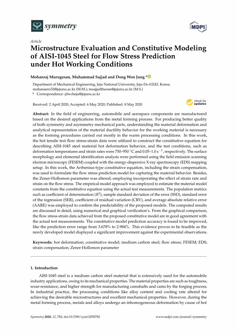
according to the ASTM-E8M-subsize standard with 25 mm gauge length and 3 mm thickness [13,14].Experiments were conducted using a computer-controlled servo-hydraulic testing machine, as shownin Figure 1a, at deformation temperatures and strain rates in a range of (750–950 ◦C) and (0.05–1.0 s−1),respectively [13,14]. To achieve an isothermal environment, the tensile specimen was covered withisolation part, Figure 1b, and in each test condition, three samples tested, Figure 1c, and recordedresults were averaged for obtaining true stress-strain (SS) curves. Later, the elastic region was takenout from the SS curves to gain the true plastic region of SS data for the material model parametersestimation [13,14].

Table 1. Chemical composition of AISI-1045 medium carbon steel (in wt.%) [13].

C Fe Mn P S

0.42–0.50 98.51–98.98 0.60–0.90 ≤0.04 ≤0.05

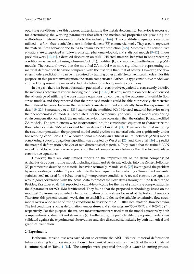
The typical AISI-1045 medium carbon steel material stress-strain (SS) curves in hot processingconditions are depicted in Figure 2 [13,14,29]. From Figure 2a–c, it is evident that all curves atdeformation temperatures 750 ◦C and 950 ◦C exhibit an increment in the flow stress in the initial stagefollowed by the steady state to strain. Moreover, in Figure 2a–c, deformation temperatures were fixedand flow stress was noticed to be escalated when the strain rate is higher. It happens because if there isan increment in the strain rate, the dislocations and inadequate dynamic recovery and re-crystallizationin the material causes the increment in flow stress [13,14]. Similarly, with fixed strain rate (ε), SS datareduces with increments of the deformation temperature (T) due to the thermal activation energy andthe average kinetic energy as it allows the crystals to achieve the dynamic recovery and recrystallizationduring deformation quickly. Simultaneously, from Figure 2b,c, at strain rates 0.05 s−1 and 0.1 s−1, theflow stress identified to be decreased dramatically after the small peak stress. This behavior arises dueto the plastic instability phenomenon that happened during the tensile test. In detail, when the tensilespecimen deformed at a particular stage, there is an unsteadiness between the increase in strengthand stress because of work hardening and thinning, respectively [13,14]. At this time, the unstabledeformation, decrease in flow stress, appears due to necking and fracture at the test specimen. Thus,this phenomenon has to be considered during the development of empirical based flow stress models.

(a) (b) (c)

Figure 1. Elevated temperature tensile testing set-up and procedures (a) Entire test set-up; (b) Testspecimen coupled with thermocouples for temperature measurement; (c) Tested specimens.

Symmetry 2020, 12, 782 4 of 18

0 0.05 0.1 0.15 0.2 0.25 0.30

25

50

75

100

125

150

175

200

225

250

275

True strain

Flow

stre

ss (M

Pa)

(a)

0 0.05 0.1 0.15 0.2 0.25 0.30

20

40

60

80

100

120

140

160

180

200

True strain

Flow

stre

ss (M

Pa)

1.0 s-1

0.5 s-1

0.1 s-1

0.05 s-1

(b)

0 0.05 0.1 0.15 0.2 0.25 0.30

20

40

60

80

100

120

140

160

True strain

Flow

stre

ss (M

Pa)

1.0 s-1

0.5 s-1

0.1 s-1

0.05 s-1

(c)

Figure 2. True stress-strain curves acheived from hot tensile tests at various temperatures (a) 750 ◦C;(b) 850 ◦C; (c) 950 ◦C under different strain rates [13,14,29].

3. Microstructure Evaluation of AISI-1045 Medium Carbon Steel

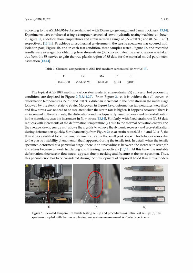
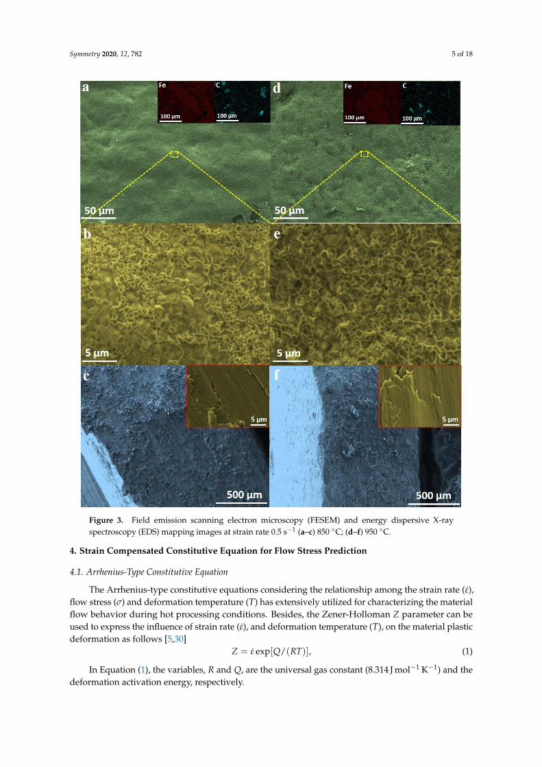
The field emission scanning electron microscopy (FESEM) and the energy dispersive X-rayspectroscopy (EDS) mapping setups employed to examine the temperature-dependent surfacemorphology (850 ◦C, 950 ◦C) and elemental identification analysis, respectively, for the testedmaterial [29]. The obtained FESEM micrographs are illustrated in Figure 3. The specimen growth andnucleation is noticed to be uniform on the magnification scale of 50 µm as displayed in Figure 3a,din tested temperature conditions. The enlarged portion of 850 ◦C specimen FESEM micrograph,Figure 3b, proves the moderate nanoneedles growth and the micro-fibrils formation at 5 µm scale [29].During temperature rise from 850 ◦C to 950 ◦C, the samples were observed to have an apparent growth,nucleation of nanoneedles in the vertical direction along with the micro-fibrils. As a result, it confirmsthe temperature effect on the tested sample surface, as depicted in Figure 3e. Besides, as shown inFigure 3a,d, the EDS mapping analysis confirms the existence of iron (Fe) and carbon (C) elementsall over the examined sample surface (100 µm scale). For proving the thickness reduction in testedsamples, at fracture location, the samples scanned at 500 µm scale as displayed in Figure 3c,f. Moreover,the inset micrographs (Figure 3c,f) illustrate the rough surface morphology of samples at the damagedlocation (5 µm scale).

Symmetry 2020, 12, 782 5 of 18

Figure 3. Field emission scanning electron microscopy (FESEM) and energy dispersive X-rayspectroscopy (EDS) mapping images at strain rate 0.5 s−1 (a–c) 850 ◦C; (d–f) 950 ◦C.

4. Strain Compensated Constitutive Equation for Flow Stress Prediction

4.1. Arrhenius-Type Constitutive Equation

The Arrhenius-type constitutive equations considering the relationship among the strain rate (ε),flow stress (σ) and deformation temperature (T) has extensively utilized for characterizing the materialflow behavior during hot processing conditions. Besides, the Zener-Holloman Z parameter can beused to express the influence of strain rate (ε), and deformation temperature (T), on the material plasticdeformation as follows [5,30]

Z = ε exp[Q/(RT)], (1)

In Equation (1), the variables, R and Q, are the universal gas constant (8.314 J mol−1 K−1) and thedeformation activation energy, respectively.

Symmetry 2020, 12, 782 6 of 18

At steady-state, the flow stress levels used to select the peak flow stress to estimate ασ valuesto choose the proper Z equation. There are three levels of Z equation such as the power-law,the exponential, and the hyperbolic sine-law equations as follows [10,30]

Z =

A1σn1 if ασ < 0.8

A2 exp(βσ) if ασ > 1.2

A[sinh(ασ)]n for all σ,

(2)

where A1, n1, A2, β, A, n and α are the model constants. α is the stress multiplier, α = β/n1. Firstly,by replacing the Z parameter in Equation (2) substituting Equation (1), and then performing the logtransformations gives [11,15,30,31]

ln ε = ln A1 + n1 ln σ− [Q/(RT)], (3)

ln ε = βσ + ln A2 − [Q/(RT)], (4)

ln ε = n ln[sinh(ασ)] + ln A− [Q/(RT)]. (5)

It is clear that Equations (3)–(5) tend to have a linear relationship form, and the data distributed inFigures 4–6 depicts that the correlation exists between the independent variable (x), and the responsevariable (Y) noticed to be linear. So, the linear regression model is more than enough to capture thevariation, and the mathematical form is

E(Y|x) = a0 + a1x

yi = a0 + a1xi, i = 1, 2, 3, ..., n. (6)

In Equation (6), a0, a1 and n are the model intercept, the slope and the number of samples used forthe model construction, respectively. Subsequently, the model unknown coefficients are determinedusing the least squares method as given below

a1 =

n∑

i=1yixi −

(n∑

i=1yi

)(n∑

i=1xi

)n

n∑

i=1x2

i −

(n∑

i=1xi

)2

n

, (7)

a0 =1n

(n

∑i=1

yi − a1

n

∑i=1

xi

). (8)

Considering constant deformation temperature, T, from Equations (3)–(5), by taking partialderivatives, the material model constants, n1, β and n, can be estimated as follows [11,30]

n1 =∂ ln ε

∂ ln σ

∣∣∣∣T

, β =∂ ln ε

∂σ

∣∣∣∣T

, n =∂ ln ε

∂ ln[sinh(ασ)

∣∣∣∣T

.

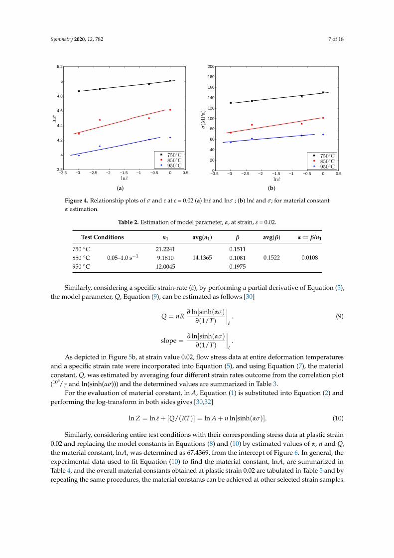
In order to estimate the model constants, α and n, for example, the stress values associated with theplastic strain value of 0.02, was chosen at tested conditions. By substituting the corresponding valuesto Equations (3) and (4) and performing the linear regression analysis using Equations (7) and (8), β,n1, and n were determined from the correlation plots of lnε and σ, lnε and σ and lnε and ln(sinh(ασ)),respectively, as illustrated in Figures 4a,b and 5a. To give a proper understanding of the calculationprocedures, the detailed estimation of the model parameter, α, at each test conditions and their meanvalues are listed in Table 2.

Symmetry 2020, 12, 782 7 of 18

−3.5 −3 −2.5 −2 −1.5 −1 −0.5 0 0.53.8

4

4.2

4.4

4.6

4.8

5

5.2

lnε

lnσ

750◦C

850◦C

950◦C

(a)

−3.5 −3 −2.5 −2 −1.5 −1 −0.5 0 0.50

20

40

60

80

100

120

140

160

180

200

lnε

σ(M

Pa)

750◦C850◦C950◦C

(b)

Figure 4. Relationship plots of σ and ε at ε = 0.02 (a) lnε and lnσ ; (b) lnε and σ; for material constantα estimation.

Table 2. Estimation of model parameter, α, at strain, ε = 0.02.

Test Conditions n1 avg(n1) β avg(β) α = β/n1

750 ◦C0.05–1.0 s−1

21.224114.1365

0.15110.1522 0.0108850 ◦C 9.1810 0.1081

950 ◦C 12.0045 0.1975

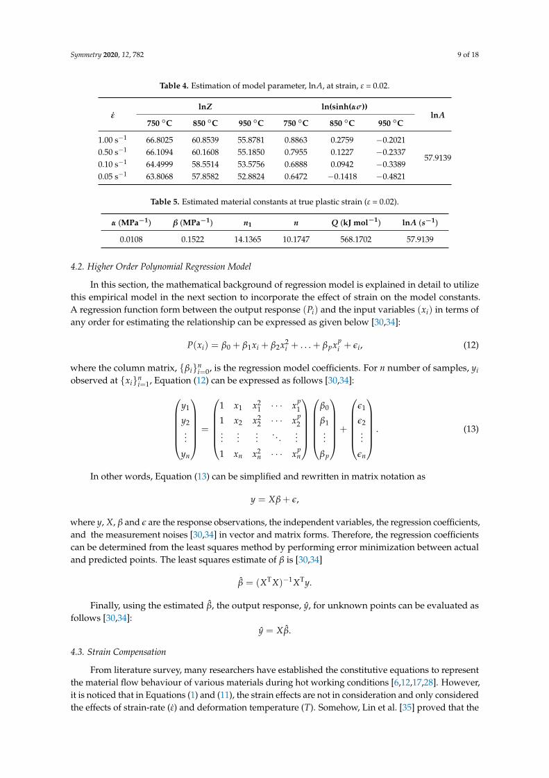
Similarly, considering a specific strain-rate (ε), by performing a partial derivative of Equation (5),the model parameter, Q, Equation (9), can be estimated as follows [30]

Q = nR∂ ln[sinh(ασ)

∂(1/T)

∣∣∣∣ε

. (9)

slope =∂ ln[sinh(ασ)

∂(1/T)

∣∣∣∣ε

.

As depicted in Figure 5b, at strain value 0.02, flow stress data at entire deformation temperaturesand a specific strain rate were incorporated into Equation (5), and using Equation (7), the materialconstant, Q, was estimated by averaging four different strain rates outcome from the correlation plot(103

/T and ln(sinh(ασ))) and the determined values are summarized in Table 3.For the evaluation of material constant, ln A, Equation (1) is substituted into Equation (2) and

performing the log-transform in both sides gives [30,32]

ln Z = ln ε + [Q/(RT)] = ln A + n ln[sinh(ασ)]. (10)

Similarly, considering entire test conditions with their corresponding stress data at plastic strain0.02 and replacing the model constants in Equations (8) and (10) by estimated values of α, n and Q,the material constant, lnA, was determined as 67.4369, from the intercept of Figure 6. In general, theexperimental data used to fit Equation (10) to find the material constant, lnA, are summarized inTable 4, and the overall material constants obtained at plastic strain 0.02 are tabulated in Table 5 and byrepeating the same procedures, the material constants can be achieved at other selected strain samples.

Symmetry 2020, 12, 782 8 of 18

After estimating the model parameters at selected strain samples from 0.02 to 0.25 at the interval of0.01, accordingly the constitutive equation for the flow stress computation can be derived by combiningEquations (1) and (2) as follows [30,32,33]

σ(ε, T) =1α

arcsinh{

exp[

ln ε− ln A + Q/(RT)n

]}. (11)

−3.5 −3 −2.5 −2 −1.5 −1 −0.5 0 0.5−0.5

0

0.5

1

lnε

ln[sinh(α

σ)]

750◦C850◦C950◦C

(a)

0.8 0.85 0.9 0.95 1−0.6

−0.4

−0.2

0

0.2

0.4

0.6

0.8

1

103

TK

−1

ln[sinh(α

σ)]

0.05s−1

0.1s−1

0.5s−1

1.0s−1

(b)

Figure 5. Relationship plot of σ and ε at ε = 0.02 (a) lnε and ln(sinh(ασ)); (b) 103/T and ln(sinh(ασ)); for

material constants n and Q estimation.

Table 3. Estimation of model parameters, n and Q, at strain, ε = 0.02.

T n avg(n) ε slope avg(slope) Q (kJ mol −1)

750 ◦C 12.730410.1747

0.05 s−1 7.1290

6.7165 568.1702850 ◦C 7.2567 0.1 s−1 6.4418950 ◦C 10.5371 0.5 s−1 6.4801

1.0 s−1 6.8153

−0.5 0 0.5 152

54

56

58

60

62

64

66

68

ln[sinh(ασ)]

lnZ

DataLinear fit

Figure 6. Correlation plot of stress and strain rate at ε = 0.02 for material constant lnA estimation.

Symmetry 2020, 12, 782 9 of 18

Table 4. Estimation of model parameter, lnA, at strain, ε = 0.02.

εlnZ ln(sinh(ασ))

lnA750 ◦C 850 ◦C 950 ◦C 750 ◦C 850 ◦C 950 ◦C

1.00 s−1 66.8025 60.8539 55.8781 0.8863 0.2759 −0.2021

57.91390.50 s−1 66.1094 60.1608 55.1850 0.7955 0.1227 −0.23370.10 s−1 64.4999 58.5514 53.5756 0.6888 0.0942 −0.33890.05 s−1 63.8068 57.8582 52.8824 0.6472 −0.1418 −0.4821

Table 5. Estimated material constants at true plastic strain (ε = 0.02).

α (MPa−1) β (MPa−1) n1 n Q (kJ mol−1) lnA (s−1)

0.0108 0.1522 14.1365 10.1747 568.1702 57.9139

4.2. Higher Order Polynomial Regression Model

In this section, the mathematical background of regression model is explained in detail to utilizethis empirical model in the next section to incorporate the effect of strain on the model constants.A regression function form between the output response (Pi) and the input variables (xi) in terms ofany order for estimating the relationship can be expressed as given below [30,34]:

P(xi) = β0 + β1xi + β2x2i + . . . + βpxp

i + εi, (12)

where the column matrix, {βi}ni=0, is the regression model coefficients. For n number of samples, yi

observed at {xi}ni=1, Equation (12) can be expressed as follows [30,34]:

y1

y2...

yn

=

1 x1 x2

1 · · · xp1

1 x2 x22 · · · xp

2...

......

. . ....

1 xn x2n · · · xp

n

β0

β1...

βp

+

ε1

ε2...

εn

. (13)

In other words, Equation (13) can be simplified and rewritten in matrix notation as

y = Xβ + ε,

where y, X, β and ε are the response observations, the independent variables, the regression coefficients,and the measurement noises [30,34] in vector and matrix forms. Therefore, the regression coefficientscan be determined from the least squares method by performing error minimization between actualand predicted points. The least squares estimate of β is [30,34]

β = (XTX)−1XTy.

Finally, using the estimated β, the output response, y, for unknown points can be evaluated asfollows [30,34]:

y = Xβ.

4.3. Strain Compensation

From literature survey, many researchers have established the constitutive equations to representthe material flow behaviour of various materials during hot working conditions [6,12,17,28]. However,it is noticed that in Equations (1) and (11), the strain effects are not in consideration and only consideredthe effects of strain-rate (ε) and deformation temperature (T). Somehow, Lin et al. [35] proved that the

Symmetry 2020, 12, 782 10 of 18

strain is having an accountable effect on the flow stress, so the influence of strain should be consideredto construct the flow stress model accurately.

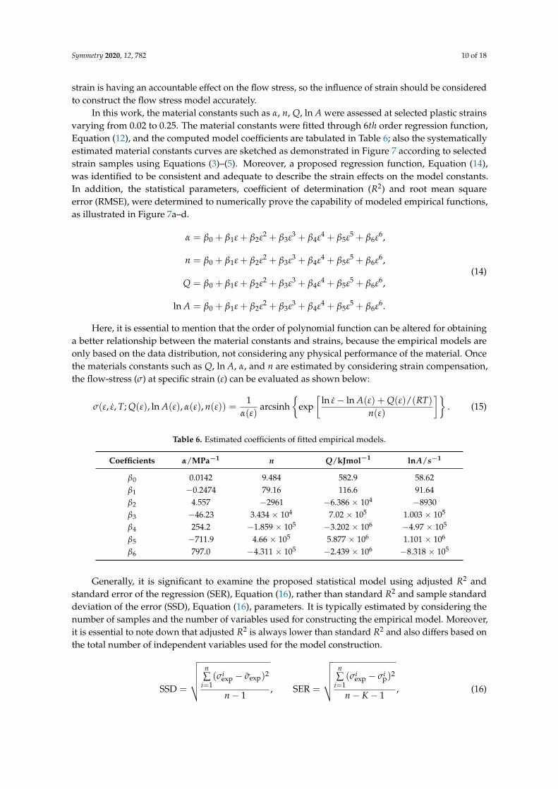
In this work, the material constants such as α, n, Q, ln A were assessed at selected plastic strainsvarying from 0.02 to 0.25. The material constants were fitted through 6th order regression function,Equation (12), and the computed model coefficients are tabulated in Table 6; also the systematicallyestimated material constants curves are sketched as demonstrated in Figure 7 according to selectedstrain samples using Equations (3)–(5). Moreover, a proposed regression function, Equation (14),was identified to be consistent and adequate to describe the strain effects on the model constants.In addition, the statistical parameters, coefficient of determination (R2) and root mean squareerror (RMSE), were determined to numerically prove the capability of modeled empirical functions,as illustrated in Figure 7a–d.

α = β0 + β1ε + β2ε2 + β3ε3 + β4ε4 + β5ε5 + β6ε6,

n = β0 + β1ε + β2ε2 + β3ε3 + β4ε4 + β5ε5 + β6ε6,

Q = β0 + β1ε + β2ε2 + β3ε3 + β4ε4 + β5ε5 + β6ε6,

ln A = β0 + β1ε + β2ε2 + β3ε3 + β4ε4 + β5ε5 + β6ε6.

(14)

Here, it is essential to mention that the order of polynomial function can be altered for obtaininga better relationship between the material constants and strains, because the empirical models areonly based on the data distribution, not considering any physical performance of the material. Oncethe materials constants such as Q, ln A, α, and n are estimated by considering strain compensation,the flow-stress (σ) at specific strain (ε) can be evaluated as shown below:

σ(ε, ε, T; Q(ε), ln A(ε), α(ε), n(ε)) =1

α(ε)arcsinh

{exp

[ln ε− ln A(ε) + Q(ε)/(RT)

n(ε)

]}. (15)

Table 6. Estimated coefficients of fitted empirical models.

Coefficients α/MPa−1 n Q/kJmol−1 lnA/s−1

β0 0.0142 9.484 582.9 58.62β1 −0.2474 79.16 116.6 91.64β2 4.557 −2961 −6.386 × 104 −8930β3 −46.23 3.434 × 104 7.02 × 105 1.003 × 105

β4 254.2 −1.859 × 105 −3.202 × 106 −4.97 × 105

β5 −711.9 4.66 × 105 5.877 × 106 1.101 × 106

β6 797.0 −4.311 × 105 −2.439 × 106 −8.318 × 105

Generally, it is significant to examine the proposed statistical model using adjusted R2 andstandard error of the regression (SER), Equation (16), rather than standard R2 and sample standarddeviation of the error (SSD), Equation (16), parameters. It is typically estimated by considering thenumber of samples and the number of variables used for constructing the empirical model. Moreover,it is essential to note down that adjusted R2 is always lower than standard R2 and also differs based onthe total number of independent variables used for the model construction.

SSD =

√√√√√ n∑

i=1(σi

exp − σexp)2

n− 1, SER =

√√√√√ n∑

i=1(σi

exp − σip)

2

n− K− 1, (16)

Symmetry 2020, 12, 782 11 of 18

Coefficient of residual variation (CRV) =SERσexp

× 100%. (17)

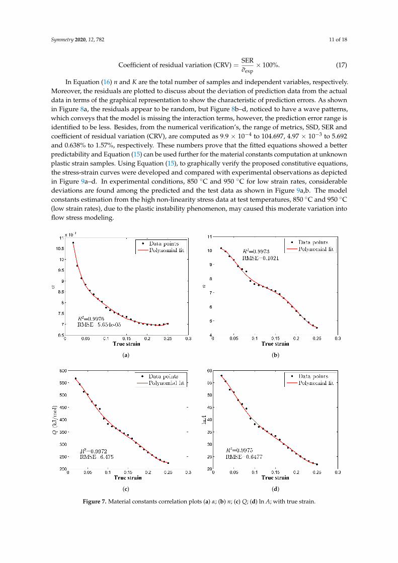
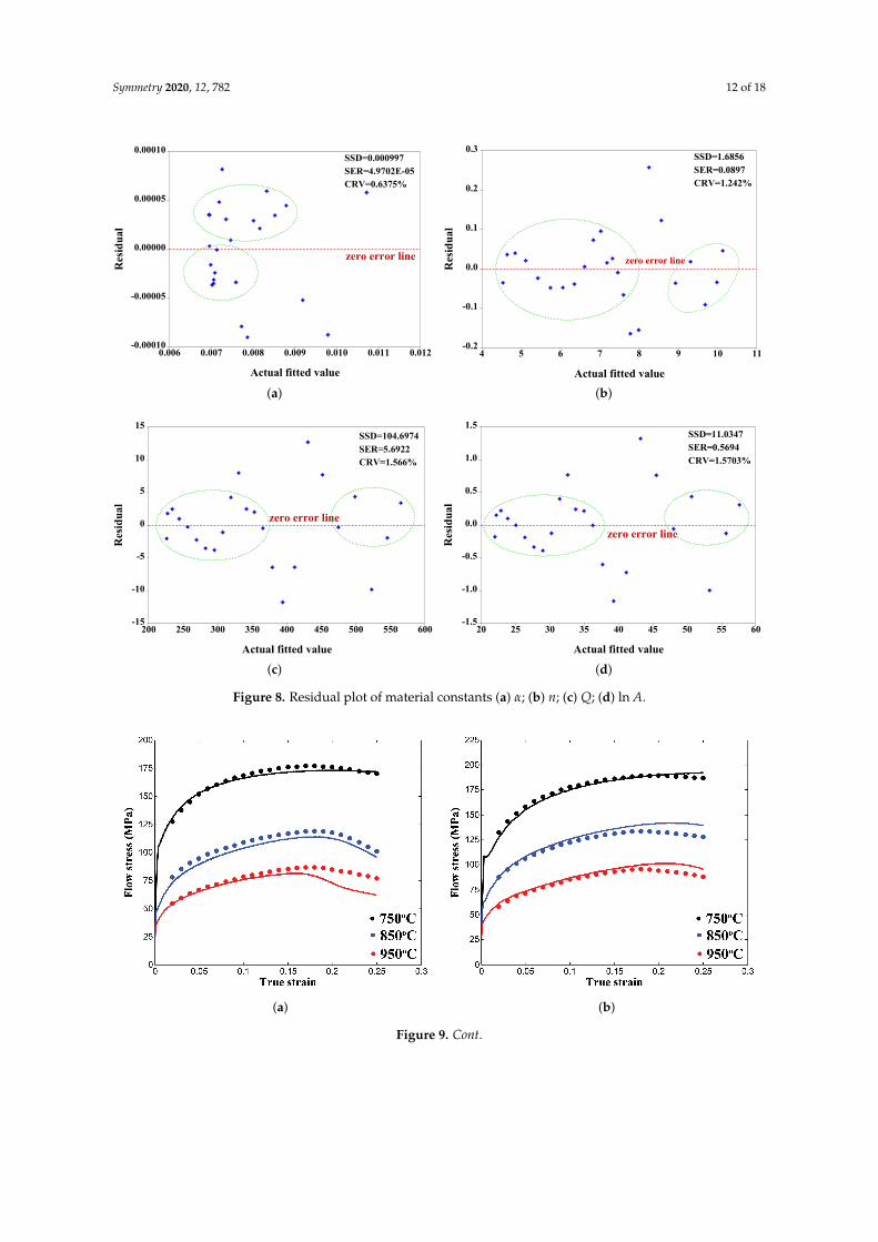
In Equation (16) n and K are the total number of samples and independent variables, respectively.Moreover, the residuals are plotted to discuss about the deviation of prediction data from the actualdata in terms of the graphical representation to show the characteristic of prediction errors. As shownin Figure 8a, the residuals appear to be random, but Figure 8b–d, noticed to have a wave patterns,which conveys that the model is missing the interaction terms, however, the prediction error range isidentified to be less. Besides, from the numerical verification’s, the range of metrics, SSD, SER andcoefficient of residual variation (CRV), are computed as 9.9 × 10−4 to 104.697, 4.97 × 10−3 to 5.692and 0.638% to 1.57%, respectively. These numbers prove that the fitted equations showed a betterpredictability and Equation (15) can be used further for the material constants computation at unknownplastic strain samples. Using Equation (15), to graphically verify the proposed constitutive equations,the stress-strain curves were developed and compared with experimental observations as depictedin Figure 9a–d. In experimental conditions, 850 ◦C and 950 ◦C for low strain rates, considerabledeviations are found among the predicted and the test data as shown in Figure 9a,b. The modelconstants estimation from the high non-linearity stress data at test temperatures, 850 ◦C and 950 ◦C(low strain rates), due to the plastic instability phenomenon, may caused this moderate variation intoflow stress modeling.

(a) (b)

(c) (d)

Figure 7. Material constants correlation plots (a) α; (b) n; (c) Q; (d) ln A; with true strain.

Symmetry 2020, 12, 782 12 of 18

0.0120.0110.0100.0090.0080.0070.006

0.00010

0.00005

0.00000

-0.00005

-0.00010

Actual fitted value

Res

idua

l

zero error line

CRV=0.6375%SER=4.9702E-05SSD=0.000997

(a)

1110987654

0.3

0.2

0.1

0.0

-0.1

-0.2

Actual fitted value

Res

idua

l

zero error line

CRV=1.242%SER=0.0897SSD=1.6856

(b)

600550500450400350300250200

15

10

5

0

-5

-10

-15

Actual fitted value

Res

idua

l

zero error line

CRV=1.566%SER=5.6922SSD=104.6974

(c)

605550454035302520

1.5

1.0

0.5

0.0

-0.5

-1.0

-1.5

Actual fitted value

Res

idua

l

zero error line

CRV=1.5703%SER=0.5694SSD=11.0347

(d)

Figure 8. Residual plot of material constants (a) α; (b) n; (c) Q; (d) ln A.

(a) (b)

Figure 9. Cont.

Symmetry 2020, 12, 782 13 of 18

(c) (d)

Figure 9. Stress-strain curves comparison against the predicted curves from the modified constitutiveequation (a) 0.05 s−1; (b) 0.1 s−1; (c) 0.5 s−1; (d) 1.0 s−1.

5. Constitutive Model Verification

Statistical measurements, such as R2, RMSE, and an average absolute relative error (AARE), areutilized to verify the developed constitutive equations prediction capability at individual strains for enentire test conditions. The first metric—R2 describes how the dependent variables are related to theindependent variables in terms of prediction strength; the higher value is better in terms of quality offit. On the other hand, adjusted R2 explains the model quality based on the number of independentvariables used for the model construction. The second metric, RMSE explains the residual locations likehow the measured data are diffused to the prediction line; e.g., if RMSE quantity is close to 0, it meansthe measured data are scattered alongside the regression line or vice versa. The last metric, AAREused to verify the proposed model against the experimental observations considering a term-by-termprediction error [34,36].

R2 = 1−

n∑

i=1(σi

e − σip)

2

n∑

i=1(σi

e − σe)2, (18)

Adjusted R2 = 1−

n∑

i=1(σi

e−σip)

2

/(n−K−1)n∑

i=1(σi

e−σe)2

/(n−1)

, (19)

RMSE =

√√√√√ n∑

i=1(actuali − predictedi)

2

n, (20)

AARE =1n

n

∑i=1

∣∣∣∣∣σie − σi

p

σie

∣∣∣∣∣× 100%, (21)

where σe, σp, σe are the experimental observations, the predicted stress, and the average stress,respectively. It is most common that R2 adopted to explain the prediction quality of the construtedempirical model. However, the higher value of R2 does not necessarily mean that the model has abetter fit, it may be due to the number of data points in the selected samples [34,36]. Thus, to confirmthe model capability, the graphical validation with systematic comparison was also adopted in thisinvestigation. In this research, to discuss in detail about the prediction strength, an each experimental

Symmetry 2020, 12, 782 14 of 18

conditions were examined individually by computing statistical parameters such as R2 and AARE assummarized in Table 7.

Table 7. Estimated statistical values of the conventional Arrhenius-type constitutive model.

Counts Test Conditions R2 Adj.R2 Overall-R2 AARE (%) Overall-AARE (%)

24 samples 0.05–1.0 s−11023 K 0.9516 0.9511

0.98172.9204

3.67811123 K 0.9406 0.9400 4.25281223 K 0.9427 0.9421 3.8609

As outlined in Table 7, the computed numerical numbers such as R2, 0.9817, and AARE, 3.6781%,proves that the proposed constitutive equation is significantly appropriate to represent the materialbehavior at elevated temperatures; also it is much more suitable for future flow stress predictionat unknown strains. However, from prediction error (AARE), it is identified that there are somedifference among the actual test and estimated data in test conditions, 850 ◦C and 950 ◦C (0.05 s−1

and 0.1 s−1). But somewhat, the disparities are considerably adequate as it shows the significantimprovement in the overall metrics as summarized in Table 7. On the other hand, Krishnan et al. [28]and Lin et al. [35] demonstrated that with appropriate modification of the Z parameter consideringstrain rate compensation, the best prediction for an entire flow stress data can be achieved betweenflow curves. Thus, the modified Z

′parameter with the multiplication factor ε1/3 is [28]

Z′= ε4/3 exp(Q/RT), (22)

σ =1α

ln

(

Z′

A

)1/n

+

(Z′

A

)2/n

+ 1

1/2 , (23)

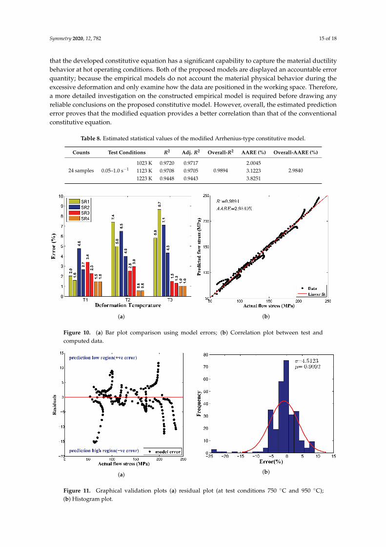
where the material constants α, n, Q and lnA can be estimated from the polynomial equationspresented in Equation (14). In Equation (22), to find out the best modification parameter, by assuminglower (−) and upper (+) value increments from the middle (0) value, ε4/3 was replaced byconsidering three different multiplication factors such as ε4/5, ε9/10 and ε19/20. Using Equation (23),out of these combinations, ε9/10 was found to have a small prediction error, AARE, as 2.9840%,against experimental data. Table 8 displays that the prediction capability was found to be adequateby strain rate compensation in the constitutive equation. Figures 9a–d and 10a are evident thatthe developed flow stress equation showed a better resemblance against the actual test data exceptin the test conditions, 850 ◦C and 950 ◦C at low strain rates. Besides the numerical verification,the graphical methods are developed using the correlation plot, the residual plot, and the histogramplot as depicted in Figures 10b and 11a,b, and Figure 10b is evident that the strong prediction wasobserved against the measured data. Further, from Figure 11a, it is noted that the data distributionin the residual plot exhibits the random pattern, indicating a good fit for the proposed constitutivemodel. In detail, as shown in Figure 11a, the error distributions are found to be quite irregular in bothpositive and negative prediction error regions. Moreover, the residuals exhibit no correlation amongthem; as a result, the proposed constitutive model can not be improved further by the use of any otheradditional main or interaction effect terms and on the other hand, the developed constitutive equationis considered to be significant for the flow stress prediction.

Besides the residual plot, the error values are plotted to represent the data distribution in amore accurate manner using a histogram plot as illustrated in Figure 11b. Figure 11b is morehelpful for understanding about how the residuals are spread out in the space and from Figure 11b,the residuals are identified to fall in a quite acceptable range varies from −8% to 8%. Moreover,from the normal distribution curve, it can be seen that most of the errors fallen inside the rangeof −5% to 5%, and also the area of probability is not too wide. This graphical evidence suggests

Symmetry 2020, 12, 782 15 of 18

that the developed constitutive equation has a significant capability to capture the material ductilitybehavior at hot operating conditions. Both of the proposed models are displayed an accountable errorquantity; because the empirical models do not account the material physical behavior during theexcessive deformation and only examine how the data are positioned in the working space. Therefore,a more detailed investigation on the constructed empirical model is required before drawing anyreliable conclusions on the proposed constitutive model. However, overall, the estimated predictionerror proves that the modified equation provides a better correlation than that of the conventionalconstitutive equation.

Table 8. Estimated statistical values of the modified Arrhenius-type constitutive model.

Counts Test Conditions R2 Adj. R2 Overall-R2 AARE (%) Overall-AARE (%)

24 samples 0.05–1.0 s−11023 K 0.9720 0.9717

0.98942.0045

2.98401123 K 0.9708 0.9705 3.12231223 K 0.9448 0.9443 3.8251

(a) (b)

Figure 10. (a) Bar plot comparison using model errors; (b) Correlation plot between test andcomputed data.

(a) (b)

Figure 11. Graphical validation plots (a) residual plot (at test conditions 750 ◦C and 950 ◦C);(b) Histogram plot.

Symmetry 2020, 12, 782 16 of 18

6. Conclusions

The stress-strain (SS) curves of AISI-1045 steel were investigated to describe the material flowbehavior under hot working conditions. The test conditions such as deformation temperatures andstrain rates are 750–950 ◦C and 0.05–1.0 s−1, respectively. As well as, the temperature dependent surfacemorphology, and elemental identification analysis of AISI-1045 steel were carried out using the FESEMand the EDS mapping setup. The Arrhenius-type constitutive equation was developed by consideringboth influence of strain and strain rate effects on the material constants. A sixth-order regressionfunction was adopted to fit the material constants, and the model adequacies were explained with thehelp of both numerical and graphical validations. Comparison with experimental results proved thatthe material flow behavior could be more precisely captured by the modified constitutive equationthan the traditional constitutive model. In addition, the conventional constitutive model adequacy wasquantified using the statistical parameters and the numerical numbers of R2 and AARE were computedas 0.9817 and 3.6781%, respectively, whereas for the modified constitutive model, the numericalnumbers computed as 0.9894 and 2.9840%, respectively. The statistical parameters reflect the significantprediction capability of the proposed strain rate and strain compensated constitutive model. Besides,the newly proposed model can be used in FE tools for performing numerical simulations under hotworking conditions.

Author Contributions: In this paper, parts such as experiments, mathematical calculations and the originaldraft preparation is done by the authors, M.M. and M.S., PhD scholars, and supervision is carried out by D.W.J.All authors have read and agreed to the published version of the manuscript.

Funding: This research received no external funding.

Conflicts of Interest: The authors declare no conflict of interest.

References

1. Li, C.; Liu, Y.; Tan, Y.; Zhao, F. Hot Deformation Behavior and Constitutive Modeling of H13-Mod Steel.Metals 2018, 8, 846. [CrossRef]

2. Li, H.; Jiao, W.; Feng, H.; Li, X.; Jiang, Z.; Li, G.; Wang, L.; Fan, G.; Han, P. Deformation Characteristic andConstitutive Modeling of 2707 Hyper Duplex Stainless Steel under Hot Compression. Metals 2016, 6, 223.[CrossRef]

3. Liang, Z.; Zhang, Q. Quasi-Static Loading Responses and Constitutive Modeling of Al–Si–Mg alloy. Metals2018, 8, 838. [CrossRef]

4. Lei, B.; Chen, G.; Liu, K.; Wang, X.; Jiang, X.; Pan, J.; Shi, Q. Constitutive Analysis on High-Temperature FlowBehavior of 3Cr-1Si-1Ni Ultra-High Strength Steel for Modeling of Flow Stress. Metals 2019, 9, 42. [CrossRef]

5. Cai, J.; Li, F.; Liu, T.; Chen, B.; He, M. Constitutive equations for elevated temperature flow stress ofTi–6Al–4V alloy considering the effect of strain. Mater. Des. 2011, 32, 1144–1151. [CrossRef]

6. Slooff, F.A.; Zhou, J.; Duszczyk, J.; Katgerman, L. Constitutive analysis of wrought magnesium alloyMg–Al4–Zn1. Scr. Mater. 2007, 57, 759–762. [CrossRef]

7. Ravindranadh, B.; Vemuri, M.; Ashok Kumar, G. Tensile behaviour of aluminium 7017 alloy at varioustemperatures and strain rates. J. Mater. Res. Technol. 2016, 5, 190–197.

8. Gan, C.L.; Zheng, K.H.; Qi, W.J.; Wang, M.J. Constitutive equations for high temperature flow stressprediction of 6063 Al alloy considering compensation of strain. Trans. Nonferrous Met. Soc. China 2014,24, 3486–3491. [CrossRef]

9. Ma, M.-L.; Li, X.-G.; Li, Y.-J.; He, L.-Q.; Zhang, K.; Wang, X.-W.; Chen, L.-F. Establishment and application offlow stress models of Mg-Y-MM-Zr alloy. Trans. Nonferrous Met. Soc. China. 2011, 21, 857–862. [CrossRef]

10. Ren, F.-C.; Chen, J. Modeling Flow Stress of 70Cr3Mo Steel Used for Back-Up Roll During Hot DeformationConsidering Strain Compensation. J. Iron Steel Res. Int. 2013, 20, 118–124. [CrossRef]

11. Chai, R.; Guo, C.; Yu, L. Two flowing stress models for hot deformation of XC45 steel at high temperature.Mater. Sci. Eng. A 2012, 534, 101–110. [CrossRef]

Symmetry 2020, 12, 782 17 of 18

12. Rokni, M.R.; Zarei-Hanzaki, A.; Widener, C.A.; Changizian, P. The Strain-Compensated ConstitutiveEquation for High Temperature Flow Behavior of an Al-Zn-Mg-Cu Alloy. J. Mater. Eng. Perform. 2014,23, 4002–4009. [CrossRef]

13. Murugesan, M.; Jung, D.W. Johnson Cook Material and Failure Model Parameters Estimation of AISI-1045Medium Carbon Steel for Metal Forming Applications. Materials 2019, 12, 609. [CrossRef] [PubMed]

14. Murugesan, M.; Jung, D.W. Two flow stress models for describing hot deformation behavior of AISI-1045medium carbon steel at elevated temperatures. Heliyon 2019, 5, e01347. [CrossRef]

15. Mirzadeh, H.; Najafizadeh, A. Flow stress prediction at hot working conditions. Mater. Sci. Eng. A 2010,527, 1160–1164. [CrossRef]

16. Yang, L.; Pan, Y.; Chen, I.; Lin, D. Constitutive Relationship Modeling and Characterization of Flow Behaviorunder Hot Working for Fe–Cr–Ni–W–Cu–Co Super-Austenitic Stainless Steel. Metal 2015, 5, 1717–1731.[CrossRef]

17. Quan, G.; Lv, W.; Mao, Y.; Zhang, Y.; Zhou, J. Prediction of flow stress in a wide temperature range involvingphase transformation for as-cast Ti–6Al–2Zr–1Mo–1V alloy by artificial neural network. Mater. Des. 2013,50, 51–61. [CrossRef]

18. Sun, M.; Hao, L.; Li, S.; Li, D.; Li, Y. Modeling flow stress constitutive behavior of SA508-3 steel for nuclearreactor pressure vessels. J. Nucl. Mater. 2011, 418, 269–280. [CrossRef]

19. Abbasi-Bani, A.; Zarei-Hanzaki, A.; Pishbin, M.H.; Haghdadi, N. A comparative study on the capabilityof Johnson–Cook and Arrhenius-type constitutive equations to describe the flow behavior of Mg–6Al–1Znalloy. Mech. Mater. 2014, 71, 52–61. [CrossRef]

20. He, A.; Xie, G.; Zhang, H.; Wang, X. A comparative study on Johnson–Cook, modified Johnson-Cookand Arrhenius-type constitutive models to predict the high temperature flow stress in 20CrMo alloy steel.Mater. Des. 2013, 52, 677–685. [CrossRef]

21. Han, Y.; Qiao, G.; Sun, J.P.; Zou, D. A comparative study on constitutive relationship of as-cast 904L austeniticstainless steel during hot deformation based on Arrhenius-type and artificial neural network models. Comput.Mater. Sci. 2013, 67, 93–103. [CrossRef]

22. Senthilkumar, V.; Balaji, A.; Arulkirubakaran, D. Application of constitutive and neural network models forprediction of high temperature flow behavior of Al/Mg based nanocomposite. Trans. Nonferrous Met. Soc.China 2013, 23, 1737–1750. [CrossRef]

23. Samantaray, D.; Mandal, S.; Bhaduri, A.K. A comparative study on Johnson Cook, modifiedZerilli–Armstrong and Arrhenius-type constitutive models to predict elevated temperature flow behaviourin modified 9Cr–1Mo steel. Comput. Mater. Sci. 2009, 47, 568–576. [CrossRef]

24. Lin, Y.C.; Chen, M.S.; Zhang, J. Modeling of flow stress of 42CrMo steel under hot compression. Mater. Sci.Eng. A 2009, 499, 88–92. [CrossRef]

25. Wu, R.H.; Liu, J.T.; Chang, H.B.; Hsu, T.Y.; Ruan, X.Y. Prediction of the flow stress of0.4C–1.9Cr–1.5Mn–1.0Ni–0.2Mo steel during hot deformation. J. Mater. Process. Technol. 2001, 24, 211–218.[CrossRef]

26. Xiao, X.; Liu, G.Q.; Hu. B.F.; Zheng, X.; Wang, L.N.; Chen, S.J.; Ullah, A. A comparative study onArrhenius-type constitutive equations and artificial neural network model to predict high-temperaturedeformation behaviour in 12Cr3WV steel. Comput. Mater. Sci. 2012, 62, 227–234. [CrossRef]

27. Mandal, S.; Rakesh, V.; Sivaprasad, P.V.; Venugopal, S.; Kasiviswanathan, K.V. Constitutive equations topredict high temperature flow stress in a Ti-modified austenitic stainless steel. Mater. Sci. Eng. A 2009,500, 114–121. [CrossRef]

28. Krishnan, S.A.; Phaniraj, C.; Ravishankar, C.; Bhaduri, A.K.; Sivaprasad, P.V. Prediction of high temperatureflow stress in 9Cr-1Mo ferritic steel during hot compression. Int. J. Press. Vessels Pip. 2011, 88, 501–506.[CrossRef]

29. Murugesan, M.; Sajjad, M.; Jung, D.W. Hybrid Machine Learning Optimization Approach to Predict HotDeformation Behavior of Medium Carbon Steel Material. Metal 2019, 9, 1315. [CrossRef]

30. Lee, K.; Murugesan, M.; Lee, S.M.; Kang, B.S. A Comparative Study on Arrhenius-Type Constitutive Modelswith Regression Methods. Trans. Mater. Process. 2017, 26, 18–27. [CrossRef]

31. Ren, F.Z.; Zhang, J.T.; Gao, Q.R.; Zhu, Y.M.; Su, J.H. Constitutive Equation of Mg-3.5Zn-0.6Y-0.5Zr Alloyunder Hot Compression Deformation. Adv. Mater. Res. 2013, 800, 271–275. [CrossRef]

Symmetry 2020, 12, 782 18 of 18

32. Zhang, Y.; Fan, Q.; Zhang, X.; Zhou, Z.; Xia, Z.; Qian, Z. Avrami Kinetic-Based Constitutive Relationship forArmco-Type Pure Iron in Hot Deformation. Metals 2019, 9, 365. [CrossRef]

33. Yonghua, D.; Lishi, M.; Huarong, Q.; Runyue, L.; Ping, L. Developed constitutive models, processing mapsand microstructural evolution of Pb-Mg-10Al-0.5B alloy. Mater. Charact. 2017, 129, 353–366.

34. Murugesan, M.; Kang, B.S.; Lee, K. Multi-Objective Design Optimization of Composite Stiffened PanelUsing Response Surface Methodology. J. Compos. Res. 2015, 28, 297–310. [CrossRef]

35. Lin, Y.C.; Chen, M.S.; Zhong, J. Constitutive Modeling for Elevated Temperature Flow Behavior of 42CrMoSteel. Comput. Mater. Sci. 2007, 42, 470–477. [CrossRef]

36. Rezaei Ashtiani, H.R.; Shahsavari, P. A comparative study on the phenomenological and artificial neuralnetwork models to predict hot deformation behavior of AlCuMgPb alloy. J. Alloys Compd. 2016, 687, 263–273.[CrossRef]

c© 2020 by the authors. Licensee MDPI, Basel, Switzerland. This article is an open accessarticle distributed under the terms and conditions of the Creative Commons Attribution(CC BY) license (http://creativecommons.org/licenses/by/4.0/).