Mergers, Brand Competition, and the Price of aPint

by

Joris Pinkse and Margaret E. Slade

Department of Economics

University of British Columbia

Vancouver, BC V6T 1Z1

CanadaEmail: slade@econ.ubc.ca

June 2000

Abstract:

Mergers in the UK brewing industry in the last decade have reduced the number ofnational brewers from six to four. The number of brands, in contrast, has remainedrelatively constant. We analyze the effects of the mergers on brand competition andpricing. Brand–level demand equations are estimated from a panel that includes alldraft beers that accounted for at least 1/2% of local markets. We model brand–substitution possibilities in a very flexible way. In particular, we estimate the matrixof cross–price elasticities nonparametrically. We use the estimated demand equationsto assess the strength of brand competition along various dimensions, and we evaluatethe effects of the mergers by computing equilibria of pricing games with differentnumbers of players.

Journal of Economic Literature classification numbers: L13, L41, L66, L81

Keywords: Beer, mergers, brand competition, differentiated products, market con-duct, semiparametric estimation, instrumental variables.

This research was supported by grants from the Social Sciences and Humanities Re-search Council of Canada. We would like to thank the following people for thoughtfulcomments: Aviv Nevo and seminar participants at the ES meetings in Boston andthe universities of Oxford and Paris I.

1 Introduction

Historically, the brewing industry in the UK developed in a very different fashion fromthose in, for example, the US, Canada, and France, which were dominated by a fewlarge brewers that sold rather homogeneous national brands of lagers. Indeed, the UKindustry, which was relatively unconcentrated, produced a large variety of ales, andregional variation in product offerings was substantial. Moreover, national advertisingplayed a less important role than in many other countries. In the last decade, however,there have been a succession of successful mergers that have increased concentrationin brewing, as well as proposed mergers that, if successful, would have added to thattrend.1 It is thus natural to ask how those mergers have changed both product pricingand product offerings. In particular, the mergers could have resulted in higher prices,a reduction in the number of brands produced, an increase in brand uniformity, and amove towards competition through national advertising rather than through productdifferences.

In this paper, we use panel data on all brands of beer that constitute at leastone half of one percent of a regional market to evaluate the mergers. We estimatedemand equations for brands of draft beers sold in two regions of the country (GreaterLondon and Anglia) in two bimonthly time periods (Aug/Sept and Oct/Nov 1995) andin two types of public houses (multiples and independents). We model substitutionpossibilities among brands using a technique that was developed in Pinkse, Slade,and Brett (1998) to deal with differentiated products.2 In particular, we estimatethe matrix of cross–price elasticities nonparametrically as a function of a number ofmeasures of the distance between brands in product–characteristic space. We thenuse our estimated demand equations, together with engineering data on costs, toevaluate the game that the brewers are engaged in. Finally, we evaluate the effects ofthe mergers on prices by solving for the equilibria of games with different numbers ofplayers. In other words, we undo a merger by allowing the prices of the merged brandsto be chosen by two separate players that correspond to the pre–merger configuration,and we assess proposed mergers by performing the reverse exercise — by allowing asingle player to choose the prices of all brands brewed by the merger partners.

The organization of the paper is as follows. In the next section, we set the stageby describing the structure of the UK brewing industry and contrasting it with thesituation that prevails in other countries. We also look at recent decisions of the UKMonopolies and Mergers Commission (MMC) that have affected the structure of theindustry. These include the ‘Beer Orders’ of 1989 that changed the structure of thedownstream or retailing sector, as well as decisions involving mergers in the upstreamor brewing sector.

1Courage and Grand Met merged to form Courage, Allied Lyons and Carlsberg merged to formCarlsberg–Tetley, and the merged Courage merged with Scottish & Newcastle to form ScottishCourage. In addition, a merger between Bass and Carlsberg–Tetley was attempted, which wouldhave further reduced the number of national brewers to three.

2The application in that paper involves products that are differentiated in geographic space,whereas the application in this paper involves differentiation in product–characteristic space.

1

Section 3 contains a brief review of the literature that attempts to model differ-entiated products both theoretically and empirically. It also contrasts our method ofassessing the demand for branded products with those that are commonly used byother researchers.

Section 4 presents our model of the demand for brands by heterogeneous individuals.3

Each consumer has an ideosyncratic utility function, which we approximate with afunctional form that has two important characteristics: it places no restrictions onbrand substitution possibilities, and it satisfies the restrictions that are required forexact aggregation across individuals. Demands for brands are obtained by partiallydifferentiating the aggregate utility function with respect to prices. We allow eachcross–price elasticity in the resulting system of demand equations to depend on anumber of measures of the distance between brands in product–characteristic space,and we estimate the functional form of that dependence. Finally, we discuss how onecan use the estimated demand equations to evaluate the game that the brewers play.

Section 5 discusses our estimation technique. We use a series expansion to approxi-mate the function of the distance measures that determines the cross–price elasticities.Furthermore, since the prices of all brands are, at least potentially, jointly determinedand thus endogenous, we use an instrumental–variables semiparametric technique.

Section 6 presents the data and discusses our choice of measures of distance inproduct–characteristic space, whereas sections 7 and 8 contain our econometric esti-mates of demand and our assessment of equilibrium in the market. Finally, section 9discusses solutions to the merger games. To anticipate, we fail to reject a Bertrand–pricing game among the brewers. Furthermore, we find that the Scottish–Couragemerger had little effect on prices, whereas a merger between Bass and Carlsberg–Tetley would have resulted in more substantial price increases.

2 The UK Beer Market

2.1 International Comparisons

Although beer markets have certain features in common across countries, cross–country differences are also striking. To get a feel for the UK industry, it is thereforeuseful to begin with international comparisons. Table 1 summarizes some of thedifferences between the UK, US, Canada, France, and Germany.

The first part of table 1 shows that, when it comes to beer consumption per headand the fraction of beer sales that originate abroad, the UK lies between France andGermany, with Germany having higher per capita consumption and France relyingmore heavily on imports. Consumers in the US and Canada, who are similar to eachother, drink less beer per capita and consume fewer imports than their counterparts inthe UK. Finally, over time, per capita beer consumption has fallen in most countries,whereas imports have risen.

3This section differs from Pinkse, Slade, and Brett (1998), where derived rather than consumerdemand is assessed.

2

Whereas the UK is not an outlier with respect to the statistics contained in table1A, it is clearly different from the other countries with respect to the ratio of draft tototal beer sales, as can be seen in table 1B. Indeed, draft sales in the UK accountedfor almost three times the comparable percentages in France and Germany and aboutsix times the percentages in North America. In all countries, however, draft’s fractionhas fallen, as more beer has been consumed at home. Table 1B also shows that UKbeers are of lower strength than those from the other countries, which is due to thefact that more ale and less lager is consumed, and lagers tend to be stronger.

Turning to production, table 1C compares one important aspect of the industry —its concentration, or lack thereof, into the hands of a small number of brewers.4 TheUK industry is clearly less concentrated than its counterparts in the US, Canada, andFrance, where beer tends to be mass produced. Production in Germany, in contrast,where specialty beers predominate, is much less concentrated. It thus seems thatbrand heterogeneity and an unconcentrated brewing sector go hand in hand.

2.2 The UK Industry

The UK beer industry has undergone substantial changes in both production andconsumption in the last few decades, some of which are summarized in table 2. Beerscan be divided into three broad categories: ales, stouts, and lagers. Although UKconsumers have traditionally preferred ales to lagers, the consumption of lager hasincreased at a steady pace. Indeed, from less than 1% of the market in 1960 (notshown in the table), lager became the most popular drink in 1990, with sales exceed-ing the sum of ale and stout, and its popularity continues to grow. Most UK lagersbear the names of familiar non–British beers such as Budweiser, Fosters, and Kro-nenbourg. Almost all, however, are brewed under license in the UK and are thereforenot considered imports.

A second important aspect of beer consumption is the popularity of ‘real’ or cask–conditioned ale. Real products are alive and undergo a second fermentation in thecask, whereas keg and tank products are sterilized. The statistics in table 2, however,which show real ale’s market share increasing, must be interpreted with caution sincethey show percentages of the ale market. As a percentage of the total beer market,which includes lager, real products have lost ground.

The final trend in consumption is the decline in on–premise sales. On–premiseconsumption includes sales in bars, hotels, and clubs, whereas off–premise consump-tion refers to beer that is purchased in a store and consumed at home, out of doors,or in nonlicensed establishments. Clearly, draft sales are a subset of on–premiseconsumption, since some packaged products are consumed in licensed establishments.

With respect to production, table 2 shows that the number of brewers has de-clined steadily. Indeed, in 1900, there were nearly 1,500 brewery companies (notshown in the table), but this number fell during the century and is currently aboutsixty. However, in addition to incorporated brewers, there are approximately 200

4With the exception of Germany, the table shows three–firm concentration ratios. Any otherconcentration measure, however, would tell the same story.

3

microbreweries operating at very small scales. In fact, most brewers are small, andfew produce products that account for more then 1/2% of local markets.5

This snapshot of the UK beer industry shows significant changes in tastes andconsumption habits as well as a decline in the number of companies that cater tothose tastes. Nevertheless, as we have seen, compared to many other countries, theUK brewing sector was only moderately concentrated. Recent developments in theindustry, however, have resulted in substantial changes in ownership patterns.

2.3 Public Policy Towards the UK Beer Industry

It is not unusual for the beer industry to attract the attention of politicians and civilservants. Government involvement in the industry stems from four concerns: thesocial consequences of alcohol consumption, the revenue obtained from alcohol sales,the level of concentration in the brewing sector, and the extent of brewer control overretailing. In recent years, moreover, public scrutiny of the industry has accelerated.Indeed, there have been over thirty reviews by UK and European Union authoritiessince the 1960s. Many of those investigations were triggered by proposed mergers inthe industry. Several, however, were more general assessments of prices, profits, andtied sales.6

For our analysis, four mergers, three actual and one proposed, are of primaryinterest. These are the successful mergers between Courage and Grand Metropolitan(Grand Met) in 1990, Allied Lyons and Carlsberg in 1992, and Courage and Scottish& Newcastle (S&N) in 1995, and the proposed merger between Bass and Carlsberg–Tetley (CT) that was denied in 1997. It is difficult to discuss the positions taken bythe Monopolies and Mergers Commission (MMC) and Office of Fair Trading (OFT)with respect to the mergers, however, without a brief discussion of their views on thelinks between brewers and their retail outlets.

2.3.1 The Beer Orders

Prior to the late 1980s, a large fraction of UK public houses (pubs) were ownedby brewers and operated under exclusive–purchasing agreements (ties) that limitedthe pubs to selling brands that were produced by their affiliated brewer.7 Publicofficials have long been concerned that those tying arrangements would somehowextend the market power that they perceived in the upstream or brewing sector tothe downstream or retailing sector. Absent the system of ties, they believed thatretailing would be competitive.

In the late 1980’s, the OFT requested the MMC to undertake a major industryreview. The product of that investigation was the 500–page MMC report entitled

5In the greater London area, there are only 10 companies that produce brands whose sales areas large as 1/2%, whereas in Anglia the comparable number is 9.

6For an analysis of tied sales in the UK brewing sector, see Slade (1998).7Such tying arrangements are illegal in the US. See Slade (1999) for a discussion of the legal

differences.

4

“The Supply of Beer,” which appeared in February of 1989. The MMC recommendedmeasures that eventually led brewers to divest themselves of 14,000 public houses.The Commission claimed that their recommendations would lower retail prices andincrease consumer choice. There has been considerable doubt, however, that theirobjectives were achieved. Indeed, after divestiture, retail beer prices actually rose(Slade 1998).

The MMC report is unclear about the economic reasoning that led to the decisionto force divestiture. Nevertheless, the MMC alleged that, due to high concentration,the brewers possessed market power and their involvment in retailing protected thatpower.

2.3.2 The Mergers

After the Beer Orders, the brewing industry became more concentrated. Increasesin brewing–market concentration were due to mergers, which the MMC allowed, aswell as to the fact that some firms (e.g. Boddingtons) ceased brewing, whereas others(e.g. Courage) ceased retailing. Nevertheless, the MMC continues to favor recom-mendations that focus on the retail sector and the vertical linkages between brewersand public houses, in spite of their claim that the source of monopoly power lies inbrewing. The discussion below illustrates the position that the MMC has taken.

The Courage/Grand Met Merger: The merger between Courage and Grand Metthat occurred in 1990, just after the Beer Orders were passed, reduced the number ofnational brewers from six to five.8 This event was complex. However, the details areunimportant. Briefly, Grand Met sold its brewing interests to Courage and ceasedoperating in the upstream market, whereas Courage sold its public houses to GrandMet and ceased operating in the downstream market.9 In addition, Courage was givenan exclusive contract to supply Grand Met’s pubs. At the time of the merger, GrandMet controlled 11% of the beer market, whereas Courage controlled 9%. The mergertransformed Courage into the second largest producer, just behind Bass, which had amarket share of 22%. Nevertheless, three of the four MMC recommendations involvedthe tied estate rather than increases in brewing concentration per se.

The Allied Lyons/Carlsberg Joint Venture: In 1992, Allied Lyons, a British foodcompany that owned breweries, formed a joint venture with Carlsberg, a Danishbrewer. Their combined brewing assets, which were renamed Carlsberg–Tetley, be-came jointly owned by the two parents. At the time of the joint venture, Allied Lyonscontrolled 12% of the beer market, whereas Carlsberg controlled 4%. Their sharesof the lager market, however, were higher, with 8 and 13%, respectively. The jointventure became the third largest brewer, behind Bass and Courage. The numberof national brewers, however, was unchanged, since Carlsberg was not one of them.

8Courage is itself owned by Fosters, an Australian company.9More precisely, some of the former public houses of both Courage and Grant Met became jointly

owned by Grand Met and Elders, whereas others became owned by Inntrepreneur, which was in turnowned by Grant Met and Courage and managed by Grand Met.

5

The MMC was principally concerned with the fact that Carlsberg was one of a veryfew brewers without a tied estate.10 Indeed, prior to the merger, over half of Carls-berg’s sales went to Courage and S&N. As a consequence, all three of the MMC’srecommendations involved vertical linkages between CT and the retail sector.

The Courage S&N Merger: In 1995, the merged firm Courage merged again withScottish & Newcastle. This event, which reduced the number of national brewersfrom five to four, created the largest brewer in the UK. The combined firm, with amarket share of 28%, was substantially larger than Bass, which had a market shareof 23% and thus dropped from number one to two. In spite of the fact that themajority of the groups that were asked to comment on the merger favored a fullinvestigation by the MMC, the OFT did not refer the matter to the MMC. Instead,it allowed the merger to proceed subject to a number of undertakings, all of whichinvolved the tied estate.11 The OFT rejected the idea of divestiture of breweries orbrands but instead favored “the alternative remedy that has generally been adoptedfollowing previous references ... to weaken the extent of vertical links with the mergedcompany.” (DGFT, 1995, p.3).

The Bass/CT Merger: The fourth and largest merger was proposed in 1997 but notconsummated. This involved the numbers two and three brewers, Bass and Carlsberg–Tetley, and would have created a new firm, BCT, with an overall market share of 37%.Moreover, it would have further reduced the number of national brewers from four tothree. At the time, Bass controlled 23% of the beer market, CT controlled 14%, andScottish Courage, which would have become the second largest firm, had a marketshare of 28%. The MMC estimated that, after the merger, the Hirshman/Herfindahlindex of concentration (HHI) would rise from 1,678 to 2,332. Furthermore, it notedthat the US Department of Justice’s 1992 Merger Guidelines specify that a mergershould raise concerns about competition if the post–merger HHI is over 1,800 and thechange in the HHI is at least 50 points. Nevertheless, the MMC recommended that themerger be allowed to go forward.12 We quote from their recommendations to illustratetheir concern with vertical linkages at the expense of horizontal concentration.

The proposed merger would lead to some net efficiency gains which would

not be achieved in the absence of the merger. But in our judgment these

benefits would not be sufficient to outweigh the adverse effects we have

identified. The majority of us believe that it is possible to remedy the ad-

verse effects of the proposed merger with measures designed to counteract

the increase in Bass’s market power. To that end we recommend a pack-

10Brewers without tied estates are not vertically integrated into retailing and have no exclusive–purchasing agreements.

11After the earlier merger with Allied Lyons, unlike S&N, Courage did not have a tied estate.Nevertheless, it had exclusive–supply contracts with Inntrepreneur (see footnotenote 9).

12The one economist on the Commission, David Newbery, wrote a dissenting opinion.

6

age of remedies involving a reduction in the number of Bass’s tied houses

to a maximum of 2,500 (MMC 1997, p. 3).

In spite of the MMC’s favorable recommendation, the BCT merger was not con-summated because the president of the Board of Trade did not accept the MMC’sadvice.

Table 3 summarizes the market shares of each firm before and after each merger.One can see that, a few years after a merger, the merged firm’s market share is lessthan the sum of the premerged shares, which could mean that increased efficiencydoes not overwhelm increased market power. Figure 1 shows the chronology of theimportant merger events in the industry.

3 Related Literature

3.1 Theoretical Models of Differentiated–Products

In any market where price is posted and transactions occur at posted prices, priceis the obvious strategic variable. Most retail markets fit this description. Thereare, however, many varieties of pricing games, and each is associated with a set ofpredictions about the structure of the market and the nature of the rivalry withinthat market.

With one–dimensional–spatial models, whether linear (Hotelling 1929), circular(Salop 1979), or vertical (Gabszewicz and Thisse 1979), each firm competes directlyonly with its two neighbors, one on either side. In other words, conditional on neighborprices, fluctuations in prices of more distant competitors have no effect on own sales.13

In equilibrium, however, prices of more distant competitors can have an indirect effectwhen they cause changes at neighboring locations.

In direct contrast to spatial models, where competition is local, models of monop-olistic competition in the spirit of Chamberlin (1933) (e.g., Spence 1976 and Dixitand Stiglitz 1977) are based on the notion that competition is not only global butalso symmetric.14 Indeed, sales and profits depend only on the distribution of rivalprices and not on the identities or locations of the firms that post those prices.

A number of models of differentiated products lie somewhere in between thesetwo extremes. For example, with the characteristics approach to demand (Lancaster1966, Baumol 1967, and Gorman 1980) products compete along several dimensions.Moreover, as the number of dimensions increases, so does the number of neighbors.15

13This assumes that there is no mill–price undercutting (see Eaton and Lipsey 1976).14We use the term global competition to describe a situation where all cross–price elasticities are

positive but need not be equal. With local competition, in contrast, most cross–price elasticities arezero a priori.

15For example, Archibald and Rosenbluth (1975) show that when the dimension of the character-istic space is three, firms have on average six neighbors. With four or more dimenions, however, thenumber of neighbors depends only on the number of firms and is independent of the dimension of

7

Researchers have also investigated classes of preferences that give rise to the twoextremes as special cases (e.g. the rank–ordering model of Deneckere and Rothschild(1992) and the symmetric/circle model of Anderson and de Palma (2000)).

When evaluating a merger, it is important to locate the industry on the global/localspectrum. Indeed, markets where competition is global tend to be more competitivethan markets where rivalry is local. This is true because, in a global market, all prod-ucts compete with all others, whereas in a local market, firms have protected marketniches. Moreover, when competition is symmetric, the identities of the merging firmsare unimportant and only their market shares matter. With local competition, incontrast, the characteristics of the products that each firm produces are crucial indetermining the effect of the merger on prices.

3.2 Empirical Models of Differentiated Products

When products are homogenous, only total supply matters, and a single price prevailsin the market. There is therefore only one price elasticity of demand to estimate.When products are differentiated, in contrast, the situation is more complex from aneconometric point of view. Indeed, suppose that there are n brands of a differentiatedproducts where n is large. The data, however, consist of a single cross section or ashort panel. In order to estimate the n2 cross–price elasticities, considerable structuremust be imposed on the problem. The choice of structure to impose differentiates thevarious studies.

Most empirical studies of markets in which products are differentiated are cast in adiscrete–choice framework. This means that individuals purchase at most one unit oftheir most preferred brand.16 Within this framework, there are two commonly usedclasses of models: a global random–utility model in which each product competeswith every other, albeit with varying intensity, and a local spatial model in whichmost cross–price elasticities are assumed to be zero.

A typical random–utility model makes use of a utility function that is linear inproduct characteristics, product price, and an ideosyncratic term that is often as-sumed to have an extreme–value distribution. Aggregation of individual demandsis accomplished by integrating over this distribution. If individual draws from thedistribution are independent and identically distributed, one has a multinomial logit,which places severe restrictions on substitution possibilities. Indeed, the i.i.d. as-sumption imposes symmetry a priori. If, in contrast, consumer tastes are allowed tobe correlated across products in a restricted fashion that involves a priori productgroupings, one has a nested multinomial logit (NML) that is somewhat more flexible.Finally, if the coefficients of the product–characteristic variables are allowed to varymore generally, one has a random–coefficients model that allows for quite general

the characteristic space.16A large fraction of the empirical papers deals with the automobile market (e.g. Bresnahan 1981

and 1987, Berry, Levinsohn, and Pakes 1995, Feenstra and Levinsohn 1995, Goldberg 1995, Verboven1996, Fershtman and Gandal 1998, and Petrin 1998), where this assumption is reasonable.

8

patterns of substitution.17

Highly localized spatial models are less common than random–utility models, andwe discuss only two. Bresnahan (1981 and 1987) estimates a model of vertical productdifferentiation with a single parameter that captures quality differences. With hismodel, products compete directly only with their two nearest neighbors, one of higherand the other of lower quality. Feenstra and Levinsohn (1995), in contrast, allow formultiple dimensions of diversity and compute endogenous market boundaries in thislarger space. They do this by assuming that the transport–cost (or utility–loss)function is quadratic in m–dimensional Euclidean space, where m is the number ofcharacteristics. With both models, products that do not share a market boundary donot compete directly (i.e., their cross–price elasticities are zero).

Empirical models that allow for variety in consumption of a non–random sort areless common in the differentiated–products literature. A recent study by Hausman,Leonard, and Zona (1995), however, is based on the notion that consumers can, andoften do, purchase several varieties or brands. These authors consider a multi–stagebudgeting problem, where consumers first decide how much of the product (beer)to consume, then decide which product types to purchase (e.g. premium, regular,or light), and finally select individual brands. The structure of their model, whichinvolves a priori product groups, is thus similar to a NML. Substitution possibilitieswithin groups, however, are more flexible than with a NML, but the number of brandsthat can be included in each group is smaller.

Empirical models of differentiated products have been used to assess many practi-cal economic issues, including the effects of mergers. For example, Werden and Froeb(1994) use a logit demand model to evaluate mergers among US long–distance carriers,Hausman, Leonard and Zona (1994) use an ‘almost ideal demand system’ to evaluatemergers in the US brewing industry, and Nevo (1997a) uses a random–coefficientsmodel to evaluate mergers in the US ready–to–eat breakfast–cereal industry. .

In the next sections we develop a model in which individuals, who have a taste fordiversity, purchase variable amounts of one or more brands of a differentiated prod-uct. We make no distributional assumptions; instead, we impose the conditions thatare required for exact aggregation, and we model unobserved heterogeneity nonpara-metrically. Our method can handle endogenous prices and measurement error in astraight–forward fashion through the use of instrumental variables. Furthermore, ourframework nests global and local models. Nesting is accomplished through the use ofseveral notions of distance, or its inverse closeness. Some of those measures allow thestrength of competition to decay gradually with distance and are thus global, whereasothers are discrete or local.

17Examples of the use of a NML include Goldberg (1995), Verboven (1996), and Fershtman andGandal (1998). Bresnahan, Stern, and Trajtenberg (1997) estimate a generalized extreme valuemodel that is not hierarchical. Finally, Berry, Levinsohn, and Pakes (1995), Nevo (1997a and b),Davis (1997), and Petrin (1998) estimate random–coefficients models. For a more comprehensivediscussion of these models, see Berry (1994).

9

4 The Beer Brands Model

In Pinkse, Slade, and Brett (1998), we develop an empirical method that can be usedto locate real–world markets on the global/local spectrum. We consider the casewhere buyers are downstream firms and start with the their individual demands. Wethen aggregate their choices into upstream–firm demands for each product. Here, weextend that model to encompass buyers that are individuals. The principal differ-ence is that, whereas there are no restrictions that must be satisfied for consistentaggregation of competitive profit functions, consistent aggregation of utility functionsrequires additional assumptions.

We consider a situation where heterogeneous individuals consume varying amountsof the brands of a differentiated product. In addition, it is possible that some individ-uals consume no brand of this product. All other commodities are aggregated into anoutside good that all individuals consume. The market for the differentiated productis assumed to be imperfectly competitive, whereas the outside good is competitivelysupplied. In what follows, the demand and cost sides of the market are described andequilibria of pricing games are discussed.

4.1 Demand

Suppose that there are n brands of a differentiated product, each of which is producedby one of K firms.18 No two brands are identical. Let pi be the nominal price of theith brand, i = 1, . . . , n. There is also an outside good that is sold at a nominal pricep0.

The hth individual consumes a vector qh = (q1h, . . . , qnh)T of the differentiated

product, with qih ≥ 0, i = 1, . . . , n, and q0h of the outside good, with q0h > 0, h =1, . . . , H. Furthermore, this individual has nominal income yH and indirect–utilityfunction uh(p0, p, yh), where p = (p1, . . . , pn)T . By Roy’s theorem, individual demandsfor the differentiated product are

qih =∂uh/∂pi−∂uh/∂yh

. (1)

Not knowing the functional form of uh, we approximate it with a flexible func-tional form. We choose a normalized quadratic (Berndt, Fuss, and Waverman 1977and McFadden 1978), where prices and incomes are normalized or divided by p0.Specifically, uh(p0, p, yh) ≈ p0uh(1, p, yh), where p = p−1

0 p, yh = p−10 yh,

uh(1, p, yh) = −[a0h + aThp− p0yh(γ0 + γTp) +

p0

2pTBhp

], (2)

and each Bh is an arbitrary n× n symmetric, negative–semidefinite matrix.Equation (2) is flexible in prices. In other words, it places no restrictions on the

matrix of elasticities of substitution between brands of the differentiated product.Moreover, each individual occupies a different location in taste space and thus has a

18Firms can produce more than one brand, but no brand is produced by more than one firm.

10

different set of substitution patterns. Finally, the utility function is in Gorman polarform and can therefore be aggregated to obtain brand–level demands.19

Using (1) and (2), individual demands are

qih =aih +

∑j bijhpj − γiyh

p0(γ0 + γTp). (3)

In equation (3), p0(γ0 + γTp) = γ0p0 + γT p is a price index that can, without loss ofgenerality, be set equal to one in a cross section or very short time series. After thisnormalization, aggregate product demands become

qi =∑h

aih +∑j

(∑h

bijh

)pj − γi

(∑h

yh

)= ai +

∑j

bijpj − γiy, (4)

where ai =∑h aih, bij =

∑h bijh, and y =

∑h yh is aggregate income.

Unfortunately, it is not possible to estimate the parameters of (4) from a singlecross section or short panel of n brands.20 It is therefore necessary to place somestructure on the parameters, which we do as follows. Following Pinkse, Slade, andBrett (1998), we assume that ai, which determines the size of brand i’s market,and bii, which determines the own–price elasticity, depend on brand and regionalcharacteristics and time–period dummies.21 For example, when the product is beer,the product characteristics might be the brand’s alcohol content, product type (e.g.lager, ale, or stout), and brewer identity, whereas regional characteristics might bepopulation, per capita income, and unemployment rate.

bij, j 6= i, in contrast, which determines substitutability between products i andj, is assumed to depend on a set of measures of distance (or its inverse closeness),dij, between the two products in some set of metrics. For example, when the productis beer, the measures of closeness might be market–share proximity, alcohol–contentproximity, and dummy variables that indicate whether the brands are brewed by thesame brewer and whether they belong to the same product type (e.g. whether bothare lagers). In addition, one can construct distance indicators that have been used byothers, such as the common–market–boundary measure of Feenstra and Levinsohn(1995), that depend on the prices and locations of all brands. Although restrictive,these assumptions on the parameters of the aggregate–demand functions are consis-tent with uncoordinated choices of heterogeneous utility–maximizing individuals.

Let X = (xim),m = 1, . . . ,M , be a matrix of observed brand, regional, andtime–period variables. If in addition there are unobserved brand and regional char-acteristics, u, (4) can be written in matrix notation as

q = α +Xβ +Bp+ u, (5)

19See Gorman (1953, 1961) or Blackorby, Primont, and Russell (1978) for a discussion of theconditions that are required for consistent aggregation across households.

20The matrix B = [bij ] alone has n(n+ 1)/2 parameters.21Regions of the country have not been mentioned. One can model different regions by assuming

that each brand/region pair is a different product with zero cross–price elasticities across regions.

11

where α is a vector of intercepts that we treat as random effects, and β is a vector ofparameters that must be estimated.

The matrix B = (bij) has two parts: bii is a parametric function of Xi =(xi1, xi2, . . . , xiM)T , and bij = g(dij), i 6= j, is a function of the measures of dis-tance between brands i and j. As we are interested in placing as little structure aspossible on substitution patterns, we estimate g(.) by semiparametric methods.

Finally, The random variable u, which captures the influence of unobserved prod-uct and regional variables, can be heteroskedastic and correlated across observations.We assume, however, that the unobserved characteristics, u, are mean independentof the observed characteristics, X. Whereas this assumption is problematic, it isstandard in the literature.22 Moreover, it can be tested.

4.2 Marginal Costs

A good approximation to demand is necessary but not sufficient for our equilibriumcalculations. In addition, we need estimates of marginal costs. There are two commonmethods of estimating marginal costs econometrically. With the first, researchersassume that a particular game is being played (e.g. Bertrand–Nash) and write downthe first–order conditions for that game. Those conditions typically include marginal–cost variables. One can therefore estimate the first–order condition along with thedemand equation and use the estimated equations to infer marginal costs23 Thismethod is efficient if the firms are indeed playing the assumed game. If they areplaying a different game, however, the estimates of marginal cost so obtained arebiased.

The second method involves estimating marginal costs from first–order conditionsthat also involve a vector of parameters Θ, which are often called market–conductparameters. These parameters summarize the outcome of the game that the firms areplaying without specifying that game. In other words, the econometrician takes anagnostic position and lets the data determine if the observed market outcome is in-distinguishable from the equilibrium of a particular static game. No attempt is madeto model the actual game, however, or to determine the reasons why players mightdeviate from static equilibrium. This literature, which is summarized in Bresnahan(1989), has recently been criticized. Indeed, the interpretation, and therefore the use-fulness, of the market–conduct parameters that have been estimated using standardtechniques has been questioned by Corts (1999). He points to problems with theidentification of the market–conduct parameters that can lead to biased estimates,especially when deviations from static equilibrium are large.24

22For a discussion of the difficulties involved in relaxing this assumption, see Berry (1994).23See, for example, Berry (1994), Berry, Levinsohn, and Pakes (1995), and Petrin (1999).24Genesove and Mullin (1998) use engineering data on marginal costs, which they compare to

marginal–cost estimates obtained in the above manner. They find that the bias is small in theirapplication. However, the outcomes for their industry (sugar) were close to Θ = 0, a situation inwhich the bias is predicted to be small.

12

We do not use either of the econometric techniques to obtain our marginal costs.Instead we make use of a detailed engineering study of beer–production costs by prod-uct type that was performed by the Monopolies and Mergers Commission (1989).25

We update the MMC estimates to reflect inflationary trends, and we use the updatedcosts, together with our estimated demand equation, to solve for market–conductparameters analytically. In so doing, we avoid the difficulties that are inherent in themore standard techniques.

4.3 Pricing Games

The estimated demands and costs can be used to evaluate the brewers’ game. Webegin by considering a static pricing game and then discuss how we can test theBertrand assumption.

4.3.1 The Static Game

Suppose that player k, k = 1, . . . , K, controls a set of prices pi with i ∈ k, whereκ = [1, 2, . . . , K] is a partition of the integers 1, . . . , n. Let −k be the set of integersthat are not in k, pk be the set of prices that k controls, and p−k be the set that kdoes not control. For given κ, player k seeks to

maxpk

πk(p, κ) =∑j∈k

(pj − cj)(Aj +

n∑m=1

bjmpm)− fk, (6)

where, in the notation of equation (5), Aj = αj + βTXj, cj is the marginal cost ofproducing brand j, and fk is firm k’s fixed cost.

The n first–order conditions for this game are linear in the unknown price vector,p. In theory, one can solve the game by simply solving those equations, a procedurethat involves only matrix inversion. In practice, however, a solution obtained in thismanner can violate the constraints, pi ≥ 0, qi ≥ 0, i = 1, . . . , n. When violationsoccur, one must compute constrained equilibria.26

To solve the constrained game, we use a technique that is developed in Slade(1994). In that paper, necessary and sufficient conditions are derived that, whensatisfied by individual payoff functions, πk(., .), imply that the game is observationallyequivalent to a single–agent maximization problem.27 Since maximization problemsare easier to solve than equilibrium problems, especially when constraints are involved,games that satisfy those conditions are easier to work with.

25Exogenous cost information is also used by, e.g., Genesove and Mullin (1998), Nevo (1997b),and Wolfram (1999).

26It is standard in the literature to either approximate the solution to the post–merger game usingpre–merger market shares (e.g. Hausman, Leonard, and Zona 1994 and Werden and Froeb 1994) orto solve the unconstrained problem (e.g. Nevo 1997a).

27By observationally equivalent, we mean that it has the same first–order conditions.

13

When the appropriate conditions are satisfied, we call the function that theoligopolistic market ‘maximizes’ a fictitious–objective function.28 It is straightfor-ward to show that such a function exists if and only if the individual profit functionscan be written as29

πk(p, κ) = F (p, κ) + Γk(p−k, κ). (7)

Moreover, the fictitious–objective function is F (p, κ).With the profit functions (6), a fictitious–objective function exists if and only

if bij = bji for all i and j, a condition that is also required by the theory (i.e., ifthe demands come from a utility function). With our problem, B is symmetric ifall of the distance measures are symmetric, a requirement that can be fulfilled byconstruction. When B is symmetric, the fictitious-objective function correspondingto profit functions (6) is

F (p, κ) =n∑j=1

[Aj + bjj(pj − cj)

]pj

+K∑k=1

∑j∈k

[ ∑r∈k,r>j

bjr(2pjpr − crpj − cjpr)]

+K∑k=1

∑j∈k

[ ∑m∈−k,m>j

bjmpjpm

]. (8)

With this game, a merger (divestiture) involves changingK, the number of players,and κ, the partition of the integers. For any partition, the appropriate F (., .) can befound, and it can be maximized subject to the nonnegativity constraints.

4.3.2 Testing the Bertrand Assumption

The approach just described is valid as long as the firms in the market are engagedin a static pricing (Bertrand) game. There are a number of reasons, however, whythis might not be the case. Complexities arise for at least two reasons: the game isrepeated, and it is played by agents, not principals. Dynamic strategic and/or agencyconsiderations might therefore surface.30

28Such a function has also been called a ‘potential’ function (see Monderer and Shapley 1996).29This is an obvious generalization of the result in Slade (1994) to the case where each player

controls more than one variable.30When firms are engaged in a supergame, we know from the famous folk theorem of repeated

games that any individually rational outcome can be sustained as a subgame–perfect equilibriumof that game. In addition, except in the case of managed public houses, which are owned by thebrewer and operated by an employee of the brewer, publicans (retailers) set retail prices, whereasbrewers (manufacturers) set wholesale prices. When a game is played by agents, principals have amotive for distorting their agents’ incentives. See, for example, Fershtman and Judd (1987), where

14

If the equilibrium assumption is incorrect, the model’s predictions will be biased.It is therefore important to assess our equilibrium–solution concept. To do this, weestimate market–conduct parameters, one for each brand, where a market–conductparameter adjusts the Lerner index or price/cost margin to allow for rival responses.31

Equation (6) expresses firm k’s objective function. A fairly general first–ordercondition for the choice of pi by k, with i in k can be written as

Ai +∑j∈k

[(bij + bji)pj − bjicj] +∑m∈−k

bimpm

+∑j∈k

(pj − cj)

∑m∈−k

Θmibjm

= 0, i = 1, . . . , n. (9)

The Bertrand–Nash equilibrium is obtained by setting Θmi = 0 for all m and i andsolving for p.

There are n first–order conditions of the form of (9), but there can be as manyas n(n− 1) Θ’s. For tractability, we assume that Θmi = θi for all m in −k. In otherwords, we assume that there is one market–conduct parameter per brand.

Equation (9) with Θmi = θi can be used to test our equilibrium assumption.Specifically, given price and cost vectors, p and c, one can solve for the vector ofmarket–conduct parameters, θ. Since the estimates, θi, i = . . . , n, are random vari-ables, one can test if they are, on average, zero.

5 Estimation and Testing

5.1 Estimation

Our semiparametric estimator is described in detail in Pinkse, Slade, and Brett (1998)and is therefore discussed only briefly here. Additional details can be found in ap-pendix A. Our estimating equation is the demand function (5). This equation containsa vector, d, of measures of distance between brands in different metrics. Specifically,we have assumed that the off–diagonal elements of the matrix B, bij, i 6= j, whichdetermine the cross–price elasticities, are a common function g(.) of the distancemeasures, dij. The elements of d must be specified by the econometrician; the func-tional form of g, however, is determined by the data.

delegation leads to more aggresive behavior, and Bonnano and Vickers (1988) and Rey and Stiglitz(1995), where it leads to less. Slade (1998) assesses the game that is played by agents in the UKbeer industry.

31The term ‘conjecture’ is often used instead of market conduct because the parameters are ofteninterpreted as conjectured responses, Θji = ∂pj/∂pi, j ∈ −k. This interpretation, however, is notuseful in a situation where nonzero parameters can arise for so many reasons. Nevertheless, thefirst–order conditions are obtained by allowing these partial derivatives to be non–zero.

15

(5) can be rewritten as

qirt = biirtpirt +∑j 6=i

g(dijrt)pjrt + βTXirt + uirt,

i = 1, . . . , n, r = 1, . . . , R, t = 1, . . . , T, (10)

where the intercepts have been included in X,32 n is the number of brands, R is thenumber of regions, and T is the number of time periods.

We use a series expansion to approximate g and, as is standard, allow the numberof expansion terms that are estimated to increase with the sample size. There arethree concerns that must be dealt with in deriving our estimator. First, the right–hand–side variables contain rival prices that are apt to be correlated with u, second, inaddition to the error term u, there is an approximation error that is due to neglectedexpansion terms, and third, the number of instruments must grow as the number ofexpansion terms increases.

We deal with endogeneity by taking an instrumental–variables (IV) approach.Our concern here is with the choice of instruments. In particular, we need instru-ments that vary by brand. The exogenous demand and cost variables, X and c,are obvious choices, and some of those variables vary by brand. A number of otherpossible choices of instruments have been discussed in the differentiated–products lit-erature. For example, Baker and Bresnahan (1985) suggest using individual–brandcost shifters. Unfortunately, however, brand–specific cost variables are hard to find.Hausman, Leonard, and Zona (1994), in contrast, assume that systematic cost factorsare common across regions and that short–run shocks to demand are not correlatedwith those costs. This allows them to use prices in one city as instruments for pricesin another. Finally, Berry, Levinsohn, and Pakes (1995) point out that, since a givenproduct’s price is affected by variations in the characteristics of competing products,one can use rival–product characteristics as instruments.

The identifying assumptions that we make involve a combination of the secondand third suggestions. Specifically, we assume that prices in region one are valid in-struments for prices in region two and vice versa. In addition to the above argumentfor the weak exogeneity of these instruments, the brands of beer that are sold inone region are not substitutes for those that are sold in another. Profit–maximizingdecision makers will therefore not coordinate their price choices across regions. Fur-thermore, in the majority of establishments (85%), prices are chosen by the retailer(the publican) and not by the manufacturer (the brewer).

We also use rival characteristics to form instruments by multiplying the vectorsof characteristics by weighting matrices W , where each W is an element of d. Toillustrate, suppose that W 1 is the same–product–type matrix (i.e., the matrix whosei, j element is one if brands i and j are the same type of product — both stoutsfor example — and zero otherwise) and that x1 is the vector of alcohol contents ofthe brands. The product, W 1x1, has as ith element the average alcohol content ofrival brands that are of the same type as i.33 We are thus able to create additional

32The random parts of the intercepts have been included in u.33The weighting matrices are normalized so that the rows sum to one.

16

instruments, and our model is overidentified.Finally, we create additional instruments when the number of expansion terms

grows by applying the same functions to the instruments as to the distance measures.For example, if the series approximation involves polynomials, we take powers of theinstruments as well as of the distance measures.

In Pinkse, Slade, and Brett (1998) we suggest a semiparametric estimator for gand β that is based on the traditional parametric IV estimator. Furthermore, wedemonstrate that g and β are identified and that our estimator is consistent, and wederive the limiting distributions of β and g. Finally, we show how their covariancematrix can be estimated. Our covariance–matrix estimator is similar to the onethat is proposed in Newey and West (1987) in a time–series context. In particular,observations that are close to one another are assumed to have nonzero covariances,where closeness is measured by one of the distance metrics. Our estimator, however,which involves correlation in space rather than time, can be used when the errors arenonstationary, as is more apt to be the case in a spatial context.

5.2 Tests of Instrument Validity

We have assumed that our instruments are valid (i.e., that they are uncorrelated withthe errors in our estimating equation). The exogeneity of some of our instruments,however, in particular price in the other region, is questionable. Furthermore, manyother instruments are created from this variable and thus might also be suspect. Wetherefore employ a formal test of exogeneity, one that is valid in the presence ofheteroskedasticity and spatial correlation of an unknown form.

Suppose that the estimating equation is y = Rγ + u and that (zi, ui, Qi, Ri)is i.i.d., where zi is the suspect instrument, Qi is the set of nonsuspect instruments,Ri is the set of explanatory variables, which includes at least one endogenous re-gressor, and ui is the error for observation i. For z to be a valid instrument, u andz must be element–wise uncorrelated, i.e. E(ziui) = 0. Let PQ = Q(QTQ)−1QT ,Ω = V ar(u|R, z,Q), M = I − R(RTPQR)−1RTPQ, V = zTMΩMz, where Ω is ourestimate of Ω, and u be the residuals from an IV estimatation using Q (but not z) asinstruments. Then, under mild regularity conditions on Ω,

V −1/2zT u = V −1/2zTMu (11)

has a limiting N(0, 1) distribution (see Pinkse, Slade and Brett (1998)).If one wants to test more than one instrument at a time, it is possible to use

a matrix Z instead of the vector z to get a limiting N(0, I) distribution. Takingthe squared length, one has a limiting χ2–distribution whose number of degrees offreedom is equal to the number of instruments tested.

17

6 Data and Preliminary Data Analysis

6.1 Demand Data

Most of the data were collected by StatsMR, a subsidiary of A.C. Nielsen Company.An observation is a brand of beer sold in a type of establishment, region of the country,and time period. Brands are included in the sample if they accounted for at least onehalf of one percent of one of the markets. There are 63 brands. Two bimonthly timeperiods are considered, Aug/Sept and Oct/Nov 1995, two regions of the country,London and Anglia, and two types of establishments, multiples and independents.There are therefore potentially 504 observations. Some brands, however, were not soldin a particular region, time period, and type of establishment. When this occurredthe corresponding observation was dropped in both regions of the country.34 Thisprocedure reduced the sample to 444 observations.

Establishments are divided into two types. Multiples are public houses that eitherbelong to an organization (a brewer or a chain) that operates 50 or more public housesor to estates with less than 50 houses that are operated by a brewer. Most of thesehouses operate under exclusive–purchasing agreements (ties) that limit sales to thebrands of their affiliated brewer.35 Independents, in contrast, can be public housesthat are not owned by a brewer or chain, clubs,36 or bars in hotels, theaters, cinemas,or restaurants. Independent establishments are usually not tied to a brewer.

For each observation, we have price, sales volume, and coverage. Price, whichis measured in pence per pint, is the average for that brand, type of establishment,region, and time period. This variable is denoted PRICE. Volume, which is measuredin 100 barrels, is total sales of the brand in the region, time period, and type ofestablishment. This variable is denoted VOL. Finally, coverage, which is the percent-age of outlets in the region and type of establishment that stocked the brand at thebeginning of the time period, is denoted COV.

In addition, we have data that vary by brand but not by region, establishmenttype, or time period. Those variables are alcohol content, product type, and breweridentity.

Each brand has an alcohol content that is measured in percentage. This continuousvariable is denoted ALC. Moreover, brands whose alcohol contents are greater than4.2% are called premium, whereas those with lower alcohol contents are called regularbeers. We therefore created a dichotomous alcohol–content variable PREM thatequals one for premium brands and zero otherwise.

Brands are classified into four product types, lagers, stouts, keg ales, and real ales.Two types of ales are distinguished because real or cask–conditioned ales undergo asecond fermentation in the cask, whereas keg ales are sterilized. Unfortunately, three

34Dropping an observation in both regions of the country is necessary because we use prices inone region as instruments for prices in the other.

35Many tied houses also sell brands that are brewed by firms that do not have tied estates (e.g.Guiness) as well as a ‘guest’ cask–conditioned ale.

36A club is an organization where consumption of liquor is restricted to members and their guests.

18

brands — Tetley, Boddingtons, and John Smiths — have both cask and keg–deliveredvariants. Since it is not possible to obtain separate data on the two variants of thesebrands, we adopt the classification that is used by StatsMR. Dummy variables thatdistinguish the four product types are denoted PRODi, i = 1, . . . , 4.

There are ten brewers in the sample, the four nationals, Bass, Carlsberg–Tetley,Scottish Courage, and Whitbread, two brewers without tied estate, Guiness and An-heuser Busch, and four regional brewers, Charles Wells, Greene King, Ruddles, andYoungs. Brewers are distinguished by dummy variables, BREWi, i = 1, . . . , 10.

We created dummy variables that distinguish the establishment types, PUBM andPUBI for multiples and independents, regions of the country REGL and REGA, forLondon and Anglia, and time periods, PER1 and PER2.

We also created a number of interaction variables, which are denoted PRXXX,where XXX is a characteristic. For example, PRALCi is PRICEi×ALCi.

Finally, as a straw man, we created an average–rival–price variable, RPSHARE,which is a market–share–weighted average of the prices of each brand’s rivals. This isthe most symmetric measure of rivalry that we use. Indeed, it has something in com-mon with a logit–demand system, since it implies that only the distribution of pricesmatters and not the identities of the brands that post those prices. Furthermore, itimplies that market shares alone determine substitution possibilities.

The set of endogenous variables consists of all variables that are constructed fromprices or volumes. Coverage, in contrast, is considered to be weakly exogenous.37

Whereas coverage would be endogenous in a longer-run model, according to people inthe industry, there is considerable inertia in brand offerings. This is partially due tothe existence of contracts between wholesalers and retailers and partially due to theneed to change taps when brands are changed.38 Finally, coverage is defined as thefraction of establishments that offered the brand at the beginning of the bimonthlyperiod and does not change during that period.

6.2 Preliminary Data Analysis

Table 4 shows summary statistics by product type. 4A divides observations into thethree major product groups: lagers, stouts, and ales, whereas 4B gives statistics forthe two types of ales. In these tables, total volume is the sum of sales for that producttype, whereas average volume is average sales per establishment. 4A shows that, onaverage, stouts are more expensive than lagers, which are more expensive than ales,and that lagers have the highest alcohol contents, followed by stouts and then ales. Inaddition, average coverage is highest for stouts. This statistic, however, is somewhatmisleading, since it is due to the fact that Guiness is an outlier that is carried bya very large fraction of establishments. Finally, cask–conditioned ales have higherprices and sell larger volumes than keg ales. However, the volume statistics must beviewed with caution, since some of the most popular brands have keg variants.

37This assumption is tested below.38The guest beer is an exception. With such beers, a sign with the name of the brand is merely

hung over the tap.

19

Table 5 contains summary statistics by establishment type and region of the coun-try. This table shows that prices are higher and volumes are lower in multiple estab-lishments. In addition, both prices and volumes are higher in London.

6.3 Marginal Costs

The Monopolies and Mergers Commission performed a detailed study of brewing andwholesaling costs by brand. In addition, they assessed retailing costs in managedpublic houses.39 A summary of the results of this study is published in MMC (1989).Although the assessment of costs was conducted on a brand basis, only aggregatecosts by product type are publicly available. The MMC used volume weights tocalculate average unit costs, where the volumes were based on the sales of each brandin managed houses.

Brewing and wholesaling costs include material, delivery, excise, and advertisingand marketing expenses per unit sold. Retailing costs include labor and wastage,and combined costs include VAT.40 If brewing were subject to constant returns toscale, these would be marginal costs. Under increasing returns, however, unit costsoverestimate marginal costs. Unfortunately, we have no quantitative information oneconomies of scale and therefore use the MMC unit–cost figures.

We updated the MMC cost figures to reflect inflation. To do this, we collected theclosest available price index for each category of expense. We then multiplied eachcost category by the ratio of the appropriate price index in 1995 to the correspondingindex in 1985.

6.4 The Metrics

To implement the estimation, we must specify the elements of the distance vectord. We experimented with a number of notions of distance or its inverse, closeness:beers that are of the same product type, are brewed by the same brewer, have similarcoverages, and have similar alcohol contents. Furthermore, we considered beers thatare nearest neighbors or share a market boundary in alcohol/coverage space. Wediscuss each metric in turn.

Table 4 shows that each of the four product types has a unique set of character-istics. It is reasonable to assume, therefore, that many customers who drink stout,for example, and do not find their favorite brand are apt to choose another brandof stout as a substitute. Our first measure of closeness, which we denote WPROD,has i, j element equal to one if beers i and j are the same type of product and zerootherwise.

Normally, one would not expect brewer identity to play a large role in determiningsubstitution patterns. The UK system of tied houses, however, that involves brewer

39Managed public houses are owned and operated by the brewer.40See Slade (2000) for more details about brewing and retailing costs.

20

exclusivity agreements, could cause beers that are brewed by the same firm to substi-tute for one another.41 Our second measure of closeness, which we denote WBREW,has i, j element equal to one if beers i and j are brewed by the same firm.

The above measures are discrete or local. We also consider two continuous orglobal measures of closeness. The first of these captures closeness in coverage space.Specifically, WCOVij = 1/[1 + | log(COVi) − log(COVj)|].42 We use this measure totest if, for example, popular national brands are substitutes for other popular nationalbrands, whereas specialty brands are substitutes for other specialty brands.

Our second continuous measure captures closeness in alcohol–content space. Specif-ically, WALCij = 1/(1+2|ALCi−ALCj|). We use this measure to test if, for example,light beers substitute for other light beers, and so forth.

Our two continuous characteristics are also used to construct two–dimensionalmarket areas. These can be defined either exogenously, as a function of Euclideandistance, or endogenously, as a function of prices and ‘transport costs’. There arefour market configurations for each measure: London/Aug/Sept, London/Oct/Nov,Anglia/Aug/Sept, and Anglia/Oct/Nov.43 To construct these configurations, we av-eraged over multiple and independent establishments using volume weights.

First, consider the nearest–neighbor measures. The elements of the first matrix,denoted WNNX, where X stands for exogenous, are dummy variables that equal oneif beer i is beer j’s nearest neighbor and vice versa, 1/2 if i is j’s nearest neighbor orj is i’s nearest neighbor but not vice versa, and zero otherwise. In performing thiscalculation, i’s nearest neighbor is the beer that is the shortest Euclidean distancefrom i in alcohol/coverage space.

With the second nearest–neighbor matrix, WNNN, the nearest neighbor is deter-mined endogenously, and the letter N is used to indicate this fact. With this measure,brand i’s nearest neighbor has the lowest ‘delivered price’ at i’s location. To find deliv-ered prices, we used a quadratic utility–loss function. Specifically, a consumer locatedat a point x = (xa, xc)

T who purchases a brand located at a point y = (ya, yc)T , with

subscripts a and c denoting positions on the alcohol and coverage axes, receives autility loss (or pays a delivered price) equal to PRICEy + ba(xa − ya)2 + bc(xc − yc)2.

To find the utility–loss coefficients, ba and bc, we maximized the fit between ob-served market shares and those predicted using our utility-loss function, where brandi’s market area is the set of customers for whom the utility loss associated with i’sproduct is at least as low as the utility loss of any other brand. To perform this cal-culation, we assumed that consumers are uniformly distributed in alcohol/coveragespace, and we normalized so that both alcohol and coverage range between 0 and1. Normalization implies that a brand’s market area and its market share are equal.Finally, we performed a grid search to find the coefficients, ba and bc that yield the

41Brands brewed by the same brewer could also be complements, since a high price of one brandcould cause customers to avoid the brewer’s tied houses altogether.

42The functional form of this measure was chosen somewhat arbitrarily. With the nonparametricmeasures, funcitonal form is irrelevant.

43Alcohol content does not vary by market, but coverage does. Moreoever, variation in coverageacross regions is substantial.

21

best fit. Appendix B describes the endogenous calculations in greater detail.There are also two common–boundary measures, which we denote WCBX and

WCBN, for exogenous and endogenous measures, respectively. The elements of thefirst common–boundary matrix, WCBX, are dummy variables that equal one if iand j share an exogenous–market boundary, but are not nearest neighbors, and zerootherwise, where i’s exogenous market consists of the set of consumers who are atleast as close in Euclidean distance to i as to any other brand. The boundary betweenmarkets i and j thus consists of customers who are equidistant from the two and arenot closer to any other brand.

The second common–boundary measure, with associated matrix WCBN, is similarto the first except that market boundaries are endogenous.44 In other words, withthis measure, boundaries are determined by relationships of equality of utility losses,and i’s market area consists of those customers for whom the loss associated withi’s product is less than or equal to the loses of all other brands. To illustrate, figure2 depicts endogenous market areas for London in the first time period. Notice thatbrands are not uniformly distributed in coverage space. In particular, one brand(Guiness) is an outlier with unusually high coverage.

We also constructed variables NCBX (NCBN) to equal the number of exogenous(endogenous) common–boundary neighbors for each brand. On average, brands have7 common–boundary neighbors.

Matrices corresponding to each discrete metric were normalized so that the ele-ments of each row sum to one. This normalization was performed so that when theprice vector is multiplied by a matrix, the ith element of the resulting vector is theaverage price of, for example, rival beers that are of the same type of product as i.We therefore have measures of the mean of the distribution of rival prices accordingto each metric as well as the number of competitors over which each mean is taken.

7 The Econometric Estimates

7.1 Parametric Estimates of Demand

Table 6 summarizes the IV estimates of demand. 6A is divided into three sections:the first is the intercept term, ai, whereas the second is the own–price term, bii.Both of these are functions of the characteristic vector, Xi. The characteristics inbii, however, have been interacted with price. The third section is the rival–priceterm bij, which is a function of the distance measures, dij. Variables in this sectionare weighted averages of rival prices and are denoted RPW, where W is one of thedistance matrices. The straw–man variable, RPSHARE, is also included in the thirdsection for comparison purposes.

To conserve on space, the estimated coefficients of the characteristics variables,X, are not shown. Instead, the first row in table 6A indicates their signs, whereas insubsequent rows, their significance is indicated. Furthermore, each equation in this

44This measure of closeness is very similar to the one used by Feenstra and Levinsohn (1995).

22

table contains at most one distance measure. Finally, since brewer fixed effects arenever significant, and product-type fixed effects are significant only in specificationsin which own and rival-price coefficients are not functions of the characteristics anddistance measures, the equations that are shown do not include fixed effects.

In theory, all characteristics that are included in Xi could enter both ai and bii. Inpractice, however, each characteristic is highly correlated with the interaction of thatcharacteristic with price. For this reason, the variables that appear in ai and thosethat appear in bii are never the same. We have tried to allocate the variables in whatwe think is a sensible fashion. Nevertheless, the allocation is somewhat arbitrary. Inaddition, since a brand’s coverage was found to be an important determinant of bothits market size and its own–price elasticity of demand, we have included coverage inboth parts of the table. To avoid collinearity, we use different functional forms in thetwo parts, with LCOV = log(COV) and COVR = 1/COV.

First consider the intercepts, ai. In all specifications, high coverage is associatedwith high sales. In addition, sales are higher in independent establishments and inLondon. Finally, a high alcohol content has a positive but weak effect on sales. Noneof these results is surprising.

Next consider the own–price effects, bii. Premium and popular brands have steeper(i.e., more negative) slopes (recall that COVR is an inverse measure of coverage). Inaddition, when a brand has a large number of neighbors, its sales are more pricesensitive.

More important and the focus of the paper are the determinants of brand substi-tutability. The table shows that the most significant measure of rivalry is RPPROD,which implies that competition is strongest among brands that are of the same prod-uct type. In addition, a high share–weighted rival price stimulates sales. The coef-ficient of RPSHARE, however, is unrealistically large. Indeed, it implies an averagetotal cross-price elasticity of about 100.45 None of the other measures of substitutionis significantly different from 0 at the 5% level.

The equation with the similar–coverage distance measure is very different from theother equations. Indeed, the sizes and significance of the coefficients of the X variablesare somewhat aberrant. Furthermore, equations that contain RPCOV are unstablein the sense that minor changes in specification lead to large changes in estimatedcoefficients.46 For this reason, further specifications do not include RPCOV.

Table 6B shows a specification with multiple distance measures. As before, thediscrete measure same-product-type has the highest explanatory power. In additionbeers with similar alcohol contents tend to compete, but this effect is weaker.

Table 6C shows the final parametric specification. Since it is important to have

45The poor performance of RPSHARE is probably due to misspecification. In particular, this rival–price measure does not satisfy our mixing condition that requires that dependence decay sufficientlyfast with distance. See Pinkse, Slade, and Brett (1998).

46Instability seems to be related to the presence of brands with very small market shares. Indeed,the problem disappears when only brands with volumes greater than or equal to 5 are used (75% ofthe sample). With the smaller sample, the coefficeint of RPCOV is positive and not significant (tstat = 0.5).

23

precise measures of substitution patterns, and since some of the distance measuresare correlated with some of the others, only the same–product–type and similar–alcohol–content measures, RPPROD and RPALC, are included in this specification.This demand equation is thus similar to a nested multinomial logit, where the nestsare product types. In addition to the product groupings, however, beers with similaralcohol contents compete, regardless of type. Finally, the standard errors in this equa-tion have been corrected for heteroskedasticity and spatial correlation of an unknownform using our covariance–matrix estimator.

7.2 Nonparametric Estimates of Demand

We have carried out experiments in which g is an unspecified function of the dis-tance between brands in alcohol (and/or coverage) space and several discrete brand–similarity measures. The results are not qualitatively different from the fully paramet-ric case, and hence we present only one specification. This specification is identicalto the third equation in table 6A, except that the same–product–type distance mea-sure, WPROD, is interacted with terms of a Fourier–series expansion of difference inalcohol contents (see appendix A).

We report specifications with 3 and 5 expansion terms, which can be found in thebottom portion of table 6A. The standard errors in these equations are corrected forheteroskedasticity and spatial correlation of unknown form, as described in appendixA. The table shows that the semiparametric estimates are identical in sign and similarin significance to the parametric ones. However, since the number of regressors isgreater in a semiparametric specification, standard errors tend to be larger.

The estimates of the function g for this specification are shown in figure 3. Thegraphs show how competition between brands that are of the same product typevaries as the difference in their alcohol contents increases. In addition we show 5 and2.5% asymptotic one–sided pointwise (Bonferroni) confidence bands. These bandshave been corrected for spatial correlation, which makes them wider than withoutsuch a correction. At a 5% level of significance, we conclude that the cross–priceelasticities are nonzero. However, we cannot reject the hypothesis that g is constantat any reasonable level of confidence.

Given that g is an approximately linear function of the distance measures, whichmeans that our IV estimates are consistent, we used the equation that appears intable 6C for the assessment of the model and the analysis of the merger games. First,however, we assessed identification using the test of correlation between the residualsin that equation and various groups of instruments (see subsection 5.2). This processrevealed no evidence of endogeneity. For example, when we examined price in theother region by itself, the p–value for the test was 0.20, and when we examined theinstruments as a group, the p–value was 0.38.

24

8 Model Assessment

Prior to evaluating the mergers, we assess the validity of our model of demand, cost,and market equilibrium. We do this in three ways. First, we examine the impliedown and cross–price elasticities and compare them to previous elasticity estimates forbeer. Second, we test if our equilibrium assumption is consistent with the observedmarket outcome, and third, we compare observed and predicted equilibrium pricesunder the ownership structure that prevailed when the data were collected.

8.1 Own and Cross–Price Elasticities

Estimated own–price elasticities for individual brands, which are calculated holdingthe prices of rival brands constant, vary with the characteristics of the brands. Onaverage, however, they are -5.6, which seems plausible. In particular, our estimatesare in line with those obtained by Hausman, Leonard, and Zona (1994), whose own–price elasticities average -5.0. There are few other studies that consider demand atthe brand level.

There are, in contrast, many previous estimates of the total price elasticity ofdemand for beer, which is the percentage change in total beer consumption due to a1% increase in the prices of all brands. Our estimated total price elasticity is -0.5,which is also in line with previous estimates. For example, Clements and Johnson(1983), Johnson, et. al. (1992), Lee and Tremblay (1992), and Hogarty and Elzinga(1972) estimate total own–price elasticities for beer to be -0.1, -0.3, -0.6, and -0.9,respectively.

Partial cross–price elasticities, which are percentage changes in one brand’s salesdue to a 1% increase in the price of a single rival, vary by brand pair. One can,however, define a total cross-price elasticity, which is the percentage change in onebrand’s sales due to a 1% increase in the prices of all of its rivals. This elasticity,which varies only by brand, averages 4.1.47

As there are many brands, individual partial cross–price elasticities are small.Indeed, since our cross-price elasticities are nonnegative (i.e., the brands are substi-tutes), stability requires that, on average, their sum be less than the absolute valueof the own–price elasticities. In other words, the sum of the elements in a row of theelasticity matrix should, in general, be negative.

It is not practical to examine 63 own and approximately 4,000 cross–price elastic-ities. Table 7 therefore contains elasticities for a selected subsample of brands. Thissubsample contains two premium lagers, Lowenbrau and Stella Artois, one regularlager, Tennants Pilsner, two keg ales, Toby and Websters Yorks Bitter, two real ales,and one stout. One of the real ales, Courage Best, is a best–selling brand brewed by anational brewer, whereas the other, Greene King IPA, is a small–sales brand brewedby a regional brewer. Finally, the stout, Guiness, is an outlier with a coverage thatis substantially higher than that of any other brand in the sample. In addition to

47It is possible to make a rough estimate of average total cross–price elasticities from the numbersshown in the tables in Hausman, Leonard, and Zona (1995). This rough estimate is 3.6.

25

identifying the type of each brand, the first row of the table shows the brand’s alcoholcontent and the number of its exogenous common–boundary neighbors.

The table shows that there is substantial variation in own-price elasticities. Mostof the magnitudes are plausible. Nevertheless, the own-price elasticity of the small-sales brand, Greene King IPA, seems unrealistically high. This is due to the factthat elasticity estimates are inversely related to sales. It seems likely that the modeloverestimates magnitudes of elasticities for brands with very small market shares.Finally, all of the own-price elasticities in the table are greater than one in magnitudeexcept for Guiness, which has few neighbors in characteristic space.

Turning to the brand cross–price elasticities, the table illustrates that, as expected,these are greater when brands are of the same type and have similar alcohol contents.To illustrate, the three lagers are closer substitutes for one another than for the otherbrands in the table, and the two premium lagers, Stella and Lowenbrau, are closersubstitutes for one another than for the regular lager, Tennants. The table also showsthat Guiness is not a close substitute for any of the other brands. In addition, thecross–price elasticities for the small–coverage brand, Greene King IPA, seem highrelative to the other estimates, which is a further indication that the model overpredicts substitution possibilities for brands with small market shares.

Finally, all of the eigenvalues of the estimated matrix B, which determines substi-tution possibilities, are nonnegative. This must be the case if B is negative semidefi-nite and is an indication that the model is well behaved.

8.2 Testing the Equilibrium Assumption

We can use our estimates of demand and cost to test our equilibrium assumption. Inparticular, we wish to determine if a static game in prices is a reasonable descriptionof interactions in this market. To do this, we estimate market–conduct parameters,one for each brand, and test if they are on average zero.

Figure 4 contains a histogram of the estimated market–conduct parameters, θi.These parameters are for London; those for Anglia are similar. There is one verylarge parameter that corresponds to Guiness (θi = 2.0), which is not shown in thefigure. Due to its extremely high coverage, Guiness is an outlier. For this reason, thediscussion that follows excludes Guiness.48

The mean n−1∑ni=1 θi is 0.006, the standard deviation is 0.115, and the t–statistic

for the hypothesis that n−1∑ni=1 θi = 0 is 0.57.49 One cannot reject the hypothesis

that, on average, the market–conduct parameters are zero. A static Nash equilibriumin price is therefore not an unreasonable assumption for this market.

48We conclude that, whereas the model performs well on average, it predicts less well when brandsare in the tails of the market–share or coverage distribution.

49The test is based on the fact that any sequence of i.i.d. variates with uniformly bounded momentsgreater than two, whether they are estimators or not, have a limiting normal distribution; this followsfrom the Lindeberg theorem, e.g. Doob (1953), theorem 4.2. The notion that the estimators θi areindependent, even in the limit, is debatable. If they are dependent however, the t–statistics wouldgenerally be smaller.

26

On average, the market–conduct parameters are zero. There are, however, sys-tematic deviations from zero in the estimated θs. In particular, popular and premiumbrands and brands sold in multiple establishments have larger θs. This means thattheir observed prices are higher than those predicted by our model of demand, cost,and market equilibrium. The reasons for systematic deviations are beyond the scopeof this paper.50 However, since we are interested in analysing the average responseof prices to mergers and divestitures, in subsequent analysis we accept the hypoth-esis that θ = 0 and solve for static Nash–equlibrium prices under various ownershipstructures.

8.3 Comparing Observed and Predicted Prices

The Status Quo ownership configuration is the situation that prevailed when thedata were collected. In other words, with the Status Quo, there are ten brewers, fournationals, Bass, Carlsberg–Tetley, Scottish Courage, and Whitbread, two brewerswithout tied estate, and four regionals.

The first columns of table 8 show observed and Nash–equilibrium prices calculatedunder the Status Quo assumption for London. The average predicted price is 168.4,slightly higher than the observed average of 167.8, and the standard deviation is 29.5,compared to 20.2. Status Quo prices are thus approximately centered around thetrue value but are more variable. Moreover, as with the market-conduct parameters,there are systematic deviations between observed and predicted prices. In particular,the model underpredicts prices of premium products and products sold in multipleestablishments.51 Nevertheless, we feel that, on average, the model predicts well.

9 The Mergers

Our formal analysis of the impacts of mergers and divestitures involves solution ofmarket games under different assumptions about ownership structure. In other words,we compare predicted equilibrium prices. In addition, we examine possible implica-tions for product selection and costs savings more informally.

9.1 Equilibrium Prices

Static NE prices are calculated under three scenarios: Before, the Status Quo, andAfter. The Before scenario is created by undoing the Scottish Courage merger. With

50See Slade (1998) for an analysis of why prices in multiple or tied houses are higher than thosein independent houses.

51The reasons for under prediction of prices are the same as for positive market–conduct param-eters. Both indicate that price setting in multiple establishments and of premium brands is lesscompetitive. In particular, the price difference between premium and regular brands is substantiallygreater than the cost difference.

27

this scenario, there are five national brewers, and the prices of the brands that be-longed to Courage before the merger are chosen by one player, whereas the prices ofthe brands that belonged to S&N are chosen by another. The After scenario is createdby allowing the Bass/Carlsberg–Tetley merger to occur. With this scenario, there arethree national brewers, and the prices of all Bass and Carlsberg–Tetley brands arechosen by a single player. With all three scenarios, the structure of the rest of theindustry is unchanged.

Equilibrium prices under the various scenarios are summarized in table 8. Forconsistency, Before and After prices are compared to Status Quo, rather than to ob-served prices. The table shows that undoing the Scottish Courage merger is predictedto have little effect on prices. Indeed, the price decline is less than one percent. Amerger between Bass and Carlsberg–Tetley, in contrast, is predicted to result in anoverall price increase of 3%. To us, this number seems substantial.

Why is the merger between S&N and Courage not predicted to cause substantialprice increases? The answer lies in both the geographic and the brand fit. Geograph-ically, S&N had most of its market in the north, whereas Courage was a southernbeer. In London, therefore, Courage dominated S&N, and the local difference in theirmarket shares was greater than the national difference. Moreover, Courage had astrong position in lagers, with best selling Fosters and Kronenbourg. S&N, in con-trast, had only Becks, which was not a heavy seller. Comparing ales, both CourageBest and John Smiths were big brands for Courage, whereas S&N’s biggest seller,Theakstons, had a much smaller share of the London market. Finally, neither brewerhad a best-selling stout.

The brand overlap between Bass and CT, in contrast, was more substantial, par-ticularly in lagers. Indeed, both had top selling lagers, Carling for Bass and Carlsbergfor CT, as well as several other popular brands (Tennents for Bass and Castlemaineand Lowenbrau for CT). The overlap in ales was less strong, with only Tetley a verypopular brand in London. Geographically, the firms originated in the north (Tet-ley) or north central (Bass) part of the country.52 Their geographic strengths werethus more similar than those of Courage and S&N, which meant that their local andnational market shares were closer.

The geographic and brand overlap (or lack thereof) is undoubtedly responsiblefor the different impacts that the mergers are predicted to have on prices. Indeed,the difference in market shares, 37% for Scottish Courage versus 34% for BCT in thegeographic and brand market studied, is small. Moreover, if one were to considerlocal–market shares alone, one would expect the Scottish Courage merger to be moreanticompetitive, which is the opposite of what we find.

9.2 Brand Selection

Mergers can affect all aspects of a firm’s business, not just prices. In this subsection,we examine the possible ramifications for brand selection informally. Specifically, wecompare brand offerings in 1985 to those in 1995.

52Carlsberg, of course, originated in Denmark.

28

Although, in general, there is considerable brand churn, very little of it concernsproducts than constitute as much as 1/2% of local markets. Moreover, it is clear frominterviews with industry managers and marketers that firms are principally interestedin the fate of their best-selling brands. None of these disappeared during the ten–year period. Furthermore, according to people in the industry, the brands that diddisappear would have done so absent the merger, albeit at a possibly different rate.

In contrast to brand disappearance, new best–selling brands were introduced.These fall into two classes: foreign-owned lagers and hybrid ales. The lagers that arein the sample but were not sold in the UK in 1985 are Grolsch, a Dutch beer that isnow brewed by Bass, and Coors, an American beer that is now brewed by ScottishCourage. It is highly unlikely, however, that absent the mergers (or in the case ofBCT, had the merger occurred) these brands would not have entered the market.

Hybrid ales are a relatively recent addition to the UK market. A hybrid is a kegale that uses a nitrogen and carbon dioxide mix in dispensing that causes it to besmoother and to more closely resemble a cask ale. It also has a cloudy appearancewhen initially dispensed, but the tiny bubbles disappear in a matter of minutes.Caffreys is the most popular hybrid ale. After Bass introduced Caffreys, other brewersfollowed suit. None of the other brands, however, has been as successful as Caffreys.As with the lagers, it is highly unlikely that the introduction of hybrid ales wouldhave been retarded or aborted by mergers or divestitures.53

The two mergers under consideration are thus unlikely to have had much of animpact on product selection. According to industry sources, however, the mergersmight have had the effect of concentrating promotional efforts on a smaller number ofbest–selling brands. If true, the end result could have been less variety in consumptionif not in offerings.

9.3 Possible Efficiencies

When a merger occurs it is usually accompanied by restructuring and cost reduction.Indeed, increased efficiency is one of the reasons why firms undertake mergers. It istherefore theoretically possible that cost reductions could have offset market–powerincreases. If so, the ultimate result could have been no change in prices or even adecline.

The BCT merger, like other mergers in the brewing industry, was expected toresult in cost savings of two types: brewery closings and savings in distribution andwholesaling costs through the elimination of duplicate facilities. Retail costs werenot supposed to be affected. In the absence of the merger, however, the breweriesthat were scheduled to close have in fact closed (two that belonged to Bass and threethat belonged to CT). In contrast, there has been little reduction in distribution andsales forces. If there are merger-specific offsetting cost savings, we must thereforelook for them in a reduction in wholesaling costs, and, according to the MMC’s costestimates, wholesaling costs constitute only 10% of the retail price of beer.

53Both Bass and CT brew a hybrid. However, both were introduced before the BCT merger wasproposed.

29

It is possible to assess the issue of whether cost reductions could have offset theforecast increase in market power formally. To do this, we solved for the cost reductionthat would be required to insure that, in equilibrium and on average, no price increasewould have occured. In performing this exercise, we recognized that only the costsof the merging firms would have been reduced.54 When we made this calculation, wefound that the costs of the merging firms would have to have fallen by just under 20%to offset the increase in market power. Given that wholesaling costs are only 10% ofprice, and given that only wholesaling costs were expected to fall, a reduction of therequired magnitude would not have been possible.

Finally, entry is unlikely to mitigate the effects of mergers. The number of brewershas been in decline for decades, and no firms have entered the national segment of theindustry. Indeed, there were six national brewers in 1960, each of which is roughlyidentifiable with one of the six that existed in 1990, just prior to the Courage/GrandMet merger.

10 Conclusions

Our analysis of brand substitution in UK markets for draft beer indicates that com-petition is relatively local. In particular, we find that brands that are the of sameproduct type (i.e., both lagers), compete most vigorously. Our model of demand isthus similar to a nested multinomial logit. Competition among groups of products,however, is not a maintained assumption, since this possibility is encompassed in abroader model of substitution. We also find that beers with similar alcohol contents(e.g., two light beers) compete regardless of type, but the strength of this competitionis considerably weaker.

When we use our estimated demands and costs to analyse the game that the brew-ers are playing, we find that a static Nash equilibrium in prices (i.e, a Bertrand game)cannot be rejected. We therefore use the Bertrand assumption to predict the effectsof mergers and divestitures, both actual and counterfactual. It is of course possiblethat changes in ownership structure could cause changes in market conduct. If higherconcentration is associated with more collusive outcomes, however, our estimates ofprice changes due to mergers and divestitures are conservative.

Our analysis of the mergers indicates that, whereas the (consumated) merger be-tween Courage and Scottish & Newcastle had little effect on prices, the proposedmerger between Bass and Carlsberg–Tetley would have raised prices by a more sub-stantial amount. This conclusion relies heavily on our findings about the structureof demand. Indeed, the local–market shares of the post–merger firms are not thatdifferent from one another, so that, if competition had been symmetric, the effects ofthe mergers would have been very similar. With localized competition, in contrast,the identity and product mix of each merger partner is key in determining whether

54Specifically, we substituted ci = (1− α)× ci if i was a BCT brand, and ci = ci if not, into theAfter first–order conditions, and we solved for the value of α that would leave prices unchanged onaverage.

30

the merger is anticompetitive.Finally, our analysis involves only the horizontal–market structure of the beer in-

dustry; the complex vertical links that exist are ignored. Indeed, the retail sectorin our model is perfectly competitive. Nevertheless, we find that increases in hori-zontal concentration can lead to increased pricing power. This means that the UKMonopolies and Mergers Commission’s emphasis on divestiture of retail outlets inmerger cases involving the brewing industry is inadequate and perhaps even coun-terproductive. For example, if there is market power at the retail level, divestiturecould lead to double marginalization and successive output restrictions. With beerretailing, spatial location, the personality of the publican, and the quality of the foodand other nonbeer services can endow each establishment with some pricing power.The price changes that are associated with increased horizontal concentration couldtherefore be exaccerbated by vertical divestiture.55

References Cited

Anderson, S.P. and de Palma, A. (2000) “From Local to Global Competition,” Eu-ropean Economic Review, 44: 423-448.

Archibald, G.C. and Rosenbluth, G. (1975) “The ‘New’ Theory of Consumer Demandand Competition,” Quarterly Journal of Economics, 89: 569–590.

Baker, J.B. and Bresnahan, T.F. (1985) “The Gains from Merger or Collusion in Product-Differentiated Industries,” Journal of Industrial Economics, 33: 427–444.

Baumol, W.J. (1967) “Calculation of Optimal Product and Retailer Characteristics:The Abstract Product Approach,” Journal of Political Economy, 75: 674–85.

Berndt, E.R., Fuss, M.A., and Waverman, L. (1977) “Dynamic Models of the Indus-trial Demand for Energy,” Electric Power Institute, EA-580, Palo Alto, CA.

Berry, S. (1994) “Estimating Discrete–Choice Models of Product Differentiation,”RAND Journal of Economics, 25: 242–262.

Berry, S., Levinsohn, J., and Pakes, A. (1995) “Automobile Prices in Market Equi-librium,” Econometrica, 63: 841–890.

Blackorby, C. Primont, D. and Russell, R. (1978) Duality, Separability, and FunctionalStructure: Theory and Economic Applications, Amsterdam: North Holland.

Bonanno, G. and Vickers, J. (1988) “Vertical Separation,” Journal of Industrial Eco-nomics, 36, 257–266.

55Slade (1998) concludes that forced divestiture has in fact led to higher prices, holding thehorizontal–market structure constant.

31

Bresnahan, T. F. (1981) “Departures from Marginal–Cost Pricing in the AmericanAutomobile Industry,” Journal of Econometrics, 17: 201–277.

Bresnahan, T. F. (1987) “Competition and Collusion in the American Auto Industry:The 1955 Price War,” Journal of Industrial Economics, 35: 457–482.

Bresnahan, T.F. (1989) “Empirical Studies of Industries With Market Power,” inThe Handbook of Industrial Organization , Vol 1, R. Schmalansee and R. Willig(eds.) Amsterdam: Elsevier.

Bresnahan, T.F., Stern, S., and Trajtenberg, M. (1997) “Market Segmentation andthe Sources of Rents from Innovation : Personal Computers in the Late 1980s,”RAND Journal of Economics, 28: S17–S44.

Brewers and Licensed Retailers Association (BLRA) (1998) Statistical Handbook, Lon-don.

Chamberlin, E.H. (1933) The Theory of Monopolistic Competition, Cambridge: Har-vard University Press.

Clements, K.W. and Johnson, L.W. (1983) “The Demand for Beer, Wine, and Spir-its: A Systemwide Analysis,” Journal of Business, 56: 273-304.

Corts, K.S. (1999) “Conduct Parameters and the Measurement of Market Power,”Journal of Econometrics, 88: 227–250.

Davis, P. (1997) “Spatial Competition in Retail Markets: Movie Theaters,” Yale Uni-versity mimeo.

Deneckere, R. and Rothschild, M. (1992) “Monopolistic Competition and PreferenceDiversity,” Review of Economic Studies, 59: 361–373.

Director General of Fair Trading (DGFT) (1995) Memo to the Secretary of State forTrade and Industry.

Dixit, A. and Stiglitz, J. (1977) “Monopolistic Competition and Optimum ProductDifferentiation,” American Economic Review, 67: 297–308.

Doob, J.L. (1953) Stochastic Processes, Wiley: New York.

Eaton, B.C. and Lipsey, R.G. (1976) “The Nonuniqueness of Equilibrium in the LoschianLocation Model,” American Economic Review, 66: 77–93.

Feenstra, R.C. and Levinsohn, J.A. (1995) “Estimating Markups and Market Con-duct with Multidimensional Product Attributes,” Review of Economic Studies,62: 19–52.

Fershtman, C. and Judd, K.L. (1987) “Equilibrium Incentives in Oligopoly,” Amer-ican Economic Review, 77: 927–940.

32

Fershtman, C. and Gandal, N. (1998) “The Effect of the Arab Boycott on Israel: TheAutomobile Market,” RAND Journal of Economics, 29: 193–214.

Gabszewicz, J.J. and Thisse, J.-F. (1979) “Price Competition, Quality, and IncomeDisparities,” Journal of Economic Theory, 20: 340–359.

Genesove, D. and Mullin, W.P. (1998) “Testing Static Oligopoly Models: Conductand Cost in the Sugar Industry, 1890–1914,” RAND Journal of Economics, 29:355–377.

Goldberg, P.K. (1995) “ Product Differentiation and Oligopoly in International Mar-kets: The Case of the U.S. Automobile Industry,” Econometrica, 63: 891–951.

Gorman, W.M. (1953) “Community Preference Fields,” Econometrica, 21: 63–80.

Gorman, W.M. (1961) “On a Class of Preference Fields,” Metroeconomica, 13: 53–56.

Gorman, W.M. (1980) “A Possible Procedure for Analyzing Quality Differentials inthe Egg Market,” Review of Economic Studies, 47: 843–856.

Hausman, J., Leonard, G., and Zona, D. (1994) “Competitive Analysis with Differ-entiated Products,” Annales d’Econometrie et de Statistique, 34: 159-180.

Hogarty, T.F. and Elzinga, K.G. (1972) “The Demand for Beer,” Review of Economicsand Statistics, 54: 196-198.

Hotelling, H. (1929) “Stability in Competition,” Economic Journal, 39: 41–57.

Johnson, J.A., Oksanen, E.H., Veall, M.R., and Fretz, D. (1992) “Short–Run and Long–Run Elasticities for Canadian Comsumption of Alcoholic Beverages: An Error–Correction Mechanism/Cointegration Approach,” Review of Economics and Statis-tics, 74: 64-74.

Lancaster, K.J. (1966) “A New Approach to Consumer Theory,” Journal of PoliticalEconomy, 74: 132–157.

Lee, B. and Tremblay, V.J. (1992) “Advertising and the Market Demand for Beer,”Applied Economics, 24: 69-76.

McFadden, D. (1978) “The General Linear Profit Function,” in Production Economics:A Dual Approach to Theory and Applications, Vol. 1, M. Fuss and D. McFadden(eds.) Amsterdam: North Holland, 269-286.

Monopolies and Mergers Commission (MMC) (1989) The Supply of Beer, London:Her Majesty’s Stationary Office.

Monopolies and Mergers Commission (MMC) (1997) Bass PLC, Carlsberg A/S, andCarlsberg–Tetley PLC: A Report on the Merger Situation, London: Her Majesty’sStationary Office.

33

Monderer, D. and Shapley, L.S. (1996) “Potential Games,” Games and Economic Be-havior, 14: 124–143.

Nevo, A. (1997a), “Mergers with Differentiated Products: The Case of the Ready-to-Eat Cereal Industry,” University of California, Berkeley, mimeo.

Nevo, A. (1997b), “Measuring Market Power in the Ready–to–Eat Cereal Industry,”forthcoming in Econometrica.

Newey, W.K. and K.D. West (1987) “A Simple Positive Semi–Definite, Heteroskedas-ticity and Autocorrelation Consistent Covariance Matrix Estimator,” Econo-metrica, 55: 703–708.

Petrin, E. (1999) “Quantifying the Benefits of New Products: The Case of the Mini-van,” University of Chicago mimeo.

Pinkse, J. and Slade, M.E. (1998) “Contracting in Space: An Application of SpatialStatistics to Discrete-Choice Models,” Journal of Econometrics, 85–1: 125–154.

Pinkse, J., Slade, M.E., and Brett, C. (1998) “Spatial Price Competition: A Semi-parametric Approach,” University of British Columbia mimeo.

Rey, P. and Stiglitz, J. (1995) “The Role of Exclusive Territories in Producers’ Com-petition,” RAND Journal of Economics, 26: 431–451.

Salop, S. (1979) “Monopolistic Competition with Outside Goods,” Bell Journal ofEconomics, 10: 141–156.

Slade, M.E. (1994) “What Does an Oligopoly Maximize?” Journal of Industrial Eco-nomics, 57: 45–62.

Slade, M.E. (1998) “Beer and the Tie: Did Divestiture of Brewer–Owned PublicHouses Lead to Higher Beer Prices?” Economic Journal, 108: 565–602.

Slade, M.E. (1999), “Regulating Manufacturers and Their Exclusive Retailers,” forth-coming in Foundations of Competition Policy, M. Berg and E. Hope (eds.),London: Routledge.

Slade, M.E. (2000), “Assessing Market Power in the UK Brewing Industry,” Univer-sity of BC mimeo.

Spence, M. (1976) “Product Selection, Fixed Costs, and Monopolistic Competition,”Review of Economic Studies, 43: 217–235.

Verboven, F. (1996) “International Price Discrimination in the European Car Mar-ket,” RAND Journal of Economics, 27: 240–268.

Werden, G.J., and Froeb, L.M. (1994) “The Effects of Mergers in Differentiated Prod-ucts Industries: Logit Demand and Merger Policy,” Journal of Law, Economics,and Organization, 10: 407–426.

34

Wolfram, C.D. (1999) “Measuring Duopoly Power in the British Electricity SpotMarket,” American Economic Review, 89: 805-826.

A Semiparametric Estimation

A.1 Outline

The semiparametric estimation method used here is that of Pinkse, Slade and Brett(1998). The method allows the arguments of the function g to be a combination ofdiscrete and continuous measures. The discrete measures can only take finitely manydifferent values and the function g should be continuous in each of the continuousmeasures, which preferably have a compact support (as we assume is the case here).

Suppose that there are C permutations of the values of the discrete distance mea-sures. For each category we could allow for a different continuous function of thecontinuous distance measures. In the semiparametric specification discussed in sec-tion 7.2, however, gij is assumed zero whenever observations i and j correspond todifferent regions, time periods or product types, which leaves us with just one con-tinuous function to be estimated, say g∗.

The function g∗ can be written as an infinite order linear combination of function-als chosen by us and unknown coefficients. We use a Fourier series expansion, meaningthat we express g∗ (on [0, 2π]) in terms of the series 1, cosx, sin x, cos(2x), sin(2x), . . ..We cannot estimate all infinitely many unknown coefficients, but limit ourselves (inthe application) to the first three or five. The number of expansion terms can bechosen by graphical inspection (which we do) or by an automatic selection method.We did not find much variation in the results across reasonable choices of the numberof expansion coefficients estimated. An estimate of g∗ can then be constructed as alinear combination of coefficient estimates and the corresponding functionals.

More concretely, the model in (10) can be rewritten as

qirt = birtpirt + n−1Girt

∑j∈Girt

g∗(dCijrt)pjrt + βTxirt + uirt, (12)

= birtpirt +L−1∑l=0

αln−1Girt

∑j∈Girt

el(dCijrt)pjrt + u∗irt, (13)

where dCijrt contains the continuous distance measures, Girt is the set of rival brandsof brand i in region r at time t, nGirt is the number of such brands, the el’s are theseries expansion functionals and the αl’s the corresponding coefficients. u∗irt includesboth uirt and the portion of the expansion which is not estimated. What is left is amodel linear in coefficients with some endogenous regressors.

Pinkse, Slade and Brett (1998) have shown that both the coefficient estimators ofthe remaining regressors and the estimator of g have limiting normal distributions.The variance/covariance matrix is consistently estimable even though errors can becorrelated across time and space. The procedure suggested by Pinkse, Slade and Brett(1998) is similar to the White (1980) or Newey–West (1987) covariance estimators.

35

Instead of only putting squared residuals on the diagonal of the variance matrix, as inWhite (1980), we also include cross products of residuals in some of the off–diagonalelements. The cross products correspond to the observations that we expect to havethe greatest residual correlation. For consistency, the number of cross products thusincluded should increase with the sample size, albeit at a slower rate.

Since the expansion terms are interacted with rival prices, the number of en-dogenous regressors increases with the sample size. Additional instruments can begenerated in the same way as if the model were fully parametric: expansion termscan be interacted with rival prices in the other region and/or with exogenous rivalcharacteristics.

A.2 Some Identification Issues

The issue of identification is somewhat different from that in Pinkse, Slade and Brett(1998). First, the expansion is here in terms of variables that can also enter theX–part of the regression model. Second, we now have the potential for an infinitenumber of rivals (in the limit) at a finite distance from each brand. For example,alcohol contents are unlikely to fall outside of the range 2% to 6%, whereas geographicdistance support was assumed to increase with the sample size in our earlier work.56

If the number of rival brands at a finite distance increases to a finite limit, thenidentification–related issues are addressed in our earlier paper. If the number of rivalbrands at a finite distance increases without bound with the sample size, then theinfluence of each individual brand is assumed to be asymptotically negligble. Inessence, one is then estimating a conditional mean, where the conditioning variableis the brand’s location in taste space, say its alcohol level and perhaps the productgroup to which it belongs.

Since alcohol can also enter as an X–regressor it is not immediately obvious thatg is identified, even if alcohol only enters X linearly. However, provided that pricedistributions are different across regions and/or time periods and if g is the sameacross regions and time periods, then g can still be identified. For instance, a regres-sion with dependent variable qi2t−qi1t eliminates the alcohol–component of X as wellas any time dummies, but not g. Combinations are also possible to simultaneouslyeliminate time and region fixed effects.

The above procedure is not necessary if discrete distance measures (such as prod-uct groupings) are used in g, but no corresponding product dummies are includedin X, which is the case in the results that we present in section 7. In general, theprocedure will not work well if price distributions and/or locations in taste space donot vary much across categories.

56Commonly used terminology is ‘fill–in asymptotics’ versus ‘increasing domain asymptotics’.

36

B Calculation of Endogenous Common Boundaries

The procedure for determining endogenous common boundaries involves a grid searchover possible values of the utility–loss parameters ba, bc. For each set of values (ba, bc)market areas are computed. The size of the market area (in [0, 1] × [0, 1]) of eachbrand is then matched up to the corresponding fraction of the sales volume. Themarket areas corresponding to the value of (ba, bc) that minimizes an absolute lossfunction are then used to determine common boundary relationships.

Below we describe the procedure for finding market areas for specific (ba, bc). Theprocedure consists of three steps detailed in appendices B.1 through B.3. In the firststep, described in appendix B.1, market areas are computed for each observationwithout regard for the fact that the entire market is contained in [0, 1]× [0, 1]. In thesecond step (appendix B.2) market areas are ‘cropped’ to lie inside [0, 1] × [0, 1]. Inthe third and final step, which is described in appendix B.3, the sizes of the marketareas are computed.

B.1 Determining Market Areas

We first ignore the fact that taste space is [0, 1] × [0, 1] and determine market areasthat possibly extend infinitely far. Each market area is a convex polygon (possiblyextending to infinity) and contains the set of points at which the utility loss of brandi is less than that of all other brands.

We carry out the following procedure for each brand i.

1. Determine any brands j 6= i with which i shares a boundary extending toinfinity. Brands i and j share a common boundary if the set of points at whichthe utility loss of both brands is the same and is no greater than that of anyother brand. The common boundary extends to infinity if the afore–mentionedutility loss can be made arbitrarily large. The number of brands j 6= i withwhich brand i shares an infinite border is either zero or two.

2. If there are no brands j 6= i, for which i and j have common boundaries thatextend to infinity, then find a ‘corner point’ of the market area of i. A cornerpoint is a point at which the utility loss of distinct brands i, j, t is the same andis no greater than that of any other brand. If brand i has no corner points, theimputed size of its market area for the utility–loss parameters used is zero, andthe procedure can go on to the next brand.

3. Now find the remaining corner points to complete the convex polygon. Thereis one other corner point involving brands i, j (and not involving t in case i andj do not share a boundary of infinite length). Find this corner point, which isthe next corner of the polygon and involves brands i, j, s, s 6= i, j, t. The cornerpoint after the (i, j, s) one involves brands i, s and a third brand, which needsto be determined. Repeat the procedure until the polygon is complete or untilthe other infinite boundary is reached.

37

B.2 Cropping

The cropping procedure is used to eliminate all parts of the uncropped market areasthat extend outside [0, 1]× [0, 1]. A full description of the cropping procedure wouldbe too lengthy to include in this paper, but is available from the authors upon request.All brands whose market areas computed in section B.1 are completely outside thebox are added to the list of brands with zero market area. Note that brands are notnecessarily located inside their own market area.

B.3 Computing Market Area Sizes

We compute areas by noting that a convex polygon is made up of a number oftriangles. The area of a triangle is easily computed. Assume that ν1, ν2, ν3 are cornerpoints of a triangle, then ν4 = (1−α)ν1 +αν2, with α = (ν3−ν1)T (ν2−ν1)/||ν2−ν1||2,is the orthogonal projection of ν3 onto the line segment connecting ν1 and ν2. Thenthe area of the triangle is ||ν1 − ν2|| ||ν3 − ν4||/2. We have carved the polygon intotriangles as follows. Pick a corner point ν∗1 and move along the polygon labeling theremaining corner points in order ν∗2 , . . . , ν

∗nν with nν the number of corner points of

the polygon. The triangles are those with corner points ν∗1 , ν∗2 , ν

∗3 , ν∗1 , ν

∗3 , ν

∗4 , ν∗1 , ν

∗4 , ν

∗5 ,

etcetera.

38

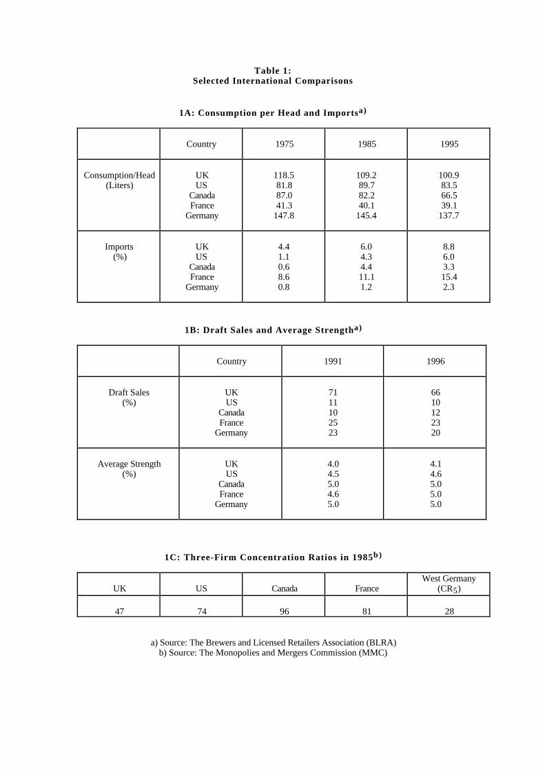
Table 1:Selected International Comparisons

1A: Consumption per Head and Importsa)

Country 1975 1985 1995

Consumption/Head(Liters)

UKUS

CanadaFrance

Germany

118.581.887.041.3

147.8

109.289.782.240.1

145.4

100.983.566.539.1

137.7

Imports(%)

UKUS

CanadaFrance

Germany

4.41.10.68.60.8

6.04.34.411.11.2

8.86.03.315.42.3

1B: Draft Sales and Average Strengtha)

Country 1991 1996

Draft Sales(%)

UKUS

CanadaFrance

Germany

7111102523

6610122320

Average Strength(%)

UKUS

CanadaFrance

Germany

4.04.55.04.65.0

4.14.65.05.05.0

1C: Three-Firm Concentration Ratios in 1985b)

UK US Canada FranceWest Germany

(CR5)

47 74 96 81 28

a) Source: The Brewers and Licensed Retailers Association (BLRA)b) Source: The Monopolies and Mergers Commission (MMC)

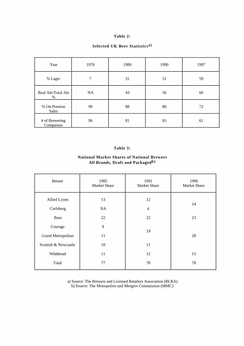
Table 2:

Selected UK Beer Statisticsa)

Year 1970 1980 1990 1997

% Lager 7 31 51 59

Real Ale/Total Ale%

NA 43 56 60

% On PremiseSales

90 88 80 72

# of BreweringCompanies

96 81 65 61

Table 3:

National Market Shares of National BrewersAll Brands, Draft and Packagedb)

Brewer 1985Market Share

1991Market Share

1996Market Share

Allied Lyons

Carlsberg

Bass

Courage

Grand Metropolitan

Scottish & Newcastle

Whitbread

Total

13

NA

22

9

11

10

11

77

12

4

22

19

11

12

78

14

23

28

13

78

a) Source: The Brewers and Licensed Retailers Association (BLRA)b) Source: The Monopolies and Mergers Commission (MMC)

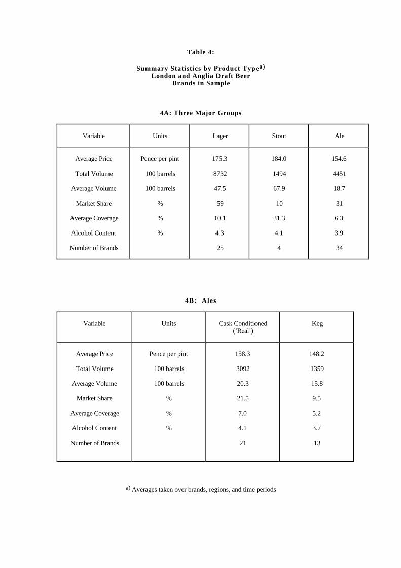
Table 4:

Summary Statistics by Product Typea)

London and Anglia Draft BeerBrands in Sample

4A: Three Major Groups

Variable Units Lager Stout Ale

Average Price

Total Volume

Average Volume

Market Share

Average Coverage

Alcohol Content

Number of Brands

Pence per pint

100 barrels

100 barrels

%

%

%

175.3

8732

47.5

59

10.1

4.3

25

184.0

1494

67.9

10

31.3

4.1

4

154.6

4451

18.7

31

6.3

3.9

34

4B: Ales

Variable Units Cask Conditioned(‘Real’)

Keg

Average Price

Total Volume

Average Volume

Market Share

Average Coverage

Alcohol Content

Number of Brands

Pence per pint

100 barrels

100 barrels

%

%

%

158.3

3092

20.3

21.5

7.0

4.1

21

148.2

1359

15.8

9.5

5.2

3.7

13

a) Averages taken over brands, regions, and time periods

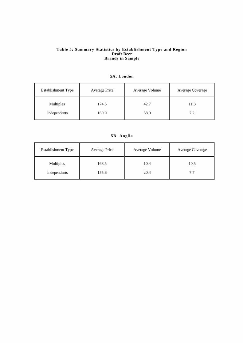
Table 5: Summary Statistics by Establishment Type and RegionDraft Beer

Brands in Sample

5A: London

Establishment Type Average Price Average Volume Average Coverage

Multiples

Independents

174.5

160.9

42.7

58.0

11.3

7.2

5B: Anglia

Establishment Type Average Price Average Volume Average Coverage

Multiples

Independents

168.5

155.6

10.4

20.4

10.5

7.7

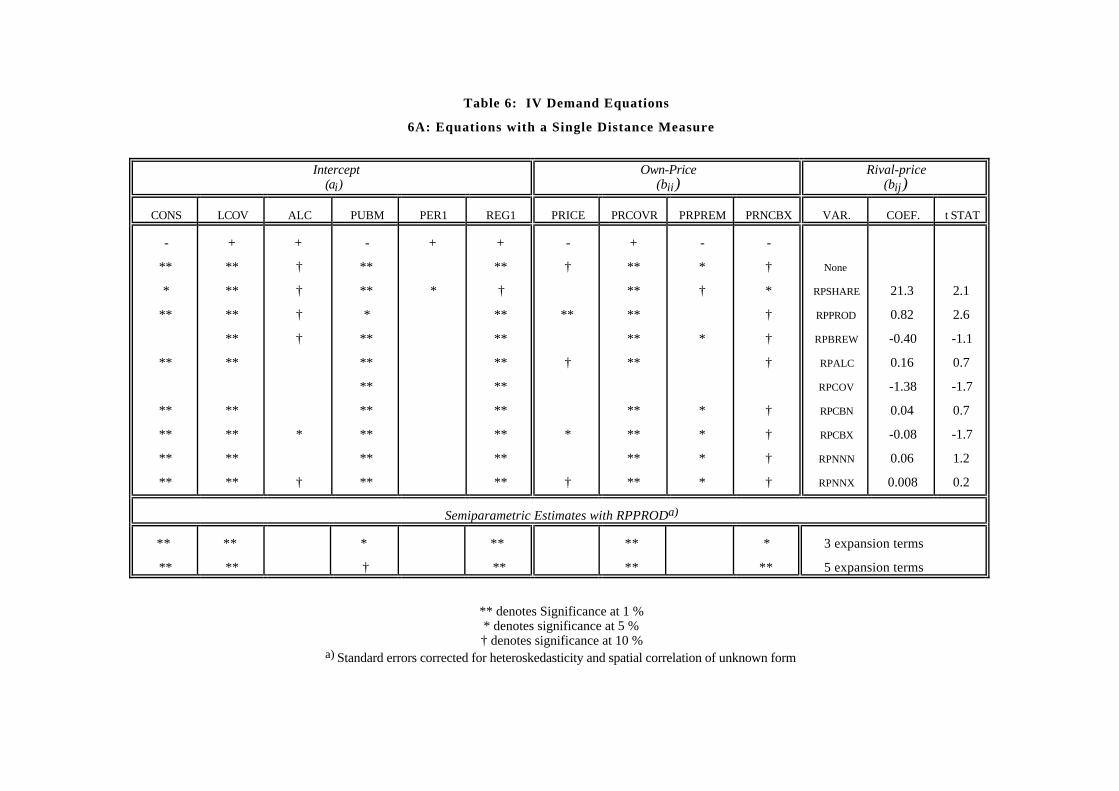
Table 6: IV Demand Equations

6A: Equations with a Single Distance Measure

Intercept(ai)

Own-Price(bii)

Rival-price(bij)

CONS LCOV ALC PUBM PER1 REG1 PRICE PRCOVR PRPREM PRNCBX VAR. COEF. t STAT

-

**

*

**

**

**

**

**

**

+

**

**

**

**

**

**

**

**

**

+

†

†

†

†

*

†

-

**

**

*

**

**

**

**

**

**

**

+

*

+

**

†

**

**

**

**

**

**

**

**

-

†

**

†

*

†

+

**

**

**

**

**

**

**

**

**

-

*

†

*

*

*

*

*

-

†

*

†

†

†

†

†

†

†

None

RPSHARE

RPPROD

RPBREW

RPALC

RPCOV

RPCBN

RPCBX

RPNNN

RPNNX

21.3

0.82

-0.40

0.16

-1.38

0.04

-0.08

0.06

0.008

2.1

2.6

-1.1

0.7

-1.7

0.7

-1.7

1.2

0.2

Semiparametric Estimates with RPPRODa)

**

**

**

**

*

†

**

**

**

**

*

**

3 expansion terms

5 expansion terms

** denotes Significance at 1 %* denotes significance at 5 %† denotes significance at 10 %

a) Standard errors corrected for heteroskedasticity and spatial correlation of unknown form

6B: IV Equation With Multiple Distance Measuresa)

RPPROD RPBREW RPALC RPCBN RPNNN

0.82

(2.5)

-0.19

(-0.5)

0.16

(1.2)

0.02

(0.3)

0.05

(0.9)

a) Asymptotic t statistics in parentheses

6C: IV Equation Used in Evaluation of Gamesa) b)

Intercept(ai)

Own-Price(bii)

Rival-price(bij)

CONS LCOV ALC PUBM PER1 REGL PRICE PRCOVR PRPREM PRNCBX RPPROD RPALC

-159.1

(-4.0)

60.3

(11.7)

8.80

(0.7)

-11.0

(-1.9)

3.81

(0.8)

31.5

(6.4)

-1.13

(-2.9)

0.17

(7.8)

-0.03

(-0.1)

-0.12

(-2.7)

0.71

(2.6)

0.22

(1.1)

a) Asymptotic t statistics in parentheses

b) Standard errors corrected for heteroskedasticity and spatial correlation of an unknown form

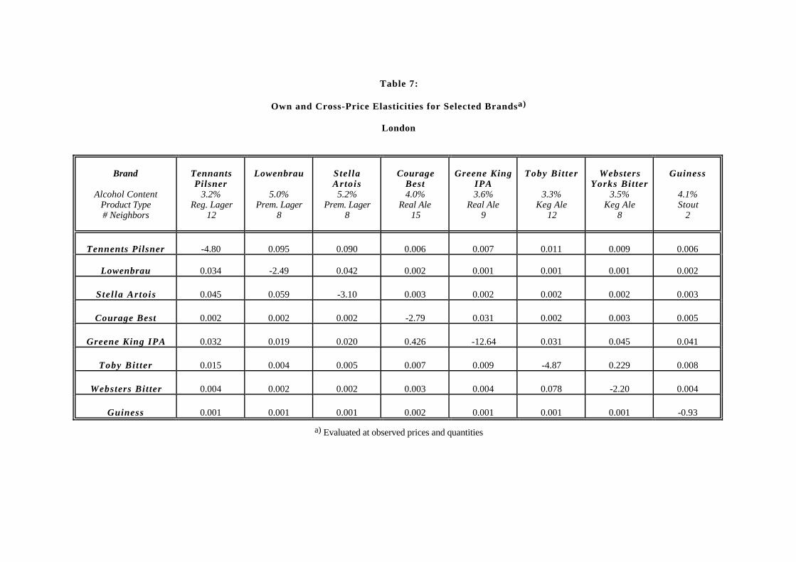
Table 7:

Own and Cross-Price Elasticities for Selected Brandsa)

London

a) Evaluated at observed prices and quantities

Brand

Alcohol ContentProduct Type# Neighbors

TennantsPilsner

3.2%Reg. Lager

12

Lowenbrau

5.0%Prem. Lager

8

StellaArtois5.2%

Prem. Lager8

CourageBest4.0%

Real Ale15

Greene KingIPA3.6%

Real Ale9

Toby Bit ter

3.3%Keg Ale

12

WebstersYorks Bit ter

3.5%Keg Ale

8

Guiness

4.1%Stout

2

Tennents Pilsner -4.80 0.095 0.090 0.006 0.007 0.011 0.009 0.006

Lowenbrau 0.034 -2.49 0.042 0.002 0.001 0.001 0.001 0.002

Stel la Artois 0.045 0.059 -3.10 0.003 0.002 0.002 0.002 0.003

Courage Best 0.002 0.002 0.002 -2.79 0.031 0.002 0.003 0.005

Greene King IPA 0.032 0.019 0.020 0.426 -12.64 0.031 0.045 0.041

Toby Bit ter 0.015 0.004 0.005 0.007 0.009 -4.87 0.229 0.008

Websters Bitter 0.004 0.002 0.002 0.003 0.004 0.078 -2.20 0.004

Guiness 0.001 0.001 0.001 0.002 0.001 0.001 0.001 -0.93

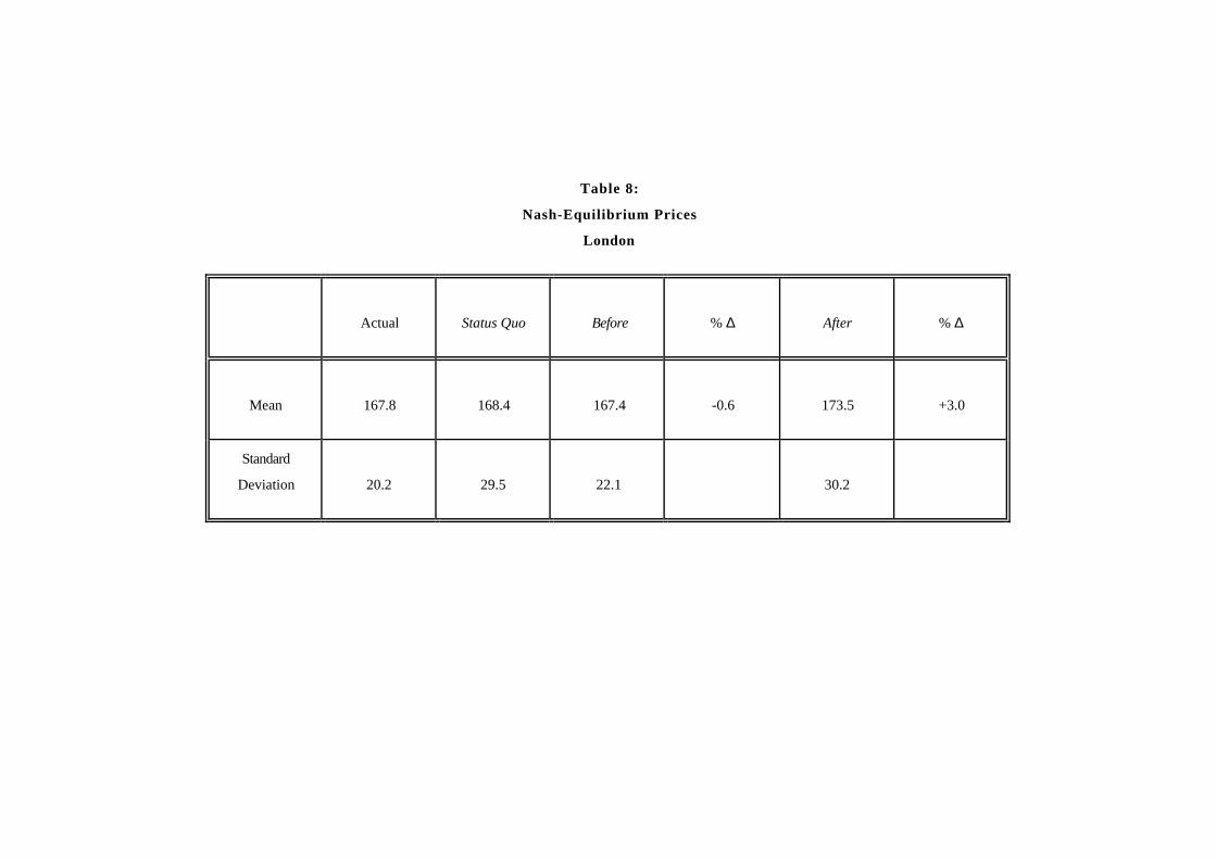
Table 8:

Nash-Equilibrium Prices

London

Actual Status Quo Before % ∆ After % ∆

Mean 167.8 168.4 167.4 -0.6 173.5 +3.0

Standard

Deviation 20.2 29.5 22.1 30.2

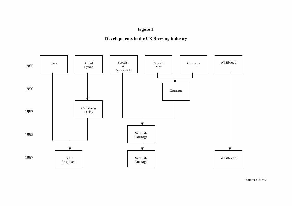
Figure 1:

Developments in the UK Brewing Industry

1985

1990

1992

1995

1997

Source: MMC

Bass AlliedLyons

Scottish&

Newcastle

GrandMet

Courage Whitbread

Courage

CarlsbergTetley

ScottishCourage

BCTProposed

ScottishCourage

Whitbread

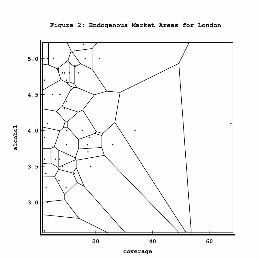
Figure 2: Endogenous Market Areas for London

coverage

alcohol

20 40 60

3.0

3.5

4.0

4.5

5.0

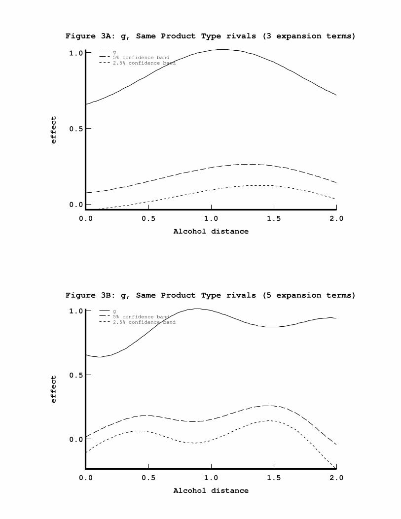
Figure 3A: g, Same Product Type rivals (3 expansion terms)

Alcohol distance

effect

0.0 0.5 1.0 1.5 2.0

0.0

0.5

1.0 g5% confidence band2.5% confidence band

Figure 3B: g, Same Product Type rivals (5 expansion terms)

Alcohol distance

effect

0.0 0.5 1.0 1.5 2.0

0.0

0.5

1.0 g5% confidence band2.5% confidence band

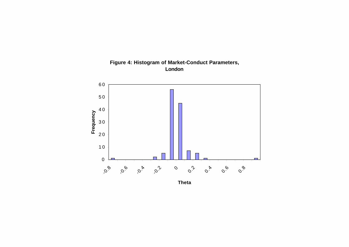
Figure 4: Histogram of Market-Conduct Parameters, London

0

1 0

2 0

3 0

4 0

5 0

6 0

-0.8

-0.6

-0.4

-0.2 0

0.2 0.4 0.6 0.8

Theta

Fre

quen

cy