Embed Size (px)
Citation preview
Mechanical linkages,
dynamic geometry software,
and argumentation:
Supporting a classroom culture of
mathematical proof
Jill Loris Vincent
Submitted in total fulfilment of the requirements
of the degree of Doctor of Philosophy
December 2002
Department of Science and Mathematics Education
The University of Melbourne

iii
Abstract
Euclidean geometry and geometric proof have occupied a central place in
mathematics education from classical Greek society through to twentieth century
Western culture. It is proof which sets mathematics apart from the empirical
sciences, and forms the foundation of our mathematical knowledge, yet students
often fail to understand the purpose of proof, they are unable to construct proofs,
and instead readily accept empirical evidence or the authority of textbooks or
teachers.
This research focuses on the role of mechanical linkages (devices based on
systems of hinged rods) and dynamic geometric software as cognitive bridges
between empirical justification and deductive reasoning. The participants in the
research were 29 Year 8 students at a private girls’ school in Melbourne,
Australia. Following pre-testing with a van Hiele test to measure geometric
understanding, and a Proof Questionnaire (Healy & Hoyles, 1999) to determine
the students understanding of mathematical proof, the whole class took part in the
introductory conjecturing-proving lessons. In these lessons, mechanical linkages
and dynamic geometry software provided the contexts for the students’
conjecturing, argumentation, and deductive reasoning. Approximately half of the
students then participated in pairs in video-recorded interview sessions, which
again involved investigatory tasks with mechanical linkages and dynamic
geometry software. After these interview sessions were completed, the van Hiele
test and the Proof Questionnaire were administered as post-tests.
The provision of motivating contexts was found to foster conjecturing and
argumentation, during which the Year 8 students engaged in sustained deductive
reasoning in support of their conjectures and achieved high levels of success with
geometric proof. Although students with lower levels of geometric understanding
were sometimes handicapped by their poor knowledge of geometric properties
and their lack of fluency with the language of geometry, they still developed an
understanding of deductive proof, as well as making significant progress in their
understanding of geometric properties and relationships. Mechanical linkages and

iv
their dynamic geometry computer simulations were shown by this research to be
highly suitable contexts for bridging empirical and deductive reasoning.
v
Declaration
This is to certify that
(i) The thesis comprises my original work towards the PhD,
(ii) Due acknowledgement has been made in the text to all other material used,
(iii) The thesis is less than 100,000 words in length, exclusive of tables,
bibliographies and appendices.

vii
Acknowledgements
I thank my supervisors, Dr. Helen Chick and Mr. Barry McCrae, for their
continued guidance, support, and much-valued constructive criticism throughout
the time I have been working on this thesis. I thank Professor Celia Hoyles
(Institute of Education, University of London) for allowing me to use the Proof
Questionnaire; Dr. Christine Lawrie (University of New England, Australia) for
her permission to use the van Hiele test; and Professor Maria Bartolini Bussi
(University of Modena and Reggio Emilia, Italy) for generously sending me
copies of all her published work relating to research in the teaching and learning
of geometry, and a CD ROM depicting models and drawings of historical
mathematical machines. I express my sincere gratitude to the Year 8 students for
their willingness to participate in the research lessons. I also wish to thank my
husband, John; my daughters, Kylie and Claire; the Principal of Melbourne Girls
Grammar School, Mrs Christine Briggs; and members of the Department of
Science and Mathematics Education; for their encouragement and support,
without which this thesis would not have been possible.

ix
Refereed papers arising from this research
Vincent, J., & McCrae, B. (2001a). Mechanical linkages and the need for proof in
secondary school geometry. In M. van den Heuvel-Panhuizen (Ed.),
Proceedings of the 25th Conference of the International Group for the
Psychology of Mathematics Education, Vol. 4 (pp. 367–374). Utrecht, The
Netherlands: PME.
Vincent, J., & McCrae, B. (2001b). Mechanical linkages, dynamic geometry
software and mathematical proof. Australian Senior Mathematics Journal,
15 (1), 56–63.
Vincent, J., Chick, H., & McCrae, B. (2002). Mechanical linkages as bridges to
deductive reasoning: A comparison of two environments. In A. Cockburn &
E. Nardi (Eds.), Proceedings of the 26th Conference of the International
Group for the Psychology of Mathematics Education, Vol. 4 (pp. 313–320).
Norwich, UK: PME.

xi
Table of Contents
Abstract ...............................................................................................iii
Declaration...........................................................................................v
Acknowledgements............................................................................vii
Refereed papers arising from this research.....................................ix
List of Tables ....................................................................................xix
List of Figures ...................................................................................xxi
Chapter 1: Introduction .....................................................................1 1.1 Background ................................................................................................. 1
1.2 The aim of the research ............................................................................... 3
1.3 Outline of the thesis .................................................................................... 3
Chapter 2: Proof and Argumentation...............................................7 2.1 Introduction ................................................................................................. 7
2.2 The role of proof in mathematics ................................................................ 7
2.2.1 What is mathematical proof? .......................................................... 7
2.2.2 The meaning of proof in school mathematics ................................. 9
2.2.3 Defining ‘proof’ and proof-related terms...................................... 11
2.2.4 A rationale for proof in the school mathematics curriculum ........ 12
2.2.5 Proof as conviction........................................................................ 13
2.2.6 Proof as explanation...................................................................... 14
2.2.7 Proof as an aid to understanding ................................................... 15
2.3 Argumentation and proof .......................................................................... 17
2.3.1 Argumentation and the process of proving ................................... 17
2.3.2 The conflict between argumentation and proof ............................ 18
2.3.3 Analysing the structure of arguments ........................................... 20
2.3.4 The structure of school geometry proofs ...................................... 23
2.4 How well can students construct proofs?.................................................. 27
2.5 Why do students have difficulty with proof in mathematics?................... 30
xii
2.5.1 Cognitive readiness for proof ........................................................ 30
2.5.2 Motivation for proof ...................................................................... 34
2.5.3 Understanding the requirement of generality of a mathematical
proof .............................................................................................. 36
2.5.4 Understanding the role of counter-examples in proofs ................. 37
2.5.5 Understanding deductive reasoning .............................................. 39
2.5.6 Ritualistic approach to teaching and learning proof...................... 45
2.5.7 Using diagrams in geometric reasoning ........................................ 49
2.6 Alternative approaches to the teaching and learning of proof................... 51
2.7 Recent curriculum recommendations on proof ......................................... 53
2.8 Motivation, peer interaction, and the quality of argumentation ................ 55
2.8.1 Motivation ..................................................................................... 55
2.8.2 Peer interaction .............................................................................. 56
2.9 Conclusion................................................................................................. 58
Chapter 3: Dynamic Environments as Contexts for
Conjecturing and Proving .............................................61 3.1 Introduction ............................................................................................... 61
3.2 Mathematical visualisation and dynamic imagery .................................... 62
3.2.1 Reasoning by continuity ................................................................ 63
3.2.2 Transformational reasoning........................................................... 64
3.2.3 Geometric transformations and anticipatory images ..................... 65
3.2.4 Dynamic imagery using filmstrips ................................................ 68
3.3 Dynamic geometry software...................................................................... 69
3.3.1 What is dynamic geometry software? ........................................... 69
3.3.2 Dynamic geometry software: Concerns and cautions ................... 72
3.4 Visualisation and reasoning with dynamic geometry software ................. 75
3.4.1 Contexts for using dynamic geometry software ............................ 75
3.4.2 Construction tasks ......................................................................... 75
3.4.3 Exploratory tasks ........................................................................... 80
3.4.4 Proof tasks in a dynamic geometry environment .......................... 81
3.4.5 Different roles of dragging in a dynamic geometry environment .82
xiii
3.4.6 The relationship between students’ use of dragging and their
reasoning ....................................................................................... 83
3.4.7 Connecting empirical and deductive reasoning in a dynamic
geometry environment .................................................................. 86
3.4.8 Assessing students’ reasoning in a dynamic geometry
environment................................................................................... 90
3.4.9 The motivational effect of a dynamic geometry environment ...... 93
3.5 Mechanical linkages as rich sources of geometry..................................... 95
3.5.1 What are mechanical linkages?..................................................... 95
3.5.2 Rhombus linkages ......................................................................... 96
3.5.3 Parallelogram linkages .................................................................. 98
3.5.4 Linkages containing similar and congruent triangles.................... 98
3.5.5 Pantographs ................................................................................... 99
3.5.6 Pascal’s angle trisector................................................................ 101
3.5.7 Consul, the educated monkey ..................................................... 102
3.5.8 Tchebycheff’s linkage................................................................. 105
3.6 Visualisation and reasoning with mechanical linkages........................... 106
3.6.1 Using real contexts in geometry.................................................. 106
3.6.2 The use of historic drawing instruments in school mathematics 107
3.6.3 Computer modelling of mechanical linkages.............................. 112
3.7 Conclusion .............................................................................................. 115
Chapter 4: Methodology.................................................................117 4.1 Introduction ............................................................................................. 117
4.2 The current study..................................................................................... 118
4.2.1 The research questions ................................................................ 118
4.2.2 The context of mechanical linkages and dynamic geometry
software ....................................................................................... 118
4.2.3 Establishing a need for proof ...................................................... 119
4.3 Pilot study ............................................................................................... 120
4.3.1 Purpose of the pilot study............................................................ 120
4.3.2 Students’ understanding of mathematical proof ......................... 120
4.3.3 Linkage tasks............................................................................... 121
xiv
4.4 Research design ....................................................................................... 124
4.4.1 An ethnographic study................................................................. 124
4.4.2 The participants ........................................................................... 125
4.4.3 Overall research design ............................................................... 127
4.4.4 Pre-testing and post-testing ......................................................... 129
4.4.5 Selecting students for the case study pairs .................................. 130
4.4.6 Selecting the research contexts for conjecturing and proving..... 131
4.4.7 Preparatory lessons ...................................................................... 135
4.4.8 Whole-class teaching lessons ...................................................... 135
4.4.9 Case study interview lessons ....................................................... 139
4.5 Data analysis............................................................................................ 145
4.5.1 Analysis of pre-test and post-test van Hiele data ........................ 145
4.5.2 Analysis of pre-test and post-test Proof Questionnaire data....... 145
4.5.3 Data from case study interview lessons....................................... 146
4.5.4 Linkage questionnaire.................................................................. 148
4.6 Overview of the data sources................................................................... 148
Chapter 5: Measuring Geometric Understanding .......................151 5.1 Introduction ............................................................................................. 151
5.2 The Mayberry/Lawrie van Hiele test....................................................... 151
5.2.1 Description of the Mayberry/Lawrie van Hiele Test................... 151
5.2.2 Evaluation of the Mayberry/Lawrie van Hiele Test .................... 153
5.3 Year 8 students’ pre-test van Hiele levels ............................................... 156
5.4 Selecting students for the additional conjecturing-proving tasks............ 159
5.5 Comparing the van Hiele pre-test and post-test levels ............................ 160
5.5.1 Comparing the distributions of students across the levels for six
concepts ....................................................................................... 160
5.5.2 Progress in Level 3 understanding............................................... 166
5.5.3 Progress in Level 4 understanding............................................... 170
5.6 The case study students ........................................................................... 172
5.7 Conclusion............................................................................................... 173
xv
Chapter 6: A Case Study of Two Students ...................................175 6.1. Introduction ............................................................................................. 175
6.1.1. How the case study addresses the research questions................. 175
6.1.2. Selection of the case study students ............................................ 175
6.1.3. The introductory whole class lessons.......................................... 177
6.1.4. Additional conjecturing-proving tasks completed by Anna and
Kate ............................................................................................. 183
6.2. Analysis of the argumentations............................................................... 185
6.2.1. Pascal’s Angle Trisector ............................................................. 185
6.2.2. Enlarging Pantograph.................................................................. 196
6.2.3. Joining Midpoints ....................................................................... 209
6.2.4. Quadrilateral Midpoints .............................................................. 212
6.2.5. Angles in Circles ......................................................................... 220
6.2.6. Consul ......................................................................................... 230
6.2.7. Sylvester’s Pantograph................................................................ 248
6.3. Addressing the research questions .......................................................... 258
6.3.1. A culture of proving .................................................................... 258
6.3.2. Motivation................................................................................... 259
6.3.3. The role of static and dynamic feedback..................................... 262
6.3.4. The influence of conjecturing and argumentation on proof
construction ................................................................................. 266
6.3.5. Satisfying the need for conviction .............................................. 268
6.3.6. Relationship between van Hiele levels and conjecturing-proving
ability .......................................................................................... 269
6.4. Conclusion .............................................................................................. 274
Chapter 7: Case Study Comparisons ............................................277 7.1. Introduction ............................................................................................. 277
7.2. The case study comparison students ....................................................... 278
7.3. The Level 2–3 case study students.......................................................... 279
7.3.1. Consul argumentations: Liz and Meg, and Lucy and Rose ........ 279
7.3.2. Sylvester’s Pantograph: Lucy and Rose...................................... 298
xvi
7.3.3. Angles in Circles: Liz and Meg................................................... 306
7.3.4. The other Level 2–3 case study students ..................................... 311
7.4. The Level 1–2 case study students .......................................................... 312
7.4.1. Jane and Sara ............................................................................... 312
7.4.2. Comparing argumentation profiles: Anna and Kate, and Jane and
Sara .............................................................................................. 340
7.4.3. Emma and Jess ............................................................................ 342
7.5. Whole class responses to the linkage questionnaires .............................. 344
7.6. Conclusion............................................................................................... 347
Chapter 8: The Proof Questionnaire.............................................349 8.1. Introduction ............................................................................................. 349
8.2. The Proof Questionnaire ......................................................................... 350
8.3. Students’ views of proof in mathematics ................................................ 351
8.3.1. Year 8 students views of proof .................................................... 351
8.3.2. Anna and Kate: Comparing pre-test and post-test responses ...... 355
8.4. Students’ judgements of proofs ............................................................... 357
8.4.1. Questions G1/G3 ......................................................................... 357
8.4.2. Question G6................................................................................. 363
8.4.3. Students’ recognition of the validity of proofs............................ 365
8.4.4. Question G2: Generality of a proof ............................................. 370
8.4.5. Question G5................................................................................. 370
8.5. Constructing proofs: Questions G4 and G7............................................. 372
8.5.1. Question G4................................................................................. 372
8.5.2. Forms of arguments used in the students’ proofs ........................ 372
8.5.3. Assessing the constructed proofs for correctness ........................ 374
8.5.4. Year 8 students’ proofs................................................................ 378
8.5.5. Proof constructions of the case study students ............................ 383
8.6. Deductive reasoning ability..................................................................... 388
8.7. Conclusion............................................................................................... 391
Chapter 9: Discussion and Conclusions ........................................395 9.1. Introduction ............................................................................................. 395
xvii
9.2. Issues associated with the research ......................................................... 395
9.2.1. The role of teacher intervention .................................................. 395
9.2.2. Proof as explanation in the context of the linkage tasks ............. 397
9.2.3. Tools for analysing the argumentations and proofs .................... 399
9.2.4. Limitations of the research design .............................................. 401
9.2.5. Assessment of students’ argumentations .................................... 403
9.2.6. Further research........................................................................... 403
9.3. Interpreting the findings in terms of the research questions ................... 404
9.3.1. Motivational engagement............................................................ 404
9.3.2. Static and dynamic feedback....................................................... 407
9.3.3. The influence of conjecturing and argumentation on proof........ 411
9.3.4. Satisfying the need for conviction .............................................. 414
9.3.5. Relationship between van Hiele levels and conjecturing-
proving ability ............................................................................. 416
9.3.6. A culture of proving .................................................................... 419
9.4. Conclusions ............................................................................................. 422
9.4.1. Overall findings from the research.............................................. 422
9.4.2. Implications for the teaching and learning of proof.................... 426
References ........................................................................................427
Appendices .......................................................................................445 Appendix 1: Van Hiele Test............................................................................. 445
Appendix 2: Criteria for assigning van Hiele Levels 1 to 4............................. 461
Appendix 3: Proof Questionnaire.................................................................... 463
Appendix 4: Whole class conjecturing-proving tasks...................................... 475
Appendix 5: Additional conjecturing-proving tasks used with the case study
students........................................................................................ 489
Appendix 6: Linkage questionnaire ................................................................. 503
Appendix 7: Number of tasks completed and Proof Scores for Year 8 class
(N = 28) ....................................................................................... 505

xix
List of Tables Table 2-1: Percentage responses for the statement “the sum of the interior angles
of a triangle is 180o” [From de Villiers, 1991, Table 1, p. 256]. ....... 14
Table 2-2: Constructed proofs: Criteria for assigning scores for correctness
[From Healy and Hoyles, 1999, Table 3, p. 13]................................. 29
Table 2-3: Percentage distribution of students’ scores for proof construction
questions [From Healy & Hoyles, 1999, pp. 41–42] ......................... 29
Table 2-4: Descriptions of Van Hiele Levels 1–4 ............................................... 31
Table 2-5: Percentage distribution of students’ choices for Question G6
(N = 2459) [From Healy & Hoyles, 1999, Figure 5, p. 19]. .............. 47
Table 4-1: Pseudonyms assigned to the case study students ............................. 127
Table 4-2: Summary of the lesson sequence for the research............................ 128
Table 4-3: Geometric figures used for the pencil-and-paper and Cabri tasks ... 132
Table 4-4: Mechanical linkages and their associated geometry ........................ 133
Table 4-5: Rationale for the use of the van Hiele test, the Proof Questionnaire
and the Linkage Questionnaire......................................................... 149
Table 4-6: Summary of sources of data relevant to each research question...... 150
Table 5-1: Success criteria for Levels 1–4 for the concept Squares
[From Lawrie, personal communication, 1/5/1997] ........................ 153
Table 5-2: Number of items at each of the four van Hiele levels in the
48-item test used in the current research.......................................... 155
Table 5-3: Year 8 students’ pre-test van Hiele levels for six concepts ............. 157
Table 5-4: Van Hiele pre-test profiles for fourteen selected students ............... 160
Table 5-5: Year 8 students’ pre-test and post-test van Hiele levels................... 161
Table 5-6: Pre-test and post-test total scores for van Hiele Levels 1–4 ........... 167
Table 6-1: Anna and Kate: Pre-test van Hiele levels for six concepts .............. 176
Table 6-2: Additional conjecturing-proving tasks completed by Anna
and Kate ........................................................................................... 184
Table 6-3: Responses for linkage questionnaire, Item 3.................................... 262
Table 6-4: Responses for linkage questionnaire, Item 4.................................... 265
Table 6-5: Anna and Kate: Assessment of the usefulness of the models .......... 266
xx
Table 6-6: Comparison of pre-test and post-test van Hiele levels and total
scores for Anna and Kate ................................................................. 270
Table 7-1: Conjecturing-proving tasks completed by six pairs of case
study students ................................................................................... 278
Table 7-2: Comparing the number of turns classified as guidance,
observations, and data-gathering for four tasks completed by
Anna and Kate, and Jane and Sara ................................................... 341
Table 8-1: Proof Questionnaire: Description of geometry questions ................ 351
Table 8-2: Description of forms of argument [From Healy & Hoyles,
1999, Table 2, p. 13]......................................................................... 358
Table 8-3: Classification of arguments used in question G1 ............................. 358
Table 8-4: Percentage of students choosing a correct proof for G1................... 362
Table 8-5: Number of students choosing a correct proof for G6 ....................... 365
Table 8-6: Scoring of response profiles for G1 and G6 [as described by
Healy & Hoyles, 1999, p. 14]........................................................... 368
Table 8-7: Analysis of variance for Year 8 students’ pre-test and post-test
validity ratings for questions G1/G3 and G6.................................... 369
Table 8-8: Pre-test and post-test mean validity scores for Year 8 students
(N = 29) and mean validity scores for Year 10 Proof Study
students for algebra and geometry (N = 2459) ................................. 370
Table 8-9: Constructed proofs: Criteria for assigning scores for correctness
[Healy & Hoyles, 1999, Table 3, p. 13] ........................................... 374
Table 8-10: Pre-test and post-test scores for G4 and G7...................................... 376
Table 8-11: Questions G4 and G7: Mean scores for Year 8 students (N = 29),
case study students who completed three or more additional tasks
(n = 10), and Year 10 Proof Study students (N = 2459)................... 377
Table 8-12: Number of additional conjecturing-proving tasks, post-test van
Hiele Level 4 total scores, G4 and G7 scores, and Proof Scores
for students with pre-test van Hiele total Level 3 scores ≥ 30 ......... 389
Table 8-13: Correlations between pre-test total Level 3 scores, number of
additional conjecturing-proving tasks, and Proof Scores for
students with total pre-test Level 3 scores ≥ 30 ............................... 390
xxi
List of Figures Figure 2-1. Can these angles be inscribed in the circle?..................................... 15
Figure 2-2. Tangent problems 1 and 2 [From Schoenfeld, 1989, Figure 1,
p. 339]. ............................................................................................ 16
Figure 2-3. Tangent problem 3 [From Schoenfeld, 1989, Figure 2, p. 339]. ..... 16
Figure 2-4. Standard diagrammatic representation of premises and
conclusions [After Freeman, 1991, p. 2].......................................... 21
Figure 2-5. Independent and linked premises..................................................... 21
Figure 2-6. Toulmin’s model for the structure of an argument [From
Toulmin, 1958, p. 104]..................................................................... 22
Figure 2-7. Example of the structure of an argument [From Toulmin, 1958,
p. 105]. ............................................................................................. 22
Figure 2-8. Alternate angles ABC and BCD are equal........................................ 23
Figure 2-9. Geometry proof example [From Connected Geometry,
Connected Geometry Development Team, 2000, p. 123]................ 24
Figure 2-10. Example of paragraph style proof [From Connected Geometry,
Connected Geometry Development Team, 2000, p. 123]................ 25
Figure 2-11. Example of outline proof [From Connected Geometry, Connected
Geometry Development Team, 2000, p. 124].................................. 25
Figure 2-12. Example of two-column proof [From Connected Geometry,
Connected Geometry Development Team, 2000, p. 124]................ 25
Figure 2-13. Toulmin’s argument model applied to the proofs in Figures
2-10 – 2-12 ....................................................................................... 26
Figure 2-14. Proof construction question from CDASSG Proof Test [From
Senk, 1985, Figure 6, p. 452]. .......................................................... 27
Figure 2-15. Proof questions A4, A7, G4 and G7 [From Proof Questionnaire,
Healy & Hoyles, 1999]. ................................................................... 28
Figure 2-16. Quadrilateral midpoints [From de Villiers, 1991, Figure 1,
p. 256]. ............................................................................................. 36
Figure 2-17. The Quadrilaterals item [From Galbraith, 1981, pp. 10–11]. .......... 38
xxii
Figure 2-18. Parallelogram problem [Translated from Duval, 1991, Fig. 2,
p. 237].............................................................................................. 40
Figure 2-19. Diagrammatic representation of responses of students MB and
SM [Translated from Duval, 1991, Figure 3, p. 239]....................... 41
Figure 2-20. Parallelogram problem [From Duval, 1991, Figure 5, p. 249]......... 42
Figure 2-21. One student’s diagrammatic representation of steps in deductive
reasoning [Translated from Duval, 1991, p. 251]............................ 43
Figure 2-22. Example of proof flowchart [From Connected Geometry,
Connected Geometry Development Team, 2000, p. 132]. ............... 44
Figure 2-23. Question G6 [From Proof Questionnaire, Healy & Hoyles, 1999]. 46
Figure 2-24. Year 8 Mathematical reasoning survey: Question G3 [From
Küchemann & Hoyles, 2001, Figure 5, Vol. 3, p. 261].................... 48
Figure 2-25. Parallelogram problem [From Duval, 1998, p. 41]. ......................... 50
Figure 2-26. Relevant subfigures [From Duval, 1998, Figure 3, p. 41]................ 50
Figure 3-1. Equilateral triangle problem [From Goldenberg, 1995, Figure 1,
p. 204]............................................................................................... 63
Figure 3-2. A transformational approach to the angle sum of a triangle [From
Fischbein, 1982, Figure 5, p. 18]....................................................... 65
Figure 3-3. Opening of ‘lazy tongs’ [From Piaget & Inhelder, 1956, Fig. 24,
p. 305]................................................................................................ 66
Figure 3-4. Children’s drawings of the transformation of the ‘lazy tongs’
[From Piaget & Inhelder, 1956, Fig. 25, p. 306]. ............................. 67
Figure 3-5. Extract from filmstrip relating to triangle properties [From
Nicolet, Le dessin animé, 1944, p. 31–32]. ...................................... 68
Figure 3-6. Dragging a Cabri triangle. ................................................................ 70
Figure 3-7. The crossed quadrilateral [From de Villiers, 1998, Fig. 15.10,
p. 385]............................................................................................... 71
Figure 3-8. Defining internal angles in quadrilaterals [From de Villiers, 1998,
p. 387, Figure 15.11]. ....................................................................... 72
Figure 3-9. Geometer’s Sketchpad circle angles activity [From Redden &
Clark, 1996, pp. 85–86]. ................................................................... 73
xxiii
Figure 3-10. Two students’ by-eye constructions of a rectangle after dragging
[From Vincent, 1998, Fig. 7.1, p. 111, and Fig. 7.11, p. 121]. ....... 75
Figure 3-11. Eve’s isosceles triangle construction. [From Vincent & McCrae,
1999, Fig. 1, p. 17] ........................................................................... 76
Figure 3-12. Initial unsuccessful attempt at the construction of an invariant
‘house’ shape by Anna and Mary [From Vincent, 1998, Fig. 7.39,
p. 144]. ............................................................................................ 77
Figure 3-13. Successful Cabri construction of an invariant ‘house’ shape by
two Year 8 students [From Vincent, 1998, Figs. 7.40–7.42, pp.
146-148]. .......................................................................................... 78
Figure 3-14. Bisecting an angle in Cabri. ............................................................. 79
Figure 3-15. Dragging the first flag so that the points and their reflections
come together [After Noss & Hoyles, 1996, Figure 5.3, p. 115]. .... 80
Figure 3-16. Tracing the path of A as it is dragged to retain the right angle at A. 83
Figure 3-17. Cabri construction of the angle bisectors of a quadrilateral ABCD. 83
Figure 3-18. Systematic dragging of quadrilateral ABCD.................................... 84
Figure 3-19. Concurrent angle bisectors and the circumscribed quadrilateral
property. ........................................................................................... 84
Figure 3-20. Inscribed circle in quadrilateral ABCD. ........................................... 85
Figure 3-21. Tracing the path of D so that the bisectors of angles BAD and
ABC remain perpendicular. .............................................................. 89
Figure 3-22. Software use associated with the different levels of justification
used in exploring the midpoints of chords investigation [as
described by Galindo,1998]. ............................................................ 92
Figure 3-23. The quadrilateral circumcircle problem: The computer file
displayed by the teacher [From Hölzl, 2001, Figure 9, p. 73]. ........ 94
Figure 3-24. Descartes’ linkage mechanism for drawing a hyperbola [From
Descartes, 1637/1954, p. 52]............................................................ 95
Figure 3-25. Scheiner’s pantograph (1631) used for perspective drawing
[From Bartolini Bussi, Nasi, et al., 1999, History, Images 91,
91-1]. ................................................................................................ 95
Figure 3-26. Rhombus linkages in a riveting tool. ............................................... 96
xxiv
Figure 3-27. Rhombus car jack ............................................................................. 97
Figure 3-28. Isosceles triangle car jack................................................................. 97
Figure 3-29. Cabri models of (a) rhombus and (b) isosceles triangle car jacks.... 97
Figure 3-30. (a) Cabri model of the parallelogram linkages of a ‘cherry picker’
and (b) the relationship between the rigid frames, ABC and DEF. .. 98
Figure 3-31. Folding ironing-table linkage. .......................................................... 98
Figure 3-32. Cabri model of Sylvester’s pantograph. ........................................... 99
Figure 3-33. Enlarging pantograph, 1763 [From Bartolini Bussi, Nasi, et al.,
1999, History, Image 91-2]. ........................................................... 100
Figure 3-34. Cabri model of an enlarging pantograph........................................ 100
Figure 3-35. Pascal’s angle trisector [From Bartolini Bussi, Nasi, et al., 1999,
Machines, Image 146m]. ................................................................ 101
Figure 3-36. Cabri construction of Pascal’s angle trisector. ............................... 101
Figure 3-37. (i) Consul, the educated monkey; (ii) superimposed diagram
showing the geometry of the linkage.............................................. 102
Figure 3-38. Cabri construction of the Consul linkage. ...................................... 103
Figure 3-39. Cabri construction of the Consul linkage showing right-angle
APB. ................................................................................................ 104
Figure 3-40. Consul: Arrangement of numbers for the multiplication table. ..... 104
Figure 3-41. Cabri construction of Tchebycheff’s linkage showing
approximately linear motion of the midpoint, P, of AB. ................ 105
Figure 3-42. Tchebycheff’s linkage in three special positions. .......................... 106
Figure 3-43. Sylvester’s pantograph: Model of the linkage [From Bartolini
Bussi, Nasi, et al., 1999, Machines, Image 123m]. ........................ 108
Figure 3-44. Diagram of Sylvester’s pantograph................................................ 108
Figure 3-45. Configurations of the pantograph for ϕ = 0 to ϕ = π [From
Bartolini Bussi, 1993, p. 98]........................................................... 109
Figure 3-46. Two configurations of Sylvester’s pantograph [From Bartolini
Bussi, 1998, Figure 2, p. 741]......................................................... 110
Figure 3-47. Geometer’s Sketchpad model of windscreen wiper linkage
[From Steeg, Wake, & Williams, 1993, p. 27]............................... 113
xxv
Figure 3-48. Geometer’s Sketchpad model of garage door mechanism
[From Steeg et al., 1993, p. 28]..................................................... 113
Figure 3-49. Geometer’s Sketchpad model of enlarging pantograph linkage
[From Steeg et al., 1993, p. 28]..................................................... 114
Figure 3-50. Zig Zag corkscrew. ........................................................................ 115
Figure 3-51. Cabri model of a corkscrew [From Laborde, 1995b, p. 68]. ......... 115
Figure 4-1. The response of one student, Alice, to the question
“What is proof in mathematics for?” ............................................. 121
Figure 4-2. Observations of the cherry picker linkage: Student A. .................. 122
Figure 4-3. Drawings of the cherry-picker linkage by two Pilot Study
students........................................................................................... 122
Figure 4-4. Pilot study students investigating the car jack. .............................. 123
Figure 4-5. Three students’ conjectures about the geometry of the car jack.... 123
Figure 4-6. Proof constructed by Pilot Study students, J and R. ...................... 123
Figure 4-7. Tchebycheff’s linkage: Page 1 of worksheet. ................................ 136
Figure 4-8. Cabri model of Tchebycheff’s linkage. ......................................... 137
Figure 4-9. Modelled proof for the statement: The angles of a triangle
add to 180o. .................................................................................... 138
Figure 4-10. One students’ written proof for the statement: The opposite
angles of a parallelogram are equal................................................ 139
Figure 4-11. Equipment for mechanical linkage tasks. ...................................... 141
Figure 4-12. Task 1: Joining Midpoints. ............................................................ 142
Figure 4-13. Task 2: Quadrilateral Midpoints. .................................................. 142
Figure 4-14. Task 3: Angles in Circles ............................................................... 143
Figure 4-15. Different status of points in Cabri.................................................. 144
Figure 5-1. Van Hiele test Item 38 [original Mayberry Item 56]. .................... 154
Figure 5-2. Van Hiele test Item 48 [original Mayberry Item 55]. .................... 154
Figure 5-3. Pre-test distribution of students across van Hiele Levels 0–4
for six concepts .............................................................................. 158
Figure 5-4. Pre-test: Numbers of students who satisfied the Level 3 or
Level 4 criteria ............................................................................. 159
xxvi
Figure 5-5. Post-test distribution of students across across van Hiele Levels
1–4 for six concepts........................................................................ 162
Figure 5-6. Post-test numbers of students at van Hiele Level 3 or higher ........ 162
Figure 5-7. Squares: Pre-test and post-test distribution of van Hiele levels ..... 164
Figure 5-8. Right-angled triangles: Pre-test and post-test distribution of
van Hiele levels .............................................................................. 164
Figure 5-9. Isosceles triangles: Pre-test and post-test distribution of van
Hiele levels ..................................................................................... 164
Figure 5-10. Parallel lines: Pre-test and post-test distribution of van Hiele
levels.............................................................................................. 165
Figure 5-11. Similarity: Pre-test and post-test distribution of van Hiele levels.. 165
Figure 5-12. Congruency: Pre-test and post-test distribution of van Hiele
levels............................................................................................... 165
Figure 5-13. Pre-test and post-test comparison of numbers of students at
van Hiele Level 3 or above............................................................. 166
Figure 5-14. Distribution of (a) pre-test and (b) post-test total scores for
van Hiele Level 3 items. ................................................................. 168
Figure 5-15. Relationship between pre-test and post-test total scores for
Level 3 items (N = 28).................................................................... 169
Figure 5-16. Pre-test and post-test comparison of numbers of students at
van Hiele Level 4............................................................................ 170
Figure 5-17. Relationship between post-test total score for Level 3 items
and total score for Level 4 items (N = 28)...................................... 171
Figure 6-1. Drawings of the rhombus linkage by Anna and Kate. ................... 178
Figure 6-2. Anna and Kate: Descriptions of the rhombus linkage.................... 178
Figure 6-3. Anna and Kate: Observing the Cabri model of the rhombus
linkage. .......................................................................................... 178
Figure 6-4. Anna and Kate’s tracings of the paths of points............................. 179
Figure 6-5. Observations of the loci of points on Tchebycheff’s linkage......... 179
Figure 6-6. Anna and Kate tracing the path of the “car attachment point”....... 180
Figure 6-7. Anna’s conjecture for the car jack.................................................. 180
xxvii
Figure 6-8. Anna and Kate’s proof for the car jack prior to the class
discussion. ...................................................................................... 181
Figure 6-9. Anna’s final written proof for the car jack. ................................... 181
Figure 6-10. Anna and Kate: Conjecturing about the ironing table. .................. 182
Figure 6-11. Anna’s diagram and explanation for the Folding Ironing Table
task. ................................................................................................ 182
Figure 6-12. Kate’s explanation for the Folding Ironing Table task.................. 182
Figure 6-13. The Folding Ironing Table task: Anna’s and Kate’s proofs. ......... 183
Figure 6-14. Pascal’s Angle Trisector task: Written proofs............................... 194
Figure 6-15. Pascal’s Angle Trisector task: Diagrammatic representation of
Anna’s and Kate’s written proofs. ................................................. 195
Figure 6-16. Anna and Kate: Argumentation profile for Pascal’s Angle
Trisector task.................................................................................. 196
Figure 6-17. Written proofs for the Enlarging Pantograph task........................ 206
Figure 6-18. Enlarging Pantograph task: Diagrammatic representations of
Anna’s and Kate’s written proofs .................................................. 207
Figure 6-19. Anna and Kate: Argumentation profile for the Enlarging
Pantograph task ............................................................................. 208
Figure 6-20. Joining Midpoints task: Written proofs. ........................................ 210
Figure 6-21. Joining Midpoints task: Diagrammatic representation of Anna’s
and Kate’s written proofs ............................................................... 211
Figure 6-22. Anna and Kate: Argumentation profile for the Joining Midpoints
task ................................................................................................. 212
Figure 6-23. Anna: Written proof for the Quadrilateral Midpoints task. .......... 215
Figure 6-24. Kate: Written proof for the Quadrilateral Midpoints task. ........... 216
Figure 6-25. Quadrilateral Midpoints: Diagrammatic representation of
Anna’s written proof ...................................................................... 217
Figure 6-26. Quadrilateral Midpoints: Diagrammatic representation of
Kate’s written proof ....................................................................... 218
Figure 6-27. Anna and Kate: Argumentation profile for the Quadrilateral
Midpoints task. ............................................................................... 219
xxviii
Figure 6-28. Anna and Kate: Argumentation profile for the Angles in Circles
task.................................................................................................. 229
Figure 6-29: Consul: Kate’s written proof. ......................................................... 244
Figure 6-30. Consul: Diagrammatic representation of Kate’s written proof. ..... 245
Figure 6-31. Anna and Kate: Argumentation profile for Consul. ....................... 247
Figure 6-32. Sylvester’s Pantograph: Anna’s written proof............................... 255
Figure 6-33. Sylvester’s Pantograph: Diagrammatic representation of Anna’s
written proof. .................................................................................. 256
Figure 6-34. Anna and Kate: Argumentation profile for the Sylvester’s
Pantograph task.............................................................................. 257
Figure 6-35. Post-test responses for Item 38 (Level 3)....................................... 271
Figure 6-36. Post-test responses for Item 46 (Level 4)....................................... 272
Figure 6-37. Post-test responses for Item 43 (Level 4)....................................... 273
Figure 6-38. Post-test responses for Item 47 (Level 4)....................................... 274
Figure 7-1. Liz and Meg’s written proof for Consul......................................... 292
Figure 7-2. Liz and Meg: Diagrammatic representation of written Consul
proof. .............................................................................................. 293
Figure 7-3. Lucy and Rose’s written proof for Consul. .................................... 295
Figure 7-4. Lucy and Rose: Diagrammatic representation of written Consul
proof. .............................................................................................. 296
Figure 7-5. Liz and Meg: Argumentation profile for Consul............................ 297
Figure 7-6. Rose and Lucy: Argumentation profile for Consul. ....................... 298
Figure 7-7. Rose: Written proof for Sylvester’s Pantograph. ........................... 303
Figure 7-8. Rose: Diagrammatic representation of written proof for
Sylvester’s Pantograph................................................................... 305
Figure 7-9. Lucy and Rose: Argumentation profile for the Sylvester’s
Pantograph task.............................................................................. 306
Figure 7-10. Liz and Meg: Written ‘proof’ for the pencil-and-paper
Angles in Circles task. .................................................................... 310
Figure 7-11. Liz and Meg: Diagrammatic representation of written proof for
the Angles in Circles task. .............................................................. 310
xxix
Figure 7-12. Jane and Sara: Argumentation profile for the Pascal’s Angle
Trisector task.................................................................................. 318
Figure 7-13. Sara: Written proof for the Joining Midpoints task. ...................... 323
Figure 7-14. Sara: Diagrammatic representation of written proof for the
Joining Midpoints task. .................................................................. 323
Figure 7-15. Jane and Sara: Argumentation profile chart for the Joining
Midpoints task ................................................................................ 324
Figure 7-16. Jane and Sara: Written proofs for the Quadrilateral Midpoints
task. ................................................................................................ 330
Figure 7-17. Jane and Sara: Diagrammatic representation of incomplete
‘proofs’ for the Joining Midpoints task.......................................... 331
Figure 7-18. Jane and Sara: Argumentation profile for the Joining Midpoints
task. ................................................................................................ 332
Figure 7-19. Jane: Written proof for the Angles in Circles investigation........... 339
Figure 7-20. Jane: Diagrammatic representation of written proof for the
Angles in Circles task...................................................................... 339
Figure 7-21. Jane and Sara: Argumentation profile for the Angles in Circles
task. ................................................................................................ 340
Figure 7-22. Emma: Initial construction of the geostrip model for the
Enlarging pantograph task. ........................................................... 343
Figure 7-23. Emma: Worksheet diagram of the enlarging pantograph. ............. 343
Figure 7-24. Emma: Written proof for the Enlarging Pantograph task............. 343
Figure 7-25. Emma: Diagrammatic representation of written proof for the
Enlarging Pantograph task. ........................................................... 344
Figure 7-26. Whole class responses to: “Operating the linkage made the
geometric properties more obvious”. ............................................. 344
Figure 7-27. Whole class responses to: “The Cabri model was more helpful
than the actual linkage for finding out why the linkage worked”. 345
Figure 7-28. Whole class responses to: “I enjoyed working with the Cabri
model more than with the actual model”. ..................................... 346
xxx
Figure 7-29. Whole class responses to: “Once I moved the linkage and saw
how it worked I was not really interested in knowing why it
worked”. ......................................................................................... 347
Figure 8-1. Introductory question from the Proof Questionnaire, Healy &
Hoyles, 1999................................................................................... 351
Figure 8-2. Year 8 students and Year 10 Proof study students: Views of
mathematical proof. ........................................................................ 352
Figure 8-3. Students 1 and 19: Pre-test views of mathematical proof. ............. 353
Figure 8-4. Emma: Pre-test view of mathematical proof. ................................. 353
Figure 8-5. Student 18: Pre-test view of mathematical proof. .......................... 354
Figure 8-6. Student 24: Pre-test and post-test views of mathematical proof. ... 354
Figure 8-7. Amy: Pre-test and post-test views of mathematical proof. ............ 355
Figure 8-8. Anna: Pre-test and post-test views of mathematical proof............. 356
Figure 8-9. Kate: Pre-test and post-test views of mathematical proof. ............. 356
Figure 8-10. Proof Questionnaire, Question G1 [Healy & Hoyles, 1999]. ........ 357
Figure 8-11. Question G1: Pre-test distribution of students’ choices for ‘Own
approach’ and ‘Best mark’. ........................................................... 359
Figure 8-12. Question G1: Post-test distribution of students’ choices for
‘Own approach’ and ‘Best mark’. .................................................. 360
Figure 8-13. Question G1: Pre-test and post-test distributions of students’
choices for ‘Own approach’. .......................................................... 361
Figure 8-14. Question G1: Pre-test and post-test distributions of students’
choices for ‘Best mark’. ................................................................. 361
Figure 8-15. Question G3: Yorath’s visual argument [Proof Questionnaire,
Healy & Hoyles, 1999].................................................................. 362
Figure 8-16. Question G6 [Proof Questionnaire, Healy & Hoyles, 1999]. ........ 363
Figure 8-17. Question G6: Year 8 students’ pre-test and post-test choices for
‘Own approach’. ............................................................................. 364
Figure 8-18. Question G6: Year 8 students’ pre-test and post-choices for
‘Best mark’. .................................................................................... 365
Figure 8-19. G1/G3: Comparison of pre-test and post-test numbers of students
who believed that the argument contained a mistake. .................... 366
xxxi
Figure 8-20. G1/G3: Comparison of pre-test and post-test numbers of students
who agreed that the argument shows that the statement is always
true. ................................................................................................ 367
Figure 8-21. G1/G3: Comparison of pre-test and post-test numbers of
students who agreed that the argument shows that the statement is
true for only some triangles............................................................ 367
Figure 8-22. G5: Distribution of pre-test and post-test responses for “Own
approach”. ...................................................................................... 371
Figure 8-23. G5: Distribution of pre-test and post-test responses for
“Best mark”................................................................................... 371
Figure 8-24. Question G4 [Proof Questionnaire, Healy & Hoyles, 1999]......... 372
Figure 8-25. Question G7 [Proof Questionnaire, Healy & Hoyles, 1999]......... 372
Figure 8-26. Question G4: Distribution of forms of argument used by the
Year 8 students and the Year 10 Proof Study students .................. 373
Figure 8-27. Question G7: Distribution of forms of argument used by the
Year 8 students and the Year 10 Proof Study students .................. 374
Figure 8-28. Sarah’s proof for question G4 [From Healy & Hoyles, 1998,
Figure 3, p. 161] ............................................................................. 375
Figure 8-29. Susie’s proof for question G7 [From Healy & Hoyles, 1998,
Figure 6, p. 165] ............................................................................. 375
Figure 8-30. Question G4: Pre-test and post-test distribution of Year 8
students’ scores. ............................................................................ 378
Figure 8-31. Question G7: Pre-test and post-test distribution of Year 8
students’ scores. ............................................................................. 378
Figure 8-32. Students 22 and 3: Pre-test responses for question G4. ................. 379
Figure 8-33. Students 4 (Amy) and 15: Pre-test narrative arguments for
question G4. ................................................................................... 379
Figure 8-34. Students 3 and 24: Post-test responses for question G4. ............... 380
Figure 8-35. Students 12 and 22: Pre-test arguments for question G7............... 380
Figure 8-36. Students 3 and 23: Pre-test responses for question G7. ................. 381
Figure 8-37. Students 14 and 26: Post-test naïve arguments for question G7.... 381
Figure 8-38. Rose: Post-test response for question G7 ...................................... 382

xxxii
Figure 8-39. Lyn: Post-test response for question G7......................................... 382
Figure 8-40. Anna: Pre-test and post-test responses for question G4. ................ 383
Figure 8-41. Kate: Post-test correct analytic response for question G4.............. 383
Figure 8-42. Anna and Kate: Post-test responses for question G7. .................... 384
Figure 8-43. Sara: Post-test enactive argument for question G4. ....................... 385
Figure 8-44. Jane: Pre-test enactive argument for question G4. ......................... 385
Figure 8-45. Jane: Post-test narrative analytic argument for question G4.......... 385
Figure 8-46. Jane: Post-test formal analytic response for question G7............... 386
Figure 8-47. Emma: Pre-test and post-test responses for question G4. .............. 386
Figure 8-48. Jess: Pre-test and post-test responses for question G4. .................. 387
Figure 8-49. Emma: Post-test argument for question G7. .................................. 387
Figure 8-50. Jess: Post-test response for question G7......................................... 388
Figure 8-51. Relationship between Proof Scores and number of additional
conjecturing-proving tasks for students with pre-test total
Level 3 scores ≥ 30. ........................................................................ 390
Figure 9-1. Toulmin’s model applied to the structure of the
conjecturing-proving tasks. ............................................................ 398
Figure 9-2. Lucy and Rose: Argumentation profile chart for the Sylvester’s
Pantograph task.............................................................................. 400
Figure 9-3. Jane: Diagrammatic representation of proof for Angles in
Circles task. .................................................................................... 401
Figure 9-4. Kate: A special configuration in the Angles in Circles task........... 408
Figure 9-5. Meg: Dragging the Cabri Consul construction into special
positions.......................................................................................... 408
Figure 9-6. Anna and Kate: Converging traces in the Sylvester’s Pantograph
task.................................................................................................. 409
1
Chapter 1: Introduction
The systematic and formal way in which mathematics is often presented conveys an
image of mathematics which is at odds with the way it actually develops.
Mathematical discoveries, conjectures, generalisations, counter-examples,
refutations and proofs are all part of what it means to do mathematics. School
mathematics should show the intuitive and creative nature of the process, and also
the false starts and blind alleys, the erroneous conceptions and errors of reasoning
which tend to be a part of mathematics. (Australian Education Council, 1991, p. 14)
1.1 Background
Euclidean geometry and geometric proof have occupied a central place in
mathematics education from classical Greek society through to twentieth century
Western culture. It is proof which sets mathematics apart from the empirical
sciences, and forms the foundation of our mathematical knowledge, or, in the
words of one Year 8 pilot study student (see section 4.3.2), “Proof is the concrete
base of a house built of maths”. The latter part of the twentieth century, however,
witnessed the demise of both Euclidean geometry and proof in school
mathematics curricula in many countries (see van Dormolen, 1977, for example).
Research (for example, de Villiers, 1991) indicates that students often fail to
understand the purpose of mathematical proof, and readily base their conviction
on empirical evidence or the authority of a textbook or teacher. A major large-
scale survey of above average Year 10 students in the UK (Healy & Hoyles, 1999)
has shown that many students, even those who have been taught proof, have little
idea of the significance of mathematical proof, are unable to recognise a valid
proof, and are unable to construct a proof in either familiar or unfamiliar contexts.
More recently, though, there has been renewed interest in proof in school
mathematics, and mathematics curricula, at least in some countries (see, for
example, National Council of Teachers of Mathematics, 2000), are emphasising
the need for students to justify and explain their reasoning. Some research studies
(for example, Boero, 1999), suggest that students develop a greater understanding
of proof if they are given the opportunity to engage in argumentation and
2
conjecturing as part of the proving process. Critics of this approach to proof,
argue, however, that the natural language of students’ argumentation is in conflict
with the logic associated with deductive reasoning. Balacheff (1999), for example,
regards argumentation in the mathematics classroom as an invitation to convince,
by whatever means the students choose.
Debate about proof in school mathematics curricula has also been driven by the
development and introduction into schools of dynamic geometry software, such as
Cabri Geometry IITM and The Geometer’s Sketchpad®. With in-built Euclidean
geometry tools and a drag facility, these dynamic geometry environments have the
potential to transform the teaching and learning of geometry. Concern has been
expressed (for example, see Noss & Hoyles, 1996), however, that dynamic
geometry software may be contributing to a data-gathering approach to school
geometry, where empirical evidence is becoming a substitute for proof. In many
classrooms it appears that visual and numerical feedback from dragging screen
drawings is usurping the role of proof as verification, with little or no attempt by
teachers to introduce students to deductive reasoning. There are therefore
conflicting viewpoints regarding the role of dynamic geometry software in the
teaching and learning of geometric proof. On the one hand there is criticism of the
empirical emphasis inherent in the use of the software, but there is also a strong
feeling that the rich dynamic imagery associated with use of the software has the
potential to play a significant part in geometric reasoning.
During 1999, in the course of my “playing” with Cabri Geometry II (referred to
from now on in this thesis as Cabri), I experimented one day with the construction
of a Cabri model of a folding music stand. It was in this way that my attention was
drawn to mechanical linkages, or systems of hinged rods, in my quest for a
context which would eliminate or minimise the traditional obstacles to students’
success in proof. Linkages are found in many everyday items—for example,
umbrellas and car jacks—as well as in historical drawing instruments such as
pantographs and Pascal’s angle trisector. Many of these linkages are based on
simple geometric shapes—for example, rhombuses, isosceles triangles, similar
triangles—and can be regarded as dynamic, physical embodiments of Euclidean
3
geometry. Furthermore, the unique capabilities of dynamic geometry software—
precise geometric construction; dragging, which allows properties based on the
software’s inbuilt geometric tools to remain invariant; and tracing the paths of
points—permit the construction of computer models which simulate the behaviour
of the actual linkage, but at the same time represent it as a theoretical geometric
figure. It appeared to me, then, that mechanical linkages, represented both as
physical models and as Cabri models, may provide an excellent context for
introducing students to geometric proof.
1.2 The aim of the research
The research aims to explore the potential of mechanical linkages and dynamic
geometry software to promote a culture of proving in a Year 8 mathematics
classroom. Associated with this aim are a number of issues, for example: What
approach could be used to establish the students’ acceptance of a need for proof?
Is Year 8 an appropriate age to introduce students to deductive reasoning and
proof? Would the students exhibit curiosity about how the linkages work, and if
so, would this motivate them to engage in argumentation, conjecturing and
proving? Would involvement in argumentation and conjecturing facilitate
deductive reasoning? How would the students’ prior levels of geometric
understanding influence their ability to cope with deductive reasoning? These
issues form the basis of the research questions stated in chapter 4 (see section
4.2.1).
1.3 Outline of the thesis
Chapter 2 discusses the research literature relating to mathematical proof,
particularly geometric proof. The chapter focuses on the roles of proof in
mathematics, and on the difficulties students experience with proof as a concept
and proving as a process. Chapter 3 provides an overview of the literature relating
to dynamic environments, including dynamic geometry software and mechanical
linkages, as environments for learning geometry, with a particular emphasis on
geometric proof. Chapter 3 also includes a description of the geometry of selected
mechanical linkages.
4
In chapter 4 the questions underlying the current research are defined, and the
design of the research is discussed. Included in the chapter are descriptions of the
testing instruments, the method of selection of case study students, and the
conjecturing-proving tasks used in the research lessons with the whole class and
with the case study students. A small pilot study conducted prior to the current
study provided encouraging evidence that mechanical linkages provided a
motivating environment for introducing Year 8 students to the concept of
mathematical proof. Chapter 4 also discusses the findings from this pilot study.
Chapter 5 discusses the van Hiele test used in the research for measuring levels of
geometric understanding. Its strengths and weaknesses as an instrument for
assigning the students’ pre-test and post-test van Hiele levels are considered. The
selection of students for video-taped interviews on the basis of their van Hiele pre-
test levels is described, and differences between pre-test and post-test levels are
analysed.
Throughout this thesis pseudonyms are used for students. One pair of students,
Anna and Kate, who were at Levels 2 or 3 for most or all of the concepts on the
van Hiele pre-test, and who completed a total of seven video-recorded
conjecturing/proof tasks, were selected as a special case study. The progress of
these two students is discussed in detail in chapter 6. The generalised argument
model proposed by Toulmin (1958) is used to provide a theoretical framework for
analysing the students’ argumentations and proof constructions. Socio-
mathematical interaction and phases in the argumentation process are also
analysed, and represented diagrammatically as argumentation profile charts.
Chapter 7 compares Anna and Kate with several other pairs of students, some of
whom had comparable van Hiele pre-test profiles to them, and some who were
only at van Hiele levels 1 and 2 for all or most concepts of the pre-test.
The Proof Questionnaire, used as a pre-test and post-test in the current research,
formed part of the large-scale UK study on proof: Justifying and Proving in
School Mathematics (Healy & Hoyles, 1999). Chapter 8 analyses the Proof
Questionnaire data, comparing pre-test and post-test data for the Year 8 students,
as well as comparing the Year 8 students with the above-average Year 10 students
5
reported in the UK study. Included in this analysis are discussions of the students’
views of mathematical proof, their ability to recognise valid proofs in geometry,
and their ability to construct correct proofs in both familiar and unfamiliar
geometry contexts.
Chapter 9 discusses the effectiveness of the linkage tasks in the establishment of a
classroom culture of proving, and the role of dynamic feedback from both the
physical linkages and dynamic geometry screen figures in facilitating students’
conjecturing and proving. The levels of cognitive engagement, the argumentation
profiles, and the quality of observations, data gathering, conjecturing and proving
are compared for students with different pre-test van Hiele levels. The chapter
also discusses the overall conclusions in terms of the research questions, and the
implications of the research findings for the teaching and learning of geometric
proof.
The appendices include the van Hiele test, and the criteria for assigning van Hiele
levels; the Proof Questionnaire; the linkage questionnaire; worksheets used in the
whole-class and case study lessons; and whole-class data not included in the main
body of the thesis.

7
Chapter 2: Proof and Argumentation
To find the proof for a proposition we have to imagine all the propositions already
known from which it can be deduced and choose the one that is relevant. On this
method the most exact reasoner may be baffled if he is not inventive. The
consequence is that instead of making us find the proofs for ourselves, the teacher
dictates them to us; instead of teaching us to reason he reasons for us and only
exercises our memory. (Rousseau, 1762. In W. Boyd, 1956)
2.1 Introduction
For many generations of students, Euclidean geometry, and the proofs which
underpin it, formed a substantial part of the study of mathematics. However, in
response to the difficulty that many students experience with proof, there has been
a general decline in the emphasis on proof in school mathematics curricula during
the last few decades. The broadening of curricula to include geometry-related
areas such as transformations, networks, and vectors, has been accompanied by a
largely empirical approach to the remaining Euclidean geometry. This chapter will
discuss the various interpretations of proof, particularly in relation to school
mathematics; the multiple roles of proof, both in the mathematical community and
in the mathematics classroom; the difficulties that students experience with
deductive proof; the role of conjecturing and argumentation in developing
understanding of deductive proof; and evidence of some changing curriculum
directions with respect to proof.
2.2 The role of proof in mathematics
2.2.1 What is mathematical proof?
Healy and Hoyles (1999), in their report on the project Justifying and Proving in
School Mathematics, assert that
Proof is at the heart of mathematical thinking, and deductive reasoning, which
underpins the process of proving, exemplifies the distinction between mathematics
and the empirical sciences. (p. 1)
8
Although it is generally accepted that proof is essential to mathematics, there is no
universally accepted definition of such proof. Common to any proof is the
validation of a statement, but the means of achieving this validation may take
different forms. Hanna and Jahnke (1993) assert that the role of proof and the
norms to which it must adhere have been influenced by historical and cultural
change. Although the rigorous proof of the ancient Greeks continued in geometry,
“in analysis and algebra it was accepted practice in the 17th and 18th centuries that
theorems may ‘suffer exceptions’, which, as a rule, one need not point out”
(p. 421). Hanna and Jahnke note, for example, that Newton “saw no problem in
‘proving’ the rule that the integral of xn is equal to (n+1)–1xn+1 simply by working
through a numerical example, without specifically acknowledging the exception
n = -1, since it could easily be seen that the formula does not work in this case”
(p. 421). Not until the 19th century did mathematicians develop rigorous axiomatic
proofs in algebra.
The French language allows for a distinction between preuve: an explanation
accepted by a given community at a given time, and démonstration: a
mathematical proof based on deductive reasoning. Hersh (1993) defines proof
from the perspective of mathematicians as “convincing argument, as judged by
qualified judges” (p. 389), that is, in the sense of the French preuve. He asserts
that even amongst mathematicians, particularly applied mathematicians, the
formal-logic view of proof “is not a truthful picture of real-life mathematical
proof” (p. 391). Douek (1998) argues that formal proof may be defined as “proof
reduced to a logical calculation”, but “mathematical proof is what in the past and
today is recognized as such by people working in the mathematical field” (p. 128).
Douek notes that this interpretation of mathematical proof “covers Euclid’s proofs
as well as the proofs published in high school mathematics textbooks, and current
modern-day mathematicians’ proofs, as communicated in specialized workshops
or published in mathematical journals” (p. 129).
2.2.2 The meaning of proof in school mathematics
The absence of English equivalents for the French preuve and démonstration
contributes to the range of interpretations of proof in school mathematics, from
9
empirical evidence to formal deductive proofs. Although at times proof and
deductive reasoning are used synonymously, proof is often used more broadly to
mean convincing either oneself or others. When referring to students’ proofs,
Sowder and Harel (1998), for example, note that they use the word proof in “the
broader psychological sense of justification rather than the narrower sense of
deductive mathematical proof” (p. 670), and that an individual’s proof scheme is
whatever convinces and persuades for that person. In discussing the cognitive
development of proof, Balacheff (1988) refers to pragmatic proofs: “those having
recourse to actual action or showings”, and conceptual proofs: those that “rest on
formulations of the properties in question and relations between them” (p. 217).
Balacheff notes that even though students’ pragmatic justifications may not
establish the truth of an assertion, “we talk of proof because they are recognised as
such by their producers” (p. 218).
The US Principles and Standards for School Mathematics (National Council of
Teachers of Mathematics, 2000), for example, suggests that at Grades 6–8
although mathematical argument at this level lacks the formalism and rigor often
associated with mathematical proof, it shares many of its important features,
including formulating a plausible conjecture, testing the conjecture, and displaying
the associated reasoning for evaluation by others. (p. 263)
Connected Geometry (Connected Geometry Development Team, 2000), an
American textbook for a full-year high school geometry course, adopts a
deductive approach, describing proof as
a logical argument designed to explain a new observation in terms of facts one
already understands. In a proof, you start with statements everyone agrees with.
From them, using only logic that everyone agrees with, you convince yourself, or
others, that other statements have to follow. It must be clear that no alternate
interpretations or counterexamples are possible. (p. 120)
The issue of proof in school mathematics is further complicated by the range of
proof-related verbs commonly used, though not consistently, in mathematics text-
books: convince, demonstrate, explain, justify, show, verify, as well as prove. In
the following questions from Connected Geometry (Connected Geometry
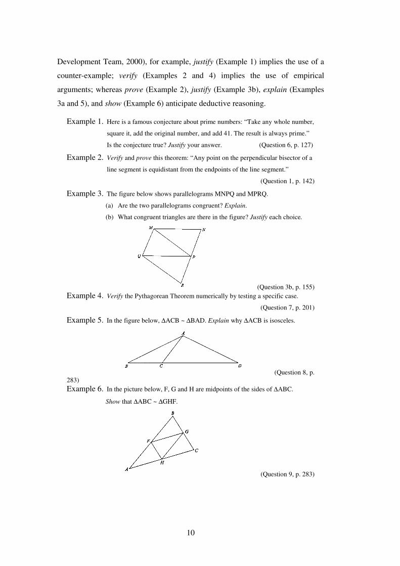
10
Development Team, 2000), for example, justify (Example 1) implies the use of a
counter-example; verify (Examples 2 and 4) implies the use of empirical
arguments; whereas prove (Example 2), justify (Example 3b), explain (Examples
3a and 5), and show (Example 6) anticipate deductive reasoning.
Example 1. Here is a famous conjecture about prime numbers: “Take any whole number,
square it, add the original number, and add 41. The result is always prime.”
Is the conjecture true? Justify your answer. (Question 6, p. 127)
Example 2. Verify and prove this theorem: “Any point on the perpendicular bisector of a
line segment is equidistant from the endpoints of the line segment.”
(Question 1, p. 142)
Example 3. The figure below shows parallelograms MNPQ and MPRQ.
(a) Are the two parallelograms congruent? Explain.
(b) What congruent triangles are there in the figure? Justify each choice.
(Question 3b, p. 155) Example 4. Verify the Pythagorean Theorem numerically by testing a specific case.
(Question 7, p. 201)
Example 5. In the figure below, ∆ACB ~ ∆BAD. Explain why ∆ACB is isosceles.
(Question 8, p. 283) Example 6. In the picture below, F, G and H are midpoints of the sides of ∆ABC.
Show that ∆ABC ~ ∆GHF.
(Question 9, p. 283)
11
In this particular textbook, then, it seems that verify may be interpreted to mean
‘convince yourself’, with the implication that empirical evidence is used for this
purpose. Justify implies providing some form of support for your statements,
perhaps a counter-example or deductive reasoning, in order to convince someone
else, whereas show, explain, and prove are used synonymously to mean providing
a logical argument.
2.2.3 Defining ‘proof’ and proof-related terms
From the discussion of proof in sections 2.2.1 and 2.2.2, it is seen that
mathematical proof can mean different things to different people and in different
contexts. In addition, there are many proof-related terms such as conjecture,
argument, and argumentation which will be used throughout this thesis, and it is
important at this stage to define the sense in which these terms are to be used. The
number of terms will be limited to those essential to the discussion of the issues
surrounding proof in school mathematics. As far as possible, these terms will be
used consistently, except with reference to quotations where authors may have
implied different meanings.
Conjecture An informed guess or hypothesis based on a
mathematical observation.
Argument A sequence of mathematical statements that aims to
convince. An argument may therefore be either a sub-
structure arising in the course of an argumentation, or the
end-product of the argumentation.
Argumentation A process of logically connected mathematical discourse.
Empirical argument An argument, based on a number of specific cases, that
supports a conjecture.
Mathematical proof An argument that confirms the truth of a conjecture for
all cases, or that refutes a conjecture by counter-example.
Deductive reasoning Reasoning based on deducing statements from
definitions, previously deduced statements, or given
information.
12
2.2.4 A rationale for proof in the school mathematics curriculum
Hanna (1995) argues that “proof should be part of any mathematics curriculum
that purports to reflect mathematics itself” (p. 42), while Davis and Hersh (1983)
suggest that “the novice who studies proofs gets closer to the creation of new
mathematics” (p. 151). Connected Geometry (Connected Geometry Development
Team, 2000) advises students that building on the work of experienced people is
an important part of all learning: “you study what they do, and then in your own
way make their techniques your own” (p. xi). The preface to the textbook gives a
clear message that the foundations of mathematics lie in deductive proof: “Every
branch of knowledge has its own way of establishing major results. In
mathematics, the major results are known as theorems, which are established
through deductive proof” (p. xiii).
The promotion of proof as the foundation of mathematics will not necessarily
motivate students, though, unless it is accompanied by an approach to proof
learning where the students feel that they are participating in meaningful
mathematical discovery. As Hanna and Jahnke (1993) note,
the challenge of actual mathematical enquiry cannot be entirely reproduced. All the
parties to the classroom interaction, teachers and students, know that they are
dealing with theorems that have already been proven by others. (p. 433)
The question arises, then, whether mathematical proof serves other functions that
might be relevant in school mathematics. Hersh (1993) asserts that “mathematical
proof can convince, and it can explain. In mathematical research, its primary role
is convincing. At the high-school or undergraduate level, its primary role is
explaining” (p. 398). Hanna (1995, p. 42) suggests that “the main function of
proof in the classroom reflects one of its key functions in mathematics itself: the
promotion of understanding”. The next three sections will focus on the roles of
proof as conviction, as explanation, and as an aid to understanding, in the
mathematics classroom.
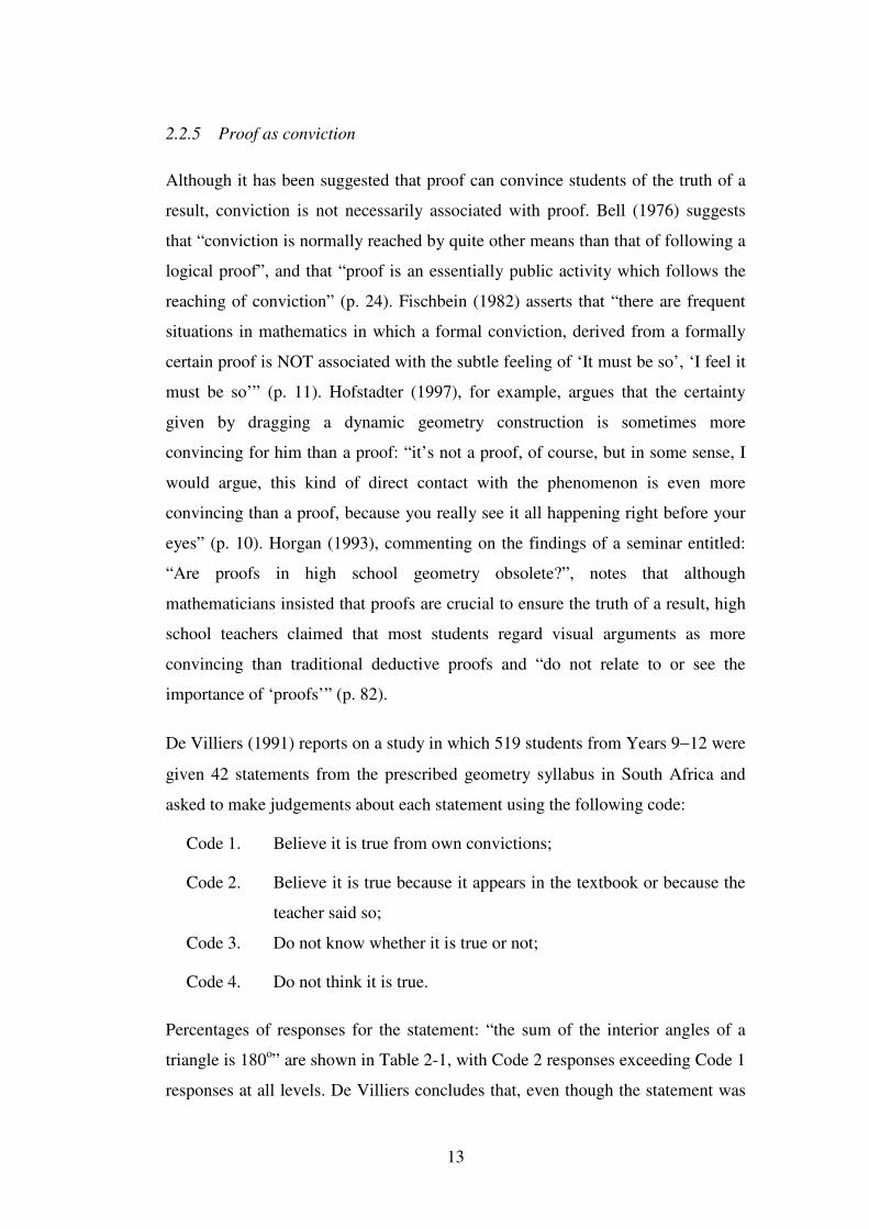
13
2.2.5 Proof as conviction
Although it has been suggested that proof can convince students of the truth of a
result, conviction is not necessarily associated with proof. Bell (1976) suggests
that “conviction is normally reached by quite other means than that of following a
logical proof”, and that “proof is an essentially public activity which follows the
reaching of conviction” (p. 24). Fischbein (1982) asserts that “there are frequent
situations in mathematics in which a formal conviction, derived from a formally
certain proof is NOT associated with the subtle feeling of ‘It must be so’, ‘I feel it
must be so’” (p. 11). Hofstadter (1997), for example, argues that the certainty
given by dragging a dynamic geometry construction is sometimes more
convincing for him than a proof: “it’s not a proof, of course, but in some sense, I
would argue, this kind of direct contact with the phenomenon is even more
convincing than a proof, because you really see it all happening right before your
eyes” (p. 10). Horgan (1993), commenting on the findings of a seminar entitled:
“Are proofs in high school geometry obsolete?”, notes that although
mathematicians insisted that proofs are crucial to ensure the truth of a result, high
school teachers claimed that most students regard visual arguments as more
convincing than traditional deductive proofs and “do not relate to or see the
importance of ‘proofs’” (p. 82).
De Villiers (1991) reports on a study in which 519 students from Years 9−12 were
given 42 statements from the prescribed geometry syllabus in South Africa and
asked to make judgements about each statement using the following code:
Code 1. Believe it is true from own convictions;
Code 2. Believe it is true because it appears in the textbook or because the
teacher said so;
Code 3. Do not know whether it is true or not;
Code 4. Do not think it is true.
Percentages of responses for the statement: “the sum of the interior angles of a
triangle is 180o” are shown in Table 2-1, with Code 2 responses exceeding Code 1
responses at all levels. De Villiers concludes that, even though the statement was
14
formally proved in Year 9, the majority of students based their beliefs on
authoritarian grounds rather than on their own convictions.
Table 2-1
Percentage Responses for the Statement “The sum of the interior angles of a
triangle is 180o” [From De Villiers, 1991, Table 1, P. 256].
Code 1 2 3 4 Unanswered
Year 9 37.1 50.5 6.7 5.7 0
Year 10 23.1 71.4 3.4 2.1 0
Year 11 22.8 71.0 3.4 2.1 0.7
Year 12 18.7 74.8 3.3 2.4 0.8
In two other studies cited by de Villiers (Smith, 1987; de Villiers & Njisane,
1987), 1465 students in Years 9 and 10 from ten different schools, and 494
students in Years 11 and 12 from four different schools, were asked whether they
were certain of the truth of the following two statements, and on what grounds
they based their certainty or uncertainty:
1. In an isosceles triangle the angles opposite the equal sides are equal.
2. If two parallel lines are cut by a transversal, then the alternate angles are
equal.
In both cases, proofs of the statements were included in the Year 9 curriculum. De
Villiers noted that “although 88% of students were certain of the truth of both
these statements, only 7% indicated that they were correct because they could be
proved, and the majority just repeated the statements as reasons or simply left the
second parts unanswered” (p. 256).
2.2.6 Proof as explanation
Dreyfus and Hadas (1996) contend that “a proof that convinces is also likely to
have explanatory value: Having been convinced by a proof of the correctness of a
statement, one is more likely to feel that one understands it” (p. 1). They describe
an activity in which students were provided with the diagrams shown in Figure
2-1. The students were asked to copy the angles onto a transparency and then
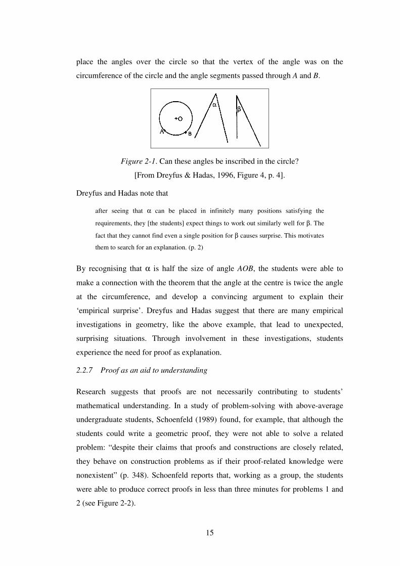
15
place the angles over the circle so that the vertex of the angle was on the
circumference of the circle and the angle segments passed through A and B.
Figure 2-1. Can these angles be inscribed in the circle?
[From Dreyfus & Hadas, 1996, Figure 4, p. 4].
Dreyfus and Hadas note that
after seeing that α can be placed in infinitely many positions satisfying the
requirements, they [the students] expect things to work out similarly well for β. The
fact that they cannot find even a single position for β causes surprise. This motivates
them to search for an explanation. (p. 2)
By recognising that α is half the size of angle AOB, the students were able to
make a connection with the theorem that the angle at the centre is twice the angle
at the circumference, and develop a convincing argument to explain their
‘empirical surprise’. Dreyfus and Hadas suggest that there are many empirical
investigations in geometry, like the above example, that lead to unexpected,
surprising situations. Through involvement in these investigations, students
experience the need for proof as explanation.
2.2.7 Proof as an aid to understanding
Research suggests that proofs are not necessarily contributing to students’
mathematical understanding. In a study of problem-solving with above-average
undergraduate students, Schoenfeld (1989) found, for example, that although the
students could write a geometric proof, they were not able to solve a related
problem: “despite their claims that proofs and constructions are closely related,
they behave on construction problems as if their proof-related knowledge were
nonexistent” (p. 348). Schoenfeld reports that, working as a group, the students
were able to produce correct proofs in less than three minutes for problems 1 and
2 (see Figure 2-2).
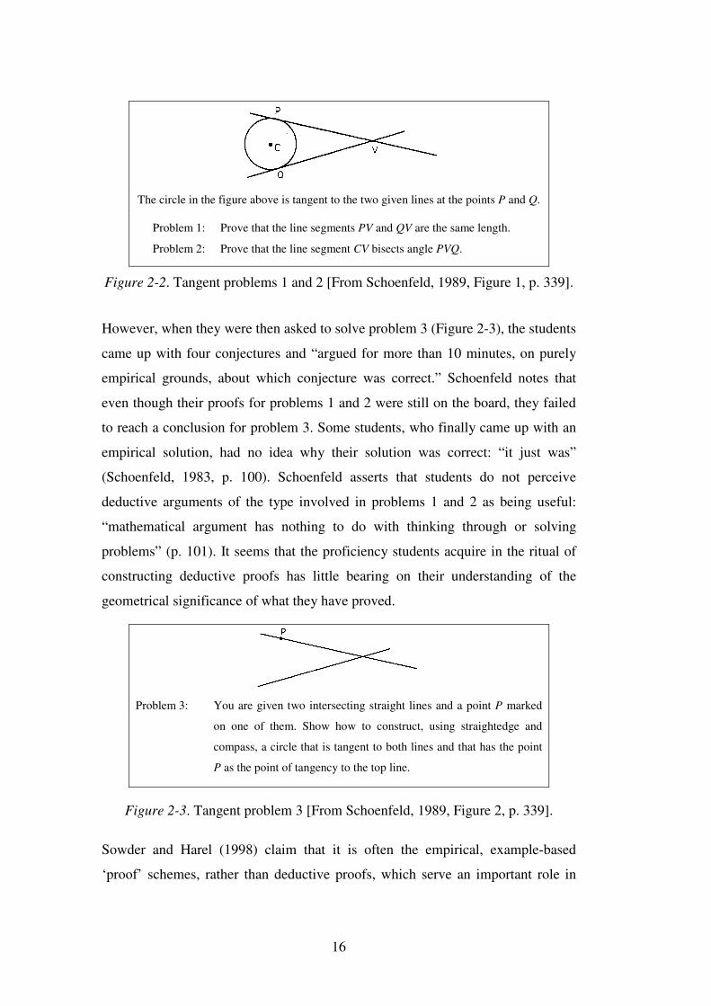
16
The circle in the figure above is tangent to the two given lines at the points P and Q.
Problem 1: Prove that the line segments PV and QV are the same length.
Problem 2: Prove that the line segment CV bisects angle PVQ.
Figure 2-2. Tangent problems 1 and 2 [From Schoenfeld, 1989, Figure 1, p. 339].
However, when they were then asked to solve problem 3 (Figure 2-3), the students
came up with four conjectures and “argued for more than 10 minutes, on purely
empirical grounds, about which conjecture was correct.” Schoenfeld notes that
even though their proofs for problems 1 and 2 were still on the board, they failed
to reach a conclusion for problem 3. Some students, who finally came up with an
empirical solution, had no idea why their solution was correct: “it just was”
(Schoenfeld, 1983, p. 100). Schoenfeld asserts that students do not perceive
deductive arguments of the type involved in problems 1 and 2 as being useful:
“mathematical argument has nothing to do with thinking through or solving
problems” (p. 101). It seems that the proficiency students acquire in the ritual of
constructing deductive proofs has little bearing on their understanding of the
geometrical significance of what they have proved.
Problem 3: You are given two intersecting straight lines and a point P marked
on one of them. Show how to construct, using straightedge and
compass, a circle that is tangent to both lines and that has the point
P as the point of tangency to the top line.
Figure 2-3. Tangent problem 3 [From Schoenfeld, 1989, Figure 2, p. 339].
Sowder and Harel (1998) claim that it is often the empirical, example-based
‘proof’ schemes, rather than deductive proofs, which serve an important role in
17
increasing understanding. They caution, though, that students “must become
aware of the tentative nature of conjectures formed on the basis of examples, and
they must grow in their abilities to offer better justifications than those offered by
examples” (p. 673); that is, they must move towards deductive proof schemes.
2.3 Argumentation and proof
2.3.1 Argumentation and the process of proving
The relationship between argumentation and proof has been the subject of much
debate (for example, Balacheff, 1991, 1999; Boero, 1999; Douek, 1998; Duval,
1991), with Balacheff (1991, p. 188) going so far as to assert that “‘argumentative
behaviors’ … are genuine epistemological obstacles to the learning of
mathematical proof”. What, though, are the common features of, and differences
between, argumentation and proof?
As stated in section 2.2.3, argument is defined in this thesis as “a sequence of
mathematical statements that aims to convince” and argumentation as “a process
of logically connected mathematical discourse”. Krummheuer (1995) views an
argument as either a specific sub-structure within a complex argumentation or the
outcome of an argumentation: “The final sequence of statements accepted by all
participants, which are more or less completely reconstructable by the participants
or by an observer as well, will be called an argument” (p. 247). We can therefore
distinguish between argumentation as a process and argument as a product.
Krummheuer notes that argumentation traditionally relates to an individual
convincing a group of listeners but may also be an internal process carried out by
an individual. He uses the term ‘collective argumentation’ to describe an
argumentation accomplished by a group of individuals.
Douek (1998) asserts that, although “argumentations are usually held informally
between mathematicians to develop, discuss or communicate mathematical
problems and results” (p. 130), there are strong links between argumentation and
the process of proving in mathematics: “proving and arguing, as processes, have
many common aspects from the cognitive and epistemological points of view,
though significant differences exist between them as socially situated products”
18
(p. 126). He argues that both are concerned with the validity of statements, and
that associated with both is a body of related information, the ‘reference corpus’,
which will include, for example, knowledge about the subject, experimental
evidence, or visual evidence, which is used to support the steps of reasoning.
There may be differences, however, in the forms of reasoning employed in the
products of the two processes; whereas a proof is generally based on deductive
reasoning, arguments may use a variety of forms of reasoning.
2.3.2 The conflict between argumentation and proof
Balacheff (1999) asserts that there is a contradiction between the natural language
of students’ argumentation and the logic associated with deductive reasoning. He
cites Toulmin (1958) and Perelman (1970), and contrasts their theoretical
conceptions of argument. According to Toulmin, the structure of the discourse
determines the validity of an argument, with each statement serving a particular
role in the argument, whereas Perelman believes that the strength of an argument
lies in its capacity to convince the listener, rather than in establishment of the
validity of the statement in question. Although Balacheff (1991) concedes that
“social interaction while solving a problem can favour the appearance of students’
proving processes” (p. 188), he aligns himself with Perelman’s view of argument,
asserting that argumentation implies the freedom to convince by whatever means
one chooses:
The aim of argumentation is to obtain the agreement of the partner in the interaction,
but not in the first place to establish the truth of some statement. As a social
behavior it is an open process, in other words it allows the use of any kind of means;
whereas, for mathematical proofs, we have to fit the requirement for the use of some
knowledge taken from a common body of knowledge on which people
(mathematicians) agree. (Balacheff, 1991, p. 188−189)
More recently, Balacheff (1999) again makes the strong assertion that
argumentation is an obstacle to the teaching of proof because of this inherent
conflict between mathematical proof [démonstration], which must “exist relative
to an explicit axiom system”, and argumentation, which implies freedom to
choose how to convince:
19
The sources of argumentative competence are in natural language and in practices
whose rules are frequently of a profoundly different nature from those required by
mathematics, and carry a profound mark of the speakers and circumstances. (p. 3)
Argumentation as a process need not necessarily involve deductive reasoning.
Likewise, an argument does not need to be based on deductive logic; arguments
may use, for example, empirical data, visual data, or narrative explanations.
However, argumentation and deductive logic are not mutually exclusive.
Responding to Balacheff’s views on argumentation and proof, Boero (1999)
focuses on the distinction between ‘proving’ as a process, that is, argumentation,
and ‘proof’ as a product. He notes that from this perspective the nature of
arguments used by students depends on the establishment of a culture of theorems
in the classroom, on the nature of the task, and the specific kinds of reasoning
emphasised by the teacher. Boero regards Balacheff’s reference to “the freedom
one could give oneself as a person in the play of an argument” as inappropriate, as
strong teacher intervention should ensure that students’ arguments are based on
sound mathematical logic.
Hanna (1995) also emphasises that teacher intervention must be a part of any
learning methods which encourage students to interact with each other. She
asserts, though, that where classroom practice is informed by constructivist
theories, evidence indicates that in many cases teachers are not intervening:
… teachers tend not to present mathematical arguments or take a substantive part in
their discussion. They tend to provide only limited support to students, leaving them
in large measure to make sense of arguments by themselves. (p. 44)
Hanna notes, however, that constructivist theory itself does not preclude teacher
intervention. She cites Yackel and Cobb (1994) who emphasise the crucial role of
the teacher:
… when students give explanations and arguments in the mathematics classroom
their purpose is to describe and clarify their thinking for others, to convince others of
the appropriateness of their solution methods, but not to establish the veracity of a
new mathematical “truth”. … The meaning of what counts as an acceptable
mathematical explanation is interactively constituted by the teacher and the
20
children. (Yackel & Cobb, 1994, p. 3, cited in Hanna, 1995) [emphasis in the
original]
The issue of teacher intervention is of paramount importance in the current
research, in that the teacher challenges students to give deductive reasons in their
argumentations.
2.3.3 Analysing the structure of arguments
Argument theories have been developed that provide a theoretical framework for
analysing the structure of arguments, particularly deductive arguments, as well as
the structure of the reasoning that occurs during a process of argumentation.
Freeman (1991) points out that an argument theory is useful only if it provides a
rationale for recognising the different functions of statements in the argument.
These functions are based on a theory of what rational argumentation is: its
primary function is to convince, but to convince with a reasoned justification. The
theory, and any associated method of diagrammatic representation, must allow an
argument to be analysed without having to distort the argument to fit the theory.
According to the standard argument model described by Freeman (1991), there
are just two types of elements in arguments—premises and conclusions, and the
function of an element is indicated by its position in the argument diagram, as
shown in Figure 2-4a. Conclusions, that appear at the head of the arrow, may
sometimes be supported by two or more independent or linked premises. Figure
2-4b shows two independent premises, P1 and P2, either of which supports
conclusion C, whereas in Figure 2-4c, P1 and P2 are linked premises that together
support the conclusion, C. In Figure 2-5a, for example, either premise will support
the conclusion that ABC is an isosceles triangle, whereas in Figure 2-5b, neither
premise alone is sufficient to support the conclusion that ABCD is a
parallelogram. In many arguments, a conclusion becomes a premise for a further
conclusion, as shown in Figure 2-4d, where the conclusion C1 becomes the
premise for conclusion C2.
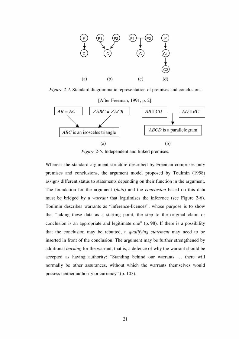
21
P
C
P1 P2
C
P1 P2
C
C2
P
C1
(a) (b) (c) (d)
Figure 2-4. Standard diagrammatic representation of premises and conclusions
[After Freeman, 1991, p. 2].
(a) (b)
Figure 2-5. Independent and linked premises.
Whereas the standard argument structure described by Freeman comprises only
premises and conclusions, the argument model proposed by Toulmin (1958)
assigns different status to statements depending on their function in the argument.
The foundation for the argument (data) and the conclusion based on this data
must be bridged by a warrant that legitimises the inference (see Figure 2-6).
Toulmin describes warrants as “inference-licences”, whose purpose is to show
that “taking these data as a starting point, the step to the original claim or
conclusion is an appropriate and legitimate one” (p. 98). If there is a possibility
that the conclusion may be rebutted, a qualifying statement may need to be
inserted in front of the conclusion. The argument may be further strengthened by
additional backing for the warrant, that is, a defence of why the warrant should be
accepted as having authority: “Standing behind our warrants … there will
normally be other assurances, without which the warrants themselves would
possess neither authority or currency” (p. 103).
AB || CD AD || BC
ABCD is a parallelogram
AB = AC ∠ABC = ∠ACB
ABC is an isosceles triangle
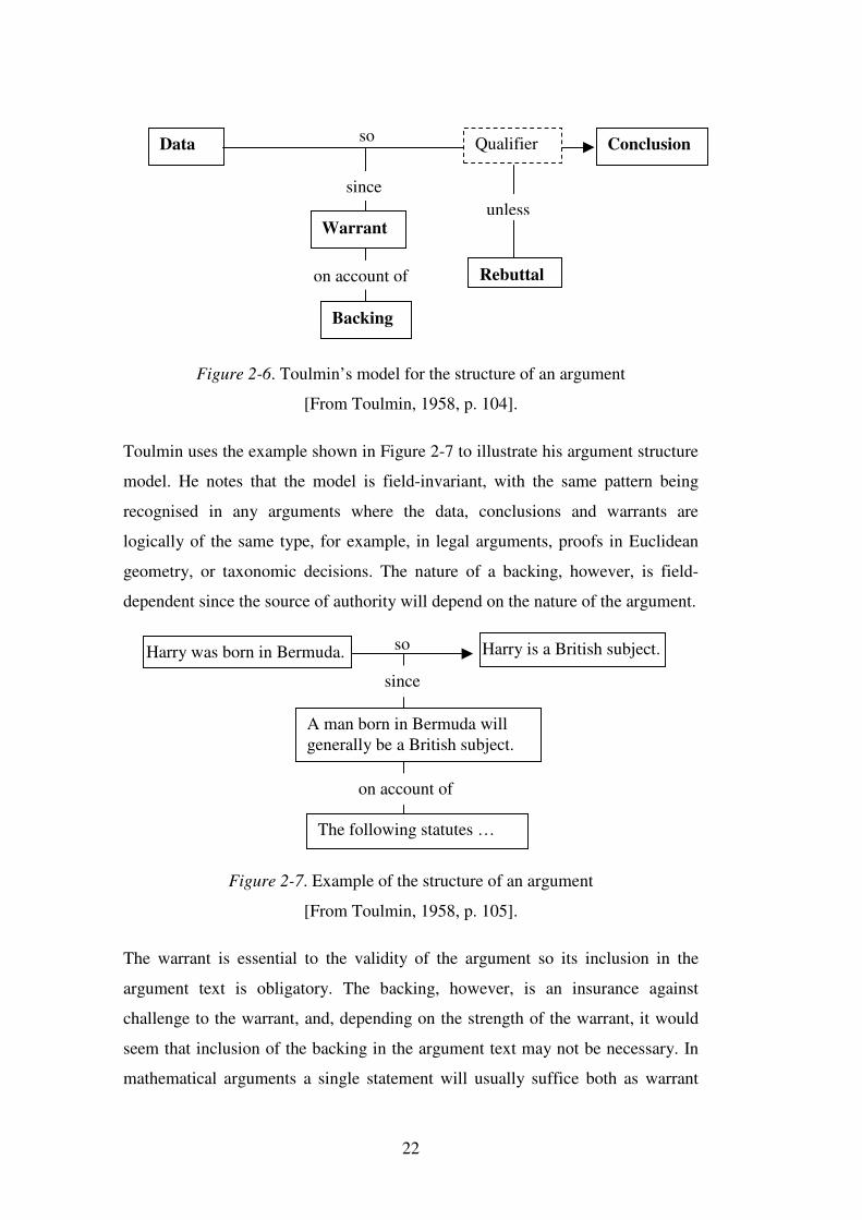
22
Figure 2-6. Toulmin’s model for the structure of an argument
[From Toulmin, 1958, p. 104].
Toulmin uses the example shown in Figure 2-7 to illustrate his argument structure
model. He notes that the model is field-invariant, with the same pattern being
recognised in any arguments where the data, conclusions and warrants are
logically of the same type, for example, in legal arguments, proofs in Euclidean
geometry, or taxonomic decisions. The nature of a backing, however, is field-
dependent since the source of authority will depend on the nature of the argument.
Figure 2-7. Example of the structure of an argument
[From Toulmin, 1958, p. 105].
The warrant is essential to the validity of the argument so its inclusion in the
argument text is obligatory. The backing, however, is an insurance against
challenge to the warrant, and, depending on the strength of the warrant, it would
seem that inclusion of the backing in the argument text may not be necessary. In
mathematical arguments a single statement will usually suffice both as warrant
Conclusion Data so
Backing
Warrant
since
on account of
unless
Rebuttal
Qualifier
Harry was born in Bermuda. Harry is a British subject. so
since
A man born in Bermuda will generally be a British subject.
The following statutes …
on account of
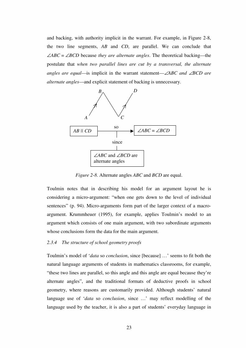
23
and backing, with authority implicit in the warrant. For example, in Figure 2-8,
the two line segments, AB and CD, are parallel. We can conclude that
∠ABC = ∠BCD because they are alternate angles. The theoretical backing—the
postulate that when two parallel lines are cut by a transversal, the alternate
angles are equal—is implicit in the warrant statement—∠ABC and ∠BCD are
alternate angles—and explicit statement of backing is unnecessary.
Figure 2-8. Alternate angles ABC and BCD are equal.
Toulmin notes that in describing his model for an argument layout he is
considering a micro-argument: “when one gets down to the level of individual
sentences” (p. 94). Micro-arguments form part of the larger context of a macro-
argument. Krummheuer (1995), for example, applies Toulmin’s model to an
argument which consists of one main argument, with two subordinate arguments
whose conclusions form the data for the main argument.
2.3.4 The structure of school geometry proofs
Toulmin’s model of ‘data so conclusion, since [because] …’ seems to fit both the
natural language arguments of students in mathematics classrooms, for example,
“these two lines are parallel, so this angle and this angle are equal because they’re
alternate angles”, and the traditional formats of deductive proofs in school
geometry, where reasons are customarily provided. Although students’ natural
language use of ‘data so conclusion, since …’ may reflect modelling of the
language used by the teacher, it is also a part of students’ everyday language in
A C
D B
AB || CD ∠ABC = ∠BCD
∠ABC and ∠BCD are alternate angles
so
since
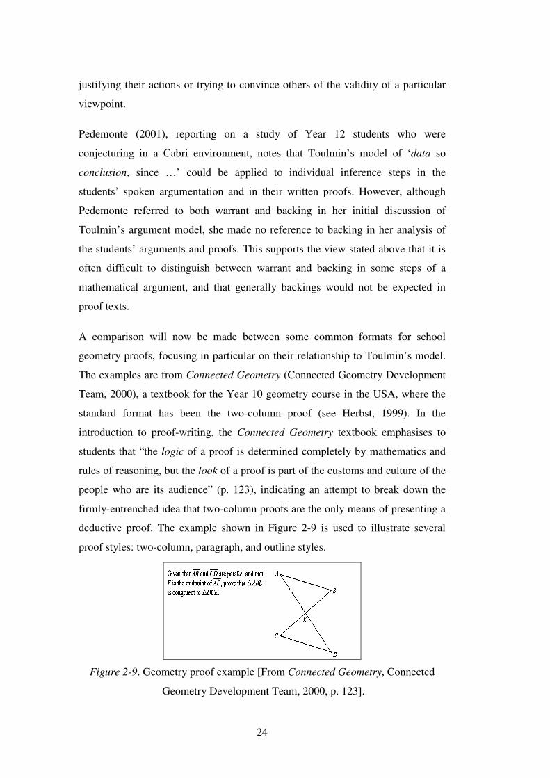
24
justifying their actions or trying to convince others of the validity of a particular
viewpoint.
Pedemonte (2001), reporting on a study of Year 12 students who were
conjecturing in a Cabri environment, notes that Toulmin’s model of ‘data so
conclusion, since …’ could be applied to individual inference steps in the
students’ spoken argumentation and in their written proofs. However, although
Pedemonte referred to both warrant and backing in her initial discussion of
Toulmin’s argument model, she made no reference to backing in her analysis of
the students’ arguments and proofs. This supports the view stated above that it is
often difficult to distinguish between warrant and backing in some steps of a
mathematical argument, and that generally backings would not be expected in
proof texts.
A comparison will now be made between some common formats for school
geometry proofs, focusing in particular on their relationship to Toulmin’s model.
The examples are from Connected Geometry (Connected Geometry Development
Team, 2000), a textbook for the Year 10 geometry course in the USA, where the
standard format has been the two-column proof (see Herbst, 1999). In the
introduction to proof-writing, the Connected Geometry textbook emphasises to
students that “the logic of a proof is determined completely by mathematics and
rules of reasoning, but the look of a proof is part of the customs and culture of the
people who are its audience” (p. 123), indicating an attempt to break down the
firmly-entrenched idea that two-column proofs are the only means of presenting a
deductive proof. The example shown in Figure 2-9 is used to illustrate several
proof styles: two-column, paragraph, and outline styles.
Figure 2-9. Geometry proof example [From Connected Geometry, Connected
Geometry Development Team, 2000, p. 123].
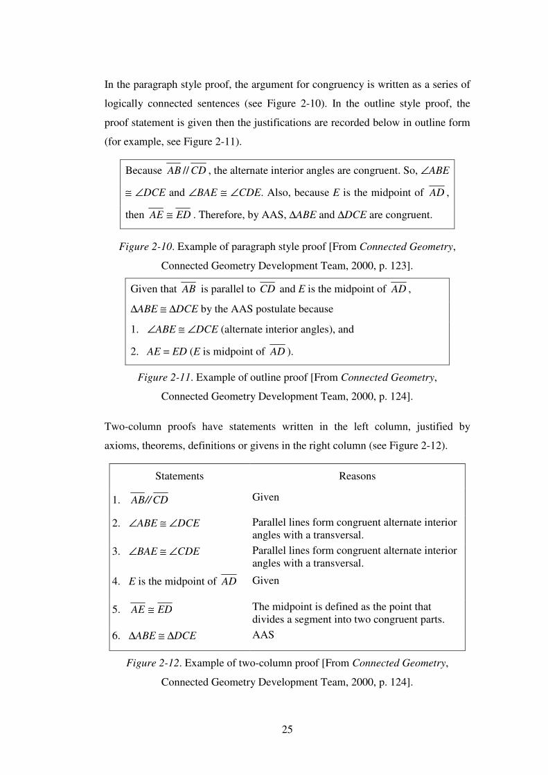
25
In the paragraph style proof, the argument for congruency is written as a series of
logically connected sentences (see Figure 2-10). In the outline style proof, the
proof statement is given then the justifications are recorded below in outline form
(for example, see Figure 2-11).
Because CDAB // , the alternate interior angles are congruent. So, ∠ABE
≅ ∠DCE and ∠BAE ≅ ∠CDE. Also, because E is the midpoint of AD ,
then EDAE ≅ . Therefore, by AAS, ∆ABE and ∆DCE are congruent.
Figure 2-10. Example of paragraph style proof [From Connected Geometry,
Connected Geometry Development Team, 2000, p. 123].
Given that AB is parallel to CD and E is the midpoint of AD ,
∆ABE ≅ ∆DCE by the AAS postulate because
1. ∠ABE ≅ ∠DCE (alternate interior angles), and
2. AE = ED (E is midpoint of AD ).
Figure 2-11. Example of outline proof [From Connected Geometry,
Connected Geometry Development Team, 2000, p. 124].
Two-column proofs have statements written in the left column, justified by
axioms, theorems, definitions or givens in the right column (see Figure 2-12).
Statements Reasons
1. CD//AB Given
2. ∠ABE ≅ ∠DCE Parallel lines form congruent alternate interior angles with a transversal.
3. ∠BAE ≅ ∠CDE Parallel lines form congruent alternate interior angles with a transversal.
4. E is the midpoint of AD Given
5. EDAE ≅ The midpoint is defined as the point that divides a segment into two congruent parts.
6. ∆ABE ≅ ∆DCE AAS
Figure 2-12. Example of two-column proof [From Connected Geometry,
Connected Geometry Development Team, 2000, p. 124].
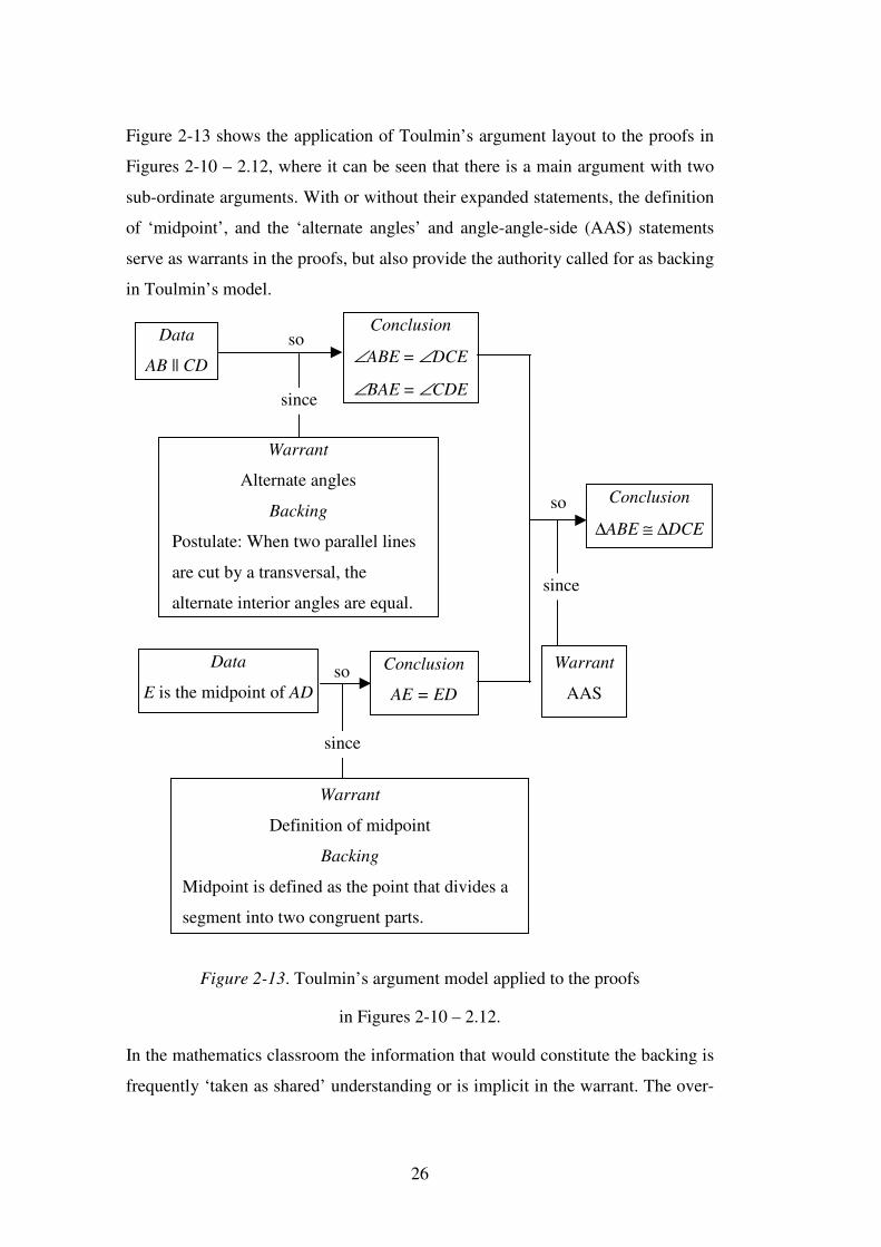
26
Figure 2-13 shows the application of Toulmin’s argument layout to the proofs in
Figures 2-10 – 2.12, where it can be seen that there is a main argument with two
sub-ordinate arguments. With or without their expanded statements, the definition
of ‘midpoint’, and the ‘alternate angles’ and angle-angle-side (AAS) statements
serve as warrants in the proofs, but also provide the authority called for as backing
in Toulmin’s model.
Figure 2-13. Toulmin’s argument model applied to the proofs
in Figures 2-10 – 2.12.
In the mathematics classroom the information that would constitute the backing is
frequently ‘taken as shared’ understanding or is implicit in the warrant. The over-
Data
AB || CD
Conclusion
∠ABE = ∠DCE
∠BAE = ∠CDE
Warrant
Alternate angles
Backing
Postulate: When two parallel lines
are cut by a transversal, the
alternate interior angles are equal.
Data
E is the midpoint of AD
Conclusion
AE = ED
Warrant
Definition of midpoint
Backing
Midpoint is defined as the point that divides a
segment into two congruent parts.
Conclusion
∆ABE ≅ ∆DCE
Warrant
AAS
so
so
so
since
since
since
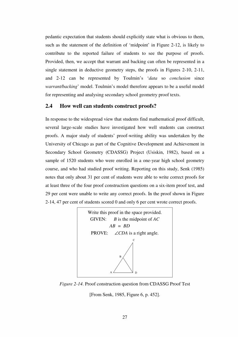
27
pedantic expectation that students should explicitly state what is obvious to them,
such as the statement of the definition of ‘midpoint’ in Figure 2-12, is likely to
contribute to the reported failure of students to see the purpose of proofs.
Provided, then, we accept that warrant and backing can often be represented in a
single statement in deductive geometry steps, the proofs in Figures 2-10, 2-11,
and 2-12 can be represented by Toulmin’s ‘data so conclusion since
warrant/backing’ model. Toulmin’s model therefore appears to be a useful model
for representing and analysing secondary school geometry proof texts.
2.4 How well can students construct proofs?
In response to the widespread view that students find mathematical proof difficult,
several large-scale studies have investigated how well students can construct
proofs. A major study of students’ proof-writing ability was undertaken by the
University of Chicago as part of the Cognitive Development and Achievement in
Secondary School Geometry (CDASSG) Project (Usiskin, 1982), based on a
sample of 1520 students who were enrolled in a one-year high school geometry
course, and who had studied proof writing. Reporting on this study, Senk (1985)
notes that only about 31 per cent of students were able to write correct proofs for
at least three of the four proof construction questions on a six-item proof test, and
29 per cent were unable to write any correct proofs. In the proof shown in Figure
2-14, 47 per cent of students scored 0 and only 6 per cent wrote correct proofs.
Write this proof in the space provided. GIVEN: B is the midpoint of AC
AB = BD PROVE: ∠CDA is a right angle.
C
DA
B
Figure 2-14. Proof construction question from CDASSG Proof Test
[From Senk, 1985, Figure 6, p. 452].
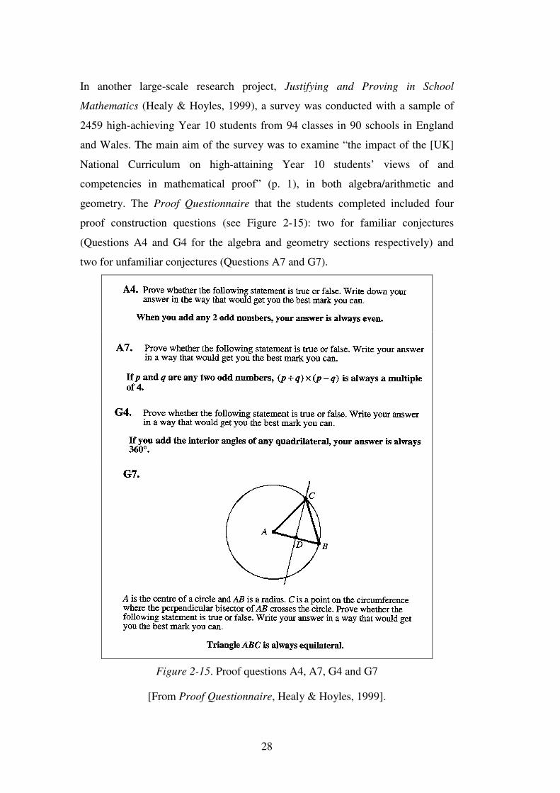
28
In another large-scale research project, Justifying and Proving in School
Mathematics (Healy & Hoyles, 1999), a survey was conducted with a sample of
2459 high-achieving Year 10 students from 94 classes in 90 schools in England
and Wales. The main aim of the survey was to examine “the impact of the [UK]
National Curriculum on high-attaining Year 10 students’ views of and
competencies in mathematical proof” (p. 1), in both algebra/arithmetic and
geometry. The Proof Questionnaire that the students completed included four
proof construction questions (see Figure 2-15): two for familiar conjectures
(Questions A4 and G4 for the algebra and geometry sections respectively) and
two for unfamiliar conjectures (Questions A7 and G7).
Figure 2-15. Proof questions A4, A7, G4 and G7
[From Proof Questionnaire, Healy & Hoyles, 1999].
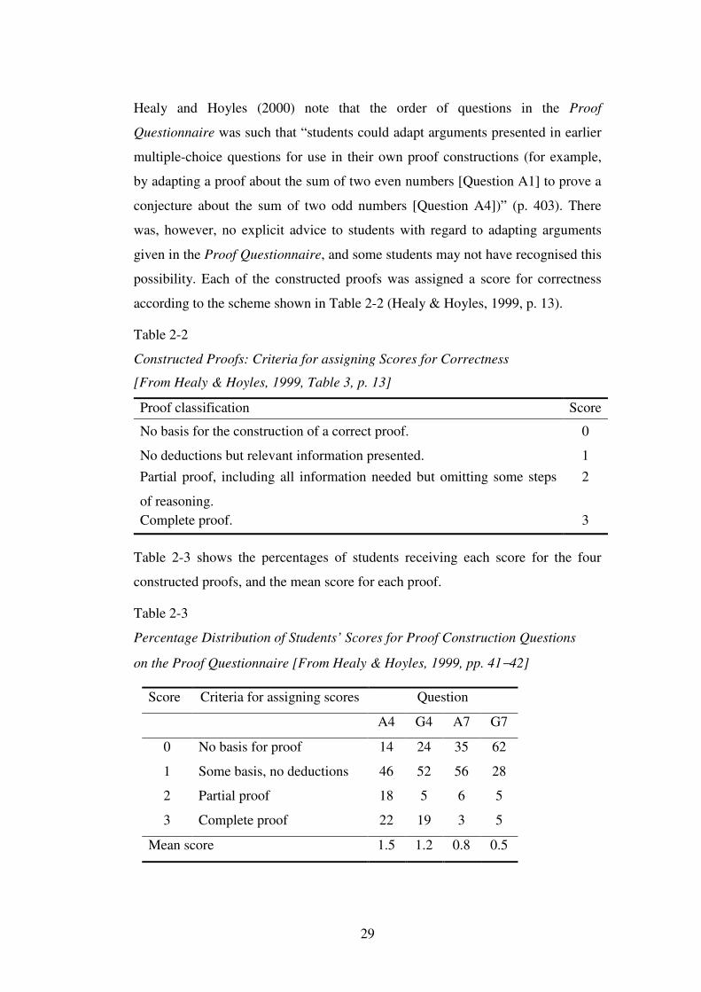
29
Healy and Hoyles (2000) note that the order of questions in the Proof
Questionnaire was such that “students could adapt arguments presented in earlier
multiple-choice questions for use in their own proof constructions (for example,
by adapting a proof about the sum of two even numbers [Question A1] to prove a
conjecture about the sum of two odd numbers [Question A4])” (p. 403). There
was, however, no explicit advice to students with regard to adapting arguments
given in the Proof Questionnaire, and some students may not have recognised this
possibility. Each of the constructed proofs was assigned a score for correctness
according to the scheme shown in Table 2-2 (Healy & Hoyles, 1999, p. 13).
Table 2-2
Constructed Proofs: Criteria for assigning Scores for Correctness
[From Healy & Hoyles, 1999, Table 3, p. 13]
Proof classification Score
No basis for the construction of a correct proof. 0
No deductions but relevant information presented. 1 Partial proof, including all information needed but omitting some steps
of reasoning.
2
Complete proof. 3
Table 2-3 shows the percentages of students receiving each score for the four
constructed proofs, and the mean score for each proof.
Table 2-3
Percentage Distribution of Students’ Scores for Proof Construction Questions
on the Proof Questionnaire [From Healy & Hoyles, 1999, pp. 41−42]
Score Criteria for assigning scores Question
A4 G4 A7 G7
0 No basis for proof 14 24 35 62
1 Some basis, no deductions 46 52 56 28
2 Partial proof 18 5 6 5
3 Complete proof 22 19 3 5
Mean score 1.5 1.2 0.8 0.5
30
The students coped considerably better with the familiar conjectures (A4 and G4)
than with the unfamiliar conjectures (A7 and G7), with significantly better
performance for algebra than for geometry proofs. Empirical arguments were
widely used, with deductive reasoning displayed by only 24% of students in the
familiar geometry question (G4) and 40% for the familiar algebra question (A4).
Even fewer students used deductive reasoning for the unfamiliar questions: 10%
for G7 and 9% for A7. Healy and Hoyles (1999) note that although the majority of
these high-attaining Year 10 students showed a consistent pattern of poor
performance in constructing proofs, many of them understood the generality of a
proof, and were able to recognise a valid mathematical argument.
2.5 Why do students have difficulty with proof in mathematics?
Whereas major studies such as those of Senk (1985) and Healy and Hoyles (1999)
demonstrate that many students have a poor understanding of mathematical proof,
other studies have examined the specific difficulties which students experience
with proof. Some studies have focused on students’ understanding of the concept
of proof (for example, Galbraith, 1981; de Villiers, 1991) whereas others (for
example, Duval, 1991) have looked at students’ difficulty with construction of
proofs, in particular deductive proofs. These two areas of difficulty are not
independent and several underlying issues, which will be discussed in sections
2.5.1 to 2.5.7, may be identified: students’ cognitive readiness for proof, students’
need for motivation for proof, understanding the requirement of generality in
mathematical proof, understanding the use of counter-examples, understanding
the structure of deductive reasoning, the often ritualistic approach to the teaching
and learning of proof, and the role of diagrams in geometric proof.
2.5.1 Cognitive readiness for proof
In many mathematics curricula, for example Australia’s Victorian Curriculum and
Standards Framework II (Board of Studies, 2000), it is assumed that students will
progress from empirical reasoning in primary and lower secondary years to
deductive reasoning at the upper level of secondary schooling. Implicit in this
hierarchy of mathematical reasoning is the notion of cognitive readiness for proof.
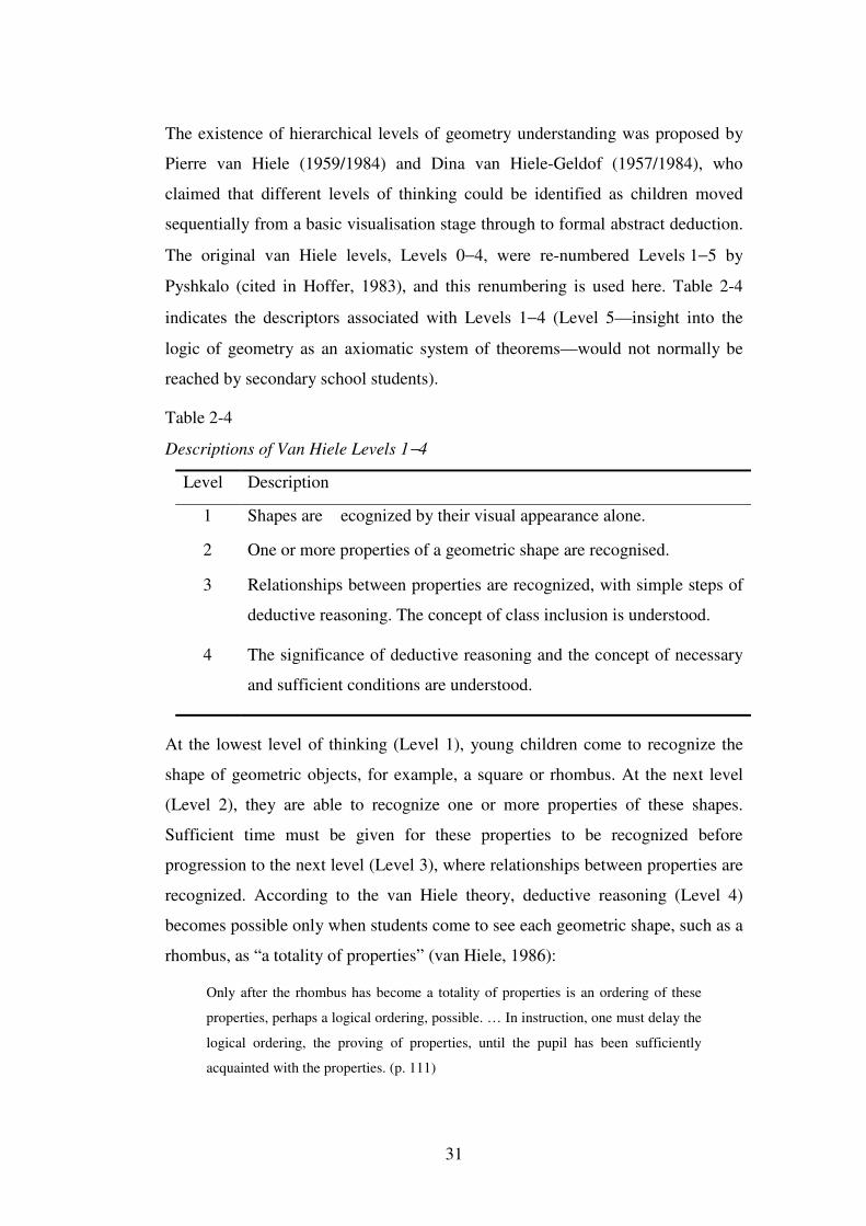
31
The existence of hierarchical levels of geometry understanding was proposed by
Pierre van Hiele (1959/1984) and Dina van Hiele-Geldof (1957/1984), who
claimed that different levels of thinking could be identified as children moved
sequentially from a basic visualisation stage through to formal abstract deduction.
The original van Hiele levels, Levels 0−4, were re-numbered Levels 1−5 by
Pyshkalo (cited in Hoffer, 1983), and this renumbering is used here. Table 2-4
indicates the descriptors associated with Levels 1−4 (Level 5—insight into the
logic of geometry as an axiomatic system of theorems—would not normally be
reached by secondary school students).
Table 2-4
Descriptions of Van Hiele Levels 1−4
Level Description
1 Shapes are �ecognized by their visual appearance alone.
2 One or more properties of a geometric shape are recognised.
3 Relationships between properties are recognized, with simple steps of
deductive reasoning. The concept of class inclusion is understood.
4 The significance of deductive reasoning and the concept of necessary
and sufficient conditions are understood.
At the lowest level of thinking (Level 1), young children come to recognize the
shape of geometric objects, for example, a square or rhombus. At the next level
(Level 2), they are able to recognize one or more properties of these shapes.
Sufficient time must be given for these properties to be recognized before
progression to the next level (Level 3), where relationships between properties are
recognized. According to the van Hiele theory, deductive reasoning (Level 4)
becomes possible only when students come to see each geometric shape, such as a
rhombus, as “a totality of properties” (van Hiele, 1986):
Only after the rhombus has become a totality of properties is an ordering of these
properties, perhaps a logical ordering, possible. … In instruction, one must delay the
logical ordering, the proving of properties, until the pupil has been sufficiently
acquainted with the properties. (p. 111)
32
Several major studies of the van Hiele theory (for example, Usiskin, 1982; Fuys,
Geddes, & Tischler, 1988) have supported the hierarchical nature of children’s
learning of geometry, but suggest that the levels are continuous, rather than
discrete, and that students may operate on different levels for different concepts.
The emphasis on class inclusion as a signifier of Level 3 thinking has also been
questioned (for example, Pegg, 1992), since it appears that understanding of this
concept depends on the learning environment, and is not a natural part of students’
progress in geometry.
Van Dormolen (1977) contends that too often in the past there was “for many
students a forced [unsuccessful] operating on the second level of thinking
[Level 3], whereas they had not as yet reached or sufficiently explored the first
[Level 2]” (p. 33). He asserts that worldwide reaction to this situation resulted in a
curriculum where “more students can enjoy mathematics because they are allowed
to continue operating on the ground level [Level 1]” (p. 33) but where insufficient
opportunities are provided for those who are ready to progress to higher levels.
Senk (1989) analysed data from the Cognitive Development and Achievement in
Secondary School Geometry (CDASSG) project (Usiskin, 1982), and reports that
the van Hiele score accounted for 34% of the variance (p < 0.0001) in proof-
writing achievement of secondary school students enrolled in a full year geometry
course. Although some students entering the year at Level 1 were able to do
simple standard geometry proofs by the end of the year, “Level 2 appears to be the
critical entry level”, with students entering at this level having a 50% chance of
mastering proof writing (p. 319). This positive correlation between van Hiele level
and proof writing ability is hardly surprising—if students fail to recognise
properties or to appreciate the relationships between these properties, they are
unlikely to be able to write a proof, even at the level of rote learning of standard
proofs, as steps in the proof will hold little meaning for them.
Tall (1995) also proposes a hierarchical model of mathematical development,
where visualisation and symbolisation interact with each other through
diagrammatic representations, and in turn give rise at a later stage to the need for
33
formal definition and proof. Tall argues, though, that the move from the visual
representations of elementary mathematics to formal representations is not only
hierarchical, but requires a major cognitive reconstruction. Formal proof is
therefore meaningful and possible only when the student has reached an
appropriate level of cognitive development.
Duval (1998), however, questions a hierarchical model for the growth in students’
understanding of geometry and proof, asserting that three cognitive processes—
visualisation, construction, and reasoning—are closely connected and “their
synergy is cognitively necessary for proficiency in geometry” (p. 38). He suggests
that visualisation, reasoning, and analytic and synthetic processes are operative at
each age level, from young children to maturity. Although there will be
interaction between the processes, and in particular contexts one may predominate
over others, Duval claims that they each have specific and independent
development, and asserts that
this rules out any model of development in which different kinds of cognitive
activities would be organized into a strict hierarchy from the concrete to the most
abstract, from visualisation to the axiomatic rigour. (pp. 49−50)
Similarly, Hoyles (1997) questions the existence of a hierarchy in students’
understanding of proof, suggesting that such hierarchies are artefacts of
methodology. She asserts that the design of many studies leads inevitably to an
interpretation of a hierarchical classification:
The empirical core of the study comprises the identification and analysis of students’
written responses to a range of questions concerning proof. The meaning of what is
required as a proof is not made explicit; neither is it clear what the students have
been taught, what has been emphasised and what forms of presentation are deemed
to be acceptable. The influences of the content and sequencing of the curriculum are
ignored in an analysis which takes the individual student and their constructions of
proof as the object of attention—an analysis that leads almost inevitably to some
kind of hierarchical classification. (p. 7)
Hoyles contends that alternative interpretations should consider social and
pedagogical dimensions such as teachers’ attitude to what constitutes an
34
acceptable proof, how proof is introduced to the students, and the sequencing in
mathematics curricula.
Despite these conflicting views on the development of children’s reasoning, there
has been a widespread assumption in current school mathematics curricula that the
development is hierarchical, and that there must be a progression from empirical,
inductive reasoning to deductive reasoning. The outcome of this assumption is
that deductive reasoning is reserved for later years of secondary school
mathematics, and few students are given the opportunity to progress beyond
empirical reasoning. Healy and Hoyles (1999) note, for example, that the National
Curriculum in the UK
prescribes an approach to proving … in which the introduction of formal proofs is
reserved for ‘exceptional performance’, and thus delayed until after students have
progressed through early stages of reasoning empirically and explaining their
conjectures. Most of the requirements to explain and justify take place within
investigations driven by numerical data. (p. 1)
Hoyles (1997) asserts that “we must resist the temptation to assume that situations
that engage students with proof must follow a linear sequence from induction to
deduction” (p. 15). The US Principles and Standards for School Mathematics
(National Council of Teachers of Mathematics, 2000) suggests that even very
young children, for example, Pre-kindergarten − Grade 2, should be engaging in
deductive reasoning:
They use a combination of ways of justifying their answers—perception, empirical
evidence, and short chains of deductive reasoning grounded in previously accepted
facts. They make conjectures and reach conclusions that are logical and defensible
from their perspective. (p. 122)
Students’ readiness for formal proof may depend, then, on the laying down of
appropriate foundations in the early years, where justifying goes beyond empirical
evidence to include simple steps of deductive reasoning.
35
2.5.2 Motivation for proof
Students are likely to find difficulty appreciating the role of proof if they do not
experience a need for conviction. Dreyfus and Hadas (1996) argue that the failure
of many students to understand the need for proof rests with the type of statements
students are asked to prove: “students of Euclidean geometry are so often asked to
prove statements that seem patently obvious to them” (p. 1). Reporting on a
survey of students’ perception of the meaning of proof, Galbraith (1979) notes the
response of one 15-year-old:
It means to show, perhaps by different methods something that someone has already
shown, but it does not show anything new. … To prove something is to show what
is already known often using a long winded method to get to the already known
answer. (p. 58)
Goldenberg, Cuoco, and Mark (1998) suggest that
proof for beginners might need to be motivated by the uncertainties that remain
without the proof, or by a need for an explanation of why a phenomenon occurs.
Proof of the too obvious would likely feel ritualistic and empty. (p. 6)
In the case of self-evident statements or statements which had been verified
empirically in earlier years, de Villiers (1991) found that there was considerable
improvement in students’ appreciation for the role of proof by explicitly telling
them that the aim was to find out why certain statements were true. De Villiers
(1998) claims that the teachers’ language is crucial in establishing a positive
approach to proof. He suggests that instead of asking students to argue
deductively to achieve conviction, it is more meaningful to emphasise the
explanatory role of proof using the following approach:
We now know this result to be true from our extensive experimental investigation.
Let us now see if we can EXPLAIN WHY it is true in terms of other well-known
geometric results, in other words, how it is a logical consequence of these other
results. (p. 388)
De Villiers (1991) notes that, in the case of a “new or relatively unknown”
problem, for the majority of students the need for personal conviction is satisfied
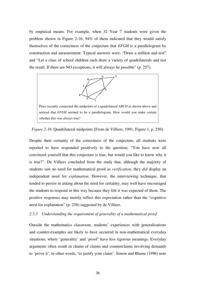
36
by empirical means. For example, when 32 Year 7 students were given the
problem shown in Figure 2-16, 94% of them indicated that they would satisfy
themselves of the correctness of the conjecture that EFGH is a parallelogram by
construction and measurement. Typical answers were: “Draw a million and test”
and “Let a class of school children each draw a variety of quadrilaterals and test
the result. If there are NO exceptions, it will always be possible” (p. 257).
Peter recently connected the midpoints of a quadrilateral ABCD as shown above and
noticed that EFGH seemed to be a parallelogram. How would you make certain
whether this was always true?
Figure 2-16. Quadrilateral midpoints [From de Villiers, 1991, Figure 1, p. 256].
Despite their certainty of the correctness of the conjecture, all students were
reported to have responded positively to the question; “You have now all
convinced yourself that this conjecture is true, but would you like to know why it
is true?”. De Villiers concluded from the study that, although the majority of
students saw no need for mathematical proof as verification, they did display an
independent need for explanation. However, the interviewing technique, that
tended to persist in asking about the need for certainty, may well have encouraged
the students to respond in this way because they felt it was expected of them. The
positive responses may merely reflect this expectation rather than the “cognitive
need for explanation” (p. 258) suggested by de Villiers.
2.5.3 Understanding the requirement of generality of a mathematical proof
Outside the mathematics classroom, students’ experiences with generalisations
and counter-examples are likely to have occurred in non-mathematical everyday
situations, where ‘generality’ and ‘proof’ have less rigorous meanings. Everyday
arguments often result in chains of claims and counterclaims involving demands
to ‘prove it’, in other words, ‘to justify your claim’. Simon and Blume (1996) note
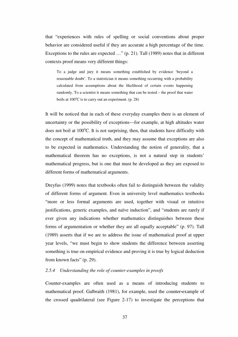
37
that “experiences with rules of spelling or social conventions about proper
behavior are considered useful if they are accurate a high percentage of the time.
Exceptions to the rules are expected …” (p. 21). Tall (1989) notes that in different
contexts proof means very different things:
To a judge and jury it means something established by evidence ‘beyond a
reasonable doubt’. To a statistician it means something occurring with a probability
calculated from assumptions about the likelihood of certain events happening
randomly. To a scientist it means something that can be tested – the proof that water
boils at 100oC is to carry out an experiment. (p. 28)
It will be noticed that in each of these everyday examples there is an element of
uncertainty or the possibility of exceptions—for example, at high altitudes water
does not boil at 100oC. It is not surprising, then, that students have difficulty with
the concept of mathematical truth, and they may assume that exceptions are also
to be expected in mathematics. Understanding the notion of generality, that a
mathematical theorem has no exceptions, is not a natural step in students’
mathematical progress, but is one that must be developed as they are exposed to
different forms of mathematical arguments.
Dreyfus (1999) notes that textbooks often fail to distinguish between the validity
of different forms of argument. Even in university level mathematics textbooks
“more or less formal arguments are used, together with visual or intuitive
justifications, generic examples, and naïve induction”, and “students are rarely if
ever given any indications whether mathematics distinguishes between these
forms of argumentation or whether they are all equally acceptable” (p. 97). Tall
(1989) asserts that if we are to address the issue of mathematical proof at upper
year levels, “we must begin to show students the difference between asserting
something is true on empirical evidence and proving it is true by logical deduction
from known facts” (p. 29).
2.5.4 Understanding the role of counter-examples in proofs
Counter-examples are often used as a means of introducing students to
mathematical proof. Galbraith (1981), for example, used the counter-example of
the crossed quadrilateral (see Figure 2-17) to investigate the perceptions that
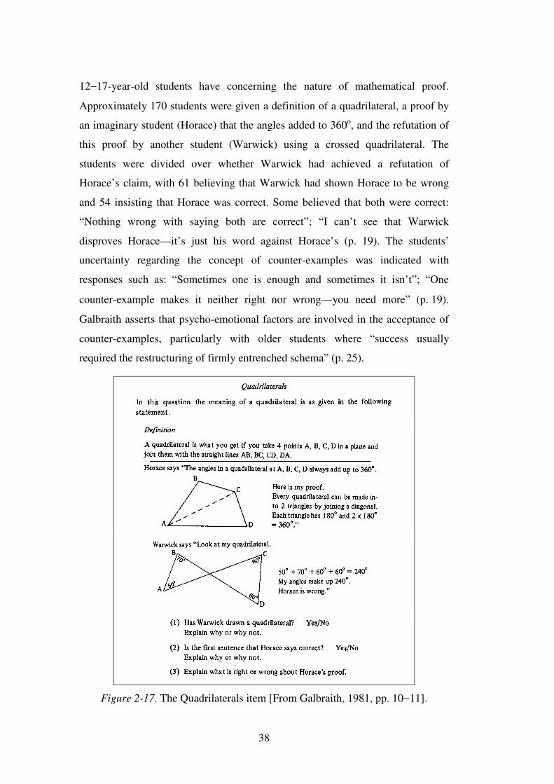
38
12−17-year-old students have concerning the nature of mathematical proof.
Approximately 170 students were given a definition of a quadrilateral, a proof by
an imaginary student (Horace) that the angles added to 360o, and the refutation of
this proof by another student (Warwick) using a crossed quadrilateral. The
students were divided over whether Warwick had achieved a refutation of
Horace’s claim, with 61 believing that Warwick had shown Horace to be wrong
and 54 insisting that Horace was correct. Some believed that both were correct:
“Nothing wrong with saying both are correct”; “I can’t see that Warwick
disproves Horace—it’s just his word against Horace’s (p. 19). The students’
uncertainty regarding the concept of counter-examples was indicated with
responses such as: “Sometimes one is enough and sometimes it isn’t”; “One
counter-example makes it neither right nor wrong—you need more” (p. 19).
Galbraith asserts that psycho-emotional factors are involved in the acceptance of
counter-examples, particularly with older students where “success usually
required the restructuring of firmly entrenched schema” (p. 25).
Figure 2-17. The Quadrilaterals item [From Galbraith, 1981, pp. 10−11].
39
Balacheff (1991) questions the use of counter-examples in the teaching of proof,
noting that students who use naïve empiricism as a basis for their belief in a
mathematical statement are likely to claim that a counter-example is merely a
special case. Simon and Blume (1996) also question the suitability of counter-
examples, noting that “exceptions to the rules are expected … If students did not
expect the conjecture to be always true, then the counter-example is not a
compelling refutation” (p. 21).
2.5.5 Understanding deductive reasoning
Students’ difficulty with mathematical proof may be substantially due to their
failure to understand the structure of deductive reasoning. Tall (1989, p. 30) notes
the importance of involving students in making deductions of the form ‘if I know
something, then I know something else’, particularly in cases where the converse
is not true. Students must learn that ‘if P then Q’ is not the same as ‘if Q then P’.
According to Piaget (1928), young children’s’ use of conjunctions such as
“because” and “then” in natural language is not based on logical reasoning. For
example, a nine-year-old child, when asked to complete the sentence “Half of 9 is
not 4 because …” replied “he can’t count” (p. 26). Whereas there was progress in
the logical use of “because” before the age of seven for some children, Piaget
noted that the logical use of “then” occurred at a later age. The USA Principles
and Standards for School Mathematics (National Council of Teachers of
Mathematics, 2000) emphasises that the development of reasoning is closely
related to language development, particularly the acquisition of basic logic words,
such as “if … then”, “because”, “all”, and “some”: “teachers should help students
gain familiarity with the language of logic by using such words frequently”
(p. 125).
Duval (1991) contends that the similarity in linguistic forms between deductive
reasoning and the sometimes informal language of argumentation is one of the
main reasons why students do not understand the requirements of mathematical
proof. In deductive reasoning, the position of statements in an inference
determines their operational status—that is, whether they have the status of
premise or conclusion. In argumentative reasoning in the classroom, though, it is
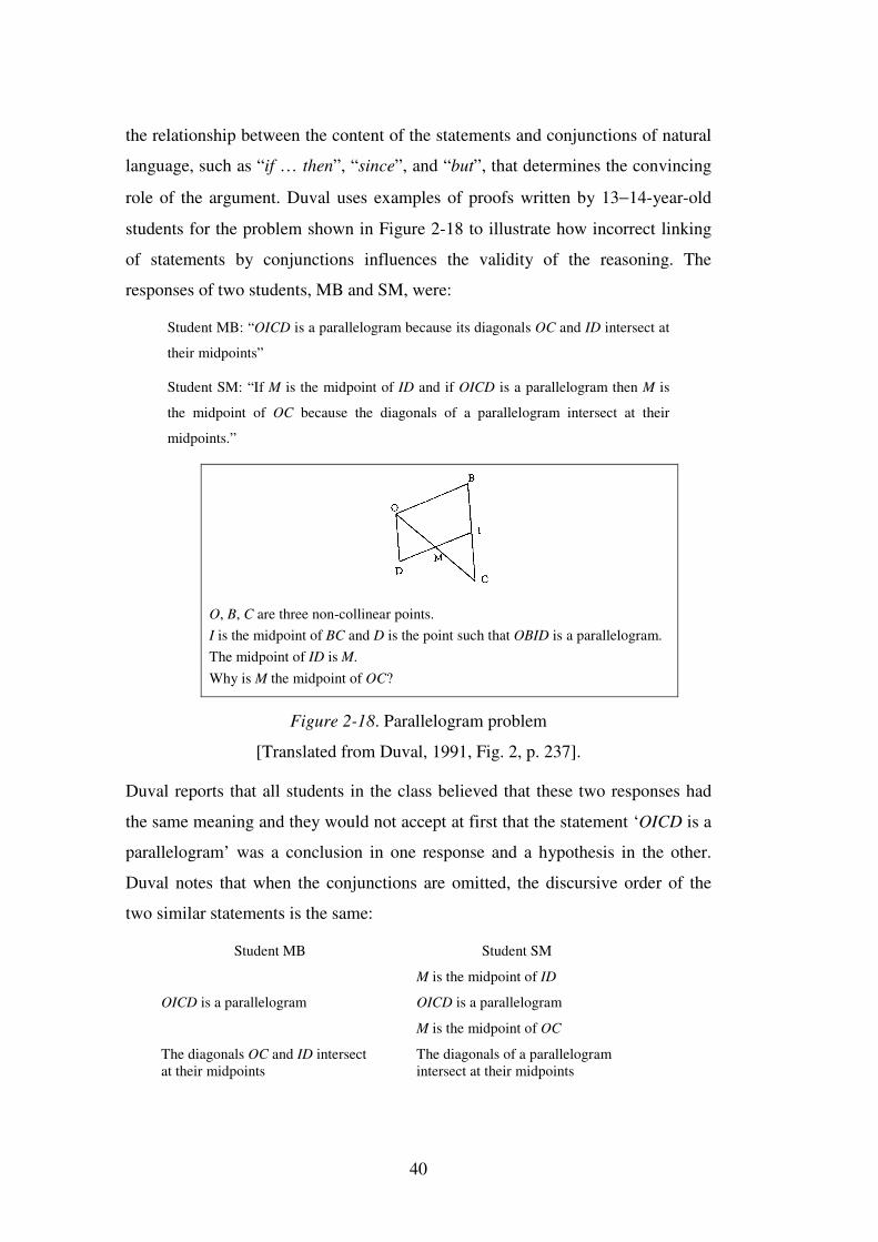
40
the relationship between the content of the statements and conjunctions of natural
language, such as “if … then”, “since”, and “but”, that determines the convincing
role of the argument. Duval uses examples of proofs written by 13−14-year-old
students for the problem shown in Figure 2-18 to illustrate how incorrect linking
of statements by conjunctions influences the validity of the reasoning. The
responses of two students, MB and SM, were:
Student MB: “OICD is a parallelogram because its diagonals OC and ID intersect at
their midpoints”
Student SM: “If M is the midpoint of ID and if OICD is a parallelogram then M is
the midpoint of OC because the diagonals of a parallelogram intersect at their
midpoints.”
O, B, C are three non-collinear points. I is the midpoint of BC and D is the point such that OBID is a parallelogram. The midpoint of ID is M. Why is M the midpoint of OC?
Figure 2-18. Parallelogram problem
[Translated from Duval, 1991, Fig. 2, p. 237].
Duval reports that all students in the class believed that these two responses had
the same meaning and they would not accept at first that the statement ‘OICD is a
parallelogram’ was a conclusion in one response and a hypothesis in the other.
Duval notes that when the conjunctions are omitted, the discursive order of the
two similar statements is the same:
Student MB Student SM
M is the midpoint of ID
OICD is a parallelogram OICD is a parallelogram
M is the midpoint of OC
The diagonals OC and ID intersect at their midpoints
The diagonals of a parallelogram intersect at their midpoints
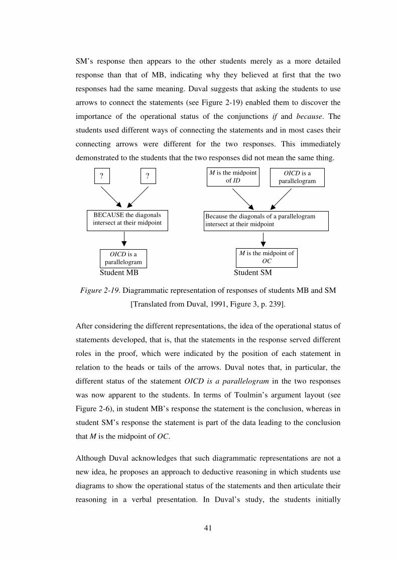
41
SM’s response then appears to the other students merely as a more detailed
response than that of MB, indicating why they believed at first that the two
responses had the same meaning. Duval suggests that asking the students to use
arrows to connect the statements (see Figure 2-19) enabled them to discover the
importance of the operational status of the conjunctions if and because. The
students used different ways of connecting the statements and in most cases their
connecting arrows were different for the two responses. This immediately
demonstrated to the students that the two responses did not mean the same thing.
Student MB Student SM
Figure 2-19. Diagrammatic representation of responses of students MB and SM
[Translated from Duval, 1991, Figure 3, p. 239].
After considering the different representations, the idea of the operational status of
statements developed, that is, that the statements in the response served different
roles in the proof, which were indicated by the position of each statement in
relation to the heads or tails of the arrows. Duval notes that, in particular, the
different status of the statement OICD is a parallelogram in the two responses
was now apparent to the students. In terms of Toulmin’s argument layout (see
Figure 2-6), in student MB’s response the statement is the conclusion, whereas in
student SM’s response the statement is part of the data leading to the conclusion
that M is the midpoint of OC.
Although Duval acknowledges that such diagrammatic representations are not a
new idea, he proposes an approach to deductive reasoning in which students use
diagrams to show the operational status of the statements and then articulate their
reasoning in a verbal presentation. In Duval’s study, the students initially
? ?
BECAUSE the diagonals intersect at their midpoint
OICD is a parallelogram
M is the midpoint of ID
OICD is a parallelogram
Because the diagonals of a parallelogram intersect at their midpoint
M is the midpoint of OC
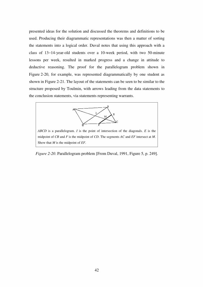
42
presented ideas for the solution and discussed the theorems and definitions to be
used. Producing their diagrammatic representations was then a matter of sorting
the statements into a logical order. Duval notes that using this approach with a
class of 13−14-year-old students over a 10-week period, with two 50-minute
lessons per week, resulted in marked progress and a change in attitude to
deductive reasoning. The proof for the parallelogram problem shown in
Figure 2-20, for example, was represented diagrammatically by one student as
shown in Figure 2-21. The layout of the statements can be seen to be similar to the
structure proposed by Toulmin, with arrows leading from the data statements to
the conclusion statements, via statements representing warrants.
ABCD is a parallelogram. I is the point of intersection of the diagonals. E is the
midpoint of CB and F is the midpoint of CD. The segments AC and EF intersect at M.
Show that M is the midpoint of EF.
Figure 2-20. Parallelogram problem [From Duval, 1991, Figure 5, p. 249].
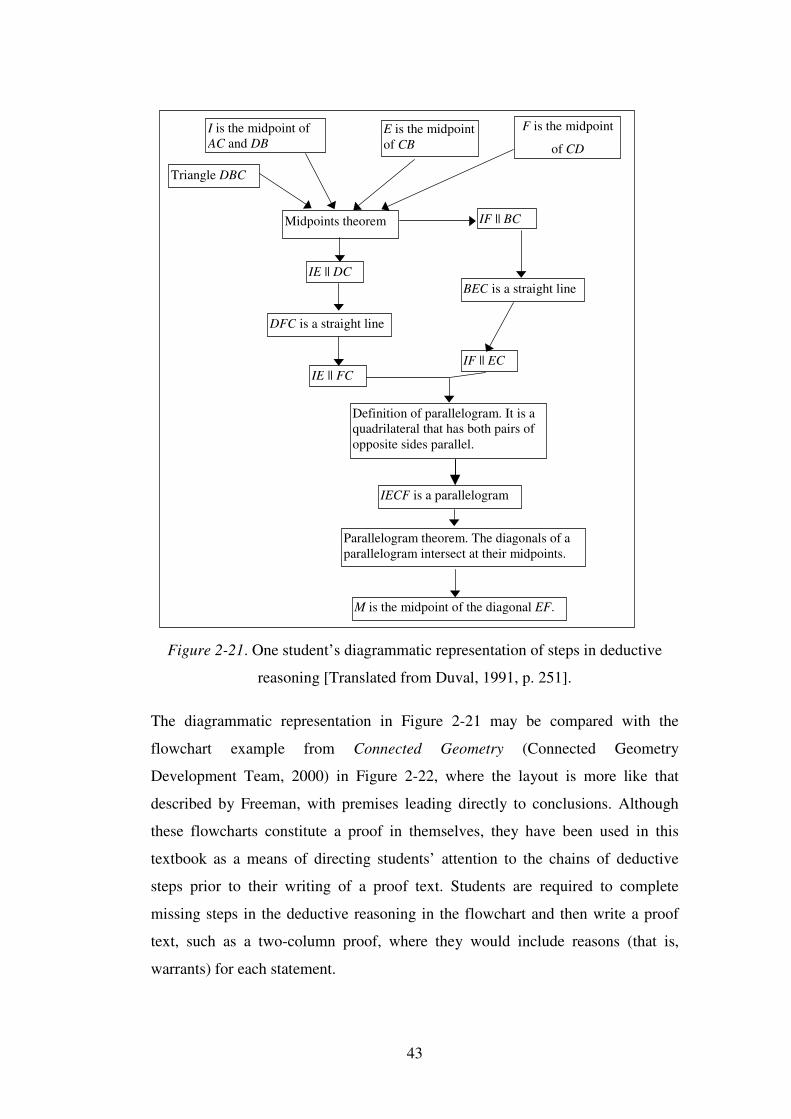
43
Figure 2-21. One student’s diagrammatic representation of steps in deductive
reasoning [Translated from Duval, 1991, p. 251].
The diagrammatic representation in Figure 2-21 may be compared with the
flowchart example from Connected Geometry (Connected Geometry
Development Team, 2000) in Figure 2-22, where the layout is more like that
described by Freeman, with premises leading directly to conclusions. Although
these flowcharts constitute a proof in themselves, they have been used in this
textbook as a means of directing students’ attention to the chains of deductive
steps prior to their writing of a proof text. Students are required to complete
missing steps in the deductive reasoning in the flowchart and then write a proof
text, such as a two-column proof, where they would include reasons (that is,
warrants) for each statement.
I is the midpoint of AC and DB
E is the midpoint of CB
F is the midpoint
of CD
Triangle DBC
Midpoints theorem IF || BC
BEC is a straight line
IF || EC
IE || DC
IE || FC
DFC is a straight line
IECF is a parallelogram
Definition of parallelogram. It is a quadrilateral that has both pairs of opposite sides parallel.
Parallelogram theorem. The diagonals of a parallelogram intersect at their midpoints.
M is the midpoint of the diagonal EF.
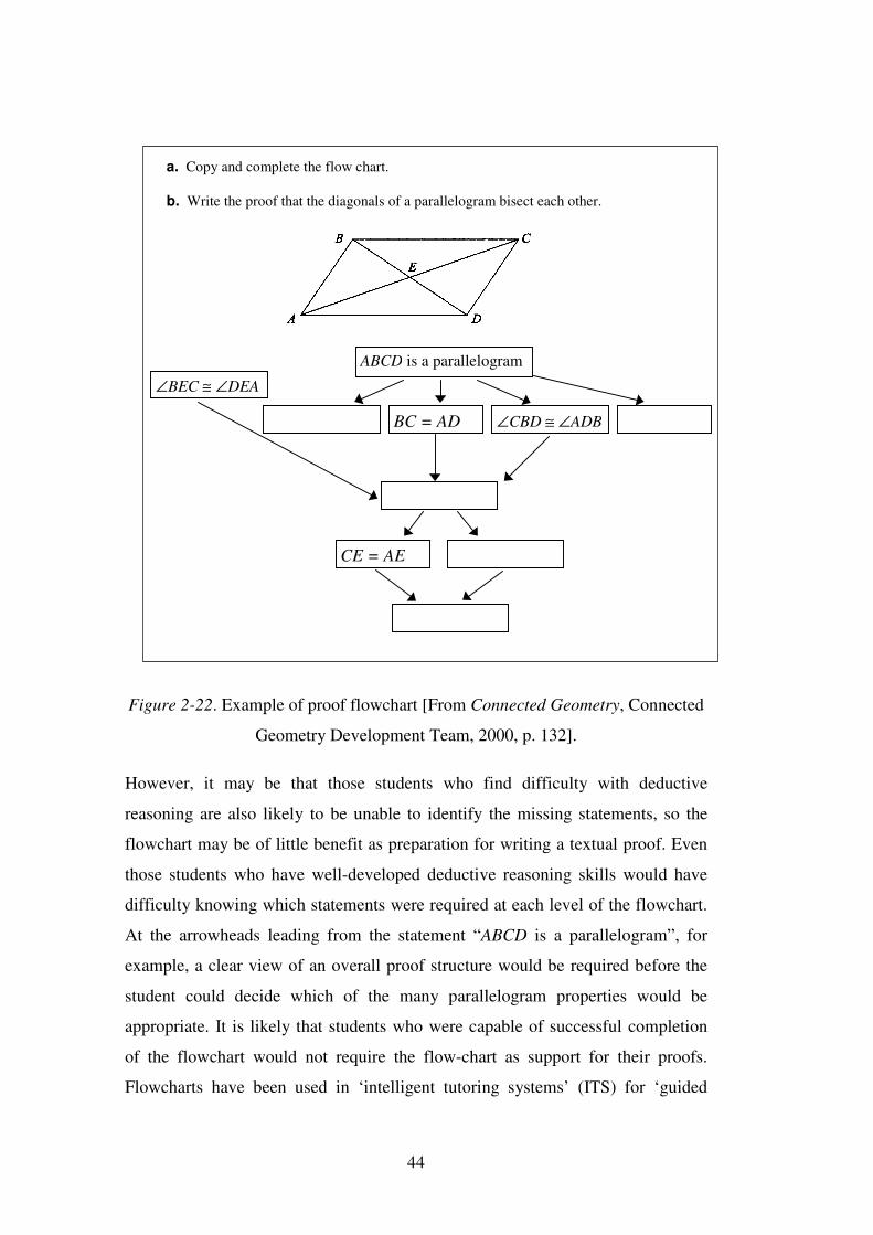
44
a. Copy and complete the flow chart.
b. Write the proof that the diagonals of a parallelogram bisect each other.
Figure 2-22. Example of proof flowchart [From Connected Geometry, Connected
Geometry Development Team, 2000, p. 132].
However, it may be that those students who find difficulty with deductive
reasoning are also likely to be unable to identify the missing statements, so the
flowchart may be of little benefit as preparation for writing a textual proof. Even
those students who have well-developed deductive reasoning skills would have
difficulty knowing which statements were required at each level of the flowchart.
At the arrowheads leading from the statement “ABCD is a parallelogram”, for
example, a clear view of an overall proof structure would be required before the
student could decide which of the many parallelogram properties would be
appropriate. It is likely that students who were capable of successful completion
of the flowchart would not require the flow-chart as support for their proofs.
Flowcharts have been used in ‘intelligent tutoring systems’ (ITS) for ‘guided
∠BEC ≅ ∠DEA
ABCD is a parallelogram
∠CBD ≅ ∠ADB BC = AD
CE = AE
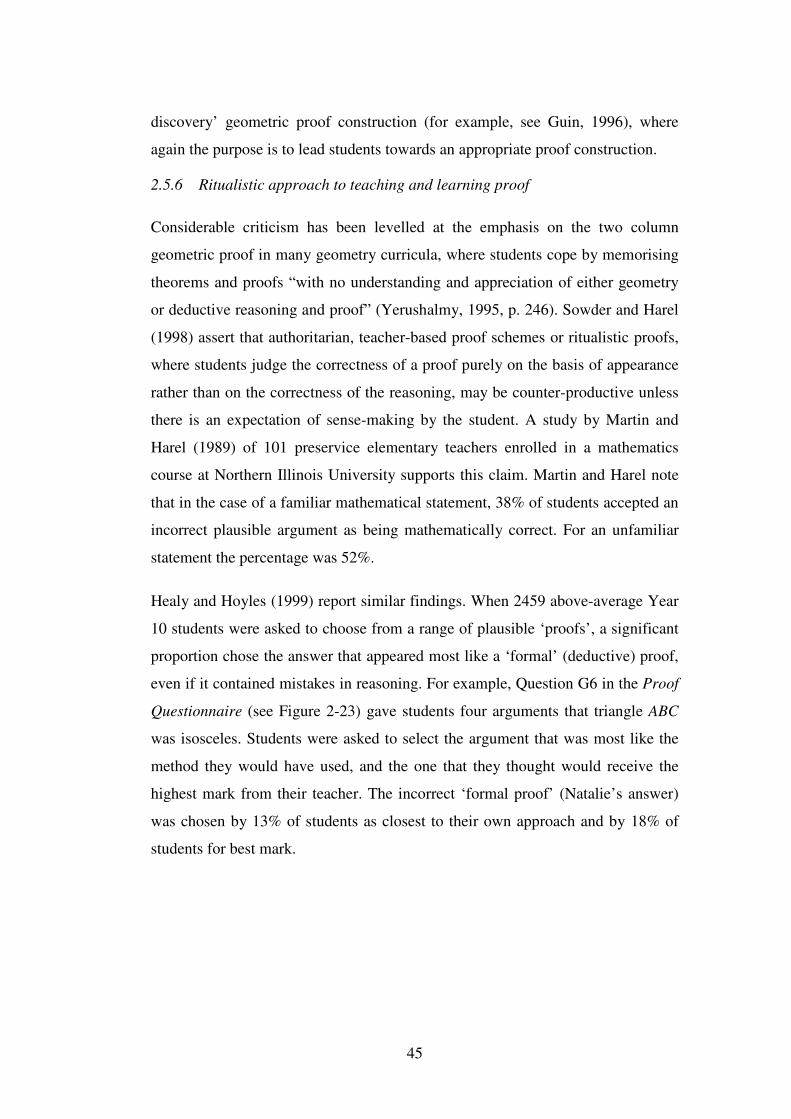
45
discovery’ geometric proof construction (for example, see Guin, 1996), where
again the purpose is to lead students towards an appropriate proof construction.
2.5.6 Ritualistic approach to teaching and learning proof
Considerable criticism has been levelled at the emphasis on the two column
geometric proof in many geometry curricula, where students cope by memorising
theorems and proofs “with no understanding and appreciation of either geometry
or deductive reasoning and proof” (Yerushalmy, 1995, p. 246). Sowder and Harel
(1998) assert that authoritarian, teacher-based proof schemes or ritualistic proofs,
where students judge the correctness of a proof purely on the basis of appearance
rather than on the correctness of the reasoning, may be counter-productive unless
there is an expectation of sense-making by the student. A study by Martin and
Harel (1989) of 101 preservice elementary teachers enrolled in a mathematics
course at Northern Illinois University supports this claim. Martin and Harel note
that in the case of a familiar mathematical statement, 38% of students accepted an
incorrect plausible argument as being mathematically correct. For an unfamiliar
statement the percentage was 52%.
Healy and Hoyles (1999) report similar findings. When 2459 above-average Year
10 students were asked to choose from a range of plausible ‘proofs’, a significant
proportion chose the answer that appeared most like a ‘formal’ (deductive) proof,
even if it contained mistakes in reasoning. For example, Question G6 in the Proof
Questionnaire (see Figure 2-23) gave students four arguments that triangle ABC
was isosceles. Students were asked to select the argument that was most like the
method they would have used, and the one that they thought would receive the
highest mark from their teacher. The incorrect ‘formal proof’ (Natalie’s answer)
was chosen by 13% of students as closest to their own approach and by 18% of
students for best mark.
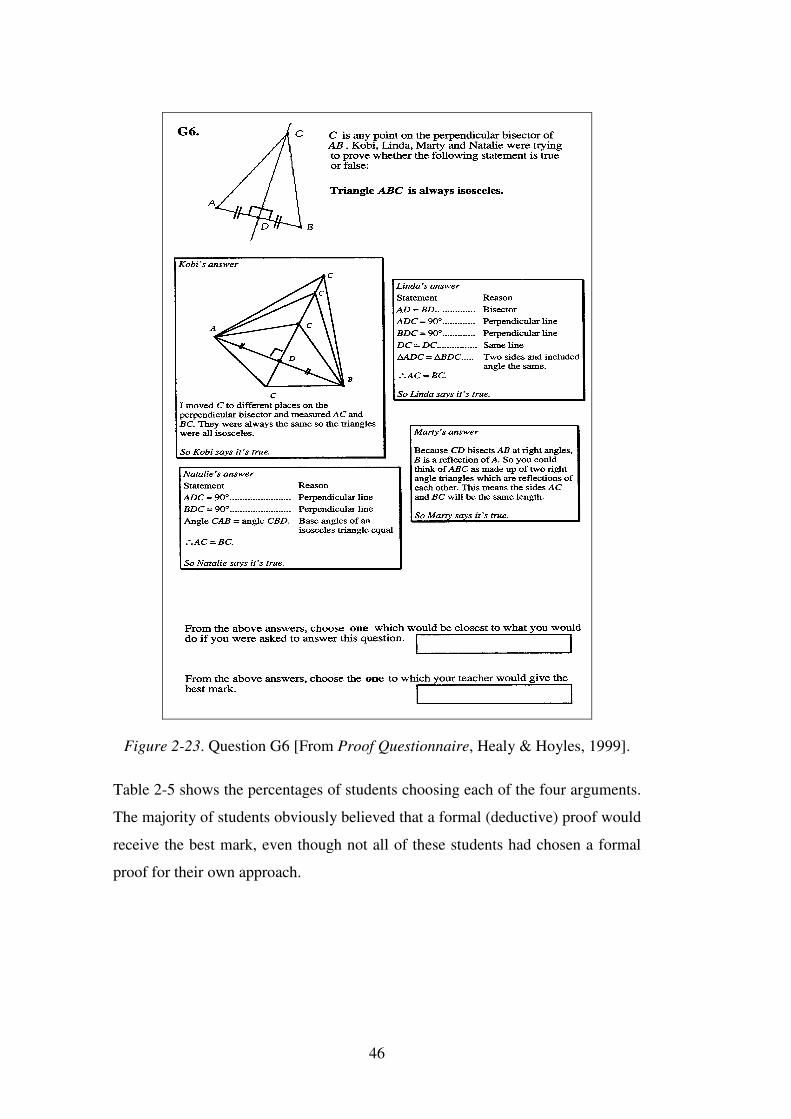
46
Figure 2-23. Question G6 [From Proof Questionnaire, Healy & Hoyles, 1999].
Table 2-5 shows the percentages of students choosing each of the four arguments.
The majority of students obviously believed that a formal (deductive) proof would
receive the best mark, even though not all of these students had chosen a formal
proof for their own approach.
47
Table 2-5
Percentage Distribution of Students’ Choices for Question G6 (N = 2459) [From
Healy & Hoyles, 1999, Figure 5, p. 19]
Own approach Best mark
Empirical (Kobi) 40 19
Formal incorrect (Natalie) 13 18
Formal correct (Linda) 21 48
Narrative correct (Marty) 26 15
Healy and Hoyles found a similar response pattern for the other multiple-choice
geometry questions, G1 and G5, as well as for the three algebra questions, A1, A5
and A6. The percentages of students choosing the incorrect ‘formal proofs’ for
best mark were A1: 41%; A5: 11%; A6: 24%; G1: 15%; and G5: 23%. In each
case more students chose the incorrect ‘formal proof’ for best mark than for their
own approach, and fewer students generally chose empirical or narrative answers
for best mark than for their own approach, even if the narrative answer was
correct, as in the case of Marty’s answer in Question G6. These findings suggest
that some students were selecting on the basis of the formal appearance of the
arguments rather than the correctness of the argument, supporting the observations
of Martin and Harel (1989). Herbst (1999, p. 3) asserts that the writing of proofs
has too often become an end in itself: “a routine exercise whose purpose is to
reproduce itself (that is, teachers do some proofs to model how students should do
them, and students do some proofs to learn how to do proofs)”.
As part of a three-year longitudinal study of mathematical reasoning, Küchemann
and Hoyles (2001) conducted a written survey with 2797 high-attaining Year 8
(14-year-old) students in England, where some of the questions were similar to the
multiple-choice questions used in the Year 10 Proof Study. Question G3 (see
Figure 2-24), for example, presented students with a conjecture and four
arguments in support of it. As in the Year 10 study, students were asked to select
the one that was closest to what they would do, and the one that they thought
would receive the best mark from their teacher. Once again, the most popular
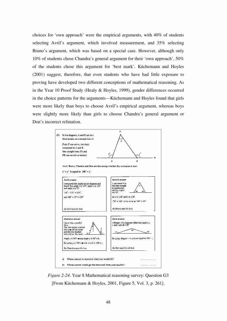
48
choices for ‘own approach’ were the empirical arguments, with 40% of students
selecting Avril’s argument, which involved measurement, and 35% selecting
Bruno’s argument, which was based on a special case. However, although only
10% of students chose Chandra’s general argument for their ‘own approach’, 50%
of the students chose this argument for ‘best mark’. Küchemann and Hoyles
(2001) suggest, therefore, that even students who have had little exposure to
proving have developed two different conceptions of mathematical reasoning. As
in the Year 10 Proof Study (Healy & Hoyles, 1999), gender differences occurred
in the choice patterns for the arguments—Küchemann and Hoyles found that girls
were more likely than boys to choose Avril’s empirical argument, whereas boys
were slightly more likely than girls to choose Chandra’s general argument or
Don’s incorrect refutation.
Figure 2-24. Year 8 Mathematical reasoning survey: Question G3
[From Küchemann & Hoyles, 2001, Figure 5, Vol. 3, p. 261].
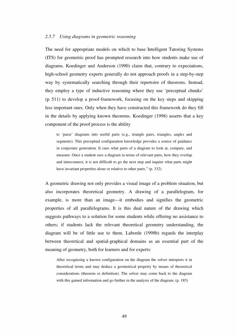
49
2.5.7 Using diagrams in geometric reasoning
The need for appropriate models on which to base Intelligent Tutoring Systems
(ITS) for geometric proof has prompted research into how students make use of
diagrams. Koedinger and Anderson (1990) claim that, contrary to expectations,
high-school geometry experts generally do not approach proofs in a step-by-step
way by systematically searching through their repertoire of theorems. Instead,
they employ a type of inductive reasoning where they use ‘perceptual chunks’
(p. 511) to develop a proof-framework, focusing on the key steps and skipping
less important ones. Only when they have constructed this framework do they fill
in the details by applying known theorems. Koedinger (1998) asserts that a key
component of the proof process is the ability
to ‘parse’ diagrams into useful parts (e.g., triangle pairs, triangles, angles and
segments). This perceptual configuration knowledge provides a source of guidance
in conjecture generation. It cues what parts of a diagram to look at, compare, and
measure. Once a student sees a diagram in terms of relevant parts, how they overlap
and interconnect, it is not difficult to go the next step and inquire what parts might
have invariant properties alone or relative to other parts.” (p. 332)
A geometric drawing not only provides a visual image of a problem situation, but
also incorporates theoretical geometry. A drawing of a parallelogram, for
example, is more than an image—it embodies and signifies the geometric
properties of all parallelograms. It is this dual nature of the drawing which
suggests pathways to a solution for some students while offering no assistance to
others; if students lack the relevant theoretical geometry understanding, the
diagram will be of little use to them. Laborde (1998b) regards the interplay
between theoretical and spatial-graphical domains as an essential part of the
meaning of geometry, both for learners and for experts:
After recognising a known configuration on the diagram the solver interprets it in
theoretical terms and may deduce a geometrical property by means of theoretical
considerations (theorem or definition). The solver may come back to the diagram
with this gained information and go further in the analysis of the diagram. (p. 185)
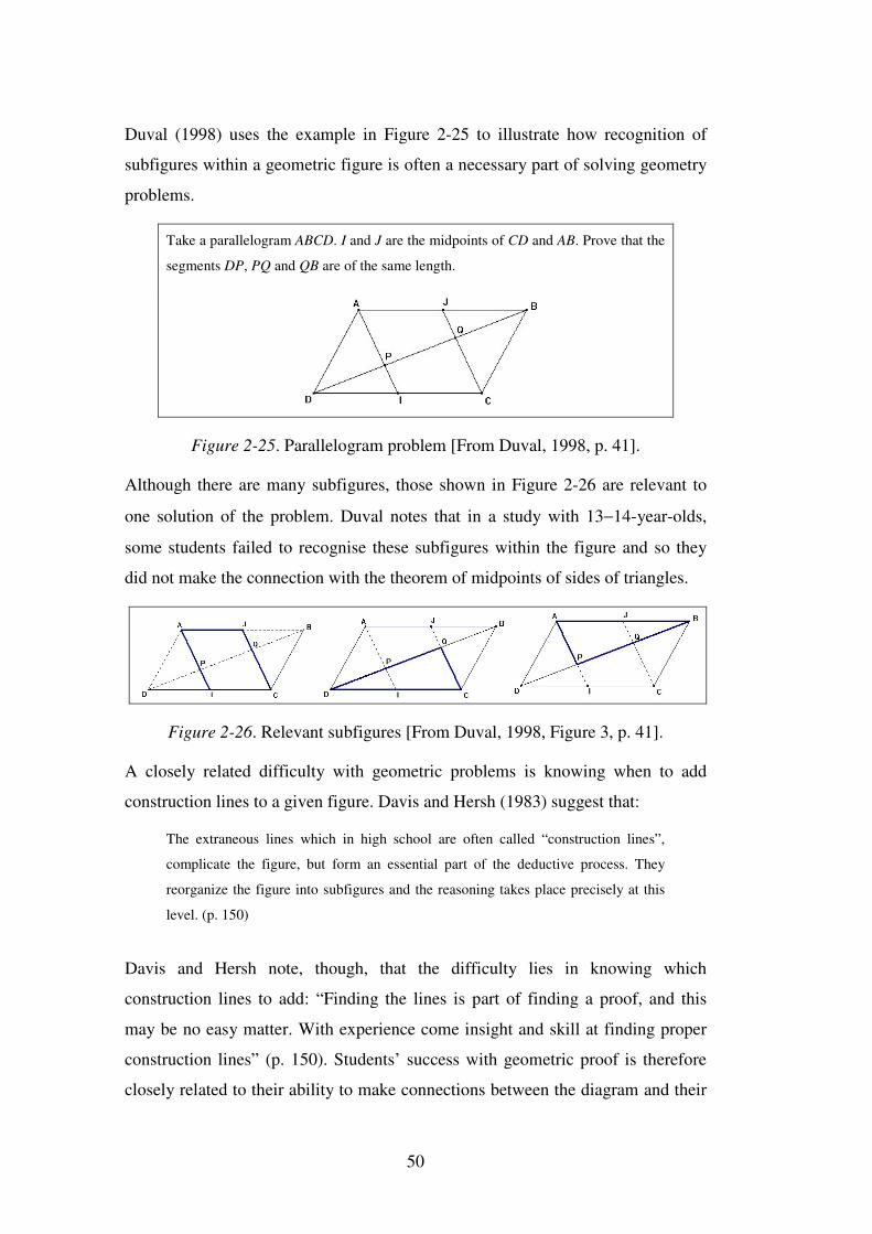
50
Duval (1998) uses the example in Figure 2-25 to illustrate how recognition of
subfigures within a geometric figure is often a necessary part of solving geometry
problems.
Take a parallelogram ABCD. I and J are the midpoints of CD and AB. Prove that the
segments DP, PQ and QB are of the same length.
Figure 2-25. Parallelogram problem [From Duval, 1998, p. 41].
Although there are many subfigures, those shown in Figure 2-26 are relevant to
one solution of the problem. Duval notes that in a study with 13−14-year-olds,
some students failed to recognise these subfigures within the figure and so they
did not make the connection with the theorem of midpoints of sides of triangles.
Figure 2-26. Relevant subfigures [From Duval, 1998, Figure 3, p. 41].
A closely related difficulty with geometric problems is knowing when to add
construction lines to a given figure. Davis and Hersh (1983) suggest that:
The extraneous lines which in high school are often called “construction lines”,
complicate the figure, but form an essential part of the deductive process. They
reorganize the figure into subfigures and the reasoning takes place precisely at this
level. (p. 150)
Davis and Hersh note, though, that the difficulty lies in knowing which
construction lines to add: “Finding the lines is part of finding a proof, and this
may be no easy matter. With experience come insight and skill at finding proper
construction lines” (p. 150). Students’ success with geometric proof is therefore
closely related to their ability to make connections between the diagram and their
51
theorem-based knowledge of geometry. If students are unable to make these
connections, diagrams may be of little use to them.
2.6 Alternative approaches to the teaching and learning of proof
As discussed in section 2.5, there are many factors that appear to contribute to
students’ difficulties with mathematical proof. Several recent studies have focused
on alternative approaches to the teaching and learning of proof in an attempt to
eliminate some of these difficulties. Attempts have been made, for example, to
create links between empirical justification and deductive reasoning. Hoyles
(1998, p. 169) asserts that
we need to design new learning contexts which require the use of clearly formulated
statements and definitions and agreed procedures of deduction but which also allow
opportunities for their connection with empirical justification and the conviction this
engenders.
Similarly, Tall (1989), referring specifically to A-level mathematics in the UK,
but in a statement equally relevant to school mathematics at any level, asserts that
we need
experiences that encourage students to make convincing arguments in meaningful
situations. What we must do is introduce these experiences in a way that is both an
end in itself for the vast majority of students who will go on to study other
disciplines, but also provides the cognitive foundations of formal proof for the tiny
minority of mathematics specialists who will later make logical deductions from
precise definitions. (p. 32)
Several recent research studies (for example Hölzl, 2001; Mariotti, 2000; Hadas,
Hershkowitz, & Schwarz, 2000; Arzarello et al, 1998) have focused on linking
empirical reasoning and deductive reasoning in a dynamic geometry computer
environment. The findings from a number of these studies will be discussed in
chapter 3. Hoyles (1998), however, cautions against the assumption that the
computer will automatically “help to build bridges between the empirical and the
deductive”, noting that “there remains the question of how to develop a ‘need for
proof’” (p. 171).
52
Other studies have explored the role of conjecturing and argumentation in
students’ successful proof construction. Mariotti, Bartolini Bussi, Boero, Ferri,
and Garuti (1997), for example, assert that it is the questioning by the students of
the truth of a statement which is critical, and that suitable contexts are required in
which students can produce their own conjectures and engage in argumentation:
In our opinion, the uncertainty status of the truth of a statement is crucial for the
initial construction of the meaning of theorems and calls for the careful selection of
problem-solving situations, where the production of a conjecture is required.
(p. 182)
Mariotti et al. summarise the findings of a series of Italian studies undertaken
during the 1990s on the approach to geometry theorems in schools. The studies,
which have been discussed in a number of reports, involved students in Years 5,
8, and 10. Although they had different thematic contexts, the studies shared some
common features: “general goals, research methodology, epistemological analysis
and cultural, cognitive and educational hypotheses” (p. 180). Mariotti et al. note
that the studies were based on the constructs of ‘mathematical discussion’ and
‘field of experience’—defined by Boero et al. (1995) as “a sector of human
culture which the teacher and students can recognise and consider as unitary and
homogenous” (p. 153).
The ‘fields of experience’ used in the investigations at Years 5, 8, and 10 were,
respectively, the representation of geometric perspective, an investigation of the
properties of sunshadows formed by vertical and oblique sticks, and exploration
of Cabri constructions, such as the angle bisectors of a quadrilateral (see
section 3.4.3), all of which involve the possibility of dynamic exploration. In
offering a rationale for the choice of these fields of experience, Garuti, Boero, and
Lemut (1998) state that they were influenced by Simon’s (1996) concept of
‘transformational reasoning’ (see section 3.2.2), where students develop an
understanding of how a mathematical system works by mentally or physically
‘running’ the system.
Boero, Garuti, Lemut, and Mariotti (1996) note that the theoretical framework for
the Italian studies was also influenced by the strong relationship between
53
conjecturing and proving evident in historical mathematical documents. Boero et
al. use the term ‘cognitive unity’ to signify the continuity that they assert must
exist between the production of a conjecture during argumentation and the
successful construction of its proof:
During the production of the conjecture, the student progressively works out his/her
statement through an intensive argumentative activity functionally intermingled with
the justification of the plausibility of his/her choices. During the subsequent
statement-proving stage, the student links up with this process in a coherent way,
organising some of the justifications (‘arguments’) produced during the construction
of the statement according to a logical chain. (p. 113)
Boero et al. (1996) assert that the relationship between the students’
argumentation, conjecturing, and proofs in the studies is consistent with the
hypothesis of cognitive unity. They claim that the reasoning which takes place
during the process of argumentation plays a crucial role in the subsequent proof
construction: “it allows students to consciously explore different alternatives, to
progressively specify the statement [of the conjecture] and to justify the
plausibility of the produced conjecture” (p. 118). Boero et al. note that “poor
argumentation during the production of the statement [conjecture] always
corresponds to lack of arguments during the construction of the proof” (p. 118).
Garuti et al. (1998) claim that if a student is given a statement and asked to prove
it, without being involved in the conjecturing, the continuity of the reasoning is
absent, and may be restored only by a reappropriation of the conjecture through a
new process of exploration, that is, “reconstructing the whole cycle: exploring,
producing a conjecture, coming back to the exploration, reorganizing it into a
proof” (p. 345).
2.7 Recent curriculum recommendations on proof
Following the largely unsuccessful axiomatic approaches to the teaching of
geometry which prevailed in most countries until the 1950s and 1960s, and the
subsequent decades where there has been a reduction in the emphasis on
Euclidean geometry and proof, curriculum changes are again being recommended.
In the UK, for example, where geometry has become largely empirical, with little
54
emphasis on deductive reasoning, the report of the Royal Society and Joint
Mathematical Council Working Group: Teaching and learning geometry 11−19
(2001) suggests that school geometry should encourage
the use of logical argument, which builds upon what is already known by the pupil
in order to demonstrate the truth of some geometrical result, possibly one
conjectured by the pupil after conducting a well-chosen experiment. … The level of
sophistication expected in the logical argument will depend upon the age and ability
of the pupil concerned, and the proof produced might equally be called an
‘explanation’ or ‘justification’ or ‘reason’ for the result. (p. 9)
In the USA, the Principles and Standards for School Mathematics (National
Council of Teachers of Mathematics, 2000) includes in its vision for school
mathematics the statement that “Teachers help students make, refine, and explore
conjectures on the basis of evidence and use a variety of reasoning and proof
techniques to confirm or disprove those conjectures” (p. 3). There is clearly a
belief that formulating conjectures and constructing logical arguments are
important aspects of the development of students’ mathematical reasoning and
understanding. Similarly, in Australia, the Mathematics Key Learning Area of the
Victorian Curriculum and Standards Framework II (Board of Studies, 2000)
states that
forming and testing conjectures is an important aspect of the Mathematical
reasoning substrand, and is also a common feature of students’ mathematical activity
at all levels. Strategies for testing conjectures will range from simple checking of
cases, through the use of counter-examples to the generation of logical arguments
and proof. Students will be able to produce chains of mathematical reasoning of
increasing length and refinement as their familiarity with and knowledge of
mathematical concepts and logical structure increase. This will include the capability
to recognise the underlying patterns of proof which have been used, and to develop
an increasingly sophisticated recognition of when a particular chain of reasoning is,
or is not, sufficient to establish a general result. (p. 24)
Beneath the rhetoric, however, there is no significant change in approach to the
teaching and learning of proof. Whereas the emphasis at Levels 4 and 5 (Years
5−8) of the Curriculum and Standards Framework II is on empirical checking of
conjectures for exceptions and reasonableness, at Level 6 (Years 9 and 10) it is
55
stated that students should be able to “develop a convincing mathematical
argument based on several pieces of related information” (p. 221). At this level,
students are expected to “follow formal proofs for results appropriate to the
material for their level, and construct simple proofs of their own” (p. 164). The
Space strand of Level 6 extension (prescribed for Year 10 students proceeding to
mathematics at Years 11 and 12) refers specifically to geometric proof (p. 171),
but there is no indication that there should be a different approach to proof
teaching from the unsuccessful axiomatic methods of the past:
6.10 extension
Use knowledge of
geometrical properties
to develop a logical
series of steps to justify
a geometric theorem.
This is evident when the student is able to:
• Set out simple proofs involving triangles and
parallelograms using knowledge of geometric theorems
• Prove that the angle at the centre of a circle is twice the
angle at the circumference
• Set out simple proofs involving angles in circles
It seems from the Curriculum and Standards Framework II level descriptors that a
considerable cognitive leap may be required from the empirical-based conjectures
and arguments of earlier levels to deductive proofs. There is little reference to
what constitutes a valid and acceptable proof at each level, or to the need to
engage students at higher levels in conjecturing and argumentation as part of their
own proof construction processes.
2.8 Motivation, peer interaction, and the quality of argumentation
2.8.1 Motivation
Students’ motivation for proof, and engaging students in conjecturing and
argumentation, stand out as key current issues in the teaching and learning of
mathematical proof. Although it is not the intention of this research to focus on
constructivist learning environments, certain constructivist concepts—for
example, cognitive engagement, motivation, and peer interactions—have
implications for the quality of argumentation and proof in the mathematics
classroom. How can students’ lack of motivation for mathematical proof be
addressed? What are the signifiers of motivation? How does the nature of the task
56
influence cognitive engagement? How is cognitive conflict resolved in the context
of peer interactions? How do peer interactions affect the quality of argumentation?
Helme and Clarke (2001) note that “engagement” has been used by researchers to
include both motivational and cognitive aspects. They cite Stipek (1996), who
“describes actively engaged students as approaching challenging tasks eagerly,
exerting intense effort using active (that is, deliberate) problem-solving strategies,
and persisting in the face of difficulty” (Helme & Clarke, p. 131). Helme and
Clarke define cognitive engagement as “the deliberate task-specific thinking that a
student undertakes while participating in a classroom activity” (p. 134). Ainley
(2001) notes that recent theories relating to the constructs of interest and intrinsic
motivation regard positive affect—“feelings of surprise, excitement and
enjoyment” (p. 118)—as an essential part of these states. Helme and Clarke
(2001) cite studies by Blumenfeld et al. (1992), which show that high levels of
motivation are not necessarily associated with high levels of cognitive
engagement. Motivation, then, can be regarded as an affective state that
complements, but does not necessarily imply, cognitive engagement.
Helme and Clarke (2001) suggest that indicators of cognitive engagement
associated with small group activity include “questioning; completing peer
utterances; exchanging ideas, directions, explanations, or reasoning; justifying an
argument; particular gestures” (p. 138). Ainley (2001) notes that “persistence,
attention, concentration and feelings of surprise, excitement and enjoyment are
important processes which occur together when the state of interest is aroused”
(p. 129). Task engagement is characterised, then, by an overlap of cognitive and
affective states: “a complex interaction between the dispositions and past
experiences which a student brings to the classroom and the structure of the
situation they encounter” (p. 129).
2.8.2 Peer interaction
In classrooms where peer interaction is an integral part of the learning process, the
level of interaction will influence the learning which takes place. Forman and
Cazden (1985), in a study of collaborative problem-solving between pairs of
57
students, identified three different forms of peer interaction: parallel, in which the
students share materials and exchange comments about the task, but tend to work
individually, with little attempt to share ideas; associative, in which students
exchange information and ideas, but develop these ideas separately; and
cooperative, where the students “constantly monitor each other’s work and play
coordinated roles in performing task procedures” (p. 333). It would seem that a
fourth category may be required, if one or both students make no attempt to
interact.
Closely associated with peer interaction in the classroom is Vygotsky’s (1978)
notion of the zone of proximal development: that is, “learning awakens a variety
of developmental processes that are able to interact only when the child is
interacting with people in his environment and in collaboration with his peers”
(p. 90). Forman and Cazden (1985), reporting on their study of collaborative
problem-solving, note that one pair of students, who were the most successful
collaborators during a series of eleven related problem-solving tasks, did not show
the same consistently high level of functioning when they were post-tested
separately. Also, the students who worked in pairs during the problem-solving did
not do better on the post-test than students who had worked individually on the
same tasks. Forman and Cazden interpret their findings in terms of Vygotsky’s
theory, suggesting that “the observing, guiding, and correcting role” performed by
one member of the pair provides support which “seems to enable the two
collaborators to solve problems together before they are capable of solving the
same problems alone” (p. 341).
Holton and Thomas (2001), in analysing lessons from the Classroom Learning
Project (Clarke, 2001), note that “the mathematical interactions that appear to
have been of the highest quality took place between students in situations where
they were presented with problems of a demanding nature” (p. 102). They suggest
that where problems are too easy, there is no need for students to engage in
productive conversation, but if the difficulty level is too high, students will be
unable to discuss the problem: the optimum situation for productive talk between
peers occurs when “the cognitive demand of the task is sufficiently high that the
58
children need to discuss how they will proceed to its completion but not so high
that it is beyond their ability to make progress” (p. 82).
2.9 Conclusion
There is a strong belief amongst many mathematics educators that proof should be
a part of school mathematics, and should be seen by students as fundamental to
the way mathematics is constructed. The difficulties which students experience
with proof indicate, however, that new ways of approaching the teaching and
learning of proof are necessary. There appear to be two main issues associated
with these difficulties—firstly, students’ motivation and cognitive need for proof,
and secondly, their understanding of how to construct proofs, particularly
deductive proofs. The first of these implies an acceptance of the need for proof as
fundamental to how our mathematical knowledge has been built up, and
recognition of the purposes of proof. Where students are presented with a
statement to prove, as was the case for many generations of students, construction
of the proof frequently becomes an end in itself, with the majority of students
failing to understand either the need for, or the purposes of, proof. Proof-related
activities need to be designed so that students experience a genuine cognitive need
for conviction beyond the conviction traditionally engendered by a textbook or the
authority of the teacher. Equally important, the proving process should offer
students the satisfaction of being able to explain why their conjectures are true.
The second issue, that of students’ understanding of the process of proving,
involves a number of factors, including recognition of the properties and
relationships that underpin the proof, appreciating the role of counter-examples,
and understanding the structure of deductive reasoning. Although empirical
evidence and the use of counter-examples play an important part in mathematical
reasoning, as students’ mathematical knowledge increases, deductive reasoning
should assume a greater role. Ideally, proving activities will encourage students to
make links between empirical justifications and deductive reasoning.
Research suggests that if students are to be successful in constructing proofs, they
must be allowed to engage in tasks where they can produce their own conjectures,
59
and develop their own reasoned arguments through a process of classroom
argumentation. During the argumentation process, where justifications are being
continually modified and refined, the continuity that exists between conjecturing
and proving appears to facilitate the students’ logical ordering of statements in
their proofs. Classroom argumentation has been criticised, however, on the
grounds that the natural language of arguments, where the aim is to convince at all
costs, conflicts with mathematical reasoning. If students are left to themselves to
argue, this criticism may indeed apply. It is essential, then, that the teacher fulfils
the role of ‘qualified judge’ with regard to the validity of students’ arguments, and
to the appropriateness and acceptability of these arguments for the particular level.
It is also essential that the teacher should model appropriate mathematical
reasoning.
Although the importance of conjectures and arguments in relation to mathematical
reasoning is now being emphasised in the national curricula statements for
mathematics in several countries, the focus is on arguments as products, rather
than on the process of argumentation. In the context of these curricula statements,
arguments may range from simple explanations based on empirical evidence to
formal deductive proofs, depending on the level of the students. The problem
remains, however, as to how students can negotiate the considerable cognitive gap
between these different forms of justification to become successful provers.
Chapter 3 will focus on the relationship between argumentation, conjecturing, and
proving in the context of dynamic environments, which may be able to play a key
role in assisting students to bridge the gap between empirical justifications and
deductive proofs. Chapter 3 will also consider the motivational potential of
dynamic environments.

61
Chapter 3: Dynamic Environments as
Contexts for Conjecturing and Proving
To grasp the meaning of a thing, an event or a situation is to see it in its relations to
other things; to note how it operates or functions, what consequences follow from it;
what causes it, what uses it can be put to. In contrast what we have called the brute
thing, the thing without meaning to us, is something whose relations are not grasped.
(Dewey, 1933, p. 135)
3.1 Introduction
The lack of success of traditional methods of teaching proof in mathematics has
prompted researchers to seek new approaches. As seen in chapter 2, there is some
evidence that students are better able to understand and construct proofs if they
have been involved in a process of conjecturing and argumentation. Mariotti,
Bartolini Bussi, Boero, Ferri, and Garuti (1997) assert that successful proof
construction is dependent on continuity of reasoning, or ‘cognitive unity’,
between producing a conjecture and constructing a proof of the conjecture, with
the process of argumentation creating a bridge between statements made during
conjecturing and statements used in the proof construction. Bartolini Bussi (1993),
for example, as part of a teaching project linking history and mathematics, has
introduced students to conjecturing, argumentation, and proving through a study
of the geometry of historical drawing instruments. Other recent research studies
on the teaching of geometric proof (for example, Hölzl, 2001; Arzarello et al.,
1998; and Mariotti, 2000) have focused on dynamic geometry software, although
King and Schattschneider (1997, p. xiii) note that “some teachers have been
reluctant to use the software because they fear that visually convincing evidence
will replace proofs of theorems”.
A common feature of these two contrasting dynamic environments—the old
technology of mechanical linkages and historic drawing instruments, and the new
technology of dynamic geometry software—is the potential for dynamic
visualisation, which may play a key role in students’ production and testing of
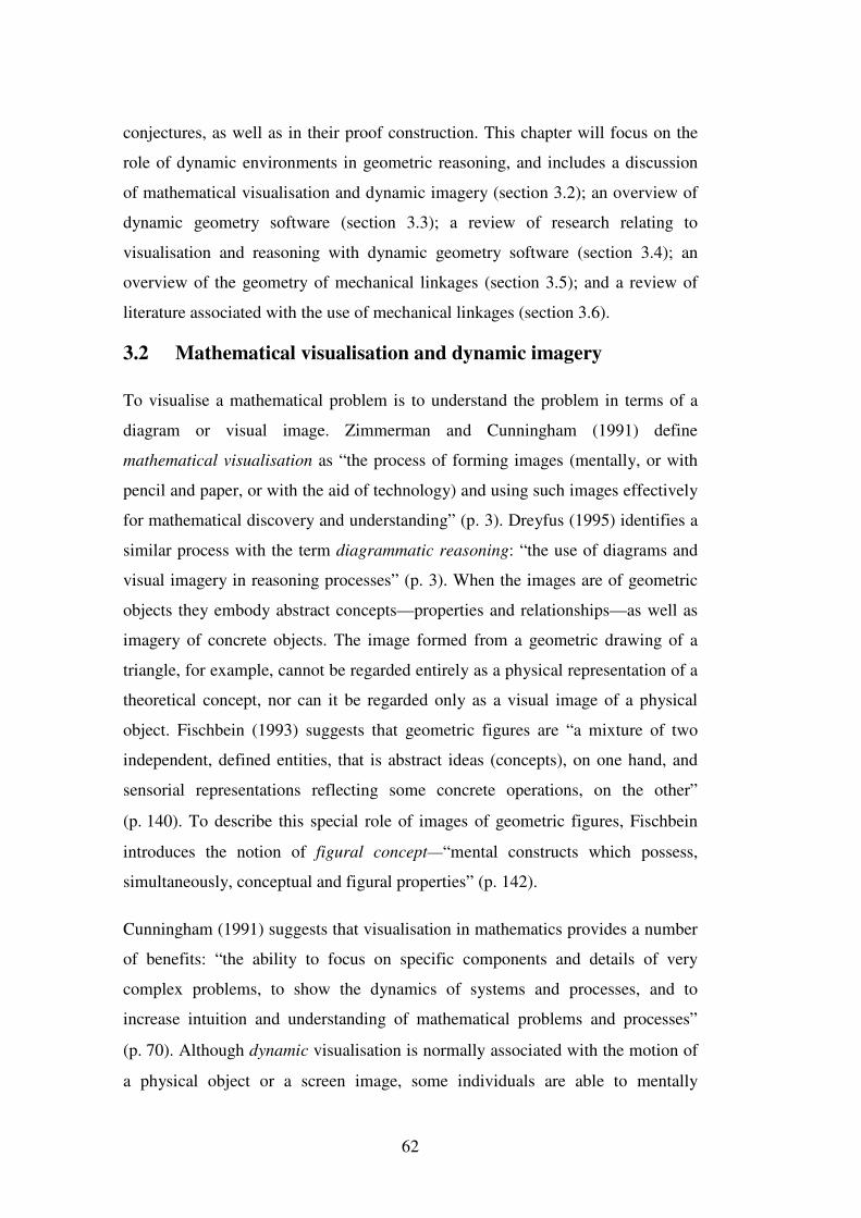
62
conjectures, as well as in their proof construction. This chapter will focus on the
role of dynamic environments in geometric reasoning, and includes a discussion
of mathematical visualisation and dynamic imagery (section 3.2); an overview of
dynamic geometry software (section 3.3); a review of research relating to
visualisation and reasoning with dynamic geometry software (section 3.4); an
overview of the geometry of mechanical linkages (section 3.5); and a review of
literature associated with the use of mechanical linkages (section 3.6).
3.2 Mathematical visualisation and dynamic imagery
To visualise a mathematical problem is to understand the problem in terms of a
diagram or visual image. Zimmerman and Cunningham (1991) define
mathematical visualisation as “the process of forming images (mentally, or with
pencil and paper, or with the aid of technology) and using such images effectively
for mathematical discovery and understanding” (p. 3). Dreyfus (1995) identifies a
similar process with the term diagrammatic reasoning: “the use of diagrams and
visual imagery in reasoning processes” (p. 3). When the images are of geometric
objects they embody abstract concepts—properties and relationships—as well as
imagery of concrete objects. The image formed from a geometric drawing of a
triangle, for example, cannot be regarded entirely as a physical representation of a
theoretical concept, nor can it be regarded only as a visual image of a physical
object. Fischbein (1993) suggests that geometric figures are “a mixture of two
independent, defined entities, that is abstract ideas (concepts), on one hand, and
sensorial representations reflecting some concrete operations, on the other”
(p. 140). To describe this special role of images of geometric figures, Fischbein
introduces the notion of figural concept—“mental constructs which possess,
simultaneously, conceptual and figural properties” (p. 142).
Cunningham (1991) suggests that visualisation in mathematics provides a number
of benefits: “the ability to focus on specific components and details of very
complex problems, to show the dynamics of systems and processes, and to
increase intuition and understanding of mathematical problems and processes”
(p. 70). Although dynamic visualisation is normally associated with the motion of
a physical object or a screen image, some individuals are able to mentally
63
manipulate the image of a static situation, as in ‘reasoning by continuity’
(Goldenberg, 1995), ‘transformational reasoning’ (Simon, 1996), or the formation
of anticipatory images (Piaget & Inhelder, 1956). These will be described below.
3.2.1 Reasoning by continuity
Goldenberg (1995) notes that some people are able to move and manipulate
objects mentally without any formal teaching, whereas others do not develop this
ability. He speculates on whether it is possible to teach mental manipulation skills,
and if so, what part dynamic geometry tools such as Cabri might play. Goldenberg
quotes the case of Richard, an ‘average’ student in mathematics, who was able to
reason dynamically and to recognise where it would be useful. Richard was faced
with a multiple-choice question involving an equilateral triangle of side 10 units,
with an internal point D. He had to determine which one of five numerical choices
was the sum of the distances from D to the sides of the triangle (see Figure 3-1).
A B
C
D
P
Q
R
Figure 3-1. Equilateral triangle problem
[From Goldenberg, 1995, Figure 1, p. 204].
Richard reasoned that because the problem did not state where D was, he could
move it around to help him solve the problem. He moved D close to C, where DQ
and DP were nearly zero and DR was nearly an altitude. Although he did not
express his solution in formal language, he reasoned that as D approaches C, the
sum of the three distances, DP + DQ + DR, approaches DR, which in turn
approaches CR, an altitude. Goldenberg suggests that “tools like Cabri-géomètre
allow students to design their own experiments, get a ‘feel’ and ‘vision’ for their
dynamics, and develop the kind of reasoning by continuity that Richard used”
(p. 205).
64
3.2.2 Transformational reasoning
Simon (1996) notes that students are often observed to draw upon
‘transformational reasoning’ in helping them understand why a particular
mathematical system works. He defines transformational reasoning as
the mental or physical enactment of an operation or set of operations on an object or
set of objects that allows one to envision the transformations that these objects
undergo and the set of results of these operations. (p. 201)
Simon asserts that the key feature of transformational reasoning is the ability to
consider “a dynamic process by which a new state or a continuum of states are
generated” (p. 201). He suggests that this form of reasoning involves “not just the
ability to carry out a particular mental or physical enactment, but also the
realization of the appropriateness of that process to a particular mathematical
situation” (p. 203). The example is given of Mary, a Year 10 geometry student
who, when asked “Could you make an isosceles triangle by specifying two angles
and the included side?”, responded: “Well, I know that if two people walked from
the ends of this side at equal angles towards each other, when they meet, they
would have walked the same distance” (p. 199). Mary’s response to the question
“What would happen if the person on the left walked at a smaller angle to the
side?”, was “Then that person would walk further [than the person on the right]
before they meet.” Simon notes that
Mary was able to see an isosceles triangle, not as a static figure of particular
dimensions, but as a dynamic process that generates triangles from the two ends of a
line segment. Her dynamic mental model allowed her to know, not only the
relationship between the base angles of an isosceles triangle, but also to reason about
the relative lengths of the legs of a triangle given unequal base angles. (p. 199)
Simon’s transformational reasoning may be regarded perhaps as a special form of
inductive reasoning (that is, drawing a generalised conclusion from a set of
particular cases), where dynamic mental imagery generates the particular cases
which lead to a generalised conclusion.
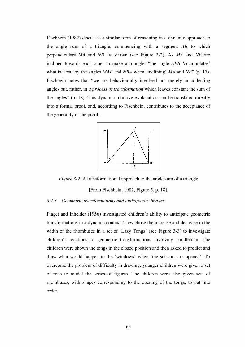
65
Fischbein (1982) discusses a similar form of reasoning in a dynamic approach to
the angle sum of a triangle, commencing with a segment AB to which
perpendiculars MA and NB are drawn (see Figure 3-2). As MA and NB are
inclined towards each other to make a triangle, “the angle APB ‘accumulates’
what is ‘lost’ by the angles MAB and NBA when ‘inclining’ MA and NB” (p. 17).
Fischbein notes that “we are behaviourally involved not merely in collecting
angles but, rather, in a process of transformation which leaves constant the sum of
the angles” (p. 18). This dynamic intuitive explanation can be translated directly
into a formal proof, and, according to Fischbein, contributes to the acceptance of
the generality of the proof.
Figure 3-2. A transformational approach to the angle sum of a triangle
[From Fischbein, 1982, Figure 5, p. 18].
3.2.3 Geometric transformations and anticipatory images
Piaget and Inhelder (1956) investigated children’s ability to anticipate geometric
transformations in a dynamic context. They chose the increase and decrease in the
width of the rhombuses in a set of ‘Lazy Tongs’ (see Figure 3-3) to investigate
children’s reactions to geometric transformations involving parallelism. The
children were shown the tongs in the closed position and then asked to predict and
draw what would happen to the ‘windows’ when ‘the scissors are opened’. To
overcome the problem of difficulty in drawing, younger children were given a set
of rods to model the series of figures. The children were also given sets of
rhombuses, with shapes corresponding to the opening of the tongs, to put into
order.
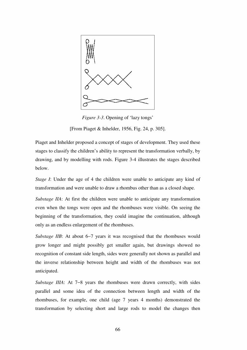
66
Figure 3-3. Opening of ‘lazy tongs’
[From Piaget & Inhelder, 1956, Fig. 24, p. 305].
Piaget and Inhelder proposed a concept of stages of development. They used these
stages to classify the children’s ability to represent the transformation verbally, by
drawing, and by modelling with rods. Figure 3-4 illustrates the stages described
below.
Stage I: Under the age of 4 the children were unable to anticipate any kind of
transformation and were unable to draw a rhombus other than as a closed shape.
Substage IIA: At first the children were unable to anticipate any transformation
even when the tongs were open and the rhombuses were visible. On seeing the
beginning of the transformation, they could imagine the continuation, although
only as an endless enlargement of the rhombuses.
Substage IIB: At about 6−7 years it was recognised that the rhombuses would
grow longer and might possibly get smaller again, but drawings showed no
recognition of constant side length, sides were generally not shown as parallel and
the inverse relationship between height and width of the rhombuses was not
anticipated.
Substage IIIA: At 7−8 years the rhombuses were drawn correctly, with sides
parallel and some idea of the connection between length and width of the
rhombuses, for example, one child (age 7 years 4 months) demonstrated the
transformation by selecting short and large rods to model the changes then
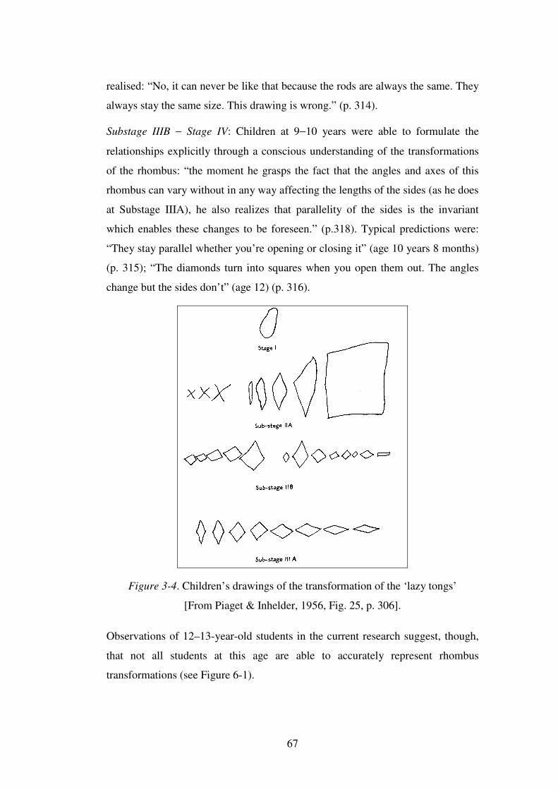
67
realised: “No, it can never be like that because the rods are always the same. They
always stay the same size. This drawing is wrong.” (p. 314).
Substage IIIB − Stage IV: Children at 9−10 years were able to formulate the
relationships explicitly through a conscious understanding of the transformations
of the rhombus: “the moment he grasps the fact that the angles and axes of this
rhombus can vary without in any way affecting the lengths of the sides (as he does
at Substage IIIA), he also realizes that parallelity of the sides is the invariant
which enables these changes to be foreseen.” (p.318). Typical predictions were:
“They stay parallel whether you’re opening or closing it” (age 10 years 8 months)
(p. 315); “The diamonds turn into squares when you open them out. The angles
change but the sides don’t” (age 12) (p. 316).
Figure 3-4. Children’s drawings of the transformation of the ‘lazy tongs’
[From Piaget & Inhelder, 1956, Fig. 25, p. 306].
Observations of 12–13-year-old students in the current research suggest, though,
that not all students at this age are able to accurately represent rhombus
transformations (see Figure 6-1).
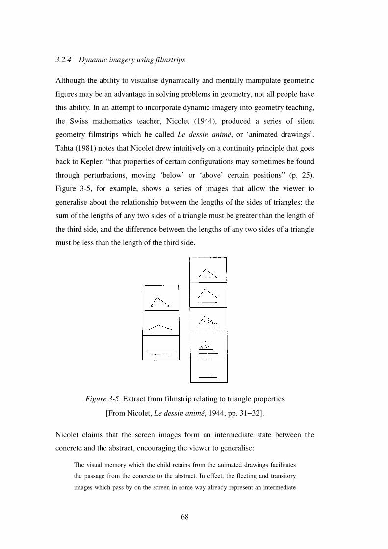
68
3.2.4 Dynamic imagery using filmstrips
Although the ability to visualise dynamically and mentally manipulate geometric
figures may be an advantage in solving problems in geometry, not all people have
this ability. In an attempt to incorporate dynamic imagery into geometry teaching,
the Swiss mathematics teacher, Nicolet (1944), produced a series of silent
geometry filmstrips which he called Le dessin animé, or ‘animated drawings’.
Tahta (1981) notes that Nicolet drew intuitively on a continuity principle that goes
back to Kepler: “that properties of certain configurations may sometimes be found
through perturbations, moving ‘below’ or ‘above’ certain positions” (p. 25).
Figure 3-5, for example, shows a series of images that allow the viewer to
generalise about the relationship between the lengths of the sides of triangles: the
sum of the lengths of any two sides of a triangle must be greater than the length of
the third side, and the difference between the lengths of any two sides of a triangle
must be less than the length of the third side.
Figure 3-5. Extract from filmstrip relating to triangle properties
[From Nicolet, Le dessin animé, 1944, pp. 31−32].
Nicolet claims that the screen images form an intermediate state between the
concrete and the abstract, encouraging the viewer to generalise:
The visual memory which the child retains from the animated drawings facilitates
the passage from the concrete to the abstract. In effect, the fleeting and transitory
images which pass by on the screen in some way already represent an intermediate
69
state between the concrete and the abstract, favourable to mathematical
understanding. The animated drawings lead to abstract reasoning, the prime object
of mathematics teaching, and allow one to see that a truth is independent of certain
variable circumstances. (Translated from Nicolet, 1944, p. 5)
Tahta (1981) notes that “the animations were beautifully timed, lingering slowly
so that the viewer was often ready to construct a meaning before the film
confirmed it” (p. 25):
The classical textbooks showed that two particular ‘angles at the circumference
subtended by the same chord’ were equal. But in one brief film, Nicolet displayed
all such angles as a class and by natural animation to the limit revealed the same
class in the so-called alternate segment or cyclic quadrilateral theorems. I remember
vividly the fourth form with whom I first viewed this film as a young and
inexperienced teacher who had flogged them [Tahta’s students] stolidly through the
angle-theorems for what had seemed a very long time. Their delight in seeing them
all displayed as one theorem was accompanied by an accusing amazement that I
could have previously so wasted their time. (p. 26)
Whereas Nicolet’s films required the viewer to mentally act upon a series of static
images, the last two decades have seen the development of a number of ‘dynamic
geometry’ computer software programs where dragging and animation of screen
figures results in continuously changing images. Section 3.3 describes the unique
environment of dynamic geometry software, where dynamic imagery can be
applied to Euclidean geometry, and discusses some concerns associated with its
classroom use.
3.3 Dynamic geometry software
3.3.1 What is dynamic geometry software?
“Dynamic geometry software” has become a generic term for a class of geometry
software environments, for example, Cabri Geometry II�, The Geometer’s
Sketchpad�, and Geometry Expert, where geometric objects can be continuously
transformed on the screen by dragging, with only those features based on
geometric properties remaining invariant. Accurate measurements can be
performed, and the software incorporates Euclidean geometry tools, such as angle
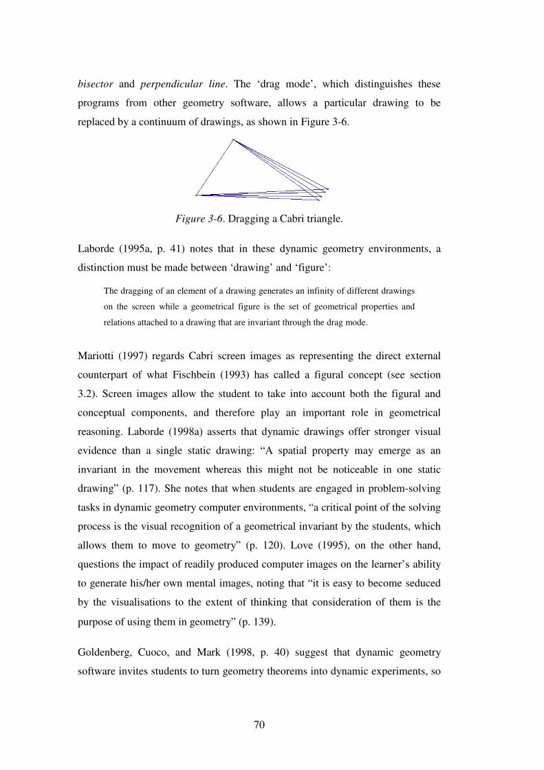
70
bisector and perpendicular line. The ‘drag mode’, which distinguishes these
programs from other geometry software, allows a particular drawing to be
replaced by a continuum of drawings, as shown in Figure 3-6.
Figure 3-6. Dragging a Cabri triangle.
Laborde (1995a, p. 41) notes that in these dynamic geometry environments, a
distinction must be made between ‘drawing’ and ‘figure’:
The dragging of an element of a drawing generates an infinity of different drawings
on the screen while a geometrical figure is the set of geometrical properties and
relations attached to a drawing that are invariant through the drag mode.
Mariotti (1997) regards Cabri screen images as representing the direct external
counterpart of what Fischbein (1993) has called a figural concept (see section
3.2). Screen images allow the student to take into account both the figural and
conceptual components, and therefore play an important role in geometrical
reasoning. Laborde (1998a) asserts that dynamic drawings offer stronger visual
evidence than a single static drawing: “A spatial property may emerge as an
invariant in the movement whereas this might not be noticeable in one static
drawing” (p. 117). She notes that when students are engaged in problem-solving
tasks in dynamic geometry computer environments, “a critical point of the solving
process is the visual recognition of a geometrical invariant by the students, which
allows them to move to geometry” (p. 120). Love (1995), on the other hand,
questions the impact of readily produced computer images on the learner’s ability
to generate his/her own mental images, noting that “it is easy to become seduced
by the visualisations to the extent of thinking that consideration of them is the
purpose of using them in geometry” (p. 139).
Goldenberg, Cuoco, and Mark (1998, p. 40) suggest that dynamic geometry
software invites students to turn geometry theorems into dynamic experiments, so
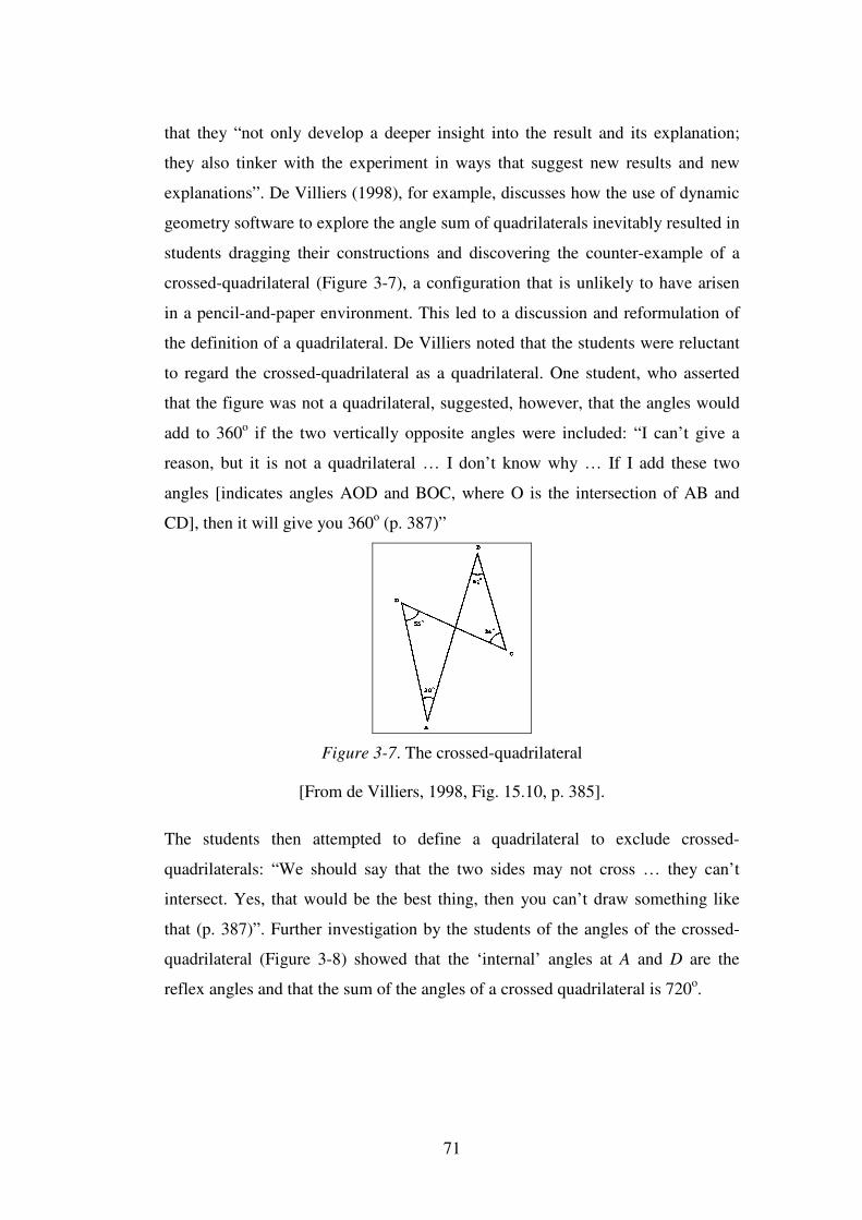
71
that they “not only develop a deeper insight into the result and its explanation;
they also tinker with the experiment in ways that suggest new results and new
explanations”. De Villiers (1998), for example, discusses how the use of dynamic
geometry software to explore the angle sum of quadrilaterals inevitably resulted in
students dragging their constructions and discovering the counter-example of a
crossed-quadrilateral (Figure 3-7), a configuration that is unlikely to have arisen
in a pencil-and-paper environment. This led to a discussion and reformulation of
the definition of a quadrilateral. De Villiers noted that the students were reluctant
to regard the crossed-quadrilateral as a quadrilateral. One student, who asserted
that the figure was not a quadrilateral, suggested, however, that the angles would
add to 360o if the two vertically opposite angles were included: “I can’t give a
reason, but it is not a quadrilateral … I don’t know why … If I add these two
angles [indicates angles AOD and BOC, where O is the intersection of AB and
CD], then it will give you 360o (p. 387)”
Figure 3-7. The crossed-quadrilateral
[From de Villiers, 1998, Fig. 15.10, p. 385].
The students then attempted to define a quadrilateral to exclude crossed-
quadrilaterals: “We should say that the two sides may not cross … they can’t
intersect. Yes, that would be the best thing, then you can’t draw something like
that (p. 387)”. Further investigation by the students of the angles of the crossed-
quadrilateral (Figure 3-8) showed that the ‘internal’ angles at A and D are the
reflex angles and that the sum of the angles of a crossed quadrilateral is 720o.
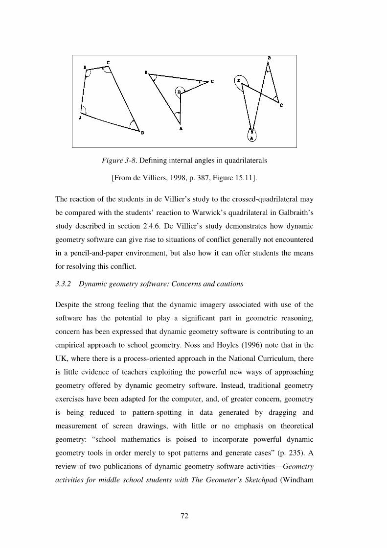
72
Figure 3-8. Defining internal angles in quadrilaterals
[From de Villiers, 1998, p. 387, Figure 15.11].
The reaction of the students in de Villier’s study to the crossed-quadrilateral may
be compared with the students’ reaction to Warwick’s quadrilateral in Galbraith’s
study described in section 2.4.6. De Villier’s study demonstrates how dynamic
geometry software can give rise to situations of conflict generally not encountered
in a pencil-and-paper environment, but also how it can offer students the means
for resolving this conflict.
3.3.2 Dynamic geometry software: Concerns and cautions
Despite the strong feeling that the dynamic imagery associated with use of the
software has the potential to play a significant part in geometric reasoning,
concern has been expressed that dynamic geometry software is contributing to an
empirical approach to school geometry. Noss and Hoyles (1996) note that in the
UK, where there is a process-oriented approach in the National Curriculum, there
is little evidence of teachers exploiting the powerful new ways of approaching
geometry offered by dynamic geometry software. Instead, traditional geometry
exercises have been adapted for the computer, and, of greater concern, geometry
is being reduced to pattern-spotting in data generated by dragging and
measurement of screen drawings, with little or no emphasis on theoretical
geometry: “school mathematics is poised to incorporate powerful dynamic
geometry tools in order merely to spot patterns and generate cases” (p. 235). A
review of two publications of dynamic geometry software activities—Geometry
activities for middle school students with The Geometer’s Sketchpad (Windham
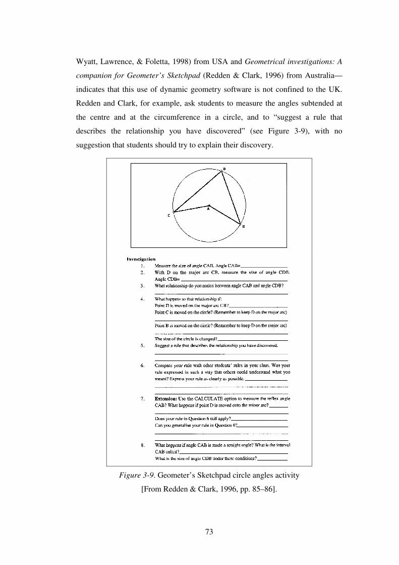
73
Wyatt, Lawrence, & Foletta, 1998) from USA and Geometrical investigations: A
companion for Geometer’s Sketchpad (Redden & Clark, 1996) from Australia—
indicates that this use of dynamic geometry software is not confined to the UK.
Redden and Clark, for example, ask students to measure the angles subtended at
the centre and at the circumference in a circle, and to “suggest a rule that
describes the relationship you have discovered” (see Figure 3-9), with no
suggestion that students should try to explain their discovery.
Figure 3-9. Geometer’s Sketchpad circle angles activity
[From Redden & Clark, 1996, pp. 85–86].
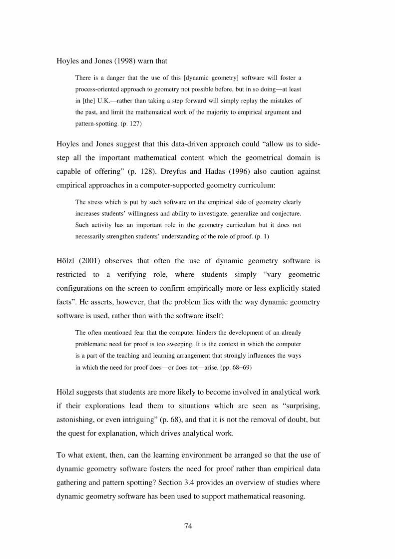
74
Hoyles and Jones (1998) warn that
There is a danger that the use of this [dynamic geometry] software will foster a
process-oriented approach to geometry not possible before, but in so doing—at least
in [the] U.K.—rather than taking a step forward will simply replay the mistakes of
the past, and limit the mathematical work of the majority to empirical argument and
pattern-spotting. (p. 127)
Hoyles and Jones suggest that this data-driven approach could “allow us to side-
step all the important mathematical content which the geometrical domain is
capable of offering” (p. 128). Dreyfus and Hadas (1996) also caution against
empirical approaches in a computer-supported geometry curriculum:
The stress which is put by such software on the empirical side of geometry clearly
increases students’ willingness and ability to investigate, generalize and conjecture.
Such activity has an important role in the geometry curriculum but it does not
necessarily strengthen students’ understanding of the role of proof. (p. 1)
Hölzl (2001) observes that often the use of dynamic geometry software is
restricted to a verifying role, where students simply “vary geometric
configurations on the screen to confirm empirically more or less explicitly stated
facts”. He asserts, however, that the problem lies with the way dynamic geometry
software is used, rather than with the software itself:
The often mentioned fear that the computer hinders the development of an already
problematic need for proof is too sweeping. It is the context in which the computer
is a part of the teaching and learning arrangement that strongly influences the ways
in which the need for proof does—or does not—arise. (pp. 68−69)
Hölzl suggests that students are more likely to become involved in analytical work
if their explorations lead them to situations which are seen as “surprising,
astonishing, or even intriguing” (p. 68), and that it is not the removal of doubt, but
the quest for explanation, which drives analytical work.
To what extent, then, can the learning environment be arranged so that the use of
dynamic geometry software fosters the need for proof rather than empirical data
gathering and pattern spotting? Section 3.4 provides an overview of studies where
dynamic geometry software has been used to support mathematical reasoning.
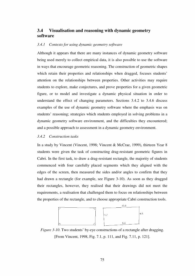
75
3.4 Visualisation and reasoning with dynamic geometry software
3.4.1 Contexts for using dynamic geometry software
Although it appears that there are many instances of dynamic geometry software
being used merely to collect empirical data, it is also possible to use the software
in ways that encourage geometric reasoning. The construction of geometric shapes
which retain their properties and relationships when dragged, focuses students’
attention on the relationships between properties. Other activities may require
students to explore, make conjectures, and prove properties for a given geometric
figure, or to model and investigate a dynamic physical situation in order to
understand the effect of changing parameters. Sections 3.4.2 to 3.4.6 discuss
examples of the use of dynamic geometry software where the emphasis was on
students’ reasoning; strategies which students employed in solving problems in a
dynamic geometry software environment, and the difficulties they encountered;
and a possible approach to assessment in a dynamic geometry environment.
3.4.2 Construction tasks
In a study by Vincent (Vincent, 1998; Vincent & McCrae, 1999), thirteen Year 8
students were given the task of constructing drag-resistant geometric figures in
Cabri. In the first task, to draw a drag-resistant rectangle, the majority of students
commenced with four carefully placed segments which they aligned with the
edges of the screen, then measured the sides and/or angles to confirm that they
had drawn a rectangle (for example, see Figure 3-10). As soon as they dragged
their rectangles, however, they realised that their drawings did not meet the
requirements, a realisation that challenged them to focus on relationships between
the properties of the rectangle, and to choose appropriate Cabri construction tools.
Figure 3-10. Two students’ by-eye constructions of a rectangle after dragging.
[From Vincent, 1998, Fig. 7.1, p. 111, and Fig. 7.11, p. 121].
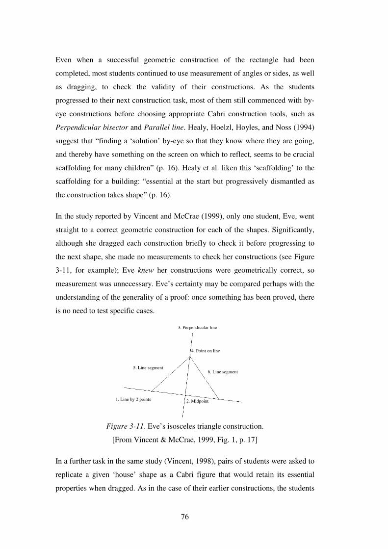
76
Even when a successful geometric construction of the rectangle had been
completed, most students continued to use measurement of angles or sides, as well
as dragging, to check the validity of their constructions. As the students
progressed to their next construction task, most of them still commenced with by-
eye constructions before choosing appropriate Cabri construction tools, such as
Perpendicular bisector and Parallel line. Healy, Hoelzl, Hoyles, and Noss (1994)
suggest that “finding a ‘solution’ by-eye so that they know where they are going,
and thereby have something on the screen on which to reflect, seems to be crucial
scaffolding for many children” (p. 16). Healy et al. liken this ‘scaffolding’ to the
scaffolding for a building: “essential at the start but progressively dismantled as
the construction takes shape” (p. 16).
In the study reported by Vincent and McCrae (1999), only one student, Eve, went
straight to a correct geometric construction for each of the shapes. Significantly,
although she dragged each construction briefly to check it before progressing to
the next shape, she made no measurements to check her constructions (see Figure
3-11, for example); Eve knew her constructions were geometrically correct, so
measurement was unnecessary. Eve’s certainty may be compared perhaps with the
understanding of the generality of a proof: once something has been proved, there
is no need to test specific cases.
3. Perpendicular line
1. Line by 2 points 2. Midpoint
4. Point on line
5. Line segment6. Line segment
Figure 3-11. Eve’s isosceles triangle construction.
[From Vincent & McCrae, 1999, Fig. 1, p. 17]
In a further task in the same study (Vincent, 1998), pairs of students were asked to
replicate a given ‘house’ shape as a Cabri figure that would retain its essential
properties when dragged. As in the case of their earlier constructions, the students
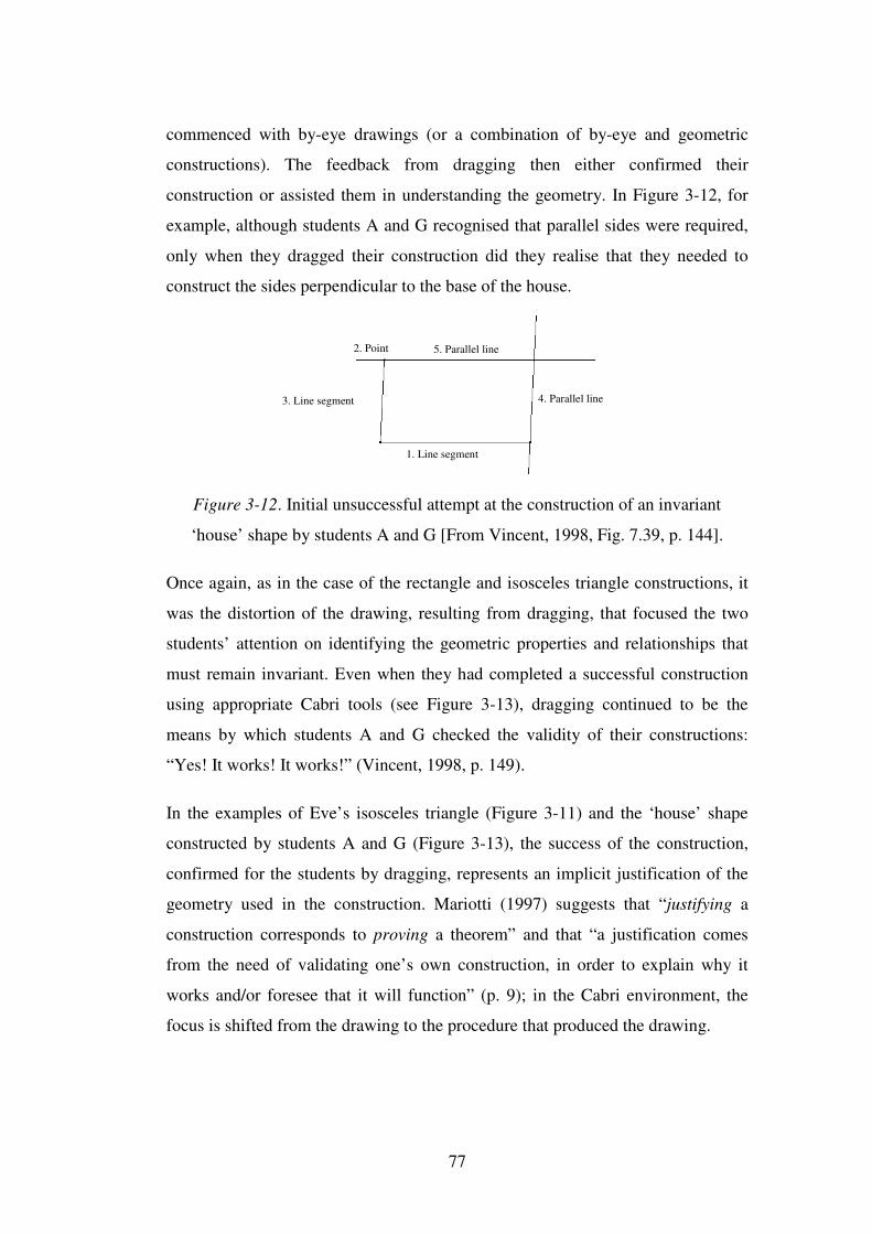
77
commenced with by-eye drawings (or a combination of by-eye and geometric
constructions). The feedback from dragging then either confirmed their
construction or assisted them in understanding the geometry. In Figure 3-12, for
example, although students A and G recognised that parallel sides were required,
only when they dragged their construction did they realise that they needed to
construct the sides perpendicular to the base of the house.
1. Line segment
3. Line segment 4. Parallel line
5. Parallel line2. Point
Figure 3-12. Initial unsuccessful attempt at the construction of an invariant
‘house’ shape by students A and G [From Vincent, 1998, Fig. 7.39, p. 144].
Once again, as in the case of the rectangle and isosceles triangle constructions, it
was the distortion of the drawing, resulting from dragging, that focused the two
students’ attention on identifying the geometric properties and relationships that
must remain invariant. Even when they had completed a successful construction
using appropriate Cabri tools (see Figure 3-13), dragging continued to be the
means by which students A and G checked the validity of their constructions:
“Yes! It works! It works!” (Vincent, 1998, p. 149).
In the examples of Eve’s isosceles triangle (Figure 3-11) and the ‘house’ shape
constructed by students A and G (Figure 3-13), the success of the construction,
confirmed for the students by dragging, represents an implicit justification of the
geometry used in the construction. Mariotti (1997) suggests that “justifying a
construction corresponds to proving a theorem” and that “a justification comes
from the need of validating one’s own construction, in order to explain why it
works and/or foresee that it will function” (p. 9); in the Cabri environment, the
focus is shifted from the drawing to the procedure that produced the drawing.
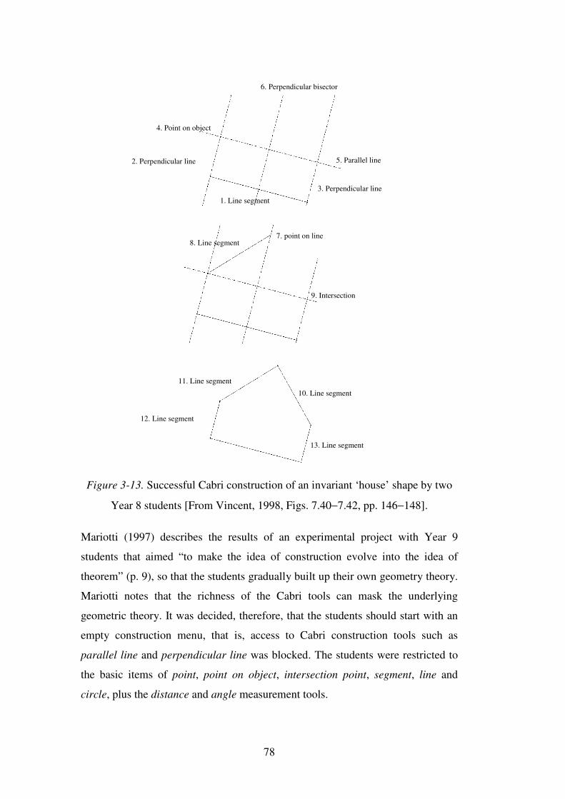
78
6. Perpendicular bisector
1. Line segment
2. Perpendicular line
3. Perpendicular line
4. Point on object
5. Parallel line
7. point on line8. Line segment
9. Intersection
10. Line segment
13. Line segment
12. Line segment
11. Line segment
Figure 3-13. Successful Cabri construction of an invariant ‘house’ shape by two
Year 8 students [From Vincent, 1998, Figs. 7.40−7.42, pp. 146−148].
Mariotti (1997) describes the results of an experimental project with Year 9
students that aimed “to make the idea of construction evolve into the idea of
theorem” (p. 9), so that the students gradually built up their own geometry theory.
Mariotti notes that the richness of the Cabri tools can mask the underlying
geometric theory. It was decided, therefore, that the students should start with an
empty construction menu, that is, access to Cabri construction tools such as
parallel line and perpendicular line was blocked. The students were restricted to
the basic items of point, point on object, intersection point, segment, line and
circle, plus the distance and angle measurement tools.
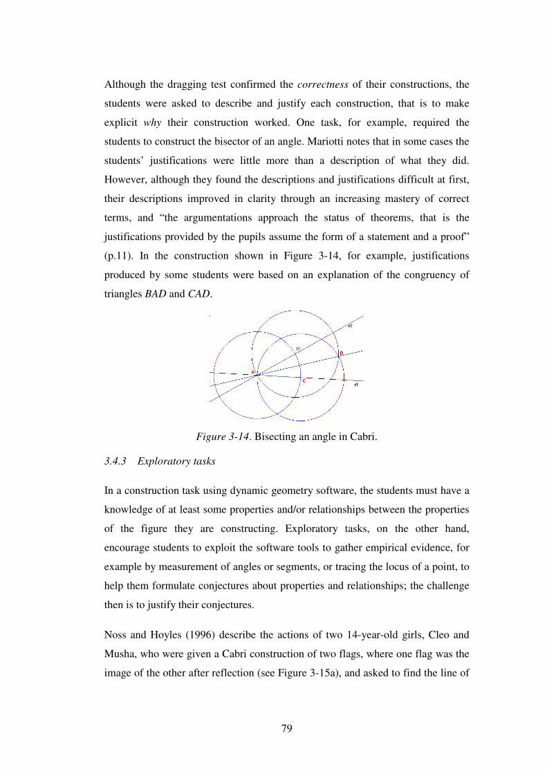
79
Although the dragging test confirmed the correctness of their constructions, the
students were asked to describe and justify each construction, that is to make
explicit why their construction worked. One task, for example, required the
students to construct the bisector of an angle. Mariotti notes that in some cases the
students’ justifications were little more than a description of what they did.
However, although they found the descriptions and justifications difficult at first,
their descriptions improved in clarity through an increasing mastery of correct
terms, and “the argumentations approach the status of theorems, that is the
justifications provided by the pupils assume the form of a statement and a proof”
(p.11). In the construction shown in Figure 3-14, for example, justifications
produced by some students were based on an explanation of the congruency of
triangles BAD and CAD.
Figure 3-14. Bisecting an angle in Cabri.
3.4.3 Exploratory tasks
In a construction task using dynamic geometry software, the students must have a
knowledge of at least some properties and/or relationships between the properties
of the figure they are constructing. Exploratory tasks, on the other hand,
encourage students to exploit the software tools to gather empirical evidence, for
example by measurement of angles or segments, or tracing the locus of a point, to
help them formulate conjectures about properties and relationships; the challenge
then is to justify their conjectures.
Noss and Hoyles (1996) describe the actions of two 14-year-old girls, Cleo and
Musha, who were given a Cabri construction of two flags, where one flag was the
image of the other after reflection (see Figure 3-15a), and asked to find the line of
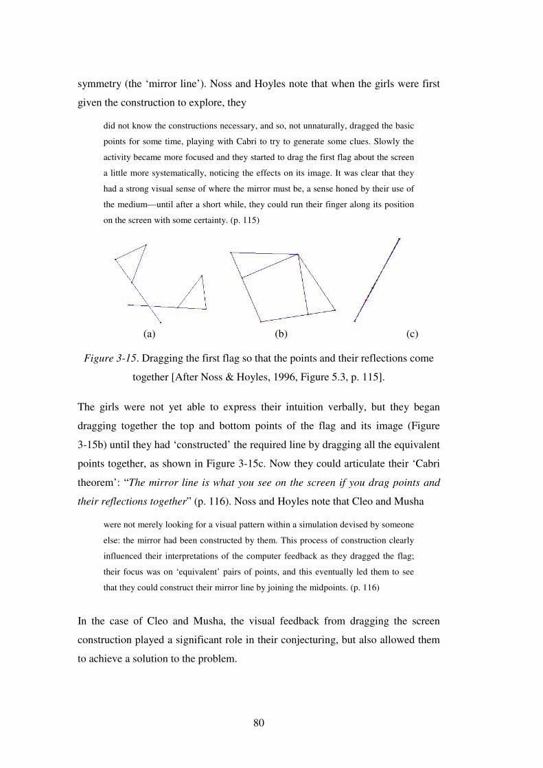
80
symmetry (the ‘mirror line’). Noss and Hoyles note that when the girls were first
given the construction to explore, they
did not know the constructions necessary, and so, not unnaturally, dragged the basic
points for some time, playing with Cabri to try to generate some clues. Slowly the
activity became more focused and they started to drag the first flag about the screen
a little more systematically, noticing the effects on its image. It was clear that they
had a strong visual sense of where the mirror must be, a sense honed by their use of
the medium—until after a short while, they could run their finger along its position
on the screen with some certainty. (p. 115)
(a) (b) (c)
Figure 3-15. Dragging the first flag so that the points and their reflections come
together [After Noss & Hoyles, 1996, Figure 5.3, p. 115].
The girls were not yet able to express their intuition verbally, but they began
dragging together the top and bottom points of the flag and its image (Figure
3-15b) until they had ‘constructed’ the required line by dragging all the equivalent
points together, as shown in Figure 3-15c. Now they could articulate their ‘Cabri
theorem’: “The mirror line is what you see on the screen if you drag points and
their reflections together” (p. 116). Noss and Hoyles note that Cleo and Musha
were not merely looking for a visual pattern within a simulation devised by someone
else: the mirror had been constructed by them. This process of construction clearly
influenced their interpretations of the computer feedback as they dragged the flag;
their focus was on ‘equivalent’ pairs of points, and this eventually led them to see
that they could construct their mirror line by joining the midpoints. (p. 116)
In the case of Cleo and Musha, the visual feedback from dragging the screen
construction played a significant role in their conjecturing, but also allowed them
to achieve a solution to the problem.
81
3.4.4 Proof tasks in a dynamic geometry environment
Hadas, Hershkowitz, and Schwarz (2000) suggest that the problem of students
being too readily convinced in a dynamic geometry environment may be
overcome by the use of problems that lead to unexpected or surprising situations.
They designed an activity that was intended to create a contradiction between
Year 8 students’ conjectures about the sum of the exterior angles of a polygon as
the number of sides of the polygon increases, and the results obtained when the
students measured the angles using dynamic geometry software. The students
were first required to measure the internal angles of a number of polygons and
explain their conclusion. The second task asked them to determine by
measurement the sum of the exterior angles of a quadrilateral, to conjecture what
would happen to the sum as the number of sides increased, and then to check their
conjecture by measurement. In 37 of the 49 responses (41 written responses from
82 students working in pairs and eight students interviewed individually), students
conjectured that the sum of the exterior angles would increase as the number of
sides increased, when in fact it is always 360o.
Despite their incorrect conjecture, many of the students were able to explain the
actual result. Hadas et al. (2000) report that even though the students had only just
commenced their study of Euclidean geometry, nine of the 50 explanations (one
interview student gave two different explanations), were “complete deductive
explanations and eight more used partial deductive or inductive explanations”
(p. 139). Seventeen of the remaining responses were categorised as “no
explanation”, two as “inductive”, and sixteen as “visual-variations”. Hadas et al.
note that
the students ceased to be recipients of formal proofs, but were engaged in an activity
of construction and evaluation of arguments in which certainty and understanding
were at stake, and they had to use their geometrical knowledge to explain
contradictions and overcome uncertainty. (p. 149)
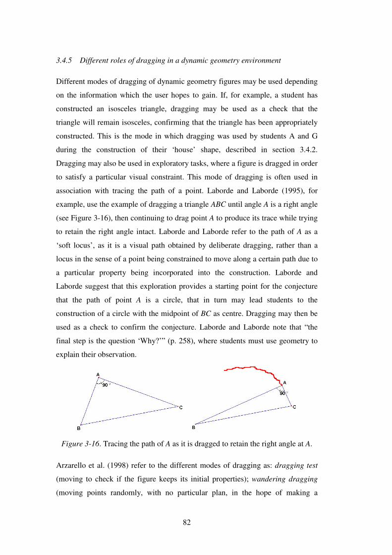
82
3.4.5 Different roles of dragging in a dynamic geometry environment
Different modes of dragging of dynamic geometry figures may be used depending
on the information which the user hopes to gain. If, for example, a student has
constructed an isosceles triangle, dragging may be used as a check that the
triangle will remain isosceles, confirming that the triangle has been appropriately
constructed. This is the mode in which dragging was used by students A and G
during the construction of their ‘house’ shape, described in section 3.4.2.
Dragging may also be used in exploratory tasks, where a figure is dragged in order
to satisfy a particular visual constraint. This mode of dragging is often used in
association with tracing the path of a point. Laborde and Laborde (1995), for
example, use the example of dragging a triangle ABC until angle A is a right angle
(see Figure 3-16), then continuing to drag point A to produce its trace while trying
to retain the right angle intact. Laborde and Laborde refer to the path of A as a
‘soft locus’, as it is a visual path obtained by deliberate dragging, rather than a
locus in the sense of a point being constrained to move along a certain path due to
a particular property being incorporated into the construction. Laborde and
Laborde suggest that this exploration provides a starting point for the conjecture
that the path of point A is a circle, that in turn may lead students to the
construction of a circle with the midpoint of BC as centre. Dragging may then be
used as a check to confirm the conjecture. Laborde and Laborde note that “the
final step is the question ‘Why?’” (p. 258), where students must use geometry to
explain their observation.
Figure 3-16. Tracing the path of A as it is dragged to retain the right angle at A.
Arzarello et al. (1998) refer to the different modes of dragging as: dragging test
(moving to check if the figure keeps its initial properties); wandering dragging
(moving points randomly, with no particular plan, in the hope of making a
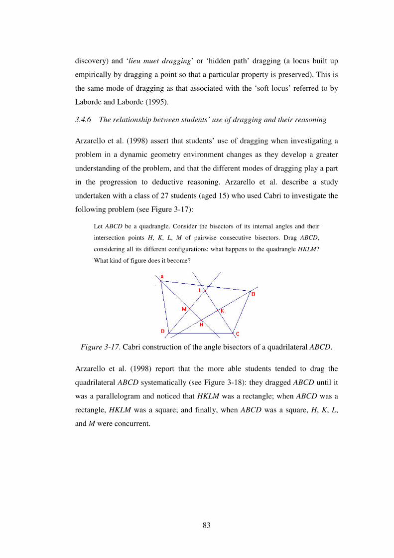
83
discovery) and ‘lieu muet dragging’ or ‘hidden path’ dragging (a locus built up
empirically by dragging a point so that a particular property is preserved). This is
the same mode of dragging as that associated with the ‘soft locus’ referred to by
Laborde and Laborde (1995).
3.4.6 The relationship between students’ use of dragging and their reasoning
Arzarello et al. (1998) assert that students’ use of dragging when investigating a
problem in a dynamic geometry environment changes as they develop a greater
understanding of the problem, and that the different modes of dragging play a part
in the progression to deductive reasoning. Arzarello et al. describe a study
undertaken with a class of 27 students (aged 15) who used Cabri to investigate the
following problem (see Figure 3-17):
Let ABCD be a quadrangle. Consider the bisectors of its internal angles and their
intersection points H, K, L, M of pairwise consecutive bisectors. Drag ABCD,
considering all its different configurations: what happens to the quadrangle HKLM?
What kind of figure does it become?
Figure 3-17. Cabri construction of the angle bisectors of a quadrilateral ABCD.
Arzarello et al. (1998) report that the more able students tended to drag the
quadrilateral ABCD systematically (see Figure 3-18): they dragged ABCD until it
was a parallelogram and noticed that HKLM was a rectangle; when ABCD was a
rectangle, HKLM was a square; and finally, when ABCD was a square, H, K, L,
and M were concurrent.
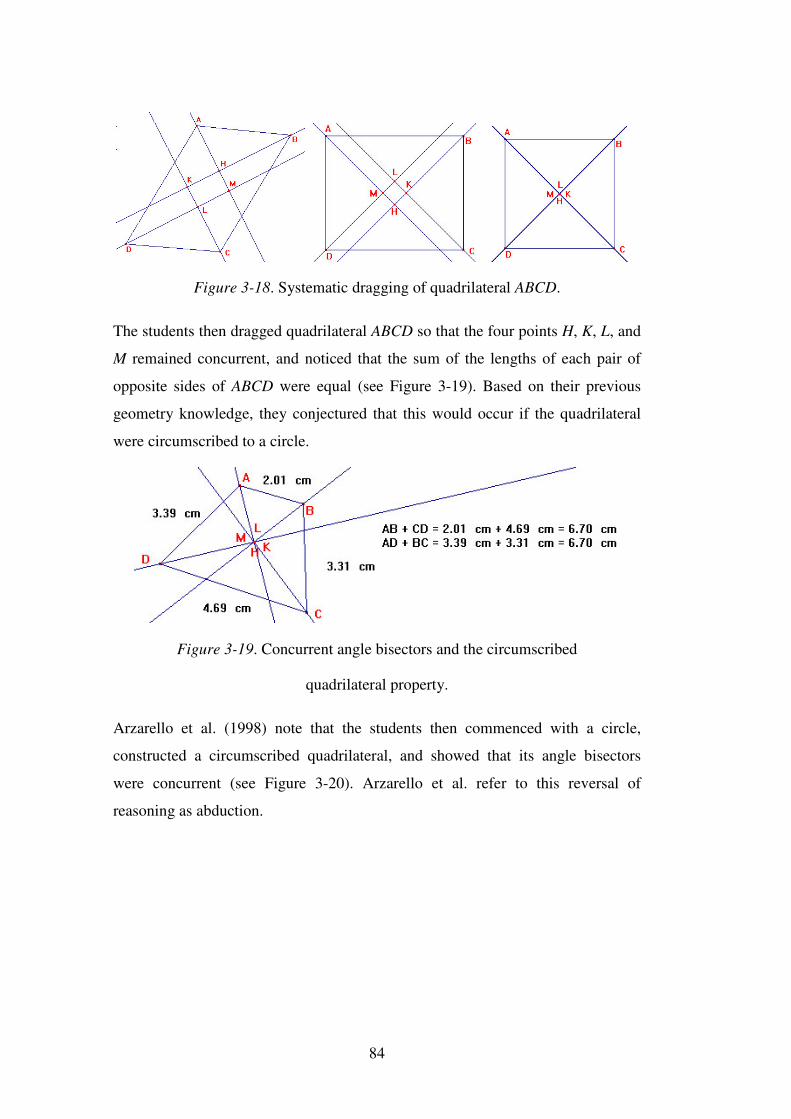
84
Figure 3-18. Systematic dragging of quadrilateral ABCD.
The students then dragged quadrilateral ABCD so that the four points H, K, L, and
M remained concurrent, and noticed that the sum of the lengths of each pair of
opposite sides of ABCD were equal (see Figure 3-19). Based on their previous
geometry knowledge, they conjectured that this would occur if the quadrilateral
were circumscribed to a circle.
Figure 3-19. Concurrent angle bisectors and the circumscribed
quadrilateral property.
Arzarello et al. (1998) note that the students then commenced with a circle,
constructed a circumscribed quadrilateral, and showed that its angle bisectors
were concurrent (see Figure 3-20). Arzarello et al. refer to this reversal of
reasoning as abduction.
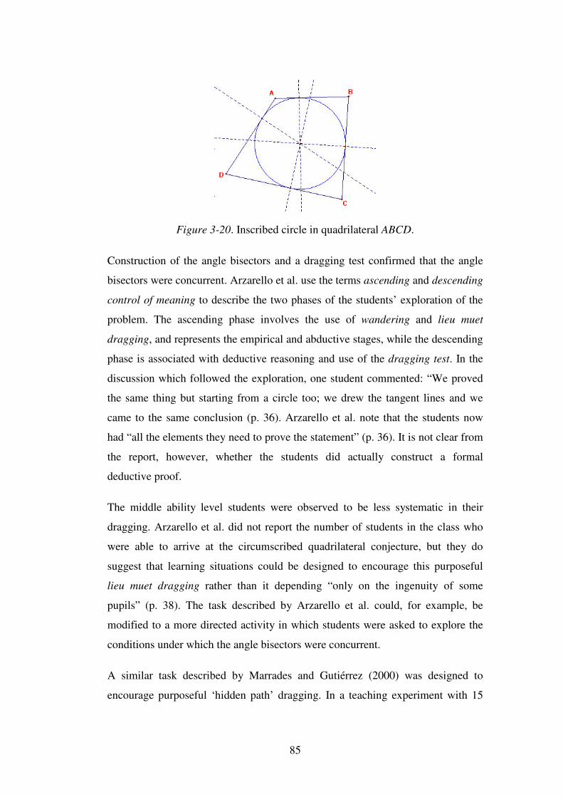
85
Figure 3-20. Inscribed circle in quadrilateral ABCD.
Construction of the angle bisectors and a dragging test confirmed that the angle
bisectors were concurrent. Arzarello et al. use the terms ascending and descending
control of meaning to describe the two phases of the students’ exploration of the
problem. The ascending phase involves the use of wandering and lieu muet
dragging, and represents the empirical and abductive stages, while the descending
phase is associated with deductive reasoning and use of the dragging test. In the
discussion which followed the exploration, one student commented: “We proved
the same thing but starting from a circle too; we drew the tangent lines and we
came to the same conclusion (p. 36). Arzarello et al. note that the students now
had “all the elements they need to prove the statement” (p. 36). It is not clear from
the report, however, whether the students did actually construct a formal
deductive proof.
The middle ability level students were observed to be less systematic in their
dragging. Arzarello et al. did not report the number of students in the class who
were able to arrive at the circumscribed quadrilateral conjecture, but they do
suggest that learning situations could be designed to encourage this purposeful
lieu muet dragging rather than it depending “only on the ingenuity of some
pupils” (p. 38). The task described by Arzarello et al. could, for example, be
modified to a more directed activity in which students were asked to explore the
conditions under which the angle bisectors were concurrent.
A similar task described by Marrades and Gutiérrez (2000) was designed to
encourage purposeful ‘hidden path’ dragging. In a teaching experiment with 15
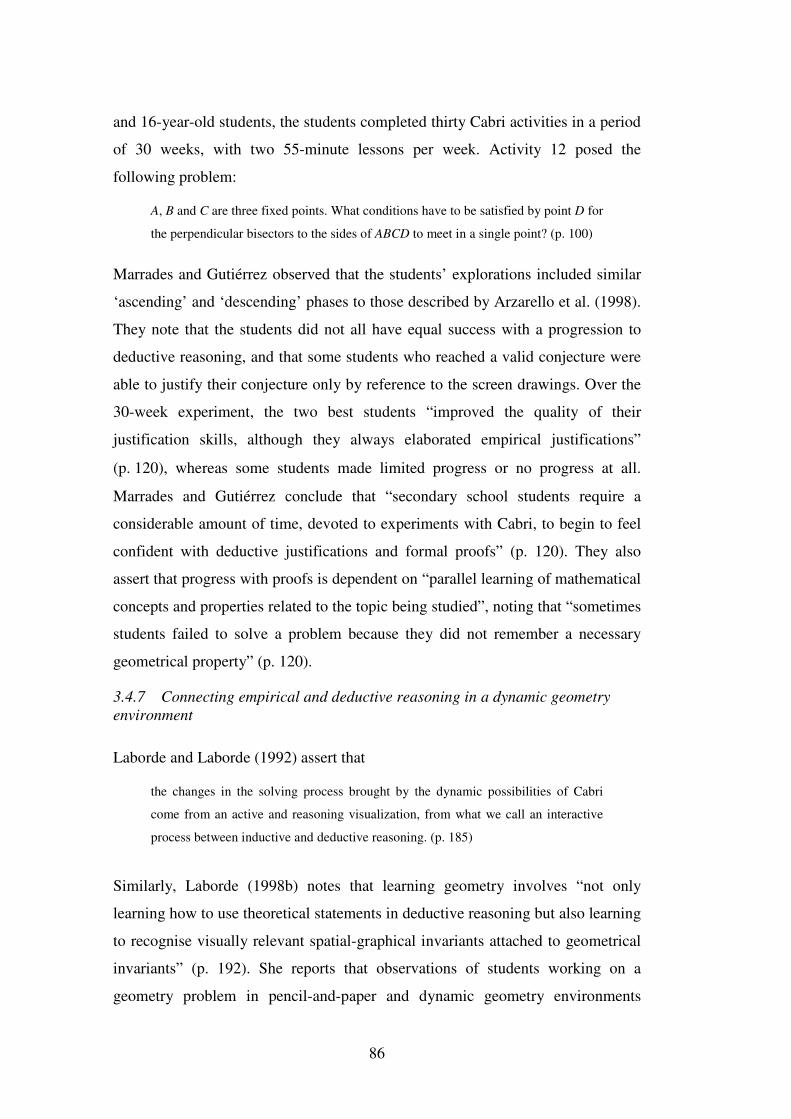
86
and 16-year-old students, the students completed thirty Cabri activities in a period
of 30 weeks, with two 55-minute lessons per week. Activity 12 posed the
following problem:
A, B and C are three fixed points. What conditions have to be satisfied by point D for
the perpendicular bisectors to the sides of ABCD to meet in a single point? (p. 100)
Marrades and Gutiérrez observed that the students’ explorations included similar
‘ascending’ and ‘descending’ phases to those described by Arzarello et al. (1998).
They note that the students did not all have equal success with a progression to
deductive reasoning, and that some students who reached a valid conjecture were
able to justify their conjecture only by reference to the screen drawings. Over the
30-week experiment, the two best students “improved the quality of their
justification skills, although they always elaborated empirical justifications”
(p. 120), whereas some students made limited progress or no progress at all.
Marrades and Gutiérrez conclude that “secondary school students require a
considerable amount of time, devoted to experiments with Cabri, to begin to feel
confident with deductive justifications and formal proofs” (p. 120). They also
assert that progress with proofs is dependent on “parallel learning of mathematical
concepts and properties related to the topic being studied”, noting that “sometimes
students failed to solve a problem because they did not remember a necessary
geometrical property” (p. 120).
3.4.7 Connecting empirical and deductive reasoning in a dynamic geometry environment
Laborde and Laborde (1992) assert that
the changes in the solving process brought by the dynamic possibilities of Cabri
come from an active and reasoning visualization, from what we call an interactive
process between inductive and deductive reasoning. (p. 185)
Similarly, Laborde (1998b) notes that learning geometry involves “not only
learning how to use theoretical statements in deductive reasoning but also learning
to recognise visually relevant spatial-graphical invariants attached to geometrical
invariants” (p. 192). She reports that observations of students working on a
geometry problem in pencil-and-paper and dynamic geometry environments
87
showed that the problem made sense for the students only after they were able to
visually manipulate their screen construction. Laborde argues that in a pencil-
and-paper environment, students’ movement between the spatial-graphical and
theoretical domains is restricted, whereas the software environment promotes
links between the two domains.
Scher (1999, p. 24) asserts that dynamic geometry software can influence the style
of experimentation and reasoning so that “the boundary between deductive
reasoning and dynamic geometry becomes blurred: the software finds its way into
the proof process”. De Villiers (1997) notes that in cases of his own personal
discoveries using dynamic geometry software, actual conviction based on
continual experimental confirmation preceded the eventual proof, and that
manipulation of the dynamic geometry construction provided him with the
necessary insight to develop the proof.
Although it might be expected that in a dynamic geometry environment students
would make connections between empirical data and deductive reasoning, studies
have shown that this is not necessarily the case. Healy and Hoyles (Healy, 2000;
Hoyles, 1998; Hoyles & Healy, 1999) describe aspects of a classroom research
project in which fifteen 15-year-old students of above average mathematical
attainment (five students from each of three different schools) were introduced to
a culture of conjecture and proof in a Cabri environment. Despite a deliberate
attempt in the research design to facilitate links between inductive and deductive
reasoning, it was found that many of the students failed to make connections
between their empirical Cabri work and proofs.
The teaching experiment consisted of three classroom sessions with three
follow-up homework activities. During the first session the students used Cabri to
explore the conditions for triangle congruency. The second session, which
introduced the students to formal proof writing, drew upon their “actions,
conjectures and explanations” from the first session and the homework activity.
Hoyles (1998) notes that examples in the second session were designed “to
motivate the use of a precise formal language for proof, the careful separation of
the givens from what has been proved and the need for a logical chain of
88
deductions and reasons” (p. 175). These examples included a condition which
appeared visually to be true, but was not true in general; a circular argument,
where what had to be proved was used in the argument; and an ambiguous
narrative proof. Following a Cabri task of constructing different quadrilaterals and
justifying their constructions, the students were then given the following problem
in the third session:
Can you construct a quadrilateral in which the angle bisectors of two adjacent angles
cross at right angles? What are its properties?
At the completion of this task the students were presented with what was
anticipated to be a simple extension:
Can you construct a triangle with the same condition (i.e., with two adjacent angle
bisectors perpendicular)?
The majority of students were observed to work experimentally on the first part of
the problem, setting up the vertices A, B, C and D for the quadrilateral (see Figure
3-21), constructing angle bisectors at A and B, then purposefully dragging D (or
C) to keep the angle bisectors perpendicular. In this way they constructed a ‘soft
locus’ of point D, equivalent to ‘lieu muet’ dragging, as described by Arzarello et
al. (1998). It was anticipated that tracing the path of ‘successful’ positions of D
would lead the students to “see that the sides AD and BC must be parallel and
once making this observation they would be able to construct the quadrilateral
which satisfies the given conditions, reflect on all its properties and then prove
that it must be a trapezium” (p. 179). Hoyles and Healy (1999) note that “despite
being utterly convinced of the [parallel] property in the initial construction”
(p. 107), 11 of the 15 students predicted that they could construct the triangle in
the second task, and only realised it was impossible to construct when they tried.
It is possible, however, that the students believed that the task was another
construction task and therefore did not actually give any serious thought to the
theoretical impossibility of the construction until they attempted it.
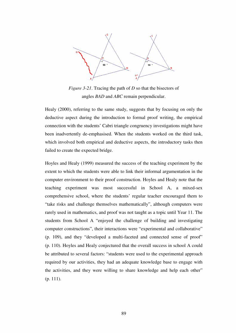
89
Figure 3-21. Tracing the path of D so that the bisectors of
angles BAD and ABC remain perpendicular.
Healy (2000), referring to the same study, suggests that by focusing on only the
deductive aspect during the introduction to formal proof writing, the empirical
connection with the students’ Cabri triangle congruency investigations might have
been inadvertently de-emphasised. When the students worked on the third task,
which involved both empirical and deductive aspects, the introductory tasks then
failed to create the expected bridge.
Hoyles and Healy (1999) measured the success of the teaching experiment by the
extent to which the students were able to link their informal argumentation in the
computer environment to their proof construction. Hoyles and Healy note that the
teaching experiment was most successful in School A, a mixed-sex
comprehensive school, where the students’ regular teacher encouraged them to
“take risks and challenge themselves mathematically”, although computers were
rarely used in mathematics, and proof was not taught as a topic until Year 11. The
students from School A “enjoyed the challenge of building and investigating
computer constructions”, their interactions were “experimental and collaborative”
(p. 109), and they “developed a multi-faceted and connected sense of proof”
(p. 110). Hoyles and Healy conjectured that the overall success in school A could
be attributed to several factors: “students were used to the experimental approach
required by our activities, they had an adequate knowledge base to engage with
the activities, and they were willing to share knowledge and help each other”
(p. 111).
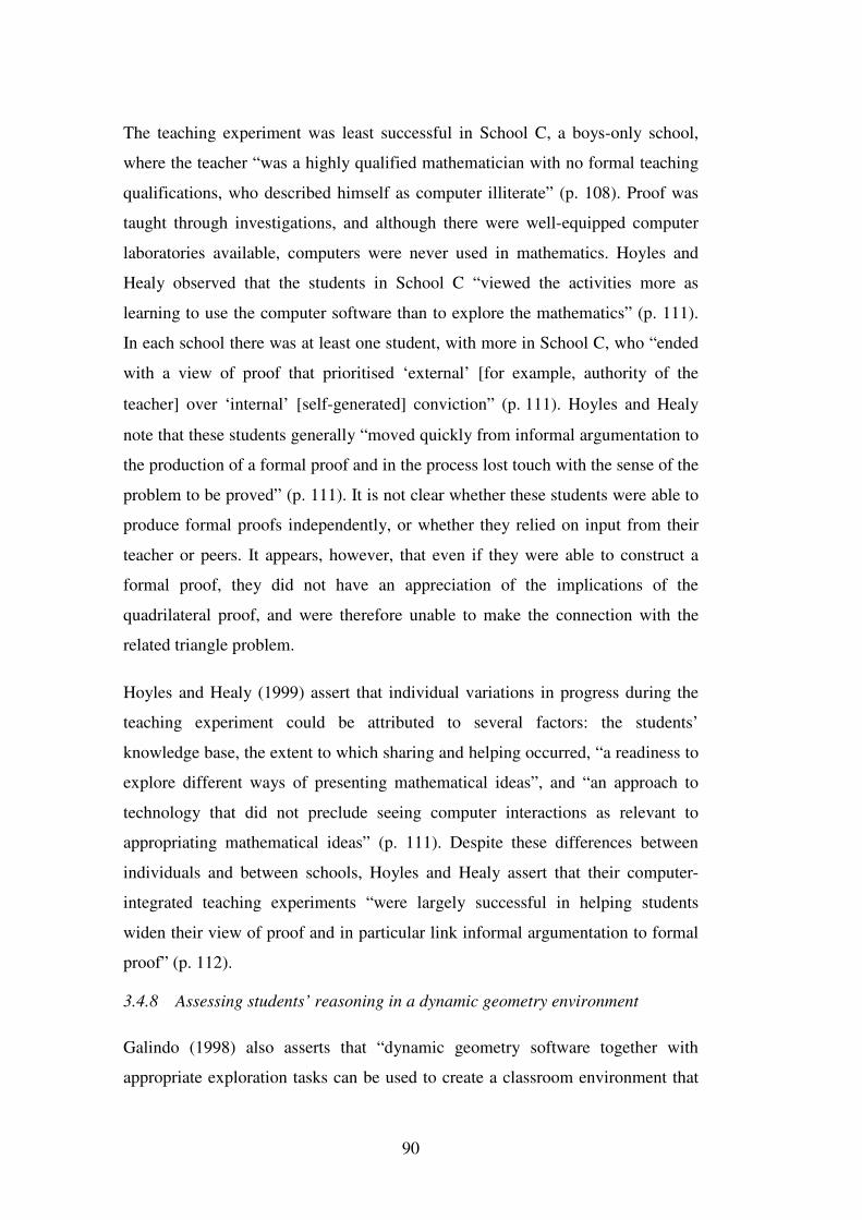
90
The teaching experiment was least successful in School C, a boys-only school,
where the teacher “was a highly qualified mathematician with no formal teaching
qualifications, who described himself as computer illiterate” (p. 108). Proof was
taught through investigations, and although there were well-equipped computer
laboratories available, computers were never used in mathematics. Hoyles and
Healy observed that the students in School C “viewed the activities more as
learning to use the computer software than to explore the mathematics” (p. 111).
In each school there was at least one student, with more in School C, who “ended
with a view of proof that prioritised ‘external’ [for example, authority of the
teacher] over ‘internal’ [self-generated] conviction” (p. 111). Hoyles and Healy
note that these students generally “moved quickly from informal argumentation to
the production of a formal proof and in the process lost touch with the sense of the
problem to be proved” (p. 111). It is not clear whether these students were able to
produce formal proofs independently, or whether they relied on input from their
teacher or peers. It appears, however, that even if they were able to construct a
formal proof, they did not have an appreciation of the implications of the
quadrilateral proof, and were therefore unable to make the connection with the
related triangle problem.
Hoyles and Healy (1999) assert that individual variations in progress during the
teaching experiment could be attributed to several factors: the students’
knowledge base, the extent to which sharing and helping occurred, “a readiness to
explore different ways of presenting mathematical ideas”, and “an approach to
technology that did not preclude seeing computer interactions as relevant to
appropriating mathematical ideas” (p. 111). Despite these differences between
individuals and between schools, Hoyles and Healy assert that their computer-
integrated teaching experiments “were largely successful in helping students
widen their view of proof and in particular link informal argumentation to formal
proof” (p. 112).
3.4.8 Assessing students’ reasoning in a dynamic geometry environment
Galindo (1998) also asserts that “dynamic geometry software together with
appropriate exploration tasks can be used to create a classroom environment that
91
promotes meaningful justification and is conducive to building students’
understanding of proof” (p. 81). Based on his observations that students’
interactions with the software give rise to varying use of empirical and deductive
reasoning, Galindo has developed an assessment model for reasoning in a
dynamic geometry environment. Using the example of high school students’
exploration of the midpoints of all chords that can be drawn from a given point on
a circle, Galindo queries the nature of students’ justifications in a dynamic
geometry environment:
Is the appearance of the computer-generated diagram enough evidence to conclude
that the locus of the chords’ midpoints is a circle? What would be considered an
appropriate answer from a student in a geometry class using such software? More
generally, what can be considered evidence of students’ meaningful justification of
ideas in geometry classes that use dynamic geometry software? (p. 76)
Galindo classifies the responses of the students into four types (see Figure 3-22).
(i) After generating the trace of the midpoints the student concludes that the
locus is a circle.
(ii) After generating the locus and conjecturing that it is a circle, the student
uses the software to construct a circle with diameter AO, comparing it with
the locus.
(iii) Following the tracing of the locus and the conjecture that it is a circle, the
student constructs the segment FE, where F is the midpoint of the radius
AO, and uses the constant length of FE to conclude that the locus is a circle
and that its radius is FE.
(iv) The student constructs and measures segment FE, and the constant length
emphasises the need for proof. Using previous knowledge of circles and
chords, the student uses the fact that ∆AEO is right-angled and constructs
segment GF parallel to EO, then proves that segments AG and EG are equal
and right-angled triangles AGF and EGF are congruent. This congruency is
used to conclude that the length of segment FE is constant and equal to half
the length of segment AO.
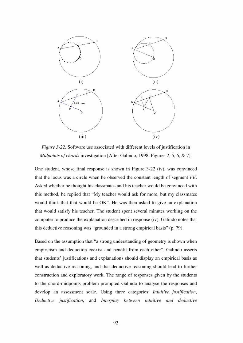
92
(i) (ii)
(iii) (iv)
Figure 3-22. Software use associated with different levels of justification in
Midpoints of chords investigation [After Galindo, 1998, Figures 2, 5, 6, & 7].
One student, whose final response is shown in Figure 3-22 (iv), was convinced
that the locus was a circle when he observed the constant length of segment FE.
Asked whether he thought his classmates and his teacher would be convinced with
this method, he replied that “My teacher would ask for more, but my classmates
would think that that would be OK”. He was then asked to give an explanation
that would satisfy his teacher. The student spent several minutes working on the
computer to produce the explanation described in response (iv). Galindo notes that
this deductive reasoning was “grounded in a strong empirical basis” (p. 79).
Based on the assumption that “a strong understanding of geometry is shown when
empiricism and deduction coexist and benefit from each other”, Galindo asserts
that students’ justifications and explanations should display an empirical basis as
well as deductive reasoning, and that deductive reasoning should lead to further
construction and exploratory work. The range of responses given by the students
to the chord-midpoints problem prompted Galindo to analyse the responses and
develop an assessment scale. Using three categories: Intuitive justification,
Deductive justification, and Interplay between intuitive and deductive
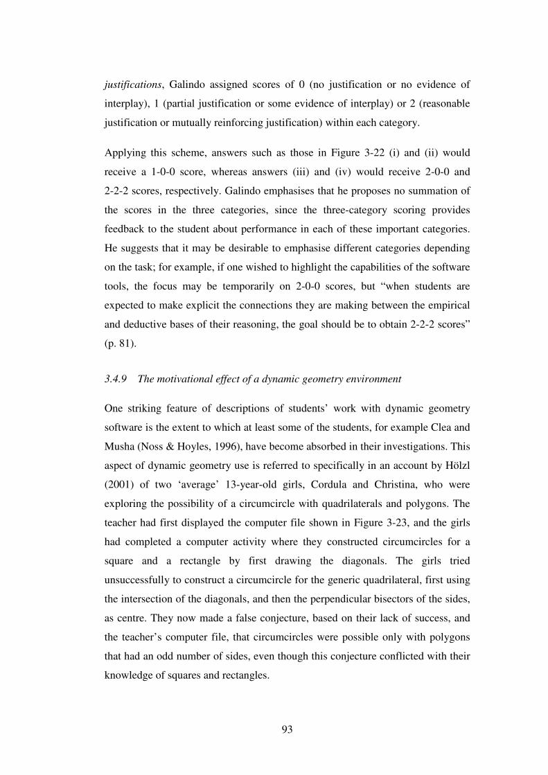
93
justifications, Galindo assigned scores of 0 (no justification or no evidence of
interplay), 1 (partial justification or some evidence of interplay) or 2 (reasonable
justification or mutually reinforcing justification) within each category.
Applying this scheme, answers such as those in Figure 3-22 (i) and (ii) would
receive a 1-0-0 score, whereas answers (iii) and (iv) would receive 2-0-0 and
2-2-2 scores, respectively. Galindo emphasises that he proposes no summation of
the scores in the three categories, since the three-category scoring provides
feedback to the student about performance in each of these important categories.
He suggests that it may be desirable to emphasise different categories depending
on the task; for example, if one wished to highlight the capabilities of the software
tools, the focus may be temporarily on 2-0-0 scores, but “when students are
expected to make explicit the connections they are making between the empirical
and deductive bases of their reasoning, the goal should be to obtain 2-2-2 scores”
(p. 81).
3.4.9 The motivational effect of a dynamic geometry environment
One striking feature of descriptions of students’ work with dynamic geometry
software is the extent to which at least some of the students, for example Clea and
Musha (Noss & Hoyles, 1996), have become absorbed in their investigations. This
aspect of dynamic geometry use is referred to specifically in an account by Hölzl
(2001) of two ‘average’ 13-year-old girls, Cordula and Christina, who were
exploring the possibility of a circumcircle with quadrilaterals and polygons. The
teacher had first displayed the computer file shown in Figure 3-23, and the girls
had completed a computer activity where they constructed circumcircles for a
square and a rectangle by first drawing the diagonals. The girls tried
unsuccessfully to construct a circumcircle for the generic quadrilateral, first using
the intersection of the diagonals, and then the perpendicular bisectors of the sides,
as centre. They now made a false conjecture, based on their lack of success, and
the teacher’s computer file, that circumcircles were possible only with polygons
that had an odd number of sides, even though this conjecture conflicted with their
knowledge of squares and rectangles.
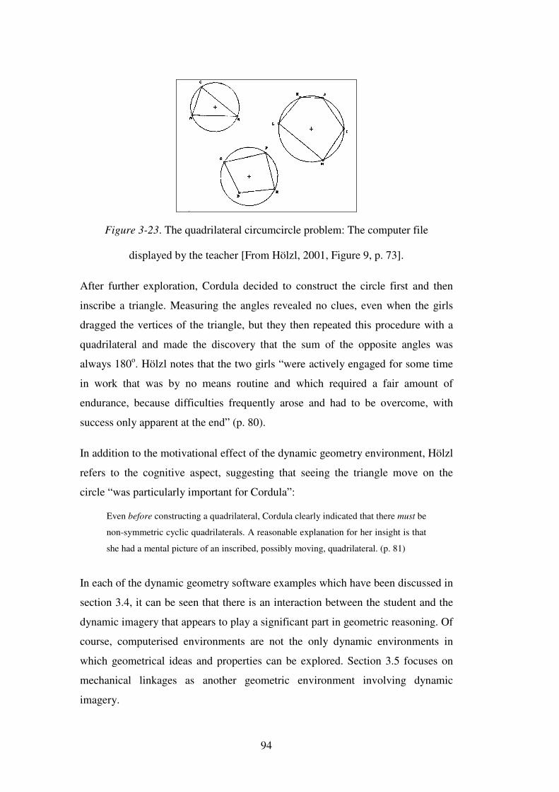
94
Figure 3-23. The quadrilateral circumcircle problem: The computer file
displayed by the teacher [From Hölzl, 2001, Figure 9, p. 73].
After further exploration, Cordula decided to construct the circle first and then
inscribe a triangle. Measuring the angles revealed no clues, even when the girls
dragged the vertices of the triangle, but they then repeated this procedure with a
quadrilateral and made the discovery that the sum of the opposite angles was
always 180o. Hölzl notes that the two girls “were actively engaged for some time
in work that was by no means routine and which required a fair amount of
endurance, because difficulties frequently arose and had to be overcome, with
success only apparent at the end” (p. 80).
In addition to the motivational effect of the dynamic geometry environment, Hölzl
refers to the cognitive aspect, suggesting that seeing the triangle move on the
circle “was particularly important for Cordula”:
Even before constructing a quadrilateral, Cordula clearly indicated that there must be
non-symmetric cyclic quadrilaterals. A reasonable explanation for her insight is that
she had a mental picture of an inscribed, possibly moving, quadrilateral. (p. 81)
In each of the dynamic geometry software examples which have been discussed in
section 3.4, it can be seen that there is an interaction between the student and the
dynamic imagery that appears to play a significant part in geometric reasoning. Of
course, computerised environments are not the only dynamic environments in
which geometrical ideas and properties can be explored. Section 3.5 focuses on
mechanical linkages as another geometric environment involving dynamic
imagery.
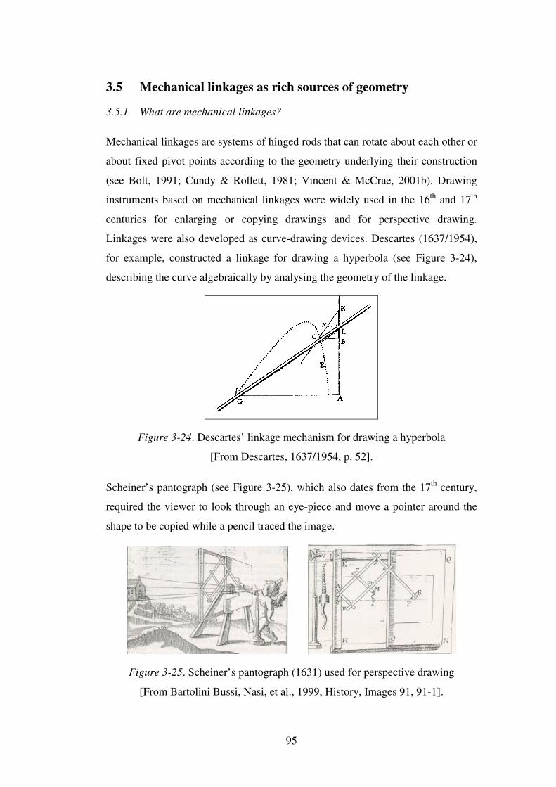
95
3.5 Mechanical linkages as rich sources of geometry
3.5.1 What are mechanical linkages?
Mechanical linkages are systems of hinged rods that can rotate about each other or
about fixed pivot points according to the geometry underlying their construction
(see Bolt, 1991; Cundy & Rollett, 1981; Vincent & McCrae, 2001b). Drawing
instruments based on mechanical linkages were widely used in the 16th and 17th
centuries for enlarging or copying drawings and for perspective drawing.
Linkages were also developed as curve-drawing devices. Descartes (1637/1954),
for example, constructed a linkage for drawing a hyperbola (see Figure 3-24),
describing the curve algebraically by analysing the geometry of the linkage.
Figure 3-24. Descartes’ linkage mechanism for drawing a hyperbola
[From Descartes, 1637/1954, p. 52].
Scheiner’s pantograph (see Figure 3-25), which also dates from the 17th century,
required the viewer to look through an eye-piece and move a pointer around the
shape to be copied while a pencil traced the image.
Figure 3-25. Scheiner’s pantograph (1631) used for perspective drawing
[From Bartolini Bussi, Nasi, et al., 1999, History, Images 91, 91-1].
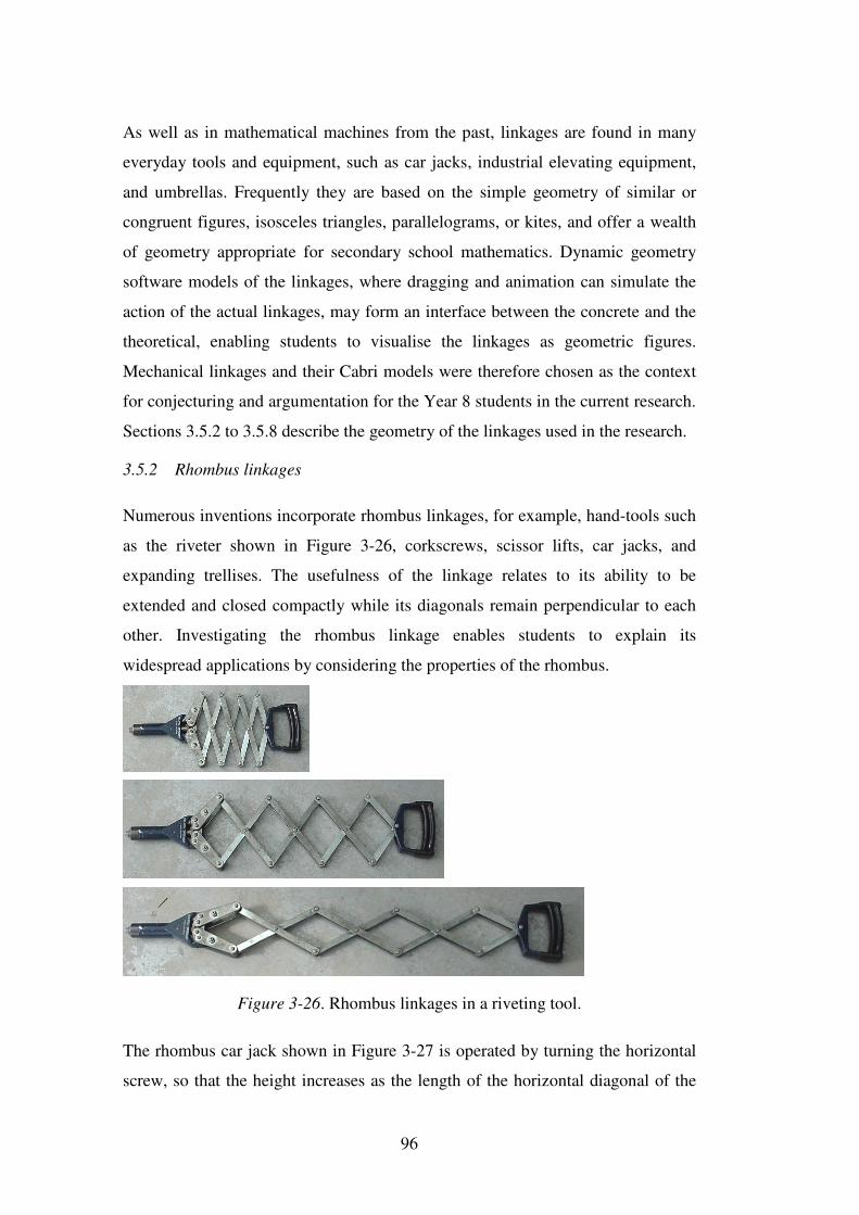
96
As well as in mathematical machines from the past, linkages are found in many
everyday tools and equipment, such as car jacks, industrial elevating equipment,
and umbrellas. Frequently they are based on the simple geometry of similar or
congruent figures, isosceles triangles, parallelograms, or kites, and offer a wealth
of geometry appropriate for secondary school mathematics. Dynamic geometry
software models of the linkages, where dragging and animation can simulate the
action of the actual linkages, may form an interface between the concrete and the
theoretical, enabling students to visualise the linkages as geometric figures.
Mechanical linkages and their Cabri models were therefore chosen as the context
for conjecturing and argumentation for the Year 8 students in the current research.
Sections 3.5.2 to 3.5.8 describe the geometry of the linkages used in the research.
3.5.2 Rhombus linkages
Numerous inventions incorporate rhombus linkages, for example, hand-tools such
as the riveter shown in Figure 3-26, corkscrews, scissor lifts, car jacks, and
expanding trellises. The usefulness of the linkage relates to its ability to be
extended and closed compactly while its diagonals remain perpendicular to each
other. Investigating the rhombus linkage enables students to explain its
widespread applications by considering the properties of the rhombus.
Figure 3-26. Rhombus linkages in a riveting tool.
The rhombus car jack shown in Figure 3-27 is operated by turning the horizontal
screw, so that the height increases as the length of the horizontal diagonal of the
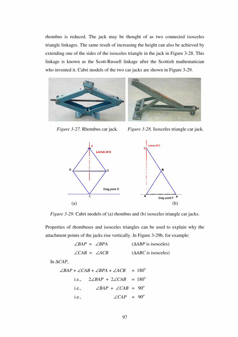
97
rhombus is reduced. The jack may be thought of as two connected isosceles
triangle linkages. The same result of increasing the height can also be achieved by
extending one of the sides of the isosceles triangle in the jack in Figure 3-28. This
linkage is known as the Scott-Russell linkage after the Scottish mathematician
who invented it. Cabri models of the two car jacks are shown in Figure 3-29.
Figure 3-27. Rhombus car jack. Figure 3-28. Isosceles triangle car jack.
(a) (b)
Figure 3-29. Cabri models of (a) rhombus and (b) isosceles triangle car jacks.
Properties of rhombuses and isosceles triangles can be used to explain why the
attachment points of the jacks rise vertically. In Figure 3-29b, for example:
∠BAP = ∠BPA (∆ABP is isosceles)
∠CAB = ∠ACB (∆ABC is isosceles)
In ∆CAP,
∠BAP + ∠CAB + ∠BPA + ∠ACB = 180o
i.e., 2∠BAP + 2∠CAB = 180o
i.e., ∠BAP + ∠CAB = 90o
i.e., ∠CAP = 90o
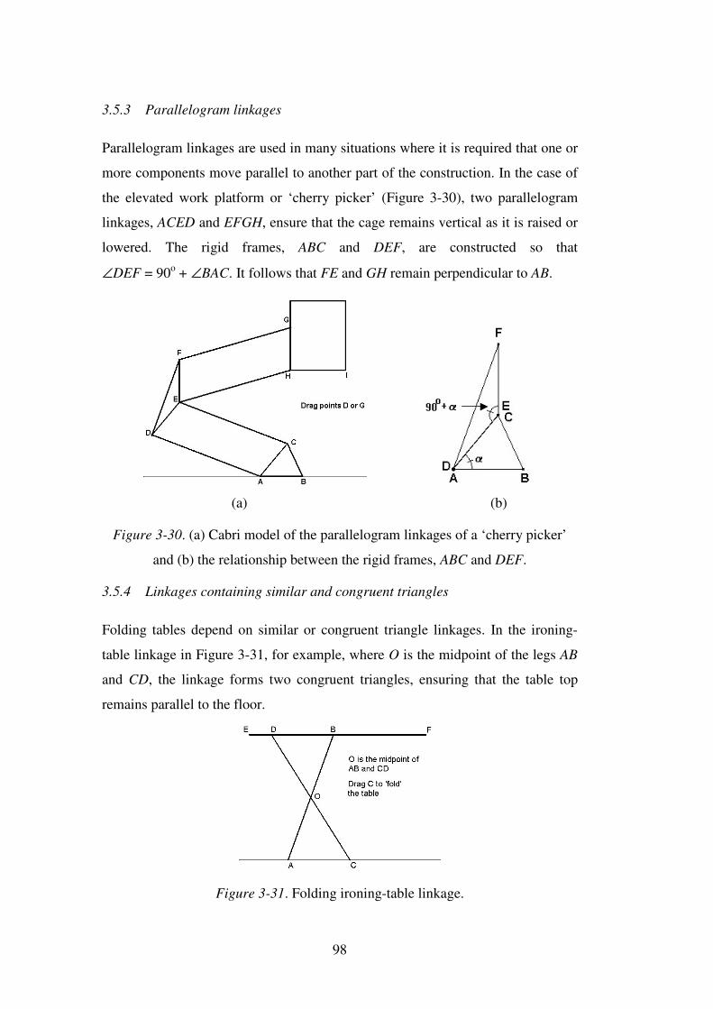
98
3.5.3 Parallelogram linkages
Parallelogram linkages are used in many situations where it is required that one or
more components move parallel to another part of the construction. In the case of
the elevated work platform or ‘cherry picker’ (Figure 3-30), two parallelogram
linkages, ACED and EFGH, ensure that the cage remains vertical as it is raised or
lowered. The rigid frames, ABC and DEF, are constructed so that
∠DEF = 90o + ∠BAC. It follows that FE and GH remain perpendicular to AB.
(a) (b)
Figure 3-30. (a) Cabri model of the parallelogram linkages of a ‘cherry picker’
and (b) the relationship between the rigid frames, ABC and DEF.
3.5.4 Linkages containing similar and congruent triangles
Folding tables depend on similar or congruent triangle linkages. In the ironing-
table linkage in Figure 3-31, for example, where O is the midpoint of the legs AB
and CD, the linkage forms two congruent triangles, ensuring that the table top
remains parallel to the floor.
Figure 3-31. Folding ironing-table linkage.
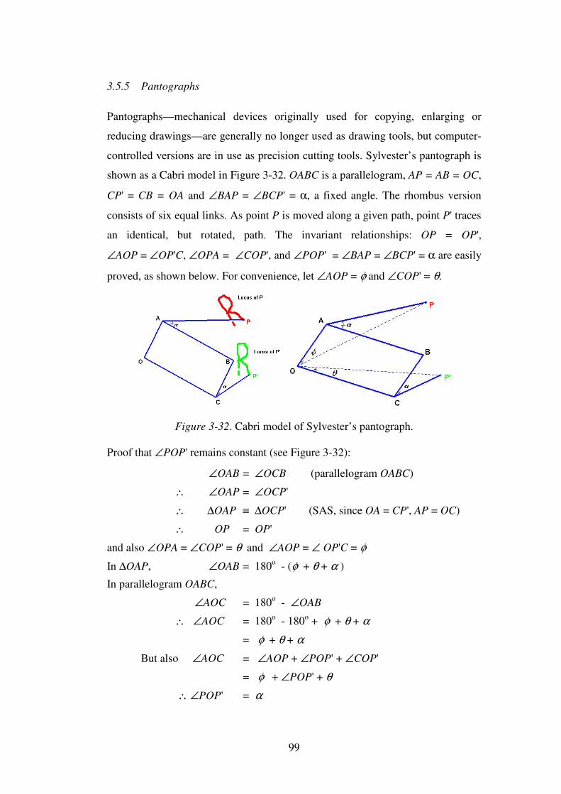
99
3.5.5 Pantographs
Pantographs—mechanical devices originally used for copying, enlarging or
reducing drawings—are generally no longer used as drawing tools, but computer-
controlled versions are in use as precision cutting tools. Sylvester’s pantograph is
shown as a Cabri model in Figure 3-32. OABC is a parallelogram, AP = AB = OC,
CP' = CB = OA and ∠BAP = ∠BCP' = α, a fixed angle. The rhombus version
consists of six equal links. As point P is moved along a given path, point P' traces
an identical, but rotated, path. The invariant relationships: OP = OP',
∠AOP = ∠OP'C, ∠OPA = ∠COP', and ∠POP' = ∠BAP = ∠BCP' = α are easily
proved, as shown below. For convenience, let ∠AOP = φ and ∠COP' = θ.
Figure 3-32. Cabri model of Sylvester’s pantograph.
Proof that ∠POP' remains constant (see Figure 3-32):
∠OAB = ∠OCB (parallelogram OABC)
∴ ∠OAP = ∠OCP'
∴ ∆OAP ≡ ∆OCP' (SAS, since OA = CP', AP = OC)
∴ OP = OP'
and also ∠OPA = ∠COP' = θ and ∠AOP = ∠ OP'C = φ
In ∆OAP, ∠OAB = 180o - (φ + θ + α )
In parallelogram OABC,
∠AOC = 180o - ∠OAB
∴ ∠AOC = 180o - 180o + φ + θ + α
= φ + θ + α
But also ∠AOC = ∠AOP + ∠POP' + ∠COP'
= φ + ∠POP' + θ
∴ ∠POP' = α
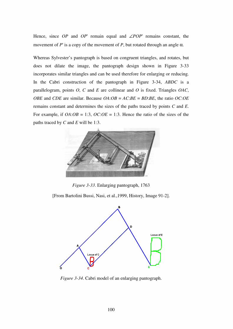
100
Hence, since OP and OP' remain equal and ∠POP' remains constant, the
movement of P' is a copy of the movement of P, but rotated through an angle α.
Whereas Sylvester’s pantograph is based on congruent triangles, and rotates, but
does not dilate the image, the pantograph design shown in Figure 3-33
incorporates similar triangles and can be used therefore for enlarging or reducing.
In the Cabri construction of the pantograph in Figure 3-34, ABDC is a
parallelogram, points O, C and E are collinear and O is fixed. Triangles OAC,
OBE and CDE are similar. Because OA:OB = AC:BE = BD:BE, the ratio OC:OE
remains constant and determines the sizes of the paths traced by points C and E.
For example, if OA:OB = 1:3, OC:OE = 1:3. Hence the ratio of the sizes of the
paths traced by C and E will be 1:3.
Figure 3-33. Enlarging pantograph, 1763
[From Bartolini Bussi, Nasi, et al.,1999, History, Image 91-2].
Figure 3-34. Cabri model of an enlarging pantograph.
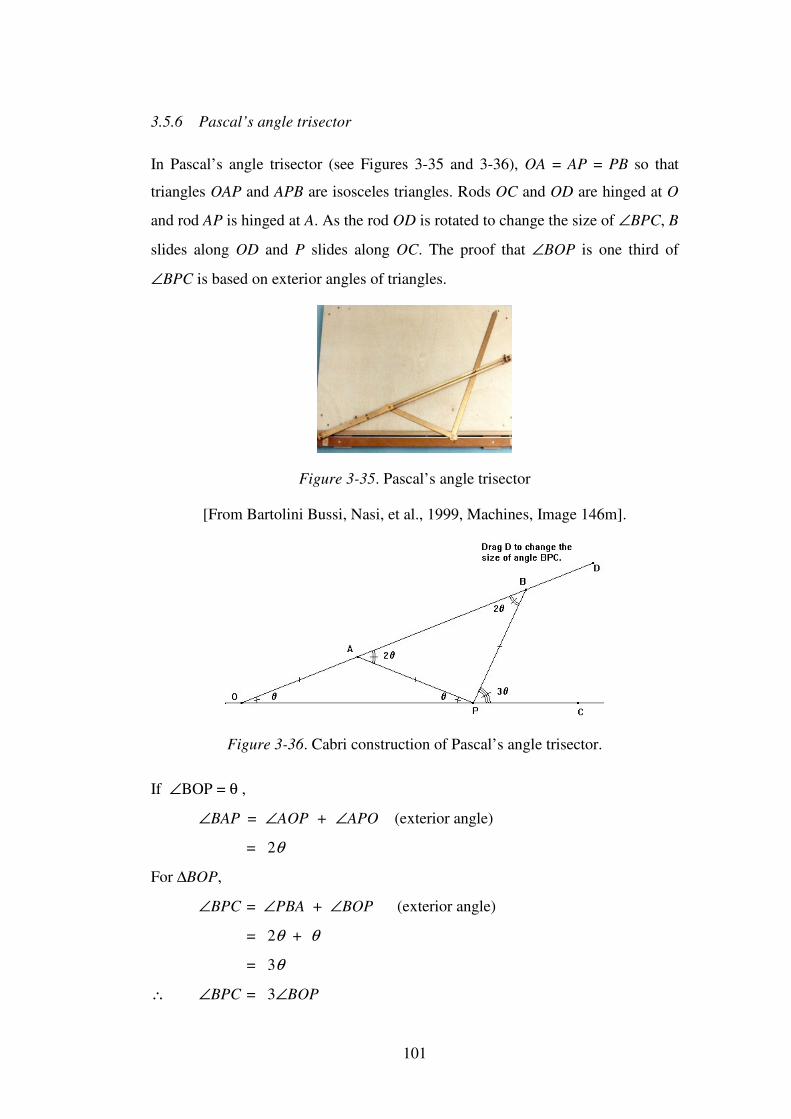
101
3.5.6 Pascal’s angle trisector
In Pascal’s angle trisector (see Figures 3-35 and 3-36), OA = AP = PB so that
triangles OAP and APB are isosceles triangles. Rods OC and OD are hinged at O
and rod AP is hinged at A. As the rod OD is rotated to change the size of ∠BPC, B
slides along OD and P slides along OC. The proof that ∠BOP is one third of
∠BPC is based on exterior angles of triangles.
Figure 3-35. Pascal’s angle trisector
[From Bartolini Bussi, Nasi, et al., 1999, Machines, Image 146m].
Figure 3-36. Cabri construction of Pascal’s angle trisector.
If ∠BOP = θ ,
∠BAP = ∠AOP + ∠APO (exterior angle)
= 2θ
For ∆BOP,
∠BPC = ∠PBA + ∠BOP (exterior angle)
= 2θ + θ
= 3θ
∴ ∠BPC = 3∠BOP
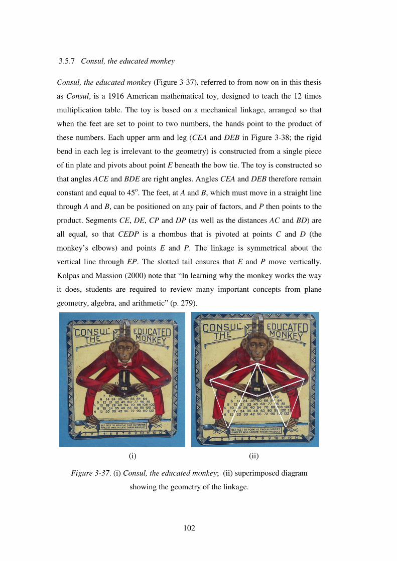
102
3.5.7 Consul, the educated monkey
Consul, the educated monkey (Figure 3-37), referred to from now on in this thesis
as Consul, is a 1916 American mathematical toy, designed to teach the 12 times
multiplication table. The toy is based on a mechanical linkage, arranged so that
when the feet are set to point to two numbers, the hands point to the product of
these numbers. Each upper arm and leg (CEA and DEB in Figure 3-38; the rigid
bend in each leg is irrelevant to the geometry) is constructed from a single piece
of tin plate and pivots about point E beneath the bow tie. The toy is constructed so
that angles ACE and BDE are right angles. Angles CEA and DEB therefore remain
constant and equal to 45o. The feet, at A and B, which must move in a straight line
through A and B, can be positioned on any pair of factors, and P then points to the
product. Segments CE, DE, CP and DP (as well as the distances AC and BD) are
all equal, so that CEDP is a rhombus that is pivoted at points C and D (the
monkey’s elbows) and points E and P. The linkage is symmetrical about the
vertical line through EP. The slotted tail ensures that E and P move vertically.
Kolpas and Massion (2000) note that “In learning why the monkey works the way
it does, students are required to review many important concepts from plane
geometry, algebra, and arithmetic” (p. 279).
(i) (ii)
Figure 3-37. (i) Consul, the educated monkey; (ii) superimposed diagram
showing the geometry of the linkage.
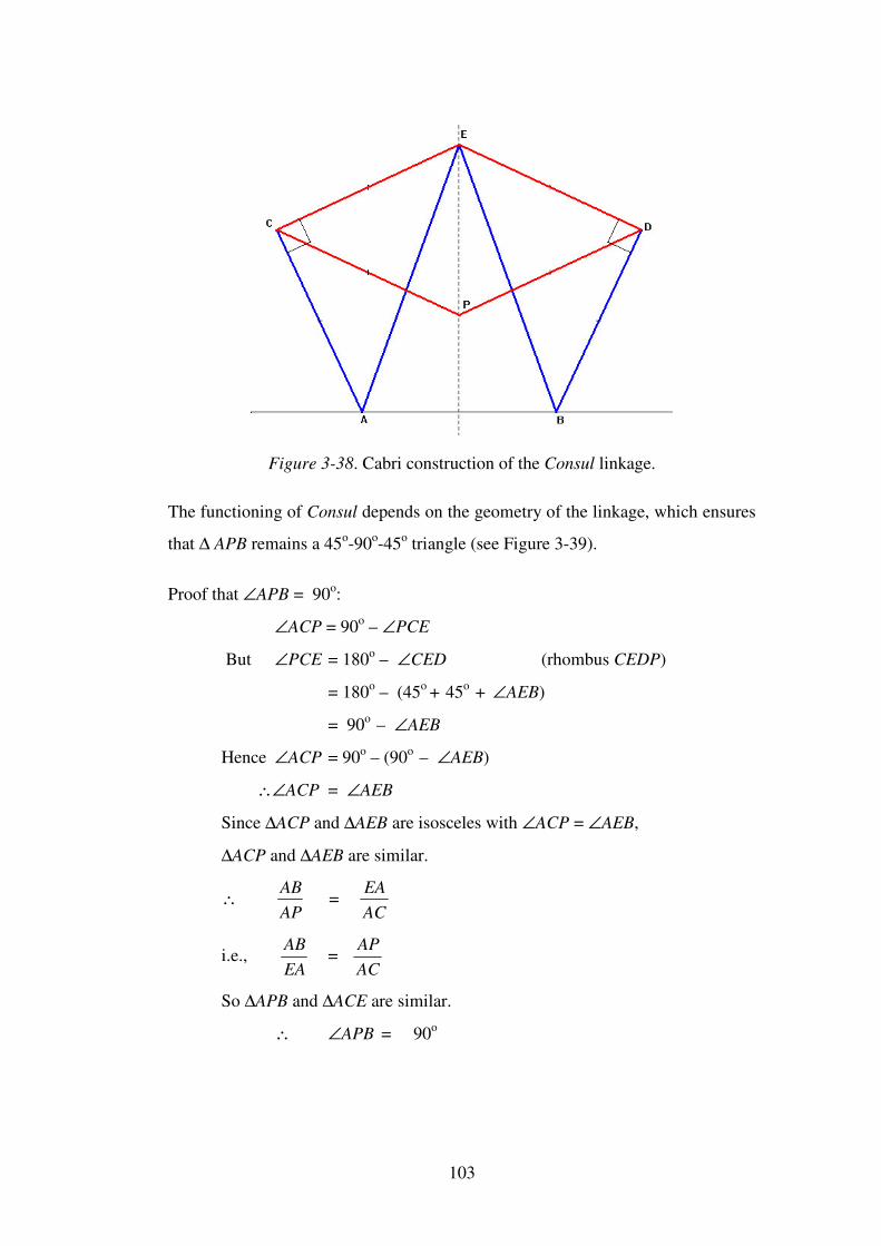
103
Figure 3-38. Cabri construction of the Consul linkage.
The functioning of Consul depends on the geometry of the linkage, which ensures
that ∆ APB remains a 45o-90o-45o triangle (see Figure 3-39).
Proof that ∠APB = 90o:
∠ACP = 90o – ∠PCE
But ∠PCE = 180o – ∠CED (rhombus CEDP)
= 180o – (45o + 45o + ∠AEB)
= 90o – ∠AEB
Hence ∠ACP = 90o – (90o – ∠AEB)
∴∠ACP = ∠AEB
Since ∆ACP and ∆AEB are isosceles with ∠ACP = ∠AEB,
∆ACP and ∆AEB are similar.
∴ APAB
= ACEA
i.e., EAAB
= ACAP
So ∆APB and ∆ACE are similar.
∴ ∠APB = 90o
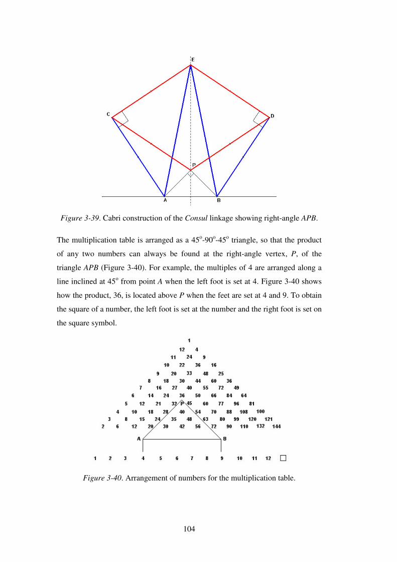
104
Figure 3-39. Cabri construction of the Consul linkage showing right-angle APB.
The multiplication table is arranged as a 45o-90o-45o triangle, so that the product
of any two numbers can always be found at the right-angle vertex, P, of the
triangle APB (Figure 3-40). For example, the multiples of 4 are arranged along a
line inclined at 45o from point A when the left foot is set at 4. Figure 3-40 shows
how the product, 36, is located above P when the feet are set at 4 and 9. To obtain
the square of a number, the left foot is set at the number and the right foot is set on
the square symbol.
Figure 3-40. Arrangement of numbers for the multiplication table.
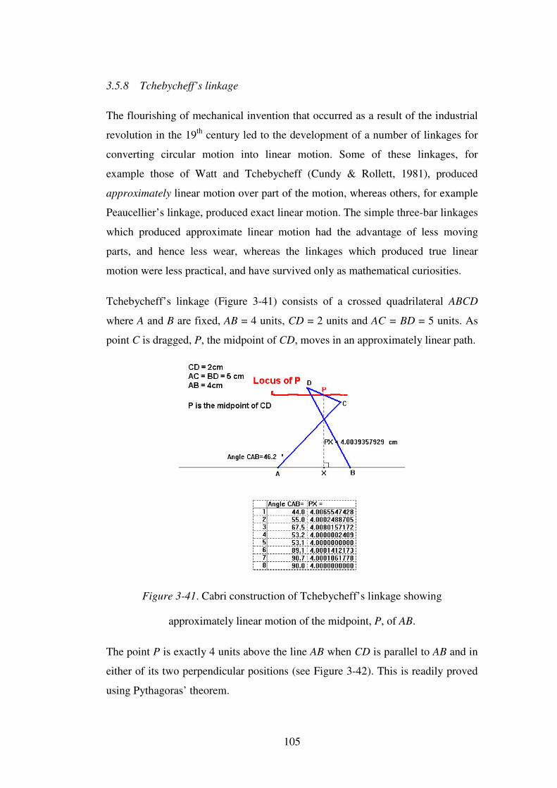
105
3.5.8 Tchebycheff’s linkage
The flourishing of mechanical invention that occurred as a result of the industrial
revolution in the 19th century led to the development of a number of linkages for
converting circular motion into linear motion. Some of these linkages, for
example those of Watt and Tchebycheff (Cundy & Rollett, 1981), produced
approximately linear motion over part of the motion, whereas others, for example
Peaucellier’s linkage, produced exact linear motion. The simple three-bar linkages
which produced approximate linear motion had the advantage of less moving
parts, and hence less wear, whereas the linkages which produced true linear
motion were less practical, and have survived only as mathematical curiosities.
Tchebycheff’s linkage (Figure 3-41) consists of a crossed quadrilateral ABCD
where A and B are fixed, AB = 4 units, CD = 2 units and AC = BD = 5 units. As
point C is dragged, P, the midpoint of CD, moves in an approximately linear path.
Figure 3-41. Cabri construction of Tchebycheff’s linkage showing
approximately linear motion of the midpoint, P, of AB.
The point P is exactly 4 units above the line AB when CD is parallel to AB and in
either of its two perpendicular positions (see Figure 3-42). This is readily proved
using Pythagoras’ theorem.
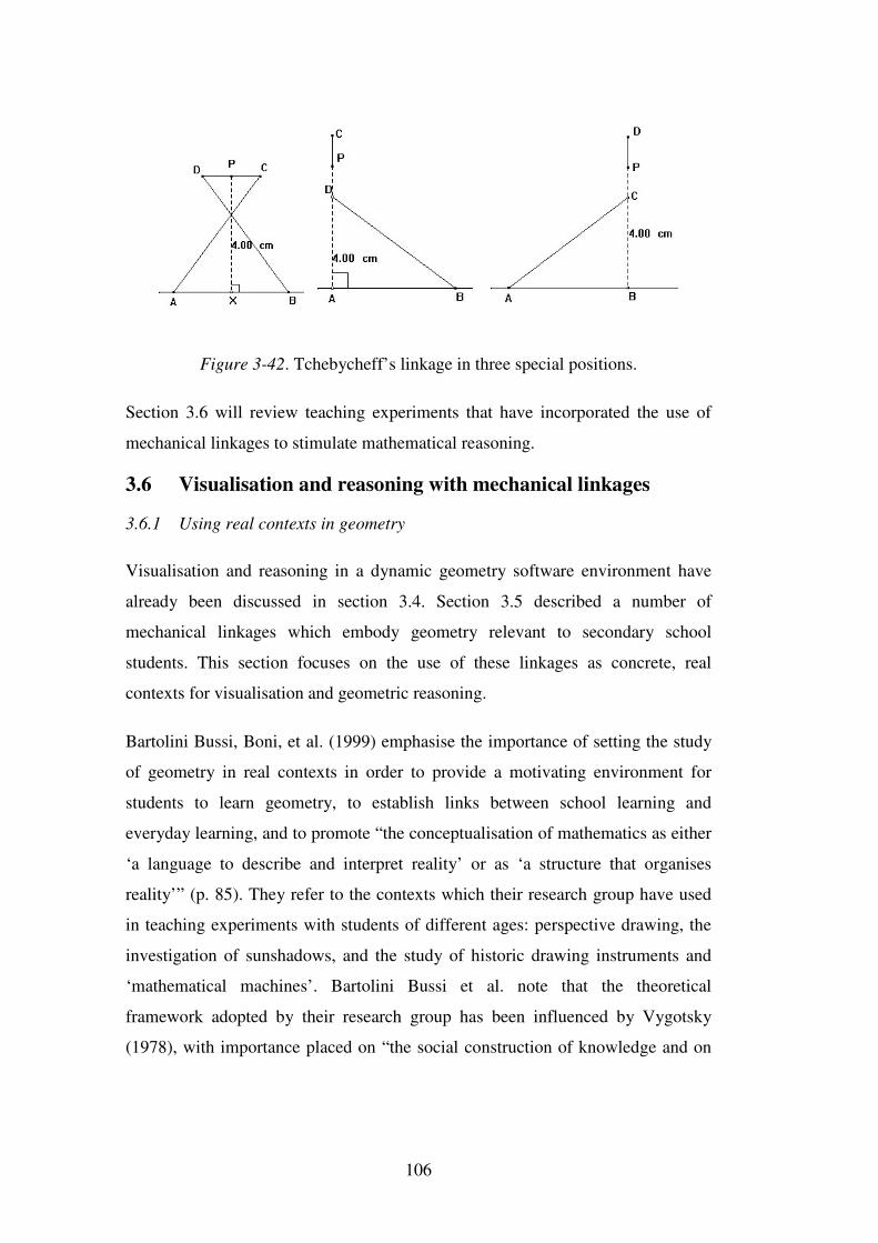
106
Figure 3-42. Tchebycheff’s linkage in three special positions.
Section 3.6 will review teaching experiments that have incorporated the use of
mechanical linkages to stimulate mathematical reasoning.
3.6 Visualisation and reasoning with mechanical linkages
3.6.1 Using real contexts in geometry
Visualisation and reasoning in a dynamic geometry software environment have
already been discussed in section 3.4. Section 3.5 described a number of
mechanical linkages which embody geometry relevant to secondary school
students. This section focuses on the use of these linkages as concrete, real
contexts for visualisation and geometric reasoning.
Bartolini Bussi, Boni, et al. (1999) emphasise the importance of setting the study
of geometry in real contexts in order to provide a motivating environment for
students to learn geometry, to establish links between school learning and
everyday learning, and to promote “the conceptualisation of mathematics as either
‘a language to describe and interpret reality’ or as ‘a structure that organises
reality’” (p. 85). They refer to the contexts which their research group have used
in teaching experiments with students of different ages: perspective drawing, the
investigation of sunshadows, and the study of historic drawing instruments and
‘mathematical machines’. Bartolini Bussi et al. note that the theoretical
framework adopted by their research group has been influenced by Vygotsky
(1978), with importance placed on “the social construction of knowledge and on
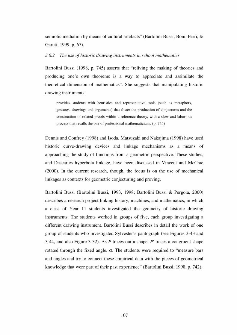
107
semiotic mediation by means of cultural artefacts” (Bartolini Bussi, Boni, Ferri, &
Garuti, 1999, p. 67).
3.6.2 The use of historic drawing instruments in school mathematics
Bartolini Bussi (1998, p. 745) asserts that “reliving the making of theories and
producing one’s own theorems is a way to appreciate and assimilate the
theoretical dimension of mathematics”. She suggests that manipulating historic
drawing instruments
provides students with heuristics and representative tools (such as metaphors,
gestures, drawings and arguments) that foster the production of conjectures and the
construction of related proofs within a reference theory, with a slow and laborious
process that recalls the one of professional mathematicians. (p. 745)
Dennis and Confrey (1998) and Isoda, Matsuzaki and Nakajima (1998) have used
historic curve-drawing devices and linkage mechanisms as a means of
approaching the study of functions from a geometric perspective. These studies,
and Descartes hyperbola linkage, have been discussed in Vincent and McCrae
(2000). In the current research, though, the focus is on the use of mechanical
linkages as contexts for geometric conjecturing and proving.
Bartolini Bussi (Bartolini Bussi, 1993, 1998; Bartolini Bussi & Pergola, 2000)
describes a research project linking history, machines, and mathematics, in which
a class of Year 11 students investigated the geometry of historic drawing
instruments. The students worked in groups of five, each group investigating a
different drawing instrument. Bartolini Bussi describes in detail the work of one
group of students who investigated Sylvester’s pantograph (see Figures 3-43 and
3-44, and also Figure 3-32). As P traces out a shape, P' traces a congruent shape
rotated through the fixed angle, α. The students were required to “measure bars
and angles and try to connect these empirical data with the pieces of geometrical
knowledge that were part of their past experience” (Bartolini Bussi, 1998, p. 742).
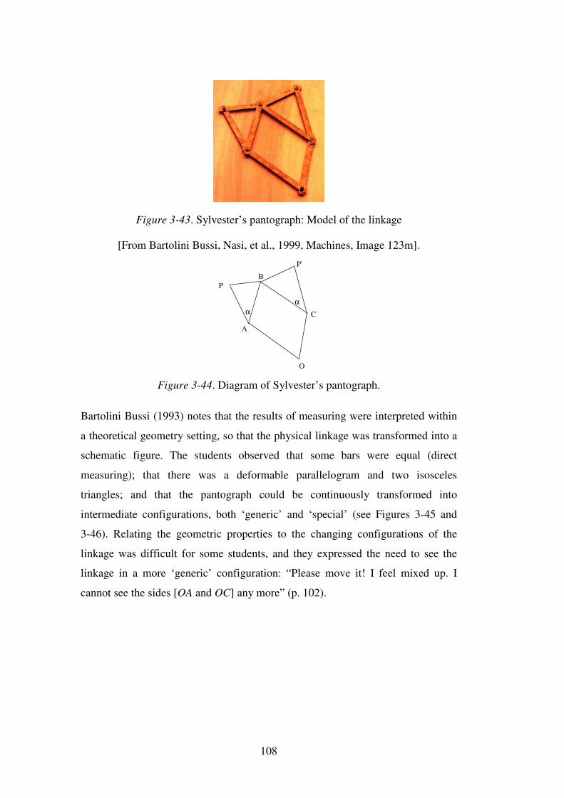
108
Figure 3-43. Sylvester’s pantograph: Model of the linkage
[From Bartolini Bussi, Nasi, et al., 1999, Machines, Image 123m].
O
P
A
B
C
P'
αα
Figure 3-44. Diagram of Sylvester’s pantograph.
Bartolini Bussi (1993) notes that the results of measuring were interpreted within
a theoretical geometry setting, so that the physical linkage was transformed into a
schematic figure. The students observed that some bars were equal (direct
measuring); that there was a deformable parallelogram and two isosceles
triangles; and that the pantograph could be continuously transformed into
intermediate configurations, both ‘generic’ and ‘special’ (see Figures 3-45 and
3-46). Relating the geometric properties to the changing configurations of the
linkage was difficult for some students, and they expressed the need to see the
linkage in a more ‘generic’ configuration: “Please move it! I feel mixed up. I
cannot see the sides [OA and OC] any more” (p. 102).
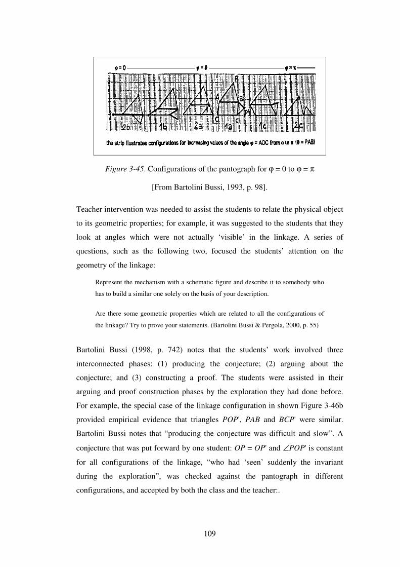
109
Figure 3-45. Configurations of the pantograph for ϕ = 0 to ϕ = π
[From Bartolini Bussi, 1993, p. 98].
Teacher intervention was needed to assist the students to relate the physical object
to its geometric properties; for example, it was suggested to the students that they
look at angles which were not actually ‘visible’ in the linkage. A series of
questions, such as the following two, focused the students’ attention on the
geometry of the linkage:
Represent the mechanism with a schematic figure and describe it to somebody who
has to build a similar one solely on the basis of your description.
Are there some geometric properties which are related to all the configurations of
the linkage? Try to prove your statements. (Bartolini Bussi & Pergola, 2000, p. 55)
Bartolini Bussi (1998, p. 742) notes that the students’ work involved three
interconnected phases: (1) producing the conjecture; (2) arguing about the
conjecture; and (3) constructing a proof. The students were assisted in their
arguing and proof construction phases by the exploration they had done before.
For example, the special case of the linkage configuration in shown Figure 3-46b
provided empirical evidence that triangles POP', PAB and BCP' were similar.
Bartolini Bussi notes that “producing the conjecture was difficult and slow”. A
conjecture that was put forward by one student: OP = OP' and ∠POP' is constant
for all configurations of the linkage, “who had ‘seen’ suddenly the invariant
during the exploration”, was checked against the pantograph in different
configurations, and accepted by both the class and the teacher:.
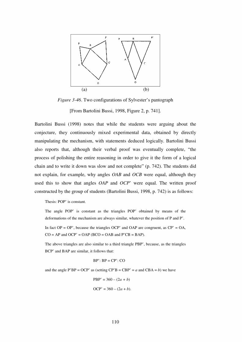
110
(a) (b)
Figure 3-46. Two configurations of Sylvester’s pantograph
[From Bartolini Bussi, 1998, Figure 2, p. 741].
Bartolini Bussi (1998) notes that while the students were arguing about the
conjecture, they continuously mixed experimental data, obtained by directly
manipulating the mechanism, with statements deduced logically. Bartolini Bussi
also reports that, although their verbal proof was eventually complete, “the
process of polishing the entire reasoning in order to give it the form of a logical
chain and to write it down was slow and not complete” (p. 742). The students did
not explain, for example, why angles OAB and OCB were equal, although they
used this to show that angles OAP and OCP’ were equal. The written proof
constructed by the group of students (Bartolini Bussi, 1998, p. 742) is as follows:
Thesis: POP’ is constant.
The angle POP’ is constant as the triangles POP’ obtained by means of the
deformations of the mechanism are always similar, whatever the position of P and P’.
In fact OP = OP’, because the triangles OCP’ and OAP are congruent, as CP’ = OA,
CO = AP and OCP’ = OAP (BCO = OAB and P’CB = BAP).
The above triangles are also similar to a third triangle PBP’, because, as the triangles
BCP’ and BAP are similar, it follows that:
BP’: BP = CP’: CO
and the angle P’BP = OCP’ as (setting CP’B = CBP’ = a and CBA = b) we have
PBP’ = 360 – (2a + b)
OCP’ = 360 – (2a + b).
111
This is true because prolonging the line BC from the side of C the angle
supplementary to BCP’ is equal to 2a and the angle supplementary to BCO is equal to
b as two contiguous angles of a parallelogram are always supplementary.
Significantly, even though the students’ written proof was incomplete and not in a
logical sequence, when they refined it with the teacher’s help, it still remained
meaningful for them:
The order of the steps recalls the sequence of production of statements, as observed
during the small group work, rather than the logical chain that could have been used
by an expert. Nevertheless it was easily transformed later with the teacher’s help
into the accepted format with reference to elementary �uclidean geometry; yet,
what is important, the time given to laboriously produce their own proof ensured
that the final product in the mathematician’s style, where the genesis of the proof
was eventually hidden, retained meaning for the students. (Bartolini Bussi, 1998,
p. 743)
Bartolini Bussi and Pergola (2000) note that
the linkage itself created the need to be understood, and, even in the presence of the
teacher, the students doubted his statements when they were not self-evident for
them and tested them on the linkage. (p. 61)
Bartolini Bussi (1993) contrasts the classroom experiment, where physical models
of the drawing instruments were used, with a computer environment. She notes
that, although in both there is an interaction between verbal-logical and visual-
image activity, there is an absence of visual-tactile activity in the computer
environment. Bartolini Bussi (2000) notes that concrete approaches are often
viewed unfavourably in more advanced school mathematics because “the risk is
always that the attention is captured by isolated facts and that the argument, if
any, is not detached from everyday styles of reasoning” (p. 26). She asserts,
however, “that material activity is supposed to be fundamental also in the work of
professional mathematicians” (p. 26). Despite her reservations about computer
models, Bartolini Bussi refers to the development of ‘virtual linkworks’, using
both Cabri and Java, as part of the research project linking history, machines and
mathematics. She also cites Gao, Zhu, and Huang (1998) who produced linkage
112
models with their own software Geometry Expert, and who claim that computer
models are “more powerful, flexible, convenient, and intuitive than models built
of real materials like plastics and wood” (Bartolini Bussi, 2000, p. 32).
Bartolini Bussi (2000) asserts that a careful classroom study is needed to analyse
the relative advantages and disadvantages of physical and virtual models, and
notes that even different virtual models may have significant differences. She
compares the Cabri and Java models and suggests, for example, that the more
flexible control offered by the Cabri linkages and “the possibility of realising
infinitely many experiments with a sole gesture of dragging might ‘kill’ the need
of constructing proofs of the produced conjectures” (p. 32). Scher (1999, p. 24),
on the other hand, who uses the example of a Geometer’s Sketchpad model of
Sylvester’s pantograph, suggests that “the constant interplay between deductive
reasoning and software-supported experimentation” can contribute to the
conjecturing and proving processes, providing “not only data to feed a conjecture,
but tools to jump-start ideas and feed a proof”.
3.6.3 Computer modelling of mechanical linkages
Vivet (1996) refers to a study in which 11−14-year-old pupils used Logo and
Fischer-Technik toys to model robots and mechanical devices. He suggests that
computer-modelling of robots can be used as a source of motivation for geometry
and “can lead to the necessity of proving properties in the geometrical
descriptions of a given robot. … The need for proofs in geometry can be shown in
very motivating environments based upon trucks, cranes, arms” (p. 231). Vivet
notes that “the very impressive motivation shown by the pupils when working
with these tools is an encouragement to do more” (p. 237).
Steeg, Wake, and Williams (1993) used dynamic geometry software to model
mechanical linkages with a group of Year 10 students in a cross-curriculum study
of linkages in technology and mathematics. They suggest that dynamic geometry
software may fill a need for a design tool for exploration of linkages in
technology, although they acknowledge that there are certain problems associated
with the use of the software for this purpose. The students were introduced to The
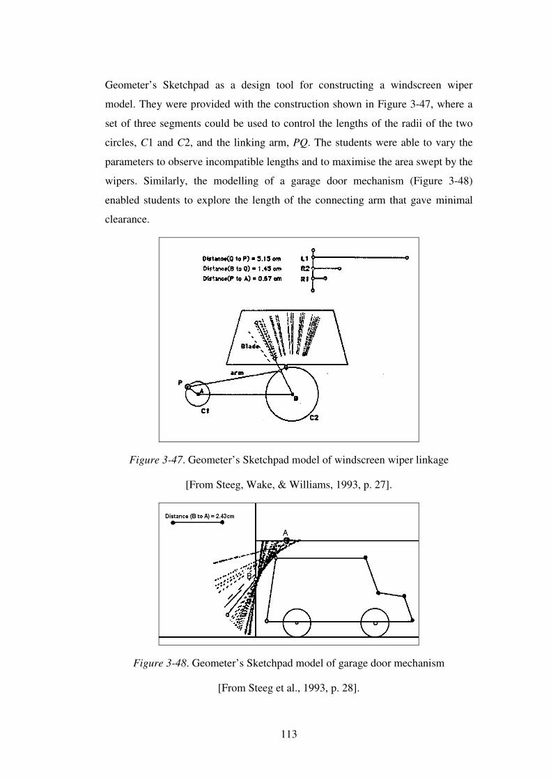
113
Geometer’s Sketchpad as a design tool for constructing a windscreen wiper
model. They were provided with the construction shown in Figure 3-47, where a
set of three segments could be used to control the lengths of the radii of the two
circles, C1 and C2, and the linking arm, PQ. The students were able to vary the
parameters to observe incompatible lengths and to maximise the area swept by the
wipers. Similarly, the modelling of a garage door mechanism (Figure 3-48)
enabled students to explore the length of the connecting arm that gave minimal
clearance.
Figure 3-47. Geometer’s Sketchpad model of windscreen wiper linkage
[From Steeg, Wake, & Williams, 1993, p. 27].
Figure 3-48. Geometer’s Sketchpad model of garage door mechanism
[From Steeg et al., 1993, p. 28].
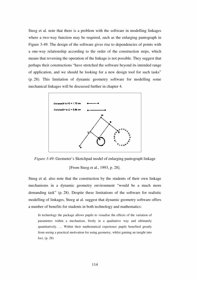
114
Steeg et al. note that there is a problem with the software in modelling linkages
where a two-way function may be required, such as the enlarging pantograph in
Figure 3-49. The design of the software gives rise to dependencies of points with
a one-way relationship according to the order of the construction steps, which
means that reversing the operation of the linkage is not possible. They suggest that
perhaps their constructions “have stretched the software beyond its intended range
of application, and we should be looking for a new design tool for such tasks”
(p. 28). This limitation of dynamic geometry software for modelling some
mechanical linkages will be discussed further in chapter 4.
Figure 3-49. Geometer’s Sketchpad model of enlarging pantograph linkage
[From Steeg et al., 1993, p. 28].
Steeg et al. also note that the construction by the students of their own linkage
mechanisms in a dynamic geometry environment “would be a much more
demanding task” (p. 28). Despite these limitations of the software for realistic
modelling of linkages, Steeg at al. suggest that dynamic geometry software offers
a number of benefits for students in both technology and mathematics:
In technology the package allows pupils to visualise the effects of the variation of
parameters within a mechanism, firstly in a qualitative way and ultimately
quantitatively. … Within their mathematical experience pupils benefited greatly
from seeing a practical motivation for using geometry, whilst gaining an insight into
loci. (p. 28)
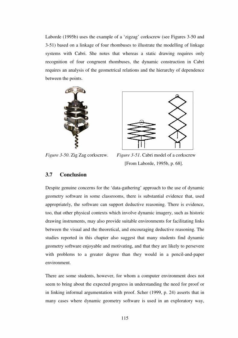
115
Laborde (1995b) uses the example of a ‘zigzag’ corkscrew (see Figures 3-50 and
3-51) based on a linkage of four rhombuses to illustrate the modelling of linkage
systems with Cabri. She notes that whereas a static drawing requires only
recognition of four congruent rhombuses, the dynamic construction in Cabri
requires an analysis of the geometrical relations and the hierarchy of dependence
between the points.
Figure 3-50. Zig Zag corkscrew. Figure 3-51. Cabri model of a corkscrew
[From Laborde, 1995b, p. 68].
3.7 Conclusion
Despite genuine concerns for the ‘data-gathering’ approach to the use of dynamic
geometry software in some classrooms, there is substantial evidence that, used
appropriately, the software can support deductive reasoning. There is evidence,
too, that other physical contexts which involve dynamic imagery, such as historic
drawing instruments, may also provide suitable environments for facilitating links
between the visual and the theoretical, and encouraging deductive reasoning. The
studies reported in this chapter also suggest that many students find dynamic
geometry software enjoyable and motivating, and that they are likely to persevere
with problems to a greater degree than they would in a pencil-and-paper
environment.
There are some students, however, for whom a computer environment does not
seem to bring about the expected progress in understanding the need for proof or
in linking informal argumentation with proof. Scher (1999, p. 24) asserts that in
many cases where dynamic geometry software is used in an exploratory way,
116
“having used the software to convince themselves of a theorem’s plausibility,
mathematics classes turn to the traditional pencil-and-paper medium to ponder a
proof. In the process, they create a boundary between the computer and deductive
reasoning”.
The success of these dynamic environments may depend, then, on the design of
tasks that encourage students to engage in a process of argumentation, during
which they can explore, produce their own conjectures, test their ideas, and
develop and refine their arguments to the point where they can construct a
reasoned proof. Chapter 4 describes the research design for the current study,
where the rich visual environments of dynamic geometry software and mechanical
linkages are combined to create a context for conjecturing, argumentation, and
proving.
117
Chapter 4: Methodology
There are ways in which learning tasks can be structured in order to increase the
likelihood that students will experience interest. Coming face-to-face with
information which challenges the known categories, being surprised by a novel
perspective, having the opportunity to investigate the points of uncertainty, to
examine a surprising event, allow these interest processes to support change in the
learner’s knowledge and understanding. (Ainley, 2001, p. 129)
Section 4.2 Introduction
As chapter 2 has shown, students may experience difficulty with proof in
mathematics for a variety of reasons, which may include a failure to see the need
for proof, a lack of understanding of proof as a process, or, in the case of
geometric proof, an inability to relate geometric diagrams to theoretical geometry.
There is evidence (see sections 2.6, 3.4.7, and 3.6.2), however, that active
participation in argumentation and conjecturing leads to greater success in the
proving process, provided the teacher mediates to set the students’ argumentation
within a framework of geometric theory. Chapter 3 has shown that dynamic
geometry software has the potential to aid students’ geometric reasoning, and that
mechanical linkages represent a rich source of relevant geometry. In designing the
teaching experiment in which Year 8 students were introduced to deductive
reasoning and geometric proof, these issues have been taken into account.
Section 4.2 locates the current study in the relevant theoretical framework
presented in chapters 2 and 3, and presents the research questions. Section 4.3
discusses the pilot study for the current research. Section 4.4 describes the
research design, including the rationale for the tests used, and section 4.5 outlines
the approach to data analysis. Section 4.6 provides an overview of the
methodology, with a summary of the data sources and the research questions
which they address.
118
4.2 The current study
4.2.1 The research questions
The research sought answers to the following questions in the context of a Year 8
mathematics classroom:
1. Can a culture of geometric proving be established in a Year 8 mathematics
classroom in the context of mechanical linkages and dynamic geometry
software?
2. Are Year 8 students motivated to engage in argumentation, conjecturing,
and deductive reasoning in the context of mechanical linkages and
dynamic geometry software?
3. Does the static and dynamic feedback provided by mechanical linkages
and dynamic geometry software support Year 8 students’ cognitive
engagement in argumentation, conjecturing, and deductive reasoning?
4. Do the processes of argumentation and conjecturing contribute to
successful constructions of proofs?
5. Does the empirical feedback provided by dynamic geometry software
satisfy Year 8 students’ need for convincing?
6. Are the students’ abilities to make conjectures and to construct deductive
proofs related to their measured van Hiele levels?
4.2.2 The context of mechanical linkages and dynamic geometry software
Important considerations are the establishment of a need for proof (see section
2.5.2); provision of a motivating and meaningful context that is conducive to
argumentation and conjecturing (see section 2.3); rich visual imagery, both static
and dynamic (see section 3.4.7); and geometry appropriate for this level (see
section 3.5). My choice of mechanical linkages and dynamic geometry software
(Cabri Geometry II) as potentially favourable contexts was determined by these
considerations. In the conjecturing environment of mechanical linkages, where
students can make visual judgements about the action of a linkage, it might be
expected that proof would assume the multiple roles of verification, for example,
119
that apparent invariants are in fact invariant; understanding of geometric
relationships; and explanation, that is, giving an insight into why the linkage
works the way it does.
The simple geometry of many mechanical linkages—for example, similar and
congruent triangles, isosceles triangles, parallelograms, or kites—is particularly
suitable for Year 8 students. Physical models of the linkages provide a tactile, as
well as visual, medium for geometric exploration, which I anticipated would be
motivational for students at Year 8 level. Pre-constructed dynamic geometry
software models of the linkages, while lacking the tactile dimension of the
physical models, offer the possibility of accurate measurement, the tracing of loci,
addition of construction lines, and instant feedback when the construction is
dragged. They would be expected, therefore, to form a bridge between the
concrete and the theoretical, enabling students to visualise the linkages as
theoretical geometric figures.
4.2.3 Establishing a need for proof
To establish a need for proof I proposed to create a situation where visual
evidence would mislead students into a false conjecture. Mechanical linkages
designed to produce approximate linear motion, such as that of Tchebycheff (see
section 3.5.8), came to mind. Tchebycheff’s linkage seemed particularly
appropriate for my purpose, as it is simple to construct from geostrips (see Figure
4-11d), the visual evidence of apparent linear motion is readily obtainable with the
geostrip linkage, and the Cabri model of the linkage demonstrates clearly that the
motion is an extraordinarily good approximation of linear motion (see Figure 4-8).
The linkage also has the advantage that students can determine precise positions
on the approximately linear locus by applying Pythagoras’ theorem to three
special positions of the linkage. The use of Tchebycheff’s linkage, where visual
evidence conflicted with the more precise, although still empirical, feedback from
Cabri, was designed therefore to sow a seed of doubt in the students’ minds so
that they could never be sure whether visual evidence was to be trusted.
120
There remained, however, the question of whether the students might still regard
Cabri evidence as proof. A pencil-and-paper proof task—that the sum of the
angles of any triangle is 180o (see Appendix 4, A4.4.3)—was therefore
deliberately set in a Cabri context to develop the notion that although Cabri
measurements can be extremely convincing, they are simply more accurate
versions of those obtained using traditional tools (this of course ignores the
question of whether the design of the software means that it uses the property to
be proved in the computation of measurements).
4.3 Pilot study
4.3.1 Purpose of the pilot study
A small pilot study was conducted in 2000 with a mathematics class of above-
average Year 8 girls at the same school as the participants in the current research
(Vincent & McCrae, 2000; Vincent & McCrae, 2001a). The main purposes of this
pilot study were to investigate the students’ understanding of the nature of
mathematical proof, and to assess the suitability of mechanical linkages and their
dynamic geometry software models as contexts for conjecturing and proving. It
was important in terms of the current research to know whether a need for proof
could be established with Year 8 students. In particular, would the linkages
provoke argumentation and conjecturing, and would feedback from operating the
linkages and their Cabri models support deductive reasoning? The pilot study
focused in particular on the following questions:
1. What does mathematical proof mean to Year 8 students?
2. Do students at Year 8 level accurately observe geometric properties of
the linkages?
3. Do they recognise a need for geometric proof?
4. Are students at this age able to construct their own arguments based on
simple steps of deductive reasoning?
4.3.2 Students’ understanding of mathematical proof
In response to the preliminary question “What is proof in mathematics for?”, 16 of
the 29 students in the pilot study class were able to articulate at least one aspect of
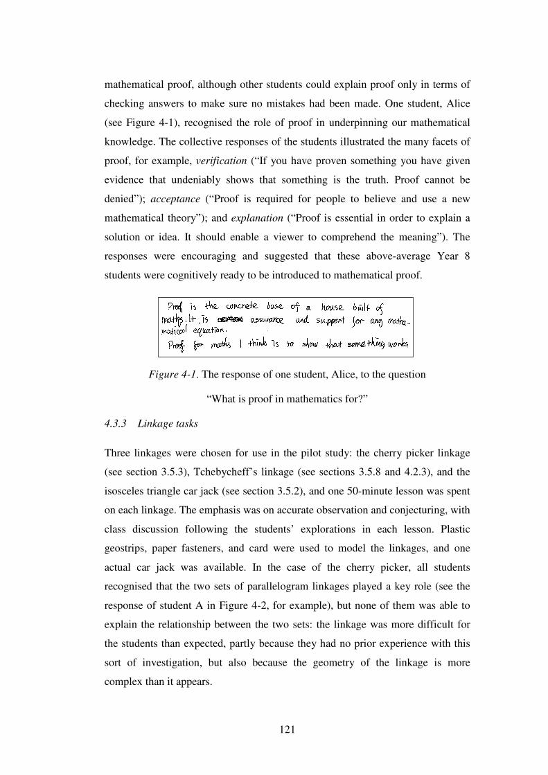
121
mathematical proof, although other students could explain proof only in terms of
checking answers to make sure no mistakes had been made. One student, Alice
(see Figure 4-1), recognised the role of proof in underpinning our mathematical
knowledge. The collective responses of the students illustrated the many facets of
proof, for example, verification (“If you have proven something you have given
evidence that undeniably shows that something is the truth. Proof cannot be
denied”); acceptance (“Proof is required for people to believe and use a new
mathematical theory”); and explanation (“Proof is essential in order to explain a
solution or idea. It should enable a viewer to comprehend the meaning”). The
responses were encouraging and suggested that these above-average Year 8
students were cognitively ready to be introduced to mathematical proof.
Figure 4-1. The response of one student, Alice, to the question
“What is proof in mathematics for?”
4.3.3 Linkage tasks
Three linkages were chosen for use in the pilot study: the cherry picker linkage
(see section 3.5.3), Tchebycheff’s linkage (see sections 3.5.8 and 4.2.3), and the
isosceles triangle car jack (see section 3.5.2), and one 50-minute lesson was spent
on each linkage. The emphasis was on accurate observation and conjecturing, with
class discussion following the students’ explorations in each lesson. Plastic
geostrips, paper fasteners, and card were used to model the linkages, and one
actual car jack was available. In the case of the cherry picker, all students
recognised that the two sets of parallelogram linkages played a key role (see the
response of student A in Figure 4-2, for example), but none of them was able to
explain the relationship between the two sets: the linkage was more difficult for
the students than expected, partly because they had no prior experience with this
sort of investigation, but also because the geometry of the linkage is more
complex than it appears.
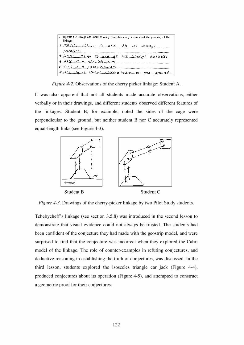
122
Figure 4-2. Observations of the cherry picker linkage: Student A.
It was also apparent that not all students made accurate observations, either
verbally or in their drawings, and different students observed different features of
the linkages. Student B, for example, noted the sides of the cage were
perpendicular to the ground, but neither student B nor C accurately represented
equal-length links (see Figure 4-3).
Student B Student C
Figure 4-3. Drawings of the cherry-picker linkage by two Pilot Study students.
Tchebycheff’s linkage (see section 3.5.8) was introduced in the second lesson to
demonstrate that visual evidence could not always be trusted. The students had
been confident of the conjecture they had made with the geostrip model, and were
surprised to find that the conjecture was incorrect when they explored the Cabri
model of the linkage. The role of counter-examples in refuting conjectures, and
deductive reasoning in establishing the truth of conjectures, was discussed. In the
third lesson, students explored the isosceles triangle car jack (Figure 4-4),
produced conjectures about its operation (Figure 4-5), and attempted to construct
a geometric proof for their conjectures.
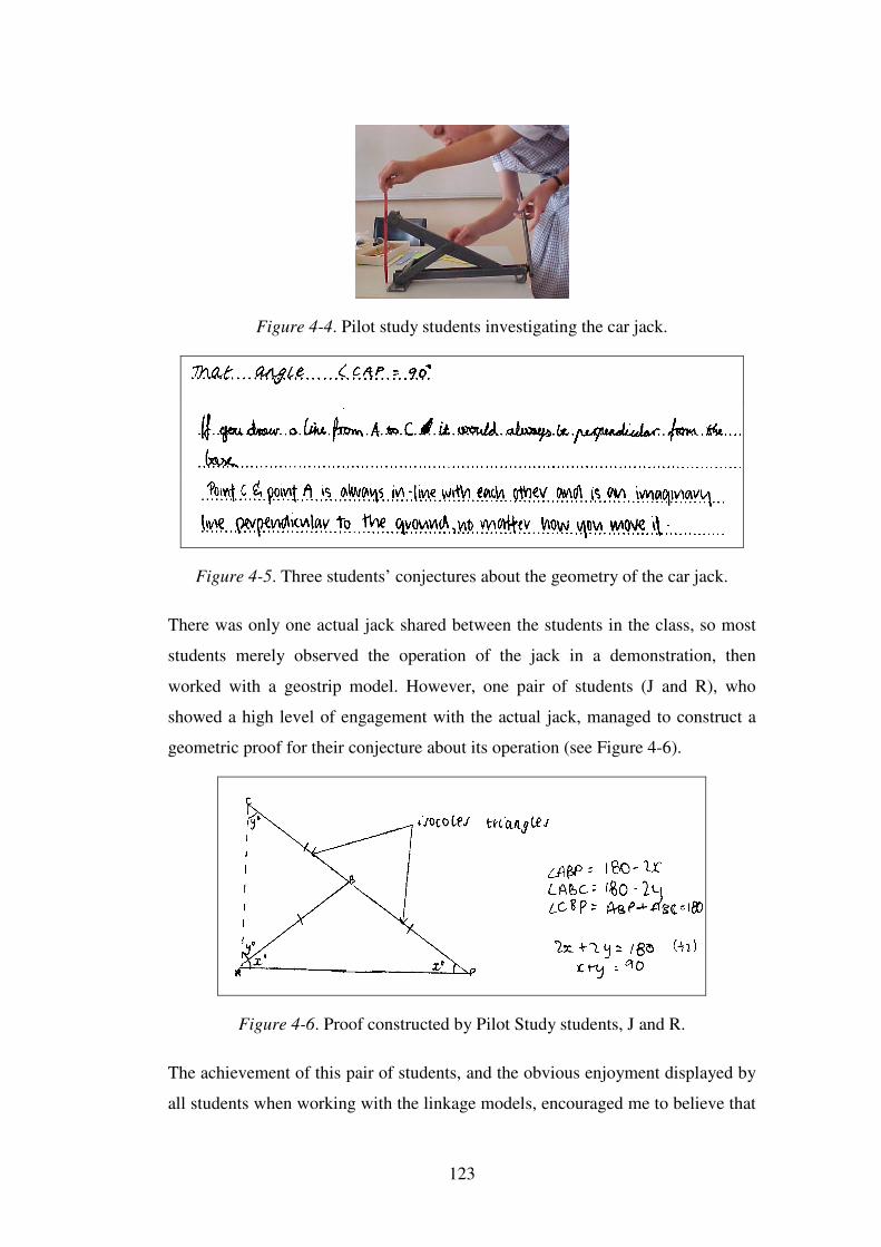
123
Figure 4-4. Pilot study students investigating the car jack.
Figure 4-5. Three students’ conjectures about the geometry of the car jack.
There was only one actual jack shared between the students in the class, so most
students merely observed the operation of the jack in a demonstration, then
worked with a geostrip model. However, one pair of students (J and R), who
showed a high level of engagement with the actual jack, managed to construct a
geometric proof for their conjecture about its operation (see Figure 4-6).
Figure 4-6. Proof constructed by Pilot Study students, J and R.
The achievement of this pair of students, and the obvious enjoyment displayed by
all students when working with the linkage models, encouraged me to believe that
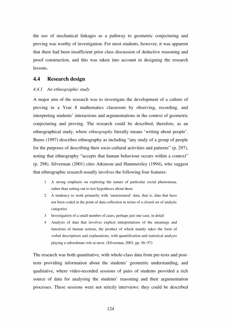
124
the use of mechanical linkages as a pathway to geometric conjecturing and
proving was worthy of investigation. For most students, however, it was apparent
that there had been insufficient prior class discussion of deductive reasoning and
proof construction, and this was taken into account in designing the research
lessons.
4.4 Research design
4.4.1 An ethnographic study
A major aim of the research was to investigate the development of a culture of
proving in a Year 8 mathematics classroom by observing, recording, and
interpreting students’ interactions and argumentations in the context of geometric
conjecturing and proving. The research could be described, therefore, as an
ethnographical study, where ethnography literally means ‘writing about people’.
Burns (1997) describes ethnography as including “any study of a group of people
for the purposes of describing their socio-cultural activities and patterns” (p. 297),
noting that ethnography “accepts that human behaviour occurs within a context”
(p. 298). Silverman (2001) cites Atkinson and Hammersley (1994), who suggest
that ethnographic research usually involves the following four features:
1 A strong emphasis on exploring the nature of particular social phenomena,
rather than setting out to test hypotheses about them
2 A tendency to work primarily with ‘unstructured’ data, that is, data that have
not been coded at the point of data collection in terms of a closed set of analytic
categories
3 Investigation of a small number of cases, perhaps just one case, in detail
4 Analysis of data that involves explicit interpretations of the meanings and
functions of human actions, the product of which mainly takes the form of
verbal descriptions and explanations, with quantification and statistical analysis
playing a subordinate role at most. (Silverman, 2001, pp. 56−57)
The research was both quantitative, with whole-class data from pre-tests and post-
tests providing information about the students’ geometric understanding, and
qualitative, where video-recorded sessions of pairs of students provided a rich
source of data for analysing the students’ reasoning and their argumentation
processes. These sessions were not strictly interviews: they could be described
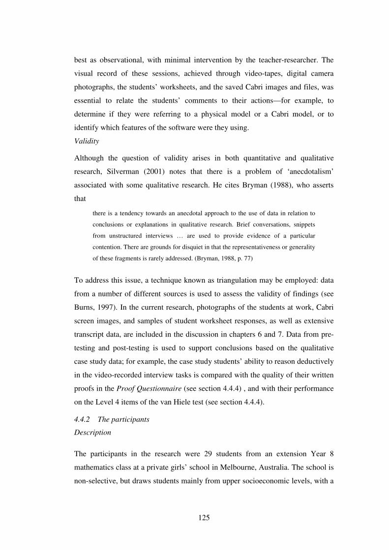
125
best as observational, with minimal intervention by the teacher-researcher. The
visual record of these sessions, achieved through video-tapes, digital camera
photographs, the students’ worksheets, and the saved Cabri images and files, was
essential to relate the students’ comments to their actions—for example, to
determine if they were referring to a physical model or a Cabri model, or to
identify which features of the software were they using.
Validity
Although the question of validity arises in both quantitative and qualitative
research, Silverman (2001) notes that there is a problem of ‘anecdotalism’
associated with some qualitative research. He cites Bryman (1988), who asserts
that
there is a tendency towards an anecdotal approach to the use of data in relation to
conclusions or explanations in qualitative research. Brief conversations, snippets
from unstructured interviews … are used to provide evidence of a particular
contention. There are grounds for disquiet in that the representativeness or generality
of these fragments is rarely addressed. (Bryman, 1988, p. 77)
To address this issue, a technique known as triangulation may be employed: data
from a number of different sources is used to assess the validity of findings (see
Burns, 1997). In the current research, photographs of the students at work, Cabri
screen images, and samples of student worksheet responses, as well as extensive
transcript data, are included in the discussion in chapters 6 and 7. Data from pre-
testing and post-testing is used to support conclusions based on the qualitative
case study data; for example, the case study students’ ability to reason deductively
in the video-recorded interview tasks is compared with the quality of their written
proofs in the Proof Questionnaire (see section 4.4.4) , and with their performance
on the Level 4 items of the van Hiele test (see section 4.4.4).
4.4.2 The participants
Description
The participants in the research were 29 students from an extension Year 8
mathematics class at a private girls’ school in Melbourne, Australia. The school is
non-selective, but draws students mainly from upper socioeconomic levels, with a
126
high proportion of the students from families where at least one parent is likely to
be a tertiary-educated professional. The age of the students in April 2001, when
the classroom research commenced, ranged from 12 years 4 months to 14 years 1
month. The 29 students had a range of ethnic backgrounds: Anglo-Celtic,
Chinese, Indian, Indonesian, Vietnamese, Sri-Lankan and Afrikaans, with the
majority being Anglo-Celtic. One student left the school during the period of the
research, so sometimes the data is based on only 28 students.
The students represented the upper 25% of Year 8 students in mathematics at the
school, and were placed in the extension class on the basis of their non-verbal
reasoning as measured by Ravens’ Progressive Matrices (De Lemos, 1989), their
performance on mathematics tests throughout Year 7, and teacher
recommendations. As a member of the teaching staff of the school, I was both the
researcher and the regular mathematics teacher for the class during the school
year, February−December, 2001.
Consent to participate
To invite the students to participate in the research, a letter which provided
information about the nature and purpose of the research was given to each
student and her parents. The letter explained that all students were to be tested and
would complete the same set of classroom activities, but several pairs of students
would be selected for additional tasks. If these selected students agreed, they
would be withdrawn in pairs from up to seven or eight lessons in other subjects in
order to work on the tasks in video-recorded sessions.
It was made clear to the students and to their parents that the students’ Year 8
mathematics assessment would not be influenced by their performance on any of
the research tasks. They were informed that although they could not withdraw
from the classroom testing or activities, they were free to withhold consent for
data to be used in the research, and to withdraw from additional activities outside
of normal mathematics class time. The letter also pointed out that the proof
activities were not part of the normal Year 8 mathematics curriculum, but would
be a valuable learning experience for the students. The students had no previous
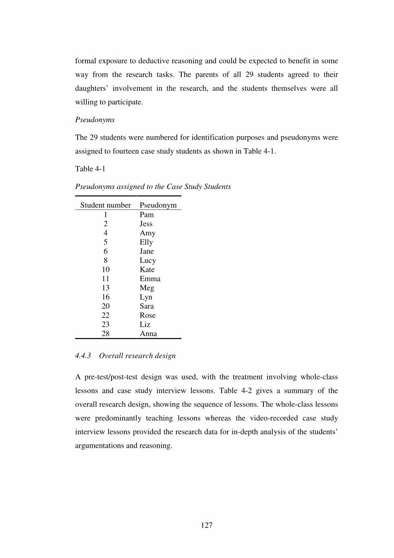
127
formal exposure to deductive reasoning and could be expected to benefit in some
way from the research tasks. The parents of all 29 students agreed to their
daughters’ involvement in the research, and the students themselves were all
willing to participate.
Pseudonyms
The 29 students were numbered for identification purposes and pseudonyms were
assigned to fourteen case study students as shown in Table 4-1.
Table 4-1
Pseudonyms assigned to the Case Study Students
Student number Pseudonym 1 2 4 5
Pam Jess Amy Elly
6 Jane 8 Lucy
10 Kate 11 Emma 13 16
Meg Lyn
20 Sara 22 Rose 23 Liz 28 Anna
4.4.3 Overall research design
A pre-test/post-test design was used, with the treatment involving whole-class
lessons and case study interview lessons. Table 4-2 gives a summary of the
overall research design, showing the sequence of lessons. The whole-class lessons
were predominantly teaching lessons whereas the video-recorded case study
interview lessons provided the research data for in-depth analysis of the students’
argumentations and reasoning.
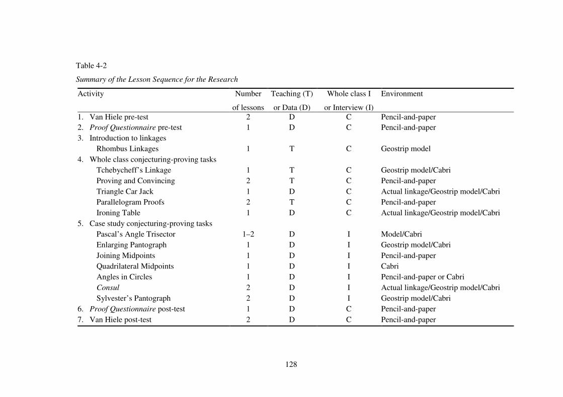
128
Table 4-2
Summary of the Lesson Sequence for the Research
Activity Number
of lessons
Teaching (T)
or Data (D)
Whole class I
or Interview (I)
Environment
1. Van Hiele pre-test 2 D C Pencil-and-paper 2. Proof Questionnaire pre-test 1 D C Pencil-and-paper 3. Introduction to linkages
Rhombus Linkages 1 T C Geostrip model 4. Whole class conjecturing-proving tasks
Tchebycheff’s Linkage 1 T C Geostrip model/Cabri Proving and Convincing 2 T C Pencil-and-paper Triangle Car Jack 1 D C Actual linkage/Geostrip model/Cabri Parallelogram Proofs 2 T C Pencil-and-paper Ironing Table 1 D C Actual linkage/Geostrip model/Cabri
5. Case study conjecturing-proving tasks Pascal’s Angle Trisector 1–2 D I Model/Cabri Enlarging Pantograph 1 D I Geostrip model/Cabri Joining Midpoints 1 D I Pencil-and-paper Quadrilateral Midpoints 1 D I Cabri Angles in Circles 1 D I Pencil-and-paper or Cabri Consul 2 D I Actual linkage/Geostrip model/Cabri Sylvester’s Pantograph 2 D I Geostrip model/Cabri
6. Proof Questionnaire post-test 1 D C Pencil-and-paper 7. Van Hiele post-test 2 D C Pencil-and-paper
129
4.4.4 Pre-testing and post-testing
1. Van Hiele test
The primary purpose of the van Hiele pre-test was to ascertain the students’ initial
levels of geometric understanding so that matched pairs of students could be
selected for the case study interview lessons. The van Hiele pre-test levels were
also used as a benchmark against which progress in geometric understanding over
the period of the research could be measured. The van Hiele test was therefore re-
administered as a post-test.
The van Hiele test used in the current research comprised 48 items designed to
assess students’ van Hiele levels (1−4) for six geometric concepts: squares, right-
angled triangles, isosceles triangles, parallel lines, congruency, and similarity. The
test items were selected from a 58-item van Hiele test, constructed originally as an
interview test by Mayberry (1983), and later developed into a written test by
Lawrie (1993; personal communication, 1/5/1997—see Appendix 1). The
Mayberry/Lawrie test covered seven concepts: squares, right-angled triangles,
isosceles triangles, parallel lines, congruency, similarity, and circles. As circle
geometry was not included in the Year 7 or Year 8 mathematics curriculum for
the students in the current study, items for the concept circles were omitted.
2. Proof Questionnaire
The Proof Questionnaire (Healy & Hoyles, 1999—see Appendix 3) formed part
of a nationwide study of proof in the United Kingdom. It was designed to gather
information about above-average Year 10 students’ understanding of the meaning
of mathematical proof, their ability to recognise a valid proof, and their ability to
construct proofs for both familiar and unfamiliar conjectures in algebra and
geometry. The content of the geometry section was within the scope of the Year 8
students in this research. A discussion with Hoyles (personal communications
19/09/2000, 12/12/2000) confirmed that the Euclidean geometry approach of the
geometry section of the Proof Questionnaire would be more appropriate for my
purpose than the Year 8 Questionnaire which was being developed for the UK
Proof Study.
130
In the current research, the Proof Questionnaire provided information about the
students’ prior understanding of the concept of geometric proof: Did they
understand the meaning of mathematical proof? Were they able to distinguish
between valid and invalid geometric arguments in both familiar and unfamiliar
contexts? Were they able to construct simple proofs in both familiar and
unfamiliar contexts? Comparison of the students’ pre-test and post-test Proof
Questionnaire performances provided information about changes in the students’
understanding of mathematical proof over the period of the conjecturing/proving
lessons.
Test administration
The van Hiele pre-test and the Proof Questionnaire were administered by me, as
the teacher-researcher, in April 2001, during normal mathematics lessons. The
students were given two 50-minute lessons to complete the van Hiele test, and one
50-minute lesson for the Proof Questionnaire. At the conclusion of the
conjecturing-proving tasks, which were spread over six to seven weeks in
May−early June, the students studied no further geometry before being re-tested
with the Proof Questionnaire in late June. It was assumed that the students’
responses would not be influenced by their having completed the same Proof
Questionnaire two months earlier. The van Hiele test was re-administered as a
post-test in October, that is six months after the pre-testing, and approximately
four months after completion of the conjecturing-proving tasks. The time lapse
between completing the conjecturing/proof tasks and the re-testing was largely
due to the need to continue uninterrupted with the normal Year 8 extended
mathematics curriculum once the main data collection had been completed. If the
students had made genuine progress in terms of their levels of geometric
understanding during the conjecturing/proving lessons, the length of time before
re-testing should not have affected their measured van Hiele levels.
4.4.5 Selecting students for the case study pairs
As discussed in section 2.4.5, the Cognitive Development and Achievement in
Secondary School Geometry (CDASSG) project (Usiskin, 1982) found that
students are more likely to be able to cope with deductive reasoning and proof if
131
they have already reached at least van Hiele Level 2. In selecting students for the
case study interview tasks, I therefore focused initially on those students who had
satisfied the Mayberry/Lawrie Level 3 criteria for at least three of the six
concepts: squares, right-angled triangles, isosceles triangles, parallel lines,
similarity, and congruency. Ten students were selected and eight of them were
matched in pairs on the basis of class friendship groups, as I believed this would
favour interaction and argumentation. The fifth pair were not members of the
same class friendship group, although they were not unfriendly towards each
other. For comparison, two additional pairs of students were selected on the basis
of friendship groups from the students who were at Level 1 or 2 on most concepts.
The students’ lesson timetables also needed to be taken into account. In practice,
because the students were being withdrawn from lessons in other subjects for the
purposes of the video-recorded interview lessons, I was restricted by their
individual subject timetables. The members of each student pair were not
necessarily in the same classes for other subjects, and certain subject teachers
were less willing for students to miss their classes. If two students had similar
subject timetables for their classes, it was easier to find a suitable time to
withdraw the students together.
As a result of these difficulties, not all student-pairs completed the same number
of tasks. It was also apparent that the pair of students who were not from the same
friendship group did not interact well. In fact, one of these students seemed unable
or unwilling to participate in her first conjecturing-proving task, despite having
satisfied the Level 3 criteria for all six concepts on the van Hiele pre-test. The
other student completed the task almost entirely on her own, with a little
prompting from me. As a consequence of this incompatibility, as well as the
difficulty of finding lessons where these two students could be withdrawn
together, this pair completed only one task. One other pair of students who were
in fact still at Level 1 on some concepts, and who found their first conjecturing-
proving task difficult, completed only one task. These two students did progress in
their geometric understanding, and this is discussed further in chapter 7, but again
it was not possible find a lesson when they could be withdrawn together.
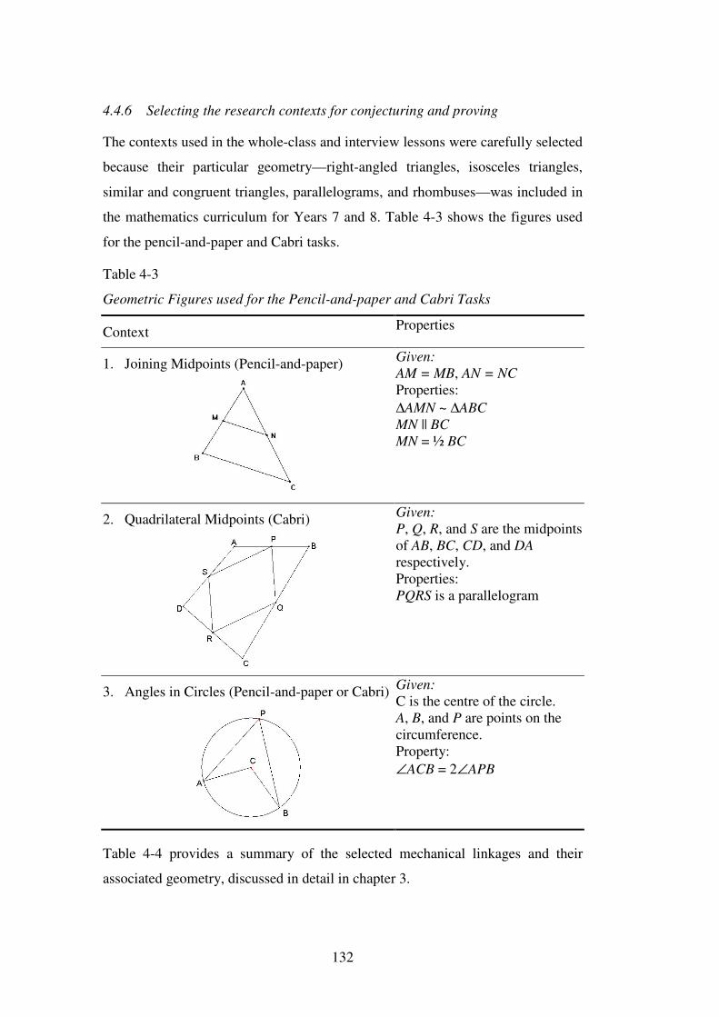
132
4.4.6 Selecting the research contexts for conjecturing and proving
The contexts used in the whole-class and interview lessons were carefully selected
because their particular geometry—right-angled triangles, isosceles triangles,
similar and congruent triangles, parallelograms, and rhombuses—was included in
the mathematics curriculum for Years 7 and 8. Table 4-3 shows the figures used
for the pencil-and-paper and Cabri tasks.
Table 4-3
Geometric Figures used for the Pencil-and-paper and Cabri Tasks
Context Properties
1. Joining Midpoints (Pencil-and-paper)
Given: AM = MB, AN = NC Properties: ∆AMN ~ ∆ABC MN || BC MN = ½ BC
2. Quadrilateral Midpoints (Cabri)
Given: P, Q, R, and S are the midpoints of AB, BC, CD, and DA respectively. Properties: PQRS is a parallelogram
3. Angles in Circles (Pencil-and-paper or Cabri)
Given: C is the centre of the circle. A, B, and P are points on the circumference. Property: ∠ACB = 2∠APB
Table 4-4 provides a summary of the selected mechanical linkages and their
associated geometry, discussed in detail in chapter 3.
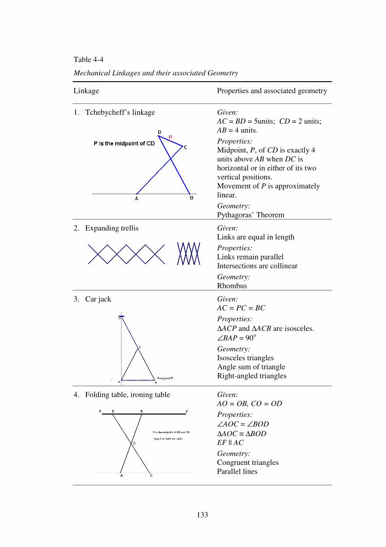
133
Table 4-4
Mechanical Linkages and their associated Geometry
Linkage Properties and associated geometry
1. Tchebycheff’s linkage
Given: AC = BD = 5units; CD = 2 units; AB = 4 units. Properties: Midpoint, P, of CD is exactly 4 units above AB when DC is horizontal or in either of its two vertical positions. Movement of P is approximately linear. Geometry: Pythagoras’ Theorem
2. Expanding trellis
Given: Links are equal in length Properties: Links remain parallel Intersections are collinear Geometry: Rhombus
3. Car jack
Given: AC = PC = BC Properties: ∆ACP and ∆ACB are isosceles. ∠BAP = 90o Geometry: Isosceles triangles Angle sum of triangle Right-angled triangles
4. Folding table, ironing table
Given: AO = OB, CO = OD Properties: ∠AOC = ∠BOD ∆AOC ≡ ∆BOD EF || AC Geometry: Congruent triangles Parallel lines
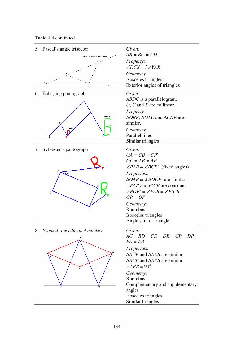
134
Table 4-4 continued
5. Pascal’s angle trisector
Given: AB = BC = CD. Property: ∠DCX = 3∠YAX Geometry: Isosceles triangles Exterior angles of triangles
6. Enlarging pantograph
Given: ABDC is a parallelogram. O, C and E are collinear. Property: ∆OBE, ∆OAC and ∆CDE are similar. Geometry: Parallel lines Similar triangles
7. Sylvester’s pantograph
Given: OA = CB = CP’ OC = AB = AP ∠PAB = ∠BCP’ (fixed angles) Properties: ∆OAP and ∆OCP’ are similar. ∠PAB and P’CB are constant. ∠POP’ = ∠PAB = ∠P’CB OP = OP’ Geometry: Rhombus Isosceles triangles Angle sum of triangle
8. ‘Consul’ the educated monkey
Given: AC = BD = CE = DE = CP = DP EA = EB Properties: ∆ACP and ∆AEB are similar. ∆ACE and ∆APB are similar. ∠APB = 90o
Geometry: Rhombus Complementary and supplementary angles Isosceles triangles Similar triangles
135
4.4.7 Preparatory lessons
The students had followed the regular Year 7 geometry component of the
mathematics curriculum during the previous school year: angles in triangles,
quadrilaterals, and polygons. All students had their own notebook computers, with
Cabri Geometry II installed as part of the mathematics software, but they had not
used Cabri in Year 7. At the start of Year 8, prior to commencement of the
research, geometry that would be required in the conjecturing and proving tasks
was taught or revised: properties of triangles and quadrilaterals; angles associated
with parallel lines cut by a transversal; Pythagoras’ theorem; and similar and
congruent triangles. During these lessons, the students used Cabri to investigate
angle properties of triangles, including exterior angles; properties of
quadrilaterals, including diagonal properties; and angles associated with parallel
lines cut by a transversal. The emphasis in each of these exploratory activities,
however, was on empirical data and identifying properties, with no reference to
why these properties were true. This was important so that conjecturing and
argumentation in geometry, and the concept of proof, would be new experiences
for the students when they came to the lessons associated with the research.
The students also used Cabri to complete several construction tasks, such as a
drag-resistant rectangle and isosceles triangle, and they were competent users of
the software construction and measurement tools. They had limited experience
with the Cabri Tabulation facility, and were aware of the Trace option, that allows
the locus of a selected point to be traced when a screen construction is dragged,
but they had not used this tool in any specific tasks.
4.4.8 Whole-class teaching lessons
The eight whole-class teaching lessons (see Table 4-2) that followed the pre-
testing were designed to introduce the students to mechanical linkages via the
simple rhombus linkage, to establish the need for mathematical proof, to explain
the nature of deductive reasoning, and to provide opportunities for the students to
engage in conjecturing and proving in the context of two simple mechanical
linkages. The worksheets associated with these eight lessons are included in
Appendix 4.
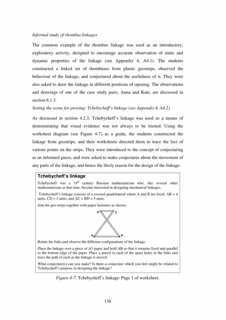
136
Informal study of rhombus linkages
The common example of the rhombus linkage was used as an introductory,
exploratory activity, designed to encourage accurate observation of static and
dynamic properties of the linkage (see Appendix 4, A4.1). The students
constructed a linked set of rhombuses from plastic geostrips, observed the
behaviour of the linkage, and conjectured about the usefulness of it. They were
also asked to draw the linkage in different positions of opening. The observations
and drawings of one of the case study pairs, Anna and Kate, are discussed in
section 6.1.3.
Setting the scene for proving: Tchebycheff’s linkage (see Appendix 4, A4.2)
As discussed in section 4.2.3, Tchebycheff’s linkage was used as a means of
demonstrating that visual evidence was not always to be trusted. Using the
worksheet diagram (see Figure 4-7) as a guide, the students constructed the
linkage from geostrips, and their worksheets directed them to trace the loci of
various points on the strips. They were introduced to the concept of conjecturing
as an informed guess, and were asked to make conjectures about the movement of
any parts of the linkage, and hence the likely reason for the design of the linkage.
Tchebycheff’s linkage Tchebycheff was a 19th century Russian mathematician who, like several other mathematicians at that time, became interested in designing mechanical linkages.
Tchebycheff’s linkage consists of a crossed quadrilateral where A and B are fixed, AB = 4 units, CD = 2 units, and AC = BD = 5 units.
Join the geo-strips together with paper fasteners as shown:
D
A B
C
Rotate the links and observe the different configurations of the linkage.
Place the linkage over a piece of A3 paper and hold AB so that it remains fixed and parallel to the bottom edge of the paper. Place a pencil in each of the spare holes in the links and trace the path of each as the linkage is moved.
What conjecture(s) can you make? Is there a conjecture which you feel might be related to Tchebycheff’s purpose in designing the linkage?
Figure 4-7. Tchebycheff’s linkage: Page 1 of worksheet.
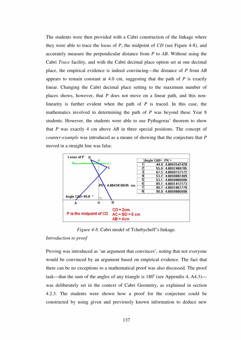
137
The students were then provided with a Cabri construction of the linkage where
they were able to trace the locus of P, the midpoint of CD (see Figure 4-8), and
accurately measure the perpendicular distance from P to AB. Without using the
Cabri Trace facility, and with the Cabri decimal place option set at one decimal
place, the empirical evidence is indeed convincing—the distance of P from AB
appears to remain constant at 4.0 cm, suggesting that the path of P is exactly
linear. Changing the Cabri decimal place setting to the maximum number of
places shows, however, that P does not move on a linear path, and this non-
linearity is further evident when the path of P is traced. In this case, the
mathematics involved in determining the path of P was beyond these Year 8
students. However, the students were able to use Pythagoras’ theorem to show
that P was exactly 4 cm above AB in three special positions. The concept of
counter-example was introduced as a means of showing that the conjecture that P
moved in a straight line was false.
Figure 4-8. Cabri model of Tchebycheff’s linkage.
Introduction to proof
Proving was introduced as ‘an argument that convinces’, noting that not everyone
would be convinced by an argument based on empirical evidence. The fact that
there can be no exceptions to a mathematical proof was also discussed. The proof
task—that the sum of the angles of any triangle is 180o (see Appendix 4, A4.3)—
was deliberately set in the context of Cabri Geometry, as explained in section
4.2.3. The students were shown how a proof for the conjecture could be
constructed by using given and previously known information to deduce new
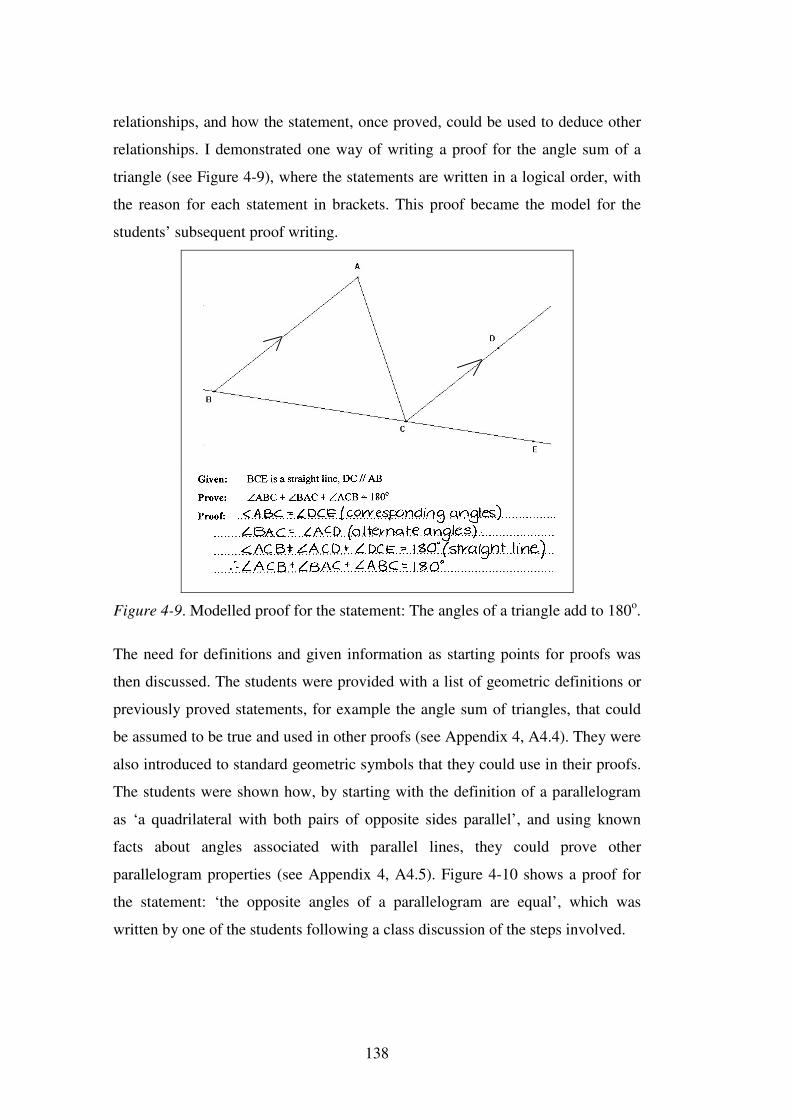
138
relationships, and how the statement, once proved, could be used to deduce other
relationships. I demonstrated one way of writing a proof for the angle sum of a
triangle (see Figure 4-9), where the statements are written in a logical order, with
the reason for each statement in brackets. This proof became the model for the
students’ subsequent proof writing.
Figure 4-9. Modelled proof for the statement: The angles of a triangle add to 180o.
The need for definitions and given information as starting points for proofs was
then discussed. The students were provided with a list of geometric definitions or
previously proved statements, for example the angle sum of triangles, that could
be assumed to be true and used in other proofs (see Appendix 4, A4.4). They were
also introduced to standard geometric symbols that they could use in their proofs.
The students were shown how, by starting with the definition of a parallelogram
as ‘a quadrilateral with both pairs of opposite sides parallel’, and using known
facts about angles associated with parallel lines, they could prove other
parallelogram properties (see Appendix 4, A4.5). Figure 4-10 shows a proof for
the statement: ‘the opposite angles of a parallelogram are equal’, which was
written by one of the students following a class discussion of the steps involved.
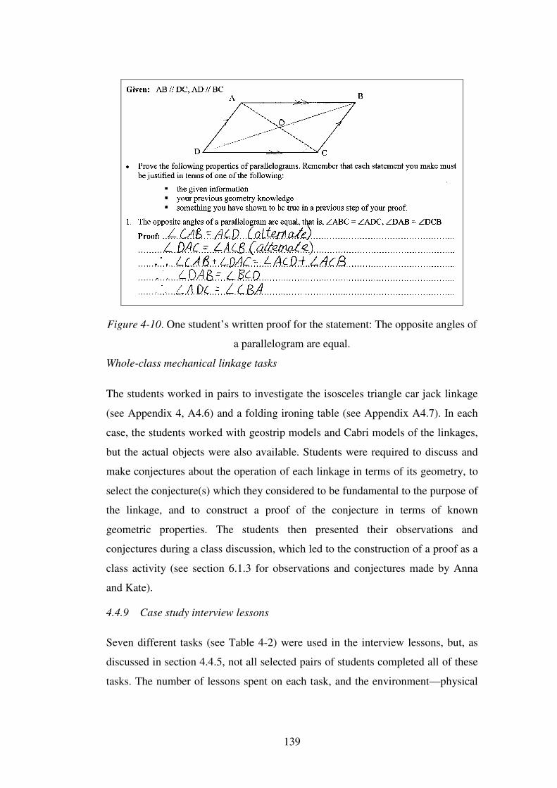
139
Figure 4-10. One student’s written proof for the statement: The opposite angles of
a parallelogram are equal.
Whole-class mechanical linkage tasks
The students worked in pairs to investigate the isosceles triangle car jack linkage
(see Appendix 4, A4.6) and a folding ironing table (see Appendix A4.7). In each
case, the students worked with geostrip models and Cabri models of the linkages,
but the actual objects were also available. Students were required to discuss and
make conjectures about the operation of each linkage in terms of its geometry, to
select the conjecture(s) which they considered to be fundamental to the purpose of
the linkage, and to construct a proof of the conjecture in terms of known
geometric properties. The students then presented their observations and
conjectures during a class discussion, which led to the construction of a proof as a
class activity (see section 6.1.3 for observations and conjectures made by Anna
and Kate).
4.4.9 Case study interview lessons
Seven different tasks (see Table 4-2) were used in the interview lessons, but, as
discussed in section 4.4.5, not all selected pairs of students completed all of these
tasks. The number of lessons spent on each task, and the environment—physical
140
model, Cabri, or pencil-and-paper—used for each task are shown in Table 4-2.
The worksheets associated with each of the tasks are included in Appendix 5.
For each interview, two selected students were withdrawn from their other classes
to work in a quiet room. A video camera was set up to record their actions and
conversations as they worked with the models or the computer. I, as the teacher-
researcher, sometimes asked questions to clarify what the students were saying,
and intervened to make suggestions if they seemed unable to proceed. I also took
photographs with a digital camera, and operated the video camera to ensure it was
always focused on their actions, for example, when the students moved from
working with a geostrip model to working with the Cabri model. I closely
followed the students’ actions when they were using Cabri so that I could ask
them to save the file at appropriate stages, or I used the computer Printscreen
option to save a screen that included the trace of points (Cabri traces are transient
and cannot be saved with the file). The Cabri Replay Construction option enabled
me to retrace, later, the order in which the students made Cabri measurements or
changed the drawing in any way, for example, by adding further lines.
Mechanical linkage interview tasks
For each of the mechanical linkage tasks, the students were given a worksheet,
which included a diagram of the linkage (see Appendix 5), and sufficient plastic
geostrips and paper fasteners to construct the linkage. In certain cases, for
example with ‘Consul, the educated monkey’, the students were also given the
actual linkage. The students were invited to investigate the linkage, and make
conjectures about why the linkage operated in the observed way. After they had
made, or attempted to make, their initial conjectures they were introduced to the
dynamic geometry model. They could then choose to work with either model,
moving backwards and forwards between the two if they wished. Through a
process of argumentation the students then used their geometric understanding to
explain their conjectures by constructing verbal and written proofs. If it became
obvious that strict adherence to the worksheets would inhibit or interfere with the
students’ argumentation, the students were left to pursue their own direction in
their argumentation, rather than being directed back to worksheet questions. At
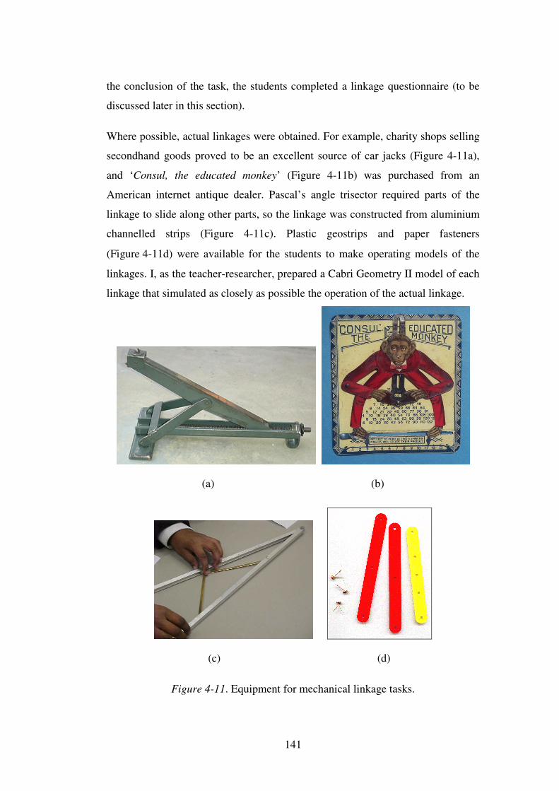
141
the conclusion of the task, the students completed a linkage questionnaire (to be
discussed later in this section).
Where possible, actual linkages were obtained. For example, charity shops selling
secondhand goods proved to be an excellent source of car jacks (Figure 4-11a),
and ‘Consul, the educated monkey’ (Figure 4-11b) was purchased from an
American internet antique dealer. Pascal’s angle trisector required parts of the
linkage to slide along other parts, so the linkage was constructed from aluminium
channelled strips (Figure 4-11c). Plastic geostrips and paper fasteners
(Figure 4-11d) were available for the students to make operating models of the
linkages. I, as the teacher-researcher, prepared a Cabri Geometry II model of each
linkage that simulated as closely as possible the operation of the actual linkage.
(a) (b)
(c) (d)
Figure 4-11. Equipment for mechanical linkage tasks.
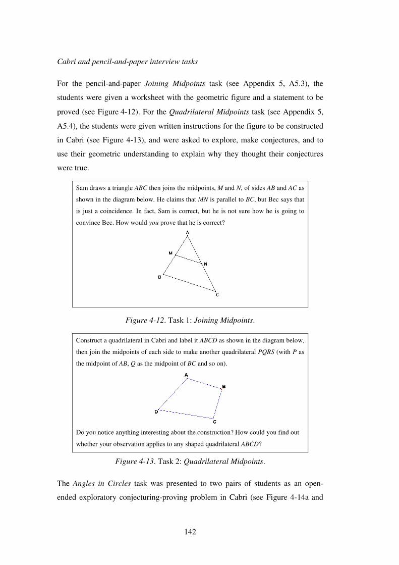
142
Cabri and pencil-and-paper interview tasks
For the pencil-and-paper Joining Midpoints task (see Appendix 5, A5.3), the
students were given a worksheet with the geometric figure and a statement to be
proved (see Figure 4-12). For the Quadrilateral Midpoints task (see Appendix 5,
A5.4), the students were given written instructions for the figure to be constructed
in Cabri (see Figure 4-13), and were asked to explore, make conjectures, and to
use their geometric understanding to explain why they thought their conjectures
were true.
Sam draws a triangle ABC then joins the midpoints, M and N, of sides AB and AC as
shown in the diagram below. He claims that MN is parallel to BC, but Bec says that
is just a coincidence. In fact, Sam is correct, but he is not sure how he is going to
convince Bec. How would you prove that he is correct?
Figure 4-12. Task 1: Joining Midpoints.
Construct a quadrilateral in Cabri and label it ABCD as shown in the diagram below,
then join the midpoints of each side to make another quadrilateral PQRS (with P as
the midpoint of AB, Q as the midpoint of BC and so on).
Do you notice anything interesting about the construction? How could you find out
whether your observation applies to any shaped quadrilateral ABCD?
Figure 4-13. Task 2: Quadrilateral Midpoints.
The Angles in Circles task was presented to two pairs of students as an open-
ended exploratory conjecturing-proving problem in Cabri (see Figure 4-14a and
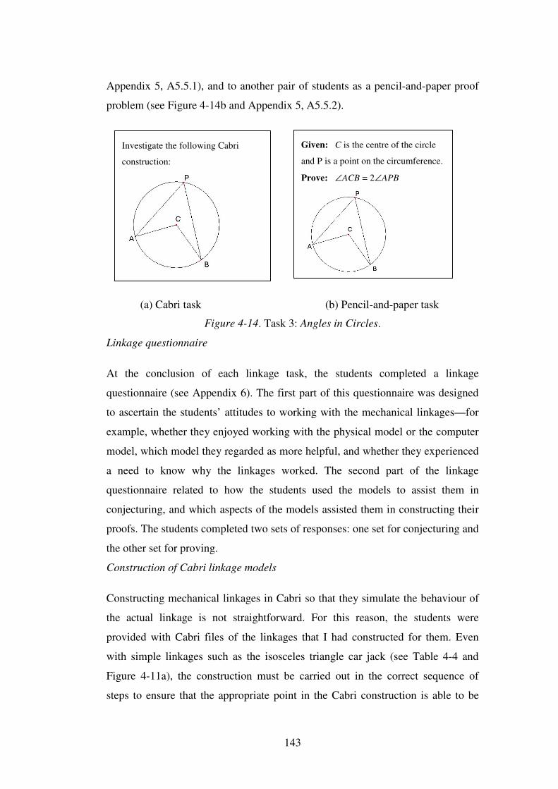
143
Appendix 5, A5.5.1), and to another pair of students as a pencil-and-paper proof
problem (see Figure 4-14b and Appendix 5, A5.5.2).
(a) Cabri task (b) Pencil-and-paper task
Figure 4-14. Task 3: Angles in Circles.
Linkage questionnaire
At the conclusion of each linkage task, the students completed a linkage
questionnaire (see Appendix 6). The first part of this questionnaire was designed
to ascertain the students’ attitudes to working with the mechanical linkages—for
example, whether they enjoyed working with the physical model or the computer
model, which model they regarded as more helpful, and whether they experienced
a need to know why the linkages worked. The second part of the linkage
questionnaire related to how the students used the models to assist them in
conjecturing, and which aspects of the models assisted them in constructing their
proofs. The students completed two sets of responses: one set for conjecturing and
the other set for proving.
Construction of Cabri linkage models
Constructing mechanical linkages in Cabri so that they simulate the behaviour of
the actual linkage is not straightforward. For this reason, the students were
provided with Cabri files of the linkages that I had constructed for them. Even
with simple linkages such as the isosceles triangle car jack (see Table 4-4 and
Figure 4-11a), the construction must be carried out in the correct sequence of
steps to ensure that the appropriate point in the Cabri construction is able to be
Given: C is the centre of the circle
and P is a point on the circumference.
Prove: ∠ACB = 2∠APB
Investigate the following Cabri
construction:
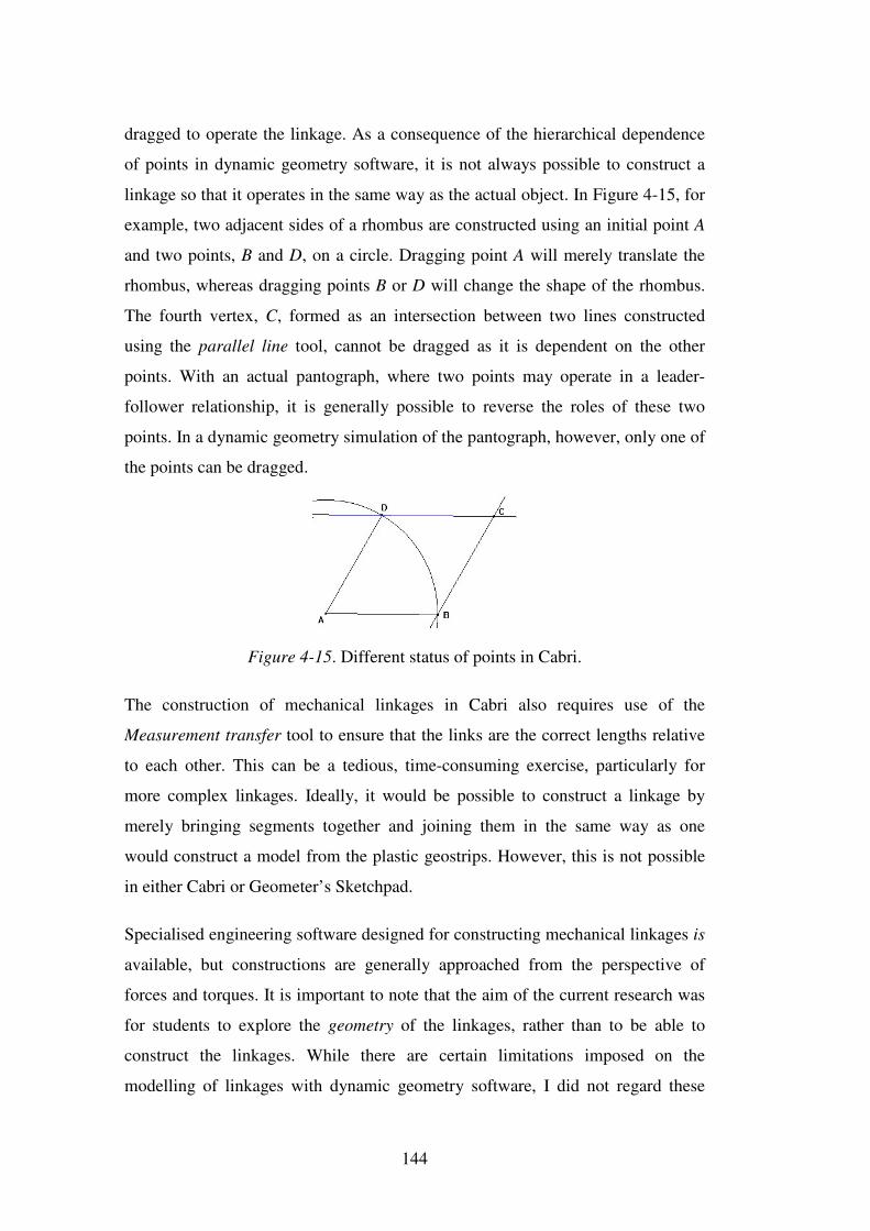
144
dragged to operate the linkage. As a consequence of the hierarchical dependence
of points in dynamic geometry software, it is not always possible to construct a
linkage so that it operates in the same way as the actual object. In Figure 4-15, for
example, two adjacent sides of a rhombus are constructed using an initial point A
and two points, B and D, on a circle. Dragging point A will merely translate the
rhombus, whereas dragging points B or D will change the shape of the rhombus.
The fourth vertex, C, formed as an intersection between two lines constructed
using the parallel line tool, cannot be dragged as it is dependent on the other
points. With an actual pantograph, where two points may operate in a leader-
follower relationship, it is generally possible to reverse the roles of these two
points. In a dynamic geometry simulation of the pantograph, however, only one of
the points can be dragged.
Figure 4-15. Different status of points in Cabri.
The construction of mechanical linkages in Cabri also requires use of the
Measurement transfer tool to ensure that the links are the correct lengths relative
to each other. This can be a tedious, time-consuming exercise, particularly for
more complex linkages. Ideally, it would be possible to construct a linkage by
merely bringing segments together and joining them in the same way as one
would construct a model from the plastic geostrips. However, this is not possible
in either Cabri or Geometer’s Sketchpad.
Specialised engineering software designed for constructing mechanical linkages is
available, but constructions are generally approached from the perspective of
forces and torques. It is important to note that the aim of the current research was
for students to explore the geometry of the linkages, rather than to be able to
construct the linkages. While there are certain limitations imposed on the
modelling of linkages with dynamic geometry software, I did not regard these
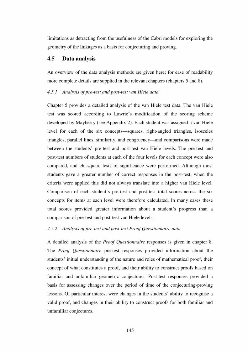
145
limitations as detracting from the usefulness of the Cabri models for exploring the
geometry of the linkages as a basis for conjecturing and proving.
4.5 Data analysis
An overview of the data analysis methods are given here; for ease of readability
more complete details are supplied in the relevant chapters (chapters 5 and 8).
4.5.1 Analysis of pre-test and post-test van Hiele data
Chapter 5 provides a detailed analysis of the van Hiele test data. The van Hiele
test was scored according to Lawrie’s modification of the scoring scheme
developed by Mayberry (see Appendix 2). Each student was assigned a van Hiele
level for each of the six concepts—squares, right-angled triangles, isosceles
triangles, parallel lines, similarity, and congruency—and comparisons were made
between the students’ pre-test and post-test van Hiele levels. The pre-test and
post-test numbers of students at each of the four levels for each concept were also
compared, and chi-square tests of significance were performed. Although most
students gave a greater number of correct responses in the post-test, when the
criteria were applied this did not always translate into a higher van Hiele level.
Comparison of each student’s pre-test and post-test total scores across the six
concepts for items at each level were therefore calculated. In many cases these
total scores provided greater information about a student’s progress than a
comparison of pre-test and post-test van Hiele levels.
4.5.2 Analysis of pre-test and post-test Proof Questionnaire data
A detailed analysis of the Proof Questionnaire responses is given in chapter 8.
The Proof Questionnaire pre-test responses provided information about the
students’ initial understanding of the nature and roles of mathematical proof, their
concept of what constitutes a proof, and their ability to construct proofs based on
familiar and unfamiliar geometric conjectures. Post-test responses provided a
basis for assessing changes over the period of time of the conjecturing-proving
lessons. Of particular interest were changes in the students’ ability to recognise a
valid proof, and changes in their ability to construct proofs for both familiar and
unfamiliar conjectures.
146
A Proof Score (maximum possible score = 15) was determined for each student
by combining the total scores on the two proof construction items—G4 and G7—
of the Proof Questionnaire with the score for Level 4 items on the van Hiele test
These Proof Scores are shown in Appendix 7.
4.5.3 Data from case study interview lessons
Transcribed video-recordings provided the main source of data from the case
study interview lessons. Cabri screen images and digital camera photographs, as
well as scanned diagrams, notes, and responses from the students’ worksheets,
were inserted into the files of the transcripts to provide a comprehensive picture of
the students’ argumentations. The argumentations were then analysed from
several perspectives: the students’ motivational and cognitive engagement with
the tasks; the nature of the student-student interactions; evidence of deductive
reasoning; and instances where dynamic visualisation influenced the students’
reasoning.
Identifying phases within each argumentation
In each of the tasks, the students were seen to be involved in four different phases
of activity. First, an observation phase commenced with task orientation, where
the students familiarised themselves with the task by referring, for example, to the
given data or to how the linkage moved. Following this task orientation phase, or
sometimes associated with it, was a data gathering or fact-finding phase that led
into conjecturing and proving phases. The phases were not always distinct, and
observations and data gathering often continued throughout the conjecturing
phase, and statements of deductive reasoning occasionally occurred in the task
orientation phase. For some of the linkages, particularly where the purpose of the
linkage was not obvious, the task orientation phase tended to overlap conjecturing
and proving as the action of the linkage became clearer.
For each task, students’ speaking turns associated with observations, data
gathering, conjectures, or deductive reasoning, were identified. In order to provide
a visual display of the features of each argumentation, I devised an argumentation
profile chart (for example, see Figure 6-16) to indicate the sequence of speaking
147
turns, including my guiding interventions, for the entire argumentation. Each
argumentation profile chart also shows the phases of the argumentation (task
orientation, data gathering, conjecturing, proving); and when the students were
working with the geostrip model, the Cabri model, or pencil-and-paper.
Teacher-researcher intervention
As discussed in section 2.3.2, teacher intervention is crucial in a constructivist
learning situation. Hanna (1995), for example, emphasises the need for teacher
intervention where learning methods encourage students to interact with each
other, and Boero (1999) notes that “the development of Toulmin-type …
argumentations calls for very strong teacher mediation” (p. 1). My involvement in
the argumentations had several purposes, including clarification of the content of
the students’ statements, probing the meaning of statements, answering queries,
correcting false statements, and re-directing the students’ thinking if they had
reached an impasse. The most important aspect of my mediation, however, was to
ensure that the students’ arguments were based on sound mathematical logic.
Also, as the students’ mathematics teacher I believed that a lesson should not end
without some sense of achievement and at least partial success in the
conjecturing/proving process, and this belief motivated some of my interventions.
Interventions which were classified as guidance were of three main types: hints,
which focused the students’ attention on mechanical aspects of the linkages or on
geometric properties; corrections to incorrect geometric statements; and warrant-
prompts, which provoked deductive reasoning by asking the students to justify
their statements. An example of a warrant-prompt is: “Why do you say that?” in
response to a students’ claim: “Those two angles are equal”. These classifications
are used in the argumentation profile charts (see, for example, Figure 6-31).
Students’ use of gesture
A prominent feature of the argumentations was the students’ use of gesture. When
referring to angles, the students frequently pointed to the angles concerned and
stated, for example, “Those two angles are equal”, rather than naming the angles. I
deliberately chose to allow them to identify geometric features in this way to
148
facilitate the fluency of their natural language argumentation. Occasionally, when
it was unclear to which features they were referring, I asked for clarification. The
video camera was always focused on either the linkage or the computer screen,
depending on where the students’ attention was directed. In transcribing the
videotapes it was therefore easy to identify the geometric objects to which the
students were referring.
Analysing the reasoning
Sequences of deductive reasoning during the argumentations, and the students’
written proofs, have been represented diagrammatically for each task (see Figure
6-15, for example) using an argument layout based on that proposed by Toulmin
(1958; see section 2.3.3). In most of the tasks, the proving process could be parsed
into sequences of reasoning that represented intermediate stages in the overall
reasoning. These sequences may be likened to the “negotiative events” described
by Clarke (2001) in the analysis of classroom dialogue. Clarke notes that by
parsing classroom dialogue into negotiative events, the emphasis in the analysis is
on the interaction between the participants rather than “the separate utterances of
the individuals participant in the interaction” (p. 36).
4.5.4 Linkage questionnaire
The linkage questionnaire responses provided a check on the validity of the
interpretation of motivational aspects of the tasks and the relative usefulness of
the Cabri and linkage models in conjecturing and proving. Responses of the case
study students, and of the whole class for the two whole-class linkage tasks, were
analysed item-wise to see if patterns or individual differences occurred in the
responses.
4.6 Overview of the data sources
This section provides an overview of the various data sources used in the research,
the rationale for their choice (see section 4.4), and how the analysis of data from
each of these sources addresses one or more of the research questions. Table 4-5
summarises data sources and their rationales. Table 4-6 provides a summary of
how each data source addresses one or more of the research questions.
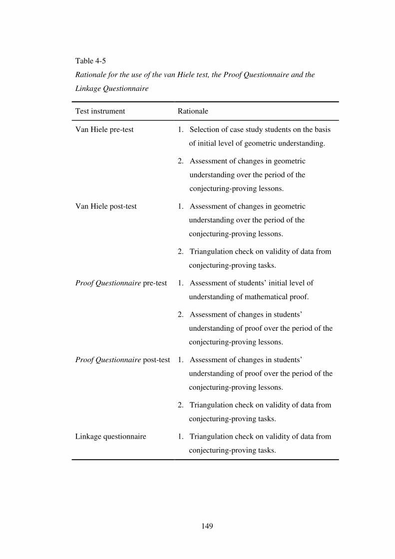
149
Table 4-5
Rationale for the use of the van Hiele test, the Proof Questionnaire and the
Linkage Questionnaire
Test instrument Rationale
Van Hiele pre-test 1. Selection of case study students on the basis
of initial level of geometric understanding.
2. Assessment of changes in geometric
understanding over the period of the
conjecturing-proving lessons.
Van Hiele post-test 1. Assessment of changes in geometric
understanding over the period of the
conjecturing-proving lessons.
2. Triangulation check on validity of data from
conjecturing-proving tasks.
Proof Questionnaire pre-test 1. Assessment of students’ initial level of
understanding of mathematical proof.
2. Assessment of changes in students’
understanding of proof over the period of the
conjecturing-proving lessons.
Proof Questionnaire post-test 1. Assessment of changes in students’
understanding of proof over the period of the
conjecturing-proving lessons.
2. Triangulation check on validity of data from
conjecturing-proving tasks.
Linkage questionnaire 1. Triangulation check on validity of data from
conjecturing-proving tasks.
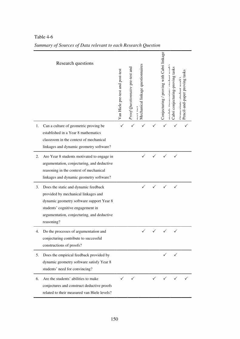
150
Table 4-6
Summary of Sources of Data relevant to each Research Question
Research questions
V
an H
iele
pre
-tes
t and
pos
t-te
st
Pro
of Q
uest
ionn
aire
pre
-tes
t and
post
-tes
t
Mec
hani
cal l
inka
ge q
uest
ionn
aire
s
Con
ject
urin
g / p
rovi
ng w
ith C
abri
link
age
mod
els
(tra
nscr
ipts
; stu
dent
wor
k)
Cab
ri c
onje
ctur
ing-
prov
ing
task
s
(tra
nscr
ipts
; stu
dent
wor
k)
Penc
il-an
d-pa
per p
rovi
ng ta
sks
1. Can a culture of geometric proving be
established in a Year 8 mathematics
classroom in the context of mechanical
linkages and dynamic geometry software?
� � � � � � �
2. Are Year 8 students motivated to engage in
argumentation, conjecturing, and deductive
reasoning in the context of mechanical
linkages and dynamic geometry software?
� � � �
3. Does the static and dynamic feedback
provided by mechanical linkages and
dynamic geometry software support Year 8
students’ cognitive engagement in
argumentation, conjecturing, and deductive
reasoning?
� � � �
4. Do the processes of argumentation and
conjecturing contribute to successful
constructions of proofs?
� � � �
5. Does the empirical feedback provided by
dynamic geometry software satisfy Year 8
students’ need for convincing?
� �
6. Are the students’ abilities to make
conjectures and construct deductive proofs
related to their measured van Hiele levels?
� � � � � �
151
Chapter 5: Measuring Geometric
Understanding
Only after the rhombus has become a totality of properties is an ordering of these
properties, perhaps a logical ordering, possible. … In instruction, one must delay the
logical ordering, the proving of properties, until the pupil has been sufficiently
acquainted with the properties. (van Hiele, 1986, p. 111)
5.1 Introduction
According to the van Hiele theory, understanding of geometric properties and
relationships, that is, Level 3 understanding, is a prerequisite for deductive
reasoning (see section 2.5.1). It could be expected, then, that a van Hiele test
would identify those students who were cognitively ready for the conjecturing-
proving tasks, and that comparison of the students’ pre-test and post-test levels
would indicate the influence of the conjecturing-proving tasks on the students’
geometric reasoning.
This chapter presents and analyses the data from the van Hiele pre-testing and
post-testing. Section 5.2 discusses the van Hiele test used in the current research,
section 5.3 analyses the Year 8 students’ pre-test van Hiele levels, and section 5.4
discusses the selection of the case study students on the basis of their pre-test
levels. Section 5.5 compares the students’ pre-test and post-test levels, and section
5.6 focuses on the progress made by the case study students.
5.2 The Mayberry/Lawrie van Hiele test
5.2.1 Description of the Mayberry/Lawrie van Hiele Test
The Mayberry/Lawrie van Hiele Test is based on a 62-item interview test
constructed by Mayberry (1983), covering seven concepts: squares, right-angled
triangles, isosceles triangles, circles, parallel lines, similarity, and congruency.
Mayberry constructed the items on the basis of the van Hiele level descriptors for
Levels 1 to 5, and each item was designed to test students’ understanding of a
specific van Hiele level. Mayberry noted that her study supported the hierarchical
152
nature of the van Hiele levels, but showed that students could be at different levels
for different concepts. A student could, for example, be at Level 3 for the concept
squares, but at Level 2 for the concept isosceles triangles. Lawrie (1993; personal
communication, 1/5/1997) replicated Mayberry’s work, and, after omitting the
Level 5 items, converted the remaining items into a 58-item written test.
For each concept and each van Hiele level Mayberry set success criteria so that
students who correctly answered sufficient questions to satisfy the criterion for a
particular level were deemed to have mastered that van Hiele level for that
concept. In accordance with the assumed hierarchical nature of the van Hiele
levels, a student could not be assigned a particular level unless the criteria for all
lower levels had been satisfied. If, for example, a student satisfied the criteria for
Levels 1, 2, and 4 for a particular concept, but did not meet the Level 3 criterion,
the student would be assessed as being at Level 2 for that concept.
My main reason for administering a van Hiele test was to identify the students’
levels of geometric understanding to enable me to select approximately matched
pairs for the conjecturing-proving tasks, and for this purpose the test seemed
appropriate. However, because the geometry which the students in the current
study had completed did not include circles, and because I wished to reduce the
length of the test slightly, I omitted the items for the concept circles. The
remaining 48 items, covering six concepts, were renumbered consecutively (see
Appendix 1).
Lawrie (1993) claims that certain of Mayberry’s items did not measure the level
for which they were designed (see section 5.2.2). She therefore modified some
items, as well as amending Mayberry’s assessment criteria, and it was these
amended items and criteria which were used in the current study (Lawrie, personal
communication, 1/5/1997). Table 5-1 shows, for example, the success criteria for
the concept squares, with the score required out of the maximum possible score at
each level to demonstrate mastery of that level. Correct responses to either Item 1
or both parts of Item 5, for example, represent mastery of Level 1 for the concept
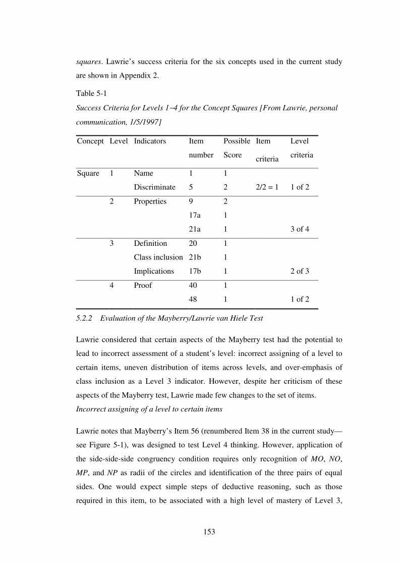
153
squares. Lawrie’s success criteria for the six concepts used in the current study
are shown in Appendix 2.
Table 5-1
Success Criteria for Levels 1−4 for the Concept Squares [From Lawrie, personal
communication, 1/5/1997]
Concept Level Indicators Item
number
Possible
Score
Item
criteria
Level
criteria
Square 1 Name 1 1
Discriminate 5 2 2/2 = 1 1 of 2
2 Properties 9 2
17a 1
21a 1 3 of 4
3 Definition 20 1
Class inclusion 21b 1
Implications 17b 1 2 of 3
4 Proof 40 1
48 1 1 of 2
5.2.2 Evaluation of the Mayberry/Lawrie van Hiele Test
Lawrie considered that certain aspects of the Mayberry test had the potential to
lead to incorrect assessment of a student’s level: incorrect assigning of a level to
certain items, uneven distribution of items across levels, and over-emphasis of
class inclusion as a Level 3 indicator. However, despite her criticism of these
aspects of the Mayberry test, Lawrie made few changes to the set of items.
Incorrect assigning of a level to certain items
Lawrie notes that Mayberry’s Item 56 (renumbered Item 38 in the current study—
see Figure 5-1), was designed to test Level 4 thinking. However, application of
the side-side-side congruency condition requires only recognition of MO, NO,
MP, and NP as radii of the circles and identification of the three pairs of equal
sides. One would expect simple steps of deductive reasoning, such as those
required in this item, to be associated with a high level of mastery of Level 3,
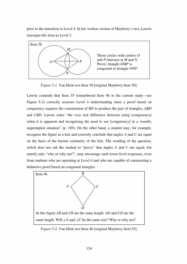
154
prior to the transition to Level 4. In her written version of Mayberry’s test, Lawrie
reassigns this item as Level 3.
Figure 5-1. Van Hiele test Item 38 [original Mayberry Item 56].
Lawrie contends that Item 55 (renumbered Item 46 in the current study—see
Figure 5-2) correctly assesses Level 4 understanding since a proof based on
congruency requires the construction of BD to produce the pair of triangles, ABD
and CBD. Lawrie notes “the very real difference between using [congruency]
when it is apparent and recognising the need to use [congruency] in a visually
unprompted situation” (p. 189). On the other hand, a student may, for example,
recognise the figure as a kite and correctly conclude that angles A and C are equal
on the basis of the known symmetry of the kite. The wording of the question,
which does not ask the student to “prove” that angles A and C are equal, but
merely asks “why or why not?”, may encourage such lower-level responses, even
from students who are operating at Level 4 and who are capable of constructing a
deductive proof based on congruent triangles.
Item 46
In this figure AB and CB are the same length. AD and CD are the
same length. Will ∠A and ∠C be the same size? Why or why not?
Figure 5-2. Van Hiele test Item 46 [original Mayberry Item 55].
O
M
N
P
These circles with centres O and P intersect at M and N. Prove: triangle OMP is congruent to triangle ONP.
Item 38
A C
D
B
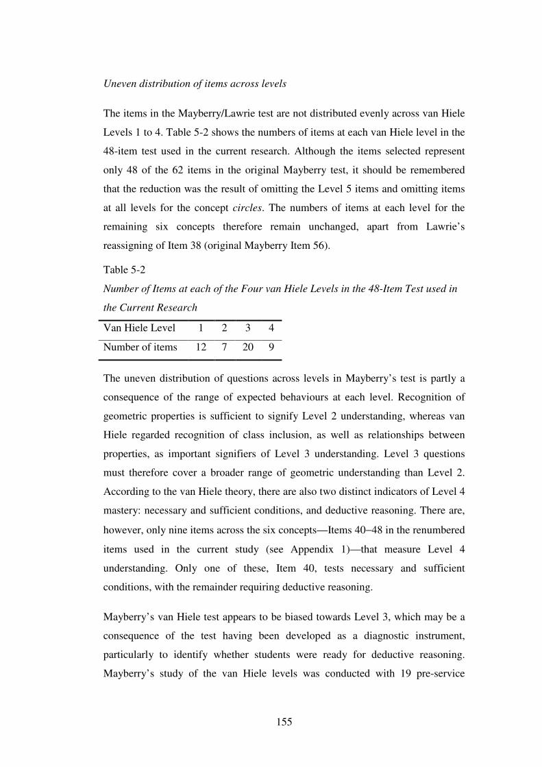
155
Uneven distribution of items across levels
The items in the Mayberry/Lawrie test are not distributed evenly across van Hiele
Levels 1 to 4. Table 5-2 shows the numbers of items at each van Hiele level in the
48-item test used in the current research. Although the items selected represent
only 48 of the 62 items in the original Mayberry test, it should be remembered
that the reduction was the result of omitting the Level 5 items and omitting items
at all levels for the concept circles. The numbers of items at each level for the
remaining six concepts therefore remain unchanged, apart from Lawrie’s
reassigning of Item 38 (original Mayberry Item 56).
Table 5-2
Number of Items at each of the Four van Hiele Levels in the 48-Item Test used in
the Current Research
Van Hiele Level 1 2 3 4
Number of items 12 7 20 9
The uneven distribution of questions across levels in Mayberry’s test is partly a
consequence of the range of expected behaviours at each level. Recognition of
geometric properties is sufficient to signify Level 2 understanding, whereas van
Hiele regarded recognition of class inclusion, as well as relationships between
properties, as important signifiers of Level 3 understanding. Level 3 questions
must therefore cover a broader range of geometric understanding than Level 2.
According to the van Hiele theory, there are also two distinct indicators of Level 4
mastery: necessary and sufficient conditions, and deductive reasoning. There are,
however, only nine items across the six concepts—Items 40−48 in the renumbered
items used in the current study (see Appendix 1)—that measure Level 4
understanding. Only one of these, Item 40, tests necessary and sufficient
conditions, with the remainder requiring deductive reasoning.
Mayberry’s van Hiele test appears to be biased towards Level 3, which may be a
consequence of the test having been developed as a diagnostic instrument,
particularly to identify whether students were ready for deductive reasoning.
Mayberry’s study of the van Hiele levels was conducted with 19 pre-service
156
elementary teachers, six of whom had not completed the one-year high school
geometry course. For most of the seven concepts the majority of the students were
shown to be below Level 3, with few students reaching Level 4. Lawrie (1997)
also used the test with pre-service primary teachers, and found that the majority of
students “have mastery of Levels 1 and 2, but little or no understanding of the
higher levels” (p. 297).
Over-emphasis of class inclusion as a Level 3 indicator
The importance van Hiele placed on the understanding of class inclusion is
reflected in Mayberry’s Level 3 questions. Three of the six questions for the
concept of squares at Level 3, for example, depend on recognition that a square is
also a rectangle. Since the criterion for Level 3 on this concept is a score of 4 out
of 6, a student who does not recognise class inclusion could not be assigned to
Level 3. Lawrie (1993) cites Pegg (1992, p. 24), who suggests that
it is not sufficient to say that a student is not at Level 3 if he/she does not believe a
square is a rectangle. Class inclusion is not simply a part of natural mathematical
development. It is linked very closely to a teaching/learning process. It depends
upon what has been established as properties. … The main feature of Level 3 should
not, in my view, be the acceptance of class inclusion but the willingness, ability and
the perceived need to discuss the issue.
This emphasis on class inclusion at Level 3 will be discussed further in section
5.5.1 in relation to the Year 8 students’ responses.
5.3 Year 8 students’ pre-test van Hiele levels
The pre-test van Hiele levels of each of the students in the Year 8 class,
determined using the Mayberry/Lawrie level criteria in Appendix 2, are shown in
Table 5-3. Over the six concepts for the 29 students, there were only three
instances where a student satisfied the criterion for a level without satisfying the
criterion for the level below: Amy, Jane, and Meg each satisfied the Level 4
criterion for one concept (where the success criterion was one correct response out
of two), although they did not give sufficient correct responses to satisfy the
Level 3 criterion for the concept. In each case the girls were assessed as being at
Level 2 for that concept. One student, student 12, did not satisfy the criteria at any
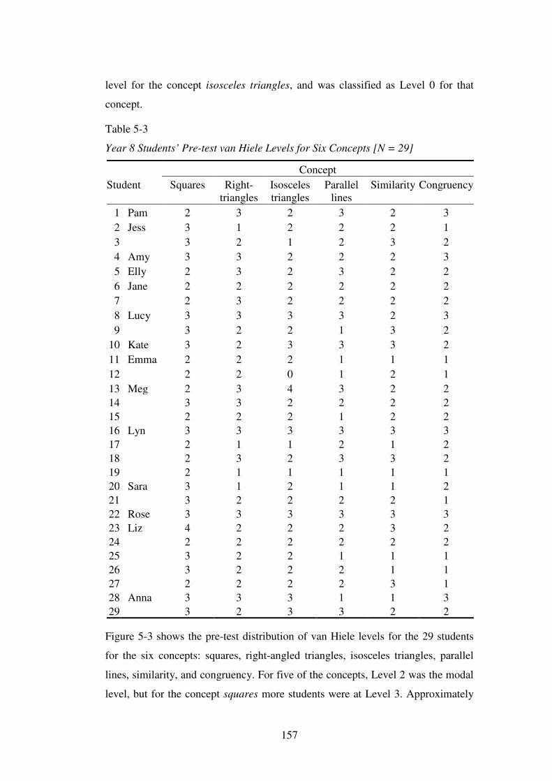
157
level for the concept isosceles triangles, and was classified as Level 0 for that
concept.
Table 5-3 Year 8 Students’ Pre-test van Hiele Levels for Six Concepts [N = 29]
Concept Student Squares Right-
triangles Isosceles triangles
Parallel lines
Similarity Congruency
1 Pam 2 3 2 3 2 3 2 Jess 3 1 2 2 2 1 3 3 2 1 2 3 2 4 Amy 3 3 2 2 2 3 5 Elly 2 3 2 3 2 2 6 Jane 2 2 2 2 2 2 7 2 3 2 2 2 2 8 Lucy 3 3 3 3 2 3 9 3 2 2 1 3 2
10 Kate 3 2 3 3 3 2 11 Emma 2 2 2 1 1 1 12 2 2 0 1 2 1 13 Meg 2 3 4 3 2 2 14 3 3 2 2 2 2 15 2 2 2 1 2 2 16 Lyn 3 3 3 3 3 3 17 2 1 1 2 1 2 18 2 3 2 3 3 2 19 2 1 1 1 1 1 20 Sara 3 1 2 1 1 2 21 3 2 2 2 2 1 22 Rose 3 3 3 3 3 3 23 Liz 4 2 2 2 3 2 24 2 2 2 2 2 2 25 3 2 2 1 1 1 26 3 2 2 2 1 1 27 2 2 2 2 3 1 28 Anna 3 3 3 1 1 3 29 3 2 3 3 2 2
Figure 5-3 shows the pre-test distribution of van Hiele levels for the 29 students
for the six concepts: squares, right-angled triangles, isosceles triangles, parallel
lines, similarity, and congruency. For five of the concepts, Level 2 was the modal
level, but for the concept squares more students were at Level 3. Approximately
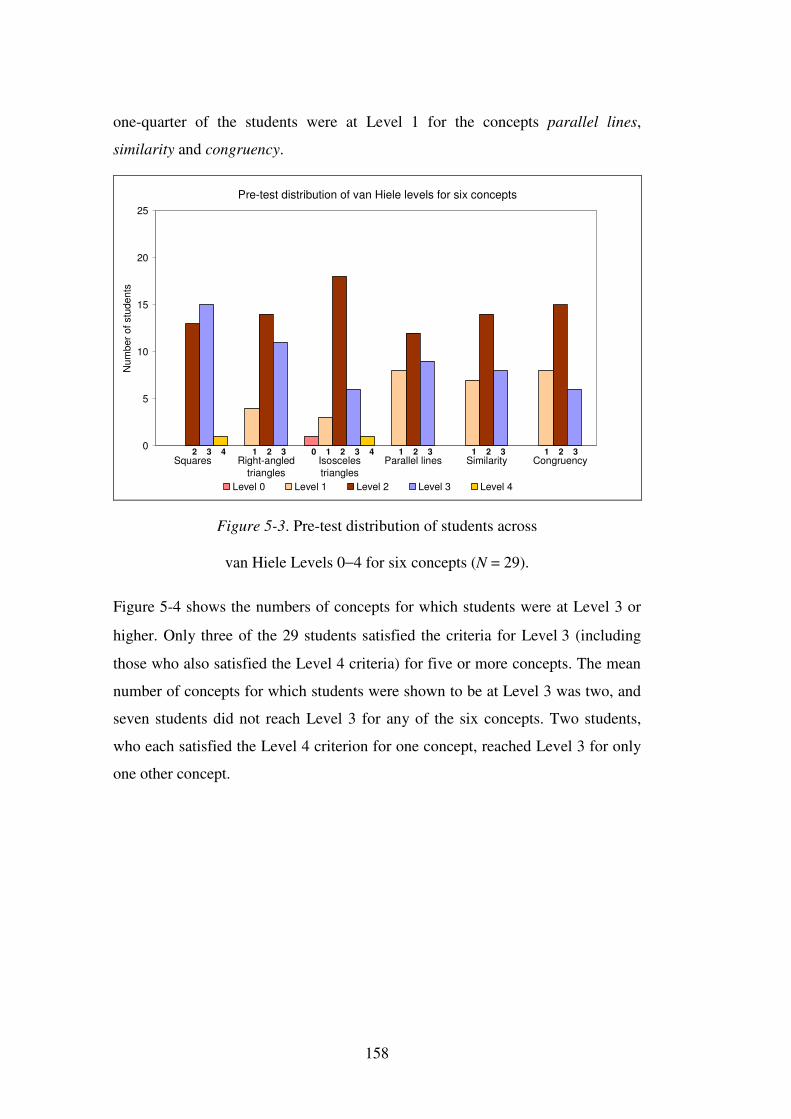
158
one-quarter of the students were at Level 1 for the concepts parallel lines,
similarity and congruency.
Pre-test distribution of van Hiele levels for six concepts
0
5
10
15
20
25
Squares Right-angledtriangles
Isoscelestriangles
Parallel lines Similarity Congruency
Num
ber o
f stu
dent
s
Level 0 Level 1 Level 2 Level 3 Level 4
2 3 4 1 2 3 1 2 3 1 2 3 0 1 2 3 4 1 2 3
Figure 5-3. Pre-test distribution of students across
van Hiele Levels 0−4 for six concepts (N = 29).
Figure 5-4 shows the numbers of concepts for which students were at Level 3 or
higher. Only three of the 29 students satisfied the criteria for Level 3 (including
those who also satisfied the Level 4 criteria) for five or more concepts. The mean
number of concepts for which students were shown to be at Level 3 was two, and
seven students did not reach Level 3 for any of the six concepts. Two students,
who each satisfied the Level 4 criterion for one concept, reached Level 3 for only
one other concept.
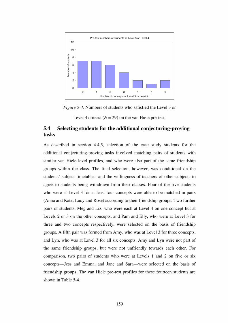
159
Pre-test numbers of students at Level 3 or Level 4
0
2
4
6
8
10
12
0 1 2 3 4 5 6
Number of concepts at Level 3 or Level 4
Num
ber o
f stu
dent
s
Figure 5-4. Numbers of students who satisfied the Level 3 or
Level 4 criteria (N = 29) on the van Hiele pre-test.
5.4 Selecting students for the additional conjecturing-proving tasks
As described in section 4.4.5, selection of the case study students for the
additional conjecturing-proving tasks involved matching pairs of students with
similar van Hiele level profiles, and who were also part of the same friendship
groups within the class. The final selection, however, was conditional on the
students’ subject timetables, and the willingness of teachers of other subjects to
agree to students being withdrawn from their classes. Four of the five students
who were at Level 3 for at least four concepts were able to be matched in pairs
(Anna and Kate; Lucy and Rose) according to their friendship groups. Two further
pairs of students, Meg and Liz, who were each at Level 4 on one concept but at
Levels 2 or 3 on the other concepts, and Pam and Elly, who were at Level 3 for
three and two concepts respectively, were selected on the basis of friendship
groups. A fifth pair was formed from Amy, who was at Level 3 for three concepts,
and Lyn, who was at Level 3 for all six concepts. Amy and Lyn were not part of
the same friendship groups, but were not unfriendly towards each other. For
comparison, two pairs of students who were at Levels 1 and 2 on five or six
concepts—Jess and Emma, and Jane and Sara—were selected on the basis of
friendship groups. The van Hiele pre-test profiles for these fourteen students are
shown in Table 5-4.
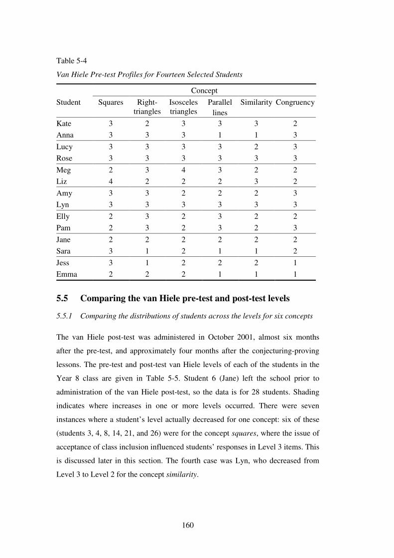
160
Table 5-4
Van Hiele Pre-test Profiles for Fourteen Selected Students
Concept Student Squares Right-
triangles Isosceles triangles
Parallel lines
Similarity Congruency
Kate 3 2 3 3 3 2 Anna 3 3 3 1 1 3 Lucy 3 3 3 3 2 3 Rose 3 3 3 3 3 3 Meg 2 3 4 3 2 2 Liz 4 2 2 2 3 2 Amy 3 3 2 2 2 3 Lyn 3 3 3 3 3 3 Elly 2 3 2 3 2 2 Pam 2 3 2 3 2 3 Jane 2 2 2 2 2 2 Sara 3 1 2 1 1 2 Jess 3 1 2 2 2 1 Emma 2 2 2 1 1 1
5.5 Comparing the van Hiele pre-test and post-test levels
5.5.1 Comparing the distributions of students across the levels for six concepts
The van Hiele post-test was administered in October 2001, almost six months
after the pre-test, and approximately four months after the conjecturing-proving
lessons. The pre-test and post-test van Hiele levels of each of the students in the
Year 8 class are given in Table 5-5. Student 6 (Jane) left the school prior to
administration of the van Hiele post-test, so the data is for 28 students. Shading
indicates where increases in one or more levels occurred. There were seven
instances where a student’s level actually decreased for one concept: six of these
(students 3, 4, 8, 14, 21, and 26) were for the concept squares, where the issue of
acceptance of class inclusion influenced students’ responses in Level 3 items. This
is discussed later in this section. The fourth case was Lyn, who decreased from
Level 3 to Level 2 for the concept similarity.
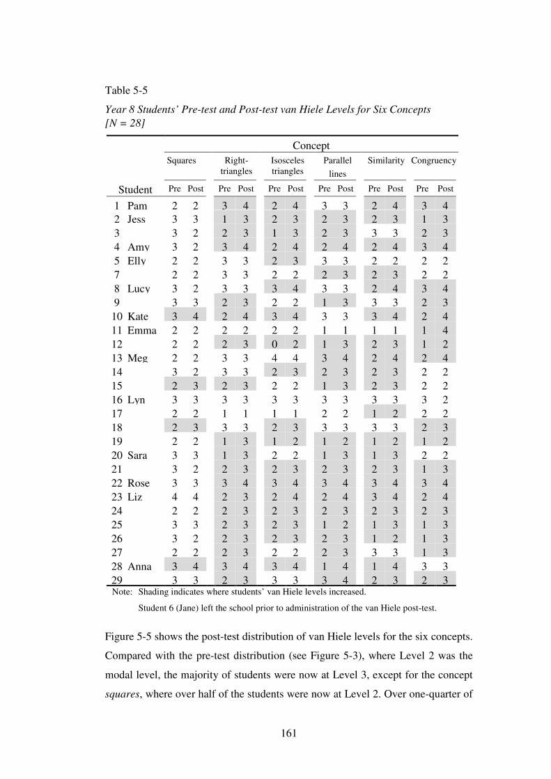
161
Table 5-5 Year 8 Students’ Pre-test and Post-test van Hiele Levels for Six Concepts [N = 28]
Concept Squares Right-
triangles Isosceles triangles
Parallel lines
Similarity Congruency
Student Pre Post Pre Post Pre Post Pre Post Pre Post Pre Post
1 Pam 2 2 3 4 2 4 3 3 2 4 3 4 2 Jess 3 3 1 3 2 3 2 3 2 3 1 3 3 3 2 2 3 1 3 2 3 3 3 2 3 4 Amy 3 2 3 4 2 4 2 4 2 4 3 4 5 Elly 2 2 3 3 2 3 3 3 2 2 2 2 7 2 2 3 3 2 2 2 3 2 3 2 2 8 Lucy 3 2 3 3 3 4 3 3 2 4 3 4 9 3 3 2 3 2 2 1 3 3 3 2 3
10 Kate 3 4 2 4 3 4 3 3 3 4 2 4 11 Emma 2 2 2 2 2 2 1 1 1 1 1 4 12 2 2 2 3 0 2 1 3 2 3 1 2 13 Meg 2 2 3 3 4 4 3 4 2 4 2 4 14 3 2 3 3 2 3 2 3 2 3 2 2 15 2 3 2 3 2 2 1 3 2 3 2 2 16 Lyn 3 3 3 3 3 3 3 3 3 3 3 2 17 2 2 1 1 1 1 2 2 1 2 2 2 18 2 3 3 3 2 3 3 3 3 3 2 3 19 2 2 1 3 1 2 1 2 1 2 1 2 20 Sara 3 3 1 3 2 2 1 3 1 3 2 2 21 3 2 2 3 2 3 2 3 2 3 1 3 22 Rose 3 3 3 4 3 4 3 4 3 4 3 4 23 Liz 4 4 2 3 2 4 2 4 3 4 2 4 24 2 2 2 3 2 3 2 3 2 3 2 3 25 3 3 2 3 2 3 1 2 1 3 1 3 26 3 2 2 3 2 3 2 3 1 2 1 3 27 2 2 2 3 2 2 2 3 3 3 1 3 28 Anna 3 4 3 4 3 4 1 4 1 4 3 3 29 3 3 2 3 3 3 3 4 2 3 2 3
Note: Shading indicates where students’ van Hiele levels increased.
Student 6 (Jane) left the school prior to administration of the van Hiele post-test.
Figure 5-5 shows the post-test distribution of van Hiele levels for the six concepts.
Compared with the pre-test distribution (see Figure 5-3), where Level 2 was the
modal level, the majority of students were now at Level 3, except for the concept
squares, where over half of the students were now at Level 2. Over one-quarter of
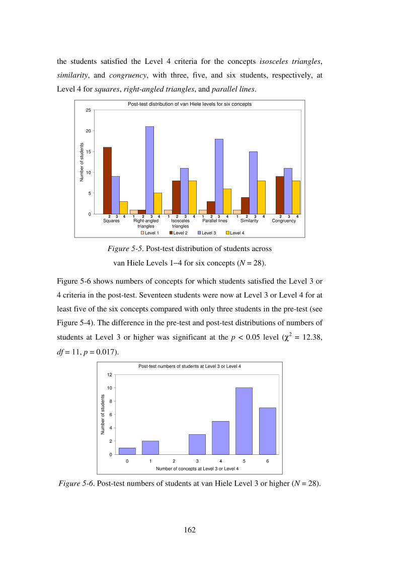
162
the students satisfied the Level 4 criteria for the concepts isosceles triangles,
similarity, and congruency, with three, five, and six students, respectively, at
Level 4 for squares, right-angled triangles, and parallel lines.
Post-test distribution of van Hiele levels for six concepts
0
5
10
15
20
25
Squares Right-angledtriangles
Isoscelestriangles
Parallel lines Similarity Congruency
Num
ber o
f stu
dent
s
Level 1 Level 2 Level 3 Level 4
2 3 4 2 3 4 1 2 3 4 1 2 3 4 1 2 3 4 1 2 3 4
Figure 5-5. Post-test distribution of students across
van Hiele Levels 1−4 for six concepts (N = 28).
Figure 5-6 shows numbers of concepts for which students satisfied the Level 3 or
4 criteria in the post-test. Seventeen students were now at Level 3 or Level 4 for at
least five of the six concepts compared with only three students in the pre-test (see
Figure 5-4). The difference in the pre-test and post-test distributions of numbers of
students at Level 3 or higher was significant at the p < 0.05 level (χ2 = 12.38,
df = 11, p = 0.017).
Post-test numbers of students at Level 3 or Level 4
0
2
4
6
8
10
12
0 1 2 3 4 5 6
Number of concepts at Level 3 or Level 4
Num
ber o
f stu
dent
s
Figure 5-6. Post-test numbers of students at van Hiele Level 3 or higher (N = 28).
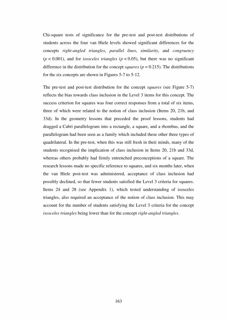
163
Chi-square tests of significance for the pre-test and post-test distributions of
students across the four van Hiele levels showed significant differences for the
concepts right-angled triangles, parallel lines, similarity, and congruency
(p < 0.001), and for isosceles triangles (p < 0.05), but there was no significant
difference in the distribution for the concept squares (p = 0.215). The distributions
for the six concepts are shown in Figures 5-7 to 5-12.
The pre-test and post-test distribution for the concept squares (see Figure 5-7)
reflects the bias towards class inclusion in the Level 3 items for this concept. The
success criterion for squares was four correct responses from a total of six items,
three of which were related to the notion of class inclusion (Items 20, 21b, and
33d). In the geometry lessons that preceded the proof lessons, students had
dragged a Cabri parallelogram into a rectangle, a square, and a rhombus, and the
parallelogram had been seen as a family which included these other three types of
quadrilateral. In the pre-test, when this was still fresh in their minds, many of the
students recognised the implication of class inclusion in Items 20, 21b and 33d,
whereas others probably had firmly entrenched preconceptions of a square. The
research lessons made no specific reference to squares, and six months later, when
the van Hiele post-test was administered, acceptance of class inclusion had
possibly declined, so that fewer students satisfied the Level 3 criteria for squares.
Items 24 and 28 (see Appendix 1), which tested understanding of isosceles
triangles, also required an acceptance of the notion of class inclusion. This may
account for the number of students satisfying the Level 3 criteria for the concept
isosceles triangles being lower than for the concept right-angled triangles.
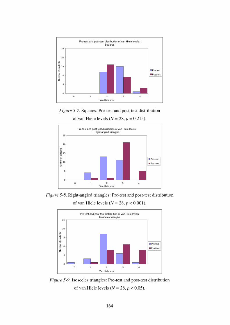
164
Pre-test and post-test distribution of van Hiele levels: Squares
0
5
10
15
20
25
0 1 2 3 4
Van Hiele level
Num
ber o
f stu
dent
s
Pre-test
Post-test
Figure 5-7. Squares: Pre-test and post-test distribution
of van Hiele levels (N = 28, p = 0.215).
Pre-test and post-test distribution of van Hiele levels: Right-angled triangles
0
5
10
15
20
25
0 1 2 3 4Van Hiele level
Num
ber o
f stu
dent
s
Pre-test
Post-test
Figure 5-8. Right-angled triangles: Pre-test and post-test distribution
of van Hiele levels (N = 28, p < 0.001).
Pre-test and post-test distribution of van Hiele levels: Isosceles triangles
0
5
10
15
20
25
0 1 2 3 4
Van Hiele level
Num
ber o
f stu
dent
s
Pre-test
Post-test
Figure 5-9. Isosceles triangles: Pre-test and post-test distribution
of van Hiele levels (N = 28, p < 0.05).
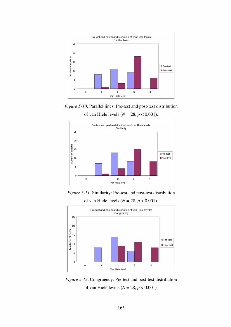
165
Pre-test and post-test distribution of van Hiele levels: Parallel lines
0
5
10
15
20
25
0 1 2 3 4
Van Hiele level
Num
ber
of s
tude
nts
Pre-test
Post-test
Figure 5-10. Parallel lines: Pre-test and post-test distribution
of van Hiele levels (N = 28, p < 0.001).
Pre-test and post-test distribution of van Hiele levels: Similarity
0
5
10
15
20
25
0 1 2 3 4
Van Hiele level
Num
ber o
f stu
dent
s
Pre-test
Post-test
Figure 5-11. Similarity: Pre-test and post-test distribution
of van Hiele levels (N = 28, p < 0.001).
Pre-test and post-test distribution of van Hiele levels: Congruency
0
5
10
15
20
25
0 1 2 3 4
Van Hiele level
Num
ber o
f stu
dent
s
Pre-test
Post-test
Figure 5-12. Congruency: Pre-test and post-test distribution
of van Hiele levels (N = 28, p < 0.001).
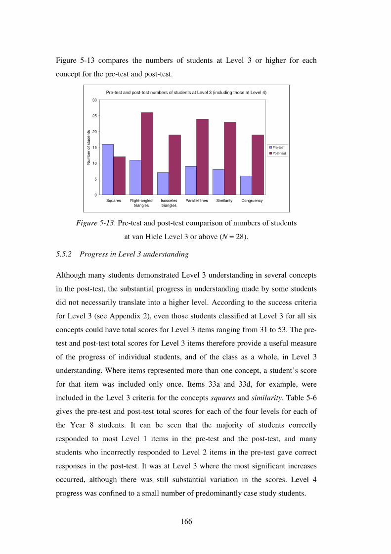
166
Figure 5-13 compares the numbers of students at Level 3 or higher for each
concept for the pre-test and post-test.
Pre-test and post-test numbers of students at Level 3 (including those at Level 4)
0
5
10
15
20
25
30
Squares Right-angledtriangles
Isoscelestriangles
Parallel lines Similarity Congruency
Num
ber
of s
tude
nts
Pre-test
Post-test
Figure 5-13. Pre-test and post-test comparison of numbers of students
at van Hiele Level 3 or above (N = 28).
5.5.2 Progress in Level 3 understanding
Although many students demonstrated Level 3 understanding in several concepts
in the post-test, the substantial progress in understanding made by some students
did not necessarily translate into a higher level. According to the success criteria
for Level 3 (see Appendix 2), even those students classified at Level 3 for all six
concepts could have total scores for Level 3 items ranging from 31 to 53. The pre-
test and post-test total scores for Level 3 items therefore provide a useful measure
of the progress of individual students, and of the class as a whole, in Level 3
understanding. Where items represented more than one concept, a student’s score
for that item was included only once. Items 33a and 33d, for example, were
included in the Level 3 criteria for the concepts squares and similarity. Table 5-6
gives the pre-test and post-test total scores for each of the four levels for each of
the Year 8 students. It can be seen that the majority of students correctly
responded to most Level 1 items in the pre-test and the post-test, and many
students who incorrectly responded to Level 2 items in the pre-test gave correct
responses in the post-test. It was at Level 3 where the most significant increases
occurred, although there was still substantial variation in the scores. Level 4
progress was confined to a small number of predominantly case study students.
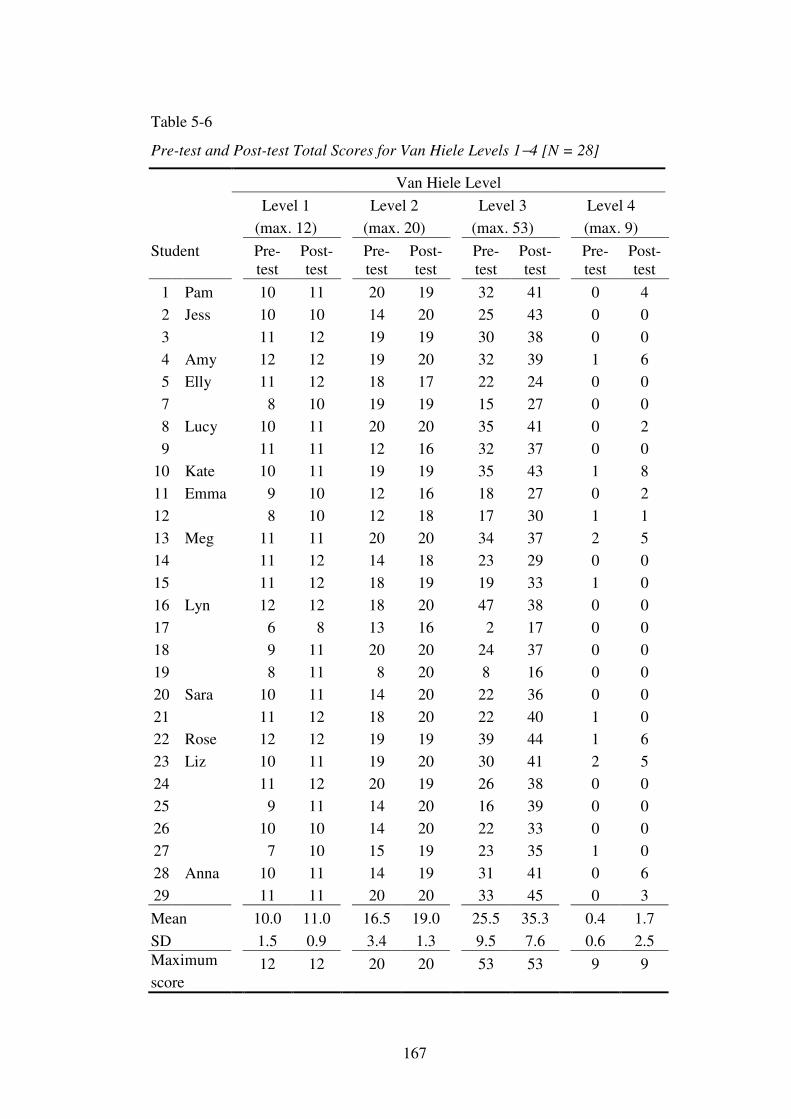
167
Table 5-6
Pre-test and Post-test Total Scores for Van Hiele Levels 1−4 [N = 28]
Van Hiele Level Level 1
(max. 12) Level 2
(max. 20) Level 3
(max. 53) Level 4 (max. 9)
Student Pre-test
Post-test
Pre-test
Post-test
Pre-test
Post-test
Pre-test
Post-test
1 Pam 10 11 20 19 32 41 0 4 2 Jess 10 10 14 20 25 43 0 0 3 11 12 19 19 30 38 0 0 4 Amy 12 12 19 20 32 39 1 6 5 Elly 11 12 18 17 22 24 0 0 7 8 10 19 19 15 27 0 0 8 Lucy 10 11 20 20 35 41 0 2 9 11 11 12 16 32 37 0 0
10 Kate 10 11 19 19 35 43 1 8 11 Emma 9 10 12 16 18 27 0 2 12 8 10 12 18 17 30 1 1 13 Meg 11 11 20 20 34 37 2 5 14 11 12 14 18 23 29 0 0 15 11 12 18 19 19 33 1 0 16 Lyn 12 12 18 20 47 38 0 0 17 6 8 13 16 2 17 0 0 18 9 11 20 20 24 37 0 0 19 8 11 8 20 8 16 0 0 20 Sara 10 11 14 20 22 36 0 0 21 11 12 18 20 22 40 1 0 22 Rose 12 12 19 19 39 44 1 6 23 Liz 10 11 19 20 30 41 2 5 24 11 12 20 19 26 38 0 0 25 9 11 14 20 16 39 0 0 26 10 10 14 20 22 33 0 0 27 7 10 15 19 23 35 1 0 28 Anna 10 11 14 19 31 41 0 6 29 11 11 20 20 33 45 0 3 Mean 10.0 11.0 16.5 19.0 25.5 35.3 0.4 1.7 SD 1.5 0.9 3.4 1.3 9.5 7.6 0.6 2.5 Maximum score
12 12 20 20 53 53 9 9
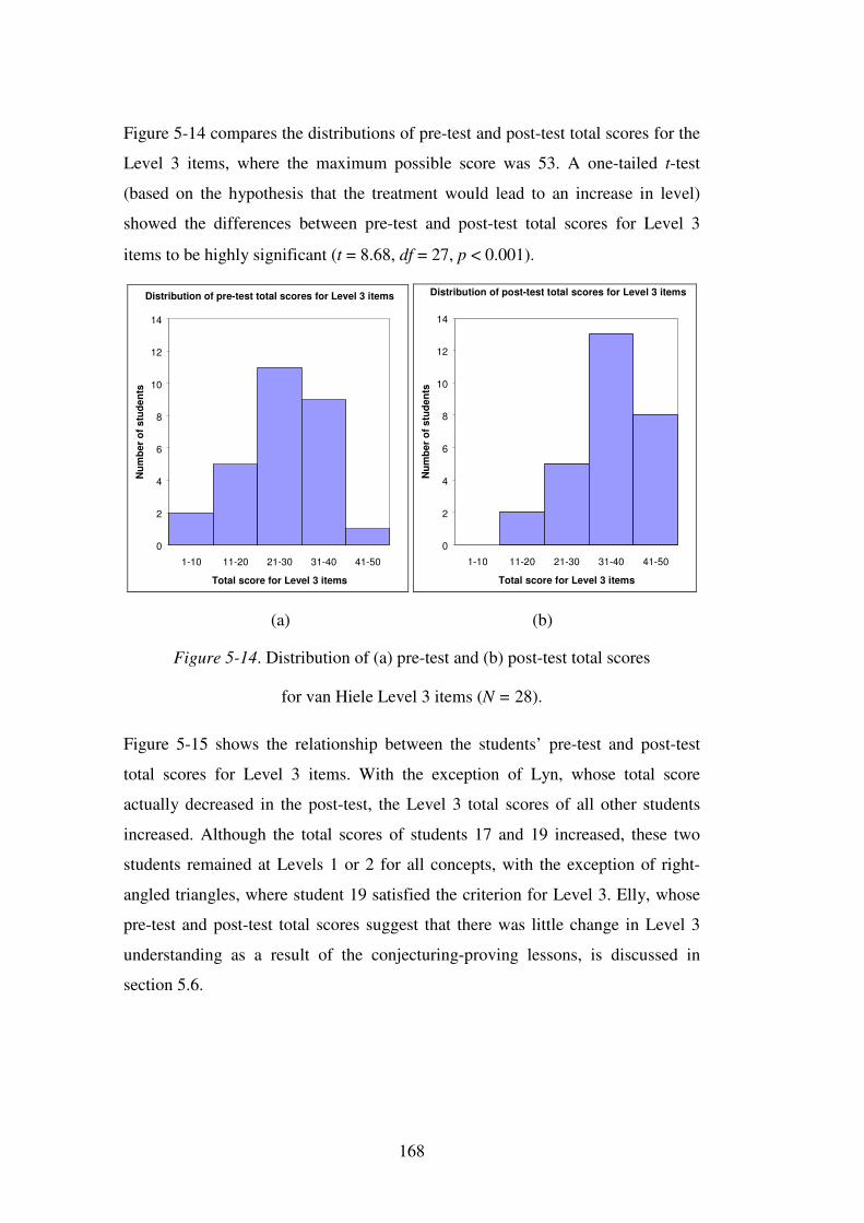
168
Figure 5-14 compares the distributions of pre-test and post-test total scores for the
Level 3 items, where the maximum possible score was 53. A one-tailed t-test
(based on the hypothesis that the treatment would lead to an increase in level)
showed the differences between pre-test and post-test total scores for Level 3
items to be highly significant (t = 8.68, df = 27, p < 0.001).
Distribution of pre-test total scores for Level 3 items
0
2
4
6
8
10
12
14
1-10 11-20 21-30 31-40 41-50
Total score for Level 3 items
Num
ber
of s
tude
nts
Distribution of post-test total scores for Level 3 items
0
2
4
6
8
10
12
14
1-10 11-20 21-30 31-40 41-50
Total score for Level 3 items
Num
ber
of s
tude
nts
(a) (b)
Figure 5-14. Distribution of (a) pre-test and (b) post-test total scores
for van Hiele Level 3 items (N = 28).
Figure 5-15 shows the relationship between the students’ pre-test and post-test
total scores for Level 3 items. With the exception of Lyn, whose total score
actually decreased in the post-test, the Level 3 total scores of all other students
increased. Although the total scores of students 17 and 19 increased, these two
students remained at Levels 1 or 2 for all concepts, with the exception of right-
angled triangles, where student 19 satisfied the criterion for Level 3. Elly, whose
pre-test and post-test total scores suggest that there was little change in Level 3
understanding as a result of the conjecturing-proving lessons, is discussed in
section 5.6.
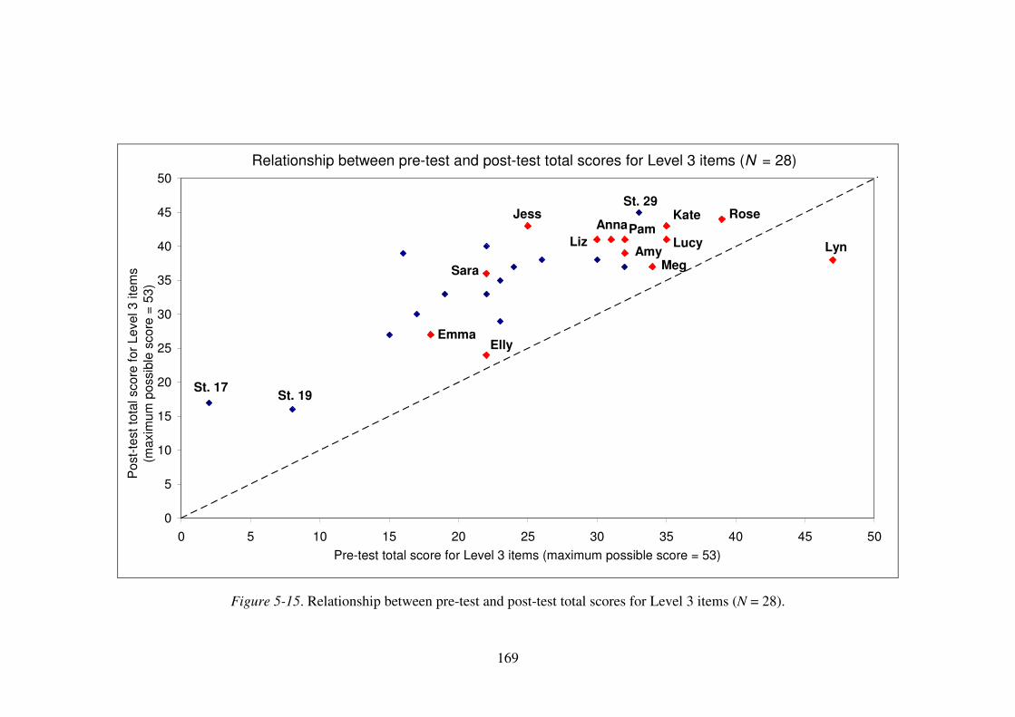
169
Relationship between pre-test and post-test total scores for Level 3 items (N = 28)
0
5
10
15
20
25
30
35
40
45
50
0 5 10 15 20 25 30 35 40 45 50Pre-test total score for Level 3 items (maximum possible score = 53)
Pos
t-tes
t tot
al s
core
for L
evel
3 it
ems
(max
imum
pos
sibl
e sc
ore
= 53
)
Elly
Anna
Meg
Lucy
Rose
Sara
PamLiz
KateJess
Emma
LynAmy
St. 29
St. 17St. 19
Figure 5-15. Relationship between pre-test and post-test total scores for Level 3 items (N = 28).
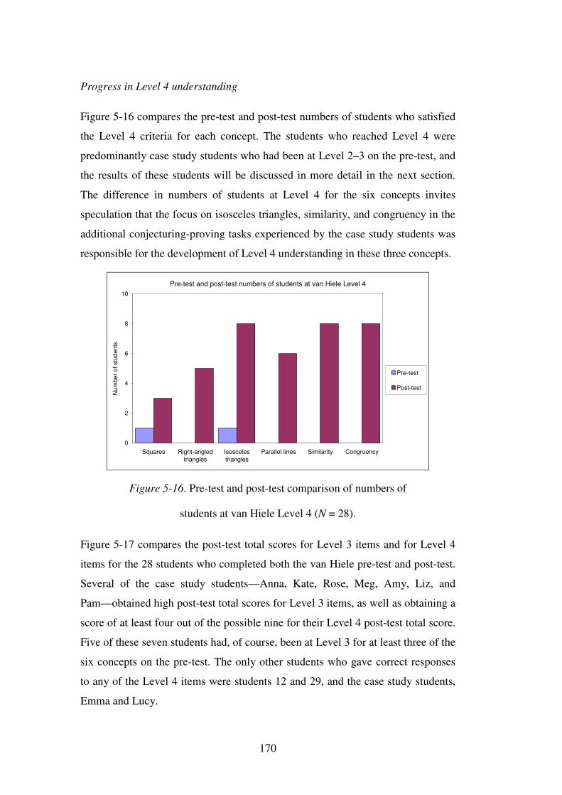
170
Progress in Level 4 understanding
Figure 5-16 compares the pre-test and post-test numbers of students who satisfied
the Level 4 criteria for each concept. The students who reached Level 4 were
predominantly case study students who had been at Level 2–3 on the pre-test, and
the results of these students will be discussed in more detail in the next section.
The difference in numbers of students at Level 4 for the six concepts invites
speculation that the focus on isosceles triangles, similarity, and congruency in the
additional conjecturing-proving tasks experienced by the case study students was
responsible for the development of Level 4 understanding in these three concepts.
Pre-test and post-test numbers of students at van Hiele Level 4
0
2
4
6
8
10
Squares Right-angledtriangles
Isoscelestriangles
Parallel lines Similarity Congruency
Num
ber o
f stu
dent
s
Pre-test
Post-test
Figure 5-16. Pre-test and post-test comparison of numbers of
students at van Hiele Level 4 (N = 28).
Figure 5-17 compares the post-test total scores for Level 3 items and for Level 4
items for the 28 students who completed both the van Hiele pre-test and post-test.
Several of the case study students—Anna, Kate, Rose, Meg, Amy, Liz, and
Pam—obtained high post-test total scores for Level 3 items, as well as obtaining a
score of at least four out of the possible nine for their Level 4 post-test total score.
Five of these seven students had, of course, been at Level 3 for at least three of the
six concepts on the pre-test. The only other students who gave correct responses
to any of the Level 4 items were students 12 and 29, and the case study students,
Emma and Lucy.
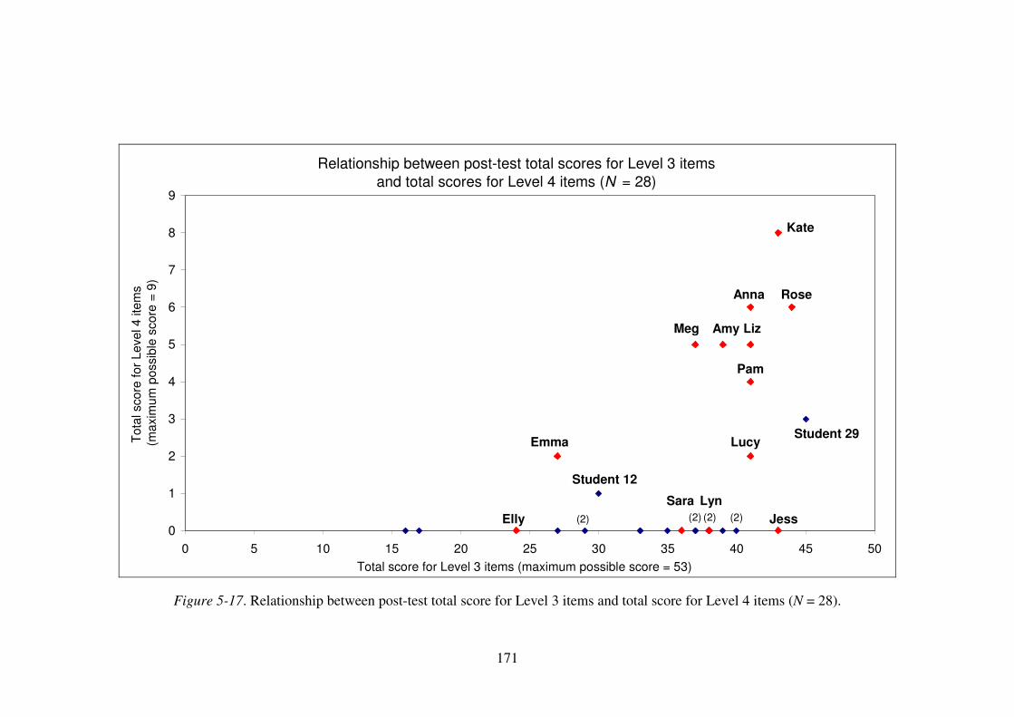
171
Relationship between post-test total scores for Level 3 items and total scores for Level 4 items (N = 28)
0
1
2
3
4
5
6
7
8
9
0 5 10 15 20 25 30 35 40 45 50Total score for Level 3 items (maximum possible score = 53)
Tota
l sco
re fo
r Lev
el 4
item
s (m
axim
um p
ossi
ble
scor
e =
9)
Liz
Anna
Kate
Meg
Rose
Pam
LucyEmma
Amy
EllySara
Jess(2)(2) (2)Lyn
(2)
Student 29
Student 12
Figure 5-17. Relationship between post-test total score for Level 3 items and total score for Level 4 items (N = 28).
172
5.6 The case study students
Five of the nine case study students who initially had been at Level 2–3 for at
least three concepts—Anna, Kate, Rose, Liz, and Amy—now satisfied the Level 4
criteria for five of the six concepts. In addition, Meg was now at Level 4 for four
concepts, and Pam and Lucy were at Level 4 for three concepts. It seems
reasonable to conclude that engagement in the conjecturing-proving
argumentations provided the opportunity for the development of deductive
reasoning. Of the case study students who had initially been at Level 3 for at least
three of the concepts, Lyn was the only student who did not progress to Level 4
for any concepts. Although Lyn received the highest pre-test total score for Level
3 items in the class of 29 students, her post-test total score for Level 3 items was
lower than her pre-test total score, and she did not answer any of the Level 4
items. Lyn completed only one additional conjecturing-proving task—the pencil-
and-paper Joining Midpoints task—in which she made no attempt to engage in
argumentation with her partner, Amy (see section 7.3.4). Lyn’s lack of motivation
appeared to be unrelated to the tasks, and attributable to circumstances beyond
school.
Three of the case study students—Elly, Jess, and Sara—did not satisfy the Level 4
criteria for any concepts. Jess and Sara had been at Level 1–2 for all concepts on
the pre-test. Sara did progress, however, from Level 1 to Level 3 for three
concepts, with a substantial increase in her total score for Level 3 items, and this
progress in understanding of properties and relationships was evident during the
argumentations. Jess, who also commenced at Level 1 or 2 for most concepts,
now satisfied the Level 3 criteria for all concepts, progressing two levels for the
concepts right-angled triangles and congruency. Elly’s slow, meticulous approach
to her written responses, and her fear of making mistakes, meant that she did not
complete many of the test items, but her lack of confidence with properties and
relationships was also a handicap. However, Elly scored well for questions G4
and G7 on the Proof Questionnaire post-test, indicating that she had grasped the
essential features of a deductive argument.
173
Emma, whose pre-test levels remained unchanged at Level 1 or Level 2 for five of
the six concepts, surprisingly satisfied both the Level 3 and Level 4 criteria for
Congruency on the post-test. It is perhaps significant that the only additional
conjecturing-proving task completed by Emma was the Enlarging Pantograph,
where her proof involved congruent triangles (see Figures 7-24 and 7-25). Even
though Emma had struggled at first with this task, she seemed to have acquired an
understanding of the concept of congruency.
5.7 Conclusion
The majority of students made considerable progress in geometric understanding
across the six concepts tested. Although this was not always apparent in the
students’ post-test levels, a comparison of total scores for items at each level
revealed substantial increases for many students, particularly at Level 3. Although
it could be argued that using the same test for pre-test and post-test contributed to
the increase in scores, it should be remembered that the students had no feedback
on their pre-test responses, and the post-test was administered six months after the
pre-test, and approximately four months after completion of the conjecturing-
proving lessons (see section 4.4.4).
For the students who commenced at lower van Hiele levels—that is, students who
were initially at Levels 1 or 2 for most concepts—the sequence of conjecturing-
proving tasks appeared to play a significant part in increasing their understanding
of geometric properties and relationships. However, satisfying the Level 4 criteria
on the van Hiele test was largely confined to case study students who were
initially at Levels 2 or 3 for at least half of the six concepts. At the conclusion of
the study, eight of the 28 students in the Year 8 class were assessed at van Hiele
Level 4 for three or more concepts. These eight students were all case study
students, and, with the exception of Amy, they had all completed at least three
additional conjecturing-proving tasks. Only one non-case study student
progressed to Level 4: student 29 satisfied the Level 4 criterion for the concept
parallel lines. It would be reasonable to assume, then, that the additional
conjecturing-proving tasks were successful in developing the students’
understanding of deductive reasoning.
174
On the other hand, the conjecturing-proving tasks showed that even those students
with lower levels of geometric understanding were capable of deductive
reasoning, suggesting that the Level 4 items on the van Hiele test were inadequate
in providing students with the opportunity to demonstrate their reasoning ability.
This represents a criticism of the van Hiele theory, which focuses on end products
of students’ understanding, rather than on the cognitive processes which lead to
those end products; whereas the van Hiele pre-test and post-test data were useful
in identifying individual differences and changes in the students’ understanding of
properties and relationships, the post-test results did not reflect the substantial
progress in deductive reasoning demonstrated by many students in the
conjecturing-proving tasks and the post-test Proof Questionnaire responses. The
performance of these students will be examined in the following chapters.
175
Chapter 6: A Case Study of Two Students
We had fallen into the habit of thinking of the child as an ‘active scientist’,
constructing hypotheses about the world, reflecting upon experience, interacting
with the physical environment and formulating increasingly complex structures of
thought. But this active, constructing child had been conceived as a rather isolated
being, working alone at her problem-solving. Increasingly we see now that, given an
appropriate, shared social context, the child seems more competent as an intelligent
social operator than she is as a ‘lone scientist’ coping with a world of unknowns.
(Bruner & Haste, 1987, p. 1)
6.1 Introduction
6.1.1 How the case study addresses the research questions
A detailed analysis of the progress made by one pair of students on a variety of
tasks is used to examine how successfully a culture of geometric conjecturing and
proving was established for these Year 8 students. The case study also addresses
the issues of whether the dynamic contexts of mechanical linkages and dynamic
geometry software motivate students to engage in geometric argumentation, and
whether the feedback from these dynamic contexts supports conjecturing and
deductive reasoning. Of further interest is the potential for dynamic geometry
software to satisfy students’ need for convincing, thereby removing their cognitive
need for proof. This chapter focuses on two students, Anna and Kate, who had
reached Level 3 on four of the six concepts measured by the van Hiele pre-test
(see section 6.1.2, Table 6-1). Section 6.1 discusses the selection of Anna and
Kate as case study students, and their responses in the introductory whole-class
lessons. Section 6.2 provides an analysis of each of the seven additional
conjecturing-proving tasks completed by Anna and Kate. Section 6.3 considers
Anna and Kate’s argumentations in terms of the research questions.
6.1.2 Selection of the case study students
As described in chapter 5, the selection of students for the case study interview
tasks focused initially on students who had satisfied the Level 3 criteria for at least
three of the six concepts: squares, right-angled triangles, isosceles triangles,
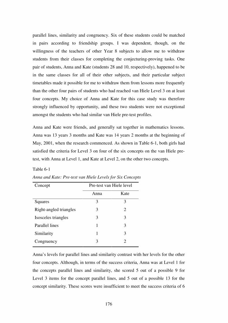
176
parallel lines, similarity and congruency. Six of these students could be matched
in pairs according to friendship groups. I was dependent, though, on the
willingness of the teachers of other Year 8 subjects to allow me to withdraw
students from their classes for completing the conjecturing-proving tasks. One
pair of students, Anna and Kate (students 28 and 10, respectively), happened to be
in the same classes for all of their other subjects, and their particular subject
timetables made it possible for me to withdraw them from lessons more frequently
than the other four pairs of students who had reached van Hiele Level 3 on at least
four concepts. My choice of Anna and Kate for this case study was therefore
strongly influenced by opportunity, and these two students were not exceptional
amongst the students who had similar van Hiele pre-test profiles.
Anna and Kate were friends, and generally sat together in mathematics lessons.
Anna was 13 years 3 months and Kate was 14 years 2 months at the beginning of
May, 2001, when the research commenced. As shown in Table 6-1, both girls had
satisfied the criteria for Level 3 on four of the six concepts on the van Hiele pre-
test, with Anna at Level 1, and Kate at Level 2, on the other two concepts.
Table 6-1
Anna and Kate: Pre-test van Hiele Levels for Six Concepts
Concept Pre-test van Hiele level
Anna Kate
Squares 3 3
Right-angled triangles 3 2
Isosceles triangles 3 3
Parallel lines 1 3
Similarity 1 3
Congruency 3 2
Anna’s levels for parallel lines and similarity contrast with her levels for the other
four concepts. Although, in terms of the success criteria, Anna was at Level 1 for
the concepts parallel lines and similarity, she scored 5 out of a possible 9 for
Level 3 items for the concept parallel lines, and 5 out of a possible 13 for the
concept similarity. These scores were insufficient to meet the success criteria of 6
177
out of 9 and 8 out of 13, respectively, for parallel lines and similarity. Her Level 2
responses, for which she scored 0/2 for parallel lines and 2/4 for similarity, did not
meet the respective success criteria of 2/2 and 3/4 for the two concepts.
6.1.3 The introductory whole-class lessons
The case study commences with the introductory whole-class lessons (see
Appendix 4), where an analysis of the worksheet responses of Anna and Kate
provides the background against which the analysis of their subsequent interview
tasks is set. As noted in section 6.1.2, Anna and Kate generally sat together in
mathematics lessons. Their partnership in the introductory whole-class lessons
was therefore a natural partnership, and not a consequence of them having been
selected as a case study pair. Anna and Kate usually recorded their responses to
worksheet questions independently, and sometimes the responses of both students
have been included in the analysis. On other occasions, where Anna and Kate
produced a collaborative response, to avoid repetition only one students’ response
has been included. Anna and Kate’s responses in the following whole-class tasks
indicate that the two students, particularly Anna, did not always recognise
geometric properties and relationships, and sometimes made naïve observations of
the shape or movement of the linkage.
Rhombus linkage (see Appendix 4, A4.1)
There was a striking difference between the two students’ representations of the
rhombus linkage (see Figure 6-1). Anna was focusing on the changing shape of
the rhombuses, whereas Kate accurately depicted the invariant properties of
parallel, equal length links, as well as the changing shape of the rhombuses. These
drawings, and Anna’s and Kate’s written descriptions of the rhombus linkages
(see Figure 6-2), may be compared with observations made by Piaget and Inhelder
(1956) of children of different ages opening and closing a set of ‘lazy tongs’ (see
section 3.2.3). Piaget and Inhelder claimed that 10–12 year-old children (Stage
IIIB–Stage IV in Piaget’s stages) could recognise and make explicit the parallel
relationship of the sides of the rhombus, coinciding with their recognition that the
angles could change even though the sides remained the same lengths. Both Anna
and Kate referred to the shapes of the rhombuses rather than relationships
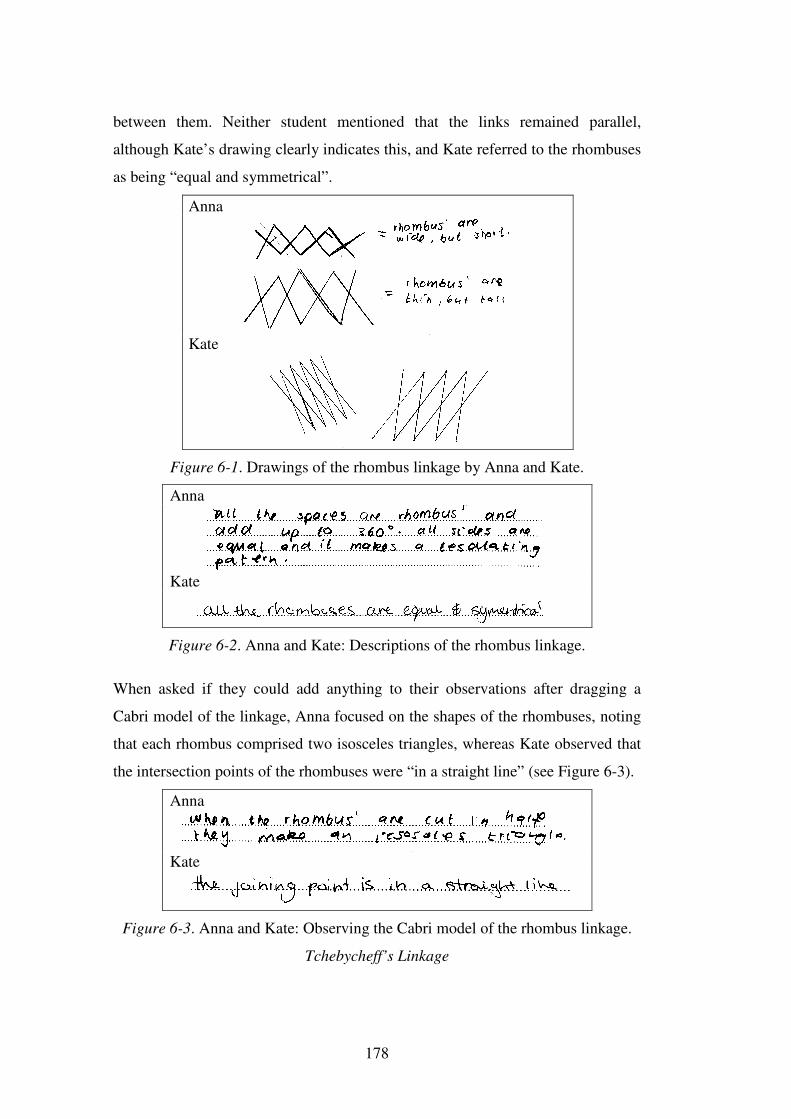
178
between them. Neither student mentioned that the links remained parallel,
although Kate’s drawing clearly indicates this, and Kate referred to the rhombuses
as being “equal and symmetrical”.
Anna
Kate
Figure 6-1. Drawings of the rhombus linkage by Anna and Kate.
Anna
Kate
Figure 6-2. Anna and Kate: Descriptions of the rhombus linkage.
When asked if they could add anything to their observations after dragging a
Cabri model of the linkage, Anna focused on the shapes of the rhombuses, noting
that each rhombus comprised two isosceles triangles, whereas Kate observed that
the intersection points of the rhombuses were “in a straight line” (see Figure 6-3).
Anna
Kate
Figure 6-3. Anna and Kate: Observing the Cabri model of the rhombus linkage.
Tchebycheff’s Linkage
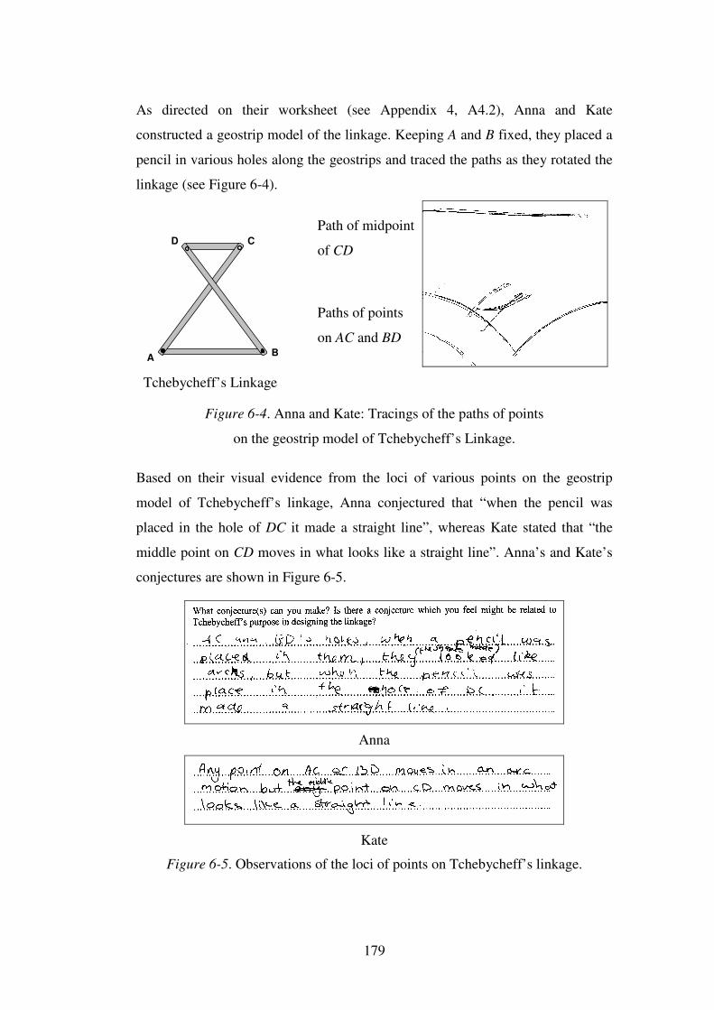
179
As directed on their worksheet (see Appendix 4, A4.2), Anna and Kate
constructed a geostrip model of the linkage. Keeping A and B fixed, they placed a
pencil in various holes along the geostrips and traced the paths as they rotated the
linkage (see Figure 6-4).
D
A B
C
Tchebycheff’s Linkage
Figure 6-4. Anna and Kate: Tracings of the paths of points
on the geostrip model of Tchebycheff’s Linkage.
Based on their visual evidence from the loci of various points on the geostrip
model of Tchebycheff’s linkage, Anna conjectured that “when the pencil was
placed in the hole of DC it made a straight line”, whereas Kate stated that “the
middle point on CD moves in what looks like a straight line”. Anna’s and Kate’s
conjectures are shown in Figure 6-5.
Anna
Kate
Figure 6-5. Observations of the loci of points on Tchebycheff’s linkage.
Path of midpoint
of CD
Paths of points
on AC and BD
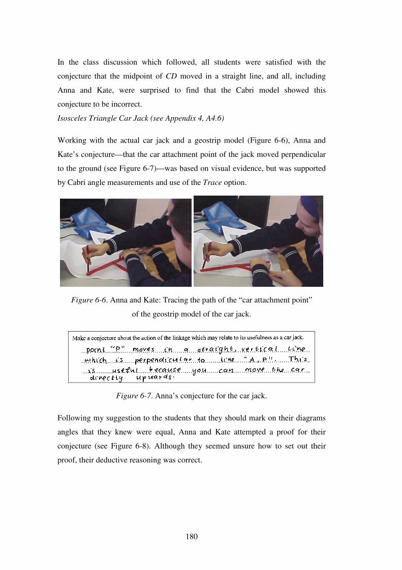
180
In the class discussion which followed, all students were satisfied with the
conjecture that the midpoint of CD moved in a straight line, and all, including
Anna and Kate, were surprised to find that the Cabri model showed this
conjecture to be incorrect.
Isosceles Triangle Car Jack (see Appendix 4, A4.6)
Working with the actual car jack and a geostrip model (Figure 6-6), Anna and
Kate’s conjecture—that the car attachment point of the jack moved perpendicular
to the ground (see Figure 6-7)—was based on visual evidence, but was supported
by Cabri angle measurements and use of the Trace option.
Figure 6-6. Anna and Kate: Tracing the path of the “car attachment point”
of the geostrip model of the car jack.
Figure 6-7. Anna’s conjecture for the car jack.
Following my suggestion to the students that they should mark on their diagrams
angles that they knew were equal, Anna and Kate attempted a proof for their
conjecture (see Figure 6-8). Although they seemed unsure how to set out their
proof, their deductive reasoning was correct.
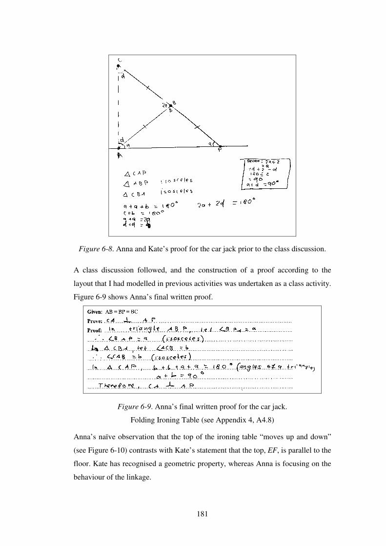
181
Figure 6-8. Anna and Kate’s proof for the car jack prior to the class discussion.
A class discussion followed, and the construction of a proof according to the
layout that I had modelled in previous activities was undertaken as a class activity.
Figure 6-9 shows Anna’s final written proof.
Figure 6-9. Anna’s final written proof for the car jack.
Folding Ironing Table (see Appendix 4, A4.8)
Anna’s naïve observation that the top of the ironing table “moves up and down”
(see Figure 6-10) contrasts with Kate’s statement that the top, EF, is parallel to the
floor. Kate has recognised a geometric property, whereas Anna is focusing on the
behaviour of the linkage.
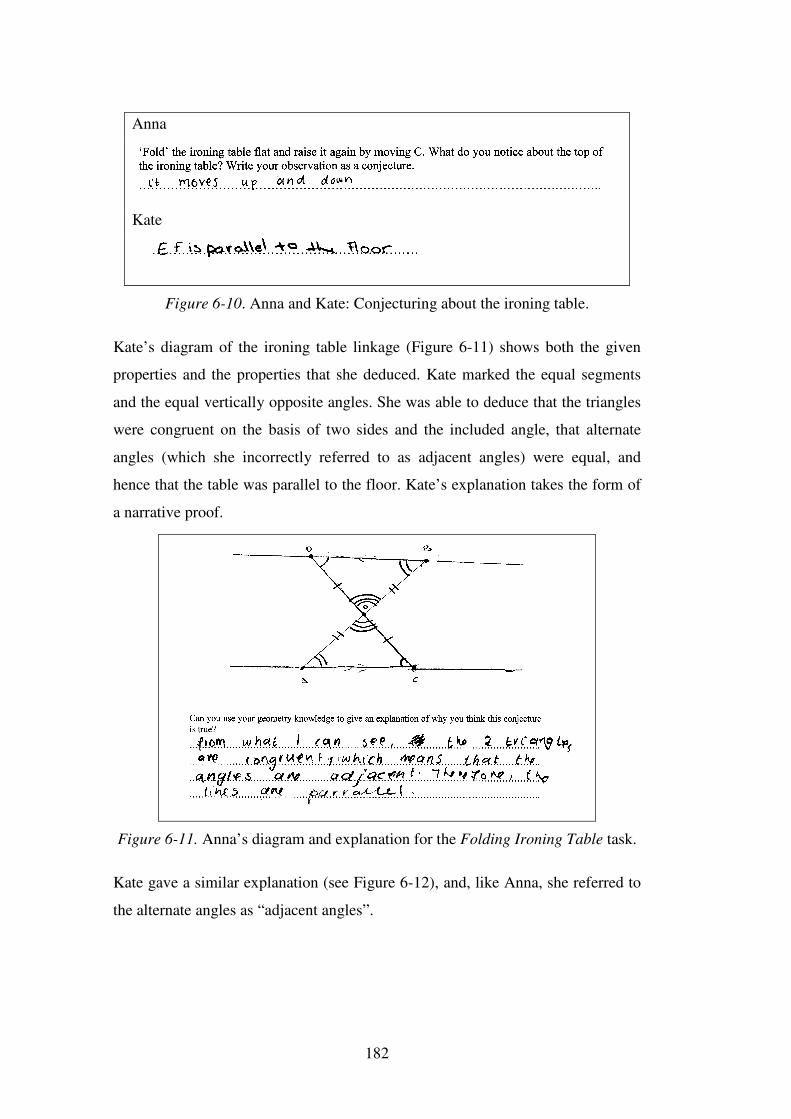
182
Anna
Kate
Figure 6-10. Anna and Kate: Conjecturing about the ironing table.
Kate’s diagram of the ironing table linkage (Figure 6-11) shows both the given
properties and the properties that she deduced. Kate marked the equal segments
and the equal vertically opposite angles. She was able to deduce that the triangles
were congruent on the basis of two sides and the included angle, that alternate
angles (which she incorrectly referred to as adjacent angles) were equal, and
hence that the table was parallel to the floor. Kate’s explanation takes the form of
a narrative proof.
Figure 6-11. Anna’s diagram and explanation for the Folding Ironing Table task.
Kate gave a similar explanation (see Figure 6-12), and, like Anna, she referred to
the alternate angles as “adjacent angles”.
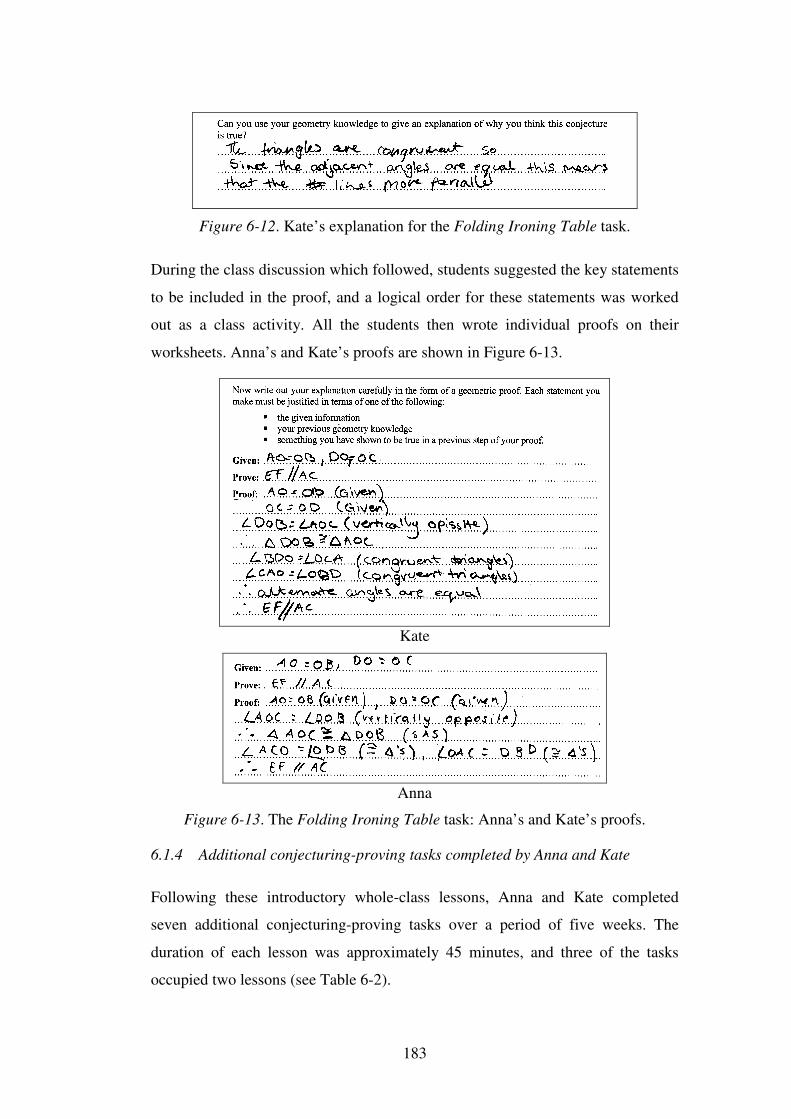
183
Figure 6-12. Kate’s explanation for the Folding Ironing Table task.
During the class discussion which followed, students suggested the key statements
to be included in the proof, and a logical order for these statements was worked
out as a class activity. All the students then wrote individual proofs on their
worksheets. Anna’s and Kate’s proofs are shown in Figure 6-13.
Kate
Anna
Figure 6-13. The Folding Ironing Table task: Anna’s and Kate’s proofs.
6.1.4 Additional conjecturing-proving tasks completed by Anna and Kate
Following these introductory whole-class lessons, Anna and Kate completed
seven additional conjecturing-proving tasks over a period of five weeks. The
duration of each lesson was approximately 45 minutes, and three of the tasks
occupied two lessons (see Table 6-2).
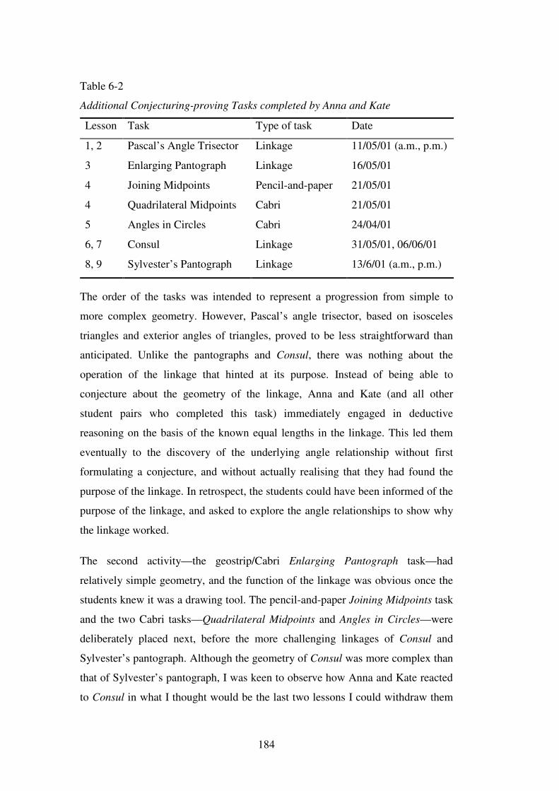
184
Table 6-2
Additional Conjecturing-proving Tasks completed by Anna and Kate
Lesson Task Type of task Date
1, 2 Pascal’s Angle Trisector Linkage 11/05/01 (a.m., p.m.)
3 Enlarging Pantograph Linkage 16/05/01
4 Joining Midpoints Pencil-and-paper 21/05/01
4 Quadrilateral Midpoints Cabri 21/05/01
5 Angles in Circles Cabri 24/04/01
6, 7 Consul Linkage 31/05/01, 06/06/01
8, 9 Sylvester’s Pantograph Linkage 13/6/01 (a.m., p.m.)
The order of the tasks was intended to represent a progression from simple to
more complex geometry. However, Pascal’s angle trisector, based on isosceles
triangles and exterior angles of triangles, proved to be less straightforward than
anticipated. Unlike the pantographs and Consul, there was nothing about the
operation of the linkage that hinted at its purpose. Instead of being able to
conjecture about the geometry of the linkage, Anna and Kate (and all other
student pairs who completed this task) immediately engaged in deductive
reasoning on the basis of the known equal lengths in the linkage. This led them
eventually to the discovery of the underlying angle relationship without first
formulating a conjecture, and without actually realising that they had found the
purpose of the linkage. In retrospect, the students could have been informed of the
purpose of the linkage, and asked to explore the angle relationships to show why
the linkage worked.
The second activity—the geostrip/Cabri Enlarging Pantograph task—had
relatively simple geometry, and the function of the linkage was obvious once the
students knew it was a drawing tool. The pencil-and-paper Joining Midpoints task
and the two Cabri tasks—Quadrilateral Midpoints and Angles in Circles—were
deliberately placed next, before the more challenging linkages of Consul and
Sylvester’s pantograph. Although the geometry of Consul was more complex than
that of Sylvester’s pantograph, I was keen to observe how Anna and Kate reacted
to Consul in what I thought would be the last two lessons I could withdraw them
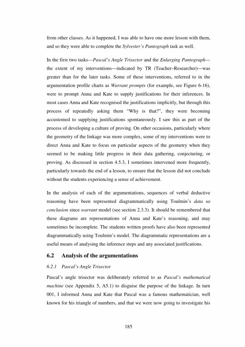
185
from other classes. As it happened, I was able to have one more lesson with them,
and so they were able to complete the Sylvester’s Pantograph task as well.
In the first two tasks—Pascal’s Angle Trisector and the Enlarging Pantograph—
the extent of my interventions—indicated by TR (Teacher–Researcher)—was
greater than for the later tasks. Some of these interventions, referred to in the
argumentation profile charts as Warrant prompts (for example, see Figure 6-16),
were to prompt Anna and Kate to supply justifications for their inferences. In
most cases Anna and Kate recognised the justifications implicitly, but through this
process of repeatedly asking them “Why is that?”, they were becoming
accustomed to supplying justifications spontaneously. I saw this as part of the
process of developing a culture of proving. On other occasions, particularly where
the geometry of the linkage was more complex, some of my interventions were to
direct Anna and Kate to focus on particular aspects of the geometry when they
seemed to be making little progress in their data gathering, conjecturing, or
proving. As discussed in section 4.5.3, I sometimes intervened more frequently,
particularly towards the end of a lesson, to ensure that the lesson did not conclude
without the students experiencing a sense of achievement.
In the analysis of each of the argumentations, sequences of verbal deductive
reasoning have been represented diagrammatically using Toulmin’s data so
conclusion since warrant model (see section 2.3.3). It should be remembered that
these diagrams are representations of Anna and Kate’s reasoning, and may
sometimes be incomplete. The students written proofs have also been represented
diagrammatically using Toulmin’s model. The diagrammatic representations are a
useful means of analysing the inference steps and any associated justifications.
6.2 Analysis of the argumentations
6.2.1 Pascal’s Angle Trisector
Pascal’s angle trisector was deliberately referred to as Pascal’s mathematical
machine (see Appendix 5, A5.1) to disguise the purpose of the linkage. In turn
001, I informed Anna and Kate that Pascal was a famous mathematician, well
known for his triangle of numbers, and that we were now going to investigate his
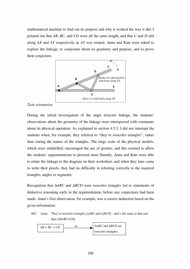
186
mathematical machine to find out its purpose and why it worked the way it did. I
pointed out that AB, BC, and CD were all the same length, and that C and D slid
along AX and AY respectively as AY was rotated. Anna and Kate were asked to
explore the linkage, to conjecture about its geometry and purpose, and to prove
their conjecture.
A
B
C
D
Y
X
Rotate AY, allowing D toslide freely along AY.
Allow C to slide freely along AX
Task orientation
During the initial investigation of the angle trisector linkage, the students’
observations about the geometry of the linkage were interspersed with comments
about its physical operation. As explained in section 4.5.3, I did not interrupt the
students when, for example, they referred to “they’re isosceles triangles”, rather
than stating the names of the triangles. The large scale of the physical models,
which were unlabelled, encouraged the use of gesture, and this seemed to allow
the students’ argumentations to proceed more fluently. Anna and Kate were able
to relate the linkage to the diagram on their worksheet, and when they later came
to write their proofs, they had no difficulty in referring correctly to the required
triangles, angles or segments.
Recognition that ∆ABC and ∆BCD were isosceles triangles led to statements of
deductive reasoning early in the argumentation, before any conjectures had been
made. Anna’s first observation, for example, was a correct deduction based on the
given information:
002 Anna: They’re isosceles triangles [∆ABC and [∆BCD] – that’s the same as that and
that [AB=BC=CD].
AB = BC = CD ∆ABC and ∆BCD are
isosceles triangles.
so
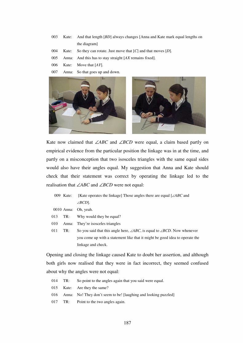
187
003 Kate: And that length [BD] always changes [Anna and Kate mark equal lengths on
the diagram]
004 Kate: So they can rotate. Just move that [C] and that moves [D].
005 Anna: And this has to stay straight [AX remains fixed].
006 Kate: Move that [AY].
007 Anna: So that goes up and down.
Kate now claimed that ∠ABC and ∠BCD were equal, a claim based partly on
empirical evidence from the particular position the linkage was in at the time, and
partly on a misconception that two isosceles triangles with the same equal sides
would also have their angles equal. My suggestion that Anna and Kate should
check that their statement was correct by operating the linkage led to the
realisation that ∠ABC and ∠BCD were not equal:
009 Kate: [Kate operates the linkage] Those angles there are equal [∠ABC and
∠BCD].
0010 Anna: Oh, yeah.
013 TR: Why would they be equal?
010 Anna: They’re isosceles triangles
011 TR: So you said that this angle here, ∠ABC, is equal to ∠BCD. Now whenever
you come up with a statement like that it might be good idea to operate the
linkage and check.
Opening and closing the linkage caused Kate to doubt her assertion, and although
both girls now realised that they were in fact incorrect, they seemed confused
about why the angles were not equal:
014 TR: So point to the angles again that you said were equal.
015 Kate: Are they the same?
016 Anna: No! They don’t seem to be! [laughing and looking puzzled]
017 TR: Point to the two angles again.
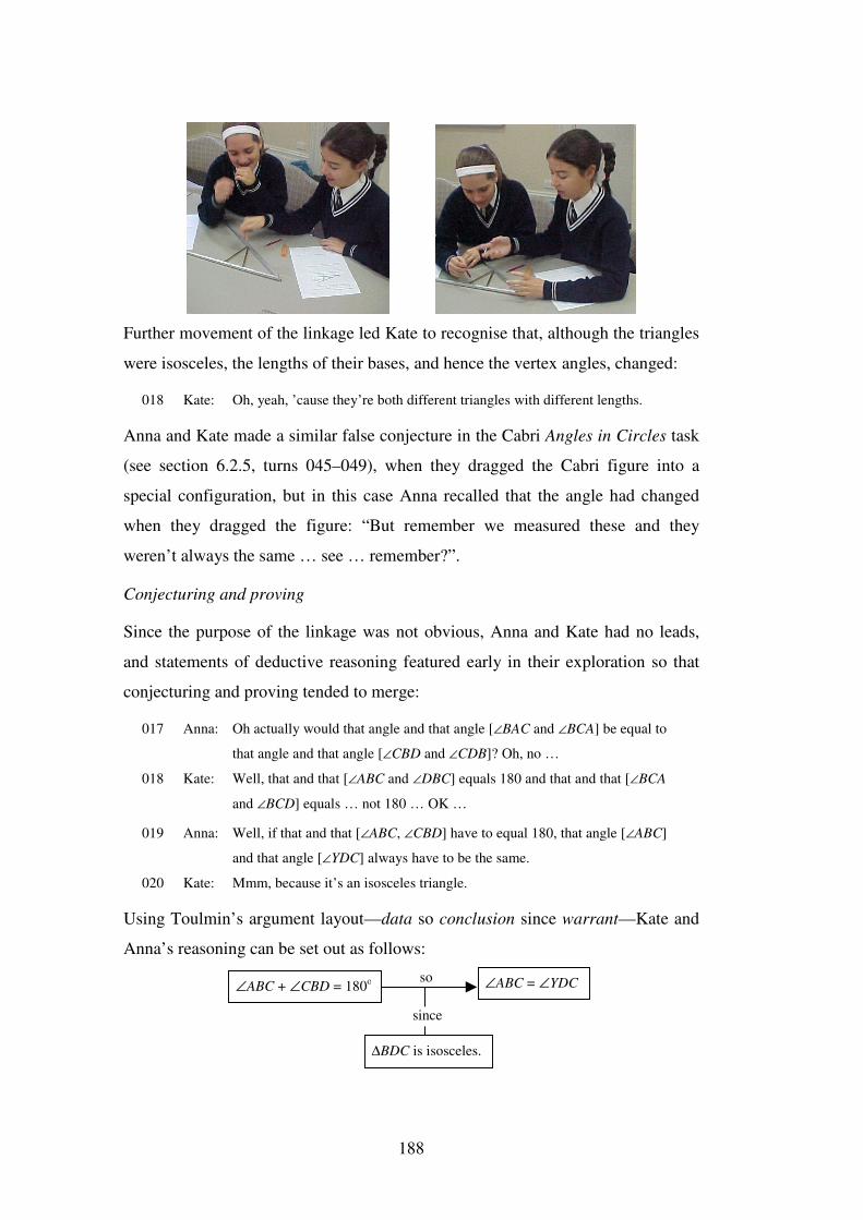
188
Further movement of the linkage led Kate to recognise that, although the triangles
were isosceles, the lengths of their bases, and hence the vertex angles, changed:
018 Kate: Oh, yeah, ’cause they’re both different triangles with different lengths.
Anna and Kate made a similar false conjecture in the Cabri Angles in Circles task
(see section 6.2.5, turns 045–049), when they dragged the Cabri figure into a
special configuration, but in this case Anna recalled that the angle had changed
when they dragged the figure: “But remember we measured these and they
weren’t always the same … see … remember?”.
Conjecturing and proving
Since the purpose of the linkage was not obvious, Anna and Kate had no leads,
and statements of deductive reasoning featured early in their exploration so that
conjecturing and proving tended to merge:
017 Anna: Oh actually would that angle and that angle [∠BAC and ∠BCA] be equal to
that angle and that angle [∠CBD and ∠CDB]? Oh, no …
018 Kate: Well, that and that [∠ABC and ∠DBC] equals 180 and that and that [∠BCA
and ∠BCD] equals … not 180 … OK …
019 Anna: Well, if that and that [∠ABC, ∠CBD] have to equal 180, that angle [∠ABC]
and that angle [∠YDC] always have to be the same.
020 Kate: Mmm, because it’s an isosceles triangle.
Using Toulmin’s argument layout—data so conclusion since warrant—Kate and
Anna’s reasoning can be set out as follows:
∠ABC + ∠CBD = 180o ∠ABC = ∠YDC
∆BDC is isosceles.
so
since
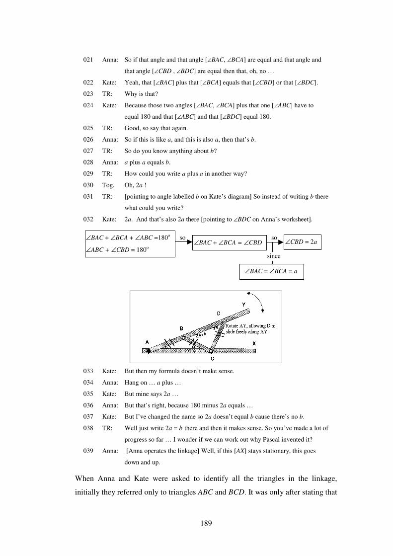
189
021 Anna: So if that angle and that angle [∠BAC, ∠BCA] are equal and that angle and
that angle [∠CBD , ∠BDC] are equal then that, oh, no …
022 Kate: Yeah, that [∠BAC] plus that [∠BCA] equals that [∠CBD] or that [∠BDC].
023 TR: Why is that?
024 Kate: Because those two angles [∠BAC, ∠BCA] plus that one [∠ABC] have to
equal 180 and that [∠ABC] and that [∠BDC] equal 180.
025 TR: Good, so say that again.
026 Anna: So if this is like a, and this is also a, then that’s b.
027 TR: So do you know anything about b?
028 Anna: a plus a equals b.
029 TR: How could you write a plus a in another way?
030 Tog. Oh, 2a !
031 TR: [pointing to angle labelled b on Kate’s diagram] So instead of writing b there
what could you write?
032 Kate: 2a. And that’s also 2a there [pointing to ∠BDC on Anna’s worksheet].
033 Kate: But then my formula doesn’t make sense.
034 Anna: Hang on … a plus …
035 Kate: But mine says 2a …
036 Anna: But that’s right, because 180 minus 2a equals …
037 Kate: But I’ve changed the name so 2a doesn’t equal b cause there’s no b.
038 TR: Well just write 2a = b there and then it makes sense. So you’ve made a lot of
progress so far … I wonder if we can work out why Pascal invented it?
039 Anna: [Anna operates the linkage] Well, if this [AX] stays stationary, this goes
down and up.
When Anna and Kate were asked to identify all the triangles in the linkage,
initially they referred only to triangles ABC and BCD. It was only after stating that
∠BAC + ∠BCA + ∠ABC =180o
∠ABC + ∠CBD = 180o ∠BAC + ∠BCA = ∠CBD ∠CBD = 2a
∠BAC = ∠BCA = a
so so
since
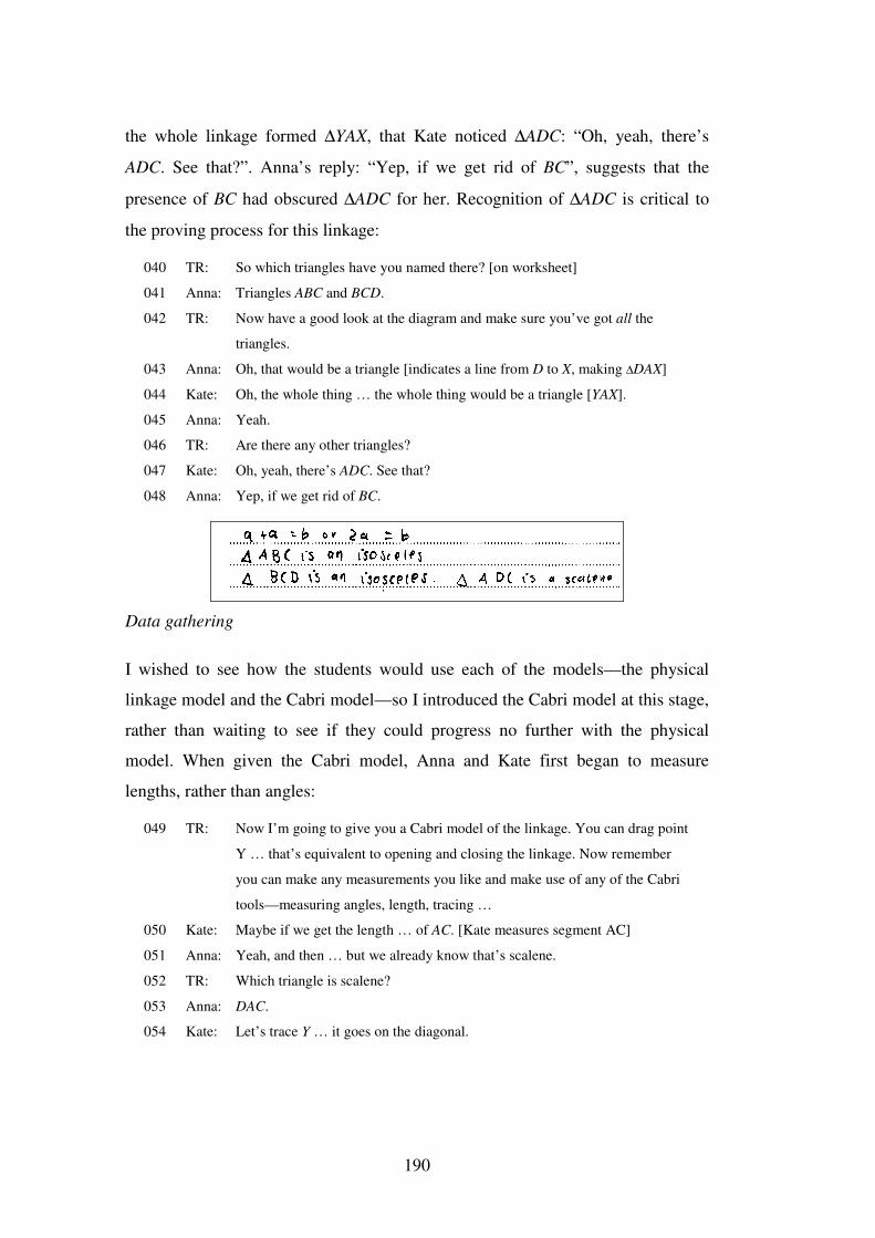
190
the whole linkage formed ∆YAX, that Kate noticed ∆ADC: “Oh, yeah, there’s
ADC. See that?”. Anna’s reply: “Yep, if we get rid of BC”, suggests that the
presence of BC had obscured ∆ADC for her. Recognition of ∆ADC is critical to
the proving process for this linkage:
040 TR: So which triangles have you named there? [on worksheet]
041 Anna: Triangles ABC and BCD.
042 TR: Now have a good look at the diagram and make sure you’ve got all the
triangles.
043 Anna: Oh, that would be a triangle [indicates a line from D to X, making ∆DAX]
044 Kate: Oh, the whole thing … the whole thing would be a triangle [YAX].
045 Anna: Yeah.
046 TR: Are there any other triangles?
047 Kate: Oh, yeah, there’s ADC. See that?
048 Anna: Yep, if we get rid of BC.
Data gathering
I wished to see how the students would use each of the models—the physical
linkage model and the Cabri model—so I introduced the Cabri model at this stage,
rather than waiting to see if they could progress no further with the physical
model. When given the Cabri model, Anna and Kate first began to measure
lengths, rather than angles:
049 TR: Now I’m going to give you a Cabri model of the linkage. You can drag point
Y … that’s equivalent to opening and closing the linkage. Now remember
you can make any measurements you like and make use of any of the Cabri
tools—measuring angles, length, tracing …
050 Kate: Maybe if we get the length … of AC. [Kate measures segment AC]
051 Anna: Yeah, and then … but we already know that’s scalene.
052 TR: Which triangle is scalene?
053 Anna: DAC.
054 Kate: Let’s trace Y … it goes on the diagonal.
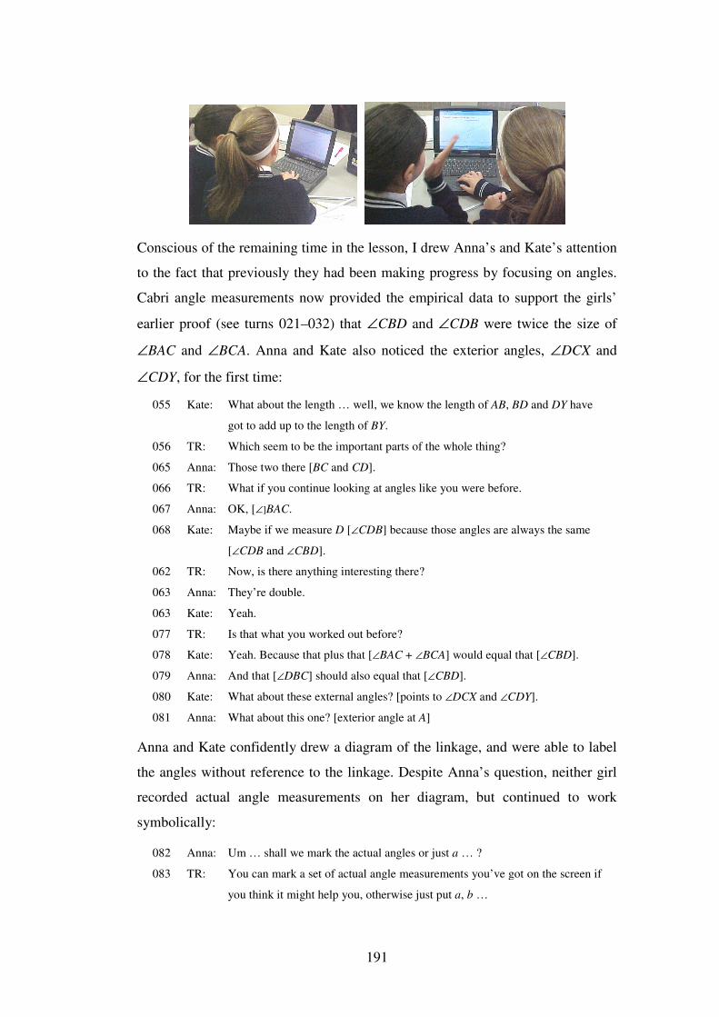
191
Conscious of the remaining time in the lesson, I drew Anna’s and Kate’s attention
to the fact that previously they had been making progress by focusing on angles.
Cabri angle measurements now provided the empirical data to support the girls’
earlier proof (see turns 021–032) that ∠CBD and ∠CDB were twice the size of
∠BAC and ∠BCA. Anna and Kate also noticed the exterior angles, ∠DCX and
∠CDY, for the first time:
055 Kate: What about the length … well, we know the length of AB, BD and DY have
got to add up to the length of BY.
056 TR: Which seem to be the important parts of the whole thing?
065 Anna: Those two there [BC and CD].
066 TR: What if you continue looking at angles like you were before.
067 Anna: OK, [∠]BAC.
068 Kate: Maybe if we measure D [∠CDB] because those angles are always the same
[∠CDB and ∠CBD].
062 TR: Now, is there anything interesting there?
063 Anna: They’re double.
063 Kate: Yeah.
077 TR: Is that what you worked out before?
078 Kate: Yeah. Because that plus that [∠BAC + ∠BCA] would equal that [∠CBD].
079 Anna: And that [∠DBC] should also equal that [∠CBD].
080 Kate: What about these external angles? [points to ∠DCX and ∠CDY].
081 Anna: What about this one? [exterior angle at A]
Anna and Kate confidently drew a diagram of the linkage, and were able to label
the angles without reference to the linkage. Despite Anna’s question, neither girl
recorded actual angle measurements on her diagram, but continued to work
symbolically:
082 Anna: Um … shall we mark the actual angles or just a … ?
083 TR: You can mark a set of actual angle measurements you’ve got on the screen if
you think it might help you, otherwise just put a, b …
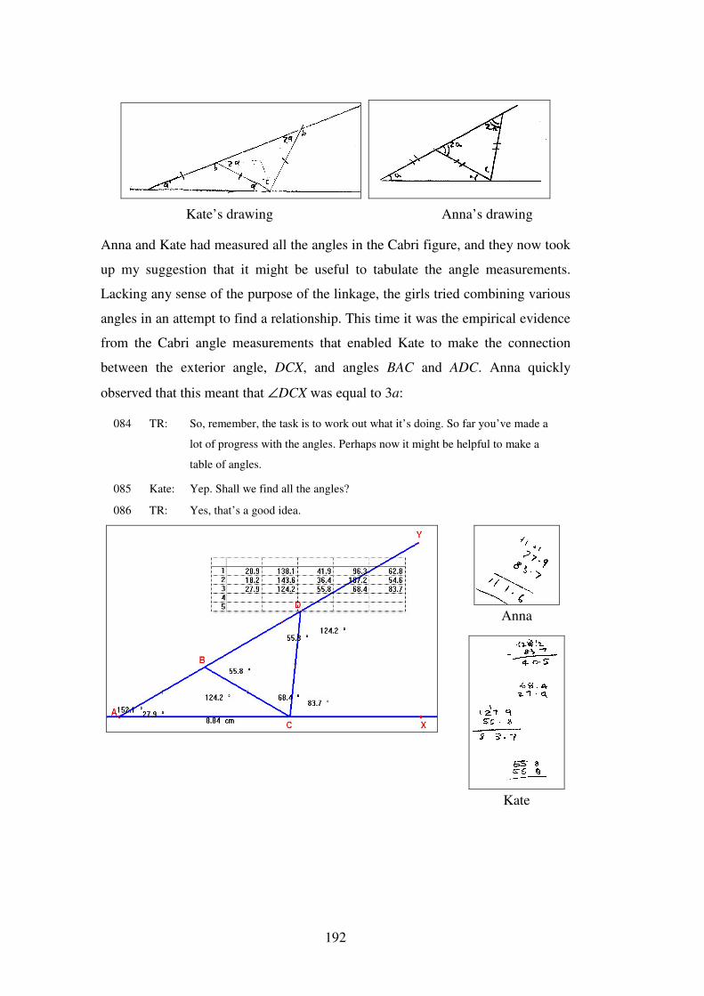
192
Kate’s drawing Anna’s drawing
Anna and Kate had measured all the angles in the Cabri figure, and they now took
up my suggestion that it might be useful to tabulate the angle measurements.
Lacking any sense of the purpose of the linkage, the girls tried combining various
angles in an attempt to find a relationship. This time it was the empirical evidence
from the Cabri angle measurements that enabled Kate to make the connection
between the exterior angle, DCX, and angles BAC and ADC. Anna quickly
observed that this meant that ∠DCX was equal to 3a:
084 TR: So, remember, the task is to work out what it’s doing. So far you’ve made a
lot of progress with the angles. Perhaps now it might be helpful to make a
table of angles.
085 Kate: Yep. Shall we find all the angles?
086 TR: Yes, that’s a good idea.
Anna
Kate
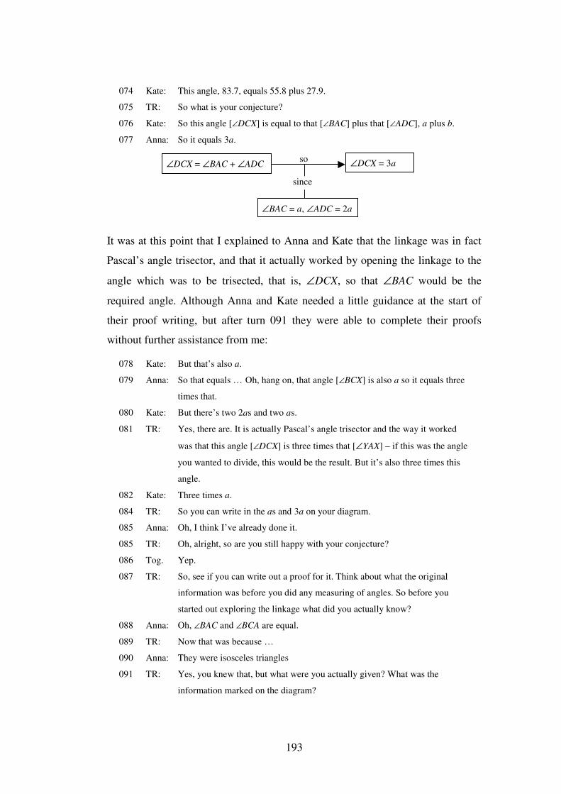
193
074 Kate: This angle, 83.7, equals 55.8 plus 27.9.
075 TR: So what is your conjecture?
076 Kate: So this angle [∠DCX] is equal to that [∠BAC] plus that [∠ADC], a plus b.
077 Anna: So it equals 3a.
It was at this point that I explained to Anna and Kate that the linkage was in fact
Pascal’s angle trisector, and that it actually worked by opening the linkage to the
angle which was to be trisected, that is, ∠DCX, so that ∠BAC would be the
required angle. Although Anna and Kate needed a little guidance at the start of
their proof writing, but after turn 091 they were able to complete their proofs
without further assistance from me:
078 Kate: But that’s also a.
079 Anna: So that equals … Oh, hang on, that angle [∠BCX] is also a so it equals three
times that.
080 Kate: But there’s two 2as and two as.
081 TR: Yes, there are. It is actually Pascal’s angle trisector and the way it worked
was that this angle [∠DCX] is three times that [∠YAX] – if this was the angle
you wanted to divide, this would be the result. But it’s also three times this
angle.
082 Kate: Three times a.
084 TR: So you can write in the as and 3a on your diagram.
085 Anna: Oh, I think I’ve already done it.
085 TR: Oh, alright, so are you still happy with your conjecture?
086 Tog. Yep.
087 TR: So, see if you can write out a proof for it. Think about what the original
information was before you did any measuring of angles. So before you
started out exploring the linkage what did you actually know?
088 Anna: Oh, ∠BAC and ∠BCA are equal.
089 TR: Now that was because …
090 Anna: They were isosceles triangles
091 TR: Yes, you knew that, but what were you actually given? What was the
information marked on the diagram?
∠DCX = ∠BAC + ∠ADC ∠DCX = 3a
∠BAC = a, ∠ADC = 2a
so
since
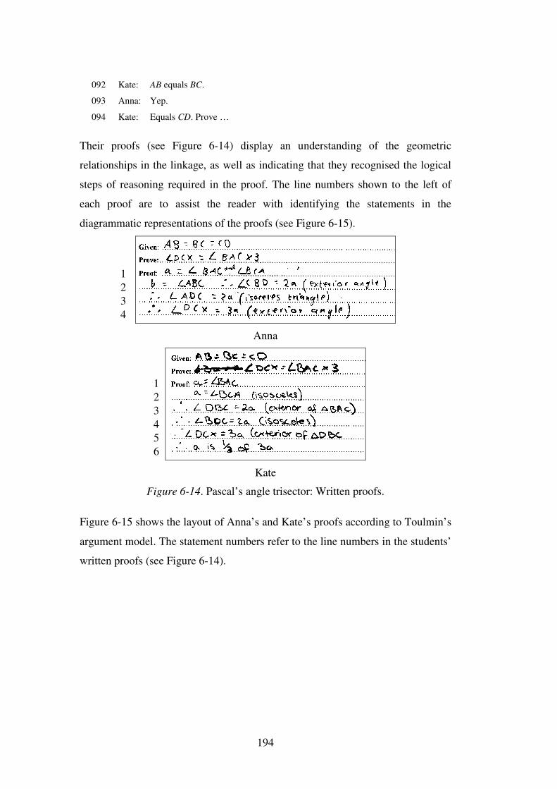
194
092 Kate: AB equals BC.
093 Anna: Yep.
094 Kate: Equals CD. Prove …
Their proofs (see Figure 6-14) display an understanding of the geometric
relationships in the linkage, as well as indicating that they recognised the logical
steps of reasoning required in the proof. The line numbers shown to the left of
each proof are to assist the reader with identifying the statements in the
diagrammatic representations of the proofs (see Figure 6-15).
Anna
Kate
Figure 6-14. Pascal’s angle trisector: Written proofs.
Figure 6-15 shows the layout of Anna’s and Kate’s proofs according to Toulmin’s
argument model. The statement numbers refer to the line numbers in the students’
written proofs (see Figure 6-14).
1234
123456
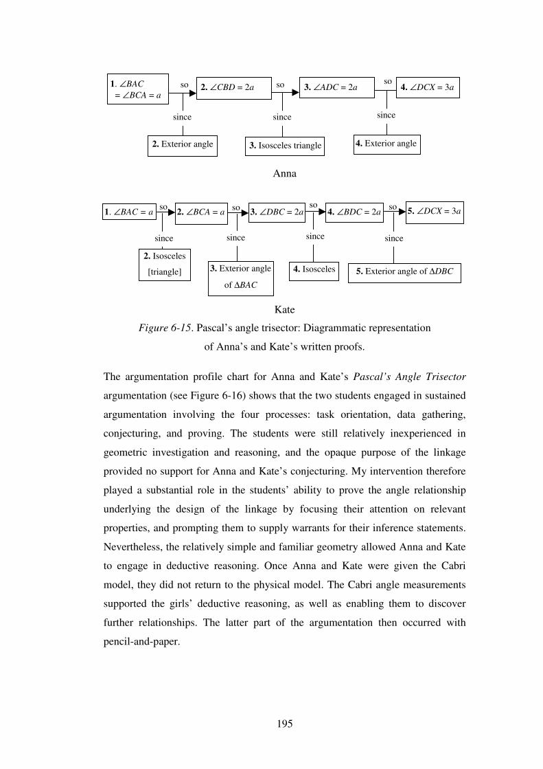
195
Anna
Kate
Figure 6-15. Pascal’s angle trisector: Diagrammatic representation
of Anna’s and Kate’s written proofs.
The argumentation profile chart for Anna and Kate’s Pascal’s Angle Trisector
argumentation (see Figure 6-16) shows that the two students engaged in sustained
argumentation involving the four processes: task orientation, data gathering,
conjecturing, and proving. The students were still relatively inexperienced in
geometric investigation and reasoning, and the opaque purpose of the linkage
provided no support for Anna and Kate’s conjecturing. My intervention therefore
played a substantial role in the students’ ability to prove the angle relationship
underlying the design of the linkage by focusing their attention on relevant
properties, and prompting them to supply warrants for their inference statements.
Nevertheless, the relatively simple and familiar geometry allowed Anna and Kate
to engage in deductive reasoning. Once Anna and Kate were given the Cabri
model, they did not return to the physical model. The Cabri angle measurements
supported the girls’ deductive reasoning, as well as enabling them to discover
further relationships. The latter part of the argumentation then occurred with
pencil-and-paper.
1. ∠BAC = ∠BCA = a
2. Exterior angle
2. ∠CBD = 2a
3. Isosceles triangle
3. ∠ADC = 2a 4. ∠DCX = 3a
4. Exterior angle
so so so
since since since
1. ∠BAC = a 2. ∠BCA = a 3. ∠DBC = 2a 4. ∠BDC = 2a 5. ∠DCX = 3a
2. Isosceles
[triangle] 4. Isosceles 3. Exterior angle
of ∆BAC 5. Exterior angle of ∆DBC
so so so so
since since since since
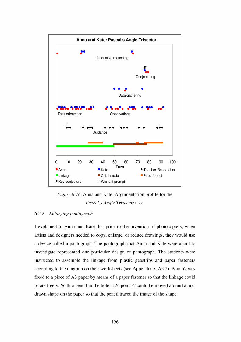
196
Anna and Kate: Pascal's Angle Trisector
0 10 20 30 40 50 60 70 80 90 100Turn
Anna Kate Teacher-Researcher
Linkage Cabri model Paper/pencil
Key conjecture Warrant prompt
Deductive reasoning
Conjecturing
Data-gathering
Observations
Guidance
Task orientation
Figure 6-16. Anna and Kate: Argumentation profile for the
Pascal’s Angle Trisector task.
6.2.2 Enlarging pantograph
I explained to Anna and Kate that prior to the invention of photocopiers, when
artists and designers needed to copy, enlarge, or reduce drawings, they would use
a device called a pantograph. The pantograph that Anna and Kate were about to
investigate represented one particular design of pantograph. The students were
instructed to assemble the linkage from plastic geostrips and paper fasteners
according to the diagram on their worksheets (see Appendix 5, A5.2). Point O was
fixed to a piece of A3 paper by means of a paper fastener so that the linkage could
rotate freely. With a pencil in the hole at E, point C could be moved around a pre-
drawn shape on the paper so that the pencil traced the image of the shape.
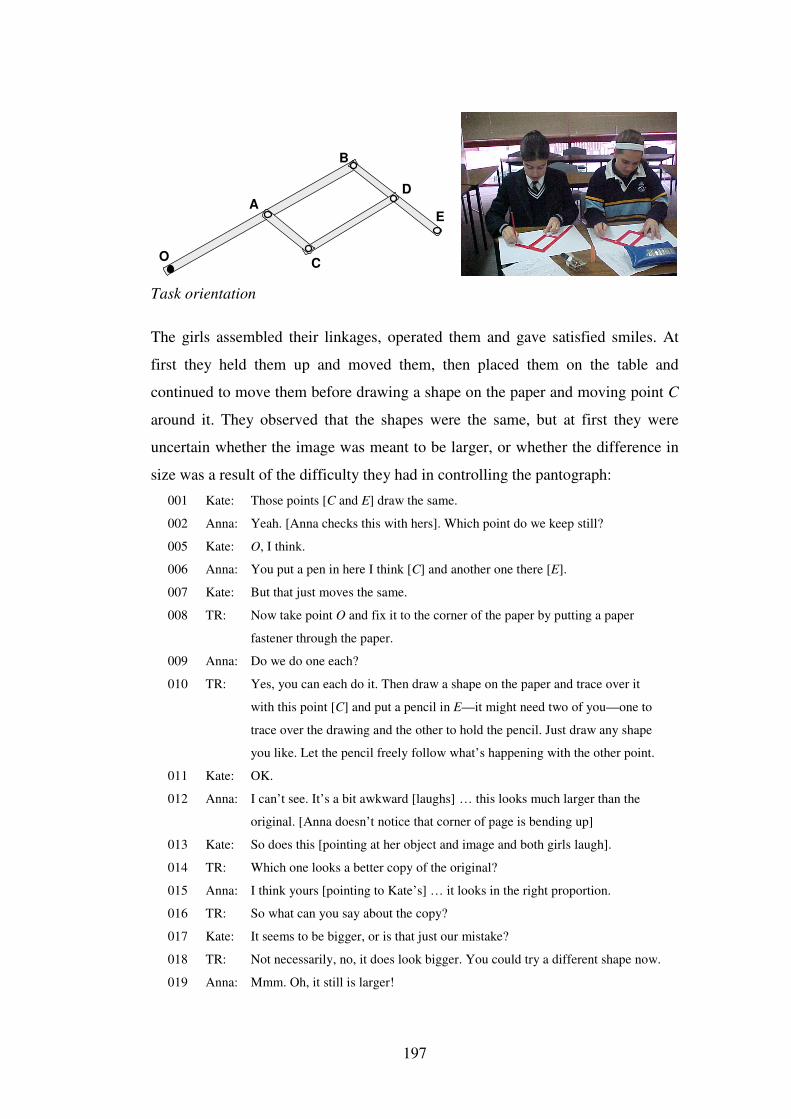
197
EA
B
O C
D
Task orientation
The girls assembled their linkages, operated them and gave satisfied smiles. At
first they held them up and moved them, then placed them on the table and
continued to move them before drawing a shape on the paper and moving point C
around it. They observed that the shapes were the same, but at first they were
uncertain whether the image was meant to be larger, or whether the difference in
size was a result of the difficulty they had in controlling the pantograph:
001 Kate: Those points [C and E] draw the same.
002 Anna: Yeah. [Anna checks this with hers]. Which point do we keep still?
005 Kate: O, I think.
006 Anna: You put a pen in here I think [C] and another one there [E].
007 Kate: But that just moves the same.
008 TR: Now take point O and fix it to the corner of the paper by putting a paper
fastener through the paper.
009 Anna: Do we do one each?
010 TR: Yes, you can each do it. Then draw a shape on the paper and trace over it
with this point [C] and put a pencil in E—it might need two of you—one to
trace over the drawing and the other to hold the pencil. Just draw any shape
you like. Let the pencil freely follow what’s happening with the other point.
011 Kate: OK.
012 Anna: I can’t see. It’s a bit awkward [laughs] … this looks much larger than the
original. [Anna doesn’t notice that corner of page is bending up]
013 Kate: So does this [pointing at her object and image and both girls laugh].
014 TR: Which one looks a better copy of the original?
015 Anna: I think yours [pointing to Kate’s] … it looks in the right proportion.
016 TR: So what can you say about the copy?
017 Kate: It seems to be bigger, or is that just our mistake?
018 TR: Not necessarily, no, it does look bigger. You could try a different shape now.
019 Anna: Mmm. Oh, it still is larger!
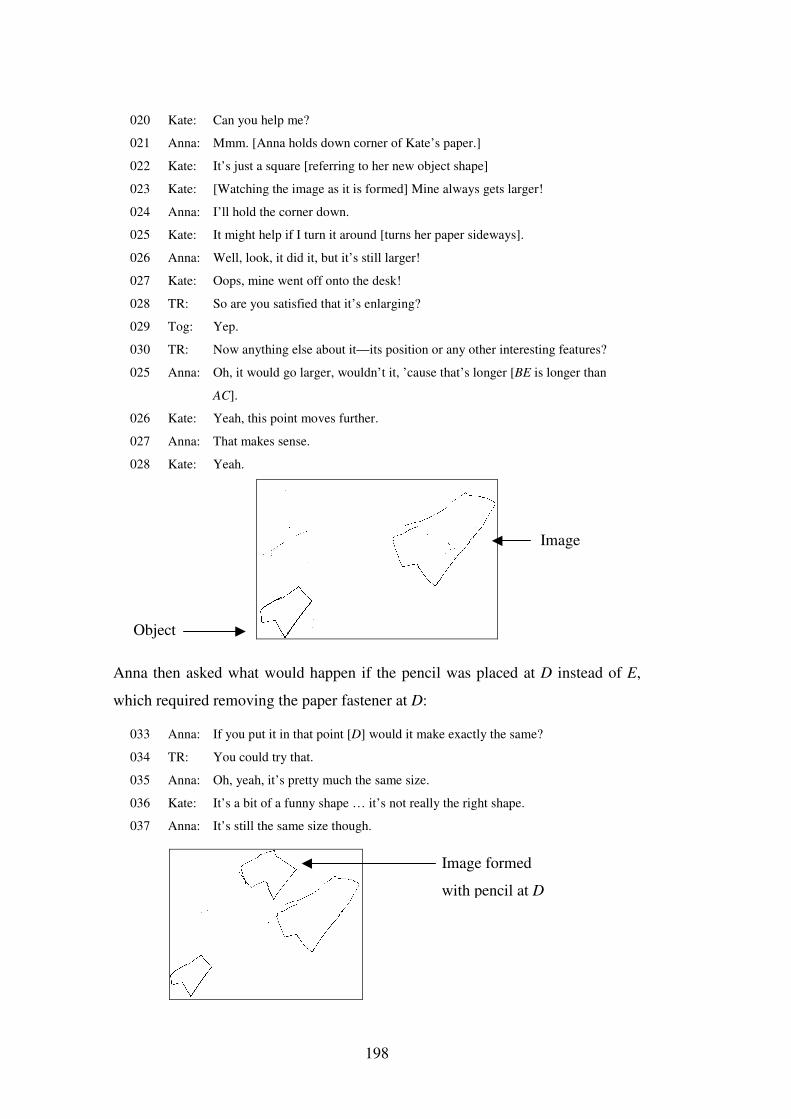
198
020 Kate: Can you help me?
021 Anna: Mmm. [Anna holds down corner of Kate’s paper.]
022 Kate: It’s just a square [referring to her new object shape]
023 Kate: [Watching the image as it is formed] Mine always gets larger!
024 Anna: I’ll hold the corner down.
025 Kate: It might help if I turn it around [turns her paper sideways].
026 Anna: Well, look, it did it, but it’s still larger!
027 Kate: Oops, mine went off onto the desk!
028 TR: So are you satisfied that it’s enlarging?
029 Tog: Yep.
030 TR: Now anything else about it—its position or any other interesting features?
025 Anna: Oh, it would go larger, wouldn’t it, ’cause that’s longer [BE is longer than
AC].
026 Kate: Yeah, this point moves further.
027 Anna: That makes sense.
028 Kate: Yeah.
Anna then asked what would happen if the pencil was placed at D instead of E,
which required removing the paper fastener at D:
033 Anna: If you put it in that point [D] would it make exactly the same?
034 TR: You could try that.
035 Anna: Oh, yeah, it’s pretty much the same size.
036 Kate: It’s a bit of a funny shape … it’s not really the right shape.
037 Anna: It’s still the same size though.
Image
Object
Image formed
with pencil at D
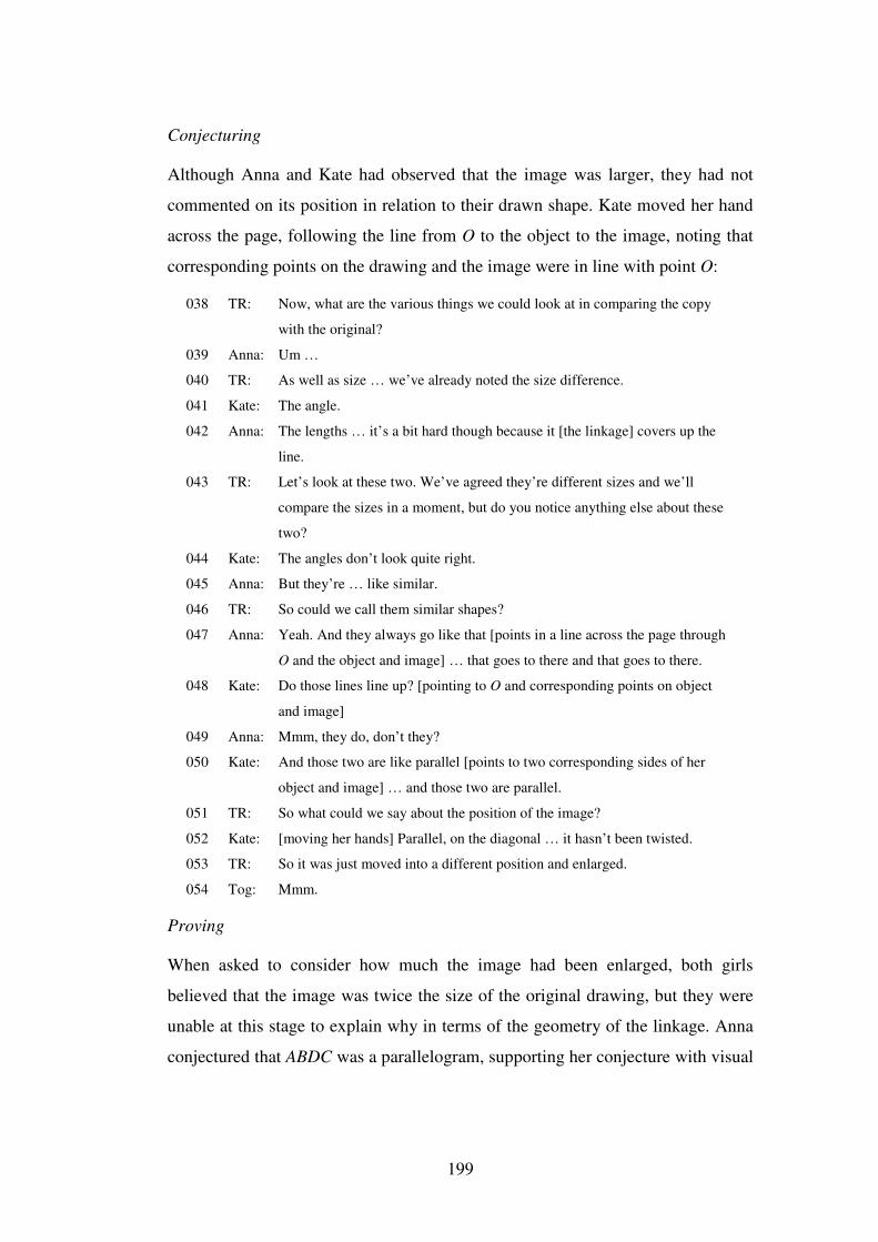
199
Conjecturing
Although Anna and Kate had observed that the image was larger, they had not
commented on its position in relation to their drawn shape. Kate moved her hand
across the page, following the line from O to the object to the image, noting that
corresponding points on the drawing and the image were in line with point O:
038 TR: Now, what are the various things we could look at in comparing the copy
with the original?
039 Anna: Um …
040 TR: As well as size … we’ve already noted the size difference.
041 Kate: The angle.
042 Anna: The lengths … it’s a bit hard though because it [the linkage] covers up the
line.
043 TR: Let’s look at these two. We’ve agreed they’re different sizes and we’ll
compare the sizes in a moment, but do you notice anything else about these
two?
044 Kate: The angles don’t look quite right.
045 Anna: But they’re … like similar.
046 TR: So could we call them similar shapes?
047 Anna: Yeah. And they always go like that [points in a line across the page through
O and the object and image] … that goes to there and that goes to there.
048 Kate: Do those lines line up? [pointing to O and corresponding points on object
and image]
049 Anna: Mmm, they do, don’t they?
050 Kate: And those two are like parallel [points to two corresponding sides of her
object and image] … and those two are parallel.
051 TR: So what could we say about the position of the image?
052 Kate: [moving her hands] Parallel, on the diagonal … it hasn’t been twisted.
053 TR: So it was just moved into a different position and enlarged.
054 Tog: Mmm.
Proving
When asked to consider how much the image had been enlarged, both girls
believed that the image was twice the size of the original drawing, but they were
unable at this stage to explain why in terms of the geometry of the linkage. Anna
conjectured that ABDC was a parallelogram, supporting her conjecture with visual
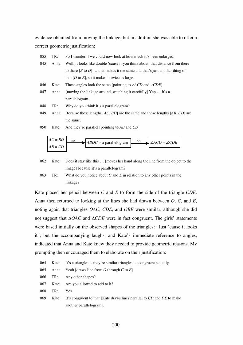
200
evidence obtained from moving the linkage, but in addition she was able to offer a
correct geometric justification:
055 TR: So I wonder if we could now look at how much it’s been enlarged.
045 Anna: Well, it looks like double ’cause if you think about, that distance from there
to there [B to D] … that makes it the same and that’s just another thing of
that [D to E], so it makes it twice as large.
046 Kate: Those angles look the same [pointing to ∠ACD and ∠CDE].
047 Anna: [moving the linkage around, watching it carefully] Yep … it’s a
parallelogram.
048 TR: Why do you think it’s a parallelogram?
049 Anna: Because those lengths [AC, BD] are the same and those lengths [AB, CD] are
the same.
050 Kate: And they’re parallel [pointing to AB and CD]
062 Kate: Does it stay like this … [moves her hand along the line from the object to the
image] because it’s a parallelogram?
063 TR: What do you notice about C and E in relation to any other points in the
linkage?
Kate placed her pencil between C and E to form the side of the triangle CDE.
Anna then returned to looking at the lines she had drawn between O, C, and E,
noting again that triangles OAC, CDE, and OBE were similar, although she did
not suggest that ∆OAC and ∆CDE were in fact congruent. The girls’ statements
were based initially on the observed shapes of the triangles: “Just ’cause it looks
it”, but the accompanying laughs, and Kate’s immediate reference to angles,
indicated that Anna and Kate knew they needed to provide geometric reasons. My
prompting then encouraged them to elaborate on their justification:
064 Kate: It’s a triangle … they’re similar triangles … congruent actually.
065 Anna: Yeah [draws line from O through C to E].
066 TR: Any other shapes?
067 Kate: Are you allowed to add to it?
068 TR: Yes.
069 Kate: It’s congruent to that [Kate draws lines parallel to CD and DE to make
another parallelogram].
ABDC is a parallelogram AC = BD
AB = CD ∠ACD = ∠CDE so so
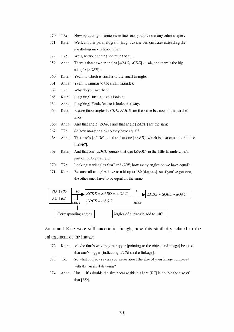
201
070 TR: Now by adding in some more lines can you pick out any other shapes?
071 Kate: Well, another parallelogram [laughs as she demonstrates extending the
parallelogram she has drawn]
072 TR: Well, without adding too much to it …
059 Anna: There’s those two triangles [∆OAC, ∆CDE] … oh, and there’s the big
triangle [∆OBE].
060 Kate: Yeah … which is similar to the small triangles.
061 Anna: Yeah … similar to the small triangles.
062 TR: Why do you say that?
063 Kate: [laughing] Just ’cause it looks it.
064 Anna: [laughing] Yeah, ’cause it looks that way.
065 Kate: ’Cause those angles [∠CDE, ∠ABD] are the same because of the parallel
lines.
066 Anna: And that angle [∠OAC] and that angle [∠ABD] are the same.
067 TR: So how many angles do they have equal?
068 Anna: That one’s [∠CDE] equal to that one [∠ABD], which is also equal to that one
[∠OAC].
069 Kate: And that one [∠DCE] equals that one [∠AOC] in the little triangle … it’s
part of the big triangle.
070 TR: Looking at triangles OAC and OBE, how many angles do we have equal?
071 Kate: Because all triangles have to add up to 180 [degrees], so if you’ve got two,
the other ones have to be equal … the same.
Anna and Kate were still uncertain, though, how this similarity related to the
enlargement of the image:
072 Kate: Maybe that’s why they’re bigger [pointing to the object and image] because
that one’s bigger [indicating ∆OBE on the linkage].
073 TR: So what conjecture can you make about the size of your image compared
with the original drawing?
074 Anna: Um … it’s double the size because this bit here [BE] is double the size of
that [BD].
∠CDE = ∠ABD = ∠OAC
∠DCE = ∠AOC
∆CDE ~ ∆OBE ~ ∆OAC
Corresponding angles Angles of a triangle add to 180o
so
since since
OB || CD
AC || BE
so
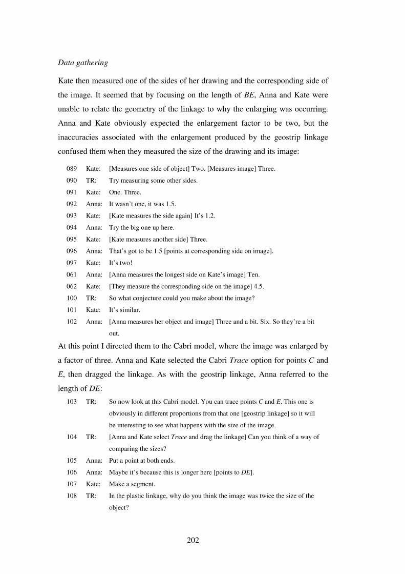
202
Data gathering
Kate then measured one of the sides of her drawing and the corresponding side of
the image. It seemed that by focusing on the length of BE, Anna and Kate were
unable to relate the geometry of the linkage to why the enlarging was occurring.
Anna and Kate obviously expected the enlargement factor to be two, but the
inaccuracies associated with the enlargement produced by the geostrip linkage
confused them when they measured the size of the drawing and its image:
089 Kate: [Measures one side of object] Two. [Measures image] Three.
090 TR: Try measuring some other sides.
091 Kate: One. Three.
092 Anna: It wasn’t one, it was 1.5.
093 Kate: [Kate measures the side again] It’s 1.2.
094 Anna: Try the big one up here.
095 Kate: [Kate measures another side] Three.
096 Anna: That’s got to be 1.5 [points at corresponding side on image].
097 Kate: It’s two!
061 Anna: [Anna measures the longest side on Kate’s image] Ten.
062 Kate: [They measure the corresponding side on the image] 4.5.
100 TR: So what conjecture could you make about the image?
101 Kate: It’s similar.
102 Anna: [Anna measures her object and image] Three and a bit. Six. So they’re a bit
out.
At this point I directed them to the Cabri model, where the image was enlarged by
a factor of three. Anna and Kate selected the Cabri Trace option for points C and
E, then dragged the linkage. As with the geostrip linkage, Anna referred to the
length of DE:
103 TR: So now look at this Cabri model. You can trace points C and E. This one is
obviously in different proportions from that one [geostrip linkage] so it will
be interesting to see what happens with the size of the image.
104 TR: [Anna and Kate select Trace and drag the linkage] Can you think of a way of
comparing the sizes?
105 Anna: Put a point at both ends.
106 Anna: Maybe it’s because this is longer here [points to DE].
107 Kate: Make a segment.
108 TR: In the plastic linkage, why do you think the image was twice the size of the
object?
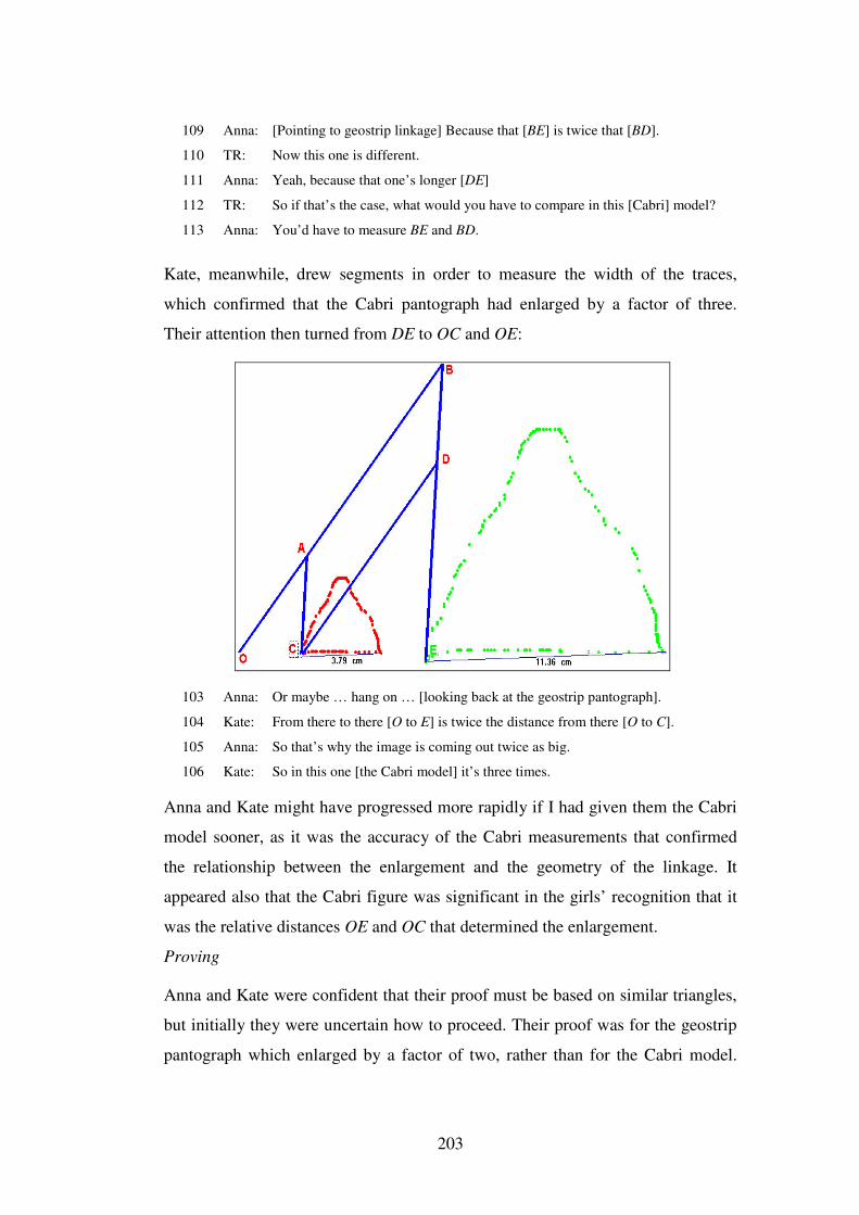
203
109 Anna: [Pointing to geostrip linkage] Because that [BE] is twice that [BD].
110 TR: Now this one is different.
111 Anna: Yeah, because that one’s longer [DE]
112 TR: So if that’s the case, what would you have to compare in this [Cabri] model?
113 Anna: You’d have to measure BE and BD.
Kate, meanwhile, drew segments in order to measure the width of the traces,
which confirmed that the Cabri pantograph had enlarged by a factor of three.
Their attention then turned from DE to OC and OE:
103 Anna: Or maybe … hang on … [looking back at the geostrip pantograph].
104 Kate: From there to there [O to E] is twice the distance from there [O to C].
105 Anna: So that’s why the image is coming out twice as big.
106 Kate: So in this one [the Cabri model] it’s three times.
Anna and Kate might have progressed more rapidly if I had given them the Cabri
model sooner, as it was the accuracy of the Cabri measurements that confirmed
the relationship between the enlargement and the geometry of the linkage. It
appeared also that the Cabri figure was significant in the girls’ recognition that it
was the relative distances OE and OC that determined the enlargement.
Proving
Anna and Kate were confident that their proof must be based on similar triangles,
but initially they were uncertain how to proceed. Their proof was for the geostrip
pantograph which enlarged by a factor of two, rather than for the Cabri model.
204
Kate mistakenly thought that if triangles had two pairs of corresponding sides
equal, then the third pair of sides would be equal. Anna’s counter-claim, “No …
you can change the angle”, indicates the influence of the dynamic environment:
108 Kate: So we can prove the triangles are similar because the angles … no …
109 Anna: Yeah, because that’s [AC] the same length as that [DE] and that’s [OA] the
same length as that [CD], the angles have to be … different.
110 Kate: Because DE equals AC and DC equals AO then the last side has to be the
same length.
111 Anna: No … you can change the angle.
112 Kate: Oh, yeah. But those angles are equal.
123 Anna: No, they’re not.
Although their subsequent reasoning was sound, Anna and Kate did not clearly
identify the sides they needed in their side-angle-side proof of similarity
(conditions for similarity and congruency of triangles were included in the
introductory geometry lessons prior to conjecturing-proving lessons), omitting
AC, and referring to BD rather than to DE. This might have been due partly to an
earlier confusion over which triangles they were using, when Kate referred to
triangles OAC and CDE, while Anna was looking at triangles OAC and OBE:
124 Kate: Side angle side, they are … look … that angle equals that angle.
125 Anna: But if they were the same and they were the same, then the triangles would
be congruent.
126 Kate: They are congruent!
127 TR: I think Kate’s thinking about the little triangles [OAC and CDE] and you’re
looking at the big triangle [OBE] and the little triangles.
128 Kate: You’re adding two equal lengths [points to OC and CE], so that’s [OE] twice
that [OC].
129 TR: So you can either look at the large triangle or the two smaller triangles. If we
look at the large triangle, what do we know about the sides?
130 Kate: That’s [BE] twice that [BD] and that’s [OB] twice that [OA].
131 TR: And what else do we know.
132 Anna: That angle’s [OAC] the same as that [OBE].
133 TR: Why?
134 Kate: Because they’re … corresponding angles.
135 TR: But how do we know they’re equal?
136 Anna: Because that’s [OB] parallel to that [CD] because that’s [ABDC] a
parallelogram.
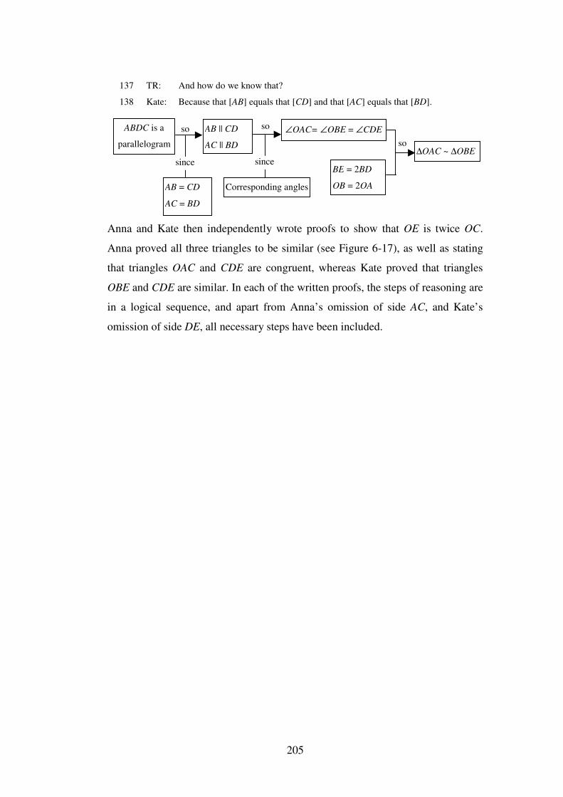
205
137 TR: And how do we know that?
138 Kate: Because that [AB] equals that [CD] and that [AC] equals that [BD].
Anna and Kate then independently wrote proofs to show that OE is twice OC.
Anna proved all three triangles to be similar (see Figure 6-17), as well as stating
that triangles OAC and CDE are congruent, whereas Kate proved that triangles
OBE and CDE are similar. In each of the written proofs, the steps of reasoning are
in a logical sequence, and apart from Anna’s omission of side AC, and Kate’s
omission of side DE, all necessary steps have been included.
AB = CD
AC = BD
AB || CD
AC || BD
ABDC is a
parallelogram
∠OAC= ∠OBE = ∠CDE
∆OAC ~ ∆OBE
Corresponding angles
BE = 2BD
OB = 2OA
so so
so
since since
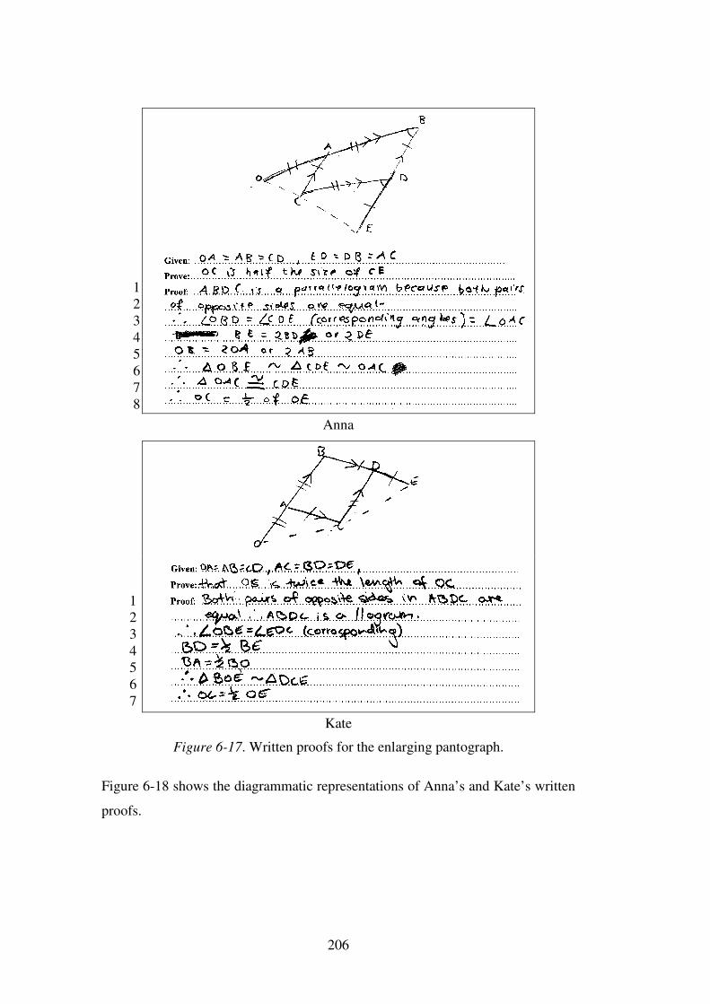
206
Anna
Kate
Figure 6-17. Written proofs for the enlarging pantograph.
Figure 6-18 shows the diagrammatic representations of Anna’s and Kate’s written
proofs.
12345678
1234567
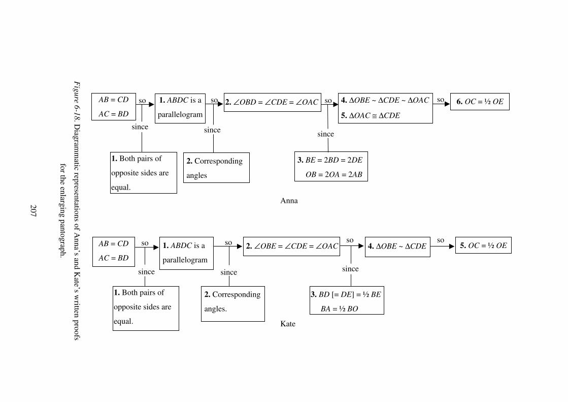
207
Figure 6-18. D
iagramm
atic representations of Anna’s and K
ate’s written proofs
for the enlarging pantograph.
Anna
2. Corresponding
angles
so so AB = CD
AC = BD
4. ∆OBE ~ ∆CDE ~ ∆OAC
5. ∆OAC ≅ ∆CDE
1. ABDC is a
parallelogram
2. ∠OBD = ∠CDE = ∠OAC 6. OC = ½ OE
3. BE = 2BD = 2DE
OB = 2OA = 2AB
1. Both pairs of
opposite sides are
equal.
so so
since since since
so
AB = CD
AC = BD 4. ∆OBE ~ ∆CDE 1. ABDC is a
parallelogram
2. ∠OBE = ∠CDE = ∠OAC 5. OC = ½ OE
3. BD [= DE] = ½ BE
BA = ½ BO
so
2. Corresponding
angles.
so
1. Both pairs of
opposite sides are
equal. Kate
since since since
so so
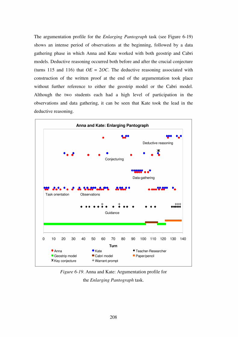
208
The argumentation profile for the Enlarging Pantograph task (see Figure 6-19)
shows an intense period of observations at the beginning, followed by a data
gathering phase in which Anna and Kate worked with both geostrip and Cabri
models. Deductive reasoning occurred both before and after the crucial conjecture
(turns 115 and 116) that OE = 2OC. The deductive reasoning associated with
construction of the written proof at the end of the argumentation took place
without further reference to either the geostrip model or the Cabri model.
Although the two students each had a high level of participation in the
observations and data gathering, it can be seen that Kate took the lead in the
deductive reasoning.
Anna and Kate: Enlarging Pantograph
0 10 20 30 40 50 60 70 80 90 100 110 120 130 140
TurnAnna Kate Teacher-ResearcherGeostrip model Cabri model Paper/pencilKey conjecture Warrant prompt
Deductive reasoning
Conjecturing
Data-gathering
Observations
Guidance
Task orientation
Figure 6-19. Anna and Kate: Argumentation profile for
the Enlarging Pantograph task.
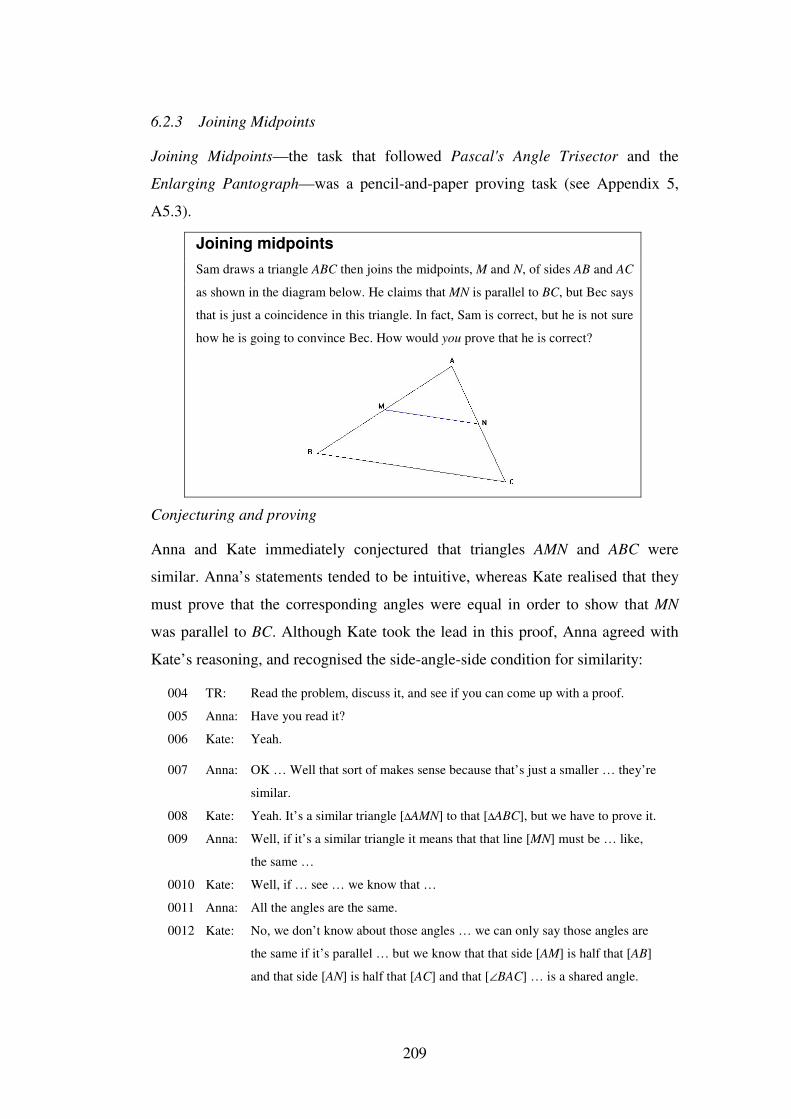
209
6.2.3 Joining Midpoints
Joining Midpoints—the task that followed Pascal's Angle Trisector and the
Enlarging Pantograph—was a pencil-and-paper proving task (see Appendix 5,
A5.3).
Joining midpoints Sam draws a triangle ABC then joins the midpoints, M and N, of sides AB and AC
as shown in the diagram below. He claims that MN is parallel to BC, but Bec says
that is just a coincidence in this triangle. In fact, Sam is correct, but he is not sure
how he is going to convince Bec. How would you prove that he is correct?
Conjecturing and proving
Anna and Kate immediately conjectured that triangles AMN and ABC were
similar. Anna’s statements tended to be intuitive, whereas Kate realised that they
must prove that the corresponding angles were equal in order to show that MN
was parallel to BC. Although Kate took the lead in this proof, Anna agreed with
Kate’s reasoning, and recognised the side-angle-side condition for similarity:
004 TR: Read the problem, discuss it, and see if you can come up with a proof.
005 Anna: Have you read it?
006 Kate: Yeah.
007 Anna: OK … Well that sort of makes sense because that’s just a smaller … they’re
similar.
008 Kate: Yeah. It’s a similar triangle [∆AMN] to that [∆ABC], but we have to prove it.
009 Anna: Well, if it’s a similar triangle it means that that line [MN] must be … like,
the same …
0010 Kate: Well, if … see … we know that …
0011 Anna: All the angles are the same.
0012 Kate: No, we don’t know about those angles … we can only say those angles are
the same if it’s parallel … but we know that that side [AM] is half that [AB]
and that side [AN] is half that [AC] and that [∠BAC] … is a shared angle.
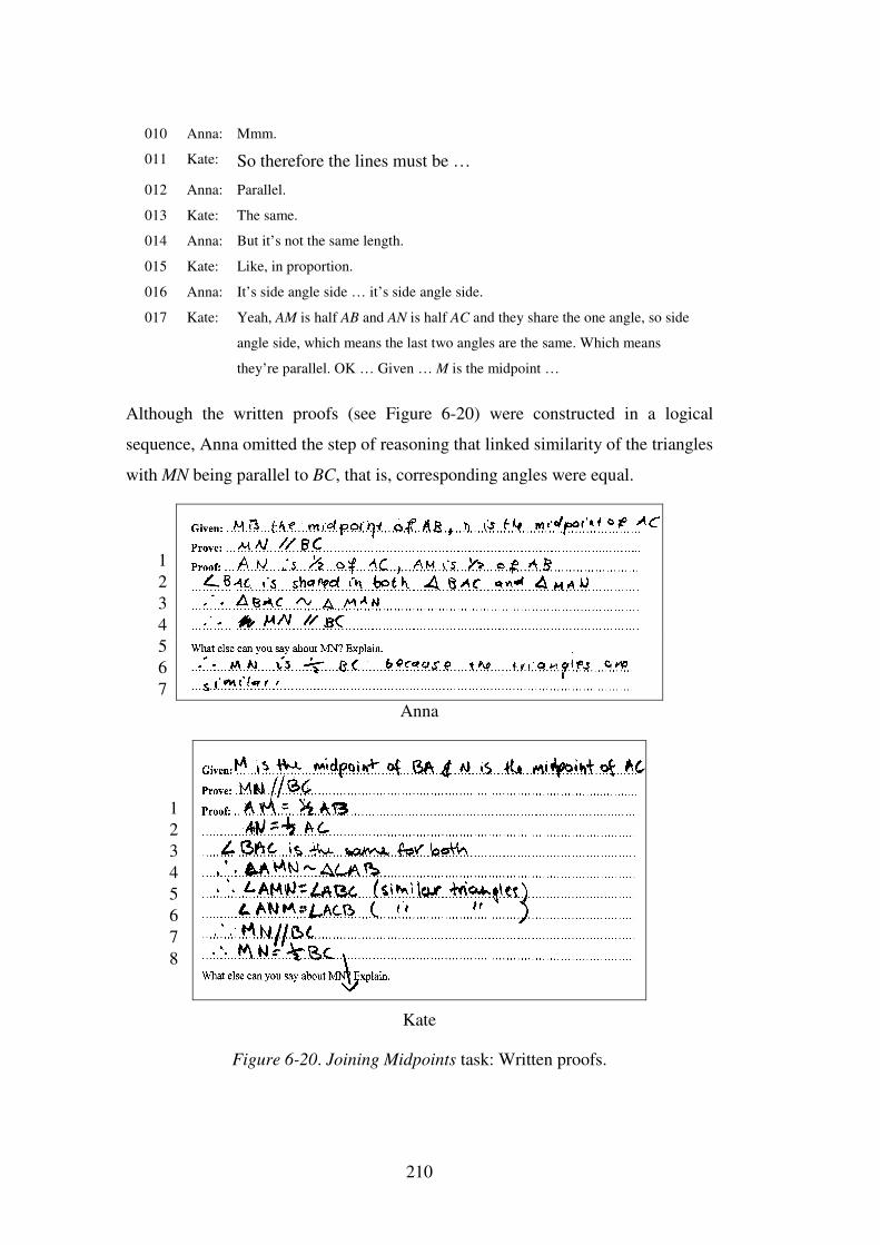
210
010 Anna: Mmm.
011 Kate: So therefore the lines must be …
012 Anna: Parallel.
013 Kate: The same.
014 Anna: But it’s not the same length.
015 Kate: Like, in proportion.
016 Anna: It’s side angle side … it’s side angle side.
017 Kate: Yeah, AM is half AB and AN is half AC and they share the one angle, so side
angle side, which means the last two angles are the same. Which means
they’re parallel. OK … Given … M is the midpoint …
Although the written proofs (see Figure 6-20) were constructed in a logical
sequence, Anna omitted the step of reasoning that linked similarity of the triangles
with MN being parallel to BC, that is, corresponding angles were equal.
Anna
Kate
Figure 6-20. Joining Midpoints task: Written proofs.
1234567
12345678
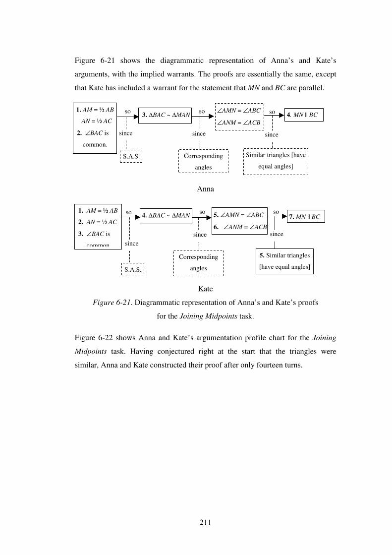
211
Figure 6-21 shows the diagrammatic representation of Anna’s and Kate’s
arguments, with the implied warrants. The proofs are essentially the same, except
that Kate has included a warrant for the statement that MN and BC are parallel.
Anna
Kate
Figure 6-21. Diagrammatic representation of Anna’s and Kate’s proofs
for the Joining Midpoints task.
Figure 6-22 shows Anna and Kate’s argumentation profile chart for the Joining
Midpoints task. Having conjectured right at the start that the triangles were
similar, Anna and Kate constructed their proof after only fourteen turns.
1. AM = ½ AB
AN = ½ AC
2. ∠BAC is
common.
4. MN || BC 3. ∆BAC ~ ∆MAN ∠AMN = ∠ABC
∠ANM = ∠ACB
S.A.S. Similar triangles [have
equal angles]
Corresponding
angles
so so so
since since since
1. AM = ½ AB
2. AN = ½ AC
3. ∠BAC is
common.
7. MN || BC 4. ∆BAC ~ ∆MAN 5. ∠AMN = ∠ABC
6. ∠ANM = ∠ACB
S.A.S.
5. Similar triangles
[have equal angles] Corresponding
angles
so so so
since since since
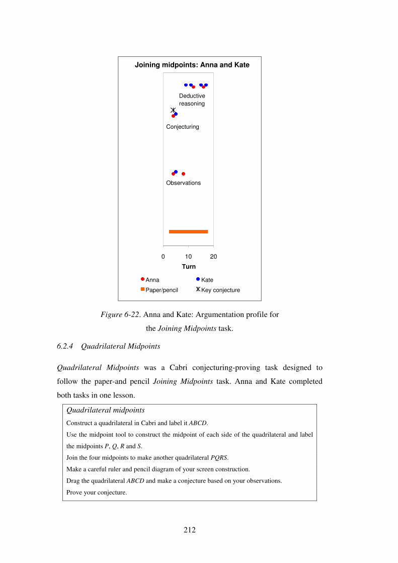
212
Joining midpoints: Anna and Kate
0 10 20
Turn
Anna Kate
Paper/pencil Key conjecture
Observations
Conjecturing
Deductive reasoning
Figure 6-22. Anna and Kate: Argumentation profile for
the Joining Midpoints task.
6.2.4 Quadrilateral Midpoints
Quadrilateral Midpoints was a Cabri conjecturing-proving task designed to
follow the paper-and pencil Joining Midpoints task. Anna and Kate completed
both tasks in one lesson.
Quadrilateral midpoints
Construct a quadrilateral in Cabri and label it ABCD.
Use the midpoint tool to construct the midpoint of each side of the quadrilateral and label
the midpoints P, Q, R and S.
Join the four midpoints to make another quadrilateral PQRS.
Make a careful ruler and pencil diagram of your screen construction.
Drag the quadrilateral ABCD and make a conjecture based on your observations.
Prove your conjecture.
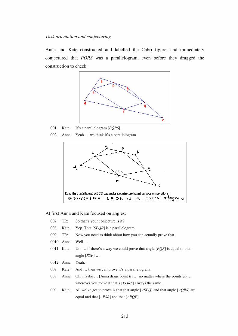
213
Task orientation and conjecturing
Anna and Kate constructed and labelled the Cabri figure, and immediately
conjectured that PQRS was a parallelogram, even before they dragged the
construction to check:
001 Kate: It’s a parallelogram [PQRS].
002 Anna: Yeah … we think it’s a parallelogram.
At first Anna and Kate focused on angles:
007 TR: So that’s your conjecture is it?
008 Kate: Yep. That [SPQR] is a parallelogram.
009 TR: Now you need to think about how you can actually prove that.
0010 Anna: Well …
0011 Kate: Um … if there’s a way we could prove that angle [PQR] is equal to that
angle [RSP] …
0012 Anna: Yeah.
007 Kate: And … then we can prove it’s a parallelogram.
008 Anna: Oh, maybe … [Anna drags point B] … no matter where the points go …
wherever you move it that’s [PQRS] always the same.
009 Kate: All we’ve got to prove is that that angle [∠SPQ] and that angle [∠QRS] are
equal and that [∠PSR] and that [∠RQP].
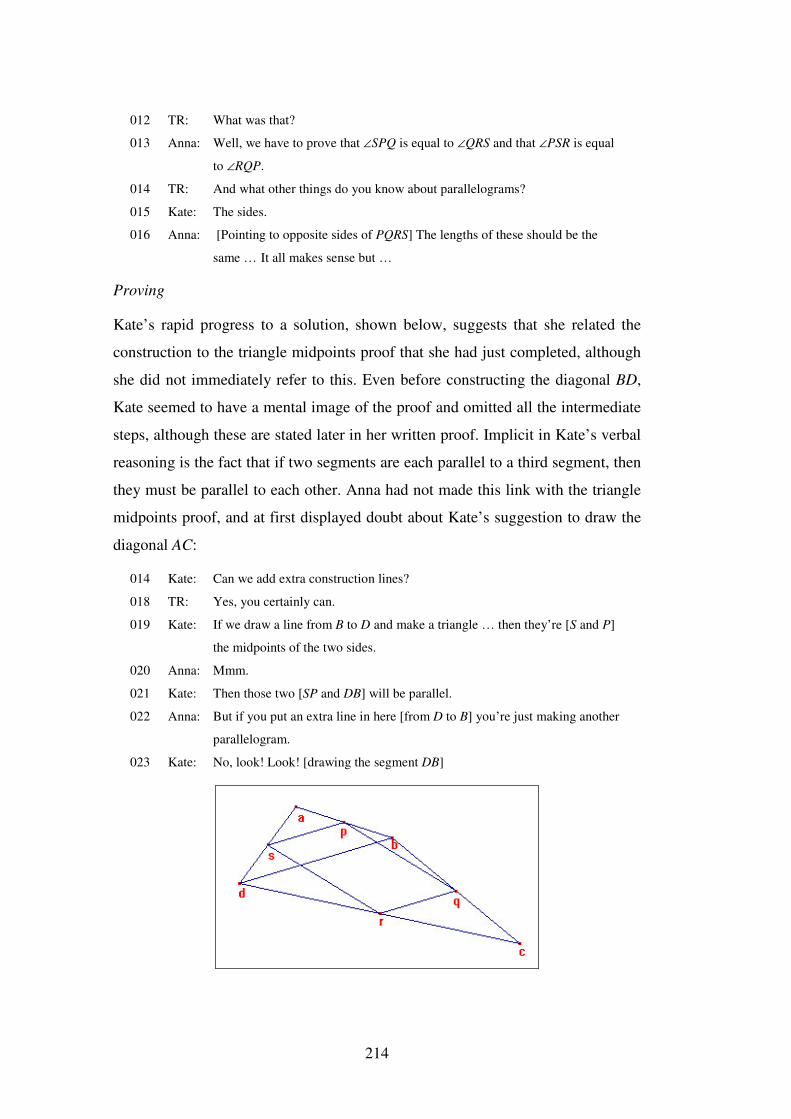
214
012 TR: What was that?
013 Anna: Well, we have to prove that ∠SPQ is equal to ∠QRS and that ∠PSR is equal
to ∠RQP.
014 TR: And what other things do you know about parallelograms?
015 Kate: The sides.
016 Anna: [Pointing to opposite sides of PQRS] The lengths of these should be the
same … It all makes sense but …
Proving
Kate’s rapid progress to a solution, shown below, suggests that she related the
construction to the triangle midpoints proof that she had just completed, although
she did not immediately refer to this. Even before constructing the diagonal BD,
Kate seemed to have a mental image of the proof and omitted all the intermediate
steps, although these are stated later in her written proof. Implicit in Kate’s verbal
reasoning is the fact that if two segments are each parallel to a third segment, then
they must be parallel to each other. Anna had not made this link with the triangle
midpoints proof, and at first displayed doubt about Kate’s suggestion to draw the
diagonal AC:
014 Kate: Can we add extra construction lines?
018 TR: Yes, you certainly can.
019 Kate: If we draw a line from B to D and make a triangle … then they’re [S and P]
the midpoints of the two sides.
020 Anna: Mmm.
021 Kate: Then those two [SP and DB] will be parallel.
022 Anna: But if you put an extra line in here [from D to B] you’re just making another
parallelogram.
023 Kate: No, look! Look! [drawing the segment DB]
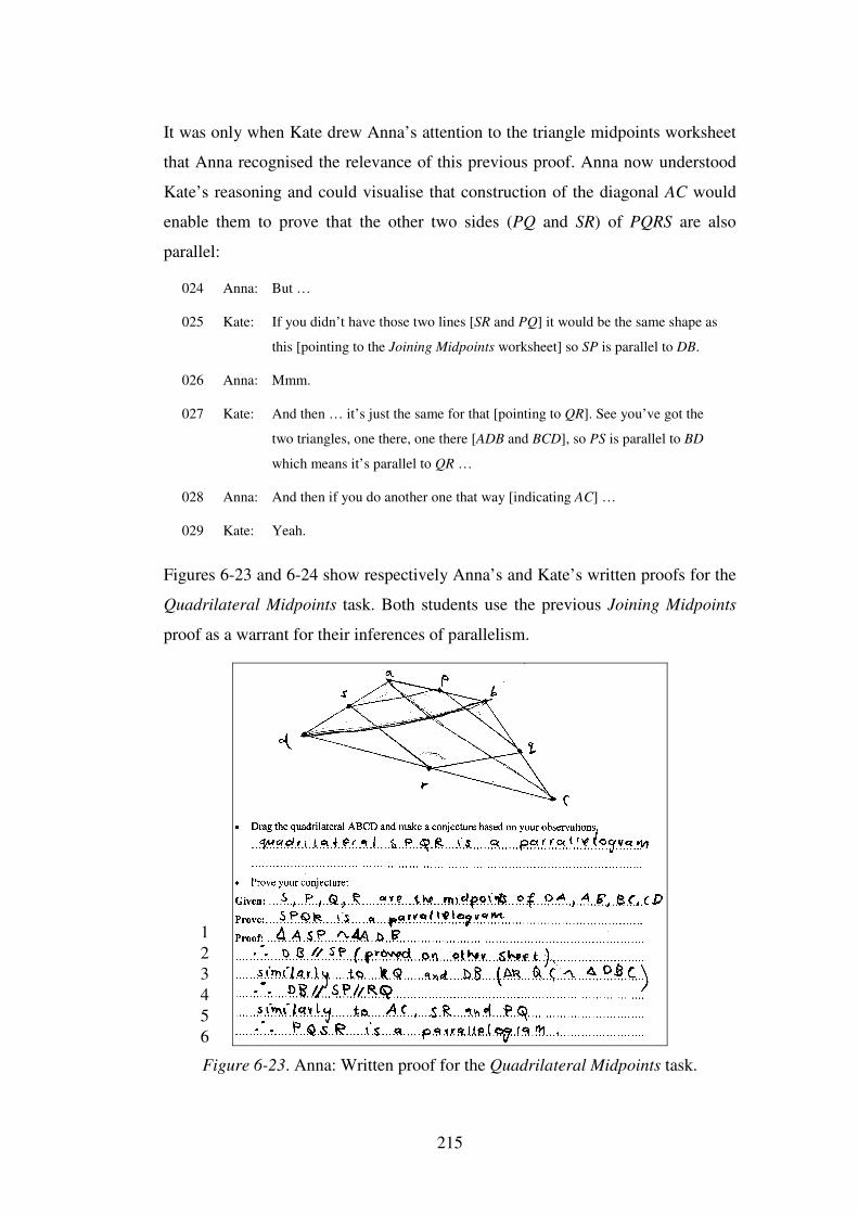
215
It was only when Kate drew Anna’s attention to the triangle midpoints worksheet
that Anna recognised the relevance of this previous proof. Anna now understood
Kate’s reasoning and could visualise that construction of the diagonal AC would
enable them to prove that the other two sides (PQ and SR) of PQRS are also
parallel:
024 Anna: But …
025 Kate: If you didn’t have those two lines [SR and PQ] it would be the same shape as
this [pointing to the Joining Midpoints worksheet] so SP is parallel to DB.
026 Anna: Mmm.
027 Kate: And then … it’s just the same for that [pointing to QR]. See you’ve got the
two triangles, one there, one there [ADB and BCD], so PS is parallel to BD
which means it’s parallel to QR …
028 Anna: And then if you do another one that way [indicating AC] …
029 Kate: Yeah.
Figures 6-23 and 6-24 show respectively Anna’s and Kate’s written proofs for the
Quadrilateral Midpoints task. Both students use the previous Joining Midpoints
proof as a warrant for their inferences of parallelism.
Figure 6-23. Anna: Written proof for the Quadrilateral Midpoints task.
123456
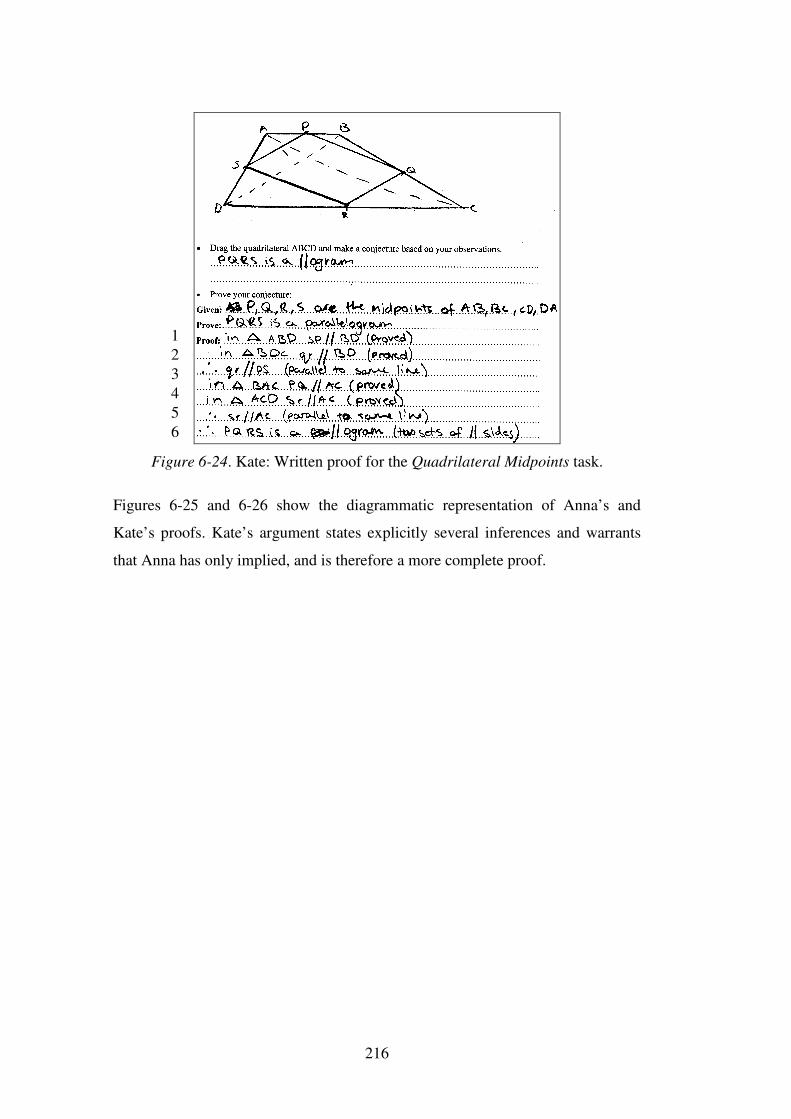
216
Figure 6-24. Kate: Written proof for the Quadrilateral Midpoints task.
Figures 6-25 and 6-26 show the diagrammatic representation of Anna’s and
Kate’s proofs. Kate’s argument states explicitly several inferences and warrants
that Anna has only implied, and is therefore a more complete proof.
123456
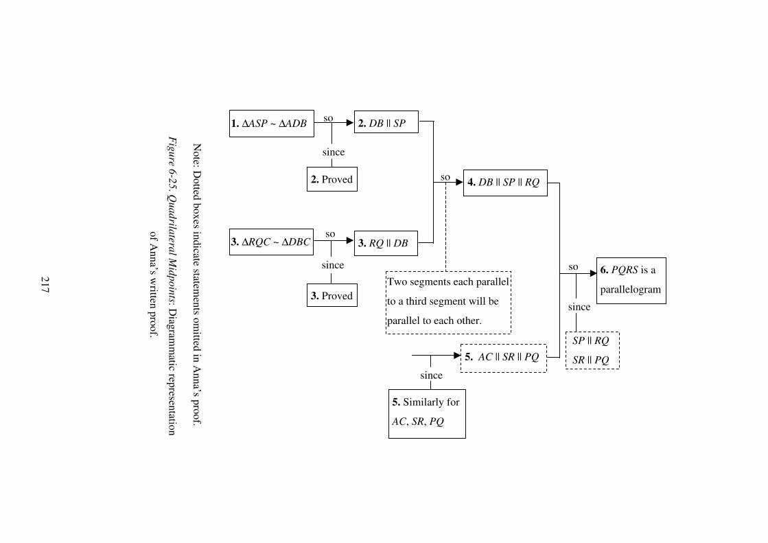
217
Note: D
otted boxes indicate statements om
itted in Anna’s proof.
Figure 6-25. Q
uadrilateral Midpoints: D
iagramm
atic representation
of Anna’s w
ritten proof.
1. ∆ASP ~ ∆ADB 2. DB || SP
2. Proved
3. RQ || DB
4. DB || SP || RQ
5. AC || SR || PQ
5. Similarly for
AC, SR, PQ
6. PQRS is a
parallelogram
3. ∆RQC ~ ∆DBC
3. Proved
so
SP || RQ
SR || PQ
Two segments each parallel
to a third segment will be
parallel to each other.
since
since
since
since
so
so
so
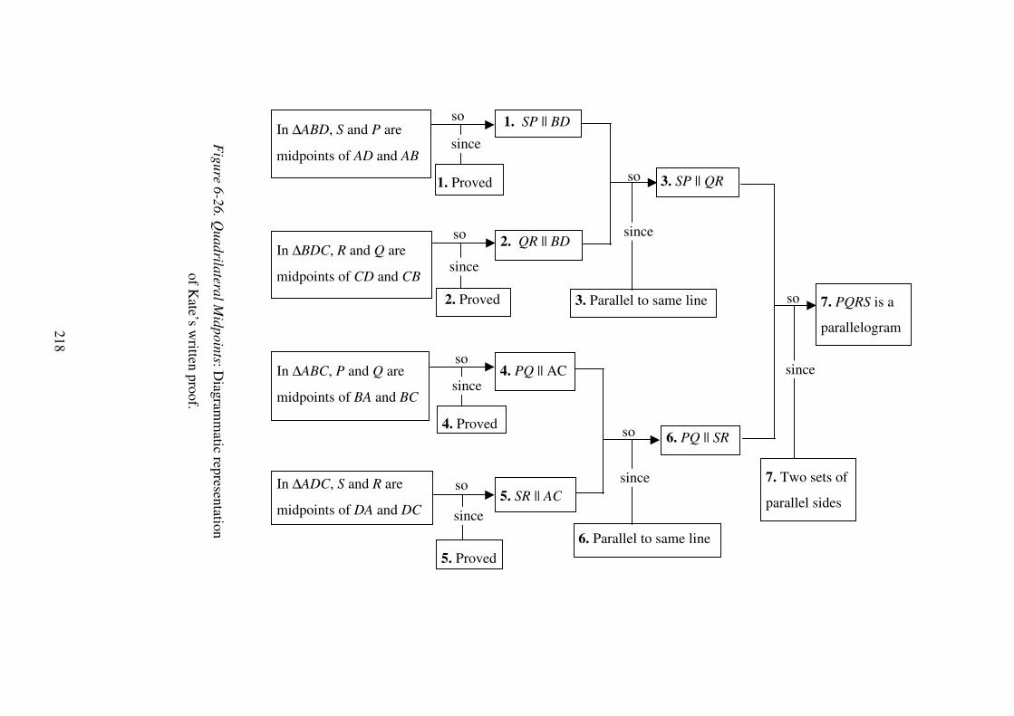
218
Figure 6-26. Q
uadrilateral Midpoints: D
iagramm
atic representation
of Kate’s w
ritten proof.
3. SP || QR
6. PQ || SR
In ∆ABD, S and P are
midpoints of AD and AB
In ∆BDC, R and Q are
midpoints of CD and CB
In ∆ABC, P and Q are
midpoints of BA and BC
In ∆ADC, S and R are
midpoints of DA and DC
1. Proved
2. Proved
4. Proved
5. Proved
1. SP || BD
2. QR || BD
4. PQ || AC
5. SR || AC
7. PQRS is a
parallelogram
6. Parallel to same line
3. Parallel to same line
7. Two sets of
parallel sides
so
so
so
so
so
so
so
since
since
since
since
since
since
since
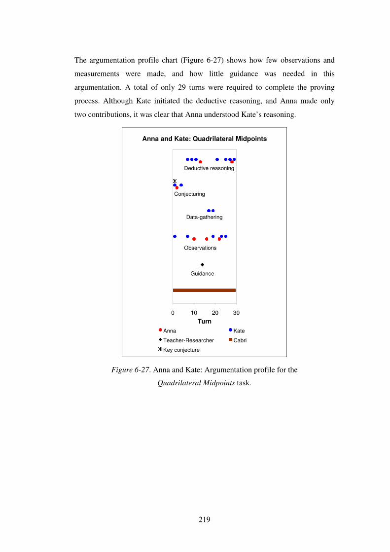
219
The argumentation profile chart (Figure 6-27) shows how few observations and
measurements were made, and how little guidance was needed in this
argumentation. A total of only 29 turns were required to complete the proving
process. Although Kate initiated the deductive reasoning, and Anna made only
two contributions, it was clear that Anna understood Kate’s reasoning.
Anna and Kate: Quadrilateral Midpoints
0 10 20 30Turn
Anna Kate
Teacher-Researcher Cabri
Key conjecture
Deductive reasoning
Conjecturing
Data-gathering
Observations
Guidance
Figure 6-27. Anna and Kate: Argumentation profile for the
Quadrilateral Midpoints task.
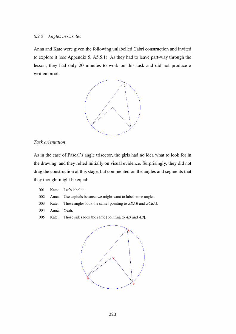
220
6.2.5 Angles in Circles
Anna and Kate were given the following unlabelled Cabri construction and invited
to explore it (see Appendix 5, A5.5.1). As they had to leave part-way through the
lesson, they had only 20 minutes to work on this task and did not produce a
written proof.
Task orientation
As in the case of Pascal’s angle trisector, the girls had no idea what to look for in
the drawing, and they relied initially on visual evidence. Surprisingly, they did not
drag the construction at this stage, but commented on the angles and segments that
they thought might be equal:
001 Kate: Let’s label it.
002 Anna: Use capitals because we might want to label some angles.
003 Kate: Those angles look the same [pointing to ∠DAB and ∠CBA].
004 Anna: Yeah.
005 Kate: Those sides look the same [pointing to AD and AB].
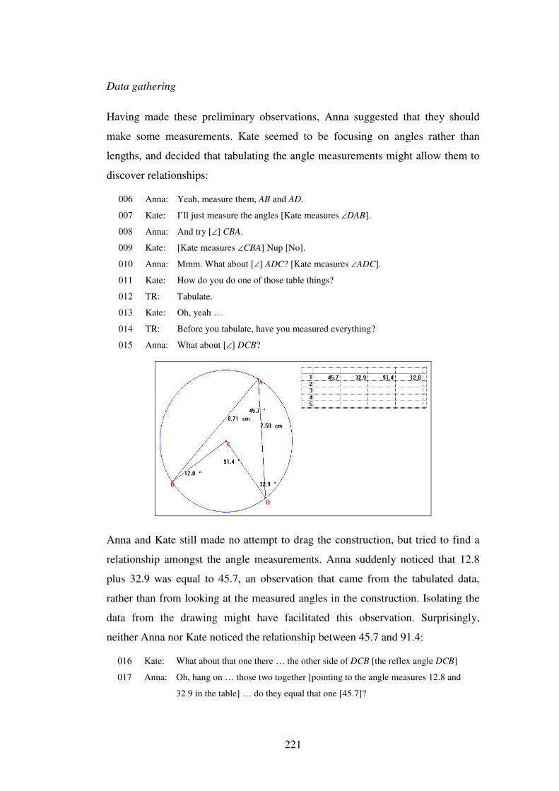
221
Data gathering
Having made these preliminary observations, Anna suggested that they should
make some measurements. Kate seemed to be focusing on angles rather than
lengths, and decided that tabulating the angle measurements might allow them to
discover relationships:
006 Anna: Yeah, measure them, AB and AD.
007 Kate: I’ll just measure the angles [Kate measures ∠DAB].
008 Anna: And try [∠] CBA.
009 Kate: [Kate measures ∠CBA] Nup [No].
010 Anna: Mmm. What about [∠] ADC? [Kate measures ∠ADC].
011 Kate: How do you do one of those table things?
012 TR: Tabulate.
013 Kate: Oh, yeah …
014 TR: Before you tabulate, have you measured everything?
015 Anna: What about [∠] DCB?
Anna and Kate still made no attempt to drag the construction, but tried to find a
relationship amongst the angle measurements. Anna suddenly noticed that 12.8
plus 32.9 was equal to 45.7, an observation that came from the tabulated data,
rather than from looking at the measured angles in the construction. Isolating the
data from the drawing might have facilitated this observation. Surprisingly,
neither Anna nor Kate noticed the relationship between 45.7 and 91.4:
016 Kate: What about that one there … the other side of DCB [the reflex angle DCB]
017 Anna: Oh, hang on … those two together [pointing to the angle measures 12.8 and
32.9 in the table] … do they equal that one [45.7]?
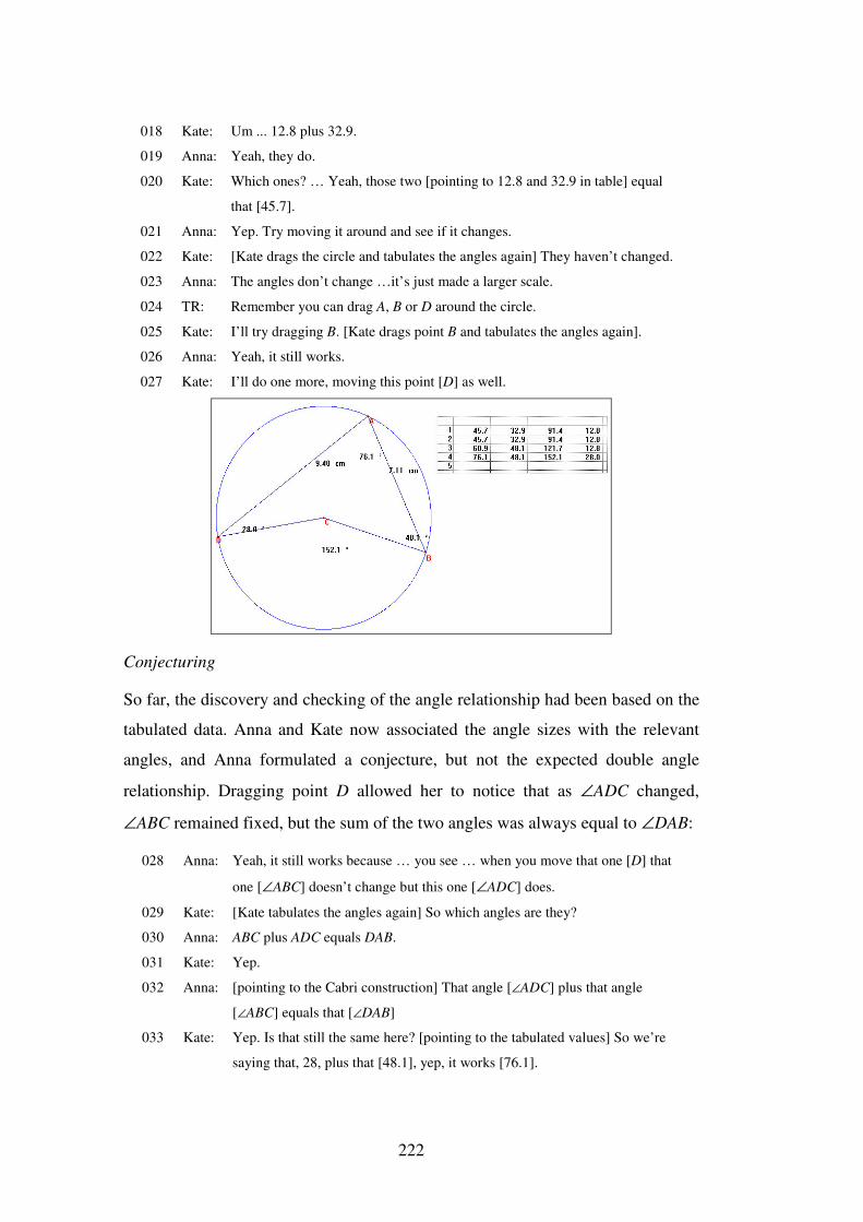
222
018 Kate: Um ... 12.8 plus 32.9.
019 Anna: Yeah, they do.
020 Kate: Which ones? … Yeah, those two [pointing to 12.8 and 32.9 in table] equal
that [45.7].
021 Anna: Yep. Try moving it around and see if it changes.
022 Kate: [Kate drags the circle and tabulates the angles again] They haven’t changed.
023 Anna: The angles don’t change …it’s just made a larger scale.
024 TR: Remember you can drag A, B or D around the circle.
025 Kate: I’ll try dragging B. [Kate drags point B and tabulates the angles again].
026 Anna: Yeah, it still works.
027 Kate: I’ll do one more, moving this point [D] as well.
Conjecturing
So far, the discovery and checking of the angle relationship had been based on the
tabulated data. Anna and Kate now associated the angle sizes with the relevant
angles, and Anna formulated a conjecture, but not the expected double angle
relationship. Dragging point D allowed her to notice that as ∠ADC changed,
∠ABC remained fixed, but the sum of the two angles was always equal to ∠DAB:
028 Anna: Yeah, it still works because … you see … when you move that one [D] that
one [∠ABC] doesn’t change but this one [∠ADC] does.
029 Kate: [Kate tabulates the angles again] So which angles are they?
030 Anna: ABC plus ADC equals DAB.
031 Kate: Yep.
032 Anna: [pointing to the Cabri construction] That angle [∠ADC] plus that angle
[∠ABC] equals that [∠DAB]
033 Kate: Yep. Is that still the same here? [pointing to the tabulated values] So we’re
saying that, 28, plus that [48.1], yep, it works [76.1].
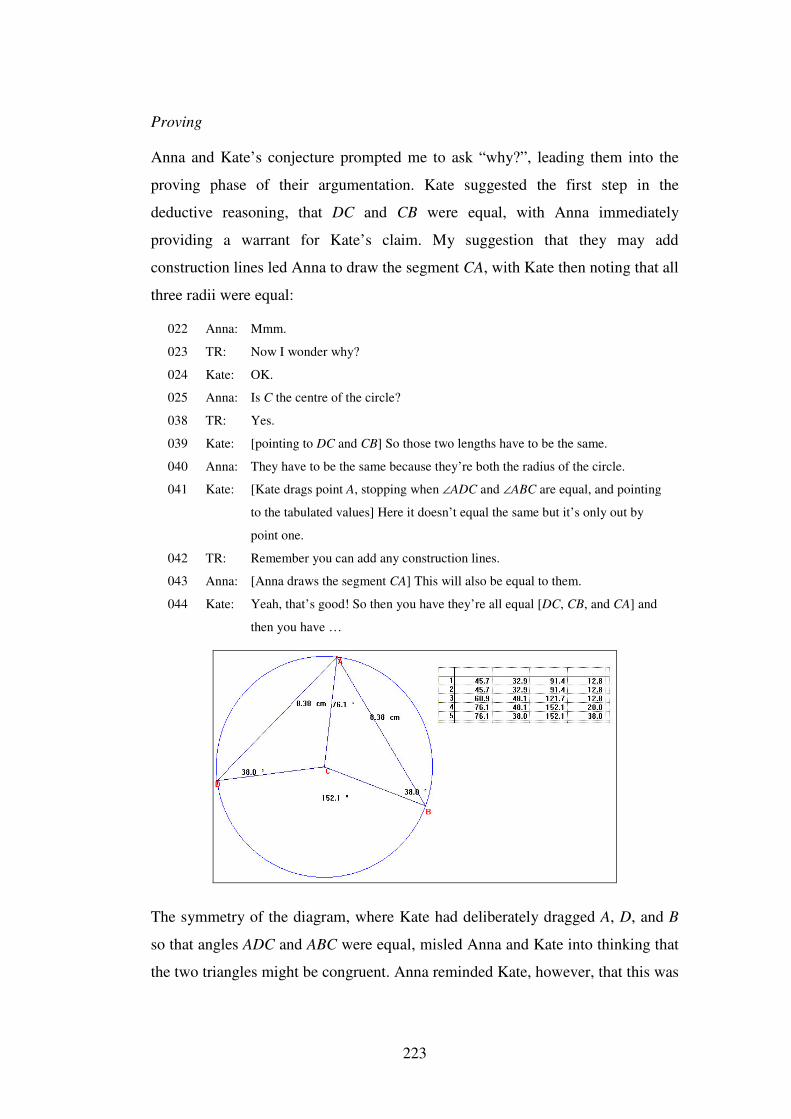
223
Proving
Anna and Kate’s conjecture prompted me to ask “why?”, leading them into the
proving phase of their argumentation. Kate suggested the first step in the
deductive reasoning, that DC and CB were equal, with Anna immediately
providing a warrant for Kate’s claim. My suggestion that they may add
construction lines led Anna to draw the segment CA, with Kate then noting that all
three radii were equal:
022 Anna: Mmm.
023 TR: Now I wonder why?
024 Kate: OK.
025 Anna: Is C the centre of the circle?
038 TR: Yes.
039 Kate: [pointing to DC and CB] So those two lengths have to be the same.
040 Anna: They have to be the same because they’re both the radius of the circle.
041 Kate: [Kate drags point A, stopping when ∠ADC and ∠ABC are equal, and pointing
to the tabulated values] Here it doesn’t equal the same but it’s only out by
point one.
042 TR: Remember you can add any construction lines.
043 Anna: [Anna draws the segment CA] This will also be equal to them.
044 Kate: Yeah, that’s good! So then you have they’re all equal [DC, CB, and CA] and
then you have …
The symmetry of the diagram, where Kate had deliberately dragged A, D, and B
so that angles ADC and ABC were equal, misled Anna and Kate into thinking that
the two triangles might be congruent. Anna reminded Kate, however, that this was
224
not always the case. While it is generally assumed that the dynamic visualisation
made possible by dragging helps students to identify invariant properties, this
advantage of the Cabri environment will be negated if students focus on a special
configuration.
045 Anna: Are these two congruent triangles?
046 Kate: Yeah, you’ve got …
047 Anna: But remember we measured these and they weren’t always the same … see
… remember?
048 Kate: Oh, yeah …
049 Anna: Remember they weren’t the same?
Kate then acknowledged that the triangles were isosceles (turn 050), although
Anna did not seem to recognise this until later (turn 055). Anna commented again
on the relationship between angles ADC, ABC, and DAB which they had
discovered previously. Her statement: “if we didn’t have that construction line
there” resembles a previous comment with Pascal’s angle trisector: “if we get rid
of BC” (see section 6.2.1, turn 048), suggesting that Anna did not consider that
∠DAB existed until the radius AC, that divided ∠DAB, was removed. Anna and
Kate then became excited when they suddenly recognised the explanation for their
conjecture:
050 Kate: So you’ve got two isosceles triangles.
051 Anna: Mmm.
052 Kate: What about that angle and that [∠DAC, ∠BAC]? Oh, but … but, but, but …
053 Anna: That one [∠ADC] plus that one [∠ABC] equals the big one [∠DAB] if we
didn’t have that construction line there.
054 Kate: But! …
055 Anna: Oh, they might be isosceles triangles … they are isosceles triangles.
057 Kate: Yeah?
058 Anna: Oh, but that makes sense, look! See, it’s an isosceles triangle [pointing to
∆CAB] and that …
059 Kate: That plus that [∠CAD +∠CAB] equals that plus that [∠ADC + ∠ABC].
060 Anna: So both of them together [∠CAD and ∠CAB] equal that [∠ADC] and that
[∠ABC]. CBA equals CAB because it’s an isosceles triangle ...
061 Kate: Yep.
062 Anna: And [∠]CAD equals [∠]ADC because it’s also an isosceles and them
together [∠CAD and ∠CAB] equal DAB.
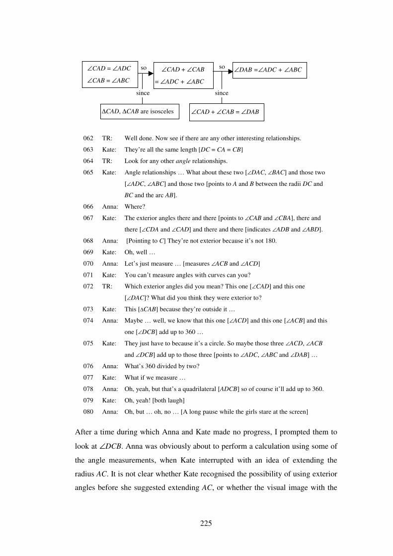
225
062 TR: Well done. Now see if there are any other interesting relationships.
063 Kate: They’re all the same length [DC = CA = CB]
064 TR: Look for any other angle relationships.
065 Kate: Angle relationships … What about these two [∠DAC, ∠BAC] and those two
[∠ADC, ∠ABC] and those two [points to A and B between the radii DC and
BC and the arc AB].
066 Anna: Where?
067 Kate: The exterior angles there and there [points to ∠CAB and ∠CBA], there and
there [∠CDA and ∠CAD] and there and there [indicates ∠ADB and ∠ABD].
068 Anna: [Pointing to C] They’re not exterior because it’s not 180.
069 Kate: Oh, well …
070 Anna: Let’s just measure … [measures ∠ACB and ∠ACD]
071 Kate: You can’t measure angles with curves can you?
072 TR: Which exterior angles did you mean? This one [∠CAD] and this one
[∠DAC]? What did you think they were exterior to?
073 Kate: This [∆CAB] because they’re outside it …
074 Anna: Maybe … well, we know that this one [∠ACD] and this one [∠ACB] and this
one [∠DCB] add up to 360 …
075 Kate: They just have to because it’s a circle. So maybe those three ∠ACD, ∠ACB
and ∠DCB] add up to those three [points to ∠ADC, ∠ABC and ∠DAB] …
076 Anna: What’s 360 divided by two?
077 Kate: What if we measure …
078 Anna: Oh, yeah, but that’s a quadrilateral [ADCB] so of course it’ll add up to 360.
079 Kate: Oh, yeah! [both laugh]
080 Anna: Oh, but … oh, no … [A long pause while the girls stare at the screen]
After a time during which Anna and Kate made no progress, I prompted them to
look at ∠DCB. Anna was obviously about to perform a calculation using some of
the angle measurements, when Kate interrupted with an idea of extending the
radius AC. It is not clear whether Kate recognised the possibility of using exterior
angles before she suggested extending AC, or whether the visual image with the
∠CAD + ∠CAB
= ∠ADC + ∠ABC
∆CAD, ∆CAB are isosceles
∠DAB =∠ADC + ∠ABC ∠CAD = ∠ADC
∠CAB = ∠ABC
so so
since since
∠CAD + ∠CAB = ∠DAB
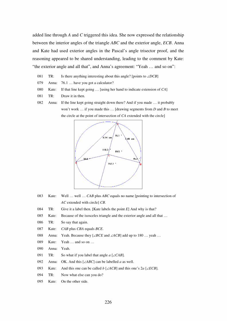
226
added line through A and C triggered this idea. She now expressed the relationship
between the interior angles of the triangle ABC and the exterior angle, ECB. Anna
and Kate had used exterior angles in the Pascal’s angle trisector proof, and the
reasoning appeared to be shared understanding, leading to the comment by Kate:
“the exterior angle and all that”, and Anna’s agreement: “Yeah … and so on”:
081 TR: Is there anything interesting about this angle? [points to ∠DCB]
079 Anna: 76.1 … have you got a calculator?
080 Kate: If that line kept going … [using her hand to indicate extension of CA]
081 TR: Draw it in then.
082 Anna: If the line kept going straight down there? And if you made … it probably
won’t work … if you made this … [drawing segments from D and B to meet
the circle at the point of intersection of CA extended with the circle]
083 Kate: Well … well … CAB plus ABC equals no name [pointing to intersection of
AC extended with circle] CB.
084 TR: Give it a label then. [Kate labels the point E] And why is that?
085 Kate: Because of the isosceles triangle and the exterior angle and all that …
086 TR: So say that again.
087 Kate: CAB plus CBA equals BCE.
088 Anna: Yeah. Because they [∠BCE and ∠ACB] add up to 180 … yeah …
089 Kate: Yeah … and so on …
090 Anna: Yeah.
091 TR: So what if you label that angle a [∠CAB].
092 Anna: OK. And this [∠ABC] can be labelled a as well.
093 Kate: And this one can be called b [∠ACB] and this one’s 2a [∠ECB].
094 TR: Now what else can you do?
095 Kate: On the other side.
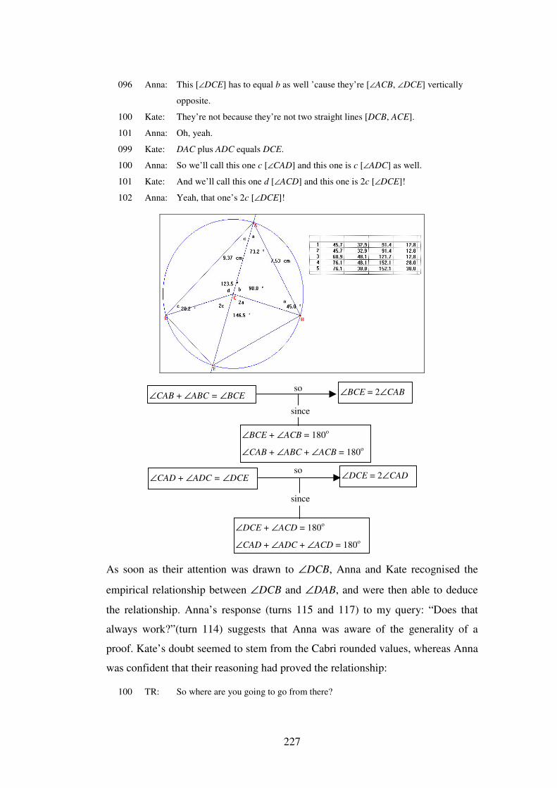
227
096 Anna: This [∠DCE] has to equal b as well ’cause they’re [∠ACB, ∠DCE] vertically
opposite.
100 Kate: They’re not because they’re not two straight lines [DCB, ACE].
101 Anna: Oh, yeah.
099 Kate: DAC plus ADC equals DCE.
100 Anna: So we’ll call this one c [∠CAD] and this one is c [∠ADC] as well.
101 Kate: And we’ll call this one d [∠ACD] and this one is 2c [∠DCE]!
102 Anna: Yeah, that one’s 2c [∠DCE]!
As soon as their attention was drawn to ∠DCB, Anna and Kate recognised the
empirical relationship between ∠DCB and ∠DAB, and were then able to deduce
the relationship. Anna’s response (turns 115 and 117) to my query: “Does that
always work?”(turn 114) suggests that Anna was aware of the generality of a
proof. Kate’s doubt seemed to stem from the Cabri rounded values, whereas Anna
was confident that their reasoning had proved the relationship:
100 TR: So where are you going to go from there?
∠CAB + ∠ABC = ∠BCE
∠BCE + ∠ACB = 180o
∠CAB + ∠ABC + ∠ACB = 180o
∠BCE = 2∠CAB so
since
∠CAD + ∠ADC = ∠DCE
∠DCE + ∠ACD = 180o
∠CAD + ∠ADC + ∠ACD = 180o
∠DCE = 2∠CAD so
since
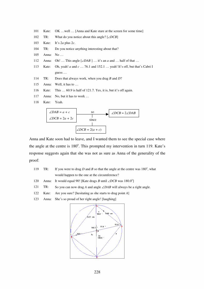
228
101 Kate: OK …well … [Anna and Kate stare at the screen for some time]
102 TR: What do you notice about this angle? [∠DCB]
103 Kate: It’s 2a plus 2c.
104 TR: Do you notice anything interesting about that?
105 Anna: No …
112 Anna: Oh! … This angle [∠DAB ] … it’s an a and … half of that …
113 Kate: Oh, yeah! a and c … 76.1 and 152.1 … yeah! It’s off, but that’s Cabri I
guess …
114 TR: Does that always work, when you drag B and D?
115 Anna: Well, it has to …
116 Kate: This … 60.9 is half of 121.7. Yes, it is, but it’s off again.
117 Anna: No, but it has to work …
118 Kate: Yeah.
Anna and Kate soon had to leave, and I wanted them to see the special case where
the angle at the centre is 180o. This prompted my intervention in turn 119. Kate’s
response suggests again that she was not as sure as Anna of the generality of the
proof:
119 TR: If you were to drag D and B so that the angle at the centre was 180o, what
would happen to the one at the circumference?
120 Anna: It would equal 90! [Kate drags B until ∠DCB was 180.0o]
121 TR: So you can now drag A and angle ∠DAB will always be a right angle.
122 Kate: Are you sure? [hesitating as she starts to drag point A]
123 Anna: She’s so proud of her right angle! [laughing]
∠DCB = 2∠DAB ∠DAB = a + c
∠DCB = 2a + 2c
so
∠DCB = 2(a + c)
since
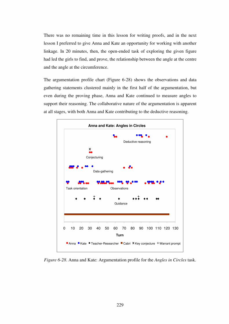
229
There was no remaining time in this lesson for writing proofs, and in the next
lesson I preferred to give Anna and Kate an opportunity for working with another
linkage. In 20 minutes, then, the open-ended task of exploring the given figure
had led the girls to find, and prove, the relationship between the angle at the centre
and the angle at the circumference.
The argumentation profile chart (Figure 6-28) shows the observations and data
gathering statements clustered mainly in the first half of the argumentation, but
even during the proving phase, Anna and Kate continued to measure angles to
support their reasoning. The collaborative nature of the argumentation is apparent
at all stages, with both Anna and Kate contributing to the deductive reasoning.
Anna and Kate: Angles in Circles
0 10 20 30 40 50 60 70 80 90 100 110 120 130
Turn
Anna Kate Teacher-Researcher Cabri Key conjecture Warrant prompt
Deductive reasoning
Conjecturing
Data-gathering
Observations
Guidance
Task orientation
Figure 6-28. Anna and Kate: Argumentation profile for the Angles in Circles task.
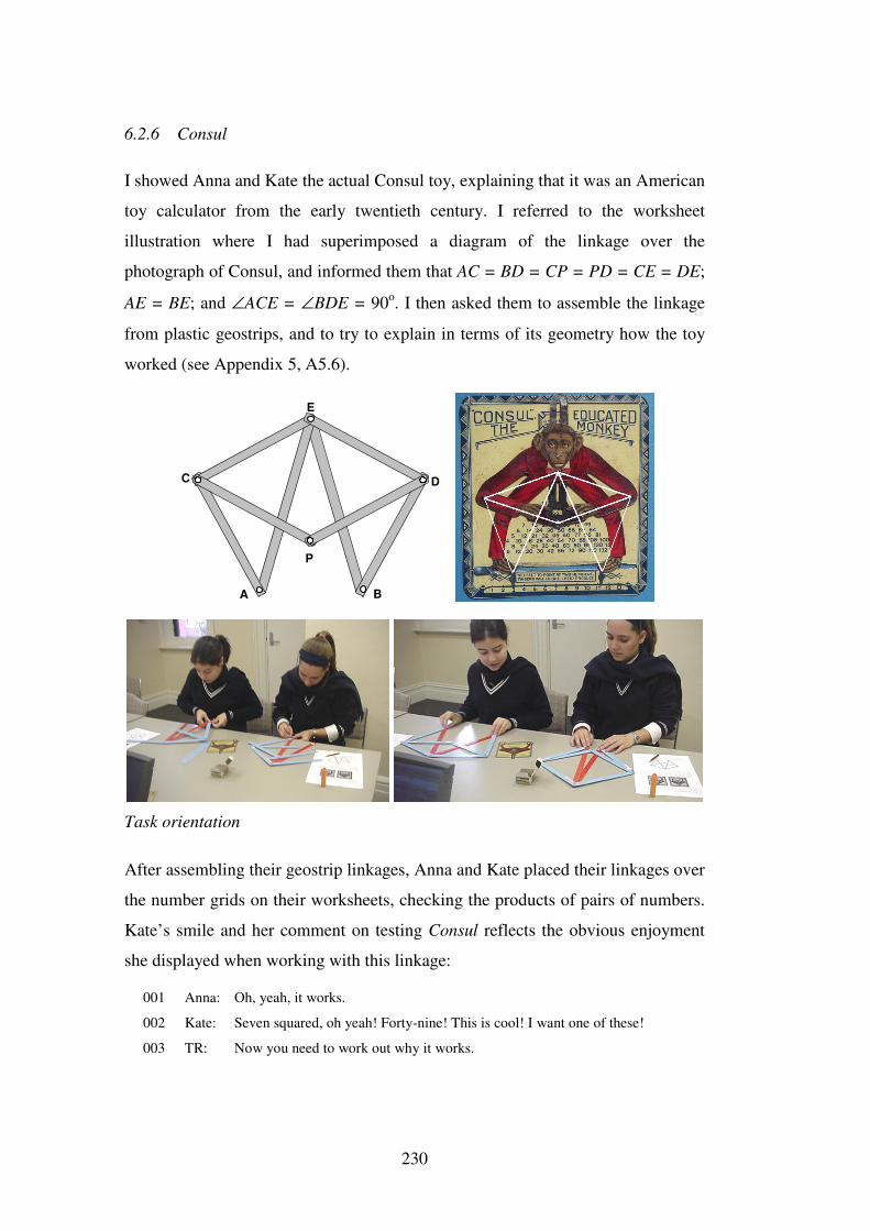
230
6.2.6 Consul
I showed Anna and Kate the actual Consul toy, explaining that it was an American
toy calculator from the early twentieth century. I referred to the worksheet
illustration where I had superimposed a diagram of the linkage over the
photograph of Consul, and informed them that AC = BD = CP = PD = CE = DE;
AE = BE; and ∠ACE = ∠BDE = 90o. I then asked them to assemble the linkage
from plastic geostrips, and to try to explain in terms of its geometry how the toy
worked (see Appendix 5, A5.6).
A
P
E
DC
B
Task orientation
After assembling their geostrip linkages, Anna and Kate placed their linkages over
the number grids on their worksheets, checking the products of pairs of numbers.
Kate’s smile and her comment on testing Consul reflects the obvious enjoyment
she displayed when working with this linkage:
001 Anna: Oh, yeah, it works.
002 Kate: Seven squared, oh yeah! Forty-nine! This is cool! I want one of these!
003 TR: Now you need to work out why it works.
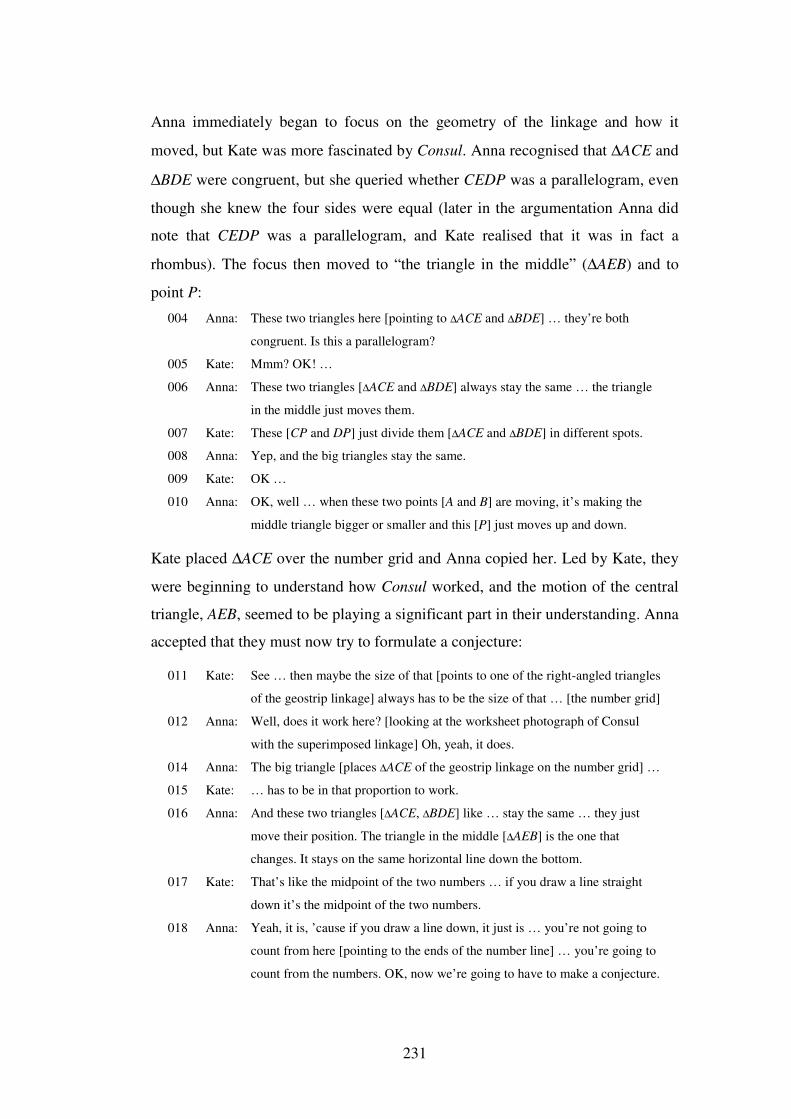
231
Anna immediately began to focus on the geometry of the linkage and how it
moved, but Kate was more fascinated by Consul. Anna recognised that ∆ACE and
∆BDE were congruent, but she queried whether CEDP was a parallelogram, even
though she knew the four sides were equal (later in the argumentation Anna did
note that CEDP was a parallelogram, and Kate realised that it was in fact a
rhombus). The focus then moved to “the triangle in the middle” (∆AEB) and to
point P:
004 Anna: These two triangles here [pointing to ∆ACE and ∆BDE] … they’re both
congruent. Is this a parallelogram?
005 Kate: Mmm? OK! …
006 Anna: These two triangles [∆ACE and ∆BDE] always stay the same … the triangle
in the middle just moves them.
007 Kate: These [CP and DP] just divide them [∆ACE and ∆BDE] in different spots.
008 Anna: Yep, and the big triangles stay the same.
009 Kate: OK …
010 Anna: OK, well … when these two points [A and B] are moving, it’s making the
middle triangle bigger or smaller and this [P] just moves up and down.
Kate placed ∆ACE over the number grid and Anna copied her. Led by Kate, they
were beginning to understand how Consul worked, and the motion of the central
triangle, AEB, seemed to be playing a significant part in their understanding. Anna
accepted that they must now try to formulate a conjecture:
011 Kate: See … then maybe the size of that [points to one of the right-angled triangles
of the geostrip linkage] always has to be the size of that … [the number grid]
012 Anna: Well, does it work here? [looking at the worksheet photograph of Consul
with the superimposed linkage] Oh, yeah, it does.
014 Anna: The big triangle [places ∆ACE of the geostrip linkage on the number grid] …
015 Kate: … has to be in that proportion to work.
016 Anna: And these two triangles [∆ACE, ∆BDE] like … stay the same … they just
move their position. The triangle in the middle [∆AEB] is the one that
changes. It stays on the same horizontal line down the bottom.
017 Kate: That’s like the midpoint of the two numbers … if you draw a line straight
down it’s the midpoint of the two numbers.
018 Anna: Yeah, it is, ’cause if you draw a line down, it just is … you’re not going to
count from here [pointing to the ends of the number line] … you’re going to
count from the numbers. OK, now we’re going to have to make a conjecture.
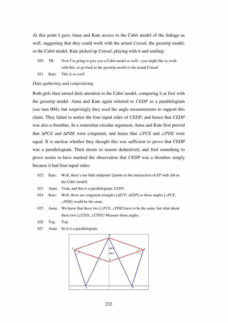
232
At this point I gave Anna and Kate access to the Cabri model of the linkage as
well, suggesting that they could work with the actual Consul, the geostrip model,
or the Cabri model. Kate picked up Consul, playing with it and smiling:
020 TR: Now I’m going to give you a Cabri model as well—you might like to work
with this, or go back to the geostrip model or the actual Consul.
021 Kate: This is so cool!
Data gathering and conjecturing
Both girls then turned their attention to the Cabri model, comparing it at first with
the geostrip model. Anna and Kate again referred to CEDP as a parallelogram
(see turn 004), but surprisingly they used the angle measurements to support this
claim. They failed to notice the four equal sides of CEDP, and hence that CEDP
was also a rhombus. In a somewhat circular argument, Anna and Kate first proved
that ∆PCE and ∆PDE were congruent, and hence that ∠PCE and ∠PDE were
equal. It is unclear whether they thought this was sufficient to prove that CEDP
was a parallelogram. Their desire to reason deductively and find something to
prove seems to have masked the observation that CEDP was a rhombus simply
because it had four equal sides:
022 Kate: Well, there’s our little midpoint! [points to the intersection of EP with AB on
the Cabri model]
023 Anna: Yeah, and this is a parallelogram, CEDP.
024 Kate: Well, those are congruent triangles [∆ECP, ∆EDP] so those angles [∠PCE,
∠PDE] would be the same.
025 Anna: We know that those two [∠PCE, ∠PDE] have to be the same, but what about
those two [∠CED, ∠CPD]? Measure those angles.
026 Tog: Yep.
027 Anna: So it is a parallelogram.
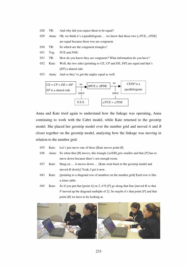
233
028 TR: And why did you expect them to be equal?
029 Anna: Oh, we think it’s a parallelogram … we know that those two [∠PCE, ∠PDE]
are equal because those two are congruent.
030 TR: So which are the congruent triangles?
031 Tog: PCE and PDE.
031 TR: How do you know they are congruent? What information do you have?
032 Kate: Well, the two sides [pointing to CE, CP and DE, DP] are equal and that’s
[EP] a shared side.
033 Anna: And so they’ve got the angles equal as well.
Anna and Kate tried again to understand how the linkage was operating, Anna
continuing to work with the Cabri model, while Kate returned to the geostrip
model. She placed her geostrip model over the number grid and moved A and B
closer together on the geostrip model, analysing how the linkage was moving in
relation to the number grid:
035 Kate: Let’s just move one of these [Kate moves point B].
036 Anna: So when that [B] moves, this triangle [∆AEB] gets smaller and that [P] has to
move down because there’s not enough room.
037 Kate: Hang on … it moves down … [Kate went back to the geostrip model and
moved B slowly] Yeah, I get it now.
043 Kate: [pointing to a diagonal row of numbers on the number grid] Each row is like
a times table.
045 Kate: So if you put that [point A] on 2, it’ll [P] go along that line [moved B so that
P moved up the diagonal multiple of 2]. So maybe it’s that point [P] and that
point [B] we have to be looking at.
CE = CP = DE = DP
EP is a shared side ∆PCE ≅ ∆PDE
CEDP is a
parallelogram
∠PCE = ∠PDE
so so
since
S.S.S.
since

234
Anna now drew lines on the number grid from P to A and from P to B, as well as
on the Cabri figure. She also labelled the intersection of EB and PD as G, but at
this stage she did not appear to notice triangle PAB. Meanwhile, Kate was still
focusing on the relationship between the geostrip linkage and the number grid.
Unlike the other tasks, where the two girls engaged in a joint argumentation, here
they were largely working independently, Anna with the Cabri model, and Kate
with the geostrip model and Consul. These preferences to work with the different
models were reflected later in the girls’ responses to the linkage questionnaire (see
Appendix 6).
048 Anna: Mmm …
049 Kate: Where that point [B] to that point [P] is …
050 Anna: Mmm … let’s say there was a triangle here [indicating lines from P to A and
P to B on the number grid] then they’d be congruent.
051 Kate: Mmm? What triangles?
051 Anna: These [∆PGB and its reflection in EF].
052 Kate: If we say put this on eleven …
053 Anna: Do you want to add them on here?
054 Kate: What?
055 Anna: Construction lines.
056 Anna: Ooh, is that one [pointing to the right half of ∆APB] congruent to that one?
[∆BDE] Look … it sort of works … that [from F to B] is the same as that [F
to P] … or is it?
048 Anna: Yep, they’re equal, but it doesn’t really help us much.
049 Kate: And that’d [AF] be equal too.
050 Anna: And those would both be right angles [∠PFA, ∠PFB]
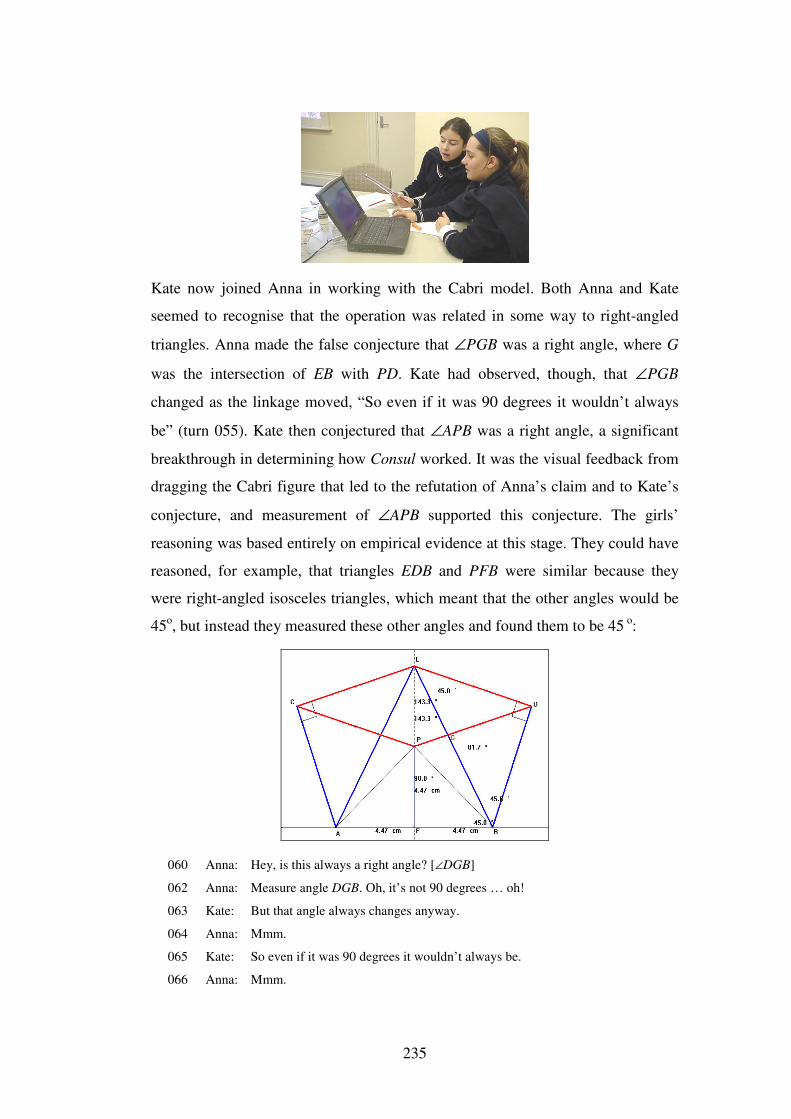
235
Kate now joined Anna in working with the Cabri model. Both Anna and Kate
seemed to recognise that the operation was related in some way to right-angled
triangles. Anna made the false conjecture that ∠PGB was a right angle, where G
was the intersection of EB with PD. Kate had observed, though, that ∠PGB
changed as the linkage moved, “So even if it was 90 degrees it wouldn’t always
be” (turn 055). Kate then conjectured that ∠APB was a right angle, a significant
breakthrough in determining how Consul worked. It was the visual feedback from
dragging the Cabri figure that led to the refutation of Anna’s claim and to Kate’s
conjecture, and measurement of ∠APB supported this conjecture. The girls’
reasoning was based entirely on empirical evidence at this stage. They could have
reasoned, for example, that triangles EDB and PFB were similar because they
were right-angled isosceles triangles, which meant that the other angles would be
45o, but instead they measured these other angles and found them to be 45 o:
060 Anna: Hey, is this always a right angle? [∠DGB]
062 Anna: Measure angle DGB. Oh, it’s not 90 degrees … oh!
063 Kate: But that angle always changes anyway.
064 Anna: Mmm.
065 Kate: So even if it was 90 degrees it wouldn’t always be.
066 Anna: Mmm.
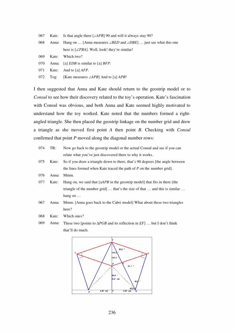
236
067 Kate: Is that angle there [∠APB] 90 and will it always stay 90?
068 Anna: Hang on … [Anna measures ∠BED and ∠DBE] … just see what this one
here is [∠PBA]. Well, look! they’re similar!
069 Kate: Which two?
070 Anna: [∆] EDB is similar to [∆] BFP.
071 Kate: And to [∆] AFP.
072 Tog: [Kate measures ∠APB] And to [∆] APB!
I then suggested that Anna and Kate should return to the geostrip model or to
Consul to see how their discovery related to the toy’s operation. Kate’s fascination
with Consul was obvious, and both Anna and Kate seemed highly motivated to
understand how the toy worked. Kate noted that the numbers formed a right-
angled triangle. She then placed the geostrip linkage on the number grid and drew
a triangle as she moved first point A then point B. Checking with Consul
confirmed that point P moved along the diagonal number rows:
074 TR: Now go back to the geostrip model or the actual Consul and see if you can
relate what you’ve just discovered there to why it works.
075 Kate: So if you draw a triangle down to there, that’s 90 degrees [the angle between
the lines formed when Kate traced the path of P on the number grid].
076 Anna: Mmm.
077 Kate: Hang on, we said that [∆APB in the geostrip model] that fits in there [the
triangle of the number grid] … that’s the size of that … and this is similar …
hang on …
067 Anna: Mmm. [Anna goes back to the Cabri model] What about these two triangles
here?
068 Kate: Which ones?
069 Anna: These two [points to ∆PGB and its reflection in EF] … but I don’t think
that’ll do much.
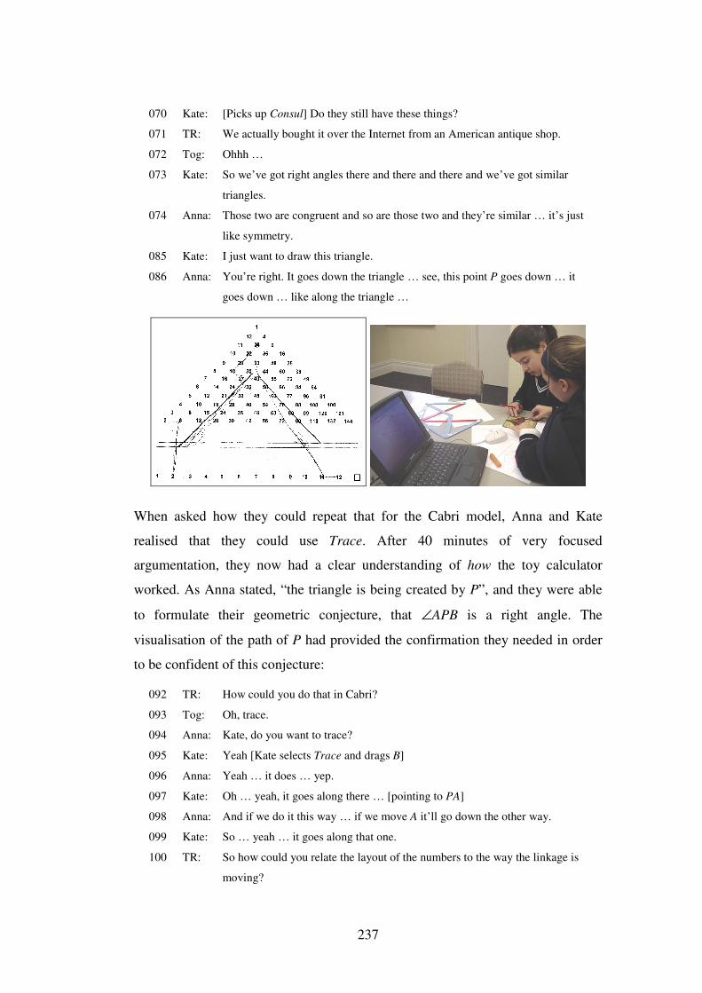
237
070 Kate: [Picks up Consul] Do they still have these things?
071 TR: We actually bought it over the Internet from an American antique shop.
072 Tog: Ohhh …
073 Kate: So we’ve got right angles there and there and there and we’ve got similar
triangles.
074 Anna: Those two are congruent and so are those two and they’re similar … it’s just
like symmetry.
085 Kate: I just want to draw this triangle.
086 Anna: You’re right. It goes down the triangle … see, this point P goes down … it
goes down … like along the triangle …
When asked how they could repeat that for the Cabri model, Anna and Kate
realised that they could use Trace. After 40 minutes of very focused
argumentation, they now had a clear understanding of how the toy calculator
worked. As Anna stated, “the triangle is being created by P”, and they were able
to formulate their geometric conjecture, that ∠APB is a right angle. The
visualisation of the path of P had provided the confirmation they needed in order
to be confident of this conjecture:
092 TR: How could you do that in Cabri?
093 Tog: Oh, trace.
094 Anna: Kate, do you want to trace?
095 Kate: Yeah [Kate selects Trace and drags B]
096 Anna: Yeah … it does … yep.
097 Kate: Oh … yeah, it goes along there … [pointing to PA]
098 Anna: And if we do it this way … if we move A it’ll go down the other way.
099 Kate: So … yeah … it goes along that one.
100 TR: So how could you relate the layout of the numbers to the way the linkage is
moving?
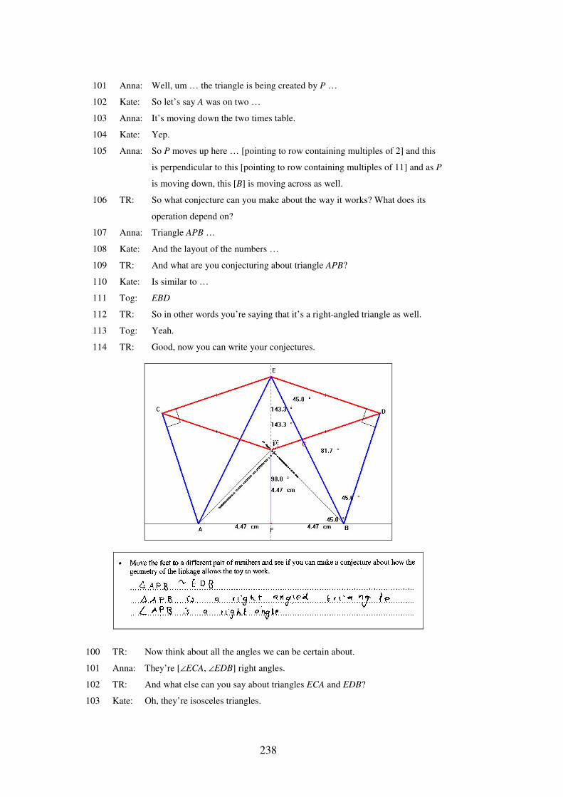
238
101 Anna: Well, um … the triangle is being created by P …
102 Kate: So let’s say A was on two …
103 Anna: It’s moving down the two times table.
104 Kate: Yep.
105 Anna: So P moves up here … [pointing to row containing multiples of 2] and this
is perpendicular to this [pointing to row containing multiples of 11] and as P
is moving down, this [B] is moving across as well.
106 TR: So what conjecture can you make about the way it works? What does its
operation depend on?
107 Anna: Triangle APB …
108 Kate: And the layout of the numbers …
109 TR: And what are you conjecturing about triangle APB?
110 Kate: Is similar to …
111 Tog: EBD
112 TR: So in other words you’re saying that it’s a right-angled triangle as well.
113 Tog: Yeah.
114 TR: Good, now you can write your conjectures.
100 TR: Now think about all the angles we can be certain about.
101 Anna: They’re [∠ECA, ∠EDB] right angles.
102 TR: And what else can you say about triangles ECA and EDB?
103 Kate: Oh, they’re isosceles triangles.
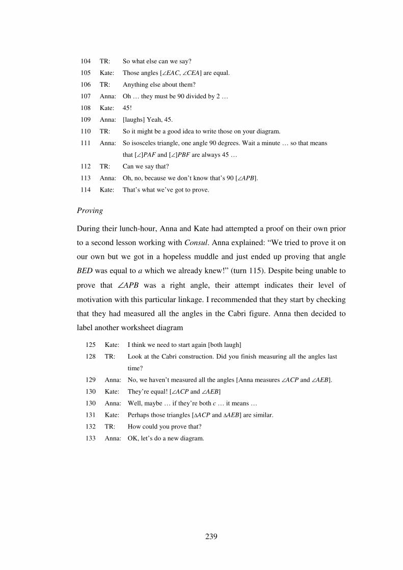
239
104 TR: So what else can we say?
105 Kate: Those angles [∠EAC, ∠CEA] are equal.
106 TR: Anything else about them?
107 Anna: Oh … they must be 90 divided by 2 …
108 Kate: 45!
109 Anna: [laughs] Yeah, 45.
110 TR: So it might be a good idea to write those on your diagram.
111 Anna: So isosceles triangle, one angle 90 degrees. Wait a minute … so that means
that [∠]PAF and [∠]PBF are always 45 …
112 TR: Can we say that?
113 Anna: Oh, no, because we don’t know that’s 90 [∠APB].
114 Kate: That’s what we’ve got to prove.
Proving
During their lunch-hour, Anna and Kate had attempted a proof on their own prior
to a second lesson working with Consul. Anna explained: “We tried to prove it on
our own but we got in a hopeless muddle and just ended up proving that angle
BED was equal to a which we already knew!” (turn 115). Despite being unable to
prove that ∠APB was a right angle, their attempt indicates their level of
motivation with this particular linkage. I recommended that they start by checking
that they had measured all the angles in the Cabri figure. Anna then decided to
label another worksheet diagram
125 Kate: I think we need to start again [both laugh]
128 TR: Look at the Cabri construction. Did you finish measuring all the angles last
time?
129 Anna: No, we haven’t measured all the angles [Anna measures ∠ACP and ∠AEB].
130 Kate: They’re equal! [∠ACP and ∠AEB]
130 Anna: Well, maybe … if they’re both c … it means …
131 Kate: Perhaps those triangles [∆ACP and ∆AEB] are similar.
132 TR: How could you prove that?
133 Anna: OK, let’s do a new diagram.
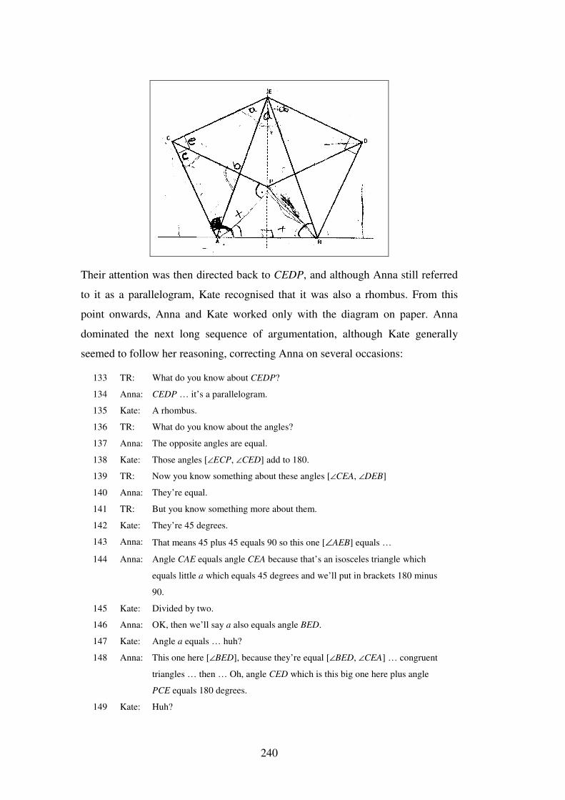
240
Their attention was then directed back to CEDP, and although Anna still referred
to it as a parallelogram, Kate recognised that it was also a rhombus. From this
point onwards, Anna and Kate worked only with the diagram on paper. Anna
dominated the next long sequence of argumentation, although Kate generally
seemed to follow her reasoning, correcting Anna on several occasions:
133 TR: What do you know about CEDP?
134 Anna: CEDP … it’s a parallelogram.
135 Kate: A rhombus.
136 TR: What do you know about the angles?
137 Anna: The opposite angles are equal.
138 Kate: Those angles [∠ECP, ∠CED] add to 180.
139 TR: Now you know something about these angles [∠CEA, ∠DEB]
140 Anna: They’re equal.
141 TR: But you know something more about them.
142 Kate: They’re 45 degrees.
143 Anna: That means 45 plus 45 equals 90 so this one [∠AEB] equals …
144 Anna: Angle CAE equals angle CEA because that’s an isosceles triangle which
equals little a which equals 45 degrees and we’ll put in brackets 180 minus
90.
145 Kate: Divided by two.
146 Anna: OK, then we’ll say a also equals angle BED.
147 Kate: Angle a equals … huh?
148 Anna: This one here [∠BED], because they’re equal [∠BED, ∠CEA] … congruent
triangles … then … Oh, angle CED which is this big one here plus angle
PCE equals 180 degrees.
149 Kate: Huh?
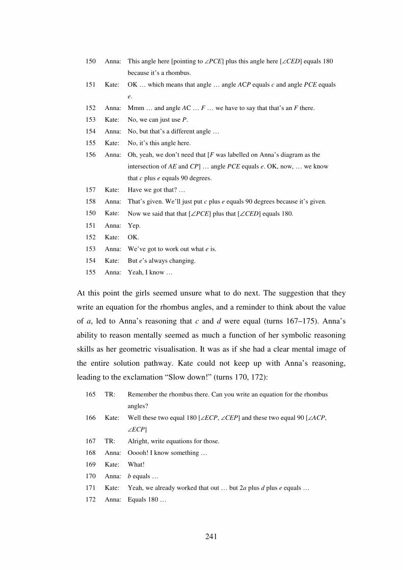
241
150 Anna: This angle here [pointing to ∠PCE] plus this angle here [∠CED] equals 180
because it’s a rhombus.
151 Kate: OK … which means that angle … angle ACP equals c and angle PCE equals
e.
152 Anna: Mmm … and angle AC … F … we have to say that that’s an F there.
153 Kate: No, we can just use P.
154 Anna: No, but that’s a different angle …
155 Kate: No, it’s this angle here.
156 Anna: Oh, yeah, we don’t need that [F was labelled on Anna’s diagram as the
intersection of AE and CP] … angle PCE equals e. OK, now, … we know
that c plus e equals 90 degrees.
157 Kate: Have we got that? …
158 Anna: That’s given. We’ll just put c plus e equals 90 degrees because it’s given.
150 Kate: Now we said that that [∠PCE] plus that [∠CED] equals 180.
151 Anna: Yep.
152 Kate: OK.
153 Anna: We’ve got to work out what e is.
154 Kate: But e’s always changing.
155 Anna: Yeah, I know …
At this point the girls seemed unsure what to do next. The suggestion that they
write an equation for the rhombus angles, and a reminder to think about the value
of a, led to Anna’s reasoning that c and d were equal (turns 167–175). Anna’s
ability to reason mentally seemed as much a function of her symbolic reasoning
skills as her geometric visualisation. It was as if she had a clear mental image of
the entire solution pathway. Kate could not keep up with Anna’s reasoning,
leading to the exclamation “Slow down!” (turns 170, 172):
165 TR: Remember the rhombus there. Can you write an equation for the rhombus
angles?
166 Kate: Well these two equal 180 [∠ECP, ∠CEP] and these two equal 90 [∠ACP,
∠ECP]
167 TR: Alright, write equations for those.
168 Anna: Ooooh! I know something …
169 Kate: What!
170 Anna: b equals …
171 Kate: Yeah, we already worked that out … but 2a plus d plus e equals …
172 Anna: Equals 180 …
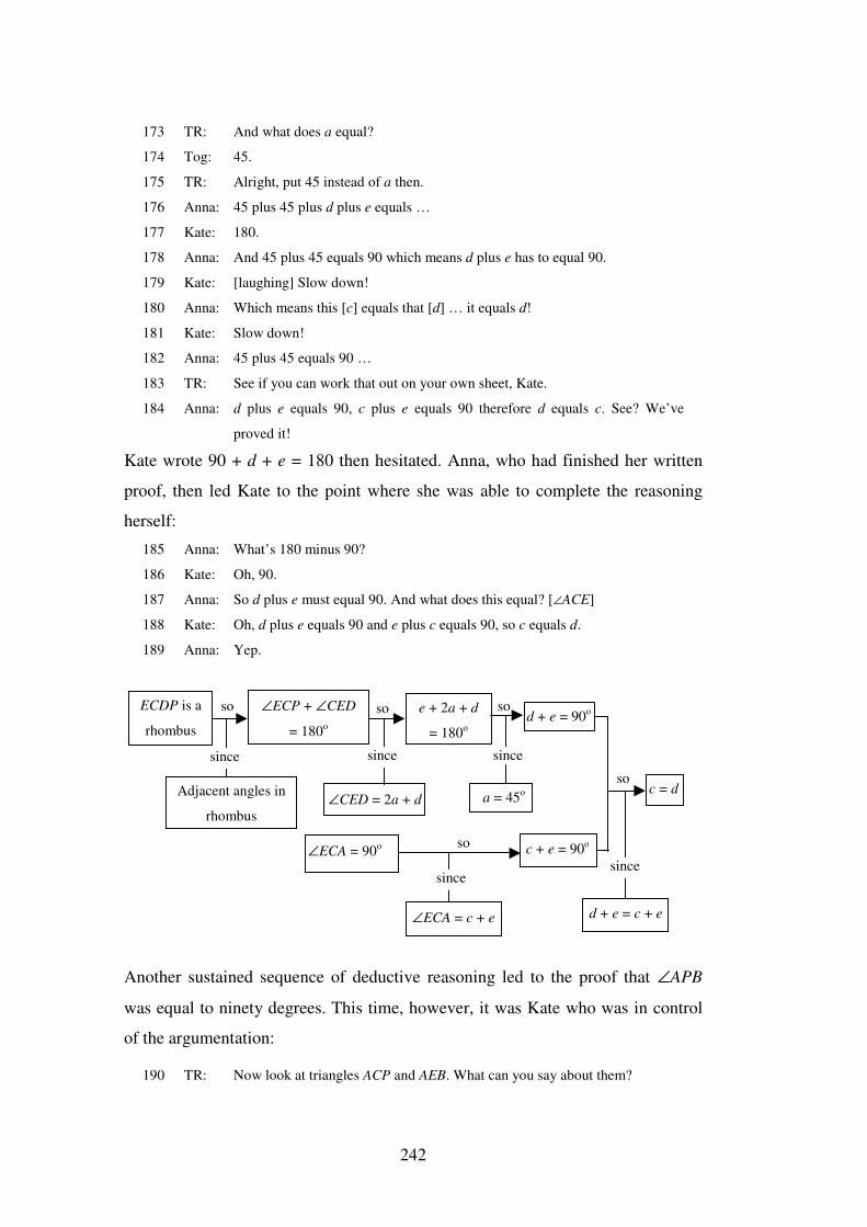
242
173 TR: And what does a equal?
174 Tog: 45.
175 TR: Alright, put 45 instead of a then.
176 Anna: 45 plus 45 plus d plus e equals …
177 Kate: 180.
178 Anna: And 45 plus 45 equals 90 which means d plus e has to equal 90.
179 Kate: [laughing] Slow down!
180 Anna: Which means this [c] equals that [d] … it equals d!
181 Kate: Slow down!
182 Anna: 45 plus 45 equals 90 …
183 TR: See if you can work that out on your own sheet, Kate.
184 Anna: d plus e equals 90, c plus e equals 90 therefore d equals c. See? We’ve
proved it!
Kate wrote 90 + d + e = 180 then hesitated. Anna, who had finished her written
proof, then led Kate to the point where she was able to complete the reasoning
herself:
185 Anna: What’s 180 minus 90?
186 Kate: Oh, 90.
187 Anna: So d plus e must equal 90. And what does this equal? [∠ACE]
188 Kate: Oh, d plus e equals 90 and e plus c equals 90, so c equals d.
189 Anna: Yep.
Another sustained sequence of deductive reasoning led to the proof that ∠APB
was equal to ninety degrees. This time, however, it was Kate who was in control
of the argumentation:
190 TR: Now look at triangles ACP and AEB. What can you say about them?
∠ECP + ∠CED
= 180o
e + 2a + d
= 180o d + e = 90o
c + e = 90o
c = d Adjacent angles in
rhombus a = 45o
ECDP is a
rhombus
∠CED = 2a + d
∠ECA = 90o
∠ECA = c + e
so so so
so
so
since since
since
since
d + e = c + e
since
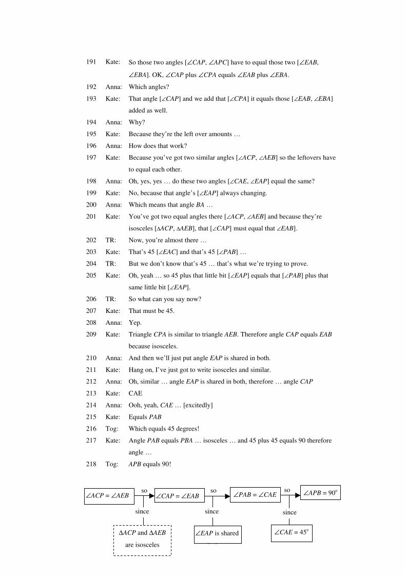
243
191 Kate: So those two angles [∠CAP, ∠APC] have to equal those two [∠EAB,
∠EBA]. OK, ∠CAP plus ∠CPA equals ∠EAB plus ∠EBA.
192 Anna: Which angles?
193 Kate: That angle [∠CAP] and we add that [∠CPA] it equals those [∠EAB, ∠EBA]
added as well.
194 Anna: Why?
195 Kate: Because they’re the left over amounts …
196 Anna: How does that work?
197 Kate: Because you’ve got two similar angles [∠ACP, ∠AEB] so the leftovers have
to equal each other.
198 Anna: Oh, yes, yes … do these two angles [∠CAE, ∠EAP] equal the same?
199 Kate: No, because that angle’s [∠EAP] always changing.
200 Anna: Which means that angle BA …
201 Kate: You’ve got two equal angles there [∠ACP, ∠AEB] and because they’re
isosceles [∆ACP, ∆AEB], that [∠CAP] must equal that ∠EAB].
202 TR: Now, you’re almost there …
203 Kate: That’s 45 [∠EAC] and that’s 45 [∠PAB] …
204 TR: But we don’t know that’s 45 … that’s what we’re trying to prove.
205 Kate: Oh, yeah … so 45 plus that little bit [∠EAP] equals that [∠PAB] plus that
same little bit [∠EAP].
206 TR: So what can you say now?
207 Kate: That must be 45.
208 Anna: Yep.
209 Kate: Triangle CPA is similar to triangle AEB. Therefore angle CAP equals EAB
because isosceles.
210 Anna: And then we’ll just put angle EAP is shared in both.
211 Kate: Hang on, I’ve just got to write isosceles and similar.
212 Anna: Oh, similar … angle EAP is shared in both, therefore … angle CAP
213 Kate: CAE
214 Anna: Ooh, yeah, CAE … [excitedly]
215 Kate: Equals PAB
216 Tog: Which equals 45 degrees!
217 Kate: Angle PAB equals PBA … isosceles … and 45 plus 45 equals 90 therefore
angle …
218 Tog: APB equals 90!
∠ACP = ∠AEB ∠CAP = ∠EAB
∆ACP and ∆AEB
are isosceles
∠PAB = ∠CAE
∠EAP is shared
∠APB = 90o
∠CAE = 45o
so so so
since since since
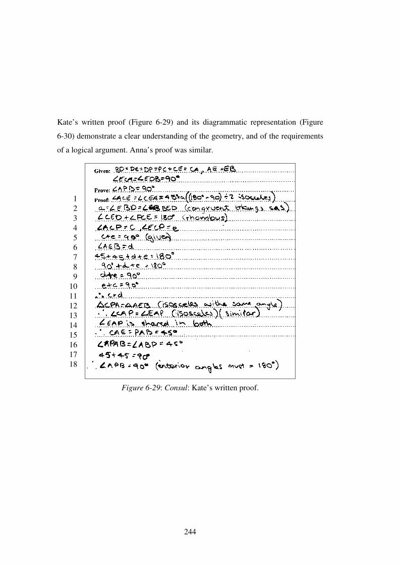
244
Kate’s written proof (Figure 6-29) and its diagrammatic representation (Figure
6-30) demonstrate a clear understanding of the geometry, and of the requirements
of a logical argument. Anna’s proof was similar.
Figure 6-29: Consul: Kate’s written proof.
123456789
101112131415161718
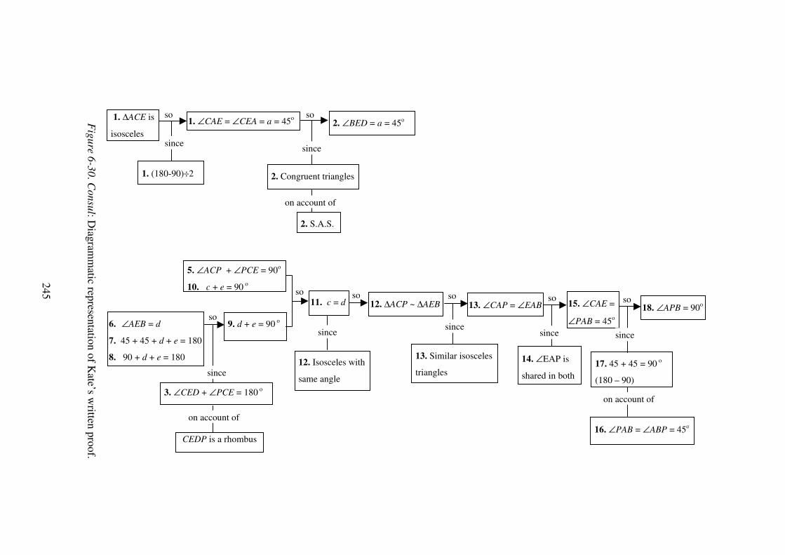
245
Figure 6-30 . C
onsul: Diagram
matic representation of K
ate’s written proof.
1. ∠CAE = ∠CEA = a = 45o 1. ∆ACE is
isosceles
1. (180-90)÷2
2. ∠BED = a = 45o
2. Congruent triangles
2. S.A.S.
so
3. ∠CED + ∠PCE = 180 o
CEDP is a rhombus
on account of
since since
5. ∠ACP + ∠PCE = 90o
10. c + e = 90 o
9. d + e = 90 o
so
on account of
6. ∠AEB = d
7. 45 + 45 + d + e = 180
8. 90 + d + e = 180
so
since 12. Isosceles with
same angle
12. ∆ACP ~ ∆AEB 13. ∠CAP = ∠EAB
14. ∠EAP is
shared in both
11. c = d 15. ∠CAE =
∠PAB = 45o
so so
13. Similar isosceles
triangles
since
so so
since
18. ∠APB = 90o
17. 45 + 45 = 90 o
(180 – 90)
16. ∠PAB = ∠ABP = 45o
since
so
on account of
since
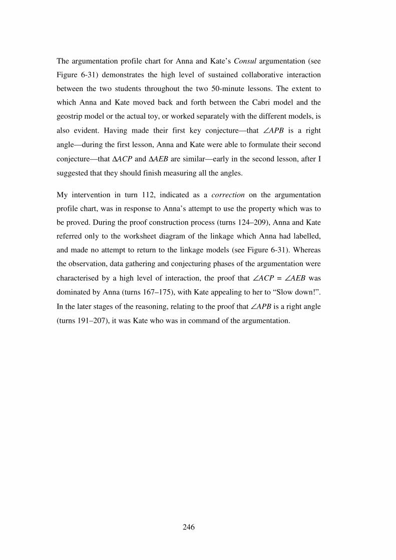
246
The argumentation profile chart for Anna and Kate’s Consul argumentation (see
Figure 6-31) demonstrates the high level of sustained collaborative interaction
between the two students throughout the two 50-minute lessons. The extent to
which Anna and Kate moved back and forth between the Cabri model and the
geostrip model or the actual toy, or worked separately with the different models, is
also evident. Having made their first key conjecture—that ∠APB is a right
angle—during the first lesson, Anna and Kate were able to formulate their second
conjecture—that ∆ACP and ∆AEB are similar—early in the second lesson, after I
suggested that they should finish measuring all the angles.
My intervention in turn 112, indicated as a correction on the argumentation
profile chart, was in response to Anna’s attempt to use the property which was to
be proved. During the proof construction process (turns 124–209), Anna and Kate
referred only to the worksheet diagram of the linkage which Anna had labelled,
and made no attempt to return to the linkage models (see Figure 6-31). Whereas
the observation, data gathering and conjecturing phases of the argumentation were
characterised by a high level of interaction, the proof that ∠ACP = ∠AEB was
dominated by Anna (turns 167–175), with Kate appealing to her to “Slow down!”.
In the later stages of the reasoning, relating to the proof that ∠APB is a right angle
(turns 191–207), it was Kate who was in command of the argumentation.
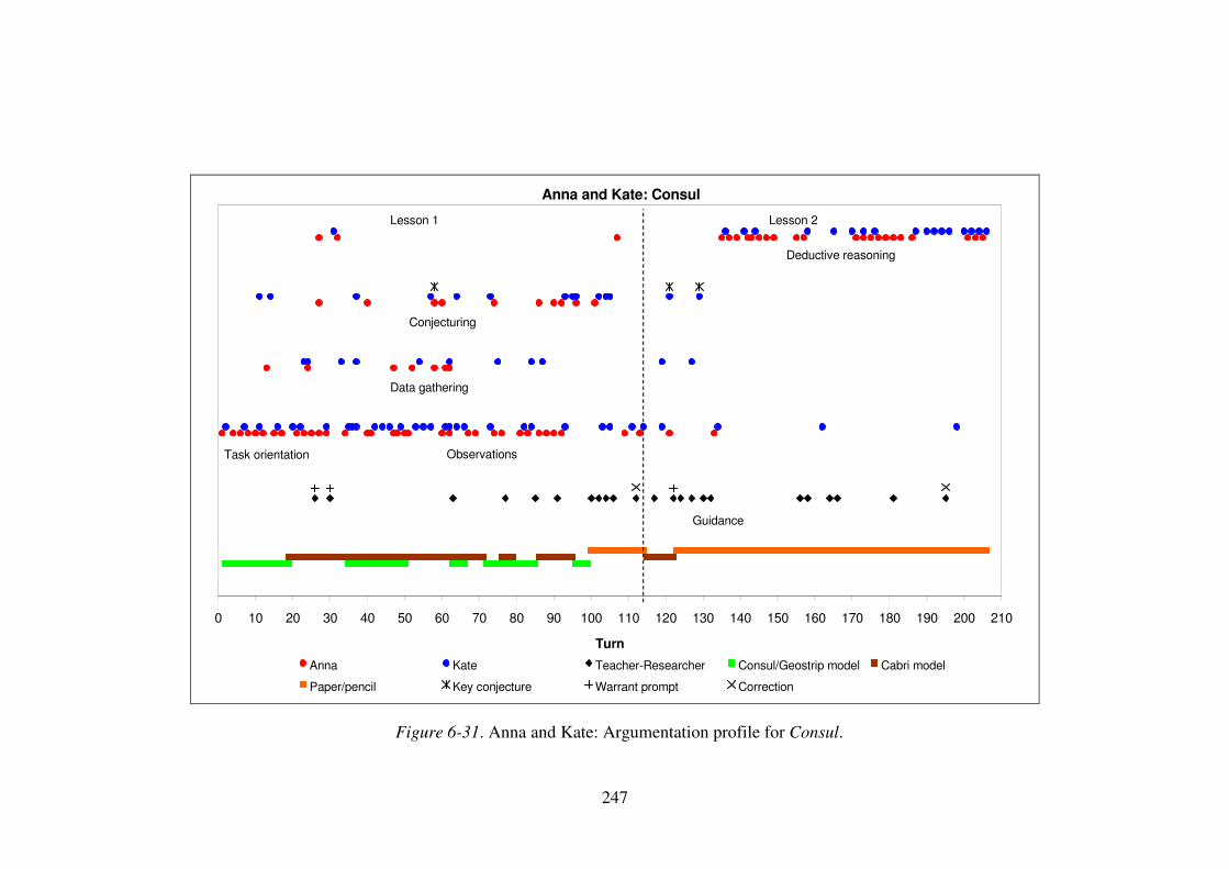
247
Anna and Kate: Consul
0 10 20 30 40 50 60 70 80 90 100 110 120 130 140 150 160 170 180 190 200 210
Turn
Anna Kate Teacher-Researcher Consul/Geostrip model Cabri model
Paper/pencil Key conjecture Warrant prompt Correction
Deductive reasoning
Conjecturing
Data gathering
Observations
Guidance
Lesson 1 Lesson 2
Task orientation
Figure 6-31. Anna and Kate: Argumentation profile for Consul.
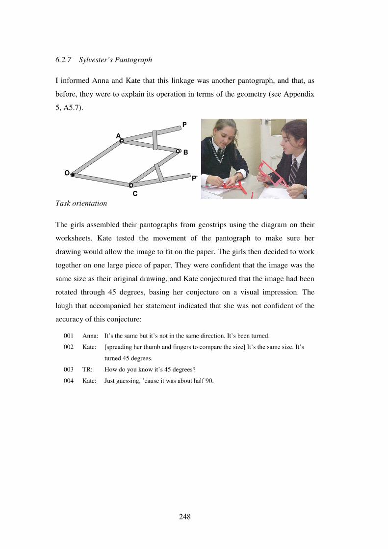
248
6.2.7 Sylvester’s Pantograph
I informed Anna and Kate that this linkage was another pantograph, and that, as
before, they were to explain its operation in terms of the geometry (see Appendix
5, A5.7).
O
P
C
B
A
P'
Task orientation
The girls assembled their pantographs from geostrips using the diagram on their
worksheets. Kate tested the movement of the pantograph to make sure her
drawing would allow the image to fit on the paper. The girls then decided to work
together on one large piece of paper. They were confident that the image was the
same size as their original drawing, and Kate conjectured that the image had been
rotated through 45 degrees, basing her conjecture on a visual impression. The
laugh that accompanied her statement indicated that she was not confident of the
accuracy of this conjecture:
001 Anna: It’s the same but it’s not in the same direction. It’s been turned.
002 Kate: [spreading her thumb and fingers to compare the size] It’s the same size. It’s
turned 45 degrees.
003 TR: How do you know it’s 45 degrees?
004 Kate: Just guessing, ’cause it was about half 90.
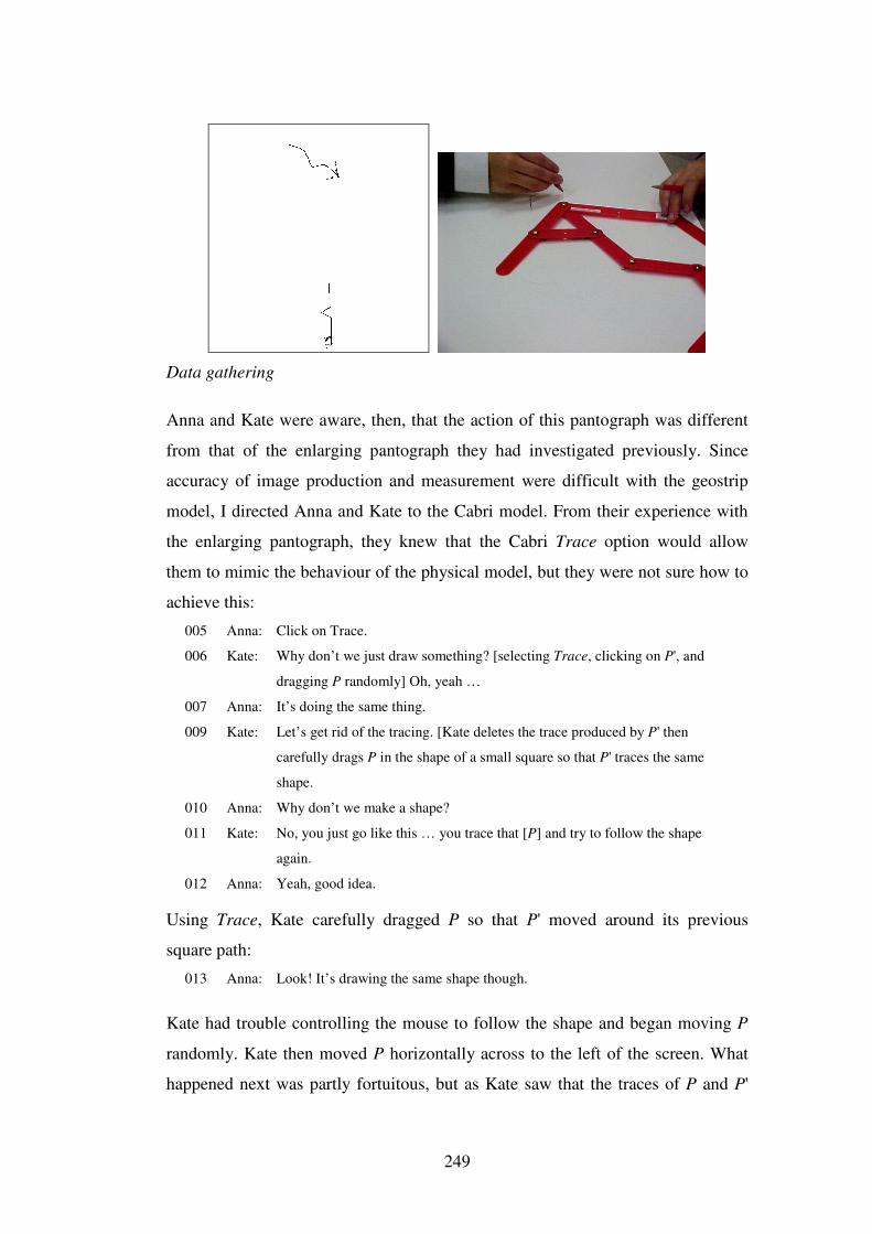
249
Data gathering
Anna and Kate were aware, then, that the action of this pantograph was different
from that of the enlarging pantograph they had investigated previously. Since
accuracy of image production and measurement were difficult with the geostrip
model, I directed Anna and Kate to the Cabri model. From their experience with
the enlarging pantograph, they knew that the Cabri Trace option would allow
them to mimic the behaviour of the physical model, but they were not sure how to
achieve this:
005 Anna: Click on Trace.
006 Kate: Why don’t we just draw something? [selecting Trace, clicking on P', and
dragging P randomly] Oh, yeah …
007 Anna: It’s doing the same thing.
009 Kate: Let’s get rid of the tracing. [Kate deletes the trace produced by P' then
carefully drags P in the shape of a small square so that P' traces the same
shape.
010 Anna: Why don’t we make a shape?
011 Kate: No, you just go like this … you trace that [P] and try to follow the shape
again.
012 Anna: Yeah, good idea.
Using Trace, Kate carefully dragged P so that P' moved around its previous
square path:
013 Anna: Look! It’s drawing the same shape though.
Kate had trouble controlling the mouse to follow the shape and began moving P
randomly. Kate then moved P horizontally across to the left of the screen. What
happened next was partly fortuitous, but as Kate saw that the traces of P and P'
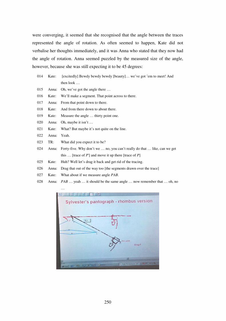
250
were converging, it seemed that she recognised that the angle between the traces
represented the angle of rotation. As often seemed to happen, Kate did not
verbalise her thoughts immediately, and it was Anna who stated that they now had
the angle of rotation. Anna seemed puzzled by the measured size of the angle,
however, because she was still expecting it to be 45 degrees:
014 Kate: [excitedly] Bewdy bewdy bewdy [beauty]… we’ve got ’em to meet! And
then look …
015 Anna: Oh, we’ve got the angle there …
016 Kate: We’ll make a segment. That point across to there.
017 Anna: From that point down to there.
018 Kate: And from there down to about there.
019 Kate: Measure the angle … thirty point one.
020 Anna: Oh, maybe it isn’t …
021 Kate: What? But maybe it’s not quite on the line.
022 Anna: Yeah.
023 TR: What did you expect it to be?
024 Anna: Forty-five. Why don’t we … no, you can’t really do that … like, can we get
this … [trace of P'] and move it up there [trace of P]
025 Kate: Huh? Well let’s drag it back and get rid of the tracing.
026 Anna: Drag that out of the way too [the segments drawn over the trace]
027 Kate: What about if we measure angle PAB.
028 Anna: PAB … yeah … it should be the same angle … now remember that … oh, no
…
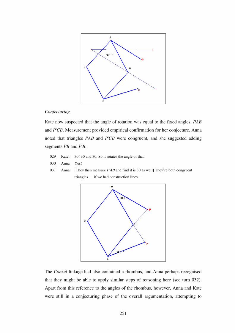
251
Conjecturing
Kate now suspected that the angle of rotation was equal to the fixed angles, PAB
and P'CB. Measurement provided empirical confirmation for her conjecture. Anna
noted that triangles PAB and P'CB were congruent, and she suggested adding
segments PB and P'B:
029 Kate: 30! 30 and 30. So it rotates the angle of that.
030 Anna Yes!
031 Anna: [They then measure P'AB and find it is 30 as well] They’re both congruent
triangles … if we had construction lines …
The Consul linkage had also contained a rhombus, and Anna perhaps recognised
that they might be able to apply similar steps of reasoning here (see turn 032).
Apart from this reference to the angles of the rhombus, however, Anna and Kate
were still in a conjecturing phase of the overall argumentation, attempting to
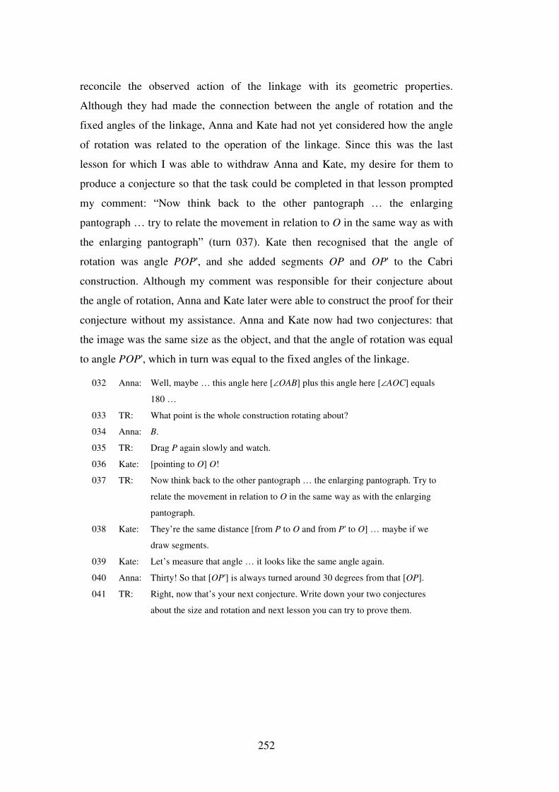
252
reconcile the observed action of the linkage with its geometric properties.
Although they had made the connection between the angle of rotation and the
fixed angles of the linkage, Anna and Kate had not yet considered how the angle
of rotation was related to the operation of the linkage. Since this was the last
lesson for which I was able to withdraw Anna and Kate, my desire for them to
produce a conjecture so that the task could be completed in that lesson prompted
my comment: “Now think back to the other pantograph … the enlarging
pantograph … try to relate the movement in relation to O in the same way as with
the enlarging pantograph” (turn 037). Kate then recognised that the angle of
rotation was angle POP', and she added segments OP and OP' to the Cabri
construction. Although my comment was responsible for their conjecture about
the angle of rotation, Anna and Kate later were able to construct the proof for their
conjecture without my assistance. Anna and Kate now had two conjectures: that
the image was the same size as the object, and that the angle of rotation was equal
to angle POP', which in turn was equal to the fixed angles of the linkage.
032 Anna: Well, maybe … this angle here [∠OAB] plus this angle here [∠AOC] equals
180 …
033 TR: What point is the whole construction rotating about?
034 Anna: B.
035 TR: Drag P again slowly and watch.
036 Kate: [pointing to O] O!
037 TR: Now think back to the other pantograph … the enlarging pantograph. Try to
relate the movement in relation to O in the same way as with the enlarging
pantograph.
038 Kate: They’re the same distance [from P to O and from P' to O] … maybe if we
draw segments.
039 Kate: Let’s measure that angle … it looks like the same angle again.
040 Anna: Thirty! So that [OP'] is always turned around 30 degrees from that [OP].
041 TR: Right, now that’s your next conjecture. Write down your two conjectures
about the size and rotation and next lesson you can try to prove them.
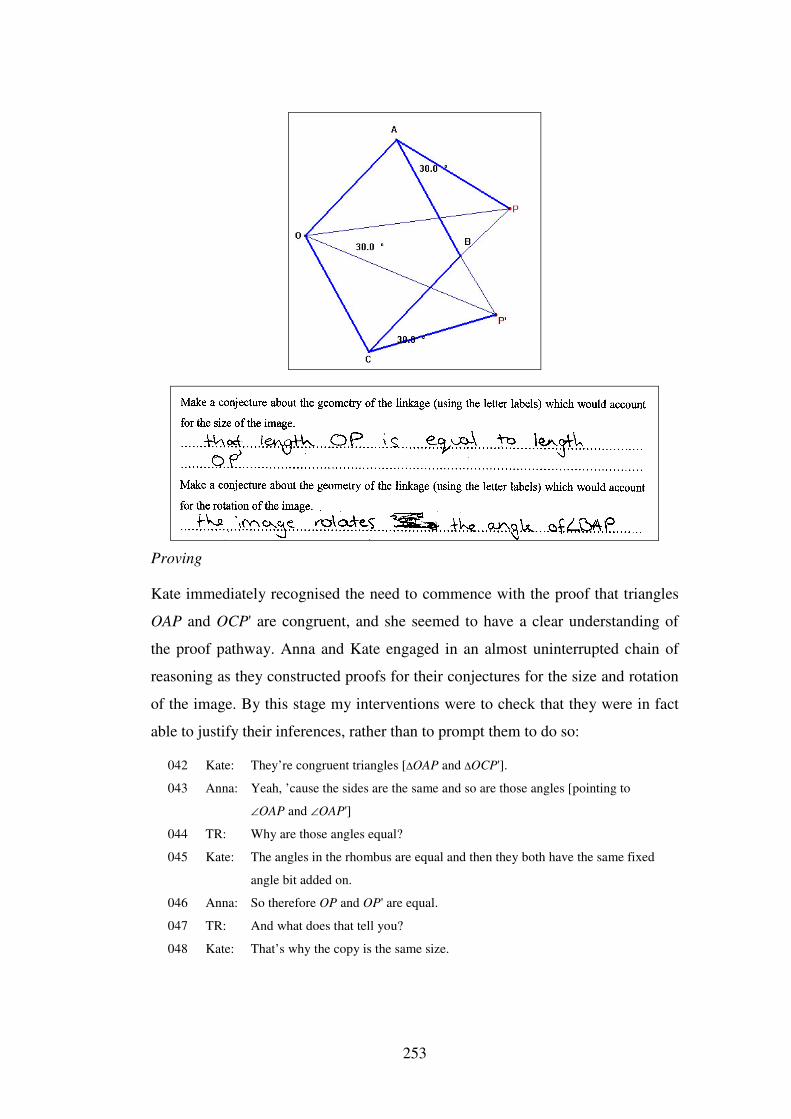
253
Proving
Kate immediately recognised the need to commence with the proof that triangles
OAP and OCP' are congruent, and she seemed to have a clear understanding of
the proof pathway. Anna and Kate engaged in an almost uninterrupted chain of
reasoning as they constructed proofs for their conjectures for the size and rotation
of the image. By this stage my interventions were to check that they were in fact
able to justify their inferences, rather than to prompt them to do so:
042 Kate: They’re congruent triangles [∆OAP and ∆OCP'].
043 Anna: Yeah, ’cause the sides are the same and so are those angles [pointing to
∠OAP and ∠OAP']
044 TR: Why are those angles equal?
045 Kate: The angles in the rhombus are equal and then they both have the same fixed
angle bit added on.
046 Anna: So therefore OP and OP' are equal.
047 TR: And what does that tell you?
048 Kate: That’s why the copy is the same size.
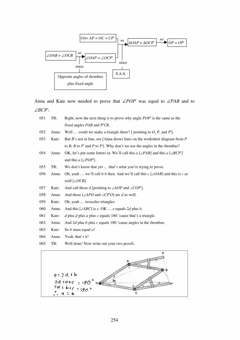
254
Anna and Kate now needed to prove that ∠POP' was equal to ∠PAB and to
∠BCP':
051 TR: Right, now the next thing is to prove why angle POP' is the same as the
fixed angles PAB and P'CB.
052 Anna: Well … could we make a triangle there? [ pointing to O, P, and P'].
053 Kate: But B’s not in line, see [Anna draws lines on the worksheet diagram from P
to B, B to P' and P to P']. Why don’t we use the angles in the rhombus?
054 Anna: OK, let’s put some letters in. We’ll call this a [∠PAB] and this a [∠BCP']
and this a [∠POP'].
055 TR: We don’t know that yet … that’s what you’re trying to prove.
056 Anna: Oh, yeah … we’ll call it b then. And we’ll call this c [∠OAB] and this is c as
well [∠OCB].
057 Kate: And call those d [pointing to ∠AOP and ∠COP'].
058 Anna: And those [∠APO and ∠CP'O] are d as well.
059 Kate: Oh, yeah … isosceles triangles.
060 Anna: And this [∠ABC] is e. OK … e equals 2d plus b.
061 Kate: d plus d plus a plus c equals 180 ’cause that’s a triangle.
062 Anna: And 2d plus b plus c equals 180 ’cause angles in the rhombus.
063 Kate: So b must equal a!
064 Anna: Yeah, that’s it!
065 TR: Well done! Now write out your two proofs.
∠OAB = ∠OCB
OA= AP = OC = CP'
∠OAP = ∠OCP'
Opposite angles of rhombus
plus fixed angle
so
so
since
∆OAP ≅ ∆OCP' OP = OP'
S.A.S.
so
since
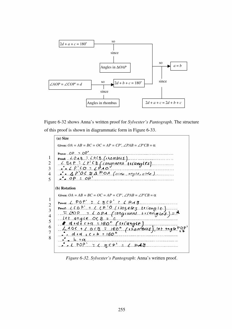
255
Figure 6-32 shows Anna’s written proof for Sylvester’s Pantograph. The structure
of this proof is shown in diagrammatic form in Figure 6-33.
(a) Size
Given: OA = AB = BC = OC = AP = CP', ∠PAB = ∠P'CB = α
(b) Rotation
Given: OA = AB = BC = OC = AP = CP', ∠PAB = ∠P'CB = α
Figure 6-32. Sylvester’s Pantograph: Anna’s written proof.
2d + a + c = 180o
Angles in ∆OAP
∠AOP = ∠COP' = d 2d + b + c = 180o
Angles in rhombus
a = b
so
so
so
since
since
2d + a + c = 2d + b + c
since
12345
12345678
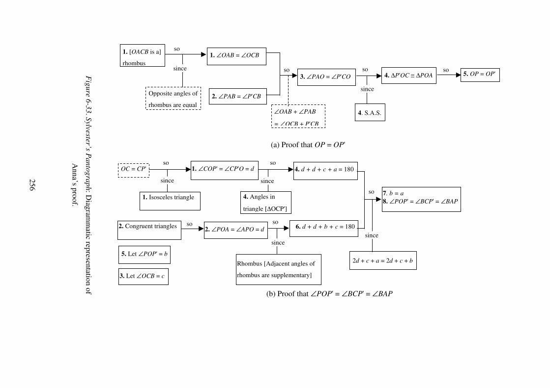
256
Figure 6-33 . Sylvester’s P
antograph: Diagram
matic representation of
Anna’s proof.
so
1. ∠COP' = ∠CP'O = d
1. Isosceles triangle
2. ∠POA = ∠APO = d 2. Congruent triangles
4. d + d + c + a = 180
3. Let ∠OCB = c
5. Let ∠POP' = b
6. d + d + b + c = 180
7. b = a 8. ∠POP' = ∠BCP' = ∠BAP
OC = CP'
4. Angles in
triangle [∆OCP']
Rhombus [Adjacent angles of
rhombus are supplementary]
2d + c + a = 2d + c + b
so
so
so
since
since
since
since
1. ∠OAB = ∠OCB
2. ∠PAB = ∠P'CB
3. ∠PAO = ∠P'CO
1. [OACB is a]
rhombus
4. S.A.S.
4. ∆P'OC ≅ ∆POA 5. OP = OP'
Opposite angles of
rhombus are equal ∠OAB + ∠PAB
= ∠OCB + P'CB
so so so
so
since
since
(b) Proof that ∠POP' = ∠BCP' = ∠BAP
(a) Proof that OP = OP'
so
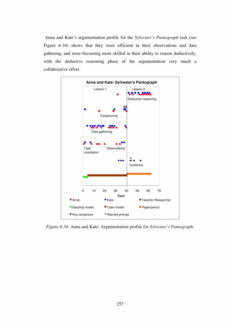
257
Anna and Kate’s argumentation profile for the Sylvester’s Pantograph task (see
Figure 6-34) shows that they were efficient in their observations and data
gathering, and were becoming more skilled in their ability to reason deductively,
with the deductive reasoning phase of the argumentation very much a
collaborative effort.
Anna and Kate: Sylvester's Pantograph
0 10 20 30 40 50 60 70
TurnAnna Kate Teacher-Researcher
Geostrip model Cabri model Paper/pencil
Key conjecture Warrant prompt
Guidance
Observations
Data gathering
Conjecturing
Deductive reasoning
Task orientation
Lesson 1 Lesson 2
Figure 6-34. Anna and Kate: Argumentation profile for Sylvester’s Pantograph.
258
6.3 Addressing the research questions
6.3.1 A culture of proving
Can a culture of geometric proving be established in a Year 8
mathematics classroom in the context of mechanical linkages and
dynamic geometry software?
Anna and Kate, while basing their conjectures on empirical evidence, seemed to
accept readily that proving was an inherent aspect of geometry. Occasionally
Kate’s confidence in a proved conjecture wavered when relationships did not
appear to be exact due to rounding of decimal places in Cabri, as indicated, for
example, by her comments in the Angles in Circles task (section 6.2.5). Anna, on
the other hand, recognised that because they had proved their conjecture, there
was no question of its truth:
Circle angles (section 6.2.5)
114 TR: Does that always work, when you drag B and D?
115 Anna: Well, it has to …
116 Kate: This … 60.9 is half of 121.7. Yes, it is, but it’s off again.
117 Anna: No, but it has to work …
In the Consul argumentation (section 6.2.6), Anna and Kate readily accepted, once
prompted, that they could not assume something that they had not proved:
Consul (section 6.2.6)
112 TR: Can we say that?
113 Anna: Oh, no, because we don’t know that’s 90 [∠APB].
114 Kate: That’s what we’ve got to prove.
Anna’s comment later in the Consul argumentation indicates her recognition that
proof can be achieved by deductive reasoning.
175
Anna: d plus e equals 90, c plus e equals 90 therefore d equals c. See? We’ve
proved it!
259
Clearly, Anna and Kate accepted the need for proof, and they recognised that
although empirical evidence helped in the formulation of conjectures, it did not
constitute proof.
6.3.2 Motivation
Are Year 8 students motivated to engage in argumentation,
conjecturing, and deductive reasoning in the context of mechanical
linkages and dynamic geometry software?
The extent to which Anna and Kate remained focused on each task for the
duration of the lesson, and the sustained argumentations that took place are
evidence of a high level of both motivation and cognitive engagement (see section
2.8.1). Specific indicators of motivation include statements that express their
enjoyment, excitement, satisfaction, or perseverance, as shown in the following
excerpts from the argumentations:
Enjoyment
Angles in Circles (section 6.2.5):
123 Anna: She’s so proud of her right angle!
Consul (section 6.2.6):
002 Kate: Seven squared, oh yeah! 49! This is cool! I want one of these!
019 Kate: This is so cool!
070 Kate: Do they still have these things?
Excitement
Consul (section 6.2.6):
159 Anna: Ooooh! I know something …
175 Anna: d plus e equals 90, c plus e equals 90 therefore d equals c. See? We’ve
proved it!
Sylvester’s Pantograph (section 6.2.7):
014 Kate: Bewdy bewdy bewdy [beauty] … we’ve got ’em to meet!
Satisfaction
Angles in Circles (section 6.2.5):
044 Kate: Yeah, that’s good! So then you have they’re all equal and then you have …
Perseverance
Consul (section 6.2.6):
260
115 Anna: We tried to prove it on our own and we just got in a hopeless muddle and just
ended up proving that angle BED was equal to a which we already knew!
As discussed in section 2.8.1, indicators of cognitive engagement include
reflective statements, statements that involve shared meaning, statements that
draw upon earlier interactions, or in interactions where one student completes a
statement made by the other. Anna and Kate’s argumentations suggest high levels
of cognitive engagement:
Completion of a statement made by the other student
Consul (section 6.2.6):
013 Kate: The big triangle …
014 Anna: … has to be in that proportion to work.
Joining Midpoints (section 6.2.3):
011 Anna: So therefore the lines must be …
012 Kate: Parallel.
Reflection
Enlarging Pantograph (section 6.2.2):
029 Anna: Oh, it would go larger, wouldn’t it, ’cause that’s longer.
Shared meaning
Quadrilateral Midpoints (section 6.2.4):
027 Kate: And then … it’s just the same for that. See you’ve got the two triangles, one
there, one there, so PS is parallel to BD which means it’s parallel to QR …
028 Anna: And then if you do another one that way …
029 Kate: Yeah.
Angles in Circles (section 6.2.5):
088 Kate: Because of the isosceles triangle and the exterior angle and all that …
091 Kate: Yeah. Because they add up to 180 … yeah …
092 Anna: Yeah … and so on …
Reference to previous observations
Angles in Circles (section 6.2.5):
047 Anna: But remember we measured these and they weren’t always the same … see
… remember?
048 Kate: Oh, yeah …
049 Anna: Remember they weren’t the same?
Explanation when the other student has not followed the reasoning
Consul (section 6.2.6):
261
176 Anna: What’s 180 minus 90?
177 Kate: Oh, 90.
178 Anna: So d plus e must equal 90. And what does this equal?
179 Kate: Oh, d plus e equals 90 and e plus c equals 90, so c equals d.
180 Anna: Yep.
As well as being able prove their geometric conjectures for each of the linkages,
Anna and Kate displayed a desire to understand why each linkage operated the
way it did. In the case of the enlarging pantograph, for example, after I had drawn
their attention to the pivot point, O, they could explain why the pantograph was
enlarging by a factor of two.
115 Kate: From there to there [O to E] is twice the distance from there [O to C].
116 Anna: So that’s why the image is coming out twice as big.
Similarly, in the case of Sylvester's Pantograph, Anna and Kate’s geometric
conjectures—“They’re the same distance [OP and OP']”; “So that [OP'] is always
turned around thirty degrees from that [OP]”—suggest that they had at least a
superficial understanding of how the pantograph worked. Their geometric proof
satisfied Anna and Kate’s need for explanation, as indicated by Kate’s comment
“That’s why the copy is the same size” (section 6.2.7, turn 048) when they were
asked to explain the significance of their proof that OP = OP'.
Whether it was the highly engaging quality of Consul, or some other reason, the
two girls moved back and forth between the geostrip linkage and the Cabri model
to a greater extent than for the other linkages. Anna’s comment “You’re right. It
goes down the triangle … see this point P goes down … it goes down … like
along the triangle” (section 6.2.6, turn 076) again suggests that Anna and Kate
were keen to understand how Consul worked. This is supported by the students’
responses to Item 5 on the linkage questionnaire (Appendix 6)—“Once I moved
the linkage and saw how it worked, I was not really interested in knowing why it
worked”—where both Anna and Kate consistently disagreed. Although this may
be interpreted as a desire to please, and an unwillingness to admit if they were not
really interested, their responses do seem to be genuine when considered in
conjunction with their obvious task engagement.
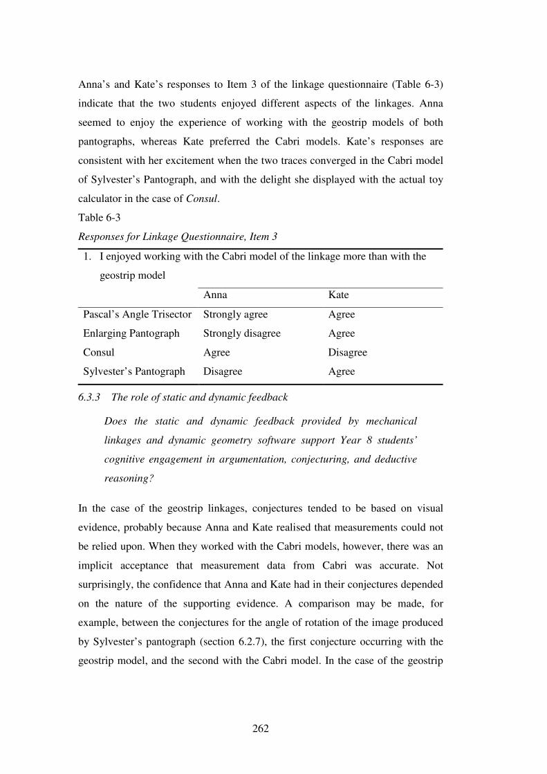
262
Anna’s and Kate’s responses to Item 3 of the linkage questionnaire (Table 6-3)
indicate that the two students enjoyed different aspects of the linkages. Anna
seemed to enjoy the experience of working with the geostrip models of both
pantographs, whereas Kate preferred the Cabri models. Kate’s responses are
consistent with her excitement when the two traces converged in the Cabri model
of Sylvester’s Pantograph, and with the delight she displayed with the actual toy
calculator in the case of Consul.
Table 6-3
Responses for Linkage Questionnaire, Item 3
1. I enjoyed working with the Cabri model of the linkage more than with the
geostrip model
Anna Kate
Pascal’s Angle Trisector Strongly agree Agree
Enlarging Pantograph Strongly disagree Agree
Consul Agree Disagree
Sylvester’s Pantograph Disagree Agree
6.3.3 The role of static and dynamic feedback
Does the static and dynamic feedback provided by mechanical
linkages and dynamic geometry software support Year 8 students’
cognitive engagement in argumentation, conjecturing, and deductive
reasoning?
In the case of the geostrip linkages, conjectures tended to be based on visual
evidence, probably because Anna and Kate realised that measurements could not
be relied upon. When they worked with the Cabri models, however, there was an
implicit acceptance that measurement data from Cabri was accurate. Not
surprisingly, the confidence that Anna and Kate had in their conjectures depended
on the nature of the supporting evidence. A comparison may be made, for
example, between the conjectures for the angle of rotation of the image produced
by Sylvester’s pantograph (section 6.2.7), the first conjecture occurring with the
geostrip model, and the second with the Cabri model. In the case of the geostrip
263
model, even though a protractor was available, Anna and Kate made no attempt to
measure the angle of rotation.
Example 1: Geostrip model
002 Kate: It’s the same size. It’s turned 45 degrees.
003 TR: How do you know it’s 45 degrees?
004 Kate: Just guessing, ’cause it was about half 90.
Example 2: Cabri model
029 Kate: Thirty! 30 and 30. So it rotates the angle of that!
039 Kate: Let’s measure that angle … it looks like the same angle again.
040 Anna: Thirty! So that is always turned around 30 degrees from that.
Although the static feedback in the form of Cabri measurements assisted Anna
and Kate in their conjecturing and deductive reasoning, it was often the dynamic
visualisation associated with the geostrip models and with the Cabri models that
enabled them to identify invariant properties, and to check and modify their
reasoning. The following examples from the argumentations illustrate how this
dynamic visualisation contributed to both conjecturing and proving:
Pascal’s Angle Trisector (section 6.2.1)
012 TR: So point to the angles again that you said were equal.
013 Kate: Are they the same?
014 Anna: No! They don’t seem to be!
016 Kate: Oh, yeah, ’cause they’re both different triangles with different lengths.
Enlarging Pantograph (section 6.2.2)
058 Anna: [moving the linkage around] Yep … it’s a parallelogram.
Angles in Circles (section 6.2.5)
Example 1:
025 Kate: I’ll try dragging B.
026 Anna: Yeah, it still works.
027 Kate: I’ll do one more, moving this point as well.
Example 2:
047 Anna: But remember we measured these and they weren’t always the same … see
… remember?
048 Kate: Oh, yeah …
049 Anna: Remember they weren’t the same?
Consul (section 6.2.6)
264
006 Anna: These two triangles always stay the same … the triangle in the middle just
moves them.
007 Kate: These just divide them in different spots.
008 Anna: Yep, and the big triangles stay the same.
009 Kate: OK …
010 Anna: OK, well … when these two points are moving, it’s making the middle
triangle bigger or smaller and this just moves up and down.
Consul (section 6.2.6)
051 Anna: Hey, is this always a right angle?
052 Anna: Measure angle DGB. Oh, it’s not 90 degrees … oh!
053 Kate: But that angle always changes anyway.
054 Anna: Mmm.
055 Kate: So even if it was 90 degrees it wouldn’t always be.
056 Anna: Mmm.
057 Kate: Is that angle there 90 and will it always stay 90?
Consul (section 6.2.6)
088 Anna: It’s moving down the two times table.
090 Anna: So P moves up here … and this is perpendicular to this and as P is moving
down, this is moving across as well.
Sylvester's Pantograph (section 6.2.7)
014 Kate: Bewdy bewdy bewdy [beauty] … we’ve got ’em to meet! And then look …
015 Anna: Oh, we’ve got the angle there …
Competency with Cabri (see section 4.4.7) was a key element in the success of
Anna and Kate’s conjecturing and proving as it allowed unimpeded flow of their
argumentations. Anna and Kate used the various construction and measurement
tools appropriately to aid them in their formulation and testing of conjectures.
They were able to act on my suggestion to tabulate angles in the case of the
Pascal’s Angle Trisector task (see section 6.2.1), although, when Kate recognised
that it might be useful to tabulate angles in the Angles in Circles task (see section
6.2.5), she asked: “How do you do one of those table things?”. Anna and Kate
used the Trace tool for the two pantographs (sections 6.2.2 and 6.2.7), and Kate
was quick to exploit the apparent accidental convergence of the two traced paths
in the case of Sylvester’s pantograph. Although they used Cabri confidently, they
265
were not exceptional amongst the students in their ability to employ the various
Cabri tools.
In their responses to Item 2 of the linkage questionnaire—“Operating the linkage
models made the geometric properties more obvious”—Anna and Kate
consistently agreed that the linkage models made the geometric properties more
obvious. In the case of the Enlarging Pantograph, Anna strongly agreed.
Responses to Item 4 (Table 6-4) indicate that Anna and Kate generally believed
the Cabri model to be more helpful than the geostrip model for finding why the
linkage worked. An exception was Consul, where Anna believed that the geostrip
model was more useful. This was possibly because the breakthrough in
discovering how Consul worked came when Kate recognised that P could move
down the rows of numbers in two perpendicular directions when she was working
with the geostrip model and the actual toy calculator. Kate, on the other hand,
believed that the Cabri model was more useful, perhaps because it was she who
made the Cabri angle measurements that led to the discovery of similar triangles
AEB and ACP.
Table 6-4
Responses for Linkage Questionnaire, Item 4
4. The Cabri model was more helpful than the geostrip model for finding out
why the linkage worked.
Linkage Anna Kate
Pascal’s Angle Trisector Strongly agree Strongly agree
Enlarging Pantograph Agree Agree
Consul Disagree Strongly agree
Sylvester’s Pantograph Strongly agree Agree
It was the accuracy of the feedback from Cabri (see for example, Consul, section
6.2.6, turns 119–121; Sylvester’s Pantograph, section 6.2.7, turns 029 and 040)
and the opportunity to modify the Cabri figure by the addition of construction
lines (see for example, Quadrilateral Midpoints, section 6.2.4, turn 019; Angles in
Circles, section 6.2.5, turns 083, 086, 088) that facilitated Anna and Kate’s
explorations and provided support for their conjectures. As shown in Table 6-5,
266
Anna and Kate were able to exploit a range of Cabri tools, but at the end of each
argumentation, when they completed the linkage questionnaires, their responses
indicated that they could not distinguish whether a particular aspect of the models
had helped them in the conjecturing, or in the proving, phase of their
argumentations.
Table 6-5.
Anna and Kate’s Assessment of the Usefulness of the Models
Pascal’s
Angle
Trisector
Enlarging
Pantograph
Sylvester’s
Pantograph
Consul
Actual linkage / geostrip model
1. Watching how the linkage moved. � � � �
2. Tracing the paths of certain points. � � �
3. Measuring angles.
4. Measuring lengths in the linkage.
Cabri model
1. Seeing the linkage as a diagram. � � � �
2. Dragging the linkage. � � � �
3. Tracing the paths of certain points. � � �
4. Measuring angles. � � �
5. Measuring lengths. � � �
6. Adding extra construction lines. � �
6.3.4 The influence of conjecturing and argumentation on proof construction
Do the processes of argumentation and conjecturing contribute to
successful constructions of proofs?
In each of Anna and Kate’s argumentations, there was a high level of interaction
between empirical reasoning and deductive reasoning. As progress was made in
identifying the geometric properties and relationships of the linkage, and in
conjecturing, statements of deductive reasoning occurred more frequently, either
as single inferences or as chains of reasoning. A significant characteristic of Anna
and Kate’s later argumentations was the use of shared understanding, gained from
267
the earlier tasks, to skip steps in their reasoning. Koedinger (1998, p. 332) notes
that recognition of useful parts in a diagram, and the use of “perceptual chunks” to
develop a proof framework is characteristic of “high-school geometry experts”
(see section 2.5.7). In the Quadrilateral Midpoints task, Kate recognised the
relationship to the previous triangle midpoints task, then Anna was able to see that
the same reasoning applied to the other pair of segments, PQ and SR. This
relationship was mutually understood and did not need further elaboration:
Quadrilateral Midpoints (section 6.2.4):
027 Kate: And then … it’s just the same for that. See, you’ve got the two triangles, one
there, one there, so PS is parallel to BD which means it’s parallel to QR …
028 Anna: And then if you do another one that way …
029 Kate: Yeah.
Angles in Circles (section 6.2.5):
088 Kate: Because of the isosceles triangle and the exterior angle and all that …
091 Kate: Yeah. Because they add up to 180 … yeah …
092 Anna: Yeah … and so on …
Similarly, in constructing their proof for Sylvester’s pantograph, Anna and Kate
confidently used the rhombus property of equal opposite angles, as well as the
property of supplementary adjacent angles which they had used previously in the
Consul proof:
Sylvester’s Pantograph (section 6.2.7)
045 Kate: The angles in the rhombus are equal and then they both have the same fixed
angle bit added on.
051 Kate: Why don’t we use the angles in the rhombus?
060 Anna: And 2d plus b plus c equals 180 ’cause angles in the rhombus.
In the later tasks—Consul and Sylvester’s Pantograph (see sections 6.2.6 and
6.2.7)—it was also observed that Anna and Kate were able to engage in more
sustained sequences of deductive reasoning than in earlier tasks, where short
chains of reasoning were often followed by further data-gathering or my
prompting before progress occurred. On one occasion, in the Consul
argumentation, Kate was unable to keep pace with Anna’s reasoning, causing her
to exclaim “Slow down!” (see section 6.2.6). Anna appeared to be able to
visualise the entire sequence of reasoning:
268
169 Anna: And 45 plus 45 equals 90 which means d plus e has to equal 90.
170 Kate: [laughing] Slow down!
171 Anna: Which means this [c] equals that [d] … it equals d!
172 Kate: Slow down!
A little later on in the same argumentation (see section 6.2.6, turns 182–198), Kate
engaged in a similar rapid sequence of reasoning.
Anna and Kate’s ability to integrate empirical data and deductive reasoning
contrasts with observations by Hoyles and Healy (1999), who found that 15-year-
old students of above average mathematical attainment did not make the
anticipated connections between empirical Cabri work and proofs (see section
3.4.7). Using the assessment scheme for dynamic geometry investigations
proposed by Galindo (1998; see also section 3.4.8), where a score of 0, 1, or 2 is
assigned for each of three categories: Intuitive justification, Deductive
justification, and Interplay between intuitive and deductive justifications, Anna
and Kate’s argumentations would be appropriately assessed as 2-2-2.
The ability of Anna and Kate to construct their written proofs at the end of each
argumentation provides strong support for the concept of cognitive unity
discussed by Boero, Garuti, Lemut, and Mariotti (1996; see also section 2.6).
Boero et al. assert that the process of argumentation, involving conjecturing and
justifying, enables students to order their statements logically when constructing
their proofs. This certainly seemed to be the case with Anna and Kate.
6.3.5 Satisfying the need for conviction
Does the empirical feedback provided by dynamic geometry software
satisfy Year 8 students’ need for convincing?
Implicit in each of the argumentations was an understanding that empirical
evidence did not constitute a proof. In the case of the Enlarging Pantograph
(section 6.2.2), for example, Kate and Anna laughed as they offered visual
evidence as a reason, and Kate immediately gave an explanation based on
geometric properties.
059 Anna: There’s those two triangles … oh, and there’s the big triangle.
269
060 Kate: Yeah … which is similar to the small triangles.
061 Anna: Yeah … similar to the small triangles.
062 TR: Why do you say that?
063 Kate: Just ’cause it looks it.
064 Anna: Yeah, ’cause it looks that way.
065 Kate: ’Cause those angles are the same because of the parallel lines.
Similarly, when Cabri measurement data convinced Anna and Kate of a
conjecture, their justification was based on deductive reasoning:
Quadrilateral Midpoints (section 6.2.4)
007 Kate: Um … If there’s a way we could prove that angle [PQR] is equal to that
angle [∠RSP] …
008 Anna: Yeah.
009 Kate: And … then we can prove it’s a parallelogram.
Consul (section 6.2.6)
023 Anna: Measure those angles.
024 Tog: Yep.
025 Anna: So it is a parallelogram.
027 Anna: We think it’s a parallelogram … we know that those two are equal because
those two are congruent.
028 TR: So which are the congruent triangles?
029 Tog: PCE and PDE.
030 TR: How do you know they are congruent? What information do you have?
031 Kate: Well, the two sides are equal and that’s a shared side.
032 Anna: And so they’ve got the angles equal as well.
6.3.6 Relationship between van Hiele levels and conjecturing-proving ability
Are the students’ abilities to make conjectures and construct deductive
proofs in geometry related to their measured van Hiele levels?
The van Hiele pre-test showed Anna and Kate to be at Level 3 for four of the six
tested concepts, and at Level 1 or Level 2 for the remaining concepts. It was
obvious throughout the argumentations that the confidence with which they
engaged in deductive reasoning was related to their understanding of geometric
properties and relationships. Occasionally their reasoning was flawed, as for
example in the Pascal’s Angle Trisector task (see section 6.2.1) when they
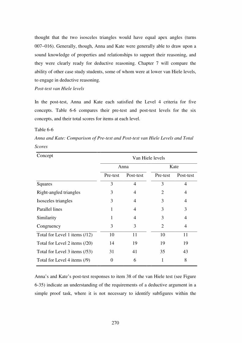
270
thought that the two isosceles triangles would have equal apex angles (turns
007−016). Generally, though, Anna and Kate were generally able to draw upon a
sound knowledge of properties and relationships to support their reasoning, and
they were clearly ready for deductive reasoning. Chapter 7 will compare the
ability of other case study students, some of whom were at lower van Hiele levels,
to engage in deductive reasoning.
Post-test van Hiele levels
In the post-test, Anna and Kate each satisfied the Level 4 criteria for five
concepts. Table 6-6 compares their pre-test and post-test levels for the six
concepts, and their total scores for items at each level.
Table 6-6
Anna and Kate: Comparison of Pre-test and Post-test van Hiele Levels and Total
Scores
Concept Van Hiele levels
Anna Kate
Pre-test Post-test Pre-test Post-test
Squares 3 4 3 4
Right-angled triangles 3 4 2 4
Isosceles triangles 3 4 3 4
Parallel lines 1 4 3 3
Similarity 1 4 3 4
Congruency 3 3 2 4
Total for Level 1 items (/12) 10 11 10 11
Total for Level 2 items (/20) 14 19 19 19
Total for Level 3 items (/53) 31 41 35 43
Total for Level 4 items (/9) 0 6 1 8
Anna’s and Kate’s post-test responses to item 38 of the van Hiele test (see Figure
6-35) indicate an understanding of the requirements of a deductive argument in a
simple proof task, where it is not necessary to identify subfigures within the
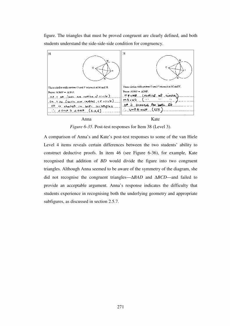
271
figure. The triangles that must be proved congruent are clearly defined, and both
students understand the side-side-side condition for congruency.
Anna Kate
Figure 6-35. Post-test responses for Item 38 (Level 3).
A comparison of Anna’s and Kate’s post-test responses to some of the van Hiele
Level 4 items reveals certain differences between the two students’ ability to
construct deductive proofs. In item 46 (see Figure 6-36), for example, Kate
recognised that addition of BD would divide the figure into two congruent
triangles. Although Anna seemed to be aware of the symmetry of the diagram, she
did not recognise the congruent triangles—∆BAD and ∆BCD—and failed to
provide an acceptable argument. Anna’s response indicates the difficulty that
students experience in recognising both the underlying geometry and appropriate
subfigures, as discussed in section 2.5.7.
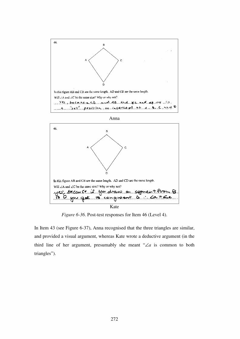
272
Anna
Kate
Figure 6-36. Post-test responses for Item 46 (Level 4).
In Item 43 (see Figure 6-37), Anna recognised that the three triangles are similar,
and provided a visual argument, whereas Kate wrote a deductive argument (in the
third line of her argument, presumably she meant “∠a is common to both
triangles”).
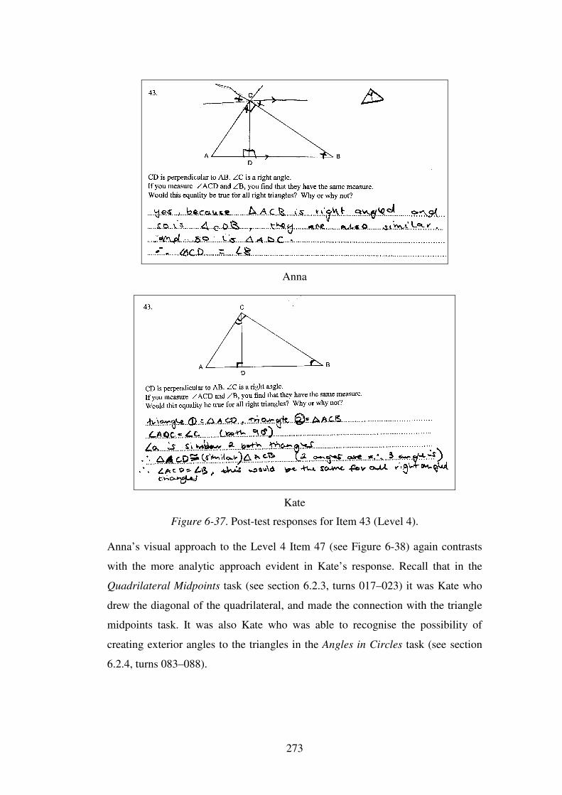
273
Anna
Kate
Figure 6-37. Post-test responses for Item 43 (Level 4).
Anna’s visual approach to the Level 4 Item 47 (see Figure 6-38) again contrasts
with the more analytic approach evident in Kate’s response. Recall that in the
Quadrilateral Midpoints task (see section 6.2.3, turns 017–023) it was Kate who
drew the diagonal of the quadrilateral, and made the connection with the triangle
midpoints task. It was also Kate who was able to recognise the possibility of
creating exterior angles to the triangles in the Angles in Circles task (see section
6.2.4, turns 083–088).
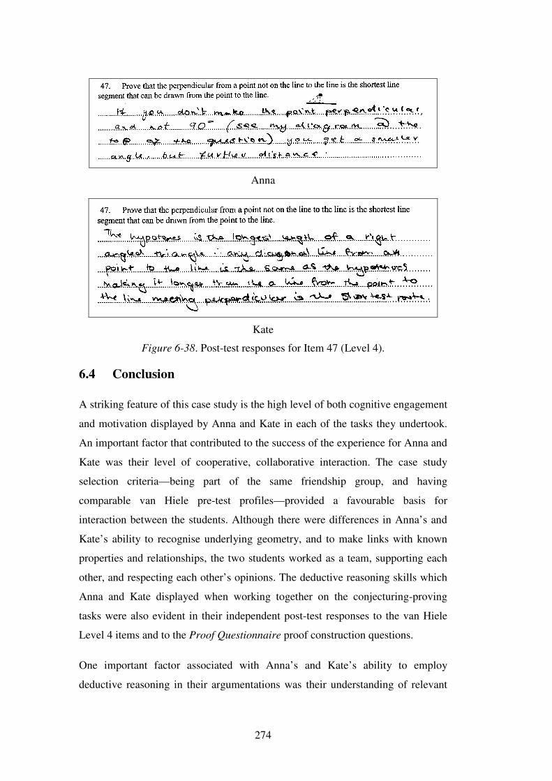
274
Anna
Kate
Figure 6-38. Post-test responses for Item 47 (Level 4).
6.4 Conclusion
A striking feature of this case study is the high level of both cognitive engagement
and motivation displayed by Anna and Kate in each of the tasks they undertook.
An important factor that contributed to the success of the experience for Anna and
Kate was their level of cooperative, collaborative interaction. The case study
selection criteria—being part of the same friendship group, and having
comparable van Hiele pre-test profiles—provided a favourable basis for
interaction between the students. Although there were differences in Anna’s and
Kate’s ability to recognise underlying geometry, and to make links with known
properties and relationships, the two students worked as a team, supporting each
other, and respecting each other’s opinions. The deductive reasoning skills which
Anna and Kate displayed when working together on the conjecturing-proving
tasks were also evident in their independent post-test responses to the van Hiele
Level 4 items and to the Proof Questionnaire proof construction questions.
One important factor associated with Anna’s and Kate’s ability to employ
deductive reasoning in their argumentations was their understanding of relevant
275
geometric properties and relationships, and their reasoning would have been
substantially restricted if they did not have this body of geometric knowledge to
draw upon. Nevertheless, there were times when Anna and Kate were not aware
of, or had misconceptions about, certain properties or relationships. In such cases
it was frequently the dynamic nature of the feedback that challenged, and allowed
them to modify, their understanding.
Empirical feedback from the linkage models, particularly the Cabri models,
provided the support for each of Anna’s and Kate’s conjectures, and engendered
confidence that a proof would be possible. The physical linkages aroused Anna
and Kate’s curiosity, motivating them to find out why the linkages worked the
way they did. Although the feedback from these physical linkages provided some
assistance in the formulation of conjectures, it was the Cabri models which
contributed most to the quality of the argumentations. The accuracy of the Cabri
feedback, and the assistance provided by other Cabri tools, such as tabulating
data, tracing paths of points, and adding construction lines, gave Anna and Kate
insight into the underlying geometry of the linkages, as well as assisting them
with intermediate steps required in the proving process. This was also the case in
the Cabri-based Quadrilateral Midpoints and Angles in Circles tasks. Anna and
Kate used the Cabri software confidently, selecting appropriate tools to provide
them with the data they needed, but they were able also to exploit unexpected
outcomes, such as the converging traces in Sylvester’s pantograph (see section
6.2.7). The ease with which they used the software no doubt contributed to the
overall success of the tasks.
Chapter 7 will compare Anna and Kate’s argumentations and written proofs with
those of the other case study students.

277
Chapter 7: Case Study Comparisons
We propose that an essential feature of learning is that it creates the zone of
proximal development; that is, learning awakens a variety of developmental
processes that are able to interact only when the child is interacting with people in
his environment and in collaboration with his peers. (Vygotsky, 1978, p. 90)
7.1 Introduction
Chapter 6 demonstrated the high level of engagement and deductive reasoning
ability of Anna and Kate in the seven conjecturing-proving tasks that they
completed. This chapter focuses on the other pairs of case study students—four
pairs who were at Level 3 for several concepts, and two pairs who were at Level 1
or 2 on most or all of the six concepts—comparing them with Anna and Kate with
respect to task engagement, collaboration, the contribution of static and dynamic
feedback to the conjecturing and proving processes, and the students’ ability to
reason deductively. This chapter also looks at the effectiveness of the
conjecturing-proving tasks with respect to the Year 8 class as a whole.
Section 7.2 introduces the twelve case study comparison students, and lists the
additional conjecturing-proving tasks completed by these students. Section 7.3
compares the conjecturing-proving performance of Anna and Kate with that of the
four pairs of students who had comparable van Hiele pre-test profiles.
Comparisons are made between aspects of the Consul argumentations for Anna
and Kate, Lucy and Rose, and Liz and Meg, and of the Sylvester’s Pantograph
argumentations for Lucy and Rose, and Anna and Kate. Section 7.3 also compares
Liz and Meg’s reasoning in the pencil-and-paper Angles in Circles task with the
Cabri-based argumentations of the other two pairs of students who completed this
task—Anna and Kate, and Jane and Sara—as well as briefly discussing four other
Level 2–3 students—Amy and Lyn, and Pam and Elly. Section 7.4 focuses on the
Level 1–2 students, Jane and Sara, comparing them with Anna and Kate for the
four tasks: Pascal’s Angle Trisector, Joining Midpoints, Quadrilateral Midpoints,
and Angles in Circles; section 7.4 also discusses some aspects of the Enlarging
Pantograph investigation of another Level 1–2 pair of students, Jess and Emma.
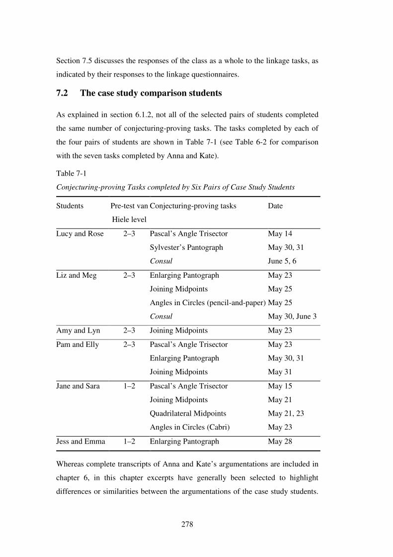
278
Section 7.5 discusses the responses of the class as a whole to the linkage tasks, as
indicated by their responses to the linkage questionnaires.
7.2 The case study comparison students
As explained in section 6.1.2, not all of the selected pairs of students completed
the same number of conjecturing-proving tasks. The tasks completed by each of
the four pairs of students are shown in Table 7-1 (see Table 6-2 for comparison
with the seven tasks completed by Anna and Kate).
Table 7-1
Conjecturing-proving Tasks completed by Six Pairs of Case Study Students
Students Pre-test van
Hiele level
Conjecturing-proving tasks Date
Lucy and Rose 2–3 Pascal’s Angle Trisector
Sylvester’s Pantograph
Consul
May 14
May 30, 31
June 5, 6
Liz and Meg 2–3 Enlarging Pantograph
Joining Midpoints
Angles in Circles (pencil-and-paper)
Consul
May 23
May 25
May 25
May 30, June 3
Amy and Lyn 2–3 Joining Midpoints May 23
Pam and Elly 2–3 Pascal’s Angle Trisector May 23
Enlarging Pantograph May 30, 31
Joining Midpoints May 31
Jane and Sara 1–2 Pascal’s Angle Trisector
Joining Midpoints
Quadrilateral Midpoints
Angles in Circles (Cabri)
May 15
May 21
May 21, 23
May 23
Jess and Emma 1–2 Enlarging Pantograph May 28
Whereas complete transcripts of Anna and Kate’s argumentations are included in
chapter 6, in this chapter excerpts have generally been selected to highlight
differences or similarities between the argumentations of the case study students.
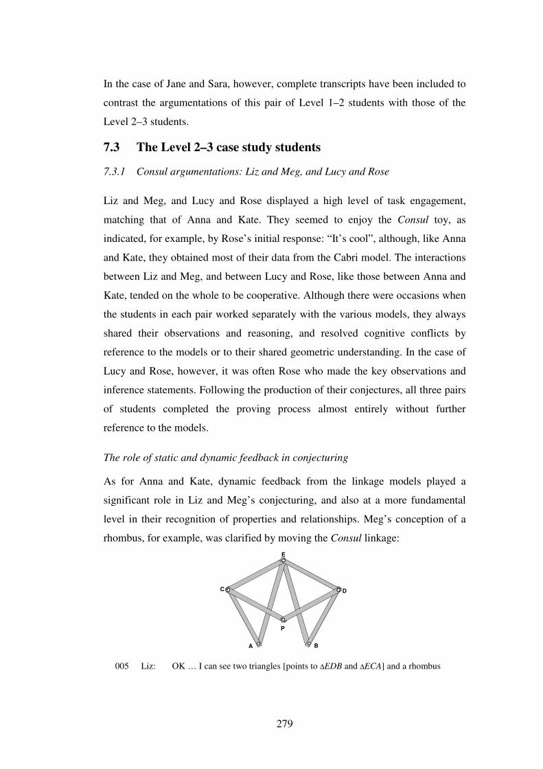
279
In the case of Jane and Sara, however, complete transcripts have been included to
contrast the argumentations of this pair of Level 1–2 students with those of the
Level 2–3 students.
7.3 The Level 2–3 case study students
7.3.1 Consul argumentations: Liz and Meg, and Lucy and Rose
Liz and Meg, and Lucy and Rose displayed a high level of task engagement,
matching that of Anna and Kate. They seemed to enjoy the Consul toy, as
indicated, for example, by Rose’s initial response: “It’s cool”, although, like Anna
and Kate, they obtained most of their data from the Cabri model. The interactions
between Liz and Meg, and between Lucy and Rose, like those between Anna and
Kate, tended on the whole to be cooperative. Although there were occasions when
the students in each pair worked separately with the various models, they always
shared their observations and reasoning, and resolved cognitive conflicts by
reference to the models or to their shared geometric understanding. In the case of
Lucy and Rose, however, it was often Rose who made the key observations and
inference statements. Following the production of their conjectures, all three pairs
of students completed the proving process almost entirely without further
reference to the models.
The role of static and dynamic feedback in conjecturing
As for Anna and Kate, dynamic feedback from the linkage models played a
significant role in Liz and Meg’s conjecturing, and also at a more fundamental
level in their recognition of properties and relationships. Meg’s conception of a
rhombus, for example, was clarified by moving the Consul linkage:
A
P
E
DC
B
005 Liz: OK … I can see two triangles [points to ∆EDB and ∆ECA] and a rhombus
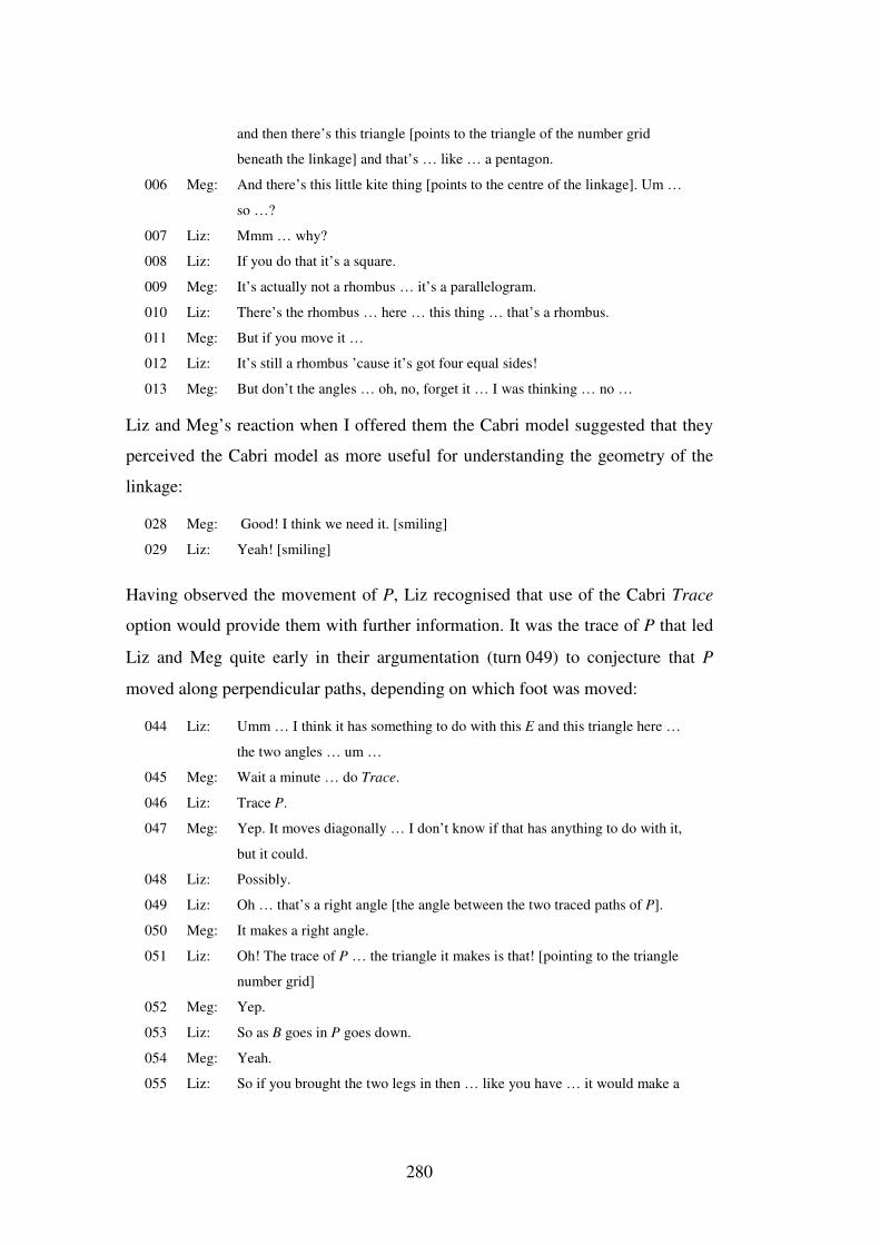
280
and then there’s this triangle [points to the triangle of the number grid
beneath the linkage] and that’s … like … a pentagon.
006 Meg: And there’s this little kite thing [points to the centre of the linkage]. Um …
so …?
007 Liz: Mmm … why?
008 Liz: If you do that it’s a square.
009 Meg: It’s actually not a rhombus … it’s a parallelogram.
010 Liz: There’s the rhombus … here … this thing … that’s a rhombus.
011 Meg: But if you move it …
012 Liz: It’s still a rhombus ’cause it’s got four equal sides!
013 Meg: But don’t the angles … oh, no, forget it … I was thinking … no …
Liz and Meg’s reaction when I offered them the Cabri model suggested that they
perceived the Cabri model as more useful for understanding the geometry of the
linkage:
028 Meg: Good! I think we need it. [smiling]
029 Liz: Yeah! [smiling]
Having observed the movement of P, Liz recognised that use of the Cabri Trace
option would provide them with further information. It was the trace of P that led
Liz and Meg quite early in their argumentation (turn 049) to conjecture that P
moved along perpendicular paths, depending on which foot was moved:
044 Liz: Umm … I think it has something to do with this E and this triangle here …
the two angles … um …
045 Meg: Wait a minute … do Trace.
046 Liz: Trace P.
047 Meg: Yep. It moves diagonally … I don’t know if that has anything to do with it,
but it could.
048 Liz: Possibly.
049 Liz: Oh … that’s a right angle [the angle between the two traced paths of P].
050 Meg: It makes a right angle.
051 Liz: Oh! The trace of P … the triangle it makes is that! [pointing to the triangle
number grid]
052 Meg: Yep.
053 Liz: So as B goes in P goes down.
054 Meg: Yeah.
055 Liz: So if you brought the two legs in then … like you have … it would make a
281
smaller triangle so if you had the right numbers on it it would …
056 Meg: Yep … so what does that mean?
Anna and Kate identified the right angle at approximately the same stage of their
argumentation, after drawing the segments PA and PB in the Cabri model: “Is that
angle there [∠APB] 90 and will it always stay 90?” (see section 6.2.6, Kate: turn
057). Anna and Kate did not trace the path of P in the Cabri model until later in
their argumentation (turn 080).
Liz and Meg were confident that the trace of P was forming a right angle, but they
could not yet understand why this was occurring. Meg dragged A until P and E
coincided, perhaps thinking that the special configuration would provide insight
into the geometry—an approach described by Goldenberg (1995) as ‘reasoning by
continuity’ (see section 3.2.1):
061 Liz: Wait, P makes … What’s P at right angles to? … to make that triangle?
062 Meg: What?
063 Liz: What’s P at right angles to to make that?
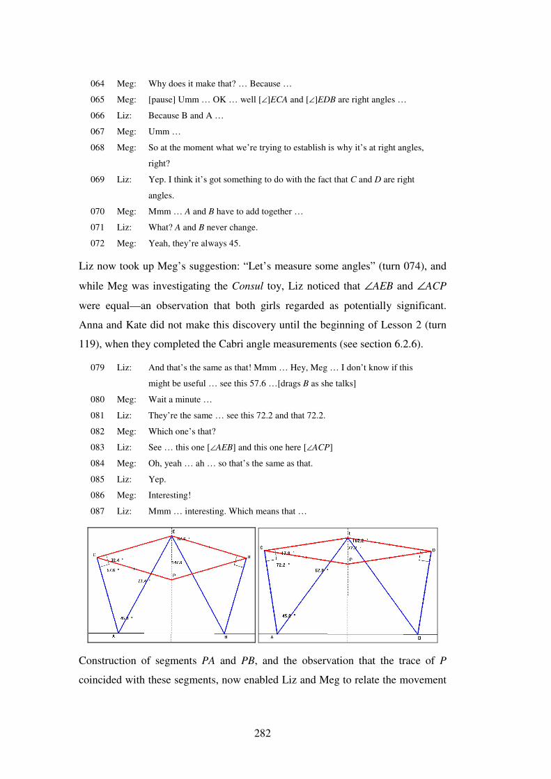
282
064 Meg: Why does it make that? … Because …
065 Meg: [pause] Umm … OK … well [∠]ECA and [∠]EDB are right angles …
066 Liz: Because B and A …
067 Meg: Umm …
068 Meg: So at the moment what we’re trying to establish is why it’s at right angles,
right?
069 Liz: Yep. I think it’s got something to do with the fact that C and D are right
angles.
070 Meg: Mmm … A and B have to add together …
071 Liz: What? A and B never change.
072 Meg: Yeah, they’re always 45.
Liz now took up Meg’s suggestion: “Let’s measure some angles” (turn 074), and
while Meg was investigating the Consul toy, Liz noticed that ∠AEB and ∠ACP
were equal—an observation that both girls regarded as potentially significant.
Anna and Kate did not make this discovery until the beginning of Lesson 2 (turn
119), when they completed the Cabri angle measurements (see section 6.2.6).
079 Liz: And that’s the same as that! Mmm … Hey, Meg … I don’t know if this
might be useful … see this 57.6 …[drags B as she talks]
080 Meg: Wait a minute …
081 Liz: They’re the same … see this 72.2 and that 72.2.
082 Meg: Which one’s that?
083 Liz: See … this one [∠AEB] and this one here [∠ACP]
084 Meg: Oh, yeah … ah … so that’s the same as that.
085 Liz: Yep.
086 Meg: Interesting!
087 Liz: Mmm … interesting. Which means that …
Construction of segments PA and PB, and the observation that the trace of P
coincided with these segments, now enabled Liz and Meg to relate the movement
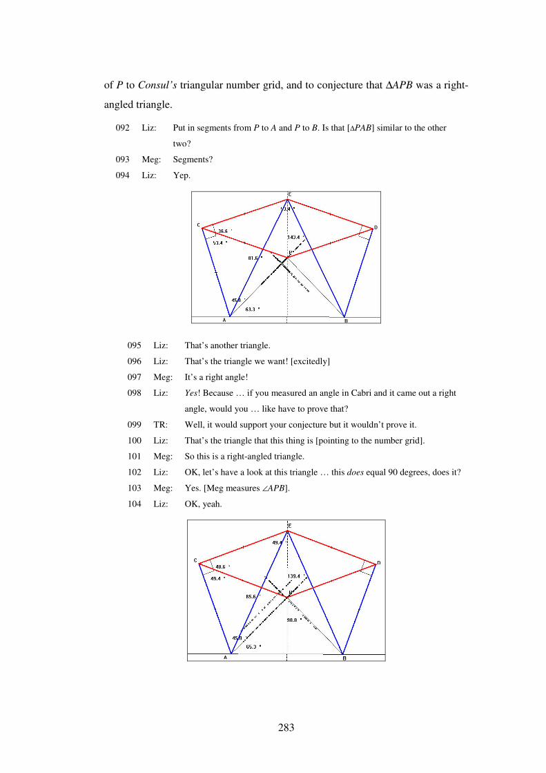
283
of P to Consul’s triangular number grid, and to conjecture that ∆APB was a right-
angled triangle.
092 Liz: Put in segments from P to A and P to B. Is that [∆PAB] similar to the other
two?
093 Meg: Segments?
094 Liz: Yep.
095 Liz: That’s another triangle.
096 Liz: That’s the triangle we want! [excitedly]
097 Meg: It’s a right angle!
098 Liz: Yes! Because … if you measured an angle in Cabri and it came out a right
angle, would you … like have to prove that?
099 TR: Well, it would support your conjecture but it wouldn’t prove it.
100 Liz: That’s the triangle that this thing is [pointing to the number grid].
101 Meg: So this is a right-angled triangle.
102 Liz: OK, let’s have a look at this triangle … this does equal 90 degrees, does it?
103 Meg: Yes. [Meg measures ∠APB].
104 Liz: OK, yeah.
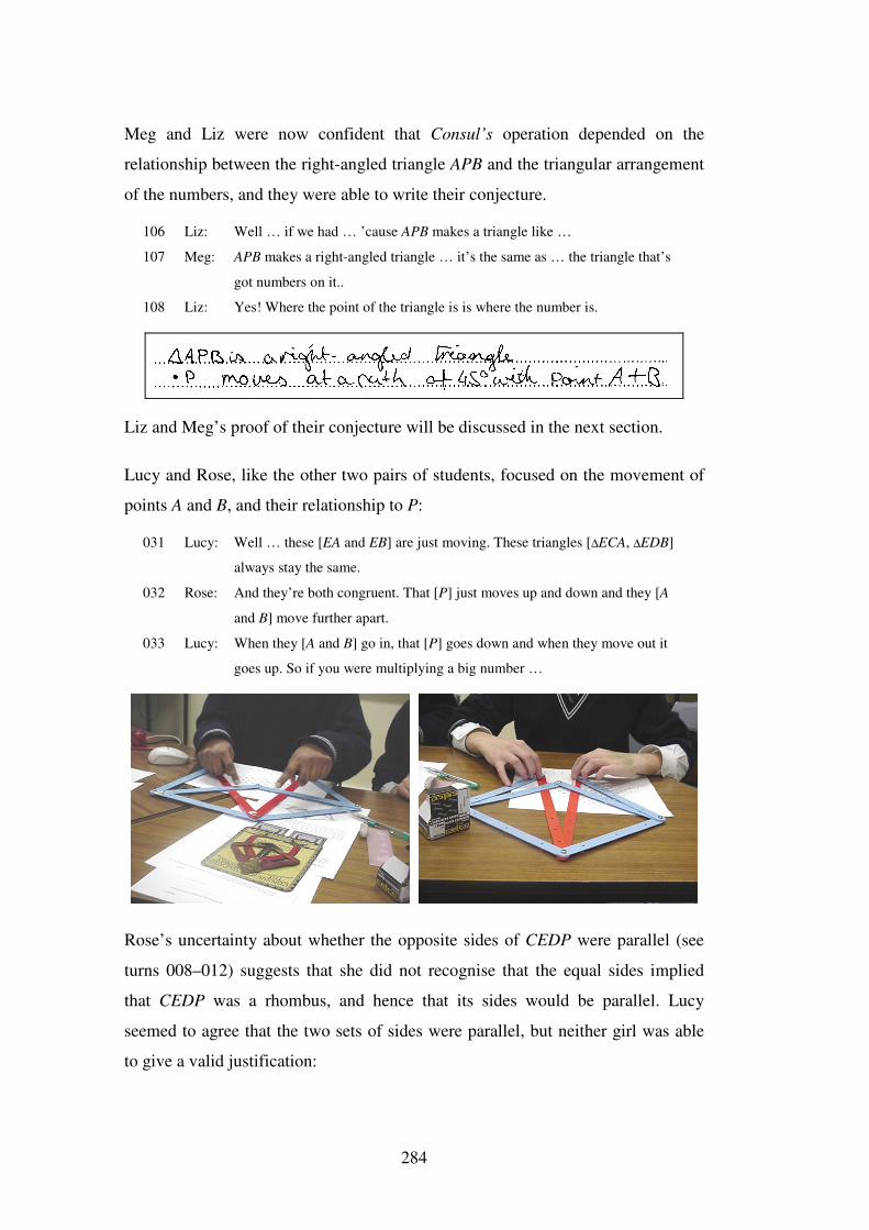
284
Meg and Liz were now confident that Consul’s operation depended on the
relationship between the right-angled triangle APB and the triangular arrangement
of the numbers, and they were able to write their conjecture.
106 Liz: Well … if we had … ’cause APB makes a triangle like …
107 Meg: APB makes a right-angled triangle … it’s the same as … the triangle that’s
got numbers on it..
108 Liz: Yes! Where the point of the triangle is is where the number is.
Liz and Meg’s proof of their conjecture will be discussed in the next section.
Lucy and Rose, like the other two pairs of students, focused on the movement of
points A and B, and their relationship to P:
031 Lucy: Well … these [EA and EB] are just moving. These triangles [∆ECA, ∆EDB]
always stay the same.
032 Rose: And they’re both congruent. That [P] just moves up and down and they [A
and B] move further apart.
033 Lucy: When they [A and B] go in, that [P] goes down and when they move out it
goes up. So if you were multiplying a big number …
Rose’s uncertainty about whether the opposite sides of CEDP were parallel (see
turns 008–012) suggests that she did not recognise that the equal sides implied
that CEDP was a rhombus, and hence that its sides would be parallel. Lucy
seemed to agree that the two sets of sides were parallel, but neither girl was able
to give a valid justification:
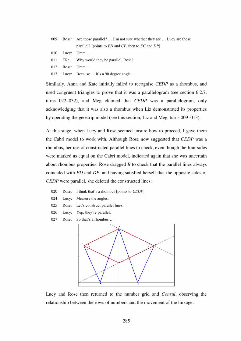
285
009 Rose: Are those parallel? … I’m not sure whether they are … Lucy are those
parallel? [points to ED and CP, then to EC and DP]
010 Lucy: Umm …
011 TR: Why would they be parallel, Rose?
012 Rose: Umm …
013 Lucy: Because … it’s a 90 degree angle …
Similarly, Anna and Kate initially failed to recognise CEDP as a rhombus, and
used congruent triangles to prove that it was a parallelogram (see section 6.2.7,
turns 022–032), and Meg claimed that CEDP was a parallelogram, only
acknowledging that it was also a rhombus when Liz demonstrated its properties
by operating the geostrip model (see this section, Liz and Meg, turns 009–013).
At this stage, when Lucy and Rose seemed unsure how to proceed, I gave them
the Cabri model to work with. Although Rose now suggested that CEDP was a
rhombus, her use of constructed parallel lines to check, even though the four sides
were marked as equal on the Cabri model, indicated again that she was uncertain
about rhombus properties. Rose dragged B to check that the parallel lines always
coincided with ED and DP, and having satisfied herself that the opposite sides of
CEDP were parallel, she deleted the constructed lines:
020 Rose: I think that’s a rhombus [points to CEDP]
024 Lucy: Measure the angles.
025 Rose: Let’s construct parallel lines.
026 Lucy: Yep, they’re parallel.
027 Rose: So that’s a rhombus …
Lucy and Rose then returned to the number grid and Consul, observing the
relationship between the rows of numbers and the movement of the linkage:
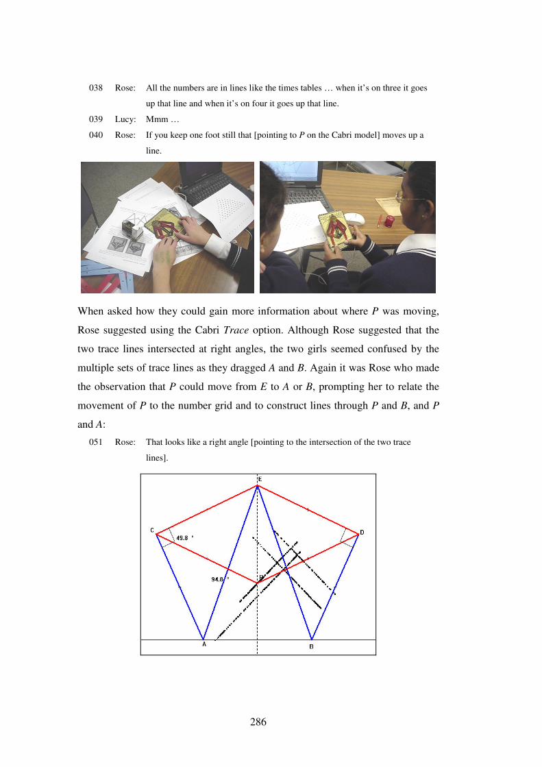
286
038 Rose: All the numbers are in lines like the times tables … when it’s on three it goes
up that line and when it’s on four it goes up that line.
039 Lucy: Mmm …
040 Rose: If you keep one foot still that [pointing to P on the Cabri model] moves up a
line.
When asked how they could gain more information about where P was moving,
Rose suggested using the Cabri Trace option. Although Rose suggested that the
two trace lines intersected at right angles, the two girls seemed confused by the
multiple sets of trace lines as they dragged A and B. Again it was Rose who made
the observation that P could move from E to A or B, prompting her to relate the
movement of P to the number grid and to construct lines through P and B, and P
and A:
051 Rose: That looks like a right angle [pointing to the intersection of the two trace
lines].
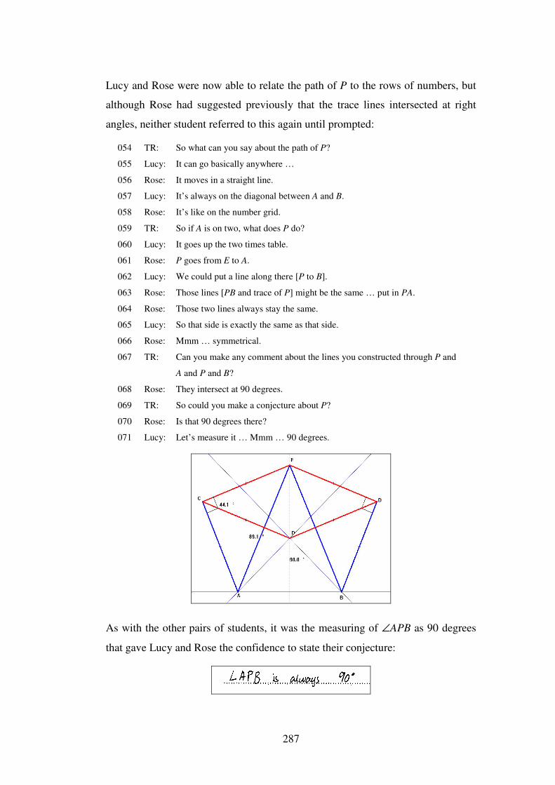
287
Lucy and Rose were now able to relate the path of P to the rows of numbers, but
although Rose had suggested previously that the trace lines intersected at right
angles, neither student referred to this again until prompted:
054 TR: So what can you say about the path of P?
055 Lucy: It can go basically anywhere …
056 Rose: It moves in a straight line.
057 Lucy: It’s always on the diagonal between A and B.
058 Rose: It’s like on the number grid.
059 TR: So if A is on two, what does P do?
060 Lucy: It goes up the two times table.
061 Rose: P goes from E to A.
062 Lucy: We could put a line along there [P to B].
063 Rose: Those lines [PB and trace of P] might be the same … put in PA.
064 Rose: Those two lines always stay the same.
065 Lucy: So that side is exactly the same as that side.
066 Rose: Mmm … symmetrical.
067 TR: Can you make any comment about the lines you constructed through P and
A and P and B?
068 Rose: They intersect at 90 degrees.
069 TR: So could you make a conjecture about P?
070 Rose: Is that 90 degrees there?
071 Lucy: Let’s measure it … Mmm … 90 degrees.
As with the other pairs of students, it was the measuring of ∠APB as 90 degrees
that gave Lucy and Rose the confidence to state their conjecture:
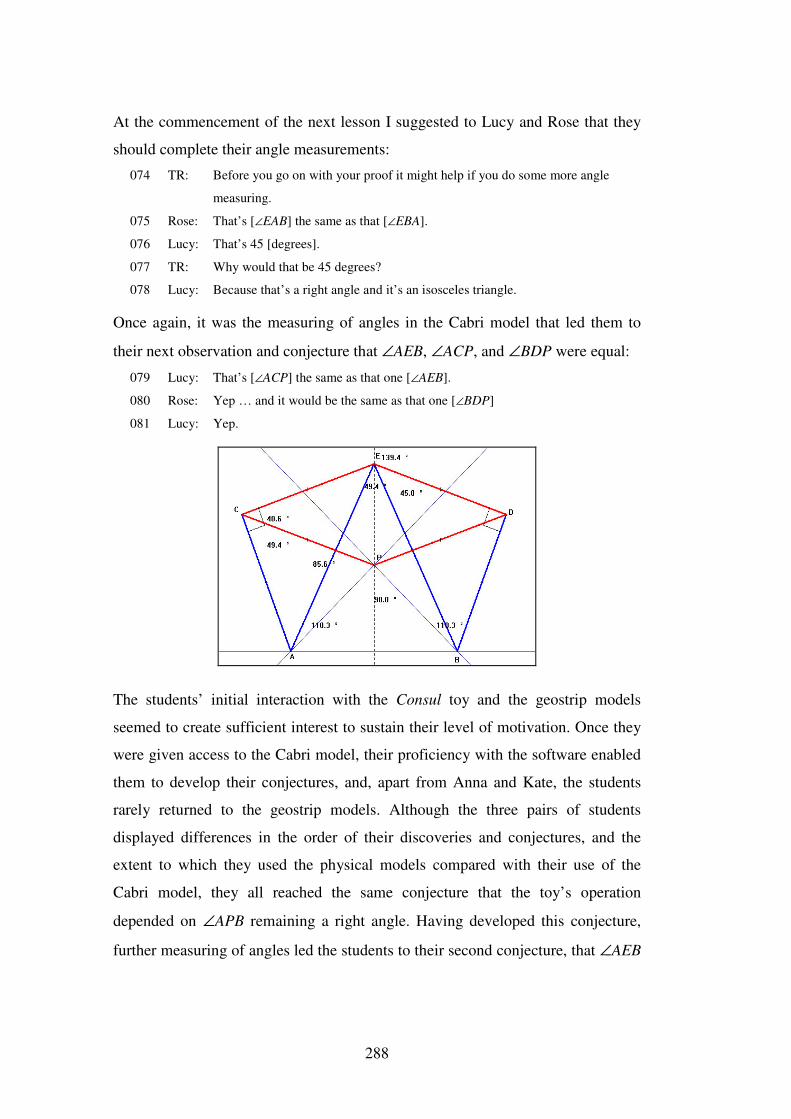
288
At the commencement of the next lesson I suggested to Lucy and Rose that they
should complete their angle measurements:
074 TR: Before you go on with your proof it might help if you do some more angle
measuring.
075 Rose: That’s [∠EAB] the same as that [∠EBA].
076 Lucy: That’s 45 [degrees].
077 TR: Why would that be 45 degrees?
078 Lucy: Because that’s a right angle and it’s an isosceles triangle.
Once again, it was the measuring of angles in the Cabri model that led them to
their next observation and conjecture that ∠AEB, ∠ACP, and ∠BDP were equal:
079 Lucy: That’s [∠ACP] the same as that one [∠AEB].
080 Rose: Yep … and it would be the same as that one [∠BDP]
081 Lucy: Yep.
The students’ initial interaction with the Consul toy and the geostrip models
seemed to create sufficient interest to sustain their level of motivation. Once they
were given access to the Cabri model, their proficiency with the software enabled
them to develop their conjectures, and, apart from Anna and Kate, the students
rarely returned to the geostrip models. Although the three pairs of students
displayed differences in the order of their discoveries and conjectures, and the
extent to which they used the physical models compared with their use of the
Cabri model, they all reached the same conjecture that the toy’s operation
depended on ∠APB remaining a right angle. Having developed this conjecture,
further measuring of angles led the students to their second conjecture, that ∠AEB
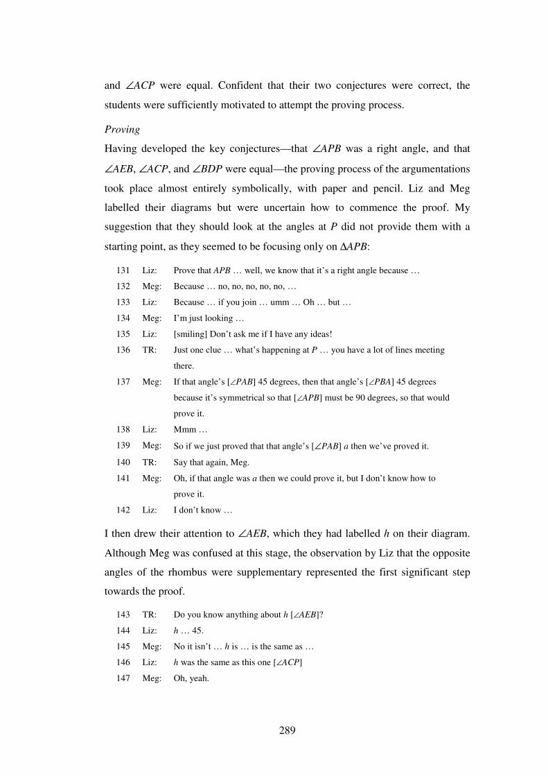
289
and ∠ACP were equal. Confident that their two conjectures were correct, the
students were sufficiently motivated to attempt the proving process.
Proving
Having developed the key conjectures—that ∠APB was a right angle, and that
∠AEB, ∠ACP, and ∠BDP were equal—the proving process of the argumentations
took place almost entirely symbolically, with paper and pencil. Liz and Meg
labelled their diagrams but were uncertain how to commence the proof. My
suggestion that they should look at the angles at P did not provide them with a
starting point, as they seemed to be focusing only on ∆APB:
131 Liz: Prove that APB … well, we know that it’s a right angle because …
132 Meg: Because … no, no, no, no, no, …
133 Liz: Because … if you join … umm … Oh … but …
134 Meg: I’m just looking …
135 Liz: [smiling] Don’t ask me if I have any ideas!
136 TR: Just one clue … what’s happening at P … you have a lot of lines meeting
there.
137 Meg: If that angle’s [∠PAB] 45 degrees, then that angle’s [∠PBA] 45 degrees
because it’s symmetrical so that [∠APB] must be 90 degrees, so that would
prove it.
138 Liz: Mmm …
139 Meg: So if we just proved that that angle’s [∠PAB] a then we’ve proved it.
140 TR: Say that again, Meg.
141 Meg: Oh, if that angle was a then we could prove it, but I don’t know how to
prove it.
142 Liz: I don’t know …
I then drew their attention to ∠AEB, which they had labelled h on their diagram.
Although Meg was confused at this stage, the observation by Liz that the opposite
angles of the rhombus were supplementary represented the first significant step
towards the proof.
143 TR: Do you know anything about h [∠AEB]?
144 Liz: h … 45.
145 Meg: No it isn’t … h is … is the same as …
146 Liz: h was the same as this one [∠ACP]
147 Meg: Oh, yeah.
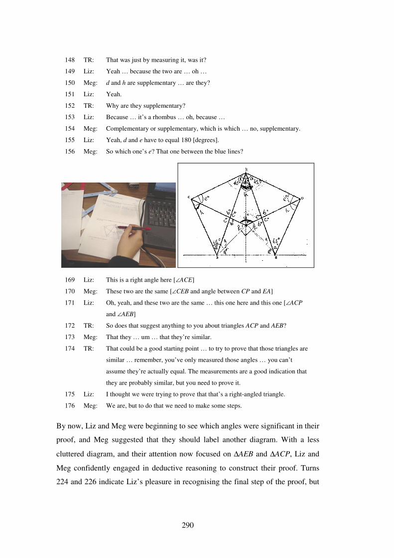
290
148 TR: That was just by measuring it, was it?
149 Liz: Yeah … because the two are … oh …
150 Meg: d and h are supplementary … are they?
151 Liz: Yeah.
152 TR: Why are they supplementary?
153 Liz: Because … it’s a rhombus … oh, because …
154 Meg: Complementary or supplementary, which is which … no, supplementary.
155 Liz: Yeah, d and e have to equal 180 [degrees].
156 Meg: So which one’s e? That one between the blue lines?
169 Liz: This is a right angle here [∠ACE]
170 Meg: These two are the same [∠CEB and angle between CP and EA]
171 Liz: Oh, yeah, and these two are the same … this one here and this one [∠ACP
and ∠AEB]
172 TR: So does that suggest anything to you about triangles ACP and AEB?
173 Meg: That they … um … that they’re similar.
174 TR: That could be a good starting point … to try to prove that those triangles are
similar … remember, you’ve only measured those angles … you can’t
assume they’re actually equal. The measurements are a good indication that
they are probably similar, but you need to prove it.
175 Liz: I thought we were trying to prove that that’s a right-angled triangle.
176 Meg: We are, but to do that we need to make some steps.
By now, Liz and Meg were beginning to see which angles were significant in their
proof, and Meg suggested that they should label another diagram. With a less
cluttered diagram, and their attention now focused on ∆AEB and ∆ACP, Liz and
Meg confidently engaged in deductive reasoning to construct their proof. Turns
224 and 226 indicate Liz’s pleasure in recognising the final step of the proof, but
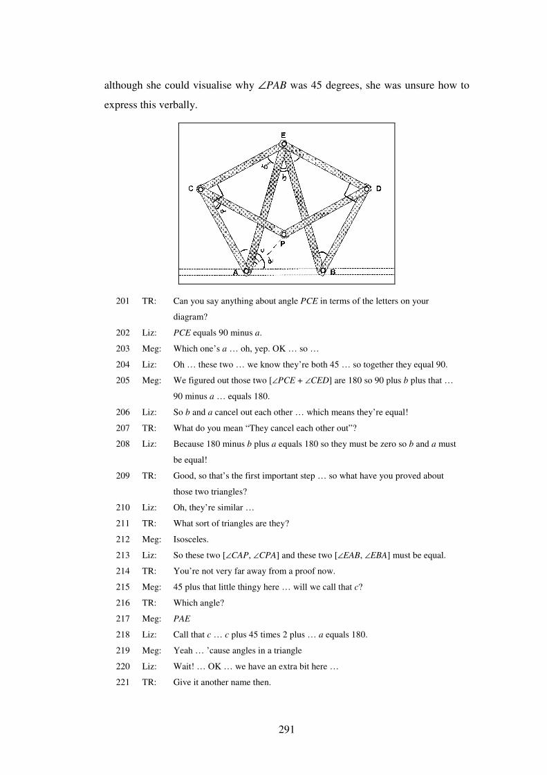
291
although she could visualise why ∠PAB was 45 degrees, she was unsure how to
express this verbally.
201 TR: Can you say anything about angle PCE in terms of the letters on your
diagram?
202 Liz: PCE equals 90 minus a.
203 Meg: Which one’s a … oh, yep. OK … so …
204 Liz: Oh … these two … we know they’re both 45 … so together they equal 90.
205 Meg: We figured out those two [∠PCE + ∠CED] are 180 so 90 plus b plus that …
90 minus a … equals 180.
206 Liz: So b and a cancel out each other … which means they’re equal!
207 TR: What do you mean “They cancel each other out”?
208 Liz: Because 180 minus b plus a equals 180 so they must be zero so b and a must
be equal!
209 TR: Good, so that’s the first important step … so what have you proved about
those two triangles?
210 Liz: Oh, they’re similar …
211 TR: What sort of triangles are they?
212 Meg: Isosceles.
213 Liz: So these two [∠CAP, ∠CPA] and these two [∠EAB, ∠EBA] must be equal.
214 TR: You’re not very far away from a proof now.
215 Meg: 45 plus that little thingy here … will we call that c?
216 TR: Which angle?
217 Meg: PAE
218 Liz: Call that c … c plus 45 times 2 plus … a equals 180.
219 Meg: Yeah … ’cause angles in a triangle
220 Liz: Wait! … OK … we have an extra bit here …
221 TR: Give it another name then.
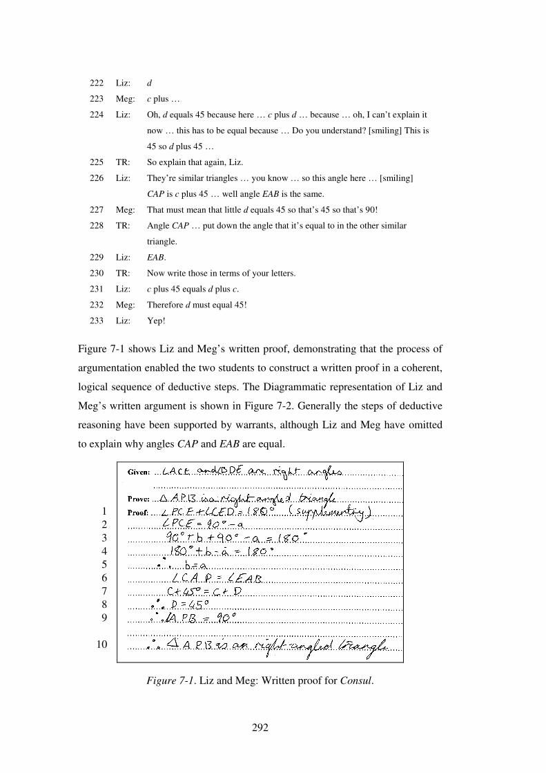
292
222 Liz: d
223 Meg: c plus …
224 Liz: Oh, d equals 45 because here … c plus d … because … oh, I can’t explain it
now … this has to be equal because … Do you understand? [smiling] This is
45 so d plus 45 …
225 TR: So explain that again, Liz.
226 Liz: They’re similar triangles … you know … so this angle here … [smiling]
CAP is c plus 45 … well angle EAB is the same.
227 Meg: That must mean that little d equals 45 so that’s 45 so that’s 90!
228 TR: Angle CAP … put down the angle that it’s equal to in the other similar
triangle.
229 Liz: EAB.
230 TR: Now write those in terms of your letters.
231 Liz: c plus 45 equals d plus c.
232 Meg: Therefore d must equal 45!
233 Liz: Yep!
Figure 7-1 shows Liz and Meg’s written proof, demonstrating that the process of
argumentation enabled the two students to construct a written proof in a coherent,
logical sequence of deductive steps. The Diagrammatic representation of Liz and
Meg’s written argument is shown in Figure 7-2. Generally the steps of deductive
reasoning have been supported by warrants, although Liz and Meg have omitted
to explain why angles CAP and EAB are equal.
Figure 7-1. Liz and Meg: Written proof for Consul.
123456789
10
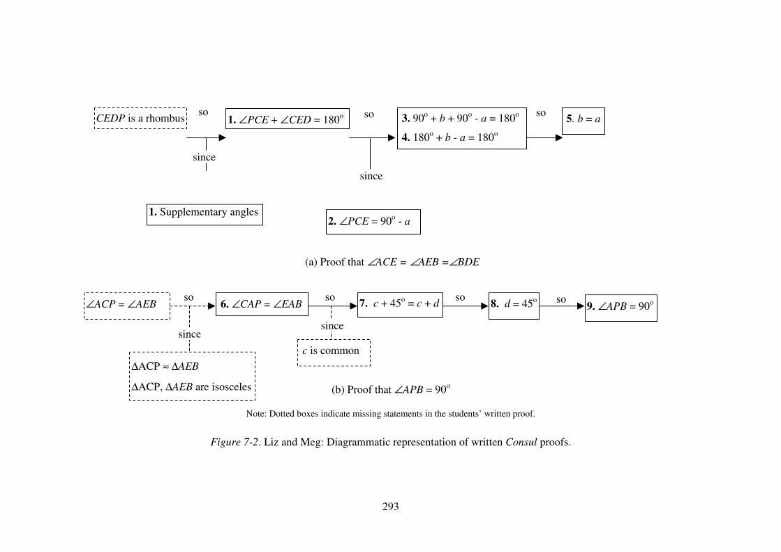
293
(a) Proof that ∠ACE = ∠AEB =∠BDE
(b) Proof that ∠APB = 90o
Note: Dotted boxes indicate missing statements in the students’ written proof.
Figure 7-2. Liz and Meg: Diagrammatic representation of written Consul proofs.
9. ∠APB = 90o ∠ACP = ∠AEB
6. ∠CAP = ∠EAB 7. c + 45o = c + d
c is common
8. d = 45o
∆ACP ≈ ∆AEB
∆ACP, ∆AEB are isosceles
so so so so
since since
CEDP is a rhombus
1. Supplementary angles
1. ∠PCE + ∠CED = 180o 3. 90o + b + 90o - a = 180o
4. 180o + b - a = 180o
2. ∠PCE = 90o - a
5. b = a so so so
since
since
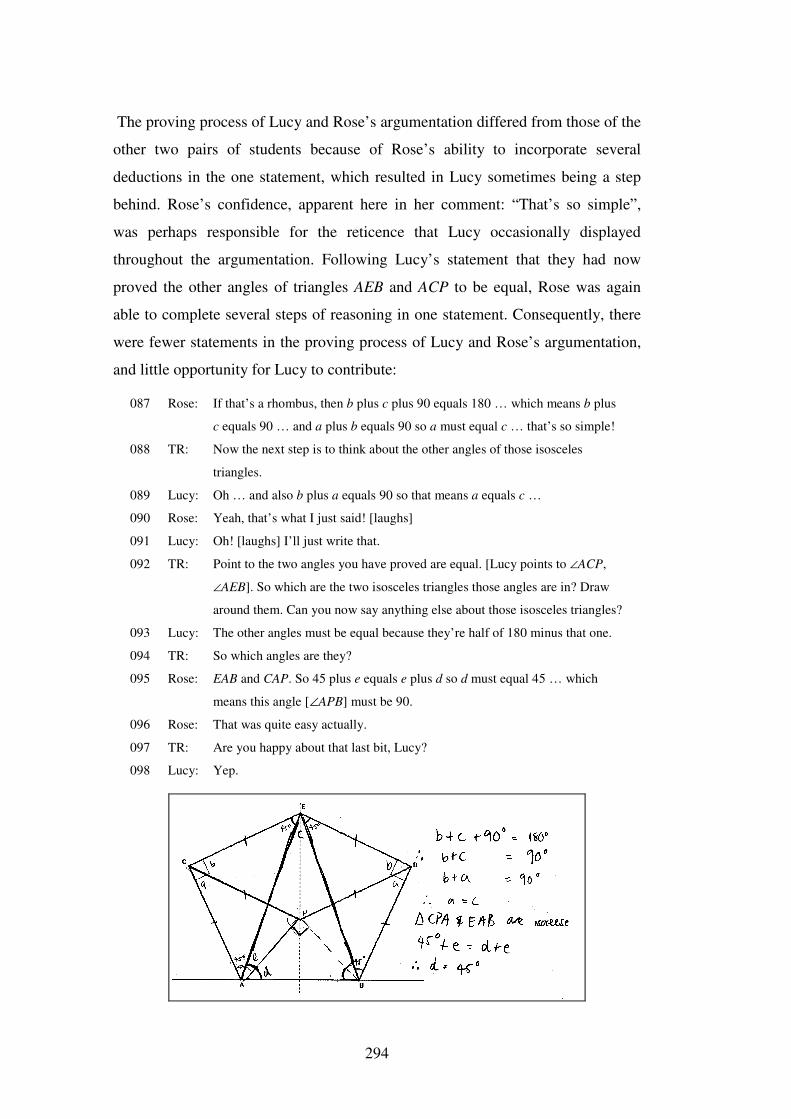
294
The proving process of Lucy and Rose’s argumentation differed from those of the
other two pairs of students because of Rose’s ability to incorporate several
deductions in the one statement, which resulted in Lucy sometimes being a step
behind. Rose’s confidence, apparent here in her comment: “That’s so simple”,
was perhaps responsible for the reticence that Lucy occasionally displayed
throughout the argumentation. Following Lucy’s statement that they had now
proved the other angles of triangles AEB and ACP to be equal, Rose was again
able to complete several steps of reasoning in one statement. Consequently, there
were fewer statements in the proving process of Lucy and Rose’s argumentation,
and little opportunity for Lucy to contribute:
087 Rose: If that’s a rhombus, then b plus c plus 90 equals 180 … which means b plus
c equals 90 … and a plus b equals 90 so a must equal c … that’s so simple!
088 TR: Now the next step is to think about the other angles of those isosceles
triangles.
089 Lucy: Oh … and also b plus a equals 90 so that means a equals c …
090 Rose: Yeah, that’s what I just said! [laughs]
091 Lucy: Oh! [laughs] I’ll just write that.
092 TR: Point to the two angles you have proved are equal. [Lucy points to ∠ACP,
∠AEB]. So which are the two isosceles triangles those angles are in? Draw
around them. Can you now say anything else about those isosceles triangles?
093 Lucy: The other angles must be equal because they’re half of 180 minus that one.
094 TR: So which angles are they?
095 Rose: EAB and CAP. So 45 plus e equals e plus d so d must equal 45 … which
means this angle [∠APB] must be 90.
096 Rose: That was quite easy actually.
097 TR: Are you happy about that last bit, Lucy?
098 Lucy: Yep.
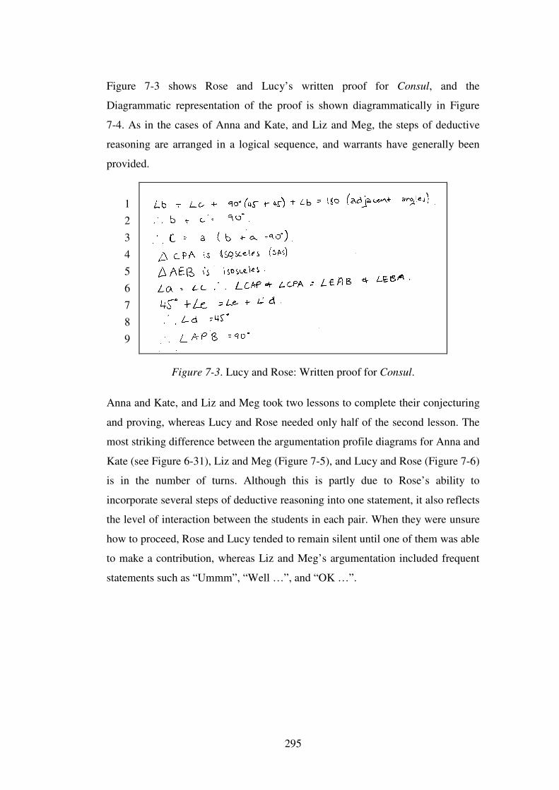
295
Figure 7-3 shows Rose and Lucy’s written proof for Consul, and the
Diagrammatic representation of the proof is shown diagrammatically in Figure
7-4. As in the cases of Anna and Kate, and Liz and Meg, the steps of deductive
reasoning are arranged in a logical sequence, and warrants have generally been
provided.
Figure 7-3. Lucy and Rose: Written proof for Consul.
Anna and Kate, and Liz and Meg took two lessons to complete their conjecturing
and proving, whereas Lucy and Rose needed only half of the second lesson. The
most striking difference between the argumentation profile diagrams for Anna and
Kate (see Figure 6-31), Liz and Meg (Figure 7-5), and Lucy and Rose (Figure 7-6)
is in the number of turns. Although this is partly due to Rose’s ability to
incorporate several steps of deductive reasoning into one statement, it also reflects
the level of interaction between the students in each pair. When they were unsure
how to proceed, Rose and Lucy tended to remain silent until one of them was able
to make a contribution, whereas Liz and Meg’s argumentation included frequent
statements such as “Ummm”, “Well …”, and “OK …”.
1 2 3 4 5 6 7 8 9
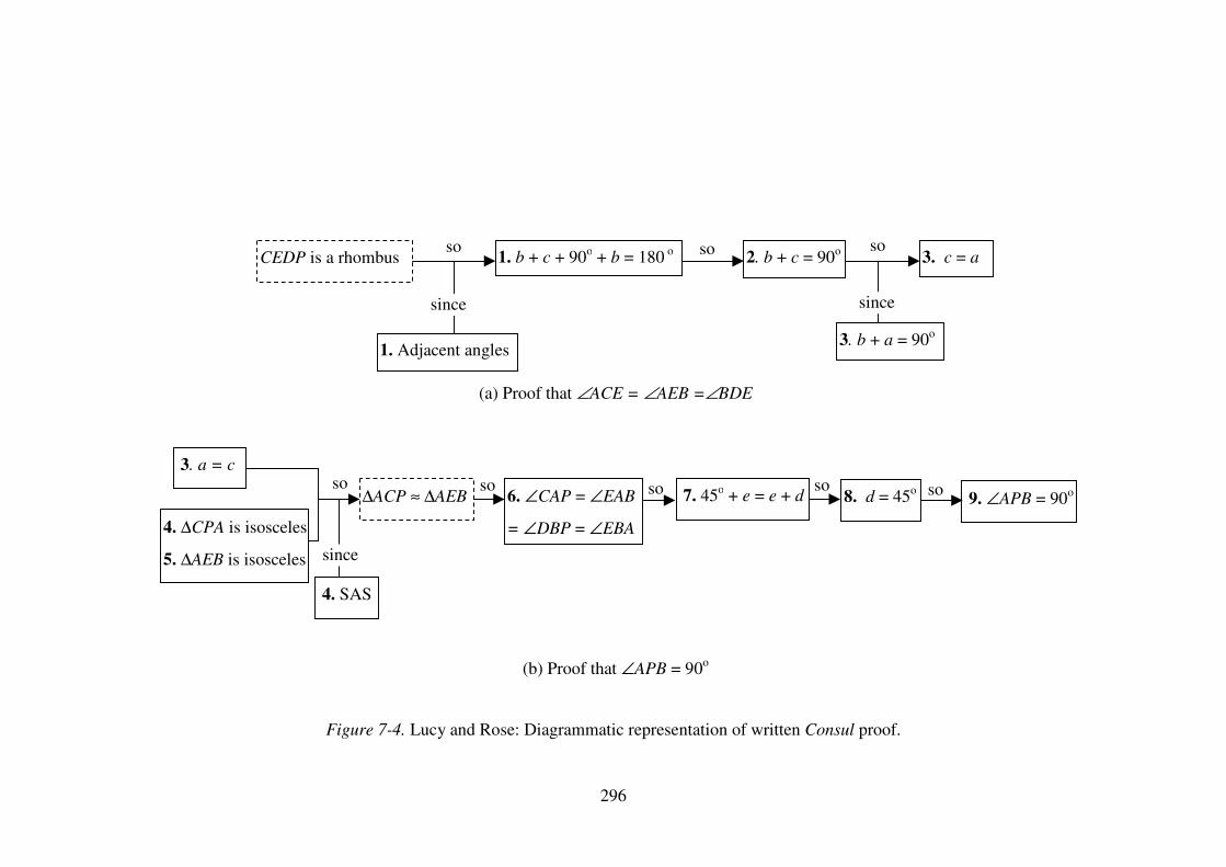
296
(a) Proof that ∠ACE = ∠AEB =∠BDE
(b) Proof that ∠APB = 90o
Figure 7-4. Lucy and Rose: Diagrammatic representation of written Consul proof.
CEDP is a rhombus 1. b + c + 90o + b = 180 o 2. b + c = 90o 3. c = a
3. b + a = 90o 1. Adjacent angles
so so so
since since
4. ∆CPA is isosceles
5. ∆AEB is isosceles
3. a = c
∆ACP ≈ ∆AEB 8. d = 45o 9. ∠APB = 90o 7. 45o + e = e + d
4. SAS
6. ∠CAP = ∠EAB
= ∠DBP = ∠EBA
so so so so so
since
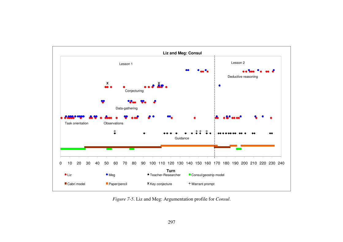
297
Liz and Meg: Consul
0 10 20 30 40 50 60 70 80 90 100 110 120 130 140 150 160 170 180 190 200 210 220 230 240
TurnLiz Meg Teacher-Researcher Consul/geostrip model
Cabri model Paper/pencil Key conjecture Warrant prompt
Deductive reasoning
Conjecturing
Data-gathering
Observations
Guidance
Lesson 1 Lesson 2
Task orientation
Figure 7-5. Liz and Meg: Argumentation profile for Consul.
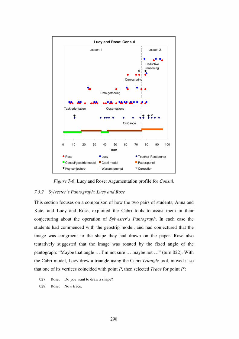
298
Lucy and Rose: Consul
0 10 20 30 40 50 60 70 80 90 100
Turn
Rose Lucy Teacher-Researcher
Consul/geostrip model Cabri model Paper/pencil
Key conjecture Warrant prompt Correction
Guidance
Observations
Data gathering
Conjecturing
Deductive reasoning
Lesson 1 Lesson 2
Task orientation
Figure 7-6. Lucy and Rose: Argumentation profile for Consul.
7.3.2 Sylvester’s Pantograph: Lucy and Rose
This section focuses on a comparison of how the two pairs of students, Anna and
Kate, and Lucy and Rose, exploited the Cabri tools to assist them in their
conjecturing about the operation of Sylvester’s Pantograph. In each case the
students had commenced with the geostrip model, and had conjectured that the
image was congruent to the shape they had drawn on the paper. Rose also
tentatively suggested that the image was rotated by the fixed angle of the
pantograph: “Maybe that angle … I’m not sure … maybe not …” (turn 022). With
the Cabri model, Lucy drew a triangle using the Cabri Triangle tool, moved it so
that one of its vertices coincided with point P, then selected Trace for point P':
027 Rose: Do you want to draw a shape?
028 Rose: Now trace.
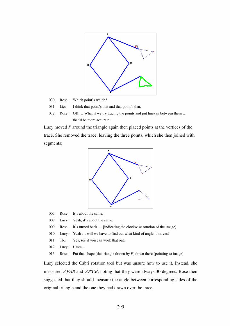
299
030 Rose: Which point’s which?
031 Liz: I think that point’s that and that point’s that.
032 Rose: OK … What if we try tracing the points and put lines in between them …
that’d be more accurate.
Lucy moved P around the triangle again then placed points at the vertices of the
trace. She removed the trace, leaving the three points, which she then joined with
segments:
007 Rose: It’s about the same.
008 Lucy: Yeah, it’s about the same.
009 Rose: It’s turned back … [indicating the clockwise rotation of the image]
010 Lucy: Yeah … will we have to find out what kind of angle it moves?
011 TR: Yes, see if you can work that out.
012 Lucy: Umm …
013 Rose: Put that shape [the triangle drawn by P] down there [pointing to image]
Lucy selected the Cabri rotation tool but was unsure how to use it. Instead, she
measured ∠PAB and ∠P'CB, noting that they were always 30 degrees. Rose then
suggested that they should measure the angle between corresponding sides of the
original triangle and the one they had drawn over the trace:

300
042 TR: That’s [the Cabri Rotation tool] for rotating an object by a specified amount
… but that was a good idea you had.
043 Lucy: Maybe we should get rid of trace … when you move that [P] …
044 Lucy: So it’s 30 degrees the whole time [∠PAB and ∠P'CB].
045 Rose: So we want to measure …
046 Lucy: This angle? Twenty-nine point one … it’s point nine off.
047 TR: So what is your conjecture then?
048 Lucy: That the angle which the copy of the shape rotates is that angle of the
pantograph.
Lucy and Rose were still uncertain why the image was rotated:
056 TR: What determines where the image is formed?
057 Rose: The smaller this angle [ABC] the further out these go [P and P'] and the
further apart these [P and P'] get …
058 Lucy: Oh … so they do get further apart …
059 Rose: If you just rotate it …
060 Lucy: When you move it round a shape they stay the same distance apart.
061 Rose: Yeah …
062 TR: Look at where the linkage is attached to the paper and watch that in relation
to the object and the image.
063 Rose: Perhaps this angle is always the same …
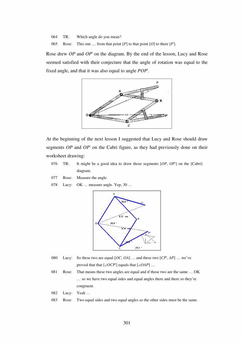
301
064 TR: Which angle do you mean?
065 Rose: This one … from that point [P] to that point [O] to there [P'].
Rose drew OP and OP' on the diagram. By the end of the lesson, Lucy and Rose
seemed satisfied with their conjecture that the angle of rotation was equal to the
fixed angle, and that it was also equal to angle POP'.
At the beginning of the next lesson I suggested that Lucy and Rose should draw
segments OP and OP' on the Cabri figure, as they had previously done on their
worksheet drawing:
076 TR: It might be a good idea to draw those segments [OP, OP'] on the [Cabri]
diagram.
077 Rose: Measure the angle.
078 Lucy: OK … measure angle. Yep, 30 …
080 Lucy: So these two are equal [OC, OA] … and these two [CP', AP] … we’ve
proved that that [∠OCP'] equals that [∠OAP] …
081 Rose: That means these two angles are equal and if those two are the same … OK
… so we have two equal sides and equal angles there and there so they’re
congruent.
082 Lucy: Yeah …
083 Rose: Two equal sides and two equal angles so the other sides must be the same.
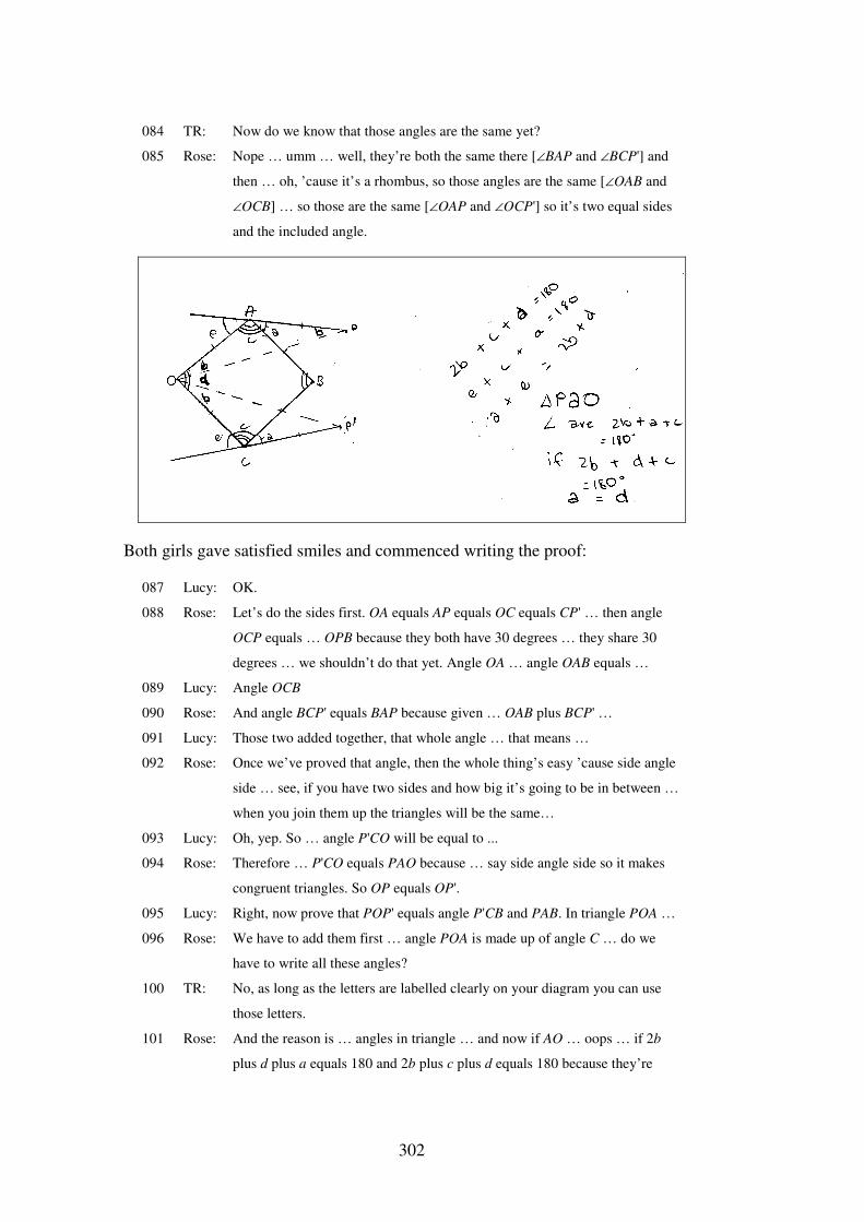
302
084 TR: Now do we know that those angles are the same yet?
085 Rose: Nope … umm … well, they’re both the same there [∠BAP and ∠BCP'] and
then … oh, ’cause it’s a rhombus, so those angles are the same [∠OAB and
∠OCB] … so those are the same [∠OAP and ∠OCP'] so it’s two equal sides
and the included angle.
Both girls gave satisfied smiles and commenced writing the proof:
087 Lucy: OK.
088 Rose: Let’s do the sides first. OA equals AP equals OC equals CP' … then angle
OCP equals … OPB because they both have 30 degrees … they share 30
degrees … we shouldn’t do that yet. Angle OA … angle OAB equals …
089 Lucy: Angle OCB
090 Rose: And angle BCP' equals BAP because given … OAB plus BCP' …
091 Lucy: Those two added together, that whole angle … that means …
092 Rose: Once we’ve proved that angle, then the whole thing’s easy ’cause side angle
side … see, if you have two sides and how big it’s going to be in between …
when you join them up the triangles will be the same…
093 Lucy: Oh, yep. So … angle P'CO will be equal to ...
094 Rose: Therefore … P'CO equals PAO because … say side angle side so it makes
congruent triangles. So OP equals OP'.
095 Lucy: Right, now prove that POP' equals angle P'CB and PAB. In triangle POA …
096 Rose: We have to add them first … angle POA is made up of angle C … do we
have to write all these angles?
100 TR: No, as long as the letters are labelled clearly on your diagram you can use
those letters.
101 Rose: And the reason is … angles in triangle … and now if AO … oops … if 2b
plus d plus a equals 180 and 2b plus c plus d equals 180 because they’re
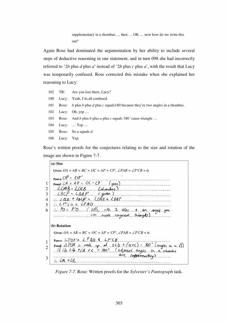
303
supplementary in a rhombus … then … OK … now how do we write this
out?
Again Rose had dominated the argumentation by her ability to include several
steps of deductive reasoning in one statement, and in turn 098 she had incorrectly
referred to ‘2b plus d plus a’ instead of ‘2b plus c plus a’, with the result that Lucy
was temporarily confused. Rose corrected this mistake when she explained her
reasoning to Lucy:
102 TR: Are you lost there, Lucy?
100 Lucy: Yeah, I’m all confused.
101 Rose: b plus b plus d plus c equals180 because they’re two angles in a rhombus.
102 Lucy: Oh, yep …
103 Rose: And b plus b plus a plus c equals 180 ’cause triangle …
104 Lucy: … Yep …
105 Rose: So a equals d.
106 Lucy: Yep.
Rose’s written proofs for the conjectures relating to the size and rotation of the
image are shown in Figure 7-7.
(a) Size
Given: OA = AB = BC = OC = AP = CP', ∠PAB = ∠P'CB = α
(b) Rotation
Given: OA = AB = BC = OC = AP = CP', ∠PAB = ∠P'CB = α
Figure 7-7. Rose: Written proofs for the Sylvester’s Pantograph task.
1 2 3 4 5 6
1 2 3
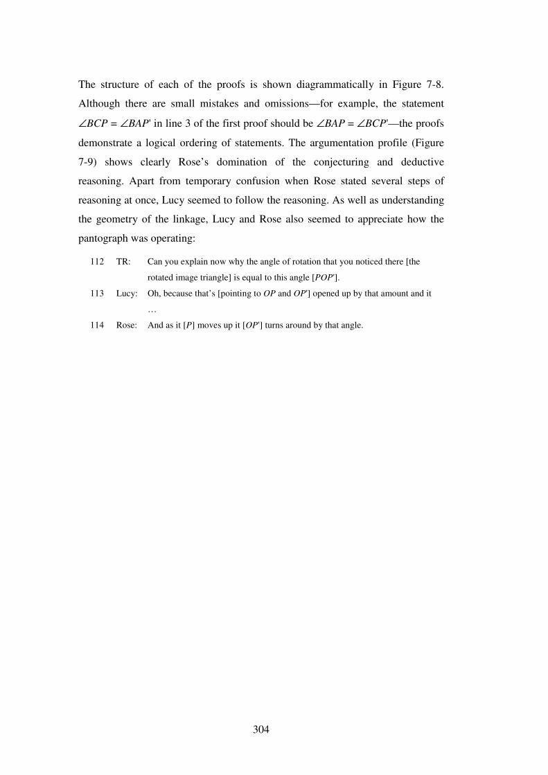
304
The structure of each of the proofs is shown diagrammatically in Figure 7-8.
Although there are small mistakes and omissions—for example, the statement
∠BCP = ∠BAP' in line 3 of the first proof should be ∠BAP = ∠BCP'—the proofs
demonstrate a logical ordering of statements. The argumentation profile (Figure
7-9) shows clearly Rose’s domination of the conjecturing and deductive
reasoning. Apart from temporary confusion when Rose stated several steps of
reasoning at once, Lucy seemed to follow the reasoning. As well as understanding
the geometry of the linkage, Lucy and Rose also seemed to appreciate how the
pantograph was operating:
112 TR: Can you explain now why the angle of rotation that you noticed there [the
rotated image triangle] is equal to this angle [POP'].
113 Lucy: Oh, because that’s [pointing to OP and OP'] opened up by that amount and it
…
114 Rose: And as it [P] moves up it [OP'] turns around by that angle.
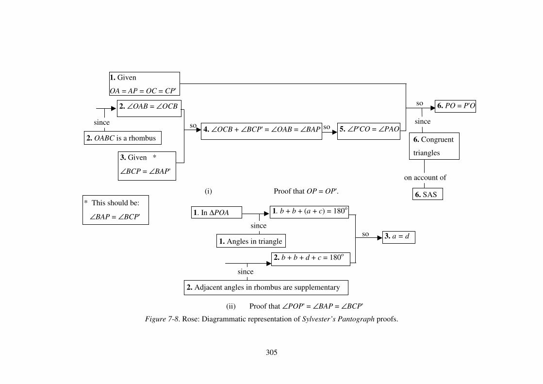
305
(i) Proof that OP = OP'.
(ii) Proof that ∠POP' = ∠BAP = ∠BCP'
Figure 7-8. Rose: Diagrammatic representation of Sylvester’s Pantograph proofs.
6. PO = P'O
6. Congruent
triangles
6. SAS
so
since
on account of
1. Given
OA = AP = OC = CP'
4. ∠OCB + ∠BCP' = ∠OAB = ∠BAP
5. ∠P'CO = ∠PAO
3. Given *
∠BCP = ∠BAP'
so
2. ∠OAB = ∠OCB
2. OABC is a rhombus
so since
1. b + b + (a + c) = 180o
2. b + b + d + c = 180o
2. Adjacent angles in rhombus are supplementary
1. Angles in triangle 3. a = d so
since
since
1. In ∆POA * This should be:
∠BAP = ∠BCP'
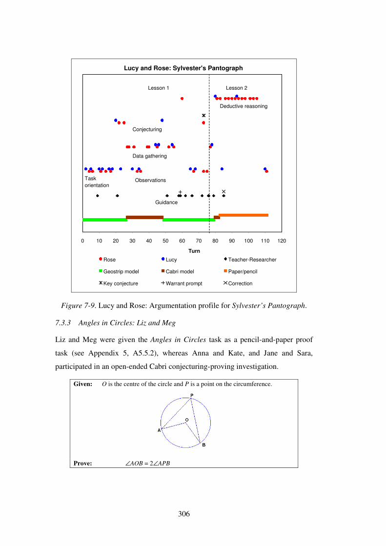
306
Lucy and Rose: Sylvester's Pantograph
0 10 20 30 40 50 60 70 80 90 100 110 120
Turn
Rose Lucy Teacher-Researcher
Geostrip model Cabri model Paper/pencil
Key conjecture Warrant prompt Correction
Guidance
Observations
Data gathering
Conjecturing
Deductive reasoning
Lesson 1 Lesson 2
Task orientation
Figure 7-9. Lucy and Rose: Argumentation profile for Sylvester’s Pantograph.
7.3.3 Angles in Circles: Liz and Meg
Liz and Meg were given the Angles in Circles task as a pencil-and-paper proof
task (see Appendix 5, A5.5.2), whereas Anna and Kate, and Jane and Sara,
participated in an open-ended Cabri conjecturing-proving investigation.
Given: O is the centre of the circle and P is a point on the circumference.
Prove: ∠AOB = 2∠APB
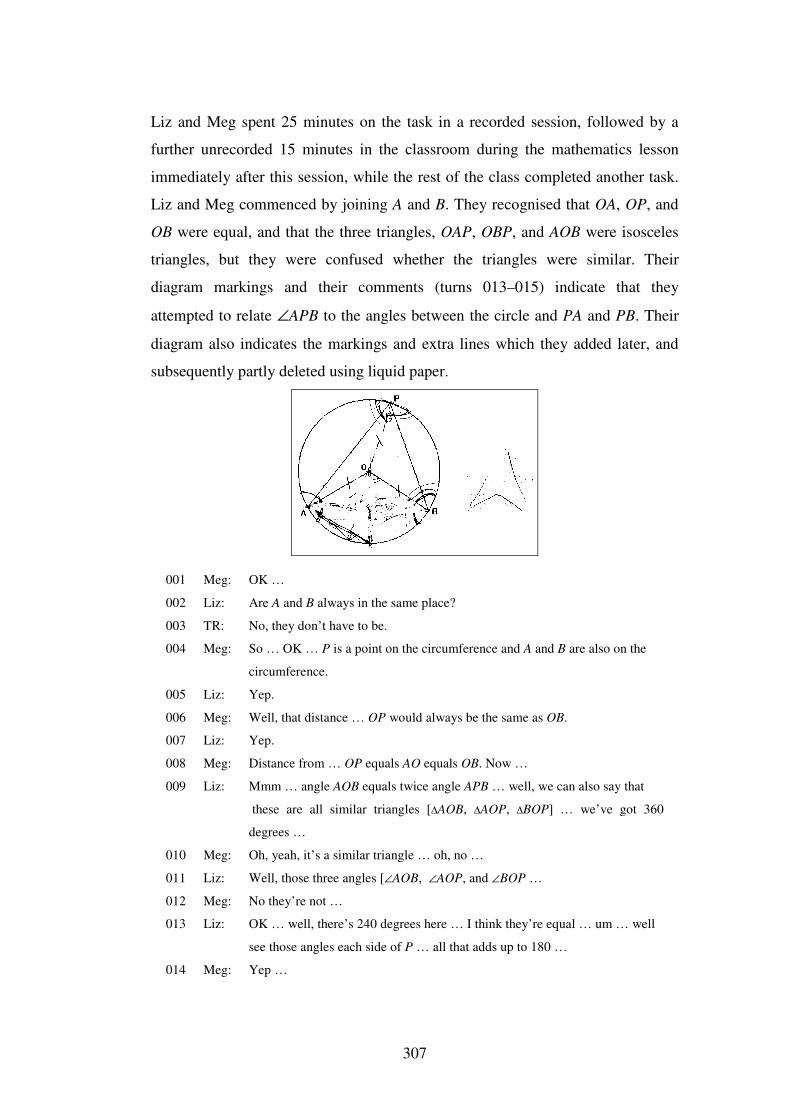
307
Liz and Meg spent 25 minutes on the task in a recorded session, followed by a
further unrecorded 15 minutes in the classroom during the mathematics lesson
immediately after this session, while the rest of the class completed another task.
Liz and Meg commenced by joining A and B. They recognised that OA, OP, and
OB were equal, and that the three triangles, OAP, OBP, and AOB were isosceles
triangles, but they were confused whether the triangles were similar. Their
diagram markings and their comments (turns 013–015) indicate that they
attempted to relate ∠APB to the angles between the circle and PA and PB. Their
diagram also indicates the markings and extra lines which they added later, and
subsequently partly deleted using liquid paper.
001 Meg: OK …
002 Liz: Are A and B always in the same place?
003 TR: No, they don’t have to be.
004 Meg: So … OK … P is a point on the circumference and A and B are also on the
circumference.
005 Liz: Yep.
006 Meg: Well, that distance … OP would always be the same as OB.
007 Liz: Yep.
008 Meg: Distance from … OP equals AO equals OB. Now …
009 Liz: Mmm … angle AOB equals twice angle APB … well, we can also say that
these are all similar triangles [∆AOB, ∆AOP, ∆BOP] … we’ve got 360
degrees …
010 Meg: Oh, yeah, it’s a similar triangle … oh, no …
011 Liz: Well, those three angles [∠AOB, ∠AOP, and ∠BOP …
012 Meg: No they’re not …
013 Liz: OK … well, there’s 240 degrees here … I think they’re equal … um … well
see those angles each side of P … all that adds up to 180 …
014 Meg: Yep …
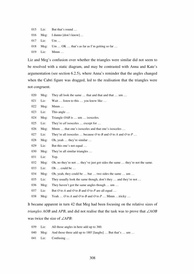
308
015 Liz: But that’s round …
016 Meg: I dunno [don’t know]…
017 Liz: Um …
018 Meg: Um … OK … that’s as far as I’m getting so far …
019 Liz: Mmm …
Liz and Meg’s confusion over whether the triangles were similar did not seem to
be resolved with a static diagram, and may be contrasted with Anna and Kate’s
argumentation (see section 6.2.5), where Anna’s reminder that the angles changed
when the Cabri figure was dragged, led to the realisation that the triangles were
not congruent.
020 Meg: They all look the same … that and that and that … um …
021 Liz: Wait … listen to this … you know like …
022 Meg: Mmm …
023 Liz: This angle …
024 Meg: Triangle OAB is … um … isosceles.
025 Liz: They’re all isosceles … except for …
026 Meg: Mmm … that one’s isosceles and that one’s isosceles …
027 Liz: They’re all isosceles … because O to B and O to A and O to P …
028 Meg: Oh, yeah … they’re similar …
029 Liz: But this one’s not equal …
030 Meg: They’re all similar triangles …
031 Liz: Yep.
032 Meg: Oh, no they’re not … they’ve just got sides the same … they’re not the same.
033 Liz: Oh … could be …
034 Meg: Oh, yeah, they could be … but … two sides the same … um …
035 Liz: They usually look the same though, don’t they … and they’re not …
036 Meg: They haven’t got the same angles though … um …
037 Liz: But O to A and O to B and O to P are all equal …
038 Meg: Yeah … O to A and O to B and O to P … Mmm …tricky …
It became apparent in turn 42 that Meg had been focusing on the relative sizes of
triangles AOB and APB, and did not realise that the task was to prove that ∠AOB
was twice the size of ∠APB:
039 Liz: All those angles in here add up to 360.
040 Meg: And those three add up to 180! [laughs] … But that’s … um …
041 Liz: Confusing …
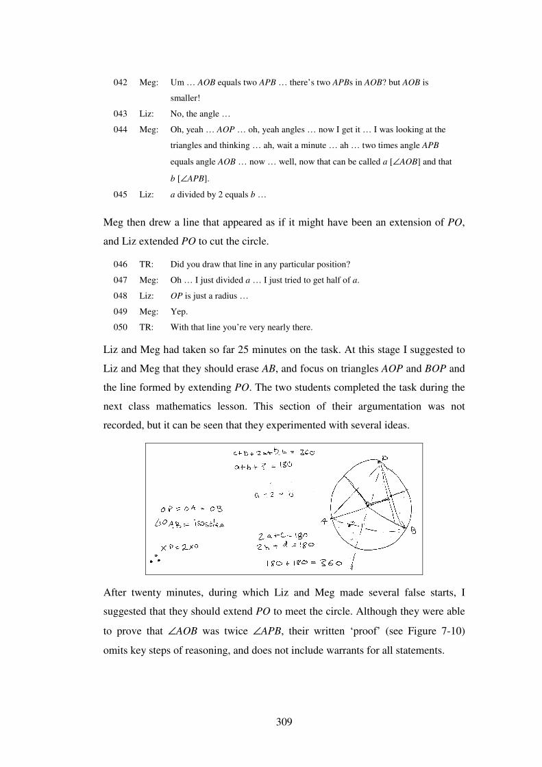
309
042 Meg: Um … AOB equals two APB … there’s two APBs in AOB? but AOB is
smaller!
043 Liz: No, the angle …
044 Meg: Oh, yeah … AOP … oh, yeah angles … now I get it … I was looking at the
triangles and thinking … ah, wait a minute … ah … two times angle APB
equals angle AOB … now … well, now that can be called a [∠AOB] and that
b [∠APB].
045 Liz: a divided by 2 equals b …
Meg then drew a line that appeared as if it might have been an extension of PO,
and Liz extended PO to cut the circle.
046 TR: Did you draw that line in any particular position?
047 Meg: Oh … I just divided a … I just tried to get half of a.
048 Liz: OP is just a radius …
049 Meg: Yep.
050 TR: With that line you’re very nearly there.
Liz and Meg had taken so far 25 minutes on the task. At this stage I suggested to
Liz and Meg that they should erase AB, and focus on triangles AOP and BOP and
the line formed by extending PO. The two students completed the task during the
next class mathematics lesson. This section of their argumentation was not
recorded, but it can be seen that they experimented with several ideas.
After twenty minutes, during which Liz and Meg made several false starts, I
suggested that they should extend PO to meet the circle. Although they were able
to prove that ∠AOB was twice ∠APB, their written ‘proof’ (see Figure 7-10)
omits key steps of reasoning, and does not include warrants for all statements.
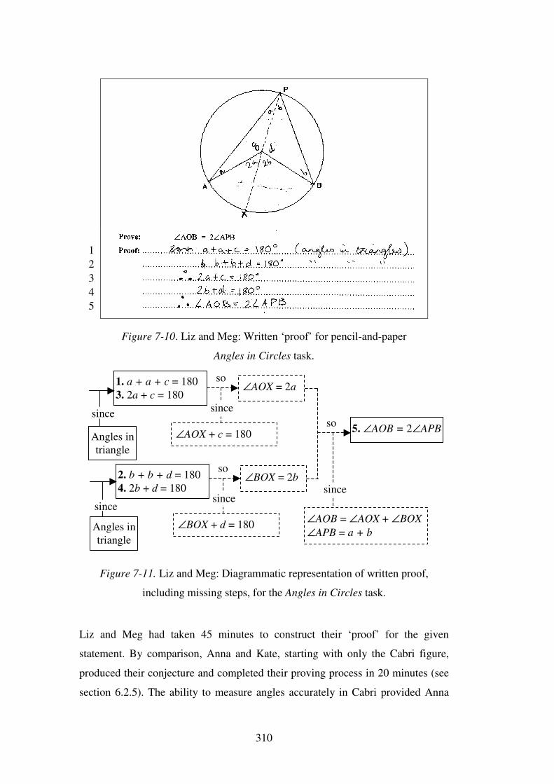
310
Figure 7-10. Liz and Meg: Written ‘proof’ for pencil-and-paper
Angles in Circles task.
Figure 7-11. Liz and Meg: Diagrammatic representation of written proof,
including missing steps, for the Angles in Circles task.
Liz and Meg had taken 45 minutes to construct their ‘proof’ for the given
statement. By comparison, Anna and Kate, starting with only the Cabri figure,
produced their conjecture and completed their proving process in 20 minutes (see
section 6.2.5). The ability to measure angles accurately in Cabri provided Anna
1 2 3 4 5
1. a + a + c = 180 3. 2a + c = 180
∠AOX + c = 180
∠AOX = 2a so
since
2. b + b + d = 180 4. 2b + d = 180
∠BOX + d = 180
∠BOX = 2b so
since
5. ∠AOB = 2∠APB
∠AOB = ∠AOX + ∠BOX ∠APB = a + b
so
since
Angles in triangle
Angles in triangle
since
since
311
and Kate with a pathway towards their conjecturing, but also towards their proof.
Their discovery led them to measure other angles, to notice invariant
relationships, and to make the link with exterior angles. The fixed nature of the
pencil-and-paper diagram seemed to hinder the reasoning process for Liz and
Meg.
7.3.4 The other Level 2–3 case study students
Pam and Elly
To avoid the presentation of repetitive data, argumentations for Pam and Elly are
not discussed. In each of the three additional conjecturing-proving tasks that they
completed, Pam and Elly displayed a high level of motivation, and the
argumentations were cooperative, with both students engaging in deductive
reasoning.
Amy and Lyn
As Amy and Lyn were available for only 20 minutes on the first occasion, I
decided to commence with the Joining Midpoints task. The two students were not
part of the same friendship group, although they did not appear to be unfriendly
towards each other. Any attempt on Amy’s part to engage Lyn in discussion
failed, however, and Lyn appeared completely unmotivated or unable to
participate, resulting in greater guidance from me in order to support Amy. Lyn’s
lack of response was not confined to this task, and in fact she seemed to have
general motivational problems at school. Because of this lack of interaction, as
well as the difficulty of finding another lesson when I could withdraw this pair of
students, Amy and Lyn did not have an opportunity to complete any of the other
additional conjecturing-proving tasks.
Whereas Lyn developed little understanding of deductive reasoning, Amy
performed as well as some of the students who had completed a greater number of
additional tasks, with a post-test score of 6 out of a possible 9 for the van Hiele
Level 4 items (see Table 5-5). By contrast, Lyn’s Level 3 total score decreased
from 52 to 42, and she made no correct responses to Level 4 items. The
performance of these students on the proof construction items, G4 and G7, of the
Proof Questionnaire is discussed in chapter 8.
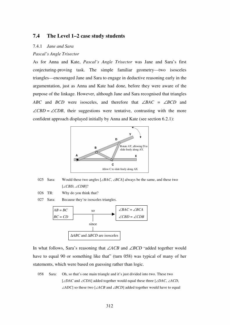
312
7.4 The Level 1–2 case study students
7.4.1 Jane and Sara
Pascal’s Angle Trisector
As for Anna and Kate, Pascal’s Angle Trisector was Jane and Sara’s first
conjecturing-proving task. The simple familiar geometry—two isosceles
triangles—encouraged Jane and Sara to engage in deductive reasoning early in the
argumentation, just as Anna and Kate had done, before they were aware of the
purpose of the linkage. However, although Jane and Sara recognised that triangles
ABC and BCD were isosceles, and therefore that ∠BAC = ∠BCD and
∠CBD = ∠CDB, their suggestions were tentative, contrasting with the more
confident approach displayed initially by Anna and Kate (see section 6.2.1):
A
B
C
D
Y
X
Rotate AY, allowing D toslide freely along AY.
Allow C to slide freely along AX
025 Sara: Would these two angles [∠BAC, ∠BCA] always be the same, and these two
[∠CBD, ∠CDB]?
026 TR: Why do you think that?
027 Sara: Because they’re isosceles triangles.
In what follows, Sara’s reasoning that ∠ACB and ∠BCD “added together would
have to equal 90 or something like that” (turn 058) was typical of many of her
statements, which were based on guessing rather than logic.
058 Sara: Oh, so that’s one main triangle and it’s just divided into two. These two
[∠DAC and ∠CDA] added together would equal these three [∠DAC, ∠ACD,
∠ADC] so these two [∠ACB and ∠BCD] added together would have to equal
AB = BC
BC = CD
∠BAC = ∠BCA
∠CBD = ∠CDB
∆ABC and ∆BCD are isosceles
so
since
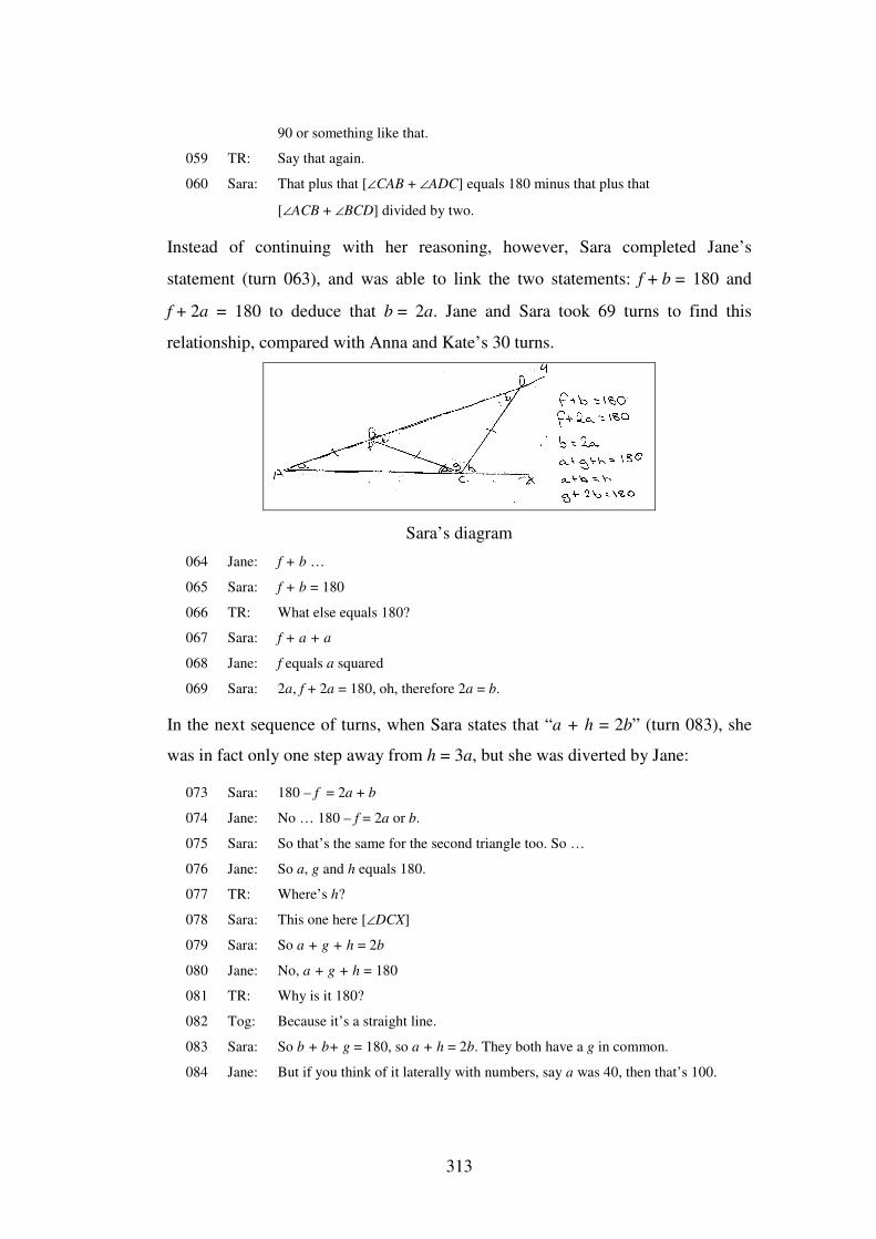
313
90 or something like that.
059 TR: Say that again.
060 Sara: That plus that [∠CAB + ∠ADC] equals 180 minus that plus that
[∠ACB + ∠BCD] divided by two.
Instead of continuing with her reasoning, however, Sara completed Jane’s
statement (turn 063), and was able to link the two statements: f + b = 180 and
f + 2a = 180 to deduce that b = 2a. Jane and Sara took 69 turns to find this
relationship, compared with Anna and Kate’s 30 turns.
Sara’s diagram
064 Jane: f + b …
065 Sara: f + b = 180
066 TR: What else equals 180?
067 Sara: f + a + a
068 Jane: f equals a squared
069 Sara: 2a, f + 2a = 180, oh, therefore 2a = b.
In the next sequence of turns, when Sara states that “a + h = 2b” (turn 083), she
was in fact only one step away from h = 3a, but she was diverted by Jane:
073 Sara: 180 – f = 2a + b
074 Jane: No … 180 – f = 2a or b.
075 Sara: So that’s the same for the second triangle too. So …
076 Jane: So a, g and h equals 180.
077 TR: Where’s h?
078 Sara: This one here [∠DCX]
079 Sara: So a + g + h = 2b
080 Jane: No, a + g + h = 180
081 TR: Why is it 180?
082 Tog: Because it’s a straight line.
083 Sara: So b + b+ g = 180, so a + h = 2b. They both have a g in common.
084 Jane: But if you think of it laterally with numbers, say a was 40, then that’s 100.
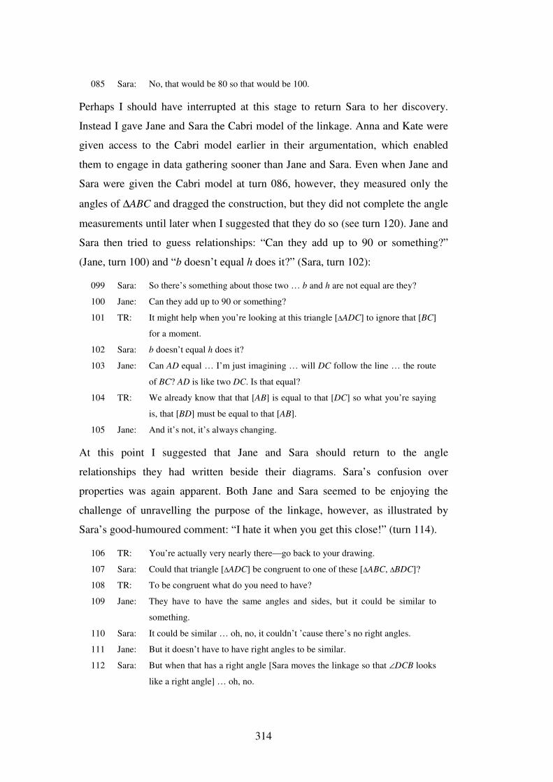
314
085 Sara: No, that would be 80 so that would be 100.
Perhaps I should have interrupted at this stage to return Sara to her discovery.
Instead I gave Jane and Sara the Cabri model of the linkage. Anna and Kate were
given access to the Cabri model earlier in their argumentation, which enabled
them to engage in data gathering sooner than Jane and Sara. Even when Jane and
Sara were given the Cabri model at turn 086, however, they measured only the
angles of ∆ABC and dragged the construction, but they did not complete the angle
measurements until later when I suggested that they do so (see turn 120). Jane and
Sara then tried to guess relationships: “Can they add up to 90 or something?”
(Jane, turn 100) and “b doesn’t equal h does it?” (Sara, turn 102):
099 Sara: So there’s something about those two … b and h are not equal are they?
100 Jane: Can they add up to 90 or something?
101 TR: It might help when you’re looking at this triangle [∆ADC] to ignore that [BC]
for a moment.
102 Sara: b doesn’t equal h does it?
103 Jane: Can AD equal … I’m just imagining … will DC follow the line … the route
of BC? AD is like two DC. Is that equal?
104 TR: We already know that that [AB] is equal to that [DC] so what you’re saying
is, that [BD] must be equal to that [AB].
105 Jane: And it’s not, it’s always changing.
At this point I suggested that Jane and Sara should return to the angle
relationships they had written beside their diagrams. Sara’s confusion over
properties was again apparent. Both Jane and Sara seemed to be enjoying the
challenge of unravelling the purpose of the linkage, however, as illustrated by
Sara’s good-humoured comment: “I hate it when you get this close!” (turn 114).
106 TR: You’re actually very nearly there—go back to your drawing.
107 Sara: Could that triangle [∆ADC] be congruent to one of these [∆ABC, ∆BDC]?
108 TR: To be congruent what do you need to have?
109 Jane: They have to have the same angles and sides, but it could be similar to
something.
110 Sara: It could be similar … oh, no, it couldn’t ’cause there’s no right angles.
111 Jane: But it doesn’t have to have right angles to be similar.
112 Sara: But when that has a right angle [Sara moves the linkage so that ∠DCB looks
like a right angle] … oh, no.
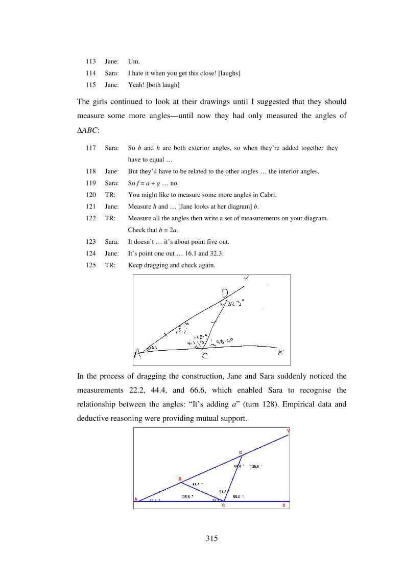
315
113 Jane: Um.
114 Sara: I hate it when you get this close! [laughs]
115 Jane: Yeah! [both laugh]
The girls continued to look at their drawings until I suggested that they should
measure some more angles—until now they had only measured the angles of
∆ABC:
117 Sara: So b and h are both exterior angles, so when they’re added together they
have to equal …
118 Jane: But they’d have to be related to the other angles … the interior angles.
119 Sara: So f = a + g … no.
120 TR: You might like to measure some more angles in Cabri.
121 Jane: Measure h and … [Jane looks at her diagram] b.
122 TR: Measure all the angles then write a set of measurements on your diagram. Check that b = 2a.
123 Sara: It doesn’t … it’s about point five out.
124 Jane: It’s point one out … 16.1 and 32.3.
125 TR: Keep dragging and check again.
In the process of dragging the construction, Jane and Sara suddenly noticed the
measurements 22.2, 44.4, and 66.6, which enabled Sara to recognise the
relationship between the angles: “It’s adding a” (turn 128). Empirical data and
deductive reasoning were providing mutual support.
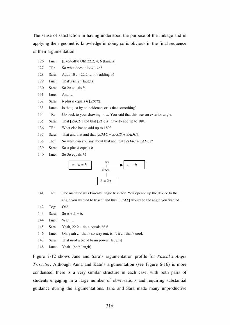
316
The sense of satisfaction in having understood the purpose of the linkage and in
applying their geometric knowledge in doing so is obvious in the final sequence
of their argumentation:
126 Jane: [Excitedly] Oh! 22.2, 4, 6 [laughs]
127 TR: So what does it look like?
128 Sara: Adds 10 … 22.2 … it’s adding a!
129 Jane: That’s silly! [laughs]
130 Sara: So 2a equals b.
131 Jane: And …
132 Sara: b plus a equals h [∠DCX].
133 Jane: Is that just by coincidence, or is that something?
134 TR: Go back to your drawing now. You said that this was an exterior angle.
135 Sara: That [∠ACD] and that [∠DCX] have to add up to 180.
136 TR: What else has to add up to 180?
137 Sara: That and that and that [∠DAC + ∠ACD + ∠ADC].
138 TR: So what can you say about that and that [∠DAC + ∠ADC]?
139 Sara: So a plus b equals h.
140 Jane: So 3a equals h!
141 TR: The machine was Pascal’s angle trisector. You opened up the device to the
angle you wanted to trisect and this [∠YAX] would be the angle you wanted.
142 Tog: Oh!
143 Sara: So a + b = h.
144 Jane: Wait …
145 Sara Yeah, 22.2 + 44.4 equals 66.6.
146 Jane: Oh, yeah … that’s so way out, isn’t it … that’s cool.
147 Sara: That used a bit of brain power [laughs]
148 Jane: Yeah! [both laugh]
Figure 7-12 shows Jane and Sara’s argumentation profile for Pascal’s Angle
Trisector. Although Anna and Kate’s argumentation (see Figure 6-16) is more
condensed, there is a very similar structure in each case, with both pairs of
students engaging in a large number of observations and requiring substantial
guidance during the argumentations. Jane and Sara made many unproductive
a + b = h 3a = h
b = 2a
so
since
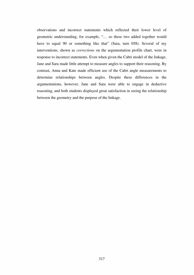
317
observations and incorrect statements which reflected their lower level of
geometric understanding, for example, “… so these two added together would
have to equal 90 or something like that” (Sara, turn 058). Several of my
interventions, shown as corrections on the argumentation profile chart, were in
response to incorrect statements. Even when given the Cabri model of the linkage,
Jane and Sara made little attempt to measure angles to support their reasoning. By
contrast, Anna and Kate made efficient use of the Cabri angle measurements to
determine relationships between angles. Despite these differences in the
argumentations, however, Jane and Sara were able to engage in deductive
reasoning, and both students displayed great satisfaction in seeing the relationship
between the geometry and the purpose of the linkage.
318
Jane and Sara: Pascal's Angle Trisector
0 10 20 30 40 50 60 70 80 90 100 110 120 130 140 150Turn
Sara Jane Teacher-Researcher Linkage Cabri model
Paper/pencil Key conjecture Warrant prompt Correction
Guidance
Observations
Data gathering
Deductive reasoning
Conjecturing
Task orientation
Figure 7-12. Jane and Sara: Argumentation profile for Pascal’s Angle Trisector.
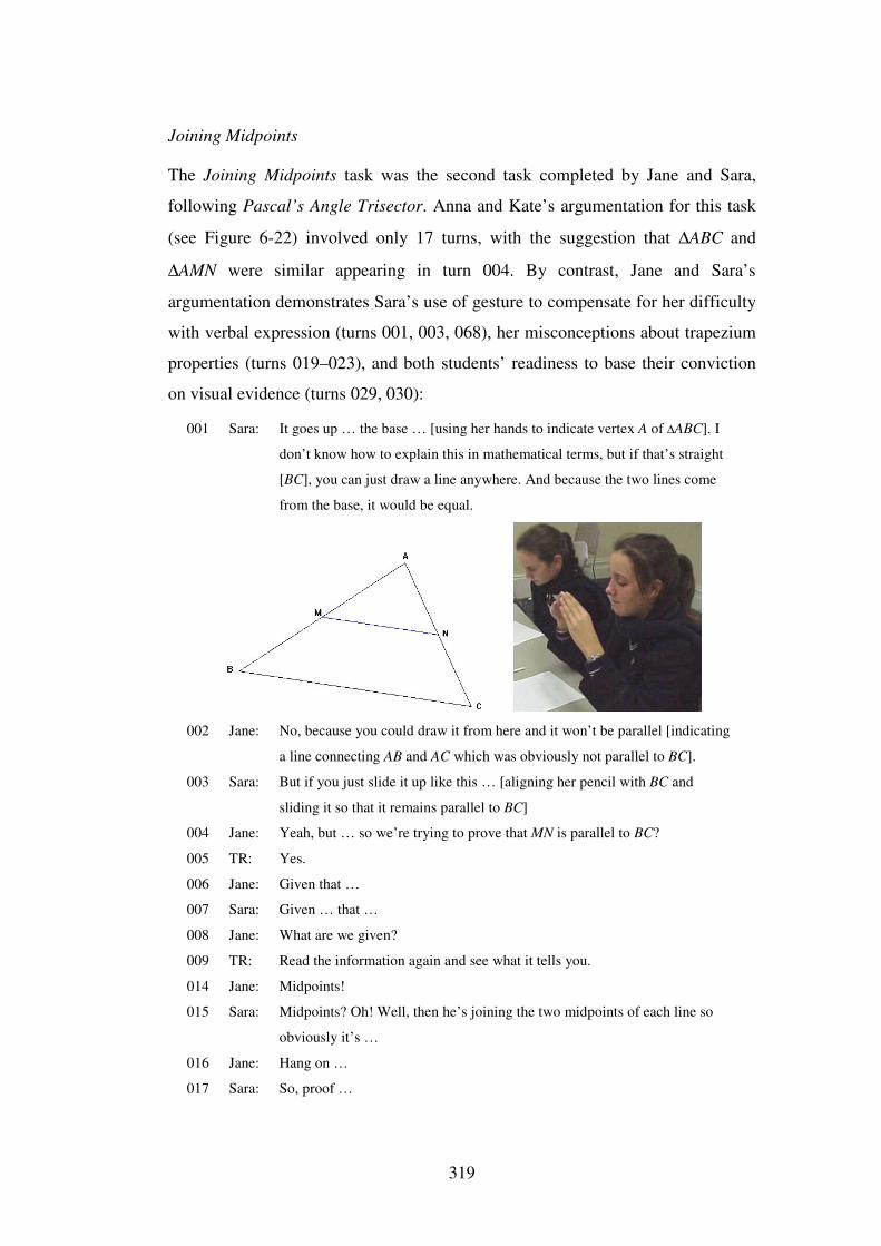
319
Joining Midpoints
The Joining Midpoints task was the second task completed by Jane and Sara,
following Pascal’s Angle Trisector. Anna and Kate’s argumentation for this task
(see Figure 6-22) involved only 17 turns, with the suggestion that ∆ABC and
∆AMN were similar appearing in turn 004. By contrast, Jane and Sara’s
argumentation demonstrates Sara’s use of gesture to compensate for her difficulty
with verbal expression (turns 001, 003, 068), her misconceptions about trapezium
properties (turns 019–023), and both students’ readiness to base their conviction
on visual evidence (turns 029, 030):
001 Sara: It goes up … the base … [using her hands to indicate vertex A of ∆ABC]. I
don’t know how to explain this in mathematical terms, but if that’s straight
[BC], you can just draw a line anywhere. And because the two lines come
from the base, it would be equal.
002 Jane: No, because you could draw it from here and it won’t be parallel [indicating
a line connecting AB and AC which was obviously not parallel to BC].
003 Sara: But if you just slide it up like this … [aligning her pencil with BC and
sliding it so that it remains parallel to BC]
004 Jane: Yeah, but … so we’re trying to prove that MN is parallel to BC?
005 TR: Yes.
006 Jane: Given that …
007 Sara: Given … that …
008 Jane: What are we given?
009 TR: Read the information again and see what it tells you.
014 Jane: Midpoints!
015 Sara: Midpoints? Oh! Well, then he’s joining the two midpoints of each line so
obviously it’s …
016 Jane: Hang on …
017 Sara: So, proof …
320
018 Jane: This is a trapezium, so just forget about …
019 Sara: A trapezium has to have … parallel lines.
020 Jane: Parallel lines …
021 Sara: Yeah, parallel lines, but we don’t know they’re parallel.
022 Jane: But we can’t say that … we don’t know it’s a trapezium.
023 Sara: It doesn’t have a right angle.
024 Jane: It doesn’t need to have a right angle.
025 Sara: Doesn’t it?
026 Jane: Not for a trapezium.
027 Sara: Oh, my Dad just told me at the weekend that it does. Oh! I was so confused
when I was trying to work something out and my Dad says it does.
028 Jane: No …
029 TR: If you could prove the lines were parallel would it be a trapezium?
030 Tog: Yes.
031 TR: So, in other words, when you are trying to prove something you can’t use
what you’re trying to prove as one of your bits of information, can you?
032 Jane: [laughing] No.
033 Sara: So the lines both start at the same spot at the bottom and finish at the top and
they’re both at the middle point of each thing … It just has to be parallel.
034 Jane: It is parallel. It just is. It doesn’t need to be proved [laughs]. It just is.
Sara’s suggestion that ∆ABC and ∆AMN were similar, together with my
prompting, eventually led the two students to prove that the two triangles were
similar.
035 Sara: Um … oh, is it because … um … C … triangle ABC is congruent to NMA?
036 TR: What do you think about that, Jane?
037 Jane: Triangle ABC … they’re not congruent.
038 Sara: Yeah, it is … I mean, similar triangles.
039 TR: They might be similar. Could you prove that they are?
040 Sara: Yeah, because angle … no, side side side.
041 Jane: We can’t prove that because we …
042 Sara: Oh, angle side angle because they have both the same angles.
043 Jane: That’s cool!
044 TR: What do you know about the sides of the little triangle?
045 Sara: They’re the same.
046 Jane: No, they’re not the same.
047 TR: Do you know anything else then?
048 Jane: No … oh, yes, AM is equal to that [MB] and that [AN] is equal to that [NC]
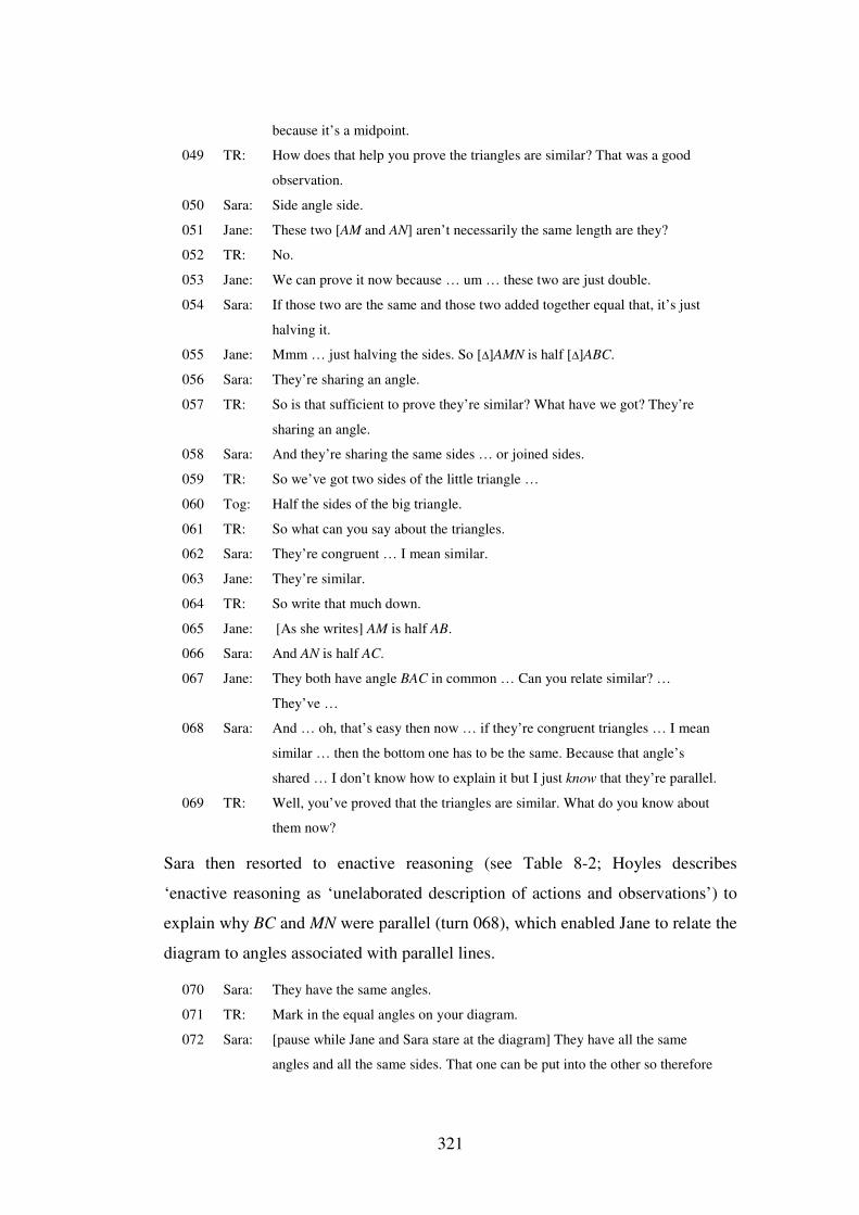
321
because it’s a midpoint.
049 TR: How does that help you prove the triangles are similar? That was a good
observation.
050 Sara: Side angle side.
051 Jane: These two [AM and AN] aren’t necessarily the same length are they?
052 TR: No.
053 Jane: We can prove it now because … um … these two are just double.
054 Sara: If those two are the same and those two added together equal that, it’s just
halving it.
055 Jane: Mmm … just halving the sides. So [∆]AMN is half [∆]ABC.
056 Sara: They’re sharing an angle.
057 TR: So is that sufficient to prove they’re similar? What have we got? They’re
sharing an angle.
058 Sara: And they’re sharing the same sides … or joined sides.
059 TR: So we’ve got two sides of the little triangle …
060 Tog: Half the sides of the big triangle.
061 TR: So what can you say about the triangles.
062 Sara: They’re congruent … I mean similar.
063 Jane: They’re similar.
064 TR: So write that much down.
065 Jane: [As she writes] AM is half AB.
066 Sara: And AN is half AC.
067 Jane: They both have angle BAC in common … Can you relate similar? …
They’ve …
068 Sara: And … oh, that’s easy then now … if they’re congruent triangles … I mean
similar … then the bottom one has to be the same. Because that angle’s
shared … I don’t know how to explain it but I just know that they’re parallel.
069 TR: Well, you’ve proved that the triangles are similar. What do you know about
them now?
Sara then resorted to enactive reasoning (see Table 8-2; Hoyles describes
‘enactive reasoning as ‘unelaborated description of actions and observations’) to
explain why BC and MN were parallel (turn 068), which enabled Jane to relate the
diagram to angles associated with parallel lines.
070 Sara: They have the same angles.
071 TR: Mark in the equal angles on your diagram.
072 Sara: [pause while Jane and Sara stare at the diagram] They have all the same
angles and all the same sides. That one can be put into the other so therefore
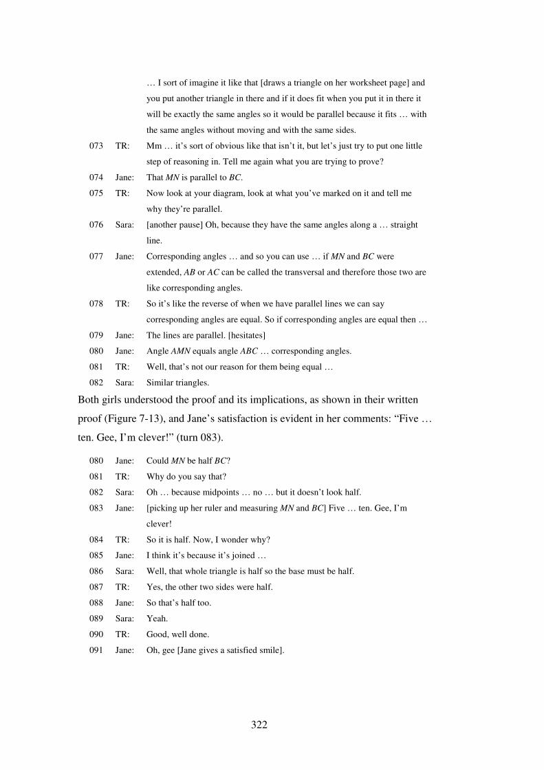
322
… I sort of imagine it like that [draws a triangle on her worksheet page] and
you put another triangle in there and if it does fit when you put it in there it
will be exactly the same angles so it would be parallel because it fits … with
the same angles without moving and with the same sides.
073 TR: Mm … it’s sort of obvious like that isn’t it, but let’s just try to put one little
step of reasoning in. Tell me again what you are trying to prove?
074 Jane: That MN is parallel to BC.
075 TR: Now look at your diagram, look at what you’ve marked on it and tell me
why they’re parallel.
076 Sara: [another pause] Oh, because they have the same angles along a … straight
line.
077 Jane: Corresponding angles … and so you can use … if MN and BC were
extended, AB or AC can be called the transversal and therefore those two are
like corresponding angles.
078 TR: So it’s like the reverse of when we have parallel lines we can say
corresponding angles are equal. So if corresponding angles are equal then …
079 Jane: The lines are parallel. [hesitates]
080 Jane: Angle AMN equals angle ABC … corresponding angles.
081 TR: Well, that’s not our reason for them being equal …
082 Sara: Similar triangles.
Both girls understood the proof and its implications, as shown in their written
proof (Figure 7-13), and Jane’s satisfaction is evident in her comments: “Five …
ten. Gee, I’m clever!” (turn 083).
080 Jane: Could MN be half BC?
081 TR: Why do you say that?
082 Sara: Oh … because midpoints … no … but it doesn’t look half.
083 Jane: [picking up her ruler and measuring MN and BC] Five … ten. Gee, I’m
clever!
084 TR: So it is half. Now, I wonder why?
085 Jane: I think it’s because it’s joined …
086 Sara: Well, that whole triangle is half so the base must be half.
087 TR: Yes, the other two sides were half.
088 Jane: So that’s half too.
089 Sara: Yeah.
090 TR: Good, well done.
091 Jane: Oh, gee [Jane gives a satisfied smile].
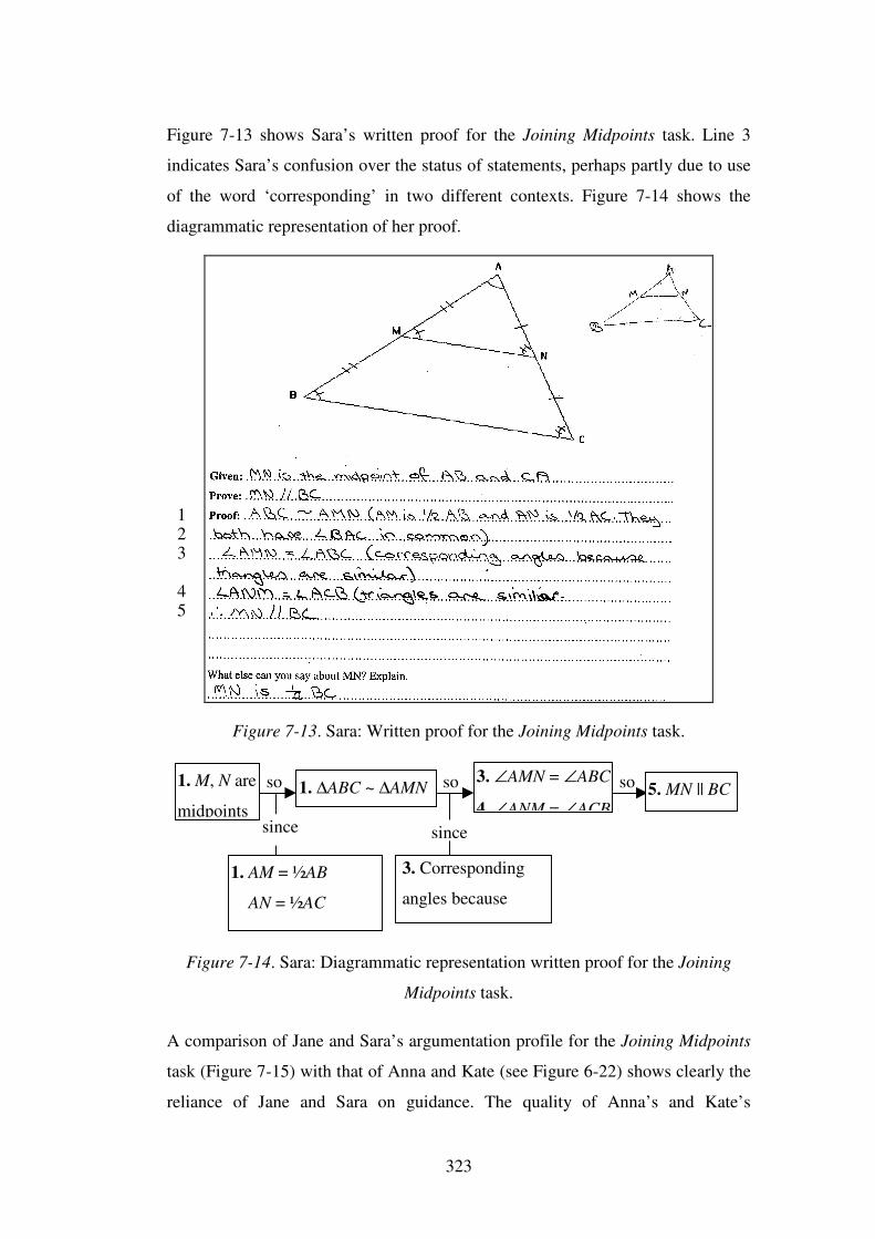
323
Figure 7-13 shows Sara’s written proof for the Joining Midpoints task. Line 3
indicates Sara’s confusion over the status of statements, perhaps partly due to use
of the word ‘corresponding’ in two different contexts. Figure 7-14 shows the
diagrammatic representation of her proof.
Figure 7-13. Sara: Written proof for the Joining Midpoints task.
Figure 7-14. Sara: Diagrammatic representation written proof for the Joining
Midpoints task.
A comparison of Jane and Sara’s argumentation profile for the Joining Midpoints
task (Figure 7-15) with that of Anna and Kate (see Figure 6-22) shows clearly the
reliance of Jane and Sara on guidance. The quality of Anna’s and Kate’s
1. ∆ABC ~ ∆AMN 3. ∠AMN = ∠ABC
4. ∠ANM = ∠ACB
1. AM = ½AB
AN = ½AC
2. ∠BAC is common
3. Corresponding
angles because
triangles are similar.
5. MN || BC 1. M, N are
midpoints
so so so
since since
1 2 3 4 5
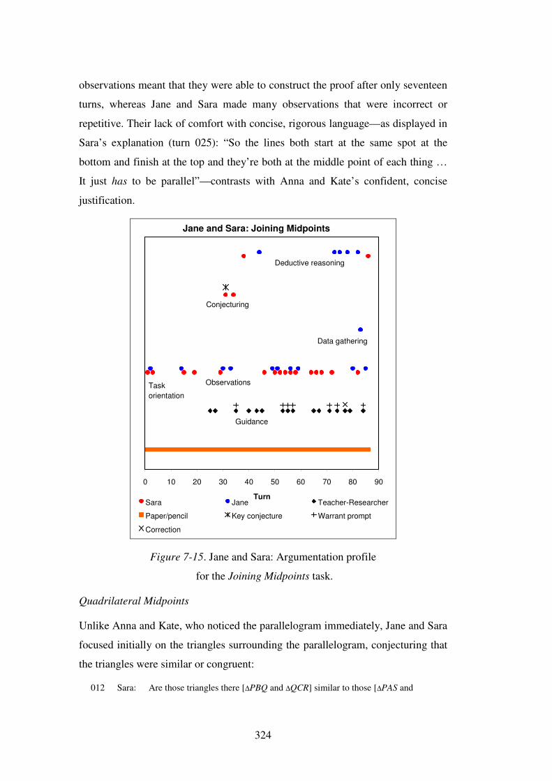
324
observations meant that they were able to construct the proof after only seventeen
turns, whereas Jane and Sara made many observations that were incorrect or
repetitive. Their lack of comfort with concise, rigorous language—as displayed in
Sara’s explanation (turn 025): “So the lines both start at the same spot at the
bottom and finish at the top and they’re both at the middle point of each thing …
It just has to be parallel”—contrasts with Anna and Kate’s confident, concise
justification.
Jane and Sara: Joining Midpoints
0 10 20 30 40 50 60 70 80 90
TurnSara Jane Teacher-Researcher
Paper/pencil Key conjecture Warrant prompt
Correction
Guidance
Observations
Conjecturing
Deductive reasoning
Data gathering
Task orientation
Figure 7-15. Jane and Sara: Argumentation profile
for the Joining Midpoints task.
Quadrilateral Midpoints
Unlike Anna and Kate, who noticed the parallelogram immediately, Jane and Sara
focused initially on the triangles surrounding the parallelogram, conjecturing that
the triangles were similar or congruent:
012 Sara: Are those triangles there [∆PBQ and ∆QCR] similar to those [∆PAS and
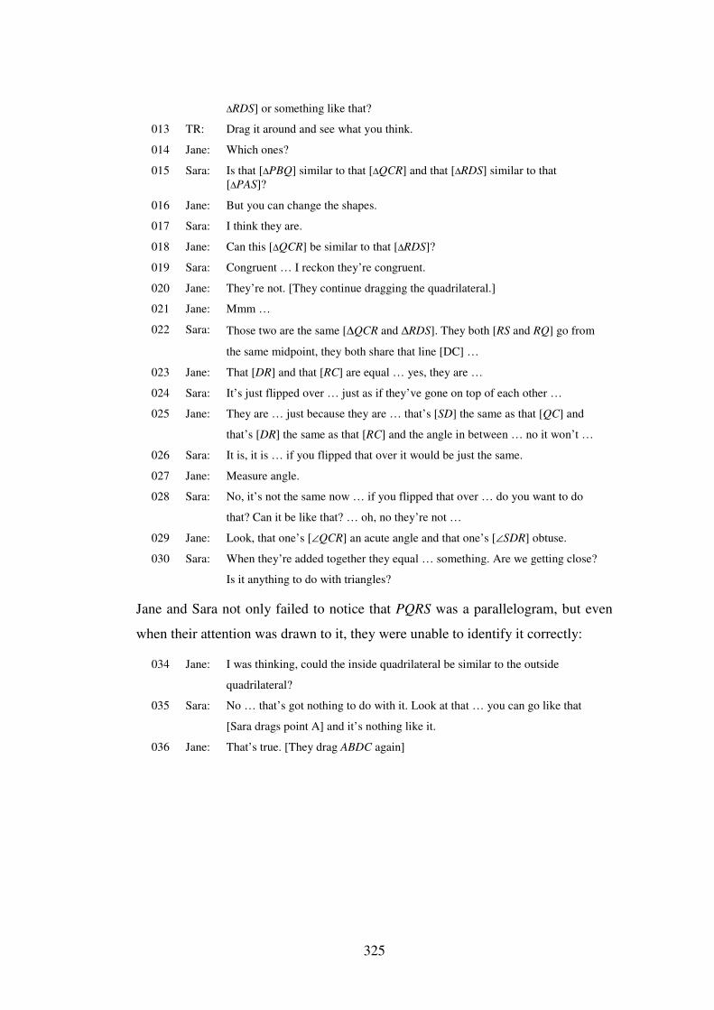
325
∆RDS] or something like that?
013 TR: Drag it around and see what you think.
014 Jane: Which ones?
015 Sara: Is that [∆PBQ] similar to that [∆QCR] and that [∆RDS] similar to that [∆PAS]?
016 Jane: But you can change the shapes.
017 Sara: I think they are.
018 Jane: Can this [∆QCR] be similar to that [∆RDS]?
019 Sara: Congruent … I reckon they’re congruent.
020 Jane: They’re not. [They continue dragging the quadrilateral.]
021 Jane: Mmm …
022 Sara: Those two are the same [∆QCR and ∆RDS]. They both [RS and RQ] go from
the same midpoint, they both share that line [DC] …
023 Jane: That [DR] and that [RC] are equal … yes, they are …
024 Sara: It’s just flipped over … just as if they’ve gone on top of each other …
025 Jane: They are … just because they are … that’s [SD] the same as that [QC] and
that’s [DR] the same as that [RC] and the angle in between … no it won’t …
026 Sara: It is, it is … if you flipped that over it would be just the same.
027 Jane: Measure angle.
028 Sara: No, it’s not the same now … if you flipped that over … do you want to do
that? Can it be like that? … oh, no they’re not …
029 Jane: Look, that one’s [∠QCR] an acute angle and that one’s [∠SDR] obtuse.
030 Sara: When they’re added together they equal … something. Are we getting close?
Is it anything to do with triangles?
Jane and Sara not only failed to notice that PQRS was a parallelogram, but even
when their attention was drawn to it, they were unable to identify it correctly:
034 Jane: I was thinking, could the inside quadrilateral be similar to the outside
quadrilateral?
035 Sara: No … that’s got nothing to do with it. Look at that … you can go like that
[Sara drags point A] and it’s nothing like it.
036 Jane: That’s true. [They drag ABDC again]
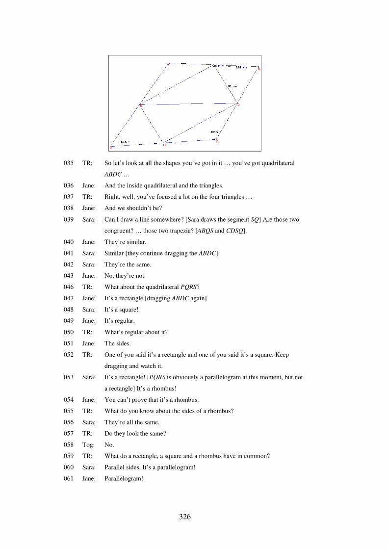
326
035 TR: So let’s look at all the shapes you’ve got in it … you’ve got quadrilateral
ABDC …
036 Jane: And the inside quadrilateral and the triangles.
037 TR: Right, well, you’ve focused a lot on the four triangles …
038 Jane: And we shouldn’t be?
039 Sara: Can I draw a line somewhere? [Sara draws the segment SQ] Are those two
congruent? … those two trapezia? [ABQS and CDSQ].
040 Jane: They’re similar.
041 Sara: Similar [they continue dragging the ABDC].
042 Sara: They’re the same.
043 Jane: No, they’re not.
046 TR: What about the quadrilateral PQRS?
047 Jane: It’s a rectangle [dragging ABDC again].
048 Sara: It’s a square!
049 Jane: It’s regular.
050 TR: What’s regular about it?
051 Jane: The sides.
052 TR: One of you said it’s a rectangle and one of you said it’s a square. Keep
dragging and watch it.
053 Sara: It’s a rectangle! [PQRS is obviously a parallelogram at this moment, but not
a rectangle] It’s a rhombus!
054 Jane: You can’t prove that it’s a rhombus.
055 TR: What do you know about the sides of a rhombus?
056 Sara: They’re all the same.
057 TR: Do they look the same?
058 Tog: No.
059 TR: What do a rectangle, a square and a rhombus have in common?
060 Sara: Parallel sides. It’s a parallelogram!
061 Jane: Parallelogram!
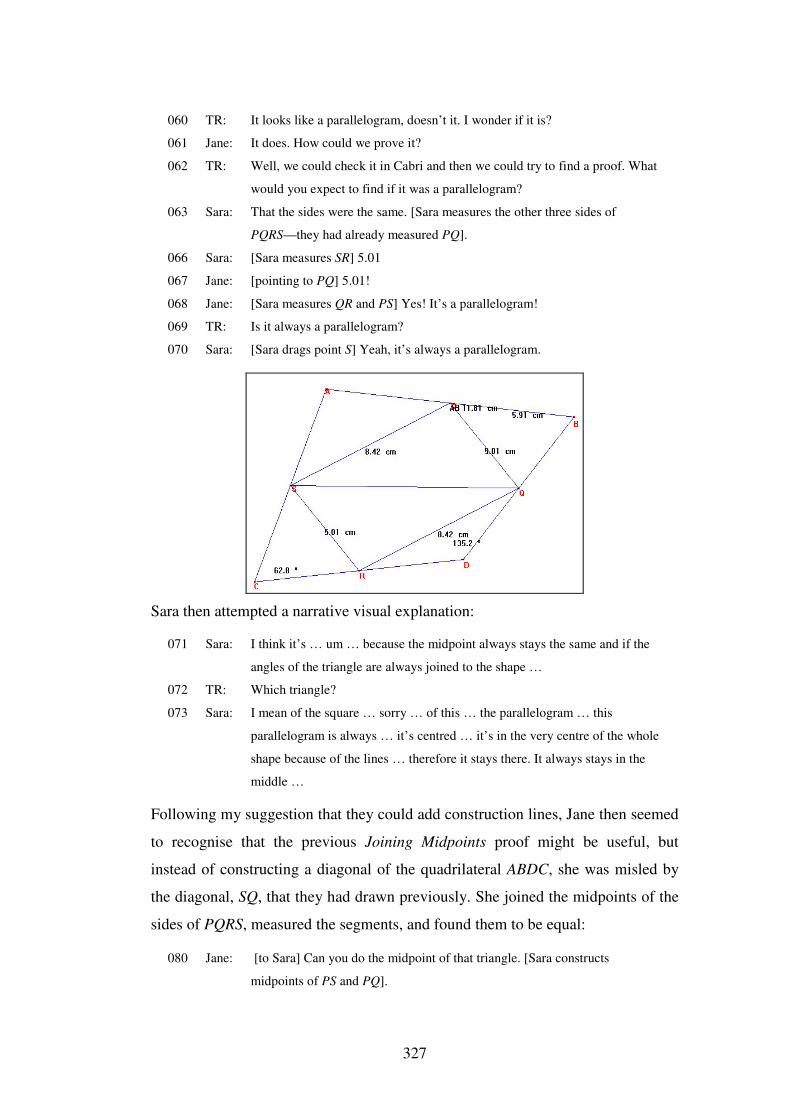
327
060 TR: It looks like a parallelogram, doesn’t it. I wonder if it is?
061 Jane: It does. How could we prove it?
062 TR: Well, we could check it in Cabri and then we could try to find a proof. What
would you expect to find if it was a parallelogram?
063 Sara: That the sides were the same. [Sara measures the other three sides of
PQRS—they had already measured PQ].
066 Sara: [Sara measures SR] 5.01
067 Jane: [pointing to PQ] 5.01!
068 Jane: [Sara measures QR and PS] Yes! It’s a parallelogram!
069 TR: Is it always a parallelogram?
070 Sara: [Sara drags point S] Yeah, it’s always a parallelogram.
Sara then attempted a narrative visual explanation:
071 Sara: I think it’s … um … because the midpoint always stays the same and if the
angles of the triangle are always joined to the shape …
072 TR: Which triangle?
073 Sara: I mean of the square … sorry … of this … the parallelogram … this
parallelogram is always … it’s centred … it’s in the very centre of the whole
shape because of the lines … therefore it stays there. It always stays in the
middle …
Following my suggestion that they could add construction lines, Jane then seemed
to recognise that the previous Joining Midpoints proof might be useful, but
instead of constructing a diagonal of the quadrilateral ABDC, she was misled by
the diagonal, SQ, that they had drawn previously. She joined the midpoints of the
sides of PQRS, measured the segments, and found them to be equal:
080 Jane: [to Sara] Can you do the midpoint of that triangle. [Sara constructs
midpoints of PS and PQ].
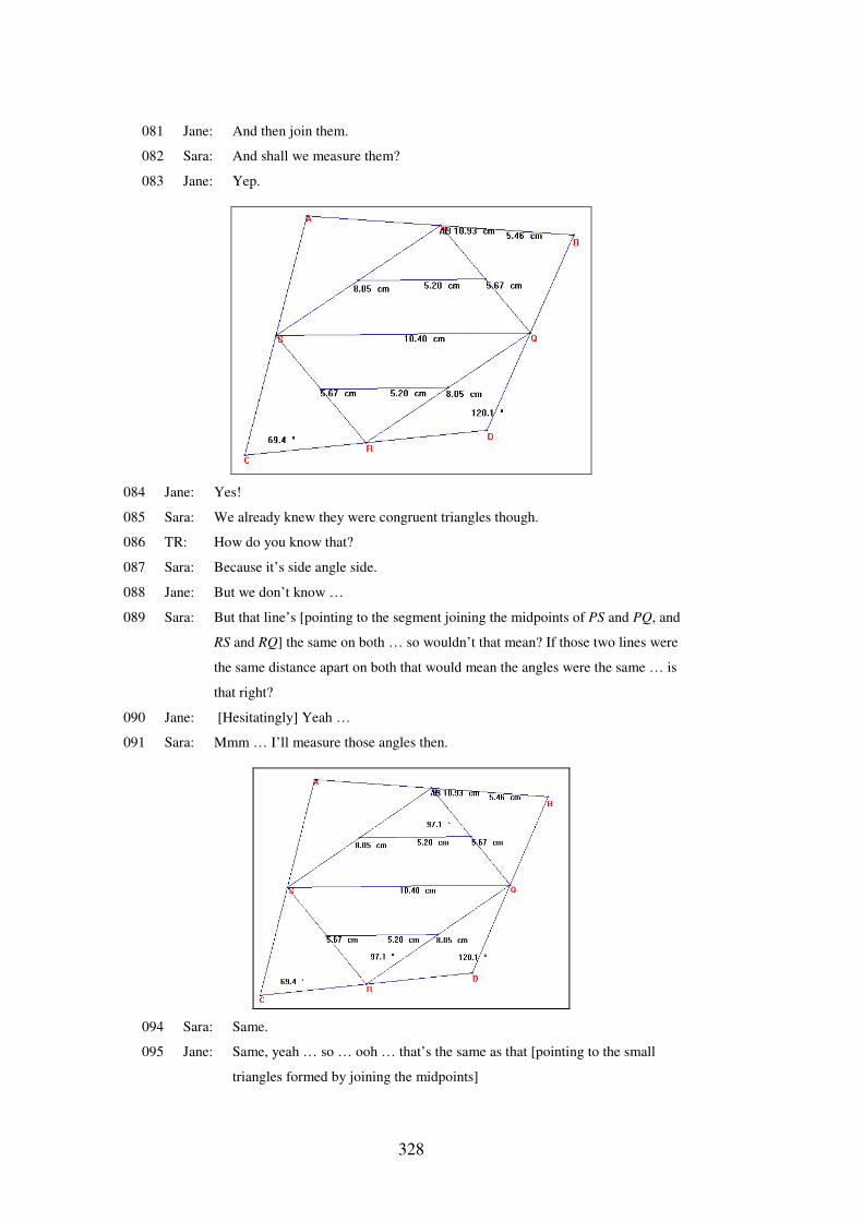
328
081 Jane: And then join them.
082 Sara: And shall we measure them?
083 Jane: Yep.
084 Jane: Yes!
085 Sara: We already knew they were congruent triangles though.
086 TR: How do you know that?
087 Sara: Because it’s side angle side.
088 Jane: But we don’t know …
089 Sara: But that line’s [pointing to the segment joining the midpoints of PS and PQ, and
RS and RQ] the same on both … so wouldn’t that mean? If those two lines were
the same distance apart on both that would mean the angles were the same … is
that right?
090 Jane: [Hesitatingly] Yeah …
091 Sara: Mmm … I’ll measure those angles then.
094 Sara: Same.
095 Jane: Same, yeah … so … ooh … that’s the same as that [pointing to the small
triangles formed by joining the midpoints]
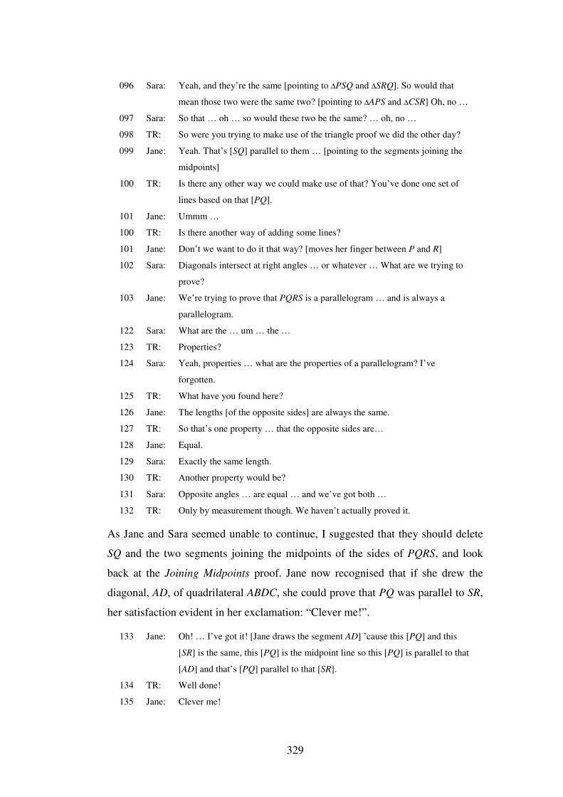
329
096 Sara: Yeah, and they’re the same [pointing to ∆PSQ and ∆SRQ]. So would that
mean those two were the same two? [pointing to ∆APS and ∆CSR] Oh, no …
097 Sara: So that … oh … so would these two be the same? … oh, no …
098 TR: So were you trying to make use of the triangle proof we did the other day?
099 Jane: Yeah. That’s [SQ] parallel to them … [pointing to the segments joining the
midpoints]
100 TR: Is there any other way we could make use of that? You’ve done one set of
lines based on that [PQ].
101 Jane: Ummm …
100 TR: Is there another way of adding some lines?
101 Jane: Don’t we want to do it that way? [moves her finger between P and R]
102 Sara: Diagonals intersect at right angles … or whatever … What are we trying to
prove?
103 Jane: We’re trying to prove that PQRS is a parallelogram … and is always a
parallelogram.
122 Sara: What are the … um … the …
123 TR: Properties?
124 Sara: Yeah, properties … what are the properties of a parallelogram? I’ve
forgotten.
125 TR: What have you found here?
126 Jane: The lengths [of the opposite sides] are always the same.
127 TR: So that’s one property … that the opposite sides are…
128 Jane: Equal.
129 Sara: Exactly the same length.
130 TR: Another property would be?
131 Sara: Opposite angles … are equal … and we’ve got both …
132 TR: Only by measurement though. We haven’t actually proved it.
As Jane and Sara seemed unable to continue, I suggested that they should delete
SQ and the two segments joining the midpoints of the sides of PQRS, and look
back at the Joining Midpoints proof. Jane now recognised that if she drew the
diagonal, AD, of quadrilateral ABDC, she could prove that PQ was parallel to SR,
her satisfaction evident in her exclamation: “Clever me!”.
133 Jane: Oh! … I’ve got it! [Jane draws the segment AD] ’cause this [PQ] and this
[SR] is the same, this [PQ] is the midpoint line so this [PQ] is parallel to that
[AD] and that’s [PQ] parallel to that [SR].
134 TR: Well done!
135 Jane: Clever me!
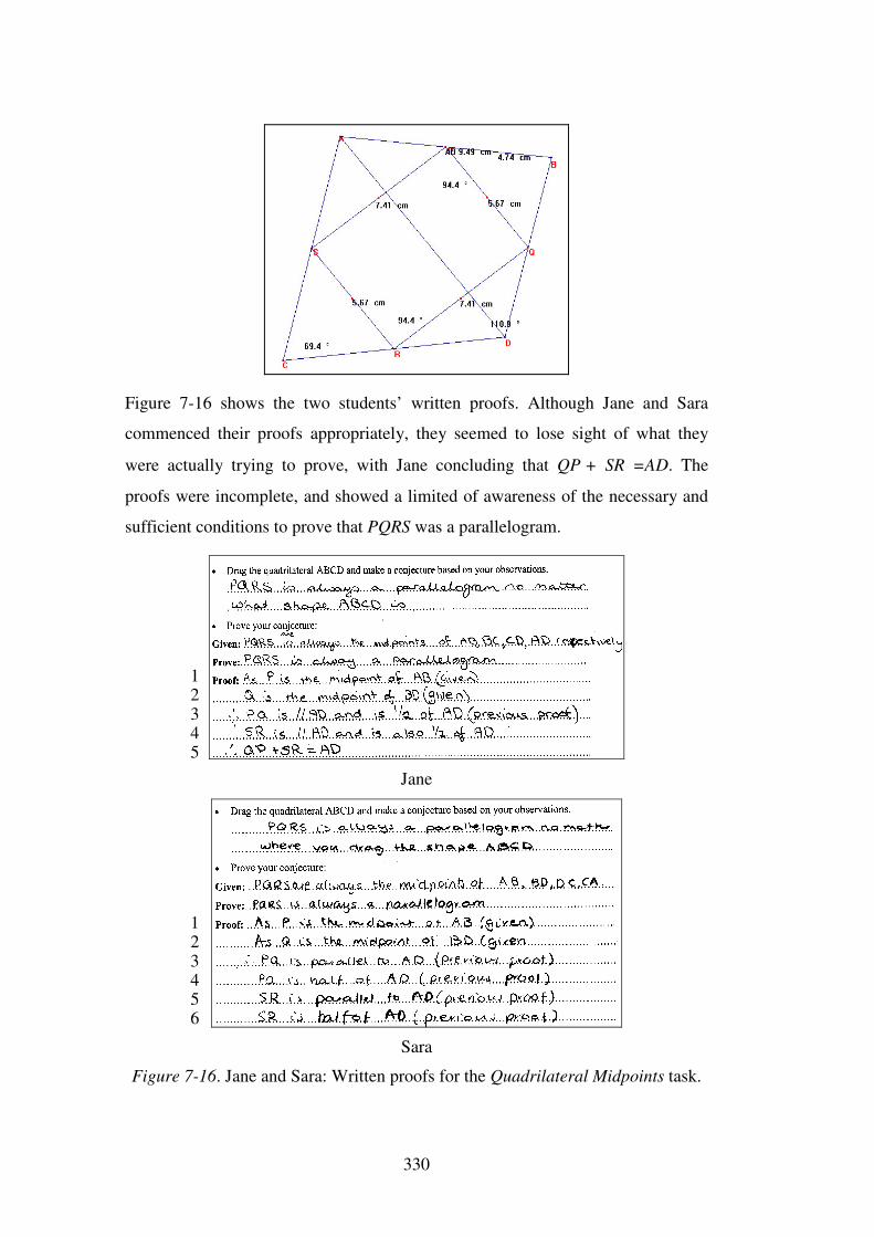
330
Figure 7-16 shows the two students’ written proofs. Although Jane and Sara
commenced their proofs appropriately, they seemed to lose sight of what they
were actually trying to prove, with Jane concluding that QP + SR =AD. The
proofs were incomplete, and showed a limited of awareness of the necessary and
sufficient conditions to prove that PQRS was a parallelogram.
Jane
Sara
Figure 7-16. Jane and Sara: Written proofs for the Quadrilateral Midpoints task.
1 2 3 4 5
1 2 3 4 5 6
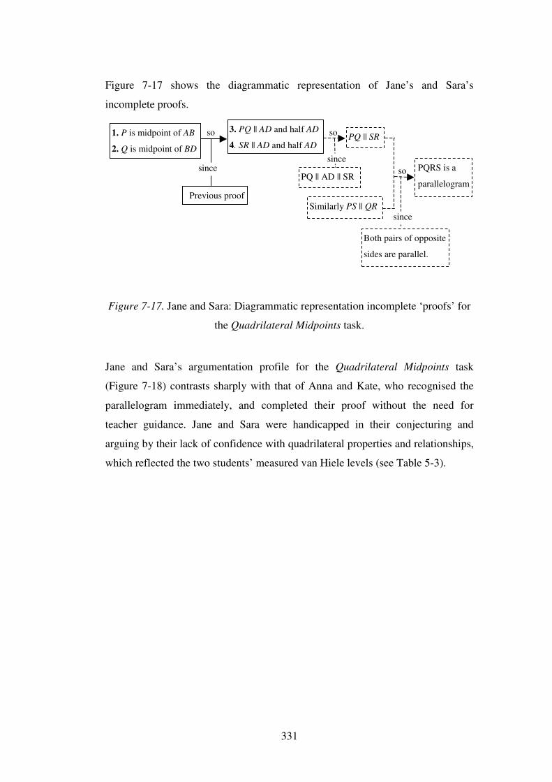
331
Figure 7-17 shows the diagrammatic representation of Jane’s and Sara’s
incomplete proofs.
Figure 7-17. Jane and Sara: Diagrammatic representation incomplete ‘proofs’ for
the Quadrilateral Midpoints task.
Jane and Sara’s argumentation profile for the Quadrilateral Midpoints task
(Figure 7-18) contrasts sharply with that of Anna and Kate, who recognised the
parallelogram immediately, and completed their proof without the need for
teacher guidance. Jane and Sara were handicapped in their conjecturing and
arguing by their lack of confidence with quadrilateral properties and relationships,
which reflected the two students’ measured van Hiele levels (see Table 5-3).
1. P is midpoint of AB
2. Q is midpoint of BD
3. PQ || AD and half AD
4. SR || AD and half AD
Previous proof
since
so PQ || SR
PQRS is a
parallelogram
Similarly PS || QR
PQ || AD || SR
Both pairs of opposite
sides are parallel.
since
since
so
so
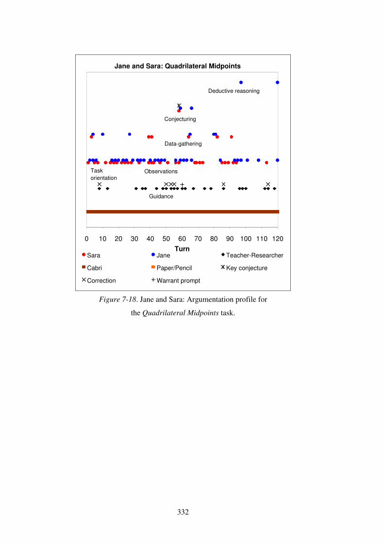
332
Jane and Sara: Quadrilateral Midpoints
0 10 20 30 40 50 60 70 80 90 100 110 120Turn
Sara Jane Teacher-Researcher
Cabri Paper/Pencil Key conjecture
Correction Warrant prompt
Deductive reasoning
Conjecturing
Data-gathering
Observations
Guidance
Task orientation
Figure 7-18. Jane and Sara: Argumentation profile for
the Quadrilateral Midpoints task.
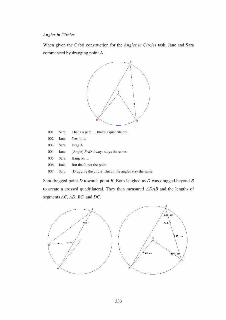
333
Angles in Circles
When given the Cabri construction for the Angles in Circles task, Jane and Sara
commenced by dragging point A.
001 Sara: That’s a para … that’s a quadrilateral.
002 Jane: Yes, it is.
003 Sara: Drag A.
004 Jane: [Angle] BAD always stays the same.
005 Sara: Hang on …
006 Jane: But that’s not the point.
007 Sara: [Dragging the circle] But all the angles stay the same.
Sara dragged point D towards point B. Both laughed as D was dragged beyond B
to create a crossed quadrilateral. They then measured ∠DAB and the lengths of
segments AC, AD, BC, and DC.
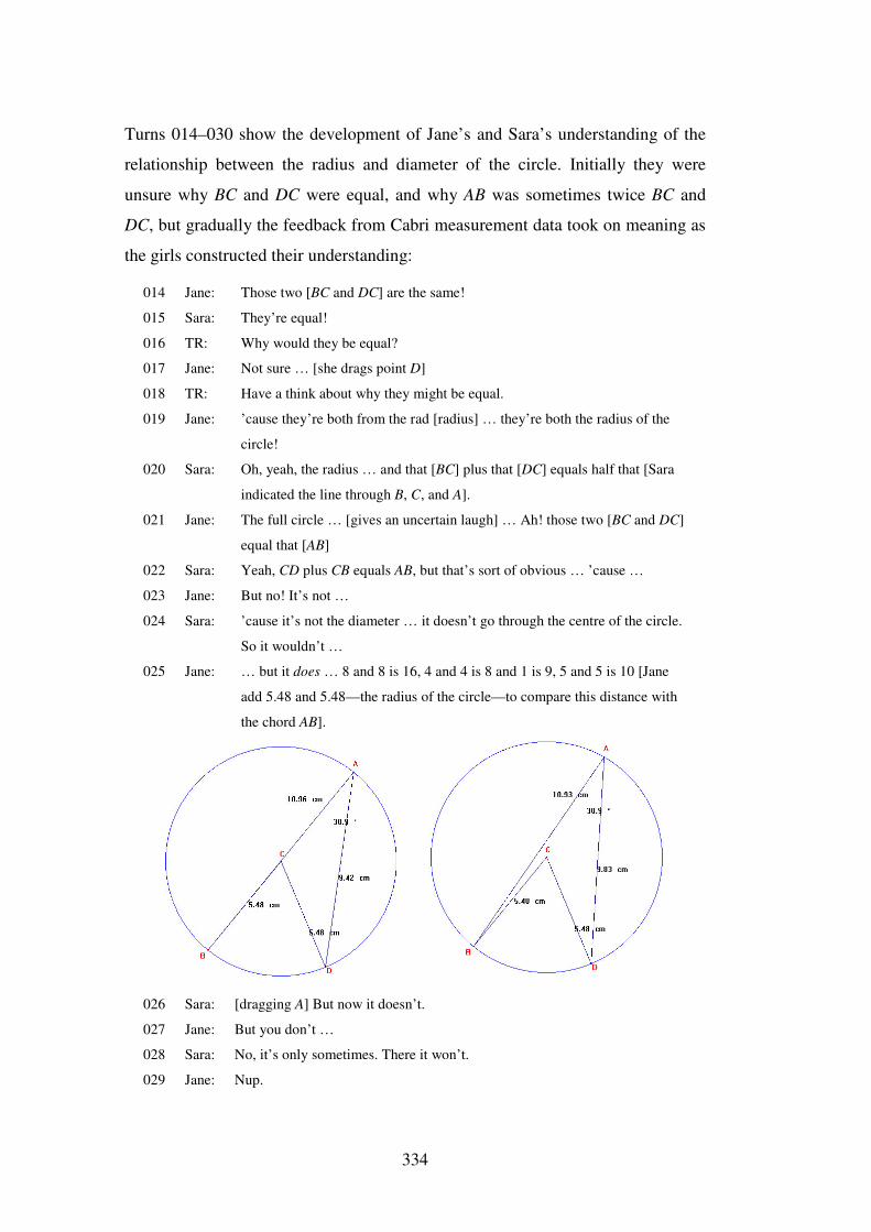
334
Turns 014–030 show the development of Jane’s and Sara’s understanding of the
relationship between the radius and diameter of the circle. Initially they were
unsure why BC and DC were equal, and why AB was sometimes twice BC and
DC, but gradually the feedback from Cabri measurement data took on meaning as
the girls constructed their understanding:
014 Jane: Those two [BC and DC] are the same!
015 Sara: They’re equal!
016 TR: Why would they be equal?
017 Jane: Not sure … [she drags point D]
018 TR: Have a think about why they might be equal.
019 Jane: ’cause they’re both from the rad [radius] … they’re both the radius of the
circle!
020 Sara: Oh, yeah, the radius … and that [BC] plus that [DC] equals half that [Sara
indicated the line through B, C, and A].
021 Jane: The full circle … [gives an uncertain laugh] … Ah! those two [BC and DC]
equal that [AB]
022 Sara: Yeah, CD plus CB equals AB, but that’s sort of obvious … ’cause …
023 Jane: But no! It’s not …
024 Sara: ’cause it’s not the diameter … it doesn’t go through the centre of the circle.
So it wouldn’t …
025 Jane: … but it does … 8 and 8 is 16, 4 and 4 is 8 and 1 is 9, 5 and 5 is 10 [Jane
add 5.48 and 5.48—the radius of the circle—to compare this distance with
the chord AB].
026 Sara: [dragging A] But now it doesn’t.
027 Jane: But you don’t …
028 Sara: No, it’s only sometimes. There it won’t.
029 Jane: Nup.
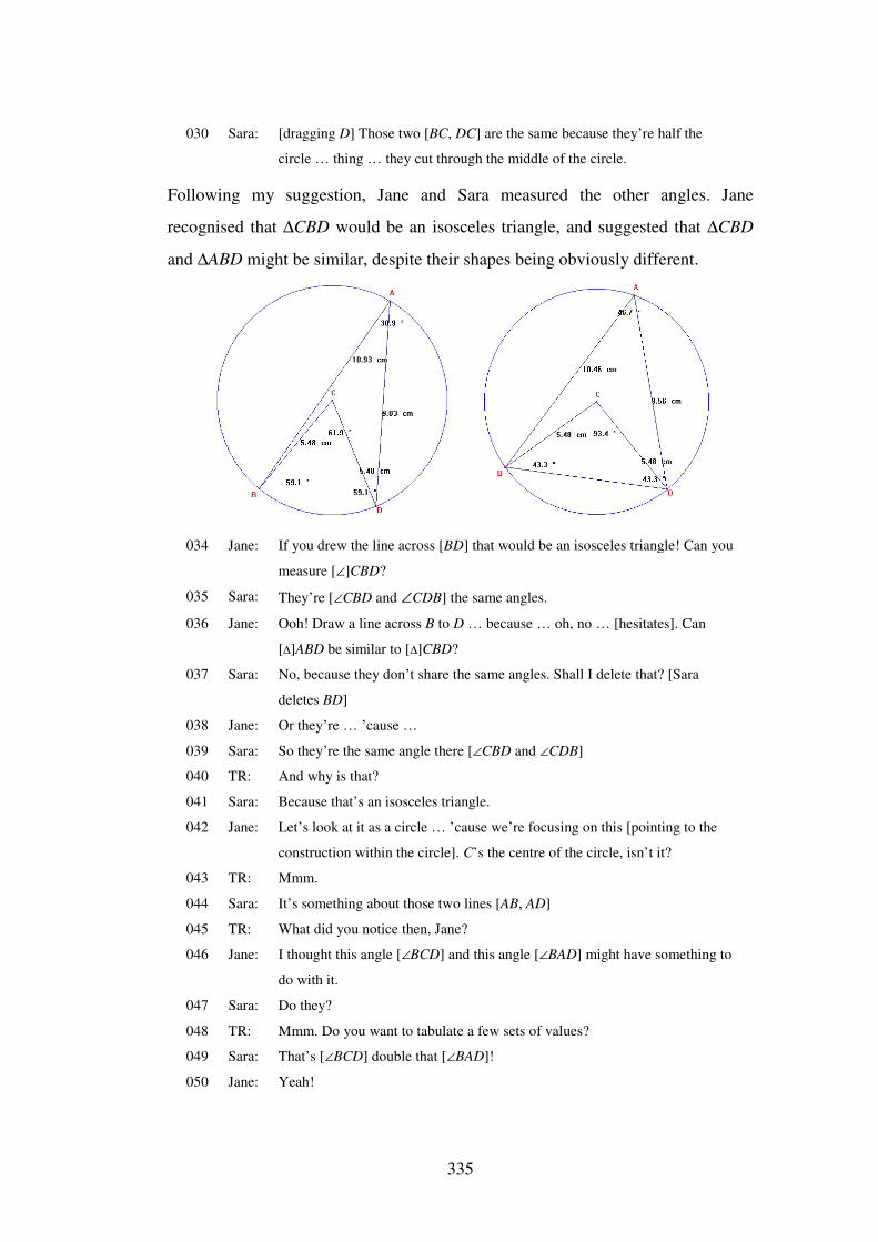
335
030 Sara: [dragging D] Those two [BC, DC] are the same because they’re half the
circle … thing … they cut through the middle of the circle.
Following my suggestion, Jane and Sara measured the other angles. Jane
recognised that ∆CBD would be an isosceles triangle, and suggested that ∆CBD
and ∆ABD might be similar, despite their shapes being obviously different.
034 Jane: If you drew the line across [BD] that would be an isosceles triangle! Can you
measure [∠]CBD?
035 Sara: They’re [∠CBD and ∠CDB] the same angles.
036 Jane: Ooh! Draw a line across B to D … because … oh, no … [hesitates]. Can
[∆]ABD be similar to [∆]CBD?
037 Sara: No, because they don’t share the same angles. Shall I delete that? [Sara
deletes BD]
038 Jane: Or they’re … ’cause …
039 Sara: So they’re the same angle there [∠CBD and ∠CDB]
040 TR: And why is that?
041 Sara: Because that’s an isosceles triangle.
042 Jane: Let’s look at it as a circle … ’cause we’re focusing on this [pointing to the
construction within the circle]. C’s the centre of the circle, isn’t it?
043 TR: Mmm.
044 Sara: It’s something about those two lines [AB, AD]
045 TR: What did you notice then, Jane?
046 Jane: I thought this angle [∠BCD] and this angle [∠BAD] might have something to
do with it.
047 Sara: Do they?
048 TR: Mmm. Do you want to tabulate a few sets of values?
049 Sara: That’s [∠BCD] double that [∠BAD]!
050 Jane: Yeah!
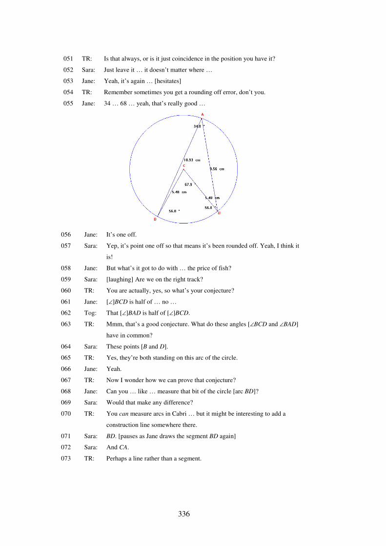
336
051 TR: Is that always, or is it just coincidence in the position you have it?
052 Sara: Just leave it … it doesn’t matter where …
053 Jane: Yeah, it’s again … [hesitates]
054 TR: Remember sometimes you get a rounding off error, don’t you.
055 Jane: 34 … 68 … yeah, that’s really good …
056 Jane: It’s one off.
057 Sara: Yep, it’s point one off so that means it’s been rounded off. Yeah, I think it
is!
058 Jane: But what’s it got to do with … the price of fish?
059 Sara: [laughing] Are we on the right track?
060 TR: You are actually, yes, so what’s your conjecture?
061 Jane: [∠]BCD is half of … no …
062 Tog: That [∠]BAD is half of [∠]BCD.
063 TR: Mmm, that’s a good conjecture. What do these angles [∠BCD and ∠BAD]
have in common?
064 Sara: These points [B and D].
065 TR: Yes, they’re both standing on this arc of the circle.
066 Jane: Yeah.
067 TR: Now I wonder how we can prove that conjecture?
068 Jane: Can you … like … measure that bit of the circle [arc BD]?
069 Sara: Would that make any difference?
070 TR: You can measure arcs in Cabri … but it might be interesting to add a
construction line somewhere there.
071 Sara: BD. [pauses as Jane draws the segment BD again]
072 Sara: And CA.
073 TR: Perhaps a line rather than a segment.
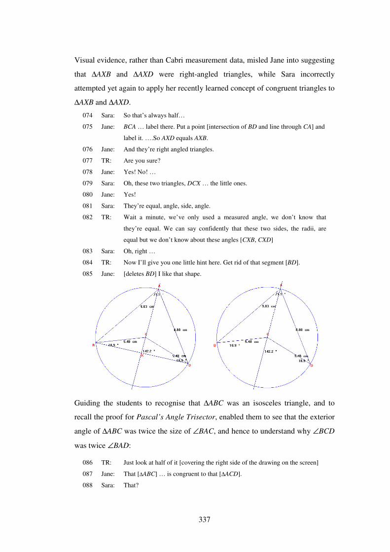
337
Visual evidence, rather than Cabri measurement data, misled Jane into suggesting
that ∆AXB and ∆AXD were right-angled triangles, while Sara incorrectly
attempted yet again to apply her recently learned concept of congruent triangles to
∆AXB and ∆AXD.
074 Sara: So that’s always half…
075 Jane: BCA … label there. Put a point [intersection of BD and line through CA] and
label it. ….So AXD equals AXB.
076 Jane: And they’re right angled triangles.
077 TR: Are you sure?
078 Jane: Yes! No! …
079 Sara: Oh, these two triangles, DCX … the little ones.
080 Jane: Yes!
081 Sara: They’re equal, angle, side, angle.
082 TR: Wait a minute, we’ve only used a measured angle, we don’t know that
they’re equal. We can say confidently that these two sides, the radii, are
equal but we don’t know about these angles [CXB, CXD]
083 Sara: Oh, right …
084 TR: Now I’ll give you one little hint here. Get rid of that segment [BD].
085 Jane: [deletes BD] I like that shape.
Guiding the students to recognise that ∆ABC was an isosceles triangle, and to
recall the proof for Pascal’s Angle Trisector, enabled them to see that the exterior
angle of ∆ABC was twice the size of ∠BAC, and hence to understand why ∠BCD
was twice ∠BAD:
086 TR: Just look at half of it [covering the right side of the drawing on the screen]
087 Jane: That [∆ABC] … is congruent to that [∆ACD].
088 Sara: That?
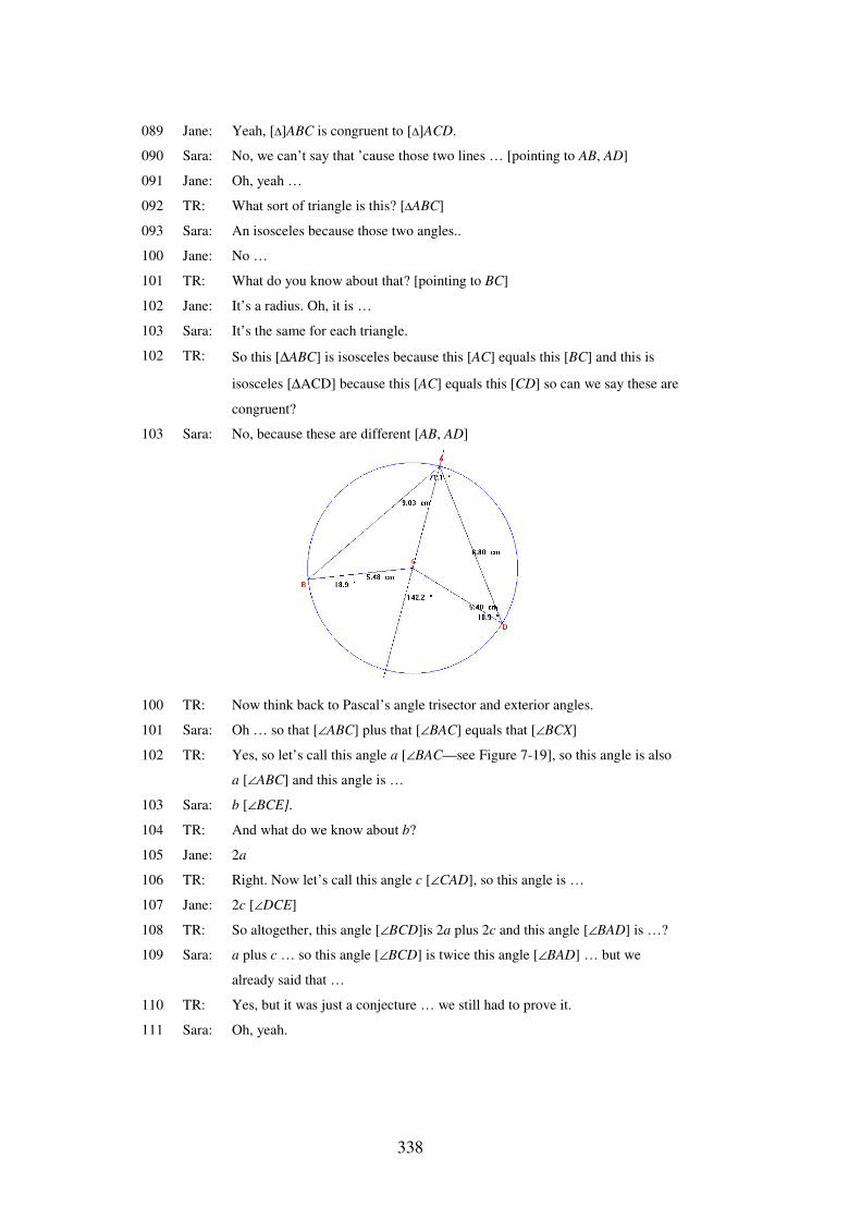
338
089 Jane: Yeah, [∆]ABC is congruent to [∆]ACD.
090 Sara: No, we can’t say that ’cause those two lines … [pointing to AB, AD]
091 Jane: Oh, yeah …
092 TR: What sort of triangle is this? [∆ABC]
093 Sara: An isosceles because those two angles..
100 Jane: No …
101 TR: What do you know about that? [pointing to BC]
102 Jane: It’s a radius. Oh, it is …
103 Sara: It’s the same for each triangle.
102 TR: So this [∆ABC] is isosceles because this [AC] equals this [BC] and this is
isosceles [∆ACD] because this [AC] equals this [CD] so can we say these are
congruent?
103 Sara: No, because these are different [AB, AD]
100 TR: Now think back to Pascal’s angle trisector and exterior angles.
101 Sara: Oh … so that [∠ABC] plus that [∠BAC] equals that [∠BCX]
102 TR: Yes, so let’s call this angle a [∠BAC—see Figure 7-19], so this angle is also
a [∠ABC] and this angle is …
103 Sara: b [∠BCE].
104 TR: And what do we know about b?
105 Jane: 2a
106 TR: Right. Now let’s call this angle c [∠CAD], so this angle is …
107 Jane: 2c [∠DCE]
108 TR: So altogether, this angle [∠BCD]is 2a plus 2c and this angle [∠BAD] is …?
109 Sara: a plus c … so this angle [∠BCD] is twice this angle [∠BAD] … but we
already said that …
110 TR: Yes, but it was just a conjecture … we still had to prove it.
111 Sara: Oh, yeah.
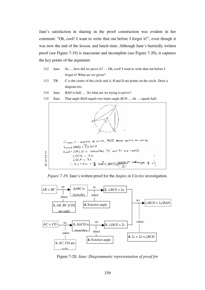
339
Jane’s satisfaction in sharing in the proof construction was evident in her
comment: “Oh, cool! I want to write that out before I forget it!”, even though it
was now the end of the lesson, and lunch time. Although Jane’s hurriedly written
proof (see Figure 7-19) is inaccurate and incomplete (see Figure 7-20), it captures
the key points of the argument:
112 Jane: So … how did we prove it? … Oh, cool! I want to write that out before I
forget it! What are we given?
113 TR: C is the centre of the circle and A, B and D are points on the circle. Draw a
diagram too.
114 Jane: BAD is half. … So what are we trying to prove?
115 Sara: That angle BAD equals two times angle BCD … oh … equals half.
Figure 7-19. Jane’s written proof for the Angles in Circles investigation.
Figure 7-20. Jane: Diagrammatic representation of proof for
AC = CD 1. ∆ACD is
isosceles
1. AC, CD are radii
3. ∠DCE = 2c
4. Exterior angle 4. 2c + 2a =∠BCD
so so
∠BCD = 2∠BAD
AB = BC ∆ABC is
isosceles
1. AB, BC [CD]
are radii
2. ∠BCE = 2a
4. Exterior angle
since
so so
so since
since
since
since
1 2 3 4
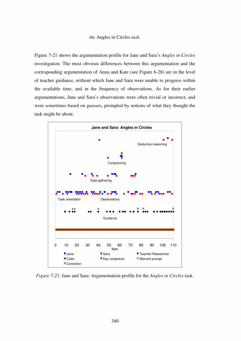
340
the Angles in Circles task.
Figure 7-21 shows the argumentation profile for Jane and Sara’s Angles in Circles
investigation. The most obvious differences between this argumentation and the
corresponding argumentation of Anna and Kate (see Figure 6-28) are in the level
of teacher guidance, without which Jane and Sara were unable to progress within
the available time, and in the frequency of observations. As for their earlier
argumentations, Jane and Sara’s observations were often trivial or incorrect, and
were sometimes based on guesses, prompted by notions of what they thought the
task might be about.
Jane and Sara: Angles in Circles
0 10 20 30 40 50 60 70 80 90 100 110Turn
Jane Sara Teacher-ResearcherCabri Key conjecture Warrant promptCorrection
Guidance
Observations
Data gathering
Conjecturing
Deductive reasoning
Task orientation
Figure 7-21. Jane and Sara: Argumentation profile for the Angles in Circles task.
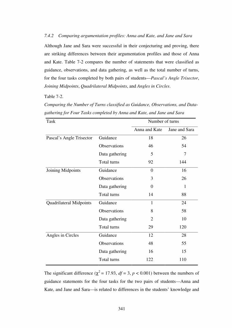
341
7.4.2 Comparing argumentation profiles: Anna and Kate, and Jane and Sara
Although Jane and Sara were successful in their conjecturing and proving, there
are striking differences between their argumentation profiles and those of Anna
and Kate. Table 7-2 compares the number of statements that were classified as
guidance, observations, and data gathering, as well as the total number of turns,
for the four tasks completed by both pairs of students—Pascal’s Angle Trisector,
Joining Midpoints, Quadrilateral Midpoints, and Angles in Circles.
Table 7-2.
Comparing the Number of Turns classified as Guidance, Observations, and Data-
gathering for Four Tasks completed by Anna and Kate, and Jane and Sara
Task Number of turns
Anna and Kate Jane and Sara
Pascal’s Angle Trisector Guidance 18 26
Observations 46 54
Data gathering 5 7
Total turns 92 144
Joining Midpoints Guidance 0 16
Observations 3 26
Data gathering 0 1
Total turns 14 88
Quadrilateral Midpoints Guidance 1 24
Observations 8 58
Data gathering 2 10
Total turns 29 120
Angles in Circles Guidance 12 28
Observations 48 55
Data gathering 16 15
Total turns 122 110
The significant difference (χ2 = 17.93, df = 3, p < 0.001) between the numbers of
guidance statements for the four tasks for the two pairs of students—Anna and
Kate, and Jane and Sara—is related to differences in the students’ knowledge and
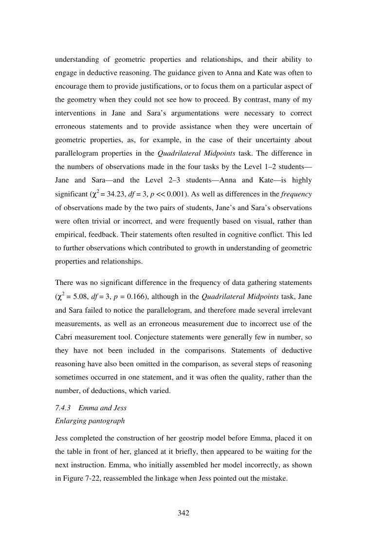
342
understanding of geometric properties and relationships, and their ability to
engage in deductive reasoning. The guidance given to Anna and Kate was often to
encourage them to provide justifications, or to focus them on a particular aspect of
the geometry when they could not see how to proceed. By contrast, many of my
interventions in Jane and Sara’s argumentations were necessary to correct
erroneous statements and to provide assistance when they were uncertain of
geometric properties, as, for example, in the case of their uncertainty about
parallelogram properties in the Quadrilateral Midpoints task. The difference in
the numbers of observations made in the four tasks by the Level 1–2 students—
Jane and Sara—and the Level 2–3 students—Anna and Kate—is highly
significant (χ2 = 34.23, df = 3, p << 0.001). As well as differences in the frequency
of observations made by the two pairs of students, Jane’s and Sara’s observations
were often trivial or incorrect, and were frequently based on visual, rather than
empirical, feedback. Their statements often resulted in cognitive conflict. This led
to further observations which contributed to growth in understanding of geometric
properties and relationships.
There was no significant difference in the frequency of data gathering statements
(χ2 = 5.08, df = 3, p = 0.166), although in the Quadrilateral Midpoints task, Jane
and Sara failed to notice the parallelogram, and therefore made several irrelevant
measurements, as well as an erroneous measurement due to incorrect use of the
Cabri measurement tool. Conjecture statements were generally few in number, so
they have not been included in the comparisons. Statements of deductive
reasoning have also been omitted in the comparison, as several steps of reasoning
sometimes occurred in one statement, and it was often the quality, rather than the
number, of deductions, which varied.
7.4.3 Emma and Jess
Enlarging pantograph
Jess completed the construction of her geostrip model before Emma, placed it on
the table in front of her, glanced at it briefly, then appeared to be waiting for the
next instruction. Emma, who initially assembled her model incorrectly, as shown
in Figure 7-22, reassembled the linkage when Jess pointed out the mistake.
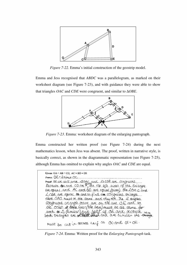
343
E
A
B
OC
D
Figure 7-22. Emma’s initial construction of the geostrip model.
Emma and Jess recognised that ABDC was a parallelogram, as marked on their
worksheet diagram (see Figure 7-23), and with guidance they were able to show
that triangles OAC and CDE were congruent, and similar to ∆OBE.
Figure 7-23. Emma: worksheet diagram of the enlarging pantograph.
Emma constructed her written proof (see Figure 7-24) during the next
mathematics lesson, when Jess was absent. The proof, written in narrative style, is
basically correct, as shown in the diagrammatic representation (see Figure 7-25),
although Emma has omitted to explain why angles OAC and CDE are equal.
Figure 7-24. Emma: Written proof for the Enlarging Pantograph task.
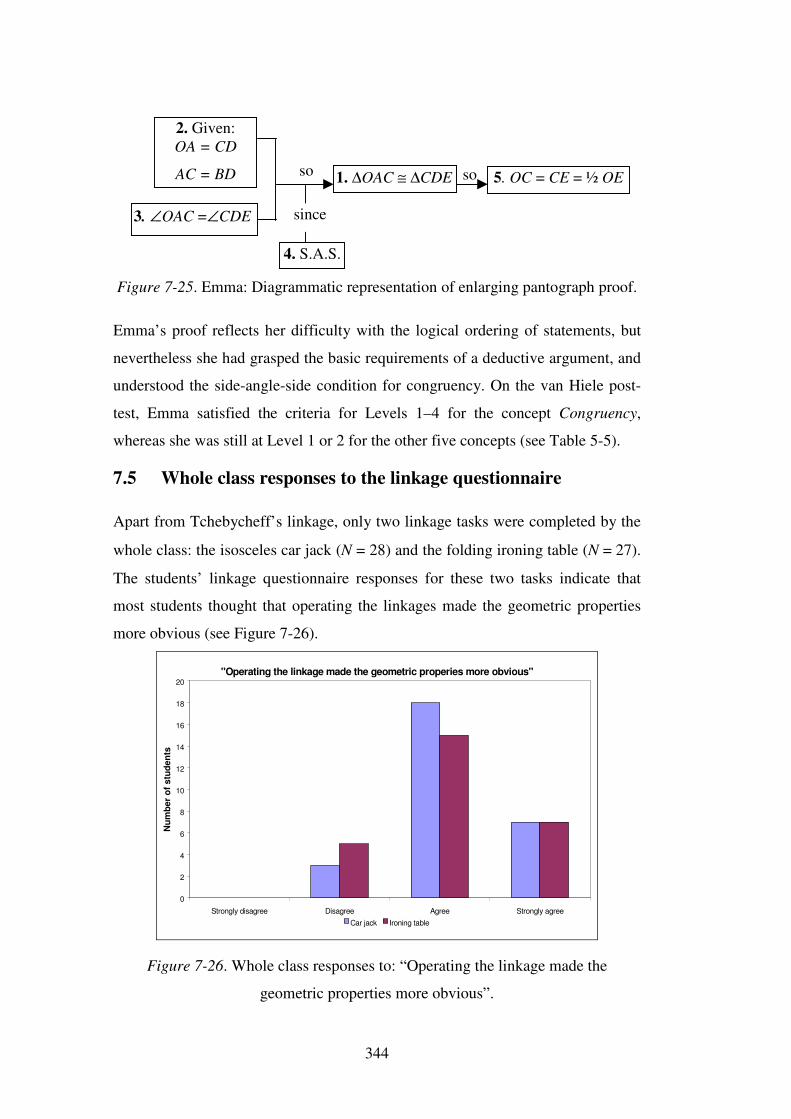
344
Figure 7-25. Emma: Diagrammatic representation of enlarging pantograph proof.
Emma’s proof reflects her difficulty with the logical ordering of statements, but
nevertheless she had grasped the basic requirements of a deductive argument, and
understood the side-angle-side condition for congruency. On the van Hiele post-
test, Emma satisfied the criteria for Levels 1–4 for the concept Congruency,
whereas she was still at Level 1 or 2 for the other five concepts (see Table 5-5).
7.5 Whole class responses to the linkage questionnaire
Apart from Tchebycheff’s linkage, only two linkage tasks were completed by the
whole class: the isosceles car jack (N = 28) and the folding ironing table (N = 27).
The students’ linkage questionnaire responses for these two tasks indicate that
most students thought that operating the linkages made the geometric properties
more obvious (see Figure 7-26).
"Operating the linkage made the geometric properies more obvious"
0
2
4
6
8
10
12
14
16
18
20
Strongly disagree Disagree Agree Strongly agree
Num
ber
of s
tude
nts
Car jack Ironing table
Figure 7-26. Whole class responses to: “Operating the linkage made the
geometric properties more obvious”.
2. Given: OA = CD
AC = BD
3. ∠OAC =∠CDE
1. ∆OAC ≅ ∆CDE
4. S.A.S.
5. OC = CE = ½ OE
so so
since
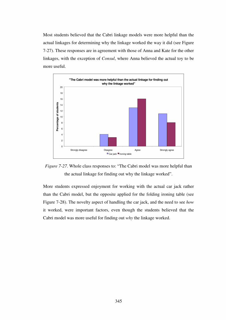
345
Most students believed that the Cabri linkage models were more helpful than the
actual linkages for determining why the linkage worked the way it did (see Figure
7-27). These responses are in agreement with those of Anna and Kate for the other
linkages, with the exception of Consul, where Anna believed the actual toy to be
more useful.
"The Cabri model was more helpful than the actual linkage for finding out why the linkage worked"
0
2
4
6
8
10
12
14
16
18
20
Strongly disagree Disagree Agree Strongly agree
Per
cent
age
of s
tude
nts
Car jack Ironing table
Figure 7-27. Whole class responses to: “The Cabri model was more helpful than
the actual linkage for finding out why the linkage worked”.
More students expressed enjoyment for working with the actual car jack rather
than the Cabri model, but the opposite applied for the folding ironing table (see
Figure 7-28). The novelty aspect of handling the car jack, and the need to see how
it worked, were important factors, even though the students believed that the
Cabri model was more useful for finding out why the linkage worked.
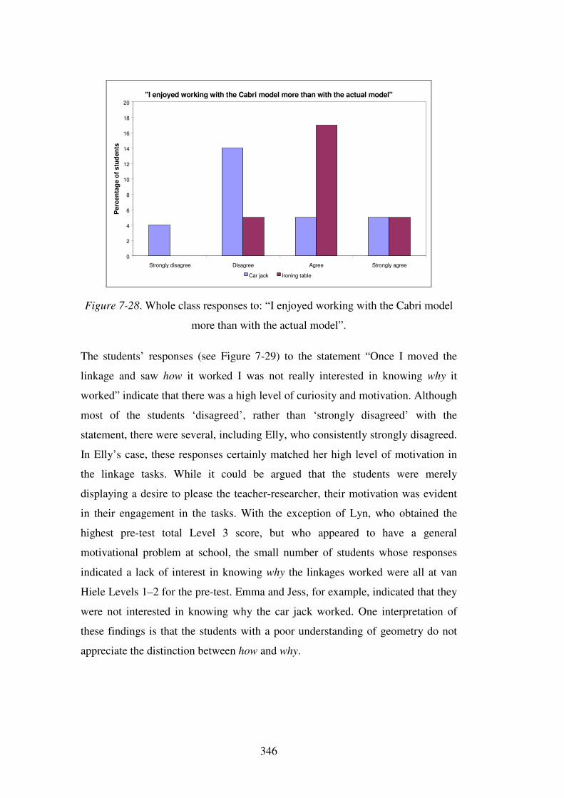
346
"I enjoyed working with the Cabri model more than with the actual model"
0
2
4
6
8
10
12
14
16
18
20
Strongly disagree Disagree Agree Strongly agree
Per
cent
age
of s
tude
nts
Car jack Ironing table
Figure 7-28. Whole class responses to: “I enjoyed working with the Cabri model
more than with the actual model”.
The students’ responses (see Figure 7-29) to the statement “Once I moved the
linkage and saw how it worked I was not really interested in knowing why it
worked” indicate that there was a high level of curiosity and motivation. Although
most of the students ‘disagreed’, rather than ‘strongly disagreed’ with the
statement, there were several, including Elly, who consistently strongly disagreed.
In Elly’s case, these responses certainly matched her high level of motivation in
the linkage tasks. While it could be argued that the students were merely
displaying a desire to please the teacher-researcher, their motivation was evident
in their engagement in the tasks. With the exception of Lyn, who obtained the
highest pre-test total Level 3 score, but who appeared to have a general
motivational problem at school, the small number of students whose responses
indicated a lack of interest in knowing why the linkages worked were all at van
Hiele Levels 1–2 for the pre-test. Emma and Jess, for example, indicated that they
were not interested in knowing why the car jack worked. One interpretation of
these findings is that the students with a poor understanding of geometry do not
appreciate the distinction between how and why.
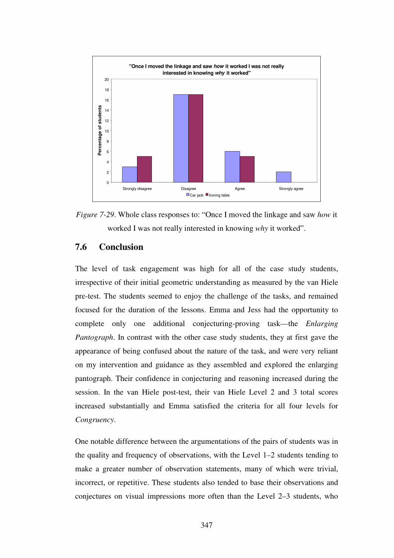
347
"Once I moved the linkage and saw how it worked I was not really interested in knowing why it worked"
0
2
4
6
8
10
12
14
16
18
20
Strongly disagree Disagree Agree Strongly agree
Per
cent
age
of s
tude
nts
Car jack Ironing table
Figure 7-29. Whole class responses to: “Once I moved the linkage and saw how it
worked I was not really interested in knowing why it worked”.
7.6 Conclusion
The level of task engagement was high for all of the case study students,
irrespective of their initial geometric understanding as measured by the van Hiele
pre-test. The students seemed to enjoy the challenge of the tasks, and remained
focused for the duration of the lessons. Emma and Jess had the opportunity to
complete only one additional conjecturing-proving task—the Enlarging
Pantograph. In contrast with the other case study students, they at first gave the
appearance of being confused about the nature of the task, and were very reliant
on my intervention and guidance as they assembled and explored the enlarging
pantograph. Their confidence in conjecturing and reasoning increased during the
session. In the van Hiele post-test, their van Hiele Level 2 and 3 total scores
increased substantially and Emma satisfied the criteria for all four levels for
Congruency.
One notable difference between the argumentations of the pairs of students was in
the quality and frequency of observations, with the Level 1–2 students tending to
make a greater number of observation statements, many of which were trivial,
incorrect, or repetitive. These students also tended to base their observations and
conjectures on visual impressions more often than the Level 2–3 students, who
348
frequently commenced their data gathering at an earlier stage of the
argumentation, and based their conjectures on empirical evidence. This difference
may be related to the greater ability of the Level 2–3 students to judge which
properties—angles or lengths, for example—were likely to be significant in
constructing conjectures and proofs. Jane and Sara were often handicapped in
their reasoning by misconceptions and poor understanding of properties and
relationships, with their argumentations clearly reflecting the students’ measured
van Hiele levels. Nevertheless, the experiences were still valuable for these Level
1–2 students in terms of considerable growth in geometric understanding, and a
developing awareness of the structure of deductive reasoning and geometric proof.
Anna and Kate, who had the opportunity to complete a greater number of tasks
than any of the other students, became more confident in their proving processes,
and more skilled in constructing their written proofs. They were able to recognise
particular diagrammatic configurations, for example, exterior angles of triangles,
and apply steps of deductive reasoning from previous proofs that allowed them to
skip steps of reasoning in their argumentations. They generally, however, included
complete reasoning in their written proofs. Since there was no indication that
Anna and Kate had superior ability or geometric understanding prior to the
conjecturing-proving tasks, it would seem reasonable to assume that their better
progress was due to the number of tasks they completed, and to their level of
cooperative argumentation.
Chapter 8, which focuses on the Year 8 students’ pre-test and post-test responses
to the Proof Questionnaire, shows the progress made by many of the students, in
particular, the case study students, in recognising correct arguments, and in
constructing their own written proofs in both familiar and unfamiliar contexts.
349
Chapter 8: The Proof Questionnaire
What the child can do in cooperation today he can do alone tomorrow. Therefore the
only good kind of instruction is that which marches ahead of development and leads
it; it must be aimed not so much at the ripe as at the ripening functions. (Vygotsky,
1962, p. 104)
8.1 Introduction
The argumentations of the case study students discussed in chapters 6 and 7
demonstrate the extent to which the students were able to engage in deductive
reasoning. Although most of the case study students were able to participate in
deductive reasoning, those students who were at van Hiele Levels 2−3 prior to the
conjecturing-proving lessons were better able to make more relevant observations,
were often more selective in their data gathering, and were more successful in
engaging in sustained sequences of reasoning. All argumentations took place in a
collaborative environment, where the students supported each other in their
reasoning, and where my interventions prompted them to supply justifications,
and, when necessary, focused their attention on particular aspects of the geometry.
The van Hiele post-test results (see Table 5-5) indicate changes in the students’
geometric understanding, particularly at Levels 3 and 4. The Proof Questionnaire
(Healy & Hoyles, 1999—see Appendix 3) post-test provides further insight into
individual students’ understanding of proof, and their ability to recognise and
construct valid proofs.
The geometry section of the Proof Questionnaire was incorporated into the
current research as a pre-test and as a post-test to provide information about
changes in the Year 8 students’ understanding of geometric proof. Although the
Proof Questionnaire was designed for high-attaining Year 10 students (14–15
years), the geometry section was considered to be appropriate for the above-
average Year 8 students (12−13 years) in this study (see section 4.4.4). Pre-testing
took place in April 2001, and the post-test was administered in late June 2001,
following completion of the conjecturing-proving tasks in early June. This chapter
compares the pre-test and post-test responses of the Year 8 students to each of the
350
Proof Questionnaire questions. Section 8.2 provides a brief overview of the Proof
Questionnaire. Section 8.3 focuses on the Year 8 students’ views of proof; section
8.4 compares the Year 8 students’ pre-test and post-test judgements of proofs; and
section 8.5 looks at the overall improvement in the quality of the Year 8 students’
proof constructions, with particular reference to the case study students. In each
section, the Year 8 students’ responses are also compared with those of the
Year 10 Proof Study students.
8.2 The Proof Questionnaire
Healy and Hoyles (1999) note that the purpose of the Proof Questionnaire is to
provide data about students’ views of mathematical proof, their ability to
recognise correct proofs in algebra and geometry, and their ability to construct
proofs in familiar and unfamiliar contexts. The Proof Questionnaire was
designed, piloted, and revised before being administered to 2459 high-attaining
Year 10 students in England and Wales. Ninety of the 94 classes in the Proof
Study were the top mathematics sets in their schools, three classes were second
sets, and one class was mixed-ability. The majority of students—an average of
80% across all classes—was expected to be entered for the GCSE higher-tier
paper. Healy and Hoyles note that the most common approach to the teaching of
mathematical justification in the Proof Study schools was through investigations,
and that students were more likely to be expected to read and write proofs in
algebra than in geometry—students in 51% of classes were expected to write
algebraic proofs compared with 32% of classes for geometric proofs.
The first question of the Proof Questionnaire invites students to explain what
proof in mathematics means to them. The remainder of the questionnaire is
divided into two parallel sections—one for arithmetic/algebra and the other for
geometry. In each section students are presented with multiple-choice questions
where they are required to select from a range of arguments according to two
criteria—which argument would be most like their own approach, and which
argument they think would receive the best mark. In addition, each section of the
Proof Questionnaire requires the students to construct two proofs: one familiar
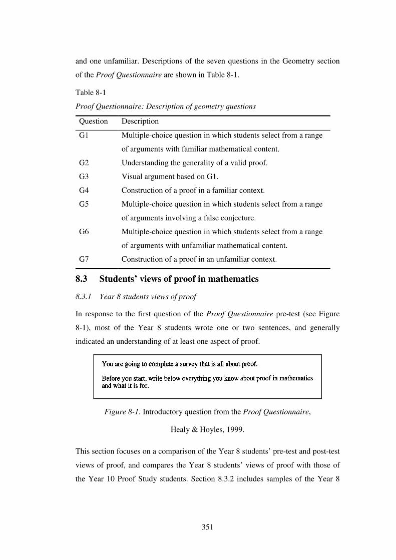
351
and one unfamiliar. Descriptions of the seven questions in the Geometry section
of the Proof Questionnaire are shown in Table 8-1.
Table 8-1
Proof Questionnaire: Description of geometry questions
Question Description
G1 Multiple-choice question in which students select from a range
of arguments with familiar mathematical content.
G2 Understanding the generality of a valid proof.
G3 Visual argument based on G1.
G4 Construction of a proof in a familiar context.
G5 Multiple-choice question in which students select from a range
of arguments involving a false conjecture.
G6 Multiple-choice question in which students select from a range
of arguments with unfamiliar mathematical content.
G7 Construction of a proof in an unfamiliar context.
8.3 Students’ views of proof in mathematics
8.3.1 Year 8 students views of proof
In response to the first question of the Proof Questionnaire pre-test (see Figure
8-1), most of the Year 8 students wrote one or two sentences, and generally
indicated an understanding of at least one aspect of proof.
Figure 8-1. Introductory question from the Proof Questionnaire,
Healy & Hoyles, 1999.
This section focuses on a comparison of the Year 8 students’ pre-test and post-test
views of proof, and compares the Year 8 students’ views of proof with those of
the Year 10 Proof Study students. Section 8.3.2 includes samples of the Year 8
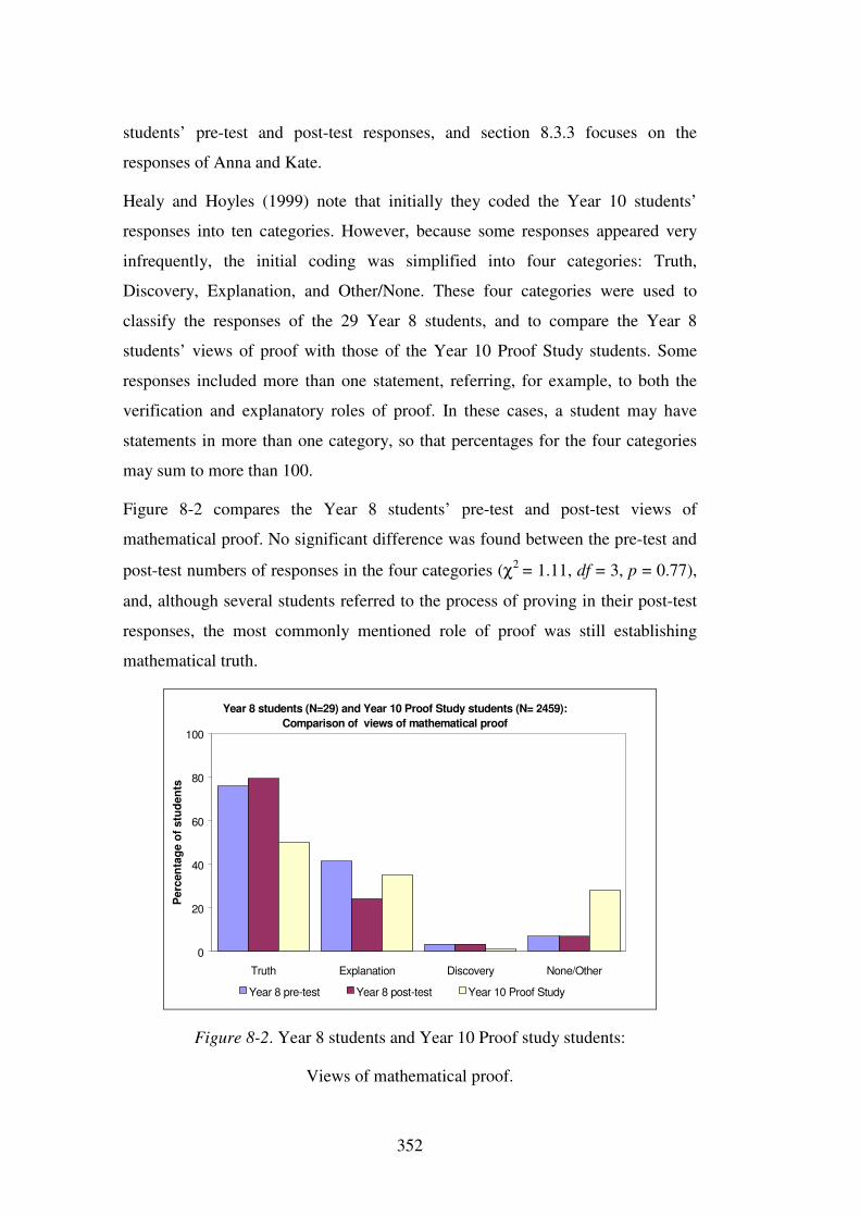
352
students’ pre-test and post-test responses, and section 8.3.3 focuses on the
responses of Anna and Kate.
Healy and Hoyles (1999) note that initially they coded the Year 10 students’
responses into ten categories. However, because some responses appeared very
infrequently, the initial coding was simplified into four categories: Truth,
Discovery, Explanation, and Other/None. These four categories were used to
classify the responses of the 29 Year 8 students, and to compare the Year 8
students’ views of proof with those of the Year 10 Proof Study students. Some
responses included more than one statement, referring, for example, to both the
verification and explanatory roles of proof. In these cases, a student may have
statements in more than one category, so that percentages for the four categories
may sum to more than 100.
Figure 8-2 compares the Year 8 students’ pre-test and post-test views of
mathematical proof. No significant difference was found between the pre-test and
post-test numbers of responses in the four categories (χ2 = 1.11, df = 3, p = 0.77),
and, although several students referred to the process of proving in their post-test
responses, the most commonly mentioned role of proof was still establishing
mathematical truth.
Year 8 students (N=29) and Year 10 Proof Study students (N= 2459): Comparison of views of mathematical proof
0
20
40
60
80
100
Truth Explanation Discovery None/Other
Per
cent
age
of s
tude
nts
Year 8 pre-test Year 8 post-test Year 10 Proof Study
Figure 8-2. Year 8 students and Year 10 Proof study students:
Views of mathematical proof.
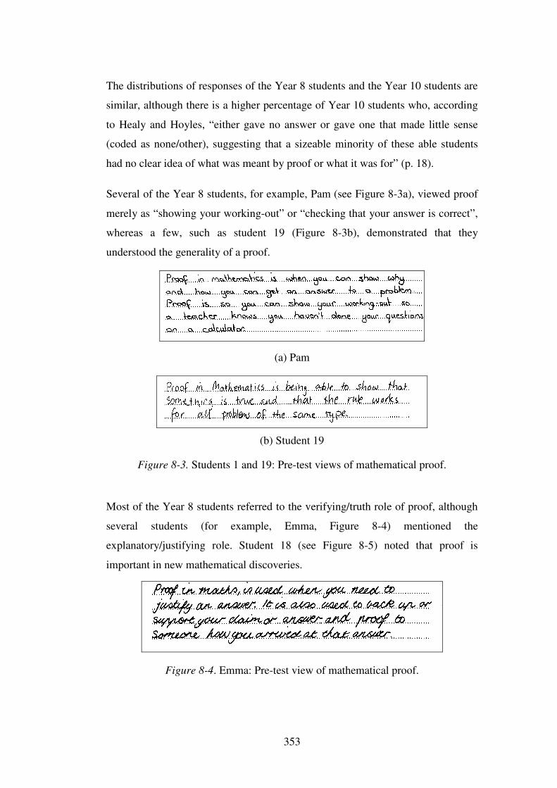
353
The distributions of responses of the Year 8 students and the Year 10 students are
similar, although there is a higher percentage of Year 10 students who, according
to Healy and Hoyles, “either gave no answer or gave one that made little sense
(coded as none/other), suggesting that a sizeable minority of these able students
had no clear idea of what was meant by proof or what it was for” (p. 18).
Several of the Year 8 students, for example, Pam (see Figure 8-3a), viewed proof
merely as “showing your working-out” or “checking that your answer is correct”,
whereas a few, such as student 19 (Figure 8-3b), demonstrated that they
understood the generality of a proof.
(a) Pam
(b) Student 19
Figure 8-3. Students 1 and 19: Pre-test views of mathematical proof.
Most of the Year 8 students referred to the verifying/truth role of proof, although
several students (for example, Emma, Figure 8-4) mentioned the
explanatory/justifying role. Student 18 (see Figure 8-5) noted that proof is
important in new mathematical discoveries.
Figure 8-4. Emma: Pre-test view of mathematical proof.
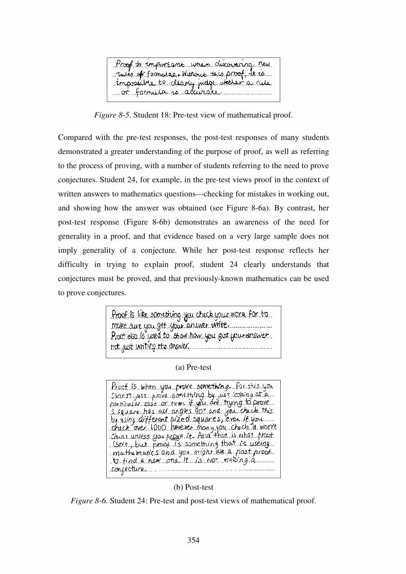
354
Figure 8-5. Student 18: Pre-test view of mathematical proof.
Compared with the pre-test responses, the post-test responses of many students
demonstrated a greater understanding of the purpose of proof, as well as referring
to the process of proving, with a number of students referring to the need to prove
conjectures. Student 24, for example, in the pre-test views proof in the context of
written answers to mathematics questions—checking for mistakes in working out,
and showing how the answer was obtained (see Figure 8-6a). By contrast, her
post-test response (Figure 8-6b) demonstrates an awareness of the need for
generality in a proof, and that evidence based on a very large sample does not
imply generality of a conjecture. While her post-test response reflects her
difficulty in trying to explain proof, student 24 clearly understands that
conjectures must be proved, and that previously-known mathematics can be used
to prove conjectures.
(a) Pre-test
(b) Post-test
Figure 8-6. Student 24: Pre-test and post-test views of mathematical proof.
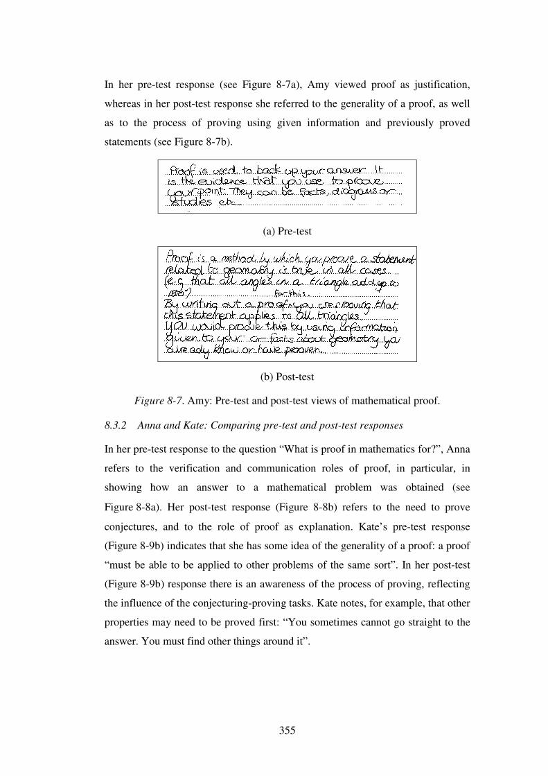
355
In her pre-test response (see Figure 8-7a), Amy viewed proof as justification,
whereas in her post-test response she referred to the generality of a proof, as well
as to the process of proving using given information and previously proved
statements (see Figure 8-7b).
(a) Pre-test
(b) Post-test
Figure 8-7. Amy: Pre-test and post-test views of mathematical proof.
8.3.2 Anna and Kate: Comparing pre-test and post-test responses
In her pre-test response to the question “What is proof in mathematics for?”, Anna
refers to the verification and communication roles of proof, in particular, in
showing how an answer to a mathematical problem was obtained (see
Figure 8-8a). Her post-test response (Figure 8-8b) refers to the need to prove
conjectures, and to the role of proof as explanation. Kate’s pre-test response
(Figure 8-9b) indicates that she has some idea of the generality of a proof: a proof
“must be able to be applied to other problems of the same sort”. In her post-test
(Figure 8-9b) response there is an awareness of the process of proving, reflecting
the influence of the conjecturing-proving tasks. Kate notes, for example, that other
properties may need to be proved first: “You sometimes cannot go straight to the
answer. You must find other things around it”.
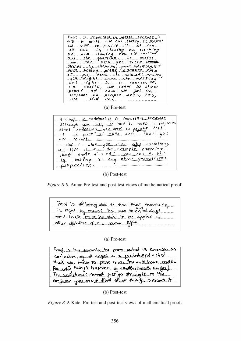
356
(a) Pre-test
(b) Post-test
Figure 8-8. Anna: Pre-test and post-test views of mathematical proof.
(a) Pre-test
(b) Post-test
Figure 8-9. Kate: Pre-test and post-test views of mathematical proof.
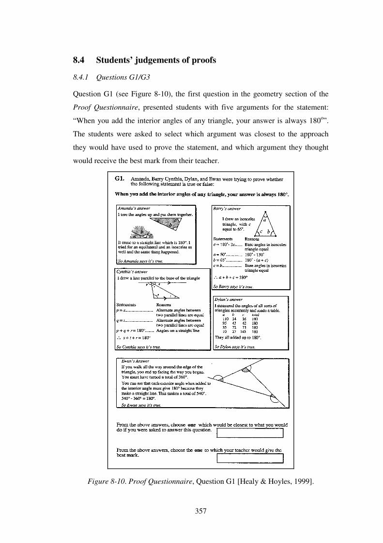
357
8.4 Students’ judgements of proofs
8.4.1 Questions G1/G3
Question G1 (see Figure 8-10), the first question in the geometry section of the
Proof Questionnaire, presented students with five arguments for the statement:
“When you add the interior angles of any triangle, your answer is always 180o”.
The students were asked to select which argument was closest to the approach
they would have used to prove the statement, and which argument they thought
would receive the best mark from their teacher.
Figure 8-10. Proof Questionnaire, Question G1 [Healy & Hoyles, 1999].
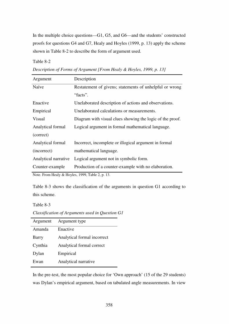
358
In the multiple choice questions—G1, G5, and G6—and the students’ constructed
proofs for questions G4 and G7, Healy and Hoyles (1999, p. 13) apply the scheme
shown in Table 8-2 to describe the form of argument used.
Table 8-2
Description of Forms of Argument [From Healy & Hoyles, 1999, p. 13]
Argument Description
Naïve Restatement of givens; statements of unhelpful or wrong
“facts”.
Enactive Unelaborated description of actions and observations.
Empirical Unelaborated calculations or measurements.
Visual Diagram with visual clues showing the logic of the proof.
Analytical formal
(correct)
Logical argument in formal mathematical language.
Analytical formal
(incorrect)
Incorrect, incomplete or illogical argument in formal
mathematical language.
Analytical narrative Logical argument not in symbolic form.
Counter-example Production of a counter-example with no elaboration.
Note. From Healy & Hoyles, 1999, Table 2, p. 13.
Table 8-3 shows the classification of the arguments in question G1 according to
this scheme.
Table 8-3
Classification of Arguments used in Question G1
Argument Argument type
Amanda Enactive
Barry Analytical formal incorrect
Cynthia Analytical formal correct
Dylan Empirical
Ewan Analytical narrative
In the pre-test, the most popular choice for ‘Own approach’ (15 of the 29 students)
was Dylan’s empirical argument, based on tabulated angle measurements. In view
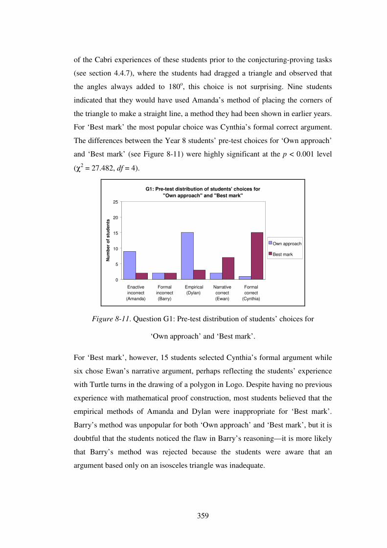
359
of the Cabri experiences of these students prior to the conjecturing-proving tasks
(see section 4.4.7), where the students had dragged a triangle and observed that
the angles always added to 180o, this choice is not surprising. Nine students
indicated that they would have used Amanda’s method of placing the corners of
the triangle to make a straight line, a method they had been shown in earlier years.
For ‘Best mark’ the most popular choice was Cynthia’s formal correct argument.
The differences between the Year 8 students’ pre-test choices for ‘Own approach’
and ‘Best mark’ (see Figure 8-11) were highly significant at the p < 0.001 level
(χ2 = 27.482, df = 4).
G1: Pre-test distribution of students' choices for "Own approach" and "Best mark"
0
5
10
15
20
25
Enactiveincorrect(Amanda)
Formalincorrect(Barry)
Empirical(Dylan)
Narrativecorrect(Ewan)
Formalcorrect
(Cynthia)
Num
ber
of s
tude
nts
Own approach
Best mark
Figure 8-11. Question G1: Pre-test distribution of students’ choices for
‘Own approach’ and ‘Best mark’.
For ‘Best mark’, however, 15 students selected Cynthia’s formal argument while
six chose Ewan’s narrative argument, perhaps reflecting the students’ experience
with Turtle turns in the drawing of a polygon in Logo. Despite having no previous
experience with mathematical proof construction, most students believed that the
empirical methods of Amanda and Dylan were inappropriate for ‘Best mark’.
Barry’s method was unpopular for both ‘Own approach’ and ‘Best mark’, but it is
doubtful that the students noticed the flaw in Barry’s reasoning—it is more likely
that Barry’s method was rejected because the students were aware that an
argument based only on an isosceles triangle was inadequate.
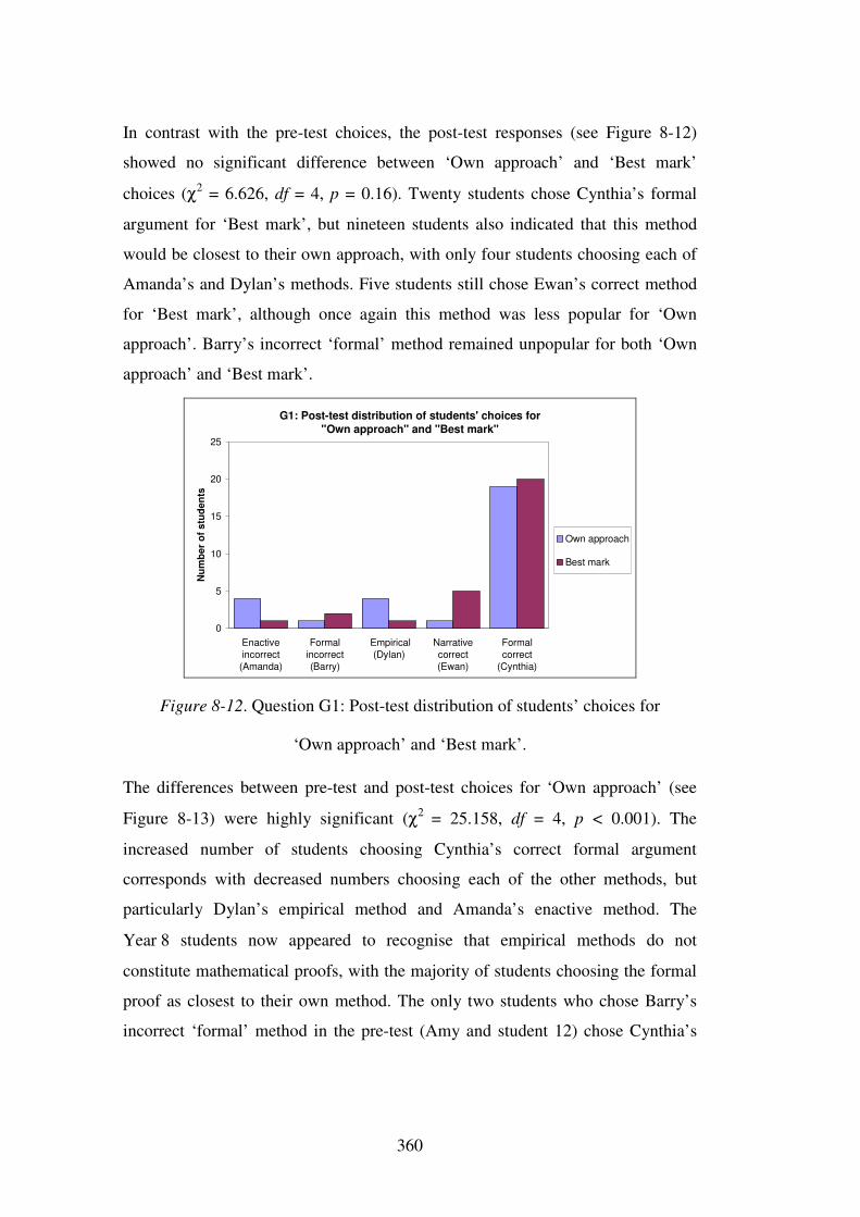
360
In contrast with the pre-test choices, the post-test responses (see Figure 8-12)
showed no significant difference between ‘Own approach’ and ‘Best mark’
choices (χ2 = 6.626, df = 4, p = 0.16). Twenty students chose Cynthia’s formal
argument for ‘Best mark’, but nineteen students also indicated that this method
would be closest to their own approach, with only four students choosing each of
Amanda’s and Dylan’s methods. Five students still chose Ewan’s correct method
for ‘Best mark’, although once again this method was less popular for ‘Own
approach’. Barry’s incorrect ‘formal’ method remained unpopular for both ‘Own
approach’ and ‘Best mark’.
G1: Post-test distribution of students' choices for "Own approach" and "Best mark"
0
5
10
15
20
25
Enactiveincorrect
(Amanda)
Formalincorrect(Barry)
Empirical(Dylan)
Narrativecorrect(Ewan)
Formalcorrect
(Cynthia)
Num
ber
of s
tude
nts
Own approach
Best mark
Figure 8-12. Question G1: Post-test distribution of students’ choices for
‘Own approach’ and ‘Best mark’.
The differences between pre-test and post-test choices for ‘Own approach’ (see
Figure 8-13) were highly significant (χ2 = 25.158, df = 4, p < 0.001). The
increased number of students choosing Cynthia’s correct formal argument
corresponds with decreased numbers choosing each of the other methods, but
particularly Dylan’s empirical method and Amanda’s enactive method. The
Year 8 students now appeared to recognise that empirical methods do not
constitute mathematical proofs, with the majority of students choosing the formal
proof as closest to their own method. The only two students who chose Barry’s
incorrect ‘formal’ method in the pre-test (Amy and student 12) chose Cynthia’s
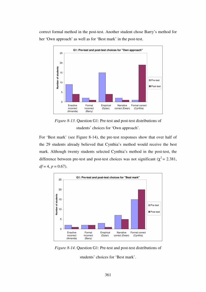
361
correct formal method in the post-test. Another student chose Barry’s method for
her ‘Own approach’ as well as for ‘Best mark’ in the post-test.
G1: Pre-test and post-test choices for "Own approach"
0
5
10
15
20
25
Enactiveincorrect(Amanda)
Formalincorrect(Barry)
Empirical(Dylan)
Narrativecorrect (Ewan)
Formal correct(Cynthia)
Num
ber
of s
tude
nts
Pre-test
Post-test
Figure 8-13. Question G1: Pre-test and post-test distributions of
students’ choices for ‘Own approach’.
For ‘Best mark’ (see Figure 8-14), the pre-test responses show that over half of
the 29 students already believed that Cynthia’s method would receive the best
mark. Although twenty students selected Cynthia’s method in the post-test, the
difference between pre-test and post-test choices was not significant (χ2 = 2.381,
df = 4, p = 0.67).
G1: Pre-test and post-test choices for "Best mark"
0
5
10
15
20
25
Enactiveincorrect(Amanda)
Formalincorrect(Barry)
Empirical(Dylan)
Narrativecorrect (Ewan)
Formal correct(Cynthia)
Num
ber
of s
tude
nts
Pre-test
Post-test
Figure 8-14. Question G1: Pre-test and post-test distributions of
students’ choices for ‘Best mark’.
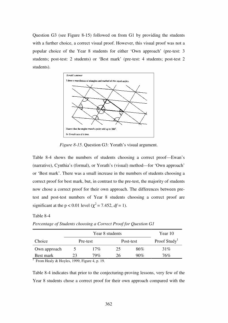
362
Question G3 (see Figure 8-15) followed on from G1 by providing the students
with a further choice, a correct visual proof. However, this visual proof was not a
popular choice of the Year 8 students for either ‘Own approach’ (pre-test: 3
students; post-test: 2 students) or ‘Best mark’ (pre-test: 4 students; post-test 2
students).
Figure 8-15. Question G3: Yorath’s visual argument.
Table 8-4 shows the numbers of students choosing a correct proof—Ewan’s
(narrative), Cynthia’s (formal), or Yorath’s (visual) method—for ‘Own approach’
or ‘Best mark’. There was a small increase in the numbers of students choosing a
correct proof for best mark, but, in contrast to the pre-test, the majority of students
now chose a correct proof for their own approach. The differences between pre-
test and post-test numbers of Year 8 students choosing a correct proof are
significant at the p < 0.01 level (χ2 = 7.452, df = 1).
Table 8-4
Percentage of Students choosing a Correct Proof for Question G1
Year 8 students Year 10
Choice Pre-test Post-test Proof Study1
Own approach 5 17% 25 86% 31% Best mark 23 79% 26 90% 76%
1 From Healy & Hoyles, 1999, Figure 4, p. 19.
Table 8-4 indicates that prior to the conjecturing-proving lessons, very few of the
Year 8 students chose a correct proof for their own approach compared with the
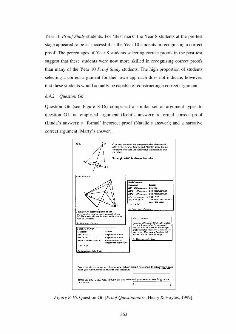
363
Year 10 Proof Study students. For ‘Best mark’ the Year 8 students at the pre-test
stage appeared to be as successful as the Year 10 students in recognising a correct
proof. The percentages of Year 8 students selecting correct proofs in the post-test
suggest that these students were now more skilled in recognising correct proofs
than many of the Year 10 Proof Study students. The high proportion of students
selecting a correct argument for their own approach does not indicate, however,
that these students would actually be capable of constructing a correct argument.
8.4.2 Question G6
Question G6 (see Figure 8-16) comprised a similar set of argument types to
question G1: an empirical argument (Kobi’s answer); a formal correct proof
(Linda’s answer); a ‘formal’ incorrect proof (Natalie’s answer); and a narrative
correct argument (Marty’s answer).
Figure 8-16. Question G6 [Proof Questionnaire, Healy & Hoyles, 1999].
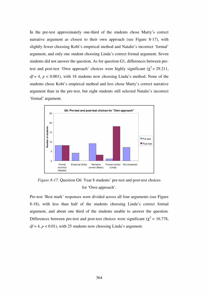
364
In the pre-test approximately one-third of the students chose Marty’s correct
narrative argument as closest to their own approach (see Figure 8-17), with
slightly fewer choosing Kobi’s empirical method and Natalie’s incorrect ‘formal’
argument, and only one student choosing Linda’s correct formal argument. Seven
students did not answer the question. As for question G1, differences between pre-
test and post-test ‘Own approach’ choices were highly significant (χ2 = 29.211,
df = 4, p < 0.001), with 18 students now choosing Linda’s method. None of the
students chose Kobi’s empirical method and less chose Marty’s correct narrative
argument than in the pre-test, but eight students still selected Natalie’s incorrect
‘formal’ argument.
G6: Pre-test and post-test choices for "Own approach"
0
5
10
15
20
25
Formalincorrect(Natalie)
Empirical (Kobi) Narrativecorrect (Marty)
Formal correct(Linda)
Not answered
Num
ber
of s
tude
nts
Pre-test
Post-test
Figure 8-17. Question G6: Year 8 students’ pre-test and post-test choices
for ‘Own approach’.
Pre-test ‘Best mark’ responses were divided across all four arguments (see Figure
8-18), with less than half of the students choosing Linda’s correct formal
argument, and about one third of the students unable to answer the question.
Differences between pre-test and post-test choices were significant (χ2 = 16.778,
df = 4, p < 0.01), with 25 students now choosing Linda’s argument.
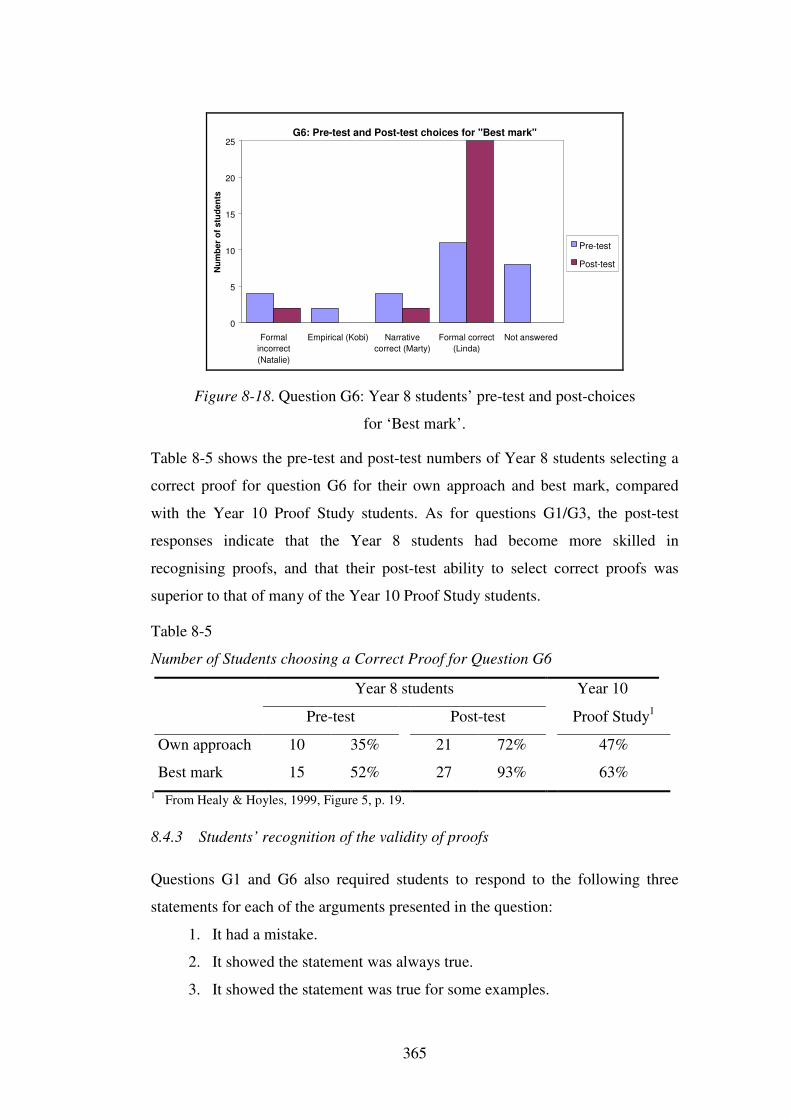
365
G6: Pre-test and Post-test choices for "Best mark"
0
5
10
15
20
25
Formalincorrect(Natalie)
Empirical (Kobi) Narrativecorrect (Marty)
Formal correct(Linda)
Not answered
Num
ber
of s
tude
nts
Pre-test
Post-test
Figure 8-18. Question G6: Year 8 students’ pre-test and post-choices
for ‘Best mark’.
Table 8-5 shows the pre-test and post-test numbers of Year 8 students selecting a
correct proof for question G6 for their own approach and best mark, compared
with the Year 10 Proof Study students. As for questions G1/G3, the post-test
responses indicate that the Year 8 students had become more skilled in
recognising proofs, and that their post-test ability to select correct proofs was
superior to that of many of the Year 10 Proof Study students.
Table 8-5
Number of Students choosing a Correct Proof for Question G6
Year 8 students Year 10
Pre-test Post-test Proof Study1
Own approach 10 35% 21 72% 47%
Best mark 15 52% 27 93% 63% 1 From Healy & Hoyles, 1999, Figure 5, p. 19.
8.4.3 Students’ recognition of the validity of proofs
Questions G1 and G6 also required students to respond to the following three
statements for each of the arguments presented in the question:
1. It had a mistake.
2. It showed the statement was always true.
3. It showed the statement was true for some examples.
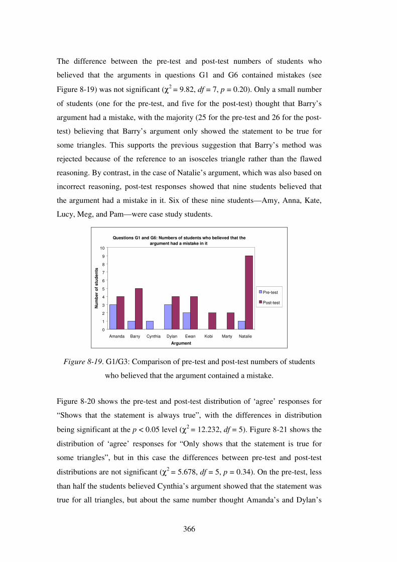
366
The difference between the pre-test and post-test numbers of students who
believed that the arguments in questions G1 and G6 contained mistakes (see
Figure 8-19) was not significant (χ2 = 9.82, df = 7, p = 0.20). Only a small number
of students (one for the pre-test, and five for the post-test) thought that Barry’s
argument had a mistake, with the majority (25 for the pre-test and 26 for the post-
test) believing that Barry’s argument only showed the statement to be true for
some triangles. This supports the previous suggestion that Barry’s method was
rejected because of the reference to an isosceles triangle rather than the flawed
reasoning. By contrast, in the case of Natalie’s argument, which was also based on
incorrect reasoning, post-test responses showed that nine students believed that
the argument had a mistake in it. Six of these nine students—Amy, Anna, Kate,
Lucy, Meg, and Pam—were case study students.
Questions G1 and G6: Numbers of students who believed that the argument had a mistake in it
0
1
2
3
4
5
6
7
8
9
10
Amanda Barry Cynthia Dylan Ewan Kobi Marty Natalie
Argument
Num
ber
of s
tude
nts
Pre-test
Post-test
Figure 8-19. G1/G3: Comparison of pre-test and post-test numbers of students
who believed that the argument contained a mistake.
Figure 8-20 shows the pre-test and post-test distribution of ‘agree’ responses for
“Shows that the statement is always true”, with the differences in distribution
being significant at the p < 0.05 level (χ2 = 12.232, df = 5). Figure 8-21 shows the
distribution of ‘agree’ responses for “Only shows that the statement is true for
some triangles”, but in this case the differences between pre-test and post-test
distributions are not significant (χ2 = 5.678, df = 5, p = 0.34). On the pre-test, less
than half the students believed Cynthia’s argument showed that the statement was
true for all triangles, but about the same number thought Amanda’s and Dylan’s
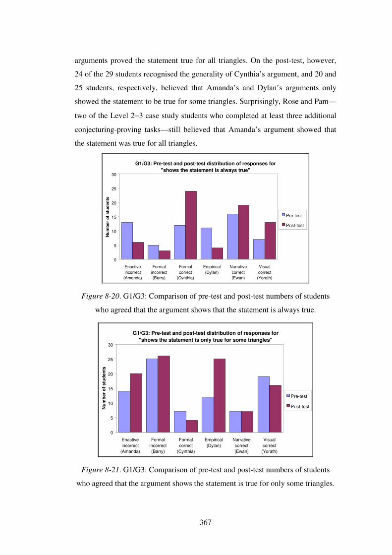
367
arguments proved the statement true for all triangles. On the post-test, however,
24 of the 29 students recognised the generality of Cynthia’s argument, and 20 and
25 students, respectively, believed that Amanda’s and Dylan’s arguments only
showed the statement to be true for some triangles. Surprisingly, Rose and Pam—
two of the Level 2−3 case study students who completed at least three additional
conjecturing-proving tasks—still believed that Amanda’s argument showed that
the statement was true for all triangles.
G1/G3: Pre-test and post-test distribution of responses for "shows the statement is always true"
0
5
10
15
20
25
30
Enactiveincorrect(Amanda)
Formalincorrect(Barry)
Formalcorrect
(Cynthia)
Empirical(Dylan)
Narrativecorrect(Ewan)
Visualcorrect(Yorath)
Num
ber
of s
tude
nts
Pre-test
Post-test
Figure 8-20. G1/G3: Comparison of pre-test and post-test numbers of students
who agreed that the argument shows that the statement is always true.
G1/G3: Pre-test and post-test distribution of responses for "shows the statement is only true for some triangles"
0
5
10
15
20
25
30
Enactiveincorrect
(Amanda)
Formalincorrect(Barry)
Formalcorrect
(Cynthia)
Empirical(Dylan)
Narrativecorrect(Ewan)
Visualcorrect
(Yorath)
Num
ber
of s
tude
nts
Pre-test
Post-test
Figure 8-21. G1/G3: Comparison of pre-test and post-test numbers of students
who agreed that the argument shows the statement is true for only some triangles.
368
Calculation of validity ratings
For questions G1 and G6, validity ratings were calculated for each student based
on their profiles of responses to the three statements—It had a mistake; It showed
the statement was always true; It showed the statement was true for some
examples—using the method described by Healy and Hoyles (1999, p. 14). A
validity rating of 0, 1 or 2 was assigned to each student for each argument
according to their profile of responses (agree; disagree; don’t know), as shown in
Table 8-6. The validity ratings for the six proofs in G1 and the four proofs in G6
were then combined to give each student an overall validity score, ranging from 0
to 20.
Table 8-6
Scoring of Response Profiles for Questions G1 and G6
[as described by Healy & Hoyles, 1999, p. 14]
Response profile Score Entirely correct profile of responses 2
Correctly noted if the argument was general, specific or wrong, but was unsure of other factors
1
All other profiles 0
Analysis of variance for the 29 students’ pre-test and post-test validity ratings for
each of the ten arguments (see Table 8-7) indicates that there were highly
significant differences for Cynthia’s and Linda’s formal correct arguments, with
the majority of students now recognising the generality of these two arguments.
Correspondingly, the majority of students rejected the generality of Dylan’s and
Kobi’s empirical methods, with the pre-test/post-test differences again being
highly significant.
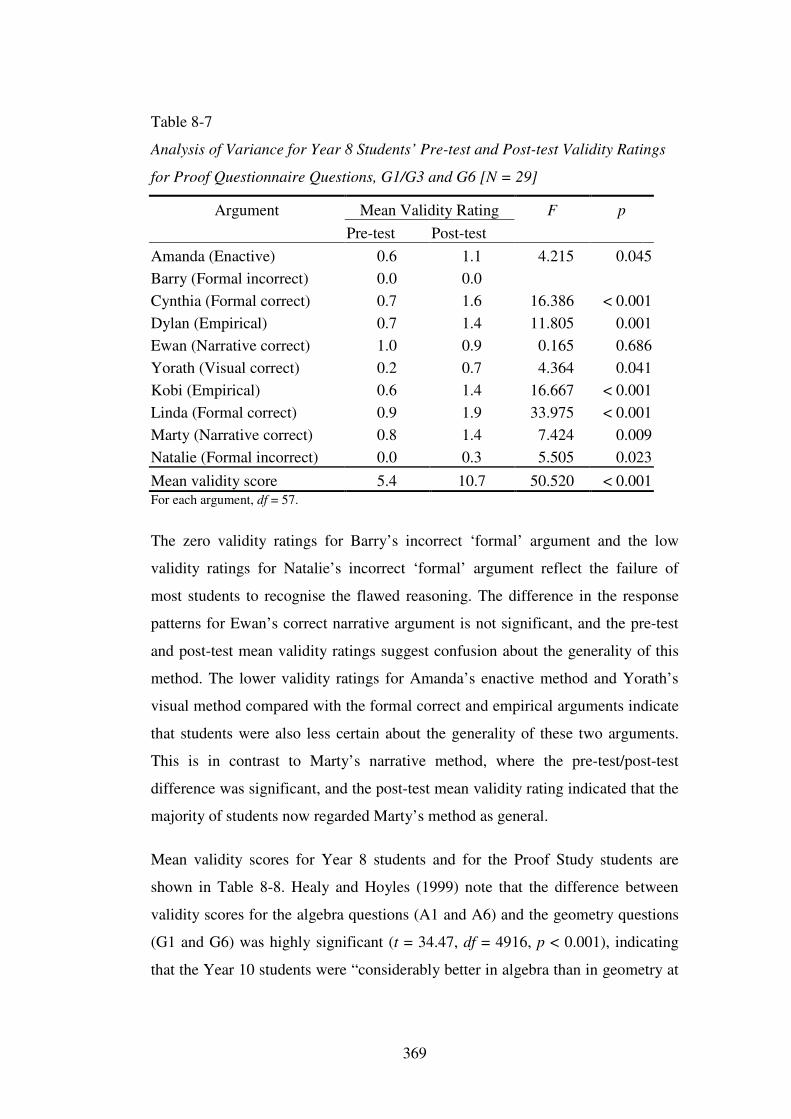
369
Table 8-7
Analysis of Variance for Year 8 Students’ Pre-test and Post-test Validity Ratings
for Proof Questionnaire Questions, G1/G3 and G6 [N = 29]
Argument Mean Validity Rating F p Pre-test Post-test Amanda (Enactive) 0.6 1.1 4.215 0.045 Barry (Formal incorrect) 0.0 0.0 Cynthia (Formal correct) 0.7 1.6 16.386 < 0.001 Dylan (Empirical) 0.7 1.4 11.805 0.001 Ewan (Narrative correct) 1.0 0.9 0.165 0.686 Yorath (Visual correct) 0.2 0.7 4.364 0.041 Kobi (Empirical) 0.6 1.4 16.667 < 0.001 Linda (Formal correct) 0.9 1.9 33.975 < 0.001 Marty (Narrative correct) 0.8 1.4 7.424 0.009 Natalie (Formal incorrect) 0.0 0.3 5.505 0.023 Mean validity score 5.4 10.7 50.520 < 0.001 For each argument, df = 57.
The zero validity ratings for Barry’s incorrect ‘formal’ argument and the low
validity ratings for Natalie’s incorrect ‘formal’ argument reflect the failure of
most students to recognise the flawed reasoning. The difference in the response
patterns for Ewan’s correct narrative argument is not significant, and the pre-test
and post-test mean validity ratings suggest confusion about the generality of this
method. The lower validity ratings for Amanda’s enactive method and Yorath’s
visual method compared with the formal correct and empirical arguments indicate
that students were also less certain about the generality of these two arguments.
This is in contrast to Marty’s narrative method, where the pre-test/post-test
difference was significant, and the post-test mean validity rating indicated that the
majority of students now regarded Marty’s method as general.
Mean validity scores for Year 8 students and for the Proof Study students are
shown in Table 8-8. Healy and Hoyles (1999) note that the difference between
validity scores for the algebra questions (A1 and A6) and the geometry questions
(G1 and G6) was highly significant (t = 34.47, df = 4916, p < 0.001), indicating
that the Year 10 students were “considerably better in algebra than in geometry at
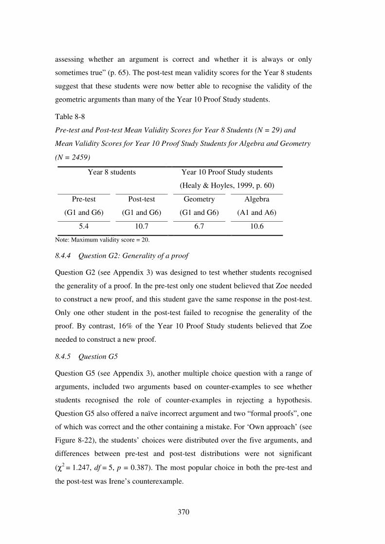
370
assessing whether an argument is correct and whether it is always or only
sometimes true” (p. 65). The post-test mean validity scores for the Year 8 students
suggest that these students were now better able to recognise the validity of the
geometric arguments than many of the Year 10 Proof Study students.
Table 8-8
Pre-test and Post-test Mean Validity Scores for Year 8 Students (N = 29) and
Mean Validity Scores for Year 10 Proof Study Students for Algebra and Geometry
(N = 2459)
Year 8 students Year 10 Proof Study students
(Healy & Hoyles, 1999, p. 60)
Pre-test
(G1 and G6)
Post-test
(G1 and G6)
Geometry
(G1 and G6)
Algebra
(A1 and A6)
5.4 10.7 6.7 10.6
Note: Maximum validity score = 20.
8.4.4 Question G2: Generality of a proof
Question G2 (see Appendix 3) was designed to test whether students recognised
the generality of a proof. In the pre-test only one student believed that Zoe needed
to construct a new proof, and this student gave the same response in the post-test.
Only one other student in the post-test failed to recognise the generality of the
proof. By contrast, 16% of the Year 10 Proof Study students believed that Zoe
needed to construct a new proof.
8.4.5 Question G5
Question G5 (see Appendix 3), another multiple choice question with a range of
arguments, included two arguments based on counter-examples to see whether
students recognised the role of counter-examples in rejecting a hypothesis.
Question G5 also offered a naïve incorrect argument and two “formal proofs”, one
of which was correct and the other containing a mistake. For ‘Own approach’ (see
Figure 8-22), the students’ choices were distributed over the five arguments, and
differences between pre-test and post-test distributions were not significant
(χ2 = 1.247, df = 5, p = 0.387). The most popular choice in both the pre-test and
the post-test was Irene’s counterexample.
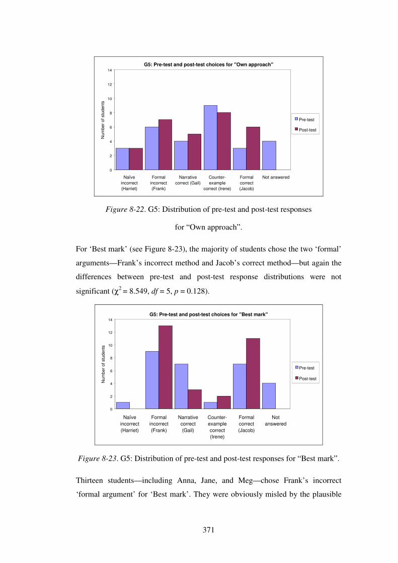
371
G5: Pre-test and post-test choices for "Own approach"
0
2
4
6
8
10
12
14
Naïveincorrect(Harriet)
Formalincorrect(Frank)
Narrativecorrect (Gail)
Counter-example
correct (Irene)
Formalcorrect(Jacob)
Not answered
Num
ber o
f stu
dent
s
Pre-test
Post-test
Figure 8-22. G5: Distribution of pre-test and post-test responses
for “Own approach”.
For ‘Best mark’ (see Figure 8-23), the majority of students chose the two ‘formal’
arguments—Frank’s incorrect method and Jacob’s correct method—but again the
differences between pre-test and post-test response distributions were not
significant (χ2 = 8.549, df = 5, p = 0.128).
G5: Pre-test and post-test choices for "Best mark"
0
2
4
6
8
10
12
14
Naïveincorrect(Harriet)
Formalincorrect(Frank)
Narrativecorrect(Gail)
Counter-examplecorrect(Irene)
Formalcorrect(Jacob)
Notanswered
Num
ber o
f stu
dent
s
Pre-test
Post-test
Figure 8-23. G5: Distribution of pre-test and post-test responses for “Best mark”.
Thirteen students—including Anna, Jane, and Meg—chose Frank’s incorrect
‘formal argument’ for ‘Best mark’. They were obviously misled by the plausible
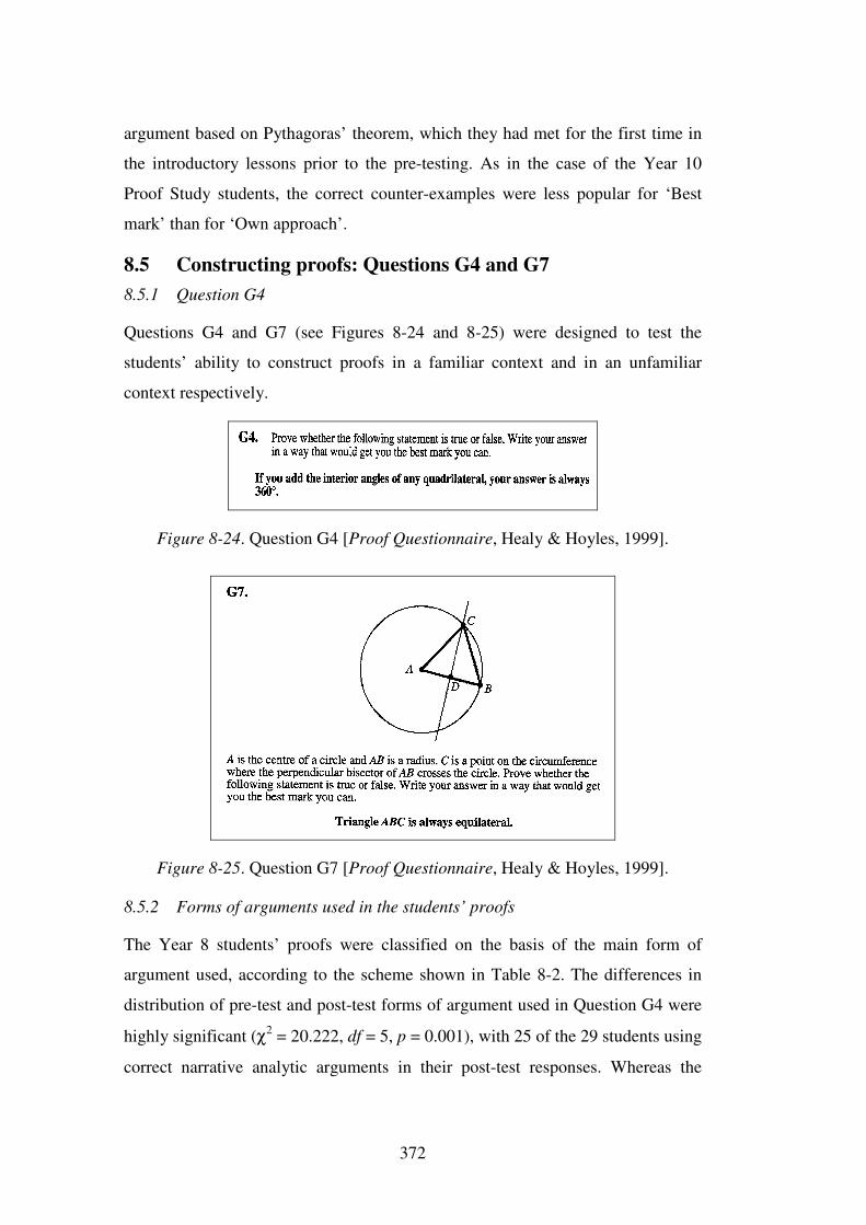
372
argument based on Pythagoras’ theorem, which they had met for the first time in
the introductory lessons prior to the pre-testing. As in the case of the Year 10
Proof Study students, the correct counter-examples were less popular for ‘Best
mark’ than for ‘Own approach’.
8.5 Constructing proofs: Questions G4 and G7 8.5.1 Question G4
Questions G4 and G7 (see Figures 8-24 and 8-25) were designed to test the
students’ ability to construct proofs in a familiar context and in an unfamiliar
context respectively.
Figure 8-24. Question G4 [Proof Questionnaire, Healy & Hoyles, 1999].
Figure 8-25. Question G7 [Proof Questionnaire, Healy & Hoyles, 1999].
8.5.2 Forms of arguments used in the students’ proofs
The Year 8 students’ proofs were classified on the basis of the main form of
argument used, according to the scheme shown in Table 8-2. The differences in
distribution of pre-test and post-test forms of argument used in Question G4 were
highly significant (χ2 = 20.222, df = 5, p = 0.001), with 25 of the 29 students using
correct narrative analytic arguments in their post-test responses. Whereas the
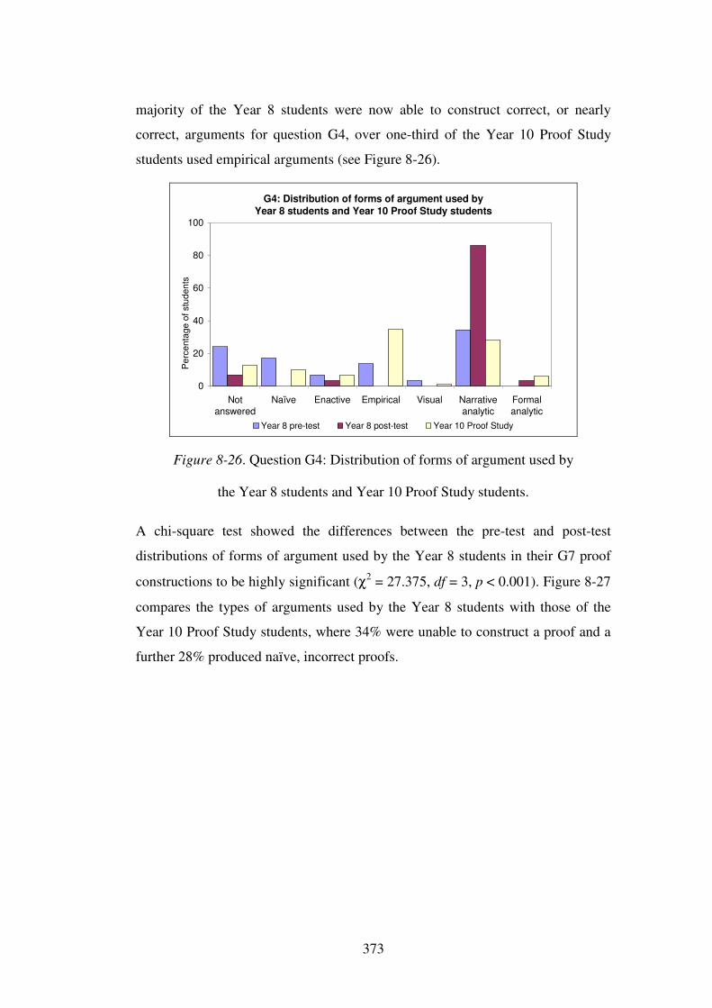
373
majority of the Year 8 students were now able to construct correct, or nearly
correct, arguments for question G4, over one-third of the Year 10 Proof Study
students used empirical arguments (see Figure 8-26).
G4: Distribution of forms of argument used by Year 8 students and Year 10 Proof Study students
0
20
40
60
80
100
Notanswered
Naïve Enactive Empirical Visual Narrativeanalytic
Formalanalytic
Year 8 pre-test Year 8 post-test Year 10 Proof Study
Per
cent
age
of s
tude
nts
Figure 8-26. Question G4: Distribution of forms of argument used by
the Year 8 students and Year 10 Proof Study students.
A chi-square test showed the differences between the pre-test and post-test
distributions of forms of argument used by the Year 8 students in their G7 proof
constructions to be highly significant (χ2 = 27.375, df = 3, p < 0.001). Figure 8-27
compares the types of arguments used by the Year 8 students with those of the
Year 10 Proof Study students, where 34% were unable to construct a proof and a
further 28% produced naïve, incorrect proofs.
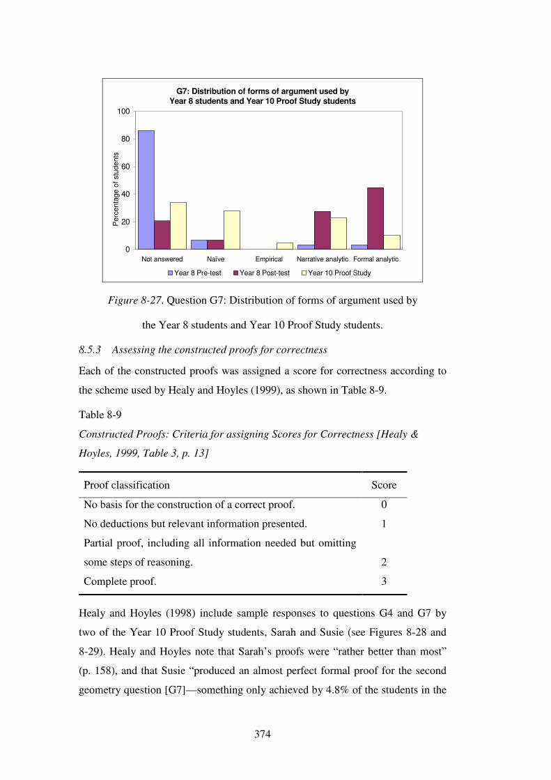
374
G7: Distribution of forms of argument used by Year 8 students and Year 10 Proof Study students
0
20
40
60
80
100
Not answered Naïve Empirical Narrative analytic Formal analytic
Year 8 Pre-test Year 8 Post-test Year 10 Proof Study
Per
cent
age
of s
tude
nts
Figure 8-27. Question G7: Distribution of forms of argument used by
the Year 8 students and Year 10 Proof Study students.
8.5.3 Assessing the constructed proofs for correctness
Each of the constructed proofs was assigned a score for correctness according to
the scheme used by Healy and Hoyles (1999), as shown in Table 8-9.
Table 8-9
Constructed Proofs: Criteria for assigning Scores for Correctness [Healy &
Hoyles, 1999, Table 3, p. 13]
Proof classification Score
No basis for the construction of a correct proof. 0
No deductions but relevant information presented. 1
Partial proof, including all information needed but omitting
some steps of reasoning.
2
Complete proof. 3
Healy and Hoyles (1998) include sample responses to questions G4 and G7 by
two of the Year 10 Proof Study students, Sarah and Susie (see Figures 8-28 and
8-29). Healy and Hoyles note that Sarah’s proofs were “rather better than most”
(p. 158), and that Susie “produced an almost perfect formal proof for the second
geometry question [G7]—something only achieved by 4.8% of the students in the
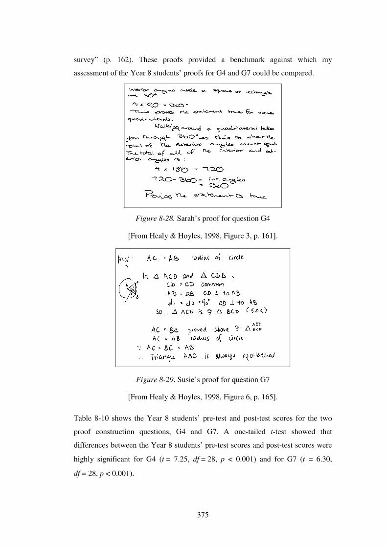
375
survey” (p. 162). These proofs provided a benchmark against which my
assessment of the Year 8 students’ proofs for G4 and G7 could be compared.
Figure 8-28. Sarah’s proof for question G4
[From Healy & Hoyles, 1998, Figure 3, p. 161].
Figure 8-29. Susie’s proof for question G7
[From Healy & Hoyles, 1998, Figure 6, p. 165].
Table 8-10 shows the Year 8 students’ pre-test and post-test scores for the two
proof construction questions, G4 and G7. A one-tailed t-test showed that
differences between the Year 8 students’ pre-test scores and post-test scores were
highly significant for G4 (t = 7.25, df = 28, p < 0.001) and for G7 (t = 6.30,
df = 28, p < 0.001).
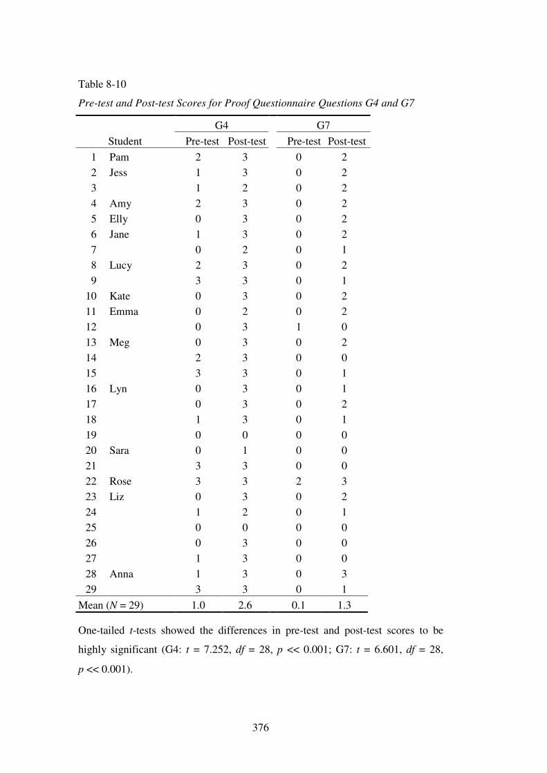
376
Table 8-10
Pre-test and Post-test Scores for Proof Questionnaire Questions G4 and G7
G4 G7 Student Pre-test Post-test Pre-test Post-test
1 Pam 2 3 0 2 2 Jess 1 3 0 2 3 1 2 0 2 4 Amy 2 3 0 2 5 Elly 0 3 0 2 6 Jane 1 3 0 2 7 0 2 0 1 8 Lucy 2 3 0 2 9 3 3 0 1
10 Kate 0 3 0 2 11 Emma 0 2 0 2 12 0 3 1 0 13 Meg 0 3 0 2 14 2 3 0 0 15 3 3 0 1 16 Lyn 0 3 0 1 17 0 3 0 2 18 1 3 0 1 19 0 0 0 0 20 Sara 0 1 0 0 21 3 3 0 0 22 Rose 3 3 2 3 23 Liz 0 3 0 2 24 1 2 0 1 25 0 0 0 0 26 0 3 0 0 27 1 3 0 0 28 Anna 1 3 0 3 29 3 3 0 1
Mean (N = 29) 1.0 2.6 0.1 1.3
One-tailed t-tests showed the differences in pre-test and post-test scores to be
highly significant (G4: t = 7.252, df = 28, p << 0.001; G7: t = 6.601, df = 28,
p << 0.001).
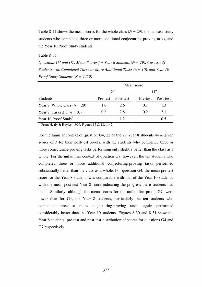
377
Table 8-11 shows the mean scores for the whole class (N = 29), the ten case study
students who completed three or more additional conjecturing-proving tasks, and
the Year 10 Proof Study students.
Table 8-11
Questions G4 and G7: Mean Scores for Year 8 Students (N = 29), Case Study
Students who Completed Three or More Additional Tasks (n = 10), and Year 10
Proof Study Students (N = 2459)
Mean score
G4 G7
Students Pre-test Post-test Pre-test Post-test
Year 8: Whole class (N = 29) 1.0 2.6 0.1 1.3
Year 8: Tasks ≥ 3 (n = 10) 0.8 2.8 0.2 2.1
Year 10 Proof Study1 1.2 0.5 1 From Healy & Hoyles, 1999, Figures 17 & 18, p. 42.
For the familiar context of question G4, 22 of the 29 Year 8 students were given
scores of 3 for their post-test proofs, with the students who completed three or
more conjecturing-proving tasks performing only slightly better than the class as a
whole. For the unfamiliar context of question G7, however, the ten students who
completed three or more additional conjecturing-proving tasks performed
substantially better than the class as a whole. For question G4, the mean pre-test
score for the Year 8 students was comparable with that of the Year 10 students,
with the mean post-test Year 8 score indicating the progress these students had
made. Similarly, although the mean scores for the unfamiliar proof, G7, were
lower than for G4, the Year 8 students, particularly the ten students who
completed three or more conjecturing-proving tasks, again performed
considerably better than the Year 10 students. Figures 8-30 and 8-31 show the
Year 8 students’ pre-test and post-test distribution of scores for questions G4 and
G7 respectively.
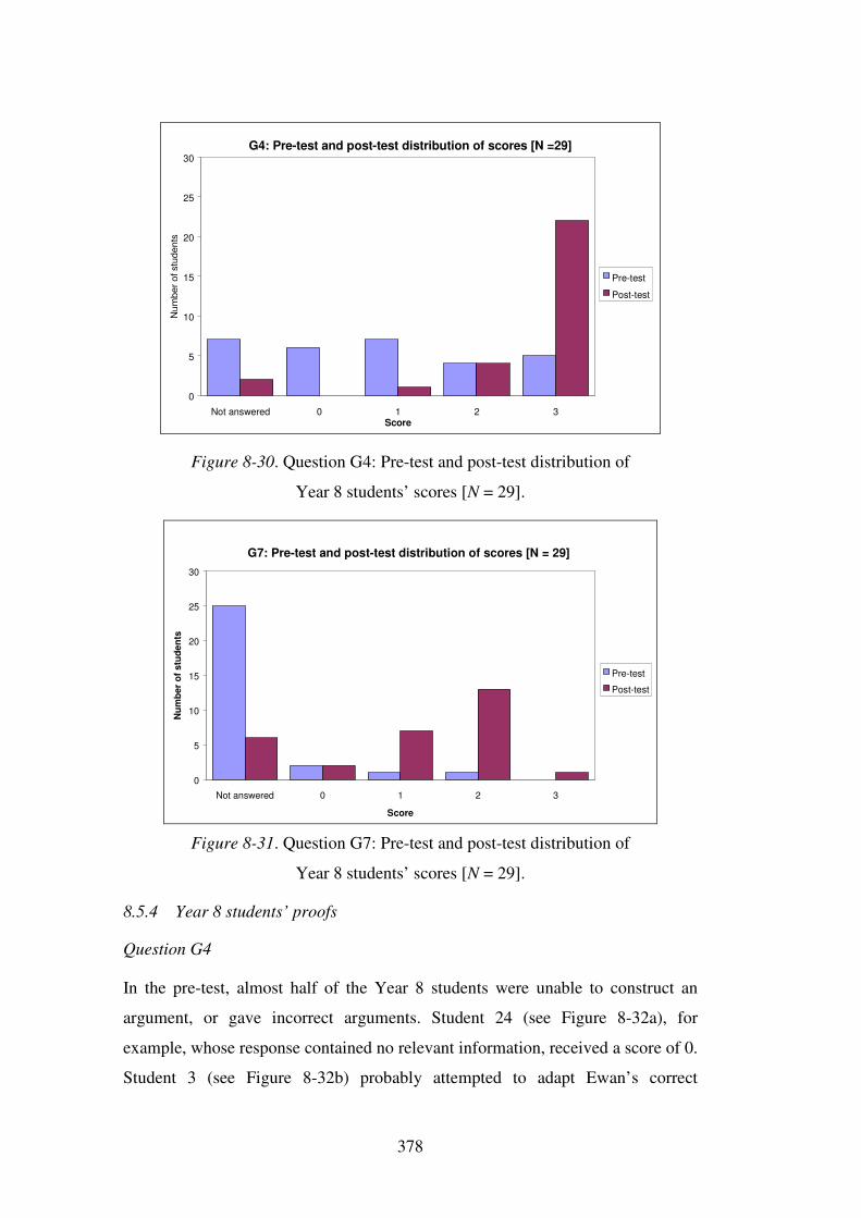
378
G4: Pre-test and post-test distribution of scores [N =29]
0
5
10
15
20
25
30
Not answered 0 1 2 3Score
Pre-test
Post-test
Num
ber o
f stu
dent
s
Figure 8-30. Question G4: Pre-test and post-test distribution of
Year 8 students’ scores [N = 29].
G7: Pre-test and post-test distribution of scores [N = 29]
0
5
10
15
20
25
30
Not answered 0 1 2 3
Score
Num
ber
of s
tude
nts
Pre-test
Post-test
Figure 8-31. Question G7: Pre-test and post-test distribution of
Year 8 students’ scores [N = 29].
8.5.4 Year 8 students’ proofs
Question G4
In the pre-test, almost half of the Year 8 students were unable to construct an
argument, or gave incorrect arguments. Student 24 (see Figure 8-32a), for
example, whose response contained no relevant information, received a score of 0.
Student 3 (see Figure 8-32b) probably attempted to adapt Ewan’s correct
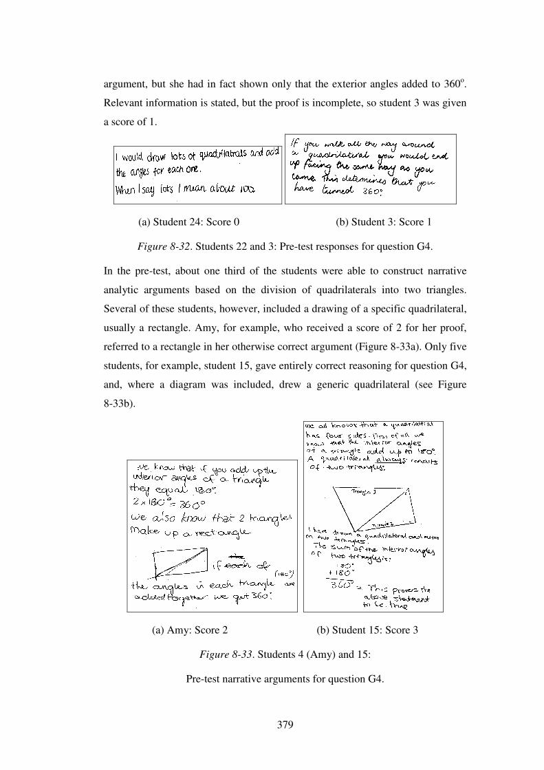
379
argument, but she had in fact shown only that the exterior angles added to 360o.
Relevant information is stated, but the proof is incomplete, so student 3 was given
a score of 1.
(a) Student 24: Score 0 (b) Student 3: Score 1
Figure 8-32. Students 22 and 3: Pre-test responses for question G4.
In the pre-test, about one third of the students were able to construct narrative
analytic arguments based on the division of quadrilaterals into two triangles.
Several of these students, however, included a drawing of a specific quadrilateral,
usually a rectangle. Amy, for example, who received a score of 2 for her proof,
referred to a rectangle in her otherwise correct argument (Figure 8-33a). Only five
students, for example, student 15, gave entirely correct reasoning for question G4,
and, where a diagram was included, drew a generic quadrilateral (see Figure
8-33b).
(a) Amy: Score 2 (b) Student 15: Score 3
Figure 8-33. Students 4 (Amy) and 15:
Pre-test narrative arguments for question G4.
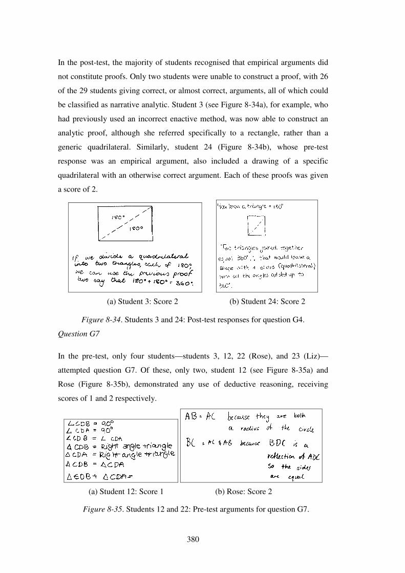
380
In the post-test, the majority of students recognised that empirical arguments did
not constitute proofs. Only two students were unable to construct a proof, with 26
of the 29 students giving correct, or almost correct, arguments, all of which could
be classified as narrative analytic. Student 3 (see Figure 8-34a), for example, who
had previously used an incorrect enactive method, was now able to construct an
analytic proof, although she referred specifically to a rectangle, rather than a
generic quadrilateral. Similarly, student 24 (Figure 8-34b), whose pre-test
response was an empirical argument, also included a drawing of a specific
quadrilateral with an otherwise correct argument. Each of these proofs was given
a score of 2.
(a) Student 3: Score 2 (b) Student 24: Score 2
Figure 8-34. Students 3 and 24: Post-test responses for question G4.
Question G7
In the pre-test, only four students—students 3, 12, 22 (Rose), and 23 (Liz)—
attempted question G7. Of these, only two, student 12 (see Figure 8-35a) and
Rose (Figure 8-35b), demonstrated any use of deductive reasoning, receiving
scores of 1 and 2 respectively.
(a) Student 12: Score 1 (b) Rose: Score 2
Figure 8-35. Students 12 and 22: Pre-test arguments for question G7.
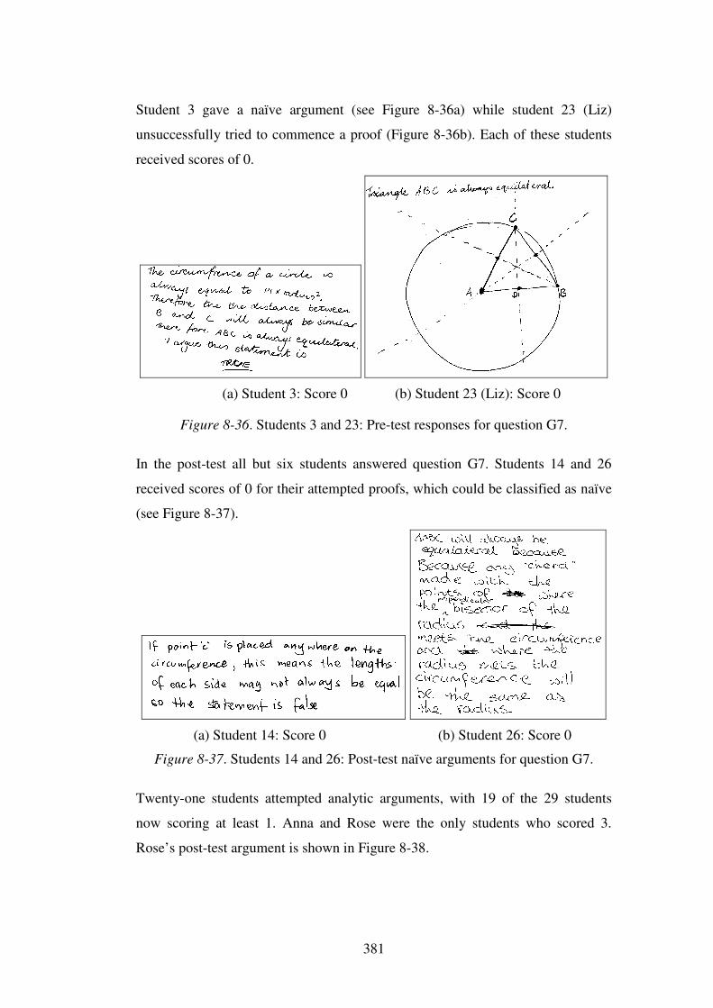
381
Student 3 gave a naïve argument (see Figure 8-36a) while student 23 (Liz)
unsuccessfully tried to commence a proof (Figure 8-36b). Each of these students
received scores of 0.
(a) Student 3: Score 0 (b) Student 23 (Liz): Score 0
Figure 8-36. Students 3 and 23: Pre-test responses for question G7.
In the post-test all but six students answered question G7. Students 14 and 26
received scores of 0 for their attempted proofs, which could be classified as naïve
(see Figure 8-37).
(a) Student 14: Score 0 (b) Student 26: Score 0
Figure 8-37. Students 14 and 26: Post-test naïve arguments for question G7.
Twenty-one students attempted analytic arguments, with 19 of the 29 students
now scoring at least 1. Anna and Rose were the only students who scored 3.
Rose’s post-test argument is shown in Figure 8-38.
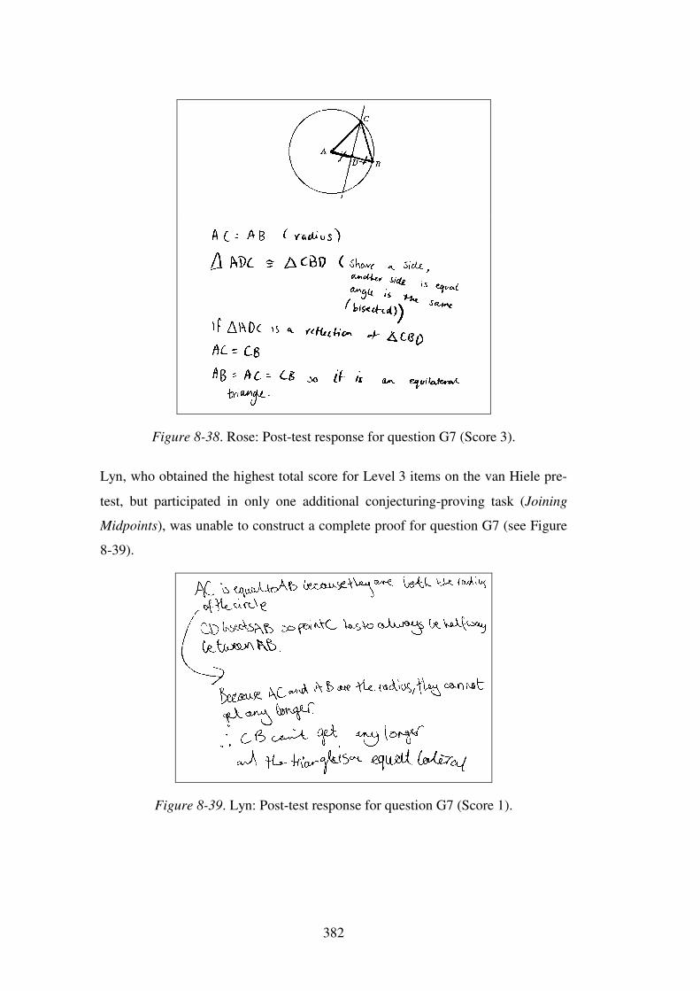
382
Figure 8-38. Rose: Post-test response for question G7 (Score 3).
Lyn, who obtained the highest total score for Level 3 items on the van Hiele pre-
test, but participated in only one additional conjecturing-proving task (Joining
Midpoints), was unable to construct a complete proof for question G7 (see Figure
8-39).
Figure 8-39. Lyn: Post-test response for question G7 (Score 1).
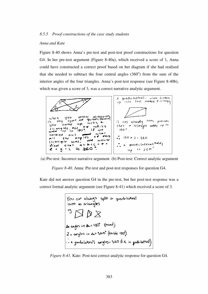
383
8.5.5 Proof constructions of the case study students
Anna and Kate
Figure 8-40 shows Anna’s pre-test and post-test proof constructions for question
G4. In her pre-test argument (Figure 8-40a), which received a score of 1, Anna
could have constructed a correct proof based on her diagram if she had realised
that she needed to subtract the four central angles (360o) from the sum of the
interior angles of the four triangles. Anna’s post-test response (see Figure 8-40b),
which was given a score of 3, was a correct narrative analytic argument.
(a) Pre-test: Incorrect narrative argument (b) Post-test: Correct analytic argument
Figure 8-40. Anna: Pre-test and post-test responses for question G4.
Kate did not answer question G4 in the pre-test, but her post-test response was a
correct formal analytic argument (see Figure 8-41) which received a score of 3.
Figure 8-41. Kate: Post-test correct analytic response for question G4.
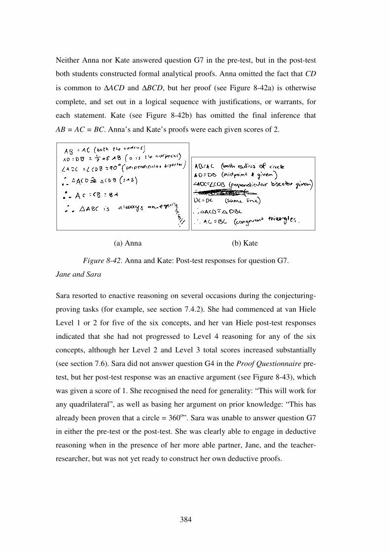
384
Neither Anna nor Kate answered question G7 in the pre-test, but in the post-test
both students constructed formal analytical proofs. Anna omitted the fact that CD
is common to ∆ACD and ∆BCD, but her proof (see Figure 8-42a) is otherwise
complete, and set out in a logical sequence with justifications, or warrants, for
each statement. Kate (see Figure 8-42b) has omitted the final inference that
AB = AC = BC. Anna’s and Kate’s proofs were each given scores of 2.
(a) Anna (b) Kate
Figure 8-42. Anna and Kate: Post-test responses for question G7.
Jane and Sara
Sara resorted to enactive reasoning on several occasions during the conjecturing-
proving tasks (for example, see section 7.4.2). She had commenced at van Hiele
Level 1 or 2 for five of the six concepts, and her van Hiele post-test responses
indicated that she had not progressed to Level 4 reasoning for any of the six
concepts, although her Level 2 and Level 3 total scores increased substantially
(see section 7.6). Sara did not answer question G4 in the Proof Questionnaire pre-
test, but her post-test response was an enactive argument (see Figure 8-43), which
was given a score of 1. She recognised the need for generality: “This will work for
any quadrilateral”, as well as basing her argument on prior knowledge: “This has
already been proven that a circle = 360o”. Sara was unable to answer question G7
in either the pre-test or the post-test. She was clearly able to engage in deductive
reasoning when in the presence of her more able partner, Jane, and the teacher-
researcher, but was not yet ready to construct her own deductive proofs.
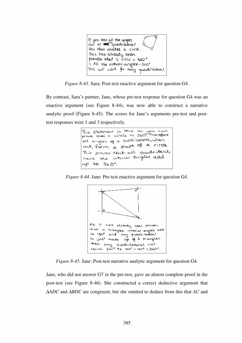
385
Figure 8-43. Sara: Post-test enactive argument for question G4.
By contrast, Sara’s partner, Jane, whose pre-test response for question G4 was an
enactive argument (see Figure 8-44), was now able to construct a narrative
analytic proof (Figure 8-45). The scores for Jane’s arguments pre-test and post-
test responses were 1 and 3 respectively.
Figure 8-44. Jane: Pre-test enactive argument for question G4.
Figure 8-45. Jane: Post-test narrative analytic argument for question G4.
Jane, who did not answer G7 in the pre-test, gave an almost complete proof in the
post-test (see Figure 8-46). She constructed a correct deductive argument that
∆ADC and ∆BDC are congruent, but she omitted to deduce from this that AC and
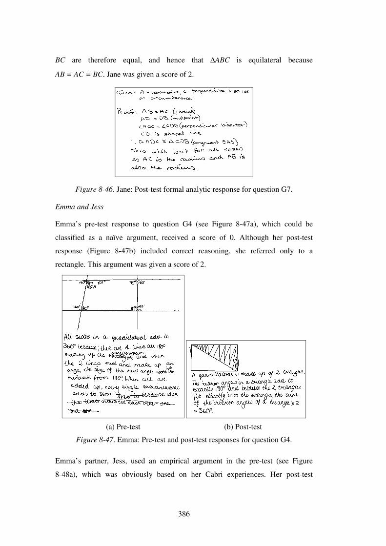
386
BC are therefore equal, and hence that ∆ABC is equilateral because
AB = AC = BC. Jane was given a score of 2.
Figure 8-46. Jane: Post-test formal analytic response for question G7.
Emma and Jess
Emma’s pre-test response to question G4 (see Figure 8-47a), which could be
classified as a naïve argument, received a score of 0. Although her post-test
response (Figure 8-47b) included correct reasoning, she referred only to a
rectangle. This argument was given a score of 2.
(a) Pre-test (b) Post-test
Figure 8-47. Emma: Pre-test and post-test responses for question G4.
Emma’s partner, Jess, used an empirical argument in the pre-test (see Figure
8-48a), which was obviously based on her Cabri experiences. Her post-test
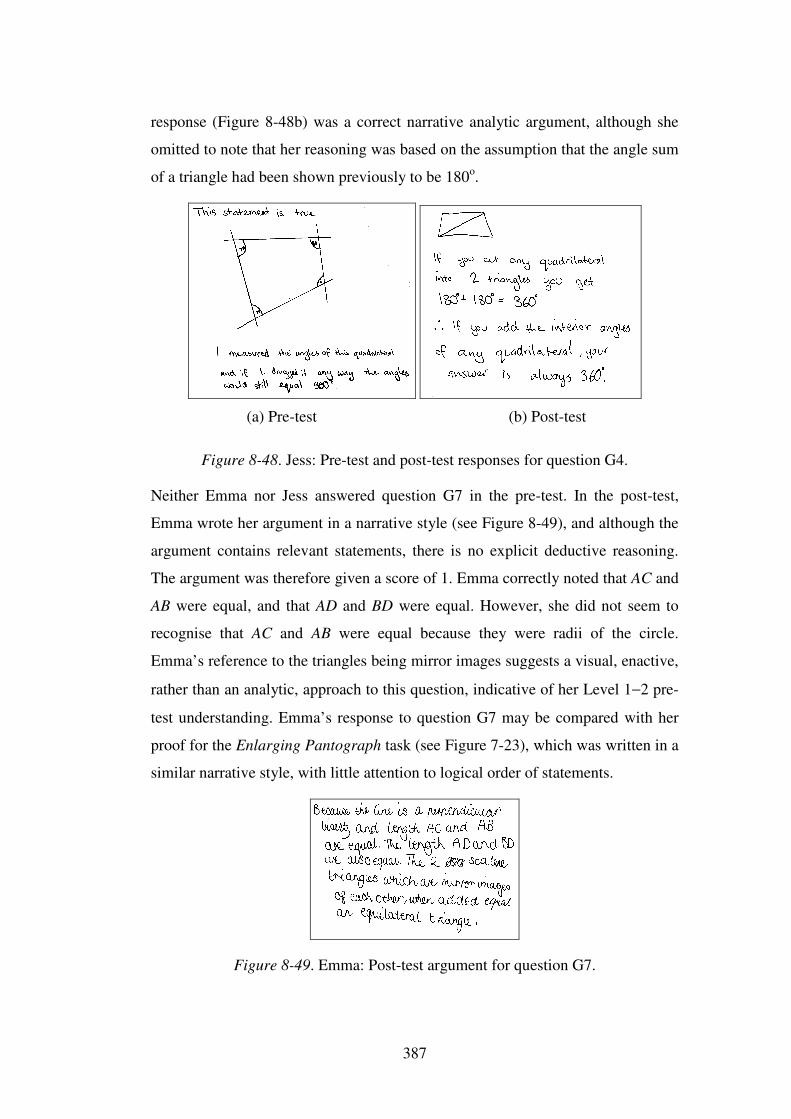
387
response (Figure 8-48b) was a correct narrative analytic argument, although she
omitted to note that her reasoning was based on the assumption that the angle sum
of a triangle had been shown previously to be 180o.
(a) Pre-test (b) Post-test
Figure 8-48. Jess: Pre-test and post-test responses for question G4.
Neither Emma nor Jess answered question G7 in the pre-test. In the post-test,
Emma wrote her argument in a narrative style (see Figure 8-49), and although the
argument contains relevant statements, there is no explicit deductive reasoning.
The argument was therefore given a score of 1. Emma correctly noted that AC and
AB were equal, and that AD and BD were equal. However, she did not seem to
recognise that AC and AB were equal because they were radii of the circle.
Emma’s reference to the triangles being mirror images suggests a visual, enactive,
rather than an analytic, approach to this question, indicative of her Level 1−2 pre-
test understanding. Emma’s response to question G7 may be compared with her
proof for the Enlarging Pantograph task (see Figure 7-23), which was written in a
similar narrative style, with little attention to logical order of statements.
Figure 8-49. Emma: Post-test argument for question G7.
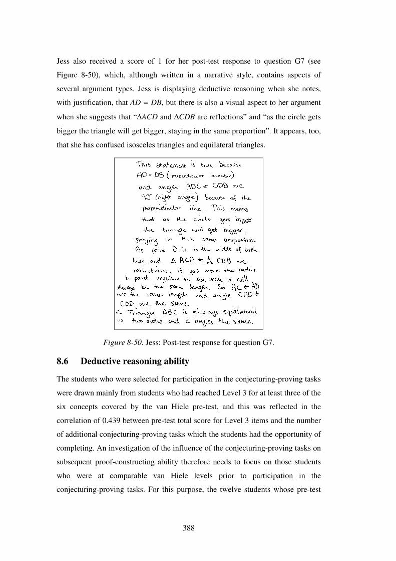
388
Jess also received a score of 1 for her post-test response to question G7 (see
Figure 8-50), which, although written in a narrative style, contains aspects of
several argument types. Jess is displaying deductive reasoning when she notes,
with justification, that AD = DB, but there is also a visual aspect to her argument
when she suggests that “∆ACD and ∆CDB are reflections” and “as the circle gets
bigger the triangle will get bigger, staying in the same proportion”. It appears, too,
that she has confused isosceles triangles and equilateral triangles.
Figure 8-50. Jess: Post-test response for question G7.
8.6 Deductive reasoning ability
The students who were selected for participation in the conjecturing-proving tasks
were drawn mainly from students who had reached Level 3 for at least three of the
six concepts covered by the van Hiele pre-test, and this was reflected in the
correlation of 0.439 between pre-test total score for Level 3 items and the number
of additional conjecturing-proving tasks which the students had the opportunity of
completing. An investigation of the influence of the conjecturing-proving tasks on
subsequent proof-constructing ability therefore needs to focus on those students
who were at comparable van Hiele levels prior to participation in the
conjecturing-proving tasks. For this purpose, the twelve students whose pre-test
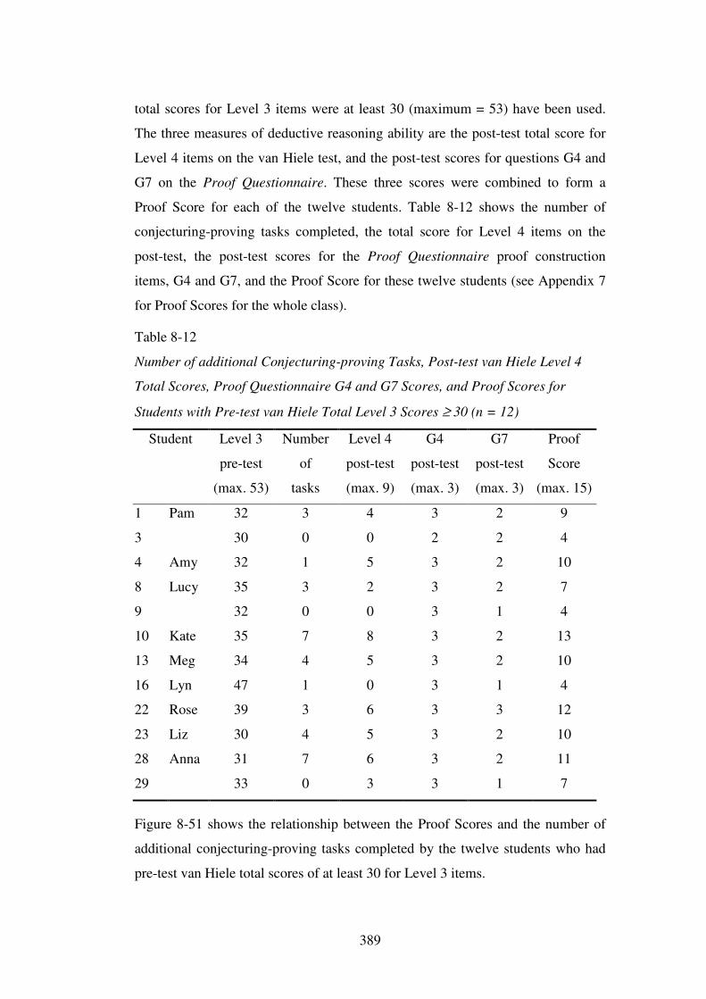
389
total scores for Level 3 items were at least 30 (maximum = 53) have been used.
The three measures of deductive reasoning ability are the post-test total score for
Level 4 items on the van Hiele test, and the post-test scores for questions G4 and
G7 on the Proof Questionnaire. These three scores were combined to form a
Proof Score for each of the twelve students. Table 8-12 shows the number of
conjecturing-proving tasks completed, the total score for Level 4 items on the
post-test, the post-test scores for the Proof Questionnaire proof construction
items, G4 and G7, and the Proof Score for these twelve students (see Appendix 7
for Proof Scores for the whole class).
Table 8-12
Number of additional Conjecturing-proving Tasks, Post-test van Hiele Level 4
Total Scores, Proof Questionnaire G4 and G7 Scores, and Proof Scores for
Students with Pre-test van Hiele Total Level 3 Scores ≥ 30 (n = 12)
Student Level 3
pre-test
(max. 53)
Number
of
tasks
Level 4
post-test
(max. 9)
G4
post-test
(max. 3)
G7
post-test
(max. 3)
Proof
Score
(max. 15)
1 Pam 32 3 4 3 2 9
3 30 0 0 2 2 4
4 Amy 32 1 5 3 2 10
8 Lucy 35 3 2 3 2 7
9 32 0 0 3 1 4
10 Kate 35 7 8 3 2 13
13 Meg 34 4 5 3 2 10
16 Lyn 47 1 0 3 1 4
22 Rose 39 3 6 3 3 12
23 Liz 30 4 5 3 2 10
28 Anna 31 7 6 3 2 11
29 33 0 3 3 1 7
Figure 8-51 shows the relationship between the Proof Scores and the number of
additional conjecturing-proving tasks completed by the twelve students who had
pre-test van Hiele total scores of at least 30 for Level 3 items.
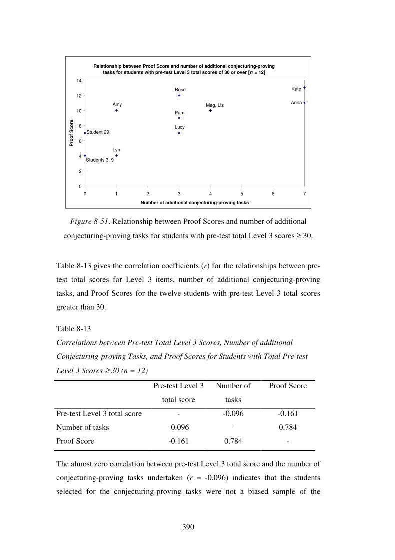
390
Relationship between Proof Score and number of additional conjecturing-proving tasks for students with pre-test Level 3 total scores of 30 or over [n = 12]
0
2
4
6
8
10
12
14
0 1 2 3 4 5 6 7
Number of additional conjecturing-proving tasks
Pro
of S
core
Kate
AnnaMeg, Liz
Lucy
Pam
Rose
Amy
Lyn
Students 3, 9
Student 29
Figure 8-51. Relationship between Proof Scores and number of additional
conjecturing-proving tasks for students with pre-test total Level 3 scores ≥ 30.
Table 8-13 gives the correlation coefficients (r) for the relationships between pre-
test total scores for Level 3 items, number of additional conjecturing-proving
tasks, and Proof Scores for the twelve students with pre-test Level 3 total scores
greater than 30.
Table 8-13
Correlations between Pre-test Total Level 3 Scores, Number of additional
Conjecturing-proving Tasks, and Proof Scores for Students with Total Pre-test
Level 3 Scores ≥ 30 (n = 12)
Pre-test Level 3
total score
Number of
tasks
Proof Score
Pre-test Level 3 total score - -0.096 -0.161
Number of tasks -0.096 - 0.784
Proof Score -0.161 0.784 -
The almost zero correlation between pre-test Level 3 total score and the number of
conjecturing-proving tasks undertaken (r = -0.096) indicates that the students
selected for the conjecturing-proving tasks were not a biased sample of the
391
students who scored at least 30 for the Level 3 pre-test van Hiele items. The
correlation between the pre-test total scores for van Hiele Level 3 items and the
Proof Score (r = -0.161) indicates that for this group of twelve students a higher
total pre-test score for Level 3 items did not guarantee greater success in
independent proof construction. However, the moderately strong correlation
(r = 0.784) between the number of additional conjecturing-proving tasks
undertaken and the students’ Proof Scores suggests that participation in these
tasks did result in transferable independent proof-construction skills.
8.7 Conclusion
The students’ pre-test and post-test responses to the Proof Questionnaire suggest
that their views of proof had been influenced by their experiences in the
conjecturing-proving lessons. In their descriptions of mathematical proof, most
students referred initially to the purpose of proof, for example, the verifying or
explanatory roles. However, in their post-test responses, many students referred to
the process of proving and to the generality of a proof. There were also significant
differences between the students’ pre-test and post-test ability to recognise correct
proofs, and to construct proofs, particularly amongst those students who had
participated in the additional conjecturing-proving tasks. In the pre-test, many
students had chosen empirical, enactive, or incorrect arguments in the multiple
choice questions, G1, G5, and G6, but after participating in the conjecturing-
proving lessons, the majority of students were able to recognise a correct proof.
Almost all students now accepted that an empirical argument did not constitute a
proof. As well as making appropriate choices for the arguments which would
receive the best mark, more students were also selecting correct arguments for the
method which would be closest to what they would have done. It should be borne
in mind, however, that the proof lessons may have over-emphasised deductive
proofs, so that some students possibly gained the impression that these were the
only correct proofs.
Prior to the conjecturing-proving lessons, very few students were able to construct
a proof, either in the familiar context of question G4—the angle sum of a
triangle—or in the unfamiliar context of question G7. In the post-test, the majority
392
of students in the class could construct a simple proof for question G4, although
the students who constructed correct, or almost correct, proofs for question G7
were predominantly the case study students who had been at Level 3 for at least
three of the six concepts of the van Hiele pre-test. These students were able to
construct their proofs logically with justifications for their statements,
demonstrating that they had developed an understanding of the requirements of
deductive reasoning.
Emma and Jess, two of the van Hiele Level 1−2 case study students, recognised in
their post-test responses that relationships between properties formed the basis of
proving. Although they were able to construct the simple proof for question G4
(see Figures 8-47b and 8-48b), however, they were unable to order their
statements logically in the multi-step proof in question G7 (see Figures 8-49 and
8-50). This lends support to the claim by Senk (1989, p. 319) that “Level 2
appears to be the critical entry level” for students to be successful in proof
construction. Sara, who was also at van Hiele Level 1 for three of the six pre-test
concepts, in the Proof Questionnaire post-test used an enactive argument for
question G4 (see Figure 8-43) and was unable to answer question G7, despite
having participated in four conjecturing-proving tasks. By contrast, Jane, who was
at Level 2 for all six pre-test concepts, wrote a complete proof for question G4
(see Figure 8-45), and an almost complete deductive proof for question G7
(Figure 8-46) in the Proof Questionnaire post-test.
The strength of the correlation between scores for the Proof Questionnaire proof
construction questions—G4 and G7—and the number of additional conjecturing-
proving tasks supports the view that the tasks were successful in developing
students’ understanding of deductive reasoning, and that the skills acquired in
these tasks were able to be transferred to independent proof constructions. The
ability of these students to construct valid proofs in the contexts of questions G4
and G7 surpassed that of many of the Year 10 Proof Study students. Even those
Year 8 students who were at lower pre-test van Hiele levels acquired some
understanding of deductive reasoning through their participation in the
conjecturing-proving tasks, and were able to construct partially correct proofs,
393
particularly in the familiar context of question G4. It is reasonable to assume that
the conjecturing-proving lessons had promoted a culture of proving for the Year 8
students.

395
Chapter 9: Discussion and Conclusions
Proof is not merely to support conviction, nor to respond to a distrustful nature of
self-doubt, nor to be done as part of an obsessive ritual. Proof serves to provide
explanation, and therefore is a central technique in research. … In real life, both in
and out of mathematics, the distinction between empirical and theoretical
investigations breaks down: We must move back and forth between “doing stuff”
and understanding what we have done. Seen in this way, proof (or at least the
precursors to proof) is a natural step in satisfying curiosity to understand what we
have observed. (Goldenberg, Cuoco, & Mark, 1998, p. 42)
9.1 Introduction
This chapter discusses the research findings and the conclusions that can be drawn
from these. Section 9.2 discusses issues associated with the research: the role of
teacher intervention in the argumentations, proof as explanation in the context of
the linkage tasks, Toulmin’s argument model and the argumentation profile charts
as tools in analysing the argumentations, and limitations of the research. Section
9.3 relates the findings to the research questions, discussing the motivational
engagement of the students, their need for conviction, the role of static and
dynamic feedback from the linkage models, the relationship between the students’
level of geometric understanding and their ability to engage in conjecturing and
proving, the influence of the processes of conjecturing and argumentation on the
students’ ability to construct proofs, and evidence that a culture of proving was
developing in the Year 8 class. Section 9.4 then considers the overall conclusions
that can be drawn from the research, and the implications of the findings for the
teaching and learning of mathematical proof.
9.2 Issues associated with the research
9.2.1 The role of teacher intervention
As discussed in sections 2.3.2 and 4.5.3, teacher intervention is essential in
learning situations where students are encouraged to interact and engage in
argumentations. Boero’s (1999) claim that “the development of Toulmin-type …
argumentations calls for very strong teacher mediation” (p. 1) is highly relevant in
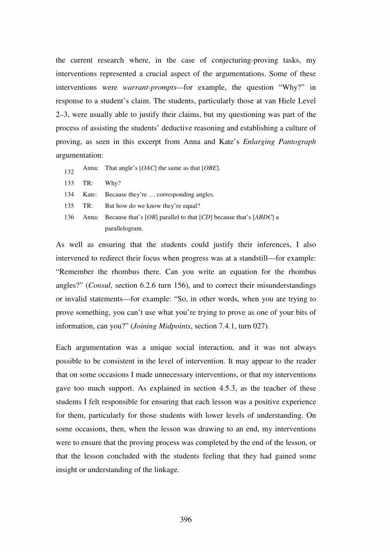
396
the current research where, in the case of conjecturing-proving tasks, my
interventions represented a crucial aspect of the argumentations. Some of these
interventions were warrant-prompts—for example, the question “Why?” in
response to a student’s claim. The students, particularly those at van Hiele Level
2–3, were usually able to justify their claims, but my questioning was part of the
process of assisting the students’ deductive reasoning and establishing a culture of
proving, as seen in this excerpt from Anna and Kate’s Enlarging Pantograph
argumentation:
132 Anna: That angle’s [OAC] the same as that [OBE].
133 TR: Why?
134 Kate: Because they’re … corresponding angles.
135 TR: But how do we know they’re equal?
136 Anna: Because that’s [OB] parallel to that [CD] because that’s [ABDC] a
parallelogram.
As well as ensuring that the students could justify their inferences, I also
intervened to redirect their focus when progress was at a standstill—for example:
“Remember the rhombus there. Can you write an equation for the rhombus
angles?” (Consul, section 6.2.6 turn 156), and to correct their misunderstandings
or invalid statements—for example: “So, in other words, when you are trying to
prove something, you can’t use what you’re trying to prove as one of your bits of
information, can you?” (Joining Midpoints, section 7.4.1, turn 027).
Each argumentation was a unique social interaction, and it was not always
possible to be consistent in the level of intervention. It may appear to the reader
that on some occasions I made unnecessary interventions, or that my interventions
gave too much support. As explained in section 4.5.3, as the teacher of these
students I felt responsible for ensuring that each lesson was a positive experience
for them, particularly for those students with lower levels of understanding. On
some occasions, then, when the lesson was drawing to an end, my interventions
were to ensure that the proving process was completed by the end of the lesson, or
that the lesson concluded with the students feeling that they had gained some
insight or understanding of the linkage.
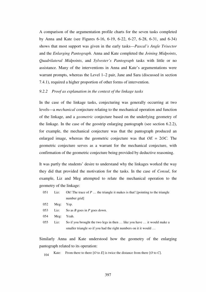
397
A comparison of the argumentation profile charts for the seven tasks completed
by Anna and Kate (see Figures 6-16, 6-19, 6-22, 6-27, 6-28, 6-31, and 6-34)
shows that most support was given in the early tasks—Pascal’s Angle Trisector
and the Enlarging Pantograph. Anna and Kate completed the Joining Midpoints,
Quadrilateral Midpoints, and Sylvester’s Pantograph tasks with little or no
assistance. Many of the interventions in Anna and Kate’s argumentations were
warrant prompts, whereas the Level 1–2 pair, Jane and Sara (discussed in section
7.4.1), required a higher proportion of other forms of intervention.
9.2.2 Proof as explanation in the context of the linkage tasks
In the case of the linkage tasks, conjecturing was generally occurring at two
levels—a mechanical conjecture relating to the mechanical operation and function
of the linkage, and a geometric conjecture based on the underlying geometry of
the linkage. In the case of the geostrip enlarging pantograph (see section 6.2.2),
for example, the mechanical conjecture was that the pantograph produced an
enlarged image, whereas the geometric conjecture was that OE = 2OC. The
geometric conjecture serves as a warrant for the mechanical conjecture, with
confirmation of the geometric conjecture being provided by deductive reasoning.
It was partly the students’ desire to understand why the linkages worked the way
they did that provided the motivation for the tasks. In the case of Consul, for
example, Liz and Meg attempted to relate the mechanical operation to the
geometry of the linkage:
051 Liz: Oh! The trace of P … the triangle it makes is that! [pointing to the triangle
number grid]
052 Meg: Yep.
053 Liz: So as B goes in P goes down.
054 Meg: Yeah.
055 Liz: So if you brought the two legs in then … like you have … it would make a
smaller triangle so if you had the right numbers on it it would …
Similarly Anna and Kate understood how the geometry of the enlarging
pantograph related to its operation:
104 Kate: From there to there [O to E] is twice the distance from there [O to C].
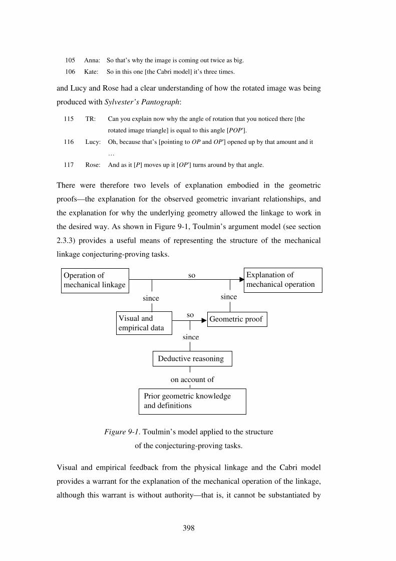
398
105 Anna: So that’s why the image is coming out twice as big.
106 Kate: So in this one [the Cabri model] it’s three times.
and Lucy and Rose had a clear understanding of how the rotated image was being
produced with Sylvester’s Pantograph:
115 TR: Can you explain now why the angle of rotation that you noticed there [the
rotated image triangle] is equal to this angle [POP'].
116 Lucy: Oh, because that’s [pointing to OP and OP'] opened up by that amount and it
…
117 Rose: And as it [P] moves up it [OP'] turns around by that angle.
There were therefore two levels of explanation embodied in the geometric
proofs—the explanation for the observed geometric invariant relationships, and
the explanation for why the underlying geometry allowed the linkage to work in
the desired way. As shown in Figure 9-1, Toulmin’s argument model (see section
2.3.3) provides a useful means of representing the structure of the mechanical
linkage conjecturing-proving tasks.
Figure 9-1. Toulmin’s model applied to the structure
of the conjecturing-proving tasks.
Visual and empirical feedback from the physical linkage and the Cabri model
provides a warrant for the explanation of the mechanical operation of the linkage,
although this warrant is without authority—that is, it cannot be substantiated by
Operation of mechanical linkage
Explanation of mechanical operation
Visual and empirical data
Geometric proof
so
since
Prior geometric knowledge and definitions
since
Deductive reasoning
on account of
since
so
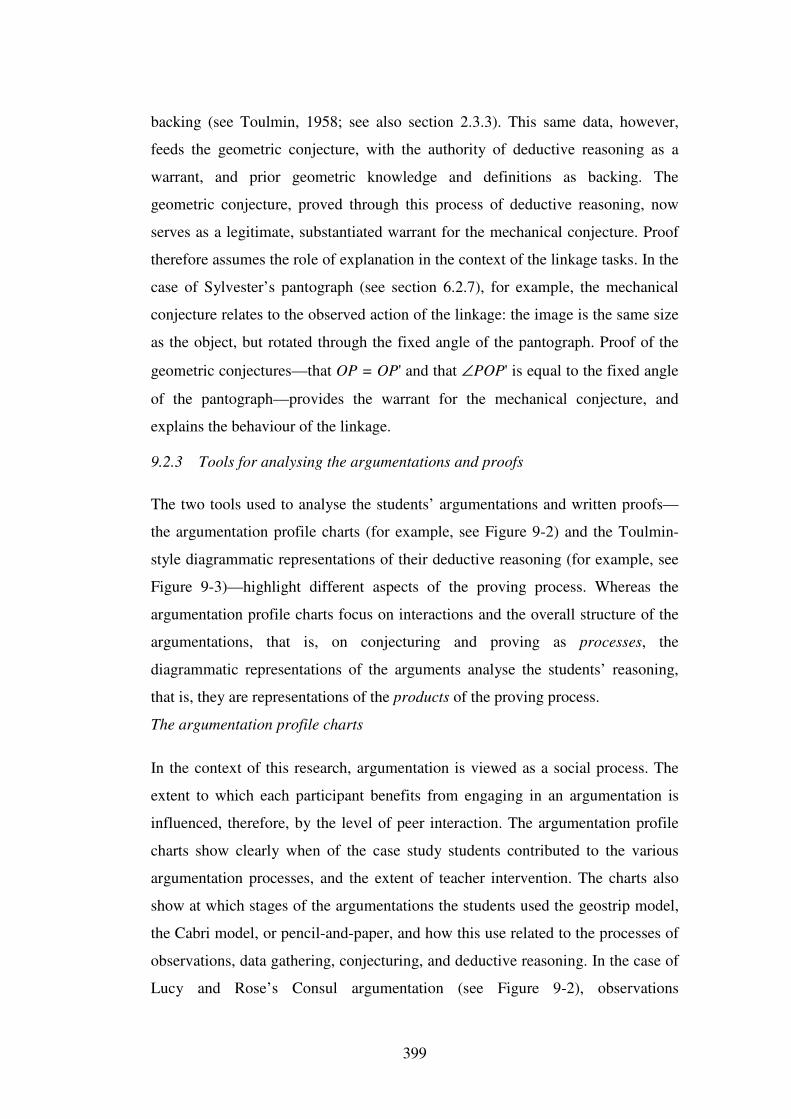
399
backing (see Toulmin, 1958; see also section 2.3.3). This same data, however,
feeds the geometric conjecture, with the authority of deductive reasoning as a
warrant, and prior geometric knowledge and definitions as backing. The
geometric conjecture, proved through this process of deductive reasoning, now
serves as a legitimate, substantiated warrant for the mechanical conjecture. Proof
therefore assumes the role of explanation in the context of the linkage tasks. In the
case of Sylvester’s pantograph (see section 6.2.7), for example, the mechanical
conjecture relates to the observed action of the linkage: the image is the same size
as the object, but rotated through the fixed angle of the pantograph. Proof of the
geometric conjectures—that OP = OP' and that ∠POP' is equal to the fixed angle
of the pantograph—provides the warrant for the mechanical conjecture, and
explains the behaviour of the linkage.
9.2.3 Tools for analysing the argumentations and proofs
The two tools used to analyse the students’ argumentations and written proofs—
the argumentation profile charts (for example, see Figure 9-2) and the Toulmin-
style diagrammatic representations of their deductive reasoning (for example, see
Figure 9-3)—highlight different aspects of the proving process. Whereas the
argumentation profile charts focus on interactions and the overall structure of the
argumentations, that is, on conjecturing and proving as processes, the
diagrammatic representations of the arguments analyse the students’ reasoning,
that is, they are representations of the products of the proving process.
The argumentation profile charts
In the context of this research, argumentation is viewed as a social process. The
extent to which each participant benefits from engaging in an argumentation is
influenced, therefore, by the level of peer interaction. The argumentation profile
charts show clearly when of the case study students contributed to the various
argumentation processes, and the extent of teacher intervention. The charts also
show at which stages of the argumentations the students used the geostrip model,
the Cabri model, or pencil-and-paper, and how this use related to the processes of
observations, data gathering, conjecturing, and deductive reasoning. In the case of
Lucy and Rose’s Consul argumentation (see Figure 9-2), observations
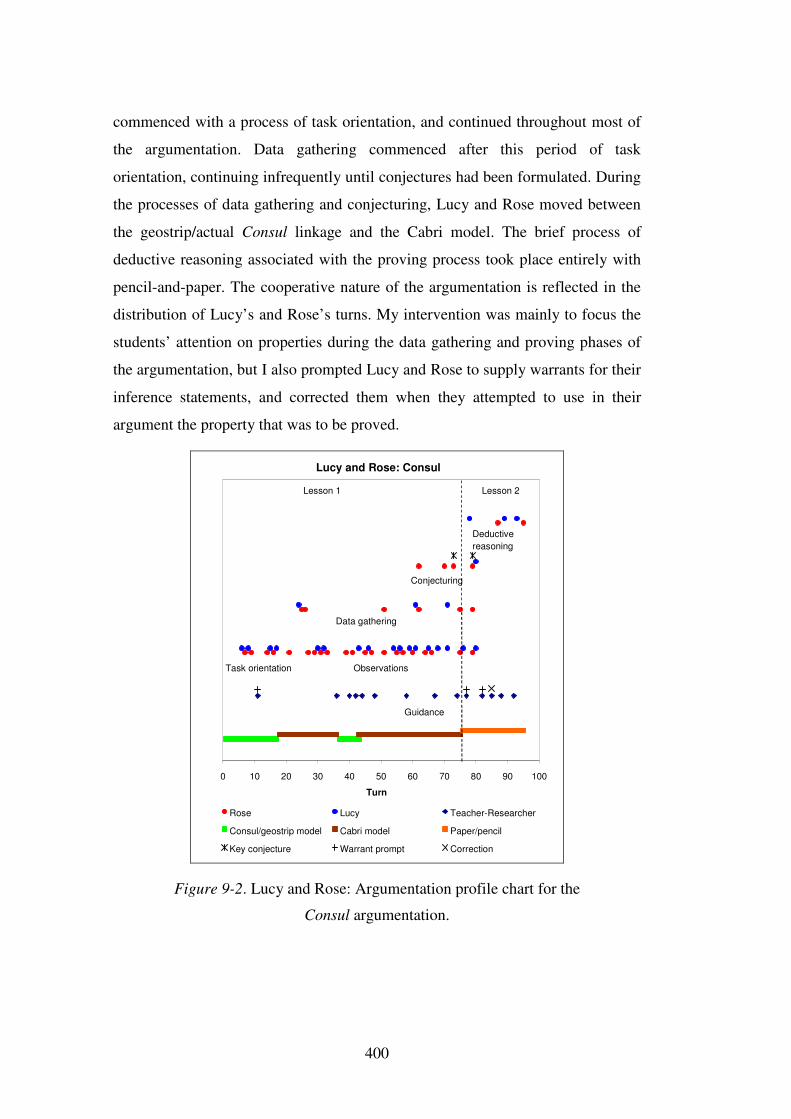
400
commenced with a process of task orientation, and continued throughout most of
the argumentation. Data gathering commenced after this period of task
orientation, continuing infrequently until conjectures had been formulated. During
the processes of data gathering and conjecturing, Lucy and Rose moved between
the geostrip/actual Consul linkage and the Cabri model. The brief process of
deductive reasoning associated with the proving process took place entirely with
pencil-and-paper. The cooperative nature of the argumentation is reflected in the
distribution of Lucy’s and Rose’s turns. My intervention was mainly to focus the
students’ attention on properties during the data gathering and proving phases of
the argumentation, but I also prompted Lucy and Rose to supply warrants for their
inference statements, and corrected them when they attempted to use in their
argument the property that was to be proved.
Lucy and Rose: Consul
0 10 20 30 40 50 60 70 80 90 100
Turn
Rose Lucy Teacher-Researcher
Consul/geostrip model Cabri model Paper/pencil
Key conjecture Warrant prompt Correction
Guidance
Observations
Data gathering
Conjecturing
Deductive reasoning
Lesson 1 Lesson 2
Task orientation
Figure 9-2. Lucy and Rose: Argumentation profile chart for the
Consul argumentation.
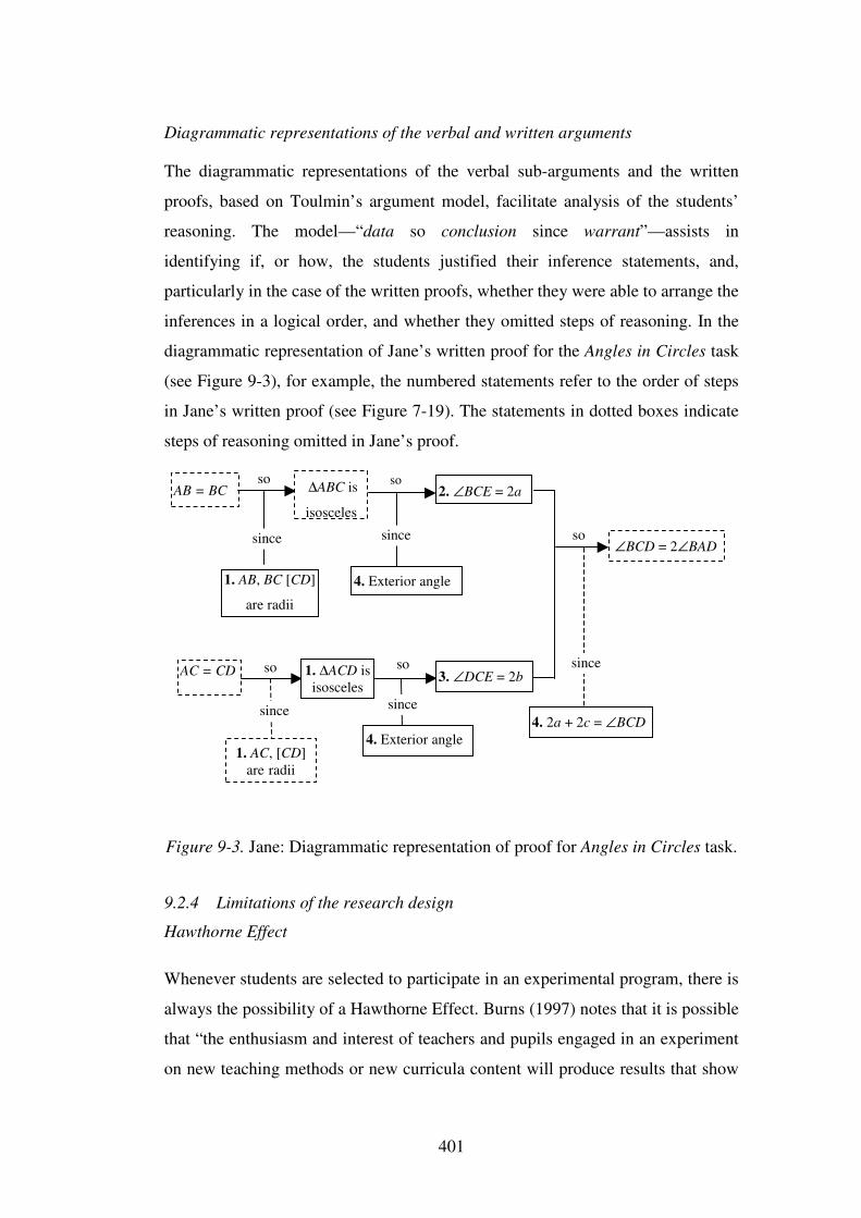
401
Diagrammatic representations of the verbal and written arguments
The diagrammatic representations of the verbal sub-arguments and the written
proofs, based on Toulmin’s argument model, facilitate analysis of the students’
reasoning. The model—“data so conclusion since warrant”—assists in
identifying if, or how, the students justified their inference statements, and,
particularly in the case of the written proofs, whether they were able to arrange the
inferences in a logical order, and whether they omitted steps of reasoning. In the
diagrammatic representation of Jane’s written proof for the Angles in Circles task
(see Figure 9-3), for example, the numbered statements refer to the order of steps
in Jane’s written proof (see Figure 7-19). The statements in dotted boxes indicate
steps of reasoning omitted in Jane’s proof.
Figure 9-3. Jane: Diagrammatic representation of proof for Angles in Circles task.
9.2.4 Limitations of the research design
Hawthorne Effect
Whenever students are selected to participate in an experimental program, there is
always the possibility of a Hawthorne Effect. Burns (1997) notes that it is possible
that “the enthusiasm and interest of teachers and pupils engaged in an experiment
on new teaching methods or new curricula content will produce results that show
AC = CD 1. ∆ACD is isosceles
1. AC, [CD] are radii
3. ∠DCE = 2b
4. Exterior angle 4. 2a + 2c = ∠BCD
so so
∠BCD = 2∠BAD
AB = BC ∆ABC is
isosceles
1. AB, BC [CD]
are radii
2. ∠BCE = 2a
4. Exterior angle
since
so so
so since
since
since
since
402
tremendous gains in performance” (p. 143). The novelty of being withdrawn from
other lessons to participate in the conjecturing-proving tasks may have influenced
both the level of motivation and the cognitive engagement of the case study
students. To overcome the possibility of a Hawthorne Effect, the research would
need to be carried out over a longer period of time. The sustained argumentations
of these students also might have been partly dependent on the physical
environment in which these sessions were conducted, and might not have been of
the same quality in the classroom, where other distractions inevitably occur. The
reaction of the students to the linkage tasks that were presented to the whole class,
and the students’ subsequent post-test performance, were encouraging, however,
indicating that all students would have benefited from completing more of the
conjecturing-proving tasks if time had been available.
Emphasis on deductive proofs
The students’ pre-test responses to Proof Questionnaire question G2 (see 8.4.4)
showed that the majority of students seemed aware of the universality of proof.
The students seemed less certain, however, about which arguments were general,
and although the conjecturing-proving lessons resulted in significant changes in
the students’ recognition that empirical arguments did not constitute proof, their
post-test Proof Questionnaire responses indicated that many students were still
uncertain about the generality of correct, but non-formal, arguments. Validity
ratings (see section 8.4.3, Table 8-5) were higher for the correct formal proofs—
Cynthia’s and Linda’s arguments—than for the correct, but non-formal proofs—
Ewan’s, Yorath’s, and Marty’s arguments—demonstrating the students’
uncertainty of the generality of correct, non-formal arguments. In the case of
Ewan’s correct narrative argument in question G1, for example, Kate agreed,
whereas Anna disagreed, that the argument showed the statement to be true for all
triangles. An unintentional outcome of the conjecturing-proving lessons was
therefore that at least some of the students gained the impression that ‘formal’
deductive arguments were the only correct proofs.
403
9.2.5 Assessment of the students’ argumentations
Although it was not an intention of the current research to assess the students’
argumentations quantitatively, the model developed by Galindo (1998—see
section 3.4.8) to assess students’ reasoning in a dynamic geometry environment
could be applied to the argumentations. Galindo asserts that there should be an
empirical component and a deductive reasoning component to students’
explorations, with interaction between the two components. His assessment model
is therefore based on three levels of justification: Intuitive justification, Deductive
justification, and Interplay between intuitive and deductive, with scores within
each category of 0 (no justification or no evidence of interplay), 1 (partial
justification or some evidence of interplay) or 2 (reasonable justification or
mutually reinforcing justification). Galindo notes that the desired score for a
particular task would depend on the focus of the task, but “when students are
expected to make explicit the connections they are making between the empirical
and deductive bases of their reasoning, the goal should be to obtain 2-2-2 scores”
(p. 81). This is the situation in the current research, and the argumentations of the
Level 2–3 case study students satisfied the criteria for this 2-2-2 score. In the case
of Jane and Sara, however, the categories deductive justification and interplay
between intuitive and deductive relied substantially on my intervention. Jane and
Sara’s argumentations would be assessed as 2-1-1.
9.2.6 Further research
The Level 2–3 case study students developed a greater understanding of proof,
and were better able to construct written proofs, particularly in unfamiliar contexts
(see Table 8-11), than most other students in the Year 8 class. It would be
reasonable to assume that the performance of these students was related to the
number of additional conjecturing-proving tasks that they completed. Further
research is necessary, however, to explore whether it is possible to achieve the
same outcomes if the sequence of additional conjecturing-proving tasks is used in
a whole-class situation (see section 9.2.4). Observations of the students in the
whole-class conjecturing-proving lessons which preceded the case study lessons
404
suggest that the lesson sequence would be successful, provided teacher
intervention and class discussion were integral aspects of the lessons.
There is also the possibility of gender differences in level of motivation, in the
ability to reason deductively, and in the recognition of whether a particular
mathematical argument is universal. It will be recalled, for example, that Healy
and Hoyles (1999) and Küchemann and Hoyles (2001) found that when students
were presented with a range of arguments, there were differences in the choice
patterns of boys and girls (see section 2.5.7). Of interest, too, are the long term
effects of the Year 8 students’ introduction to deductive reasoning and proof, in
particular, whether the students’ understanding of proof is transferable to algebra,
and whether the development of a culture of proving at this Year 8 level has
produced lasting changes in the students’ mathematical ways of thinking.
9.3 Interpreting the findings in terms of the research questions
The first research question (see section 4.2.1), which relates to the development of
a culture of proving, is discussed in section 9.3.6.
9.3.1 Motivational engagement
Are Year 8 students motivated to engage in argumentation,
conjecturing and deductive reasoning in the context of mechanical
linkages and dynamic geometry software?
As discussed in section 6.3.3, specific indicators of motivation—enjoyment,
excitement, satisfaction, and perseverance—and of cognitive engagement (see
section 2.8.3)—reflective statements, statements that involve shared meaning,
statements that draw upon earlier interactions, or in interactions where one student
completes a statement made by the other—were apparent throughout the
argumentations of the Level 2–3 and the Level 1–2 case study students. The high
levels of motivation and cognitive engagement displayed by the students could be
attributed to several aspects of the tasks: there was inherent interest in the novel
context of mechanical linkages, the students’ curiosity was aroused to explain
why the linkages operated in the observed way, and the underlying geometry of
the linkage and Cabri-based tasks was sufficiently familiar for the students to be
405
able to engage in productive argumentation. Once the roles of proof were
established—in particular, proof as the verification of the truth of a conjecture,
and proof as explanation of why the conjecture was true—the students accepted
the challenge of the linkage tasks and Cabri investigations, tackling them with
something approaching the spirit of a game. In the Pascal’s Angle Trisector task,
for example, Sara commented with a laugh: “I hate it when you get this close!”
(section 7.4.1, Pascal’s Angle Trisector, turn 114).
The tactile experience of operating the physical linkages seemed to play an
important role in the initial arousal of interest in the linkage tasks, so that
motivational engagement and cognitive engagement were closely connected.
There seemed little doubt that the majority of students enjoyed the novel
experience of operating the linkages, but much of their motivation was directed
towards unravelling the relationship between how the linkage worked and its
geometry, as seen, for example, in Kate and Anna’s investigation of Consul
(section 6.2.6):
075 Kate: I just want to draw this triangle.
076 Anna: You’re right. It goes down the triangle … see, this point P goes down … it
goes down … like along the triangle …
and Sara’s and Jane’s responses to the discovery of the angle relationships in
Pascal’s angle trisector (section 7.4.1):
128 Sara: Adds 10 … 22.2 … it’s adding a!
Proof was now being seen by the students as a means of explaining geometric
facts that previously they might have taken for granted, and this seemed to
engender a strong sense of satisfaction, as shown in Jane’s comment at the end of
the Pascal’s Angle Trisector task: “Oh, yeah … that’s so way out, isn’t it … that’s
cool” (Jane, section 7.4.1, Pascal’s Angle Trisector, turn 146). Liz displayed a
strong sense of satisfaction, indicated by her smile, when she recognised the
implication of similar triangles in the Consul proof (turns 224 and 226), even
though she found difficulty in explaining her reasoning:
Ohhh, d equals 45 because here … c plus d … because … oh, I can’t explain it now
… this has to be equal because … Do you understand? This is 45 so d plus 45 …
406
They’re similar triangles … you know … so this angle here … CAP is c plus 45 …
well angle EAB is the same.
The same sense of satisfaction also existed with the Cabri-based tasks, as seen, for
example, in Jane’s comments: “Clever me!” (section 7.4.1, Quadrilateral
Midpoints, turn 117), and “So … how did we prove it? … Oh, cool! I want to
write that out before I forget it!” (section 7.4.1, Angles in Circles, turn 112).
In contrast to the other case study students, Emma and Jess showed little outward
sign of enjoyment of the task until they began to understand the geometry of the
linkage. These two students lacked the obvious curiosity and spirit of enquiry that
was apparent with the other case study students, including Jane and Sara who had
similar Level 1–2 van Hiele pre-test profiles. One could not necessarily conclude
that Emma and Jess were unmotivated with respect to the linkage task, but their
lack of understanding of geometry seemed to create a barrier between the linkage
as a drawing instrument and the linkage as a geometric object. The initial teacher-
dependence exhibited by the two students gradually gave way, however, to
increased involvement and interest as they began to understand the geometry.
The acceptance by these Year 8 students of the need for proof and their sustained
engagement in the process of proof construction, despite the strength of
conviction based on empirical Cabri data, substantiates the claim by Hölzl (2001;
see section 3.3.2) that it is the context, rather than the computer itself, that
determines whether or not a need for proof arises. Hölzl asserts that it is the quest
for explanation which drives the reasoning process, and this indeed seemed to be
the case for these Year 8 students. As noted by Bartolini Bussi and Pergola (2000,
p. 61) in the case of Sylvester’s pantograph (see section 3.6.2), “the linkage itself
created the need to be understood”. Support is also given to the views of de
Villiers (1998) and Goldenberg, Cuoco, and Mark (1998)—that proof becomes
meaningful to students when it explains (see section 2.4.4)—and to the assertion
of Dreyfus and Haddas (1996) that students experience the need for proof when
unexpected or surprising situations are involved (see section 2.2.6). The linkage
tasks seemed to provide these opportunities.
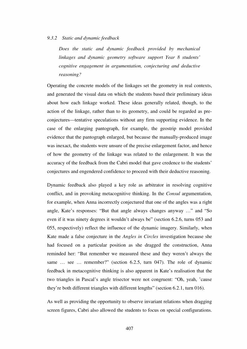
407
9.3.2 Static and dynamic feedback
Does the static and dynamic feedback provided by mechanical
linkages and dynamic geometry software support Year 8 students’
cognitive engagement in argumentation, conjecturing and deductive
reasoning?
Operating the concrete models of the linkages set the geometry in real contexts,
and generated the visual data on which the students based their preliminary ideas
about how each linkage worked. These ideas generally related, though, to the
action of the linkage, rather than to its geometry, and could be regarded as pre-
conjectures—tentative speculations without any firm supporting evidence. In the
case of the enlarging pantograph, for example, the geostrip model provided
evidence that the pantograph enlarged, but because the manually-produced image
was inexact, the students were unsure of the precise enlargement factor, and hence
of how the geometry of the linkage was related to the enlargement. It was the
accuracy of the feedback from the Cabri model that gave credence to the students’
conjectures and engendered confidence to proceed with their deductive reasoning.
Dynamic feedback also played a key role as arbitrator in resolving cognitive
conflict, and in provoking metacognitive thinking. In the Consul argumentation,
for example, when Anna incorrectly conjectured that one of the angles was a right
angle, Kate’s responses: “But that angle always changes anyway …” and “So
even if it was ninety degrees it wouldn’t always be” (section 6.2.6, turns 053 and
055, respectively) reflect the influence of the dynamic imagery. Similarly, when
Kate made a false conjecture in the Angles in Circles investigation because she
had focused on a particular position as she dragged the construction, Anna
reminded her: “But remember we measured these and they weren’t always the
same … see … remember?” (section 6.2.5, turn 047). The role of dynamic
feedback in metacognitive thinking is also apparent in Kate’s realisation that the
two triangles in Pascal’s angle trisector were not congruent: “Oh, yeah, ’cause
they’re both different triangles with different lengths” (section 6.2.1, turn 016).
As well as providing the opportunity to observe invariant relations when dragging
screen figures, Cabri also allowed the students to focus on special configurations.
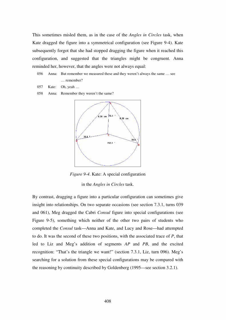
408
This sometimes misled them, as in the case of the Angles in Circles task, when
Kate dragged the figure into a symmetrical configuration (see Figure 9-4). Kate
subsequently forgot that she had stopped dragging the figure when it reached this
configuration, and suggested that the triangles might be congruent. Anna
reminded her, however, that the angles were not always equal:
056 Anna: But remember we measured these and they weren’t always the same … see
… remember?
057 Kate: Oh, yeah …
058 Anna: Remember they weren’t the same?
Figure 9-4. Kate: A special configuration
in the Angles in Circles task.
By contrast, dragging a figure into a particular configuration can sometimes give
insight into relationships. On two separate occasions (see section 7.3.1, turns 039
and 061), Meg dragged the Cabri Consul figure into special configurations (see
Figure 9-5), something which neither of the other two pairs of students who
completed the Consul task—Anna and Kate, and Lucy and Rose—had attempted
to do. It was the second of these two positions, with the associated trace of P, that
led to Liz and Meg’s addition of segments AP and PB, and the excited
recognition: “That’s the triangle we want!” (section 7.3.1, Liz, turn 096). Meg’s
searching for a solution from these special configurations may be compared with
the reasoning by continuity described by Goldenberg (1995—see section 3.2.1).
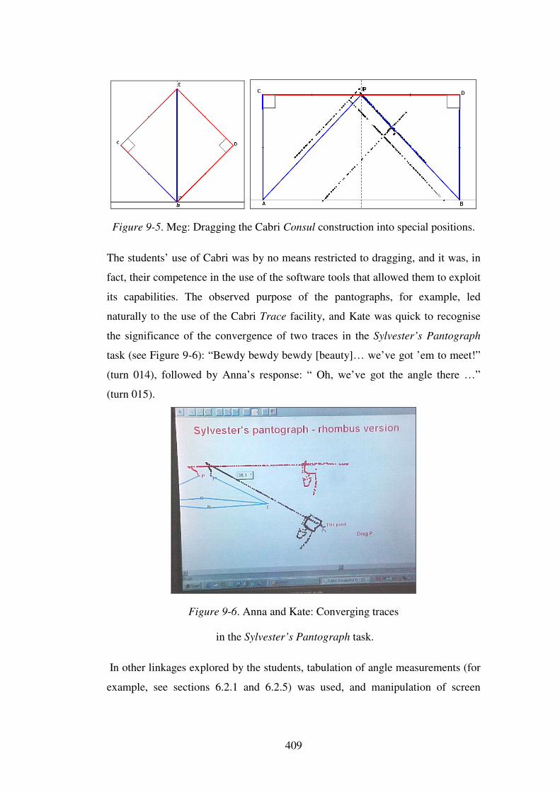
409
Figure 9-5. Meg: Dragging the Cabri Consul construction into special positions.
The students’ use of Cabri was by no means restricted to dragging, and it was, in
fact, their competence in the use of the software tools that allowed them to exploit
its capabilities. The observed purpose of the pantographs, for example, led
naturally to the use of the Cabri Trace facility, and Kate was quick to recognise
the significance of the convergence of two traces in the Sylvester’s Pantograph
task (see Figure 9-6): “Bewdy bewdy bewdy [beauty]… we’ve got ’em to meet!”
(turn 014), followed by Anna’s response: “ Oh, we’ve got the angle there …”
(turn 015).
Figure 9-6. Anna and Kate: Converging traces
in the Sylvester’s Pantograph task.
In other linkages explored by the students, tabulation of angle measurements (for
example, see sections 6.2.1 and 6.2.5) was used, and manipulation of screen
410
drawings prompted students to add construction lines to assist them in identifying
invariant properties or relationships (for example, sections 6.2.5, 6.2.6, and 6.2.7).
The students’ prior familiarity with the features of Cabri was therefore an
important aspect of their successful use of the Cabri linkage models in helping
them to produce their conjectures and construct proofs. The ease with which the
students could trace the paths of points, add construction lines, and accurately
measure angles and distances, meant that they did not usually return to the
geostrip model after they had been given access to the Cabri model.
Although the formulation of conjectures and deductive reasoning was usually
associated with the Cabri figure, deductive reasoning sometimes took place almost
entirely with pencil and paper, particularly in the case of Anna and Kate’s later
tasks—Consul and Sylvester’s Pantograph (see Figures 6-31 and 6-34). The Cabri
construction appeared to form a bridge between the physical linkage and its
representation as a geometric figure in the worksheet diagram. The students were
able to move easily into the pencil-and-paper environment, with a clear ability to
relate the properties and relationships they had observed
The success of the case study students, particularly the Level 2–3 students, in the
application of deductive reasoning raises the question of how these students
would have fared if they had been given statements to prove, without first
engaging in conjecturing. The one task for which a direct comparison can be made
is the Angles in Circles task. Anna and Kate, and Jane and Sara completed the task
as an open-ended Cabri conjecturing-proving task, whereas Liz and Meg were
given a statement to prove as a pencil-and-paper task. The visual and empirical
feedback from Cabri allowed Anna and Kate, and also Jane and Sara, to discover
apparent angle relationships and to formulate conjectures, but the software also
enabled the resolution of cognitive conflict. Anna and Kate’s resolution of the
issue of congruency through reference to the dynamic feedback in the Angles in
Circles investigation (see section 6.2.5, turns 045–049), for example, contrasts
with the confusion that arose in the case of Liz and Meg’s pencil-and-paper
Angles in Circles proof (see section 7.3.3, turns 020–038). This time there was no
sense of resolution, with Meg concluding: “Mmm … tricky”, supporting

411
Laborde’s (1998b) assertion that students do not have the same opportunity to
move between spatial and theoretical domains in a pencil-and-paper environment
(see section 3.4.7).
Laborde (1998a) suggests that dynamic geometry computer environments focus
students’ attention on invariant properties which they may not notice in a static
drawing, and it is the recognition of these invariant properties that provides access
to the underlying geometry (see section 3.3.1). Duval (1998), reporting on a study
with 13–14-year-olds, notes that the students did not always recognise subfigures
within a figure (see section 2.5.7). In Duval’s study the students were working
with static diagrams. Despite the dynamic nature of the imagery provided by
Cabri, however, it cannot be assumed that all students will notice invariant
properties. It was some time, for example, before Jane and Sara recognised the
invariant parallelogram in the Quadrilateral Midpoints task (see section 7.4.1),
despite their dragging of the quadrilateral. Having convinced themselves that the
task was about similar or congruent triangles, Jane and Sara had focused on the
triangles surrounding the parallelogram, and failed to notice the parallelogram.
Their poor understanding of properties of special quadrilaterals no doubt
contributed to this lack of observation, but there was also a tendency for these
students to draw hasty conclusions and to focus on their most recently acquired
knowledge, which in this case was similar and congruent triangles. By contrast,
Anna and Kate saw the parallelogram immediately, even before they dragged the
figure.
9.3.3 The influence of conjecturing and argumentation on proof
Do the processes of argumentation and conjecturing contribute to
successful proof constructions?
Comparing the quality of the argumentations as the students progressed through
several tasks is complicated by the differing levels of complexity of the
conjecturing-proving tasks. Pascal’s Angle Trisector (introduced to the students
as Pascal’s mathematical machine) differed from the other linkage tasks because
the students were not informed of the purpose of the linkage as this would have
revealed the geometry. In this respect, the task resembled the Cabri-based Angles
412
in Circles investigation. In the other linkage tasks, the method of operating the
linkage could be demonstrated without disclosing the geometry, as in the case of
the pantographs. The linkages also varied in their geometric complexity. The
enlarging pantograph, for example, comprises a parallelogram and similar
triangles, while Sylvester’s pantograph is based on a rhombus and congruent
triangles. It might be expected that these two linkages would be of equivalent
complexity, but the relationship between the angle of rotation of the image and the
geometry of Sylvester’s pantograph is not immediately obvious, and two separate
proofs are required—one for the congruent image and another for the angle of
rotation. Superficially, the enlarging pantograph requires only proof that the
triangles are similar, but a more rigorous proof would also require it to be shown
that the relevant points are collinear. In the case of Consul, identifying how the
operation of the linkage was related to the geometry presented an even more
difficult problem, and the proof involved a sub-proof. Despite these differences
between the tasks it is possible to identify progress in the students’ conjecturing
and proving skills, as well as features of the geostrip and Cabri environments that
influenced this progress.
One prominent characteristic of the argumentations was the ease with which the
case study students, particularly those at van Hiele Levels 2–3, were able to
synthesise their deductive reasoning into coherent, logical written proofs once
they had formulated conjectures and engaged in deductive reasoning during the
argumentation. The students did not seem to experience the difficulties observed
by Duval (1991; see section 2.5.5 and Figure 2-19), who noted that students
initially failed to recognise the different status of statements in an argument.
Duval’s observations were based on students working on pencil-and-paper proofs,
where they had not been involved in the production of conjectures. Bartolini Bussi
(1998), in discussing Year 11 students conjecturing and proving with Sylvester’s
pantograph, notes that “the process of polishing the entire reasoning in order to
give it the form of a logical chain and to write it down was slow and not
complete” (p. 742).
413
In the current research, the strong empirical support from Cabri, and the
argumentation that accompanied the production of each conjecture, had already
given the students some insight into the underlying geometry. Proving then
became a process of justifying observed relationships, and, although these
justifications did not always follow in a logical sequence in the proving phase of
the argumentation, geometric dependencies were made explicit. By the time the
students began to produce their written proofs, they had already acquired a strong
sense of logical order for the steps of deductive reasoning. The statements in each
proof were generally ordered into a logical sequence, and supporting statements,
that is, warrants, were frequently included. Anna and Kate’s written proof for
Sylvester’s pantograph, for example (see Figure 6-32), may be compared with the
Year 11 students’ proof (see section 3.6.2) in the study described by Bartolini
Bussi (1998). Once Anna and Kate had completed the verbal argumentation
process, they had no difficulty in producing their written proof.
In their later argumentations, Anna and Kate—the two students who completed
the greatest number of conjecturing-proving tasks—were recalling steps of
reasoning from previous proofs and incorporating these into new proofs. In the
Quadrilateral Midpoints task (see section 6.2.4, turns 019−029), for example,
Kate recognised the subfigure of the triangle midpoints which she had
encountered in the Joining Midpoints task (section 6.2.3). Similarly, in the Angles
in Circles task (section 6.2.5, turns 085−093), Kate and Anna recognised the
configuration of the isosceles triangle and its exterior angle—“Because of the
isosceles triangle and the exterior angle and all that”—which occurred in Pascal’s
Angle Trisector (see section 6.2.1, turns 022−032).
As discussed in section 2.5.7, Koedinger and Anderson (1990) assert that this
ability to skip steps in reasoning by parsing a geometric diagram into subfigures,
or ‘perceptual chunks’, is a characteristic of high school geometry proof experts.
Even the Level 1–2 students, Jane and Sara, were beginning to notice particular
configurations, as in the case of the Quadrilateral Midpoints proof, for example,
where Jane recognised a connection with the Joining Midpoints proof (turns
90−115). Unlike Kate, however, Jane was initially unable to visualise which
414
construction lines were required, indicating her weaker understanding of
relationships within the figure.
Except for Amy and Lyn, the case study students’ argumentations were
characterised by collaboration and cooperation, and it is likely that the students
reached a level of understanding that they would not have achieved from working
alone. In the case of Lucy and Rose, the argumentations could be described as
cooperative, and generally collaborative, but it was frequently Rose who made
significant observations and conjectures. Proof construction then seemed to come
easily to Rose, and her enthusiasm to explain her reasoning meant that Lucy did
not always have an opportunity to contribute to the reasoning. In the Consul
proof, for example, Rose stated several steps in one turn (section 7.3.1, Lucy and
Rose’s Consul argumentation, turn 087), leaving Lucy to catch up with her
reasoning: “If that’s a rhombus, then b plus c plus 90 equals 180 … which means
b plus c equals 90 … and a plus b equals 90 so a must equal c … that’s so
simple!”. On these occasions Lucy tended to rely on Rose’s explanation when
producing her written proof, which suggests she had not acquired the same sense
of ownership of the proof as had Rose. This is reflected in Lucy’s van Hiele
Level 4 post-test responses, where she reached Level 4 for only three concepts,
compared with Anna, Kate, and Rose, who reached Level 4 for five concepts.
The findings from this research therefore strongly support the notion of cognitive
unity proposed by Boero, Garuti, Lemut and Mariotti (1996). As discussed in
section 2.5.1, Boero et al. believe that the conjectures and associated justifications
put forward during the argumentation play a key role in the logical ordering of
statements and are critical to students’ successful proof construction.
9.3.4 Satisfying the need for conviction
Does the empirical feedback provided by dynamic geometry software
satisfy Year 8 students’ need for convincing?
The establishment of the need for proof through the use of Tchebycheff’s linkage
(see sections 3.5.8 and 4.2.3) in the first conjecturing task seemed to be critical to
the success of the subsequent conjecturing-proving lessons. The geostrip model
415
encouraged the students to conjecture that one of the points of the linkage was
moving in a straight line, whereas other points were moving on circular paths.
When the students then dragged the Cabri linkage, their realisation that the path
was not in fact linear, and their astonishment at seeing how little the path actually
deviated from a straight line, was sufficient to convince them that visual and
empirical evidence could not be trusted. One could argue that in principle this
approach was little different from traditional textbook use of optical illusions to
demonstrate a need for proof. What seemed to be significant, however, was that
the students themselves had been actively involved in the generation of the false
conjecture.
In general, it was Cabri data that underpinned the students’ conjectures, and their
implicit trust in the accuracy of the Cabri data served to strengthen their
confidence in their conjectures. Only on one occasion (see section 7.3.1, The role
of static and dynamic feedback in conjecturing) was the status of Cabri evidence
queried:
097 Meg: It’s a right angle!
098 Liz: Yes! Because … if you measured an angle in Cabri and it came out a right
angle, would you … like have to prove that?
Despite their strength of conviction with Cabri, however, the Level 2–3 students
accepted that proof was still necessary—as an explanation for why the
relationships expressed in a conjecture were true. By contrast, it was Jane and
Sara—the Level 1–2 case study students—who, in the Joining Midpoints task (see
section 7.4.1, Joining Midpoints), claimed: “It just has to be parallel” (Sara, turn
029), and “It is parallel. It just is. It doesn’t need to be proved. It just is” (Jane,
turn 030). Sara also seemed confused about the Angles in Circles proof (see
section 7.4.1, Angles in Circles), with her comment—“But we already said
that”—referring to the empirical observation of the angle relationship.
109 Sara: a plus c … so this angle [∠BCD] is twice this angle [∠BAD] … but we
already said that …
110 TR: Yes, but it was just a conjecture … we still had to prove it.
111 Sara: Oh, yeah.
416
Despite their conviction based on visual and empirical feedback, however, Jane
and Sara participated enthusiastically in the proving process in each of their
argumentations.
9.3.5 Relationship between van Hiele levels and conjecturing-proving ability
Are the students’ abilities to make conjectures and to construct
deductive proofs related to their measured van Hiele levels?
Comparison of the argumentations of the Level 1–2 and Level 2–3 case study
students reveals marked differences in the quality of observations and data
gathering. Jane and Sara, for example, who were at Levels 1–2 for all six concepts
on the pre-test, were frequently confused over properties of simple geometric
shapes, as seen, for example, in Sara’s confusion over trapezium properties (see
section 7.4.1, Joining Midpoints, turns 18–23). Jane and Sara were easily
sidetracked by irrelevant aspects of a geometric figure as a result of preconceived
ideas about the nature of the task, which often led to inappropriate data gathering
and incorrect conjectures. In the Quadrilateral Midpoints task (see section 7.4.1),
for example, they focused on the triangles surrounding the parallelogram formed
by the midpoints, and failed to notice the invariant parallelogram. Even when they
eventually recognised the invariant properties of the figure, they incorrectly
referred to it as a square, a rhombus, and a rectangle. Sara’s reasoning was again
limited by her low level of geometric understanding, and her explanation reflects
Level 1 visual understanding (section 7.4.1, Quadrilateral Midpoints, turn 071):
I mean of the square … sorry … of this … the parallelogram … this parallelogram is
always … it’s centred … it’s in the very centre of the whole shape because of the
lines … therefore it stays there. It always stays in the middle …
There were occasional instances where Level 2–3 students displayed a poor
understanding of properties, for example, in the Consul argumentation (see
section 7.3.1, Consul, turns 009–016), when Meg failed to recognise that four
equal sides defined a rhombus. In general, however, the Level 2–3 case study
students were more knowledgeable about properties, used appropriate geometric
terminology confidently, and were more discerning in their data gathering. Kate,
417
for example, realised that it was likely to be angle measurements, rather than
distance measurements, that were important in the Angles in Circles exploration
(see section 6.2.5). In the Quadrilateral Midpoints task (see section 6.2.4), Anna
and Kate recognised immediately that the figure formed by joining the midpoints
of the sides of the quadrilateral was a parallelogram.
Fluency with the language of geometry also contributed to the students’ ability to
construct reasoned arguments. Anna and Kate, for example, generally were able to
articulate their reasoning, whereas the Level 1–2 students often found difficulty
explaining their observations in geometric terms, and Sara, in particular,
sometimes resorted to gesture and enactive reasoning (see Table 8-2), as
illustrated by Sara’s comment in the Joining Midpoints task (section 7.4.1, Joining
Midpoints, turn 001):
It goes up … the base … [using her hands to indicate the vertex A of ∆ABC]. I don’t
know how to explain this in mathematical terms, but if that’s straight [BC], you can
just draw a line anywhere. And because the two lines come from the base, it would
be equal.
On several occasions Sara tried to use visual reasoning, as seen, for example, in
her explanation for the parallel segments in the Joining Midpoints task (section
7.4.1, Joining Midpoints, turns 064–068). However, even when she claimed that it
was “easy then now”, she could still provide only an enactive argument:
And … oh, that’s easy then now … if they’re congruent triangles … I mean similar
… then the bottom one has to be the same. Because that angle’s shared … I don’t
know how to explain it but I just know that they’re parallel.
They have all the same angles and all the same sides. That one can be put into the
other so therefore … I sort of imagine it like that [draws triangle on paper] and you
put another triangle in there and if it does fit when you put it in there it will be
exactly the same angles so it would be parallel because it fits … with the same
angles without moving and with the same sides. (section 7.4.1, Joining Midpoints,
Sara, turn 068)
Sara’s visual reasoning in this example may be compared with the
transformational reasoning described by Simon (1996—see section 3.2.2).
According to Simon, this form of reasoning is characterised by the ability to
418
perform a particular mental or physical enactment, but also by the ability to
recognise that it is appropriate in a particular mathematical situation. Sara could
clearly visualise the similarity of the triangles through a process of mental
translation of the small triangle formed by joining the midpoints of two sides of
the triangle. Sara’s reasoning, however, is also an indicator of her van Hiele
Level 1 understanding. Although Sara was able to recognise visually that the line
joining the midpoints of two sides of the triangle was parallel to the third side, she
did not have the appropriate understanding of properties, and relationships
between properties, to give a geometric explanation.
Sara’s visual reasoning may be contrasted with Rose’s visualisation in the
Sylvester’s Pantograph argumentation (section 7.3.2, turn 092), which may also
be considered as transformational reasoning. Unlike Sara, Rose was able to link
her visual reasoning with deductive reasoning:
Once we’ve proved that angle, then the whole things easy ’cause side angle side …
see, if you have two sides and how big it’s going to be in between … when you join
them up the triangles will be the same…
Not only did Rose recognise the relevance of the side-angle-side congruency
condition to the pantograph proof, but she had a clear visual understanding of why
the condition guaranteed congruency.
As well as differences between the argumentations of the Level 2–3 students and
those students at lower van Hiele levels, differences were also apparent between
the written proofs, as seen for example in the Quadrilateral Midpoints proofs of
Anna and Kate (see Figures 6-23 and 6-24), and Jane and Sara (see Figure 7-16).
The Level 2–3 case study students were able to order their statements logically in
their written proofs, and generally provided appropriate warrants. This was
evident both in the conjecturing-proving tasks and in the Proof Questionnaire
proof constructions for questions G4 and G7. By contrast, the written proofs of
the Level 1–2 case study students—Jane, Sara, Emma, and Jess—were not always
logically ordered, and warrants were often omitted or inappropriate warrants were
given. Emma’s use of a narrative style in her written proofs (see Figures 7-23 and
419
8-49) did not provide any supporting structure for her to order her statements
logically.
Despite their difficulties with proof construction, and their greater reliance on my
intervention, the Level 1–2 case study students were able to engage in deductive
reasoning. This may be seen, for example, in Emma’s written proof in the
Enlarging Pantograph task (see Figure 7-24), Sara’s ability to deduce the
relationship between angles in the Pascal’s Angle Trisector task (see section
7.4.1, Pascal’s Angle Trisector, turns 064–069), and Jane’s eventual recognition
of the application of the Joining Midpoints proof to the Quadrilateral Midpoints
proof (see section 7.4.1, Quadrilateral Midpoints, turn 115):
Oh! … I’ve got it! ’cause this [PQ] and this [SR] is the same, this [PQ] is the
midpoint line so this [PQ] is parallel to that [AD] and that’s [PQ] parallel to that
[SR].
Although there were differences in reasoning ability, it was primarily the
Level 1−2 students’ inadequate knowledge of geometric properties and
relationships that set them apart from the Level 2–3 students. The ability of the
Level 1−2 students to reason deductively, albeit less efficiently and with greater
teacher intervention, raises questions about the usefulness of the van Hiele theory
in assessing students’ reasoning ability in the context of argumentations. Jane and
Sara, for example, demonstrated clearly that they were able to engage in deductive
reasoning, yet they were unable to satisfy the Level 4 criteria on the van Hiele
post-test.
9.3.6 A culture of proving
Can a culture of geometric proving be established in a Year 8
mathematics classroom in the context of mechanical linkages and
dynamic geometry software?
Contrary to the assertion by Balacheff (1999; see also section 2.3.2) that
argumentation in the mathematics classroom is an “epistemological obstacle to the
teaching of mathematical proof”, the Year 8 students grasped the concept of
deductive reasoning very quickly. The introductory whole class lessons had
420
established that visual evidence could not be relied upon, and although the
students used empirical and visual evidence in producing their conjectures, they
accepted that arguments grounded in geometry were required when it came to
proving. This supports the claim by Boero (1999; see also section 2.3.2) that the
nature of students’ arguments depend on the establishment of a culture of
theorems in the classroom, on the nature of the task, and the specific kinds of
reasoning emphasised by the teacher.
Closely related to the development of a culture of proving was my emphasis on
students’ justification of their reasoning. The word because, which occurred in the
students’ natural language, gradually became a spontaneous part of their
mathematical reasoning. Take, for example, this comment by Anna when Kate
was labelling points in the Cabri Angles in Circles construction: “Use capitals
because [my emphasis] we might want to label some angles” (turn 002), or her
observation: “Yeah, it still works because … you see … when you move that one,
that one doesn’t change but this one does” (turn 028). In each of these examples,
Anna’s use of because is not related to a geometric inference or to the provision of
a warrant. By contrast, in the following examples from the Angles in Circles
argumentation, Anna uses because in the sense of Toulmin’s use of since in
providing warrants for inferences: “They have to be the same because they’re
both the radius of the circle” (turn 040), and “CBA equals CAB because it’s an
isosceles triangle” (turn 059).
The transition from the natural language use of because to its association with
warrants did not occur spontaneously, but needed to be developed through my
modelling and questioning. When Anna and Kate were asked to provide a reason
for their statement that the triangles in the enlarging pantograph were similar, their
first responses were: “Just ’cause it looks it” (Anna, turn 060), “Yeah, ’cause it
looks that way” (Kate, turn 061). Their laughs, however, indicated that they
already realised that something more than a visual reason was expected, and Kate
was able to provide an appropriate warrant: “’Cause those angles are the same
because of the parallel lines.” (turn 062). At a later stage in the same
421
argumentation, Anna and Kate’s understanding of properties and relationships
again allowed them to provide appropriate warrants when asked:
120 Anna: That angle’s [∠OAC] the same as that [∠OBE].
121 TR: Why?
122 Kate: Because they’re … corresponding angles.
123 TR: But how do we know they’re equal?
124 Anna: Because that’s [OB] parallel to that [CD] because that’s [ABDC] a
parallelogram.
125 TR: And how do we know that?
126 Kate: Because that [AB] equals that [CD] and that [AC] equals that [BD].
In later argumentations, Anna and Kate often provided warrants spontaneously, as
for example in Anna’s statement in the Consul argumentation: “This angle here
plus this angle here equals 180 because it’s a rhombus” (section 6.2.6, turn 141).
In the Angles in Circles task Kate used shared understanding of exterior angles of
triangles, previously encountered in Pascal’s Angle Trisector, to abbreviate her
verbal argument: “Because of the isosceles triangle and the exterior angle and all
that”.
The post-test performances of the Year 8 students in the proof construction
questions, G4 and G7 (see Tables 8-10 and 8-11), support the evidence from the
argumentations that many of the students made substantial progress in
understanding, and engaging in, deductive reasoning, and show that many of the
students were now capable of independent proof construction. The differences
between pre-test and post-test scores were highly significant for both questions
(see section 8.5.3). The majority of students scored 3/3 for their post-test
responses to G4 (see Figure 8-24), where the context—the angle sum of a
triangle—was familiar. Sara, a Level 1–2 student, however, scored 1 for her
enactive G4 proof (see Figure 8-43), reflecting her difficulty in constructing
deductive arguments in the conjecturing-proving tasks.
For question G7 (see Figure 8-25), which required a greater number of steps of
deductive reasoning, the case study students performed considerably better than
the class as a whole. Of the fourteen case study students, Anna and Rose scored 3;
a further ten students scored 2 for their almost complete proofs; Lyn, who was at
422
Level 3 for all six concepts on the pre-test, scored 1; and Sara did not answer the
question (see Table 8-10). Four of the non-case study students scored 1, and two
students scored 2. The remaining nine students were unable to answer the
question. As shown in Table 8-11, the Year 8 students out-performed many of the
Year 10 Proof Study students, where only 10 per cent of the students received
scores of 2 or 3, and 62 percent of students scored 0.
Post-test responses to van Hiele Level 4 items confirm that the case study students
understood the implications of deductive reasoning, and could construct simple
proofs independently (see section 5.5.1). As shown in Table 5-4, eight of the case
study students reached Level 4 for at least three of the six concepts tested, with
Amy, Anna, Kate, Liz, and Rose now at Level 4 for five of the six concepts. Elly,
Jess, Lyn, and Sara did not reach Level 4 for any concepts on the post-test, but
Emma satisfied the criteria for Levels 1–4 for the concept congruency. One non-
case study student reached Level 4 for one concept.
The progress made by the Year 8 students, particularly the case study students, is
impressive when compared with that of the students in the CDASSG study (Senk,
1985—see section 2.4), and of the above average Year 10 Proof Study students
(Healy and Hoyles, 1999—see section 2.4 and chapter 8). Healy and Hoyles note
that the most common form of proof teaching for the Proof Study students was
through investigations, suggesting that for most students these investigations were
not contributing to the students’ ability to construct proofs independently. By
contrast, the investigations in the current research were highly successful.
9.4 Conclusions
9.4.1 Overall findings from the research
Although the Year 8 students who were the subjects of this study were regarded as
the top 25% of Year 8 students in mathematics in their school, the van Hiele pre-
test showed that they were in no way exceptional as a group with respect to their
geometric understanding. Although many of the students showed by their pre-test
responses that they had some understanding of the purpose of mathematical proof,
very few had any idea of how to construct a proof, even in a simple, familiar
423
context (see Table 8-10). By the conclusion of the research, however, even
students with low initial levels of geometric understanding (van Hiele Levels 1–2)
understood the basic concept of deductive reasoning, were able to recognise
differences in the quality of geometric arguments, and were able to construct
complete or partially complete proofs in the case of a simple familiar conjecture.
The progress made by the students in their understanding of proof and their ability
to construct geometric proofs is undeniable, and it would seem that the success of
the tasks was related to a number of factors: the establishment of a need for proof,
the motivating context provided by the linkages, the static and dynamic imagery
associated with the linkages and Cabri, the students’ engagement in
argumentation, and my intervention.
The need for geometric proof was established by means of Tchebycheff’s linkage,
where the students themselves conjectured that the path of one of the points on the
linkage was linear. Their astonishment on discovering the almost imperceptible
deviation of the point from a linear path was sufficient to convince them of the
need for proof. Tchebycheff’s linkage sowed the seed of doubt in the students’
minds so that they could never be sure of the truth of the apparent relations which
they formulated in their conjectures. Critical to this doubt was the fact that it was
the students themselves who had produced the conjecture. This supports the
assertions by Dreyfus and Haddas (1996; see section 2.2.6) and Hölzl (2001; see
section 3.3) that the need for proof may be achieved by presenting students with
situations which lead to unexpected or surprising results. Despite the students’
confidence in their Cabri-based conjectures, they were still motivated to seek a
proof, supporting Hölzl’s claim (see section 3.1) that it is not the removal of
doubt, but the quest for explanation, which drives analytical work.
The high levels of both motivation and cognitive engagement of the majority of
students (see chapters 6 and 7) suggest that the cognitive demands of the tasks
were appropriate for these Year 8 students. All students were operating in familiar
cognitive territory with respect to the pre-requisite knowledge on which to base
their reasoning. The extent of their knowledge base obviously influenced the
students’ proficiency in generating valid conjectures and constructing reasoned
424
arguments, as well as the level of scaffolding they required. Even those students
with weaker understanding of geometric properties and relationships, however,
were sufficiently familiar with the underlying geometric shapes—isosceles
triangles, rhombuses, and similar triangles, for example—to be able to engage in
meaningful argumentation, albeit with greater support from the teacher.
The research supports the assertion by Hölzl (2001, pp. 68−69) that “it is the
context in which the computer is a part of the teaching and learning arrangement
that strongly influences the ways in which the need for proof does—or does not—
arise”. The students obviously enjoyed working with the linkages and their
curiosity was aroused to find out why each linkage worked in the observed way.
Although the tactile experience and satisfaction of working with actual linkages
represented a significant motivational aspect, at least for some students, the
students recognised that the Cabri models provided them with more useful
empirical feedback. Their trust in Cabri data strengthened their confidence in their
conjectures, and encouraged them to seek geometric explanations. As physical
objects the linkages had meaning for the students, but as geometric figures
embodying theoretical geometry, the linkages created a cognitive bridge between
the concrete and the theoretical. As noted by Laborde (1998b), learning geometry
involves “not only learning how to use theoretical statements in deductive
reasoning but also learning to recognise visually relevant spatial-graphical
invariants attached to geometrical invariants” (p. 192).
Mariotti, Bartolini Bussi, Boero, Ferri, and Garuti (1997) assert that it is the
questioning by the students of the truth of a statement which is critical to the
process of proof. As discussed in section 3.1, they claim that successful proof
construction depends on continuity of reasoning, or ‘cognitive unity’, between
producing a conjecture and constructing a proof of the conjecture. In the case of
the linkage tasks, experimentation with the physical and Cabri models led the
students to their conjectures, but throughout the associated argumentations, static
and dynamic feedback focused the students’ attention on geometric properties and
relationships. All the elements of the proof were present in the argumentation, and
these gradually assumed an ordered form. Consequently, when the students came
425
to construct their written proofs, they already had a sound understanding of the
logical order of statements and the relevant justifications. Rather than eliminating
the need for proof, then, the convincing evidence and the unique opportunities for
exploration and discovery that the software provided gave the students the
confidence and desire to go ahead to prove their conjectures. From the
introduction of Tchebycheff’s linkage to the additional conjecturing-proving
tasks, the mechanical linkages and dynamic geometry software together provoked
intense argumentation, and established a culture of proving in this class of Year 8
students.
A crucial feature of the argumentations was my intervention, which not only
provided cognitive support for the students, but encouraged the development of a
culture of proving, where students accepted the need to justify their claims, and
where deductive reasoning was seen as a sequence of logical steps. As noted by
Boero (1999; see section 2.3.2), the specific kinds of reasoning emphasised by the
teacher play a significant role in the nature of the students’ reasoning. Contrary to
the assertion by Balacheff (1999; see section 2.3.2) that argumentation encourages
students to focus on convincing their peers, the Year 8 students were aware that
their arguments must be mathematically sound. That is not to say that their
statements were always correct, but the combined influences of metacognition,
peer counter-responses, and teacher-researcher intervention served as checks on
the students’ reasoning.
With all but one pair of students (Amy and Lyn—see section 7.3.4) engaging in
productive talk, the linkage and Cabri-based tasks matched the optimum situation
described by Holton and Thomas (2001; see section 2.8.2): the cognitive level of
the tasks was neither too easy so that students felt no need for collaboration, nor
too difficult so that the students were deterred from engaging in argumentation. In
Vygotskian terms, a zone of proximal development was being created (Vygotsky,
1978, p. 90), where all the students were being challenged to move beyond their
current levels of understanding. It is unlikely that individually these Year 8
students would have achieved the high level of success in proof construction for
the linkage and Cabri-based tasks without my interventions and the peer
426
interaction which took place during the argumentation processes. As suggested by
Forman and Cazden (1985; see section 2.8.2) “the observing, guiding, and
correcting role” performed by one member of the pair provides support which
“seems to enable the two collaborators to solve problems together before they are
capable of solving the same problems alone” (p. 341).
9.4.2 Implications for the teaching and learning of proof
The difficulty experienced by students with low levels of understanding of
geometric properties and relationships highlights the need for greater emphasis on
building a solid geometric knowledge base at all levels of schooling. Although the
seeds of logical reasoning must be sown in the early years, Year 8 appears to be
an appropriate level at which to introduce students to deductive reasoning in
geometry in the context of tasks that draw upon and reinforce the students’
geometric understanding.
It is crucial, however, that the teacher presides over the argumentations as mentor
and adjudicator to support and guarantee the mathematical validity of the
students’ reasoning. Intervention is required to correct misconceptions in the
students’ understanding of mathematical facts, to draw attention to aspects of the
problem that the students may not have noticed, as well as to check that the
students’ deductive reasoning is based on sound mathematical logic.
If tasks are motivating, and sufficiently challenging to engage students in
sustained argumentation involving formulation and justification of conjectures,
Year 8 students can achieve high levels of success with geometric proof.
Mechanical linkages and their dynamic geometry computer simulations have been
shown by this research to be highly suitable contexts for bridging empirical and
deductive reasoning and for fostering a classroom culture of proving.
427
References
Ainley, M. (2001). Interest in learning and classroom interaction. In D. J. Clarke
(Ed.), Perspectives on practice and meaning in mathematics and science
classrooms (pp. 105−130). Dordrecht, The Netherlands: Kluwer.
Artigue, M. (2002). Didactic engineering in support of reasoning, explanation and
proof. In J. Abramsky (Ed.), Reasoning, explanation and proof in school
mathematics and their place in the intended curriculum: Proceedings of the
Qualifications and Curriculum Authority International Seminar
(pp. 108−129). London: QCA.
Arzarello, F., Micheletti, C., Olivero, F., Robutti, O., Paola, D., & Gallino, G.
(1998). Dragging in Cabri and modalities of transition from conjectures to
proof in geometry. In A. Olivier & K. Newstead (Eds.), Proceedings of the
22nd Psychology of Mathematics Education Conference (Vol. 2, pp. 32−39).
Stellenbosch, South Africa: PME.
Australian Education Council (1991). A national statement on mathematics for
Australian schools. Carlton, Victoria: Curriculum Corporation.
Balacheff, N. (1988). Aspects of proof in pupils’ practice of school mathematics
(Trans. by D. Pimm). In D. Pimm (Ed.), pp. 216−235. Mathematics, teachers
and children, London: Hodder & Stoughton.
Balacheff, N. (1991). The benefits and limits of social interaction: The case of
mathematical proof. In A. Bishop, S. Mellin-Olsen, & J. van Dormolen
(Eds.), Mathematical knowledge: Its growth through teaching (pp. 175−194).
Dordrecht, The Netherlands, Kluwer Academic Publishers.
Balacheff, N. (1999). L’argumentation est-elle un obstacle? Invitation à un débat.
International Newsletter on the Teaching and Learning of Mathematical
Proof. May/June.
http://www-didactique.imag.fr/Preuve/Newsletter/990506Theme/990506
ThemeF.html accessed 30/8/2001.
428
Bartolini Bussi, M. (1993). Geometrical proofs and mathematical machines: An
exploratory study. In I. Hirabayashi, N. Nohda, K. Shigematsu, & F.-L. Lin.
(Eds.), Proceedings of the 17th Psychology of Mathematics Education
Conference (Vol. 2, pp. 97−104). Tsukuba, Japan: PME.
Bartolini Bussi, M. (1998). Drawing instruments: Theories and practices from
history to didactics. In Proceedings of the International Congress of
Mathematicians (Vol. 3, pp. 735−746). Berlin: ICM.
Bartolini Bussi, M. (2000). The geometry of drawing instruments: Arguments for
a didactical use of real and virtual copies. In B. Selkik, C. Kirfel, & M.
Johnsen Hoines (Eds.), Mathematics in perspective of history, culture and
society (pp. 19−47). Bergen: Hogskolen I Bergen.
Bartolini Bussi, M., Boni, M., Ferri, F., & Garuti, R. (1999). Early approach to
theoretical thinking: Gears in primary school. Educational Studies in
Mathematics, 39, 67−87.
Bartolini Bussi, M. G., Nasi, D., Martinez, A., Pergola, M., Zanoli, C., Turrini, M.
et al. (1999). Laboratorio di Matematica: Theatrum Machinarum, CD ROM
del Museo, Modena: Museo Universitario di Storia Naturale e della
Stumentazione Scientifica.
Bartolini Bussi, M. G., & Pergola, M. (2000). History in the mathematics
classroom: Linkages and kinematic geometry. In H. N. Jahnke, N. Knoche, &
M. Otte (Eds.), History of mathematics education: Ideas and experiences
(pp. 39−67). Gottingen: Vandenhoek & Ruprecht.
Bell, A. W. (1976). A study of pupils’ proof-explanations in mathematical
situations. Educational Studies in Mathematics, 7, 23−40.
Board of Studies (2000). Curriculum and standards framework II: Mathematics.
Carlton, Victoria: Author.
429
Boero, P. (1999). Argumentation and mathematical proof: A complex, productive,
unavoidable relationship in mathematics and mathematics education.
International Newsletter on the Teaching and Learning of Mathematical
Proof. July/August.
http://www-didactique.imag.fr/Preuve/Newsletter/990708Theme/990708
ThemeUK.html accessed 30/8/2001.
Boero, P., Dapueto, C., Ferrari, P., Ferrero, E., Garuti, R., Lemut, E., Parenti, L.,
& Scali, E. (1995). Aspects of the mathematics-culture relationship in
mathematics teaching-learning in compulsory school. In L. Meira & D.
Carraher (Eds.), Proceedings of the 19th Conference of the International
Group for the Psychology of Mathematics Education, (Vol. 1, pp. 151−166).
Recife, Brazil: PME.
Boero, P., Garuti, R., Lemut, E., & Mariotti, A. M. (1996). Challenging the
traditional school approach to theorems: A hypothesis about the cognitive
unity of theorems. In L. Puig & A. Gutiérrez (Eds.), Proceedings of the 20th
Conference of the International Group for the Psychology of Mathematics
Education, (Vol. 2, pp. 113−120). Valencia, Spain: PME.
Bolt, B. (1991). Mathematics meets technology. Cambridge, UK: Cambridge
University Press.
Boyd, W. (1956). Emile for today: The Emile of Jean Jacques Rousseau. London:
Heinemann.
Bruner, J., & Haste, H. (1987). Making sense: The child’s construction of the
world. Bath: Methuen.
Burns, R. B. (1997). Introduction to research methods. Melbourne: Longman.
Clarke, D. J. (2001). Untangling uncertainty, negotiation and intersubjectivity. In
D. J. Clarke (Ed.), Perspectives on practice and meaning in mathematics and
science classrooms (pp. 33−52). Dordrecht, The Netherlands: Kluwer.
Connected Geometry Development Team (2000). Connected geometry. Chicago:
Everyday Learning Corporation.
430
Cundy, H. M., & Rollett, A. P. (1981). Mathematical models. Norfolk, England:
Tarquin Publications.
Cunningham, S. (1991). The visualization environment for mathematics
education. In W. Zimmermann & S. Cunningham, Visualization in teaching
and learning mathematics. Mathematical Association of America Notes 19
(pp. 67−76). Washington, DC: The Mathematical Association of America.
Davis, P. J., & Hersh, R. (1983). The mathematical experience. London: Penguin.
De Lemos, M. (1989). Ravens’ standard progressive matrices. [Australian
edition. Original, J. Ravens, 1938]. Hawthorn: Australian Council for
Educational Research.
Dennis, D., & Confrey, J. (1998). Geometric curve-drawing devices as an
alternative approach to analytic geometry: An analysis of the methods, voice,
and epistemology of a high-school senior. In R. Lehrer & D. Chazan (Eds.),
Designing learning environments for developing understanding of geometry
and space (pp. 297−318). Mahwah, NJ: Lawrence Erlbaum.
Descartes, R. (1954). The geometry of Rene Descartes with a facsimile of the first
edition. (D. E. Smith & M. Latham, Trans.). New York: Dover Publications.
(Original work published 1637, translated 1925, republished 1954).
De Villiers, M. (1991). Pupils’ need for conviction and explanation within the
context of geometry. In F. Furinghetti (Ed.), Proceedings of the 15th
Conference of the International Group for the Psychology of Mathematics
Education (Vol. 1, pp. 255−262). Assisi, Italy: PME.
De Villiers, M. (1997). The role of proof in investigative, computer-based
geometry: Some personal reflections. In J. King, & D. Schattschneider (Eds.),
Geometry turned on: Dynamic software in learning, teaching, and research.
Mathematical Association of America Notes 41 (pp. 15−24). Washington,
DC: The Mathematical Association of America.
431
De Villiers, M. (1998). An alternative approach to proof in dynamic geometry. In
R. Lehrer & D. Chazan (Eds.), Designing learning environments for
developing understanding of geometry and space (pp. 369−393). Mahwah,
NJ: Lawrence Erlbaum.
Dewey, J. (1933). How we think. Boston: Heath.
Douek, N. (1998). Some remarks about argumentation and mathematical proof
and their educational implications. In I. Schwank (Ed.), Proceedings of the
First European Conference for Research in Mathematics Education
(pp. 125−139). Osnabrück, Germany.
http://www.fmd.uni-osnabrueck.de/ebooks/erme/cerme1-
proceedings/cerme1-proceedings.html accessed 1/2/2002
Dreyfus, T. (1995). Imagery for diagrams. In R. Sutherland & J. Mason (Eds.),
Exploiting mental imagery with computers in mathematics education
(pp. 3−19). NATO Advanced Science Institute Series. Berlin: Springer-
Verlag.
Dreyfus, T. (1999). Why Johnny can’t prove. Educational Studies in
Mathematics, 38, 85−109.
Dreyfus, T., & Hadas, N. (1996). Proof as an answer to the question why.
Zentralblatt für Didaktik der Mathematik: International Reviews on
Mathematical Education. 28 (1), 1−5.
Duval, R. (1991). Structure du raisonnement déductif et apprentissage de la
démonstration. Educational Studies in Mathematics, 22, 233−261.
Duval, R. (1998). Geometry from a cognitive point of view. In C. Mammana &
V. Villani (Eds.), Perspectives on the teaching of geometry for the 21st
century (pp. 37−52). Dordrecht, The Netherlands: Kluwer.
Fischbein, E. (1982). Intuition and proof. For the Learning of Mathematics, 3,
9−18, 24.
432
Fischbein, E. (1993). The theory of figural concepts. Educational Studies in
Mathematics, 24, 139−162.
Forman, E. A., & Cazden, C. B. (1985). Exploring Vygotskian perspectives in
education: the cognitive value of peer interaction. In J. V. Wertsch (Ed.),
Culture, communication, and cognition: Vygotskian perspectives (pp.
323−347). Cambridge: Cambridge University Press.
Freeman, J. B. (1991). Dialectics and the macrostructure of arguments: A theory
of argument structure. Berlin: Foris Publications.
Fuys, D., Geddes, D., & Tischler, R. (1988). The van Hiele model of thinking in
geometry among adolescents. (Monograph No. 3). Reston, VA: NCTM.
Galbraith, P. (1979). Pupils proving. Nottingham: Shell Centre for Mathematical
Education.
Galbraith, P. (1981). Aspects of proving: A clinical investigation of process.
Educational Studies in Mathematics, 12, 1−28.
Galindo, E. (1998). Assessing justification and proof in geometry classes taught
using dynamic software. The Mathematics Teacher, 19, 76−82.
Gao, X.-S., Zhu, C.-C., & Huang, Y. (1998). Building dynamic models with
Geometry Expert: II, Linkages. In Z. B. Li (Ed.), Proceedings of the Third
Asian Symposium on Computer Mathematics (pp. 15−22). LanZhou:
LanZhou University Press.
Garuti, R., Boero, P., & Lemut, E. (1998). Cognitive unity of theorems and
difficulty of proof. In A. Olivier & K. Newstead (Eds.), Proceedings of the
22nd Psychology of Mathematics Education Conference (Vol. 2,
pp. 345−352). Stellenbosch, South Africa: PME.
Goldenberg, E. P. (1995). Ruminations about dynamic imagery (and a strong plea
for research). In R. Sutherland & J. Mason (Eds.), Exploiting mental imagery
with computers in mathematics education (pp. 202−22). NATO Advanced
Science Institute Series. Berlin: Springer-Verlag.
433
Goldenberg, E. P., Cuoco, A., & Mark, J. (1998). A role for geometry in general
education. In R. Lehrer & D. Chazan (Eds.), Designing learning
environments for developing understanding of geometry and space
(pp. 3−44). Mahwah, NJ: Lawrence Erlbaum.
Guin, D. (1996). A cognitive analysis of geometry proof focused on intelligent
tutoring systems. In J.-M. Laborde (Ed.), Intelligent learning environments:
The case of geometry (pp. 82−93). NATO Advanced Science Institute Series.
Springer-Verlag: Berlin.
Hadas, N., Hershkowitz, R., & Schwarz, B. (2000). The role of contradiction and
uncertainty in promoting the need to prove in dynamic geometry
environments. Educational Studies in Mathematics, 44, 127−150.
Hanna, G. (1995). Challenges to the importance of proof. For the Learning of
Mathematics, 15, 42−49.
Hanna, G., & Jahnke, H. N. (1993). Proof and application. Educational Studies in
Mathematics, 24, 421−438.
Healy, L. (2000). Identifying and explaining geometrical relationship: Interactions
with robust and soft Cabri constructions. In T. Nakahara & M. Koyama
(Eds.), Proceedings of the 24th Conference of the International Group for the
Psychology of Mathematics Education (Vol. 1, pp. 103−117). Hiroshima:
PME.
Healy, L., Hoelzl, R., Hoyles, C., & Noss, R. (1994). Cabri constructions.
Micromath, 10 (2), 13−16.
Healy, L., & Hoyles, C. (1998). Students’ performance in proving: Competence or
curriculum? In I. Schwank (Ed.), Proceedings of the First European
Conference for Research in Mathematics Education (pp. 153−167).
Osnabrück, Germany.
http://www.fmd.uni-osnabrueck.de/ebooks/erme/cerme1-
proceedings/cerme1-proceedings.html accessed 1/2/2002
434
Healy, L., & Hoyles, C. (1999). Technical report on the nationwide survey:
Justifying and proving in school mathematics. London: Institute of
Education, University of London.
Healy, L., & Hoyles, L. (2000). A study of proof conceptions in algebra. Journal
for Research in Mathematics Education, 31 , 396−428.
Helme, S., & Clarke, D. (2001). Cognitive engagement in the mathematics
classroom. In D. Clarke (Ed.), Perspectives on practice and meaning in
mathematics and science classrooms (pp. 131−153). Dordrecht, The
Netherlands: Kluwer.
Herbst, P. (1999). On proof, the logic of practice of geometry teaching and the
two-column proof format. International Newsletter on the Teaching and
Learning of Mathematical Proof. January/February:
http://www-didactique.imag.fr/Preuve/Newsletter/990102Theme
/990102ThemeUK.html accessed 12/11/2001
Hersh, R. (1993). Proving is convincing and explaining. Educational Studies in
Mathematics, 24, 389−399.
Hoffer, A. (1983). Van Hiele-based research. In R. Lesh & M. Landau (Eds.),
Acquisition of mathematical concepts and processes (pp. 205−227). Orlando,
Florida: Academic Press.
Hofstadter, D. (1997). Discovery and dissection of a geometric gem. In J. King, &
D. Schattschneider (Eds.), Geometry turned on: Dynamic software in
learning, teaching, and research. Mathematical Association of America
Notes 41 (pp. 3−14). Washington, DC: The Mathematical Association of
America.
Holton, D., & Thomas, G. (2001). Mathematical interactions and their influence
on learning. In D. Clarke (Ed.), Perspectives on practice and meaning in
mathematics and science classrooms (pp. 75−104). Dordrecht, The
Netherlands: Kluwer.
435
Hölzl, R. (2001). Using dynamic geometry software to add contrast to geometric
situations—A case study. International Journal of Computers for
Mathematical Learning, 6, 63−86.
Horgan, J. (1993). The death of proof. Scientific American, October, 74−82.
Hoyles, C. (1995). Exploratory software, exploratory cultures? In A. di Sessa, C.
Hoyles, & R. Noss (Eds.), Computers and exploratory learning (pp.
199−219). NATO Advanced Science Institute Series. Berlin: Springer-
Verlag.
Hoyles, C. (1997). The curricular shaping of students’ approaches to proof. For
the Learning of Mathematics, 17, 7−16.
Hoyles, C. (1998). A culture of proving in school mathematics. In J. Tinsley & D.
Johnson (Eds.), Information and communication technologies in school
mathematics (pp. 169−181). London: Chapman Hall.
Hoyles, C., & Healy, L. (1999). Linking informal argumentation with formal
proof through-computer integrated teaching experiments. In O. Zaslavsky
(Ed.), Proceedings of the 23rd Conference of the International Group for the
Psychology of Mathematics Education, (Vol. 3, pp. 105−112). Haifa, Israel:
PME.
Hoyles, C., & Jones, K. (1998). Proof in dynamic geometry contexts. In
C. Mammana & V. Villani (Eds.), Perspectives on the teaching of geometry
for the 21st century (pp. 121−128). Dordrecht, The Netherlands: Kluwer.
Isoda, M., Matsuzaki, A., & Nakajima, M. (1998). Mathematics inquiry enhanced
by harmonized approach via technology: A crank mechanism represented by
LEGO and graphing tools. In Proceedings of the First International
Commission on Mathematics Instruction: East Asia Regional Conference on
Mathematics Education (Vol. 3, pp. 267−278). Korea: Korea National
University of Education.
436
King, J., & Schattschneider, D. (1997). Making geometry dynamic. In J. King &
D. Schattschneider (Eds.), Geometry turned on: Dynamic software in
learning, teaching, and research (pp. ix−xiv). Mathematical Association of
America Notes 41. Washington, DC: The Mathematical Association of
America.
Koedinger, K. (1998). Conjecturing and argumentation in high-school geometry
students. In R. Lehrer & D. Chazan (Eds.), Designing learning environments
for developing understanding of geometry and space (pp. 319−347).
Mahwah, NJ: Lawrence Erlbaum.
Koedinger, K., & Anderson, J. R. (1990). Abstract planning and perceptual
chunks: Elements of expertise in geometry. Cognitive Science, 14, 511−550.
Kolpas, S. J., & Massion, G. R. (2000). Consul, the educated monkey. The
Mathematics Teacher, 93, 276−279.
Krummheuer, G. (1995). The ethnography of argumentation. In P. Cobb &
H. Bauersfeld (Eds.), The emergence of mathematical meaning: Interaction
in classroom cultures (pp. 229−269). Hillsdale, NJ: Lawrence Erlbaum.
Küchemann, D., & Hoyles, C. (2001). Investigating factors that influence
students’ mathematical reasoning. In M. van den Heuvel-Panhuizen (Ed.),
Proceedings of the 25th Conference of the International Group for the
Psychology of Mathematics Education (Vol. 3, pp. 257−264). Utrecht, The
Netherlands: PME.
Laborde, C. (1995a). Designing tasks for learning geometry in a computer-based
environment: The case of Cabri-géomètre. In L. Burton & B. Jaworski (Eds.),
Technology in mathematics teaching—A bridge between teaching and
learning (pp. 35−67). Bromley, Kent: Chartwell-Bratt.
Laborde, C. (1995b). Cabri-géomètre in one lesson. In R. Hunting, G. Fitzsimons,
P. Clarkson, & A. Bishop (Eds.), Proceedings of ICMI Conference: Regional
collaboration in mathematics education (pp. 59−68). Melbourne: Monash
University.
437
Laborde, C. (1998a). Visual phenomena in the teaching/learning of geometry in a
computer-based environment. In C. Mammana & V. Villani (Eds.),
Perspectives on the teaching of geometry for the 21st century (pp. 113−121).
Dordrecht, The Netherlands: Kluwer.
Laborde, C. (1998b). Relationships between the spatial and theoretical in
geometry: The role of computer dynamic representations in problem solving.
In J. Tinsley & D. Johnson (Eds.), Information and communication
technologies in school mathematics (pp. 183−194). London: Chapman Hall.
Laborde, C. (2000). Dynamic environments as a source of rich learning contexts
for the complex activity of proving. Educational Studies in Mathematics, 44,
151−161.
Laborde, C., & Laborde, J.-M. (1992). Problem solving in geometry: From
microworlds to intelligent computer environments. In J. P. Ponte, J. F. Matos,
J. M. Matos, & D. Fernandes (Eds.), Mathematical problem solving and new
information technologies (pp. 177−192). NATO Advanced Science Institute
Series F, 89. Berlin: Springer-Verlag.
Laborde, C., & Laborde, J.-M. (1995). What about a learning environment where
Euclidean concepts are manipulated with a mouse? In A. di Sessa, C. Hoyles,
& R. Noss (Eds.), Computers and exploratory learning (pp. 241−262).
NATO Advanced Science Institute Series. Berlin: Springer-Verlag.
Lawrie, C. (1993). Some problems identified with Mayberry test items in
assessing students’ van Hiele levels. In B. Atweh, C. Kanes, M. Carss, &
G. Booker (Eds.), Contexts in mathematics education, Proceedings of the
16th Annual Conference of the Mathematics Education Research Group of
Australasia (pp. 381−386). Brisbane: MERGA.
Lawrie, C. (1997). An evaluation of two coding systems in determining van Hiele
levels. In F. Biddulph & K. Carr (Eds.), People in mathematics education,
Proceedings of the 20th Annual Conference of the Mathematics Education
Research Group of Australasia (pp. 294−301). Rotorua, NZ: MERGA.
438
Love, E. (1995). The functions of visualisation in learning geometry. In
R. Sutherland & J. Mason (Eds.), Exploiting mental images with computers
in mathematics education: Proceedings of NATO Advanced Workshop
(pp. 125−141). Berlin: Springer-Verlag.
Mariotti, M. A. (1997). Justifying and proving in geometry: the mediation of a
microworld.
http://www-cabri.imag.fr/Preuve/Resumes/Mariotti/Mariotti97a/Mariotti97
accessed 25/5/2000.
Revised and extended version of Mariotti, M. A. (1997). Justifying and
proving in geometry: the mediation of a microworld. In M. Hejny &
J. Novotna (Eds.) Proceedings of the European Conference on Mathematical
Education (pp. 21−26). Prague: Prometheus Publishing House.
Mariotti, M. A. (2000). Introduction to proof: The mediation of a dynamic
software environment. Educational Studies in Mathematics, 44, 25−53.
Mariotti, M. A., Bartolini Bussi, M. G., Boero, P., Ferri, F., & Garuti, R. (1997).
Approaching geometry theorems in contexts: From history and epistemology
to cognition. In E. Pehkonen (Ed.), Proceedings of the 21st Conference of the
International Group for the Psychology of Mathematics Education (Vol. 1,
pp. 180−195). Lahti, Finland: PME.
Marrades, R., & Gutiérrez, A. (2000). Proofs produced by secondary school
students learning geometry in a dynamic computer environment. Educational
Studies in Mathematics, 44, 87−125.
Martin, W. G., & Harel, G. (1989). Proof frames of preservice elementary
teachers. Journal for Research in Mathematics Education, 20, 41−51.
Mayberry, J. (1983). The van Hiele levels of geometric thought in undergraduate
preservice teachers. Journal for Research in Mathematics Education, 14,
58−69.
439
National Council of Teachers of Mathematics (2000). Principles and standards
for school mathematics. NCTM. Electronic format:
http://standards.nctm.org accessed 25/11/2001
Nicolet, J.-L. (1944). Le dessin animé: Appliqué a l’enseignement des
mathématiques et des sciences. Lausanne: Scientifilm.
Noss, R., & Hoyles, C. (1996). Windows on mathematical meanings: Learning
cultures and computers. Mathematics Education Library, Vol. 17. Dordrecht,
The Netherlands: Kluwer Academic Press.
Pedemonte, B. (2001). Some cognitive aspects of the relationship between
argumentation and proof in mathematics. In M. van den Heuvel-Panhuizen
(Ed.), Proceedings of the 25th Conference of the International Group for the
Psychology of Mathematics Education (Vol. 4, pp. 33−40). Utrecht, The
Netherlands: PME.
Pegg, J. (1992). Students’ understanding of geometry: Theoretical perspectives. In
B. Southwell, B. Perry, & K. Owens (Eds.), Space: The first and final
frontier. Proceedings of the 15th Annual Conference of the Mathematics
Education Group of Australasia (pp. 18−35). Sydney: MERGA.
Piaget, J. (1928). Judgment and reasoning in the child. London: Routledge &
Kegan Paul.
Piaget, J., & Inhelder, B. (1956). The child’s conception of space. Translated from
French by F. J. Langdon & J. L. Lunzer. London: Routledge & Kegan Paul.
Redden, E., & Clark, G. (1996). Geometrical investigations: A companion for
Geometer’s Sketchpad. Adelaide, Australia: Australian Association of
Mathematics Teachers.
Royal Society/Joint Mathematical Council Working Group (2001). Teaching and
learning geometry 11−19. London: The Royal Society.
Scher, D. (1999). Problem solving and proof in the age of dynamic geometry.
Micromath, 15 (1), 24−30.
440
Schoenfeld, A. H. (1983). On failing to think mathematically: Some kinds of
mathematical malfunctions in college students. Focus on Learning Problems
in Mathematics, 5, 93−104.
Schoenfeld, A. H. (1989). Explorations of students’ mathematical beliefs and
behavior. Journal for Research in Mathematics Education, 20, 338−355.
Senk, S. L. (1985). How well do students write geometry proofs? Mathematics
Teacher, 78, 449−456.
Senk, S. L. (1989). Van Hiele levels and achievement in writing geometry proofs.
Journal for Research in Mathematics Education, 20, 309−321.
Silverman, D. (2001). Interpreting qualitative data. London: Sage Publications.
Simon, M. (1996). Beyond inductive and deductive reasoning: The search for a
sense of knowing. Educational Studies in Mathematics, 30, 197−210.
Simon, M., & Blume, G. (1996). Justification in the mathematics classroom: A
study of prospective elementary teachers. Journal of Mathematical Behavior,
15, 3−31.
Sowder, L., & Harel, G. (1998). Types of students’ justifications. The
Mathematics Teacher, 91, 670−675.
Steeg, T., Wake, G., & Williams, J. (1993). Linkages. Micromath, 9 (2), 26−29.
Tahta, D. (1981). Some thoughts arising from the new Nicolet films, Mathematics
Teaching, 94, 25.
Tall, D. (1989). The nature of mathematical proof. Mathematics Teaching, 127,
28−32.
Tall, D. (1995). Cognitive development, representations and proof. In L. Healy &
C. Hoyles (Eds.), Proceedings of the Conference: Justifying and Proving in
School Mathematics (pp. 27−38). London: Institute of Education.
http://www-cabri.imag.fr/Preuve/Resumes/Tall/Tall9 accessed 25/5/2000.
441
Toulmin, S.E. (1958). The uses of argument. Cambridge: Cambridge University
Press.
Usiskin, Z. (1982). Van Hiele levels and achievement in secondary school
geometry. (Final report of the Cognitive Development and Achievement in
Secondary School Geometry Project). Chicago: University of Chicago.
(ERIC Document Reproduction Service, No. ED 220 288).
Van Dormolen, J. (1977). Learning to understand what giving a proof really
means. Educational Studies in Mathematics, 8, 27−34.
Van Hiele, P. M. (1959/1984). The child’s thought and geometry. In D. Fuys,
D. Geddes, & R. Tischler (Eds.), English translation of selected writings of
Dina van Hiele-Geldof and Pierre M. van Hiele (pp. 243−252). Brooklyn:
Brooklyn College. Original document in French. (ERIC Document
Reproduction Service, No. ED 287 697).
Van Hiele-Geldof, D. (1957/1984). The didactics of geometry in the lowest class
of secondary school. In D. Fuys, D. Geddes, & R. Tischler (Eds.), English
translation of selected writings of Dina van Hiele-Geldof and Pierre M. van
Hiele (pp. 1−214). Brooklyn: Brooklyn College. Original document in Dutch.
De didakteik van de meetkunde in de eerste klas van het V.H.M.O.
Unpublished thesis, University of Utrecht, 1957. (ERIC Document
Reproduction Service, No. ED 287 697).
Van Hiele, P. M. (1986). Structure and insight: A theory of mathematics
education, New York: Academic Press.
Vincent, J. (1998). Learning geometry: Cabri-géomètre and the van Hiele levels.
Unpublished M.Ed. thesis. Melbourne: University of Melbourne.
Vincent, J., & McCrae, B. (1999). How do you draw an isosceles triangle? The
Australian Mathematics Teacher, 55 (2), 17−20.
442
Vincent, J., & McCrae, B. (2000). Dynamic geometry and geometric proof: Can a
monkey and a crank teach maths? In J. Wakefield (Ed.), Mathematics:
Shaping the future. Proceedings of the 37th Conference of The Mathematical
Association of Victoria (pp. 94−105). Brunswick, Australia: MAV.
Vincent, J., & McCrae, B. (2001a). Mechanical linkages and the need for proof in
secondary school geometry. In M. van den Heuvel-Panhuizen (Ed.),
Proceedings of the 25th Conference of the International Group for the
Psychology of Mathematics Education, (Vol. 4, pp. 367−374). Utrecht, The
Netherlands: PME.
Vincent, J., & McCrae, B. (2001b). Mechanical linkages, dynamic geometry
software and mathematical proof. Australian Senior Mathematics Journal,
15 (1), 56−63.
Vivet, M. (1996). Micro-robots as a source of motivation for geometry. In
J.-M. Laborde (Ed.), Intelligent learning environments: The case of geometry
(pp. 231−245). NATO Advanced Science Institute Series. Berlin: Springer-
Verlag.
Vygotsky, L. S. (1962). Thought and language. (E. Hanfmann & G. Vakar,
Trans.). Cambridge, MA: MIT Press.
Vygotsky, L. S. (1978). Mind in society: The development of higher psychological
processes. M. Cole, V. John-Steiner, S. Scribner, & E. Souberman (Eds.).
Cambridge, MA: Harvard University Press.
Windham Wyatt, K., Lawrence, A., & Foletta, G. M. (1998). Geometry activities
for middle school students with The Geometer’s Sketchpad. Berkeley, CA:
Key Curriculum Press.
Yerushalmy, M. (1996). Complex factors of generalization within a computerized
microworld: The case of geometry. In J.-M. Laborde (Ed.). Intelligent
learning environments: The case of geometry (pp. 246−261). NATO
Advanced Science Institute Series. Berlin: Springer-Verlag.
443
Zimmermann, W., & Cunningham, S. (1991). What is mathematical
visualization? In W. Zimmermann & S. Cunningham (Eds.). Visualization in
teaching and learning mathematics. MAA Notes 19 (pp. 1−7). Washington,
DC: The Mathematical Association of America.

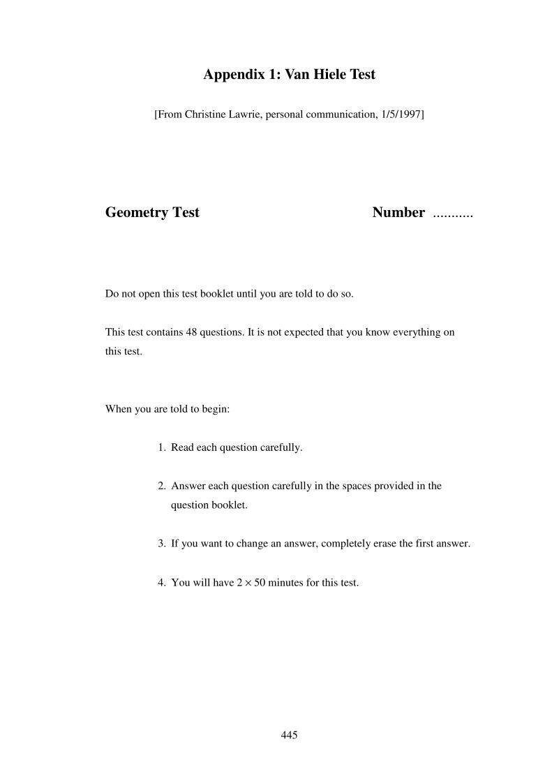
445
Appendix 1: Van Hiele Test
[From Christine Lawrie, personal communication, 1/5/1997]
Geometry Test Number ...........
Do not open this test booklet until you are told to do so.
This test contains 48 questions. It is not expected that you know everything on
this test.
When you are told to begin:
1. Read each question carefully.
2. Answer each question carefully in the spaces provided in the
question booklet.
3. If you want to change an answer, completely erase the first answer.
4. You will have 2 × 50 minutes for this test.
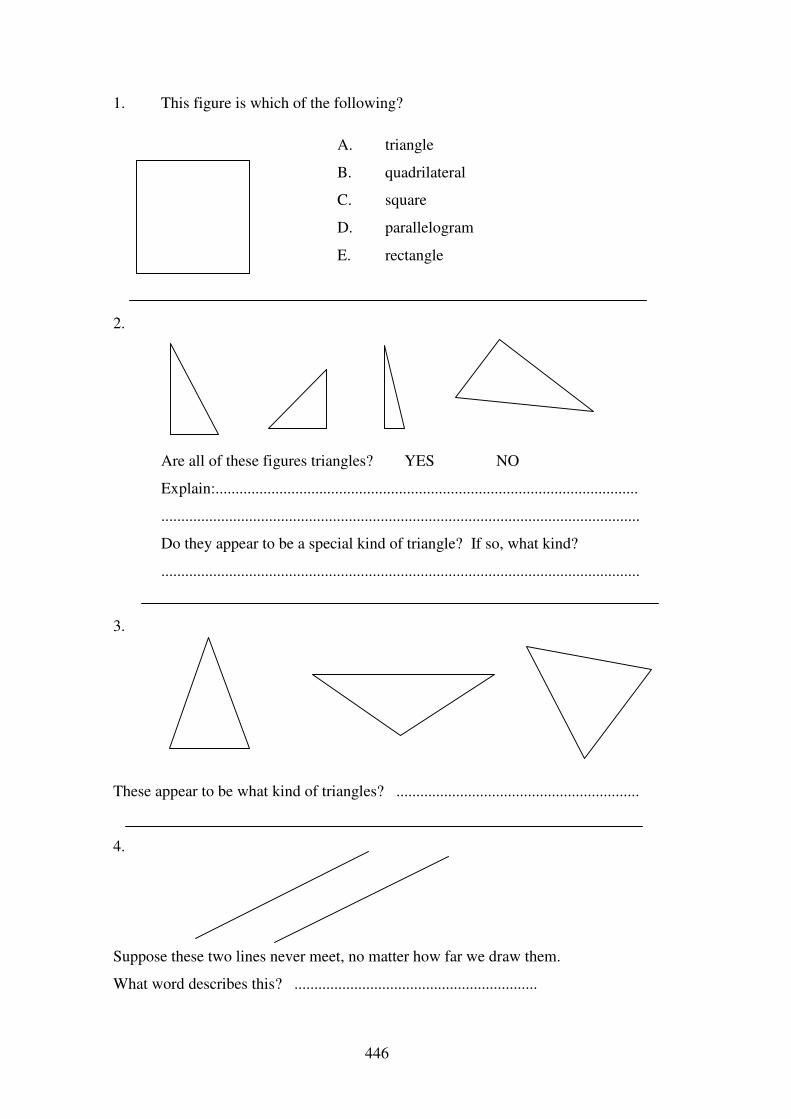
446
1. This figure is which of the following?
2.
Are all of these figures triangles? YES NO
Explain:..........................................................................................................
........................................................................................................................
Do they appear to be a special kind of triangle? If so, what kind?
........................................................................................................................
3.
These appear to be what kind of triangles? .............................................................
4.
Suppose these two lines never meet, no matter how far we draw them.
What word describes this? .............................................................
A. triangle
B. quadrilateral
C. square
D. parallelogram
E. rectangle
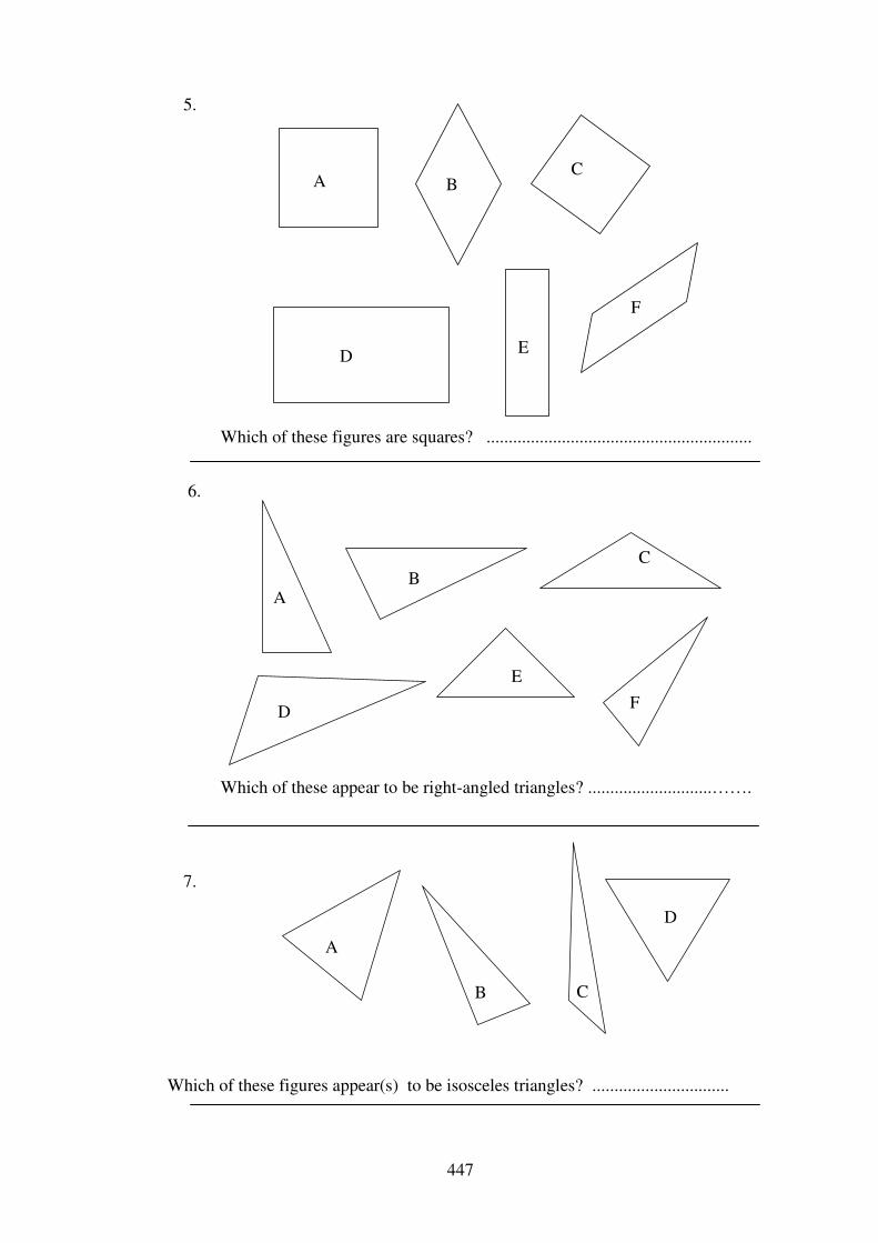
447
Which of these figures are squares? ............................................................
Which of these appear to be right-angled triangles? ............................…….
Which of these figures appear(s) to be isosceles triangles? ...............................
A B C
D E
F
A B
C
D
E F
A
B C
D
6.
7.
5.
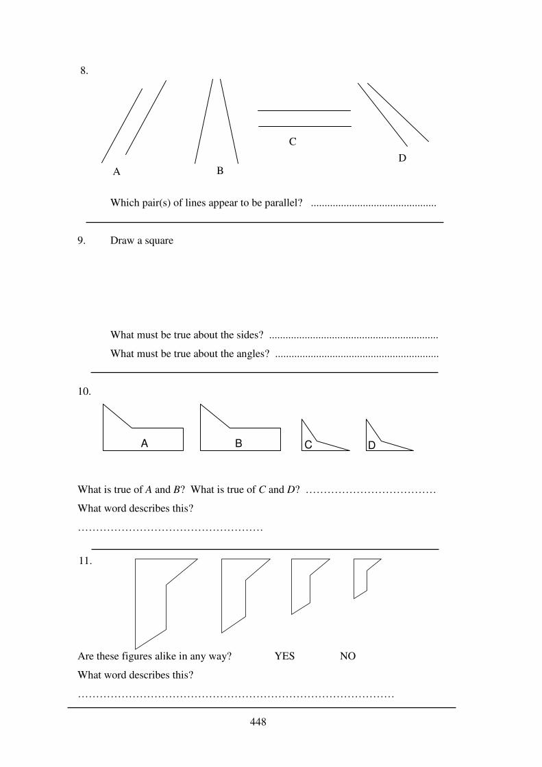
448
8.
Which pair(s) of lines appear to be parallel? ..............................................
9. Draw a square
What must be true about the sides? ..............................................................
What must be true about the angles? ............................................................
10.
A DCB
What is true of A and B? What is true of C and D? ………………………………
What word describes this?
……………………………………………
Are these figures alike in any way? YES NO
What word describes this?
……………………………………………………………………………
A B
C D
11.
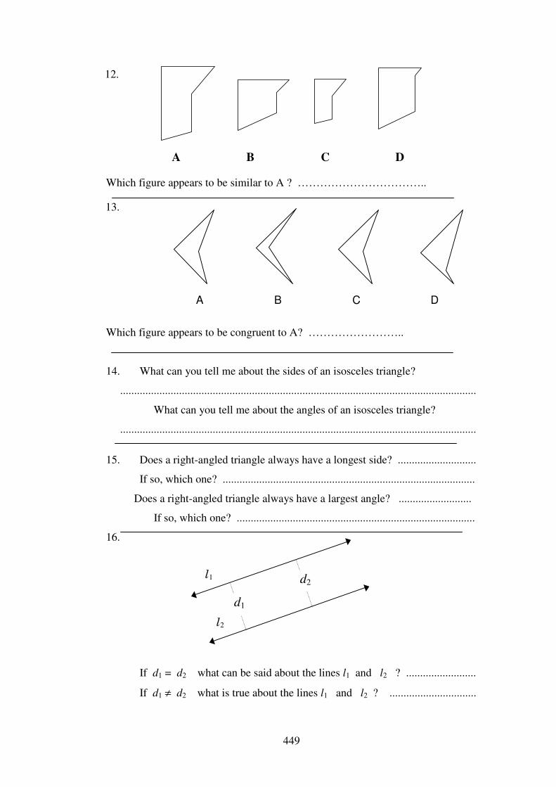
449
A B DC
Which figure appears to be similar to A ? ……………………………..
A DB C
Which figure appears to be congruent to A? ……………………..
14. What can you tell me about the sides of an isosceles triangle?
...............................................................................................................................
What can you tell me about the angles of an isosceles triangle?
...............................................................................................................................
15. Does a right-angled triangle always have a longest side? ............................
If so, which one? ..........................................................................................
Does a right-angled triangle always have a largest angle? ..........................
If so, which one? .....................................................................................
16.
If d1 = d2 what can be said about the lines l1 and l2 ? .........................
If d1 ≠ d2 what is true about the lines l1 and l2 ? ...............................
d1
d2 l1
l2
12.
13.
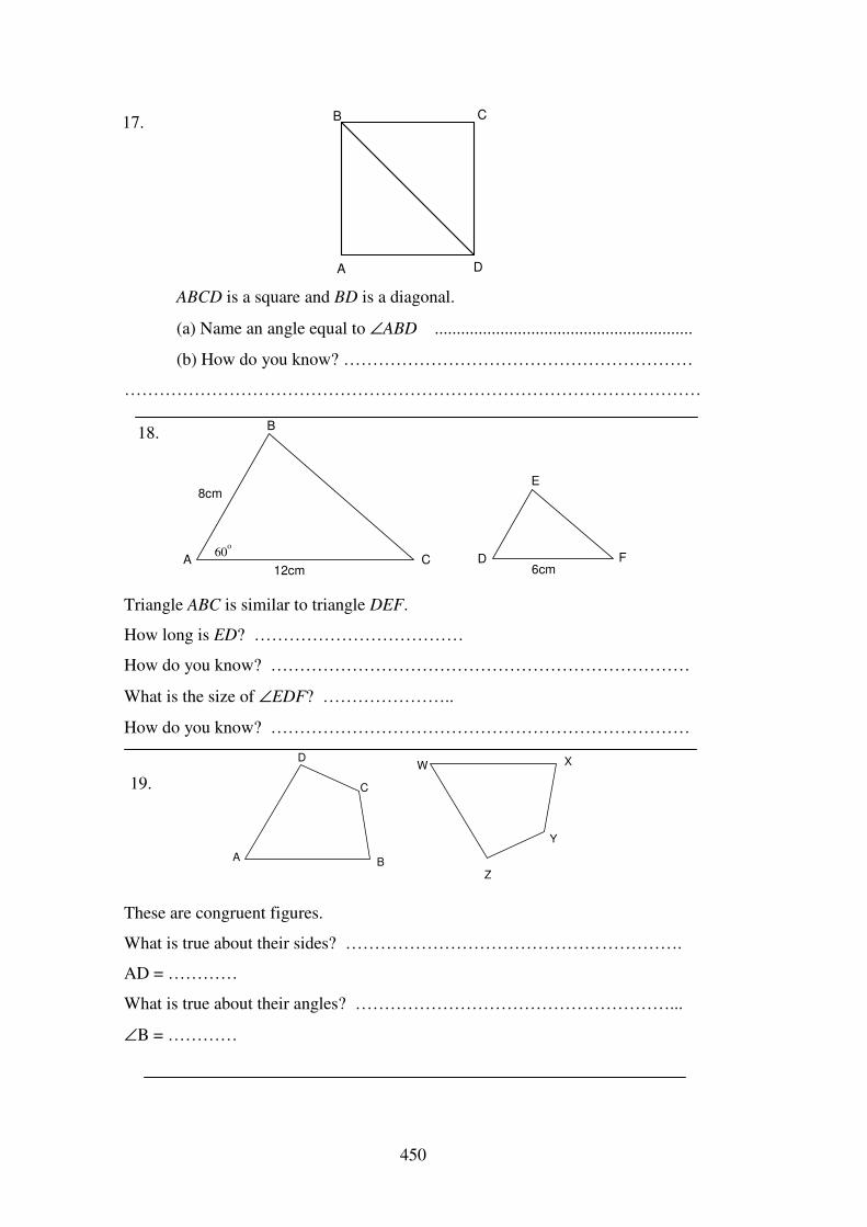
450
B
A
C
D ABCD is a square and BD is a diagonal.
(a) Name an angle equal to ∠ABD ...........................................................
(b) How do you know? ……………………………………………………
………………………………………………………………………………………
60o
A
E
DC F
B
8cm
6cm12cm Triangle ABC is similar to triangle DEF.
How long is ED? ………………………………
How do you know? ………………………………………………………………
What is the size of ∠EDF? …………………..
How do you know? ………………………………………………………………
A
C
D
B
Y
XW
Z
These are congruent figures.
What is true about their sides? ………………………………………………….
AD = …………
What is true about their angles? ………………………………………………...
∠B = …………
17.
18.
19.
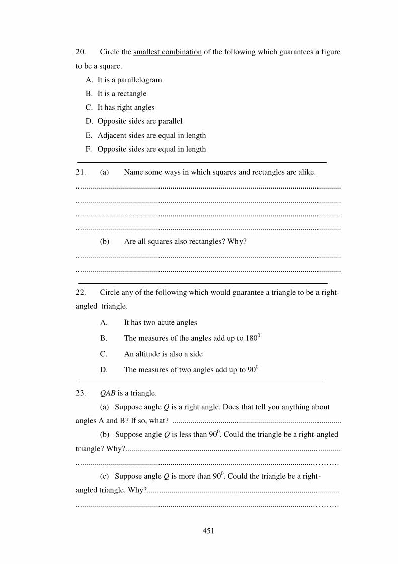
451
20. Circle the smallest combination of the following which guarantees a figure
to be a square.
A. It is a parallelogram
B. It is a rectangle
C. It has right angles
D. Opposite sides are parallel
E. Adjacent sides are equal in length
F. Opposite sides are equal in length
21. (a) Name some ways in which squares and rectangles are alike.
....................................................................................................................................
....................................................................................................................................
....................................................................................................................................
....................................................................................................................................
(b) Are all squares also rectangles? Why?
....................................................................................................................................
....................................................................................................................................
22. Circle any of the following which would guarantee a triangle to be a right-
angled triangle.
A. It has two acute angles
B. The measures of the angles add up to 1800
C. An altitude is also a side
D. The measures of two angles add up to 900
23. QAB is a triangle.
(a) Suppose angle Q is a right angle. Does that tell you anything about
angles A and B? If so, what? ....................................................................................
(b) Suppose angle Q is less than 900. Could the triangle be a right-angled
triangle? Why?...........................................................................................................
......................................................................................................................……….
(c) Suppose angle Q is more than 900. Could the triangle be a right-
angled triangle. Why?................................................................................................
......................................................................................................................……….
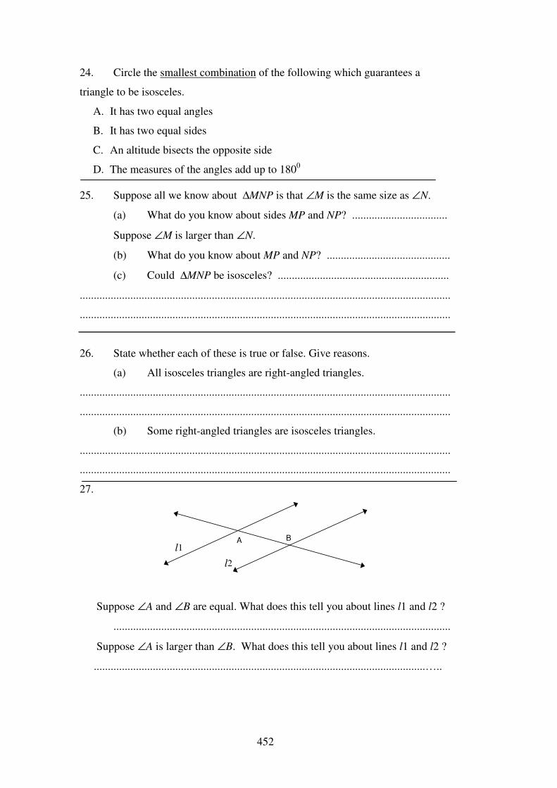
452
24. Circle the smallest combination of the following which guarantees a
triangle to be isosceles.
A. It has two equal angles
B. It has two equal sides
C. An altitude bisects the opposite side
D. The measures of the angles add up to 1800
25. Suppose all we know about ∆MNP is that ∠M is the same size as ∠N.
(a) What do you know about sides MP and NP? ..................................
Suppose ∠M is larger than ∠N.
(b) What do you know about MP and NP? ............................................
(c) Could ∆MNP be isosceles? .............................................................
....................................................................................................................................
....................................................................................................................................
26. State whether each of these is true or false. Give reasons.
(a) All isosceles triangles are right-angled triangles.
....................................................................................................................................
....................................................................................................................................
(b) Some right-angled triangles are isosceles triangles.
....................................................................................................................................
....................................................................................................................................
27.
A B
l2l1
Suppose ∠A and ∠B are equal. What does this tell you about lines l1 and l2 ?
........................................................................................................................
Suppose ∠A is larger than ∠B. What does this tell you about lines l1 and l2 ?
......................................................................................................................…..
453
28. (a) Triangle DEF has three equal sides. Is it an isosceles triangle?
Why or why not? .......................................................................................…..
(b) Is the following true or false?
All equilateral triangles are isosceles.
...................................................…….
29. Decide whether each of the following pairs of lines or line segments are
parallel
always
sometimes
never
Give reasons for each answer.
(a) Two lines which do not intersect .....................................................
Reason:.......................................................................................................................
....................................................................................................................................
(b) Two lines which are perpendicular to the same line .................................
Reason:.......................................................................................................................
....................................................................................................................................
(c) Two line segments in a square .......................................................
Reason:.......................................................................................................................
.................…...............................................................................................................
(d) Two line segments in a triangle .......................................................
Reason:.......................................................................................................................
....................................................................................................................................
(e) Two line segments which do not intersect
...................................…………
Reason:.......................................................................................................................
....................................................................................................................................
30. What does it mean to say that two figures are similar?
………………………………………………………………………………………
………………………………………………………………………………………
454
31. How do you recognise that lines are parallel?
........................................................................................................................
........................................................................................................................
32. Triangle ABC is similar to triangle DEF (in that order).
Are the following (a) certain , (b) possible, or (c) impossible?
Give reasons for your answers.
(a) AB = DE ……………………………………………………………………
(b) AB > DE ……………………………………………………………………
(c) ∠A = ∠E ……………………………………………………………………
(d) ∠A > ∠E ……………………………………………………………………
(e) AB = EF ……………………………………………………………………
(f) ∠A > ∠D ……………………………………………………………………
33. Will figures A and B be similar
I - always II - sometimes or III – never ?
Figure A Figure B
(a) a square (a) a square ………………….
(b) an isosceles triangle (b) an isosceles triangle …………………
(c) a triangle congruent to B (c) a triangle congruent to A …………………
(d) a rectangle (d) a square …………………
(e) a rectangle (e) a triangle …………………
34. ∆ABC is congruent to ∆DEF (in that order).
Are the following (a) certain, (b) possible, or (c) impossible ?
Give reasons for your answers.
(a) AB = DE …………………………………………………………………
(b) ∠A = ∠E …………………………………………………………………
(c) ∠A < ∠D …………………………………………………………………
(d) AB = EF …………………………………………………………………
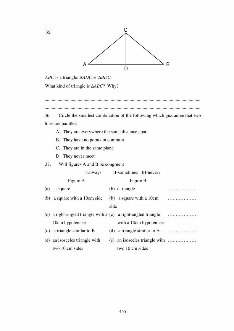
455
A
C
BD
ABC is a triangle. ∆ADC ≡ ∆BDC.
What kind of triangle is ∆ABC? Why?
....................................................................................................................................
....................................................................................................................................
36. Circle the smallest combination of the following which guarantee that two
lines are parallel.
A. They are everywhere the same distance apart
B. They have no points in common
C. They are in the same plane
D. They never meet
37. Will figures A and B be congruent
I-always II-sometimes III-never?
Figure A Figure B
(a) a square (b) a triangle ………………
(b) a square with a 10cm side (b) a square with a 10cm
side
………………
(c) a right-angled triangle with a
10cm hypotenuse
(c) a right-angled triangle
with a 10cm hypotenuse
………………
(d) a triangle similar to B (d) a triangle similar to A ………………
(e) an isosceles triangle with
two 10 cm sides
(e) an isosceles triangle with
two 10 cm sides
………………
35.
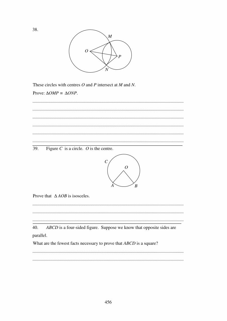
456
38.
These circles with centres O and P intersect at M and N.
Prove: ∆OMP ≡ ∆ONP.
....................................................................................................................................
....................................................................................................................................
....................................................................................................................................
....................................................................................................................................
....................................................................................................................................
....................................................................................................................................
39. Figure C is a circle. O is the centre.
Prove that ∆ AOB is isosceles.
....................................................................................................................................
....................................................................................................................................
....................................................................................................................................
40. ABCD is a four-sided figure. Suppose we know that opposite sides are
parallel.
What are the fewest facts necessary to prove that ABCD is a square?
....................................................................................................................................
....................................................................................................................................
O
M
N
P
O
A
C
B
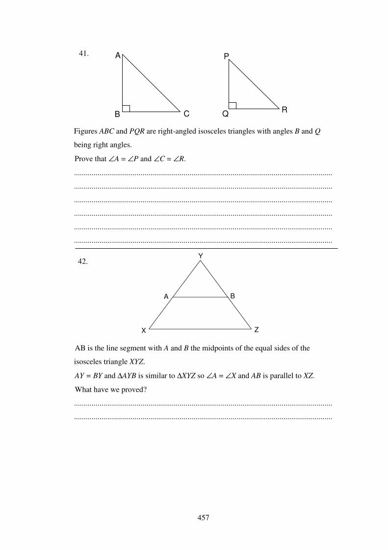
457
A
C RQ
P
B
Figures ABC and PQR are right-angled isosceles triangles with angles B and Q
being right angles.
Prove that ∠A = ∠P and ∠C = ∠R.
....................................................................................................................................
....................................................................................................................................
....................................................................................................................................
....................................................................................................................................
....................................................................................................................................
....................................................................................................................................
X
A B
Y
Z
AB is the line segment with A and B the midpoints of the equal sides of the
isosceles triangle XYZ.
AY = BY and ∆AYB is similar to ∆XYZ so ∠A = ∠X and AB is parallel to XZ.
What have we proved?
....................................................................................................................................
....................................................................................................................................
41.
42.
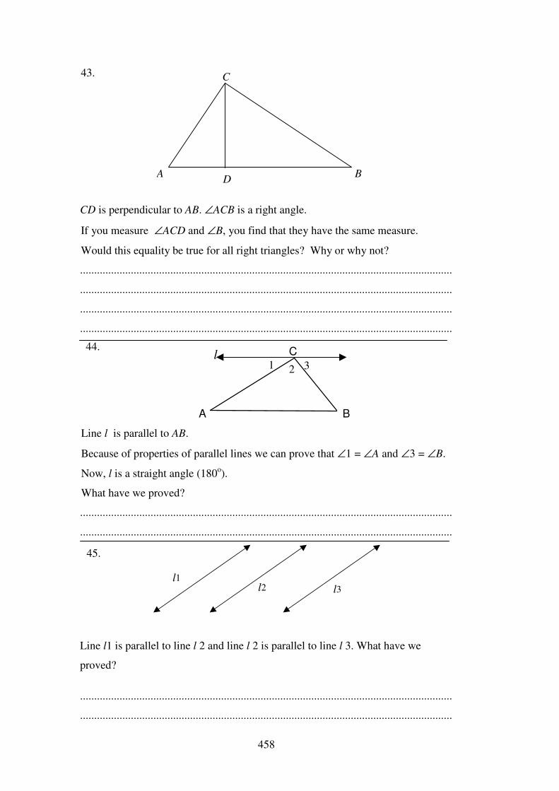
458
43.
CD is perpendicular to AB. ∠ACB is a right angle.
If you measure ∠ACD and ∠B, you find that they have the same measure.
Would this equality be true for all right triangles? Why or why not?
....................................................................................................................................
....................................................................................................................................
....................................................................................................................................
....................................................................................................................................
C
A B
21 3l
Line l is parallel to AB.
Because of properties of parallel lines we can prove that ∠1 = ∠A and ∠3 = ∠B.
Now, l is a straight angle (180o).
What have we proved?
....................................................................................................................................
....................................................................................................................................
l1l2 l3
Line l1 is parallel to line l 2 and line l 2 is parallel to line l 3. What have we
proved?
....................................................................................................................................
....................................................................................................................................
A B
C
D
44.
45.
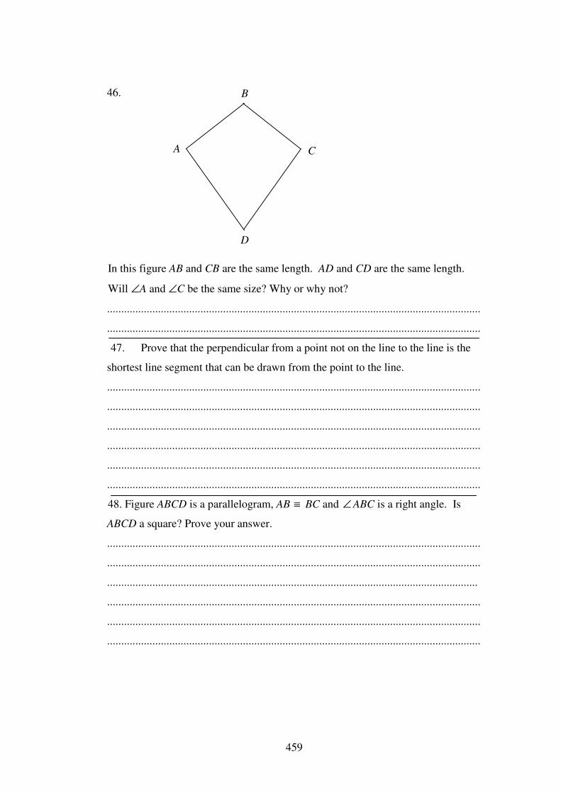
459
46.
In this figure AB and CB are the same length. AD and CD are the same length.
Will ∠A and ∠C be the same size? Why or why not?
....................................................................................................................................
....................................................................................................................................
47. Prove that the perpendicular from a point not on the line to the line is the
shortest line segment that can be drawn from the point to the line.
....................................................................................................................................
....................................................................................................................................
....................................................................................................................................
....................................................................................................................................
....................................................................................................................................
....................................................................................................................................
48. Figure ABCD is a parallelogram, AB ≡ BC and ∠ ABC is a right angle. Is
ABCD a square? Prove your answer.
....................................................................................................................................
....................................................................................................................................
...................................................................................................................................
....................................................................................................................................
....................................................................................................................................
....................................................................................................................................
A
B
C
D

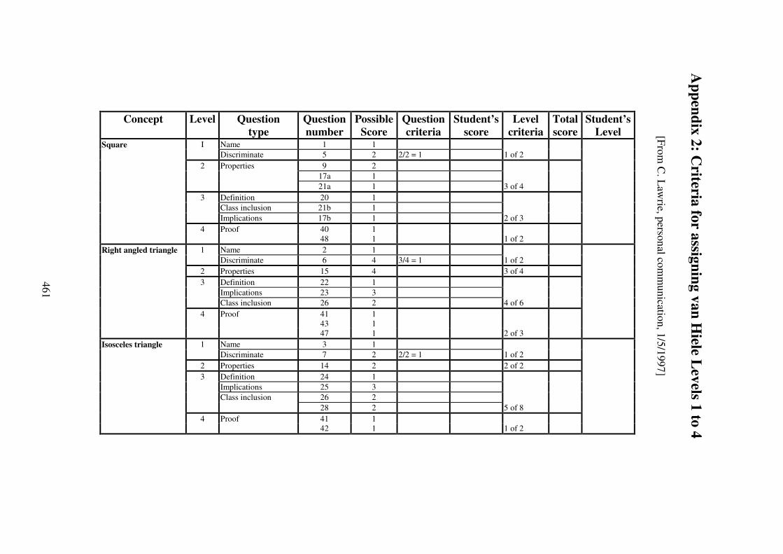
Concept Level Question type
Question number
Possible Score
Question criteria
Student’s score
Level criteria
Total score
Student’s Level
Square I Name 1 1 Discriminate 5 2 2/2 = 1 1 of 2 2 Properties 9 2 17a 1 21a 1 3 of 4 3 Definition 20 1 Class inclusion 21b 1 Implications 17b 1 2 of 3 4 Proof 40 1 48 1 1 of 2 Right angled triangle 1 Name 2 1 Discriminate 6 4 3/4 = 1 1 of 2 2 Properties 15 4 3 of 4 3 Definition 22 1 Implications 23 3 Class inclusion 26 2 4 of 6 4 Proof 41 1 43 1 47 1 2 of 3 Isosceles triangle 1 Name 3 1 Discriminate 7 2 2/2 = 1 1 of 2 2 Properties 14 2 2 of 2 3 Definition 24 1 Implications 25 3 Class inclusion 26 2 28 2 5 of 8 4 Proof 41 1 42 1 1 of 2
Appendix 2: C
riteria for assigning van Hiele L
evels 1 to 4
[From C
. Law
rie, personal comm
unication, 1/5/1997]
461
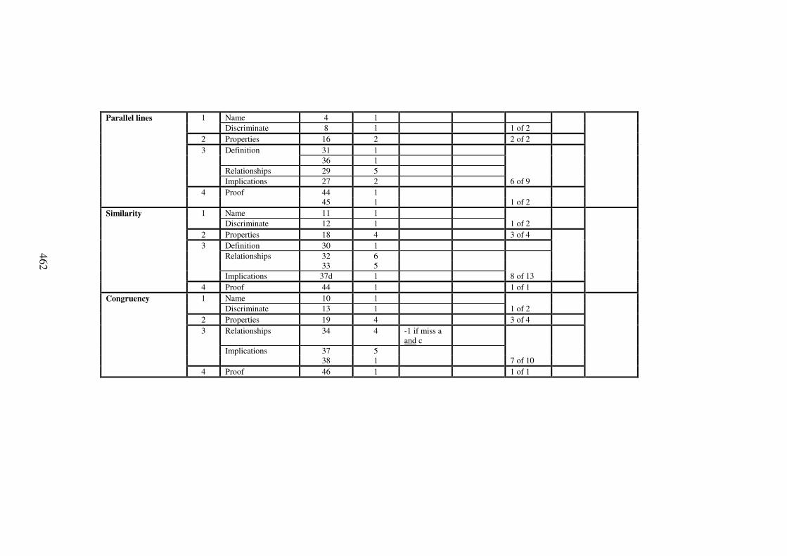
Parallel lines 1 Name 4 1 Discriminate 8 1 1 of 2 2 Properties 16 2 2 of 2 3 Definition 31 1 36 1 Relationships 29 5 Implications 27 2 6 of 9 4 Proof 44 1 45 1 1 of 2 Similarity 1 Name 11 1 Discriminate 12 1 1 of 2 2 Properties 18 4 3 of 4 3 Definition 30 1 Relationships 32 6 33 5 Implications 37d 1 8 of 13 4 Proof 44 1 1 of 1 Congruency 1 Name 10 1 Discriminate 13 1 1 of 2 2 Properties 19 4 3 of 4 3 Relationships 34 4 -1 if miss a
and c
Implications 37 5 38 1 7 of 10 4 Proof 46 1 1 of 1
462
463
Appendix 3: Proof Questionnaire
[From Healy & Hoyles, 1999]
Permission to use the Proof Questionnaire: C. Hoyles, personal communications,
19/09/2000, 12/12/2000.

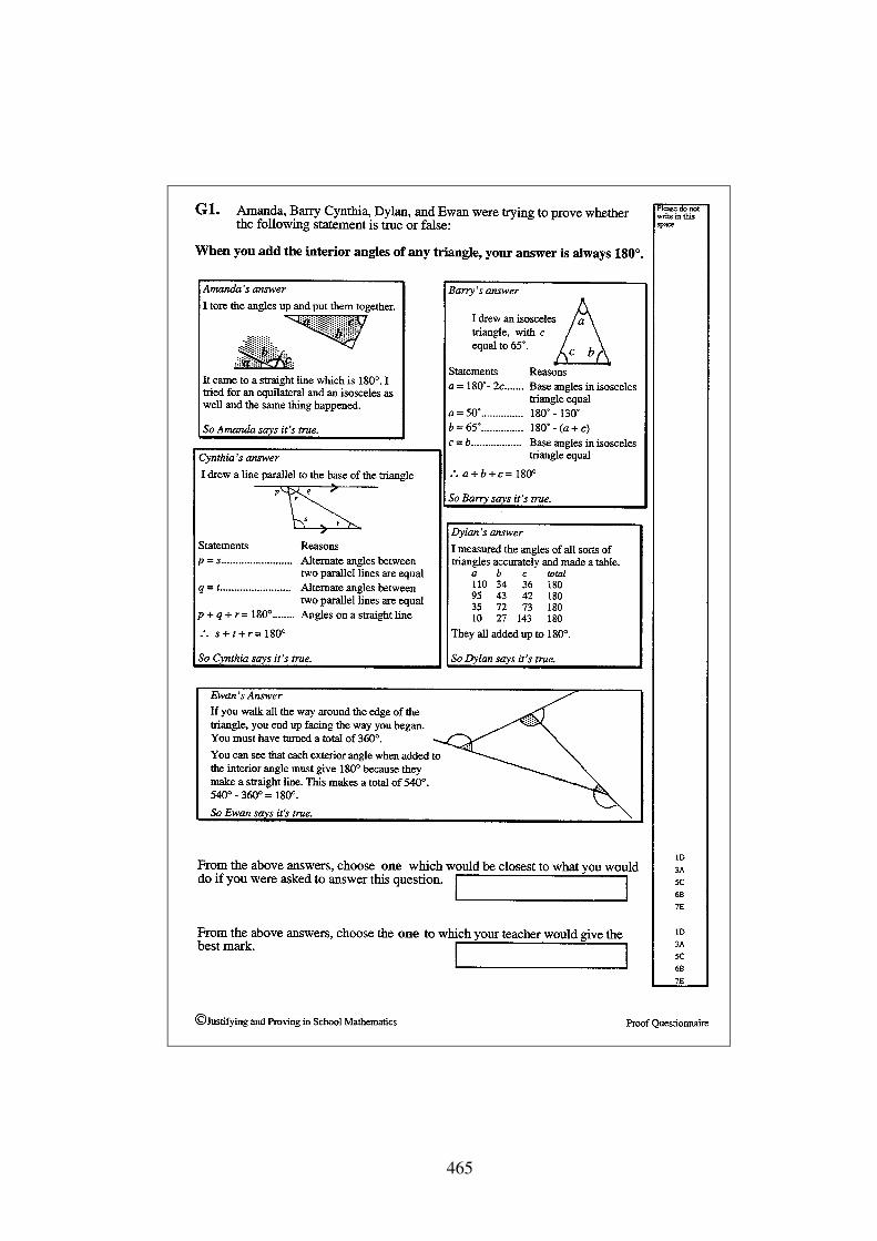
465
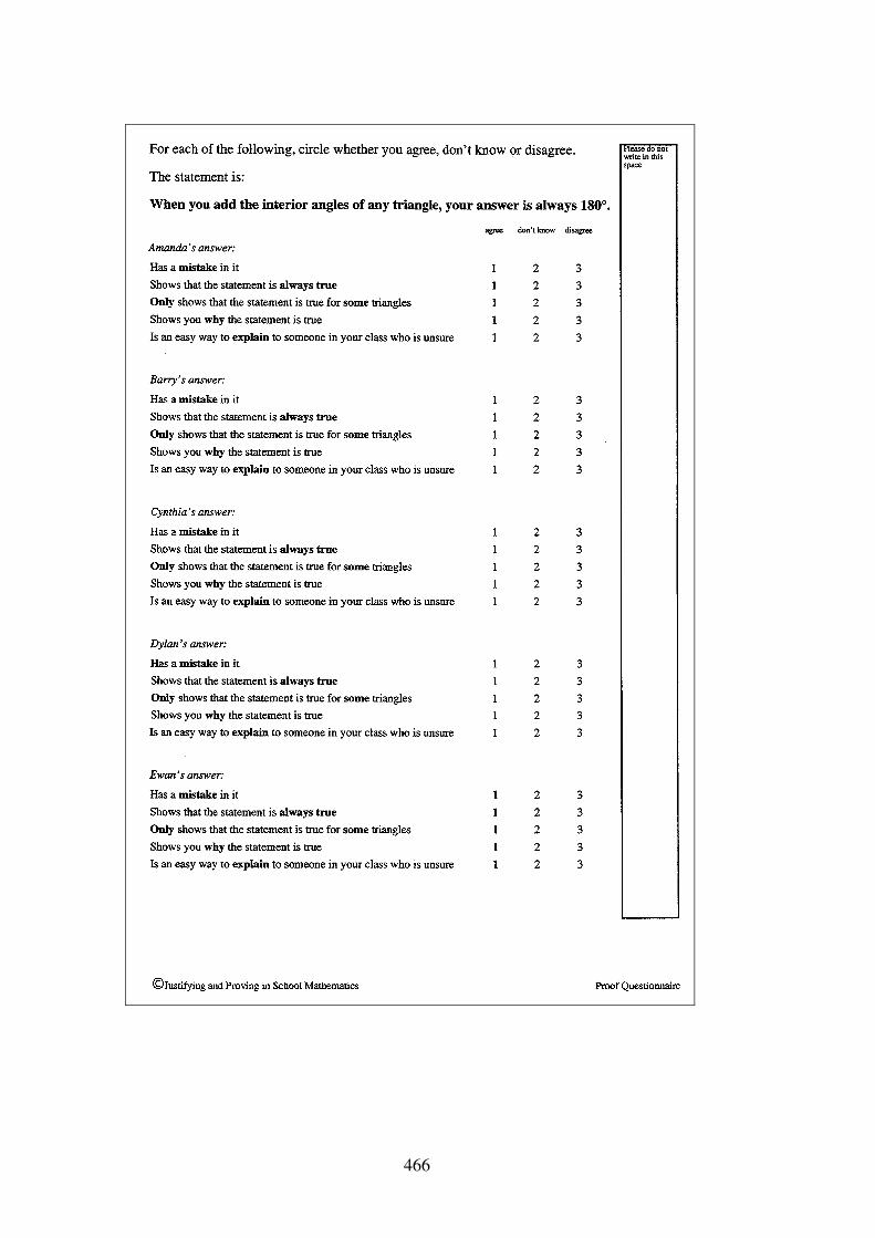
466
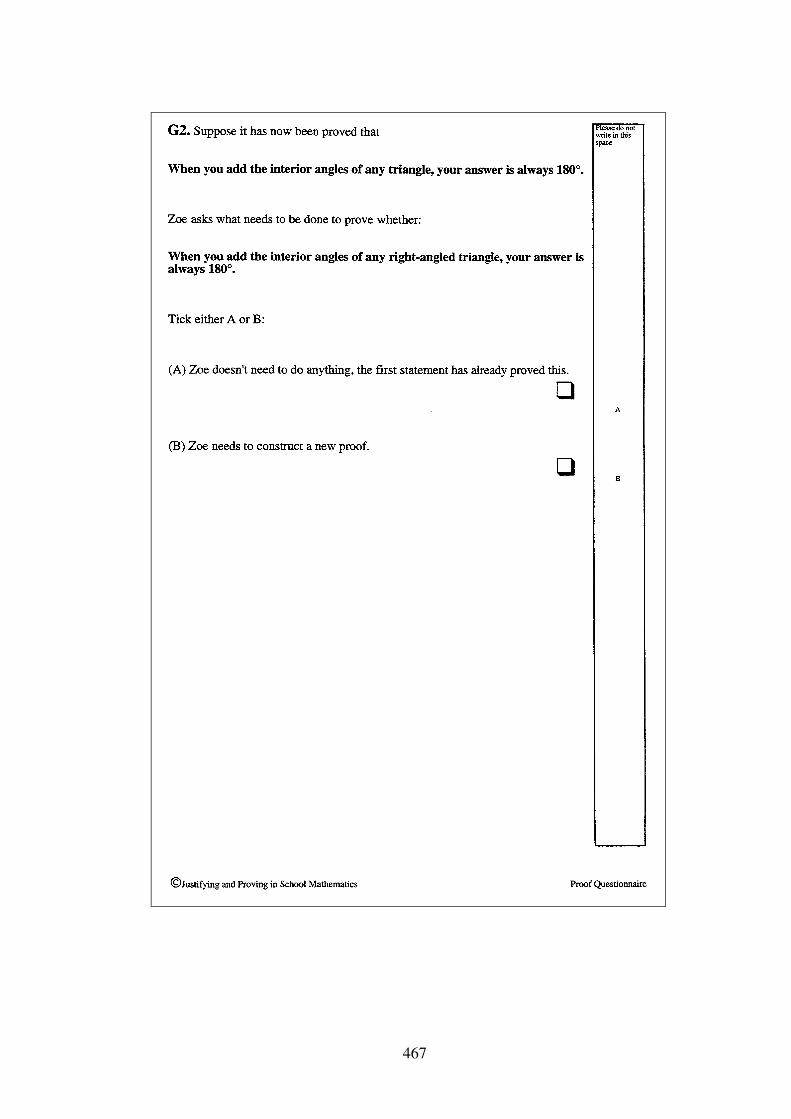
467
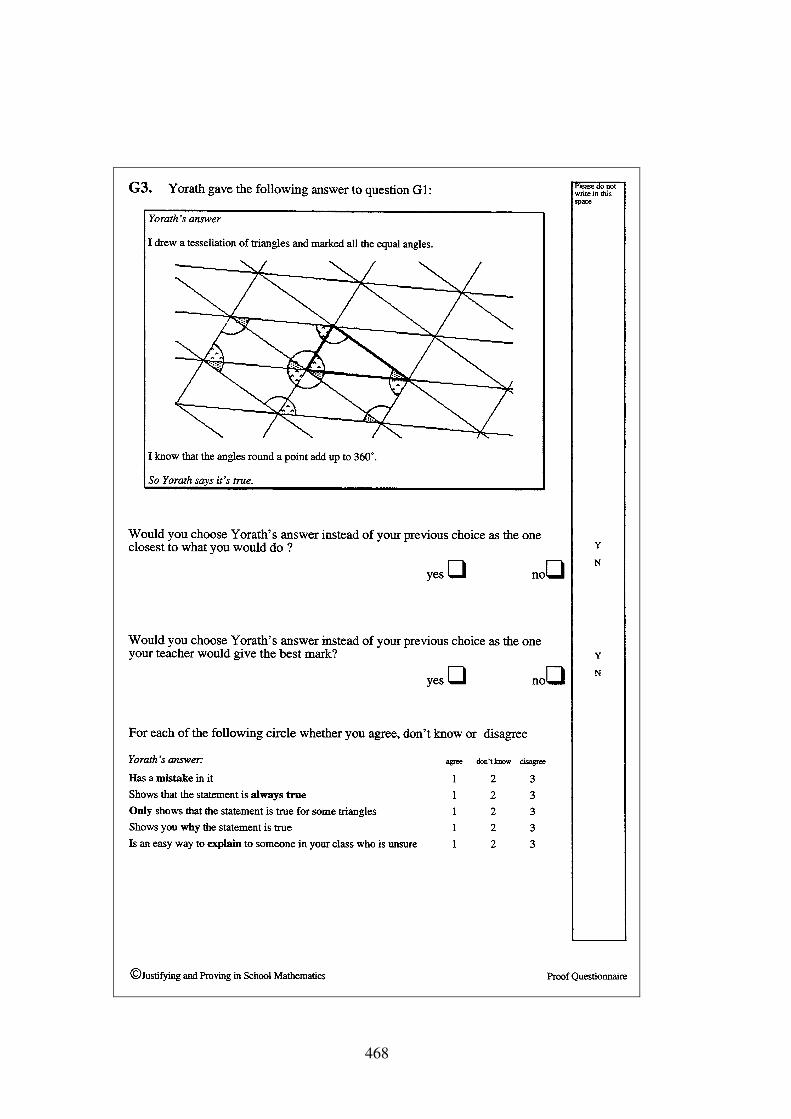
468
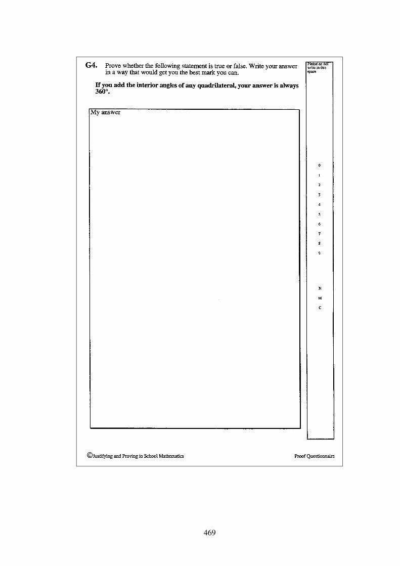
469
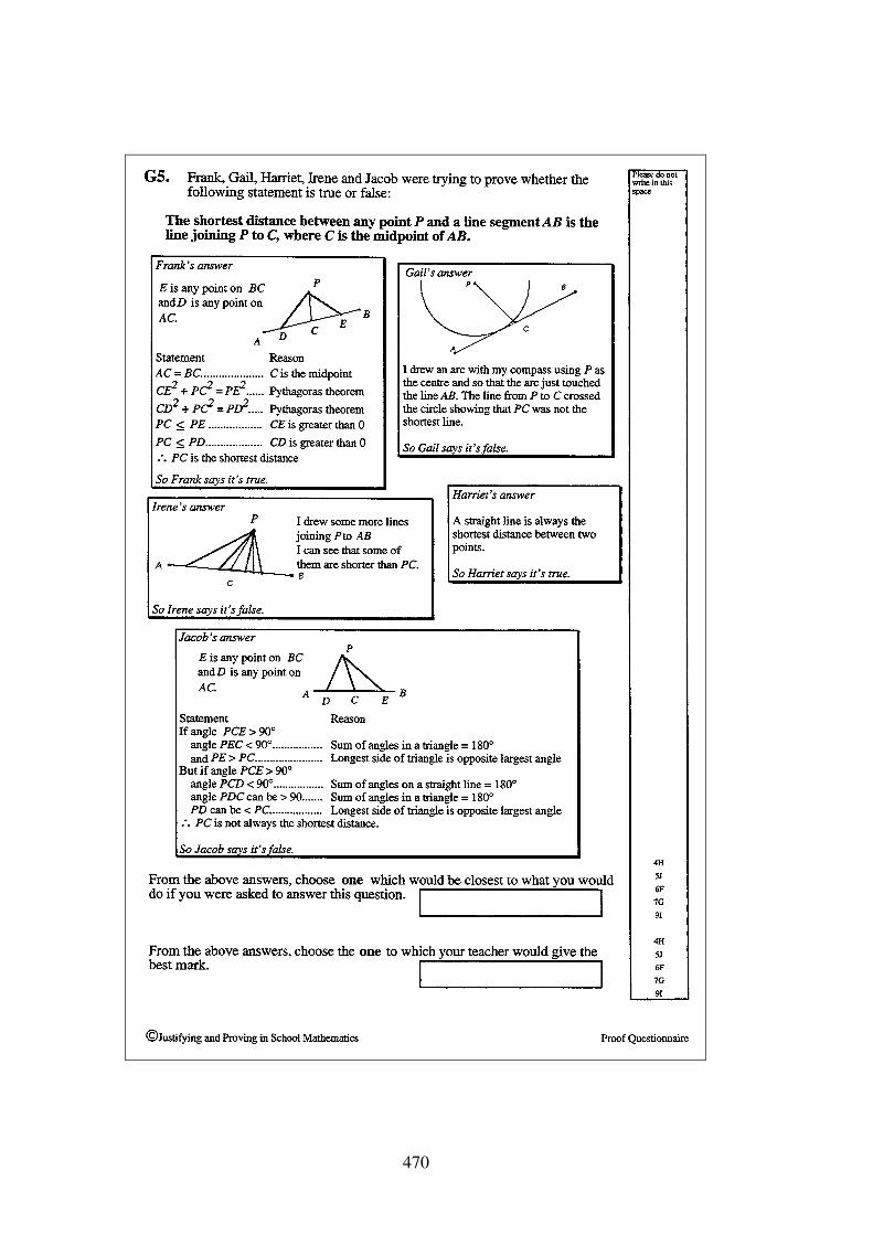
470
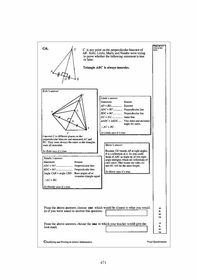
471
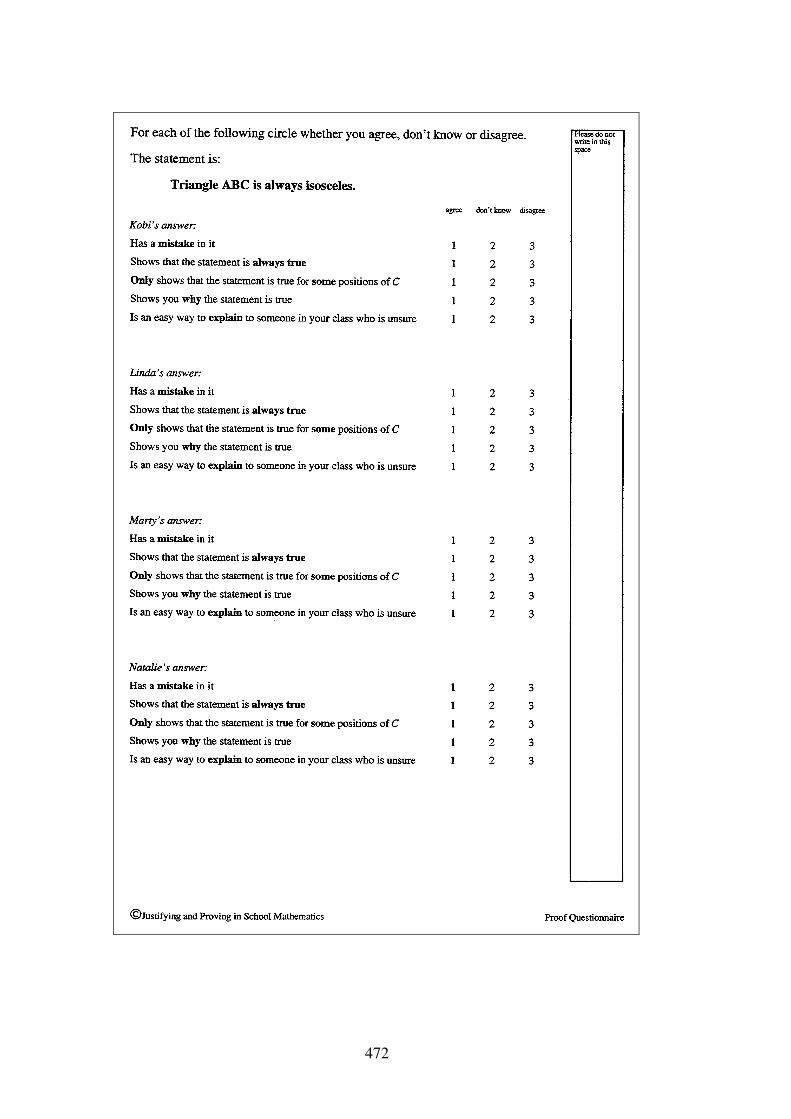
472
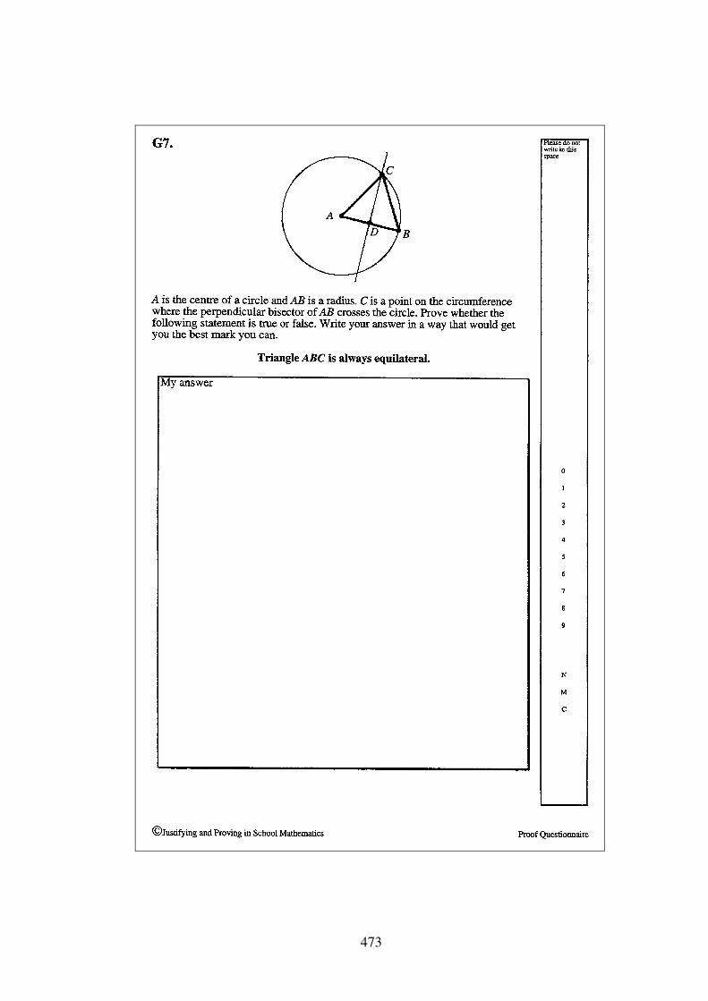
473

474
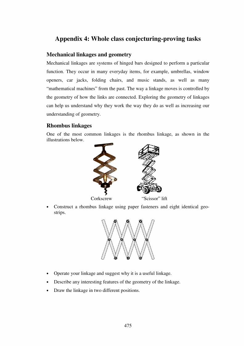
475
Appendix 4: Whole class conjecturing-proving tasks
Mechanical linkages and geometry Mechanical linkages are systems of hinged bars designed to perform a particular
function. They occur in many everyday items, for example, umbrellas, window
openers, car jacks, folding chairs, and music stands, as well as many
“mathematical machines” from the past. The way a linkage moves is controlled by
the geometry of how the links are connected. Exploring the geometry of linkages
can help us understand why they work the way they do as well as increasing our
understanding of geometry.
Rhombus linkages One of the most common linkages is the rhombus linkage, as shown in the illustrations below.
Corkscrew “Scissor” lift
• Construct a rhombus linkage using paper fasteners and eight identical geo-strips.
• Operate your linkage and suggest why it is a useful linkage.
• Describe any interesting features of the geometry of the linkage.
• Draw the linkage in two different positions.
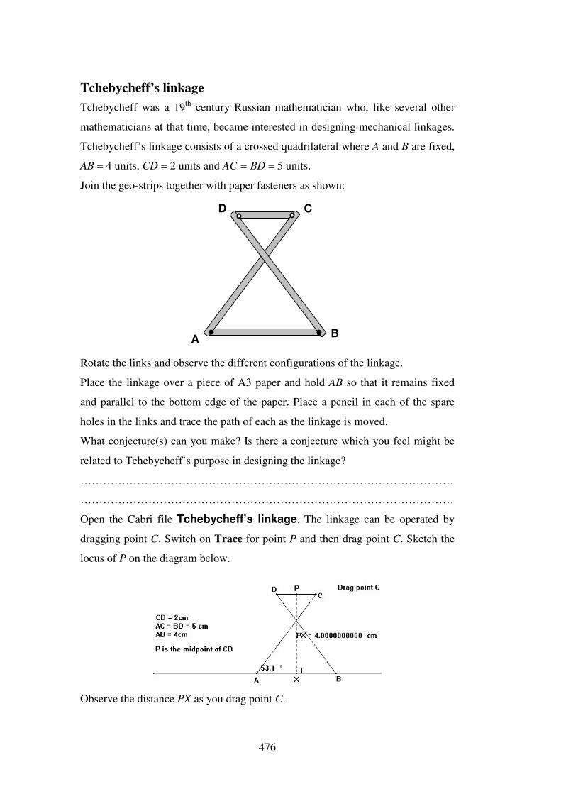
476
Tchebycheff’s linkage Tchebycheff was a 19th century Russian mathematician who, like several other
mathematicians at that time, became interested in designing mechanical linkages.
Tchebycheff’s linkage consists of a crossed quadrilateral where A and B are fixed,
AB = 4 units, CD = 2 units and AC = BD = 5 units.
Join the geo-strips together with paper fasteners as shown:
D
A B
C
Rotate the links and observe the different configurations of the linkage.
Place the linkage over a piece of A3 paper and hold AB so that it remains fixed
and parallel to the bottom edge of the paper. Place a pencil in each of the spare
holes in the links and trace the path of each as the linkage is moved.
What conjecture(s) can you make? Is there a conjecture which you feel might be
related to Tchebycheff’s purpose in designing the linkage?
………………………………………………………………………………………
………………………………………………………………………………………
Open the Cabri file Tchebycheff’s linkage. The linkage can be operated by
dragging point C. Switch on Trace for point P and then drag point C. Sketch the
locus of P on the diagram below.
Observe the distance PX as you drag point C.
477
Can you show why PX = 4cm when the linkage is in the position shown above?
Hint: Draw a line through C perpendicular to AB.
………………………………………………………………………………………
………………………………………………………………………………………
………………………………………………………………………………………
………………………………………………………………………………………
………………………………………………………………………………………
Can you find another position where the distance PX seems to be exactly 4cm?
Draw the linkage in this position and show why you think PX is exactly 4cm.
Drag point C and record some values for the length PX and the corresponding size
of ∠CAB.
When ∠CAB = ……….. o , PX = ……………………… cm
When ∠CAB = ……….. o , PX = ……………………… cm
When ∠CAB = ……….. o , PX = ……………………… cm
These cases where PX is not exactly 4cm are called counter-examples, where
“counter” means “opposite” or “against”. The counter-examples show us that the
conjecture that P moves in a straight line parallel to AB is not true.
How many counter-examples do you think we would need to prove that P does
not move in a straight line parallel to AB? Explain.
………………………………………………………………………………………
………………………………………………………………………………………
………………………………………………………………………………………
………………………………………………………………………………………
478
If you had not been able to find any counter-examples could you assume that the
conjecture that P moves in a straight line parallel to AB was true? Explain.
………………………………………………………………………………………
………………………………………………………………………………………
………………………………………………………………………………………
………………………………………………………………………………………
………………………………………………………………………………………
So finding a counter-example can tell us if a conjecture is incorrect, but if we
can’t find any counter-examples, …………………………………………………..
………………………………………………………………………………………
………………………………………………………………………………………
………………………………………………………………………………………
………………………………………………………………………………………
Why was Tchebycheff’s linkage useful?
Many nineteenth century inventions were based on the circular motion of a wheel
driven by a steam engine moving another part of the machine in a straight-line
path. Some of these linkages were very complicated and the moving parts were
subjected to wear. To minimise the wear on moving parts, simpler linkages which
did not produce exact straight-line motion were sometimes used.
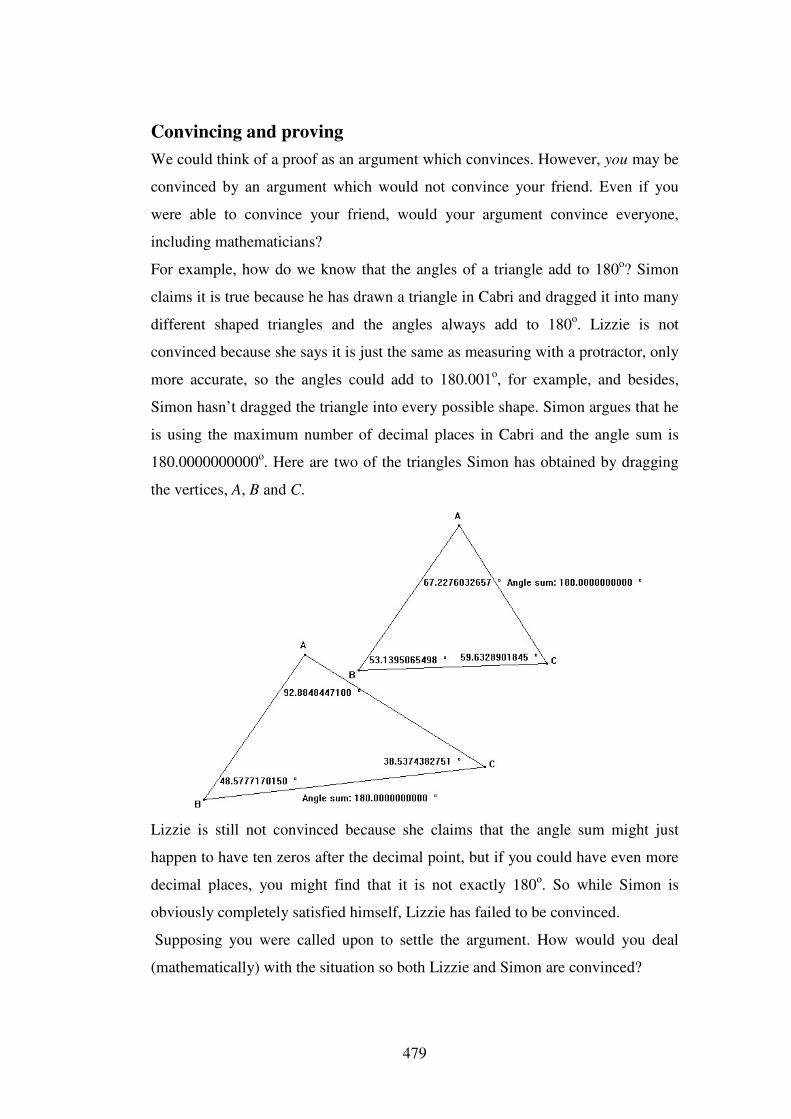
479
Convincing and proving We could think of a proof as an argument which convinces. However, you may be
convinced by an argument which would not convince your friend. Even if you
were able to convince your friend, would your argument convince everyone,
including mathematicians?
For example, how do we know that the angles of a triangle add to 180o? Simon
claims it is true because he has drawn a triangle in Cabri and dragged it into many
different shaped triangles and the angles always add to 180o. Lizzie is not
convinced because she says it is just the same as measuring with a protractor, only
more accurate, so the angles could add to 180.001o, for example, and besides,
Simon hasn’t dragged the triangle into every possible shape. Simon argues that he
is using the maximum number of decimal places in Cabri and the angle sum is
180.0000000000o. Here are two of the triangles Simon has obtained by dragging
the vertices, A, B and C.
Lizzie is still not convinced because she claims that the angle sum might just
happen to have ten zeros after the decimal point, but if you could have even more
decimal places, you might find that it is not exactly 180o. So while Simon is
obviously completely satisfied himself, Lizzie has failed to be convinced.
Supposing you were called upon to settle the argument. How would you deal
(mathematically) with the situation so both Lizzie and Simon are convinced?
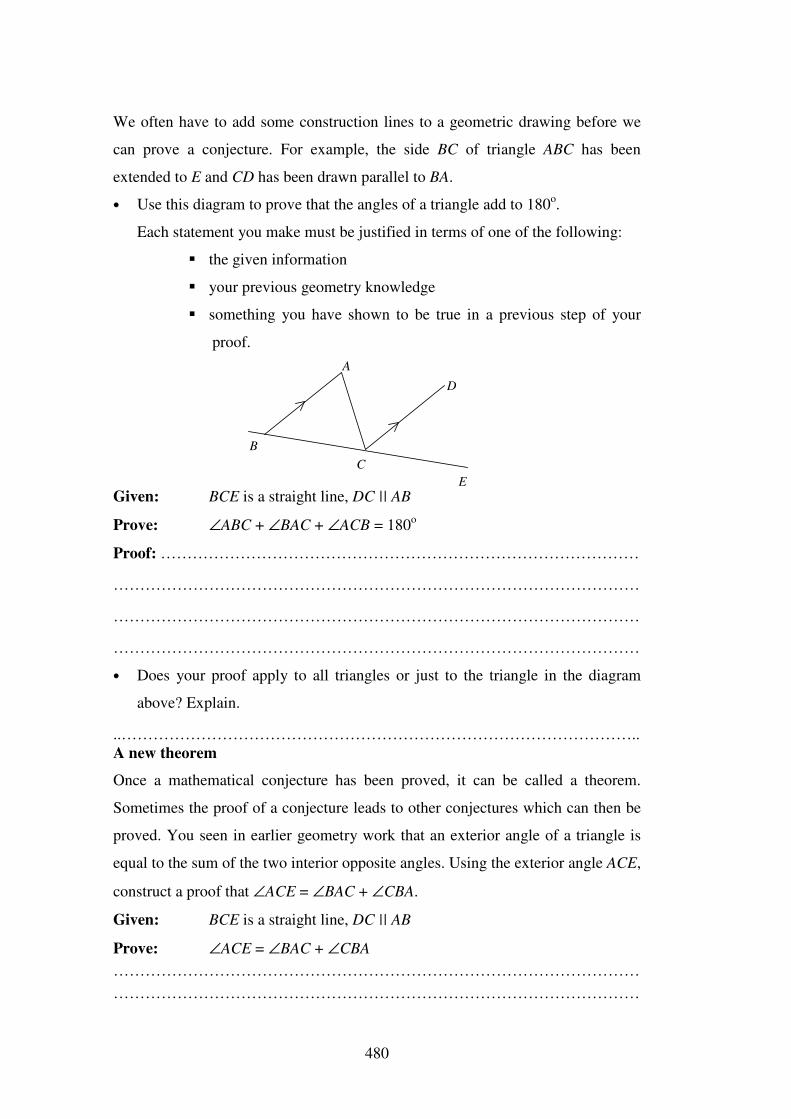
480
We often have to add some construction lines to a geometric drawing before we
can prove a conjecture. For example, the side BC of triangle ABC has been
extended to E and CD has been drawn parallel to BA.
• Use this diagram to prove that the angles of a triangle add to 180o.
Each statement you make must be justified in terms of one of the following:
��the given information
��your previous geometry knowledge
��something you have shown to be true in a previous step of your
proof.
A
C
D
E
B
Given: BCE is a straight line, DC || AB
Prove: ∠ABC + ∠BAC + ∠ACB = 180o
Proof: ………………………………………………………………………………
………………………………………………………………………………………
………………………………………………………………………………………
………………………………………………………………………………………
• Does your proof apply to all triangles or just to the triangle in the diagram
above? Explain.
..…………………………………………………………………………………….. A new theorem
Once a mathematical conjecture has been proved, it can be called a theorem.
Sometimes the proof of a conjecture leads to other conjectures which can then be
proved. You seen in earlier geometry work that an exterior angle of a triangle is
equal to the sum of the two interior opposite angles. Using the exterior angle ACE,
construct a proof that ∠ACE = ∠BAC + ∠CBA.
Given: BCE is a straight line, DC || AB
Prove: ∠ACE = ∠BAC + ∠CBA ……………………………………………………………………………………… ………………………………………………………………………………………
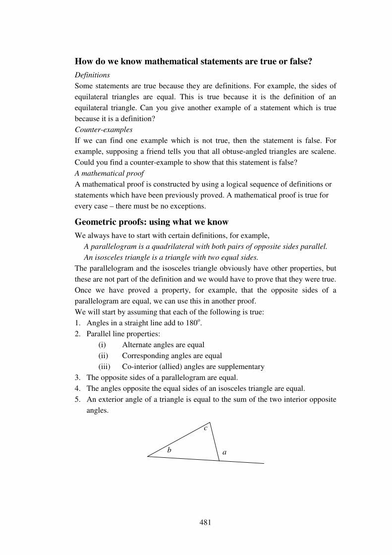
481
How do we know mathematical statements are true or false? Definitions Some statements are true because they are definitions. For example, the sides of equilateral triangles are equal. This is true because it is the definition of an equilateral triangle. Can you give another example of a statement which is true because it is a definition? Counter-examples If we can find one example which is not true, then the statement is false. For example, supposing a friend tells you that all obtuse-angled triangles are scalene. Could you find a counter-example to show that this statement is false? A mathematical proof A mathematical proof is constructed by using a logical sequence of definitions or statements which have been previously proved. A mathematical proof is true for every case – there must be no exceptions.
Geometric proofs: using what we know We always have to start with certain definitions, for example,
A parallelogram is a quadrilateral with both pairs of opposite sides parallel. An isosceles triangle is a triangle with two equal sides.
The parallelogram and the isosceles triangle obviously have other properties, but these are not part of the definition and we would have to prove that they were true. Once we have proved a property, for example, that the opposite sides of a parallelogram are equal, we can use this in another proof. We will start by assuming that each of the following is true: 1. Angles in a straight line add to 180o. 2. Parallel line properties:
(i) Alternate angles are equal (ii) Corresponding angles are equal (iii) Co-interior (allied) angles are supplementary
3. The opposite sides of a parallelogram are equal. 4. The angles opposite the equal sides of an isosceles triangle are equal. 5. An exterior angle of a triangle is equal to the sum of the two interior opposite
angles.
a
c
b
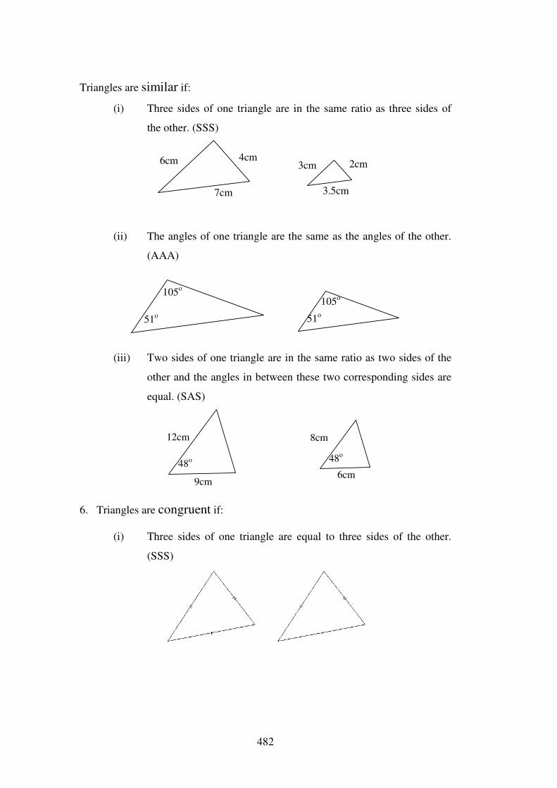
482
Triangles are similar if:
(i) Three sides of one triangle are in the same ratio as three sides of
the other. (SSS)
2cm
7cm 3.5cm
6cm 3cm 4cm
(ii) The angles of one triangle are the same as the angles of the other.
(AAA)
105o
51o
105o
51o
(iii) Two sides of one triangle are in the same ratio as two sides of the
other and the angles in between these two corresponding sides are
equal. (SAS)
48o 48o
6cm
8cm 12cm
9cm
6. Triangles are congruent if:
(i) Three sides of one triangle are equal to three sides of the other.
(SSS)
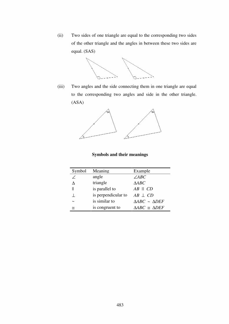
483
(ii) Two sides of one triangle are equal to the corresponding two sides
of the other triangle and the angles in between these two sides are
equal. (SAS)
(iii) Two angles and the side connecting them in one triangle are equal
to the corresponding two angles and side in the other triangle.
(ASA)
Symbols and their meanings
Symbol Meaning Example ∠ angle ∠ABC ∆ triangle ∆ABC || is parallel to AB || CD ⊥ is perpendicular to AB ⊥ CD ~ is similar to ∆ABC ~ ∆DEF ≅ is congruent to ∆ABC ≅ ∆DEF
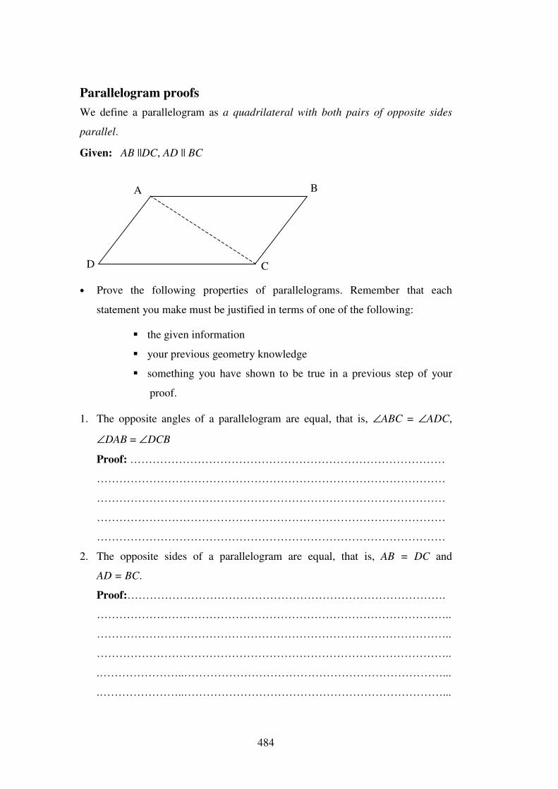
484
Parallelogram proofs We define a parallelogram as a quadrilateral with both pairs of opposite sides
parallel.
Given: AB ||DC, AD || BC
A
D C
B
• Prove the following properties of parallelograms. Remember that each
statement you make must be justified in terms of one of the following:
��the given information
��your previous geometry knowledge
��something you have shown to be true in a previous step of your
proof.
1. The opposite angles of a parallelogram are equal, that is, ∠ABC = ∠ADC,
∠DAB = ∠DCB
Proof: …………………………………………………………………………
…………………………………………………………………………………
…………………………………………………………………………………
…………………………………………………………………………………
…………………………………………………………………………………
2. The opposite sides of a parallelogram are equal, that is, AB = DC and
AD = BC.
Proof:………………………………………………………………………….
…………………………………………………………………………………..
…………………………………………………………………………………..
…………………………………………………………………………………..
.…………………..……………………………………………………………...
.…………………..……………………………………………………………...
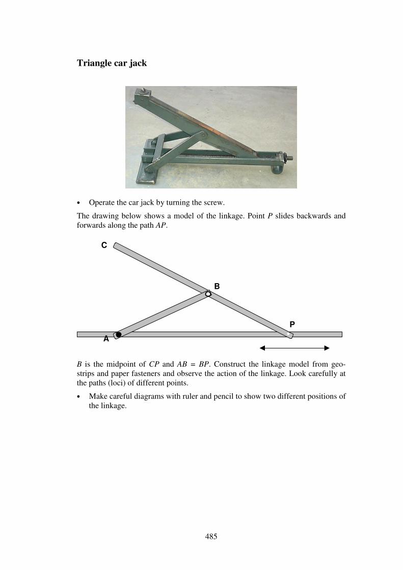
485
Triangle car jack
• Operate the car jack by turning the screw.
The drawing below shows a model of the linkage. Point P slides backwards and forwards along the path AP.
A
C
B
• P
B is the midpoint of CP and AB = BP. Construct the linkage model from geo-strips and paper fasteners and observe the action of the linkage. Look carefully at the paths (loci) of different points.
• Make careful diagrams with ruler and pencil to show two different positions of the linkage.
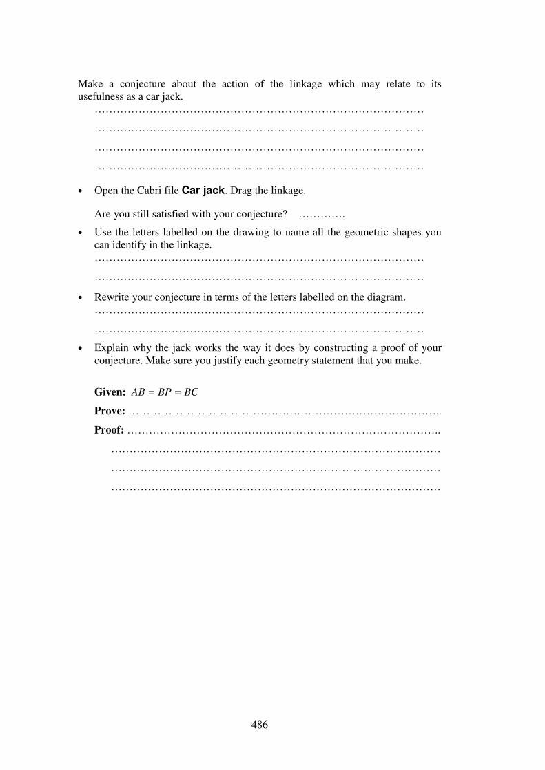
486
Make a conjecture about the action of the linkage which may relate to its usefulness as a car jack.
………………………………………………………………………………
………………………………………………………………………………
………………………………………………………………………………
………………………………………………………………………………
• Open the Cabri file Car jack. Drag the linkage.
Are you still satisfied with your conjecture? ………….
• Use the letters labelled on the drawing to name all the geometric shapes you can identify in the linkage. ………………………………………………………………………………
………………………………………………………………………………
• Rewrite your conjecture in terms of the letters labelled on the diagram. ………………………………………………………………………………
………………………………………………………………………………
• Explain why the jack works the way it does by constructing a proof of your conjecture. Make sure you justify each geometry statement that you make.
Given: AB = BP = BC
Prove: …………………………………………………………………………..
Proof: …………………………………………………………………………..
………………………………………………………………………………
………………………………………………………………………………
………………………………………………………………………………
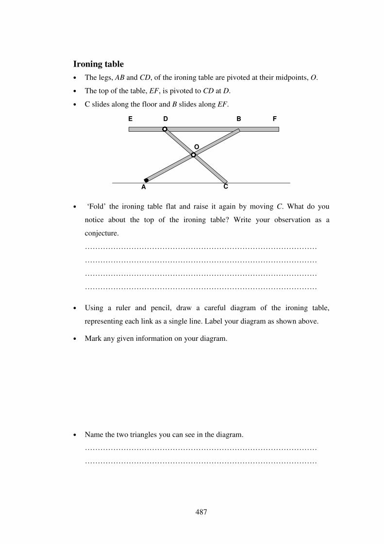
487
Ironing table • The legs, AB and CD, of the ironing table are pivoted at their midpoints, O.
• The top of the table, EF, is pivoted to CD at D.
• C slides along the floor and B slides along EF.
O
B
A C
D F E
• ‘Fold’ the ironing table flat and raise it again by moving C. What do you
notice about the top of the ironing table? Write your observation as a
conjecture.
………………………………………………………………………………
………………………………………………………………………………
………………………………………………………………………………
………………………………………………………………………………
• Using a ruler and pencil, draw a careful diagram of the ironing table,
representing each link as a single line. Label your diagram as shown above.
• Mark any given information on your diagram.
• Name the two triangles you can see in the diagram.
………………………………………………………………………………
………………………………………………………………………………
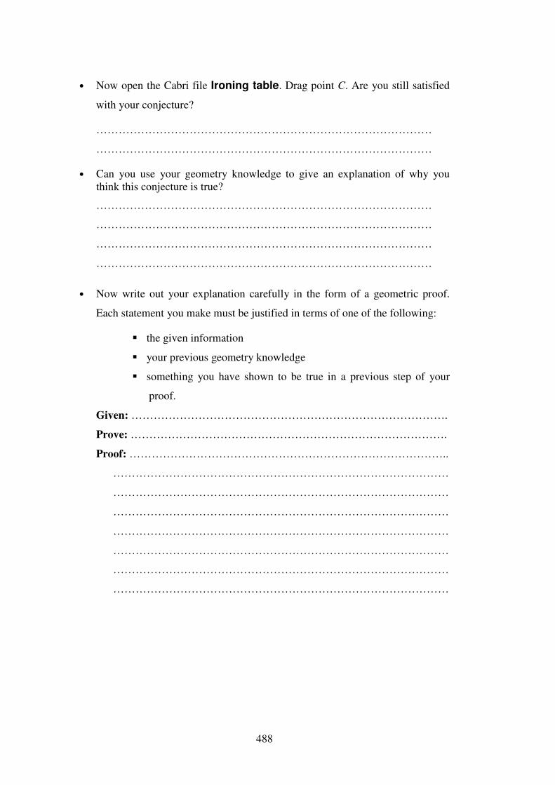
488
• Now open the Cabri file Ironing table. Drag point C. Are you still satisfied
with your conjecture?
………………………………………………………………………………
………………………………………………………………………………
• Can you use your geometry knowledge to give an explanation of why you think this conjecture is true?
………………………………………………………………………………
………………………………………………………………………………
………………………………………………………………………………
………………………………………………………………………………
• Now write out your explanation carefully in the form of a geometric proof.
Each statement you make must be justified in terms of one of the following:
��the given information
��your previous geometry knowledge
��something you have shown to be true in a previous step of your
proof.
Given: ………………………………………………………………………….
Prove: ………………………………………………………………………….
Proof: …………………………………………………………………………..
………………………………………………………………………………
………………………………………………………………………………
………………………………………………………………………………
………………………………………………………………………………
………………………………………………………………………………
………………………………………………………………………………
………………………………………………………………………………
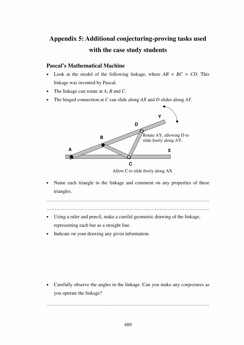
489
Appendix 5: Additional conjecturing-proving tasks used
with the case study students
Pascal’s Mathematical Machine • Look at the model of the following linkage, where AB = BC = CD. This
linkage was invented by Pascal.
• The linkage can rotate at A, B and C.
• The hinged connection at C can slide along AX and D slides along AY.
A
B
C
D
Y
X
Rotate AY, allowing D toslide freely along AY.
Allow C to slide freely along AX
• Name each triangle in the linkage and comment on any properties of these
triangles.
………………………………………………………………………………………
………………………………………………………………………………………
• Using a ruler and pencil, make a careful geometric drawing of the linkage,
representing each bar as a straight line.
• Indicate on your drawing any given information.
• Carefully observe the angles in the linkage. Can you make any conjectures as
you operate the linkage?
………………………………………………………………………………………
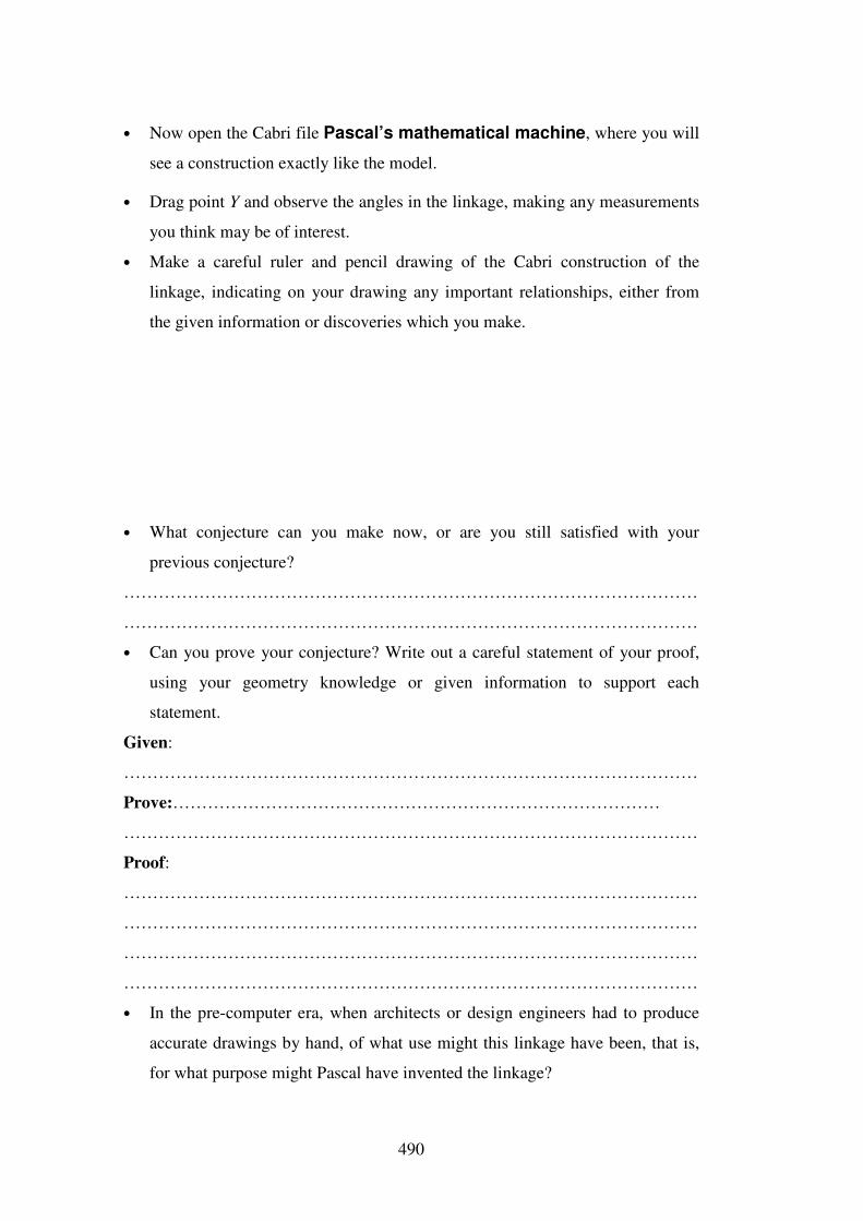
490
• Now open the Cabri file Pascal’s mathematical machine, where you will
see a construction exactly like the model.
• Drag point Y and observe the angles in the linkage, making any measurements
you think may be of interest.
• Make a careful ruler and pencil drawing of the Cabri construction of the
linkage, indicating on your drawing any important relationships, either from
the given information or discoveries which you make.
• What conjecture can you make now, or are you still satisfied with your
previous conjecture?
………………………………………………………………………………………
………………………………………………………………………………………
• Can you prove your conjecture? Write out a careful statement of your proof,
using your geometry knowledge or given information to support each
statement.
Given:
………………………………………………………………………………………
Prove:…………………………………………………………………………
………………………………………………………………………………………
Proof:
………………………………………………………………………………………
………………………………………………………………………………………
………………………………………………………………………………………
………………………………………………………………………………………
• In the pre-computer era, when architects or design engineers had to produce
accurate drawings by hand, of what use might this linkage have been, that is,
for what purpose might Pascal have invented the linkage?
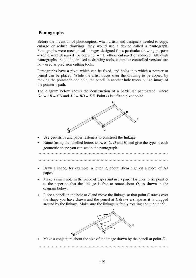
491
Pantographs
Before the invention of photocopiers, when artists and designers needed to copy, enlarge or reduce drawings, they would use a device called a pantograph. Pantographs were mechanical linkages designed for a particular drawing purpose – some were designed for copying, while others enlarged or reduced. Although pantographs are no longer used as drawing tools, computer-controlled versions are now used as precision cutting tools.
Pantographs have a pivot which can be fixed, and holes into which a pointer or pencil can be placed. While the artist traces over the drawing to be copied by moving the pointer in one hole, the pencil in another hole traces out an image of the pointer’s path.
The diagram below shows the construction of a particular pantograph, where OA = AB = CD and AC = BD = DE. Point O is a fixed pivot point.
E 1.1.1.
B
O C
D
• Use geo-strips and paper fasteners to construct the linkage. • Name (using the labelled letters O, A, B, C, D and E) and give the type of each
geometric shape you can see in the pantograph. ………………………………………………………………………………………
………………………………………………………………………………………
• Draw a shape, for example, a letter R, about 10cm high on a piece of A3 paper.
• Make a small hole in the piece of paper and use a paper fastener to fix point O to the paper so that the linkage is free to rotate about O, as shown in the diagram below.
• Place a pencil in the hole at E and move the linkage so that point C traces over the shape you have drawn and the pencil at E draws a shape as it is dragged around by the linkage. Make sure the linkage is freely rotating about point O.
E 1.1.1.
B
O C
D
• Make a conjecture about the size of the image drawn by the pencil at point E.
………………………………………………………………………………………
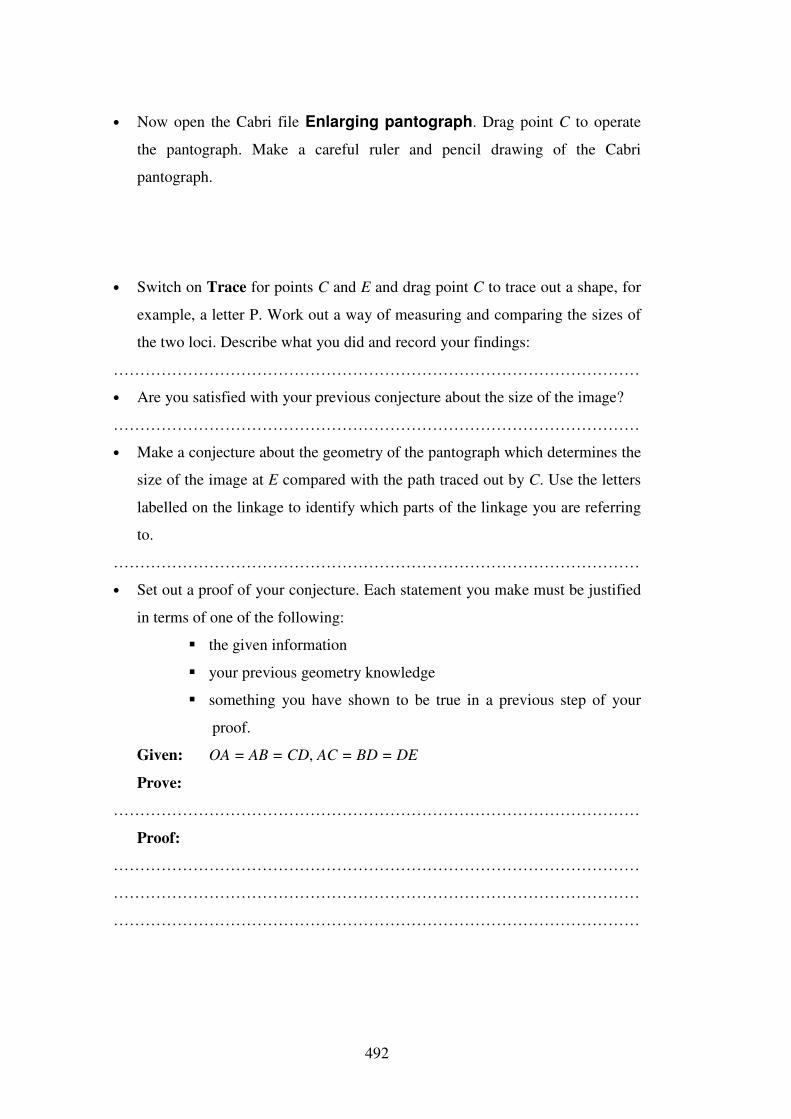
492
• Now open the Cabri file Enlarging pantograph. Drag point C to operate
the pantograph. Make a careful ruler and pencil drawing of the Cabri
pantograph.
• Switch on Trace for points C and E and drag point C to trace out a shape, for
example, a letter P. Work out a way of measuring and comparing the sizes of
the two loci. Describe what you did and record your findings:
………………………………………………………………………………………
• Are you satisfied with your previous conjecture about the size of the image?
………………………………………………………………………………………
• Make a conjecture about the geometry of the pantograph which determines the
size of the image at E compared with the path traced out by C. Use the letters
labelled on the linkage to identify which parts of the linkage you are referring
to.
………………………………………………………………………………………
• Set out a proof of your conjecture. Each statement you make must be justified
in terms of one of the following:
��the given information
��your previous geometry knowledge
��something you have shown to be true in a previous step of your
proof.
Given: OA = AB = CD, AC = BD = DE
Prove:
………………………………………………………………………………………
Proof:
………………………………………………………………………………………
………………………………………………………………………………………
………………………………………………………………………………………
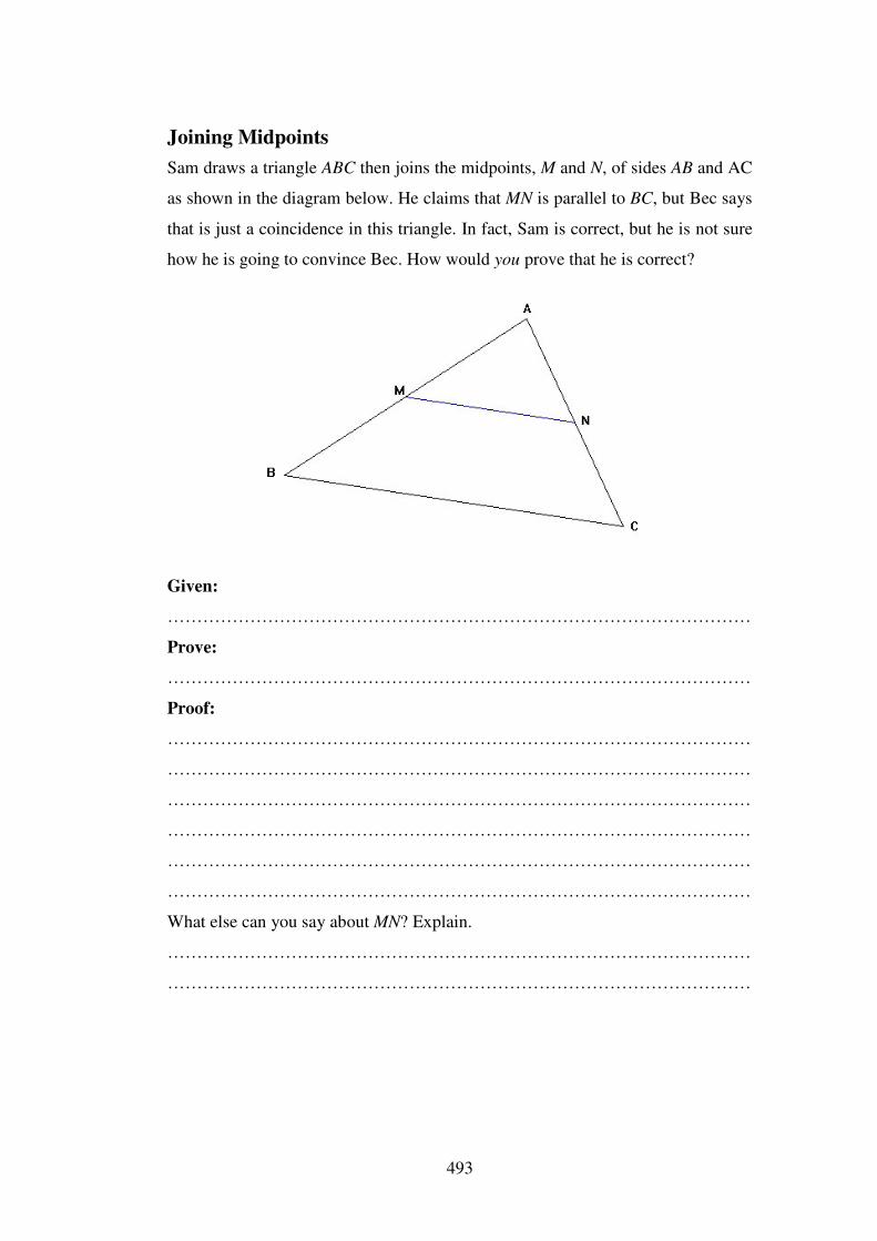
493
Joining Midpoints Sam draws a triangle ABC then joins the midpoints, M and N, of sides AB and AC
as shown in the diagram below. He claims that MN is parallel to BC, but Bec says
that is just a coincidence in this triangle. In fact, Sam is correct, but he is not sure
how he is going to convince Bec. How would you prove that he is correct?
Given:
………………………………………………………………………………………
Prove:
………………………………………………………………………………………
Proof:
………………………………………………………………………………………
………………………………………………………………………………………
………………………………………………………………………………………
………………………………………………………………………………………
………………………………………………………………………………………
………………………………………………………………………………………
What else can you say about MN? Explain.
………………………………………………………………………………………
………………………………………………………………………………………
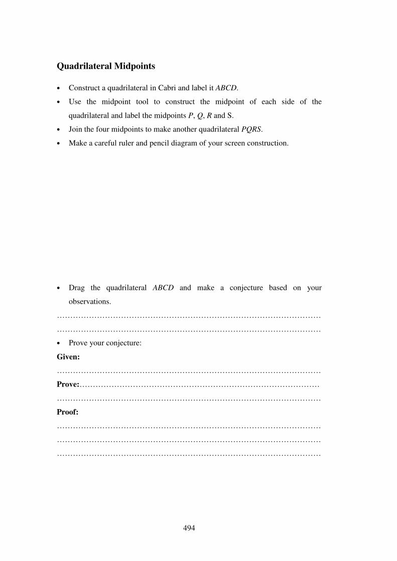
494
Quadrilateral Midpoints
• Construct a quadrilateral in Cabri and label it ABCD.
• Use the midpoint tool to construct the midpoint of each side of the
quadrilateral and label the midpoints P, Q, R and S.
• Join the four midpoints to make another quadrilateral PQRS.
• Make a careful ruler and pencil diagram of your screen construction.
• Drag the quadrilateral ABCD and make a conjecture based on your
observations.
………………………………………………………………………………………
………………………………………………………………………………………
• Prove your conjecture:
Given:
………………………………………………………………………………………
Prove:………………………………………………………………………………
………………………………………………………………………………………
Proof:
………………………………………………………………………………………
………………………………………………………………………………………
………………………………………………………………………………………
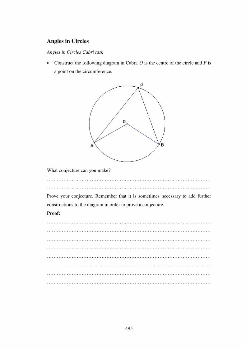
495
Angles in Circles
Angles in Circles Cabri task
• Construct the following diagram in Cabri. O is the centre of the circle and P is
a point on the circumference.
What conjecture can you make?
………………………………………………………………………………………
………………………………………………………………………………………
Prove your conjecture. Remember that it is sometimes necessary to add further
constructions to the diagram in order to prove a conjecture.
Proof:
………………………………………………………………………………………
………………………………………………………………………………………
………………………………………………………………………………………
………………………………………………………………………………………
………………………………………………………………………………………
………………………………………………………………………………………
………………………………………………………………………………………
………………………………………………………………………………………
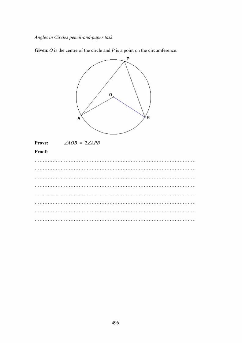
496
Angles in Circles pencil-and-paper task
Given: O is the centre of the circle and P is a point on the circumference.
Prove: ∠AOB = 2∠APB
Proof:
………………………………………………………………………………………
………………………………………………………………………………………
………………………………………………………………………………………
………………………………………………………………………………………
………………………………………………………………………………………
………………………………………………………………………………………
………………………………………………………………………………………
………………………………………………………………………………………
497
‘Consul’, the Educated Monkey ‘Consul’, the Educated Monkey is an American toy, invented in 1916 to teach
children multiplication tables, factors and simple addition and subtraction. The tin
toy is based on a linkage which is designed so that when the feet are set to point to
two numbers, the hands point to the product. The multiplication card behind the
monkey can be replaced by an addition card.
E
P
C D
A B
Each upper arm and leg is constructed from a single piece of tin plate so that
∠ACE and ∠BDE are right angles. These two pieces of tin pivot about a point (E)
beneath the bow tie. The feet, at A and B, can move only in a straight line through
A and B and can be positioned on any pair of factors. Segments CE, DE, CP and
DP (as well as the distances AC and BD) are all equal, so that CEDP is a rhombus
which is pivoted at points C and D (the monkey’s elbows) and points E and P.
The linkage is symmetrical about the vertical line through EP. The slotted tail
ensures that E and P move vertically, which is essential if P is to be located above
the correct answer.
• Construct the linkage from geo-strips and paper fasteners as shown below.
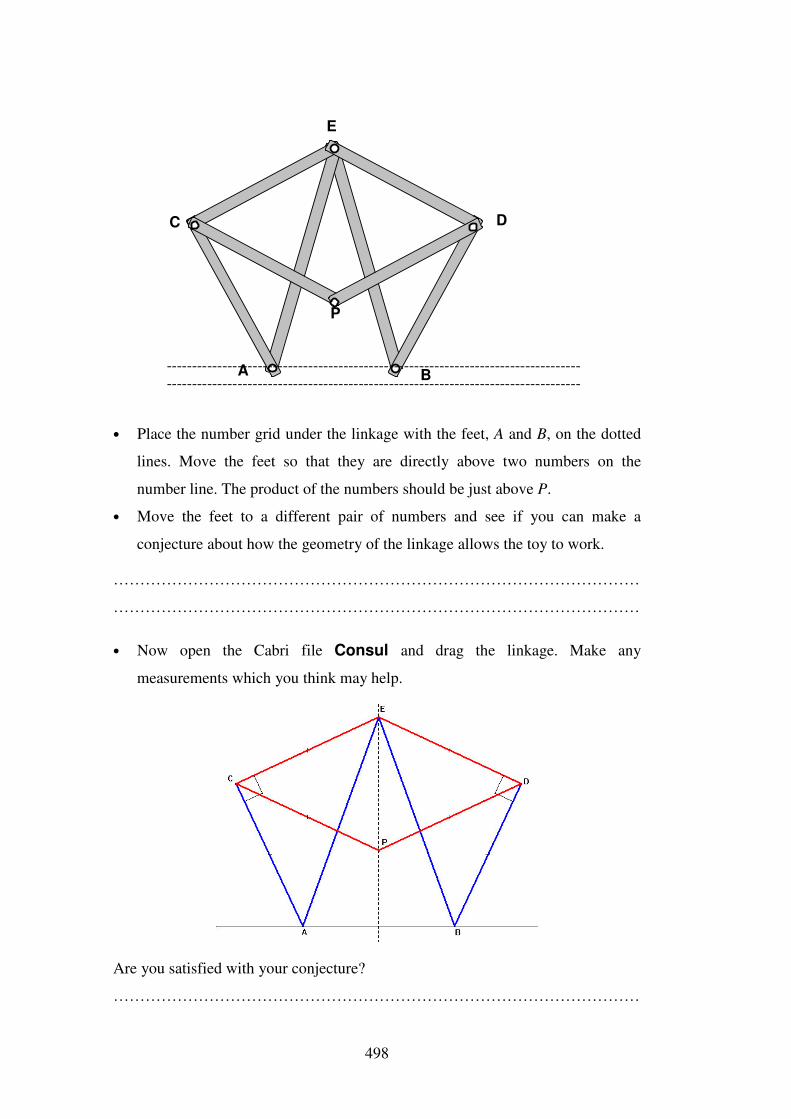
498
A
P
E
D C
B ---------------------------------------------------------------------------------- ----------------------------------------------------------------------------------
• Place the number grid under the linkage with the feet, A and B, on the dotted
lines. Move the feet so that they are directly above two numbers on the
number line. The product of the numbers should be just above P.
• Move the feet to a different pair of numbers and see if you can make a
conjecture about how the geometry of the linkage allows the toy to work.
………………………………………………………………………………………
………………………………………………………………………………………
• Now open the Cabri file Consul and drag the linkage. Make any
measurements which you think may help.
Are you satisfied with your conjecture?
………………………………………………………………………………………
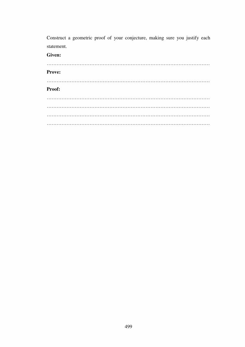
499
Construct a geometric proof of your conjecture, making sure you justify each
statement.
Given:
………………………………………………………………………………………
Prove:
………………………………………………………………………………………
Proof:
………………………………………………………………………………………
………………………………………………………………………………………
………………………………………………………………………………………
………………………………………………………………………………………
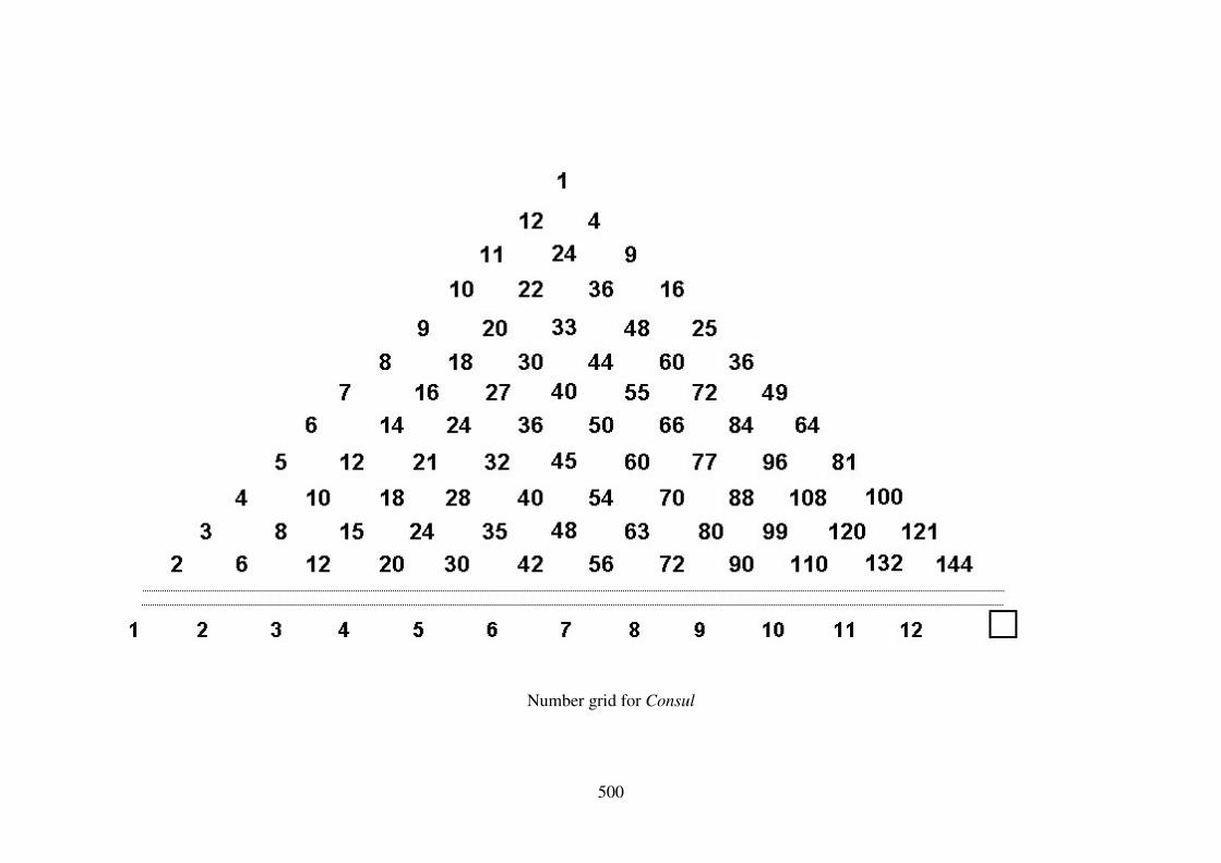
500
Number grid for Consul
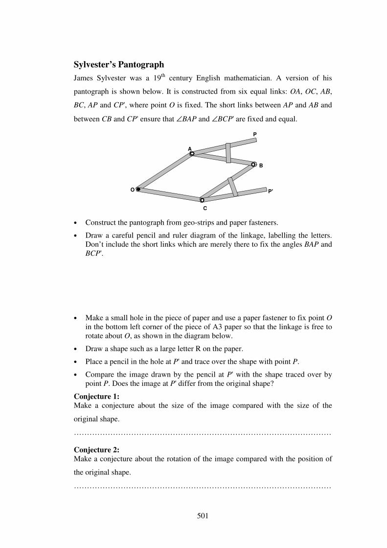
501
Sylvester’s Pantograph James Sylvester was a 19th century English mathematician. A version of his
pantograph is shown below. It is constructed from six equal links: OA, OC, AB,
BC, AP and CP', where point O is fixed. The short links between AP and AB and
between CB and CP' ensure that ∠BAP and ∠BCP' are fixed and equal.
O
P
C
B
A
P'
• Construct the pantograph from geo-strips and paper fasteners.
• Draw a careful pencil and ruler diagram of the linkage, labelling the letters. Don’t include the short links which are merely there to fix the angles BAP and BCP'.
• Make a small hole in the piece of paper and use a paper fastener to fix point O in the bottom left corner of the piece of A3 paper so that the linkage is free to rotate about O, as shown in the diagram below.
• Draw a shape such as a large letter R on the paper.
• Place a pencil in the hole at P' and trace over the shape with point P.
• Compare the image drawn by the pencil at P' with the shape traced over by point P. Does the image at P' differ from the original shape?
Conjecture 1: Make a conjecture about the size of the image compared with the size of the
original shape.
………………………………………………………………………………………
Conjecture 2: Make a conjecture about the rotation of the image compared with the position of
the original shape.
………………………………………………………………………………………
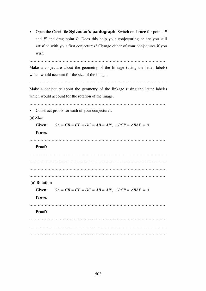
502
• Open the Cabri file Sylvester’s pantograph. Switch on Trace for points P
and P' and drag point P. Does this help your conjecturing or are you still
satisfied with your first conjectures? Change either of your conjectures if you
wish.
………………………………………………………………………………………
Make a conjecture about the geometry of the linkage (using the letter labels)
which would account for the size of the image.
………………………………………………………………………………………
Make a conjecture about the geometry of the linkage (using the letter labels)
which would account for the rotation of the image.
………………………………………………………………………………………
• Construct proofs for each of your conjectures:
(a) Size
Given: OA = CB = CP = OC = AB = AP', ∠BCP = ∠BAP' = α.
Prove:
………………………………………………………………………………………
Proof:
………………………………………………………………………………………
………………………………………………………………………………………
………………………………………………………………………………………
………………………………………………………………………………………
(a) Rotation
Given: OA = CB = CP = OC = AB = AP', ∠BCP = ∠BAP' = α.
Prove:
………………………………………………………………………………………
Proof:
………………………………………………………………………………………
………………………………………………………………………………………
………………………………………………………………………………………
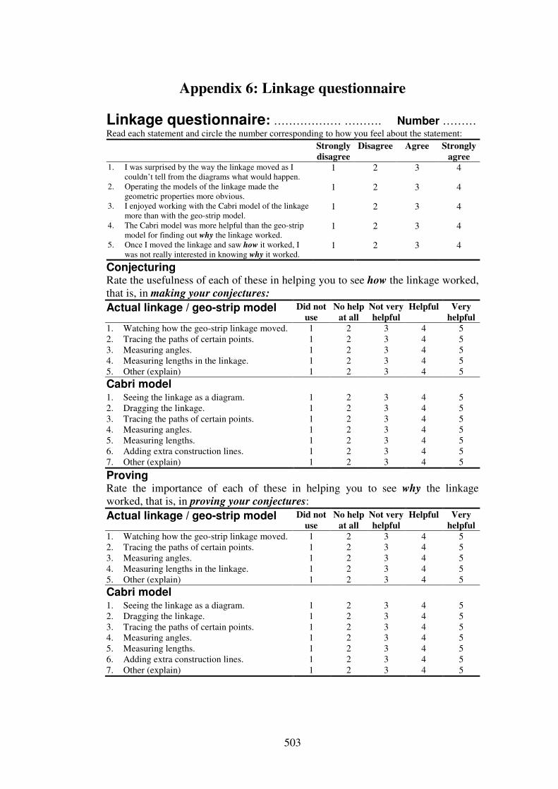
503
Appendix 6: Linkage questionnaire
Linkage questionnaire: ……………… ………. Number ……… Read each statement and circle the number corresponding to how you feel about the statement: Strongly
disagree Disagree Agree Strongly
agree 1. I was surprised by the way the linkage moved as I
couldn’t tell from the diagrams what would happen. 1 2 3 4
2. Operating the models of the linkage made the geometric properties more obvious.
1 2 3 4
3. I enjoyed working with the Cabri model of the linkage more than with the geo-strip model.
1 2 3 4
4. The Cabri model was more helpful than the geo-strip model for finding out why the linkage worked.
1 2 3 4
5. Once I moved the linkage and saw how it worked, I was not really interested in knowing why it worked.
1 2 3 4
Conjecturing Rate the usefulness of each of these in helping you to see how the linkage worked, that is, in making your conjectures: Actual linkage / geo-strip model Did not
use No help
at all Not very helpful
Helpful Very helpful
1. Watching how the geo-strip linkage moved. 1 2 3 4 5 2. Tracing the paths of certain points. 1 2 3 4 5 3. Measuring angles. 1 2 3 4 5 4. Measuring lengths in the linkage. 1 2 3 4 5 5. Other (explain) 1 2 3 4 5 Cabri model 1. Seeing the linkage as a diagram. 1 2 3 4 5 2. Dragging the linkage. 1 2 3 4 5 3. Tracing the paths of certain points. 1 2 3 4 5 4. Measuring angles. 1 2 3 4 5 5. Measuring lengths. 1 2 3 4 5 6. Adding extra construction lines. 1 2 3 4 5 7. Other (explain) 1 2 3 4 5
Proving Rate the importance of each of these in helping you to see why the linkage worked, that is, in proving your conjectures: Actual linkage / geo-strip model Did not
use No help
at all Not very helpful
Helpful Very helpful
1. Watching how the geo-strip linkage moved. 1 2 3 4 5 2. Tracing the paths of certain points. 1 2 3 4 5 3. Measuring angles. 1 2 3 4 5 4. Measuring lengths in the linkage. 1 2 3 4 5 5. Other (explain) 1 2 3 4 5 Cabri model 1. Seeing the linkage as a diagram. 1 2 3 4 5 2. Dragging the linkage. 1 2 3 4 5 3. Tracing the paths of certain points. 1 2 3 4 5 4. Measuring angles. 1 2 3 4 5 5. Measuring lengths. 1 2 3 4 5 6. Adding extra construction lines. 1 2 3 4 5 7. Other (explain) 1 2 3 4 5

504
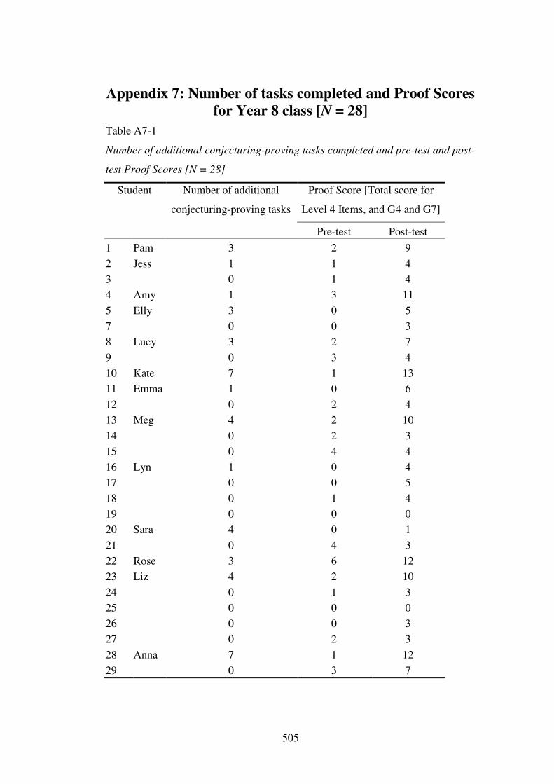
505
Appendix 7: Number of tasks completed and Proof Scores for Year 8 class [N = 28]
Table A7-1
Number of additional conjecturing-proving tasks completed and pre-test and post-
test Proof Scores [N = 28]
Student Number of additional
conjecturing-proving tasks
Proof Score [Total score for
Level 4 Items, and G4 and G7]
Pre-test Post-test 1 Pam 3 2 9 2 Jess 1 1 4 3 0 1 4 4 Amy 1 3 11 5 Elly 3 0 5 7 0 0 3 8 Lucy 3 2 7 9 0 3 4 10 Kate 7 1 13 11 Emma 1 0 6 12 0 2 4 13 Meg 4 2 10 14 0 2 3 15 0 4 4 16 Lyn 1 0 4 17 0 0 5 18 0 1 4 19 0 0 0 20 Sara 4 0 1 21 0 4 3 22 Rose 3 6 12 23 Liz 4 2 10 24 0 1 3 25 0 0 0 26 0 0 3 27 0 2 3 28 Anna 7 1 12 29 0 3 7

506
Minerva Access is the Institutional Repository of The University of Melbourne
Author/s:Vincent, Jill Loris
Title:Mechanical linkages, dynamic geometry software, and argumentation: supporting aclassroom culture of mathematical proof
Date:2002-12
Citation:Vincent, J. L. (2002). Mechanical linkages, dynamic geometry software, and argumentation:supporting a classroom culture of mathematical proof. PhD thesis, Department of Scienceand Mathematics Education, The University of Melbourne.
Publication Status:Unpublished
Persistent Link:http://hdl.handle.net/11343/38998
Terms and Conditions:Terms and Conditions: Copyright in works deposited in Minerva Access is retained by thecopyright owner. The work may not be altered without permission from the copyright owner.Readers may only download, print and save electronic copies of whole works for their ownpersonal non-commercial use. Any use that exceeds these limits requires permission fromthe copyright owner. Attribution is essential when quoting or paraphrasing from these works.


