Embed Size (px)
Citation preview
������������� ������������������ ����������������� �������� ������ �����
������������������� ����������
����������� �����!��"#�$���%��
&��� ��'Improving the distributional impact of transfers may be costly if it reduces labour supply. In this paperwe show how effects of changes in the design of the child benefit programme can be examined byderiving information from behavioural and non-behavioural simulations on micro data. The directdistributional effects are assessed by tax−benefit model calculations. Female labour supplyresponses to alternative child benefit schemes are simulated under the assumption that choices arediscrete. The discrete choice model is justified with reference to the complicated process of finding anew job, and the existence of peaks in the empirical distribution of hours is interpreted as variation innumber of jobs across states. The distribution of income after labour supply responses is alsoshown. The analysis confirms that enhanced distributional impact is traded against reductions inlabour supply.
(���� #�' Micro simulation, Labour supply, Discrete choice, Means-testing
)*+��"���%������'�!,-�������.�,��.,���)��
&�/���"�# �����'�We particularly thank John Dagsvik for many helpful comments andsuggestions. Valuable comments are also received from Iulie Aslaksen, Nils M. Stølen, Rolf Aabergeand seminar participants at the 1998 annual meeting for the Economic Research Programme onTaxation, Halvorsbøle (Norway) and at the 55th Congress of the International Institute of PublicFinance, Moscow, August 1999. We have benefited from research assistance by Ingeborg F. Solliand Bård Lian. Financial support from the Norwegian Research Council is gratefully acknowledged.
&## ���' Thor O. Thoresen, Statistics Norway, Research Department. E-mail:[email protected], Tom Kornstad, Statistics Norway, Research Department, E-mail: [email protected]

������������� � comprise research papers intended for international journals or books. As a preprint aDiscussion Paper can be longer and more elaborate than a standard journal article by in-cluding intermediate calculation and background material etc.
Abstracts with downloadable PDF files ofDiscussion Papers are available on the Internet: http://www.ssb.no
For printed Discussion Papers contact:
Statistics NorwaySales- and subscription serviceN-2225 Kongsvinger
Telephone: +47 62 88 55 00Telefax: +47 62 88 55 95E-mail: [email protected]

3
�������������The transfers to families with children have increased steadily the last decade in Norway. One
important reason for this is that the child benefit expenditures have increased by about 25 per cent in
real terms from 1990 to 1998, to about NOK 13 billions in 1998. All families with children less than
16 years receive child benefit, and uncertainty about whether the substantial costs of the scheme are
justified by favourable distributional effects or simplicity of the universal design, have led to proposals
of changes in the child benefit programme. Taxation of the child benefit as wage income or testing the
transfer against family income are two alternatives of means-testing that have been suggested. Both
proposals are associated with an income inequality reducing effect, as it is expected that the transfer
will be more targeted towards low-income groups by these changes.
While recent contributions on means-testing and targeting either neglect effects on work incentives or
employ only numerical illustrations when discussing such effects (cf., e.g., Besley 1990; Creedy 1996;
Creedy 1998), the present analysis is detailed on labour supply effects. Labour supply responses are
important both from an efficiency point of view and because labour supply responses influence the
distribution of income, both within and between families. In the following we discuss taxation and
income-testing of the child benefit with respect to 1) direct distributional effects between families, 2)
labour supply responses and 3) distributional effects after labour supply responses.1
The direct (non-behavioural) distributional effects of altering the child benefit transfer system are
described by tax-benefit model calculations, whereas a structural labour supply model is applied in the
analysis of the labour supply responses. The analysis is restricted to married mothers, since the labour
supply decision of lone mothers is assumed to depend on special support programmes for lone parents.
The labour supply simulations are carried out for (married) mothers only, since men are rather
insensitive to alterations in taxes and transfers (Blundell 1993).
Empirical specifications of labour supply models have been extensively discussed the last decades, cf.
the survey in Blundell and MaCurdy (1998). It is typically assumed that hours of work is a continuous
variable, and a major problem has been how to handle the problems related to non-linearities in the
budget constraints induced by tax- and transfer systems. Today the standard approach is to
approximate the budget constraint by a piecewise-linear budget constraint, and estimate the model by
maximum likelihood. MaCurdy et al. (1990), however, show that maximum likelihood estimation of
labour supply models with piecewise-linear budget sets, invoke restrictions that influence on
1 Of course, there might be other important motives when determining the child benefit scheme. For instance, Sadka et al.(1982) emphasise the stigma associated with income-testing, while Lundberg et al. (1997) stress the importance of the childbenefit on the intra-family distribution of consumption.

4
estimates. The present analysis therefor employ a less restrictive approach by modelling labour supply
behaviour as a discrete choice problem, see, e.g., van Soest (1995), Bingley et al. (1995), Duncan and
Weeks (1997), Aaberge et al. (1995) and Dagsvik and Strøm (1997) for other labour supply analyses
employing discrete choice models.
In the specification of our model, we argue that finding work is a complex process, since job offers
differ with respect to hours of work, wage rate and non-pecuniary benefits, and job searchers don’t
have full information about all these aspects. Job searchers then simplify the choice process by
classifying jobs into different hours of work intervals, for instance full-time jobs, overtime jobs and
part-time jobs in addition to the possibility of not participating in the labour market. By grouping jobs,
they ignore that different jobs within an interval involve (minor) differences in hours of work and
focus on the main feature of hours of work. The job searchers then optimise to a range of hours rather
than to an exact level of hours of work, and the hours of work choice should then be analysed as a
discrete choice problem. In contrast to Duncan and Weeks (1997) who refer to institutional constraints
at the demand side as justification for their discrete choice approach, our validiation is based on the
supply side behaviour of individuals.
An advantage of this approach is that the peaks in the empirical distribution of hours of work (for
instance at full-time work) can be more realistically included in model specifications. One method of
taking account of peaks is to introduce dummy variables in the specification of preferences, see van
Soest (1995). We do, however, interpret the peaks as a sign of extensions in the number of job offers.
Under this exposition the number of jobs in the various intervals should be included as parameters in
the specification of the likelihood-function. Since the data do not include this information, the relative
number of jobs in the various intervals are treated as parameters, which are estimated.
Compared to models which treat hours of work as a continuous variable, the discrete choice approach
gains from treating non-convex budget sets and income-tested transfers without further complicating
the estimation- and simulation procedures. By simulating the labour supply responses for each female,
the analysis also takes care of the heterogeneous responses to changes in the tax and transfer system.
The results show that taxation of the child benefit as wage income for married females is not as
beneficial for the lower deciles as might be expected. The reason is that the progressive components of
the Norwegian income tax are not very effective in this case. From an income redistributive point of
view, it is more efficient to test the transfer against family income. According to the behavioural
simulation results, the responses from taxing the child benefit as wage income for the mothers are
quite small. The labour supply effects of testing the child benefit against family income are, however,

5
substantial. The income-testing is carried out by deducting one tenth of a NOK in child benefit for
every NOK the family earns in excess of NOK 250 000 and then redistributing the revenue surplus as
increased child benefit rates. We predict that total labour supply for married females is reduced by
about 5 per cent if the child benefit scheme is altered in this revenue-neutral mode.
In the final part of the paper we study how the distribution of income is affected by these labour
supply responses. Income-testing gives reductions in the middle of the income distribution, measured
by reductions in equivalent income.
The paper is organised as follows: Section 2 provides a rather detailed presentation of our discrete-
choice model and the estimation results. The direct effects of means-testing are described in Section 3,
while the labour supply effects and the distribution of income after responses are discussed in Section
4. Section 5 concludes.
���������������������������������������
��������������������������
The specification of the labour supply model is motivated from the two following observations: Firstly, it
is difficult to compare the utility of having various jobs. Job offers differ along a variety of dimensions
such as hours of work, pre-tax wage rates for ordinary as well as overtime work, tasks and work
pressure, work environment and non-pecuniary benefits, and one has only limited information about
these variables. Hence it is reasonable to assume that one somehow simplifies this process. Secondly,
there are peaks in the empirical distribution of hours, for instance around full-time work. Nevertheless,
data show that there are many other working times present, which indicates some flexibility with
respect to hours of work.2 The challenge is, thus, to establish a discrete choice model where the job
searcher can choose between jobs with a large variation in hours of work and where the numbers of
job offers varies across the working hours distribution.
The model specification suggested here implies that each female is assumed to choose between a large,
but finite number of jobs consisting of a particular combination of hours of work, pre-tax wage rate and a
package of non-pecuniary benefits. However, she simplifies the choice by classifying all jobs into
different working time categories, corresponding to overtime jobs, full-time jobs, and a number of
part-time jobs, in addition to the option of working at home. For simplicity, we divide the weekly
2 The main reason that there are more full-time than part-time jobs is that there are economies of scale with respect toworking time, such as the demand for full-time workers is higher than for part-time workers.

6
hours of work into 6 intervals of the same length. It is assumed that the female can choose between
overtime jobs (45-55 hours per week), full-time jobs (34-44 hours per week), three types of part-time
jobs corresponding to 23-33 hours per week, 12-22 hours per week, and 1-11 hours per week, and the
possibility of not participating in the labour market.3 The choice set of weekly hours of work, ��{�����
���������� �} is chosen as the middle point values of these intervals.
We also simplify by assuming that the pre-tax wage rate (�) is constant across all job offers for a
particular worker.4 The main reason for this assumption is that we do not know the wage rate
distributions for the individuals in the sample. We believe that constancy of pre-tax wage rates across
jobs for a particular individual is in accordance with wage bargaining in Norway, since wage rates are
typically determined in negotiations with trade unions that do not discriminate between full-time and
part-time workers. The wage rates for non-workers are obtained from a wage equation, see section 2.2
for further details.
Household consumption corresponding to choosing a job with hours of work in interval � is given by
.),,()1( ���������� MMMM ∈−+=
Non-labour incomes (k) include the households’ capital incomes, child allowances, and other public
transfers as well as labour income of the spouse.5 In contrast to van Soest (1995), we do not include
unemployment benefits as income in the non-working state. The reason is that it is difficult to receive
unemployment benefits and be voluntarily without work in the Norwegian system.
A tax-benefit model is employed in the calculation of income taxes (T). This means that we take into
account the most detailed aspects of the Norwegian tax system, and joint as well as separate filing are
considered.
We assume that household preferences can be represented by a «Box-Cox» type utility function. See,
for instance, MaCurdy (1981) and Aaberge et al. (1995) for empirical analyses applying this
3 Notice that the interval length is assumed to be fixed, which implies that a modification of the likelihood function with
respect to different length of intervals is avoided.4 Cf. Aaberge et al. (1995) for an approach with differing wage rates.5 A basic assumption in our work is that the female makes her working time conditioned on her husband’s, as opposed to theanalysis in e.g. Aaberge et al. (1995).

7
specification6. The utility of having a particular job � with hours of work in interval � can then be
written as
MMNMMN ���� ∈+= ,)2( ε ,
where
,1)1(1
)3(21
0
21
βαα
γαα
��
��
�
M
M
M
−−+
−≡
is the structural part of the utility function. Here, �M is the choice set of jobs with weekly hours of
work in interval �, γ 0 , α���α� are parameters, β�is a vector of parameters and � =8760 is the total
number of annual hours. The vector of household-specific taste-modifier variables � includes ln(age)
( � 1 ), ln(age) squared ( � 2 ), the number of children aged less than three years ( � 3 ) and the number
of children aged three to sixteen ( � 4 ). The classification according to children’s age takes into
account the high contribution rate for older pre-schoolers at child care centres, which makes these
children more similar to school children. For the utility function to be quasi-concave, we require α1<1
and α2 <1. Note also that if α1 → 0 and α2 →0, the utility function converges to a log-linear function.
Whereas the study assumes that individuals are rational in the sense that they make choices that
maximise their perceived utility subject to the budget constraint, there are errors in this maximisation
due to imperfect perception and imperfect optimisation. Such errors may arise from unobserved
alternative specific variables influencing utility, for instance fringe benefits. The study assumes that
the effects of these components on utility can be summarised into additive, job specific error terms MNε
that are i.i.d. according to the standard type I extreme value distribution,
R.)),exp(-exp(-)Pr()4( ∈=< εεεε MN
The model specification may also suffer from other types of errors such as unobserved household
characteristics or measurement errors of hours of work. For the sake of simplicity we ignore hours of
work errors since they cannot be considered without complicating the estimation procedure, see Ben-
Akiva and Lerman (1985) and van Soest (1995). Unobserved household characteristics are only
considered in so far as they do not make the error term correlated across jobs.
6 Dagsvik and Strøm (1997) provide further justification for this choice.

8
Given our distributional assumption and the assumption that utility is maximised, it is well known (cf.
Maddala 1983) that the probability of choosing a particular job � with working time in interval � is
given by
U
U
M
U
Y
%VU
Y
UV%VU
MNMN
�
�����������
∈∈ ΣΣ
=
=≡)5( ,
where �U and �M are household utility (2) evaluated at hours of work corresponding to interval � and �.
We are, however, primarily interested in the probability of choosing some arbitrary job with working
time in interval �. This probability is given by
U
M
U
U
M
M
M
Y
UU
Y
M
Y
%VU
Y
%V
%V
MVM��
��
�
���
Σ=
ΣΣ
Σ==
∈
∈
∈∑)6( ,
where �U�denotes the number of jobs with hours of work in interval �. The peaks in the distribution of
hours of work, which indicates that the number of job offers varies across intervals, are represented by
the assumption that there are more full-time jobs (�� ) and non-participation possibilities (�� ), while
the number of different part-time and overtime jobs are identical, i.e. �U = � for ������� �
Equation (6) then implies that the probability of having a job with working time corresponding to
interval � is given by
404
5,3,2,10
)7(Y
U
YY
Y
M
M
������
���
U
M
++=
∑=
.
Dividing numerator and denominator by � and rearranging the resulting equation, yield
)/ln(
5,3,2,1
)/ln(
)/ln(
4400)8(
QQY
U
YQQY
QQY
M
���
��
U
MM
+
=
+
+
++=
∑.
This equation shows how the probabilities in the likelihood function can be modified to account for
the differing number of job offers across intervals. Consequently, the specification of probabilities

9
should be adjusted by adding the logarithm of the fraction between the number of jobs in the interval
and �, i.e. representing the deviations from � for non-working and full-time working intervals.
A problem in that respect is that one typically does not observe the number of jobs, but this problem
can be taken care of by noticing that �!�L"�#, for $��������� , are parameters that vary across intervals,
but not across individuals. These parameters can then be treated as interval specific parameters, and in
the specification of the likelihood function we do that by introducing two dummy variables. The
dummy variable %1 is 1 for full-time work and 0 otherwise, whereas %2 is 1 if the person works and
0 otherwise. The full-time dummy is justified by reference to demand side factors, as economies of
scale with respect to working hours.7 Accordingly, the out-of-work alternative is given special
treatment, since the number of non-working options deviates from number of jobs in the market.
� ���������������������������
In the calculations of the direct effects of the child benefit we apply the Norwegian tax-benefit model
LOTTE8 and the 1994-wave of the Income Distribution Survey (IDS). LOTTE calculates taxes and
transfers for a sample of individuals, more than 40 000 in 1994. Of these, about 17 000 belong to a
household with a mother eligible for child benefit.
IDS does not include information about wage rates or hours of work, but these data are available from
the Standard of Living Survey. We utilise that the Standard of Living Survey 1995 is a sub-sample of
IDS-94 and that these two surveys can be linked on the basis of personal identification numbers. Thus,
the estimation and simulations of the behavioural effects are based on smaller samples of individuals
than the calculations of the direct effects. After restricting to married, female wage-earners/home-
workers older than 24 and younger than 65, the sample used in the estimation includes about 500
women. This sample also includes females without children, since it is assumed that their behaviour in
the labour market contains information about the labour supply behaviour of mothers. In contrast, the
simulations are executed only for the child benefit-eligible females in this sample, approximately 300
mothers. Table 1 provides sample statistics for the data set exploited in the estimation.
7 There might be other candidates for explaining peaks in the hours of work distribution. For instance can females’preferences concerning working hours be mutually influenced in favour of working full-time. Neumark and Postlewaite(1998) and Woittiez and Kapteyn (1998) provide results that can interpreted in favour of this rationalisation.8 The model is extensively used in the preparation of the national budgets in Norway.

10
��������������������������
&��$�' � ���� ()��*��*�*��$�)$+�
Household disposable income (NOK) 324794 102955
Age of wife 42.7 10.0
Number of children 0−2 years 0.18 0.42
Number of children 3−15 years 0.84 1.00
Full-time dummy 0.46 0.50
Participation dummy 0.86 0.35
Gross wage rate (NOK) 103.1 33.0
Working hours per week 27.0 14.1
Hourly gross wage rates are calculated from dividing yearly labour income by yearly hours of work.
Additional information, such as indications of transitory connections to work, is employed in order to
improve wage estimates (see Appendix A).
For non-workers the pre-tax wage rates are estimated using a wage rate equation, where log(w) is the
dependent variable and years of education, experience (measured as age minus years of education and
minus pre-school years), and experience squared are the explanatory variables. We have considered
selectivity bias in the estimation of the wage rate equation, but the parameter estimate of the Mills
ratio is not statistically significant. The reason is that the participation rate is very high in Norway,
about 85 per cent for married women, cf. Table 1.
Table 2 reports the estimates of the parameters in the utility function. The parameters (α�, γ�) and (α�,
β�, β�, β�, β�, β�) determine the utility of consumption and leisure respectively. In order to ensure that
the deterministic part of preferences is strictly quasi-concave in (�,�), α� and α� must be less than one.
According to the table, the estimates of these parameters are 0.78 and -11.61 respectively, and the
parameters are determined quite precisely.9
The estimates of β�, β�, and β� imply that women’s preferences for leisure increase with age.
Preference for leisure also increases if the woman has children and the point estimates indicate that
preferences for leisure are not much stronger if the children are young (β�) than if they are older (β�).
9 A 12-state version has also been estimated with very similar results.

11
������ ���������������������������������������������������
&��$�' �, -,)$��)�, ).,)�)$,)$/
Consumption � 0.458 2.5
� 0.776 6.5
Leisure β� 49.257 2.2
β� -27.538 2.2
β� 3.882 2.2
β� 0.315 1.7
β� 0.256 2.0
� -11.610 7.4
Full-time dummy δ� 1.125 5.6
Participation dummy δ� -1.045 5.1
In order to evaluate the model specifications, Figure 1 displays the observed and simulated distribution
of hours of work. It demonstrates that the model reproduces the observed distribution quite well.
�������������������������������� ���������������������!��"������������
0,0
0,1
0,2
0,3
0,4
0,5
0 1-11 12-22 23-33 34-44 45+
Hours of work
Pro
babi
lity
Simulated
Observed
#����������������������������������������������
#��������������������
This section discusses the direct distributional effects of alterations in the child benefit scheme, as
described by simulation results from the tax-benefit model. Empirical evaluations of the direct effect
of changes in taxes and transfers are associated with methodological controversies. Income definitions
and techniques for the re-weighting of income may impact on the assessment of distributional effects
of tax policy changes. An extensive examination of these issues is beyond the scope of this paper, but
the following points summarise our main assumptions:

12
• Post-tax income is defined as gross income minus taxes, plus a number of tax-free benefits such as
the child benefit, housing benefits, social security benefits, etc. Interest expenses, for instance from
house acquisitions, are not deducted, due to the undervaluation of imputed income from owner-
occupied homes in our data.10
• Post-tax income is aggregated over household members, weighted with an equivalence scale and
each household is represented with as many persons as the number of household members. The
equivalence scale is defined by the square root of number of household members (Buhmann et al.
1988), where the relative weight given to a child is 0.75 of an adult.
#� ����$�������������������������
According to Bradshaw et al. (1993, p. 70) the Norwegian child benefit scheme is rather generous
compared to other countries’ schemes. It is paid to the mothers of children younger than 16 years of
age. For the first child they received NOK 10 416 in 1994; the amount per child increases with the
number of children in the family.11 In Table 3 we present the distribution of equivalent income and the
corresponding equivalent child benefit for married couples with children between 0−16 years of age.12
Table 3 also includes estimates for working hours in deciles. These are imputed from the sample of
approximately 300 married mothers, exploited in Section 2. The table shows a positive correlation
between equivalent income and female working hours. Ranking of individual well-being according to
equivalent income is thus questionable, but this problem is ignored in the following.
According to the table, the distributional impact of the child benefit can be characterised as favourable
since the lower income deciles on average receive more of the benefit than the richer individuals. The
result is due to a negative correlation between equivalent income and number of benefit-eligible
children.
It has been proposed to tax the child benefit as wage income for the mother. Since the Norwegian tax
system is progressive, one would normally assume that the inclusion of the child benefit in taxable
income would prove relatively advantageous to the poorest families. However, as seen in Table 4, the
direct effect of taxing the child benefit as wage income is not very beneficial for the lower deciles. The
distribution of the benefit, as depicted in Table 3, is important when interpreting this result. Another
reason is the ambiguous relationship between the ranking by equivalence scales and the ranking by tax
10 By calculating an average ratio between the market value (only reported by a smaller number of individuals) and theincome tax return value of housing, we have estimated income from housing and defined an alternative income concept. Thedistribution of income when including «market profits» from housing and deducting interest rates is not very different fromthe distribution of income when using the standard definition.11 For instance, the child benefit for the fifth child was 13 392 NOK in 1994.12 There are special arrangements for lone parents.

13
progression (see, e.g., Lambert 1993), implying that persons with high incomes might be found in the
lower equivalent income deciles. Most crucially, the key progressive element in the Norwegian tax
system, the surtax,13 is not very effective in this case. The tax revenue increases by about NOK 4,3
billion with this reform, but only about seven per cent is due to the surtax. This means that only a smaller
fraction of mothers is liable to surtax.
������#� � �������%� �������������&'()*������������������������������� ������������������!��"������������������������������+�������������!������������,−�-���������../
%�/$ � -01$�� ��)�$�/+�� -,)$��)�*���1�'���+2����� 3�+1�,�+2��+���2+���+)���,4
-01$�� ��)�/�$ *�'���2$)
1 89 875 12 13 599
2 120 295 18 12 502
3 135 436 18 11 650
4 147 697 26 11 003
5 158 662 26 11 299
6 169 888 28 11 050
7 182 727 28 10 314
8 199 012 31 9 801
9 222 466 31 9 801
10 342 266 30 9 746
Average 176 832 25 11 076
*The measures for working hours have been imputed from the sub-sample of married mothers exploited in the behavioural
analysis.
Since the lower deciles’ share in the increased tax burden is larger than the upper deciles’ share, the
reform cannot be recommended on equity grounds, as defined here. In fact, measured by the Gini
coefficient, the inequality among individuals in households with children increases by about three per
cent by including the child benefit in taxable income. A three per cent increase in the Gini coefficient
corresponds to introducing an equal-sized lump-sum tax of three percent of the mean income and
redistributing the collected tax revenue as proportional transfers where each unit receives three per
cent of its income (Aaberge 1997). Alternatively, it can be interpreted as a three per cent increase in
the expected difference in incomes between two individuals drawn at random from the income
distribution (Jenkins 1991).
However, the distributional effects can be improved by redistributing the collected revenue into an
equal sized increase in all child benefit rates. The direct distributional effect of this revenue-neutral
13 The first threshold for the surtax was at 208 000 NOK for tax class 1 in 1994, for spouses filing separately.

14
reform is presented in Table 5. The table clearly shows that low-income individuals in decile 1 gain
the most, while the 30 per cent richest lose out. Individuals in the middle of the income distribution are
only marginally influenced. In total, the inequality (measured by the Gini coefficient) is reduced by
0.5 per cent by implementing this revenue-neutral reform.
������/� � �������%� �������������&'()*������������������������������� ������������������������$���!����������������������������������$�������������+�������������!������������,−�-���������../
Decile -01$�� ��)�$�/+�� ����'1�*���$�/���,��!���,1��*��,��*1/)$+�,�$���01$�� ��)�$�/+��#
1 89 875 4 210
2 120 295 4 827
3 135 436 4 548
4 147 697 4 179
5 158 662 4 236
6 169 888 4 149
7 182 727 3 968
8 199 012 3 972
9 222 466 3 963
10 342 266 4 130
Average 176 832 4 218
������0� 1� �����������������2�����������������������$��������������������������������������������������� ���������������������3����������� �������%� �������������&'()*������������������������������� ����������������������%� ��������������+�������������!������������,−�-���������../
%�/$ �, -01$�� ��)�$�/+�� 5�*1/)$+��$�
�01$�� ��)�$�/+��
1 89 875 -1 076
2 120 295 189
3 135 436 165
4 147 697 -10
5 158 662 -18
6 169 888 97
7 182 727 187
8 199 012 477
9 222 466 476
10 342 266 695
Average 176 832 118

15
#�#���������������������������������
Enhanced redistributional effect can be achieved by testing the transfer against family income. Many
alternatives of income-testing transfers imply thresholds in the budget constraint with immense
increases in effective marginal tax rates. The model of income-testing analysed here is a linearised
version of income-testing, involving a deduction of one-tenth of a Norwegian krone in child benefit
for every krone the family earns in excess of NOK 250 000. In reality, this means a ten per cent
increase in marginal tax rates for incomes above NOK 250 000. Thus, a family with two children and
a child benefit of NOK 21 336 will “lose” it’s child benefit in the interval from NOK 250 000 to 463
360 in family income.
As for the analysis of taxation, we provide results for income-testing in combination with child benefit
rate increases, as well as for income-testing only. Table 6 shows that both alternatives imply
unambiguous redistributional effects. Compared to the effects from taxation of the child benefit,
described in table 4 and 5 above, income-testing entails more advantageous distributional effects.
When income-testing the allowance and using the collected revenue as child benefit rate increases, the
reform reduces inequality by nearly six per cent, as measured by the Gini coefficient. The 30 per cent
poorest individuals gain at the expense of the 60 per cent richest.14 Individuals in decile 4 are less
affected.
This assessment of the direct distributional effects of targeting the child benefit, have shown that
income-testing implies stronger positive distributional effects than taxation. Only the alternative where
the child benefit is taxed as wage income without increasing rates, is predicted to increase inequality.
However, both taxation and income-testing might also involve substantial adjustments in behaviour. In
the next section we discuss the labour supply responses.
14 The average figure in the last column in Table 6 implies that the reform is not strictly revenue-neutral for households withmarried mothers, revenue neutrality is achieved for all households under the transfer arrangement.

16
������-� ����������������������������������������������������������������������������������� ������������������������������������3����������� �������%� �������������&'()*������������������������������� �����������������������%� ��������������+�������������!������������,−�-���������../
%�/$ � -01$�� ��)�$�/+�� 5�*1/)$+��$���01$�� ��)
$�/+����$�/+��.)�,)$�6
5�*1/)$+��$���01$�� ��)$�/+����$�/+��.)�,)$�6���*
��)��$�/���,�
1 89 875 52 -4 709
2 120 295 747 -3 750
3 135 436 2183 -1 962
4 147 697 3568 -325
5 158 662 4982 1 076
6 169 888 6170 2 584
7 182 727 7286 4 215
8 199 012 8029 5 586
9 222 466 8677 7 132
10 342 266 8666 7 805
Average 176 832 5036 1 765
/�� ������������������������������������������
/�����������������������$�����
In this section we use the empirical labour supply model presented in Section 2, to evaluate the labour
supply responses of taxation of the child benefit. The estimates in table 2 are applied in order to
simulate the response for about 300 child benefit-eligible mothers. Application of this model requires
calculations of disposable income for each household corresponding to the different states of labour
supply and the various schemes for the child benefit. The tax-benefit model LOTTE is employed in
these calculations.
Taxation of the child benefit implies that labour supply is influenced by two contradictory effects. The
reduction in non-labour income will increase labour supply, since mothers will reduce their con-
sumption of leisure (assuming that leisure is a normal good). The second effect stems from the tax
base extension, which might involve reductions in marginal post-tax wage income, since some
mothers will be forced into another tax-band. It is normally assumed that female labour supply is
negatively influenced by reductions in the after-tax wage rate (cf. Blundell and MaCurdy [1998] for
survey of international studies and Aaberge et al. [1995] for responses by Norwegian females).

17
Figure 2 shows the probabilities of choosing various labour market states due to the altered child
benefit regime. Probabilities for both the non-revenue-neutral version and the revenue-neutral version
of taxation are compared to pre-reform probabilities. Most notably, the responses are rather limited.
������ �� ��������������������������!��"���������������� ��������������������������
0,0
0,1
0,2
0,3
0,4
0,5
0 1-11 12-22 23-33 34-44 45+
Hours of work
Pro
babi
lity
Pre-reform probabilities
Taxation
Taxation and increased rates, revenue neutrality
However, we notice that taxation (only) implies that the probabilities of choosing working hours less
than 12 hours and more than 33 hours decrease slightly, compared to the pre-reform probabilities.
Thus, it is predicted that this reform will imply more part-time work and less full-time and non-
working states. On aggregate, the expected hours of work increase by 0.1 per cent only. This estimate,
however, ignores uncertainty about parameter values and possible selection bias of the sample used in
the simulations.
When redistributing the collected revenue in terms of increased child benefit rates, the overall effect is
a reduction in the labour supply. Aggregate expected working hours decreases by approximately 0.4
per cent, since taxation is combined with increases in non-labour income, which induces women to
consume more leisure.
Thus, we predict that taxation of the child benefit as wage income will induce a small increase in
labour supply. However, if this reform is made revenue-neutral by redistributing the collected revenue
as increased child benefit rates, we expect a small reduction in labour supply. In other words, taxation
and rate increases, which was shown to be the distributionally beneficial alternative (see Section 3),
will presumably lead to a reduction in labour supply. This is in line with conventional understanding
about the trade-off between equity and efficiency concerns.

18
/� �������������������������������
As discussed in Section 3.3, income-testing is carried out by deducting one-tenth of a krone in child
benefit for every krone the family earns in excess of NOK 250 000. Figure 3 shows that the labour
supply effects are stronger when targeting the child benefit through income-testing, than in the
taxation examples above. The probabilities of choosing longer hours of work decrease under the new
child benefit scheme. Income-testing and increasing child benefit rates (revenue neutrality) is
predicted to reduce the mothers’ labour supply by about 5 per cent, while income-testing (only)
reduces aggregate female labour supply by approximately 3.9 per cent, according to the simulations.
These responses can be converted into substantial reductions in market production.
In other words, when improving the distributional effect of the child benefit scheme through income-
testing, we expect that female labour supply will be substantially reduced. As for taxation, the
preferred version of the reform on equity grounds, income-testing and rate increases, implies the
largest reductions in labour supply.
������#� ��������������������������!��"���������������� ��������������������������
0,0
0,1
0,2
0,3
0,4
0,5
0 1-11 12-22 23-33 34-44 45+
Hours of work
Pro
babi
lity
Pre-reform probabilities
Income-testing
Income-testing and incrased rates, revenue neutrality
One main advantage of the micro simulation approach is that the distribution of income after labour
supply responses can be considered. In table 7 we demonstrate how the behavioural adjustments
impact on the distribution of income. We use the revenue-neutral alternative of income-testing,
income-testing and increased rates, as example. Both pre-reform and post-reform income are
calculated as the mathematical expectation of post-tax income. This is done by multiplying post-tax
income corresponding to each labour supply interval, by the respective probability of choosing that
interval, and summarising over all intervals. The individuals are ranked according to the same income
definition as in tables 3 to 6. The figures in table 7 are based on the limited sample of households

19
which we have information about the labour supply responses for. Thus, the figures for average
equivalent income in table 7 are different from figures in the tables above.
Table 7 shows that the income reductions are larger in the middle of the distribution. The small effects
in decile 1 and decile 10 result from the arrangement of the income-testing. Since the income-testing
start at 250 000 NOK in family income, mothers in decile 1 are less affected by the reform because
their family incomes are often below 250 000 NOK, regardless of the mother’s choice of hours of
work. These families typically have low male incomes. Similarly, the husbands in the households in
decile 10 typically have very high incomes, so high that the child benefit can be totally deducted
against their income. The composite marginal tax rates of the females are then unchanged by the
deduction of child benefit against total wage income for the household. It can also be shown that the
mothers in decile 10 are somewhat less responsive to tax law changes than the others. The average
reduction in equivalent income is approximately one per cent of the income in the reference system.
������4� � �������%� �������������&'()*������������������������������� ������������������5�����%� ������������������������������������������������������������������������������+�������������!������������,−�-���������../
Decile -01$�� ��)�$�/+�� 5�*1/)$+�,�$���01$�� ��)�$�/+���*1�)+� �'+1��,177 3���,7+�,�,
1 111 166 713
2 133 159 1 247
3 144 419 2 189
4 153 922 2 279
5 162 917 2 630
6 171 192 3 049
7 180 945 3 109
8 194 767 2 527
9 213 456 2 309
10 296 224 996
Average 176 217 2 105*The figures are calculated by comparing expected disposable income under the tax law for 1994 and expecteddisposable income when the child benefit transfer scheme is altered.
0��6�������������"�This study presents a micro simulation framework for analysing means-testing of transfer schemes.
We suggest to analyse this issue by considering results from non-behavioural and behavioural
simulations on micro data. This implies that the behavioural effects of various designs of the child
benefit scheme can be explicitly considered. The mothers’ labour supply responses to alternative child
benefit schemes are simulated under the assumption that choices are discrete. We argue that a discrete

20
choice specification represent a realistic depiction of the rather complex job-finding process, as the
individual simplify the choice process by classifying jobs into different hours of work intervals. It is
shown that the peaks in the hours of work distribution can be interpreted as differing number of job
offers across intervals, under this framework.
From a policy-making perspective, the present analysis offers information about advantages and
limitations of various transfer schemes, with respect to the distributional impact and labour supply
effects. The distributional impacts of the behavioural adjustments are also described. In addition, the
policy-makers might also emphasise the social stigma associated with income-testing, and the effects
on the intra-family distribution of consumption might also be valued. When comparing taxation and
income-testing of the child benefit, we find that the distribution of income among families with
children improves when the transfer is income-tested, but at the expense of reductions in female labour
supply. Taxation of the child benefit has very modest effects on both the income distribution and the
female labour supply.

21
1���������Aaberge R. (1997): Interpretation of Changes in Rank-Dependent Measures of Inequality, -/+�+�$/8�))��, 00, 215–19.
Aaberge, R., J.K. Dagsvik and S. Strøm (1995): Labor Supply Responses and Welfare Effects of TaxReforms, (/��*$���$���9+1��� �+2�-/+�+�$/, .4, 635–659.
Ben-Akiva, M. and S. Lerman (1985): %$,/��)����+$/��:�� 3,$,, Cambridge (MA): MIT Press.
Besley, T. (1990): Means Testing Versus Universal Provision in Poverty Alleviation Programmes,-/+�+�$/� 04, 119–29.
Bingley, P., G. Lanot, Elizabeth Symons and I. Walker (1995), Child Support Reform and the LabourSupply of Lone Mothers in the United Kingdom, ����9+1��� �+2�;1����5�,+1�/�, #,, 256–279.
Blundell, R.W. (1993): “UK Taxation and Labour Supply Incentives”, in A.B. Atkinson and G.V.Mogensen (eds.): <� 2������*�<+���=�/��)$��,>�:�?+�)�.-1�+7�������,7�/)$��, Oxford: ClarendonPress.
Blundell, R. and T. MaCurdy (1998): Labor supply: A Review of Alternative Approaches, WorkingPaper Series No. W98/18, The Institute for Fiscal Studies.
Bradshaw, J., J. Ditch, H. Holmes and P. Whiteford (1993): Support for Children. A Comparison ofArrangements in Fifteen Countries, Research Report No. 21, Department of Social Security, HMSO.
Buhmann, B., L. Rainwater, G. Schmaus and T.M. Smeeding (1988): Equivalence-scales, well-being,inequality, and poverty: sensitivity estimates across ten countries using the Luxembourg Income Study(LIS) database, 5��$���+2�=�/+�����*�<�� )��#/, 115–142.
Creedy, J. (1996): Comparing Tax and Transfer Systems: Poverty, Inequality and Target Efficiency,-/+�+�$/� -#, S163-S174.
Creedy, J. (1998): Means-Tested versus Universal Transfers: Alternative Models and ValueJudgements, ���/��,)���(/�++ �+2�-/+�+�$/���*�(+/$� �()1*$�, --, 100–117.
Dagsvik, J. and S. Strøm (1997): A Framework for Labor Supply Analysis in the Presence ofComplicated Budget Restrictions and Qualitative Opportunity Aspects, Memorandum fromDepartment of Economics, University of Oslo.
Duncan, A. and M. Weeks (1997): Behavioural Tax Microsimulation with Finite Hours Choices,-1�+7����-/+�+�$/�5��$�� /�, 619–626.
Jenkins, S. (1991): “The Measurement of Economic Inequality”, in Osberg, L (ed.): 5��*$�6,�+�-/+�+�$/�=��01� $)3, New York: Sharpe, 3–38.

22
Klevmarken, N.A., I. Andersson, P. Brose, E. Grønkvist, P. Olovsson and M. Stoltenberg-Hansen(1995): Labor Supply Responses to Swedish Tax Reforms 1985–1992, Tax Reform Evaluation Reportno. 11, National Institute of Economic Research, Stockholm.
Lambert, P. (1993): Evaluating Impact Effects of Tax Reforms,�9+1��� �+2�-/+�+�$/�(1���3,�4, 205–242.
Lundberg, S.J., R.A. Pollak and T.J. Wales (1997): Do Husbands and Wives Pool Their Resources?Evidence from the United Kingdom Child Benefit, 9+1��� �+2�;1����5�,+1�/�, # , 463–480.
MaCurdy, T.E. (1981): An Empirical Model of Labor Supply in a Life-cycle Setting, 9+1��� �+2�+ $)$/� �-/+�+�3 7., 1059–1084.
MaCurdy, T.E., D. Green and H. Paarsch (1990): Assessing Empirical Approaches for AnalyzingTaxes and Labour Supply, 9+1��� �+2�;1����5�,+1�/�, 0, 415–490.
Maddala, G.S. (1983): 8$�$)�*.*�7��*��)���*�@1� $)�)$���&��$�' �,�$��-/+�+��)�$/,, Cambridge
(U.S.): Cambridge University Press.
Neumark, D. and A. Postlewaite (1998): Relative Income Concerns and the Rise in Married Women’sEmployment, 9+1��� �+2��1' $/�-/+�+�$/, 4,, 157-183.
Sadka, E., I. Garfinkel and K. Moreland (1982): “Income Testing and Social Welfare: An OptimalTax-Transfer Model”, in I. Garfinkel (ed.): =�/+��.��,)�*�����,2�����+6���,>�)�����,��A+����*:6�$�,), New York: Academic Press.
van Soest, A. (1995): Structural Models of Family Labor Supply. A Discrete Choice Approach, ���9+1��� �+2�;1����5�,+1�/�, #,, 63–88.
Woittiez, I. and A. Kapteyn (1998): Social Interactions and Habit Formation in a Model of FemaleLabour Supply, 9+1��� �+2��1' $/�-/+�+�$/, 4,, 185-205.

23
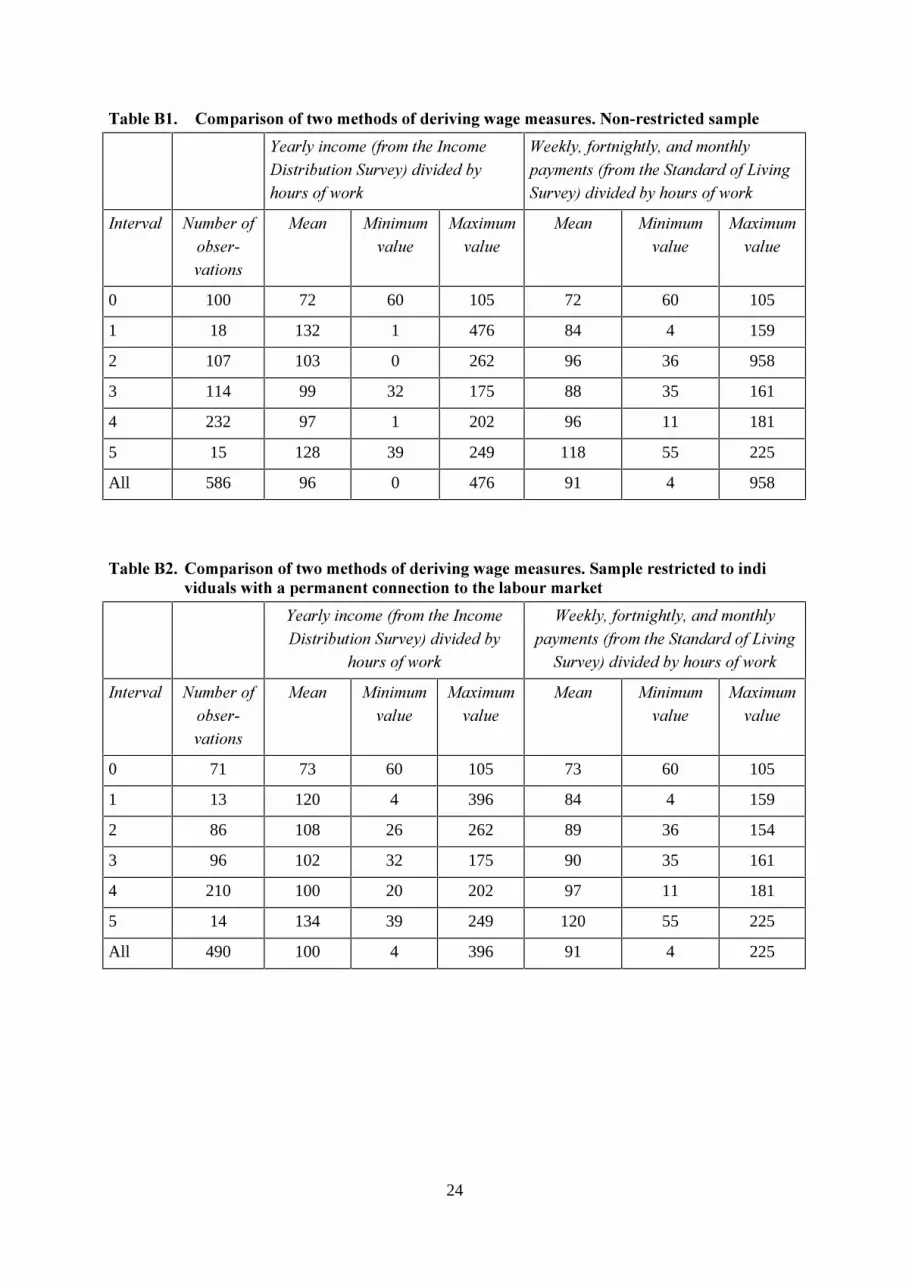
������$��
Key variables in labour supply analysis are hours of work and hourly wage rate. Unfortunately, these
variables are not easily measured. In the present analysis the hourly wage rate is measured by
combining information about annual hours of work obtainable in the Standard of Living Survey and
labour income15 from the Income Distribution Survey. The wage rates for women without work have
been obtained from an estimated wage equation, where log(w) is the dependent variable and years of
education, experience (measured as age minus years of education and minus pre-school years), and
experience squared are the explanatory variables.
The Standard of Living Survey also includes questions about the actual wage rate, either the hourly
wage or weekly, fortnightly, and monthly payments. In order to calculate the hourly gross wage rate
from these questions, we divide the weekly, fortnightly, and monthly payments by hours of work for
the corresponding period.16 Thus, the data contain two sources of deriving wage rates measures. Table
B1 presents average wage rates in intervals (corresponding to the 6 different states in the discrete
choice model) by the two methods of obtaining information about wages. The table reveals that the
means in each interval differ widely by the two methods.17 The correlation between the two wage
measures is only about 0.25 (when interval 0 is excluded).18 This low correlation is below the figures
reported in Klevmarken et al. (1995), who discuss a related problem in Swedish data.
One of the disadvantages of our method is that the interviews in the Standard of Living Survey were
carried out in January and February 1995, while the income data cover 1994. This, for instance, leads
to a situation in which the estimates on the wage rate for individuals with temporary variations in the
employment rate, could be biased. For this reason we exclude females who have received
unemployment benefit and those who have given a positive response to the question about strong
variations in hours of work. This has reduced the sample from 586 to 507 subjects. For 490 of these
507 we have observations on both wage measures, and Table B2 provides a comparison. The
correlation coefficient increases from 0.25 to 0.58, when restricting the sample to individuals with a
permanent connection to the labour market.
15 The unemployment benefit is subtracted from labour income.16 Assuming that there are 4.35 weeks in a month.17 The calculations for interval 1 are identical in the two methods.18 Since information about the wage rates is missing for some observations we restrict the comparison in Table 3 to femaleswith non-missing wage rates.
24
������8�� 6��������������!��������������� ����!�������������'�������������������
B��� 3�$�/+���!2�+��)���=�/+��%$,)�$'1)$+��(1���3#�*$�$*�*�'3�+1�,�+2��+��
<��� 3��2+�)�$6�) 3����*��+�)� 37�3���),�!2�+��)���()��*��*�+2�8$�$�6(1���3#�*$�$*�*�'3��+1�,�+2��+��
=�)���� ?1�'���+2+',��.��)$+�,
���� �$�$�1��� 1�
���$�1��� 1�
���� �$�$�1��� 1�
���$�1��� 1�
0 100 72 60 105 72 60 105
1 18 132 1 476 84 4 159
2 107 103 0 262 96 36 958
3 114 99 32 175 88 35 161
4 232 97 1 202 96 11 181
5 15 128 39 249 118 55 225
All 586 96 0 476 91 4 958
������8 � 6��������������!��������������� ����!������������������������������������ �����!�������������������������������������������"��
B��� 3�$�/+���!2�+��)���=�/+��%$,)�$'1)$+��(1���3#�*$�$*�*�'3
�+1�,�+2��+��
<��� 3��2+�)�$6�) 3����*��+�)� 37�3���),�!2�+��)���()��*��*�+2�8$�$�6
(1���3#�*$�$*�*�'3��+1�,�+2��+��
=�)���� ?1�'���+2+',��.��)$+�,
���� �$�$�1��� 1�
���$�1��� 1�
���� �$�$�1��� 1�
���$�1��� 1�
0 71 73 60 105 73 60 105
1 13 120 4 396 84 4 159
2 86 108 26 262 89 36 154
3 96 102 32 175 90 35 161
4 210 100 20 202 97 11 181
5 14 134 39 249 120 55 225
All 490 100 4 396 91 4 225


