Embed Size (px)
Citation preview

Introduction toCost–Benefi t AnalysisLooking for Reasonable Shortcuts
Ginés de Rus
Professor of Cost–Benefi t AnalysisUniversity of Las Palmas de G.C., SpainUniversity Carlos III de Madrid, Spain
Edward ElgarCheltenham, UK • Northampton, MA, USA

© Ginés de Rus 2010
This is a revised and extended version of Análisis Coste–Benefi cio: Evaluación económica de políticas y proyectos de inversión, 3rd edition, Barcelona: Ariel Economía, published in Spanish.© Ginés de Rus 2010Translated by Ginés de Rus with additional material.
All rights reserved. No part of this publication may be reproduced, stored in a retrieval system or transmitted in any form or by any means, electronic, mechanical or photocopying, recording, or otherwise without the prior permission of the publisher.
Published byEdward Elgar Publishing LimitedThe Lypiatts15 Lansdown RoadCheltenhamGlos GL50 2JAUK
Edward Elgar Publishing, Inc.William Pratt House9 Dewey CourtNorthamptonMassachusetts 01060USA
A catalogue record for this bookis available from the British Library
Library of Congress Control Number: 2010925993
ISBN 978 1 84844 852 0 (cased)
Printed and bound by MPG Books Group, UK
04

v
Contents
Foreword by C.A. Nash viii
Preface ix
1 Introduction 1
1.1 The rationale of cost–benefi t analysis 1
1.2 Steps of cost–benefi t analysis and overview of the book 7
2 The economic evaluation of social benefi ts 14
2.1 Introduction 14
2.2 The basic framework 16
2.3 Private and social benefi ts 19
2.4 Alternative approaches for the measurement of social
benefi ts 26
2.5 Winners and losers 32
Things to remember 36
3 The economic evaluation of indirect eff ects 39
3.1 Introduction 39
3.2 Indirect eff ects 40
3.3 Direct eff ects measured with a derived demand 45
3.4 Wider economic eff ects 47
3.5 Location eff ects and regional development 53
Things to remember 55
4 Opportunity costs, market and shadow prices 57
4.1 Introduction 57
4.2 The factor price as an approximation of the opportunity
cost 58
4.3 Avoidable costs and sunk costs 60
4.4 Incremental cost and average cost 62
4.5 Costs with and without the project 64
4.6 Market and shadow price of factors 68
4.7 Market price and the social opportunity cost of labour 71
4.8 The shadow price of public funds 76
4.9 Social benefi t and fi nancial equilibrium 78
Things to remember 80

vi Introduction to cost–benefi t analysis
5 Economic valuation of non- marketed goods (I) 82
5.1 Introduction 82
5.2 The economic valuation of non- marketed goods 83
5.3 Willingness to pay and willingness to accept 86
5.4 Valuation through revealed preferences 90
Things to remember 95
6 Economic valuation of non- marketed goods (II) 97
6.1 Introduction 97
6.2 Valuation through stated preferences: the contingent
valuation method 98
6.3 Conjoint analysis 105
6.4 Individual preferences and social welfare 108
6.5 The value of life 110
6.6 Benefi ts transfer 115
Things to remember 117
7 Discounting and decision criteria (I) 119
7.1 Introduction 119
7.2 Discounting the future 120
7.3 The mechanics of discounting: some useful formulas 125
7.4 Decision criteria: the net present value 129
Things to remember 133
8 Discounting and decision criteria (II) 135
8.1 Introduction 135
8.2 Decision criteria: diff erent lifespans and optimal timing 136
8.3 The marginal rate of time preference and the marginal
productivity of capital 142
8.4 The social rate of discount and the rate of interest 144
8.5 Intergenerational discount 147
Things to remember 150
9 Uncertainty and risk analysis 152
9.1 Introduction 152
9.2 Risk in a private project 154
9.3 Risk in the public sector 158
9.4 Risk analysis 161
9.5 Interpreting the results of risk analysis 167
Things to remember 175
10 Applications 177
10.1 Introduction 177
10.2 Investment projects: economic evaluation of
infrastructure 178
10.3 Cost–benefi t analysis of high speed rail: an illustration 182
10.4 Policy evaluation: cost–benefi t analysis of privatization 187

Contents vii
10.5 Cost–benefi t analysis of the concession of a residential
water supply 193
10.6 Institutional design, contracts and economic evaluation 198
Things to remember 208
11 Microeconomic foundations of cost–benefi t analysis 211
11.1 Introduction 211
11.2 From individual utility to social welfare 211
11.3 Measurement of producer surplus 216
11.4 Compensating variation, equivalent variation and
consumer surplus 223
11.5 Uncertainty 233
References 237
Index 245

viii
Foreword
The technique of cost–benefi t analysis may seem an obvious approach to
the appraisal of projects and policies to practising economists, but to many
others it is confusing at the least, and sometimes even absurd. Isn’t it based
on the proposition that only money matters? How can we place money
values on people’s lives? Surely creating jobs is a benefi t not a cost?
Ginés de Rus has written a book that concentrates on explaining the
philosophy of the cost–benefi t analysis approach to appraisal. He does
give quite a lot of technical detail, but the key messages are put across
simply and with many examples, so the book should be accessible to all
concerned with appraisal.
The book incorporates the latest thinking on issues such as the use
of distributive weights, the treatment of risk and uncertainty and the
importance of institutional arrangements in ensuring the proper use of
the technique. These issues are also blended into the approach taken in
the examples, rather than treated as optional extras, as in some texts.
The examples themselves are also very much the centre of current debate
– in what circumstances to build new high speed rail lines, the case for
privatization of water supply.
I fi rst met Ginés many years ago when he attended my lectures on cost–
benefi t analysis as part of our MA in Transport Economics. It is a great
pleasure for me therefore now to write the Foreword for his book on the
subject, and to be able to recommend it as a clear and up- to- date text that
will be of great value to all who need to know about this technique.
C.A. Nash
ITS, The University of Leeds, UK

ix
Preface
The aim of this book is to try to understand whether public decisions, like
investing in high speed railway lines, privatizing a public enterprise or
protecting a natural area, increase social welfare. It is written not only for
economists but for anyone interested in the economic eff ects of projects
and public policies, generally fi nanced with public money.
People may be interested in cost–benefi t analysis for diff erent reasons.
Some individuals have to decide which projects will be undertaken, others
have to inform those who decide on the social merit of these projects, or
perhaps they need stronger arguments to defend their legitimate inter-
est group position, to be better informed for the next election or simply
because they enjoy applied economics.
One does not need to be an economist to understand the basics
of cost–benefi t analysis, but some previous knowledge of economics
helps. Introductory microeconomics is clearly an advantage, not only
to benefi t more from this book but also for the interpretation and better
understanding of many aspects of the economy and everyday life.1
The book is non- technical and I hope the exposition is simple and
easy to follow. Its coverage is not comprehensive but I also hope the
key elements for understanding and applying cost–benefi t analysis are
adequately treated. Although this is not a theoretical book it is analytic
in the sense that it tries to follow the logic of arguments using some basic
models, which are made explicit in their assumptions, limitations and
implications.
The fi eld of cost–benefi t analysis has experienced a tremendous change
in the last decades but the main economic principles behind this tool for
public decision making remain unchanged. Moreover, despite the devel-
opment of new techniques for the economic valuation of non- marketed
goods, the refi nement of demand forecasting or dealing with uncertainty,
present practitioners in the fi eld share the same aspiration as their col-
leagues in the past: to reach a reasonable degree of confi dence regarding
the contribution of the project to social welfare.
I am indebted to many people in the writing of this book. First,
my colleagues Jorge Valido, Aday Hernández, Enrique del Moral and
Eduardo Dávila for their help during the production process of succes-
sive drafts. They not only helped with corrections but also providing
x Introduction to cost–benefi t analysis
valuable feedback. The book began as course notes for undergraduate and
postgraduate courses at the University of Las Palmas and the University
Carlos III de Madrid. I wish to thank my students and many other par-
ticipants in short courses on cost–benefi t analysis who read my class notes
and helped me to decide how to convert them into book form.
I have received very useful comments and invaluable advice on
draft chapters from Per- Olov Johannson, of the Stockholm School of
Economics, and Chris Nash, of the Institute for Transport Studies at the
University of Leeds. I am in debt to them for their patience, generosity and
encouragement.
Finally I wish to thank the staff at Edward Elgar for their help,
encouragement and advice as I prepared the manuscript.
I am the only one responsible for any remaining errors.
Ginés de Rus
University of Las Palmas de G.C., Spain
University Carlos III de Madrid, Spain
NOTE
1. Excellent introductory textbooks are, for example: Frank and Bernanke (2003), Krugman and Wells (2004), Mankiw (2003) and Samuelson and Nordhaus (2004). For an uncon-ventional and outstanding overview of economic reasoning see Landsburg (1993). For a rigorous theoretical framework of cost–benefi t analysis see, for example, Drèze and Stern (1987) and Johansson (1993).

1
1. Introduction
Any project can be viewed as a perturbation of the economy from what it would have been had some other project been undertaken instead. To determine whether the project should be undertaken, we fi rst need to look at the levels of consumption of all commodities by all the individuals at all dates under the two diff erent situations. If all individuals are better off with the project than without it, then clearly it should be adopted (if we adopt an individualistic social welfare function). If all the individuals are worse off , then clearly it should not be adopted. If some individuals are better off and others are worse off , whether we should adopt it or not depends critically on how we weight the gains and losses of diff erent individuals. Although this is obviously the ‘correct’ procedure to follow in evaluating projects, it is not a practical one; the problem of benefi t–cost analysis is simply whether we can fi nd reasonable shortcuts.
(Joseph E. Stiglitz, 1982, p. 120)
1.1 THE RATIONALE OF COST–BENEFIT ANALYSIS
Cost–benefi t analysis is not about money. It is not about inputs or outputs
either. It is about welfare. Money is central to fi nancial analysis but only
instrumental in the economic appraisal of projects and policies. Money is
the common unit in which economists express the social costs and benefi ts
of projects. Volume of drinking water, accidents avoided, time savings and
energy and labour consumed are measured in diff erent units and we need
a common unit of measure to express all these heterogeneous items in a
homogeneous fl ow. This is the key role of money in cost–benefi t analysis.
The creation of jobs is frequently presented as a benefi t of a project, but
labour is an input not an output. A motorway is not constructed to create
jobs but to move people and goods. Workers building and maintaining a
motorway represent a social cost equal to the net value lost in the next best
use of this input. It is true that if a worker is unemployed, society does not
lose as much as in the case of a similar worker already employed, but this
only shows that cost values are context dependent.
The output of a project is easier to measure than its welfare eff ects.
Public agencies report their activities with indicators such as passengers,
water, electricity or the number of students taught within a training

2 Introduction to cost–benefi t analysis
programme, but cost–benefi t analysis sees output as a means to increase
welfare. The success of a new facility cannot be explained by the number
of users. It is possible to subsidize prices to induce people to use the new
facility without increasing social welfare. Therefore, cost–benefi t analysis
is interested in the social value achieved from the outputs of the project to
compare with the value of other goods sacrifi ced elsewhere for the sake of
the project.
Cost–benefi t analysis is about the well- being of individuals aff ected
by the project and not about the number of trips or visits. The change in
welfare is what economists want to measure, and this is quite a challenging
task because welfare cannot be directly measured. To solve this problem,
economists have found an alternative: to use money as an expression of
welfare. I do not know how great the utility1 of a particular individual is
when driving his car from A to B at a particular date and time, but if I am
able to determine the amount of money to charge for this trip that makes
him indiff erent between driving or not, then interesting things can be said.
Cost–benefi t analysis is not about money but money helps.
Cost–benefi t analysis conceived as a toolkit for the selection of projects
and policies, in the general interest of the society, presupposes the exist-
ence of a social planner, a benevolent government that compares benefi ts
and costs before the implementation of projects and policies. Many econo-
mists and non- economists would consider such a view as naïve, to say the
least. An alternative view2 explains a government’s action by the political
power of diff erent interest groups. Subsidies to agriculture, for example,
could be better explained by the pressure of farmers than by an independ-
ent assessment of the social benefi ts and costs of agricultural policy.
Do we need to believe in the goodwill of the government to practise
cost–benefi t analysis? The answer is no. If we believe that a government’s
acts are better explained by the infl uence of interest groups, cost–benefi t
analysis can show who benefi ts and who loses as a result of particular
projects, and the magnitudes of the gains and losses. This assessment can
be very helpful in explaining which policies are adopted or even in infl u-
encing a government’s decision. ‘Cost–benefi t analysis may be in the battle
against misleading information spread by self- interested political pressure
groups. Still, these analysts can infl uence political outcomes by making
enough voters aware of the true eff ects of diff erent policies’ (Becker, 2001,
p. 316).
To present the conceptual foundations and methods of cost–benefi t
analysis we will proceed ‘as if’ the government would aim for the best
projects in the general interest of the society. Although we know of many
cases that show that such an assumption is unrealistic, the simplifi cation is
harmless. As we proceed to identify benefi ts and costs, winners and losers

Introduction 3
and try to measure and value the main eff ects of the project under evalua-
tion, the analysis is not going to change whatever our particular beliefs on
the government’s behaviour are.3
We have started assuming the existence of a benevolent government.
This is not the only assumption and simplifi cation in this book; in fact,
there is no way to deal with the analysis of the economy but through the
use of simplifying assumptions, replacing the actual world with a model
that refl ects the essence of the more complex reality that we want to
understand.
To move forward, we need to clarify what is understood by acting in
the general interest of the society. Let us consider that our benevolent
government is evaluating the construction of a dam and a hydroelectric
power station. The government doubts whether it should accept the
project. By undertaking the project, the region would obtain electricity
at a lower cost than without the project, recreation benefi ts, both in the
stock of water (e.g. fi shing and boating) and on the fl ow of reservoir
release (e.g. rafting), and some jobs would be created at the time of its
construction and during the lifetime of the project. Furthermore, there
might be a multiplier eff ect, as the project would create new economic
activity induced by the expenditure associated with the construction and
operation of the project.
Economists point out that from the benefi ts described above we have to
deduct some costs. First, the construction and maintenance costs, equal to
the net benefi ts of alternative needs that have not been attended to because
the public money has been assigned to the dam and power station, have to
be deducted. They also argue that labour is an input, not an output, so it is
a cost of the project, though its magnitude will depend on what is lost when
the worker is employed within the project. The multiplier eff ect, if it exists,
turns out to be irrelevant if it is also associated with the alternatives.
Second, all the other costs associated with the relocation of the inhab-
itants of the village in the area where the dam would be built and with
the people negatively aff ected by the alteration of the fl ow and course
of the river should be deducted. The magnitude of these costs could be
substantial.
The government considers all the relevant benefi ts and costs regard-
less, in principle, of who the benefi ciaries and the losers are (assume for
simplicity that all the eff ects are inside the country) and the government
decides to undertake the project if, given the available information,
the society improves. Its decision is not based on the arguments of the
private companies that will build the dam and power station, nor on the
campaign of the opponents. The decision takes into account the whole
society, with social welfare as the unique reference. The challenge for our

4 Introduction to cost–benefi t analysis
benevolent government is how to value all the benefi ts and costs and how
to compare them given that benefi ciaries and losers are individuals with
diff erent income, education, health, and so on, and are aff ected at diff erent
moments during the lifespan of the project.
This water project, as any other public infrastructure such as parks, high
speed rail, highways, ports or the introduction of policies such as environ-
mental regulations, can be interpreted as perturbations in the economy
aff ecting the welfare of diff erent individuals at diff erent moments in time
compared with the situation without the project or policy, which does not
necessarily mean the status quo but what would have happened in the
absence of the project or policy.
The assessment of the eff ects of the project requires a benchmark. It is
necessary to compare the world with and without the project: to recreate
an alternative world, or the so- called counterfactual. Cost–benefi t analysis
practitioners have to solve two main problems. First, they have to build the
counterfactual and this means to replicate the world without the project,
a dynamic world that evolves without the perturbation introduced by the
project. This is not an easy task because the time period for this exercise
may be quite long, 40 years or more, and the values of key variables will
possibly change in each one of these years, only some of them in predict-
able ways. Second, the practitioner has to imagine the world with the
project, forecasting the main changes with respect to the counterfactual
that he has previously created.
The expected changes when the project is implemented are then the
result of the comparison with the counterfactual: the worse the counter-
factual, the better the project. Hence, it is important to present all the
assumptions and the data used to complete this exercise. Transparency
and ex post evaluation can help to avoid both innocent errors and strategic
misrepresentation.
Suppose the counterfactual and the world with the project have been
properly designed and the expected changes have been estimated: time
savings, enhanced water quality or a reduction in the number of fatal acci-
dents. Now, the analyst has to convert these values into monetary units
($)4 assuming that this is technically possible and morally acceptable.
We want to measure changes in the welfare of the individuals who
compose the society; however individuals’ utility cannot be measured
in the same way as the amount of electricity produced or the number
of people displaced to build the dam. To decide on the goodness of the
project we need to measure something that is unobservable. Furthermore
what is observable – the production of electricity, number of individuals
involved, extension of fl ooded surface, and so on – is not very useful if
we do not translate the physical units into a common measure related to

Introduction 5
changes in individual utility, which allows the comparison between what
is gained and what is lost.
Hence, though the ideal way of measuring the impact of our project
is through utility functions (we would measure the change in utility of
each individual) the problem is that these utility functions and the asso-
ciated utility changes are unobservable. Converting the unobservable
utility changes through an ‘exchange rate’ between utility and income to
observable monetary units gives us a way of calculating the impact of the
project.
One alternative solution might be to submit the project to a referendum
and to accept the outcome: that is, accepting the view of the majority. Let
us have a look at this in more detail. Table 1.1 collects the information
(expressed in monetary units) of the benefi ts and costs of those aff ected
by the construction of the dam and the hydroelectric power station. Our
society consists of fi ve individuals.5
The individual B, for example, benefi ts from cheaper energy (+$2) but
he also fi shes downstream and the dam prevents him from practising his
favourite sport in the initial conditions (–$8). The result is a net loss of $6
for individual B. We could interpret the values in the column ‘net benefi ts’
as the monetary compensation that will be needed with the project to leave
each individual indiff erent without the project: for example, the individual
B would be willing to accept $6 and the individual A would be willing to
pay $7.6
The column ‘net benefi ts’ allows us to anticipate that the project would
be rejected in a referendum. Individuals A and D would vote in favour, but
individuals B, C and E would vote against it. Would it be a good decision
to reject the construction of the water project? To answer this question we
have to check whether the construction of the dam is a social improvement
and for this purpose we need to defi ne a decision criterion.
A possible criterion is the strong Pareto improvement. To move from
one situation to another is a social improvement (in the sense of Pareto)
if at least one person is better off without making anyone else worse off .
Table 1.1 Benefi ts and costs of a hydroelectric power station (values in $)
Individual Benefi ts Costs Net benefi ts
A 7 0 7
B 2 8 −6
C 3 4 −1
D 9 1 8
E 1 6 −5

6 Introduction to cost–benefi t analysis
There are winners and nobody loses. We have seen that the referendum
would result in the rejection of the project. Would it be possible, in these
circumstances, to reach a Pareto improvement despite the outcome of the
ballot?
Although it seems clear that the project under discussion would not
be approved in a referendum, the society may gain from the project if, as
it happens to be in this case, the benefi ts ($22) outweigh the costs ($19).
Suppose the project is carried out and part of the benefi ts is used to com-
pensate individuals B, C and E, so that their net benefi t is zero, leaving
them indiff erent. Table 1.1 shows that, after compensation, there is a net
benefi t of $3 to share out as deemed appropriate. If the project is rejected
this net gain would be lost.
On the other hand, when comparing the benefi ts and costs of the
project, the magnitude of gains and losses counts. Individual C is against
the project because it costs him $1, while D stands for the project because
he gains benefi ts of $8. If we ignore the intensity of preferences, like in a
referendum, we lose the potential gains arising from the project.
As we have seen, the Pareto improvement criterion requires no losers
(i.e. there is full compensation to those initially harmed by the project).
This rarely happens in the real world since, in many cases, the situation is
similar to that described, but without full compensation to the losers.7 If
a project produces a positive balance of benefi ts to the society as a whole
and there are losers who, for some reason, cannot be fully compensated,
it is normal practice to undertake such a project (the winners could have
compensated the losers and still remain winners).
This criterion, in which the compensation is only hypothetical, is known
as the potential compensation criterion, or Kaldor–Hicks criterion.8 If the
losers are compensated, it would result in a Pareto improvement. Unless
the project has unacceptable distributional consequences, the economic
evaluation of projects and policies rests basically on the criterion of
potential compensation just described.
To be more precise, we need – at least for a small project – to weigh
individual (or group) i’s monetary gain with the marginal utility of income
of individual i, and with the social welfare weight attributed to individual
i refl ecting the social welfare function. Hence, the marginal social utility
of income (see Chapters 2 and 11) attributed to i depends on what social
welfare function9 we assume and the income distribution.
We can multiply the social marginal utility of income by the monetary
valuation of the project (willingness to pay or willingness to accept) of
individual i and sum over all individuals. So if initial welfare distribution
is optimal (and where the marginal utility of income might vary across
individuals since they might have very diff erent utility functions: one

Introduction 7
being a dedicated wildlife person, another being a passionate consumer of
diamonds) the marginal social utility of income is the same for everyone.
Then a project so small that it leaves the welfare distribution unchanged as
a linear approximation can be evaluated simply by summing willingness to
pay or willingness to accept across individuals/groups.
The common justifi cation of the Kaldor–Hicks compensation criterion
in practice is based on the argument that redistribution can be performed
more effi ciently through the fi scal system and that, overall, given the large
amount of diff erent projects being carried out, the positive and negative
distributional eff ects tend to off set each other, and everybody wins in the
long run, or they are unimportant, or the costs of identifying winners and
losers and paying compensation are higher than the benefi ts.
1.2 STEPS OF COST–BENEFIT ANALYSIS AND OVERVIEW OF THE BOOK
The economic appraisal of investment projects and public policies must be
fl exible enough to capture the specifi c characteristics of each case study;
however there exist some steps that have to be followed independently of
the particular aspects of the project under evaluation. These are described
below.
(i) Objective of the Project and Examination of the Relevant Alternatives
Before evaluating the project, its objective – that is, the problem to be
solved – has to be clearly defi ned and the relevant alternatives identifi ed.
To analyse an isolated project without considering its role within the
programme or policy where it belongs can lead to wrong conclusions.
Moreover, before working with data and applying the methodology of
economic evaluation, it is essential to analyse the relevant alternatives
that allow the achievement of the same objective. An improper analysis
of available alternatives can lead to important errors despite the methods
and techniques being rigorous.
There are two a priori approaches for the practitioners in the appraisal
of a project: fi rst, when the analyst has to evaluate a particular project, for
example, a price reduction in a public service; second, when the project is
the improvement of a public service. If the goal of the regulator were to
benefi t consumers without damaging service quality, a possible measure
could be to reduce prices, keeping the fi nancial equilibrium with public
subsidies. However there are also other policies to achieve this goal.
An alternative could consist of introducing a system of incentives that

8 Introduction to cost–benefi t analysis
compensates for eff orts in the reduction of costs that allow price cuts.
Another policy could be a private concession of the public service.
The consideration of diff erent projects to achieve the same goal is a
previous stage to the identifi cation and quantifi cation of benefi ts and
costs in the evaluation given that the omission of more effi cient alterna-
tives is to lose the opportunity to gain better results. It is not enough to
have positive social benefi ts, it is required that those benefi ts are greater
than the benefi ts in the best available alternative. The same happens
with investment projects. The question ‘is the investment the best way of
solving the problem?’ must be answered. Other possible reversible and
less costly options must be analysed, such as diff erent management of
the facility.
In the stage of the search for relevant alternatives it is very useful for
the economist to interact with and receive feedback from other specialists
more familiar with the technology or fi eld related to the project. The objec-
tive of this step is to avoid errors because of a lack of precise information
about more effi cient methods to achieve the same goal. The greater refi ne-
ment in the evaluation methodology would be useless if better alternatives
had not been taken into consideration.
Finally, it is not convenient to defi ne projects with too broad a scope
because a positive evaluation of the aggregate can hide separable projects
with negative expected returns. Therefore their inclusion, without dif-
ferentiation, in a programme or a more global project can lead to wrong
conclusions. To establish the limits of a project is not always easy but a
careful discussion of the project with experts can allow us to distinguish
intrinsic complexity from the inclusion of independent projects that are
perfectly separable.
On the other hand it is nonsense to evaluate a project narrowly defi ned
in the sense that its existence is not possible without complementary
actions. Suppose that an investment project is composed of two main parts
(e.g. a port and an access road) and the social net present value (NPV)
is negative. The strategy of promoters could be to evaluate only the fi rst
part (the construction of the port) and, once it has been built, to present
another project consisting of the complementary infrastructure to connect
the port with the road network. In this case, the road project will prob-
ably be socially worthy because the investment cost of the already existing
port is now irrelevant in the evaluation of the construction of the road,
a principle that is not applicable to the lost benefi ts if the port cannot be
operated.
In this chapter, we present the basic concepts of cost–benefi t analy-
sis and make explicit the simplifi cation used to deal with the economic
evaluation of projects that have medium and long term eff ects.
Introduction 9
(ii) Identifi cation of Costs and Benefi ts
Once the project is defi ned and bounded, it is necessary to identify the
benefi ts and costs derived from its implementation. In some cases, this step
is immediate and must not bring up greater diffi culties, for example when
projects have only direct eff ects (Chapter 2).
The identifi cation of the costs and benefi ts of a project with signifi cant
indirect eff ects on other markets is more complicated because the impact
must be located in markets diff erent from the ones where direct eff ects are
produced. The more reasonable approximation, when the analysis is not
conducted within a general equilibrium framework, consists of identifying
the main secondary markets aff ected by the project as would be the case
with the evaluation of a new railway line that reduces the demand for an
existing airport (Chapter 3).
In fi nancial analysis, the identifi cation is much simpler: benefi ts are
revenues and costs are the payment of inputs valued at market prices.
However, in economic analysis, benefi ts are those that are enjoyed by the
individual independently of their conversion into revenues, and costs are
net social benefi ts lost in the best available alternative.
Moreover, it is necessary to decide ‘who stands’ in cost–benefi t analysis.
Generally, country frontiers delimitate who must be included. Citizenship
is the reference when the project has no global or controversial eff ects
beyond the national boundaries. Sometimes it depends on who fi nances
the project. In a co- fi nanced project with supranational funds it would
not be acceptable to exclude citizens of countries that contribute with
their taxes to fi nancing the project. On the contrary, it is not uncommon
for a region only to consider local benefi ts and costs, ignoring positive or
negative eff ects that take place in the rest of the country.
(iii) Measurement of Costs and Benefi ts
Projects’ benefi ts can be measured through individuals’ willingness to pay
(or willingness to accept). Sometimes a monetary measure of the utility
change that is derived from the project can be obtained by observing the
behaviour of consumers in the market; that is, from market data. This is
the case with the measurement of direct benefi ts in the primary market
aff ected by the project (Chapter 2), the indirect eff ects in the secondary
markets related to the primary market (Chapter 3), and in the valuation
of non- marketed goods when the analyst can fi nd an ‘ally’ market where
some useful information is revealed about the willingness to pay of the
individuals (Chapters 5 and 6).
On other occasions, economists have to estimate project benefi ts by

10 Introduction to cost–benefi t analysis
asking people directly about their willingness to pay (stated preferences);
this consists of asking individuals about monetary quantities that refl ect
the change in their welfare thanks to the project. This approximation
is used for non- marketed goods like environmental impacts or safety
changes (Chapter 6).
In general, projects and public policies that are subject to evaluation
imply the use or saving of resources. The costs of a standard investment
project can be classifi ed as: construction, maintenance, labour, equip-
ment and energy – costs that are measured from the quantity of the inputs
valued by their respective prices. From an economic point of view, the
cost of input use is the net social benefi t lost in the next best alternative.
Market prices will sometimes be a good approximation of the opportunity
cost, but in other cases it will be necessary to introduce some correction
in market prices to approximate the social opportunity cost of the inputs,
and this is what are called shadow prices (Chapter 4).
(iv) Benefi ts and Costs Aggregation
Benefi ts and costs occur in diff erent periods of time and aff ect diff erent
individuals. The aggregation requires homogeneity, but benefi ts and costs
that occur in successive years or aff ect individuals with diff erent social
conditions are not homogeneous. If they are directly summed, the implicit
weight associated with each benefi t or cost is the unity: a unit of benefi t is
identical disregarding the year or the individual.
Many infrastructure projects have lifetime periods over 30 years.
Moreover, in the case of public policies that modify educational or health
programmes, introduce or eliminate taxes, and so on, the ex ante lifespan
is practically infi nite. To discount future benefi ts and costs is a process of
homogenizing to allow comparison. The discounting is performed using
a discount rate greater than zero. This implies that the value of the ben-
efi ts and costs decreases with time. The basic idea consists of the fact that
individuals generally give more value to present than to future consump-
tion and, therefore, future units of consumption are counted with a lower
present value (Chapters 7 and 8).
Project costs and benefi ts aff ect individuals’ utility. To go from net
individual benefi ts to aggregate social benefi ts implies redistributive
eff ects. If the society gives, for example, more weight to the income of
poor people, then the benefi ts and costs of a project cannot be added
without social weighting. The net social benefi t of the project should
ideally be obtained as the weighted sum of the individual net benefi ts
(Chapters 2 and 11).

Introduction 11
(v) Interpretation of Results and Decision Criteria
The aspiration of the practitioner of cost–benefi t analysis is to obtain a
fi gure that summarizes the fl ows of benefi ts and costs. This fi gure is the
NPV of the project, and helps with the decision to accept–reject or to
choose between a set of projects.
To obtain a unique fi gure is not always easy. There are positive or nega-
tive impacts that resist the reduction to a monetary fi gure as happens to be
the case with some environmental impacts. There are situations in which it
can be appropriate to make a qualitative description of some eff ects, and
then to attach this information to the NPV obtained with the eff ects that
can be unambiguously measured.
Decision criteria based on the discounted value of benefi ts and costs are
straightforward. If the NPV is positive and the redistributive eff ects of the
project are positive or unimportant, the project increases social welfare.
If we have to compare projects it may be necessary to homogenize before
choosing the project with the higher NPV (Chapters 7 and 8).
Results must be subject to a risk analysis with the objective of determin-
ing the sensitivity of the NPV to changes in key variables. Ideally, it is pref-
erable to compute a probability distribution of NPV instead of obtaining a
unique NPV fi gure. Risk analysis allows the decision maker to have some
information about the likelihood of the feasible results. Risk analysis does
not eliminate the risk of the project but makes more evident the actual risk
of the project to the decision maker (Chapter 9).
(vi) Comparison of the Project with a Base Case
In cost–benefi t analysis, it is important to avoid a comparison of the
project with an irrelevant base case. For example, comparing with the
situation before the project, the NPV can be high because it can be hiding
the fact that without the project that situation does not remain constant.
There are maintenance policies or a minimum renewal of equipment, and
so on, that could be implemented without the project. Thus, in the evalua-
tion of the construction of a high speed rail line, we have to compare with a
counterfactual where the demand changes and the supply of conventional
rail and competing modes also changes.10
The situation without the project is known as the base case. We have
to distinguish between do nothing and do minimum, which consists of the
minimum intervention that is foreseen without the project. The distinction
can be made clearer with an example. Consider that the objective is to
substitute the water pipes that supply water to the city, because of exces-
sive water leaks. In this project the reasonable base case is a do minimum

12 Introduction to cost–benefi t analysis
because, without the project, there will be maintenance operations and
selective actions to avoid greater damage. Now consider that the project
consists of a maintenance plan instead of investing in a new network. In
this case the base case would be a do nothing.
(vii) Economic Return and Financial Feasibility
Cost–benefi t analysis compares the social benefi ts and costs in contrast
with fi nancial analysis, which uses revenues instead of social benefi ts and
private costs instead of social costs. However it is very important for the
analyst to have a report that not only includes the economic return of
the project but also the fi nancial result or commercial feasibility of the
project.
It is perfectly possible for a project or public policy to generate social
benefi ts that exceed social costs and, at the same time, to present a negative
fi nancial result. Let us consider, for example, the case of a reforesting policy
that reduces land erosion and delivers new space for recreation. Moreover,
the responsible public agency obtains some revenues from charging for
parking close to the recreation area. It is likely that this project presents
a positive social NPV and a negative fi nancial result. The analyst must
present both results to the decision maker for two main reasons.
First, the real world is characterized by the presence of budget con-
straints; therefore it is really useful for the public agency to have informa-
tion on the social net benefi t of the project as well as on the proportion of
costs that are covered by revenues. Second, many projects produce a wide
range of NPVs as a function, for example, of the pricing policy applied. It
is usual for projects that admit the possibility of charging users to present
diff erent possible combinations of social NPV and fi nancial NPV. For
example, a road project can be evaluated as a free access road or as a
toll road. If the second option is chosen, several possible price structures
exist: it is possible to discriminate by time, vehicle type or use intensity.
It is likely that social benefi ts diminish with the toll; however collected
revenues can contribute to fi xed costs. To report the diff erent options
available and their social and fi nancial NPV increases the usefulness of
cost–benefi t analysis.
NOTES
1. We use the terms ‘utility’ and ‘individual welfare’ as synonymous. 2. George Stigler, Gary Becker and Sam Peltzman are among the top economists promot-
ing the ‘interest group competition model’.

Introduction 13
3. Nevertheless, once the conventional cost–benefi t analysis is completed, we need to address explicitly the institutional design and the possible confl icting objectives, and we attend to that in Chapter 10.
4. We use the dollar symbol, $, as representing an undefi ned monetary unit without any relation to its actual market value.
5. We assume the individual is the best judge of his own interest; hence we ignore problems derived from distorted preferences (see Adler and Posner, 2001).
6. We assume for simplicity here that willingness to pay and willingness to accept coincide. For a technical discussion on the why these monetary measures of utility changes diff er, see Chapter 11.
7. As is the case with legal expropriation. 8. There is a simplifi cation here with the Kaldor–Hicks hypothetical compensation.
Boadway pointed out that a positive sum of compensating variations, for example, is not equivalent to gainers being able to compensate losers. The problem known as the Boadway paradox is that the act of compensation might aff ect relative prices and hence welfare/utility of an individual (see Boadway, 1974; Jones, 2002).
9. For a Utilitarian society the marginal social utility or welfare weight is unity for all i, for a Rawlsian society it is equal to zero for all but the worst- off individual or group.
10. The comparison with an irrelevant alternative can be an error of the analyst, or a strategy for getting the project through.
14
2. The economic evaluation of social benefi ts
We like the cost–benefi t criterion fi rst because we think its application makes almost everybody better off over the long haul, and second because it is easy to apply. In other words, the benefi ts are high and the costs are low. The reasoning may be slightly circular, but the cost–benefi t criterion recommends itself highly.
(Steven E. Landsburg, 1993, p. 105)
2.1 INTRODUCTION
The measurement of changes in social welfare and the decision criteria
for the economic assessment of projects1 can be approached by model-
ling the economy as a set of individuals who, given their preferences,
try to maximize their utility subject to two constraints: the available
resources and the technology. A project changes the equilibrium in the
markets in which individuals participate as consumers, owners of pro-
duction factors, taxpayers, or aff ected by externalities, and cost–benefi t
analysis tries to measure the change in the utility of individuals to assess
whether the project represents an improvement for an aggregate called
society.
Given the scarcity of resources, people are typically forced to choose
between diff erent uses, and the available technology limits the quantity,
variety and quality of goods produced from those resources. In a society
where what matters is the welfare of its individuals, the focus is not on
increasing production but the utility of individuals. In this sense, prefer-
ences limit the utility that individuals can reach for a given endowment of
resources and technology, which is particularly relevant in the decisions
that the public sector takes outside the discipline of the market.
In addition to the decisions of the individuals, the government also
intervenes with projects that alter the equilibrium of some markets and
aff ect social welfare. Its decisions aff ect the quantity, quality and compo-
sition of goods and services and their distribution. This chapter presents
some economic concepts to build a basic framework for practical cost–
benefi t analysis.2

The economic evaluation of social benefi ts 15
The basic model is described in section 2.2, where we simplify the
society into several groups: consumer, taxpayers, the owners of produc-
tion factors and the ‘rest of society’ to account for the external eff ects.
Consumer surplus and producer surplus, key concepts in cost–benefi t
analysis, are explained in section 2.3, where the crucial distinction between
price, cost and value is addressed.
To decide whether a project should be approved we have to compare
its social benefi ts with its social costs, previously identifi ed and measured.
We need, fi rst, to quantify in monetary terms the changes in individuals’
utility; second, to use some criteria for the aggregation of the benefi ts and
costs aff ecting diff erent individuals at diff erent points in time; and, fi nally,
to use some decision criteria to accept–reject or select from among a set
of them.
In this chapter we focus attention mainly on the benefi ts, although we
refer to the costs when it helps the argument (the detailed treatment of
costs is in Chapter 4). One of the main points in this chapter is the distinc-
tion of two alternative procedures for assessing the net benefi ts in section
2.4: the sum of the changes in surpluses of individuals and the sum of the
changes in the willingness to pay and in real resources, ignoring transfers.
This distinction turns out to be quite important in practical cost–benefi t
analysis, and following carefully one approach or the other can help to
avoid common mistakes.
Effi ciency is not the only reference in society and who wins and who
loses with a project are very important in public decision making. Section
2.5 discusses the conversion of income into individual utility and of
individual utility into social welfare.
The evaluation procedures contained in this chapter apply to projects
that are ‘small’.3 This requirement is necessary in order to simplify, to
focus on the project’s impact mainly on the primary market and on the
most directly aff ected secondary markets. The construction of a waste
water plant is a project whose eff ects on infl ation and government defi cit
are not generally expected to be signifi cant. ‘Large’ projects that aff ect the
macroeconomic variables should be analysed, where possible, with general
equilibrium models.
When not specifi ed, we will deal with market demand functions.
Although the ideal would be to work with compensated demands, the
results obtained using the observed quantities in the market are some-
what acceptable in many cases (see Chapter 11). In this book we assume
that the conditions required for using market demands for monetary
measurements of changes in the utility of the individual hold.
16 Introduction to cost–benefi t analysis
2.2 THE BASIC FRAMEWORK
A Simplifi ed Economy
A project can be contemplated as a perturbation in the economy that
aff ects the utility of individuals. The project’s impact occurs in the primary
market (the directly aff ected market), and also in the so- called secondary
markets, related to the primary because their products are complements
or substitutes (see Chapter 3). Furthermore, the eff ects generally last for a
long period of time, particularly in civil engineering projects, in the case of
environmental impacts or policies that modify market structure.
The construction of a water irrigation project or a transport infrastruc-
ture, investment in education and the improvement of air quality have in
common the eff ect on the welfare of the individuals aff ected by the project.
Some individuals are better off and others worse off ; they are located
somewhere and this position is relevant to take into account whether their
change in welfare counts or whether it is ignored. This is the question of
standing, the problem of who counts in cost–benefi t analysis. Usually
the nation establishes the boundaries to who counts but sometimes it
is the type of project, as is the case with the preservation of worldwide
endangered species. On other occasions the co- fi nancing by supranational
organizations determines the countries that should be included. Although
common sense can help in many cases, the diffi culties could be signifi cant
in some projects with global externalities. To make the problem manage-
able, we will simplify as much as we can and work with a very simple
model of the economy as described below.4
In our simplifi ed economy, in which we are going to evaluate projects,
there are three owners of production factors: fi rst, the ‘owners of capital’
(O), generally called producers, who have a variety of equipment, infra-
structure and facilities where goods and services are produced; second, the
‘owners of labour’ (L) including employees of diff erent skills and produc-
tivity levels, but in our simplifi ed model they all belong to the only existing
group of owners of labour or ‘workers’; and, fi nally, the owner of the third
factor of production, the land.
The factor of production ‘land’ is defi ned in a wide sense including not
only the soil for agriculture or the land for residential or productive uses,
but also natural and environmental resources such as climate, water, air,
fl ora and fauna and landscapes, which may be aff ected by projects. One
important distinction is between the land under private ownership and
the natural resources that are common property. We distinguish the ‘land
owners’ (R) from another group of ‘owners’ of natural and environmental
resources (also called ‘natural capital’), which we call the ‘rest of society’

The economic evaluation of social benefi ts 17
(E), where we also include any other external eff ect, like those aff ecting
safety.
The combination of production factors creates a fl ow of goods and serv-
ices. The income paid to those factors of production allows us to identify
additional agents: ‘consumers’ (C) and ‘taxpayers’ (G), so that society is
composed of six groups of individuals. Obviously, one can be a member of
more than one group and must necessarily belong to group C. Moreover,
this simplifi ed society has another feature: the value of a unit of benefi t (or
cost) is the same regardless of to whom it may accrue (this assumption will
be relaxed in section 2.5).
In this unsophisticated world, the social surplus (SS) is the sum of
individual surplus:
SS 5 CS 1 GS 1 OS 1 LS 1 RS 1 ES, (2.1)
where consumers’ surplus (CS) is the diff erence between what consumers
are willing to pay for the goods and what they actually pay. Taxpayers’
surplus (GS) equals tax revenues less public expenditure. The surpluses of
workers (LS) and land owners (RS) are equal to the wage and land income,
respectively, less the minimum pay they are willing to accept for the use of
the factor; that is, its opportunity cost. Interestingly payment for land, like
any other fi xed factor, is usually what producers are willing to pay for the
activity that requires the use of that fi xed factor in competitive markets.
The surplus of the owners of capital (OS) is equal to fi rm revenues less
variable costs and, fi nally, the surplus of the ‘rest of society’ (ES) includes
the social value of non- marketed goods such as landscape, clean air and
climate, and also external eff ects aff ecting health and safety levels that may
change when a project is carried out, for example, a power plant that con-
tributes to global warming or an investment in alternative energy sources
that reduces it. There are many ways in which environmental goods can
aff ect individual welfare, directly aff ecting individual utility, for example
having access to a water reservoir of improved quality for recreation pur-
poses or, indirectly, through the impact of this increase in water quality on
the production costs of fi rms (see Chapters 5 and 6).
The government’s decision to invest in a project or to introduce a spe-
cifi c policy to change prices, costs or quality, aff ects the surplus of the
social groups over the years for which the project continues producing its
positive and negative eff ects, so that the total impact of the project can be
expressed as the aggregate of changes in the surpluses of the individuals:
DSS 5 aT
t50
dt(DCSt 1 DGSt 1 DOSt 1 DLSt 1 DRSt 1 DESt) , (2.2)
18 Introduction to cost–benefi t analysis
where Δ denotes an increase or decrease in the surplus of the various agents
and dt is the discount factor that allows us to express in present value the
fl ow of benefi ts and costs over the lifespan of the project. For example, if
individuals are indiff erent between $95 in the present (year zero) and $100
within a year, the discount factor that converts the benefi t in year one into
units comparable to the benefi ts in year zero is equal to 0.95 (see Chapters
7 and 8).
To make the model even simpler, we assume that owners of factors of
production (except the owners of capital) receive a payment equal to their
opportunity cost, so their surpluses are equal to zero (they are indiff erent
between the situation with and without the project). We also assume that
there are no taxes or public expenditure and there are no external eff ects and
fi xed factors. Finally, calling ‘producer surplus’ (PS) to the capital owners’
surplus (OS), the expression (2.2) is reduced to the familiar expression:5
DSS 5 aT
t50
dt(DCSt 1 DPSt) . (2.3)
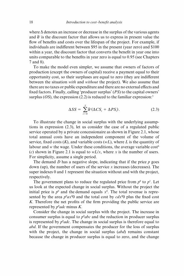
To illustrate the change in social surplus with the underlying assump-
tions in expression (2.3), let us consider the case of a regulated public
service operated by a private concessionaire as shown in Figure 2.1, whose
total annual costs have an independent component of the volume of
service, fi xed costs (K), and variable costs (wL), where L is the quantity of
labour and w the wage. Under these conditions, the average variable cost6
(c) shown in Figure 2.1 is equal to wL/x, where x is the number of users.
For simplicity, assume a single period.
The demand D has a negative slope, indicating that if the price p goes
down (up), the number of users of the service x increases (decreases). The
super indexes 0 and 1 represent the situation without and with the project,
respectively.
The government plans to reduce the regulated price from p0 to p1. Let
us look at the expected change in social surplus. Without the project the
initial price is p0 and the demand equals x0. The total revenue is repre-
sented by the area p0ax00 and the total cost by cdx00 plus the fi xed cost
K. Therefore the net profi ts of the fi rm providing the public service are
represented by p0adc minus K.
Consider the change in social surplus with the project. The increase in
consumer surplus is equal to p0abc and the reduction in producer surplus
is represented by p0adc. The change in social surplus is therefore equal to
abd. If the government compensates the producer for the loss of surplus
with the project, the change in social surplus (abd) remains constant
because the change in producer surplus is equal to zero, and the change

The economic evaluation of social benefi ts 19
in taxpayers’ surplus (ΔGS) is negative and equal to the amount of the
compensation (p0adc). The change in consumer surplus is unaff ected.
Therefore the change in social surplus is still represented by the area abd
once the change in taxpayers’ surplus is included. Income transfers do not
change the results.
What about workers’ surplus? Looking at what happens in Figure 2.1
(right), the increase in production causes a shift in labour demand from
DL0 to DL1, generating an increase in the level of employment L1 − L0.
Should we count the earnings of the additional workers as an increase in
the social surplus? If the answer was yes, we would have to add efL1L0 to
the area abd in Figure 2.1 (left).
However the answer is no, because while these additional workers
receive a wage that they did not receive previously, they now lose the net
value of what they were doing before they were employed, their opportu-
nity cost (perhaps the value of leisure) that in the conditions represented
by the labour supply SL is exactly equal to the wages being paid (efL1L0).
In the described circumstances, workers are indiff erent between working
and not working at the wage w, and therefore the change in their surplus
(ΔLS) is zero.7
2.3 PRIVATE AND SOCIAL BENEFITS
Price, Cost and Value
When a private company operating in a competitive market assesses
whether a particular activity is profi table it compares the revenues and
p
p0
p1 = c
w
x L
D DL0
w
x0 x10 0
a
d b
L0 L1
SLe f
DL1
Figure 2.1 Price reduction in a public service

20 Introduction to cost–benefi t analysis
costs attributable to such an activity. It can be argued that, in general, the
value per unit of product for the fi rm matches the net price of the product
sold, and the unit cost is equal to the internal cost to the fi rm in terms of
the use of materials, labour and other inputs. However price is not nec-
essarily equal to value, private value does not necessarily coincide with
social value and private cost is not necessarily equal to social cost.
An open access natural park has a cost of maintenance and manage-
ment and, although nothing is charged for its enjoyment, its use has value
for the individuals who visit the park.8 The distinction between price,
value and cost, and between private and social in the last two concepts,
facilitates the task of valuing goods in order to evaluate projects.
Although the maximum that an individual is willing to pay for a good
that can be purchased in the market refl ects the economic value, expressed
in monetary terms, of the good for the individual, the maximum willing-
ness to pay does not necessarily coincide with what is actually paid: the
user of a sport centre may be willing to pay an amount of money higher
than the existing fee for the use of the facilities. The user of a health care
service with free access may be willing to pay a certain amount of money
for the use of this service, were the access conditional on the payment of
a fee.
The private value of the good to an individual coincides with the social
value of the good unless there are external costs or benefi ts. Continuing
with the example of the health service, a vaccination campaign is benefi cial
not only to the users of the service but also to the society as a whole given
the reduction in the spread of the disease. This is what is called a positive
externality.
We must distinguish between total and marginal value. The fi rst concept
refers to what an individual would be willing to pay for the consumption
of all units, while the second refers to the value of the last unit consumed.
The case of water illustrates the diff erence between the two concepts: the
total value is very high for any individual, while the marginal value of
the last unit consumed is usually very low, at least in societies without
scarcity problems. In a fi rst approximation, the total value for the society
is obtained by adding the willingness to pay of the individuals (for
distributional issues, see section 2.5).
The price of a good is what is charged in the market for its consump-
tion. If there is no price discrimination, the price does not coincide with
the valuation of the individuals of any unit consumed but the last one,
whose marginal value does coincide with the price because, with decreas-
ing demand curves, for the remainder of the units consumed, individuals
are willing to pay per unit more than the market price. The fact that the
market price equals only the marginal value of the last unit exchanged in

The economic evaluation of social benefi ts 21
the market points to the inaccuracy of using revenues as social benefi ts.
When a single price is charged, the total value or social benefi t of the good
is therefore higher than total revenues.
The cost of a good is the benefi t lost in the next best alternative; that
is, the net value of other goods that one must renounce for that good (the
opportunity cost). In competitive markets, not distorted by subsidies or
taxes for example, the price of the production factors used in producing
the good is the opportunity cost of that good. The distinction between
private cost and social cost is necessary in cases where the production
requires not only inputs traded in the market, but non- marketed goods
(e.g. environmental resources), or when it generates positive or negative
externalities that the fi rm does not internalize; that is, that fall on the ‘rest
of society’.
The diff erence between these concepts can be illustrated by the follow-
ing example: a water supply fi rm serves a city, incurring a total cost that
has two components: a fi xed cost for the entire system of production and
distribution (K) and a constant variable cost per unit of water produced
and distributed (c). Figure 2.2 shows the water demand of the company9
and how at price pb consumers demand quantity xb. It also shows how each
unit of water has a diff erent valuation.
The fi rst units of water are possibly used to meet basic needs, so that
their valuation is very high. The maximum reservation price (g), at which
the company would not sell any water, might be the price of an alternative
supply system, for example, delivering water in a road tanker. As water
consumption increases, the value of each additional unit decreases, indi-
cating that the following units of water are intended to cover less valuable
needs.
a
bpb
c
d
p(x)
e
0 xxa xb xd xe
�
Figure 2.2 Value, price and cost

22 Introduction to cost–benefi t analysis
Every unit of water to the left of xb is valued above the price pb, hence
the user valuation of a unit of water only matches the price in the case of
the last unit of the quantity xb. As the variable cost of supplying one unit of
water is equal to c, the diff erence between revenue, social benefi ts and costs
is evident. The value of use of the water consumed, equal to the sum of the
values of each unit, is represented by the distance between the horizontal
axis and the demand (. . .+ a +. . .+ b +. . .+ e +. . .). With a price equal to
pb, the sum of all the unit values equals the area between 0 and xb below
the market demand p = p(x); that is, the area gbxb0. The revenue (pbbxb0)
is part of the total value, and the private cost is equal to K 1 cxb.
To calculate the social benefi t of a policy that changes the consumption
of water, it is generally incorrect to use revenues as social benefi ts since we
have seen that revenues are only part of them. Observe that, at the right of
xb in Figure 2.2, there are consumers whose marginal valuations are above
the cost (for example at point d). When the price is equal to marginal cost
(c), the marginal value coincides with the average variable cost and the
price, but fi xed costs (K) are not covered. Beyond point e, individuals value
the units of the good below their marginal cost. Producing at the right of xe
is ineffi cient since the value of the good is below its opportunity cost.
Consumer Surplus and Producer Surplus in a Competitive Market
Figure 2.3 shows a competitive market in equilibrium. Firms in the market
are price- takers and there are no barriers to entry or exit. The market
demand xd = x(pd) is the horizontal sum of individual demand and collects
information on the amounts that consumers are willing to buy at diff erent
prices. The inverse of this function, pd = p(xd), represents what consumers
are willing to pay for diff erent units of the good. This function approxi-
mately10 refl ects the subjective valuations of the good and, in the absence
of externalities, other distortions and problems of equity, the gross social
benefi t of exchanging diff erent quantities of that good.
In Figure 2.3, consumers are willing to pay for the quantity xm the area
gd xm 0. If the price is p0, the maximum they are willing to pay is represented
by the area gd bx00. It can be seen that the price chosen determines the total
value of the good for the individuals. In the case of Figure 2.3, consumers
pay p0, consume x0 and the total value of the good to them is gd bx00. Since
they pay p0bx00, they obtain a surplus gd bp0 that is equal to the diff erence
between what they are willing to pay and what they actually pay. This is
the concept of consumer surplus (CS), which is equal to the diff erence
between what individuals are willing to pay (WTP) and what they actually
pay (revenue represented by the price multiplied by the quantity). For the
quantity x0 and the corresponding price p0(x0):

The economic evaluation of social benefi ts 23
CS(x0) 5 WTP(x0
) 2 p0x0. (2.4)
The supply curve xs = x(ps) represents what producers are willing to
off er at diff erent prices. It is given by the sum of the horizontal supply
functions of all the fi rms operating in the market. The inverse of this func-
tion ps = p(xs) represents the marginal cost of production. Between 0 and
x0 the total cost of production (assuming that there are no other variable
costs than those represented by the supply curve) is represented by the area
under the supply function between 0 and x0. This area (gsbx00) represents
the opportunity cost of producing the quantity x0. Producers sell x0 at a
price p0, obtaining a gross profi t equal to the area p0bx00 − gsbx00. The
producer surplus (PS), which corresponds to x0, is equal to the area p0bgs11
and it can be expressed as:
PS(x0) 5 p0x0 2 C0, (2.5)
where C0 is the variable cost of producing x0.
With the assumptions made in the previous section, the social surplus
is conventionally defi ned as the sum of the surpluses of consumers and
producers, so we can express it as:
SS(x0) 5 CS(x0
) 1 PS(x0) 5 WTP(x0
) 2 C0, (2.6)
where the term p0x0 in (2.4) and (2.5) nets out since it is an expenditure for
consumers and a revenue for producers.
Expression (2.6) is represented in Figure 2.4 showing the net social
0 x0
�s
p0
b
�d
p
xxm
p(xs)
p(xd)
Figure 2.3 Social surplus in a competitive market
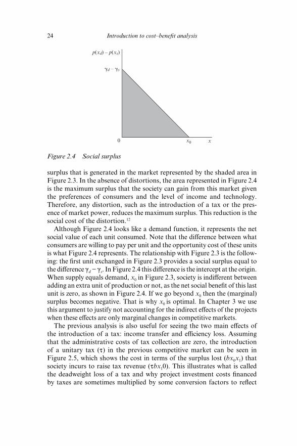
24 Introduction to cost–benefi t analysis
surplus that is generated in the market represented by the shaded area in
Figure 2.3. In the absence of distortions, the area represented in Figure 2.4
is the maximum surplus that the society can gain from this market given
the preferences of consumers and the level of income and technology.
Therefore, any distortion, such as the introduction of a tax or the pres-
ence of market power, reduces the maximum surplus. This reduction is the
social cost of the distortion.12
Although Figure 2.4 looks like a demand function, it represents the net
social value of each unit consumed. Note that the diff erence between what
consumers are willing to pay per unit and the opportunity cost of these units
is what Figure 2.4 represents. The relationship with Figure 2.3 is the follow-
ing: the fi rst unit exchanged in Figure 2.3 provides a social surplus equal to
the diff erence gd − gs. In Figure 2.4 this diff erence is the intercept at the origin.
When supply equals demand, x0 in Figure 2.3, society is indiff erent between
adding an extra unit of production or not, as the net social benefi t of this last
unit is zero, as shown in Figure 2.4. If we go beyond x0 then the (marginal)
surplus becomes negative. That is why x0 is optimal. In Chapter 3 we use
this argument to justify not accounting for the indirect eff ects of the projects
when these eff ects are only marginal changes in competitive markets.
The previous analysis is also useful for seeing the two main eff ects of
the introduction of a tax: income transfer and effi ciency loss. Assuming
that the administrative costs of tax collection are zero, the introduction
of a unitary tax (t) in the previous competitive market can be seen in
Figure 2.5, which shows the cost in terms of the surplus lost (bx0x1) that
society incurs to raise tax revenue (tbx10). This illustrates what is called
the deadweight loss of a tax and why project investment costs fi nanced
by taxes are sometimes multiplied by some conversion factors to refl ect
p(xd) – p(xs)
�d – �s
x00 x
Figure 2.4 Social surplus

The economic evaluation of social benefi ts 25
their opportunity costs. In Figure 2.5 investment costs represented by an
income transfer equal to tbx10 have an additional social cost of bx0x1.
We now assume that the tax is zero and analyse the social cost of nega-
tive externalities with the help of Figure 2.6. The consumption and produc-
tion of goods do not only generate benefi ts and costs for the individuals
who consume or produce them. The supply of a good can produce positive
or negative externalities on other individuals and fi rms (e.g. the producer
that pollutes a river reduces the welfare of fi shermen and walkers).
In this case, the sum of the changes in consumer surplus and producer
�d – �s
�b
0 x1 x0 x
p(xd) – p(xs)
Figure 2.5 The social cost of a tax
p(xd) – p(xs)
�d – �s
�d – �s – �
0
b
d
e
x0x1 x
Figure 2.6 Loss of social surplus because of an externality

26 Introduction to cost–benefi t analysis
surplus overstates the social surplus. We have to add the change in the
surplus of the ‘rest of society’ represented by ΔES in the expression (2.2)
to take into account the loss of welfare for individuals aff ected by the
negative externalities associated with the production of the good.
To represent the impact of a negative external eff ect that we assume to
be constant per unity and equal to f on the social surplus in Figure 2.6,
we only need to add the externality to the private unit cost. Given that the
equilibrium quantity does not change (fi rms do not internalize the exter-
nality), the eff ect on the surplus can be represented by shifting the curve of
the surplus in the amount of the externality.
The externality f has the eff ect of reducing the social surplus in the
area dx0be. Note that by subtracting the loss to the initial area dx00, the
resulting surplus is equal to the diff erence in areas (ex10) − (x1x0b). From
x1 to x0, the production of the good or service in this market has a negative
impact on welfare because what consumers are willing to pay is below the
social opportunity cost. Then, why is it produced? Because producers do
not internalize the cost of the external eff ect, making their market deci-
sions with a cost function that does not refl ect the social opportunity cost
(this is what is called a market failure).
2.4 ALTERNATIVE APPROACHES FOR THE MEASUREMENT OF SOCIAL BENEFITS
Real and Monetary Values
Cost–benefi t analysis aims to compare the fl ow of benefi ts and costs over
the lifetime of a project. The relevant concepts are the social benefi ts
derived from the increase in individual utility and the opportunity cost of
the resources. The unit of measure used to express these benefi ts and costs
is irrelevant.
Data can be presented in current or constant terms.13 The result of the
evaluation will not change because the variables are expressed in real or
monetary terms. In general the fl ow of benefi ts and costs is usually expressed
in constant units of the base year; that is, in real terms, ignoring infl ation.
We are not concerned with the evolution of nominal values, but with the
use of resources and the fl ow of benefi ts associated with the project.
However, the analyst might work with data expressed in current units.
Sometimes the variables are expressed in these units (refl ecting real
changes and infl ation). This is the case in infrastructure projects where
users pay for the use and the private sector is involved as a manager or
concessionaire.

The economic evaluation of social benefi ts 27
Whatever the reason for the fl ows being expressed in real or nominal
terms, the only recommendation is to be consistent. If the data are
expressed in current units of each year, we have to use a nominal interest
rate. If the data are expressed in monetary units of the base year, the real
discount rate is the right one.
It may happen that the prices of some items evolve over or below the
general infl ation. In this case we must account for the diff erence. For
example, suppose that the expected annual infl ation over the 20 years of
project life is 2 per cent, and the expected changes in the price of a raw
material used in signifi cant quantities for the project amount to 5 per cent,
refl ecting infl ation and opportunity cost. By expressing the variables in
monetary units of the base year, we only correct the element of general
infl ation (2 per cent), hence allowing the price of the raw material to grow
at a 3 per cent rate to refl ect the change in the real value of the resources.
Although this approach is the right one, for projects lasting more than 20
years, fi guring out the evolution of prices for each element of costs and
benefi ts is not always possible.
The relationship between the real and nominal NPV is:
aT
t50
Bt 2 Ct
(1 1 i) t5 a
T
t50
(Bt 2 Ct) (1 1 y) t
(1 1 in) t
, (2.7)
where:
Bt,Ct: benefi ts and costs in real terms
y: infl ation rate
i: real discount rate
in: nominal discount rate.
From (2.7):
1
1 1 i5
1 1 y
1 1 in
. (2.8)
Solving for i we obtain the formula to calculate the real discount rate:
i 5in 2 y
1 1 y. (2.9)
Expression (2.9) is often approximated as in 2 y. For a nominal rate of
6 per cent and infl ation of 3 per cent, the real rate is 2.9 per cent accord-
ing to (2.9) instead of 3 per cent, which is obtained directly by subtracting
infl ation from the nominal rate. We assume for simplicity that i and y are
constant over time.

28 Introduction to cost–benefi t analysis
Sum of Surpluses or Change in Willingness to Pay and Resources
Let us assume we have decided to measure the fl ow of benefi ts and costs in
constant terms and at market prices. There is still another choice between
two alternative approaches. The fi rst is the sum of changes in the surpluses
of the diff erent social agents. The second is to calculate the changes in will-
ingness to pay and in the resources, ignoring the transfers of income. Both
methods, properly used, lead to the same result. One of the most common
errors in cost–benefi t analysis is the double counting of benefi ts, and one
of the best remedies to prevent it is to be systematic once one of the two
methods described above has been chosen.
The following example illustrates the application of both approaches.
It is worth emphasizing the importance of not mixing the two. Consider
the case of a competitive market, as depicted in Figure 2.7, in a country
with full employment. The demand curve shows the annual quantities
demanded at each price and the supply curve represents the annual quan-
tities off ered at each price. There are no other eff ects on the economy
beyond those refl ected in the market represented in the fi gure. Without the
project, the exchanged quantity is equal to x0, where the superscript zero
denotes ‘without project’ and the price is equal to p0. Note that with this
price the quantity off ered is equal to the quantity demanded, the market
is in equilibrium, and the consumer surplus (area gdbp0) and the producer
surplus (area p0bgs) generate the maximum social surplus.
What kind of project could improve the society in the described circum-
stances? In Figure 2.7, without the project p0 5 c0. Suppose that if the gov-
ernment spends public money (I) on a new technology, the marginal cost of
production is reduced from c0 to c1 regardless of the quantity produced. If
SN
SI
p0 = c0
p1 = c1
�d
�s
b
x1N
x1W
D
p
x0
d
x0
fe
Figure 2.7 The eff ects of a project

The economic evaluation of social benefi ts 29
the government invests I at zero cost to fi rms, it is then possible to produce
in two ways, either with the costs represented by the original supply curve
(SN) or with the new supply curve (SI). Assume that the two technologies
are compatible. It can be seen that it is cheaper to produce with the new
technology only from x1N.
To determine whether the project’s benefi ts outweigh its costs, we must
compare the government investment (I) at the beginning of year 1 with the
social benefi ts over the lifetime of the project (T), assuming that B and C
are situated at the end of the year. If the condition (2.10) holds, the project
is socially profi table:
aT
t51
Bt 2 Ct
(1 1 i) t. I . (2.10)
The introduction of the new technology reduces the market price to p1,
as Figure 2.7 shows, which is the new marginal cost of production, and the
annual quantity increases to x1W as all the consumers who are willing to
pay the opportunity cost c1 fi nd someone who sells. It is interesting to note
that the new quantity exchanged (x1W) is not all from the new technology,
as it is still more effi cient to produce the quantity (x1N) with the previous
technology.
Consider the change in the surpluses of diff erent agents. Consumer
surplus changes from the situation without the project (area gdbp0) to the
situation with the project (area gddp1), so the increase in consumer surplus
is equal to the area p0bdp1. Producer surplus without the project equals
area p0bgs, and with the project p1fgs, so there is a reduction equal to p0bfp1.
Adding the change in the surplus of producers and consumers, we have a
net gain equal to the area bdf.
The change in consumer surplus can be expressed as:
(p0 2 p1)x0 11
2(p0 2 p1) (x1
W 2 x0) . (2.11)
Equation (2.11) shows the two components of the consumer surplus.
The fi rst term represents the surplus thanks to the reduction of the price
aff ecting the initial quantity (x0). The second term (the additional quan-
tity demanded when the price decreases) is multiplied by 1/2 because the
surplus of the fi rst unit is the initial price and the surplus of the last unit is
zero (the willingness to pay equals the price).
Operating in (2.11) we obtain what is known in practical cost–benefi t
analysis as the ‘rule of a half’:14
1
2(p0 2 p1) (x0 1 x1
W) . (2.12)

30 Introduction to cost–benefi t analysis
The change in the producer surplus is:
p1x1W 2 p0x0 2 C
1 1 C 0, (2.13)
where C 0 is the cost without the project and C1 the cost with the project.
Adding expressions (2.12) and (2.13) we obtain the change in social
surplus:
1
2(p0 2 p1) (x1
W 2 x1N) . (2.14)
Let us examine in more detail the origin of this benefi t. Recall that
the price fall has increased the surplus of consumers in the area p0bdp1.
However part (p0bfp1) of that gain is a transfer from producers to con-
sumers that leaves the social surplus unaff ected. This does not happen
with the benefi t represented by area bdf, which does not exist without the
project. This benefi t has two sources. The fi rst is by increasing the quantity
produced (x1W 2 x0), which does not increase the surplus of the producers
because it is priced at a marginal cost, but it increases the surplus of the
consumers (bde), who are willing to pay bdx1Wx0 but only pay edx1
Wx0.
The second source of project benefi ts is the cost savings of producing
the quantity x0 2 x1N that was previously produced at cost fbx0x1
N and now
is produced at cost fex0x1N. The cost savings go entirely to the consumers
since we are in a competitive market. To the change in the consumer and
producer surpluses, during the lifespan of the project, we have to add the
change in taxpayer surplus (2I ).
Alternatively, the second approach is concentrated on the changes in
the willingness to pay and resources, ignoring transfers. The increase in
willingness to pay (area bdx1Wx0) comes from the additional units sold in
the market, and the change in resources equals the incremental cost of the
new production (area edx1Wx0) and the savings of producing x0 2 x1
N with
the new technology (area fbe). The annual gross benefi t is represented by
area bdf. Once we have summed the discounted annual benefi ts during the
lifetime of the project, we must subtract the investment costs (I).
Assuming that the annual net social benefi t (denoted B ) is constant over
time and equal to area bdf in Figure 2.7 and that T goes to infi nity then
the NPV is:15
NPV 5 aT
t51
Bt 2 Ct
(1 1 i) t2 I 5
B
i2 I , (2.15)
when B/i . I , the NPV is positive and the project is socially desirable.
The case represented in Figure 2.7 can equally be applied to a public

The economic evaluation of social benefi ts 31
policy. Suppose, for example, that the market in Figure 2.7 corresponds
to an economy without international trade, initially in equilibrium with
price p0 and production (completely national) equal to x0. The evaluated
public policy consists of opening the economy and allowing imports at a
lower price (p1). Since imports are allowed, demand increases for the same
reason as in the case of the investment project in new technology discussed
previously. The only diff erence between the two cases is that the NPV is
greater now than in the case of the introduction of a new technology. The
net social benefi t of opening the economy to external trade is equal to B/i. In fact, openness to international trade is like the introduction of a new
technology with zero investment costs.16 We can produce more cheaply
and allocate resources (initially used to produce x0 2 x1N) to more pro-
ductive activities. From x1N it is cheaper to import than to produce in the
country. If the opportunity cost of the resources is represented by SN, this
policy is like the introduction of a new costless technology that allows an
increase in welfare.
The Treatment of Taxes
We can apply the two alternative approaches described above in the pres-
ence of taxes. With the sum of surpluses, taxpayers’ surplus should now be
included. Through the change in willingness to pay and in real resources,
we must ignore transfers and include the willingness to pay that corre-
sponds to the additional units sold independently of the fact that this ‘new’
willingness to pay is partly transferred to taxpayers through the tax.17
Let us see how the presence of taxes aff ects the ‘rule of a half’ by intro-
ducing a unit tax on production. The market price (p0) is equal to the unit
cost (c0) plus the tax (t). The change with the project consists of a reduc-
tion in price, resulting from a reduction in the unit cost of production
(c1 < c0), and the subsequent change in the quantity demanded (x1 > x0).
Without the project, p0 5 c0 1 t. With the project, the price ( p1 5 c1 1 t)
is below the initial price (p0) with a diff erence equal to the unit cost (c0 2 c1).
The change in social surplus is equal to the change in consumer surplus, the
change in producer surplus (equal to zero in this case) and the change in
the surplus of the taxpayers.
If the calculation of the benefi t is realized through the change in will-
ingness to pay and the use of resources, we have a reduction in the cost
of producing the initial quantity without the project and an increase in
the willingness to pay minus the cost of the resources used in the new
production.
Applying the rule of a half, the change in consumer surplus (CS) can be
expressed as:

32 Introduction to cost–benefi t analysis
DCS 51
2(p0 2 p1) (x0 1 x1) . (2.16)
As the price is equal to the unit cost plus the tax, and the tax does not
change:
DCS 51
2(c0 2 c1) (x0 1 x1) . (2.17)
The change in producer surplus (PS) is equal to the change in profi ts
(equal to zero in this case):
DPS 5 (p1 2 c1 2 t)x1 2 (p0 2 c0 2 t)x0. (2.18)
The change in taxpayers’ surplus (GS) is limited to the increase in tax
revenue as a result of increasing the quantity sold (the unit tax remains
unchanged):
DGS 5 t(x1 2 x0) . (2.19)
The change in social surplus is equal to:
DSS 51
2(c0 2 c1) (x0 1 x1) 1 t(x1 2 x0) . (2.20)
The previous argument holds provided that the additional demand
comes from income increases and not from the diversion of demand from
other existing activities. If the increase in the quantity demanded (x1 − x0)
has been diverted from other activities, it must be borne in mind that in
these activities tax revenues will be reduced, so the surplus of the taxpayers
is unaff ected, unless the tax rate is diff erent, in which case only the diff er-
ence matters. This shows that applying general rules such as ‘taxes should
be ignored because they are income transfers’ can sometimes be mislead-
ing. When the new quantity is not diverted from other activities or, if it
is, these activities are taxed at a diff erent rate, the indirect tax (wholly or
partially) is a benefi t in the same sense as profi ts or consumer surplus.
2.5 WINNERS AND LOSERS
Virtually all investment projects and public policies unevenly aff ect the dif-
ferent groups of individuals that compose the society. It is quite unlikely
for a project to distribute its costs and benefi ts uniformly. There are many
projects whose costs are borne entirely by taxpayers, while the benefi ts
are concentrated in a particular group; for example the construction of a

The economic evaluation of social benefi ts 33
park in a residential area benefi ts the land owners in this area, and visitors
and those passing by. In other cases, such as the construction of a power
plant for a region, larger groups benefi t, but their negative external eff ects,
through for example, emissions are primarily borne by the population
living close to the plant.
Sometimes the benefi ts go beyond the limits of the target group, and the
generated externality distributes its eff ects across a wider population. This
is the case with an immunization campaign improving the general health
of all people, including the unvaccinated, because of the reduction in the
probability of infection.
A challenging task is to fi nd out the fi nal benefi ciaries of the project. A
water policy that reduces the cost of irrigation can benefi t producers who
now have a lower cost of production, or consumers of agricultural prod-
ucts if the market is competitive. However, if land is scarce, it is likely that
the owners of the fi xed factor are the benefi ciaries because of changes in
the price of the land.
Why should we worry about the distributional issues in cost–benefi t
analysis? The rationale is that if society attaches more value to the utility of
A than that of B, and the project distributes its net benefi ts so that A wins
100 and B loses 100 with the same increase in individuals’ utility, the gov-
ernment considers that this project is not a zero sum game. Furthermore,
even assuming that a unit of utility to A is socially equal to B, one unit of
income does not produce the same increase in utility unless the marginal
utility of income is the same for A and B.
Conversion of Income Changes into Welfare
When conducting a cost–benefi t analysis instead of a fi nancial analysis,
the practitioner is looking for the net benefi t for the whole society, result-
ing from the aggregation of the changes in utility of winners and losers.
The result would be a good measure of the change in social welfare arising
from the implementation of the project, if it were possible to measure and
compare these changes in utility.
According to the analysis performed in Chapter 11, the change in social
welfare (ΔW) from a variation in the quantities of the n goods consumed
by the m individuals who form the society can be somewhat expressed as:
DW 5 an
j51a
m
i51
DW
DUi
DUi
Dxij
Dxij. (2.21)
Reading from right to left in equation (2.21), we can see the process
through which an increase in the amount of good j consumed by individual

34 Introduction to cost–benefi t analysis
i ultimately aff ects social welfare. First, the project increases the amount of
good j for the individual i, by the amount Dxij. Its consumption increases
the utility (U) of that individual to a greater or lesser extent depending on
the value of DUi/Dxij, which is the marginal utility of the good for the indi-
vidual and whose value depends on the preferences of the individual with
respect to the good delivered by the project and the amount of the endow-
ment that the individual has in the present. By multiplying the amount of
good j by the marginal utility of that good (Dxij(DUi/Dxij
)) , it can be seen
that we convert the physical units of the project into units of utility. Then
we multiply by the social marginal utility (DW/DUi) ; that is, the social
value of a unit of individual utility, leading to the change in social welfare.
To make operational the measurement of social benefi ts in (2.21) and
taking into account that individual utility is not observable, we replace
DUi/Dxij with (DUi/DM)pj, since we know18 that for the individual i, to
maximize his utility, DUi/Dxij 5 (DUi/DM)pj , where DUi/DMi is the indi-
vidual marginal utility of income, and (2.21) is then equivalent to:
DW 5 an
j51a
m
i51
DW
DUi
DUi
DMi
pj Dxij. (2.22)
Condition (2.22) shows how the change in goods consumed by the indi-
viduals as a result of the project originates a change in welfare. Reading
from right to left, a small increase in goods is converted into monetary
units multiplying for the willingness to pay (the price for small changes).19
It is not enough to estimate the changes in the quantities of goods con-
sumed by individuals, we also need to know the variation in the utility
when income changes (DUi/DMi) and how much the society values the
improvement experienced by the individual (DW/DUi) .
Taking into account that (DW/DUi) (DUi/DM) is the social marginal
utility of income for the individual i (which we call bi), the expression
(2.23) is a weighted sum of the benefi ts (positive or negative) that individu-
als receive:
DW 5 an
j51a
m
i51
bipjDxij. (2.23)
The introduction of weights, to account for income diff erences, alters
the net social benefi t of the project (provided that the weights are diff er-
ent from one). By making the weights depend on the level of income or
other criteria, we could obtain diff erent values of b, so that the greater the
bi, the greater the weight that society attaches to the benefi ts and costs of
individual i.

The economic evaluation of social benefi ts 35
The problem with this approach is that we do not know the values of bi
and the result of the economic evaluation of projects will depend on the
values we choose. The introduction of weights changes the result of the
project since the benefi ts and costs of the individuals involved will change
depending on the value of a parameter that is quite diffi cult to estimate. The
question is: what does the decision maker gain when altering the effi ciency
result by introducing the weights according to the expression (2.23)?
A Practical Approach
It is probable that an unweighted NPV jointly presented with a break-
down of benefi ts and costs by income levels, geographical areas and some
other characteristic of interest can be more helpful to the decision maker
than a single fi gure obtained by applying social weights.
Moreover, a socially unworthy project, in terms of effi ciency, could be
approved if the weights for certain individuals are suffi ciently high, which
makes no sense before comparing it with a direct transfer of income. If
redistribution is the objective, it pays to select the most effi cient method
of distribution.
The use of the potential compensation criterion, implicit in the NPV
calculation, implies that the value of the social marginal utility of income
is equal to one and therefore we simply need to compare benefi ts with
costs in order to determine whether the project is socially desirable or not.
Although omitting the distributional eff ects of the project simplifi es the
evaluation, we run the risk of obtaining misleading results.
However the redistributive eff ects are not always important enough for
their inclusion in the analysis. Moreover many projects include imperfect
compensation schemes (i.e. compensation in a legal expropriation) that,
although imperfect, ameliorate the undesirable redistribution eff ects of the
projects.
Many public policies (health, primary education) and investment projects
(electricity, telecommunications) will probably benefi t the majority of the
population when the fi nal eff ects are considered. A public investment that
lowers the cost of telephone services in a competitive market ultimately
benefi ts the fi nal users, which can be practically the whole population in
a developed economy. In assessing a policy of this nature, redistributive
eff ects might be negligible.
Redistributive eff ects can be signifi cant, but the cost of identifying the
winners and losers and how much they win and lose can be high enough to
consider a priori that the gains arising from the information on the distri-
butional eff ects do not outweigh the costs of obtaining such information.
This is especially true when those aff ected are many and heterogeneous.

36 Introduction to cost–benefi t analysis
In the practice of cost–benefi t analysis, equity weights are rarely
included, it being much more common that the public agency that evalu-
ates or commissions the evaluation is interested in disaggregating the
eff ects of the project in terms of the groups and geographic areas aff ected,
and also in having an estimate of the jobs that will be created as a result of
the project. However remember the risk of double counting if labour has
already been priced at its opportunity cost in the calculation of the project
benefi ts (see Chapter 4).
THINGS TO REMEMBER
It is worth having a simplifi ed model of the society and a clear ●
idea of the main impacts of the project before measurement. Time
devoted to thinking about the characteristics of the problem and
to assessing whether its appraisal can be reasonably dealt with in
that simplifi ed framework is a prerequisite to the identifi cation and
measurement of benefi ts.
Revenues are not synonymous with social benefi t. Under some con- ●
ditions the willingness to pay for the project is the social benefi t, and
revenues are part of this benefi t. The rest is called consumer surplus
and is a benefi t of the same nature as the revenue. Free access
facilities do not generate revenue but social benefi ts are there, in the
hands of social agents.
Two main approaches are available for measurement: the sum of ●
changes in the surpluses of economic agents and the sum of changes
in willingness to pay and in real resources, ignoring transfers. Both
of them lead to the same result, but they should always be kept
apart. Be careful with taxes. Taxes can commonly, but not always,
be treated as income transfers.
Cost–benefi t analysis deals with real values. The change in real ●
things is what really matters: saving lives, improving the quality of
water, reducing the resources required to produce the same amount
of food, etc. The unit to measure real values is not important, so the
only warning is to be consistent. The net present value of the project
is not going to change whether infl ation is included or not.
Identify winners and losers when feasible. The net present value of ●
the project accompanied by a list of who benefi ts and who is harmed
can be helpful for the decision maker. At least do not forget that the
aggregate NPV is an effi ciency measure that gives the same value to
a unit of benefi t and a unit of cost, regardless of who the aff ected
party is.
The economic evaluation of social benefi ts 37
NOTES
1. We use the term ‘project’ for both projects and policies. 2. For a more formal treatment see Chapter 11. 3. One defi nition of a small project is that it is virtually infi nitesimally small. Then one
can draw on envelope theorems implying that secondary eff ects ‘net out’. For example, if we change an output price (ceteris paribus) we obtain the supply function (from the profi t function) minus the demand function, both multiplied by the marginal utility of income if we have a single- individual (or Robinson Crusoe) economy. Other supplies and demand are aff ected by the price change but these eff ects net out. This is so at least in the absence of tax wedges. Alternatively, one might consider a perturbation as a linear approximation. The project is so small that higher order eff ects can be ignored. This produces the same general equilibrium cost–benefi t rule.
4. Sometimes individuals might be altruists in the sense that they care about damage caused by their activities on human beings or other species, or on the environment in other countries. For example, suppose country A replaces hydropower electricity with country B’s electricity produced by coal- fi red plants. A’s citizens might – but need not necessarily – include the negative environmental impact in their utility functions (see Chapters 5 and 6).
5. Despite the simplifi cation, with the society composed of consumers and producers, an individual can be both a consumer and a shareholder. We assume that the individual is able to distinguish, when asked about his willingness to pay for a project that aff ects the price of a product (and company profi ts), the eff ect on his surplus as consumer and as producer, so by adding the change in the consumer surplus and the producer surplus we do not incur double counting. For the eff ect of this bias on stated preferences see Johansson (1993).
6. Using a cost function where the marginal cost is not constant does not change the analysis, as long as the payment of factors at the marginal cost still holds.
7. When the wage is higher than the social opportunity cost of labour, the increase in employment is an additional benefi t (see Chapter 4).
8. The total value of environmental goods includes the value of that use, and also the non- use or passive use value. Passive use value refl ects what individuals are willing to pay for the good being available now or in the future, or simply for the mere fact of its existence. The economic interpretation of these concepts and their measurement are discussed in Chapters 5 and 6.
9. We assume that the market demand for water coincides with the compensated demand (see Chapter 11).
10. Assuming the income eff ect is very small.11. If the industry is in long term equilibrium, profi ts tend to zero. The surplus of the pro-
ducer that appears on the fi gure could be the compensation of some factor that remains fi xed in the long term, for example, land. Producers have zero profi ts, since fi rms would bid for the fi xed factor. The price of land would rise to absorb the producer surplus. Therefore, to obtain the social surplus, we would have to add the surplus of the owners of the fi xed factors. Both procedures lead to the same result if one does not count the surplus twice (which is called double counting, a common error in cost–benefi t analysis).
12. Plus the additional costs of the chosen mechanism. For example, in the case of the tax, the time lost in making the statements, the payment to staff dedicated to tax collection, fraud prosecution, and so on.
13. Costs and benefi ts can be expressed at market prices or factor costs (subtracting indirect taxes and adding subsidies). It seems preferable to express them at market prices and then make the necessary corrections, for example, when the market prices do not refl ect the opportunity cost of resources (see Chapter 4).
14. The rule of a half assumes that all other prices remain unchanged, otherwise the demand curve (as well as the supply curve) might shift. Moreover it assumes a linear demand curve.

38 Introduction to cost–benefi t analysis
15. For a benefi t B constant to perpetuity, the discounted present value is equal to B/i (see Chapter 7).
16. This oversimplifi es the benefi ts of open trade as far as international trade has its own transaction costs.
17. This is only true when the new quantity is not paid with money deviated from other markets with an identical tax rate.
18. We assume that the solution is interior (see Chapter 11).19. When the change aff ects prices pj
Dxij is calculated with ‘the rule of a half’.

39
3. The economic evaluation of indirect eff ects
. . . any project is likely to have some perceptible eff ect on the demand and supply of goods produced by other industries, the main eff ects of this type being in the industries which supply the materials used by the project, and the industries which supply goods which are either complementary to or competitive with the project’s output. If, as a consequence of a project, changes occur in the output of an industry for which, at the margin, social benefi ts equal social costs, no adjustment need be made.
(Arnold C. Harberger, 1965, p. 47)
3.1 INTRODUCTION
Calculating the social NPV of a project through changes in the primary
market is inadequate according to many who argue that investment
projects and public policies have signifi cant impacts on the economy
beyond the visible eff ects in the primary market. A project may imply the
reduction of production costs or an increase in the quality of the environ-
ment. Besides these direct eff ects, it is argued that the project may boost
the economic activity in other markets and bring an increase in labour pro-
ductivity and changes in fi rm location, among other eff ects of a broader
scope than the direct eff ects described in the previous chapter. These other
eff ects are called indirect eff ects and wider economic benefi ts.
Does cost–benefi t analysis include all the relevant economic benefi ts
of investment projects or does it ignore some important indirect eff ects
on the economy? Indirect eff ects are those induced by the project beyond
the primary market. When building a wind farm that reduces the price of
energy, the direct eff ect occurs in the electricity market, but it also aff ects
the fi rms that build the windmills or supply inputs for the wind farm.
There are other indirect eff ects, since the product of the primary market,
the supply of electricity, is related to other markets whose products are
complements to or substitutes for the electricity produced by windmills:
the electricity produced by a fuel burning plant is a substitute for the
electricity from the windmills, and appliances are a complement (e.g. the
demand for electric stoves increases if the price of electricity falls).

40 Introduction to cost–benefi t analysis
There is another relationship of the primary market with other markets
that tends to be confused with the earlier one but whose nature is completely
diff erent, as we can see in section 3.3. The relationship is established when
the product of the primary market aff ected by the project, such as electricity
or transport, is an input for the production of other goods that use these as
inputs. With respect to the goods for which the electricity is an input, the list
is endless (including the entire production process of this book).
We therefore have a broad set of candidate markets for measuring the
eff ects of the project beyond the primary market. In general, and this
signifi cantly simplifi es the job of the analyst, the indirect eff ects can be
ignored provided that, in the markets where they occur, the marginal
social benefi t equals the marginal social cost.
Therefore, in competitive markets in which there are no distortions
such as externalities or taxes, the indirect eff ects are equal to zero. In the
case of distortions we must include the indirect eff ects, but it should be
noted that these indirect eff ects do not necessarily increase social benefi ts.
Many projects are small enough to keep income constant, so if demand in
a secondary market increases it must be decreased in some other markets.
So it is basically an almost philosophical question of the magnitude of the
discrepancy between price and marginal cost in the diff erent markets. In
any case it is very diffi cult to trace these eff ects unless the analyst has a
computable general equilibrium model.
We deal with the analysis of the indirect eff ects in two parts. The fi rst,
which is covered in section 3.2, includes the eff ects that could be called
genuinely indirect. The second, when the product of the primary market is
an input for other markets, is analysed in section 3.3. In general, we assume
that it is possible to identify some markets where the main indirect eff ects
concentrate and then proceed as if the rest of indirect eff ects net out.
In general, the challenge in identifying the benefi ts in cost–benefi t analy-
sis is to separate the genuine indirect eff ects from those that are double
counting. With this purpose, it is useful to distinguish, within the eco-
nomic eff ects that are not direct, between the indirect eff ects and the wider
economic benefi ts, covered in section 3.4, and to emphasize that both can
increase or decrease the social benefi t of the project. Finally, in section
3.5, we address the so- called territorial eff ects and regional development
induced by infrastructure investment projects.
3.2 INDIRECT EFFECTS
Investment in a natural area used for recreation increases the demand for
hotels and restaurants in a village near the place aff ected by the project.
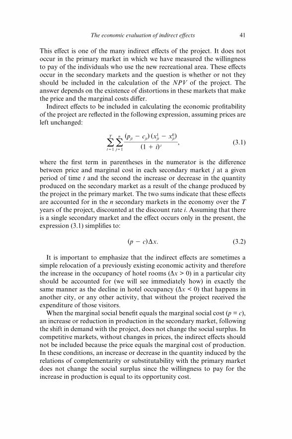
The economic evaluation of indirect eff ects 41
This eff ect is one of the many indirect eff ects of the project. It does not
occur in the primary market in which we have measured the willingness
to pay of the individuals who use the new recreational area. These eff ects
occur in the secondary markets and the question is whether or not they
should be included in the calculation of the NPV of the project. The
answer depends on the existence of distortions in these markets that make
the price and the marginal costs diff er.
Indirect eff ects to be included in calculating the economic profi tability
of the project are refl ected in the following expression, assuming prices are
left unchanged:
aT
t51a
n
j51
(pjt 2 cjt) (x1
jt 2 x0jt)
(1 1 i) t, (3.1)
where the fi rst term in parentheses in the numerator is the diff erence
between price and marginal cost in each secondary market j at a given
period of time t and the second the increase or decrease in the quantity
produced on the secondary market as a result of the change produced by
the project in the primary market. The two sums indicate that these eff ects
are accounted for in the n secondary markets in the economy over the T
years of the project, discounted at the discount rate i. Assuming that there
is a single secondary market and the eff ect occurs only in the present, the
expression (3.1) simplifi es to:
(p 2 c)Dx. (3.2)
It is important to emphasize that the indirect eff ects are sometimes a
simple relocation of a previously existing economic activity and therefore
the increase in the occupancy of hotel rooms (Δx > 0) in a particular city
should be accounted for (we will see immediately how) in exactly the
same manner as the decline in hotel occupancy (Δx < 0) that happens in
another city, or any other activity, that without the project received the
expenditure of those visitors.
When the marginal social benefi t equals the marginal social cost (p = c),
an increase or reduction in production in the secondary market, following
the shift in demand with the project, does not change the social surplus. In
competitive markets, without changes in prices, the indirect eff ects should
not be included because the price equals the marginal cost of production.
In these conditions, an increase or decrease in the quantity induced by the
relations of complementarity or substitutability with the primary market
does not change the social surplus since the willingness to pay for the
increase in production is equal to its opportunity cost.

42 Introduction to cost–benefi t analysis
When there are distortions in the secondary markets (p ≠ c) and the
products of these markets are complements to or substitutes for the
product of the primary market, the indirect eff ect may increase or decrease
the benefi ts of the project. The ultimate sign of these eff ects on the NPV
of the project will depend on whether the price in the secondary market is
higher or lower than the marginal social cost and the combination of one
of these cases with the fact that goods are complements or substitutes.
The fi gures in this section are built, for simplicity, under the assump-
tions of demand shifts to the right in the secondary market (Δx > 0 in
(3.2)). Depending on what happens in the primary market (rising or falling
prices, changes in quality, etc.) and the relations of complementarity or
substitutability with the secondary markets, demand shifts may be to the
right or to the left. Assuming that price is equal to marginal cost in the
primary market, we have several cases depending on whether the second-
ary market price is equal to marginal cost.1
Indirect Eff ects in Competitive Markets
Suppose that the price of electricity falls, increasing the demand for elec-
tricity (primary market) and shifting the demand for electric stoves (sec-
ondary market). This indirect eff ect of reducing the price of electricity is
represented in Figure 3.1.
The reduction in the price of electricity increases the demand for elec-
tric stoves in this secondary market, and demand changes from D0 to D1
in Figure 3.1, without changes in utility since, in the primary market, the
willingness to pay for the electricity incorporates the utility of its use, and
the price of electric stoves is unchanged because the supply is perfectly
p
p0 S
D0
x0 x0 x1
D1
a b
Figure 3.1 Indirect eff ects (without price changes and distortions)

The economic evaluation of indirect eff ects 43
elastic as assumed in Figure 3.1; or in the case of a positive slope supply,
because the shift in demand is marginal in the market for electric stoves,
leaving the price constant.
Let us see what happens with the producer’s surplus. In the market for
electric stoves, the increase in demand induced by the price reduction of
electricity does not change the price of the good in the secondary market
(whose supply is perfectly elastic as Figure 3.1 shows), with incremental
revenue equal to incremental costs (area abx1x0). Therefore the producer’s
surplus remains unchanged in this market.
The case depicted in Figure 3.1 is the case of a complement of the good
directly aff ected by the project. In the case of a substitute the analysis is
similar, changing the direction of the demand shift, now to the left but
with the same result: as the social surplus does not change in the second-
ary market we can also ignore the indirect eff ect as these changes do not
aff ect welfare.
Negative Externalities and Subsidies
When in the secondary market the price is lower than the marginal social
cost, we have either the case of a negative externality or the case of a subsidy
(which does not internalize a positive externality), as shown in Figure 3.2.
Consider the case of a negative externality (atmospheric pollution,
noise, etc.). Initially, we are located at the equilibrium point e of a second-
ary market in which there is a constant negative externality equal to f per
unit. While the increase in demand does not aff ect the price, the social
cost is now higher than the private cost. In the initial equilibrium, the
marginal social cost exceeds the price paid by users in f. With the increase
in demand from D0 to D1, there is no change in the utility of consumers or
p
p0 + �
p0
0 xx0 x1
D0 D1
a b
ed
S + �
S
Figure 3.2 Secondary market with externality or subsidy

44 Introduction to cost–benefi t analysis
producers (revenue edx1x0 equals private cost), but there is an additional
increase in social cost represented by the area abde, which reduces the
surplus of the ‘rest of society’ and therefore must be included.
Interpreting f as a subsidy in Figure 3.2, the analysis is similar to the
previous one. The marginal social cost is p0 + f but the fi rm produces as if
the cost is equal to p0. When the demand shifts to the right in the second-
ary market, there is no change in consumer and producer surpluses; on the
contrary, taxpayers’ surplus is reduced in the area abde.2
This analysis is valid provided there are no other distortions in the
economy (or those other distorted markets are unaff ected by the project
under consideration); that is, if all other aff ected markets are of the type
illustrated in Figure 3.1.
Taxes and Unemployment
In the earlier cases the increase in production in the secondary market
reduced the social benefi ts of the project. In the cases of revenue raising
taxes and involuntary unemployment the price is above the marginal cost
in (3.2) and the indirect eff ects of increased production in the secondary
market have a positive eff ect on the project’s NPV.
Consider the case of a unitary tax included in the market price in the
secondary market as represented in Figure 3.3. The marginal cost is now
p0 − t instead of p0, and therefore the increase in the demand for electric
stoves in the secondary market, induced by the reduction in the price of
electricity in the primary market, produces an increase in the social surplus
equal to the tax revenue abde.
With the demand shift the price does not change, but the social cost is
now lower than the private cost. Initially the social marginal cost is equal
to p0 − t. Given the increase in demand from D0 to D1, with no change in
p
p0
p0 – �
0
D0 D1
a b
e d
S
S – �
x0 x1 x
Figure 3.3 Secondary market with taxes
The economic evaluation of indirect eff ects 45
the utility of consumers or producers (revenue abx1x0 equals private costs),
there is an increase in the surplus of taxpayers equal to the area abde.
Taxes have to be accounted for in this case as an increase in the social
benefi t of the project. In this case, taxes are not a transfer of income to be
ignored in order to avoid double counting (unless in another secondary
market a similar reduction in tax collection occurs).
In the event that there is unemployment and the opportunity cost of
labour is less than the market wage, p0 − t could be interpreted as the
social opportunity cost of producing electric stoves in a situation of unem-
ployment and minimum wage regulation, and p0 as its market price. The
area abde should be counted as a social benefi t (an increase in the surplus
of workers) since, given the increase in demand in the secondary market,
the real cost of the resources used to increase production is equal to edx1x0
(the opportunity cost of production). The area abde would be measuring
the benefi t of job creation (see section 4.7 for a more detailed treatment).
3.3 DIRECT EFFECTS MEASURED WITH A DERIVED DEMAND
A shortcut to the measurement of the benefi ts of a project that reduces
the cost of an input used by many fi rms is to calculate the benefi ts in the
input’s market, instead of calculating fi rm by fi rm the surplus of diff erent
economic agents. When building a new infrastructure that reduces trans-
port costs, the eff ects are enjoyed by fi rms whose profi ts may increase, or
by consumers who travel at a lower generalized price or consume goods
at a lower price.
Transport demand is derived from the needs in the markets for fi nal
goods and services. This is called derived demand and is very useful for
measuring the direct eff ects of the reduction in transport costs on social
surplus. An interesting result in the evaluation of investment projects that
reduce transport costs is that we can focus our attention on the market
in which the reduction in the cost of transport occurs and measure in this
market the benefi ts of the project, without having to worry about changes
in other markets (provided they are competitive) using the transport
service.
By concentrating the eff ort on measuring the demand for transport we
avoid the identifi cation and measurement of changes in the surpluses of
a large number of fi rms and their consumers. This does not mean that
companies in other markets using the services of transport do not benefi t
from the project that reduces the cost of transport, or that consumers do
not benefi t from lower prices; it is simply to avoid counting the same eff ect

46 Introduction to cost–benefi t analysis
twice, because the benefi ts of reducing such a cost have been measured in
the primary market for transport.
Figure 3.4 in its upper part shows the impact of the reduction of transport
costs on the supply of a product and its eff ects on producer and consumer
surpluses. S 0+ and S 0− are the supply curves without the project, gross and
net of transport cost respectively. The situation without the project shows
a competitive market in equilibrium where we assume that producers are
located at the same point in the space but consumers are located at diff erent
distances from producers, which off er the product according to the supply
function S 0+. The supply (S 0+) and the demand determine the equilibrium
without the project at price p0 and the quantity produced x0.
The market price paid by the consumers p0 is not fully received by the
producers since the cost of transport (assume price equals marginal cost
in the transport market) reduces the price that producers receive (p0−). All
Product demand
p0
p0–
p
x1
S0–
S0+
S1+
x0
p1–
p1
0
Derived demand
c0
c1
c
0
x
x
Figure 3.4 Measurement of benefi ts with the derived demand

The economic evaluation of indirect eff ects 47
the units produced are transported to their ultimate consumers and there-
fore at the cost of transport without the project c0 (equal to p0 − p0−) the
quantity produced is equal to that eff ectively transported.
So far this fi gure provides little help. However, when we assume a
reduction in the cost of transport with the project, Figure 3.4 shows how
the derived demand for transport is very useful for measuring welfare
changes. With the project, the cost of transportation is reduced, and in
the upper part of the fi gure the supply function is shifted to the right so
that the new equilibrium is determined by the supply function S1+ and the
demand, being the new price with the project p1 and the quantity produced
x1. In the lower part of the fi gure x0 increases to x1.
The change in social surplus, in the upper part of the fi gure, is composed
of the change in the surplus of consumers and producers. Applying the
rule of a half (see Chapter 2), the change in consumer surplus is equal to:
1
2(p0 2 p1) (x0 1 x1) , (3.3)
and in producer surplus:
1
2(p12 2 p02) (x0 1 x1) . (3.4)
These are the eff ects of the reduction in transport costs (under the
assumption of perfect competition). The diffi culty of measuring such sur-
pluses in the markets for fi nal goods is easy to imagine; but the demand for
transport as represented in the lower part of Figure 3.4 shows a shortcut
to the measurement of the change in social surplus by applying the rule of
a half with the transportation costs and trips realized.
1
2(c0 2 c1) (x0 1 x1) . (3.5)
Expression (3.5) is equal to the sum of (3.3) and (3.4). Measuring the
change in social surplus with the market for the transport input following
(3.5), we can not add as benefi ts the impacts of reducing the cost of trans-
port on the market for goods in those competitive markets using transport
as an input. If we do so, we would double count the benefi ts.
3.4 WIDER ECONOMIC EFFECTS
We have distinguished between indirect eff ects and wider economic ben-
efi ts. Indirect eff ects are those that occur in the secondary markets linked

48 Introduction to cost–benefi t analysis
to the primary market by relations of complementarity or substitutability
and have already been analysed in section 3.2, concluding that they have
to be included whenever there is a distortion in these markets and the cross
elasticities are not zero. The impossibility of concluding a priori whether
the fi nal sign of the indirect eff ects would be positive or negative, depend-
ing on the circumstances of the aff ected markets, was also highlighted.
Market distortions produce other eff ects, the so- called wider economic
benefi ts, which in principle should be included in the calculation of the
social profi tability of the project because they are not double counting and
can be important in certain contexts. With no intention of being exhaus-
tive we discuss some of these eff ects such as the agglomeration economies,
imperfect competition in markets that use transport as an input and the
eff ect of increasing competition as a result of the implementation of the
project.
Agglomeration Economies
Agglomeration economies are in fact a positive externality that fi rms gen-
erate when they locate close to other fi rms. If productivity increases with
the density of fi rms in an area, productivity depends on the location deci-
sion of each fi rm. A company, when deciding where to install the plant,
takes into account its own benefi ts but not the increase in the profi ts of
other fi rms.
The benefi ts of time savings of a transport project are valued by the
fi rms, which now change the location and increase the density of fi rms in
a city or an industrial park (as measured by the derived demand function),
but would be lower than the increases in productivity enjoyed by all the
fi rms. Following the same reasoning, the reduction in the density of fi rms
in the area where the companies were initially located reduces productivity
and therefore it is a negative eff ect that must be accounted for.
There are several reasons explaining why fi rms in areas with a higher
fi rm density are more productive, and why fi rms choose these locations
despite the higher labour and land costs among other drawbacks. These
reasons include access to wider markets, the availability of a more spe-
cialized labour market that matches the needs of fi rms, and the access to
technologies and the production processes of fi rms in the area.
There is empirical evidence of the positive eff ect of a higher eff ective
density on productivity, understanding eff ective density as an indicator
of the degree of agglomeration, such as employment in the area and its
surrounding areas (weighted by the generalized cost of transport), so
that it appears that an increase in eff ective density increases the average
productivity of the area.

The economic evaluation of indirect eff ects 49
A project that reduces transport costs may also induce an increase in the
concentration of jobs in an area where there are economies of agglomera-
tion by reducing the cost of commuting for workers who, with the project,
are now more willing to move to the city or the industrial park. However
the opposite might also occur if the reduction in transport costs encour-
ages the dispersion of economic activity. For an urban project that reduces
the costs of travel within the city it is more likely that the positive eff ect
will dominate, while for an intercity transport project the possibility that
the dispersion will increase cannot be ruled out, depending on a set of local
factors such as land prices, wage diff erences between areas, and so on (see
Duranton and Puga, 2004; Graham, 2007; Venables, 2007).
Productivity gains arising from economies of agglomeration must
include the additional tax revenues that are collected as a result of the
increase in economic activity. Additional gains, for example that workers
value when they take their decision to migrate to the area of highest
density of employment, are net of taxes; nevertheless tax revenues are
also productivity gains (Venables, 2007). This is another example, by the
way, that taxes are sometimes mere transfers and at other times represent
welfare gains.
Imperfect Competition in Markets that Use Transport as an Input
To estimate the welfare gains of a project that reduces the cost of transport,
it is quite practical, as we saw earlier, to use the derived demand in order
to avoid the diffi culty of measuring the eff ects on every market aff ected by
the project. A necessary condition for the fi nal eff ects to be calculated in
the transport market was that product markets were perfectly competitive.
What happens in the presence of market power?
In markets with imperfect competition the price is higher than the
opportunity cost, and fi rms are in equilibrium at a point where consum-
ers are willing to pay above the marginal cost. This is the typical textbook
case of a monopoly. If the producer is unable to discriminate prices, a
price reduction to attract new customers reduces revenues on the initial
units and thus what the monopolist compares with the marginal cost when
deciding to increase or decrease its output is the marginal revenue, not the
price.
The economic consequence of a profi t maximizing monopolist is well
known: a suboptimal equilibrium quantity and the corresponding loss of
effi ciency. How does this fact aff ect the evaluation of a project that reduces
the cost of transport for fi rms with market power? Figure 3.5 shows the
eff ect of a reduction in transport cost on the marginal cost of a profi t
maximizing monopolistic fi rm whose unit cost changes from c0 to c1. It

50 Introduction to cost–benefi t analysis
can be seen that initially the fi rm is in equilibrium at point a, and now the
equilibrium is at point b with a reduction in consumer prices from p0 to
p1. The increase in producer surplus is represented by the area c0fhc1. The
consumer surplus increases in the area p0abp1.
One might think that in the transport market these areas are measured
by the change in total surplus in Figure 3.4 by applying the rule of a half
as refl ected in expression (3.5); however, although this is the case for com-
petitive markets, where the marginal change in output has zero value, this
does not happen in markets with imperfect competition, where the price–
marginal cost margin is positive.
To see this intuitively, we can think of a very small change in Figure 3.4,
so the areas in the fi gure reduce to the following expression:
2xDc 1 (p 2 c)Dx. (3.6)
If the product market that uses transport as an input is competitive,
the social value of the last unit exchanged is close to zero as the price is
equal to the marginal cost (as shown in Figure 3.4) and therefore expres-
sion (3.6) is equivalent to (3.5), whereas in the imperfect competition case,
the value of the last unit equals the price minus the marginal cost (greater
than zero as shown in Figure 3.5) and therefore the application of (3.5)
ignores the second term of expression (3.6). Although consumers are not
willing to pay more than the equilibrium price for an additional unit and
neither are producers willing to produce it (because its marginal revenue
equals the marginal cost), there is an additional benefi t by producing that
p0
c0
p1
c1
0
Marginal revenue Product demand
a
b
e
d
h
g
f
x0 x1 x
Figure 3.5 Measurement of social benefi ts and imperfect competition

The economic evaluation of indirect eff ects 51
marginal unit that the transport project makes possible and it is equal to (p 2 c) .
Ignoring transfers, the change in total surplus equals the cost reduc-
tion in the production of x0 (area c0fgc1) plus the willingness to pay (net of
costs) of Δx (area abhg).
Besides the increase in social surplus, measured in the primary market,
we now have an additional benefi t not included in the primary market
and that is a reduction in the deadweight loss, because of the existence of
imperfect competition, equivalent to the increase in production multiplied
by the diff erence between the price and the marginal cost (Venables and
Gasoriek, 1999). It should be noted that the eff ect can be negative if in the
secondary markets with market power fi rms sell less because the reduction
in transport costs aff ects, for example, a product positively that is a substi-
tute for the product in the secondary markets.
Higher Competition
When transport costs are high, projects that reduce them can facilitate the
entry of new fi rms who fi nd it profi table to off er their products compared
with the situation without the project when the incumbent fi rms were
protected by the barriers to entry that in fact represent the transport costs.
This eff ect should not be confused with welfare gains arising from the
expansion of output in imperfectly competitive markets when they reduce
transport costs. We can say that this eff ect, previously discussed, does not
increase competition but that fi rms with market power (e.g. in markets
with product diff erentiation) fi nd it profi table to increase their production
given the reduction in transport costs.
The pure competition eff ect, with the entry of new fi rms, is less likely to
occur in countries with a mature infrastructure network. In these countries
signifi cant increases in effi ciency resulting from the fact that a transport
project reduces travel time are not expected. However it is an eff ect that
could be important in any project that aff ects a part of the country that is
poorly connected and in which some fi rms enjoy market power because of
poor accessibility.
Recent Findings in the Literature on Wider Economic Benefi ts
Recent research on the nature and magnitude of wider economic benefi ts
is still far from producing practical rules for the economic evaluation of
transport projects subject to the usual constraints of time, money and
technical resources.
Some recommendations are as follows (OECD, 2007). The additional

52 Introduction to cost–benefi t analysis
economic eff ects not captured in conventional cost–benefi t analysis exist
and they have their origin in the existence of increasing returns, agglomer-
ation economies, market power or the benefi ts of a broader labour market.
Moreover, fi rms and households take long term decisions in reacting to
the changes in transport costs. However the sign and magnitude of these
eff ects are very diff erent between projects and it is not possible to transfer
them to new projects being evaluated.
A practical suggestion for small projects is to work under the assump-
tion that the wider economic benefi ts do not exist or are unimportant.
Although this approach runs the risk of ignoring them in the case where
they are signifi cant, there is consensus on the fact that this risk is off set by
the elimination of the risk of double counting and delays in project evalua-
tion. For large projects or for the evaluation of investment programmes it
may be justifi ed to undertake more sophisticated analyses.
Aggregate studies that focus on global impacts have problems detect-
ing the direction of causality. Moreover they do not contain information
with a suffi cient level of detail on the particular infrastructure that makes
the results useful in evaluating projects. In addition, there is some confu-
sion about whether these studies measure wider economic eff ects, ignored
in standard cost–benefi t analysis, or whether they only measure the fi nal
impact of the direct eff ects already measured.
More detailed ‘microscopic’ studies seeking to capture the eff ects of
transport cost reductions on the internal reorganization of fi rms and
families are scarce. This is not surprising since this type of longer term
response is diffi cult to integrate into micro- focused modelling that analy-
ses the interaction in the markets; however it is known that companies and
households make reorganization decisions in response to new transport
conditions.
Ex post studies are also scarce. Existing ones have found no robust evi-
dence on the existence of wider economic benefi ts. The latest research sug-
gests that if one wants to go beyond the conventional cost–benefi t analysis
to include any possible additional benefi ts, one should distinguish between
direct benefi ts and impacts on productivity, competition and the labour
market. Furthermore, when there are spatial spillover eff ects, regardless
of including the wider benefi ts, we must expect diff erent results in the
evaluation if the size of the geographic area analysed varies. Moreover,
the economies of agglomeration may also have negative eff ects because
of the increase in traffi c congestion that may even lead to negative wider
economic benefi ts.
In the modelling of agglomeration eff ects, as with the spillover eff ects,
there is concern about using a ‘black box’ of questionable utility in the
evaluation of projects. Advancing in the ‘microscopic’ analysis of the

The economic evaluation of indirect eff ects 53
agglomeration benefi ts would be very useful for a better understanding of
the eff ects on production, product distribution and access to inputs, and
for a better understanding of mechanisms that tend to spread the activity
because of the reduction in transport costs through just- in- time processes
or the advantages of having separate plants to avoid upward pressures on
wages.
The existence of spatial spillovers requires extreme care in estimating
the eff ects of local agglomeration. For example, the study of the London
Crossrail link concluded that the benefi ts of conventional cost–benefi t
analysis had to be increased by 20 per cent to include the eff ects of agglom-
eration, but it could not demonstrate the extent to which these wider
benefi ts were losses in other geographical areas.
From the available empirical evidence and the evaluation of the experts
on whether conventional cost–benefi t analysis is suffi cient to estimate
the social profi tability of a project, the general recommendation is to be
extremely cautious since, although economists are advancing with the
knowledge and measurement of wider eff ects, they are still far from turning
the results into practical rules for their inclusion in cost–benefi t analysis.
The risk of double counting is so high that the best approach is not to
include wider economic benefi ts in small projects and focus the eff orts on
the direct eff ects. With the available evidence, it does not seem reasonable
to transfer the results from other studies, using percentages or similar
procedures, if we take into account the variability in the magnitude of the
wider eff ects, and even the sign when the negative eff ects resulting from
congestion outweigh the agglomeration benefi ts.
3.5 LOCATION EFFECTS AND REGIONAL DEVELOPMENT
Even assuming that there are no wider economic eff ects, and that the
benefi ts of the project have been properly identifi ed and measured, the
location of these benefi ts is usually an important element for the deci-
sion taker, together with the net social benefi t, when considering public
investment decisions.
The location of fi rms and the induced increase in economic activity is
one of the arguments used in the defence of investment projects in public
infrastructure. It is assumed for example that the construction of high-
ways or railway lines, which reduce transport costs from a poor region
to another more developed region, will enable greater economic growth
for the former thanks to the higher attraction of the poor region for the
location of fi rms.

54 Introduction to cost–benefi t analysis
This argument is not supported by empirical evidence. Roads can
be used to export goods from the poor region to the rich region but
also from the rich to the poor. Therefore, in principle, a reduction in
transport costs between the two regions does not guarantee the desired
location eff ects. When one admits the existence of agglomeration econo-
mies, a reduction in transport costs can facilitate a greater concentration
of activity in the rich region, which could now export its products at a
lower cost to the poor region, rather than directly produce in the poor
region.
The emphasis on the location eff ects of fi rms in deprived areas may be
of interest to governments or lobby groups who want the project to be
approved; however, from the point of view of the economy as a whole, it
does not seem reasonable to introduce as benefi ts the more than doubt-
ful location eff ects of fi rms that could even materialize in the opposite
direction than the one originally planned.
The so- called new economic geography has shown that the eff ects of
reducing transport costs in the less developed regions do not only depend
on the characteristics of the project but also on the economic context.3 A
simplifi ed explanation of the diffi culty of establishing a priori the location
eff ect of an infrastructure is as follows.
Let us consider a country with two regions, the rich (R) and the poor
(P), separated by an inadequate transport infrastructure (we will call the
initial quality level – travel time, route conservation, safety, etc. – ‘bad’).
There is only one factor of production, labour, and wages are initially
identical in the two regions.
Economic activity and the location of fi rms between the region R and
the region P are in equilibrium. There are more companies in R and
more unemployment in P. The equilibrium is explained by several factors
including the level of infrastructure. First, producing in R and exporting
to P, using the infrastructure, has the advantage of reaping the economies
of agglomeration (economies of scale and access to specialized inputs, for
example) that give rise to a lower unit cost in R than in P. Locating the
fi rm in P has the advantage of avoiding the transport costs incurred when
producing in R and exporting to P.
The trade- off between the pros and cons of producing in one region has
been resolved with an initial level of activity and location of fi rms that we
take as a starting point and that allows us to call one region ‘rich’ and the
other one ‘poor’.
Suppose we have to evaluate a project that allows the infrastructure to
pass from level ‘bad’ to ‘good’, reducing the transport costs between the
two regions. How will this project aff ect the location of fi rms between the
two regions? It is often argued that investment projects in infrastructure

The economic evaluation of indirect eff ects 55
improve the situation of the poor region by allowing its development. The
empirical evidence is not so optimistic, with several possible outcomes.
In the simplifi ed world described here, the availability of a better
infrastructure changes the initial equilibrium. The only change that has
occurred is a reduction in the transport cost, hence it is more profi table to
produce in R, take advantage of economies of agglomeration and export
to P using the improved infrastructure. The result is the relocation of
fi rms in R. The new economic activity raises wages in R and attracts the
labour force from P to R, which allows the containment of wages and the
reinforcement of the relocation in R.
Suppose now that a new project improves the infrastructure from level
‘good’ to ‘very good’ and that transport costs are further reduced. We can
visualize two plausible scenarios. In the fi rst, wage agreements are negoti-
ated at the national level. If so the cheaper costs will intensify the reloca-
tion eff ect benefi ting region R. The second scenario involves regional wage
bargaining. In this case wages will rise in the region R and fall or remain
constant in P.
If the wage diff erential is suffi ciently high and transport costs are suf-
fi ciently low, it may happen that companies move to the poor region and
export to the rich. Everything will depend on the trade- off between the
benefi ts of agglomeration economies in R and the lower production costs
in P.
The previous example is a note of caution on the diffi culty of predicting
the fi nal location eff ects, or regional development eff ects, of infrastructure
investments projects without incorporating other factors, sometimes more
critical than the infrastructure per se, such as the labour market situation.
Companies, when making their location decisions, take into account a
set of factors, one of which is transport cost. A reduction in one factor
changes the equilibrium and may foster agglomeration or dispersion,
depending on the combined eff ects of the set of relevant factors.
THINGS TO REMEMBER
Secondary markets are aff ected by the change in the primary market, ●
the one where the direct eff ects of the project take place. Indirect
eff ects and wider economic benefi ts may be signifi cant.
The measurement of direct benefi ts can sometimes be performed ●
with an input derived demand, as is the case with a transport
project. Derived demand has the advantage of concentrating valu-
able economic information that simplifi es the calculus of the direct
benefi ts.

56 Introduction to cost–benefi t analysis
Indirect eff ects may be positive or negative depending on the rela- ●
tionship of complementarity or substitutability between the goods
in the primary and the secondary markets (cross- elasticities diff erent
from zero), and the existence of distortions.
Wider economic benefi ts can also be present because of, for example, ●
economies of agglomeration that induce productivity increases
when a project helps to increase the employment density in an area.
Some of the positive eff ects derived from agglomeration economies
have the side eff ect of congestion or the reduction of similar benefi ts
in those areas losing fi rms and workers.
A reasonable line of action is to concentrate attention and eff ort ●
on the identifi cation and measurement of the direct eff ects, and the
closest substitutes and complements in distorted markets, ignor-
ing the minor adjustment in many markets where measurement
would be too costly to justify the benefi ts in terms of accuracy in the
calculation of the NPV.
Regional development is one of the arguments used in the defence ●
of major infrastructure projects in poor regions, but this argument
is not supported by empirical evidence. Transport infrastructure can
be used in both ways and a reduction in transport costs between two
regions does not guarantee the desired location eff ects.
NOTES
1. If price is not equal to marginal social cost in the primary market, the number of possible cases increases.
2. For simplicity we ignore the deadweight loss produced by the taxes required to subsidize the amount abde (see section 4.8).
3. See, among others, Krugman and Venables (1996) and Puga (2002).

57
4. Opportunity costs, market and shadow prices
Circle the best answer to the following questionYou won a free ticket to see an Eric Clapton concert (which has no resale value). Bob Dylan is performing on the same night and is your next- best alternative activity. Tickets to see Dylan cost $40. On any given day, you would be willing to pay up to $50 to see Dylan. Assume there are no other costs of seeing either performer. Based on this information, what is the opportunity cost of seeing Eric Clapton?1
A. $0; B. $10; C. $40; D. $50
4.1 INTRODUCTION
Policies and projects evaluated within the public sector are undertaken
because their social benefi ts are expected to exceed their social costs (at
least this would be desirable). It is diffi cult to fi nd situations where there are
benefi ts without any cost; in general, to obtain benefi ts, it is necessary to use
production factors whose opportunity costs are usually greater than zero.
In other words one must give up some goods in order to acquire others.2
The correct measure of costs is essential to any economic assessment.
The market price of the production factors employed in the implementa-
tion of any project does not always refl ect the opportunity cost. The costs
of projects can come from the use of land and natural resources, labour
and capital. From an economic point of view, the cost of the input is the
social benefi t in the best available alternative, which has been lost in order
to undertake the project.
Frequently, when the demand for an input for the project is small with
respect to the market size of the input, its market price is a good approxi-
mation of the social cost resulting from its use. If the project involves a
change in the market prices of some inputs (e.g. in the case of a specifi c
input available in short supply), the economic valuation of this input
requires us to distinguish between resources of new supply and resources
diverted from other uses as a consequence of rising prices derived from the
shift in input demand in the factor market.
In sections 4.2 to 4.4 we discuss some useful concepts for the identifi cation

58 Introduction to cost–benefi t analysis
and assessment of project costs such as the opportunity cost, avoidable
versus sunk costs or incremental versus average cost. In section 4.5 we
analyse how costs change with and without the project. Then, in section
4.6, we show the circumstances in which the market prices of inputs are
reasonable approximations of the opportunity costs of production factors,
and the situations in which it is advisable to correct them and estimate
so- called shadow prices. Section 4.7 discusses the interaction of supply
and demand to estimate cost changes in the labour market. Section 4.8
covers how to deal with the cost of public funds; and fi nally section 4.9
analyses the problem of projects that, evaluated with shadow prices, show
a positive social NPV but a negative fi nancial result.
4.2 THE FACTOR PRICE AS AN APPROXIMATION OF THE OPPORTUNITY COST
What is the opportunity cost of seeing Eric Clapton? The opening quote
of this chapter was the only question included in a survey carried out with
students in an academic meeting in Philadelphia. Of the 200 respondents,
45 per cent were from institutions currently ranked in the top 30 US eco-
nomics departments, one- third of the sample were students and around 60
per cent of the respondents had taught an introductory economics course
at university level. Before checking your answer it is worth noting that the
result was the following:
A. $0 (25.1%) B. $10 (21.6%) C. $40 (25.6%) D. $50 (27.6%)
The fi gures show that the respondents appear to be randomly distrib-
uted across the possible answers. Only one out of four gave the correct
answer. Let us see why $10 is the right one. By going to see Eric Clapton
you lose $50, the amount you value going to see Bob Dylan (which is the
next best alternative), but save $40, required to go to the Dylan concert. So
the actual loss is the net value lost ($50 – $40).
It is worth emphasizing that the value you give to the Clapton concert
is irrelevant to answer the question of the opportunity cost of this concert.
Moreover we do not know whether you will go to the Clapton concert or
not. The only thing we do know is that if you go, the value of the Clapton
concert is at least $10.
The cost of a project is what the society loses by giving up a particular
set of goods because of its implementation. Such costs are not the goods
that we must renounce, but the utility lost by renouncing these goods. This
value is, expressed in monetary terms, the amount that individuals are
willing to pay for the goods that are no longer produced.

Opportunity costs, market and shadow prices 59
If a bridge is built, its cost is the net value of all the goods we have
renounced in return for the new infrastructure. The cost of the bridge
would be, in a strict sense, the utility lost by the individuals because of
the loss of goods that could have been produced had the factors of pro-
duction employed in its construction been employed in the best available
alternative, instead of the construction of the bridge.
Expression (4.1) refl ects this idea:
Cj 5 as
k51
pkdxk, (4.1)
where Cj is the total cost of producing good j (i.e. the bridge) and dxk is the
marginal reduction in the quantity produced of the k good lost to produce
good j multiplied by the marginal willingness to pay for those goods pk
(under the assumption of a small project). In practical terms it is very dif-
fi cult to identify which goods are no longer produced because a particular
project is carried out. One solution to this informational problem is to
fi nd an approximation in the factor market, where the demand is derived
from what is happening in the market for goods, and the factor supply
represents the opportunity cost of the factor. In the case of good k we
will assume for simplicity that its production function depends on two
production factors z1 and z2.
xk 5 f(zk1, zk2) . (4.2)
The total diff erential of (4.2) shows that the variation in output depends
on the amount of factors used and their marginal productivities.
dxk 50xk
0zk1
dzk1 10xk
0zk2
dzk2. (4.3)
Substituting (4.3) in (4.1) we obtain the following expression:
Cj 5 as
k51
pka 0xk
0zk1
dzk1 10xk
0zk2
dzk2b. (4.4)
We know that in a competitive market fi rms purchase additional units
of the production factor while the value to the company of its marginal
productivity is greater than its price. In equilibrium the company that pro-
duces good k will employ additional units of factor until:
60 Introduction to cost–benefi t analysis
pk
0xk
0zk1
5 w1,
pk
0xk
0zk2
5 w2, (4.5)
where w1 and w2 are the factor prices.
Substituting (4.5) in (4.4) and taking into account that the sums of dzk1
and dzk2 are dzj1 and dzj2 respectively, we obtain expression (4.6), which is
an operational formula for calculating the cost of the project; however it
must be remarked that (4.6) was derived under the assumption of perfect
competition in the market for goods. We analyse below the corrections
to be made in order to measure the costs of the project when we relax the
assumption of perfect competition.
Cj 5 w1dzj1 1 w2dzj2. (4.6)
Now, with expression (4.6), the cost of the project (the production of
good j) can be calculated from the quantities of factors required for the
production of j (dzj1 and dzj2) and their respective prices (w1 and w2). It
should be emphasized that equation (4.6) is valid for small changes in the
use of the factors. Later we will also analyse the corrections to be made
when the amount of factors required for the project is not marginal, as well
as the changes to be made when there are distortions (taxes and subsidies)
in the factor markets.
4.3 AVOIDABLE COSTS AND SUNK COSTS
Figure 4.1 shows the case of a good supplied by a monopoly with a cost func-
tion given by C 5 K 1 cx. With this cost function, the average variable cost
is equal to c, which also represents the marginal cost. The presence of fi xed
costs K (assumed sunk) makes the average cost greater than the marginal
cost c. In the case represented in this fi gure the price charged p0 is higher
than the average cost c*. The profi ts are equivalent to the area p0abc*.
Suppose we evaluate a policy consisting of a small change in the price
of the product represented in Figure 4.1: what is the change in costs? If
there are no capacity constraints, the change in production from x0, a
consequence of the price reduction, increases the costs cΔx but not c*Δx,
because the fi xed costs K do not vary with the policy.
Suppose now that the project consists of closing the fi rm. What are
the cost savings? What is the change in welfare? If one thinks in terms of
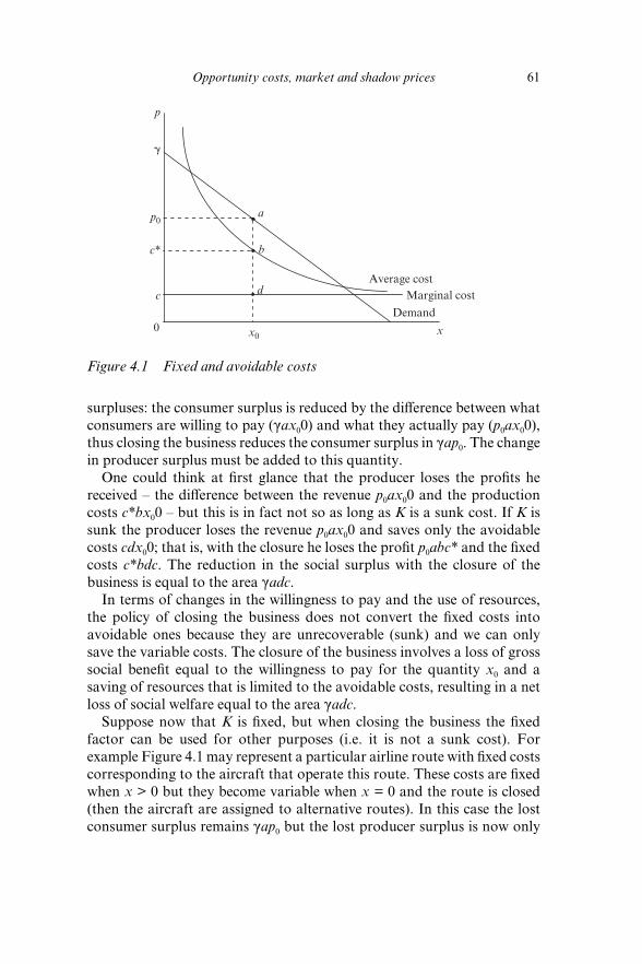
Opportunity costs, market and shadow prices 61
surpluses: the consumer surplus is reduced by the diff erence between what
consumers are willing to pay (gax00) and what they actually pay (p0ax00),
thus closing the business reduces the consumer surplus in gap0. The change
in producer surplus must be added to this quantity.
One could think at fi rst glance that the producer loses the profi ts he
received – the diff erence between the revenue p0ax00 and the production
costs c*bx00 – but this is in fact not so as long as K is a sunk cost. If K is
sunk the producer loses the revenue p0ax00 and saves only the avoidable
costs cdx00; that is, with the closure he loses the profi t p0abc* and the fi xed
costs c*bdc. The reduction in the social surplus with the closure of the
business is equal to the area gadc.
In terms of changes in the willingness to pay and the use of resources,
the policy of closing the business does not convert the fi xed costs into
avoidable ones because they are unrecoverable (sunk) and we can only
save the variable costs. The closure of the business involves a loss of gross
social benefi t equal to the willingness to pay for the quantity x0 and a
saving of resources that is limited to the avoidable costs, resulting in a net
loss of social welfare equal to the area gadc.
Suppose now that K is fi xed, but when closing the business the fi xed
factor can be used for other purposes (i.e. it is not a sunk cost). For
example Figure 4.1 may represent a particular airline route with fi xed costs
corresponding to the aircraft that operate this route. These costs are fi xed
when x > 0 but they become variable when x = 0 and the route is closed
(then the aircraft are assigned to alternative routes). In this case the lost
consumer surplus remains gap0 but the lost producer surplus is now only
p
x
�
p0
c*
c
a
b
dAverage cost
Marginal cost
Demand
0 x0
Figure 4.1 Fixed and avoidable costs
62 Introduction to cost–benefi t analysis
p0abc*, because the avoidable costs when the business is closed are now
c*bx00. Now the loss of social surplus is lower: gabc*.
In economic evaluation it is very useful to distinguish between fi xed and
sunk costs because, depending on the project, the variation in the costs
may diff er substantially, as shown in the previous case. It is not advisable
to follow a rigid taxonomy. In the previous example of the airline, the air-
craft could be considered as a fi xed factor but not sunk. Nevertheless if for
example there is an excess capacity of aircraft and when closing the route
the aircraft are not needed in any other place, the aircraft costs are sunk.3
4.4 INCREMENTAL COST AND AVERAGE COST
The calculation of opening, upgrading or closing a health, recreational or
transport service cannot be simply based on the product of the average cost
per user by the number of users. A usual source of error in the allocation of
costs to services is the use of the average cost rather than the incremental
cost. The incremental cost of providing a service is the change in total cost
resulting from such an action. A procedure to estimate the incremental
cost is to introduce the concept of units of activity; such as number of beds
and staff hours in a health service, bus miles and hours worked by drivers
in a transport service, and so on.
Consider the following example. A service is provided by the local author-
ity with a total cost denoted by C. The expression breaks down the total cost
into cost subgroups that may be reasonably related to some activity units:
C 5 LC 1 CC 1 VC, (4.7)
where LC is the total cost of the staff , CC is the cost of capital equipment
and VC represents the variable costs that depend directly on the number of
users (for example a meal served or a dose of medicine). Once the service
is analysed it appears that the total costs are a function of the total hours
worked (H) by the specialists attending the service, the number of units of
equipment used (E) and the number of users served (U), according to the
following expression:
C 5 hH 1 eE 1 uU , (4.8)
where:
h 5LC
H; e 5
CC
E; u 5
VC
U. (4.9)

Opportunity costs, market and shadow prices 63
If a given project consists of extending a service to a population not
covered so far, and the evaluation of this project is based on the average
cost instead of the incremental, it is likely that we will incur some mistakes
when calculating the cost of this project. Furthermore the error increases
with the heterogeneity of the users attended. If the users diff er in the ratio
of hours of specialist/user and capital/user, by using the average cost we
underestimate or overestimate the incremental cost of expanding the
service under evaluation.
A procedure to calculate the cost of the project is to identify the type of
service required by the targeted population: to determine how many activ-
ity units are required and then calculate the cost of expanding the service
by using the coeffi cients h, e and u. The following numerical example
illustrates the consequences of using the average cost rather than the incre-
mental cost in the evaluation of a project, when the users diff er in the type
of service required.
A public centre that provides health services to a population of 100 users
has a total cost of $1000. The breakdown of these costs is as follows: staff
costs ($600), costs of equipment ($300) and costs varying with the number
of users ($100). The total values of the units of activity on which the costs
depend are: 200 hours of specialist input (H), 10 hours of equipment (E)
and 100 users (U). There are three diff erent services (A, B and C) that use
the units of activity according to the distribution in Table 4.1.
Given this allocation and taking into account that according to (4.9) the
unit costs are h = 3, e = 30 and u = 1, the total and average costs of the
three services can be calculated as shown in Table 4.2.
Table 4.1 Cost allocation
Services Units of activity
H E U
A 40 2 70
B 120 3 20
C 40 5 10
Total 200 10 100
Table 4.2 Total and average costs ($)
Services hH eE uU Total cost Average cost
A 120 60 70 250 3.6
B 360 90 20 470 23.5
C 120 150 10 280 28

64 Introduction to cost–benefi t analysis
With this data, assume that it is necessary to assess a policy consisting of
the expansion of a health service to a population of 35 users. This service
requires the following units of activity: an additional hour of capital
equipment and 20 more hours of specialists. Using the average total cost
($10), the cost of the expansion of the service is equal to $350; however, if
one calculates the incremental cost (ΔC), the expansion would cost:
DC 5 20h 1 e 1 35u 5 125. (4.10)
On many occasions the average cost is a good approximation of the
incremental cost but, as shown with this example, the average cost may
be misleading and lead to overestimation or underestimation of the actual
incremental cost because the project capital/users, hours/users or any
other relevant ratios diff er from the mean values.
4.5 COSTS WITH AND WITHOUT THE PROJECT
Many projects aim to reduce the cost of producing a particular good or
providing a service. The cost of water, electricity or transport is reduced by
investments that incorporate some new technology or through a capacity
expansion. In the quantifi cation of the expected savings it is not enough to
compare the costs of the two technologies or the levels of the two capaci-
ties. We must take into account the behaviour of demand and determine
how the new equilibrium determines the costs that are relevant to the
comparison.
With the help of Figures 4.2 to 4.4 it is easy to show how the benefi ts
of a project consisting of the reduction of the user’s cost cannot be pre-
dicted by examining the supply side only. Cost savings for existing users
do not depend only on investment (new technology, capacity expansion,
etc.). The behaviour of the demand is also crucial for the calculus of the
social benefi t of the project. The interplay between costs and demand
and its impact on the NPV of the project is refl ected in the four fi gures
below.
In Figure 4.2 the average cost function AC 0 shifts to AC1 with the
project. This cost function shows the time that each consumer invests
when using the service or facility in question, for example a road for a
given level of demand. For a low traffi c volume, travel time does not vary
with the number of users. In the equilibrium the generalized price (time
multiplied by the value of time, for simplicity) is equal to g0. The benefi t
of a project reducing the cost from AC 0 to AC 1 can be decomposed into
two parts. Up to x0 the benefi t is measured as the area between the cost

Opportunity costs, market and shadow prices 65
function without the project and the new one with the project (g0adg1).
The benefi t of increasing the quantity (x1 − x0) is measured as the diff er-
ence between the willingness to pay (abx1x0) and the incremental cost of
meeting that demand (dbx1x0).
The benefi ts of generated traffi c are equal to the area abd in Figure 4.2
and abe in Figure 4.3. We are interested here in the diff erences that occur
in the benefi ts for the existing traffi c. In Figure 4.2 there is no congestion
without the project and the investment reduces the generalized price of
travelling from g0 to g1 (e.g. the construction of a tunnel). The potential
travel time savings of the project are equal to g0 − g1, and given the absence
of congestion these potential savings become actual savings. This is not so
in the case represented in Figure 4.3, where there is congestion with and
AC0
AC1
g1
g0 a
b
x0 x1
D
g
x0
d
Figure 4.2 Benefi ts of cost reduction (without congestion)
AC0
AC1
g0a
b
x0 x1
D
g
x0
eg1
1
g12 d
Figure 4.3 Benefi ts of cost reduction (with congestion)

66 Introduction to cost–benefi t analysis
without the project. Now the potential saving of the user (g0 − g12) is not the
actual saving (g0 − g11) since the reduced travel time generates an increase
in the numbers of users and then congestion increases resulting in a higher
generalized price than g12.
Now the equilibrium is at point b with a generalized price g11 for all users.
The diff erence in costs for the existing quantity is g0 − g11, which is lower
than g0 − g12. If we do not take into account the interaction between costs
and demand, we may overestimate the benefi t of the project.
An extreme case that illustrates the importance of considering the
behaviour of the demand when assessing an expansion capacity project
is represented in Figure 4.4. The potential time reduction g0 − g12, if the
project is undertaken, does not materialize as a result of the increase in
demand. Let us consider this case in more detail.
The case represented in Figure 4.4 refl ects the idea argued by those
opposed to new investments in roads when they reason that the new capac-
ity is absorbed in a short time by new traffi c. Suppose there are two roads,
A and B, between two cities. Using road A (the one represented in Figure
4.4) takes half an hour if there is no congestion (the intersect of AC0 with
the vertical axis), but A is a narrow road that rapidly becomes congested
as shown by the slope of AC 0.
Road B has a larger capacity and it is never congested, but its layout is
not as straightforward as that of A. The trip takes 45 minutes (g0) regard-
less of the traffi c volume. With respect to other characteristics the two
roads are identical and drivers always choose the fastest. Assume that B
has a traffi c volume much higher than A; hence, as long as it is faster using
A than B, new drivers will be diverted from B to A. The perfectly elastic
demand function in A refl ects this fact with g0 equal to 45 minutes.
AC0
AC1
x0 x1
g0= g11
g12
a bD
g
x
d
0
Figure 4.4 Benefi ts of cost reduction with perfectly elastic demand

Opportunity costs, market and shadow prices 67
We can see that, without the project, there is not other equilibrium dif-
ferent from a with x0 users using A with a generalized price equal to g0.
When the number of vehicles is less than x0, the travel time on A is less
than g0 (i.e. less than 45 minutes invested in B), and thus additional users
will leave B and come to A until travel time is equalized on both roads. In
the same way, traffi c on A cannot exceed x0, since in this case the travel
time on A is more than 45 minutes and it would be preferable to switch to
B.
Consider a project that increases the number of lanes on A (represented
by a shift in the generalized cost function from AC 0 to AC1) and remember
that traffi c on B is always higher than the volume that A can absorb. If the
traffi c is kept fi xed at x0, travel time saving would be g0 − g12, distance ad in
Figure 4.4. We could be tempted to estimate the annual benefi ts of invest-
ment as (g0 − g12)x
0, plus the benefi ts of generated traffi c. However the
reduction in travel time on A attracts new users until the travel times on
both roads are equalized. The new equilibrium with the project is located
at b with traffi c x1 and travel time g11 = g0, which implies that the project
does not generate social benefi ts.4
Shifts in Demand and Estimation of Benefi ts
Given the slope of the cost function, the magnitude of the annual benefi ts
after the cost reduction depends, as we have seen, on the reduction in costs
with the project and the slope of the demand function. The larger the slope
the larger the benefi ts for the existing demand after the implementation
of the project that reduces costs. On the other hand, the smaller the slope
the smaller the benefi ts, with the extreme case of zero benefi ts when the
demand is perfectly elastic (as shown in Figure 4.4).
The interaction between costs and demand does not fi nish here
because demand does not remain constant over time either. Demand
shifts because of changes in income or in the population, and each year
we must re- estimate the equilibrium that will take place and that will
aff ect the magnitude of the benefi ts. It is not enough to calculate the
benefi t the fi rst year and then apply an annual growth rate if the average
cost is a function of x and the demand changes because of exogenous
factors.
Figure 4.5 represents an average cost function increasing with the
volume of demand. Although the project represents a potential reduc-
tion in the generalized price of travel equal to the distance between AC 0
and AC1, the movement in demand after the price reduction generates
an increase in the quantity demanded from x0t to x1
t , where t denotes
the period of time, which results in (more) congestion, making the fi nal

68 Introduction to cost–benefi t analysis
generalized price (g1t ) greater than that initially expected. This is what
we have seen in Figure 4.3. What happens next year (t + 1)? The main
change that we must incorporate is the shift in the demand function.
To calculate the benefi ts in future years it is necessary to determine the
equilibrium with and without the project in each of the years during the
life of the project.
In Figure 4.5 the demand grows because of exogenous changes in
income, population, tastes, and so on in period t + 1, showing again that
the change in costs aff ects the estimation of social benefi ts. The demanded
quantities needed for calculating the annual benefi ts are now x0t11 and x1
t11
for period t + 1, x0t12 and x1
t12 for period t + 2, and so on until period T (the
fi nal year of the project’s life).
It can be seen that in period t + 1 the quantity without the project is
x0t11, for which the generalized price is higher than that in period t because
of an exogenous change in demand. The relevant level of demand for the
measurement is Dt11, for which the distance between AC1 and AC 0 is equal
to g0t11 2 g1
t11.
4.6 MARKET AND SHADOW PRICE OF FACTORS
In the economic evaluation of projects an input is valued at its market
price if this price is a reasonable approximation of the opportunity cost of
the resource. Unfortunately the market price of a production factor used
in a public project does not always refl ect its opportunity cost and some
correction has to be made. The name given to the new price is shadow
price. Let us see some examples.
AC0
AC1
Dt
g
x0
Dt + 1
x1t + 1
g1t + 1
x0t + 1
g0t + 1
Figure 4.5 Benefi ts of the project and changes in costs (year t + 1)

Opportunity costs, market and shadow prices 69
The Cost of Land
A wide range of projects require land and sometimes this land is situated
in locations with limited possibilities of substitution. This is the case, for
example, with dams and airports. In principle, determining the cost of the
land required for an infrastructure investment project should not present
major problems as long as the land market operates under competitive
conditions and there are no distortions causing the real price to diff er from
the true opportunity cost of the input.
The opportunity cost of land used in the construction of infrastructures
is the net benefi t lost in the best possible alternative use of that land. For
example, when the best alternative use is in agriculture, the market price of
land will refl ect the discounted market value (net of variable cost) of agri-
cultural production during the time of use of the land for the project. This
price will be higher the more valued the production is in that piece of land
and the smaller the possibility of substitution is for other pieces of land.
Therefore, if the market is competitive, the price of the land will reliably
refl ect the opportunity cost.
The determination of the land price in a competitive market with a fi xed
supply is represented in Figure 4.6. At point b the supply curve S and the
initial demand for land D0 intersect determining the price w0, for which all
the available land is used for those purposes with a higher willingness to
pay. A marginal increase in demand in this market as a result of the project
would not signifi cantly change the equilibrium at b, and the price w0 could
be used as an approximation of the land’s unit cost.
w0
w1
D0
D1
w
z
da
b
0 zbza
S
Figure 4.6 Market of a fi xed supply input

70 Introduction to cost–benefi t analysis
When the project represents a signifi cant change in the demand for land,
such as the case represented in Figure 4.6, the shift of the demand function
from D0 to D1 refl ects that the project requires the amount of land repre-
sented by the distance ad, and the equilibrium changes from b to d, raising
the price to w1. The initial demand for land is reduced to za, releasing for
the project the extension of land zb − za. The opportunity cost of that
land is represented by the area abzbza; that is, the willingness to pay of the
private sector for zb − za, a quantity of land that it is no longer in demand
because of the price increase.
The area abzbza can be estimated using the initial and fi nal prices and the
initial and fi nal quantities:
w0 (zb 2 za) 1
1
2(w1 2 w0) (zb 2 za
) , (4.11)
or what is the same (the rule of a half):
1
2(w0 1 w1) (zb 2 za
) . (4.12)
We assume here that all other prices remain virtually unchanged.
The application of expression (4.12) is straightforward: we have to
multiply the mean of the initial and fi nal prices by the quantity of land
required by the project. Nevertheless, determining the opportunity cost of
land presents additional diffi culties related to the speculation to which the
land market is subject and the externalities resulting from the land use in
surrounding areas.
Quite often the infrastructure project requires the use of non- marketed
land, for example when a highway crosses a natural park with unique
wildlife. Economic valuation of the cost of this land requires calculation of
the opportunity cost of the input beyond any payment for the expropria-
tions that might be required, estimating the value of what the society is
giving up because of the impact of the infrastructure on the original use of
the land. Moreover it is not enough to calculate the cost of the land used,
because the surrounding areas will suff er the negative eff ects of this type of
project, further increasing the opportunity cost of the land required.
The Cost of Equipment, Materials and Energy
The use of capital equipment, energy and materials in virtually all invest-
ment projects requires the use of prices that when multiplied by the quanti-
ties of the inputs result in the cost of these inputs.
The cost–benefi t analysis of the construction of high speed lines (see
Chapter 10), for example, distinguishes between construction costs, rolling

Opportunity costs, market and shadow prices 71
stock, maintenance and operation. The cost of locomotives, wagons and
electric power were estimated from the prediction of demand and the
number of trains required to meet that demand. With the number of
services needed and the kilometres travelled, energy consumption require-
ments were calculated.
The prices used to convert these physical units into a monetary value are
the market prices net of taxes. This option is applicable to the majority of
projects whose demand is marginal in the factor markets or to those for
which, without having marginal demand at the national level, there is an
international market where at the price w0 the supply is perfectly elastic.5
Figure 4.7 represents the market for an input and it is assumed that the
demand of this input for the project is marginal with respect to the total
factor market. The shift in the demand function D is negligible, and the
equilibrium price w0 is not changed because of the project. The existence of
a tax makes the market price w0 diff er from the opportunity cost of using
the input. The shadow price in this case is w0 − t, where t is the tax per unit
in absolute value. The tax, in this case, is a mere transfer of income.
4.7 MARKET PRICE AND THE SOCIAL OPPORTUNITY COST OF LABOUR
Virtually any investment project requires the use of labour. The construc-
tion of public infrastructure needs workers with diff erent skills. Moreover,
w0
w0 – �
z0
w
a
b
D
0
S
S – �
z
Figure 4.7 Market of an input with taxes

72 Introduction to cost–benefi t analysis
once the construction is fi nished, additional labour is required for main-
tenance and operation during the life of the project. Labour is required in
the case of a project consisting of restoring the damage to a natural envi-
ronment, as well as in educational or health- related projects.
Once we have estimated the number of workers required for the project
we need a price to calculate the cost of labour. Should we use the gross or
the net wage? How should we account for the creation of new jobs in areas
of high unemployment?
It is useful to distinguish three possible sources concerning the amount
of labour demanded by a project:
Workers who are already employed in other productive activities. ●
Voluntarily unemployed workers at the current wage, who would ●
work for a marginally higher wage.
Involuntarily unemployed workers, who are willing to work if jobs ●
were available at the current wage.
Once the requirement of labour for the project and the proportions of
the three sources have been estimated, we must look for the opportunity
cost of labour. Market wages, however, do not always refl ect the social
opportunity cost of labour. The discussion of the labour market in this
section assumes that the project has signifi cant eff ects changing the equi-
librium wage. The aim is to illustrate the ways to obtain the shadow price
of labour in diff erent labour market conditions, even if in practice wages
do not change signifi cantly with the project. Let us start with the simplest
case of a competitive labour market without taxes or unemployment
benefi t, represented in Figure 4.8.
The factor supply function refl ects the marginal value of leisure to the
workers and the demand function the value of the marginal productivity
of labour (L) for the fi rm. This shows that at the equilibrium wage (w0) the
value of marginal productivity is equal to the value of leisure to the mar-
ginal worker. If the amount of labour required for the project is marginal
we can use the equilibrium wage w0. Suppose on the contrary that, as it
is represented in Figure 4.8, the project requires (L1 − La) work units, as
represented by the movement of the demand function from D0 to D1at a
distance ad.
By increasing the demand for labour work from a to d the market wage
increases from w0 to w1 and the number of workers employed in the labour
market increases from L0 to L1. To see what shadow price should be used in
the project it is necessary to know the source of the employees absorbed in the
project under evaluation. Figure 4.8 shows how the use of labour increases
from L0 to L1, and thus the number of employees L1 − L0 should be valued by
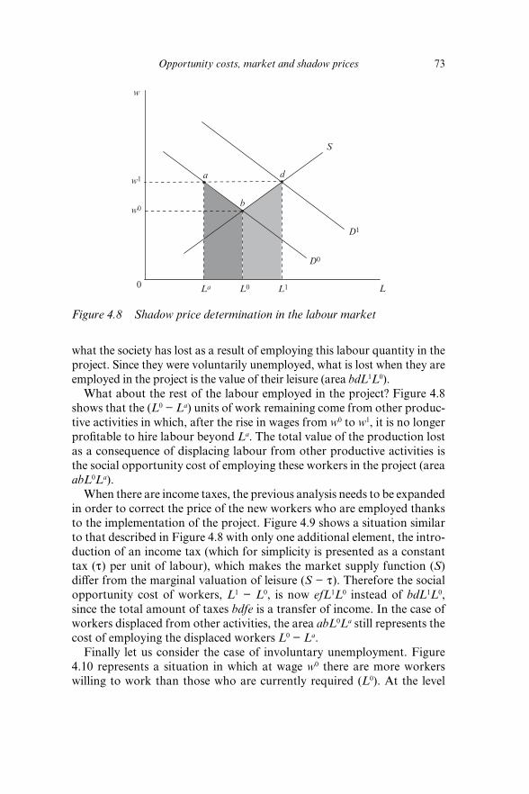
Opportunity costs, market and shadow prices 73
what the society has lost as a result of employing this labour quantity in the
project. Since they were voluntarily unemployed, what is lost when they are
employed in the project is the value of their leisure (area bdL1L0).
What about the rest of the labour employed in the project? Figure 4.8
shows that the (L0 − La) units of work remaining come from other produc-
tive activities in which, after the rise in wages from w0 to w1, it is no longer
profi table to hire labour beyond La. The total value of the production lost
as a consequence of displacing labour from other productive activities is
the social opportunity cost of employing these workers in the project (area
abL0La).
When there are income taxes, the previous analysis needs to be expanded
in order to correct the price of the new workers who are employed thanks
to the implementation of the project. Figure 4.9 shows a situation similar
to that described in Figure 4.8 with only one additional element, the intro-
duction of an income tax (which for simplicity is presented as a constant
tax (t) per unit of labour), which makes the market supply function (S)
diff er from the marginal valuation of leisure (S − t). Therefore the social
opportunity cost of workers, L1 − L0, is now efL1L0 instead of bdL1L0,
since the total amount of taxes bdfe is a transfer of income. In the case of
workers displaced from other activities, the area abL0La still represents the
cost of employing the displaced workers L0 − La.
Finally let us consider the case of involuntary unemployment. Figure
4.10 represents a situation in which at wage w0 there are more workers
willing to work than those who are currently required (L0). At the level
w
L
w0
a
b
D0
0 L0
w1
S
d
L1La
D1
Figure 4.8 Shadow price determination in the labour market

74 Introduction to cost–benefi t analysis
of demand D0 there is involuntary unemployment. The project repre-
sents a shift in the labour demand to D1, which means an increase in the
demand for previously unemployed labour, L1 − L0. What is the social
cost of employing the involuntarily unemployed? If there were no taxes
or unemployment benefi ts for these workers, the existing wage w0 would
be the social cost of a unit of labour and therefore the total cost would be
represented by the area abL1L0.
w
L
w0
a
b
D0
0 L0
w1
S
d
L1La
D1w1 – � f
e
S – �
Figure 4.9 Shadow price determination in the labour market (with taxes)
w
L
w1 – �
w0 – � – �
a b
D0
D1
0 L0
w0 S
d
L1
e
f g
Figure 4.10 Shadow price with involuntary unemployment

Opportunity costs, market and shadow prices 75
In the presence of income taxes (t) and unemployment benefi ts (s) the
total social cost would be represented by the area fgL1L0, because tax
revenue (abed) and unemployment benefi ts (degf) are transfers of income
and should be deducted. The shadow price of labour is therefore reduced
to the marginal value of leisure; this quantity can be obtained by reducing
the gross wage of a worker by the amount given by the income tax and the
unemployment benefi t. That is to say remuneration (w0 − t − s) equals
the marginal value of leisure. In any case it is what the society loses by
employing the worker in the project.
The following numerical example illustrates why a worker would not
accept a wage smaller than w0. Assuming that the unemployed worker
receives a subsidy of $100 and he values his leisure at $40, the worker will
not accept work for less than $150, as after being been contracted he has to
pay $10 in taxes. This numerical example can help to distinguish between
the private opportunity cost of the worker joining the labour market
($150) and the social opportunity cost ($40). The latter is the shadow price
of labour to be used in the project.
When there is a minimum wage regulation we also need to correct
the market wage to account for the social opportunity cost of labour in
the same manner as described above, just looking for what the society
loses by employing the workers in the project. This could be approached
through the mean of the minimum wage and the minimum reservation
wage, as no one accepting work would have a reservation wage lower
than the minimum wage, and the reservation wage of anyone employed
for the project could be higher than the minimum reservation wage. In
the absence of information on the minimum reservation wage, the shadow
wage could be estimated as one half of the minimum wage (i.e. assuming
the minimum reservation wage is zero).
The previous treatment of the shadow price for labour when there is
unemployment does not take into account what happens to the output
that is generated by the project. If the production generated by the
project is sold in a competitive market and reduces the price, it may
happen that labour is reduced as a result of business closures in the
private sector of the economy; but it could also be true that the product
or service associated with the project is complementary to other com-
petitive markets and therefore it encourages job creation (see Chapter
3). Determining the true shadow price in these cases is not immediate. In
any case a careful analysis of the markets closely related to the project
and its potential impact on them can help the evaluator (see Johansson,
1991).
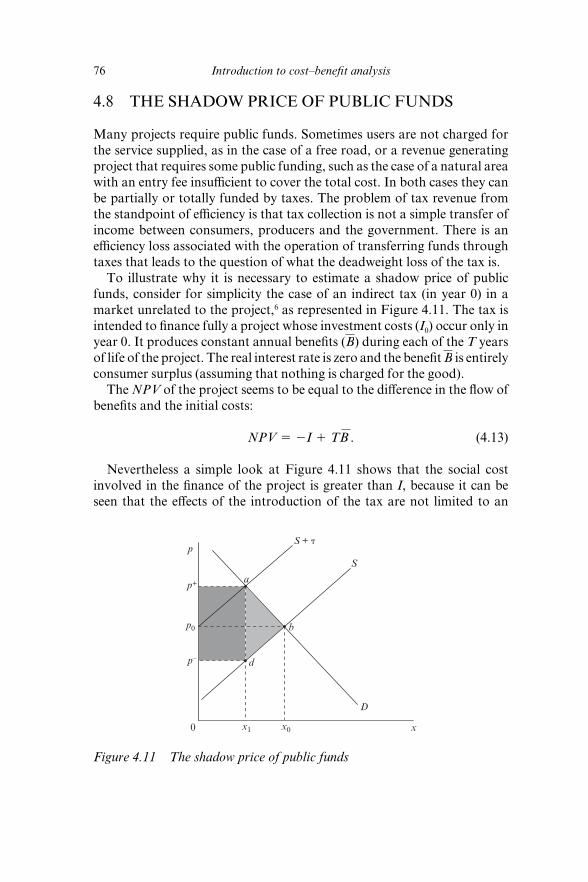
76 Introduction to cost–benefi t analysis
4.8 THE SHADOW PRICE OF PUBLIC FUNDS
Many projects require public funds. Sometimes users are not charged for
the service supplied, as in the case of a free road, or a revenue generating
project that requires some public funding, such as the case of a natural area
with an entry fee insuffi cient to cover the total cost. In both cases they can
be partially or totally funded by taxes. The problem of tax revenue from
the standpoint of effi ciency is that tax collection is not a simple transfer of
income between consumers, producers and the government. There is an
effi ciency loss associated with the operation of transferring funds through
taxes that leads to the question of what the deadweight loss of the tax is.
To illustrate why it is necessary to estimate a shadow price of public
funds, consider for simplicity the case of an indirect tax (in year 0) in a
market unrelated to the project,6 as represented in Figure 4.11. The tax is
intended to fi nance fully a project whose investment costs (I0) occur only in
year 0. It produces constant annual benefi ts (B) during each of the T years
of life of the project. The real interest rate is zero and the benefi t B is entirely
consumer surplus (assuming that nothing is charged for the good).
The NPV of the project seems to be equal to the diff erence in the fl ow of
benefi ts and the initial costs:
NPV 5 2I 1 TB . (4.13)
Nevertheless a simple look at Figure 4.11 shows that the social cost
involved in the fi nance of the project is greater than I, because it can be
seen that the eff ects of the introduction of the tax are not limited to an
x1 x0
p
x
p+
b
D
0
p0
S
d
a
p–
S + �
Figure 4.11 The shadow price of public funds

Opportunity costs, market and shadow prices 77
income transfer. Initially the market is in equilibrium at b with a price p0
and a quantity equal to x0. The introduction of the tax changes the equilib-
rium of the market by raising the price paid by consumers to p+ and reduc-
ing the quantity demanded to x1. The price received by producers is p− and
tax collection is represented by the area p+adp−, which is equal to I.
The introduction of the tax has caused a reduction in the quantity from
x0 to x1. This reduction of the quantity represents a negative eff ect on the
economy, as the consumers were willing to pay the area abx0x1 for goods
or services whose opportunity cost is represented by the area dbx0x1. The
net loss of effi ciency caused by no longer producing x0 − x1 equals the area
abd. This extra cost of obtaining public funds should be included in the
evaluation of the project.
Assuming that the area abd is, for example, 25 per cent of the tax
revenue, the shadow price (or shadow multiplier) of public funds is equal
to 1.25, and the cost of the project is equal to 1.25I0. Let lg be the shadow
price of public funds; then we must modify (4.13) in order to refl ect the
opportunity cost of the investment:
NPV 5 2lgI 1 TB , (4.14)
so we can appreciate that, to obtain an NPV greater than zero, the follow-
ing must be satisfi ed:
TB
I. lg. (4.15)
The economic interpretation of expression (4.15) indicates that, for a
project funded by taxes to be socially profi table, the social benefi t obtained
per unit of money invested has to be greater than the opportunity cost of
the public funds.
The previous argument is based on the assumption that the project is
fi nanced entirely by taxes and that it does not have operating revenues and
costs. A more general case is represented by the expression:
NPV 5 2I0lg 1 aT
t51
CSt 1 lgPSt
(1 1 i) t, (4.16)
where:
CSt: consumer surplus in year t
PSt: producer surplus in year t
i: social discount rate.
Expression (4.16) shows that the shadow price of public funds has to be
applied to both costs and revenues. The annual net revenue reduces the

78 Introduction to cost–benefi t analysis
need for public funding and therefore the need for taxes, so that $1 col-
lected by charging the users in any year of life of the project has a present
value lg(1 1 i)2t.
4.9 SOCIAL BENEFIT AND FINANCIAL EQUILIBRIUM
The use of social benefi ts in cost–benefi t analysis rather than revenues, as
in fi nancial analysis, and the use of shadow prices trying to approximate
the opportunity cost rather than market prices, raises a fundamental
problem: projects whose economic evaluation yields a positive social NPV
are often associated with poor fi nancial results; that is, they are not viable
from a commercial point of view.
Consider the case of a project consisting of a public service as repre-
sented in Figure 4.12. The demand function is x = 100 − p. Therefore the
demand quantity (x) of this service is 100 users per time period when the
price (p) is zero and zero when the price is $100.
Suppose the monetary cost of this service is $25,000 (of which $5000 is
indirect taxes levied on the building materials used), independent of the
number of users for the ten years of life of the facilities. The social discount
rate, and the interest rate, are equal to zero.
The social NPV can be expressed as:
NPVs 5 220,000 1 10B , (4.17)
where $5000 has been subtracted corresponding to taxes (transfer) to
express the cost of the project as an opportunity cost (the actual resources
p
100
D
0 100
50
2500
1250
50
1250
x
Figure 4.12 Social benefi t and fi nancial equilibrium

Opportunity costs, market and shadow prices 79
used in the project are valued at $20,000) and where B represents the
constant gross benefi t in every period.
On the other hand the fi nancial NPV is:
NPVf 5 225,000 1 10px, (4.18)
where, in contrast with the social NPV, costs are measured at market
prices (tax included) and the benefi t is reduced to the revenue collected.
Trying with diff erent prices it is possible to calculate the resulting
revenue and consumer surplus and consequently the social and fi nan-
cial NPV. It can be seen that the highest possible social NPV is equal to
$30,000 and corresponds to a price equal to zero. This maximum social
NPV is associated with a negative fi nancial result of $25,000. The com-
mercial defi cit is equal to the fi xed costs when the service is free.
With a single price the best fi nancial outcome is achieved when the price
is equal to $50. In this case the revenue is equal to the costs. The improve-
ment in the fi nancial result is parallel to a reduction in the social NPV,
which is now equal to $17,500.
This case illustrates the importance of being consistent with the use of
shadow prices when evaluating public projects. Suppose we are evaluat-
ing the previous project in a context of budgetary restrictions, which
require costs to be covered once the service under evaluation has started
its operation.
While counting the cost net of taxes in the evaluation we should not
forget that the actual price will include these taxes in order to meet the fi nan-
cial constraint. Obviously the estimated demand will not be compatible with
a consumer surplus of $50,000, the one obtained with the free service.
The estimated demand (100) will not be achieved, since the budget
constraint requires operation with a higher price than optimal. If the price
to be charged to consumers is $50, the number of consumers is halved,
with the corresponding reduction in social benefi ts. Furthermore, when
there are multiple technological options, the choice of the combination of
inputs may be biased in favour of inputs with lower shadow prices – which
increase the social NPV. This choice may, later in the operation of the
service, compromise the commercial viability of the project since market
prices must be charged.
When calculating the social NPV with shadow prices, the fi nancial
implications of these assumptions and the restrictions that have to be
faced should be considered simultaneously. The use of shadow prices
requires taking into account what will happen later during the life of the
project. The use of shadow prices can make some projects socially viable,
which would not be feasible using market prices.
80 Introduction to cost–benefi t analysis
An example that illustrates this problem is the construction of a port in
an area of structural unemployment. Faced with two alternatives, capital
intensive or labour intensive, the use of shadow prices for labour could
make more socially profi table the construction of a less capital intensive
port. Once the port has been built it is assigned to the port authority with
the commercial target of breaking even according to market prices. The
paradox arises because the port is placed at a disadvantage with respect to
the competing ports that are capital intensive. If the port authority does
not receive an equivalent subsidy (which may be prohibited by the rules of
competition) that makes the use of labour cheaper (as was shown in the ex
ante evaluation with shadow prices), the port will lose traffi c in favour of
other more effi cient ports.
In the economic evaluation of the project shadow prices can be used
even if there are no subsidies to reduce market wages. However, if the
port will later be exploited under market standards, the demand should be
forecast with those prices that correspond to the costs compatible with the
inputs valued at market prices.
THINGS TO REMEMBER
The opportunity cost of an input is the net value lost in its next best ●
alternative. The market price in the factor markets is the fi rst candi-
date to approximate the opportunity cost. There are circumstances,
such as taxes, externalities or unemployment, where the market
price has to be corrected to obtain the real opportunity cost. This is
what is called a shadow price.
The incremental cost refl ects the opportunity cost of using an ●
input, and the average cost refl ects the mean value of the oppor-
tunity cost of diff erent units of this input, so the average cost is
irrelevant for cost–benefi t analysis unless the input productivity is
constant.
The intersection between supply and demand changes over time so ●
the benefi ts and costs of the fi rst year will usually be diff erent from
subsequent years. Examine the equilibrium with and without the
project every year during the project’s lifespan.
Labour is an input, not an output. The opportunity cost of labour in ●
cost–benefi t analysis varies, as many other inputs, depending on the
preceding use of the input. When a worker is previously employed
his gross wage can be used as the opportunity cost. With involuntary
unemployment the shadow price can be as low as the value of the
worker’s leisure.
Opportunity costs, market and shadow prices 81
There are many projects requiring public fi nancing. Some projects ●
are provided free and others have charges that are not high enough
to break even. When projects have to be fi nanced, partially or
totally, by taxes we have to consider the distortionary eff ect of taxa-
tion. Tax collection is not a simple transfer between individuals and
the government. There is economic value lost along the way. The
deadweight loss of the tax has to be included in the shadow price of
public funds.
The social ● NPV shows the discounted net social benefi t of the
project; the fi nancial NPV indicates whether the project generates
enough revenues to cover total costs. A private fi rm is interested in
the fi nancial NPV, the practitioner of cost–benefi t analysis requires
the information provided by both of them.
NOTES
1. Ferraro and Taylor (2005). Check your answer in section 4.2.2. And sometimes to incur losses of effi ciency in some markets to obtain an overall socially
desirable result. In certain circumstances it may be optimal to set a price below or above the marginal cost in a regulated market, when there are substitutes or complements for which it is not possible to set a price equal to the marginal cost. This policy is derived from the theory of second best (Lypsey and Lancaster, 1956).
3. In some cases, one must add scrap values. Most buildings and machines have such a value after a particular activity is closed.
4. We might think that investing in capacity in these circumstances is always a bad policy; however there are alternatives to obtaining social benefi ts with investment projects such as the one described. The introduction of road pricing would produce gross benefi ts. Moreover, road pricing is an alternative to be considered before investment in new capacity is decided.
5. For the input market with an increasing supply, and where the project causes signifi cant shifts in demand, we can apply the same reasoning as in the labour market (Figures 4.8 and 4.9).
6. For simplicity we assume that the only eff ects of the tax occur in this primary market. There are no other products or input markets aff ected by the introduction of the tax. For the eff ects on other markets related to the primary market by complementary or substi-tutability relationships see Chapter 3. We also ignore the issue of optimal taxation; that is, the way to collect tax revenue minimizing deadweight losses (see Ramsey, 1927).

82
5. Economic valuation of non- marketed goods (I)
Only the fool confuses value with price.(Antonio Machado1)
5.1 INTRODUCTION
The evaluation of positive and negative impacts of projects and public
policies is particularly diffi cult (and controversial) when there is no market
for such impacts. Sometimes the project is specifi cally designed to improve
an environmental good or to prevent its deterioration. On other occasions
the purpose is of a diff erent nature and the environmental impact is a side
eff ect of the project.
For example, there are safety policies that reduce the risk of death on
the job and projects that increase the recreational value of lakes and rivers
by improving the water quality. In contrast there are policies such as the
promotion of industrial production (or livestock) that contribute to global
warming and projects like the construction of an airport, with external
eff ects such as noise or deterioration of the landscape.
Ignoring the negative or positive externalities of a project may hide its
true opportunity cost or, equivalently, the true benefi ts that society obtains
from its implementation. If the social profi tability of the project is sensitive
to the magnitude of the externality it may even change the accept–reject
decision, or alter the ranking if the decision is to choose among a set of
projects. The problem is how to value the benefi ts and costs of goods
for which no quantities are exchanged in the market and no prices are
available for their valuation.
Section 5.2 describes how externalities and public goods are a challenge
for economic valuation. The willingness to pay or willingness to accept
when there is no market where the good aff ected by the project is exchanged
imposes the need to seek solutions such as the use of ‘ally’ markets or the
design of questionnaires that would put individuals in hypothetical situa-
tions and allow us to obtain relevant information to estimate the economic
value of non- marketed goods. Measurement requires prior understanding
Economic valuation of non- marketed goods (I) 83
of the key relationships behind the change in the non- marketed good and
the well- being of the individuals and these relationships are also biological
and ecological.
The monetary measures of changes in individuals’ utility is addressed in
section 5.3. A change in the quantity or quality of a public good changes
individual well- being, but utility is unobservable and the economist relies
on monetary measures of the change in utility. Compensating variation
and equivalent variation are discussed, their relationship with the property
rights and the reasons explaining why they usually diverge.
There are basically two approaches to the valuation of non- marketed
goods: the fi rst based on revealed preferences and the second through
interviews with individuals, the so- called stated preferences (Chapter 6).
The revealed preferences approach has two main methods, presented in
section 5.4, the travel cost and the hedonic price method. In both, the
practitioner relies on a related market where information on willingness
to pay is obtained.
5.2 THE ECONOMIC VALUATION OF NON- MARKETED GOODS
Externalities and Public Goods
The private cost of a good is the net benefi t lost by an economic agent in
the next best alternative of the resources used in the production of that
good, while in the social cost this net benefi t is the one lost by the society.
The diff erence is pertinent when individuals, by consuming or producing
goods, aff ect the welfare of other individuals outside the market transac-
tion. In this case we say that there is an externality, and the private and
social costs diff er. Externalities can be positive or negative, and can be
produced by fi rms or consumers.
An example of positive externality is associated with a security service
hired by an individual who is paying for the service while other residents
are benefi ting from a safer neighbourhood without paying for it. A nega-
tive externality would be caused by a company that pollutes the air and
damages the health of residents aff ected by emissions. In the fi rst case
there is an externality generated by an individual that benefi ts other indi-
viduals, while the second is a company that produces an external eff ect
that harms individuals. There may be diff erent possibilities, and they all
have in common the diffi culty of establishing markets for such goods and,
sometimes, the mere absence of them.
The marginal social cost equals the marginal private cost plus the

84 Introduction to cost–benefi t analysis
externality. If there are no externalities or any other distortions such as
taxes, the social cost of producing one unit of good equals its private cost.
If the externality is negative the social cost equals the private cost plus the
extra cost that the externality generates. If the external eff ect is positive the
social cost will be lower than the private cost. The diff erence between social
and private marginal cost (i.e. the value of the externality) does not need to
be constant and may increase or decrease with the scale of the activity.
When an individual consumes a private good another individual cannot
enjoy that good (rivalry) and the supplier can exclude the individual if he
refuses to pay the price (excludability). We have argued that the produc-
tion or consumption of some goods aff ects other individuals outside the
market, but there is an extreme case of non- rivalry and non- excludability
that is called a pure public good. If the good is non- rival and non-
excludable, it cannot be produced and sold in the market. Lighthouses
have been the classical textbook example.2
In cost–benefi t analysis there are many cases of changes in the provision
of a public good (such as the reduction of air pollution or the enhancement
of the quality of the water of a river) that need to be evaluated, though
there are no market transactions where we can obtain information on
willingness to pay.
Sometimes the change in the level of the public good is not the primary
target but the project produces side eff ects that change that level. This is
the case with public works that reduce the visibility of scenic views. Hence
the social cost, represented by the reduction in the pleasure of contemplat-
ing the landscape, is a cost of the project. Another completely diff erent
issue is the diffi culty of sensibly expressing this cost as a number for the
calculation of the net social benefi t of the project.
Other important non- marketed goods in cost–benefi t analysis are
related to health and safety. Investment in road safety has as a primary
objective: the reduction of the number and severity of accidents. The
output of this type of project is measured in the number of lives saved and
injuries avoided. Other projects aff ect the health status of people though
this is not the primary objective of the project, for example a power station
that increases the production of electricity and reduces the quality of air.
In both cases the welfare of the aff ected individuals changes, and the
economist trying to calculate the economic value of these eff ects has to
overcome the problem of the absence of markets for these goods.
In our simplifi ed society a change in the natural resources and environ-
mental goods, as well as in the level of risk, aff ects consumers and producers
through the market. This is the case with an increase in the quality of water
in a reservoir that reduces the prices of agricultural products. In other cases
the consumer benefi ts directly, and not through a market transaction; for

Economic valuation of non- marketed goods (I) 85
instance when the government provides more recreational areas in a city.
On other occasions individuals are aff ected through a market transaction in
which they do not participate as sellers or buyers, as happens in the case of an
airport that produces noise suff ered by people who are not direct users. We
have called this group the ‘rest of society’ to distinguish the external eff ects
not accounted for in consumer and producer surplus (see Chapter 2).
Moreover, when considering the owners of the production factors, the
provision of a public good can increase the rent of a factor of fi xed supply,
as happens in the case of the restoration of a polluted natural area that
increases the value of the surrounding private land within the bounda-
ries. Finally the taxpayers will in most of the cases be negatively aff ected,
bearing the investment and maintenance costs.
It is worth emphasizing here that individuals can belong to more than
one group in our simplifi ed society and hence their welfare can be aff ected
through diff erent channels because of their several ‘identities’. The intro-
duction of a clean air regulation can make the individual better off as a
citizen who belongs to the group ‘rest of society’ or as the owner of the
land, and worse off as a producer and as a consumer of electricity or a
tenant now paying a higher rent for his house.3
The practical side of this argument is that the analyst needs a model before
going into the quantifi cation of benefi ts and costs. Adding the change in
consumer surplus, producer surplus and ‘rest of society’ can lead to double
or triple counting if the change in consumer surplus has been obtained by
asking individuals how much they are willing to pay for the implementation
of the clean air regulation. In this case the reduction in profi ts of the fi rms
aff ected by the stricter policy or the higher quality of the air they breathe will
normally be included in their answers. The individual is not only a consumer.
He can also be a shareholder and so the question this individual is asked
must be clearly formulated before we make use of any resulting number. This
gives us a clue as to the diffi culties associated with the economic valuation of
non- marketed goods based on the responses obtained by surveying individu-
als about their monetary valuation of changes in the natural resources, the
environmental attributes or the level of risk in their lives.
The Eff ect on Welfare of a Change in the Non- Marketed Good
The understanding of the relationship between the change in the environ-
mental good and social welfare is not restricted to its economic content.
Some knowledge is required of the biological and ecological links behind
the changes in the quantity and quality of the environmental and resource
service fl ows. Freeman (2003) proposes to view the economic value of
these fl ows as the product of three sets of functional relationships.
86 Introduction to cost–benefi t analysis
The fi rst is the link between the human intervention and the change in
the environmental good (e.g. biomass of some species for commercial or
recreational use or quality of the air). Two types of human interventions
are relevant here. One occurs in the market when a factory pollutes the air.
The other is the government actions to regulate the commercial activities
that aff ect the environment (e.g. internalization of externalities through
Pigovian taxes) or actions that directly focus on the protection or enhance-
ment of the environmental good (e.g. the creation of wildlife sanctuaries).
The eff ect of human impact on the environmental good has two chan-
nels, one is direct, such as the increase in fauna when land use is restricted
through a government regulation, and the other is indirect, such as the
behaviour of private agents changing with the new regulation. The reac-
tion of the individual and fi rms has to be contemplated before predicting
the fi nal eff ect of the government action on the environmental good.
Once the change in the quality or quantity of the environmental good
is established a second relationship is required in order to know the eff ect
on the human uses of the good. The uses of the resources can happen in
the market, as is the case with commercial fi shing, or could be the level of
quality of the resource for recreational activities (e.g. number of days of
acceptable quality of the water for sport activities in a river). Again, there
is a direct eff ect on the output (e.g. tons of fi sh caught and days of rec-
reational activity) and the level (quantity or quality) of the environmental
good, and an indirect eff ect as the output is also aff ected by the use of other
inputs beside the environmental good, and the quantities of those other
inputs vary as a response to the change in the level of the environmental
good (e.g. climate change aff ects the crop indirectly as farmers change the
use of inputs as a reaction to the new conditions of production).
The third relationship is the link between the output, or resource fl ow,
and welfare. This consists of the economic valuation of the change in
the environmental good. The aim of the economist is not to measure the
change in the number of days the river is open for recreational purposes
or some physical indicator of the pollutants in the air after government
action to improve the environment. The objective is to measure the change
in social welfare, and this may include two types of value, the use value
and the non- use value of the change in the environmental good.
5.3 WILLINGNESS TO PAY AND WILLINGNESS TO ACCEPT
The problem with goods such as clean air, silence and scenic views is that
there is no market in which they are traded and therefore a variation in the

Economic valuation of non- marketed goods (I) 87
level of atmospheric pollution, noise or visual intrusion associated with a
project is diffi cult to measure in economic terms.
In the absence of a market in which to obtain the valuation we must
look for other related goods for which a market exists that refl ects the
economic eff ects of the changes in the good not directly subject to market
transactions. For example the real estate market refl ects in housing prices
the noise that is involved in the operation of a nearby airport or the provi-
sion of parkland. When there is no possibility of using an ‘ally’ market the
alternative is to ask individuals directly for the economic value of the eff ect
on their welfare. The fi rst case is called revealed preferences and the second
stated preferences.
Starting from the indirect utility function U 5 V(P, M ) , where the
utility (U ) of the individual depends indirectly on the prices (P) of goods
consumed and his income (M ) (see Chapter 11), we incorporate a public
good (Johansson, 1993) so that, according to (5.1), we can express the indi-
vidual’s utility as a function of the price vector of private goods, the level
of provision, defi ned in terms of the quantity or quality, of public good (g)
and his income:
V(P, g, M ) . (5.1)
Suppose that a given project improves the public good g; we assume it is
environmental quality. Then, suppose the project increases air quality or
reduces noise. The initial utility of the individual is represented as U 0 and
the fi nal utility, once the project has been carried out, as U 1 (the super-
scripts 0 and 1 indicate without and with the project respectively):
U 0 5 V(P
0, g 0, M ) , (5.2)
U 1 5 V(P
0, g 1, M ) . (5.3)
The increase in individuals’ welfare that occurs as a result of the
enhancement in the public good is equal to U 1 2 U
0. Ideally the change in
utility resulting from the project is what we should measure, but the utility
is not observable and economists, unable to measure utility directly, rely
on monetary measures of changes in utility (see Chapter 11). There are two
approximations for obtaining individual valuations of changes in the non-
marketed good: the willingness to pay and the willingness to accept.
One way to measure in monetary terms the utility change experienced
by an individual is to ask how much money he would be willing to pay for
the improvement. This is the compensating variation (CV) and, assuming
that the individual responds with sincerity, he would be willing to pay an

88 Introduction to cost–benefi t analysis
amount (CV ) that would leave him indiff erent with respect to the initial
situation without the improvement. Expression (5.4) captures the idea of
how to measure the improvement in the public good:
U 0 5 V(P
0, g 0, M ) 5 V(P
0, g1, M 2 CV ) , (5.4)
where it is assumed that the individual’s income does not vary with the
project.
Another way to measure the increase in an individual’s utility in mon-
etary terms is to ask the individual for the minimum amount of income
that he would accept to forgo the improvement. This is the equivalent
variation (EV) and, assuming that the individual responds with sincerity,
he would be willing to accept an amount that would leave him indiff erent
with respect to the situation he would have reached with the improvement.
Expression (5.5) incorporates the application of the concept of EV to an
improvement in the public good:
U 1 5 V(P
0, g1, M ) 5 V(P 0, g
0, M 1 EV ) . (5.5)
An example will help to clarify the diff erence between the two concepts
and their practical use. Consider the case of an individual whose hobby is
fi shing in a river that will be contaminated if the project of constructing
a factory is approved. The expected fall in the quality of life of this indi-
vidual has to be valued for its inclusion in the evaluation of the project
that involves the river pollution among its social costs; the absence of a
market for the good ‘clean water’ creates the diffi culty of valuation of this
damage. If you ask the fi sherman how much he is willing to pay to avoid
the damage, he would probably angrily answer zero and that, in any case,
we should compensate him for the damage.
Consider now the case in which the factory has the right to pollute.
The question of how much the individual would be willing pay to avoid
the damage now has another connotation to the respondent and, if he
answers truthfully, the response would be, within the limits of his income,
the maximum that would make him indiff erent to continuing to fi sh in
unpolluted waters.
Assume alternatively that the individual has the right to uncontami-
nated water. The question that would now make sense is: how much is the
minimum compensation he would accept for the pollution of the river?
Depending on the importance that the individual gives to fi shing, and the
closeness of substitutes, he would require a larger or smaller amount of
compensation; compensation that, in this case, would not be limited by his
income, so it could be infi nite.4

Economic valuation of non- marketed goods (I) 89
The case of the fi sherman shows that the measurement of external
eff ects is not unique and it depends on who has the property rights.
Suppose alternatively that the individual fi shes in a polluted river and that
the project substantially improves the fi shing conditions. If the property
rights of clean water belong to the fi sherman, the valuation question is
how much he would be willing to accept to continue with the river pol-
luted (i.e. not to undertake the renovation project). Here, there would be
no income limit to the compensation. In the case in which the factory has
the right to pollute, the question is how much the fi sherman is willing to
pay for clean water. Now the response is limited by the individual’s income
(Table 5.1 represents the various possibilities).
This example shows that in some questions there is a limit of income
and in others there is not. Furthermore there is no reason to expect that
the amounts of income accepted or paid by individuals in their responses
are equal, as the standard of living of the individual varies with the type of
question to answer, and if the marginal utility of income is not constant, the
compensating and equivalent variations do not coincide (see Chapter 11).
According to the modelling of the society made in Chapter 2, a project
that enhances environmental quality aff ects diff erent social groups, for
example the group ‘rest of society’ (better environmental quality enjoyed
by excursionists), ‘producers’ (higher profi ts because of cost reductions
derived from the highest quality), ‘consumers’ (through the lower prices
of goods supplied by producers with lower costs) and ‘taxpayers’ (who
fi nance the project through taxes).
In practice the correct formulation of the question that induces the indi-
vidual to calculate the monetary valuation of the change experienced by
an environmental good is critical. If the individual is asked about willing-
ness to pay for the environmental improvement, without any qualifi cation,
we will probably obtain a value that includes the individual’s surplus as a
consumer but also as a producer or as a taxpayer. Unless the individual
is informed that his valuation of the change in the environmental good
Table 5.1 Methods to value the externality
Who has the property right to clean water?
Fisherman Factory
Clean river to be polluted CV/WTA EV/WTP
Polluted river to be cleaned EV/WTA CV/WTP
Note: CV: compensating variation; WTA: willingness to accept; EV: equivalent variation; WTP: willingness to pay.
90 Introduction to cost–benefi t analysis
should exclude the change in his income as a shareholder or taxpayer,
the sum of the surpluses of the social groups that make up our simplifi ed
society in this chapter would be incorrect.5
We have seen that CV and EV may be diff erent (see Chapter 11 for a
more detailed explanation), but the observed disparity between willingness
to pay (WTP) and willingness to accept (WTA) is larger than the income
eff ect would explain. An empirical study (Horowitz and McConnell, 2002)
concluded that there are signifi cant disparities: the diff erences are minimal
for private goods, the ratio WTA/WTP is about 10 for public goods and
the explanation cannot be found in survey related problems.
Other ideas have been presented to explain the disparity; for example sub-
stitutions eff ects in the case of goods with hardly any substitutes available,
as happens with some environmental goods. If the possibilities of substitu-
tion are scarce higher compensation will be required for a reduction in the
quantity or quality of the environmental good (Hanemann, 1991). Other
explanations refer to concepts like loss aversion and reference dependency
meaning that the individual gives more weight to a loss than to an identi-
cal gain (see Kahnemann and Tversky, 2000). Another argument is based
on the idea of irreversibility in the context of uncertainty (see section 8.2).
The additional cost of killing an option (when the environmental good is
not kept at the present level) could be refl ected in the higher compensation
required for the reduction of that level (Zhao and Kling, 2001).
5.4 VALUATION THROUGH REVEALED PREFERENCES
There are two approaches to measuring the benefi t of a project involving
an environmental good: the measurement based on revealed preferences
and the one based on stated preferences; that is, surveying individuals to
seek information about their preferences.
The simplest situation occurs when the change in the non- marketed
good is an input for the production of a marketed good. For example,
when a public project improves the quality of water used as the input for
a residential water supply fi rm, the benefi ts of the provision of the public
good (water quality in reservoirs or underground) aff ect the cost function
of the water supply fi rm because they reduce the average cost of producing
drinking water. This cost reduction interacts with the demand function,
aff ecting the utility of consumers if prices fall (assuming that water quality,
as an output, remains constant) and the utility of the owners of production
factors if their surpluses increase.
The problem of not having a market for the valuation of a public good
Economic valuation of non- marketed goods (I) 91
can be illustrated with two examples of actions that aff ect environmental
goods. The fi rst consists of a municipal project to provide the city with a
green area. The second is the construction of an airport that increases the
noise in the surrounding residential area.
In both cases the evaluator needs to know the change in the social
benefi t with the project: in one case the benefi t of the individuals derived
from the new green area; and in the other case the loss of social benefi t as
a result of the noise produced by the aircraft. In the second case one might
think that, as we know how much it costs to soundproof a house, we could
estimate the cost of noise by calculating the cost per household and multi-
plying by the number of houses within the noise map. Is this really the cost
of noise? Actually not, because exposure to noise cannot be avoided when
the individuals go outside or open their windows.
The problem with defensive expenditures, as well as averting behaviour
(i.e. costs individuals incur in actions to avoid noise or a higher risk of
illness) is that they do not measure the value of the change in the non-
marketed bad (e.g. noise) but a lower bound of the maximum willingness
to pay of the individuals to avoid the loss of utility.
In both the cases of the green area and the noise, we can try to estimate
the economic value of the non- marketed good by observing behaviour
in an ‘ally’ market, for example the property market, or in the case of
health risks the labour market. This method aims to obtain information
on the use value of the environmental good and therefore cannot provide
information on the non- use value.
The Hedonic Prices Method
An approach based on revealed preferences is to see how noise aff ects
the price of housing, comparing prices of houses near to the airport with
others of similar characteristics but diff erent levels of noise exposure. The
starting assumption is that among a set of similar houses, individuals pay
more for those that are less exposed to noise, we can obtain a monetary
measurement of willingness to pay to avoid it, and infer from that price
diff erence the implicit price of noise for individuals.
This approximation is based on the conception of the good as a set of
attributes (Lancaster, 1966). Thus a house is described as a composite
good of a number of rooms, size of garden, views, quality of construction,
location, and so on. If we also add to this that the houses have diff erent
levels of noise exposure, we can fi nd the implicit price of noise.
The problem is that the price diff erence between a house exposed to noise
and another house that is not exposed cannot be explained solely by this
fact, because the airport also benefi ts the area by increasing, for example,

92 Introduction to cost–benefi t analysis
the accessibility to the city centre with access roads or by building new
subway lines that are part of the airport construction project. Moreover
those who have chosen to live near the airport may not have the same prefer-
ences and therefore the disutility of noise is not representative of the average
individual. Let us see how this method tries to solve these diffi culties.6
Suppose the price of housing (P) is a function of the following
variables:
P 5 f(R, N, A, F, O) , (5.6)
where:
P: housing price
R: number of rooms
N: noise level
A: access time to city centre
F: characteristics of the area (crime rate, number and quality of schools,
etc.)
O: other factors.
Once we have a representative sample of houses, we estimate the func-
tion (5.6) whose functional form is often assumed to be logarithmic:
ln P 5 b0 1 b1 ln R 1 b2 ln N 1 b3 ln A 1 b4 ln F 1 b5 ln O. (5.7)
First we want to know how the price of housing varies with respect to
changes in the noise level, and equation (5.7) allows us to estimate this
relationship. If we compute the derivative of the logarithm of price with
respect to noise level, holding the other explanatory variables constant, we
obtain the elasticity of price with respect to noise level:
0 ln P
0 ln N5 b2, (5.8)
or
b2 50P0N
N
P. (5.9)
In expression (5.9), 0P/0N is the change in the price of houses when the
noise level changes, which is called the implicit price or the hedonic price
of noise. Solving for 0P/0N in (5.9) we can obtain the value of the hedonic
price of noise:
0P0N
5 b2
P
N. (5.10)

Economic valuation of non- marketed goods (I) 93
As shown by expression (5.10) the price of noise depends on the param-
eter estimate (which is expected to be negative), the price of housing and
the level of noise. Therefore the hedonic price of noise is not constant
unless P and N always vary in the same proportion, which is not what
is known from empirical work, as the price of the private good does not
have a linear relationship with the environmental quality at the observed
levels.
It is worth recalling what measures 0P/0N. This partial derivative is the
price of noise understood as how much the price of the house decreases
when the noise increases in the area where it is located. This hedonic price
is therefore the net present value of the negative externality during the
lifespan of the house. The externality is therefore measured by a single
fi gure for the whole period. A note of caution on the risk of double count-
ing is necessary since any other measurement of noise damage in individu-
als would already be accounted for in the loss of home values, assuming,
of course, perfectly informed individuals.
The problems with this method are associated with the diffi culties
of information on long term damage to health, selection bias, omitted
variables, suffi cient variability of the observations, and so on.
The Travel Cost Method
The travel cost method is also based on the use of ‘ally’ markets: the market
of goods related to the non- marketed good under evaluation. The idea is
to estimate a demand function that captures what the visitors who come,
for example, to a wildlife park are willing to pay for its use. Total willing-
ness to pay, which includes the admission fee, travel costs (gasoline, for
example), spending on equipment (fi shing and climbing equipment, etc.)
and time spent on the trip from their place of residence. The population is
constituted by the individuals who visit the wildlife park.
It is often used to measure the benefi ts that individuals gain from the
enjoyment of recreational activities and outdoor sports such as fi shing,
rowing or simply visiting the parks. The farther away the visitor lives the
more expensive the visit. There will be a distance for which the general-
ized price is so high that the demand is zero. Individuals make a diff erent
number of visits according to the distance, the closeness of substitutes,
income, and so on. The researcher’s task is to obtain a demand function
that relates the number of visits and the generalized prices they pay by
having to travel from longer distances.
Consider the case of a natural park that receives individuals from
diff erent concentric zones increasingly distant from the park. Suppose
we have identifi ed those areas with their respective population, income,

94 Introduction to cost–benefi t analysis
education, age, and so on. The number of visits to the park from zone i
can be expressed as:
Qi 5 f(Ci, Hi, Fi, Oi) , (5.11)
where:
Qi: number of visits originated in zone i
Ci: generalized cost of travel from zone i
Hi: population of zone i
Fi: characteristics of the population of zone i
Oi: other characteristics of zone i.
In expression (5.11) the generalized travel cost Ci can be expressed as:
Ci 5 cDi 1 viTi 1 P, (5.12)
where:
Ci: generalized cost of travel from zone i
c: cost per kilometre
Di: distance from zone i
vi: value of time in zone i
Ti: travel time from zone i
P: park entry fee.
Once we have estimated an equation relating the number of visits to
the explanatory variables according to (5.11) the results usually show
that the number of visitors is lower when the generalized cost increases.
The next step is to assume that by raising the admission fee the number
of visits will be lower according to the estimated coeffi cients from the
sample that includes all the areas that generate trips to the park. In this
way we construct a market demand function with the number of visits on
the horizontal axis and the price of entry on the vertical axis, whose points
are obtained by raising the price and seeing how the increase in cost aff ects
the number of visits. The maximum reservation price is the one that would
make the number of visits equal to zero.
It should be emphasized that this hypothetical demand function is
constructed under the assumption that the observed relationship between
the number of visits and the change in generalized cost (with a constant
admission fee) can be extended to the relationship between the number of
visits and the entry fee. Once we have this demand function the estima-
tion of the surplus that individuals obtain from their visits to the park is
immediate.
The travel cost method is therefore based on the valuation of a good for
which there is no market (visits to the park) through the cost of accessing

Economic valuation of non- marketed goods (I) 95
it (entry ticket, travel costs, equipment, etc.). Just as with hedonic prices,
the travel cost method assumes weak complementarity between the
environmental good and private goods that are jointly consumed, which
means that, when spending in private goods is zero, the utility derived
from the environmental good is zero; so the travel cost method measures
only the value of use, ignoring passive use value. The assumption implies
that the value of a natural park is only related to its use. With this method,
the value of the park is zero for non- visitors.
THINGS TO REMEMBER
The reduction of accidents or the enhancement of an environmental ●
good can be the main objectives of a project. In other cases, changes
in the number of accidents and in the quality of some environmental
goods are side eff ects of projects that pursue the fulfi lment of com-
pletely diff erent objectives. In both cases we need to measure the
benefi ts and costs of non- marketed goods.
It is important to have some knowledge of the physical and bio- ●
logical relationships between the environmental impact and the fi nal
eff ect on individual well- being; otherwise some key elements might
be overlooked, aff ecting the validity of the results.
The economic valuation when there is no market where the good ●
is exchanged follows two basic approaches. One is based on the
revealed preferences, using ‘ally’ markets; the other consists in the
design of surveys that would lead individuals to face hypothetical
trade- off s to obtain their willingness to pay or accept with respect to
changes in a particular non- marketed good.
The two main methods, based on revealed preferences, for the eco- ●
nomic valuation of the change in the resource or the environmental
good are the hedonic price and the travel cost. The estimation of the
economic value through the costs associated with defensive expendi-
ture and averting behaviour can only be considered a lower bound
of the maximum willingness to pay of the individual to avoid the
negative eff ect of the impact.
In the travel cost and hedonic price methods the analyst works ●
with an ‘ally’ market where some useful information is revealed
about the willingness to pay of the individuals. This approach for
the economic valuation of the non- marketed good reveals informa-
tion on the use value of the environmental good; hence, if the good
had a non- use or passive value, the total economic value would be
underestimated.

96 Introduction to cost–benefi t analysis
NOTES
1. Spanish poet (1875–1939).2. The lighthouse example was questioned by Ronald Coase after reviewing the history of
lighthouses and fi nding that they had been privately operated in England and Wales, though others argue that this only means that there are alternative mechanisms for the provision of public goods (in this case, the government allowed charges levied on ships that used nearby ports). Global Positioning System (GPS) may be a more updated example of public good. There is probably, an almost infi nite number of variations, ranging from a pure public good to a strictly private one. A bridge is an example of a variation where drivers may be excluded unless they pay a fee. However, as long as the marginal cost is equal to zero, the use of the bridge is non- rival and the outcome is inef-fi cient. Then, when demand is high enough, congestion appears and the marginal cost is positive.
3. In the extreme case of a world of identical preferences only the owner of the fi xed factor would benefi t from this regulation. See the excellent chapter ‘The indiff erence principle’ in Landsburg (1993).
4. An example illustrating why infi nite compensation might be needed is where there is a high risk of dying. Typically you are not prepared to take large risks even if the compen-sation goes to infi nity.
5. For a rigorous analysis of how to express the equivalent and compensating variation when it results in questions posed to individuals, see Johansson (1993).
6. Two common assumptions in the hedonic price method are that the individual’s utility function is weakly separable and that weak complementarity exists. The fi rst assump-tion implies that the marginal rate of substitution between housing and noise level does not depend on the quantities of other goods. The second assumption is that if housing demand is zero, so is the willingness to pay to avoid noise. The value of passive use or non- use (section 6.2) of environmental quality is not captured by this method because it is not refl ected in the price of housing.
97
6. Economic valuation of non- marketed goods (II)
Disaster demands a response, but it is often the wrong one. That is what the experience of Sir Bernard Crossland, a safety expert who led the inquiry into a disastrous underground railway fi re in London in 1987 which killed 31 people, suggests. This week Sir Bernard questioned the £300m ($450m) spent on fi re- proof doors, metal escalators and suchlike on London’s underground after the disaster. The money, he said, might better have been spent on putting smoke detectors in people’s houses. It would have paid for one in every house in the country. House fi res kill around 500 people a year, mostly in homes without smoke detectors.
(From The Economist, 11 September 2003)
6.1 INTRODUCTION
When economic measures of changes in the non- marketed good cannot be
derived from direct observation of individuals’ choices, economists try to
obtain this information by asking the individuals directly through carefully
designed surveys to reveal the monetary value of changes in the environ-
mental good or in the safety level. This is specially the case in the so-called
non- use value or passive value (willingness to pay for the existence or the
conservation of an environmental good with independence of its direct use).
There are two opposite positions with respect to measurement of the
economic value of the environmental. One rejects the possible quantifi ca-
tion in monetary terms of changes in the environmental good or in the
probability of physical risk (having an accident); the other admits the pos-
sibility of assigning monetary values to air pollution, the preservation of
wildlife or a reduction in the risk of dying.
Section 6.2 explains the concept of non- use value and the attempt to
measure it through the contingent valuation method, a survey based tech-
nique that creates a hypothetical market where the practitioner tries to
elicit values through a questionnaire. We present the main elements of this
stated preference method, carefully designed to avoid the most obvious
biases, as well as the position of the economists who consider these design
eff orts are not suffi cient to modify the hypothetical nature of the exercise.

98 Introduction to cost–benefi t analysis
The stated preference approach is not reduced to contingent valuation.
When the non- marketed good is defi ned as a set of attributes, conjoint
analysis is an alternative to elicit individuals’ preferences. Section 6.3
describes one of the most used methodologies for the application of con-
joint analysis, the so- called choice experiments consisting of the description
of the good according to the selected attributes and levels. The respondent
has to choose between options which can include a price. From the trade-
off s revealed by the interviewee, it is possible to estimate the monetary
valuation of diff erent attributes.
In section 6.4 we discuss some issues concerning individual willingness
to pay and social welfare. First, the treatment of altruism in cost–benefi t
analysis mainly concerned with the possibility of double counting if the
altruistic motive is added to the purely selfi sh valuation. Second, the
ethical problem associated with the monetary measures of some unique
environmental goods, impacts on future generation or human life. Third,
when individual preferences may be distorted and a confl ict arises between
the satisfaction of individual preferences and individual welfare.
The economic valuation of changes in physical risk is presented in
section 6.5. The value of saving a statistical life is addressed as well as the
methods most commonly used for its estimation. Changes in the prob-
ability of accidents can be converted into numbers of injuries and deaths
and by observing people’s trade- off s between safety and other goods, or
through stated preferences it is possible to elicit individual values with
respect to changes in the level of risk. Finally, in section 6.6, we discuss
the use of values obtained in other studies to avoid the costs of conducting
specifi c surveys and its potential drawbacks.
6.2 VALUATION THROUGH STATED PREFERENCES: THE CONTINGENT VALUATION METHOD
Passive Use Value
The economic value of an environmental good cannot be reduced to what
its direct users are willing to pay. The value of this good is higher than
its valuation for the direct users (e.g. those who walk in a natural area).
For environmental economists the value of non- use (or passive use) is the
value that individuals attach to environmental goods that they do not use
directly, though they would be willing to pay a positive amount of money
for their conservation.
The total value consists not only of the use value, bequest and option

Economic valuation of non- marketed goods (II) 99
values (to have the possibility of future use). The endangered species
or national parks also have intrinsic or existence value, not necessarily
related to their direct or indirect use by individuals (Pearce and Turner,
1990). The passive use value of environmental goods and the various
positions that can be taken against the possible monetary valuation can
be illustrated by the example of a public policy consisting of declaring an
area as protected for endangered fauna or leasing the area for mining. If
one opts for the natural reserve the public will not be allowed to visit it,
so the social benefi t is only derived from the passive use value (Carson et
al., 2001).
One position taken with regard to the possible quantifi cation of passive
use value is that passive use value cannot be expressed in money. Although
non- use value has to be taken into account in, for example, the decision to
declare the area a nature reserve or for mining, the decision maker assisted
by experts will make the choice. Alternatively, the cost–benefi t analysis of
the project must include the benefi ts that individuals gain from the passive
use of the resource, and these benefi ts can be monetized by asking indi-
viduals their willingness to pay for the existence of the nature reserve.
The report from NOAA on the contingent valuation method,1 which
is often cited as the original academic support2 for the valuation of the
non- use value of environmental goods, justifi es the concept of passive use
of natural resources and their monetary valuation. The aim of the report
was to evaluate procedures for the assessment of environmental damages
resulting from oil spills into the sea.
The authors distinguish between use value and passive use value. The
fi rst can be identifi ed and measured through the information contained
in market transactions. Damage to the professional fi shermen and loss of
revenue from tourism are easier to estimate than damages to fi shermen and
other sports people who visit the place in which oil spills occur, although
such damage can also be estimated with somewhat more diffi culty.
The losses of direct users are what is known as the use values because
they are enjoyed by those who make active use of the damaged resource.
Nevertheless, as stated in NOAA (1993, p. 4602), these are not the only
losses associated with the environmental impact, as:
. . . for at least the last twenty- fi ve years, economists have recognized the possi-bility that individuals who make no active use of a particular beach, river, bay, or other such natural resource might, nevertheless, derive satisfaction from its mere existence, even if they never intend to make active use of it.
This concept has been denominated as the existence value and it is
the main component of what is now called non- use value or passive use
value.

100 Introduction to cost–benefi t analysis
The limitations of methods based on revealed preferences to determine
the value of a non- marketed good, especially with regard to passive use
value, led economists to use surveys in which, by creating a hypothetical
market, individuals are asked directly how much they are willing to pay to
preserve the conservation of endangered species or to prevent a negative
impact on a scenic view (or to avoid an increase in health risk).
Economists have made great eff orts to assess in monetary terms the
damage to environmental goods, and the benefi ts of specifi c policies for
the conservation and improvement of such goods. The sceptics of the
methods based on surveys for the valuation of environmental goods point
to the origin of the data (stated preferences), as many economists prefer
data obtained by observing market behaviour. Nevertheless, this bias in
favour of the estimates obtained by direct observation of behaviour is not
shared by other social sciences (Carson et al., 2001).
It does not seem, however, that the resistance to accept this valuation
method and its results to decide on the approval of projects is limited to
the use of stated preferences in a simulated context. The theoretical and
practical diffi culties are signifi cant, and the positions that some prominent
academic economists take on this method of valuation cannot be ignored.
The need to value the environment beyond the use value of the resource
seems obvious when it comes, for example, to the valuation of damage
from oil spills into the sea. It does not seem reasonable to limit the eco-
nomic value of the damage to the compensation that insurance companies
must pay to those directly aff ected. The environmental good is a public
good, it is neither excludable nor rival. Many individuals would be willing
to pay for the conservation of the oceans free of contamination despite not
enjoying direct use.
Contingent Valuation
The contingent valuation method tries to capture the non- use value of
environmental goods; value that, as we have seen, is not captured by the
hedonic price method or the travel cost method. In section 5.3 we reviewed
the concepts of compensating and equivalent variation and their relation-
ship with the willingness to pay and to accept, and how the use of one or
the other depends on the status quo and the allocation of property rights.
In the practice of contingent valuation the willingness to pay is generally
used in order to make the exercise of valuation more credible. Basically
this method relies on asking individuals how much they are willing to pay
for an action that prevents particular environmental damage or improves
the existing situation.
Hanemann (1994) suggests that in research the details matter and

Economic valuation of non- marketed goods (II) 101
therefore the way the survey is designed and conducted is crucial, and there
is now accumulated experience and good practice to carry it out sensibly.
The point is how to capture the value that the environmental resource has
to the individual. Two key developments have been that the individual is
faced with a specifi c and realistic situation rather than abstractions, and
that he tries to respond to closed- ended questions that simulate the context
of voting in a referendum.
Since the objective is to measure the preferences of individuals, the
good practice of contingent valuation avoids general questions like: How
much would you be willing to pay to conserve the forests? According to
Hanemann (1994, p. 22) such questions are meaningless: ‘what is meaning-
ful is paying higher taxes or prices to fi nance particular actions by some-
body to protect a particular wilderness in some particular manner’.
In this quest to simulate actual situations and to escape abstraction,
Hanemann recommends avoiding a counterfactual, such as ‘What would
you pay not to have had the Exxon Valdez oil spill?’ Because the situation
is irreversible, it is an extremely hypothetical situation. Faced with this
question, the following alternative is much more tangible: ‘What would
you pay for this new programme that will limit damage from any future
oil spill in Prince William Sound (the place where the Exxon Valdez oil
spill occurred)?’
The compensating variation (CV) or maximum willingness to pay for
the project (environmental improvement in the discussion below) could be
obtained from the open question that refl ects expression (5.4), where g is
an environmental good that will experience an improvement through the
project. Gathering this information for all individuals we would have the
monetary expression of the change in utility caused by the project.
The problem is that this open question did not lead to good results in the
past and it was replaced by the closed question in expressions (6.1), (6.2)
and (6.3), where Ω is a quantity asked by the interviewer that varies in dif-
ferent subsamples. If W . CV the individual prefers the situation without
the project; if W , CV the individual prefers the project; and if what he is
asked to pay is equal to its reservation price he will be indiff erent.3
U 0 5 V(P
0, g 0, M ) . V(P
0, g1, M 2 W) , (6.1)
U 0 5 V(P
0, g 0, M ) , V(P
0, g1, M 2 W) , (6.2)
U 0 5 V(P
0, g 0, M ) 5 V(P
0, g1, M 2 W) . (6.3)
Unlike private good prices (P) the willingness to pay of individuals is
not observable. Individuals know (if you accept that he has well formed

102 Introduction to cost–benefi t analysis
preferences on the good about which he is surveyed) his reservation price
but the analyst does not know it. Expressions (6.1), (6.2) and (6.3) have
a random component that allows them to be expressed in terms of prob-
ability and therefore to build on the responses a cumulative probability
function that allows us to infer the willingness to pay for the environmen-
tal good.
To obtain an estimate of the value of Ω that satisfi es (6.3) is the objec-
tive of these surveys. Most of them contain the following (Carson et al.,
2001):
An introductory section that contextualizes the project. ●
A detailed description of the good on which the interviewee must ●
respond.
The institutional framework where the environmental good is ●
provided.
The methods of payment. ●
A method to obtain the individual’s preferences with respect to the ●
good.
Clarifi cation questions that allow us to know why the individual ●
answered some questions as he did.
A set of questions on the characteristics of the individual, including ●
attitudes and demographic information.
All the above elements require the interviewee to understand exactly
what is asked and to be convinced by the information the interviewer has
provided before he is asked to answer questions concerning the changes in
the environmental good. The survey must be designed so that the individ-
ual believes that his responses will infl uence the decision making process
regarding the environmental good. For the exercise to be credible it is
necessary for the method of payment to be realistic and for the respondent
really to believe he will have to pay the amount stated in his answers if the
project is approved.
‘Hypothetical Answers to Hypothetical Questions’
For many economists these design eff orts are not suffi cient to modify the
hypothetical nature of the exercise. The critique of contingent valuation
can be summarized in the sentence: ‘We receive hypothetical answers
to hypothetical questions.’ Diamond and Hausman (1994) argue that
this method of valuation is not valid for measuring the non- use value of
environmental goods. Given that we have no real data on transactions
in the market for environmental goods for making comparisons with the

Economic valuation of non- marketed goods (II) 103
responses from respondents about hypothetical willingness to pay, we
need standards for judging credibility, reliability and accuracy. The accu-
racy is improved by increasing the number of responses, but the credibility
and the absence of signifi cant bias are not.
Diamond and Hausman (1994, p. 63) argue that the main problem with
contingent valuation is not the survey design but that this method does not
measure the preferences of individuals:
. . . we do not think that people generally hold views about individual envi-ronmental sites (many of which they have never heard of); or that, within the confi nes of the time available for survey instruments, people will focus success-fully on the identifi cation of preferences, to the exclusion of other bases for answering survey questions. This absence of preferences shows up as inconsist-ency in responses across surveys and implies that the survey responses are not satisfactory bases for policy.
Problems with the contingent valuation method are well known: the
hypothetical bias routed in the hypothetical nature of the survey; the
strategic bias as the individual intentionally changes its true value to aff ect
the result; the so- called ‘embedding eff ect’ meaning that when the scope of
the environmental good changes the responses do not vary signifi cantly;
anchoring bias meaning the infl uence of the fi rst number provided to the
interviewee on his response; and framing bias, which refers to the infl u-
ence on the way the information and questions aff ect the individual’s
response.
The contingent valuation experts have redesigned their surveys to avoid
the most obvious biases, but Diamond and Hausman put the emphasis of
their criticism on the fact that the method produces answers that are not
consistent with economic theory. They cite the embedding eff ect, as the
willingness to pay values obtained in diff erent surveys are similar regard-
less of the magnitude of the problem faced by the respondent.
If when asked how much individuals are willing to pay to solve a
problem that kills 2000 birds the answer is about the same as when the
fi gure is 20,000 or 200,000 (Desvousges et al., 1993), something worrying is
happening, and it may well be explained by the absence of individual pref-
erences with respect to the public good and the failure of the individuals to
consider the implications of their answers on their budget constraints.4
If the responses do not measure the intensity of preferences of individu-
als, the amount they are willing to pay for the environmental good, then
what do they measure assuming that these are not random numbers?
According to Diamond and Hausman respondents may be expressing
an attitude towards the environmental good, expressed on a monetary
scale, because this is what has been requested by the interviewer. Maybe

104 Introduction to cost–benefi t analysis
they are receiving some sort of reward for their moral support for a good
cause, especially when they do not actually have to pay for it. They may
be making a kind of informal cost–benefi t analysis on what they consider
to be good for the country. They may even be expressing their reaction to
the action that has occurred (discharge of oil into the sea) instead of the
economic valuation of the change in the environmental good.
Faced with this criticism Carson et al. (2001) point out that consumer
sovereignty is an essential principle in economic theory and then it does
not make any diff erence if the willingness to pay for the non- marketed
good is motivated by moral satisfaction. Economic theory does not go
into analysing the reasons behind the utility obtained when the individual
consumes the goods he chooses. Nevertheless the motive is not irrelevant
if moral satisfaction does not arise from contributing to the continued
existence of an environmental good or raising its quality, for example, but
to please the interviewer. The problem now is that the willingness to pay
revealed does not refl ect any connection to the good, but to the interaction
with the interviewer. This eff ect is avoided by competent interviewers and
careful design of the survey.
Regarding the insensitivity of responses to the size or scope of the
environmental good, there is empirical evidence that supports the critical
position on the irrelevance of the size or scale of the good being valued
(2000, 20,000 or 200,000 birds), and also against those who argue that this
is a general problem of contingent valuation. Carson et al. (2001) discuss
the available evidence holding that, besides the hypothesis of insensitivity
being rejected in most studies, the identifi ed problems are associated with
poor design of the survey and how it is carried out, problems that have dis-
appeared in contingent valuation surveys that are performed nowadays.5
Another problem is the information handled by the individual about
the phenomenon under analysis when responding to the survey. The
individual may be interested in preserving some species of birds but be
unaware of key biological facts, like the relationship between population
size and the probability of survival, as well as the impact of the ecological
damage under evaluation with respect to the size variation in the popula-
tion of that species.
According to Diamond and Hausman these preferences based on limited
information are a bad basis for environmental policy, so it would be pref-
erable to have an expert assessment on the impact of the environmental
change instead of asking the public directly. For those who believe that
the economic valuation of non- marketed goods is possible and its validity
depends on a serious eff ort of the survey design, any relevant information
(like the critical population for the survival of some species), should be
presented to the interviewee in order to obtain meaningful responses.

Economic valuation of non- marketed goods (II) 105
Probably part of the discredit of the contingent valuation method
is a result of work carried out by many of its proponents. There is no
doubt that to devise a hypothetical market, to convince the respondent
to answer honestly regarding the valuation of something not directly
experienced and to obtain reliable answers is a diffi cult task. In the words
of Hanemann, one of the most prominent economists in the theory and
practice of contingent valuation:
. . . it would be misleading for me to suggest that contingent valuation surveys can be made to work well in all circumstances. I am sure situations could exist where a contingent valuation researcher might be unable to devise a plausible scenario for the item of interest. Nor would I wish to argue that all contingent valuation surveys are of high quality. The method, though simple in its directness, is in fact diffi cult to implement without falling into various types of design problems that require eff ort, skill and imagination to resolve. Each particular study needs to be scrutinized carefully. But the same is true of any empirical study. While I believe in the feasibility of using contingent valuation to measure people’s value for the environment, I do not mean to advocate a narrow benefi t–cost analysis for all environmental policy decisions, nor to suggest that every thing can or should be quantifi ed. There will be cases where the inform-ation is inadequate, the uncertainties too great, or the consequences too pro-found or too complex to be reduced to a single number. (1994, p. 38)
6.3 CONJOINT ANALYSIS
The conceptual basis of conjoint analysis rests on the modelling of
the demand of a good as the demand of a given bundle of attributes
(Lancaster, 1966). Any good can be seen as a set of characteristics (e.g. a
car consists of a given engine, accessories, size, safety devices, design and
price). The consumer’s preferences are defi ned over the set of attributes
and it is possible to estimate the values of the characteristics asking the
individual to choose between diff erent alternatives consisting of bundles
containing diff erent levels of the attributes (e.g. in one option, the attribute
spaciousness improves but speed is lower, in another speed and price are
higher and so on).
This valuation method has been widely used in marketing and in trans-
port economics. Public transport has been analysed by means of this
approach (Domenich and McFadden, 1975). Public transport users value
travel time, waiting time, access and egress time, reliability and price, so
conjoint analysis off ers the practitioner the possibility of estimating how
much the individuals value the diff erent characteristics of the service and
therefore to allow the economic valuation of diff erent programmes of
spending to improve public transport.

106 Introduction to cost–benefi t analysis
There are diff erent methodologies for the practical application of con-
joint analysis (choice experiments, contingent ranking, contingent rating
and paired comparison) but the basics consists of the description of the
good according to the selected characteristics and the levels of these char-
acteristics. The individual is asked to rank, rate or choose several options
(diff erentiated by their characteristics and levels). Choosing or ranking is
considered better than rating because respondents are not forced to trans-
late the intensity of their preferences into numbers. The advantage of this
approach is that by including price or cost in the options, the trade- off s
stated by the respondents allow us to estimate the monetary valuation of
diff erent attributes.
Pearce et al. (2006) provide an example of conjoint analysis applied
to the clean- up of the river Thames. The objective is to evaluate several
investment options to reduce the amount of storm water (sewage litter)
entering the river and degrading water quality. The investment costs are
known and so we need the economic valuation of improving this non-
marketed good. This environmental good is defi ned as the reduction of
sewage overfl ow entering the river and its attributes are: decreased visual
disamenity, fewer days when the exposure to the river water is a health
risk, and fewer fi sh deaths.
The respondent has to choose between the diff erent options, where the
level of attributes varies, including the clean- up cost. The utility of indi-
vidual i is assumed to be a linear function of the attributes (and its levels)
in the j diff erent alternatives the respondent is presented and some unob-
served factors.
Uij 5 b1(sewage)
ij 1 b2(health)
ij 1 b3(fish)
ij 1 b4(cost) ij 1 eij, (6.4)
where sewage is the proportion of sewage litter in the river; health is the
number of days per year when water sports are not advisable because of
increased health risk (minor illness); fi sh is the number of signifi cant fi sh
deaths per year; cost is the cost of an option (for the respondent). The
coeffi cients b1, b2, b3, b4 are unknown parameters, and eij is an error term to
account for unobservable characteristics.
The estimated coeffi cients in equation (6.4) are negative, as an increase
of any part of this attribute reduces the respondent’s utility.6 Each coef-
fi cient shows the weight an average household places on the correspond-
ing attribute. This is the marginal utility with respect to an attribute; for
example, b1 is the change in total utility with respect to a small change in
the proportion of sewage litter in the river.
The ratio of one coeffi cient to another measures the marginal rate
of substitution between two characteristics. In this study the estimated

Economic valuation of non- marketed goods (II) 107
coeffi cients are b1 5 20.035;b2 5 20.007;b3 5 20.029;b4 5 20.019. The
ratio b3/b2, for example, indicates that the average household values the
fi sh- kills roughly four times as bad as the increase in exposure to minor
health risks.
From equation (6.4) it is possible to obtain an average measure of the
willingness to pay of the households in the sample (1214 Thames Water
customers). The ratio of any coeffi cient with respect to the cost coeffi cient
indicates the willingness to pay to reduce the value of the corresponding
variable. In this study the average household is willing to pay b1/b4 for a
reduction of the attribute sewage, and the value of this ratio is £1.84; b2/b4
for a reduction of the exposure to risk represented by the attribute health
(£0.37); and b3/b4 for a reduction in the fi sh deaths represented by the
attribute fi sh (£1.53).
From these implicit prices of the changes in the attributes it is possible
to calculate the total benefi ts of an investment project that reduces the
storm water (sewage litter) entering the river. Taking the status quo as the
base case characterized by the physical value for each attribute without
the project, once we know the expected physical values with the project,
the total willingness to pay of the average household to eliminate storm
water overfl ows is:
WTP 5 1.84Dsewage 1 0.37Dhealth 1 1.53Dfish, (6.5)
where WTP is the average willingness to pay of each household. Multiplying
this value (£76) by the 5.6 million households in the Thames Water area we
obtain an estimation of the total willingness to pay per year.
It has been argued that this method is superior to contingent valuation
as it is possible to estimate the values of the main characteristics of the
environmental good under evaluation. Besides, respondents (in choice
and rank modelling) do not have to put a monetary value on his prefer-
ences, though a number is obtained through the information revealed in
the trade- off s when choosing between options where a cost variable has
been included.
Although conjoint analysis can be considered a better option when
the environmental good is complex and has multiple attributes, it is
true that this complexity creates problems of validity and reliability
common to any stated preference method. The cognitive diffi culties of
the respondent facing choices between bundles with several attributes
and several levels for each attribute are quite obvious in creating prob-
lems of design and interpretation (see Adamowicz et al., 1998; Pearce
et al., 2006).
108 Introduction to cost–benefi t analysis
6.4 INDIVIDUAL PREFERENCES AND SOCIAL WELFARE
Altruism and Non- Use Value
It is argued that individuals are willing to pay to increase the welfare of
others besides themselves and, therefore, that the altruistic motive should
be added to the purely selfi sh valuation. If so the value of preserving the
environment would be higher than the valuation that does not incorporate
altruism. The characteristics of the environmental good favour the indi-
vidual being willing to pay more for their conservation if he cares about
the welfare of others.
Although the results in stated preferences based surveys suggest that
people are willing to pay in excess of their private values, it is important to
consider the nature of these altruistic feelings in order to answer the ques-
tion on whether the additional willingness to pay of individual i, because
of concern with respect to individual j, should be included in cost–benefi t
analysis.
With non- paternalistic altruism the utility function of individual i
includes the utility of individual j as an argument. This means that individ-
ual i cares about the well- being of j but the consumption bundles of j are
irrelevant for i. In the case of paternalistic altruism the consumption of the
environmental good, or the safety increase, by individual j is an argument
in the utility function of individual i.
It is considered that when the altruism is non- paternalistic the altru-
istic feeling is irrelevant to cost–benefi t analysis. The following example
(Bergstrom, 2006) serves to illustrate that it is easy to make a signifi cant
bias in the valuation if the right question is not formulated. Suppose A and
B are a couple who maintain separate budgets and are wondering whether
to rent a larger apartment with two extra rooms. One room will be exclu-
sively used as a study by A and the other as a playroom for B exclusively. A
is willing to pay $100 for the study and, as she loves B, she would pay $50
more to see B happy with his playroom (which A will never use). Similarly
B is willing to pay $100 for his playroom and, as he loves A, he would pay
$50 more for A to have her study (which B will never use).
The additional rent for the new apartment is $250, which will be
divided equally. Should they rent it? If the altruistic willingness to pay is
included the answer is yes (300 > 250) and if it is excluded the answer is no
(200 < 250). What is the correct answer?
Consider the case where the apartment is rented on the basis of inclu-
sion of the willingness to pay for the welfare of the other in addition to
one’s own welfare. Once the apartment is rented individual A is worse off

Economic valuation of non- marketed goods (II) 109
because she values the change at $100 and must pay $125 (half the addi-
tional rent). However, as she cares about B, she reviews the status of her
partner and notes that he is also worse off (he paid $125 for something
that brings a satisfaction of $100). They were wrong to rent the larger
apartment.
The paradox of this result is solved by considering that if the benefi ts
are included, the costs should also be included. Each of the individuals
is better off if the other has a good that makes the other happy, but they
are also worse off if their partner has to pay a higher rent. The problem
is solved in practice by including the costs in the question, or directly
excluding altruism. Both alternatives lead to the same result.
It is argued that the willingness to pay of the individuals who care for
the well- being of others (e.g. their safety, the consumption of environ-
mental goods) should be included in cost–benefi t analysis when the altru-
ism is paternalistic. Then, as important as the intensity of the altruistic
preferences is the nature of these preferences. For example, in the case of
projects saving lives, it is important to consider how the value of a statis-
tical life has been estimated. Jones- Lee (1992) has shown that with pure
paternalism, the value of a statistical life increases signifi cantly (10 to 40
per cent larger in the case of the UK) than the value for a society of purely
self- interested individuals.
Moral Principles and Economic Valuation
The economic valuation of environmental impacts has also been criticized
on ethical or moral principles, with the basic position that the passive use
value cannot be measured in monetary terms. Within the passive use value
is the existence value. Using willingness to pay, for example, to determine
that a species persists is unreasonable from this ethical position. Abortion
is moral or immoral and it is still one thing or the other regardless of the
amounts that individuals are willing to pay to allow or prohibit it; and it is
still moral or immoral at diff erent points in time even if one of the fronts
benefi ts from higher income and declares a higher willingness to pay.
Assuming that the problems of design and implementation of the survey
have been solved, contingent valuation has limitations that, although
common to the neoclassical measurement of the value of goods, should
not be overlooked because of the impact they have on the valuation of
unique environmental goods. The fi rst is the acceptance that the willing-
ness to pay is the value of the goods to the society, taking into account that
the willingness to pay not only refl ects the preferences of the individuals
interviewed but also their income. The second limitation is that the pref-
erences of future generations do not count. Only the preferences of the

110 Introduction to cost–benefi t analysis
present generation with respect to itself and to future generations matter,
which in terms of the environmental goods legacy to new generations
creates an ethical problem.
Distorted Preferences
There is another problem that particularly aff ects the environment and
health issues, and it is the distinction between the satisfaction of individual
preferences and individual welfare. Adler and Posner (2001) call atten-
tion to the uninformed preferences, distinguishing between instrumental,
intrinsic, adaptive and objectively bad. Instrumental preferences are
changed by providing information: for example refusal to drink water
with fl uoride because the individual believes that fl uoridation causes
cancer. The intrinsic preferences change too, but not because there is an
error in the individual’s beliefs but because the individual does not have
enough information when asked and such information changes the prefer-
ences: the willingness to pay for an art project is low because the individual
does not know the aesthetic qualities of the project.
The adaptive and the objectively bad preferences create an obvious
confl ict with the principle of consumer sovereignty. The individual lives
in miserable conditions and his preferences have adapted to this situa-
tion of precariousness and loss of self- esteem so that, according to those
adaptive preferences, he negatively value, for example, an improvement in
his environment because his misfortune and social resentment make him
believe that the improvement is bad for him. Regarding the objectively
bad preferences, again they violate the principle of consumer sovereignty,
but if society accepts that there is no social benefi t from children smoking,
it could give zero value to the loss of profi ts of the tobacco industry if a
project reduces the number of children who smoke. In any case, these are
extreme examples and situations that do not aff ect most projects, but with
regard to environmental impacts such as global warming it can be useful
to consider the previous arguments about the sometimes complex relation-
ship between individual preferences and social welfare.
6.5 THE VALUE OF LIFE
There are projects and policies whose main objective is to reduce physical
risk. Other public initiatives, regulations or investment projects, involve
an increase or decrease in injuries and deaths, either in the construction
phase or during the life of those actions.
The title of this section may seem immoral; one should hasten to make
Economic valuation of non- marketed goods (II) 111
clear that we are not talking about the life of a particular individual.
Human life generally has an infi nite value when it comes to one’s own
life; this is also so if we are asked to value the lives of our loved ones,
and even, in extreme circumstances, many people risk their lives to save
a stranger. Apparently neither does the society set limits to saving the life
of any given individual. A mountaineer in danger of death will receive all
kinds of assistance from the government in order to rescue him, and rescue
eff orts will not be paralysed because they have reached a certain level of
spending.
Nevertheless economists argue that the scarcity of resources makes
choices unavoidable and those choices also aff ect safety. Let us think for
a moment what would happen to the number of fatal accidents if it were
forbidden to drive at more than 30 km per hour. It is more than likely
that the number of deaths in road accidents would be reduced drastically;
however, if we ask individuals if they would accept this prohibition in
exchange for a reduced number of deaths, in which they or their families
have a low but certain probability of being involved, almost certainly a
majority would answer no. The reason: the higher cost of travel, with all
the inconveniences and economic losses associated with such a reduction
in the speed limit.
The above example is deliberately extreme, but it serves to illustrate that
individuals trade comfort, speed and income for physical risk, sometimes
uninformed, but at many other times they are aware of the risk they bear
in exchange for other goods. When one accepts this implicit trade- off we
enter the fi eld of the economic valuation of life. The meaning of the valu-
ation is as follows: to the extent that society accepts risks that could be
reduced by giving up other public and private goods, it is interesting to see
how much individuals are willing to make this transaction. The term value
of life acquires a less dramatic and more practical dimension, because
what is at stake is not really the value of life in the strict sense but how
much individuals are willing to forgo other goods in exchange for living
with higher levels of safety, and vice versa.
We will see that in reality what is valued in cost–benefi t analysis is the
increase or decrease in the likelihood of accidents that can result in injuries
or deaths. We are referring to the increase in physical danger through fact
of undertaking an activity, like building a bridge or driving a vehicle. The
role of economics in this context is that resources are scarce and the need
to choose among alternative uses also counts in decisions that include the
good safety.
Suppose we are considering building a dam and among its costs we
include the probable loss of fi ve anonymous lives during the lifetime of
the project. Should the dam be built? If the value of life were infi nite, this

112 Introduction to cost–benefi t analysis
project would never be carried out; however it is more than probable that
if the benefi ts in terms of electricity production, for example, suffi ciently
outweigh the costs of constructing, maintaining and operating the dam,
the project will be carried out. If one takes the extreme position of not
giving a specifi c value to the anonymous lives that will be lost, we will be
giving them a zero value in the economic evaluation of the project.
Another utility derived from having a fi gure that is used to quantify in
monetary terms the cost of accidents aff ects the ranking of projects within
a limited budget: suppose that the value of a statistical life is estimated at
$3 million and we are choosing several projects within a limited budget.
One project involves a road that saves time and has the additional benefi t
of removing a level crossing. It is very expensive, but its implementation
is expected to prevent ten deaths per year. The mere inclusion of an addi-
tional $30 million per year from the elimination of the level crossing could
situate this project above the rest in the ranking.
Finally, it is worth making a distinction between the value of life and
the value of a statistical life. In the former case we have a single individual;
in the latter case we have a cohort of population of individuals. The value
of life is simply the marginal rate of substitution between risk and income.
The value of a statistical life is the average of the marginal rate of substitu-
tion between risk and income in the cohort.
The value of a statistical life is also estimated through survey- based
techniques such as the contingent valuation method and nowadays more
commonly through choice experiments (see sections 6.2 and 6.3). The
problems associated with the values obtained by surveys in which indi-
viduals are asked for their willingness to pay for or accept changes in
safety levels are similar to those previously described in the valuation of
environmental goods.
Similarly to the environmental good, the revealed preference approach
has also been followed to estimate the value of a statistical life. The
compensating wage diff erential is a method based on the identifi cation of
contexts in which the individual trades off income against changes in the
probability of death or injury. Previous to the analysis of this method we
describe the human capital approach based on lost earnings as a result of
the death of the individual, which is used for determining compensation in
wrongful death settlements.
Human Capital
A valuation method used to estimate the value of life is to calculate the
present value of the expected future earnings of the victim, given life
expectancy and expected income. In legal disputes, for establishing death
Economic valuation of non- marketed goods (II) 113
compensations in lawsuits, it is common to employ the discounted value of
future earnings. A lawyer would argue that the death of a highly qualifi ed
professional should be compensated to the value of a sum equivalent to
the wages that he had earned during his life.
The value of the discounted earnings (DE) lost as a result of a death is
the discounted fl ow of annual wages of the victim for the rest of the years
that he would have lived if the accident had not happened. Suppose we
are estimating the value of the earnings lost as a result of a project in 2010
that causes the death of an individual in that year. One way to calculate it
is shown in expression (6.6) where w is the wage of each year and p is the
probability in the base year that the individual is still alive in a given year
(denoted by the superscript). In expression (6.7) the length of the series
does not matter provided that we do not exclude the years in which p is
signifi cantly diff erent from zero.
DE 5 w2010p20102010 1
w2011p20112010
(1 1 i)1 . . . 1
w2100p21002010
(1 1 i) 90. (6.6)
In general,
DE 5 a`
t5t0
wtptt0
(1 1 i)2(t2t0), (6.7)
where t0 is the base year.
The weakness of this method of valuation is that it uses labour market
information in a wrong sense. The value of earnings lost represents the
marginal product of the worker to the employer; it is the economic value
for the company but not for the individual. Furthermore, taking the argu-
ment to the extreme, it could be argued that the death of a pensioner, or a
permanently unemployed person, does not imply any social loss.
Compensating Wage Diff erential
This method is based on revealed preferences and it also uses labour market
information. The idea is to study the behaviour of wages at diff erent levels
of risk. If the individual accepts an additional death risk of 1 in 10,000
when he accepts a particular job, and demands an annual wage compensa-
tion of $300, he would be implicitly valuing his life at $3 million.
If we had this information for a suffi ciently large number of individuals
exposed to diff erent levels of risk that they are aware of, and with diff erent
wage premiums to compensate for taking such risks, an estimate of the
value of a statistical life could be obtained.

114 Introduction to cost–benefi t analysis
In practice, and from a representative sample of the workforce, this
method tries to determine the relationship between the wage gap in dif-
ferent professions with diff erent known probabilities of death, but the
required assumptions that workers voluntarily choose those professions
and that they are fully aware of the probabilities of losing their lives is not
always true.
The estimation of a simple model as in (6.8) would yield b1, the value of
a statistical life, by isolating in the coeffi cient b1 the eff ects of other vari-
ables such as sex, experience, age and a set of relevant elements of utility
or disutility of the job.7
Annual wage 5 b0 1 b1 risk of death in the year
1 an
i52
bi other relevant variables 1 e, (6.8)
where e is an error term to account for the infl uence of unobserved
variables.
A key question with respect to the values obtained in the labour market
is whether these values of a statistical life can be extrapolated to the rest
of the population. Can we use the value of a statistical life obtained in the
labour market to measure the value of life in a project where the aff ected
individuals have characteristics far diff erent from workers of the sample?
In general, the value of a statistical life represented by b1 should be taken
as a lower bound when extrapolated to the whole population. Moreover,
there is not a single value of life even for the same individual. The wage
compensation that individual A requires depends on the level of safety in
which he is situated in the labour market. It may well be that b1 has been
estimated in relatively safe conditions because of strict labour regulations,
which means that the compensation that the worker requires is infl uenced
by the ‘high’ safety level in which he is located. Had the same worker nego-
tiated the compensation situated in a lower level of safety, he would have
required a higher wage: the marginal rate of substitution between income
and safety has changed with the level of safety.
Furthermore it is assumed that the worker is a well- informed individual
who clearly perceives the probabilities of death in the diff erent jobs being
off ered, and that he negotiates on an equal footing with the employer
when setting his wage. In the real world these conditions are very easily
violated. A worker born in a mining area with high unemployment may
have no other job alternatives and therefore the risk premium received
is not the result of a free negotiation. The consequence of this fact is the
underestimation of the value of a statistical life.
As the objective is to extrapolate the value of a statistical life obtained
Economic valuation of non- marketed goods (II) 115
in the labour market to the rest of the population; that is, for projects
involving deaths from pollution, road accidents and other reasons that
have nothing to do with the labour market where the value was estimated,
let us consider the highly probable case of a downward bias in the valua-
tion of a statistical life. Suppose the case of two diff erent individuals: the
worker A and the individual B, who is more risk averse than A. Both A and
B are willing to accept higher risks if they are compensated with income;
however the compensation required by B is higher than that required by A.
If one accepts that individuals who accept hazardous jobs have, at equiva-
lent levels of risk, a risk attitude less conservative than the rest of the popu-
lation, the compensation for A underestimates what B would require.
Another problem is to use the value of a statistical life obtained in the
labour market for projects in which deaths will occur among workers in
the sample because of a risk of double counting. If workers have been
compensated by raising their wages in free negotiations and with full infor-
mation of the risks assumed, it is wrong to include separately the cost of
accidents by the procedure of multiplying the value of life by the number
of estimated deaths resulting from the implementation of the project.
To conclude, it should be emphasized that what is looked for in cost–
benefi t analysis is that the loss of lives resulting from the implementa-
tion of a project, or the lives saved thanks to a project, receive adequate
treatment in the calculation of the social profi tability of implementing
such projects. Maintaining a radical position against that valuation can
simply imply that the lives lost, or deaths avoided, receive a value of zero.
Economists do not try to calculate ‘the value of life’ in a literal sense, but
to approximate the implicit value of the society on another inescapable
trade- off : how much of the scarce resources the individuals are willing to
sacrifi ce to reduce risk in their lives and therefore to reduce the number of
injured and dead.
6.6 BENEFITS TRANSFER
A practical problem in the economic valuation of non- marketed goods
concerns the transferability of the results. In practice, given the impossibil-
ity of performing specifi c studies in the evaluation of some projects, prac-
titioners often resort to the use of values obtained in other studies (and
other contexts). The popularity of this procedure requires understanding
what we are doing when transferring values from other studies.
The main diffi culty with respect to the transfer of values of environmen-
tal impacts of existing studies is that such values have been obtained in
specifi c contexts that may be hardly similar to the context of the project to
116 Introduction to cost–benefi t analysis
be transferred. It is very important to know exactly what the interviewee
was asked when we received his monetary valuation of a given impact. A
clear example of the risk of transferring values without prior considera-
tion about how the information was obtained is the following (Johansson,
1993).
Suppose an individual is asked in a survey about his willingness to pay
for a Jaguar; in a second study he is asked how much he is willing to pay
for a Mercedes; and in the third study for a Volvo. It seems unreasonable
to add the three values to obtain the total willingness to pay of this indi-
vidual for cars. There are two correct and alternative ways to proceed. The
fi rst is to ask in sequence about the willingness to pay for a car conditional
on the money already spent on the other two cars. The second is to ask
directly for the total willingness to pay for the three cars.
As noted by Johansson, the transfer of values from other existing
studies to another project is often equivalent to the initial questions about
the willingness to pay for each car, in the sense that we are actually adding
willingness to pay that has not been conveniently conditioned.
The intuition of the previous example is that if we add unconditional
willingness to pay from diff erent studies we may be overestimating the
economic value of an environmental good. However the opposite may
also occur and we can underestimate a negative environmental impact by
adding valuations from studies in a diff erent context.
The mentioned undervaluation can be illustrated with a project involv-
ing the purchase of an expensive protection system that prevents oil spills
on a coastline that has many beaches. If we add the willingness to pay to
protect each separate beach we will be underestimating the value that users
attach to the elimination of the risk of contamination.
The reason for the underestimation is that, by adding willingness to pay to
keep each beach clean, an individual knows he has any of the other beaches
as substitutes and therefore his monetary valuation of the beach he visits
will be less than if you ask him how much he is willing to pay to preserve
the current state of the beach conditional on the other beaches also being
contaminated. To calculate the total willingness to pay we would have to
proceed as in the example of cars, resulting in this case in a greater willing-
ness to pay for preserving the beaches given that we have conditioned the
question on the fact that the other beaches have also been contaminated.
It is common practice to use values of other studies when budget con-
straints do not allow conducting a specifi c survey or perhaps as a fi rst step
before a proper estimation of the local values is carried out. In any case, it
is advisable to avoid a mechanical transfer of values from other contexts
without a previous correction according with some characteristics of the
population in site as per capita income.

Economic valuation of non- marketed goods (II) 117
Sometimes a statistical analysis of a number of studies (meta- analysis)
is available, relating the average willingness to pay for a particular non-
market good to a set of economic and demographic variables. In this case
it is possible to improve the process compared with the unadjusted trans-
fer of values that ignore key diff erences between the site where the value
comes and the context where the value is transferred.
An example of a meta- analysis of the value of a statistical life can be
found in Miller (2000). A useful result in this study, for an adjusted trans-
fer, is that the elasticity of the change in the estimated value with respect
to changes in income per capita is equal to one, hence the value of life
changes by the same percentage that output per capita changes. Miller
suggests that the results obtained allow us to transfer these values to other
countries. The values of a statistical life in this study show that multiplying
per capita income by 120 we obtain an approximate value of a statistical
life for the chosen country, except for those countries whose income per
capita is below $2000.
THINGS TO REMEMBER
The stated preference approach tries to elicit users’ values through ●
survey- based methods. Contingent valuation or conjoint analysis
are two techniques based on the construction of a hypothetical
market in which the respondents reveal their willingness to pay for a
change in an environmental good or in level of physical risk.
These methods are an alternative to the revealed preference approach ●
when it is not possible to observe users’ behaviour in a related
market. This is the case of the non- use value, or passive value, of
environmental goods, which requires the construction of hypotheti-
cal situations and whose results are very sensitive to the design of the
survey. Some critics argue that the main problem is not accuracy but
credibility, the fact that the responses obtained in these surveys do
not measure the intensity of preferences of individuals. Important
research eff ort has been made to improve the methods and avoid the
most obvious biases.
Conjoint analysis has been presented as an alternative to contingent ●
valuation as the respondent only has to choose between options and
indirectly reveal his willingness to pay for the attributes of the non-
marketed good. Conjoint analysis is particularly appropriate when
the good has multiple attributes but this also has its drawbacks in
terms of the increased complexity of the exercise and its correspond-
ing cognitive diffi culties for the interviewee.
118 Introduction to cost–benefi t analysis
Changes in physical risk, such as the reduction of the probability ●
of severe injury or death, is the objective or a side eff ect of many
projects. Practitioners conducting cost–benefi t analysis of regula-
tory proposals and investment projects that prevent, or increase, the
number and seriousness of accidents, need to assign an economic
value to these eff ects. The aim is to include them in the calculation
of the social profi tability of such projects. Maintaining a radical
position against that valuation can simply imply that the lives lost,
or deaths avoided, receive a value of zero.
A common practice in cost–benefi t analysis is to transfer values ●
obtained in other studies to avoid the costs of conducting specifi c
surveys. It is important to emphasize the fact that the values of a sta-
tistical life or environmental impacts of existing studies are context
specifi c and perhaps not comparable to the context of the project to
be transferred. A prerequisite to the transferability of values is to
know exactly what the interviewee was asked when he provided his
monetary valuation of a given impact.
NOTES
1. National Oceanic and Atmospheric Administration (1993).2. The report is signed by Kenneth Arrow, Robert Solow, Raul R. Portney, Edward E.
Leamer, Roy Radner and Howard Schuman.3. The elicitation question to obtain Ω has been presented in diff erent formats: open- ended,
bidding game, payment card, single- bounded dichotomous choice, double- bounded dichotomous choice and one and a half- bounded dichotomous choice (see Pearce et al., 2006).
4. For a review of similar cases in surveys of willingness to pay for public goods, see Frederick and Fischhoff (1998).
5. For a discussion of the problems with contingent valuation see Pearce et al. (2006).6. For a complete description of the study see EFTEC (2003).7. Viscusi (1993) reviews 24 studies that estimated the value of life in labour markets. The
results were in the range of 3–7 million dollars in 1990. In a study conducted by Miller (2000) the estimated values are taken from the value of a statistical life in 68 studies for 13 diff erent countries. Miller estimates an equation relating the value of a statistical life to the gross national product per capita (1995) in the country. The results obtained by treating the value of each country as a single observation show an average of $3.45 million in 1995 with a coeffi cient of variation of 65 per cent. We must keep in mind that there is disparity of income per capita among the 13 countries, which include Australia and South Korea, for example.
119
7. Discounting and decision criteria (I)
This picture, in the large, of society arranging, modifying, adjusting its total income stream as between this year and later years is the most important picture we can draw of investment opportunity not only because it automatically leaves out borrowing and lending, or buying and selling, but also because it automatically reduces the picture of income to its fundamental terms of real or, as I prefer to call it, enjoyment income and its obverse, labor pain. We do not have to think so vividly, as we do in the case of an individual, of money items and intermediate processes. We can without diffi culty fi x our attention on the fi nal consumption. Society is like Robinson Crusoe picking and eating his berries, however complicated may be the apparatus which intervenes between the labor of picking and the enjoyment of eating.
(Irving Fisher, 1930)
7.1 INTRODUCTION
Benefi ts and costs occurring in diff erent years have to be aggregated to
obtain the net present value (NPV) of the project. In cost–benefi t analysis,
economists add in a single dimension the benefi ts and costs of diff erent
nature. To add units of benefi ts or costs corresponding to diff erent indi-
viduals or to diff erent time periods we require a weighting system. The fi rst
weighting would be basically for reasons of equity (see section 2.5), and
the second one, covered in this chapter and the next, because the temporal
dimension of benefi ts and costs matters. The average individual prefers
(without infl ation) a monetary unit today rather than next year.
This chapter covers the mechanics of discounting (sections 7.2 and 7.3).
Homogenization involving the arithmetic of discounting allows the com-
parison of the sacrifi ce of present consumption implied by the decision to
invest in a project with the fl ow of net benefi ts that occurs throughout the
life of this project. Once the benefi ts and costs have been discounted we
need a decision criterion in order to accept–reject a project and compare
between diff erent projects. In section 7.4 we present the most important
economic indicator, the NPV, to help take those decisions. The NPV
allows us to express the whole fl ow of benefi ts and costs of the project in a
single fi gure. The internal rate of return and the benefi t/cost ratio are also
discussed.
120 Introduction to cost–benefi t analysis
7.2 DISCOUNTING THE FUTURE
Most projects involve costs in the present in exchange for a stream of net
benefi ts in the future.1 The fl ows of expected benefi ts and costs resulting
from the implementation of the project must be aggregated in order to
obtain the NPV. This economic indicator represents in a single fi gure the
net benefi t of the project, the profi tability (social or private) of the project
under evaluation.
The basic decision rule in both the fi nancial and the economic evaluation
of projects is: accept the project if the NPV is positive and reject it if it is
negative,2 since in that case we can make better use of the resources in other
alternatives. A positive NPV is a necessary condition to undertake a project,
but not a suffi cient condition, since other projects with a positive NPV could
be more socially desirable than the fi rst in a context of limited funding.
Even in the absence of uncertainty, individuals do not generally assign
the same value to a monetary unit regardless of the time period in which it
is received. Only in cases where individuals are indiff erent between present
consumption and future consumption could the net benefi ts of diff erent
periods be added unweighted. An expression for the calculus of the NPV
that allows for a positive marginal rate of time preference (1 unit is more
highly valued at present than in the future) is the following:
NPV 5 aT
t50
dt(Bt 2 Ct) , (7.1)
where:
Bt: benefi ts in year t
Ct: costs in year t
T: life of the project
dt: discount factor (assumed to be constant over time).
The common discount factor used in cost–benefi t analysis is shown
in expression (7.2). This is what is called exponential discounting, which
gives exponentially decreasing weight to the benefi ts and costs occurring
in the future:
dt 51
(1 1 i) t, (7.2)
where i is the social discount rate.
The mechanics of discounting values generated in diff erent time periods
is based on the assumption that the individual has a stronger preference
for the present than the future. If the individual’s utility depends on

Discounting and decision criteria (I) 121
consumption in successive periods we assume that the individual gives
more weight to the consumption that is closer to the present, so that his
utility function includes a positive marginal rate of time preference that
discounts the value of consumption according to its location in time.
There are two opposing forces in the utility function of individuals with
regard to the discounting of consumption over time. One supports the idea
of not discounting because of the diminishing marginal utility of consump-
tion; the other one goes in the opposite direction and supports discounting
because of the impatience of individuals, whatever the reasons for it. The
fi rst justifi es the individual trying to spread the consumption over diff erent
time periods. The second explains that an individual values a consumer
unit today more than a consumer unit in the future, valuing it less the more
we move away from today.
It can be seen that the discount factor in (7.2) has two fundamental
characteristics: it is less than 1 for values of i > 0 and t > 0, and it decreases
rapidly as t increases. Its implementation implies reducing the present
value of benefi ts and costs that occur when t > 1 and also implies that
benefi ts and costs far apart in time are irrelevant.
If the discount rate is, for instance, 6 per cent, a rate in real terms widely
used in the economic evaluation of projects in recent years, the value of
100 units of benefi t (or cost) in year one is converted into 94 units in the
base year. In the fi fth year 100 units are equivalent to 75 once they are
discounted to the present. In 30 years the 100 units are reduced to 17 in the
year zero. In 100 years the present value of 100 is 0.3.
This fact has been of concern to environmental economists, who believe
that exponential discounting penalizes projects whose benefi ts are realized
in the long term (e.g. reforestation), and benefi ts projects with huge costs
in the distant future (e.g. radioactive waste). That is, it ignores the welfare
of future generations.
As an alternative to exponential discounting, some economists have
proposed using a hyperbolic discount factor, which, although it is also less
than 1 for values of i > 0 and t > 0, its value decreases more slowly when
t increases. Unlike exponential discounting, with hyperbolic discounting
the present value of benefi ts and costs that occur in the distant future does
aff ect the profi tability of the project. It has also been argued that when
there are diff erent interest rates to refl ect individual diff erences in intertem-
poral preferences, and the government takes an average of these prefer-
ences, the resulting interest rate decreases with time, tending to the lowest
value of the range of rates as we move away in time (see section 8.5).
The time horizon of many projects can exceed 40 years or can be con-
sidered as infi nite for evaluation (e.g. some sections of roads built by the
Roman Empire are still in use).The choice of discount rate is one of the

122 Introduction to cost–benefi t analysis
key aspects of economic evaluation as it can dramatically aff ect the prof-
itability of the project, or alter the selection of projects as it changes the
relative profi tability of a project in relation to others that are competing
for funding. When the fl ows of net benefi ts of the projects being compared
have diff erent profi les, the discount rate may be decisive in the selection
process, as we shall see below.
As noted previously the common approach to discounting is shown
in expression (7.2). This discounting procedure is generally accepted for
those projects that do not involve a loss of human lives or environmental
impacts, or signifi cantly aff ect the welfare of future generations.
Let us see with an example the arithmetic of discounting. Project A, rep-
resented in Figure 7.1, has a duration of 11 years. Initially (base year: t = 0)
it requires an investment of $2500. After a year3 the project generates net
benefi ts of $2000. From the second until the eleventh year, the annual net
benefi ts are $100. At the end of the project the residual value is zero.
According to (7.1) the economic profi tability of project A is as follows:
NPV(A) 5 22500 12000
1 1 i1 a
11
t52
100
(1 1 i) t. (7.3)
The profi tability of the project, measured by the NPV, heavily depends
on the chosen discount factor. Suppose that the discount rate is 5 per cent.
In this case the NPV of the project is positive (NPV(A/i 5 0.05) 5 140),
so the discounted net benefi ts are larger than the initial investment costs.
The value of $140 is equal to the investment less the discounting value of
the benefi ts from years 1 to 11. This positive diff erence of $140 indicates
that the project allows the remuneration of the investment at the oppor-
tunity cost, recovering the invested capital and generating a social surplus
that, valued in year zero, is equal to $140.
Let us maintain the same time profi le of project A and the same initial
investment, but change the discount rate. For example suppose that the
interest rate on this project is 10 per cent instead of 5 per cent. The result of
the investment is now negative (NPV(A/i 5 0.10) 5 2123). The fl ow of
net income represented in Figure 7.1 is not enough to off set an investment
that now demands a higher return, raising its opportunity cost.
100 1002000–2500
1120 1
Project A
Figure 7.1 Time profi le of project A (values in $)
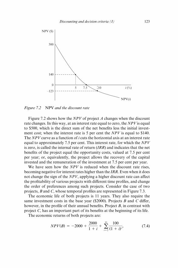
Discounting and decision criteria (I) 123
Figure 7.2 shows how the NPV of project A changes when the discount
rate changes. In this way, at an interest rate equal to zero, the NPV is equal
to $500, which is the direct sum of the net benefi ts less the initial invest-
ment cost; when the interest rate is 5 per cent the NPV is equal to $140.
The NPV curve as a function of i cuts the horizontal axis at an interest rate
equal to approximately 7.5 per cent. This interest rate, for which the NPV
is zero, is called the internal rate of return (IRR) and indicates that the net
benefi ts of the project equal the opportunity costs, valued at 7.5 per cent
per year; or, equivalently, the project allows the recovery of the capital
invested and the remuneration of the investment at 7.5 per cent per year.
We have seen how the NPV is reduced when the discount rate rises,
becoming negative for interest rates higher than the IRR. Even when it does
not change the sign of the NPV, applying a higher discount rate can aff ect
the profi tability of various projects with diff erent time profi les, and change
the order of preferences among such projects. Consider the case of two
projects, B and C, whose temporal profi les are represented in Figure 7.3.
The economic life of both projects is 11 years. They also require the
same investment costs in the base year ($2000). Projects B and C diff er,
however, in the profi le of their annual benefi ts. Project B, in contrast with
project C, has an important part of its benefi ts at the beginning of its life.
The economic returns of both projects are:
NPV(B) 5 22000 12000
1 1 i1 a
11
t52
100
(1 1 i) t, (7.4)
NPV ($)
NPV(i)
i (%)10 7.5 5
140
–123
500
0
Figure 7.2 NPV and the discount rate

124 Introduction to cost–benefi t analysis
NPV(C) 5 22000 1 a9
t51
100
(1 1 i) t1
2000
(1 1 i) 101
2100
(1 1 i) 11. (7.5)
It can be appreciated how the value considered for the interest rate
aff ects the two projects unequally. Suppose that initially the interest rate
is 5 per cent. Applying this discount rate, project C is preferred to project
B since NPV(C/i 5 0.05) 5 1166 and NPV(B/i 5 0.05) 5 640. Both
projects are socially desirable when the interest rate is 5 per cent and there
are no budget constraints because they have an NPV greater than zero.
However, in cases where there are limited funds ($2000), project C would
be preferred to project B.
What happens with a higher discount rate, for example an interest rate
of 10 per cent? The two projects are still profi table, NPV(B/i 5 0.1) 5 377
and NPV(C/i 5 0.1) 5 83, but now project B is preferable to project C.
It is interesting to examine why the selection of projects changes when we
change the interest rate. The rationale is that the profi tability of a project
depends not only on the magnitude of its benefi ts, but also on when they
occur; that is, their location in time. Without discounting, the net benefi ts
of project C are higher than those of B; however they occur later in time.
A high interest rate ‘penalizes’ these benefi ts, indicating that they have less
present value for the individuals because they occur in the future.
The discount factor acts as a weight for the benefi ts and costs over the
life of the project. This weight tends to zero as t increases (provided that
i is greater than zero). The economic rationale is clear: if the interest rate
applicable to the project rises, the opportunity cost of the initial invest-
ment increases and the later the benefi t is realized the lower its present
value is. Figure 7.4 shows how the ranking of two mutually exclusive
projects changes when modifying the interest rates.
As Figure 7.4 shows, the profi tability of a project compared with its
alternative is sensitive to the interest rate. For interest rates between 0 and
–2000 100 1002000
1120 1
Project B
Project C
9 10
–2000 2100
110 1
2000100100
Figure 7.3 Time profi le of projects B and C (values in $)

Discounting and decision criteria (I) 125
approximately 7.9 per cent, C is preferred to B; however, for values of
i > 0.079, the comparative advantage of C disappears. Raising the inter-
est rate has changed the order of preferences of two mutually exclusive
projects.
7.3 THE MECHANICS OF DISCOUNTING: SOME USEFUL FORMULAS
Cost–benefi t analysis is most frequently applied to physical investment
projects that involve some initial years with costs only, and benefi ts and
operating costs when the project is open to public use and until the end of its
life. The evaluation of regulatory measures, or any other public policy that
can sensibly be quantifi ed in economic terms, has an associated fl ow of ben-
efi ts and costs during the T years that have to be added to obtain the NPV.
Year T may not be the last year of the life of the project but its duration
for evaluation purposes. The reason that T can be less than the real life of the
project may be because the regulatory framework so requires, because it is
pertinent to evaluate the period covered by the contract of private participa-
tion or because it is expected that, technologically, T is the maximum length
that can reasonably be considered before technical obsolescence applies.
In any of the above cases it is necessary to calculate the residual value of
the project. This value is the net present value in year T of the benefi ts and
costs of the project until infi nity. This could mean the cost of dismantling
a provisional infrastructure with no further use beyond T; or perhaps the
benefi ts obtained from the future use of the assets and deducting the costs
0 5 10 i (%)
B
C
NPV ($)
3000
10001166
640
377
83
7.9
Figure 7.4 NPV as a function of the interest rate
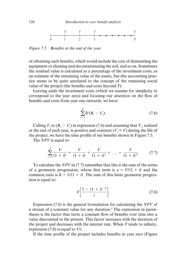
126 Introduction to cost–benefi t analysis
of obtaining such benefi ts, which would include the cost of dismantling the
equipment or cleaning and decontaminating the soil, and so on. Sometimes
the residual value is calculated as a percentage of the investment costs, as
an estimate of the remaining value of the assets, but this accounting prac-
tice seems to be quite unrelated to the concept of the remaining social
value of the project (the benefi ts and costs beyond T).
Leaving aside the investment costs (which we assume for simplicity to
correspond to the year zero) and focusing our attention on the fl ow of
benefi ts and costs from year one onwards, we have:
aT
t51
dt(Bt 2 Ct) . (7.6)
Calling Vt to (Bt 2 Ct) in expression (7.6) and assuming that Vt, realized
at the end of each year, is positive and constant (Vt = V) during the life of
the project, we have the time profi le of net benefi ts shown in Figure 7.5.
The NPV is equal to:
aT
t51
V
(1 1 i) t5
V
(1 1 i)1
V
(1 1 i) 21 . . . 1
V
(1 1 i)T. (7.7)
To calculate the NPV in (7.7) remember that this is the sum of the terms
of a geometric progression, whose fi rst term is a 5 V/ (1 1 i) and the
common ratio is d 5 1/ (1 1 i) . The sum of this fi nite geometric progres-
sion is equal to:
V c 1 2 (1 1 i)2T
id . (7.8)
Expression (7.8) is the general formulation for calculating the NPV of
a stream of a constant value for any duration.4 The expression in paren-
theses is the factor that turns a constant fl ow of benefi ts over time into a
value discounted to the present. This factor increases with the duration of
the project and decreases with the interest rate. When T tends to infi nity,
expression (7.8) is equal to V/i.
If the time profi le of the project includes benefi ts in year zero (Figure
3
V VV V
T20 1
Figure 7.5 Benefi ts at the end of the year

Discounting and decision criteria (I) 127
7.6) we simply have to add V to expression (7.8). Calculating the sum of
the progression of T + 1 terms we obtain expression (7.9).
NPV 5V(1 1 i)
ia1 2
1
(1 1 i)T11b. (7.9)
Expressions (7.8) and (7.9) for the NPV rely on the assumption of con-
stant annual benefi ts. When benefi ts change over time according to a con-
stant average annual rate, both expressions must be corrected. Suppose
that V is a function of GDP and grows at an annual rate equal to q, so that
Vt11 5 Vt(1 1 q) . Now the time profi le is represented by Figure 7.7, and
the equation for the NPV is:
NPV 5V
(1 1 i)1
V(1 1 q)
(1 1 i) 21 . . . 1
V(1 1 q)T21
(1 1 i)T. (7.10)
If q < i, (7.10) is equal to:
NPV 5 V c 1 2 (1 1 q)T (1 1 i)2T
i 2 qd . (7.11)
When T S ∞, if q < i, (1 1 q/1 1 i)T S 0, and thus for a given V in the
fi rst period that grows at a rate q to perpetuity:
NPV 5V
i 2 q. (7.12)
The benefi ts and costs may occur at the end of the year, quarterly or
monthly, or almost continuously, as with the demand for a dam that sup-
plies water without interruption or a road that saves time for a continuous
fl ow of vehicles driving on it since opening up to T.
3
V VV V
T20 1
V
Figure 7.6 Benefi ts in year zero and at the end of the year
3
V (1 + �)V V (1 + �)2 V (1 + �)T – 1
T20 1
Figure 7.7 Benefi ts grow at a constant rate

128 Introduction to cost–benefi t analysis
When benefi ts are produced twice a year, for example, and the annual
discount rate is i, we have the time profi le shown in Figure 7.8.
To discount the benefi ts, we need the semester interest rate is equivalent
to the corresponding annual rate i (or, in general, the interest rate that
matches the corresponding subperiod) for the discounting of the benefi ts
that occur every six months (or in other periods shorter than a year) called
Vs, so we have:
(1 1 is) s 5 (1 1 i) , (7.13)
where s is the number of subperiods (semesters in this case). Solving for is:
is 5 (1 1 i) 1/s 2 1. (7.14)
Given that 1 1 is 5 (1 1 i) 1/s, the discounting for the fi rst four semes-
ters in Figure 7.8 is as follows:
NPV 5Vs
(1 1 i) 0.51
Vs
(1 1 i)1
Vs
(1 1 i) 1.51
Vs
(1 1 i) 2 (7.15)
or
NPV 5Vs
(1 1 is)
1Vs
(1 1 is) 2
1Vs
(1 1 is) 3
1Vs
(1 1 is) 4
. (7.16)
Expression (7.17) generalizes the calculus of the NPV of a stream of ben-
efi ts Vs that occur in periods shorter than a year. It is obtained by replacing
the number of subperiods and the subperiod interest rate obtained accord-
ing to (7.14) in (7.8):
NPV 5 Vs c 1 2 (1 1 is)2Ts
is
d . (7.17)
The discount formulas obtained above are useful for constant fl ows of
benefi ts and costs (Vt 5 V) or those that grow at constant rates (qt 5 q). In
practice this is not often the case, as the annual values do not conform to a
pattern that allows the direct application of the previous expressions.5
It is interesting to note that many projects have annual benefi ts V that
3 T20 1
VsVsVsVsVsVsVs
Figure 7.8 Benefi ts occur more than once a year

Discounting and decision criteria (I) 129
are generated in an almost continuous manner, but they are often treated
as if they occur at the end of year, as in Figure 7.5. Consider the case of an
airport, a dam or a sports centre whose output is produced from 1 January
until 31 December. It seems obvious that if the benefi ts are located at the
end of the year, as happens to be the case, the NPV appears to be lower
(the further in time the benefi ts the lower the present value).
It can be argued that if benefi ts and costs occur every day of the year,
and must be located in an instant of the year, it is more appropriate to
place them in the middle of the year than at the beginning or the end. The
time profi le is shown in Figure 7.9.
The formula for discounting the annual benefi ts located in the middle of
the year, applying the annual discount rate, is as follows:
NPV 5 V c 1 2 (1 1 i)2T
id (1 1 i) 0.5. (7.18)
Expression (7.18) corrects the annual discount formula (7.8) with the
factor (1 1 i) 0.5 in order to place the discounted value at time zero, other-
wise the application of (7.8) would have located it at time ‘−0.5’. Applying
(7.18) we would obtain the same results as applying (7.17) with benefi ts
expressed per day (Vs 5 V/365); that is, the benefi ts are realized daily and
discounted with a daily discount rate that corresponds to the annual rate.
If the project delivers a continuous fl ow from the beginning of the fi rst
year of operation (health service, roads, airports, water supply, etc.), it
seems reasonable in view of these results to place V in the middle of the
year, which is equivalent to treating the benefi ts as if they occur daily or
continuously, but applying an annual discount rate.
7.4 DECISION CRITERIA: THE NET PRESENT VALUE
Accept–Reject
There are several alternative ways to measure the social profi tability of a
project whose benefi ts and costs occur in diff erent years. The most reliable
indicator is the NPV of the fl ow of benefi ts and costs (see Brealey and
Myers, 1996). The NPV summarizes in a single fi gure the social value of
V
3
V V
T20 1
Figure 7.9 Benefi ts in the middle of the year

130 Introduction to cost–benefi t analysis
the project by subtracting the costs (C) from the benefi ts (B), once both
have been discounted with the appropriate discount rate (i). A general
expression is as follows:
NPV 5 B0 2 C0 1B1 2 C1
1 1 i1
B2 2 C2
(1 1 i) 21 . . . 1
BT 2 CT
(1 1 i)T. (7.19)
If expression (7.19) is zero, the project’s present value of benefi ts is equal
to the present value of its costs, which would leave the decision maker indif-
ferent between approving or rejecting the project, because implementing the
project will only allow the reimbursement of the initial investment and the
interest payment, which is what one can obtain by leaving the investment for
the next best alternative. This is the starting point for the fi rst decision rule:
NPV > 0 S accept the project.
NPV < 0 S reject the project.
The economic logic of this decision rule is based on the concept of oppor-
tunity cost. Consider an investment project of $2486.70 that produces
constant benefi ts equal to $1000 during its three years of life. Suppose the
discount rate i is the bank interest rate (10 per cent) at which this investment
would be remunerated if it was not invested in the project. The opportunity
cost of this investment expressed at the end of the third year is:
First year: C0(1 1 i) .
Second year: C0(1 1 i) (1 1 i) 5 C0
(1 1 i) 2.
Third year: C0(1 1 i) 2 (1 1 i) 5 C0
(1 1 i) 3.
An initial fi gure of $2486.70 reaches the value of $3309.80 in the third
year if it is lent to a fi nancial institution. This is the opportunity cost of
investing in the project, the renouncing of receiving $3309.80 in the third
year because of the project. Therefore, if we invest $2486.70 in the project,
we should expect at least $3309.80 in the third year or an equivalent
amount during the lifetime of the project, for example $1000 every year
over the three years.
When we invest $2486.70 in the project and gain $3309.80 in the third
year, the NPV is:
NPV 5 22486.70 13309.80
(1 1 0.1)35 0. (7.20)

Discounting and decision criteria (I) 131
The NPV is zero, indicating that the same payoff is obtained by lending
the money to the bank or investing it in the project. The same happens if
we gain $1000 each year because:
NPV 5 22486.70 11000
(1 1 0.1)1
1000
(1 1 0.1)21
1000
(1 1 0.1)35 0. (7.21)
If by investing $2486.70 in the project we obtain an NPV > 0, the
funds invested in the project generate benefi ts that exceed the opportu-
nity cost, allowing the recovery of the invested funds plus the interest
payment.
When there is uncertainty over the future benefi ts and costs, the invest-
ment is partially or totally irreversible, and it is possible to postpone the
investment decision to acquire more information, Dixit and Pindyck
(1994) point out that the NPV rule can be misleading unless it includes the
opportunity cost of exercising the option to invest. This investment option
is clear in the case of governments that have the property rights for land
and natural resources and the competence to decide on the construction of
projects of general interest now or later in the future.
In these circumstances of irreversibility, uncertainty and the possibility
of postponing, if we invest today we have renounced the value of the infor-
mation that will be revealed in successive periods, including information
that could change the decision to invest, which cannot be altered once the
decision to invest has been taken, given the irreversibility of investment
and hence the unrecoverable nature of the costs (sunk costs). In the next
chapter (section 8.2) we analyse the timing decision, justifying that the
NPV rule is perfectly valid if we include the cost of losing the value of the
information that is revealed by waiting.
Choosing Between Profi table Projects
The NPV rule is not only valid for the acceptance or rejection of a project
that is evaluated individually. The NPV is also the appropriate criterion
to choose between mutually exclusive projects or to select from a group of
projects in a wider range when there is a budget constraint. In this case the
objective is to choose the projects that maximize the NPV.
Table 7.1 illustrates the use of the NPV in contrast with the benefi t/cost
ratio (B/C). The B/C ratio is the fraction of the discounted benefi ts and the
discounted costs, and it is frequently used to present the social profi tability
of projects. In Table 7.1 four projects are ranked according to their B/C. It
can be seen how project E is the one with the highest B/C value (1.5) but G
has the highest NPV value, so the B/C criterion provides a wrong ranking

132 Introduction to cost–benefi t analysis
of the projects in Table 7.1. The lowest benefi t per unit of cost corresponds
to project H, 0.8. One explanation of the rationale for rejecting project
H is because B/C = 0.8 is less than unity and hence for each monetary
unit invested in the project we only recover 0.8, thereby 20 per cent of the
investment is lost.
The NPV rule would have rejected project H because it implies losses
of $240 if it is undertaken. The criterion of accepting the project with
NPV > 0 indicates that the profi table projects are E, F and G, all of them
with a B/C greater than 1.
A pervasive characteristic of the real world is the presence of budget
constraints; there are more projects with an NPV > 0, or B/C > 1, than
funds available and public agencies are forced to choose between the set
of profi table projects, a subset that simultaneously ensures the maximum
social welfare and satisfi es the budget constraint.
Consider that the budget constraint is $800. In this case we choose
projects E and F, and the total NPV is $280. The ranking of projects by
the indicator B/C leads to the same selection. Suppose now that the budget
is extended to $1600. In this case the projects that allow a higher overall
NPV ($430) are F and G; and E, the one with the higher B/C, is outside
the subset.
An additional problem with the use of B/C as an indicator of project
profi tability is that it is sensitive to the way the benefi ts and costs are com-
puted, unlike the NPV, which produces the same result whether the costs
are defi ned as costs or as negative benefi ts.
Take for example project E of Table 7.1 and suppose that it is composed
of two periods – the year zero, in which the investment is materialized, and
the year one – and a 10 per cent discount rate. Consider two alternatives
compatible with an NPV of $100.
NPV 5 2200 1330
1 1 i5 100, (7.22)
NPV 5 2100 1330 2 110
1 1 i5 100. (7.23)
Table 7.1 Indicators for project selection (discounted values in $)
Project Benefi ts Costs NPV Benefi ts/Costs
E 300 200 100 1.50
F 780 600 180 1.30
G 1250 1000 250 1.25
H 960 1200 –240 0.80

Discounting and decision criteria (I) 133
In the fi rst alternative the ratio B/C is equal to 1.5, as shown in Table
7.1. In the second it depends on how we defi ne the costs. If the costs are
defi ned as such, the value of $110 is a discounted cost with a value of 100,
and B/C is equal to 1.5. However, if the cost is treated as a negative benefi t
(e.g. an aggregation of winners and losers is equal to $220), the B/C would
be equal to two. Note that the NPV is $100 in both cases.
Although there may be situations in which the NPV is not an immediate
criterion, for example when comparing projects of diff erent durations that
solve a common problem (see section 8.2), the NPV is widely considered
the most reliable criterion, and the only recommendation is to avoid its
mechanical use without thinking about the characteristics of the projects
that we wish to compare.
The Internal Rate of Return (IRR)
Another indicator is the IRR, which consists of fi nding the value of i that
makes the NPV equal to zero. The IRR is thus the highest discount rate
that leaves the project on the border of profi tability (see Figure 7.2). The
more profi table the project is, the greater the range of values of i with a
positive NPV.
The decision rule is:
IRR > discount rate S accept the project
IRR < discount rate S reject the project
Going back to Figure 7.2 it can be seen how the NPV and the interest
rate are inversely related. If we conveniently increase i, a value of i* for
which the NPV becomes zero is reached (i* = 7.5 per cent). This is the IRR
and the decision rule is to accept the project if i* is higher than the interest
rate, and to reject it otherwise.
The IRR also has some problems, since there may be more than one
value of i that makes the NPV equal to zero. This can happen if during the
life of the project net benefi ts change the sign. Moreover it is not always
the highest IRR project that has the greatest NPV.
THINGS TO REMEMBER
Benefi ts and costs occur at diff erent moments during the lifetime ●
of the project. There are projects with a lifespan of 40 years and
others whose eff ects, in practical terms, can last forever. People are
134 Introduction to cost–benefi t analysis
not indiff erent with respect to when benefi ts and costs happen and
usually prefer a unit of benefi t today rather than tomorrow.
If people discount the future we need a method to homogenize the ●
fl ow of benefi ts and costs. Exponential discounting is the common
procedure to express all the future benefi ts and costs in present
terms. The logic of compounding interest is the rationale behind
exponential discounting. If $1 has a value of (1 + i) next year, the
present value of $1 next year equals 1/(1 + i), where i is the interest
rate.
The net present value of a project is the main economic indicator to ●
express the social value of a project. It consists of the sum of all the
discounted benefi ts and costs of the project and hence the election of
a value for the discount rate is crucial in the calculation of the NPV.
There are other decision criteria such as the benefi t/cost ratio or the
internal rate of return. The NPV is the most reliable.
NOTES
1. The project life is determined by the evaluating agency. It may or not coincide with the physical life, but it generally coincides with the estimated economic life, which is usually shorter than the physical life. In the case of a longer lifespan than the period chosen for evaluation we need to include the residual value.
2. It should be noted that the basic rule of decision based on the NPV without further qualifi cation requires the investment to be reversible; that is, if the annual benefi ts are not the expected ones the investment can be recovered; or even if it is irreversible the invest-ment decision cannot be postponed (‘now or never’). If investment is irreversible, there is uncertainty of demand and it is possible to postpone the investment, when calculat-ing the NPV the opportunity cost of killing the option to invest should be included (see section 8.2).
3. Between zero and one, 365 days have passed, so in fact zero and one are moments in time and the year is the interval. For simplicity we refer to the points zero, one, two, etc. in Figure 7.1, and the like, as year zero, year one, year two, etc.
4. Assuming benefi ts start in year one. This formula allows us, solving for V, to calculate the annual value that corresponds to the present value of an asset or a fi xed cost that must be annualized: V 5 NPV ( (1 1 i) Ti) / ( (1 1 i) T 2 1).
5. Spreadsheets have available the NPV and IRR in the menu of formulas.

135
8. Discounting and decision criteria (II)
Should Americans work harder and invest more to increase industrial production? The economist’s answer is, only if it makes them happier. Newscasters report economic growth as if it were a benefi t with no off setting cost. Growth does benefi t individuals, because it allows them to increase their consumption in the future. The conditions that create growth impose costs on individuals, who must work harder and consume less in the present. Is this trade- off worth it? The answer depends solely on the preferences of the individuals themselves.
(Steven E. Landsburg, 1993, p. 101)
8.1 INTRODUCTION
The option accept–reject is the simplest situation we may face when evalu-
ating a project and the sign of the net present value (NPV) is enough to
make the decision. In other cases we have to choose between diff erent
projects, with a positive NPV, that are not comparable because of their
scale or duration. At other times the NPV is positive, but is higher in an
alternative project that consists of delaying the project. In section 8.2 we
discuss the decision criteria when one has to choose between mutually
exclusive projects with diff erent lifespans and, fi nally, when the decision
can be postponed; that is, it is not a ‘now or never’ proposition, and we
need to check the optimal timing.
The social discount rate is a key parameter for the economic evalua-
tion of projects. It determines in many circumstances whether a project
is socially worthy, which means that it is desirable to renounce a certain
amount of present consumption for the reward of future goods. In section
8.3 we review the concepts of marginal rate of time preference, marginal
productivity of capital and interest rate. In perfect capital markets the
social discount rate is easy to determine because the three rates are equal.
With distortions, like taxes on savings and investment returns, the inter-
est rate is no longer the same as the marginal rate of time preference, and
the marginal productivity of capital, hence in section 8.4 we discuss how
to calculate the social discount rate in these conditions. Finally, in section
8.5, we address the problem of discounting when future generations are
involved.
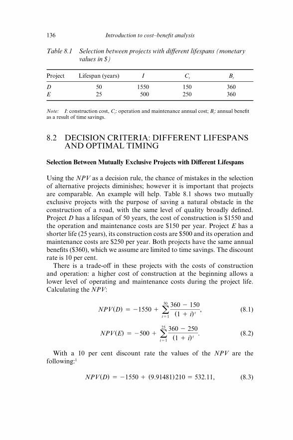
136 Introduction to cost–benefi t analysis
8.2 DECISION CRITERIA: DIFFERENT LIFESPANS AND OPTIMAL TIMING
Selection Between Mutually Exclusive Projects with Diff erent Lifespans
Using the NPV as a decision rule, the chance of mistakes in the selection
of alternative projects diminishes; however it is important that projects
are comparable. An example will help. Table 8.1 shows two mutually
exclusive projects with the purpose of saving a natural obstacle in the
construction of a road, with the same level of quality broadly defi ned.
Project D has a lifespan of 50 years, the cost of construction is $1550 and
the operation and maintenance costs are $150 per year. Project E has a
shorter life (25 years), its construction costs are $500 and its operation and
maintenance costs are $250 per year. Both projects have the same annual
benefi ts ($360), which we assume are limited to time savings. The discount
rate is 10 per cent.
There is a trade- off in these projects with the costs of construction
and operation: a higher cost of construction at the beginning allows a
lower level of operating and maintenance costs during the project life.
Calculating the NPV:
NPV(D) 5 21550 1 a50
t51
360 2 150
(1 1 i) t, (8.1)
NPV(E) 5 2500 1 a25
t51
360 2 250
(1 1 i) t. (8.2)
With a 10 per cent discount rate the values of the NPV are the
following:1
NPV(D) 5 21550 1 (9.91481)210 5 532.11, (8.3)
Table 8.1 Selection between projects with diff erent lifespans (monetary
values in $)
Project Lifespan (years) I Ct Bt
D 50 1550 150 360
E 25 500 250 360
Note: I: construction cost, Ct: operation and maintenance annual cost; Bt: annual benefi t as a result of time savings.
Discounting and decision criteria (II) 137
NPV(E) 5 2500 1 (9.07704)110 5 498.47. (8.4)
One might think that project D is better than project E because its NPV
is higher; however the projects are not strictly comparable because, while
resolving a problem with the same degree of eff ectiveness, project D does
so for 50 years and project E for 25.
The comparison of the two projects requires a previous process of
homogenization. Two procedures to make the projects comparable are as
follows. The fi rst is based on considering an imaginary project that con-
sists of constructing E twice to resolve the problem for the same time inter-
val as project D. From (8.4) we know that the net present value of project
E equals $498.47. An identical project E is constructed at the beginning of
year 26 and the fl ow of net benefi ts lasts from year 26 to year 50. The NPV
of this identical project is $498.47 but situated at the end of year 25 (or at
the beginning of year 26), so to obtain the present value of the NPV in year
25 we need to divide by (1 1 i) 25.
NPV(2E) 5 498.47 1498.47
(1 1 i) 25. (8.5)
For a period of 25 years and a 10 per cent discount rate, the discount
factor is equal to 0.09230, therefore:
NPV (2E) = 498.47 + (0.0923)498.47 = 544.48. (8.6)
This result shows that it is more profi table to choose alternative E,
which will be repeated at the end of its useful life.
The other procedure is to calculate the equivalent annual net benefi ts (B̂ ),
which consists of calculating the average annual benefi t, which, multiplied
by factor S (see Note 1) corresponding to the lifespan and the discount
rate, is equal to the NPV of the project:
NPV 5 SB̂ . (8.7)
Solving for B̂ , we obtain the equivalent annual net benefi t:
B̂ 5NPV
S. (8.8)
The value of B̂ for project D is equal to $53.668 and for project E is
equal to $54.916, so project E is preferable to project D, despite having a
smaller NPV.

138 Introduction to cost–benefi t analysis
To Invest or to Wait: When Postponing is Profi table
When the fl ows of benefi ts and costs of a project are discounted, and
they are compared with the initial investment, we obtain the NPV of
the project as a single fi gure that indicates, if positive, that the project is
socially worthy. Claiming that the project has a positive NPV in the base
year does not mean that the project should be started. Let us consider two
possibilities.
When additional information is not revealed by waiting
Sometimes the comparison between projects consists of checking whether
it is more profi table to start today or to wait until next year. There may
be many circumstances in a certain world that make it sensible to post-
pone the project, when this is technically feasible. Perhaps the demand
is growing and the social benefi ts derived from attending to the demand
in the fi rst year do not off set the opportunity cost of the required funds.
Suppose that the project involves an initial investment equal to I and
annual net benefi ts equal to Bt. Postponing the project by one year is
profi table if:
iI
1 1 i1
BT11
(1 1 i)T11.
B1
1 1 i. (8.9)
The strict inequality in (8.9) reports, in the left hand side, the present
value of the benefi t of postponing the project by one year, and con-
sists of the interest payment on the investment cost multiplied by the
discount actor (1/(1 + i)) and the benefi ts obtained in period T + 1 as
a result of starting the project a year later. The right hand side repre-
sents the discounted lost benefi t in year one because of postponing the
project.
Assuming that the benefi t in the year T + 1 is not signifi cant, we can
simplify expression (8.9) to:
i .B1
I, (8.10)
where B1/I is the rate of return on investment in the fi rst year. If the
discount rate is higher than the fi rst year rate of return investing in the
project, waiting is preferable.
When delaying the project reveals additional information
When the investment is irreversible, there is uncertainty about the social
benefi ts generated by the project during its lifetime and it is possible

Discounting and decision criteria (II) 139
to postpone the project, the alternative of delaying cannot be ignored
without aff ecting the standard NPV as a decision criterion.
If delaying the project reveals valuable information on the annual net
benefi ts, the economic value of that information is lost when the investment
is made. Under the described conditions (i.e. irreversibility, uncertainty
and the possibility of delay) there is an opportunity cost of undertaking
the investment in the present. Investing today will imply the loss of the
economic value of the information revealed by waiting, and therefore it
should be included as a cost. The NPV rule is still valid if the mentioned
opportunity cost is included as a cost when calculating the NPV.2
What is the cost of losing this information by investing now? It is the
amount the investor (assume it is risk neutral) would be willing to pay to
have the option of fl exibility. We calculate the NPV by investing in period
zero, then we calculate it again but delaying the project, and the diff erence
is the value that is lost if we do not wait and therefore the cost of investing
now.
The above reasoning to calculate the cost of investing now can be
presented more intuitively in the cost–benefi t analysis framework. The
problem could be presented as the decision between two mutually exclu-
sive projects: one consisting of investing now, and the other one delaying
the investment. We only have to calculate the NPV of both projects and
choose the one with a higher NPV.
An example may help us to understand the signifi cance of considering
the option of waiting as an alternative. The project represented in Figure
8.1 shows an investment in port infrastructure for trans- shipment con-
tainer traffi c.
The project requires an investment of $2200 in the base year. The social
benefi ts in year one are $150. In the second year, depending on the decision
of a shipping company to sign a long term contract with the port or with a
competing port, the benefi ts go up $200 or down $100 with equal probabil-
ity and forever (T S ̀ ). The decision of the shipping company is known at
the beginning of year two. The social rate of discount is 5 per cent.
We face an irreversible investment, there is demand uncertainty and the
100
200200200
150–2200
T2
0 1
3
100 100
Figure 8.1 Example: A project with demand uncertainty

140 Introduction to cost–benefi t analysis
investment decision may be postponed to learn the decision of the ship-
ping company. We assume there is no strategic action that may aff ect the
decision of the shipping company, or other additional benefi ts or social
costs than those already described.
The expected NPV of this investment project is as follows:
E(NPV) 5 22200 1150
1 1 i1 a
`
t52
100 # (0.5) 1 200 # (0.5)
(1 1 i) t5 800.
(8.11)
As indicated, once the investment has been made and after the fi rst year
(with certain benefi ts of $150), the benefi ts in the rest of the years may
increase to $200 or decrease to $100 with equal probability, depending on
the decision of the shipping company.
Therefore, the NPV of the project if the company does not sign the con-
tract, given that the life of the project is infi nite, is:
NPV(no contract) 5 22200 1150
1 1 i1 a
`
t52
100
(1 1 i) t5 2152. (8.12)
Alternatively, in the event that the shipping company signs the contract:
NPV(contract) 5 22200 1150
1 1 i1 a
`
t52
200
(1 1 i) t5 1752. (8.13)
These results show that the investment will lead to a loss of $152 or a
benefi t of $1752 with the same probability (i.e. 0.5). Therefore the expected
NPV is equal to 2152 # (0.5) 1 1752 # (0.5) 5 800, a result that we had
already obtained in (8.11). If the agent who takes the decision is risk
neutral, the project is accepted.
It is worth pointing out that postponing this project by one year would
not be profi table if the information revealed in year two is not taken
into account, as the benefi ts of the fi rst year are higher than the interest
rate multiplied by the investment (see (8.10)). Therefore apparently there
are no gains obtained by waiting. In reality, however, delaying not only
implies losing the benefi t of the fi rst year and saving the opportunity cost
of the money invested (refl ected in the discount rate), there is also an
additional benefi t that comes from the valuable information revealed by
waiting.
When the project is delayed by one year we lose the benefi ts of the fi rst
year, but we now know whether the shipping company will sign the con-
tract or not. Therefore we know whether the yearly benefi ts are $100 or
$200 from year two onwards.

Discounting and decision criteria (II) 141
Consider an alternative project consisting of not investing in the
present and waiting a year. Once the expected NPV has been calculated,
compare this value with the expected NPV of investing now, and then
choose the option with the highest expected NPV. If by waiting we know
that the company is not going to sign the contract and therefore the
benefi ts are equal to $100, the best option is not to invest and because
of this decision the negative NPV in (8.12) is avoided, so the NPV is in
this case zero.
As this result (NPV = 0) can occur with equal probability to the contract
being signed and the annual benefi ts being equal to $200, the expected
NPV of delaying is:
E(NPV) (delaying) 51
2a22200
1 1 i1 a
`
t52
200
(1 1 i) tb 5 857. (8.14)
Comparing the expected NPV of investing now ($800) with the expected
NPV of postponing the investment one year ($857), the decision is to delay
the project, and after waiting a year, build only if the shipping company
chooses to operate in the port. The willingness to pay to maintain the
option to invest (i.e. to have the fl exibility of choosing at the start of the
investment) is the diff erence between (8.14) and (8.11).
It is interesting to note that the expected NPV of investing in the present
is positive and therefore the project would be approved if the investment
is of the ‘now or never’ type. Even waiting a year would not be profi table
when no additional information is revealed. However, if the option to
wait is feasible, we may think of it as if there is another project consisting
of waiting, that we must compare with the project of investing now. The
decision in the previous example is to wait.
The conventional NPV rule is still valid if the issue is addressed as
the choice between two mutually exclusive projects – one investing now;
another one, waiting one year – since otherwise the mechanical application
of the NPV rule would lead to misleading conclusions.
Using the NPV rule as a decision criterion is useful in contexts similar to
those described in this example, provided that the cost of investing in the
present includes the opportunity cost of not waiting, or that the option to
wait is defi ned as an alternative to investing now, and comparing the NPV
of both projects.
Finally it should be emphasized that in the previous discussion we have
assumed that the investor is risk neutral. If instead the investor is risk
averse, the comparison between investing now and waiting introduces
a new element of variability in the outcome that aff ects the decision:
by investing now, the outcome is a loss (−$152) or benefi ts ($1752); by
142 Introduction to cost–benefi t analysis
waiting one year the possibilities are quite diff erent when the project is
rejected (zero benefi ts) or when it is accepted ($1714).3
8.3 THE MARGINAL RATE OF TIME PREFERENCE AND THE MARGINAL PRODUCTIVITY OF CAPITAL
The economic analysis of the intertemporal choice that individuals make
between present consumption and future consumption helps us to under-
stand the problem of the choice of the social rate of discount. Although
it is possible that the present consumption (x0) and future consumption
(x1) are perfect substitutes for some individuals, it is more likely that the
trade- off s happen at rates changing according to the endowment of both
goods that the individual has at the time of making a choice. The higher x0
is with respect to x1, the more willing the individual will be to give up x0 by
an additional unit of x1.
The compensation the individual requires in excess of a unit of future
consumption in exchange for giving up a unit of consumption today is
called the marginal rate of time preference (x). Therefore the individual
is indiff erent between a unit of x0 and (1 + x) of x1. However the market
compensates the individual with a return that does not necessarily coincide
with x. The rate that indicates what the individual receives is the interest
rate (i) that represents the additional amount that is obtained on a unit in
the future if we give up a unit in the present.
Both x and i may be negative: x is negative in cases where the individual
has a very high initial endowment of present consumption compared with
future consumption, and is willing to give up a unit of x0 in exchange, for
example, for 0.9 units of x1 (x = −0.1). It can also be negative in the case
of individuals whose future is uncertain in terms of the income they expect
to receive or their health status. A negative interest rate is possible if the
nominal interest rate is close to the rate of infl ation and there are taxes on
the interest payment of fi nancial assets.
A third rate in the analysis of intertemporal decisions is the marginal
productivity of capital or the internal rate of return on investment (r),
which indicates what the individual receives as a return if he invests
one unit in productive projects. Ignoring the existence of taxes and
uncertainty, if r is greater than i, investing in a project is attractive
because it yields higher returns than putting the money in the bank.
Assume that all the projects are ordered from the most to the least
profi table. The individual will undertake all the productive investment
projects that satisfy r > i until in the last project he is indiff erent

Discounting and decision criteria (II) 143
between investing in the project and putting the money in the bank
(r = i).
An individual who allocates his funds according to this criterion maxi-
mizes the present value of his wealth; and once the NPV is the maximum pos-
sible, he take his consumption choices between present and future according
to his marginal rate of time preference. If x < i he will lend money to the bank
and if x > i he will borrow. In equilibrium the three rates are equal.
The equality (r = i = x) means that the marginal rate of time preference
is equal to the rate of marginal productivity of capital and the interest
rate. This result shows that all the investment projects that off ered higher
profi tability than the individual was willing to sacrifi ce in terms of present
consumption have been carried out. This is so because the existence of a
perfect capital market discourages one from investing in his own projects
with lower profi tability than other investment projects available in the
economy, whose profi tability is represented by the market interest rate.
An investment project or a public policy means, in many cases, compro-
mising public funds obtained from the private sector with the purpose of
fi nancing projects decided by the government that are expected to increase
social welfare. The use of these public funds to fi nance projects has an
opportunity cost. Assuming that these projects are funded with taxpayers’
money, they have given up consumption or investment, which was left
without funding because the public sector has absorbed those funds.
We have seen how the interest rate, the marginal rate of time prefer-
ence and the marginal productivity of capital coincide when there are no
restrictions on the fi nancial markets, no taxes and no distortions in the
production or consumption that prevent the achievement of the equality
of the three rates.
Figure 8.2 represents the capital market in an economy without distor-
tions. The interest rate i is the opportunity cost of capital for the fi nancing
of projects. At i0 the curves of demand and supply of the available funds
(K) intersect. The demand curve D represents the investment options in the
economy, investment opportunities with declining marginal productivity.
When the interest rate falls, new projects turn out to be profi table in the
private sector because the internal rates of return of these projects are now
higher than the cost of fi nancing (interest rate).
The supply of available funds (S), savings, increases with the interest
rate, indicating that as i increases, individuals are willing to substitute
more future consumption for present consumption. The value of S at the
interest rate i0 is the marginal rate of time preference; at the interest rate
level i0 savings are equal to K0, with no more individuals willing to give up
present consumption for future consumption at this interest rate.
Let us see what happens with a volume of available funds K*, where

144 Introduction to cost–benefi t analysis
the marginal rate of time preference (x*) is less than the marginal rate of
return on capital (r*). In this disequilibrium case there are some projects
that produce higher returns than lenders require to give up present con-
sumption. It is socially desirable to transfer funds from lenders to inves-
tors, and this is what will happen in the capital market if there are no
distortions that prevent it.
For the level of investment K0 there is no investment project whose
internal rate of return is less than the rate of time preference. Then it
makes no sense to invest in public projects that do not achieve a return
equal to i0 (remember that there are no distortions such as externalities
or taxes). If the public agency decides to invest in projects with a rate of
return lower than i0, the social welfare decreases, as present consumption
will be replaced by future consumption at a suboptimal rate. It can be con-
cluded therefore that, under the conditions described above, the marginal
rate of time preference equals the social discount rate and the interest rate
(i = x = r).
8.4 THE SOCIAL RATE OF DISCOUNT AND THE RATE OF INTEREST
Figure 8.3 represents a capital market with distortions caused by taxes
on savings and corporate profi ts. The supply curve S shifts upwards, S*
being the function that represents the interest rates required for diff erent
amounts of savings. The height of the shift is the tax, which is assumed
�*
K* K0
D
0
i0
i
K
S
r*
Figure 8.2 The market for available funds

Discounting and decision criteria (II) 145
to be constant per unit of returns on savings. Similarly the investment
demand function shifts to the left and downward in the amount of the
unitary tax on profi ts, refl ecting the fact that the internal rate of return on
investment has declined for all the projects.
The new equilibrium interest rate can be equal to (as in Figure 8.3 for
convenience), greater than or less than the one in a market without restric-
tions, depending on the elasticities of supply and demand. The amount
of investment Kb is clearly lower than K0, because of the higher cost of
borrowing and the lower returns on investment. The social discount rate
in a capital market without distortions is equal to the market interest rate
because i 5 x 5 r, while in the most realistic case represented in Figure 8.3
i 2 x 2 r. The question is which of the three rates should be used as the
social rate of discount.
If the project is fi nanced with savings of the consumers, the social dis-
count rate is id, which is the marginal social rate of time preference, lower
than the market interest rate as represented in Figure 8.3; on the contrary,
if the project is fi nanced with funds displaced from private investment
projects, we have to use the social rate of discount ie, higher than the
market interest rate, as this marginal rate of return on capital is what is
being obtained from the displaced projects in the private sector of the
economy.
It is convenient to distinguish two diff erent situations: fi rst when the
public sector competes with the private sector to implement a specifi c
investment project (in this case the marginal rate of return on capital
d
Kb K0
D
0
i0
i
Se
D*
S*
ie
ab
id
Figure 8.3 Determination of the social rate of discount

146 Introduction to cost–benefi t analysis
should be used as the social rate of discount); and second when we evalu-
ate projects within the public sector, discussed below.
When the project receives funding from several sources, one way to fi nd
the social rate of discount is to fi nd a weighted average of the marginal
rate of time preference (x) and the marginal rate of return on capital (r).
Thus the social rate of discount is equal to ar 1 (1 2 a)x, where a is the
proportion of funds obtained by the displacement of private investment
and (1 − a) the proportion of funds that come from shifting consumption.
The calculus of the social discount rate as the weighted average of both
rates requires information on the source of investment funds (Harberger,
1976).
The economic criticism of this approach leads to a more complicated
alternative. The methodology proposed as an alternative to the weighted
average of Harberger4 is the discounting of the fl ow of benefi ts and costs
using the marginal social rate of time preference as the social discount
rate, but having previously converted the fl ow of net benefi ts into a fl ow
of consumption, using the shadow price of capital. For example if in the
private sector the marginal rate of return on capital before taxes is 20 per
cent and the marginal social rate of time preference is 5 per cent, in the
margin, an additional investment unit is four times more valuable than a
unit of consumption.
The society is investing below the optimum (Kb < K0 in Figure 8.3) and
therefore the fl ow of benefi ts is corrected depending on its destination
(consumption or investment). If funds are reinvested, they will be multi-
plied by the shadow price (in our example, r/ x = 4) and then they will be
discounted with the marginal social rate of time preference. Another way
to see the logic of this procedure is as follows: in year t if the benefi ts V
are wholly reinvested, each subsequent year we obtain rV of return in con-
sumption and reinvest V, so rV in perpetuity is equal to rV / x, which will
be discounted by multiplying by 1/(1 + x)t.
This procedure is more complicated because of the information that
is required on the destination of the benefi ts throughout the life of the
project. For this reason, in the practice of economic evaluation, practition-
ers frequently choose more pragmatic approaches consisting of using, for
example, the interest rate of long term treasury bonds in the belief that in
the private sector no investment will be undertaken with a lower marginal
return.
However we must not forget that when there are taxes on profi ts, mar-
ginal rates of return on investment are greater than the interest rate; and in
the case of taxes on funds supplied by savers who do not displace private
projects, it is possible to fi nd very low marginal rates of time preference.
In this and the previous chapter we have seen the consequences of the

Discounting and decision criteria (II) 147
value of the social discount rate in the allocation of consumption between
the present and the future. Based on the empirical evidence,5 a social time
preference rate in the 3–5 per cent range seems appropriate. These rates
are considerably lower than the 6–8 per cent recommended in the recent
past in the EU and the US, and it is convenient to have in mind that these
rates are risk free, so it is assumed that the fl ows of benefi ts and costs are
expressed in certain equivalents. In practical terms, a reasonable course
of action may be to work with the lower and upper bounds and to see the
sensitivity of the project’s social profi tability.
8.5 INTERGENERATIONAL DISCOUNT
The conversion of future benefi ts and costs to present values, according
to the traditional procedure based on the logic of compound interest, pro-
duces results in which the distant future does not apply unless the discount
rate is very low. When the future is defi ned within the coordinates of the
private sector, 20 or 30 years is regarded as the very long term. In the evo-
lution of species, 300 years is an insignifi cant period.
Exponential discounting is appropriate for projects or policies that
aff ect the same individuals at diff erent time periods. Many public projects
with a lifespan of 20 or 30 years can be evaluated with the usual discount
approach of the fi nancial analysis. The problem arises when investment
projects or policies that aff ect the stock of natural resources have a posi-
tive or negative impact on the welfare of future generations.6 Should the
costs and benefi ts of future generations be discounted?
Applying the method of exponential discount the distant future becomes
irrelevant for relatively low interest rates. The present value (assuming
zero infl ation) of benefi ts (or costs) of $100 million that occur within 300
years is $2.60 if discounted at 6 per cent (a rate frequently used in the
last decade). The benefi ts of preserving some species or preventing global
warming are very low if they are discounted with the same discount rates
as short term actions. With the above fi gures, it would not be profi table to
invest $3 today at a 6 per cent discount rate to avoid a loss of $100 million
within 300 years.7
In the case of the energy policy, the choice of discount rate is criti-
cal. If we want to have alternative sources of energy available for future
generations we must begin to investigate this in the present. The research
and development costs are very high and the expected benefi ts are distant
in time, therefore by applying a high discount rate it may become an
unprofi table R&D policy in sustainable energies (Lind, 1982).
The same argument applies to nuclear power, which produces immediate

148 Introduction to cost–benefi t analysis
benefi ts (cheap energy) but social costs that may occur hundreds of years
later. In this case many fi nd it morally unacceptable to apply a discount
rate that renders negligible the costs associated with exposure to radiation
that may be suff ered by future generations. In contrast, an argument in
favour of discounting the benefi ts of future generations is the possibility of
per capita income continuing its past growth rate. If future generations are
much wealthier than we are, to what extent is the sacrifi ce of the present
generation justifi ed? Nevertheless, this argument does not seem to apply to
serious irreversible damages.
Another view of this issue is that discounting fl ows of benefi ts and costs
of future generations is fundamentally an ethical problem, and so it might
be adequate to separate the discounting of the benefi ts and costs that occur
in diff erent periods of time with issues of intergenerational equity. This
position suggests that the problem is not the choice of the value of the
discount rate, but the state of the stock of natural resources that we must
leave in the best possible conditions to future generations. In this view the
debate over the use of natural resources would take place in the context of
sustainable development (Heal, 1997).
Criticism of exponential discounting in projects with very long term
eff ects is not exclusively based on ethical arguments. The evidence on the
preferences of individuals with regard to the trade- off between present and
future consumption shows the existence of a wide range of discount rates.
Two interesting lines of work are those described below. Both are based
on the preferences stated by individuals when they are interviewed about
their intertemporal preferences in the long term. Both lead to the conclu-
sion that future benefi ts and costs should count.
Based on the stated preferences in interviews with 3200 households with
respect to the implicit discounting of deaths avoided at various future
dates, Cropper et al. (1992) concluded that, although the respondents give
more value to lives saved in the present than in the future, the implied
discount rate in accordance with their responses is not constant. Instead
of the exponential discounting, a hyperbolic discount factor fi ts the pref-
erences stated by individuals subject to the dilemma between lives saved
in the present and in the future. The results of the work of Cropper et al.
are:
A high proportion of respondents would not accept life- saving pro- ●
grammes in the future at the expense of giving up programmes that
save lives in the present, even if the number of lives saved in the future
is 50 times larger. The reason why many of the respondents always
preferred to save lives in the present lies in the belief that society would
fi nd other means of saving those lives in the future (hence they did not
Discounting and decision criteria (II) 149
accept the alternative suggested in the survey). The other reasons are
because this will protect them and their loved ones, and programmes
of the future (especially those in 100 years time) will not.
The implicit discount rates obtained are signifi cantly higher than ●
zero, even at horizons as far as 100 years. Although individuals
discounted the future, they did not do so at a constant exponential
discount rate. The discount rates are much higher for short time
horizons than for distant horizons, and there is considerable hetero-
geneity of discount rates. The standard deviation of the distribution
of discount rates is approximately equal to the average of all the
time horizons.
Information from the survey indicates therefore that individuals use dif-
ferent discount rates depending on the trade- off proposed between present
and future. The pattern that seems to follow the discount rate over time is
that of a convex curve with a negative slope.8
Hyperbolic discounting has been criticized because it implies inconsist-
ent intertemporal preferences as individuals change their discount rate
when situated in diff erent years, which is not the case with exponential
discounting. This being true, these discount rates appear to conform to the
stated preferences of individuals subjected to hypothetical choices between
present and future.
Another contribution regarding the determination of the social discount
rate is called gamma discount and its rationale is as follows (Weitzman,
2001): from 2000 interviews with economists from 48 diff erent countries,
and from the values of their responses on the type of discount, Weitzman
obtained the distribution of discount rates, which ranged from zero to a
maximum of 20 per cent. The distribution is of type gamma with higher
frequencies between 3 per cent and 5 per cent, and a long tail on the right
with very low frequencies.
Weitzman noted the error of averaging from the distribution of indi-
vidual rates in order to obtain the social rate of discount. We must average
discount factors, not discount rates. Let us see the logic of this proposal
with an example. Consider a project that consists exclusively of future ben-
efi ts of $100 million within 300 years. If the discount rate is 1 per cent the
present value of these benefi ts is equal to $5,053,449. If the discount rate
is 10 per cent, the present value is practically zero ($0.00004). In addition
to showing the eff ects of exponential discounting on future benefi ts, this
example illustrates the eff ect of averaging the interest rates instead of the
discount factors.
Suppose that the economy is composed of two individuals, A and B,
with discount rates of 1 per cent and 10 per cent respectively, and that the

150 Introduction to cost–benefi t analysis
government uses, as a social discount rate, the average for discounting the
benefi ts of $100 million in 300 years. If we apply the average rate of the
two individual discount rates (5.5 per cent), the result is a present value
of $10.60, which does not seem reasonable given that individual A values
the $100 million as $5 million in the present and individual B gives a value
close to zero. The average of these two values is $2.5 million, a fi gure signif-
icantly higher than the $10.60 that results from applying the average rate.
The key is that we cannot average rates but discount factors. If we cal-
culate the implicit discount rate, which is to convert $100 million received
within 300 years into $2.5 million in the present, we obtain a discount rate
of 1.2 per cent, very close to 1 per cent, the minimum value of the distribu-
tion of types (see Table 8.2).
Table 8.2 shows how, in the early years, the outcome of averaging the
discount rates does not produce very diff erent results compared with the
average of discount factors. However, in a relatively close time horizon
of 30 years, using the average of the discount factors implies doubling
the benefi ts that result from applying an average discount rate. It can be
seen how the implicit discount rate, which is the average of the present
values that both individuals attach to $100 million, decreases with time,
approaching the lowest value in the range of discount rates.
THINGS TO REMEMBER
A positive ● NPV is a necessary condition for the approval of a
project. When projects are mutually exclusive the use of the NPV
Table 8.2 Discount rates and discount factors (present value of $100 million
received at diff erent times, discounted at 1%, 10%, the average of
the discount rates and the average of the discount factors)
Year 1% 10% Average of
rates
Average of
factors
Implicit rate
(%)
5 95 146 569 62 092 132 76 513 435 78 619 351 4.92866
10 90 528 695 38 554 329 58 543 058 64 541 512 4.47589
20 81 954 447 14 864 363 34 272 896 48 409 405 3.69397
30 74 192 292 5 730 855 20 064 402 39 961 574 3.10473
50 60 803 882 851 855 6 876 652 30 827 869 2.38142
100 36 971 121 7 257 472 883 18 489 189 1.70231
200 13 668 638 0.5 2 236 6 834 319 1.35065
300 5 053 449 0.0 10.6 2 526 724 1.23363

Discounting and decision criteria (II) 151
requires a homogenization of projects. Moreover a positive NPV
requires us to examine the optimal timing of the project. Postponing
the project may be socially profi table.
The marginal rate of time preference, the marginal productivity of ●
capital and the interest rate are not equal unless very unlikely cir-
cumstances occur. Hence the selection of the social discount rate is
diffi cult and controversial. The practitioner takes the discount rate
as a parameter given by the government, and can introduce several
plausible values to see how sensitive the results are with respect to
changes in the discount rate.
It is not clear whether exponential discounting is appropriate for ●
dealing with benefi ts and costs aff ecting future generations. Many
argue that exponential discounting gives too little value to the future
and hence it does not refl ect individuals’ preferences, but if future
generations are expected to be signifi cantly wealthier than we are the
case for discounting is stronger. The use of lower rates of discount
for environmental impacts or life savings is already being introduced
in conventional cost–benefi t analysis.
NOTES
1. The discounted sum (S) of a unit of net benefi t during T years is S 5 (1 2 (1 1 i) 2T ) /i;
for i = 0.1 and T = 25, S = 9.07704; with T = 50, S = 9.91481.2. See Pindyck (1991); Dixit and Pindyck (1994). Earlier contributions are: Arrow and
Fisher (1974), Henry (1974), Fisher and Hanemann (1987). See also Mensink and Requate (2005).
3. When the decision maker is risk averse, the utility of the expected value is higher than the expected utility. For the analysis of uncertainty in the investment projects and the public sector attitude toward risk, see Chapter 9.
4. Little and Mirrlees (1974); Bradford (1975).5. See Evans (2007); Pearce and Ulph (1999); European Commission (2008); HM Treasury
(2003); and other cost–benefi t analysis guidelines.6. Although it is also argued that, in the case of discounting the benefi ts from the reduction
of deaths and injuries, the marginal rate of time preference does not necessarily coincide with the one used for the discount of other kind of benefi ts and costs.
7. Which on the other hand may seem reasonable, because by saving $3 today we will have $117 million within 300 years if the interest rate is 6 per cent. The problem is that there is no guarantee of maintaining during 300 years the fl ow of benefi ts that would, within 300 years, compensate the individuals living at that date.
8. The answers given by respondents to the contingency of saving anonymous lives in the present or in 5, 10, 25, 50 or 100 years (for each respondent only one option was given) allow us to infer a possible implicit discount rate from 16.8 per cent in the lives saved in year 5, to 11.2 per cent in year 10, 7.4 per cent in year 25, 4.8 per cent in year 50 and 3.8 per cent in the year 100.

152
9. Uncertainty and risk analysis
Nothing is more soothing or more persuasive than the computer screen, with its imposing arrays of numbers, glowing colors, and elegantly struc-tured graphs. As we stare at the passing show, we become so absorbed that we tend to forget that the computer only answers questions; it does not ask them. Whenever we ignore that truth, the computer supports us in our con-ceptual errors. Those who live only by the numbers may fi nd that the com-puter has simply replaced the oracles to whom people resorted in ancient times for guidance in risk management and decision- making.
(Peter L. Bernstein, 1996, p. 336)
9.1 INTRODUCTION
The future is uncertain and uncertainty means variability in the outcome
associated with a given action. It is impossible to live without risk. Driving
to work or purchasing fi nancial assets, for example, are actions associ-
ated with the risk of suff ering an accident or losing income. Individuals
who want to reduce risk in their lives can do so to some extent by insuring
themselves and thus reducing the variability of the possible outcomes, and
by avoiding the exposure to risk. In both cases individuals pay to reduce
the risk to more bearable levels.
An individual whose hobby is mountain climbing can reduce the risk of
death by reducing the diffi culty of the challenges, or simply by leaving this
risky sport. In exchange the individual would have to pay a price in terms
of the resulting loss of utility. Similarly buying insurance can reduce the
risk of a severe loss of income if the house burns down. The price to pay in
this case is the annual insurance premium.
The approach to risk in the private sector is the content of section 9.2.
Private investors decide which projects to undertake, taking into consider-
ation the risk involved. A risky project is in principle less attractive unless
the higher returns compensate for the likelihood of losing money if the cir-
cumstances are unfavourable. Investors require higher rates of return for
riskier projects, as compensation for assuming the probability of a loss.
When undertaking a project with a 30- year lifespan whose annual net
benefi ts depend on various contingencies such as rainy or dry weather, or
the economy growing at 2 or 3 per cent, part of the project’s success will
Uncertainty and risk analysis 153
inevitably depend on our luck; however the results are not always random.
As Bernstein (1996) points out, there is a diff erence between gambling and
those games in which skill infl uences the outcome. The same principles
apply to roulette, dice or slot machines; but something else is required to
explain the results in poker or betting on horses. It could be that the new-
comer wins a round, but when the game is repeated many times, eventually
the professional wins.
When an entrepreneur assesses the purchase of a fi nancial asset, which
consists of an initial payment of $1000 in year zero for $1100 in exchange in
year one, he is comparing a certain present amount with some other certain
amount in the future. The asset has a safe yield of 10 per cent.
Suppose that the entrepreneur has also the option to invest $1000
in a business from which, depending on the economic cycle, he would
gain $1600 if the economy is ‘doing well’ and recovering the $1000 if the
economy ‘goes wrong’, with a probability of 0.5 for both outcomes.
Given the two contingencies and associated probabilities, the expected
value equals $1300 (i.e. the return is $0 or $600 with equal probability).
However, if the investor is risk averse, he does not consider the expected
value as a safe amount. It may well be that the individual decides to buy the
asset where a $100 return can be obtained with certainty, as opposed to the
asset that off ers an expected yield of $300. The explanation is: in the risky
asset he can obtain $0 or $600 with equal probability, but never $300, in con-
trast with the certain $100 in the fi rst option. If he is indiff erent between both
assets, his certainty equivalent1 of an expected profi t of $300 is $100 or less.
The idea of a certainty equivalent lower than the expected value is
similar to the discount of future risky benefi ts at a discount rate higher
than the interest rate. The only reason for a risk averse investor to accept
a risky business is that the expected return, once discounted with a higher
rate (it includes a risk premium), is positive.
A key question we address in section 9.3 is whether the public sector
should act in the same way as the private sector by calculating expected
values with a higher discount that includes a risk premium, or whether it
should behave diff erently.
Complete certainty does not exist, therefore investment projects or
public policies that have lasting eff ects require predictions of their impacts
and estimations of their magnitude. The uncertainty associated with the
benefi ts and costs of a project indicates that the results rest on a range
of values and their associated probabilities, rather than on deterministic
values. Sections 9.4 and 9.5 contain the fundamentals of risk analysis, a
tool that, instead of using deterministic values, introduces ranges of fea-
sible values of key variables and their probabilities of occurrence. Risk
analysis provides useful information to enhance decision making.

154 Introduction to cost–benefi t analysis
9.2 RISK IN A PRIVATE PROJECT
A common approach to dealing with risk is to distinguish between risk and
uncertainty. The decision under risk would be one in which the individual
knows the true probabilities assigned to individual events; for example the
probability of obtaining two when throwing a dice is one in six (if the game
is repeated a suffi ciently high number of times, we obtain two approxi-
mately 16.67 per cent of the time). On the contrary, under uncertainty, we
do not have an objective set of probabilities associated with the diff erent
possible cases, for example when predicting the next technological break-
through in energy.
From the perspective of project evaluation this distinction is not very
useful. Decision makers live in a world of uncertainty where their degree of
belief concerning the diff erent possible relevant cases under consideration
can be subject to hard or soft probabilities (Hirshleifer and Riley, 1992).
This subjective probability concept applies equally to tossing a fair coin or
a coin that could also have two tails or two heads. In both cases one has to
work with the same probability function – one half for each state (tail or
head) – though in the case of a previously tested coin we are working with
hard (objective) probabilities.
The relevance of this distinction for project evaluation is linked to two
types of actions the individual faces under uncertainty: terminal action and
informational action. In a situation of terminal action it does not matter
whether the individual knows a priori the number of heads on the coin to
be tossed. On the contrary, in a context of informational action, the inves-
tor could be interested in spending money to obtain some information on
the type of coin he is going to toss.
The decision maker has to move between these actions in project
appraisal depending on the circumstances. He has to evaluate the project
with subjective probabilities associated with diff erent possible states but
sometimes can improve confi dence in the future possible outcomes by
investing money and eff ort to acquire additional information on the true
probabilities associated with the diff erent states of nature (for example
designing contracts to increase the probability of selecting an effi cient
constructor and therefore reducing the project costs).
The perceived risk is dependent on the analysis of the so- called a priori
information, the expert opinion and the judgement of the analyst who
interprets all the information at hand. In a public tender for granting
the concession of a road there will probably be diff erent traffi c forecasts;
one cannot assert ex ante that one is better than another because, from a
common fact, diff erent bidders assign diff erent probabilities to the various
contingencies that can be considered to determine the volume of traffi c.2

Uncertainty and risk analysis 155
An individual deciding whether to invest the amount I in a project needs
to estimate its net present value, to check whether it is greater than or
equal to zero and so to satisfy the following condition:
aT
t51
(ptxt 2 Ct)
(1 1 i) t$ I0, (9.1)
where I0 is the investment cost (realized in year zero), pt the price, Ct the
annual cost and xt the quantity during the T years of the project, and i
denotes the discount rate.
Expression (9.1) represents an investment project in which there are no
other fi xed costs than the investment cost in year zero. We must estimate
the costs of initial investment (oil drilling, launching a new product, build-
ing a dam, etc.) and predict the benefi ts and costs over the T- year horizon
of the project. If T is suffi ciently high, it can be virtually assured that the
values fi nally taken by the main variables, such as input and output prices,
will diff er from those initially predicted.
Let us consider the case of a private project involving the construction
of a complex of 150 apartments for renting in a tourist resort. The cost of
construction is budgeted at $13,000 and the annual net profi t over the life-
time of the project (T = 15) depends on the number of rooms occupied (x),
the rent per apartment and year (p) and annual maintenance and opera-
tion costs (C). We are facing a risky investment. The revenues and costs of
construction and operation of the apartments can vary for several reasons,
including changes in the domestic and the global economy (eff ect on
costs), changes in the economy of countries of origin of tourists (eff ect on
demand) and variation in the prices of competitors (eff ect on demand).
To incorporate into the analysis the uncertainty that has to face an
entrepreneur who is evaluating whether to invest in the project, assume
that the annual demand only takes two values: high, which means a
maximum daily occupation (x = 150), and low (x = 125). Both states are
equally likely, and we initially assume that once a value is observed, high
or low, in the fi rst year, it will remain for the rest of the coming years. The
annual operating cost is $400 regardless of occupancy rates, and the rent
per apartment and year is $10.
The expected net present value of the project can be expressed as:
NPV 5 213,000 1(0.5 3 1100 1 0.5 3 850)
1 1 i
1 . . . 1(0.5 3 1100 1 0.5 3 850)
(1 1 i) 15. (9.2)

156 Introduction to cost–benefi t analysis
Assuming for simplicity that the real interest rate is zero, the expected
NPV is equal to:
NPV 5 213,000 1 (975 3 15) 5 1625. (9.3)
To understand how uncertainty aff ects the project let us think about
what a profi t of $1625 means. This value is not an actual return; it is an
expected return, expected in the sense of mathematical expectation; that
is, the value to which the benefi t tends if this project is repeated to infi nity.
The real return that the investor receives from the project is either a $3500
gain if the demand is high or a $250 loss if the demand is low. These are the
real values the investor will receive: $3500 or –$250.
If it were possible to have full insurance at zero cost, the fair premium
equals $1875 (the diff erence between the result with high demand and
the expected value). This is a fully comprehensive insurance that guaran-
tees the expected value of $1625 in any of the contingencies: high or low
demand.
With this comprehensive insurance, the variability of the results disap-
pears, and a risk averse investor will buy the insurance to guarantee the
expected value. It is worth emphasizing that, once insured, he will not
incur losses, but neither will he get the maximum benefi ts. A risk loving
entrepreneur would reject the off er of the insurance company to have the
opportunity to win $3500.
In Figure 9.1 we can see the profi ts with low demand (–$250), the profi ts
with high demand ($3500), the expected value ($1625) and two new values
($1250 and $200) explained below.
In the initial situation, without insurance, let us suppose now that a tour
operator off ers the investor the following contract: full occupancy rent of
the apartments is ensured during the 15 years in exchange for a payment
below the ‘free market rent’. The guaranteed price per apartment will
be $9 for the 150 apartments regardless of how many are occupied (the
0
1425
1875
2250
–250 3500 200 1250
3300
1625
Figure 9.1 Profi ts under uncertainty

Uncertainty and risk analysis 157
entrepreneur is not allowed to rent the unoccupied ones). The demand
may still be high or low, but now, in any event, the entrepreneur receives
a fi xed payment of $1250 located in Figure 9.1 on the left of the expected
value:
NPV 5 213,000 1 (950 3 15) 5 1250. (9.4)
Would the entrepreneur accept this off er? We cannot answer this ques-
tion without knowing the attitude toward risk of the entrepreneur; however
a simple observation of reality shows that many individuals accept similar
off ers every day. They would be willing to accept a smaller but certain
amount (e.g. $1250) by giving up a higher expected value ($1625). They are
risk averse and there exists a safe value (certainty equivalent) lower than
the expected value for which the entrepreneurs are indiff erent between
accepting the safe value or playing the game consisting of a potential gain
of $3500 and a potential loss of $250. The off er of the tour operator is
similar to fully comprehensive insurance where the entrepreneur pays a
$2250 premium in exchange for having a safe profi t of $1250.
Suppose now that the certainty equivalent of the entrepreneur is $200
as represented in Figure 9.1; that is, he is indiff erent between receiving
$200 of safe benefi ts against the possibility of winning $3500 or losing
$250 with equal probability. This means that, although the expected value
of the investment is $1625, the variability associated with this expected
value (profi t of $3500 or loss of $250) represents a cost to the individual of
$1425, which makes him indiff erent between the safe profi t of $200 and the
expected value of $1625.
This is equivalent to saying that the entrepreneur is indiff erent between
paying a premium of $3300 in order to ensure the maximum profi t of
$3500, or investing without insurance. As the tour operator is off ering a
better contract – asking for less ($2250) than the entrepreneur is willing to
pay ($3300) – the entrepreneur will accept the off er.
From the arguments above, we conclude that a risk averse private inves-
tor does not use the expected value of annual net profi ts for the calculation
of the NPV, but the certainty equivalent corresponding to the expected
value of each year, certainty equivalents that will be smaller than the
annual expected values, with a diff erence increasing with the degree of the
investor’s risk aversion.
Instead of assigning certainty equivalents corresponding to the expected
values of annual net benefi ts, the treatment of risk in private projects is
sometimes based on raising the interest rate that is used to discount the
expected annual net benefi ts; that is, introducing a risk premium, which is
added to the interest rate.

158 Introduction to cost–benefi t analysis
While increasing the interest rate reduces the profi tability of the project,
this approach is not the same as using certainty equivalents. Adding a
constant risk premium to the interest rate implicitly assumes that uncer-
tainty grows exponentially with time and this may well not be the case;
sometimes the risk is higher during the fi rst years of the project, or may not
refl ect the risk attitude of individuals.3 It is therefore better to work with
the certainty equivalents of benefi ts and costs, and discount the fl ows with
the risk free discount rate.
9.3 RISK IN THE PUBLIC SECTOR
There are economic reasons that support a diff erent treatment of risk
when projects are evaluated in the public sector. We have seen that,
for a private investor who is risk averse, there is a safe level of profi t-
ability (the certainty equivalent) lower than the expected value, which
leaves the investor indiff erent between the risky project and a risk free
return.
For the private entrepreneur it makes sense to discount the profi ts at a
more demanding rate, because the risk is a real cost for a risk averse inves-
tor. In Figure 9.1 the expected profi tability of the project is $1625, but the
certainty equivalent is $200. The diff erence ($1425) is the subjective cost of
risk. This cost is a real cost to the society, since the benefi ts and costs are
measured by what individuals are willing to pay for goods and services and
what the individuals are willing to pay to avoid the risk. In Figure 9.1 the
entrepreneur accepts the off er because the tour operator asks for a lower
price than the one the entrepreneur is willing to pay for the risk transfer
to a third party.
Should the public sector maximize the NPV of the net expected social
benefi ts of investment projects and public policies? Or should it maximize
the NPV of the net social benefi ts adjusted for risk?
The theoretical foundation to discard the risk approach in public sector
projects is supported by the theorem of Arrow and Lind (1970). Positions
prior to the Arrow–Lind theorem about whether the public sector should
introduce risk premiums into the discount rate, as the private sector does,
are the following:
The public sector should use the same risk adjusted discount rate as ●
the private sector because, if the public sector uses a risk free dis-
count rate while the private sector introduces a risk premium, there
will be a misallocation of resources by overinvestment in the public
sector.
Uncertainty and risk analysis 159
The public sector should ignore uncertainty and act as if it were ●
indiff erent to risk. Project evaluation should be performed with
the expected values and a risk free discount rate. Given that many
similar and independent projects are carried out, the results will tend
to the expected value. This can be interpreted as if the public sector
is insuring itself by paying for the losses in adverse situations with
the gains in favourable ones.
In contrast with the second argument, Arrow and Lind’s theorem is
not based on the diversifi cation of risk (by investing in a large number of
projects the return will tend to the expected value) but it is based on the
idea of risk spreading, as the diff erence between the expected value and
the certainty equivalent tends to zero when the benefi ts (or losses) of the
project are divided among a large number of participants (taxpayers), and
then the cost of risk tends to zero.
It is true that, unless the individuals are risk neutrals or risk lovers, the
expected net present value overestimates what those individuals are willing
to pay. The social cost of risk will depend on the preferences of the individ-
uals who enjoy the benefi ts and pay the costs, and the relative importance
of these costs and benefi ts with respect to their wealth.
What Arrow and Lind’s theorem shows for the economic evaluation of
projects is the following: suppose a world in which the government charges
the benefi ciaries their willingness to pay and the fi nal net benefi ts, either
positive or negative, are equally distributed among the taxpayers. As long
as the impact of the project on their income is very small, the social cost of
risk tends to zero and the expected value is close to the true benefi t of the
project when the number of people aff ected is large enough. The argument
also applies to the case of a major project, as long as it involves a negligible
change in the taxpayers’ income.
In the real world, costs and benefi ts are not always distributed in that
way. Too often the government assumes the investment costs of the project
and the individuals receive the benefi ts (and some other costs such as envi-
ronmental impacts, accidents, etc.) whose magnitude can be equivalent
to a signifi cant proportion of their income. In many projects there will be
costs paid by taxpayers, and signifi cant costs and benefi ts paid/received by
the individuals.
According to Arrow and Lind’s theorem, in the calculus of the NPV of
the project, the costs and benefi ts of the public sector are reckoned in terms
of their expected values and using a discount rate without the risk premium;
on the contrary, if the costs and benefi ts are borne by the private sector,
some adjustments have to be made refl ecting their preferences, which
means using the certainty equivalents instead of the expected values.

160 Introduction to cost–benefi t analysis
An additional diffi culty emerges because of the aggregated nature of the
data used in the evaluation of projects. Given that costs and benefi ts are
frequently aggregated they may hide diff erent eff ects on diff erent groups of
individuals. Moreover aggregated social benefi ts may include benefi ts for
some and costs for others. In this case the adjustment to account for risk is
more complicated. If, as in many public projects, the investment and oper-
ating costs are borne by taxpayers and the benefi ts (and other costs) are
borne by groups of individuals, the investment and operating costs should
be discounted with the risk free discount rate and the benefi ts (and other
costs) to individuals should be adjusted downward (upward) according to
the uncertainty with which they are associated.
Johansson and Kriström (2009) warn of the use of certainty equivalents
when there are other costs that could be easily ignored. Consider the fol-
lowing proposed project. A hydropower plant was asked to reduce its pro-
duction by 3.7 gigawatt hours (GWh) annually. The benefi ts of this project
are environmental and recreational. A web- based contingent valuation
study was undertaken among people living along the river. A referendum-
style willingness- to- pay question was asked and in total the residents were
willing to pay around $2.6m, expressed as a present value.
The Nordic (Nord Pool) spot market for electricity is illustrated in
Figure 9.2. There are diff erent production technologies, each assumed to
have constant marginal costs. Hydropower and wind power have very low
marginal costs. Nuclear power is intermediate and fossil- fi red plants have
the highest marginal costs. The market price is $50,000 per GWh. In reality
there are more alternatives available and demand fl uctuates over time,
implying that the fi gure provides a highly simplifi ed picture of the market.
The owner of the hydropower plant seems willing to accept a once- and-
for- all payment; that is, a certainty equivalent, of $2.6m in exchange for
reducing annual electricity production by 3.7 GWh. This is a kind of cer-
tainty equivalent since the alternative is associated with price uncertainty
and the fi rm uses a much higher discount rate (> 7 per cent) than society
(3 per cent in this case). So it seems as if a deal is possible. The local resi-
dents – or the taxpayers – could pay for the loss of profi ts. And certainly,
nobody can prevent two parties making such a deal. Still, the question is if
the project is socially profi table.
The social cost is the cost of replacing 3.7 GWh annually. In terms of
Figure 9.2 the ‘supply ladder’ shifts to the left by 3.7 GWh. The annual cost
of replacing almost cost free hydropower by fossil- based electricity with a
marginal cost of $50,000 per GWh is 50,000×3.7 = $185,000. If the social dis-
count rate is 3 per cent, then the present value cost is around $6m. According
to this analysis the proposed project is highly unprofi table for society.
From the point of view of society we have to crowd- out consumption
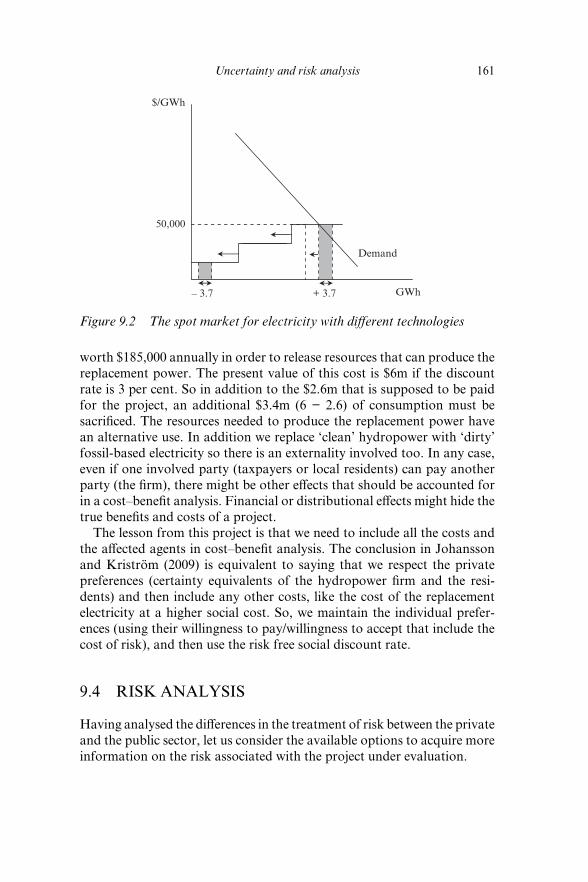
Uncertainty and risk analysis 161
worth $185,000 annually in order to release resources that can produce the
replacement power. The present value of this cost is $6m if the discount
rate is 3 per cent. So in addition to the $2.6m that is supposed to be paid
for the project, an additional $3.4m (6 − 2.6) of consumption must be
sacrifi ced. The resources needed to produce the replacement power have
an alternative use. In addition we replace ‘clean’ hydropower with ‘dirty’
fossil- based electricity so there is an externality involved too. In any case,
even if one involved party (taxpayers or local residents) can pay another
party (the fi rm), there might be other eff ects that should be accounted for
in a cost–benefi t analysis. Financial or distributional eff ects might hide the
true benefi ts and costs of a project.
The lesson from this project is that we need to include all the costs and
the aff ected agents in cost–benefi t analysis. The conclusion in Johansson
and Kriström (2009) is equivalent to saying that we respect the private
preferences (certainty equivalents of the hydropower fi rm and the resi-
dents) and then include any other costs, like the cost of the replacement
electricity at a higher social cost. So, we maintain the individual prefer-
ences (using their willingness to pay/willingness to accept that include the
cost of risk), and then use the risk free social discount rate.
9.4 RISK ANALYSIS
Having analysed the diff erences in the treatment of risk between the private
and the public sector, let us consider the available options to acquire more
information on the risk associated with the project under evaluation.
GWh+ 3.7– 3.7
50,000
$/GWh
Demand
Figure 9.2 The spot market for electricity with diff erent technologies
162 Introduction to cost–benefi t analysis
In the economic evaluation of projects, the use of a deterministic analy-
sis is not uncommon, choosing unique values for quantities and prices,
values that come from the best available information and are treated as if
they were to be realized in the future.
However reality does not support the calculation of the NPV under the
assumption that variables are deterministic. The uncertainty surrounding
demand and costs recommends the inclusion of random variables that
allow us to obtain a range of net present values and their corresponding
associated probabilities. Before we describe risk analysis let us briefl y
examine the rationale of sensitivity analysis.
Sensitivity Analysis
Sensitivity analysis consists of changing the value of one variable and
checking how this aff ects the outcome of the project. When several vari-
ables are modifi ed simultaneously we are using scenarios.
Returning to the case analysed in section 9.2, 150 apartments are built
for which full occupation is expected. For simplicity no externalities are
added, shadow prices are not considered and the discount rate is set to
zero. The social benefi t of the project is $3500; so, if the decision is to
approve or reject, the apartment complex project is approved.
Let us see the sensitivity of the NPV of this project to alternative
changes of x and C. For example when the demand is 125 the profi ts are
−$250, and when the costs equal $600 the profi ts are $500. Therefore the
analyst knows that when the occupancy rate falls and only 125 fl ats are
occupied, the outcome equals losses of $250. The selection of 125 is ad
hoc based on the a priori belief that this value is the worst situation the
investor thinks possible.
An option within the sensitivity analysis is to calculate the threshold
values of the relevant variables. This check of the sensitivity of the results
is performed by changing the value of the selected variable until the NPV
is zero, and it is often presented in relative terms, as the percentage change
in the target variable that makes the benefi ts of the project equal to zero.
For example, in the case of the construction costs, the maximum increase
before the NPV becomes negative is 26.9 per cent, the reduction in price is
15.6 per cent and the increase in annual costs 58.3 per cent.
The rationale of scenarios is not substantially diff erent to sensitivity
analysis. Instead of modifying a single variable and holding the others
fi xed, in scenario analysis we look at the combined eff ect of changes
in some selected variables, changes corresponding to diff erent possible
scenarios. For example we can change three variables altogether (con-
struction costs, annual operating costs and demand). The scenarios are

Uncertainty and risk analysis 163
called, for example, ‘optimistic’ (high demand and low cost), ‘expected’
(average values for costs and demand) and ‘pessimistic’ (high costs and
low demand).
The sensitivity analysis and the use of scenarios have the advantage of
revealing the degree of robustness of the results obtained by the change
in the value of a variable or a set of them, and comparing the results with
those obtained in the deterministic analysis. In our example, when demand
falls 16 per cent from the initial value of 150, the project loses money. This
simple sensitivity analysis indicates that, before undertaking the project,
we should put greater eff ort into obtaining a more reliable forecast of
demand, or even seek a contract that guarantees revenue in some way.
Once the usefulness of sensitivity analysis and scenarios is acknowl-
edged, we must note their limitations because of the use of unique values
instead of a range of values and the likelihood of the NPV being positive
or negative given these other values within the feasible range. The use of
single values does not imply an objective system. By choosing values of
individual variables, the interrelationship between them can be neglected.
The randomness of many of the events that aff ect the project will result in
a joint realization of the values of variables that does not need to conform
to a rigid choice of scenarios.
Risk Analysis
The alternative cannot be based on the addition of more variables to the
sensitivity analysis as the number of possible combinations multiplies,
providing too much information of little practical use to the decision
taker. The alternative to the sensitivity analysis and scenarios consists of
analysing the impact of the variables on the NPV of the project in a more
systematic way. The alternative approach is called risk analysis. In the fol-
lowing we describe risk analysis using the previous example.
In sensitivity analysis the demand could take the value of 150 in the best
case and 125 in the worst case. An alternative to the previous approach is
to work with probability distributions, allowing all possible values between
125 and 150. This introduces more realism into the assessment. The main
point is that in the sensitivity analysis we fi x the demand value to 150 or
125 but we do not use our beliefs on the likelihood of any of these values or
any other possible value in the range. If, given the available information, it
is estimated for example that the most likely value is 140, the minimum is
125 and the maximum 150, we could use a triangular distribution function
like the one in Figure 9.3.
Risk analysis seeks to make the most of the available information. If
some information is available on the a priori reasonable range over which

164 Introduction to cost–benefi t analysis
the relevant variables are expected to fall, it is preferable to use all the
values, weighted by the probability of occurrence. Any software for risk
analysis will carry out in a short time a very high number of iterations,
each one computing a diff erent value for the NPV. This is because the
software will randomly select a number of apartments occupied according
to the information provided by the triangular distribution in Figure 9.3, or
any other, previously selected. The most frequently chosen values will be
140 and those close to this value.
Instead of computing a single NPV and then performing sensitivity
analysis with two or three values of demand to see how the profi t changes,
now we can have a very high number of diff erent NPVs, which were
obtained with random demand values within the range 125- 150 and their
assigned probabilities of occurrence in the selected probability distribu-
tion function. The risk analysis is based on the following four stages.4
1. Modelling the project
This stage is actually common to any fi nancial or cost–benefi t analysis,
either deterministic or stochastic (incorporating uncertainty). It consists
of constructing a model that captures the relationship between costs and
benefi ts over time in order to predict the NPV of the project according to
the values taken by the variables.
In the case of the project of the apartment complex the model is simple.
It has four variables – construction costs, operating costs, the number of
apartments occupied and price – that may take diff erent values over the 15
years of the project life.
In general the decision on the variables of the project depends on its
characteristics. Suppose a contract was signed with the construction fi rm
0150125 140
0.08
Figure 9.3 Triangular probability distribution

Uncertainty and risk analysis 165
fi xing the price and the construction deadline. The contract includes a
clause providing for an automatic review of the price if during the years
of construction the labour costs change. If the labour costs are expected
to vary and they are a signifi cant part of total costs, the price of labour
should be a random variable of the model.
It could also happen that the construction costs are sensitive to certain
features of the terrain, impossible to determine accurately a priori, so it
would be advisable to use two variables: the cost of materials used and
labour costs.
2. Selection of risk variables
Of all the variables that determine the profi tability of the project, one
should choose only those that, besides being likely to change, if they do,
the results of the project are signifi cantly modifi ed. Therefore the variables
that meet one of the following two conditions could be excluded: (i) they
have a high impact if they change, but it is unlikely that they will change,
or (ii) they are likely to change, but if they do, their impact is irrelevant.
The reason to reduce as much as possible the number of variables
included in the risk analysis is that the more variables are included, the
more diffi cult it is to establish correlations between them and the more
likely it is that the results will be inconsistent when random simulations are
generated. Furthermore, by reducing the number of variables, we can focus
our eff ort on the behaviour and the interactions of the selected variables.
3. Probability distributions for the variables
Under the presence of uncertainty it is diffi cult to determine the value of
the variables of the model. Knowing the exact occupancy rate during the
next 15 years is virtually impossible; however we may be able to determine
the expected range for the percentage of occupied apartments in the 15
years. If, given the situation and characteristics of the complex, with infor-
mation based on past experience and expert opinion, we predict that the
occupancy rate will be in the range between 70 per cent and 90 per cent, for
example, we are in a better position with respect to the situation in which
we use only two values.
Once we have the minimum and maximum values, we must decide
which probability distribution is the most appropriate. The choice of the
range and type of probability function is indeed a prediction of the future
that is based on data from the past and also on our subjective view of what
we think the future will be like.5
Suppose that in the case of the apartments, the statistical informa-
tion on occupation rates in recent decades and the information gathered
through interviews with experts do not provide any reasonable belief that

166 Introduction to cost–benefi t analysis
one particular value within the feasible range is more likely than the rest.
We only know the minimum (125) and the maximum (150). In this case the
uniform probability distribution (Figure 9.4) is the one that refl ects our a
priori beliefs.
Given this probability distribution, it does not seem reasonable to
perform the risk analysis with two or three values, as in the sensitivity
analysis or with scenarios. The discrete uniform probability distribution
of Figure 9.4 shows 26 equally likely values. Given this expected demand
pattern, the available information on the extreme values helped to build
the probability function that is used to perform simulations. In many
cases, given the nature of the project, it may happen that one has to choose
a probability distribution knowing only the most likely value and having a
rough idea of the changes on both sides of the mean.
For example it may happen that we expect the demand quantity for a
service to be around a mean value of 100 and a standard deviation of 5,
with the probability distribution approximately symmetrical. In this case
a normal distribution is appropriate. In general the symmetric distribu-
tions should be used when the value of the variable ultimately depends on
opposing forces of a similar weight, while the asymmetric distributions
refl ect situations where there is rigidity on one side of the distribution. If
it is expected that the price of land is located in a range in which higher
values are more likely, we should use an asymmetric distribution.
In many cases a uniform distribution (i.e. an equal probability assigned
to each value) as represented in Figure 9.4 may be appropriate if there is
no evidence that supports assigning a greater weight to any of the values
within the range formed by the minimum and maximum. The uniform
0125 150
0.0385
Figure 9.4 Probability distribution of the demand

Uncertainty and risk analysis 167
distribution is therefore the baseline, the one compatible with the lowest
level of information.
4. Correlated variables
Risk analysis is based on a computer program in which the specifi ed model
to calculate the NPV is run many times, taking in each iteration the fi xed
value of deterministic variables and randomly drawing a value for the risk
variables according to the selected probability distribution. At the end
of the process, the program yields a range of NPVs with their respective
probabilities.
In the computation process, the program draws a value for each risk
variable regardless of the value chosen for the others, a procedure that
can lead to inconsistent results since, if some variables are correlated, this
relationship should be included in the program if we want to avoid incon-
sistent outcomes. If airport delay depends on the ratio ‘fl ights per hour/
airport capacity’, it makes no sense that the program can choose a high
waiting time value and simultaneously a low value for the ratio. The pro-
cedure to prevent the program generating inconsistent results is to create a
correlation matrix in which the relationship between one variable and the
others is refl ected.
9.5 INTERPRETING THE RESULTS OF RISK ANALYSIS
The model of our example was as simple as:
NPV 5 2I0 1 a15
t51
(ptxt 2 Ct) . (9.5)
Risk analysis uses the previously selected deterministic variables. In our
example I is always equal to 13,000, p is equal to 10 and C is equal to 400.
These three variables are not subject to variability and any time we run
the program an NPV value is generated with these predetermined values.
On the contrary, x is the risk variable. The probability distribution for the
risk variable is represented in Figure 9.4, a uniform distribution with a
minimum at 125 and a maximum at 150. We assign the same probability
to any of the 26 possible values that can take the variable demand in a
given year.
Once the software has generated a high enough number of iterations,
the results can be displayed as a probability distribution function, which
represents the probability distribution associated with the NPV of the

168 Introduction to cost–benefi t analysis
project, and it will allow us to calculate the probability of the NPV being
above or below a certain value or within a range of values.
The NPV of the project is not now a single number that receives a greater
or lower signifi cance depending on the risk aversion of the decision maker.
With the risk analysis we have a probability distribution of the NPV of
the project that contributes to a more informed decision. Obviously the
risk of the project is exactly the same with the simple analysis of expected
values, the sensitivity test, the use of scenarios or Monte Carlo analysis,
but the risk of making a wrong decision diminishes after a well conducted
risk analysis.
Recall that in our case of the investment in apartments an evaluation
of the project based on the expected value of the benefi ts and an annual
demand given by either 125 or 150 with equal probability results in an
expected profi t of $1625 (see Figure 9.1). If the demand takes the highest
value the benefi ts are equal to $3500, while if it takes the lowest value the
project results in losses of $250.
Suppose alternatively that the value the demand takes in a year does not
determine the demand in the following years. Under this assumption we
have to make the draw from the random variable x for each of the 15 years
of the project. The NPV obtained in a given iteration will be the result of
drawing 15 values of x within the 26 possible ones for each of the 15 years.
This process is routinely repeated by the computer thousands, or hundreds
of thousands, of times.
We must emphasize that the risk analysis does not only provide NPV
values but also their probability of occurrence. If I had to invest 50 per
cent of my annual salary in a business with only one potential negative
outcome, I would be interested in knowing whether the probability of
occurrence of the adverse outcome is similar to the one of obtaining a head
in tossing a coin, or winning the fi rst prize in the national lottery.
Figure 9.5 shows the probability distribution of the benefi ts correspond-
ing to 100,000 iterations of the model; it is the picture of 100,000 NPV
values obtained by randomly drawing 100,000 values for the demand for
each of the 15 years. The mean NPV is $1625, which coincides with the one
obtained with the expected value of demand (see Figure 9.1). This does not
add any value to what we already know. Nevertheless the distribution of
the net present values provides new valuable information. If our assump-
tion on the demand’s behaviour is correct, we know now that a negative
NPV is unlikely. Why? Because negative NPV values require that low
demand values are drawn for many years, which is certainly unlikely.
The probability distribution of profi ts represented in Figure 9.5 shows
that a negative result is almost impossible, since the minimum value is
$420 and the maximum $2880, with an expected value of $1625 and a

Uncertainty and risk analysis 169
standard deviation of $291. However we know that there are demand
values that generate losses. When the demand is 125, the loss is $250, and
as Figure 9.4 shows the value 125 is as likely as any other. The paradox is
solved when one recalls that for a negative profi t of $250 the demand must
take the lowest value (125) during the 15 years.6
What the risk analysis shows, after repeating the calculation of the NPV
a suffi ciently high number of times, is the impossibility of such a negative
result. The variable demand takes the value 125 in a given year 3.85 per
cent of the time, but the number of drawings that are made is 15, and
in these 15 subsequent and independent extractions the value 125 must
be realized. The trend is toward the mean, and this is what Figure 9.5
represents.
The cumulative probability distribution represented in Figure 9.6 is
another way to show that this is not a risky project because there is no
case in which the returns are less than $420. Figure 9.7 shows the curve
fi tted to the histogram of Figure 9.5. The adjusted density shows that, for
example, 99 per cent of the potential net present values are in the range
of positive profi ts (890; 2360), with virtually zero probability of having
negative results.
Should we rule out the possibility of losses in this project? The answer
is yes if the model we have used to represent the investment in apartments
is appropriate and refl ects the behaviour of the variables. Risk analysis
software works with the inputs it receives from the user, but cannot dis-
criminate between a model of realistic behaviour and another based on
inadequate assumptions.
The key assumption regarding the risk variable in our example is that
0024 28801625
0.0014
Figure 9.5 Histogram of the probability distribution of the NPV (one
uniform probability distribution of demand for each year of the
project)

170 Introduction to cost–benefi t analysis
the demand is random each year, regardless of what happened in the previ-
ous year, and also that the number of occupied apartments will never be
less than 125 out of the 150 to be constructed, any of them being equally
probable, including the minimum and maximum.
To illustrate the importance of the assumptions of the model, suppose
alternatively, as we did at the beginning of the chapter, that the demand
is random only in the fi rst year within the same limits of 125 and 150, and
once a value of x has been drawn for the fi rst year, it remains constant
0
1
420 28801625
0.5
Figure 9.6 Cumulative probability distribution of the NPV (one uniform
probability distribution of demand for each year of the project)
4200
0.0016
890 2360 2880
99%
Figure 9.7 Probability density function of the NPV (one uniform
probability distribution of demand for each year of the project)

Uncertainty and risk analysis 171
during the following years. If this is the assumption that represents the real
world we are trying to model, the results change dramatically. Although
the mean is the same ($1625), the minimum and maximum NPV values
change (−$250 and $3500) with a standard deviation of $1125 ($291 in the
previous case).
The drastic change in the results is represented in Figures 9.8 and
9.9, which show two fundamental diff erences with respect to the previ-
ous outcome. First, the project presents the possibility of higher returns
(an NPV of $3500 is as likely as the mean) and, second, it increases the
0–250 35001625
0.00027
Figure 9.8 Probability density function of the NPV (one uniform
distribution of demand for the whole lifetime of the project)
0
1
–250 1625 3500
0.5
Figure 9.9 Cumulative probability distribution of the NPV (one uniform
distribution of demand for the whole lifetime of the project)

172 Introduction to cost–benefi t analysis
variability of the results (including the possibility of losses: −$250 is as
likely as any other within the range).
As expected, the same data lead to diff erent results depending on the
assumptions about the behaviour of the demand. From the previous
analysis we can appreciate the importance of the eff ort to develop a con-
sistent model that refl ects the real behaviour of the variables as closely as
possible, since the consequences of incorrectly modelling such behaviour
might have a decisive impact on the evaluation results. This modelling
allows the decision taker to work with possible results and their respective
probabilities but its relevance depends on how well the model represents
the real world.
Sometimes this information is enough to take a decision on the desir-
ability of a project; in other cases nothing can be concluded with a single
decision rule, especially when comparing projects. We will now see several
possibilities using the results of risk analysis, useful when the decision is
either ‘to approve or reject’ or ‘to select between two mutually exclusive
projects’.
Decision Criteria Under Uncertainty
Accept or reject a project
If the decision is to accept or reject a project and the probability distribu-
tion of the NPV does not show any positive value, the criterion is the same
as in the case of an evaluation with deterministic variables in which the
NPV is negative: reject the project.
When all the values of the probability distribution of the NPV are
positive, the criterion is, in principle, to accept the project. The ulti-
mate acceptance of the project requires the fi nancial result also to be
positive, because if the fi nancial NPV is negative, or if there is a high
probability of negative results, the decision will depend on the budgetary
constraint.
When the expected value of the social NPV is positive and the fi nancial
result is acceptable, the project should be approved if the decision maker
is risk neutral. However, unlike the situation with deterministic values,
we know now the probability of the occurrence of negative results (10
per cent in Figure 9.10) and therefore we have additional information
to make a decision that will also depend on the existence of budget con-
straints and the attitude towards risk aversion of those who take the deci-
sion. Examining other pricing policies, capacity size, level of service, and
so on may be a way to improve the balance between the project’s social
and fi nancial profi tability, provided that the foreseeable worsening of the
social NPV does not go beyond acceptable levels.

Uncertainty and risk analysis 173
Choice between projects
The basic criterion for choosing between two alternative projects, A and
B, is to select the project whose probability density function shows a
clear superiority over the other. In Figure 9.11 the corresponding prob-
ability distributions do not intersect and one project is clearly superior
to the other. It must be remembered that even in this favourable situa-
tion it is necessary to check, in the case of budget constraints, that the
fi nancial result is positive (or has a satisfactorily high probability of being
positive).
It may occur that the cumulative density distributions of the two
projects do not intersect but the density functions do, as in Figure 9.12. In
this case the choice may heavily depend on the fi nancial results. In Figure
9.12 project B is preferable to project A because it has a higher expected
value and furthermore there are no negative values in the probability
density function; however, if the fi nancial results matter, it may be that A
is preferable to B if A has a positive fi nancial result and B a negative one.
Let us see the case of two projects whose cumulative density functions
intersect. The decision on which project is selected depends, as in the
0 Expected
NPV
0
10%
Expected
NPV
0
0.1
0.5
1
Figure 9.10 Accept–reject
0 Expected
NPV B
Project BProject A
Project BProject A
Expected
NPV A
0 Expected
NPV B
Expected
NPV A
0
0.5
1
Figure 9.11 Density functions do not intersect

174 Introduction to cost–benefi t analysis
previous cases, on the social NPV, the fi nancial results and the level of
risk.
A fi rst criterion for choosing between the two projects represented in
Figure 9.13 is to check which project has a higher expected social NPV. As
Figure 9.13 shows, project B has a higher expected NPV than project A. If
the fi nancial NPV is positive in both projects, project B is preferred unless
the wider range and cumulative probabilities of negative values in project
B and the risk aversion of the public agency taking the decision make
project A more attractive (a smaller but less risky expected NPV).
When the fi nancial NPV of project A is positive and that of project B
is negative, it would be preferable to choose A in the presence of a budget
constraint. If in addition the risk associated with project A is smaller, as in
Figure 9.13, it is more in favour of project A.
When the fi nancial NPV is negative for both projects and there are
budget constraints, the best option is to look at how the social NPV is
aff ected by changes in the price level, in the capacity design, in the quality
of service, and so on. There is a trade- off between a reduction in the social
NPV and the improvement in the fi nancial performance.
0 Expected
NPV B
Project B
Project A
Project BProject A
Expected
NPV A
0 Expected
NPV B
Expected
NPV A
0
0.5
1
Figure 9.12 Density functions intersect
0 Expected
NPV B
Project B
Project A
Project B
Project A
Expected
NPV A
0 Expected
NPV B
Expected
NPV A
0
0.5
1
Figure 9.13 Cumulative density functions intersect
Uncertainty and risk analysis 175
THINGS TO REMEMBER
Uncertainty is common to any project, so the economic evaluation ●
of projects has to deal with the variability of results. For risk averse
individuals the expected value ignores the cost of risk. People are
willing to accept a lower amount than the expected value if by doing
so they avoid the variability of the results. Hence the valuation of
benefi ts and costs for specifi c groups of aff ected individuals needs an
adjustment to account for the cost of risk.
According to the Arrow–Lind theorem, the public sector should ●
decide with regard to the expected values. The rationale of this posi-
tion is based on the idea of risk spreading, as the diff erence between
the expected value and the certainty equivalent tends to zero when
the results of a project are divided among a large number of partici-
pants (taxpayers), so that the cost of risk tends to zero. Nevertheless,
in the case of costs borne by specifi c groups of individuals, the
certain equivalent is still the right approach.
Although the public sector can be considered as risk neutral and ●
bases its decisions on expected values, the information obtained
through risk analysis is helpful. Information on the probability
of good and bad results gives the decision taker a more complete
picture of the project’s expected performance and its consequences.
A decision of the type accept–reject or a selection between projects ●
can rarely be exclusively based on the social NPV. The fi nancial
NPV may be useful for making the fi nal decision. Usually we have
to face a trade- off consisting of a lower social NPV in exchange for
fi nancial viability.
The best software available for risk analysis does not remove the ●
need to have a good model that represents the case we want to
evaluate.
NOTES
1. The certainty equivalent of a gamble is the amount of money that produces the same utility as the expected utility of playing the game. The certainty equivalent leaves the individual indiff erent between playing and not playing. Let us consider a game that con-sists of tossing a coin, winning a million if it is heads and zero if it is tails. The certainty equivalent is the minimum amount of money we have to off er to leave the individual indiff erent between accepting this amount and not playing, or rejecting it and playing (see Chapter 11).
2. When several competitors in a public tender have a diff erent view on the auction that has a ‘common value’ (e.g. the stock of crude oil in an oil reservoir), it is said that the winner may suff er the ‘winner’s curse’ and be bankrupt later. The explanation is that if the value

176 Introduction to cost–benefi t analysis
of the object is unique and common to all (unlike a piece of art, for example), the bidder making an off er above the others may have interpreted the information in an optimistic way and overstated the value of the auctioned object.
3. One monetary unit in year one, using a 5 per cent discount rate, has a value of 0.952 in year zero, in years 10 and 15 the values are 0.614 and 0.481 in year zero, respectively. By adding a 3 per cent risk premium the present values are respectively (between brackets, the reduction of the value with respect to the situation without risk): 0.926 (−2.7%); 0.463 (−24.6%); 0.315 (−34.5%).
4. The description of the required stages to account for risk using Monte Carlo simulations is based on Savvides (1994).
5. Bernstein (1996) emphasizes that the story told in his book is marked all the way through by a persistent tension between those who assert that the best decisions are based on quantifi cations and numbers, determined by the patterns of the past, and those who base their decisions on more subjective degrees of belief about the uncertain future, and points out this is a controversy that has never been resolved.
6. The probability of this event is (0.0385)15 = 6.05 × 10⁻²².

177
10. Applications
. . .I think we must take it for granted that our estimates of future costs and benefi ts (particularly the latter) are inevitably subject to a wide margin of error, in the face of which it makes little sense to focus on subtleties aimed at discriminating accurately between investments that might have an expected yield of 10.5 per cent and those that would yield only 10 per cent per annum. As the fi rst order of business we want to be able to distinguish the 10 per cent investments from those yielding 5 or 15 per cent, while looking forward hopefully to the day when we have so well solved the many problems of project evaluation that we can seriously face up to trying to distinguish 10 per cent yields from those of 9 or 11 per cent.
(Arnold C. Harberger, 1964, p. 1)
10.1 INTRODUCTION
This is a chapter on applications of the criteria and rules derived previ-
ously. In this book we have approached cost–benefi t analysis as a set of
reasonable shortcuts in the search for the social profi tability of projects
in a wide sense. There are many possible candidates for cost–benefi t
analysis.
The economic evaluation of transport infrastructure is the content
of sections 10.2 and 10.3. Investment in high speed rail infrastructure is
costly, irreversible and subject to cost and demand uncertainty. A cost–
benefi t analysis of high speed rail is quite similar to road, port or airport
evaluation, with time savings, increase in quality, reduction in congestion
and the willingness to pay of generated trips as its main benefi ts. It is a
typical investment that can be analysed within a cost–benefi t analysis
framework without major diffi culties and the practical approach can be
generalized to any other infrastructure.
A controversial policy is the change of ownership of public fi rms, either
understood as the sale of public assets or, as it is widely applied around the
world, as concession contracts through which the public sector concedes
the provision of public services to the private sector for a predetermined
period of time, according to the conditions established in the contract
agreement. Section 10.4 presents a basic model, which is easy to apply to
the privatization of public fi rms, and section 10.5 gives an application to a
178 Introduction to cost–benefi t analysis
water supply concession contract. The analytical framework is applicable
to the evaluation of price or quality regulation.
The content of section 10.6 is not an application but it is critical for
the application of cost–benefi t analysis: the importance of incentives.
This is a topic that has not received suffi cient attention in the economic
evaluation of projects, though it is essential to the success of cost–benefi t
analysis as a tool for informed decision making. The importance of
incentives in institutional and contract design and the loss of value of
cost–benefi t analysis when the objective functions of social agents are
overlooked.
Ex ante evaluation may become an empty bureaucratic procedure
unless we understand the institutional context and the confl icting objective
functions of the agents involved. The understanding of the diff erent levels
of government usually involved in major projects and policies, as well as
the implication of a menu of contracts for private participation, is a fun-
damental step if we want to avoid the conversion of cost–benefi t analysis
into a useless administrative procedure instead of an economic tool for
rational decision taking.
10.2 INVESTMENT PROJECTS: ECONOMIC EVALUATION OF INFRASTRUCTURE
Investment in high speed rail has won the support of its direct users, who
value its high quality and speed; of governments, who see it as an instru-
ment for integration and for the reduction of congestion on roads and at
airports; of railway authorities, for which it has been a path of renewal, in
a context of railways’ declining market share in the distribution of traffi c
between modes of transport; and fi nally of the industrial fi rms producing
railway equipment, for the volume of business that it involves.
The introduction of the technology known as high speed rail, consisting
of infrastructure and rolling stock that allows the movement of passenger
trains at 350 km/hour, has led to a revival of rail transport. Apart from
the industry propaganda and the myth of high speed trains, this technol-
ogy competes with road and air transport over distances of 400–600 km,
in which it usually is the main mode of transport. For short distance trips,
the private vehicle recovers the market share, and for long distance travel,
air becomes the hegemonic mode of transport.
The fundamental problem of high speed is not technological, but eco-
nomic: the cost of high speed rail infrastructure is high, sunk and associ-
ated with strong indivisibilities (the size of the infrastructure is virtually the
same for a line regardless of the volume of existing demand). In corridors

Applications 179
with low traffi c density, the cost per passenger is very high, which makes
the fi nancial stability unfeasible.
As investment costs in high speed infrastructure are well above those
required by conventional trains, and its use is associated with very pro-
nounced decreasing average costs, population density largely determines
the fi nancial and social viability of the investment. In this section we
present a simple model for assessing high speed rail investment. Regardless
of market shares and the political rhetoric about its role in territorial
integration and regional development, we intend to answer the following
question: is society willing to pay for the social cost of high speed rail?1
Cost–Benefi t Analysis of High Speed Rail Investment: A Basic Framework
Although the eff ects of building high speed rail infrastructure are many,
the fi rst direct eff ect is the reduction of travel time (while simultaneously
increasing the quality of travel) and, when cross eff ects are signifi cant, the
reduction of congestion in roads and airports.
In cases where the saturation of the conventional rail network requires
capacity expansions, the construction of a new high speed line has to be
evaluated as an alternative to the improvement and extension of the conven-
tional network, with the additional benefi t of releasing capacity. Obviously
the additional capacity has value when the demand exceeds the existing
capacity on the route. In these circumstances the additional capacity can be
valuable not only because it can absorb the growth of traffi c between cities
served by the high speed railway but also because it releases capacity on
existing lines to meet other traffi c, such as suburban or freight.
The generated traffi c is a direct benefi t for the users, which is generally
valued as half of the benefi ts of existing users according to the ‘rule of a
half’ (see Chapter 2). However there is a debate over whether this gener-
ated traffi c involves greater economic benefi ts that are not captured in
conventional cost–benefi t analysis. Leisure travel and business trips can
benefi t the destination, though it is crucial to distinguish whether it is a
genuine expansion of economic activity or a simple relocation of jobs and
previous economic activity.
The debate on these issues focuses on whether these changes are addi-
tional economic activity or a simple relocation of the pre- existing activity.
Besides, many indirect benefi ts are associated with investment in transport
infrastructure in general and not exclusively in high speed, so even if they
increase the social return on the investment in transport, they do not neces-
sarily place high speed in a better position over other options for transport
investment. Moreover, in undistorted competitive markets, theory tells us
that there the net benefi t of marginal change in congestion is zero.

180 Introduction to cost–benefi t analysis
Regarding the spatial eff ects, high speed lines tend to favour central
locations, so that if the aim is to regenerate the central cities, high speed
train investment could be benefi cial. However, if the depressed areas are
on the periphery, the eff ect can be negative. The high speed train can
also allow the expansion of markets and the exploitation of economies of
scale, reducing the impact of imperfect competition and encouraging the
location of jobs in major urban centres where there are external benefi ts
of agglomeration (Graham, 2007). Any of these eff ects are most likely to
be present in the case of service industries (Bonnafous, 1987) (see Chapter
3).
The environmental impact of investment in high speed rail points in
two directions: one of them is the reduction in air and road traffi c. In such
cases its contribution to reducing the negative externalities of these modes
could be positive, though we must not forget that it requires a signifi cant
deviation of passengers from these modes. Moreover, the use of capacity
must be high enough to off set the pollution associated with the production
of electric power consumed by high speed trains as well as noise pollu-
tion. Rail infrastructure also has a negative environmental impact such as
the barrier eff ect as well as the land taken for the access roads needed for
construction and subsequent maintenance and operation. The net balance
of these eff ects depends on the value of the aff ected areas, the number of
people aff ected, the benefi ts of the diverted traffi c and so on (Nash, 2009).
The assessment of the social profi tability of high speed rail requires us
to consider this public action as an investment in fi xed infrastructure and
specialized rolling stock, which incurs for its operation thereafter costs of
maintenance, energy, materials and labour, some fi xed and others depend-
ent on the volume of demand. The initial investment and the annual costs
allow us to obtain a fl ow of benefi ts over the life of the infrastructure.
The costs of building the railway infrastructure and the subsequent
maintenance and operation costs can be expressed in a simplifi ed form as
follows:
TC 5 I0 1 aT
t51
(C(xt) 1 Ct
)
(1 1 i) t, (10.1)
where:
TC: total costs
I0: investment costs in year 0
C(xt): annual operating costs dependent on xt
Ct: annual fi xed costs of maintenance and operation in year t
T: project life
i: social discount rate
xt: passenger trips in year t.

Applications 181
For simplicity we assume here that the benefi ts of high speed rail invest-
ment are limited to time savings and quality improvements. Indirect eff ects
and the net balance of environmental impacts are considered irrelevant.
The investment in high speed rail would be socially profi table if its bene-
fi ts outweigh its costs, requiring expression (10.2) to be greater than zero:
NPV 5 2I0 1 aT
t51
(B(xt) 2 C(xt
)) (1 1 q) t21 2 Ct
(1 1 i) t, (10.2)
where B(xt) are the annual benefi ts and q is the annual growth rate of
annual net benefi ts.
Given the indivisibilities aff ecting high speed infrastructure, the values
of I0 and Ct are not very sensitive to the volume of demand (for a given
line length). The higher the values of these parameters, the harder it is to
reach a positive NPV. This also applies to the variable cost, although this
cost depends on the demand volume. The key is therefore the benefi ts that,
for a given T, depend on the number of users during the life of the project.
The level of demand (the initial volume and its growth rate) appears as
the basic determinant of satisfying the condition of social profi tability in
(10.2).
The importance of demand can be illustrated by Figure 10.1, which rep-
resents the function of the average cost (AC) and marginal cost (MC) of a
high speed train, whose total cost function is C 5 K 1 cx, where K is the
annualized fi xed cost, c is the marginal cost per passenger trip and x the
number of passenger trips per year (constant over the life of the project).
The graph shows two demand curves: the D1 curve for a country of low
MC
AC
xx2x10
p = c
h
a
�1
�2
b
d g
e
f
p, c
D2D1
Figure 10.1 Demand, costs and social benefi ts of high speed rail

182 Introduction to cost–benefi t analysis
population density, and D2, corresponding to a country with high popula-
tion density (assume both have the same level of income per capita).
Assuming that the price is equal to the marginal cost, the revenues are
lower than the total costs in both countries, requiring public funding to
ensure fi nancial stability. In the cases shown in Figure 10.1 the fi xed costs
are not covered. However the cost–benefi t analysis of both projects shows
very diff erent social profi tability.
In the case of a high demand country (D2), the revenues cgx20 only cover
the variable costs and losses are represented by the area hfgc, representing
the annual fi xed cost; however the willingness to pay of individuals exceeds
the cost of the train: the area g2gx20, which is the total value of the high
speed rail to the individuals (assuming that there are no indirect eff ects or
externalities, or any other distortions), allows the variable costs cgx20 to
be covered. The resulting consumer surplus g2gc (which we might call the
willingness to pay for capacity) exceeds the cost of that capacity hfgc since
g2eh is greater than efg. The economic result is positive despite the fi nan-
cial result being negative. In this case, the high speed rail infrastructure
increases social welfare.
In the case of the low demand country (D1) the fi nancial result is nega-
tive and equal to the area abdc; however, unlike in the country with high
demand, the inclusion of the consumer surplus as a benefi t of the project
does not allow positive results. The willingness to pay for capacity in
this country (g1dc) is less than the cost of capacity (abdc). The economic
evaluation shows an annual social loss equivalent to the area abdg1, so the
conclusion is that the country with demand D1 should not build the high
speed infrastructure.
It is worth recalling here the assumptions on which the conclusions
regarding the desirability of building the infrastructure rest. The fi rst
is that there are no other relevant eff ects; the second is that there are
no budgetary constraints that would increase the opportunity cost of
public funds required and therefore would reduce the social returns; the
third is that we are evaluating a project in isolation and the decision is
of the ‘accept–reject’ type, hence an NPV > 0 is a suffi cient condition to
accept the project; and the fourth is that effi ciency is the only decision
criterion.
10.3 COST–BENEFIT ANALYSIS OF HIGH SPEED RAIL: AN ILLUSTRATION
Let us consider an investment project in a new high speed rail line of 500
km without intermediate stations. This line would be built in a corridor

Applications 183
where conventional rail, road and air transport are in operation. The
lifespan of the project is 30 years.
The investment costs amount to $4500 million for the base year of the
project (year 0); the residual value is zero, and the average variable cost
of the high speed train is constant and equals $45 per passenger trip. The
ticket price of the high speed train is set at $55. The average costs of the
conventional train, car and plane are also constant and equal to $36, $50
and $90 respectively, and in all three cases the price is equal to the average
cost. The generalized price of travel for each transport mode is given by
gi 5 pi 1 viti (i = train, car and air). The travel times ti for each mode and
time values vi are listed in Table 10.1.
The time values in Table 10.1 are identical for all the users within each
mode, and they grow every year by the same proportion as income. The
interest rate equals the social rate of discount (5 per cent). All the values
are expressed in real terms.
There is uncertainty about the volume of demand for the project; hence,
for illustrative purposes, we consider two scenarios for predicting future
demand. The fi rst scenario is pessimistic, with an annual volume of 3
million passenger trips for the fi rst year of the project, while the second
scenario is optimistic, with a volume of 6 million passenger trips for the
initial year. We assume an elasticity of demand with respect to income of
1.2 and an income growth rate of 2.5.
In Chapter 2 we discussed two equivalent approaches for conducting
cost–benefi t analysis: the fi rst, adding the changes in the surpluses of the
social agents; the second, calculating time savings, the benefi ts of the gen-
erated traffi c, the costs of accidents avoided and the change in costs. We
assume that no other benefi ts or costs exist.
Change in Social Surplus
Following the fi rst procedure we must add the surpluses of the various
social agents. First the user gains in terms of generalized price (money
Table 10.1 Travel time and value of time (line length: 500 km)
High speed
train
Conventional
train
Car Air
Total travel time
(in decimal terms)
2.67 6.67 5.30 2.58
Value of time ($)
(in year t = 1)
– 10 10 20

184 Introduction to cost–benefi t analysis
plus time), calculated separately for each group of users of other modes of
transport that shifts to the high speed train. The introduction of high speed
implies changes in the generalized price by mode as refl ected in Table 10.2.
From these data on the changes in the generalized price per passenger
trip we can evaluate the benefi ts for the users of the high speed train.
Previously we had to distinguish between those passenger trips changing
mode (whose consumer surplus is obtained as the diff erence in generalized
prices)2 from generated passenger trips. In the latter case the increase in
consumer surplus generated with the introduction of high speed is equal
to the triangle bounded by the demand curve and the price and quantities
diff erences. The benefi ts are calculated as half of the diff erence in the gen-
eralized costs, with and without the project, multiplied by the generated
passenger trips.
Table 10.3 shows, for the low demand scenario (3 million passenger
trips), the incoming users from diff erent modes and the generated traffi c
(the same proportions are assumed for the case of high demand) and the
benefi ts that these users obtain in the fi rst year.
In the fi rst year of the project the costs and benefi ts are:
Time savings and generated traffi c: 58,087,500 ●
Reduction in accidents: 1,800,000 ●
Revenue: 55 × 3,000,000 = 165,000,000 ●
Operating costs: 45 × 3,000,000 = 135,000,000. ●
The results obtained for the whole project in both demand scenarios are
as shown in Table 10.4.
Changes in Willingness To Pay and Resources
The second approach to calculating the NPV of the project is to focus on
the changes in the willingness to pay and the resources, ignoring transfers.
Table 10.2 Changes in the generalized prices of diverted passengers (fi rst
year)
Generalized price in the
original mode (1)
Generalized price in
HSR (2)
Change
(1) − (2)
Conventional
train
36 + 6.67 × 10 = 102.7 55 + 2.67 × 10 = 81.7 21.0
Car 50 + 5.30 × 10 = 103 55 + 2.67 × 10 = 81.7 21.3
Air 90 + 2.58 × 20 = 141.6 55 + 2.67 × 20 = 108.4 33.2

Applications 185
Figure 10.2 shows, for the case of the conventional train in the low
demand scenario, the benefi ts of time savings for existing users (the dark
shaded area).
In Figure 10.2 the benefi ts of generated trips are represented by the light
shaded area. It can be seen how, for this generated traffi c, the benefi ts are
obtained by calculating the willingness to pay for the new trips (the area
under the demand function in the segment of the 648,000 generated trips)
minus the total value of the time spent on such trips (the operating costs
of attending this traffi c are not represented in the fi gure and have to be
deducted to obtain the benefi t of generated traffi c).
Similarly, considering separately the benefi ts of the existing passengers’
Table 10.3 First year users’ benefi ts (low demand)(values in $)
Users’ benefi ts
in the deviated
demand group
Users’ benefi ts
in the generated
demand group
Total
benefi t
Conventional train 1,500,000 × 21
= 31,500,000
0.5 × 648,000 × 21
= 6,804,000
38,304,000
Car 300,000 × 21.3
= 6,390,000
0.5 × 126,000 × 21.3
= 1,341,900
7,731,900
Air 300,000 × 33.2
= 9,960,000
0.5 × 126,000 × 33.2
= 2,091,600
12,051,600
Total 47,850,000 10,237,500 58,087,500
Table 10.4 Social and fi nancial benefi ts of the project (millions of $,
discounted values)
Low demand
q = 3,000,000
High demand
q = 6,000,000
Time savings and generated traffi c 2013 4027
Accidents reduction 37 37
Revenue 3617 7233
Operating costs –2959 –5918
Infrastructure costs –4500 –4500
Social NPV –1792 879
Financial NPV –3842 –3185
Note: Project life = 30 years; income growth rate = 2.5%; discount rate = 5%; income- demand elasticity = 1.2; income- value of time elasticity = 1; p = 55.

186 Introduction to cost–benefi t analysis
trips and the new ones, the calculations are made for road and air trans-
port. For the benefi ts obtained in this way we must add those benefi ts
resulting from a cost reduction in the transport modes that lose traffi c and
the benefi ts of avoided accidents. Finally one must subtract the costs of the
g, p, c
D
q
102.7
81.7
55
36
1,500,000 2,148,0000
Figure 10.2 Benefi ts of the high speed train (conventional train users)
Table 10.5 Benefi ts of high speed rail (millions of $, discounted values)
High demand Low demand
Time savings from deviated trips 2085 4170
Train 1858 3715
Car 244 488
Air −17 −33
Benefi ts of generated trips 1440 2881
Cost savings 2105 4209
Train 1184 2367
Car 329 658
Air 592 1184
Accidents 37 37
Investment costs −4500 −4500
Maintenance and operating costs −2959 −5918
NPV (social) −1792 879
NPV (fi nancial) −3842 −3185
Note: Project life = 30 years; income growth rate = 2.5%; discount rate = 5%; income- demand elasticity = 1.2; income- value of time elasticity = 1; p = 55; low demand (fi rst year) = 3,000,000; high demand (fi rst year) = 6,000,000.

Applications 187
project to obtain the social NPV. The results obtained using this alterna-
tive approach are shown in Table 10.5. As we can see the social NPV is
equal in both approaches.
The conclusion to be drawn from this evaluation is that this project is not
socially worthy in the low demand scenario since both the social NPV and
the fi nancial NPV are negative. By contrast, in the high demand scenario the
result of the social NPV changes and yields a positive value, although the
fi nancial NPV remains negative. Even with high demand, this project would
not be fi nancially profi table as its revenues do not cover its costs, so that it
could not be operated by the private sector without subsidy. Nevertheless,
from a social point of view, and placed in a context without budget con-
straint, the benefi ts from time and cost savings, generated trips and acci-
dents avoided outweigh the costs of constructing and operating the project.
10.4 POLICY EVALUATION: COST–BENEFIT ANALYSIS OF PRIVATIZATION
The economic evaluation of a privatization policy has three key elements:
fi rst, the existence of cost diff erences between the public and the private
sector; second, the type of market where the company operates and the
ability to exercise monopoly power; and third, the sale price.
Even assuming that the privatization policy results in net benefi ts for the
society these benefi ts may not be well distributed. It may be that produc-
ers are better off with privatization, but consumers and workers are worse
off . Therefore, to assess a privatization project in practice, the practitioner
should make a detailed assessment of winners and losers. This will be nec-
essary to design the compensation mechanisms, for reasons of equity or to
make the project politically acceptable.
In this section we present a basic model and an application to assess
whether the society wins or loses with the privatization of a public fi rm
or service. The privatization model can equally be applied to the evalu-
ation of privatization in the strict sense or a concession, and can also be
extended to the evaluation of price and quality regulation.
Social Benefi ts of Privatization and Sale Price
Often the success of privatization has been associated with the sale price
achieved. It is possible that the emphasis on the fi nancial aspects of priva-
tization has made us forget that in the sale of public assets, unlike a trans-
action between private agents, it is necessary to know what happens after
the exchange; for example, a high sale price for the public company may

188 Introduction to cost–benefi t analysis
simply be refl ecting the net present value of monopoly profi ts expected by
the buyer of the company.
Let us consider, as a starting point, the case of the public fi rm repre-
sented in Figure 10.3, and the evaluation of the project consisting of its
privatization.3
The public company charges a price pg and produces at the unit cost cg,
its annual profi t is therefore equal to (pg 2 cg)xg, equivalent to the area
pgabcg in Figure 10.3. When the company is public the variables are identi-
fi ed by the subscript g (government) and when it passes into private hands
by the subscript p (private).
How much is the maximum a private entrepreneur would be willing to
pay for the public company represented in Figure 10.3 if there is no change
in either the price (pp = pg) or the cost (cp = cg)? Assuming that the lifespan
of the fi rm is T years, and the rate of discount is zero for both the public
and the private sector, the private value of the company in private hands
(Vpp) can be expressed as:
Vpp 5 T(pp 2 cp)xp. (10.3)
If the entrepreneur pays Vpp for the fi rm, the public sector gains the
discounted benefi ts generated by the company in private hands during his
lifetime T. If we call Z the price paid by the entrepreneur to the govern-
ment for the privatization, the highest possible value of Z is Vpp.
It should be recalled here that, unless money has a higher value in the
hands of the government than in private hands, Z is a mere transfer of
income and therefore the government would be indiff erent to the value of
Z. Hence we assume that the value of money in public hands (lg) is higher
than the value of money in private hands (lp), lp having a value equal to
D
0
cg
pg
xg x
p, c
a
b
Figure 10.3 Privatization without a change in either price or cost

Applications 189
unity, and (lg − lp) is the additional value of a dollar when it passes from
private to public hands.4
Returning to Figure 10.3, for the social surplus to increase with the pri-
vatization, the following condition must hold:
lgZ 2 lpZ 2 lgTpg 1 lpTpp . 0, (10.4)
where pg and pp are the benefi ts before and after the privatization (i.e. in
public and private hands, respectively).
Expression (10.4) shows the changes that occur with the sale of the
public company, valued with shadow prices of the money held by the gov-
ernment and the private sector. It can be seen how Z is received by the gov-
ernment and paid for by the private buyer. Also the government loses the
annual profi t obtained before the sale (pg) and, by moving the company to
the private sector, the buyer obtains pp. Since we have assumed in Figure
10.3 that the price and the cost do not change, we know that pg = pp = p,
and (10.4) can be expressed as:
(lg 2 lp) (Z 2 Tp) . 0, (10.5)
the necessary condition to increase the social surplus that cannot be met,
since Z cannot be greater than Vpp = Tp.
Given the situation represented in Figure 10.3, if the government
manages to sell the company at the highest price the buyer is willing to
pay, privatization does not change the social surplus. If the entrepreneur
pays a price below Tp the society loses from the privatization.
Suppose now that, as shown in Figure 10.4, the private fi rm is more
effi cient than the public enterprise (cp < cg) and the price does not change
(hence, xp = xg). By privatizing, the producer surplus increases by (cg 2 cp)xp
each year and therefore the private value of the company in private hands
(Vpp) increases by T times this amount. The increase in Vpp may or may not
be translated to an increase in Z, depending on the procedure chosen for
the sale. What seems clear is that T(cg 2 cp)xp (T times the area cgbdcp) is
the effi ciency gain resulting from privatization.
To assess the change in social surplus from the sale of public companies,
we can use the following expressions:
DSS 5 Vsp 2 Vsg 1 (lg 2 lp)Z, (10.6)
Vsp 5 T(Sp 1 lppp) , (10.7)
Vsg 5 T(Sg 1 lgpg) , (10.8)

190 Introduction to cost–benefi t analysis
where:
DSS: change in social surplus
Vsp: social value of the fi rm in private hands
Vsg: social value of the fi rm in public hands
Sp: consumer surplus when the fi rm is private
Sg: consumer surplus when the fi rm is public.
Expression (10.6) presents the change in social surplus as the diff erence
between the social value of the company in private hands and the social
value of the company in public hands plus a proportion of the sale price.
We cannot forget that the sale price is a transfer of income between the
private buyer and the government (taxpayers) and, unless the money in
the hands of government is assigned a higher weight, the sale price does
not aff ect welfare.
Substituting (10.7) and (10.8) into (10.6), considering that as the price
is kept constant, Sg = Sp = S (area gapg) and assuming that the fi rm is sold
for the maximum value that the buyer is willing to pay (Z = Vpp = Tpp), we
obtain the social benefi ts of privatization, in terms of surpluses:
DSS 5 T(S 1 lppp 2 S 2 lgpg) 1 (lg 2 lp
)Tpp. (10.9)
Simplifying (10.9) we obtain the maximum social value that can be
obtained from privatization:
DSS 5 T lg(pp 2 pg
) . (10.10)
The expression in brackets in (10.10) is equal to cgbdcp in Figure 10.4.
The maximum potential social value of privatization is obtained when
D
0
cg
pp = pg
xg = xp x
p, c
cp
a
b
d
�
Figure 10.4 Privatization with cost reduction

Applications 191
the effi ciency gain achieved pp − pg is multiplied by the T years of the
project, multiplied by the shadow price of money in government hands. If
the sale procedure fails to transfer effi ciency gains to the government, the
social surplus will be smaller despite the annual effi ciency gain remaining
cgbdcp. We can also see why, given that there is no change in the consumer
surplus, the area gapg does not appear in equation (10.10).
The government has two objectives with privatization according to
(10.6): to sell the public enterprise to the bidder that generates the
maximum increase in social surplus, and to obtain the highest possible
price from this bidder.5
Previously we assumed that the price did not change after privatiza-
tion and therefore the consumer surplus remained constant (Sg = Sp = S).
We now abandon this assumption and consider the general case in which
prices, costs and quantities change after privatization, the discount rate is
positive and the privatized company returns to the government some of its
profi ts as taxes.
The social values of the company in the public sector and in the private
sector are, respectively:
Vsg 5 aT
t50
1
(1 1 i) t[Sg
(t) 1 lgpg(t) ], (10.11)
Vsp 5 aT
t50
1
(1 1 i) t[Sp
(t) 1 lppp(t) 1 (lg 2 lp
)Y(t) ], (10.12)
where:
Y(t): post- privatization taxes
i: social discount rate (we assume it equals the interest rate).
The change in social surplus is obtained by substituting (10.11) and
(10.12) into (10.6):
DSS 5 aT
t50
1
(1 1 i) t[Sp
(t) 1 lppp(t) 1 (lg 2 lp
)Y(t)
2 Sg(t) 2 lgpg
(t) ] 1 (lg 2 lp)Z. (10.13)
Operating in (10.13), and adding and subtracting lgpp, we obtain:
DSS 5 aT
t50
1
(1 1 i) t[Sp
(t) 2 Sg(t) 1 lg
(pp(t) 2 pg
(t)) ]
2 (lg 2 lp) ca
T
t50
1
(1 1 i) t(pp
(t) 2 Y(t)) 2 Z d . (10.14)

192 Introduction to cost–benefi t analysis
It is quite diffi cult for the government to make the buyer pay a price Z
that is equal to the maximum that the buyer is willing to pay; that is, the
private value of the company in private hands (Vpp). This value is equal
to:
Vpp 5 aT
t50
1
(1 1 i) t(pp
(t) 2 Y(t)) . (10.15)
Substituting (10.15) into (10.14) and expressing the diff erences in sur-
pluses as increases, we have an operational expression to calculate the
social benefi ts of privatization:
DSS 5 aT
t50
1
(1 1 i) t[DS(t) 1 lgDp (t) ] 2 (lg 2 lp
) (Vpp 2 Z) . (10.16)
For privatization involving an increase in social surplus, expression
(10.16) must be greater than zero. The economic interpretation of (10.16)
is as follows: for the typical case lg > lp, and assuming that the govern-
ment sells the company at the maximum price the buyer is willing to pay
(Z = Vpp), the social benefi t of the privatization equals the value of the sum
of the change in consumer and producer surpluses, the latter multiplied by
the shadow multiplier of money in government hands.
Let us examine more closely expression (10.16). For a given discount
rate and assuming (for simplicity) that, after the sale, both the cost and the
price are lower, the maximum social benefi t to be derived from privatiza-
tion is in the expression in brackets: the increase in consumer surplus and
the change in profi ts by reducing costs (this last benefi t is fully transferred
to the government, and so it appears multiplied by lg) when the price
of the sale equals the maximum willingness to pay of the buyer. When
the sale price Z is less than the willingness to pay for the fi rm (Vpp), the
social benefi t decreases relative to the maximum included in brackets, in
proportion to the deviation that occurs (Vpp − Z).
Welfare Eff ects of Price Regulations
Another mechanism that aff ects the results is the pricing policy post-
privatization. When the company operates as a monopoly, its price tends
to be regulated. If the fi rm is awarded to a private entrepreneur under
concession, it is usual to introduce procedures for the regulation of prices.
The potential effi ciency gains from privatization become social benefi ts
when they go to the consumers through lower prices or higher quality, or
they become a benefi t of the private fi rm, or go to the government as the
result of a well designed sale.

Applications 193
If we set a price equal to the marginal cost (pp = cp), where cp < cg, the
effi ciency gains increase with the increase in the quantity sold, with the
consumers as benefi ciaries of the privatization and, unless the shadow
price of public funds is suffi ciently high and the elasticity of demand suffi -
ciently low, welfare is improved in relation to the situation where the price
is unchanged.
The previous argument introduces an implicit assumption that is not
credible. First, if the buyer knows that the price is going to be equal to the
marginal cost, why buy the company? Moreover why should the entrepre-
neur try to reduce costs if the regulator sets a price equal to the cost?
A price regulation scheme that prevents this problem of incentives is
to introduce a maximum price (price- cap), for example pp = kpg, where k
is less than one and higher than the expected proportion of the reduction
in the unit cost. Now the cost of the private fi rm does not appear in the
regulatory mechanism, and the company has, in principle, incentives to
lower costs because the price is fi xed (kpg) and therefore, if the entrepre-
neur manages to reduce the cost below the regulated price, it will increase
its profi t.6
A combination of price regulation schemes based on incentives, with an
auction design that maximizes the revenue from the sale of the company,
is the way to maximize the social surplus if the market is not competitive.
The privatization of services like water supply, electricity or public trans-
port is a good example.
10.5 COST–BENEFIT ANALYSIS OF THE CONCESSION OF A RESIDENTIAL WATER SUPPLY
In this section we evaluate a policy of privatizing (through a concession
contract) the water supply in a medium sized city. The aim is to show how
the theoretical framework of the preceding sections can be applied to real
data on costs and prices in an actual market. The methodology is equally
applicable to any other public service.
To calculate the increase in social surplus we need to compute the
expression (10.16). This requires information about the values of lg, lp
and Vpp and also about the water demand. We will make the following
simplifying assumptions:
Assumption ● 1. The shadow price of money in public and private hands
is equal to one: lg = lp = 1. This assumption eliminates the last term
of expression (10.16), which could also be achieved by assuming that

194 Introduction to cost–benefi t analysis
the winning bidder pays the maximum (Z = Vpp). The assumption
lg = lp = 1 has the additional advantage of implying equal weights
for changes in consumer surplus and profi ts in expression (10.16).
Assumption 2. ● The water demand is linear and therefore we apply the
‘rule of a half ’ to calculate the consumer surplus. Using this assump-
tion the changes in consumer surplus and profi ts are:
DS(t) 51
2(pg
(t) 2 pp(t)) (xg
(t) 1 xp(t) ) . (10.17)
Dp (t) 5 (pp(t) 2 cp
(t))xp(t) . (10.18)
Assumption 3. ● The average cost is lower when the fi rm is in private
hands (cp < cg). The changes in consumer surplus and profi ts are
constant over time:
ΔS(t) = ΔS; Δp(t) = Δp. (10.19)
Assumption 4. ● There are no subsidies. The public company covers
costs (pg = cg), while regulated private companies are allowed to set
pp = kcp, where k ≥ 1 is determined by the regulator. This assumption
is imposed to abstract the problem discussed here – the evaluation
of the increase in welfare through a change of ownership – from
considerations of optimal pricing and optimal subsidies, plus the
problem of asymmetric information.
The fourth assumption allows us to determine the price levels pg and pp
required to evaluate ΔSS. Relaxing this assumption would imply making
additional assumptions about the level of subsidy.
The four assumptions we have made allow us to simplify (10.16) to:
DSS 5 aT
t50
1
(1 1 i) tc 12
(pg 2 kcp) (xg 1 xp
) 1 (k 2 1)cpxp d , (10.20)
where (k − 1) ≥ 0 is the mark- up (the margin of the price over the cost) that
the regulated private fi rm is allowed to set.
Graphically, if D is the linear function of water demand represented in
Figure 10.5, the terms in brackets in expression (10.20) represent the value
of the area pgabdcp. The area pgabpp is the change obtained in consumer
surplus, while ppbdcp represents the profi ts of the company in the case
k > 1.
In order to evaluate the change in welfare obtained through privatiza-
tion, using expression (10.20) the only new values needed are pg, cp, xp, i

Applications 195
and k. We know that pg and xg are the observed values of the price (equal
to the marginal cost in this case) and the production level of the public
enterprise.
Table 10.6 shows the basic data of the projects consisting of privatizing
the public water supply fi rm. The concession will last 30 years, the benefi ts
are produced at the end of each year and the terminal value is zero. The
rate of discount and the interest rate are equal to 5 per cent. The public
apg = cg
b
D
0
p
x per year
ed
xg
f
xp
pp
cp
Figure 10.5 Privatization of a residential water supply
Table 10.6 Basic data for the evaluation of the water concession project
I 0
T 30
i 5%
xg 300,000
Demand- price
elasticity
Triangular probability distribution* (−0.7; –0.4; −0.2)
Demand- income
elasticity
Uniform probability distribution** (0.25; 0.5)
pg = cg 2
pp 1.1 cp
cp Triangular probability distribution (1; 1.6; 2). This implies a
range for cost reduction (%) of 0–50, with 20% as the most
likely value
Income growth
rate
Uniform probability distribution (0.01; 0.03) (each year)
Notes: * Triangular probability distribution (min., most likely, max.); ** Uniform probability distribution (min., max.).

196 Introduction to cost–benefi t analysis
company sells 300,000 m3 of water per year at a price (equal to the mar-
ginal cost) of $2. The private company will be allowed a mark- up of 10
per cent over its private marginal cost (cp). Although the reduction in the
post- privatization cost is unknown, we assume a range with a maximum
of 50 per cent and a minimum of zero, and with 20 per cent as the most
likely value.
We need to predict the demand post- privatization. There is evidence on
residential water demand elasticities (see the meta- analysis by Espey et al.,
1997; also see Dalhuisen et al., 2003). Based on this evidence, and after the
elimination of outliers and the less likely values, we use a triangular prob-
ability distribution with a minimum demand- price elasticity value of −0.7
and a maximum value of −0.2, with −0.4 as the most likely value.
The income grows during the concession period. We assume that the
annual rate of growth can be represented by a uniform probability distri-
bution with a minimum value of 1 per cent and a maximum of 3 per cent.
We also assume that the demand- income elasticity is within the range
0.25–0.5 but we do not know anything about the likelihood of any particu-
lar value, so we use a uniform probability distribution.
Then we have four random variables in the evaluation: two for the
demand elasticities, one for the post- privatization cost reduction and
one for the annual growth of income. There is an important diff erence
between the last one and the other three. When calculating the NPV,
the computer program, according to our model, draws one value from
the probability distribution of the income growth rate for each year of the
30 years of the concession period. Hence, for any NPV value there are 30
independent drawings from the income growth rate probability distribu-
tion. This implicitly assumes that the annual growth rate is uncorrelated
with previous annual rates.
On the contrary, the other three probability distributions refl ect evalu-
ation uncertainty. This means that we do not know the exact values of
some parameters, so we tell the program to choose only one value of each
probability distribution and keep this value fi xed for the T years in any
iteration. The program will choose another value in the next iteration.
Figures 10.6 and 10.7 represent the social and fi nancial probability
distributions for the NPV. Both probability distributions support the
approval of the policy. The ranges of likely social and fi nancial net present
values are positive and the expected values are $2.5 million and $0.8
million for the social and fi nancial NPV respectively.
Nevertheless the probability distribution of the consumer surplus rep-
resented in Figure 10.8 shows that although the expected value is $1.6
million there is an 8.3 per cent probability of a negative consumer surplus
of between $1 million and zero. The reason for this segment of negative

Applications 197
values for the consumers rests on the possibility of a 10 per cent mark- up
combined with a cost reduction that ranges between 0 and 50 per cent. Any
10 per cent increase in price with insuffi cient cost reduction can produce an
increase in price for the consumer, which in terms of the social NPV is par-
tially compensated for by an increase in producer surplus. The deadweight
loss of effi ciency is generally compensated for, in this particular case, by
the gain in effi ciency thanks to the cost reduction.
One lesson from this case study is that by working exclusively with
expected values we miss some valuable information. Risk analysis pro-
vides the decision maker with a more complete picture of what is expected.
00
4
Valu
es x
10
–7
$ millions
2.5 5.9
Figure 10.6 Social NPV
0
6
Valu
es x
10
–6
$ millions
0.8 10.5
Figure 10.7 Financial NPV

198 Introduction to cost–benefi t analysis
Another lesson is that too much aggregation hides useful information.
In this case the probability distribution of consumer surplus shows that
consumers may be losers in this privatization with an 8.3 per cent prob-
ability. This may be considered tolerable. Perhaps the regulator could
contemplate the introduction of a price cap equal to the existing price
before privatization.
10.6 INSTITUTIONAL DESIGN, CONTRACTS AND ECONOMIC EVALUATION
The development of any project involving initial investment costs and
maintenance and operating costs in subsequent years requires an esti-
mate of those costs in accordance with the criteria that have been devel-
oped in previous chapters. A positive net social benefi t in the ex ante
cost–benefi t analysis does not guarantee the realization of this benefi t
during the life of the project. Unfortunately it is common to fi nd some
projects that should not have been built according to their ex post ben-
efi ts and costs.7
The explanation for the discrepancy between expected and actual values
in the case of infrastructure lies partly in the nature of the engineering
works. The fact that the expected benefi ts do not materialize according to
the ex ante cost–benefi t analysis is explained by contemplating the charac-
teristics of the activity being evaluated. Transport energy and water infra-
structures have a long life (over 30 years), have few alternative uses, are
0
–1
Valu
es x
10
–7
$ millions
5.11.6
8.3%
3.5
Figure 10.8 Consumer surplus

Applications 199
very expensive and the actual demand tends to deviate from that predicted
for such long periods of time.
External shocks caused, for example, by the decline of economic activ-
ity, or a reduction in the population of the region where the infrastructure
was built, signifi cantly aff ect the demand of electricity, the highway or the
company that supplies water; and thus the social benefi t of the project. It
might also happen that costs in the construction phase and subsequent
maintenance and operation phases experience changes because of unex-
pected increases in the prices and quantities of the inputs (energy, labour,
etc.) required for the normal operation of infrastructures.
These mismatches between predictions and reality are usual and una-
voidable in the economic life of a project. Little can be done beyond
improving forecasting techniques and risk analysis. However the predic-
tion errors are not the only explanation for the diff erences between ex ante
and ex post economic profi tability. The institutional design and the type
of contracts used for the construction and operation may enhance or miti-
gate the negative eff ects stemming from unanticipated changes in costs,
demand and technology on the ex post benefi ts of the evaluated project,
modifying the behaviour of economic agents and aff ecting the level of
eff ort to minimize costs or the selection of the appropriate technology.
Now we discuss the consequences of the existence of diff erent levels of
government with confl icting objectives and their implications for the selec-
tion of contracts for private participation. The understanding of these
issues for cost–benefi t analysis is paramount in a context of asymmetric
information and demand and cost uncertainty.
Two Levels of Government and their Eff ects on the Selection of Projects
The construction of a major infrastructure project is an expensive task. It
is an investment that gathers the following characteristics: lumpy, irrevers-
ible and costly. The decision to invest public funds in the construction of a
dam or a road is subject to cost and particularly demand uncertainty. The
irreversibility of the decision makes the economic appraisal of the project
quite relevant. Hence it is sensible to examine how the institutional design
aff ects the fi nal choice in the allocation of public funds to these types of
projects.
National and supranational governments support the implementa-
tion of key infrastructure with public funds. To understand the eff ects
of this public support in the investment decision it is useful to distin-
guish two levels in the process of decision making and funding of major
infrastructure projects. The fi rst one relates to the institutional design, in
which supranational and national governments (or national and regional

200 Introduction to cost–benefi t analysis
governments) agree on the projects to be fi nanced. The second one is
related to the selection of contracts for the construction and operation of
the infrastructure. This level includes the relationship between the national
(or regional government) benefi ciary of the project with the operator(s)
responsible for the construction and operation of the project.8
There are two extreme cases in the menu of contracts: the cost- plus
and the fi xed- price. In the fi rst case the agency responsible pays the full
cost of the project and in the second case it pays an ex ante fi xed amount.
This characterization of contracts can be applied to funding, price regula-
tion, construction contracts, and so on. The common ‘contract’ between
national and regional government for the fi nancing of an infrastructure
project is a kind of cost- plus.
The problem with this type of cost- plus fi nancing mechanism is that
the public funds a national government obtains from the supranational
agency, or the regional government obtains from the national govern-
ment, increase with the total investment costs and decrease with the net
revenues. Hence this fi nancing mechanism penalizes the internalization of
externalities, leads to excessive demand and biases the capacity size and
the choice of technology.
Let us suppose that a country facing a problem of capacity in the trans-
port network is considering mutually exclusive projects, including the con-
struction of a new high speed rail line that can apply for fi nancial support
from a supranational planner that maximizes social welfare. The country
is governed by a politician who must decide the main characteristics of
the project (let us say high speed rail or an upgraded conventional train),
make a cost–benefi t analysis and report it to the supranational planner in
order to receive funds for the construction of the infrastructure.
The eff ects of the present system of co- fi nancing in the EU, or any other
system in which a national government pays for the infrastructure within
the national budget and the regional government decides on the type of
project to be fi nanced, can be modelled in the following way (de Rus and
Socorro, 2010). Suppose only two periods. During the fi rst period the new
rail infrastructure is constructed. During the second period the citizens
of the country use it. The real construction costs are paid by the supra-
national government. We know that actual costs do not necessarily coin-
cide with the minimum investment cost. To minimize construction costs
requires the politician to make an eff ort, which is a cost for him.
It is not uncommon for national governments to be better informed
than the supranational agency about the transport problem and the set of
alternatives available and therefore about the minimum investment cost
required to solve the problem. For this reason we assume that the suprana-
tional planner cannot observe (or verify) either the minimum investment

Applications 201
cost or the eff ort exerted by the politician in order to be effi cient. Moreover
the national government has to decide the price to be charged for the use
of the new infrastructure and consequently the number of users. There are
also operating and maintenance costs, which are privately known, and in
many cases diff erent technologies and/or capacity sizes with signifi cant
cost diff erences.9
Once we abandon the idea of perfect information and assume that the
utility function of the politician (the national government) depends on
his own private income (only obtained if the politician is governing the
country), we can go further in explaining some of the evidence concerning
national government decisions on expensive infrastructure and suboptimal
pricing.10 The higher the welfare of voters in the second period, the higher
the probability of re- election. The welfare of voters in the second period is
the sum of their consumer surplus and the value of social expenditures.
In a world of perfect information, the supranational agency maximizes
social welfare, forcing the national government to exert the maximum
level of eff ort and so minimizing project costs and introducing marginal
social cost pricing. In the real world, eff orts and marginal costs are not
observable and the behaviour of the national government will respond to
the incentives of the fi nancing mechanism.
With the present fi nancing mechanism (as well as with any other cost-
plus fi nancing system) it is costly to be effi cient. Governments have no
incentives to minimize investment costs or to introduce optimal pricing.
There is a bias in favour of expensive latest technology mega- projects, and
the pricing will depart from user pays or polluter pays principles as the
higher the price for the use of the new national infrastructure, the lower
the consumer surplus of voters and the lower the probability of re- election.
As a consequence the politician will choose the maximum number of users
and will not charge for the external costs.
The evidence supports these conclusions. It is remarkable that national
and regional governments have promoted the construction of expensive
projects with a demand too low to pass a strict cost–benefi t analysis.
Forecasting error is not an explanation and strategic misrepresentation has
been detected worldwide. Many projects show overcapacity, the use of an
excessive and expensive technology given the problem to be solved, cost over-
runs and, in general, renegotiations that eventually allow the modifi cation of
the contract conditions, extending the construction periods, increasing costs
and prices and hence breaking the basic rules of public procurement.
These disappointing results are not completely unexpected. As we have
already discussed, national governments are in general better informed
than supranational planners about the costs and benefi ts of the infra-
structure projects to be constructed in their own regions, and they do not

202 Introduction to cost–benefi t analysis
necessarily share the same objectives. Governments may have incentives to
manipulate project evaluation to gain more funds from the supranational
planner. In a context of asymmetric information and diff erent objectives,
the relationship between national governments and supranational planners
cannot be modelled in a conventional cost–benefi t analysis framework.
In this context cost–benefi t analysis lacks its original power as a tool for
decision making. The existence of information asymmetries and confl ict-
ing interests requires a diff erent approach in which incentives are explic-
itly accounted for. A fi xed- price fi nancing mechanism may provide the
necessary incentives to reduce costs and charge the socially optimal price.
Moreover, with a ‘fi xed- price’ type of fi nancing mechanism, cost–benefi t
analysis is a very useful tool for governments to allocate the supranational
funds in the most effi cient way.
The fi xed- price mechanism in this context is an ex ante fi xed quantity of
external funding unrelated to costs and revenue. The idea of a fi xed quan-
tity fi nancing mechanism is to make national governments (in the case of
supranational funding) or regional governments (in the case of national
funding) responsible for insuffi cient revenues and cost ineffi ciencies as they
receive a fi xed amount of funding and are the residual claimants for eff ort.
The incentive to introduce optimal pricing is now high as the costs of inef-
fi cient pricing are also borne by the politician.
It is worth emphasizing that by giving national (regional) governments
an ex ante fi xed amount of funds, the supranational agency (national gov-
ernment) loses its infl uence over the selection of projects. If supranational
(national) governments want to establish infrastructure investment priori-
ties, an intermediate solution is to substitute the cost- plus funding method
by an alternative fi nancing scheme based on an ex ante fi xed- quantity
funding linked to generic objectives such as investing in ‘accessibility’ or
‘minimizing the total social cost of the water supply’ in particular areas, a
mechanism that should be dissociated in any case from costs and revenues
and the selection of any specifi c technology. The risk of building a socially
unprofi table infrastructure would be dissociated from the public funding
mechanism as the selection of the more expensive (and maybe inappropri-
ate) project will now have a completely diff erent opportunity cost for the
national (regional) governments.11
Contracts, Incentives and Risk Allocation
Private participation in the construction and operation of infrastructure
is carried out, mainly, through fi xed term concession contracts. The
purpose of the concession system is, fi rst the selection of the most effi cient
concessionaire among those presented to the public tender; and, second,
Applications 203
obtaining the greatest social benefi t possible over the life of the infrastruc-
ture, while allowing the concessionaire to cover costs. To achieve both
objectives, the selection system and the subsequent regulation should take
into account the problems of demand and cost information that character-
ize the activities under concession.
The fi xed- term concession contract is in theory a fi xed- price contract but
it is a kind of cost- plus in practice, given the widely extended use of renego-
tiation of this type of contract all over the world (Guasch, 2004). The design
of fi xed- term contracts allocates the demand risk to the concessionaire and
this creates problems concerning the selection of the most effi cient bidders
and the minimization of operating costs during the life of the concession.
Let us consider the case of an infrastructure with construction costs
I0 and maintenance and annual operation costs Ct, independent of the
number of users xt. In the fi xed- term concession system the concession is
awarded to the bidder who proposes to charge the lowest price,12 having
previously announced the concession period T. Cost coverage requires
that the discounted value of the net revenue equals the investment cost:
I0 5 aT
t51
1
(1 1 i) t(ptxt 2 Ct
) . (10.21)
One version of the fi xed- term contract is to fi x, ex ante, the concession
period and the price to be charged, and let the bidders compete in off er-
ing a canon to the public agency. With perfect information on demand,
the maximum canon that a bidder will off er equals the present value of
expected benefi ts over the life of the concession.13
All the existing types of fi xed- term concession contract14 share the problem
of uncertainty of demand, so it is usual to introduce clauses to guarantee
minimum revenue, and contract renegotiations are common throughout
the life of the concession. This kind of cost- plus contract has eff ects on the
incentives to minimize costs and on the realization of ex ante social benefi t;
hence it should be considered in the cost–benefi t analysis of projects.
Assuming for simplicity that the discount rate is zero and that pt, xt and
Ct are constants in expression (10.21), during the life of the concession
(T ), for an entrepreneur to be willing to participate in the competition he
should expect that the revenue stream would at least cover the total costs:
pxT $ I 1 CT . (10.22)
If the annual revenues px are greater than the annual costs C, we can
determine the value of T that will allow the concessionaire to cover its total
costs:

204 Introduction to cost–benefi t analysis
Tf 5I
px 2 C, (10.23)
where Tf represents the duration of the concession determined ex ante by
the regulator.
With perfect information on demand, the regulator will have set a value
of Tf and the concessionaire (supposing that there is no strategic behav-
iour) will have off ered the best bid (canon paid, lower price to charge the
users, etc.) that makes it possible for expression (10.22) to be satisfi ed as
an equality. Figure 10.9 shows the equilibrium situation.
With the concession term Tf it can be seen how the total costs are
covered by commercial revenue. At the same time Figure 10.9 shows that
the compatibility of a fi xed concession period and the fi nancial equilib-
rium of the company rest on unrealistic assumptions: perfect information
about demand and effi cient behaviour by the concessionaire.
Demand uncertainty is common during the life of the project. One can
argue that it is virtually impossible to predict demand accurately over a
30- year horizon. On the cost side there are also information problems.
The bidder knows the costs, but the regulator does not (this is called asym-
metric information). Therefore, if we abandon the assumption of perfect
information and allow the possibility of losses and profi ts over the life of
a long term concession, one must analyse the implications of the type of
contract chosen.
Suppose that the concession goes to the bidder that, with the same
quality, off ers to charge the users the lowest price for a given Tf. The basic
Time 0
I
Revenue
cost
I + CT
pxT
I + CT = pxT
Tf
Figure 10.9 Concessionaire’s revenues and costs with fi nancial equilibrium

Applications 205
idea behind this auction is that fi rms interested in obtaining the concession
will off er the lowest possible price consistent with their costs. Since there
is no information on the costs of rival fi rms, the effi cient bidder (who is
identifi ed with the subscript i) will try, like others, to increase the prob-
ability of winning the contract by off ering a price that allows it to receive
normal benefi ts:
pi 5Ii 1 CiTf
xTf
. (10.24)
In expression (10.24) it can be observed that if the level of demand x
were known, a lowest price auction with a fi xed- term concession Tf would
achieve its goal: the concession would be won by the fi rm that has the
lowest total cost to implement the project. However, given the problem
of uncertainty about demand x and the various estimates that companies
can use when preparing their off ers, the award mechanism based on a
fi xed- term concession does not guarantee that the outcome is the best
possible.
Because of factors completely exogenous to the concessionaire, demand
may signifi cantly fl uctuate over the life of a concession. For simplicity con-
sider that there are only two possibilities for the number of users during
the lifetime of the project: high demand (xh) with probability p or low (xl)
with probability 1 − p.
Since bidders are not sure about future demand they will work with an
expected value of demand (xe), which we defi ne as xe = p xh + (1−p)xl.
Once the concession has been awarded and the infrastructure has been
built, the demand is xh or xl and the company may be in a position of
profi ts or losses.
Figure 10.10 shows a situation where, given a concession term Tf,
the fi nancial equilibrium would be achieved for the expected volume of
demand xe but not for the situations of high or low demand. In the case of
high demand revenues are higher than costs in the distance af; and if the
demand is low costs are not covered and losses are equal to fb. In practice
both cases are common and a renegotiation of the concession contract is
often required to restore the fi nancial equilibrium.
In the case of inelastic demand, if the demand scenario is low and there
is no minimum income guarantee, the adjusting variable is p. By author-
izing an increase in the price, the revenue function pxlT shifts upward to
cut the cost function at point f, so the fi nancial equilibrium is ensured.
Another possibility is to extend the concession period to Tl.
If, on the contrary, the demand is high, the economic profi ts will be
politically undesirable since they would appear to the public as a situation
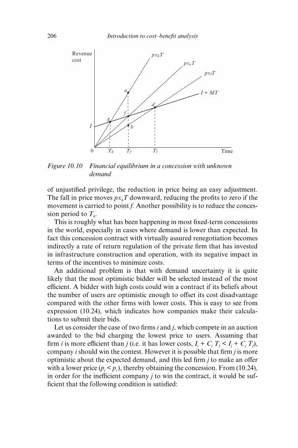
206 Introduction to cost–benefi t analysis
of unjustifi ed privilege, the reduction in price being an easy adjustment.
The fall in price moves pxhT downward, reducing the profi ts to zero if the
movement is carried to point f. Another possibility is to reduce the conces-
sion period to Th.
This is roughly what has been happening in most fi xed- term concessions
in the world, especially in cases where demand is lower than expected. In
fact this concession contract with virtually assured renegotiation becomes
indirectly a rate of return regulation of the private fi rm that has invested
in infrastructure construction and operation, with its negative impact in
terms of the incentives to minimize costs.
An additional problem is that with demand uncertainty it is quite
likely that the most optimistic bidder will be selected instead of the most
effi cient. A bidder with high costs could win a contract if its beliefs about
the number of users are optimistic enough to off set its cost disadvantage
compared with the other fi rms with lower costs. This is easy to see from
expression (10.24), which indicates how companies make their calcula-
tions to submit their bids.
Let us consider the case of two fi rms i and j, which compete in an auction
awarded to the bid charging the lowest price to users. Assuming that
fi rm i is more effi cient than j (i.e. it has lower costs, Ii + Ci Tf < Ij + Cj Tf),
company i should win the contest. However it is possible that fi rm j is more
optimistic about the expected demand, and this led fi rm j to make an off er
with a lower price (pj < pi ), thereby obtaining the concession. From (10.24),
in order for the ineffi cient company j to win the contract, it would be suf-
fi cient that the following condition is satisfi ed:
Time0
I
Revenue
cost
I + MT
pxeT
Tf
pxlT
pxhT
Th Tl
g
a
f
b
d
Figure 10.10 Financial equilibrium in a concession with unknown
demand

Applications 207
Ii 1 CiTf
xeiTf
.Ij 1 CjTf
xejTf
, (10.25)
or, equivalently,
xe
j
xei
.Ij 1 CjTf
Ii 1 CiTf
. (10.26)
Expression (10.26) shows that the less effi cient fi rm can win the contract
if it is optimistic (xej . xe
i) enough to off set its cost disadvantage. It can be
seen that the condition (10.26) can be met if the ineffi cient fi rm j is inef-
fi cient either in absolute terms (both construction and maintenance costs
are greater than those of i) or in relative terms (its total cost Ij + Cj Tf is
higher for a fi xed duration, although it might be Ij < Ii or Cj < Ci).
In conclusion one can note three major negative economic consequences
of the conventional fi xed- term concession system based on auctions with
bids for the minimum price to charge the users:
In the absence of perfect information on demand, this type of ●
auction does not guarantee the selection of the fi rm with the lowest
costs since the existence of diff erent beliefs about future demand
may cause an ineffi cient and optimistic fi rm to win the contract.
If fi rms anticipate that it may be possible to renegotiate the conces- ●
sion contract in the future because of changes in the volume of users,
the incentives to operate at minimum cost are weak since eff orts to
operate effi ciently can be substituted by negotiation with the regula-
tor requiring a price change to restore the normal benefi ts.
With the fi xed- term system and inelastic demand, price becomes an ●
accounting adjustment variable, tending to rise when demand is low
and decline when demand is high, which can lead to an ineffi cient
use of the infrastructure, contrary to what would be desirable from
an economic standpoint. In general when demand is low there will
be no pressure on existing capacity, and it would be desirable for the
price to encourage the use of infrastructure. When demand is high
and congestion problems occur, the price should rise in order to
ration the available capacity.
The three consequences this type of contract reduce the ex post NPV of
the project. The problems of private participation in infrastructure with
fi xed- term concession contracts are a result of the economic character-
istics of these projects, and especially the uncertainty of demand. High
costs, long life and asset specifi city, coupled with the inability to predict

208 Introduction to cost–benefi t analysis
the demand for the life of the concession, are the elements that cause the
renegotiation of contracts and the loss of the essence of a public tender.
An alternative contract to avoid these problems is to change the mech-
anism of fi nancial adjustment of the concession system. According to our
analysis above, the problem of demand uncertainty translates into uncer-
tainty about the revenue the fi rm expects from the concession. This is the
fundamental point that generates the risk of failure of the concessionaires
(in the case of low demand) or of the government reducing prices (in the
case where demand is high). One possible solution is for the government
to fi x the price, the level of quality and the discount rate, and for fi rms to
make off ers on the revenue they want to receive during the life of the con-
cession, thus eliminating revenue uncertainty, and letting the contract last
as long as it takes to earn the revenue included in the winning bid.15
THINGS TO REMEMBER
Even assuming that the privatization policy results in net benefi ts ●
for the society, these benefi ts may not be well distributed. It may be
that producers are better off with privatization, but consumers and
workers are worse off . Therefore, to assess a privatization project
in practice, the practitioner should make a detailed assessment of
winners and losers. This will be necessary in order to design the com-
pensation mechanisms, for reasons of equity or to make the project
politically acceptable.
Working exclusively with expected values may neglect some valuable ●
information. Risk analysis provides the decision maker with a more
complete picture as too much aggregation hides useful information.
It is really impossible to foresee all the circumstances a project has ●
to go through during its lifespan. Ex ante demand and costs do not
necessarily coincide with ex post values; hence, the economic evalu-
ation of project has to take into account the facts that explain this
divergence.
Actual demand depends on some unpredictable contingencies but ●
also, to some extent, on decisions taken by economic agents.
Contract designs both allocate risk and aff ect the level of eff ort
exerted by fi rms to reduce costs. There are two basic types of con-
tracts, the cost- plus and the fi xed- price, and diff erent combinations
depending on the degree of risk and incentives.
The eff ects of public support by supranational agencies on the ●
investment decision taken by national governments vary with the
institutional design. The existence of two levels of government, in

Applications 209
which supranational and national governments (or national and
regional governments) can modify the incentives in the selection
of projects, aff ects the value of cost–benefi t analysis as a tool for
informed decision taking.
Private participation requires the design of contracts. The govern- ●
ment wants to select the most effi cient contractor and to off er a
contract that keeps the fi rm interested in minimizing costs. To
achieve their objectives, the government and the fi rms have to work
in a world of uncertainty and asymmetric information. The type of
contract can have profound eff ects on the ex post net present value
of projects.
NOTES
1. For a more detailed analysis see de Rus (2008, 2009), de Rus and Nombela (2007). 2. Time savings are assumed to be the same within each group of users changing
mode. 3. The basic model in this section summarizes the excellent work by Jones et al. (1990). 4. The justifi cation for lg > lp is that when the government obtains funds through taxes it
imposes an additional burden (deadweight loss of the tax) on the economy and there-fore it implicitly gives more value to money in its hands than in the hands of the private sector. Therefore, if with the privatization of the public fi rm the government obtains funds without distorting the economy, the shadow price of these funds should refl ect the additional benefi t of avoiding the distortion of raising the same revenue through taxes (see section 4.8).
5. Sticking to the four most common types of auctions (English, Dutch, sealed auction and Vickrey auction) the fi rst objective can be achieved with the English and Vickrey auctions, but the second is not guaranteed by any of the four; and therefore we can expect that in general Z is less than Vpp, especially when, as happens to be the case, the number of bidders is not very high in a privatization process. For a more detailed discussion on auctions see Klemperer (1999).
6. For an analysis of the design of concession contracts and price regulation see Guasch (2004). The importance of these issues in cost–benefi t analysis is crucial, since the actual social NPV arising from the implementation of projects is largely aff ected by regulatory mechanisms.
7. A major infrastructure project was the Channel Tunnel. It links Britain to the Continent 40 m under the sea. A recent evaluation concludes: ‘The cost benefi t appraisal of the Channel Tunnel reveals that overall the British economy would have been better off if the Tunnel had never been constructed, as the total resource cost has been greater than the benefi ts generated’ (Anguera, 2006, p. 314).
8. This second level has been widely analysed in the economic literature (Laff ont and Tirole, 1993; Bajari and Tadelis, 2001; Guasch, 2004; Olsen and Osmundsen, 2005).
9. Cost overruns are common in large infrastructure projects and it has been demon-strated that the deviation is not only explained by unforeseen events (Flyvbjerg et al., 2003).
10. The implementation of the user pays and the polluter pays principles and the reduc-tion of public expenditure have signifi cant political costs (Sobel, 1998). Downs (1957), Niskanen (1971) and Becker (1983) have often assumed that legislators attempt to max-imize electoral support. Even if re- election may not be the primary factor motivating

210 Introduction to cost–benefi t analysis
their legislative behaviour, it is still true that legislators react in predictable ways to the electoral costs and benefi ts of their choices. Thus legislators will favour actions that increase the probability of re- election over decisions that lower it (Sobel, 1998; Robinson and Torvik, 2005).
11. As is common with fi xed- price contracts, some kind of quality regulation may be required.
12. In practice a multicriteria tender is commonly used, with several variables among which the price is included.
13. To simplify the exposition we assume that bidders bid their reservation prices; that is, they present their off ers with the most that they are willing to pay, so they earn normal profi ts.
14. Another method is to set the price and award the concession to the bidder who requests the shortest concession period. This case is actually a variation of the fi xed- term conces-sion contract since once the public tender fi nishes the concession period is as fi xed as in the price (or canon) concession system.
15. If the concession period is allowed to be variable instead of fi xed (remember that Tf is predetermined in the case of the traditional concession), it would be possible to accom-modate situations of high or low demand without the need to renegotiate the contract or having to make unwanted changes in prices. For example, in Figure 10.10, in a situ-ation of low demand (xl) the length of the concession is automatically extended to Tl, thus allowing the recovery of the total costs. By contrast, in a case of high demand, in a period Th such recovery of total costs would have been realized earlier and ending the concession at that time would avoid economic profi ts. This system was fi rst applied in the UK in the construction and operation of a bridge. Later, it was used in the road concession Santiago–Valparaíso–Viña del Mar in Chile. See Engel et al. (2001) and Nombela and de Rus (2004) for an analysis of variable- term concessions.

211
11. Microeconomic foundations of cost–benefi t analysis1
One summer, a colleague asked me why I have not bought a parking permit. I replied that not having a convenient place to park made me more likely to ride my bike. He accused me of inconsistency: As a believer in rationality, I should be able to make the correct choice between sloth and exercise without fi rst rigging the game. My response was that rationality is an assumption I made about other people. I know myself well enough to allow for the consequences of my own irrationality. But for the vast mass of my fellow humans, about whom I know very little, rationality is the best predictive assumption available.
(David Friedman, 1996, p. 5)
11.1 INTRODUCTION
This chapter covers the basic theoretical framework of cost–benefi t
analysis. The objective is to give a clearer picture of what is behind the
concept of social welfare and the decision criteria based on the net present
value. The approach is theoretical but neither exhaustive nor extremely
technical.
The way from individual preferences to social welfare is the content of
section 11.2. Section 11.3 addresses the measurement of producer surplus
in the product and factor markets. Section 11.4 analyses the three money
measures of changes in individual utility most frequently used to evaluate
economic changes: compensating variation, equivalent variation and con-
sumer surplus. Section 11.5 deals with uncertainty.
11.2 FROM INDIVIDUAL UTILITY TO SOCIAL WELFARE
Given the social welfare function in (11.1), assuming independent utili-
ties and taking total diff erentials, the change in social welfare (W) can be
expressed as (11.2): the sum of the variations in the utility (U) of the m
individuals who form the society, weighted by the relative importance the

212 Introduction to cost–benefi t analysis
society attaches to the utility of each individual (i.e. social marginal utility:
0W/0Ui).2
W 5 W(U1, U2, . . ., Um) , (11.1)
dW 5 am
i51
0W0Ui
dUi. (11.2)
The utility of individuals depends on the quantities of the n goods and
services (x) available for consumption. In the case of individual i:
Ui 5 Ui(xi1, xi2, . . ., xin
) . (11.3)
Assuming that individual i maximizes utility, subject to the constraint
that aggregate expenditure cannot be greater than his income, we have the
following expression:
Maxxi1, xi2, . . ., xin
Ui(xi1, xi2, . . ., xin
) 2 mi aan
j51
pjxij 2 Mib, (11.4)
where:
xij: quantity of good j consumed by individual i
Mi: income of individual i
pj: price of good j
μi: Lagrange multiplier.
First order conditions are as follows:
0Ui
0xij
2 mi pj 5 0, j 5 1, . . ., n, (11.5)
an
j51
pjxij 2 Mi 5 0. (11.6)
The economic interpretation of the fi rst order conditions is the follow-
ing: to maximize utility, the individual allocates his income so that, at the
optimum and for the selected goods, the marginal utility of consuming the
last unit of the good (0Ui/0xij) is equal to the disutility of paying the price
(mipj) as mi is the marginal utility of income. Moreover the spending on all
the chosen goods exhausts the individual’s income.
Solving for pj in (11.5):
pj 5
0Ui
0xij
mi
. (11.7)

Microeconomic foundations of cost–benefi t analysis 213
At the optimum, the individual consumes additional units of good j
until the price is equal to the marginal valuation of the good (the ratio of
expression (11.7)). Whenever the marginal valuation of the good is greater
than its price, the individual increases the consumption of the good until
the budget constraint is binding. It may happen that the price is higher
than the marginal valuation of the good for some goods and the individual
does not consume them. In this case the fi rst order condition is satisfi ed as
a strict inequality (corner solution).
By diff erentiating (11.3) we obtain expression (11.8), where the varia-
tion in the total utility of individuals depends on the marginal utility of
each good and the variation in the quantity consumed of that good:
dUi 5 an
j51
0Ui
0xij
dxij. (11.8)
Substituting the fi rst order condition (11.5) in (11.8) we obtain the vari-
ation in individual welfare:
dUi 5 an
j51
mi pj dxij. (11.9)
Equation (11.9) contemplates utility as a function of quantities con-
sumed, given the prices of goods and services and the income of the indi-
vidual. The variation of the utility of individual i depends on the marginal
variation in the quantities of the n goods consumed, multiplied by their
price (which we assume to be constant) and converted to utilities by multi-
plying by the marginal utility of income (mi).
A useful concept for money measures of changes in individual utili-
ties is the indirect utility function. Individual utility used in its original
functional form (11.3) is a function of the quantities of goods and services
consumed by the individuals, given prices and income. Going back to the
fi rst order conditions (11.5) and (11.6), and obtaining the values of x that
maximize the utility function as a function of the vector of prices (P) and
income (M), the indirect utility function is the utility function expressed as
U = U(X(P, M)), or:
Vi(p1, p2, . . ., pn, Mi
) 5 Ui(xi1
(p1, p2, . . ., pn, Mi) , xi2
( # ) , . . ., xin( # )) .
(11.10)
Adding the budget constraint to (11.10) we can use the indirect utility
function to express the utility maximization as a function of prices and
income:

214 Introduction to cost–benefi t analysis
Vi(p1, . . ., pn, Mi
) 5 Ui(xi1
(p1, p2, . . ., pn, Mi) , xi2
( # ) , . . ., xin( # ))
2 miaan
h51
phxih(p1, . . ., pn, Mi
) 2 Mib. (11.11)
At the optimum, diff erentiating with respect to pj and noting that
V(P, M) = U(X(P, M)), we obtain how the utility varies with an infi nitesi-
mal variation of price:
0Vi
0pj
5 an
h51
0Ui
0xih
0xih
0pj
2 miaxij 1 an
h51
0xih
0pj
phb, (11.12)
0Vi
0pj
5 an
h51
a 0Ui
0xih
2 mi phb 0xih
0pj
2 mixij 5 2mixij, (11.13)
because at the optimum (see fi rst order condition (11.5)),
a 0Ui
0xih
2 mi phb 0xih
0pj
5 0; h = 1, 2 . . . n. (11.14)
The result obtained in (11.13) is well known in microeconomic theory
as Roy’s Identity. As we have seen, it is easily derived by applying the
envelope theorem.3
By totally diff erentiating (11.10) we obtain the expression (11.15), where
the variation in the total utility of the individual depends on the marginal
utility with respect to each change in price multiplied by the price changes,
plus the marginal utility of income multiplied by the change in income:
dVi 5 an
j51
0Vi
0pj
dpj 10Vi
0Mi
dMi. (11.15)
Keeping income constant (dMi = 0) and using the result in (11.13):
dVi 5 2 an
j51
mi xij dpj. (11.16)
This expression is equivalent to (11.9) for projects with price changes
(keeping quantities constant). In this chapter we only deal with changes
either in the quantities of goods (11.9) or in the prices (11.16) without
changes in the costs. In Chapter 2 we deal with situations in which prices
and quantities change simultaneously.4
Expressions (11.9) and (11.16) show how to assess the change in indi-
vidual utility as a result of a change in quantities and prices. The change

Microeconomic foundations of cost–benefi t analysis 215
in prices is multiplied by the quantity and the change in quantities is
multiplied by prices. To convert this change in utility, expressed in mon-
etary units, we need μi to be constant and, unless μi is constant, we cannot
directly associate the monetary changes with changes in utility. Identical
increases in income result in diff erent changes in utility if the marginal
utility of income is not constant.
With utility increasing with income (0U/0M . 0) but less than propor-
tionately (02U/0M2 , 0), unless we know the value of the marginal utility of
income for individuals with diff erent income levels, it is not possible to convert
the aggregate changes in quantities or prices of goods in utility changes.
The above argument is useful for understanding the economic rationale
of the measurement of social benefi ts arising from the implementation of
a project. As the utility is not observable, we use monetary measures that
refl ect the change in the utility of individuals. We are not directly measur-
ing the change in utility, but the change in the willingness to pay or accept,
with monetary measures that, despite their limitations, allow us to gain
approximations of what we win and lose with the project.
Returning to the social welfare function (11.1) and its total diff erential
(11.2), and using the results derived in this section, we can express the
eff ect of a small change in quantities (11.17) and prices (11.18) on social
welfare:
dW 5 an
j51a
m
i51
0W0Ui
0Ui
0Mi
pj dxij, (11.17)
dW 5 2an
j51a
m
i51
0W0Ui
0Ui
0Mi
xij dpj. (11.18)
For the economic interpretation of both expressions it is useful to read
them from right to left. The project may involve a change in quantities
(with p constant) or a change in prices (with x constant). In both cases
these changes are converted into monetary units, multiplying by price or
quantity, respectively.
For such monetary changes to be converted into changes in social
welfare there are two types of weights. First, the marginal value of income
for each individual (0Ui/0Mi) , which depends on the income level of the
individual. This weight transforms income into individual utility. The
second weight (0W/0Ui) converts individual utility into social welfare.
For society to improve, with the increase in individual utility, 0W/0Ui
must be positive. The partial derivative 0W/0Ui can be diff erent for dif-
ferent individuals. The society may give more weight to social groups
with diff erent income levels, health conditions or any other relevant

216 Introduction to cost–benefi t analysis
characteristic. The two weights interpreted together are the social mar-
ginal utility of income.
Expressions (11.17) and (11.18) aggregate the change experienced by
the m individuals, initially measured in monetary units, using the weights
described. In (11.17) and (11.18) there is an implicit social welfare func-
tion that determines how to proceed with regard to the weighting scheme.
The simplest case is the potential compensation, or Kaldor–Hicks crite-
rion, in which benefi ts and costs are added unweighted (i.e. it is implicitly
assumed that the two weights in (11.17) and (11.18) are equal to one).
The potential compensation criterion implies that the marginal utility
of income is constant, and society gives the same weight to the utility
changes of all individuals regardless of income, health status, and so on.
Other approaches are possible with equations (11.17) and (11.18). One
possibility is to correct for the marginal utility of income and add the changes
in utility, giving the same social value to the utility of any individual. In this
way, if the marginal utility of income is decreasing, we will outweigh the
benefi ts and costs of those with lower income. It should be emphasized that
this correction does not have any redistributive basis although it may seem
so if we compare it with the potential compensation criterion.
Another possibility is a welfare function that introduces the social aver-
sion to inequality. In this case, once the net benefi ts of each individual are
corrected according to their marginal utility of income, it introduces an
additional weight (the social marginal utility) that varies inversely with the
income of the individual in higher or lower proportions depending on the
degree of egalitarianism.
11.3 MEASUREMENT OF PRODUCER SURPLUS
The diff erence between a fi rm’s revenues and variable costs of production
is called producer surplus. This surplus is the gross profi t in the sense that
fi xed costs have not been deducted. Suppose a company has an annual
revenue of 100 and its total costs are equal to 100, of which 50 are variable
and 50 fi xed. Variable costs are by defi nition avoidable if the fi rm produces
nothing. Assume that the fi xed costs are sunk costs. With this information
the fi rm has zero profi ts and a producer surplus equal to 50.
Suppose the owner of the company is asked for the maximum he is
willing to pay to keep the fi rm open once production has started. Excluding
any strategic consideration his answer is 50. Though the company earns
a profi t of zero, the producer surplus indicates the maximum he is willing
to pay to stay open. If it closes he loses 50; if it remains open he covers
costs. The fi xed cost could be higher and the response would not change.

Microeconomic foundations of cost–benefi t analysis 217
The producer surplus is positive, so the owner would be willing to pay
for continued production. Producing with a positive surplus contributes
to the recovery of fi xed costs. Depending on the size of the surplus, the
fi xed costs could be partially or wholly covered or the company could even
make a profi t.
What happens if the question about willingness to pay to avoid the
closure was made to the owner before spending on the fi xed factor?
Would the producer surplus be the highest potential payment for avoiding
closure? The answer is yes, and this maximum is now zero. Before starting
the production, all the factors are variable and with the numbers of our
example the surplus is zero. In general, if there are no fi xed costs, the profi t
and producer surplus are identical.
More often the analyst needs to know the changes in the producer’s
surplus rather than the absolute value of the surplus; for example the
change caused because the price or the production costs have changed.
Consider the case of a fi rm operating in competitive markets of factors
and products that supplies a good x, with a well behaved production func-
tion, x 5 x(L, K) , with a variable factor of production L with price w and
a fi xed factor K whose price is assumed to be one. The company’s profi t in
the short term is equal to:
p 5 px(L) 2 wL 2 K. (11.19)
As a decision rule to start production we can say that the fi rm will not
invest unless the producer’s surplus (PS) is equal to or greater than the
fi xed cost:
PS 5 px(L) 2 wL $ K. (11.20)
In the short term, deriving (11.19) with respect to L, we obtain the fi rst
order condition of profi t maximization:
pdx(L)
dL2 w 5 0, (11.21)
which indicates that, to maximize profi t, we should further increase pro-
duction as long as the value of the marginal productivity of the variable
factor is greater than the price of that factor.
With a fi xed factor, under standard assumptions, the marginal pro-
ductivity of L will eventually decrease, so that for the given prices ( p, w)
equality (11.21) must be met. The profi t function depends therefore on the
price of the good (p) and the price factor (w).

218 Introduction to cost–benefi t analysis
The profi t equation (11.19) can be expressed as a value function, which
depends indirectly on p and w (we use the same idea as in the case of the
indirect utility function):
V(p, w) 5 px(p, w) 2 wL(p, w) 2 K. (11.22)
The derivative of the function (11.22) with respect to the price of the
good (a parameter for the competitive fi rm) shows the variation that
occurs in the fi rm’s profi t at the maximum. Therefore it should not be
interpreted as a fi rst order condition, but the eff ect on profi ts of a change
in the price at the optimum.
0V0p
5 x(p, w) 1 p0x0L
0L0p
2 w0L0p
5 x(p, w) . (11.23)
The increase in the benefi t of an infi nitesimal change in price is equal to
the quantity sold by the fi rm (the envelope theorem) since, as the fi rm is
located at the optimal production level, we know that:
ap0x0L
2 wb 0L0p
5 0. (11.24)
The result obtained in (11.23) is very useful for calculating the change in
producer surplus when the price changes, because we simply need to inte-
grate the function x(p,w) , which is the supply function of the company,
using as integration limits the initial and the fi nal prices:
DPS 5 3p1
p0
x(p, w)dp. (11.25)
Figure 11.1 shows the change in producer surplus when the price
increases from p0 to p1. This change, represented by the area p1bap0,
coincides with the change in the fi rm’s profi t. Note that for a very small
price increase the surplus reduces to x0; that is, to the results stated in
(11.23).
Deriving expression (11.22) with respect to the factor price (exogenous
to the fi rm), we obtain the variation that occurs in the fi rm’s profi t when
the factor price changes; just as happens with the price of a good, the idea
is not to obtain a condition of maximization but to calculate the change in
profi ts at the optimum when a parameter changes.
0V0w
5 p0x0L
0L0w
2 L(p,w) 2 w0L0w
5 2L(p,w) . (11.26)
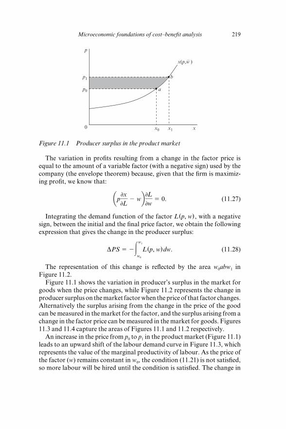
Microeconomic foundations of cost–benefi t analysis 219
The variation in profi ts resulting from a change in the factor price is
equal to the amount of a variable factor (with a negative sign) used by the
company (the envelope theorem) because, given that the fi rm is maximiz-
ing profi t, we know that:
ap0x0L
2 wb 0L0w
5 0. (11.27)
Integrating the demand function of the factor L(p, w) , with a negative
sign, between the initial and the fi nal price factor, we obtain the following
expression that gives the change in the producer surplus:
DPS 5 23w1
w0
L(p, w)dw. (11.28)
The representation of this change is refl ected by the area w0abw1 in
Figure 11.2.
Figure 11.1 shows the variation in producer’s surplus in the market for
goods when the price changes, while Figure 11.2 represents the change in
producer surplus on the market factor when the price of that factor changes.
Alternatively the surplus arising from the change in the price of the good
can be measured in the market for the factor, and the surplus arising from a
change in the factor price can be measured in the market for goods. Figures
11.3 and 11.4 capture the areas of Figures 11.1 and 11.2 respectively.
An increase in the price from p0 to p1 in the product market (Figure 11.1)
leads to an upward shift of the labour demand curve in Figure 11.3, which
represents the value of the marginal productivity of labour. As the price of
the factor (w) remains constant in w0, the condition (11.21) is not satisfi ed,
so more labour will be hired until the condition is satisfi ed. The change in
p0
p1
x1x0 x
p
x(p,w– )
b
a
0
Figure 11.1 Producer surplus in the product market

220 Introduction to cost–benefi t analysis
producer surplus in the factor market equals the area bdfa, between the
two curves of factor demand limited by the factor price that remains con-
stant at the new equilibrium.
Similarly, a price reduction in the factor market (Figure 11.2) results in
a downward shift of the supply curve in the product market (Figure 11.4),
which represents the reduction in the marginal cost of production. As the
price of the good is kept constant, reducing the marginal cost makes an
increase in production profi table. The change in producer surplus in the
market for goods equals the area bdfa, between the two supply curves of
the good limited by the constant price at the new level of production.5
L(p–1,w)L(p–0,w)
w0
L1L0 L
w
0
a
b
df
Figure 11.3 Eff ect of a change in the price of the good, measured in the
factor market
L(p–,w)
w1
w0
L1L0 L
w
a
b
0
Figure 11.2 Producer surplus in the factor market

Microeconomic foundations of cost–benefi t analysis 221
Producer Surplus and the Surplus of the Owners of the Production Factors
The change in producer surplus as a result of the implementation of a
project does not show who the benefi ciaries of this surplus are. The pro-
ducer surplus is a little confusing because eventually this change in the
surplus may be a change in the income of the company owners, the owners
of land and other fi xed factors, the taxpayers or the workers.
Suppose factor L is an imported raw material. In this case the reduction
in the cost of production increases producer surplus and this is the change in
social surplus (given that p does not change, the consumer surplus remains
constant). By contrast, if L is domestic labour, the change in the surplus of
workers has to be taken into account like the surplus of any other social
agent. A reduction in w as a result of the privatization of a public company
represents a reduction in the workers’ surplus, which for constant x off sets
the increase in producers’ surplus, leaving social welfare unaff ected.
Workers off er their labour if they are paid wages at least equal to their
opportunity costs. Quite often, in the economic evaluation of projects,
worker surplus obtained by subtracting the opportunity cost of working
(for example the value of leisure) from the wages is not included, prin-
cipally because many projects do not produce signifi cant changes in the
labour market, changing the equilibrium wage.
Figure 11.5 represents a function of labour supply SL(w) . The minimum
reservation wage is wr, below which no one is willing to work in the market
represented in the fi gure. This might be because there is an unemployment
benefi t or because the informal economy off ers jobs paid around wr.
Suppose that the labour market represented in Figure 11.5 is in
p0
x1x0 x
p
0
b
a
d f
x(p,w–1)
x(p,w–0)
Figure 11.4 Eff ect of a change in the price of the factor, measured in the
product market

222 Introduction to cost–benefi t analysis
equilibrium at point d, so that at wage w0, L0 workers are employed. If the
wage rises to w1, the change from d to b generates new jobs (from L0 to L1).
In the event that b is an equilibrium, new employees are willing to work for
their opportunity cost (area dbL1L0). However they receive as wages the
area abL1L0, resulting in a surplus for the new employees equal to the area
abd. Existing workers also benefi t from the wage increase and their surplus
goes from w0dwr to w1adwr; or, which is the same, the surplus of existing
workers increases in the area w1adw0.
It should be emphasized that we could ignore the concept of producer
surplus and simply add up the surpluses of the social agents: landowners,
shareholders, consumers, workers and taxpayers. Although any individual
belongs to more than one category, this functional classifi cation is useful
in cost–benefi t analysis.
In practice it is interesting to distinguish between fi xed factors imposed
by the nature that persists in the long term, such as the available land in a
particular urban area or the agricultural land of particular characteristics,
and fi xed factors by law, such as some licences that restrict the entry of
new suppliers into the market.
Although it is straightforward to sum the surpluses of the agents,
including the owners of fi xed factors, the use of the producer’s surplus can
be suitable when information is scarce and one has to work with assump-
tions about what happens in the market at a very aggregate level.
Finally, a note of caution to avoid double counting. Suppose that
Figure 11.1 represents an increase in the surplus of farmers as a result
of rising agricultural prices. In assessing the change that has occurred in
the market, we can use the producer’s surplus represented in Figure 11.1
w1
w0
w
aSL
b
d
wr
0 L0 L1 L
Figure 11.5 Workers’ surplus

Microeconomic foundations of cost–benefi t analysis 223
or the income of the landowners if we expect land rents to be updated to
absorb the benefi ts of farmers, but not both.
11.4 COMPENSATING VARIATION, EQUIVALENT VARIATION AND CONSUMER SURPLUS
A price reduction or an increase in product quality allows the individual
to reach a higher level of utility. The individual has improved, although
we do not know the magnitude of improvement since the value that is
assigned to both levels of utility is completely arbitrary.
In cost–benefi t analysis we aim to go further and want to know the
change in the social welfare of such individual improvements and this
requires aggregating the changes in individual utilities. If the magnitude
of the diff erences in utility is arbitrary (it only matters that the utility in
one state is higher than in the other), it makes even less sense to add the
changes in utility for diff erent individuals.
One way out of these problems is to rely on the monetary valuation
that individuals give to the utility change, and then add these individual
values (remember that the aggregation of individual valuations requires,
for conversion to social welfare, to weight them according to the marginal
social utility of income).
The three money measures of changes in individual utility most fre-
quently used to evaluate economic changes are the compensating varia-
tion, the equivalent variation and consumer surplus.
The compensating variation (CV) can be defi ned as the income that can
be taken from the individual once the change occurs, leaving him at the
same level of utility as before the change.6 The equivalent variation (EV)
can be defi ned as the income to be given to the individual to attain the
same level of utility reached with the change, but without the change (that
is the amount of income that is equivalent to the change). The advantage
of the CV and the EV is that they are money measures of the change in
the individual’s utility. The consumer surplus (CS) can be defi ned as the
sum of the willingness to pay of each unit consumed (the area under the
demand function between zero and the last unit consumed) minus the total
expenditure on the good. The change in CS is therefore the diff erence in
surplus before and after the change.
To see the theoretical justifi cation of these money measures of utility, we
start by minimizing the expenditure of an individual subject to a constant
level of utility U (for simplicity of notation we omit the subscript i):
Minx1, . . ., xn
an
j51
pj xj 2 m (U(x1, . . ., xn) 2 U ) . (11.29)

224 Introduction to cost–benefi t analysis
The fi rst order conditions are:
pj 2 m0U0xj
5 0, j 5 1, . . ., n, (11.30)
U(x1, . . ., xn) 5 U . (11.31)
Obtaining from (11.30) and (11.31) the values xj that minimize (11.29),
we obtain an expenditure function at the optimal e(P, U) in which P is the
vector of prices (p1, . . ., pn):
e 5 an
j51
pjxj(P,U) 2 m [ (U(x(P, U)) 2 U ]. (11.32)
Deriving this value function with respect to pj:
0e0pj
5 xj(P,U) 1 a
n
h51
ph
0xh
0pj
2 man
h51
0U0xh
0xh
0pj
5 xj(P, U) . (11.33)
Expression (11.33) shows that the variation in expenditure when the
price of a good is changed infi nitesimally is equal to the compensated
demand xj(P, U) because, at the optimum, according to (11.30):
aph 2 m0U0xh
b 0xh
0pj
5 0; h = 1, 2 . . ., n. (11.34)
The demand function xj(P, U) is called compensated or Hicksian
demand and the utility is constant, while with the market demand
xj(P, M) income is constant. The compensated demand function shows
how the demanded quantity changes when the price of the good changes,
while the income is adjusted so that the utility remains constant.
Using the indirect utility function V(P, M) 5 U , where U is the level of
utility that minimizes the expenditure in (11.32), and two levels of utility
for U , the one before the change U0 and the one obtained after the change
U1, we see that the individual improves when the sign of (11.35) is positive
and is worse off when the sign is negative:
V(P 1, M
0) 2 V(P 0, M
0) . (11.35)
Expression (11.35) tells us the sign of the change, but it does not give us
any information on the magnitude of the change.7 In cost–benefi t analysis,
it is not enough to know that some individuals improve and others become

Microeconomic foundations of cost–benefi t analysis 225
worse off . If the money measure for taxpayers is a reduction of 1000 with
the project, it is not enough for the decision maker to know that workers,
employers and consumers will be better off . He also needs to know the
magnitude of the improvement to compare it with the costs incurred, and
to know whether the benefi ts of the benefi ciaries of the project are high
enough to off set the costs.
We need money measures of changes in the utility. The compensating
variation (CV) is one of them (see Jara- Díaz and Farah, 1988). Suppose
that income remains constant and prices fall. In expression (11.36) we see
how the CV measures the improvement, expressed in monetary terms,
experienced by the individual:
U 0 5 V(P
0, M 0) 5 V(P
1, M 0 2 CV ) . (11.36)
With initial prices and income (P 0, M
0), the utility is equal to U 0 (we
are at the point of departure, before the change). Expression (11.36) shows
the income that should be taken (CV) from the individual in order to pre-
serve the utility at the initial level in the new situation. If the change was
an increase in prices, the CV would be negative (we would increase the
income of the individual). Inverting (11.36):
M 0 5 e(P
0, U 0) and M
0 2 CV 5 e(P 1, U
0) , (11.37)
so that the CV can be expressed as:
CV 5 e(P 0, U
0) 2 e(P 1, U
0) , (11.38)
which in the case of independent goods can be expressed as:
CV 5 an
j51
3p0
j
p1j
xj(P, U
0)dpj. (11.39)
In equation (11.38) the CV appears as the diff erence in the minimum
amount of income required to achieve the level of utility U
0 given the
initial and fi nal prices. If the diff erence is positive, the individual has
improved (as you can take income to leave him at the same level of utility).
If the diff erence is negative, the individual is worse off because we have to
give him income to compensate for the change.
The CV in (11.39) is valid for the case of independent goods and uses the
result in (11.33), where the derivative of the expenditure at the optimum
with respect to price is the compensated demand function xj(P, U
0) . If
we integrate the compensated demand function, using the initial and fi nal

226 Introduction to cost–benefi t analysis
prices as integration limits, we obtain an area equal to the CV, since the
compensated demand does not incorporate the income eff ect.
We can proceed in the same way for the equivalent variation:
U 1 5 V(P
1, M 0) 5 V(P
0, M 0 1 EV ) . (11.40)
With the income constant and the fi nal prices (P 1, M
0) the utility is equal
to U 1 (the level of utility after the change). Suppose that at this utility level
U 1 the individual has improved because the prices P
1 are lower than P 0.
Expression (11.40) shows that the EV consists of giving income to the
individual in order, with the initial prices (P 0) and without the change, to
make him as well off as in the level of utility U 1, equivalent to the change.
If the change was an increase in prices, the EV would be negative (income
will be taken from the individual). Inverting (11.40):
M 0 5 e(P
1, U 1) and M
0 1 EV 5 e(P 0, U
1) , (11.41)
and the EV can be expressed as:
EV 5 e(P 0, U
1) 2 e(P 1, U
1) , (11.42)
which in the case of independent goods can be expressed as:
EV 5 an
j51
3p0
j
p1j
xj(P, U
1)dpj. (11.43)
In expression (11.42), the EV appears as the minimum income required
for attaining the level of utility U 1 with the initial and fi nal prices. If the
diff erence is positive, the individual has improved (as an increase in income
is equal to a change that leads to a higher level of utility). If the diff erence
is negative, the individual is worse off since the change is equivalent to a
loss of income.
In the same way as with the CV, expression (11.43) is only valid for
independent goods and uses the result in (11.33) where the derivative of
the expenditure in the optimum with respect to price is the compensated
demand function, though now at a diff erent level of utility xj(P, U
1) . By
integrating the compensated demand function for a level of utility U 1 and
using the initial and fi nal price of the good j as limits of integration, an
area equal to the EV is obtained.
The CV and the EV do not necessarily coincide. They both measure
changes in the value of the individual’s utility in terms of money, with respect
to the initial level in the case of CV and the fi nal level in the case of EV.

Microeconomic foundations of cost–benefi t analysis 227
Figure 11.6 represents, in the upper part, the indiff erence curves and the
budget constraint of a consumer who chooses between good x1 (in the verti-
cal axis) and other goods, or income (in the horizontal axis). Initially, the
individual is located at point b, where the indiff erence curve U0 is tangent
to the budget constraint zM2. Their income level is equal to M2, which is
the maximum amount of other goods that the individual could consume if
he does not consume x1. Suppose that we reduce the price of x1, shifting the
budget constraint to hM2, and now the individual chooses point l. The CV
consists of taking away income from the individual such that he reaches the
same level of utility enjoyed in b but once the price of x1 has changed. Point
d is the new location, and is achieved by reducing income by M2 2 M1.
Applying the defi nition of EV, we should give income to the individual at
M1
M
A B
U0
U1
�U
�M
�U
�M
M3M2
M1 M3M2
M
x1
f
d
l
b
z
h
Figure 11.6 Why do CV and EV not coincide?
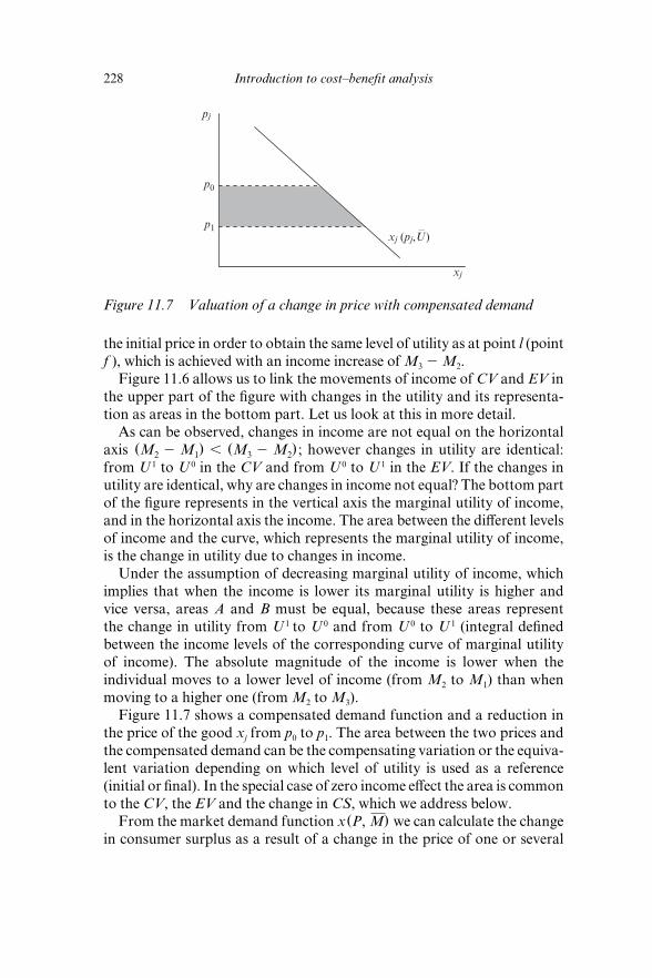
228 Introduction to cost–benefi t analysis
the initial price in order to obtain the same level of utility as at point l (point
f ), which is achieved with an income increase of M3 2 M2.
Figure 11.6 allows us to link the movements of income of CV and EV in
the upper part of the fi gure with changes in the utility and its representa-
tion as areas in the bottom part. Let us look at this in more detail.
As can be observed, changes in income are not equal on the horizontal
axis (M2 2 M1) , (M3 2 M2
) ; however changes in utility are identical:
from U 1 to U 0 in the CV and from U 0 to U 1 in the EV. If the changes in
utility are identical, why are changes in income not equal? The bottom part
of the fi gure represents in the vertical axis the marginal utility of income,
and in the horizontal axis the income. The area between the diff erent levels
of income and the curve, which represents the marginal utility of income,
is the change in utility due to changes in income.
Under the assumption of decreasing marginal utility of income, which
implies that when the income is lower its marginal utility is higher and
vice versa, areas A and B must be equal, because these areas represent
the change in utility from U 1 to U 0 and from U 0 to U 1 (integral defi ned
between the income levels of the corresponding curve of marginal utility
of income). The absolute magnitude of the income is lower when the
individual moves to a lower level of income (from M2 to M1) than when
moving to a higher one (from M2 to M3).
Figure 11.7 shows a compensated demand function and a reduction in
the price of the good xj from p0 to p1. The area between the two prices and
the compensated demand can be the compensating variation or the equiva-
lent variation depending on which level of utility is used as a reference
(initial or fi nal). In the special case of zero income eff ect the area is common
to the CV, the EV and the change in CS, which we address below.
From the market demand function x(P, M) we can calculate the change
in consumer surplus as a result of a change in the price of one or several
p0
p1
pj
xj
xj (pj,U–
)
Figure 11.7 Valuation of a change in price with compensated demand

Microeconomic foundations of cost–benefi t analysis 229
goods. Let p0 be the initial price of good j and p1 the fi nal price; since con-
sumer surplus is the diff erence between what individuals are willing to pay
and what they actually pay, the change in consumer surplus (ΔCS) as a
result of the change in prices is equal to:
DCS 5 an
j51
3p
0j
p1j
xj(P, M )dpj. (11.44)
The change in consumer surplus presents several problems; for example
we do not always obtain a single number because if several prices change,
or prices and income change, the result depends on the path of integra-
tion. Another drawback of expression (11.44) is that, although consumer
surplus has a unique value, regardless of the order in which the changes in
prices are integrated, it does not measure changes in the utility unless the
marginal utility of income is constant.8 Consider this last point in more
detail. From (11.13) we know that
xj 5 2
0V0pj
m, (11.45)
and substituting in (11.44):
DCS 5 2an
j51
3p0
j
p1j
1
m 0V0pj
dpj. (11.46)
If we want to relate the change in CS to changes in the utility, it is
required that the marginal utility of income is constant. If μ is not con-
stant, it can even happen that the change in CS has a diff erent sign to
the change in utility if the price changes have diff erent signs (see Just et
al., 1982). The representation of expression (11.44) for the change in one
price is the area between the initial price and the fi nal price and the market
demand function (see Figure 11.8).
Market Demand and Compensated Demand
In most economic evaluations of projects, market demand functions are
required. Market demand allows us to calculate changes in consumer
surplus and even the total surplus if there is available information to
approximate the maximum reservation price. The use of the market
demand function to estimate the change in the welfare of individuals has
the disadvantage of including the income eff ect.

230 Introduction to cost–benefi t analysis
Market demand is the horizontal sum of individual demands. Figure
11.8 shows a consumer maximizing his utility, with the good x on the hori-
zontal axis and the other goods (or income) on the vertical axis. Located
initially at point a he consumes the quantity xa of good x and M1 of the
other goods, reaching a level of utility U 0, represented by the indiff erence
curve. The bottom part of the fi gure represents the inverse market demand
function of good xj, x(p, M 0) . Point a in the bottom part of the fi gure
shows that at price p0 the consumer demands the quantity xa.
Consider that, as a result of launching a public project, the price of good
x changes from p0 to p1, which is represented in Figure 11.3 by reducing the
slope of the budget constraint (which goes from (1) to (2)) while maintain-
ing the same intersect on the vertical axis (the price of other goods does
not change).
How has the individual improved with the change? One way of answer-
ing this question is to ask the consumer how much money he would be
M1a
b
d
b'
U0
M
(1)(2)(3)
x
xa xxb xd
xa xb xd
p0
p1
p
db
x(p,U0)
x(p,M0)
a
Figure 11.8 Market demand and compensated demand

Microeconomic foundations of cost–benefi t analysis 231
willing to pay in order to leave him at the level of utility at which he was
located before the change in price (U 0 indiff erence curve). Recall that this
concept is the compensating variation.
The problem with the above question is that indiff erence curves are not
observable. It is diffi cult and expensive to obtain the information through
consumer surveys, especially if there is an observable ordinary demand
function in the market from which we can estimate the improvement. Can
we get the measurement of the improvement with the consumer demand
observed in the market? Consider two possible equilibria (d and b’) once the
change in price happens and the consumer adjusts his basket of consump-
tion. The reason why the individual chooses point d or b’ depends entirely
on his preferences, since both points are on the budget constraint line.
Suppose that d is the point through which the new indiff erence curve is
tangent to (2), increasing consumption of good x to xd and reducing the con-
sumption of other goods. At the bottom of the fi gure, the market demand
function shows the shift from a to d as a result of reducing the price to p1. The
change in consumer surplus equals the area p0adp1. Compare this surplus
with the compensating variation, taking away income from the individual
in the upper part of the fi gure to leave him indiff erent to the situation prior
to the completion of the project (point b and quantity xb). We leave the indi-
vidual with only the substitution eff ect (budget constraint line (3) parallel to
(2)) by removing the income eff ect. The demand function that goes from a
to b is the compensated demand (without income eff ect) and the area p0abp1
measures the compensating variation. What does the area adb represent?
To answer this question, imagine that the new indiff erence curve tangent
to (2) passed through b’ instead of d. The quantity chosen is now xb. In
order to obtain the compensating variation we would lead the individual
to point b (the same as above), but now we see that the functions of market
demand and compensated demand coincide. The explanation is in the
income eff ect. When the individual is at b after taking away income from
his budget (regardless of whether he comes from d or b’), the improvement
experienced by the individual as a result of the price reduction is measured
by the area p0abp1.
This is the improvement that we want to measure and not what the
consumer is going to spend this improvement on. When the individual
chooses b’ the income eff ect derived from the improvement is entirely dedi-
cated to good M (the income eff ect in good x is zero); but if the individual
spends part of the improvement represented in the area p0abp1 on consum-
ing more x (at point d with quantity xd), the area of the demand function
p0adp1 would overestimate the change in the welfare of the individual by
the amount adb, which is simply part of the area p0abp1 now spent on good
x rather than on other goods.

232 Introduction to cost–benefi t analysis
The Magnitude of the Error
In the practice of cost–benefi t analysis it is unusual to work with the
compensated demand function. It has been shown that the bias resulting
from the use of the ordinary demand curve can be insignifi cant when the
expenditure on the good or goods aff ected by the project does not repre-
sent a high percentage of the budget of the individual, in which case the
consumer surplus estimated with the ordinary demand is a good approxi-
mation in most cases (see Willig, 1976). On the other hand it should not
be forgotten that in the evaluation of the project we only know the initial
price and the initial quantity; therefore the price reduction and the demand
response are only estimates. Errors associated with poor data quality are
probably more important than those derived from calculating the change
in consumer utility in money terms with the market demand instead of the
compensated demand.
Let us very briefl y analyse why we can use consumer surplus as a monetary
measure of changes in the welfare of individuals. Returning to Figure 11.8,
where the ordinary demand x(p, M 0) is represented, we want to evaluate
the improvement experienced by the consumer after the price drops from
p0 to p1. The change in consumer surplus (ΔCS) is equal to the area p0adp1
and the compensating variation is equal to the area p0abp1. The diff erence
between the two areas is adb. This is the overestimation of the benefi ts if we
use ΔCS instead of the CV. What is the magnitude of this error?
The area adb is triangular and for small price changes it is approxi-
mately equal to the area 1/2 DpDx, where Dp is the change in the price and
Dx is the income eff ect (shift from xb to xd).
The elasticity of demand with respect to income is:
h 5dx
dM M
x. (11.47)
For small changes:
Dx 5 hxDM
M, (11.48)
and also DM M DCS. Substituting into (11.48):
Dx 5 hxDCS
M, (11.49)
so that the area adb is equal to:

Microeconomic foundations of cost–benefi t analysis 233
1
2DpDx 5
1
2hDCSx
Dp
M. (11.50)
The CV is equal to the change in consumer surplus minus the overesti-
mation represented by the area adb. We know that for a small change in
the price DCS M xDp. Solving for Dp and substituting into (11.50):
CV 5 DCS 2h
2M(DCS) 2. (11.51)
Operating in (11.51):
CV 2 DCS
DCS5 2
1
2hDCS
M. (11.52)
According to (11.52), the relative error of using the CS instead of the
CV is low if h or DCS/M are low enough. For example, with a high
income-demand elasticity (h = 2) and DCS/M # 0.05, or for h = 1 and
DCS/M # 0.1, the error is less than or equal to 5 per cent.
In the case of non- marketed goods, the compensating and equivalent
variations are quite useful and their estimation is carried out with con-
sumer surveys through which the analyst tries to measure the willingness
to pay or willingness to accept of an impact that changes the utility of the
individual.
Theoretically these measurements do not bear the drawbacks of con-
sumer surplus; however the responses that individuals give to the inter-
viewer are not necessarily the true EV or CV if the individual has no
preferences (is able to realize the trade- off ) on this kind of goods, or the
individual suspects that his response may infl uence the outcome of the
evaluation. Furthermore we are implicitly assuming that the individual
fully understands the questions in the survey, and that what is asked
exactly refl ects what we want to know, among other possible problems (see
Chapters 5 and 6).
11.5 UNCERTAINTY
Assuming that consumers and fi rms maximize their utility, their choices
are taken in relation to the results that are associated with these decisions.
The problem is that there are often several possible outcomes associated
with the same decision. The purchase of shares in a company can produce
profi ts or losses for shareholders depending on the ‘states of nature’; that

234 Introduction to cost–benefi t analysis
is, the circumstances in the world that aff ect the profi tability of the shares
and in which the shareholder is unable to intervene.
The uncertainty is associated with the existence of diff erent possible
states of nature. If the individual buys a fi nancial asset whose profi tability
depends on the state of nature, the risk is present in his decisions. The chal-
lenge now is to make decisions that involve risk.
Most individuals do not like the variability in the results. They are risk
averse and they typically buy insurance to ensure a stable pattern of con-
sumption (or profi ts) not subject to the uncertain states of nature.
An action subject to risk is the investment in infrastructure. Long life,
specifi c assets, sunk costs and uncertain demand make the net present
value of these investments very diffi cult to predict. If the demand rises
or falls over the life of the investment project, profi tability can change
dramatically.
There are a number of useful concepts for the analysis and understand-
ing of the economic consequences of uncertainty: decreasing marginal
utility, expected value, utility of the expected value, expected utility and
certainty equivalent. Figure 11.9 can help with the defi nitions and the
subsequent explanation.
The total utility (U) represented in Figure 11.9 is increasing and posi-
tive. When the individual receives income (M on the horizontal axis) his
utility is positive; when he receives more income his utility increases. The
concavity of the total utility curve adds a third assumption, that the utility
increases with income but less than proportionately; that is, the marginal
utility of income is positive but decreasing.
U (1)
1
2U (1)
0.5 1 M ($ millions)
U
0.2
U (0.5)
V (M)
U (0) 0
Figure 11.9 Uncertainty

Microeconomic foundations of cost–benefi t analysis 235
Positive and increasing income and total utility mean that the higher
the income the happier the individual. Positive and diminishing marginal
utility means that when you receive additional income, your happiness
increases more when you are ‘poor’ than when you are ‘rich’. Suppose
the individual whose utility curve is represented in Figure 11.9 is off ered,
for no payment, the following game:9 a coin is thrown; if it is heads he
wins a million dollars, if it is tails he wins nothing. Before throwing the
coin he is off ered an amount of money for not playing. The individual
may abandon the game and accept the money or reject the money and
play.
The expected value of the game is equal to half a million dollars (1
20 1 121) but if the individual plays this result will never occur. The result
will be either heads and he wins a million, or tails and he wins nothing.
The expected value (0.5) is the approximate result that would occur if the
game is repeated a suffi ciently large number of times; but the individual
plays only once. What is the minimum amount we should off er him for
not playing?
The minimum we would have to off er (his reservation price for not
playing) should correspond to a similar level of utility to the one attained
if he accepts the game. It is the amount of income that leaves the individual
indiff erent between playing and not playing. This level of income varies
among individuals and is related, in addition to the initial level of income,
to the degree of risk aversion.
Individuals with similar incomes may have diff erent reservation prices.
In the case of the individual in Figure 11.9 the reservation price is
$200,000. If he is off ered a lower amount, he will play. The value 0.2 on the
horizontal axis corresponds to a level of utility that is identical to the level
he would achieve if he accepts the game.
It should be emphasized that the level of utility of accepting the game is
an expected level of utility (12U(0) 1 1
2U(1)) . This expected level of utility
corresponds to the option ‘accept the game’ and not the utility obtained
after playing it, which is either U(0) or U(1). The individual is indiff erent
between playing the game with the same probability of obtaining the level
of utility U(0) or U(1) and not playing if the off er is at least $200,000. This
amount of money, which gives the same level of utility as the one obtained
by playing the game, is denominated the ‘certainty equivalent’.
It can be seen that the risk aversion of the individual makes the utility of
the expected value U(0.5) higher than the expected utility (12U(0) 1 1
2U(1)) .
This individual would be willing to pay a maximum of $800,000 for insur-
ance before playing. If he ensures the guarantee of 1 million dollars what-
ever the result of the coin tossing, he will always gain the level of utility 0.2.
If it is heads, he wins 1 million, less the premium of 0.8, he has 0.2. If it is

236 Introduction to cost–benefi t analysis
tails he has zero but the insurance will compensate him with 1, and this 1
minus the premium of 0.8 is again 0.2.
As the expected value is what would be obtained if the game is repeated
many times, an insurance company (which might also be thought of as an
agreement among the large group of individuals identical to the one rep-
resented in Figure 11.9) could off er an insurance policy at a premium for
which it would have to charge each individual at least 0.5 (which is called a
fair premium10), and the individuals would pay a maximum of 0.8.
NOTES
1. For a review of the basic theory, see for example Varian (1999). More advanced treatment of the utility and profi t functions and the theoretical justifi cation of the measurements of welfare changes can be found in Just et al. (1982), Johansson (1993), Mas- Colell et al. (1995), Varian (1992) and Adler and Posner (2001).
2. Note that expression (11.2) does not specify the procedure for aggregating the ben-efi ts of the m individuals. It is compatible with any external criterion imposed by the analyst.
3. The derivative of the value of an objective function at the optimum with respect to an exogenous parameter is equal to the derivative of the objective function with respect to the parameter. Only the direct eff ect must be considered.
4. Utility, and profi ts, can also be aff ected through a change in the level of an environmen-tal good (e.g. air quality). This is covered in Chapters 5 and 6.
5. The previous analysis is generalized for multiple goods and factors (see Just et al., 1982).
6. To defi ne the CV as the income ‘taken’ or ‘given’ is arbitrary. Here it is defi ned as the amount of income to be taken from the individual after the change to bring him back to the initial level of utility, so an increase in utility will be associated with a CV with a positive sign, whereas a loss of utility will have a CV with a negative sign (‘taken’ with a negative sign is the same as ‘given’).
7. Recall that any monotonic increasing transformation of the original utility function is also valid. If a utility function, which represents the preferences of an individual before the project is implemented, has a value of U0 = 1 and after the project U1 = 3, we know that the individual has improved. If transforming the original function, the new values were U0 = 1 and U1 = 9, the economic interpretation has not changed. The ranking of the basket of goods of the individual is identical. In U1 the individual is better off than in U0, but we do not know the magnitude of the change because the scale is arbitrary.
8. For a rigorous treatment of the limitations of consumer surplus as a money measure of utility see for example Just et al. (1982) or Varian (1992). For a concise and clear treat-ment see Jara- Díaz and Farah (1988).
9. Although the individual enters the game with a positive level of income and a positive level of total utility, we assume for simplicity, as Figure 11.9 shows, that U(0) is the point corresponding to his original position before playing the game.
10. Assuming that there are no operating costs of the insurance company or transaction costs between individuals to reach an agreement and compliance are zero.

237
References
Adamowicz, W.J., J. Louviere and J. Swait (1998), Introduction to
Attribute- Based Stated Choice Methods, Final Report to National
Oceanic and Atmospheric Administration (NOAA), US Department
of Commerce, Washington, DC: National Oceanic and Atmospheric
Administration.
Adler, M.D. and E.A. Posner (2001), ‘Implementing cost–benefi t analysis
when preferences are distorted’, in M.D. Adler and E.A Posner (eds),
Cost–Benefi t Analysis: Legal, Economic and Philosophical Perspectives,
London: University of Chicago Press.
Anguera, R. (2006), ‘The Channel Tunnel – an ex post economic evalua-
tion’, Transportation Research Part A, 40 (4), 291–315.
Arrow, K.J. and A.C. Fisher (1974), ‘Environmental preservation, uncer-
tainty, and irreversibility’, Quarterly Journal of Economics, 88 (2),
312–19.
Arrow, K.J. and R.C. Lind (1970), ‘Uncertainty and the evaluation
of public investment decisions’, American Economic Review, 60 (3),
364–78.
Bajari, P. and S. Tadelis (2001), ‘Incentives versus transactions costs: a
theory of procurement contracts’, RAND Journal of Economics, 32 (3),
387–407.
Becker, G.S. (1983), ‘A theory of competition among pressure groups
for political infl uence’, The Quarterly Journal of Economics, 98 (3),
371–400.
Becker, G.S. (2001), ‘A comment on the conference on cost–benefi t
analysis’, in M.D. Adler and E.A Posner (eds), Cost–Benefi t Analysis:
Legal, Economic and Philosophical Perspectives, Chicago: University of
Chicago Press.
Bergstrom, T.C. (2006), ‘Benefi t–cost in a benevolent society’, American
Economic Review, 96 (1), 339–51.
Bernstein, P.L. (1996), Against the Gods: A Remarkable Story of Risk,
Toronto, Canada: Wiley.
Boadway, R. (1974), ‘The welfare foundations of cost–benefi t analysis’,
Economic Journal, 84 (336), 926–39.
Bonnafous, A. (1987), ‘The regional impact of the TGV’, Transportation,
14 (2), 127–37.

238 Introduction to cost–benefi t analysis
Bradford, D.F. (1975), ‘Constraints on government investment opportu-
nities and the choice of discount rate’, American Economic Review, 65
(5), 887–99.
Brealey, R.A. and S.C. Myers (1996), Principles of Corporate Finance, 5th
edition, New York: McGraw- Hill.
Carson, R., N. Flores and N. Meade (2001), ‘Contingent valuation: con-
troversies and evidence’, Environmental and Resource Economics, 19 (2),
173–210.
Cropper, M.L., S.K. Aydede, and P.R. Portney (1992), ‘Rate of time
preference for saving lives’, American Economic Review (Papers and
Proceedings), 82 (2), 469–72.
Dalhuisen, J.M., J.R. Florax, H.L. de Groot and P. Nijkamp (2003), ‘Price
and income elasticities of residential water demand: a meta- analysis’,
Land Economics, 79 (2), 292–308.
de Rus, G. (2008), ‘The economic eff ects of high speed rail investment’,
Joint OECD ITF Transport Research Centre, Discussion Paper No.
2008–16.
de Rus, G. (2009), ‘Interurban passenger transport: economic assessment
of major infrastructure projects’, Joint OECD ITF Transport Research
Centre, Discussion Paper No. 2009–18.
de Rus, G. and G. Nombela (2007), ‘Is investment in high speed rail socially
profi table?’, Journal of Transport Economics and Policy, 41 (1), 3–23.
de Rus, G. and M.P. Socorro (2010), ‘Infrastructure investment and incen-
tives with supranational funding’, Transition Studies Review, 17 (3),
551–567.
Desvousges, W.H., F.R. Johnson, R.W. Dunford, S.P. Hudson, K.N.
Wilson and K.J. Boyle (1993), ‘Measuring natural resource damages with
contingent valuation: tests of validity and reliability’, in J.A. Hausman
(ed.), Contingent Valuation: A Critical Assessment, Amsterdam: North-
Holland, pp. 91–164.
Diamond, P.A. and J.A. Hausman (1994), ‘Contingent valuation: is some
number better than no number?’, Journal of Economic Perspectives, 8
(4), 45–64.
Dixit, A.K. and R.S. Pindyck (1994), Investment under Uncertainty,
Princeton, NJ: Princeton University Press.
Domenich, T. and D. McFadden (1975), Urban Travel Demand: A
Behavioral Analysis, Amsterdam: North Holland.
Downs, A. (1957), An Economic Analysis of Democracy, New York:
Harper & Row.
Drèze, J. and N. Stern (1987), ‘The theory of cost–benefi t analysis’, in A.J.
Auerbach and M. Feldstein I (eds), Handbook of Public Economics, Vol.
II, Amsterdam: North- Holland, pp. 909–89.

References 239
Duranton, G. and D. Puga (2004), ‘Micro- foundations of urban agglom-
eration economies’, in J.V. Henderson and J.- F. Thisse (eds), Handbook
of Urban and Regional Economics, Vol. 4: Cities and Geography, North
Holland: Elsevier, pp. 2063–117.
EFTEC (2003), The Thames Tideway: Stated Preference Survey, Report to
Thames Water, plc, London: EFTEC.
Engel, E., R. Fischer and A. Galetovic (2001), ‘Least- present- value-
of- revenue auctions and highway franchising’, Journal of Political
Economy, 109 (5), 993–1020.
European Commission (2008), Guide to Cost–Benefi t Analysis of Investment
Projects, Directorate General Regional Policy, Brussels: EU.
Espey, M., J. Espey and W.D. Shaw (1997), ‘Price elasticity of residential
demand for water: a meta- analysis’, Water Resources Research, 33 (6),
1369–74.
Evans, D. (2007), ‘Social discount rates for the European Union: new
estimates’, in M. Florio (ed.), Cost–Benefi t Analysis and Incentives in
Evaluation: The Structural Funds of the European Union, Cheltenham,
UK and Northampton, MA, USA: Edward Elgar.
Ferraro, P.J. and L.O. Taylor (2005), ‘Do economists recognize an oppor-
tunity cost when they see one? A dismal performance from the dismal
science’, Contributions to Economic Analysis and Policy, 4 (1), Article 7.
Fisher, A.C. and W.M. Hanemann (1987), ‘Quasi- option value: some
misconceptions dispelled’, Journal of Environmental Economics and
Management, 14 (2), 183–90.
Fisher, I. (1930), The Theory of Interest, New York: Macmillan (free
online edition available at www. econlib.org/library/YPDBooks/Fisher/
fshToICover.html)
Flyvbjerg, B., N. Bruzelius and W. Rothengatter (2003), Megaprojects and
Risk: An Anatomy of Ambition, Cambridge: Cambridge University Press.
Frank, R.H. and B. Bernanke (2003), Principles of Microeconomics, New
York: McGraw- Hill/Irwin.
Frederick, S.W. and B. Fischhoff (1998), ‘Scope (in)sensitivity in elicited
valuations’, Risk, Decision, and Policy, 3 (2), 109–23.
Freeman III, A.M. (2003), The Measurement of Environmental and Resource
Values. Theory and Methods, Washington DC: Resources for the Future.
Friedman, D. (1996), Hidden Order. The Economics of Everyday Life, New
York: HarperBusiness.
Graham, D.J. (2007), ‘Agglomeration, productivity and transport invest-
ment’, Journal of Transport Economics and Policy, 41 (3), 317–43.
Guasch, J.L. (2004), Granting and Renegotiating Infrastructure Concessions:
Doing it Right, Washington, DC: WBI Development Studies, The
World Bank.

240 Introduction to cost–benefi t analysis
Hanemann, W.M. (1991), ‘Willingness to pay and willingness to accept:
how much can they diff er?’, American Economic Review, 81 (3), 635–47.
Hanemann, W.M. (1994), ‘Valuing the environment through contingent
valuation’, Journal of Economic Perspectives, 8 (4), 19–43.
Harberger, A.C. (1964), ‘Techniques of project appraisal’, paper pre-
sented at the Conference on Economic Planning, reprinted in A.C.
Harberger, Project Evaluation (Collected Papers) (Midway Reprint
Series), Chicago: University of Chicago Press.
Harberger, A.C. (1965), ‘Survey of literature on cost–benefi t analy-
sis for industrial project evaluation’, paper prepared for the Inter-
Regional Symposium in Industrial Project Evaluation, reprinted in A.C.
Harberger, Project Evaluation (Collected Papers) (Midway Reprint
Series), Chicago: University of Chicago Press.
Harberger, A.C. (1976), Project Evaluation (Collected Papers), Chicago:
Midway Reprint, University of Chicago Press.
Heal, G. (1997), ‘Valuing our future. Cost–benefi t analysis of sustainability’,
United Nations Development Programme, Discussion Papers Series, 13.
Henry, C. (1974), ‘Investment decisions under uncertainty: the irrevers-
ibility eff ect’, American Economic Review, 64 (6), 1006–12.
Hirshleifer, J. and J.G. Riley (1992), The Analytics of Uncertainty and
Information, Cambridge: Cambridge University Press.
HM Treasury (2003), The Green Book. Appraisal and Evaluation in Central
Government, London: Stationery Offi ce Books.
Horowitz, J. and K. McConnell (2002), ‘A review of WTA/WTP studies’,
Journal of Environmental Economics and Management, 44 (3), 426–47.
Jara- Díaz, S.R. and M. Farah (1988), ‘Valuation of users’ benefi ts in
transport systems’, Transport Reviews, 8 (3), 197–218.
Johansson, P.- O. (1991), An Introduction to Modern Welfare Economics,
Cambridge: Cambridge University Press.
Johansson, P.- O. (1993), Cost–Benefi t Analysis of Environmental Change,
Cambridge: Cambridge University Press.
Johansson, P.- O. and B. Kriström (2009), ‘A blueprint for a cost–benefi t
analysis of a water use confl ict. Hydroelectricity versus other uses’,
Working Paper.
Jones, C. (2002), ‘The Boadway Paradox revisited’, School of Economics,
Working Paper, No. 42.
Jones, L.P., P. Tandon and I. Vogelsang (1990), Selling Public Enterprises:
A Cost–Benefi t Methodology, Cambridge, MA: MIT Press.
Jones- Lee, M.W. (1992), ‘Paternalistic altruism and the value of statistical
life’, The Economic Journal, 102 (410), 80–90.
Just, R.E., D.L. Hueth and A. Schmitz (1982), Applied Welfare Economics
and Public Policy, Englewood Cliff s, NJ: Prentice Hall.

References 241
Kahnemann, D. and A. Tversky (eds) (2000), Choice, Values and Frames,
Cambridge: Cambridge University Press.
Klemperer, P. (1999), ‘Auction theory: a guide to the literature’, Journal of
Economic Surveys, 13 (3), 227–86.
Krugman, P.R. and A.J. Venables (1996), ‘Integration, specialization and
adjustment’, European Economic Review, 40 (3–5), 959–67.
Krugman, P.R. and R. Wells (2004), Microeconomics, New York: Worth
Publishers.
Laff ont, J.J. and J. Tirole (1993), A Theory of Incentives in Procurement
and Regulation, Cambridge, MA: MIT Press.
Lancaster, K. (1966), ‘A new approach to consumer theory’, Journal of
Political Economy, 74 (2), 132–57.
Landsburg, S.E. (1993), The Armchair Economist, New York: The Free
Press.
Lind, R.C. (1982), ‘A primer on the major issues relating to the dis-
count rate for evaluating national energy options’, in R.C. Lind,
K.L. Arrow and G.R. Corey (eds), Discounting for Time and Risk in
Energy Policy, Baltimore, MD: Johns Hopkins University Press, pp.
21–94.
Little, I.M.D. and J.A. Mirrlees (1974), Project Appraisal and Planning for
Developing Countries, London: Heinemann.
Lypsey, R.G. and K. Lancaster (1956), ‘The general theory of second
best’, Review of Economic Studies, 24 (1), 11–32.
Mankiw, N.G. (2003), Principles of Economics, Cincinnati, OH: South-
Western College Publishing.
Mas- Colell, A., M.D. Whinston and J.R. Green (1995), Microeconomic
Theory, New York: Oxford University Press.
Mensink, P. and T. Requate (2005), ‘The Dixit–Pindyck and the Arrow–
Fisher–Hanemann–Henry option values are not equivalent: a note on
Fisher (2000)’, Resource and Energy Economics, 27 (1), 83–8.
Miller, T.R. (2000), ‘Variations between countries in values of statistical
life’, Journal of Transport Economics and Policy, 34 (2), 169–88.
Nash, C.A. (2009), ‘When to invest in high- speed rail links and networks?’,
Joint OECD ITF Transport Research Centre, Discussion Paper No.
2009–16.
National Oceanic and Atmospheric Administration (1993), ‘Report of
the NOAA panel on contingent valuation’, Federal Register, 58 (10),
4602–14.
Niskanen, W.A. (1971), Bureaucracy and Representative Government,
Chicago: Aldine- Atherton.
Nombela, G. and G. de Rus (2004), ‘Flexible- term contracts for road fran-
chising’, Transportation Research A, 38 (3), 163–247.

242 Introduction to cost–benefi t analysis
OECD (2007), ‘Macro- , meso- and micro- economics planning and invest-
ment tools’, JTRC, Round Table 140.
Olsen, T. and P. Osmundsen (2005), ‘Sharing of endogenous risk in
construction’, Journal of Economic Behavior and Organization, 58 (4),
511–26.
Pearce, D.W. and R. Turner (1990), Economics of Natural Resources and
the Environment, Baltimore, MD: Johns Hopkins University Press.
Pearce, D.W, G. Atkinson and S. Mourato (2006), Cost–Benefi t
Analysis and the Environment: Recent Developments, Paris: OECD
Publishing.
Pearce, D.W. and D. Ulph (1999), ‘A social discount rate for the United
Kingdom’, in D.W. Pearce (ed.), Economics and Environment: Essays on
Ecological Economics and Sustainable Development, Cheltenham, UK
and Northampton, MA, USA: Edward Elgar.
Pindyck, R.S. (1991), ‘Irreversibility, uncertainty, and investment’, Journal
of Economic Literature, 29 (3), 1110–48.
Puga, D. (2002), ‘European regional policies in light of recent location
theories’, Journal of Economic Geography, 2 (4), 373–406.
Ramsey, F.P. (1927), ‘A contribution to the theory of taxation’, The
Economic Journal, 37 (145), 47–61.
Robinson, J.A. and R. Torvik (2005), ‘White elephants’, Journal of Public
Economics, 89 (2–3), 197–210.
Samuelson, P. and W. Nordhaus (2004), Economics, New York: McGraw-
Hill/Irwin.
Savvides, S. (1994), ‘Risk analysis in investment appraisal’, Project
Appraisal, 9 (1), 3–18.
Sobel, R.S. (1998), ‘The political costs of tax increases and expenditure
reductions: evidence from state legislative turnover’, Public Choice, 96
(1–2), 61–80.
Stiglitz, J.E. (1982), ‘Discounting for time and risk in energy policy’, in R.
Layard and S. Glaister (eds) (1994), Cost–Benefi t Analysis, Cambridge:
Cambridge University Press, pp. 116–59.
Varian, H.R. (1992), Microeconomic Analysis, New York: W.W. Norton
& Co.
Varian, H.R. (1999), Intermediate Microeconomics: A Modern Approach,
New York: W.W. Norton & Co.
Venables, A.J. (2007), ‘Evaluating urban transport improvements. Cost–
benefi t analysis in the presence of agglomeration and income taxation’,
Journal of Transport Economics and Policy, 41 (2), 173–88.
Venables, A.J. and M. Gasoriek (1999), The Welfare Implications of
Transport Improvements in the Presence of Market Failure, London:
Department of the Environment, Transport and the Regions.

References 243
Viscusi, W.K. (1993), ‘The value of risk to life and health’, Journal of
Economic Literature, 31 (4), 1912–46.
Weitzman, M.L. (2001), ‘Gamma discounting’, American Economic
Review, 91 (1), 260–71.
Willig, R. (1976), ‘Consumer’s surplus without apology’, American
Economic Review, 66 (4), 589–97.
Zhao, J. and C. Kling (2001), ‘A new explanation for the WTP/WTA
disparity’, Economics Letters, 73 (3), 293–300.


245
Adler, M.D. 110agglomeration economies 48–9,
52–3aggregation of costs and benefi ts
10alternative projects, identifying 7–8altruism 108–109application of criteria and rules
high speed rail investment 178–87privatization 187–98
Arrow, K.J. 158–9average costs 62–4averaging discount rates 149–50avoidable costs 60–2
base case 11–12Becker, G.S. 2benefi ts
aggregation of 10alternative measurement of social
26–32discrepancy between predicted and
actual 198–9identifi cation of 9measurement of 9–10private and social 19–26shifts in demand and estimation of
76–8transfer between projects 115–17winners and losers 32–6see also non-marketed goods; wider
economic benefi tsBernstein, P.L. 153, 176
Carson, R. 102, 104compensating variation 87–8, 101,
223–6compensating wage diff erential
113–15competitive markets, indirect eff ects in
40, 42–3
conjoint analysis 105–7consumer surplus 22–6, 29, 31–2, 47,
223, 228–31, 232–3contingent valuation 98–105, 109contracts
and project outcomes 199cost-plus/fi xed-price types 200, 202fi xed term concession 202–8
correlated variables 167costs
aggregation of 10average 62–4avoidable 60–2discrepancy between predicted and
actual 198–9distinguished from price and value
19–22factor price 58–60identifi cation of 9incremental 62–4land 69–70market price of factors 68–71measurement of 9–10opportunity cost 58–60shadow price of factors 68–71sunk costs 60–2winners and losers 32–6with/without project 64–8see also non-marketed goods
Cropper, M.L. 148–9
decision criteriainternal rate of return (IRR), 133lifespan of projects 136–7NPV 129–33postponing projects 138–42under uncertainty 172–4use of 11
decreasing marginal utility 234–5derived demand, direct eff ects
measured with 45–7
Index

246 Introduction to cost–benefi t analysis
Diamond, P.A. 102, 103, 104discounting
averaging discount rates 149–50decision criteria 129–33exponential 147–8formulas 125–9gamma 149hyperbolic 148, 149interest rate changes 124–5intergenerational 147–50internal rate of return (IRR), 123,
133, 142–4lifespan of projects 136–7marginal productivity of capital
142–4marginal rate of time preference
142–4mechanics of 120–5NPV as decision criteria 129–33NPV formula 120postponing projects 138–42residual value of projects 125–6social rate of discount 144–7
distorted preferences 110distributional issues 33–6
economic return 12eff ective density 48energy, cost of 70–1environmental goods. see non-
marketed goodsequipment, cost of 70–1equivalent variation 88, 223, 226–8existence value 99expected level of utility 235exponential discounting 147–8externalities 83–5
factor price 58–60factors of production 16–17
surpluses 18Fisher, Irving 119fi xed term concession contracts
202–8Freeman, A.M. 85Friedman, David 211
gamma discounting 149government
two levels of 199–202
Hanemann, W.M. 100–101, 105Harberger, Arnold C. 39, 177Hausman, J.A. 102, 103, 104health and safety see non-marketed
goodshedonic price method 91–3, 96high speed rail investment
application of criteria and rules 178–87
cost-benefi t analysis of project 182–6eff ects of 179–80framework for analysis 179–82social benefi ts 187
higher competition as benefi t 51hyperbolic discounting 148, 149
identifi cation of costs and benefi ts 9imperfect competition 49–51income changes, conversion into
welfare 33–6incremental costs 62–4indirect eff ects
and unemployment 45defi ned 39–40genuine 40–5in competitive markets 42–3negative externalities 43–4taxes 44–5
indirect utility function 213–14individual utility to social welfare
211–6institutional design 199intergenerational discounting 147–50internal rate of return (IRR), 123, 133,
142–4interpretation of results 11
Johansson, P.-O. 116, 160, 161Jones-Lee, M.W. 109
Kaldor-Hicks criterion 6–7Kriström, B. 160, 161
laboursocial opportunity cost of 71–5
landcost of 69–70Landsburg, Steven E. 14
life, value of 110–15lifespan of projects 136–7

Index 247
Lind, R.C. 158–9location eff ects 53–5location of costs and benefi ts 9, 16
Machado, Antonio 82marginal productivity of capital 142–4marginal rate of time preference 142–4marginal value 20market demand 229–31market price
of factors 68–71social opportunity cost of labour
71–5see also non-marketed goods
materials, cost of 70–1measurement of costs and benefi ts
9–10, 26–32meta-analysis 117Miller, T.R. 117monetary value 26–7money
utility changes converted to 4moral principles 109–10
national government 199–202National Oceanic and Atmospheric
Administration (NOAA) 99negative externalities 43–4, 83net present value (NPV)
as decision criteria 129–33discounting formulas 125–9lifespan of projects 136–7positive social/negative fi nancial
78–80postponing projects 138–42
non-marketed goodsaltruism 108–109benefi ts transfer 115–17compensating wage diff erential
113–15conjoint analysis 105–7contingent valuation 98–105, 109discounted earnings 113distorted preferences 110eff ect on welfare of change in 85–6externalities and public goods 83–5individual preferences and social
welfare 108–10moral principles 109–10passive use value 98–100
revealed preferences 90–5stated preferences 98–105value of life 110–15willingness to pay/accept 86–90
non-use value 98–100
objectives, identifying 7–8opportunity cost 58–60, 69–70, 71–5owners of production factors
surpluses 18
Pareto improvement criterion 5–6passive use value 98–100, 109Pearce, D.W. 106positive externality 20, 83Posner, E.A. 110postponing projects 138–42potential compensation criterion 6–7,
35price(s)
distinguished from cost and value 19–22
market price of factors 68–71regulation under privatization 192–3
private cost 20, 21private sector, risk in 154–8private value 20privatization
of water supply 193–8price regulation 192–3sale price 187–92social benefi ts of 187–92
probability distribution in risk analysis 165–71, 196–8
producer surplus 22–6change in 29, 32, 47measurement of 216–23
production factorssurpluses 18
public funds, shadow price of 76–8public sector, risk in 158–61
real value 26–7regional development 53–5residual value of projects 125–6resources, change in 30–1, 184–7revealed preferences 90–5, 112risk
analysis 161–7in private projects 154–8

248 Introduction to cost–benefi t analysis
in public sector 158–61interpretation of analysis results
167–72sensitivity analysis 162–3
rule of a half 29–30, 31–2, 37, 47
sale price in privatization 187–92scenario analysis 162–3secondary market see indirect eff ectssensitivity analysis 162–3shadow price
in evaluation of public projects 79–80
of factors 68–71of labour 72–5of public funds 76–8
shifts in demand and estimation of benefi ts 76–8
simplifi ed model of economy 16–19social benefi ts
alternative measurement of 26–32and fi nancial equilibrium 78–80consumer and producer surplus
22–6high speed rail investment 187price, cost and value distinguished
19–22privatization 187–92winners and losers 32–6
social cost 21social opportunity cost of labour 71–5social rate of discount 144–7social surplus
change in 30, 32, 47change in for high speed rail project
183–4sum of consumer and producer
surpluses 23–4social value 20social welfare, from individual utility
to 211–6standing 9, 16stated preferences 98–105steps of cost-benefi t analysis
aggregation of costs and benefi ts 10base cases, comparison of projects
with 11–12decision criteria, use of 11economic return 12fi nancial feasibility 12
identifi cation of costs and benefi ts 9
interpretation of results 11measurement of costs and benefi ts
9–10objectives, identifying 7–8
Stiglitz, Joseph E. 1sunk costs 60–2supranational government 199–202surpluses
change in for high speed rail project 183–4
consumer 22–6, 228–31, 232–3producer 22–6, 216–23sum of 28–30, 31–2taxpayers’ 32
surveys on willingness to payas alternative to revealed preferences
100conjoint analysis 105–107contingent valuation 100–105, 109
taxeff ects of introducing 24–5indirect eff ects 44–5shadow price of public funds 76–8social opportunity cost of labour
73, 75sum of surpluses 31–2
transfer of benefi ts between projects 115–17
travel cost method 93–5
uncertaintydecision criteria under 172–4distinguished from risk 154economic consequences of 233–6interpretation of risk analysis results
167–72private projects 154–8risk analysis 161–7sensitivity analysis 162–3terminal/informational action 154
unemploymentand indirect eff ects 45and social opportunity cost of
labour 73–5uninformed preferences 110utility of the expected value 235–6utility to social welfare 211–16

Index 249
valuedistinguished from price and cost
19–22existence 99of life 110–15passive use 98–100, 109real and monetary 26–7residual value of projects 125–6transfer of between projects
115–17use 99
variables in risk analysis 165–7
wages, social opportunity cost of labour 75
water supply privatization 193–8weights, introduction of 34–5Weitzman, M.L. 149
welfareconversion of income changes into
33–6wider economic benefi ts
agglomeration economies 48–9, 52–3and imperfect competition 49–51defi ned 39–40higher competition 51recommendations concerning 51–3
willingness to pay/acceptchange in 30–31high speed rail project 184–7maximum 20non-marketed goods 86–90see also surveys on willingness to
paywinners and losers, identifying 32–6workers’ surpluses 19


