Embed Size (px)
Citation preview
HAL Id: hal-03224248https://hal.archives-ouvertes.fr/hal-03224248
Submitted on 11 May 2021
HAL is a multi-disciplinary open accessarchive for the deposit and dissemination of sci-entific research documents, whether they are pub-lished or not. The documents may come fromteaching and research institutions in France orabroad, or from public or private research centers.
L’archive ouverte pluridisciplinaire HAL, estdestinée au dépôt et à la diffusion de documentsscientifiques de niveau recherche, publiés ou non,émanant des établissements d’enseignement et derecherche français ou étrangers, des laboratoirespublics ou privés.
Maxwell-Bloch modeling of an x-ray pulse amplificationin a one-dimensional photonic crystal
Olivier Peyrusse, P Jonnard, J.-M André
To cite this version:Olivier Peyrusse, P Jonnard, J.-M André. Maxwell-Bloch modeling of an x-ray pulse amplificationin a one-dimensional photonic crystal. Physical Review A, American Physical Society, 2021, 103,pp.043508. �10.1103/PhysRevA.103.043508�. �hal-03224248�
Version 03
Maxwell-Bloch modeling of an x-ray pulse amplification in a
one-dimensional photonic crystal
O. Peyrusse∗
Aix-Marseille Univ., CNRS UMR 7345, PIIM Marseille, France
P. Jonnard, J.-M. Andre
Sorbonne Universite, Faculte des Sciences et Ingenierie, UMR CNRS,
Laboratoire de Chimie Physique - Matiere et Rayonnemment,
4 Place Jussieu, F-75252 Paris Cedex 05, France
(Dated: April 6, 2021)
Abstract
We present an implementation of the Maxwell-Bloch (MB) formalism for the study of x-ray
emission dynamics from periodic multilayer materials whether they are artificial or natural. The
treatment is based on a direct Finite-Difference-Time-Domain (FDTD) solution of Maxwell equa-
tions combined with Bloch equations incorporating a random spontaneous emission noise. Besides
periodicity of the material, the treatment distinguishes between two kinds of layers, those being
active (or resonant) and those being off-resonance. The numerical model is applied to the problem
of Kα emission in multilayer materials where the population inversion could be created by fast
inner-shell photoionization by an x-ray free-electron-laser (XFEL). Specificities of the resulting am-
plified fluorescence in conditions of Bragg diffraction is illustrated by numerical simulations. The
corresponding pulses could be used for specific investigations of non-linear interaction of x-rays
with matter.
1
I. INTRODUCTION
Non-linear optical devices (NLO) have been a vivid subject of study for their numerous
applications. Within the domain of x-ray quantum optics [1, 2], the field of non-linear x-ray
(NLX-ray) devices is much less explored since, compared with the optical range, the control
of x-rays is more difficult. The simplest NLX-ray device is an ensemble of 2,3-level atoms
for which different studies of pulse propagation and of several non-linear effects have been
reported (see for instance [3]). Another typical NLX-ray devices are multilayer materials
which are used in x-ray optics. Short and ultra-intense x-ray sources such as x-ray free elec-
tron lasers (XFELs) are pushing the boundaries of the response to x-rays in such devices.
Besides this, it has been proved that XFEL sources have the potential to create large popu-
lation inversions in gases [4], clusters [5], solids [6–8] and liquids [9], resulting in the creation
of an x-ray amplifying medium. These approaches based on lasing in atomic media have an
important potential to obtain useful short and coherent x-ray pulses. Indeed, high-quality
short pulses going beyond the inherent defaults of SASE XFEL pulses (of spiky and chaotic
nature) are a prequisite for future investigations concerning x-ray quantum optics, x-ray
scattering, precision spectroscopy or pump-probe experiments requiring a coherent probe.
Compared with conventional lasers, these approaches suffer from the lack of a resonator to
extract most of the energy stored in an inverted medium. In other words, there remains the
problem of realizing x-ray feedback to achieve laser oscillation in the x-ray range. Hence a
work going in that direction has recently been reported [10]. In this reported work a clas-
sical multipass meter-sized laser cavity has been set up. The x-ray lasing medium being a
liquid jet pumped by an XFEL. Besides this, within the context of XFEL excitation and to
extract energy stored in an inverted medium, the idea of using the phenomenon of collective
spontaneous decay or superradiance (named also superfluorescence) has been discussed and
explored [11] but in the visible range. Independently, it has been suggested that a laser
action in the x-ray range can be provided by Bragg reflection inside a natural crystal or
inside an artificial multilayer material [12–14]. Note that in the first case, Bragg condition
is constrained by the crystal periodicity.
The goal of this paper is to study numerically x-ray feedback under Bragg conditions as
well as pulse propagation in 1D photonic crystals in which a population inversion has been
initiated by some external source. Here we go beyond a description where the multilayer is
2
simply described by the complex refractive index of each layer [14]. Even when the complex
part of the refractive index is negative (i.e. amplifying), such a description is basically linear
and corresponds to the linear phase of the interaction of an x-ray pulse with the material.
Note that this remark concerns the active layers only. Passive layers, for which no resonant
response is expected, can still be described by a complex refractive index. This defines the
specificity of our description which mixes a non-linear treatment and a linear treatment, i.e.
more precisely using a Maxwell-Bloch (MB) formalism or a standard formalism, depending
on the kind of layer (active or passive).
In this paper we consider a large number of photons in the radiation modes. As a conse-
quence, quantum fluctuations are neglected and the electromagnetic (EM) field is described
by Mawxell equations. In the absence of an external source, one shortcoming of the MB
description is that there is no mechanism for spontaneous emission. It is well-known that
this problem can be overcome by adding a phenomenological fluctuating polarization source
that simulates spontaneous emission (although this approach has some drawbacks as dis-
cussed below). Compared with many calculations of x-ray lasing in gas or plasmas (see for
instance Refs [15–18]) short spatial scales involved in this multilayer context, do not permit
the use of the slowly varying envelope approximation so that basic Maxwell equations have
to be solved directly. This is done here using the so-called Finite-Difference-Time-Domain
(FDTD) method [19]. Futhermore, in this multilayer (or 1D photonic crystal) context, we
consider a 1D plane geometry. Also, we consider only two levels resonantly coupled to the
EM field in the MB system. Other levels are taken into account through relaxation and
source terms in the equations governing populations of these two levels.
In the following, we present the physical model used here (Sec. II), underlining the
specific choices made for considering 1D photonic crystals in the x-ray range. Then, we turn
to a discussion of simulation results in Sec. III. Physical situations considered here evolve
gradually from very formal situations to situations close to actual experimental conditions.
More precisely, we begin with a situation intended at testing the FDTD implementation
in the context of the fluorescence of a multilayer. Here there is no solving of the Bloch
equations, instead a source of emission is assumed in each cell (Sec. III-A). Then, after these
considerations on the validity of the FDTD implementation, we turn to MB calculations and
we consider in detail the problem of an x-ray pulse propagation in a particular stack of bi-
layers (Mg/Co) in which an initial population inversion is supposed (Sec. III-B). After this,
3
one considers the self-emission of such a stack, i.e. as initiated by spontaneous emission
(Sec. III-C). Finally, we turn to situations where an XFEL source is used for pumping (i.e.
for creating the population inversion) either a multilayer (such as a bi-layer (Mg/Co) stack,
Sec. III-D) or a simple Ni crystal (Sec. III-E). Section IV summarizes these results.
II. THEORETICAL APPROACH
A. Basic equations
As said in the introduction, the medium considered here consists of alternating active
and passive materials with a given periodicity. Active in the sense of resonantly coupled
with the EM field at some pulsation ωo and passive if there is no resonant coupling. The two
first basic equations of our approach are the Faraday and the Ampere’s laws, respectively
written in the form (SI units)
~∇× ~E = −∂t ~B (1)
1
µo
~∇× ~B = ǫoǫr∂t ~E +~j (2)
~E, ~B are the electric and the magnetic fields (real quantities), respectively. ǫo, µo are the
vacuum permittivity and permeability, respectively. ǫr is the relative permittivity (here
time-independent) and ~j is the local current induced by the EM field. In a linear material,
i.e. here in a passive layer, ~j = σ ~E where σ is the electric conductivity. At pulsation ωo,
adiabatic properties of the material (in the sense of an instantaneous response to the applied
field) are included in the real quantities ǫr and σ. If the material is described by a complex
refractive index of the form (as in current data tables [20, 21]),
n = (1− δ)− iβ,
there is an equivalence between the conductivity approach and the refractive index in the
sense that
ǫr = (1− δ)2 − β2
σ = 2(1− δ)βωoǫo
4
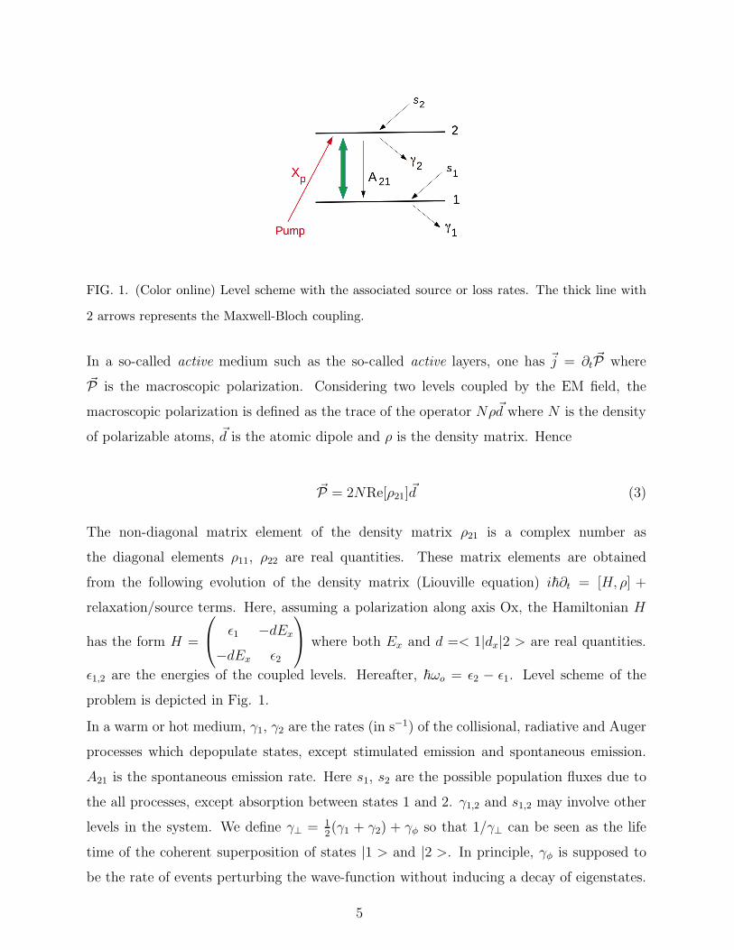
FIG. 1. (Color online) Level scheme with the associated source or loss rates. The thick line with
2 arrows represents the Maxwell-Bloch coupling.
In a so-called active medium such as the so-called active layers, one has ~j = ∂t ~P where
~P is the macroscopic polarization. Considering two levels coupled by the EM field, the
macroscopic polarization is defined as the trace of the operator Nρ~d where N is the density
of polarizable atoms, ~d is the atomic dipole and ρ is the density matrix. Hence
~P = 2NRe[ρ21]~d (3)
The non-diagonal matrix element of the density matrix ρ21 is a complex number as
the diagonal elements ρ11, ρ22 are real quantities. These matrix elements are obtained
from the following evolution of the density matrix (Liouville equation) i~∂t = [H, ρ] +
relaxation/source terms. Here, assuming a polarization along axis Ox, the Hamiltonian H
has the form H =
ǫ1 −dEx
−dEx ǫ2
where both Ex and d =< 1|dx|2 > are real quantities.
ǫ1,2 are the energies of the coupled levels. Hereafter, ~ωo = ǫ2 − ǫ1. Level scheme of the
problem is depicted in Fig. 1.
In a warm or hot medium, γ1, γ2 are the rates (in s−1) of the collisional, radiative and Auger
processes which depopulate states, except stimulated emission and spontaneous emission.
A21 is the spontaneous emission rate. Here s1, s2 are the possible population fluxes due to
the all processes, except absorption between states 1 and 2. γ1,2 and s1,2 may involve other
levels in the system. We define γ⊥ = 12(γ1 + γ2) + γφ so that 1/γ⊥ can be seen as the life
time of the coherent superposition of states |1 > and |2 >. In principle, γφ is supposed to
be the rate of events perturbing the wave-function without inducing a decay of eigenstates.
5
Hereafter, we called populations of states 1 and 2 the macroscopic quantities N1 = Nρ11,
N2 = Nρ22, respectively.
In an active layer, the set of equations to be solved locally for the populations N1, N2 and
for the macroscopic coherence P = Nρ21, is then,
∂tN1 = −2
~dExIm[P ] + s1 − γ1N1 + A21N2 (4)
∂tN2 =2
~dExIm[P ] + s2 − γ2N2 − A21N2 +Xp (5)
∂tP = −iωoP − γ⊥P − i(N2 −N1)dEx + S (6)
where we added in Eq. (5), a pump source term Xp. S is a phenomenological random source
modeling the spontaneous emission. In the absence of external incoming radiation, S acts
as an energy seed for energy injection in the system. Eqs.(1)-(6) correspond to our set of
Maxwell-Bloch equations where Eqs. (4)-(6) concern the active layers only. In the literature,
the name of Maxwell-Bloch [22], or sometimes Maxwell-Schrodinger [15], is often given to
the coupling of complex slowly varying envelopes of the EM field with the Bloch equations
for the density matrix. Here, there is no approximation concerning the field variation both
in space and time.
B. Wave equations in a 1D photonic medium at oblique incidence
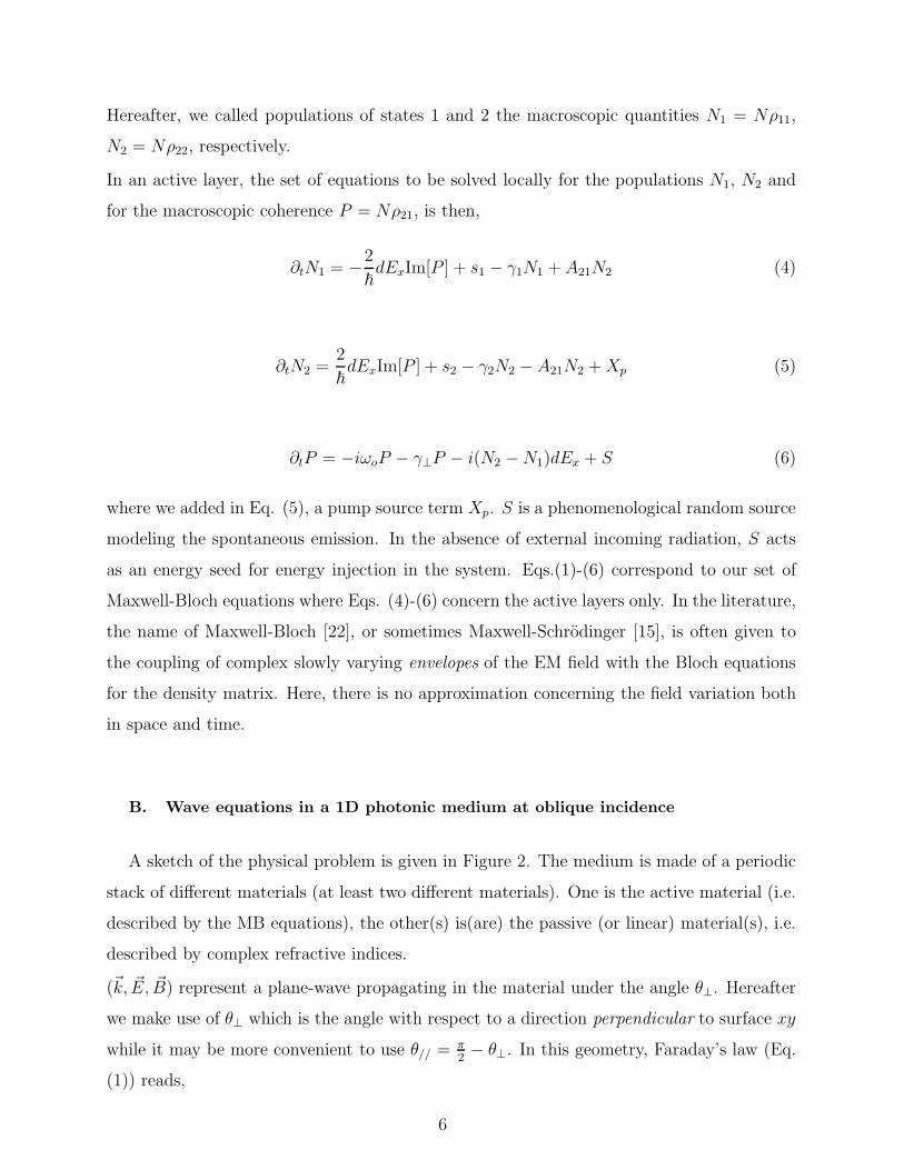
A sketch of the physical problem is given in Figure 2. The medium is made of a periodic
stack of different materials (at least two different materials). One is the active material (i.e.
described by the MB equations), the other(s) is(are) the passive (or linear) material(s), i.e.
described by complex refractive indices.
(~k, ~E, ~B) represent a plane-wave propagating in the material under the angle θ⊥. Hereafter
we make use of θ⊥ which is the angle with respect to a direction perpendicular to surface xy
while it may be more convenient to use θ// =π2− θ⊥. In this geometry, Faraday’s law (Eq.
(1)) reads,
6
FIG. 2. (Color online) Sketch of a stack of bilayers made of one active element (yellow) and
of one passive element. On one side the stack is submitted to a source of excitation (the pump).
Propagation of the emerging radiation is described by Maxwell equations at some frequency (which
is resonant for the active layers). In active layers, response is described by the Bloch equations
while in passive layers, response is given by the refractive index.
∂zEx = −∂tBy (7)
∂yEx = ∂tBz (8)
while the Ampere’s law (Eq. (2)) reads
−∂zBy + ∂yBz =ǫrc2∂tEx + µojx (9)
where jx = σEx in a passive layer. In an active layer, ǫr = 1 and jx = ∂tPx, Px being
deduced from Eq. (3), i.e. Px = 2dRe[P ]. Translating (7), (8), (9) from the time-domain to
the frequency-domain gives three equations in which Ex has the behavior Ex ∼ exp(iωot±iky sin θ⊥). Eliminating Bz and going back to the time domain (iωo → ∂t) finally gives
the following two equations governing the behavior of a plane-wave for an arbitrary oblique
incidence in the multilayer material,
∂zEx = −∂tBy (10)
− ∂zBy =1
c2(ǫr − sin 2θ⊥)∂tEx + µojx. (11)
To solve these equations, one uses the usual FDTD method [19] namely a second-order cen-
tral difference scheme introduced by Yee [23]. Yee’s scheme consists in writing the central
7
differences of Ex and By, shifted in space by half a cell and in time by half a time step.
In our implementation, B is evaluated at the edge of each cell while E is evaluated at the
center. Accordingly, proper boundary conditions for B have to be applied on each side of
the multilayer. Considering that the two external layers (on both sides) correspond to the
vacuum (refractive index n = 1), and in order to remove reflections from these boundaries,
we used second-order Absorbing Boundary Conditions (ABC) [24]. Together with Ex, the
quantities N1, N2 and P are cell-centered and are advanced in time using a Crank-Nicolson
scheme.
Concerning the sampling in space, typically at least 20 steps per wavelength are necessary.
This involves a subdivision of each layer in much smaller layers of thicknesses ∆z. Accord-
ingly, the sampling in time is governed by the Courant limit. More precisely, an inspection
of Eq. (11) shows that the front phase velocity is c/√
ǫr − sin2 θ⊥. Then the time-step must
be such that
∆t ≤ ∆z
c
√
ǫr − sin2 θ⊥.
C. Incident source - Spontaneous emission
For some applications, it may be useful to consider the seeding of the multilayer by some
incident external polarized X-ray pulse (see Sec. III-B below). Practically, this can be an
external source of X-rays at ωo generated independently. Note that we distinguish this po-
tential seeding source at ωo from another source (not at ωo) allowing to create a population
inversion. In order to follow an X-ray pulse propagating in one specific direction, the positive
z-direction for instance (see Fig. 2), this source at ωo has to be properly implemented. As
usual in FDTD simulations, this is accomplished using a total-field/scattered-field (TFSF)
boundary [25] at the point where the source(s) is(are) put. For instance, this source can be
placed in the left vacuum cell of our simulation domain. More precisely, one defines both
an incident electric field Einc and an incident magnetic field Binc = cos θ⊥√ǫrE
inc (ǫr = 1
in the vacuum). At the location of the source, according to the TFSF method, E must be
replaced by E − Einc in the discretized evolution of the B field while B must be replaced
by B +Binc in the discretized evolution of the E field.
8
Independently of any external source at ωo, the source of spontaneous emission in Eq.
(6) (the term S) can be modeled as a Gaussian white noise following the guidelines of Ref.
[16], an approach followed later by others [17, 18]. The interest of this approach is that it
provides the correct spectral behavior for the field [16]. Here, one starts from the simplified
(local) system (see Eq. (11) and Eq. (6)) coupling the electric field and P = Nρ21
dE
dt= αRe[
dP
dt] (α = −2µoc
2d) (12)
dP
dt= −iωoP − γP + S (13)
where the noise source S (complex) has the correlation function 〈S∗(t′)S(t)〉 = Fδ(t′ − t).
The notation 〈...〉 is used to represent the statistical ensemble averaging and F is a constant
defined by the following arguments. From the density of the electric field ǫo2E2, one defines
an average power density W which must be equal to the power emitted by spontaneous
emission (in one direction) so that,
W =d
dt(ǫo2〈E2〉) = 1
4πN2A21~ωo (14)
From the formal solution of Eq. (12), E(t) = α∫ t
−∞ Re[dP (t′)dt′
]dt′, one gets
W = ǫo〈E dEdt〉 = α2ǫo
∫ t
−∞〈Re[dP (t′)dt′
]Re[dP (t)dt
]〉dt′. Using (13), W becomes,
W =ǫo4α2
∫ t
−∞
(
〈dP∗(t′)
dt′dP (t)
dt〉+ 〈dP (t′)
dt′dP ∗(t)
dt〉)
dt′. (15)
From the formal solution of Eq. (13), P (t) =∫ t
−∞ S(t′)e−iωo(t−t′)e−γ(t−t′)dt′, it is easy to
calculate quantities 〈...〉, so that after averaging over one period, calculation of the integrals
in (15) gives (since ωo >> γ) W = ǫo4α2 F
2ω2o
γ2 . Then from relation (14), one gets
F (z, t) =2A21~ωoN2(z, t)
α2πǫo
γ2
ω2o
. (16)
Practically, over a time step ∆t, the noise source term S in Eq. (6) is a random complex
number u+ it distributed according to the law 1πσ2
S
exp [−(u2 + t2)/σ2S] with σS =
√F∆t.
The action of this local phenomenological model of spontaneous emission as set from
Eqs. 12, 13, is to inject a random macroscopic coherence at each point and at each instant.
While giving the correct number of photons, a shortcoming of this approach (as discussed
9
also later in the text) is that, in the limit of weak excitation (i.e. weak population of
the upper level), the simulated temporal profile of the emission (supposed to be driven by
spontaneous emission) is not entirely decreasing exponentially.
III. SIMULATIONS RESULTS
A numerical code based on the model described above has been built. The activematerials
considered in this article are K-shell photoionized magnesium (Secs III-A,B,C,D) or nickel
(Sec. III-E). In magnesium, according to the level scheme depicted in Fig. 1, level 2 stands
for 1s 2s2 2p6 [3s2] and level 1 stands for 1s2 2s2 2p5 [3s2]. In nickel, level 2 stands for
1s 2s2 2p21/22p43/2 3s23p63d8 [4s2] and level 1 stands for 1s2 2s2 2p21/22p
33/2 3s23p63d8 [4s2].
Compared with neutral atoms, outer electrons in solid Mg or Ni (denoted by [...]) are
delocalized. In what follows, we either set populations 2 and 1 (likewise the density of
inversion) (Secs III-B,C) or we explicitely consider a time-dependent pumping (Secs III-
D,E).
In this last case, initial atoms (in the state |0〉 ≡ 1s2 2s2 2p6 [3s2] for Mg or [Ar]3d8 [4s2]
for Ni) are photoionized by an external X-ray source (supposedly an XFEL beam) hereafter
named as ”the pump”, tuned above the K edge. This pumping results in the population
of the core-excited state |2〉 radiatively coupled to state |1〉 by the decay 2p → 1s. In
conditions of weak pumping, this coupling corresponds to the usual Kα fluorescence. Note
that in conditions of weak pumping, state |2〉 predominantly decays via Auger decay (with
the rate Γ2) while both states |1, 2〉 are also affected by the photoionizing pump. In Mg, we
neglect the fine-structure splitting of the Kα line since it is smaller than the Auger width.
For Ni, the splitting Kα1 −Kα2 exceeds largely the Auger width and we chose to consider
the Kα1 line only. Levels |1, 2〉 are the two levels considered in our Maxwell-Bloch modeling.
According to Fig. 1 and Fig. 2, quantities γ1, γ2 and Xp depend on the local intensity of
the pump Ip in the sense that
10
γ1(z, t) = σ1sIp(z, t)
hνp(17)
γ2(z, t) = Γ2 (18)
Xp(z, t) = σ1sNo(z, t)Ip(z, t)
hνp(19)
where σ1s denotes the 1s photoionization cross-section at energy hνp. Ip, hνp are the intensity
(here a power per surface unit) and the photon energy of the pump, respectively. No is the
population density of state |0〉. If hνp is greater than the second 1s ionization threshold, the
term σ1s
2
Ip(z,t)
hνpmust be added to the right side of Eq. (18). At this step it is important to
remark that, for a normal incidence and being off an accidental situation where the period
of the material would be an integer of λ/2 (i.e. off-Bragg), one may adopt for the pump the
simple corpuscular point of view of photon absorption. Hence, for a pump propagating from
the right (see Fig. 2), the pump intensity obeys the following photon transport equation
1
c
∂Ip(z, t)
∂t− ∂Ip(z, t)
∂z= −kp(z, t) Ip(z, t) (20)
with
kp(z, t) = σ1sNo(z, t) + σ1sN1(z, t) +σ1s
2N2(z, t) (in the active material)
= σpassiveNpassive(z, t) (in the passive material)
in which Npassive(z, t) is the atom density in a passive layer, σpassive being the corresponding
absorption cross section at hνp. Finally, the population of state |0〉 evolves as
∂No(z, t)
∂t= −σ1sNo(z, t)
Ip(z, t)
hνp. (21)
In the case where the pump is explicitely taken into account, equations (17)-(21) have to be
solved simultaneously with the previous Maxwell-Bloch set of equations.
In the following, after checking the right behavior of the FDTD implementation (Sec.
III-A), we describe the propagation of an X-ray pulse at the Kα energy for different situ-
ations of increasing complexity whether the pulse is of external origin (Sec. III-B) or not
(i.e. originating from spontaneous emission, Secs III-C,D,E). Note that, in Secs III-D,E we
explicitely consider the pumping by an external photoionizing x-ray source.
11
A. Simple propagation in a multilayer material
A first and minimal implementation amounts to considering that all the layers are of
passive nature, i.e. simply described by a complex refractive index. The goal is to as-
sess the necessary number of subdivisions of each layer in our specificic problem of wave
propagation in the x-ray range, in a stratified medium made of nm-size layers. Indeed,
this number of subdivisions defines a typical space interval ∆z on which Maxwell equations
are discretized according to the FDTD scheme mentioned above. Of course, this defines
the time step ∆t as discussed in Sec. II-B. As a test case, we consider here a sample al-
ready considered in a context of synchrotron irradiation [26]. It consists in a stack of 30
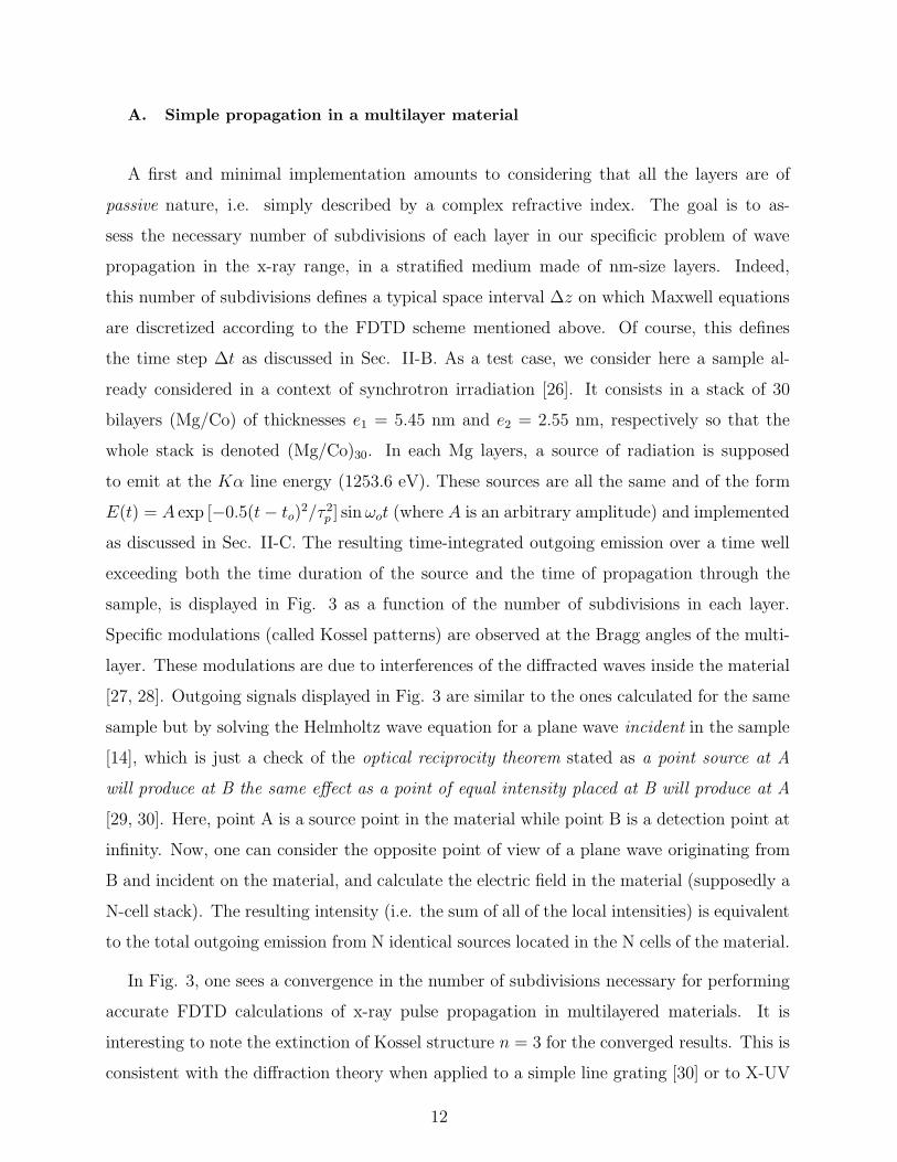
bilayers (Mg/Co) of thicknesses e1 = 5.45 nm and e2 = 2.55 nm, respectively so that the
whole stack is denoted (Mg/Co)30. In each Mg layers, a source of radiation is supposed
to emit at the Kα line energy (1253.6 eV). These sources are all the same and of the form
E(t) = A exp [−0.5(t− to)2/τ 2p ] sinωot (where A is an arbitrary amplitude) and implemented
as discussed in Sec. II-C. The resulting time-integrated outgoing emission over a time well
exceeding both the time duration of the source and the time of propagation through the
sample, is displayed in Fig. 3 as a function of the number of subdivisions in each layer.
Specific modulations (called Kossel patterns) are observed at the Bragg angles of the multi-
layer. These modulations are due to interferences of the diffracted waves inside the material
[27, 28]. Outgoing signals displayed in Fig. 3 are similar to the ones calculated for the same
sample but by solving the Helmholtz wave equation for a plane wave incident in the sample
[14], which is just a check of the optical reciprocity theorem stated as a point source at A
will produce at B the same effect as a point of equal intensity placed at B will produce at A
[29, 30]. Here, point A is a source point in the material while point B is a detection point at
infinity. Now, one can consider the opposite point of view of a plane wave originating from
B and incident on the material, and calculate the electric field in the material (supposedly a
N-cell stack). The resulting intensity (i.e. the sum of all of the local intensities) is equivalent
to the total outgoing emission from N identical sources located in the N cells of the material.
In Fig. 3, one sees a convergence in the number of subdivisions necessary for performing
accurate FDTD calculations of x-ray pulse propagation in multilayered materials. It is
interesting to note the extinction of Kossel structure n = 3 for the converged results. This is
consistent with the diffraction theory when applied to a simple line grating [30] or to X-UV
12
0 5 10 15 20θ// (deg)
0
200
400
600
800
Inte
nsity
(arb
. uni
t)
nsub = 36nsub = 72nsub = 144nsub = 288
n = 1
n = 2
n = 3
n = 4
FIG. 3. (Color online) Calculated angular scan for the Mg Kα radiation emitted by a stack
(Mg/Co)30 (e1 = 5.45 nm and e2 = 2.55 nm) where a same source of Kα radiation has been put
in each Mg layer. Kossel patterns are labelled by their Bragg order n.
interference mirrors [31]. Indeed, the first extinction should occur for the ratio Λe2
= 3.
Taking for e2 and for the period Λ = e1 + e2, the values given above, one finds a value very
close to 3. These different remarks validate our minimal implementation.
B. Propagation in an amplifying multilayer material
We consider here the problem of a short pulse originating at the left, i.e. in the vacuum
cell of our computational domain (see Sec. II-B) and then propagating from left to right
in a multilayer similar to the stack considered in the previous paragraph, albeit with an
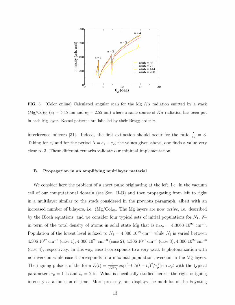
increased number of bilayers, i.e. (Mg/Co)60. The Mg layers are now active, i.e. described
by the Bloch equations, and we consider four typical sets of initial populations for N1, N2
in term of the total density of atoms in solid state Mg that is nMg = 4.3063 1022 cm−3.
Population of the lowest level is fixed to N1 = 4.306 1018 cm−3 while N2 is varied between
4.306 1017 cm−3 (case 1), 4.306 1020 cm−3 (case 2), 4.306 1021 cm−3 (case 3), 4.306 1022 cm−3
(case 4), respectively. In this way, case 1 corresponds to a very weak 1s photoionization with
no inversion while case 4 corresponds to a maximal population inversion in the Mg layers.
The ingoing pulse is of the form E(t) = 1√2πτp
exp [−0.5(t− to)2/τ 2p ] sinωot with the typical
parameters τp = 1 fs and to = 2 fs. What is specifically studied here is the right outgoing
intensity as a function of time. More precisely, one displays the modulus of the Poynting
13
0 5 10 15time (fs)
0.0001
0.001
0.01
0.1
1
10
S av (
atom
ic u
nits
)
case 1case 2case 3case 4
FIG. 4. (Color online) Modulus of the Poynting vector outgoing from the stack (Mg/Co)60 in the
normal direction (θ// = 90o), as a function of time. See text for the characterics of the ingoing
signal and for the definition of cases 1-4.
vector, averaged over one period, i.e. Sav = 1T
∫ T
0|S|dt with µ2
oS2 = (ExBz)
2 + (ExBy)2,
Bz =1cEx sin θ⊥. Hereafter, units for the Poynting vector are the atomic units, i.e. Sav is in
unit of e12
(4πǫo)6m4
e
~9. For a signal ingoing in the normal direction, calculations are diplayed in
Fig. 4.
Compared with the weak signal (case 1), one sees the gradual effect of a gain material
on the intensity temporal shape of the outgoing pulse. In particular, one notices an increase
of the outgoing pulse duration with respect to the ingoing pulse duration. In the case
of strong (and here maximal) inversion (case 4), a typical effect such as ”ringing” of the
outgoing signal is observed. This correspond to the well-known Burnham-Chiao ringing
[32]. Present simulations are in the time domain. Of course, taking the Fourier transform
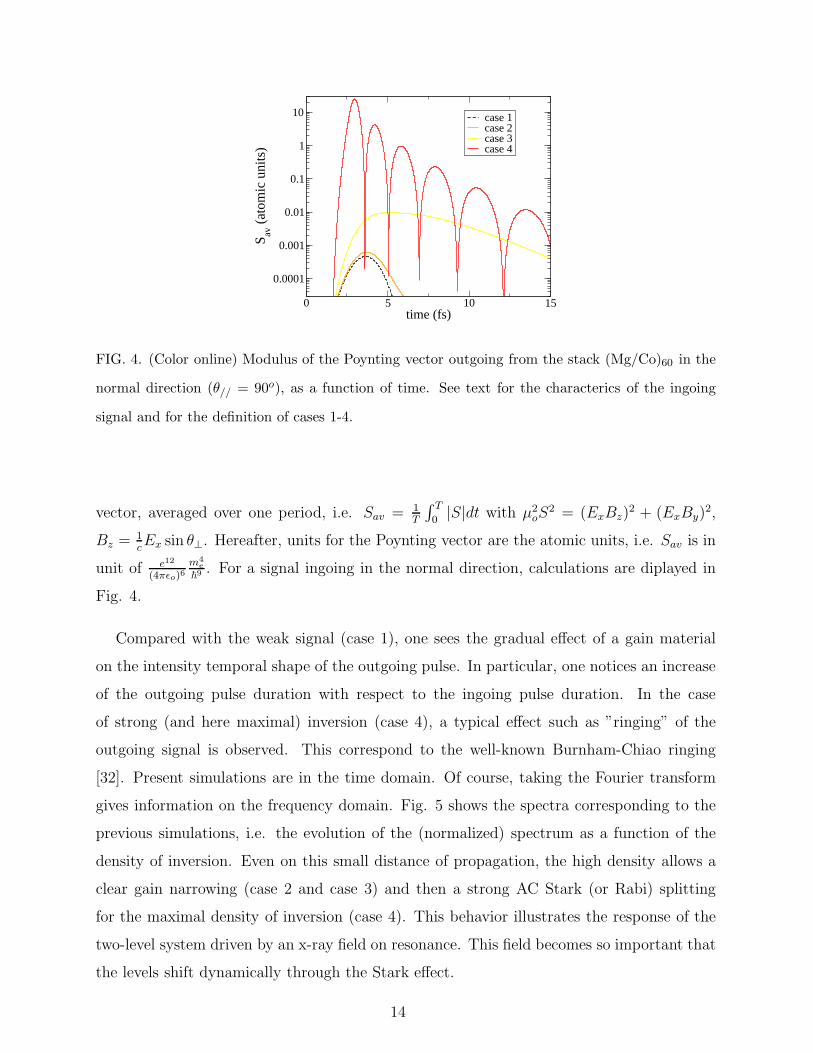
gives information on the frequency domain. Fig. 5 shows the spectra corresponding to the
previous simulations, i.e. the evolution of the (normalized) spectrum as a function of the
density of inversion. Even on this small distance of propagation, the high density allows a
clear gain narrowing (case 2 and case 3) and then a strong AC Stark (or Rabi) splitting
for the maximal density of inversion (case 4). This behavior illustrates the response of the
two-level system driven by an x-ray field on resonance. This field becomes so important that
the levels shift dynamically through the Stark effect.
14
1248 1250 1252 1254 1256 1258 1260Photon energy (eV)
0
0.2
0.4
0.6
0.8
1.0
Spec
trum
(arb
. uni
t)
case 1case 2case 3case 4
FIG. 5. (Color online) Normalized spectra corresponding to the signals of Figure 4.
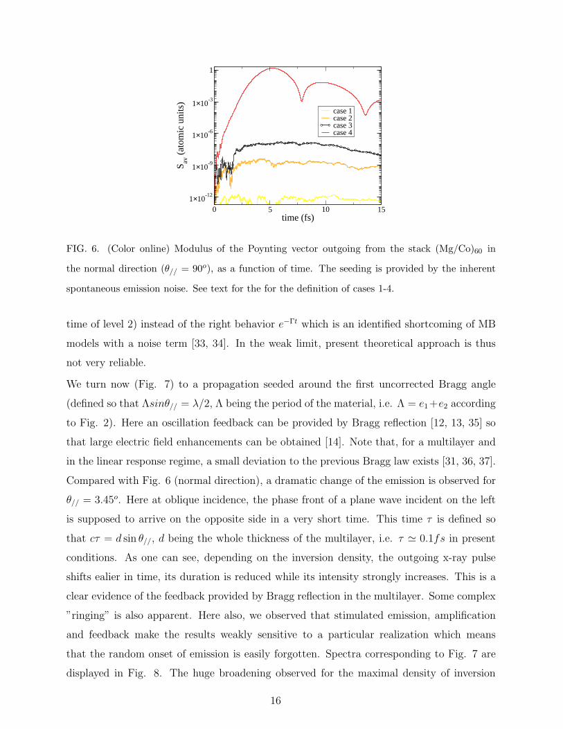
C. Self-emission of an amplifying multilayer material
In this paragraph, we do not consider the propagation of an external pulse but the signal
originating from the noisy source of spontaneous emission in each active cell of a multilayer.
More precisely, we study how spontanenous emission emitted in one direction propagates and
how stimulated emission sets in. Present calculations rely on the modeling of spontaneous
emission presented in Sec. II-C. Still for the same multilayer (Mg/Co)60 and the same sets
of initial populations (N1, N2) in Mg layers, Fig. 6 displays simulations of the outgoing
X-ray emission in the normal direction.
We see the weak noisy signal for a low initial excitation (case 1) while, gradually with the
density of inversion, a collective emission is set up independently of any external pulse ingo-
ing into the material. For the maximal initial population inversion (case 4), characteristics
of the superradiance, namely time delay for the peak of emission and ringing are clearly
visible. We emphazise that these results are just single realizations which may be subjected
to large fluctuations. However, what we observed is that in case of strong population in-
version, stimulated emission and amplification make the results weakly sensitive to a given
realization. A fact which is somehow reflected by the smooth aspect of graph corresponding
to case 4. In case of weak or absent stimulated emission, the right temporal behavior can be
recovered only by performing an average over many realizations. For case 1, 2, we checked
that an average over at least a few tens of realizations gives a decaying behavior for large
time. Furthermore, in this weak limit, we observed a behavior as te−Γt (Γ being the decay
15
0 5 10 15time (fs)
1×10-12
1×10⁻⁹
1×10⁻⁶
1×10⁻³
1
S av (
atom
ic u
nits
)
case 1case 2case 3case 4
FIG. 6. (Color online) Modulus of the Poynting vector outgoing from the stack (Mg/Co)60 in
the normal direction (θ// = 90o), as a function of time. The seeding is provided by the inherent
spontaneous emission noise. See text for the for the definition of cases 1-4.
time of level 2) instead of the right behavior e−Γt which is an identified shortcoming of MB
models with a noise term [33, 34]. In the weak limit, present theoretical approach is thus
not very reliable.
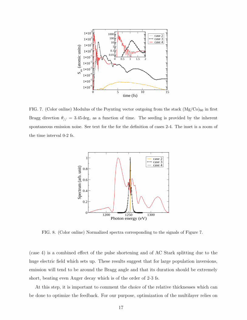
We turn now (Fig. 7) to a propagation seeded around the first uncorrected Bragg angle
(defined so that Λsinθ// = λ/2, Λ being the period of the material, i.e. Λ = e1+e2 according
to Fig. 2). Here an oscillation feedback can be provided by Bragg reflection [12, 13, 35] so
that large electric field enhancements can be obtained [14]. Note that, for a multilayer and
in the linear response regime, a small deviation to the previous Bragg law exists [31, 36, 37].
Compared with Fig. 6 (normal direction), a dramatic change of the emission is observed for
θ// = 3.45o. Here at oblique incidence, the phase front of a plane wave incident on the left
is supposed to arrive on the opposite side in a very short time. This time τ is defined so
that cτ = d sin θ//, d being the whole thickness of the multilayer, i.e. τ ≃ 0.1fs in present
conditions. As one can see, depending on the inversion density, the outgoing x-ray pulse
shifts ealier in time, its duration is reduced while its intensity strongly increases. This is a
clear evidence of the feedback provided by Bragg reflection in the multilayer. Some complex
”ringing” is also apparent. Here also, we observed that stimulated emission, amplification
and feedback make the results weakly sensitive to a particular realization which means
that the random onset of emission is easily forgotten. Spectra corresponding to Fig. 7 are
displayed in Fig. 8. The huge broadening observed for the maximal density of inversion
16
0 5 10 15time (fs)
1×10⁻⁶
1×10⁻⁵
1×10⁻⁴
1×10⁻³
1×10⁻²
1×10⁻¹
1×100
1×101
1×10²
1×10³
S av (
atom
ic u
nits
)
case 2case 3case 4
0 0.5 1 1.5 20.01
0.11
10100
1000
FIG. 7. (Color online) Modulus of the Poynting vector outgoing from the stack (Mg/Co)60 in first
Bragg direction θ// = 3.45 deg, as a function of time. The seeding is provided by the inherent
spontaneous emission noise. See text for the for the definition of cases 2-4. The inset is a zoom of
the time interval 0-2 fs.
1200 1250 1300Photon energy (eV)
0
0.2
0.4
0.6
0.8
1
Spec
trum
(arb
. uni
t)
case 2case 3case 4
FIG. 8. (Color online) Normalized spectra corresponding to the signals of Figure 7.
(case 4) is a combined effect of the pulse shortening and of AC Stark splitting due to the
huge electric field which sets up. These results suggest that for large population inversions,
emission will tend to be around the Bragg angle and that its duration should be extremely
short, beating even Auger decay which is of the order of 2-3 fs.
At this step, it is important to comment the choice of the relative thicknesses which can
be done to optimize the feedback. For our purpose, optimization of the multilayer relies on
17
0 5 10 15 20 25 30time (fs)
1×10⁻⁹
1×10⁻⁸
1×10⁻⁷
1×10⁻⁶
1×10⁻⁵
1×10⁻⁴
1×10⁻³
1×10⁻²
S av (
atom
ic u
nits
)
1016
W/cm2
1017
W/cm2
1018
W/cm2
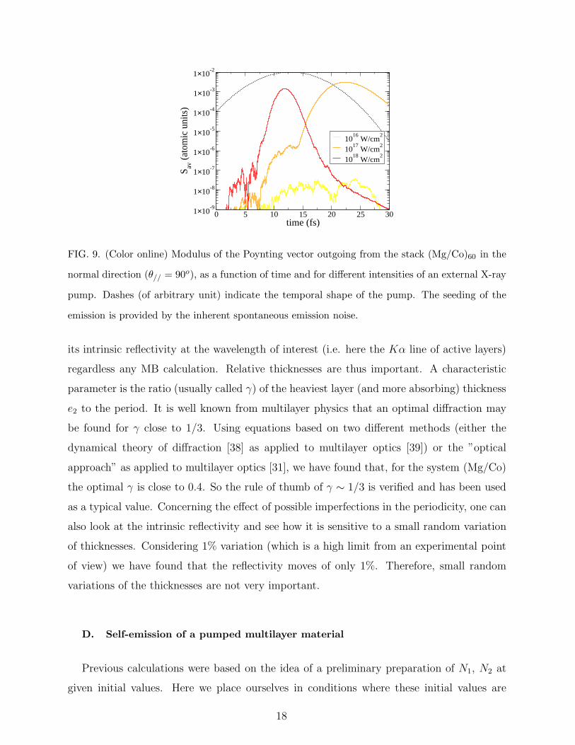
FIG. 9. (Color online) Modulus of the Poynting vector outgoing from the stack (Mg/Co)60 in the
normal direction (θ// = 90o), as a function of time and for different intensities of an external X-ray
pump. Dashes (of arbitrary unit) indicate the temporal shape of the pump. The seeding of the
emission is provided by the inherent spontaneous emission noise.
its intrinsic reflectivity at the wavelength of interest (i.e. here the Kα line of active layers)
regardless any MB calculation. Relative thicknesses are thus important. A characteristic
parameter is the ratio (usually called γ) of the heaviest layer (and more absorbing) thickness
e2 to the period. It is well known from multilayer physics that an optimal diffraction may
be found for γ close to 1/3. Using equations based on two different methods (either the
dynamical theory of diffraction [38] as applied to multilayer optics [39]) or the ”optical
approach” as applied to multilayer optics [31], we have found that, for the system (Mg/Co)
the optimal γ is close to 0.4. So the rule of thumb of γ ∼ 1/3 is verified and has been used
as a typical value. Concerning the effect of possible imperfections in the periodicity, one can
also look at the intrinsic reflectivity and see how it is sensitive to a small random variation
of thicknesses. Considering 1% variation (which is a high limit from an experimental point
of view) we have found that the reflectivity moves of only 1%. Therefore, small random
variations of the thicknesses are not very important.
D. Self-emission of a pumped multilayer material
Previous calculations were based on the idea of a preliminary preparation of N1, N2 at
given initial values. Here we place ourselves in conditions where these initial values are
18
0 5 10 15 20 25 30time (fs)
1×10⁻²
1×10⁻¹
1×100
1×101
S av (
atom
ic u
nits
)
1016
W/cm2
1017
W/cm2
1018
W/cm2
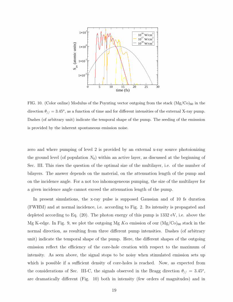
FIG. 10. (Color online) Modulus of the Poynting vector outgoing from the stack (Mg/Co)60 in the
direction θ// = 3.45o, as a function of time and for different intensities of the external X-ray pump.
Dashes (of arbitrary unit) indicate the temporal shape of the pump. The seeding of the emisssion
is provided by the inherent spontaneous emission noise.
zero and where pumping of level 2 is provided by an external x-ray source photoionizing
the ground level (of population N0) within an active layer, as discussed at the beginning of
Sec. III. This rises the question of the optimal size of the multilayer, i.e. of the number of
bilayers. The answer depends on the material, on the attenuation length of the pump and
on the incidence angle. For a not too inhomogeneous pumping, the size of the multilayer for
a given incidence angle cannot exceed the attenuation length of the pump.
In present simulations, the x-ray pulse is supposed Gaussian and of 10 fs duration
(FWHM) and at normal incidence, i.e. according to Fig. 2. Its intensity is propagated and
depleted according to Eq. (20). The photon energy of this pump is 1332 eV, i.e. above the
Mg K-edge. In Fig. 9, we plot the outgoing Mg Kα emission of our (Mg/Co)60 stack in the
normal direction, as resulting from three different pump intensities. Dashes (of arbitrary
unit) indicate the temporal shape of the pump. Here, the different shapes of the outgoing
emission reflect the efficiency of the core-hole creation with respect to the maximum of
intensity. As seen above, the signal stops to be noisy when stimulated emission sets up
which is possible if a sufficient density of core-holes is reached. Now, as expected from
the considerations of Sec. III-C, the signals observed in the Bragg direction θ// = 3.45o,
are dramatically different (Fig. 10) both in intensity (few orders of magnitudes) and in
19
temporal shape. About the different angles of emission, a question arise here. In principle,
spontaneous emission (which is isotropic) generates photons in all directions although at
different times and different locations. For this reason, the fields corresponding to all di-
rections should be calculated so that Eqs 4-6 include the contribution of all directions. In
term of computation time, such a treatment is prohibitive since, as discussed in Sec. III-A
and seen in Fig. 3, a very fine spatial zoning and a very fine angular gridding is needed
to resolve the Kossel structures. Here our purpose is to show that a multilayer structure
may present preferential directions of emission for which initial photons emitted around
the Bragg angle ”catch on” the stimulated emission as does a standard cavity. This point
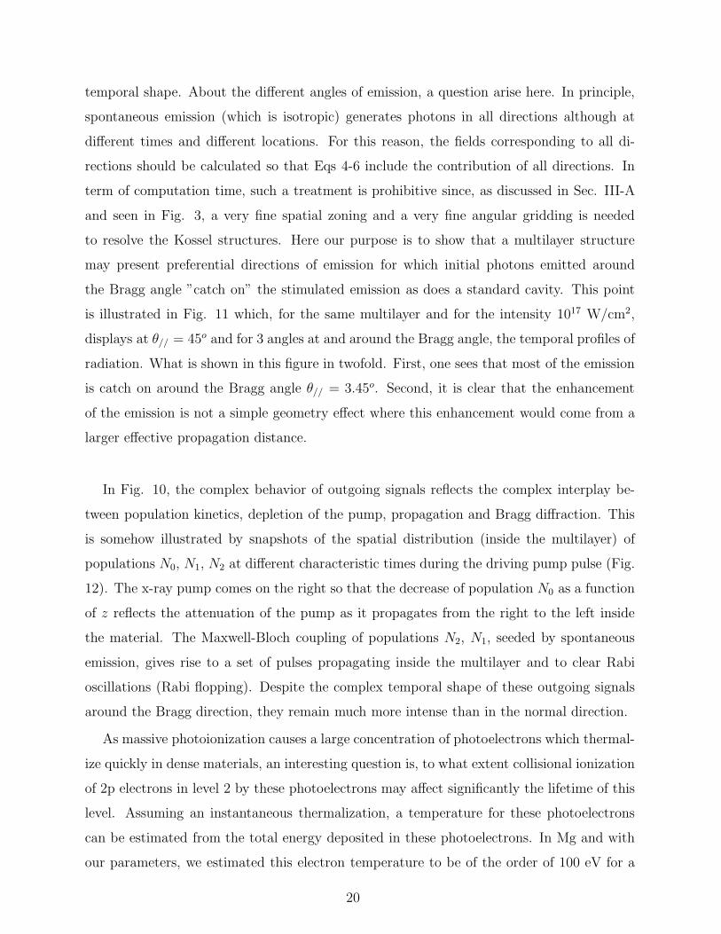
is illustrated in Fig. 11 which, for the same multilayer and for the intensity 1017 W/cm2,
displays at θ// = 45o and for 3 angles at and around the Bragg angle, the temporal profiles of
radiation. What is shown in this figure in twofold. First, one sees that most of the emission
is catch on around the Bragg angle θ// = 3.45o. Second, it is clear that the enhancement
of the emission is not a simple geometry effect where this enhancement would come from a
larger effective propagation distance.
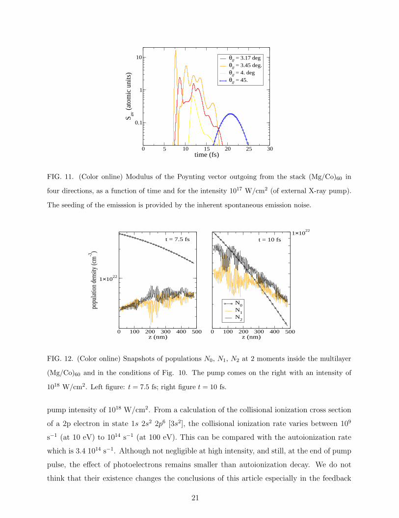
In Fig. 10, the complex behavior of outgoing signals reflects the complex interplay be-
tween population kinetics, depletion of the pump, propagation and Bragg diffraction. This
is somehow illustrated by snapshots of the spatial distribution (inside the multilayer) of
populations N0, N1, N2 at different characteristic times during the driving pump pulse (Fig.
12). The x-ray pump comes on the right so that the decrease of population N0 as a function
of z reflects the attenuation of the pump as it propagates from the right to the left inside
the material. The Maxwell-Bloch coupling of populations N2, N1, seeded by spontaneous
emission, gives rise to a set of pulses propagating inside the multilayer and to clear Rabi
oscillations (Rabi flopping). Despite the complex temporal shape of these outgoing signals
around the Bragg direction, they remain much more intense than in the normal direction.
As massive photoionization causes a large concentration of photoelectrons which thermal-
ize quickly in dense materials, an interesting question is, to what extent collisional ionization
of 2p electrons in level 2 by these photoelectrons may affect significantly the lifetime of this
level. Assuming an instantaneous thermalization, a temperature for these photoelectrons
can be estimated from the total energy deposited in these photoelectrons. In Mg and with
our parameters, we estimated this electron temperature to be of the order of 100 eV for a
20
0 5 10 15 20 25 30time (fs)
0.1
1
10
S av (a
tom
ic u
nits
)
θ// = 3.17 degθ// = 3.45 deg.θ// = 4. degθ// = 45.
FIG. 11. (Color online) Modulus of the Poynting vector outgoing from the stack (Mg/Co)60 in
four directions, as a function of time and for the intensity 1017 W/cm2 (of external X-ray pump).
The seeding of the emisssion is provided by the inherent spontaneous emission noise.
0 100 200 300 400 500z (nm)
1×10²²
popu
latio
n de
nsity
(cm
-3)
N0
N1
N2
0 100 200 300 400 500z (nm)
1×10²²
t = 7.5 fs t = 10 fs
FIG. 12. (Color online) Snapshots of populations N0, N1, N2 at 2 moments inside the multilayer
(Mg/Co)60 and in the conditions of Fig. 10. The pump comes on the right with an intensity of
1018 W/cm2. Left figure: t = 7.5 fs; right figure t = 10 fs.
pump intensity of 1018 W/cm2. From a calculation of the collisional ionization cross section
of a 2p electron in state 1s 2s2 2p6 [3s2], the collisional ionization rate varies between 109
s−1 (at 10 eV) to 1014 s−1 (at 100 eV). This can be compared with the autoionization rate
which is 3.4 1014 s−1. Although not negligible at high intensity, and still, at the end of pump
pulse, the effect of photoelectrons remains smaller than autoionization decay. We do not
think that their existence changes the conclusions of this article especially in the feedback
21
regime which shortens the emission duration.
E. Self-emission of a pumped natural crystal
In this last section, one examines the case of a natural crystal whose periodicity of atomic
layers may provide the same kind of Bragg oscillations. One considers here a Ni crystal where
for an orientation (111) of planes parallel to the surface, atomic layer spacing is d = 0.216
nm. A strong pumping of 1s core electrons in Ni may give rise to an amplification on the
2p → 1s Kα1 line at 7478.15 eV. At this energy the first Bragg angle is around 22.6o
(with respect to the surface). 1D Periodicity is introduced in the calculations by considering
the (supposedly perfect) crystal as a stack of bilayers of period d and where the first layer
(the active layer) is a layer of Ni atoms while the second layer is just empty (then passive)
and of refractive index 1. Such a replacement of real atoms by a uniform layer of a given
thickness e1 (See Fig. 2) is a rough method to simulate the problem of a distribution of
individual small scatterers. Its validity is semi-empirical. A relevant quantity to measure
its effectiveness is the reflectivity of the system (element/vacuum)n which for a wavelength
of interest can be calculated around the Bragg angle and compared with a model giving the
reflectivity of a real crystal. From x-ray reflectivity calculations based on a solution of the
Helmholtz equation applied to stacks (element/vacuum)n, we performed such comparisons
with a software available at Sergey Stepanov’s X-ray server [40] allowing a calculation of
the reflectivity in real crystals. We found that, taking for the element thickness a typical
value of 0.4 d (d being the proper inter-reticular distance in the crystal of interest) and
renormalizing properly the number of atoms in this element layer to the right number of
atoms (per volume unit), this approach gives results close to those of the Stepanov’s X-ray
server. Accordingly, we used this recipe in our Maxwell-Bloch calculations.
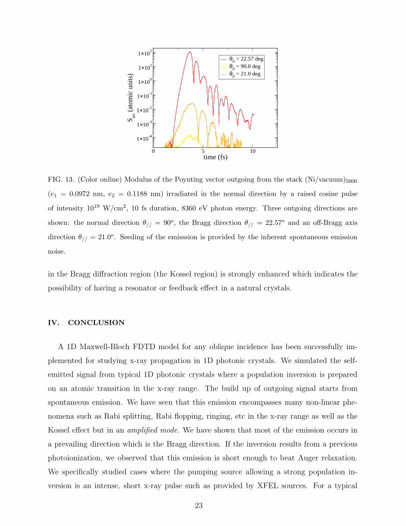
Simulations presented here correspond to a Ni thickness of 1.08 µm, i.e. to the stack
(Ni/vacuum)5000. Simulation results are displayed in Fig. 13. Irradiation conditions are a
raised cosine pulse of 10 fs duration (FWHM), 8360 eV of photon energy (i.e. above the Ni
K-edge) and of intensities 1019 W/cm2, and at normal incidence, i.e. in the geometry of Fig.
2. Fig. 13 displays a comparison of the outgoing Ni Kα1 signal (i.e. seeded by spontaneous
emission) observed in the normal direction θ// = 90o, in the Bragg direction θ// = 21.57o
and in some off-Bragg direction, respectively. Compared with the other directions, emission
22
0 5 10time (fs)
1×10⁻⁴
1×10⁻³
1×10⁻²
1×10⁻¹
1×100
1×101
1×10²
S av (
atom
ic u
nits
)
θ// = 22.57 degθ// = 90.0 degθ// = 21.0 deg
FIG. 13. (Color online) Modulus of the Poynting vector outgoing from the stack (Ni/vacuum)5000
(e1 = 0.0972 nm, e2 = 0.1188 nm) irradiated in the normal direction by a raised cosine pulse
of intensity 1019 W/cm2, 10 fs duration, 8360 eV photon energy. Three outgoing directions are
shown: the normal direction θ// = 90o, the Bragg direction θ// = 22.57o and an off-Bragg axis
direction θ// = 21.0o. Seeding of the emisssion is provided by the inherent spontaneous emission
noise.
in the Bragg diffraction region (the Kossel region) is strongly enhanced which indicates the
possibility of having a resonator or feedback effect in a natural crystals.
IV. CONCLUSION
A 1D Maxwell-Bloch FDTD model for any oblique incidence has been successfully im-
plemented for studying x-ray propagation in 1D photonic crystals. We simulated the self-
emitted signal from typical 1D photonic crystals where a population inversion is prepared
on an atomic transition in the x-ray range. The build up of outgoing signal starts from
spontaneous emission. We have seen that this emission encompasses many non-linear phe-
nomena such as Rabi splitting, Rabi flopping, ringing, etc in the x-ray range as well as the
Kossel effect but in an amplified mode. We have shown that most of the emission occurs in
a prevailing direction which is the Bragg direction. If the inversion results from a previous
photoionization, we observed that this emission is short enough to beat Auger relaxation.
We specifically studied cases where the pumping source allowing a strong population in-
version is an intense, short x-ray pulse such as provided by XFEL sources. For a typical
23
multilayer and for realistic conditions of pumping, calculations show a strong enhancement
of the emission in the Bragg direction. For the case of natural crystals, this enhancement is
also noticeable.
Results of this study motivate future experimental investigations of the behavior of pho-
tonic crystals whether they are natural or artificial (multilayers). It motivates also many
other theorerical investigations on different multilayers or natural crystals to optimize x-ray
emission at different wavelengths.
ACKNOWLEDGMENTS
At numerous times during the course of this work, one of us (O. Peyrusse) has benefited
from discussions and helpful advices concerning the use of computational resources from
Paul Genesio at PIIM laboratory.
24
[1] B.W. Adams et al., J. Mod. Opt. 60, 2 (2013).
[2] B.W. Adams, Nonlinear Optics, Quantum Optics and Ultrafast Phenomena with X-rays
(Kluwer Academic Publisher, Norwell, MA, 2008).
[3] Yu-Ping Sun, Ji-Cai Liu, Chuan-Kui Wang, and Faris Gel’mukhanov, Phys. Rev. A 81,
013812 (2010).
[4] N. Rohringer et al., Nature 481, 488 (2012).
[5] A. Benediktovitch, L. Mercadier, O. Peyrusse, A. Przystawik, T. Laarmann, B. Langbehn,
et al., Phys. Rev. A 101, 063412 (2020).
[6] M. Beye et al., Nature 501, 191 (2013).
[7] H. Yoneda et al., Nature 524, 446 (2015).
[8] P. Jonnard et al., Struct. Dyn. 4, 054306 (2017).
[9] T. Kroll, C. Weninger, R. Alonso-Mori, D. Sokaras, D. Zhu, L. Mercadier, et al., Phys. Rev.
Lett. 120, 133203 (2018).
[10] A. Halavanau et al., P.N.A.S. 117, 15511 (2020).
[11] M. Nagasono et al., Phys. Rev. Lett. 107, 193603 (2011).
[12] A. Yariv and P. Yeh, Optics Comm. 22, 5 (1977).
[13] J.-M. Andre, K. Le Guen, and P. Jonnard, Laser Phys. 24, 085001 (2014).
[14] O. Peyrusse, P. Jonnard, K. LeGuen, and J.-M. Andre, Phys. Rev. A 101, 013818 (2020).
[15] J.C. MacGillivray and M.S. Feld, Phys. Rev. A 14, 1169 (1976).
[16] O. Larroche, D. Ros, A. Klisnick, A. Sureau, C. Moller, and H. Guennou, Phys. Rev. A 62,
043815 (2000).
[17] Clemens Weninger and Nina Rohringer, Phys. Rev. A 90, 063828 (2014).
[18] C. Lyu, S.M. Cavaletto, C.H. Keitel, et al., Sci. Rep. 10, 9439 (2020).
[19] A. Taflove, Computational Electrodynamics. The Finite-Difference Time-Domain Method
(Artech House, 1995).
[20] B.L. Henke, E.M. Gullikson, and J.C. Davis, At. Data. Nucl. Data Tables 54, 181 (1993).
[21] CXRO http://www.cxro.lbl.gov/.
[22] M.O. Scully and M.S. Zubairy, Quantum optics (Cambridge University Press, Cambridge,
England, 1997).
25
[23] K.S. Yee, IEEE Trans. Antennas Propag. 14, 302 (1966).
[24] B. Engquist and A. Majda, Math. Comput. 31, 629 (1977).
[25] D.E. Merewether, R. Fisher, and F.W. Smith, IEEE Trans. Nucl. Sc. 27, 1829 (1980).
[26] P. Jonnard et al., J. Phys. B 47, 165601 (2014).
[27] E. Langer and S. Dabritz, IOP Conf. Series: Materials Science and Engineering 7, 012015
(2010).
[28] K. Le Guen et al., J. Nanosci. Nanotechnol. 19, 593 (2019).
[29] W. Schulke and D. Brummer, Z. Naturforsch. Tail A 17, 208 (1962).
[30] M. Born and E. Wolf, Principles of Optics, Sixth Edition (Pergamon Press, 1980).
[31] B. Pardo, T. Megademini, and J.M. Andre, Revue Phys. Appl. 23, 1579 (1988).
[32] D.C. Burnham and R.Y. Chiao, Phys. Rev. 188, 667 (1969).
[33] S. Krusic, K. Bucar, A. Mihelic, and M. Zitnik, Phys. Rev. A 98, 013416 (2018).
[34] Andrei Benediktovitch, Vinay P. Majety, and Nina Rohringer, Phys. Rev. A 99, 013839
(2019).
[35] A. Yariv, Appl. Phys. Lett. 25, 105 (1974).
[36] D. Attwood, Soft X-rays and Extreme Ultraviolet Radiation (University of California, Berkeley,
2007).
[37] C.T. Chantler and R.D. Deslattes, Rev. Sci. Instrum. 66, 5123 (1995).
[38] B.W. Batterman and H. Coles, Rev. Mod. Phys. 36, 681 (1964).
[39] I.V. Kozhevnikov and A.V. Vinogradov, Physica Scripta T17, 137 (1987).
[40] Stepanov’s X-ray server https://x-server.gmca.aps.anl.gov.
26


![Ernest Bloch Collection [finding aid]. Music Division, Library of](https://img.dokumen.tips/doc/110x75/6323b8cc3a06c6d45f063ee0/ernest-bloch-collection-finding-aid-music-division-library-of-.jpg)


