Material and Energy Productivity

Published: January 6, 2011

r 2011 American Chemical Society 1169 dx.doi.org/10.1021/es1028537 | Environ. Sci. Technol. 2011, 45, 1169–1176

POLICY ANALYSIS

pubs.acs.org/est

Material and Energy ProductivityJulia K. Steinberger*,†,‡ and Fridolin Krausmann†

†Institute of Social Ecology Vienna (IFF, University of Klagenfurt), Schottenfelgasse 29, A-1070, Vienna, Austria‡Sustainability Research Institute, School of Earth and Environment, University of Leeds, LS2 9JT, U.K.

bS Supporting Information

ABSTRACT: Resource productivity, measured as GDP output per resource input, is a widespread sustainability indicatorcombining economic and environmental information. Resource productivity is ubiquitous, from the IPAT identity to the analysis ofdematerialization trends and policy goals. High resource productivity is interpreted as the sign of a resource-efficient, and hencemore sustainable, economy. Its inverse, resource intensity (resource per GDP) has the reverse behavior, with higher valuesindicating environmentally inefficient economies. In this study, we investigate the global systematic relationship between material,energy and carbon productivities, and economic activity. We demonstrate that different types of materials and energy exhibitfundamentally different behaviors, depending on their international income elasticities of consumption. Biomass is completelyinelastic, whereas fossil fuels tend to scale proportionally with income. Total materials or energy, as aggregates, have intermediatebehavior, depending on the share of fossil fuels and other elastic resources. We show that a small inelastic share is sufficient for thetotal resource productivity to be significantly correlated with income. Our analysis calls into question the interpretation of resourceproductivity as a sustainability indicator. We conclude with suggestions for potential alternatives.

’ INTRODUCTION

The simplicity of the GDP output per resource input ratiomakes resource productivity an appealing and widespread en-vironmental sustainability indicator. An abundant literature dis-cusses both resource productivity and its inverse, resource inten-sity, for a variety of resources (see the Supporting Information fora partial list). The goal of this article is to analyze and explain thelinks between economic activity and resource productivity. Thebasic assumption underlying the use of resource productivityas an indicator is that, under business-as-usual circumstances,resource use scales proportionally with economic growth, andthat deviations from this proportionality are to be commended ordiscouraged on environmental grounds. In fact, as we show, incurrent industrialized societies, the scaling rule between eco-nomic growth and resource use depends on the type of resource,with significant implications for the interpretation of this popularindicator. We start by reviewing the different interpretations ofresource productivity: as a measure of technology, efficiency, orsavings and dematerialization.

Technology: The IPAT identity by Commoner, Ehrlich, andHoldren1,2 describes environmental impact, I, as the product ofPopulation (P), Affluence (A), and Technology (T), defining asImpact/GDP. In many cases (though not for specific pollutants),resource use can be a proxy for environmental impact, so quiteoften Technology = Resource/GDP. This term is also known as“intensity of use”3 and “resource intensity.” Technology is ameasure of the technological performance of an economy: themore advanced, the lower this ratio. In this interpretation, T isthe only lever against the twin growing drivers Population andAffluence, since T can presumably be reduced.4,5 Following theFactor Four call for a quadrupling in productivity 6, resource pro-ductivity became a cornerstone of the EU sustainable resource

use policy 7 and of the Japanese 3R material flow policy.8 Inongoing climate negotiations, China and India are proposingcarbon intensity targets rather than emissions targets.

Efficiency: Resource productivity/intensity is often used tomeasure the overall efficiency of the economic process.9 Themeaning of the efficiency increase goes beyond technology, andencompasses economic structural shifts.10 This interpretation isfurther explored through Index Decomposition Analysis10,11 andStructural Decomposition Analysis12 which quantify the con-tributions of both economic and technical drivers to changes inresource use. These methods often use sector-specific productiv-ities, which we expect to be more informative environmentalindicators than the national averages.

Savings or Dematerialization: In this viewpoint, any increase inproductivity is seen as a sign of a real reduction in resource use.Even if total resource use grows, it is argued that without theimprovement in resource productivity, the growth in resourceuse “would be even larger”. Two quotes help illustrate this pointof view. “Weighted by 1990 activity levels, intensities wereroughly 15-20% lower in 1994/5 than in 1973, which in turnmeant real savings of energy; energy demand in IEA countries isroughly this much below what it would have been for the sameGDP had these savings not occurred.”13 “We define demater-ialization, or resource sparing by consumer behavior, as a decli-ning [energy intensity]...”.5

Resource productivity, and its change over time, are often usedin conjunction with projections of economic and population

Received: August 29, 2010Accepted: December 13, 2010Revised: November 25, 2010

1170 dx.doi.org/10.1021/es1028537 |Environ. Sci. Technol. 2011, 45, 1169–1176

Environmental Science & Technology POLICY ANALYSIS

growth to create scenarios of future resource use or emissions.Differences in development patterns are used to hypothesizefuture trends.14,15 Past trends are studied for carbon emissions16

through the Kaya identity,17 a variant of IPAT, and for globalmaterial use,18 with applications in scenarios.19,20

Several authors have expressed skepticism toward resourceproductivity as a robust or informative indicator. Buttel expressedconcerns with the accuracy of measurement,9 and Auty arguedfor a detailed causal analysis of changes in material intensity.21

Ang points out that both the resource and economic measuresare rather arbitrarily weighted composites, with contributionsfrom many sectors at varying prices for GDP, and diverse fueltypes of varying quality for energy.10 Sun15 argues that changes inresource productivity should be assessed differently if they comefrom changes in renewable or nonrenewable resource use. Thedependency of productivity on both resource and economiccomposition has been noted by many authors,3,22,23 even somewho argue it measures resource efficiency and savings.10,13

In this work, we conduct an international study of resourceproductivity for a variety of resources at one point in time: theyear 2000. Innovatively, we systematically relate our results to themeasured income elasticities of these resources. This relationprovides an analytic framework connecting international andtime series research on resource productivity. The data are des-cribed in Materials and Methods, the mathematical relations areexplained in simple terms in the Analysis, and these are followedby the Results and Discussion.

’MATERIALS AND METHODS

Our data set is compiled for the year 2000. For resource use,we choose energy (two alternative data sets in energy units),material flows, and carbon emissions (in mass units). The firstenergy accounting system is that of the International EnergyAgency, at the Total Primary Energy Supply (TPES) level.24,25

The IEA includes biomass sources only when they are used forheating or cooking purposes, not when used as food or fodder. Infact, TPES has no “biomass” category: the closest equivalent is“Combustible renewables and waste”, which includes both woodfuel and municipal waste incinerators with energy recovery. Thuswe also analyze Domestic Energy Consumption (DEC), whichencompasses an energy estimate of all biomass inputs to thesociety: as energy, food, fodder, and materials, as well as fossil,nuclear, and high-tech renewables.26,27 For materials, DomesticMaterial Consumption (DMC) comprises four principal cate-gories: fossil fuels, biomass, construction minerals, and ores/industrial minerals.28 As for DEC, biomass DMC includes food,fodder, energy, and materials uses. Finally, we also includeterritorial carbon emissions from fossil fuels and the manufactureof cement.29 The energy and materials data are apparent con-sumption: extraction þ physical imports - physical exports. Anindicator often used in material flow analysis is DMI, extractionþ imports: a parallel analysis yielded results nearly identical tothose for DMC.

GDP is in Market Exchange Rate USD currency.30 Our resultsare also presented in terms of Purchasing Power Parity in theSupporting Information. The data on population come from theFAO.31 Because none of these databases cover the same group ofcountries, the largest possible reliable data sample for each resourcecategory is used in our analysis, resulting in varying sample sizesand some inconsistencies in the results. We prefer this choicethan to limit ourselves to the small number of countries with all

types of data. For measuring correlations, we conduct linear least-squares regressions on logged variables.

’ANALYSIS

This study is based on three total quantities, measured at thenational level: (i) resource use (materials energy, and emissions,such as CO2), (ii) GDP, and (iii) population. To compare coun-tries of vastly different sizes, the preferred indicators are scale-invariant ratios of these total quantities-intensive rather thanextensive variables. (Note that we use the term “consumption” tomean “national resource use per capita”, not final or householdconsumption.)

Income ¼ GDPPopulation

Consumption ¼ ResourcePopulation

Productivity ¼ GDPResource

¼ IncomeConsumption

ð1Þ

It is obvious that income, consumption, and productivity arenot independent quantities, but are closely connected to eachother. The goal of this work is to understand these connections,and their implications for the interpretation of resource produc-tivity as an indicator.

In order for our analysis to be sensitive to nonlinear relation-ships, we use the usual log-linear expression to relate consump-tion/capita and income:

Consumption ¼ expðaÞ 3 IncomebS logðConsumptionÞ ¼ aþ b 3 logðIncomeÞ ð2Þ

The exponent b is the quantity of interest (as a is just a scalingconstant): b is known in economics as the “income elasticity” ofresource use.

The income elasticity quantifies the nonlinearity of the rela-tion between income and consumption: b is the percentagechange in per capita resource use corresponding to a 1% increasein income:• b = 1: consumption is proportional to income; a 1% increasein income will result in a 1% increase in resource use percapita.

• b > 1: consumption is elastic with income; a 1% increase inincome will result in a larger increase in resource use percapita.

• 0<b < 1: consumption is inelasticwith income; a 1% increasein income will result in a smaller increase in resource use percapita.

• b = 0: consumption is independent of income.• if b < 0, consumption decreases with growth in income.The mathematical relation among productivity, income, and

income elasticity can be expressed as follows (combining eqs 1and 2):

Productivity ¼ Income=Consumption

¼ Income=ðexpðaÞ 3 IncomebÞ¼ expð- aÞ 3 Income1- b ð3Þ

It is clear that the link between consumption and income,quantified by the income elasticity, in fact determines the relation



between productivity and income (as previously noted in refs 5and 28). We can expect international resource productivity tovary between rich and poor countries when b 6¼ 1: when therelation is between income and consumption is not proportional.This can be tested by conducting linear least-squares regressionson the following equation, and verifying that d = 1 - b:

Productivity ¼ expðcÞ 3 IncomedS logðProductivityÞ ¼ cþ d 3 logðIncomeÞ ð4Þ

In the IPAT framework, the link between income and tech-nology (the inverse of productivity) would lead to a simplifyingof the equation:

Resource ¼ Population 3 Income 3 Technology

¼ Population 3 Income= expð- aÞ 3 Income1- bh i

¼ expðaÞ 3 Population 3 Incomeb ð5Þso that the entire IPAT relation becomes equivalent to eq 2.

These simple mathematical relations among consumption,income, and productivity lead to very different conclusions.Waggoner and Ausubel,5 who interpret resource productivity asdematerialization, rejoice at the dependence of resource pro-ductivity on income and elasticity: “Because declining intensityof use [...] is dematerialization, raising income inescapably dema-terializes whenever income elasticity of consumption per personis less than 1. Conversely, lowering income materializes when-ever elasticity of consumption per person is less than 1 and sodoes not lessen impact in proportion to the declining income.” In

other words, the value of the productivity indicator is of moreimportance than the actual level of consumption. In our pre-vious work, where we independently derived the same func-tional interdependency, we came to the opposite conclusion:28

“These results call into question the use of material productiv-ity or material intensity as an international indicator of envi-ronmental performance, since it would seem to favor highincome countries (which also have higher material use) overlow income countries, simply because materials have an in-elastic relation with income.”

In the rest of this analysis, we explore the implications of thelinks between income and productivity through elasticity.

’RESULTS

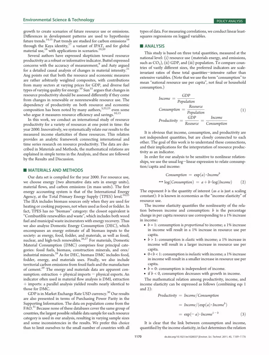
First, we measure the income elasticities for energy, materials,and CO2 emissions (column 1 of Table 1). We consider the sub-components of the total energy and materials, dividing these intobiomass, fossil, and other components. The components havemarkedly different behavior, with biomass (necessary for themost basic subsistence) and fossil fuels (used by highly indus-trialized economies) at either extreme. The consumption of fossilfuels, whether measured as energy, material, or CO2 emissions, isalmost proportional to income, with income elasticities above0.8. (Any difference between the fossil fuels results from theTPES andDEC data sets comes from slight differences in conver-sion factors and the country sample). In contrast, biomass con-sumption (energy or materials) has a very poor correlation withincome, with elasticities at or below 0.1: consumption is totallyinelastic. Along with the low goodness-of-fit, this signifies thatvariations in biomass consumption cannot be explained by

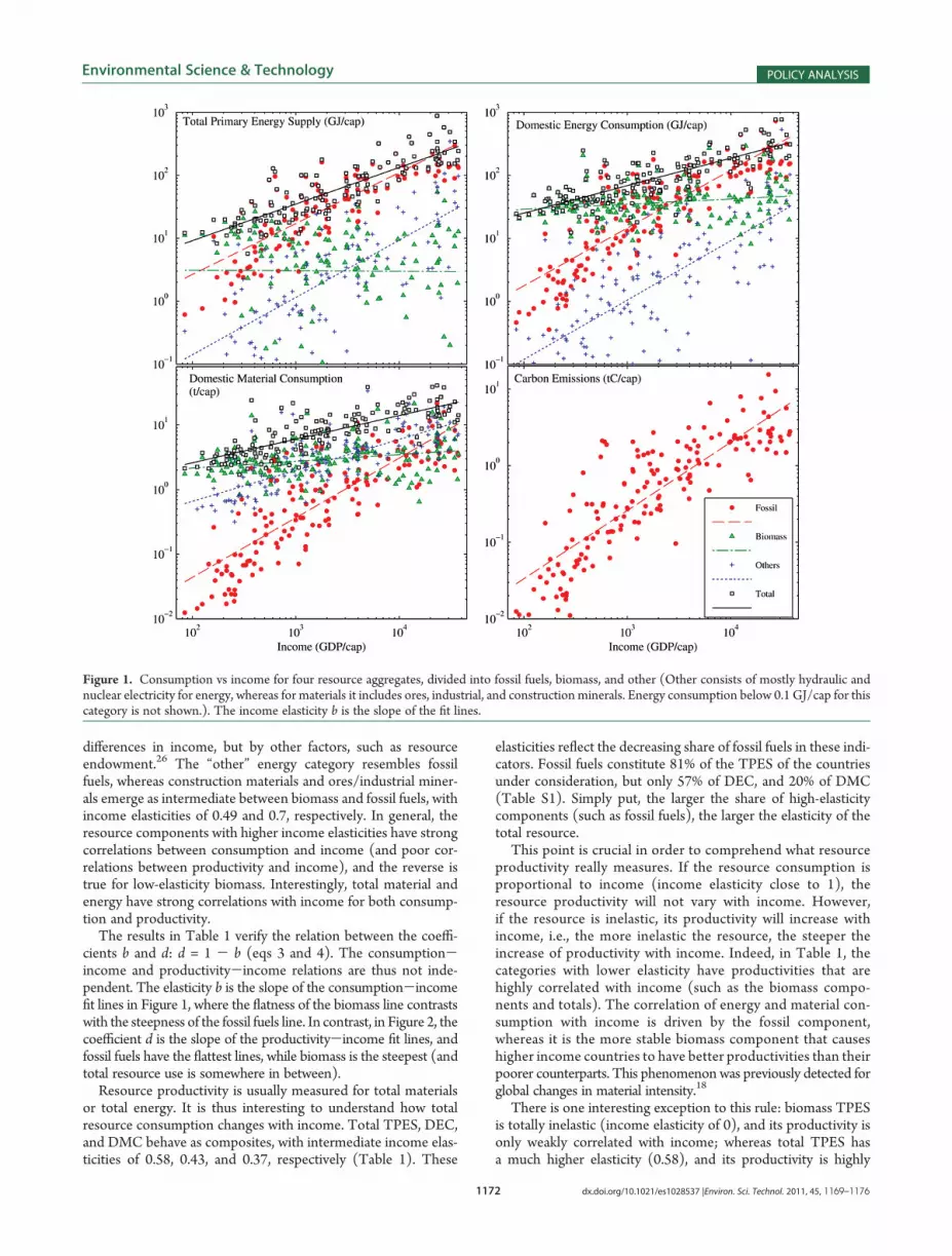
Table 1. Regression Results for Income-Consumption (eq 2) in Column 1 and Productivity-Income (eq 4) in Column 2a

(1) Income-Consumption (2) Income-Productivity number of countries

R2 income elasticity b R2 d

Total Primary Energy Supply;TPES

total 0.736 0.582 (0.031) 0.590 0.418 (0.031) 131

fossil 0.691 0.810 (0.048) 0.110 0.190 (0.048) 131

biomassb 0.000 -0.009 (0.114) 0.387 1.010 (0.114) 125

otherc 0.466 0.910 (0.092) 0.008 0.090 (0.092) 115

Domestic Energy Consumption;DEC

total 0.663 0.435 (0.024) 0.768 0.565 (0.024) 164

fossil 0.731 0.918 (0.044) 0.021 0.082 (0.044) 164

biomass 0.047 0.082 (0.029) 0.860 0.918 (0.029) 167

otherc 0.491 0.943 (0.082) 0.003 0.057 (0.082) 140

Domestic Material Consumption;DMC

total 0.636 0.366 (0.022) 0.840 0.634 (0.022) 155

fossil 0.690 0.924 (0.049) 0.015 0.076 (0.049) 161

biomass 0.075 0.104 (0.029) 0.857 0.896 (0.029) 165

const. min. 0.755 0.491 (0.022) 0.767 0.509 (0.022) 159

ores/ind. min. 0.417 0.696 (0.073) 0.120 0.304 (0.073) 131

GHG emissions

fossil CO2 0.729 0.891 (0.043) 0.039 0.109 (0.043) 162aR2 is the goodness-of-fit, ranging from 0 (no correlation) to 1 (perfect correlation), and can be interpreted as the percentage of variation in log(y)explained by log(x). Values of R2 above 0.4 are shown in bold. The values in parentheses are the standard errors of the coefficients. bThe TPES biomasscategory is known as “combustible renewables and waste”, and is a mixture of traditional biomass for heating and high-tech energy recovery from wasteincineration. cThe “other” energy category includes all nonfossil nonbiomass energy sources: principally hydraulic and nuclear electricity.



differences in income, but by other factors, such as resourceendowment.26 The “other” energy category resembles fossilfuels, whereas construction materials and ores/industrial miner-als emerge as intermediate between biomass and fossil fuels, withincome elasticities of 0.49 and 0.7, respectively. In general, theresource components with higher income elasticities have strongcorrelations between consumption and income (and poor cor-relations between productivity and income), and the reverse istrue for low-elasticity biomass. Interestingly, total material andenergy have strong correlations with income for both consump-tion and productivity.

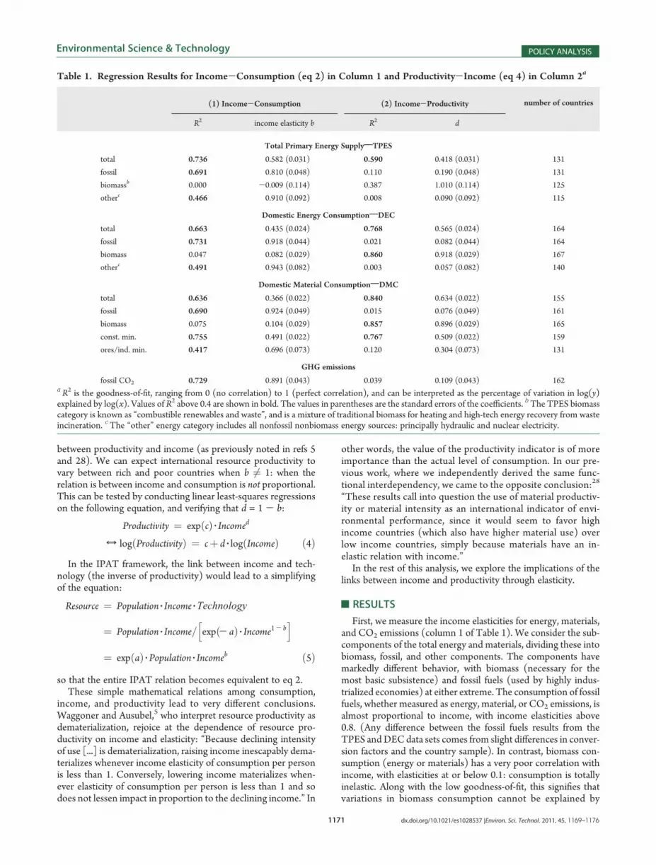
The results in Table 1 verify the relation between the coeffi-cients b and d: d = 1 - b (eqs 3 and 4). The consumption-income and productivity-income relations are thus not inde-pendent. The elasticity b is the slope of the consumption-incomefit lines in Figure 1, where the flatness of the biomass line contrastswith the steepness of the fossil fuels line. In contrast, in Figure 2, thecoefficient d is the slope of the productivity-income fit lines, andfossil fuels have the flattest lines, while biomass is the steepest (andtotal resource use is somewhere in between).

Resource productivity is usually measured for total materialsor total energy. It is thus interesting to understand how totalresource consumption changes with income. Total TPES, DEC,and DMC behave as composites, with intermediate income elas-ticities of 0.58, 0.43, and 0.37, respectively (Table 1). These

elasticities reflect the decreasing share of fossil fuels in these indi-cators. Fossil fuels constitute 81% of the TPES of the countriesunder consideration, but only 57% of DEC, and 20% of DMC(Table S1). Simply put, the larger the share of high-elasticitycomponents (such as fossil fuels), the larger the elasticity of thetotal resource.

This point is crucial in order to comprehend what resourceproductivity really measures. If the resource consumption isproportional to income (income elasticity close to 1), theresource productivity will not vary with income. However,if the resource is inelastic, its productivity will increase withincome, i.e., the more inelastic the resource, the steeper theincrease of productivity with income. Indeed, in Table 1, thecategories with lower elasticity have productivities that arehighly correlated with income (such as the biomass compo-nents and totals). The correlation of energy and material con-sumption with income is driven by the fossil component,whereas it is the more stable biomass component that causeshigher income countries to have better productivities than theirpoorer counterparts. This phenomenon was previously detected forglobal changes in material intensity.18

There is one interesting exception to this rule: biomass TPESis totally inelastic (income elasticity of 0), and its productivity isonly weakly correlated with income; whereas total TPES hasa much higher elasticity (0.58), and its productivity is highly

Figure 1. Consumption vs income for four resource aggregates, divided into fossil fuels, biomass, and other (Other consists of mostly hydraulic andnuclear electricity for energy, whereas for materials it includes ores, industrial, and construction minerals. Energy consumption below 0.1 GJ/cap for thiscategory is not shown.). The income elasticity b is the slope of the fit lines.



correlated with income. The biomass category of TPES is a mix-ture of traditional biomass use for energy (such as wood fuel andcharcoal) and high-tech energy recovery from biomass wasteincineration in industrialized countries. The consumption levelof biomass TPES thus depends on a combination of resourceavailability and technical infrastructures, and thus has a diffe-rent behavior than biomass DEC and DMC, which measure thetotality of biomass inputs to society for food, material, or energypurposes.

For greenhouse gas emissions, we are limited by only usingfossil CO2 emissions, which behave exactly like fossil inputs.CH4 and NOx, other potent greenhouse gases, are closely tied toagriculture and land use, and have been shown to be quiteinelastic.32 The inelasticity of non-CO2 GHG emissions is rele-vant to the discussion of the regressivity of CO2 or GHG taxes.33

Total GHG emissions would thus be expected to also behave asan aggregate, with both GHG per capita and GHG productivityhighly correlated with income.

Total resource productivity thus tends to systematicallyincrease with income, and increases faster if the indicator usedfor measuring resource use has a larger share of nonfossil, orinelastic, components, such as biomass. Intuitively, a compo-site resource indicator will tend to behave like its dominantcomponent. This can be easily demonstrated. Imagine an ag-gregate measure of resource use, with consumption per capita

Ctotal, composed of two parts C1 and C2, with elasticities b1and b2:

Ctotal ¼ C1 þC2 ¼ expða1Þ 3 Ib1 þ expða2Þ 3 Ib2 ð6ÞThe elasticity of the total resource consumption is

bt ¼ DCtotal

DI 3I

Ctotal¼ b1 3 expða1Þ 3 Ib1 þ b2 3 expða2Þ 3 Ib2

Ctotal

¼ b1 3C1

Ctotalþ b2 3

C2

Ctotalð7Þ

It is clear from eq 7 that the total elasticity bt will lie betweenb1 and b2, and will be closest to the elasticity of the componentwith the largest share of consumption. Simply put, a fossil-dominated aggregate, such as TPES, will behave most like fossilfuels, and a biomass-dominated aggregate like DMC will behavemore like biomass.

An elasticity-based understanding of composite resource con-sumption (eq 6) shows that it is extremely unlikely thateconomies will reduce fossil fuels in favor of biomass consump-tion, as suggested by Sun15 for “environmentally friendly” impro-vements in energy intensity, for example by shifting to biofuels.From an elasticity perspective, the use of biomass in high-techapplications will not reduce resource use overall, but instead

Figure 2. Productivity vs income for four resource aggregates, divided into fossil fuels, biomass, and other (Other consists of mostly hydraulic andnuclear electricity for energy, whereas for materials it includes ores, industrial, and construction minerals. Energy productivity above 9� 104 GJ/cap isnot shown.). The coefficient d is the slope of the fit lines.



increase the elasticity of biomass consumption by coupling it evermore tightly to the economy. Because biomass is a renewable butlimited resource, the implications for subsistence consumption inlow-income countries are quite alarming.

There is more to be learned from the analysis of aggregateresource elasticity in eq 7. The shares of resource consumptionare also dependent on income: as income rises, so does the shareof elastic resources. At low incomes the lower elasticity compo-nent will dominate, at higher incomes the higher elasticity com-ponent will dominate. The total elasticity is thus a logistic curvegoing from the lower elasticity value at low incomes to the higherelasticity value at high incomes:

bt ¼ b1þðb2- b1Þ 3C2

Ctotal

¼ b1þðb2- b1Þ 31

1þ expða1 - a2Þ 3 Ib1- b2ð8Þ

’DISCUSSION

What are the implications of our findings for the interpretationof productivity/intensity as an indicator of the technologicalachievement of an economy, with energy and materials as input,

and GDP as output? We have learned that international differ-ences in productivity are correlated with income, and that thiscorrelation can be explained by the inelasticity of resource use asan aggregate, itself caused by an inelastic component, usuallybiomass.

The rationale for using resource productivity as an indicator ofenvironmental sustainability assumes that resource use scaleswith the economy and that a higher economic output per resourceuse indicates more sustainable economic activity. The resourceproductivities of all of the total energy and material indicatorsconsidered are strongly correlated with income. If resource pro-ductivity were naively interpreted as an indicator of more sus-tainable economic performance, the conclusion would be thatricher countries are more sustainable, despite their higher levelsof resource use.

In technological terms, higher productivity economies arebenefiting from an apparent effect: they produce GDP in (moreor less) exact proportion to their consumption of fossil fuels, butmore than proportionally to their consumption of biomass. Bio-mass consumption varies from country to country, but almostentirely independently of income: poor countries, which con-sume similar levels of biomass, but far less fossil fuels, than richcountries, thus have a lower aggregate productivity. In economicefficiency terms, economic output can be seen asmainly fossil-driven,

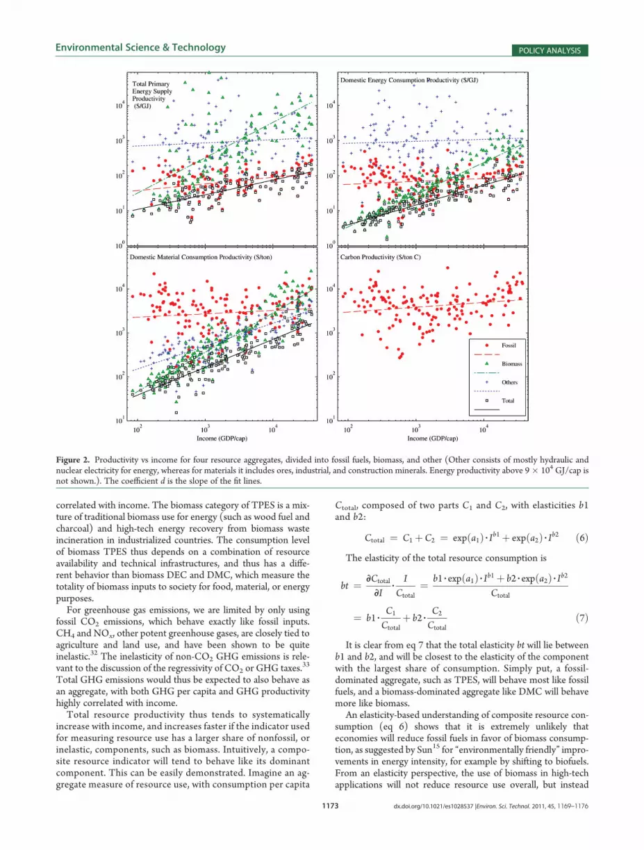
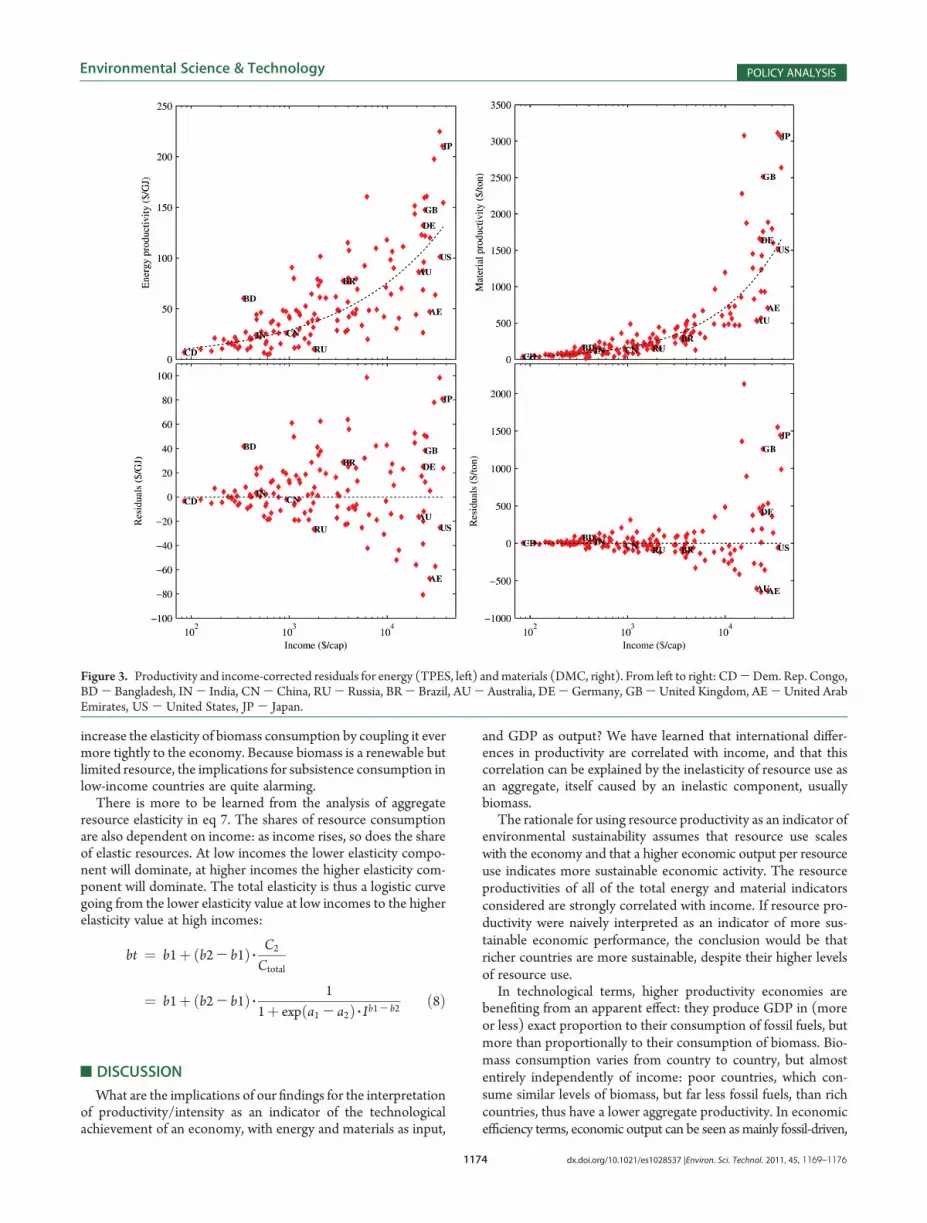
Figure 3. Productivity and income-corrected residuals for energy (TPES, left) andmaterials (DMC, right). From left to right: CD-Dem. Rep. Congo,BD- Bangladesh, IN- India, CN- China, RU- Russia, BR- Brazil, AU- Australia, DE-Germany, GB- United Kingdom, AE-United ArabEmirates, US - United States, JP - Japan.



with rather steady fossil productivity across countries of differentincomes (Table S1). The inclusion of inelastic biomass in theenergy/material input to economies makes those who areconsuming less fossil fuels seem inefficient in comparison withtheir richer counterparts.

In terms of the “resource efficiency of an economy” interpre-tation of resource productivity, it would be desirable to removethe systematic dependence on income. To correct internationalproductivity comparisons for systematic income dependence,several options are possible. The first would be to comparenational productivities not to each other, but to their positionalong the international income trend, i.e., compare the residualsrather than absolute values, as first suggested by Van der Voetet al.34 Other options would limit either the income range or theresources under consideration: compare countries within narrowincome ranges, where the income effect is expected to be smallcompared to the cross-country variability; or limit resource pro-ductivity comparisons to economically bound resources, thosewith income elasticities above 0.75, for example.

An example of the income-corrected (or elasticity-corrected)residual approach is shown for energy (TPES) and materials(DMC) in Figure 3. Energy productivity of Bangladesh is halfthat of the United Kingdom; in the income-corrected perspec-tive, they are very similar. The U.S., United Arab Emirates,and Australia have material productivities far above the globalaverage, but when these are corrected for income, they are eitherexactly average (U.S.) or far below (Australia and United ArabEmirates). In general, extractive and fossil-exporting economieshave lower income-corrected productivities, while poorer, smal-ler, or importing countries have higher income-corrected pro-ductivities. Recent studies have performed trade-corrected esti-mations of national consumption for CO2 and GHG emis-sions.32,35,36 Trade-corrected emissions would reduce the gapbetween exporting and importing nations, thus leading to evenstronger income dependence for productivity.

As an indicator used in analysis of trends and as a basis forscenarios, with the goal of explaining past and future resourceuse, income elasticity of consumption is a more meaningful androbust quantity than resource productivity. In contrast to re-source productivity, income elasticity is likely to evolve slowlyover time, mostly in response to price and technology. Efficiencyimprovements in the delivery of energy services have been shownto model long-term economic growth impressively well.37 Theunderstanding of past changes in income elasticities,38 along withconsiderations of trade shifts and macro-economic reboundeffects,39 should thus be emphasized as a research priority inorder to improve resource and climate scenarios. Other researchpriorities could be the study of this phenomenon over time, asour results hold only for the year 2000 and should change depen-ding on the development trajectories of different countries. Furtherdisaggregation by resource composition is also promising: forinstance ores/industrial materials and construction mineralshave distinct profiles from each other and fossil fuels.

In terms of resource savings or dematerialization, our conclu-sion is that resource productivity indicates no such thing, since itis mostly determined by national income and international elas-ticity. If economic growth and development result in ever gro-wing incomes, dematerialization in fact requires null or nega-tive income elasticity: the economic growth must be accompa-nied by decreases in resource use. It is likely that such a decreasein resource use is only possible at low economic growth rates: ator below the rates of physical technical improvement.

As a policy target,7,8 resource productivity mostly rewardsbusiness-as-usual developments of simultaneous economic,productivity, and resource consumption growth. If the objectiveis an absolute reduction in resource use and emissions, produc-tivity targets are insufficient, unless they are coupled with limitsto economic growth;politically a difficult proposal. Direct em-phasis on resource inputs and emissions is ultimately the onlyway to ensure effective policy.

’ASSOCIATED CONTENT

bS Supporting Information. Additional discussion, results,acronyms, and literature cited. This material is available free ofcharge via the Internet at http://pubs.acs.org.

’AUTHOR INFORMATION

Corresponding Author*E-mail: [email protected]; phone: þ43 (0) 1 522 4000 411.

’ACKNOWLEDGMENT

We thank Marina Fischer-Kowalski, Cynthia Alff-Steinberger,and three anonymous reviewers for their comments. We grate-fully acknowledge the support of the Austrian Science Fund(FWF) project P21012-G11.

’REFERENCES

(1) Commoner, B. The Closing Circle; Knopf: New York, 1971.(2) Ehrlich, P. R.; Holdren, J. P. Closing Circle - Commoner, B. Sci.

Public Affairs-Bull. At. Sci. 1972, 28 (5), 16.(3) Cleveland, C. J.; Ruth, M. Indicators of Dematerialization and

the Materials Intensity of Use. J. Ind. Ecol. 1999, 2 (3), 15–50.(4) Chertow, M. R. The IPAT Equation and Its Variants. Changing

Views of Technology and Environmental Impact. J. Ind. Ecol. 2000, 4(4), 13–30.

(5) Waggoner, P. E.; Ausubel, J. H. A framework for sustainabilityscience: A renovated IPAT identity. Proc. Natl. Acad. Sci. U.S.A. 2002, 99(12), 7860–7865.

(6) Weizs€acker, E. U. v.; Lovins, A. B.; Lovins, H. L. Factor fourdoubling wealth - halving resource use. The new report to the Club of Rome;Earthscan: London, 1997.

(7) Commission of the EuropeanCommunities.Thematic strategy onthe sustainable use of natural resources (Communication and Annexes);COM (2005) 670 final, SEC 1684; Commission of the EuropeanCommunities (CEC): Brussels, 2005.

(8) Takiguchi, H.; Takemoto, K. Japanese 3R Policies Based onMaterial Flow Analysis. J. Ind. Ecol. 2008, 12 (5-6), 792–798.

(9) Buttel, F. H. Social Structure and Energy Efficiency: a prelimin-ary cross-national analysis. Hum. Ecol. 1978, 6 (2), 145–164.

(10) Ang, B. W. Monitoring changes in economy-wide energyefficiency: From energy-GDP ratio to composite efficiency index. EnergyPolicy 2006, 34 (5), 574–582.

(11) Ang, B. W.; Zhang, F. Q. A survey of index decompositionanalysis in energy and environmental studies. Energy 2000, 25 (12),1149–1176.

(12) Hoekstra, R.; van den Bergh, J. C. J. M. Structural Decomposi-tion Analysis of Physical Flows in the Economy. Environ. Resour. Econ.2002, 23 (3), 357–378.

(13) Schipper, L.; Grubb, M. On the rebound? Feedback betweenenergy intensities and energy uses in IEA countries. Energy Policy 2000,28 (6-7), 367–388.

(14) Goldemberg, J. A note on the energy intensity of developingcountries. Energy Policy 1996, 24 (8), 759–761.



(15) Sun, J. W. Three types of decline in energy intensity - anexplanation for the decline of energy intensity in some developingcountries. Energy Policy 2003, 31, 519–526.(16) Canadell, J. G.; Le Quere, C.; Raupach, M. R.; Field, C. B.;

Buitenhuis, E. T.; Ciais, P.; Conway, T. J.; Gillett, N. P.; Houghton, R. A.;Marland, G. Contributions to accelerating atmospheric CO2 growthfrom economic activity, carbon intensity, and efficiency of natural sinks.Proc. Natl. Acad. Sci. U.S.A. 2007, 104 (47), 18866–18870.(17) Kaya, Y. Impact of Carbon Dioxide Emission Control on GNP

Growth: Interpretation of Proposed Scenarios; IPCC Energy and IndustrySubgroup, Response Strategies Working Group: Paris, 1990.(18) Krausmann, F.; Gingrich, S.; Eisenmenger, N.; Erb, K.-H.;

Haberl, H.; Fischer-Kowalski, M. Growth in global materials use, GDPand population during the 20th century. Ecol. Econ. 2009, 68 (10),2696–2705.(19) Nakicenovic, N.; Swart, R. Special Report on Emission Scenarios;

Intergovernmental Panel on Climate Change (IPCC), CambridgeUniversity Press: Cambridge, 2000.(20) Giljum, S.; Behrens, A.; Hinterberger, F.; Lutz, C.; Meyer, B.

Modelling scenarios towards a sustainable use of natural resources inEurope. Environ. Sci. Policy 2008, 11 (3), 204–216.(21) Auty, R.Materials intensity ofGDP:Research issues on themeasure-

ment and explanation of change. Resour. Policy 1985, 11 (4), 275–283.(22) Cleveland, C. J.; Costanza, R.; Hall, C. A. S.; Kaufmann, R. K.;

Stern, D. I. Energy and the U.S. Economy: A Biophysical Perspective.Science 1984, 225 (4665), 890–897.(23) OECD.OECDEnvironmental Indicators: Development, Measure-

ment and Use; Reference Paper; Organisation for Economic Co-Opera-tion and Development (OECD): Paris, France, 2003.(24) International Energy Agency (IEA), Organisation of Economic

Co-Operation and Development (OECD). Energy Balances of OECDCountries, 2004-2005, CD-ROM, 2007.(25) International Energy Agency (IEA), Organisation of Economic

Co-Operation andDevelopment (OECD). EnergyBalances of non-OECDCountries, 2004-2005, CD-ROM, 2007.(26) Krausmann, F.; Erb, K.-H.; Gingrich, S.; Lauk, C.; Haberl, H.

Global patterns of socioeconomic biomass flows in the year 2000: Acomprehensive assessment of supply, consumption and constraints.Ecol. Econ. 2008, 65 (3), 471–487.(27) Haberl, H. The Energetic Metabolism of Societies, Part I:

Accounting Concepts. J. Ind. Ecol. 2001, 5 (1), 11–33.(28) Steinberger, J. K.; Krausmann, F.; Eisenmenger, N. Global

patterns of material use: A socioeconomic and geophysical analysis.Ecol. Econ. 2010, 69 (5), 1148–1158.(29) Marland, G., Boden, T. A., Andres, R. J. In Trends: A Compen-

dium of Data on Global Change; Carbon Dioxide Information AnalysisCenter (CDIAC), Oak Ridge National Laboratory, U.S. Department ofEnergy: Oak Ridge, TN, 2007.(30) The World Bank Group. www.worldbank.org. (accessed Oct

2007).(31) FAO. FAOSTAT 2004, FAO Statistical Databases: Agriculture,

Fisheries, Forestry, Nutrition; FAO: Rome, 2004.(32) Hertwich, E.; Peters, G. P. Carbon Footprint of Nations: A

Global, Trade-Linked Analysis. Environ. Sci. Technol. 2009, 43 (16),6414–6420.(33) Feng, K.; Hubacek, K.; Guan, D.; Contestabile, M.; Minx, J.;

Barrett, J. Distributional Effects of Climate Change Taxation: The Caseof the UK. Environ. Sci. Technol. 2010, 44 (10), 3670–3676.(34) van der Voet, E.; van Oers, L.; Moll, S.; Sch€utz, H.; Bringezu, S.;

De Bruyn, S. M.; Sevenster, M.; Warringa, G. Policy Review on Decou-pling: Development of indicators to assess decoupling of economic develop-ment and environmental pressure in the EU-25 and AC-3 countries; CMLreport 166; Universitair Grafisch Bedrijf: Leiden, 2005.(35) Peters, G. P.; Hertwich, E. G. CO2 Embodied in International

Trade with Implications for Global Climate Policy. Environ. Sci. Technol.2008, 42 (5), 1401–1407.(36) Davis, S. J.; Caldeira, K. Consumption-based accounting of

CO2 emissions. Proc. Natl. Acad. Sci. U.S.A. 2010, 107 (12), 5687–5692.

(37) Ayres, R. U.; Turton, H.; Casten, T. Energy efficiency, sustain-ability and economic growth. Energy 2007, 32 (5), 634–648.

(38) Ang, B. W.; Liu, N. A cross-country analysis of aggregate energyand carbon intensities. Energy Policy 2006, 34 (15), 2398–2404.

(39) Dimitropoulos, J. Energy productivity improvements and therebound effect: An overview of the state of knowledge. Energy Policy2007, 35 (12), 6354–6363.

Documents

Material and Energy Productivity