Embed Size (px)
Citation preview

Contracting and Organizations Research Institute, University of Missouri 143 Mumford Hall, Columbia, Missouri 65211-6200
Tel. 573-884-9459 • Fax 573-882-3958 • http://cori.missouri.edu
Politics and Productivity
Peter G. Klein and Hung Luu
Contracting and Organizations Research Institute
Working Paper No. 02-02
July 2002
Keywords: economic freedom, policy stability, institutions, productivity, stochastic frontier
JEL Classification: O40, O30, H10, N40, D23
Politics and Productivity
Peter G. Klein
University of Missouri
Hung Luu
Merrill Lynch Capital Markets Bank Ltd.
November 2002
Forthcoming, Economic Inquiry.
Abstract: We use a stochastic-frontier approach to study the effects of political and regulatoryinstitutions on aggregate productivity in 39 countries from 1975 to 1990. We show that techni-cal efficiency is positively related to policies supporting laissez-faire and political structures thatpromote policy stability. Moreover, models of technical efficiency incorporating both measures per-form better than models including only one or the other. This suggests that economic performancedepends not only on current policies, but also on the confidence of market participants and outsideinvestors that these policies will remain in place.
JEL: O40, O30, H10, N40, D23
Keywords: economic freedom, policy stability, institutions, productivity, stochastic frontier
We thank James Gwartney, Witold Henisz, Randall Holcombe, Robert Lawson, Knox Lovell, DavidRobinson, Dexter Samida, Chris Westley, and an anonymous referee for helpful comments, KathrinZoeller for research assistance, and Witold Henisz for supplying data. The first author thanks theUniversity of Georgia Research Foundation for financial support.
Contact information:
Peter G. Klein Hung LuuContracting and Organizations Research Institute Debt Capital MarketsUniversity of Missouri Merrill Lynch Capital Markets Bank Ltd.Columbia, MO 65211 60311 FrankfurtUSA [email protected] hung [email protected]—7008 (phone)573-882-3958 (fax)
1. Introduction
Economic studies of long-run performance are focusing increasingly on political, legal, financial,
and social factors. Development is no longer regarded as a gradual, inevitable transformation
from self-sufficiency to specialization and participation in the division of labor. Instead, progress
follows the creation and evolution of institutions that support social and commercial relationships.
The “new institutional economics” explains that growth requires that the potential hazards of
trade (shirking, opportunism, risk, and so on) be controlled by institutions like secure property
rights, reliable procedures for resolving disputes, and means of enforcing contracts in the absence
of close social ties. These institutions reduce information costs, encourage capital formation and
capital mobility, allow risks to be priced and shared, and otherwise facilitate cooperation (North
and Thomas, 1973; North, 1990; Drobak and Nye, 1997; Levine, 1997). In particular, political
authorities must make credible commitments not to expropriate private resources once investments
have been made.1
Despite widespread agreement that institutions matter, there is no consensus on how they should
be incorporated into the analysis. Even the best empirical studies of productivity and growth treat
institutional characteristics in an eclectic way. Barro’s (1991) influential paper, for example, uses
the numbers of assassinations and revolutions per capita as proxies for political instability, finding
these measures negatively correlated with growth and investment. Scully (1988) regresses growth
rates on dummy variables derived from Gastil’s (1982) ordinal rankings of political and economic
liberty. King and Levine (1993a, 1993b, 1993c) derive various measures of the quality of financial
intermediaries and show that these measures are good predictors of growth.
This paper presents a different approach to analyzing the relationship between institutions and
aggregate economic performance. Following the modern productivity literature (see, for example,
Fried, Lovell and Schmidt, 1993), we model economic performance with a stochastic production
frontier. Frontier analysis is a sophisticated way to “benchmark” productive units. It analyzes
a group of branches, firms, nations, or other units by identifying “best practices” and evaluating
each member’s performance relative to the best-practice frontier. The results produce not only
qualitative rankings of the group members, but also numerical efficiency scores that can be used
to assess the effects of various policies and characteristics. For this reason, frontier analysis is well
1For general surveys of the new institutional economics see Furubotn and Richter (1997) and Klein (2000). North(1991) summarizes the literature as it applies specifically to economic development.
1
suited for studying the effects of legal and political institutions on the economic performance of
nations.
To capture institutional factors we use two comprehensive indexes of legal, regulatory, and
political conditions. Working with a broad sample of countries from 1975 to 1990, we incorporate a
widely used measure of economic freedom along with a new measure of policy stability to represent
a country’s institutional environment. The new institutional economics suggests that countries
with high levels of economic freedom (protection of private property rights, respect for the rule of
law, an unhampered price system, and so on) and policy stability (commitment not to change the
rules of the game ex post) will be closer to the best-practice frontier.
In our model, economic freedom and policy stability affect economic performance by enhancing
technical efficiency. In other words, these institutions do not alter the state of technology, but they
allow producers to squeeze more out of current technology. For instance, countries with more stable
policies attract more foreign investment than countries with less stable policies, ceteris paribus; this
leads to increased competition among producers, which in turn brings efficiency gains. Similarly,
countries with lower taxes, milder regulatory burdens, lower inflation, fewer restrictions on foreign
ownership, and so on are likely to produce output more efficiently than countries with policies that
restrict production, inhibit capital formation, and reduce competition.2
Our results strongly support the claim that the institutional environment affects technical effi-
ciency. Specifically, we find that both economic freedom and policy stability are highly significant
determinants of a country’s relationship to the best-practice frontier. Moreover, models of techni-
cal efficiency incorporating both measures perform better than models including only one or the
other. This suggests that economic performance depends not only on current policies, but on the
confidence of market participants and outside investors that these policies will remain in place.
Economic freedom is important, but even more so when combined with policy stability, and vice
versa. These results hold whether a composite measure or individual components of economic
freedom are used.
The remainder of the paper is organized as follows. Section 2 outlines the stochastic-frontier
model and describes the data. Section 3 presents results using the composite measure of economic
freedom. Section 4 explores the effects of individual components of economic freedom. Section 5
2We are using the term “technical efficiency” broadly, defining it to include anything that brings a country closerto the best-practice frontier. This could include improvements in allocative as well as productive efficiency. Of course,a more general model would also explore the relationship between institutions and the state of technology.
2
examines our results for endogeneity, and section 6 concludes.
2. Methods and data
We model the best-practice frontier for our sample countries as a stochastic production frontier.
The concept of a stochastic production frontier was proposed independently by Aigner, Lovell, and
Schmidt (1977), and Meeusen and van den Broeck (1977). The original specification involved
a production frontier for cross-sectional data with an error term consisting of two components,
one to account for random error and another to account for technical inefficiency. The original
model was later extended to incorporate time-series variation and with the prediction of technical
efficiency scores by appropriate explanatory variables. We use a panel data version of Battese and
Coelli (1993, 1995) that allows simultaneous estimation of technology parameters of a stochastic
production frontier and the parameters of an inefficiency model.
Our specification proceeds as follows. Suppose producer i at time t uses a vector of inputs xit ∈RN+ to produce scalar output yit ∈ R+ with technology
yit = f(xit,β) exp(vit − uit), and (1)
uit = zit · δ + wit ≥ 0, (2)
where i = 1, ..., I indexes producers, t = 1, ..., T indexes time, f denotes the production frontier,
and β is a vector of technology parameters to be estimated. The vits represent random errors
and are assumed to be iid N(0,σ2v). Technical inefficiency is captured by the uits, which are
assumed to be independently distributed as N+(zit ·δ,σ2u). They are also assumed to be distributedindependently of the vits. The parameter zit is a vector of explanatory variables associated with
technical inefficiency, and δ is a vector of unknown parameters to be estimated. The wits are
defined by the normal distribution with mean zero and variance σ2u and are truncated at −zit · δ,which ensures that uit ≥ 0. The log-likelihood is expressed in terms of the variance parametersσ2 ≡ σ2u + σ2v and γ = σ2u/σ
2. The variance ratio γ, bounded by zero and one, can be interpreted
as an inefficiency indicator. As γ goes to zero, variation in σ2 is attributed entirely to noise. As γ
goes to one, variation in σ2 is attributed entirely to inefficiency.3
In this context, technical efficiency is defined as the ratio of observed to maximum feasible
3See Battese and Coelli (1993) for the derivation of the log-likelihood.
3
output. Formally,
TEit =yit
f(xit,β) exp(vit)= exp(−uit) = exp(−zit · δ − wit) (3)
where TEit denotes technical efficiency of producer i in period t. Battese and Coelli (1993) show
that the minimum-mean-squared error predictor of technical efficiency is given by
E[exp(−uit)|vit − uit] .
Maximum-likelihood estimates for the parameters of both the stochastic production frontier and the
technical inefficiency model can be obtained from the computer program FRONTIER 4.1 (Coelli,
1996).4
Our data on inputs and outputs are taken from the Penn World Table (Summers and Heston,
1991), which provides income and expenditure data for about 150 countries from 1950 to the
present. The expenditure entries are denominated in common prices in a common currency to
permit real comparisons across countries and over time.
A key advantage of our approach over others typically used in the growth literature is that we
use output levels, rather than growth rates, to estimate our stochastic frontiers. The Penn World
Table was designed to compare income levels using “international prices” to adjust for differences
in the purchasing power of currencies. It turns out that these “international prices” most closely
resemble those of Hungary. Nuxoll (1994, p. 1423) notes that use of these prices tends to overstate
growth rates for countries wealthier than Hungary and to understate growth rates for countries less
wealthy than Hungary. He writes (p. 1434) that “probably the ideal is to use Penn World Table
numbers for levels and the usual national-accounts data for growth rates.” Our stochastic-frontier
approach avoids such bias by focusing on input and output levels, not growth rates.5
To capture the role of institutions, we begin with the composite measure of economic freedom
(EF) provided by Gwartney, Lawson, and Samida (2000). In their definition, “[i]ndividuals have
4Scully (1988) also uses a frontier approach to examine the effects of social institutions. He shows that ordinalrankings of political, civil, and economic liberty positively affect a country’s ability to convert capital per workerinto output per worker. However, Scully’s two-stage approach poses problems. In the first stage he estimatesa deterministic production frontier and predicts technical efficiency scores for each country under the assumptionthat the technical efficiency scores are identically distributed. The second stage involves a regression of the predictedtechnical efficiency scores on three measures of liberty. But this is inconsistent with the initial assumption of identicallydistributed technical efficiency scores. Our formulation avoids this problem with a one-stage approach that estimatesthe technology parameters of the stochastic production frontier and the parameters of the inefficiency model together.
5Temple (1999, p. 119) also discusses problems caused by confusing income levels with growth rates. Reliance ondata from the Penn World Table may explain why so many studies have failed to find convergence in growth ratesamong countries.
4
economic freedom when: (a) their property acquired without the use of force, fraud, or theft
is protected from physical invasions by others and (b) they are free to use, exchange, or give
their property to another as long as their actions do not violate the identical rights of others.”
Working with this definition, Gwartney, Lawson, and Samida construct an index measuring how
strongly these rights are protected across a broad sample of countries over time. The composite
EF measure consists of twenty-three components allocated to four major areas: (1) money and
inflation, (2) government operations and regulations, (3) takings and discriminatory taxation, and
(4) international trade. The composite measure represents the degree to which government policy
fosters savings, foreign investment, and commercial and industrial development.6 The data are
provided in a series of five-year cross-sections from 1970 to 2000.7
We interpret EFt as characterizing the policy “status quo” in year t. Economic development
clearly requires desirable policies, but it also requires policy stability; investors must believe that
desirable policies are likely to remain in place. We therefore add to our model a new measure
of policy constraints (PC) developed by Henisz (2000a).8 This measure, derived from a spatial
model of political interaction, describes how easily the status quo can be changed. It comprises two
elements: the number of potential veto points in the political system and the current alignment of
political interests, defined as the degree to which political actors agree on the desired policy, what-
ever that policy may be.9 Veto points make it difficult to change the status quo by administrative
or executive fiat; alignment of interests makes it unlikely that political actors will want to change
the status quo.
Henisz suggests two channels through which policy constraints affect economic performance.
First, by reducing the risk of wealth expropriation through arbitrary changes in tax, regulatory,
or other policy areas, stable policies encourage foreign investment, especially where relationship-
specific investments are at stake. Second, under stable policy regimes, fewer resources tend to be
6A value of ten represents very high economic freedom and a value of zero very low economic freedom. While theaggregate country ranking is given on this ten-point scale, the individual components are derived from quantitativemeasurements, not subjective, qualitative assessments. For this reason, the data are unlikely to be biased in favor of apositive relationship between economic freedom and economic performance (as would be the case if researchers tendedto assign high EF rankings to more prosperous countries). See also our discussion of the individual components insection 4 below.
7Other papers on institutions and growth using the Gwartney, Lawson, and Samida data include Easton andWalker (1997), Dawson (1998, 2002), Gwartney, Holcombe, and Lawson (1998, 1999), Norton (1998), Ayal ad Karras(1998), La Porta, Lopez-de-Silanes, Shleifer, and Vishny (1999), Ali and Crain (2002), and Carlsson and Lundstrom.
8The PC measure is also used in Henisz (2000b) and Henisz and Zelner (2001).
9A value of one represents very high policy stability and a value of zero very low policy stability.
5
spent in rent-seeking activities, freeing those resources to create wealth. We consider the effects
of EF and PC both separately and together, presuming that economic freedom should be more
valuable in the presence of policy constraints, and policy constraints should be more valuable in
the presence of economic freedom.10
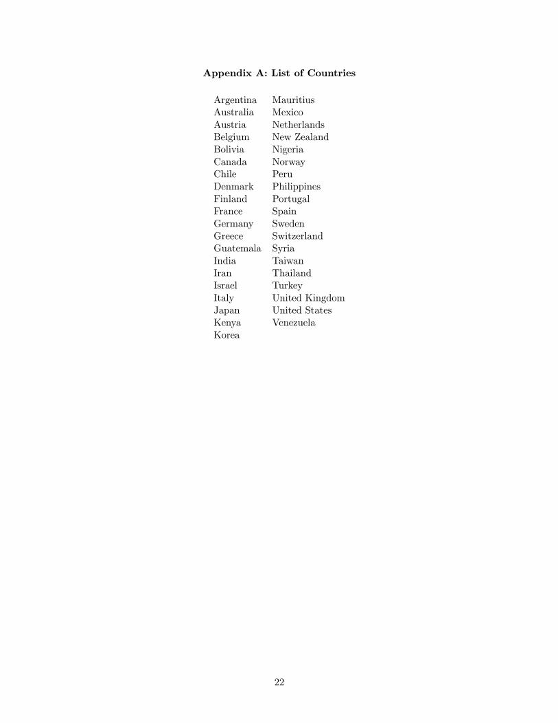
Drawing from these sources, and eliminating observations with missing data, we construct
a balanced panel of 39 countries for the years 1975, 1980, 1985 and 1990 with a total of 156
observations.11 (The list of countries is included as Appendix A.) Real GDP per worker and
capital stock per worker in 1985 international prices are taken from Summers and Heston (1991).
Summary statistics for all variables are provided in Table 1.
[Table 1 about here]
Are high levels of EF associated with high levels of PC? In our sample the correlation between
EF and PC is 0.538, smaller than we initially expected. Some countries, like the United States,
Canada, and Switzerland, score high on both measures, while others, like Turkey, Iran, and Syria,
score low on both. However, economic freedom and policy constraints do not necessarily go together.
Israel, Portugal, and Spain rank high on PC but low on EF; these countries have very stable policies,
but the content of those policies inhibits efficient resource allocation through markets. Guatemala,
by contrast, scores high on EF but low on PC. Guatemala has relatively laissez-faire policies, but
provides investors and entrepreneurs little assurance that those policies will remain in place.
10Policy stability should not be confused with political stability. Political stability refers to the likelihood that thecurrent regime will remain in power. Zaire under Mobutu Sese Seko was an example of a country with a highly stablepolitical regime but increasingly arbitrary policies. Similarly, policy stability does not measure “political freedom”–an extended franchise, the right to form political parties, an independent press, and so on. In our framework, suchpolitical rights affect productivity only to the extent that they affect economic freedom. For more on the relationshipbetween political and economic freedom, see the classic treatments by Mises (1927), Hayek (1944), and Friedman(1962).
11The Penn World Table contains data on 152 countries, but not all variables are available in all four years.Henisz’s dataset on political constraints includes the same 152 countries, while the Gwartney, Lawson, and Samidadata include from 83 to 123 countries, depending on the year, though some individual components of EF are missingin particular years. Our panel includes the 39 countries for which all necessary variables were available in all fouryears.
6
3. Basic results
We employ a Cobb-Douglas stochastic production frontier in logarithmic form:
ln yit = β0 + β1 lnxit +4Xt=2
ηtDt +39Xi=2
λiDi + vit − uit (4)
where ln yit is the natural log of real GDP per worker for country i in period t, lnxit is the natural
log of capital stock per worker for country i in period t, Dt is a time dummy for period t intended
to capture technical change (see Baltagi and Griffin, 1988), Di is a country dummy for country i
to control for unobserved heterogeneity, and vit and uit are defined as above.12
To explore the effects of EF and PC on productivity we use four specifications of the technical
inefficiency component:
uit = δ0 + δ1EFit + wit (5)
uit = δ0 + δ1PCit + wit (6)
uit = δ0 + δ1EFit + δ2PCit + wit (7)
uit = δ0 + δ1EFit + δ2PCit + δ3EF · PC + wit (8)
The first specification includes only EF as a source of inefficiency, the second includes only PC, the
third includes both, and the fourth adds an interaction term. Table 2 provides parameter estimates
for all four specifications.
[Table 2 about here]
The results strongly support the idea that EF and PC are important determinants of technical
efficiency. The elasticity of RGDP per worker with respect to capital per worker, β1, ranges from
0.599 to 0.712. The inefficiency indicator, γ, is very close to one and highly significant, implying
that nearly all the variation in σ2 can be attributed to inefficiency. In the technical inefficiency
component of the model, the key parameters δ1 and δ2 (the coefficients on EF and PC, respectively)
have the expected signs and are highly significant: the higher the EF and the higher the PC, the
12We chose this functional form because scale effects are unlikely to matter at this level of aggregation and becauseour focus lies on the inefficiency component of the model. As a robustness check, we also regressed the natural log ofreal GDP on the natural log of labor and the natural log of capital stock to allow for variable returns to scale. Thecorresponding results (not reported here) are similar to the results reported in this section.
7
less inefficient the country in converting capital per worker into RGDP per worker. The coefficient
on the interaction term also has the expected sign, though it is not significant.13
Likelihood ratio tests suggest focusing on specification (7). The estimated coefficient on PC in
this specification is −0.333. Mean technical efficiency for the sample is 0.8904, which implies thatmean uit is 0.116. If the mean PC score were one-third of a standard deviation (0.11 units or 21
percent) above its current level, ceteris paribus, the mean uit would fall by −0.333 ·0.11 = −0.0337to −0.0794. In turn, mean technical efficiency would rise to 0.9237. Similarly, if mean EF wereone-third of a standard deviation (0.473 units or 10 percent) above its current level, ceteris paribus,
mean uit would fall by −0.198 · 0.473 = −0.0937 to −0.0223. Mean technical efficiency would thenrise substantially to 0.9780, eliminating almost all waste! Of course, these quantitative statements
should be interpreted with caution, since it is unclear what constitutes a “unit” of EF or PC.
Nonetheless, the results strongly support the proposition that EF and PC enhance economic growth
through technical efficiency gains.
This exercise also sheds light on the debate about the rise of the “East Asian Tigers.” A 1993
World Bank study attributed the impressive growth rates of Taiwan, South Korea, and Thailand
from 1960 to 1990 to high rates of productivity growth, dubbing their strong economic performance
the “East Asian miracle.” Young (1994), by contrast, suggested that the major source of their
economic growth was increased utilization of capital and labor, not productivity growth. Krugman
(1994) popularized the idea that East Asian growth was no miracle, claiming that higher output
was driven merely by an increase in inputs. Without productivity growth, of course, output growth
cannot be sustained for long.
Table 3 provides the raw data and technical efficiency scores for South Korea, Taiwan, Thailand,
and eight other countries in the sample. South Korea, Taiwan, and Thailand all show significant
improvement in technical efficiency from 1975 to 1990. South Korea and Thailand had technical
efficiency growth rates of 2.15 and 1.86 percent per year, respectively, the highest efficiency growth
rates in our sample. Taiwan ranked 9th with average annual efficiency growth of 1.17 percent over
13As discussed in footnote 10 above, PC is a measure of policy stability, not political stability. However, to checkthe robustness of our results we experimented with an additional set of specifications including an additional controlvariable, the average annual number of revolutions and coups during the previous five years (the most common proxyfor political stability used in the growth literature). The data were obtained from Arthur Banks’s Cross NationalTime-Series Data Archive.The results (not reported here) were virtually identical to those reported in Table 2. PC and EF retain the
expected signs and significance levels, their point estimates are about the same as before, and the new variable isnot statistically significant. This suggests that dramatic regime changes are important only to the extent they affectpolicy stability and economic freedom (the content of current policies), not independent of them.
8
the same period.
[Table 3 about here]
Moreover, the raw data reveal that during this period these three countries experienced sub-
stantial improvements in EF, PC, or both. For the entire sample, the mean increase in PC between
1975 and 1990 was 0.09 units, and the mean increase in EF over the same period was 0.95 units.
South Korea had the highest increase in PC, 0.48 units, along with an above-average increase in
EF of 1.1 units (19th best). Similarly, Thailand had an increase in PC of 0.07 units (13th highest)
and an increase in EF of 1.6 units (10th highest). Taiwan appears less impressive, with a 0.01-unit
decrease in PC (35th best) and a 1.2-unit increase in EF (12th best). However, Taiwan started
with a high 1975 PC score of 0.72, which leaves little room for improvement. In short, our results
suggest that the South Korean, Taiwanese, and Thai economies expanded not only through capi-
tal accumulation, but also through productivity growth fostered by policies and institutions that
increased economic freedom and improved policy stability.
This result is not exclusive to the East Asian Tigers. Other countries with substantial increases
in EF and PC leading to improvements in technical efficiency include India, Chile, and Portugal.
Like South Korea, India achieved substantial improvements in PC (0.25 units, 7th best in the
sample) and EF (0.7 units, 21st best), and witnessed a corresponding increase in technical efficiency
of 1.54 percent per year (6th best). Like Taiwan, Chile and Portugal maintained high levels of PC
during the 1975—90 period, while also increasing EF, by 3.3 units (best in the sample) and 1.7 units
(9th best), respectively. They simultaneously experienced annual technical efficiency growth rates
of 0.73 (12th best) and 1.61 (4th best), respectively.
By contrast, consider Iran, Nigeria and Syria. These countries experienced technical efficiency
declines of 7.59, 3.37, and 1.26 percent, respectively. Our analysis suggests that these productivity
losses were due to reductions in EF. All three countries rank at the bottom in EF change (Iran is
worst at −1.70, Syria third worst at −0.70, and Nigeria fifth worst at 0.10). All three countries arealso effectively dictatorships, with PC scores of 0.00 in 1975 and 1990. These EF changes and PC
levels largely explain their inability to attract foreign investment. For further illustration, suppose
that Iran, Nigeria, and Syria had the same 1975—90 increases in EF and PC as South Korea (1.1 and
0.48 units, respectively). According to the estimated coefficients from model (7), Iran would have
more than doubled technical efficiency from 0.330 to 0.675, Nigeria would have increased technical
9
efficiency from 0.615 to 0.88, and Syria would have almost doubled technical efficiency from 0.671
to 1.127. (Syria would have an output-input ratio beyond what is feasible for any members of the
current sample!)
Another example illustrates our point that both PC and EF are necessary for productivity
growth. Both Argentina and Peru experienced substantial increases in PC over the sample period,
0.41 units for Argentina (third best in the sample) and 0.38 units for Peru (fourth best). However,
both had below-average increases in EF of 0.3 units. Despite these increases in PC, Argentina
and Peru experienced technical efficiency declines of 1.61% (fifth worst) and 2.51% (third worst),
respectively. Policy constraints are important, but only if current policies leave markets relatively
free of government intervention.
4. Individual components of economic freedom
The composite measure of economic freedom provided by Gwartney, Lawson, and Samida (2000)
is derived from individual rankings of all countries in twenty-three specific areas. To be sure our
results using the composite measure were not driven by Gwartney, Lawson, and Samida’s particular
aggregation method, we reestimated our results using individual components of EF in place of the
composite measure. Besides constituting a robustness check for the results presented above, this
approach helps shed light on those specific policies most conducive to economic development.14
Of the twenty-three individual components provided by Gwartney, Lawson, and Samida, ten
were available for all our sample countries in all four years.15 We thus reestimated the technical
inefficiency component of our production frontier as
uit = δ0 + δ1PCit +12Xj=2
δjzjit + wit , (9)
where zjit represents country i’s score in year t on the following j components zj :
1. z2, the difference between the annual growth rate of the money supply (M1) and the annualgrowth rate of potential real GDP;
14Other papers focusing on the individual components of the Gwartney, Lawson, and Samida index include Ayaland Karras (1998), Carlsson and Lundstrom (2002), and Dawson (2002).
15Gwartney, Lawson, and Samida (2000) use alternative weights to construct the composite measure of EF forcountry-years in which one or more of the individual components of EF is missing. First, they try to construct arating in each of the four major areas (money and inflation, government operations and regulations, takings anddiscriminatory taxation, and international exchange). For example, suppose an area consists of three components.They calculate an area rating if at least two of the three components exist by allocating the missing component’sweight to the two available components. Next, they use a similar process to construct the composite rating from thearea ratings.
10
2. z3, government consumption as a percent of total consumption;
3. z4, government-consumption-to-total-consumption squared (used for reasons explained be-low);
4. z5, the presence and role of state-operated enterprises (SOEs) (a higher rating means thatgovernment enterprises play a less significant role);
5. z6, the right to own foreign currency domestically (zero or ten);
6. z7, the freedom to engage in capital (investment) transactions with foreigners (zero, two, five,eight or ten);
7. z8, the right to own a bank account abroad (zero or ten);
8. z9, the use of conscripts to obtain military personnel (zero or ten);
9. z10, the average tax rate on international trade;
10. z11, actual size of trade sector (imports and exports as a percentage of GDP) compared tothe expected size; and
11. z12, the difference between the official exchange rate and the black-market rate.16
Results are presented in Table 4. As in the model with the composite measure of EF, the
coefficient on PC is negative and significant, indicating that countries with strong policy constraints
are less inefficient than countries with weak policy constraints. All components of EF except the
two international trade proxies are statistically significant, and most have the expected signs.
[Table 4 about here]
The coefficient on z2, inflation, is positive and significant, consistent with a substantial empirical
literature showing that high inflation rates inhibit trade and capital formation by distorting relative
prices (Aarstol, 1996; Kaul and Seyhun, 1990; see also Scully, 1992). The coefficient on z3, gov-
ernment expenditures, is significant but negative, indicating that countries with high government
expenditures are less inefficient than countries with low government expenditures. This is surpris-
ing, given that most of the empirical growth literature finds a negative correlation between the
size of the public sector and economic growth (Kormendi and Meguire, 1985; and Landau, 1983),
and it seems inconsistent with our laissez-faire argument. Some authors suggest that government
expenditures on certain “core functions”–protection of property rights, enforcement of contracts,
16Gwartney, Lawson, and Samida (2000) express all rankings on ordinal scales. For greater precision, we havesubstituted for z2, z6, z9, z10, and z11 the actual numbers.
11
and a legal system to resolve disputes, and possibly some goods like public infrastructure and
education–stimulate economic growth (Gwartney, Holcombe, and Lawson, 1998, pp. 165—66).17
Barro (1990) develops a growth model in which the level of government expenditures contributes
positively to economic growth up to a certain level (for example, 25 percent of GDP), but reduces
growth beyond that level. Branson and Lovell (2000), following similar reasoning, estimate an
optimal level of government spending for New Zealand of 22 percent.
An alternative explanation for our coefficient on z3, however, is that the level of government
expenditures is likely to be a poor proxy for the role of government intervention in the economy.
It is increasingly recognized that government activities such as statutes, administrative regulation,
and the judicial interpretation of legal rules redirect resources as much as, or more than, taxes
and spending (Peltzman, 1980; Lindbeck, 1985; Borcherding, 1985; Block, 1991). For this reason,
recent research on the U.S. has used alternative measures of government intervention such as the
number of pages in the Federal Register (Westley, 1998; see also Goff, 1996). More generally, as
Higgs (1987, p. 29) points out, “all quantitative indexes of the size of government share a common
defect: their changes may indicate either changes in the scope of effective governmental authority
or merely changes in the level at which government operates within a constant scope of authority.”
Nonetheless, to allow comparison of our results to those of similar studies, we follow Branson
and Lovell (2000) and include a second-order term to solve for the level of government expenditures
(GOV) associated with minimum technical inefficiency. We model the inefficiency component as
u = δ0 + δ3GOV +1
2δ4GOV
2 (10)
(abstracting from the other independent variables and omitting time and country subscripts). This
implies that∂u
∂GOV= δ3 + δ4GOV . (11)
The theory that government spending up to a certain level is beneficial implies that δ3 should be
negative and δ4 positive. Setting that expression equal to zero yields the “optimal” GOV equal to
−δ3/δ4. As Table 2 shows, δ4 is positive and significant, suggesting an optimal GOV of about 30percent, somewhat higher than Branson and Lovell’s figure.18
17However, as emphasized by Rothbard (1970), Friedman (1973), Benson (1990, 1998), and others, even the “pro-tective” functions of government such as securing law and order are also provided by markets.18Our GOV measures government consumption relative to total consumption, not government expenditures relative
to GDP, so our measure is not directly comparable to theirs.
12
Consistent with our overall position, the coefficient on z5, the presence and role of state-owned
enterprises, is negative and significant. (Recall that a higher score on z5 indicates a smaller role
for SOEs.) The empirical literature on privatization strongly suggests that SOEs are less efficient
than private-sector benchmarks (Boardman and Vining, 1989; Ehrlich, Gallais-Hamonno, Liu, and
Lutter, 1994; Majumdar, 1996; Dewenter and Malatesta, 2001; see also Megginson and Netter,
2001). Like this literature, we find that aggregate economic performance is lower when SOEs play
a more important role.
The results on the remaining variables are mixed. The negative coefficients on z6, the right
to own foreign currency domestically, and z7, the freedom to engage in capital transactions with
foreigners, support the claim that these liberties enhance productivity by encouraging foreign trade.
On the other hand, the positive coefficient on z8, the right to own foreign bank accounts, does not
appear to support our argument, unless foreign accounts are regarded as repositories of illegal
gains that would have otherwise been invested domestically. The coefficient on z9, conscription,
is positive and significant at the 10 percent level, suggesting that forced military service is less
efficient than voluntary arrangements.
Finally, the coefficients on z10 and z11, the two variables that relate directly to international
trade, are not statistically significant. Despite arguments that trade barriers can increase productiv-
ity by correcting factor-market distortions, protecting “infant industries,” and so on, it is generally
agreed that free trade should produce efficiency gains from improved resource allocation due to
specialization according to comparative advantage. Most empirical studies find that openness to
trade, usually proxied by the ratio of exports or imports to RGDP, has a significant positive (but
small) impact on growth (see, for example, Feder, 1983; Kormendi and Meguire, 1985). However,
our model fails to pick up a significant effect. Possibly, neither variable is a good measure of a coun-
try’s openness to trade; Ayal and Karras (1998) also find that the average tax rate on international
trade is not a significant determinant of economic growth in a neoclassical framework.19 An ideal
measure of trade liberalization would be an aggregate, weighted index of the divergence between
world and domestic prices; unfortunately, such a measure has not yet been constructed. We do
find that the coefficient on z12, the black-market exchange premium, is positive and significant
19One potential problem with z10, the average tax on international trade, is that it is strongly correlated withper-capita GDP (Easterly and Rebelo, 1993). Less developed countries tend to rely heavily on tariffs because theylack the administrative ability to collect other types of taxes. To see if the inclusion of z10 had biased the coefficientson the remaining right-hand-side variables, we reestimated the regression reported in Table 4 without z10. The pointestimates and significance levels for the remaining variables were essentially the same as those reported in Table 4.
13
(countries with high premiums are less efficient). The black-market premium is usually used as a
measure of distortions on foreign trade, but may also be interpreted more generally as a proxy for
other distortionary policies and for macroeconomic instability.
In general, these results in this section support our hypothesis that EF and PC raise technical
efficiency even if we employ components of EF instead of a composite measure of EF. Our basic
conclusion is thus robust to the precise measurement of EF.
5. Endogeneity
Clearly, then, the institutional environment, as captured by EF and PC, is highly correlated with
technical efficiency. However, we have not yet established a causal relation between institutions
and efficiency. So far we have treated EF and PC as determinants of productivity. Conceivably,
the relationship could go the other way: countries that are more productive are wealthier, and
wealthy countries can afford to have stable, laissez-faire policies. This could be the underlying
causal explanation for our results.
In a historical context, this argument makes little sense. Countries with interventionist, unstable
policies did not become rich and then suddenly reduce the sizes of their public sectors and stick
to established rules of the game. Rather, it was the stable, laissez-faire economies that became
wealthy in the first place (Rosenberg and Birdzell, 1986, Landes, 1998). Nonetheless, to explore
the possibility that our results reflect a causal relationship from wealth to EF and PC, we estimated
panel regressions of EF and PC on RGDP per worker and RGDP per worker lagged one period.
Results from both random-effects and fixed-effects regressions are presented in Panel A of Table 5.
As seen in the table, the coefficients on RGDP per worker are positive and highly significant in both
EF regressions and positive in both PC regressions (though significant only in the random-effects
model). This means that income is contemporaneously correlated with both dependent variables.
However, lagged RGDP per worker is not significant in any regression. Controlling for current
income, then, past values of income are not good predictors of EF or PC.
[Table 5 about here]
By contrast, as seen in Panel B of Table 5, lagged values of EF and PC are generally good
predictors of RGDP per worker, controlling for current values of EF and PC. These findings suggest
that EF and PC are best understood as drivers of productivity, not simply consequences of economic
14
well-being. Gwartney, Lawson, and Holcombe (1999) also look at whether growth causes EF. They
find that the value of the composite measure of EF in a year, and the change in EF over time,
affects growth over a period of decades. However, they find no correlation between economic growth
and future changes in EF. In other words, higher growth in the present is not correlated with
higher levels of EF in the future. Dawson (2002) applies Granger causality testing to individual
components of EF and finds that strong property rights and relatively unfettered markets are
primary drivers of growth, while other components of EF, such as the size of government and
controls on international finance, are more likely the result of growth. (Yet other components, such
as those related to monetary and price stability, appear to be jointly determined with growth.)
Along with these results, our findings reported in Table 5 support the idea that the institutional
environment is an important determinant of economic performance, not merely its consequence.
6. Conclusions
Economists have become increasingly aware that technology, and not resource endowment,
is usually the most important driver of economic performance over time. Our analysis shows
that cross-country differences in technical efficiency need not be treated as exogenous–indeed,
these differences can themselves be explained largely by differences in institutional environments.
Countries with legal and regulatory frameworks that promote trade and competition, and relatively
stable political systems, tend to be closest to the best-practice frontier.
More generally, our findings for the 1975—90 period complement the modern literature on long-
term economic performance. Recent work in economic history argues that the emergence of long-
distance trade, and later industrialization, were dependent on political and social institutions. In
early societies, agency problems were typically solved through kinship or other close social ties.
Greif (1989), for example, shows how eleventh-century Jewish traders in the Mediterranean area
enforced codes of conduct by maintaining close social relationships, using the threat of ostracism as a
disciplinary device. Later, standardized weights and measures, units of account, media of exchange,
and procedures to resolve disputes (such as merchant law courts) supported the expansion of trade
by lowering information costs. Capital markets could flourish only in societies where rulers could
credibly commit not to expropriate private wealth; North and Weingast (1989) show how capital
markets emerged in Britain after the Glorious Revolution of 1688 placed parliamentary limits on
the authority of the Crown. The growth of product and factor markets depends similarly on
establishing secure property rights. Furthermore, as an economy industrializes, more and more
15
commercial activity involves “transacting”: trade, finance, banking, insurance, and management
(Wallis and North, 1986). Industrialization requires institutions to mitigate the costs associated
with these transactions.
A key to understanding economic development, then, is institutional development. “The central
issue of economic history and of economic development is to account for the evolution of political and
economic institutions that create an economic environment that induces increasing productivity”
(North, 1991, p. 98). In future work we hope to study the evolution of institutions that promote
technical efficiency, rather than taking institutions as exogenous as we do in the present paper.
We also hope to incorporate measures of financial-market development, though this raises potential
endogeneity problems. A further issue concerns the relationship between changes in PC and changes
in EF over time. Is the change in one of these variables a necessary precondition to a change in
the other? Our sample includes countries that experienced increases in PC without corresponding
increases in EF, and failed to enjoy efficiency gains as a result. However, there are no similar
examples of countries that experienced an increase in EF without corresponding increases in PC,
suggesting that a change in PC tends to precede a change in EF. Further work on the co-movement
of these variables over time may provide valuable guidance for economic reform in the developing
and post-Communist world.
In short, we are convinced that productivity analysis can benefit from closer study of political
and regulatory institutions, and that the new institutional economics can benefit from more ex-
plicit theorizing about the channels through which institutional factors affect aggregate economic
performance. We look forward to future research that combines these two strands of literature.
16
7. References
Aarstol, Michael. 1996. The Impact of Inflation Upon Capital Markets and Growth. Ph.D.dissertation, Department of Economics, Stanford University.
Aigner, Dennis, C.A. Knox Lovell, and Peter Schmidt. 1977. “Formulation and Estimation ofStochastic Frontier Production Function Models.” Journal of Econometrics 6: 21—37.
Ali, Abdiweli M. and W. Mark Crain. 2002. “Institutional Distortions, Economic Freedom andGrowth.” Cato Journal 21(3): 415—26.
Ayal, Elizier B., and Georgios Karras. 1998. “Components of Economic Growth and Growth: AnEmpirical Study.” Journal of Developing Areas 32: 327—38.
Baltagi, Badi H., and James M. Griffin. 1988. “A General Index of Technical Change.” Journalof Political Economy 96(1): 20—41.
Barro, Robert J. 1990. “Government Spending in a Simple Model of Endogenous Growth.” Jour-nal of Political Economy 98(5): 103—26.
Barro, Robert J. 1991. “Economic Growth in a Cross Section of Countries.” Quarterly Journalof Economics 106: 407—43.
Battese, George E., and Tim J. Coelli. 1993. “A Stochastic Frontier Production Function In-corporating a Model for Inefficiency Effects.” Working Papers in Econometrics and AppliedStatistics No.69, Department of Econometrics, University of New England, Armidale.
Battese, George E., and Tim J. Coelli. 1995. “A Model for Technical Inefficiency Effects in aStochastic Frontier Production Function for Panel Data.” Empirical Economics 20(2): 325—32.
Benson, Bruce L. 1990. The Enterprise of Law: Justice Without the State. San Francisco: PacificResearch Institute for Public Policy Research.
Benson, Bruce L. 1998. To Serve and Protect: Privatization and Community in Criminal Justice.New York: New York University Press.
Block, Walter. 1991. Economic Freedom: Toward a Theory of Measurement. Vancouver: FraserInstitute.
Boardman, Anthony, and Aidan R. Vining. 1989. “Ownership and Performance in Competi-tive Environments: A Comparison of the Performance of Private, Mixed, and State-OwnedEnterprises.” Journal of Law and Economics 32: 1—33.
Borcherding, Thomas E. 1985. “The Causes of Government Expenditure Growth: A Survey ofthe U.S. Evidence.” Journal of Public Economics 28: 359—82.
Branson, J., and C. A. Knox Lovell. 2000. “Taxation and Economic Growth in New Zealand.”In Gerald W. Scully and Patrick J. Caragata, eds., Taxation and the Limits of Government.Boston: Kluwer Academic Publishers.
Carlsson, Fredrick, and Susanna Lundstrom. 2002. “Economic Freedom and Growth: Decompos-ing the Effects.” Public Choice, forthcoming.
17
Coelli, Tim J. 1996. “A Guide to FRONTIER Version 4.1: A Computer Program for Frontier Pro-duction Function Estimation.” CEPA Working Paper 96/07, Department of Econometrics,University of New England, Armidale.
Dawson, John W. 1998. “Institutions, Investment, and Growth: New Cross-Country and PanelData Evidence.” Economic Inquiry 36: 603—19.
Dawson, John W. 2002. “Causality in the Freedom-Growth Relationship.” European Journal ofPolitical Economy, forthcoming.
Dewenter, Kathryn, and Paul H. Malatesta. 2001. “State-Owned and Privately-Owned Firms:An Empirical Analysis of Profitability, Leverage, and Labor Intensity.” American EconomicReview 91(1): 320—34.
Drobak, John N., and John V. Nye. 1997. The Frontiers of the New Institutional Economics. SanDiego: Harcourt Brace.
Easterly, William, and Sergio Rebelo. 1993. “Fiscal Policy and Economic Growth: An EmpiricalInvestigation.” Journal of Monetary Economics 32(3): 417—58.
Easton, Steven T., and Michael A. Walker. 1997. “Income, Growth, and Economic Freedom.”American Economic Review 87(2): 328—32.
Ehrlich, Isaac, Georges Gallais-Hamonno, Zhiqiang Liu, and Randall Lutter. 1994. “ProductivityGrowth and Firm Ownership: An Empirical Investigation.” Journal of Political Economy102: 1006—38.
Feder, Gershon. 1983. “On Exports and Economic Growth.” Journal of Development Economics12(1/2): 59-73.
Fried, Harold O., C.A. Knox Lovell, and Sheldon S. Schmidt, eds. 1993. The Measurement ofProductive Efficiency: Techniques and Applications. New York: Oxford University Press.
Friedman, David D. 1973. The Machinery of Freedom: A Guide to a Radical Capitalism. NewYork: Harper & Row.
Friedman, Milton. 1962. Capitalism and Freedom. Chicago: University of Chicago Press.
Furubotn, Eirik G., and Rudolf Richter. 1997. Institutions and Economic Theory: The Con-tribution of the New Institutional Economics. Ann Arbor: University of Michigan Press,1997.
Gastil, Raymond D. 1982. Freedom in the World. Westport, Conn.: Greenwood Press.
Goff, Brian. 1996. Regulation and Macroeconomic Performance. Boston: Kluwer.
Greif, Avner. 1989. “Reputation and Coalitions in Medieval Trade: Evidence on the MaghribiTraders.” Journal of Economic History 49: 857—82.
Gwartney, James, and Robert Lawson, with Dexter Samida. 2000. Economic Freedom of theWorld: 2000 Annual Report. Vancouver: Fraser Institute. Data retrieved from http://www.freetheworld.com
Gwartney, James, Randall Holcombe, and Robert Lawson. 1998. “The Scope of Government andthe Wealth of Nations.” Cato Journal 18: 163—90.
18
Gwartney, James, Robert Lawson, and Randall Holcombe. 1999. “Economic Freedom and theEnvironment for Economic Growth.” Journal of Institutional and Theoretical Economics155(4): 643—63.
Hayek, F. A. 1944. The Road to Serfdom. Chicago: University of Chicago Press.
Henisz, Witold J. 2000a. “The Institutional Environment for Economic Growth.” Economics andPolitics 12(1): 1—32.
Henisz, Witold J. 2000b. “The Institutional Environment for Multinational Investment.” Journalof Law, Economics & Organization 16(2): 334—64.
Henisz, Witold J., and Bennet A. Zelner. 2001. “The Institutional Environment for Telecommu-nications Investment.” Journal of Economics & Management Strategy 10(1) 128—48.
Higgs, Robert. 1987. Crisis and Leviathan: Critical Episodes in the Growth of American Govern-ment. New York: Oxford University Press.
Kaul, Gautam, and H. Nejat Seyhun. 1990. “Relative Price Variability, Real Shocks, and theStock Market.” Journal of Finance 45: 479—96.
King, Robert G., and Ross Levine. 1993a. “Finance, Entrepreneurship, and Growth: Theory andEvidence.” Journal of Monetary Economics 32(3): 513—42.
King, Robert G., and Ross Levine. 1993b. “Finance and Growth: Schumpeter Might Be Right.”Quarterly Journal of Economics 108(3): 717—37.
King, Robert G., and Ross Levine. 1993c. “Financial Intermediation and Economic Develop-ment.” In Colin Mayer and Xavier Vives, eds., Financial Intermediation in the Constructionof Europe. London: Centre for Economic Policy Research, pp. 156—89.
Klein, Peter G. 2000. “New Institutional Economics.” In Boudewin Bouckeart and Gerrit DeGeest, eds., Encyclopedia of Law and Economics. Cheltenham, U.K.: Edward Elgar, pp.456—89.
Kormendi, Roger C., and Philip G. Meguire. 1985. “Macroeconomic Determinants of Growth:Cross-Country Evidence.” Journal of Monetary Economics 16(2): 141—63.
Krugman, Paul. 1994. “The Myth of Asia’s Miracle.” Foreign Affairs 76(3): 62—78.
La Porta, Rafael, Florencio Lopez-de-Silanes, Andrei Shleifer, and Robert Vishny. 1999. “TheQuality of Government.” Journal of Law, Economics and Organization 15: 222—79.
Landes, David S. 1998. The Wealth and Poverty of Nations: Why Some Are So Rich and SomeSo Poor. New York: Norton.
Landau, Daniel L. 1983. “Government Expenditure and Economic Growth: A Cross-CountryStudy.” Southern Economic Journal 49(3): 783—92.
Levine, Ross. 1997. “Financial Development and Economic Growth: Views and Agenda.” Journalof Economic Literature 35: 688—726.
Lindbeck, Assar. 1985. “Redistribution Policy and the Expansion of the Public Sector.” Journalof Public Economics 28: 309—28.
19
Majumdar, Sumit K. 1996. “Assessing Comparative Efficiency of the State-Owned, Mixed, andPrivate Sectors in Indian Industry.” Public Choice 96: 1—24.
Meeusen, Wim, and Julien van den Broeck. 1977. “Efficiency Estimation from Cobb-DouglasProduction Functions with Composed Error.” International Economic Review 18: 435—44.
Megginson, William L., and Jeffry M. Netter. 2001. “From State to Market: A Survey of EmpiricalStudies on Privatization.” Journal of Economic Literature 39: 321—89.
Mises, Ludwig von. 1927. Liberalism: In the Classical Tradition. Irvington-on-Hudson, N.Y.:Foundation for Economic Education, 1985.
North, Douglass C. 1990. Institutions, Institutional Change and Economic Performance. Cam-bridge, Cambridge University Press.
North, Douglass C. 1991. “Institutions.” Journal of Economic Perspectives 5: 97—112.
North, Douglass C., and Robert Paul Thomas. 1973. The Rise of the Western World: A NewEconomic History. Cambridge: Cambridge University Press.
North, Douglass C., and Barry R. Weingast. 1989. “Constitution and Commitment: The Evolu-tion of Institutions Governing Public Choice in 17th Century England.” Journal of EconomicHistory 49: 803—32.
Norton, Seth W. 1998. “Poverty, Property Rights, and Human Well-Being: A Cross-NationalStudy.” Cato Journal 18 (2): 233—45.
Nuxoll, Daniel A. 1994. “Differences in Relative Prices and International Differences in GrowthRates.” American Economic Review 84(5): 1423—36.
Peltzman, Sam. 1980. “The Growth of Government.” Journal of Law and Economics 23: 209—87.
Rosenberg, Nathan, and L. E. Birdzell, Jr. 1986. How the West Grew Rich: the EconomicTransformation of the Industrial World. New York: Basic Books.
Rothbard, Murray N. 1970. Power and Market: Government and the Economy. Kansas City:Sheed Andrews and McMeel.
Scully, Gerald W. 1988. “The Institutional Framework and Economic Development.” Journal ofPolitical Economy 96(3): 652-62.
Scully, Gerald W. 1992. Constitutional Environments and Economic Growth. Princeton, N.J.:Princeton University Press.
Summers, Robert, and Alan Heston. 1991. “The Penn World Table (Mark V): An Expanded Setof International Comparisons 1950—1988.” Quarterly Journal of Economics 106: 327—68.
Temple, Jonathan 1999. “The New Growth Evidence.” Journal of Economic Literature 37(1):112-56.
Wallis, John J., and Douglass C. North. 1986. “Measuring the Transaction Sector in the AmericanEconomy, 1870—1970.” In Stanley Engerman and Robert Gallman, eds., Income and Wealth:Long-Term Factors in American Economic Growth. Chicago: University of Chicago Press.
20
Westley, Christopher. 1998. “Government Regulation and Income Inequality in the United States,1970—1990.” Applied Economics Letters 5: 805—08.
World Bank. 1993. The East Asian Miracle: Economic Growth and Public Policy. New York:Oxford University Press.
Yeager, Timothy J. 1999. Institutions, Transition Economies, and Economic Development. Boul-der, Colo.: Westview Press.
Young, Alvin. 1994. “Lessons from the East Asian NICs: A Contrarian View.” European Eco-nomic Review 38: 964—73.
21
Appendix A: List of Countries
Argentina MauritiusAustralia MexicoAustria NetherlandsBelgium New ZealandBolivia NigeriaCanada NorwayChile PeruDenmark PhilippinesFinland PortugalFrance SpainGermany SwedenGreece SwitzerlandGuatemala SyriaIndia TaiwanIran ThailandIsrael TurkeyItaly United KingdomJapan United StatesKenya VenezuelaKorea
22
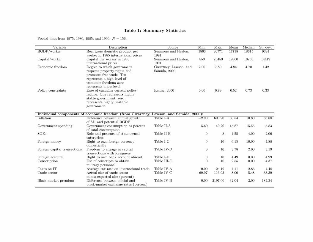
Table 1: Summary Statistics
Pooled data from 1975, 1980, 1985, and 1990. N = 156.
Variable Description Source Min. Max. Mean Median St. dev.RGDP/worker Real gross domestic product per Summers and Heston, 1863 36771 17718 18615 9391
worker in 1985 international prices 1991Capital/worker Capital per worker in 1985 Summers and Heston, 553 73459 19860 18733 14419
international prices 1991Economic freedom Degree to which government Gwartney, Lawson, and 2.00 7.80 4.84 4.70 1.42
respects property rights and Samida, 2000promotes free trade. Tenrepresents a high level ofeconomic freedom; zerorepresents a low level.
Policy constraints Ease of changing current policy Henisz, 2000 0.00 0.89 0.52 0.73 0.33regime. One represents highlystable government; zerorepresents highly unstablegovernment.
Individual components of economic freedom (from Gwartney, Lawson, and Samida, 2000):Inflation Difference between annual growth Table I-A −2.90 690.20 30.54 10.80 86.88
of M1 and potential RGDPGovernment spending Government consumption as percent Table II-A 5.60 40.20 15.87 15.55 5.83
of total consumptionSOEs Role and presence of state-owned Table II-B 0 8 4.55 4.00 2.06
enterprisesForeign money Right to own foreign currency Table I-C 0 10 6.15 10.00 4.88
domesticallyForeign capital transactions Freedom to engage in capital Table IV-D 0 10 3.78 2.00 3.19
transactions with foreignersForeign account Right to own bank account abroad Table I-D 0 10 4.49 0.00 4.99Conscription Use of conscripts to obtain Table III-C 0 10 2.55 0.00 4.37
military personnelTaxes on IT Average tax rate on international trade Table IV-A 0.00 24.19 4.11 2.83 4.48Trade sector Actual size of trade sector Table IV-C −69.97 116.93 8.00 5.48 33.39
minus expected size (percent)Black-market premium Difference between official and Table IV-B 0.00 2197.00 32.04 2.00 184.34
black-market exchange rates (percent)
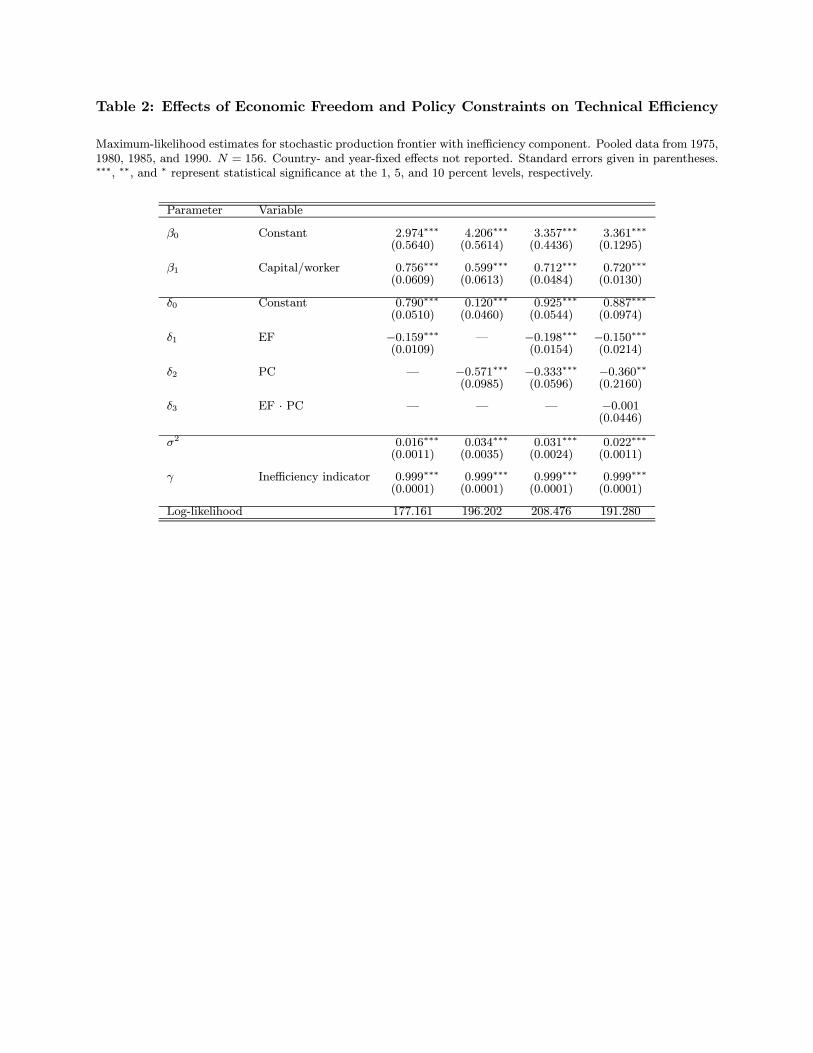
Table 2: Effects of Economic Freedom and Policy Constraints on Technical Efficiency
Maximum-likelihood estimates for stochastic production frontier with inefficiency component. Pooled data from 1975,1980, 1985, and 1990. N = 156. Country- and year-fixed effects not reported. Standard errors given in parentheses.∗∗∗, ∗∗, and ∗ represent statistical significance at the 1, 5, and 10 percent levels, respectively.
Parameter Variable
β0 Constant 2.974∗∗∗ 4.206∗∗∗ 3.357∗∗∗ 3.361∗∗∗(0.5640) (0.5614) (0.4436) (0.1295)
β1 Capital/worker 0.756∗∗∗ 0.599∗∗∗ 0.712∗∗∗ 0.720∗∗∗(0.0609) (0.0613) (0.0484) (0.0130)
δ0 Constant 0.790∗∗∗ 0.120∗∗∗ 0.925∗∗∗ 0.887∗∗∗(0.0510) (0.0460) (0.0544) (0.0974)
δ1 EF −0.159∗∗∗ – −0.198∗∗∗ −0.150∗∗∗(0.0109) (0.0154) (0.0214)
δ2 PC – −0.571∗∗∗ −0.333∗∗∗ −0.360∗∗(0.0985) (0.0596) (0.2160)
δ3 EF · PC – – – −0.001(0.0446)
σ2 0.016∗∗∗ 0.034∗∗∗ 0.031∗∗∗ 0.022∗∗∗(0.0011) (0.0035) (0.0024) (0.0011)
γ Inefficiency indicator 0.999∗∗∗ 0.999∗∗∗ 0.999∗∗∗ 0.999∗∗∗(0.0001) (0.0001) (0.0001) (0.0001)
Log-likelihood 177.161 196.202 208.476 191.280
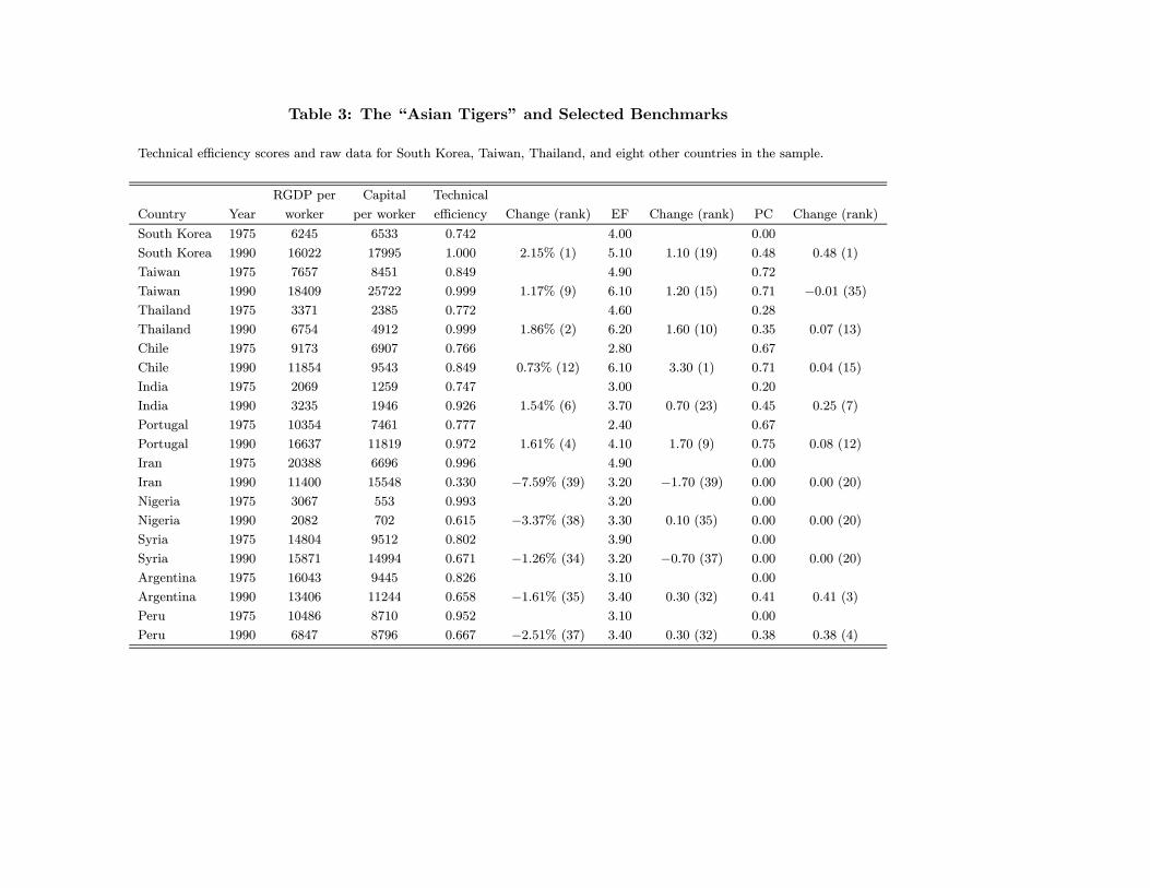
Table 3: The “Asian Tigers” and Selected Benchmarks
Technical efficiency scores and raw data for South Korea, Taiwan, Thailand, and eight other countries in the sample.
RGDP per Capital Technical
Country Year worker per worker efficiency Change (rank) EF Change (rank) PC Change (rank)
South Korea 1975 6245 6533 0.742 4.00 0.00
South Korea 1990 16022 17995 1.000 2.15% (1) 5.10 1.10 (19) 0.48 0.48 (1)
Taiwan 1975 7657 8451 0.849 4.90 0.72
Taiwan 1990 18409 25722 0.999 1.17% (9) 6.10 1.20 (15) 0.71 −0.01 (35)Thailand 1975 3371 2385 0.772 4.60 0.28
Thailand 1990 6754 4912 0.999 1.86% (2) 6.20 1.60 (10) 0.35 0.07 (13)
Chile 1975 9173 6907 0.766 2.80 0.67
Chile 1990 11854 9543 0.849 0.73% (12) 6.10 3.30 (1) 0.71 0.04 (15)
India 1975 2069 1259 0.747 3.00 0.20
India 1990 3235 1946 0.926 1.54% (6) 3.70 0.70 (23) 0.45 0.25 (7)
Portugal 1975 10354 7461 0.777 2.40 0.67
Portugal 1990 16637 11819 0.972 1.61% (4) 4.10 1.70 (9) 0.75 0.08 (12)
Iran 1975 20388 6696 0.996 4.90 0.00
Iran 1990 11400 15548 0.330 −7.59% (39) 3.20 −1.70 (39) 0.00 0.00 (20)
Nigeria 1975 3067 553 0.993 3.20 0.00
Nigeria 1990 2082 702 0.615 −3.37% (38) 3.30 0.10 (35) 0.00 0.00 (20)
Syria 1975 14804 9512 0.802 3.90 0.00
Syria 1990 15871 14994 0.671 −1.26% (34) 3.20 −0.70 (37) 0.00 0.00 (20)
Argentina 1975 16043 9445 0.826 3.10 0.00
Argentina 1990 13406 11244 0.658 −1.61% (35) 3.40 0.30 (32) 0.41 0.41 (3)
Peru 1975 10486 8710 0.952 3.10 0.00
Peru 1990 6847 8796 0.667 −2.51% (37) 3.40 0.30 (32) 0.38 0.38 (4)
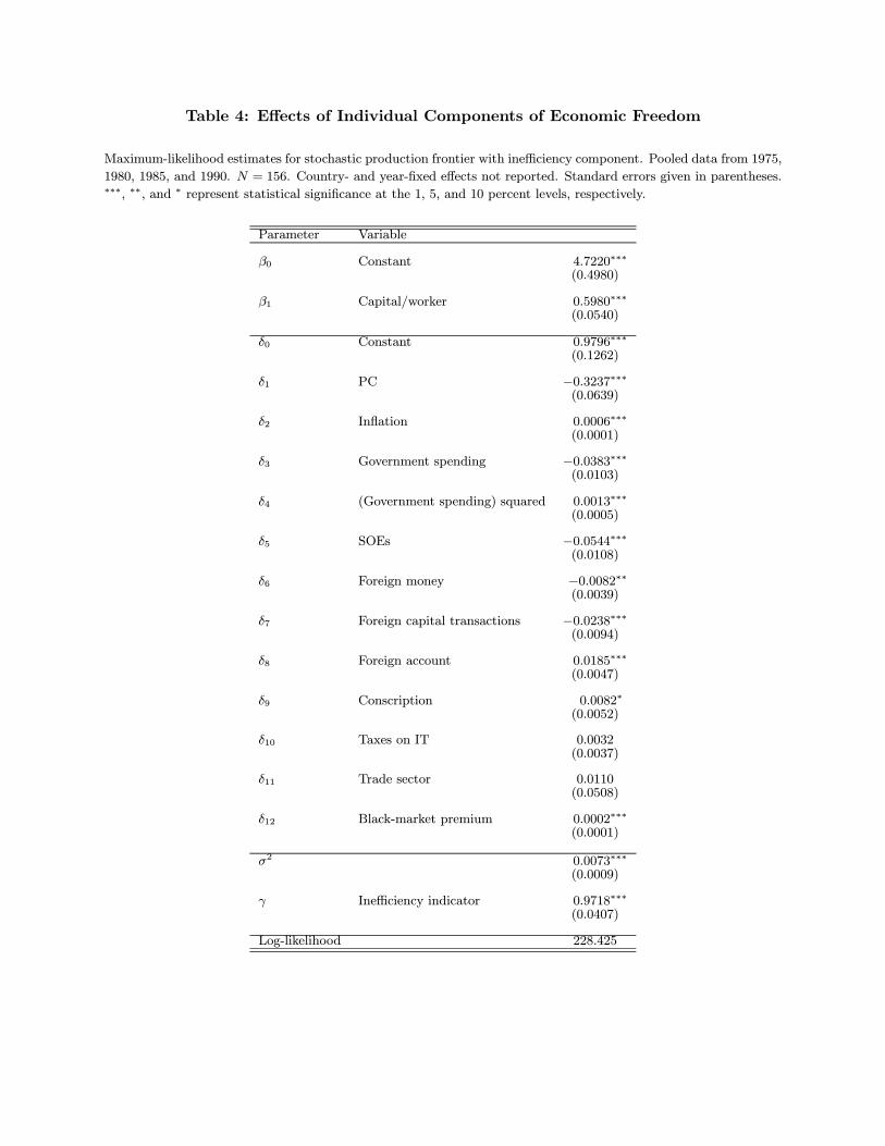
Table 4: Effects of Individual Components of Economic Freedom
Maximum-likelihood estimates for stochastic production frontier with inefficiency component. Pooled data from 1975,
1980, 1985, and 1990. N = 156. Country- and year-fixed effects not reported. Standard errors given in parentheses.∗∗∗, ∗∗, and ∗ represent statistical significance at the 1, 5, and 10 percent levels, respectively.
Parameter Variable
β0 Constant 4.7220∗∗∗
(0.4980)
β1 Capital/worker 0.5980∗∗∗
(0.0540)
δ0 Constant 0.9796∗∗∗
(0.1262)
δ1 PC −0.3237∗∗∗(0.0639)
δ2 Inflation 0.0006∗∗∗
(0.0001)
δ3 Government spending −0.0383∗∗∗(0.0103)
δ4 (Government spending) squared 0.0013∗∗∗
(0.0005)
δ5 SOEs −0.0544∗∗∗(0.0108)
δ6 Foreign money −0.0082∗∗(0.0039)
δ7 Foreign capital transactions −0.0238∗∗∗(0.0094)
δ8 Foreign account 0.0185∗∗∗
(0.0047)
δ9 Conscription 0.0082∗
(0.0052)
δ10 Taxes on IT 0.0032(0.0037)
δ11 Trade sector 0.0110(0.0508)
δ12 Black-market premium 0.0002∗∗∗
(0.0001)
σ2 0.0073∗∗∗
(0.0009)
γ Inefficiency indicator 0.9718∗∗∗
(0.0407)
Log-likelihood 228.425
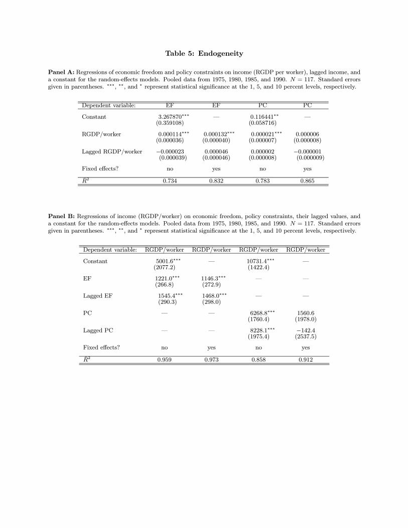
Table 5: Endogeneity
Panel A: Regressions of economic freedom and policy constraints on income (RGDP per worker), lagged income, anda constant for the random-effects models. Pooled data from 1975, 1980, 1985, and 1990. N = 117. Standard errorsgiven in parentheses. ∗∗∗, ∗∗, and ∗ represent statistical significance at the 1, 5, and 10 percent levels, respectively.
Dependent variable: EF EF PC PC
Constant 3.267870∗∗∗ – 0.116441∗∗ –(0.359108) (0.058716)
RGDP/worker 0.000114∗∗∗ 0.000132∗∗∗ 0.000021∗∗∗ 0.000006(0.000036) (0.000040) (0.000007) (0.000008)
Lagged RGDP/worker −0.000023 0.000046 0.000002 −0.000001(0.000039) (0.000046) (0.000008) (0.000009)
Fixed effects? no yes no yes
R2 0.734 0.832 0.783 0.865
Panel B: Regressions of income (RGDP/worker) on economic freedom, policy constraints, their lagged values, anda constant for the random-effects models. Pooled data from 1975, 1980, 1985, and 1990. N = 117. Standard errorsgiven in parentheses. ∗∗∗, ∗∗, and ∗ represent statistical significance at the 1, 5, and 10 percent levels, respectively.
Dependent variable: RGDP/worker RGDP/worker RGDP/worker RGDP/worker
Constant 5001.6∗∗∗ – 10731.4∗∗∗ –(2077.2) (1422.4)
EF 1221.0∗∗∗ 1146.3∗∗∗ – –(266.8) (272.9)
Lagged EF 1545.4∗∗∗ 1468.0∗∗∗ – –(290.3) (298.0)
PC – – 6268.8∗∗∗ 1560.6(1760.4) (1978.0)
Lagged PC – – 8228.1∗∗∗ −142.4(1975.4) (2537.5)
Fixed effects? no yes no yes
R2 0.959 0.973 0.858 0.912