Embed Size (px)
Citation preview
THU 90/13June 1990
MARKOV TRACES AND II1 FACTORS
IN CONFORMAL FIELD THEORY
Jan de Boer∗ and Jacob Goeree†
Institute for Theoretical PhysicsPrincetonplein 5P.O. Box 80.0063508 TA UtrechtThe Netherlands
ABSTRACT
Using the duality equations of Moore and Seiberg we define for every primaryfield in a Rational Conformal Field Theory a proper Markov trace and hence aknot invariant. Next we define two nested algebras and show, using results ofOcneanu, how the position of the smaller algebra in the larger one reproducespart of the duality data. A new method for constructing Rational ConformalField Theories is proposed.
1 Introduction
In the past few years several attempts have been made to find the basic underlying prin-ciples and structures governing Rational Conformal Field Theories (RCFT). In one ap-proach, quantum groups are proposed as the underlying algebraic structure of RCFT [21].In [21] the philosophy is that the quantum group can be seen as the centralizer of a repre-sentation of the braid group. This approach is in particular successful for WZW models,where one can compute braid matrices using the analogue of 6j−symbols. The result ofthis construction for arbitrary RCFT is, however, unclear.
In another approach, Rational Conformal Field Theories are seen to be intimatelyrelated with three-dimensional generally covariant field theories [16, 3]. Here, the Hilbertspace associated to a constant time slice with charges in the three dimensional theory isequal to the space of conformal blocks of a RCFT. The observables of the three-dimensionaltheory are knotted links whose expectation values can also be computed (as we will show)from RCFT.
In this paper we will take a look at these two approaches from a somewhat differentangle. Instead of quantum groups we will end up with inclusions of certain II1 factors.These are infinite dimensional algebras that can be obtained by taking a certain limit offinite dimensional ones. They arise as algebras of paths on a graph constructed from thefusion rules, and a primary field φ. The graph is closely related to the fusion graph, butnot necessarily identical to it. For instance for a field φ with the fusion rule φ2 = 1 + φthe graph is the Dynkin graph A4.
An outline of the contents and the results of this paper is as follows:
In section 2 we will give a review of the duality relations that govern RCFT. Using theseit will be shown in section 3 how one can obtain link invariants from arbitrary RationalConformal Field Theories, by construction of a proper Markov trace. Some examples willbe given where the invariant is equivalent to some well-known knot invariant. In particularthis shows that there exists a well-defined three-dimensional topological field theory, wherethe expectation values of links agree with the link invariant obtained from RCFT. Onecould in principle use this to properly define expectation values of graphs as well, as hasbeen done for Chern-Simons theories in [14], and more recently for arbitrary RCFT in [5].
In sections 4, 5 and 6 we will explain the relation between II1 factors and RCFT,using Ocneanu’s path algebras [9]. The algebras presented in those sections have theproperties that their representation theory coincides with part of the fusion rules, andthat the intertwiners between these representations are (up to a normalization) braidingmatrices. In the case that the special chosen field φ is self-dual, our construction shouldgive the same resulting algebras as in [21], suggesting a close relation between quantumgroups and path algebras. The precise relation is, however, unclear, and must presumablybe sought along the lines of Witten’s work [15].
As a by-product of our graphic representation of the string algebras we find in sec-tion 7 a relation between the positive half of the Virasoro algebra and the Temperley-Lieb
1
algebra. These results are also valid for certain statistical mechanical models, because wecan define an IRF model based on the same string algebras, where the Boltzmann weightsare braiding matrices. In this context the elements of the string algebras can be seen astransfer matrices.
The final part of this paper consists of a study of the reverse process, namely con-structing Rational Conformal Field Theories out of inclusions of factors. We establishsome necessary (but, unfortunately, not sufficient) conditions for inclusions to produceRational Conformal Field Theories, and present some examples.
2 Duality in CFT
Rational Conformal Field Theories are conformal field theories in which the Hilbert spacedecomposes into a finite sum of irreducible representations of the (maximally extended)chiral algebra AL ⊗AR
H =⊕
i,ıHi ⊗Hı
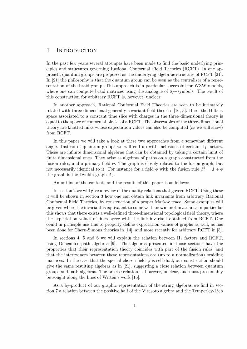
The physical correlation functions in such a theory can be expressed in terms of finitesums of holomorphic times antiholomorphic functions, which are called the conformalblocks. Whereas these conformal blocks are multivalued functions, the physical correlationfunctions are constructed out of the conformal blocks in a monodromy invariant way.Graphically, we can represent a n-point conformal block Fφ1,...,φn as a skeleton diagram.For example, a 4-point conformal block on a genus two surface can be represented as
@R@
@I@
φ1
φ2
φ4
φ3
The number of blocks can be easily computed from the fusion rules Nkij , which for the
above case gives
number of blocks =∑p
Tr(Nφ1 Nφ2 Np) Tr(NpNφ3 Nφ4)
where (Np)ij = Npij .
The idea here is that a punctured Riemann surface can be formed by sewing a numberof trinions (i.e. three holed spheres). This sewing procedure gives the different conformalblocks when one sums over the intermediate states in the channel that is formed by thesewn holes. Of course, the same punctured Riemann surface can be obtained by differentsewing procedures. For example, the four punctured sphere can be obtained from two dif-ferent sewing procedures, as shown in figure 1. These different sewing procedures give rise
2
to different conformal blocks. Now, the basic axiom of duality in Conformal Field Theory[1] assures that the vector space spanned by the conformal blocks is independent of thesewing procedure. This means that the conformal blocks obtained from one sewing pro-cedure are linear combinations of conformal blocks obtained from another. The matricesrepresenting these linear transformations are called ‘duality matrices’.
Moore and Seiberg [2] have shown that the duality data of a Conformal Field The-ory are contained in the braiding and fusion matrices and the modular matrix S(j) (seebelow). Furthermore, they have proven that the conditions on these duality matrices,stemming from the requirement of duality and modular covariance on arbitrary genus,can be represented by a finite number of equations, the polynomial equations. We willreview these polynomial equations below.
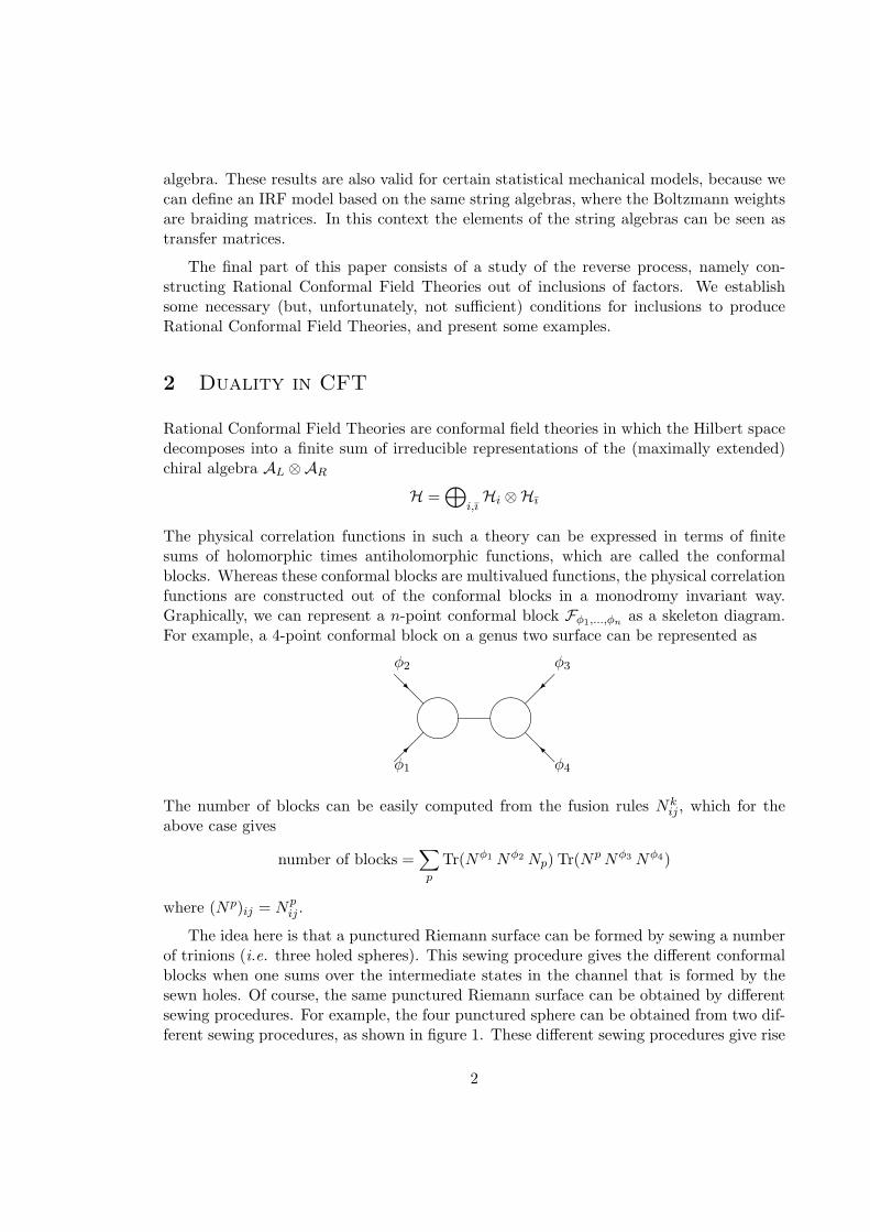
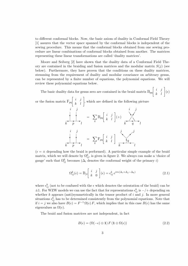
The basic duality data for genus zero are contained in the braid matrix Bpq
[i jk l
](ε)
or the fusion matrix Fpq
[i jk l
], which are defined in the following picture
? ?
k l
i j
p
=∑q
Bpq
[i jk l
](+)
JJ
JJ
k l
i j
q
? ?
k l
i j
p
=∑q
Fpq
[i jk l
]
@R@?
k l
i j
q
(ε = ± depending how the braid is performed). A particular simple example of the braidmatrix, which we will denote by Ωk
ij , is given in figure 2. We always can make a ‘choice ofgauge’ such that Ωk
ij becomes (∆i denotes the conformal weight of the primary i)
Ωkij(ε) = Bji
[i jk 0
](ε) = εkij e
iπε(∆i+∆j−∆k) (2.1)
where εkij (not to be confused with the ε which denotes the orientation of the braid) can be±1. For WZW models we can use the fact that for representations εkij is −/+ depending onwhether k appears (anti)symmetrically in the tensor product of i and j. In more generalsituations εkij has to be determined consistently from the polynomial equations. Note thatif i = j we also have B(ε) = F−1 Ω(ε)F , which implies that in this case B(ε) has the sameeigenvalues as Ω(ε).
The braid and fusion matrices are not independent, in fact
B(ε) = (Ω(−ε)⊗ 1)F (1⊗ Ω(ε)) (2.2)
3
which can be easily deduced when one applies the simple moves shown in figure 3. From(2.2) we have B(ε) B(−ε) = 1, which is obvious. Furthermore, since Ω∗(ε) = Ω(−ε) andF∗ = F∨, we have B∗(ε) = B∨(−ε) where B∨ denotes the braid matrix with the fields φireplaced by their duals φ∨i (recall that the dual φ∨ of a field φ is the unique field withwhich φ has the fusion rule φ×φ∨ = 1+ · · ·). One can easily prove that this implies thatthe braid matrix B(ε) is in fact unitary.
Applying a series of B and F moves on special conformal blocks one can easily derive
lots of identities for the Bpq
[i jk l
]and Fpq
[i jk l
]. The results of Moore and Seiberg
guarantee that all these identities are in fact equivalent to just two identities, which wewill now derive. The first is called the hexagon identity and is expressed graphically infigure 4. In terms of the fusion matrix it reads
F (Ω(ε)⊗ 1)F = (1⊗ Ω(ε))F (1⊗ Ω(ε)) (2.3)
The second fundamental identity is called the pentagon identity. Its graphic derivationis given in figure 5, which gives the following expression in terms of fusion matrices
F23 F12 F23 = P23 F13 F12 (2.4)
where P is the permutation operator. Using (2.3) and the connection between the B andF matrix as in (2.2), we can rewrite (2.4) as
B12(ε)B23(ε)B12(ε) = B23(ε)B12(ε)B23(ε) (2.5)
whose graphic interpretation is given in figure 6. Equation (2.5) is the Yang-Baxter equa-tion and is due to the fact that the B matrices form a representation of the braid group.
In addition to the genus zero equations which we have derived above, there are of courseduality constraints from higher genus. One of the surprising results of Moore and Seibergis that the only new fundamental duality equations come from genus one. We will nowderive these equations. First, the new duality data in genus one are given by the modularmatrices S(j) and T , where S(j) represents the behavior of the one point functions on thetorus under the transformation τ → −1/τ , and T equals Tij = δije
2iπ(∆i− c24
). Since themodular matrices S(j) and T should form a (projective) representation of the modulargroup, we have the following two identities
S(j)T S(j) = T−1 S(j)T−1 (2.6)S2(j) = ±e−iπ∆j C (2.7)
where C is the charge conjugation matrix Cij = N0ij , which maps the field φi to its dual
φ∨i .
4
Besides these two identities we have one more genus one relation, which can be rep-resented pictorially as in figure 7, and which gives the following constraint on the dualitymatrices
(S ⊗ 1)F (1⊗Θ(−)Θ(+))F−1 (S−1 ⊗ 1) = F P F−1(1⊗ Ω(−)) (2.8)
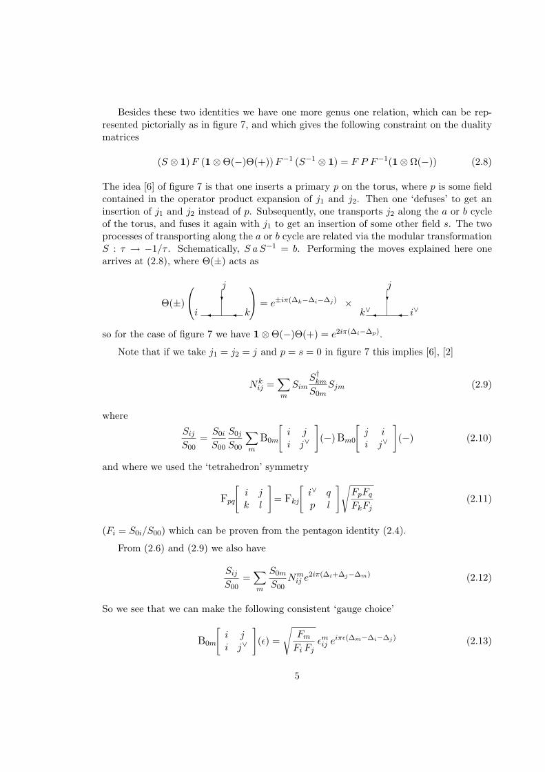
The idea [6] of figure 7 is that one inserts a primary p on the torus, where p is some fieldcontained in the operator product expansion of j1 and j2. Then one ‘defuses’ to get aninsertion of j1 and j2 instead of p. Subsequently, one transports j2 along the a or b cycleof the torus, and fuses it again with j1 to get an insertion of some other field s. The twoprocesses of transporting along the a or b cycle are related via the modular transformationS : τ → −1/τ . Schematically, S aS−1 = b. Performing the moves explained here onearrives at (2.8), where Θ(±) acts as
Θ(±)
i k
?
j = e±iπ(∆k−∆i−∆j) ×k∨ i∨
?
j
so for the case of figure 7 we have 1⊗Θ(−)Θ(+) = e2iπ(∆i−∆p).
Note that if we take j1 = j2 = j and p = s = 0 in figure 7 this implies [6], [2]
Nkij =
∑m
SimS†kmS0m
Sjm (2.9)
where
SijS00
=S0i
S00
S0j
S00
∑m
B0m
[i ji j∨
](−) Bm0
[j ii j∨
](−) (2.10)
and where we used the ‘tetrahedron’ symmetry
Fpq
[i jk l
]= Fkj
[i∨ qp l
]√FpFqFkFj
(2.11)
(Fi = S0i/S00) which can be proven from the pentagon identity (2.4).
From (2.6) and (2.9) we also have
SijS00
=∑m
S0m
S00Nmij e
2iπ(∆i+∆j−∆m) (2.12)
So we see that we can make the following consistent ‘gauge choice’
B0m
[i ji j∨
](ε) =
√FmFi Fj
εmij eiπε(∆m−∆i−∆j) (2.13)
5
Taking the tetrahedron symmetry into account this is in fact the only gauge choice con-sistent with (2.1).
The above equations (2.3–2.4) and (2.6–2.8) are the polynomial equations which encap-ture the fundamental duality relations of a Conformal Field Theory. In the next section wewill explore these polynomial equations to show that we can define for every primary fieldin a Conformal Field Theory a topological invariant of knots (or more generally links). Aswe will see, these invariants are intimately connected with so-called Markov traces, whichalready appeared in a slightly different context in [40]. In the next section we will givea proof of the existence of such traces in Conformal Field Theory using the polynomialequations of Moore and Seiberg.
3 Topological Aspects of CFT
To define a topological invariant of links for Rational Conformal Field Theories we firsthave to discuss the relation between knots or links and braids. The braid group defined onn strands will be denoted by Bn and is generated by the simple braids < σ1, . . . , σn−1 >which satisfy
σiσi+1σi = σi+1σiσi+1 (3.1)σiσj = σjσi |i− j| ≥ 2 (3.2)
The Bpq
[i jk l
]encountered in the previous section form a representation of the braid
group, and the Yang-Baxter equation (2.5) is a direct consequence of (3.1).
To discuss links in terms of braids, we will take a two dimensional point of viewtowards links. When one projects a link down to two dimensions to get a knot diagram,as in figure 8, the question which diagrams give equivalent links arises. A theorem in knottheory [4] states that knot diagrams give equivalent links when they can be transformedinto each other via so-called Reidemeister moves, shown in figure 9. A link invariant definedon the level of these diagrams should of course be invariant under these Reidemeister movesto be a true topological invariant.
It is more or less obvious that every link can be obtained by the closure of a braid.Such a closure of a braid α (see figure 10) will be denoted by α. According to a theoremof Markov, this means that an invariant L(α) defined in terms of braids α, should satisfythe following properties
L(αβ) = L(βα) α, β ∈ Bn (3.3)
L(ασ±1n ) = L(α) α ∈ Bn (3.4)
where the trace property (3.3) is clear when one closes the braid, and (3.4) is the conse-quence of the first Reidemeister move.
6
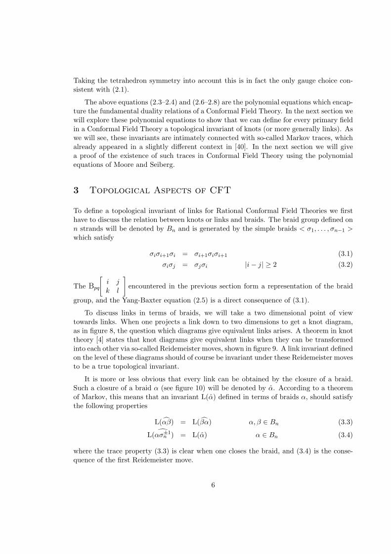
The representation π of the braid group Bn that we will study here is a representationon special conformal blocks. These are genus zero blocks with n external φ lines and one‘spectator’ field j [21]
φ- j
?
φ?
φ
. . . ?
φ?
φ
pn−2p1
Such conformal blocks will be denoted as F (n)φ,j . The dimension d
(n)φ,j of the vector space
spanned by these conformal blocks is easily computed as
d(n)φ,j =
(Nn−1φ
)φj
So for a fixed spectator field j the braid matrices π(σi) are elements of Mat(d(n)φ,j ,C),
the space of complex square matrices of dimension d(n)φ,j . We can use this to build finite
dimensional C∗-algebras C(n)φ as follows
C(n)φ =
⊕j
Mat(d(n)φ,j ,C)
This gives us a sequence of inclusions of C∗-algebras
C(2)φ ⊂ C(3)
φ ⊂ · · · ⊂ C(n)φ ⊂ · · · (3.5)
with the inclusion matrix given by Nφ.
To define a link invariant for Rational Conformal Field Theories we will first look fora so-called Markov trace Mφ, which is defined on Cφ =
⋃nC
(n)φ , and satisfies the following
properties
M(π(1)) = 1 (3.6)M(π(αβ)) = M(π(βα)) α, β ∈ Bn (3.7)
M(π(ασn)) = zM(π(α)) α ∈ Bn (3.8)M(π(ασ−1
n )) = zM(π(α)) α ∈ Bn (3.9)
where z is called the Markov parameter. Once we have such a Markov trace we can easilydefine a topological invariant out of it, as follows
L(α) = (z z)−n2
(z
z
)w(α)2
M(π(α)) α ∈ Bn (3.10)
7
where w(α) is the wraith of the braid α, i.e. the number of overcrossings minus the numberof undercrossings in a knot diagram (with the choice that the σi generate overcrossingsand the σ−1
i undercrossings). Note that we have the following normalization
L
(6)
=1|z|
(3.11)
The idea now is, that in order to study knots or links we first write them as the closureof braids, and then assign numbers to these braids as follows. We perform the same braidson the conformal block of (3.5), which then equals
∑q1,...,qn−2
Bφ,jp1,...,pn−2;q1,...,qn−2
(α) ×φ- j
?
φ?
φ
. . . ?
φ?
φ
qn−2q1
where Bφ,jp1,...,pn−2;q1,...,qn−2
(α) is a product of the braiding matrices Bpq
[φ φi j
], so it is a
map from the braid group Bn to Cφ. Taking the trace inside each C(n)φ we get another
map tφj from Cφ to C
tφj : Cφ → C
tφj (π(α)) =∑
p1,...,pn−2
Bφ,jp1,...,pn−2;p1,...,pn−2
(α)
and tφj (π(α)) is the number we want to associate with the braid α.
The reason we restricted ourselves to the conformal blocks of (3.5), is that since wewant to study links in terms of braids all the external lines have to be the same, otherwisethe braid cannot always be closed.
The final step is to construct out of the numbers tφj (π(α)) a Markov trace Mφ(π(α)).A proposal for such a Markov trace is given in [21] (and implicitly in [16]). We will notrepeat the arguments leading to this proposal here, but simply state the result
Mφ(π(α)) =
(S00
S0φ
)n∑j
S0j
S00tφj (π(α)) (3.12)
Note that due to (2.9) Mφ(π(1)) = 1. We will now prove that this proposal for the Markovtrace indeed satisfies the Markov properties (3.7) and (3.8). As one can easily verify thetrace property (3.7) is fulfilled due to the fact that we taken the trace inside each C
(n)φ .
To prove the second Markov property (3.8) we first have to determine what it meansin terms of the braid matrices. Setting α = 1 in (3.8) and evaluating it on F (2)
φ,j gives for
8
the Markov parameter z
z =
(S00
S0φ
)2∑j
S0j
S00N jφφ ε
jφφ e
iπ(2∆φ−∆j) (3.13)
which we will show to be equal to
z =e−2iπ∆φ
S0φ/S00(3.14)
The implication of (3.8) for general conformal blocks and general braids α is workedout in figure 11. From (3.12) and figure 11 we deduce that (3.8) becomes
∑j
S0j
S00Bpp
[φ φk j
](+) = z
S0φ
S00
S0p
S00Nφpk (3.15)
Note that for k = 0 this equation reduces to (3.13), so to show that (3.12) defines a goodMarkov trace we only have to prove (3.15). Using (2.13) we can rewrite the l.h.s. of (3.15)as
l.h.s. =S0p
S00
S0φ
S00
∑j
B0j
[p φp φ∨
](−)Bj0
[φ pp φ∨
](−) e2iπ(∆j−∆p−∆φ) Bpp
[φ φk j
](+)
=S0p
S00
S0φ
S00e2iπ(∆p−∆φ−∆k)
∑j
B0j
[p φp φ∨
](−)Bpp
[φ φk j
](−)Bj0
[φ pp φ∨
](−)
=S0p
S00
S0φ
S00e2iπ(∆p−∆φ−∆k)Ωk
pφ(−) Ωkpφ(−) B00
[φ φφ φ∨
](−)
=S0p
S00e−2iπ∆φ Nφ
pk (3.16)
where going from the first to the second line we used (2.2) and from the second to thethird we used the Yang-Baxter equation. So we have proven that (3.12) indeed satisfiesthe Markov properties with the Markov parameter z given by (3.14).
We thus have produced for every primary field φ a link invariant given by
Lφ(α) = e2iπ∆φw(α)∑j
S0j
S00tφj (π(α)) (3.17)
with (3.11) replaced by
Lφ
(6)
= Fφ (3.18)
9
If we specialize the above invariant to the case of a SU(N)k WZW model, with φcorresponding to the fundamental representation, φ = 2, our invariant is in fact the Jonespolynomial [7]. This can be proven as follows. The fundamental representation for SU(N)has the ‘fusion’ rule
2×2 = ⊕
The weights of the fields appearing in this product are given by
∆2 =(N − 1)(N + 1)
2N(k +N); ∆ =
(N − 2)(N + 1)N(k +N)
; ∆ =(N − 1)(N + 2)N(k +N)
which implies that the eigenvalue equation for the braid matrices π(σi) becomes(q−
12N π(σi) +
√q) (q−
12N π(σi)− 1/
√q)
= 0 (3.19)
(here q = e2iπk+N ) which (after some renormalization) is the Hecke relation.
From (3.19) we can derive the following property of the link invariant (3.17)
qN2 L−2 − q−
N2 L+
2 =
(√q − 1√q
)L0
2 (3.20)
where L+2 stands for the value of a link with at some point an overcrossing, L−2 is the value
of the same link with the overcrossing replaced by an undercrossing and L02 is the value
of the link with the crossing removed.
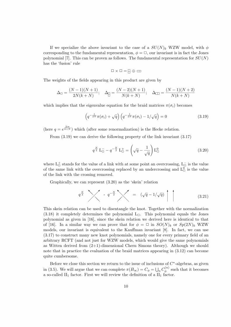
Graphically, we can represent (3.20) as the ‘skein’ relation
qN2
@@I
@@- q−
N2
@@@I = (
√q − 1/
√q) 6 6
(3.21)
This skein relation can be used to disentangle the knot. Together with the normalization(3.18) it completely determines the polynomial L2. This polynomial equals the Jonespolynomial as given in [16], since the skein relation we derived here is identical to thatof [16]. In a similar way we can prove that for φ = 2 in SO(N)k or Sp(2N)k WZWmodels, our invariant is equivalent to the Kauffman invariant [8]. In fact, we can use(3.17) to construct many new knot polynomials, namely one for every primary field of anarbitrary RCFT (and not just for WZW models, which would give the same polynomialsas Witten derived from (2+1)-dimensional Chern Simons theory). Although we shouldnote that in practice the evaluation of the braid matrices appearing in (3.12) can becomequite cumbersome.
Before we close this section we return to the issue of inclusions of C∗-algebras, as givenin (3.5). We will argue that we can complete π(B∞) = Cφ =
⋃nC
(n)φ such that it becomes
a so-called II1 factor. First we will review the definition of a II1 factor.
10
An algebra A is a factor if:
- A is a von Neumann algebra, i.e. an algebra of bounded operators on a Hilbertspace H, such that it contains the identity, it is closed under taking adjoints, and itis closed in the ultraweak topology∗.
- the center of A is trivial.
It is of type II1 if it is infinite dimensional and admits a finite normalized trace tr : A→ Csuch that
tr(1) = 1tr(ab) = tr(ba), a, b ∈ A (3.22)tr(a∗a) ≥ 0, a ∈ A
This trace is always unique.
Jones has shown [10] how to associate to a II1 factor M and a subfactor N , a number[M : N ], called the index, which measures ”how many times N fits into M”, similar tothe index [G : H] for finite groups. The index need not be an integer however.
There is one more property we will need: a factor is hyperfinite if it contains a denseincreasing sequence of finite dimensional sub *-algebras A1 ⊂ A2 ⊂ · · · ⊂ A. Up toisomorphism there is only one hyperfinite II1 factor [11] usually denoted by R. In a senseR is the smallest possible II1 factor [12]: Any II1 subfactor of R is again isomorphic toR, and any II1 factor contains R. Another property of R is that the range of the index[R : R′], where R′ runs over all possible subfactors of R, equals [10]
[R : R′] ∈ 4 cos2 π
nn≥3 ∪ [4,+∞] (3.23)
Using the Markov trace Mφ we can define an inner product on π(B∞) = Cφ
〈x|y〉 = Mφ(x∗y) (3.24)
Using this inner product we can take the weak closure of π(B∞). It can be proven thatthis closure π(B∞) satisfies all the requirements in the definition of a hyperfinite II1 factor,so we see that it is in fact isomorphic to the hyperfinite II1 factor R.
With this factor, naturally comes a subfactor as follows. Take for B′∞ the braid groupgenerated by the elements < σ2, σ3, . . . > then π(B′∞) is a subfactor of π(B∞). The indexof this subfactor can be calculated as
[π(B∞) : π(B′∞)
]= lim
n→∞
∑j
(Nn+1φ
)2
φj∑j
(Nnφ
)2
φj
=(S0φ
S00
)2
(3.25)
∗this means if ψ1, ψ2 ∈ H, an ∈ A, a ∈ B(H) and 〈ψ1|anψ2〉 → 〈ψ1|aψ2〉 then a ∈ A as well.
11
since S0φ/S00 is the largest eigenvalue of Nφ.
For the special value 3 of the index, Jones [34] noted that (for φ = 2 in SU(2)4)π(B′∞) ⊂ π(B∞), is equivalent to the pair RD3 ⊂ RZ2 , where RG denotes the set of fixedpoints of R under an outer action (i.e. not of the form g x g−1) of the finite group G.Furthermore, at this value of the index the link invariant (3.17), in this case the Jonespolynomial, is equal to ±i times a power of
√3, for any link L. A similar situation occurs
for index equal to 5. Here, (φ = 2 in Sp(4)2) π(B′∞) ⊂ π(B∞) can be described asRD5 ⊂ RZ2 , and the link invariant (3.17), now called the Kauffman invariant, is equal to±i times a power of
√5.
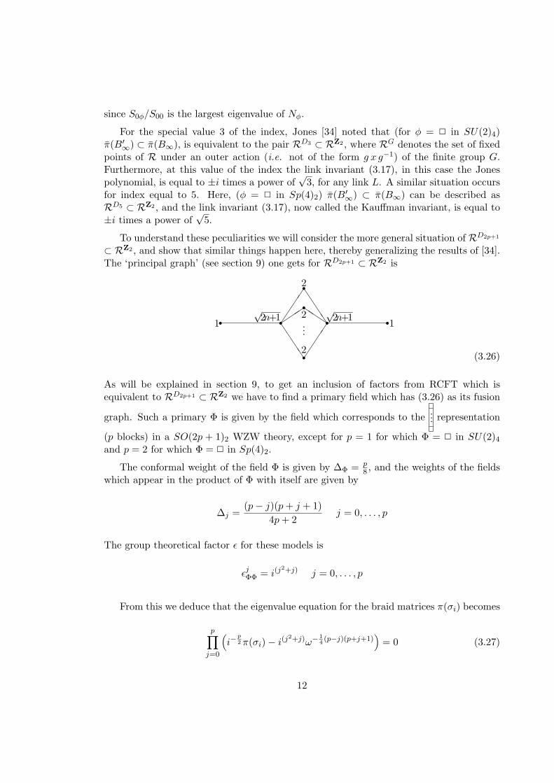
To understand these peculiarities we will consider the more general situation of RD2p+1
⊂ RZ2 , and show that similar things happen here, thereby generalizing the results of [34].The ‘principal graph’ (see section 9) one gets for RD2p+1 ⊂ RZ2 is
r r r rr
rr
J
JJJ
JJJJ
Q
2
2
2
1 1√
2n+1√
2n+1...
(3.26)
As will be explained in section 9, to get an inclusion of factors from RCFT which isequivalent to RD2p+1 ⊂ RZ2 we have to find a primary field which has (3.26) as its fusion
graph. Such a primary Φ is given by the field which corresponds to the ... representation
(p blocks) in a SO(2p + 1)2 WZW theory, except for p = 1 for which Φ = 2 in SU(2)4
and p = 2 for which Φ = 2 in Sp(4)2.
The conformal weight of the field Φ is given by ∆Φ = p8 , and the weights of the fields
which appear in the product of Φ with itself are given by
∆j =(p− j)(p+ j + 1)
4p+ 2j = 0, . . . , p
The group theoretical factor ε for these models is
εjΦΦ = i(j2+j) j = 0, . . . , p
From this we deduce that the eigenvalue equation for the braid matrices π(σi) becomes
p∏j=0
(i−
p2π(σi)− i(j
2+j)ω−14
(p−j)(p+j+1))
= 0 (3.27)
12
where ω = e2iπ
2p+1 . We can rewrite this product such that it becomes
p∏j=0
(ip2π(σi) + i−p
2ωj
2)
= 0 (3.28)
This allows us to take for the σi the so-called ‘Gaussian’ representation [34]
π(σi) =i−
p2
√2p+ 1
2p∑j=0
ω−j2uji
where the ui satisfy
u2p+1i = 1
ui ui+1 = ω2 ui+1 ui
ui uj = uj ui |i− j| ≥ 2
since the eigenvalue equation for π(σi) with σi defined in this way is equivalent to (3.28).
Now it is shown in [34] that the Markov trace evaluated on a braid in the Gaussianrepresentation gives (up to some constant C which is a power of 2p+ 1)∑
v∈H1(S;Z2p+1)
ω<v,v> (3.29)
where S is a Seifert surface for the closed braid, and 〈 , 〉 is the Seifert pairing (for anexplanation of these terms, see for example [4]). For the link invariant LΦ given by (3.17)this implies that, whenever 2p + 1 is prime, |LΦ(α)| equals C (2p + 1)ν+µ
2 , where (µ)ν isthe number of (non)zero eigenvalues of the Seifert pairing.
With the Gaussian representation at our disposal, we can now easily show why π(B′∞) ⊂π(B∞) is equivalent to RD2p+1 ⊂ RZ2 . Following [34] we deduce that the completion ofthe algebra generated by ui, denoted by A = Alg(u1, u2, . . .), is isomorphic to R. On A wehave the following Z2-action: ui → u−1
i , whose fixed points are the π(σi), so π(B∞) ∼= RZ2 .Furthermore, we have an Z2p+1-action on A given by: u1 → ω u1 and ui → ui for i ≥ 2,whose fixed point algebra is generated by the < u2, u3, . . . >. Since D2p+1 = Z2#c Z2p+1,this implies that the II1 factor generated by the < σ2, σ3, . . . >, i.e. π(B′∞), is isomorphictoRD2p+1 . So we can finally conclude that π(B′∞) ⊂ π(B∞) is equivalent toRD2p+1 ⊂ RZ2 .
4 II1 Factors Coming from RCFT
In this section we will define what a coupling system is and how they can be obtainedfrom Rational Conformal Field Theories. Some background material on coupling systemsand their relation with inclusions of factors is gathered in Appendix A.
13
Let G be an unoriented graph. A path of length n on G has the obvious meaning.The vertex where a path ξ starts will be denoted by s(ξ) (source), the endpoint by r(ξ)(range). In particular a path of length one is just an edge with an orientation. The reverseξ∼ of a path ξ is the same path walked along in the opposite direction. If we have twopaths ξ1 and ξ2, and ξ2 starts where ξ1 ends, ξ1 ξ2 will stand for the path ”first ξ1 andthen ξ2”. The set of all paths of length n starting at x and ending at a vertex y will bedenoted by Pathnx,y, the length of a path by |ξ|.
A standard finite measure graph is a finite connected graph G with a distinguishedvertex ∗ = ∗G adjacent to only one other vertex ∗∗G via one edge, and with a natural Z2
grading given by the distance of a vertex to ∗. The even vertices will be denoted by Geven,so ∗ ∈ Geven, and the odd vertices by Godd. Let Λ be the incidence matrix of G , then byPerron-Frobenius theory Λ has a unique eigenvector with only positive entries and suchthat its entry at ∗ is 1. The eigenvalue will be denoted by ‖Λ‖, and the components willbe labeled by Fx where x is a vertex of G.
We have the following definition: a local coupling system is a quadruple (G,H, τ,W ),where G and H are finite standard measure graphs with ‖ΛG‖ = ‖ΛH‖. Furthermore τ isan involution on the set of vertices of G ∪ H, satisfying
τ(∗G) = ∗G τ(∗H) = ∗H τ(∗∗G) = ∗ ∗Hτ(Geven) = Geven τ(Godd) = Hodd τ(Heven) = Heven (4.1)
Fτ(x) = Fx
W is map which associates to any cell (a1, a2, a3, a4) consisting of four oriented edgeswith τ(r(ai)) = s(ai+1), a number W (a1, a2, a3, a4) ∈ C satisfying five axioms which wewill give below.
Consider a RCFT and pick a field Φ. We make a graph by taking 2N vertices if N isthe number of primary fields in the theory, and label them by φi and φ′j , where i runs from1 to N . Next we draw N j
Φi edges from φi to φ′j . Let G be the connected component ofthe resulting graph containing the identity operator 1, and let ∗G = 1. Also let H be theconnected component containing 1′ and let ∗H = 1′. From now on we will usually identifyφi and φ′i. We see that G is the graph obtained by alternatingly fusing with Φ and its dualfield Φ∨, and H is obtained by the same process, starting however with Φ∨. Therefore,as graphs G and H are identical. Note that not all fields need occur in G and H. Theeigenvalues for the Perron-Frobenius eigenvector are given by ‖ΛG‖ = ‖ΛH‖ = S0Φ/S00.The contragradient map is defined by τ(φi) = φ∨i or τ(φi) = φ′∨i (compare with thecharge conjugation matrix C of section 2). This can be done in such a way that it iscompatible with the demands stated above in the definition of a coupling system. ThePerron-Frobenius eigenvector has components Fi=S0φi/S00.
The definition of W for RCFT’s is a bit more involved. Fix once and for all anε, which may be either + or –. Consider a cell (a1, a2, a3, a4) consisting of four edges
14
((φ1, φ∨2 ), (φ2, φ
∨3 ), (φ3, φ
∨4 ), (φ4, φ
∨1 )). We have to consider four different cases
φ1 ∈ Godd →W (1)(a1, a2, a3, a4) = Bφ∨2 φ∨4
[Φ Φφ1 φ3
](ε) 4
√F1F3
F2F4(4.2)
φ1 ∈ Geven →W (2)(a1, a2, a3, a4) = Bφ∨4 φ∨2
[Φ Φ∨
φ1 φ3
](ε) 4
√F1F3
F2F4(4.3)
φ1 ∈ Hodd →W (3)(a1, a2, a3, a4) = Bφ∨2 φ∨4
[Φ∨ Φ∨
φ1 φ3
](ε) 4
√F1F3
F2F4(4.4)
φ1 ∈ Heven →W (4)(a1, a2, a3, a4) = Bφ∨4 φ∨2
[Φ∨ Φφ1 φ3
](ε) 4
√F1F3
F2F4(4.5)
For NkΦi > 1 a pair of vertices does not specify an edge and we would have to include
into the definition of W also a dependence on couplings ε, which are elements of a NkΦi
dimensional vector space. We have suppressed these as they would just complicate theexpressions. Furthermore, Ocneanu has defined a notion of equivalence of two couplingsystems, stating that two coupling systems are equivalent precisely when they differ by aunitary transformation in the space of couplings, and therefore everything is independentof a choice of basis in the space of couplings.
In order to check the axioms that W has to satisfy, let us recall some of the symmetriesof the braid matrices
Bpq
[j1 j2i k
](ε) = Bik
[j∨1 j2p q
](−ε)
√FpFqFiFk
(4.6)
Bpq
[j1 j2i k
](ε) = Bp∨q∨
[j2 j1k∨ i∨
](ε) (4.7)
Bpq
[j1 j2i k
](ε) = Bqp
[j∨1 j∨2k i
](ε) (4.8)
where (4.6) is a consequence of (2.2) and (2.11), (4.7) is due to our convention for theconformal blocks and (4.8) is a direct consequence of (4.6) and (4.7).
First we will check the three axioms that Ocneanu calls local [9].
- The first axiom is that of inversion symmetry: for any cell (a1, a2, a3, a4) we musthave
W (a∼4 , a∼3 , a
∼2 , a
∼1 ) = W (a1, a2, a3, a4) (4.9)
From now on we will assume that
(a1, a2, a3, a4) = ((φ1, φ∨2 ), (φ2, φ
∨3 ), (φ3, φ
∨4 ), (φ4, φ
∨1 )) (4.10)
15
In order to check the inversion symmetry we would in principle have to distinguishbetween four cases, depending on whether φ1 is in G or in H, and whether it isan even or odd vertex. We will just prove it for one case, the other three beingcompletely similar. So assuming φ1 ∈ Godd, we have
W (a∼4 , a∼3 , a
∼2 , a
∼1 ) = W (3)((φ∨1 , φ4), (φ∨4 , φ3), (φ∨3 , φ2), (φ∨2 , φ1))
= Bφ4φ2
[Φ∨ Φ∨
φ∨1 φ∨3
](ε) 4
√F1F3
F2F4
= Bφ2φ4
[Φ Φφ∨3 φ∨1
](ε) 4
√F1F3
F2F4
= Bφ∨2 φ∨4
[Φ Φφ1 φ3
](ε) 4
√F1F3
F2F4
= W (1)(a1, a2, a3, a4)
- The next axiom is the axiom of rotation symmetry
W (a2, a3, a4, a1) = W (a1, a2, a3, a4)∗ (4.11)
To check this, take for example φ1 ∈ Geven. We have
W (3)(a2, a3, a4, a1) = Bφ∨3 φ∨1
[Φ∨ Φ∨
φ2 φ4
](ε) 4
√F2F4
F1F3
= Bφ2φ4
[Φ Φ∨
φ∨3 φ∨1
](−ε)
√F1F3
F2F4
4
√F2F4
F1F3
=
(Bφ∨2 φ
∨4
[Φ∨ Φφ3 φ1
](ε)
)∗4
√F1F3
F2F4
=
(Bφ∨4 φ
∨2
[Φ Φ∨
φ1 φ3
](ε) 4
√F1F3
F2F4
)∗= W (2)(a1, a2, a3, a4)∗
where in the second line we used B∗(ε) = B∨(−ε), see section 2.
- The third and last local axiom is the axiom of bi-unitarity. This axiom states thatthe connection is a unitary matrix, after a certain renormalization. In our case thatmeans that we have to check whether the braid matrices in (4.2–4.5), without thenormalization factors, are unitary. This fact was already noted in section 2 belowequation (2.2), and therefore the third axiom is also satisfied.
This completes the proof that the connections obtained from Rational ConformalField Theories satisfy all the local axioms.
16
Next we want to prove the two remaining axioms, which are called the global axioms, tomake the coupling system a global one. To state these, one needs to extend the definitionof W from cells to more general surfaces, using Ocneanu’s cell calculus, where the map Wis extended to a map defined on contours. A contour consists of four paths (ξ1, ξ2, ξ3, ξ4)in either G or H, with |ξ1| = |ξ3|, |ξ2| = |ξ4| and s(ξi+1) = τ(r(ξi)). A surface s is a familyof cells c(i, j) = (c(i, j)1, c(i, j)2, c(i, j)3, c(i, j)4) (i = 1 . . .m, j = 1 . . . n) having matchingwalls: c(i + 1, j)4 = c(i, j)∼2 and c(i, j + 1)1 = c(i, j)∼3 . The boundary of s is a contour(ξ1, ξ2, ξ3, ξ4) with ξ1 = c(n, 1) · · · c(1, 1) etc. For a surface s, one defines
W (s) =∏i,j
W (c(i, j)) (4.12)
and for a contour c,
W (c) =∑s
W (s) (4.13)
where the sum is taken over all surfaces having boundary c.
To see what these expressions mean in RCFT, observe that W (c) consists of a sumof products of braid matrices. As we have seen, similar expressions are encountered inthe computation of knot invariants for RCFT’s. So it is tempting to find a knot whoseexpectation value in 3-d topological field theory equals W (c). However, as it turns out, weneed a graph instead of a knot. This is because braid matrices are related to expectationvalues of graphs rather than knots. The precise relation [14] is given in figure 12. Fromnow on we will take ε = +; if one takes ε = − instead one just has to replace overcrossingsby undercrossings and vice versa.
If we have a graph projected onto a plane and a preferred ‘time’ direction, the compu-tation of the expectation value involves a summation over all possible ways to fill in thegraph, as explained in [14]. This corresponds precisely to a sum over all surfaces with afixed boundary as in equation (4.13).
Consider now an arbitrary contour c = (ξ1, ξ2, ξ3, ξ4), and suppose that
ξ1 = (ψ(1)n−1, ψ
(1)n ) (ψ(1)
n−2, ψ(1)n−1) · · · (ψ(1)
0 , ψ(1)1 ) (4.14)
with similar expressions for ξ2, ξ3 and ξ4. The boundary of our graph will consist of therectangle with the labeling of the fields as indicated in figure 13. Next we have to fill thisgraph with a set of horizontal and vertical lines in such a way that is compatible with thegrid depicted in figure 14. A typical example we might get in the case m = 4, n = 6 andψ
(1)0 ∈ Geven is shown in figure 15. The unmarked lines in the graph will always represent
our special chosen field Φ. Again we might also have to include labels, at every vertexof the graph where three lines meet, to represent the couplings. As remarked before, wewill not do this, but the reader should keep in mind that it is always possible to explicitlyinclude the couplings at any stage.
17
Denote the graph obtained in this way by Γ(c). A careful computation of 〈Γ(c)〉S3
based on the results of Witten [14], using as time direction south-east to north-west,shows that this expectation value precisely equals W (c), up to a normalization factor.This normalization factor can also be computed, where one has to pay special attentionto the boundary of the graph (see also [15]). The result is
W (c) = F−(|ξ1|+|ξ2|+|ξ3|+|ξ4|)/4Φ (Fs(ξ1)Fs(ξ2)Fs(ξ3)Fs(ξ4))
−1/4 〈Γ(c)〉S3 (4.15)
Using this formula we can now prove that the two global axioms a global coupling systemhas to fulfill are also valid.
The first one, the parallel transport axiom, states that for any contour c with r(ξi) =s(ξi) = ∗G or ∗H
W (c) = δ(ξ1, ξ∼3 )δ(ξ2, ξ
∼4 ) (4.16)
In this case, let us take for example r(ξi) = s(ξi) = ∗G , the graph Γ(c) consists of twodisconnected components, as shown sketchy in figure 16. Due to the topological invariancein this theory we can move the two pieces apart and using equation (4.15) we find
W (c)F (|ξ1|+|ξ2|+|ξ3|+|ξ4|)/4Φ = 〈Γ1#Γ2〉S3 = 〈Γ1〉S3 〈Γ2〉S3 (4.17)
Expectation values of graphs are topological invariant. One can also prove this directlywhere invariance under the Reidemeister moves (figure 9) is due to the Yang-Baxter equa-tion (2.5), and invariance under moving a line over a vertex where three lines meet is dueto the pentagon identity (2.4).
Now it remains to compute 〈Γ1〉S3 . Using Witten’s cutting prescriptions [14, 16]based on the fact that for one-dimensional Hilbert spaces we have 〈a|b〉〈c|d〉 = 〈a|d〉〈c|b〉,it follows that
〈Γ1〉S3 = δ(ξ1, ξ∼3 )
⟨Φ
??6 ψ
(1)2
⟩S3
⟨ψ
(1)3
??6 ψ
(1)2
⟩S3· · ·⟨
Φ
??6 ψ
(1)n−2
⟩S3⟨
6ψ(1)
2
⟩S3
⟨6ψ(1)
3
⟩S3· · ·⟨6ψ(1)n−2
⟩S3
(4.18)From section 3 we have (cf. equation (3.18))⟨
6ψ⟩S3
= Fψ (4.19)
which implies ⟨ψ1
??6 ψ2
⟩S3
= FΦ0
[ψ∨1 ψ1
ψ∨2 ψ∨2
]Fψ1 Fψ2 =
√Fψ1Fψ2FΦ (4.20)
18
Using this result we find
〈Γ1〉S3 = Fn/2Φ δ(ξ1, ξ
∼3 ) = F
(|ξ1|+|ξ3|)/4Φ δ(ξ1, ξ
∼3 ) (4.21)
Putting everything together the final result is
W (c) = δ(ξ1, ξ∼3 )δ(ξ2, ξ
∼4 ) (4.22)
as requested.
Finally, the global contragradient axiom states that for any vertex x ∈ G ∪H, there isa contour (ξ1, ξ2, ξ3, ξ4) with s(ξ1) = s(ξ3) = ∗G or ∗H, s(ξ2) = x and s(ξ4) = τ(x), andsuch that W (c) 6= 0. For such a contour we find
〈Γ(c)〉S3 =
1Fx〈Γ1〉S3 〈Γ2〉S3 (4.23)
where Γ1 is given in figure 17, for the case s(ξ1) = s(ξ3) = ∗G . Cutting along the dashedline in figure 17 shows that
〈Γ1〉S3 = 〈ψ(1)2 . . . ψ
(1)n−1|ψ
(3)n−1 . . . ψ
(3)1 〉, (4.24)
i.e. the inner product of two states in the Hilbert space of the punctured two-sphere withcharges as those occurring along the dashed line. Now if we let the ψ’s vary, both statesin this inner product run through a basis of this Hilbert space, so it is certainly possibleto choose them such that this inner product is nonzero. Therefore, the connection alsosatisfies the global contragradient axiom, and this completes the proof that the connectionobtained from RCFT gives rise to a coupling system.
Due to the one-one relation between coupling systems and irreducible finite index finitedepth inclusions of II1 factors [9], this proves that for every RCFT together with a field Φthere is a corresponding inclusion of such II1 factors (in fact there are two, as we can takeboth ε = + and ε = −, but these two choices need not be inequivalent). An immediateconsequence is that we always have
S0Φ
S00∈
cosn
π
n≥3∪ [2,∞] (4.25)
Although this method would enable one to construct many examples of irreducibleinclusions of II1 factors, and maybe even new ones, we will be mainly interested in thereverse process: given an inclusion, when does this correspond to a RCFT? To answer thisquestion we will first take a closer look at the II1 factors coming from RCFT.
19
5 The String Algebras
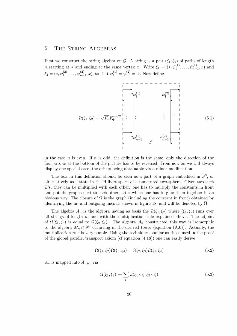
First we construct the string algebra on G. A string is a pair (ξ1, ξ2) of paths of lengthn starting at ∗ and ending at the same vertex x. Write ξ1 = (∗, ψ(1)
1 , . . . , ψ(1)n−1, x) and
ξ2 = (∗, ψ(2)1 , . . . , ψ
(2)n−1, x), so that ψ(1)
1 = ψ(2)1 = Φ. Now define
Ω(ξ1, ξ2) =√FxF
−n/2Φ
-
-
-
-
?
?
- 6
6ψ
(1)1
ψ(1)n−1 x
ψ(2)n−1
ψ(2)1
......
...... (5.1)
in the case n is even. If n is odd, the definition is the same, only the direction of thefour arrows at the bottom of the picture has to be reversed. From now on we will alwaysdisplay one special case, the others being obtainable via a minor modification.
The box in this definition should be seen as a part of a graph embedded in S3, oralternatively as a state in the Hilbert space of a punctured two-sphere. Given two suchΩ’s, they can be multiplied with each other: one has to multiply the constants in frontand put the graphs next to each other, after which one has to glue them together in anobvious way. The closure of Ω is the graph (including the constant in front) obtained byidentifying the in- and outgoing lines as shown in figure 18, and will be denoted by Ω.
The algebra An is the algebra having as basis the Ω(ξ1, ξ2) where (ξ1, ξ2) runs overall strings of length n, and with the multiplication rule explained above. The adjointof Ω(ξ1, ξ2) is equal to Ω(ξ2, ξ1). The algebra An constructed this way is isomorphicto the algebra Mn ∩ N ′ occurring in the derived tower (equation (A.6)). Actually, themultiplication rule is very simple. Using the techniques similar as those used in the proofof the global parallel transport axiom (cf equation (4.18)) one can easily derive
Ω(ξ1, ξ2)Ω(ξ3, ξ4) = δ(ξ2, ξ3)Ω(ξ1, ξ4) (5.2)
An is mapped into An+1 via
Ω(ξ1, ξ2)→∑ζ
Ω(ξ1 ζ, ξ2 ζ) (5.3)
20
where the sum is over all edges starting at x. A trace on An compatible with this mapAn → An+1 is given by
tr(Ω(ξ1, ξ2)) = F−nΦ
⟨Ω(ξ1, ξ2)
⟩S3 (5.4)
= FxF−nΦ δ(ξ1, ξ2)
This trace can be used to complete ∪An into a von Neumann algebra A. This algebraA is in fact a subspace of the space of all conformal blocks. A similar construction worksfor H where the paths start at ∗H. The graphs occurring in the definition of Ω have in thiscase all the arrows of the in- and outgoing lines reversed. In this way one gets algebrasBn which may be completed into a von Neumann algebra B. The notation used here forthe operators Ω(ξ1, ξ2) is more or less similar to the notation used for instance in [17, 40]to label the bases of spaces of intertwiners.
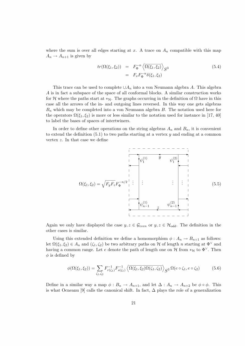
In order to define other operations on the string algebras An and Bn, it is convenientto extend the definition (5.1) to two paths starting at a vertex y and ending at a commonvertex z. In that case we define
Ω(ξ1, ξ2) =√FyFzF
−n/2Φ
-
-
-
-
?
?
- 6
6ψ
(1)1
ψ(1)n−1 z
ψ(2)n−1
ψ(2)1
......
......
y
(5.5)
Again we only have displayed the case y, z ∈ Geven or y, z ∈ Hodd. The definition in theother cases is similar.
Using this extended definition we define a homomorphism φ : An → Bn+1 as follows:let Ω(ξ1, ξ2) ∈ An and (ζ1, ζ2) be two arbitrary paths on H of length n starting at Φ∨ andhaving a common range. Let e denote the path of length one on H from ∗H to Φ∨. Thenφ is defined by
φ(Ω(ξ1, ξ2)) =∑ζ1,ζ2
F−1r(ζ1)F
−1s(ζ1)
⟨Ω(ξ1, ξ2)Ω(ζ1, ζ2)
⟩S3 Ω(e ζ1, e ζ2) (5.6)
Define in a similar way a map φ : Bn → An+1, and let ∆ : An → An+2 be φ φ. Thisis what Ocneanu [9] calls the canonical shift. In fact, ∆ plays the role of a generalization
21
of the comultiplication for these string algebras. The map φ can be used to define ahomomorphism φ : A → B, and the inclusion of II1 factors belonging to this couplingsystem is precisely the inclusion φ(A) ⊂ B.
To see how the even vertices of G correspond to A−A modules, fix a vertex x ∈ Geven,and consider a pair (α, β) of paths of length n, having common range, while α starts at∗G and β starts at x. These pairs (α, β), so-called open strings, together form the basisof a linear space An(x). Let Ω(ξ1, ξ2) ∈ An, then Ω(ξ1, ξ2) acts on (α, β) from the left asfollows:
Ω(ξ1, ξ2) · (α, β) = δ(ξ2, α)(ξ1, β) (5.7)
To define the right action we need a generalization of (5.5)†
(α, β) · Ω(ξ1, ξ2) =∑
γ∈Pathnx,r(α)
(F−1r(α)F
−1x
⟨Ω(ξ1, ξ2)Ω(γ, β)
⟩S3
)(α, γ) (5.8)
What goes into this definition is precisely Ocneanu’s notion of parallel transport. We seethat An(x) is a An − An bimodule and after taking an appropriate completion we get aA−A bimodule A(x). These are irreducible [9]. Therefore we have the interesting resultthat the irreducible modules of the string algebras correspond to certain primary fields ofthe underlying RFCT.
If we consider vertices in Godd or in H we must also consider left and right actions ofBn. Again, the expressions are the same as those occurring in (5.7) and (5.8).
6 Tensor Products and the Number of Paths
How do the fusion rules arise in this context? Take for simplicity two even vertices ofG, say (x, y), and let (α, β) be a pair of paths starting at respectively x and y havingcommon range. On the linear space An(x, y) which has as basis the pairs (α, β) one canagain define a left and a right action of An, similar as in (5.8)
Ω(ξ1, ξ2) · (α, β) =∑
γ∈Pathnx,r(α)
(F−1r(α)F
−1x
⟨Ω(ξ1, ξ2)Ω(α, γ)
⟩S3
)(γ, β) (6.1)
(α, β) · Ω(ξ1, ξ2) =∑
γ∈Pathny,r(α)
(F−1r(α)F
−1y
⟨Ω(ξ1, ξ2)Ω(γ, β)
⟩S3
)(α, γ) (6.2)
An(x, y) will decompose into irreducible An − An modules: An(x, y) = ⊕An(z). We willpresent some dimensional arguments why we expect that
An(x, y) =⊕z
Nφzφ∨xφy
An(z) (6.3)
†It is an interesting exercise to check that this right action is indeed compatible with the algebrastructure on An
22
where φx is the field corresponding to the vertex x etc. Actually, An(x, y) is preciselywhat one finds when one studies the tensor product of the representations A(x) and A(y)using the generalized comultiplication. Therefore, we see that the fusion rules are just therules for decomposing the tensor product of representations of the string algebras.
Let fij(t) be the generating function for the number of paths from i to j; that is,
fij(t) =∞∑k=0
∣∣∣Pathki,j∣∣∣ tk (6.4)
It is easy to check that fij(t) = (1 − tΛG)−1ij , where 1 represents the unit matrix. We
would like to check whether
fij(t) =∑k
Nki∨jf0k(t) (6.5)
or equivalently whether
gij(t) =∑k
Nki∨jg0k(t) (6.6)
where
gij(t) = det(1− tΛG)(1− tΛG)−1ij (6.7)
Using
Nkij =
∑α
SαiSαjS∗αk
Sα0
and (S2)ij = C = δij∨ , SS∗ = 1 one can derive the following expressions for fij(t) interms of the modular matrix S
fij(t) =∑α
S∗αi1
1− t2∣∣∣SαΦSα0
∣∣∣2Sαj , i, j ∈ Geven or Godd (6.8)
fij(t) =∑α
S∗αitS∗αΦ/Sα0
1− t2∣∣∣SαΦSα0
∣∣∣2Sαj , i ∈ Geven, j ∈ Godd (6.9)
fij(t) =∑α
S∗αitSαΦ/Sα0
1− t2∣∣∣SαΦSα0
∣∣∣2Sαj , i ∈ Godd, j ∈ Geven (6.10)
Similar expressions are valid for H, where SαΦ/Sα0 is replaced by its complex conjugate.The last relation we need in order to put everything together is
S∗αiSαj =∑k
Nki∨jSα0Sαk (6.11)
It is now obvious that relation (6.5) is fulfilled, and that we therefore have a perfectagreement with the decomposition rule (6.3), at least as far as dimensions are concerned.
23
As a side remark, observe that
limt→S00/S0Φ
f0i(t)f0j(t)
=FiFj
(6.12)
so in a sense Fi measures how many paths there are from ∗ to i. A remarkable fact is that[33]
FiFj
= limq→1
χi(q)χj(q)
(6.13)
where the character χi is the trace of q(L0−c/24) in the representation corresponding to φi.We thus see that the number of states in the ith representation grow asymptotically at thesame rate relative to each other as the number of paths.
Another way to obtain the fusion rules from path algebras has been studied in [31, 32],by techniques similar to the ones in section 9.
7 Algebras Hidden in the Path Algebras
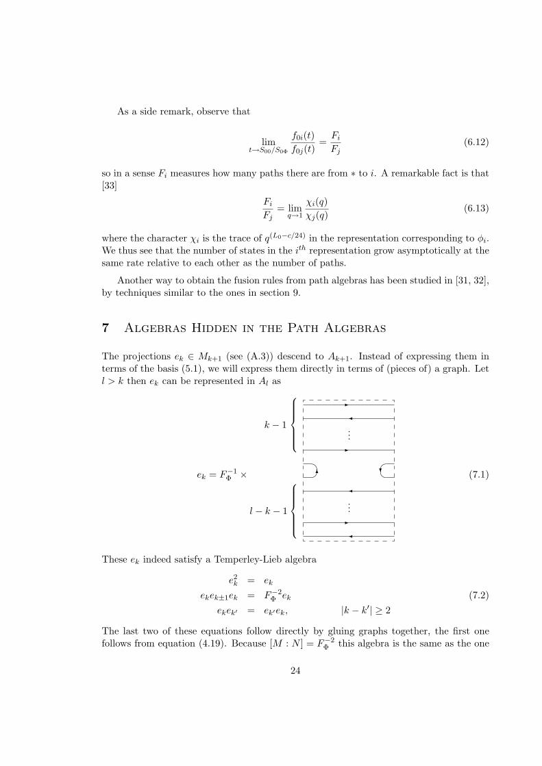
The projections ek ∈ Mk+1 (see (A.3)) descend to Ak+1. Instead of expressing them interms of the basis (5.1), we will express them directly in terms of (pieces of) a graph. Letl > k then ek can be represented in Al as
ek = F−1Φ ×
-
-
-
...
...
6 ?
l − k − 1
k − 1
(7.1)
These ek indeed satisfy a Temperley-Lieb algebra
e2k = ek
ekek±1ek = F−2Φ ek (7.2)
ekek′ = ek′ek, |k − k′| ≥ 2
The last two of these equations follow directly by gluing graphs together, the first onefollows from equation (4.19). Because [M : N ] = F−2
Φ this algebra is the same as the one
24
appearing in (A.4). Similar pictures to represent the Temperley-Lieb algebra have alreadybeen given in [18]. The generators ek can be expressed in terms of the basis (5.1) of Alvia the identity
ek =∑ξ3,ξ4
⟨ekΩ(ξ4, ξ3)
⟩S3 Ω(ξ3, ξ4) (7.3)
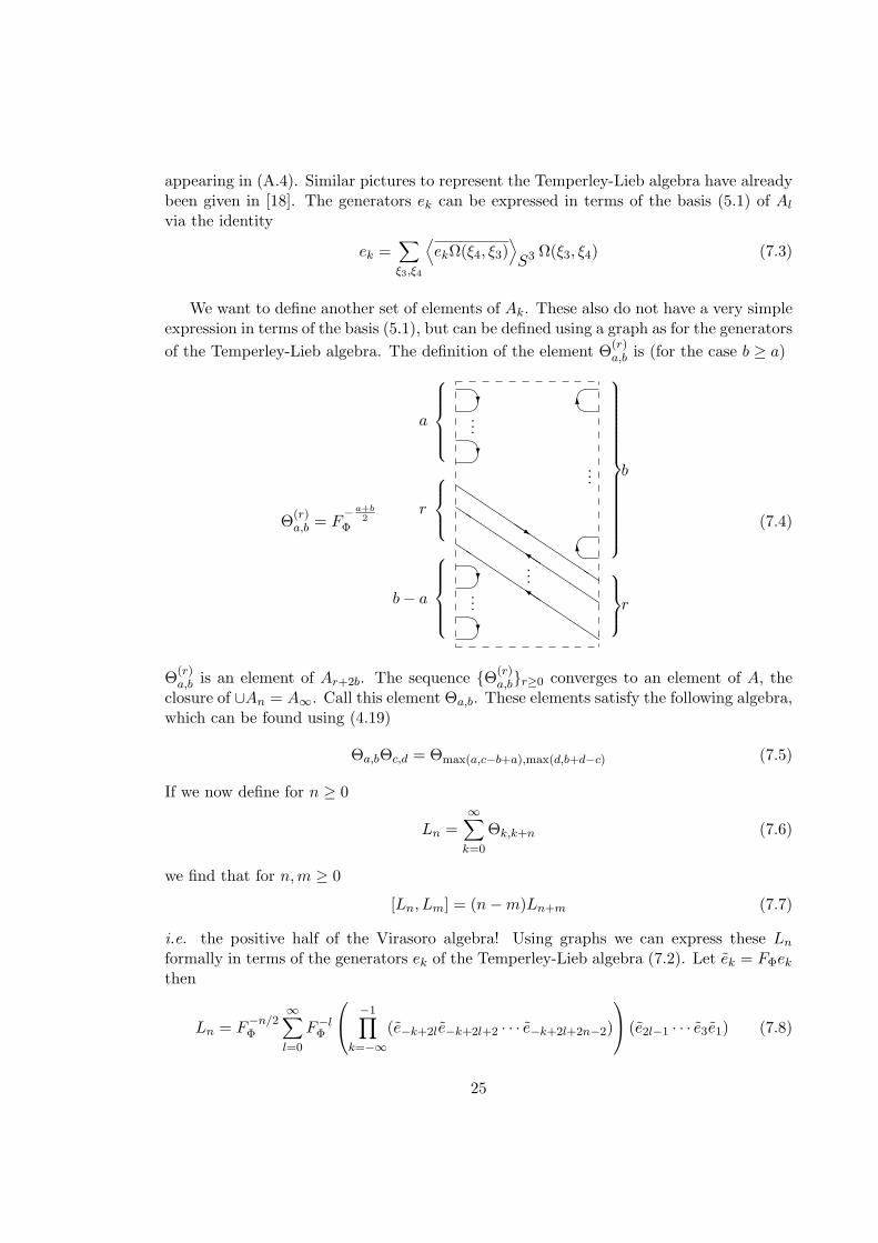
We want to define another set of elements of Ak. These also do not have a very simpleexpression in terms of the basis (5.1), but can be defined using a graph as for the generatorsof the Temperley-Lieb algebra. The definition of the element Θ(r)
a,b is (for the case b ≥ a)
Θ(r)a,b = F
−a+b2
Φ
?
?
?
?
6
6
QQQQQQsQQQQQ
QQQQk Q
QQQk
QQQ
QQQ
...
...
...
...
b− a
r
a
r
b
(7.4)
Θ(r)a,b is an element of Ar+2b. The sequence Θ(r)
a,br≥0 converges to an element of A, theclosure of ∪An = A∞. Call this element Θa,b. These elements satisfy the following algebra,which can be found using (4.19)
Θa,bΘc,d = Θmax(a,c−b+a),max(d,b+d−c) (7.5)
If we now define for n ≥ 0
Ln =∞∑k=0
Θk,k+n (7.6)
we find that for n,m ≥ 0
[Ln, Lm] = (n−m)Ln+m (7.7)
i.e. the positive half of the Virasoro algebra! Using graphs we can express these Lnformally in terms of the generators ek of the Temperley-Lieb algebra (7.2). Let ek = FΦekthen
Ln = F−n/2Φ
∞∑l=0
F−lΦ
−1∏k=−∞
(e−k+2le−k+2l+2 · · · e−k+2l+2n−2)
(e2l−1 · · · e3e1) (7.8)
25
This can be seen as an indication of the suspected relation between the Virasoro algebraand the Temperley-Lieb algebra [19, 20]. It would be interesting to have the negative halfof the Virasoro algebra as well, although it seems difficult to express them in a similarway as in (7.6).
8 Reconstruction of RCFT
We would now like to consider the the reverse problem: given an irreducible finite indexfinite depth subfactor of the hyperfinite factor R, when does this inclusion correspond toone obtained from a Rational Conformal Field Theory?
First recall how to get the graphs G and H from RCFT. We took 2N vertices labeled φiand φ′j and drew N j
Φi edges from φi to φ′j . Call the resulting graph Γ, which in general willconsist of several connected components. If 1 and 1′ are in the same connected component,G and H will be the same graph, having a Z2-automorphism with no fixed points (mappingφi to φ′i). Otherwise G andH will be different but identical graphs. Let Γ1 . . .Γr denote theother connected components of the graph, i.e. those not containing 1 or 1′. At first sightthey could be anything, but in fact the possibilities are quite restricted due to the following
TheoremThe graphs Γi have the following properties
spec(Γi) ⊂ spec(G) (8.1)‖Γi‖ = ‖G‖ (8.2)
The spectrum of a graph means here the set of eigenvalues of the incidence matrix, notcounting multiplicities. Note that the graphs Γi also have no loops of odd length, justlike G and H. These conditions on the graphs Γi do not determine them completely, butusually only a few possibilities are left. (For more on graph spectra, see e.g. [13, 22].)
To prove the theorem, define the 2N × 2N matrix Λ
Λ = ΛG(⊕ΛH)⊕ ΛΓ1 ⊕ · · · ⊕ ΛΓr (8.3)
and let‡
ωj = arg
(SΦj
S0j
)(8.4)
with the convention that arg(0) = 0. Now we define 2N eigenvectors of Λ called v(p); theyare defined by the values they take at the vertices corresponding to φj and φ′j indicated
‡arg means the argument of a complex number: arg(reiφ) = φ
26
by labels j and j′. The index p takes values in the same set. We put
v(p)j =
SjpS0p
(8.5)
v(p)j′ = eπiωj
SjpS0p
(8.6)
v(p′)j =
SjpS0p
(8.7)
v(p′)j′ = −eπiωj Sjp
S0p(8.8)
These 2N orthogonal eigenvectors all have the value 1 at the vertex ∗G corresponding tothe identity 1. Therefore, all eigenvectors v(p) correspond to an eigenvalue of Λ occurringin spec(ΛG). This shows that
spec(Λ) = spec(ΛG) (8.9)
Property (8.1) now follows from
spec(Λ) = spec(ΛG)(∪spec(ΛH)) ∪ spec(ΛΓ1) ∪ · · · ∪ spec(ΛΓr) (8.10)
and property (8.2) is a direct consequence of the fact that S0i/S00 > 0, so that v(0) is thePerron-Frobenius eigenvector of Λ.
Part of the reconstruction of a RCFT now goes as follows
- Start with an inclusion R′ ⊂ R and determine G and H; the first constraint here isthat as unlabeled graphs, G and H must be identical.
- If G and H have a Z2-automorphism with no fixed points, we may have to omit Haltogether.
- Label the vertices of G (and H) with φi and φ′i in a way consistent with how G (andH) were constructed (i.e. τ(φi) = φ∨i or φ∨i
′, 1 = ∗G (1′ = ∗H) and there are onlyedges between primed and unprimed fields).
- Try to determine the S-matrix and check whether S = St; if this is not true, try torepeat the procedure with extra graphs Γi satisfying (8.1) and (8.2).
- Try to determine T from (ST )3 = S2.
In general this procedure will grow more and more complex as we take more graphs Γiso the best thing to do is to use the smallest number of graphs possible. The reason whywe expect this to give a well-defined conformal field theory, is that in the original graphsG and H we automatically have good fusion rules and braiding matrices, and the hopeis that they can be extended to the other graphs Γi as well. The only severe restrictions
27
here are St = S and the fact that G and H must be identical as graphs. In the latter casewe will call the inclusion of factors self-dual, because as paragroups H can be consideredas the dual of G. In the case of finite groups this would restrict us to abelian groups only.Later on we will do some speculation on the meaning of St = S.
Another remark concerns the solution of (ST )3 = S2. This equation only determinesthe value of the central charge modulo 8 and of the conformal weights modulo 1, butcertainly not all possibilities are realized. The two constraints we know of, are that thefollowing two numbers must be nonnegative integers:
6
(N(N − 1)
12+N−1∑i=0
(c
24−∆i)
)(8.11)
12M(M − 1) +M(∆i + ∆j + ∆k + ∆l)−
∑s
(N sijNkls +N s
ikNjls +N silNjks)∆s (8.12)
where N is the number of primary fields, M = N sijNkls, and i, j, k, l are arbitrary. These
conditions follow from considerations of the characters of RCFT’s [23, 24].
9 Examples
We will now give several examples of inclusions of factors of type II1. We start withinclusions with index smaller than 4, so that the index equals 4 cos2(π/m) for some m ≥ 3.Then ‖G‖ = 2 cos(π/m) and the only possible graphs are the Dynkin diagrams An, Dn
and E6, E7 and E8 belonging to m = n+ 1, 2n− 2, 12, 18 and 30 respectively. Accordingto Ocneanu, G cannot be equal to E7 or Dn with n odd, but the other possibilities doindeed occur. Inclusions producing the Dynkin diagrams An can be constructed in termsof the ek occurring in (7.2).
Given an inclusion we try to find RCFT’s, which correspond to this inclusion in theway outlined in the previous sections. However, to prove this correspondence, one would ingeneral also have to compare the connection obtained from the inclusion with the braidingmatrices of the Rational Conformal Field Theories. We will not do this, but we believe thatthis will not cause any problems, for the following reason. Usually, the number of possibleconnections is very small (at most two if the index is smaller than four [9]), certainly ifone identifies the connections that are related to each other by an automorphism of thegraphs. Therefore, we think that in the examples that follow, and it is certainly true ifthe index is smaller than four, the only possible connections are equivalent to those inequations (4.2)-(4.5) with ε = + or −.
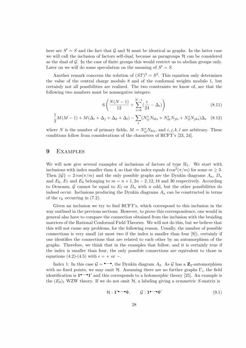
Index 1: In this case G = r r, the Dynkin diagram A2. As G has a Z2-automorphismwith no fixed points, we may omit H. Assuming there are no further graphs Γi, the fieldidentification is 1 r r1′ and this corresponds to a holomorphic theory [25]. An example isthe (E8)1 WZW theory. If we do not omit H, a labeling giving a symmetric S-matrix is
H : 1′ r rΦ, G : 1 r rΦ′ (9.1)
28
corresponding to SU(2)1. Allowing extra graphs Γi, these must all be equal to G, sincethis is the unique graph with norm one§. Examples producing an arbitrary number of Γiare rational Gaussian models, and RCFT’s having Φ as a simple current [26]. In particularthis shows directly that the condition that Φ is a simple current is equivalent to ΦΦ∨ = 1,and to S0Φ/S00 = 1 as well.
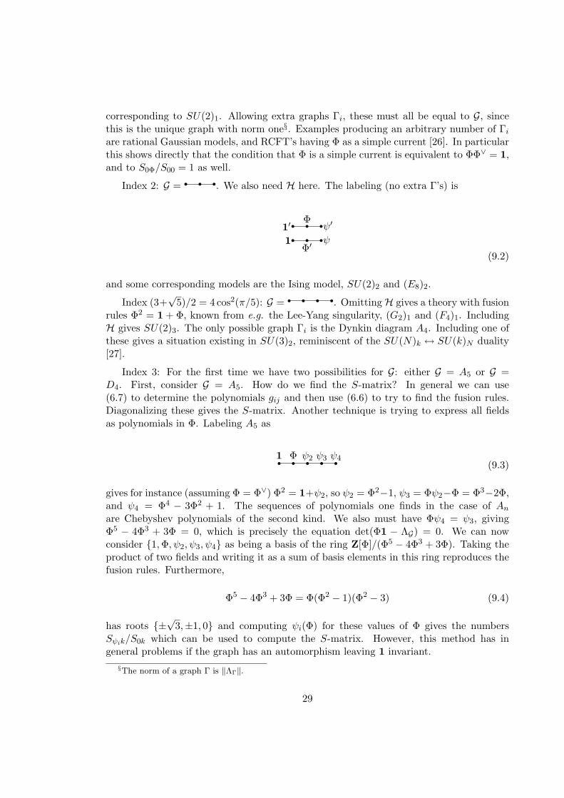
Index 2: G = r r r. We also need H here. The labeling (no extra Γ’s) is
r r rr r r11′
ψ
ψ′
Φ′
Φ
(9.2)
and some corresponding models are the Ising model, SU(2)2 and (E8)2.
Index (3+√
5)/2 = 4 cos2(π/5): G = r r r r. OmittingH gives a theory with fusionrules Φ2 = 1 + Φ, known from e.g. the Lee-Yang singularity, (G2)1 and (F4)1. IncludingH gives SU(2)3. The only possible graph Γi is the Dynkin diagram A4. Including one ofthese gives a situation existing in SU(3)2, reminiscent of the SU(N)k ↔ SU(k)N duality[27].
Index 3: For the first time we have two possibilities for G: either G = A5 or G =D4. First, consider G = A5. How do we find the S-matrix? In general we can use(6.7) to determine the polynomials gij and then use (6.6) to try to find the fusion rules.Diagonalizing these gives the S-matrix. Another technique is trying to express all fieldsas polynomials in Φ. Labeling A5 as
r r r r r1 Φ ψ2 ψ3 ψ4(9.3)
gives for instance (assuming Φ = Φ∨) Φ2 = 1+ψ2, so ψ2 = Φ2−1, ψ3 = Φψ2−Φ = Φ3−2Φ,and ψ4 = Φ4 − 3Φ2 + 1. The sequences of polynomials one finds in the case of Anare Chebyshev polynomials of the second kind. We also must have Φψ4 = ψ3, givingΦ5 − 4Φ3 + 3Φ = 0, which is precisely the equation det(Φ1 − ΛG) = 0. We can nowconsider 1,Φ, ψ2, ψ3, ψ4 as being a basis of the ring Z[Φ]/(Φ5 − 4Φ3 + 3Φ). Taking theproduct of two fields and writing it as a sum of basis elements in this ring reproduces thefusion rules. Furthermore,
Φ5 − 4Φ3 + 3Φ = Φ(Φ2 − 1)(Φ2 − 3) (9.4)
has roots ±√
3,±1, 0 and computing ψi(Φ) for these values of Φ gives the numbersSψik/S0k which can be used to compute the S-matrix. However, this method has ingeneral problems if the graph has an automorphism leaving 1 invariant.§The norm of a graph Γ is ‖ΛΓ‖.
29
G = H = A5 are graphs obtained from SU(2)4. If G = H = D4, there is a problem,because we cannot construct a symmetric S-matrix. Including extra graphs Γi which mustnecessarily also be equal to D4 according to (8.1) and (8.2) might resolve this problem,but we do not know of any example where this occurs. (This case has also been consideredin [37] where it was found to be inconsistent with the duality relations of RCFT).
Index 4 cos2(π/11): G = A10, omitting H gives (E8)3 or (F4)2, including H givesSU(2)9.
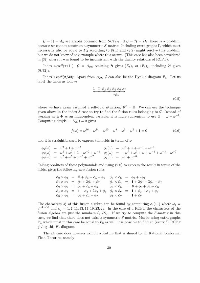
Index 4 cos2(π/30): Apart from A29, G can also be the Dynkin diagram E8. Let uslabel the fields as follows
r r r r r r r1 Φ φ2 φ3 φ4 φ6 φ7rφ5
(9.5)
where we have again assumed a self-dual situation, Φ∨ = Φ. We can use the techniquegiven above in the index 3 case to try to find the fusion rules belonging to G. Instead ofworking with Φ as an independent variable, it is more convenient to use Φ = ω + ω−1.Computing det(Φ1− ΛE8) = 0 gives
f(ω) = ω16 + ω14 − ω10 − ω8 − ω6 + ω2 + 1 = 0 (9.6)
and it is straightforward to express the fields in terms of ω
φ2(ω) = ω2 + 1 + ω−2 φ3(ω) = ω3 + ω + ω−1 + ω−3
φ4(ω) = ω4 + ω2 + 1 + ω−2 + ω−4 φ5(ω) = −ω7 + ω3 + ω + ω−1 + ω−3 − ω−7
φ6(ω) = ω7 + ω5 + ω−5 + ω−7 φ7(ω) = ω6 + ω−6
Taking products of these polynomials and using (9.6) to express the result in terms of thefields, gives the following new fusion rules
φ2 × φ3 = Φ + φ3 + φ5 + φ6 φ3 × φ6 = φ2 + 2φ4
φ2 × φ4 = φ2 + 2φ4 + φ7 φ4 × φ4 = 1 + 2φ2 + 3φ4 + φ7
φ2 × φ6 = φ3 + φ5 + φ6 φ4 × φ5 = Φ + φ3 + φ5 + φ6
φ3 × φ3 = 1 + φ2 + 2φ4 + φ7 φ6 × φ6 = 1 + φ2 + φ4 + φ7
φ3 × φ5 = φ2 + φ4 + φ7 φ7 × φ7 = 1 + φ7
The characters λji of this fusion algebra can be found by computing φi(ωj) where ωj =eiπkj/30 and kj = 1, 7, 11, 13, 17, 19, 23, 29. In the case of a RCFT the characters of thefusion algebra are just the numbers Sij/S0j . If we try to compute the S-matrix in thiscase, we find that there does not exist a symmetric S-matrix. Maybe using extra graphsΓi, which must in this case be equal to E8 as well, it is possible to find an (exotic?) RCFTgiving this E8 diagram.
The E8 case does however exhibit a feature that is shared by all Rational ConformalField Theories, namely
30
TheoremFor any RCFT, Sij/S0j is always the sum of roots of unity with integer coefficients. Theproof of this can be found in appendix B.
We proceed with the index four case: there are infinitely many graphs with norm 2,namely the A, D and E series. The A series are ruled out as candidates for G, becausethey have no distinguished vertex ∗. Subfactors of R producing graphs of type A, D andE can be constructed as follows [13]: realize the hyperfinite factor R as the completion of∞⊗ M2(C), where Mn(C) denotes the algebra of complex n × n matrices. SU(2) acts onR by conjugation on every M2(C), so in particular any finite closed subgroup G of SU(2)acts on R. In the same way we can define an action of G on R ⊗M2(C). Consider theinclusion
RG ⊂ (R⊗M2(C))G (9.7)
whereRG stands for the elements ofR left invariant by the action of G. Then the principalgraph is precisely one of the A, D or E series, giving the McKay correspondence betweenaffine Dynkin diagrams and finite subgroups of SU(2). One can obtain the graphs directlyfrom G: take as fusion rules the representation ring of G, and let Φ correspond to the2-dimensional representation of G obtained by restricting the fundamental representationof SU(2) to G. Then the construction as in section 4 yields the corresponding A, D andE graphs.
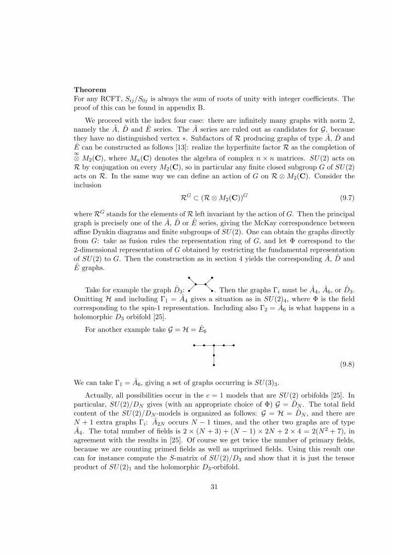
Take for example the graph D3: r rr rr r
@@ . Then the graphs Γi must be A4, A6, or D3.
Omitting H and including Γ1 = A4 gives a situation as in SU(2)4, where Φ is the fieldcorresponding to the spin-1 representation. Including also Γ2 = A6 is what happens in aholomorphic D3 orbifold [25].
For another example take G = H = E6r r r r rrr (9.8)
We can take Γ1 = A6, giving a set of graphs occurring is SU(3)3.
Actually, all possibilities occur in the c = 1 models that are SU(2) orbifolds [25]. Inparticular, SU(2)/DN gives (with an appropriate choice of Φ) G = DN . The total fieldcontent of the SU(2)/DN -models is organized as follows: G = H = DN , and there areN + 1 extra graphs Γi: A2N occurs N − 1 times, and the other two graphs are of typeA4. The total number of fields is 2 × (N + 3) + (N − 1) × 2N + 2 × 4 = 2(N2 + 7), inagreement with the results in [25]. Of course we get twice the number of primary fields,because we are counting primed fields as well as unprimed fields. Using this result onecan for instance compute the S-matrix of SU(2)/D3 and show that it is just the tensorproduct of SU(2)1 and the holomorphic D3-orbifold.
31
As a final class of examples, consider the following situation: suppose the finite groupG acts outerly on R. Suppose furthermore that G is the semidirect or crossed product oftwo subgroups H and A, G = H#c A, such that A is a normal and abelian subgroup ofG. In that case we can start with the inclusion
R#c H ⊂ R#c G (9.9)
or equivalently with RG ⊂ RH , to try to find Rational Conformal Field Theories, becausein this case the graphs G and H are equal (cf. [29] and [30, par 8.2]). The even vertices ofG correspond to the irreducible representations of G, the odd vertices correspond to theirreducible representations of H, and the number of edges between a representation π1 ofG and a representation π2 of H is given by the number of times π2 occurs in the restrictionof π1 to H. The Perron-Frobenius vector (”the S0φ/S00”) has the value dim(π1) at thevertex corresponding to π1, and the value
√[G : H] dim(π2) at π2. In particular the index
[R#c G : R#c H] = [G : H] = |A|.
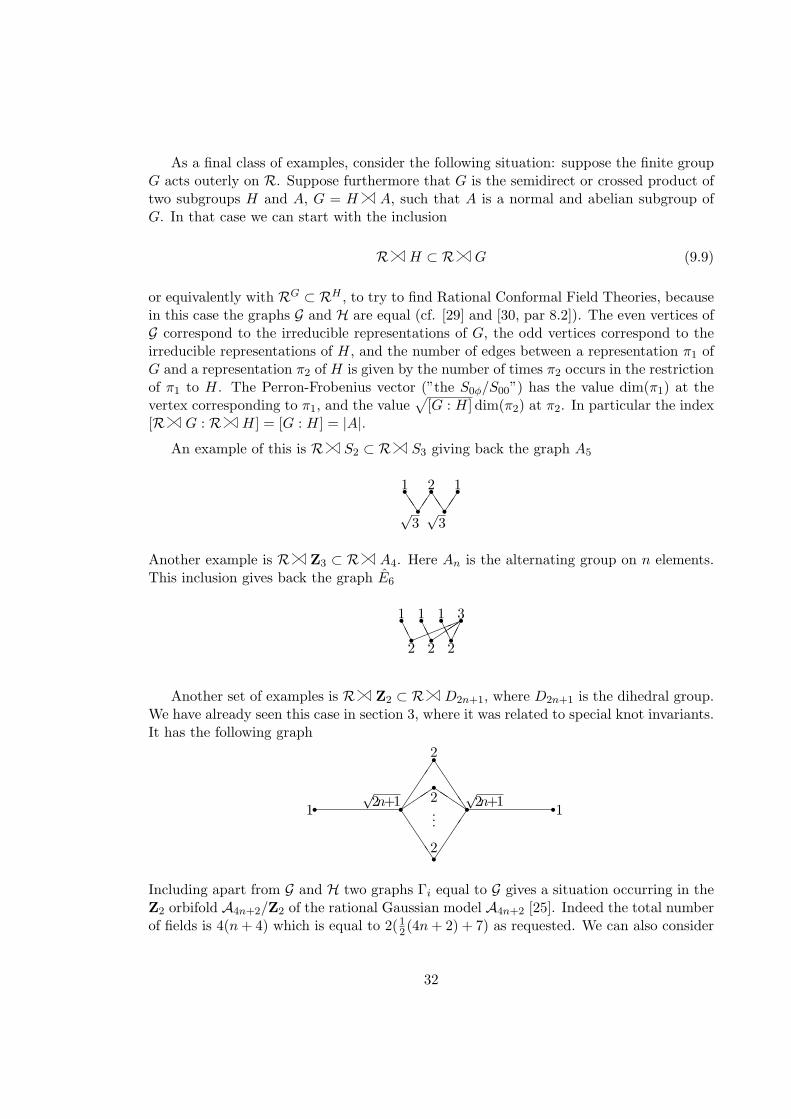
An example of this is R#c S2 ⊂ R#c S3 giving back the graph A5
r r rr r JJ JJ1 1
√3√
3
2
Another example is R#c Z3 ⊂ R#c A4. Here An is the alternating group on n elements.This inclusion gives back the graph E6
r r r rr r rAAAAAA!!!!
2 2 2
1 1 1 3
Another set of examples is R#c Z2 ⊂ R#c D2n+1, where D2n+1 is the dihedral group.We have already seen this case in section 3, where it was related to special knot invariants.It has the following graph
r r r rr
rr
J
JJJ
JJJJ
Q
2
2
2
1 1√
2n+1√
2n+1...
Including apart from G and H two graphs Γi equal to G gives a situation occurring in theZ2 orbifold A4n+2/Z2 of the rational Gaussian model A4n+2 [25]. Indeed the total numberof fields is 4(n+ 4) which is equal to 2(1
2(4n+ 2) + 7) as requested. We can also consider
32
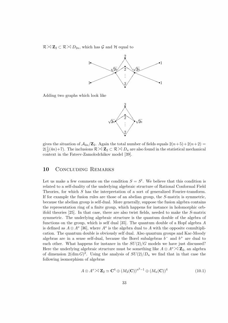
R#c Z2 ⊂ R#c D2n, which has G and H equal to
r rr r
r r
r
rr
!!!!
!!! !!
!!!!!aaaaaaa aaaaaaa
J
JJJ
JJJJ
Q
2
2
2
1
1
1
1√2n
√2n
...
Adding two graphs which look like
r rr
rr
J
JJJ
JJJJ
Q
2
2
2
√2n
√2n...
gives the situation of A4n/Z2. Again the total number of fields equals 2(n+5)+2(n+2) =2(1
2(4n)+7). The inclusionsR#c Z2 ⊂ R#c Dn are also found in the statistical mechanicalcontext in the Fateev-Zamolodchikov model [39].
10 Concluding Remarks
Let us make a few comments on the condition S = St. We believe that this condition isrelated to a self-duality of the underlying algebraic structure of Rational Conformal FieldTheories, for which S has the interpretation of a sort of generalized Fourier-transform.If for example the fusion rules are those of an abelian group, the S-matrix is symmetric,because the abelian group is self-dual. More generally, suppose the fusion algebra containsthe representation ring of a finite group, which happens for instance in holomorphic orb-ifold theories [25]. In that case, there are also twist fields, needed to make the S-matrixsymmetric. The underlying algebraic structure is the quantum double of the algebra offunctions on the group, which is self dual [35]. The quantum double of a Hopf algebra Ais defined as A⊗Ao [36], where Ao is the algebra dual to A with the opposite comultipli-cation. The quantum double is obviously self dual. Also quantum groups and Kac-Moodyalgebras are in a sense self-dual, because the Borel subalgebras b− and b+ are dual toeach other. What happens for instance in the SU(2)/G models we have just discussed?Here the underlying algebraic structure must be something like A⊗ Ao#c Z2, an algebraof dimension 2(dimG)2. Using the analysis of SU(2)/Dn we find that in that case thefollowing isomorphism of algebras
A⊗Ao#c Z2 ' C4 ⊕ (M2(C))n2−1 ⊕ (Mn(C))4 (10.1)
33
There are a lot of possible constructions which produce new inclusions from given ones.Some of these seem remarkably similar to certain constructions in Rational ConformalField Theories
M1 ⊂M2, M2 ⊂M3 ⇒ M1 ⊂M3 tensor productsM1 ⊂M2, S ⊂M1 ⇒ S′ ∩M1 ⊂ S′ ∩M2 coset constructionM1 ⊂M2 ⇒ MG
1 ⊂MG2 orbifold construction
M1 ⊂M2 ⇒ M1#c G ⊂M2#c G extended algebras
For instance, we have seen that A2n/Z2 can be realized as RDn ⊂ RZ2 , which lookslike a Z2 orbifold of RZn ⊂ R which would then correspond to A2n. However in generalthere is a problem with models like An, as they always give the trivial inclusion R ⊂ Rfor any choice of field Φ. Our construction seems to forget about any abelian structurepresent in the theory.
Another remark concerns the central charge. It would be nice to have a simple inter-pretation of the central charge in terms of subfactors. If we consider the examples of theprevious section, then we find a wide variety of central charges in the models giving thesame subfactors. The only constraint seems to be that eiπc must be in the same ring Z[ω]as Sij/S0j and in particular the index (S0Φ/S00)2 (see appendix B).
A related issue we have not touched upon is to the problem of the classification ofmodular invariants. This can in certain cases also be accomplished using techniques similarto those occurring in our string algebras [38]. However, this technique does not seem tohave a direct natural interpretation in the II1 language.
To conclude, we have established a precise connection between Rational ConformalField Theories and II1 factors. It would be very interesting to translate the remarks aboveinto precise conditions on inclusions, thus providing us with a new handle on the widevariety of solutions of the duality equations.
A Appendix : Inclusions of Factors and Coupling Sys-tems
In [9] Ocneanu has introduced a machinery to study the position of a subalgebra in alarger one. If A ⊂ B and A′ ⊂ B′ are two inclusions of algebras, A and A′ have the sameposition if there is an isomorphism f : B → B′ such that f(A) = A′. Associated to suchan inclusion is an invariant object called a paragroup. It is invariant in the sense that ifA and A′ have the same position, the paragroups will be the same as well. In paragroups,the underlying set of a group is replaced by a graph, the group elements are substitutedby strings on the graph, and a geometrical connection stands for the composition law.
Of special interest is the case where A and B are II1 factors, and in particular whenthey are both isomorphic to the hyperfinite factor R (see section 3).
34
Ocneanu [9] has given a complete classification of irreducible subfactors R0 of R offinite index and finite depth, in terms of so-called coupling systems, which are particularpresentations of paragroups. Here irreducible means that R′0 ∩ R = C, that is, the onlyelements of R that commute with all of R0 are the scalar multiples of the identity. Whatfinite depth means will be explained in a moment. In section 4 we have shown how givena RCFT and a particular primary field Φ one can define a coupling system, and hence asubfactor R0 of R, with index
[R : R0] = (S0Φ/S00)2 (A.1)
Let us first explain how to construct a coupling system from an inclusion N ⊂ M offactors. First of all, one constructs the infinite tower
M0 =N ⊂M1 =M ⊂M2 ⊂M3 ⊂ · · · (A.2)
by iterating the fundamental construction of Jones [10]. Equivalently, one can takeMk+1 = Mk ⊗Mk−1
Mk, Mk+1 = EndMk−1(Mk), the endomorphisms of Mk viewed as
a right Mk−1-module, or Mk+1 = 〈Mk, ek〉, the II1 factor generated by Mk and ek onL2(Mk, tr). This requires some explanation: let trk be the faithful normalized trace onMk, then by L2(Mk, trk) = H we mean the Hilbert space obtained by completing Mk withrespect to the inner product 〈x|y〉 = trk(x∗y). The left multiplication of Mk extends toan action of Mk on L2(Mk, trk), so that Mk is realized as a subalgebra of B(H). Now letek be the orthogonal projection¶
ek : L2(Mk, trk)→ L2(Mk−1, trk−1) (A.3)
Note that trk−1 is equal to the restriction of trk to Mk−1. These projections ek satisfy aTemperley-Lieb algebra
e2k = ek
ekek±1ek =1
[M : N ]ek (A.4)
ekek′ = ek′ek, |k − k′| ≥ 2
Furthermore the trk’s are Markov traces in the sense that
trk+1(xek) =1
[M : N ]trk(x), x ∈Mk (A.5)
A nice account of these topics can also be found in the book [13].
¶The restriction Ek of ek to Mk is what is called the conditional expectation from Mk to Mk−1; forx ∈Mk and y ∈Mk−1 we have trk(xy) = trk−1(Ek(x)y)
35
Given the tower M0 ⊂ M1 ⊂ M2 ⊂ · · · one can construct two unoriented bipartitegraphs G and H , i.e. graphs that admit a Z2-grading of the vertices, so that no twovertices with the same grade are connected via an edge. Equivalently, the graph has noloops of odd length, or it is bicolorable. The even vertices of G represent the inequivalentirreducible N−N subbimodules of M0, M1, M2, . . ., the odd vertices of G correspondto the inequivalent irreducible M−N subbimodules, and the even and odd vertices of Hcorrespond in the same way to irreducible M−M and N−M subbimodules respectively.
The number of edges between an N−N bimodule X and a M−N bimodule Y is givenby the number of times X occurs in Y if the left action of M is restricted to N . Thenumber of edges between a M−M and a N−M bimodule is determined similarly.
Furthermore there is a map τ from the set of vertices of G ∪H to itself mapping P−Qmodules to Q−P modules by interchanging the left and right actions. If P acts on theleft on X via p · x→ px then it acts on the right via x · p→ p∗x. This map τ is called thecontragradient map.
The last ingredient of a coupling system is the connection. Given a N−N bimoduleX and a M−M bimodule Y , there are two ways to induce X to Y : via M−N and viaN−M bimodules. The way in which these two results differ is expressed in terms of acomplex number W associated to each set of four bimodules, one of each type. The mapW is called the connection.
The inclusion N ⊂M is said to be of finite depth if the number of vertices of G andH isfinite. Actually G is equal to the principal graph of the derived tower of finite dimensionalalgebras
∂M/∂N = N ′∩M0 ⊂ N ′∩M1 ⊂ N ′∩M2 ⊂ · · · (A.6)
the finiteness of G means here that the Bratelli diagram for ∂M/∂N eventually becomesperiodic.
To see why a coupling system can be seen as a generalization of group theory considerthe example R ⊂ R#c G. Here R#c G means the crossed product of R by the finitegroup G: suppose G acts on R by outer automorphisms ρg and ρgρh = ρgh. Then R#c Ghas as elements
∑agug where ug is unitary, ag ∈ R, and ugau
∗g = ρg(a). In this case the
coupling system reproduces all the information contained in G. The graph G has one oddvertex and the even vertices are in one-one correspondence with the elements of G, whileH has one odd vertex and one even vertex for every irreducible representation of G. So Hcan be considered as being the dual of G.
B Appendix: A Proof
In this appendix we will supply the proof of
Theorem
36
For any RCFT, Sij/S0j is always the sum of roots of unity with integer coefficients.
The idea of the proof is to use a famous theorem in algebraic number theory byKronecker and Weber stating that a field extension of Q is contained in a cyclotomic fieldQ[ω] if the extension is normal and has an abelian Galois group [28].
Let L be the field extension of Q generated over Q by the set SijS0ji,j . The numbers
SijS0j
for fixed i are the roots of the polynomial
det(λ1−Ni) = 0 (B.1)
where Ni is the matrix (Ni)pq = N qip. Therefore this is a normal field extension of Q. Now
let g be an element of the Galois group of L, g ∈ Gal(L/Q). Because the numbers SijS0j
areprecisely the inequivalent solutions of the fusion rules,
SajS0j
SbjS0j
=∑c
N cab
ScjS0j
(B.2)
and the fusion rules are invariant under the action of the Galois group, we must have
g(SijS0j
) =SikS0k
(B.3)
with k independent of i, so we can put k = g(j). Because SS∗ = 1 we find
g
(1S0j
)2
= g
(∑i
(SijS0j
)(SijS0j
)∗)
=∑i
(Sig(j)S0g(j)
)(Sig(j)S0g(j)
)∗
=
(1
S0g(j)
)2
(B.4)
and combining equations (B.3) and (B.4) yields
g((Sij)2
)= g
(SijS0j
)2
/
(1S0j
)2
=
(Sig(j)S0g(j)
)2
/
(1
S0g(j)
)2
=(Sig(j)
)2(B.5)
37
We now use the fact that S = St so that (B.5) must be symmetric as well; this impliesthat (Sig(j))2 = (Sg(i)j)2 and taking i = 0 gives in particular
Sg(0)j
S0g(j)= ±1 (B.6)
Take now arbitrary g, h ∈ Gal(L/Q). We have
gh
(SijS0j
)= g
h
((SijSi0
)(S0i
S00
)(S00
S0j
))
= g
(Sh(i)j
Sh(i)0
Sh(0)i
Sh(0)0
Sh(0)0
Sh(0)j
)
= g
(Sh(i)j
S0j
S0j
Sh(0)j
Sh(0)i
Sh(i)0
)
=Sh(i)g(j)
Sh(0)g(j)g
(Sh(0)i
Sh(i)0
)(B.7)
On the other hand
hg
(SijS0j
)= h
(Sig(j)S0g(j)
)
= h
(Sg(j)iS0i
Si0S00
S00
S0g(j)
)
=Sg(j)h(i)
Sh(0)g(j)
Sh(0)i
Sh(i)0(B.8)
Since g(±1) = ±1 we see from (B.6) that (B.7) and (B.8) are in fact the same. Therefore,the action of gh and hg on L is the same, and we conclude that Gal(L/Q) is abelian.Applying the theorem of Kronecker and Weber now tells us that L ⊂ Q[ω] for some rootof unity ω. Since Sij/S0j is a solution of equation (B.1), which is a polynomial withinteger coefficients and leading coefficient one, these numbers are also algebraic integers.The subring of algebraic integers of Q[ω] is precisely Z[ω] [28], and this completes theproof that Sij/S0j is a sum of roots of unity with integer coefficients.
38
References
[1] A. A. Belavin, A. M. Polyakov, A. B. Zamolodchikov, Infinite Conformal Symmetryin Two Dimensional Quantum Field Theory, Nucl. Phys. B241 (1984) 333
[2] G. Moore, N. Seiberg, Classical and Quantum Conformal Field Theory, Comm. Math.Phys. 123 (1989) 177
[3] G. Moore, N. Seiberg, Taming the Conformal Zoo, Phys. Lett. B220 (1989) 422
[4] L. H. Kauffman, On Knots, Ann. of Math. Stud. 115, Princeton University Press,1987
[5] M. Li, M. Yu, Braiding Matrices, Modular Transformations and Topological FieldTheories in 2+1 Dimensions, Comm. Math. Phys. 127 (1990) 195; M. Li, Dualityand Modular Invariance Invariance in Rational Conformal Field Theories, Copen-hagen preprint NBI-HE-90-12; P. Degiovanni, Topological Field Theory and RationalConformal Field Theory, preprint LPTENS 89/25.
[6] E. Verlinde, Fusion Rules and Modular Transformations in 2D Conformal Field The-ory, Nucl. Phys. B300 (1988) 360
[7] V. F. R. Jones, A Polynomial Invariant for Knots via von Neumann Algebras, Bull.Am. Math. Soc. 12 (1985) 103
[8] L. H. Kauffman, State Models and the Jones Polynomial, Topology 26 (1987) 395
[9] A. Ocneanu, Quantized Groups, String Algebras and Galois Theory for Algebras, inOperator Algebras and Applications vol II, LMS 136, 1988
[10] V.F.R. Jones, Index for Subfactors, Invent. Math. 72 (1983) 1
[11] F. Murray, J. von Neumann, On Rings of Operators IV, Ann. Math. 44 (1943) 716
[12] A. Connes, Ann. Math. 104 (1976) 73
[13] F. M. Goodman, P. de la Harpe, V. F. R. Jones, Coxeter Graphs and Towers ofAlgebras, Springer Verlag, 1989
[14] E. Witten, Gauge Theories and Integrable Lattice Models, Nucl. Phys. B322 (1989)629
[15] E. Witten, Gauge Theories, Vertex Models and Quantum Groups, Nucl. Phys. B330(1990) 285
[16] E. Witten, Quantum Field Theory and the Jones Polynomial, Comm. Math. Phys.121 (1989) 351
[17] N. Reshetikhin, Quantized Universal Envelopping Algebras, the Yang-Baxter Equa-tion and Invariants of Links, LOMI preprints E-17-87
39
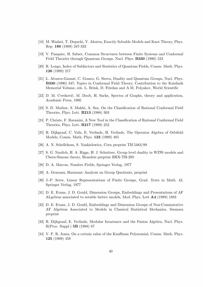
[18] M. Wadati, T. Deguchi, Y. Akutsu, Exactly Solvable Models and Knot Theory, Phys.Rep. 180 (1989) 247-332
[19] V. Pasquier, H. Saluer, Common Structures between Finite Systems and ConformalField Theories through Quantum Groups, Nucl. Phys. B330 (1990) 523
[20] R. Longo, Index of Subfactors and Statistics of Quantum Fields, Comm. Math. Phys.126 (1989) 217
[21] L. Alvarez-Gaume, C. Gomez, G. Sierra, Duality and Quantum Groups, Nucl. Phys.B330 (1990) 347; Topics in Conformal Field Theory, Contribution to the KnizhnikMemorial Volume, eds. L. Brink, D. Friedan and A.M. Polyakov, World Scientific
[22] D. M. Cvetkovic, M. Doob, H. Sachs, Spectra of Graphs, theory and application,Academic Press, 1980
[23] S. D. Mathur, S. Mukhi, A. Sen, On the Classification of Rational Conformal FieldTheories, Phys. Lett. B213 (1988) 303
[24] P. Christe, F. Ravanini, A New Tool in the Classification of Rational Conformal FieldTheories, Phys. Lett. B217 (1989) 252
[25] R. Dijkgraaf, C. Vafa, E. Verlinde, H. Verlinde, The Operator Algebra of OrbifoldModels, Comm. Math. Phys. 123 (1989) 485
[26] A. N. Schellekens, S. Yankielowicz, Cern preprint TH.5483/89
[27] S. G. Naulich, H. A. Riggs, H. J. Schnitzer, Group level duality in WZW-models andChern-Simons theory, Brandeis preprint BRX-TH-293
[28] D. A. Marcus, Number Fields, Springer Verlag, 1977
[29] A. Ocneanu, Harmonic Analysis on Group Quotients, preprint
[30] J.-P. Serre, Linear Representations of Finite Groups, Grad. Texts in Math. 42,Springer Verlag, 1977
[31] D. E. Evans, J. D. Gould, Dimension Groups, Embeddings and Presentations of AFALgebras associated to sovable lattice models, Mod. Phys. Lett A4 (1989) 1883
[32] D. E. Evans, J. D. Gould, Embeddings and Dimension Groups of Non-CommutativeAF Algebras Associated to Models in Classical Statistical Mechanics, Swanseapreprint
[33] R. Dijkgraaf, E. Verlinde, Modular Invariance and the Fusion Algebra, Nucl. Phys.B(Proc. Suppl.) 5B (1988) 87
[34] V. F. R. Jones, On a certain value of the Kauffman Polynomial, Comm. Math. Phys.125 (1989) 459
40
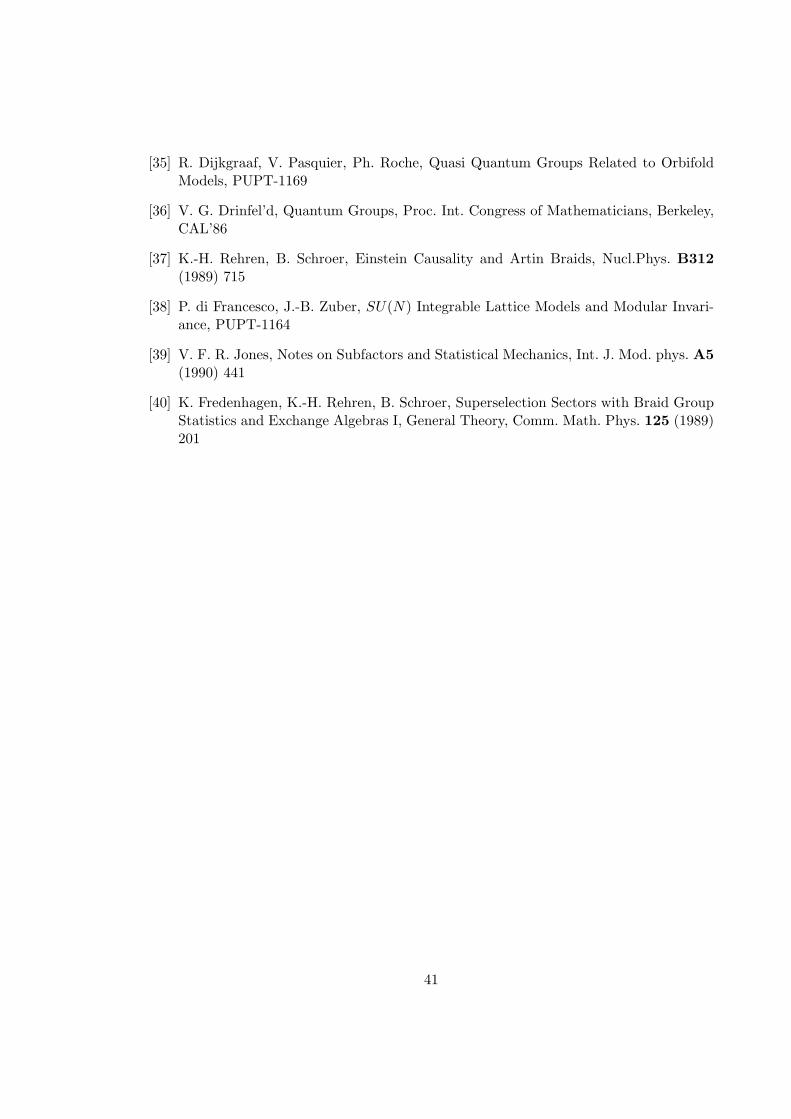
[35] R. Dijkgraaf, V. Pasquier, Ph. Roche, Quasi Quantum Groups Related to OrbifoldModels, PUPT-1169
[36] V. G. Drinfel’d, Quantum Groups, Proc. Int. Congress of Mathematicians, Berkeley,CAL’86
[37] K.-H. Rehren, B. Schroer, Einstein Causality and Artin Braids, Nucl.Phys. B312(1989) 715
[38] P. di Francesco, J.-B. Zuber, SU(N) Integrable Lattice Models and Modular Invari-ance, PUPT-1164
[39] V. F. R. Jones, Notes on Subfactors and Statistical Mechanics, Int. J. Mod. phys. A5(1990) 441
[40] K. Fredenhagen, K.-H. Rehren, B. Schroer, Superselection Sectors with Braid GroupStatistics and Exchange Algebras I, General Theory, Comm. Math. Phys. 125 (1989)201
41
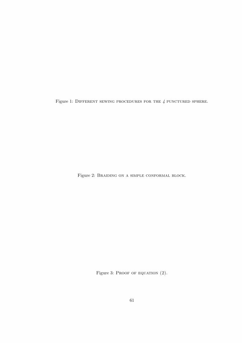
Figure 1: Different sewing procedures for the 4 punctured sphere.
Figure 2: Braiding on a simple conformal block.
Figure 3: Proof of equation (2).
61

Figure 4: Proof of the hexagon identity.
Figure 5: Proof of the pentagon identity.
62

Figure 6: Proof of the Yang-Baxter equation.
Figure 7: Proof of the genus one identity.
Figure 8: A knot diagram.
63
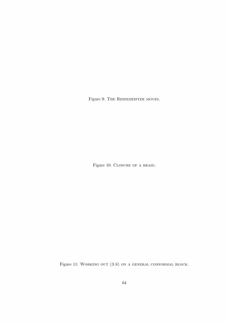
Figure 9: The Reidemeister moves.
Figure 10: Closure of a braid.
Figure 11: Working out (3.8) on a general conformal block.
64
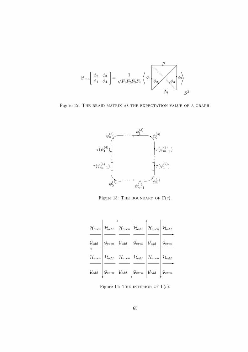
Bmn
[φ2 φ3
φ1 φ4
]=
1√F1F2F3F4
⟨6
-
?
@@@
@@R@@
n
φ1φ2
m
φ3
φ4
⟩
S3
Figure 12: The braid matrix as the expectation value of a graph.
& %
' $
I
R
6
6
-
?
?
. . .
. . .
......
ψ(1)0
τ(ψ(4)m−1)
τ(ψ(4)1 )
ψ(3)n
ψ(3)1
ψ(1)n−1
ψ(1)n
ψ(3)0
τ(ψ(2)1 )
τ(ψ(2)m−1)
Figure 13: The boundary of Γ(c).
? ? ?
6 6
-
-
Geven Geven Geven
Geven Geven Geven
Hodd Hodd Hodd
Hodd Hodd Hodd
Godd Godd Godd
Godd Godd Godd
Heven Heven Heven
Heven Heven Heven
Figure 14: The interior of Γ(c).
65
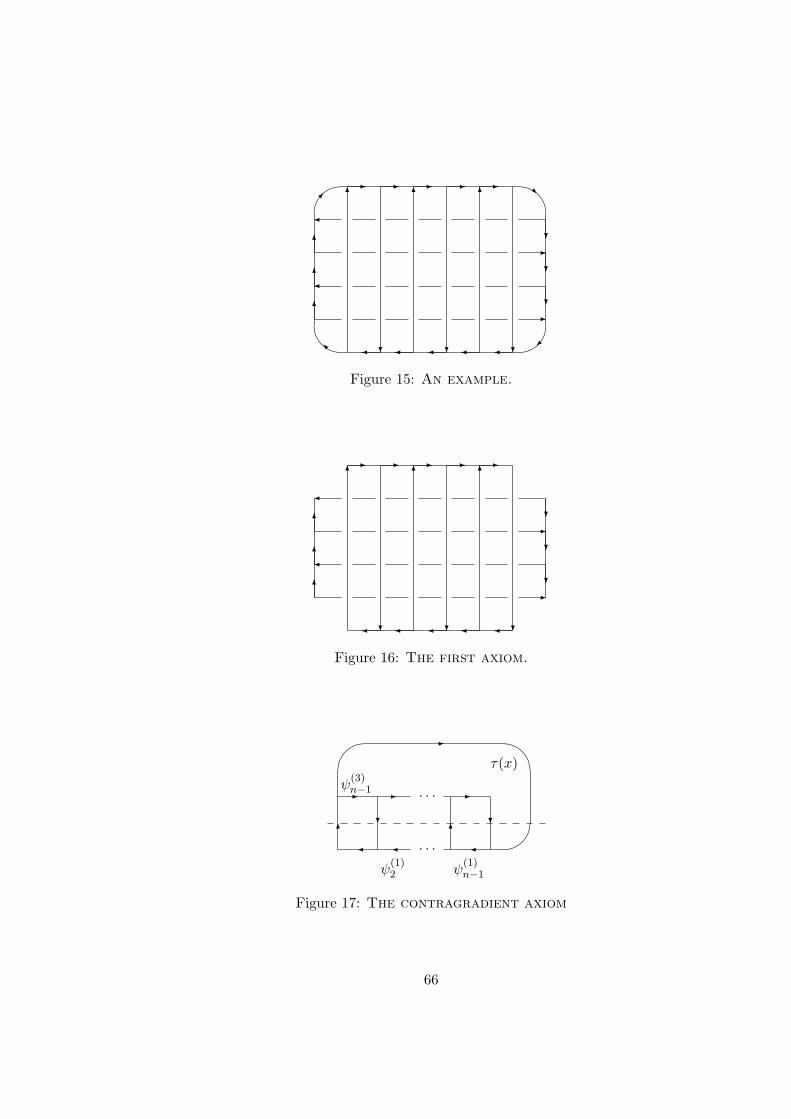
&
'
%
$
I
R
6
6
6?
?
?
- - - - -6 6 6
? ? ?
-
-
Figure 15: An example.
6
6
6?
?
?
- - - - -6 6 6
? ? ?
-
-
Figure 16: The first axiom.
6 6? ?
- - -
. . .
. . .
' - $
%
τ(x)ψ
(3)n−1
ψ(1)2 ψ
(1)n−1
Figure 17: The contragradient axiom
66
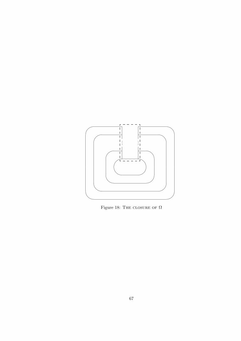
''''
$$$$
& %& %& %
......
& %Figure 18: The closure of Ω
67
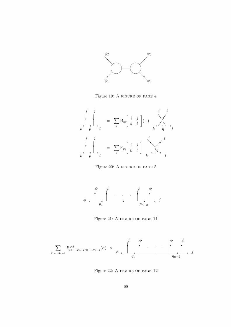
@R@
@I@
φ1
φ2
φ4
φ3
Figure 19: A figure of page 4
? ?
k l
i j
p
=∑q
Bpq
[i jk l
](+)
JJ
JJ
k l
i j
q
? ?
k l
i j
p
=∑q
Fpq
[i jk l
]
@R@?
k l
i j
q
Figure 20: A figure of page 5
φ- j
?
φ?
φ
. . . ?
φ?
φ
pn−2p1
Figure 21: A figure of page 11
∑q1,...,qn−2
Bφ,jp1,...,pn−2;q1,...,qn−2
(α) ×φ- j
?
φ?
φ
. . . ?
φ?
φ
qn−2q1
Figure 22: A figure of page 12
68
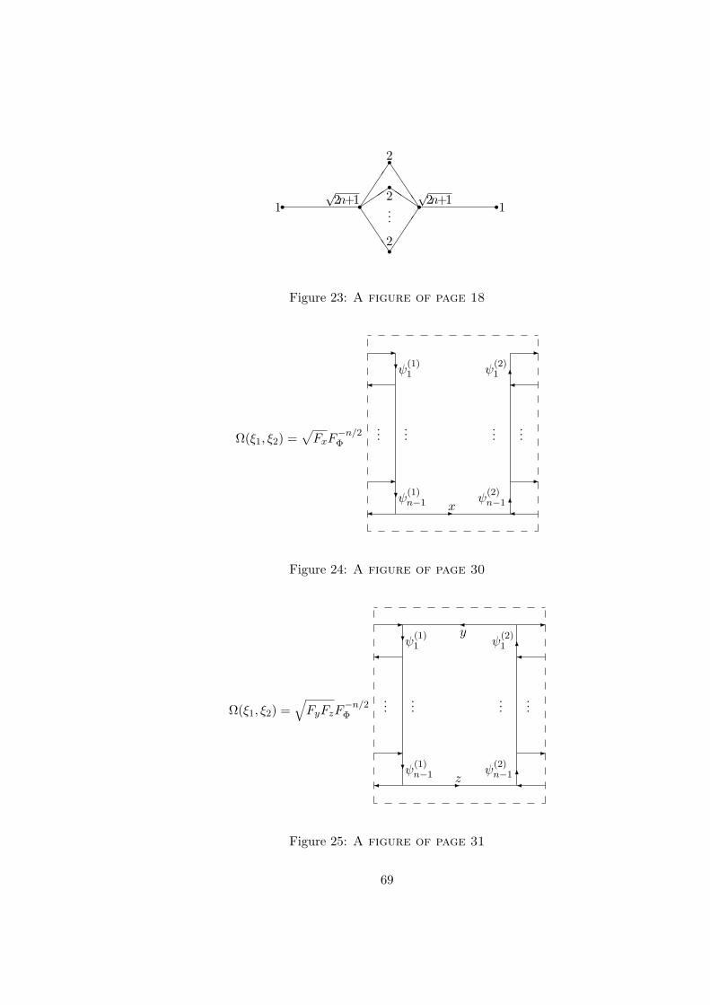
r r r rr
rr
J
JJJ
JJJJ
Q
2
2
2
1 1√
2n+1√
2n+1...
Figure 23: A figure of page 18
Ω(ξ1, ξ2) =√FxF
−n/2Φ
-
-
-
-
?
?
- 6
6ψ
(1)1
ψ(1)n−1 x
ψ(2)n−1
ψ(2)1
......
......
Figure 24: A figure of page 30
Ω(ξ1, ξ2) =√FyFzF
−n/2Φ
-
-
-
-
?
?
- 6
6ψ
(1)1
ψ(1)n−1 z
ψ(2)n−1
ψ(2)1
......
......
y
Figure 25: A figure of page 31
69
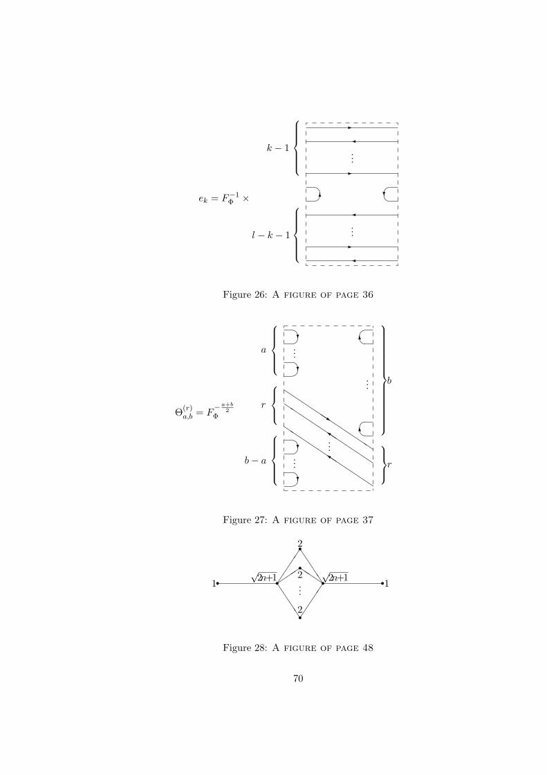
ek = F−1Φ ×
-
-
-
...
...
6 ?
l − k − 1
k − 1
Figure 26: A figure of page 36
Θ(r)a,b = F
−a+b2
Φ
?
?
?
?
6
6
QQQQQQsQQQQQ
QQQQk Q
QQQk
QQQ
QQQ
...
...
...
...
b− a
r
a
r
b
Figure 27: A figure of page 37
r r r rr
rr
J
JJJ
JJJJ
Q
2
2
2
1 1√
2n+1√
2n+1...
Figure 28: A figure of page 48
70
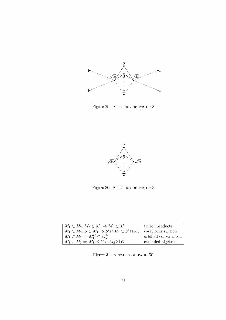
r rr r
r r
r
rr
!!!!
!!! !!
!!!!!aaaaaaa aaaaaaa
J
JJJ
JJJJ
Q
2
2
2
1
1
1
1√2n
√2n
...
Figure 29: A figure of page 48
r rr
rr
J
JJJ
JJJJ
Q
2
2
2
√2n
√2n...
Figure 30: A figure of page 48
M1 ⊂M2, M2 ⊂M3 ⇒ M1 ⊂M3 tensor productsM1 ⊂M2, S ⊂M1 ⇒ S′ ∩M1 ⊂ S′ ∩M2 coset constructionM1 ⊂M2 ⇒ MG
1 ⊂MG2 orbifold construction
M1 ⊂M2 ⇒ M1#c G ⊂M2#c G extended algebras
Figure 31: A table of page 50
71


