Lung-Targeted Receptor Occupancy by Drug Inhalation

warwick.ac.uk/lib-publications

A Thesis Submitted for the Degree of PhD at the University of Warwick

Permanent WRAP URL:

http://wrap.warwick.ac.uk/88540

Copyright and reuse:

This thesis is made available online and is protected by original copyright.

Please scroll down to view the document itself.

Please refer to the repository record for this item for information to help you to cite it.

Our policy information is available from the repository home page.

For more information, please contact the WRAP Team at: [email protected]

http://go.warwick.ac.uk/lib-publications

http://wrap.warwick.ac.uk/88540

mailto:[email protected]

Lung-Targeted Receptor Occupancy by Drug Inhalation:

an Experimental and Computational Evaluation

by

Elin Boger

A thesis submitted for the degree of

Doctor of Philosophy in Engineering

University of Warwick, School of Engineering

May 2016

“We shall not cease from exploration, and the end of all our exploring

will be to arrive where we started and know the place for the first time”

T.S. Eliot

i

Table of contents

List of figures ............................................................................................................... v

List of tables ................................................................................................................ ix

Acknowledgements ..................................................................................................... xi

Declaration ................................................................................................................ xiv

Journal articles: ...................................................................................................... xiv

Conferences: ........................................................................................................... xv

Abstract .................................................................................................................... xvii

List of abbreviations ................................................................................................ xviii

Chapter 1 Introduction ................................................................................................. 1

1.1 Aims and objectives ........................................................................................... 5

1.2 Thesis outline ..................................................................................................... 6

Chapter 2 Background.................................................................................................. 9

2.1 Introduction .................................................................................................... 9

2.2 Inhalation pharmacokinetics ............................................................................... 9

2.2.1 General background to inhalation ............................................................... 9

2.2.2 Lung anatomy............................................................................................ 10

2.2.3. Pharmacokinetics and pharmacodynamics .............................................. 13

2.2.4 Systemic and local PK after inhaled drug delivery ................................... 17

2.2.4.1 Dose-response for inhaled corticosteroids ......................................... 19

2.2.5 Pulmonary drug disposition after inhalation ............................................. 20

2.2.5.1 Pulmonary drug dissolution and absorption ....................................... 20

2.2.5.2 Regional drug deposition ................................................................... 23

2.2.5.3 Mucociliary clearance and macrophage clearance ............................. 29

2.2.5.4 Strategies for enhancing lung retention.............................................. 30

2.2.6 Preclinical inhalation studies .................................................................... 33

2.2.6.1 Inhalation pharmacokinetic studies in drug discovery ....................... 33

2.2.6.2 Dose estimation .................................................................................. 36

2.2.6.3 Exposure measurements ..................................................................... 38

2.3 Modelling ......................................................................................................... 42

2.3.1 Empirical compartmental modelling (PK) ................................................ 42

2.3.2 Physiologically based PK models ............................................................. 46

2.3.3 Structural identifiability and parameter estimation ................................... 50

2.3.4 Sensitivity analysis .................................................................................... 53

2.4 Summary .......................................................................................................... 56

ii

Chapter 3 Development of an in vivo receptor occupancy methodology .................. 57

3.1 Introduction ...................................................................................................... 57

3.2 Tracer identification and development of an in vivo protocol .......................... 60

3.2.1 Methods ..................................................................................................... 61

3.2.1.1 Chemicals and animals ....................................................................... 61

3.2.1.2 Tracer identification in vitro .............................................................. 62

3.2.1.3 Studies for in vivo protocol development........................................... 64

3.2.1.4 Evaluation of tracer dose .................................................................... 66

3.2.1.5 Evaluation of nonspecific binding ..................................................... 67

3.2.1.6 PK-study ............................................................................................. 67

3.2.1.7 Evaluation of tracer function in other organs ..................................... 68

3.2.1.8 General procedures and final protocol for in vivo receptor occupancy

measurements ................................................................................................. 68

3.2.1.9 Calculation of receptor occupancy ..................................................... 69

3.2.1.10 Analytical procedures ...................................................................... 70

3.2.1.11 Statistical analysis ............................................................................ 73

3.2.1.12 Modelling of tissue concentrations of tracer .................................... 73

3.2.2 Results ....................................................................................................... 75

3.2.2.1 Tracer identification in vitro .............................................................. 75

3.2.2.2 Evaluation of tracer dose .................................................................... 75

3.2.2.3 Evaluation of nonspecific binding ..................................................... 80

3.2.2.4 PK-study ............................................................................................. 80

3.3.2.5 Evaluation of tracer function in other organs ..................................... 81

3.3 Application of the methodology ....................................................................... 82

3.3.1 Method ...................................................................................................... 83

3.3.1.1 Dose-receptor occupancy relationship ............................................... 83

3.3.1.2 Receptor occupancy time profile ....................................................... 83

3.3.1.3 Statistical analysis .............................................................................. 84

3.3.1.4 Modelling of the dose-receptor occupancy relationship .................... 85

3.3.2 Results ....................................................................................................... 87

3.3.2.1 Dose-receptor occupancy relationship ............................................... 87

3.3.2.2 Receptor occupancy time profile ....................................................... 94

3.3.2.3 Concentration-receptor occupancy relationship in the spleen ........... 95

3.4 Discussion ........................................................................................................ 95

3.5 Summary ........................................................................................................ 100

Chapter 4 Temporal relationship between target site exposure and receptor

occupancy ................................................................................................................. 102

iii

4.1 Introduction .................................................................................................... 102

4.2 Receptor occupancy studies after IV-administration ..................................... 105

4.2.1 Choice of IV-dose ................................................................................... 105

4.2.2 IV-study, budesonide .............................................................................. 106

4.2.3 Analytical procedures.............................................................................. 107

4.2.4 Results ..................................................................................................... 107

4.3 Pharmacokinetic studies ................................................................................. 108

4.3.1 Preparation of dose solutions .................................................................. 109

4.3.2 In life pharmacokinetic study .................................................................. 110


4.3.3.1 Analytical procedures for fluticasone propionate ............................ 112

4.3.3.2 Analytical procedures for budesonide .............................................. 113

4.3.4 Modelling of plasma pharmacokinetics .................................................. 114

4.4 Modelling of binding kinetics ........................................................................ 118

4.4.1 Characterisation of binding kinetics ....................................................... 118

4.4.2 Sensitivity analysis .................................................................................. 122

4.5 Receptor occupancy studies after nose-only exposure ................................... 124

4.5.1 Nose-only exposure studies..................................................................... 124


4.5.3 Results ..................................................................................................... 133

4.6 Discussion ...................................................................................................... 134

4.7 Summary ........................................................................................................ 137

Chapter 5 A mechanistic inhalation PBPK model for prediction of local and systemic

PK and receptor occupancy ...................................................................................... 139

5.1 Introduction .................................................................................................... 139

5.2 Development of a PBPK model including lung disposition ........................... 141

5.2.1 Model structure ....................................................................................... 141

5.2.1.1 Structural model ............................................................................... 141

5.2.1.2 Particle size distribution, regional deposition and mucociliary

clearance ....................................................................................................... 144

5.2.1.3 Dissolution of drug ........................................................................... 149

5.2.1.4 Derivation of the change of radius equation .................................... 152

5.2.2 Parameterisation ...................................................................................... 155

5.2.2.1 Drug-specific input parameters ........................................................ 155

5.2.2.2 Formulation-specific input parameters ............................................ 162

5.2.2.3 System-specific input parameters .................................................... 166

5.3 Application of the developed model .............................................................. 170

iv

5.3.1 Fluticasone propionate (model validation and verification) ................... 171

5.3.1.1 Intravenous administration ............................................................... 171

5.3.1.2 Nose-only exposure .......................................................................... 174

5.3.1.3 Sensitivity analysis for fluticasone propionate ................................ 177

5.3.2 Budesonide .............................................................................................. 179

5.3.2.1 Intravenous administration ............................................................... 179

5.3.2.2 Nose-only exposure .......................................................................... 181

5.3.3 Evaluation of concepts for lung-selectivity............................................. 183

5.3.3.1 Definition of lung-selectivity ........................................................... 184

5.3.3.2 Evaluation of drug-, formulation- and system-specific input

parameters .................................................................................................... 184

5.3.4 Evaluation of different concepts ............................................................. 189

5.3.4.1 Intravenous administration versus instillation of dissolved drugs

without any pulmonary retention mechanism .............................................. 189

5.3.4.2 Impact of mucociliary clearance on the pharmacokinetics .............. 192

5.3.4.3 Evaluation of the impact of permeability on pulmonary absorption 193

5.3.4.4 Evaluation of the extent of nasal drug absorption ............................ 198

5.3.4.5 Impact of permeability in the central lung ....................................... 201

5.3.5 Repeated dosing ...................................................................................... 205

5.3.5.1 Technical implementation of repeated dosing ................................. 205

5.3.5.2 Technical implementation of a deposition model ............................ 206

5.3.5.3 Repeated dosing of poorly and highly soluble compounds ............. 221

5.3.5.4 Effect of increasing inhaled doses ................................................... 224

5.4 Discussion ...................................................................................................... 232

5.6 Summary ........................................................................................................ 241

Chapter 6 Conclusions ............................................................................................. 243

6.1 Future research and limitations ...................................................................... 251

6.2 Personal reflections ........................................................................................ 256

Chapter 7 References ............................................................................................... 260

Appendix A .............................................................................................................. 276

Appendix B .............................................................................................................. 294

Appendix C .............................................................................................................. 304

v

List of figures

Figure 2.1 Illustration of the lung heterogeneity. ...................................................... 13

Figure 2.2 Schematic representation of the fate of an orally inhaled drug ............... 19

Figure 2.3 Drug deposition mechanisms. .................................................................. 29

Figure 2.4 Two compartments of a compartmental system ...................................... 44

Figure 2.5 A 2-compartment model parameterised using a) micro-constants (k10, k12,

k21 and V1), and b) physiological parameters (CL, V1, CLd and V2) ........................... 45

Figure 2.6 A schematic representation of a typical whole-body physiologically based

pharmacokinetic (PBPK) model ................................................................................ 48

Figure 3.1 Chemical structures ................................................................................. 62

Figure 3.2 Evaluation of total (white circles) and nonspecific (black diamonds) lung

concentration of tracer after IV-administration of four different tracer doses ........... 78

Figure 3.3 A sensitivity analysis ............................................................................... 79

Figure 3.4 Model simulations of the ratio between total (Ccontrol) and nonspecific

(Cnonspec) lung concentration of tracer ........................................................................ 79

Figure 3.5 Characterisation of the plasma pharmacokinetics (PK) of the tracer ...... 81

Figure 3.6 Tissue tracer concentration in a) the lung, and b) the spleen after IV-

administration of three escalating doses of fluticasone propionate ........................... 91

Figure 3.7 Dose-receptor occupancy relationship ..................................................... 91

Figure 3.8 A sensitivity analysis ............................................................................... 92

Figure 3.9 Corticosterone and receptor occupancy ................................................... 93

Figure 3.10 Time course of receptor occupancy ....................................................... 94

Figure 3.11 A relationship between receptor occupancy in the spleen and spleen

concentrations of fluticasone propionate ................................................................... 95

Figure 4.1 Glucocorticoid receptor (GR) occupancy .............................................. 108

vi

Figure 4.2 Graphical illustration of a 3-compartment model .................................. 116

Figure 4.3 Plasma concentration (Cp) after intravenous (IV) administration ......... 116

Figure 4.4 Weighted residuals ................................................................................. 117

Figure 4.5 Concentration of receptor-drug complex in the spleen .......................... 121

Figure 4.6 An exhaustive search ............................................................................. 121

Figure 4.7 Sensitivity analysis ................................................................................ 124

Figure 4.8 a) Total lung concentrations (Clung) and b) plasma concentrations (Cp)

after inhalation ......................................................................................................... 131

Figure 4.9 Glucocorticoid receptor (GR) occupancy .............................................. 133

Figure 4.10 Drug concentration profiles after nose-only exposure ......................... 134

Figure 5.1 Schematic representation of the developed PBPK model ..................... 142

Figure 5.2 Parameter estimation of the solubility ................................................... 162

Figure 5.3 Characterisation of mucociliary clearance ............................................. 169

Figure 5.4 Model predictions and observations of fluticasone propionate

administered as an IV-bolus ..................................................................................... 173

Figure 5.5 Model predictions and observations after nose-only exposure of

fluticasone propionate .............................................................................................. 176

Figure 5.6 Sensitivity analysis ................................................................................ 179

Figure 5.7 Model predictions and observations of budesonide administered as an IV-

bolus ......................................................................................................................... 181

Figure 5.8 Observations and model predictions after nose-only exposure of

budesonide ............................................................................................................... 183

Figure 5.9 The impact of different drug-, formulation- and system-specific

properties on lung-selectivity ................................................................................... 188

vii

Figure 5.10 Plasma concentration (Cp) profiles were simulated after intratracheal

instillation of dissolved drug (20 nmol/kg, blue line) and intravenous (IV)

administration ........................................................................................................... 190

Figure 5.11 Receptor occupancy profiles were simulated after intratracheal

instillation of dissolved drug (20 nmol/kg) and intravenous (IV) administration ... 191

Figure 5.12 Percent of drug particles deposited in the nose and central lung that are

removed by the mucociliary clearance ..................................................................... 193

Figure 5.13 The impact of permeability (P) on pulmonary absorption .................. 197

Figure 5.14 The amount of drug absorbed from the nose (Anose) after nose-only

exposure ................................................................................................................... 200

Figure 5.15 The amount of drug absorbed from the lung (Alung) after nose-only

exposure ................................................................................................................... 200

Figure 5.16 Three different scenarios were simulated to investigate what impact a

lower permeability in the central lung would have on the pharmacokinetics .......... 204

Figure 5.17 The deposition fractions (df) in a) the extrathoracic region, b) the

alveolar region, c) the tracheobronchial region, and d) all three regions ................. 215

Figure 5.18 The effect of the tidal volume (VT) on the deposition fraction ............ 216

Figure 5.19 The effect of the breathing frequency (fbr) on the deposition fraction . 217

Figure 5.20 The probability of deposition by three deposition mechanisms .......... 218

Figure 5.21 The probability of deposition by different deposition mechanisms .... 219

Figure 5.22 Simulations of repeated nose-only exposure ....................................... 224

Figure 5.23 Simulations of receptor occupancy in the central lung (ROc, dashed

lines) and in the spleen (ROsp, solid lines) after increasing lung deposited doses ... 228



viii





ix

List of tables

Table 3.1 Parameter estimates from modelling of tissue concentrations of tracer .... 77

Table 3.2 Estimated correlation matrix of the parameter estimates .......................... 80

Table 3.3 Parameter estimates from PK-modelling of tracer .................................... 81

Table 3.4 Total and nonspecific tracer concentrations .............................................. 82

Table 3.5 Post-hoc test for the lung tracer concentrations ........................................ 88

Table 3.6 Post-hoc test for the spleen tracer concentrations ..................................... 89

Table 3.7 Parameter estimates from the modelling of the dose-receptor occupancy

relationship ................................................................................................................. 92

Table 3.8 Estimated correlation matrix of the parameter estimates .......................... 93

Table 4.1 Estimated pharmacokinetic parameters for fluticasone propionate (FP) and

budesonide ............................................................................................................... 115

Table 4.2 Estimated correlation matrix for the parameters obtained from modelling

of the pharmacokinetics of fluticasone propionate .................................................. 116

Table 4.3 Estimated correlation matrix for the parameters obtained from modelling

of the pharmacokinetics of budesonide .................................................................... 117

Table 4.4 Estimated binding kinetics parameters for fluticasone propionate (FP) and

budesonide ............................................................................................................... 121

Table 4.5 Estimated correlation matrix for the parameters estimates obtained from

modelling of the binding kinetics of fluticasone propionate .................................... 122

Table 4.6 Estimated correlation matrix for the parameters estimates obtained from

modelling of the binding kinetics of budesonide ..................................................... 122

Table 4.7 Characterisation of particle size distribution ........................................... 132

Table 5.1 Tissue-to-unbound plasma partition coefficients .................................... 158

Table 5.2 Calculated tissue-to-plasma partition coefficients .................................. 159

x

Table 5.3 Drug- and formulation-specific input parameters for budesonide .......... 164

Table 5.4 Drug- and formulation-specific input parameters for fluticasone propionate

.................................................................................................................................. 165

Table 5.5 System-specific input parameters for the rat ........................................... 169

Table 5.6 System-specific input parameters for the central lung, the peripheral lung

and the nose .............................................................................................................. 170

Table 5.7 Details for the inhalation studies with budesonide .................................. 183

Table 5.8 Lung structure of a rat lung ..................................................................... 220

xi

Acknowledgements

So many people have been instrumental in the completion of this PhD project and I

am forever grateful for their support. First and foremost I would like to thank my

main supervisor Dr Markus Fridén, who guided me, not only scientifically but also

personally, towards becoming a more senior scientist. I am very grateful for all our

discussions and I keep to be stunned by your insightfulness. Thanks also for finding

the delicate balance of initially setting much time aside for supervision to gradually

decrease the guidance to ensure that I would develop into an independent researcher.

I would also like to thank my academic supervisors Dr Michael Chappell and Dr Neil

Evans for their invaluable guidance and support throughout my studies. My

co-supervisors Dr Pär Ewing and Prof Margareta Hammarlund-Udenaes have both

been important discussion partners during the journey of this PhD.

I would like to express my sincere gratitude to the Marie Curie FP7 People ITN

European Industrial Doctorate (EID) [Project No.316736] for funding this research.

I would also like to express my appreciation to everyone at RIA DMPK at

AstraZeneca for creating a friendly and warm working environment where laughter

is as important as science. Many scientists at AstraZeneca have provided important

guidance and support for completing this research and some names stand out. I

would like extend my sincere gratitude to Susanne Arlbrandt, Dr Britt-Marie Fihn,

Kajsa Claesson, Louise Hammarberg, Marie Johansson and Gina Hyberg for their

invaluable contributions to the in vivo studies. I cannot emphasise enough how

impressed I am by your laboratory skills. Another contribution, which indeed

constituted a step-change for this project, was the improved bioanalytical

methodology for FP conducted by Dr Anders Lundqvist. That particular analysis

enabled the important validation of the developed model’s ability to predict the

xii

systemic PK and I am deeply grateful for this contribution. Sara Johansson and

Annica Jarke are acknowledged for their help with formulating nanosuspensions of

FP and budesonide for the PK studies. I would also like to thank Anders Wigenborg

for controlling and operating the inhalation system as well as setting time aside to

explain to me how it works. Furthermore, I would like to thank Dr Jan Westergren,

Dr Ulrika Tehler and Dr Ulf Eriksson for fruitful discussions.

I was exceptionally fortunate to have Erica Bäckström sitting next to me at AZ,

being the best possible office neighbour! Besides having great (and perhaps a bit

geeky) scientific discussions on inhalation pharmacokinetics, we have laughed

enough to extend our lives by several years. Thanks for being awesome!

I would also like to thank each and everyone of the Biomedical Superheroes for

making my time in the UK a great experience. In particular I would like to thank

Magnus Trägårdh and Linnéa Bergenholm. Magnus has, despite his perhaps slightly

overly optimistic attitude, been a great support for me on several levels. I have

learned a lot from our various discussions, but first and foremost thanks for being a

great friend. Linnéa, thanks for sharing your seemingly endless energy, optimism and

for making everyday life much more fun. Once my knee gets better, I’m sure we will

climb Mount Everest!

My friends and family have been very supportive, understanding and encouraging

during this PhD journey. Most importantly, you have done what you do best; been

yourself and I am just so happy to be surrounded by you guys! In particular, I would

like to thank mum, dad, Frida and “stor-Oskar”. Thanks for your endless support and

for always being there for me.

I also want to take the opportunity to thank my gym and my running routes for

providing exceptional tools for effectively controlling the fluctuating stress levels of

xiii

a PhD student. I am confident that I have never been stronger than I am at the time of

writing.

And last but not least, I would like to thank Oskar. Clearly, no words are worthy to

describe how grateful I am to have you in my life and for how you have supported

me during this journey. Thanks for everything –you make me complete.

xiv

Declaration

This thesis is submitted to the University of Warwick in support of my application

for the degree of Doctor of Philosophy. It has been composed by myself and has not

been submitted in any previous application for any degree apart from the

experiments described in sections ‘3.2.1.2 Tracer identification in vitro’ and ‘3.2.1.4

Evaluation of tracer dose’ which was previously submitted for a master’s degree. The

experiment described in section ‘3.2.1.5 Evaluation of nonspecific binding’ was done

whilst I was employed at AstraZeneca R&D. The mathematical modelling of the

aforementioned data was all performed as part of this project. This thesis has not

been submitted for a degree at any other university.

Where any of the content presented in this thesis is the result from collaborative

research this is clearly stated in the text such that it is possible to ascertain how much

of the work is my own.

Parts of this thesis have been published by the author:

Journal articles:

Boger, E., Ewing, P., Eriksson, U.G., Fihn, B.M., Chappell, M., Evans, N. & Fridén,

M. (2015). A novel in vivo receptor occupancy methodology for the glucocorticoid

receptor: towards an improved understanding of lung PK/PD. The Journal of

Pharmacology and Experimental Therapeutics, 353(2), 279-287.

Boger, E., Evans, N., Chappell, M., Lundqvist, A., Ewing, P., Wigenborg, A. &

Fridén, M. (2016). A systems pharmacology approach for prediction of pulmonary

xv

and systemic pharmacokinetics and receptor occupancy of inhaled drugs. CPT:

Pharmacometrics & Systems Pharmacology, 5(4), 201-210.

Conferences:


Fridén, M. A systems pharmacology approach for prediction of pulmonary and

systemic pharmacokinetics and receptor occupancy of inhaled drugs, PKUK

Conference 2015: Programme and Abstract Book. PKUK Conference 2015, Chester,

UK, 18-20 November 2015.

Fridén, M., Boger, E., A Systems Pharmacology Approach for Prediction of

Systemic and Pulmonary PK for Inhaled Drugs. Oral presentation at QSP Europe,

Basel, Switzerland, 29 April, 2015

Fridén, M., Boger, E., Towards estimation of unbound drug concentrations in the

lung: utility of lung slices and target occupancy methodologies. Oral presentation at

Phys Chem Forum, Uppsala, Sweden, January 29, 2015


Fridén, M., Development of a PBPK model with lung disposition – towards an

increased understanding of PK and PK/PD for inhaled drugs. Presented at

AstraZeneca’s Modelling and Simulation Symposium, Mölndal, Sweden, 17-18

December, 2014

xvi

Fridén, M., Boger, E., Glucocorticoid receptor occupancy and PBPK-PD models for

inhalation. Oral presentation at AstraZeneca modeling and simulation symposium,

Mölndal, Sweden, 17 December 2014


M. Development and application of a novel pulmonary in vivo receptor occupancy

methodology for the glucocorticoid receptor, PKUK Conference 2014: Programme

and Abstract Book. PKUK Conference 2014, Bath, UK, 5-7 November 2014.


M. Development and Application of a Novel Pulmonary in vivo Target Occupancy

Methodology for the Glucocorticoid Receptor. Presented at AAPS, San Diego, USA,

2-6 November, 2014

Boger, E., Ewing, P., Eriksson, U.G., Fihn, B.M., Chappell, M., M., Evans, Jirstrand,

M., Hammarlund-Udenaes & M., Fridén M. Development of a novel pulmonary in

vivo target occupancy methodology for the glucocorticoid receptor. Oral presentation

at AstraZeneca Modelling & Simulation Symposium, Alderley Park, 3-4 December

2013

Boger, E., Ewing, P., Eriksson, U.G., Fihn, B.M., Chappell, M., M., Evans, Jirstrand,

M., Hammarlund-Udenaes & M., Fridén M. Development of a novel pulmonary in

vivo target occupancy methodology for the glucocorticoid receptor, PKUK

Conference 2013: Programme and Abstract Book. PKUK Conference 2013,

Harrogate, UK, 1-2 November 2013.

xvii

Abstract Inhalation is attractive for treating respiratory diseases since it offers an opportunity

to achieve lung-selectivity, i.e. high local and low systemic levels of unbound drug.

Nevertheless, evaluation and prediction of the former is challenging for reasons

including: 1) the unbound blood concentration cannot be assumed to reflect the free

lung target site exposure after inhalation, 2) it is not possible directly measure

unbound drug concentrations locally in the lung, and 3) pulmonary drug disposition

is known to be a complex interplay between numerous processes. This thesis

therefore aims to increase the understanding of how different drug- and formulation-

specific properties relate to the free target site exposure to inhaled drug. This was

done by: 1) developing and subsequently applying an experimental methodology for

measuring pulmonary and systemic occupancy of a receptor targeted by inhaled

drugs, and 2) developing a rat physiologically-based pharmacokinetic (PBPK)

model, which mechanistically describes underlying processes of pulmonary drug

disposition. Experimental studies provided data on the time-course of the PK and

receptor occupancy after intravenous (IV) and inhaled drug delivery of fluticasone

propionate (FP). The binding kinetics parameters, which were estimated from data

generated after IV-dosing, were used as input parameters to the developed model

together with other properties specific to FP. The model accurately described the PK

and receptor binding for several IV-doses. Predictions were consistent with the

observations from inhalation studies, confirming that FP has a dissolution rate-

limited absorption and highlighting that drug in solid state does not contribute to

receptor binding. As the model is mechanistic, it can assess how different drug- and

formulation-specific properties, or combinations thereof, give rise to lung-selectivity.

Specific findings include lung-selectivity possibly being unattainable in well-

perfused lung regions and that slow drug-receptor dissociation can provide lung-

selectivity. Hence, the model lends itself to guiding the design of inhaled compounds

and formulations.

xviii

List of abbreviations

ADME Absorption, distribution, metabolism and excretion

ANOVA Analysis of variance

AUC Area under the curve

BAL Broncho-alveolar lavage

BDP Beclomethasone dipropionate

Bmax Receptor density

Ccontrol Tissue concentration of tracer in drug-naïve control

animals

CELF Total drug concentration in the epithelial lining fluid

CL Clearance

CLb Blood clearance

CLp Plasma clearance

Clung Total drug concentration in the lung

Cnonspec Nonspecific tissue concentration of tracer

COPD Chronic Obstructive Pulmonary Disease

Cp Total drug concentration in the plasma

Cs Solubility

Cspec,max Maximum specific tissue concentration of tracer

Cspleen Total drug concentration in the spleen

Ctest Tissue concentration of tracer in test animals

CYP Cytochrome P450

D Diffusion coefficient

da Aerodynamic diameter

dg Geometric diameter

xix

ED50 Dose giving 50% efficacy

EH Hepatic extraction ratio

ELF Epithelial lining fluid

F Bioavailability

fabs Fraction absorbed from the gastroinstestinal tract

FaSSIF Fasted-state small intestinal fluid

FDA Food and Drug Administration

FEV Forced expiratory volume

fgut Fraction that escapes gut extraction

fh Fraction that escapes hepatic extraction

FP Fluticasone propionate

ftb Target-bound fraction

fu Fraction unbound in plasma

fu,fluid Unbound fraction in the ELF or the nasal lining fluid

fu,h Fraction unbound in lung homogenate

GI Gastrointestinal

GR Glucocorticoid receptor

ICS Inhaled corticosteroids

ID Total inhaled dose

IT Intratracheal

IV Intravenous

Kd Dissociation constant

Koff Dissociation rate constant

Kon Association rate constant

Kp Tissue-to-plasma partition coefficient

xx

Kp,u Tissue-to-unbound plasma partition coefficient

LADME Liberation, absorption, distribution, metabolism and

excretion

LC-MS/MS Liquid chromatography tandem mass spectrometry

LDD Lung deposited dose

LLE Liquid liquid extraction

LLOQ Lower limit of quantification

logD7.4 The logarithm of the ratio of concentrations of a

compound (unionized+ionized) between octanol and

water buffered to pH 7.4

logP The logarithm of the ratio of the concentrations of a

compound (unionized) between octanol and water

MCC Mucociliary clearance

MMAD Mass Median Aerodynamic Diameter

MTBE Methyl-tertbutyl ether

ODE Ordinary differential equation

P Permeability

Papp Apparent permeability

PBPK Physiologically-based pharmacokinetic

PD Pharmacodynamics

PEF Peak expiratory flow

PET Positron emission tomography

PK Pharmacokinetics

ROave Weighted average of receptor occupancy in the central

and peripheral lung

xxi

ROc Receptor occupancy in the central lung

ROp Receptor occupancy in the peripheral lung

ROspleen Receptor occupancy in the spleen

SPE Solid phase extraction

Stk Stokes number

TI Therapeutic index

Vd Apparent volume of distribution

Vdss Steady state volume of distribution

Vu,lung Unbound lung volume of distribution

ρ Density

1

Chapter 1 Introduction

Inhalation is an attractive route of administration that has been employed for more

than 2000 years [1]. Delivery of drug directly to the diseased target organ has been

associated with advantages such as a rapid onset of action and a higher and more

sustained local tissue concentration [2]. The latter offers an opportunity to increase

the therapeutic index (TI), which often is defined as the ratio of the dose that causes a

toxic response to the dose that produces the desired, therapeutic effect in 50% of the

population [3]. The TI can be increased by achieving lung-selectivity and thereby

fulfil the aim of locally acting inhaled drugs, i.e. to obtain high drug concentrations

at the lung target site whilst the systemic concentrations are kept at a minimum [4].

In order to minimise the systemic exposure, and thus systemic side-effects, drug

discovery typically aims to develop inhaled drugs with high hepatic clearance to

obtain a rapid elimination and to avoid absorption from the gastrointestinal (GI) tract

[5].

However, assessment and prediction of lung-selectivity has so far proven to be

elusive. Collection of relevant exposure measurements is recognised as a challenge

both within clinical and preclinical research. Since the appearance of drug in the

systemic circulation is the result of pulmonary absorption, unbound drug

concentrations in plasma (Cu,p) cannot be assumed to reflect the unbound target site

concentration in the lung [2]. In contrast, this assumption can generally be held as

valid for systemically acting drugs. This constitutes a challenge for evaluation of

locally acting inhaled drugs since Cu,p usually forms the basis for establishing a

quantitative relationship between the drug exposure (pharmacokinetics - PK) and the

2

drug effect (pharmacodynamics - PD), commonly referred to as a PK/PD-

relationship.

To date, it is not possible to measure the unbound, and thus pharmacologically

active, target site concentrations locally in lung tissue. In a preclinical setting, the

lungs can be collected by destructive sampling at several time points after inhalation

of drug, where destructive sampling implies that the animal is euthanized during the

process of sampling (i.e. only one sample/animal). Drug concentrations are

subsequently measured in lung tissue homogenates, providing a time profile of total

lung concentrations where the lung, despite its heterogeneous nature, is reflected as

one anatomical entity. Moreover, the homogenisation process severely distorts data

interpretation by dissolving solid drug particles [6]. Indeed, the establishment of

PK/PD-relationships based on total lung concentrations is known to be more

challenging for poorly soluble compounds [7]. This can be attributed to a large, but

quantitatively unknown, fraction of the deposited drug still being undissolved when

the lung is dissected, meaning that it could not have contributed to the

pharmacological effect. As receptor occupancy is driven by the unbound drug

concentration at the target site, such measurements would clarify the PK, as well as

the PK/PD, after topical administration. Developing an experimental methodology

for measuring receptor occupancy of an inhaled target would thus bring us one step

closer towards understanding the time course of free target site exposure to inhaled

drugs. Yet another dimension would be added if such a methodology not only

allowed for measurements of receptor occupancy in the lung, but also in another

organ, which thus could be used as a reference organ for the systemic exposure of

drug after inhalation. Studies utilising such a methodology would not only provide

results, which inherently contain information about the local target site exposure, but

3

also provide a quantitative readout of the degree of lung-selectivity that was achieved

by inhalation. The latter information can thus be obtained by comparing the

pulmonary and the systemic receptor occupancy.

Data on local and systemic receptor occupancy would thus inherently contain

information about the fate of an inhaled drug and thereby be informative about the

underlying processes in this system. While this doubtlessly would provide one piece

of the puzzle, these measurements alone would not be sufficient enough to build a

deeper mechanistic understanding and thereby enabling predictions of how the extent

and time course of the free target site exposure to inhaled drug would be affected by

changes in drug- and/or formulation-specific properties (e.g. the solubility and the

particle size distribution). Hence, it would still remain challenging to identify rational

strategies for: 1) the chemical design of inhaled compound series, 2) the inhaled

formulation design for clinical studies, and 3) targeting appropriate dose ranges for

clinical studies utilising the inhaled route.

To understand why predicting the fate of an inhaled drug is held as particularly

challenging, we need to consider the complexity of pulmonary drug disposition. This

can be illustrated by considering some of the events that follow inhaled drug

delivery. In preclinical inhalation studies, rodents are generally exposed via nose-

only inhalation, where a substantial deposition of drug particles will occur in the

nose [6]. Drug deposited in the lung and the nose will both be subject to a self-

cleansing mechanism called mucociliary clearance (MCC), which transports drug

particles towards the pharynx where they are eventually swallowed [8]. Accordingly,

the resulting plasma PK is a result of parallel absorption from the lung, the nose and

the GI-tract [9,10]. Nevertheless, predicting regional drug concentrations in the lung

is even more demanding since pulmonary drug disposition involves numerous

4

processes including regional drug deposition, dissolution of solid drug particles and

MCC. Furthermore, additional complexity comes from the heterogeneous nature of

the organ with distinct differences between the tracheobronchial and alveolar regions

[11]. An integrated understanding, which takes the mechanistic processes as well as

the organ heterogeneity into account, would thus be desirable.

Simulation models have previously been used to predict the systemic exposure of

inhaled drugs in humans. Hochhaus and Weber [12] developed a compartmental

simulation tool, in which the lung was divided into two subcompartments

representing the central and peripheral region, respectively. The model also included

features such as MCC and drug dissolution described by rate constants [12].

Chaudhuri et al. used GastroPlus™ to predict the systemic PK of budesonide [13].

The simulated plasma profiles of both models proved to agree well with

experimental data. These simulation studies thus aimed at characterising the systemic

and not the local exposure. There has also been research focusing on predicting the

local exposure to inhaled drug. A simulation study by Hochhaus et al. evaluated

lung-selectivity in terms of pulmonary and systemic receptor occupancy [14].

However, those simulations relied on a very simple model structure where the lung

was described by a single compartment and the receptor binding by a static model.

Furthermore, the drug dissolution was non-mechanistically described by a single rate

constant. Thus the simple model structure and the incorporation of only a few,

empirically described drug disposition processes cannot provide a sufficiently

detailed description of the system to understand the interplay between different

processes and thereby e.g. make inferences on the optimal design of inhaled

compounds and/or formulations. Even so, despite its simplicity, the model by

5

Hochhaus et al. could e.g. identify that lung-selectivity is attained during the

dissolution process.

Nevertheless, a mechanistic model predictive of local tissue concentrations

combined with measurements such as receptor occupancy for validation is currently

lacking. Such a model would be necessary to elucidate the highly complex processes

involved in pulmonary drug disposition [15]. Clearly, some of these processes will

be affected by pulmonary diseases [16]. For instance, simulations have proposed that

the drug deposition will be enhanced at the sites of airway narrowing in asthmatic

patients [17]. Whilst this research focuses on healthy lungs, it opens up for later

research to evaluate how the pathophysiology of a given disease might affect

processes of pulmonary drug disposition and thereby the local lung concentrations.

In this thesis, a mechanistic and physiologically-based rat inhalation PK and

receptor occupancy model is developed. The presented model provides the

pharmaceutical industry with a novel systems modelling tool for understanding how

the free target site exposure to inhaled drug relates to different drug- and

formulation-specific properties and thereby enables informed decisions on e.g. the

chemical and formulation design.

1.1 Aims and objectives

The aim of this thesis is to increase the understanding of how the level and time

course of free lung target site exposure to inhaled drug relate to different drug- and

formulation-specific properties. Therefore the objectives of this thesis are to:

6

1. Continue and complete an ongoing development of an in vivo receptor

occupancy methodology for an inhaled target, the glucocorticoid receptor

(GR).

2. Apply the developed in vivo receptor occupancy methodology to characterise

and compare the time course of receptor occupancy after intravenous- and

inhaled drug delivery.

3. Characterise the binding kinetics of a GR agonist using the intravenous route.

4. Develop a mechanistic, mathematical framework to predict the time course of

target site exposure to unbound drug and receptor occupancy after inhalation,

taking into account the physiology of the species and processes judged to be

important for pulmonary drug disposition.

5. Apply the developed model to understand what drug- and formulation-

specific properties, or combinations thereof, that give rise to lung-selectivity

in terms of local and systemic receptor occupancy.

1.2 Thesis outline

This thesis will lead up to the development of a mechanistic and physiologically-

based inhalation PK model, which subsequently is used to gain an understanding of

how different drug- and/or formulation-specific properties can (or cannot) give rise

to lung-selectivity. As detailed below, this aim can be obtained by conducting the

research in a stepwise manner.

Chapter 2 introduces relevant background information, which has been divided into

two main categories: inhalation PK and modelling, respectively. The focus of the

former category is primarily on processes that are unique for pulmonary drug

disposition, but it also covers e.g. lung anatomy, preclinical inhalation models and

7

general PK concepts. Clearly, it is crucial to build an understanding about these

different subcategories as it will provide the foundation for the model development

and the subsequent validation.

Chapter 3 presents the development of an in vivo receptor occupancy methodology

for an inhaled target (the GR) in rats. As outlined in the introduction, such

measurements will inherently contain information about the free target site exposure

to inhaled drug, which cannot be directly measured. The developed methodology is

subsequently evaluated by testing its ability to demonstrate a dose-receptor

occupancy relationship as well as to characterise the time course of receptor

occupancy after intravenous administration of a GR agonist (fluticasone propionate,

FP).

In chapter 4, the developed experimental methodology is applied to study the time

course of receptor occupancy and the PK after nose-only exposure of FP as well as

after intravenous administration of another GR-agonist (budesonide). Mathematical

modelling is subsequently used to estimate the unknown in vivo binding kinetics

parameters for both compounds using the data generated from intravenous dosing.

Chapter 5 describes the development of a physiologically based pharmacokinetic

(PBPK) model, which places emphasis on mechanistically describing the underlying

processes of pulmonary drug disposition. Here it also becomes clear that chapter 4

serves two important purposes. Firstly, it provides estimates of the binding kinetics

parameters Kon and Koff, which are then used as input parameters to the presented

model. Secondly, the receptor occupancy measurements as well as the PK from the

nose-only exposure studies can used for model validation purposes. The ability of the

model to mechanistically describe PK and the receptor binding after intravenous and

inhaled drug delivery is thus evaluated using FP as a test compound. The developed

8

PBPK model is subsequently used to explore various aspects of pulmonary drug

disposition, including how the interplay between different drug- and formulation-

specific properties can produce lung-selectivity.

The overall project conclusions and recommendations for future research are

discussed in chapter 6.

9

Chapter 2 Background

2.1 Introduction

This thesis is set out to explore how the target site exposure to inhaled drug relates to

different drug- and formulation-specific properties. Ultimately, this will lead up to

the development of a new systems model, which is built by formulating

mathematical descriptions of the system based on the current understanding of

pulmonary drug disposition and rodent physiology. Such a model can be evaluated

using drug- and formulation-specific properties as input parameters and subsequently

be validated using different experimental measurements. Clearly, developing such a

model requires knowledge about several different areas including inhalation

pharmacokinetics (PK) and modelling.

This chapter, which aims to introduce relevant background information, has

therefore broadly been divided into two main sections: inhalation PK and modelling,

respectively. The focus of the former section is primarily on processes that are

unique for pulmonary drug disposition, but it also covers e.g. lung anatomy,

preclinical inhalation models and general PK concepts. The latter section will

introduce various modelling techniques and concepts that are useful for this thesis

such as physiologically-based pharmacokinetic (PBPK) modelling.

2.2 Inhalation pharmacokinetics

2.2.1 General background to inhalation

The ability to deliver drug specifically to its site of action has made inhalation an

attractive route of administration for respiratory diseases. This feature has been

associated with advantages such as a rapid onset of action and a higher and more

10

sustained local tissue concentration [2]. The latter can lead to an increased

therapeutic index by achieving lung-selectivity and thus fulfilling the aim of locally

acting inhaled drugs, i.e. to obtain high unbound drug concentrations at the lung

target site while the systemic (unbound) concentrations are kept at a minimum [4].

Clearly, the unbound lung target site concentrations are expected to drive the desired

pharmacological effect, whereas the unbound systemic concentration might exert

unwanted systemic side-effects [18]. Inhalation is therefore generally held as the

optimal route of administration of the first-line therapy for asthma [19] and chronic

obstructive pulmonary disease (COPD) [20].

Nevertheless, the large absorptive surface area of the lung has also led to

widespread interest in using inhalation as an alternative route of administration for

the systemic delivery of drug. Furthermore, relative to oral administration, inhalation

might significantly reduce pre-systemic metabolism since the lung is expected to

have a lower metabolic capacity than the GI-tract [21]. These features thus serve to

illustrate why inhalation might be advantageous for systemic drug delivery.

Expressed differently, the utility of using inhalation for both lung-targeted drug

treatment and systemic drug delivery are two sides of the same coin. Hence, we need

to understand what combinations of drug- and formulation-specific properties are

beneficial for either creating a lung-selective drug exposure or for systemic drug

delivery.

2.2.2 Lung anatomy

This subsection aims to provide a short overview of the lung anatomy and to

introduce fundamental terms, which will be used in this thesis.

11

The respiratory system is often divided into two different regions: the conducting

airways and the respiratory airways. As can be understood from the terminology, one

important function of the conducting airways (nose, pharynx, larynx, trachea,

bronchi and nonalveolized bronchioles) is to conduct inhaled air into the respiratory

airways (respiratory bronchioles, alveolar ducts and alveolar air sacs) where gas-

exchange takes place [22].

There are two different circulatory systems in the lung: bronchial and pulmonary

circulation, which supply the conducting and the respiratory airways, respectively

[23]. The primary function of the pulmonary circulation is to carry deoxygenated

blood from the heart to the alveoli for gas-exchange. It is a circulation system

connected in series with the systemic circulation and it receives the entire cardiac

output [24]. The bronchial circulation, on the other hand, is part of the systemic

circulation and a fraction of the cardiac output thus supplies the conducting airways

with oxygen and nutrients [23].

According to an alternative division of the respiratory system, three different

regions can be defined: the extrathoracic region, the tracheobronchial region and the

alveolar region. The extrathoracic region then refers to the respiratory tract proximal

to the trachea (i.e. the nose, pharynx and larynx). The tracheobronchial region is also

referred to as the ‘lower airways’, consisting of the airways that conduct air from the

larynx to the alveolar region. Expressed differently, anatomically this region starts at

the trachea and stops at the end of the terminal bronchioles [25].

The human airways show a bifurcation pattern starting at the trachea (generation

0), which divides into the left and right main stem bronchi (generation 1), which in

turn undergo bifurcations into additional bronchi (generation 2) [26]. The branching

pattern continues in this manner until the last generation has been reached, which is

12

illustrated in fig. 2.1a from [11]. There are several different anatomical models for

the lung, which differ to some extent in e.g. the total number of airway generations

(n = 23-26) [27]. In contrast to humans, rat airways follow a monopodial

(asymmetric) branching [22]. This different branching pattern has been an important

factor to consider e.g. when developing realistic particle deposition models for rats.

Models that have been constructed for describing the lung anatomy also serve to

highlight one of the main features of the organ: its large surface area. Clearly, this

feature is of great importance for gas-exchange.

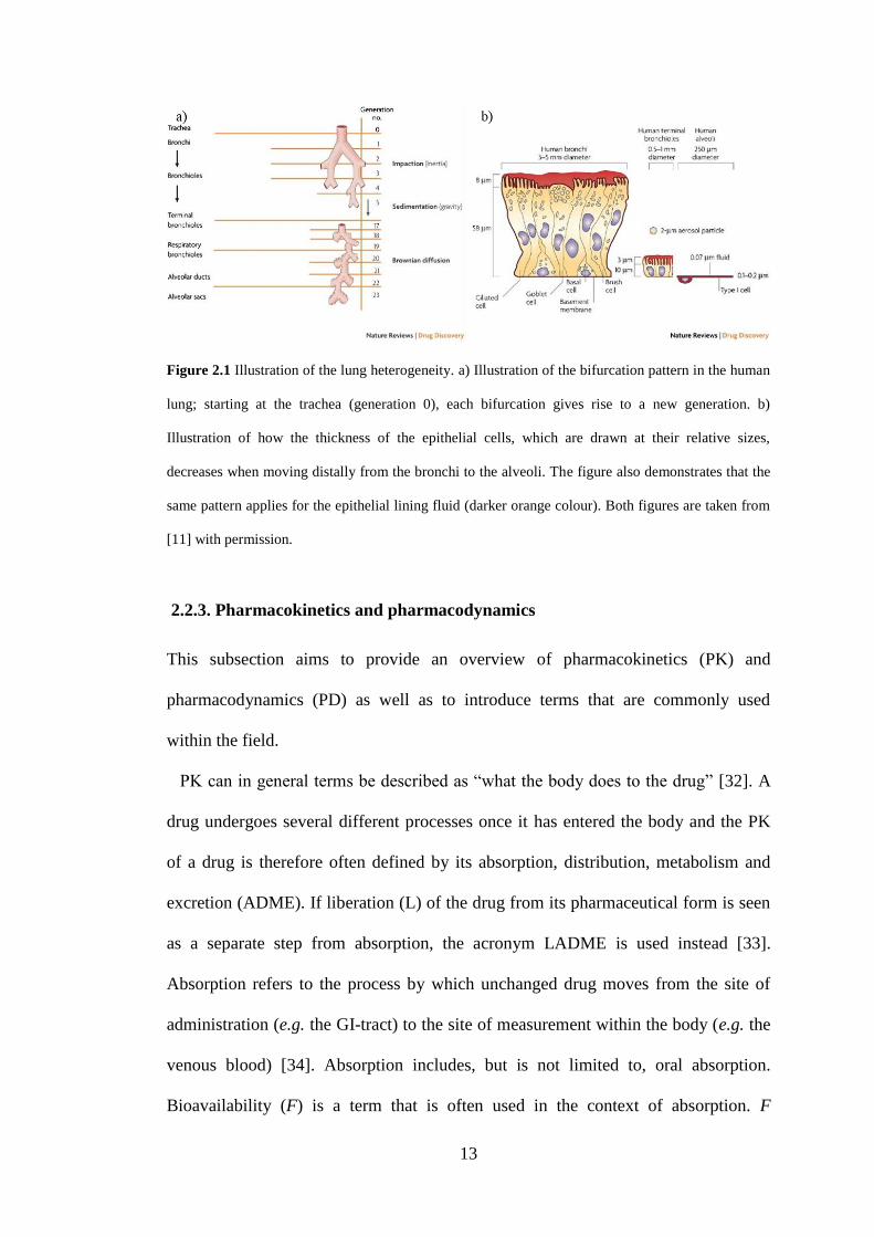
The lung is considered to be a complex and heterogeneous organ [28] with distinct

regional differences. Moving from the trachea to the alveolar region, both the type of

epithelium and its thickness will change. In humans, the thickness of the epithelium

decreases from 58 µm in the bronchi to 0.1-0.2 µm in the alveoli [11]. In rats, the

bronchi epithelium thickness is 13 µm [29]. Likewise, there are also distinct

differences in both the composition and the thickness of the lung wall [30]. The same

principle applies for the epithelial lining fluid (ELF), which is a thin fluid layer that

covers the epithelial surface. The ELF also becomes thinner throughout the lung;

ranging from 8 µm in the human bronchi and gradually decreasing until reaching a

final value of 0.07 µm in the alveoli [11]. The heterogeneity of the lung epithelium

and the decreasing thickness of the ELF are both illustrated in fig 2.1b from [11].

The ELF is slightly acidic (pH 6.6) and mainly consists of water (96%), salts,

phospholipids, protein and mucins [4]. Its composition is held to vary between

different lung regions. Nevertheless, this information is incomplete due to the

technical challenges associated with sampling the ELF from different regions [31].

13

Figure 2.1 Illustration of the lung heterogeneity. a) Illustration of the bifurcation pattern in the human

lung; starting at the trachea (generation 0), each bifurcation gives rise to a new generation. b)

Illustration of how the thickness of the epithelial cells, which are drawn at their relative sizes,

decreases when moving distally from the bronchi to the alveoli. The figure also demonstrates that the

same pattern applies for the epithelial lining fluid (darker orange colour). Both figures are taken from

[11] with permission.

2.2.3. Pharmacokinetics and pharmacodynamics

This subsection aims to provide an overview of pharmacokinetics (PK) and

pharmacodynamics (PD) as well as to introduce terms that are commonly used

within the field.

PK can in general terms be described as “what the body does to the drug” [32]. A

drug undergoes several different processes once it has entered the body and the PK

of a drug is therefore often defined by its absorption, distribution, metabolism and

excretion (ADME). If liberation (L) of the drug from its pharmaceutical form is seen

as a separate step from absorption, the acronym LADME is used instead [33].

Absorption refers to the process by which unchanged drug moves from the site of

administration (e.g. the GI-tract) to the site of measurement within the body (e.g. the

venous blood) [34]. Absorption includes, but is not limited to, oral absorption.

Bioavailability (F) is a term that is often used in the context of absorption. F

14

describes the extent of drug absorption and is defined as the fraction of the

administered dose that reaches the systemic circulation in an unchanged form [35]. F

following oral absorption can be written as

habsgut fffF . (2.1)

That is, F accounts for the fraction absorbed from the GI-tract (fabs), the fraction that

escapes from gut (fgut) and hepatic extraction (fh). The fgut of a drug can be caused by

luminal degradation, efflux transporters and/or gut metabolism. The fraction of

absorbed drug that has escaped gut extraction (i.e. fabs×fgut) will initially enter the

liver via the portal vein, where a fraction of the drug can be metabolised prior to

reaching the systemic circulation. The hepatic extraction ratio, EH, thus accounts for

the so-called hepatic first-pass extraction and is dependent on the extent of

metabolism in the liver [36]. EH can also be written as

hH fE 1 . (2.2)

The process by which a drug is reversibly transferred from one location to another

within the body is referred to as distribution [37]. The rate and extent of distribution

of a particular drug to various organs is dependent on several factors including

binding within blood and tissue, lipid solubility and regional blood flow [35]. At

equilibrium, the extent of distribution in the body is described by the apparent

volume of distribution (Vd), which is calculated by

15

p

bd

C

AV , (2.3)

where Ab is the amount of drug in the body and Cp is the plasma concentration of the

drug [34]. Expressed differently, Vd can be seen as a theoretical volume that would

have been required to obtain the drug concentration that was measured in plasma

given the amount of drug in the body.

The amount of drug in the body will decline with time as a result of drug

elimination, which can take place via two different processes: metabolism and

excretion. Metabolism, which describes an enzyme-catalysed conversion of a drug

into its metabolites [35], can take place in several organs. Nevertheless, the liver has

the highest metabolic capacity and is therefore generally the major site for

metabolism [37]. Metabolism, or biotransformation, can be divided into two different

phases. Phase I involves enzymatic reactions that change the parent compound by

oxidation, reduction or hydrolysis. The resulting metabolite may or may not be

pharmacologically active. The role of phase I is generally to create derivatives

amenable to phase 2 biotransformation, in which the molecules undergo conjugation

reactions. Phase 2 makes the molecule more hydrophilic and thus more easily

excreted. Excretion describes the different processes by which a molecule or its

metabolite is eliminated from the body. The major excreting organ is the kidney [35].

An essential term within the field of PK that is used for evaluating the elimination of

drug is clearance (CL), which relates the drug concentration (C) to the rate of

elimination (RoE) [34]:

CCL RoE . (2.4)

16

If C refers to the plasma or blood concentration of drug, CL describes either the

plasma or blood clearance, respectively (the concentration in these two biological

matrices are not necessarily equal) [37].

Another concept worthwhile introducing is the area under the curve (AUC), which

is the definite integral of the plasma/blood concentration of drug as a function of

time (C(t)) in the interval [a, b], i.e.

b

a

dttCAUC )( . (2.5)

Generally, one of the two following time intervals are used: [0, 24] or [0, ∞] h.

PD can be described as “what the drug does to the body” [32]. More formally, in

[38] it is defined as “the study of the biologic effects resulting from the interaction

between drugs and biologic systems”. Hence, PK describes the drug-concentration

time course that follows after administration of a certain dose and PD describes the

pharmacological effect that results from a certain drug concentration.

Clearly, it is important to understand the link between PK and PD, which can be

done by PK/PD-modelling. PK/PD-models aim to describe the effect-time course

that results from administration of a certain drug dose [39]. Such models can be of

great value both in drug discovery and drug development. Preclinically, they can, for

instance, be used to select the most promising drug candidate to test in humans.

PK/PD-modelling has several applications in drug development, including assisting

in the design of clinical trials by, for instance, selecting an optimal dose and

sampling scheme [40]. Over recent years, the discipline has progressed from using

empirical functions to purely describe the observed data to utilising mechanism-

based PK/PD-modelling. As opposed to just describing the data, the latter aims to

17

quantitatively describe the underlying principles of the pharmacology, of the

physiology and of the pathology. By virtue of relying on actual mechanisms, such

models are expected to have a better predictive capability [41].

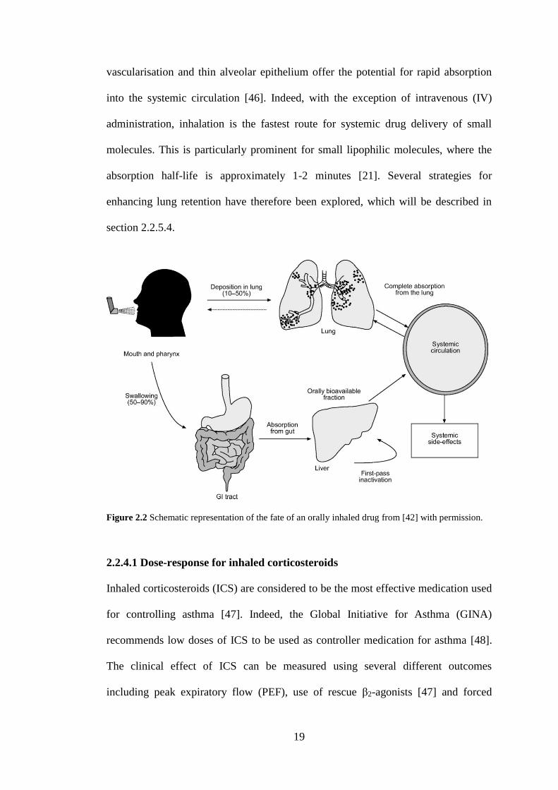
2.2.4 Systemic and local PK after inhaled drug delivery

Figure 2.2 from [42] shows a schematic representation of the PK for an orally

inhaled drug. In patients, inhalation devices are used to deliver the drug directly to

the lung whilst animal studies typically rely on tidal breathing. After inhalation, a

large fraction of the dose will deposit in the mouth and the pharynx. Given that this

portion of the dose is not completely rinsed out of the mouth by the patient, it may be

swallowed and reach the GI-tract. The swallowed dose will thus be treated by the

body as an oral dose with the potential of being absorbed from the GI-tract.

Absorbed drug that escapes first-pass metabolism in the liver will reach the systemic

circulation in an unchanged form, potentially increasing the risk of systemic side-

effects [18]. A fraction of the delivered dose will deposit in the lung, where it will

have to be dissolved in the ELF prior to absorption to the pulmonary/systemic

circulation [15]. The deposited drug will also be subject to a self-cleansing

mechanism called mucociliary clearance (MCC), which acts by transporting particles

from the airways towards the pharynx, where they subsequently can be swallowed

and reach the GI-tract [8]. Although not included in figure 2.2, solid drug particles

deposited in the alveolar region may be phagocytosed by alveolar macrophages.

However, this is a slow process that might take weeks or months to complete [43].

Accordingly, given that the drug is orally bioavailable, the resulting plasma PK is a

result of parallel absorption from the lung and the GI-tract.

18

Hence, the total amount of drug that will reach the systemic circulation after

inhalation will be dependent on the absorption from both the GI-tract and the lung as

well as on the ability of the lung to remove the substance. The latter includes

clearance in terms of MCC or macrophage uptake as well as metabolic processes.

However, the lung has low levels of metabolising enzymes. In fact, the total

cytochrome P450s (CYP) content constitutes only 1% of the corresponding value in

the liver. Thus, the lung is only expected to play a minor role in the metabolism

process compared with the liver. Interestingly, the relatively low metabolic capacity

combined with the large surface area of the lung has also lead to a widespread

interest in using inhalation for the systemic delivery of drugs [7]. In these instances,

the lung is seen as an entry port to the systemic circulation rather than as the target

organ for the pharmacological effect.

In contrast, when the pulmonary route is used for direct treatment of disease

localised in the lung, the focus is on improving the benefit-safety ratio by

maximising the pulmonary and minimising the systemic unbound drug exposure

[45]. From the description above, it becomes clear that the level of

pharmacologically active drug in the lung will be the result of several complex and

simultaneously occurring processes including, but not restricted to, MCC, the

dissolution rate of solid particles (if applicable) and flux to/from the systemic

circulation.

In order to minimise the systemic exposure, and thus the systemic side-effects,

drug discovery typically aims to develop inhaled drugs with high hepatic clearances

and low oral bioavailabilities in order to obtain rapid elimination and to avoid

absorption from the GI-tract [5]. Nevertheless, achieving lung-selective drug

exposure after inhalation is not a trivial task. The large surface area, good

19

vascularisation and thin alveolar epithelium offer the potential for rapid absorption

into the systemic circulation [46]. Indeed, with the exception of intravenous (IV)

administration, inhalation is the fastest route for systemic drug delivery of small

molecules. This is particularly prominent for small lipophilic molecules, where the

absorption half-life is approximately 1-2 minutes [21]. Several strategies for

enhancing lung retention have therefore been explored, which will be described in

section 2.2.5.4.

Figure 2.2 Schematic representation of the fate of an orally inhaled drug from [42] with permission.

2.2.4.1 Dose-response for inhaled corticosteroids

Inhaled corticosteroids (ICS) are considered to be the most effective medication used

for controlling asthma [47]. Indeed, the Global Initiative for Asthma (GINA)

recommends low doses of ICS to be used as controller medication for asthma [48].

The clinical effect of ICS can be measured using several different outcomes

including peak expiratory flow (PEF), use of rescue β2-agonists [47] and forced

20

expiratory volume (FEV) [49]. Meta-analyses of clinical studies investigating the

effect(s) of ICS in asthma have shown that although ICS demonstrate a clinical

benefit versus placebo, the dose-response curve for efficacy measurements is

relatively flat. This is in contrast to the dose-response curve for side-effects, which

has been reported to be steep [49,50]. However, due to paucity of data, the meta-

analysis described in [50] could not investigate the effect of dose on systemic side-

effects such as hypothalamo-pituitary axis function. The analysis instead focused on

local side-effects related to deposition of ICS in the oropharynx. In [49] a steep dose-

response relationship was found for local side-effects and one of the included studies

reported significantly lower cortisol levels (systemic side-effect) after a high dose of

fluticasone propionate. References [47] and [51] also state that there is a steep dose-

response curve for systemic side-effects. Overall this implies that only a small

clinical benefit is expected from increasing the clinical ICS doses whilst the risk of

side-effects is considerably increased.

2.2.5 Pulmonary drug disposition after inhalation

2.2.5.1 Pulmonary drug dissolution and absorption

Compared with other routes of administration, there is only limited information on

the absorption of inhaled drugs. Generally, the epithelium is considered to constitute

the main barrier for absorption from the airway lumen [11]. It is worth noting that the

thickness of this cell barrier varies throughout the lung, starting at about 60 µm thick

columnar epithelia in the bronchi and then decreases along the lung generations until

reaching a final thickness of about 0.2 µm in the alveoli [4]. Due to differences both

in thickness and blood perfusion, regional differences in absorption rates might be

expected in different areas of the lung [15].

21

Drug molecules are absorbed across the epithelium both via passive and active

transport mechanisms. The process by which a molecule moves from a point with

higher concentration (e.g. the ELF) to a point with a lower concentration (e.g. the

submucosa) is referred to as passive diffusion. The drug transport of lipophilic

compounds across the cellular barriers is generally considered to rely on transcellular

diffusion, whereas hydrophilic compounds appear to rely on paracellular diffusion

[4]. Hydrophilic compounds can also be actively transported across cells [52] and

over the recent years there has been an increased interest in the role of drug

transporters in the lung [53]. Nevertheless, evaluation of the role of drug transporters

on pulmonary drug disposition does not fall within the scope of this thesis.

Experiments have shown that lipophilic compounds are rapidly absorbed from the

lung (absorption half-lives ranging from seconds to a few minutes), whereas

hydrophilic compounds are absorbed more slowly (absorption half-lives of about 1

hour). Interestingly, the absorption half-life did not appear to be dependent on logP

other than enabling the identification of two distinct groups in the data: hydrophilic

(logP < 0) and lipophilic (logP > 0). Another interesting finding was that within the

molecular weight range of 100-1000 Da there was no discernible trend of the

pulmonary absorption rate being size-dependent [21].

Before drug absorption can take place, the solid drug particles must firstly dissolve

in the ELF. The pulmonary dissolution rate will depend on different properties of the

drug, the formulation and the system (i.e. physiological and anatomical

characteristics). One important property is the solubility, which will depend on e.g.

the compound and the composition of the dissolution medium (i.e. the ELF). The

measured solubility will therefore be different depending on the choice of dissolution

medium. Although fluids have been specifically developed to mimic the ELF,

22

so-called simulated lung fluids, the lung has unique features that are considered

difficult to replicate in vitro [54]. To date, development of in vitro dissolution

methods predictive of the in vivo situation is therefore an ongoing challenge.

Moreover, as will be discussed in depth in section 2.2.5.4, a commonly used strategy

for enhancing lung retention is to develop poorly soluble drugs. Previous research

aiming to predict the in vivo dissolution rate in the GI-tract based on measurements

of the aqueous solubility have found poor in vitro-in vivo correlation for poorly

soluble compounds [55], which emphasises the need to choose a bio-relevant

dissolution medium for this particular compound class.

As mentioned in section 2.2.2, the total volume of ELF available for dissolving the

deposited drug particles is small. Moreover, the thickness of ELF gradually decreases

along the lung generations from 5 µm centrally [56] to 0.07 µm in the alveolar region

[11]. This suggests that the dissolution rate might be higher centrally. Nevertheless,

due to the complexity of the system other factors could actually lead to the opposite

behaviour [4].

As pulmonary drug dissolution has been speculated to be the rate-limiting process

for several inhaled compounds [15], there is a recognised need for further research in

this area.

As mentioned in section 2.2.4, the lung has a metabolic capacity that is low relative

to the corresponding capacity of the liver. For most inhaled compounds, pulmonary

metabolism is therefore not expected to largely influence the extent of pulmonary

absorption. However, the possible impact of metabolism in the target organ needs to

be considered on a drug-specific basis. This can be exemplified by the drug

beclomethasone dipropionate (BDP), which is rapidly metabolized by esterases in the

lung to its active metabolite 17-beclomethasone monopropionate [57].

23

The effect of pulmonary metabolism of different ICS has been investigated in vitro

in human precision-cut lung slices [58]. In this experiment, lung slices were

incubated with different ICS including FP and BDP for several hours to monitor the

concentrations of parent compound and metabolites over time. FP was shown to be

metabolically stable in this test system, i.e. no metabolites were found in the

incubation medium. In contrast, the levels of BDP decreased over time and

metabolites were detected in the medium. Hence, whilst some compounds might

unaffected by pulmonary metabolism, this study emphasises the importance of

considering the impact of this process on a drug-specific basis.

2.2.5.2 Regional drug deposition

After drug inhalation, the particles/droplets will deposit in different regions

throughout the lung, which is generally referred to as the pulmonary deposition

pattern. The optimal site for deposition is often reasoned to be dependent on the drug

target. For instance, delivery of drug to a lung region devoid of the receptor of

interest might result in a suboptimal response to the drug treatment [59]. As

mentioned in the previous section, absorption rates of drug might be expected to vary

throughout the lung [15]. Hence, different deposition patterns may be desired

depending on the aim of the treatment and/or knowledge of the target location. It is

therefore of interest to be able to predict the regional deposition pattern of inhaled

particles and particle deposition modelling is used for this purpose.

The deposition of inhaled particles depends on several factors including: 1) the

anatomy of the respiratory tract, 2) the respiratory physiology, and 3) the physics of

aerosol particles. All of these factors need to be considered in mathematical

deposition models. Due to the complexity of these factors, most models make

24

simplifying assumptions related to e.g. the structure of the respiratory tract, the

airflow rate and the breathing pattern [60].

In short, an anatomical model is used to provide a geometric description of the

airway structure. A commonly used anatomical model type is the so-called “single-

path” model. In this model type, all airways in a given airway generation have

identical dimensions. This feature leads to identical pathways of the inhaled particles

travelling from the nose to the alveoli. Expressed differently, all pathways can be

represented by a single path [61]. Two important respiratory parameters used as input

for predicting regional particle deposition are the breathing frequency (fbr), i.e. the

number of breaths per minute, and the tidal volume (VT), i.e. the volume of air that is

inspired in a single breath during normal breathing conditions. Both fbr and VT

depend on the level of physical activity [61], which thus will have an impact on the

deposition pattern. Another important parameter is the particle velocity (u), which

will decrease distally throughout the lung. As a result of the lower velocities in the

distal parts, particles have longer mean residence times peripherally.

One of the most important parameters for determining regional drug deposition is

the aerodynamic diameter (da) of the aerosol particle [59]. The da is defined as the

diameter of a unit density sphere that would have the same aerodynamic behaviour as

the particle in question. The da can be calculated by

p

ga dd , (2.6)

where dg is the geometric diameter of the particle, ρp is the density of the particle and

χ is a dynamic shape factor that can be used if da needs to be modified to account for

25

shape irregularity. That is, the value χ depends on the shape of the particle; e.g. χ is

1.00 and 1.08 for spheres and cubes, respectively [62]. Expressed differently,

particles with the same da can have different shapes and densities.

There are several mechanisms by which a particle can be forced to leave the stream

of inhaled air and deposit in the airways. Three main mechanisms are: 1) inertial

impaction, 2) gravitational sedimentation, and 3) Brownian diffusion [61]. Each of

these mechanisms will be described below and they are graphically illustrated in

figure 2.3, which is taken from [63].

As a result of inertia, a particle may not be able to follow the air streamline when

the curvature of the airway is changing, but it instead continues along its initial

trajectory. The Stokes number (Stk) is a dimensionless parameter that can be used to

characterise inertial impaction. Stk is the ratio of the particle’s relaxation time tr (the

time it takes for a particle to reach equilibrium with a new set of forces acting on it,

i.e. the time it takes to respond to the changes in the local flow) to the time taken to

flow past an obstacle. Stk can therefore be seen as a measure of how rapidly a

particle can adjust to changes in the flow field. A small Stk implies that the particle

closely follows the streamlines while a large Stk implies that the particle takes a

longer time to adjust to the flow distortion; i.e. it might deviate from the streamline

and deposit due to its inertia [64]. If the characteristic length of the obstacle is set to

the radius of the airway (Di/2), the Stk can be calculated by [65,66]

i

ia

i

iri

D

ud

D

utStk

95.0

2

0 , (2.7)

where Stki is Stokes number in generation i, ρ0 is the unit particle density (1 g/cm3),

da is the aerodynamic diameter, η is the viscosity of air and Di is the diameter of the

26

airway in generation i. From eq. 2.7 it is thus evident that large particles with high

velocities will have higher Stk and thus be more prone to inertial impaction. Hence, it

follows that inertial impaction is most effective for large particles in the upper airway

generations [61].

Deposition due to gravity is referred to as gravitational sedimentation. Deposition

by this mechanism is e.g. dependent on the residence time in the airway (ti) and the

gravitational settling velocity (vg), which can be calculated as

18

2

0 gdgtv a

rg , (2.8)

where ρ0 is the unit particle density (1 g/cm3) and g is the acceleration due to gravity.

From eq. 2.8 it is clear that vg increases rapidly with particle size as it is proportional

to the square of da. However, eq. 2.8 is only valid for larger particles unless the

Cunningham slip correction factor (Cd) is used. Therefore, eq. 2.8 can be rewritten as

[65,66]

18

2

0 dag

gCdv , (2.9)

with [65]

ad

a

d ed

C55.0

8.0514.21 , (2.10)

where λ is the mean free path of air molecules. As the deposition efficiency by

gravitational sedimentation increases with ti and vg [67], deposition by this

27

mechanism is important for larger particles in the distal lung regions where ti is

longer.

The third deposition mechanism that is generally accounted for by deposition

models is Brownian diffusion. When fine particles are suspended in air, collisions

with the surrounding gas molecules will cause the particles to wobble randomly. This

random motion of particles suspended in a gas is referred to as Brownian motion and

it may cause a particle to randomly deviate from the streamline and deposit on the

airway wall [60]. As the Brownian diffusion coefficient (Dmol) is inversely

proportional to the particle size, this mechanism is particularly important for smaller

particles. Dmol is calculated as [65,66]

d

TCkD dB

mol3

, (2.11)

where kB is the Boltzmann constant and T is the absolute temperature. Like

gravitational sedimentation, a prolonged ti increases the probability of deposition by

this mechanism. Brownian diffusion is thus the predominant deposition mechanism

for smaller particles in the alveolar region [61].

Several different analytical equations have been published for calculating the

deposition probability by each of these three mechanisms in cylindrical airways [61].

As can be understood from the description of each mechanism above, the probability

of particle deposition by each mechanism will vary over the different lung

generations. The resulting deposition probability of a particle in generation i (Pi) is

given by [68]

28

)1)(1)(1(1 ,,, idisiimi DEDEDEP , (2.12)

where DEim,i, DEd,i and DEs,i are the probabilities of particle deposition by inertial

impaction, Brownian diffusion and gravitational sedimentation, respectively. When

eq. 2.12 is combined with the inhaled air volume passing through each generation i

as well as the fraction of particles already deposited in the preceding lung

generations, the particle deposition in generation i (DEi) can be calculated during the

inhalation phase. The value of DEi can be calculated for each of the three stages of a

breath: inhalation (DEiin), breath-holding (DEi

b) and exhalation (DEiex) [66]. The

total deposition (DEitot) during a breath is subsequently given by

ex

i

b

i

in

i

tot

i DEDEDEDE . (2.13)

Some models developed for rats exclude the breath-holding phase since this interval

is short compared to the breathing-phase [65]. Generally, the particle deposition is

reported for larger lung regions rather than an individual lung generation. The

deposition in a lung region (DEregion) between region j and k is then defined as

k

ji

ex

i

b

i

in

iregion DEDEDEDE )( . (2.14)

The resulting deposition fraction in a certain region (DFregion) is subsequently

obtained by dividing the amount of deposited drug in a predefined region (eq. 2.14)

by the amount inhaled.

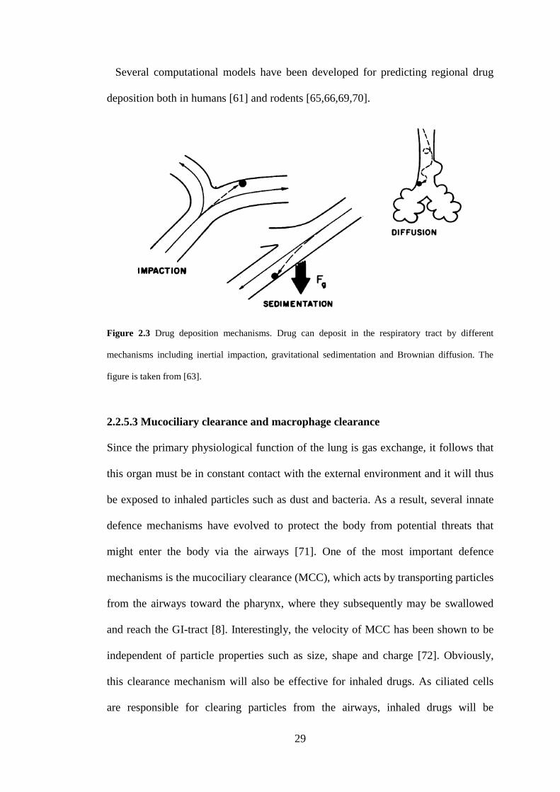
29

Several computational models have been developed for predicting regional drug

deposition both in humans [61] and rodents [65,66,69,70].

Figure 2.3 Drug deposition mechanisms. Drug can deposit in the respiratory tract by different

mechanisms including inertial impaction, gravitational sedimentation and Brownian diffusion. The

figure is taken from [63].

2.2.5.3 Mucociliary clearance and macrophage clearance

Since the primary physiological function of the lung is gas exchange, it follows that

this organ must be in constant contact with the external environment and it will thus

be exposed to inhaled particles such as dust and bacteria. As a result, several innate

defence mechanisms have evolved to protect the body from potential threats that

might enter the body via the airways [71]. One of the most important defence

mechanisms is the mucociliary clearance (MCC), which acts by transporting particles

from the airways toward the pharynx, where they subsequently may be swallowed

and reach the GI-tract [8]. Interestingly, the velocity of MCC has been shown to be

independent of particle properties such as size, shape and charge [72]. Obviously,

this clearance mechanism will also be effective for inhaled drugs. As ciliated cells

are responsible for clearing particles from the airways, inhaled drugs will be

30

subjected to MCC in the ciliated parts of the airways (unless the particles are readily

dissolved) [73]. Consequently, MCC can reduce the pulmonary bioavailability after

inhalation and this effect is expected to be more pronounced for slowly dissolving

drugs.

MCC is primarily associated with the tracheobronchial region [74], however, there

is another innate defence mechanism in the peripheral parts of the lung. Solid drug

particles deposited in the alveolar region may be phagocytosed by alveolar

macrophages. Nevertheless, this is a slow process that might take weeks or months to

complete [43]. It is hypothesised that some of these macrophages might migrate to

the ciliated terminal bronchioles, where they are subsequently cleared from the lung

via MCC [74].

2.2.5.4 Strategies for enhancing lung retention

Regardless of route of administration, it is crucial to develop drugs with appropriate

effect duration. Clearly, there are no general rules defining either the desired level or

the duration of effect of a drug, but these need to be evaluated on a case-by-case

basis for each drug target and disease. Nevertheless, it is often desirable to have an

efficacious response throughout the entire dose interval. Once-daily is generally the

preferred dosing regimen since this is convenient for the patient. As a result, it is

important to design locally acting inhaled drugs such that sufficiently high

concentrations can be obtained throughout the entire dosing interval . As previously

described in section 2.2.4, depending on drug properties, inhaled drugs might be

rapidly absorbed to the systemic circulation. Achieving a sustained lung exposure is

therefore not a trivial task and several different strategies have been explored for

enhancing lung retention of inhaled drugs.

31

One commonly used strategy to prolong the pulmonary residence time is to

develop drugs with a low solubility in order to reduce the dissolution rate. Indeed, a

low aqueous solubility has been demonstrated to give a prolonged lung retention

preclinically . Two poorly soluble inhaled compounds are fluticasone propionate

(FP) and BDP. Clinical data have shown that the average pulmonary absorption time

of FP (5-7 h) is considerably longer compared with more soluble ICS such as

budesonide and triamcinolone acetonide (2.9 and 1 h, respectively) [11]. The

prolonged absorption time has been suggested to be caused by the slow dissolution of

FP [75]. Moreover, the absorption across membranes is a rapid process for lipophilic

ICS, which further strengthens the hypothesis of dissolution rate-limited absorption

[76]. This approach is thus well-known for yielding high lung concentrations as well

as a prolonged lung retention. Even so, there are potential caveats with this strategy.

One important factor to bear in mind when considering using this approach is that

undissolved drug cannot elicit a pharmacological response. Moreover, solid drug

particles will be removed by MCC . Hence, this is a strategy that elucidates the

importance of understanding the complex interplay between different pulmonary

processes; more research is needed to understand what compound- and formulation-

specific properties are required for this strategy to be advantageous.

Another approach that is commonly used to obtain lung retention is to chemically

design the inhaled compounds to be bases. Cooper et al. [7] showed that the ion class

strongly influences lung retention. A comprehensive data set was generated

preclinically, where the amount of drug remaining in the lung was monitored after

intratracheal instillation of dissolved compounds belonging to different ion classes.

The researchers noted that the compounds could be broadly grouped by ion class: 1)

neutral, acidic and zwitterionic compounds tended to have a generally short

32

pulmonary half-life (t½,lung), 2) basic compounds had an intermediate t½,lung, and 3) di-

bases had a long t½,lung. One potential explanation for this phenomenon is lysosomal

trapping. The working hypothesis is that basic compounds are sequestered in

lysosomes, i.e. this organelle can be seen as a subcellular drug reservoir which then

acts like a slowly eluting pool. Lysosomal trapping has been demonstrated to take

place in vitro in lung slices [77]. However, to the best of my knowledge, the kinetics

of this process has not yet been characterised in the literature.

The lung retention of the ICS budesonide is held to rely on a completely different

mechanism. Reversible fatty acid esterification of the molecule has been found to

take place intracellularly, which results in an intracellular reservoir of inactive drug.

The ester, budesonide-oleate, will then be hydrolysed back to its active form as the

intracellular concentration of free budesonide decreases. The ester is thus suggested

to act like an intracellular depot of budesonide, which would prolong lung retention

of the molecule. This reasoning may be supported by the following observations: 1)

the esterification is a rapid process, 2) a large fraction of the molecules (70-80%) was

found to be in the esterified form in the central airways after intratracheal

administration of the compound [78], and 3) preclinical PK-studies have shown that

similar tissue concentrations of budesonide-oleate and budesonide are obtained after

IV-administration and inhalation of the parent compound [79].

Another approach that has been speculated to drive lung- and effect duration is a

slow dissociation rate from the receptor. Some inhaled drugs are held to have this

property, e.g. in vitro experiments have shown a slow drug-receptor dissociation rate

for FP. Högger and Rohdewald state that the long half-life of the drug-receptor

complex might provide a scientific rationale for the dosing interval of FP. However,

they also emphasise that in vitro dissociation rates are not necessarily translatable to

33

the in vivo situation [80]. Nevertheless, in order to use this strategy it is crucial to

understand if sufficiently high unbound concentrations can be obtained at the lung

target site prior to the drug is being absorbed to the systemic circulation and/or

cleared from the lung.

To summarise, several different strategies can be used for enhancing lung retention

of inhaled drugs. From the literature review it is also clear that a more thorough

mechanistic understanding is desirable to enable informed decisions about the choice

of strategy.

2.2.6 Preclinical inhalation studies

2.2.6.1 Inhalation pharmacokinetic studies in drug discovery

In drug discovery, several different methodologies can be employed for studying

pulmonary drug delivery. These can roughly be divided into two different categories:

exposure methods and direct dosing methods.

Exposure methods rely on creating a controlled atmosphere of drug exposure.

Depending on how the test animals are exposed to the drug atmosphere, such

systems fall into different subcategories of whole-body exposure, nose-only

exposure, head-only exposure and specialised exposure methods. In this section, the

first two categories will be introduced.

In whole-body exposure, the test animal is placed in a chamber with a controlled

atmosphere of drug exposure. The methodology thus resembles environmental or

work-place exposure of potentially toxic vapours. The animals can be housed either

individually or in groups [81]. This methodology is straightforward from an

experimental perspective. Nevertheless, results from such studies might be difficult

to interpret since the entire animal is exposed to drug, which inevitably will lead to

34

contamination of the fur. This has the potential to confound the results in two

different ways. Firstly, in conjunction with blood sampling, there is a risk of the

samples being contaminated by drug from the fur. Secondly, as a result of the animal

cleaning process, the test subjects are likely to swallow compound from the

contaminated fur. The latter might cause substantial oral absorption of the drug. In

drug discovery, nose-only exposure studies are therefore generally favoured . In

contrast to whole-body exposure, such systems are designed to minimise fur- and

skin exposure of drug by only exposing the nose to the drug atmosphere. This can be

obtained by keeping each animal in a separate tube, which has an adjustable back

restraint preventing the animal from backing out. The tube is open at one end to a

chamber containing aerosolised compound. Thus, the opening has been designed

such that only the nose will protrude into the chamber. Nose-only exposure systems

are well suited for rodents, such as the rat, since they are obligate nasal breathers.

Furthermore, in comparison with whole-body exposure systems, a lower amount of

compound is required for conducting an inhalation study [81]. Perhaps the biggest

challenge associated with exposure methods in general is that the lung deposited

dose (LDD) cannot be directly measured, but instead needs to be estimated, which

will be discussed in detail in section 2.2.6.2.

In contrast to exposure methods, direct dosing via intratracheal (IT) instillation

offers the advantage of delivering a known amount of compound directly into the

lung. Moreover, much less compound is needed for such studies, making it attractive

for early drug discovery projects. IT-instillation is generally performed by inserting a

catheter into the trachea of an anesthetised animal. A small volume of the test

compound, either as solution or suspension, is subsequently injected through the

catheter into the lungs [81]. Clearly, there are distinct differences between exposure

35

methods and instillation. Whereas exposure methods provide a natural route of entry

to the lung, IT-instillation is an invasive delivery method. One of the most important

disparities between these two methods is the distribution of particles. As opposed to

exposure methods, which produce a relatively homogenous distribution of particles

throughout the lung, IT-instillation tends to result in a denser distribution centrally

compared to the peripheral regions as the drug is injected specifically at the site

where the opening of the catheter resides (i.e. in the central region). These regional

differences can have an impact on e.g. doses to certain cells and lung regions as well

as on the degree and site of systemic absorption. Another important aspect to bear in

mind is that IT-instillation bypasses deposition in the upper respiratory tract, i.e.

above the site of drug delivery. Moreover, prior to delivering a drug via the IT route,

it is important to carefully consider the choice of the instillation volume as well as

the vehicle used to solubilise or suspend the compound. A too large instillate volume

can potentially cause a too rapid mechanical clearance from the lung due to

coughing, which clearly would have an impact on the pulmonary PK. It is also

important to ensure that the vehicle does not have an influence on either the PD or

the PK [82].

Regardless of the experimental methodology used to study pulmonary drug

delivery in a preclinical setting destructive sampling is a necessity in order to obtain

measurements of lung concentrations. That is, the animal is euthanized in

conjunction with sampling and only one sample is obtained from each test subject.

Expressed differently, n animals are needed to create a concentration-time profile of

n observations. Interindividual variability in PK-parameters is thus expected to be

seen in such profiles. Equally important, variability in the delivered dose is expected

from inhalation PK studies that utilise exposure methods. Cooper et al. suggest that a

36

majority of the variability seen in such PK-studies can be attributed to interindividual

variability in the inhaled dose rather than in the PK parameters [7].

2.2.6.2 Dose estimation

As opposed to e.g. oral and intravenous drug delivery where the given dose is easily

controlled, dose estimation after inhalation is very complex. The same degree of

control can essentially be achieved in a preclinical setting if the drug is directly

instilled in the lung via the trachea (direct dosing methods). However, as mentioned

in the previous subsection, techniques such as IT-instillation generally generate a less

homogenous dose distribution throughout the lung.

In order to achieve a more uniform distribution in a preclinical setting, drugs can

be inhaled from a chamber that contains a cloud of material (exposure methods). The

total inhaled dose (ID) is defined as the total amount of drug that is inhaled by the

animal, whereas the lung deposited dose (LDD) is defined as the actual amount of

drug that is deposited in the lung. ID and LDD are calculated accordingly:

BW

DRMVCID

(2.15)

and

DFIDBW

DFDRMVCLDD

, (2.16)

where C is the concentration of substance in the air (mg/L), RMV is the respiratory

minute volume (L/min), D is the duration of exposure (min), BW is the body weight

(kg) and DF is the deposition fraction of the particles [83]. As can be seen from eqs.

37

2.15-2.16, several assumptions must be made in order to estimate LDD such as a

consistent breathing pattern throughout the dosing period.

From eqs. 2.15-2.16 it is also clear that C is a key value for calculation of LDD. To

enable calculation of C, a filter is included in the inhalation system setup.

Air/compound is extracted to the filter at a predefined flow rate throughout the

duration of exposure, D. The amount of drug collected on the filter (mfilter) is

subsequently quantified using, for instance, liquid chromatography-tandem mass

spectrometry (LC-MS/MS) and C is then calculated as

Dfr

mC

filter

, (2.17)

where fr is the filter flow rate [7].

It is well-known that different aerodynamic diameters have different deposition

probabilities in different lung regions, i.e. DF will be dependent on the particle size

distribution. Prior to preclinical inhalation studies, this distribution is generally

characterised using a cascade impactor, which provides a discrete aerodynamic

particle size distribution. By using this discrete distribution and the DF

corresponding to each particle size range, the total DF can be calculated for the batch

used in a particular study. In the absence of such data, a default value of DF of 10%

is generally used for deposition in rodent lungs [7]. 10% is also the conservative DF

used for inhalation rodent studies by the Food and Drug Administration (FDA) [84].

An alternative approach to determining LDD is to quantify the amount of drug in the

lung at the end of the exposure period. Under certain circumstances this method may

represent LDD. However, the following criteria need to be met: 1) the inhalation

period is short, 2) the pulmonary absorption that takes place from the start of the

38

exposure until the sampling of the lung is negligible, and 3) potential pulmonary

metabolism of the parent compound is negligible. If any of these criteria are not met,

then there is a substantial risk of underestimating LDD . Given that several

compounds are rapidly absorbed to the systemic circulation [21], this method is

inappropriate for numerous inhaled drugs. An alternative approach is to determine

the area under the curve (AUC) in blood/plasma following inhalation. By comparing

the AUC generated after inhalation of an unknown LDD with an AUC from a known

dose, e.g. obtained from IV-dosing, it is possible to calculate LDD. Nevertheless, this

approach also has its limitations. Firstly, if a poorly soluble drug is delivered, then

the drug is likely to be transported away from the lung by MCC, which would lead to

a reduction in the AUC relative to IV-delivery of the same dose. Secondly, drug

absorption from the GI-tract would increase the AUC after inhaled drug delivery

leading to overestimation of LDD. Thirdly, it is essential to assume a negligible first-

pass pulmonary extraction . Consequently, much prior information of the PK of the

drug candidate is needed to confidently rely on this approach.

To summarise, dose estimation is not straightforward after inhalation and the

method used for estimating LDD should be chosen with care based on prior

knowledge of the drug.

2.2.6.3 Exposure measurements

This subsection aims to provide an overview of the different exposure measurements

that are often collected in preclinical inhalation PK-studies. This text also aims to

underline potential limitations/challenges associated with the different

measurements.

39

The PK-properties of inhaled compounds are routinely investigated by

measurements of total lung concentrations (Clung) and plasma concentrations (Cp). It

is worth mentioning that measurements of Cp generally put high demands on the

analytical sensitivity due to low Cp-values . This can primarily be attributed to two

features: 1) inhalation doses are typically low, and 2) inhaled drug candidates tend to

have a high clearance. For this reason, it can be very challenging to properly

characterise the systemic PK after inhalation.

After inhalation, appearance of drug in plasma is a downstream event that follows

after pulmonary absorption [2]. The Cp-profile is thus expected to inherently contain

information on the pulmonary absorption, the events preceding the absorption as well

as on the systemic PK.

It is generally accepted that the unbound drug concentration at the target site drives

the pharmacological effect, a theory that often is referred to as ‘the free drug

hypothesis’ [85]. For systemically acting drugs, the unbound plasma concentrations

are usually assumed to reflect the free target site concentration. However, since the

appearance of drug in the systemic circulation is the result of pulmonary absorption,

unbound concentrations in plasma cannot be assumed to reflect the free target site

concentration in the lung [2]. This constitutes a challenge since unbound plasma

concentrations usually form the basis for establishing PK/PD-relationships.

As previously mentioned, it is possible to measure Clung in a preclinical setting. To

obtain such measurements, lungs are collected by destructive sampling at several

time points after IT-instillation or exposure inhalation. In most studies, the entire

lung is dissected and homogenised. Drug concentrations are subsequently measured

in lung tissue homogenates, providing a time profile of Clung where the organ is

erroneously reflected as one anatomical entity. Moreover, the homogenisation

40

process also severely distorts the data interpretation by disrupting the normal

compartmentalisation (e.g. lysosomal trapping) and by dissolving solid drug particles

[6]. Indeed, the establishment of PK/PD-relationships based on total lung

concentrations is known to be more challenging for poorly soluble compounds .

Great caution should thus be exercised when interpreting such data, especially for the

latter compound class.

As opposed to measurements of the fraction unbound in plasma (fu), it is

challenging from a technical point of view to measure the fraction unbound in lung

tissue (fu,lung) . Perhaps even more important, the information obtained from

measuring the fraction unbound in a heterogeneous organ, such as the lung, should

not be used in the same manner as fu since it is unlikely that one value would be

reflective of the entire organ. Expressed differently, fu,lung cannot be used to convert a

measured total organ concentration (i.e. Clung) into one unbound lung target site

concentration. Nevertheless, two different in vitro methodologies have previously

been employed for measuring the unbound fraction in lung homogenate (fu,h):

equilibrium dialysis and ultra-filtration. It is well-known that measurements obtained

from these two methods potentially are confounded due to the necessity to

homogenise the lung tissue, which disrupts the normal compartmentalisation of the

cells and thereby can release drug that was entrapped in lysosomes and/or other

endosomal compartments [77,84]. This experimental caveat needs to be taken into

account when interpreting data and it is particularly prominent for basic compounds.

Since lysosomes are acidic organelles, basic compounds are expected to be trapped

in these cellular compartments due to a higher proportion of the molecules being

charged in the acidic environment of the lysosome (pH 4-5) as compared to the

cytosol (pH 7.4). Furthermore, the lung is a lysosome-rich tissue [86] and lysosomal

41

trapping might therefore be even more pronounced in this tissue. To overcome this

potential experimental caveat, a lung slice methodology was developed, by virtue of

using freshly prepared rat lung slices, the compartmentalisation of the lung tissue is

kept intact. This can therefore be considered as a better in vitro system for studying

the extent of lung tissue distribution. The lung slice methodology provides

measurements of the unbound lung volume of distribution (Vu,lung). If Vu,lung and 1/fu,h

differ from unity, the deviation is likely to be caused by the investigated substance

being trapped in lysosomes and/or displaying carrier-mediated transport. Indeed, a

systematic deviation from unity has been demonstrated for several basic compounds

[77].

A procedure called bronchoalveolar lavage (BAL) is occasionally also used for

preclinical PK-investigations to estimate the drug concentration in the epithelial

lining fluid (ELF). This technique does not allow for direct measurements of ELF

alone, but it is retrieved indirectly by repeated instillation of sterile saline. That is,

technically the saline is diluted by an unknown volume of ELF. Thus a meaningful

quantification of the drug concentration in this fluid would require determination of

the volume of ELF obtained by BAL [84]. As urea diffuses freely throughout the

body, the concentration of urea is expected to be the same in plasma and ELF. By

using this knowledge, simultaneous measurements of urea in both fluids enables

calculation of the dilution factor. However, diffusion of urea into the BAL fluid

during the instillation has shown to confound this calculation in a time-dependent

matter. It has therefore been suggested that the volume of ELF obtained from using

this correction method should be referred to as an apparent volume of ELF [87].

Consequently, such measurements should also be interpreted with care.

42

Hence, there are several limitations with the different exposure measurements

currently used to characterise the PK and PK/PD of inhaled drugs. Clearly, under

many circumstances the utility of using the described exposure measurements for

establishing PK/PD-relationships for locally acting inhaled drugs can be questioned.

This problem is also reflected by the sparse scientific literature within the area of

inhaled drugs, where the focus instead is typically on systemic effects driven by

systemic exposure [88,89,90]. A few studies quantitatively link the pulmonary PK to

the local effect by relating ELF concentrations to minimum inhibitory concentrations

of antibiotics. This is, however, not following topical, but systemic, administration

[91,92]. Interestingly, a PK/PD-analysis by Hochhaus et al. suggested that cardiac

side-effects, but not the local pulmonary effects, could be described by the plasma

PK after inhalation. The analysis instead implied that the free concentrations of drug

were higher at the target site in the lung as compared to the plasma thus indicating a

lung-selective drug exposure [93].

To conclude, the lack of exposure measurements that are relevant from a PK/PD

perspective significantly hampers basic PK/PD understanding for locally acting

inhaled drugs. Besides, due to the heterogeneous nature of the lung, the unbound

concentration cannot be expected to be homogenous throughout the entire organ.

Further research within this field is thus an important avenue for drug discovery as

well as drug development.

2.3 Modelling

2.3.1 Empirical compartmental modelling (PK)

In the field of pharmacokinetics, empirical compartmental models are often used to

describe the concentration time-profiles that follow after drug administration. In

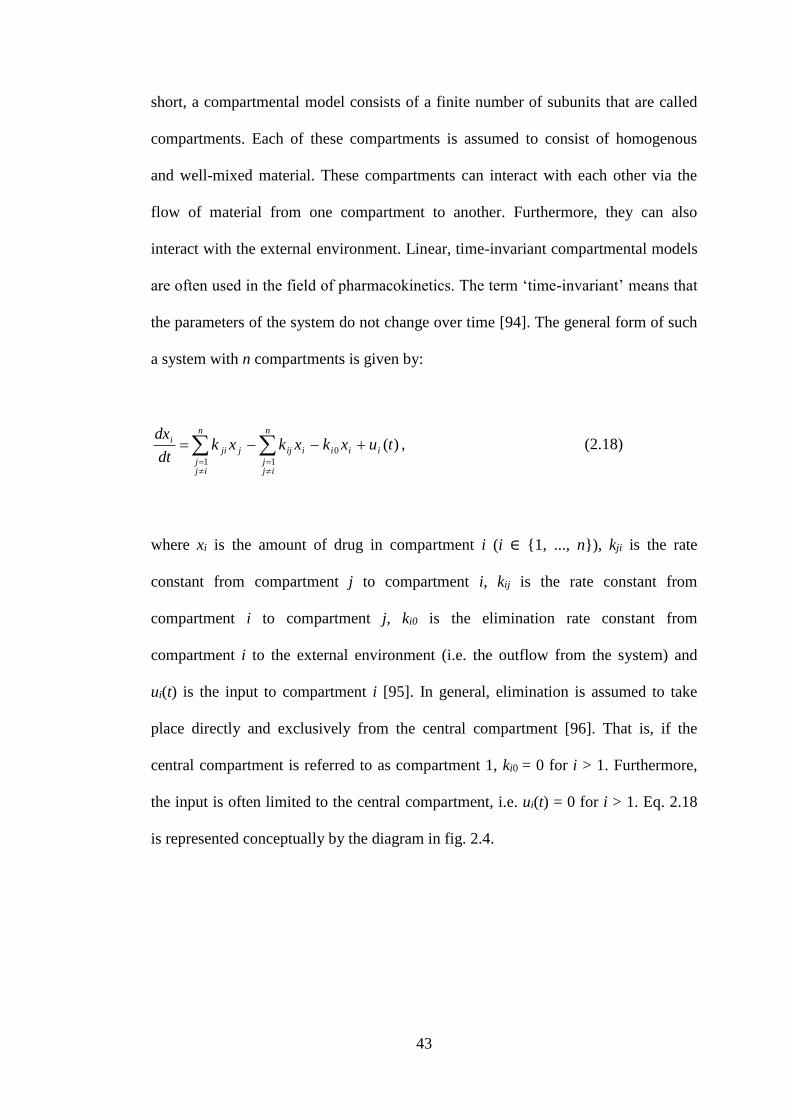
43

short, a compartmental model consists of a finite number of subunits that are called

compartments. Each of these compartments is assumed to consist of homogenous

and well-mixed material. These compartments can interact with each other via the

flow of material from one compartment to another. Furthermore, they can also

interact with the external environment. Linear, time-invariant compartmental models

are often used in the field of pharmacokinetics. The term ‘time-invariant’ means that

the parameters of the system do not change over time [94]. The general form of such

a system with n compartments is given by:

)(0

11

tuxkxkxkdt

dxiii

n

ijj

iij

n

ijj

jji

i

, (2.18)

where xi is the amount of drug in compartment i (i ∈ {1, ..., n}), kji is the rate

constant from compartment j to compartment i, kij is the rate constant from

compartment i to compartment j, ki0 is the elimination rate constant from

compartment i to the external environment (i.e. the outflow from the system) and

ui(t) is the input to compartment i [95]. In general, elimination is assumed to take

place directly and exclusively from the central compartment [96]. That is, if the

central compartment is referred to as compartment 1, ki0 = 0 for i > 1. Furthermore,

the input is often limited to the central compartment, i.e. ui(t) = 0 for i > 1. Eq. 2.18

is represented conceptually by the diagram in fig. 2.4.

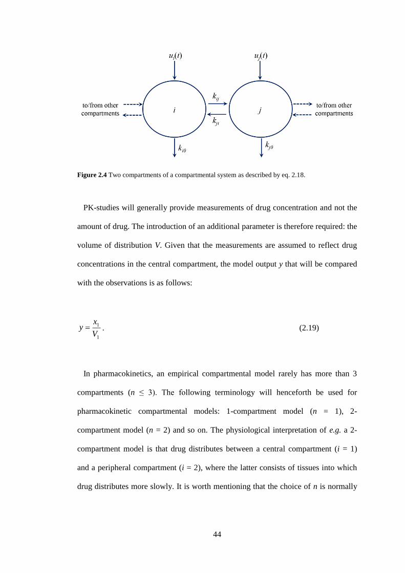
44

Figure 2.4 Two compartments of a compartmental system as described by eq. 2.18.

PK-studies will generally provide measurements of drug concentration and not the

amount of drug. The introduction of an additional parameter is therefore required: the

volume of distribution V. Given that the measurements are assumed to reflect drug

concentrations in the central compartment, the model output y that will be compared

with the observations is as follows:

1

1

V

xy . (2.19)

In pharmacokinetics, an empirical compartmental model rarely has more than 3

compartments (n ≤ 3). The following terminology will henceforth be used for

pharmacokinetic compartmental models: 1-compartment model (n = 1), 2-

compartment model (n = 2) and so on. The physiological interpretation of e.g. a 2-

compartment model is that drug distributes between a central compartment (i = 1)

and a peripheral compartment (i = 2), where the latter consists of tissues into which

drug distributes more slowly. It is worth mentioning that the choice of n is normally

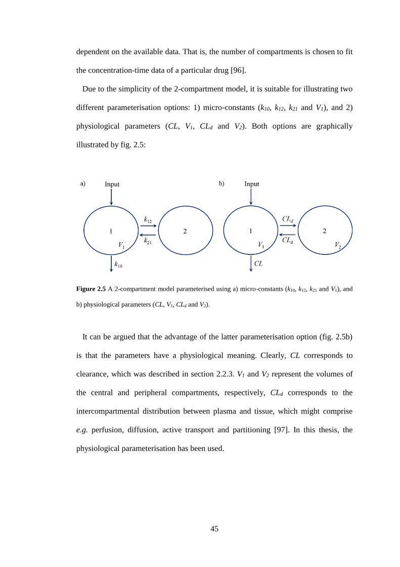
45

dependent on the available data. That is, the number of compartments is chosen to fit

the concentration-time data of a particular drug [96].

Due to the simplicity of the 2-compartment model, it is suitable for illustrating two

different parameterisation options: 1) micro-constants (k10, k12, k21 and V1), and 2)

physiological parameters (CL, V1, CLd and V2). Both options are graphically

illustrated by fig. 2.5:

Figure 2.5 A 2-compartment model parameterised using a) micro-constants (k10, k12, k21 and V1), and

b) physiological parameters (CL, V1, CLd and V2).

It can be argued that the advantage of the latter parameterisation option (fig. 2.5b)

is that the parameters have a physiological meaning. Clearly, CL corresponds to

clearance, which was described in section 2.2.3. V1 and V2 represent the volumes of

the central and peripheral compartments, respectively, CLd corresponds to the

intercompartmental distribution between plasma and tissue, which might comprise

e.g. perfusion, diffusion, active transport and partitioning [97]. In this thesis, the

physiological parameterisation has been used.

46

2.3.2 Physiologically based PK models

Within drug discovery, there is generally much information gathered about

individual drug candidates. In order to guide PK decisions physicochemical, in vitro

and/or structural properties are characterised. In addition, at later stages, emphasis is

put on studying in vivo PK of the compounds. Empirical compartmental models are

often used for analysing in vivo studies as described in the previous section. These

models are indeed very useful for many purposes, including characterisation of in

vivo PK and guidance of future study design. However, by virtue of being empirical,

these models cannot accommodate prior information on either the compound or the

physiology. This feature restricts their ability to predict the PK for compounds with

slightly different properties or to use such models for extrapolation to different

physiological conditions [55]. Hence, although much information is available only a

small fraction is used in the model development.

As opposed to the empirical compartmental models, physiologically-based

pharmacokinetic (PBPK) models aim to integrate the current knowledge of

physiological processes with physicochemical properties and/or other available

information about the drug candidate in order to simulate complex biological

processes. The level of detail is dependent on several factors, including nature and

knowledge of the process(es) studied and the level of complexity needed reach a

predictive capability. Hence, these models aim to provide a mechanistic

understanding of the system by mathematically describing the relevant processes and

integrating prior information on the drug. This approach carries advantages and there

are several examples of when they have been used to provide new insights into

important biological processes [98]. As observed PK-profiles are the result of several

underlying processes, they can be said to carry subtle information on different

47

mechanisms driving the PK. Any discrepancies between the predicted and observed

outcomes may therefore be informative as they can provide insights into mechanisms

that have not been accounted for by the model. As such, PBPK models can be used

for hypothesis generation, to design experiments aimed at supporting/rejecting the

hypothesis and to answer key questions in drug discovery and development projects

[99].

Traditionally, PBPK models have been said to consist of a structural model and

two distinctive groups of input parameters: 1) system-specific input parameters, such

as blood flows and organ volumes that are specific for the investigated species, and

2) drug-specific input parameters, such as permeability, clearance and binding

kinetics parameters that are unique for each investigated drug. The structural model

comprises a compartmental representation of organs and tissues connected by the

blood flow [100], where each compartment is represented by a discrete tissue volume

perfused uniformly by its specific blood flow [101]. A schematic representation of a

typical whole body PBPK model is shown in figure 2.6.

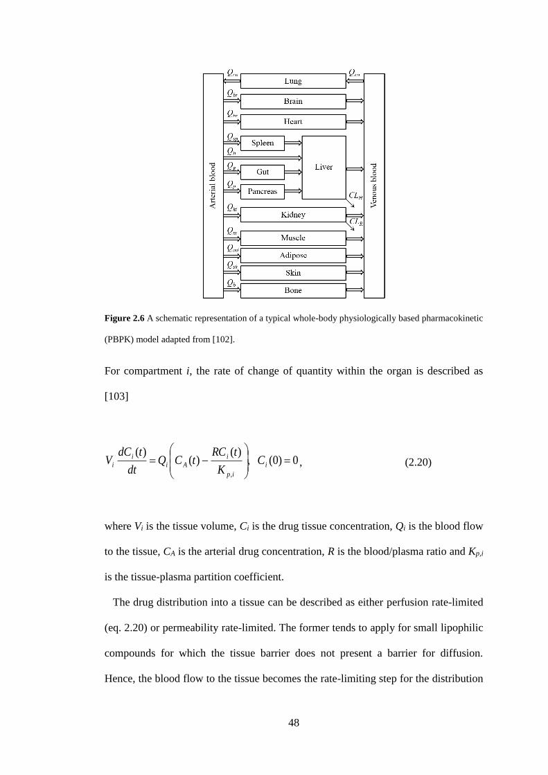
48

Figure 2.6 A schematic representation of a typical whole-body physiologically based pharmacokinetic

(PBPK) model adapted from [102].

For compartment i, the rate of change of quantity within the organ is described as

[103]

0)0( ,)(

)()(

,

i

ip

i

Ai

i

i CK

tRCtCQ

dt

tdCV , (2.20)

where Vi is the tissue volume, Ci is the drug tissue concentration, Qi is the blood flow

to the tissue, CA is the arterial drug concentration, R is the blood/plasma ratio and Kp,i

is the tissue-plasma partition coefficient.

The drug distribution into a tissue can be described as either perfusion rate-limited

(eq. 2.20) or permeability rate-limited. The former tends to apply for small lipophilic

compounds for which the tissue barrier does not present a barrier for diffusion.

Hence, the blood flow to the tissue becomes the rate-limiting step for the distribution

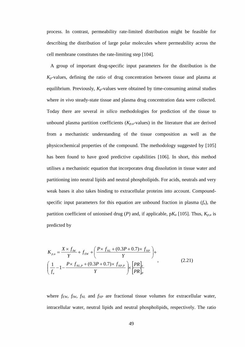
49

process. In contrast, permeability rate-limited distribution might be feasible for

describing the distribution of large polar molecules where permeability across the

cell membrane constitutes the rate-limiting step [104].

A group of important drug-specific input parameters for the distribution is the

Kp-values, defining the ratio of drug concentration between tissue and plasma at

equilibrium. Previously, Kp-values were obtained by time-consuming animal studies

where in vivo steady-state tissue and plasma drug concentration data were collected.

Today there are several in silico methodologies for prediction of the tissue to

unbound plasma partition coefficients (Kp,u-values) in the literature that are derived

from a mechanistic understanding of the tissue composition as well as the

physicochemical properties of the compound. The methodology suggested by [105]

has been found to have good predictive capabilities [106]. In short, this method

utilises a mechanistic equation that incorporates drug dissolution in tissue water and

partitioning into neutral lipids and neutral phospholipids. For acids, neutrals and very

weak bases it also takes binding to extracellular proteins into account. Compound-

specific input parameters for this equation are unbound fraction in plasma (fu), the

partition coefficient of unionised drug (P) and, if applicable, pKa [105]. Thus, Kp,u is

predicted by

P

TPNPPNL

u

NPNLEW

IWup

PR

PR

Y

fPfP

f

Y

fPfPf

Y

fXK

,,

,

)7.03.0(1

1

)7.03.0(

, (2.21)

where fEW, fIW, fNL and fNP are fractional tissue volumes for extracellular water,

intracellular water, neutral lipids and neutral phospholipids, respectively. The ratio

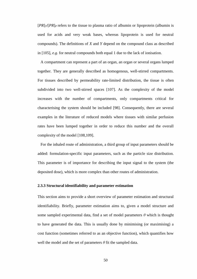
50

[PR]T/[PR]P refers to the tissue to plasma ratio of albumin or lipoprotein (albumin is

used for acids and very weak bases, whereas lipoprotein is used for neutral

compounds). The definitions of X and Y depend on the compound class as described

in [105], e.g. for neutral compounds both equal 1 due to the lack of ionisation.

A compartment can represent a part of an organ, an organ or several organs lumped

together. They are generally described as homogenous, well-stirred compartments.

For tissues described by permeability rate-limited distribution, the tissue is often

subdivided into two well-stirred spaces [107]. As the complexity of the model

increases with the number of compartments, only compartments critical for

characterising the system should be included [98]. Consequently, there are several

examples in the literature of reduced models where tissues with similar perfusion

rates have been lumped together in order to reduce this number and the overall

complexity of the model [108,109].

For the inhaled route of administration, a third group of input parameters should be

added: formulation-specific input parameters, such as the particle size distribution.

This parameter is of importance for describing the input signal to the system (the

deposited dose), which is more complex than other routes of administration.

2.3.3 Structural identifiability and parameter estimation

This section aims to provide a short overview of parameter estimation and structural

identifiability. Briefly, parameter estimation aims to, given a model structure and

some sampled experimental data, find a set of model parameters θ which is thought

to have generated the data. This is usually done by minimising (or maximising) a

cost function (sometimes referred to as an objective function), which quantifies how

well the model and the set of parameters θ fit the sampled data.

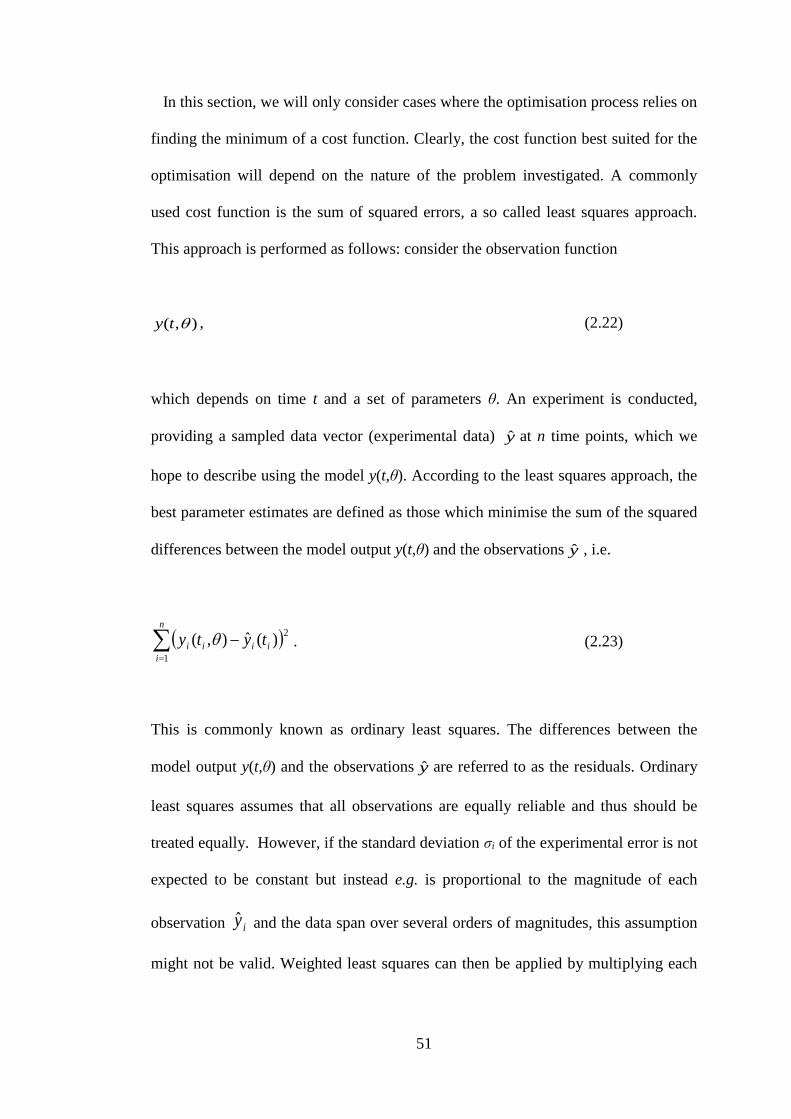
51

In this section, we will only consider cases where the optimisation process relies on

finding the minimum of a cost function. Clearly, the cost function best suited for the

optimisation will depend on the nature of the problem investigated. A commonly

used cost function is the sum of squared errors, a so called least squares approach.

This approach is performed as follows: consider the observation function

),( ty , (2.22)

which depends on time t and a set of parameters θ. An experiment is conducted,

providing a sampled data vector (experimental data) y at n time points, which we

hope to describe using the model y(t,θ). According to the least squares approach, the

best parameter estimates are defined as those which minimise the sum of the squared

differences between the model output y(t,θ) and the observations y , i.e.

n

i

iiii tyty1

2)(ˆ),( . (2.23)

This is commonly known as ordinary least squares. The differences between the

model output y(t,θ) and the observations y are referred to as the residuals. Ordinary

least squares assumes that all observations are equally reliable and thus should be

treated equally. However, if the standard deviation σi of the experimental error is not

expected to be constant but instead e.g. is proportional to the magnitude of each

observation iy and the data span over several orders of magnitudes, this assumption

might not be valid. Weighted least squares can then be applied by multiplying each

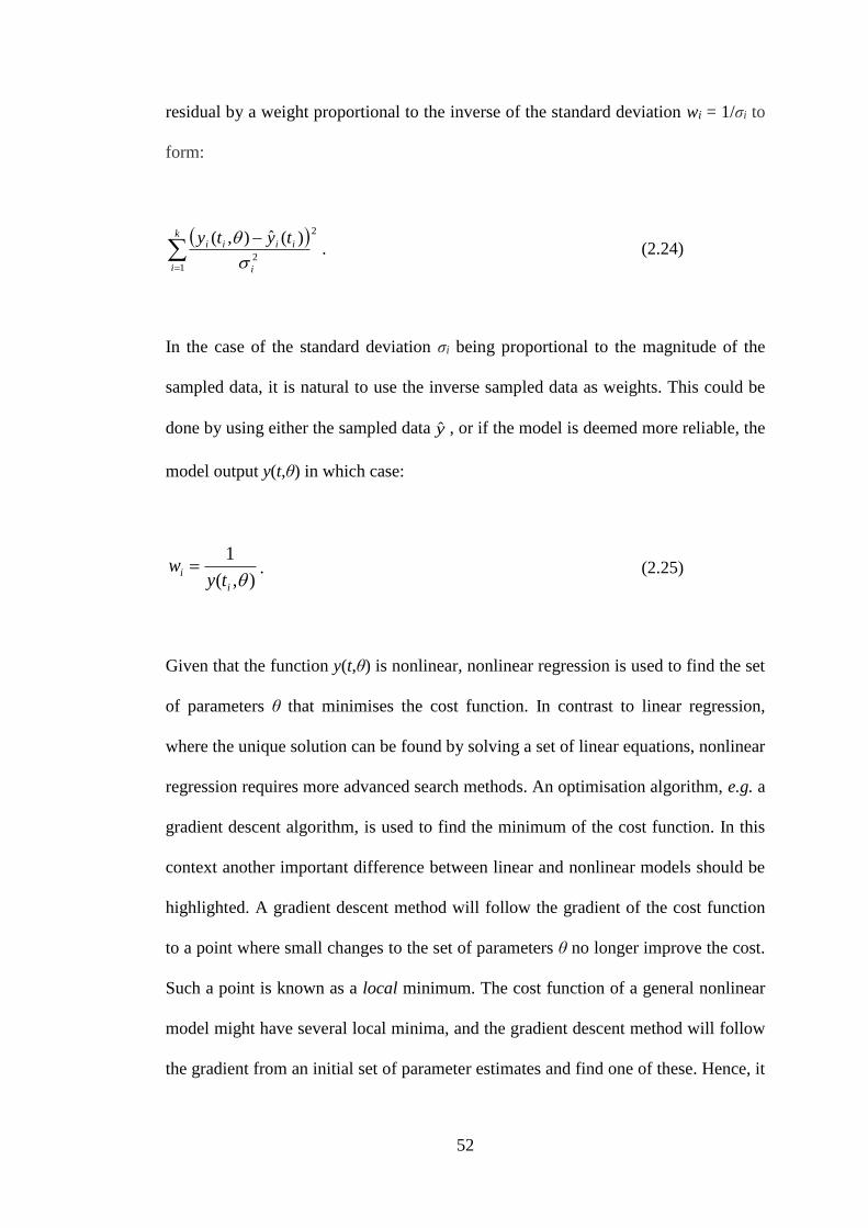
52

residual by a weight proportional to the inverse of the standard deviation wi = 1/σi to

form:

k

i i

iiii tyty

1

2

2

)(ˆ),(

. (2.24)

In the case of the standard deviation σi being proportional to the magnitude of the

sampled data, it is natural to use the inverse sampled data as weights. This could be

done by using either the sampled data y , or if the model is deemed more reliable, the

model output y(t,θ) in which case:

),(

1

i

ity

w . (2.25)

Given that the function y(t,θ) is nonlinear, nonlinear regression is used to find the set

of parameters θ that minimises the cost function. In contrast to linear regression,

where the unique solution can be found by solving a set of linear equations, nonlinear

regression requires more advanced search methods. An optimisation algorithm, e.g. a

gradient descent algorithm, is used to find the minimum of the cost function. In this

context another important difference between linear and nonlinear models should be

highlighted. A gradient descent method will follow the gradient of the cost function

to a point where small changes to the set of parameters θ no longer improve the cost.

Such a point is known as a local minimum. The cost function of a general nonlinear

model might have several local minima, and the gradient descent method will follow

the gradient from an initial set of parameter estimates and find one of these. Hence, it

53

will be unknown if it is the “best”, global minimum. The linear model on the other

hand will only have one minimum, which is then the global minimum.

Importantly, for parameter estimates to be meaningful, the aim of parameter

estimation needs to be extended: the aim is to find a set of uniquely identifiable

parameters θ that minimises (or maximises) an appropriately chosen cost function.

From this revised aim, it is clear that structural identifiability is a prerequisite for

parameter estimation. Briefly, a model is said to be structurally identifiable if it is

possible to uniquely determine all model parameters under ideal circumstances with

an error-free, continuous set of observations [110,111]. In case of a non-identifiable

model, several combinations of parameters will produce identical input-output

behaviours. Hence, whilst a non-identifiable model might well describe the data, the

parameter values estimated from such model should be interpreted very cautiously.

2.3.4 Sensitivity analysis

A sensitivity analysis can be used to quantify how “sensitive” the output of a system

is to changes in e.g. parameter values, initial conditions or inputs [112]. Such

analyses can be useful for several reasons. One important application is to understand

which parameters are the most influential on the outcome/response of the system.

Such information can be useful per se to gain a better understanding of the input-

output behaviour of the system. Moreover, if it is possible to minimise the

uncertainty of one/some of the input parameters, information from a sensitivity

analysis can be useful for prioritising which input parameter(s) to choose in order to

reduce the uncertainty of the output the most [113]. It can also be useful for optimal

experimental design by e.g. identifying sampling times that would generate

informative data, which is crucial for parameter estimation accuracy.

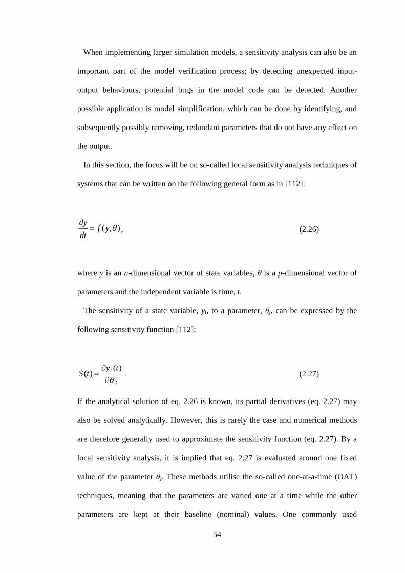
54

When implementing larger simulation models, a sensitivity analysis can also be an

important part of the model verification process; by detecting unexpected input-

output behaviours, potential bugs in the model code can be detected. Another

possible application is model simplification, which can be done by identifying, and

subsequently possibly removing, redundant parameters that do not have any effect on

the output.

In this section, the focus will be on so-called local sensitivity analysis techniques of

systems that can be written on the following general form as in [112]:

),( yfdt

dy , (2.26)

where y is an n-dimensional vector of state variables, θ is a p-dimensional vector of

parameters and the independent variable is time, t.

The sensitivity of a state variable, yi, to a parameter, θj, can be expressed by the

following sensitivity function [112]:

j

i tytS

)()( . (2.27)

If the analytical solution of eq. 2.26 is known, its partial derivatives (eq. 2.27) may

also be solved analytically. However, this is rarely the case and numerical methods

are therefore generally used to approximate the sensitivity function (eq. 2.27). By a

local sensitivity analysis, it is implied that eq. 2.27 is evaluated around one fixed

value of the parameter θj. These methods utilise the so-called one-at-a-time (OAT)

techniques, meaning that the parameters are varied one at a time while the other

parameters are kept at their baseline (nominal) values. One commonly used

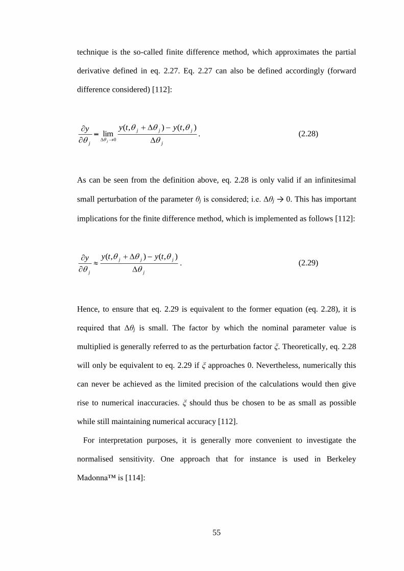
55

technique is the so-called finite difference method, which approximates the partial

derivative defined in eq. 2.27. Eq. 2.27 can also be defined accordingly (forward

difference considered) [112]:

j

jjj

j

tytyy

j

),(),(lim

0. (2.28)

As can be seen from the definition above, eq. 2.28 is only valid if an infinitesimal

small perturbation of the parameter θj is considered; i.e. Δθj → 0. This has important

implications for the finite difference method, which is implemented as follows [112]:

j

jjj

j

tytyy

),(),(. (2.29)

Hence, to ensure that eq. 2.29 is equivalent to the former equation (eq. 2.28), it is

required that Δθj is small. The factor by which the nominal parameter value is

multiplied is generally referred to as the perturbation factor ξ. Theoretically, eq. 2.28

will only be equivalent to eq. 2.29 if ξ approaches 0. Nevertheless, numerically this

can never be achieved as the limited precision of the calculations would then give

rise to numerical inaccuracies. ξ should thus be chosen to be as small as possible

while still maintaining numerical accuracy [112].

For interpretation purposes, it is generally more convenient to investigate the

normalised sensitivity. One approach that for instance is used in Berkeley

Madonna™ is [114]:

56

),(),(

/

),(),()(

jjj

jj

jjj tytytytytS

. (2.30)

2.4 Summary

Chapter 2 provides a summary of the relevant and necessary theoretical background

that was used in this thesis for designing, performing and interpreting experiments as

well as to develop and apply mathematical models. The latter category includes

modelling of the in vivo binding kinetics of two corticosteroids and the development

of a mechanistic in silico model for predicting the systemic PK, the local tissue

concentrations as well as the resulting receptor occupancy after inhalation.

57

Chapter 3 Development of an in vivo receptor occupancy

methodology

3.1 Introduction

One of the main findings of the literature review was that researchers investigating

pharmacokinetics via the inhaled route face the tough challenge of not being able to

directly measure unbound drug concentrations locally in the lung tissue.

Furthermore, the appearance of drug in the blood is a downstream event that follows

from absorption of inhaled drug from the lung [2]. As a result, the unbound drug

concentration in the blood cannot be assumed to reflect the unbound drug

concentration at the target site in the lung . Clearly, this constitutes a challenge for

the understanding of PK/PD-relationships for locally acting inhaled drugs. As

receptor occupancy is driven by the unbound drug concentration at the target site,

such measurements would clarify the PK- and PK/PD-evaluation of locally acting

inhaled drugs and provide a quantitative estimate of target engagement in the target

organ. Receptor occupancy methodologies amenable to targets of inhaled drugs, such

as the glucocorticoid receptor (GR), are therefore desired.

Inhaled corticosteroids have been stated to constitute the cornerstone of asthma

treatment [115]. The pharmacological effect of this compound class is mediated by

binding to the cytoplasmic GR, which forms a dimer and translocates to the nucleus,

where it either binds to sites on the DNA called glucocorticoid responsive elements

(transactivation) or interacts with transcription factors (transrepression) [116].

Hence, it was proposed at an early stage that receptor-binding properties could be

important in order to link the PK to the PD for this compound class [117]. Indeed,

58

more recently PK/PD-relationships for receptor/gene-mediated effects of

intravenously administered corticosteroids were described in the liver [118].

Estimates of drug occupancy are typically obtained by assessing the number of free

binding sites using a tracer ligand that, when administered at a sufficiently low dose,

binds with high affinity and specificity to the target of interest. A tracer for the GR

amenable to in vivo occupancy studies has not been previously reported, although

numerous attempts have been made to develop positron emission tomography (PET)

radiotracers for this receptor [119]. Receptor occupancy of the GR has been

measured in the rat using ex vivo binding assays where the tracer is incubated with

the tissue sample after collection from the animal [120,121]. Receptor occupancy

profiles generated from this methodology were shown to be similar after intravenous

(IV) and intratracheal instillation of an aqueous solution of triamcinolone acetonide

[120].

While in vitro and ex vivo binding assays rely on radiolabelled tracer ligands, tracer

analysis by liquid chromatography tandem mass spectrometry (LC-MS/MS) offers

advantages including simultaneous determination of occupancy and drug

concentration. Furthermore, tracer quantification with LC-MS/MS is made without

interference of metabolites [122], a feature that is of particular interest for in vivo

receptor occupancy studies where the tracer is administered to the animal.

Based on the properties of several inhaled drugs, it can be reasoned that a fully in

vivo based receptor occupancy methodology would carry advantages over ex vivo

binding assays for the study of inhalation drugs. This reasoning is primarily based on

the anticipated risk of additional particle dissolution and thus subsequent formation

of drug-receptor complexes post-sacrifice during the processing steps of tissues,

which could lead to overestimation of pulmonary occupancy if the tracer is added ex

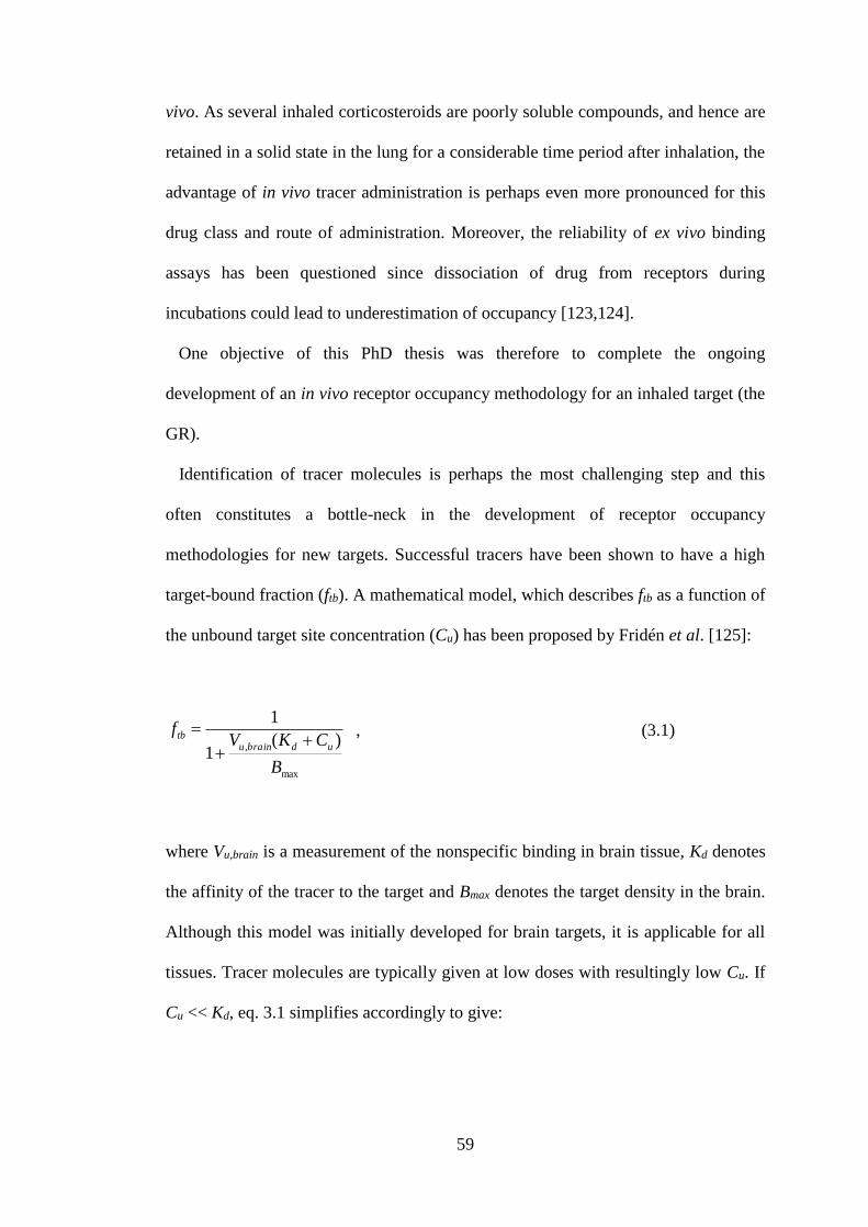
59

vivo. As several inhaled corticosteroids are poorly soluble compounds, and hence are

retained in a solid state in the lung for a considerable time period after inhalation, the

advantage of in vivo tracer administration is perhaps even more pronounced for this

drug class and route of administration. Moreover, the reliability of ex vivo binding

assays has been questioned since dissociation of drug from receptors during

incubations could lead to underestimation of occupancy [123,124].

One objective of this PhD thesis was therefore to complete the ongoing

development of an in vivo receptor occupancy methodology for an inhaled target (the

GR).

Identification of tracer molecules is perhaps the most challenging step and this

often constitutes a bottle-neck in the development of receptor occupancy

methodologies for new targets. Successful tracers have been shown to have a high

target-bound fraction (ftb). A mathematical model, which describes ftb as a function of

the unbound target site concentration (Cu) has been proposed by Fridén et al. [125]:

max

, )(1

1

B

CKVf

udbrainutb

, (3.1)

where Vu,brain is a measurement of the nonspecific binding in brain tissue, Kd denotes

the affinity of the tracer to the target and Bmax denotes the target density in the brain.

Although this model was initially developed for brain targets, it is applicable for all

tissues. Tracer molecules are typically given at low doses with resultingly low Cu. If

Cu << Kd, eq. 3.1 simplifies accordingly to give:

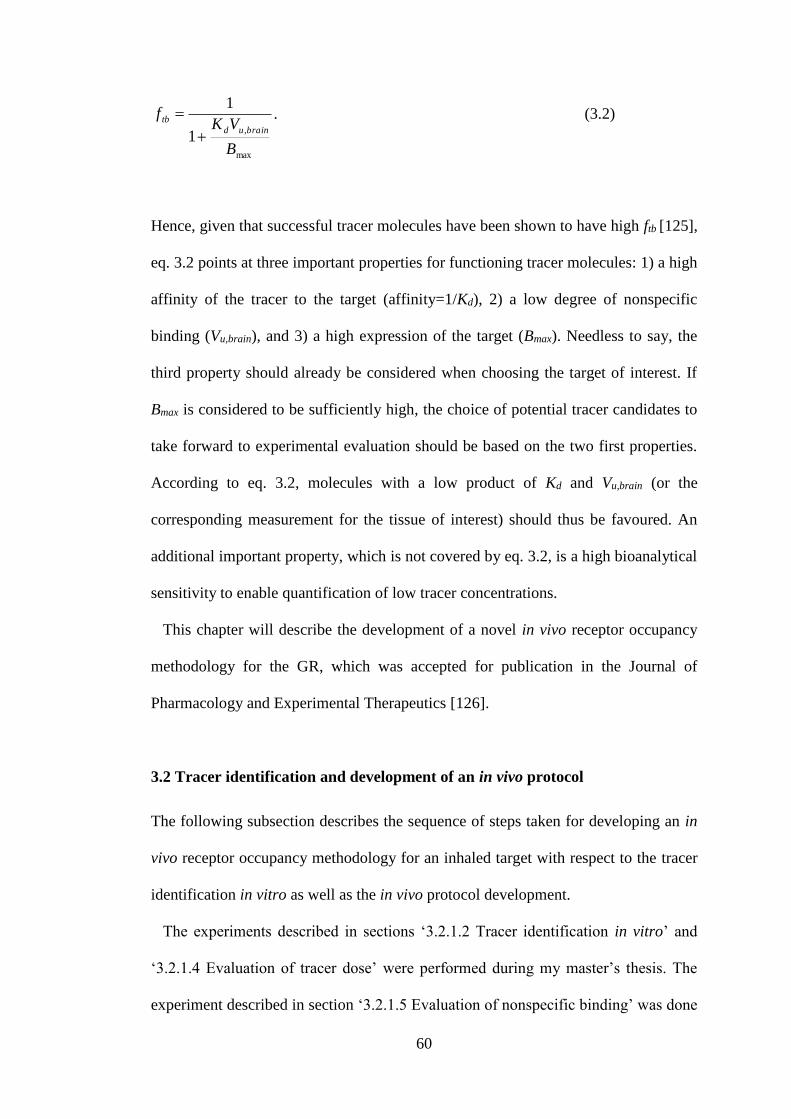
60

max

,1

1

B

VKf

brainud

tb

. (3.2)

Hence, given that successful tracer molecules have been shown to have high ftb [125],

eq. 3.2 points at three important properties for functioning tracer molecules: 1) a high

affinity of the tracer to the target (affinity=1/Kd), 2) a low degree of nonspecific

binding (Vu,brain), and 3) a high expression of the target (Bmax). Needless to say, the

third property should already be considered when choosing the target of interest. If

Bmax is considered to be sufficiently high, the choice of potential tracer candidates to

take forward to experimental evaluation should be based on the two first properties.

According to eq. 3.2, molecules with a low product of Kd and Vu,brain (or the

corresponding measurement for the tissue of interest) should thus be favoured. An

additional important property, which is not covered by eq. 3.2, is a high bioanalytical

sensitivity to enable quantification of low tracer concentrations.

This chapter will describe the development of a novel in vivo receptor occupancy

methodology for the GR, which was accepted for publication in the Journal of

Pharmacology and Experimental Therapeutics [126].

3.2 Tracer identification and development of an in vivo protocol

The following subsection describes the sequence of steps taken for developing an in

vivo receptor occupancy methodology for an inhaled target with respect to the tracer

identification in vitro as well as the in vivo protocol development.

The experiments described in sections ‘3.2.1.2 Tracer identification in vitro’ and

‘3.2.1.4 Evaluation of tracer dose’ were performed during my master’s thesis. The

experiment described in section ‘3.2.1.5 Evaluation of nonspecific binding’ was done

61

whilst employed at AstraZeneca R&D Gothenburg. In contrast to the data collection

described in the aforementioned three sections, which was done prior to the PhD

studies, modelling of the data generated from experiments described in sections

‘3.2.1.4 Evaluation of tracer dose’ and ‘3.2.1.5 Evaluation of nonspecific binding’

was performed as part of this PhD project.

The author was responsible for the design and the execution of all studies. All

studies but one were carried out by the author alone: during the in vivo part of the

PK-study assistance was received from Dr Markus Fridén at AstraZeneca R&D

Gothenburg.

3.2.1 Methods

3.2.1.1 Chemicals and animals

Chemicals. Bovine serum albumin fraction v was purchased from Roche (Penzberg,

Germany), KCl, MgSO4, HEPES, NaHCO3, NaOH, glucose, N,N-

dimethylacetamide, dexamethasone, 5,5-diethyl-1,3-diphenyl-2-iminobarbituric acid

and polyethylene glycol 400 were obtained from Sigma-Aldrich (St. Louis, MO,

USA). NaCl, CaCl2, KH2PO4 and ascorbic acid were purchased from Merck

(Darmstadt, Germany). Fluticasone propionate, R-budesonide, compound 1 (fig.

3.1a), and compound 2 (fig. 3.1b) were synthesised by chemists at AstraZeneca R&D

Gothenburg. Compound 1 and 2 were discovered as part of a collaboration between

AstraZeneca and Bayer HealthCare in the field of selective glucocorticoid receptor

modulators. Chemicals were of analytical grade and all solvents of HPLC grade.

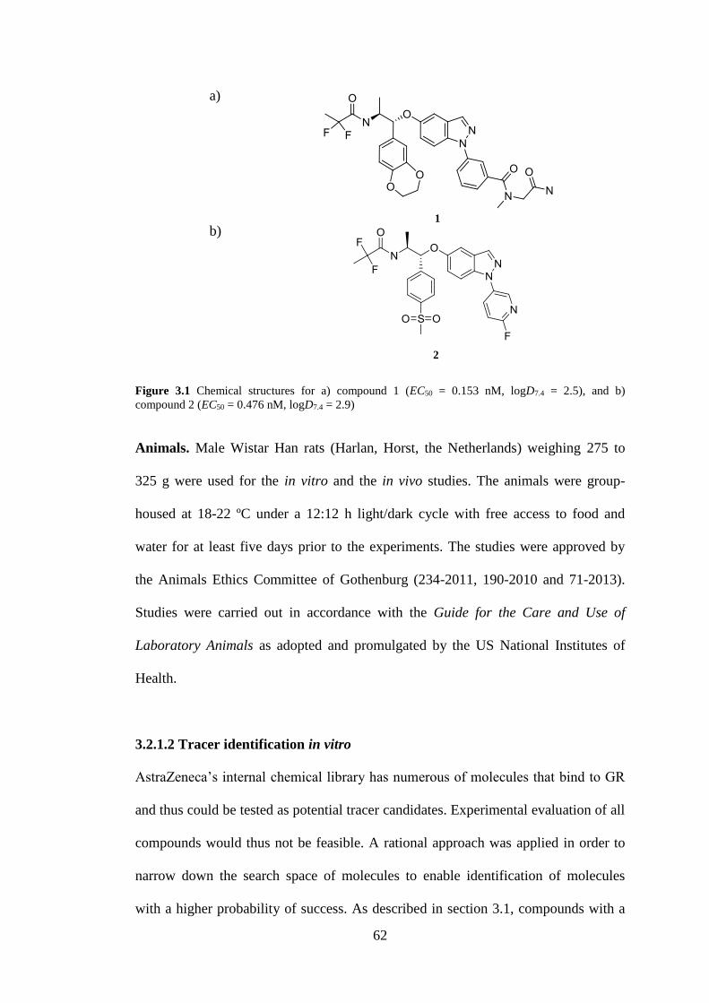
62

Figure 3.1 Chemical structures for a) compound 1 (EC50 = 0.153 nM, logD7.4 = 2.5), and b)

compound 2 (EC50 = 0.476 nM, logD7.4 = 2.9)

Animals. Male Wistar Han rats (Harlan, Horst, the Netherlands) weighing 275 to

325 g were used for the in vitro and the in vivo studies. The animals were group-

housed at 18-22 ºC under a 12:12 h light/dark cycle with free access to food and

water for at least five days prior to the experiments. The studies were approved by

the Animals Ethics Committee of Gothenburg (234-2011, 190-2010 and 71-2013).

Studies were carried out in accordance with the Guide for the Care and Use of

Laboratory Animals as adopted and promulgated by the US National Institutes of

Health.

3.2.1.2 Tracer identification in vitro

AstraZeneca’s internal chemical library has numerous of molecules that bind to GR

and thus could be tested as potential tracer candidates. Experimental evaluation of all

compounds would thus not be feasible. A rational approach was applied in order to

narrow down the search space of molecules to enable identification of molecules

with a higher probability of success. As described in section 3.1, compounds with a

1

2

a)

b)

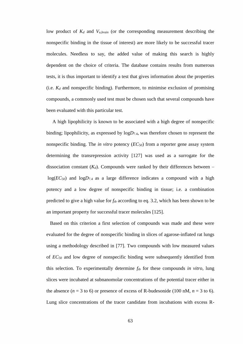
63

low product of Kd and Vu,brain (or the corresponding measurement describing the

nonspecific binding in the tissue of interest) are more likely to be successful tracer

molecules. Needless to say, the added value of making this search is highly

dependent on the choice of criteria. The database contains results from numerous

tests, it is thus important to identify a test that gives information about the properties

(i.e. Kd and nonspecific binding). Furthermore, to minimise exclusion of promising

compounds, a commonly used test must be chosen such that several compounds have

been evaluated with this particular test.

A high lipophilicity is known to be associated with a high degree of nonspecific

binding; lipophilicity, as expressed by logD7.4, was therefore chosen to represent the

nonspecific binding. The in vitro potency (EC50) from a reporter gene assay system

determining the transrepression activity [127] was used as a surrogate for the

dissociation constant (Kd). Compounds were ranked by their differences between –

log(EC50) and logD7.4 as a large difference indicates a compound with a high

potency and a low degree of nonspecific binding in tissue; i.e. a combination

predicted to give a high value for ftb according to eq. 3.2, which has been shown to be

an important property for successful tracer molecules [125].

Based on this criterion a first selection of compounds was made and these were

evaluated for the degree of nonspecific binding in slices of agarose-inflated rat lungs

using a methodology described in [77]. Two compounds with low measured values

of EC50 and low degree of nonspecific binding were subsequently identified from

this selection. To experimentally determine ftb for these compounds in vitro, lung

slices were incubated at subnanomolar concentrations of the potential tracer either in

the absence (n = 3 to 6) or presence of excess of R-budesonide (100 nM, n = 3 to 6).

Lung slice concentrations of the tracer candidate from incubations with excess R-

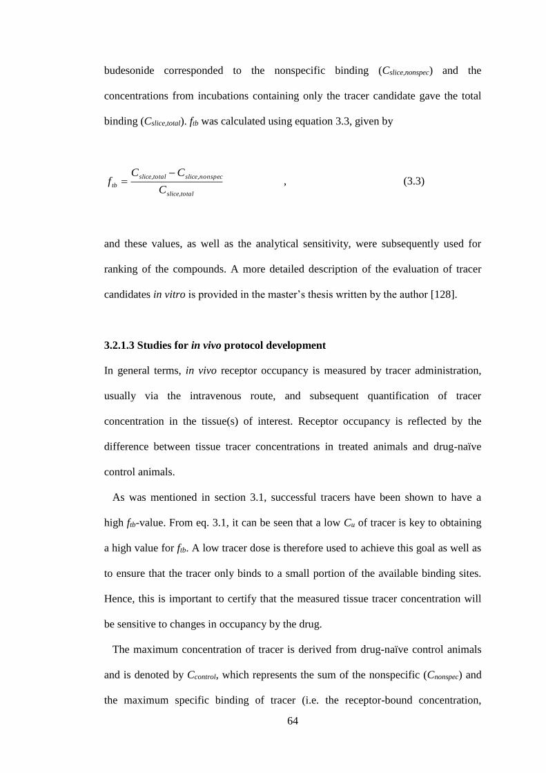
64

budesonide corresponded to the nonspecific binding (Cslice,nonspec) and the

concentrations from incubations containing only the tracer candidate gave the total

binding (Cslice,total). ftb was calculated using equation 3.3, given by

totalslice

nonspecslicetotalslice

tbC

CCf

,

,, , (3.3)

and these values, as well as the analytical sensitivity, were subsequently used for

ranking of the compounds. A more detailed description of the evaluation of tracer

candidates in vitro is provided in the master’s thesis written by the author [128].

3.2.1.3 Studies for in vivo protocol development

In general terms, in vivo receptor occupancy is measured by tracer administration,

usually via the intravenous route, and subsequent quantification of tracer

concentration in the tissue(s) of interest. Receptor occupancy is reflected by the

difference between tissue tracer concentrations in treated animals and drug-naïve

control animals.

As was mentioned in section 3.1, successful tracers have been shown to have a

high ftb-value. From eq. 3.1, it can be seen that a low Cu of tracer is key to obtaining

a high value for ftb. A low tracer dose is therefore used to achieve this goal as well as

to ensure that the tracer only binds to a small portion of the available binding sites.

Hence, this is important to certify that the measured tissue tracer concentration will

be sensitive to changes in occupancy by the drug.

The maximum concentration of tracer is derived from drug-naïve control animals

and is denoted by Ccontrol, which represents the sum of the nonspecific (Cnonspec) and

the maximum specific binding of tracer (i.e. the receptor-bound concentration,

65

Cspec,max) and corresponds to 0% occupancy (i.e. all receptors are available to the

tracer). Cnonspec thus has to be taken into account to enable estimation of the level of

specific tracer binding to derive the occupancy by drug from the tracer concentration

measured in animals pre-treated with test compound (Ctest). A second group of

animals is therefore dedicated to determination of Cnonspec. These animals are pre-

treated with a high dose of another ligand, with the purpose of occupying all

receptors of interest, prior to the tracer administration. Hence, the lower tissue

concentration of tracer measured in these animals is only reflective of Cnonspec and is

assigned to a value of 100% occupancy. To summarise, three different groups of

animals are included in in vivo receptor occupancy methodologies: 1) drug-naïve

control animals (Ccontrol), 2) animals dedicated to determination of the nonspecific

binding (Cnonspec), and 3) animals treated with test compound (Ctest). The measured

tissue concentrations of tracer in the drug-naïve control animals and the treated

animals can be described accordingly:

max,specnonspeccontrol CCC (3.4)

)1(max, ROCCC specnonspectest (3.5)

An appropriate time period, a so-called post-tracer survival interval, is needed after

tracer administration for the tracer to bind the receptor and for the nonspecific

binding to decrease so that a high ratio of total-to-nonspecific binding is achieved

[129].

Consequently, once a promising tracer candidate has been identified, several tracer

doses, and sometimes also post-tracer survival intervals, are tested in order to

66

develop experimental procedures that yield a high ratio of total-to-nonspecific

binding.

3.2.1.4 Evaluation of tracer dose

Three dose levels of the tracer candidate compound 1 were assessed (40, 400 and

4000 nmol/kg, respectively). Henceforth, compound 1 will be referred to as the

tracer. At each dose level the animals were divided into two groups in order to

investigate if Ccontrol was distinguishable from Cnonspec. A post-tracer survival interval

of 30 minutes was tested since it has proven successful for several in vivo receptor

occupancy methodologies [130,131]. For determination of tissue concentrations of

tracer, the animals were injected via the tail vein with their group specific dose of

tracer (n = 3). Animals dedicated to determination of Cnonspec were pre-treated with a

high IV-dose of compound 2 via the tail vein 30 minutes prior to the tracer

administration (compound 2, 5.0 µmol/kg, n = 2, n = 3 and n = 2 for the 40, 400 and

4000 nmol/kg dose groups, respectively). A high dose of compound 2 was used as

pre-treatment since it is a highly potent compound (transrepression EC50 = 0.476 nM)

with a long half-life in blood, and was thus expected to give a high occupancy over a

long time period. This study was complemented with an additional dose level (4

nmol/kg, n = 3) using an identical protocol except that the animals dedicated to the

determination of Cnonspec were pre-treated with dexamethasone (20 mg/kg, n = 3).

The vehicle used for all three compounds was N,N-dimethylacetamide, polyethylene

glycol 400 and water (1:1:1, w/w/w). Thirty minutes after administration of the tracer

candidate, a blood sample was taken and the lung was dissected for concentration

determination.

67

3.2.1.5 Evaluation of nonspecific binding

To confirm that only nonspecifically-bound tracer remained after pre-treatment with

compound 2, Cnonspec was measured after pre-treatment with dexamethasone (20

mg/kg, n = 3). Dexamethasone was injected via the tail vein 30 minutes prior to IV-

administration of tracer (40 nmol/kg). Thirty minutes after the tracer administration,

a terminal blood sample was collected and the lung was dissected for concentration

determination.

3.2.1.6 PK-study

The plasma PK of a low tracer dose (30 nmol/kg) was investigated over the first 30

minutes after IV-administration of the tracer, i.e. over the so called post-tracer

survival interval. This experiment thus aimed to characterise the PK over this time

period. As in vivo receptor occupancy methodologies benefit from low tracer doses

and the bioanalytical sensitivity allowed for using a slightly lower tracer dose than

the one used in section 3.2.1.5, a tracer dose of 30 nmol/kg was selected. All

animals (n = 8) were anaesthetised by inhalation of isoflurane shortly before the

tracer administration. A heparinised catheter was inserted in arteria femoralis, the

tracer was subsequently injected via the tail vein (30 nmol/kg). Blood samples (100-

150 µL/sample) were then repeatedly collected directly in Microvette® 300 LH tubes

(Sarstedt, Nürnbrecht, Germany) from the arterial catheter at the following time

points: 2, 5, 10, 15, 20, 25 and 30 min. The animals were maintained under

inhalation anaesthesia during the entire study and were then euthanized in

conjunction with the last sample by cutting the abdominal aorta.

68

3.2.1.7 Evaluation of tracer function in other organs

To investigate the functionality of the tracer in various organs, Ccontrol and Cnonspec

were compared in several organs. Animals dedicated to measurements of Cnonspec

were pre-treated intravenously with dexamethasone (20 mg/kg, n = 5) prior to tracer

administration, whereas animals dedicated to measurements of Ccontrol did not receive

any pre-treatment (n = 5). Dexamethasone was injected via the tail vein 30 minutes

prior to IV-administration of tracer (30 nmol/kg). All animals were sacrificed 30

minutes after tracer administration, a terminal blood sample was collected and organs

(lung, liver, brain, kidney and spleen) were dissected for concentration

determination.

3.2.1.8 General procedures and final protocol for in vivo receptor occupancy

measurements

The tracer, compound 1, was given intravenously via the tail vein (30 nmol/kg).

Animals dedicated to determination of Cnonspec had been pre-treated intravenously

with dexamethasone (20 mg/kg) 30 minutes prior to the tracer administration. In

contrast, animals set aside for determination of Ccontrol did not receive any pre-

treatment. Animals were anaesthetised by inhalation of isoflurane during the

administration(s) and were then allowed to wake up. Anaesthesia during tail vein

administrations was made a standard procedure since the tail is sensitive. In

conjunction with the termination, the rats were anesthetised once more by inhalation

of isoflurane. The fur was rinsed with 70% ethanol and laparotomy was conducted.

Heparin (2000 IU) was injected into vena cava, a terminal blood sample was

collected (3-4 mL) in a heparinised tube from the abdominal aorta and the rat was

subsequently euthanized by cutting the abdominal aorta. The terminal blood sample

69

was taken 30 minutes after the tracer administration. The diaphragm was then

removed and the apex was incised along its transverse axis. The pulmonary

circulation was perfused by room-tempered bovine serum albumin solution (40 mL,

2.5% bovine serum albumin) via the pulmonary artery in order to clear the tissue of

blood. The heart and lung were removed from the thorax en bloc. The trachea was

dissected from the lung and a predefined section of the spleen (~200 mg) was

dissected. The lung and spleen samples were weighed and stored separately in tissue

tubes and Eppendorf tubes respectively at - 20 ºC until sample handling and analysis,

a detailed description of these procedures is provided in section 3.2.1.10. Receptor

occupancy was then calculated for each animal (eq. 3.6, section 3.2.1.9).

3.2.1.9 Calculation of receptor occupancy

Receptor occupancy calculations are made for each animal using a previously

established method [130,131,132,133] described below:

1

11100(%)occupancy Receptor

c

t

Ratio

Ratio, (3.6)

where

nonspec

testt

C

CRatio (3.7)

and

nonspec

controlc

C

CRatio . (3.8)

Ratiot refers to the ratio of total tracer concentration in tissue from animals treated

with test compound (Ctest) divided by the mean value of Cnonspec obtained from the

70

group of animals pre-treated with a high dose of another ligand. Ratioc represents the

ratio of Ccontrol to Cnonspec, where Ccontrol is the mean value of the total tissue

concentration of tracer obtained from a drug-naïve control group. Accordingly, when

Ratiot is equal to Ratioc this corresponds to an occupancy of 0% and when the Ratiot

is 1 (i.e. the tracer concentration in the treated animal is equal to Cnonspec) to an

occupancy of 100%.

3.2.1.10 Analytical procedures

Sample handling. The blood samples were collected in heparinised tubes which

were centrifuged for 10 minutes at 4000g (Rotanta 46R, Hettich, Germany). The

plasma samples were subsequently transferred to Eppendorf tubes and stored at -20

ºC until analysis.

The tissue tubes containing lung samples were separately flash-frozen in liquid

nitrogen and then immediately placed into Covaris CryoPrep™ (Covaris Inc.,

Woburn, Massachusetts, USA) for pulverisation. This freeze-fracture-procedure was

repeated until pulverisation was judged as being sufficient, generally three times. The

pulverised samples were then transferred to separate glass tubes and Ringer-buffer

was added to each lung sample (4.0 mL). Covaris E210 and SonoLab software

v.4.2.0 (intensity 10.0, cycles 1000, treatment time 180 s, bath degree 40 °C) were

used for dissolution of the samples.

Predefined parts of the liver, brain, spleen and kidney were weighed in Eppendorf

tubes and homogenised in 3 volumes of distilled water (w/v) with an ultrasonic

probe. The samples were stored at -20 ºC until analysis.

Analytical methods. Concentrations of tracer and FP in tissues and plasma were

quantified using reversed phase LC-MS/MS with the electrospray ionization source

71

set in positive mode. The LC-system used was LC Agilent 1200 Series gradient

pump (Agilent Technologies, Waldbronn, Germany), a CTC autosampler (CTC

Analytics, Zwingen, Switzerland), a HALO C18 column (30×2.1 mm, 2.7 µm,

Advancedmaterialtechnology) and an Agilent 6460 detector (Santa Clara, CA, USA).

Gradient elution over 1.5 minutes time with acetonitrile and 0.2% formic acid and a

flow rate of 0.7 mL/min was performed.

Protein precipitation was used for all samples except lung homogenates. A defined

volume (50 µL) of each sample was added in triplicate to a NUNC 96-deepwell plate

(Nalge Nunc International, Rochester, NY) and was then protein precipitated by

addition of cold acetonitrile containing 0.2% formic acid and 100 nM of 5,5-diethyl-

1,3-diphenyl-2-iminobarbituric acid as internal standard (200 µL) to each sample.

After two minutes of mixing with a VWR VX-2500 Multi-Tube Vortexer (VWR

International west Chester, Pennsylvania, USA) and 20 minutes of centrifugation at

4000 rpm at 4 ºC (Centrifuge 5810 R Eppendorf, Hamburg, Germany) the

supernatants (75 µL) were transferred to a new plate, where each sample was diluted

by addition of 0.2% formic acid (75 µL). The diluted samples were then injected (20

µL) to the HPLC system.

Liquid-liquid extraction was performed before analysis of the lung homogenates. A

certain volume (50 µL) of each sample was added in triplicate to glass vials to which

a carbonate buffer pH 10 (50 mM Na2CO3, 50 mM NaHCO3) containing 100 nM of

5,5-diethyl-1,3-diphenyl-2-iminobarbituric acid as internal standard was added (50

µL). Each sample was extracted with methyl-tertbutyl ether (MTBE, 600 µL). After

sealing the vials with silicon cover, the vials were shaken horizontally for 5 minutes

(150 min-1, Edmund Bühler Swip, POCD Scientific, Artarmon, Australia), followed

by 15 minutes of mixing with a VWR VX-2500 Multi-Tube Vortexer (speed 5,

72

VWR International west Chester, Pennsylvania, USA). A defined volume of the

upper organic layer (450 µL) was then transferred to glass vials, which were

vaporised to dryness with a Techne Sample Concentrator (Techne Incorporated,

Staffordshire, UK) during approximately 20 minutes. Samples were reconstituted in

33% acetonitrile and 0.2% formic acid in water (150 µL) and placed in an ultrasonic

bath (5210 Branson, Gemini, Apeldoorn, the Netherlands) for 10 minutes. Except

from the sample preparation technique of the lung homogenates, the analytical

procedure was identical to the one applied for the other samples.

The compounds were quantified using Mass Hunter Workstation Software for

Quantitative Analysis (Agilent Technologies Inc., Santa Clara, CA, USA). A

standard curve was created for each sample type: plasma, lung, spleen, liver, brain

and kidney. The standard curve samples contained a biological matrix, not to be

confused with the mathematical term, (blank plasma, blank lung homogenate, blank

spleen homogenate, blank liver homogenate, blank brain homogenate and blank

kidney homogenate, respectively) in a 1:9 volume ratio in order to match the

samples. The highest point of the standard curve was always followed by two

injections of blank matrix in order to clean the system and avoid possible

contamination. The LLOQ of the tracer was 0.10 nM in all investigated matrices

except for the brain homogenate, which had a LLOQ of 0.35 nM. The LLOQ of FP

was 1.4, 2.1 and 8.6 nM in lung homogenate, spleen homogenate and plasma,

respectively. Corticosterone plasma levels were analysed using an ELISA-kit

(ab108821, Abcam, Cambridge, UK).

73

3.2.1.11 Statistical analysis

Statistical comparisons between two groups were made using a two-tailed, unpaired

Student’s t-test. The level of significance was set at p ≤ 0.05. Data are presented as

mean ± standard deviation and precision of the estimated parameters is presented as

standard errors.

3.2.1.12 Modelling of tissue concentrations of tracer

The four different tracer doses were evaluated by a modelling approach where the

tissue concentration of tracer was assumed to consist of two parts: 1) linear

nonspecific binding determined by the plasma tracer concentration (Cp) and a

partitioning constant for nonspecific binding (Kp,ns), and 2) nonlinear binding to the

target determined by Cp, the dissociation constant (Kd) and the receptor density

(Bmax), given by:

pd

p

nsppcontrolCK

CBKCC

max

, (3.9)

and

nsppnonspec KCC , . (3.10)

The model was implemented in MATLAB R2013a (Mathworks Inc., Natick, MA,

USA) with fitting performed using nonlinear least squares (lsqnonlin) and iterative

reweighting using predicted data. The default optimisation algorithm of ‘lsqnonlin’

was used (the trust region-reflective algorithm). In case of several local minima

within the expected parameter space, an exhaustive search was conducted in

MATLAB to ensure that the optimization algorithm had not converged to a local

74

minimum. The sum of squares was evaluated at 4503 combinations of parameter

values, where Bmax varied between 0.1 and 40 nM, Kp,ns varied between 0.1 and 10

and Kd varied between 0.1 and 30 nM.

A sensitivity analysis was performed to investigate how the function responds to

small perturbations of the parameters over a broad range of Cp (0.1-10000 nM). Only

the function describing Ccontrol (eq. 3.9) was considered since Cnonspec (eq. 3.10) is a

component of that function. The sensitivities were generated by considering the

partial derivatives of the output Y with respect to each parameter xi and these were

calculated keeping all other parameters fixed at their assigned values (x0), i.e.

0xix

Y

(3.11)

The partial derivatives were solved analytically to give:

p

nsp

control CK

C

,

, (3.12)

2max

dp

p

d

control

KC

CB

K

C

(3.13)

and

dp

pcontrol

KC

C

B

C

max

. (3.14)

75

3.2.2 Results

3.2.2.1 Tracer identification in vitro

Fifteen GR binders were selected from AstraZeneca’s internal chemical library on

the basis of having large numerical differences between the values of –log(EC50) and

logD7.4. Based on the measured nonspecific binding in lung slices and the analytical

sensitivity a refined selection of two compounds was made. The chemical structures

of compounds 1 and 2 are shown in figure 3.1. Incubation of lung slices in the

absence and presence of excess of R-budesonide resulted in statistically significant

differences between Cslice,total and Cslice,nonspec for both compounds. ftb was calculated

to be 0.56 ± 0.071 and 0.48 ± 0.069 for compound 1 and 2, respectively. ftb and

analytical sensitivity were subsequently used for ranking. Based on these criteria,

compound 1 was identified as the most promising tracer candidate.

3.2.2.2 Evaluation of tracer dose

As illustrated in figure 3.2, which shows Ccontrol and Cnonspec for each tracer dose,

there was a separation between Ccontrol and Cnonspec at the second lowest dose level

(40 nmol/kg). Ccontrol was 9.2 ± 2.1 nM and Cnonspec was 3.8 ± 0.32 nM, resulting in a

Ccontrol/Cnonspec ratio of 2.4, corresponding to a value for ftb of 0.59. The ratio between

Ccontrol and Cnonspec decreased with ascending tracer doses (2.4, 1.5 and 1.3 for 40,

400 and 4000 nmol/kg, respectively). Cnonspec was below the lower limit of

quantification (LLOQ) at the lowest dose level (4 nmol/kg) and therefore the ratio

could not be calculated. Cnonspec was proportional to Cp and thus they were found to

be highly correlated (r2 = 0.99).

The dependence of Ccontrol and Cnonspec on Cp was captured by the model. Parameter

estimates and standard errors for the model are presented in table 3.1. The

76

correlations between the estimated parameters are presented in table 3.2. The

correlation between Bmax and Kd was found to be reasonably high (0.886). Whilst

Kp,ns had a high parameter precision, the confidence intervals for Bmax and Kd were

somewhat wider. Thus, some caution should be exercised when interpreting these

two parameter estimates.

In the exhaustive search, the minimum cost function was found at the following

parameter values: Kp,ns = 0.761, Bmax = 21.2 nM and Kd = 10.4 nM. The same

minimum was thus found when using nonlinear least squares (the trust region-

reflective algorithm as the optimisation algorithm) and the exhaustive search

algorithm, which confirms that the global minimum had been found within the

investigated parameter space.

A partial derivative based sensitivity analysis was performed as described in

section 3.2.1.12 and the results are presented in figure 3.3a-c. The plot of

∂Ccontrol/∂Kd as a function of Cp (fig. 3.3a) indicates that samples from the two

intermediate dose groups (40 and 400 nmol/kg) were informative with respect to Kd.

In contrast, at the Cp resulting from the highest and the lowest dose group (4000 and

4 nmol/kg, respectively), a change in Kd only had a minor effect on the output. As

can be seen from eq. 3.14 and fig. 3.3b, the influence of Bmax on the output becomes

more pronounced with increasing Cp until Cp >> Kd when the maximum value of

∂Ccontrol/∂Bmax has been reached (i.e. ∂Ccontrol/∂Bmax tends towards 1 as Cp >> Kd). Eq.

3.15 shows that ∂Ccontrol/∂Kp,ns equals Cp (fig. 3.3c), i.e. the higher Cp the more

pronounced is the effect of Kp,ns on the output.

By using the developed model and its final parameter estimates, the ratio

Ccontrol/Cnonspec could be simulated for a range of Cp-values of tracer. According to the

simulations, the ratio consistently increased with lower Cp-levels of tracer (fig. 3.4).

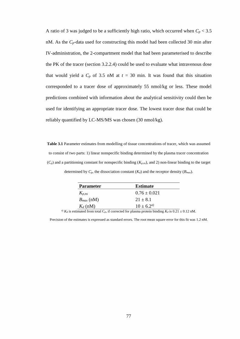
77

A ratio of 3 was judged to be a sufficiently high ratio, which occurred when Cp < 3.5

nM. As the Cp-data used for constructing this model had been collected 30 min after

IV-administration, the 2-compartment model that had been parameterised to describe

the PK of the tracer (section 3.2.2.4) could be used to evaluate what intravenous dose

that would yield a Cp of 3.5 nM at t = 30 min. It was found that this situation

corresponded to a tracer dose of approximately 55 nmol/kg or less. These model

predictions combined with information about the analytical sensitivity could then be

used for identifying an appropriate tracer dose. The lowest tracer dose that could be

reliably quantified by LC-MS/MS was chosen (30 nmol/kg).

Table 3.1 Parameter estimates from modelling of tissue concentrations of tracer, which was assumed

to consist of two parts: 1) linear nonspecific binding determined by the plasma tracer concentration

(Cp) and a partitioning constant for nonspecific binding (Kp,ns), and 2) non-linear binding to the target

determined by Cp, the dissociation constant (Kd) and the receptor density (Bmax).

Parameter Estimate

Kp,ns 0.76 ± 0.021

Bmax (nM) 21 ± 8.1

Kd (nM) 10 ± 6.2a) a) Kd is estimated from total Cp, if corrected for plasma protein binding Kd is 0.21 ± 0.12 nM.

Precision of the estimates is expressed as standard errors. The root mean square error for this fit was 1.2 nM.

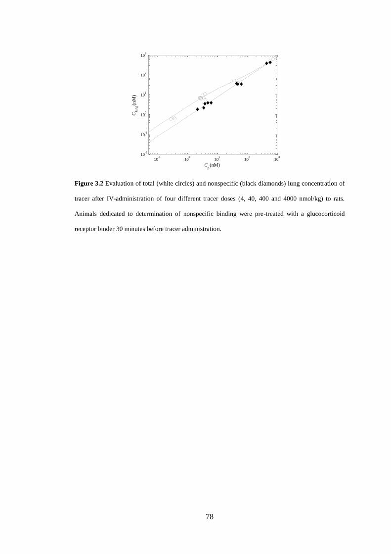
78

10-1

100

101

102

103

10-2

10-1

100

101

102

103

Clu

ng (n

M)

Cp(nM)

Figure 3.2 Evaluation of total (white circles) and nonspecific (black diamonds) lung concentration of

tracer after IV-administration of four different tracer doses (4, 40, 400 and 4000 nmol/kg) to rats.

Animals dedicated to determination of nonspecific binding were pre-treated with a glucocorticoid

receptor binder 30 minutes before tracer administration.

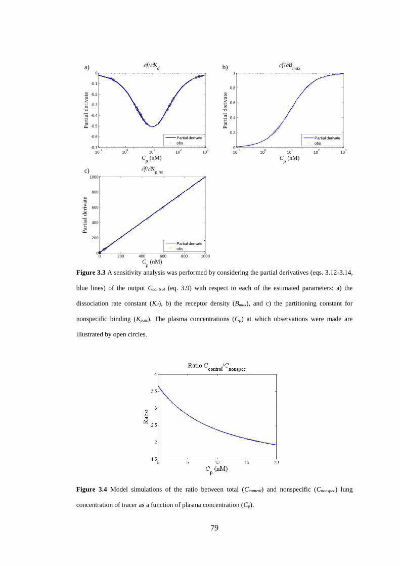
79

10-1

100

101

102

103

0

0.2

0.4

0.6

0.8

1

f/Bmax

Cp (nM)

Part

ial

deri

vate

Partial derivate

obs

0 200 400 600 800 10000

200

400

600

800

1000

f/Kp,ns

Cp (nM)

Part

ial

deri

vate

Partial derivate

obs

10-1

100

101

102

103

-0.7

-0.6

-0.5

-0.4

-0.3

-0.2

-0.1

0

f/Kd

Cp (nM)

Part

ial

deri

vate

Partial derivate

obs

a)

c)

b)

Figure 3.3 A sensitivity analysis was performed by considering the partial derivatives (eqs. 3.12-3.14,

blue lines) of the output Ccontrol (eq. 3.9) with respect to each of the estimated parameters: a) the

dissociation rate constant (Kd), b) the receptor density (Bmax), and c) the partitioning constant for

nonspecific binding (Kp,ns). The plasma concentrations (Cp) at which observations were made are

illustrated by open circles.

Figure 3.4 Model simulations of the ratio between total (Ccontrol) and nonspecific (Cnonspec) lung

concentration of tracer as a function of plasma concentration (Cp).

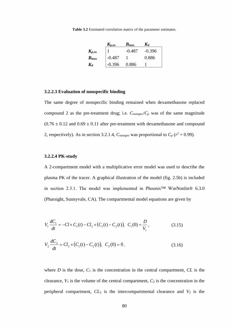
80

Table 3.2 Estimated correlation matrix of the parameter estimates.

Kp,ns Bmax Kd

Kp,ns 1 -0.487 -0.396

Bmax -0.487 1 0.886

Kd -0.396 0.886 1

3.2.2.3 Evaluation of nonspecific binding

The same degree of nonspecific binding remained when dexamethasone replaced

compound 2 as the pre-treatment drug; i.e. Cnonspec/Cp was of the same magnitude

(0.76 ± 0.12 and 0.69 ± 0.11 after pre-treatment with dexamethasone and compound

2, respectively). As in section 3.2.1.4, Cnonspec was proportional to Cp (r2 = 0.99).

3.2.2.4 PK-study

A 2-compartment model with a multiplicative error model was used to describe the

plasma PK of the tracer. A graphical illustration of the model (fig. 2.5b) is included

in section 2.3.1. The model was implemented in Phoenix™ WinNonlin® 6.3.0

(Pharsight, Sunnyvale, CA). The compartmental model equations are given by

1

121211

1 )0( ,)()()(V

DCtCtCCltCCl

dt

dCV , (3.15)

0)0( ,)()( 22122

2 CtCtCCldt

dCV . (3.16)

where D is the dose, C1 is the concentration in the central compartment, CL is the

clearance, V1 is the volume of the central compartment, C2 is the concentration in the

peripheral compartment, CL2 is the intercompartmental clearance and V2 is the

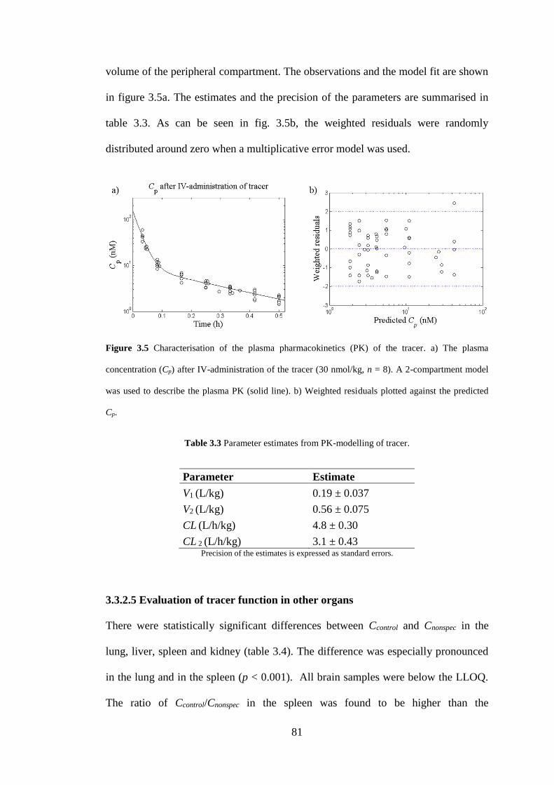
81

volume of the peripheral compartment. The observations and the model fit are shown

in figure 3.5a. The estimates and the precision of the parameters are summarised in

table 3.3. As can be seen in fig. 3.5b, the weighted residuals were randomly

distributed around zero when a multiplicative error model was used.

Figure 3.5 Characterisation of the plasma pharmacokinetics (PK) of the tracer. a) The plasma

concentration (Cp) after IV-administration of the tracer (30 nmol/kg, n = 8). A 2-compartment model

was used to describe the plasma PK (solid line). b) Weighted residuals plotted against the predicted

Cp.

Table 3.3 Parameter estimates from PK-modelling of tracer.

Parameter Estimate

V1 (L/kg) 0.19 ± 0.037

V2 (L/kg) 0.56 ± 0.075

CL (L/h/kg) 4.8 ± 0.30

CL 2 (L/h/kg) 3.1 ± 0.43 Precision of the estimates is expressed as standard errors.

3.3.2.5 Evaluation of tracer function in other organs

There were statistically significant differences between Ccontrol and Cnonspec in the

lung, liver, spleen and kidney (table 3.4). The difference was especially pronounced

in the lung and in the spleen (p < 0.001). All brain samples were below the LLOQ.

The ratio of Ccontrol/Cnonspec in the spleen was found to be higher than the

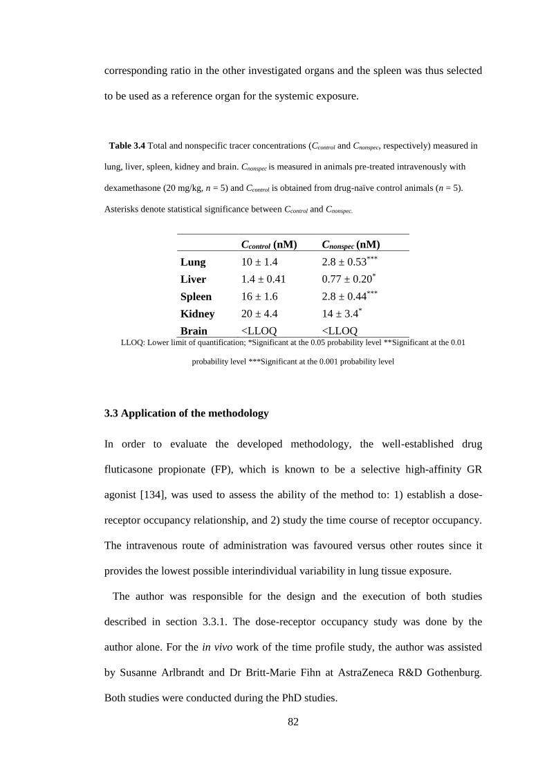
82

corresponding ratio in the other investigated organs and the spleen was thus selected

to be used as a reference organ for the systemic exposure.

Table 3.4 Total and nonspecific tracer concentrations (Ccontrol and Cnonspec, respectively) measured in

lung, liver, spleen, kidney and brain. Cnonspec is measured in animals pre-treated intravenously with

dexamethasone (20 mg/kg, n = 5) and Ccontrol is obtained from drug-naïve control animals (n = 5).

Asterisks denote statistical significance between Ccontrol and Cnonspec.

Ccontrol (nM) Cnonspec (nM)

Lung 10 ± 1.4 2.8 ± 0.53***

Liver 1.4 ± 0.41 0.77 ± 0.20*

Spleen 16 ± 1.6 2.8 ± 0.44***

Kidney 20 ± 4.4 14 ± 3.4*

Brain <LLOQ <LLOQ LLOQ: Lower limit of quantification; *Significant at the 0.05 probability level **Significant at the 0.01

probability level ***Significant at the 0.001 probability level

3.3 Application of the methodology

In order to evaluate the developed methodology, the well-established drug

fluticasone propionate (FP), which is known to be a selective high-affinity GR

agonist [134], was used to assess the ability of the method to: 1) establish a dose-

receptor occupancy relationship, and 2) study the time course of receptor occupancy.

The intravenous route of administration was favoured versus other routes since it

provides the lowest possible interindividual variability in lung tissue exposure.

The author was responsible for the design and the execution of both studies

described in section 3.3.1. The dose-receptor occupancy study was done by the

author alone. For the in vivo work of the time profile study, the author was assisted

by Susanne Arlbrandt and Dr Britt-Marie Fihn at AstraZeneca R&D Gothenburg.

Both studies were conducted during the PhD studies.

83

3.3.1 Method

3.3.1.1 Dose-receptor occupancy relationship

The dose-receptor occupancy relationship for FP was assessed by measuring GR

occupancy 1.5 hours after IV-administration of three escalating doses of FP: 20

nmol/kg (n = 4), 150 nmol/kg (n = 6) and 750 nmol/kg (n = 6). Prior to both the

administration of FP and tracer, plasma samples were taken for measurements of

corticosterone in order to investigate if the endogenous ligand was a potential source

of variability. To allow for interindividual differences in plasma corticosterone, the

IV-administrations of FP were spread out over the time course of a day (8 a.m. – 7

p.m.). One group of animals was pre-treated with dexamethasone via the IV-route

(20 mg/kg) 30 minutes prior to tracer administration (n = 6), whereas the animals

dedicated to determination of the maximum tissue tracer concentration did not

receive any pre-treatment (n = 8). Receptor occupancy was calculated for each

animal treated with FP according to eq. 3.6 (section 3.2.1.9).

3.3.1.2 Receptor occupancy time profile

The time course of receptor occupancy was studied after IV-administration of FP (90

nmol/kg). As detailed in section 4.2.1, the choice of the IV-dose was based on the

ED50 of FP in a preclinical PD-model. Tracer was administered intravenously at the

following time points after drug administration: 0.5, 1, 2, 4, 7, 24 and 48 hours (3

animals/time point). Receptor occupancy was calculated for each animal according to

eq. 3.6 (section 3.2.1.9).

84

3.3.1.3 Statistical analysis

One-way analysis of variance (ANOVA). A one-way analysis of variance

(ANOVA) was used to determine whether there was a statistically significant

difference between any of the mean values of the five different groups in the dose-

receptor occupancy study.

An ANOVA compares the mean values of a dependent variable between different

groups that are categorised by an independent variable. In this case the dependent

variable is the tracer concentration in the lung or in the spleen and the independent

variable is the group (i.e. the three FP-dose groups, the group of animals pre-treated

with dexamethasone and the group of drug-naïve control animals). That is, an

ANOVA tests the following null hypothesis (H0)

nH ...: 210 , (3.17)

where µi is the mean value of group i and n is the total number of groups. H0 is

violated if there is a statistically significant difference between at least two of the

group means. Three assumptions should be met in order to make an ANOVA: 1) the

dependent variable should have a normal distribution within each group, 2) the data

should have equal variances in each group, and 3) the observations should be

independent. This statistical test is known to be robust against modest violations of

the normality assumption. The second assumption regarding homogeneity of

variances can be tested using Levene’s Test [135].

Importantly, an ANOVA does not give any information on which specific groups

are statistically significantly different from each other. A significant result should

therefore be followed up by a post-hoc test in order to find where the difference(s)

85

exist. If the assumption regarding equal variances is met, Tukey’s honestly

significant difference test can be used [135].

One-way ANOVA using MATLAB. The data were initially tested for equality of

variances using Levene’s test, which tests the null-hypothesis that the variances are

equal. The null-hypothesis was considered to be violated if p ≤ 0.05, this level of

significance applies to all statistical tests in this section. A MATLAB-script for

Levene’s test was obtained from [136]. Provided that the null-hypothesis was not

violated, an ANOVA was carried out.

An ANOVA was conducted in MATLAB using the command ‘anova1’ for both

lung and spleen tracer concentrations. Provided that the null-hypothesis was rejected,

a post-hoc test was performed using the command ‘multcompare’ with the

information in the ‘stats’ structure as input. The ‘stats’ structure had been obtained

from the ANOVA-analysis and it contained the information needed for a post-hoc

analysis. Tukey’s honestly significant difference test was selected.

3.3.1.4 Modelling of the dose-receptor occupancy relationship

A nonlinear Emax-model with a baseline (eq. 3.18) was used to describe the dose-

receptor occupancy relationship, using

50

max, 1EDD

DCCC specnonspeci (3.18)

where Ci is the tissue tracer concentration in animal i, Cnonspec is the nonspecific

binding, Cspec,max is the maximum specific binding, D is the dose and ED50 is the dose

which gives 50% occupancy at 1.5 hours. A high dose (10000 nmol/kg) was assigned

86

to the animals pre-treated with dexamethasone (n = 6) and D was set to 0 for drug-

naïve control animals (n = 8).

An exhaustive-search algorithm was used to obtain initial estimates for Cnonspec,

Cspec,max and ED50 for the subsequent parameter estimation. This was done by

evaluating the sum of squares at 1503 combinations of parameter values for both data

from the lung and the spleen. For the lung, Cnonspec varied between 0 and 6 nM,

Cspec,max varied between 2 and 12 nM and ED50 varied between 10 and 60 nmol/kg.

For the spleen, Cnonspec varied between 0 and 6 nM, Cspec,max varied between 2 and 14

nM and ED50 varied between 20 and 80 nmol/kg.

The parameter estimation was implemented in MATLAB R2013a using nonlinear

least squares (lsqnonlin), which minimised the difference between the measured and

the predicted Ci. The default optimisation algorithm of ‘lsqnonlin’ was used (trust

region-reflective algorithm). Ccontrol for drug-naïve control animals was then

calculated as follows

nonspecspeccontrol CCC max, . (3.19)

A sensitivity analysis was performed to investigate how the function responds to

changes in the parameters over a broad dose range (0.1-1000 nmol/kg). The

sensitivities were generated by considering the partial derivatives of the output Ci

with respect to each parameter xi and these were calculated whilst keeping all other

parameters fixed at their assigned values (x0) as described by eq. 3.11 (section

3.2.1.12). That is, the following partial derivatives were generated:

87

1

nonspec

i

C

C, (3.20)

50max,

1EDD

D

C

C

spec

i

(3.21)

and

2

50

max,

50 )( DED

DC

ED

C speci

. (3.22)

The analysis was implemented using the MATLAB symbolic math toolbox.

3.3.2 Results

3.3.2.1 Dose-receptor occupancy relationship

A dose-dependent decrease in tracer concentrations was observed in the lung and the

spleen, which is illustrated in figures 3.6a and 3.6b, respectively. An ANOVA was

used to determine whether there was a statistically significant difference between any

of the mean values for the five different groups. The statistical analysis resulted in a

rejection of the null-hypothesis for both measured tissue concentrations of tracer

(F(4,25) = 75.52, p = 1.38×10-13 and F(4,25) = 107.42, p = 2.29×10-15 for the lung

and the spleen tracer concentrations, respectively).

The results of the two post-hoc tests of all possible pairings of the groups are

summarised in tables 3.5 and 3.6. Table 3.5 contains the results of the analysis in

which the lung tracer concentration was the dependent variable, whereas the analysis

of the spleen tracer concentration is presented in table 3.6.

Table 3.5 shows that the mean values of the lung tracer concentration in the control

group and the lowest dose group (20 nmol/kg, FP) were statistically significantly

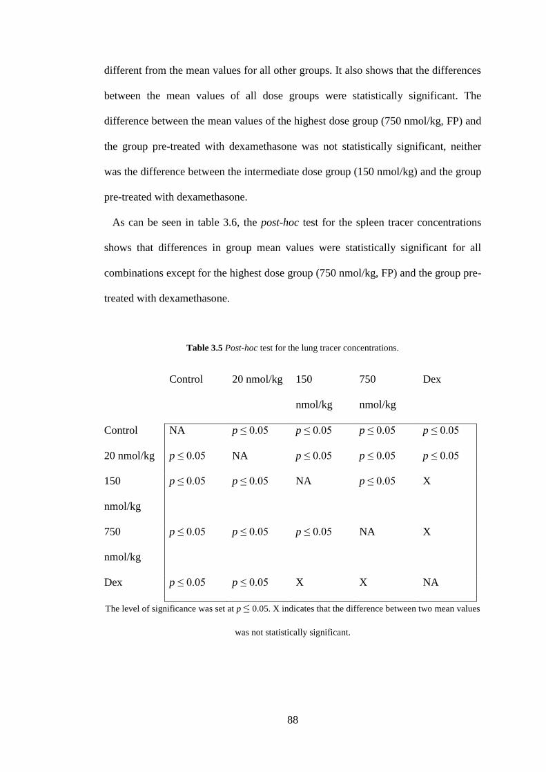
88

different from the mean values for all other groups. It also shows that the differences

between the mean values of all dose groups were statistically significant. The

difference between the mean values of the highest dose group (750 nmol/kg, FP) and

the group pre-treated with dexamethasone was not statistically significant, neither

was the difference between the intermediate dose group (150 nmol/kg) and the group

pre-treated with dexamethasone.

As can be seen in table 3.6, the post-hoc test for the spleen tracer concentrations

shows that differences in group mean values were statistically significant for all

combinations except for the highest dose group (750 nmol/kg, FP) and the group pre-

treated with dexamethasone.

Table 3.5 Post-hoc test for the lung tracer concentrations.

Control 20 nmol/kg 150

nmol/kg

750

nmol/kg

Dex

Control NA p ≤ 0.05 p ≤ 0.05 p ≤ 0.05 p ≤ 0.05

20 nmol/kg p ≤ 0.05 NA p ≤ 0.05 p ≤ 0.05 p ≤ 0.05

150

nmol/kg

p ≤ 0.05 p ≤ 0.05 NA p ≤ 0.05 X

750

nmol/kg

p ≤ 0.05 p ≤ 0.05 p ≤ 0.05 NA X

Dex p ≤ 0.05 p ≤ 0.05 X X NA

The level of significance was set at p ≤ 0.05. X indicates that the difference between two mean values

was not statistically significant.

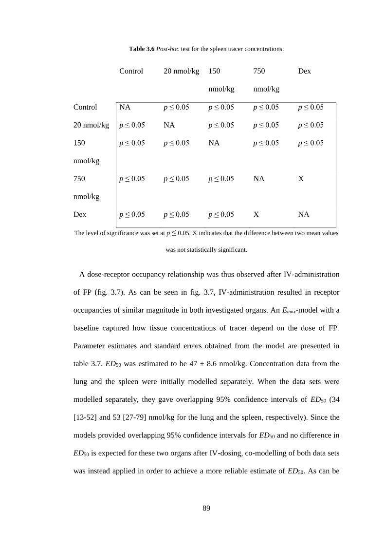
89

Table 3.6 Post-hoc test for the spleen tracer concentrations.

Control 20 nmol/kg 150

nmol/kg

750

nmol/kg

Dex

Control NA p ≤ 0.05 p ≤ 0.05 p ≤ 0.05 p ≤ 0.05

20 nmol/kg p ≤ 0.05 NA p ≤ 0.05 p ≤ 0.05 p ≤ 0.05

150

nmol/kg

p ≤ 0.05 p ≤ 0.05 NA p ≤ 0.05 p ≤ 0.05

750

nmol/kg

p ≤ 0.05 p ≤ 0.05 p ≤ 0.05 NA X

Dex p ≤ 0.05 p ≤ 0.05 p ≤ 0.05 X NA

The level of significance was set at p ≤ 0.05. X indicates that the difference between two mean values

was not statistically significant.

A dose-receptor occupancy relationship was thus observed after IV-administration

of FP (fig. 3.7). As can be seen in fig. 3.7, IV-administration resulted in receptor

occupancies of similar magnitude in both investigated organs. An Emax-model with a

baseline captured how tissue concentrations of tracer depend on the dose of FP.

Parameter estimates and standard errors obtained from the model are presented in

table 3.7. ED50 was estimated to be 47 ± 8.6 nmol/kg. Concentration data from the

lung and the spleen were initially modelled separately. When the data sets were

modelled separately, they gave overlapping 95% confidence intervals of ED50 (34

[13-52] and 53 [27-79] nmol/kg for the lung and the spleen, respectively). Since the

models provided overlapping 95% confidence intervals for ED50 and no difference in

ED50 is expected for these two organs after IV-dosing, co-modelling of both data sets

was instead applied in order to achieve a more reliable estimate of ED50. As can be

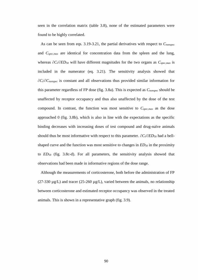
90

seen in the correlation matrix (table 3.8), none of the estimated parameters were

found to be highly correlated.

As can be seen from eqs. 3.19-3.21, the partial derivatives with respect to Cnonspec

and Cspec,max are identical for concentration data from the spleen and the lung,

whereas ∂Ci/∂ED50 will have different magnitudes for the two organs as Cspec,max is

included in the numerator (eq. 3.21). The sensitivity analysis showed that

∂Ci/∂Cnonspec is constant and all observations thus provided similar information for

this parameter regardless of FP dose (fig. 3.8a). This is expected as Cnonspec should be

unaffected by receptor occupancy and thus also unaffected by the dose of the test

compound. In contrast, the function was most sensitive to Cspec,max as the dose

approached 0 (fig. 3.8b), which is also in line with the expectations as the specific

binding decreases with increasing doses of test compound and drug-naïve animals

should thus be most informative with respect to this parameter. ∂Ci/∂ED50 had a bell-

shaped curve and the function was most sensitive to changes in ED50 in the proximity

to ED50 (fig. 3.8c-d). For all parameters, the sensitivity analysis showed that

observations had been made in informative regions of the dose range.

Although the measurements of corticosterone, both before the administration of FP

(27-330 µg/L) and tracer (25-260 µg/L), varied between the animals, no relationship

between corticosterone and estimated receptor occupancy was observed in the treated

animals. This is shown in a representative graph (fig. 3.9).

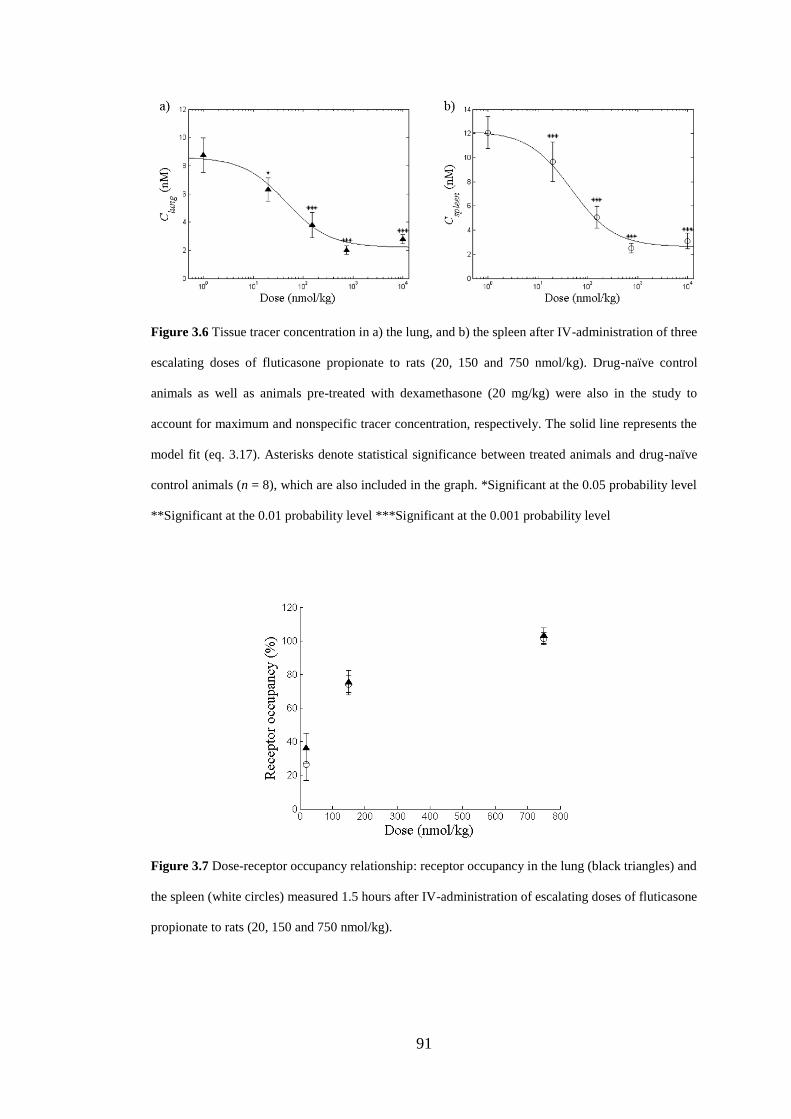
91

Figure 3.6 Tissue tracer concentration in a) the lung, and b) the spleen after IV-administration of three

escalating doses of fluticasone propionate to rats (20, 150 and 750 nmol/kg). Drug-naïve control

animals as well as animals pre-treated with dexamethasone (20 mg/kg) were also in the study to

account for maximum and nonspecific tracer concentration, respectively. The solid line represents the

model fit (eq. 3.17). Asterisks denote statistical significance between treated animals and drug-naïve

control animals (n = 8), which are also included in the graph. *Significant at the 0.05 probability level

**Significant at the 0.01 probability level ***Significant at the 0.001 probability level

Figure 3.7 Dose-receptor occupancy relationship: receptor occupancy in the lung (black triangles) and

the spleen (white circles) measured 1.5 hours after IV-administration of escalating doses of fluticasone

propionate to rats (20, 150 and 750 nmol/kg).

92

Table 3.7 Parameter estimates from the modelling of the dose-receptor occupancy relationship, in

which the tracer concentration was described with a nonlinear Emax-model with a baseline.

Parameter Estimate

Cnonspec,lung (nM) 2.2 ± 0.28

Cspec,max,lung (nM) 6.4 ± 0.44

Cnonspec,spleen (nM) 2.6 ± 0.30

Cspec,max,spleen (nM) 9.6 ± 0.44

ED50 (nmol/kg) 47 ± 8.6

Precision of the estimates is expressed as standard errors. The root mean square error for this fit was 0.99 nM.

Figure 3.8 A sensitivity analysis was performed by considering the partial derivatives of the output Ci

with respect to: a) Cnonspec, b) Cspec,max, c) ED50 (using parameter estimates specific for the lung) and d)

ED50 (using parameter estimates specific for the spleen).

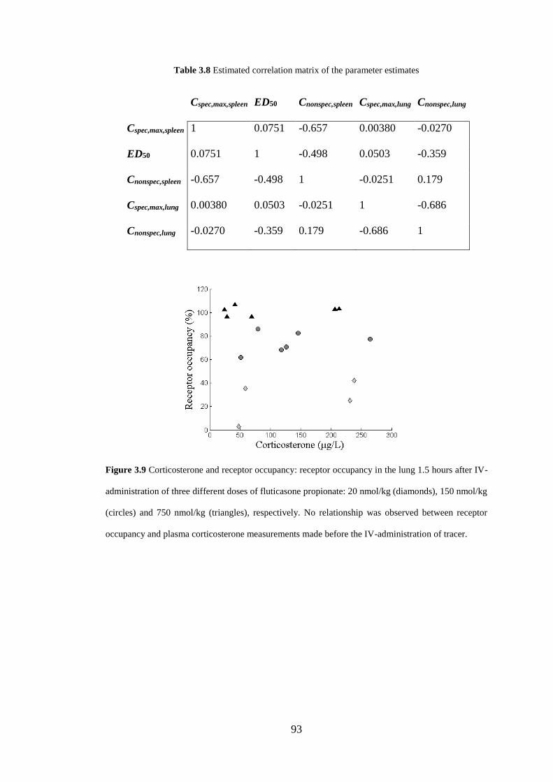
93

Table 3.8 Estimated correlation matrix of the parameter estimates

Cspec,max,spleen ED50 Cnonspec,spleen Cspec,max,lung Cnonspec,lung

Cspec,max,spleen 1 0.0751 -0.657 0.00380 -0.0270

ED50 0.0751 1 -0.498 0.0503 -0.359

Cnonspec,spleen -0.657 -0.498 1 -0.0251 0.179

Cspec,max,lung 0.00380 0.0503 -0.0251 1 -0.686

Cnonspec,lung -0.0270 -0.359 0.179 -0.686 1

Figure 3.9 Corticosterone and receptor occupancy: receptor occupancy in the lung 1.5 hours after IV-

administration of three different doses of fluticasone propionate: 20 nmol/kg (diamonds), 150 nmol/kg

(circles) and 750 nmol/kg (triangles), respectively. No relationship was observed between receptor

occupancy and plasma corticosterone measurements made before the IV-administration of tracer.

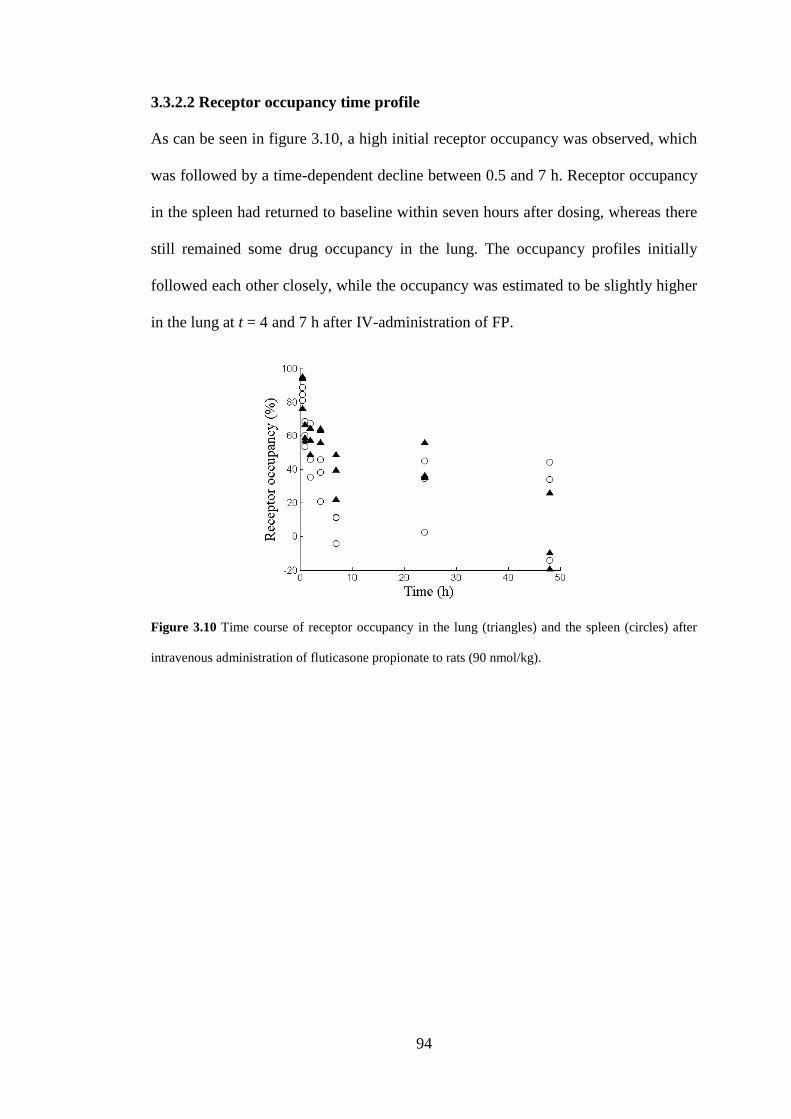
94

3.3.2.2 Receptor occupancy time profile

As can be seen in figure 3.10, a high initial receptor occupancy was observed, which

was followed by a time-dependent decline between 0.5 and 7 h. Receptor occupancy

in the spleen had returned to baseline within seven hours after dosing, whereas there

still remained some drug occupancy in the lung. The occupancy profiles initially

followed each other closely, while the occupancy was estimated to be slightly higher

in the lung at t = 4 and 7 h after IV-administration of FP.

Figure 3.10 Time course of receptor occupancy in the lung (triangles) and the spleen (circles) after

intravenous administration of fluticasone propionate to rats (90 nmol/kg).

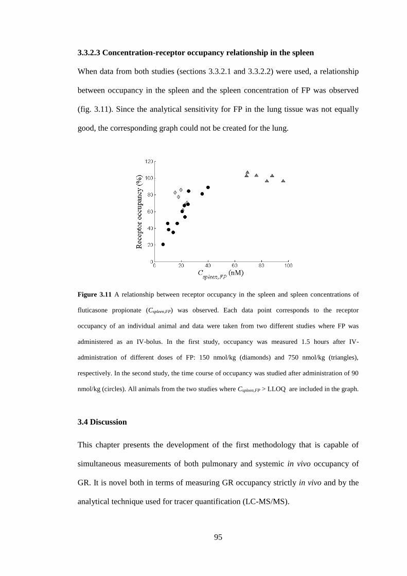
95

3.3.2.3 Concentration-receptor occupancy relationship in the spleen

When data from both studies (sections 3.3.2.1 and 3.3.2.2) were used, a relationship

between occupancy in the spleen and the spleen concentration of FP was observed

(fig. 3.11). Since the analytical sensitivity for FP in the lung tissue was not equally

good, the corresponding graph could not be created for the lung.

Figure 3.11 A relationship between receptor occupancy in the spleen and spleen concentrations of

fluticasone propionate (Cspleen,FP) was observed. Each data point corresponds to the receptor

occupancy of an individual animal and data were taken from two different studies where FP was

administered as an IV-bolus. In the first study, occupancy was measured 1.5 hours after IV-

administration of different doses of FP: 150 nmol/kg (diamonds) and 750 nmol/kg (triangles),

respectively. In the second study, the time course of occupancy was studied after administration of 90

nmol/kg (circles). All animals from the two studies where Cspleen,FP > LLOQ are included in the graph.

3.4 Discussion

This chapter presents the development of the first methodology that is capable of

simultaneous measurements of both pulmonary and systemic in vivo occupancy of

GR. It is novel both in terms of measuring GR occupancy strictly in vivo and by the

analytical technique used for tracer quantification (LC-MS/MS).

96

Identifying a tracer molecule is a prerequisite for developing a receptor occupancy

methodology for a new target and this is indeed recognised as a challenging task. As

highlighted in section 3.2.1.2, AstraZeneca’s internal library contains numerous

compounds with affinity for the GR, which thus theoretically could be considered as

potential tracer candidates. However, it would not be feasible to experimentally

evaluate each candidate and a rational approach was thus needed to narrow down the

search space and select compounds with a higher probability of success as GR

tracers. Potential tracer candidates were therefore selected based on molecular and

pharmacological properties as suggested by Fridén et al. [125]. This strategy proved

to be successful and one of these compounds, which had demonstrated a high ftb in

vitro and a sufficiently high analytical sensitivity, was brought forward to in vivo

evaluation. The in vivo studies showed that it was a successful tracer for the GR in

lung tissue as an appropriate ratio of Ccontrol/Cnonspec was obtained at a low tracer dose

(30 nmol/kg, IV). As expected, this ratio was demonstrated to decrease with higher

tracer doses since the relative contribution of Cnonspec increases with higher tracer

exposure (fig. 3.2). This behaviour was captured by a model, which described the

receptor- and nonspecifically-bound tracer concentrations as a function of Cp (eqs.

3.9-3.10). Simulations of this model evaluated at its final parameter estimates

showed that the ratio Ccontrol/Cnonspec consistently increased with lower Cp-levels of

tracer (fig. 3.4). Thus, an appropriate tracer dose should be low while still ensuring

that the resulting tissue tracer concentrations exceed the LLOQ. By combining PK-

model predictions with information about the analytical sensitivity, a low tracer dose

that could be reliably quantified by LC-MS/MS was selected (30 nmol/kg). A post-

tracer survival interval of 30 minutes was tested since it is commonly used in other

preclinical in vivo receptor occupancy methodologies [130,131]. As it proved to give

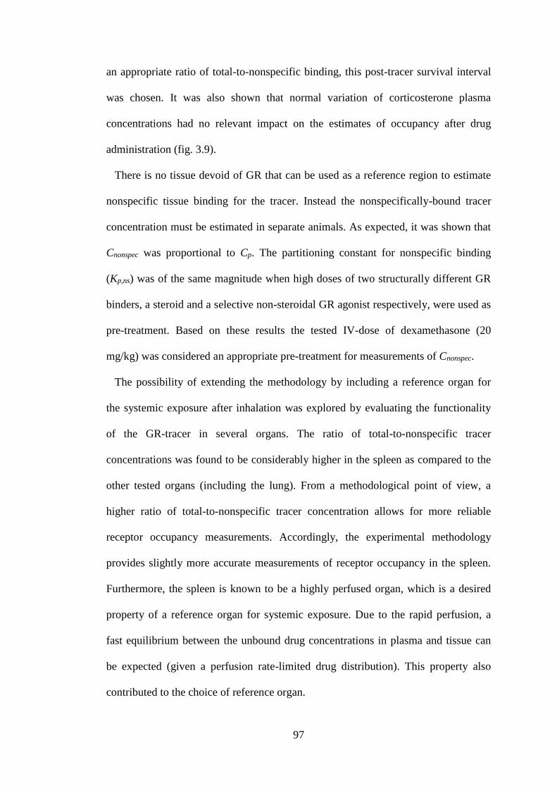
97

an appropriate ratio of total-to-nonspecific binding, this post-tracer survival interval

was chosen. It was also shown that normal variation of corticosterone plasma

concentrations had no relevant impact on the estimates of occupancy after drug

administration (fig. 3.9).

There is no tissue devoid of GR that can be used as a reference region to estimate

nonspecific tissue binding for the tracer. Instead the nonspecifically-bound tracer

concentration must be estimated in separate animals. As expected, it was shown that

Cnonspec was proportional to Cp. The partitioning constant for nonspecific binding

(Kp,ns) was of the same magnitude when high doses of two structurally different GR

binders, a steroid and a selective non-steroidal GR agonist respectively, were used as

pre-treatment. Based on these results the tested IV-dose of dexamethasone (20

mg/kg) was considered an appropriate pre-treatment for measurements of Cnonspec.

The possibility of extending the methodology by including a reference organ for

the systemic exposure after inhalation was explored by evaluating the functionality

of the GR-tracer in several organs. The ratio of total-to-nonspecific tracer

concentrations was found to be considerably higher in the spleen as compared to the

other tested organs (including the lung). From a methodological point of view, a

higher ratio of total-to-nonspecific tracer concentration allows for more reliable

receptor occupancy measurements. Accordingly, the experimental methodology

provides slightly more accurate measurements of receptor occupancy in the spleen.

Furthermore, the spleen is known to be a highly perfused organ, which is a desired

property of a reference organ for systemic exposure. Due to the rapid perfusion, a

fast equilibrium between the unbound drug concentrations in plasma and tissue can

be expected (given a perfusion rate-limited drug distribution). This property also

contributed to the choice of reference organ.

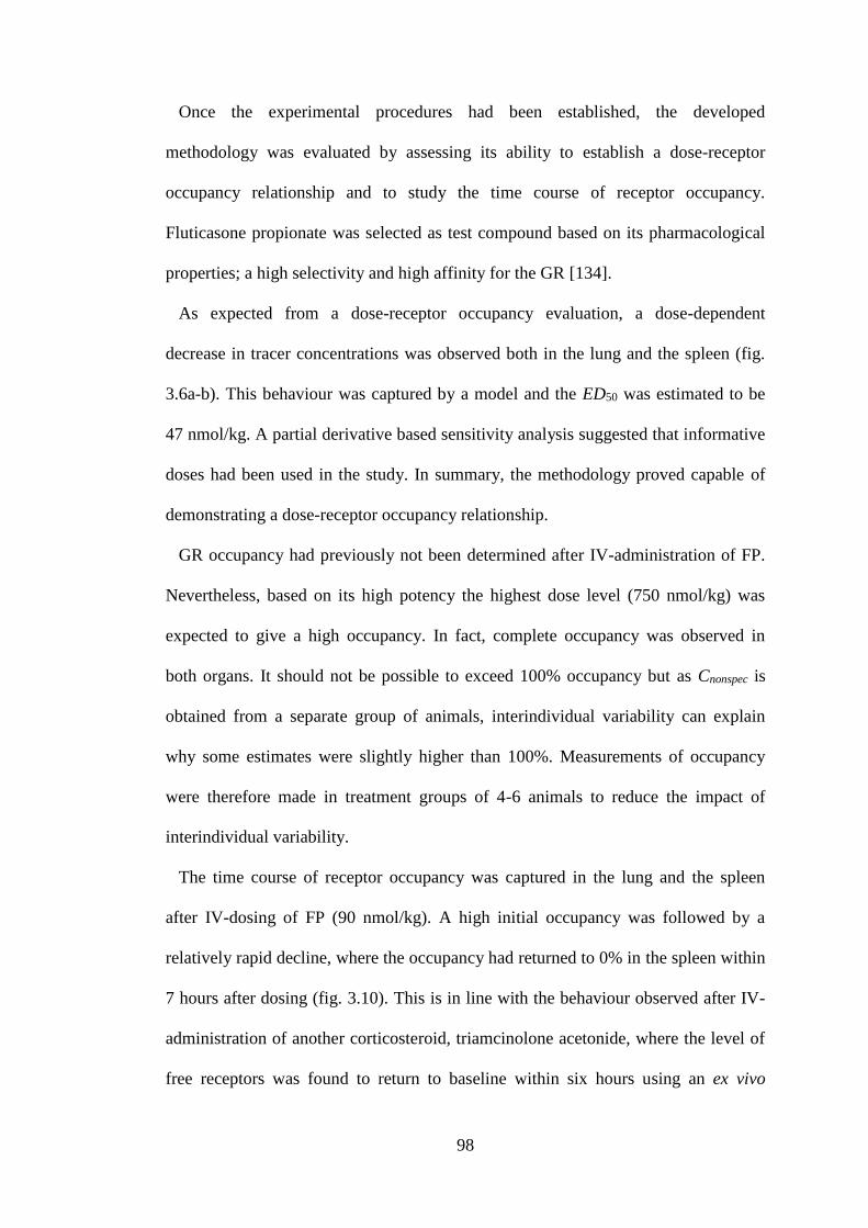
98

Once the experimental procedures had been established, the developed

methodology was evaluated by assessing its ability to establish a dose-receptor

occupancy relationship and to study the time course of receptor occupancy.

Fluticasone propionate was selected as test compound based on its pharmacological

properties; a high selectivity and high affinity for the GR [134].

As expected from a dose-receptor occupancy evaluation, a dose-dependent

decrease in tracer concentrations was observed both in the lung and the spleen (fig.

3.6a-b). This behaviour was captured by a model and the ED50 was estimated to be

47 nmol/kg. A partial derivative based sensitivity analysis suggested that informative

doses had been used in the study. In summary, the methodology proved capable of

demonstrating a dose-receptor occupancy relationship.

GR occupancy had previously not been determined after IV-administration of FP.

Nevertheless, based on its high potency the highest dose level (750 nmol/kg) was

expected to give a high occupancy. In fact, complete occupancy was observed in

both organs. It should not be possible to exceed 100% occupancy but as Cnonspec is

obtained from a separate group of animals, interindividual variability can explain

why some estimates were slightly higher than 100%. Measurements of occupancy

were therefore made in treatment groups of 4-6 animals to reduce the impact of

interindividual variability.

The time course of receptor occupancy was captured in the lung and the spleen

after IV-dosing of FP (90 nmol/kg). A high initial occupancy was followed by a

relatively rapid decline, where the occupancy had returned to 0% in the spleen within

7 hours after dosing (fig. 3.10). This is in line with the behaviour observed after IV-

administration of another corticosteroid, triamcinolone acetonide, where the level of

free receptors was found to return to baseline within six hours using an ex vivo

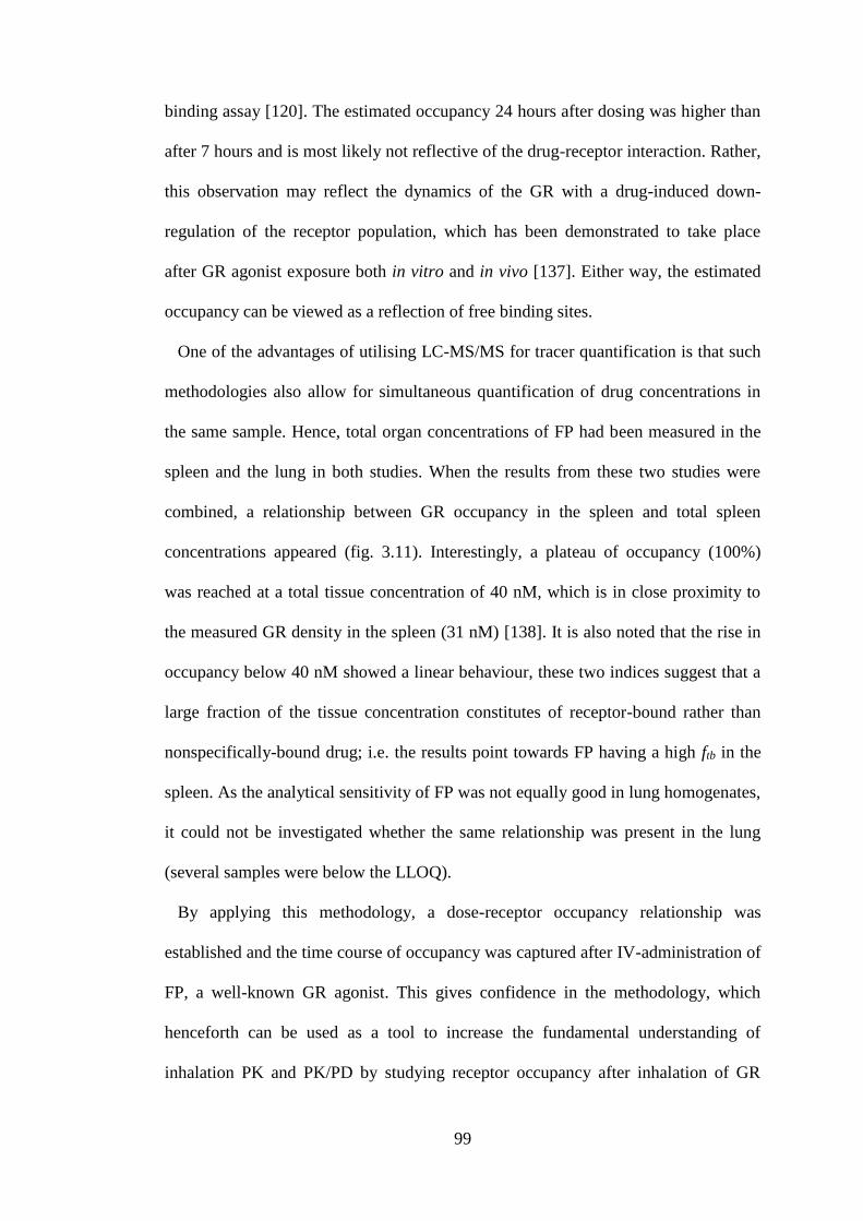
99

binding assay [120]. The estimated occupancy 24 hours after dosing was higher than

after 7 hours and is most likely not reflective of the drug-receptor interaction. Rather,

this observation may reflect the dynamics of the GR with a drug-induced down-

regulation of the receptor population, which has been demonstrated to take place

after GR agonist exposure both in vitro and in vivo [137]. Either way, the estimated

occupancy can be viewed as a reflection of free binding sites.

One of the advantages of utilising LC-MS/MS for tracer quantification is that such

methodologies also allow for simultaneous quantification of drug concentrations in

the same sample. Hence, total organ concentrations of FP had been measured in the

spleen and the lung in both studies. When the results from these two studies were

combined, a relationship between GR occupancy in the spleen and total spleen

concentrations appeared (fig. 3.11). Interestingly, a plateau of occupancy (100%)

was reached at a total tissue concentration of 40 nM, which is in close proximity to

the measured GR density in the spleen (31 nM) [138]. It is also noted that the rise in

occupancy below 40 nM showed a linear behaviour, these two indices suggest that a

large fraction of the tissue concentration constitutes of receptor-bound rather than

nonspecifically-bound drug; i.e. the results point towards FP having a high ftb in the

spleen. As the analytical sensitivity of FP was not equally good in lung homogenates,

it could not be investigated whether the same relationship was present in the lung

(several samples were below the LLOQ).

By applying this methodology, a dose-receptor occupancy relationship was

established and the time course of occupancy was captured after IV-administration of

FP, a well-known GR agonist. This gives confidence in the methodology, which

henceforth can be used as a tool to increase the fundamental understanding of

inhalation PK and PK/PD by studying receptor occupancy after inhalation of GR

100

modulators. In chapter 4, the developed methodology will be used for this very

purpose.

3.5 Summary

Chapter 3 presents the development and the subsequent evaluation of an in vivo

receptor occupancy methodology for an inhaled target: the GR. The developed

methodology is novel both in terms of being fully in vivo-based and by utilising LC-

MS/MS for tracer quantification.

A refined selection of potential tracer candidates was made based on molecular and

pharmacological properties as suggested by Fridén et al. [125]. One of these

compounds, which had a demonstrated high ftb in vitro and a sufficiently high

analytical sensitivity, was brought forward for in vivo evaluation. The in vivo studies

showed that it was a successful tracer for the GR in lung tissue as an appropriate

ratio of Ccontrol/Cnonspec was obtained at a low tracer dose (30 nmol/kg, IV) after a

post-tracer survival interval of 30 minutes. The possibility of simultaneously

estimating receptor occupancy in a reference organ for the systemic exposure was

explored by evaluating the functionality of the selected tracer molecule in other

organs as judged by the ratio of Ccontrol/Cnonspec. Based on this criterion and the high

splenic perfusion rate, the spleen was considered to be an appropriate reference

organ.

Once the experimental in vivo protocol had been finalised, the developed

methodology was evaluated by assessing its ability to establish a dose-receptor

occupancy relationship and to characterise a time course of receptor occupancy. Both

studies used a selective, high-affinity GR agonist as test compound (FP). As

expected from a dose-receptor occupancy evaluation utilising the IV-route, a dose-

101

dependent decrease in tracer concentrations was observed (fig. 3.6a-b) and the

occupancies were of similar magnitude in both organs (fig. 3.7). Hence, the

methodology proved capable of demonstrating a dose-receptor occupancy

relationship after IV-administration. The dose-dependency was described by a

mathematical model and the ED50 was estimated to be 47 nmol/kg. A partial

derivative based sensitivity analysis suggested that informative doses had been

selected for the study. In the time course study, the highest receptor occupancy

observation was made at the first time point (t = 30 min). The peak was followed by

a relatively rapid decline and the receptor occupancy had returned to 0% in the

spleen within 7 hours after dosing (fig. 3.10).

Besides being a selective and high-affinity GR-agonist, FP has interesting

properties from an inhalation PK perspective. These properties will be discussed in

more detail in chapter 4, in which the developed methodology is used for studying

receptor occupancy after nose-only exposure of this compound.

102

Chapter 4 Temporal relationship between target site exposure and

receptor occupancy

4.1 Introduction

As highlighted in chapter 3, contemporary experimental methodologies do not allow

for direct measurements of unbound drug concentrations locally in the lung tissue.

Since receptor occupancy is driven by the unbound drug concentration at the target

site, such measurements would clarify the PK- and PK/PD-evaluation of locally

acting inhaled drugs. The in vivo receptor occupancy methodology, the development

of which was described in chapter 3, could thus be used for this purpose. Fluticasone

propionate (FP) was selected as a test compound for various reasons. Firstly, it is a

well-established drug that is broadly used in the clinic, for example for the treatment

of asthma [48]. Secondly, it is a highly selective and potent glucocorticoid receptor

(GR) agonist [79]. Thirdly, its lung retention is held to rely on its low solubility and

thus slow dissolution rate [4]. Although a low solubility is a commonly used strategy

for achieving lung retention after inhalation, more in-depth knowledge is needed to

better understand potential benefits and limitations of this strategy. As measurements

of total lung concentrations (Clung) after inhalation does not distinguish between solid

and dissolved drug, preclinical inhalation studies of poorly soluble compounds are

held to be exceedingly difficult to interpret. Furthermore, the complex interplay

between e.g. dissolution, mucociliary clearance and permeation into lung tissue

makes the interpretation even more challenging. The third property is thus clearly the

most interesting one from an inhalation PK perspective. When switching focus from

the pulmonary to the systemic PK, it becomes clear that FP, and several other inhaled

corticosteroids, has properties strategically chosen to minimise the systemic exposure

following inhalation: a high clearance and a low oral bioavailability [18]. In

103

summary, characterisation of the receptor occupancy of FP after nose-only exposure

has the potential to yield interesting information about inhalation PK.

In contrast to drug delivery via the inhaled route, the unbound plasma

concentration (Cu) is generally assumed to reflect the target site concentration after

IV-administration of drug. This is based on the assumption that unbound drug freely

distributes between blood and tissues, hence at equilibrium the Cu and the unbound

drug concentration in tissues (CuT) will be the same (the ‘free drug hypothesis’).

Assuming that the drug of interest has a perfusion rate-limited drug distribution, i.e.

membranes do not present a barrier to distribution but the rate determining step is the

blood flow to the tissue, the tissue distribution half-life (t½,distr) can be calculated

from the distribution rate constant kT accordingly [139]:

pi

i

veinpi

veiniT

KV

Q

CKV

CQk

in tissueAmount

leaving of Rate, (4.1)

T

distrk

t2ln

½, , (4.2)

where Qi is the flow to tissue i, Cvein is the venous concentration of drug, Vi is the

volume of tissue i and Kp is the tissue-to-plasma partition coefficient. Parameters

specific for the spleen were used to investigate whether it would be feasible to

assume that measurements of Cu would be representative of the unbound drug

concentration in the spleen. By setting Qspleen to 1.485 L/h/kg (cardiac output, QCO =

20.77 L/h/kg [140] and the spleen receives 7.15% of QCO [141]), Vspleen to 2 mL/kg

[142] and Kp to e.g. 2.5, eq. 4.2 gives a t½,distr of 8.4 s. Hence, the Cu can be assumed

to be reflective of the unbound drug concentration in the spleen. This has interesting

implications; given that receptor occupancy is measured in the spleen, the more

104

easily accessible Cu can be used to mathematically describe the relationship between

target site exposure and receptor occupancy after IV-administration. Expressed

differently, such studies would enable characterisation of the in vivo binding kinetics

by estimating the association rate constant (Kon) and the dissociation rate constant

(Koff). The binding kinetics of several GR agonists have previously been

characterised in in vitro systems. However, data generated from an in vitro system

are not necessarily translatable to the in vivo situation. In fact, results from previous

work have indicated that this might be the case. In an in vitro system, the Koff of the

corticosteroid triamcinolone acetonide was experimentally determined to be 5.5×10-4

min-1, which corresponds to a dissociation half-life of 21 h [143]. In contrast, when

an ex vivo binding assay was used to monitor receptor occupancy following an IV-

dose of triamcinolone acetonide to rats (22 µg), the level of free receptors initially

declined rapidly after dosing, but was then found to return to baseline already within

six hours after dosing [120]. Hence, studies with triamcinolone acetonide as a model

drug suggest a disconnection between the in vitro and the in vivo situation with

respect to the dissociation half-life. To gain further understanding of inhaled

corticosteroids, it would thus be interesting to characterise the in vivo binding

kinetics for this compound class. Ultimately, if estimates of Kon and Koff subsequently

could be incorporated into a mechanistic in silico model used for predicting the local

tissue concentrations after inhalation, measurements of receptor occupancy after

inhalation would provide the first opportunity for validating such predictions.

This chapter will describe the experiments and the mathematical modelling used to

characterise the in vivo binding kinetics after IV-administration of FP and

budesonide. It also comprises the experiments used for studying the inhalation PK as

well as the receptor occupancy after nose-only exposure of FP.

105

4.2 Receptor occupancy studies after IV-administration

The time course of receptor occupancy was studied after IV-administration of FP and

budesonide. The experimental details and the results from the study with FP are

described in sections 3.3.1.2 and 3.3.2.2, respectively, whereas the budesonide study

is described in this subsection.

4.2.1 Choice of IV-dose

As the IV-studies aimed to characterise the binding kinetics of the two compounds, it

was essential to choose a dose that would significantly perturb the system and

thereby enable receptor occupancy measurements over an extended time period. It

was reasoned that data from preclinical PD-studies could be used to find an

appropriate dose. Since both compounds are usually administered via the inhaled

route, previous research at AstraZeneca has focused on characterising the compounds

after inhalation. Due to a lack of efficacy data after IV-administration, inhalation PD-

studies were used to guide the dose setting. Both compounds had been investigated

in an animal model that is used internally at AstraZeneca to evaluate the local

pulmonary effects as well as the systemic side-effects of glucocorticoid receptor

(GR) binders in rats. This animal model is e.g. described in [144]. In these studies,

the effect is studied for several different lung deposited doses (LDD). This enables

estimation of ED50, i.e. the LDD giving 50% efficacy. Since the intention was to

perturb the system such that the receptors would be occupied several hours after drug

administration, it was reasoned that the IV-dose should be several-fold higher than

the ED50 to increase the chances of achieving this goal. Clearly, the IV-dose cannot

be too high as that might jeopardise the well-being of the animals. The IV-dose was

106

therefore set to be 7.5 times ED50, which corresponded to 90 and 167 nmol/kg for FP

and budesonide, respectively.

4.2.2 IV-study, budesonide

The author was responsible for designing, coordinating, performing as well as

analysing the receptor occupancy IV-studies. Three additional researchers from

AstraZeneca R&D Gothenburg assisted the author with the in vivo aspects of the

budesonide study: Dr. Britt-Marie Fihn, Kajsa Claesson and Louise Hammarberg.


300 g were used for the IV-study with budesonide. The animals were group-housed

at 18-22 ºC under a 12:12 h light/dark cycle with free access to food and water for at

least five days prior to the experiments. The studies were approved by the Animals

Ethics Committee of Gothenburg (71-2013).

Study protocol. The animals were anaesthetised by inhalation of isoflurane during

both drug- and tracer administration. Budesonide was administered via the tail vein

(167 nmol/kg) and the animals were then allowed to wake up. Tracer was

subsequently administered via the tail vein at the following time points after drug

administration: 0.5, 1, 2, 4, 7, 24 and 48 h (3 animals/time point). Animals dedicated

to determination of Cnonspec had been pre-treated with an IV-dose of dexamethasone

(20 mg/kg) 30 minutes prior to the tracer administration (n = 6). In contrast, animals

set aside for determination of Ccontrol did not receive any pre-treatment prior to tracer

administration (n = 7). A detailed experimental protocol for the in vivo receptor

occupancy methodology as well as the sample handling is provided in section

3.2.1.8.

107

4.2.3 Analytical procedures

The sample handling as well as the analytical procedures used for the GR-tracer are

described in detail in section 3.2.1.10.

4.2.4 Results

As can be seen in fig. 4.1, the receptor occupancy in the lung (ROlung) and the spleen

(ROspleen) were of similar magnitudes after IV-administration of budesonide. The

receptor occupancy was initially high and then rapidly returned to baseline within 4

hours after dosing.

One animal, which was dosed with tracer at t = 4 h (where t = 0 h assigns the time

point of drug administration), was excluded from the study since the apex was not

incised along its transverse axis prior to perfusion of the lung. Due to this

experimental error, water assembled in the lung causing the lung weight to increase

by more than 100%. It was therefore judged as inappropriate to include

measurements from this animal.

The data generated in this study was subsequently used for characterising the in

vivo binding kinetics by mathematical modelling, which is described in section 4.4.

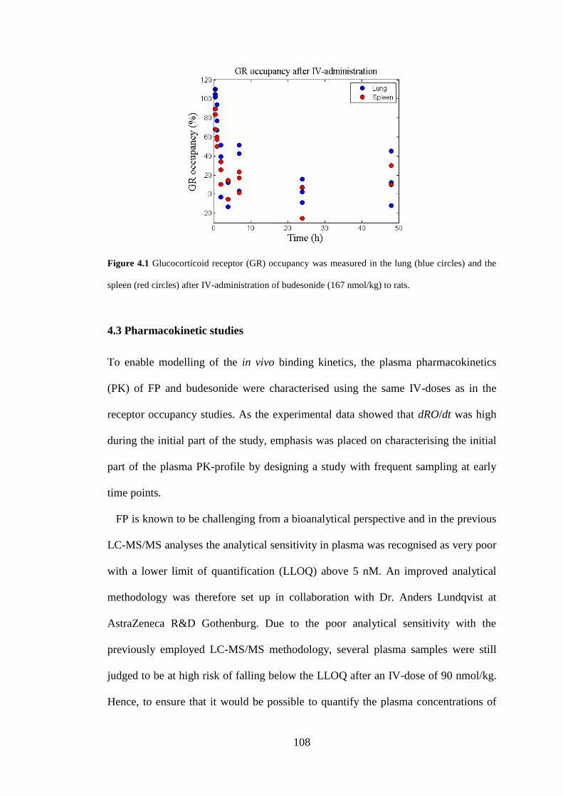
108

Figure 4.1 Glucocorticoid receptor (GR) occupancy was measured in the lung (blue circles) and the

spleen (red circles) after IV-administration of budesonide (167 nmol/kg) to rats.

4.3 Pharmacokinetic studies

To enable modelling of the in vivo binding kinetics, the plasma pharmacokinetics

(PK) of FP and budesonide were characterised using the same IV-doses as in the

receptor occupancy studies. As the experimental data showed that dRO/dt was high

during the initial part of the study, emphasis was placed on characterising the initial

part of the plasma PK-profile by designing a study with frequent sampling at early

time points.

FP is known to be challenging from a bioanalytical perspective and in the previous

LC-MS/MS analyses the analytical sensitivity in plasma was recognised as very poor

with a lower limit of quantification (LLOQ) above 5 nM. An improved analytical

methodology was therefore set up in collaboration with Dr. Anders Lundqvist at

AstraZeneca R&D Gothenburg. Due to the poor analytical sensitivity with the

previously employed LC-MS/MS methodology, several plasma samples were still

judged to be at high risk of falling below the LLOQ after an IV-dose of 90 nmol/kg.

Hence, to ensure that it would be possible to quantify the plasma concentrations of

109

FP over several hours following drug administration an additional higher dose level

was included in the PK-study (1000 nmol/kg).

4.3.1 Preparation of dose solutions

FP and budesonide were prepared as nanosuspensions at AstraZeneca’s R&D facility

in Gothenburg by Sara Johansson and Annica Jarke according to the following two

experimental protocols. In this study, nanosuspensions were favoured over the

previously used vehicle with N,N-dimethylacetamide, polyethylene glycol 400 and

water (1:1:1, w/w/w) due to newly discovered issues with possible animal discomfort

during the tail-vein administration.

Fluticasone propionate. Glass-ware and utensils were cleaned with 70% ethanol.

20 mL of the vehicle (Polyvinylpyrrolidone K30/SDS, 0.2%/0.25 mM) was prepared

by mixing polyvinylpyrrolidone K30 (1 mL), 50 mM SDS (0.1 mL) and purified

water (18.9 mL). A stock solution of 33.33 mM in DMA (stock A) was prepared by

dissolving FP (4.05 mg) in DMA (243 µL). Subsequently, a second stock solution of

3 mM (stock B) was prepared by diluting stock A (33.33 mM, 18 µL) with DMA

(182 µL).

The nanosuspension for the higher dose level was prepared by precipitating stock

A (33.33 mM, 60 µL) in vehicle (1940 µL), resulting in a final concentration of 1.0

mM. The nanosuspension for the lower dose level was prepared by precipitating

stock B (3 mM, 60 µL) in vehicle (1940 µL), resulting in a final concentration of 90

µM. Hence, the concentrations of both nanosuspensions were prepared such that the

dose volume should be 1 mL/kg. The particle size was determined by fibre-optic

detection and quasi-electric light-scattering (FOQELS); 371.7 and 297.8 nm for the

110

1.0 mM and 90 µM nanosuspensions, respectively. Both suspensions were stored in

room temperature under stirring until dosing.

Budesonide. The vial and the magnetic stirrer were cleaned using 70% ethanol.

Budesonide was weighed (57 mg) and vehicle (2% Pluronics F127, 510 µL) was

added to the substance. The slurry was put on stirring over-night. The milling vessel

was cleaned with 70% ethanol prior to the start of wet milling (4×30 min at 700 rpm

with 15 minutes intermission). A washing step with 5% filtered mannitol was then

applied (filtered through a 22 µm filter). The process resulted in a final particle size

of 186 nm. The suspension was diluted with 5% filtered mannitol providing a final

concentration of 167 µM so that the dose volume should be 1 mL/kg. The suspension

was stored in room temperature until dosing.

4.3.2 In life pharmacokinetic study

The surgeries and the PK-study were performed at AstraZeneca R&D Gothenburg.

The surgeries were performed by Marie Johansson and Gina Hyberg. The PK-study

was led, designed and coordinated by the author, who also actively took part in the

experimental study. Three additional researchers assisted the author in the

experimental parts of the PK-study: Dr. Britt-Marie Fihn, Marie Johansson and Gina

Hyberg.


350 g were used for the PK-study. The animals were group-housed at 18-22ºC under

a 12:12 h light/dark cycle with free access to food and water for at least five days

prior to the experiments. The studies were approved by the Animals Ethics

Committee of Gothenburg (71-2013).

111

Study protocol. Jugular vein catheterisation was performed on 11 rats to enable

repeated blood sampling. The surgery was followed by four days of recovery before

the start of the PK-study. On the day of the study, the functionality of the vein

catheters was tested both by injecting saline solution and by taking a blood sample.

Three catheters did not pass the test and those animals were therefore not included in

the study, leaving eight animals for the PK-study. A nanosuspension of the drug was

administered as an IV-bolus (1 mL/kg) to the three different dose groups

accordingly: 1) 167 nmol/kg budesonide (n = 3), 2) 90 nmol/kg FP (n = 2), and 3)

1000 nmol/kg FP (n = 3). Blood samples were repeatedly collected from the catheter

over 8 hours following drug administration (t = 1, 3, 5, 10, 15, 30, 60, 120, 240 and

480 min). An additional time point was included for budesonide at t = 24 h. No

sample was taken for FP at t = 24 h as the drug concentration was expected to be

below the LLOQ. The animals were euthanized by injection of pentobarbital (200

mg/kg) after the last blood collection.

Sample handling. The blood samples were collected in heparinised tubes which

were centrifuged for 10 minutes at 4000g (Rotanta 46R, Hettich, Germany). The

plasma samples were subsequently transferred to Eppendorf tubes and stored at -

20ºC until analysis.


The plasma samples were analysed at AstraZeneca R&D Gothenburg by Dr. Anders

Lundqvist according to the following experimental protocols, which were written in

collaboration with Dr. Lundqvist. Both the analytical methodology for FP and

budesonide provided an improved analytical sensitivity, i.e. a lower LLOQ, as

compared to the previously used methodologies. The improved methodologies

112

provided a LLOQ in plasma of 0.04 and 0.10 nM for FP and budesonide,

respectively.

4.3.3.1 Analytical procedures for fluticasone propionate

Sample preparation. A Solid Phase Extraction (SPE) procedure was used for

preparation of the FP plasma samples. Briefly, aliquots of 100 µL plasma samples

were pipetted to a 96-well plate and 125 µL Zinc sulphate (0.2 M) was added to each

well. The plate was sealed and vortexed for 1 minute and then centrifuged for 5 min

at 4000 rpm. The supernatants (200 µL) were loaded on an Bond Elute C18 SPE

plate (Agilent Technologies Inc., Wilmington, DE, USA), preconditioned with 200

µL acetonitrile, methanol and water, respectively and a vacuum was then applied.

The wells were washed with 200 µL water and then 200 µL of 20% methanol water

solution. FP was eluted from the plate by 300 µL of 90% acetonitrile water solution

and evaporated to dryness under nitrogen flow. The extracts were reconstituted with

125 µL of 40% acetonitrile water solution prior analysis by LC-MS/MS.

LC-MS/MS conditions. Separation was carried out on a Kinetex C18, 2.6 µm,

50×2.1 mm column (Phenomenex, CA, USA) at 45 °C, connected to a LC-20 AD

binary pump (Shimadzu Scientific Instruments, MD, USA) delivering a flow rate of

0.4 mL/min. Mobile phases A and B consisted of 0.02% ammonium hydroxide in

water and 50% acetonitrile in methanol, respectively. Gradient elution was applied

using a linear gradient of 35-95% mobile phase B from 0.2 to 1.5 minutes, held at

95% for 1 minute and returned to initial conditions in one step. Sample storage and

injection was performed by a CTC PAL HTC-xt autosampler (CTC Analytics,

Zwingen, Switzerland) keeping the samples conditioned at 12 °C. The mass

spectrometric detection was carried out by a Sciex API 5000 triple quadrupole

113

(Applied Biosystems, MDS Sciex, Toronto, Canada) operating under positive ESI in

SRM mode. The m/z transition for FP was 501.2 > 293.2. Instrument control, data

acquisition and data evaluation were performed using Analyst 1.6.

4.3.3.2 Analytical procedures for budesonide

Sample preparation. A liquid liquid extraction (LLE) procedure was used for

preparation of budesonide plasma samples. Briefly, aliquots of 50 µL plasma

samples were pipetted to glass tubes placed in a 96-well plate followed by addition

of 50 µL carbonate buffer, pH 10. Methyl-tertbutyl ether (MTBE, 600 µL) was

added to create a two phase condition. The plate was sealed and shaken for 20

minutes and then centrifuged for 5 min at 2000 rpm. The upper organic layer (550

µL) was transferred to a new set of glass tubes and evaporated to dryness under

streaming nitrogen. The extracts were reconstituted with 150 µL of 50% acetonitrile

water solution prior analysis by LC-MS/MS.

LC-MS/MS conditions. Separation was carried out on a Kinetex C18, 2.6 µm,

50×2.1 mm column (Phenomenex, CA, USA) at 45 °C, connected to a LC-20 AD

binary pump (Shimadzu Scientific Instruments, MD, USA) delivering a flow rate of

0.5 mL/min. Mobile phases A and B consisted of 10 mM ammunium acetate/0.2%

acetic acid and methanol/0.2% acetic acid, respectively. Gradient elution was applied

using a linear gradient of 45-97% mobile phase B from 0.1 to 1.0 minutes, held at

97% for 0.7 minute and returned to initial conditions in 0.3 min. Sample storage and

injection (10 µL) was performed by a CTC PAL HTC-xt autosampler (CTC

Analytics, Zwingen, Switzerland) keeping the samples conditioned at 12°C. The

mass spectrometric detection was carried out by a Sciex API 5000 triple quadrupole

(Applied Biosystems, MDS Sciex, Toronto, Canada) operating under negative ESI in

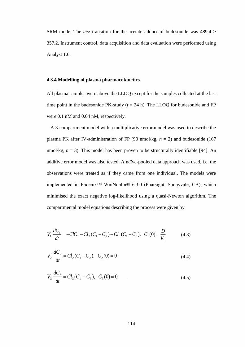
114

SRM mode. The m/z transition for the acetate adduct of budesonide was 489.4 >

357.2. Instrument control, data acquisition and data evaluation were performed using

Analyst 1.6.

4.3.4 Modelling of plasma pharmacokinetics

All plasma samples were above the LLOQ except for the samples collected at the last

time point in the budesonide PK-study (t = 24 h). The LLOQ for budesonide and FP

were 0.1 nM and 0.04 nM, respectively.

A 3-compartment model with a multiplicative error model was used to describe the

plasma PK after IV-administration of FP (90 nmol/kg, n = 2) and budesonide (167

nmol/kg, n = 3). This model has been proven to be structurally identifiable [94]. An

additive error model was also tested. A naïve-pooled data approach was used, i.e. the

observations were treated as if they came from one individual. The models were

implemented in Phoenix™ WinNonlin® 6.3.0 (Pharsight, Sunnyvale, CA), which

minimised the exact negative log-likelihood using a quasi-Newton algorithm. The

compartmental model equations describing the process were given by

1

13132121

1

1 )0( ),()(V

DCCCClCCClClC

dt

dCV (4.3)

0)0( ),( 2212

2

2 CCCCldt

dCV (4.4)

0)0( ),( 3313

3

3 CCCCldt

dCV . (4.5)

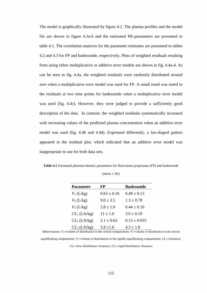
115

The model is graphically illustrated by figure 4.2. The plasma profiles and the model

fits are shown in figure 4.3a-b and the estimated PK-parameters are presented in

table 4.1. The correlation matrices for the parameter estimates are presented in tables

4.2 and 4.3 for FP and budesonide, respectively. Plots of weighted residuals resulting

from using either multiplicative or additive error models are shown in fig. 4.4a-d. As

can be seen in fig. 4.4a, the weighted residuals were randomly distributed around

zero when a multiplicative error model was used for FP. A small trend was noted in

the residuals at two time points for budesonide when a multiplicative error model

was used (fig. 4.4c). However, they were judged to provide a sufficiently good

description of the data. In contrast, the weighted residuals systematically increased

with increasing values of the predicted plasma concentration when an additive error

model was used (fig. 4.4b and 4.4d). Expressed differently, a fan-shaped pattern

appeared in the residual plot, which indicated that an additive error model was

inappropriate to use for both data sets.

Table 4.1 Estimated pharmacokinetic parameters for fluticasone propionate (FP) and budesonide

(mean ± SE)

Parameter FP Budesonide

V1 (L/kg) 0.63 ± 0.16 0.49 ± 0.13

V2 (L/kg) 9.0 ± 3.5 1.3 ± 0.78

V3 (L/kg) 2.8 ± 1.0 0.44 ± 0.10

CL1 (L/h/kg) 11 ± 1.0 3.0 ± 0.19

CL2 (L/h/kg) 2.1 ± 0.63 0.15 ± 0.035

CL3 (L/h/kg) 5.8 ±1.6 4.3 ± 1.8 Abbreviations: V1=volume of distribution in the central compartment; V2=volume of distribution in the slowly

equilibrating compartment; V3=volume of distribution in the rapidly equilibrating compartment; CL1=clearance;

CL2=slow distribution clearance; CL3=rapid distribution clearance

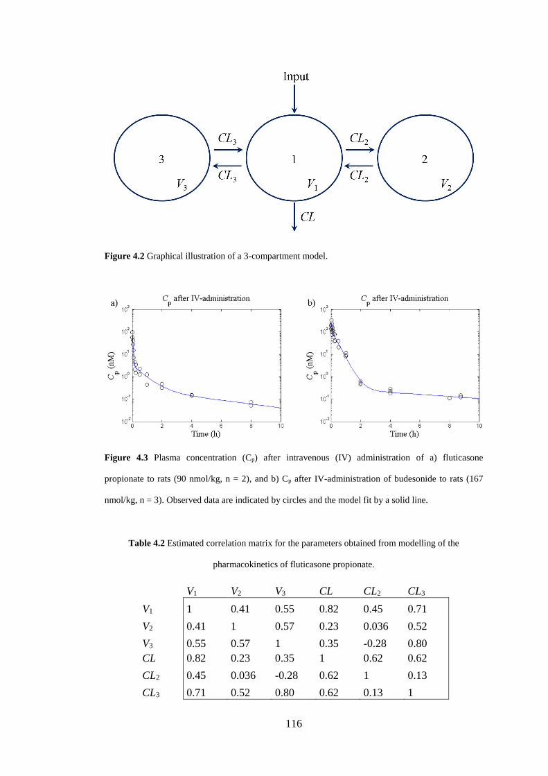
116

Figure 4.2 Graphical illustration of a 3-compartment model.

Figure 4.3 Plasma concentration (Cp) after intravenous (IV) administration of a) fluticasone

propionate to rats (90 nmol/kg, n = 2), and b) Cp after IV-administration of budesonide to rats (167

nmol/kg, n = 3). Observed data are indicated by circles and the model fit by a solid line.

Table 4.2 Estimated correlation matrix for the parameters obtained from modelling of the

pharmacokinetics of fluticasone propionate.

V1 V2 V3 CL CL2 CL3

V1 1 0.41 0.55 0.82 0.45 0.71

V2 0.41 1 0.57 0.23 0.036 0.52

V3 0.55 0.57 1 0.35 -0.28 0.80

CL 0.82 0.23 0.35 1 0.62 0.62

CL2 0.45 0.036 -0.28 0.62 1 0.13

CL3 0.71 0.52 0.80 0.62 0.13 1

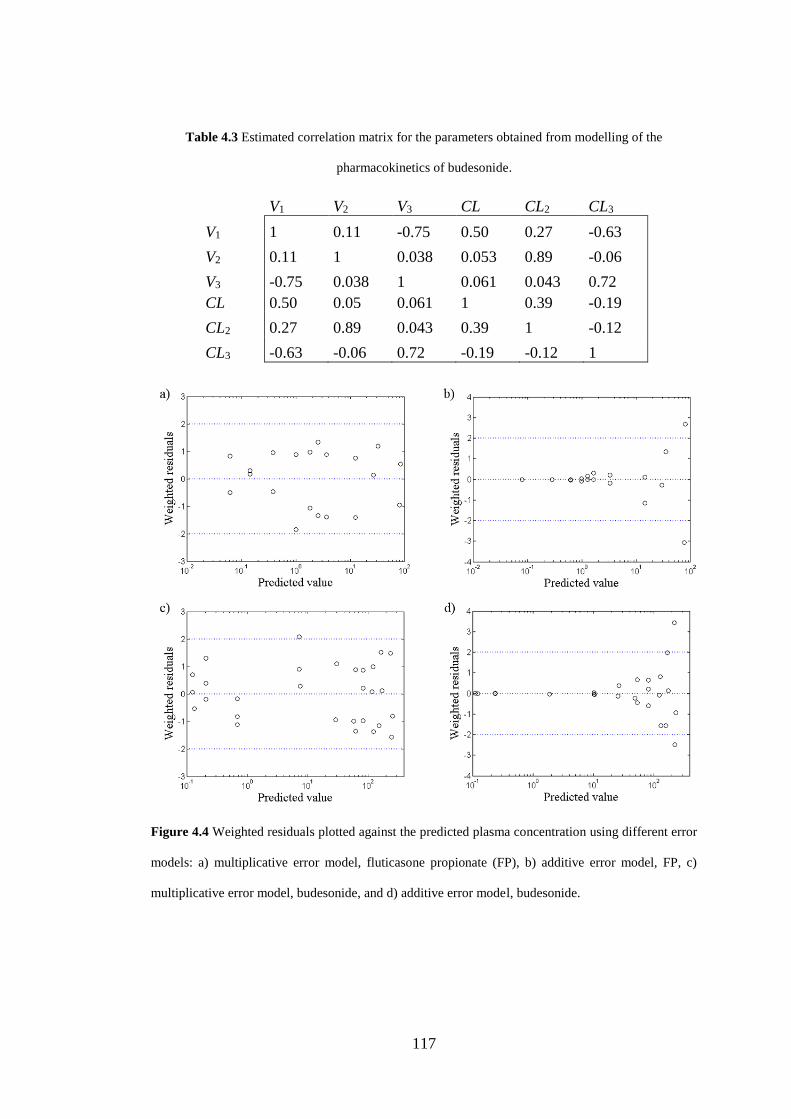
117

Table 4.3 Estimated correlation matrix for the parameters obtained from modelling of the

pharmacokinetics of budesonide.

V1 V2 V3 CL CL2 CL3

V1 1 0.11 -0.75 0.50 0.27 -0.63

V2 0.11 1 0.038 0.053 0.89 -0.06

V3 -0.75 0.038 1 0.061 0.043 0.72

CL 0.50 0.05 0.061 1 0.39 -0.19

CL2 0.27 0.89 0.043 0.39 1 -0.12

CL3 -0.63 -0.06 0.72 -0.19 -0.12 1

Figure 4.4 Weighted residuals plotted against the predicted plasma concentration using different error

models: a) multiplicative error model, fluticasone propionate (FP), b) additive error model, FP, c)

multiplicative error model, budesonide, and d) additive error model, budesonide.

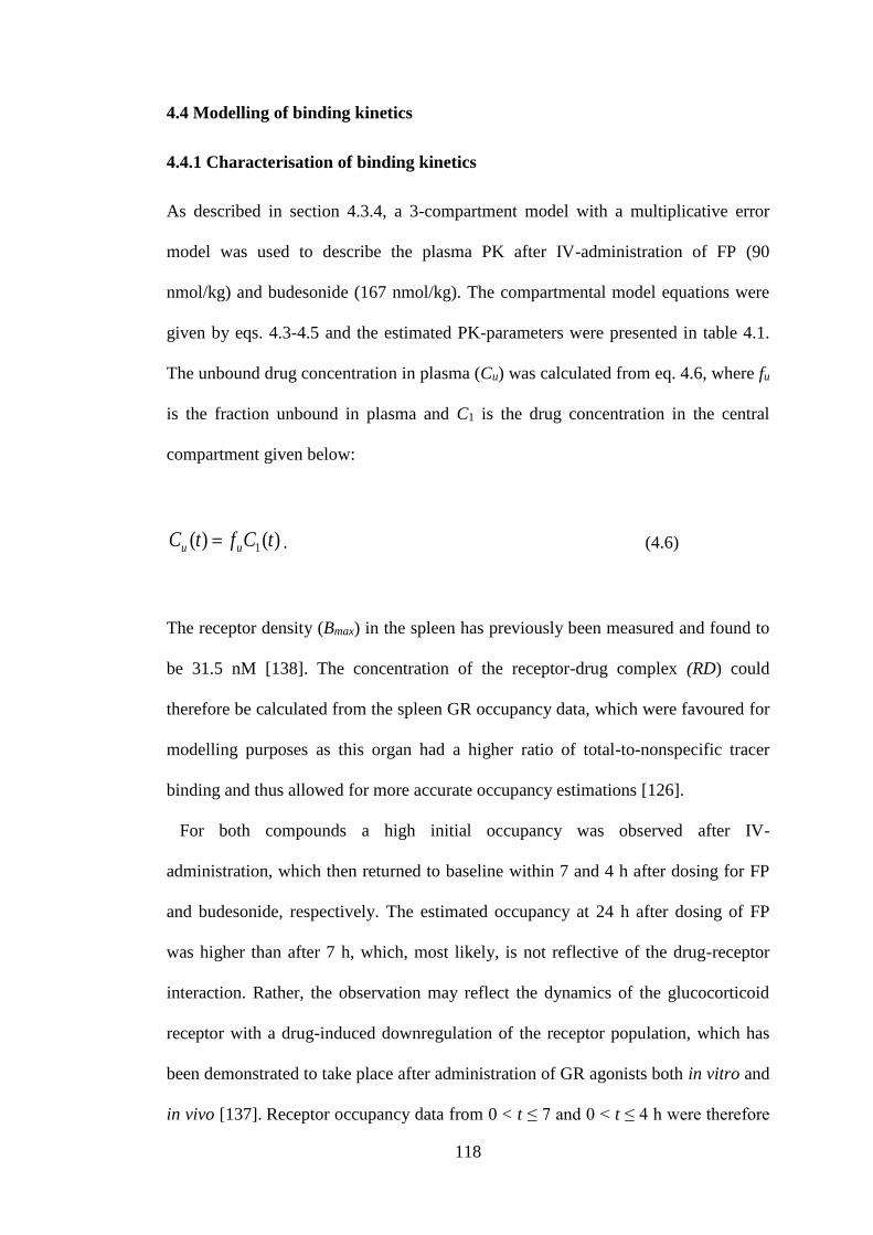
118

4.4 Modelling of binding kinetics

4.4.1 Characterisation of binding kinetics

As described in section 4.3.4, a 3-compartment model with a multiplicative error

model was used to describe the plasma PK after IV-administration of FP (90

nmol/kg) and budesonide (167 nmol/kg). The compartmental model equations were

given by eqs. 4.3-4.5 and the estimated PK-parameters were presented in table 4.1.

The unbound drug concentration in plasma (Cu) was calculated from eq. 4.6, where fu

is the fraction unbound in plasma and C1 is the drug concentration in the central

compartment given below:

)()( 1 tCftC uu . (4.6)

The receptor density (Bmax) in the spleen has previously been measured and found to

be 31.5 nM [138]. The concentration of the receptor-drug complex (RD) could

therefore be calculated from the spleen GR occupancy data, which were favoured for

modelling purposes as this organ had a higher ratio of total-to-nonspecific tracer

binding and thus allowed for more accurate occupancy estimations [126].

For both compounds a high initial occupancy was observed after IV-

administration, which then returned to baseline within 7 and 4 h after dosing for FP

and budesonide, respectively. The estimated occupancy at 24 h after dosing of FP

was higher than after 7 h, which, most likely, is not reflective of the drug-receptor

interaction. Rather, the observation may reflect the dynamics of the glucocorticoid

receptor with a drug-induced downregulation of the receptor population, which has

been demonstrated to take place after administration of GR agonists both in vitro and

in vivo [137]. Receptor occupancy data from 0 < t ≤ 7 and 0 < t ≤ 4 h were therefore

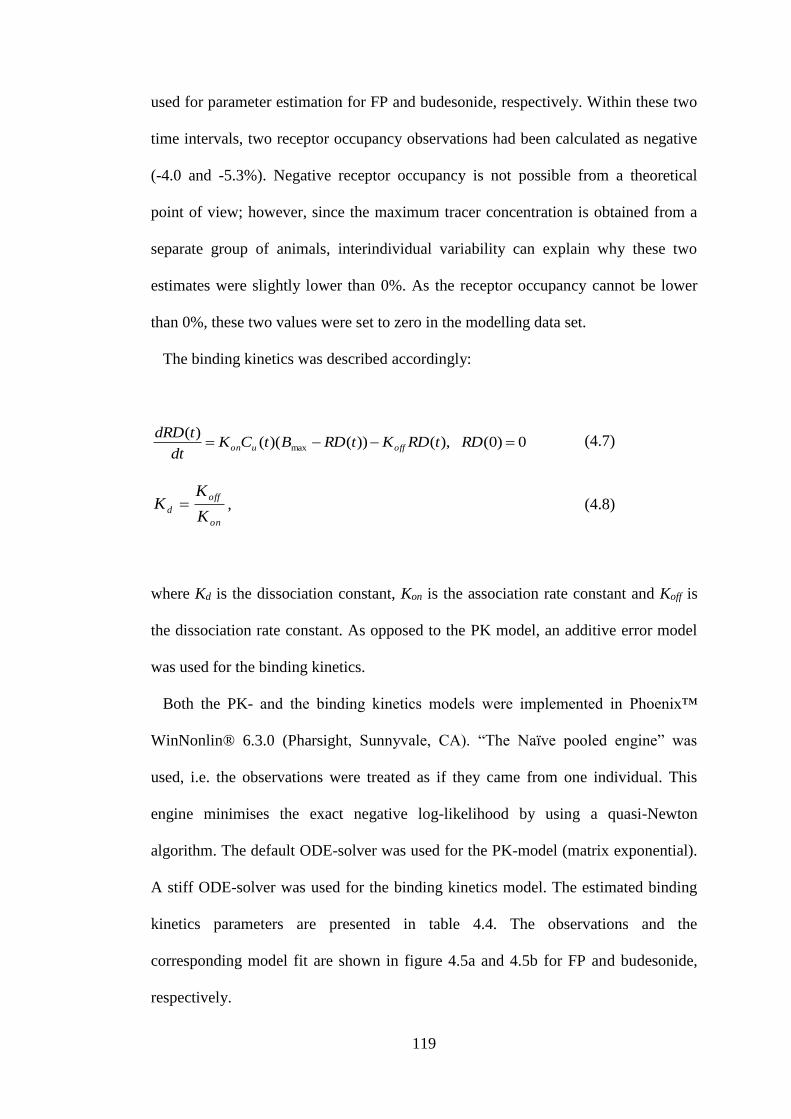
119

used for parameter estimation for FP and budesonide, respectively. Within these two

time intervals, two receptor occupancy observations had been calculated as negative

(-4.0 and -5.3%). Negative receptor occupancy is not possible from a theoretical

point of view; however, since the maximum tracer concentration is obtained from a

separate group of animals, interindividual variability can explain why these two

estimates were slightly lower than 0%. As the receptor occupancy cannot be lower

than 0%, these two values were set to zero in the modelling data set.

The binding kinetics was described accordingly:

0)0( ),())()(()(

max RDtRDKtRDBtCKdt

tdRDoffuon

(4.7)

on

off

dK

KK , (4.8)

where Kd is the dissociation constant, Kon is the association rate constant and Koff is

the dissociation rate constant. As opposed to the PK model, an additive error model

was used for the binding kinetics.

Both the PK- and the binding kinetics models were implemented in Phoenix™

WinNonlin® 6.3.0 (Pharsight, Sunnyvale, CA). “The Naïve pooled engine” was

used, i.e. the observations were treated as if they came from one individual. This

engine minimises the exact negative log-likelihood by using a quasi-Newton

algorithm. The default ODE-solver was used for the PK-model (matrix exponential).

A stiff ODE-solver was used for the binding kinetics model. The estimated binding

kinetics parameters are presented in table 4.4. The observations and the

corresponding model fit are shown in figure 4.5a and 4.5b for FP and budesonide,

respectively.

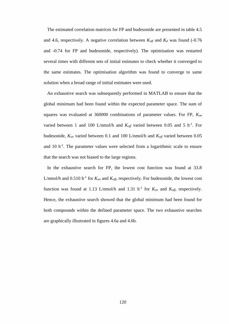
120

The estimated correlation matrices for FP and budesonide are presented in table 4.5

and 4.6, respectively. A negative correlation between Koff and Kd was found (-0.76

and -0.74 for FP and budesonide, respectively). The optimisation was restarted

several times with different sets of initial estimates to check whether it converged to

the same estimates. The optimisation algorithm was found to converge to same

solution when a broad range of initial estimates were used.

An exhaustive search was subsequently performed in MATLAB to ensure that the

global minimum had been found within the expected parameter space. The sum of

squares was evaluated at 360000 combinations of parameter values. For FP, Kon

varied between 1 and 100 L/nmol/h and Koff varied between 0.05 and 5 h-1. For

budesonide, Kon varied between 0.1 and 100 L/nmol/h and Koff varied between 0.05

and 10 h-1. The parameter values were selected from a logarithmic scale to ensure

that the search was not biased to the large regions.

In the exhaustive search for FP, the lowest cost function was found at 33.8

L/nmol/h and 0.510 h-1 for Kon and Koff, respectively. For budesonide, the lowest cost

function was found at 1.13 L/nmol/h and 1.31 h-1 for Kon and Koff, respectively.

Hence, the exhaustive search showed that the global minimum had been found for

both compounds within the defined parameter space. The two exhaustive searches

are graphically illustrated in figures 4.6a and 4.6b.

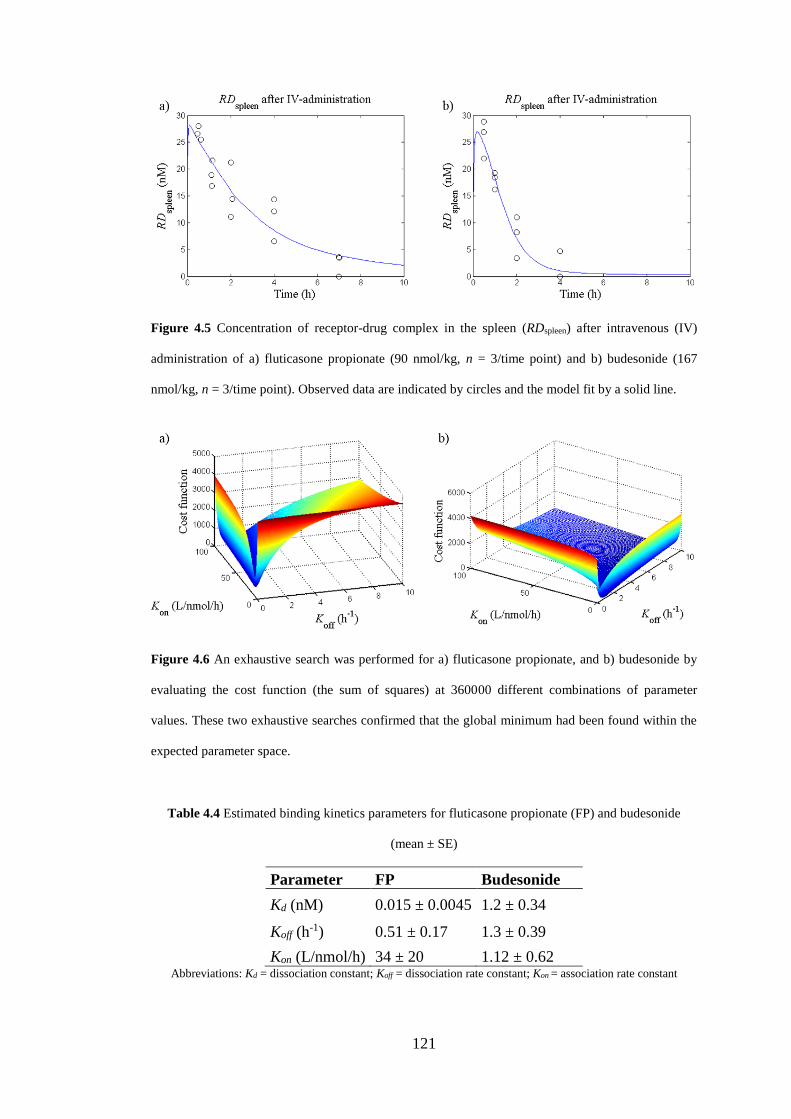
121

Figure 4.5 Concentration of receptor-drug complex in the spleen (RDspleen) after intravenous (IV)

administration of a) fluticasone propionate (90 nmol/kg, n = 3/time point) and b) budesonide (167

nmol/kg, n = 3/time point). Observed data are indicated by circles and the model fit by a solid line.

Figure 4.6 An exhaustive search was performed for a) fluticasone propionate, and b) budesonide by

evaluating the cost function (the sum of squares) at 360000 different combinations of parameter

values. These two exhaustive searches confirmed that the global minimum had been found within the

expected parameter space.

Table 4.4 Estimated binding kinetics parameters for fluticasone propionate (FP) and budesonide

(mean ± SE)

Parameter FP Budesonide

Kd (nM) 0.015 ± 0.0045 1.2 ± 0.34

Koff (h-1) 0.51 ± 0.17 1.3 ± 0.39

Kon (L/nmol/h) 34 ± 20 1.12 ± 0.62 Abbreviations: Kd = dissociation constant; Koff = dissociation rate constant; Kon

= association rate constant

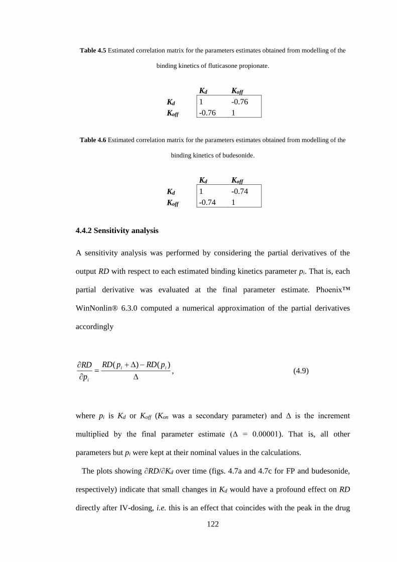
122

Table 4.5 Estimated correlation matrix for the parameters estimates obtained from modelling of the

binding kinetics of fluticasone propionate.

Kd Koff

Kd 1 -0.76

Koff -0.76 1

Table 4.6 Estimated correlation matrix for the parameters estimates obtained from modelling of the

binding kinetics of budesonide.

Kd Koff

Kd 1 -0.74

Koff -0.74 1

4.4.2 Sensitivity analysis

A sensitivity analysis was performed by considering the partial derivatives of the

output RD with respect to each estimated binding kinetics parameter pi. That is, each

partial derivative was evaluated at the final parameter estimate. Phoenix™

WinNonlin® 6.3.0 computed a numerical approximation of the partial derivatives

accordingly

)()( ii

i

pRDpRD

p

RD, (4.9)

where pi is Kd or Koff (Kon was a secondary parameter) and Δ is the increment

multiplied by the final parameter estimate (Δ = 0.00001). That is, all other

parameters but pi were kept at their nominal values in the calculations.

The plots showing ∂RD/∂Kd over time (figs. 4.7a and 4.7c for FP and budesonide,

respectively) indicate that small changes in Kd would have a profound effect on RD

directly after IV-dosing, i.e. this is an effect that coincides with the peak in the drug

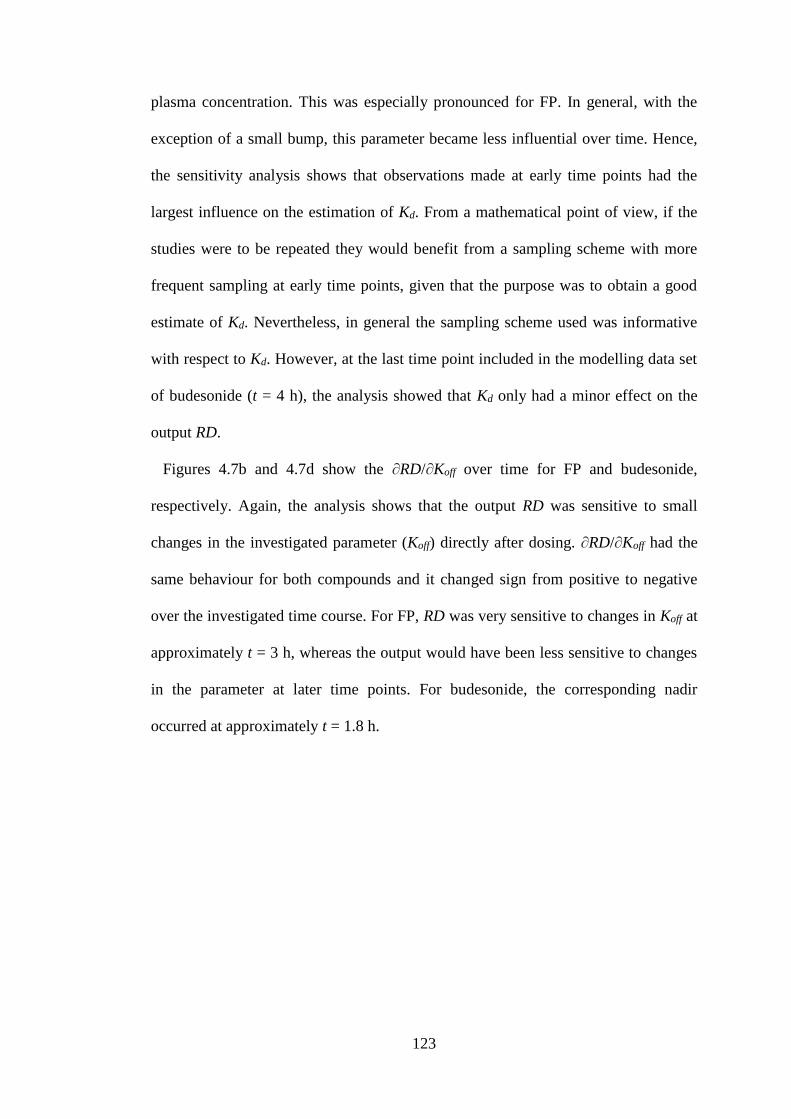
123

plasma concentration. This was especially pronounced for FP. In general, with the

exception of a small bump, this parameter became less influential over time. Hence,

the sensitivity analysis shows that observations made at early time points had the

largest influence on the estimation of Kd. From a mathematical point of view, if the

studies were to be repeated they would benefit from a sampling scheme with more

frequent sampling at early time points, given that the purpose was to obtain a good

estimate of Kd. Nevertheless, in general the sampling scheme used was informative

with respect to Kd. However, at the last time point included in the modelling data set

of budesonide (t = 4 h), the analysis showed that Kd only had a minor effect on the

output RD.

Figures 4.7b and 4.7d show the ∂RD/∂Koff over time for FP and budesonide,

respectively. Again, the analysis shows that the output RD was sensitive to small

changes in the investigated parameter (Koff) directly after dosing. ∂RD/∂Koff had the

same behaviour for both compounds and it changed sign from positive to negative

over the investigated time course. For FP, RD was very sensitive to changes in Koff at

approximately t = 3 h, whereas the output would have been less sensitive to changes

in the parameter at later time points. For budesonide, the corresponding nadir

occurred at approximately t = 1.8 h.

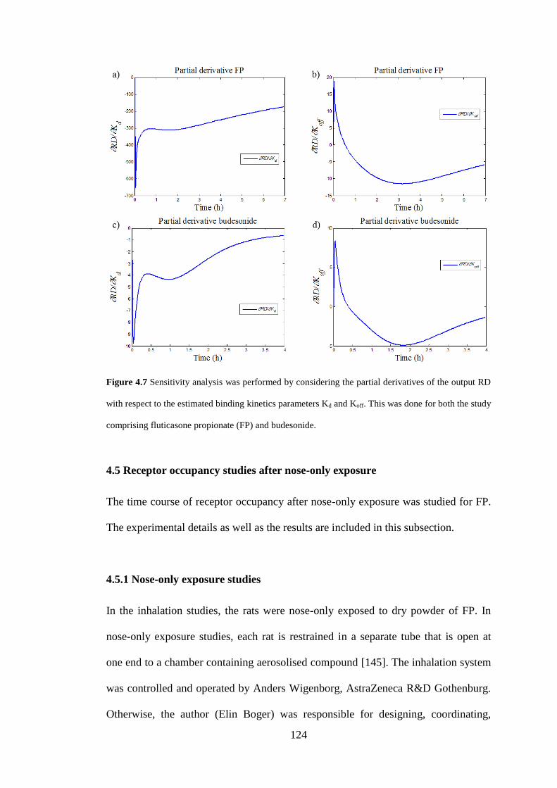
124

Figure 4.7 Sensitivity analysis was performed by considering the partial derivatives of the output RD

with respect to the estimated binding kinetics parameters Kd and Koff. This was done for both the study

comprising fluticasone propionate (FP) and budesonide.

4.5 Receptor occupancy studies after nose-only exposure

The time course of receptor occupancy after nose-only exposure was studied for FP.

The experimental details as well as the results are included in this subsection.

4.5.1 Nose-only exposure studies

In the inhalation studies, the rats were nose-only exposed to dry powder of FP. In

nose-only exposure studies, each rat is restrained in a separate tube that is open at

one end to a chamber containing aerosolised compound [145]. The inhalation system

was controlled and operated by Anders Wigenborg, AstraZeneca R&D Gothenburg.

Otherwise, the author (Elin Boger) was responsible for designing, coordinating,

125

performing as well as analysing the studies. The bioanalysis with respect to FP in the

plasma samples was done by Dr. Anders Lundqvist. Three additional researchers

from AstraZeneca R&D assisted the author in the in vivo parts of the studies: Dr

Markus Fridén, Dr Britt-Marie Fihn and Susanne Arlbrandt. The subsection

describing the inhalation system is written in collaboration with Anders Wigenborg.


375 g were used for the inhalation studies. The animals were group-housed at 18-

22ºC under a 12:12 h light/dark cycle with free access to food and water for at least

five days prior to the experiments. The studies were approved by the Animals Ethics

Committee of Gothenburg (71-2013).

Study protocol. The time course of receptor occupancy was studied after nose-

only exposure of FP. The inhalation study was performed twice using the same

experimental setup. The two studies are henceforth referred to as study 1 and study 2.

The following precautions were taken to reduce the stress for the animals: 1) all

animals were accustomed to nose-only exposure, including the restrainer tubes, prior

to the study, 2) they were accustomed to human contact prior to the study, 3) the

animals were weighed the day before the study, and 4) they were carefully moved to

the laboratory several hours before the start of the study.

The GR occupancy after nose-only exposure was investigated over 48 hours (t = 1,

2, 4, 7, 24 and 48 h, n = 3 and n = 4 per time point in study 1 and 2, respectively)

with additional PK-measurements at earlier time points (t = 45 and 75 min, n = 2 per

time point). The maximum tracer concentration was obtained from drug-naïve

control animals and the nonspecific tracer concentration from animals that had been

pre-treated intravenously with dexamethasone (n = 6, 20 mg/kg) 30 min prior to

tracer administration. The drug-naïve control animals from the two studies were

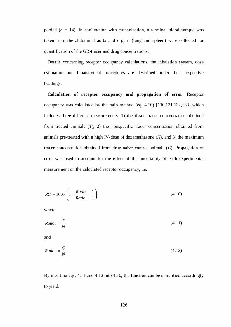
126

pooled (n = 14). In conjunction with euthanization, a terminal blood sample was

taken from the abdominal aorta and organs (lung and spleen) were collected for

quantification of the GR-tracer and drug concentrations.

Details concerning receptor occupancy calculations, the inhalation system, dose

estimation and bioanalytical procedures are described under their respective

headings.

Calculation of receptor occupancy and propagation of error. Receptor

occupancy was calculated by the ratio method (eq. 4.10) [130,131,132,133] which

includes three different measurements: 1) the tissue tracer concentration obtained

from treated animals (T), 2) the nonspecific tracer concentration obtained from

animals pre-treated with a high IV-dose of dexamethasone (N), and 3) the maximum

tracer concentration obtained from drug-naïve control animals (C). Propagation of

error was used to account for the effect of the uncertainty of each experimental

measurement on the calculated receptor occupancy, i.e.

1

11100

c

t

Ratio

RatioRO , (4.10)

where

N

TRatio t (4.11)

and

N

CRatio t . (4.12)

By inserting eqs. 4.11 and 4.12 into 4.10, the function can be simplified accordingly

to yield:

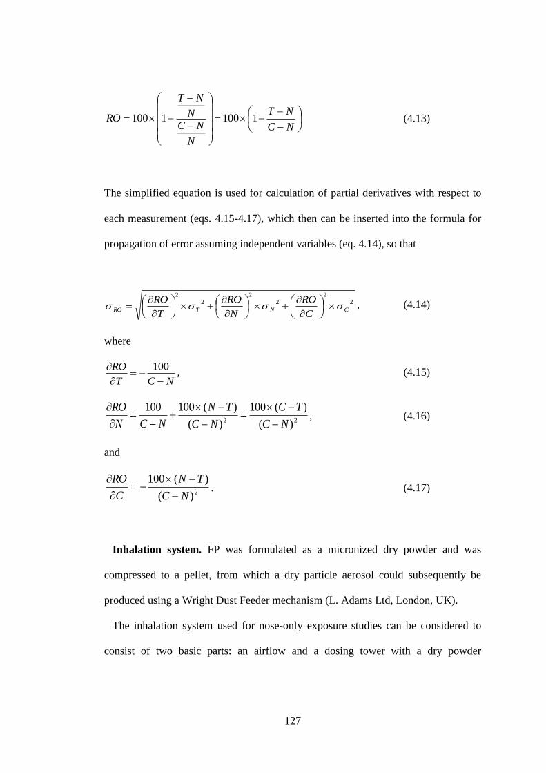
127

NC

NT

N

NCN

NT

RO 11001100 (4.13)

The simplified equation is used for calculation of partial derivatives with respect to

each measurement (eqs. 4.15-4.17), which then can be inserted into the formula for

propagation of error assuming independent variables (eq. 4.14), so that

2

2

2

2

2

2

CNTROC

RO

N

RO

T

RO

, (4.14)

where

NCT

RO

100, (4.15)

22 )(

)(100

)(

)(100100

NC

TC

NC

TN

NCN

RO

, (4.16)

and

2)(

)(100

NC

TN

C

RO

. (4.17)

Inhalation system. FP was formulated as a micronized dry powder and was

compressed to a pellet, from which a dry particle aerosol could subsequently be

produced using a Wright Dust Feeder mechanism (L. Adams Ltd, London, UK).

The inhalation system used for nose-only exposure studies can be considered to

consist of two basic parts: an airflow and a dosing tower with a dry powder

128

generator. The airflow can further be described as two separate flows: 1) an airflow

into the dosing tower, through the generator, and 2) a flow out of the dosing system.

The incoming air is mixed with the dry powder in a generator prior to entering into

the tower, and therefore acts as both a carrier for the active compound and provides

fresh air for the animals to breathe. The outflow of air/compound runs through the

animal breathing ports and the bottom of the tower, where the excess is extracted.

The driving force for this is provided by a vacuum with a slightly lower flow than the

incoming air.

The dosing tower usually consists of two concentric cylinders. The outer cylinder

is in direct contact with the animals through the dosing openings, communicating

with the inner cylinder that serves as a container for compound/air mixture. Since the

flow of air into the tower and the amount of substance generated is known, the

concentration in the inner cylinder of the tower can be calculated. The concentration

of delivered compound is measured online while dosing, using an aerosol monitor

(Casella Microdust-Pro-Aerosol-Monitoring, Bedford, UK) connected to a computer

with a software specifically developed for controlling inhalation dosing (MIVIS,

developed by Flexura AB, Sweden). MIVIS is one of the systems used to regulate

the dosing rate. This also means that the rate of the generation of powder and/or the

duration of dosing can be changed during the study if deemed necessary.

Some losses occur due to coating of the internal walls of the tower and for particles

with high kinetic energy, by impacting with the base of the tower. In either case,

these particles will not be inhaled by the animals. The actual concentration of the

compound in the aerosol and an estimate of the amount delivered to each animal can

be calculated by sampling at one of the animal ports. Air/compound is extracted to a

filter at a pre-defined flow during the time of dosing using a vacuum and the

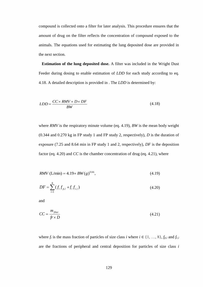
129

compound is collected onto a filter for later analysis. This procedure ensures that the

amount of drug on the filter reflects the concentration of compound exposed to the

animals. The equations used for estimating the lung deposited dose are provided in

the next section.

Estimation of the lung deposited dose. A filter was included in the Wright Dust

Feeder during dosing to enable estimation of LDD for each study according to eq.

4.18. A detailed description is provided in . The LDD is determined by:

BW

DFDRMVCCLDD

(4.18)

where RMV is the respiratory minute volume (eq. 4.19), BW is the mean body weight

(0.344 and 0.270 kg in FP study 1 and FP study 2, respectively), D is the duration of

exposure (7.25 and 8.64 min in FP study 1 and 2, respectively), DF is the deposition

factor (eq. 4.20) and CC is the chamber concentration of drug (eq. 4.21), where

66.0)(19.4 (L/min) gBWRMV , (4.19)

)( ,

8

1

, ici

i

ipi ffffDF

(4.20)

and

Dfr

mCC

filter

(4.21)

where fi is the mass fraction of particles of size class i where i ∈ {1, …, 8}, fp,i and fc,i

are the fractions of peripheral and central deposition for particles of size class i

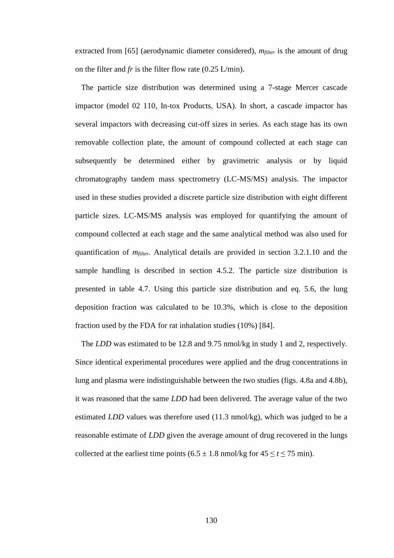
130

extracted from [65] (aerodynamic diameter considered), mfilter is the amount of drug

on the filter and fr is the filter flow rate (0.25 L/min).

The particle size distribution was determined using a 7-stage Mercer cascade

impactor (model 02 110, In-tox Products, USA). In short, a cascade impactor has

several impactors with decreasing cut-off sizes in series. As each stage has its own

removable collection plate, the amount of compound collected at each stage can

subsequently be determined either by gravimetric analysis or by liquid

chromatography tandem mass spectrometry (LC-MS/MS) analysis. The impactor

used in these studies provided a discrete particle size distribution with eight different

particle sizes. LC-MS/MS analysis was employed for quantifying the amount of

compound collected at each stage and the same analytical method was also used for

quantification of mfilter. Analytical details are provided in section 3.2.1.10 and the

sample handling is described in section 4.5.2. The particle size distribution is

presented in table 4.7. Using this particle size distribution and eq. 5.6, the lung

deposition fraction was calculated to be 10.3%, which is close to the deposition

fraction used by the FDA for rat inhalation studies (10%) [84].

The LDD was estimated to be 12.8 and 9.75 nmol/kg in study 1 and 2, respectively.

Since identical experimental procedures were applied and the drug concentrations in

lung and plasma were indistinguishable between the two studies (figs. 4.8a and 4.8b),

it was reasoned that the same LDD had been delivered. The average value of the two

estimated LDD values was therefore used (11.3 nmol/kg), which was judged to be a

reasonable estimate of LDD given the average amount of drug recovered in the lungs

collected at the earliest time points (6.5 ± 1.8 nmol/kg for 45 ≤ t ≤ 75 min).

131

Figure 4.8 a) Total lung concentrations (Clung) and b) plasma concentrations (Cp) after inhalation of

fluticasone propionate (FP) in study 1 (white circles) and study 2 (black circles).


The analytical procedures used for quantifying FP and the GR-tracer in lung

homogenates, spleen homogenates and plasma have been described in detail

previously in section 3.2.1.10. The analytical procedures used for quantifying FP in

plasma was described in section 4.3.3.1.

Sample preparation and analytical procedures connected to the filter analysis.

To enable estimation of the LDD, the amount of drug collected by a filter (mfilter)

during the inhalation period needed to be quantified. The filter was placed in a jar of

appropriate size immediately after inhalation. On the day of analysis, ethanol (4 mL)

was added to the filter and the jar was placed in an ultrasonic bath (5210 Branson;

Gemini, Apeldoorn, The Netherlands) for 20 minutes. Dimethyl sulfoxide (4 mL)

was then added to the sample to ensure that all of the substance was dissolved. A

certain volume of the resulting solution (1 mL) was filtered through 0.2 µm

Acrodisc® syringe filter (Pall Corporation, Ann Arbor, Mich.) to remove filter

particles prior to further treatment. The filtered solution was diluted by a factor of 35

by transferring a predetermined volume (20 µL) to a vial containing 40% acetonitrile

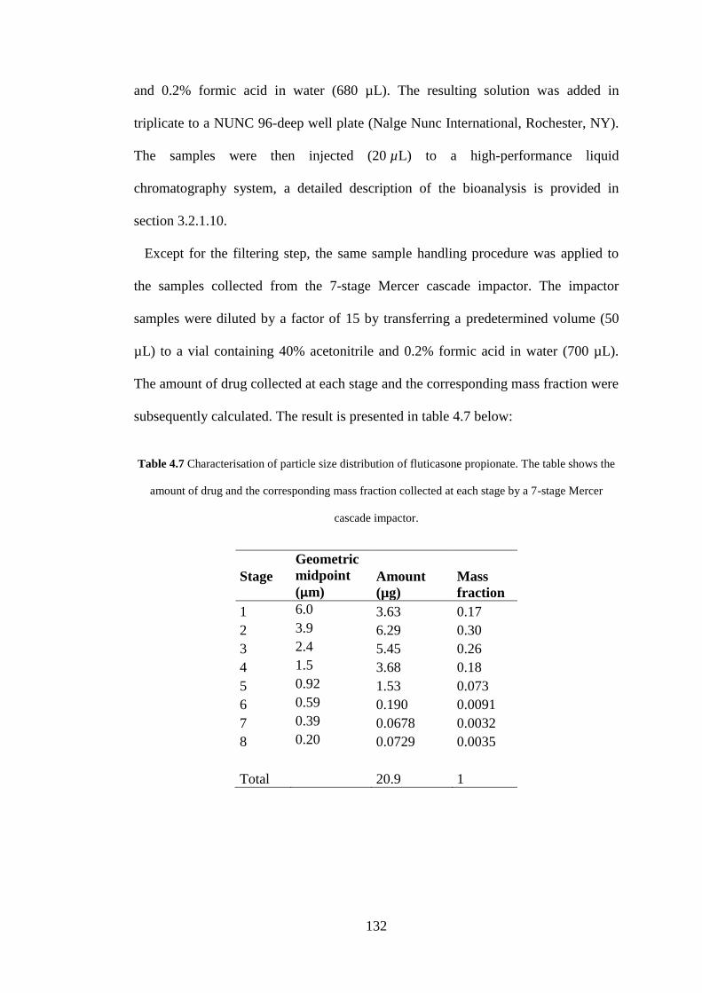
132

and 0.2% formic acid in water (680 µL). The resulting solution was added in

triplicate to a NUNC 96-deep well plate (Nalge Nunc International, Rochester, NY).

The samples were then injected (20 µL) to a high-performance liquid

chromatography system, a detailed description of the bioanalysis is provided in

section 3.2.1.10.

Except for the filtering step, the same sample handling procedure was applied to

the samples collected from the 7-stage Mercer cascade impactor. The impactor

samples were diluted by a factor of 15 by transferring a predetermined volume (50

µL) to a vial containing 40% acetonitrile and 0.2% formic acid in water (700 µL).

The amount of drug collected at each stage and the corresponding mass fraction were

subsequently calculated. The result is presented in table 4.7 below:

Table 4.7 Characterisation of particle size distribution of fluticasone propionate. The table shows the

amount of drug and the corresponding mass fraction collected at each stage by a 7-stage Mercer

cascade impactor.

Stage

Geometric

midpoint

(µm) Amount

(µg)

Mass

fraction

1 6.0 3.63 0.17

2 3.9 6.29 0.30

3 2.4 5.45 0.26

4 1.5 3.68 0.18

5 0.92 1.53 0.073

6 0.59 0.190 0.0091

7 0.39 0.0678 0.0032

8 0.20 0.0729 0.0035

Total 20.9 1

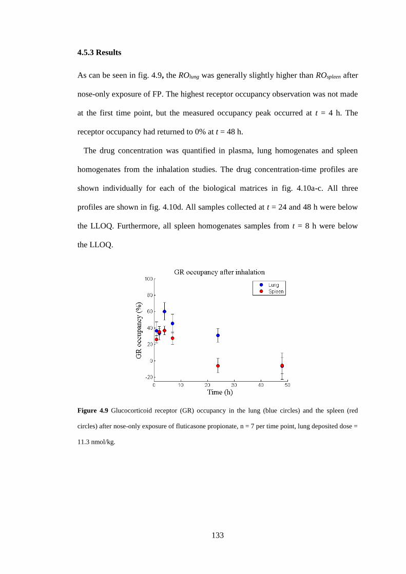
133

4.5.3 Results

As can be seen in fig. 4.9, the ROlung was generally slightly higher than ROspleen after

nose-only exposure of FP. The highest receptor occupancy observation was not made

at the first time point, but the measured occupancy peak occurred at t = 4 h. The

receptor occupancy had returned to 0% at t = 48 h.

The drug concentration was quantified in plasma, lung homogenates and spleen

homogenates from the inhalation studies. The drug concentration-time profiles are

shown individually for each of the biological matrices in fig. 4.10a-c. All three

profiles are shown in fig. 4.10d. All samples collected at t = 24 and 48 h were below

the LLOQ. Furthermore, all spleen homogenates samples from t = 8 h were below

the LLOQ.

Figure 4.9 Glucocorticoid receptor (GR) occupancy in the lung (blue circles) and the spleen (red

circles) after nose-only exposure of fluticasone propionate, n = 7 per time point, lung deposited dose =

11.3 nmol/kg.

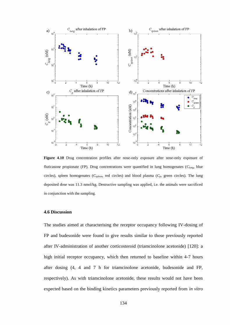
134

Figure 4.10 Drug concentration profiles after nose-only exposure after nose-only exposure of

fluticasone propionate (FP). Drug concentrations were quantified in lung homogenates (Clung, blue

circles), spleen homogenates (Cspleen, red circles) and blood plasma (Cp, green circles). The lung

deposited dose was 11.3 nmol/kg. Destructive sampling was applied, i.e. the animals were sacrificed

in conjunction with the sampling.

4.6 Discussion

The studies aimed at characterising the receptor occupancy following IV-dosing of

FP and budesonide were found to give results similar to those previously reported

after IV-administration of another corticosteroid (triamcinolone acetonide) [120]: a

high initial receptor occupancy, which then returned to baseline within 4-7 hours

after dosing (4, 4 and 7 h for triamcinolone acetonide, budesonide and FP,

respectively). As with triamcinolone acetonide, these results would not have been

expected based on the binding kinetics parameters previously reported from in vitro

135

experiments with dissociation half-lives of 21 h [143], 10 h [80] and 4.6 h [146] for

triamcinolone acetonide, FP and budesonide, respectively. These results, combined

with earlier research [120], thus suggest a disconnection between the in vitro system

used for studying binding kinetics and the in vivo situation. However, the cited in

vitro experiments were conducted at temperatures that were low relative to the

rodent’s body temperature, which could explain the deviation between the in vitro

and the in vivo situation.

As pointed out in section 4.4.1, the estimated receptor occupancy 24 hours after

IV-dosing of FP was higher than after 7 hours, which is most likely not reflective of

the drug-receptor interaction. Rather, the observation may reflect the dynamics of the

GR with a drug-induced down-regulation of the receptor population, which has been

demonstrated to take place after GR agonist exposure both in vitro and in vivo [137].

Furthermore, observations from earlier time points revealed that the receptor

occupancy had returned to baseline within 7 hours after the IV-injection. The

observations made at 24 and 48 h after dosing were therefore not included in the data

set for parameter estimation. Similarly, since receptor occupancy had returned to

baseline within 4 hours after dosing of budesonide, observations made at t > 4 h were

not judged to provide any information on the binding kinetics and were thus not used

for parameter estimation purposes.

Based on the receptor occupancy profiles obtained from the IV-studies, it can be

concluded that the chosen doses were sufficiently high to significantly perturb the

system and thus enable receptor occupancy measurements over several hours. Hence,

mathematical modelling could subsequently be applied to estimate the in vivo

binding kinetics parameters (Kon and Koff), where an exhaustive search confirmed that

136

the minimum had been found by the optimisation algorithm (within the expected

parameter space as defined in section 4.4.1).

The PK-data from the nose-only exposure studies (fig. 4.10) followed a pattern

expected from a poorly soluble inhaled drug: a large amount of drug remained in the

lung over several hours after inhalation whereas only low drug levels could be

detected in plasma. Furthermore, the plasma profile was flat as compared to the

corresponding profile resulting from IV-dosing, which indicates a slow absorption of

drug to the systemic circulation. This PK-behaviour can thus potentially be explained

by a dissolution rate-limited absorption.

The measured receptor occupancy peak occurred at t = 4 h, which possibly, at least

partly, could be explained by a slow dissolution process. The receptor occupancy

was generally slightly higher in the lung than in the reference organ for systemic

exposure (the spleen) after nose-only exposure (fig. 4.9). It is worth noting that the

low degree of lung-selectivity reflected by receptor occupancy measurements was

consistent with data from a preclinical PD-model, in which the local and systemic

effects are studied after nose-only exposure of GR modulators. In short, as described

by Källström et al. [147] this PD-model relies on inducing pulmonary inflammation

by Sephadex, which will be reflected by an increased lung weight. The local effect of

the test compound is subsequently determined by lung weight changes, whereas the

systemic effect is determined by quantifying thymic involution. Interestingly, FP was

found to have a therapeutic ratio of approximately 1 in this PD-model [148].

In chapter 5, the estimates of Kon and Koff will be incorporated into a mechanistic in

silico model developed for predicting the systemic PK, the local tissue

concentrations as well as the resulting receptor occupancy after inhalation. In

contrast to traditional PK/PD-models, this model will not rely on a top-down

137

approach where an appropriate model structure (empirical or mechanistic) is chosen

and the included parameters are optimised to minimise an objective function (e.g. the

deviation between predicted and observed data as described by the sum of squares).

Instead, the model structure will be based on the current understanding of pulmonary

drug disposition as well as on the rodent physiology and the input parameters will be

obtained from experimental data and literature sources. By subsequently comparing

model predictions from this systems model to observed data, the current

understanding of the system can be evaluated. For the first time, receptor occupancy

observations from an inhalation study will be used for validating predictions of the

local, and not only the systemic, exposure following topical administration. Any

discrepancy can be informative with respect to the existing knowledge of underlying

mechanisms and assumptions. If proven to be predictive, the model can be used to

e.g. generate hypotheses, explore scenarios that currently cannot be tested

experimentally and to provide a framework for a facilitated translation from animal

to human.

4.7 Summary

This chapter presented a sequence of research activities undertaken for characterising

the in vivo binding kinetics of the two GR agonists FP and budesonide. The two

drugs were given at sufficiently high IV-doses to perturb the system such that

receptor occupancy could be monitored over several hours (fig. 4.5a-b). For the first

time, the binding kinetics parameters for these two substances could be estimated

based on in vivo data. Parameter estimation was performed in Phoenix™. An

exhaustive search algorithm implemented in MATLAB subsequently confirmed that

the minimum objective function had been found by the optimisation algorithm

138

(within the expected parameter space). The receptor occupancy and the PK were

studied after nose-only exposure of FP (11.3 nmol/kg, LDD). The PK-data showed

high levels of unabsorbed drug in the lung following inhalation with low resulting

plasma levels. The receptor occupancy was generally slightly higher in the lung than

in the reference organ for systemic exposure (the spleen) and the data suggested a

late occupancy peak at approximately 4 h after dosing.

The estimates of the binding kinetics parameters Kon and Koff will be used as drug-

specific input parameters for a mechanistic in silico model in chapter 5 that was

developed as part of this thesis. The receptor occupancy measurements as well as the

PK from the nose-only exposure studies will be used for model validation purposes.

139

Chapter 5 A mechanistic inhalation PBPK model for prediction of

local and systemic PK and receptor occupancy

5.1 Introduction

Even though inhalation is an attractive route of administration that has been

employed for more than 2000 years [1], inhalation pharmacokinetics is still

recognised as a challenging research area. As discussed in depth in chapters 3 and 4,

the challenges are partly related to the difficulties of getting relevant exposure

measurements. Furthermore, pulmonary drug disposition of inhaled drugs is known

to be a complex interplay between numerous processes including e.g. regional drug

deposition, particle dissolution and mucociliary clearance (MCC). Additional

complexity comes from the heterogeneous nature of the organ with distinct

differences between the tracheobronchial and the alveolar regions [11]. Lung

targeting by inhalation in terms of the free target site concentration and the resulting

local receptor occupancy is therefore notoriously difficult to predict.

While some of the aforementioned processes have been thoroughly characterised

on an individual basis, a step-change in the understanding of inhalation

pharmacokinetics could be gained if we also understood the interplay between these

different processes in a physiological context. Significant progress towards achieving

this goal can be made by developing a physiologically-based pharmacokinetic

(PBPK) model, which places emphasis on lung disposition for inhaled drugs by

mathematically describing these fundamental processes. However, such a

mechanistic model predictive of local tissue concentrations combined with

measurements such as receptor occupancy for validation is currently lacking. The

recently generated data on local and systemic receptor occupancy after inhalation of

140

fluticasone propionate (FP) in combination with the estimates of its binding kinetics

parameters (Kon and Koff) thus provide an opportunity to validate such predictions.

Furthermore, data on drug concentrations in different biological matrices will also be

available for model validation.

Expressed differently, a new mathematical framework can be built by formulating

mathematical descriptions of the system based on the current understanding of

pulmonary drug disposition and rodent physiology. Once the model structure is in

place, it can be evaluated by using drug- and formulation-specific parameters,

obtained from experimental data or literature sources, as input parameters. In this

context, it is worth mentioning that the approach used to evaluate this model type,

i.e. a systems model, is different from the approach used to evaluate standard

PK/PD-models. Since systems models are built based on the current understanding of

a system, any discrepancy between model predictions and observations can be

informative with respect to the existing knowledge of underlying mechanisms and

assumptions [149]. That is, a discrepancy may for example be due to a mechanism

that is unaccounted for by the model structure or not fully understood.

If the model is proven to be predictive, it can be used to generate hypotheses and

explore scenarios that have not been tested experimentally. Another useful feature of

PBPK models is that they can separate physiological system- from drug-

/formulation-specific properties, which carries several advantages including the

possibility to explore how different drug- and formulation-specific properties, or

combinations thereof, relate to important endpoints such as the lung-selectivity of a

drug treatment. Such information could for instance be used to guide: 1) the design

of chemical series in the early phases of drug discovery, and 2) the choice of drug

formulations for clinical trials.

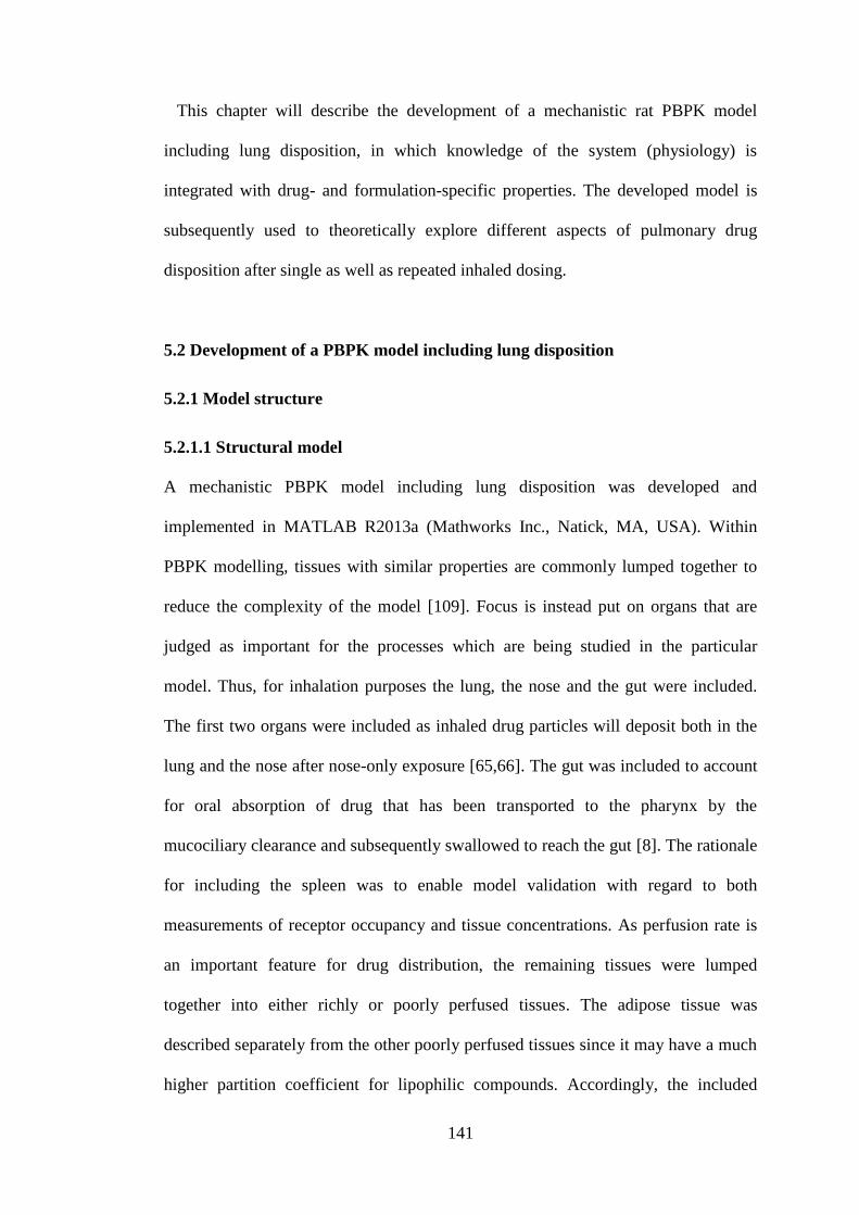
141

This chapter will describe the development of a mechanistic rat PBPK model

including lung disposition, in which knowledge of the system (physiology) is

integrated with drug- and formulation-specific properties. The developed model is

subsequently used to theoretically explore different aspects of pulmonary drug

disposition after single as well as repeated inhaled dosing.

5.2 Development of a PBPK model including lung disposition

5.2.1 Model structure

5.2.1.1 Structural model

A mechanistic PBPK model including lung disposition was developed and

implemented in MATLAB R2013a (Mathworks Inc., Natick, MA, USA). Within

PBPK modelling, tissues with similar properties are commonly lumped together to

reduce the complexity of the model [109]. Focus is instead put on organs that are

judged as important for the processes which are being studied in the particular

model. Thus, for inhalation purposes the lung, the nose and the gut were included.

The first two organs were included as inhaled drug particles will deposit both in the

lung and the nose after nose-only exposure [65,66]. The gut was included to account

for oral absorption of drug that has been transported to the pharynx by the

mucociliary clearance and subsequently swallowed to reach the gut [8]. The rationale

for including the spleen was to enable model validation with regard to both

measurements of receptor occupancy and tissue concentrations. As perfusion rate is

an important feature for drug distribution, the remaining tissues were lumped

together into either richly or poorly perfused tissues. The adipose tissue was

described separately from the other poorly perfused tissues since it may have a much

higher partition coefficient for lipophilic compounds. Accordingly, the included

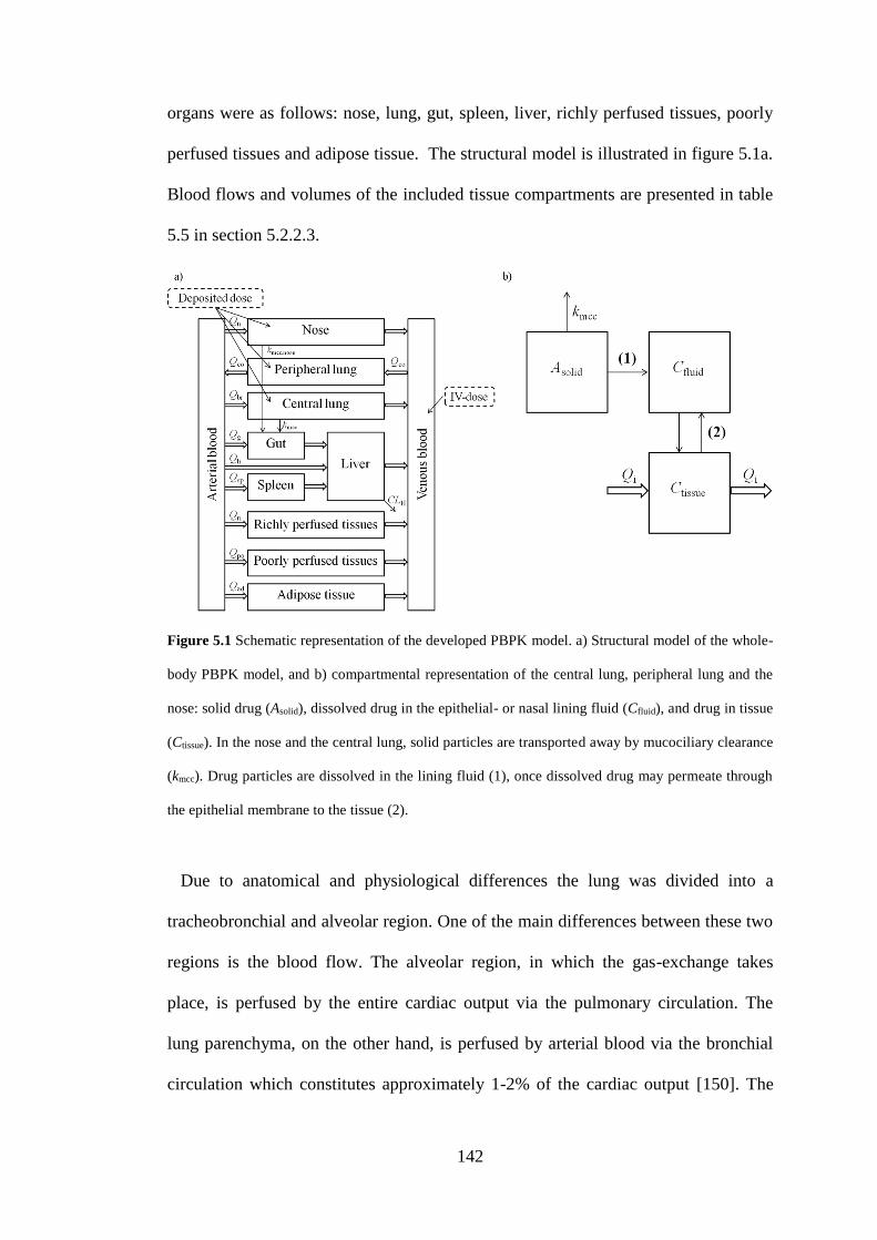
142

organs were as follows: nose, lung, gut, spleen, liver, richly perfused tissues, poorly

perfused tissues and adipose tissue. The structural model is illustrated in figure 5.1a.

Blood flows and volumes of the included tissue compartments are presented in table

5.5 in section 5.2.2.3.

Figure 5.1 Schematic representation of the developed PBPK model. a) Structural model of the whole-

body PBPK model, and b) compartmental representation of the central lung, peripheral lung and the

nose: solid drug (Asolid), dissolved drug in the epithelial- or nasal lining fluid (Cfluid), and drug in tissue

(Ctissue). In the nose and the central lung, solid particles are transported away by mucociliary clearance

(kmcc). Drug particles are dissolved in the lining fluid (1), once dissolved drug may permeate through

the epithelial membrane to the tissue (2).

Due to anatomical and physiological differences the lung was divided into a

tracheobronchial and alveolar region. One of the main differences between these two

regions is the blood flow. The alveolar region, in which the gas-exchange takes

place, is perfused by the entire cardiac output via the pulmonary circulation. The

lung parenchyma, on the other hand, is perfused by arterial blood via the bronchial

circulation which constitutes approximately 1-2% of the cardiac output [150]. The

143

thickness of the epithelial lining fluid (ELF) is also known to gradually decrease

along the lung generations [151], as is the thickness of the epithelium [11]. The latter

property is expected to give rise to permeability differences across the lung.

Interestingly, studies by Gerde et al. showed that the highly lipophilic substance BaP

was rapidly absorbed through the thin alveolar epithelium [152], whereas the

absorption through the tracheobronchial epithelium was several-fold slower [153].

Hence, these studies point towards the importance of treating the lung as a

heterogeneous organ.

Each of the two lung regions was in turn divided into three separate compartments

(fig. 5.1b). The same compartmental representation was used for the nose: 1)

undissolved drug (Asolid), 2) dissolved drug in the epithelial or nasal lining fluid

(Cfluid), and 3) drug in tissue (Ctissue). The tracheobronchial region is perfused by the

bronchial blood flow (Qbronch), the alveolar region by the entire cardiac output (QCO)

and the nose by the nasal blood flow (Qnose). The compartmental representation of

the nose and the two lung regions is shown in figure 5.1b. The system-specific input

parameters for the nose and lung are summarised in table 5.6 in section 5.2.2.3. Once

the drug has dissolved (see section 5.2.1.3) it may permeate through the epithelial

membrane to the tissue according to:

))(

)((,,

,

iup

ifluidufluidsurf

K

tCftCPA

dt

dQ , (5.1)

where dQ/dt is the molar flow of drug (nmol/h), P is the permeability, Asurf is the

surface area, fu,fluid is the unbound fraction in the lining fluid, Ci is the tissue

concentration of drug and Kp,u,i is the tissue-to-unbound plasma partition coefficient.

A detailed description of the prediction of Kp,u-values as well as the subsequent

144

calculations of Kp-values is provided in section 5.2.2.1. The in vitro apparent

permeability across CaCo2-monolayers was measured and used as the parameter P

(tables 5.3 and 5.4 in section 5.2.2.1).

Perfusion rate-limited distribution was assumed to apply for all tissues. For

compartment i, the rate of change of quantity of drug within the organ was described

as [103]

0)0( ,)(

)()(

,

i

ip

i

Ai

i

i CK

tRCtCQ

dt

tdCV , (5.2)

where Vi is the tissue volume, Ci is the drug tissue concentration, Qi is the blood flow

to the tissue, CA is the arterial drug concentration, R is the blood/plasma ratio and Kp,i

is the tissue-to-plasma partition coefficient.

5.2.1.2 Particle size distribution, regional deposition and mucociliary clearance

Inhaled drug particles can be deposited in the extrathoracic, tracheobronchial and

alveolar region. This model neglects deposition in the pharynx and the larynx, hence

only nasal deposition is considered in the extrathoracic region. Henceforth, the

tracheobronchial and alveolar regions are referred to as the central and the peripheral

lung, respectively.

Several models have been developed for prediction of regional particle deposition

in rat lungs [65,66,69,154]. By extracting the regional deposition fraction for the

relevant aerodynamic diameters from [65], the number of deposited particles can be

calculated based on the deposition fraction and the mass fraction of the relevant

particle size class via:

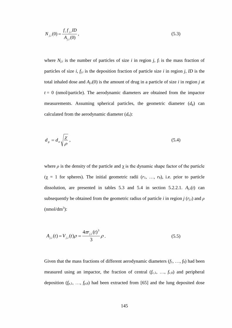
145

)0()0(

,

,

,

ij

iji

ijA

IDffN , (5.3)

where Nj,i is the number of particles of size i in region j, fi is the mass fraction of

particles of size i, fj,i is the deposition fraction of particle size i in region j, ID is the

total inhaled dose and Aj,i(0) is the amount of drug in a particle of size i in region j at

t = 0 (nmol/particle). The aerodynamic diameters are obtained from the impactor

measurements. Assuming spherical particles, the geometric diameter (dg) can

calculated from the aerodynamic diameter (da):

ag dd , (5.4)

where ρ is the density of the particle and χ is the dynamic shape factor of the particle

(χ = 1 for spheres). The initial geometric radii (r1, …, r8), i.e. prior to particle

dissolution, are presented in tables 5.3 and 5.4 in section 5.2.2.1. Aj,i(t) can

subsequently be obtained from the geometric radius of particle i in region j (rj,i) and ρ

(nmol/dm3):

3

)(4)()(

3

,

,,

trtVtA

ij

ijij . (5.5)

Given that the mass fractions of different aerodynamic diameters (f1, …, f8) had been

measured using an impactor, the fraction of central (fc,1, …, fc,8) and peripheral

deposition (fp,1, …, fp,8) had been extracted from [65] and the lung deposited dose

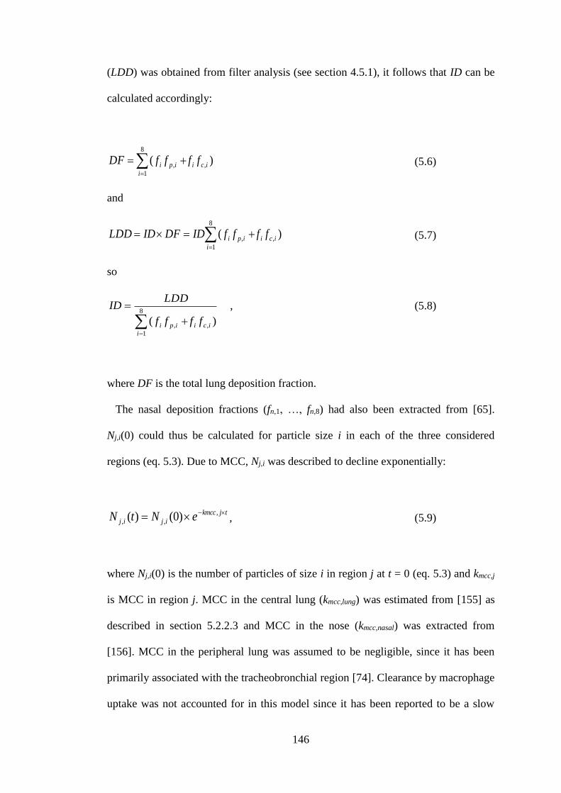
146

(LDD) was obtained from filter analysis (see section 4.5.1), it follows that ID can be

calculated accordingly:

)( ,

8

1

, ici

i

ipi ffffDF

(5.6)

and

)( ,

8

1

, ici

i

ipi ffffIDDFIDLDD

(5.7)

so

)( ,

8

1

, ici

i

ipi ffff

LDDID

, (5.8)

where DF is the total lung deposition fraction.

The nasal deposition fractions (fn,1, …, fn,8) had also been extracted from [65].

Nj,i(0) could thus be calculated for particle size i in each of the three considered

regions (eq. 5.3). Due to MCC, Nj,i was described to decline exponentially:

tjkmcc

ijij eNtN ,

,, )0()( , (5.9)

where Nj,i(0) is the number of particles of size i in region j at t = 0 (eq. 5.3) and kmcc,j

is MCC in region j. MCC in the central lung (kmcc,lung) was estimated from [155] as

described in section 5.2.2.3 and MCC in the nose (kmcc,nasal) was extracted from

[156]. MCC in the peripheral lung was assumed to be negligible, since it has been

primarily associated with the tracheobronchial region [74]. Clearance by macrophage

uptake was not accounted for in this model since it has been reported to be a slow

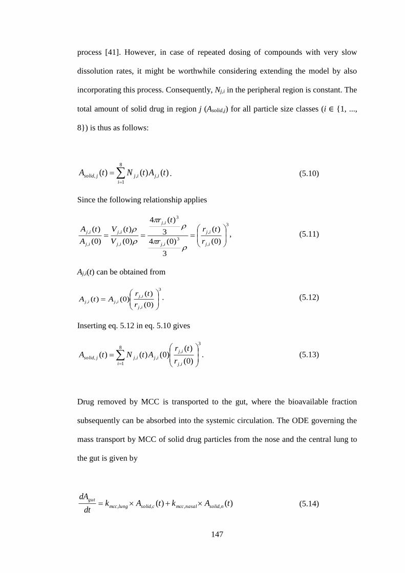
147

process [41]. However, in case of repeated dosing of compounds with very slow

dissolution rates, it might be worthwhile considering extending the model by also

incorporating this process. Consequently, Nj,i in the peripheral region is constant. The

total amount of solid drug in region j (Asolid,j) for all particle size classes (i ∈ {1, ...,

8}) is thus as follows:

8

1

,,, )()()(i

ijijjsolid tAtNtA . (5.10)

Since the following relationship applies

3

,

,

3

,

3

,

,

,

,

,

)0(

)(

3

)0(4

3

)(4

)0(

)(

)0(

)(

ij

ij

ij

ij

ij

ij

ij

ij

r

tr

r

tr

V

tV

A

tA

, (5.11)

Aj,i(t) can be obtained from

3

,

,

,,)0(

)()0()(

ij

ij

ijijr

trAtA . (5.12)

Inserting eq. 5.12 in eq. 5.10 gives

3

,

,8

1

,,,)0(

)()0()()(

ij

ij

i

ijijjsolidr

trAtNtA . (5.13)

Drug removed by MCC is transported to the gut, where the bioavailable fraction

subsequently can be absorbed into the systemic circulation. The ODE governing the

mass transport by MCC of solid drug particles from the nose and the central lung to

the gut is given by

)()( ,,,, tAktAkdt

dAnsolidnasalmcccsolidlungmcc

gut (5.14)

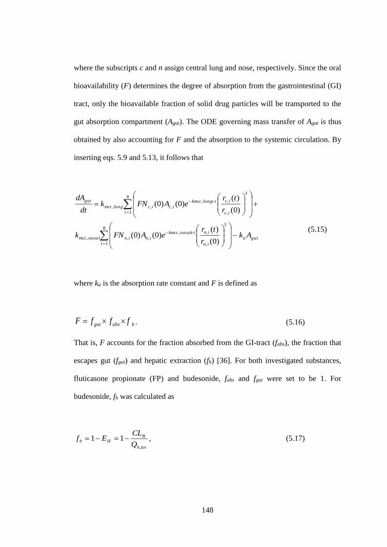
148

where the subscripts c and n assign central lung and nose, respectively. Since the oral

bioavailability (F) determines the degree of absorption from the gastrointestinal (GI)

tract, only the bioavailable fraction of solid drug particles will be transported to the

gut absorption compartment (Agut). The ODE governing mass transfer of Agut is thus

obtained by also accounting for F and the absorption to the systemic circulation. By

inserting eqs. 5.9 and 5.13, it follows that

(5.15)

where ka is the absorption rate constant and F is defined as

habsgut fffF . (5.16)

That is, F accounts for the fraction absorbed from the GI-tract (fabs), the fraction that

escapes gut (fgut) and hepatic extraction (fh) [36]. For both investigated substances,

fluticasone propionate (FP) and budesonide, fabs and fgut were set to be 1. For

budesonide, fh was calculated as

toth

BHh

Q

CLEf

,

11 , (5.17)

guta

i in

intnasalkmcc

ininnasalmcc

i ic

ictlungkmcc

iciclungmcc

gut

Akr

treAFNk

r

treAFNk

dt

dA

8

1

3

,

,,

,,,

8

1

3

,

,,

,,,

)0(

)()0()0(

)0(

)()0()0(

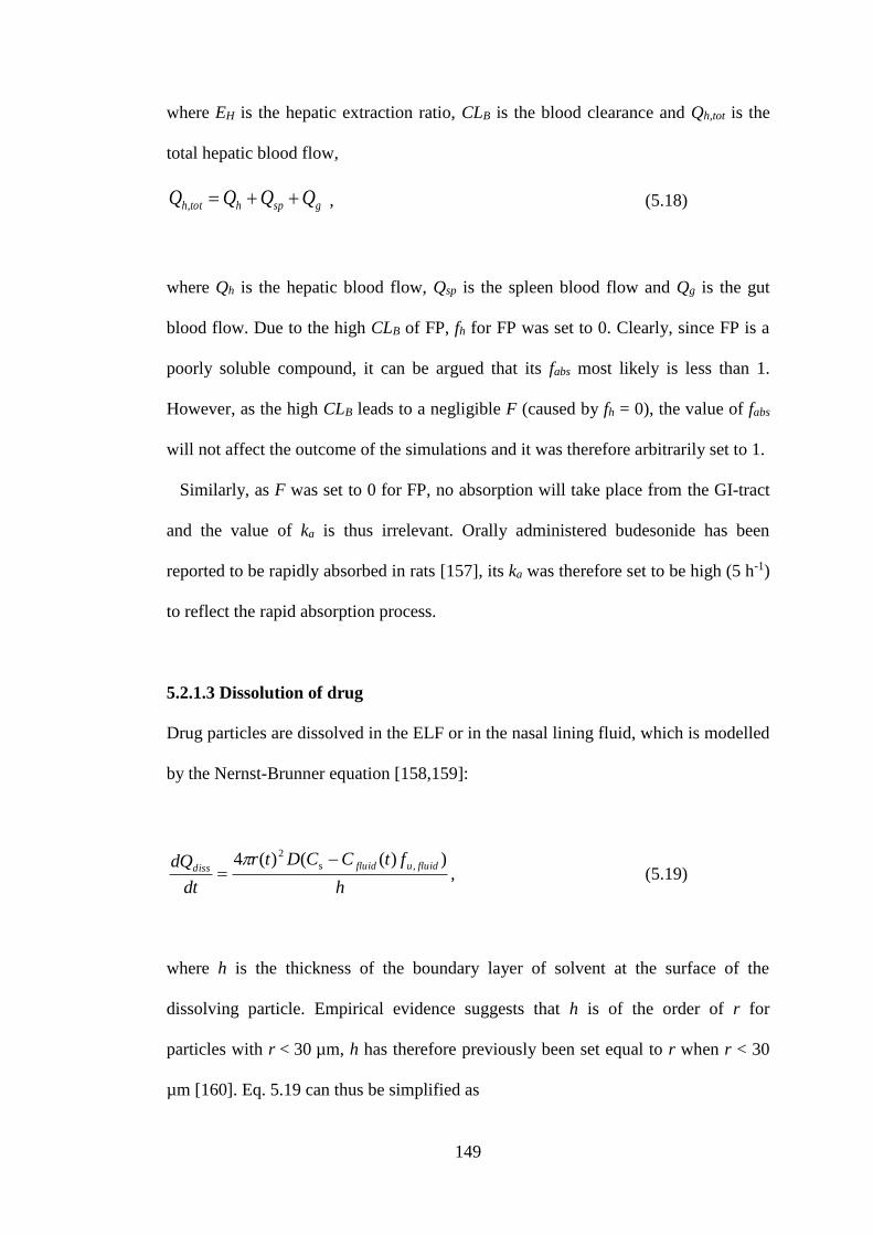
149

where EH is the hepatic extraction ratio, CLB is the blood clearance and Qh,tot is the

total hepatic blood flow,

gsphtoth QQQQ , , (5.18)

where Qh is the hepatic blood flow, Qsp is the spleen blood flow and Qg is the gut

blood flow. Due to the high CLB of FP, fh for FP was set to 0. Clearly, since FP is a

poorly soluble compound, it can be argued that its fabs most likely is less than 1.

However, as the high CLB leads to a negligible F (caused by fh = 0), the value of fabs

will not affect the outcome of the simulations and it was therefore arbitrarily set to 1.

Similarly, as F was set to 0 for FP, no absorption will take place from the GI-tract

and the value of ka is thus irrelevant. Orally administered budesonide has been

reported to be rapidly absorbed in rats [157], its ka was therefore set to be high (5 h-1)

to reflect the rapid absorption process.

5.2.1.3 Dissolution of drug

Drug particles are dissolved in the ELF or in the nasal lining fluid, which is modelled

by the Nernst-Brunner equation [158,159]:

h

ftCCDtr

dt

dQ fluidufluiddiss))(()(4 ,s

2

, (5.19)

where h is the thickness of the boundary layer of solvent at the surface of the

dissolving particle. Empirical evidence suggests that h is of the order of r for

particles with r < 30 µm, h has therefore previously been set equal to r when r < 30

µm [160]. Eq. 5.19 can thus be simplified as

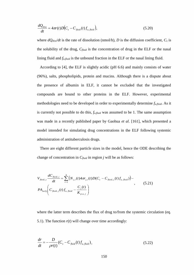
150

fluidufluids

diss ftCCDtrdt

dQ,)()(4 , (5.20)

where dQdiss/dt is the rate of dissolution (nmol/h), D is the diffusion coefficient, Cs is

the solubility of the drug, Cfluid is the concentration of drug in the ELF or the nasal

lining fluid and fu,fluid is the unbound fraction in the ELF or the nasal lining fluid.

According to [4], the ELF is slightly acidic (pH 6.6) and mainly consists of water

(96%), salts, phospholipids, protein and mucins. Although there is a dispute about

the presence of albumin in ELF, it cannot be excluded that the investigated

compounds are bound to other proteins in the ELF. However, experimental

methodologies need to be developed in order to experimentally determine fu,fluid. As it

is currently not possible to do this, fu,fluid was assumed to be 1. The same assumption

was made in a recently published paper by Gaohua et al. [161], which presented a

model intended for simulating drug concentrations in the ELF following systemic

administration of antituberculosis drugs.

There are eight different particle sizes in the model, hence the ODE describing the

change of concentration in Cfluid in region j will be as follows:

jup

j

fluidujfluidsurf,j

i

fluidujfluidsijij

jfluid

jfluid

K

tCftCPA

ftCCDtrtNdt

dCV

,,

,,

8

1

,,,,

,

,

)()(

))(()(4)(

, (5.21)

where the latter term describes the flux of drug to/from the systemic circulation (eq.

5.1). The function r(t) will change over time accordingly:

))(()(

, fluidufluids ftCCtr

D

dt

dr

, (5.22)

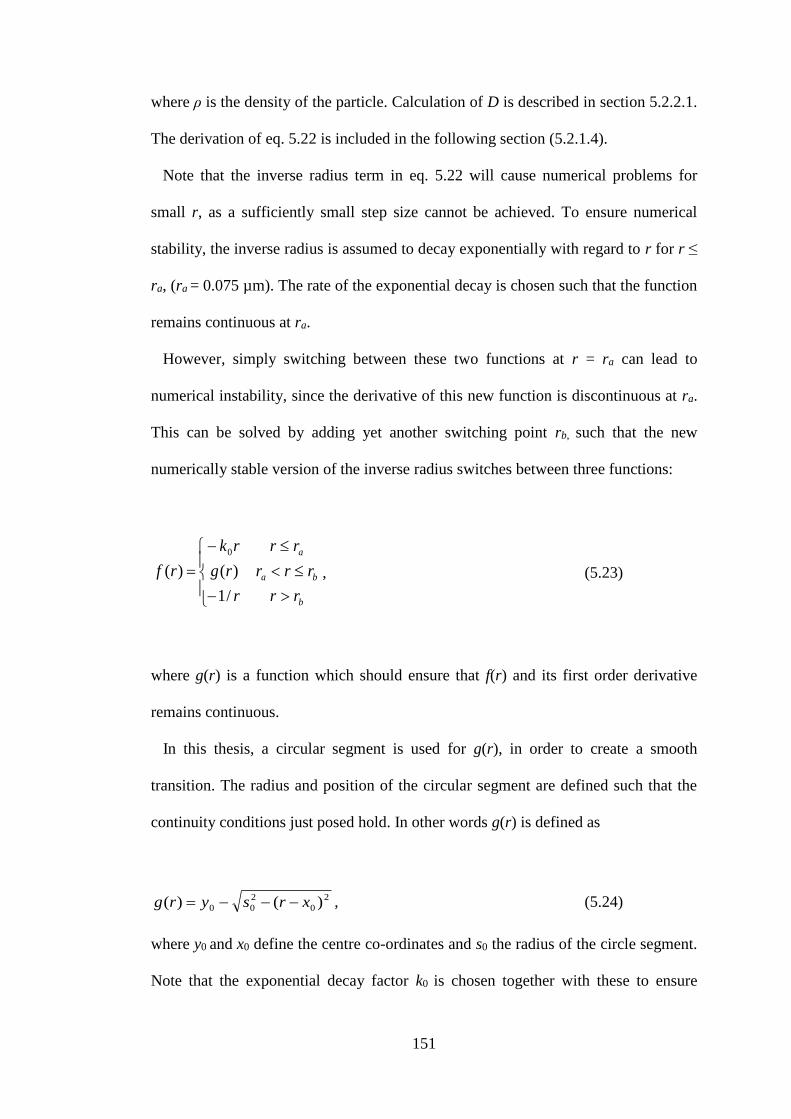
151

where ρ is the density of the particle. Calculation of D is described in section 5.2.2.1.

The derivation of eq. 5.22 is included in the following section (5.2.1.4).

Note that the inverse radius term in eq. 5.22 will cause numerical problems for

small r, as a sufficiently small step size cannot be achieved. To ensure numerical

stability, the inverse radius is assumed to decay exponentially with regard to r for r ≤

ra, (ra = 0.075 µm). The rate of the exponential decay is chosen such that the function

remains continuous at ra.

However, simply switching between these two functions at r = ra can lead to

numerical instability, since the derivative of this new function is discontinuous at ra.

This can be solved by adding yet another switching point rb, such that the new

numerically stable version of the inverse radius switches between three functions:

b

ba

a

rr

rrr

rr

r

rg

rk

rf

/1

)()(

0

, (5.23)

where g(r) is a function which should ensure that f(r) and its first order derivative

remains continuous.

In this thesis, a circular segment is used for g(r), in order to create a smooth

transition. The radius and position of the circular segment are defined such that the

continuity conditions just posed hold. In other words g(r) is defined as

2

0

2

00 )()( xrsyrg , (5.24)

where y0 and x0 define the centre co-ordinates and s0 the radius of the circle segment.

Note that the exponential decay factor k0 is chosen together with these to ensure

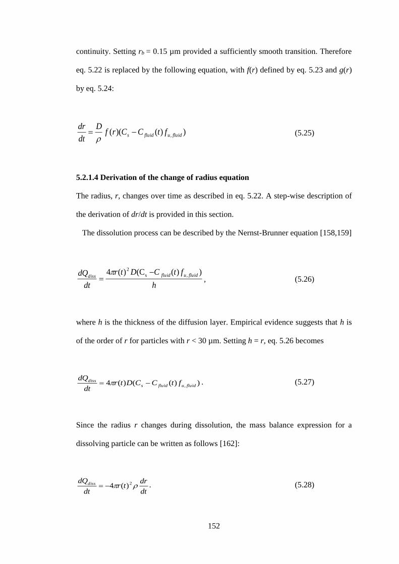
152

continuity. Setting rb = 0.15 µm provided a sufficiently smooth transition. Therefore

eq. 5.22 is replaced by the following equation, with f(r) defined by eq. 5.23 and g(r)

by eq. 5.24:

))()(( , fluidufluids ftCCrfD

dt

dr

(5.25)

5.2.1.4 Derivation of the change of radius equation

The radius, r, changes over time as described in eq. 5.22. A step-wise description of

the derivation of dr/dt is provided in this section.

The dissolution process can be described by the Nernst-Brunner equation [158,159]

h

ftCDtr

dt

dQ fluidufluiddiss))((C)(4 ,s

2

, (5.26)

where h is the thickness of the diffusion layer. Empirical evidence suggests that h is

of the order of r for particles with r < 30 µm. Setting h = r, eq. 5.26 becomes

))(()(4 , fluidufluidsdiss ftCCDtr

dt

dQ . (5.27)

Since the radius r changes during dissolution, the mass balance expression for a

dissolving particle can be written as follows [162]:

dt

drtr

dt

dQdiss 2)(4 . (5.28)

153

Eqs. 5.27 and 5.28 are independent of each other, thus equating eqs. 5.27 and 5.28

gives

dt

drtrftCCDtr fluidufluids 2

, )(4))(()(4 . (5.29)

Solving for dr/dt yields

))(()(

, fluidufluids ftCCtr

D

dt

dr

. (5.30)

5.2.1.5 Receptor binding

Receptor binding was included in all tissue compartments and was described as

)()(

)()(

,,

max tRDKK

tCtRDBK

dt

tdRDioff

iup

ii,ion

i

, (5.31)

where RDi is the concentration of the drug-receptor complex in compartment i, Kon is

the association rate constant, Bmax,i is the receptor density in compartment i and Koff is

the dissociation rate constant.

Receptor occupancy in compartment i (ROi) can be calculated via:

i

ii

B

tRDtRO

max,

)(100)( . (5.32)

154

Bmax for the spleen was obtained from [138], Bmax for the lung from section 3.2.2.2

and Bmax in the other tissue compartments was set to the mean value of Bmax in five

brain regions [163].

Since the lung has been divided into a central and a peripheral compartment,

receptor occupancy is predicted for each region individually. The whole-lung can

also be considered by using a weighted average based on the occupancy for the two

regions (ROave). The volume fractions of a rat lung consisting of central (fv,c) and

peripheral lung (fv,p) were estimated to be 0.81 and 0.19, respectively (see section

5.2.2.3). ROave could therefore be calculated via:

ppvccvave ROfROfRO ,, . (5.33)

Since the experimental methodology cannot discriminate between central and

peripheral occupancy, ROave corresponds to the observations.

155

5.2.2 Parameterisation

The input parameters are divided into three categories: 1) drug-specific, 2)

formulation-specific, and 3) system-specific input parameters. In this section, the

parameterisation of each of these categories will be described.

5.2.2.1 Drug-specific input parameters

All drug- and formulation-specific input parameters for budesonide and FP are

summarised in tables 5.3 and 5.4, respectively. The following sections contain

information on how the drug-specific input parameters were obtained.

Prediction and measurements of tissue-to-unbound plasma partition

coefficients. Tissue-to-unbound plasma partition coefficients (Kp,u) were predicted

using a method described in [105], which has been found to have good predictive

capabilities [106]. Since both FP and budesonide are neutral compounds, logD7.4 is

not expected to be different from logP. LogD7.4 was therefore used as input together

with the unbound plasma fraction (fu) for prediction of Kp,u-values. LogD7.4 was 4.2

and 2.9 for FP and budesonide, respectively [164]. fu was 0.016 and 0.09222 for FP

and budesonide, respectively [164]. In order to simplify the model structure, richly

and poorly perfused organs were lumped together to form one compartment each.

The mean value of the predicted Kp,u-values of the heart and the kidney was used as

Kp,u,richly, whereas Kp,u,poorly was defined as the mean value of the predicted Kp-values

of the bones and the muscles. All predicted Kp,u-values are presented in table 5.1.

The unbound lung volume of distribution (Vu,lung), corresponding to Kp,u,lung, was

measured for FP and budesonide by Dr. Erica Bäckström at AstraZeneca R&D

according to the protocol described in [77]. Kp,i was subsequently obtained from:

156

iupuip KfK ,,, . (5.34)

Neither prediction methodologies nor measurements of Kp,u,nose were available, this

was therefore set to Kp,u,lung.

The resulting steady-state volume of distribution (Vdss) was calculated from the

predicted and measured Kp-values (eq. 5.35) and compared to the observed Vdss

(Vdss,obs, eq. 5.36) obtained from modelling of PK-data from in vivo studies using:

8

1

,,

i

itippdss VKVV (5.35)

321, VVVV obsdss (5.36)

where Vp is the volume of the plasma and Vt,i is the volume of tissue i. The calculated

Vdss should equal Vdss,obs. Any discrepancy between the calculated Vdss and Vdss,obs can

be corrected by introducing a Kp-factor (f) given by [99]:

n

i

itip

pobsdss

VK

VVf

1

,,

, . (5.37)

Since the Kp-value of the lung was known and the nose was assumed to have the

same value, these two values were not corrected by f. The equation was thus written

in the following form:

157

6

1

,,

,, )(

i

itip

noselunglungppobsdss

VK

VVKVVf (5.38)

All predicted Kp-values were multiplied by f in order to obtain Vdss,obs. The final

Kp-values are presented in table 5.2.

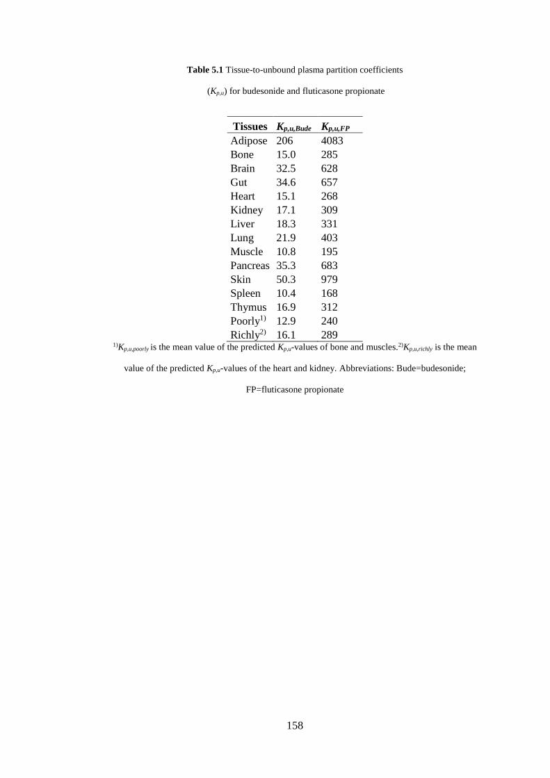
158

Table 5.1 Tissue-to-unbound plasma partition coefficients

(Kp,u) for budesonide and fluticasone propionate

Tissues Kp,u,Bude Kp,u,FP

Adipose 206 4083

Bone 15.0 285

Brain 32.5 628

Gut 34.6 657

Heart 15.1 268

Kidney 17.1 309

Liver 18.3 331

Lung 21.9 403

Muscle 10.8 195

Pancreas 35.3 683

Skin 50.3 979

Spleen 10.4 168

Thymus 16.9 312

Poorly1) 12.9 240

Richly2) 16.1 289 1)Kp,u,poorly is the mean value of the predicted Kp,u-values of bone and muscles.2)Kp,u,richly is the mean

value of the predicted Kp,u-values of the heart and kidney. Abbreviations: Bude=budesonide;

FP=fluticasone propionate

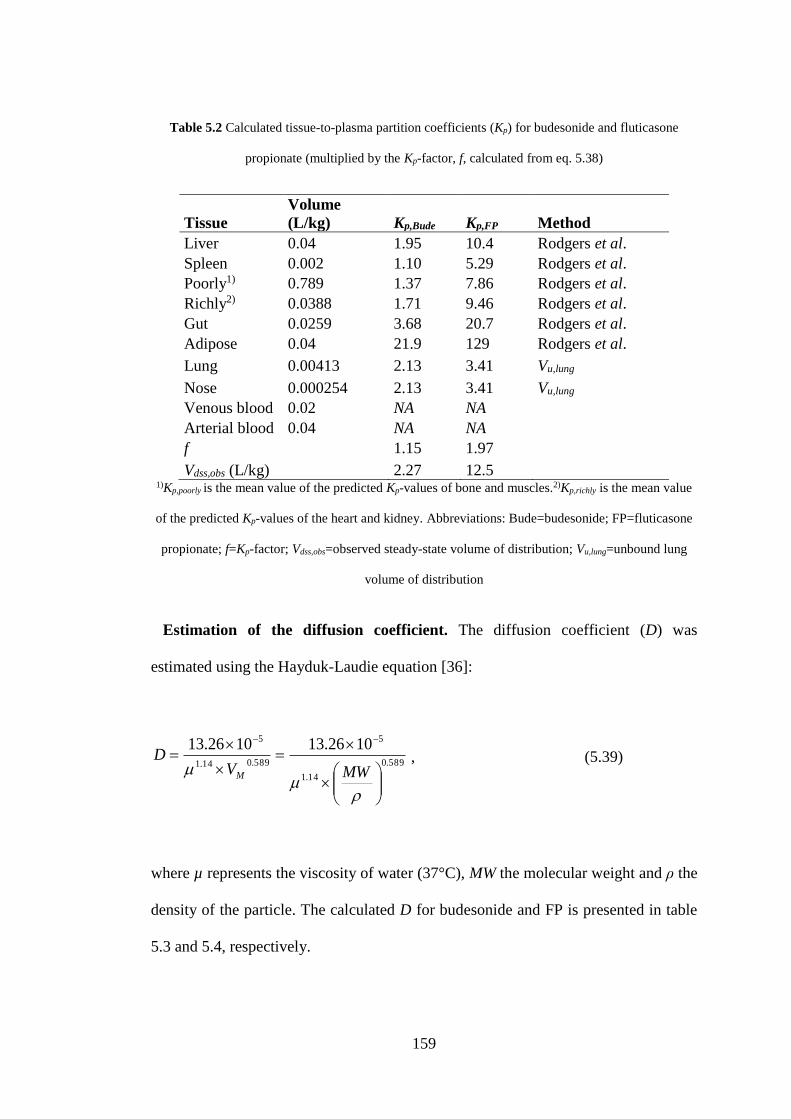
159

Table 5.2 Calculated tissue-to-plasma partition coefficients (Kp) for budesonide and fluticasone

propionate (multiplied by the Kp-factor, f, calculated from eq. 5.38)

Tissue

Volume

(L/kg) Kp,Bude Kp,FP Method

Liver 0.04 1.95 10.4 Rodgers et al.

Spleen 0.002 1.10 5.29 Rodgers et al.

Poorly1) 0.789 1.37 7.86 Rodgers et al.

Richly2) 0.0388 1.71 9.46 Rodgers et al.

Gut 0.0259 3.68 20.7 Rodgers et al.

Adipose 0.04 21.9 129 Rodgers et al.

Lung 0.00413 2.13 3.41 Vu,lung

Nose 0.000254 2.13 3.41 Vu,lung

Venous blood 0.02 NA NA

Arterial blood 0.04 NA NA

f

1.15 1.97

Vdss,obs (L/kg) 2.27 12.5 1)Kp,poorly is the mean value of the predicted Kp-values of bone and muscles.2)Kp,richly is the mean value

of the predicted Kp-values of the heart and kidney. Abbreviations: Bude=budesonide; FP=fluticasone

propionate; f=Kp-factor; Vdss,obs=observed steady-state volume of distribution; Vu,lung=unbound lung

volume of distribution

Estimation of the diffusion coefficient. The diffusion coefficient (D) was

estimated using the Hayduk-Laudie equation [36]:

589.0

14.1

5

589.014.1

5 1026.131026.13

MWVD

M

, (5.39)

where µ represents the viscosity of water (37°C), MW the molecular weight and ρ the

density of the particle. The calculated D for budesonide and FP is presented in table

5.3 and 5.4, respectively.

160

Calculation of blood clearance. The blood/plasma drug concentration ratio (R)

was determined to be 0.95 and 0.78 for FP and budesonide, respectively [164].

Experimental measurements of R were done by Pharmaron® (Pharmaron Beijing,

Co. Ltd., Bejing, China). The blood clearance (CLB) was calculated from the plasma

clearance (CLP) obtained from the PK study described in section 4.3 according to:

R

CLCL P

B . (5.40)

As CLP was estimated from venous drug concentrations, elimination was set to occur

from the venous compartment. Accordingly, CLB acts on absorbed drug prior to

entering the other organs.

Parameter estimation of the solubility. FP is a poorly soluble drug with a

measured water solubility of <779.1 nM and a fasted-state small intestinal fluid

(FaSSIF) solubility of 3120 nM [164]. FaSSIF is defined as a biorelevant medium.

As opposed to buffer, these media better reflect the composition of physiological

fluids by, for instance, containing lipids, surfactants and buffers, where the purpose

of the latter is to maintain physiological pH [165]. In contrast, budesonide has a

higher solubility with an aqueous solubility of 38.56 µM and a FaSSIF solubility of

103.6 µM [164]. Whilst the composition of the FaSSIF (pH 6.5, osmolality 270 ± 10

mOsmol/kg, 3 mM sodium taurochlorate, 0.75 mM lecithin, 28.7 mM KH2PO4 and

103.3 mM KCl [166]) is not expected to precisely reflect the composition of the

ELF, it clearly serves to illustrate how a biologically relevant medium significantly

can change the solubility of a compound.

161

Since the aqueous solubility of a poorly soluble compound tends to under-predict

the in vivo dissolution rate [55], the solubility (Cs) of FP, but not budesonide, was

estimated.

Cs was estimated as 4530 nM (95% CI [3845-5215] nM) using nonlinear least

squares in the MATLAB Curve-Fitting Toolbox, which minimised the sum of

squared deviations between observed and predicted total lung concentrations (11.3

nmol/kg, LDD). The Levenberg-Marquardt algorithm was used to find the minimum

of the cost function. The root mean squared error (RMSE) of the fit was 272 nM. The

estimated Cs was thus of the same magnitude as the measured FaSSIF solubility of

FP.

The initial estimate was selected from an exhaustive search, in which the sum of

squares was initially evaluated for 1000 candidates over a broad search space where

Cs ranged from 102 to 105 nM (fig. 5.2a). The cost function turned out to be locally

convex in the explored interval and a minimum was found at 4529.7 nM. The search

space was then confined to the proximity of the best solution Cs,0 (Cs,0-200 ≤ Cs ≤

Cs,0+200 nM), in which 300 candidates were evaluated (fig. 5.2b). The best solution

of the confined search was 4530 nM, which was close to the measured FaSSIF Cs

(3120 nM). Fig. 5.2c shows simulations of total lung concentrations using the

optimised Cs (blue line) and the FaSSIF Cs (dashed line).

Sensitivity analysis of Clung with respect to D and Cs indicated that these two

parameters might be indistinguishable (fig. 5.2d), in which case only the product can

be estimated. However, calculation of D (eq. 5.39) enables unique determination of

Cs. A detailed description of the sensitivity analysis is provided in section 5.3.1.3.

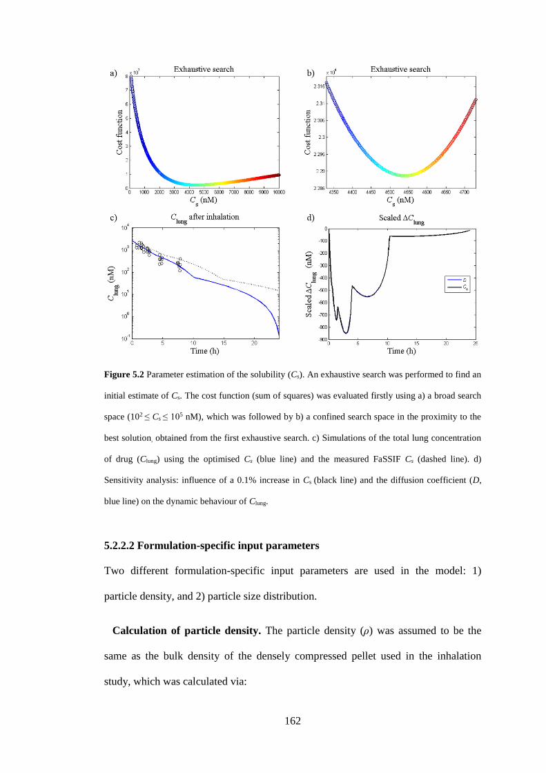
162

Figure 5.2 Parameter estimation of the solubility (Cs). An exhaustive search was performed to find an

initial estimate of Cs. The cost function (sum of squares) was evaluated firstly using a) a broad search

space (102 ≤ Cs ≤ 105 nM), which was followed by b) a confined search space in the proximity to the

best solution, obtained from the first exhaustive search. c) Simulations of the total lung concentration

of drug (Clung) using the optimised Cs (blue line) and the measured FaSSIF Cs (dashed line). d)

Sensitivity analysis: influence of a 0.1% increase in Cs (black line) and the diffusion coefficient (D,

blue line) on the dynamic behaviour of Clung.

5.2.2.2 Formulation-specific input parameters

Two different formulation-specific input parameters are used in the model: 1)

particle density, and 2) particle size distribution.

Calculation of particle density. The particle density (ρ) was assumed to be the

same as the bulk density of the densely compressed pellet used in the inhalation

study, which was calculated via:

163

V

m , (5.41)

where m is the mass of substance and V is the volume of the pellet.

Characterisation of particle size distribution. Prior to preclinical inhalation

studies, the aerodynamic particle size distribution is typically characterised using a 7-

stage Mercer cascade impactor (model 02 110, In-tox Products, USA), providing a

discrete particle size distribution with eight different size classes. The analytical

procedures applied for the characterisation are described in section 4.5.2.

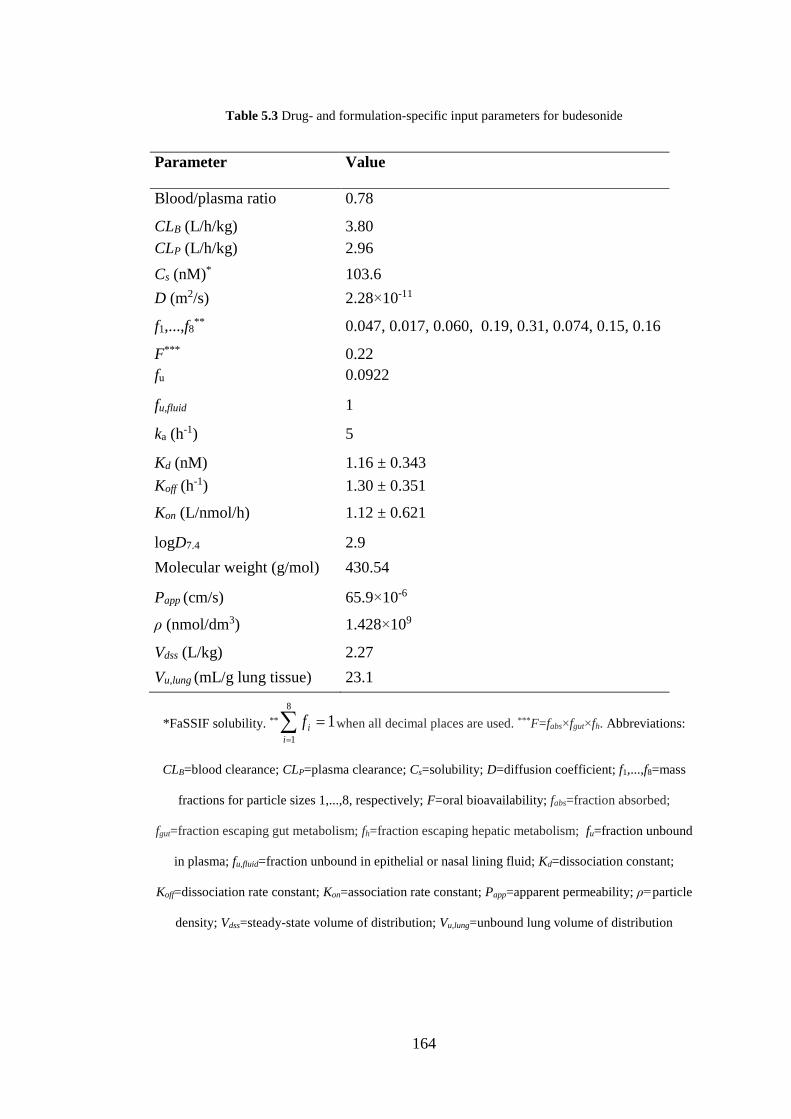
164

Table 5.3 Drug- and formulation-specific input parameters for budesonide

Parameter Value

Blood/plasma ratio 0.78

CLB (L/h/kg) 3.80

CLP (L/h/kg) 2.96

Cs (nM)* 103.6

D (m2/s) 2.28×10-11

f1,...,f8** 0.047, 0.017, 0.060, 0.19, 0.31, 0.074, 0.15, 0.16

F*** 0.22

fu 0.0922

fu,fluid 1

ka (h-1) 5

Kd (nM) 1.16 ± 0.343

Koff (h-1) 1.30 ± 0.351

Kon (L/nmol/h) 1.12 ± 0.621

logD7.4 2.9

Molecular weight (g/mol) 430.54

Papp (cm/s) 65.9×10-6

ρ (nmol/dm3) 1.428×109

Vdss (L/kg) 2.27

Vu,lung (mL/g lung tissue) 23.1

*FaSSIF solubility. ** 18

1

i

if when all decimal places are used. ***F=fabs×fgut×fh. Abbreviations:

CLB=blood clearance; CLP=plasma clearance; Cs=solubility; D=diffusion coefficient; f1,...,f8=mass

fractions for particle sizes 1,...,8, respectively; F=oral bioavailability; fabs=fraction absorbed;

fgut=fraction escaping gut metabolism; fh=fraction escaping hepatic metabolism; fu=fraction unbound

in plasma; fu,fluid=fraction unbound in epithelial or nasal lining fluid; Kd=dissociation constant;

Koff=dissociation rate constant; Kon=association rate constant; Papp=apparent permeability; ρ=particle

density; Vdss=steady-state volume of distribution; Vu,lung=unbound lung volume of distribution

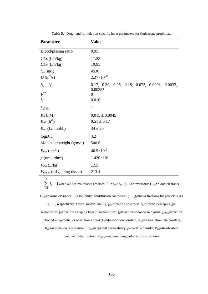
165

Table 5.4 Drug- and formulation-specific input parameters for fluticasone propionate

Parameter Value

Blood/plasma ratio 0.95

CLB (L/h/kg) 11.53

CLP (L/h/kg) 10.95

Cs (nM) 4530

D (m2/s) 2.27×10-11

f1,...,f8* 0.17, 0.30, 0.26, 0.18, 0.073, 0.0091, 0.0032,

0.0035*

F** 0

fu 0.016

fu,fluid 1

Kd (nM) 0.015 ± 0.0045

Koff (h-1) 0.51 ± 0.17

Kon (L/nmol/h) 34 ± 20

logD7.4 4.2

Molecular weight (g/mol) 500.6

Papp (cm/s) 46.9×10-6

ρ (nmol/dm3) 1.430×109

Vdss (L/kg) 12.5

Vu,lung (mL/g lung tissue) 213.4

* 18

1

i

if when all decimal places are used. **F=fabs×fgut×fh. Abbreviations: CLB=blood clearance;

CLP=plasma clearance; Cs=solubility; D=diffusion coefficient; f1,...,f8=mass fractions for particle sizes

1,...,8, respectively; F=oral bioavailability; fabs=fraction absorbed; fgut=fraction escaping gut

metabolism; fh=fraction escaping hepatic metabolism; fu=fraction unbound in plasma; fu,fluid=fraction

unbound in epithelial or nasal lining fluid; Kd=dissociation constant; Koff=dissociation rate constant;

Kon=association rate constant; Papp=apparent permeability; ρ=particle density; Vdss=steady-state

volume of distribution; Vu,lung=unbound lung volume of distribution

166

5.2.2.3 System-specific input parameters

The model includes several system-specific input parameters describing the anatomy

and physiological processes for the rat. Where possible, anatomical values were

obtained from the literature. In the absence of literature values, calculations of

parameter missing values were made based on available anatomical data. All system-

specific input parameters are summarised in tables 5.5 and 5.6, where the latter

specifies parameters for the central lung, peripheral lung and the nose.

Calculation of VELF and Vnasal. The volume of the epithelial lining fluid in the

central (VELF,C) and the peripheral lung (VELF,P) as well as the corresponding volume

in the nose (Vnasal) was calculated accordingly:

iisurfifluid dAV ,, , (5.42)

where Asurf,i is the surface area in compartment i and di is the thickness of the lining

fluid in compartment i. d in the central lung was set to be 5 µm [56], as was d in the

nose [167]. Since d is known to gradually decrease along the lung generations [151],

a smaller d was used peripherally (0.07 µm, [11]).

Calculation of central and peripheral lung tissue fractions. The volume of

region j was calculated from:

jjsurfj hAV , , (5.43)

where Asurf,j is the surface area and hj is the lung wall thickness of region j. Since

limited information on surface areas and lung wall thickness in the different

167

subregions of the central lung was available, the bronchial wall thickness was

assumed to be representative of the entire region. The rationale for choosing the

bronchial wall as a representative was that it is thinner than the tracheal- but thicker

than the bronchiolar wall. The bronchial (hc = 29 µm) and alveolar wall thickness (hp

= 1.42 µm) were obtained from [168] and [30], respectively. The central (fv,c) and

peripheral (fv,p) tissue fractions were subsequently calculated using eqs. 5.44 and

5.45, respectively, as follows:

pc

ccv

VV

Vf

, , (5.44)

cvpv ff ,, 1 . (5.45)

Calculation of nasal mucosa volume. The volume of the nasal mucosa (Vn) was

calculated using:

nnsurfn hAV , , (5.46)

where Asurf,n is the surface area of the nose and hn is the average thickness of the

nasal epithelium. The average thickness (hn = 61 µm) was obtained from [169].

Measurements from 60 day-old Sprague Dawley rats were chosen as this was in the

proximity of the age range used in the studies (9-11 weeks).

Estimation of mucociliary rate constant. The mucociliary rate constant (kmcc)

was estimated using data from [155], where clearance of a tracer from the airway by

mucociliary transport was studied in rats after inhalation (0 ≤ t ≤ 6 h, median spray

droplet size 4-6 µm) using a single-photon emission computed tomography

168

(SPECT)-based method. The fraction retained (fret) was assumed to decline

exponentially and MCC was assumed to be negligible in the peripheral region.

Hence, a baseline corresponding to the fraction of the total lung dose deposited in the

peripheral region (f0) was introduced as this fraction should not be affected by MCC.

There were no data available on the droplet size distribution, the mean value (5 µm)

was therefore used for calculation of regional deposition. The peripheral (fp,mcc) and

central deposition fractions (fc,mcc) for particles with an aerodynamic diameter of 5

µm were extracted from [65] and f0 was calculated accordingly:

2.0,,

,

0

mcccmccp

mccp

ff

ff . (5.47)

The resulting equation for fret was as follows:

tktk

retmccmcc eefff

8.02.0)1( 00

(5.48)

kmcc was estimated as 0.0472 ± 0.0011 h-1 using the MATLAB Curve Fitting Toolbox

(Mathworks Inc., Natick, MA, USA), corresponding to a half-life of 14.7 h. The

observations and model fit are shown in figure 5.3.

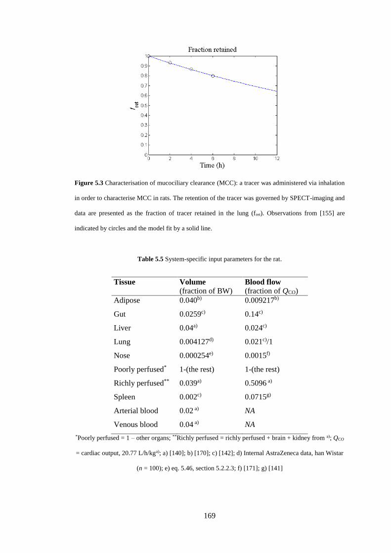
169

Figure 5.3 Characterisation of mucociliary clearance (MCC): a tracer was administered via inhalation

in order to characterise MCC in rats. The retention of the tracer was governed by SPECT-imaging and

data are presented as the fraction of tracer retained in the lung (fret). Observations from [155] are

indicated by circles and the model fit by a solid line.

Table 5.5 System-specific input parameters for the rat.

Tissue

Volume

(fraction of BW) Blood flow

(fraction of QCO)

Adipose 0.040b) 0.009217b)

Gut 0.0259c) 0.14c)

Liver 0.04a) 0.024c)

Lung 0.004127d) 0.021c)/1

Nose 0.000254e) 0.0015f)

Poorly perfused* 1-(the rest) 1-(the rest)

Richly perfused** 0.039a) 0.5096 a)

Spleen 0.002c) 0.0715g)

Arterial blood 0.02 a) NA

Venous blood 0.04 a) NA

*Poorly perfused = 1 – other organs; **Richly perfused = richly perfused + brain + kidney from a); QCO

= cardiac output, 20.77 L/h/kga); a) [140]; b) [170]; c) [142]; d) Internal AstraZeneca data, han Wistar

(n = 100); e) eq. 5.46, section 5.2.2.3; f) [171]; g) [141]

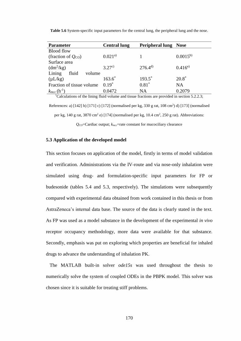
170

Table 5.6 System-specific input parameters for the central lung, the peripheral lung and the nose.

Parameter Central lung Peripheral lung Nose

Blood flow

(fraction of QCO) 0.021a) 1 0.0015b)

Surface area

(dm2/kg) 3.27c) 276.4d) 0.416e)

Lining fluid volume

(µL/kg) 163.6* 193.5* 20.8*

Fraction of tissue volume 0.19* 0.81* NA

kmcc (h-1) 0.0472 NA 0.2079

*Calculations of the lining fluid volume and tissue fractions are provided in section 5.2.2.3;

References: a) [142] b) [171] c) [172] (normalised per kg, 330 g rat, 108 cm2) d) [173] (normalised

per kg, 140 g rat, 3870 cm2 e) [174] (normalised per kg, 10.4 cm2, 250 g rat). Abbreviations:

QCO=Cardiac output; kmcc=rate constant for mucociliary clearance

5.3 Application of the developed model

This section focuses on application of the model, firstly in terms of model validation

and verification. Administrations via the IV-route and via nose-only inhalation were

simulated using drug- and formulation-specific input parameters for FP or

budesonide (tables 5.4 and 5.3, respectively). The simulations were subsequently

compared with experimental data obtained from work contained in this thesis or from

AstraZeneca’s internal data base. The source of the data is clearly stated in the text.

As FP was used as a model substance in the development of the experimental in vivo

receptor occupancy methodology, more data were available for that substance.

Secondly, emphasis was put on exploring which properties are beneficial for inhaled

drugs to advance the understanding of inhalation PK.

The MATLAB built-in solver ode15s was used throughout the thesis to

numerically solve the system of coupled ODEs in the PBPK model. This solver was

chosen since it is suitable for treating stiff problems.

171

5.3.1 Fluticasone propionate (model validation and verification)

5.3.1.1 Intravenous administration

Administrations via the IV-route (20, 90, 150, 750 and 1000 nmol/kg) were

simulated using drug-specific input parameters for FP (table 5.4). The simulations

were subsequently compared with experimental data on drug concentrations (plasma,

spleen and lung) and receptor occupancy obtained from work contained in this thesis

(sections 3.3.2.1, 3.3.2.2 and 4.3).

Model predictions of the plasma profiles as well as the time course of occupancy

(figs. 5.4a-b) were consistent with experimental IV-data (90 and 1000 nmol/kg),

supporting a perfusion rate-limited distribution of FP and validating the capability to

predict plasma PK. As expected from IV-dosing, the predicted occupancy profiles in

the two lung regions and the spleen were identical. No occupancy measurements

were available for the higher dose. Of note is that the binding kinetics parameters

(Kon and Koff) were obtained from modelling of IV-data (90 nmol/kg). As the model

was predictive of the plasma PK for this particular dose, it follows that it should also

be predictive of the corresponding receptor occupancy profile. This consistency can

thus be regarded as a verification step of the model. A test set independent of the

training data set was also available to validate model predictions of occupancy after

IV-administration. The model proved to be predictive of the test set, which

comprised of receptor occupancy measurements made 1.5 h after three IV-doses of

FP (section 3.3.2.1). Simulated occupancies were 27, 64 and 86% for 20, 150 and

750 nmol/kg, respectively. Simulations agreed well with observed data: 27 ± 9.7, 74

± 5.0 and 100 ± 3.5% for 20, 150 and 750 nmol/kg, respectively.

It was shown that inclusion of the receptor-bound concentration was essential for

the predictive capability of both the lung- and the spleen concentrations. This is

172

illustrated by figure 5.4c-d, showing predictions of tissue concentrations inclusive

(solid red line) and exclusive (dashed black line) of receptor binding.

In conjunction with the IV-simulations, it was also verified that mass balance was

preserved in the PBPK model. This was done by simulating the cumulative amount

of drug cleared from the system (Acum) and subsequently comparing Acum at t = 72 h

to the input (90 nmol/kg, IV, fig. 5.4e).

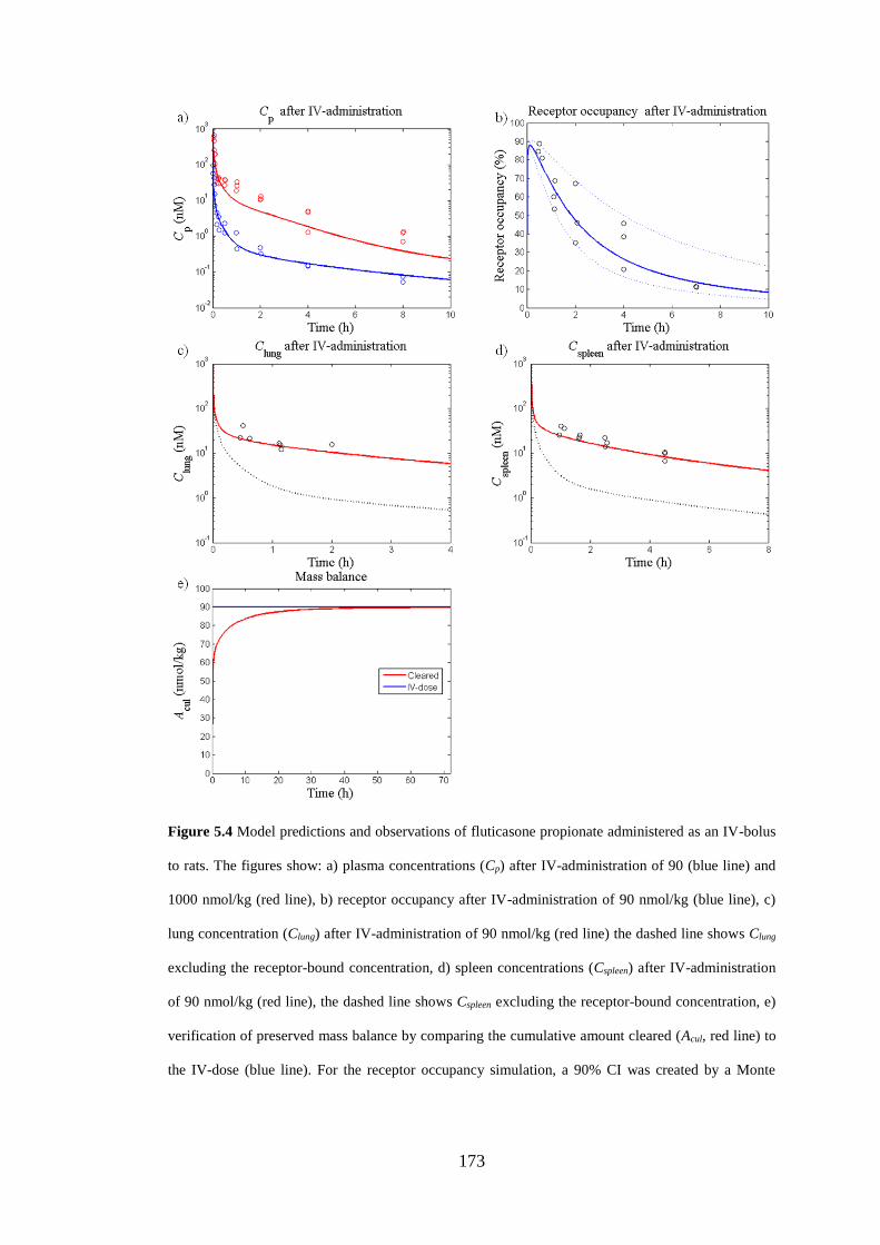
173

Figure 5.4 Model predictions and observations of fluticasone propionate administered as an IV-bolus

to rats. The figures show: a) plasma concentrations (Cp) after IV-administration of 90 (blue line) and

1000 nmol/kg (red line), b) receptor occupancy after IV-administration of 90 nmol/kg (blue line), c)

lung concentration (Clung) after IV-administration of 90 nmol/kg (red line) the dashed line shows Clung

excluding the receptor-bound concentration, d) spleen concentrations (Cspleen) after IV-administration

of 90 nmol/kg (red line), the dashed line shows Cspleen excluding the receptor-bound concentration, e)

verification of preserved mass balance by comparing the cumulative amount cleared (Acul, red line) to

the IV-dose (blue line). For the receptor occupancy simulation, a 90% CI was created by a Monte

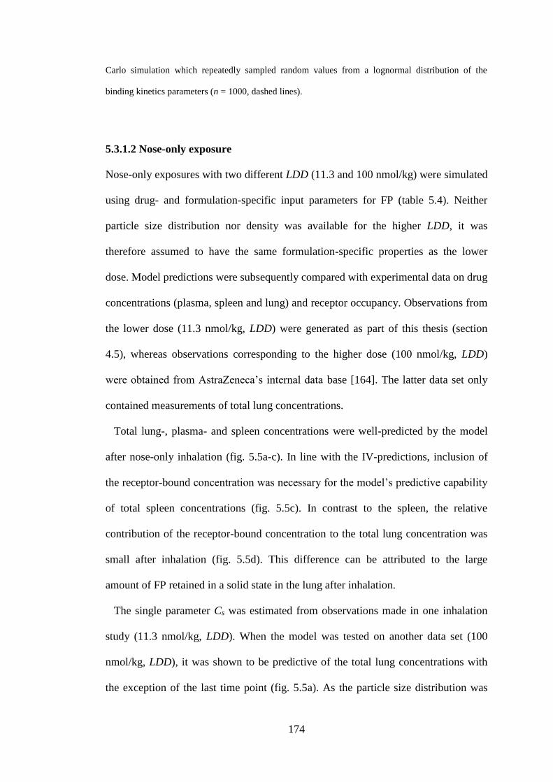
174

Carlo simulation which repeatedly sampled random values from a lognormal distribution of the

binding kinetics parameters (n = 1000, dashed lines).

5.3.1.2 Nose-only exposure

Nose-only exposures with two different LDD (11.3 and 100 nmol/kg) were simulated

using drug- and formulation-specific input parameters for FP (table 5.4). Neither

particle size distribution nor density was available for the higher LDD, it was

therefore assumed to have the same formulation-specific properties as the lower

dose. Model predictions were subsequently compared with experimental data on drug

concentrations (plasma, spleen and lung) and receptor occupancy. Observations from

the lower dose (11.3 nmol/kg, LDD) were generated as part of this thesis (section

4.5), whereas observations corresponding to the higher dose (100 nmol/kg, LDD)

were obtained from AstraZeneca’s internal data base [164]. The latter data set only

contained measurements of total lung concentrations.

Total lung-, plasma- and spleen concentrations were well-predicted by the model

after nose-only inhalation (fig. 5.5a-c). In line with the IV-predictions, inclusion of

the receptor-bound concentration was necessary for the model’s predictive capability

of total spleen concentrations (fig. 5.5c). In contrast to the spleen, the relative

contribution of the receptor-bound concentration to the total lung concentration was

small after inhalation (fig. 5.5d). This difference can be attributed to the large

amount of FP retained in a solid state in the lung after inhalation.

The single parameter Cs was estimated from observations made in one inhalation

study (11.3 nmol/kg, LDD). When the model was tested on another data set (100

nmol/kg, LDD), it was shown to be predictive of the total lung concentrations with

the exception of the last time point (fig. 5.5a). As the particle size distribution was

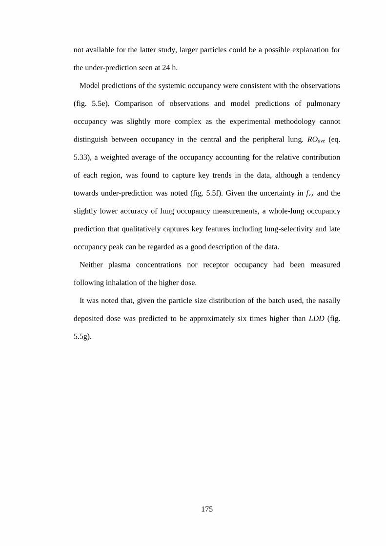
175

not available for the latter study, larger particles could be a possible explanation for

the under-prediction seen at 24 h.

Model predictions of the systemic occupancy were consistent with the observations

(fig. 5.5e). Comparison of observations and model predictions of pulmonary

occupancy was slightly more complex as the experimental methodology cannot

distinguish between occupancy in the central and the peripheral lung. ROave (eq.

5.33), a weighted average of the occupancy accounting for the relative contribution

of each region, was found to capture key trends in the data, although a tendency

towards under-prediction was noted (fig. 5.5f). Given the uncertainty in fv,c and the

slightly lower accuracy of lung occupancy measurements, a whole-lung occupancy

prediction that qualitatively captures key features including lung-selectivity and late

occupancy peak can be regarded as a good description of the data.

Neither plasma concentrations nor receptor occupancy had been measured

following inhalation of the higher dose.

It was noted that, given the particle size distribution of the batch used, the nasally

deposited dose was predicted to be approximately six times higher than LDD (fig.

5.5g).

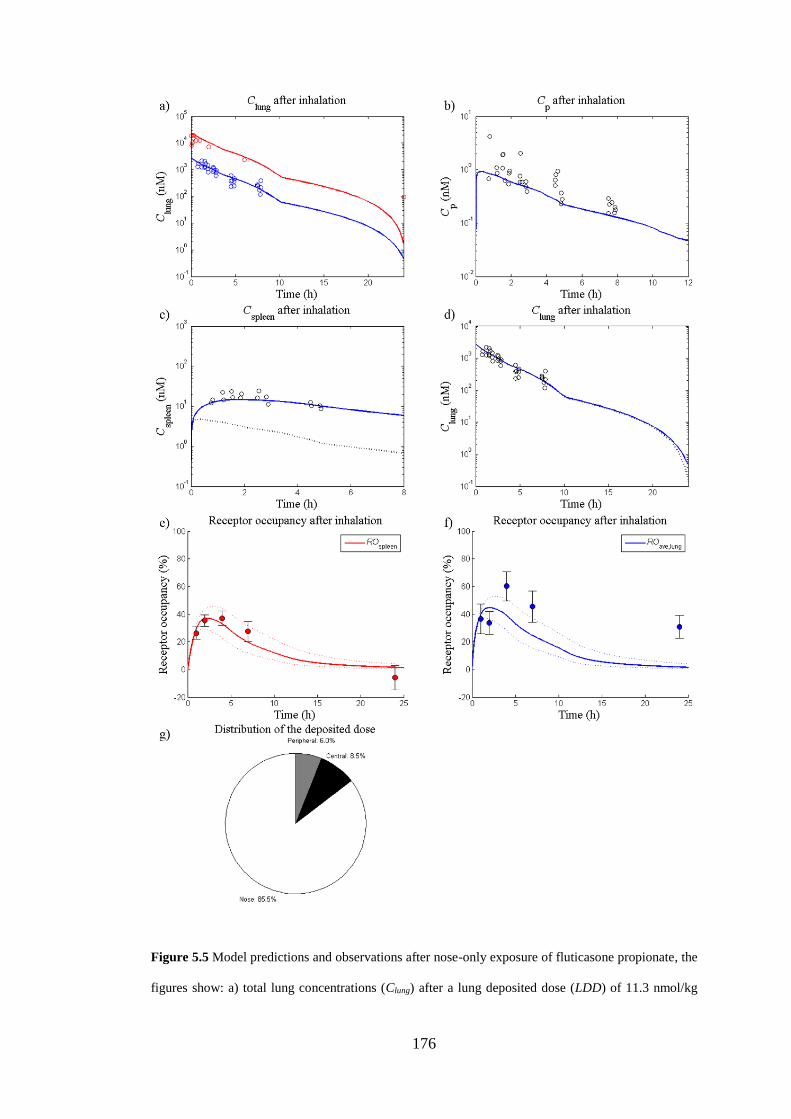
176

Figure 5.5 Model predictions and observations after nose-only exposure of fluticasone propionate, the

figures show: a) total lung concentrations (Clung) after a lung deposited dose (LDD) of 11.3 nmol/kg

177

(blue line) and 100 nmol/kg (red line), b) Cp after a LDD of 11.3 nmol/kg (blue line), c) spleen

concentration (Cspleen) after a LDD of 11.3 nmol/kg (blue line), the dashed line shows Cspleen excluding

the receptor-bound concentration, d) Clung after a LDD of 11.3 nmol/kg (blue line), the dashed line

shows Clung excluding the receptor-bound concentration, e) receptor occupancy in the spleen after a

LDD of 11.3 nmol/kg (red line), and f) whole-lung receptor occupancy after a LDD of 11.3 nmol/kg

(blue line). For each receptor occupancy simulation, a 90% CI was created by a Monte Carlo

simulation which repeatedly sampled random values from a lognormal distribution of the binding

kinetics parameters (n = 1000, dashed lines). g) Distribution of the deposited dose between the central

lung region (black), the peripheral lung region (grey) and the nasal region (white).

5.3.1.3 Sensitivity analysis for fluticasone propionate

A sensitivity analysis was performed to investigate how the dynamic behaviour of

the system responds to changes in selected input parameters. The sensitivities were

generated by considering the partial derivatives of the output Y with respect to each

parameter pi and these were calculated keeping all other parameters fixed at their

nominal values (p0), i.e.

0pip

Y

(5.49)

Two outputs were investigated: receptor occupancy in the central lung (ROc) and

receptor occupancy in the spleen (ROsp). This was done by firstly simulating the

system with all parameters at their nominal values [f(t,p0)]. Subsequently, a

simulation was performed after considering a 0.1% increment in the parameter of

interest, pi, [f(t,p)] while all other parameters were kept at their nominal values. As

mentioned in section 5.3, the MATLAB built-in solver ode15s was used to solve the

system of coupled ODEs. The choice of integrator accuracy was important to enable

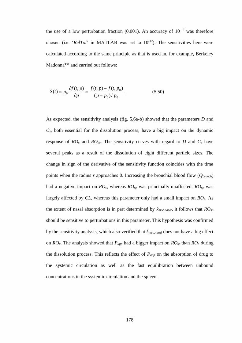
178

the use of a low perturbation fraction (0.001). An accuracy of 10-12 was therefore

chosen (i.e. ‘RelTol’ in MATLAB was set to 10-12). The sensitivities here were

calculated according to the same principle as that is used in, for example, Berkeley

Madonna™ and carried out follows:

00

00

/)(

),(),(),()(

ppp

ptfptf

p

ptfptS

. (5.50)

As expected, the sensitivity analysis (fig. 5.6a-b) showed that the parameters D and

Cs, both essential for the dissolution process, have a big impact on the dynamic

response of ROc and ROsp. The sensitivity curves with regard to D and Cs have

several peaks as a result of the dissolution of eight different particle sizes. The

change in sign of the derivative of the sensitivity function coincides with the time

points when the radius r approaches 0. Increasing the bronchial blood flow (Qbronch)

had a negative impact on ROc, whereas ROsp was principally unaffected. ROsp was

largely affected by CL, whereas this parameter only had a small impact on ROc. As

the extent of nasal absorption is in part determined by kmcc,nasal, it follows that ROsp

should be sensitive to perturbations in this parameter. This hypothesis was confirmed

by the sensitivity analysis, which also verified that kmcc,nasal does not have a big effect

on ROc. The analysis showed that Papp had a bigger impact on ROsp than ROc during

the dissolution process. This reflects the effect of Papp on the absorption of drug to

the systemic circulation as well as the fast equilibration between unbound

concentrations in the systemic circulation and the spleen.

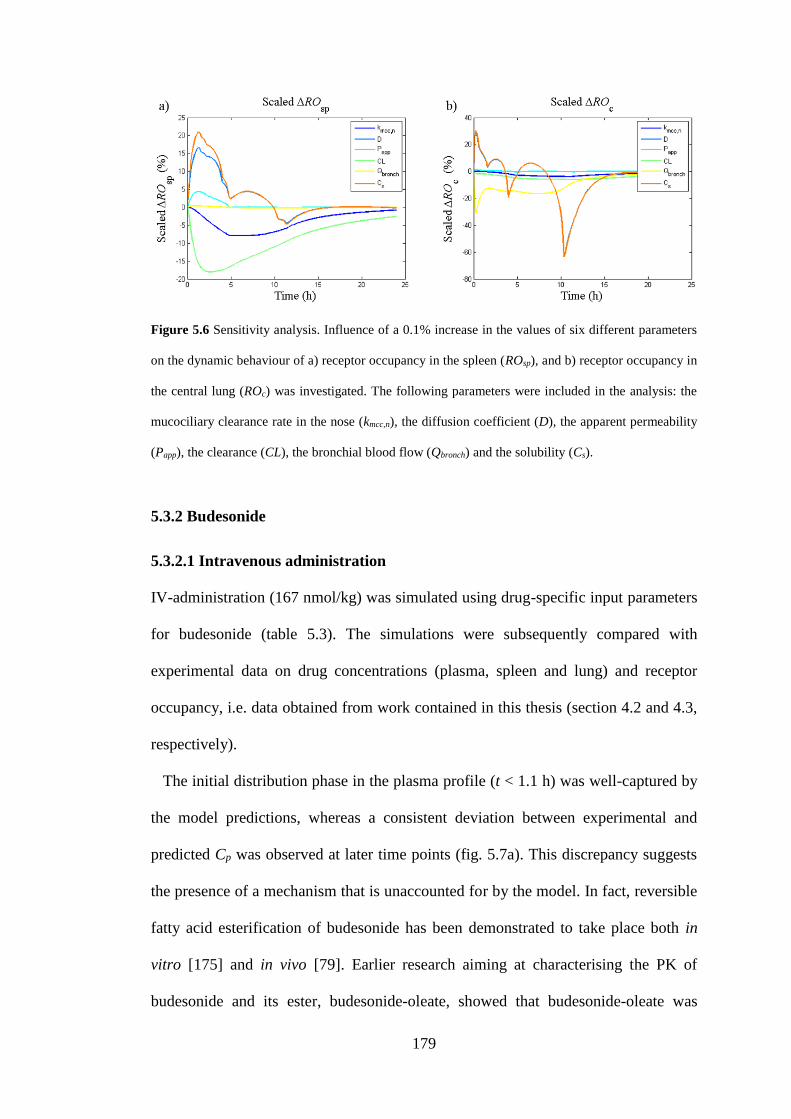
179

Figure 5.6 Sensitivity analysis. Influence of a 0.1% increase in the values of six different parameters

on the dynamic behaviour of a) receptor occupancy in the spleen (ROsp), and b) receptor occupancy in

the central lung (ROc) was investigated. The following parameters were included in the analysis: the

mucociliary clearance rate in the nose (kmcc,n), the diffusion coefficient (D), the apparent permeability

(Papp), the clearance (CL), the bronchial blood flow (Qbronch) and the solubility (Cs).

5.3.2 Budesonide

5.3.2.1 Intravenous administration

IV-administration (167 nmol/kg) was simulated using drug-specific input parameters

for budesonide (table 5.3). The simulations were subsequently compared with

experimental data on drug concentrations (plasma, spleen and lung) and receptor

occupancy, i.e. data obtained from work contained in this thesis (section 4.2 and 4.3,

respectively).

The initial distribution phase in the plasma profile (t < 1.1 h) was well-captured by

the model predictions, whereas a consistent deviation between experimental and

predicted Cp was observed at later time points (fig. 5.7a). This discrepancy suggests

the presence of a mechanism that is unaccounted for by the model. In fact, reversible

fatty acid esterification of budesonide has been demonstrated to take place both in

vitro [175] and in vivo [79]. Earlier research aiming at characterising the PK of

budesonide and its ester, budesonide-oleate, showed that budesonide-oleate was

180

rapidly formed both after IV-administration and inhalation of budesonide in rats [79].

As the resulting budesonide-oleate concentrations were in the proximity of the

budesonide concentrations, the formation and subsequent hydrolysis of the ester is

likely to have a pronounced effect on the PK of budesonide. The latter hypothesis has

also been confirmed via semi-empirical modelling approaches [79,176]. Hence, the

current PBPK model structure is not expected to be able to accurately describe the

PK of budesonide neither in plasma (fig. 5.7a) nor in tissues (5.7b and 5.7c for the

lung and the spleen, respectively).

Further research would have been required to adequately describe the esterification

of budesonide in a quantitative manner, which was not considered to fall within the

scope of this thesis. However, since budesonide-oleate is rapidly formed in tissues

[79], this process may well be reflected in the plasma profile by a rapid initial decline

followed relatively flat second phase caused by the ester accumulated in tissues

slowly being hydrolysed back to budesonide. This phenomenon is seen in the

experimental data (fig. 5.7a), but cannot be captured by the current model structure

as it does not account for this process.

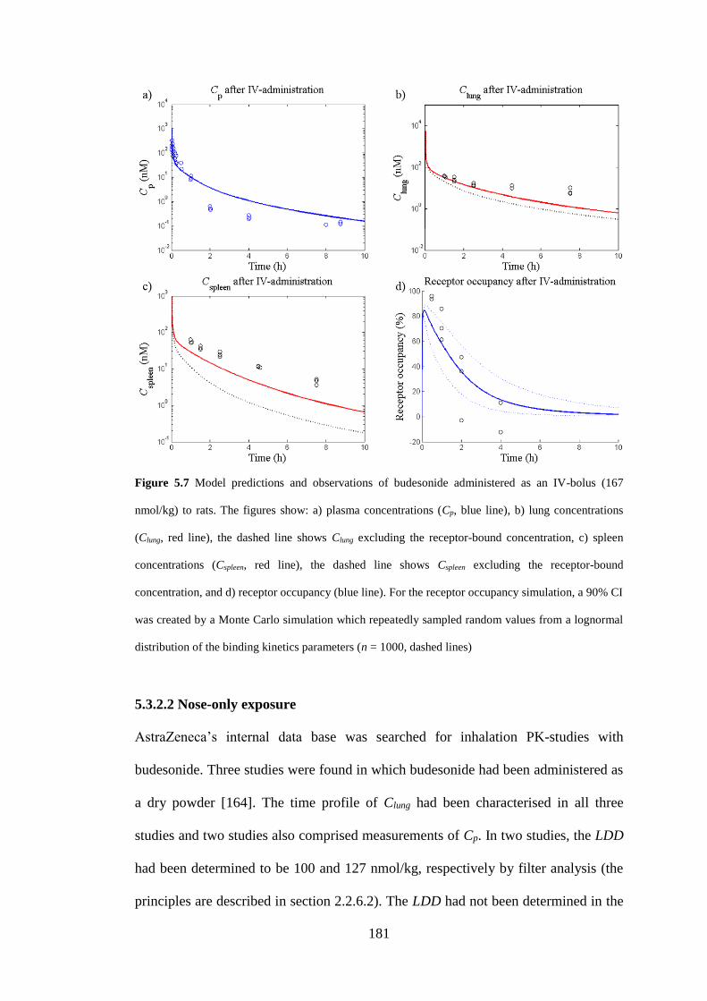
181

Figure 5.7 Model predictions and observations of budesonide administered as an IV-bolus (167

nmol/kg) to rats. The figures show: a) plasma concentrations (Cp, blue line), b) lung concentrations

(Clung, red line), the dashed line shows Clung excluding the receptor-bound concentration, c) spleen

concentrations (Cspleen, red line), the dashed line shows Cspleen excluding the receptor-bound

concentration, and d) receptor occupancy (blue line). For the receptor occupancy simulation, a 90% CI

was created by a Monte Carlo simulation which repeatedly sampled random values from a lognormal

distribution of the binding kinetics parameters (n = 1000, dashed lines)

5.3.2.2 Nose-only exposure

AstraZeneca’s internal data base was searched for inhalation PK-studies with

budesonide. Three studies were found in which budesonide had been administered as

a dry powder [164]. The time profile of Clung had been characterised in all three

studies and two studies also comprised measurements of Cp. In two studies, the LDD

had been determined to be 100 and 127 nmol/kg, respectively by filter analysis (the

principles are described in section 2.2.6.2). The LDD had not been determined in the

182

third study. However, since the measured lung concentrations were approximately

equal in the aforementioned study and the study with an LDD of 100 nmol/kg, the

LDD of the third study was also assumed to be 100 nmol/kg. For simplicity, the

details for each study have been summarised in table 5.7. The formulation-specific

parameters (particle size distribution and density) were only available for study 3 and

were assumed to be identical across the three studies (table 5.3).

Nose-only exposures with two different LDD (100 and 127 nmol/kg) were

simulated using drug- and formulation-specific input parameters for budesonide

(table 5.3). Model predictions were subsequently compared with experimental data

on lung- and plasma concentrations. There was only a small difference between the

concentration profiles generated from simulations of the two different LDD. The

initial drop in Clung was well captured by the model predictions, suggesting that

budesonide is rapidly dissolved. However, there was a consistent under-prediction of

Clung from approximately 5 h after dosing and onwards (fig. 5.8a). As expected from

the deviations between model predictions and observations of Cp after IV-

administration, the model could not describe the plasma profile after inhalation (fig.

5.8b). The discrepancy patterns between model predictions and observations were

similar for both routes of administration (IV and inhalation), again suggesting the

presence of a mechanism that is unaccounted for by the model.

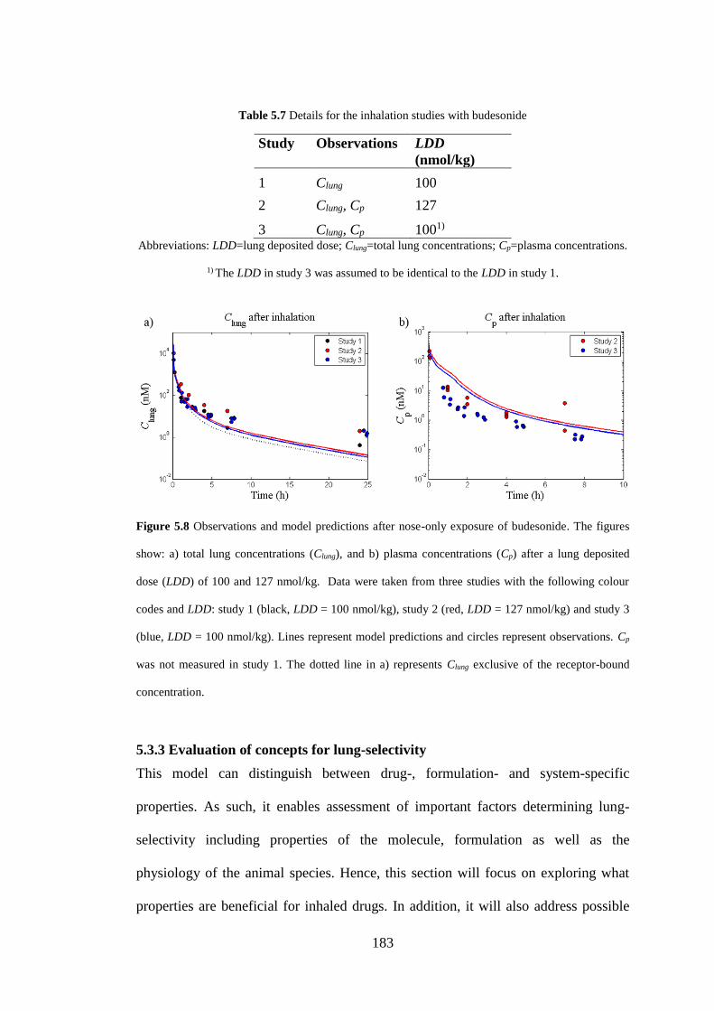
183

Table 5.7 Details for the inhalation studies with budesonide

Study

Observations

LDD

(nmol/kg)

1 Clung 100

2 Clung, Cp 127

3 Clung, Cp 1001) Abbreviations: LDD=lung deposited dose; Clung=total lung concentrations; Cp=plasma concentrations.

1) The LDD in study 3 was assumed to be identical to the LDD in study 1.

Figure 5.8 Observations and model predictions after nose-only exposure of budesonide. The figures

show: a) total lung concentrations (Clung), and b) plasma concentrations (Cp) after a lung deposited

dose (LDD) of 100 and 127 nmol/kg. Data were taken from three studies with the following colour

codes and LDD: study 1 (black, LDD = 100 nmol/kg), study 2 (red, LDD = 127 nmol/kg) and study 3

(blue, LDD = 100 nmol/kg). Lines represent model predictions and circles represent observations. Cp

was not measured in study 1. The dotted line in a) represents Clung exclusive of the receptor-bound

concentration.

5.3.3 Evaluation of concepts for lung-selectivity

This model can distinguish between drug-, formulation- and system-specific

properties. As such, it enables assessment of important factors determining lung-

selectivity including properties of the molecule, formulation as well as the

physiology of the animal species. Hence, this section will focus on exploring what

properties are beneficial for inhaled drugs. In addition, it will also address possible

184

limitations of the animal models currently used for characterisation of inhalation

drugs.

5.3.3.1 Definition of lung-selectivity

Lung-selectivity can be defined as the ratio between pulmonary and systemic

receptor occupancy, where a ratio of unity implies absence of lung-selectivity. In

accordance with the previous line of reasoning, the spleen is used as a reference

organ for the systemic exposure. Since the lung is divided into a central and a

peripheral region, lung-selectivity can be evaluated for each region individually.

Regardless of the scenario simulated, it was noted that lung-selectivity could not be

achieved if the peripheral lung was considered as the pulmonary region. A ratio of

unity was thus obtained between the occupancy in the peripheral lung (ROp) and the

spleen (ROsp) in this model. This is attributed to the high perfusion rate of this region

(entire cardiac output, QCO), which thus rapidly equilibrates with the systemic

circulation. However, under certain circumstances lung-selectivity could be obtained

in the central lung after inhalation. Henceforth, the occupancy in the central lung

(ROc) is therefore used as the pulmonary region for evaluation of lung-selectivity. In

other words, the criterion for lung-selectivity is fulfilled when

1sp

c

RO

RO. (5.51)

5.3.3.2 Evaluation of drug-, formulation- and system-specific input parameters

In the following simulations, the impact of an individual parameter pi on the degree

of lung-selectivity obtained by inhalation will be evaluated by simulating the system

using varying values of pi while all other parameters (p) are fixed at their assigned

185

values. Unless otherwise specified, drug- and formulation-specific input parameters

for FP (table 5.4) are used for the parameter vector p. For consistency, an LDD of

11.3 nmol/kg will be used unless stated otherwise.

The impact of the following drug-specific input parameters on lung-selectivity was

evaluated: CL, F, Cs, Papp and Koff. Furthermore, one formulation- and one system-

specific input parameter were investigated: particle size and nasal blood flow (Qn),

respectively. The latter parameter was included to evaluate the contribution of nasal

drug absorption following nose-only exposure, which was done by simulating and

comparing the plasma PK profile from a base-case scenario (input parameters from

tables 5.4-6) to a scenario where Qn was set to 0. The particle size distribution was

investigated by comparing the base-case scenario to one where the particles were

evenly distributed between the four smallest size classes, that is fi = 0.25 for

i ∈ {5, …, 8} and fi = 0 otherwise.

As can be seen in figure 5.9a, a longer period of lung-selectivity was obtained for a

poorly soluble drug (Cs = 2.5 µM) than for a highly soluble drug (Cs = 50 µM). Since

the dissolution phase can be prolonged by decreasing Cs (eq. 5.20), a lower Cs

resulted in an extended period of lung-selectivity. Nevertheless, a transient

concentration gradient created during dissolution of a highly soluble compound (Cs =

50 µM) could also give rise to a prolonged lung-selectivity given a slow Koff (fig.

5.9b).

The dissolution rate is not only dependent on Cs. From eq. 5.20 and 5.22 it is

evident that the particle size is also important. Moreover, the regional deposition

depends on the particle size. Accordingly, given a certain LDD, simulations showed

that the particle size distribution had an impact on the occupancy profile as well as

on the degree of lung-selectivity (fig. 5.9c).

186

According to the simulations, nasal absorption significantly contributed to the

systemic exposure (fig. 5.9d) and decreased the degree of lung-selectivity following

nose-only inhalation of FP (fig. 5.9e). Noteworthy is that the nasally deposited dose

was predicted to be several-fold higher than LDD (fig. 5.5e, section 5.3.1.2).

Papp-values are known to differ across laboratories, thus there are no strict cut-off

values for Papp assigning low, moderate and high permeability, respectively.

However, as a benchmark the following permeability ranges are used for CaCo-2

[177]:

2×10-6 cm/s > Papp (low permeability)

2×10-6 cm/s ≤ Papp ≤ 20×10-6 cm/s (moderate permeability)

20×10-6 cm/s < Papp (high permeability)

In the simulations Papp = 0.2×10-6 cm/s and Papp = 100×10-6 cm/s assigned low and

high permeability, respectively. In order to distinguish permeability from other

mechanisms of lung retention, the following changes were made in the simulations:

1) drug was administered as a solution directly in the central ELF, and 2) the Koff was

set to be 10-fold higher than the corresponding value for FP; i.e. Koff = 5.1 h-1.

Administration of a solution was done by setting the initial central ELF concentration

(CELF,C) to

CELF

CELFV

LDDC

,

, )0( , (5.52)

187

where VELF,C is the volume of ELF in the central lung. As can be seen in figure 5.9f,

simulations suggest that a low permeability alone can give rise to a prolonged period

of lung-selectivity despite the drug already being dissolved and having a fast Koff.

However, administration of a dissolved, highly permeable compound with the same

properties did not produce any lung-selectivity.

Simulations also showed that F was negatively correlated with lung-selectivity,

whereas a positive correlation was found for CL (simulations not shown).

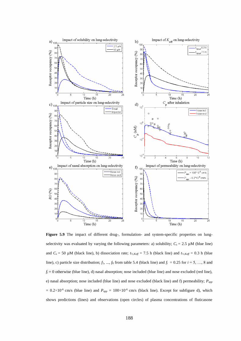
188

Figure 5.9 The impact of different drug-, formulation- and system-specific properties on lung-

selectivity was evaluated by varying the following parameters: a) solubility; Cs = 2.5 µM (blue line)

and Cs = 50 µM (black line), b) dissociation rate; t½,Koff = 7.5 h (black line) and t½,Koff = 0.3 h (blue

line), c) particle size distribution; f1, ..., f8 from table 5.4 (black line) and fi = 0.25 for i = 5, …, 8 and

fi = 0 otherwise (blue line), d) nasal absorption; nose included (blue line) and nose excluded (red line),

e) nasal absorption; nose included (blue line) and nose excluded (black line) and f) permeability; Papp

= 0.2×10-6 cm/s (blue line) and Papp = 100×10-6 cm/s (black line). Except for subfigure d), which

shows predictions (lines) and observations (open circles) of plasma concentrations of fluticasone

189

propionate (Cp), dashed lines represent receptor occupancy in the central lung and solid lines represent

occupancy in a systemic reference organ.

5.3.4 Evaluation of different concepts

5.3.4.1 Intravenous administration versus instillation of dissolved drugs without

any pulmonary retention mechanism

With exception of the intravenous route, inhalation is the fastest route of systemic

delivery of small molecules. This is particularly prominent for small lipophilic

molecules, where the absorption half-life is approximately 1-2 minutes [21]. The

model was used to confirm this feature by firstly simulating the plasma profile

following instillation of a compound in solution (LDD, 20 nmol/kg). This was done

by setting the initial concentration in the ELF in the central lung to

CELF

CELFV

C,

,

20)0( , (5.53)

where CELF,C is the drug concentration in the ELF in the central lung and VELF,C is the

volume of the ELF in ditto. An IV-dose matching the instilled dose (20 nmol/kg) was

subsequently simulated in order to compare the resulting plasma profile to the

corresponding profile obtained after inhalation. As can be seen in fig. 5.10, the

resulting arterial concentration profiles from the two administration routes were

similar for a drug without any specified pulmonary retention mechanism.

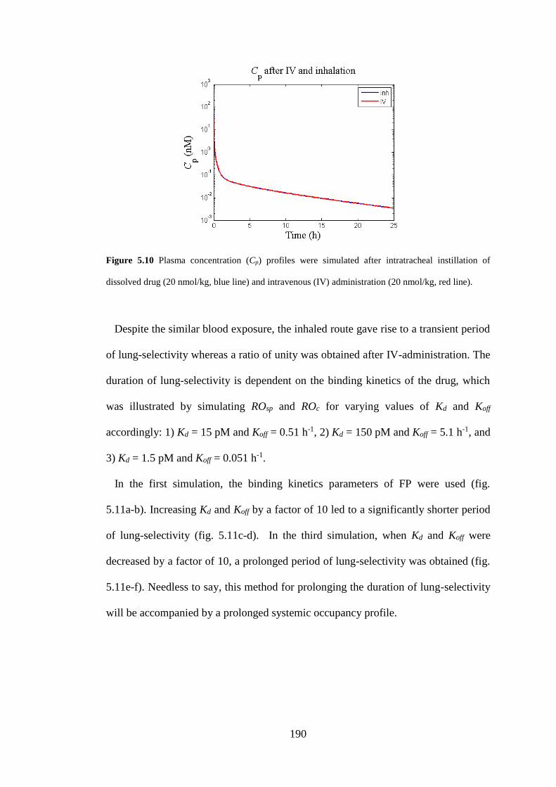
190

Figure 5.10 Plasma concentration (Cp) profiles were simulated after intratracheal instillation of

dissolved drug (20 nmol/kg, blue line) and intravenous (IV) administration (20 nmol/kg, red line).

Despite the similar blood exposure, the inhaled route gave rise to a transient period

of lung-selectivity whereas a ratio of unity was obtained after IV-administration. The

duration of lung-selectivity is dependent on the binding kinetics of the drug, which

was illustrated by simulating ROsp and ROc for varying values of Kd and Koff

accordingly: 1) Kd = 15 pM and Koff = 0.51 h-1, 2) Kd = 150 pM and Koff = 5.1 h-1, and

3) Kd = 1.5 pM and Koff = 0.051 h-1.

In the first simulation, the binding kinetics parameters of FP were used (fig.

5.11a-b). Increasing Kd and Koff by a factor of 10 led to a significantly shorter period

of lung-selectivity (fig. 5.11c-d). In the third simulation, when Kd and Koff were

decreased by a factor of 10, a prolonged period of lung-selectivity was obtained (fig.

5.11e-f). Needless to say, this method for prolonging the duration of lung-selectivity

will be accompanied by a prolonged systemic occupancy profile.

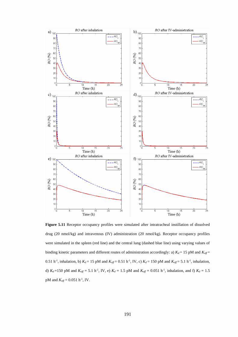
191

Figure 5.11 Receptor occupancy profiles were simulated after intratracheal instillation of dissolved

drug (20 nmol/kg) and intravenous (IV) administration (20 nmol/kg). Receptor occupancy profiles

were simulated in the spleen (red line) and the central lung (dashed blue line) using varying values of

binding kinetic parameters and different routes of administration accordingly: a) Kd = 15 pM and Koff =

0.51 h-1, inhalation, b) Kd = 15 pM and Koff = 0.51 h-1, IV, c) Kd = 150 pM and Koff = 5.1 h-1, inhalation,

d) Kd =150 pM and Koff = 5.1 h-1, IV, e) Kd = 1.5 pM and Koff = 0.051 h-1, inhalation, and f) Kd = 1.5

pM and Koff = 0.051 h-1, IV.

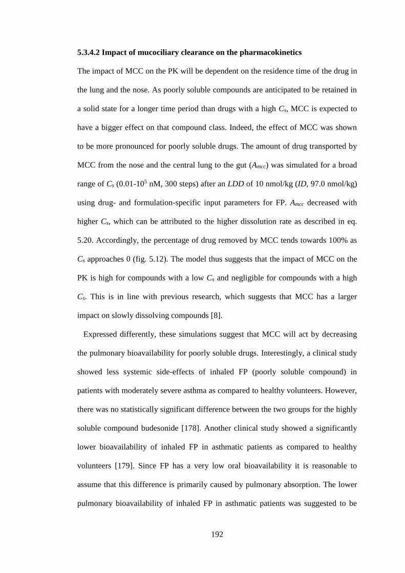
192

5.3.4.2 Impact of mucociliary clearance on the pharmacokinetics

The impact of MCC on the PK will be dependent on the residence time of the drug in

the lung and the nose. As poorly soluble compounds are anticipated to be retained in

a solid state for a longer time period than drugs with a high Cs, MCC is expected to

have a bigger effect on that compound class. Indeed, the effect of MCC was shown

to be more pronounced for poorly soluble drugs. The amount of drug transported by

MCC from the nose and the central lung to the gut (Amcc) was simulated for a broad

range of Cs (0.01-105 nM, 300 steps) after an LDD of 10 nmol/kg (ID, 97.0 nmol/kg)

using drug- and formulation-specific input parameters for FP. Amcc decreased with

higher Cs, which can be attributed to the higher dissolution rate as described in eq.

5.20. Accordingly, the percentage of drug removed by MCC tends towards 100% as

Cs approaches 0 (fig. 5.12). The model thus suggests that the impact of MCC on the

PK is high for compounds with a low Cs and negligible for compounds with a high

Cs. This is in line with previous research, which suggests that MCC has a larger

impact on slowly dissolving compounds [8].

Expressed differently, these simulations suggest that MCC will act by decreasing

the pulmonary bioavailability for poorly soluble drugs. Interestingly, a clinical study

showed less systemic side-effects of inhaled FP (poorly soluble compound) in

patients with moderately severe asthma as compared to healthy volunteers. However,

there was no statistically significant difference between the two groups for the highly

soluble compound budesonide [178]. Another clinical study showed a significantly

lower bioavailability of inhaled FP in asthmatic patients as compared to healthy

volunteers [179]. Since FP has a very low oral bioavailability it is reasonable to

assume that this difference is primarily caused by pulmonary absorption. The lower

pulmonary bioavailability of inhaled FP in asthmatic patients was suggested to be

193

caused by a higher central lung deposition of drug in the asthmatic group, which

makes the drug particles more prone to clearance by MCC [179]. Indeed, asthmatic

patients have been shown to have a higher central deposition of drug [180], which

has been suggested to be caused by the airway narrowing in this patient population

[179]. To summarise, clinical data also suggest that slowly dissolving drugs are more

prone to be cleared by MCC. Since MCC primarily is associated with the

tracheobronchial region [74], this effect is expected to be more pronounced after

central drug deposition.

Figure 5.12 Percent of drug particles deposited in the nose and central lung that are removed by the

mucociliary clearance (MCC) as a function of solubility (Cs).

5.3.4.3 Evaluation of the impact of permeability on pulmonary absorption

As mentioned in section 2.2.4, inhaled drugs may be rapidly absorbed to the systemic

circulation. The pulmonary absorption rate of a dissolved drug is for instance

expected to be dependent on the permeability of the compound. In fact, a weak

relationship (r2 = 0.45) between the lung absorption half-life in rats and the measured

CaCo-2 permeability has been shown in . It is worth mentioning that only limited

information on the experiments is available in the cited publication. Nevertheless, the

194

authors investigated the correlation between the CaCo-2 permeability and pulmonary

absorption half-life (t½,lung) after IT-instillation of solutions to rats. Since several of

the 19 included compounds were bases, the t½,lung cannot be expected to be explained

by permeability alone. Both protonation of the compound in the slightly acidic ELF

(pH 6.6 [4]) as well as intracellular lysosomal trapping might be possible

mechanisms for prolongation of t½,lung. One could argue that the slowness of the

lysosome might already be described by the Papp obtained from CaCo-2 experiments.

However, the cell model’s feasibility to capture this mechanism as well as the

relative abundance of lysosomes in CaCo-2 and lung epithelial cells remain to be

experimentally evaluated prior to confirming or rejecting that hypothesis.

Since only neutral compounds have been explored in this thesis, the current model

structure does not account for lung retention caused by basicity and the aim of this

thesis is not to theoretically/experimentally explore the mechanisms thereof.

Nevertheless, the impact of permeability on pulmonary absorption was theoretically

explored to investigate whether the model predictions are in line with the

observations made in . In that study, t½,lung was calculated based on measurements of

Clung. That approach was subsequently mimicked in this simulation study.

Administration by IT-instillation means that the drug is directly dosed into the

lung, i.e. nasal drug deposition is avoided. It has been shown that the pulmonary

deposition pattern of drug after IT-instillation is highly dependent upon the technique

of the experimentalist [164]. However, IT-instillation tends to result in a higher

deposition centrally in the lung . Hence, to mimic this dosing method drug was

administered as a solution directly in the central ELF. That is, the initial condition in

this compartment was set to

195

CELF

CELFV

LDDC

,

, )0( , (5.54)

where VELF,C is the volume of the central ELF. LDD was set to 10 nmol/kg and P

varied between 0.1×10-6 and 100×10-6 cm/s, where 40 values were selected from a

logarithmic scale. The system was simulated iteratively for 0 ≤ t ≤ 25 h for each

value of P. For each simulation, the time point at which Clung had decreased to 50%

of its value at t = 0 was extracted and used as the model prediction of t½,lung. Clearly,

this value will also be dependent on the systemic PK both in the simulations as well

as in the experimental data. This simulation exercise was subsequently repeated with

the aim of mimicking a more homogenous distribution of drug after IT-instillation,

i.e. the initial condition in each of the two ELF compartments was set to

0.5LDD/VELF.

It follows that two important assumptions are made in these simulations: 1) the

permeability is identical throughout the entire lung (i.e. the measured Papp applies for

all lung regions, which probably is not true for the alveolar region where a higher

permeability is expected), and 2) the CaCo-2 Papp equals the effective permeability.

Thus, two assumptions were made in areas which still remain to be investigated by

future research. Nevertheless, in a theoretical situation where only P differs, the

model-derived values of t½,lung can be used to evaluate the impact of P on pulmonary

absorption on a qualitative level.

Starting by evaluating the simulations resulting from a central deposition of drug,

figure 5.13a shows that t½,lung decreased with a higher permeability. The model

predictions thus agreed with the observations made by Cooper et al. [7] on a

qualitative level. As can be seen in figure 5.13b, model simulations indicate that the

196

initial profile of the lung PK-profile, which often is referred to as the ‘alpha phase’,

would be less steep for poorly permeable compounds.

As expected, lower values of P resulted in higher drug concentrations in the ELF

(CELF, fig. 5.13c), which can have interesting implications for drugs with targets

localised in the airway lumen. The same pattern, although not as pronounced, was

seen for Clung (fig. 5.13b).

Interestingly, despite the assumption of P being identical throughout the entire

lung, the simulations suggested that the pulmonary PK is largely influenced by the

initial deposition pattern. This was particularly prominent when comparing the lung

PK-profiles over the first few minutes. After IT-administration of an evenly

distributed dose, the model predictions indicated that a particularly rapid pulmonary

absorption phase took place during the first few minutes after dosing (fig. 5.13d).

However, this pattern was not present when drug administration was restricted to the

central lung (fig. 5.13e). The simulations thus suggest that pulmonary absorption is

more rapid in the rapidly perfused peripheral lung region. In contrast, a poor P

appears to be an effective mechanism for lung-retention in the central lung region.

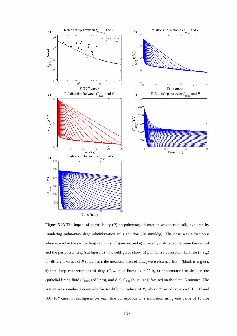
197

Figure 5.13 The impact of permeability (P) on pulmonary absorption was theoretically explored by

simulating pulmonary drug administration of a solution (10 nmol/kg). The dose was either only

administered in the central lung region (subfigure a-c and e) or evenly distributed between the central

and the peripheral lung (subfigure d). The subfigures show: a) pulmonary absorption half-life (t½,lung)

for different values of P (blue line), the measurements of t½,lung were obtained from (black triangles),

b) total lung concentrations of drug (Clung, blue lines) over 25 h, c) concentration of drug in the

epithelial lining fluid (CELF, red lines), and d-e) Clung (blue lines) focused on the first 15 minutes. The

system was simulated iteratively for 40 different values of P, where P varied between 0.1×10-6 and

100×10-6 cm/s. In subfigures b-e each line corresponds to a simulation using one value of P. The

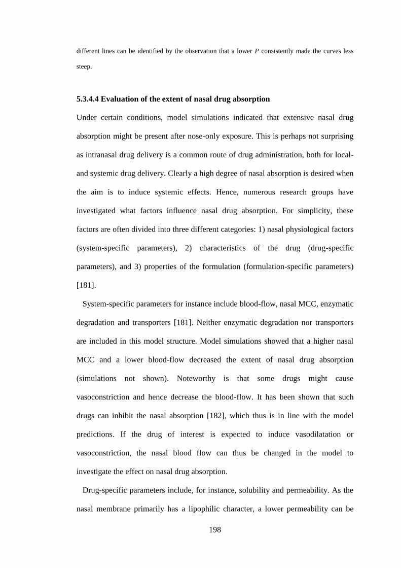
198

different lines can be identified by the observation that a lower P consistently made the curves less

steep.

5.3.4.4 Evaluation of the extent of nasal drug absorption

Under certain conditions, model simulations indicated that extensive nasal drug

absorption might be present after nose-only exposure. This is perhaps not surprising

as intranasal drug delivery is a common route of drug administration, both for local-

and systemic drug delivery. Clearly a high degree of nasal absorption is desired when

the aim is to induce systemic effects. Hence, numerous research groups have

investigated what factors influence nasal drug absorption. For simplicity, these

factors are often divided into three different categories: 1) nasal physiological factors

(system-specific parameters), 2) characteristics of the drug (drug-specific

parameters), and 3) properties of the formulation (formulation-specific parameters)

[181].

System-specific parameters for instance include blood-flow, nasal MCC, enzymatic

degradation and transporters [181]. Neither enzymatic degradation nor transporters

are included in this model structure. Model simulations showed that a higher nasal

MCC and a lower blood-flow decreased the extent of nasal drug absorption

(simulations not shown). Noteworthy is that some drugs might cause

vasoconstriction and hence decrease the blood-flow. It has been shown that such

drugs can inhibit the nasal absorption [182], which thus is in line with the model

predictions. If the drug of interest is expected to induce vasodilatation or

vasoconstriction, the nasal blood flow can thus be changed in the model to

investigate the effect on nasal drug absorption.

Drug-specific parameters include, for instance, solubility and permeability. As the

nasal membrane primarily has a lipophilic character, a lower permeability can be

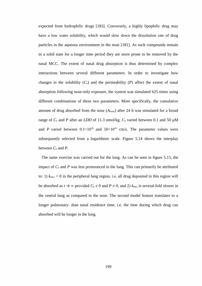
199

expected from hydrophilic drugs [183]. Conversely, a highly lipophilic drug may

have a low water solubility, which would slow down the dissolution rate of drug

particles in the aqueous environment in the nose [181]. As such compounds remain

in a solid state for a longer time period they are more prone to be removed by the

nasal MCC. The extent of nasal drug absorption is thus determined by complex

interactions between several different parameters. In order to investigate how

changes in the solubility (Cs) and the permeability (P) affect the extent of nasal

absorption following nose-only exposure, the system was simulated 625 times using

different combinations of these two parameters. More specifically, the cumulative

amount of drug absorbed from the nose (Anose) after 24 h was simulated for a broad

range of Cs and P after an LDD of 11.3 nmol/kg. Cs varied between 0.1 and 50 µM

and P varied between 0.1×10-6 and 50×10-6 cm/s. The parameter values were

subsequently selected from a logarithmic scale. Figure 5.14 shows the interplay

between Cs and P.

The same exercise was carried out for the lung. As can be seen in figure 5.15, the

impact of Cs and P was less pronounced in the lung. This can primarily be attributed

to: 1) kmcc = 0 in the peripheral lung region, i.e. all drug deposited in this region will

be absorbed as t → ∞ provided Cs ≠ 0 and P ≠ 0, and 2) kmcc is several-fold slower in

the central lung as compared to the nose. The second model feature translates to a

longer pulmonary- than nasal residence time, i.e. the time during which drug can

absorbed will be longer in the lung.

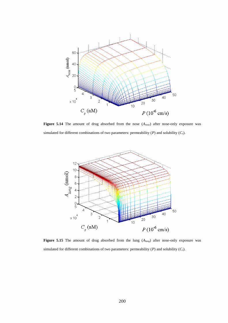
200

Figure 5.14 The amount of drug absorbed from the nose (Anose) after nose-only exposure was

simulated for different combinations of two parameters: permeability (P) and solubility (Cs).

Figure 5.15 The amount of drug absorbed from the lung (Alung) after nose-only exposure was

simulated for different combinations of two parameters: permeability (P) and solubility (Cs).

201

5.3.4.5 Impact of permeability in the central lung

Absorption of dissolved drug from the lung to the systemic circulation is generally

assumed to be slower from the tracheobronchial region as compared to the alveolar

region. This has been attributed both to the lower blood perfusion and to the thicker

airway walls in this region [15]. The proposed differences in regional absorption

rates have also been demonstrated experimentally after regional administration of

solutions [184,185]. Furthermore, the differences in regional perfusion rates and

surface area alone were shown to have a pronounced impact on the pulmonary

absorption by a simulation study described in section 5.3.4.3.

In [186], the drug permeability (P) is described as a constant that depends on the

diffusion coefficient (D) of the drug in the barrier, the thickness of the barrier (h) and

the partition coefficient into the barrier (γ):

h

DP

. (5.55)

Moving from the trachea to the alveolar region, both the type of epithelium and its

thickness will change. In humans, the thickness of the epithelium decreases from 58

µm in the bronchi to 0.1-0.2 µm, in the alveoli [11]. In rats, the bronchi epithelium

thickness is 13 µm [29]. From eq. 5.55 it thus seems plausible that P will not be

constant throughout the lung. Furthermore, it specifies that region-specific

knowledge about both γ and h is needed for proper scaling of P in different lung

regions. To the best of my knowledge, such data is currently not available. New

experimental methodologies would be desired to further investigate this issue.

Nevertheless, as the thickness of the epithelium gradually decreases when moving

202

distally throughout the lung, it is plausible that this gradual decrease in epithelium

thickness is also applicable for P.

Three different scenarios were simulated in order to investigate what impact a

lower P in the central lung region would have on the pulmonary drug disposition if

the peripheral P was kept high. The LDD was set to be 100 nmol/kg and the drug-

and formulation-specific parameters of FP specified in table 5.4 were used in all

three scenarios, whereas Papp in the central lung region varied accordingly: 1) Papp, 2)

Papp/10, and 3) Papp/100. That is, the resulting central Papp in each of the three

simulations was 46.9×10-6 cm/s (high P), 4.69×10-6 cm/s (moderate P) and

0.469×10-6 cm/s (low P), respectively.

As can be understood from eq. 5.1 (the ODE describing the flux to/from the

systemic circulation), a lower P would result in a slower permeation into the lung

tissue. The result of the slower permeation is an increased drug concentration in the

ELF (CELF, fig. 5.16a). As a higher CELF would slow down the dissolution rate (eq.

5.20) this would in turn lead to an increased retention time of drug in the lung (fig.

5.16b). The latter example thus also serves to demonstrate that P is an important

parameter for accurately predicting the lung retention of slowly dissolving drugs.

The profile of ROc would also change (fig. 5.16c), whereas the impact on ROsp would

be less pronounced (fig. 5.16d). Briefly, according to model simulations a lower P in

the central lung region might lead to a prolonged lung-retention. A lower P would

also have an effect on the Cp-profile (fig. 5.16e), where simulations show that P is an

important parameter for determining both the amplitude of the maximum Cp (Cmax)

and the time point when it occurs (tmax).

Considering the regional differences with respect to both the type of epithelium as

well as its thickness, differences in P are highly likely. As previously mentioned in

203

section 5.3.4.3, further research is required in this area to increase the understanding

of regional pulmonary permeability as well as the feasibility to use different in vitro

models for the description thereof. The Papp obtained from CaCo-2 experiments is

more likely to reflect the P in the central lung than the peripheral lung owing to the

characteristics of the cells. Simulations using the drug- and formulation-specific

input parameters for FP (table 5.4) showed that a 100-fold higher P in the peripheral

region were indistinguishable from the earlier simulations (simulations not shown

since they were indistinguishable from fig. 5.5). Hence, the model validation step has

not been biased by using the same P throughout the lung. Nevertheless, the final

model structure presented in this thesis, which also allows for repeated dosing, will

have a 100-fold higher permeability in the peripheral lung. The primary rationale for

scaling by a factor of 100 is based on the differences in epithelium thickness.

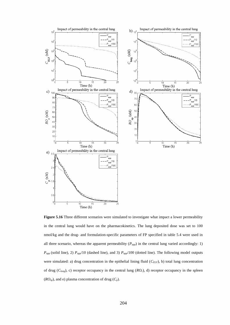
204

Figure 5.16 Three different scenarios were simulated to investigate what impact a lower permeability

in the central lung would have on the pharmacokinetics. The lung deposited dose was set to 100

nmol/kg and the drug- and formulation-specific parameters of FP specified in table 5.4 were used in

all three scenario, whereas the apparent permeability (Papp) in the central lung varied accordingly: 1)

Papp (solid line), 2) Papp/10 (dashed line), and 3) Papp/100 (dotted line). The following model outputs

were simulated: a) drug concentration in the epithelial lining fluid (CELF), b) total lung concentration

of drug (Clung), c) receptor occupancy in the central lung (ROc), d) receptor occupancy in the spleen

(ROsp), and e) plasma concentration of drug (Cp).

205

5.3.5 Repeated dosing

Up until now, the simulations have aimed to explore the fundamental principles for

systemic and local pharmacokinetics after inhaled drug delivery. Single dosing has

thus been sufficient to address these questions. Nevertheless, in the clinical situation,

inhalation is often used to treat chronic diseases such as chronic obstructive

pulmonary disease (COPD) and asthma. It is therefore essential to understand the

effects of long-term use of inhaled drug therapy. Repeated dosing was thus

implemented to enable theoretical investigations of how chronic dosing affects the

PK and PK/PD of inhaled drugs. Previously, the regional deposition fractions for the

different regions (nose, central lung and peripheral lung) and the relevant

aerodynamic diameters have been extracted from Lee et al. [65]. To enable

simulations of repeated dosing of any particle size classes, the model by Lee et al.

[65] was implemented in MATLAB and integrated with the lung simulation model.

The technical implementation of this deposition model is described in the section

5.3.5.2 below.

5.3.5.1 Technical implementation of repeated dosing

Repeated dosing was implemented in MATLAB by adding a new set of 24 ODEs

describing the change of the radius rij (where i ∈ {1, …, 8} and j ∈ {1, 2, 3}) (eq.

5.25) for each dosing occasion k, where k ∈ {1, …, n}. That is, k = 1 assigns the first

dose, k = 2 assigns the second dose and so on. The number of states in the PBPK

model was updated automatically by having k as an input to the function defining the

coupled ODEs.

Except for k = 1, the initial conditions for the set of ODEs describing the change of

rij for each dosing occasion k were initially set to 0. The parameter τ was used to

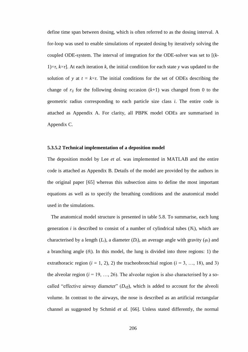
206

define time span between dosing, which is often referred to as the dosing interval. A

for-loop was used to enable simulations of repeated dosing by iteratively solving the

coupled ODE-system. The interval of integration for the ODE-solver was set to [(k-

1)×τ, k×τ]. At each iteration k, the initial condition for each state y was updated to the

solution of y at t = k×τ. The initial conditions for the set of ODEs describing the

change of rij for the following dosing occasion (k+1) was changed from 0 to the

geometric radius corresponding to each particle size class i. The entire code is

attached as Appendix A. For clarity, all PBPK model ODEs are summarised in

Appendix C.

5.3.5.2 Technical implementation of a deposition model

The deposition model by Lee et al. was implemented in MATLAB and the entire

code is attached as Appendix B. Details of the model are provided by the authors in

the original paper [65] whereas this subsection aims to define the most important

equations as well as to specify the breathing conditions and the anatomical model

used in the simulations.

The anatomical model structure is presented in table 5.8. To summarise, each lung

generation i is described to consist of a number of cylindrical tubes (Ni), which are

characterised by a length (Li), a diameter (Di), an average angle with gravity (φi) and

a branching angle (θi). In this model, the lung is divided into three regions: 1) the

extrathoracic region (i = 1, 2), 2) the tracheobronchial region (i = 3, …, 18), and 3)

the alveolar region (i = 19, …, 26). The alveolar region is also characterised by a so-

called “effective airway diameter” (Deff), which is added to account for the alveoli

volume. In contrast to the airways, the nose is described as an artificial rectangular

channel as suggested by Schmid et al. [66]. Unless stated differently, the normal

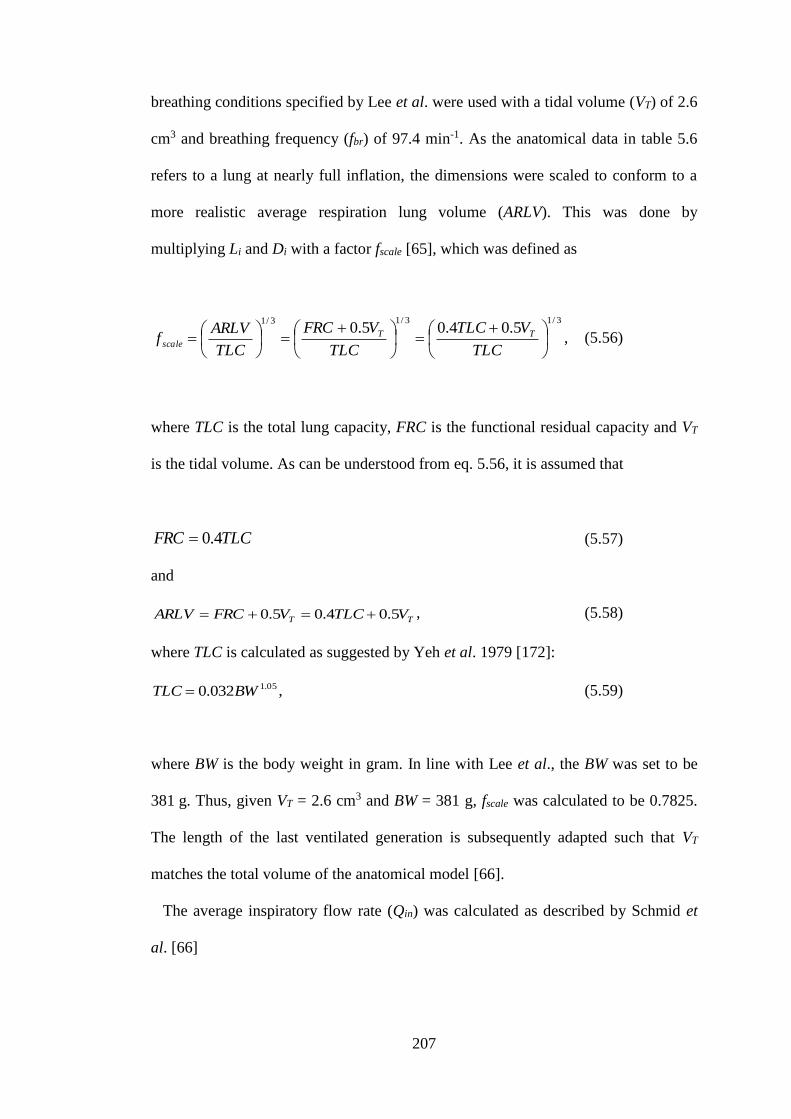
207

breathing conditions specified by Lee et al. were used with a tidal volume (VT) of 2.6

cm3 and breathing frequency (fbr) of 97.4 min-1. As the anatomical data in table 5.6

refers to a lung at nearly full inflation, the dimensions were scaled to conform to a

more realistic average respiration lung volume (ARLV). This was done by

multiplying Li and Di with a factor fscale [65], which was defined as

3/13/13/15.04.05.0

TLC

VTLC

TLC

VFRC

TLC

ARLVf TT

scale, (5.56)

where TLC is the total lung capacity, FRC is the functional residual capacity and VT

is the tidal volume. As can be understood from eq. 5.56, it is assumed that

TLCFRC 4.0 (5.57)

and

TT VTLCVFRCARLV 5.04.05.0 , (5.58)

where TLC is calculated as suggested by Yeh et al. 1979 [172]:

05.1032.0 BWTLC , (5.59)

where BW is the body weight in gram. In line with Lee et al., the BW was set to be

381 g. Thus, given VT = 2.6 cm3 and BW = 381 g, fscale was calculated to be 0.7825.

The length of the last ventilated generation is subsequently adapted such that VT

matches the total volume of the anatomical model [66].

The average inspiratory flow rate (Qin) was calculated as described by Schmid et

al. [66]

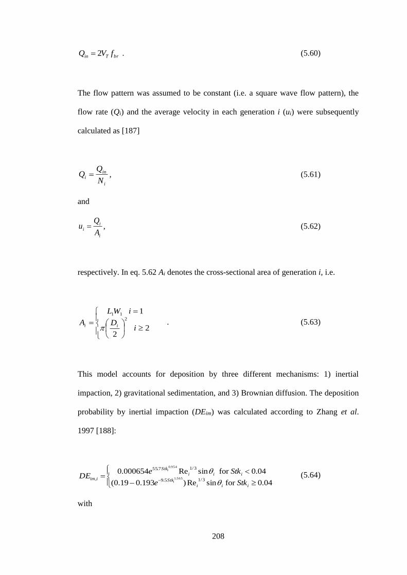
208

brTin fVQ 2 . (5.60)

The flow pattern was assumed to be constant (i.e. a square wave flow pattern), the

flow rate (Qi) and the average velocity in each generation i (ui) were subsequently

calculated as [187]

i

ini

N

QQ , (5.61)

and

i

ii

A

Qu , (5.62)

respectively. In eq. 5.62 Ai denotes the cross-sectional area of generation i, i.e.

2

2

1 2

11

iD

iWL

Aii

. (5.63)

This model accounts for deposition by three different mechanisms: 1) inertial

impaction, 2) gravitational sedimentation, and 3) Brownian diffusion. The deposition

probability by inertial impaction (DEim) was calculated according to Zhang et al.

1997 [188]:

04.0for sinRe)193.019.0(

04.0for sinRe000654.03/15.9

3/17.55

, 565.1

954.0

iii

Stk

iii

Stk

iimStke

StkeDE

i

i

(5.64)

with

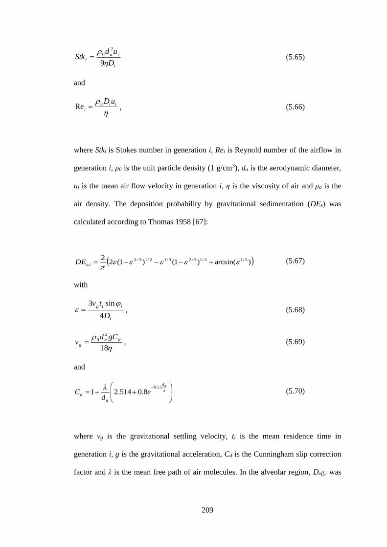
209

i

iai

D

udStk

9

2

0 (5.65)

and

iiai

uDRe , (5.66)

where Stki is Stokes number in generation i, Rei is Reynold number of the airflow in

generation i, ρ0 is the unit particle density (1 g/cm3), da is the aerodynamic diameter,

ui is the mean air flow velocity in generation i, η is the viscosity of air and ρa is the

air density. The deposition probability by gravitational sedimentation (DEs) was

calculated according to Thomas 1958 [67]:

)arcsin()1()1(22 3/12/13/23/12/13/2

,

isDE (5.67)

with

i

iig

D

tv

4

sin3 , (5.68)

18

2

0 dag

gCdv , (5.69)

and

ad

a

d ed

C55.0

8.0514.21 (5.70)

where vg is the gravitational settling velocity, ti is the mean residence time in

generation i, g is the gravitational acceleration, Cd is the Cunningham slip correction

factor and λ is the mean free path of air molecules. In the alveolar region, Deff,i was

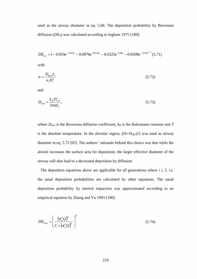
210

used as the airway diameter in eq. 5.68. The deposition probability by Brownian

diffusion (DEd) was calculated according to Ingham 1975 [189]:

3/29.12522822.8963.14

, 0509.00325.00976.0819.01 eeeeDE id (5.71)

with

2

ii

imol

Du

LD (5.72)

and

a

dBmol

d

TCkD

3 , (5.73)

where Dmol is the Brownian diffusion coefficient, kB is the Boltzmann constant and T

is the absolute temperature. In the alveolar region, (Di+Deff,i)/2 was used as airway

diameter in eq. 5.72 [65]. The authors’ rationale behind this choice was that while the

alveoli increases the surface area for deposition, the larger effective diameter of the

airway will also lead to a decreased deposition by diffusion.

The deposition equations above are applicable for all generations where i ≥ 2, i.e.

the nasal deposition probabilities are calculated by other equations. The nasal

deposition probability by inertial impaction was approximated according to an

empirical equation by Zhang and Yu 1993 [190]:

QdC

QdDE

a

aim

2

2

1, (5.74)

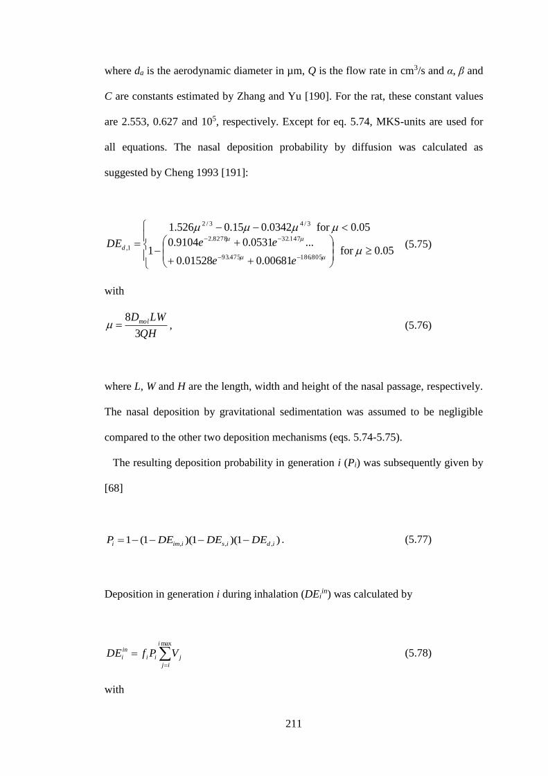
211

where da is the aerodynamic diameter in µm, Q is the flow rate in cm3/s and α, β and

C are constants estimated by Zhang and Yu [190]. For the rat, these constant values

are 2.553, 0.627 and 105, respectively. Except for eq. 5.74, MKS-units are used for

all equations. The nasal deposition probability by diffusion was calculated as

suggested by Cheng 1993 [191]:

05.0for 00681.001528.0

...0531.09104.01

05.0for 0342.015.0526.1

805.186475.93

147.328278.2

3/43/2

1,

ee

eeDEd (5.75)

with

QH

LWDmol

3

8 , (5.76)

where L, W and H are the length, width and height of the nasal passage, respectively.

The nasal deposition by gravitational sedimentation was assumed to be negligible

compared to the other two deposition mechanisms (eqs. 5.74-5.75).

The resulting deposition probability in generation i (Pi) was subsequently given by

[68]

)1)(1)(1(1 ,,, idisiimi DEDEDEP . (5.77)

Deposition in generation i during inhalation (DEiin) was calculated by

maxi

ij

jii

in

i VPfDE (5.78)

with

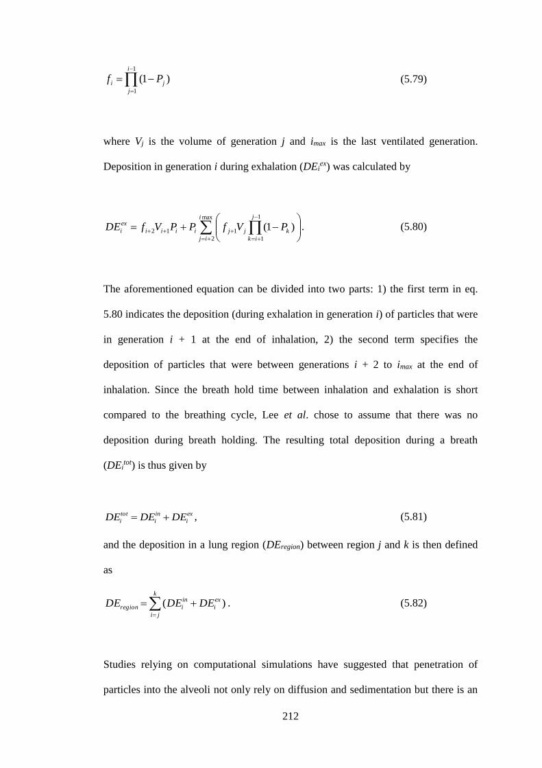
212

1

1

)1(i

j

ji Pf (5.79)

where Vj is the volume of generation j and imax is the last ventilated generation.

Deposition in generation i during exhalation (DEiex) was calculated by

max

2

1

1

112 )1(i

ij

j

ik

kjjiiii

ex

i PVfPPVfDE . (5.80)

The aforementioned equation can be divided into two parts: 1) the first term in eq.

5.80 indicates the deposition (during exhalation in generation i) of particles that were

in generation i + 1 at the end of inhalation, 2) the second term specifies the

deposition of particles that were between generations i + 2 to imax at the end of

inhalation. Since the breath hold time between inhalation and exhalation is short

compared to the breathing cycle, Lee et al. chose to assume that there was no

deposition during breath holding. The resulting total deposition during a breath

(DEitot) is thus given by

ex

i

in

i

tot

i DEDEDE , (5.81)

and the deposition in a lung region (DEregion) between region j and k is then defined

as

k

ji

ex

i

in

iregion DEDEDE )( . (5.82)

Studies relying on computational simulations have suggested that penetration of

particles into the alveoli not only rely on diffusion and sedimentation but there is an

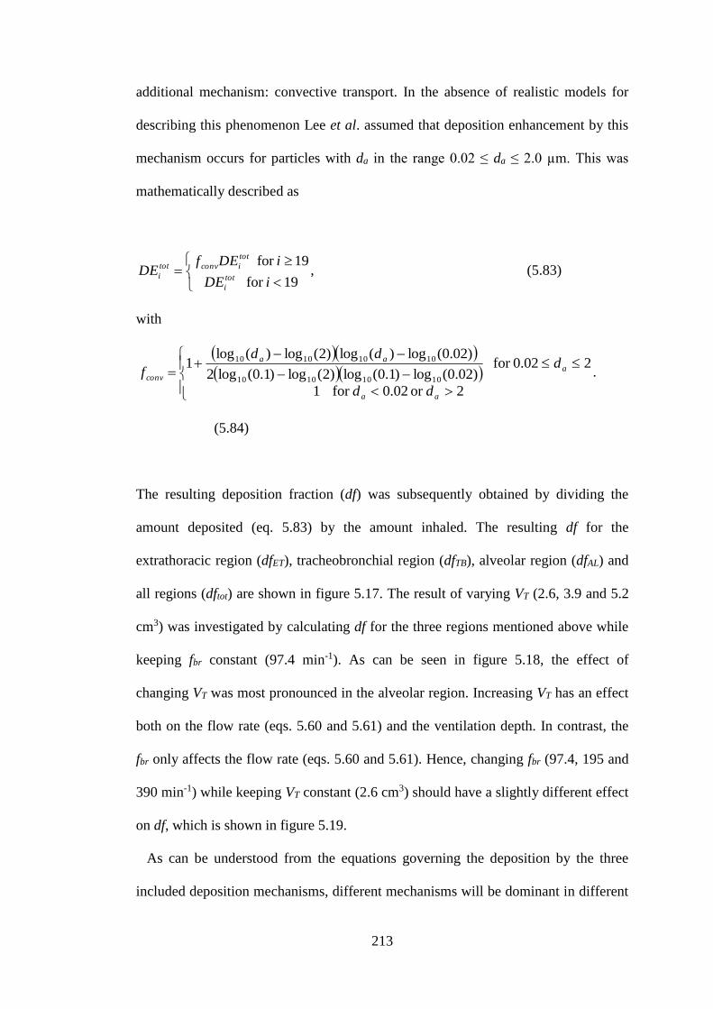
213

additional mechanism: convective transport. In the absence of realistic models for

describing this phenomenon Lee et al. assumed that deposition enhancement by this

mechanism occurs for particles with da in the range 0.02 ≤ da ≤ 2.0 µm. This was

mathematically described as

19for

19for

iDE

iDEfDE

tot

i

tot

iconvtot

i , (5.83)

with

2or 02.0for 1

202.0for )02.0(log)1.0(log)2(log)1.0(log2

)02.0(log)(log)2(log)(log1

10101010

10101010

aa

aaa

conv

dd

ddd

f .

(5.84)

The resulting deposition fraction (df) was subsequently obtained by dividing the

amount deposited (eq. 5.83) by the amount inhaled. The resulting df for the

extrathoracic region (dfET), tracheobronchial region (dfTB), alveolar region (dfAL) and

all regions (dftot) are shown in figure 5.17. The result of varying VT (2.6, 3.9 and 5.2

cm3) was investigated by calculating df for the three regions mentioned above while

keeping fbr constant (97.4 min-1). As can be seen in figure 5.18, the effect of

changing VT was most pronounced in the alveolar region. Increasing VT has an effect

both on the flow rate (eqs. 5.60 and 5.61) and the ventilation depth. In contrast, the

fbr only affects the flow rate (eqs. 5.60 and 5.61). Hence, changing fbr (97.4, 195 and

390 min-1) while keeping VT constant (2.6 cm3) should have a slightly different effect

on df, which is shown in figure 5.19.

As can be understood from the equations governing the deposition by the three

included deposition mechanisms, different mechanisms will be dominant in different

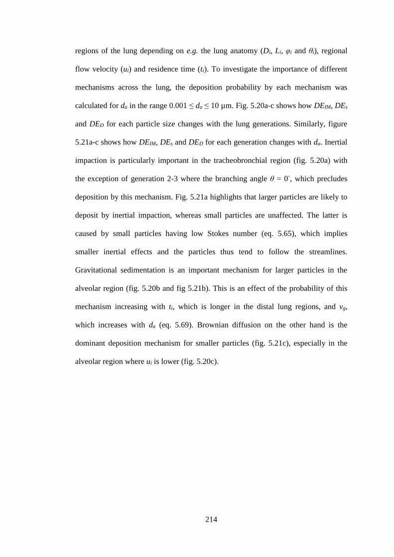
214

regions of the lung depending on e.g. the lung anatomy (Di, Li, φi and θi), regional

flow velocity (ui) and residence time (ti). To investigate the importance of different

mechanisms across the lung, the deposition probability by each mechanism was

calculated for da in the range 0.001 ≤ da ≤ 10 µm. Fig. 5.20a-c shows how DEIM, DEs

and DED for each particle size changes with the lung generations. Similarly, figure

5.21a-c shows how DEIM, DEs and DED for each generation changes with da. Inertial

impaction is particularly important in the tracheobronchial region (fig. 5.20a) with

the exception of generation 2-3 where the branching angle θ = 0◦, which precludes

deposition by this mechanism. Fig. 5.21a highlights that larger particles are likely to

deposit by inertial impaction, whereas small particles are unaffected. The latter is

caused by small particles having low Stokes number (eq. 5.65), which implies

smaller inertial effects and the particles thus tend to follow the streamlines.

Gravitational sedimentation is an important mechanism for larger particles in the

alveolar region (fig. 5.20b and fig 5.21b). This is an effect of the probability of this

mechanism increasing with ti, which is longer in the distal lung regions, and vg,

which increases with da (eq. 5.69). Brownian diffusion on the other hand is the

dominant deposition mechanism for smaller particles (fig. 5.21c), especially in the

alveolar region where ui is lower (fig. 5.20c).

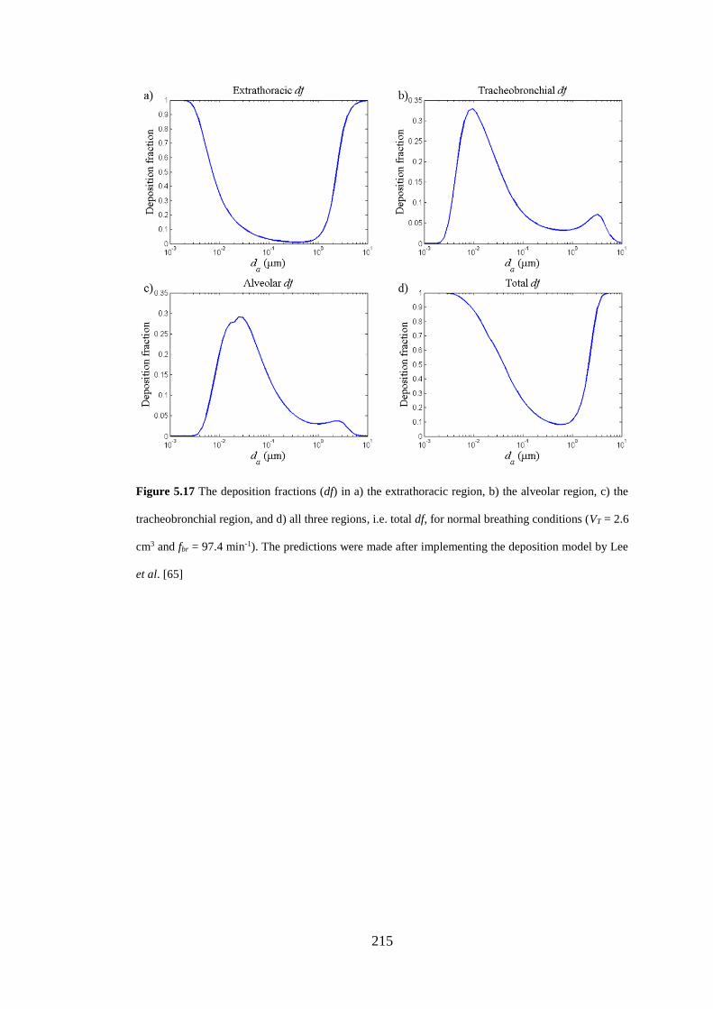
215

Figure 5.17 The deposition fractions (df) in a) the extrathoracic region, b) the alveolar region, c) the

tracheobronchial region, and d) all three regions, i.e. total df, for normal breathing conditions (VT = 2.6

cm3 and fbr = 97.4 min-1). The predictions were made after implementing the deposition model by Lee

et al. [65]

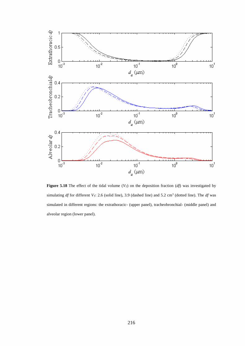
216

Figure 5.18 The effect of the tidal volume (VT) on the deposition fraction (df) was investigated by

simulating df for different VT: 2.6 (solid line), 3.9 (dashed line) and 5.2 cm3 (dotted line). The df was

simulated in different regions: the extrathoracic- (upper panel), tracheobronchial- (middle panel) and

alveolar region (lower panel).

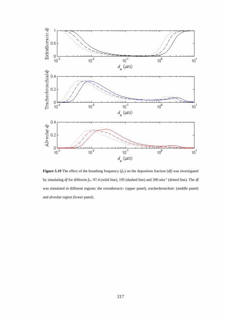
217

Figure 5.19 The effect of the breathing frequency (fbr) on the deposition fraction (df) was investigated

by simulating df for different fbr: 97.4 (solid line), 195 (dashed line) and 390 min-1 (dotted line). The df

was simulated in different regions: the extrathoracic- (upper panel), tracheobronchial- (middle panel)

and alveolar region (lower panel).

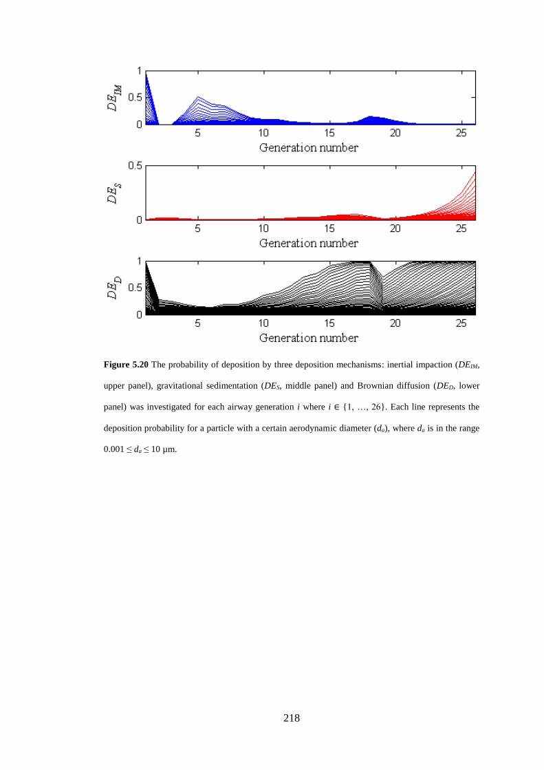
218

Figure 5.20 The probability of deposition by three deposition mechanisms: inertial impaction (DEIM,

upper panel), gravitational sedimentation (DES, middle panel) and Brownian diffusion (DED, lower

panel) was investigated for each airway generation i where i ∈ {1, …, 26}. Each line represents the

deposition probability for a particle with a certain aerodynamic diameter (da), where da is in the range

0.001 ≤ da ≤ 10 µm.

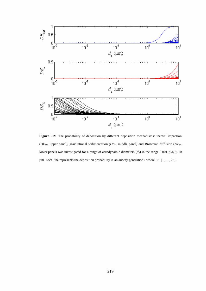
219

Figure 5.21 The probability of deposition by different deposition mechanisms: inertial impaction

(DEIM, upper panel), gravitational sedimentation (DES, middle panel) and Brownian diffusion (DED,

lower panel) was investigated for a range of aerodynamic diameters (da) in the range 0.001 ≤ da ≤ 10

µm. Each line represents the deposition probability in an airway generation i where i ∈ {1, …, 26}.

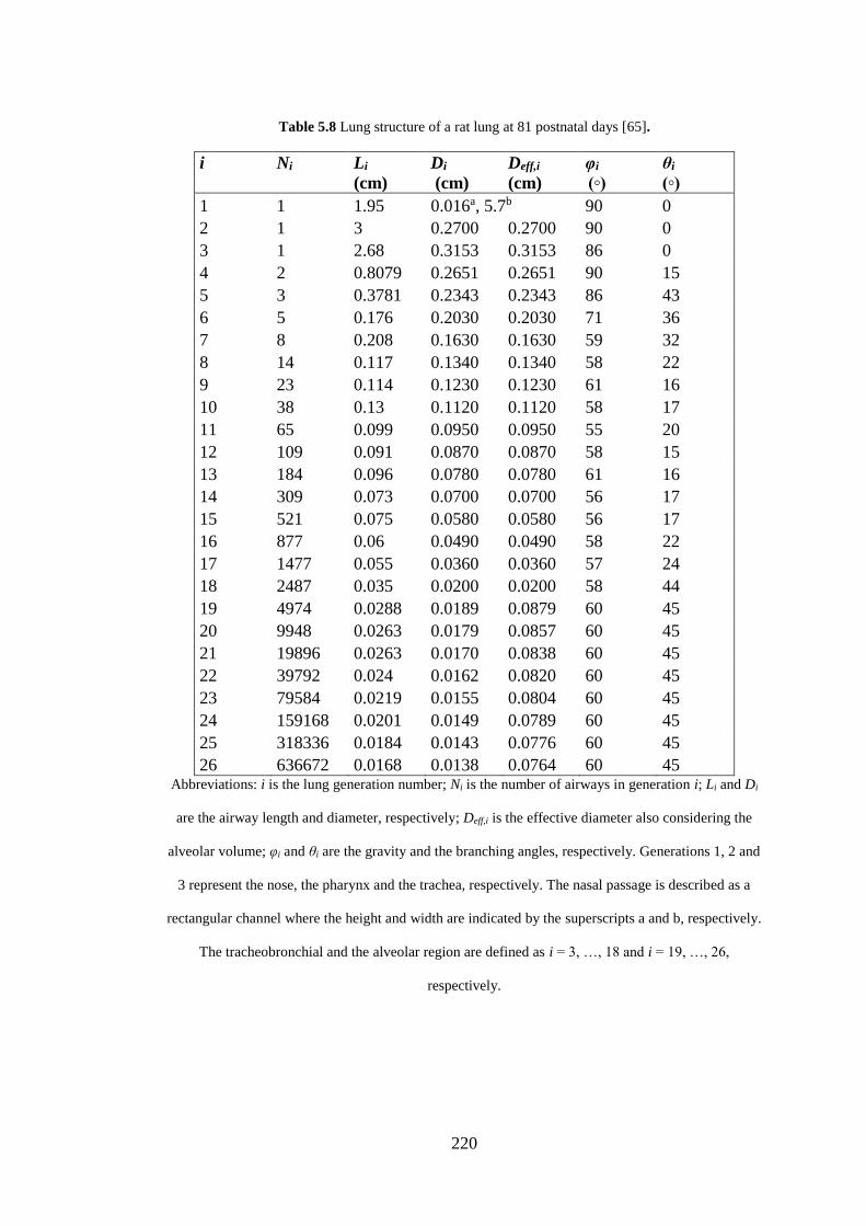
220

Table 5.8 Lung structure of a rat lung at 81 postnatal days [65].

i

Ni

Li

(cm)

Di

(cm)

Deff,i

(cm)

φi

(◦)

θi

(◦)

1 1 1.95 0.016a, 5.7b 90 0

2 1 3 0.2700 0.2700 90 0

3 1 2.68 0.3153 0.3153 86 0

4 2 0.8079 0.2651 0.2651 90 15

5 3 0.3781 0.2343 0.2343 86 43

6 5 0.176 0.2030 0.2030 71 36

7 8 0.208 0.1630 0.1630 59 32

8 14 0.117 0.1340 0.1340 58 22

9 23 0.114 0.1230 0.1230 61 16

10 38 0.13 0.1120 0.1120 58 17

11 65 0.099 0.0950 0.0950 55 20

12 109 0.091 0.0870 0.0870 58 15

13 184 0.096 0.0780 0.0780 61 16

14 309 0.073 0.0700 0.0700 56 17

15 521 0.075 0.0580 0.0580 56 17

16 877 0.06 0.0490 0.0490 58 22

17 1477 0.055 0.0360 0.0360 57 24

18 2487 0.035 0.0200 0.0200 58 44

19 4974 0.0288 0.0189 0.0879 60 45

20 9948 0.0263 0.0179 0.0857 60 45

21 19896 0.0263 0.0170 0.0838 60 45

22 39792 0.024 0.0162 0.0820 60 45

23 79584 0.0219 0.0155 0.0804 60 45

24 159168 0.0201 0.0149 0.0789 60 45

25 318336 0.0184 0.0143 0.0776 60 45

26 636672 0.0168 0.0138 0.0764 60 45 Abbreviations: i is the lung generation number; Ni is the number of airways in generation i; Li and Di

are the airway length and diameter, respectively; Deff,i is the effective diameter also considering the

alveolar volume; φi and θi are the gravity and the branching angles, respectively. Generations 1, 2 and

3 represent the nose, the pharynx and the trachea, respectively. The nasal passage is described as a

rectangular channel where the height and width are indicated by the superscripts a and b, respectively.

The tracheobronchial and the alveolar region are defined as i = 3, …, 18 and i = 19, …, 26,

respectively.

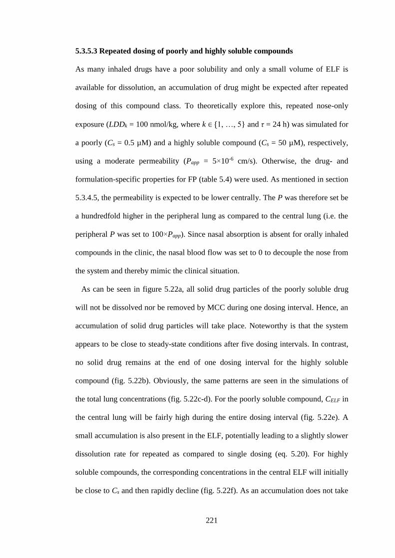
221

5.3.5.3 Repeated dosing of poorly and highly soluble compounds

As many inhaled drugs have a poor solubility and only a small volume of ELF is

available for dissolution, an accumulation of drug might be expected after repeated

dosing of this compound class. To theoretically explore this, repeated nose-only

exposure (LDDk = 100 nmol/kg, where k ∈ {1, …, 5} and τ = 24 h) was simulated for

a poorly (Cs = 0.5 µM) and a highly soluble compound (Cs = 50 µM), respectively,

using a moderate permeability (Papp = 5×10-6 cm/s). Otherwise, the drug- and

formulation-specific properties for FP (table 5.4) were used. As mentioned in section

5.3.4.5, the permeability is expected to be lower centrally. The P was therefore set be

a hundredfold higher in the peripheral lung as compared to the central lung (i.e. the

peripheral P was set to 100×Papp). Since nasal absorption is absent for orally inhaled

compounds in the clinic, the nasal blood flow was set to 0 to decouple the nose from

the system and thereby mimic the clinical situation.

As can be seen in figure 5.22a, all solid drug particles of the poorly soluble drug

will not be dissolved nor be removed by MCC during one dosing interval. Hence, an

accumulation of solid drug particles will take place. Noteworthy is that the system

appears to be close to steady-state conditions after five dosing intervals. In contrast,

no solid drug remains at the end of one dosing interval for the highly soluble

compound (fig. 5.22b). Obviously, the same patterns are seen in the simulations of

the total lung concentrations (fig. 5.22c-d). For the poorly soluble compound, CELF in

the central lung will be fairly high during the entire dosing interval (fig. 5.22e). A

small accumulation is also present in the ELF, potentially leading to a slightly slower

dissolution rate for repeated as compared to single dosing (eq. 5.20). For highly

soluble compounds, the corresponding concentrations in the central ELF will initially

be close to Cs and then rapidly decline (fig. 5.22f). As an accumulation does not take

222

place in the ELF, the dissolution rate will not be different for repeated and single

dosing. Obviously, the same patterns are found in the plasma profiles. That is, a

small accumulation is seen for the poorly soluble drug (fig. 5.22g), but not for the

highly soluble drug (fig. 5.22h). Clearly, the different dissolution profiles are

reflected in the plasma PK, where the poorly soluble compound has a flat PK-profile

with small fluctuations. In contrast, the highly soluble compound has a relatively

high peak concentration, which then rapidly declines leading to large fluctuations in

the plasma profile. The different solubilities also lead to diverse receptor occupancy

profiles. The poorly soluble drug only has small fluctuations in the receptor

occupancy profile. Moreover, lung-selectivity is obtained over the entire dosing

interval (fig. 5.22i). In contrast, the highly soluble compound has large fluctuations

in receptor occupancy and lung-selectivity is only transiently obtained directly after

dosing (fig. 5.22j).

There are few data available for validating predictions of PK after repeated

nose-only exposure. Nevertheless, unpublished AstraZeneca data of one poorly

soluble compound confirm that the systemic exposure, in terms of the maximum

plasma concentration (Cmax) and AUC0-24h, was higher after repeated dosing

compared to after a single dose. In line with the predictions, no difference in

systemic exposure was found after single and repeated dosing of a highly soluble

compound [164].

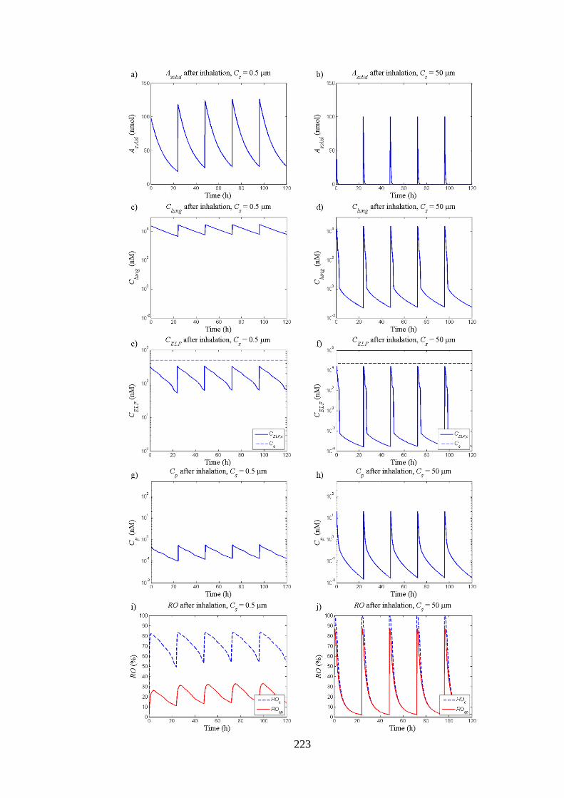
223

224

Figure 5.22 Simulations of repeated nose-only exposure. A lung deposited dose of 100 nmol/kg was

administered every 24 hours. The left panel shows simulations of a poorly soluble drug (solubility, Cs

= 0.5 µM), whereas the right panel shows the corresponding simulations of a highly soluble

compound (Cs = 50 µM). The following variables are simulated: 1) solid amount of drug in the lung

(Asolid), 2) total lung concentration (Clung), 3) concentration in epithelial lining fluid in the central lung

(CELF), 4) plasma concentrations (Cp), and 5) receptor occupancy in the central lung (ROC, dashed blue

line) and the spleen (ROsp, red line).

5.3.5.4 Effect of increasing inhaled doses

As mentioned in section 2.2.4, meta-analyses have shown a relatively flat dose-

response curve for efficacy measurements of inhaled corticosteroids. In contrast, a

steeper dose-response curve has been noted for the side-effects. Taken together, these

two relationships imply that although only a small clinical benefit is expected from

increasing the inhaled dose, the risks of side-effects is considerably increased [47].

Simulations were used to investigate the dose-response relationship of inhaled

corticosteroids with respect to both the local beneficial effects and the systemic side-

effects. Firstly, a poorly soluble compound (Cs = 0.5 µM) with a moderate

permeability (Papp = 5×10-6 cm/s) was administered repeatedly (k = 5, τ = 24 h) using

a broad range of doses (LDD = 10, 50, 250, 750 and 1250 nmol/kg). ROc and ROsp

was assumed to reflect the beneficial local effects and the systemic side-effects,

respectively. Since nasal absorption is absent for orally inhaled compounds in the

clinic, the nasal blood flow was set to 0 to decouple the nose from the system and

thereby mimic the clinical situation. In line with the reasoning in section 5.3.5.3, P

was set to be a hundredfold higher in the peripheral lung as compared to the central

lung (i.e. the peripheral P was set to 100×Papp). Otherwise, the drug- and

225

formulation-specific parameters defined in table 5.4 were used. Noteworthy is that

F = 0.

Secondly, a highly soluble compound with a moderate permeability (Papp = 5×10-6

cm/s) was used in the simulations (Cs = 50 µM). A broad range of LDD was used

(LDD = 1, 5, 25, 125 and 250 nmol/kg). Except from Cs and LDD, all parameters and

settings were identical in the two different simulation sets.

The simulations of a poorly soluble drug showed that the degree of lung-selectivity

decreased at higher LDD (fig. 5.23a-e). Expressed differently, ROsp was more

sensitive to changes in LDD at higher doses since ROc was already in the proximity

of its maximum value. Increasing LDD at that stage should thus not be expected to

provide a significantly better local effect but rather act by increasing the risk of side-

effects. Furthermore, the model elucidated an interesting phenomenon: the ELF in

the central region will be in the proximity of Cs throughout the entire dosing interval

after repeated dosing of a high LDD. For poorly permeable compounds, this

phenomenon will occur at lower LDD (simulations not shown). It thus follows that

the maximum central lung tissue concentration (and thus ROc) that can be obtained

via flux from the ELF will be limited by the interplay between e.g. P, Cs, the particle

size and the regional blood flow (i.e. Qbronch). Under such circumstances, the small

rise in ROc that results from increasing the LDD will primarily be systemically

driven as the input from the central ELF is close to its maximum.

As can be seen in figure 5.24a-e, the maximum ROc was reached already at a low

LDD for the highly soluble compound. The same pattern was subsequently noted; the

degree of lung-selectivity decreased with increasing LDD. Thus, regardless of the

solubility characteristics, the simulations at the higher end of the dose-spectrum were

consistent with the dose-response relationships found in clinical studies.

226

It is worth noting that the lung-selectivity obtained for the highly soluble

compound is the result of the dissolution process, the slow Koff (Koff = 0.51 h-1) as

well as the P. In order to investigate how the last two properties can affect the dose-

response after repeated inhaled dosing of a highly soluble compound, two additional

scenarios were explored. Firstly, Koff was set to be 10-fold lower (i.e. Koff = 0.051 h-

1). Secondly, the P was set to be 10-fold lower (i.e. Papp = 0.5×10-6 cm/s). Except

from these changes, all drug- and formulation-specific input parameters as well as

the choice of LDD remained unchanged.

As can be seen in figure 5.25a-e, a slow Koff acted by increasing the degree of lung-

selectivity. Importantly, it prolonged the period during which lung-selectivity was

obtained. In fact, for the three lower doses (LDD = 1, 5 and 25 nmol/kg) lung-

selectivity was obtained throughout the entire dosing-interval. As in the previous

simulations, the degree of lung-selectivity subsequently decreased with higher LDD.

In this simulation set, Koff was lowered by a factor of 10 whereas Kd remained

unchanged. Since Kd is defined as the ratio between Koff and Kon (eq. 4.8), it follows

that Kon was 10-fold lower. The lower receptor occupancy levels seen in figure

5.25a-c as compared with figure 5.24a-c are thus the result of the lower Kon (the

drug-receptor association is driven by Cu(t)KonR(t) as described in eq. 5.31).

Figure 5.26a-e presents the simulations in which a highly soluble compound with a

10-fold lower P was used. When comparing these simulations to the base-case

(fig. 5.24a-e), it was found that the receptor occupancy profiles were similar at the

three lowest doses used in this simulation study (LDD = 1, 5 and 25 nmol/kg). In

contrast, at the two highest doses the effect of lowering P was more pronounced (fig.

5.24d-e and 5.26d-e for the base-case and the 10-fold lower P, respectively). As a

result of the lower P and thus slower absorption from the airway lumen, high drug

227

concentrations will be maintained in the ELF over a prolonged time period. This

effect will be particularly pronounced after a high LDD since the CELF will be in

close proximity to Cs (i.e. it will be saturated with respect to drug) and thus

significantly slow down the normally rapid dissolution process. Hence, the net effect

of increasing LDD in combination with lowering P was a more sustained receptor

occupancy profile with a prolonged period of lung-selectivity.

To summarise, in all simulations described in this subsection (figs. 5.23-5.26) the

lung-selectivity decreases at high LDD. Expressed differently,

1lim

sp

c

LDD RO

RO. (5.85)

It is also clear that the ratio between ROc and ROsp will tend to infinity as LDD

approaches 0, i.e.

sp

c

LDD RO

RO

0lim . (5.86)

Expressed differently, as LDD approaches 0 it follows that both ROc and ROsp tend to

0; i.e. an undesired situation where no pharmacological effect is exerted. This clearly

emphasises the need to have a PK/PD model in place prior to making a dose

optimisation in order to establish approximately what level of receptor occupancy is

needed to exert the desired effect. Once this information is in place, it would be

possible to apply constrained optimisation for dose optimisation purposes.

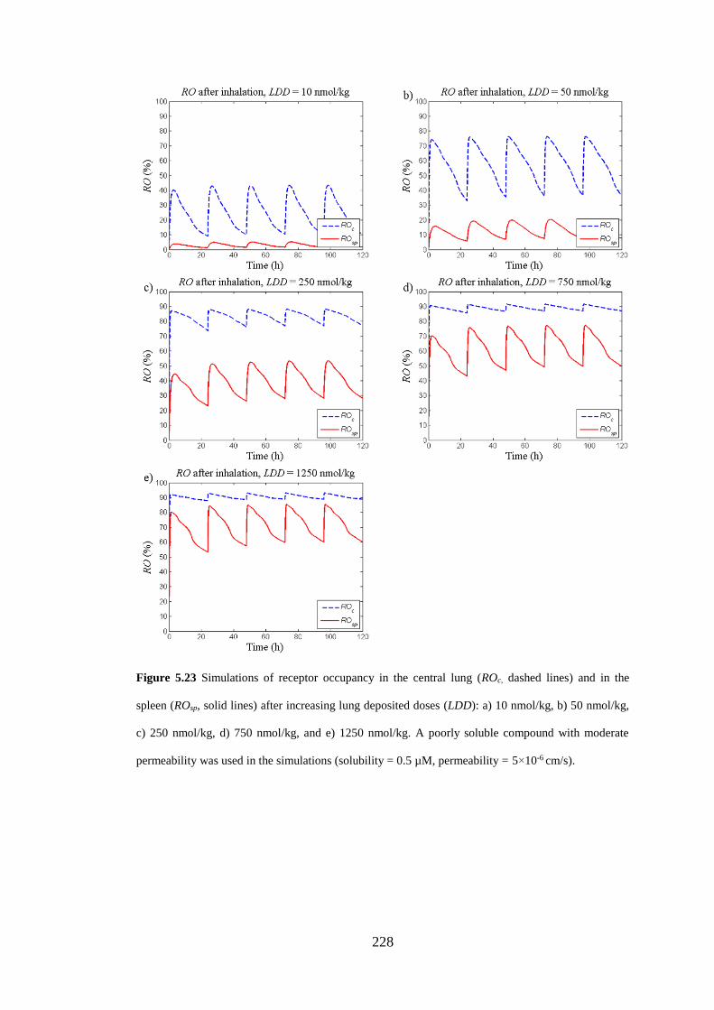
228

Figure 5.23 Simulations of receptor occupancy in the central lung (ROc, dashed lines) and in the

spleen (ROsp, solid lines) after increasing lung deposited doses (LDD): a) 10 nmol/kg, b) 50 nmol/kg,

c) 250 nmol/kg, d) 750 nmol/kg, and e) 1250 nmol/kg. A poorly soluble compound with moderate

permeability was used in the simulations (solubility = 0.5 µM, permeability = 5×10-6 cm/s).

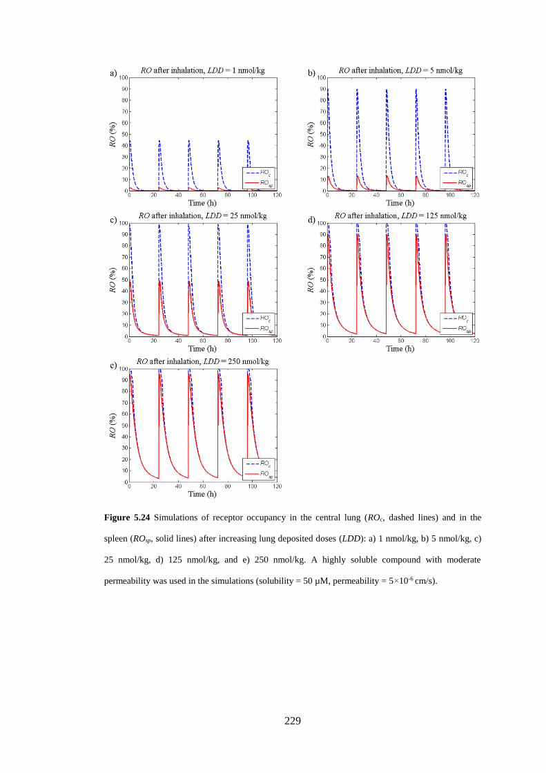
229


spleen (ROsp, solid lines) after increasing lung deposited doses (LDD): a) 1 nmol/kg, b) 5 nmol/kg, c)

25 nmol/kg, d) 125 nmol/kg, and e) 250 nmol/kg. A highly soluble compound with moderate

permeability was used in the simulations (solubility = 50 µM, permeability = 5×10-6 cm/s).

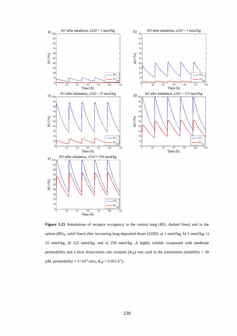
230



25 nmol/kg, d) 125 nmol/kg, and e) 250 nmol/kg. A highly soluble compound with moderate

permeability and a slow dissociation rate constant (Koff) was used in the simulations (solubility = 50

µM, permeability = 5×10-6 cm/s, Koff = 0.051 h-1).

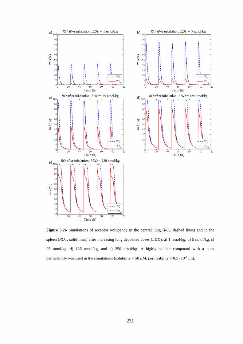
231



25 nmol/kg, d) 125 nmol/kg, and e) 250 nmol/kg. A highly soluble compound with a poor

permeability was used in the simulations (solubility = 50 µM, permeability = 0.5×10-6 cm).

232

5.4 Discussion

This chapter presents the development of a mechanistic PBPK model including lung

disposition for prediction of systemic and pulmonary PK for inhaled drugs, which

was validated by experimental measurements of drug concentrations and receptor

occupancy obtained from studies where FP was used as test compound. By virtue of

being mechanistic, this model provides a tool to theoretically explore pulmonary

drug disposition and how key processes in a physiological context produce lung-

selectivity.

Two different compounds were used for evaluating the model: FP and budesonide.

The model predictions for FP were consistent with experimental data collected from

studies utilising the IV- as well as the inhaled route, which will be described in detail

the subsequent paragraph. In contrast, regardless of the route of administration, there

were discrepancies between model predictions and observations for budesonide.

Since the model was predictive of FP, this systematic discrepancy for budesonide

might suggest the presence of a drug-specific mechanism that is unaccounted for by

the model. Indeed, as mentioned in section 5.3.2.1, a reversible fatty acid

esterification of budesonide has been shown to take place both in vitro [175] and in

vivo [79]. Upon characterisation of the PK of budesonide and its ester, budesonide-

oleate, it was demonstrated that budesonide-oleate was rapidly formed both after IV-

dosing and inhalation of budesonide in rats [79]. Since the resulting budesonide-

oleate concentrations were in the proximity of the budesonide concentrations [79],

the process of esterification and the subsequent hydrolysis is likely to have a

pronounced effect on the PK of budesonide. This hypothesis has also been confirmed

via semi-empirical modelling approaches [79,176]. Hence, the current model

structure should not be expected to accurately describe the PK of budesonide. Further

233

research would thus be required to adequately describe this mechanism in a

quantitative manner, which was not considered to fall within the scope of this thesis.

Data generated from IV-dosing as well as inhalation of FP were used for model

validation, which thus allows the model to be used to compare the two administration

routes. Model predictions of IV-administrations were consistent with experimental

data (figs. 5.4a-d), supporting a perfusion rate-limited distribution. Notably, input

parameters (CL, Vd,ss, Kon and Koff) obtained from the modelling of one data set (90

nmol/kg, IV) proved predictive of data from four other IV-dose levels (20, 150, 750

and 1000 nmol/kg), thus offering strong support and confidence in its predictive

capability to determine systemic PK and receptor occupancy. Interestingly, inclusion

of receptor binding was necessary for accurate predictions of spleen concentrations

after IV-administration as well as nose-only exposure (fig. 5.4d and 5.5c,

respectively), which verifies that FP has a high receptor-bound fraction as suggested

from the results presented in section 3.3.2.3. Similarly, inclusion of the receptor-

bound concentration was necessary for accurate predictions of Clung after IV-

administration of FP (fig. 5.4c). Taken together, this elucidates the potential pitfall of

only relying on Kp-values when predicting tissue concentrations after low doses of

highly potent compounds. Under such circumstances, under-predictions are

inevitable as Kp-values do not account for receptor binding. In contrast, since Clung

after nose-only exposure was substantially higher than the receptor density (i.e. Clung

>> Bmax, where Bmax = 21 nM), the contribution of receptor binding to Clung was

negligible after inhaled drug delivery.

As the aqueous solubility of poorly soluble compounds, such as FP, tends to under-

predict the in vivo dissolution rate [55], the single parameter Cs was estimated from

observations of total drug concentrations in the lung made in one inhalation study

234

(11.3 nmol/kg, LDD). It is worth noting that the estimate of Cs (4530 [3845-5215]

nM) was close to the measured FaSSIF-solubility (3120 nM) [164]. When the

optimised model was tested on another data set (100 nmol/kg, LDD), it was shown to

be predictive of the total lung concentrations with the exception of the last time point

(fig. 5.5a). It should be noted that neither the particle size distribution nor the density

was available for the study comprising of the higher LDD, which therefore was

assumed to have the same formulation-specific properties as the low-dose study. The

discrepancy between the predicted and observed Clung at t = 24 h could thus possibly

be explained by an inaccurately described particle size distribution. Nevertheless, it

might also reflect limitations of the Nernst-Brunner equation for the alveolar region

where the ELF layer might be smaller than the particle diameter.

Model predictions of plasma concentrations and systemic occupancy after nose-

only inhalation agreed well with experimental data (figs. 5.5e-f). This consistency

confirms that FP has a dissolution rate-limited absorption and underscores the

importance of mechanistically describing the dissolution process for such

compounds.

Validation of lung occupancy predictions was slightly more complex as these

measurements reflect whole-lung occupancy. For comparison of observations and

predictions, a weighted average accounting for the relative contribution of each

pulmonary region was thus needed. Although exact determination of the tissue

fractions cannot be made, the volume fraction of central lung (fv,c) was approximated

to be 0.19 (section 5.2.2.3). Given the uncertainty in fv,c and the slightly lower

accuracy of lung occupancy measurements (section 3.4), a whole-lung occupancy

prediction that qualitatively captures key features including lung-selectivity and late

occupancy peak (fig. 5.5d) can be regarded as a good description of the data.

235

For validation purposes, emphasis was not placed on explaining the variability in

the data, which is partly caused by the use of destructive sampling (one animal/time

point). Apart from interindividual differences in model input parameters, a high

variation in LDD is expected from preclinical studies utilising nose-only exposure

systems. The latter can partly be explained by the individual animals having slightly

different breathing patterns, the effect thereof on the deposition was illustrated by

figs. 5.18 and 5.19. Since this is not monitored in preclinical studies, the validation

instead focused on how well the model captured key features in the observations,

both at a quantitative and a qualitative level.

Since the model proved to be predictive of FP, i.e. a neutral compound with a

dissolution rate-limited absorption, it was used to theoretically explore various

aspects of pulmonary drug disposition. As expected, simulations showed that lung-

selectivity could not be obtained if the drug was administered via the IV-route. More

interestingly, a previously unforeseen finding resulting from the simulation studies

was that lung-selectivity is possibly unattainable in the well-perfused parts of the

lung after inhaled drug delivery. This can be attributed to the high perfusion rate of

the alveoli region (entire cardiac output, QCO), which thus rapidly equilibrates with

the systemic circulation. In fact, the model predicted the tissue distribution half-life

of FP in the peripheral lung to be below 2 s. However, lung-selectivity could be

obtained in the central region after inhalation as its lower perfusion rate allows for a

longer equilibration time. The receptor occupancy in the central lung (ROc) was thus

used as the pulmonary region for evaluation of lung-selectivity.

It was shown that a concentration-gradient, and thus lung-selectivity, was obtained

during the dissolution phase (fig. 5.9a). It was also demonstrated that a low oral

bioavailability and a high clearance were both important for obtaining a high degree

236

of lung-selectivity (simulations not shown). These three concepts have been

demonstrated in an earlier simulation study by Hochhaus et al. [14]. Those

simulations relied on a very simple model structure, in which the lung was described

by a single compartment, the dissolution process by a rate constant, kdiss, and the

receptor binding by a static Emax-model. The model presented in this thesis can thus

explore further aspects of pulmonary drug disposition since it has: 1) a physiological

parameterisation, 2) more sophisticated and mechanistic mathematical descriptions

of drug disposition processes, and 3) a dynamic description of receptor binding, i.e. it

is parameterised by the association rate constant (Kon) and the dissociation rate

constant (Koff).

In line with results from previous research [14], this model also described the risk

of only obtaining transient lung-selectivity after IT-administration of a dissolved

drug without any additional mechanisms enhancing its lung-retention, i.e. a scenario

resembling IV-administration where no lung-selectivity is obtained. Nevertheless, it

was unravelled that a transient concentration-gradient can give rise to an extended

period of lung-selectivity provided that the drug-receptor dissociation-rate is

relatively slow (figs. 5.11a and 5.11e). The latter feature was unforeseen by earlier

models since the receptor binding was described by a static Emax-model [14].

Interestingly, the lung-selectivity obtained via this mechanism could not be detected

from the plasma profile after inhalation, which was close to identical to the

corresponding profile obtained after administering the same dose as an IV-bolus (fig.

5.10). This example thus also serves to demonstrate that it might be inappropriate to

interpret inhalation studies solely on the basis of plasma concentrations. Simulations

in section 5.3.3.2 demonstrated how yet another drug-specific property, namely a

poor permeability, can lead to a prolonged period of lung-selectivity after IT-

237

administration of a solution (fig. 5.9f). Besides, since a poor permeability results in a

slower permeation into lung tissue and thus an increased drug concentration in the

ELF (CELF, fig. 5.13c), this property might be even more interesting if the drug target

resides in the airway lumen. According to model predictions, drug discovery projects

with targets localised in the airway lumen would benefit from chemically design

compounds that exhibit a poor permeability.

Moving back to lung-selectivity obtained by designing poorly soluble compounds

and thereby creating a slow dissolution process. As mentioned in section 4.1, a more

in-depth knowledge is needed to better understand the potential benefits and

limitations of this strategy. Clearly, simulations indicate that this strategy is

beneficial for highly potent compounds (figs. 5.9a, 5.22i, and 5.23a-e). Notably, at

the other end of the spectrum are low-affinity compounds for which a low Cs might

disrupt the opportunity of obtaining sufficiently high target site concentrations to

elicit a pharmacological response. Simulations of repeated dosing of poorly soluble

compounds elucidated this interesting phenomenon (fig. 5.23): the ELF in the central

lung region will be in the proximity of Cs throughout the entire dosing interval after

repeated doses of high LDD. The saturation of the ELF with respect to drug creates

an interesting situation where the maximum central tissue concentration, and thus

ROC, that can be obtained via flux from the airway lumen is limited by an interplay

between e.g. P, Cs, Kd and the regional blood flow (i.e. Qbronch). Thus, after having

saturated the ELF, ROC can only increase via flux from the systemic circulation. That

is, an undesirable situation has come to exist where the increase in the local effect is

driven from the systemic side and a higher LDD will thus act by decreasing the

degree of lung-selectivity. Again, this illustrates the importance of having an

integrated understanding. Nevertheless, the strategy of designing compounds with a

238

poor solubility should primarily be considered if the chemical design also allows for

a high affinity.

Simulations also demonstrated that particle size is an important determinant of the

dissolution rate, which thus can be used to partly control the dissolution process (fig.

5.9c). Due to the enlarged surface area, smaller particles will dissolve more rapidly

(eq. 5.19). Indeed, reducing the particle size has been documented to increase the in

vitro dissolution rate as well as the oral bioavailability for poorly soluble compounds

[192,193]. Nevertheless, the impact of changing the particle size is more complex for

the inhaled route as compared with the oral route. This is attributed to the particle

size also being an important determinant of the regional drug deposition. Thus, the

dissolution process should not be considered in isolation when evaluating the

consequences of changing the particle size. If a reduction of the particle size leads to

a greater drug deposition in the more rapidly perfused distal airways, one could also

expect e.g. less drug removal by MCC and a more rapid absorption from the lung to

the systemic circulation. The latter was highlighted by simulations and discussions

contained in section 5.3.4.3, which showed a more rapid pulmonary absorption of

drug deposited in the distal airways. Accordingly, for several reasons, this is

expected to be reflected in the plasma profile by a higher and earlier peak plasma

concentration (Cmax) as well as by a higher systemic bioavailability. However, when

interpreting such data, it is thus difficult to separate the effect of a higher dissolution

rate from the effects that are indirectly caused by a greater distal airway deposition.

The presented mechanistic PBPK model, which describes the interplay between these

different processes, could thus be a useful tool to understand the implications of

changing a parameter, such as the particle size, that is expected to have a pronounced

effect on several processes. This application can e.g. be useful for tailoring inhaled

239

drug formulations for clinical studies. It is worth mentioning that Usmani [194] has

shown that inhalation of different sized particles of FP indeed produces different PK

behavior. The smaller particles (1.5 µm MMAD) had a higher and earlier Cmax as

compared to the larger particles (6 µm MMAD). Furthermore, the systemic

bioavailability was higher for the smaller particles. Both simulations and

experimental data thus emphasise the importance of also considering formulation-

specific parameters when designing preclinical- and clinical studies. By using a

suboptimal particle size distribution, a compound might erroneously be considered to

have PK-properties poorly suited for inhalation and/or to have a poor efficacy and

safety profile. Clearly, the appropriate particle size distribution needs to be

considered on a case-by-case basis depending on the compound as well as on the

target.

Model predictions elucidated that a high nasal deposition, possibly accompanied by

significant absorption, is expected following nose-only exposure studies (figs. 5.5g

and 5.16a). While nasal absorption is absent for orally inhaled products in the clinic,

simulations suggest that nasal uptake reduces the degree of lung-selectivity seen in

preclinical models (figs. 5.9d-e). Accounting for this process might thus be important

for interpretation and translation of preclinical data since drug candidates otherwise

could be deselected based on false premises. Simulations indicated that the interplay

between Cs and P will affect the degree of nasal absorption, where compounds with a

high Cs and high P will be absorbed to a greater extent (fig. 5.14). A higher nasal

MCC and a lower regional blood flow were also both shown to considerably

decrease the extent of nasal absorption, suggesting that an even more careful

characterisation of those two system-specific parameters would be informative for

the model. It is worth noting that some drugs can cause vasoconstriction and thereby

240

reduce the nasal blood flow and thus the extent of nasal drug absorption, further

emphasising the need for an integrated understanding of the entire system. If the

technical challenges can be overcome, experiments addressing the extent of nasal

absorption after nose-only exposure would indeed be useful.

As mentioned in section 2.2.4.1, meta-analyses of clinical studies have shown a

relatively flat dose-response curve for inhaled corticosteroids [49,50]. In contrast, a

steeper dose-response curve was found for the side-effects. This was theoretically

investigated by model simulations, in which the nasal blood flow was set to zero to

avoid nasal absorption and thereby mimic the clinical situation. Escalating LDD-

levels were used in the simulations and ROC and ROsp were used as readouts for the

local beneficial effect and the systemic side-effect, respectively. Regardless of the

solubility characteristics of the compound (i.e. highly or poorly soluble), the model

predictions for the higher end of the dose-spectrum were consistent with the dose-

response relationships found in clinical studies (figs. 5.23-5.26). That is, at higher

LDD ROC was close to its maximum value whereas ROsp still was increasing. Hence,

these simulations combined with the results of the meta-analyses might imply a

historical tendency to over-dose inhaled corticosteroids in clinical studies.

Furthermore, the two earlier examples illustrate how the model lends itself for

translation. As it relies on a physiological parameterisation, translation from animal

to human can be done by changing from nasal to oral inhalation and exchanging

system- (rat vs. human physiology) and formulation-specific parameters (particle

size etc.). Clearly, a deposition model specifically developed for humans should be

used and the formulation-specific parameters should be adapted on a case-by-case

basis for the compound of interest. This would thus be the next natural step for future

research.

241

5.6 Summary

This chapter presents the development of a PBPK model, which places emphasis on

mechanistically describing pulmonary drug disposition after inhalation. The model

was validated by comparing model predictions to experimental measurements of

drug concentrations and receptor occupancy after administration of FP via the IV-

and inhaled route (figs. 5.4 and 5.5, respectively). The developed model was

subsequently used to theoretically explore different aspects of pulmonary drug

disposition and to identify key-determinants for lung-selectivity. Specific findings

from this work include: 1) lung-selectivity possibly being unattainable in well-

perfused parts of the lung, 2) preclinical inhalation studies might be contaminated by

extensive nasal absorption (figs. 5.9d-e), and 3) identification of two more drug-

properties that can be used to provide lung-selectivity, namely a slow Koff and a poor

permeability (figs. 5.9b and 5.9f, respectively). It was also shown that the former

property might be even more interesting for drug targets residing in the airway lumen

(fig. 5.13c), thus providing a rational strategy for drug design. Several examples

demonstrated the value of understanding the interplay between different processes

instead of focusing on one in isolation, e.g. changing the particle size distribution

will not only affect the dissolution rate, but also the deposition pattern and thus the

absorption rate to the systemic circulation as well as the extent of drug removal by

MCC. Clearly, this can have a pronounced effect on the pharmacodynamics of the

drug.

In summary, the work contained in this chapter demonstrates the value of

mechanistically describing the underlying processes of drug disposition in the lung to

understand how the delicate interactions between drug-, formulation- and system-

specific properties produce the final outcome of the system. The model can thereby

242

guide the design of compounds and inhaled drug formulations with optimal local

pharmacology and provide a logic framework for translation of inhaled drug

pharmacology.

243

Chapter 6 Conclusions

This thesis set out to explore how the free target site exposure to inhaled drug relates

to various drug- and formulation-specific properties. This aspect of inhalation

pharmacokinetics has indeed been recognised as challenging for various reasons

including: 1) the easily accessible unbound blood concentration cannot be assumed

to reflect the free lung target site exposure after topical administration, 2) it is not

possible to directly measure unbound drug concentrations locally in the lung tissue,

and 3) pulmonary drug disposition is known to be a complex interplay between

numerous processes, thus making the development and the subsequent validation of

predictive models for inhaled drugs more demanding.

The difficulties associated with both measuring and predicting the unbound drug

concentration(s) at the target site(s) after inhalation have had negative implications

for drug discovery and drug development programmes, which have been struggling

to identify rational strategies for chemical- and formulation design as well as for

targeting appropriate dose ranges for clinical studies. The ultimate aim of this thesis

has therefore been to increase the understanding of how different drug- and

formulation-specific properties, or the combination thereof, relate to the level and

time course of free lung target site exposure. As declared in the introduction chapter,

several objectives were set in order to reach this aim:

1. To continue and complete an ongoing development of an in vivo receptor

occupancy methodology for an inhaled target, the glucocorticoid receptor

(GR).

244

2. To apply the developed in vivo receptor occupancy methodology to

characterise and compare the time course of receptor occupancy after

intravenous- and inhaled drug delivery.

3. To characterise the binding kinetics of a GR agonist using the intravenous

route.

4. To develop a mechanistic, mathematical framework to predict the time course

of target site exposure to unbound drug and receptor occupancy after

inhalation, taking into account the physiology of the species and processes

judged to be important for pulmonary drug disposition.

5. To apply the developed model to understand what drug- and formulation-

specific properties, or combinations thereof, that give rise to lung-selectivity

in terms of local and systemic receptor occupancy.

The following paragraphs aim to briefly describe how each of these above-

mentioned objectives were fulfilled.

In chapter 3, the development of an in vivo receptor occupancy methodology for

the GR was presented. This method is novel in terms of measuring GR occupancy

strictly in vivo and by the analytical technique used for tracer quantification (LC-

MS/MS). An interesting feature is that it allows for simultaneous assessment of GR

occupancy in the lung and in a reference organ for the systemic exposure (the

spleen), which thus provides a quantitative readout of the degree of lung-selectivity

that is achieved by inhaled drug delivery. After having established the experimental

in vivo protocol, the method was evaluated by assessing its capability of establishing

a dose-receptor occupancy relationship of intravenously administered fluticasone

propionate (FP; 20, 150 and 750 nmol/kg). It proved capable of demonstrating such a

245

relationship (figs. 3.6a-b) and, as expected from IV-dosing, the receptor occupancies

were of similar magnitude in the lung and the spleen (fig. 3.7). The method was also

applied to study the time course of receptor occupancy after IV-administration of FP

(90 nmol/kg, fig. 3.10).

In chapter 4, the developed methodology was used to characterise the time course

of receptor occupancy after nose-only exposure of FP formulated as a dry powder

(LDD, 11.3 nmol/kg, fig. 4.9). The receptor occupancy profiles that followed from

drug delivery via the inhaled and intravenous route were shown to have distinct

differences. Firstly, the observed receptor occupancy peak occurred at the first time

point after IV-administration (t = 0.5 h), whereas the corresponding peak after nose-

only exposure was found at t = 4 h. Secondly, the receptor occupancy rapidly

declined after IV-dosing and had returned to baseline within 7 hours after dosing. In

contrast, the receptor occupancy profile was relatively flat after topical

administration. Furthermore, the drug-concentration profiles (lung, plasma and

spleen) were distinctly different after dosing via the inhaled and intravenous route.

The PK-data from the nose-only exposure studies (fig. 4.10) followed a pattern

expected from a poorly soluble inhaled drug: a large amount of unabsorbed drug in

the lung over several hours after dosing accompanied by low drug levels in plasma.

Furthermore, the plasma profile was flat as compared to the corresponding profile

resulting from IV-dosing, which indicates a slow absorption of drug to the systemic

circulation.

In chapter 4, the binding kinetics of two GR agonists (FP and budesonide) were

characterised using the intravenous route. For the first time, the binding kinetics

parameters, Kon and Koff, for these two substances were estimated based on in vivo

data. The parameter estimation was performed in Phoenix™ and an exhaustive

246

search algorithm subsequently confirmed that the minimum objective function had

been found by the optimisation algorithm (within the expected parameter space).

Combined with the data on systemic and pulmonary receptor occupancy after nose-

only exposure of FP, the estimates of Kon and Koff provided an opportunity to, for the

first time, validate model predictions of free lung target site exposure to inhaled drug.

Chapter 5 described the development of a whole-body rat physiologically based

pharmacokinetic (PBPK) model, which placed emphasis on mechanistically

describing important processes for pulmonary drug disposition after inhalation. The

following processes were included: regional drug deposition, mucociliary clearance

(MCC), drug dissolution and flux to/from the systemic circulation. Furthermore, the

model dynamically described receptor binding and thus allowed for the evaluation of

lung-selectivity in terms of local versus systemic receptor occupancy. The model was

subsequently evaluated without parameter re-estimation with FP using drug- and

formulation-specific properties from experiments or literature sources as input

parameters. Since, to the best of my knowledge, experimental methods currently do

not allow for quantitative measurements of the solubility (Cs) in the ELF, Cs was the

sole parameter to be estimated in the model. Data on drug concentrations in different

biological matrices (lung, plasma and spleen) and receptor occupancy measurements

were available for model validation with respect to both the intravenous and the

inhaled route. Importantly, the validation data set comprised data generated across a

broad dose-range in particular after intravenous- (20, 90, 150, 750 and 1000

nmol/kg) but also after inhaled drug delivery (LDD, 11.3 and 100 nmol/kg). The

model accurately described the PK and receptor binding of intravenously

administered FP (fig. 5.4). Furthermore, the model predictions of the PK and

receptor occupancy after nose-only exposure agreed well with experimental data (fig.

247

5.5). The model predictions could thereby confirm that FP has a dissolution rate-

limited drug absorption and highlight that drug in the solid state does not contribute

to receptor occupancy.

In chapter 5, the developed PBPK model was subsequently applied to assess how

different drug- and formulation-specific properties, or combinations thereof, could

give rise to lung-selectivity in terms of receptor occupancy. Interestingly, model

predictions suggested that lung-selectivity is possibly unattainable in the well-

perfused parts of the lung. This, previously unforeseen, finding can be attributed to

the high perfusion rate of the alveolar region, which thus rapidly equilibrates with the

systemic circulation.

This model thus elucidated the difficulties of obtaining lung-selectivity in the

alveolar region. In retrospect, this is perhaps not surprising given the features of this

region (large surface area, high vascularization). It is even less surprising when

considering the properties of the investigated compounds (high permeability,

neutral). Equally important, it cannot be excluded that other mechanisms

unaccounted for by this model might offer the prospect of lung-selectivity in the

alveolar region. Nevertheless, a general finding is that the anatomy of this region

significantly impairs the prospect of obtaining lung-selectivity.

Lung-selectivity could be obtained in the less perfused central lung region, which

was thus used as the pulmonary region for evaluation of lung-selectivity. Several

strategies for obtaining lung-selectivity were identified: 1) slow drug dissolution, 2)

slow drug-receptor dissociation as reflected by a slow Koff, and 3) poor permeability.

Nevertheless, it cannot be emphasised enough that one property should not be

considered in isolation, as the final outcome of the system will be the result of the

interplay between different processes and properties. An illustrative example is that

248

lung retention by having a low Cs, and thus a slow dissolution rate, should only be

considered for highly potent compounds to ensure that sufficiently high drug

concentrations can be obtained at the target site. Poorly soluble compounds with low

potency should thus not be progressed into extensive animal testing or clinical trials.

The particle size distribution provides another manifestation of the interplay between

different processes. If needed, decreasing/increasing the particle size might be used

to change the dissolution rate. However, as outlined in the discussion in chapter 5,

the particle size is expected to have a pronounced effect on several processes

including the regional deposition pattern (fig. 5.17). Assume a situation where the

pharmacological effect of a poorly soluble and highly potent inhaled drug candidate

is planned to be evaluated using a nose-only exposure system. Results from earlier

inhalation PK-studies, which used a particle size distribution with larger particles

(aerodynamic diameter, da ~ N(5, 0.5) µm), indicated a very slow dissolution rate.

Hence, the particle size needs to be reduced to obtain target site concentrations that

are sufficiently high to exert a pharmacologically meaningful effect. Since the target

of the drug is known to reside primarily in the central airways, the deposition pattern

should also be taken into account when choosing an appropriate particle size

distribution for the PD-study. Hence, the PBPK model presented in this thesis

provides drug discovery with an important tool for identifying a particle size

distribution, which satisfies these requirements. This example thus serves to illustrate

how a mechanistic PBPK model can be used to theoretically explore the wider

implications of changing a parameter such as the particle size and thereby e.g. aid the

formulation design.

Earlier research has also evaluated lung-selectivity in terms of pulmonary and

systemic receptor occupancy [14]. The simulation study conducted by Hochhaus et

249

al. [14] relied on a very simple model structure, in which the lung was described by a

single compartment, the dissolution process by a rate constant, kdiss, and the receptor

binding by a static Emax-model. Despite its simplicity, the previously published model

could identify that lung-selectivity is attained during the dissolution phase.

Furthermore, it demonstrated that low oral bioavailability and high clearance are

both important for obtaining a high degree of lung-selectivity. The model presented

in this thesis thus builds and expands on these concepts and differentiates from the

earlier work through introduction of: 1) physiological parameterisation, 2) more

sophisticated and mechanistic mathematical descriptions of pulmonary drug

disposition processes, and 3) dynamic description of receptor binding. The added

sophistication allows for the possibility to evaluate more aspects of pulmonary drug

disposition, which thereby have led to previously unforeseen findings including lung-

selectivity possibly being unattainable in well-perfused lung regions and that slow

drug-receptor dissociation can be a drug property yielding lung-selectivity.

Furthermore, by virtue of being mechanistic and relying on a physiological

parameterisation, model predictions were shown to agree with concepts of

pulmonary drug disposition that earlier have been proposed and/or demonstrated in

the literature such as: 1) MCC having a larger impact on slowly dissolving

compounds, which has been suggested by e.g. Edsbäcker et al. [8] and shown by

model predictions in fig. 5.12, 2) pulmonary absorption being more rapid in the

alveolar region, which was demonstrated by Gerde et al. [152,153], suggested from

results obtained from animal studies conducted by Schanker et al. [195,196] and

shown by model predictions in fig. 5.13d, and 3) extensive nasal absorption taking

place after nose-only exposure as shown in fig. 5.9d. Despite its important

implications, the third concept has not received much attention in the literature.

250

However, this methodological insufficiency has been reported by Sakagami et al.

[10]. Clearly, this issue would benefit from further experimental investigation to

quantify how much nasal absorption contributes to the systemic exposure and

thereby ‘contaminates’ the results obtained from nose-only exposure studies. If an

extensive nasal absorption is confirmed to take place, it would have important

implications for the interpretation of preclinical inhalation studies utilising nose-only

exposure. In this context, it is important to underline that nasal absorption will not be

an issue for orally inhaled products in the clinic and it is thus a finding that will not

translate from animal to man. Clearly, not accounting for this process might lead to

inappropriate ranking of compounds from PK- as well as PD-studies.

By having incorporated a mechanistic model that describes regional drug

deposition, this work opens up interesting opportunities for: 1) targeting specific lung

regions that are held to be particularly important for treating a given disease or

condition, and/or 2) precluding deposition in lung regions devoid of drug target (e.g.

if the target density is denser in the central lung such a strategy could minimise

unnecessary systemic absorption). Clearly, a regionally targeted drug treatment

requires in-depth knowledge about the drug target location and, in many instances,

this is not known. This example thus serves to highlight the importance of

understanding the target biology and its location. Furthermore, it also demonstrates

how a modelling exercise can lead to further questions, opening for inter-disciplinary

collaborations to break new ground.

To summarise, the PBPK model presented in this thesis provides a tool to

theoretically explore various aspects of pulmonary drug disposition, including how

the extent and time course of free target site exposure to inhaled drug relates to

different drug- and formulation-specific properties; i.e. the aim of this thesis. The

251

model can thereby guide the chemical design of compounds and tailor inhaled drug

formulations for clinical trials. Furthermore, it can provide a logical framework for

translation of inhaled drug pharmacology. These application areas would be

instrumental to any drug discovery or development programme targeting the lung via

the inhaled route.

6.1 Future research and limitations

As discussed above, the PBPK model presented in this thesis represents an

advancement of earlier simulation models and has thereby contributed to increasing

the knowledge about pulmonary drug disposition. Nevertheless, several aspects of

inhalation PK still remain to be explored, some of which may be relevant to

incorporate in a PBPK model.

As mentioned in the previous section, the model lends itself to translation from

animal to man since it is based on a physiological parameterisation. Translation to

man can be done by changing the inhalation manoeuvre (from nasal to oral

inhalation) and exchanging system-specific properties (from rat to human

physiology). Clearly, a deposition model specifically developed for humans needs to

be implemented prior to performing this research activity. Furthermore, the

formulation-specific properties should be adapted on a case-by-case basis for the

compound as well as the target of interest. The aforementioned steps would thus lead

to a new mechanistic framework for translating inhaled drug pharmacology. A

translation relying on mechanistic, instead of empirical, principles would provide a

step-change for drug discovery and drug development programmes, which thus is

expected to be a highly prioritised area for future research.

252

Whilst the focus of this work has been on increasing the understanding of

inhalation pharmacokinetics in healthy lungs, it opens up for interesting opportunities

to advance the understanding of how inhaled drugs will behave in diseased lungs. By

virtue of being mechanistic, the developed model has the potential to assess how the

pathophysiology of a disease might affect processes of pulmonary drug disposition

and thereby possibly alter the extent and/or time-course of the free drug

concentration at the site of the disease. A recent review pointed out that the impact of

pulmonary diseases on the fate of inhaled compounds is still a large underdeveloped

area and such questions needs to be addressed to optimise inhaled therapies [16].

Clearly, a mechanistic model has the potential to provide an integrated

understanding of how the pathophysiology of a given pulmonary disease affects the

local pharmacokinetics of inhaled drugs. This can be exemplified by obstructive

airway diseases such as asthma, where an enhanced deposition in the

tracheobronchial region is expected due to airway narrowing [16]. An altered

deposition pattern in asthmatic patients might not only lead to a higher drug

concentration centrally, but it may well for instance: 1) reduce the systemic

bioavailability following inhalation as a higher fraction of the dose can be cleared by

the MCC, and 2) reduce the maximum plasma concentration following inhalation.

The second feature would have been caused by a slower drug absorption in the

tracheobronchial- as compared to the alveolar region. This is in line with model

simulations in this thesis, which suggest that the pulmonary absorption is more rapid

in the alveolar region (fig. 5.13). Both these features have been observed when

comparing plasma profiles between healthy volunteers and asthmatic patients [197].

On the other hand, the rate of the MCC has been reported to be significantly slower

in asthmatic patients as compared to healthy volunteers [198]. Incorporating the

253

pathophysiology of pulmonary diseases might thus aid the understanding of how

lung diseases impact the fate of inhaled compounds and thereby e.g. tailor inhaled

doses and formulation designs to fit the diseased population. Closely investigating

the pathophysiology of pulmonary diseases and subsequently incorporating the

information within a mechanistic modelling framework would thus be an interesting

area for future research. In the current model structure, the lung is divided into a

tracheobronchial and an alveolar region. The anatomical model of the airway

structure in [65] has 24 airway generations (excluding the nose and pharynx), thus

making it possible to have up to 24 lung compartments. Increasing the number of

pulmonary compartments would open up for incorporating more detailed information

on regional physiological and anatomical differences as well as predicting drug

concentrations in more defined regions. Clearly, a model with a higher regional

resolution would be interesting, particularly if the drug target was known to be

confined to a limited space in the lung. Nevertheless, the development of such a

model would also require more detailed information on the regional differences and

the modeller would need to make informed decisions on e.g. how to scale the

permeability and blood perfusion across the lung. This leads the discussion to

another interesting topic for future research: experimental characterisation of

pulmonary permeability and, perhaps even more importantly, how it changes across

the lung. Since both the type and the height of the epithelium changes across the lung

[11], it is unlikely that one experimental assay, such as the Calu-3 cell line, would be

representative of the permeability throughout the entire organ.

The model structure presented in this thesis was developed for predicting the PK of

neutral compounds, such as FP, and does not therefore account for lung-retention

caused by basicity. Even though basicity is a commonly used strategy for obtaining

254

lung-retention , the mechanism by which this occurs is still poorly understood.

Recent research utilising empirical modelling demonstrated that a fraction of a

dissolved, basic compound (olodaterol) was slowly absorbed from the lung [199].

The delayed absorption was proposed to be caused by lysosomal trapping. To the

best of my knowledge, the temporal dynamics of this mechanism has not yet been

investigated in the literature. Clearly, the field of inhalation PK would benefit from

thoroughly investigating the mechanism(s) by which lung retention by basicity

occurs at a quantitative level and subsequently develop a mechanistic model based

on this information. This can be seen as a necessary step for progressing the

understanding of the PK-behaviour of basic inhalation compounds and to thereby

draw conclusions on how to optimise the chemical- and formulation-design of this

compound class.

Another area, which would benefit from future research, is pulmonary drug

dissolution. Firstly, measurement of compound solubility is an ongoing challenge

and contemporary assays cannot provide quantitative measurements of the solubility

in ELF, but should only be used to rank compounds with respect to solubility [200].

A quantitatively informative assay would require both a biorelevant dissolution

medium as well as conditions similar to those seen in vivo (e.g. to mimic the thin

fluid layer). Model predictions made in this thesis demonstrated that the solubility is

an important parameter for predicting the pulmonary PK and the development of

assays for measuring this property is thus an important avenue for future research.

Secondly, the use of the Noyes-Brunner equation might be limited in the alveolar

region where the particle diameter potentially exceeds the thickness of the ELF-

layer. Due to the surfactant content, there should not be a wetting problem in this

region and smaller particles are expected to be surrounded by the ELF. However,

255

depending on the thickness of the layer and the particle size, it may still limit the

legitimate use of the Noyes-Brunner equation. To assess these limitations, more

complex dissolution models involving partial differential equations might be needed.

To the best of my knowledge, such models have not yet been developed, but it is

plausible that the development of more advanced models might improve the

predictions of drug dissolution in the alveolar region.

In preclinical research, the effect of an anti-inflammatory inhaled drug is often

investigated by firstly inducing inflammation, e.g. by instillation of Sephadex as

described by Källström et al. [147]. An interesting area for future research would be

to mechanistically describe these challenge models and subsequently combine PBPK

model predictions of free target site concentrations in appropriate lung regions with a

either a PK/PD- or a systems pharmacology model to describe the drug effect.

Clearly, several obstacles need to be overcome before reaching this goal. Perhaps the

biggest challenge would be to produce time-resolved data of relevant biomarkers and

thereby enable a mechanistic description of the challenge model as well as the

pharmacological effect of the treatment. However, overcoming these challenges

would provide a step-change in the understanding of contemporary preclinical PD-

models and possibly also provide an opportunity for optimising the design of these

studies.

256

6.2 Personal reflections

This thesis not only concerns modelling of inhalation pharmacokinetics, but also

touches upon a broader topic relevant to the entire field of pharmacokinetics: the

distinct differences between descriptive, non-mechanistic modelling and predictive,

mechanistic modelling.

Pharmacokinetics is a field where experimental assays are continuously developed

with the purpose of carefully characterising drug candidates with respect to various

drug- and formulation-specific properties. Yet, the field has been dominated by

non-mechanistic modelling approaches, precluding any possibilities to incorporate

these invaluable experimental results in the modelling. Clearly, descriptive models

are indisputably useful for e.g. describing drug concentration profiles, quantifying

interindividual variability and predicting plasma pharmacokinetic profiles of a

particular compound. It should be noted that the latter application area requires

identical formulation-specific properties and its predictive capability across a broad

range of doses is highly dependent on the study design, such that nonlinearities are

detected. In this context, it cannot be emphasised enough that the choice of

modelling approach should be made based on the purpose of the modelling exercise.

Nevertheless, putting informative experimental results aside and instead relying on

non-mechanistic approaches is not likely to advance our mechanistic understanding

of the underlying drug disposition processes. From my viewpoint, this implies that

scientific progress can be made by moving towards predictive, mechanistic

modelling. By using the proposed approach, the drug- and formulation-specific

properties will not merely be characterised but also be incorporated into a

mechanistic model to progress our understanding. This brings the discussion back to

inhalation pharmacokinetics: the utility of using the inhaled route for local as well as

257

systemic drug delivery suggests that the proposed shift towards predictive,

mechanistic modelling is even more important for this particular niche of

pharmacokinetics. That is, a thorough mechanistic understanding is required to

enable identification of appropriate strategies in terms of chemical- and formulation

design to either: 1) efficiently deliver drug to the systemic circulation, or 2) create a

lung-selective drug exposure.

During this proposed journey, we will inevitably experience that our mechanistic

inhalation model occasionally fails to predict the fate of compounds. However, this

should not be seen as a failure but as a result per se as it serves to identify yet another

gap in our knowledge and thus points us towards mechanisms, which would benefit

from further exploration. Modelling should thus be an iterative process, which,

combined with cleverly designed experiments, can advance our understanding of

drug disposition processes. Clearly, identification of knowledge gaps is crucial for

any researcher. In my mind, an approach leading to the identification of knowledge

gaps should doubtlessly be favoured over the previously used non-mechanistic

modelling approaches, which cannot progress our understanding of the underlying

processes.

Easy as it may sound, introducing a new way of approaching a problem and

suggesting an approach, which might not necessarily provide the solution but point

us towards our knowledge gaps will doubtlessly face resistance within the scientific

community of pharmacokinetics. It thus needs to be communicated that this

modelling approach serves a slightly different purpose than the one previously used:

instead being a tool for describing observed data, it is a tool for increasing our

understanding of how the dynamic behaviour of the system responds to changes in

various properties. Once proven predictive, this new approach thus opens up for

258

opportunities to rationally guide the chemical- and formulation design. However, it

takes courage to leave an established approach, which is not likely to be questioned

by a project team within pharmaceutical industry. This paradigm shift would thus,

except from an effective communication, also require a project team, which is open

for approaching the problem from a different angle. If the team ends up in a situation

where the model predictions do not agree with the observed data, they might need to

challenge their current understanding of the processes involved in pulmonary drug

disposition and/or the pharmacological response of the investigated compound class.

This approach thus requires one of the toughest, yet one of the most important,

requirements on successful researchers: a humble attitude towards our limitations

and knowledge gaps. By honestly and accurately identifying these, we open up for

progressing the science.

Up until now, the focus has been on identifying knowledge gaps in the mechanistic

understanding of the underlying processes of drug disposition and/or the

pharmacological response of an investigated compound class. However, another

aspect, which is equally important for the progression of systems models in general

and mechanistic inhalation models in particular, is the technical development. The

shift from simple, empirical models to more sophisticated, mechanistic models not

only requires in-depth knowledge about the underlying processes but also places

higher demands on the technical implementation both in terms of mathematics and

programming. In the ideal situation, the progression of the biological knowledge and

the technical development will go hand in hand, enabling us to benefit the most from

both activities.

259

Personally, the shift from empirical to mechanistic models has changed my attitude

towards modelling and how it can be used to rationally guide the chemical- and

formulation design.

260

Chapter 7 References

[1]Sanders, M. Inhalation therapy: an historical review. Primary care respiratory

journal : journal of the General Practice Airways Group 16, 71-81 (2007).

[2]Bäckman, P., Adelmann, H., Petersson, G. & Jones, C.B. Advances in inhaled

technologies: understanding the therapeutic challenge, predicting clinical

performance, and designing the optimal inhaled product. Clinical pharmacology and

therapeutics 95, 509-520 (2014).

[3]Rosenfeld, G.C. & Loose, D.S. Toxicology: I. Principles and Terminology. In

Pharmacology( eds. Rosenfeld, G.C. & Loose, D.S.) 320-322 (Lippincott Williams

& Wilkins, New York, 2007).

[4]Olsson, B., et al. Pulmonary Drug Metabolism, Clearance, and Absorption. In

Controlled Pulmonary Drug Delivery( eds. Smyth, H. & Hickey, A.) 21-50

(Springer, 2011).

[5]Winkler, J., Hochhaus, G. & Derendorf, H. How the Lung Handles Drugs:

Pharmacokinetics and Pharmacodynamics of Inhaled Corticosteroids. Proceedings of

the American Thoracic Society 1, 356-363 (2004).

[6]Forbes, B., et al. Challenges in inhaled product development and opportunities for

open innovation. Adv. Drug Deliv. Rev. 63, 69-87 (2011).

[7]Cooper, A.E., Ferguson, D. & Grime, K. Optimisation of DMPK by the inhaled

route: challenges and approaches. Curr. Drug Metab. 13, 457-473 (2012).

[8]Edsbacker, S., Wollmer, P., Selroos, O., Borgstrom, L., Olsson, B. & Ingelf, J. Do

airway clearance mechanisms influence the local and systemic effects of inhaled

corticosteroids? Pulm. Pharmacol. Ther. 21, 247-258 (2008).

[9]Sakagami, M. In vivo, in vitro and ex vivo models to assess pulmonary absorption

and disposition of inhaled therapeutics for systemic delivery. Advanced drug delivery

reviews 58, 1030-1060 (2006).

[10]Sakagami, M., Kinoshita, W., Sakon, K. & Makino, Y. Fractional contribution of

lung, nasal and gastrointestinal absorption to the systemic level following nose-only

aerosol exposure in rats: a case study of 3.7- micro m fluorescein aerosols. Archives

of toxicology 77, 321-329 (2003).

[11]Patton, J.S. & Byron, P.R. Inhaling medicines: delivering drugs to the body

through the lungs. Nature reviews 6, 67-74 (2007).

[12]Weber, B. & Hochhaus, G. A pharmacokinetic simulation tool for inhaled

corticosteroids. The AAPS journal 15, 159-171 (2013).

261

[13]Chaudhuri, S.R., Lukacova, W.S. & Woltosz, W.S. Simulating the Disposition of

Budesonide from Dry Powder Inhalers (DPIs) and Nebulizer. (2013).

[14]Hochhaus, G., Mollmann, H., Derendorf, H. & Gonzalez-Rothi, R.J.

Pharmacokinetic/pharmacodynamic aspects of aerosol therapy using glucocorticoids

as a model. J. Clin. Pharmacol. 37, 881-892 (1997).

[15]Borghardt, J.M., Weber, B., Staab, A. & Kloft, C. Pharmacometric Models for

Characterizing the Pharmacokinetics of Orally Inhaled Drugs. AAPS J. (2015).

[16]Wang, Y.B., Watts, A.B., Peters, J.I. & Williams, R.O.,3rd. The impact of

pulmonary diseases on the fate of inhaled medicines--a review. Int. J. Pharm. 461,

112-128 (2014).

[17]Martonen, T., Fleming, J., Schroeter, J., Conway, J. & Hwang, D. In silico

modeling of asthma. Adv. Drug Deliv. Rev. 55, 829-849 (2003).

[18]Derendorf, H., Nave, R., Drollmann, A., Cerasoli, F. & Wurst, W. Relevance of

pharmacokinetics and pharmacodynamics of inhaled corticosteroids to asthma. Eur.

Respir. J. 28, 1042-1050 (2006).

[19]Global Initiative for Asthma (GINA). What's new in GINA 2015? 2016 (2015).

[20]Global Initiative for Chronic Obstructive Lung Disease (GOLDCOPD). At-A-

Glance Outpatient Management Reference for Chronic Obstructive Pulmonary

Disease (COPD). 2016 (2016).

[21]Patton, J.S., Fishburn, C.S. & Weers, J.G. The lungs as a portal of entry for

systemic drug delivery. Proceedings of the American Thoracic Society 1, 338-344

(2004).

[22]Schulz, H. & Mühle, H. Respiration. In The Laboratory Rat( ed. Krinke, G.J.)

323-344 (Academic Press, San Diego, 2000).

[23]Staub, C.N. Pulmonary and Bronchial Circulations. In Basic Respiratory

Physiology( ed. Staub, C.N.) 105-127 (Churchill Livingstone Inc., London, 1991).

[24]Rhoades, R.A. Pulmonary Circulation and Ventilation-Perfusion. In Medical

Physiology. Principles for Clinical Medicine( eds. Rhoades, R.A. & Bell, R.D.) 361-

373 (Wolters Kluwer | Lippincott Williams & Wilkins, Philadelphia, 2009).

[25]Finlay, W.H. Introduction to the Respiratory Tract. In The Mechanics of Inhaled

Pharmaceutical Aerosols: An Introduction( ed. Finlay, W.H.) 93-105 (Academic

Press, San Diego, 2001).

[26]Flieder, D.B. Normal Anatomy, Tissue Artifacts, and Incidental Structures. In

Pulmonary Pathology( eds. Zander, S.D. & Farver, C.F.) 1-8 (Churchill Livingstone,

Philadelphia, 2008).

262

[27]Wang, C. Morphometry of the Human Respiratory System. In Inhaled

Particles( ed. Wang, C.) 7-30 (Elsevier, London, 2005).

[28]Zhai, S. Pharmacokinetics of Isolated Lung Perfusion with Antitumor Agens. In

Handbook of Anticancer Pharmacokinetics and Pharmacodynamics( eds. Figg, D.W.

& McLeod, H.L.) 363-373 (Springer Science+Business Media, New York, 2004).

[29]Massaro, E.J. Structure and function of the respiratory tract. In Handbook of

Human Toxicology( ed. Pinkerton, K.E., et al) 469-491 (CRC Press, USA, 1997).

[30]Gehr, P. Annexe A. Anatomy and morphology of the respiratory tract. Ann.

ICRP 24, 121-166 (1994).

[31]van der Vliet, A. Antioxidant Defenses in the Lung. In Comparative Biology of

the Normal Lung( ed. Parent, R.A.) 489-510 (Academic Press, London, 2015).

[32]Gustafsson, D.L. & Bradshaw-Pierce, E.L. Fundamental Concepts in Clinical

Pharmacology. In Principles of Anticancer Drug Development( eds. Hidalgo, M.,

Eckhardt, S.G., Garret-Mayer, E. & Clendeninn, N.J.) 37-62 (Springer, New York,

2010).

[33]Ruiz-Garcia, A., Bermejo, M., Moss, A. & Casabo, V.G. Pharmacokinetics in

drug discovery. J. Pharm. Sci. 97, 654-690 (2008).

[34]Rowland, M. & Tozer, T.N. Absorption and Distribution. In Clinical

Pharmacokinetics. Concepts and Applications( eds. Rowland, M. & Tozer, T.N.) 11-

52 (William & Wilkins, Philiadelphia, 1995).

[35]Brenner, G.M. & Stevens, C.W. Principles of Pharmacology. In Pharmacology(

eds. Brenner, G.M. & Stevens, C.W.) 2-45 (Elsevier, Philadelphia, 2013).

[36]Peters, S.A. Drug absorption and gut bioavailability. In Physiologically-Based

Pharmacokinetic (PBPK) Modeling and Simulations: Principles, Methods, and

Applications in the Pharmaceutical Industry( ed. Peters, S.A.) 47 (Wiley, 2012).

[37]Rowland, M. & Tozer, T.N. Physiologic Concepts and Kinetics. In Clinical

Pharmacokinetics. Concepts and Applications( eds. Rowland, M. & Tozer, T.N.)

109-202 (William & Wilkins, Philiadelphia, 1995).

[38]Lalonde, R.L. Pharmacodynamics. In Applied Pharmacokinetics &

Pharmacodynamics. Principles of Therapeutic Drug Monitoring( eds. Burton, M.E.,

Shaw, L.M., Schentag, J.J. & Evans, W.E.) 60-81 (Lippincott Williams & Wilkins,

Philadelphia, 2006).

[39]Meibohm, B. & Derendorf, H. Basic concepts of

pharmacokinetic/pharmacodynamic (PK/PD) modelling. Int. J. Clin. Pharmacol.

Ther. 35, 401-413 (1997).

[40]Rajman, I. PK/PD modelling and simulations: utility in drug development. Drug

Discov. Today 13, 341-346 (2008).

263

[41]Danhof, M., Alvan, G., Dahl, S.G., Kuhlmann, J. & Paintaud, G. Mechanism-

based pharmacokinetic-pharmacodynamic modeling-a new classification of

biomarkers. Pharm. Res. 22, 1432-1437 (2005).

[42]Derendorf, H. Pharmacokinetic and pharmacodynamic properties of inhaled

corticosteroids in relation to efficacy and safety. Respir. Med. 91 Suppl A, 22-28

(1997).

[43]Labiris, N. & Dolovich, M. Pulmonary drug delivery. Part I: Physiological

factors affecting therapeutic effectiveness of aerosolized medications. British

Journal of Clinical Pharmacology 56, 588-599 (2003).

[44]Cooper, A., Ferguson, D. & Grime, K. Optimisation of DMPK by the inhaled

route: challenges and approaches. Current drug metabolism 13, 457-473 (2012).

[45]Rohatagi, S., Derendorf, H. & Zech, K. Risk-benefit value of inhaled

corticosteroids: a pharmacokinetic/pharmacodynamic perspective. Chest 123, 430S-

1S (2003).

[46]Agu, R.U., Ugwoke, M.I., Armand, M., Kinget, R. & Verbeke, N. The lung as a

route for systemic delivery of therapeutic proteins and peptides. Respiratory research

2, 198-209 (2001).

[47]Barnes, P.J. Inhaled Corticosteroids. Pharmaceuticals (Basel) 3, 514-540 (2010).

[48]Global Initiative for Asthma (GINA). Global strategy for Asthma Management

and Prevention, Global Initiative for Asthma (GINA) 2015. 2015 (2015).

[49]Powell, H. & Gibson, P.G. Inhaled corticosteroid doses in asthma: an evidence-

based approach. Med. J. Aust. 178, 223-225 (2003).

[50]Adams, N.P. & Jones, P.W. The dose–response characteristics of inhaled

corticosteroids when used to treat asthma: An overview of Cochrane systematic

reviews. Respir. Med. 100, 1297-1306 (2006).

[51]Barnes, P.J. Corticosteroids. In Asthma and COPD: Basic Mechanisms and

Clinical Management( eds. Barnes, P.J., Drazen, J., Rennard, S.I. & Thomson, N.C.)

639-654 (Academic Press, USA, 2009).

[52]Moynihan, A.H. & Crean, A.M. Drug partitioning and transport across biological

barriers. In The physicochemical basis of pharmaceutical( eds. Moynihan, A.H. &

Crean, A.M.) 212-254 (Oxford University Press, Oxford, 2009).

[53]Bosquillon, C. Drug transporters in the lung—do they play a role in the

biopharmaceutics of inhaled drugs? J. Pharm. Sci. 99, 2240-2255 (2010).

[54]Marques, M.R.C., Loebenberg, R. & Almukainzi, M. Simulated Biological

Fluids with Possible Application in Dissolution Testing. Dissolution Technologies

18, 15-28 (2011).

264

[55]Jones, H. & Rowland-Yeo, K. Basic concepts in physiologically based

pharmacokinetic modeling in drug discovery and development. 2, 1-12 (2013).

[56]Widdicombe, J.G. Airway liquid: a barrier to drug diffusion? The European

respiratory journal 10, 2194-2197 (1997).

[57]Wurthwein, G. & Rohdewald, P. Activation of beclomethasone dipropionate by

hydrolysis to beclomethasone-17-monopropionate. Biopharm. Drug Dispos. 11, 381-

394 (1990).

[58]Nave, R., Fisher, R. & McCracken, N. In vitro metabolism of beclomethasone

dipropionate, budesonide, ciclesonide, and fluticasone propionate in human lung

precision-cut tissue slices. Respir. Res. 8, 65-9921-8-65 (2007).

[59]Labiris, N. & Dolovich, M. Pulmonary drug delivery. Part I: Physiological

factors affecting therapeutic effectiveness of aerosolized medications. British Journal

of Clinical Pharmacology 56, 588–599. (2003).

[60]NCRP. Deposition, retention and dosimetry of inhaled radioactive substances.

125 (1997).

[61]Hofmann, W. Modelling inhaled particle deposition in the human lung—A

review. J. Aerosol Sci. 42, 693-724 (2011).

[62]Rosati, J.A., Isaacs, K.K. & Martonen, T.B. Mechanisms of Particle Deposition.

In Aerosols Handbook. Measurement, Dosimetry and Health Effects( eds. Ruzer,

L.S. & Harley, N.H.) 47-74 (CRC Press, New York, 2013).

[63]Yeh, H.C., Phalen, R.F. & Raabe, O.G. Factors influencing the deposition of

inhaled particles. Environ. Health Perspect. 15, 147-156 (1976).

[64]Ramachandran, R. Chapter 10: Particle Motion in a Viscous Medium. In

Occupational Exposure Assessment for Air Contaminants( ed. Ramachandran, R.)

129-148 (CRC Press, Roca Baton, 2005).

[65]Lee, D. & Wexler, A.S. Particle deposition in juvenile rat lungs: A model study.

J. Aerosol Sci. 42, 567-579 (2011).

[66]Schmid, O., Bolle, I., Harder, V., Karg, E., Takenaka, S. &

Schulz,H.,Ferron,G.A. Model for the deposition of aerosol particles in the respiratory

tract of the rat. I. Nonhygroscopic particle deposition. Journal of aerosol medicine

and pulmonary drug delivery 21, 291-307 (2008).

[67]Thomas, J.,W. Gravity Settling of Particles in a Horizontal Tube. Journal of the

Air Pollution Control Association 8, 32-34 (1958).

[68]Gerrity, T.R., Lee, P.S., Hass, F.J., Marinelli, A., Werner, P. & Lourenco, R.V.

Calculated deposition of inhaled particles in the airway generations of normal

subjects. Journal of Applied Physiology 47, 867-873 (1979).

265

[69]Hofmann, W., Asgharian, B., Bergmann, R., Anjilvel, S. & Miller, F.J. The

effect of heterogeneity of lung structure on particle deposition in the rat lung.

Toxicological sciences 53, 430-437 (2000).

[70]Asgharian, B. & Anjilvel, S. A multiple-path model of fiber deposition in the rat

lung. Toxicol. Sci. 44, 80-86 (1998).

[71]Munkholm, M. & Mortensen, J. Mucociliary clearance: pathophysiological

aspects. Clin. Physiol. Funct. Imaging 34, 171-177 (2014).

[72]Kirch, J., et al. Mucociliary clearance of micro- and nanoparticles is independent

of size, shape and charge--an ex vivo and in silico approach. J. Control. Release 159,

128-134 (2012).

[73]Edsbäcker, S. Uptake, Retention, and Biotransformation of Corticosteroids in the

Lung and Airways. In Inhaled Steroids in Asthma. Optimizing Effects in the Airways(

eds. Schleimer, R.P., O'Byrne, P.M., Szefler, S.J. & Brattsand, R.) 213-246 (Marcel

Dekker, New York, 2002).

[74]Lansley, A.B. Mucociliary clearance and drug delivery via the respiratory tract.

Adv. Drug Deliv. Rev. 11, 299-327 (1993).

[75]Thorsson, L., Edsbacker, S., Kallen, A. & Lofdahl, C.G. Pharmacokinetics and

systemic activity of fluticasone via Diskus and pMDI, and of budesonide via

Turbuhaler. Br. J. Clin. Pharmacol. 52, 529-538 (2001).

[76]Derendorf, H., Hochhaus, G., Möllman, H. & Krishnaswami, S. Systemic

Disposition and Effacts of Inhaled Corticosteroids. In Inhaled Steroids in Asthma.

Optimizing Effects in the Airways( eds. Schleimer, R.P., O'Byrne, P.M., Szefler, S.J.

& Brattsand, R.) 247-272 (Marcel Dekker, New York, 2002).

[77]Backstrom, E., et al. Development of a Novel Lung Slice Methodology for

Profiling of Inhaled Compounds. J. Pharm. Sci. (2015).

[78]Brattsand, R. & Miller-Larsson, A. The role of intracellular esterification in

budesonide once-daily dosing and airway selectivity. Clin. Ther. 25 Suppl C, C28-

41 (2003).

[79]Jendbro, M., Johansson, C., Strandberg, P., Falk-Nilsson, H. & Edsbaecker, S.

Pharmacokinetics of budesonide and its major ester metabolite after inhalation and

intravenous administration. Drug metabolism and disposition: the biological fate of

chemicals 29, 769-776 (2001).

[80]Hogger, P. & Rohdewald, P. Binding kinetics of fluticasone propionate to the

human glucocorticoid receptor. Steroids 59, 597-602 (1994).

[81]Wong, B.A. Inhalation exposure systems: design, methods and operation.

Toxicol. Pathol. 35, 3-14 (2007).

266

[82]Driscoll, K.E., et al. Intratracheal instillation as an exposure technique for the

evaluation of respiratory tract toxicity: uses and limitations. Toxicol. Sci. 55, 24-35

(2000).

[83]Alexander, D., et al. Association of Inhalation Toxicologists (AIT) working

party recommendation for standard delivered dose calculation and expression in non-

clinical aerosol inhalation toxicology studies with pharmaceuticals. Inhalation

toxicology 20, 1179-1189 (2008).

[84]Forbes, B., et al. Challenges in inhaled product development and opportunities

for open innovation. Advanced drug delivery reviews 63, 69-87 (2011).

[85]Smith, D.A., Di, L. & Kerns, E.H. The effect of plasma protein binding on in

vivo efficacy: misconceptions in drug discovery. Nat. Rev. Drug Discov. 9, 929-939

(2010).

[86]MacIntyre, A.C. & Cutler, D.J. The potential role of lysosomes in tissue

distribution of weak bases. Biopharm. Drug Dispos. 9, 513-526 (1988).

[87]Rennard, S.I., et al. Estimation of volume of epithelial lining fluid recovered by

lavage using urea as marker of dilution. J. Appl. Physiol. (1985) 60, 532-538 (1986).

[88]Meibohm, B., et al. A pharmacokinetic/pharmacodynamic approach to predict

the cumulative cortisol suppression of inhaled corticosteroids. J. Pharmacokinet.

Biopharm. 27, 127-147 (1999).

[89]Mollmann, H., et al. Pharmacokinetic/pharmacodynamic evaluation of systemic

effects of flunisolide after inhalation. J. Clin. Pharmacol. 37, 893-903 (1997).

[90]Mollmann, H., et al. Pharmacokinetic and pharmacodynamic evaluation of

fluticasone propionate after inhaled administration. Eur. J. Clin. Pharmacol. 53, 459-

467 (1998).

[91]Conte, J.E.,Jr, Golden, J.A., Kipps, J. & Zurlinden, E. Intrapulmonary

pharmacokinetics of linezolid. Antimicrob. Agents Chemother. 46, 1475-1480

(2002).

[92]Kikuchi, E., Kikuchi, J., Nasuhara, Y., Oizumi, S., Ishizaka, A. & Nishimura, M.

Comparison of the pharmacodynamics of biapenem in bronchial epithelial lining

fluid in healthy volunteers given half-hour and three-hour intravenous infusions.

Antimicrob. Agents Chemother. 53, 2799-2803 (2009).

[93]Hochhaus, G. & Mollmann, H. Pharmacokinetic/pharmacodynamic

characteristics of the beta-2-agonists terbutaline, salbutamol and fenoterol. Int. J.

Clin. Pharmacol. Ther. Toxicol. 30, 342-362 (1992).

[94]Bonate, P.L. The Art of Modeling. In Pharmacokinetic-Pharmacodynamic

Modeling and Simulation( ed. Bonate, P.L.) 1-60 (Springer, London, 2011).

267

[95]Godfrey, K. Introduction to Compartmental Modelling. In Compartmental

models and their application( ed. Godfrey, K.) 1-11 (Academic Press Inc., London,

1983).

[96]Rowland, M. & Tozer, T.N. Distribution kinetics. In Clinical Pharmacokinetics.

Concepts and Applications( eds. Rowland, M. & Tozer, T.N.) 313-339 (Williams &

Wilkins, Philadelphia, 1995).

[97]Gabrielsson, J. & Weiner, D. Pharmacokinetic Concepts. In Pharmacokinetic &

Pharmacodynamic Data Analysis: Concepts and Applications( eds. Gabrielsson, J. &

Weiner, D.) 11-224 (Swedish Pharmaceutical Press, Stockholm, 2007).

[98]Peters, S.A. Physiogically-Based Modeling. In Physiogically-Based

Pharmacokinetic (PBPK) Modeling and Simulation( ed. Peters, S.A.) 13-13-16

(Wiley, 2012).

[99]Peters, S.A. Hypothesis generation and pharmacokinetic precictions. In

Physiologically-Based Pharmacokinetic (PBPK) Modeling and Simulations:

Principles, Methods, and Applications in the Pharmaceutical Industry( ed. Peters,

S.A.) 273 (Wiley, 2012).

[100]Rowland, M., Peck, C. & Tucker, G. Physiologically-based pharmacokinetics

in drug development and regulatory science. Annu. Rev. Pharmacol. Toxicol. 51, 45-

73 (2011).

[101]Pang, K.S., Sun, H. & Chow, E.C.Y. Chapter 5: Impact of Physiological

Determinants: Flow, Binding, Transporters and Enzymes on Organ and Total Body

Clearance. In Enzyme- and Transporter-Based Drug-Drug Interactions: Progress

and Future Challenges( eds. Pang, K.S., Rodrigues, A.D. & Peter, R.M.) 114-107-

150 (Springer, 2009).

[102]Badhan, R.K.S., Chenel, M. & Penny, J.I. Development of a physiologically-

based pharmacokinetic model of the rat central nervous system. Pharmaceutics 6,

97-136 (2014).

[103]Peters, S.A. Physiological model for distribution. In Physiologically-Based

Pharmacokinetic (PBPK) Modeling and Simulations: Principles, Methods, and

Applications in the Pharmaceutical Industry ( ed. Peters, S.A.) 111 (Wiley, 2012).

[104]Jones, H.M., Gardner, I.B. & Watson, K.J. Modelling and PBPK Simulation in

Drug Discovery. The AAPS Journal 11, 155-166 (2009).

[105]Rodgers, T. & Rowland, M. Physiologically based pharmacokinetic modelling

2: predicting the tissue distribution of acids, very weak bases, neutrals and

zwitterions. Journal of pharmaceutical sciences 95, 1238-1257 (2006).

[106]Graham, S.G. Prediction of drug distribution in rat and human. , 18 (2012).

268

[107]Mager, D.E. & Ramanathan, M. Preclinical Pharmacokinetics. In Handbook of

pharmaceutical biotechnlogy( ed. Gad, S.C.) 272-253-273 (Wiley, New Jersey,

2007).

[108]Rowland Yeo, K., Jamei, M., Yang, J., Tucker, G.T. & Rostami-Hodjegan, A.

Physiologically based mechanistic modelling to predict complex drug-drug

interactions involving simultaneous competitive and time-dependent enzyme

inhibition by parent compound and its metabolite in both liver and gut -The effect of

diltiazem on the time-course of exposure to triazolam. European Journal of

Pharmaceutical Sciences 39, 298-309 (2010).

[109]Nestorov, I.A., Aarons, L.J., Arundel, P.A. & Rowland, M. Lumping of whole-

body physiologically based pharmacokinetic models. J. Pharmacokinet. Biopharm.

26, 21-46 (1998).

[110]Chis, O., Banga, J.R. & Balsa-Canto, E. Structural Identifiability of Systems

Biology Models: A Critical Comparison of Methods. PLoS ONE 6, e27755 (2011).

[111]Bellman, R. & Åström, K.J. On structural identifiability. Math. Biosci. 7, 329-

339 (1970).

[112]Vanrolleghem, P. & De Pauw, D. Practical aspects of sensitivity analysis for

dynamic models. (2003).

[113]Saltelli, A. Global sensitivity analysis: An introduction. , 27-43 (2004).

[114]Snelder, N., et al. PKPD modelling of the interrelationship between mean

arterial BP, cardiac output and total peripheral resistance in conscious rats. Br. J.

Pharmacol. 169, 1510-1524 (2013).

[115]van Aalderen, W.M.C. & Sprikkelman, A.B. Inhaled corticosteroids in

childhood asthma: the story continues. Eur. J. Pediatr. 170, 709-718 (2011).

[116]Barnes, P.J. Anti-inflammatory actions of glucocorticoids: molecular

mechanisms. Clin. Sci. (Lond) 94, 557-572 (1998).

[117]Derendorf, H., et al. Receptor-based pharmacokinetic-pharmacodynamic

analysis of corticosteroids. Journal of clinical pharmacology JID - 0366372 , 115-

123 (0329).

[118]Ramakrishnan, R., DuBois, D.C., Almon, R.R., Pyszczynski, N.A. & Jusko,

W.J. Fifth-generation model for corticosteroid pharmacodynamics: application to

steady-state receptor down-regulation and enzyme induction patterns during seven-

day continuous infusion of methylprednisolone in rats. J. Pharmacokinet.

Pharmacodyn. 29, 1-24 (2002).

[119]Steiniger, B., Kniess, T., Bergmann, R., Pietzsch, J. & Wuest, F.R.

Radiolabeled glucocorticoids as molecular probes for imaging brain glucocorticoid

receptors by means of positron emission tomography (PET). Mini Rev. Med. Chem.

8, 728-739 (2008).

269

[120]Hochhaus, G., Gonzalez-Rothi, R.J., Lukyanov, A., Derendorf, H., Schreier, H.

& Dalla Costa, T. Assessment of glucocorticoid lung targeting by ex-vivo receptor

binding studies in rats. Pharm. Res. 12, 134-137 (1995).

[121]Fish, L., et al. An improved method of determining ex vivo glucocorticoid

receptor occupancy using [3H]Dexamethasone in rats. 1 (2007).

[122]Chernet, E., et al. Use of LC/MS to assess brain tracer distribution in

preclinical, in vivo receptor occupancy studies: Dopamine D2, serotonin 2A and NK-

1 receptors as examples. Life Sci. 78, 340-346 (2005).

[123]Miller, T.R., et al. Use of the H3 receptor antagonist radioligand [3H]-A-

349821 to reveal in vivo receptor occupancy of cognition enhancing H3 receptor

antagonists. Br. J. Pharmacol. 157, 139-149 (2009).

[124]Kapur, S., Barlow, K., VanderSpek, S.C., Javanmard, M. & Nobrega, J.N.

Drug-induced receptor occupancy: substantial differences in measurements made in

vivo vs ex vivo. Psychopharmacology (Berl) 157, 168-171 (2001).

[125]Friden, M., Wennerberg, M., Antonsson, M., Sandberg-Stall, M., Farde, L. &

Schou, M. Identification of positron emission tomography (PET) tracer candidates by

prediction of the target-bound fraction in the brain. EJNMMI Research 4, 50 (2014).

[126]Boger, E., et al. A novel in vivo receptor occupancy methodology for the

glucocorticoid receptor: toward an improved understanding of lung

pharmacokinetic/pharmacodynamic relationships. J. Pharmacol. Exp. Ther. 353,

279-287 (2015).

[127]Edman, K., et al. The discovery of potent and selective non-steroidal

glucocorticoid receptor modulators, suitable for inhalation. Bioorg. Med. Chem. Lett.

24, 2571-2577 (2014).

[128]Boger, E. Development of target occupancy methodologies for the study of

pulmonary drug delivery and target engagement. (2012).

[129]Need, A.B., et al. The relationship of in vivo central CB1 receptor occupancy to

changes in cortical monoamine release and feeding elicited by CB1 receptor

antagonists in rats. Psychopharmacology (Berl) 184, 26-35 (2006).

[130]Need, A.B., McKinzie, J.H., Mitch, C.H., Statnick, M.A. & Phebus, L.A. In

vivo rat brain opioid receptor binding of LY255582 assessed with a novel method

using LC/MS/MS and the administration of three tracers simultaneously. Life Sci. 81,

1389-1396 (2007).

[131]Nirogi, R., et al. In-vivo rat striatal 5-HT4 receptor occupancy using non-

radiolabelled SB207145. J. Pharm. Pharmacol. 65, 704-712 (2013).

[132]Farde, L., Wiesel, F.A., Halldin, C. & Sedvall, G. Central D2-dopamine

receptor occupancy in schizophrenic patients treated with antipsychotic drugs. Arch.

Gen. Psychiatry 45, 71-76 (1988).

270

[133]Wadenberg, M.L., Kapur, S., Soliman, A., Jones, C. & Vaccarino, F. Dopamine

D2 receptor occupancy predicts catalepsy and the suppression of conditioned

avoidance response behavior in rats. Psychopharmacology (Berl) 150, 422-429

(2000).

[134]Johnson, M. Fluticasone propionate: safety profile. Cutis 57, 10-12 (1996).

[135]Laerd Statistics. One-way ANOVA. 2015.

[136]Trujillo-Ortiz, A. Levenes Test. 2015 (2003).

[137]Schaaf, M.J. & Cidlowski, J.A. Molecular mechanisms of glucocorticoid action

and resistance. J. Steroid Biochem. Mol. Biol. 83, 37-48 (2002).

[138]Miller, A.H., Spencer, R.L., Stein, M. & McEwen, B.S. Adrenal steroid

receptor binding in spleen and thymus after stress or dexamethasone. Am. J. Physiol.

259, E405-12 (1990).

[139]Tozer, N.T. & Rowland, M. Chapter 5: Disposition Following Intravenous

Bolus. In Introduction to Pharmacokinetics and Pharmacodynamics: The

Quantitative Basis of Drug Therapy ( eds. Troy, D.B. & Klingler, A.) 63-104

(Lippincott Williams & Wilkins, Philadelphia, 2006).

[140]Gearhart, J.M., Jepson, G.W., Clewell, H.J., Andersen, M.E. & Conolly, R.B.

Physiologically based pharmacokinetic and pharmacodynamic model for the

inhibition of acetylcholinesterase by diisopropylfluorophosphate. Toxicology and

applied pharmacology 106, 295-310 (1990).

[141]Chen, A. & Kaufman, S. Splenic blood flow and fluid efflux from the

intravascular space in the rat. The Journal of physiology 490, 493-499 (1996).

[142]Brown, R.P., Delp, M.D., Lindstedt, S.L., Rhomberg, L.R. & Beliles, R.P.

Physiological parameter values for physiologically based pharmacokinetic models.

Toxicology and industrial health 13, 407-484 (1997).

[143]Matic, G., Trajkovic, D., Damjanovic, S. & Petrovic, J. Modifications of rat

liver glucocorticoid receptor by insulin-induced hypoglycemia. Biochim. Biophys.

Acta 1051, 192-198 (1990).

[144]Siller, H., Taylor, J.D. & Middleton, B. Two-start design within a Sephadex

inflammatory model – A means to generate reliable ED50 data whilst significantly

reducing the number of animals used. Pulm. Pharmacol. Ther. 25, 223-227 (2012).

[145]Hamm, T.E., Vasbinder, M.A. & King-Herbert, A. Toxicology. In The

Laboratory Rat( eds. Suckow,M.A.,Weisbroth,S.H. & Franklin, C.L.) 803-817

(Elsevier Academic Press, Burlington, 2005).

[146]Esmailpour, N., Hogger, P. & Rohdewald, P. Binding kinetics of budesonide to

the human glucocorticoid receptor. Eur. J. Pharm. Sci. 6, 219-223 (1998).

271

[147]Kallstrom, L., Brattsand, R., Lovgren, U., Svensjo, E. & Roempke, K. A rat

model for testing anti-inflammatory action in lung and the effect of

glucocorticosteroids (GCS) in this model. Agents Actions 17, 355-357 (1986).

[148]AstraZeneca. AZ data on file.

[149]Agoram, B. Evaluating Systems Pharmacology Models Is Different From

Evaluating Standard Pharmacokinetic-Pharmacodynamic Models. CPT

Pharmacometrics Syst. Pharmacol. 3, e101-. Epub 2014 Feb 19

doi:10.1038/psp.2013.77 (2014).

[150]Dunning, M.B. Respiratory physiology. In Physiology secrets( ed. Raff, H.) 91-

123 (Hanley&Belfus, Philadelphia, 2003).

[151]Tronde, A. & Bosquillon,C., Forbes,B. The Isolated Perfused Lung for Drug

Absorption Studies. In Drug Absorption Studies In Situ, In Vitro and In Silico

Models( ed. Ehrhardt,C., Kim,K.J.) 135-135-163 (Springer, New York, 2008).

[152]Gerde, P., Muggenburg, B.A., Hoover, M.D. & Henderson, R.F. Disposition of

polycyclic aromatic hydrocarbons in the respiratory tract of the beagle dog. I. The

alveolar region. Toxicol. Appl. Pharmacol. 121, 313-318 (1993).

[153]Gerde, P., Muggenburg, B.A., Thornton-Manning, J.R., Lewis, J.L., Pyon, K.H.

& Dahl, A.R. Benzo[a]pyrene at an environmentally relevant dose is slowly absorbed

by, and extensively metabolized in, tracheal epithelium. Carcinogenesis 18, 1825-

1832 (1997).

[154]Anjilvel, S. & Asgharian, B. A multiple-path model of particle deposition in the

rat lung. Fundamental and applied toxicology 28, 41-50 (1995).

[155]Pesic, J., et al. In Vivo Assessment Of Mucociliary Clearance In Rodents Via

SPECT Imaging After Instillation And Inhalation Of A 99mTc-Labelled Colloid.

C37.COPD: WHAT IS NEW IN IMAGING? , A4327-A4327 (2014).

[156]Creutzenberg, O., Muhle, H. & Bellmann, B. Nasal Retention and Clearance of

Wood Dust in Rats. Ann. Occup. Hyg. 38, 895-901 (1994).

[157]Chanoine, F., Grenot, C., Heidmann, P. & Junien, J.L. Pharmacokinetics of

butixocort 21-propionate, budesonide, and beclomethasone dipropionate in the rat

after intratracheal, intravenous, and oral treatments. Drug Metabolism and

Disposition 19, 546-553 (1991).

[158]Brunner, E. & Nernst, W. Theorie der Reaktionsgeschwindigkeit in

heterogenen Systemen. Zeitschrift für physikalische Chemie, Stöchiometrie und

Verwandtschaftslehre 47, 56-102 (1904).

[159]Noyes, A. & Whitney, W.R. The rate of solution of solid substances in their

own solutions. J. Am. Chem. Soc. 19, 930-934 (1897).

272

[160]Kesisoglou, F. & Wu, Y. Understanding the effect of API properties on

bioavailability through absorption modeling. The AAPS journal 10, 516-525 (2008).

[161]Gaohua, L., et al. Development of a Multicompartment Permeability-Limited

Lung PBPK Model and Its Application in Predicting Pulmonary Pharmacokinetics of

Antituberculosis Drugs. CPT: Pharmacometrics & Systems Pharmacology , n/a-n/a

(2015).

[162]Wang, J. & Flanagan, D.R. General solution for diffusion-controlled dissolution

of spherical particles. 1. Theory. J. Pharm. Sci. 88, 731-738 (1999).

[163]Spencer, R.L., Young, E.A., Choo, P.H. & McEwen, B.S. Adrenal steroid type

I and type II receptor binding: estimates of in vivo receptor number, occupancy, and

activation with varying level of steroid. Brain Res. 514, 37-48 (1990).

[164]AstraZeneca. Internal data.

[165]Peters, S.A. Physiological models for absorption. In Physiologically-Based

Pharmacokinetics (PBPK) Modeling and Simulation( ed. Peters, S.A.) 44-88 (Wiley,

2012).

[166]Galia, E., Nicolaides, E., Hörter, D., Löbenberg, R., Reppas, C. & Dressman,

J.B. Evaluation of Various Dissolution Media for Predicting In Vivo Performance of

Class I and II Drugs. Pharm. Res. 15, 698-705 (1998).

[167]Jones, J.H. & Longworth, K.E. Comparative Biology of Airway Lining Fluid.

In Treatise on Pulmonary Toxicology, Volume I: Comparative Biology of the Normal

Lung( ed. Parent, R.A.) 621 (CRC Press, 1992).

[168]Nie, Y.C., et al. Anti-inflammatory effects of naringin in chronic pulmonary

neutrophilic inflammation in cigarette smoke-exposed rats. Journal of medicinal food

15, 894-900 (2012).

[169]Weiler, E. & Farbman, A.I. Proliferation in the rat olfactory epithelium: age-

dependent changes. J. Neurosci. 17, 3610-3622 (1997).

[170]Arundel, P.A. A multicompartment model generally applicable to

physiologically-based pharmacokinetics. , 129-133 (1997).

[171]Campbell, J.L., Andersen, M.E. & Clewell, H.J. A hybrid CFD-PBPK model

for naphthalene in rat and human with IVIVE for nasal tissue metabolism and cross-

species dosimetry. Inhalation Toxicology 26, 333-344 (2014).

[172]Yeh, H.C., Schum, G.M. & Duggan, M.T. Anatomic models of the

tracheobronchial and pulmonary regions of the rat. The Anatomical record 195, 483-

492 (1979).

[173]Jones, J.H. & Longworth, K.E. Chapter 19: Gas Exchange at Rest and During

Exercise in Mammals. In Treatise on Pulmonary Toxicology, Volume I: Comparative

273

Biology of the Normal Lung ( ed. Parent, R.A.) 271-307 (CRC Press, Florida, USA,

1992).

[174]Schreider, J.P. Nasal Airway Anatomy and Inhalation Deposition in

Experimental Animals and People. In Nasal Tumors in Animals and Man( eds.

Reznik, G. & Stinson, S.F.) 1-26 (CRC Press, Florida, USA, 1983).

[175]Tunek, A., Sjodin, K. & Hallstrom, G. Reversible formation of fatty acid esters

of budesonide, an antiasthma glucocorticoid, in human lung and liver microsomes.

Drug Metab. Dispos. 25, 1311-1317 (1997).

[176]Edsbacker, S. & Jendbro, M. Modes to Achieve Topical Selectivity of Inhaled

Glucocorticosteroids - Focus on Budesonide . 1, 71-82 (1998).

[177]Li, D. & Kerns, E.H. Permeability Methods. In Drug-like Properties: Concepts,

Structure Design and Methods: from ADME to Toxicity Optimization( eds. Li, D. &

Kerns, E.H.) 287-296 (Elsevier, UK, 2008).

[178]Harrison, T.W., Wisniewski, A., Honour, J. & Tattersfield, A.E. Comparison of

the systemic effects of fluticasone propionate and budesonide given by dry powder

inhaler in healthy and asthmatic subjects. Thorax 56, 186-191 (2001).

[179]Brutsche, M.H., et al. Comparison of pharmacokinetics and systemic effects of

inhaled fluticasone propionate in patients with asthma and healthy volunteers: a

randomised crossover study. Lancet 356, 556-561 (2000).

[180]Melchor, R., Biddiscombe, M.F., Mak, V.H., Short, M.D. & Spiro, S.G. Lung

deposition patterns of directly labelled salbutamol in normal subjects and in patients

with reversible airflow obstruction. Thorax 48, 506-511 (1993).

[181]Pires, A., Fortuna, A., Alves, G. & Falcao, A. Intranasal drug delivery: how,

why and what for? J. Pharm. Pharm. Sci. 12, 288-311 (2009).

[182]Huang, C.H., Kimura, R., Nassar, R.B. & Hussain, A. Mechanism of nasal

absorption of drugs I: Physicochemical parameters influencing the rate of in situ

nasal absorption of drugs in rats. J. Pharm. Sci. 74, 608-611 (1985).

[183]Corbo, D.C., Liu, J.C. & Chien, Y.W. Characterization of the barrier properties

of mucosal membranes. J. Pharm. Sci. 79, 202-206 (1990).

[184]Greiff, L., Wollmer, P., ErjefÃ¤lt, I., Pipkorn, U. & Persson, C.G. Clearance of

99mTc DTPA from guinea pig nasal, tracheobronchial, and bronchoalveolar airways.

Thorax 45, 841-845 (1990).

[185]Gerde, P., Muggenburg, B.A. & Henderson, R.F. Disposition of polycyclic

aromatic hydrocarbons in the respiratory tract of the beagle dog. III. Mechanisms of

the dosimetry. Toxicol. Appl. Pharmacol. 121, 328-334 (1993).

274

[186]Brodin, B., Steffansen, B. & Nielsen, C. Passive diffusion of drug substances:

the concepts of flux and permeability. In Molecular Pharmaceutics( eds. Brodin, B.,

Steffansen, B. & Nielsen, C.) 135-152 (Pharmaceutical Press, UK, 2010).

[187]Finlay, W.H. Lung Deposition Simulation. In Pharmaceutical Inhalation

Aerosol Technology( ed. Hickey, A.J.) 155-170 (Marcel Dekker, Inc., New York,

2004).

[188]Zhang, L., Asgharian, B. & Anjilvel, S. Inertial Deposition of Particles in the

Human Upper Airway Bifurcations. Aerosol Science and Technology 26, 97-110

(1997).

[189]Ingham, D.B. Diffusion of aerosols from a stream flowing through a cylindrical

tube. J. Aerosol Sci. 6, 125-132 (1975).

[190]Zhang, L. & Yu, C.P. Empirical Equations for Nasal Deposition of Inhaled

Particles in Small Laboratory Animals and Humans. Aerosol Science and Technology

19, 51-56 (1993).

[191]Cheng, Y.S. Condensation detection and diffusion size separation techniques.

In Aerosol Measurement, Principles, Techniques and Applications( eds. Baron, P.A.

& Willeke, K.) 427-451 (Van Nostrand Reinhold, New York, 1993).

[192]Kesisoglou, F., Panmai, S. & Wu, Y. Nanosizing--oral formulation

development and biopharmaceutical evaluation. Adv. Drug Deliv. Rev. 59, 631-644

(2007).

[193]Sun, J., et al. Effect of particle size on solubility, dissolution rate, and oral

bioavailability: evaluation using coenzyme Q(10) as naked nanocrystals. Int. J.

Nanomedicine 7, 5733-5744 (2012).

[194]Usmani, O.S. Exploring Aerosol Absorption in Humans: Pharmacokinetics of

Monodisperse Fluticasone Propionate. 1, 155-162 (2014).

[195]Brown, R.A.,Jr & Schanker, L.S. Absorption of aerosolized drugs from the rat

lung. Drug Metab. Dispos. 11, 355-360 (1983).

[196]Schanker, L.S., Mitchell, E.W. & Brown, R.A.,Jr. Species comparison of drug

absorption from the lung after aerosol inhalation or intratracheal injection. Drug

Metab. Dispos. 14, 79-88 (1986).

[197]Diderichsen, P.M., Cox, E., Martin, S.W., Cleton, A. & Ribbing, J.

Characterizing systemic exposure of inhaled drugs: application to the long-acting

beta2-agonist PF-00610355. Clin. Pharmacokinet. 52, 443-452 (2013).

[198]Del Donno, M., Bittesnich, D., Chetta, A., Olivieri, D. & Lopez-Vidriero, M.T.

The effect of inflammation on mucociliary clearance in asthma: an overview. Chest

118, 1142-1149 (2000).

275

[199]Borghardt, J.M., Weber, B., Staab, A., Kunz, C., Formella, S. & Kloft, C.

Investigating pulmonary and systemic pharmacokinetics of inhaled olodaterol in

healthy volunteers using a population pharmacokinetic approach. Br. J. Clin.

Pharmacol. 81, 538-552 (2016).

[200]AstraZeneca. Internal expertise. (2016).

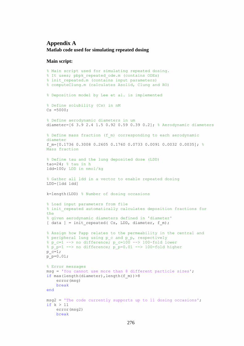
276

Appendix A Matlab code used for simulating repeated dosing

Main script:

% Main script used for simulating repeated dosing. % It uses; pbpk_repeated_ode.m (contains ODEs)

% init_repeated.m (contains input parameters) % computeClung.m (calculates Asolid, Clung and RO)

% Deposition model by Lee et al. is implemented

% Define solubility (Cs) in nM Cs =5000;

% Define aerodynamic diameters in um diameter=[6 3.9 2.4 1.5 0.92 0.59 0.39 0.2]; % Aerodynamic diameters

% Define mass fraction (f_m) corresponding to each aerodynamic

diameter f_m=[0.1736 0.3008 0.2605 0.1760 0.0733 0.0091 0.0032 0.0035]; %

Mass fraction

% Define tau and the lung deposited dose (LDD) tao=24; % tau in h ldd=100; LDD in nmol/kg

% Gather all ldd in a vector to enable repeated dosing LDD=[ldd ldd]

k=length(LDD) % Number of dosing occasions

% Load input parameters from file % init_repeated automatically calculates deposition fractions for

the % given aerodynamic diameters defined in 'diameter' [ data ] = init_repeated( Cs, LDD, diameter, f_m);

% Assign how Papp relates to the permeability in the central and

% peripheral lung using p_c and p_p, respectively % p_c=1 --> no difference; p_c=100 --> 100-fold lower % p_p=1 --> no difference; p_p=0.01 --> 100-fold higher p_c=1; p_p=0.01;

% Error messages msg = 'You cannot use more than 8 different particle sizes'; if max(length(diameter),length(f_m))>8 error(msg) break end

msg2 = 'The code currently supports up to 11 dosing occasions'; if k > 11 error(msg2) break

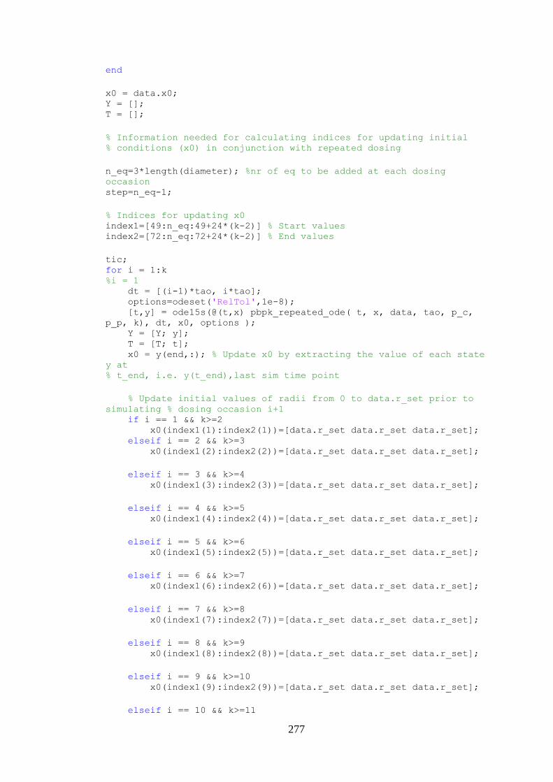
277

end

x0 = data.x0; Y = []; T = [];

% Information needed for calculating indices for updating initial % conditions (x0) in conjunction with repeated dosing

n_eq=3*length(diameter); %nr of eq to be added at each dosing

occasion step=n_eq-1;

% Indices for updating x0 index1=[49:n_eq:49+24*(k-2)] % Start values index2=[72:n_eq:72+24*(k-2)] % End values

tic; for i = 1:k %i = 1 dt = [(i-1)*tao, i*tao]; options=odeset('RelTol',1e-8); [t,y] = ode15s(@(t,x) pbpk_repeated_ode( t, x, data, tao, p_c,

p_p, k), dt, x0, options ); Y = [Y; y]; T = [T; t]; x0 = y(end,:); % Update x0 by extracting the value of each state

y at

% t_end, i.e. y(t_end),last sim time point

% Update initial values of radii from 0 to data.r_set prior to

simulating % dosing occasion i+1 if i == 1 && k>=2 x0(index1(1):index2(1))=[data.r_set data.r_set data.r_set]; elseif i == 2 && k>=3 x0(index1(2):index2(2))=[data.r_set data.r_set data.r_set];

elseif i == 3 && k>=4 x0(index1(3):index2(3))=[data.r_set data.r_set data.r_set];







elseif i == 10 && k>=11

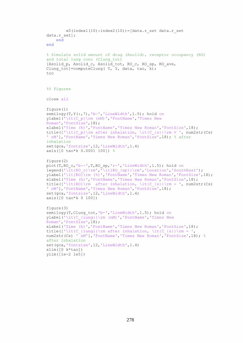
278

x0(index1(10):index2(10))=[data.r_set data.r_set

data.r_set]; end end

% Simulate solid amount of drug (Asolid), receptor occupancy (RO)

and total lung conc (Clung_tot) [Asolid_p, Asolid_c, Asolid_tot, RO_c, RO_sp, RO_ave,

Clung_tot]=computeClung( T, Y, data, tao, k); toc

%% Figures

close all

figure(1) semilogy(T,Y(:,7),'b-','LineWidth',1.5); hold on ylabel('\it{C_p}\rm (nM)','FontName','Times New

Roman','FontSize',18); xlabel('Time (h)','FontName','Times New Roman','FontSize',18); title(['\it{C_p}\rm after inhalation, \it{C_{s}}\rm = ', num2str(Cs)

' nM'],'FontName','Times New Roman','FontSize',18); % after

inhalation set(gca,'fontsize',12,'LineWidth',1.4) axis([0 tao*k 0.0001 100]) %

figure(2) plot(T,RO_c,'b--',T,RO_sp,'r-','LineWidth',1.5); hold on legend('\it{RO_c}\rm','\it{RO_{sp}}\rm','Location','SouthEast'); ylabel('\it{RO}\rm (%)','FontName','Times New Roman','FontSize',18); xlabel('Time (h)','FontName','Times New Roman','FontSize',18); title(['\it{RO}\rm after inhalation, \it{C_{s}}\rm = ', num2str(Cs)

' nM'],'FontName','Times New Roman','FontSize',18); set(gca,'fontsize',12,'LineWidth',1.4) axis([0 tao*k 0 100])

figure(3) semilogy(T,Clung_tot,'b-','LineWidth',1.5); hold on ylabel('\it{C_{lung}}\rm (nM)','FontName','Times New

Roman','FontSize',18); xlabel('Time (h)','FontName','Times New Roman','FontSize',18); title(['\it{C_{lung}}\rm after inhalation, \it{C_{s}}\rm = ',

num2str(Cs) ' nM'],'FontName','Times New Roman','FontSize',18); %

after inhalation set(gca,'fontsize',12,'LineWidth',1.4) xlim([0 k*tao]) ylim([1e-2 1e5])

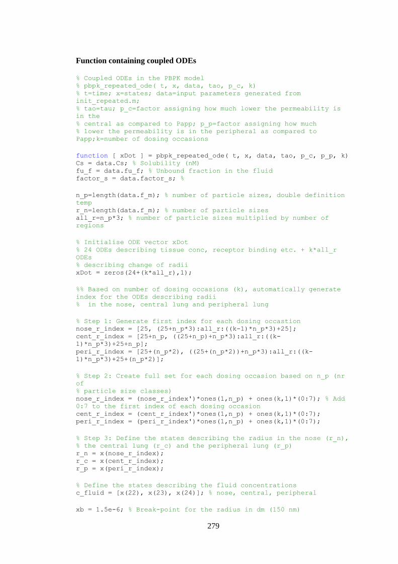
279

Function containing coupled ODEs

% Coupled ODEs in the PBPK model % pbpk_repeated_ode( t, x, data, tao, p_c, k) % t=time; x=states; data=input parameters generated from

init_repeated.m; % tao=tau; p_c=factor assigning how much lower the permeability is

in the % central as compared to Papp; p_p=factor assigning how much % lower the permeability is in the peripheral as compared to

Papp;k=number of dosing occasions

function [ xDot ] = pbpk_repeated_ode( t, x, data, tao, p_c, p_p, k) Cs = data.Cs; % Solubility (nM) fu_f = data.fu_f; % Unbound fraction in the fluid factor_s = data.factor_s; %

n_p=length(data.f_m); % number of particle sizes, double definition

temp r_n=length(data.f_m); % number of particle sizes all_r=n_p*3; % number of particle sizes multiplied by number of

regions

% Initialise ODE vector xDot % 24 ODEs describing tissue conc, receptor binding etc. + k*all_r

ODEs % describing change of radii xDot = zeros(24+(k*all_r),1);

%% Based on number of dosing occasions (k), automatically generate

index for the ODEs describing radii % in the nose, central lung and peripheral lung

% Step 1: Generate first index for each dosing occastion nose_r_index = [25, (25+n_p*3):all_r:((k-1)*n_p*3)+25]; cent_r_index = [25+n_p, ((25+n_p)+n_p*3):all_r:((k-

1)*n_p*3)+25+n_p]; peri_r_index = [25+(n_p*2), ((25+(n_p*2))+n_p*3):all_r:((k-

1)*n_p*3)+25+(n_p*2)];

% Step 2: Create full set for each dosing occasion based on n_p (nr

of % particle size classes) nose_r_index = (nose_r_index')*ones(1,n_p) + ones(k,1)*(0:7); % Add

0:7 to the first index of each dosing occasion cent_r_index = (cent_r_index')*ones(1,n_p) + ones(k,1)*(0:7); peri_r_index = (peri_r_index')*ones(1,n_p) + ones(k,1)*(0:7);

% Step 3: Define the states describing the radius in the nose (r_n), % the central lung (r_c) and the peripheral lung (r_p) r_n = x(nose_r_index); r_c = x(cent_r_index); r_p = x(peri_r_index);

% Define the states describing the fluid concentrations c_fluid = [x(22), x(23), x(24)]; % nose, central, peripheral

xb = 1.5e-6; % Break-point for the radius in dm (150 nm)

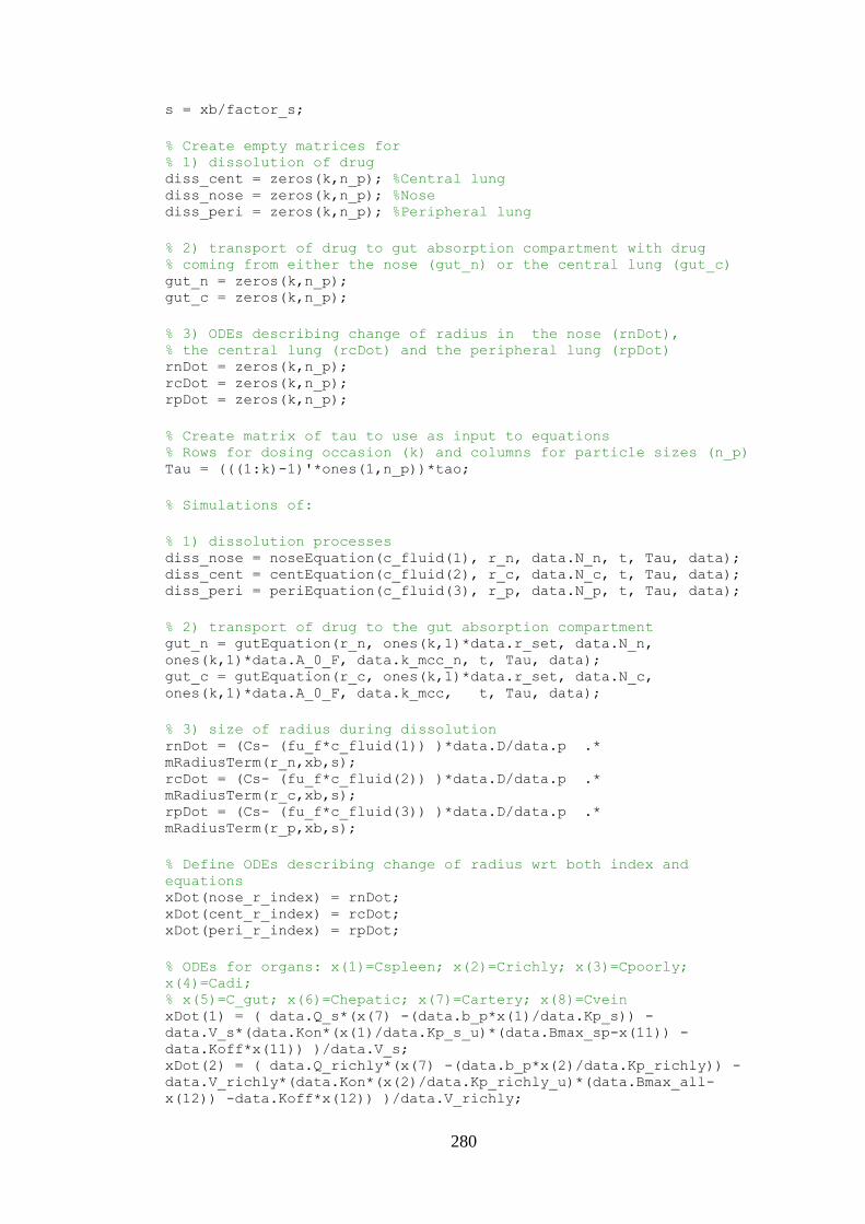
280

s = xb/factor_s;

% Create empty matrices for % 1) dissolution of drug diss_cent = zeros(k,n_p); %Central lung diss_nose = zeros(k,n_p); %Nose diss_peri = zeros(k,n_p); %Peripheral lung

% 2) transport of drug to gut absorption compartment with drug % coming from either the nose (gut_n) or the central lung (gut_c) gut_n = zeros(k,n_p); gut_c = zeros(k,n_p);

% 3) ODEs describing change of radius in the nose (rnDot), % the central lung (rcDot) and the peripheral lung (rpDot) rnDot = zeros(k,n_p); rcDot = zeros(k,n_p); rpDot = zeros(k,n_p);

% Create matrix of tau to use as input to equations % Rows for dosing occasion (k) and columns for particle sizes (n_p) Tau = (((1:k)-1)'*ones(1,n_p))*tao;

% Simulations of:

% 1) dissolution processes diss_nose = noseEquation(c_fluid(1), r_n, data.N_n, t, Tau, data); diss_cent = centEquation(c_fluid(2), r_c, data.N_c, t, Tau, data); diss_peri = periEquation(c_fluid(3), r_p, data.N_p, t, Tau, data);

% 2) transport of drug to the gut absorption compartment gut_n = gutEquation(r_n, ones(k,1)*data.r_set, data.N_n,

ones(k,1)*data.A_0_F, data.k_mcc_n, t, Tau, data); gut_c = gutEquation(r_c, ones(k,1)*data.r_set, data.N_c,

ones(k,1)*data.A_0_F, data.k_mcc, t, Tau, data);

% 3) size of radius during dissolution rnDot = (Cs- (fu_f*c_fluid(1)) )*data.D/data.p .*

mRadiusTerm(r_n,xb,s); rcDot = (Cs- (fu_f*c_fluid(2)) )*data.D/data.p .*

mRadiusTerm(r_c,xb,s); rpDot = (Cs- (fu_f*c_fluid(3)) )*data.D/data.p .*

mRadiusTerm(r_p,xb,s);

% Define ODEs describing change of radius wrt both index and

equations xDot(nose_r_index) = rnDot; xDot(cent_r_index) = rcDot; xDot(peri_r_index) = rpDot;

% ODEs for organs: x(1)=Cspleen; x(2)=Crichly; x(3)=Cpoorly;

x(4)=Cadi; % x(5)=C_gut; x(6)=Chepatic; x(7)=Cartery; x(8)=Cvein xDot(1) = ( data.Q_s*(x(7) -(data.b_p*x(1)/data.Kp_s)) -

data.V_s*(data.Kon*(x(1)/data.Kp_s_u)*(data.Bmax_sp-x(11)) -

data.Koff*x(11)) )/data.V_s; xDot(2) = ( data.Q_richly*(x(7) -(data.b_p*x(2)/data.Kp_richly)) -

data.V_richly*(data.Kon*(x(2)/data.Kp_richly_u)*(data.Bmax_all-

x(12)) -data.Koff*x(12)) )/data.V_richly;

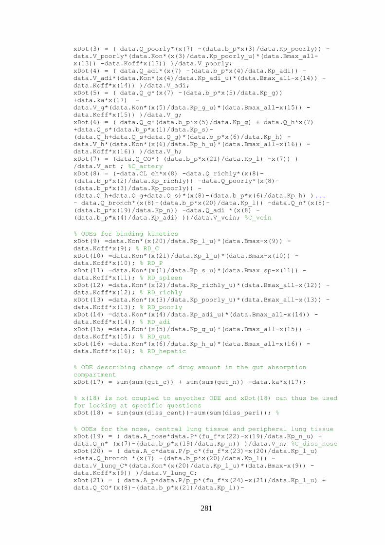
281

xDot(3) = ( data.Q_poorly*(x(7) -(data.b_p*x(3)/data.Kp_poorly)) -

data.V_poorly*(data.Kon*(x(3)/data.Kp_poorly_u)*(data.Bmax_all-

x(13)) -data.Koff*x(13)) )/data.V_poorly; xDot(4) = ( data.Q_adi*(x(7) -(data.b_p*x(4)/data.Kp_adi)) -

data.V_adi*(data.Kon*(x(4)/data.Kp_adi_u)*(data.Bmax_all-x(14)) -

data.Koff*x(14)) )/data.V_adi; xDot(5) = ( data.Q_g*(x(7) -(data.b_p*x(5)/data.Kp_g))

+data.ka*x(17) -

data.V_g*(data.Kon*(x(5)/data.Kp_g_u)*(data.Bmax_all-x(15)) -

data.Koff*x(15)) )/data.V_g; xDot(6) = ( data.Q_g*(data.b_p*x(5)/data.Kp_g) + data.Q_h*x(7)

+data.Q_s*(data.b_p*x(1)/data.Kp_s)-

(data.Q_h+data.Q_s+data.Q_g)*(data.b_p*x(6)/data.Kp_h) -

data.V_h*(data.Kon*(x(6)/data.Kp_h_u)*(data.Bmax_all-x(16)) -

data.Koff*x(16)) )/data.V_h; xDot(7) = (data.Q_CO*( (data.b_p*x(21)/data.Kp_l) -x(7)) )

/data.V_art ; %C_artery xDot(8) = (-data.CL_eh*x(8) -data.Q_richly*(x(8)-

(data.b_p*x(2)/data.Kp_richly)) -data.Q_poorly*(x(8)-

(data.b_p*x(3)/data.Kp_poorly)) -

(data.Q_h+data.Q_g+data.Q_s)*(x(8)-(data.b_p*x(6)/data.Kp_h) )... - data.Q_bronch*(x(8)-(data.b_p*x(20)/data.Kp_l)) -data.Q_n*(x(8)-

(data.b_p*x(19)/data.Kp_n)) -data.Q_adi *(x(8) -

(data.b_p*x(4)/data.Kp_adi) ))/data.V_vein; %C_vein

% ODEs for binding kinetics xDot(9) =data.Kon*(x(20)/data.Kp_l_u)*(data.Bmax-x(9)) -

data.Koff*x(9); % RD_C xDot(10) =data.Kon*(x(21)/data.Kp_l_u)*(data.Bmax-x(10)) -

data.Koff*x(10); % RD_P xDot(11) =data.Kon*(x(1)/data.Kp_s_u)*(data.Bmax_sp-x(11)) -

data.Koff*x(11); % RD_spleen xDot(12) =data.Kon*(x(2)/data.Kp_richly_u)*(data.Bmax_all-x(12)) -

data.Koff*x(12); % RD_richly xDot(13) =data.Kon*(x(3)/data.Kp_poorly_u)*(data.Bmax_all-x(13)) -

data.Koff*x(13); % RD_poorly xDot(14) =data.Kon*(x(4)/data.Kp_adi_u)*(data.Bmax_all-x(14)) -

data.Koff*x(14); % RD_adi xDot(15) =data.Kon*(x(5)/data.Kp_g_u)*(data.Bmax_all-x(15)) -

data.Koff*x(15); % RD_gut xDot(16) =data.Kon*(x(6)/data.Kp_h_u)*(data.Bmax_all-x(16)) -

data.Koff*x(16); % RD_hepatic

% ODE describing change of drug amount in the gut absorption

compartment xDot(17) = sum(sum(gut_c)) + sum(sum(gut_n)) -data.ka*x(17);

% x(18) is not coupled to anyother ODE and xDot(18) can thus be used

for looking at specific questions xDot(18) = sum(sum(diss_cent))+sum(sum(diss_peri)); %

% ODEs for the nose, central lung tissue and peripheral lung tissue xDot(19) = ( data.A_nose*data.P*(fu_f*x(22)-x(19)/data.Kp_n_u) +

data.Q_n* (x(7)-(data.b_p*x(19)/data.Kp_n)) )/data.V_n; %C_diss_nose xDot(20) = ( data.A_c*data.P/p_c*(fu_f*x(23)-x(20)/data.Kp_l_u)

+data.Q_bronch *(x(7) -(data.b_p*x(20)/data.Kp_l)) -

data.V_lung_C*(data.Kon*(x(20)/data.Kp_l_u)*(data.Bmax-x(9)) -

data.Koff*x(9)) )/data.V_lung_C; xDot(21) = ( data.A_p*data.P/p_p*(fu_f*x(24)-x(21)/data.Kp_l_u) +

data.Q_CO*(x(8)-(data.b_p*x(21)/data.Kp_l))-

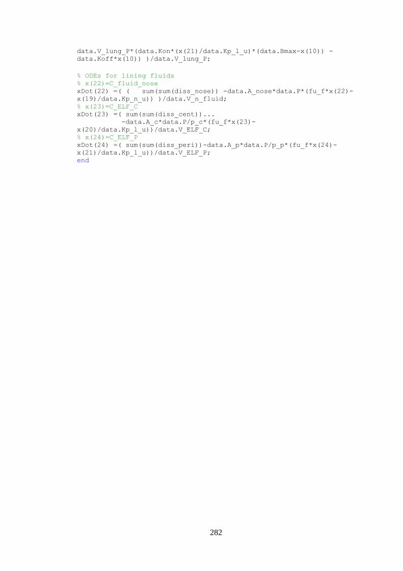
282

data.V_lung_P*(data.Kon*(x(21)/data.Kp_l_u)*(data.Bmax-x(10)) -

data.Koff*x(10)) )/data.V_lung_P;

% ODEs for lining fluids % x(22)=C_fluid_nose xDot(22) =( ( sum(sum(diss_nose)) -data.A_nose*data.P*(fu_f*x(22)-

x(19)/data.Kp_n_u)) )/data.V_n_fluid; % x(23)=C_ELF_C xDot(23) =( sum(sum(diss_cent))... -data.A_c*data.P/p_c*(fu_f*x(23)-

x(20)/data.Kp_l_u))/data.V_ELF_C;

% x(24)=C_ELF_P xDot(24) =( sum(sum(diss_peri))-data.A_p*data.P/p_p*(fu_f*x(24)-

x(21)/data.Kp_l_u))/data.V_ELF_P; end

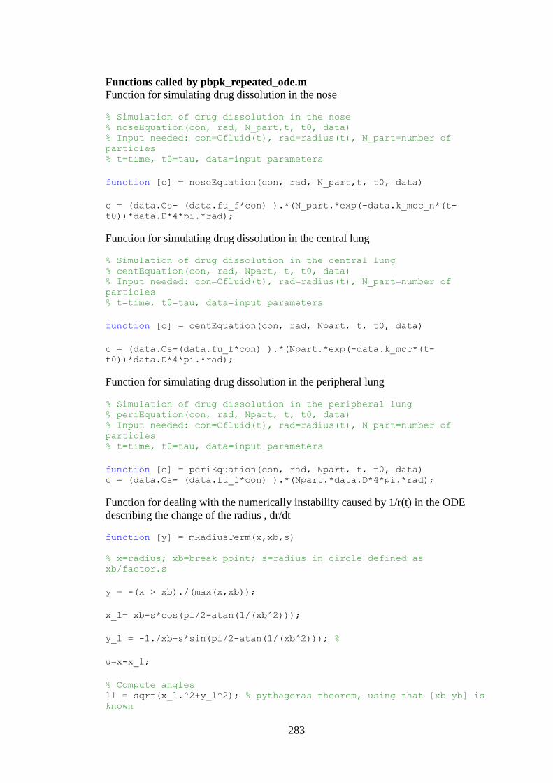
283

Functions called by pbpk_repeated_ode.m

Function for simulating drug dissolution in the nose

% Simulation of drug dissolution in the nose % noseEquation(con, rad, N_part,t, t0, data) % Input needed: con=Cfluid(t), rad=radius(t), N_part=number of

particles % t=time, t0=tau, data=input parameters

function [c] = noseEquation(con, rad, N_part,t, t0, data)

c = (data.Cs- (data.fu_f*con) ).*(N_part.*exp(-data.k_mcc_n*(t-

t0))*data.D*4*pi.*rad);

Function for simulating drug dissolution in the central lung

% Simulation of drug dissolution in the central lung % centEquation(con, rad, Npart, t, t0, data) % Input needed: con=Cfluid(t), rad=radius(t), N_part=number of


function [c] = centEquation(con, rad, Npart, t, t0, data)

c = (data.Cs-(data.fu_f*con) ).*(Npart.*exp(-data.k_mcc*(t-

t0))*data.D*4*pi.*rad);

Function for simulating drug dissolution in the peripheral lung

% Simulation of drug dissolution in the peripheral lung % periEquation(con, rad, Npart, t, t0, data) % Input needed: con=Cfluid(t), rad=radius(t), N_part=number of


function [c] = periEquation(con, rad, Npart, t, t0, data) c = (data.Cs- (data.fu_f*con) ).*(Npart.*data.D*4*pi.*rad);

Function for dealing with the numerically instability caused by 1/r(t) in the ODE

describing the change of the radius , dr/dt

function [y] = mRadiusTerm(x,xb,s)

% x=radius; xb=break point; s=radius in circle defined as

xb/factor.s

y = -(x > xb)./(max(x,xb));

x_l= xb-s*cos(pi/2-atan(1/(xb^2)));

y_l = -1./xb+s*sin(pi/2-atan(1/(xb^2))); %

u=x-x_l;

% Compute angles l1 = sqrt(x_l.^2+y_l^2); % pythagoras theorem, using that [xb yb] is

known

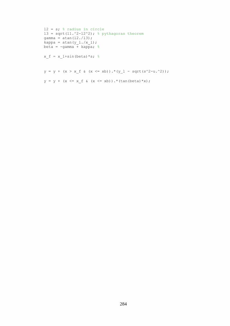
284

l2 = s; % radius in circle l3 = sqrt(l1.^2-l2^2); % pythagoras theorem gamma = atan(l2./l3); kappa = atan(y_l./x_l); beta = -gamma + kappa; %

x_f = x_l+sin(beta)*s; %

y = y + (x > x_f & (x <= xb)).*(y_l - sqrt(s^2-u.^2));

y = y + (x <= x_f & (x <= xb)).*(tan(beta)*x);

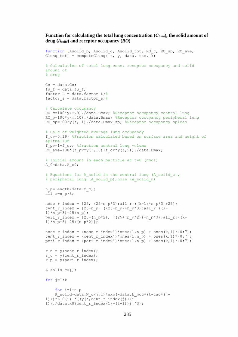
285

Function for calculating the total lung concentration (Clung), the solid amount of

drug (Asolid) and receptor occupancy (RO) function [Asolid_p, Asolid_c, Asolid_tot, RO_c, RO_sp, RO_ave,

Clung_tot] = computeClung( t, y, data, tao, k)

% Calculation of total lung conc, receptor occupancy and solid

amount of % drug

Cs = data.Cs; fu_f = data.fu_f; factor_L = data.factor_L;% factor_s = data.factor_s;%

% Calculate occupancy RO_c=100*y(:,9)./data.Bmax; %Receptor occupancy central lung RO_p=100*y(:,10)./data.Bmax; %Receptor occupancy peripheral lung RO_sp=100*y(:,11)./data.Bmax_sp; %Receptor occupancy spleen

% Calc of weighted average lung occupancy f_cv=0.19; %Fraction calculated based on surface area and height of

epithelium f_pv=1-f_cv; %fraction central lung volume RO_ave=100*(f_pv*y(:,10)+f_cv*y(:,9))./data.Bmax;

% Initial amount in each particle at t=0 (nmol) A_0=data.A_c0;

% Equations for A_solid in the central lung (A_solid_c), % peripheral lung (A_solid_p),nose (A_solid_n)

n_p=length(data.f_m); all_r=n_p*3;

nose_r_index = [25, (25+n_p*3):all_r:((k-1)*n_p*3)+25]; cent_r_index = [25+n_p, ((25+n_p)+n_p*3):all_r:((k-

1)*n_p*3)+25+n_p]; peri_r_index = [25+(n_p*2), ((25+(n_p*2))+n_p*3):all_r:((k-

1)*n_p*3)+25+(n_p*2)];

nose_r_index = (nose_r_index')*ones(1,n_p) + ones(k,1)*(0:7); cent_r_index = (cent_r_index')*ones(1,n_p) + ones(k,1)*(0:7); peri_r_index = (peri_r_index')*ones(1,n_p) + ones(k,1)*(0:7);

r_n = y(nose_r_index); r_c = y(cent_r_index); r_p = y(peri_r_index);

A_solid_c=[];

for j=1:k

for i=1:n_p A_solid=data.N_c(j,i)*exp(-data.k_mcc*(t-tao*(j-

1)))*A_0(i).*((y(:,cent_r_index(j)+(i-

1))./data.x0(cent_r_index(1)+(i-1))).^3);

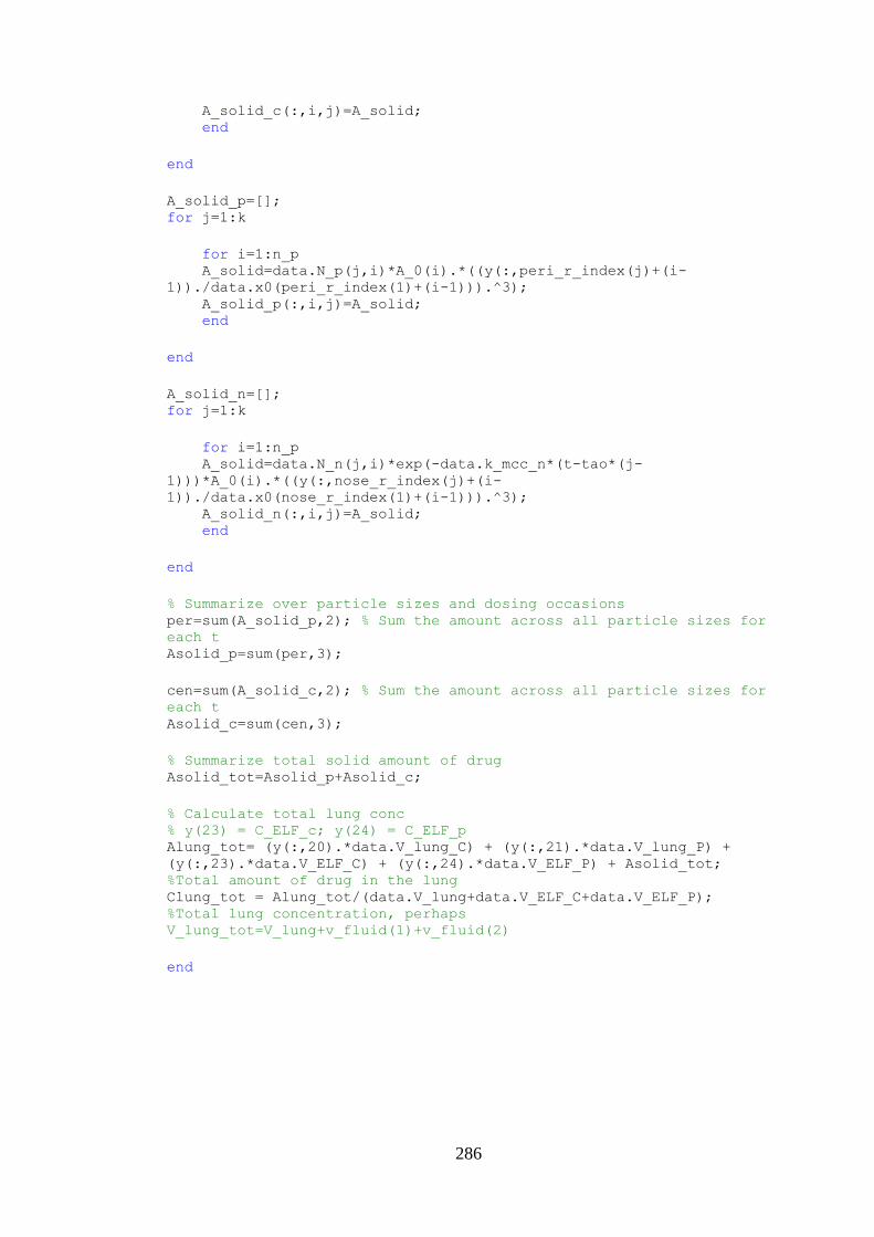
286

A_solid_c(:,i,j)=A_solid; end

end

A_solid_p=[]; for j=1:k

for i=1:n_p A_solid=data.N_p(j,i)*A_0(i).*((y(:,peri_r_index(j)+(i-

1))./data.x0(peri_r_index(1)+(i-1))).^3); A_solid_p(:,i,j)=A_solid; end

end

A_solid_n=[]; for j=1:k

for i=1:n_p A_solid=data.N_n(j,i)*exp(-data.k_mcc_n*(t-tao*(j-

1)))*A_0(i).*((y(:,nose_r_index(j)+(i-

1))./data.x0(nose_r_index(1)+(i-1))).^3); A_solid_n(:,i,j)=A_solid; end

end

% Summarize over particle sizes and dosing occasions per=sum(A_solid_p,2); % Sum the amount across all particle sizes for

each t Asolid_p=sum(per,3);

cen=sum(A_solid_c,2); % Sum the amount across all particle sizes for

each t Asolid_c=sum(cen,3);

% Summarize total solid amount of drug Asolid_tot=Asolid_p+Asolid_c;

% Calculate total lung conc % y(23) = C_ELF_c; y(24) = C_ELF_p Alung_tot= (y(:,20).*data.V_lung_C) + (y(:,21).*data.V_lung_P) +

(y(:,23).*data.V_ELF_C) + (y(:,24).*data.V_ELF_P) + Asolid_tot;

%Total amount of drug in the lung Clung_tot = Alung_tot/(data.V_lung+data.V_ELF_C+data.V_ELF_P);

%Total lung concentration, perhaps

V_lung_tot=V_lung+v_fluid(1)+v_fluid(2)

end

287

Function gathering all drug-, formulation- and system-specific parameters function [ data ] = init_repeated( Cs, LDD, diameter, f_m,

parameters ) % Initial parameters are stored in data % [ data ] = init_repeated ( Cs, LDD, diameter, f_m, parameters ) % Input needed: solubility (Cs); LDD=lung deposited dose; % diameter=aerodynamic diameters; f_m=mass fractions of each

particle size % class; parameters is not default input, only to be used in case of % MC-simulations wrt the binding kinetics parameters

k=length(LDD); % Number of doses data.factor_s = 4;%

data.Cs = Cs; % Solubility (nM) data.f_m=f_m; % Mass fractions of each particle size

% Intravenous (iv) and intraarterial (ia) dosing data.dose_iv=0; % IV-bolus dose data.dose_ia=0; % ia dose

% System-specific parameters data.k_mcc_n=0.2079; data.k_mcc=0.0472;

% Input parameters data.my=13.82816; %mol/(dm*h) data.MW=500.6; % g/mol data.p_g=715; %Density (g/dm3) data.D=13.26*10^(-5)/(data.my^1.14*(data.MW/data.p_g)^0.589);

%Diffussion coefficient data.p=1.430*10^9 ; %Density (nmol/dm3)

data.fu_f=1; % fu_fluid data.Papp=46.9; %Papp (10^(-6) cm/s) data.P_app=data.Papp*10^(-6); data.P=3600/10*data.P_app; %Papp unit conversion data.fu=0.016; % Unbound fraction in plasma data.b_p=0.95; % Blood-plasma ratio data.ka=5; % Absorption rate constant data.F=0; % Oral bioavailability

% Binding kinetics FP data.Kd_FP=0.0150934; %(nM) Value from modeling of FP-IV data.Koff=0.510892; %(h-1) Value from modeling of FP-IV data.Kon=data.Koff/data.Kd_FP;

if nargin > 4 data.Koff = parameters(1); data.Kd_FP = parameters(2); end

% Receptor density data.Bmax=21; %Receptor density in the lung (nmol/L) data.Bmax_sp=31.5; %Receptor density in the spleen (nmol/L) data.Bmax_all=23; %Mean value brain Bmax

288

%Kp-values FP data.Vu_lung=213.4; data.kp_factor=1.93; data.Kp_h=data.kp_factor*5.293087; data.Kp_s=data.kp_factor*2.686034; data.Kp_richly=data.kp_factor*4.8; data.Kp_poorly=data.kp_factor*3.990; data.Kp_l=data.Vu_lung*data.fu; data.Kp_g=data.kp_factor*10.50719; data.Kp_adi=data.kp_factor*65.32998; data.Kp_n=data.Vu_lung*data.fu;

%Kp,u-values data.Kp_h_u=data.Kp_h/data.fu; data.Kp_s_u=data.Kp_s/data.fu; data.Kp_richly_u=data.Kp_richly/data.fu; data.Kp_poorly_u=data.Kp_poorly/data.fu; data.Kp_l_u=data.Kp_l/data.fu; data.Kp_g_u=data.Kp_g/data.fu; data.Kp_adi_u=data.Kp_adi/data.fu; data.Kp_n_u=data.Kp_n/data.fu;

% Blood flows % 1) Fraction of cardiac-output, fi. From Gearhart et al. 1990

unless stated otherwise data.f_n=0.0015; % A hybrid CFD-PBPK model data.f_h=0.024; % Brown et al. data.f_s=0.0715 ; % Kaufman et al 1996 data.f_richly=0.5096; % Sum of Qrichly+Qkidney+Qbrain Gearthart et

al. data.f_g=0.14; % Delp et al data.f_bronch=0.021; %Brown et al. data.f_adi=0.009302; %Arundel:0.4 mL/min of 43 mL/min as QCO. data.f_poorly=1-

(data.f_h+data.f_s+data.f_richly+data.f_bronch+data.f_g+data.f_adi+d

ata.f_n); data.f_tot=data.f_h+data.f_s+data.f_richly+data.f_poorly+data.f_bron

ch+data.f_g+data.f_adi+data.f_n;

% 2) Blood-flows, Qi data.Q_CO=20.77; % Gearthart et al 1990 (4.57 L/h / 220 g rat) data.Q_n=data.Q_CO*data.f_n; data.Q_h=data.Q_CO*data.f_h; data.Q_s=data.Q_CO*data.f_s; data.Q_g=data.Q_CO*data.f_g; data.Q_richly=data.Q_CO*data.f_richly; data.Q_poorly=data.Q_CO*data.f_poorly; data.Q_bronch=data.Q_CO*data.f_bronch; data.Q_adi=data.Q_CO*data.f_adi;

% Surface areas data.A_nose=4*10.4*10^(-2) ; %Surface area nasal cavity, 10.4 cm2,

250 g rat. data.A_c=1.08/0.330 ; % dm2, 108 cm2, tracheobronchial airways, 330

g rat data.A_p=38.70/0.14 ; % dm2, 3870 cm2, alveolar region, 140 g rat

% Tissue volumes, Vi data.v_fluid=lining_fluid; %v_fluid(1)=V_ELF_C;

v_fluid(2)=V_ELF_P;v_fluid(3)=V_lining_nose;

289

data.V_ELF_C=data.v_fluid(1);%A_c*5*10^(-5); %Assuming ELF thickness

5 um and continuous distribution data.V_ELF_P=data.v_fluid(2);%A_p*d_peri*10^(-5); %Assuming ELF

thickness 0.07 um and continuous distribution data.V_n_fluid=data.A_nose*5*10^(-5);

data.V_h=0.04; %Gearthart et al data.V_s=0.002; %Brown et al. data.V_art=0.02; %Gearhart et al data.V_vein=0.04; %Gearhart et al data.V_richly=0.0388; %Vrichly=Vkidney+Vrichly+Vbrain, Gearhart et

al data.V_g=0.0259 ; %From Delp et al data.V_adi=0.040; %Arundel 10 mL/250 g rat data.V_lung=0.004127-(data.V_ELF_C+data.V_ELF_P); %4.127 g/kg from

100 animals, mean BW: 0.285 kg, removing VELF data.V_n=data.A_nose*61*10^(-5); % Volume nasal mucosa, 0.2538 mL,

comparison ET-volume taken from GastroPlus 0.046 mL TEMP! data.V_poorly=1-

(data.V_h+data.V_s+data.V_art+data.V_vein+data.V_richly+data.V_lung+

data.V_g+data.V_adi+data.V_n+data.V_n_fluid+data.V_ELF_C+data.V_ELF_

P);

% Calculation of central and peripheral lung tissue volumes data.lung_vol=lung_volume(data.V_lung); %lung_vol(1)=V_lung_C;

lung_vol(2)=V_lung_P data.V_lung_C=data.lung_vol(1); %Volume of central lung tissue data.V_lung_P=data.lung_vol(2); %Volume of peripheral lung tissue

% Calculation of CL_blood based on CL_plasma and B:P-ratio % Extrahepatic CL to add up to obs CL data.CL_pl=10.95; %Plasma CL data.CL_bl=data.CL_pl/data.b_p; %CL blood data.CL_eh=data.CL_bl; data.CL_h=0;

%Initial geometric radius expressed in dm x=diameter;

p_g=data.p_g/1000; % Normalise to g/cm3 n=length(x);

% Calculation of geometric radius (note: x is diameter) r=[]; for i=1:n r(i)=x(i)/2*10^(-5)/sqrt(p_g); end

% Define vector data.x0 of initial values

% Step 1: Initiate vector of 24 zeros for the 24 first states

(tissue conc, RD etc.) set_1=zeros(1,24); % 24 zeros set_initial=set_1;

% Step 2: Extract states where x(0) can be different from 0 set_initial(7)=data.dose_ia/data.V_art; % C_arterial(0) set_initial(8)=data.dose_iv/data.V_vein; % C_vein(0) set_initial(18)=0; % Agut(0)

290

% Step 3: Define initial values of geometric radii data.r_set=r;

% Step 4: Define data.x0, length of data.x0 defined by number of

dosing % occasions, k data.x0=zeros(1,(24+k*24)); data.x0(1,1:(24+n*3))=[set_initial data.r_set data.r_set

data.r_set];

% Calculate number of particles initially deposited in the nose

(data.N_n), % central (data.N_c) and peripheral lung (data.N_p)

data.N_n=[]; data.N_c=[]; data.N_p=[];

for i=1:k data.N_n(i,:)=number_n_test(LDD(i), data.f_m, diameter, data.p_g,

data.p); data.N_c(i,:)=number_c_test(LDD(i), data.f_m, diameter, data.p_g,

data.p); data.N_p(i,:)=number_p_test(LDD(i), data.f_m, diameter, data.p_g,

data.p); end

% Possibility to check data.N_x data.N_n; data.N_c; data.N_p;

[row col]=size(data.N_n);

% Initial amount in each particle at t=0 (nmol) data.A_c0=amount_particle(diameter, data.p_g, data.p);

% Include F here to account for bioavailability data.A_0_F=data.A_c0.*data.F;

% k=number of dosing occasions;n=number of particle size classes

data.m_cen=zeros(k,n); % Changed from 8 to n for j=1:k for i=1:n data.m_=data.A_c0(i)*data.N_n(j,i); data.m_cen(j,i)=data.m_; end data.dep_n(j)=sum(data.m_cen(j,:)); end

data.m_c_lung=zeros(k,n);

for j=1:k for i=1:n data.m_=data.A_c0(i)*data.N_c(j,i); data.m_c_lung(j,i)=data.m_; end

291

data.dose_c(j)=sum(data.m_c_lung(j,:)); end

data.m_p_lung=zeros(k,n);

for j=1:k for i=1:n data.m_=data.A_c0(i)*data.N_p(j,i); data.m_p_lung(j,i)=data.m_; end data.dose_p(j)=sum(data.m_p_lung(j,:)); end

for j=1:k data.dd_region(j,:)=[data.dep_n(j) data.dose_c(j) data.dose_p(j)]; end% deposited dose in each region

end

function [lining_fluids]=lining_fluid() % Returns lining fluid volumes [V_ELF_C,V_ELF_P,V_n_fluid] format long % Surface areas A_nose=4*10.4*10^(-2) ; %Surface area nasal cavity, 10.4 cm2, 250 g

rat. A_c=1.08/0.330 ; % dm2, 108 cm2, tracheobronchial airways, 330 g rat A_p=38.70/0.14 ; % dm2, 3870 cm2, alveolar region, 140 g rat

% Tissue volumes, Vi d_peri=0.07; %Byron and Patton V_ELF_C=A_c*5*10^(-5); %Assuming ELF thickness 5 um and continuous

distribution V_ELF_P=A_p*d_peri*10^(-5); %Assuming ELF thickness 0.07 um and

continuous distribution V_n_fluid=A_nose*5*10^(-5); lining_fluids=[V_ELF_C,V_ELF_P,V_n_fluid]; end

function [V_lung_k]=lung_volume(V_lung) % Returns regional tissues volumes based on total tissue volume % (V_lung), [V_lung_C V_lung_P] % V_lung=0.004127; %4.127 g/kg from 100 animals, mean BW: 0.285 kg format long f_cv=0.19; %Fraction calculated based on surface area and height of

epithelium f_pv=1-f_cv; %fraction central lung volume

% Calculation of central and peripheral lung tissue volumes V_lung_C=f_cv*V_lung; %Volume of central lung tissue V_lung_P=f_pv*V_lung; %Volume of peripheral lung tissue

V_lung_k=[V_lung_C V_lung_P]; end

292

Functions called by init_repeated.m

Function used for calculating the amount in each particle function [A_zero]=amount_particle(diameter, p_g, p_mol) % Calculation of amount in each particle at t=0 % [A_zero]=amount_particle(diameter, p_g, p_mol) % diameter=aerodynamic diameter (um); p_g=density in g/dm3

x=diameter;

p_g=p_g/1000; % Normalise to g/cm3 n=length(x);

% Calculation of geometric radius (note: x is diameter) r=[]; for i=1:n r(i)=x(i)/2*10^(-5)/sqrt(p_g); end

% Calculate volumes V=zeros(1,8); for i=1:8 V_=(4*pi*r(i)^3)/3; V(i)=V_; end

A_zero=zeros(1,8); for i=1:8 A_=V(i)*p_mol; A_zero(i)=A_; end

Function used for calculating the number of particles in the central lung (same

principle applied for both lung regions and the nose)

function [N_zero_c]=number_c_test(LDD, f_m, x, p_g, p_mol) % Calculation of numbers of particles deposited centrally % [N_zero_c]=number_c_test(LDD, f_m, x, p_g, p_mol) % LDD = lung deposited dose; f_m = mass fraction; x = aerodynamic

diameter % (um); p_g = density in g/dm3; p_mol = density in nmol/dm3

p_g=p_g/1000; % Normalise to g/cm3 n=length(x);

% Calculation of geometric radius (note: x is diameter) r=[]; for i=1:n r(i)=x(i)/2*10^(-5)/sqrt(p_g); end r;

% Extract deposition fraction given aerodynamic diameter x % 1) Define breathing conditions for deposition model V_T=2.6; % Tidal volume (mL) Lee et al. f_br=97.4; % Breathing frequency (min-1)

293

% 2) Run deposition model (for simplicity, the model code for the

deposition is attached as a separate appendix) [et tb a] = get_df_lee(x, V_T, f_br);

% Probability of peripheral deposition f_dep=a; % Probability of central deposition f_dep_c=tb; % Probability of nasal deposition f_dep_n=et;

% Calculate prob of lung deposition in both c and p lung lung_dep=zeros(1,n); for i=1:n lung_dep_=f_m(i)*f_dep(i)+f_m(i)*f_dep_c(i); lung_dep(i)=lung_dep_; end lung_dep_sum=sum(lung_dep);

% Density p=p_g; % g/dm3 p_mol=p_mol; % Density (nmol/dm3)

% Calculate volumes V=zeros(1,n); for i=1:n V_=(4*pi*r(i)^3)/3; V(i)=V_; end

dose_inh=LDD/lung_dep_sum; % Calc of inhaled dose

% Calculate number of particles initially deposited centrally N_zero_c=zeros(1,n); for i=1:n N_=f_m(i)*f_dep_c(i)*dose_inh/(V(i)*p_mol); N_zero_c(i)=N_; end

m_zero=zeros(1,n); for i=1:n m_=N_zero_c(i)*V(i)*p_mol; m_zero(i)=m_; end total_m_cen=sum(m_zero); end

294

Appendix B Matlab implementation of regional drug deposition (Lee et al)

Main function for calculating drug deposition function [df_et df_tb df_al] = get_df_lee(da, V_T, f_br) % Input: areodynamic diameter, da, [um]; tidal volume, V_T [mL] % and breathing frequency, f_br [min-1] % default values V_T=2.6 mL; f_br=97.4 min-1

% Function for calculating deposition in the lung after rodent

inhalation % "Particle deposition in juvenile rat lungs: A model study" by Lee

et al. % Anatomy values for 81-day old rats % To couple to repeated dosing

load('anat_2.mat') % anatomy data from Lee et al.

% The model automatically transforms the anatomy based on V_T and BW ANAT = anat_2;

% Extract anatomical input from the data set i_gen=ANAT(:,1); N_i=ANAT(:,2); L_i=ANAT(:,3); D_i=ANAT(:,4); D_i_eff=ANAT(:,5); V_i=ANAT(:,6); cum_Vi=ANAT(:,7); phi=ANAT(:,8); % Angle 1 theta=ANAT(:,9); % Angle 2

% Conversion from degrees to radians phi=phi.*(pi/180); theta=theta.*(pi/180);

%% Breathing conditions and anatomy

%V_T=2.6; %Tidal volume [cm3] from Lee et al. %f_br=97.4; % Breathing frequency (1/min) from Lee et al. V_min=V_T*f_br; % Minute respiration [cm3/min] Q=V_min*2/60; % Inhalation flow rate according to Schmid et al;

Q=2*Vmin [cm3/s]

BW=381; %BW [g]

% Function for transforming volumes, diameters and length % Possible to exclude transformation of i=1:2 (Schmid et al) [L_i_scaled, D_i_scaled, f_scale, D_i_eff_scaled, imax, cum_Vi_2,

V_i_2]=calcV(D_i,L_i,N_i,V_T,BW,D_i_eff,cum_Vi,V_i);

% Anatomy data for the nose; transformation based on f_scale L_n=1.95*f_scale; % Length, cm. Lee et al H_n=0.016*f_scale; % Height, cm. Lee et al. W_n=5.7*f_scale; % Width, cm. Lee et al.

% Unscaled values

295

L_i_unscaled=L_i; D_i_unscaled=D_i;

% Choose input values L_i=L_i_scaled; D_i=D_i_scaled; D_i_eff=D_i_eff_scaled;

%% Particle input parameters

% Unit particle density po=1000; % 1 g/cm3 = 1000 kg/m3

%% Calculation of airflow (Q_i), velocity (v_i) and mean residence

time (t_i)

[v_i,t_i,Q_i]=airflow(L_i,D_i,N_i,Q);

% Transformation of v_i and Q_i to SI-units v_i=v_i./100; % from cm/s to m/s Q_i=Q_i./1e6; % from cm3/s to m3/s. Note, to nasal impaction, cm3/s

should be used, otherwise m3/s.

% Get deposition parameters [Cd,vg,Dp,ne,pa,Dmol]= get_parameters(da,po); % Dmol = Dp

% Row 2 and 3 in IMP_i equals zero due to theta=0, sin(theta)=0 [stk,mu,re,eps]=Deposition_equation_parameters_lee(da,po,ne,v_i,D_i,

Dp,t_i,pa,vg,phi,D_i_eff,Cd);

% Deposition according to Lee et al. [IMP_i, SED_i,DIF_i]=deposition_probability2(stk,re,theta,eps,D_i,

D_i_eff,L_i,v_i,Dmol);

% Calculate nasal deposition; (IMP_n remains to be implemented

properly) [DIF_n IMP_n SED_n mu_n]=nose(L_n,W_n,H_n,Q_i(1),Dmol, da);

DEP_n=DIF_n + IMP_n + SED_n;

% Add nasal deposition to the pulmonary deposition fractions IMP_i(1,:)=IMP_n; SED_i(1,:)=SED_n; DIF_i(1,:)=DIF_n;

%% Change size of V_i and cum_Vi if imax<26 (maximum nr of

generations)

V_i_2=V_i_2(1:imax); cum_Vi_2=cum_Vi_2(1:imax); IMP_i=IMP_i(1:imax,:); SED_i=SED_i(1:imax,:); DIF_i=DIF_i(1:imax,:);

%% Calculate resulting deposition fractions

[ df, DEP_in, DEP_ex, f_conv ] = dfCalc2( IMP_i, SED_i, DIF_i,

V_i_2, da, imax );

296

size(df);

df_et=sum(df(1:2,:)); df_tb=sum(df(3:18,:)); df_al=sum(df(19:26,:));

end

297

Functions called by get_df_lee.m

Function for scaling the anatomy function [L_i_scaled, D_i_scaled, f_scale, D_i_eff_scaled, imax,

cum_Vi_2, V_i_2]=calcV(D_i,L_i,N_i,V_T,BW,D_i_eff,cum_Vi,V_i) % Calculation of scaled lengths (L_i_scaled), diameters (D_i_scaled) % and volumes (V_i_scaled) based on the scale factor f_scale, which

is % calculated based on BW and tidal volume (V_T) % Note that V_i_scaled(1) needs to be calc separately since it is

not a cylinder % Schmid et al only scales i=3:26 whereas Lee scales i=1:26

% Calculation of scale factor (f_scale) TLC=0.032*BW^1.05; % Total lung capacity [cm3] f_scale=((0.4*TLC+0.5*V_T)/TLC)^(1/3); %Scale factor

% Calculation of scaled volumes, i=1:2 not scaled by Schmid et al % Lee appears to have scaled the nose and the pharynx as well

L_i_scaled=L_i.*f_scale; %L_i_scaled(1:2)=L_i(1:2); % Schmid et al D_i_scaled=D_i.*f_scale; %D_i_scaled(1:2)=D_i(1:2); % Schmid et al D_i_eff_scaled=D_i_eff.*f_scale;

r_i=D_i_scaled./2; A=pi.*(r_i).^2;

V_i_scaled=N_i.*A.*L_i_scaled;

%V_i_scaled(1:2)=V_i(1:2); % Schmid et al

% Scaled nose and pharynx volumes V_i_scaled(1)=0.1770*(f_scale^3); V_i_scaled(2)=0.17180*(f_scale^3);

% Calculation of last ventilated generation, imax

% 1) Calculate cumulative lung volume, sum_Vi sum_Vi=[]; for i=1:length(V_i) sum_Vi(i)=sum(V_i_scaled(1:i)); end

% 2) Test logical conidition: V_T > sum_Vi true=V_T>sum_Vi; [min_value index]=min(true); %index gives generation when V_cum >

V_T

if index==1 % If V_T never exceeds sum_Vi all generations are

ventilated imax=26; else imax=index; end

% 3) Adapt volume of imax such that sum_Vi=V_T by changing L_imax

298

% as done by Schmid et al V_i_scaled(imax)=V_T-sum_Vi(imax-1); L_i_imax=V_i_scaled(imax)/(N_i(imax)*A(imax)); L_i_scaled(imax)=L_i_imax;

% Update cumulative V, i.e. sum_V_i for i=1:length(V_i) sum_Vi(i)=sum(V_i_scaled(1:i)); end sum_Vi=sum_Vi;

% Change name of variables cum_Vi_2=sum_Vi; V_i_2=V_i_scaled;

% If imax < 26, set arbitrarily V to i > imax (will not be used)

for i = 1:26 if i<=imax cum_Vi_2(i)=cum_Vi_2(i); elseif i>imax cum_Vi_2(i)=cum_Vi_2(imax); end end

Function for calculating air velocity, mean residence time and flow function [v_i,t_i,Q_i]=airflow(L_i_scaled,D_i_scaled,N_i,Q) % Calcultion of air velocity (v) and residence time (t_i) in each

tube % Prior to this, calculate the flow Qi for each generation i % Use L_i_scaled and D_i_scaled as input

Q_i=Q./N_i; % Unit Q [cm3/s] A_i=pi.*(D_i_scaled./2).^2; % [cm2] A=r^2*pi v_i=Q_i./A_i; % [cm/s] t_i=L_i_scaled./v_i; % Mathematically the same as below [s]

end

%V_scaled=N_i*A_i.*L_i_scaled; %t_i=V_scaled./Q_i;

Function for getting parameters

function [Cd,vg,Dp,ne,pa,Dmol]= get_parameters(da,po) % po=unit density; da=aerodynamic diameter % cd=cummingham slip correction factor; vg=gravitational settling

velocity % of a particle [m/s]; Dp=Dmol=particle diffusion constant [m2/s]; % ne=viscosity of air [kg/m/s]; pa=density of air (kg/m3) % Use SI-units consistently

da=da.*10^-6; % Transformation from um to m

k = 1.38064852*10^-23 ; % boltzmann constant [m^2·kg/(s^2·K)] T = 273.15+37.5; %311.05; % absolute temp, 37.5 degree Celcius

(range 37-37 degree C)

299

ne = 1.9224364E-5;% viscosity of air at 37.5 dgr C [kg/m/s]

(1.846*10^-5 kg/m/s at 300K) g = 9.81;% gravitational acceleration [m/s^2] pa = 1.1372; % density of air 37.5 degr C [kg/m3];

http://www.gribble.org/cycling/air_density.html lamda=0.066*10^-6; % 0.066 um,

http://myweb.uiowa.edu/tpeters/IH1/Aerosols/AerosolFormulae.pdf

% Calculations Cd= 1 + (lamda./da).*(2.514+0.8*exp(-0.55*(da./lamda))); % from Lee

et al. Dp =(k*T.*Cd)./(3*pi*ne.*da); % particle diffusion constant [m2/s] vg = (po.*((da.^2).*g.*Cd)./(18*ne)); % gravitational settling

velocity of a particle Dmol=(k*T.*Cd)./(3*pi*ne.*da); %Brownian diffusion coefficient

[m2/s]

end

Function for calculating parameters necessary for the deposition equations

function

[stk,mu,re,eps]=Deposition_equation_parameters_lee(da,po,ne,v_i,D_i,

Dp,t_i,pa,vg,phi,D_i_eff,Cd) % calculation of deposition parameters: eps, mu reynolds number and

stokes % number

% D_i_eff to be used for calc of eps if i>18

% Unit transformations

% v_i already written in the correct units

da=da.*10^-6; % Transformation from um to m D_i=D_i.*10^-2; % Transformation from cm to m D_i_eff=D_i_eff.*10^-2; % Transformation from cm to m

stk=[]; mu=[]; re=[]; eps=[];

for j=1:length(da) for i=1:length(v_i)

stk(i,j)=po*(da(j)^2)*v_i(i)/(9*ne*D_i(i)); re(i,j)=pa*D_i(i)*v_i(i)/ne;

mu(i,j)=Dp(j)*t_i(i)/(D_i(i)^2); if i <= 18 eps(i,j)=3*vg(j)*t_i(i)*sin(phi(i))/(4*D_i(i)); else eps(i,j)=3*vg(j)*t_i(i)*sin(phi(i))/(4*D_i_eff(i)); end end end

end

% eps = par in sedimentation equation

300

% mu = par in diffusion equation (not used by Lee et al but by

Schmid) % re = Reynolds number % stk= stokes number

Function used for calculating the deposition probability for the three included

deposition mechanisms: inertial impaction, gravitational sedimentation and brownian

diffusion function [DEP_i, SED_i,

DIF_i]=deposition_probability2(stk,re,theta,eps, D_i,

D_i_eff,L_i,v_i,Dmol)

% Unit transformations D_i=D_i.*10^-2; % Transformation from cm to m D_i_eff=D_i_eff.*10^-2; % Transformation from cm to m L_i=L_i*10^-2; % Transformation from cm to m

DEP_i=[]; SED_i=[]; DIF_i=[]; test=[]; [n m]=size(stk); % n=number of gen; m=number of particle sizes

for j=1:m for i=1:n if stk(i,j)<0.04

DEP_i(i,j)=0.000654*exp(55.7*stk(i,j)^0.954)*re(i,j)^(1/3)*sin(theta

(i)); else DEP_i(i,j)=(0.19...

-0.193*exp(9.5*stk(i,j)^1.565))*re(i,j)^(1/3)*sin(theta(i)); end end end

for j=1:m for i=1:n if i==1 SED_i(i,j)=0; else SED_i(i,j)=2/pi*(2*eps(i,j)*(1-eps(i,j)^(2/3))^(1/2)... -(eps(i,j)^(1/3))*(1-eps(i,j)^(2/3))^(1/2)... +asin(eps(i,j)^(1/3))); test(i,j)=asin(eps(i,j)^(1/3)); end end end

% In the alveoli region (i>=19) D=(D_i+D_i_eff)/2 D_i_d=D_i; D_ex=(D_i+D_i_eff)/2; D_i_d(19:26)=D_ex(19:26);

for j=1:m for i=1:n delta(i,j)=Dmol(j)*L_i(i)/(v_i(i)*(D_i_d(i)^2));

301

DIF_i(i,j)=1-0.819*exp(-14.63*delta(i,j))-0.0976*exp(-

89.22*delta(i,j))-0.0325*exp(-228*delta(i,j))... -0.0509*exp(-125.9*delta(i,j)^(2/3)); end end

Function for calculating drug deposition in the nose function [DIF_n IMP_n SED_n mu_n]=nose(L,W,H,Q1,Dmol,da)

% Unit transformation from cm to m (L,W and H are given in cm) L=L*0.01; W=W*0.01; H=H*0.01;

mu_n=8*Dmol.*L*W./(3*Q1*H);

[xx n_da]=size(da);

DIF_n=zeros(1,n_da); for i=1:n_da if mu_n(i) < 0.05 DIF_n(i)=1.526*mu_n(i)^(2/3)-0.15.*mu_n(i)-

0.0342.*mu_n(i)^(4/3); else DIF_n(i)=1-( 0.9104*exp(-2.8278.*mu_n(i)) + 0.0531*exp(-

32.147.*mu_n(i))... +0.01528*exp(-93.475.*mu_n(i)) + 0.00681*exp(-

186.805.*mu_n(i))); end end

% Impaction, simplified formula

al=2.553; beta=0.627; C=10^5;

Q1_im=Q1*1e6; % m3/s to cm3/s

da2Q=(da.^2).*Q1_im;

% units da [um], Q [cm3/s]; Hence, da does not need unit

transformation

IMP_n=(da2Q.^al./(C+(da2Q.^al))).^beta;

% Nasal deposition by sedimentation negligible [n,m]=size(IMP_n); SED_n=zeros(n,m);

Function used for calculating the resulting deposition fraction

function [ df, DEP_in, DEP_ex, f_conv ] = dfCalc2( IMP, SED, DIF, V,

da, imax ) % Calculation of resulting deposition fractions

% Calculation of resulting probability P P = 1-(1-IMP).*(1-SED).*(1-DIF);

302

% Convection factor for the alveolar region (i=19:26) Lee et al. f_conv = 1+0.5*(log10(da)-log10(2)).*(log10(da)-

log10(0.02))./((log10(0.1)-log10(2))*(log10(0.1)-log10(0.02))); f_conv(da < 0.02) = 1; f_conv(da > 2) = 1;

N_g = imax; % Nr of generations N_p = size(P,2); % Nr of particle sizes

% Augment P to compute fi, set the first row to 0 % --> first row in fi should equal 1 (nothing has deposited when

entering the nose) P_hat = [zeros(1,N_p); P];

% fi should consist of 27 rows (N_g+1) f = zeros(N_g+1,N_p);

% prod returns the product of each column for i = 1:(N_g+1) f(i,:) = prod([ones(1,N_p);1-P_hat(1:i,:)]); end

% Clone V into a matrix V = V(:)*ones(1,N_p);

% Create alpha, see definition below % fi(1)=1; fi(2)=(1-P1); fi(3)=(1-P1)(1-P2) etc. % term 2 exhalation starts with: f(i+3)*V(i+2) % term 1 exhalation starts with: f(i+2)*V(i+1) alpha = [f(3:end,:).*V(2:end,:)];

% Exhalation, no deposition in gen 26 x = zeros(N_g, N_p);

% x defines all that flows, the probability for deposition is taken

into account afterwards in DEP_ex: DEP_ex(i)=P(i)*x(i)

% At i = 25 alpha(25) = fi(27)*Vi(26), i.e. (1-P1)...(1-P26)*Vi(26) % --> x(26,:) = 0 % --> x(25,:) = (1-P26)*0 + (1-P1)...(1-P26)*Vi(26) % --> x(24,:) = (1-P25)*x(25,:) + fi(26)*Vi(25) % --> x(23,:) = (1-P24)*x(24,:) + fi(25)*Vi(24)

for i = N_g-1:-1:1 % 25 to 1

x(i,:) = (1-P(i+1,:)).*x(i+1,:) + alpha(i,:);

end

DEP_ex = x.*P;

% Inhalation % Create vector of cumulative volumes (take away V that stays in

each generation) sum_V=zeros(length(N_g),1); for i = 1:N_g V2=flipud(V(:,1)); sum_V(i)=sum(V2(1:(N_g+1-i))); end

303

DEP_in = zeros(N_g, N_p); for j = 1:N_p DEP_in(:,j) = f(1:end-1,j).*P(:,j).*sum_V'; end

% Result: df = (DEP_in + DEP_ex)/sum(V(1:imax,1)); df(19:imax,:) = df(19:imax,:).*(ones((imax-18),1)*f_conv);

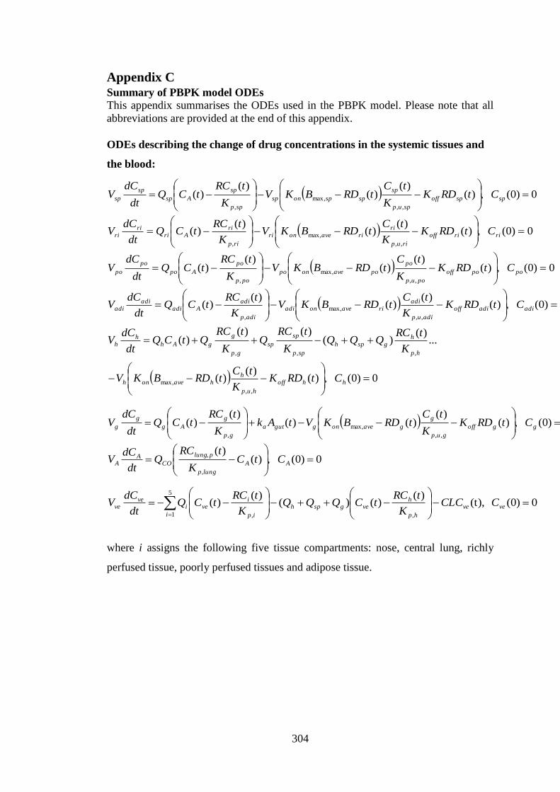
304

Appendix C Summary of PBPK model ODEs

This appendix summarises the ODEs used in the PBPK model. Please note that all

abbreviations are provided at the end of this appendix.

ODEs describing the change of drug concentrations in the systemic tissues and

the blood:

0)0( ,)()(

)()(

)(,,

max,

,

spspoff

spup

sp

spsponsp

spp

sp

Asp

sp

sp CtRDKK

tCtRDBKV

K

tRCtCQ

dt

dCV

0)0( ,)()(

)()(

)(,,

max,

,

ririoff

riup

ririaveonri

rip

riAri

riri CtRDK

K

tCtRDBKV

K

tRCtCQ

dt

dCV

0)0( ,)()(

)()(

)(,,

max,

,

popooff

poup

po

poaveonpo

pop

po

Apo

po

po CtRDKK

tCtRDBKV

K

tRCtCQ

dt

dCV

0)0( ,)()(

)()(

)(,,

max,

,

adiadioff

adiup

adiriaveonadi

adip

adiAadi

adiadi CtRDK

K

tCtRDBKV

K

tRCtCQ

dt

dCV

0)0( ,)()(

)(

...)(

)()()(

)(

,,

max,

,,,

hhoff

hup

hhaveonh

hp

hgsph

spp

sp

sp

gp

g

gAhh

h

CtRDKK

tCtRDBKV

K

tRCQQQ

K

tRCQ

K

tRCQtCQ

dt

dCV

0)0( ,)()(

)()()(

)(,,

max,

,

ggoff

gup

g

gaveongguta

gp

g

Ag

g

g CtRDKK

tCtRDBKVtAk

K

tRCtCQ

dt

dCV

0)0( ,)()(

,

,

AA

lungp

plung

COA

A CtCK

tRCQ

dt

dCV

0)0( (t),)(

)()()(

)(,

5

1 ,

veve

hp

hvegsph

i ip

ivei

veve CCLC

K

tRCtCQQQ

K

tRCtCQ

dt

dCV

where i assigns the following five tissue compartments: nose, central lung, richly

perfused tissue, poorly perfused tissues and adipose tissue.

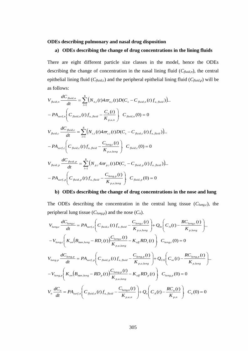
305

ODEs describing pulmonary and nasal drug disposition

a) ODEs describing the change of drug concentrations in the lining fluids

There are eight different particle size classes in the model, hence the ODEs

describing the change of concentration in the nasal lining fluid (Cfluid,n), the central

epithelial lining fluid (Cfluid,c) and the peripheral epithelial lining fluid (Cfluid,p) will be

as follows:

0)0( ,)(

)(

...))(()(4)(

,

,,

,,,

8

1

,,,,

,

,

nfluid

nup

n

fluidunfluidnsurf

i

fluidunfluidsinin

nfluid

nfluid

CK

tCftCPA

ftCCDtrtNdt

dCV

0)0( ,)(

)(

...))(()(4)(

,

,,

,

,,,

8

1

,,,,

,

,

cfluid

lungup

clung

fluiducfluidcsurf

i

fluiducfluidsicic

cfluid

cfluid

CK

tCftCPA

ftCCDtrtNdt

dCV

0)0( ,)(

)(

...))(()(4

,

,,

,

,,,

8

1

,,,,

,

,

pfluid

lungup

plung

fluidupfluidpsurf

i

fluidupfluidsipip

pfluid

pfluid

CK

tCftCPA

ftCCDtrNdt

dCV

b) ODEs describing the change of drug concentrations in the nose and lung

The ODEs describing the concentration in the central lung tissue (Clung,c), the

peripheral lung tissue (Clung,p) and the nose (Cn).

0)0( ,)()(

)(

...)(

)()(

)(

,

,,

,

max,,

,

,

,,

,

,,,

,

,

clungcoff

lungup

clung

clungonclung

lungp

clung

Abr

lungup

clung

fluiducfluidcsurf

clung

clung

CtRDKK

tCtRDBKV

K

tRCtCQ

K

tCftCPA

dt

dCV

0)0( ,)()(

)(

...)(

)()(

)(

,

,,

,

max,,

,

,

,,

,

,,,

,

,

plungpoff

lungup

plung

plungonplung

lungp

plung

veCO

lungup

plung

fluidupfluidpsurf

plung

plung

CtRDKK

tCtRDBKV

K

tRCtCQ

K

tCftCPA

dt

dCV

0)0( ,)(

)()(

)(,,,

,

,,,

n

np

nAn

nup

nlung

fluidunfluidnsurfn

n CK

tRCtCQ

K

tCftCPA

dt

dCV

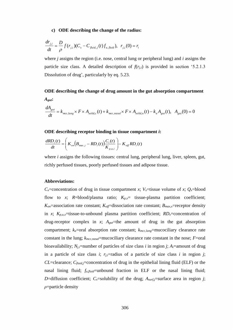
306

c) ODE describing the change of the radius:

iijfluidujfluidsij

ijrrftCCrf

D

dt

dr )0( ),)()(( ,,,,

,

where j assigns the region (i.e. nose, central lung or peripheral lung) and i assigns the

particle size class. A detailed description of f(rj,i) is provided in section ‘5.2.1.3

Dissolution of drug’, particularly by eq. 5.23.

ODE describing the change of drug amount in the gut absorption compartment

Agut:

0)0( ),()()( ,,,, gutgutansolidnasalmcccsolidlungmcc

gutAtAktAFktAFk

dt

dA

ODE describing receptor binding in tissue compartment i:

)()(

)()(

,,

,max tRDKK

tCtRDBK

dt

tdRDioff

iup

iiion

i

where i assigns the following tissues: central lung, peripheral lung, liver, spleen, gut,

richly perfused tissues, poorly perfused tissues and adipose tissue.

Abbreviations:

Cx=concentration of drug in tissue compartment x; Vx=tissue volume of x; Qx=blood

flow to x; R=blood/plasma ratio; Kp,x= tissue-plasma partition coefficient;

Kon=association rate constant; Koff=dissociation rate constant; Bmax,x=receptor density

in x; Kp,u,x=tissue-to-unbound plasma partition coefficient; RDx=concentration of

drug-receptor complex in x; Agut=the amount of drug in the gut absorption

compartment; ka=oral absorption rate constant; kmcc,lung=mucociliary clearance rate

constant in the lung; kmcc,nasal=mucociliary clearance rate constant in the nose; F=oral

bioavailability; Nj,i=number of particles of size class i in region j; Ai=amount of drug

in a particle of size class i; rj,i=radius of a particle of size class i in region j;

CL=clearance; Cfluid,j=concentration of drug in the epithelial lining fluid (ELF) or the

nasal lining fluid; fu,fluid=unbound fraction in ELF or the nasal lining fluid;

D=diffusion coefficient; Cs=solubility of the drug; Asurf,j=surface area in region j;

ρ=particle density

307

Subscripts:

sp=spleen; ri=richly perfused tissues; po=poorly perfused tissues; adi=adipose

tissues; h=hepatic; g=gut; A=arterial; ve=venous; lung,p=peripheral lung tissue;

lung,c=central lung tissue; n=nose; CO=cardiac output; c=central; p=peripheral

Documents

Lung-Targeted Receptor Occupancy by Drug Inhalation