www.elsevier.com/locate/yjtbi

Author’s Accepted Manuscript

Long run coexistence in the chemostat with multiplespecies

Alain Rapaport, Denis Dochain, Jérôme Harmand

PII: S0022-5193(08)00607-3DOI: doi:10.1016/j.jtbi.2008.11.015Reference: YJTBI5372

To appear in: Journal of Theoretical Biology

Received date: 12 June 2008Revised date: 7 October 2008Accepted date: 18 November 2008

Cite this article as: Alain Rapaport, Denis Dochain and Jérôme Harmand, Long run co-existence in the chemostat with multiple species, Journal of Theoretical Biology (2008),doi:10.1016/j.jtbi.2008.11.015

This is a PDF file of an unedited manuscript that has been accepted for publication. Asa service to our customers we are providing this early version of the manuscript. Themanuscript will undergo copyediting, typesetting, and review of the resulting galley proofbefore it is published in its final citable form. Please note that during the production processerrorsmay be discoveredwhich could affect the content, and all legal disclaimers that applyto the journal pertain.

peer

-005

5453

5, v

ersi

on 1

- 11

Jan

201

1Author manuscript, published in "Journal of Theoretical Biology 257, 2 (2009) 252"

DOI : 10.1016/j.jtbi.2008.11.015

Accep

ted m

anusc

ript

Long run coexistence in the chemostat

with multiple species∗

Alain Rapaporto, Denis Dochain&† and Jerome Harmand+

o UMR Analyse des Systemes et Biometrie, INRA,2 place Viala, 34090 Montpellier, France

& CESAME, Universite Catholique de Louvain,4-6 avenue G. Lemaıtre, 1348 Louvain-la-Neuve, Belgium

+ Laboratoire de Biotechnologies de l’Environnement, INRA,Avenue des etangs, 11100 Narbonne, France

November 25, 2008

Abstract

In this work we analyze the transient behavior of the dynamics ofmultiple species competing in a chemostat for a single resource, present-ing slow/fast characteristics. We prove that coexistence among a subsetof species, with growth functions close to each other, can last for a sub-stantially long time. For these cases, we also show that the proportion ofnon-dominant species can be increasing before decreasing, under certainconditions on the initial distribution.

Key-words. chemostat, competition, persistence, slow-fast dynamics.

1 Introduction

A popular concept in microbial ecology is the Competitive Exclusion Principle(CEP) which expresses the fact that when two or more microbial species growon the same substrate in a chemostat, at most one species, i.e. the species thathas the best affinity with the limiting substrate, will eventually survive. Thisconcept has been first introduced by Hardin [8] and has been widely mathemat-ically studied in the literature since (e.g. [2, 16, 3, 4]). However coexistenceof multiple species in chemostat is largely encountered in practical situations.Many efforts have been done to emphasize mathematically such coexistence be-havior, either via periodic inputs (e.g. [14], [5]) or via model rewriting (e.g. [6]that considers the filamentous backbone theory to emphasize the coexistence offlocks and filaments, or [9] [10] [11] where the specific growth rate models arealso dependent on the biomass, via in particular ratio dependence).

∗This work has been achieved within the INRA-INRIA project ’MERE’.†Honorary Research Director FNRS, Belgium

1

peer

-005

5453

5, v

ersi

on 1

- 11

Jan

201

1

Accep

ted m

anusc

ript

One should have in mind that the CEP characterizes an asymptotic propertyof the system, but does not provide any information on the transient dynamics,that has not yet been thoroughly investigated, to our knowledge. In the presentpaper, we propose to study the transient dynamics of multiple species growingon the same substrate, depending on the initial species distribution. When someof the species have close growth functions, on may observe a practical coexistencein the following sense: even if the species with best affinity will finally be theonly surviving one, the transient stage before the other species have almostdisappeared may eventually be substantially long. It appears that the differentspecies may coexist for a long time before the competitive exclusion practicallyapplies. More precisely, some of species may be first increasing (before finallydecreasing) depending on the initial distribution.

The motivation of considering many species with close growth functionscomes from the observations made by recent molecular approaches. In microbialecosystems, thousands of species are present whereas the number of functionsis limited [7, 13]. Moreover, the structural instability of microbial communitiesshows that same function can be carry out by several different species [17]. It isalso well-known that constant mutations rates lead to occurring new individualswith different traits and with different but close growth functions, that can beconsider as new species from the modeling point of view. In chemostat-likesystems, the main function under consideration is usually the degradation ofa given substrate, which is measured by the growth functions of each species.But only about 1 % of the overall micro-organisms observed in real ecosystemscan be isolated and cultivated in laboratory [1]. Thus micro-organisms whosegrowth functions can be clearly identified represent only a tip of the iceberg andit is most probable that among a huge number of species, many should havegrowth functions close to each other.

Our analysis is based on a slow-fast characterization of the system dynamics,and provides an estimation of bounds from below of the times at which eachspecies stops increasing and therefore starts decreasing. The slow-fast techniqueconsists in approximating the fast variables by “quasi-stationary” equilibria.Nevertheless, the validity of such an approximation has to be checked, provingthe attractivity of the slow manifold (see for instance Tikhonov’s theorem in[12]), as we do in this paper. We believe that a slow-fast analysis of the chemo-stat model with many close growth functions has not yet been addressed in theliterature, and brings a new message for biologists.

The paper is organized as follows. Section 2 is dedicated to some preliminar-ies about the system dynamics and the Competitive Exclusion Principle (CEP).Section 3 concentrates on the slow-fast description of the system dynamics. Areduced order model is deduced from the slow-fast system characterization inSection 4, where the analysis provides elements for the practical coexistence ofmultiple species with closed growth functions. Finally the proposed results areillustrated via numerical simulations in Section 5.

2

peer

-005

5453

5, v

ersi

on 1

- 11

Jan

201

1

Accep

ted m

anusc

ript

2 Preliminaries

Let us consider the chemostat model with one limited resource and m species⎧⎪⎨⎪⎩

xi = μi(s)xi −Dxi, i = 1 · · ·ms = −

m∑i=1

μi(s)yi

xi +D(Sin − s) (1)

The growth functions μi(·) are assumed to be C1 non-negative functions suchthat μi(0) = 0.

Without any loss of generality, we shall assume in the following that all yieldfactors yi have been taken equal to one (one can easily check that this amountsto replace xi by xi/yi or to change the unit measuring each stock xi). Let usfirst recall the following lemma.

Lemma 2.1 The domain

D =

{(x, s) ∈ IRm+1

+ |m∑

i=1

xi + s ≤ Sin

}

is invariant and attractive by the dynamics (1) in the non-negative cone IRm+1+ .

Proof. When xi = 0, one has xi = 0. Consequently, the trajectories cannotcross the axes xi = 0.

When s = 0, one has s = DSin > 0. The trajectories cannot approach theaxis s = 0.

From these two facts, one concludes that IRm+1+ is an invariant domain.

Consider now the variable

z =m∑

i=1

xi + s

which is solution of the ordinary differential equation z = D(Sin − z). Oneimmediately concludes that the domain D = IRm+1

+ ∩{z ≤ Sin} is invariant andattractive.

Let us now introduce the following assumption.

Assumption A0. Functions μi(·) are increasing for any i = 1 · · ·m.

Under Assumption A0, it is usual to define the break-even concentrations:

λi(D) =∣∣∣∣ si such that μi(si) = D ,

+∞ if μi(s) < D for any s ≥ 0 , (2)

for each i = 1 · · ·m. Let us recall the Competitive Exclusion Principle (CEP),(first proved for general response functions in [3]; see also Theorem 3.2 in [15]),for which the following assumption is required.

Assumption A1. There exists an unique i� ∈ {1 · · ·m} such that

λi�(D) = mini=1···m

λi(D) .

3

peer

-005

5453

5, v

ersi

on 1

- 11

Jan

201

1

Accep

ted m

anusc

ript

Proposition 2.1 (CEP) Under Assumptions A0 and A1, any trajectory of (1)with initial condition in the non-negative cone such that xi�(0) > 0 fulfills thefollowing properties:

- the substrate concentration s(·) converges asymptotically toward the steadystate value:

s� = min (λi�(D), Sin) ,

- the species concentration xi�(·) converges asymptotically toward Sin − s�,

- any species concentration xi(·) with i �= i� converges asymptotically towardzero.

Corollary 2.1 When s� < Sin, the convergence given by Proposition 2.1 isexponential.

Proof. One can easily check the m+1 eigenvalues of the Jacobian matrix atthe non-null equilibrium are −D < 0, −μ′i�(s�)(Sin−s�) < 0 and μi(s∗)−D < 0for any i �= i�.

The CEP provides information about the asymptotic behavior of solutions of(1). In the present work, we rather focus on transient stages of the trajectoriesof system (1), when some of the functions μi(·) are close to each other.

In the following, we shall assume that A0 and A1 are fulfilled with s� < Sin.

3 A slow-fast characterization

We assume that the m species are numbered such that the following assumptionis fulfilled (see Figure 1 for a graphical interpretation of this condition).

Assumption A2. There exists n ∈ {1, · · · ,m} and positive numbers η, γ suchthat:

λ(D) ≤ λi(D)− η , ∀i > n , (3)

andμ(s) > max

iμi(s) + γ , ∀s ∈ [λ(D),max

i>nλi(D)] , (4)

where λ(D) is the break-even concentration associated to the average growthfunction μ(·):

μ(s) =1n

n∑i=1

μi(s) .

Under Assumption A2, define the number

ε = maxi≤n

maxs∈[0,Sin]

|μi(s)− μ(s)| . (5)

Note that ε is positive under Assumption A1 with s� < Sin (functions μi(·)cannot coincide on the whole interval [0, Sin]). Then, consider the C1 functions

νi(s) =μi(s)− μ(s)

ε, (i = 1 · · ·n) . (6)

4

peer

-005

5453

5, v

ersi

on 1

- 11

Jan

201

1

Accep

ted m

anusc

ript

D

i>nmax λ i (D)i>n

min

η

μ

γ

S

μi

λ i (D)λ(D)

Figure 1: Illustration of the Assumption A2 and numbers η, γ.

Growth functions μi(·) can then be expressed as follows:

μi(s) = μ(s) + ενi(s) (i = 1 · · ·n) .

Let us now consider the total biomass b of the first n species, and their propor-tions pi, defined as follows:

b =n∑

i=1

xi, pi =xi

b.

Then the dynamics of the variables b, xi (i > n), s and pi (i ≤ n) are given bythe following equations:⎧⎪⎪⎪⎪⎪⎪⎪⎪⎪⎪⎪⎪⎨⎪⎪⎪⎪⎪⎪⎪⎪⎪⎪⎪⎪⎩

b = μ(s)b−Db+ ε

(n∑

i=1

νi(s)pi

)b

xi = μi(s)xi −Dxi (i > n)

s = −μ(s)b−m∑

i=n+1

μi(s)xi +D(Sin − s)− ε(

n∑i=1

νi(s)pi

)b

pi = ε

⎛⎝ n∑

j=1

(νi(s)− νj(s))pj

⎞⎠ pi (i = 1 · · ·n)

(7)

Remark 3.1 If n = m, we simply omit, by writing convention, variables xi inexpression (7).

Let us consider the change of time variable τ = εt. System (7) can then be

5

peer

-005

5453

5, v

ersi

on 1

- 11

Jan

201

1

Accep

ted m

anusc

ript

equivalently written as follows:⎧⎪⎪⎪⎪⎪⎪⎪⎪⎪⎪⎪⎪⎪⎨⎪⎪⎪⎪⎪⎪⎪⎪⎪⎪⎪⎪⎪⎩

εdb

dτ= μ(s)b−Db+ ε

(n∑

i=1

νi(s)pi

)b

εdxi

dτ= μi(s)xi −Dxi (i > n)

εds

dτ= −μ(s)b−

m∑i=n+1

μi(s)xi +D(Sin − s)− ε(

n∑i=1

νi(s)pi

)b

dpi

dτ=

⎛⎝ n∑

j=1

(νi(s)− νj(s))pj

⎞⎠ pi (i = 1 · · ·n)

(8)

When ε is small, i.e. the first n growth functions μi(·) are all close to theaverage μ(·), system (8) is in the form of “slow-fast” dynamics. The vector:

ξ =

⎛⎜⎜⎜⎜⎜⎝

bxn+1

...xm

s

⎞⎟⎟⎟⎟⎟⎠

corresponds to the “fast” variables, and the “boundary-layer” dynamics is givenby the system: ⎧⎪⎪⎨

⎪⎪⎩˙b = μ(s)b−Db˙xi = μi(s)xi −Dxi (i > n)˙s = −μ(s)b−

∑i>n

μi(s)xi +D(Sin − s)(9)

Note that system (9) has exactly the structure of (1) but in dimension m−n+2.Denote λ(·) the break-even concentration associated to function μ(·) and s =λ(D).

Remark 3.2 Note that one has necessarily s ≥ s�, due to the monotonicity ofthe growth functions μi(·).

Consider the following hypothesis.

Assumption A3. s < Sin.

Under Assumptions A1 to A3, dynamics (9) admits the equilibrium

E =

⎛⎜⎜⎜⎜⎜⎝

Sin − s0...0s

⎞⎟⎟⎟⎟⎟⎠

which is globally exponentially stable on IR+ \ {0} × IRm−n+1+ (see Corollary

2.1).

6

peer

-005

5453

5, v

ersi

on 1

- 11

Jan

201

1

Accep

ted m

anusc

ript

We show now that fixing an arbitrary small neighborhood V of E and anarbitrary small number τ , there exists ε > 0 such that, for any ε < ε the statevector ξ(·) enters and remains in V within the time τ .

Proposition 3.1 Assume that A1, A2 and A3 are fulfilled. For any initialcondition in D with b(0) > 0, there exist positive numbers α, κ and β such thatfor any ε > 0 sufficiently small, one has

||ξ(τ) − E|| ≤ αε+ κe−βτ/ε, ∀τ ≥ 0 . (10)

Proof. Let us fix an initial condition in D with b(0) > 0 and define

v(t) =n∑

i=1

νi(s(t))pi(t)

along the solution of system (7). Recall from Lemma 2.1 that the solutions of(7) remain in the bounded domain D, and from the definition (6), one has

maxs∈[0,Sin]

|νi(s)| ≤ 1, ∀i ≤ n,

whatever the value of ε. Consequently |v(·)| is bounded by 1 uniformly in ε.Consider variables

m = b+∑i>n

xi and z = s+m ,

whose time evolutions are solutions of the non-autonomous dynamics:{m = (ψ(t, z −m)−D)m ,z = D(Sin − z) , (11)

where the function ψ(·) is defined as follows

ψ(t, s) = (μ(s) + εv(t))b(t)m(t)

+m∑

i=n+1

μi(s)xi(t)m(t)

.

Note that ψ(·) is bounded by two autonomous functions

ψ−ε (s) ≤ ψ(t, s) ≤ ψ+ε (s), ∀t ≥ 0, ∀s ∈ [0, Sin],

with

ψ−ε (s) = min(μ(s)− ε,min

i>nμi(s)

),

ψ+ε (s) = max

(μ(s) + ε,max

i>nμi(s)

).

Consider then m−(·), m+(·) solutions of the ordinary differential equations

m−(·) = (ψ−ε (z(t)−m−)−D)m−, m−(0) = m(0),m+(·) = (ψ+

ε (z(t)−m+)−D)m+, m+(0) = m(0),

from which one deduces bounds on m(·):m−(t) ≤ m(t) ≤ m+(t), ∀t ≥ 0.

7

peer

-005

5453

5, v

ersi

on 1

- 11

Jan

201

1

Accep

ted m

anusc

ript

Denote s−(t) = z(t)−m−(t) and s+(t) = z(t)−m+(t) and note that variables(m−, s−) and (m+, s+) are solutions of the dynamical systems{

m− = (ψ−ε (s−)−D)m−

s− = −ψ−ε (s−)m− +D(Sin − s−) (12)

{m+ = (ψ+

ε (s+)−D)m+

s+ = −ψ+ε (s+)m− +D(Sin − s+) (13)

Systems (12) and (13) are chemostat models of the form (1) for a single fictitiousspecies with monotonic growth function ψ−ε (·) and ψ+

ε (·) respectively. Denoteλ−ε (·), resp. λ+

ε (·) the break-even concentrations associated to ψ−ε (·), resp. ψ+ε (·)

(see Definition 2). One has clearly λ+ε (D) < λ−ε (D) and when ε is small enough,

one ensures λ+ε (D) < λ−ε (D) < Sin. Then Proposition 2.1 gives the asymptotic

convergence of s−(·), resp. s+(·) toward λ−ε (D), resp. λ−ε (D), from any initialcondition with m(0) > 0. Corollary 2.1 gives also the exponential convergenceand one can easily check that an exponential decay is guaranteed uniformly inε sufficiently small. So, there exist numbers k0 > 0 and β0 > 0 such that theproperty

s(t) ∈ Iε(t) = [λ+ε (D)− k0e

−β0t, λ−ε (D) + k0e−β0t], ∀t ≥ 0 (14)

is fulfilled for any ε small enough. Note that Assumption A2 gives the equalities

λ+ε (D) = λ(D − ε), λ−ε (D) = max

i>nλi(D), (15)

when ε is small enough, and the existence of T0 < +∞ such that the property

s ∈ Iε(t) =⇒ μ(s) ≥ maxi>n

μi(s) + ε+ γ/2 (16)

is satisfied for any t > T0 and any ε < γ/2 small enough.From equations (7), the dynamics of the proportion variable q = b/m can

be written as follows

q = q(1− q)

⎛⎜⎜⎝μ(s(t)) + εv(t)−

∑i>n

μi(s(t))xi(t)∑

j>n

xj(t)

⎞⎟⎟⎠ .

Then, from (16) one obtains the inequality

q(t) ≥ γ

2q(t)(1 − q(t)) , ∀t ≥ T0 ,

for any ε small enough. Note that the hypothesis b(0) > 0 implies q(0) > 0 andconsequently q(t) > 0 for any time t. We then deduce the exponential conver-gence of the variable q toward 1, or equivalenty the exponential convergence ofthe concentrations xi towards 0 for any i > n, i.e there exists kx > 0, βx > 0such that

xi(t) ≤ kxe−βxt , ∀t ≥ T0 , ∀i > n (17)

for any ε > 0 small enough. We also deduce the existence of a finite time T1 ≥ T0

such that

μ(s)q(t) + mini>n

μi(s)(1− q(t)) ≥ μ(s)− ε , ∀s ∈ Iε(t), ∀t ≥ T1 ,

8

peer

-005

5453

5, v

ersi

on 1

- 11

Jan

201

1

Accep

ted m

anusc

ript

for any ε small enough, which implies the inequality

ψ(t, s) ≥ (μ(s)−ε)q(t)+mini>n

μi(s)(1−q(t)) ≥ μ(s)−2ε , ∀s ∈ Iε(t) , ∀t ≥ T1

to be fulfilled. Then, the following upper bound on the derivative of s is ob-tained, for any t > T1 (and ε > 0 small enough):

s = −ψ(t, s)(z(t)− s) +D(Sin − s) ≤ −(μ(s)− 2ε)(z(t)− s) +D(Sin − s) .Recall now from equations (11) that z(·) is solution of the differential equa-

tion z = D(Sin − z), independently of the functions μi(·), whose solution is

z(t) = Sin + (z(0)− Sin)e−Dt, ∀t ≥ 0 . (18)

Consequently, one has

s ≤ (D − μ(s) + 2ε)(Sin − s)− (μ(s)− 2ε)(z(0)− Sin)e−Dt, ∀t ≥ T1,

from which one deduces the existence of k1 > 0 and β1 > 0 such that

s(t) ≤ λ(D + 2ε) + k1e−β1t, ∀t ≥ T1 .

With (14) and (15), one obtains more precise bounds on the variable s

λ(D − ε)− k0e−β0t ≤ s(t) ≤ λ(D + 2ε) + k1e

−β1t, ∀t ≥ T1 . (19)

Then bounds on the variable b are obtained from (17)(18), for any t ≥ T1 andany ε small enough

Sin − λ(D + 2ε)− ζ−(t) ≤ b(t) ≤ Sin − λ(D − ε) + ζ+(t) (20)

with {ζ−(t) = k1e

−β1t + (m− n)kxe−βxt − (z(0)− Sin)e−Dt ,

ζ+(t) = k0e−β0t + (z(0)− Sin)e−Dt .

Finally, continuity of λ(·) and inequalities (17)(19)(20) give together the con-clusion (10).

Let p = (pi)i=1···n be the vector of the “slow” variables (i.e. the distributionamong the first n species) and consider the reduced dynamics:

dpi

dτ=

⎛⎝ n∑

j=1

(νi(s)− νj(s))pj

⎞⎠ pi, (i = 1 · · ·n) . (21)

In the next section, we shall study the solutions of system (21) and comparethem with the solutions of the original system (8).

4 The reduced dynamics

The reduced dynamical equations (21) of the “slow” part is given by the bilineardynamical equation

dpi

dτ=

n∑j=1

Aijpjpi (22)

9

peer

-005

5453

5, v

ersi

on 1

- 11

Jan

201

1

Accep

ted m

anusc

ript

where A = [Aij ] is a skew symmetric matrix with Aij = νi(s)− νj(s).

Let us consider the generic case with the following assumption.

Assumption A4. For any i �= j, one has νi(s) �= νj(s).

Without any loss of generality, we can assume that the n species are num-bered such that

νn(s) > νn−1(s) > · · · > ν1(s) .

Let us then define numbers Bi = Ani, where

B1 > B2 > · · · > Bn−1 > Bn = 0 . (23)

Since∑

j pj = 1, one has

∑j

Aijpj =∑

j

(νi − νj)pj = −νn + νi +∑

j

(νn − νj)pj = −Bi +∑

j

Bjpj ,

and one can write equivalently the dynamical equations (22) as follows :

dpi

dτ=

⎛⎝−Bi +

n∑j=1

Bjpj

⎞⎠ pi, i = 1 · · ·n . (24)

Remark 4.1 Under Assumptions A3 and A4, one has λn(D) = s� for ε smallenough. In accordance with the CEP, the n-th species asymptotically wins thecompetition because it has the (unique) smallest break-even concentration.

Under Assumption A4, system (24) admits exactly n distinct equilibria,which are exactly the vertexes of the simplex:

S =

{p ∈ IRn

+ |n∑

i=1

pi = 1

},

One can easily check that S is invariant by the dynamics (24) and the eigenvaluesof the Jacobian matrix at an equilibrium p ∈ S such that pi = 1 are Bi andBj−Bi for j �= i. Consequently one obtains immediately the following propertiesfor the dynamics defined on S.

- when p1 = 1, p is a source,

- when pn = 1, p is a sink,

- when pi = 1 with i ∈ 2 · · ·n− 1, p is a saddle point with a stable manifoldof dimension i− 1 contained in the face:

Fi =

⎧⎨⎩p ∈ S |

i∑j=1

pj = 1

⎫⎬⎭ .

10

peer

-005

5453

5, v

ersi

on 1

- 11

Jan

201

1

Accep

ted m

anusc

ript

Note that solutions qi(·) of dynamics qi = −Biqi (i = 1 · · ·n) fulfill ddt qi =

(−Bi +∑

j Bj qj)qi with qi = qi/∑

j qj . We deduce that the solutions of system(24) are given by the analytical formula:

pi(τ) =pi(0)e−Biτ

n∑j=1

pj(0)e−Bjτ

, i = 1 · · ·n . (25)

Let p� be the equilibrium (0, · · · , 0, 1)′ ∈ S. Its stability property is givenby the lemma.

Lemma 4.1 For any initial condition p(0) ∈ S with pn(0) > 0, the solution p(·)of the reduced dynamics (24) converges exponentially toward the equilibrium p�.

Proof. From equations (25), one has pn(τ) → 1 and pi(τ) → 0 for anyi = 1 · · ·n − 1, when τ → +∞. The linearized dynamics of (22) about p� issimply pi = −Bipi (i = 1 · · ·n). Consequently, each component pi for i < nconverges exponentially toward 0 and pn = 1−∑i<n pi converges exponentiallytoward 1.

Let us now compare the distribution p(·) of the reduced dynamics (22) withpε(·) of the original dynamics (8), when ε is small. When xn(0) > 0, we alreadyknow from Corollary 2.1 and Lemma 4.1 that both p(·) and pε(·) converge ex-ponentially toward p�. We give now a result that compares these distributionsduring their transient stage.

Corollary 4.1 Assume that A3 and A4 are fulfilled. For any initial conditionof (1) in D with xn(0) > 0 and any T > 0, there exists ε > 0 such that

ε < ε ⇒ p(τ) − pε(τ) = O(ε), uniformly for τ > T . (26)

Proof. Recalling the facts:

1. the equilibrium E of the boundary layer dynamics (9) is exponentiallystable (Corollary 2.1),

2. the equilibrium p� of the reduced dynamics (22) is exponentially stable(Lemma 4.1),

the Tikhonov’s theorem (see for instance Theorem 9.4 in [12]) gives the con-clusion (26) for any initial condition close to (E, p�) in IRm−n

+ × S, and thenextended to larger initial conditions by Proposition 3.1.

Consider now the time function:

π(τ) =n∑

j=1

Bjpj(τ) .

The transient behavior of the solutions of (7) can be characterized by π(0), asdescribed by the following result.

11

peer

-005

5453

5, v

ersi

on 1

- 11

Jan

201

1

Accep

ted m

anusc

ript

Proposition 4.1 Under Assumption A4, for any initial condition p(0) in S,the solution p(·) of (7) fulfills the following properties.

- for indexes i such that π(0) ≤ Bi, pi(·) is decreasing,

- for indexes i such that π(0) > Bi, pi(·) is increasing up to Ti such thatpi(Ti) = Bi and is then decreasing. Furthermore, one has:

Ti ≥ T i =1B1

logπ(0)(B1 −Bi)Bi(B1 − π(0))

. (27)

Proof. One has immediately:

dπ

dτ= −

n∑j=1

B2j pj +

⎛⎝ n∑

j=1

Bjpj

⎞⎠

2

= −n∑

j=1

φ(Bj)pj + φ

⎛⎝ n∑

j=1

Bjpj

⎞⎠ (28)

where φ(·) is the square function. φ(·) being a convex function, one deducesthat dπ/dτ ≤ 0. The function τ �→ π(τ) is non-increasing. Note that one hasalso:

dpi

dτ= (−Bi + π(τ))pi .

Consequently, the function τ → pi(τ) is always decreasing when π(0) ≤ Bi.Otherwise, τ → pi(τ) is increasing up to Ti such that π(Ti) = Bi and thendecreasing.

From (28), one can derive the inequality:

dπ

dτ= π2 −B1π +

n∑j=1

Bjpj(B1 −Bj) ≥ π2 −B1π ,

and deduce an estimation from below of the function π(·):π(τ) ≥ π−(τ) , τ ≥ 0 ,

where π−(·) is solution of the differential equation:

dπ

dτ

−= π−2 −B1π

− , π−(0) = π(0) .

It is straightforward to check that π−(·) is given by the following expression:

π−(τ) =π(0)B1

π(0) + (B1 − π(0))eB1τ. (29)

Let us fix an initial condition p1(0), · · · , pn(0) and consider i0 the smallestindex i = 1, · · · , n such that Bi < π(0). Note that inequality B1 > π(0) isfulfilled exactly when i0 ≤ n − 1. For i0 ≤ n − 1, the following bound frombelow of time Ti is obtained from (29).

Ti ≥ 1B1

logπ(0)(B1 −Bi)Bi(B1 − π(0))

.

12

peer

-005

5453

5, v

ersi

on 1

- 11

Jan

201

1

Accep

ted m

anusc

ript

Remark 4.2 Note that τ �→ p1(τ) is always a non-increasing function, and thefunction τ �→ pn(τ) is always non-decreasing.

Let i0 be the smallest index in 1, · · · , n such that Bi < π(0). One hasnecessarily Ti0 < Ti0+1 < · · · < Tn−1. From expression (27), one can deducethe following qualitative properties:

i. when π(0) is close to B1 (i.e. species 1 is majority at initial time), all thespecies concentrations, except for the species 1, are increasing for a longtime;

ii. when π(0) is close to Bi with i > 1, the concentrations of species j forj ≤ i are rapidly decreasing.

5 Simulation results

Numerical simulations have been performed in order to illustrate the conceptsdeveloped here above. We have considered ten species (i.e. m = 10) among twofamilies, whose specific growth rates are depicted on Figure 2. For each family,

species 6,7,8,9,10

D

species 1,2,3,4,5

0.0 0.5 1.0 1.5 2.0 2.5 3.0 3.5 4.0 4.5 5.0

0.00

0.05

0.10

0.15

0.20

0.25

0.30

0.35

0.40

0.45

Figure 2: Specific growth rates

specific growth rates are been chosen closed to each other, in terms of Monodanalytic functions

μi =μmax,is

Ks,i + s(30)

where μmax,i and Ks,i are the maximum specific rate (h−1) and the affinityconstant (g/l) associated to each species xi, respectively. Numerical values ofthe parameters are given in the following table.

species 1 2 3 4 5 6 7 8 9 10

μmax,i 0.5 0.5 0.5 0.5 0.5 0.5 0.5 0.5 0.5 0.5Ks,i 1.02 1.01 1 0.99 0.98 2.04 2.02 2 1.98 1.96

The operating conditions of the chemostat have been selected as follows:

D = 0.1 h−1, sin = 5 g/l . (31)

13

peer

-005

5453

5, v

ersi

on 1

- 11

Jan

201

1

Accep

ted m

anusc

ript

Moreover, we have considered, for the sake of simplicity, yield coefficients yi

equal to 1. The next table gives the numerical values of the break-even concen-trations defined in (2).

species 1 2 3 4 5

λi(D) 0.2550 0.2525 0.2500 0.2475 0.2450

species 6 7 8 9 10

λi(D) 0.5100 0.5050 0.5000 0.4950 0.4900

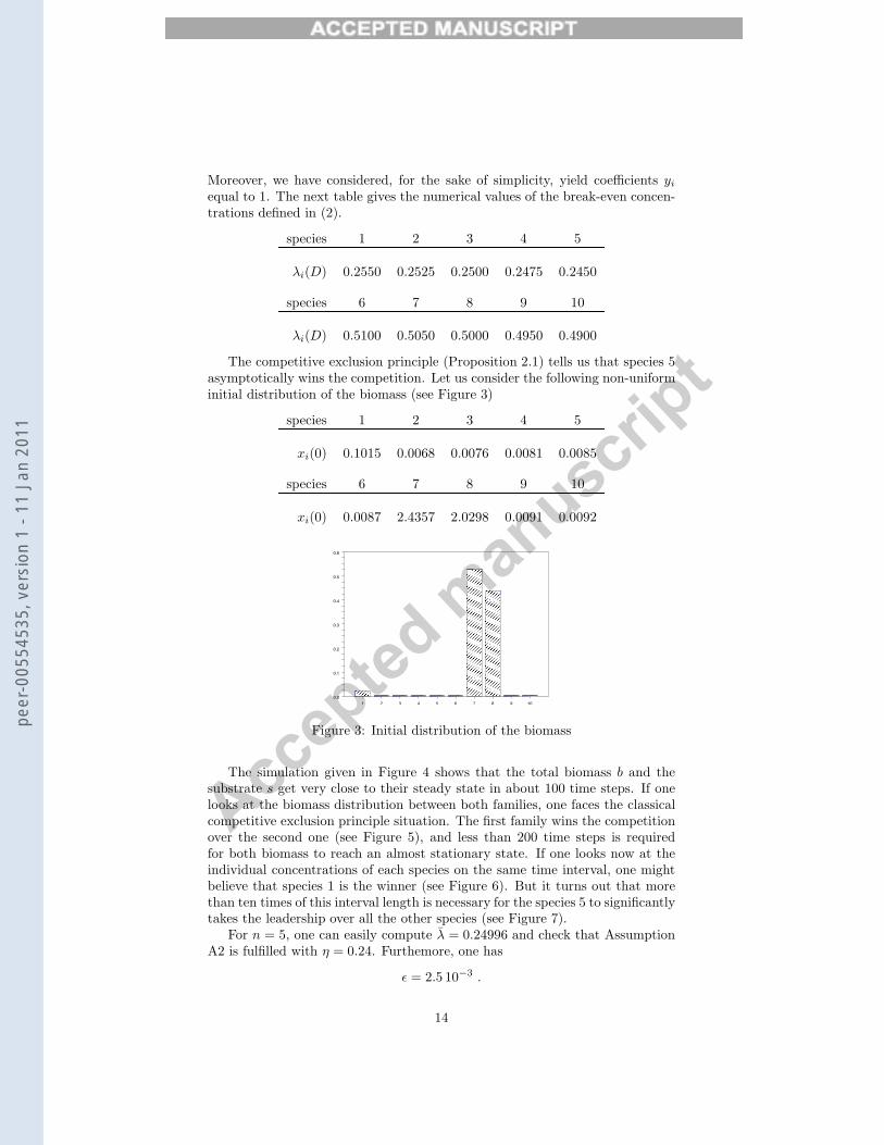
The competitive exclusion principle (Proposition 2.1) tells us that species 5asymptotically wins the competition. Let us consider the following non-uniforminitial distribution of the biomass (see Figure 3)

species 1 2 3 4 5

xi(0) 0.1015 0.0068 0.0076 0.0081 0.0085

species 6 7 8 9 10

xi(0) 0.0087 2.4357 2.0298 0.0091 0.0092

������������������������������������������������������������������������������������������������������������������

������������������������������������������������������������������������������������������������������������������

��������������������������������������������������������������������������������������������������������������������������������

��������������������������������������������������������������������������������������������������������������������������������

������������

1 2 3 4 5 6 7 8 9 10

0.0

0.1

0.2

0.3

0.4

0.5

0.6

Figure 3: Initial distribution of the biomass

The simulation given in Figure 4 shows that the total biomass b and thesubstrate s get very close to their steady state in about 100 time steps. If onelooks at the biomass distribution between both families, one faces the classicalcompetitive exclusion principle situation. The first family wins the competitionover the second one (see Figure 5), and less than 200 time steps is requiredfor both biomass to reach an almost stationary state. If one looks now at theindividual concentrations of each species on the same time interval, one mightbelieve that species 1 is the winner (see Figure 6). But it turns out that morethan ten times of this interval length is necessary for the species 5 to significantlytakes the leadership over all the other species (see Figure 7).

For n = 5, one can easily compute λ = 0.24996 and check that AssumptionA2 is fulfilled with η = 0.24. Furthemore, one has

ε = 2.5 10−3 .

14

peer

-005

5453

5, v

ersi

on 1

- 11

Jan

201

1

Accep

ted m

anusc

ript

substrate

total biomass

0 10 20 30 40 50 60 70 80 90 100

0

1

2

3

4

5

6

Figure 4: Short run simulation

6+7+8+9+10

1+2+3+4+5

0 20 40 60 80 100 120 140 160 180 200

0

1

2

3

4

5

6

Figure 5: Mid run simulation

8

5,4,3,2

6,9,10

1

7

0 20 40 60 80 100 120 140 160 180 200

0.0

0.5

1.0

1.5

2.0

2.5

3.0

3.5

Figure 6: Mid run simulation

15

peer

-005

5453

5, v

ersi

on 1

- 11

Jan

201

1

Accep

ted m

anusc

ript

9,10

1

5

4

32

7,8

0 500 1000 1500 2000 2500 3000 3500 4000 4500 5000

0.0

0.2

0.4

0.6

0.8

1.0

Figure 7: Long run simulation

We illustrate on Figure 8 that reduced dynamics whose solution given by theexplicit formula (25) is a good approximation of the dynamics of the speciesdistribution among the first family.

3

5

1

2

4

0 500 1000 1500 2000 2500 3000 3500 4000 4500 5000

0.0

0.1

0.2

0.3

0.4

0.5

0.6

0.7

0.8

0.9

1.0

Figure 8: Species distribution among the first family (reduced dynamics indashed line)

As predicted by the theory, the proportions pi(·) are increasing and thendecreasing, or monotonic with respect to time. The next table shows that thelower estimates on times Ti, provided by formula (27), give a relevant infor-mation, to be compared to the times that maximizes the proportions of eachspecies (computed on the original dynamics (7).

species 1 2 3 4 5

T i −∞ 188 531 874 +∞argmaxt pi(t) 0 231 684 1161 +∞

Finally, we have represented the time evolution of the Simpson’s diversityindex

σ(t) = 1−10∑

i=1

p2i (t)

which is commonly used to measure the diversity of an ecosystem. Figure 9shows its non-monotonic behavior, that can be explained in the present situation

16

peer

-005

5453

5, v

ersi

on 1

- 11

Jan

201

1

Accep

ted m

anusc

ript

by the exchange of leadership between species 5 and 1 that increases temporarilythe diversity, and the relatively long time before approaching zero.

0 500 1000 1500 2000 2500 3000 3500 4000 4500 5000

0.0

0.1

0.2

0.3

0.4

0.5

0.6

0.7

0.8

0.9

1.0

Figure 9: Time evolution of the Simpson’s index

6 Conclusions

In this paper we have studied the behavior of multiple species competing for thesame substrate in a chemostat, when initial conditions can substantially modifythe transient behavior of the system. We have shown in particular by consider-ing slow-fast dynamics that intermediate species can survive for a substantiallylong time before starting to decrease and leave the room for the species thathas the best affinity with the nutrient. Moreover, we give the explicit solutionof a reduced dynamics, that can be easily computed even when the size of thesystem is too large to be solved numerically, and that gives a good predictionof the time evolution of the distribution between species. This formalizes thepractical situation when coexistence of multiple species can last for long timebefore substantial decrease of the non-dominant species takes place. The resultshave been illustrated in numerical simulation.

Acknowledgments. The authors thank J.-J. Godon and C. Lobry for fruitfuldiscussions. Part of the work has been achieved while the second author was insabbatical at Montpellier, granted by INRIA.

References

[1] R.I. Amann, W. Ludwig and K.H. Schleifer KH, Phylogenetic iden-tification and in situ detection of individual microbial cells without culti-vation. Microbiol Rev, 59 (1), 143-169 (1995).

[2] R. Aris and A.E. Humphrey, Dynamics of a chemostat in which twoorganisms compete for a common substrate. Biotechnology and Bioengi-neering, 19, 1375-1386 (1977).

[3] R. Armstrong and R. McGehee (1980), Competitive exclusion, Amer-ican Naturalist, 115, 151-170 (1980).

17

peer

-005

5453

5, v

ersi

on 1

- 11

Jan

201

1

Accep

ted m

anusc

ript

[4] G.J. Butler and G.S.K. Wolkowicz, A mathematical model of thechemostat with a general class of functions describing nutrient uptake.SIAM Journal on Applied Mathematics, 45 (1), 138-151 (1985).

[5] G.J. Butler, S.B.. Hsu and P. Waltman, A mathematical model ofthe chemostat with periodic washout rate. SIAM Journal on Applied Math-ematics, 45 (3), 435-449 (1985).

[6] C. Cenens, I.Y. Smets and J.F. Van Impe, Modeling the competitionbetween floc-forming and filamentous bacteria in actiavted sludge wastewater treatment systems - II. A prototype mathematical model based onkinetic selection and filamentous backbone theory. Water Research, 34 (9),2535-2541 (2000).

[7] T.P. Curtis and W.T. Sloan, Prokaryotic diversity and its limits: mi-crobial community structure in nature and implications for microbial ecol-ogy. Current Opinion in Microbiology, 7, 221-226 (2004).

[8] G. Hardin, The competition exclusion principle. Science, 131, 1292-1298(1960).

[9] C. Lobry, F. Mazenc and A. Rapaport, Persistence in ecological mod-els of competition for a single resource. C.R. Acad. Sci. Paris, Ser I 340,199-240 (2004).

[10] C. Lobry C. and J. Harmand, A new hypothesis to explain the coexis-tence of n species in the presence of a single resource. C.R. Biologies, 329,40-46 (2006).

[11] C. Lobry, F. Mazenc and A. Rapaport, Sur un modele densite-dependant de competition pour une resource. C.R. Biologies, 329, 63-70(2006).

[12] H.K. Khalil, Nonlinear Systems, Prentice Hall, Second Edition (1996).

[13] N.R. Pace, A Molecular View of Microbial Diversity and the Biosphere.Science 276, 734-740 (1997).

[14] H.L. Smith, Competitive coexistence in an oscillating chemostat. SIAMJournal on Applied Mathematics, 40 (3), 498-522 (1981).

[15] H. Smith and P. Waltman, The Theory of the Chemostat: Dynamics ofMicrobial Competition, Cambridge Studies in Mathematical Biology, Cam-bridge University Press (1985).

[16] G. Stephanopoulos, R. Aris and A.G. Frederickson, A stochasticanalysis of the growth of competing microbial populations in a continuousbiochemical reactor. Mathematical Biosciences, 45, 99-135 (1979).

[17] E. Zumstein, R. Moletta J.J. and Godon, Examination of two yearsof community dynamics in an anaerobic bioreactor using fluorescence poly-merase chain reaction (PCR) single-strand conformation polymorphismanalysis. Environmental Microbiology 2, 69 (2000).

18

peer

-005

5453

5, v

ersi

on 1

- 11

Jan

201

1