Embed Size (px)
Citation preview

www.elsevier.com/locate/econbase
Journal of Banking & Finance 28 (2004) 1961–1985
Long-horizon regression tests of the theoryof purchasing power parity
Apostolos Serletis *, Periklis Gogas
Department of Economics, University of Calgary, Calgary, AB, Canada T2N 1N4
Received 30 September 2002; accepted 2 July 2003
Available online 25 December 2003
Abstract
In this article we test the purchasing power parity (PPP) hypothesis during the recent float-
ing exchange rate period, using quarterly data for 21 OECD countries. In doing so, we use the
long-horizon regression approach developed by Fisher and Seater [American Economic Re-
view 83 (1993) 402] and consider 60 bilateral intercountry relations. We investigate the power
of the long-horizon regression tests, using the inverse power function of Andrews [Econome-
trica 57 (1989) 1059], and provide weak evidence in favor of PPP.
� 2003 Elsevier B.V. All rights reserved.
JEL classification: C22; F31
Keywords: Purchasing power parity; Integration; Long-run derivative; Inverse power function
1. Introduction
The theory of purchasing power parity (PPP) has attracted a great deal of atten-
tion and has been explored extensively in the recent literature using recent advancesin the field of applied econometrics (that pay explicit attention to the integration and
cointegration properties of the variables). Based on the law of one price, PPP asserts
that relative goods prices are not affected by exchange rates – or, equivalently, that
exchange rate changes will be proportional to relative inflation. The relationship is
important not only because it has been a cornerstone of exchange rate models in
*Corresponding author. Tel.: +1-403-220-4092/5867; fax: +1-403-282-5262.
E-mail address: [email protected] (A. Serletis).
URL: http://econ.ucalgary.ca/serletis.htm
0378-4266/$ - see front matter � 2003 Elsevier B.V. All rights reserved.
doi:10.1016/j.jbankfin.2003.07.006

1962 A. Serletis, P. Gogas / Journal of Banking & Finance 28 (2004) 1961–1985
international economics, but also because of its policy implications; it provides a
benchmark exchange rate and hence has some practical appeal for policymakers
and exchange rate arbitragers.
Empirical studies generally fail to find support for purchasing power parity, espe-
cially during the recent floating exchange rate period. In fact, the empirical consen-sus is that PPP does not hold over this period (see, for example, Adler and Lehman,
1983; Mark, 1990; Patel, 1990; Grilli and Kaminsky, 1991; Flynn and Boucher, 1993;
Serletis, 1994; Serletis and Zimonopoulos, 1997; Coe and Serletis, 2002). But there
are also studies covering different groups of countries as well as studies covering
periods of long duration or country pairs experiencing large differentials in price
movements that report evidence of mean reversion towards PPP (see, for exam-
ple, Frenkel, 1980; Diebold et al., 1991; Glen, 1992; Perron and Vogelsang, 1992;
Phylaktis and Kassimatis, 1994; Lothian and Taylor, 1996). Also, studies usinghigh-frequency (monthly) data over the recent floating exchange rate period report
significant evidence favorable to purchasing power parity (see, for example, Pip-
penger, 1993; Cheung and Lai, 1993; Kugler and Lenz, 1993). 1
Although purchasing power parity has been studied extensively, recently Fisher
and Seater (1993) contribute to the literature on testing key classical macroeconomic
hypotheses (such as, for example, the neutrality of money proposition, the Fisher
relation, and a vertical long-run Phillips curve) by developing tests (using recent ad-
vances in the theory of nonstationary regressors) based on coefficient restrictions inbivariate vector autoregressive models. They show that meaningful tests can only be
constructed if the relevant variables satisfy certain nonstationarity conditions and
that much of the older literature violates these requirements, and hence has to be dis-
regarded.
In this paper we adopt the long-horizon regression approach of Fisher and Seater
(1993) for studying the purchasing power parity proposition. Long-horizon regres-
sions have received a lot of attention in the recent economics and finance literature,
because studies based on long-horizon variables seem to find significant results whereshort-horizon regressions commonly used in economics and finance have failed.
We use quarterly data, over the period from 1973:1 to 1998:4, for 21 OECD coun-
tries and pay particular attention to the integration properties of the variables, since
meaningful purchasing power parity tests require that both the nominal exchange
rate and the relative price satisfy certain nonstationarity conditions. The countries
involved are Australia, Austria, Belgium, Canada, Denmark, Finland, France, Ger-
many, Greece, Ireland, Italy, Japan, the Netherlands, New Zealand, Norway, Portu-
gal, Spain, Sweden, Switzerland, the United Kingdom, and the United States.Our analysis is organized as follows. Section 2 presents a brief summary of the
purchasing power parity hypothesis and reviews earlier empirical tests of the hypoth-
esis. Section 3 provides a summary of the long-horizon regression approach devel-
1 There are also recent studies that use panel methods, such as, for example, Koedijk et al. (1998) and
Papell and Theodoridis (1998), as well as studies that consider the effect of transaction costs and nonlinear
adjustments, such as, for example, Michael et al. (1997), that report evidence favorable to PPP.

A. Serletis, P. Gogas / Journal of Banking & Finance 28 (2004) 1961–1985 1963
oped by Fisher and Seater (1993). Section 4 discusses the data and presents the long-
horizon regression test results with inference based on 95% confidence bands, con-
structed using the Newey and West (1987) procedure. Section 5 investigates
the power of the long-horizon regression tests using the Andrews (1989) inverse
power function. Section 6 investigates the robustness of our results to the use ofalternative price indices and the final section closes with a brief summary and con-
clusion.
2. Earlier tests of PPP
Consider the following relationship between the (equilibrium) domestic currency
value of one unit of foreign currency and the domestic and foreign price levels:
2 Th
countr
where
details3 In
and te
coeffic
St ¼ APtP �t
; ð1Þ
where A is an arbitrary constant term, St denotes the nominal exchange rate
(domestic currency value per unit of foreign currency), Pt the domestic price level (in
domestic currency), and P �t the foreign price level (in foreign currency). Taking
logarithms we arrive at the linear relationship
st ¼ aþ pt � p�t ; ð2Þ
where a, s, p, and p� denote logarithms of A, S, P , and P �, respectively. The �absoluteversion’ of PPP states that A ¼ 1, or equivalently, that (2) holds with the additional
restriction a ¼ 0. 2
A natural test of absolute purchasing power parity – see Frenkel (1980) – is to esti-
mate the equation
st ¼ aþ bpt � b�p�t þ ut ð3Þ
and test the hypothesis that the constant term is zero, i.e., a ¼ 0 and the hypothesis
that the coefficients of domestic and foreign prices are both unity (as implied by
Eq. (2)), i.e., b ¼ b� ¼ 1. 3
e �relative version’ of PPP, relating the change in the exchange rate to the inflation rates in the two
ies, can be written as
Dst ¼ Dpt � Dp�t ;
Dpt and Dp�t denote the domestic and foreign inflation rate, respectively – see Rogoff (1996) for more
.
its relative price formulation, purchasing power parity can be tested by estimating the equation
Dst ¼ aþ bDpt � b�Dp�t þ nt
sting the hypothesis that the constant term is zero, i.e., a ¼ 0, as well as the hypothesis that the
ients of domestic and foreign inflation rates are both unity, i.e., b ¼ b� ¼ 1.

1964 A. Serletis, P. Gogas / Journal of Banking & Finance 28 (2004) 1961–1985
2.1. PPP as a cointegrating relation
Since PPP is a (backward looking) long-run relation, it can also be formulated as
a testable hypothesis in terms of cointegration. Let Yt be a multivariate stochastic
process consisting of the logarithm of the nominal exchange rate (st), the domesticprice level (pt) and the foreign price level (p�t ). Assuming that each component of
Yt is integrated of order one (or Ið1Þ in the terminology of Engle and Granger
(1987)), the absolute purchasing power parity theory implies that the PPP relation
is stationary. That is
b0Yt ¼ 1 �1 1½ �
st
pt
p�t
2664
3775 ¼ stationary: ð4Þ
In the terminology of Engle and Granger (1987), the row vector b0 is called coin-
tegrating vector for the nonstationary stochastic process Yt. This cointegrating vectorisolates (in the present context) stationary linear combinations of the nonstationary
stochastic process Yt corresponding to st, pt, and p�t .There are different approaches available to test the hypothesis that the PPP rela-
tion is stationary. First, one may directly test the stationarity of b0Yt by univariate
unit root tests. This approach, however, ignores the dynamic interrelationship of
st, pt, and p�t . Second, one may test for cointegration between st, pt, and p�t usingthe Engle and Granger (1987) methodology – this involves selecting arbitrarily a nor-
malization and regressing one variable on the others to obtain the OLS regression
residuals and testing for a unit root in these residuals. This approach, however, does
not distinguish between the existence of one or more cointegrating vectors, and the
OLS parameter estimates of the cointegrating vector depend on the arbitrary nor-
malization implicit in the selection of the dependent variable in the regression equa-
tion. Moreover, this approach breaks down when pt and p�t cointegrate. These
problems can be avoided by using Johansen’s (1988) maximum likelihood extensionof the Engle and Granger (1987) cointegration approach as, for example, in Johan-
sen and Juselius (1992); Cheung and Lai (1993); Kugler and Lenz (1993), and Serletis
(1994).
However, both the Engle and Granger (1987) and Johansen (1988) approaches are
two-stage testing procedures of long-run absolute PPP. In the first stage, the null
hypothesis of no cointegration is tested against the alternative of cointegration with
an unknown cointegrating vector. If the null is rejected, a second-stage test is carried
out with cointegration maintained under both the null and alternative. In particular,in the second stage, the null is that the data cointegrate with the specific cointegrat-
ing vector implied by long-run PPP (that is, ½ 1 �1 1 � in the case of the trivariate
system, st, pt, and p�t , or ½ 1 �1 � in the case of the bivariate system st and pt � p�t )and the alternative is that the data cointegrate with another unspecified cointegrating
vector.
A. Serletis, P. Gogas / Journal of Banking & Finance 28 (2004) 1961–1985 1965
2.2. PPP and the real exchange rate
Instead of testing for cointegration, a different approach to test the hypothesis
that the PPP relation is stationary would be to compute a linear combination of
the PPP theory variables (such as, for example, the real exchange rate) and investi-gate its univariate time series properties using usual unit root testing procedures.
Such a test (directly on the real exchange rate) is actually a test for cointegration be-
tween nominal prices and the nominal exchange rate, but with a common factor
restriction on the individual underlying dynamics and nominal exchange rate. 4
The real exchange rate, Et, can be calculated as
4 Su
for exa5 In
Det ¼
Et ¼ StP �t
Pt; ð5Þ
with St given by Eq. (1). Taking logarithms of Eq. (5), the real exchange rate becomes
a linear combination of the nominal exchange rate and the domestic and foreign
price levels, as follows:
et ¼ st þ p�t � pt;
where et is the logarithm of Et and st is given by Eq. (2). Clearly, under long-run
purchasing power parity, the long-run equilibrium real exchange rate is equal to 1 (atevery point in time) in the absolute version of PPP, which would imply et ¼ 0. 5 In
the short-run, however, we expect deviations from PPP, coming from stochastic
shocks, and the question at issue is whether these deviations are permanent or
transitory.
A sufficient condition for a violation of absolute PPP is that the real exchange rate
is characterized by a unit root. A number of approaches have been developed to test
for unit roots. Nelson and Plosser (1982), using augmented Dickey–Fuller (ADF)
type regressions (see Dickey and Fuller, 1981), argue that most macroeconomic timeseries (including real exchange rates) have a unit root. Perron (1989), however, has
shown that conventional unit root tests are biased against rejecting a unit root where
there is a break in a trend stationary process. Motivated by these considerations,
Serletis and Zimonopoulos (1997), using the methodology suggested by Perron
and Vogelsang (1992) and quarterly dollar-based and Deutschemark-based real ex-
change rates (over the period from 1957:1 to 1995:4) for 17 OECD countries, show
that the unit root hypothesis cannot be rejected even if allowance is made for the
possibility of a one-time change in the mean of the series at an unknown point intime.
However, the (apparent) random walk behaviour of the real exchange rate could
be contrasted with chaotic dynamics. This is motivated by the notion that the real
exchange rate follows a deterministic nonlinear process which generates output that
ch restrictions on the dynamics, however, could bias the results towards the null of a unit root (see,
mple, Kremers et al., 1992).
the relative version of PPP the first logged difference of the real exchange rate would be zero, that is
0.

1966 A. Serletis, P. Gogas / Journal of Banking & Finance 28 (2004) 1961–1985
mimics the output of stochastic systems. In other words, it is possible for the real
exchange rate to appear to be random but not to be really random. In fact, Serletis
and Gogas (2000) test for chaos, using the Nychka et al. (1992) test (for positivity of
the dominant Lyapunov exponent), in the dollar-based real exchange rate series used
by Serletis and Zimonopoulos (1997), and find evidence of nonlinear chaotic dynam-ics in 7 out of 15 real exchange rate series. This suggests that real exchange rate
movements might not be really random and that it is perhaps possible to model
(by means of differential/difference equations) the nonlinear chaos generating mech-
anism and build a predictive model of real exchange rates – see Barnett and Serletis
(2000) for some thoughts along these lines. 6
3. The long-horizon regression approach
In this paper we test the theory of PPP using the long-horizon regression ap-
proach developed by Fisher and Seater (1993). One important advantage to working
with the long-horizon regression approach is that cointegration is neither necessary
nor sufficient for tests on the long-run derivative.
We start with the following bivariate autoregressive representation:
6 W
regime
(1995)
vary fr
1 to 5.
by Ha
series (
author
assðLÞDhsist ¼ asxðLÞDhxixt þ est ;
axxðLÞDhxixt ¼ axsðLÞDhsist þ ext ;
where a0ss ¼ a0xx ¼ 1, D ¼ 1� L, where L is the lag operator, st is the nominal ex-
change rate, xt is the relative price, pt � p�t , and hzi represents the order of integrationof z, so that if z is integrated of order c (or IðcÞ in the terminology of Engle andGranger (1987)), then hzi ¼ c and hDzi ¼ hzi � 1. The vector ðest ; ext Þ
0is assumed to be
independently and identically distributed normal with zero mean and covarianceP
e,
the elements of which are varðest Þ, varðext Þ, covðest ; ext Þ.According to this approach, purchasing power parity can be tested in terms of the
long-run derivative of st with respect to a permanent change in xt, which is defined as
follows. If limk!1 @xtþk=@ext 6¼ 0, then
LRDs;x ¼ limk!1
@stþk=@ext@xtþk=@ext
:
Thus, in the present context LRDs;x expresses the ultimate effect of an exogenous
relative price disturbance on the nominal exchange rate, st, relative to that distur-
e also explored the presence of nonlinearities in the real exchange rate using a nonlinear, two-
, self-exciting threshold autoregressive (SETAR) model for the real exchange rate. Following Potter
and Hansen (1996), we estimated the model using least squares, allowing the threshold parameter to
om the 15th to the 85th percentile of the empirical distribution of Det and the delay parameter from
We tested the no threshold effect (single regime) null hypothesis, using the six LM-based tests used
nsen (1996). For all 60 U.S. dollar-based, DM-based, and Japanese yen-based real exchange rate
used in this paper) we reject the linear null model at the 1% level (these results are available from the
s upon request).
A. Serletis, P. Gogas / Journal of Banking & Finance 28 (2004) 1961–1985 1967
bance’s ultimate effect on the relative price, xt. When limk!1 @xtþk=@ext ¼ 0, there are
no permanent changes in xt (i.e., xt is Ið0Þ) and thus LRDs;x is undefined. In terms of
this framework, purchasing power parity requires that LRDs;x ¼ 1.
The above bivariate autoregressive system can be inverted to yield the following
vector moving average representation:
Dhsist ¼ hsxðLÞext þ hssðLÞest ;Dhxixt ¼ hxxðLÞext þ hxsðLÞest :
In terms of this moving average representation, Fisher and Seater (1993) show that
LRDs;x depends on hxi � hsi, as follows:
LRDs;x ¼ð1� LÞhxi�hsihsxðLÞjL¼1
hxxð1Þ:
Hence, meaningful purchasing power parity tests can be conducted if both st and xtsatisfy certain nonstationarity conditions. In particular, purchasing power paritytests require that both st and xt are at least Ið1Þ and of the same order of integration.
In fact, when hsi ¼ hxi ¼ 1, the long-run derivative becomes
LRDs;x ¼hsxð1Þhxxð1Þ
;
where hsxð1Þ ¼P1
j¼1 hjsx and hxxð1Þ ¼
P1j¼1 h
jxx. Above, the coefficient hsxð1Þ=hxxð1Þ is
the long-run value of the impulse-response of st with respect to xt, implying that
LRDs;x is equivalent to the long-run elasticity of st with respect to xt.Under the assumptions that covðest ; ext Þ ¼ 0 and that the relative price is exogenous
in the long-run, the coefficient hsxð1Þ=hxxð1Þ equals the zero-frequency regression
coefficient in the regression of Dhsis on Dhxix – see Fisher and Seater (1993, note
11). This estimator is given by limk!1 bk, where bk is the coefficient from the regres-
sion
Xk
j¼0
Dhsist�j
" #¼ ak þ bk
Xk
j¼0
Dhxixt�j
" #þ ekt:
In fact, when hsi ¼ hxi ¼ 1, consistent estimates of bk can be derived by applying
ordinary least squares to the regression of the growth rate of s on the growth rate
of x,
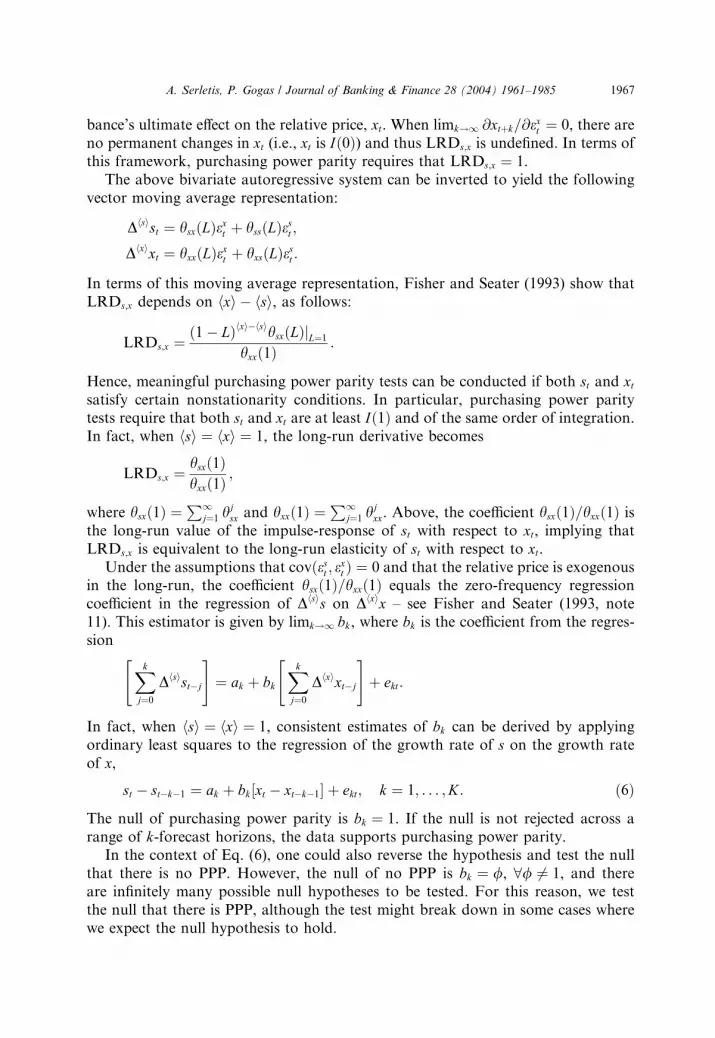
st � st�k�1 ¼ ak þ bk½xt � xt�k�1� þ ekt; k ¼ 1; . . . ;K: ð6Þ
The null of purchasing power parity is bk ¼ 1. If the null is not rejected across a
range of k-forecast horizons, the data supports purchasing power parity.In the context of Eq. (6), one could also reverse the hypothesis and test the null
that there is no PPP. However, the null of no PPP is bk ¼ /, 8/ 6¼ 1, and there
are infinitely many possible null hypotheses to be tested. For this reason, we test
the null that there is PPP, although the test might break down in some cases where
we expect the null hypothesis to hold.

1968 A. Serletis, P. Gogas / Journal of Banking & Finance 28 (2004) 1961–1985
4. Data and the LRD tests
The data, taken from the IMF International Financial Statistics, consist of quar-
terly nominal exchange rates and consumer price indices covering the period 1973:1
to 1998:4 for 21 OECD countries. A final demand price is used in the calculation ofthe relative price instead of an output price, because of unavailability of the same
quarterly output price for each country. It is to be noticed, however, that Perron
and Vogelsang (1992) argue that the results for PPP tests could depend on the price
used.
The countries involved are Australia, Austria, Belgium, Canada, Denmark, Fin-
land, France, Germany, Greece, Ireland, Italy, Japan, the Netherlands, New Zea-
land, Norway, Portugal, Spain, Sweden, Switzerland, the United Kingdom, and
the United States. In investigating purchasing power parity, however, we consider60 bilateral intercountry relations; twenty relations between the United States as
the home country and the other countries as the foreign countries; 20 relations be-
tween Germany as the home country and the other countries as the foreign countries;
and 20 relations between Japan as the home country and the other countries as the
foreign countries.
As was argued in the previous section, meaningful long-horizon regression tests of
purchasing power parity require that both st and xt are at least integrated of order
one and of the same order of integration. We investigate this issue by calculatingp-values [based on the response surface estimates given by MacKinnon (1994)] for
the augmented Dickey–Fuller (ADF) test – see Dickey and Fuller (1981) and report
the results in panel A of Tables 1–3. 7 Based on these p-values, the null hypothesis ofa unit root in log levels cannot be rejected at the 5% level, except for 10 out of the 120
series being tested.
In particular, we reject the null hypothesis of a unit root with the DM-based ex-
change rates for Austria and the Netherlands and the yen-based exchange rates for
Canada, Finland, and Switzerland. In each of these cases, LRDs;x ¼ 0 by definition,since there are no permanent changes in the exchange rate and purchasing power
parity is violated. Moreover, we reject the null hypothesis of a unit root with the
U.S.-based relative prices for Belgium, Japan, and the United Kingdom, the
Germany-based relative price for the Netherlands, and the Japan-based relative price
for the United States. In each of these cases, LRDs;x cannot be defined. It is to be
noted that traditional explanations of purchasing power parity would favor accep-
tance of purchasing power parity for the bilateral Germany–Netherlands relation,
at least more so than for many of the other bilateral relations we analyze in thispaper. In Table 2, however, the null hypotheses of a unit root in the DM-based ex-
change rate for the Netherlands as well as the Germany-based relative price for the
Netherlands are rejected at the 5% level. Although just a single case, the fact that the
7 The optimal lag length was taken to be the order selected by the Akaike Information Criterion (AIC)
plus 2 – see Pantula et al. (1994) for details regarding the advantages of this rule for choosing the number
of augmenting lags.
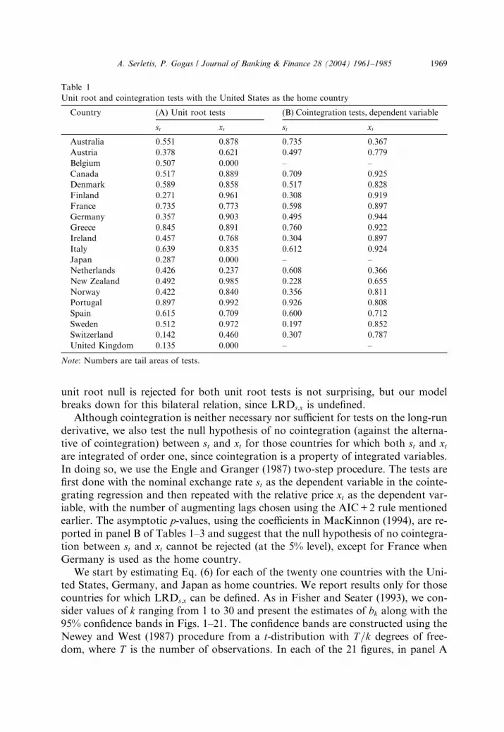
Table 1
Unit root and cointegration tests with the United States as the home country
Country (A) Unit root tests (B) Cointegration tests, dependent variable
st xt st xt
Australia 0.551 0.878 0.735 0.367
Austria 0.378 0.621 0.497 0.779
Belgium 0.507 0.000 – –
Canada 0.517 0.889 0.709 0.925
Denmark 0.589 0.858 0.517 0.828
Finland 0.271 0.961 0.308 0.919
France 0.735 0.773 0.598 0.897
Germany 0.357 0.903 0.495 0.944
Greece 0.845 0.891 0.760 0.922
Ireland 0.457 0.768 0.304 0.897
Italy 0.639 0.835 0.612 0.924
Japan 0.287 0.000 – –
Netherlands 0.426 0.237 0.608 0.366
New Zealand 0.492 0.985 0.228 0.655
Norway 0.422 0.840 0.356 0.811
Portugal 0.897 0.992 0.926 0.808
Spain 0.615 0.709 0.600 0.712
Sweden 0.512 0.972 0.197 0.852
Switzerland 0.142 0.460 0.307 0.787
United Kingdom 0.135 0.000 – –
Note: Numbers are tail areas of tests.
A. Serletis, P. Gogas / Journal of Banking & Finance 28 (2004) 1961–1985 1969
unit root null is rejected for both unit root tests is not surprising, but our model
breaks down for this bilateral relation, since LRDs;x is undefined.
Although cointegration is neither necessary nor sufficient for tests on the long-run
derivative, we also test the null hypothesis of no cointegration (against the alterna-
tive of cointegration) between st and xt for those countries for which both st and xtare integrated of order one, since cointegration is a property of integrated variables.
In doing so, we use the Engle and Granger (1987) two-step procedure. The tests are
first done with the nominal exchange rate st as the dependent variable in the cointe-grating regression and then repeated with the relative price xt as the dependent var-iable, with the number of augmenting lags chosen using the AIC+2 rule mentioned
earlier. The asymptotic p-values, using the coefficients in MacKinnon (1994), are re-
ported in panel B of Tables 1–3 and suggest that the null hypothesis of no cointegra-
tion between st and xt cannot be rejected (at the 5% level), except for France when
Germany is used as the home country.
We start by estimating Eq. (6) for each of the twenty one countries with the Uni-
ted States, Germany, and Japan as home countries. We report results only for thosecountries for which LRDs;x can be defined. As in Fisher and Seater (1993), we con-
sider values of k ranging from 1 to 30 and present the estimates of bk along with the
95% confidence bands in Figs. 1–21. The confidence bands are constructed using the
Newey and West (1987) procedure from a t-distribution with T=k degrees of free-
dom, where T is the number of observations. In each of the 21 figures, in panel A

Table 2
Unit root and cointegration tests with Germany as the home country
Country (A) Unit root tests (B) Cointegration tests, depen-
dent variable
st xt st xt
Australia 0.205 0.918 0.123 0.947
Austria 0.000 0.825 – –
Belgium 0.945 0.907 0.241 0.057
Canada 0.163 0.980 0.100 0.967
Denmark 0.991 0.971 0.252 0.163
Finland 0.079 0.816 0.145 0.980
France 0.974 0.887 0.030 0.048
Greece 0.994 0.992 0.144 0.242
Ireland 0.863 0.605 0.409 0.807
Italy 0.779 0.963 0.615 0.892
Japan 0.190 0.187 0.757 0.894
Netherlands 0.018 0.005 – –
New Zealand 0.740 0.989 0.384 0.866
Norway 0.198 0.945 0.149 0.911
Portugal 0.989 0.997 0.036 0.132
Spain 0.904 0.982 0.543 0.723
Sweden 0.174 0.999 0.074 0.958
Switzerland 0.198 0.454 0.020 0.710
United Kingdom 0.239 0.062 0.341 0.673
United States 0.357 0.903 0.495 0.944
Note: Numbers are tail areas of tests.
1970 A. Serletis, P. Gogas / Journal of Banking & Finance 28 (2004) 1961–1985
we present the results for the U.S. dollar-based exchange rates, in panel B for the
DM-based exchange rates, and in panel C for the Japanese yen-based exchange rates.
The evidence shows that the null hypothesis that bk ¼ 1 cannot be rejected for
most countries when U.S. dollar-based exchange rates are used. In particular, the
evidence in panel A of Figs. 1–21 indicates that purchasing power parity cannot
be rejected for any k 2 ½1; 30� for 11 countries: Australia, Denmark, Greece, Italy,
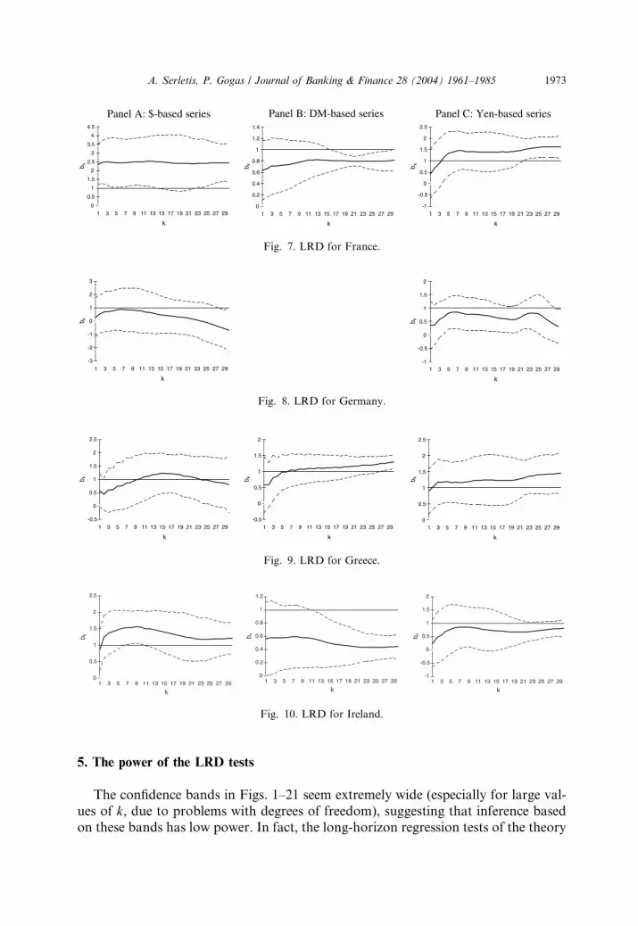
the Netherlands, New Zealand, Norway, Portugal, Spain, Sweden, and Switzerland.There is also evidence in support of purchasing power parity for Austria and Ger-
many where the null hypothesis that bk ¼ 1 is rejected only for k 2 ½28; 30�, andfor Ireland where bk ¼ 1 is rejected only for k 2 ½7; 10�. For Belgium, Japan, and
the United Kingdom there are no permanent changes in their relative prices and thus
LRDs;x is undefined.
When DM-based exchange rates are used, the evidence in panel B of Figs. 1–21
suggests that purchasing power parity cannot be rejected for all values of k only
for Australia, Portugal, and Switzerland. There is also evidence consistent with pur-chasing power parity for France for k ¼ ½1; 16�, for New Zealand for k ¼ ½1; 26�, andfor Greece and the United States for k ¼ ½1; 27�. The null hypothesis that bk ¼ 1 is
rejected for the rest of the countries, when Germany is used as the home country.
Moreover, for Austria and the Netherlands there is no purchasing power issue to
be tested since there are no permanent changes in their respective relative prices.
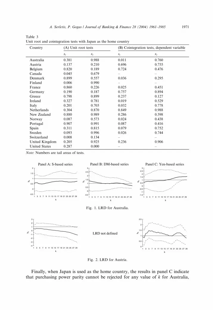
Table 3
Unit root and cointegration tests with Japan as the home country
Country (A) Unit root tests (B) Cointegration tests, dependent variable
st xt st xt
Australia 0.381 0.988 0.011 0.760
Austria 0.137 0.210 0.696 0.755
Belgium 0.820 0.189 0.724 0.476
Canada 0.045 0.679 – –
Denmark 0.899 0.557 0.036 0.295
Finland 0.006 0.990 – –
France 0.860 0.226 0.025 0.451
Germany 0.190 0.187 0.757 0.894
Greece 0.798 0.899 0.237 0.127
Ireland 0.327 0.781 0.019 0.529
Italy 0.201 0.703 0.032 0.778
Netherlands 0.304 0.870 0.849 0.988
New Zealand 0.880 0.989 0.286 0.598
Norway 0.087 0.573 0.024 0.438
Portugal 0.907 0.991 0.087 0.416
Spain 0.311 0.815 0.079 0.752
Sweden 0.093 0.996 0.026 0.744
Switzerland 0.008 0.134 – –
United Kingdom 0.205 0.925 0.236 0.906
United States 0.287 0.000 – –
Note: Numbers are tail areas of tests.
-0.5
0
0.5
1
1.5
2
1 3 5 7 9 11 13 15 17 19 21 23 25 27 29
k
b k
-0.5
0
0.5
1
1.5
2
2.5
3
1 3 5 7 9 11 13 15 17 19 21 23 25 27 29
k
b k
-1.5
-1
-0.5
0
0.5
1
1.5
2
2.5
3
1 3 5 7 9 11 13 15 17 19 21 23 25 27 29
k
b k
Panel A: $-based series Panel B: DM-based series Panel C: Yen-based series
Fig. 1. LRD for Australia.
LRD not defined
-4
-3
-2
-1
0
1
2
3
1 3 5 7 9 11 13 15 17 19 21 23 25 27 29
k
b k
0
0.5
1
1.5
2
2.5
1 3 5 7 9 11 13 15 17 19 21 23 25 27 29
k
b k
Fig. 2. LRD for Austria.
A. Serletis, P. Gogas / Journal of Banking & Finance 28 (2004) 1961–1985 1971
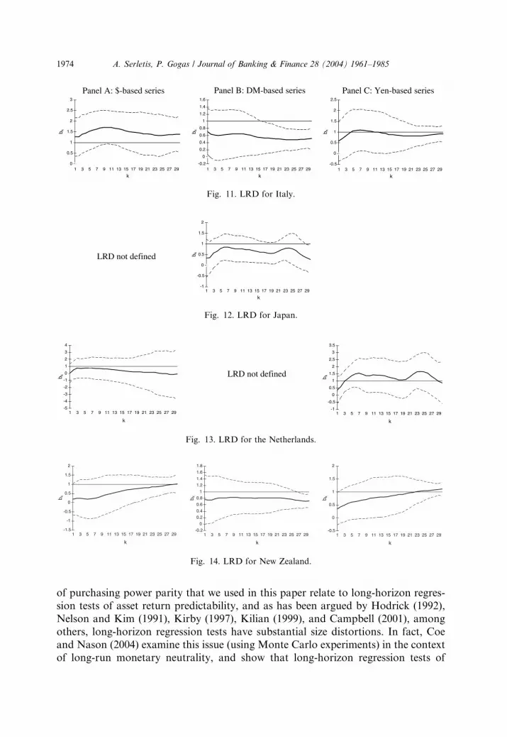
Finally, when Japan is used as the home country, the results in panel C indicate
that purchasing power parity cannot be rejected for any value of k for Australia,
LRD not defined
-20
-15
-10
-5
0
5
1 3 5 7 9 11 13 15 17 19 21 23 25 27 29
k
b k
-8
-6
-4
-2
0
2
4
6
8
10
12
1 3 5 7 9 11 13 15 17 19 21 23 25 27 29
k
b k
Panel A: $-based series Panel B: DM-based series Panel C: Yen-based series
Fig. 3. LRD for Belgium.
LRD not defined
-2
-1.5
-1
-0.5
0
0.5
1
1.5
1 3 5 7 9 11 13 15 17 19 21 23 25 27 29
k
b k
-2.5-2
-1.5-1
-0.50
0.51
1.52
2.5
1 3 5 7 9 11 13 15 17 19 21 23 25 27 29
k
b k
Fig. 4. LRD for Canada.
-2
-1
0
1
2
3
4
5
1 3 5 7 9 11 13 15 17 19 21 23 25 27 29
k
b k
0
0.2
0.4
0.6
0.8
1
1.2
1 3 5 7 9 11 13 15 17 19 21 23 25 27 29
k
b k
-1
-0.5
0
0.5
1
1.5
2
2.5
1 3 5 7 9 11 13 15 17 19 21 23 25 27 29
k
b k
Fig. 5. LRD for Denmark.
LRD not defined
-2
-1.5
-1
-0.5
0
0.5
1
1.5
2
1 3 5 7 9 11 13 15 17 19 21 23 25 27 29
k
b k
-1.5
-1
-0.5
0
0.5
1
1.5
1 3 5 7 9 11 13 15 17 19 21 23 25 27 29
k
b k
Fig. 6. LRD for Finland.
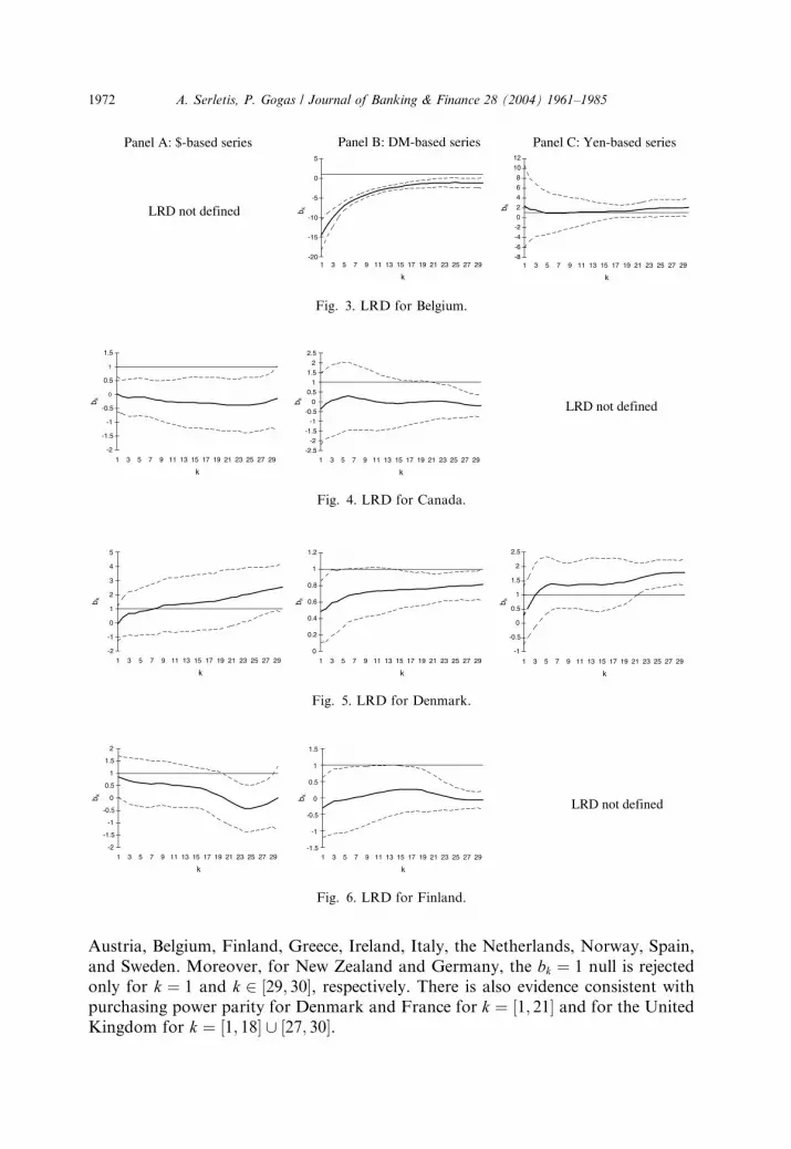
1972 A. Serletis, P. Gogas / Journal of Banking & Finance 28 (2004) 1961–1985
Austria, Belgium, Finland, Greece, Ireland, Italy, the Netherlands, Norway, Spain,
and Sweden. Moreover, for New Zealand and Germany, the bk ¼ 1 null is rejected
only for k ¼ 1 and k 2 ½29; 30�, respectively. There is also evidence consistent with
purchasing power parity for Denmark and France for k ¼ ½1; 21� and for the United
Kingdom for k ¼ ½1; 18� [ ½27; 30�.
0
0.5
1
1.5
2
2.5
3
3.5
4
4.5
1 3 5 7 9 11 13 15 17 19 21 23 25 27 29
k
b k
-1
-0.5
0
0.5
1
1.5
2
2.5
1 3 5 7 9 11 13 15 17 19 21 23 25 27 29
k
b k
0
0.2
0.4
0.6
0.8
1
1.2
1.4
1 3 5 7 9 11 13 15 17 19 21 23 25 27 29
k
b k
Panel A: $-based series Panel B: DM-based series Panel C: Yen-based series
Fig. 7. LRD for France.
-3
-2
-1
0
1
2
3
1 3 5 7 9 11 13 15 17 19 21 23 25 27 29
k
b k
-1
-0.5
0
0.5
1
1.5
2
1 3 5 7 9 11 13 15 17 19 21 23 25 27 29
k
b kFig. 8. LRD for Germany.
-0.5
0
0.5
1
1.5
2
2.5
1 3 5 7 9 11 13 15 17 19 21 23 25 27 29
k
b k
-0.5
0
0.5
1
1.5
2
1 3 5 7 9 11 13 15 17 19 21 23 25 27 29
k
b k
0
0.5
1
1.5
2
2.5
1 3 5 7 9 11 13 15 17 19 21 23 25 27 29
k
b k
Fig. 9. LRD for Greece.
0
0.5
1
1.5
2
2.5
1 3 5 7 9 11 13 15 17 19 21 23 25 27 29
k
b k
0
0.2
0.4
0.6
0.8
1
1.2
1 3 5 7 9 11 13 15 17 19 21 23 25 27 29
k
b k
-1
-0.5
0
0.5
1
1.5
2
1 3 5 7 9 11 13 15 17 19 21 23 25 27 29
k
b k
Fig. 10. LRD for Ireland.
A. Serletis, P. Gogas / Journal of Banking & Finance 28 (2004) 1961–1985 1973
5. The power of the LRD tests
The confidence bands in Figs. 1–21 seem extremely wide (especially for large val-
ues of k, due to problems with degrees of freedom), suggesting that inference basedon these bands has low power. In fact, the long-horizon regression tests of the theory
0
0.5
1
1.5
2
2.5
3
1 3 5 7 9 11 13 15 17 19 21 23 25 27 29
k
b k
-0.2
0
0.2
0.4
0.6
0.8
1
1.2
1.4
1.6
1 3 5 7 9 11 13 15 17 19 21 23 25 27 29
k
b k
-0.5
0
0.5
1
1.5
2
2.5
1 3 5 7 9 11 13 15 17 19 21 23 25 27 29
k
b k
Panel A: $-based series Panel B: DM-based series Panel C: Yen-based series
Fig. 11. LRD for Italy.
-1.5
-1
-0.5
0
0.5
1
1.5
2
1 3 5 7 9 11 13 15 17 19 21 23 25 27 29
k
b k
-0.2
0
0.2
0.4
0.6
0.8
1
1.2
1.4
1.6
1.8
1 3 5 7 9 11 13 15 17 19 21 23 25 27 29
k
b k
-0.5
0
0.5
1
1.5
2
1 3 5 7 9 11 13 15 17 19 21 23 25 27 29
k
b k
Fig. 14. LRD for New Zealand.
LRD not defined
-1
-0.5
0
0.5
1
1.5
2
1 3 5 7 9 11 13 15 17 19 21 23 25 27 29
k
b k
Fig. 12. LRD for Japan.
LRD not defined
-5
-4
-3
-2
-1
0
1
2
3
4
1 3 5 7 9 11 13 15 17 19 21 23 25 27 29
k
b k
-1
-0.5
0
0.5
1
1.5
2
2.5
3
3.5
1 3 5 7 9 11 13 15 17 19 21 23 25 27 29
k
b k
Fig. 13. LRD for the Netherlands.
1974 A. Serletis, P. Gogas / Journal of Banking & Finance 28 (2004) 1961–1985
of purchasing power parity that we used in this paper relate to long-horizon regres-
sion tests of asset return predictability, and as has been argued by Hodrick (1992),
Nelson and Kim (1991), Kirby (1997), Kilian (1999), and Campbell (2001), among
others, long-horizon regression tests have substantial size distortions. In fact, Coe
and Nason (2004) examine this issue (using Monte Carlo experiments) in the context
of long-run monetary neutrality, and show that long-horizon regression tests of

-1.5
-1
-0.5
0
0.5
1
1.5
2
2.5
1 3 5 7 9 11 13 15 17 19 21 23 25 27 29
k
b k
-1
-0.5
0
0.5
1
1.5
1 3 5 7 9 11 13 15 17 19 21 23 25 27 29
k
b k
0
0.5
1
1.5
2
2.5
1 3 5 7 9 11 13 15 17 19 21 23 25 27 29
k
b k
Panel A: $-based series Panel B: DM-based series Panel C: Yen-based series
Fig. 15. LRD for Norway.
0
0.5
1
1.5
2
2.5
3
1 3 5 7 9 11 13 15 17 19 21 23 25 27 29
k
b k
0
0.2
0.4
0.6
0.8
1
1.2
1.4
1.6
1 3 5 7 9 11 13 15 17 19 21 23 25 27 29
k
b k
0
0.5
1
1.5
2
2.5
1 3 5 7 9 11 13 15 17 19 21 23 25 27 29
k
b k
Fig. 16. LRD for Portugal.
-0.5
0
0.5
1
1.5
2
2.5
3
1 3 5 7 9 11 13 15 17 19 21 23 25 27 29
k
b k
0
0.2
0.4
0.6
0.8
1
1.2
1.4
1.6
1.8
1 3 5 7 9 11 13 15 17 19 21 23 25 27 29
k
b k
-0.5
0
0.5
1
1.5
2
2.5
3
1 3 5 7 9 11 13 15 17 19 21 23 25 27 29
k
b k
Fig. 17. LRD for Spain.
-4
-3
-2
-1
0
1
2
3
1 3 5 7 9 11 13 15 17 19 21 23 25 27 29
k
b k
-1.5
-1
-0.5
0
0.5
1
1.5
2
1 3 5 7 9 11 13 15 17 19 21 23 25 27 29
k
b k
-0.5
0
0.5
1
1.5
2
2.5
3
1 3 5 7 9 11 13 15 17 19 21 23 25 27 29
k
b k
Fig. 18. LRD for Sweden.
A. Serletis, P. Gogas / Journal of Banking & Finance 28 (2004) 1961–1985 1975
long-run monetary neutrality are uninformative because of large-size distortions and
that size-adjusted critical values do not offer greater power.
Because we have given PPP the status of the null hypothesis in a test with (appar-
ently) low power, when purchasing power parity is not rejected, only alternativesthat have low type II error probability can be ruled out. To separate those alterna-
tives to purchasing power parity that are inconsistent with the data, in this section we
LRD not defined
-1.5
-1
-0.5
0
0.5
1
1.5
2
2.5
3
1 3 5 7 9 11 13 15 17 19 21 23 25 27 29
k
b k
-1.5
-1
-0.5
0
0.5
1
1.5
2
2.5
3
1 3 5 7 9 11 13 15 17 19 21 23 25 27 29
k
b k
Panel A: $-based series Panel B: DM-based series Panel C: Yen-based series
Fig. 19. LRD for Switzerland.
LRD not defined
-1
-0.5
0
0.5
1
1.5
1 3 5 7 9 11 13 15 17 19 21 23 25 27 29
k
b k
-4
-3
-2
-1
0
1
2
3
1 3 5 7 9 11 13 15 17 19 21 23 25 27 29
k
b kFig. 20. LRD for the United Kingdom.
LRD not defined
-3
-2
-1
0
1
2
3
1 3 5 7 9 11 13 15 17 19 21 23 25 27 29
k
b k
Fig. 21. LRD for the United States.
1976 A. Serletis, P. Gogas / Journal of Banking & Finance 28 (2004) 1961–1985
follow Coe and Nason (2003) and use the inverse power function (IPF) of Andrews
(1989) to provide information about deviations from the null hypothesis (of purchas-
ing power parity) when the LRD tests fail to reject the null at a given level of signif-
icance.
In Table 4 we report ordinary least squares estimates of bk, tests of PPP, and
Andrews (1989) IPFs, at forecast horizons k ¼ 10, 15, 20, 25, and 30, for dollar-
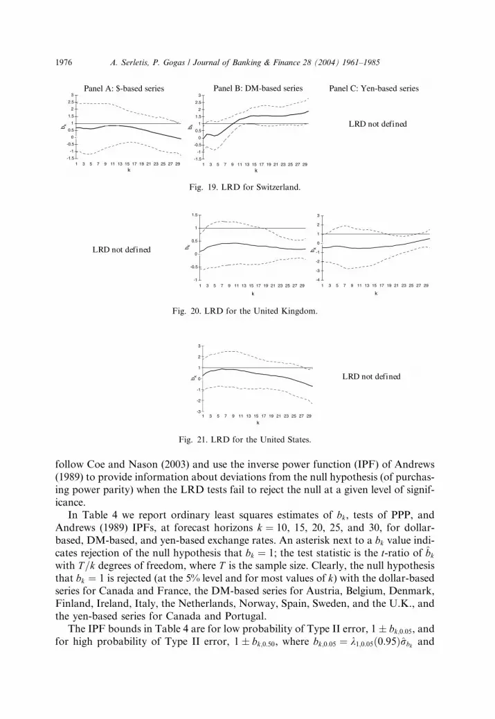
based, DM-based, and yen-based exchange rates. An asterisk next to a bk value indi-cates rejection of the null hypothesis that bk ¼ 1; the test statistic is the t-ratio of b̂kwith T=k degrees of freedom, where T is the sample size. Clearly, the null hypothesis
that bk ¼ 1 is rejected (at the 5% level and for most values of k) with the dollar-based
series for Canada and France, the DM-based series for Austria, Belgium, Denmark,
Finland, Ireland, Italy, the Netherlands, Norway, Spain, Sweden, and the U.K., and
the yen-based series for Canada and Portugal.
The IPF bounds in Table 4 are for low probability of Type II error, 1� bk;0:05, andfor high probability of Type II error, 1� bk;0:50, where bk;0:05 ¼ k1;0:05ð0:95Þr̂bk and

Table 4
CPI-Based estimates of bk , Tests of PPP, and IPF bounds
Country $-based series DM-based series Yen-based series
k ¼ 10 k ¼ 15 k ¼ 20 k ¼ 25 k ¼ 30 k ¼ 10 k ¼ 15 k ¼ 20 k ¼ 25 k ¼ 30 k ¼ 10 k ¼ 15 k ¼ 20 k ¼ 25 k ¼ 30
Australia b̂k 0.59 0.72 0.75 0.67 0.75 1.01 0.98 1.06 0.92 0.72 0.86 0.92 1.21 1.51 1.58
1� bk;0:05 )0.22 )0.33 )0.35 )0.17 )0.02 )0.52 )0.17 0.08 0.34 0.57 )1.88 )1.68 )1.02 0.01 0.34
1þ bk;0:05 2.22 2.33 2.35 2.17 2.02 2.52 2.17 1.92 1.66 1.43 3.88 3.68 3.02 1.99 1.66
1� bk;0:50 0.34 0.28 0.27 0.36 0.45 0.18 0.36 0.50 0.64 0.77 )0.57 )0.46 )0.10 0.46 0.64
1þ bk;0:50 1.66 1.72 1.73 1.64 1.55 1.82 1.64 1.50 1.36 1.23 2.57 2.46 2.10 1.54 1.36
Austria b̂k 0.32 0.04 )0.20 )0.52 )1.19� )0.09� )0.02� )0.04� )0.16� )0.24� 1.27 1.15 0.98 1.26 0.70
1� bk;0:05 )1.52 )1.40 )1.07 )1.29 – – – – – – )0.20 )0.04 )0.02 0.02 0.21
1þ bk;0:05 3.52 3.40 3.07 3.29 – – – – – – 2.20 2.04 2.02 1.98 1.79
1� bk;0:50 )0.37 )0.30 )0.13 )0.24 – – – – – – 0.35 0.43 0.45 0.47 0.57
1þ bk;0:50 2.37 2.30 2.13 2.24 – – – – – – 1.65 1.57 1.55 1.53 1.43
Belgium b̂k )0.19 0.75 1.65 2.57 2.74 )3.69� )2.14� )1.37� )1.12� )1.15� 1.06 1.25 1.44 1.99 2.06
1� bk;0:05 )1.65 )1.33 )1.37 )1.93 )3.24 – – – – – )3.73 )1.53 )0.84 )1.28 )1.131þ bk;0:05 3.65 3.33 3.37 3.93 5.24 – – – – – 5.73 3.53 2.84 3.28 3.13
1� bk;0:50 )0.44 )0.27 )0.29 )0.60 )1.30 – – – – – )1.57 )0.38 0.00 )0.24 )0.161þ bk;0:50 2.44 2.27 2.29 2.60 3.30 – – – – – 3.57 2.38 2.00 2.24 2.16
Canada b̂k )0.25� )0.28� )0.35� )0.38� )0.13 0.08 )0.09 0.01 )0.04� )0.22� )0.03 )0.50� )0.59� 0.02 0.29�
1� bk;0:05 – – – – )0.31 )1.50 )0.88 )0.45 – – )1.57 – – )0.31 –
1þ bk;0:05 – – – – 2.31 3.50 2.88 2.45 – – 3.57 – – 2.31 –
1� bk;0:50 – – – – 0.29 )0.36 )0.02 0.21 – – )0.40 – – 0.29 –
1þ bk;0:50 – – – – 1.71 2.36 2.02 1.79 – – 2.40 – – 1.71 –
Denmark b̂k 1.28 1.43 1.71 2.11 2.52 0.72 0.75� 0.76� 0.79� 0.8� 1.35 1.35 1.49 1.74� 1.80�
1� bk;0:05 )2.07 )2.02 )1.90 )1.37 )1.01 0.52 – – – – )0.30 )0.42 0.01 – –
1þ bk;0:05 4.07 4.02 3.90 3.37 3.01 1.48 – – – – 2.30 2.42 1.99 – –
1� bk;0:50 )0.67 )0.64 )0.58 )0.29 )0.09 0.74 – – – 0.29 0.23 0.46 – –
1þ bk;0:50 2.67 2.64 2.58 2.29 2.09 1.26 – – – – 1.71 1.77 1.54 – –
Finland b̂k 0.56 0.42 0.02� )0.42� 0.00 0.12� 0.26� 0.20� )0.0� )0.05� 0.71 0.67 0.36 0.37 0.48
1� bk;0:05 )0.46 )0.23 – – )0.46 – – – – – )2.53 )2.17 )0.95 0.05 0.24
1þ bk;0:05 2.46 2.23 – – 2.46 – – – – – 4.53 4.17 2.95 1.95 1.76
1� bk;0:50 0.21 0.33 – – 0.21 – – – – – )0.92 )0.72 )0.06 0.49 0.59
1þ bk;0:50 1.79 1.67 – – 1.79 – – – – – 2.92 2.72 2.06 1.51 1.41
A.Serletis,
P.Gogas/JournalofBanking&
Finance
28(2004)1961–1985
1977

Table 4 (continued)
Country $-based series DM-based series Yen-based series
k ¼ 10 k ¼ 15 k ¼ 20 k ¼ 25 k ¼ 30 k ¼ 10 k ¼ 15 k ¼ 20 k ¼ 25 k ¼ 30 k ¼ 10 k ¼ 15 k ¼ 20 k ¼ 25 k ¼ 30
France b̂k 2.52� 2.50 2.41 2.42� 2.45� 0.80 0.81 0.80� 0.79� 0.81 1.41 1.39 1.43 1.61� 1.61�
1� bk;0:05 – )1.34 )1.21 – – 0.42 0.66 – – 0.78 )0.32 )0.31 0.11 – –
1þ bk;0:05 – 3.34 3.21 – – 1.58 1.34 – – 1.22 2.32 2.31 1.89 – –
1� bk;0:50 – )0.27 )0.20 – – 0.69 0.81 – – 0.88 0.28 0.29 0.51 – –
1þ bk;0:50 – 2.27 2.20 – – 1.31 1.19 – – 1.12 1.72 1.71 1.49 – –
Germany b̂k 0.81 0.48 0.26 )0.09 )0.70� 0.77 0.66 0.57 0.78 0.28�
1� bk;0:05 )1.67 )1.17 )0.77 )0.85 – 0.01 0.18 0.29 0.05 –
1þ bk;0:05 3.67 3.17 2.77 2.85 – 1.99 1.82 1.71 1.95 –
1� bk;0:50 )0.45 )0.18 0.04 0.00 – 0.46 0.56 0.61 0.48 –
1þ bk;0:50 2.45 2.18 1.96 2.00 – 1.54 1.44 1.39 1.52 –
Greece b̂k 1.02 1.23 1.12 0.97 0.80 1.06 1.11 1.15 1.21 1.29� 1.19 1.24 1.24 1.40 1.45
1� bk;0:05 )0.44 )0.15 )0.09 )0.15 )0.21 0.26 0.37 0.53 0.65 – )0.15 )0.21 0.06 0.23 0.24
1þ bk;0:05 2.44 2.15 2.09 2.15 2.21 1.74 1.63 1.47 1.35 – 2.15 2.21 1.94 1.77 1.76
1� bk;0:50 0.22 0.37 0.41 0.38 0.34 0.60 0.66 0.75 0.81 – 0.37 0.34 0.49 0.58 0.59
1þ bk;0:50 1.78 1.63 1.59 1.62 1.66 1.40 1.34 1.25 1.19 – 1.63 1.66 1.51 1.42 1.41
Ireland b̂k 1.54� 1.41 1.25 1.19 1.21 0.57 0.49� 0.45� 0.43� 0.45� 0.84 0.72 0.67 0.74 0.80
1� bk;0:05 – 0.05 0.00 0.20 0.43 0.27 – – – – )0.24 )0.15 0.34 0.58 0.61
1þ bk;0:05 – 1.95 2.00 1.80 1.57 1.73 – – – – 2.24 2.15 1.66 1.42 1.39
1� bk;0:50 – 0.48 0.45 0.57 0.69 0.60 – – – – 0.33 0.38 0.64 0.77 0.79
1þ bk;0:50 – 1.52 1.55 1.43 1.31 1.40 – – – – 1.67 1.62 1.36 1.23 1.21
Italy b̂k 1.71 1.56 1.42 1.34 1.39 0.65 0.55 0.51� 0.48� 0.51� 1.03 0.89 0.81 0.85 0.92
1� bk;0:05 )0.26 )0.30 )0.39 )0.24 0.02 )0.05 0.24 – – – )0.57 )0.32 0.13 0.45 0.55
1þ bk;0:05 2.26 2.30 2.39 2.24 1.98 2.05 1.76 – – – 2.57 2.32 1.87 1.55 1.45
1� bk;0:50 0.31 0.29 0.25 0.33 0.47 0.43 0.59 – – – 0.15 0.28 0.53 0.70 0.75
1þ bk;0:50 1.69 1.71 1.75 1.67 1.53 1.57 1.41 – – – 1.85 1.72 1.47 1.30 1.25
Japan b̂k )0.01 )0.38 )0.85� )0.61 )0.24 0.77 0.66 0.57 0.78 0.28�
1� bk;0:05 )0.97 )1.12 – )2.02 )1.64 0.01 0.18 0.29 0.05 –
1þ bk;0:05 2.97 3.12 – 4.02 3.64 1.99 1.82 1.71 1.95 –
1� bk;0:50 )0.07 )0.15 – )0.64 )0.44 0.46 0.56 0.61 0.48 –
1þ bk;0:50 2.07 2.15 – 2.64 2.44 1.54 1.44 1.39 1.52 –
1978
A.Serletis,
P.Gogas/JournalofBanking&
Finance
28(2004)1961–1985

Netherlands b̂k 0.66 0.41 0.21 0.04 )0.12 0.15� 0.25� 0.31� 0.35� 0.36� 1.38 1.29 1.11 1.65 0.87
1� bk;0:05 )1.60 )1.65 )2.20 )3.07 )3.15 – – – – – )0.94 )0.84 )0.81 )0.75 )0.681þ bk;0:05 3.60 3.65 4.20 5.07 5.15 – – – – 2.94 2.84 2.81 2.75 2.68
1� bk;0:50 )0.41 )0.44 )0.74 )1.21 )1.26 – – – – )0.06 0.00 0.01 0.05 0.09
1þ bk;0:50 2.41 2.44 2.74 3.21 3.26 – – – – 2.06 2.00 1.99 1.95 1.91
New
Zealand
b̂k 0.42 0.65 0.79 0.89 1.03 0.83 0.80 0.72� 0.76 0.82 0.94 1.04 1.12
1� bk;0:05 )0.72 )0.33 0.04 0.35 0.42 0.16 0.26 – )0.22 )0.15 0.10 0.52 0.71
1þ bk;0:05 2.72 2.33 1.96 1.65 1.58 1.84 1.74 – 2.22 2.15 1.90 1.48 1.29
1� bk;0:50 0.07 0.28 0.48 0.64 0.69 0.54 0.60 – 0.34 0.37 0.51 0.74 0.84
1þ bk;0:50 1.93 1.72 1.52 1.36 1.31 1.46 1.40 – 1.66 1.63 1.49 1.26 1.16
Norway b̂k 0.49 0.46 0.38 0.39 0.51 0.44 0.41� 0.40� 1.08 0.92 0.82 1.13 1.21
1� bk;0:05 )1.57 )1.41 )0.97 )0.29 0.15 )0.01 – – – )0.06 )0.15 0.08 0.43 0.61
1þ bk;0:05 3.57 3.41 2.97 2.29 1.85 2.01 – – – 2.06 2.15 1.92 1.57 1.39
1� bk;0:50 )0.40 )0.31 )0.07 0.30 0.54 0.45 – – – 0.42 0.38 0.50 0.69 0.79
1þ bk;0:50 2.40 2.31 2.07 1.70 1.46 1.55 – – – 1.58 1.62 1.50 1.31 1.21
Portugal b̂k 1.35 1.41 1.44 1.56 1.70 1.15 1.13 1.14 1.58� 1.52� 1.45� 1.47� 1.54�
1� bk;0:05 0.08 0.14 0.04 0.04 0.13 0.45 0.60 0.78 – – – – –
1þ bk;0:05 1.92 1.86 1.96 1.96 1.87 1.55 1.40 1.22 – – – – –
1� bk;0:50 0.50 0.53 0.48 0.48 0.53 0.70 0.78 0.88 – – – – –
1þ bk;0:50 1.50 1.47 1.52 1.52 1.47 1.30 1.22 1.12 – – – – –
Spain b̂k 0.91 0.96 1.00 1.31 1.67 0.73 0.66 0.69� 1.47 1.31 1.11 1.18 1.30
1� bk;0:05 )0.38 )0.36 )0.55 )0.57 )0.28 0.20 0.45 – – )0.71 )0.54 )0.07 0.28 0.44
1þ bk;0:05 2.38 2.36 2.55 2.57 2.28 1.80 1.55 – – 2.71 2.54 2.07 1.72 1.56
1� bk;0:50 0.25 0.26 0.16 0.15 0.31 0.57 0.70 – – 0.07 0.16 0.42 0.61 0.69
1þ bk;0:50 1.75 1.74 1.84 1.85 1.69 1.43 1.30 – – 1.93 1.84 1.58 1.39 1.31
Sweden b̂k 0.80 0.64 )0.07 )0.73 )0.79 0.42 0.42 0.42� 1.25 1.13 0.92 1.19 1.28
1� bk;0:05 )1.49 )1.60 )2.07 )1.74 )1.73 )0.83 )0.32 – – )0.76 )0.88 )0.48 0.01 )0.081þ bk;0:05 3.49 3.60 4.07 3.74 3.73 2.83 2.32 – – 2.76 2.88 2.48 1.99 2.08
1� bk;0:50 )0.36 )0.42 )0.67 )0.49 )0.49 0.01 0.28 – – 0.04 )0.02 0.19 0.46 0.41
1þ bk;0:50 2.36 2.42 2.67 2.49 2.49 1.99 1.72 – – 1.96 2.02 1.81 1.54 1.59
A.Serletis,
P.Gogas/JournalofBanking&
Finance
28(2004)1961–1985
1979
–
–
–
0.81 0.77
0.39 0.62
1.61 1.38
0.67 0.79
1.33 1.21
0.43� 0.42�
–
–
–
–
1.11 1.11
0.67 0.71
1.33 1.29
0.82 0.84
1.18 1.16
0.60� 0.61�
–
–
–
–
0.36� 0.30�
–
–
–
–

Table 4 (continued)
Country $-based series DM-based series Yen-based series
k ¼ 10 k ¼ 15 k ¼ 20 k ¼ 25 k ¼ 30 k ¼ 10 k ¼ 15 k ¼ 20 k ¼ 25 k ¼ 30 k ¼ 10 k ¼ 15 k ¼ 20 k ¼ 25 k ¼ 30
Switzerland b̂k 0.84 0.78 0.52 0.20 )0.09 1.13 1.56 1.54 1.62 1.87 1.10 1.07 1.12 1.16 0.92
1� bk;0:05 )1.49 )0.75 )0.49 )0.55 )0.35 0.18 0.10 0.03 0.09 )0.03 )0.08 0.49 0.40 0.21 0.41
1þ bk;0:05 3.49 2.75 2.49 2.55 2.35 1.82 1.90 1.97 1.91 2.03 2.08 1.51 1.60 1.79 1.59
1� bk;0:50 )0.36 0.05 0.19 0.16 0.26 0.55 0.51 0.47 0.50 0.44 0.41 0.72 0.67 0.57 0.68
1þ bk;0:50 2.36 1.95 1.81 1.84 1.74 1.45 1.49 1.53 1.50 1.56 1.59 1.28 1.33 1.43 1.32
U.K. b̂k 0.88 0.49 0.11� 0.10� 0.64 0.42 0.35 0.29� 0.2� 0.20� )0.52 )0.48 )0.27� 0.06� 0.52
1� bk;0:05 )0.03 )0.10 – – 0.27 )0.33 )0.14 – – – )2.46 )1.81 – – )0.101þ bk;0:05 2.03 2.10 – – 1.73 2.33 2.14 – – – 4.46 3.81 – – 2.10
1� bk;0:50 0.44 0.40 – – 0.61 0.28 0.38 – – – )0.88 )0.53 – – 0.40
1þ bk;0:50 1.56 1.60 – – 1.39 1.73 1.62 – – – 2.88 2.53 – – 1.60
U.S. b̂k 0.81 0.48 0.26 )0.09 )0.70� )0.01 )0.38 )0.85� )0.61 )0.241� bk;0:05 )1.67 )1.17 )0.77 )0.85 – )0.97 )1.12 – )2.02 )1.641þ bk;0:05 3.67 3.17 2.77 2.85 – 2.97 3.12 – 4.02 3.64
1� bk;0:50 )0.45 )0.18 0.04 0.00 – )0.07 )0.15 – )0.64 )0.441þ bk;0:50 2.45 2.18 1.96 2.00 – 2.07 2.15 – 2.64 2.44
Note: An asterisk indicates rejection (of the null that bk ¼ 1) at the 5% asymptotic level.
1980
A.Serletis,
P.Gogas/JournalofBanking&
Finance
28(2004)1961–1985

A. Serletis, P. Gogas / Journal of Banking & Finance 28 (2004) 1961–1985 1981
bk;0:50 ¼ k1;0:05ð0:50Þr̂bk , with r̂bk being the standard error of b̂k. The subscripts of
kq;að1� cÞ denote the number of restrictions and the significance of the test, and cis the probability of Type II error. From Andrews (1989, Table 1) we get that
k1;0:05ð0:95Þ ¼ 3:605 and k1;0:05ð0:50Þ ¼ 1:96. In particular, 1� bk;0:05 and 1þ bk;0:05define the region X ¼ ð�1; 1� bk;0:05� [ ½1þ bk;0:05;þ1Þ where the probability ofType II error is small (0.05 or less). In this case, when we fail to reject the null,
we can say with significance 0.05 that there is evidence against any parameter value
in X, or in other words that the true value of bk is 1� bk;0:05 < bk < 1þ bk;0:05; theevidence that we have against any parameter value in X when we fail to reject, is sim-
ilar to the evidence against null parameter values when the test does reject.
Similarly, the estimates of 1� bk;0:50 and 1þ bk;0:50 define the region of high prob-
ability of Type II error, 0.50 or higher suggested as an obvious focal point by An-
drews (1989), W ¼ ½1� bk;0:50; 1þ bk;0:50�. In this region, the probability of Type IIerror is 0.50 or higher, suggesting that the power of the test, defined as P ¼ 1� c,is 0.50 or less; the test provides no evidence for parameter values in region W as
one has a better chance of rejecting a false null by tossing a fair coin than by using
the test. Clearly, the narrower regions X and W are around the tested parameter
value, the higher is the power of the test. To illustrate the usefulness of these mea-
sures of power, consider the results for Portugal with the DM-based series for
k ¼ 30. In this case, X ¼ ð�1; 0:78� [ ½1:22;þ1Þ and W ¼ ½0:88; 1:12�. This means
that the IPFs show that 0:78 < b30 < 1:22 with significance level 0:05, but due tothe low power there is no evidence that it is 0:88 < b30 < 1:12. If we accept that
bk 2 ½0:78; 1:22� is not a significant (from a theoretical point of view) deviation from
PPP, then we conclude that PPP holds.
The IPFs in Table 4 reveal the low power of some of the long-horizon regression
tests of purchasing power parity. Consider, for example, the dollar-based series for
Belgium. The estimate of bk for k ¼ 30 is 2.74 and the null hypothesis that bk ¼ 1
cannot be rejected. However, the low and high probability of type II error regions
are X ¼ ð�1;�3:24� [ ½5:24;þ1Þ and W ¼ ½�1:30; 3:30�, meaning that the LRDtest cannot rule out not only bk ¼ 1 as the true parameter value (in which case
PPP holds), but also any other parameter value in W, including 0 (in which case
PPP does not hold). Hence, we can mark as ‘‘inconclusive’’ all the tests in Table 1
where both 0 and 1 belong to W. In those cases that the null cannot be rejected
and the tests are not inconclusive, the tighter the bands of regions X and W are
around 1, the higher the power of the test is (and the more confident we are that
PPP holds). For example, the results for Portugal show that with the DM-based ser-
ies there is very strong evidence in favor of purchasing power parity, for all values ofk; W is at its widest, ½0:70; 1:30�, when k ¼ 10, and at its tightest, ½0:88; 1:12� whenk ¼ 30.
Assuming that the IPFs in the area of low power are in the region [1 ± 0.4] or
W ¼ ½0:60; 1:40�, the LRD test is powerful enough with the dollar-based series for
Ireland (for k ¼ 30), New Zealand (for k ¼ 25, 30), and the United Kingdom (for
k ¼ 15 and 30). With the DM-based series, the tests that support PPP are powerful
for Australia (for k ¼ 25, 30), France (for k ¼ 10, 15, 30), Greece (for all k except
k ¼ 30), New Zealand (for k ¼ 15, 20, 25), Portugal (for every k), Denmark and
1982 A. Serletis, P. Gogas / Journal of Banking & Finance 28 (2004) 1961–1985
Ireland (for k ¼ 10), Japan (for k ¼ 20), and Spain (for k ¼ 15). Finally, with the
yen-based series, the LRD tests that support PPP are powerful in the case of Austra-
lia (for k ¼ 30), Germany (for k ¼ 20), Ireland (for k ¼ 20, 25, 30), Italy, New Zea-
land, Norway, and Spain (for k ¼ 25, 30), and Switzerland (for k ¼ 15, 20, 30).
Of course, for cut-off values lower than 0.4, we reach different conclusions regard-ing the power of the long-horizon regression tests. Assuming for example, that the
IPFs in the area of low power are in the region [1 ± 0.1] or W ¼ ½0:90; 1:10�, thenwe conclude that the long-horizon regression tests that support PPP have low power
for all the bilateral relations considered.
6. Robustness
Although consumer price indices used so far in this paper (due to the lack of alter-
native output price indices for all 21 countries examined) are less sensitive to ex-
change rate movements, as Burstein et al. (2002) argue exchange rate fluctuations
have a bearing on output prices through the role of imported raw materials and
intermediate goods in production. In this section, we investigate the robustness of
our results to alternative output price indices, using GDP deflators as well as pro-
ducer price indices (PPIs) to calculate relative prices.
In particular, we use nominal and real GDP data from the IMF InternationalFinancial Statistics to calculate the GDP deflators for those countries for which
GDP data exist and then test for purchasing power parity in the same fashion as
in Table 4 – the results of these tests are available upon request. Greece, Ireland,
and New Zealand are not included in these tests because of data availability prob-
lems. Moreover, for a number of countries the deflator-based results are not directly
comparable to those in Table 4, because the GDP data are not available since
1973Q1. In particular, GDP data for Belgium begin in 1985Q1, Denmark in
1988Q1, the Netherlands in 1977Q1, New Zealand in 1988Q3, Portugal in1977Q1, and Sweden in 1980Q1. Based on the evidence using deflator-based relative
prices, we reject purchasing power parity with the dollar- and DM-based series for
all countries. Moreover, we reject PPP for the yen-based series except for Finland
(for k ¼ 30), France and Italy (for k ¼ 25, 30), Norway and Portugal (for k ¼ 30),
Spain (for k ¼ 25, 30), and Switzerland (for k ¼ 15, 30).
Finally, we also perform long-horizon regression tests of purchasing power parity
using producer price indices – these results are also available upon request. Finland
and Portugal are not included in these tests because of data availability problems,and the data for Belgium begin in 1980Q1, Italy in 1981Q1, and Norway in
1977Q1. With the PPI-based estimates of bk and the dollar as the base currency,
the LRD test provides evidence in support of purchasing power parity with adequate
power for Greece (for k ¼ 25, 30), Ireland (for k ¼ 30) and New Zealand (for k ¼ 20,
25, 30). With the DM-based series, the IPFs show that purchasing power parity is
supported with enough power for Australia (for k ¼ 30), Denmark and Switzerland
(for all k except k ¼ 10), Belgium, France and Greece (for all k), Ireland (for k ¼ 10),
New Zealand (for k ¼ 20, 25, 30), Spain (for all k except k ¼ 25), and Sweden (for

A. Serletis, P. Gogas / Journal of Banking & Finance 28 (2004) 1961–1985 1983
k ¼ 25, 30). Finally, with the Japanese yen as the base currency, the LRD tests sup-
port purchasing power parity with sufficient power for Australia and Spain (for
k ¼ 25, 30), Ireland (for all k except k ¼ 20), New Zealand (for k ¼ 20, 25, 30), Swe-
den (for k ¼ 30) and Switzerland (for all k except k ¼ 10).
7. Conclusion
We have tested the purchasing power parity hypothesis using quarterly data (from
the IMF International Financial Statistics) for the recent floating exchange rate per-
iod (1973:1–1998:4) for 21 OECD countries, using U.S. dollar-based, DM-based,
and Japanese yen-based exchange rates. In doing so, we have used the long-run
regression approach of Fisher and Seater (1993) and also investigated the powerof the long-run regression tests using Andrews’ (1989) inverse power functions.
We have demonstrated that the asymptotic power of the long-horizon regression
tests is low, and found weak evidence consistent with purchasing power parity,
although the evidence is stronger when producer prices are used. These results are
consistent with those empirical studies (mentioned in Section 1) covering the major
industrial countries over the recent floating exchange rate period (using tests other
than the ones we have conducted), which generally fail to find support for purchasing
power parity. They are, however, in contrast to those studies (mentioned in the intro-duction) covering different groups of countries, as well as those covering periods of
long duration, or country pairs experiencing large differentials in price movements.
In using the Fisher and Seater (1993) long-run regression approach, we assumed
that exchange rates have no long-run effects on relative prices. Although consumer
price indices are less sensitive to exchange rate movements, as already noted ex-
change rate fluctuations have a bearing on output prices through the role of im-
ported raw materials and intermediate goods in production. Hence, investigating
the robustness of our results to alternative testing methodologies such as, for exam-ple, the King and Watson (1997) approach which allows both variables to be deter-
mined endogenously, is an area for potentially productive future research.
Acknowledgements
We wish to thank Douglas Fisher, Robert King, and John Seater for comments
on an earlier version of this paper, two referees, Patrick Coe, Asghar Shahmoradi,
and conference participants at the 2003 meetings of the Canadian Economics Asso-
ciation at Carleton University. Serletis also gratefully acknowledges support from
the Social Sciences and Humanities Research Council of Canada.
References
Adler, M., Lehman, B., 1983. Deviations from purchasing power parity in the long run. Journal of
Finance 38, 1471–1487.

1984 A. Serletis, P. Gogas / Journal of Banking & Finance 28 (2004) 1961–1985
Andrews, D.W.K., 1989. Power in econometric applications. Econometrica 57, 1059–1090.
Barnett, W.A., Serletis, A., 2000. Martingales, nonlinearity, and chaos. Journal of Economic Dynamics
and Control 24, 703–724.
Burstein, A., Eichenbaum, M., Rebelo, S., 2002. Why is inflation so low after devaluations? University of
Michigan Working Paper, May 2002.
Campbell, J.Y., 2001. Why long horizons: A study of power against persistent alternatives. Journal of
Empirical Finance 8, 459–491.
Cheung, Y.-W., Lai, K., 1993. A fractional cointegration analysis of purchasing power parity. Journal of
Business and Economic Statistics 11, 103–112.
Coe, P.J., Nason, J.M., 2003. The long-horizon regression approach to monetary neutrality: How should
the evidence be interpreted? Economics Letters 78, 351–356.
Coe, P.J., Nason, J.M., 2004. Long-run monetary neutrality and long-horizon regressions. Journal of
Applied Econometrics, forthcoming.
Coe, P.J., Serletis, A., 2002. Bounds tests of the theory of purchasing power parity. Journal of Banking
and Finance 26, 179–199.
Dickey, D.A., Fuller, W.A., 1981. Likelihood ratio statistics for autoregressive time series with a unit root.
Econometrica 49, 1057–1072.
Diebold, F.X., Husted, S., Rush, M., 1991. Real exchange rates under the gold standard. Journal of
Political Economy 99, 1252–1271.
Engle, R.F., Granger, C.W., 1987. Cointegration and error correction: Representation, estimation and
testing. Econometrica 55, 251–276.
Fisher, M., Seater, J., 1993. Long-run neutrality and superneutrality in an ARIMA framework. American
Economic Review 83, 402–415.
Flynn, N.A., Boucher, J.L., 1993. Tests of long-run purchasing power parity using alternative
methodologies. Journal of Macroeconomics 15, 109–122.
Frenkel, J.A., 1980. Exchange rates, prices and money: Lessons from the 1920s. American Economic
Review (Papers and Proceedings) 70, 235–242.
Glen, J.D., 1992. Real exchange rates in the short, medium, and long run. Journal of International
Economics 33, 147–166.
Grilli, V., Kaminsky, G., 1991. Nominal exchange rate regimes and the real exchange rate: Evidence from
the United States and Great Britain, 1885–1986. Journal of Monetary Economics 27, 191–212.
Hansen, B.E., 1996. Inference when a nuisance parameter is not identified under the null hypothesis.
Econometrica 64, 413–430.
Hodrick, R.J., 1992. Dividends yields and expected stock returns: Alternative procedures for inference and
measurement. Review of Financial Studies 5, 357–386.
Johansen, S., 1988. Statistical analysis of cointegration vectors. Journal of Economic Dynamics and
Control 12, 231–254.
Johansen, S., Juselius, K., 1992. Some structural hypotheses in a multivariate cointegration analysis of the
purchasing power parity and the uncovered interest parity for the UK. Journal of Econometrics 53,
211–244.
Kilian, L., 1999. Exchange rates and monetary fundamentals: What do we learn from long-horizon
regressions? Journal of Applied Econometrics 14, 491–510.
King, R., Watson, M., 1997. Testing long-run neutrality. Federal Reserve Bank of Richmond Economic
Quarterly 83, 69–101.
Kirby, C., 1997. Measuring the predictable variation in stock and bond returns. Review of Financial
Studies 10, 579–630.
Koedijk, K.G., Schotman, P.C., Van Dijk, M.A., 1998. The re-emergence of PPP in the 1990s. Journal of
International Money and Finance 17, 51–61.
Kremer, J.J.M., Ericsson, N.R., Dolado, J.J., 1992. The power of cointegration tests. Oxford Bulletin of
Economics and Statistics 54, 325–348.
Kugler, P., Lenz, C., 1993. Multivariate cointegration analysis and the long-run validity of PPP. The
Review of Economics and Statistics, 180–184.

A. Serletis, P. Gogas / Journal of Banking & Finance 28 (2004) 1961–1985 1985
Lothian, J.R., Taylor, M.P., 1996. A real exchange rate behavior: The recent float from the perspective of
the past two centuries. Journal of Political Economy 104, 488–509.
MacKinnon, J.G., 1994. Approximate asymptotic distribution functions for unit-root and cointegration
tests. Journal of Business and Economic Statistics 12, 167–176.
Mark, N.C., 1990. Real and nominal exchange rates in the long run: An empirical investigation. Journal of
International Economics 28, 115–136.
Michael, P., Robert Nobay, A., Peel, D.A., 1997. Transactions costs and nonlinear adjustment in real
exchange rates: An empirical investigation. Journal of Political Economy 105, 862–879.
Nelson, C.R., Kim, M.J., 1991. Predictable stock returns: The role of small sample bias. Journal of
Finance 48, 641–661.
Nelson, C.R., Plosser, C.I., 1982. Trends and random walks in macroeconomic time series: Some evidence
and implications. Journal of Monetary Economics 10, 139–162.
Newey, W.K., West, K.D., 1987. A simple, positive semi-definite, heteroskedasticity and autocorrelation
consistent covariance matrix. Econometrica 55, 703–708.
Nychka, D.W., Ellner, S., Gallant, A.R., McCaffrey, D., 1992. Finding chaos in noisy systems. Journal of
Royal Statistical Society B 54, 399–426.
Pantula, S.G., Gonzalez-Farias, G., Fuller, W., 1994. A comparison of unit-root test criteria. Journal of
Business and Economic Statistics 12, 449–459.
Papell, D.H., Theodoridis, H., 1998. Increasing evidence of purchasing power parity over the current float.
Journal of International Money and Finance 17, 41–50.
Patel, J., 1990. Purchasing power parity as a long-run relation. Journal of Applied Econometrics 5, 367–
379.
Perron, P., 1989. The Great Crash, the oil price shock and the unit root hypothesis. Econometrica 57,
1361–1401.
Perron, P., Vogelsang, T.J., 1992. Nonstationarity and level shifts with an application to purchasing power
parity. Journal of Business and Economic Statistics 10, 301–320.
Pippenger, M.K., 1993. Cointegartion tests of purchasing power parity: The case of Swiss exchange rates.
Journal of International Money and Finance 12, 46–61.
Phylaktis, K., Kassimatis, Y., 1994. Does the real exchange rate follow a random walk. The Pacific Basin
perspective. Journal of International Money and Finance 13, 476–495.
Potter, S.M., 1995. A nonlinear approach to US GNP. Journal of Applied Econometrics 10, 109–125.
Rogoff, K., 1996. The purchasing power parity puzzle. Journal of Economic Literature 34, 647–668.
Serletis, A., 1994. Maximum likelihood cointegration tests of purchasing power parity: Evidence from
seventeen OECD countries. Weltwirtschaftliches Archiv 130, 476–493.
Serletis, A., Gogas, P., 2000. Purchasing power parity, nonlinearity and chaos. Applied Financial
Economics 10, 615–622.
Serletis, A., Zimonopoulos, G., 1997. Breaking trend functions in real exchange rates: Evidence from
seventeen OECD countries. Journal of Macroeconomics 19, 781–802.