Embed Size (px)
Citation preview
Policy Research Working Paper 6081
Liberia
Strategic Policy Options for Medium Term Growth and Development
Sébastien DessusJariya HoffmanHans Lofgren
The World BankAfrica RegionPoverty Reduction and Economic Management Unit &Development Economics Prospects GroupJune 2012
WPS6081P
ublic
Dis
clos
ure
Aut
horiz
edP
ublic
Dis
clos
ure
Aut
horiz
edP
ublic
Dis
clos
ure
Aut
horiz
edP
ublic
Dis
clos
ure
Aut
horiz
ed
Produced by the Research Support Team
Abstract
The Policy Research Working Paper Series disseminates the findings of work in progress to encourage the exchange of ideas about development issues. An objective of the series is to get the findings out quickly, even if the presentations are less than fully polished. The papers carry the names of the authors and should be cited accordingly. The findings, interpretations, and conclusions expressed in this paper are entirely those of the authors. They do not necessarily represent the views of the International Bank for Reconstruction and Development/World Bank and its affiliated organizations, or those of the Executive Directors of the World Bank or the governments they represent.
Policy Research Working Paper 6081
The objective of this paper is to inform Liberia’s medium-term growth and development strategy for 2012–17 and its National Vision: Liberia Rising 2030, both of which are under preparation. The analysis is based on MAMS (Maquette for MDG [Millennium Development Goal]) Simulations, a computable general equilibrium model. A base scenario (designed to represent a central case for the evolution of Liberia’s economy up to 2030) is compared to a set of non-base scenarios that introduce alternative assumptions for the mining sector, government spending on infrastructure and human development, as well as foreign borrowing. The simulations, which cover the period 2012–2030, indicate that rapid expansion of mining output, front-loaded investment in infrastructure, and improved government efficiency may bring about
This paper is a product of the Poverty Reduction and Economic Management, Africa Region; and Development Economics Prospects Group. It is part of a larger effort by the World Bank to provide open access to its research and make a contribution to development policy discussions around the world. Policy Research Working Papers are also posted on the Web at http://econ.worldbank.org. The author may be contacted at [email protected].
rapid growth. The findings underscore the importance of allocative and operational efficiency of public spending. It is also important that the government balance spending on infrastructure and human development as they complement each other and face different constraints. Spending on infrastructure tends to have relatively strong and immediate growth and poverty reduction effects, whereas spending on human development has a stronger positive impact on non-poverty MDG indicators at the cost of lowered economic growth in the short to medium terms. It is important to consider that growth driven by rapid mining expansion entails drawbacks and risks, including the persistence of an enclave economy that will not benefit the majority of the population, and increased vulnerability to fluctuations in iron ore world prices.
Liberia: Strategic Policy Options for Medium Term Growth and Development
Sébastien Dessus Jariya Hoffman Hans Lofgren
JEL classification: C68, E62, O15 Keywords: Computable General Equilibrium, MAMS, Development Strategy, Liberia,
Sector board: Economic Policy
ii
Table of Contents
1. INTRODUCTION AND SUMMARY OF MAIN FINDINGS ........................................................................... 1
2. STRUCTURE OF MAMS ........................................................................................................................... 2
3. BASE SCENARIO ...................................................................................................................................... 6
Key Assumptions ................................................................................................................................. 6
Results for BASE Scenario .................................................................................................................... 8
4. ALTERNATIVE POLICY OPTIONS ............................................................................................................ 11
5. CONCLUDING OBSERVATIONS ............................................................................................................. 14
REFERENCES ................................................................................................................................................ 15
List of Figures
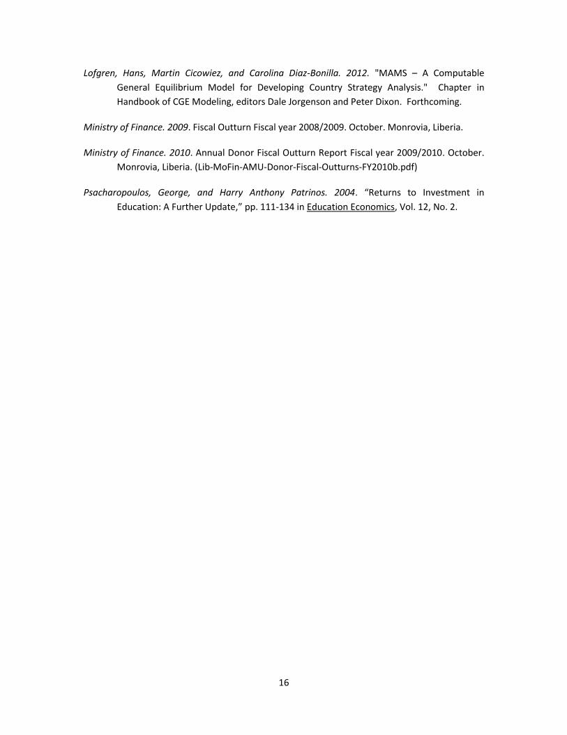
Figure 2.1 Aggregate payment flows in MAMS ........................................................................................ 17
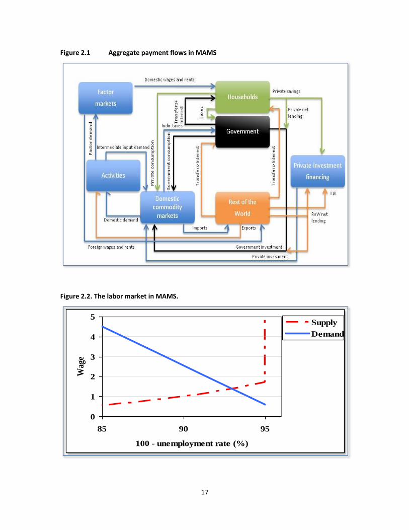
Figure 2.2 The labor market in MAMS. .................................................................................................... 17
List of Tables
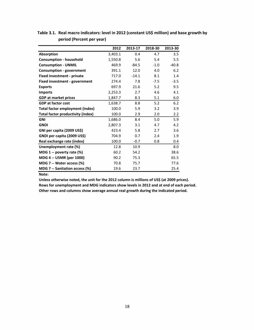
Table 3.1 Real macro indicators: level in 2012 (constant US$ million) and base growth by period (Percent per year) .................................................................................................................... 18
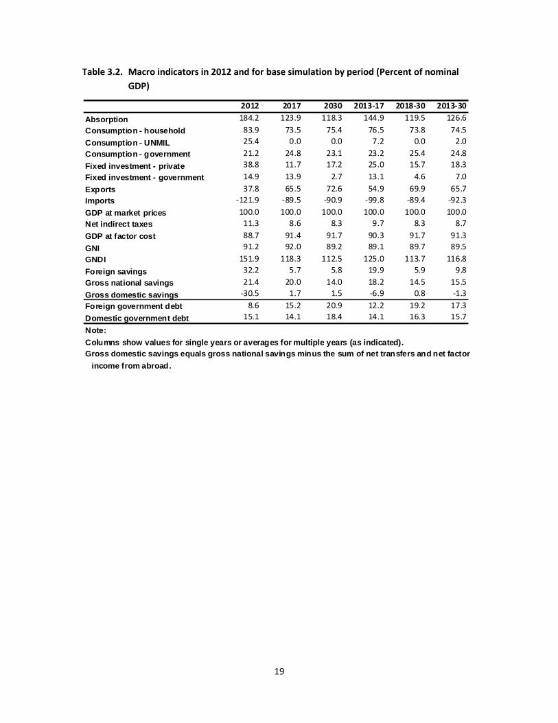
Table 3.2 Macro indicators in 2012 and for base simulation by period (Percent of nominal GDP) ....... 19
Table 3.3 Government budget in 2012 and for base simulation by period (Percent of nominal GDP) .. 20
Table 3.4 Balance of payments in 2012 and for base simulation by period (Percent of nominal GDP) . 21
Table 3.5 Sectoral GDP shares in 2012 and for base simulation by period (Percent of nominal GDP at factor cost) .............................................................................................................................. 22
Table 3.6 Real GDP at factor cost by sector: level in 2012 (constant US$mn) and base growth by period (Percent per year) .................................................................................................................... 22
Table 3.7 Sectoral structure for base scenario in 2012 and 2030 (Percent) ........................................... 23
Table 4.1 Real macro indicators in 2012 (constant US$mn) and growth 2012-2030 by simulation (Percent per year) .................................................................................................................... 24
Table 4.2 Macro indicators in 2012 and by simulation in 2030 or averages for 2012-2030 (Percent of nominal GDP)........................................................................................................................... 25
Table 4.3 Government budget in 2012 and by simulation in 2030 (Percent of nominal GDP) .............. 26
iii
Table 4.4 Balance of payments in 2012 and by simulation for 2013-2030 (Percent of nominal GDP)... 27
Table 4.5 Sectoral GDP shares in 2012 and by simulation for 2012-2030 (Percent of nominal GDP at factor cost) .............................................................................................................................. 28
Table 4.6 Real GDP at factor cost by sector: level in 2012 (constant US$ million) and growth 2013-2030 by simulation (Percent per year) ............................................................................................. 28
List of Appendices
Appendix 1 Figures with Simulation Results .............................................................................................. 29
Appendix 2 The MAMS Database ............................................................................................................... 37

1
1. INTRODUCTION AND SUMMARY OF MAIN FINDINGS1
This paper explores Liberia’s policy options in support of the development of a Medium-
Term Growth and Development Strategy (MTGDS) for 2013-2017 and a long-term national
vision, Liberia Rising 2030.2 At issue is the mismatch between available fiscal space and the
enormous development needs that the government must resolve as it prepares to transform the
economy into a middle-income country by 2030. This dilemma calls for the new administration
to make trade-offs among various priorities if it is to achieve its aspirations. For this purpose, a
Liberian version of a single-country Computable General Equilibrium (CGE) model, MAMS
(Maquette for MDG Simulations), was developed and used to conduct a set of policy
simulations, informed by analytical studies as well as sector strategies prepared in support of
Liberia’s MTGDS.3 More specifically, this paper examines the likely impacts on macroeconomic
and social indicators of alternate strategic policy scenarios. A base scenario (designed to
represent a central case for the evolution of Liberia’s economy up to 2030) was first established.
This scenario was compared to a set of non-base scenarios that introduce alternative
assumptions for the mining sector, government spending on infrastructure and human
development, and foreign borrowing.
The major findings from the analysis may be summarized as follows:
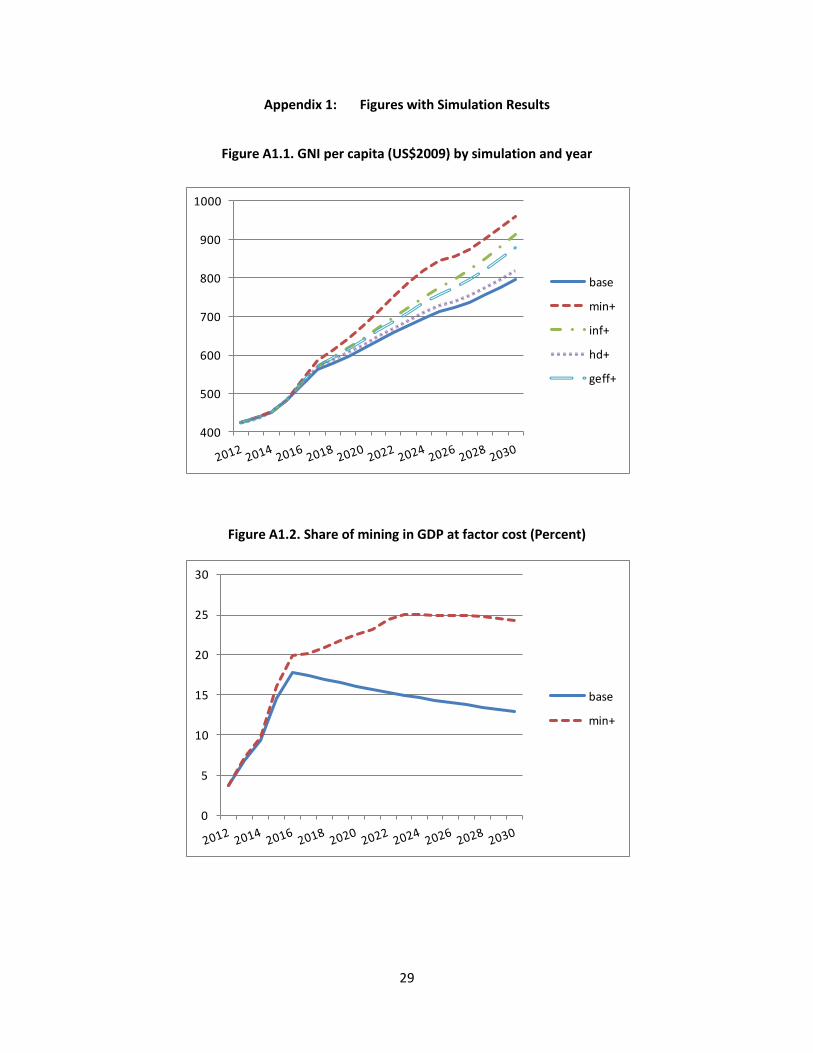
Liberia could experience rapid growth in GNI per capita between 2013 and 2030
through a rapid expansion of mining output, front-loading investment in
infrastructure, and improved government efficiency.
The findings underscore the importance of allocative and operational efficiency of
public spending.4 Further analysis is needed to identify efficiency gains by switching
1 Sébastien Dessus, Jariya Hoffman and Hans Lofgren are respectively Lead Economist (AFTP4), Senior
Economist (AFTP4) and Senior Economist (DECPG) with the World Bank. The authors are grateful for valuable comments and suggestions from Dino Merotto, Denis Medvedev, Jan Gottschalk, Antonio Nucifora, officials from the Government of Liberia led by Amara Konneh (currently Minister of Finance; Minister of Planning and Economic Affairs when the research for this paper was conducted), as well as IMF’s Liberia team, led by Chris Lane. Funding from the Knowledge for Change Program (KCP) Trust Fund to the development of MAMS is also highly appreciated. The views, findings and conclusions expressed in this paper are entirely those of the authors and do not necessarily reflect those of the World Bank, its Executive Board, or member country governments. The e-mail address of the corresponding author, Hans Lofgren, is [email protected]. 2 Unless otherwise noted, years in this paper refer to fiscal years (for example: 2013 = July 2012 – June
2013) 3 The analytical work includes a growth diagnostic, and studies of infrastructure and concessions,
infrastructure prioritization, and private sector development and concessions. 4 Allocative efficiency refers to what resources spent. Operational efficiency refers to how much output in
the form of real services and capital stocks are obtained per dollar spent.
2
public spending from administrative services to infrastructure and human
development, while improving or at least maintaining current government
efficiency.
It is important that the government balance spending on infrastructure and human
development as they complement each other in efforts to transform and diversify
Liberia’s economy. Spending on infrastructure tends to have relative strong and
immediate growth and poverty reduction effects, whereas spending more directly
on human development has a stronger positive impact on non-poverty MDG
indicators at the cost of lowered economic growth. Both infrastructure and human
development policies can be used as tools toward accelerating poverty reduction.
Strong growth driven by rapid mining expansion entails drawbacks and risks,
including the persistence of an enclave economy that will not benefit the majority of
the population and increased vulnerability to fluctuations in iron ore world prices.
The development of the oil industry (not considered in these simulations) would
bring similar opportunities and challenges.
The paper is organized into five sections including this introduction. Section 2 presents
the basic features of MAMS.5 The simulation analysis, which is the focus of the paper, is covered
in the next two sections: the base scenario in Section 3 and a set of alternative scenarios, which
are contrasted with the base scenario, in Section 4. The final section summarizes the main
findings and conclusion. Appendices 1 and 2 include a set of figures with selected simulation
results and a brief discussion of the Liberian database for MAMS, respectively.
2. STRUCTURE OF MAMS
MAMS includes three core institutions: households, government, and the rest of the
world. Payment flows of any given year are summarized in Figure 2.1 (see Appendix).
Activities produce, selling their output at home or abroad, and use their revenues to
cover their costs (of intermediate inputs, factor hiring, and taxes). Their decisions to pursue
particular activities with certain levels of factor use are driven by profit maximization. The
shares exported and sold domestically depend on the relative prices of their output in world and
domestic markets.
5 In order to meet the needs of readers who are not interested in the details of the workings of MAMS,
Sections 3 and 4 are designed to be self-contained. For more on MAMS, see Lofgren et al. (2012) and www.worldbank.org/mams.
3
Households (an aggregate domestic private institution) earn income from factors,
transfers and interest from the government (from loans to the government), and transfers from
the rest of the world (net of interest on household foreign debt).6 These are used for direct
taxes, savings, and consumption. The savings share depends on per-capita incomes. Their
consumption decisions change in response to income and price changes. By construction (and as
required by household budget constraints), the consumption value of households equals their
income net of direct taxes and savings.
The government (which also includes donors) gets its receipts from taxes and transfers
from abroad. It uses this inflow for consumption, transfers to households, and investments
(providing the capital stock required for producers of government services), drawing on
domestic and foreign borrowing for supplementary investment funding. To remain within its
budget constraint, it either adjusts some part(s) of its spending on the basis of available receipts
or mobilizes additional receipts of one type or another in order to finance its spending plans.
The rest of the world (which appears in the balance of payments) sends US dollars to
Liberia in the form of transfers to Liberia’s government and households (net of interest
payments on their foreign debts), FDI, loans, and export payments.7 Liberia uses these inflows to
finance its imports. The balance of payments clears (inflows and outflows are equalized) via
adjustments in the real exchange rate (the ratio between the international and domestic price
levels), which take place when the balance is in surplus or deficit.8
In addition to the basic three institutions, the Liberian version of MAMS also includes
UNMIL due to its significant economic role. All of its incomes stem from foreign transfers and
are used for consumption with a large import share.
Private investment financing is provided from domestic private savings (net of lending to
the government) and foreign direct investment (FDI). It is assumed that private investment
spending will adjust in response to changes in available funding.
In domestic commodity markets, flexible prices ensure balance between demand (for
domestic output from domestic demanders) and supply (to the domestic market from domestic
6 Households may lend to the government and borrow from the rest of the world; given this, it may
receive interest payments from the government and make interest payments to the rest of the world. 7 Liberia’s economy is treated as fully dollarized.
8 For example, starting from a balanced situation, a balance of payments surplus could arise from
increases in foreign exchange receipts (perhaps due to an increase in foreign aid or the world price of an export). The resulting increase in domestic demand (be it from the government or other agents) would not change international (export and import) prices, but would raise domestic prices (of domestic output sold domestically). This relative price change would encourage domestic producers to switch part of their outputs from exports to domestic sales and induce domestic demanders to switch part of their demands from domestic sources to imports. This process would continue until the balance of payments surplus is eliminated. The opposite would happen in the case of a balance of payments deficit.
4
suppliers). However, the part of domestic demand that is for imports faces exogenous world
prices – and Liberia is viewed as a small country in world markets without any impact on import
or export prices. Domestic demanders decide on import and domestic shares based on the
relative prices of commodities from these two sources. Similarly, domestic suppliers (the
activities) decide on the shares for exports and domestic supplies based on the relative prices
received in these two markets.9
Factor markets reach balance between demand and supply via wage (or rent)
adjustments. Across all factors, the factor demand curves are downward-sloping, reflecting the
responses of production activities to changes in factor wages. On the supply side of the labor
market, unemployment is endogenous – the model includes a wage curve (a supply curve) that
is upward-sloping until full employment is reached, at which point it becomes vertical (see
Figure 2.2; its supply curve assumes a minimum unemployment rate of 5%). Unemployment is
defined more broadly than in official statistics to include un- and under-employment. In the
simulations, a broad definition of unemployment increases the scope for the existing labor force
to generate a larger (smaller) amount of effective labor if the incentives to work were to
improve (deteriorate) without any change in the labor-force participation rate; typically, this
seems realistic. Over time, the labor force grows due to demography. For non-labor factors, the
supply curves are vertical in any single year (the supply is fixed) but switch over time as supplies
change (see next point).
The above discussion refers to the functioning of a model economy in a single year. In
MAMS, growth over time is endogenous. The economy grows due to accumulation of capital
(determined by investment and depreciation), labor (determined by demography), and other
factors (following exogenous growth trends), as well as because of improvements in total factor
productivity (TFP). Apart from an exogenous component, TFP depends on the levels of
government capital stocks.10
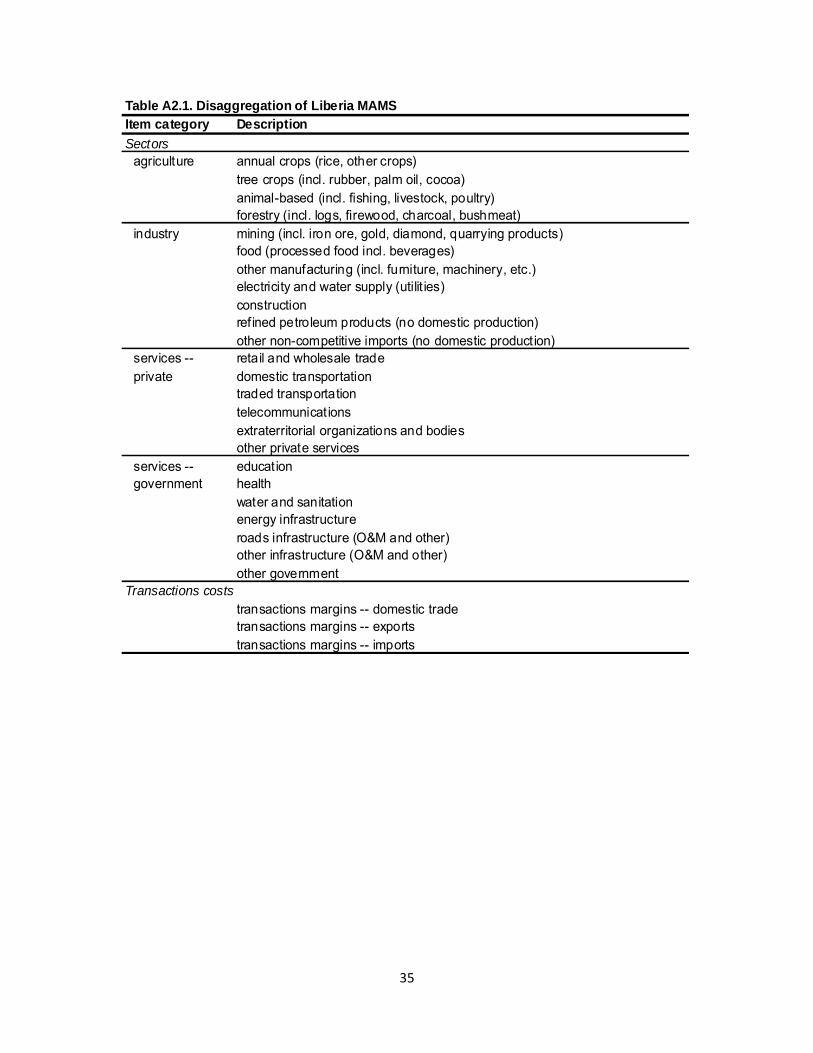
The disaggregation of MAMS varies widely across different applications depending on
data availability and the kinds of questions the model is called upon to analyze. For the Liberian
application, the database is disaggregated into some 60 accounts (for details, see Appendix
Table A2.1), indicative of the aspects of Liberia’s economy that the model considers. Most
importantly, the database includes 22 production sectors as well as two commodities without
9 Many individual production activities do not respond to changes in relative prices for exports and
domestic sales as their output only has one destination, either exported in full or sold domestically in full. By the same token, domestic demanders do not have a choice between imports and domestic output for commodities that only have one source. Such structural features reduce the flexibility of Liberia’s economy. 10
In Appendix 2 (on the MAMS database), we discuss our treatment of the links between productivity
and government capital stocks.
5
domestic production (refined petroleum and non-competitive imports). Among the sectors,
government production is represented by 7 services, covering human development,
infrastructure and other areas. The factors of production are split into labor, different types of
capital (mining, other private, and one capital type for each government service), and land
factors specific to agricultural sectors.
6
3. BASE SCENARIO
The base scenario is designed to represent a plausible projection for Liberia’s economy
for the period 2012-2030; it also serves as a benchmark for comparisons with alternative
simulations. 2012 is treated as the starting point since the analysis focuses on the impact of the
MTGDS, which starts in 2013. Our presentation of the base scenarios starts with the key
assumptions, followed by an analysis of its simulation results, with a focus on two sub-periods,
2013-2017 and 2018-2030, as well as the full period 2013-2030.
Key Assumptions
The macro aspects of MAMS under the base scenario are consistent with the
perspective of the IMF’s fiscal framework (2011a and 2011b). The assumptions for the mining
sector are also based on the IMF (2010). As noted in Section 2, GDP growth is endogenous,
determined by factor accumulation. Growth in capital stocks is endogenous while exogenous
growth is imposed for labor and other factors (for labor determined by growth in the population
in labor-force age). TFP growth has an endogenous component, related to positive productivity
effects of government capital stocks, while an exogenous component, which represents
improvements in productivity due to other causes, is assumed to grow at 1 percent per year.
The mining sector deviates from these assumptions in that growth in its sector-specific capital
stock is exogenous, set to grow at the same rate as the expected rate of output growth for the
sector.11
As noted, government budget and (off-budget) donor-financed activities are integrated
under the government heading, reflecting the fact that on- and off-budget spending in different
areas serve similar purposes and often are complementary (e.g., with the government covering
a larger share of O&M [Operation and Maintenance] and donors a larger share of investments).
The integration underlines the need to align and harmonize their activities.12 The government
receipts include direct taxes (from households and mining capital), indirect taxes, and non-tax
11 Mining capital earns most of the sector’s value-added (the sector is very capital-intensive) and the
elasticity of substitution between capital and labor is kept at a low level (0.3). Given this, the actual rate of output growth closely replicates the exogenous growth rate for the capital stock. FDI to the mining sector is also exogenous, evolving according to the same scenario for the sector. In order to maintain exogenous evolution of both the capital stock and FDI in the sector, the stock and the investment flow were decoupled. 12
The distinction between on- and off-budget aid is important for some purposes. However, keeping the two separate in the MAMS database would impose an additional data requirement and complicate the analysis given that these two activity types are complementary. For example, the government carries out the bulk O&M for infrastructure while donors are responsible for most new investments. At the same time, it would not yield any significant insights, in particular given limited knowledge about how input structures and output quality differ between donor- and government-operated activities.
7
receipts. Its revenue stems from this direct tax on mining capital value-added (VA, which equals
the operating surplus of the sector, defined as gross sales revenue net of labor and intermediate
input costs). The direct tax rate on mining capital VA changes over time on the basis of data on
projected mining sector government revenue and mining capital VA. Other tax rates – direct
taxes on households, and indirect taxes on market sales, activity gross revenues, and imports –
are all based on the Social Accounting Matrix (SAM) but scaled so that the revenue level is
similar to projections for 2012. Among non-tax receipts, both domestic transfers and domestic
government borrowing are fixed as shares of GDP. Grant aid and (concessional) borrowing from
abroad are both exogenous in real US dollars; their projections are based on the IMF.
On the spending side, the interest payments depend on the levels of the government
foreign and domestic debt stocks (the evolution of which depends on net borrowing) as well as
the levels of real interest rates, which are exogenous. Transfers to households are an exogenous
share of GDP (like the transfer that goes in the opposite direction).
Government final demand (consumption and investment), disaggregated by function,
are the only remaining spending items. It is assumed that, for each function, the government’s
capital stocks and consumption grow in tandem – consumption depends on the level of the
capital stock. Given this, an expansion of consumption (a measure of service provision) must be
preceded, in one or more preceding years (the details depend on the gestation lags), by
investments that sufficiently raise the level of the capital stock. This ensures that O&M costs are
scaled up after the completion of roads and that additional teachers are not employed without
already having a new school in place.
Each year, the government budget clears via adjustments in government consumption
and investment spending. The real growth rates for the eight different government functions
are defined in two steps. First, raw growth rates are defined exogenously for each function
drawing on government spending plans, including stronger emphasis on infrastructure than
other areas. However, unavoidably, these spending plans do not exactly match the fiscal space
that is available given endogenous growth, price changes, and other assumptions that do not
match what was known or assumed when these spending plans were conceived. Therefore, in a
second step, MAMS in each year introduces endogenous uniform percentage point adjustments
in the growth rates of each function that consider the available fiscal space.
In addition to payments involving the government (as payer or payee), the model covers
payments from the rest of the world not destined for the government: FDI (split between mining
and other private capital), and transfers from abroad to UNMIL and households – all of these
payments are exogenous in US dollars. Mining FDI follows a time profile provided by separate
mining analysis (IMF 2010). Other FDI and transfers to households grow gradually over time (at a
rate similar to GDP). Transfers to UNMIL decline rapidly during the period up to 2017, after
which they continue at a very low level.
8
Other non-government payments include private savings and investment. As noted in
Section 2, the rest of the world finances its investment (FDI) via the balance of payments. The
household (marginal and average) savings rate is gradually increased (from 7.7 percent of
household disposable income in 2012 to 14.7 percent in 2030) on the assumption that the
investment climate will improve, encouraging domestic private savings and investment. By
2030, the GDP share for private investment is around 15 percent with domestic and FDI shares
of 12.3 and 3.4 percent, respectively; these figures are similar to recent averages for low- and
middle-income countries.
The Base Scenario
The results for the base scenario are summarized in Tables 3.1-3.7. Tables 4.1-4.6
contrast the base results with those of the alternative simulations (discussed in Section 4).
The evolution of Liberia’s economy during the MTGDS period (2013-2017) is dominated
by two events: (a) very high levels of mining FDI, which permit strong expansion in mining
production and in government receipts from mining; and (b) the near-elimination of UNMIL
transfers, which dampens import growth and domestic consumption (as UNMIL today
represents large shares of both). By contrast, the post-MTGDS period (2018-2030) is less
eventful with more uniform growth across sectors and macro aggregates.
These developments are reflected in simulated changes in real macro growth, poverty
and other MDG indicators (Table 3.1). Changes in the GDP shares for macro indicators and other
indicators in the government budget and the balance of payments can be found in Tables 3.2-
3.4. Changes in the shares in GDP at factor cost for different production sectors and in the
relative magnitudes of real sector growth rates are summarized in Tables 3.5-3.6.
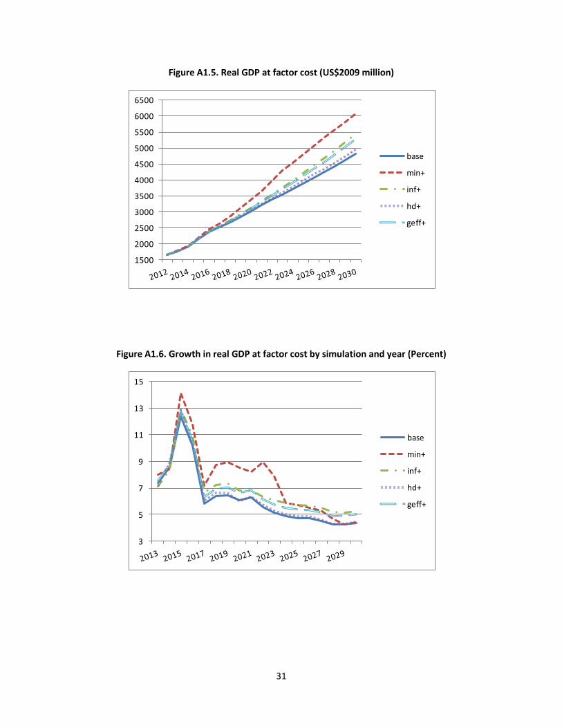
As shown in Table 3.1, during the MTGDS period, growth is very rapid for GDP at factor
cost, at 8.8 percent per year. The real exchange rate appreciates due to a large FDI volume but
depreciates when this source of additional foreign exchange stagnates during the post-MTGDS
period. (During the MTGDS, the decline in UNMIL transfers works in the opposite direction,
encouraging depreciation.) Growth in GNI is slightly slower, dampened by the impact of net
factor incomes from abroad. The impact of UNMIL is reflected not only in negative consumption
growth for UNMIL itself but also in relative slow growth in absorption (domestic final demand),
imports, and GNDI.13 Government demands and, to a lesser extent, household consumption
grow at a rapid pace, while private investment slows due to a decline in mining FDI during the
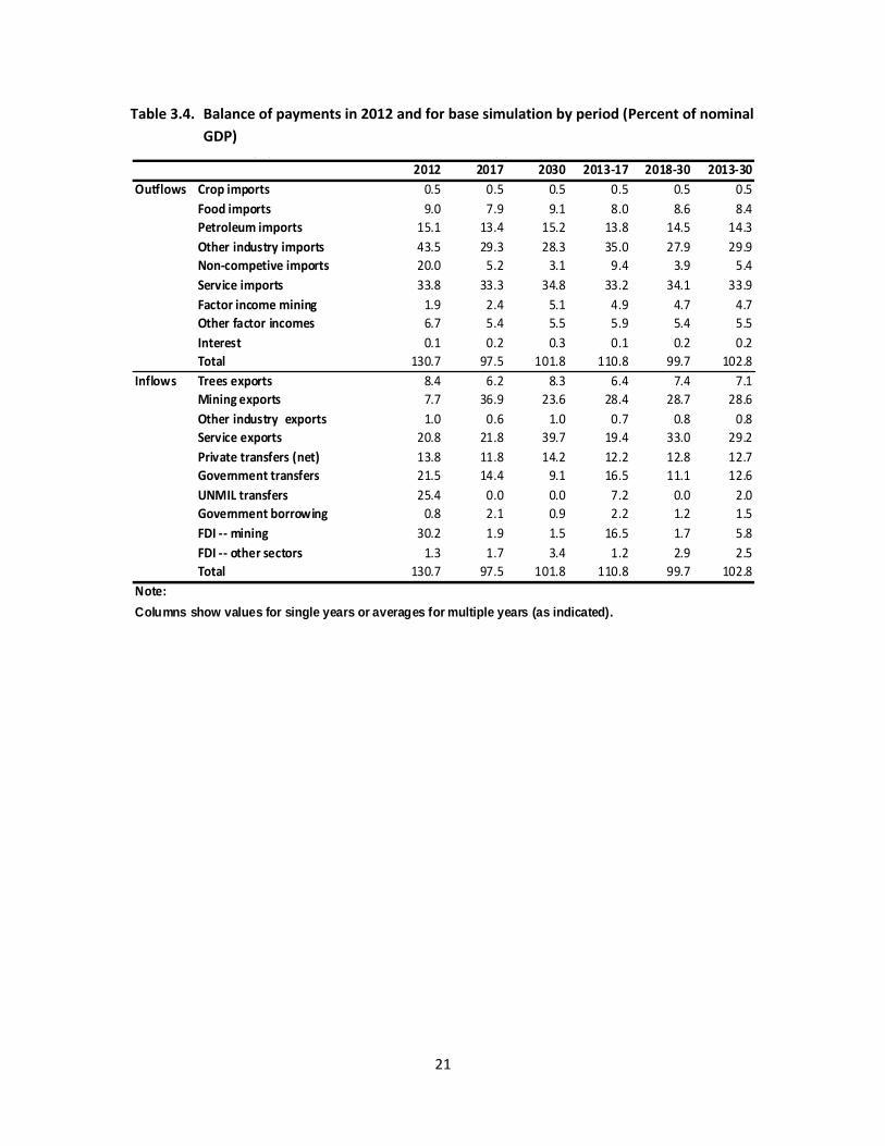
MTGDS period. The decline in the trade deficit (evidenced by the large gap between very rapid
13 By definition, the following relationships hold: GNI = GDP + net factor income from abroad. GNDI = GNI
+ net current transfers from abroad. Absorption = consumption + investment = GNDI + current account deficit of the balance of payments. For more on these relationships, see IMF (2007).
9
growth for exports and slow growth for imports) is needed to close the balance of payments
deficit that is caused by the decline in transfers to UNMIL. However, this takes place without any
significant adjustment difficulty since UNMIL itself used most of its transfers to pay for imports.
By contrast, during the post-MTGDS period, growth rates are considerably more uniform across
the different macro indicators. Government spending shifts from investment toward
consumption given slower expansion and the need to operate and maintain a much larger
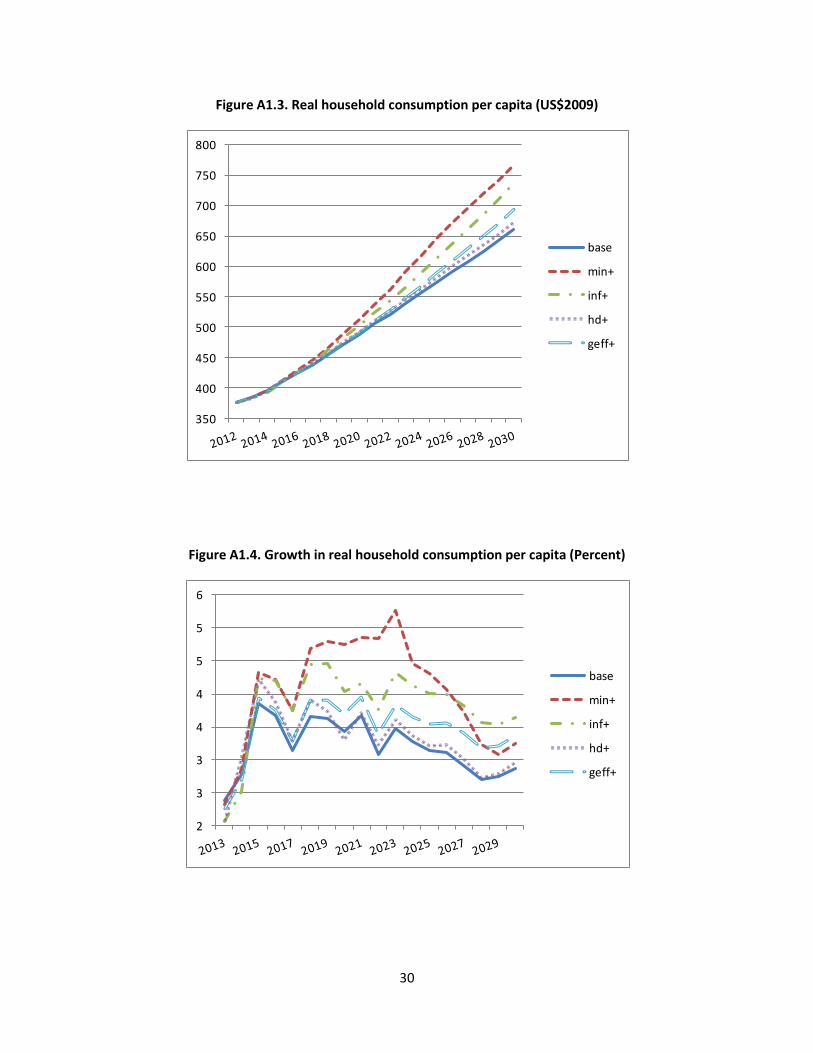
capital stock. Steady household consumption growth throughout both period results in a steady
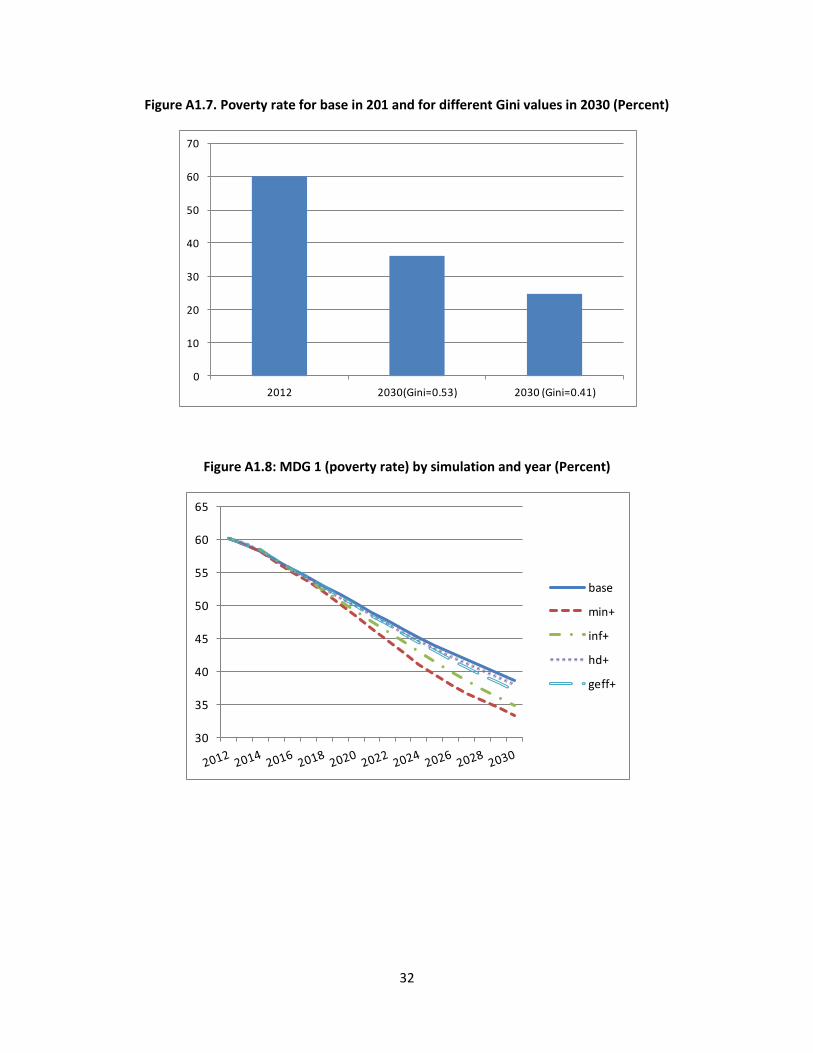
decline in the poverty rate. The analysis assumed unchanged inequality (measured by the Gini
coefficient). As shown in Figure A1.7, if Liberia’s Gini coefficient were to decrease from its
current level (52.6) to the worldwide average (40.9), progress on poverty reduction would be
considerably stronger. For the other MDG indicators, progress on an annual basis is stronger
during the MTGDS period, reflecting the role of government in human development and
infrastructure services.
Table 3.2 shows a similar set of indicators expressed as shares of GDP (in 2012 and at
the end of, and on average for, each of the two periods, MTGDS and post-MTGDS). The most
striking change (echoing the comments on Table 3.1) is the drastic decline in the trade deficit
(also reflected in the decline in absorption relative to GDP). The gap between gross national and
gross domestic savings shrinks due to the related decline in Liberia’s surplus for non-trade items
(the sum of net factor income and net current transfers) on the current account of the balance
of payments.14 The foreign debt of the government is more than doubled as a share of GDP from
9 percent to 21 percent while its domestic debt is roughly unchanged.
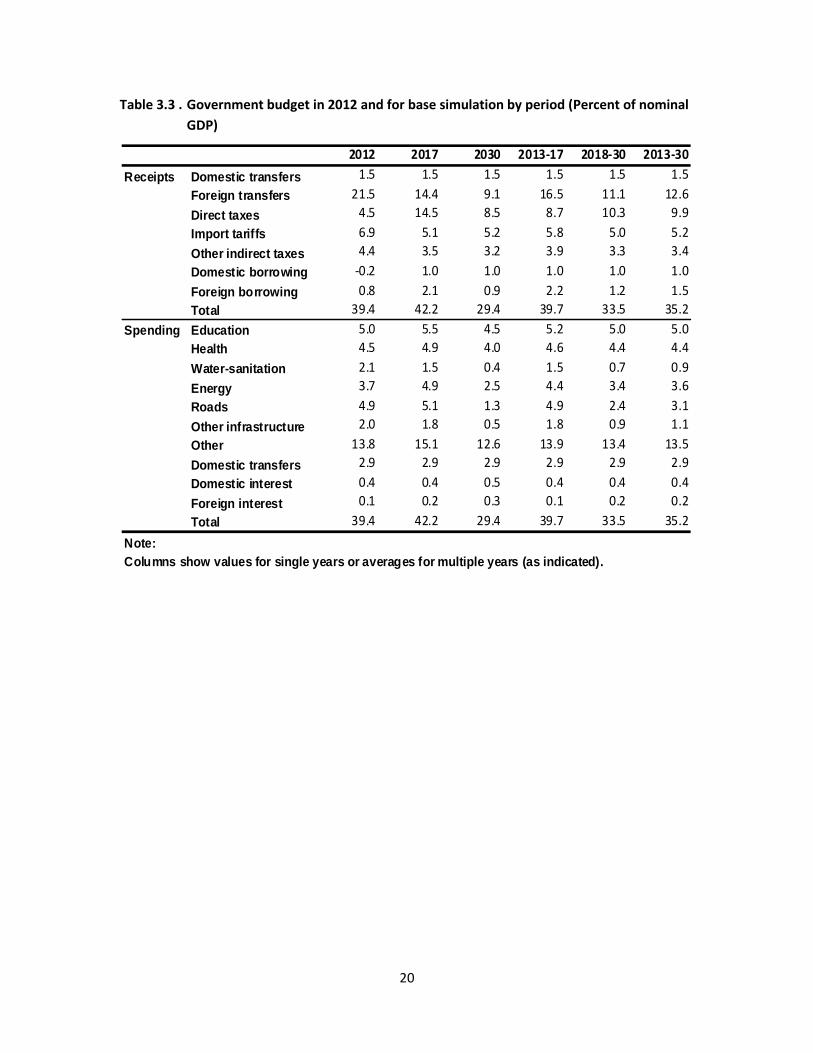
In the government budget, expressed relative to GDP, the major receipt changes during
the MTGDS period are less reliant on foreign transfers and more reliant on direct taxes, although
the latter increase is mainly due to the mining sector. This trend continues during the post-
MTGDS period for foreign transfers but is reversed for direct taxes (due to the decline in the
importance of the mining sector). On the spending side, the major change is an expansion in
total government (current and capital) spending on energy and, to a lesser extent, roads.
Government education and health, at 4.5 and 4.0 percent of GDP in 2030, are above the recent
averages for low- and middle-income countries (WDI, 2011).15
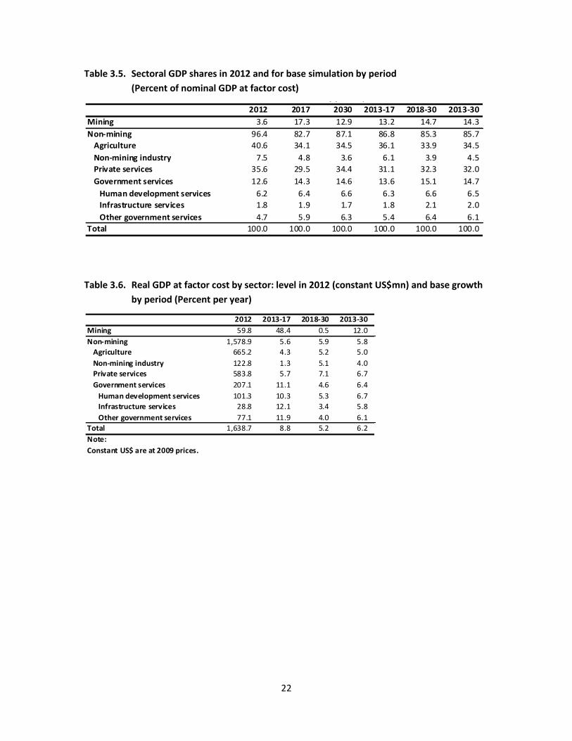
The mining expansion drastically increases the share of mining in GDP during the
MTGDS period, while the shares of other private sectors decline and those of government
services increase marginally (Tables 3.5 and 3.6). During the post-MTGDS period, these changes
14 Gross domestic savings equals gross national savings minus the sum of net factor incomes and net
current transfers from abroad. 15
For example, according to the most recent WDI numbers, average public spending on education was around 3.7 percent of GDP for low-income countries, and 4.0 percent for middle-income countries (data for 2007). For health, the corresponding figures were 2.2 and 2.9 percent of GDP, respectively (data for 2009).
10
are reversed except for a continued relative decline for the non-mining industry (Table 3.5). As
expected, a ranking of sectors in terms of real growth rates closely matches the ranking in terms
of changes in GDP shares (Table 3.6).
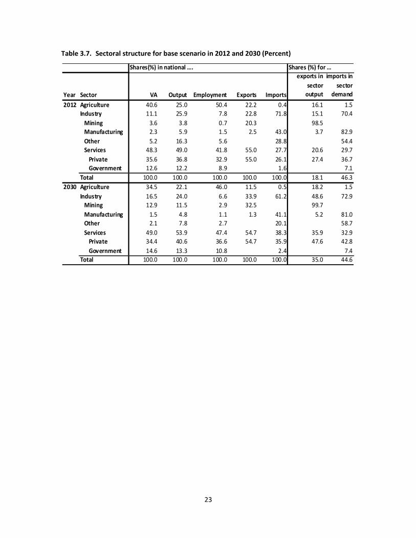
Drawing on the simulation results, Table 3.7 compares the structure of Liberia’s
economy in 2012 and 2030 under the base scenario in terms of sectoral shares in VA, output,
employment, exports and imports. The main changes that takes place between the two years
are expansions in the mining industry and, to a lesser extent, services (especially those linked to
the government) accompanied by a diminishing role for agriculture, while the importance of
non-mining industries declines to a lesser extent. Both in 2012 and 2030, imports represent a
large share in domestic demand for non-mining industrial goods and private services.
11
4. ALTERNATIVE POLICY OPTIONS
In order to better understand the consequences of alternative policy actions as well as
the possibility that mining could expand at a different pace, we constructed the following set of
alternative scenarios, each of which is identical to the base scenario apart from deviations in
one respect:16
MIN+: Stronger expansion in mining FDI, production, and tax payments. MIN+ is
motivated by the fact that additional mines may start production in the context of additional
FDI. The resulting increase in fiscal space is used to expand spending on both infrastructure and
human development.
INF+: Growth in the residual “other government” function (which is not associated with
productivity effects) is reduced by 50 percent in each year during the period 2013-2030. (Other
government is all of the government that is not linked to human development or infrastructure;
cf. Table A2.1.) The fiscal space that this creates is used to expand infrastructure spending
across the board (for energy, roads and other infrastructure) in each year by a uniform
percentage point across all infrastructure sectors. INF+ assumes that it would be feasible to
reallocate spending growth from “other government” without losses elsewhere in the economy.
Among other things, this may require a careful selection of the specific activities that would
receive less rapid funding growth.
HD+: Same changes as for INF+ except that the expansion is for education, health, and
water-sanitation. The motivation is also the same.
GEFF+: Improvement in government productive efficiency, with fiscal space gains
allocated to both infrastructure and human development spending. More specifically, in each
year: (a) the productivity of government labor increases by 2 percent (implying that, in 2030, 70
government employees can do the work that required 100 employees in 2012 under the base
scenario); and (b) when creating an additional unit of capital stock the government manages to
reduce the real cost per unit of capital stock by 1 percent per year (implying that, by 2030, the
input quantities per unit of capital stock would be 83 percent of what they were in 2030 under
the base scenario). Several measures may contribute to such efficiency gains, including better
organization of the government workplace, improved skills of civil servants, reduced
absenteeism (including elimination of multiple job holdings inside and outside government,
although the net gain for the national economy would be smaller if the workers reduce work
16 In addition, we tried a few scenarios with increased foreign borrowing, either during the MTGDS or for
the full period 2013-2030. The results indicated that marginal gains could be realized across the board for growth rates and MDG indicators at the expense of a significant increase in government debt (by 10-20 percentage points of GDP by 2030).
12
outside the government), and better procurement. On-going government efforts to improve
efficiency through PFM reforms suggest that scenarios like this should be explored. Although
productive efficiency gains are feasible, it is difficult to assess how strong they may be.
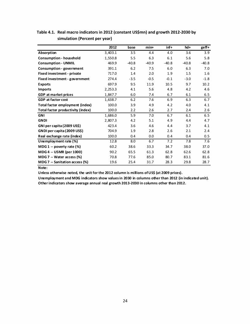
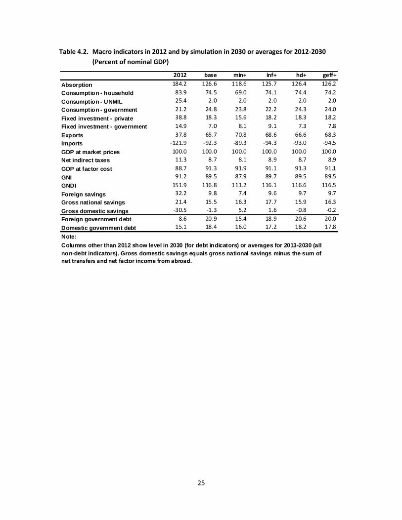
The results for these scenarios are summarized and contrasted with the base scenario in
Tables 4.1-4.6.
Strong Expansion in the Mining Sector (MIN+). Compared to the base case, under the
scenario with additional mining expansion (MIN+), GDP growth increases by 1.4 percentage
points with smaller growth gains for absorption, GNI and GNDI (all around 1 percentage point)
and stronger increases for exports and imports. Some real appreciation is needed to maintain
external balance. Domestic final demand expands across the board (except for UNMIL), with the
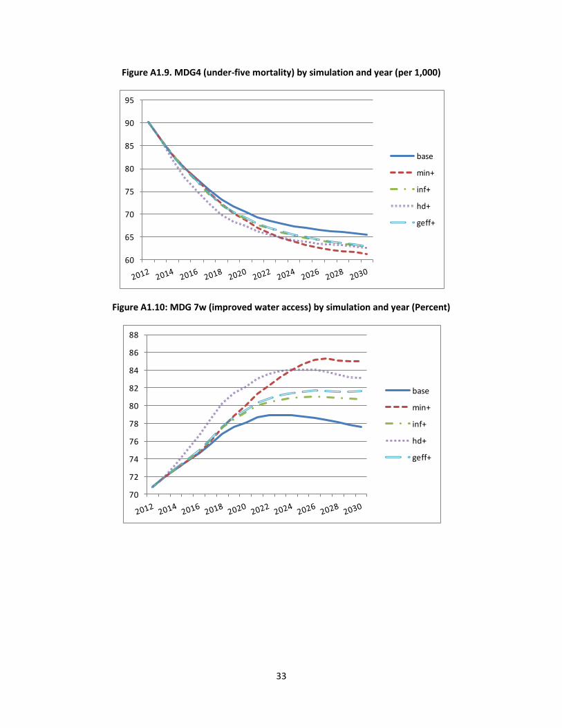
strongest expansion in the government sector. All MDG indicators improve noticeably. Given a
smaller growth gain, private final demand declines relative to GDP. The public foreign debt stock
to GDP ratio also declines given unchanged borrowing combined with stronger GDP growth
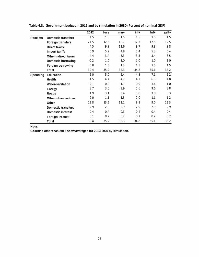
(Table 4.2). The major change in the government budget is an increase in direct taxes (from
mining). Foreign transfers are unchanged in real US dollars terms but decline relative to GDP
(due to more rapid GDP growth). Government spending expands across the board, leaving the
GDP shares for different types of spending relatively unchanged with the exception of the
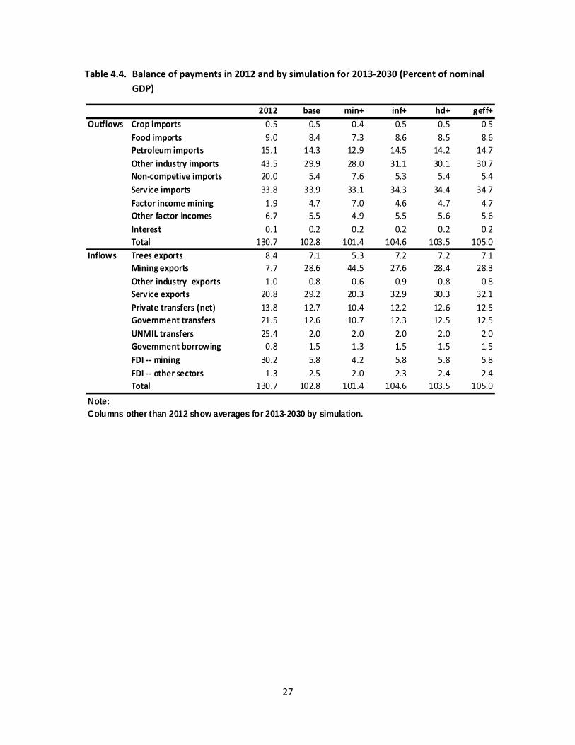
residual other government function, for which growth is unchanged (Table 4.3). In the balance
of payments (Table 4.4), the main change is a larger GDP share for exports (due to mining) and
imports; the GDP shares for non-mining exports are unchanged or decline, discouraged by the
appreciation of the real exchange rate. The share in total value-added increases for the mining
sector and decreases for non-mining sectors, especially agriculture and private services (Table
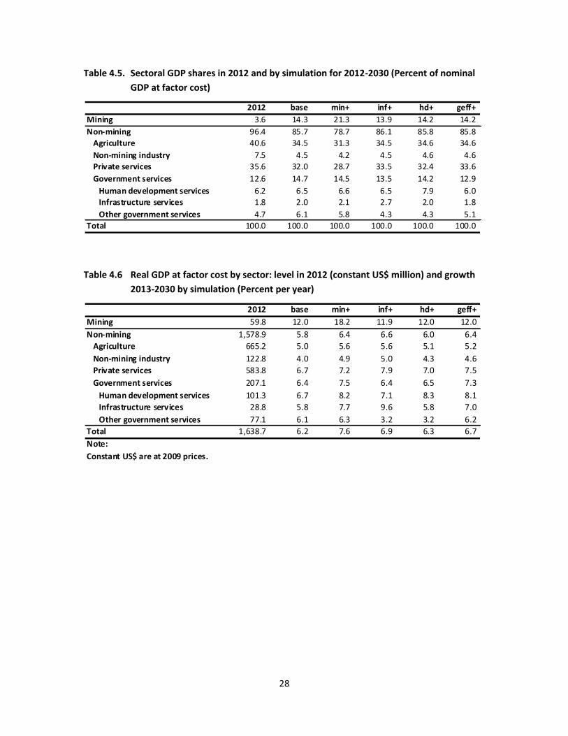
4.5); the changes in sectoral growth rates reflect a similar pattern (Table 4.6). 17
Increased Infrastructure Spending (INF+) vs. Increased Human Development Spending
(HD+). A reallocation of government spending from other government to infrastructure (INF+)
yields noticeable growth gains (around 0.6-0.8 percentage points) for most macro indicators
(Table 4.1). Within government, demand shifts from consumption to investment, reflecting the
higher capital intensity of the infrastructure sectors. All MDG indicators improve. Changes in
GDP shares (for macro indicators, the government budget and the balance of payments; Tables
4.2-4.4) reflect these government demand changes and an increase in non-mining industrial
imports (which feed into capital formation). Apart from mining (which does not change) and
other government services (which face slower growth), sectoral GDP growth rates increase. The
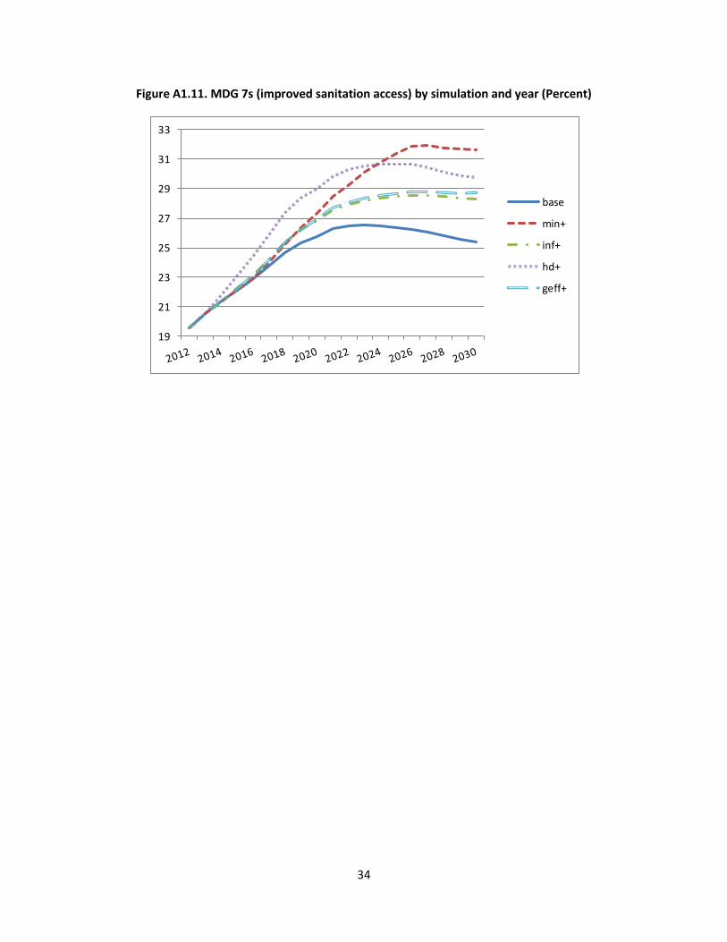
scenario INF+ should be contrasted with HD+, under which government spending instead is
reallocated toward human development (education, health and water-sanitation). The changes
in government spending and real growth for different government service sectors (from other
17 The sectors pattern for nominal GDP shares and VA growth are also reflected in real growth rates for
exports – exports grow more slowly than for the base scenario for agriculture and (private) services but more rapidly for non-mining industry.
13
government to human development) are predictable. In terms of outcomes, the most
noteworthy differences compared to INF+ are a slower growth expansion at the macro level,
less progress in poverty reduction, but faster progress for human development indicators.
Improved Productive Efficiency (GEFF+). As a result of being able to provide the original
base-level services with fewer resources, real growth in government consumption and
investments expand (translated into expansion in infrastructure and human development) while
the GDP share for aggregate government spending is less affected. As a result of this real
expansion, the economy gains significantly in terms of growth and improved MDG indicators.
Under the specific set of assumptions, the gains are similar in magnitude to what stems from
improvements in allocative efficiency (INF+ and HD+). The precise extent to which it is possible
to improve productive efficiency is, however, difficult to assess.
In addition to the tables referred to in Sections 3-4, Appendix 1 includes a set of figures
that provide more detail about the simulation results.18
18 Tables with additional and more detailed simulation outcomes are available on request.
14
5. CONCLUDING OBSERVATIONS
In sum, the simulations of this paper suggest that the expected expansion in mining
offers Liberia an opportunity to embark on an era of rapid and inclusive growth, including
progress in terms of both economic and social indicators. The extent to which the government
will be able to avail itself of this opportunity will depend on government efficiency (allocative
and productive) and policy choices, among other things influencing the extent to which less
advantaged groups have access to government services and infrastructure.
Throughout the simulated period Liberia has a very large albeit diminishing GDP share
for the government (including off-budget aid). This can continue as long as a large share of
government receipts is from foreign aid and taxes on enclave sectors. However, if such receipts
decline significantly relative to GDP, it may be very difficult and counterproductive to fully make
up for these losses by raising additional local taxes. If so, spending would have to decline
relative to GDP.
While expansion of infrastructure promises to offer stronger and quicker payoffs in
economic growth, it is important to consider the fiscal consequences of operating and
maintaining this larger infrastructure in the context of projections for government financial
resources and consideration of other spending needs.
Finally, data on Liberia’s economy are subject to a high degree of uncertainty, both in
terms of overall size and disaggregated data, making ongoing efforts to improve Liberia’s
database very important. The development of the Supply and Use Tables (SUTs) were a
prerequisite for the development of the database for the current analysis, including an input-
output table and a SAM. Among many areas, improving data on public sector activities, both on-
and off-budget, seem particularly crucial for a well-informed analysis of Liberia’s economy.
15
REFERENCES
Backiny-Yetna, Prospère, Quentin Wodon, Rose Mungai, and Clarence Tsimpo. No date. Poverty
in Liberia: Level, Profile and Determinants. World Bank.
Bourguignon, François (2003). “The growth elasticity of poverty reduction; explaining
heterogeneity across countries and time periods,” pp. 3-26 in Eicher, Theo S. and
Stephen J. Turnovsky (eds.), Inequality and Growth: Theory and Policy Implications.
Cambridge: The MIT Press.
Easterly, William (2009). “How the Millennium Development Goals are unfair to Africa”. World
Development, Vol. 37, No. 1, pp. 26-35.
Estache, Antonio. 2005. What do we know about Sub-Saharan Africa’s Infrastructure and the
Impact of its 1990s reforms? World Bank. Unpublished paper.
Estache, Antonio, and Rafael Muñoz. 2007. Building Sector Concerns into Macroeconomic
Financial Programming: Lessons from Senegal and Uganda. Africa Region Working Paper
Series No. 108. World Bank.
Foster, Vivien, and Cecilia Briceño-Garmendia, eds. 2010. Africa’s Infrastructure: A Time for
Transformation. Agence Française de Développement and World Bank.
IMF. 2007. Financial Programming and Policies. IMF Institute.
IMF. 2011a. Liberia: 2011 Sixth Review Under the Three-Year Arrangement Under the Extended
Credit Facility, Request for Extension of the Arrangement, and Augmentation of
Access—Staff Report; Staff Supplement; Press Release on the Executive Board
Discussion; and Statement by the Executive Director for Liberia. Country Report No.
11/174. July.
IMF. 2011b. Liberia: Policy Note for the Seventh Review under the Extended Credit Facility
Arrangement. August 25.
Jack, William and Maureen Lewis. 2009. “Health Investments and Economic Growth:
Macroeconomic Evidence and Microeconomic Foundations,” pp. 1-39 in eds. Spence,
Michael and Maureen Lewis. Health and Growth. Commission on Growth and
Development.
LISGIS (Liberia Institute for Statistics and Geo-Information Services). 2011. Liberia Supply and Use
Tables for the Year 2008: Handbook. March. Monrovia.
16
Lofgren, Hans, Martin Cicowiez, and Carolina Diaz-Bonilla. 2012. "MAMS – A Computable
General Equilibrium Model for Developing Country Strategy Analysis." Chapter in
Handbook of CGE Modeling, editors Dale Jorgenson and Peter Dixon. Forthcoming.
Ministry of Finance. 2009. Fiscal Outturn Fiscal year 2008/2009. October. Monrovia, Liberia.
Ministry of Finance. 2010. Annual Donor Fiscal Outturn Report Fiscal year 2009/2010. October.
Monrovia, Liberia. (Lib-MoFin-AMU-Donor-Fiscal-Outturns-FY2010b.pdf)
Psacharopoulos, George, and Harry Anthony Patrinos. 2004. “Returns to Investment in
Education: A Further Update,” pp. 111-134 in Education Economics, Vol. 12, No. 2.
17
Figure 2.1 Aggregate payment flows in MAMS
Figure 2.2. The labor market in MAMS.
0
1
2
3
4
5
85 90 95
100 - unemployment rate (%)
Wag
e
Supply
Demand
18
Table 3.1. Real macro indicators: level in 2012 (constant US$ million) and base growth by
period (Percent per year)
Table 3.1. Real macro indicators: level in 2012 (constant US$mn) and base growth by period (% per year)
2012 2013-17 2018-30 2013-30
Absorption 3,403.1 0.4 4.7 3.5
Consumption - household 1,550.8 5.6 5.4 5.5
Consumption - UNMIL 469.9 -84.5 -1.0 -40.8
Consumption - government 391.1 12.0 4.0 6.2
Fixed investment - private 717.0 -14.1 8.1 1.4
Fixed investment - government 274.4 7.8 -7.5 -3.5
Exports 697.9 21.6 5.2 9.5
Imports 2,253.3 2.7 4.6 4.1
GDP at market prices 1,847.7 8.3 5.1 6.0
GDP at factor cost 1,638.7 8.8 5.2 6.2
Total factor employment (index) 100.0 5.9 3.2 3.9
Total factor productivity (index) 100.0 2.9 2.0 2.2
GNI 1,686.0 8.4 5.0 5.9
GNDI 2,807.3 3.1 4.7 4.2
GNI per capita (2009 US$) 423.4 5.8 2.7 3.6
GNDI per capita (2009 US$) 704.9 0.7 2.4 1.9
Real exchange rate (index) 100.0 -0.7 0.8 0.4
Unemployment rate (%) 12.8 10.9 8.0
MDG 1 -- poverty rate (%) 60.2 54.2 38.6
MDG 4 -- U5MR (per 1000) 90.2 75.3 65.5
MDG 7 -- Water access (%) 70.8 75.7 77.6
MDG 7 -- Sanitation access (%) 19.6 23.7 25.4
Note:
Unless otherwise noted, the unit for the 2012 column is millions of US$ (at 2009 prices).
Rows for unemployment and MDG indicators show levels in 2012 and at end of each period.
Other rows and columns show average annual real growth during the indicated period.
19
Table 3.2. Macro indicators in 2012 and for base simulation by period (Percent of nominal
GDP)
Table 3.2. Macro indicators in 2012 and for base simulation by period (% of nominal GDP)
2012 2017 2030 2013-17 2018-30 2013-30
Absorption 184.2 123.9 118.3 144.9 119.5 126.6
Consumption - household 83.9 73.5 75.4 76.5 73.8 74.5
Consumption - UNMIL 25.4 0.0 0.0 7.2 0.0 2.0
Consumption - government 21.2 24.8 23.1 23.2 25.4 24.8
Fixed investment - private 38.8 11.7 17.2 25.0 15.7 18.3
Fixed investment - government 14.9 13.9 2.7 13.1 4.6 7.0
Exports 37.8 65.5 72.6 54.9 69.9 65.7
Imports -121.9 -89.5 -90.9 -99.8 -89.4 -92.3
GDP at market prices 100.0 100.0 100.0 100.0 100.0 100.0
Net indirect taxes 11.3 8.6 8.3 9.7 8.3 8.7
GDP at factor cost 88.7 91.4 91.7 90.3 91.7 91.3
GNI 91.2 92.0 89.2 89.1 89.7 89.5
GNDI 151.9 118.3 112.5 125.0 113.7 116.8
Foreign savings 32.2 5.7 5.8 19.9 5.9 9.8
Gross national savings 21.4 20.0 14.0 18.2 14.5 15.5
Gross domestic savings -30.5 1.7 1.5 -6.9 0.8 -1.3
Foreign government debt 8.6 15.2 20.9 12.2 19.2 17.3
Domestic government debt 15.1 14.1 18.4 14.1 16.3 15.7
Note:
Columns show values for single years or averages for multiple years (as indicated).
Gross domestic savings equals gross national savings minus the sum of net transfers and net factor
income from abroad.
20
Table 3.3 . Government budget in 2012 and for base simulation by period (Percent of nominal
GDP)
Table 3.3. Government budget in 2012 and for base simulation by period (% of nominal GDP)
2012 2017 2030 2013-17 2018-30 2013-30
Receipts Domestic transfers 1.5 1.5 1.5 1.5 1.5 1.5
Foreign transfers 21.5 14.4 9.1 16.5 11.1 12.6
Direct taxes 4.5 14.5 8.5 8.7 10.3 9.9
Import tariffs 6.9 5.1 5.2 5.8 5.0 5.2
Other indirect taxes 4.4 3.5 3.2 3.9 3.3 3.4
Domestic borrowing -0.2 1.0 1.0 1.0 1.0 1.0
Foreign borrowing 0.8 2.1 0.9 2.2 1.2 1.5
Total 39.4 42.2 29.4 39.7 33.5 35.2
Spending Education 5.0 5.5 4.5 5.2 5.0 5.0
Health 4.5 4.9 4.0 4.6 4.4 4.4
Water-sanitation 2.1 1.5 0.4 1.5 0.7 0.9
Energy 3.7 4.9 2.5 4.4 3.4 3.6
Roads 4.9 5.1 1.3 4.9 2.4 3.1
Other infrastructure 2.0 1.8 0.5 1.8 0.9 1.1
Other 13.8 15.1 12.6 13.9 13.4 13.5
Domestic transfers 2.9 2.9 2.9 2.9 2.9 2.9
Domestic interest 0.4 0.4 0.5 0.4 0.4 0.4
Foreign interest 0.1 0.2 0.3 0.1 0.2 0.2
Total 39.4 42.2 29.4 39.7 33.5 35.2
Note:
Columns show values for single years or averages for multiple years (as indicated).
21
Table 3.4. Balance of payments in 2012 and for base simulation by period (Percent of nominal
GDP)
Table 3.4. Balance of payments in 2012 and for base simulation by period (% of nominal GDP)
2012 2017 2030 2013-17 2018-30 2013-30
Outflows Crop imports 0.5 0.5 0.5 0.5 0.5 0.5
Food imports 9.0 7.9 9.1 8.0 8.6 8.4
Petroleum imports 15.1 13.4 15.2 13.8 14.5 14.3
Other industry imports 43.5 29.3 28.3 35.0 27.9 29.9
Non-competive imports 20.0 5.2 3.1 9.4 3.9 5.4
Service imports 33.8 33.3 34.8 33.2 34.1 33.9
Factor income mining 1.9 2.4 5.1 4.9 4.7 4.7
Other factor incomes 6.7 5.4 5.5 5.9 5.4 5.5
Interest 0.1 0.2 0.3 0.1 0.2 0.2
Total 130.7 97.5 101.8 110.8 99.7 102.8
Inflows Trees exports 8.4 6.2 8.3 6.4 7.4 7.1
Mining exports 7.7 36.9 23.6 28.4 28.7 28.6
Other industry exports 1.0 0.6 1.0 0.7 0.8 0.8
Service exports 20.8 21.8 39.7 19.4 33.0 29.2
Private transfers (net) 13.8 11.8 14.2 12.2 12.8 12.7
Government transfers 21.5 14.4 9.1 16.5 11.1 12.6
UNMIL transfers 25.4 0.0 0.0 7.2 0.0 2.0
Government borrowing 0.8 2.1 0.9 2.2 1.2 1.5
FDI -- mining 30.2 1.9 1.5 16.5 1.7 5.8
FDI -- other sectors 1.3 1.7 3.4 1.2 2.9 2.5
Total 130.7 97.5 101.8 110.8 99.7 102.8
Note:
Columns show values for single years or averages for multiple years (as indicated).
22
Table 3.5. Sectoral GDP shares in 2012 and for base simulation by period
(Percent of nominal GDP at factor cost)
Table 3.6. Real GDP at factor cost by sector: level in 2012 (constant US$mn) and base growth
by period (Percent per year)
Table 3.5. Sectoral GDP shares in 2012 and for base simulation by period (% of nominal GDP at factor cost)
2012 2017 2030 2013-17 2018-30 2013-30
Mining 3.6 17.3 12.9 13.2 14.7 14.3
Non-mining 96.4 82.7 87.1 86.8 85.3 85.7
Agriculture 40.6 34.1 34.5 36.1 33.9 34.5
Non-mining industry 7.5 4.8 3.6 6.1 3.9 4.5
Private services 35.6 29.5 34.4 31.1 32.3 32.0
Government services 12.6 14.3 14.6 13.6 15.1 14.7
Human development services 6.2 6.4 6.6 6.3 6.6 6.5
Infrastructure services 1.8 1.9 1.7 1.8 2.1 2.0
Other government services 4.7 5.9 6.3 5.4 6.4 6.1
Total 100.0 100.0 100.0 100.0 100.0 100.0
Table 3.6. Real GDP at factor cost by sector: level in 2012 (constant US$mn) and base growth by period (% per year)
2012 2013-17 2018-30 2013-30
Mining 59.8 48.4 0.5 12.0
Non-mining 1,578.9 5.6 5.9 5.8
Agriculture 665.2 4.3 5.2 5.0
Non-mining industry 122.8 1.3 5.1 4.0
Private services 583.8 5.7 7.1 6.7
Government services 207.1 11.1 4.6 6.4
Human development services 101.3 10.3 5.3 6.7
Infrastructure services 28.8 12.1 3.4 5.8
Other government services 77.1 11.9 4.0 6.1
Total 1,638.7 8.8 5.2 6.2
Note:
Constant US$ are at 2009 prices.
23
Table 3.7. Sectoral structure for base scenario in 2012 and 2030 (Percent)
Table 3.7. Sectoral structure for base scenario in 2012 and 2030 (%)
Shares(%) in national …. Shares (%) for …
Year Sector VA Output Employment Exports Imports
exports in
sector
output
imports in
sector
demand
2012 Agriculture 40.6 25.0 50.4 22.2 0.4 16.1 1.5
Industry 11.1 25.9 7.8 22.8 71.8 15.1 70.4
Mining 3.6 3.8 0.7 20.3 98.5
Manufacturing 2.3 5.9 1.5 2.5 43.0 3.7 82.9
Other 5.2 16.3 5.6 28.8 54.4
Services 48.3 49.0 41.8 55.0 27.7 20.6 29.7
Private 35.6 36.8 32.9 55.0 26.1 27.4 36.7
Government 12.6 12.2 8.9 1.6 7.1
Total 100.0 100.0 100.0 100.0 100.0 18.1 46.3
2030 Agriculture 34.5 22.1 46.0 11.5 0.5 18.2 1.5
Industry 16.5 24.0 6.6 33.9 61.2 48.6 72.9
Mining 12.9 11.5 2.9 32.5 99.7
Manufacturing 1.5 4.8 1.1 1.3 41.1 5.2 81.0
Other 2.1 7.8 2.7 20.1 58.7
Services 49.0 53.9 47.4 54.7 38.3 35.9 32.9
Private 34.4 40.6 36.6 54.7 35.9 47.6 42.8
Government 14.6 13.3 10.8 2.4 7.4
Total 100.0 100.0 100.0 100.0 100.0 35.0 44.6
24
Table 4.1. Real macro indicators in 2012 (constant US$mn) and growth 2012-2030 by
simulation (Percent per year)
Table 4.1. Real macro indicators in 2012 (constant US$mn) and growth 2013-2030 by simulation (% per year)
2012 base min+ inf+ hd+ geff+
Absorption 3,403.1 3.5 4.4 4.0 3.6 3.9
Consumption - household 1,550.8 5.5 6.3 6.1 5.6 5.8
Consumption - UNMIL 469.9 -40.8 -40.9 -40.8 -40.8 -40.8
Consumption - government 391.1 6.2 7.5 6.0 6.3 7.0
Fixed investment - private 717.0 1.4 2.0 1.9 1.5 1.6
Fixed investment - government 274.4 -3.5 -0.5 -0.1 -3.0 -1.8
Exports 697.9 9.5 11.9 10.5 9.7 10.2
Imports 2,253.3 4.1 5.6 4.8 4.2 4.6
GDP at market prices 1,847.7 6.0 7.4 6.7 6.1 6.5
GDP at factor cost 1,638.7 6.2 7.6 6.9 6.3 6.7
Total factor employment (index) 100.0 3.9 4.9 4.2 4.0 4.1
Total factor productivity (index) 100.0 2.2 2.6 2.7 2.4 2.6
GNI 1,686.0 5.9 7.0 6.7 6.1 6.5
GNDI 2,807.3 4.2 5.1 4.9 4.4 4.7
GNI per capita (2009 US$) 423.4 3.6 4.6 4.4 3.7 4.1
GNDI per capita (2009 US$) 704.9 1.9 2.8 2.6 2.1 2.4
Real exchange rate (index) 100.0 0.4 0.0 0.4 0.4 0.5
Unemployment rate (%) 12.8 8.0 6.7 7.2 7.8 7.6
MDG 1 -- poverty rate (%) 60.2 38.6 33.3 34.7 38.0 37.0
MDG 4 -- U5MR (per 1000) 90.2 65.5 61.3 62.8 62.6 62.8
MDG 7 -- Water access (%) 70.8 77.6 85.0 80.7 83.1 81.6
MDG 7 -- Sanitation access (%) 19.6 25.4 31.7 28.3 29.8 28.7
Note:
Unless otherwise noted, the unit for the 2012 column is millions of US$ (at 2009 prices).
Unemployment and MDG indicators show values in 2030 in columns other than 2012 (in indicated unit).
Other indicators show average annual real growth 2013-2030 in columns other than 2012.
25
Table 4.2. Macro indicators in 2012 and by simulation in 2030 or averages for 2012-2030
(Percent of nominal GDP)
Table 4.2. Macro indicators in 2012 and by simulation in 2030 or averages for 2013-2030 (% of nominal GDP)
2012 base min+ inf+ hd+ geff+
Absorption 184.2 126.6 118.6 125.7 126.4 126.2
Consumption - household 83.9 74.5 69.0 74.1 74.4 74.2
Consumption - UNMIL 25.4 2.0 2.0 2.0 2.0 2.0
Consumption - government 21.2 24.8 23.8 22.2 24.3 24.0
Fixed investment - private 38.8 18.3 15.6 18.2 18.3 18.2
Fixed investment - government 14.9 7.0 8.1 9.1 7.3 7.8
Exports 37.8 65.7 70.8 68.6 66.6 68.3
Imports -121.9 -92.3 -89.3 -94.3 -93.0 -94.5
GDP at market prices 100.0 100.0 100.0 100.0 100.0 100.0
Net indirect taxes 11.3 8.7 8.1 8.9 8.7 8.9
GDP at factor cost 88.7 91.3 91.9 91.1 91.3 91.1
GNI 91.2 89.5 87.9 89.7 89.5 89.5
GNDI 151.9 116.8 111.2 116.1 116.6 116.5
Foreign savings 32.2 9.8 7.4 9.6 9.7 9.7
Gross national savings 21.4 15.5 16.3 17.7 15.9 16.3
Gross domestic savings -30.5 -1.3 5.2 1.6 -0.8 -0.2
Foreign government debt 8.6 20.9 15.4 18.9 20.6 20.0
Domestic government debt 15.1 18.4 16.0 17.2 18.2 17.8
Note:
Columns other than 2012 show level in 2030 (for debt indicators) or averages for 2013-2030 (all
non-debt indicators). Gross domestic savings equals gross national savings minus the sum of
net transfers and net factor income from abroad.
26
Table 4.3. Government budget in 2012 and by simulation in 2030 (Percent of nominal GDP)
Table 4.3. Government budget in 2012 and by simulation in 2030 (% of nominal GDP)
2012 base min+ inf+ hd+ geff+
Receipts Domestic transfers 1.5 1.5 1.5 1.5 1.5 1.5
Foreign transfers 21.5 12.6 10.7 12.3 12.5 12.5
Direct taxes 4.5 9.9 12.6 9.7 9.8 9.8
Import tariffs 6.9 5.2 4.8 5.4 5.3 5.4
Other indirect taxes 4.4 3.4 3.3 3.5 3.4 3.5
Domestic borrowing -0.2 1.0 1.0 1.0 1.0 1.0
Foreign borrowing 0.8 1.5 1.3 1.5 1.5 1.5
Total 39.4 35.2 35.3 34.8 35.1 35.2
Spending Education 5.0 5.0 5.4 4.8 7.1 5.2
Health 4.5 4.4 4.7 4.2 6.3 4.8
Water-sanitation 2.1 0.9 1.1 0.9 1.4 1.0
Energy 3.7 3.6 3.9 5.6 3.6 3.8
Roads 4.9 3.1 3.4 5.0 3.0 3.3
Other infrastructure 2.0 1.1 1.3 2.0 1.1 1.2
Other 13.8 13.5 12.1 8.8 9.0 12.3
Domestic transfers 2.9 2.9 2.9 2.9 2.9 2.9
Domestic interest 0.4 0.4 0.3 0.4 0.4 0.4
Foreign interest 0.1 0.2 0.2 0.2 0.2 0.2
Total 39.4 35.2 35.3 34.8 35.1 35.2
Note:
Columns other than 2012 show averages for 2013-2030 by simulation.
27
Table 4.4. Balance of payments in 2012 and by simulation for 2013-2030 (Percent of nominal
GDP)
Table 4.4. Balance of payments in 2012 and by simulation for 2013-2030 (% of nominal GDP)
2012 base min+ inf+ hd+ geff+
Outflows Crop imports 0.5 0.5 0.4 0.5 0.5 0.5
Food imports 9.0 8.4 7.3 8.6 8.5 8.6
Petroleum imports 15.1 14.3 12.9 14.5 14.2 14.7
Other industry imports 43.5 29.9 28.0 31.1 30.1 30.7
Non-competive imports 20.0 5.4 7.6 5.3 5.4 5.4
Service imports 33.8 33.9 33.1 34.3 34.4 34.7
Factor income mining 1.9 4.7 7.0 4.6 4.7 4.7
Other factor incomes 6.7 5.5 4.9 5.5 5.6 5.6
Interest 0.1 0.2 0.2 0.2 0.2 0.2
Total 130.7 102.8 101.4 104.6 103.5 105.0
Inflows Trees exports 8.4 7.1 5.3 7.2 7.2 7.1
Mining exports 7.7 28.6 44.5 27.6 28.4 28.3
Other industry exports 1.0 0.8 0.6 0.9 0.8 0.8
Service exports 20.8 29.2 20.3 32.9 30.3 32.1
Private transfers (net) 13.8 12.7 10.4 12.2 12.6 12.5
Government transfers 21.5 12.6 10.7 12.3 12.5 12.5
UNMIL transfers 25.4 2.0 2.0 2.0 2.0 2.0
Government borrowing 0.8 1.5 1.3 1.5 1.5 1.5
FDI -- mining 30.2 5.8 4.2 5.8 5.8 5.8
FDI -- other sectors 1.3 2.5 2.0 2.3 2.4 2.4
Total 130.7 102.8 101.4 104.6 103.5 105.0
Note:
Columns other than 2012 show averages for 2013-2030 by simulation.
28
Table 4.5. Sectoral GDP shares in 2012 and by simulation for 2012-2030 (Percent of nominal
GDP at factor cost)
Table 4.6 Real GDP at factor cost by sector: level in 2012 (constant US$ million) and growth
2013-2030 by simulation (Percent per year)
Table 4.5. Sectoral GDP shares in 2012 and by simulation for 2013-2030 (% of nominal GDP at factor cost)
2012 base min+ inf+ hd+ geff+
Mining 3.6 14.3 21.3 13.9 14.2 14.2
Non-mining 96.4 85.7 78.7 86.1 85.8 85.8
Agriculture 40.6 34.5 31.3 34.5 34.6 34.6
Non-mining industry 7.5 4.5 4.2 4.5 4.6 4.6
Private services 35.6 32.0 28.7 33.5 32.4 33.6
Government services 12.6 14.7 14.5 13.5 14.2 12.9
Human development services 6.2 6.5 6.6 6.5 7.9 6.0
Infrastructure services 1.8 2.0 2.1 2.7 2.0 1.8
Other government services 4.7 6.1 5.8 4.3 4.3 5.1
Total 100.0 100.0 100.0 100.0 100.0 100.0
Table 4.6. Real GDP at factor cost by sector: level in 2012 (constant US$mn) and growth 2013-2030 by simulation (% per year)
2012 base min+ inf+ hd+ geff+
Mining 59.8 12.0 18.2 11.9 12.0 12.0
Non-mining 1,578.9 5.8 6.4 6.6 6.0 6.4
Agriculture 665.2 5.0 5.6 5.6 5.1 5.2
Non-mining industry 122.8 4.0 4.9 5.0 4.3 4.6
Private services 583.8 6.7 7.2 7.9 7.0 7.5
Government services 207.1 6.4 7.5 6.4 6.5 7.3
Human development services 101.3 6.7 8.2 7.1 8.3 8.1
Infrastructure services 28.8 5.8 7.7 9.6 5.8 7.0
Other government services 77.1 6.1 6.3 3.2 3.2 6.2
Total 1,638.7 6.2 7.6 6.9 6.3 6.7
Note:
Constant US$ are at 2009 prices.
29
Appendix 1: Figures with Simulation Results
Figure A1.1. GNI per capita (US$2009) by simulation and year
Figure A1.2. Share of mining in GDP at factor cost (Percent)
400
500
600
700
800
900
1000
base
min+
inf+
hd+
geff+
0
5
10
15
20
25
30
base
min+
30
Figure A1.3. Real household consumption per capita (US$2009)
Figure A1.4. Growth in real household consumption per capita (Percent)
350
400
450
500
550
600
650
700
750
800
base
min+
inf+
hd+
geff+
2
3
3
4
4
5
5
6
base
min+
inf+
hd+
geff+
31
Figure A1.5. Real GDP at factor cost (US$2009 million)
Figure A1.6. Growth in real GDP at factor cost by simulation and year (Percent)
1500
2000
2500
3000
3500
4000
4500
5000
5500
6000
6500
base
min+
inf+
hd+
geff+
3
5
7
9
11
13
15
base
min+
inf+
hd+
geff+
32
Figure A1.7. Poverty rate for base in 201 and for different Gini values in 2030 (Percent)
Figure A1.8: MDG 1 (poverty rate) by simulation and year (Percent)
0
10
20
30
40
50
60
70
2012 2030(Gini=0.53) 2030 (Gini=0.41)
30
35
40
45
50
55
60
65
base
min+
inf+
hd+
geff+
33
Figure A1.9. MDG4 (under-five mortality) by simulation and year (per 1,000)
Figure A1.10: MDG 7w (improved water access) by simulation and year (Percent)
60
65
70
75
80
85
90
95
base
min+
inf+
hd+
geff+
70
72
74
76
78
80
82
84
86
88
base
min+
inf+
hd+
geff+
34
Figure A1.11. MDG 7s (improved sanitation access) by simulation and year (Percent)
19
21
23
25
27
29
31
33
base
min+
inf+
hd+
geff+
35
Table A2.1. Disaggregation of Liberia MAMS
Item category Description
Sectors
agriculture annual crops (rice, other crops)tree crops (incl. rubber, palm oil, cocoa)animal-based (incl. fishing, livestock, poultry)forestry (incl. logs, firewood, charcoal, bushmeat)
industry mining (incl. iron ore, gold, diamond, quarrying products)food (processed food incl. beverages)other manufacturing (incl. furniture, machinery, etc.)electricity and water supply (utilit ies)constructionrefined petroleum products (no domestic production)other non-competitive imports (no domestic production)
services -- retail and wholesale tradeprivate domestic transportation
traded transportationtelecommunicationsextraterritorial organizations and bodiesother private services
services -- educationgovernment health
water and sanitationenergy infrastructureroads infrastructure (O&M and other)other infrastructure (O&M and other)other government
Transactions costs
transactions margins -- domestic tradetransactions margins -- exportstransactions margins -- imports
36
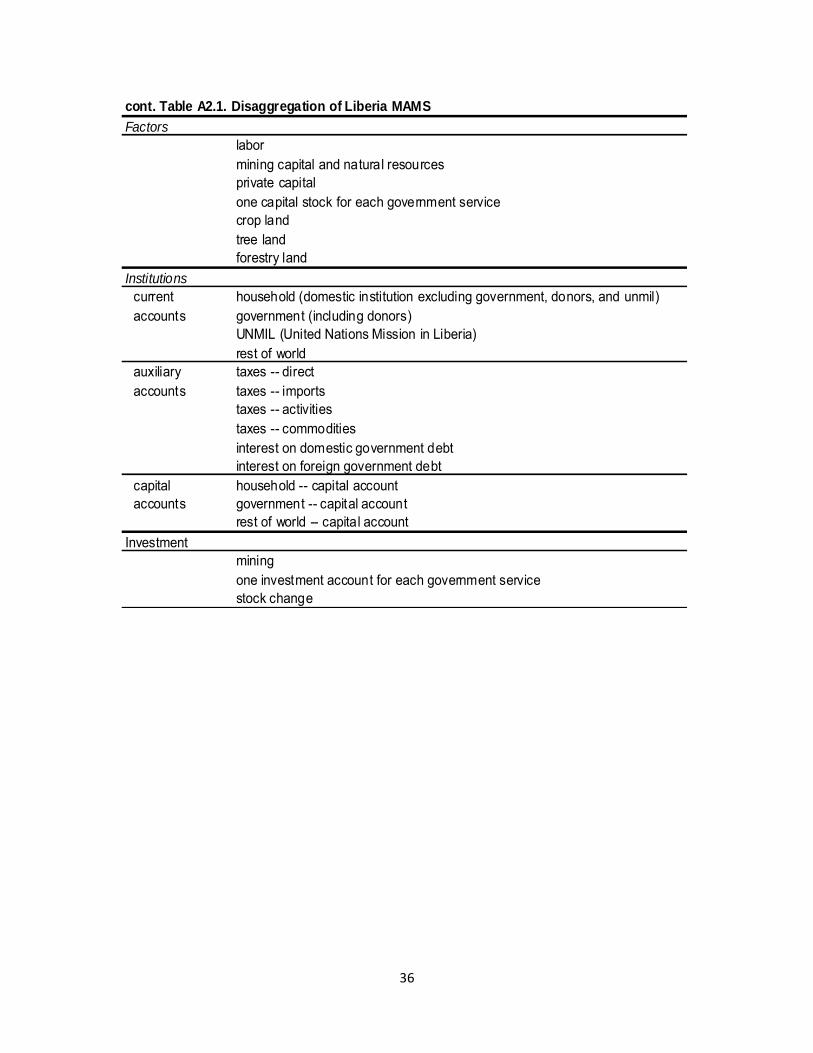
cont. Table A2.1. Disaggregation of Liberia MAMS
Factors
labormining capital and natural resourcesprivate capitalone capital stock for each government servicecrop landtree landforestry land
Institutions
current household (domestic institution excluding government, donors, and unmil)accounts government (including donors)
UNMIL (United Nations Mission in Liberia)rest of world
auxiliary taxes -- directaccounts taxes -- imports
taxes -- activitiestaxes -- commoditiesinterest on domestic government debtinterest on foreign government debt
capital household -- capital accountaccounts government -- capital account
rest of world -- capital accountInvestment
miningone investment account for each government servicestock change
37
Appendix 2. The MAMS Database
The database with this disaggregation consists of a Social Accounting Matrix (SAM), data on
stocks (of factors of production and debts), elasticities (in production, consumption, trade, and
MDG functions), and miscellaneous other data.19 Table A2.1 shows the disaggregation of the
database. The SAM, which was specifically built for this analysis, is mainly based on the 2008
Supply and Use Tables (SUTs, which also include employment data), IMF fiscal and balance of
payments data, as well as disaggregated fiscal and foreign aid data from the Ministry of Finance
on the allocation of foreign aid across different areas (LISGIS 2011; Ministry of Finance, 2009,
pp. 27-30; Ministry of Finance, 2010, p. 8). WDI (2011) provided additional indicators, both on
Liberia and across countries. Relative to earlier national accounts data (which mostly relied on
extrapolations of pre-war surveys), the SUTs offer improved coverage of non-tradable domestic
economic activities (including subsistence farming and informal service sectors). At the same
time, the SUTs are by construction incomplete when it comes to fiscal and foreign transactions,
requiring reliance on data from other sources; in this case the authors turned to IMF data.
Inconsistencies between IMF and SUT data were resolved using statistical procedures. According
to the resulting SAM, 2009 GDP was US$1,421 million, in contrast with an IMF figure of US$865
million for the same period and a SUT figure of US$2,025 million for calendar year 2008 (IMF
2011, p. 16; LISGIS 2011, p. i).20
The analysis addresses the effects of alternative government spending patterns. In MAMS, these
effects are covered via two mechanisms: (1) total factor productivity in selected production
sectors is a function of the level of government service-specific capital stocks (cf. the
disaggregation of government service sectors in Table 1), which are driven by government
investments and depreciation rates; and (2) spending on health and water-sanitation has a
direct impact on the MDGs for under-five mortality, water access, and sanitation.21 The
19 A SAM is a square matrix that provides a comprehensive, consistent economy-wide summary of the
payments in an economy during one year. It links institutions, factors, and production sectors. The latter are split into activities (which carry out production) and commodities (representing activity outputs or imports without domestic production). Given the consistency requirement, each account must be balanced – its receipts must equal its outlays. The accounts of the Liberia SAM closely match the disaggregation of MAMS (cf. Table 1). The elasticities used in MAMS draw on the international literature; given the consistency features of an economy-wide model like MAMS, as long as they stay within ranges that are widely accepted, most elasticities play a very minor role. In the analysis of the simulation results, we highlight the features of the model and the database (including elasticities) that have a significant bearing on our qualitative conclusions. 20
The higher the GDP (and GNI), the lower the average growth rate required to reach middle-income status by 2030. However, it is also worth noticing that economic activities that register the largest increases compared to earlier statistics (the informal sector and subsistence farming in particular) are less likely to grow rapidly. 21
In other MAMS applications, the impact of education has typically been captured by linking a detailed treatment of this sector to a labor market that is disaggregated by educational attainment, with higher wages (and marginal value products) for workers with more education. By permitting education spending
38
parameter values selected for these links reflect our assessment of the relevant empirical
literature and the situation in Liberia. With regard to (1), the internal rates of return (IRRs, the
interest rates at which the net present value of the investment is zero) are as follows: 38% for
energy, 34% for roads and other infrastructure, 18% for education, 15% for water and
sanitation, and 9% for health.
More specifically, government spending in these areas influence growth raising TFP in selected
activities. When calibrating these links, we calculate IRRs (internal rates of return) for different
areas of government spending on the basis of the following variables: the initial investment
cost; O&M costs linked to the resulting capital stock; gestation lags (the lag between the
investment and the time when the capital stock is available for use; longer for infrastructure);
productivity lags (the lag between the time when the capital stock is available and when it starts
to yield positive productivity effects; longer for education); the depreciation rate (once the
gestation lag is completed); the marginal productivity of the capital stock (once the productivity
lag is over); and expected growth for the sectors (when productivity increases due to the
investment). Among these, the marginal productivity figures are adjusted to generate targeted
IRRs. For empirical data on typical IRRs (approximately matched in our pre-calculations), see
Foster and Briceño-Garmendia (2010) for infrastructure; and for education (using social rates
since they have a more complete cost coverage), see Psacharopoulos and Patrinos (2004, pp.
112 and 114). With regard to the impact of health outcomes on growth, Jack and Lewis (2009, p.
2) conclude that they are difficult to measure and likely to be small; given this, we impose a
more moderate IRR for health. Given that water and sanitation are likely to have its major
effects by impacting health, we impose a similar IRR for this sector. (It should be noted that
better health and better access to water and sanitation also are objectives in their own right,
quite apart from the growth effects that they may have.) Our combined gestation and
productivity lags follow those used for Uganda by Estache and Muñoz (2007, p. 18).
With regard to (2), a set of functions covering MDGs other than poverty, were, in a first step,
calibrated to replicate projected responses given simulated growth in GNI per capita. In a
second step, the sources of the gains were assigned to the following determinants: real
government services in the relevant functional area (education, health, and water-sanitation).
The data draw on cross-country regressions and a review of the relevant literature. However, it
should be stressed that the results merely should be viewed as illustrations of plausible
responses to changes under different scenarios.
For MDG 1, here covered by headcount poverty, the results are generated by a module that
draws on the simulated evolution of household per-capita consumption, a Gini coefficient
(which is exogenous), and an initial poverty rate, assuming that consumption is log-normally
to bring about an expansion in real education services and, over time, in the educational attainments of the labor force, such a treatment endogenizes gains from education spending. However, due to a lack of data, this was not possible in this analysis of Liberia.
39
distributed. Drawing on World Bank data and the 2007 CWIQ Survey, we use a Gini coefficient of
52.6 and an initial headcount poverty rate of 63.8% (World Development Indicators 2010;
Backiny-Yetna et al. no date, p. 8). By 2012, the poverty rate is simulated to have declined to
60.2%). We report on the sensitivity of poverty outcomes to a decline in the Gini coefficient to a
gradual decline such that, by 2030, it has fallen to the current world-wide average of 40.9.22
22 It is widely accepted that a log-normal distribution provides a good approximation for within-country
income and consumption distributions (Bourguignon 2003; Easterly 2009). Inter alia, as noted by Easterly (2009, pp. 28-29), (i) empirical cross-country analysis indicates that the higher the initial poverty rate, the lower the poverty elasticity of growth, and (ii) the absolute value of the simulated poverty-elasticity of growth with a log-normal distribution is inversely related to the initial poverty rate and positively related to per-capita income. The average of the most recent Gini coefficient for all 124 countries with data for the period 2000-2008 was 40.9 (World Development Indicators, December 15, 2010).


