Lending Relationships and Loan Contract Terms

Sreedhar T. Bharath∗ Sandeep Dahiya† Anthony Saunders‡

Anand Srinivasan§

September 11, 2009

Abstract

Does repeated borrowing from the same lender affect loan contract terms? We findthat such borrowing translates into a 10 to 17 bps lowering of loan spreads. These resultshold using multiple approaches (Propensity Score Matching, Instrumental Variables, andTreatment Effects Model) that control for the endogeneity of relationships. We find thatrelationships are especially valuable when borrower transparency is low and the moral haz-ard among lending syndicate members is high. We also provide a demarcation line betweenrelationship and transactional lending. We find that spreads charged for relationship loansand non-relationship loans become indistinguishable if the borrower is in the top 30% whenranked by asset size. Similar dissipation of relationship benefits occurs if the borrower haspublic rated debt or is part of the S&P 500 index. We find that past relationships reduce col-lateral requirements. Relationships are also associated with shorter debt maturity especiallyfor the lowest quality borrowers. Our results are robust to an estimation methodology whichallows loan spread, collateral requirements, and loan maturity to be determined jointly usingan instrumental variables approach. We also find relationship borrowers obtain larger loans(scaled by the borrower’s asset size) compared to non-relationship borrowers. Our resultsimply that, even for firms that have multiple sources of outside financing, borrowing from aprior lender obtains better loan terms.

∗Stephen M. Ross School of Business, University of Michigan, 701 Tappan Street, Ann Arbor, MI 48109-1234,Tel: (734) 763-0485, E-mail: sbharath@umich.edu

†McDonough School of Business, Georgetown University, G-04 Old North, Washington DC 20057. Tel: (202)687 3808, E-mail: sd@georgetown.edu

‡Stern School of Business, New York University, New York, NY 10012. Tel: (212) 998 0711, E-mail: asaun-der@stern.nyu.edu

§National University of Singapore, 1 Business Link, BIZ1 Building 04-34, Singapore 117592, Tel: (65) 65168434, E-mail: bizas@nus.edu.sg

1 Introduction

Information asymmetry between lenders and borrowers has played a key role in the development

of financial intermediation theory. If an owner/manager cannot credibly reveal the firm’s future

prospects, lenders must invest in costly information production and due diligence so as to assess

the creditworthiness of potential borrowers and to screen out unacceptably poor quality borrowers

(adverse selection). Even if a firm is assessed as an acceptable credit risk, after making the loan

the lender must expend resources in monitoring the borrower given the firm’s incentives to invest

sub-optimally (borrower moral hazard). However, the information frictions caused by adverse

selection and moral hazard can be mitigated if the lending is done by a single private lender such

as a bank (Diamond, 1984, Ramakrishnan and Thakor, 1984, Fama, 1985). These risk mitigation

benefits are further magnified if the lending bank has had a strong past relationship with a

borrower directly producing borrower-specific durable and reusable information (Boot, 2000).1

Although an alternate view, with respect to lending relationships, can be found in Sharpe (1990)

and Rajan (1992) who suggest that relationship borrowers may be “locked-in” due to information

asymmetries between outside lenders and the borrower.

When a loan is shared among multiple lenders, as is the case of syndicated loans, there is

an additional element of moral hazard between the lead lender, who is expected to be focal in

monitoring the loan (Holmstrom and Tirole, 1997), and other members of the syndicate. Non-

lead lenders would likely anticipate less than optimal effort by the lead lender, given that it does

not have exposure to the entire loan. We refer to this as “Syndicate Moral Hazard” which results

from information asymmetries among lenders and arises due to the lead bank’s incentive to shirk

from optimal monitoring. In contrast “Borrower Moral Hazard” results from an informational

friction between the lender and borrower due to the borrower’s incentives to divert cash flows

for private benefit or to engage in excessive risk-taking. Recent research has begun examining

syndicate moral hazard.2

Our paper adds to this literature by examining a large set of bank loans to publicly listed

corporations. A key contribution of our paper is to examine the impact of relationships in

lowering information asymmetries both between lenders and borrowers as well as between multiple

lenders. Specifically, we examine how repeated borrowing from the same lender (which we call

relationship borrowing) affects observed loan contract terms. A further contribution of this paper

is our estimation of the boundary between relationship and transactional lending. To the best

of our knowledge, this is the first paper to estimate the cut-off point beyond which relationship

1A borrower can benefit from a strong relationship with its lender in a number of ways. These include sharingconfidential information such as details of R&D (Bhattacharya and Chiesa, 1995); loan contracts that allowrenegotiability (Berlin and Mester, 1992, Boot, Greenbuam, and Thakor, 1993); and the ability to smooth outloan pricing over multiple loans (Berlin and Mester, 1998).

2Sufi (2007) studies the effect of syndicate moral hazard on syndicate structure.

2

lending becomes indistinguishable from transactional lending in that there are no apparent loan

yield/spread benefits to the borrower from past lending relationships. We also examine how past

lending relationships affect loan characteristics at different levels of syndicate moral hazard.

A number of studies of small, privately held borrowers have provided support for the benefits

of relationship lending.3 In this paper, we extend this strand of literature by investigating the

role of lending relationships for publicly listed, widely held firms. Our paper differs from previous

empirical studies of relationship lending on four dimensions. The first difference is that the firms

in our sample have a much wider choice of financing options available, in that all have access to

equity markets and a significant fraction to public debt markets. Rapid change in the capital

market and increased competition among banks is more likely to impact these firms than private,

closely held firms. While Petersen and Rajan (1995) argue that increased competition is likely to

erode the benefits of relationship lending, Boot and Thakor (2000) provide a theoretical model

which envisages banks engaging in relationship lending as well as “arms-length” transactional

lending even as the competition increases. Our sample provides a natural universe to explore the

empirical boundary between relationship and transactional lending.

The second difference is that our paper focuses on firms borrowing in the syndicated loan

market, where a loan is divided among more than one lender. Typically, one or a few lenders

(denoted as the Lead Bank(s)) play a delegated monitoring role as described by Diamond (1984).

Syndicate members differ in their ability to screen and monitor and the syndicate loan structure

results in moral hazard for the lead bank, as it bears all the costs of monitoring the loan, but its

share of the loan is less than one hundred percent. Since the monitoring effort of the lead bank is

unobservable, the other syndicate members anticipate “shirking” in the level of monitoring effort

put in by the lead bank and ex-ante demand higher spreads. Past relationships, which lower

the cost of future monitoring, can be seen as a commitment to monitor and can mitigate this

syndicate moral hazard problem. Our sample is well suited to test this.

The third difference is our use of a large cross-sectional variation in proxies for information

opacity regarding the borrower (e.g. size, credit quality, analyst following etc.). We use the term

information opacity to capture the idea that higher opacity reflects lower amount of publicly

available information. Sufi (2007) provides a useful characterization of opacity “. . . of the degree to

which a financial institution must investigate and monitor the borrower.” For example, borrower

size (as measured by book value of assets) varies from $93 million at the 25th percentile to $1.6

3These include Petersen and Rajan (1994), Berger and Udell (1995), Cole (1998) and Degryse and Van Cayseele(2000). The evidence from these studies is mixed. Petersen and Rajan (1994) find that while relationships doincrease availability of credit, the interest charged for loans is unaffected. Berger and Udell (1995) report thatstrong relationships lower both the interest charged as well as collateral requirements. Cole (1998) reports thatwhile the duration of a relationship did not affect the availability of credit, increasing the scope of a relationship asproxied by the purchase of multiple information-sensitive products (such as checking accounts) from a bank, didincrease the probability of getting loans from that bank. Degryse and Van Cayselee (2000) find similar results.

3

billion at the 75th percentile. This variation allows us to test how past relationships affect loan

contract terms at different levels of borrower information opacity and loan syndicate structure.

Fourth, unlike previous relationship papers that have viewed loan contract terms in an inde-

pendent fashion we allow for joint determination of loan contract terms. Specifically, the joint

determination of loan spreads, loan maturity and loan collateral requirements. Equally important,

we also evaluate the endogeneity of relationship formation itself using three different approaches

- Propensity Score Matching, Instrumental Variables approach, and a Treatment Effects Model

approach. We believe that ours is among the first papers in relationship lending that uses all

three approaches and documents the advantages and disadvantages of each approach.

To preview our results, we find that the benefits of relationship borrowing, measured by a

reduction in the loan rate, become insignificant for the top 30% of the firms in our sample ranked

by asset size. A similar dissipation of the benefits of relationship lending occurs once a firm

has a public debt rating or is part of the S&P 500 index. We find that, on average, repeated

borrowing from the same lender is associated with an almost 10-15 basis points (bps) reduction in

loan spreads. This reduction is most pronounced for informationally opaque borrowers, consistent

with relationships mitigating information asymmetry. We also segregate our loans into groups

based on their potential for syndicate moral hazard between lead and non-lead lenders in the

syndicate. Our results show that past relationships are significant commitments to monitor, as

the presence of such relationships in high moral hazard syndicates is associated with lower spreads.

We also estimate the benefits of relationships using the Propensity Score Matching (PSM)

methodology. Specifically, this technique uses various observed borrower and loan characteristics

to generate an index that measures how likely it is that a loan would be obtained from a rela-

tionship lender. Thus, for every relationship loan it is possible to find matching non-relationship

loans that had similar propensity to use a relationship lender but did not. The difference in

spreads between the relationship loan and matched non-relationship loans allows us to measure

the causal impact that relationships have on loan spreads. Our results are remarkably robust,

and the difference in spreads ranges from 10 bps to 13 bps across different matching procedures.

We also employed two additional methodologies to test for the importance of relationships. The

first is an instrumental variables (IV) estimation using distance between the borrower and the

lender as an instrument that causes relationship formation. The second, as an alternative to the

IV approach, we employ a treatment effects model to control for the endogeneity of relationship

formation. Both approaches show significant benefits of relationships on loan spreads, consistent

with our PSM findings..

Our results on non-price terms of the loan (collateral and maturity) also find support for the

hypothesis that relationships lower information asymmetry between lenders and borrowers. In

particular, we find that relationships lower the likelihood that collateral will be pledged (consis-

4

tent with reduction in adverse selection as well as borrower moral hazard). We also find that

relationships are associated with shorter maturity of the loan for the lowest quality of borrowers.

An interpretation of relationships as credible commitments to monitor is consistent with this

finding as shorter maturity provides incentives for more frequent monitoring, which is likely to

be less costly for a relationship lender.

While the importance of non-price terms in debt contracts has been recognized in previous

studies (e.g. Melnik and Plaut, 1986) the empirical evidence has often been limited by a focus

on a single contract feature.4 In reality, all the contract terms are likely to be interdependent.

We address the econometric issues that arise if the price and non-price terms are determined

simultaneously.5 We employ an Instrumental Variables (IV) approach, explicitly recognizing and

testing for the endogeneiety of contract terms such as the price, collateral, and maturity of a loan.

We find that prior relationships continue to be associated with lower spreads, lower likelihood

of collateral, and shorter maturity of the loan (for the lowest-quality borrowers) in the joint

specification.

Finally, we examine whether access to bank financing is related to borrower-lender relation-

ships. Using the size of a loan facility (scaled by either the borrower’s assets or the borrower’s

total long-term debt) as a proxy for access to debt, we find that a firm borrowing from its re-

lationship lender is able to get a loan approximately one to two percent larger than a similar

firm borrowing from a non-relationship lender. Our paper thus complements similar evidence for

private, closely held borrowers reported by Petersen and Rajan (1994).

The remainder of the paper is organized as follows. We discuss the theoretical predictions and

testable implications in Section 2. Section 3 describes the data and our sample selection process.

Our methodology and major results are presented in Section 4. We conclude in Section 5.

2 Theoretical Predictions and Tests

Since our paper is empirical in nature, we first review the theoretical debate surrounding loan

spreads, non-price loan characteristics, and relationship lending. In doing so, we highlight how we

propose to bring new and additional insights into this debate. As discussed in the introduction,

information asymmetries between borrowers and lenders are an important element of financial

intermediation theory. Further, in the case of syndicated loans, there is an additional element of

moral hazard between the lead lender and other lenders. Below we explain in detail how lending

4For example Berger et al. (2005) examine the maturity of new loans while Berger and Udell (1995), Jimenez,Salas, and Saurina (2006) focus on the collateral requirements.

5Dennis, Nandy, and Sharpe (2000) is one of the first papers to address the interrelationship between the priceand non-price terms of a loan contract. However, of the four contract features they consider, they analyze only twocontract features together at one time. While the features within each set are assumed to be determined jointly,the two sets themselves are assumed to be independent and thus is not a true simultaneous system.

5

relationships can mitigate the adverse selection problem, curb syndicate moral hazard, and lower

borrower moral hazard.

Boot (2000) argues that relationship lending involves customer-specific information gathered

over time through multiple interactions. Further, he argues that that this information must

be costly to produce, be proprietary to the lender(s), and be reusable. This definition implies

that going back to one’s past lender is likely to reduce adverse selection concerns, since previous

transactions would have allowed the lender to generate proprietary inside information about the

borrowers.

A second effect of relationship lending is to reduce the likelihood of syndicate moral hazard. In

particular, not only does the relationship lender have lower information asymmetries with respect

to borrower, it also has a lower ongoing cost of monitoring the borrower relative to uninformed

outside lenders. As a result it can provide a more credible commitment to monitor the borrower.

This commitment to monitor is especially important in syndicated loans where the lead bank does

not fully internalize the benefits of its future monitoring effort. Thus, for syndicated loans, the

non-lead participant banks can rationally expect a lead bank with a prior relationship to monitor

more than a lead bank without a relationship.

A third effect of relationships, as a credible commitment to monitor, enables the lender to

more effectively control the borrower, once a loan is made. In particular, borrower moral hazard

is also mitigated and the borrower is discouraged from engaging in sub-optimal investment and

risk-shifting activities.

In what follows we develop hypotheses to explore these relationship effects on loan spreads,

collateral, maturity and loan amount.

2.1 Effect of relationships on spreads

2.1.1 Effect of information asymmetries between lenders and borrowers

As argued above, due to lower information asymmetries, the cost of providing future loans (and

arguably other information-sensitive services such as securities underwriting) should be lower for

a relationship lender. The relationship lender may choose to share, or pass on, these savings to its

borrower in a number of ways such as through lower costs of borrowing, more flexible loan contract

terms, or a combination of both. If a lender shares some of these benefits with its relationship

borrower, then loan costs would be lower for a borrower that uses its relationship lender. Boot

and Thakor (1994) also argue that rates charged for loans should decrease as a borrower-lender

relationship matures. We call this the relationship benefit effect.

An alternate viewpoint regarding lending relationships (Sharpe (1990), Rajan (1992)) posits

that the relationship lender may actually distort investment decisions of the borrower and exam-

ines the possibility of the borrower being “locked-in.” This lock-in effect would be most relevant

6

only for borrowers’ with few or no alternative sources of financing beyond the relationship bank.

Since most firms in our sample are publicly traded, and often have multiple bank relationships,

the lock-in effect is likely to be small. However, we do explore the potential for such a lock-in for

our sample as well.

We employ All-in-Spread Drawn (AISD) as the measure of the interest rate spread charged

on a loan. AISD measures the interest rate spread on a loan (over LIBOR) plus any associated

fees in originating the loan. Thus, AISD is an all-inclusive measure of loan price. Under the

Boot and Thakor (1994) model, relationships should lower spreads. However if the borrower

is “informationally captured” (Sharpe, 1990), such a lock-in can result in a relationship lender

failing to pass on benefits of lower information production/monitoring costs to its borrower. This

would imply that relationship loans need not be significantly cheaper in terms of spreads charged

relative to non-relationship loans. Specifically we test the following hypothesis:

Hypothesis 1 (H1) Relationship loans, on average, carry a lower All in Spread Drawn (AISD)

compared to non-relationship loans.

The models of relationships (relationship benefits versus lock-in) also have quite sharp impli-

cations regarding the effect of information opacity on spreads. If the relationship benefit effect

holds, then the amount of benefit would depend on the relationship lender’s potential to generate

proprietary incremental information (and sharing this benefit with its borrower). The benefits

may either come from a reduction in adverse selection or lower cost of future monitoring. The

greater the information opacity, the greater will be its magnitude. On the other hand, with the

lock-in effect, the greater the information opacity, the greater will be the borrower lock-in ef-

fect. We use multiple proxies to capture the relative degree of information opacity of a borrower

(thus serving as a proxy for the potential to generate proprietary information or potential for

lock-in). These include the size of a borrower’s assets, access to public debt markets, inclusion

in S&P 500 index, number of analysts that follow the borrower, lagged discretionary accruals,

and a microstructure measure of information asymmetry. We test to see whether relationship

borrowers faced with higher information asymmetry have a greater reduction in spread (relation-

ship benefit effect) or a lower reduction or even an increase in spread (lock-in effect) compared

to non-relationship borrowers. Accordingly we test the following hypothesis:

Hypothesis 2 (H2) The higher the information asymmetry faced by a large borrower, the greater

the benefits of a relationship on its cost of borrowing.

A natural implication of hypothesis 2 is that if borrower transparency is high, the benefits

of relationships can become insignificant. For such firms, banks may no longer offer relationship

loans. Most theoretical models typically assume that non-relationship or transactional lending is

7

done in the capital market, while relationship loans are assumed to be provided by banks (Rajan,

1992). However, in reality banks engage in both relationship lending as well as transactional

lending. Boot and Thakor (2000) describe a model in which the banks and capital markets

co-exist, and banks may engage in relationship or transactional loans. A central result of their

model is that there exists a critical level of borrower quality below which a bank would choose to

provide relationship loans. For higher-quality borrowers, the bank would offer transactional loans.

If relationship loans are marked by lower spreads as argued in our hypothesis 1 above, and the

effect is greater for firms that are more informationally opaque as implied by hypothesis 2, Boot

and Thakor’s (2000) model implies a third possible way to test for the impact of informational

asymmetries among lenders and borrowers. In particular, we can estimate the critical point, in

terms of borrower quality (i.e., observable measures of risk such as credit ratings and firm size),

where there is a switch from relationship lending to transactional lending. The various measures

of information opacity outlined earlier allow us to estimate the delineation point across different

borrower characteristics (such as size) where the benefits of relationship borrowing (if any) become

insignificant. We test the following hypothesis, that is conditional on finding a net relationship

benefit effect.

Hypothesis 3 (H3) There exists a borrower quality above which the benefits of relationships on

loan rates are insignificant.

2.1.2 Additional effect of syndicate moral hazard

Given that a large fraction of our loans are syndicated among multiple lenders, our data allows us

to study the interaction of past lending relationships with moral hazard among multiple lenders.

Holmstrom and Tirole (1997) show that in a setting that involves multiple lenders and where

one lender (of a few) is expected to do the monitoring, the monitoring lender faces significant

moral hazard. The intuitive idea being that the monitoring bank bears all the costs but shares

only part of the benefits from engaging in such due-diligence, and would rationally shirk from

putting in the optimum effort. Ex-ante, other lenders take these incentives into account and

demand a higher rate to compensate them for the anticipated shirking by the monitoring bank.6

Sufi (2007) tests the above model and finds that loan syndicates are structured to minimize

this moral hazard problem. In particular, he finds that lending syndicates tend to be more

concentrated and the lead bank retains a higher share of the loan for borrowers requiring high

levels of monitoring. Thus, observed syndicate structure is a reasonable proxy for the syndicate

moral hazard faced by the lead bank. We use the two measures of moral hazard used by Sufi

6A somewhat similar issue related to multiple lenders is discussed by Diamond (2004). He shows that foran appropriately structured debt contact, a large syndicate commits each lender in the syndicate to enforce thecontract even when such enforcement is costly.

8

(2007), namely share of loan retained by the lead bank and Herfindahal index of loan shares.

In addition, we also use the size of a syndicate to proxy for moral hazard. If a past lending

relationship can be viewed as a commitment to monitor diligently on future loans (and this

commitment arises because the relationship bank faces a lower ongoing cost of monitoring than a

comparable non-relationship bank), its presence would alleviate the moral hazard concerns of the

syndicate participants, resulting in lower rates for such loans. Specifically, we test the following

hypothesis:

Hypothesis 4 (H4) Relationship loans would have a lower spread compared to non-relationship

loans in syndicates with high moral hazard.

2.2 Effect of relationships on non-price terms

Next, we focus on how non-price terms are affected by lending relationships. Collateral and

duration (maturity) of a loan are considered key loan contract features. We discuss collateral first.

The use of collateral in debt contracts has been justified on two grounds: adverse selection and

borrower moral hazard. While both arguments rely on information asymmetries, they provide

opposite predictions of what type of borrowers would post collateral. The adverse selection

models (Bester, 1985, and Besanko and Thakor, 1987) argue that willingness to provide collateral

serves as a credible signal of borrower quality. These models predict that better-quality (i.e.

low credit risk) borrowers would post collateral and obtain lower spreads for the loans. These

models suggest that collateral and interest rate are substitute mechanisms. Borrower moral

hazard models (Holmstrom and Tirole, 1997, Stultz and Johnson, 1985, and Boot et al., 1991)

stress the ex-ante incentives for asset-substitution when firms take on risky debt. Holmstrom and

Tirole sum it up concisely “. . . Firms with low net worth have to turn to financial intermediaries,

who can reduce the demand for collateral by monitoring more intensively. Thus, monitoring is a

partial substitute for collateral . . . (p. 665).” These incentives are strongest for the informationally

opaque (presumably perceived as high credit risk) borrowers. In equilibrium, such borrowers can

credibly commit to lower asset-substitution by providing collateral. Thus, these models predict

that the lowest-quality borrowers are more likely to be required to provide collateral. However,

the focus of our paper is not on the determinants of collateral per se, but rather we focus on the

impact of relationships on the requirement of collateral. To the extent that relationships reduce

adverse selection problems due to lower information asymmetry, the relationship lender would

not require collateral from their borrowers since they are not subject to this problem. On the

other hand, if the borrower moral hazard view of collateral is true (again, viewing relationships

as a commitment to monitor), the relationship bank would not require as much collateral as

9

an equivalent non-relationship bank.7 Thus, the effect of relationships on collateral is to imply

a lower collateral requirement, both due to reduction of adverse selection and due to a higher

commitment to monitor. This yields our next hypothesis:

Hypothesis 5 (H5) The probability of using collateral as a loan contract non-price term de-

creases if the loan is provided by a relationship lender.

We also examine the maturity structure of loan contracts. While Flannery (1986) suggests

that debt maturity would increase as borrower quality improves, Diamond (1991) predicts that

corporate debt maturity would exhibit a non-monotonic relationship with borrower quality. One of

the central results of Flannery (1986) is that if transaction costs of debt issuance are high enough,

borrowers with good future prospects can credibly convey their unobservable quality via choice

of their debt maturity. Thus, Flannery’s model predicts a linear relationship between borrower’s

unobservable credit quality and debt maturity - better are the (unobservable) future prospects of a

firm, the shorter is its the debt maturity structure. Diamond uses a trade-off between information

asymmetries and the liquidity risk of refinancing. On one hand, frequent refinancing necessitated

by shorter maturity makes borrowing costs more sensitive to information which is desirable for

high-quality (high credit rating) firms. On the other hand, shorter maturity exposes a borrower

to liquidity risk, that is, a temporary shock which can either cause the price of loans to go higher

or financing can become difficult to obtain. Diamond summarizes the key insight of his model

as “. . . For a borrower with a sufficiently good credit rating, this liquidity risk is outweighed by

the effect of expecting future news to be favorable. For borrowers with lower ratings, the liquidity

risk outweighs the information effect . . .However, very low rated borrowers may have no choice

but to choose short-term debt, despite the incentives for inefficient liquidation that it gives to

lenders. The two types of borrowers that choose primarily short-term debt imply that the chosen

debt maturity is not a monotonic function of the borrower’s credit rating . . . empirical studies of

maturity will measure a mixture of two effects. This could make inferences complicated . . . ” Based

on the potential costs of a liquidity shock, Diamond’s model predicts that the best quality firms

(with high credit ratings) would demand short-term maturity debt while intermediate quality

firms would opt for long-term debt. The lowest quality borrowers require intense monitoring and

would thus be supplied with only short-term loans.

How do borrowing relationships interact with the effect described above - namely information

asymmetry, liquidity risk, as well as the demand-supply effects for higher and lower quality firms?

In the model described by Flannery, relationships would lower information asymmetries. As the

need to signal quality through debt maturity becomes diminished due to better information

sharing, strong relationships should result in longer maturity loans. In Diamond’s model such

7Jimenez et al. (2006) provide an extensive overview of this literature and provide empirical evidence whichthat shows that lower credit quality firms are significantly more likely to face collateral requirements.

10

a reduction in adverse selection problem is only relevant for the high- and intermediate quality

borrowers, since debt maturity for these borrowers is largely demand driven. For high and medium

quality borrowers, the reduction in information asymmetries due to past relationships leads to

two opposing effects: On one hand, better information sharing removes the need to borrow short

term to obtain favorable interest rates by the high quality firms, thus predicting longer maturity

for such borrowers. On the other hand such reduction in information asymmetries also reduces

the possibility of inefficient liquidation which makes the shorter-term debt more appealing for

both high and medium quality firms. For the lowest quality firms, however, debt maturity is

largely determined by supply factors. For these borrowers Diamond’s model predicts shorter debt

maturity to enable more frequent monitoring by the lender. Past relationships reduce the cost of

such frequent monitoring. Thus for low quality borrowers, relationship lenders would offer shorter

maturity since they face a lower monitoring cost. To summarize, the effects of relationships on

debt maturity are likely to differ across different classes of borrower quality. This is captured in

our next hypothesis:

Hypothesis 6 (H6) For low quality firms, relationship banks will commit to monitoring more

by providing shorter maturity loans. For medium- and high-quality firms, relationships may either

increase or decrease maturity.

We also examine issues relating to the simultaneity of various loan contract terms in evaluating

H5 and H6. Arguably, the interest rate (plus fees for AISD), collateral, and maturity on a loan are

determined simultaneously. Most studies on debt contract terms have not considered simultaneity

issues directly. We re-estimate the relationship between the price and non-price terms of loans

using an Instrumental Variables (IV) framework. This approach requires identification of relevant

and valid instruments for collateral, maturity, and spreads. We employ a number of possible

instruments to estimate our system and discuss them in section 4.9.

A number of studies have documented the positive association between the length of a bank-

ing relationship and availability of credit to a relationship borrower (Petersen and Rajan, 1994

and Degryse and Van Cayseele, 2000). Hoshi et al. (1990) report that for a sample of finan-

cially distressed Japanese firms, those with strong bank relationships were less likely to be credit

constrained compared to the borrowers lacking strong banking relationships.8 These empirical

findings provide support to the argument that a strong banking relationship is likely to increase

access to financing for a borrower. As such, relationships reduce lender-borrower information

asymmetries and likelihood of syndicate moral hazard. We employ the size of loan facility (which

we scale by either the borrower’s assets or its existing long-term debt) as a proxy for access to

financing. We formalize this benefit in our next hypothesis:

8In a recent study, Faulkender and Petersen (2006) report that even large publicly listed firms face creditconstraints - less transparent firms (defined as firms lacking public debt rating) have leverage levels almost 30%lower compared to more transparent borrowers.

11

Hypothesis 7 (H7) A borrower with a prior relationship with its lender would be able to obtain

a larger loan amount compared to a similar borrower that does not have a prior relationship with

its lender.

3 Data and Sample Selection

Data on individual loan facilities is obtained from the Dealscan database maintained by the

Loan Pricing Corporation (henceforth, LPC).9 LPC has been collecting information on loans

to large U.S. corporations primarily through self-reporting by lenders, SEC filings, and its staff

reporters. Strahan (1999) provides a good description of the LPC Dealscan database. While

the LPC database provides comprehensive information on loan contract terms (LIBOR spread,

maturity, collateral, etc.), it does not provide much information on borrowers. We manually

match the borrowers in the LPC database with the merged CRSP and Compustat database

following the procedure outlined in Bharath et al. (2007). We then use Compustat to extract

data on accounting variables for the given company. We also extract the primary SIC code for

the borrowers from Compustat and exclude all financial services firms (SIC codes between 6000

and 6999). To ensure that we only use accounting information that is publicly available at the

time of a loan we employed the following procedure: For those loans made in calendar year t, if

the loan activation date is 6 months or later than the fiscal year ending month in calendar year

t, we use the data of that fiscal year. If the loan activation date is less than 6 months after the

fiscal year ending month, we use the data from the fiscal year ending in calendar year t-1.

Our sample period is from 1986 to 2003. Over this period there was extensive mergers and

acquisitions activity in the U.S. banking sector. To construct a chronology of banking merg-

ers/acquisitions, we used the Federal Reserve’s National Information Center database and com-

plemented it by hand matching the data from the SDC mergers and acquisition database, Lexis-

Nexis, and the Hoover’s corporate histories database. This allows us to trace lending relationships

through time even if the original relationship lender disappears due to a merger or an acquisition.

To examine the impact that prior lending relationships have on the price and other terms of

loan, we need to segregate our loans into those that are provided by a relationship lender and

those that are provided by a non-relationship lender. Following Dahiya, Saunders, and Srinivasan

(2003) we construct the relationship measures for a particular loan i by searching all the previous

loans (over the previous 5-year window) of that borrower as recorded in the LPC database. We

note the identity of all the lead banks on these prior loans and if at least one of the lead banks

for loan i had been a lead lender in the past we classify loan i as a relationship loan. Since the

identification of the “lead” bank (or banks) for a particular loan facility is the basic building block

9LPC Dealscan database collects the data on loans made to large (mostly publicly traded) U.S. firms. It hasbeen widely employed to study the private debt market. See, for example, Drucker and Puri (2005).

12

of classifying a loan as relationship or non-relationship, we present a detailed discussion on this

identification below.

LPC’s Web-based product called LoanConnector provides a field labeled called ‘Lead Arranger

Credit’ which can take values of ‘Yes’ or ‘No’ for every bank. The banks that are classified as

a lead arranger credit hold a large fraction of the loan, on average about 58.88% over the entire

sample period. In our examination of the data we find that for most loans it is a single bank that

is accorded the role of lead arranger credit by LPC. Thus, we classify such banks as lead banks.

This mitigates the possibility that we may misclassify banks that are not relationship banks but

make a large loan commitment. Sufi (2007) uses the field lead arranger credit as the sole criterion

for classifying a bank as a lead bank.

However, we need to account for the possibility that other roles may also represent banks that

are also truly in a lead position. Therefore, we examine loan shares retained by banks in all the 38

distinct roles in our sample. We identified the following roles where the bank retained a significant

share of the loan (greater than 25%): Agent, Administrative Agent, Arranger, Lead Bank.10 We

designate banks that were retained in any of the above four roles as lead banks. Finally, sole

lender transactions by construction have a clearly identified lead bank and we designate it as

such. Thus our classification of what constitutes a lead bank is somewhat broader relative to Sufi

(2007). For close to 90% of loans in the sample, our methodology results in a single bank being

classified as the lead bank. We believe this approach mitigates the problem of misclassification

of relationship lenders.11

Next, for every facility, we construct three alternative measures of relationship strength by

looking back and searching the past borrowing record of the borrower. We search the previous

5 years by starting from the activation date of that loan facility.12 The relationship variable

is denoted by REL(M), where M is one of the three alternatives measures. In the following

paragraphs, we describe the process of constructing these relationship measures using a set of

loans obtained by Owens Corning, one of the borrowers in our sample.

In June 1997, Owens Corning borrowed $2 billion from a syndicate of banks. The lead bank

for the June 1997 issue was Credit Suisse. It was the only bank that was given lead-arranger

credit for this deal. In addition, it was the only bank retained in one of the four roles that was

10The roles have evolved over time. In the early part of the sample “Agent” was frequently used for the leadbank, in the later years “Arranger” and “Administrative Agent” have become more common.

11We see some signs that syndication is becoming a specialist job, separable from being a relationship bank. Wedid find a new role titled “Syndications Agent” that appears frequently toward the end of the sample period butdoes not appear at all in the initial years. We exclude this role from the computation of our relationship measure.

12To be classified as either a relationship or a non-relationship loan, we require that there be at least one loanin the 5-year window prior to the loan being classified. If this condition is not met, we exclude the given loanfrom the sample of classified loans. This approach also implies that the first loan of any firm in the LPC databaseis not included in our analysis since by construction there can be no prior loans to allow the classification of thefirst loan as either relationship or non-relationship.

13

considered to be a lead position. To estimate REL(M) for this $2 billion loan, we look-back on

the previous 5 years of borrowing history of Owens Corning up until the date of this loan to see if

the lead bank of the current facility had provided loans in the past 5 years. LPC reported three

loans taken by Owens Corning over this 5-year look-back period. In September 1993, it borrowed

$475 million from a syndicate where Credit Suisse was the only bank retained that was given

the lead-arranger credit and retained in the role of an agent. It borrowed another $110 million

from a syndicate led by Bank of New York in May 1994, where Bank of New York was given the

lead-arranger credit and retained in the role of an agent. Then, in December 1995, it borrowed

$99.6 million where Credit Suisse was given lead-arranger credit and retained in the role of an

agent. Thus, looking back from the point of the June 1997 loan, Owens Corning contracted three

loans totaling $684.6 million (475+110+99.6) in the 5-year look-back period. Next, we describe

the construction of various relationship measures for the June 1997 loan.

The first relationship strength variable is a binary measure of relationship and is designed to

pick up the existence of prior lending by the same lender in the past. For a particular bank m it

is denoted by - REL(Dummy)m. In our example, REL(Dummy) would equal 1 for Credit Suisse.

In case there were multiple lead banks retained, we pick the highest value of REL(Dummy) for all

the lead banks and assign it to the loan. In our example, the June 1997 loan has REL(Dummy)

=1.

The other two measures of relationship strength are continuous. The first continuous measure

of relationship strength is REL(Amount). For bank m lending to borrower i, it is calculated as

REL(Amount)m =$ Amount of loans by bank m to borrower i in the last 5 years

Total $ amount of loans by borrower i in the last 5 years(1)

Again, this measure is calculated for each of the lead banks and the highest value across all lead

banks is used in our analysis. Thus, in case of June 1997 loan to Owens Corning REL(Amount)Credit Suisse

is 0.84 (475+99.6684.6

).

The second continuous measure of relationship strength is REL(Number). For bank m lending

to borrower i, it is calculated as

REL(Number)m =Number of loans by bank m to borrower i in last 5 years

Total Number of loans by borrower i in in last 5 years(2)

In our example, REL(Number) would be 0.67 (calculated by dividing 2 by 3) for Credit Suisse.

For loans with multiple lead banks, the highest REL(Number) is used.13

13To illustrate the process of estimating REL for a particular facility with multiple lead lenders, consider a loanfacility that we need to assign a relationship measure to. Assume that this loan facility has two lead banks: bankA and bank B. To estimate whether this facility is a relationship loan we first check the previous 5 years to seeif either bank A or bank B has been a lender in the past. If this condition is true REL(Dummy) for this facilityis assigned the value one and zero otherwise. Estimation of REL(Number) (and REL(Amount)) requires that we

14

Table 1 provides the descriptive statistics for our data and segregates relationship and non-

relationship loans (i.e., loans from a bank that did not have a past relationship with the borrower).

Panel A provides the calendar-time distribution of the loan sample. The low number of obser-

vations in the early years is largely due to improvement in coverage in the LPC database over

time. Panel B illustrates the one-digit SIC classification of the borrowers. There is a strong

concentration of loans in the manufacturing sector (SIC codes between 2000-3999). Panel C lists

the primary purpose of the loan facility contracted, with loans for corporate purposes and debt

repayment the most frequently reported purposes.

Following Drucker and Puri (2005), we use the LPC reported “All-in-Spread-Drawn” (here-

after AISD) as the measure of interest rate for a loan. AISD is the coupon spread over LIBOR on

the drawn amount plus the annual fee. Since the interest charged for a loan is affected by various

loan-specific characteristics (maturity, loan size, etc.) and borrower-specific characteristics (bor-

rower size, profitability, leverage, etc.), we obtain these variables from LPC and COMPUSTAT

respectively.

Table 2 reports the various sample summary statistics. The data is winsorized at the one

percent and 99 percent level to address the problem of extreme outliers. The median AISD is

212.5 bps. The median loan facility is $50 million. The median book value of assets for our

sample of borrowers is $361 million. The high fraction of syndicated loans (79%) reflects the

historical focus of LPC on collecting data on large syndicated loans. The average maturity for

loan facilities is 43 months (median 36 months).

4 Methodology and Results

4.1 Univariate Tests of H1 (Loan Spreads)

To examine if repeated borrowing from the same lender(s) affects loan contract terms, we first

examine key loan features to see if these are significantly different for relationship vs. non-

relationship loans to the borrowers.

In Panel A of Table 3, we segregate the entire sample based on the existence of prior rela-

tionships to test if the loan contract terms reflect prior lending relationships. In the first column,

we report key loan terms for loans taken from non-relationship lenders. The second column

provides the same information for relationship loans. These loan terms include loan price vari-

ables: all-in-spread-drawn (AISD), all-in-spread-undrawn (AISU), upfront fee, and annual fee.14

estimate it for both banks. Suppose bank A has been the lead in 1 out of 3 loan facilities this borrower obtainedin the previous 5 years, it would imply that REL(Number) is 1/3 = 0.333. Now we do the same calculations forbank B - it turns out that bank B has been the lead in 2 out of the same 3 loans. In that case REL(Number) is2/3= 0.667. We assign the higher value (0.667) as the REL(number) for that facility.

14AISU is the spread paid on the undrawn loan amount.

15

Other loan-specific features reported include loan facility size, maturity, and collateral (denoted

as percentage of facilities secured). The last column reports the differences in mean (median)

loan characteristics between relationship and non-relationship loans. The results of univariate

tests of differences in means and medians provide strong evidence that relationship loans enjoy

significantly better loan price terms as well as non-price terms such as loan size and collateral

requirement. Comparing AISD (the most comprehensive measure of borrowing cost) for a com-

pany borrowing from a relationship lender, we find that on average AISD is 52 basis points lower

compared to a borrower that does not have a prior relationship with the lender. This differ-

ence is significant at the one percent level. AISU, up-front fees, and annual fees are all lower

for relationship borrowers, and the difference is significant at the one percent level. Results for

non-price loan terms show similar effects. Typically, loans to relationship borrowers are less likely

to be secured and are larger on average. Again these differences are significant at the one percent

level and economically large. Thus, the price effects documented in the univariate tests are more

consistent with the relationship benefit effect than “lock-in” effects.

While the univariate tests provide preliminary evidence that borrowers derive significant ben-

efits from having strong relationships with their lenders, these results do not take into account

potentially significant differences in borrower characteristics between the relationship borrower

and non-relationship borrower groups. It is likely that the relationship borrowers have funda-

mentally different characteristics. For example, banks may prefer to maintain relationships with

borrowers with a track record of strong financial performance. To determine if borrowers using

relationship lenders obtain better loan terms, we must first test whether the characteristics of the

two groups (relationship and non-relationship borrowers) are different, and whether these differ-

ences explain the difference observed in loan features across these two groups. We compare the

borrower characteristics in the two groups. The results are reported in Panel B of Table 3. The

average size (as measured by book value of assets) of a relationship borrower ($ 4,075 million) is

almost twice the average size of a non-relationship borrower ($ 2,126 million). This difference in

size is significant at the one percent level. Firms borrowing from relationship banks also differ

from those borrowing from non-relationship banks across measures of leverage and profitability.

For example, firms borrowing from relationship lenders have a higher EBITDA to sales ratio (16%

versus 14%), higher long-term debt to assets ratio (27% versus 25%), and lower current ratios

(1.90 versus 1.96). The higher leverage and lower current ratios of relationship borrowers suggest

that these borrowers have better access to bank loans. Relationship loans are also more likely

to have a credit rating and more likely to have an investment grade rating. These differences

between the two borrower groups are statistically significant at the one percent level. Tests for

difference in medians provide qualitatively similar results.

While the results of univariate tests suggest that firms benefit significantly by borrowing from

16

relationship banks, these results also show that some of the key borrower characteristics that

influence the cost of loans are systematically different across the relationship and non-relationship

borrowers. Consequently, to better distinguish between relationship and performance effects on

borrowing costs we employ multivariate tests.

4.2 Multivariate Tests of H1 (Loan Spreads)

Since the cost of borrowing is likely to depend on various loan-specific features such as loan size,

maturity etc., as well as on a borrower’s historical performance, we use a regression model of the

following form.

AISD = β0 + β1(REL(M)) +∑

βi(Loan Characteristicsi)

+∑

βj(Borrower Characteristicsj) +∑

βk(Controlk). (3)

The variables are defined below:

• AISD: The dependent variable is ‘All In Spread-Drawn” (AISD), which equals the coupon

spread over LIBOR on the drawn amount plus the annual fee.

• REL(M): This is the measure of relationship strength constructed by looking back and

searching the past borrowing record of the borrower. As discussed earlier, we construct 3

different specifications for this variable.

• Loan Charactersticsi: Various characteristics of loan facility as described below :

– LOG(MATURITY): The natural log of maturity of loan facility in months.

– LOG(LOAN SIZE): The natural log of loan facility amount adjusted for inflation in

year 2000 dollars.

– COLLATERAL: A dummy variable that equals 1 if the loan facility was secured and

0 otherwise.

• Borrower Characteristicsj: Various characteristics of the borrower as described below:

– LOG(ASSETS): The natural log of the book value of the assets of the borrower adjusted

for inflation in year 2000 dollars. This controls for cross-sectional variation in borrower

size in our sample.

– LEVERAGE: Ratio of book value of total debt to book value of assets.

– LOG(1+COVERAGE): Calculated as natural log of ratio (1+ EBITDAInterest Expenses

).

17

– PROFITABILITY: Ratio of EBITDA to Sales.

– TANGIBILITY: Ratio of Property, Plant, and Equipment (PPE) to total assets.

– CURRENT RATIO: Ratio of current assets to current liabilities.

– MARKET TO BOOK: Calculated as ratio of (book value of assets-book value of equity

+ market value of equity) to book value of assets.

• Controlk: These are other control variables and include dummy variables for the year of

the loan facility, loan purpose, loan type, S&P senior unsecured debt rating with not rated

firms considered as a separate group, and the industry of the borrower (one-digit SIC code).

Results of this regression (equation 3) using REL(M) as the relationship measure are reported

in Table 4. Regardless of which measure is used, the coefficient on the relationship variable is

negative and significant at the one percent level. Standard errors used to assess significance

are corrected for heteroscedasticity and firm level clustering (Rogers, 1993).15 Holding all else

constant, the cost of borrowing from a relationship lender is lower by almost 10 basis points (bps)

compared to borrowing from a non-relationship lender. Given our univariate tests that show

an approximately 50 basis point difference between relationship and non-relationship borrowers,

the multivariate result implies that relationship variable alone accounts for roughly 20% of that

difference. As foreshadowed in our univariate results, the cross-sectional differences in borrower

characteristics (relationship versus non-relationship) explains much of the variation observed in

spreads charged by lenders. For example, holding all else constant a borrower at the 75th percentile

of size (as measured by book value of assets) would on average pay approximately 70 bps lower on

a similar loan compared to a borrower at the 25th percentile of size. As expected, lower leverage,

higher profitability, higher current ratio are associated with significantly lower spreads charged

on loans.

Interestingly, the negative (and significant) coefficient for maturity and positive (significant)

coefficient for collateral are inconsistent with the notion that these non-price terms can be used as

trade-off features for price terms. These results, however, conform with those reported by Berger

and Udell (1990) who also find that borrowers that are required to post collateral are also more

likely to be paying higher spreads.

In the first three columns we use year dummies to control for calendar time effect, and in

column 4, instead of year dummies we include the prevailing market default spread at the time of

the loan. The default spread is measured as the difference between the yield on Moody’s seasoned

corporate bonds with Baa rating and 10-year U.S. government bonds. In this specification, the

coefficient for REL(Dummy) is -11.15 and is significant at the one percent level. The coefficient

15Some loan facilities make-up a single deal. Our analysis is done at the facility level. We also verified thatclustering at the deal level produces similar results.

18

for default spread prevailing at the time of the loan is 34.47 and is also significant (at the 1%

level).

4.2.1 Other Robustness Tests

We check for robustness of our results by re-estimating our main specification (equation 3) in

different ways. First, we drop all loan facilities classified as 364 day facilities in calculating

REL(Dummy).16 These facilities arguably exist only because of bank capital regulation, and

the set of borrowers that use them may be systematically different than other borrowers. The

coefficient for the revised REL(Dummy) is now -10.25 (significant at the one percent level). This

estimate is virtually identical to the original estimate of -10.55. In another exercise, we drop

all loan facilities which appear to be amendments of existing facilities, likely to be initiated by

a borrower with improving credit prospects.17 The coefficient for REL(Dummy) is now -12.80

which is significant at the 1 percent level.18

Overall, the multivariate results show that even after controlling for various loan, market, and

borrower-specific characteristics, borrowing from relationship lenders is associated with signifi-

cantly lower spreads, consistent with relationships providing benefits to borrowers.19

16All our results are robust to using REL(Number) or REL(Amount) in these tests as well as all subsequenttests in the paper. To conserve space we do not report these results in detail but these are available on request.

17We searched the amendment comment field of every loan facility in the DealScan database to check if thefacility was an amended facility.

18These robustness results are available on request.19A possible alternative explanation of our findings is that observed reduction in spreads simply reflects the

lower transaction costs of lending to the same firm. If transaction costs are the sole determinant of relationshipcost savings, then these savings should depend on the time elapsed between the current loan and the previousloan. Arguably, transaction cost savings are highest for loans that are made frequently and when the time betweensuccessive loans is short. Thus, the benefits of repeated borrowing should dissipate as the time from the first loanincreases or if the loans are infrequent. For each loan in our sample we create two measures to capture thisidea of time between loans and frequency of loans. “LOAN INDEX” equals the number of loans obtained bythe borrower prior to the current loan. “TIME TO LAST LOAN” is the time measured in months between thecurrent loan and the most recent loan. If the benefit of repeated borrowing from the same lender is due to reducedtransaction costs, we should expect the benefits to decline as both Loan Index and Time to Last Loan increase.Specifically if we interact the REL and one of these measures of time between loans, we should expect a positiveand significant coefficient for the interaction term. On the other hand if these benefits represent an enduringinformation advantage due to close relationships, the interaction term should be insignificant. To conserve spacewe do not report the results of these specifications. We find that interaction term is insignificant for both LoanIndex and Time to Last Loan. This suggests that the benefits of lower spreads for repeated borrowing from thesame lender are unlikely to be driven solely by lower transaction costs.

19

4.3 Endogeneity of Relationship Formation

4.3.1 Propensity Score Matching Tests

A basic drawback of our relationship measure is that the decision to form a relationship or to

break a relationship may be endogenous. The decision to form and stay in a relationship is to

a certain extent determined by the borrower, which in turn is likely to be related to observed

firm characteristics such as borrower size. Ideally, one would like to run an experiment with pairs

of matched firms which that are identical in all respects except relationships. One firm in each

pair would borrow from a relationship lender while other borrows from a non-relationship lender.

The observed difference in loan rates across all pairs would then be a robust estimate of the

effect of past relationships on loan rates. While such an experiment is not feasible, econometric

techniques can provide good matched samples based on observable characteristics. We employ

the Propensity Score Matching (PSM) technique described by Heckman et al. (1997, 1998). This

methodology has been used by Drucker and Puri (2005) among others in recent studies. Essen-

tially, this technique estimates the predicted probability of group membership (e.g., probability of

being in the treatment group versus the control group in a clinical drug trial) based on observed

characteristics using a probit model. In our case, for each loan we use a number of loan and bor-

rower characteristics to generate the probability of that loan being obtained from a relationship

lender. Specifically we estimate a probit model of the following form:

REL = β0 +∑

βi(Loan Characteristicsi) +

+∑

βj(Borrower Characteristicsj) +∑

βk(Controlk). (4)

The dependent variable is REL, a dummy variable that equals one if there is a past relationship

with any of the lead banks in the last 5 years before the present loan and 0 otherwise. The

loan characteristics include log of loan size, and dummy variables for the type and purpose of

the loan. Borrower characteristics include log of assets, profitability, tangibility, leverage, interest

coverage, current ratio, market to book ratio, and borrower rating. Other controls include one-

digit SIC code of the borrower, term spread, and default spreads prevailing at the time of the

loan origination. For each loan, we estimate predicted probability (i.e., propensity score) of it

being a relationship loan. We then match each relationship loan with a set of non-relationship

loans that have propensity scores similar to that of the relationship loan. Heckman, Ichimura,

and Todd (1997, 1998) describe the matched estimators we use. The NEAREST NEIGHBOR

estimator chooses for each relationship loan, the n loans with closest propensity scores and uses

the arithmetic average of the AISD of n non-relationship loans (We use n = 10 and n = 50).

The GAUSSIAN and EPANECHNIKOV estimators use a weighted average of non-relationship

20

loans, with more weight given to non-relationship loans with propensity scores that are closer

to the relationship loan propensity scores. The GAUSSIAN estimator uses all non-relationship

loans, while for the EPANECHNIKOV estimator, we specify a propensity score bandwidth (h)

that limits the sample of non-relationship loans to be used for comparison. We specify that h =

0.01.

We report our results in Table 5, Panel A. In column (1), we compute mean AISD difference

between relationship loans and non-relationship loans by using the propensity score estimators to

match them. Across all four matching specifications (NEAREST NEIGHBOR (n=10), NEAR-

EST NEIGHBOR (n=50), GAUSSIAN and EPANECHNIKOV) we find that spreads on rela-

tionship loans are 11 to 12 bps lower. These differences are significant at the one percent level

(t-ratios are estimated using standard errors obtained by bootstrapping with 50 replications).

While column 1 provides estimates of relationship effects that are robust to endogeneity issues,

we also need to address an additional concern. The group of loans we classify as non-relationship

loans includes two distinct subgroups. The first subgroup includes borrowers that had a prior

lending relationship, but for the loan being classified, chose (or were forced) to obtain it from a

non-relationship lender. Such a loan denotes a break-up of an existing relationship. A second

subgroup consists of loans where the borrower never formed a relationship in the past. Arguably

these two types of non-relationship loans may carry significantly different loan rates. For example,

the decision to switch or break up an existing relationship presents the new lender with an adverse

selection problem (Detragiache, Garella, and Guiso, 2000) and may result in higher loan spreads.

To examine this issue in more detail, we divide our sample of non-relationship loans into “break

ups” and “non-break ups.” For every non-relationship loan, we look back on the most recent loan.

If the most recent loan was a relationship loan, we classify the loan currently being examined as

a break up. If the prior loan was also a non-relationship loan, we classify the loan currently being

examined as non-break up.20

In column (2), we compute mean AISD difference between relationship loans and only those

non-relationship loans where the borrower had a relationship but chooses to obtain the loan from

a non-relationship lender, thus breaking its existing relationship. In column (3), we compute

mean AISD difference between relationship loans and only those non-relationship loans where

the borrowers did not have a past relationship. The benefit of maintaining a relationship versus

breaking it is almost 13 bps and significant at the one percent level across all 4 specifications

(column 2). The difference in spreads from borrowers who choose to stay in relationships compared

to those borrowers who do not form relationships is lower (about 8 bps) and also significant

(column 3).

20This methodology implies that there would be some non-relationship loans that cannot be classified into thesetwo sub-groups because the most recent loan is the first loan for the borrower in the LPC database and is thusunclassified. We exclude such loans from our analysis.

21

Check for Reliability of the Propensity Score Matching Results Propensity Score

Matching estimators are not consistent estimators for treatment effects if the assignment to

treatment is endogenous, i.e., if unobserved variables that affect the assignment process are also

related to the outcomes. Also, the matching method is based on the conditional independence or

unconfoundedness assumption, which states that the researcher should observe all variables simul-

taneously influencing the participation decision (propensity to form relationships, the treatment)

and outcome variables (spreads). This is a strong identifying assumption and should be justified.

If there are unobserved variables that simultaneously affect assignment into the treatment and

the outcome variable, a hidden bias might arise to which matching estimators are not robust

(Rosenbaum, 2002). In order to estimate the extent to which such “selection on unobservables”

may bias our qualitative and quantitative inferences about the effects of relationships on loan

spreads, we conducted a sensitivity analysis as outlined in Rosenbaum (2002). The details of this

analysis are described in the Appendix. Overall, results of this sensitivity analysis suggest that

selection on unobservables is unlikely to weaken our results.

4.3.2 Instrumental Variables Estimation

A potential source of endogeneity is that there may be a common unobserved factor that drives

both the formation of a relationship as well as the loan spread. Relationship is the main variable of

interest in our empirical model where we seek to explain the cross-sectional variation in observed

loan spreads (AISD). To the extent that there are other borrower specific characteristics that

we do not control for that may explain both AISD as well as the existence of relationship, our

coefficient estimates are potentially biased. Unobserved credit quality is a possible factor, in the

sense that a bank might tend to form relationships with firms of high credit quality (unobservable

to the econometrician). Thus, lower loan spreads on relationship loans might not be because of

incremental benefits of relationship lending as we have argued so far. It might simply be the

result of the relationship variable proxying for unobservable higher credit quality of the borrower.

One potential solution is to use an instrument that is correlated with the relationship formation

but does not affect the loan spreads directly except through relationships. We use the geographic

distance between the borrower and its lead lender as an instrument for relationships. A number

of papers have argued that information gathering and processing (which are at the heart of

relationship lending theories) is more easily done when the physical distance between a lender

and a borrower is shorter. For example, Berger, Miller, Petersen, Rajan, and Stein (2005) describe

this succinctly: “. . . being close to one’s customers is likely to facilitate a loan officer’s collection

of soft information . . .Being nearby might also help the loan officer to better understand the

nuances of local business environment . . . ” (Pg. 244). Coval and Moskovitz (2001) find that

mutual fund managers’ investment in firms that are physically close to the fund manager generate

22

significantly higher returns and argue that this may arise due to better information: “Investors

located near potential investments may have significant information advantages relative to the

rest of the market . . . ” (Pg. 839). Dass and Massa (2006) also use the same argument of better

information gathering/processing for physically closer borrower and cast their lender-borrower

relationship in terms of geographical distance. These papers suggest that distance is likely to

be correlated with propensity to form relationships. Other than its effect through the lending

relationship, location should not have any impact on spreads.21

For each borrower, information on that firm’s headquarters, i.e., city, state, and zip code is

taken from Compustat. For each loan we locate the city in which the borrower has its headquarters

and find the latitude and longitude of the city. We do a similar exercise for headquarters of the

lead bank. With the longitude and latitude data for both the lender and the borrower, one can

calculate the spherical distance between the two.22 As discussed in Petersen and Rajan (2002), we

use log(1+distance) to address the skewness in the distance variable. In the first stage regression,

we examine the determinants of a loan being a relationship or a non-relationship loan. The results

of this first stage probit model are provided in Panel B of Table 5. We argue that the propensity

of forming a relationship would decrease as the physical distance between the borrower and the

lender increases. Consistent with this, we find that coefficient for log(1+distance) is negative (-

0.058) and significant at the one percent level. These results suggest that log(1+distance) appears

to be sufficiently correlated with relationships formation to be a viable instrument.

Since the dependent variable in the first stage (REL) is a binary variable, we follow the same

methodology as that of Faulkender and Petersen (2006). The first stage probit is used to estimate

the predicted probability of forming a relationship and this predicted probability is used as an

instrument in the second stage estimation. Woolridge (2002) shows that this approach yields

consistent coefficients as well as correct standard errors. Panel B of Table 5 also provides the

results of our IV regression. The first stage F-statistic is 128.18 and rejects the null that the

coefficients on the instruments are insignificantly different from zero, at the one percent level.

We reproduce the OLS estimates (from Table 4, column 4 in the paper) and the IV results in

Panel B of Table 5. The coefficient of relationship is -56.90 (significant at the five percent level).

Thus, the effect of relationship on loan spreads is about five times higher when it is instrumented

using log(1+distance). Berger, Miller, Petersen, Rajan, and Stein (2005) also use IV regressions

to examine the impact of bank size on exclusivity of bank-borrower relationships. Using instru-

ments for bank size they also find a large increase in coefficient for bank size compared to OLS

21Shorter distance from the borrower increases the likelihood that lender and borrower would match up in thefirst place leading to relationship formation. Lower costs of screening and monitoring a physically close borroweris probably the key driver of relationships formation, which in turn affects the spreads charged.

22Both Coval and Moskovitz (2001) and Dass and Massa (2006) provide details of the estimating formula. Weuse the same methodology.

23

estimates (approximately 5.5 times). The results of our IV regression suggest that relationships

are associated with significant reduction in spreads for borrowers.

4.3.3 Treatment Effects Model

The unverifiable assumption in an IV estimation is that the instrument is uncorrelated with the

error term in the outcome equation. Empirically, there is no way to prove that the instrument

is not correlated with the error term, since the error is by definition unobservable. To assess

the robustness of our conclusions from our IV tests, we employ an additional empirical strategy

that involves estimating the effect of an endogenously chosen binary variable (relationship or

non-relationship) on another endogenous variable which is continuous (AISD), conditional on two

sets of independent variables. Our set-up can also be addressed using the treatment effects model

as described in Maddala (1983) and Greene (2000). We can write this as;

AISDi = xiβ + δRELi + εi (5)

Since RELi is the endogenous variable, the binary decision to borrow from relationship lender

is modeled as the outcome of an unobserved latent variable REL∗i which is assumed to be a linear

function of exogenous covariates wi and a random component ui. Specifically,

REL∗i = wiγ + ui (6)

Thus the observed outcome is modeled as

RELi =

{1, if REL∗i > 0

0, otherwise

The key assumption is that u and ε are bivariate normal with mean zero and covariance matrix[σ2 ρσ

ρσ 1

]

The treatment effects model differs from the instrumental variables estimation in terms of

assumptions made about the error term. As explained above, the IV approach assumes that the

instrument used is uncorrelated with the error term and this assumption cannot be verified for

a model that is exactly identified. The treatment effects model on the other hand, assumes that

the errors are bivariate normal - again this assumption cannot be empirically tested. Thus, both

approaches have their strengths and weaknesses and we report results for both methodologies. We

continue to use the log(1+distance) as before as an exogenous variable that affects the decision to

24

borrow from a relationship lender in the vector wi. This helps us identify the system and we do not

simply depend upon non-linearities for identification. We report the results from the treatment

effects model in Panel C of Table 5. The first column provides the estimated effect of distance on

relationship. The coefficient is -0.055 (significant at the one percent level) implying, the greater the

distance between borrower and lender, the lower is the likelihood of there being a relationship. The

second column reports the endogeneity adjusted estimate of relationship on AISD. The coefficient

is -16.91 (significant at the one percent level). The coefficient on the relationship variable is 1.5

times the size of the OLS estimate. Thus, after controlling for endogeneity, in a treatment effects

model, we continue to find that past relationships are associated with significantly lower spreads.

We also report the estimated correlation between the error terms in the two equations, ρ,

which equals 0.042, which is positive and significant at the five percent level of significance. This

signifies that any unobserved factor(s) not captured in our specification, that causes matching

between a firm and a relationship lender and also affecting the observed spread, to be positively

correlated. Of course, the treatment effects model is designed to explicitly take this correlation

into account and provide the correct coefficients and standard errors. Thus, if unobserved credit

quality causes both the formation/continuation of relationship as well as the observed spreads,

the positive correlation implies that lower unobservable credit quality firms are more likely to

borrow from relationship lenders. This result appears to alleviate a possible concern that banks

might tend to build relationships with firms of unobservably higher credit quality (in which case

ρ would have been negative).

The central issue addressed in this section related to the potential endogeneity of the rela-

tionship variable itself. We addressed this issue in three different ways (PSM, IV estimation,

and Treatment Effects Model). Our results continue to show that relationships matter for loan

spreads using all three methods that account for endogeneity. The results are in fact somewhat

stronger after addressing the endogeneity issue.

4.4 Multivariate Tests of H2 (Information Opacity)

The multivariate tests in the section 4.2 suggest that there are significant benefits of relationships

in terms of loan rates for our overall sample. The discussion in section 2.1.1 suggests that this

overall benefit should vary systematically across different types of borrowers, with a greater level

of benefit accruing to more informationally opaque borrowers. To test this, we propose the

following model

AISD = β0 + β1(REL(M)) + β2(Borrower Information Opacity)

+ β3(REL(M)) × (Borrower Information Opacity) +∑

βi(Loan Charactersticsi)

+∑

βj(Borrower Characatersticsj) +∑

βk(Controlk). (7)

25

We employ six different measures of borrower information opacity in our tests: a) Log(Assets),

b) a dummy variable for not rated firms, c) Inclusion in S&P 500 index, d) Number of analysts

following the firm, e) A microstructure measure of information asymmetry, and f) level of discre-

tionary accruals.

The results are reported in Table 6. The coefficient for REL(Dummy)×Log(Assets) is 5.50

and is significant at the one percent level. The positive coefficient indicates that as firms become

larger (less informationally opaque), the benefits of relationship lending declines, consistent with

H2. Next, we use the existence of public bonds outstanding as a proxy for information opacity

of the borrower. We create a dummy variable “Not Rated” which equals one if the firm does

not have an S&P senior secured debt rating and zero otherwise. Faulkender and Petersen (2006)

argue that the existence of an S&P debt rating is almost always associated with public debt

outstanding.23 Arguably, unrated firms face higher information asymmetries since they are not

monitored by credit rating agencies. For such firms, borrowing from relationship lenders should

be especially beneficial. The results reported in the second column of Table 6 show that the

interaction term REL(Dummy)× Not rated is -12.37 and is significant at the one percent level.

This provides evidence in support of H2. We check also (in Column 3 of Table 6) to see if the

borrower is included in the S&P 500 index at the time of loan. Firms that are part of this index are

likely to be widely followed and can be considered informationally transparent. The interaction

term is positive and significant implying that there is no significant benefit for such firms if they

borrow from relationship lenders, again consistent with the view that it is the informationally

opaque borrowers that benefit form relationship lending. We also match the number of analysts

(column 4) that issue earnings forecasts for a particular borrower at the time of the loan. We

obtain these data from I/B/E/S. Firms that have few or no analysts covering them can be

thought of as informationally opaque firms where the benefits of relationship borrowing would

be large. Column 4 provides evidence consistent with this interpretation, the interaction term is

positive and significant at the one percent level, suggesting relationship benefits decline, as more

analysts follow the firm. Columns 5 and 6 employ additional proxies of information opacity, a

microstructure measure of information asymmetry (as described in Bharath, Pasquariello, and

Wu, 2007) and the level of discretionary accruals (Dechow and Dichev, 2002). Higher levels for

these measures imply a higher level of information asymmetry and correspondingly higher benefits

from relationship borrowing and thus we expect the interaction term with REL(Dummy) to be

negative. We find that the interaction terms are indeed negative and significant at the five and ten

percent levels respectively. Taken together, the results reported in columns 1 through 6 of Table 6

provide strong empirical support for the hypothesis that repeated borrowing from the same lender

23Cantillo and Wright (2000) report that fraction of firms that had a bond rating but did not have public debtwas less than one percent.

26

is associated with larger reduction in spreads for firms with higher information opacity.24 These

results are consistent with the view that relationships mitigate information asymmetry problems

in contracting.

Our earlier results show that for borrowers that break with their past lending relationship,

the loans carry a higher spread (Table 5, Panel A). We also explore how break-ups interact with

borrower opacity. We exclude all borrowers that never form relationships. This leaves us a with

sample in which all borrowers that at some point had a lending relationship. We then create a

dummy variable “Break” that takes the value one if the borrower had a past relationship but

chooses to get the loan from a non-relationship lender (break of existing relationship) and zero

otherwise. The discontinuation of existing relationship is likely to affect the opaque firms most

acutely as the new lenders lack the proprietary information that would have been accumulated

by the existing relationship lender and the gains of which were shared with the borrower. Our

results are consistent with this argument. The interaction term (Opacity×Break) is significant

and increasing in firm opacity for all the six different measures of borrower opacity.25

A potential criticism of our results is related to the concentration of the loan syndication

market. Three banks, Citibank, JP Morgan Chase, and Bank of America, dominate the market

for syndicated loans. Arguably, these banks can show up as lead banks on loans where they may

not have a relationship with the borrower but may simply appear as repeated lenders due to

their sheer market share. The last column in Table 6 controls for this effect by including dummy

variable “Big-3 Bank” which equals 1 if any of the lead bank(s) is one of these three banks. The

coefficient for REL(Dummy) is -14.39 (significant at the 1% level). These results imply that the

lower rates on repeated borrowing from the same banks is not driven by the large market shares of

the big three banks. We employ two additional robustness tests. First, we drop all loan facilities

where any of the big three banks was involved in the role of the arranger. The coefficient for

REL(Dummy) is -12.93 (significant at the one percent level). Second, we drop all facilities in

which any of the big three banks was involved in any capacity. The coefficient for REL(Dummy)

is -15.07 which is significant at the one percent level. Thus, our results are robust to the exclusion

of big three banks.26

4.5 Multivariate Tests of H3 (Boundary of Relationship Lending)

As discussed in section 2.1.1, Boot and Thakor (2000) posit that there should exist a critical

point in terms of borrower quality below which banks engage in relationship lending and above

which banks engage in transactional lending. Since several of our proxies for borrower informa-

24The effect of lock in on spreads would result in exactly the opposite pattern: - Firms with higher informationopacity should either have a lower cost saving or a higher spread relative to firms with lower information opacity.

25Detailed results of these robustness tests are available from the authors on request.26Detailed results of these robustness tests are available from the authors on request.

27

tion opacity (e.g., size) are also correlated with observable borrower quality (e.g., existence of

credit rating), the empirical results in the previous section provide fairly robust support for the

conjecture. Our results show that the benefits of relationship lending decrease with a decrease

in borrower opacity. To examine this in further detail, we revisit the results in Table 6 column

1 where size as measured by total assets is used as a proxy for borrower quality (higher the size,

better is the borrower quality). The economic significance of this result is best illustrated by

comparing the coefficient of the interaction term with the coefficient for REL(Dummy) which is

-43.77. This specification allows us to measure the extent and significance of benefit of repeated

borrowing from the same lender for different sized borrowers. Ranked by book value of assets,

a borrower at the 10th percentile in our sample would have approximately 37 million in assets.

This translates into a relationship benefit of roughly -24 bps (-43.77 +5.50×Log(37)). For the

borrower at the 90th percentile level (asset size of 7,134 million) the net relationship coefficient is

+5.07 bps (-43.77 +5.50×Log(7,134)), which is statistically insignificant. This exercise allows us

to map the relative benefits of relationship loans across the borrower size spectrum.

Figure 1 plots the coefficient of REL(Dummy) for different asset deciles and the t-statistic

computed using the delta method for specification 1 in Table 6. The benefits of relationship decline

as the borrower becomes larger and are statistically indistinguishable from zero for borrowers at

the 70th percentile and above. This means for firms greater than $1.31 billion in asset size (in

year 2000 dollars), relationship benefits as reflected in spreads disappear. We also use the Brown,

Durbin, and Evans (1975) test to examine whether two regimes exist in our spreads regression

with respect to borrower quality. Using the Brown-Durbin-Evans test for cumulative sum of

square residuals, we find evidence that there are two regression regimes in our spreads regression

and that the most likely point of the switch is around the 56th percentile in terms of borrower

assets in year 2000 dollars (results not reported).27 Along similar lines, using the results in Table

27Brown, Durbin, and Evans (1975) propose a method to evaluate the constancy of regression parameters forpanel data sets. The null hypotheses is that there is no variation in all the regression parameters. The alternatehypothesis is that at least one of the regression parameters is not constant. Under the null hypothesis, the expectedvalue of the regression residual (defined as a recursive residual) for the nth observation computed using parametervalues estimated using the first n-1 observations is zero for all values of n. On the other hand, say the parametersswitch at observation n. In that case, the expected value of the recursive residual for the nth observation using theparameter values computed using the first n-1 observation differs from zero. Using this insight, Brown, Durbin,and Evans (1975) suggest a test is called the ‘Cumulative Sum of Square Residuals’, that involves taking the sumof the square of the recursive residuals from sequential regressions consisting of the first ‘n’ observations. Brown,Durbin, and Evans show that this scaled sum of recursive residuals has a beta distribution and derive criticalvalues for the hypothesis of constant regression parameters. Kallberg, Liu, and Srinivasan (2004) test for the mostlikely location of a switch point in the quality of limited partnerships using this method. In the context of testingthe implication of the Boot and Thakor (2000) model, we are interested principally in constancy of the regressionrelationship over borrower quality. Thus, we are interested in evaluating the variation in regression parametersover borrower quality. To this end, we choose one of the main variables that we had earlier used to proxy forquality, namely size. We rank order the firms in our sample using asset size (in real 2000 dollars) and test for theconstancy of regression parameters over variation in size. Figure 1 already provides strong and robust support for

28

6, column 2 where firm quality is measured by the presence of a credit rating, the coefficient for

the interaction term (REL(Dummy)×Not Rated) is -12.37 (significant at the one percent level).

Thus, on average, a relationship loan carries an interest rate 15 bps lower (obtained by summing

the coefficients of relationship and interaction terms) for a firm that does not have public bonds

outstanding compared to a similar borrower that has access to public debt markets. If ratings of

public debt are used as a measure of borrower quality in a Boot and Thakor (2000) setting, our

results imply that benefits of relationship dissipate significantly once a firm issues public debt.

Similar interpretation can be extended to several of the other information opacity measures. For

example, the benefits of relationship lending are insignificant if the borrower is part of S&P 500

index. The overall results of Table 6 along with Figure 1 provide support for the hypothesis that

loans to firms above a certain quality threshold tend to be transactional loans while loans to firms

of lower quality are relationship loans.

Our results show that for such high-quality firms (proxied by borrower size) there is no sig-

nificant difference in loan spreads based on whether the loan is from a relationship lender or a

non-relationship lender. We describe such loans as “Transactional Loans” in this paper.28

4.6 Multivariate Tests of H4 (Syndicate Moral Hazard)

The results so far are consistent with relationships addressing information asymmetry problems

between lenders and borrowers. However, from the discussion in section 2.1.2, we know that

relationships can also be viewed as a commitment to monitor, and further, this commitment will

be especially valuable in syndicated loans where the lead bank has an incentive to reduce its

monitoring effort by shirking. This syndicate moral hazard can exert an additional effect on the

observed loan spreads.

To isolate the impact of syndicate moral hazard we first focus on a subset of loans where this

effect is not relevant. This sub-sample consists of loans where there was one reported lender. By

construction, this sample lacks the moral hazard among lenders. The results reported in column

1 of Table 7, Panel A show that relationships are associated with almost 18 bps lowering of

observed loan spreads (significant at the one percent level). When we further restrict this single

lender sub-sample by requiring that the borrower has had a relationship with only one single

lender through all of its prior loans, our results remain largely unchanged. The coefficient of

REL is -14.44 which is significant at the five percent level (see column 2, Panel A, Table 7). The

the non-constancy of the importance of the relationship on spreads, when sorted by firm size. However, the use ofa formal statistical model of non-constant parameters can help us provide an independent method to verify thatthe benefits of relationships become insignificant as borrower size increases.

28Simply because there is no observed reduction in loan spreads, does not imply by itself that these are trans-actional loans. After all, if there is no benefit to borrowing from a relationship bank why do it? We acknowledgethat such loans may or may not be part of a larger “relationship bundle” where the benefits may appear in otherproducts that the borrower may purchase from the lender. We leave tests of this issue for future research.

29

set of relationship loans in this sub-sample, where the borrower has had only one single bank

relationship in the past and uses the same bank for the current loan, corresponds most closely

to the theoretical scenario of “lock-in” envisaged in Sharpe (1990) and Rajan (1992). Even for

this sub-sample, the relationship cost savings are comparable in magnitude to that obtained for

the rest of the sample. The results in column 1 and column 2 indicate that relationships mitigate

asymmetric information problems and that “lock-in” is not a significant issue for firms in our

sample.

Next, we try to estimate the impact of bank (or syndicate) moral hazard among the syndicate

members on loan spreads. Sufi (2007) shows that syndicates tend to be more concentrated and

the lead lender(s) retain(s) a significantly higher share of the loan when the likelihood of borrower

moral hazard is high. Thus, increasing loan share retained by the lead bank and higher loan HHI

imply higher moral hazard concerns. However, data on how the loan facility is shared among

banks is available for less than half the sample. Therefore, in addition to the observed shares, we

use the size of the syndicate as an additional proxy for syndicate moral hazard. Borrowers that

require a high level of monitoring would be most affected by the syndicate moral hazard issue.

One could argue that the observed size of a syndicate could be related to the perceived moral

hazard by the syndicate members, with larger syndicates indicating lower moral hazard.29

The last three columns of Panel A of Table 7 provide empirical support for syndicate moral

hazard playing a significant role in the determination of loan spreads. Larger syndicate size can be

considered an ex-post indication of low moral hazard among syndicate members as seen in their

willingness to join a large syndicate. We examine the role of relationship lending in the presence of

syndicate moral hazard by including log of syndicate size and an interaction term of REL(Dummy)

and log of syndicate size. If past relationships can be seen as credible commitments to monitor,

such a commitment is likely to be less valuable where syndicate moral hazard is low (i.e., a large

number of lenders are willing to join the syndicate). Overall, we find evidence consistent with

this argument. Specifically, the coefficients on REL and the interaction term are -20.27 and 8.59

respectively (Column 3 of Table 7). The combined effect of relationship is estimated by summing

the coefficients for REL(Dummy) and the interaction term. For the smallest syndicate size of one

lender, the interaction term is zero. For such a borrower, having a past relationship implies a

relationship benefit of 20.27 basis points. Since the median syndicate size is two for our sample,

we consider the case of a loan that is provided by a syndicate that has the median size of our

sample. Here the net effect of relationships is -14.31 basis points (-20.27+8.59×ln(2)). This result

suggests that benefits of past relationships are lower when syndicate size increases (i.e., syndicate

moral hazard is low). However, the overall effect of relationships at -14.31 basis points is still

29As noted earlier in Section 2.1.2, there is no prior empirical work that has established a clear link betweenlarger syndicate size and lower moral hazard. Therefore, the results on use of syndicate loan size should be seenas a secondary proxy for syndicate moral hazard, the primary ones being lead bank allocation and loan HHI.

30

statistically significant (p-value of 0.001).

Sufi (2007) shows that high syndicate moral hazard is associated with larger loan allocation to

the lead bank and higher Loan HHI. Again, we expect relationships to be of most value for loans

where such moral hazard is high. The coefficients on REL and the interaction term between REL

and lead bank allocation are 6.25 and -0.26 respectively (Column 4 of Table 7, Panel A). The

combined economic and statistical effect of relationship is estimated by summing the coefficients

for REL(dummy) and the interaction term. The median lead bank allocation in our sample is

68.75. Thus, for the median loan facility the total effect of a relationship is given by -11.86 basis

points (6.25-0.26×68.75) which is significant at the one percent level (p-value of 0.001). Thus,

past relationship provide significant benefits but those benefits are especially powerful for loans

where lead bank retains a significantly large fraction since the interaction term is negative and

significant. Consistent with this argument, assuming that the lead bank holds zero percent of

the loan (suggesting little or no syndicate moral hazard) we should expect little benefits from

relationships as a commitment to monitor. This is indeed what we find when we substitute lead

bank allocation of zero percent into the specification in column 4 of table 7 - the interaction term

drops out and the coefficient for REL (which is 6.75 basis points) is not significant. Column

5 uses the loan Herfindahl index as a measure of syndicate moral hazard. The coefficients for

REL and REL×Loan HHI are 3.57 and -0.002. The median HHI in our sample is 6,250 implying

a total relationship effect of -10.65 (3.57-0.002×6,250) which is significant at the one percent

level (p-value = 0.003). Again, this implies an overall beneficial impact of relationship which

is especially pronounced for loans with high HHI (high syndicate moral hazard). If Loan HHI

is close to zero (implying little syndicate moral hazard), the interaction term drops out and as

expected the coefficient for REL is not significant since relationships are not particularly prized

when syndicate moral hazard is very low.

We also test the relationship between observed loan spreads and syndicate moral hazard using

propensity score matching (PSM). We need to divide our sample into high syndicate moral hazard

and low syndicate moral hazard subgroups. For each loan where the entire loan is retained by

the lead bank(s), we classify the given loan as one with low syndicate moral hazard, since by

definition there is no syndicate moral hazard for this set of loans. For the remaining sub-sample,

we calculate the median lead bank allocation. We classify loans with a lead bank allocation higher

than the median as ones with high syndicate moral hazard, and loans with a lead bank allocation

below the median as ones with low syndicate moral hazard. Using the PSM procedure, we create

pairs of matched loans which are identical in all respects except that one loan in each pair would

have a higher than median lead bank allocation, and the other loan in the same pair would have

a lower than median lead bank allocation. Thus, for each pair, one loan (the one with high

lead bank allocation) will have high syndicate moral hazard, while other loan (the one with low

31

lead bank allocation) will have low syndicate moral hazard. The observed difference in loan rates

across all pairs (High - Low syndicate moral hazard) allows us to test the effect of syndicate moral

hazard on loan spreads. We should expect this difference to be positive and significant. We use

four matching methodologies as described earlier in the paper and we find a strong association

between syndicate moral hazard and loan spreads, with high syndicate moral hazard loans having

spreads of 6 to 10 bps higher than low syndicate moral hazard loans (significant at five percent

level or lower).30

We also test if relationships play a meaningful role as a credible commitment to monitor. We

focus on the subset of loans which are expected to have high syndicate moral hazard (i.e., loan

syndicates where the lead bank allocation is higher than the sample median). For this group

we use a probit model to estimate the probability of borrowing from a relationship bank (same

model as Table 5 Panel A). The predicted probabilities allow us to create pairs of matched firms

that are identical in all respects except for the relationship. One firm in each pair would have

borrowed from its relationship lender while the other did not. The observed difference in loan

rates across all pairs (Relationship - No Relationship) allows us to test the effect of relationships

in a group that is pre-selected to have high moral hazard. If past relationships mitigate syndicate

members’ concerns of shirking by the lead bank, the difference in spreads between relationship

and non-relationship loans should be negative and significant. This is indeed what we find - for

the high syndicate moral hazard group relationship loans are 11 to 19 bps lower compared to

matched non-relationship loans and statistically significant.31

Finally, a typical loan provides a number of other contractual ways in which a lender can

impact the “cost” of a loan to a borrower.32 These include extensive use of covenants and

requirements for collateral. For example, a lender can cut off credit if a covenant is violated

without having to go to extreme remedy of using foreclosure. By requiring collateral, a lender

can commit to more rigorous monitoring.33 In Panel B of Table 7, we provide some limited

evidence of past relationships being associated with a sharpening of effects of these contractual

arrangements. In column 1 we interact REL with a dummy variable for Collateral. While a

requirement of collateral is associated with higher spreads, the presence of past relationships

30The four matching estimators are NEAREST NEIGHBOR (n=10), NEAREST NEIGHBOR (n=50), GAUS-SIAN and EPANECHNIKOV methods.

31These results are not reported but are available from the authors.32We employ covenant intensity and collateral as contractual features that necessitate intensive borrower mon-

itoring (Rajan and Winton, 1995). We focus on the market to book ratio of borrowers as a measure of attractivegrowth opportunities. Arguably a lender can control a growing borrower (i.e., firm with a high market to bookratio) by cutting off credit if a covenant is violated without having to resort to foreclosure (which is expensive forboth lender and borrower). For a low market to book firm, a lender may need to control such a firm by forcinga default, but this may impose costs on the lender as well. This illustrates that covenants and collateral can beespecially useful contractual features for growing firms. Thus, relationships as a commitment to monitor, wouldmake the loan especially valuable (hence lower spreads ex-ante) if covenants and collateral are present.

33Collateral value may be sensitive to borrower actions, see Rajan and Winton (1995).

32

lowers the spread charged an average of 15 bps (significant at the 1% level). That is, collateral

as a contractual device to mitigate borrower moral hazard is more effective in the presence of

relationships, which serves as a commitment to monitor the borrower. We also construct a

covenant index as described by Bradley and Roberts (2004). We focus on five specific covenants

and assign one point to the index if that particular covenant condition is met. The covenants that

we examine are: Asset Sweep, Debt Sweep, Equity Sweep, Dividend restriction, and presence of

more than two financial ratio restrictions. Unlike Bradley and Roberts we exclude the secured

covenant since we capture it through our collateral dummy. In column 2 we report how covenant

intensity affects loan spreads when the borrower has a prior borrowing relationship with the lender

through the interaction of REL(Dummy) with Covenant Index. Again, while a higher number

of covenants by itself is associated with higher loan spreads, a past relationship in presence of a

higher covenant index lowers the observed spread but the effect is not statistically significant. In

the last two specifications (columns 3 and 4), we focus on borrowers that have attractive growth

opportunities as evidenced by high market to book ratios. Such borrowers are more credibly

controlled via threats of credit cut-offs in case of covenant violations. This is borne out by the

negative and significant coefficient for the Market to book and covenant index interaction term.

In column 4 we report how this benefit evolves if the firm has a past relationship with its lender.

While the coefficient on the three-way interaction term is negative, it is not significant.

4.7 Multivariate Tests of H5 (Collateral)

Next we focus on two specific non-price terms of loan contracts: collateral requirements and loan

maturity. First, we present our findings on how past relationships and collateral requirements are

inter-related.

As discussed in section 2.2, collateral can also serve as a credible signal of quality to address the

adverse selection problem (Bester, 1985, and Besanko and Thakor, 1987). Additionally, requiring

collateral is a contractual mechanism to control borrower’s moral hazard incentives. If past

relationships address the adverse selection problem and are credible commitments to monitor,

then such relationship loans may require less collateral. To test this we run the following logit

model:

Collateral = β0 + β1(REL(M)) + β2Log(Loan Amount) + β3(Leverage) + β4(Tangibility)

+ β5(Market to Book) + β6(Loan Concentration) + β7(Log(Maturity))

+∑

βk(Controlk). (8)

33

Collateral is a dummy variable that equals 1 if the loan was secured and 0 otherwise.34

We control for loan amount, maturity, leverage, tangibility of assets, market-to-book, loan

concentration (measured as the fraction of the loan size to the sum of existing debt plus the loan

size), and default risk. We also include industry, facility purpose, and calendar year dummies. We

use loan concentration ( Loan AmountExisting Debt+Loan Amount

) because if a particular loan facility is a significant

portion of the firm’s debt, it is more likely to be secured (Berger and Udell (1990); Boot, Thakor,

and Udell (1991); Dennis, Nandy, and Sharpe (2000)).35

Our results are reported in Table 8. The three columns provide estimates for each of the REL

measures. Regardless of which measure of relationship we employ, the coefficient is negative and

significant at the one percent level. Thus, a loan from a relationship lender is significantly less

likely to require collateral. These findings are consistent with the arguments of Holmstrom and

Tirole (1997) that if a lending relationship is a credible commitment to monitor, such loans are

less likely to require collateral. These results are also consistent with Bester (1985) that who

suggests that the reduction in adverse selection by banking relationships would reduce collateral

requirements. As reported in prior studies, we also find that loan facilities that are relatively

large compared to existing debt are more likely to be granted on a secured basis. In particular,

the coefficient for Loan Concentration is positive and significant at the one percent level.

We also address the concern about the endogeneity of relationship and collateral. It is possible

that an unobserved factor influences both the decision to form relationships and the requirement

for collateral. We use two econometric methods to address the endogeneity of relationship in

the collateral estimation. In particular, we use both an IV probit as well as bivariate probit

methodologies. We use log(1+distance) as an instrument that determines relationships but not

collateral. In the first stage, we use a probit model to estimate the probability of borrowing from

a relationship lender. The predicted probability from this estimation is used as an instrument

for the second stage probit that estimates the effect of relationship on collateral. We find that

coefficient of relationship variable for the IV estimation is -1.11 and it is significant at the one

percent level (for comparison, the coefficient on relationships in a probit equation (not correcting

for endogeneity) for collateral generates a coefficient of -0.13 significant at the one percent level.

Note that the results reported in Table 8 uses a logit specification where the coefficient for

relationship variable is -0.22, significant at the one percent level). In the bivariate probit model,

the coefficient for the relationship variable in the collateral equation is -1.33 and it is significant

at the one percent level. These results of the IV probit as well as of the bivariate probit suggest

34For nearly one-third of our loan sample LPC does not report whether the loans were secured by collateral ornot. We treat such loans as unsecured. We also ran our tests by excluding all observations for which this datawas missing. The results remain unchanged.

35We also calculate a loan concentration ratio in which we exclude lines of credit and debt repayment and theresults are unchanged.

34

that relationships are associated with lower collateral requirements, even after controlling for the

endogeneity of the relationship variable.36

4.8 Multivariate Tests of H6 (Maturity)

Next, we examine how past borrowing relationships affect (if at all) the maturity of the loan. As

discussed in the theoretical section, the pure information asymmetry model by Flannery (1986)

predicts relationships being associated with longer maturity debt while the Diamond (1991) model

predicts that relationships could both increase or decrease debt maturity, depending on the credit

rating of the firm. A factor complicating our estimation, especially in the context of the Diamond

(1991) model, is that maturity is driven by borrower demand for high and intermediate credit

rated firms and by lender supply for low rated firms. To get an insight into loan maturity-customer

relationship effect we estimate several versions of the following basic model:

Log(Maturity) = β0 + β1(REL(M)) + β2(Log(Loan Amount)) + β3(Leverage)

+ β4(Log(Assets)) + β5(Market to Book) + β6(Log(Asset Maturity))

+ β7(Regulated) + β8(Collateral) +∑

βk(Controlk). (9)

The dependant variable Log(Maturity) is the natural log of the stated maturity of the loan

facility (measured as length in months between facility activation date and maturity date). We

model the relationship between debt maturity and past banking relationships after controlling for

variables that are known determinants for debt maturity (see Barclay and Smith (1995); Barclay,

Marx, and Smith (2003)). We control for firm size, leverage, market-to-book, and two additional

variables that are unique to the maturity regressions. We use a measure of asset maturity which

is defined as the weighted average of maturity of current assets and Net PPE.37 The intuition

behind this variable is that firms try to match their debt maturity to asset maturity. Hart and

Moore (1994) describe a model of inalienability of human capital. This specificity of human

capital makes the debt contracts hard to design since an entrepreneur can threaten to walk away

from the project. They show that debt maturity can help address this problem. A key result of

their model is that the optimal repayment path (debt maturity) would depend on the maturity

structure of project payoffs and durability of assets. The model predicts that longer (shorter) life

assets are likely to be financed by longer (shorter) term debt. Thus, using asset maturity as an

explanatory variable for debt maturity is a reasonable assumption.

As another factor that might explain debt maturity, we include a dummy variable for regulated

36To conserve space we do not report these results but are available on request from the authors.37We follow the definition provided by Barclay, Marx, and Smith (2003) to estimate Asset Maturity which equals

CA(CA+NPPE) ×

CACOGS + NPPE

(CA+NPPE) ×NPPE

Depreciation

35

industries following Barclay and Smith (1995). This is because the higher regulatory oversight for

these firms should result in lower agency costs of debt, which, in turn, should result in greater use

of longer maturity debt. Alternatively, if these regulated firms have access to longer maturity debt

from capital markets, it might result in greater use of shorter maturity bank debt. In addition,

we also control for default risk using the credit rating dummies and include year dummies and

dummies for debt type and debt purpose. In one of the specifications, instead of the year dummies,

we also include a term spread measure defined as the difference in yields on 10-year and 1-year

U.S. Government bonds prevailing at the time of loan origination. Brick and Ravid (1985, 1991)

provide a model in which the firm value is increasing if it issues long-term debt when the yield

curve is upward sloping. Their argument is based on the fact that tax savings are accelerated

when larger fraction of debt payment is allocated to long-term debt. This implies that maturity

should be positively related to the term spread.

The results of these regressions are presented in Table 9. The first column reports the coeffi-

cient on REL. We find that coefficient is negative and significant at the one percent level. However,

the inference is clouded by the demand and supply effects identified by Diamond (1991). To test

if there exists any cross-sectional variation of relationship effects on loan maturity across firm

quality, we decompose the REL variable in three parts by interacting it with dummy variables

High, Middle, and Low. High equals one if the borrower is ranked in the highest tercile as ranked

by assets. Middle and Low are defined similarly. Interacting REL with each of these variables is

equivalent to running separate regressions for each of the three size subgroups. Our results are

reported in column 2. We find that effects of relationship are most pronounced for the highest

and the lowest terciles (where the relationship coefficient is negative and significant), while the

mid-sized borrowers’ debt maturity is not significantly affected by past relationships. In column

3, 4, and 5 we use the credit rating of the borrower as the measure of quality. Column 3 reports

the maturity regression results for the subsample of firms that lack a credit rating. Presumably

these firms can be viewed of being the lowest quality. Column 4 reports the same regression

for firms that do have a credit rating but are below investment grade. These borrowers can be

thought of as medium quality. Finally, in column 5 we tabulate maturity regression results for the

sub-sample of investment grade-rated (high-quality) borrowers. Comparing the REL coefficient

across these three groups shows a non-monotonic relationship between repeated borrowing from

the same lender and credit quality. The worst and the best quality borrowers appear to have

much shorter maturity loans from their relationship lender compared to medium-quality firms.

We interpret these results as follows: For the highest-quality firms, relationship loans lower the

cost of refinancing (liquidity risk) and therefore they demand even shorter loans from their rela-

tionship borrowers. For the lowest-quality firms, the relationship lenders commit to monitoring

the firms more with shorter maturity loans. Given that monitoring costs for relationship lenders

36

are likely to be lower, we expect relationship loans to have a shorter maturity for low-quality

borrowers. These results are consistent with Diamond (1991). The last column reports the as-

sociation between maturity and the prevailing term spread. We find a significant and positive

association as predicted by the models of Brick and Ravid (1985, 1991).

4.9 Instrumental Variables (IV) Estimation of Price and Non-Price

Features of Loan Facilities

Next, we address the issue of joint determination of price and non-price terms of loans. Previous

empirical studies have largely ignored the potential interaction and trade-offs among the price

and non-price terms of loans. To the extent that they are jointly determined, the true effects

of relationships on these variables may be obscured. Melnik and Plaut (1986) model bank loans

as a package of n contract terms that cannot be split and traded separately. Banks then offer

an n-dimensional array of bundles from which to choose their contracts, and borrowers trade off

contract terms in determining their optimal choice. This approach indicates that price, maturity,

and collateral terms of a bank loan contract maybe interrelated. Consequently, we re-estimate

the model specifications above for the price and non-price terms of loans using an IV framework.

We describe the approach in detail below. As in Dennis et al. (2000) we assume a unidirectional

relationship between the price (AISD) term and non-price (Collateral requirement and Maturity)

terms. This assumed structure of joint determination needs some support. In particular, we

are assuming that while maturity and collateral affect each other (bidirectional relationship),

spread is only affected by maturity and collateral (unidirectional relationship). This structure

reflects the loan syndication processes as described in discussions with industry professionals. For

example, the S&P Guide to Loan Markets (2006) describes the process in several discrete steps.

Syndication starts by the borrower appointing the lead bank, who conducts due diligence and

hammers out the non-price loan features such as amount, collateral, maturity, and covenants with

the borrower and leaves the final price (as yet) to be determined. At this stage, the lead bank

would informally poll potential syndicate members to gauge the level of interest in the loan. This

information is used to set the interest rate on the loan and it is launched for syndication. Thus,

the loan syndication process has become increasingly similar to the “book-building” process used

to sell publicly and privately placed bonds. This description of the syndication process makes

our assumption of price being determined after all other non-price terms have been settled quite

realistic. The three-equation structural model can be described as:

37

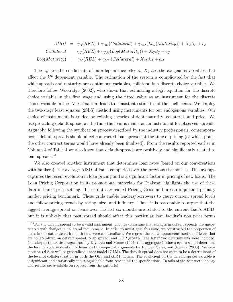
AISD = γA(REL) + γAC(Collateral) + γAM(Log(Maturity)) + XAβA + εA

Collateral = γC(REL) + γCM(Log(Maturity)) + XCβC + εC

Log(Maturity) = γM(REL) + γMC(Collateral) + XMβM + εM

The γij are the coefficients of interdependence effects. Xk are the exogenous variables that

affect the kth dependent variable. The estimation of the system is complicated by the fact that

while spreads and maturity are continuous variables, collateral is a discrete choice variable. We

therefore follow Woolridge (2002), who shows that estimating a logit equation for the discrete

choice variable in the first stage and using the fitted value as an instrument for the discrete

choice variable in the IV estimation, leads to consistent estimates of the coefficients. We employ

the two-stage least squares (2SLS) method using instruments for our endogenous variables. Our

choice of instruments is guided by existing theories of debt maturity, collateral, and price. We

use prevailing default spread at the time the loan is made, as an instrument for observed spreads.

Arguably, following the syndication process described by the industry professionals, contempora-

neous default spreads should affect contracted loan spreads at the time of pricing (at which point,

the other contract terms would have already been finalized). From the results reported earlier in

Column 4 of Table 4 we also know that default spreads are positively and significantly related to

loan spreads.38

We also created another instrument that determines loan rates (based on our conversations

with bankers): the average AISD of loans completed over the previous six months. This average

captures the recent evolution in loan pricing and is a significant factor in pricing of new loans. The

Loan Pricing Corporation in its promotional materials for Dealscan highlights the use of these

data in banks price-setting. These data are called Pricing Grids and are an important primary

market pricing benchmark. These grids enable lenders/borrowers to gauge current spread levels

and follow pricing trends by rating, size, and industry. Thus, it is reasonable to argue that the

lagged average spread on loans over the last six months are related to the current loan’s AISD,

but it is unlikely that past spread should affect this particular loan facility’s non price terms

38For the default spread to be a valid instrument, one has to assume that changes in default spreads are uncor-related with changes in collateral requirement. In order to investigate this issue, we constructed the proportion ofloans in our database each month that were collateralized. We regress the contemporaneous fraction of loans thatare collateralized on default spread, term spread, and GDP growth. The latter two determinants were included,following a) theoretical arguments by Kiyotaki and Moore (1997) that aggregate business cycles would determinethe level of collateralization of loans and b) empirical arguments by Jiminez, Salas, and Saurina (2006). We esti-mate an OLS as well as generalized linear model (GLM). The default spread does not seem to be a determinant ofthe level of collateralization in both the OLS and GLM models. The coefficient on the default spread variable isinsignificant and statistically indistinguishable from zero in all the specifications. Details of the test methodologyand results are available on request from the author(s).

38

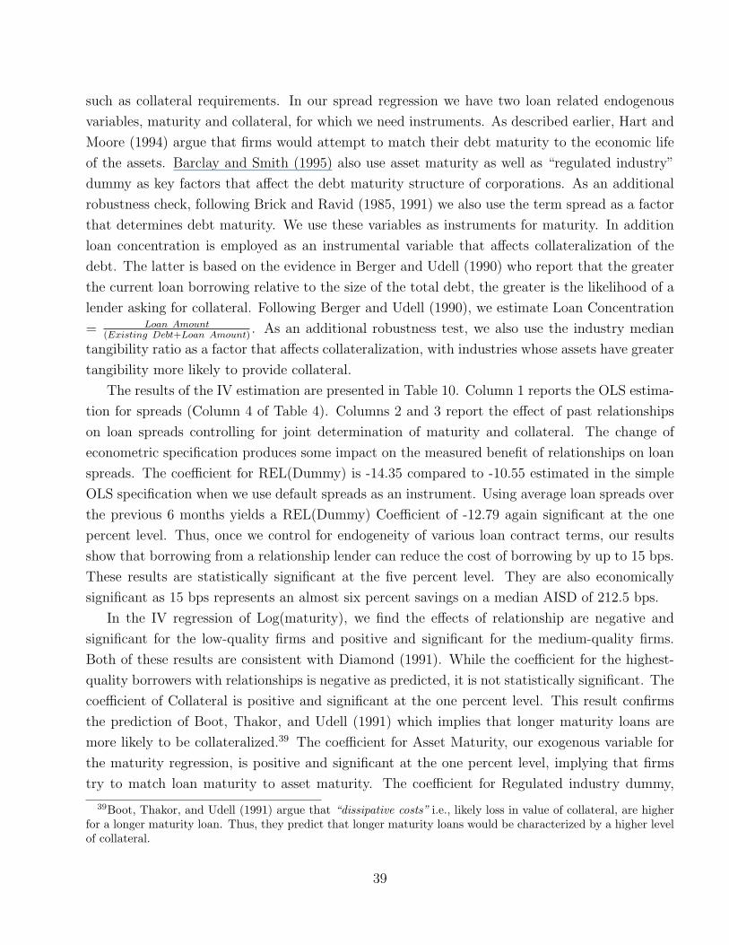
such as collateral requirements. In our spread regression we have two loan related endogenous

variables, maturity and collateral, for which we need instruments. As described earlier, Hart and

Moore (1994) argue that firms would attempt to match their debt maturity to the economic life

of the assets. Barclay and Smith (1995) also use asset maturity as well as “regulated industry”

dummy as key factors that affect the debt maturity structure of corporations. As an additional

robustness check, following Brick and Ravid (1985, 1991) we also use the term spread as a factor

that determines debt maturity. We use these variables as instruments for maturity. In addition

loan concentration is employed as an instrumental variable that affects collateralization of the

debt. The latter is based on the evidence in Berger and Udell (1990) who report that the greater

the current loan borrowing relative to the size of the total debt, the greater is the likelihood of a

lender asking for collateral. Following Berger and Udell (1990), we estimate Loan Concentration

= Loan Amount(Existing Debt+Loan Amount)

. As an additional robustness test, we also use the industry median

tangibility ratio as a factor that affects collateralization, with industries whose assets have greater

tangibility more likely to provide collateral.

The results of the IV estimation are presented in Table 10. Column 1 reports the OLS estima-

tion for spreads (Column 4 of Table 4). Columns 2 and 3 report the effect of past relationships

on loan spreads controlling for joint determination of maturity and collateral. The change of

econometric specification produces some impact on the measured benefit of relationships on loan

spreads. The coefficient for REL(Dummy) is -14.35 compared to -10.55 estimated in the simple

OLS specification when we use default spreads as an instrument. Using average loan spreads over

the previous 6 months yields a REL(Dummy) Coefficient of -12.79 again significant at the one

percent level. Thus, once we control for endogeneity of various loan contract terms, our results

show that borrowing from a relationship lender can reduce the cost of borrowing by up to 15 bps.

These results are statistically significant at the five percent level. They are also economically

significant as 15 bps represents an almost six percent savings on a median AISD of 212.5 bps.

In the IV regression of Log(maturity), we find the effects of relationship are negative and

significant for the low-quality firms and positive and significant for the medium-quality firms.

Both of these results are consistent with Diamond (1991). While the coefficient for the highest-

quality borrowers with relationships is negative as predicted, it is not statistically significant. The

coefficient of Collateral is positive and significant at the one percent level. This result confirms

the prediction of Boot, Thakor, and Udell (1991) which implies that longer maturity loans are

more likely to be collateralized.39 The coefficient for Asset Maturity, our exogenous variable for

the maturity regression, is positive and significant at the one percent level, implying that firms

try to match loan maturity to asset maturity. The coefficient for Regulated industry dummy,

39Boot, Thakor, and Udell (1991) argue that “dissipative costs” i.e., likely loss in value of collateral, are higherfor a longer maturity loan. Thus, they predict that longer maturity loans would be characterized by a higher levelof collateral.

39

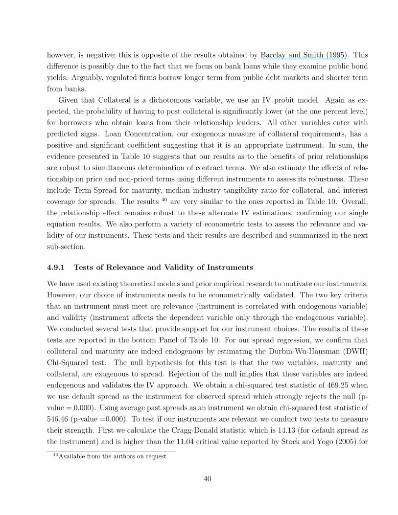
however, is negative; this is opposite of the results obtained by Barclay and Smith (1995). This

difference is possibly due to the fact that we focus on bank loans while they examine public bond

yields. Arguably, regulated firms borrow longer term from public debt markets and shorter term

from banks.

Given that Collateral is a dichotomous variable, we use an IV probit model. Again as ex-

pected, the probability of having to post collateral is significantly lower (at the one percent level)

for borrowers who obtain loans from their relationship lenders. All other variables enter with

predicted signs. Loan Concentration, our exogenous measure of collateral requirements, has a

positive and significant coefficient suggesting that it is an appropriate instrument. In sum, the

evidence presented in Table 10 suggests that our results as to the benefits of prior relationships

are robust to simultaneous determination of contract terms. We also estimate the effects of rela-

tionship on price and non-priced terms using different instruments to assess its robustness. These

include Term-Spread for maturity, median industry tangibility ratio for collateral, and interest

coverage for spreads. The results 40 are very similar to the ones reported in Table 10. Overall,

the relationship effect remains robust to these alternate IV estimations, confirming our single

equation results. We also perform a variety of econometric tests to assess the relevance and va-

lidity of our instruments. These tests and their results are described and summarized in the next

sub-section.

4.9.1 Tests of Relevance and Validity of Instruments

We have used existing theoretical models and prior empirical research to motivate our instruments.

However, our choice of instruments needs to be econometrically validated. The two key criteria

that an instrument must meet are relevance (instrument is correlated with endogenous variable)

and validity (instrument affects the dependent variable only through the endogenous variable).

We conducted several tests that provide support for our instrument choices. The results of these

tests are reported in the bottom Panel of Table 10. For our spread regression, we confirm that

collateral and maturity are indeed endogenous by estimating the Durbin-Wu-Hausman (DWH)

Chi-Squared test. The null hypothesis for this test is that the two variables, maturity and

collateral, are exogenous to spread. Rejection of the null implies that these variables are indeed

endogenous and validates the IV approach. We obtain a chi-squared test statistic of 469.25 when

we use default spread as the instrument for observed spread which strongly rejects the null (p-

value = 0.000). Using average past spreads as an instrument we obtain chi-squared test statistic of

546.46 (p-value =0.000). To test if our instruments are relevant we conduct two tests to measure

their strength. First we calculate the Cragg-Donald statistic which is 14.13 (for default spread as

the instrument) and is higher than the 11.04 critical value reported by Stock and Yogo (2005) for

40Available from the authors on request

40

an estimation with two endogenous variables. This implies that our instruments for maturity and

collateral are relevant. Another test for relevance of instruments is the Anderson-LR test of the

null hypothesis that correlations between the instrument and the endogenous variable is essentially

zero. We obtain a test statistic value of 58.98 which strongly rejects the null (p-value =0.000),

implying the instruments are strongly correlated with the endogenous variables. Results for using

average spreads as instrument are very similar. Tests of the instrument’s independence from

an unobservable error process (validity) can only be ascertained if the number of instruments

is higher than the number of endogenous variables so that the system of equations are over-

identified. Since we have two endogenous variables but four instruments for the spread equation,

we are able to estimate the Hansen-J statistic for over-identification restrictions. These are joint

tests of the null hypothesis that the correct model is specified and the orthogonality conditions

are met (correlations between the instruments and the error term is zero). A rejection of the

the null calls both of these assumptions into question. For our spread regression the Hansen-

J statistic is 4.13 with a p-value of 0.13. Thus, we fail to reject the null hypothesis, which

implies that our instruments are relevant and valid. We repeat all of these tests described so far,

for the specification in which we use the average AISD of the loans in the last 6 months as an

instrument for AISD. These results are reported in column 3 of Table 10 and are similar to results

obtained using default spread as the instrument. We report a Hansen J-statistic of 0.001 with

a p-value of 0.98 for the maturity regression, which shows that our instruments for collateral in

the maturity equation are valid. Since the maturity equation has only one endogenous variable

(collateral), we report the first stage F-statistic and the Shea Partial R-Squared statistic instead

of the Cragg-Donald statistic. We obtain a first-stage F-stat of 323.27 compared against the

benchmark of 10 suggested by Staiger and Stock (1997) and a high partial R-Squared of 8.16%.

These tests confirm the relevance of our instruments for collateral in the maturity equation.

The Anderson LR statistic of 1289 with a p-value of 0.000 rejecting the null (of zero correlation

between the instrument and endogenous variable) further strengthens our conclusions. Finally,

the Durbin-Wu-Hausman (DWH) Chi-Squared test statistic of 1170 with a p value of 0.000 shows

that collateral is indeed endogenous in the maturity equation. Since collateral is dummy variable

we cannot apply the above tests of instrument relevance and validity.41 However, we do report

the results of the Wald test to see if maturity is exogenous in the collateral equation. The null

hypothesis that maturity is exogenous is strongly rejected (p-value =0.000). Collectively, these

multiple tests provide econometric support for the relevance and validity of our instruments.

41We are not aware of any econometric tests for IV probit models.

41

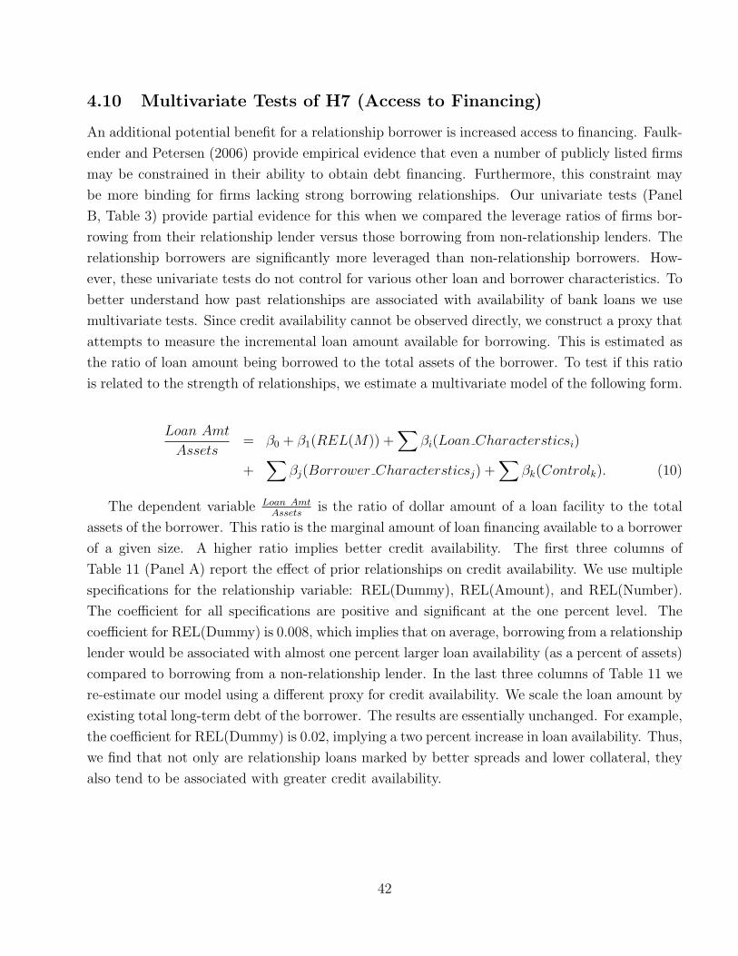
4.10 Multivariate Tests of H7 (Access to Financing)

An additional potential benefit for a relationship borrower is increased access to financing. Faulk-

ender and Petersen (2006) provide empirical evidence that even a number of publicly listed firms

may be constrained in their ability to obtain debt financing. Furthermore, this constraint may

be more binding for firms lacking strong borrowing relationships. Our univariate tests (Panel

B, Table 3) provide partial evidence for this when we compared the leverage ratios of firms bor-

rowing from their relationship lender versus those borrowing from non-relationship lenders. The

relationship borrowers are significantly more leveraged than non-relationship borrowers. How-

ever, these univariate tests do not control for various other loan and borrower characteristics. To

better understand how past relationships are associated with availability of bank loans we use

multivariate tests. Since credit availability cannot be observed directly, we construct a proxy that

attempts to measure the incremental loan amount available for borrowing. This is estimated as

the ratio of loan amount being borrowed to the total assets of the borrower. To test if this ratio

is related to the strength of relationships, we estimate a multivariate model of the following form.

Loan Amt

Assets= β0 + β1(REL(M)) +

∑βi(Loan Charactersticsi)

+∑

βj(Borrower Charactersticsj) +∑

βk(Controlk). (10)

The dependent variable Loan AmtAssets

is the ratio of dollar amount of a loan facility to the total

assets of the borrower. This ratio is the marginal amount of loan financing available to a borrower

of a given size. A higher ratio implies better credit availability. The first three columns of

Table 11 (Panel A) report the effect of prior relationships on credit availability. We use multiple

specifications for the relationship variable: REL(Dummy), REL(Amount), and REL(Number).

The coefficient for all specifications are positive and significant at the one percent level. The

coefficient for REL(Dummy) is 0.008, which implies that on average, borrowing from a relationship

lender would be associated with almost one percent larger loan availability (as a percent of assets)

compared to borrowing from a non-relationship lender. In the last three columns of Table 11 we

re-estimate our model using a different proxy for credit availability. We scale the loan amount by

existing total long-term debt of the borrower. The results are essentially unchanged. For example,

the coefficient for REL(Dummy) is 0.02, implying a two percent increase in loan availability. Thus,

we find that not only are relationship loans marked by better spreads and lower collateral, they

also tend to be associated with greater credit availability.

42

5 Conclusion

The role of strong relationships between lenders and borrowers has been an active area of research.

Theoretical models have generated a number of rich empirical implications both in terms of how

past relationships may affect loan contracts in the future as well as a set of borrower characteristics

that would make relationships more (or less) important. We find that repeated borrowing from the

same lender translates into a 10 to 17 bps lowering of loan spreads. Our results provide evidence

that hypothesized economies in information production due to repeated interaction between the

same lender and borrower are at least partly reflected in the price of loans. This result continues to

hold across various methodologies that control for the endogeneity of the relationship formation.

We also find that as the information opacity of a borrower increases, the observed reduction in

the cost of borrowing due to a relationship becomes greater. These results also shed light on the

boundary of relationship and transactional lending. We find that spreads charged for relationship

loans and non-relationship loans become indistinguishable if the borrower was in the top 30% when

ranked by asset size. Similar dissipation of relationship benefits occurs if the borrower has a rated

public debt or is part of S&P 500 index. The paper uses loan syndicate structure to examine

the interaction of past relationships and syndicate moral hazard due to multiple lenders. The

results in our paper indicate that past relationships can mitigate syndicate moral hazard issues

by serving as a commitment to monitor. We also find that relationship loans are significantly

less likely to be secured by collateral, and our results on loan maturity are broadly consistent

with Diamond (1991). Our results are robust to an estimation methodology which allows loan

spread, collateral requirement, and loan maturity to be determined jointly using an IV approach.

Finally, the relationship borrowers also obtain larger loans (scaled by the borrower’s asset size or

long-term debt) compared to non-relationship borrowers. In sum, we report significant benefits

of borrowing from relationship lenders even for publicly traded firms.

43

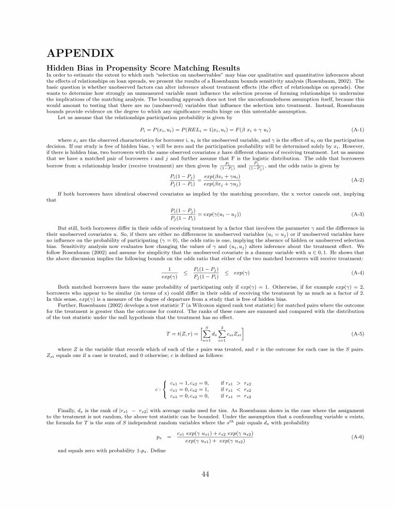
APPENDIXHidden Bias in Propensity Score Matching ResultsIn order to estimate the extent to which such “selection on unobservables” may bias our qualitative and quantitative inferences aboutthe effects of relationships on loan spreads, we present the results of a Rosenbaum bounds sensitivity analysis (Rosenbaum, 2002). Thebasic question is whether unobserved factors can alter inference about treatment effects (the effect of relationships on spreads). Onewants to determine how strongly an unmeasured variable must influence the selection process of forming relationships to underminethe implications of the matching analysis. The bounding approach does not test the unconfoundedness assumption itself, because thiswould amount to testing that there are no (unobserved) variables that influence the selection into treatment. Instead, Rosenbaumbounds provide evidence on the degree to which any significance results hinge on this untestable assumption.

Let us assume that the relationships participation probability is given by

Pi = P (xi, ui) = P (RELi = 1|xi, ui) = F (β xi + γ ui) (A-1)

where xi are the observed characteristics for borrower i, ui is the unobserved variable, and γ is the effect of ui on the participationdecision. If our study is free of hidden bias, γ will be zero and the participation probability will be determined solely by xi. However,if there is hidden bias, two borrowers with the same observed covariates x have different chances of receiving treatment. Let us assumethat we have a matched pair of borrowers i and j and further assume that F is the logistic distribution. The odds that borrowers

borrow from a relationship lender (receive treatment) are then given by Pi(1−Pi)

andPj

(1−Pj), and the odds ratio is given by

Pi(1− Pj)

Pj(1− Pi)=

exp(βxi + γui)

exp(βxj + γuj)(A-2)

If both borrowers have identical observed covariates as implied by the matching procedure, the x vector cancels out, implyingthat

Pi(1− Pj)

Pj(1− Pi)= exp(γ(ui − uj)) (A-3)

But still, both borrowers differ in their odds of receiving treatment by a factor that involves the parameter γ and the difference intheir unobserved covariates u. So, if there are either no differences in unobserved variables (ui = uj) or if unobserved variables haveno influence on the probability of participating (γ = 0), the odds ratio is one, implying the absence of hidden or unobserved selectionbias. Sensitivity analysis now evaluates how changing the values of γ and (ui, uj) alters inference about the treatment effect. Wefollow Rosenbaum (2002) and assume for simplicity that the unobserved covariate is a dummy variable with u ∈ 0, 1. He shows thatthe above discussion implies the following bounds on the odds ratio that either of the two matched borrowers will receive treatment:

1

exp(γ)≤

Pi(1− Pj)

Pj(1− Pi)≤ exp(γ) (A-4)

Both matched borrowers have the same probability of participating only if exp(γ) = 1. Otherwise, if for example exp(γ) = 2,borrowers who appear to be similar (in terms of x) could differ in their odds of receiving the treatment by as much as a factor of 2.In this sense, exp(γ) is a measure of the degree of departure from a study that is free of hidden bias.

Further, Rosenbaum (2002) develops a test statistic T (a Wilcoxon signed rank test statistic) for matched pairs where the outcomefor the treatment is greater than the outcome for control. The ranks of these cases are summed and compared with the distributionof the test statistic under the null hypothesis that the treatment has no effect.

T = t(Z, r) =

» SXs=1

ds

2Xi=1

csiZsi

–(A-5)

where Z is the variable that records which of each of the s pairs was treated, and r is the outcome for each case in the S pairs.Zsi equals one if a case is treated, and 0 otherwise; c is defined as follows:

c :

8<:cs1 = 1, cs2 = 0, if rs1 > rs2

cs1 = 0, cs2 = 1, if rs1 < rs2

cs1 = 0, cs2 = 0, if rs1 = rs2

Finally, ds is the rank of |rs1 − rs2| with average ranks used for ties. As Rosenbaum shows in the case where the assignmentto the treatment is not random, the above test statistic can be bounded. Under the assumption that a confounding variable u exists,the formula for T is the sum of S independent random variables where the sth pair equals ds with probability

ps =cs1 exp(γ us1) + cs2 exp(γ us2)

exp(γ us1) + exp(γ us2)(A-6)

and equals zero with probability 1-ps. Define

44

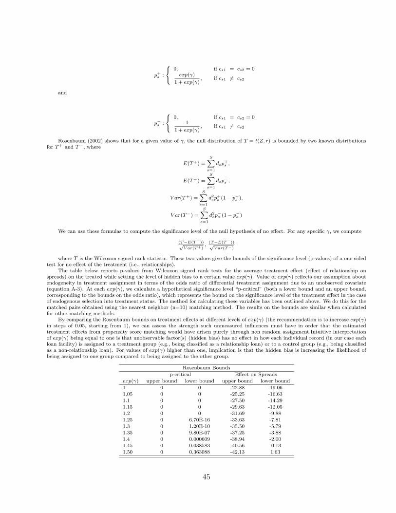
p+s :

8<:0, if cs1 = cs2 = 0

exp(γ)

1 + exp(γ), if cs1 6= cs2

and

p−s :

8<: 0, if cs1 = cs2 = 01

1 + exp(γ), if cs1 6= cs2

Rosenbaum (2002) shows that for a given value of γ, the null distribution of T = t(Z, r) is bounded by two known distributionsfor T+ and T−, where

E(T+) =

SXs=1

dsp+s ,

E(T−) =

SXs=1

dsp−s ,

V ar(T+) =SX

s=1

d2sp+

s (1− p+s ),

V ar(T−) =

SXs=1

d2sp−s (1− p−s )

We can use these formulas to compute the significance level of the null hypothesis of no effect. For any specific γ, we compute

(T−E(T+))√V ar(T+)

,(T−E(T−))√

V ar(T−)

where T is the Wilcoxon signed rank statistic. These two values give the bounds of the significance level (p-values) of a one sidedtest for no effect of the treatment (i.e., relationships).

The table below reports p-values from Wilcoxon signed rank tests for the average treatment effect (effect of relationship onspreads) on the treated while setting the level of hidden bias to a certain value exp(γ). Value of exp(γ) reflects our assumption aboutendogeneity in treatment assignment in terms of the odds ratio of differential treatment assignment due to an unobserved covariate(equation A-3). At each exp(γ), we calculate a hypothetical significance level “p-critical” (both a lower bound and an upper bound,corresponding to the bounds on the odds ratio), which represents the bound on the significance level of the treatment effect in the caseof endogenous selection into treatment status. The method for calculating these variables has been outlined above. We do this for thematched pairs obtained using the nearest neighbor (n=10) matching method. The results on the bounds are similar when calculatedfor other matching methods.

By comparing the Rosenbaum bounds on treatment effects at different levels of exp(γ) (the recommendation is to increase exp(γ)in steps of 0.05, starting from 1), we can assess the strength such unmeasured influences must have in order that the estimatedtreatment effects from propensity score matching would have arisen purely through non random assignment.Intuitive interpretationof exp(γ) being equal to one is that unobservable factor(s) (hidden bias) has no effect in how each individual record (in our case eachloan facility) is assigned to a treatment group (e.g., being classified as a relationship loan) or to a control group (e.g., being classifiedas a non-relationship loan). For values of exp(γ) higher than one, implication is that the hidden bias is increasing the likelihood ofbeing assigned to one group compared to being assigned to the other group.

Rosenbaum Bounds

p-critical Effect on Spreadsexp(γ) upper bound lower bound upper bound lower bound

1 0 0 -22.88 -19.061.05 0 0 -25.25 -16.631.1 0 0 -27.50 -14.291.15 0 0 -29.63 -12.051.2 0 0 -31.69 -9.881.25 0 6.70E-16 -33.63 -7.811.3 0 1.20E-10 -35.50 -5.791.35 0 9.80E-07 -37.25 -3.881.4 0 0.000609 -38.94 -2.001.45 0 0.038583 -40.56 -0.131.50 0 0.363088 -42.13 1.63

45

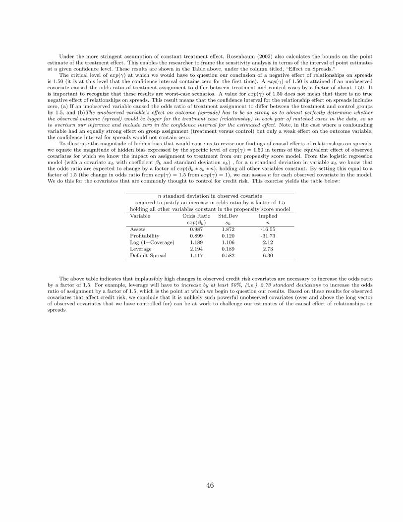
Under the more stringent assumption of constant treatment effect, Rosenbaum (2002) also calculates the bounds on the pointestimate of the treatment effect. This enables the researcher to frame the sensitivity analysis in terms of the interval of point estimatesat a given confidence level. These results are shown in the Table above, under the column titled, “Effect on Spreads.”

The critical level of exp(γ) at which we would have to question our conclusion of a negative effect of relationships on spreadsis 1.50 (it is at this level that the confidence interval contains zero for the first time). A exp(γ) of 1.50 is attained if an unobservedcovariate caused the odds ratio of treatment assignment to differ between treatment and control cases by a factor of about 1.50. Itis important to recognize that these results are worst-case scenarios. A value for exp(γ) of 1.50 does not mean that there is no truenegative effect of relationships on spreads. This result means that the confidence interval for the relationship effect on spreads includeszero, (a) If an unobserved variable caused the odds ratio of treatment assignment to differ between the treatment and control groupsby 1.5, and (b)The unobserved variable’s effect on outcome (spreads) has to be so strong as to almost perfectly determine whetherthe observed outcome (spread) would be bigger for the treatment case (relationship) in each pair of matched cases in the data, so asto overturn our inference and include zero in the confidence interval for the estimated effect. Note, in the case where a confoundingvariable had an equally strong effect on group assignment (treatment versus control) but only a weak effect on the outcome variable,the confidence interval for spreads would not contain zero.

To illustrate the magnitude of hidden bias that would cause us to revise our findings of causal effects of relationships on spreads,we equate the magnitude of hidden bias expressed by the specific level of exp(γ) = 1.50 in terms of the equivalent effect of observedcovariates for which we know the impact on assignment to treatment from our propensity score model. From the logistic regressionmodel (with a covariate xk with coefficient βk and standard deviation sk) , for a n standard deviation in variable xk we know thatthe odds ratio are expected to change by a factor of exp(βk ∗ sk ∗ n), holding all other variables constant. By setting this equal to afactor of 1.5 (the change in odds ratio from exp(γ) = 1.5 from exp(γ) = 1), we can assess n for each observed covariate in the model.We do this for the covariates that are commonly thought to control for credit risk. This exercise yields the table below:

n standard deviation in observed covariaterequired to justify an increase in odds ratio by a factor of 1.5

holding all other variables constant in the propensity score model

Variable Odds Ratio Std.Dev Impliedexp(βk) sk n

Assets 0.987 1.872 -16.55Profitability 0.899 0.120 -31.73Log (1+Coverage) 1.189 1.106 2.12Leverage 2.194 0.189 2.73Default Spread 1.117 0.582 6.30

The above table indicates that implausibly high changes in observed credit risk covariates are necessary to increase the odds ratioby a factor of 1.5. For example, leverage will have to increase by at least 50%, (i.e.) 2.73 standard deviations to increase the oddsratio of assignment by a factor of 1.5, which is the point at which we begin to question our results. Based on these results for observedcovariates that affect credit risk, we conclude that it is unlikely such powerful unobserved covariates (over and above the long vectorof observed covariates that we have controlled for) can be at work to challenge our estimates of the causal effect of relationships onspreads.

46

References

[1] Barclay, Michael J., and Clifford W. Smith, 1995, The Maturity Structure of Corporate Debt, Journal ofFinance, 50, 609-631.

[2] Barclay, Michael J., L.M. Marx and Clifford W. Smith, 2003, The Joint Determination of Leverage andMaturity, Journal of Corporate Finance, 9, 149-167.

[3] Berger, Allen, and Gregory Udell, 1990, Collateral, Loan Quality and Bank Risk, Journal of MonetaryEconomics, 25, 21-42.

[4] Berger, Allen, and Gregory Udell, 1995, Relationship Lending and Lines of Credit in Small Firm Finance,Journal of Business, 68, 351-381.

[5] Berger, Allen, Marco Espinosa-Vega, Scott Frame, and Nathan Miller, 2005, Debt Maturity, Risk, and Asym-metric Information, Journal of Finance, 60, 2895-2923.

[6] Berger, Allen, N. Miller, M. Petersen, R. Rajan, and J. Stein, 2005, Does function follow organizational form?Evidence from the lending practices of large and small banks, Journal of Financial Economics, 76, 237-269.

[7] Besanko, David, and Anjan Thakor, 1987, Collateral and Rationing: Sorting Equilibria in Monopolistic andCompetitive Credit Markets, International Economic Review, 28, 601-689.

[8] Bester, Helmut, 1985, Screening vs. Rationing in Credit Market under Asymmetric Information, Journal ofEconomic Theory, 42, 167-182.

[9] Berlin, Mitchell, and Loretta Mester, 1992, Debt Covenants and Renegotiations, Journal of Financial Inter-mediation, 2, 95-133.

[10] Berlin, Mitchell, and Loretta Mester, 1998, Deposits and Relationship Lending, Review of Financial Studies,2, 95-133.

[11] Bharath, Sreedhar, Sandeep Dahiya, Anthony Saunders, and Anand Srinivasan, 2007, So What Do I Get?The Bank’s View of Lending Relationships, Journal of Financial Economics, 85, 368-419.

[12] Bharath, Sreedhar, Paolo Pasquareillo, and Guojun Wu, 2007, Does Information Asymmetry Drive CapitalStructure Decisions, Forthcoming, Review of Financial Studies.

[13] Bhattacharya, Sudipto, and Gabriella Chiesa, 1995, Proprietary Information, Financial Intermediation andResearch Incentives, Journal of Financial Intermediation, 4, 328-357.

[14] Boot, Arnoud, 2000, Relationship Banking: What Do We Know?, Journal of Financial Intermediation, 9,7-25.

[15] Boot, Arnoud, Anjan Thakor, and Gregory Udell, 1991, Secured Lending and Default Risk: EquilibriumAnalysis, Policy Implications and Empirical Results, The Economics Journal, 101 (406), 458-472.

[16] Boot, Arnoud, Stuart Greenbaum, and Anjan Thakor, 1993, Reputation and Discretion in Financial Con-tracting, American Economic Review, 83, 1165-1183.

[17] Boot, Arnoud, and Anjan Thakor, 1994, Moral Hazard and Secured Lending in an Infinitely Repeated CreditMarket Game, International Economic Review, 35, 899-920.

[18] Boot, Arnoud, and Anjan Thakor, 2000, Can Relationship Banking Survive Competition?, Journal of Finance,55, 679-713.

[19] Bradley, Michael and M.Roberts, 2004, The Structure and Pricing of Corporate Debt Covenants. Availableat SSRN: http://ssrn.com/abstract=466240

[20] Brick, Ivan, and Abraham Ravid, 1985, On the Relevance of Debt Maturity Structure, Journal of Finance,40, 1423-1437.

47

[21] Brick, Ivan, and Abraham Ravid, 1991, Interest Rate Uncertainty and the Optimal Debt Maturity Structure,Journal of Financial and Quantitative Analysis, 26, 363-381.

[22] Brown, R. L., J. Durbin, and J. M. Evans, 1975, Techniques for Testing for the Constancy of RegressionRelationships over Time, Journal of the Royal Statistical Society, 37, 149-192.

[23] Cantillo Miguel and Julian Wright, 2000, How Do Firms Choose Their Lenders? An Empirical Investigation,Review of Financial Studies, 13, 155-189.

[24] Cole, Rebel A., 1998, The Importance of Relationships to the Availability of Credit, Journal of Banking &Finance, 22, 959-977.

[25] Coval, Joshua D. and Moskowitz, Tobias J., 2001, The Geography of Investment: Informed Trading and AssetPrices, Journal of Political Economy, 109 (4), 811-841.

[26] Dahiya, Sandeep, Anthony Saunders, and Anand Srinivasan, 2003, Financial Distress and Bank LendingRelationships, Journal of Finance, 58, 375-399.

[27] Dass, Nishant and Massimo Massa, 2006, The Bank-Firm Relationship: A Trade-off Between Better Gover-nance and Greater Information Asymmetry, Working Paper, INSEAD.

[28] Dechow, Patricia, and I. Dichev, 2002, The Quality of Accruals and Earnings: The Role of Accrual EstimationErrors, The Accounting Review, 77. Supplement, pp. 35-59.

[29] Degryse, Hans, and Patrick Van Cayseele, 2000, Relationship Lending within a Bank Based System: Evidencefrom European Small Business Data, Journal of Financial Intermediation, 9, 90-109.

[30] Dennis, Steven, Debarshi Nandy, and Ian Sharpe, 2000, Determinants of Contract Terms in Bank RevolvingLines of Credit, Journal of Financial and Quantitative Analysis, 35, 87-109.

[31] Detragiache, Enrica, Paolo Garella, and Luigi Guiso, 2000, Multiple versus Single Banking Relationships:Theory and Evidence, Journal of Finance, 55, 1005-1476.

[32] Diamond, Douglas, 1984, Financial Intermediation and Delegated Monitoring, Review of Economic Studies,62, 393-414.

[33] Diamond, Douglas, 1991, Debt Maturity and Liquidity Risk, Quraterly Journal of Economics106(3), 709-737.

[34] Diamond, Douglas, 2004, Presidential Address, Committing to Commit: Short Term Debt When EnforcementIs Costly, Journal of Finance, 59, 1447-1479.

[35] Drucker, Steven, and Manju Puri, 2005, On the Benefits of Concurrent Lending and Underwriting, Journalof Finance, 60, 2763-2799.

[36] Fama, Eugene., 1985, What’s Different About Banks? Journal of Monetary Economics 15(1), 29-39.

[37] Faulkender. Michael, and Mitchell Petersen, 2006, Does the Source of Capital Affect Capital Structure?Review of Financial Studies, 19(1), 45 - 79.

[38] Flannery, Mark, 1986, Asymmetric Information and Risky Debt Maturity Choice, Journal of Finance, 41,19-37.

[39] Greene, W. H., 2000, Econometric Analysis, 4th ed, Upper Saddle River, NJ: PrenticeHall.

[40] Hart, Oliver, and John Moore, 1994, A Theory of Debt Based on the Inalienability of Human Capital,Quarterly Journal of Economics, 109, 841-79.

[41] Heckman, James, Hidehiko Ichimura, and Petra Todd, 1997, Matching as an Econometric Evaluation Esti-mator: Evidence from Evaluating a Job Training Programme, Review of Economic Studies 64, 605-654.

[42] Heckman, James, Hidehiko Ichimura, and Petra Todd, 1998, Matching as an Econometric Evaluation Esti-mator, Review of Economic Studies 65, 261-294.

48

[43] Holmstrom, Bengt and Jean Tirole, 1997, Financial Intermediation, Loanable Funds and the Real Sector,Quarterly Journal of Economics, 112(3), 663-691.

[44] Hoshi, Takeo, Anil Kashyap, and David Scharfstein, 1990, The Role of Banks in Reducing the Costs ofFinancial Distress in Japan, Journal of Financial Economics, 27, 67-88.

[45] Jimenez, Gabriel, Vicente Salas, Jesus Saurina, 2006, Determinants of Collateral, Journal of Financial Eco-nomics, 81(2), 255-281.

[46] Kallberg. J, C. Liu, and A. Srinivasan, 2004, Limited Partnerships and Reputation Formation, Journal ofFinancial and Quantitative Analysis, 39, 631-659.

[47] Kiyotaki, N., and J. Moore, 1997, Credit Cycles Journal of Political Economy, 105, 211 - 48.

[48] Melnik, Arie and Steven Plaut, 1986, Loan Commitment Contracts, Terms of Lending, and Credit Allocation,Journal of Finance, 41, 425-435.

[49] Maddala, G. S., 1983, Limited-dependent and Qualitative Variables in Econometrics, Cambridge, UK: Cam-bridge University Press.

[50] Petersen, Mitchell, and Raghuram Rajan, 1994, The Benefits of Lending Relationships: Evidence from SmallBusiness Data, Journal of Finance, 49, 3-37.

[51] Petersen, Mitchell, and Raghuram Rajan, 1995, The Effect of Credit Market Competition on Lending Rela-tionships, Quarterly Journal of Economics, 110, 406-443.

[52] Petersen, Mitchell A., and Raghuram G. Rajan, 2002, Does Distance Still Matter? The Information Revolu-tion in Small Business Lending, Journal of Finance, 57, 2533- 2570.

[53] Rajan, Raghuram, 1992, Insiders and Outsiders: The Relationship Between Relationship and Arms LengthDebt, Journal of Finance, 47, 1367-1400.

[54] Rajan, Raghuram, and Andrew Winton, 1995, Covenants and Collateral as Incentives to Monitor, Journal ofFinance, 50,1113-1146.

[55] Ramakrishnan Ram, and Anjan Thakor, 1984, Information Reliability and a Theory of Financial Intermedi-ation, Review of Economic Studies, 51, 415-432.

[56] Rogers, William, 1993, Regression Standard Errors in Clustered Samples, Stata Technical Bulletin 13, 19-23.

[57] Rosenbaum, Paul R., 2002, Observational Studies, 2nd Edition, Springer-Verlag, New York.

[58] Sharpe, Steven, 1990, Asymmetric Information, Bank Lending and Implicit Contracts: A Stylized Model ofCustomer Relationships, Journal of Finance 45, 1069-1087.

[59] Standard & Poor’s, 2006, A Guide to the Loan Market.

[60] Staiger, Douglas and James, Stock, 1997, Instrumental Varaiables Regression with Weak Instruments, Econo-metrica, 557-586.

[61] Stock James, and Motohiro, Yogo, 2005, Testing for Weak Instruments in Linear IV Regression, in D.W.K.Andrews and J.H. Stock, eds., Identification and Inference for Econometric Models: Essays in Honor ofThomas J. Rothenberg. Cambridge: Cambridge University Press. 80-108.

[62] Strahan, Phillip, 1999, Borrower Risk and the Price and Non-price Terms of Bank Loans, Federal ReserveBank of New York, Staff Paper No. 90, Available at SSRN: http://ssrn.com/abstract=192769

[63] Stulz, Rene, and Herb Johnson, 1985, An Analysis of Secured Debt, Journal of Financial Economics, 14,501-521.

[64] Sufi, Amir, 2007, Information Asymmetry and Financing Arrangements: Evidence from Syndicated LoansJournal of Finance, 62, 629-668.

[65] Wooldridge, J. M., 2002, Econometric Analysis of Cross Section and Panel Data, The MIT Press, Cambridge,Massachusetts.

49

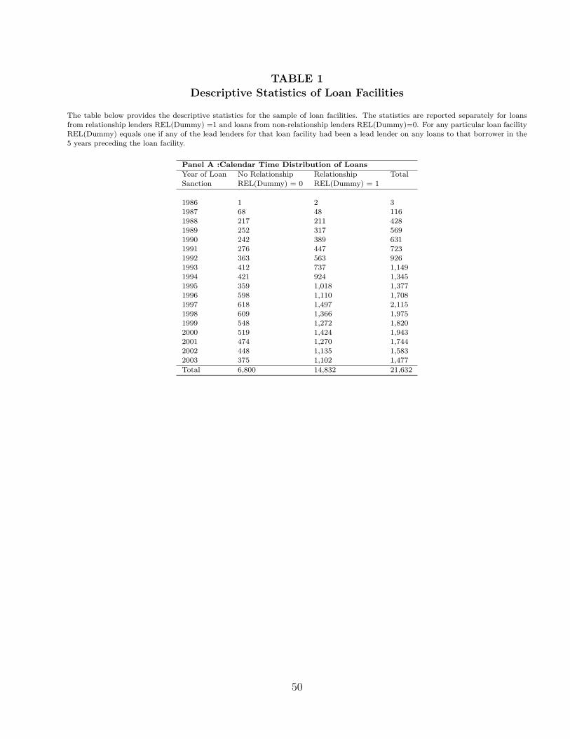
TABLE 1

Descriptive Statistics of Loan Facilities

The table below provides the descriptive statistics for the sample of loan facilities. The statistics are reported separately for loansfrom relationship lenders REL(Dummy) =1 and loans from non-relationship lenders REL(Dummy)=0. For any particular loan facilityREL(Dummy) equals one if any of the lead lenders for that loan facility had been a lead lender on any loans to that borrower in the5 years preceding the loan facility.

Panel A :Calendar Time Distribution of Loans

Year of Loan No Relationship Relationship TotalSanction REL(Dummy) = 0 REL(Dummy) = 1

1986 1 2 31987 68 48 1161988 217 211 4281989 252 317 5691990 242 389 6311991 276 447 7231992 363 563 9261993 412 737 1,1491994 421 924 1,3451995 359 1,018 1,3771996 598 1,110 1,7081997 618 1,497 2,1151998 609 1,366 1,9751999 548 1,272 1,8202000 519 1,424 1,9432001 474 1,270 1,7442002 448 1,135 1,5832003 375 1,102 1,477

Total 6,800 14,832 21,632

50

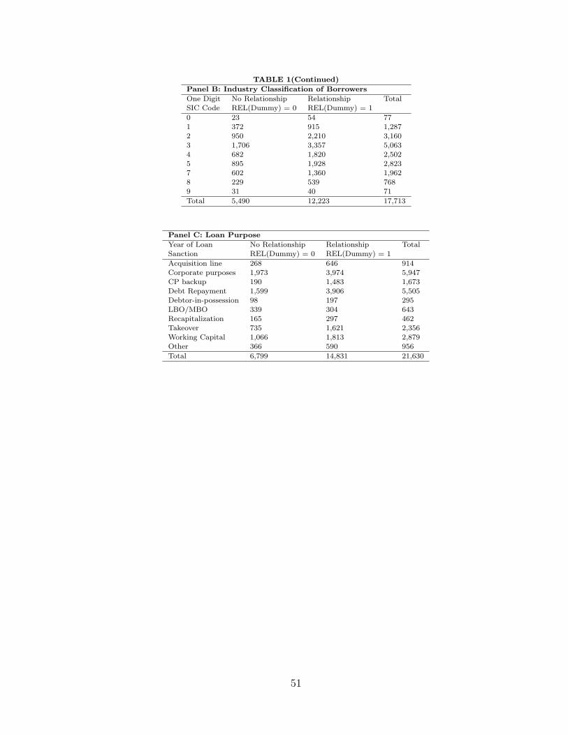
TABLE 1(Continued)

Panel B: Industry Classification of Borrowers

One Digit No Relationship Relationship TotalSIC Code REL(Dummy) = 0 REL(Dummy) = 1

0 23 54 771 372 915 1,2872 950 2,210 3,1603 1,706 3,357 5,0634 682 1,820 2,5025 895 1,928 2,8237 602 1,360 1,9628 229 539 7689 31 40 71

Total 5,490 12,223 17,713

Panel C: Loan Purpose

Year of Loan No Relationship Relationship TotalSanction REL(Dummy) = 0 REL(Dummy) = 1

Acquisition line 268 646 914Corporate purposes 1,973 3,974 5,947CP backup 190 1,483 1,673Debt Repayment 1,599 3,906 5,505Debtor-in-possession 98 197 295LBO/MBO 339 304 643Recapitalization 165 297 462Takeover 735 1,621 2,356Working Capital 1,066 1,813 2,879Other 366 590 956

Total 6,799 14,831 21,630

51

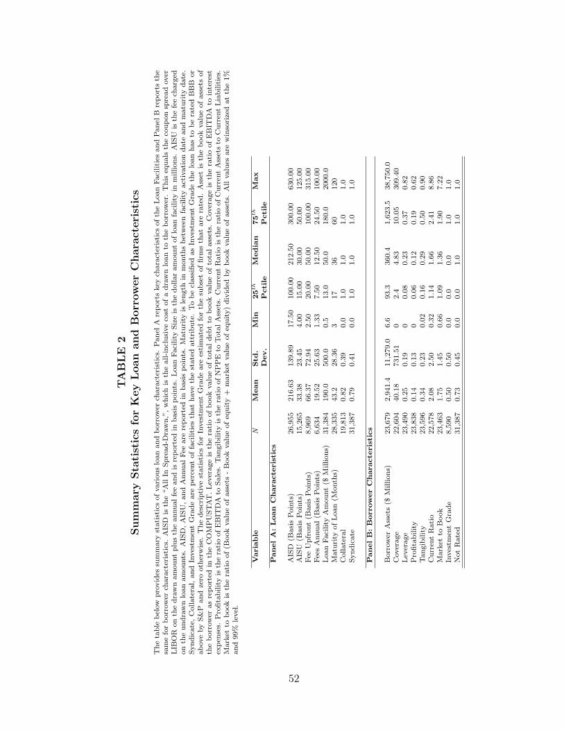
TA

BLE

2Sum

mary

Sta

tist

ics

for

Key

Loan

and

Borr

ow

er

Chara

cteri

stic

s

The

table

bel

ow

pro

vid

essu

mm

ary

stati

stic

sofvari

ous

loan

and

borr

ow

erch

ara

cter

istics

.Panel

Are

port

skey

chara

cter

istics

ofth

eLoan

Faci

lities

and

Panel

Bre

port

sth

esa

me

for

borr

ow

erch

ara

cter

istics

.A

ISD

isth

e“A

llIn

Spre

ad-D

raw

n,”

,w

hic

his

the

all-incl

usi

ve

cost

ofa

dra

wn

loan

toth

eborr

ow

er.

This

equals

the

coupon

spre

ad

over

LIB

OR

on

the

dra

wn

am

ount

plu

sth

eannualfe

eand

isre

port

edin

basi

spoin

ts.

Loan

Faci

lity

Siz

eis

the

dollar

am

ount

oflo

an

faci

lity

inm

illions.

AIS

Uis

the

fee

charg

edon

the

undra

wn

loan

am

ounts

.A

ISD

,A

ISU

,and

AnnualFee

are

report

edin

basi

spoin

ts.

Matu

rity

isle

ngth

inm

onth

sbet

wee

nfa

cility

act

ivation

date

and

matu

rity

date

.Syndic

ate

,C

ollate

ral,

and

Inves

tmen

tG

rade

are

per

cent

offa

cilities

that

have

the

state

datt

ribute

.To

be

class

ified

as

Inves

tmen

tG

rade

the

loan

has

tobe

rate

dB

BB

or

above

by

S&

Pand

zero

oth

erw

ise.

The

des

crip

tive

statist

ics

for

Inves

tmen

tG

rade

are

estim

ate

dfo

rth

esu

bse

toffirm

sth

at

are

rate

d.

Ass

etis

the

book

valu

eofass

ets

of

the

borr

ow

eras

report

edin

the

CO

MP

USTAT

.Lev

erage

isth

era

tio

ofbook

valu

eofto

taldeb

tto

book

valu

eofto

talass

ets.

Cover

age

isth

era

tio

ofE

BIT

DA

toin

tere

stex

pen

ses.

Pro

fita

bility

isth

era

tio

ofE

BIT

DA

toSale

s.Tangib

ility

isth

era

tio

ofN

PP

Eto

Tota

lA

sset

s.C

urr

ent

Ratio

isth

era

tio

ofC

urr

ent

Ass

ets

toC

urr

ent

Lia

bilitie

s.M

ark

etto

book

isth

era

tio

of(B

ook

valu

eofass

ets

-B

ook

valu

eofeq

uity

+m

ark

etvalu

eofeq

uity)

div

ided

by

book

valu

eofass

ets.

All

valu

esare

win

sori

zed

at

the

1%

and

99%

level

.

Varia

ble

NM

ean

Std

.M

in25

thM

edia

n75

thM

ax

Dev.

Pcti

leP

cti

lePanelA

:Loan

Characte

ris

tics

AIS

D(B

asi

sPoin

ts)

26,9

55

216.6

3139.8

917.5

0100.0

0212.5

0300.0

0630.0

0A

ISU

(Basi

sPoin

ts)

15,2

65

33.3

823.4

54.0

015.0

030.0

050.0

0125.0

0Fee

Upfr

ont

(Basi

sPoin

ts)

8,9

69

66.3

772.9

42.5

020.0

050.0

0100.0

0315.0

0Fee

sA

nnual(B

asi

sPoin

ts)

6,6

34

19.5

225.6

31.3

37.5

012.5

024.5

0100.0

0Loan

Faci

lity

Am

ount

($M

illions)

31,3

84

190.0

500.0

0.5

13.0

50.0

180.0

2000.0

Matu

rity

ofLoan

(Month

s)28,3

35

43.2

28.3

63

17

36

60

120

Collate

ral

19,8

13

0.8

20.3

90.0

1.0

1.0

1.0

1.0

Syndic

ate

31,3

87

0.7

90.4

10.0

1.0

1.0

1.0

1.0

PanelB

:B

orrow

er

Characte

ris

tics

Borr

ow

erA

sset

s($

Millions)

23,6

79

2,9

41.4

11,2

79.0

6.6

93.3

360.4

1,6

23.5

38,7

50.0

Cover

age

22,6

04

40.1

8731.5

10

2.4

4.8

310.0

5309.4

0Lev

erage

23,4

90

0.2

50.1

90

0.0

80.2

30.3

70.8

2P

rofita

bility

23,8

38

0.1

40.1

30

0.0

60.1

20.1

90.6

2Tangib

ility

23,5

96

0.3

40.2

30.0

20.1

60.2

90.5

00.9

0C

urr

ent

Rati

o22,5

78

2.0

82.5

00.3

21.1

41.6

62.4

18.8

6M

ark

etto

Book

23,4

63

1.7

51.4

50.6

61.0

91.3

61.9

07.2

2In

ves

tmen

tG

rade

8,5

90

0.5

00.5

00.0

0.0

0.0

1.0

1.0

Not

Rate

d31,3

87

0.7

30.4

50.0

0.0

1.0

1.0

1.0

52

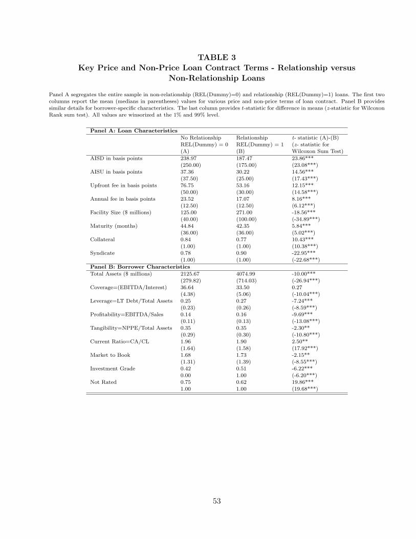
TABLE 3

Key Price and Non-Price Loan Contract Terms - Relationship versus

Non-Relationship Loans

Panel A segregates the entire sample in non-relationship (REL(Dummy)=0) and relationship (REL(Dummy)=1) loans. The first twocolumns report the mean (medians in parentheses) values for various price and non-price terms of loan contract. Panel B providessimilar details for borrower-specific characteristics. The last column provides t-statistic for difference in means (z-statistic for WilcoxonRank sum test). All values are winsorized at the 1% and 99% level.

Panel A: Loan Characteristics

No Relationship Relationship t- statistic (A)-(B)REL(Dummy) = 0 REL(Dummy) = 1 (z- statistic for(A) (B) Wilcoxon Sum Test)

AISD in basis points 238.97 187.47 23.86***(250.00) (175.00) (23.08***)

AISU in basis points 37.36 30.22 14.56***(37.50) (25.00) (17.43***)

Upfront fee in basis points 76.75 53.16 12.15***(50.00) (30.00) (14.58***)

Annual fee in basis points 23.52 17.07 8.16***(12.50) (12.50) (6.12***)

Facility Size ($ millions) 125.00 271.00 -18.56***(40.00) (100.00) (-34.89***)

Maturity (months) 44.84 42.35 5.84***(36.00) (36.00) (5.02***)

Collateral 0.84 0.77 10.43***(1.00) (1.00) (10.38***)

Syndicate 0.78 0.90 -22.95***(1.00) (1.00) (-22.68***)

Panel B: Borrower Characteristics

Total Assets ($ millions) 2125.67 4074.99 -10.00***(279.82) (714.03) (-26.94***)

Coverage=(EBITDA/Interest) 36.64 33.50 0.27(4.38) (5.06) (-10.04***)

Leverage=LT Debt/Total Assets 0.25 0.27 -7.24***(0.23) (0.26) (-8.59***)

Profitability=EBITDA/Sales 0.14 0.16 -9.69***(0.11) (0.13) (-13.08***)

Tangibility=NPPE/Total Assets 0.35 0.35 -2.30**(0.29) (0.30) (-10.80***)

Current Ratio=CA/CL 1.96 1.90 2.50**(1.64) (1.58) (17.92***)

Market to Book 1.68 1.73 -2.15**(1.31) (1.39) (-8.55***)

Investment Grade 0.42 0.51 -6.22***0.00 1.00 (-6.20***)

Not Rated 0.75 0.62 19.86***1.00 1.00 (19.68***)

53

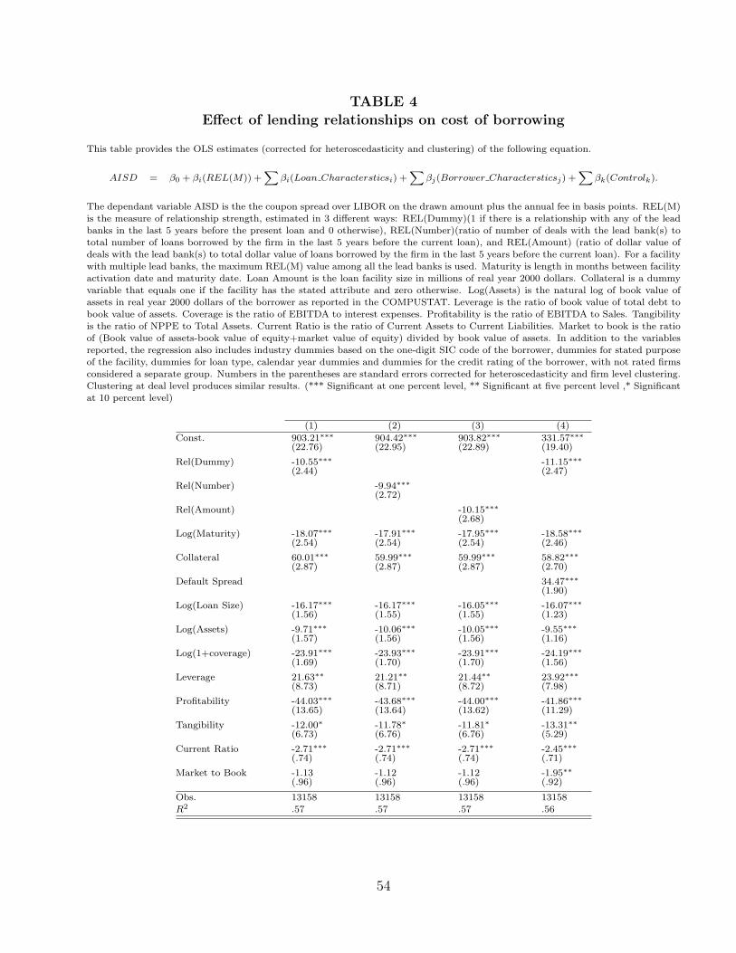
TABLE 4

Effect of lending relationships on cost of borrowing

This table provides the OLS estimates (corrected for heteroscedasticity and clustering) of the following equation.

AISD = β0 + βi(REL(M)) +X

βi(Loan Charactersticsi) +X

βj(Borrower Charactersticsj) +X

βk(Controlk).

The dependant variable AISD is the the coupon spread over LIBOR on the drawn amount plus the annual fee in basis points. REL(M)is the measure of relationship strength, estimated in 3 different ways: REL(Dummy)(1 if there is a relationship with any of the leadbanks in the last 5 years before the present loan and 0 otherwise), REL(Number)(ratio of number of deals with the lead bank(s) tototal number of loans borrowed by the firm in the last 5 years before the current loan), and REL(Amount) (ratio of dollar value ofdeals with the lead bank(s) to total dollar value of loans borrowed by the firm in the last 5 years before the current loan). For a facilitywith multiple lead banks, the maximum REL(M) value among all the lead banks is used. Maturity is length in months between facilityactivation date and maturity date. Loan Amount is the loan facility size in millions of real year 2000 dollars. Collateral is a dummyvariable that equals one if the facility has the stated attribute and zero otherwise. Log(Assets) is the natural log of book value ofassets in real year 2000 dollars of the borrower as reported in the COMPUSTAT. Leverage is the ratio of book value of total debt tobook value of assets. Coverage is the ratio of EBITDA to interest expenses. Profitability is the ratio of EBITDA to Sales. Tangibilityis the ratio of NPPE to Total Assets. Current Ratio is the ratio of Current Assets to Current Liabilities. Market to book is the ratioof (Book value of assets-book value of equity+market value of equity) divided by book value of assets. In addition to the variablesreported, the regression also includes industry dummies based on the one-digit SIC code of the borrower, dummies for stated purposeof the facility, dummies for loan type, calendar year dummies and dummies for the credit rating of the borrower, with not rated firmsconsidered a separate group. Numbers in the parentheses are standard errors corrected for heteroscedasticity and firm level clustering.Clustering at deal level produces similar results. (*** Significant at one percent level, ** Significant at five percent level ,* Significantat 10 percent level)

(1) (2) (3) (4)

Const. 903.21∗∗∗ 904.42∗∗∗ 903.82∗∗∗ 331.57∗∗∗

(22.76) (22.95) (22.89) (19.40)

Rel(Dummy) -10.55∗∗∗ -11.15∗∗∗

(2.44) (2.47)

Rel(Number) -9.94∗∗∗

(2.72)

Rel(Amount) -10.15∗∗∗

(2.68)

Log(Maturity) -18.07∗∗∗ -17.91∗∗∗ -17.95∗∗∗ -18.58∗∗∗

(2.54) (2.54) (2.54) (2.46)

Collateral 60.01∗∗∗ 59.99∗∗∗ 59.99∗∗∗ 58.82∗∗∗

(2.87) (2.87) (2.87) (2.70)

Default Spread 34.47∗∗∗

(1.90)

Log(Loan Size) -16.17∗∗∗ -16.17∗∗∗ -16.05∗∗∗ -16.07∗∗∗

(1.56) (1.55) (1.55) (1.23)

Log(Assets) -9.71∗∗∗ -10.06∗∗∗ -10.05∗∗∗ -9.55∗∗∗

(1.57) (1.56) (1.56) (1.16)

Log(1+coverage) -23.91∗∗∗ -23.93∗∗∗ -23.91∗∗∗ -24.19∗∗∗

(1.69) (1.70) (1.70) (1.56)

Leverage 21.63∗∗ 21.21∗∗ 21.44∗∗ 23.92∗∗∗

(8.73) (8.71) (8.72) (7.98)

Profitability -44.03∗∗∗ -43.68∗∗∗ -44.00∗∗∗ -41.86∗∗∗

(13.65) (13.64) (13.62) (11.29)

Tangibility -12.00∗ -11.78∗ -11.81∗ -13.31∗∗

(6.73) (6.76) (6.76) (5.29)

Current Ratio -2.71∗∗∗ -2.71∗∗∗ -2.71∗∗∗ -2.45∗∗∗

(.74) (.74) (.74) (.71)

Market to Book -1.13 -1.12 -1.12 -1.95∗∗

(.96) (.96) (.96) (.92)

Obs. 13158 13158 13158 13158R2 .57 .57 .57 .56

54

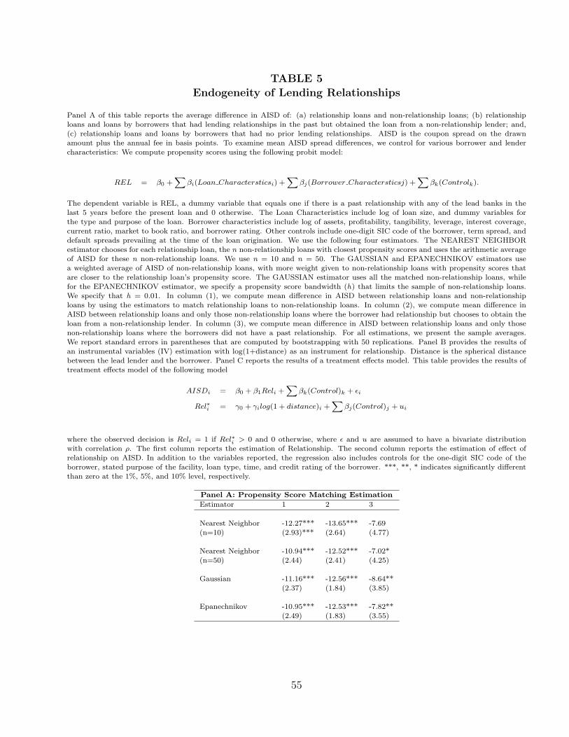
TABLE 5

Endogeneity of Lending Relationships

Panel A of this table reports the average difference in AISD of: (a) relationship loans and non-relationship loans; (b) relationshiploans and loans by borrowers that had lending relationships in the past but obtained the loan from a non-relationship lender; and,(c) relationship loans and loans by borrowers that had no prior lending relationships. AISD is the coupon spread on the drawnamount plus the annual fee in basis points. To examine mean AISD spread differences, we control for various borrower and lendercharacteristics: We compute propensity scores using the following probit model:

REL = β0 +X

βi(Loan Charactersticsi) +X

βj(Borrower Charactersticsj) +X

βk(Controlk).

The dependent variable is REL, a dummy variable that equals one if there is a past relationship with any of the lead banks in thelast 5 years before the present loan and 0 otherwise. The Loan Characteristics include log of loan size, and dummy variables forthe type and purpose of the loan. Borrower characteristics include log of assets, profitability, tangibility, leverage, interest coverage,current ratio, market to book ratio, and borrower rating. Other controls include one-digit SIC code of the borrower, term spread, anddefault spreads prevailing at the time of the loan origination. We use the following four estimators. The NEAREST NEIGHBORestimator chooses for each relationship loan, the n non-relationship loans with closest propensity scores and uses the arithmetic averageof AISD for these n non-relationship loans. We use n = 10 and n = 50. The GAUSSIAN and EPANECHNIKOV estimators usea weighted average of AISD of non-relationship loans, with more weight given to non-relationship loans with propensity scores thatare closer to the relationship loan’s propensity score. The GAUSSIAN estimator uses all the matched non-relationship loans, whilefor the EPANECHNIKOV estimator, we specify a propensity score bandwidth (h) that limits the sample of non-relationship loans.We specify that h = 0.01. In column (1), we compute mean difference in AISD between relationship loans and non-relationshiploans by using the estimators to match relationship loans to non-relationship loans. In column (2), we compute mean difference inAISD between relationship loans and only those non-relationship loans where the borrower had relationship but chooses to obtain theloan from a non-relationship lender. In column (3), we compute mean difference in AISD between relationship loans and only thosenon-relationship loans where the borrowers did not have a past relationship. For all estimations, we present the sample averages.We report standard errors in parentheses that are computed by bootstrapping with 50 replications. Panel B provides the results ofan instrumental variables (IV) estimation with log(1+distance) as an instrument for relationship. Distance is the spherical distancebetween the lead lender and the borrower. Panel C reports the results of a treatment effects model. This table provides the results oftreatment effects model of the following model

AISDi = β0 + β1Reli +X

βk(Control)k + εi

Rel∗i = γ0 + γilog(1 + distance)i +X

βj(Control)j + ui

where the observed decision is Reli = 1 if Rel∗i > 0 and 0 otherwise, where ε and u are assumed to have a bivariate distributionwith correlation ρ. The first column reports the estimation of Relationship. The second column reports the estimation of effect ofrelationship on AISD. In addition to the variables reported, the regression also includes controls for the one-digit SIC code of theborrower, stated purpose of the facility, loan type, time, and credit rating of the borrower. ***, **, * indicates significantly differentthan zero at the 1%, 5%, and 10% level, respectively.

Panel A: Propensity Score Matching Estimation

Estimator 1 2 3

Nearest Neighbor -12.27*** -13.65*** -7.69(n=10) (2.93)*** (2.64) (4.77)

Nearest Neighbor -10.94*** -12.52*** -7.02*(n=50) (2.44) (2.41) (4.25)

Gaussian -11.16*** -12.56*** -8.64**(2.37) (1.84) (3.85)

Epanechnikov -10.95*** -12.53*** -7.82**(2.49) (1.83) (3.55)

55

TA

BLE

5C

ontd

PanelB

:In

strum

enta

lV

aria

ble

sR

egress

ion

Est

imati

on

ofeffect

ofR

ela

tionsh

ipon

AIS

DFir

stSta

ge

Regress

ion

Inst

rum

enta

lV

aria

ble

sEst

imati

on

OLS

IVC

onst

ant

-4.5

52∗∗∗

Const

ant

331.5

7∗∗∗

422.1

6∗∗∗

(0.0

01)

(19.4

0)

(23.8

0)

Log(1

+dis

tance

)-0

.058∗∗∗

Rel

(Dum

my)

-11.1

5∗∗∗

-56.9

0∗∗

(0.0

11)

(2.4

7)

(25.1

4)

Log(A

sset

s)-0

.002

Log(M

atu

rity

)-1

8.5

8∗∗∗

-15.4

0∗∗∗

(0.0

15)

(2.4

6)

(2.3

2)

Log(L

oan

Siz

e)0.1

75∗∗∗

Collate

ral

58.8

2∗∗∗

71.4

1∗∗∗

(0.0

15)

(2.7

0)

(3.2

5)

Pro

fita

bility

-0.1

08

Def

ault

Spre

ad

34.4

7∗∗∗

35.7

1∗∗∗

(0.1

68)

(1.9

0)

(2.5

0)

Tangib

ility

-0.0

83

Log(L

oan

Siz

e)-1

6.0

7∗∗∗

-11.6

3∗∗∗

(0.0

82)

(1.2

3)

(2.0

1)

Lev

erage

0.4

43∗∗∗

Log(A

sset

s)-9

.55∗∗∗

-12.5

9∗∗∗

(0.0

98)

(1.1

6)

(1.4

9)

Log(1

+co

ver

age)

0.0

96∗∗∗

Log(1

+co

ver

age)

-24.1

9∗∗∗

-24.1

2∗∗∗

(0.0

16)

(1.5

6)

(2.1

2)

Curr

ent

Ratio

0.0

10

Lev

erage

23.9

2∗∗∗

55.5

6∗∗∗

(0.0

10)

(7.9

8)

(11.0

7)

Mark

etto

Book

-0.0

07

Pro

fita

bility

-41.8

6∗∗∗

-57.8

5∗∗∗

(0.0

11)

(11.2

96)

(15.7

7)

Obse

rvations

16074

Tangib

ility

-13.3

1∗∗

-20.1

4∗∗∗

Pse

udo

R2

0.0

86

(5.2

9)

(7.2

7)

Curr

ent

Ratio

-2.4

5∗∗∗

-1.7

0∗∗

(0.7

1)

(0.8

0)

Mark

etto

Book

-1.9

5∗∗

-3.2

3∗∗∗

(0.9

2)

(1.0

2)

Obs.

13158

13158

R2

0.5

60.4

9Fir

stSta

ge

F-s

tatist

ic128.1

8∗∗∗

56

TABLE 5 Contd

Panel C: Treatment Effects ModelRelationship AISD

Constant -0.22 397.62∗∗∗(0.33) (18.05)

Rel(Dummy) -16.91∗∗∗(4.07)

Log(1+distance) -0.055∗∗∗(0.01)

Default Spread 0.05∗ 35.86∗∗∗(0.03) (2.46)

Log(Loan Size) 0.14∗∗∗ -15.01∗∗∗(0.02) (1.47)

Log(Assets) 0.04∗∗ -12.19∗∗∗(0.02) (1.45)

Log(1+coverage) 0.11∗∗∗ -25.81∗∗∗(0.02) (1.86)

Leverage 0.559∗∗∗ 45.86∗∗∗(0.11) (9.67)

Profitability -0.16 -57.34∗∗∗(0.19) (15.53)

Tangibility -0.15∗ -17.13∗∗(0.09) (7.17)

Current Ratio 0.01 -1.81∗∗(0.01) (0.79)

Market to Book 0.003 -3.13∗∗∗(0.01) (1.03)

Log(Maturity) -12.79∗∗∗(1.73)

Collateral 72.07∗∗∗(3.04)

Obs. 13158 13158ρ 0.042LR test of ρ = 0 χ2(1)=4.84Probability > χ2 =0.028

57

TABLE 6Borrower Information Opacity and Benefits of Relationship

This table provides the OLS regression (corrected for heteroscedasticity and clustering) estimates of the following equation.

AISD = β0 + β1(REL(M)) + β2(Borrower Information Opacity)

+ β3(REL(M))× (Borrower Information Opacity)

+X

βi(Loan Charactersticsi) +X

βj(Borrower Charactersticsj) +X

βk(Controlk).

The dependant variable AISD is the the coupon spread on the drawn amount plus the annual fee in basis points. REL(Dummy) equals1 if there is a relationship with any of the lead banks in the last 5 years before the present loan and 0 otherwise. Maturity is lengthin months between facility activation date and maturity date. The Loan Amount is the loan facility size in millions of real year 2000dollars. Collateral, is a dummy variable that equals one if the facility has the stated attribute and zero otherwise. Log(Assets) is thenatural log of book value of assets of the borrower in millions of year 2000 real dollars as reported in the COMPUSTAT. Leverageis the ratio of book value of total debt to book value of assets. Coverage is the ratio of EBITDA to interest expenses. Profitabilityis the ratio of EBITDA to Sales. Tangibility is the ratio of NPPE to Total Assets. Current Ratio is the ratio of Current Assets toCurrent Liabilities. Market to book is the ratio of (Book value of assets-book value of equity+market value of equity) divided by bookvalue of assets. BORROWER INFORMATION OPACITY is measured by six different proxies: Borrower’s Size (Log of Assets), ifthe borrower is not rated (Not Rated Dummy), if the borrower is in the S&P 500 index, number of analysts following the borrowerfirm, a microstructure measure of information asymmetry ASY, developed by Bharath, Pasquariello, and Wu (2007), discretionaryaccruals computed according to Dechow and Dichev (2002). Big three is a dummy variable if the lead bank is either Citibank, JPMorgan Chase, or Bank of America. In addition to the variables reported, the regression also includes industry dummies based onthe one-digit SIC code of the borrower, dummies for stated purpose of the facility, dummies for loan type, calendar year dummies,and dummies for the credit rating of the borrower, with not rated firms considered a separate group. Numbers in the parenthesesare standard errors corrected for heteroscedasticity and firm-level clustering. Clustering at deal level produces similar results. (***Significant at one percent level, ** Significant at five percent level ,* Significant at 10 percent level)(Continued on next page)

58

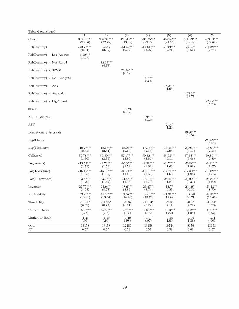
Table 6 (continued)(1) (2) (3) (4) (5) (6) (7)

Const. 927.16∗∗∗ 902.33∗∗∗ 436.46∗∗∗ 903.75∗∗∗ 909.74∗∗∗ 518.53∗∗∗ 903.09∗∗∗

(23.66) (22.75) (19.88) (23.22) (24.54) (18.49) (22.67)

Rel(Dummy) -43.77∗∗∗ -2.35 -14.42∗∗∗ -14.81∗∗∗ -9.99∗∗∗ -6.39∗ -14.39∗∗∗

(8.94) (3.65) (2.72) (3.07) (2.71) (3.50) (2.74)

Rel(Dummy) × Log(Assets) 5.50∗∗∗

(1.37)

Rel(Dummy) × Not Rated -12.37∗∗∗

(4.73)

Rel(Dummy) × SP500 26.94∗∗∗

(6.27)

Rel(Dummy) × No. Analysts .93∗∗∗

(.30)

Rel(Dummy) × ASY -3.23∗∗

(1.65)

Rel(Dummy) × Accruals -62.60∗

(34.77)

Rel(Dummy) × Big-3 bank 22.98∗∗∗

(5.28)

SP500 -12.26(8.17)

No. of Analysts -.89∗∗∗

(.32)

ASY 2.14∗

(1.29)

Discretionary Accruals 99.90∗∗∗

(33.57)

Big-3 bank -20.59∗∗∗

(4.64)

Log(Maturity) -18.27∗∗∗ -18.06∗∗∗ -18.07∗∗∗ -18.16∗∗∗ -18.49∗∗∗ -20.05∗∗∗ -18.04∗∗∗

(2.55) (2.54) (2.63) (2.55) (2.98) (3.11) (2.55)

Collateral 59.78∗∗∗ 59.80∗∗∗ 57.17∗∗∗ 59.82∗∗∗ 55.92∗∗∗ 57.64∗∗∗ 59.80∗∗∗

(2.86) (2.86) (2.90) (2.86) (3.14) (3.46) (2.86)

Log(Assets) -13.53∗∗∗ -9.73∗∗∗ -10.35∗∗∗ -9.31∗∗∗ -8.72∗∗∗ -7.88∗∗∗ -9.81∗∗∗

(1.79) (1.56) (1.59) (1.62) (1.66) (1.86) (1.57)

Log(Loan Size) -16.15∗∗∗ -16.15∗∗∗ -16.71∗∗∗ -16.10∗∗∗ -17.70∗∗∗ -17.89∗∗∗ -15.89∗∗∗

(1.55) (1.55) (1.60) (1.55) (1.63) (1.82) (1.55)

Log(1+coverage) -23.52∗∗∗ -23.76∗∗∗ -24.48∗∗∗ -23.70∗∗∗ -25.40∗∗∗ -29.09∗∗∗ -23.84∗∗∗

(1.70) (1.69) (1.73) (1.70) (1.83) (2.37) (1.69)

Leverage 22.77∗∗∗ 22.04∗∗ 18.69∗∗ 21.27∗∗ 12.75 21.19∗∗ 21.13∗∗

(8.74) (8.74) (8.86) (8.74) (9.25) (10.39) (8.70)

Profitability -43.81∗∗∗ -44.26∗∗∗ -43.08∗∗∗ -43.49∗∗∗ -41.30∗∗∗ -16.89 -43.52∗∗∗

(13.61) (13.64) (14.40) (13.70) (15.62) (16.71) (13.61)

Tangibility -12.10∗ -11.95∗ -2.35 -11.93∗ -7.10 -6.32 -11.94∗

(6.69) (6.73) (6.91) (6.72) (7.11) (7.70) (6.73)

Current Ratio -2.65∗∗∗ -2.72∗∗∗ -2.73∗∗∗ -2.68∗∗∗ -3.13∗∗∗ -3.09∗∗∗ -2.71∗∗∗

(.73) (.73) (.77) (.73) (.82) (1.04) (.73)

Market to Book -1.23 -1.15 -1.49 -1.07 -1.19 -1.06 -1.11(.95) (.96) (.98) (.97) (1.00) (1.36) (.96)

Obs. 13158 13158 12180 13158 10744 9170 13158R2 0.57 0.57 0.58 0.57 0.59 0.60 0.57

59

TABLE 7

Role of Relationships as a Bank’s Commitment to Monitor

This table provides the OLS regression (corrected for heteroscedasticity and clustering) estimates of the following equation.

AISD = β0 + β1(REL(M)) + β2(Bank Monitoring Incentive)

+ β3(REL(M))× (Bank Monitoring Incentive)

+X

βi(Loan Charactersticsi) +X

βj(Borrower Charactersticsj) +X

βk(Controlk).

The dependant variable AISD is the the coupon spread on the drawn amount plus the annual fee in basis points. REL(Dummy) equals1 if there is a relationship with any of the lead banks in the last 5 years before the present loan and 0 otherwise. Maturity is lengthin months between facility activation date and maturity date. The Loan Amount is the loan facility size in millions of real year 2000dollars. Collateral, is a dummy variable that equals one if the facility has the stated attribute and zero otherwise. Not Rated equalsone if the borrower does not have rating from S&P and zero otherwise. Log(Assets) is the natural log of book value of assets of theborrower in millions of year 2000 real dollars as reported in the COMPUSTAT. Leverage is the ratio of book value of total debt tobook value of assets. Coverage is the ratio of EBITDA to interest expenses. Profitability is the ratio of EBITDA to Sales. Tangibilityis the ratio of NPPE to Total Assets. Current Ratio is the ratio of Current Assets to Current Liabilities. Market to book is the ratioof (Book value of assets-book value of equity+market value of equity) divided by book value of assets. Syndicate moral hazard, i.e.,the incentive to monitor the borrower is measured by 3 different proxies: number of members in the syndicate, lead bank allocationof the loan in percent, the loan concentration in the syndicate measured by the Herfindahl-Hirschmann index following Sufi (2007).Covenant Index assumes the value between zero and five with the presence of each of five different covenants coded as a one and zerootherwise and summed up (Bradley and Roberts, 2004). In addition to the variables reported, the regression also includes industrydummies based on the one-digit SIC code of the borrower, dummies for stated purpose of the facility, dummies for loan type, calendaryear dummies, and dummies for the credit rating of the borrower, with not rated firms considered a separate group. Numbers in theparentheses are standard errors corrected for heteroscedasticity and firm-level clustering. Clustering at deal level produces similarresults. (*** Significant at one percent level, ** Significant at five percent level ,* Significant at 10 percent level)(Continued on next page)

60

Table 7 Panel A(1) (2) (3) (4) (5)

Const. 569.22∗∗∗ 642.95∗∗∗ 898.58∗∗∗ 855.71∗∗∗ 834.47∗∗∗(60.96) (119.35) (23.18) (38.02) (43.21)

Rel(Dummy) -18.19∗∗∗ -14.44∗∗ -20.27∗∗∗ 6.25 3.57(6.12) (7.36) (3.70) (4.96) (4.52)

Rel(Dummy) × Log(Syndicate Size) 8.59∗∗∗(2.02)

Log(Syndicate Size) -7.63∗∗∗(2.17)

Rel(Dummy) × Lead Bank Allocation -.26∗∗∗(.09)

Lead bank Allocation .49∗∗∗(.09)

Rel(Dummy) × Loan HHI -.002∗∗∗(.0008)

Loan HHI .005∗∗∗(.001)

Log(Maturity) -16.21∗∗∗ -19.15∗∗∗ -17.82∗∗∗ -15.39∗∗∗ -14.67∗∗∗(5.81) (6.44) (2.57) (3.61) (3.75)

Collateral 63.45∗∗∗ 64.70∗∗∗ 59.86∗∗∗ 60.82∗∗∗ 60.11∗∗∗(7.75) (8.53) (2.88) (3.62) (3.72)

Log(Assets) -21.10∗∗∗ -17.00∗∗∗ -9.82∗∗∗ -15.50∗∗∗ -15.33∗∗∗(3.75) (4.90) (1.59) (1.80) (1.89)

Log(Loan Size) -20.29∗∗∗ -25.61∗∗∗ -15.34∗∗∗ -11.37∗∗∗ -10.49∗∗∗(4.24) (5.04) (1.63) (2.00) (2.21)

Log(1+coverage) -15.07∗∗∗ -13.89∗∗∗ -23.58∗∗∗ -24.18∗∗∗ -24.24∗∗∗(2.71) (2.94) (1.70) (2.09) (2.15)

Leverage 54.82∗∗ 43.82 22.12∗∗ 17.91 23.59∗∗(22.46) (26.75) (8.73) (11.40) (11.89)

Profitability -110.31∗∗∗ -122.42∗∗∗ -43.73∗∗∗ -30.44∗ -35.52∗∗(42.47) (43.45) (13.58) (16.50) (16.94)

Tangibility -30.57 -18.41 -11.93∗ -13.92 -14.13(21.26) (23.54) (6.73) (8.76) (9.08)

Current Ratio -4.72∗∗ -5.49∗∗ -2.74∗∗∗ -3.80∗∗∗ -4.16∗∗∗(2.12) (2.23) (.73) (1.22) (1.24)

Market to Book .12 .52 -1.14 -1.14 -.90(2.25) (2.36) (.95) (1.17) (1.19)

Obs. 1669 1184 13158 6064 5731R2 0.43 0.44 0.57 0.58 0.58

61

Table 7 Panel B(1) (2) (3) (4)

Const. 902.95∗∗∗ 911.75∗∗∗ 909.15∗∗∗ 909.43∗∗∗(22.79) (23.14) (23.18) (23.15)

Rel(Dummy) -1.83 -9.74∗∗∗ -10.92∗∗∗ -8.44∗∗∗(3.45) (3.11) (2.44) (2.88)

Rel(Dummy) * Collateral -15.28∗∗∗(4.73)

Rel(Dummy) * Covenant Index -.85(1.68)

Market to Book * Covenant Index -3.00∗∗∗ -2.22∗∗(.81) (.95)

Rel(Dummy) * Market to Book * Covenant Index -1.16(.75)

Covenant Index 7.18∗∗∗ 11.22∗∗∗ 11.29∗∗∗(1.87) (1.90) (1.91)

Log(Maturity) -18.21∗∗∗ -18.91∗∗∗ -18.63∗∗∗ -18.64∗∗∗(2.55) (2.53) (2.52) (2.52)

Collateral 70.72∗∗∗ 49.12∗∗∗ 49.13∗∗∗ 49.16∗∗∗(4.72) (3.65) (3.65) (3.64)

Log(Assets) -9.58∗∗∗ -9.45∗∗∗ -9.81∗∗∗ -9.77∗∗∗(1.56) (1.58) (1.57) (1.57)

Log(Loan Size) -16.22∗∗∗ -16.69∗∗∗ -16.44∗∗∗ -16.47∗∗∗(1.55) (1.57) (1.57) (1.57)

Log(1+coverage) -23.79∗∗∗ -24.30∗∗∗ -24.18∗∗∗ -24.20∗∗∗(1.69) (1.72) (1.73) (1.73)

Leverage 22.18∗∗ 17.78∗∗ 18.66∗∗ 18.87∗∗(8.73) (8.76) (8.74) (8.76)

Profitability -43.74∗∗∗ -44.63∗∗∗ -44.83∗∗∗ -44.69∗∗∗(13.64) (13.64) (13.64) (13.63)

Tangibility -12.07∗ -10.27 -10.54 -10.74(6.71) (6.68) (6.68) (6.67)

Current Ratio -2.66∗∗∗ -2.52∗∗∗ -2.58∗∗∗ -2.53∗∗∗(.73) (.73) (.75) (.75)

Market to Book -1.11 -.98 1.59 1.52(.95) (.98) (1.51) (1.49)

Obs. 13158 13158 13158 13158R2 .57 .57 .58 .58

62

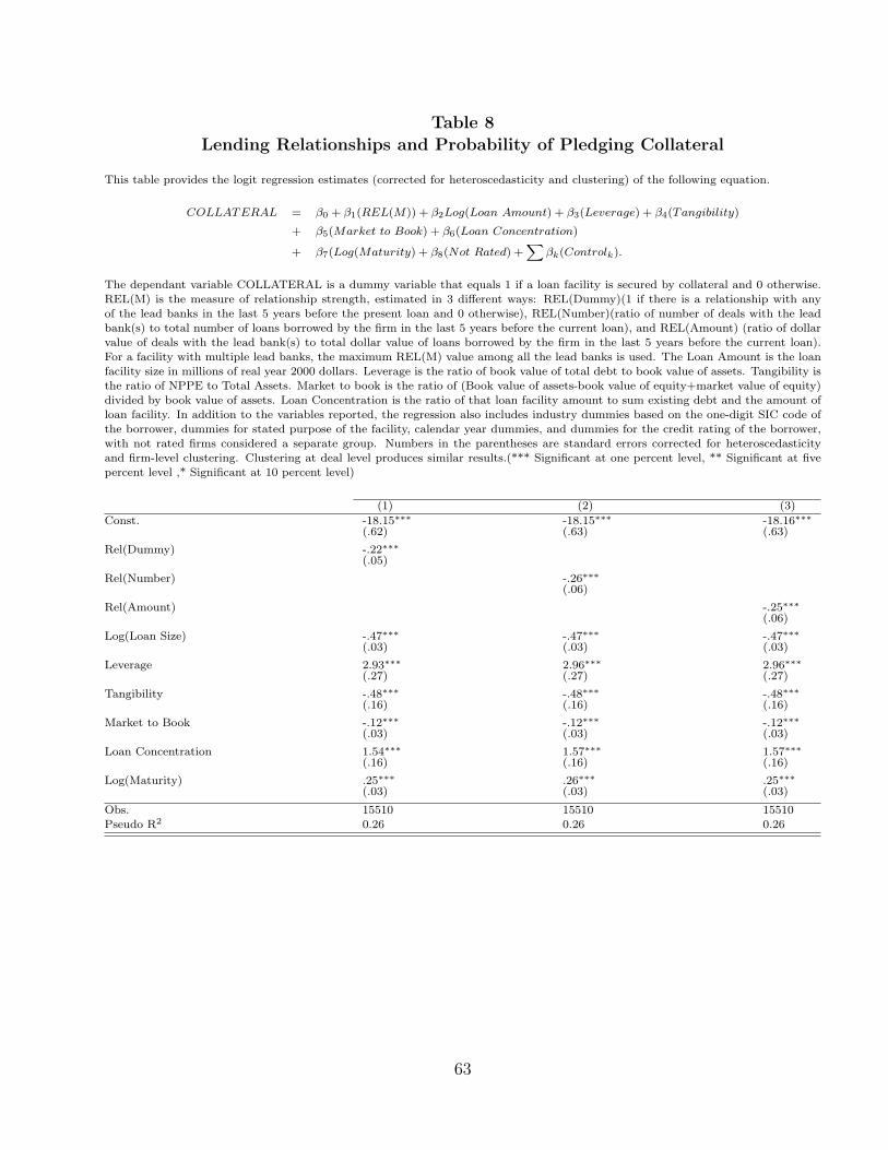
Table 8

Lending Relationships and Probability of Pledging Collateral

This table provides the logit regression estimates (corrected for heteroscedasticity and clustering) of the following equation.

COLLATERAL = β0 + β1(REL(M)) + β2Log(Loan Amount) + β3(Leverage) + β4(Tangibility)

+ β5(Market to Book) + β6(Loan Concentration)

+ β7(Log(Maturity) + β8(Not Rated) +X

βk(Controlk).

The dependant variable COLLATERAL is a dummy variable that equals 1 if a loan facility is secured by collateral and 0 otherwise.REL(M) is the measure of relationship strength, estimated in 3 different ways: REL(Dummy)(1 if there is a relationship with anyof the lead banks in the last 5 years before the present loan and 0 otherwise), REL(Number)(ratio of number of deals with the leadbank(s) to total number of loans borrowed by the firm in the last 5 years before the current loan), and REL(Amount) (ratio of dollarvalue of deals with the lead bank(s) to total dollar value of loans borrowed by the firm in the last 5 years before the current loan).For a facility with multiple lead banks, the maximum REL(M) value among all the lead banks is used. The Loan Amount is the loanfacility size in millions of real year 2000 dollars. Leverage is the ratio of book value of total debt to book value of assets. Tangibility isthe ratio of NPPE to Total Assets. Market to book is the ratio of (Book value of assets-book value of equity+market value of equity)divided by book value of assets. Loan Concentration is the ratio of that loan facility amount to sum existing debt and the amount ofloan facility. In addition to the variables reported, the regression also includes industry dummies based on the one-digit SIC code ofthe borrower, dummies for stated purpose of the facility, calendar year dummies, and dummies for the credit rating of the borrower,with not rated firms considered a separate group. Numbers in the parentheses are standard errors corrected for heteroscedasticityand firm-level clustering. Clustering at deal level produces similar results.(*** Significant at one percent level, ** Significant at fivepercent level ,* Significant at 10 percent level)

(1) (2) (3)

Const. -18.15∗∗∗ -18.15∗∗∗ -18.16∗∗∗

(.62) (.63) (.63)

Rel(Dummy) -.22∗∗∗

(.05)

Rel(Number) -.26∗∗∗

(.06)

Rel(Amount) -.25∗∗∗

(.06)

Log(Loan Size) -.47∗∗∗ -.47∗∗∗ -.47∗∗∗

(.03) (.03) (.03)

Leverage 2.93∗∗∗ 2.96∗∗∗ 2.96∗∗∗

(.27) (.27) (.27)

Tangibility -.48∗∗∗ -.48∗∗∗ -.48∗∗∗

(.16) (.16) (.16)

Market to Book -.12∗∗∗ -.12∗∗∗ -.12∗∗∗

(.03) (.03) (.03)

Loan Concentration 1.54∗∗∗ 1.57∗∗∗ 1.57∗∗∗

(.16) (.16) (.16)

Log(Maturity) .25∗∗∗ .26∗∗∗ .25∗∗∗

(.03) (.03) (.03)

Obs. 15510 15510 15510Pseudo R2 0.26 0.26 0.26

63

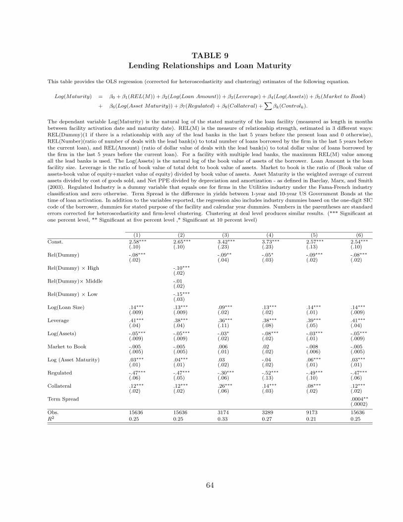
TABLE 9

Lending Relationships and Loan Maturity

This table provides the OLS regression (corrected for heteroscedasticity and clustering) estimates of the following equation.

Log(Maturity) = β0 + β1(REL(M)) + β2(Log(Loan Amount)) + β3(Leverage) + β4(Log(Assets)) + β5(Market to Book)

+ β6(Log(Asset Maturity)) + β7(Regulated) + β8(Collateral) +X

βk(Controlk).

The dependant variable Log(Maturity) is the natural log of the stated maturity of the loan facility (measured as length in monthsbetween facility activation date and maturity date). REL(M) is the measure of relationship strength, estimated in 3 different ways:REL(Dummy)(1 if there is a relationship with any of the lead banks in the last 5 years before the present loan and 0 otherwise),REL(Number)(ratio of number of deals with the lead bank(s) to total number of loans borrowed by the firm in the last 5 years beforethe current loan), and REL(Amount) (ratio of dollar value of deals with the lead bank(s) to total dollar value of loans borrowed bythe firm in the last 5 years before the current loan). For a facility with multiple lead banks, the maximum REL(M) value amongall the lead banks is used. The Log(Assets) is the natural log of the book value of assets of the borrower. Loan Amount is the loanfacility size. Leverage is the ratio of book value of total debt to book value of assets. Market to book is the ratio of (Book value ofassets-book value of equity+market value of equity) divided by book value of assets. Asset Maturity is the weighted average of currentassets divided by cost of goods sold, and Net PPE divided by depreciation and amortization - as defined in Barclay, Marx, and Smith(2003). Regulated Industry is a dummy variable that equals one for firms in the Utilities industry under the Fama-French industryclassification and zero otherwise. Term Spread is the difference in yields between 1-year and 10-year US Government Bonds at thetime of loan activation. In addition to the variables reported, the regression also includes industry dummies based on the one-digit SICcode of the borrower, dummies for stated purpose of the facility and calendar year dummies. Numbers in the parentheses are standarderrors corrected for heteroscedasticity and firm-level clustering. Clustering at deal level produces similar results. (*** Significant atone percent level, ** Significant at five percent level ,* Significant at 10 percent level)

(1) (2) (3) (4) (5) (6)

Const. 2.58∗∗∗ 2.65∗∗∗ 3.42∗∗∗ 3.73∗∗∗ 2.57∗∗∗ 2.54∗∗∗

(.10) (.10) (.23) (.23) (.13) (.10)

Rel(Dummy) -.08∗∗∗ -.09∗∗ -.05∗ -.09∗∗∗ -.08∗∗∗

(.02) (.04) (.03) (.02) (.02)

Rel(Dummy) × High -.10∗∗∗

(.02)

Rel(Dummy)× Middle -.01(.02)

Rel(Dummy) × Low -.15∗∗∗

(.03)

Log(Loan Size) .14∗∗∗ .13∗∗∗ .09∗∗∗ .13∗∗∗ .14∗∗∗ .14∗∗∗

(.009) (.009) (.02) (.02) (.01) (.009)

Leverage .41∗∗∗ .38∗∗∗ .36∗∗∗ .38∗∗∗ .39∗∗∗ .41∗∗∗

(.04) (.04) (.11) (.08) (.05) (.04)

Log(Assets) -.05∗∗∗ -.05∗∗∗ -.03∗ -.08∗∗∗ -.03∗∗∗ -.05∗∗∗

(.009) (.009) (.02) (.02) (.01) (.009)

Market to Book -.005 -.005 .006 .02 -.008 -.005(.005) (.005) (.01) (.02) (.006) (.005)

Log (Asset Maturity) .03∗∗∗ .04∗∗∗ .03 -.04 .06∗∗∗ .03∗∗∗

(.01) (.01) (.02) (.02) (.01) (.01)

Regulated -.47∗∗∗ -.47∗∗∗ -.30∗∗∗ -.52∗∗∗ -.49∗∗∗ -.47∗∗∗

(.06) (.05) (.06) (.13) (.10) (.06)

Collateral .12∗∗∗ .12∗∗∗ .26∗∗∗ .14∗∗∗ .08∗∗∗ .12∗∗∗

(.02) (.02) (.06) (.03) (.02) (.02)

Term Spread .0004∗∗

(.0002)

Obs. 15636 15636 3174 3289 9173 15636R2 0.25 0.25 0.33 0.27 0.21 0.25

64

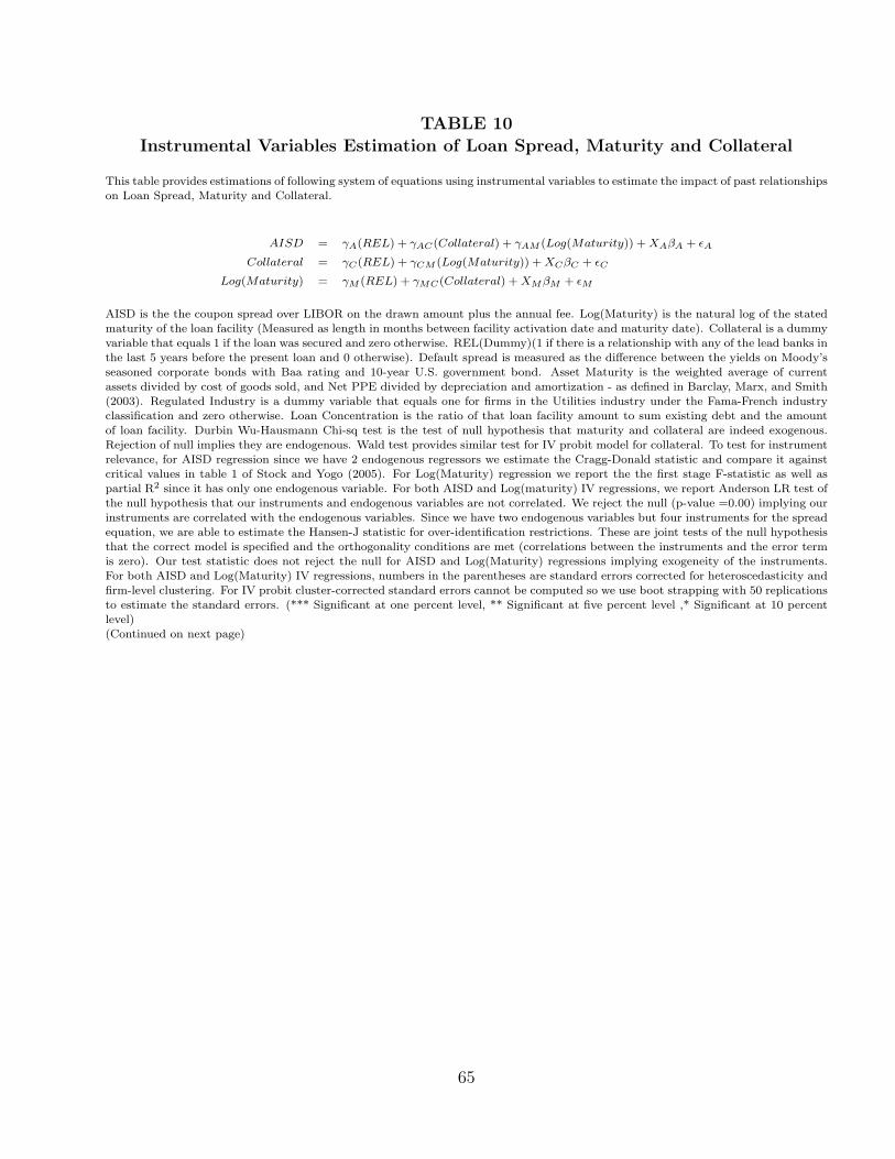
TABLE 10

Instrumental Variables Estimation of Loan Spread, Maturity and Collateral

This table provides estimations of following system of equations using instrumental variables to estimate the impact of past relationshipson Loan Spread, Maturity and Collateral.

AISD = γA(REL) + γAC(Collateral) + γAM (Log(Maturity)) + XAβA + εA

Collateral = γC(REL) + γCM (Log(Maturity)) + XCβC + εC

Log(Maturity) = γM (REL) + γMC(Collateral) + XMβM + εM

AISD is the the coupon spread over LIBOR on the drawn amount plus the annual fee. Log(Maturity) is the natural log of the statedmaturity of the loan facility (Measured as length in months between facility activation date and maturity date). Collateral is a dummyvariable that equals 1 if the loan was secured and zero otherwise. REL(Dummy)(1 if there is a relationship with any of the lead banks inthe last 5 years before the present loan and 0 otherwise). Default spread is measured as the difference between the yields on Moody’sseasoned corporate bonds with Baa rating and 10-year U.S. government bond. Asset Maturity is the weighted average of currentassets divided by cost of goods sold, and Net PPE divided by depreciation and amortization - as defined in Barclay, Marx, and Smith(2003). Regulated Industry is a dummy variable that equals one for firms in the Utilities industry under the Fama-French industryclassification and zero otherwise. Loan Concentration is the ratio of that loan facility amount to sum existing debt and the amountof loan facility. Durbin Wu-Hausmann Chi-sq test is the test of null hypothesis that maturity and collateral are indeed exogenous.Rejection of null implies they are endogenous. Wald test provides similar test for IV probit model for collateral. To test for instrumentrelevance, for AISD regression since we have 2 endogenous regressors we estimate the Cragg-Donald statistic and compare it againstcritical values in table 1 of Stock and Yogo (2005). For Log(Maturity) regression we report the the first stage F-statistic as well aspartial R2 since it has only one endogenous variable. For both AISD and Log(maturity) IV regressions, we report Anderson LR test ofthe null hypothesis that our instruments and endogenous variables are not correlated. We reject the null (p-value =0.00) implying ourinstruments are correlated with the endogenous variables. Since we have two endogenous variables but four instruments for the spreadequation, we are able to estimate the Hansen-J statistic for over-identification restrictions. These are joint tests of the null hypothesisthat the correct model is specified and the orthogonality conditions are met (correlations between the instruments and the error termis zero). Our test statistic does not reject the null for AISD and Log(Maturity) regressions implying exogeneity of the instruments.For both AISD and Log(Maturity) IV regressions, numbers in the parentheses are standard errors corrected for heteroscedasticity andfirm-level clustering. For IV probit cluster-corrected standard errors cannot be computed so we use boot strapping with 50 replicationsto estimate the standard errors. (*** Significant at one percent level, ** Significant at five percent level ,* Significant at 10 percentlevel)(Continued on next page)

65

Dependent Variable AISD Log(Maturity) Collateral

OLS IV IV OLS IV Probit IV Probit

REL(Dummy) -10.55*** -14.35** -12.79** -0.13*** -0.07***(2.44) (5.73) (5.73) (0.03) (0.31)

REL(Dummy)*High -0.10*** -0.02(0.02) (0.03)

REL(Dummy)*Middle -0.01 0.07***(0.02) (0.03)

REL(Dummy)*Low -0.15*** -0.10***(0.03) (0.04)

Log(Maturity) -18.07*** -151.6*** -146.13*** 0.15*** 0.94***(2.54) (42.70) (42.04) (0.02) (0.15)

Collateral 60.01*** 406.2*** 408.2*** 0.12*** 1.67***(2.87) (68.09) (64.94) (0.02) (0.97)

Default Spread 15.44***(7.62)

Average Spread 0.68***(0.11)

Log(Asset Maturity) 0.04*** 0.65***(0.01) (0.15)

Regulated -0.47*** -0.24***(0.05) (0.77)

Loan Concentartion 0.90*** 1.00***(0.09) (0.07)

Other Controls As in Column 1 As in Column 1 As in Column 2 As in Column 1of Table 4 of Table 4 of Table 9 of Table 8

Tests of edogeneity:Durbin-Wu-Hausmanchi-sq test 469.25 546.46 1170p-value 0.00 0.00 0.00Wald Chi-Squaretest staistic 29.56p-value 0.00Weak identification statistics::Cragg-Donald F-Stat 14.57 15.05Stock and Yogo (2004)critical value 11.03 11.03First Stage F statistic 323.27Partial R-Sqaure 8.16%Anderson -LR statistic 58.24 60.17 1289p-value 0.00 0.00 0.00Instrument exogeneity test:Hansen-J statistic 4.132 3.967 0.001p-value 0.13 0.14 0.98

66

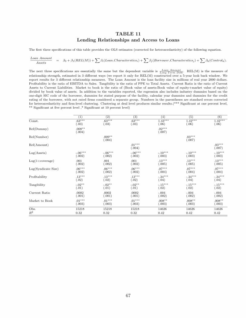
TABLE 11

Lending Relationships and Access to Loans

The first three specifications of this table provides the OLS estimates (corrected for heteroscedasticity) of the following equation.

Loan Amount

Assets= β0 + β1(REL(M)) +

Xβi(Loan Charactersticsi) +

Xβj(Borrower Charactersticsj) +

Xβk(Controlk).

The next three specifications are essentially the same but the dependent variable is Loan AmountLong Term Debt

. REL(M) is the measure of

relationship strength, estimated in 3 different ways (we report it only for REL(M) constructed over a 5-year look back window. Wereport results for 3 different relationship measures. The Loan Amount is the loan facility size in millions of real year 2000 dollars.Profitability is the ratio of EBITDA to Sales. Tangibility is the ratio of PPE to Total Assets. Current Ratio is the ratio of CurrentAssets to Current Liabilities. Market to book is the ratio of (Book value of assets-Book value of equity+market value of equity)divided by book value of assets. In addition to the variables reported, the regression also includes industry dummies based on theone-digit SIC code of the borrower, dummies for stated purpose of the facility, calendar year dummies and dummies for the creditrating of the borrower, with not rated firms considered a separate group. Numbers in the parentheses are standard errors correctedfor heteroscedasticity and firm-level clustering. Clustering at deal level produces similar results.(*** Significant at one percent level,** Significant at five percent level ,* Significant at 10 percent level)

(1) (2) (3) (4) (5) (6)

Const. .63∗∗∗ .63∗∗∗ .63∗∗∗ 1.43∗∗∗ 1.42∗∗∗ 1.42∗∗∗

(.03) (.03) (.03) (.06) (.06) (.06)

Rel(Dummy) .008∗∗ .02∗∗∗

(.004) (.007)

Rel(Number) .009∗∗ .03∗∗∗

(.004) (.007)

Rel(Amount) .01∗∗∗ .03∗∗∗

(.004) (.007)

Log(Assets) -.06∗∗∗ -.06∗∗∗ -.06∗∗∗ -.10∗∗∗ -.10∗∗∗ -.10∗∗∗

(.002) (.002) (.002) (.003) (.003) (.003)

Log(1+coverage) .001 .001 .001 .13∗∗∗ .13∗∗∗ .13∗∗∗

(.002) (.002) (.002) (.005) (.005) (.005)

Log(Syndicate Size) .06∗∗∗ .06∗∗∗ .06∗∗∗ .07∗∗∗ .07∗∗∗ .07∗∗∗

(.002) (.002) (.002) (.004) (.004) (.004)

Profitability .13∗∗∗ .13∗∗∗ .13∗∗∗ -.34∗∗∗ -.34∗∗∗ -.34∗∗∗

(.02) (.02) (.02) (.04) (.04) (.04)

Tangibility -.02∗∗ -.02∗∗ -.02∗∗ -.15∗∗∗ -.15∗∗∗ -.15∗∗∗

(.01) (.01) (.01) (.02) (.02) (.02)

Current Ratio .0002 .0002 .0002 -.004 -.004 -.004(.001) (.001) (.001) (.002) (.002) (.002)

Market to Book .01∗∗∗ .01∗∗∗ .01∗∗∗ .008∗∗ .008∗∗ .008∗∗

(.003) (.003) (.003) (.003) (.003) (.003)

Obs. 15218 15218 15218 14626 14626 14626R2 0.32 0.32 0.32 0.42 0.42 0.42

67

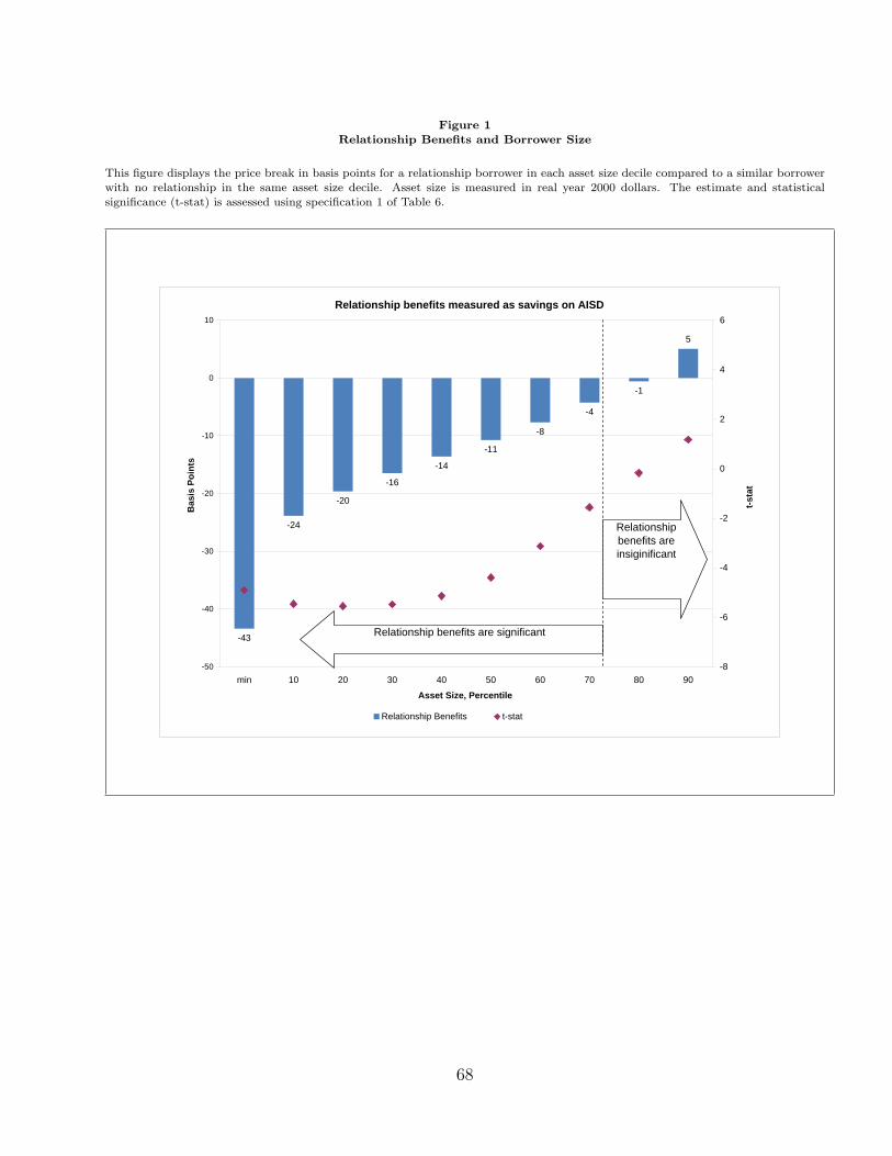
Figure 1Relationship Benefits and Borrower Size

This figure displays the price break in basis points for a relationship borrower in each asset size decile compared to a similar borrowerwith no relationship in the same asset size decile. Asset size is measured in real year 2000 dollars. The estimate and statisticalsignificance (t-stat) is assessed using specification 1 of Table 6.

Relationship benefits measured as savings on AISD

-43

-24

-20

-16

-14

-11

-8

-4

-1

5

-50

-40

-30

-20

-10

0

10

min 10 20 30 40 50 60 70 80 90

Asset Size, Percentile

Bas

is P

oint

s

-8

-6

-4

-2

0

2

4

6

t-sta

t

Relationship Benefits t-stat

Relationship benefits are insiginificant

Relationship benefits are significant

68