Large Eddy Simulation of separating flows from curved surfaces

Large Eddy Simulation of separating flows from curved surfacesTemmerman, L.

The copyright of this thesis rests with the author and no quotation from it or information

derived from it may be published without the prior written consent of the author

For additional information about this publication click this link.

http://qmro.qmul.ac.uk/jspui/handle/123456789/1833

Information about this research object was correct at the time of download; we occasionally

make corrections to records, please therefore check the published record when citing. For

more information contact [email protected]

http://qmro.qmul.ac.uk/jspui/handle/123456789/1833

Large Eddy Simulation of

separating flows from curved

surfaces

by

L. Temmerman

Department of Engineering

Queen Mary University of London Mile End Road

London El 4NS, United Kingdom

This thesis is submitted for the degree of Doctor

of Philosophy of the University of London

March 2004

(LOk""I"K

.4

Abstract

The capabilities and limitations of LES in predicting separation from curved surfaces

at high Reynolds number are at the centre of this Thesis. Issues of particular interest

are mesh resolution, subgrid-scale modelling and near-wall approximations aiming to reduce the computational cost.

Two cases are examined: a flow separating in a channel with streamwise periodic

constrictions (hills), and the flow around a single-element, high-lift aerofoil at a Reynolds number of 2.1 . 106. Prior to these studies, fully-developed channel-flow

simulations are considered. These show substantial differences among subgrid-scale

models in terms of the subgrid-scale viscosity magnitude and its wall-asymptotic

variation. Modelling and numerical errors appear to counteract each other, thus

reducing the total error. Wall functions axe shown to be a cost-effective approach,

providing a reasonably accurate approximation in near-equilibrium conditions. A-

dequate resolution remains critical, however, in achieving successful simulations. In the hill flow, separation occurs downstream of the hill crest, reattachment

takes place about half-way between two consecutive hills and partial recovery oc-

curs prior to a re-acceleration on the following hill. A highly-resolved simulation,

performed to produce -benchmark data, permits an extensive study of the flow pro-

perties. Coarser mesh simulations are then compared with the former. These high-

light the influence of the streamwise discretisation around the separation point and

the role played by the implementation details of the wall treatments, while the

subgrid-scale models influence is less significant.

The aerofoil, which features transition and separation, is extremely challenging

and at the edge of current LES capabilities. None of the simulations reproduce

2

the experimental data well. Indications on the sensitivity to various parameters, including the numerical scheme, the mesh resolution and the spanwise extent, are extracted, however. The studies indicate the need for a structured mesh of about 80 million nodes to achieve the required accuracy. For the present study, this was unaffordable.

3

Acknowledgements

First of all, I would like to express my profound gratitude to my supervisor, Prof.

Michael Leschziner, for giving me the opportunity to carry out the research pre-

sented in this Thesis, for his continuous and patient support, for many hours of rich

discussions that made this a fruitful and enjoyable relationship and for helping me to

bring this manuscript into a readable form. With the initial funding of this project

only available for two years, I am also very thankful to him for securing fundings

for a follow-up project, the results of which are not part of this work, but which

allowed me to pay my bills.

This research was made possible with the financial support of the European

Community through the LESFOIL project (reference number BRPR-CT97-0565),

part of the Framework V Brite-Euram initiative. The simulations reported in the

present work required a substantial amount of computing power, and access to

the CSAR service in Manchester was granted by EPSRC through the consortium LESUK II (grant GR/M050539). I am very grateful to EPSRC for this as well as

all the people behind the CSAR service who, while providing a very reliable service,

were also very helpful. With my work having spanned over three different UK

universities, UMIST in Manchester, Queen Mary University of London and Imperial

College London, I am grateful to all the support people in these institutions, who

provided the environment necessary to carry the present Thesis.

I would not have applied to the Research Assistant position within which the

present research was undertaken without the encouragements from my friend, Dr.

Georges Barakos. I would also like to thank Prof. Dimitris Drikakis for supporting

my application.

4

Many thanks goes to Dr. Raphael Lardat for his patience in introducing me

to the code he wrote, and many interesting discussions. I would also like to thank

Dr. Mike Ashworth and Dr. David Emerson for their hospitality at the Daresbury

Laboratory and for introducing me to the world of parallel computing. The work

on the role played by numerical and modelling errors in LES of a channel flow

resulted from discussions with Prof. Bernard Geurts from Twente University (The

Netherlands) during his stay as a visiting professor at Queen Mary University of

London.

The hill-flow chapter benefited from an extensive and very fruitful collaborative

effort with Dr. Christopher Mellen, Dr. Jochen R6hlich and Prof. Wolfgang Rodi

from the University of Karlsruhe, Germany.

During the course of the LESFOIL project, many discussions arose between the

different members of the consortium either through e-mail exchanges or during the

meetings, and these contributed greatly to this work. I am especially indebted to

Dr. Simon Diffilstrom, Dr. Christopher Mellen and Dr. Jochen R6hlich for endless discussions, among other helpful interactions.

My profound gratitude goes to Dr. Anne Dejoan who, in addition to sharing the office space with me for the last two years, proved to be a willing and well-

informed discussion partner on the subjects of LES, turbulence and many others.

My apologies goes to my two other colleagues, Dr. Yong-Jun Jang and Dr. Chen

Wang, who were subjected to an almost permanent Rench chatter. However, they

never missed an opportunity to contribute to the occasionally chaotic, but always

well-humoured atmosphere of our common space.

I am also very grateful to my other past and present colleagues, Dr. David

Apsley, Dr. Hughes Loyau, Dr. Francois Mallinger, Dr. Georges Barakos, Dr.

Aldo Bonfiglioli, Dr. Yongmann Chung, Mr. Pierre Humbert, Dr. Ken-Ichi Abe,

Dr. Xu Zhou, Dr. Xi Jiang, Dr. Eldad Avital, Dr. Sylvain Lardeau and Dr.

Richard Wilden for many enriching discussions, some of which contributed to this

Thesis, others absolutely not related, but nevertheless interesting, as well as for their

friendship, encouragements and sharing the odd beer.

During the course of this Thesis, I had the opportunity to meet many new peo-

5

ple, some of them are now my friends, while keeping strengthening older friendships.

Thanks goes thus to all my friends, particularly among them Dr. Marianna Gram-

matika, Fabrice Plangon, Dr. Patrice Bouche, Dr. Roland Pietsch, Corrado di Pisa,

Gaetan Masson, Simon Morren, Laurent Mampaey, Benoit Denet, Bernard Languil-

lier and Renaud Hendrice for the many encouragements I received from them and for the special moments we shared, among many other things. A membership to the

Anglo-Belgian Society provided for a some time much needed escape to other worlds

and the opportunity to visit some very impressive venues in London in always kind

and interesting company. Special thanks goes to Mrs. Rangoise Vermeylen who kindly provided a sometimes much needed ear.

These acknowledgements would not be complete without mentioning the very

strong support I received from my parents, Colette and Edouard Temmerman and

my sister, Charlotte, who while far away, most of the time, were close in spirit. Last but not least, the very loving presence of my companion, Miss Anne Her-

mans, as well as her patience, greatly contributed to my ability to complete this

Thesis.

6

Contents

Title 1

Abstract

Acknoledgements 4

Table of Contents 7

List of Figures 11

List of Tables 21

Nomenclature 23

1 Introduction 29

1.1 Large Eddy Simulation - Motivation and Rationale .......... 29

1.2 Objectives of the research ........................ 34

1.3 Outline of the thesis ........................... 34

2 Large Eddy Simulation -A Review 37

2.1 Overview .................................. 37

2.2 The governing equations for LES in physical space ........... 37

2.3 Subgrid-scale modelling .......................... 41

2.3.1 Overview ............................. 41

2.3.2 Subgrid-scale eddy-viscosity ................... 44

2.3.3 Scale similaxity models ...................... 45

2.3.4 Models based on transport equations .............. 47

7

2.3.5 The dynamic procedure ............... ...... 48

2.3.6 Implicit subgrid-scale modelling ........... ...... 50

2.4 Initial and boundary conditions ............... ...... 51

2.4.1 Initial condition .................... ...... 51

2.4.2 Inflow boundary condition .............. ...... 51

2.4.3 Outflow ........................ ...... 52

2.5 Neax-wall treatment ...................... ...... 53

2.6 Resolution requirements ................... ...... 55

2.7 Numerical methods ...................... ...... 56

2.8 Source of errors in LES .................... ...... 65

2.9 Practical applications of large eddy simulations ....... ...... 68

3 Aspects of modelling 72

3.1 Introduction ........................... ..... 72

3.2 Subgrid-scale modelling ..................... ..... 73

3.2.1 Subgrid-scale viscosity ................. ..... 73

3.2.2 The Smagorinsky model ................ ..... 74

3.2.3 The dynamic Smagorinsky model ........... ..... 75

3.2.4 The Localized Dynamic Smagorinsky Model ..... ..... 78

3.2.5 The mixed-scale model ................. ..... 79

3.2.6 The WALE Model ................... ..... 80

3.3 Near-wall treatment ....................... ..... 81

3.3.1 Rationale and overview ................. ..... 81

3.3.2 Log-law based approximations ............. ..... 82

3.3.3 Werner-Wengle wall law ................ .....

84

3.4 Concluding remarks ....................... ..... 84

4 Computational and implementation issues 86

4.1 Introduction ................................ 86

4.2 The finite-volume formulation ......................

87

4.3 Solution strategy and time discretisation ................ 88

4.4 Control of the time-step ......................... 91

8

4.5 Spatial discretisation ......................... .. 92

4.6 Pressure solver ............................ .. 94

4.6.1 Principles ........................... .. 94

4.6.2 The partial diagonalisation .................. .. 94

4.6.3 The multi-grid algorithm ................... .. 95

4.6.4 The line solver ........................ .. 97

4.7 Parallelisation issues ......................... .. 98

4.7.1 Overview ........................... .. 98

4.7.2 Domain decomposition ................... ... 98

4.7.3 Parallelisation associated with partial diagonalisation .. ... 101

4.7.4 Inter-block boundary condition for the pressure ..... ... 101

4.8 Boundary constraints ........................ ... 102

4.8.1 Overview .......................... ... 102

4.8.2 Mass-flux constraint .................... ... 102

4.8.3 Boundary condition on the Cartesian velocity ...... ... 103

4.8.4 Alternative wall boundary conditions ........... ... 105

4.8.5 Boundary condition for the pressure ............ ... 106

4.8.6 C-grid capability ...................... ... 107

4.8.7 Singularity point ...................... ... 108

4.9 Code performance on parallel platforms .............. ... 109

4.9.1 Hardware characteristics .................. ... 109

4.9.2 Paxallel performance for the channel flow ......... ... 110

4.9.3 Parallel performance for the Aerofoil ........... ... 112

5 Flow analysis 115

5.1 Introduction ........................... ..... 115

5.2 Statistical description ...................... ..... 115

5.3 The RANS equations ...................... ..... 117

5.4 Turbulence transport equations ................ ..... 118

5.5 Turbulence anisotropy and related post-processing ...... ..... 120

5.6 Two-point correlations ..................... ..... 124

9

5.7 Energy and velocity-spectra ....................... 124

5.8 Identification of turbulent structures .................. 125

6 Channel flow computations 127

6.1 Overview .............................. .... 127

6.2 Summary of the test cases .................... .... 128

6.3 Influence of the subgrid-scale model ............... .... 129

6.4 Influence of the near-wall treatment ............... .... 145

6.5 Error analysis ........................... .... 150

6.6 Analysis of physics of the turbulent channel flow ........ .... 163

6.6.1 Overview ......................... .... 163

6.6.2 Anisotropy-invariants map ................ .... 163

6.6.3 Turbulence-energy and Reynolds-stress budgets .... .... 164

6.6.4 Spectral analysis in the frequency domain ....... .... 171

6.6.5 Spatial two-point correlations and spectra in wave-number space 172

6.6.6 Coherent structures identification ........... .....

178

6.7 Concluding remaxks ....................... ..... 181

7 Separated flow in a streamwise periodic channel constriction 183

7.1 Introduction .............................. .. 183

7.2 The simulated configuration ..................... .. 186

7.3 Highly-resolved simulation ...................... .. 188

7.3.1 Overview ........................... .. 188

7.3.2 Resolution assessment .................... .. 190

7.3.3 Extent of computational domain ............... .. 193

7.3.4 Comparison of solutions from highly-resolved simulations . .. 194

7.3.5 Discussion of statistical properties .............. .. 198

7.3.6 Spectral analysis ....................... .. 226

7.3.7 Instantaneous structural aspects of the flow ........ .. 232

7.4 Coarse-grid LES with near-wall approximations .......... .. 251

7.4.1 Overview ........................... .. 251

7.4.2 Effects of resolution ...................... .. 254

10

7.4.3 Sensitivity to near-wall modelling on the coarsest grid ..... 257

7.4.4 Sensitivity to SGS models on the coarsest grid ......... 260

7.4.5 Comparisons for the medium Grid 2.............. 265

7.5 Concluding remarks ............................ 267

8 Flow around a high-lift aerofoil near stall 270

8.1 Introduction .............................. .. 270

8.2 Test-case description: the A-aerofoil ................ .. 273

8.3 Preliminary computations ...................... .. 275

8.3.1 Introducting comments .................... .. 275

8.3.2 Influence of modelling .................... .. 276

8.3.3 Effect of the spanwise extent ................. .. 282

8.3.4 Influence of the mesh density ................ .. 285

8.3.5 Influence of the numerical scheme and oscillation control . .. 293

8.4 Final aerofoil computations ..................... .. 297

8.5 Concluding remarks .......................... .. 322

9 Conclusions and outlook

A Filters in large eddy simulation

324

330

B Methods for the resolution of numerical systems 332

B. 1 Eigenvalues and eigenvectors for partial diagonalisation ........ 332

B. 2 Method of Samaxskii and Nikolaev ................... 333

C Assembling the turbulence energy and Reynolds-stress budgets 335

D Description of the hill shape

Bibliography

337

339

11

List of Figures

2.1 Principle of the cut-off in the 1D energy spectrum ......... .. 39

2.2 Position of the filters cut-off for the dynamic model ......... .. 49

2.3 Relationship between wall shear stress and tangential velocity ... .. 54

2.4 Alternative finite-volume arrangements ................ .. 58

2.5 Increase in computing power in recent years (Jimenez [96]) ..... .. 69

3.1 Relationship between wall shear stress and tangential velocity ..... 81

3.2 Velocity in wall co-ordinates for a turbulent channel flow ........ 82

4.1 Control volume for the discretisation of centred and staggered gradients. 93

4.2 aansfer from one grid level to the other ................. 96

4.3 Domain decomposition and allocation to processors ........... 98

4.4 Halo layer at a corner region ................ ....... 99

4.5 Periodic domain spanning on a single block ........ .......

100

4.6 Boundaries between two neighbouring blocks ....... .......

100

4.7 Interblock boundaxy for the pressure ................... 101

4.8 Halo cells for the Cartesian velocity .................... 103

4.9 Imposing an approximate boundary condition by replacing the mo-

mentum fluxes ............................... 105

4.10 Imposing an approximate boundary condition through the halo cells. 106

4.11 '1'Yeatment of the block interface in the aerofoil wake .......... 107

4.12 Discretisation in the trailing edge (singulaxity point) region ...... 108

4.13 Tilne to solution for the channel problem. 96 x 64 x4 cells ...... 111

4.14 Speed-up curve for the channel problem. 96 x 64 x4 cells ....... ill

4.15 Speed-up curve for the channel problem. 384 x 256 x4 cells ...... 112

12

4.16 Communications time expressed as a fraction of the total execution time for the Cray T3E and the channel problem. 96 x 64 x4 cells. .. 112

4.17 Communications time expressed as a fraction of the total execution time for the Cray T3E and the channel problem. 384 x 256 X4 cells. 113

4.18 Speed-up curve for aerofoil flow. 320 x 64 x 32 cells ........... 113

5.1 Anisotropy invariant map ........................ 122

6.1 Geometry of the channel flow ....................... 128

6.2 Streamwise velocity for channel flow for case CM4 ........... 133

6.3 Distribution of subgrid-scale viscosity < vt > 1v in wall units for case CM4 ..................................... 134

6.4 Distribution of r. m. s. streamwise velocity for case CM4 ......... 134

6.5 Distribution of r. m. s. wall-normal velocity for case CM4 ........ 135

6.6 Distribution of r. m. s. spanwise velocity for case CM4 .......... 136

6.7 Distribution of shear stress for case CM4 ................. 137

6.8 Distribution of subgrid-scale viscosity < vt > 1v for case CM4 .... . 138

6.9 Streamwise velocity for case CM3 .................... . 140

6.10 Distribution of r. m. s. velocities for case CM3 ............. . 141

6.11 Distribution of resolved shear stress for case CM3 ........... . 142

6.12 Subgrid-scale viscosity for case CM3 .................. . 142

6.13 Effect of the variation of the grid density with the model DSMT. .- - 144

6.14 Strearnwise velocity for channel flow (Re, = 590), sensitivity to near-

wall modelling (Case CM2) ........................ 147

6.15 Streamwise velocity for channel flow (Re, = 1050), sensitivity to

near-wall modelling (Case CM7) .................... . 147

6.16 Turbulence intensity for channel flow (Re, = 590), sensitivity to near-

wall modelling (Case CM2) ....................... . 148

6.17 Mirbulence intensity for channel flow (Re, = 1050), sensitivity to

near-wall modelling (Case CM7) .................... . 149

6.18 Comparison of the present DNS computation to that of Moser et

al [161] .................................. . 155

13

6.19 Large eddy simulation on the medium grid using SM and SM + WD2,

comparison with filtered data ....................... 156

6.20 Large eddy simulation on the coarsest grid using SM and SM + WD2,

comparison with filtered data ....................... 157

6.21 Large eddy simulation on the coarsest grid and on the medium grid

using SM and SM + WD2, comparison with filtered data ........ 158

6.22 Subgrid-scale viscosity obtained with a constant filter width for SM

and SM + WD2 .............................. 159

6.23 Contributions to error in global kinetic energy .............. 159

6.24 Contributions to error in fluctuating velocity at y+ = 2.2 ........ 160

6.25 Contributions to error in fluctuating velocity at y+ = 67.3 ....... 161

6.26 Contributions to error in fluctuating velocity at y+ = 548.4 ...... 162

6.27 Anisotropy invariants map for a channel flow (Re, = 180) ....... 164

6.28 Terms forming the turbulence energy budget for a channel flow at Re, = 180 .................................. 165

6.29 Turbulence-energy budget for a channel flow (Re, = 180) ....... 167

6.30 Terms forming the streamwise-Reynolds-stress budget for a channel flow (Re, = 180) .............................. 168

6.31 Streamwise-Reynolds-stress budget for a channel flow (Re, = 180).. 169

6.32 Wall-normal Reynolds-stress budget for a channel flow (Re, = 180). 169

6.33 Spanwise-Reynolds-stress budget for a channel flow (Re, = 180). -- 170

6.34 Shear-stress budget for a channel flow (Re, = 180) ........... 170

6.35 Velocity and energy spectra in the frequency space at four different

locations for the channel flow ....................... 171

6.36 Two-point correlations in the streamwise direction for the channel flow (Re, = 590) .............................. 173

6.37 Two-point correlations in the spanwise direction for the channel flow

(Re, = 590) ................................. 174

6.38 Two-point correlations in the near-wall region in the spanwise direc-

tion for the channel flow (Re, = 590) in wall units ........... 175

14

6.39 Velocity and turbulence-energy spectra in the streamwise direction

for the channel flow (Re, = 590) ..................... 176

6.40 Velocity and turbulence-energy spectra in the spanwise direction for

the channel flow (Re, = 590) ....................... 177

6.41 Fluctuating pressure iso-contour (p' = -0.22) .............. 179

6.42 Discriminant A iso-contour (A = 0.099) ................. 179

6.43 Second invariant iso-contour (Q = 0.008) ................. 180

6.44 A2 iso-contour (A2 : -- -0.006) ....................... 180

7.1 Iso-pressure and time-averaged streamlines contours obtained in high-

ly-resolved LES ............................... 185

7.2 Cut in the x-y plane through the grid (Grid 3) used to perform the

highly-resolved LES ............................ 189

7.3 Dimensions, in wall units, of the wall-adjacent cells near the lower wall. 191

7.4 Profiles of the ratio A/77 at six streamwise locations ..........

192

7.5 Profiles of subgrid-scale viscosity obtained with the WALE model

and the DSM model (simulation of Mellen et al [150]) at two different

strearnwise locations ............................ 192

7.6 Velocity profiles at two streamwise locations for domains made of

single and double hill-periods ....................... 194

7.7 Time-averaged streamlines for the highly-resolved simulation ...... 195

7.8 Distribution of pressure coefficient Cp along the lower and upper walls

for the highly-resolved simulation ..................... 196

7.9 Distribution of friction coefficient Cf along the lower wall for the

highly-resolved simulation ......................... 197

7.10 Velocity, normal and shear stresses and turbulence energy profiles at

x1h = 0.05 for the highly resolved simulation .............. 200


x1h = 2.0 for the highly resolved simulation ............... 205

7.12 Budgets of the normal stresses at x1h = 2.0 for the highly resolved

simulation .................................. 206

15

7.13 Budgets of the shear stress and turbulence energy at x1h = 2.0 for

the highly resolved simulation ....................... 207



7.15 Budgets of the normal stresses at x1h = 6.0 for the highly resolved

simulation .................................. 213





7.18 Velocity, normal and shear stresses and turbulence energy profiles

at x1h = 8.0 for the highly resolved simulation. These profiles are

converted into the wall normal system of coordinates at this particular location ................................... 217

7.19 Budgets of the normal stresses at x1h = 7.0 for the highly resolved simulation .................................. 220



7.21 Budgets of the half sum of the streamwise and vertical stresses, span-

wise stress and turbulence energy at x1h = 8.0 for the highly resolved

simulation .................................. 222

7.22 Invariant maps along vertical lines at four streamwise locations. ... 223

7.23 Distribution of the flatness parameter A at different streamwise loca-

tions ..................................... 225

7.24 Neax-wall velocity profiles at five streamwise locations derived from

the highly-resolved simulation ....................... 226

7.25 Power spectrum density in the centre of the recirculation zone and in

the centre of the shear layer ........................ 229

7.26 Two u-signals in the outer flow at y/h =2 and the same z-location,

one at x1h = 2.2, the other at x1h = 8.0 ................. 230

7.27 Power spectrum density at several near-wall locations .......... 231

16

7.28 Vertical cut showing two-dimensional instantaneous streamtraces. .. 232

7.29 Instantaneous positive strearnwise velocity along the lower wall of the hill flow ................................... 233

7.30 Iso-contours of wall shear stress at the lower wall for the highly-

resolved hill flow .............................. 234

7.31 Iso-contour of the pressure fluctuation for the highly-resolved hill flow. 236

7.32 Iso-contour Of A2 for the highly-resolved hill flow ............ 237

7.33 Iso-contour of Q for the highly-resolved hill flow ............. 238

7.34 Iso-contour of A for the highly-resolved hill flow ............. 239

7.35 Iso-contours of instantaneous spanwise fluctuations in ax-y plane

for the highly-resolved hill flow ...................... 239

7.36 Instantaneous velocity in the y-z plane at x1h = 0.05 ......... . 241

7.37 Instantaneous velocity in the y-z plane at x1h =2.......... . 242



7.40 Spanwise auto-correlations for the three velocity fluctuations near the

bottom wall at x1h =6.......................... 245

7.41 Instantaneous w-fluctuating velocity along the lower wall of the hill

flow ..................................... 248

7.42 Instantaneous velocity vector along the lower wall of the hill flow on

the windward face of the hill ....................... 249

7.43 Spanwise auto-correlations for the three velocity fluctuations at x1h =

8 and four different vertical locations ................... 250

7.44 Cut in the x-y plane through the coarse grid (Grid 1) ........ 251

7.45 Cut in the x-y plane through the coarse grid (Grid 2) ........ 252

7.46 Correlation between separation and reattachment locations ...... 252

7.47 Streamwise velocity, resolved streamwise stress and resolved shear

stress at x1h =2 and x1h =6 for Grids 1,2 and 3, the WALE model

and the no-slip (NS) wall condition have been used in all cases. ... 255

17

7.48 Universal wall-distance along the line passing through the centre of the wall-adjacent cells close to the lower walls; from simulations 1 and 21 using the WALE SGS model and NS ................. 256


stress at x1h =2 and x1h =6 using 4 wall-treatments and the

WALE model on the coarsest grid . ................... 259


stress at x1h =2 and x1h =6 using the point-wise and cell-integrated forms of LL2 and WW wall-treatments and the WALE model on the

coarsest grid ................................ 261

7.51 Strearnwise velocity, resolved strearnwise stress and resolved shear

stress at x1h =2 and x1h =6 using 3 SGS models together with the

WW wall function on the coarsest grid .................. 262

7.52 Streamwise velocity, resolved strearnwise stress and resolved shear

stress at x1h =2 and x1h =6 using the WALE and the DSM model together with the WW wall function on the coarsest grid ........ 263

7.53 SGS viscosity at x1h =2 and x1h =6 using 5 SGS models and the WW wall function on the coarsest grid .................. 264

7.54 Streamwise velocity and resolved shear stress at x1h =2 and x1h =6 using 3 near-wall approximations together with the WALE model on

Grid 2.................................... 266

8.1 The A-aerofoil profile and flow regions around it ............ 271

8.2 Coarse meshes for the aerofoil ....................... 275

8.3 Pressure coefficient along the aerofoil for the preliminary computations-278

8.4 Riction coefficient along the aerofoil suction side for the preliminary

computations ................................ 278

8.5 Profiles of mean streamwise velocity at four streamwise locations for

the preliminary computations ....................... 279

8.6 Profiles of r. m. s. streamwise turbulence intensity at four streamwise locations for the preliminaxy computations ................ 280

18

8.7 Mean shear stress profiles at four streamwise locations for the preliminary computations .............................

281

8.8 Pressure coefficient along the aerofoil for different spanwise box sizes. 283

8.9 Riction coefficient along the aerofoil suction side for different span-

wise box sizes ....................... .......... 283

8.10 Mean streamlines at the trailing edge for the four different spanwise box sizes . ... ...............................

284

8.11 Size of the first cell along the suction side of the aerofoil expressed in

wall units .................................. 288

8.12 Instantaneous streamwise velocity fields for five different grids ..... 289

8.13 Pressure coefficient along the aerofoil for five different grids ...... 290

8.14 Skin friction coefficient along the aerofoil suction side for five different

grids ..................................... 290

8.15 Profiles of mean streamwise velocity at four different locations for five

different grids ................................ 291

8.16 Profiles of r. m. s streamwise velocity fluctuations at four different lo-

cations for five different grids ....................... 292

8.17 Instantaneous streamwise velocity contours around the A-aerofoil for

two different blending practices ...................... 295

8.18 Pressure coefficient obtained with two different blending practices. 295

8.19 Friction coefficient obtained with two different blending functions. 296

8.20 Instantaneous streamwise, velocity contours around the A-aerofoil for

the central scheme and the upwind scheme ................ 296

8.21 Grid around the aerofoil for Comp. 17 .................. 303

8.22 Magnified views of the grid for Comp. 17 around the leading and

trailing edges of the aerofoil ........................ 304


8.24 Magnified views of the grid for Comp. 18 around the leading and

trailing edges of the aerofoil ........................ 305


19

8.26 Magnified views of the grid for Comp. 19 around the leading and trailing edges of the aerofoil ........................ 306

8.27 Distribution of the near-wall cell dimensions expressed in wall units

along the suction side of the aerofoil for the final aerofoil computations. 306

8.28 Locations of the upwind and CDS regions for Comp. 19 ........ 307

8.29 Instantaneous streamlines around the trailing edge for Comp. 19 after

2.1 dimensionless time-units ........................ 307

8.30 Pressure coefficient along the aerofoil for the final aerofoil computations. 308

8.31 Friction coefficient along the aerofoil suction side for the final aerofoil

computations ................................ 308

8.32 Averaged streamwise velocity profiles at four different locations for

the final aerofoil computations ...................... 309

8.33 Averaged strearnwise turbulence intensity profiles at four different

locations for the final aerofoil computations ............... 310

8.34 Averaged vertical turbulence intensity profiles at four different loca-

tions for the final aerofoil computations ................. 311

8.35 Averaged shear stress profiles at four different locations for the final

aerofoil computations ........................... 312

8.36 Instantaneous streamwise velocity contours for Comp. 17 ........ 313



8.39 Locations of the recording points for the time-signals extracted from

Comp. 18 .................................. 314

8.40 Spectra at locations 1 to 6 for Comp. 18 ................ . 315

8.41 Spectra at locations 7 to 12 for Comp. 18 ............... . 316

8.42 Spanwise two-point correlations at locations 1 to 6 for Comp. 18. 317

8.43 Spanwise two-point correlations at locations 7 to 12 for Comp. 18. 318

8.44 Iso-contours of spanwise fluctuations for Comp. 18 .......... . 319

8.45 Iso-contours of spanwise fluctuations for Comp. 19 .......... . 320

8.46 Iso-contours of pressure fluctuations for Comp. 19 .......... . 321

20

1 The Box Filter in physical space and in spectral space ......... 331

A. 2 The Gaussian Filter in physical space and in spectral space ...... 331

A. 3 The Fourier Cut-Off Filter in physical space and in spectral space. -- 331

D. 1 Representation of an half hill ....................... 337

21

List of Tables

4.1 System communication characteristics .................. 109

5.1 Limits to the state of turbulence ..................... 123

6.1 Summary of the channel flow cases .................... 129

6.2 Subgrid-scale models used in channel flow computations ........ 131

6.3 Predictions of wall shear stress and centreline velocity for case CM4. . 132

6.4 Predictions of wall-shear stress and centreline velocity for case CM3. - 139

6.5 Predictions of wall shear stress and centreline velocity for differ6nt

grids with the dynamic model DSMT .................. . 143

6.6 Summary of wall-treatments used in the channel computations. .- - 145

6.7 Predictions of wall shear stress and centreline velocity for the channel flow using different wall treatments for Re, = 590 (Case CM2).. --. 146

6.8 Predictions of wall shear stress and centreline velocity using different

wall functions for Re, = 1050 (Case CM7) ................

147

6.9 Description of the different levels of discretisation for a channel flow,

error analysis ................................ 151

6.10 Predictions of wall shear stress and centreline velocity for the channel

flow, error analysis ............................. 152

7.1 Comparison of the highly-resolved simulations .............. 189

7.2 Overview of computations discussed in the present section ....... 253

7.3 Sensitivity of separation and reattachment locations to grid parame-

ters at the hill crest ............................ 254

22

8.1 Description of the preliminary aerofoil computations: influence of the

modelling .................................. 277

8.2 Lift and drag coefficients predicted for the preliminary aerofoil com-

putations .................................. 277

8.3 Description of the computations preformed for different spanwise ex-

tents .................................... . 283 8.4 Description of the computations performed for different grid resolutions. 286

8.5 Maximum cell size (in wall units) for Comp. 3 and 9 to 13 ...... . 287

8.6 Lift and drag coefficients predicted for different grid densities. ... . 287

8.7 Description of the computations performed for the different blending

practices ................................. . 294

8.8 Meshes used for the final aerofoil simulations ............. . 302

8.9 Description of the computations for the final aerofoil simulations. . . 302

8.10 Lift and drag coefficients predicted for the final aerofoil computations. 303

D. 1 Spline describing the hill shape ...................... 338

23

Nomenclature

Roman

aij anisotropy stress tensor

A flatness parameter for the anisotropy stress tensor bij

A+ constant in the van Driest damping function

bij dimensionless anisotropy stress tensor

c chord length

Cm constant in the Mixed-Scale model

C. Smagorinsky constant

C. constant in the WALE model

C Dynamic coefficient

CD convective and diffusive terms in the Navier-Stokes

equations

CFL Courant-Friedrich-Lewis number (CFL = uAt/A)

Dij viscous diffusion for the turbulent stress ii

Ejj energy spectra for the ij velocity pair

E energy spectra

fC cut-off frequency

f frequency

9ij gradient-velocity tensor

G filtering kernel

h channel half width, also hill height

II second invariant of the tensor bij

III third invaxiant of the tensor bij

24

k turbulence energy kr cut-off wave-number Id van Driest damping function

Li domain extent in the i-direction

n normal direction

Ni number of cells in the i-direction

P pressure

Pij production of the turbulent stress ij

q subgrid-scale energy

Q second invariant of the velocity-gradient tensor

Ri. j two-point correlation for the ij velocity pair

Re Reynolds number

Reb Reynolds number based on bulk velocity Ub and channel

half width h (Reb ---: Ubhlv)

Re, Reynolds number based on chord length c and free-

stream velocity UO (Re, = Uoclv)

Reh Reynolds number based on hill height h and bulk velo-

city Ub at the hill crest (Reh ---: Ubhlv)

ReL, Reynolds number based on the channel height Lu and

bulk velocity Ub (ReL. = UbL,, Iv)

Re, \ Reynolds number based on inter-hill distance A and bulk

velocity Ub at the hill crest (Re, \ = UbAlv)

Re, Reynolds number based on wall shear velocity U, and

channel half width h (Re, = Ubhlv)

Sij strain rate tensor

t time

Tij turbulence transport for the turbulent stress ij

x vector position

U, V, W Cartesian components of the velocity

U, wall shear velocity (ur

U, centreline velocity

25

Ui Cartesian components of the velocity

UO freestream velocity Ub bulk velocity

Xi Cartesian coordinates

X) Y) Z Cartesian coordinates

Greek

ai ratio between the test-filter width Yi and the grid-filter

width Ai in the i-direction

blending factor

Kronecker symbol discriminant of the characteristic equation of the veloci-

ty-gradient stress tensor

At time-step

Ax cell size in the x-direction

AY cell size in the y-direction

AZ cell size in the z-direction

f dissipation

Ed discretisation effect

fij dissipation rate for the turbulent stress ii

CM modelling effect

ft total effect

77 Kolmogorov length scale

K von Karman constant A2 second eigenvalue Of SikSkj + Pik9ki

I\ inter-hill distance for wavy terrain

V kinematic viscosity

Vt subgrid-scale viscosity 0 flow variable

<0> mean component of the flow variable

26

fluctuating component of the flow variable filtered flow variable test-filtered flow variable

Ilij velocity-pressure gradient interaction term for the tur-

bulent stress ij

P density

Tij subgrid-scale stresses

Tw wall shear stress

W vorticity vector

Wi Cartesian components of the vorticity vector f2ij vorticity tensor

Subscripts

1 indicates the first cell near the wall

crest located at the top of the hill

i, j, k tensor directions, varying from 1 to 3

max maximum

reat reattachment

sep separation

wake relative to the wake region

Superscripts

+ indicates that the related variable is expressed in wall

units

n- instant n-1

n+1 instant n+1

n instant n

Abbreviations

CDS Central Difference Scheme

27

DES Detached Eddy Simulation

DNS Direct Numerical Simulation

DSM Dynamic Smagorinsky Model

LDSM Localized Dynamic Smagorinsky Model

LES Large Eddy Simulation

LL2 Two-Layer Log-Law

LL2-i integrated form of the Two-Layer Log-Law

LL3 Three-Layer Log-Law

LLK Two-Layer Log-Law based on the turbulence energy k

MILES Monotone Integrated Large Eddy Simulation

MKM Moser, Kim and Mansour

MPI Message Passing Interface

MSM Mixed-Scale Model

NS No-Slip condition

NSGS No Subgrid-Scale Model

PS Pressure Side

r. m. s. root mean square

RANS Reynolds-Averaged Navier-Stokes

SGS Subgrid-Scale

SM Smagorinsky Model

SS Suction Side

UPWIND Upwind scheme

WALE Wall-Adapted Local Eddy-viscosity

WW Werner-Wengle Wall law

WW-P pointwise form of the Werner-Wengle wall law

28

Chapter I

Introduction

1.1 Large Eddy Simulation - Motivation and Ra-

tionale

The predictive capabilities of Computational Fluid Dynamics (CFD) are challenged

by many physical processes, the most difficult among them being turbulence. This

difficulty arises from the chaotic or unpredictable behaviour of the phenomenon and

the wide range of spatial and temporal scales involved, typically covering several

orders of magnitude at the high Reynolds numbers encountered in practice.

Because turbulence is responsible for the mixing of momentum, heat and che-

mical species, it has, in most circumstances, a major impact on the distribution of

velocity, temperature and species concentrations. It also exerts a strong influence

on flow separation, re-attachment and recovery. It governs chemical reactions and

frictional losses. In addition, turbulence is responsible for structural vibrations and

the creation and propagation of noise.

The numerical representation of turbulent flows can be achieved via a number

of different techniques, each yielding a different level of detail. Statistical modelling

approaches provide the least detail. They are based on Reynolds-averaging, which

assumes the following decomposition of the flow vaxiables:

29

u (X, t) = (u (X)) + U, (X, t) (1.1) steady f luctuation

with the time-averaging operator <-> defined as:

ITU (x, t) dt (u (x» = 7; ()

where T is the period of time over which the averaging is made and is significantly

laxger than the longest time-scale associated with the turbulent motion. After intro-

ducing the decomposition (1.1) for the velocity and the pressure, the operator (1.2)

is applied to the Navier-Stokes equations. In other words, the equations are time-

averaged. The result is a new set of equations, the Reynolds-averaged Navier-Stokes

(RANS) equations, which describe the spatial evolution of the mean velocity and

pressure fields. This process results in the appearance of turbulent velocity fluctu-

ations (u'iuj'), referred to as the (kinematic) Reynolds stresses. These axe unknown

quantities and require modelling in terms of known determinable quantities. Over the past six decades, a wide vaxiety of turbulence models have been for-

mulated. These range from algebraic relationships (Prandtl [182], Van Driest [222],

Cebeci and Smith [29] among others), linking the stresses and the strains to multi-

equations transport closures consisting of evolution equations for the individual

Reynolds stresses (Launder et al [115], Speziale et al [214], Craft and Launder [42]

among others). Although the generality of even the most complex models is limi-

ted, the key advantage of the RANS strategy is computational economy, arising from

the absence of the requirement to resolve the details of the turbulent motion. This

method is therefore widely used in engineering for predictive studies within design

loops, especially when extensive parametric investigations are necessary.

An inherent limitation of the RANS approach, associated with the Reynolds

decomposition (1.1), is that it only provides an ensemble- or time-averaged picture

of the flow. Hence, it is not useful when the focus is on the resolution of temporal

features associated with the structural and temporal details of the turbulent motion. This includes free transition, noise, unsteady pressure, instabilities, unsteady loads

and heat transfer extrema. In some circumstances, the RANS method is used to

30

resolve flows that contain a periodic, low-frequency motion which is not part of the turbulence spectrum. Here, the objective is not merely to resolve the mean

motion, but also its periodic behaviour. This practice is referred to as unsteady RANS (URANS). Examples of flows to which URANS is applied are vortex shedding behind bluff bodies (Bosch and Rodi [19]), Rayleigh-Benard convection (HanjaliC'

and Kenjereý [81]), flapping flows (Barakos and Drikakis [11]), wake-blade interaction

in turbomachinery (Fan and Lakshminaxayana [57]) and piston-cylinder flows in IC

engines (Behzadi and Watkins [14]). In all such cases, a key requirement for a

meaningful application of the RANS method is a clear gap between the turbulent

motions over which the decomposition (1.1) is applied and the frequency of the

periodic component. In other words, this period must be significantly larger than

the time-period T introduced in (1.2). Even when this requirement is satisfied, however, there remains a significant level of uncertainty in this approach, even when it is applied in 3D mode, as it should be, regardless of whether or not the flow is

statiscally two-dimensional. RANS and URANS methods axe reviewed in detail in

Wilcox [236], Leschziner [122], Spalart [210].

The most fundamental approach to resolving turbulence and its effects is Direct

Numerical Simulation (DNS). In DNS, the unsteady Navier-Stokes equations are discretised and solved in time so to resolve all the turbulent scales, down to the

smallest eddies dissipated by viscosity. Thus, a fully three-dimensional and unsteady

representation of the flow is obtained. DNS allows the extraction of any flow quantity

of interest and is a very important tool in the study of turbulent flows, giving access

to quantities often beyond reach via experiments. It is, however, extremely resource-

intensive and requires the use of accurate high-order schemes, limiting the geometric

complexity of a problem that can be simulated.

As all scales have to be resolved, the number of nodes required is proportional

to the ratio between the largest and the smallest eddy. This ratio is proportional to

Re 3/4 , where Re is a Reynolds number based on length and velocity characteristic of

the largest scales. Hence, the number of nodes in a numerical grid required to resolve

all scales rises with Re 9/4 . Correspondingly, the time-step must be small enough so

that all the temporal scales of turbulence are resolved. This results in a Reynolds

31

number dependance of the CPU of 0 (Re 3) Yor example, the simulation of a fully-

developed channel flow within a domain 27rh x 2h x 47rh at Re = 6600, based on mean

velocity and half channel height, requires axound 2 . 106 nodes and 40 CPU hours

on a 150 MFlops computer. DNS is therefore not an economically tenable approach

to engineering flow at the high Reynolds numbers encountered in practice. It is,

however, extremely valuable for studying fundamental features of turbulence and

validating new turbulence modelling proposals, at least at relatively low Reynolds

numbers. The subject is reviewed in more details in Moin and Mahesh [160] and Sandham [198].

An intermediate technique between DNS and RANS, which is at the heart of

the present work, is Large Eddy Simulation (LES). In LES, only the large, most

energetic scales are directly computed, while the effect of the small scales is mo-

delled. The expectation is that, in contrast to the RANS approach, the models

will be relatively simple, since the small, unresolved scales tend to be more univer-

sal and homogeneous, and are, therefore, less affected by the mean strain and the

boundaries. The separation between the resolved and unresolved fields is effected

by applying a spatial filter on the variable field. The filter width is (or should be)

chosen so that the cut-off occurs in the inertial subrange of the turbulent energy

spectrum, that is between the generation and the dissipative ranges but preferably

close to the latter. Thus filtering entails the decomposition:

U (X, t) =U (X, t) + U, (X, t) filtered unresolved

where the filtered quantity is obtained via the application of convolution integral:

u (X, t) = ID

G (x, x') u (x', t) d2

with G, the filtering function.

The application of the filter to the flow governing equations leads to a new set

of equations, the filtered Navier-Stokes equations, which describes the motion of

the large scales. The influence of the small, unresolved scales is represented by the

subgrid-scale stresses, which are similar to the Reynolds stresses and need to be

32

approximated. While the subgrid-scale stresses are intended to constitute a minor

proportion of the respective resolved components, the relative levels depend greatly

on the coarseness of the grid. As the grid becomes coarser, at a given Reynolds

number, the cut-off limit is shifting towards the low-frequency, large-scale features,

and an increasing burden is placed on the subgrid-scale model to represent an in-

creasingly larger proportion of the effects of turbulence. Hence, the nature of the

subgrid-scale model can become influential. Simple models, formulated principally to dissipate the turbulence energy cascading down the inertial subrange, may become

inadequate. The dependence of the simulated solution on subgrid-scale modelling is

one of the issues pursued in the research documented in this Thesis.

Because LES resolves the majority of scales associated with the turbulence dy-

namics, it allows the interaction between periodic components and turbulence to be

captured realistically and unsteady features associated with the larger scales, usually the ones of practical interest, to be predicted. On the negative side, LES is costly,

albeit much less than DNS, and it is not likely to become an engineering approach for some years to come. According to Reynolds [185], the resolution requirement

away from the wall rises as Reo-5. As a wall is approached, however, the large scales diminish in size, eventually approaching the dissipation scale (Kolmogorov) in the

viscous sublayer. This leads to near-wall resolution requirements rising with Re 2.4 -

Yet, further factors adversely affecting the economy of LES axe the need for low

aspect ratio grid cells, low level of grid skewness and high numerical accuracy, the

last, requiring the use of non-diffusive, energy conserving schemes. As in DNS, the

time-step is constrained by the need to compute even the lowest temporal scale of

the resolved turbulent field. As an example, Wang and Moin [230] recently per-

formed a LES of a trailing edge at a chord Reynolds number of 2.15 - 106 on a grid

of over 7- 106 points. The complete simulation required over 1000 CPU-hours on a

CRAY C90.

With the number of nodes increasing as Re 2.4 near the walls, the resolution re-

quirements constitute a major obstacle to the exploitation of LES at high Reynolds

numbers. This is especially so in flows separating from curved surfaces, in which the near-wall flow structure can become very influential. Overcoming this obstacle,

33

by way of approximate near-wall practices employed in the RANS environment is

an objective pursued vigorously at the time this Thesis is being written, and a sub-

stantial proportion of the research pursued here addresses this challenge. Detailed

reviews on LES are available in Sagaut [193], Lesieur and Metais [124] or Moin [158].

1.2 Objectives of the research

As noted under Section 1.1, LES faces a number of challenges in respect of accuracy

and economy, which impinge on the potential of LES as a predictive tool within a design environment. Three issues of particular concerns are the resolution afforded by the numerical grid, the adequacy of subgrid-scale modelling and the quality of the

near-wall resolution. These three issues are at the heart of the present research. The

emphasis of the research is on sepaxated flows at high Reynolds number, specifically

a flow separating from a hill-shaped constriction in a streamwise periodic channel

segment and the flow around a single element high-lift aerofoil at chord Reynolds

number of 2.1 - 106. Preceding these studies, however, are investigations for plane

channel flows at shear Reynolds number ranging from 180 to 1050, undertaken with the aim of gaining insight into a number of fundamental aspects associated with grid

support, resolution, model sensitivity and performance of near-wall approximations. To perform these studies effectively, an efficient LES algorithm was developed for

massively parallel systems. This has been implemented on several axchitectures, the

principal one being a 816 processors Cray T3E computer. This Thesis therefore also

reports on computational-performance characteristics to survey resource issues and the effectiveness of parallelisation.

1.3 Outline of the thesis

The remainder of this thesis is divided into 8 Chapters. Chapter 2 reviews the relevant areas of LES, identifying the current state-of-the-art on several fronts. The

review starts with an historical survey until the 1980's when LES became established

as a research tool. A more detailed review of the most recent efforts then focuses

34

separately on subgrid-scale modelling, near-wall representation and numerical tech-

niques. In Chapter 3, the governing equations for LES are expanded and details axe given

of the subgrid-scale models and near-wall approximations employed in the course of this research.

The numerical framework and solution algorithm are explained in Chapter 4,

together with the description of the parallel-computing strategy. The final part of the

Chapter reports the outcome of computational tests on various paxallel platforms. Aspects such as efficiency, scalability and limitations as regard problem size and the

parallel/algorithmic strategy adopted are discussed.

Chapter 5 documents a range of post-processing and analysis tools employed

in the course of this work for investigating flow features and specific statistical

properties.

Chapter 6 deals with the first of three geometries considered, namely a fully-

developed plane-channel flow. This geometrically simple and well-documented case

allows important insight to be gained into numerical and modelling issues. Aspects

discussed include subgrid-scale model performance, sensitivity to grid resolution,

effectiveness of near-wall approximation, based on a log-law representation, at moderate Reynolds numbers and the influence of numerical and modelling errors.

Chapter 7 presents results of simulations for the second of the three geometries

studied, a separated spanwise-homogeneous flow in a periodic segment of an in-

finitely long channel with periodic hill-shaped bumps on one wall. This case can be

regarded as an infinite sequence of hills separated by a constant distance, and it will

be referred as the hill flow, henceforth. The hill flow is characterized by separation

occurring from the leeward surface, re-attachment taking place at approximately

half the distance between two successive hills, partial recovery along a plane-wall

portion between the hills and, finally, re-acceleration due to the windward slope of

the following hill. As done in the previous Chapter for the case of the channel flow,

a wide range of simulations axe reported in an effort to identify the dependence of

the results on grid density, subgrid-scale modelling and near-wall approximations. A highly-resolved (quasi-DNS) simulation employing 4.6.106 nodes was performed,

35

providing benchmaxk data against which coarser-grid simulations could be com-

pared. Turbulent stresses, kinetic energy budgets and other statistical quantities

were extracted from this simulation, and these axe discussed in this Chapter.

In Chapter 8, a separated flow over a single element, high-lift aerofoil is inves-

tigated. This geometry, conventionally referred as the A(erospatiale)-aerofoil, is

extremely challenging for LES, because of the very high Reynolds number (Re, =

2.1.10') of the flow, the large computational domain requiring the grid to extend to

10 chord lengths away from the aerofoil, and the variety of phenomena taking place

on the aerofoil including transition and sepaxation. The reported simulations extend

the investigations of some of the modelling issues studied in the previous Chapters

for different grid densities and spanwise extent, with the objective of identifying the

current capabilities and limitations of LES for high-Reynolds-number flows in the

context of external aerodynamics. Chapter 9 presents the conclusions for the range of simulations undertaken in the

course of this research, identifying limits and capabilities of LES for sepaxated flows

at high Reynolds numbers. Proposals for further research axe then put forward to

resolve open issues which could not be answered or addressed in the present reseaxch

effort.

36

Chapter 2

Large Eddy Simulation -A Review

2.1 Overview

Large Eddy Simulation (LES), briefly introduced in Chapter 1, is reviewed in the

present chapter in terms of its main building blocks and applications. In a first

section, the governing equations for LES are derived, alongside a discussion of the

assumptions that lead to them. This derivation is necessary to create a foundation

against which to discuss a variety of issues pertinent to LES. Major topics conside-

red are subgrid-scale modelling, near-wall treatments, numerical methodologies and

related accuracy and resolution issues. The objective of the above is to create the

appropriate backdrop against which to review representative applications rejecting

current capabilities and limitations. This is done largely in qualitative terms with details pertinent to the present research delegated to the following chapters.

2.2 The governing equations for LES in physical

space

The dynamics of an incompressible non-reading flow for a Newtonian fluid are described by the conservation laws for mass and momentum, the latter known as the Navier-Stokes equations:

37

oui 0

axi

(2.1) (9Ui +

OU-U. 7 ap + valus Tt axi p axi axil

where p is the fluid density, p is the pressure, v is the laminar viscosity (assumed

constant), ui is the velocity component in the ith direction and xi is the Cartesian

coordinate in the i" direction with i=1,2,3.

If U,, is a characteristic velocity for the considered problem and L, a characteristic length scale of the flow then the system of equations (2.1) can be written in terms

of the following non-dimensional raxiables:

t U,, Ui U,, L )Ui =-

U0 , P* =pU., , Re =v, (2.2)

where Re is the Reynolds number. The Navier-Stokes equations may hence be

written as follows:

auj* exe 0

10*1 a2Ue (2.3) aui* p+ OX*2 -ä t --. gxj* 9xi* Re j 31

For the sake of simplicity, the superscript * in the system of equations (2.3) will be

omitted henceforth, and all variables are considered as expressed in a dimensionless

form, unless otherwise specified. The governing equations for LES are obtained by applying a spatial filter to the

system of equations (2.3) by means of a convolution product:

(X, t) = ID

x, t) G(x, x) dx' (2.4)

where f (x', t) is the function to be filtered and G(x, x'), the filtering function which

must satisfy G(x, x') = fD G(x, x') dx' = 1. The filter must obey the following

properties:

conservation of a constant:

U= (2.5)

38

Resolved Unresolved E(k) Scales Scales

i5/3 Inerfial subrange (cascade)

Dissipadon range

k0 k

Figure 2.1: Principle of the cut-off in the 1D energy spectrum (k is the wavenumber).

9 linearity:

+g=7+g (2.6)

* commutativity with respect to the derivatives in space and time:

Tf- -f (2.7)

Typical filters used in LES are the Box Filter, the Gaussian Filter and the Cut-Off

Filter which axe described in Appendix A.

In practical terms, the application of a filter on any variable f leads to the

decomposition of this variable into two terms. One is related to the large energetic

scales of the turbulence spectrum, while the other pertains to the relatively small,

more isotropic and universal scales. This decomposition, expressed as:

unresolved scales

f (X, 0=f (X, 0+f, (X, t) (2.8)

resolved scales

is shown schematically in Figure 2.1, the left partition containing the resolved scales

and the right, the unresolved scales. If the filtering operation satisfies the conditions (2.5)-(2.7), Equations (2.3) become:

8u-i ýi 7X4 =0

(2.9)

: iu:: j: ap- +2 aSij aui- + 2-u Tt axj axi Re iOxj

39

where 3i-j = 0.5 (a-uilaxj + a-ujlaxi). Equations (2.9) govern Uj- and T. However,

they cannot be solved in this form because the correlation U, 7u-j is unknown. If ui is

decomposed into its resolved and subgrid-scale parts (ui = Uj- + uý), then UjUj can be expressed as:

Uiuj = uiuj+U%U. +u. v4-+U. U. = ujuj -Tij (2.10) 3&

(5ij Rj

where -rij = Cij + Rj represent the subgrid-scale stresses and require modelling. Cij axe the cross-term stresses representing the interaction between large and small

scales. Rj, known as the subgrid-scale Reynolds stresses, represent the interaction

between the small scales. Expression (2.10) poses two problems. First, the term Ui-V. 7 is not computable .7

from (2.9). Second, the subgrid-scale stresses are unknown. This latter issue will be

addressed in details in Section 2.3.

In early LES (Deardorff [49], Smagorinsky [208]), the first term on the right

hand-side of Equation (2.10) was approximated by:

Ui Ui Ui (2.11)

Leonard [120] revisited the principles of decomposition with the objective of

avoiding assumption (2.11). Following Equation (2.10), the subgrid-scale stress ten-

sor is:

- Ui 3 (2.12) Cij + R,, j = Ujuj u, -;

and the filtered Navier-Stokes equations therefore become:

a -ui a D, 2 aSij arij F =- p (2.13)

at axj axi + Te Oxj axj To address the term Ui-Vj-, Leonard [120] proposed the following decomposition:

ui uj = (ui ui - Ui uj-) +Ui uj- (2.14) %0 Lij

40

where Lij, the Leonard stress tensor, represent the interactions between the large

scales. This decomposition, known as the triple decomposition or the Leonard de-

composition, leads to the subgrid-scale stresses arising as:

Tij Ui Uý + Uj Ui + U. U Lij + Rij + Cij = Vi-u--j - Ui-Uj- (2.15) t. 7 Cij Rij

Introducing this decomposition into the filtered Navier-Stokes equations (2.10) now

leads to:

aui- au-i ap- 2 aSij arij (2.16) 49t axj ýTj + Te-'i9xj axj

Combined with the filtered continuity equation, Equations (2.16) form the governing

equations for LES as they are solved today.

An important property of the governing equations of LES is highlighted by

Speziale (213]. He showed that, as is the case with the Navier-Stokes equations, the LES equations are Galilean-invariant. This means that the description of the

physics is identical irrespective of the frame of reference. While this is also true for

the Reynolds-stress term and the sum of the Leonard and the cross stresses, the

latter two are not individually Galilean-invariant. This observation has important

implications when subgrid-scale models represent explicitly each of these terms. It

imposes the constraint that each part has to be Galilean invariant for the model to

be physically consistent.

2.3 Subgrid-scale modelling

2.3.1 Overview

The procedure and assumptions described in the previous section lead to the go-

verning equations for LES and result in the presence of correlations of small-scale

motions referred to as the subgrid-scale stresses. These extra terms axe unknown

and requires modelling. Their principal role is to extract the turbulence energy that is cascading from the large resolved scales across the cut-off as indicated in

41

Figure 2.1. In effect, the model mimics the dissipative drain occuring at the high

end of the wave number band.

The area of subgrid-scale modelling has seen many developments since Smagorin-

sky's pioneering work in the 60's and it remains a very active area of research in

LES. The purpose of the present section is to give a broad overview of the variety

of models available in the literature. A brief statement is given on the general re-

quirements that a subgrid-scale model must satisfy, followed by a discussion of the

principles of various subgrid-scale model groups. Sagaut [193] proposes that an appropriate model must satisfy the following con-

ditions:

o Galilean invariance;

e physical consistency;

e adherence to known concepts of turbulence physics;

9 numerical stability when implemented;

9 computational economy.

Chosal [68] also discusses further possible conditions that need to be considered in

the course of constructing a subgrid-scale model, namely symmetry and realizability,

the latter concerned with physical plausibility. Once a model has been formulated to satisfy these requirements, its properties

can be investigated via a-priori and a-posterio7i tests. In a-priori tests, fully re-

solved DNS data (e. g. Clark et al [39], Mcmillan and Ferziger [144], Vreman et

al [227]) or experimental data (Meneveau [152], Liu et al [130]) are first filtered in

conformity with the LES filter size. The subgrid-scale stresses are then extracted

from the filtered data. With the filtered field of motion inserted in the subgrid-scale

model, the modelled subgrid-scale stresses are obtained. The correlation between

the prediction of the model and the stresses derived from the data gives then a state-

ment of how well the model represents the stresses. This approach, while relatively

simple and economical, suffers from the fact that the numerical effects, resulting

42

from the solution of the LES equations, are not taken into account as well as the

two-way interaction between the LES solution and the subgrid-scale stresses. It is

thus occasionally observed that models giving good results in a-priori tests, perform poorly in real LES computations. A well-known example is the scale-similarity

model proposed by Bardina et al [12], which displays a high correlation in a-priori tests, results in instability in actual LES computations because of its non-dissipative

properties. The reverse observation has also been made as some of the most com-

monly used models in LES axe known to correlate rather badly in a-pHoH tests.

One example is the Smagorinsky model [208] which performs badly in a-pHori tests

(Mcmillan and Ferziger [144]), but is one of the most widely employed subgrid-scale

models in LES, and is often adequate if all that is required is the dissipation of the

turbulence energy. A-posteriori testing consists of introducing the model in a LES code and perform-

ing a computation, with subsequent examination of the full solution and possibly

of the subgrid-scale stresses. This is a more expensive process. However, it pro-

vides the definitive statement on whether the model is suitable for LES or not and

constitutes the ultimate test of the model's characteristics.

There exists a wide variety of formulations for the subgrid-scale stresses, some

formulated in physical space, others in spectral space, some isotropic and others

anisotropic, some based on the eddy-viscosity concepts and others based on non-

diffusive principles. The formulations range from relatively simple algebraic ex-

pressions to models involving transport equations. All models involve numerical

coefficients. Models may be distinguished between those which employ coefficients

that axe fixed by calibration and others which automatically (dynamically) adjust

the coefficients to the flow conditions. Models in the latter categorie axe referred to

as dynamic.

The calibration of constants for subgrid-scale models usually involves simulating

freely decaying isotropic homogeneous turbulence: energy spectra are obtained at different locations in a direct numerical simulation of the flow. Laxge eddy simulations are then performed with the considered model and various values of the

constant(s) until the correct spectra are reproduced (see Nicoud and Ducros [167],

43

Shur et al [206], Kosovic' et al [109]). Constant calibrating is also carried on other types of flow, such as channel flow (Mason and Callen [143], Deardorff [49]) or the

flow over a backward-facing step (Sagaut [192]), among others.

2.3.2 Subgrid-scale eddy-viscosity

Eddy-viscosity formulations rely on the assumption that the anisotropic part of the

stress tensor is proportional to the strain tensor via a proportionality coefficient

known as the turbulent viscosity vt, by analogy to the viscous stresses. Hence, the

subgrid-scale stresses -rij are expressed as:

Tj j- Li i Tkk -` -2vtSij (2.17) 3

where Sij = 0.5 (i9Vj-1axj + a-ujlaxi) is the strain tensor.

Based on the knowledge of turbulence properties, various models for the subgrid-

scale viscosity may be derived. Alternative formulations can be based on considerations in physical space or in spectral space. Most models are homogeneous, in the

sense that they only depend on a single filter width 2K. Anisotropy can be obtained by modifying the filter size (Scotti et al [203]). Other formulations involve a viscosity tensor, instead of a scalax coefficient pertaining to all stresses (Abba et al [1]).

While the previously cited approaches are all constructed from considerations in

physical space, models based on spectral properties have also been proposed (see

Lesieur and Metais [1241 for a complete review of such models) and indeed succesfully

applied to a wide range of flows such as the mixing layer or backward-facing step

(see Lesieur and Metais [124] for examples of applications).

For some of the eddy-viscosity models, the design is that the eddy-viscosity for-

mulation describes the energy drain in the cascade paxt of the turbulence spectrum for isotropic turbulence. These models thus involve numerical constants which are

tuned to one set of conditions and therefore are not universal. In other models, the

viscosity is adjusted dynamically following the procedure proposed by Germano et

al [65]. In practice, this is achieved by making the constant of the eddy-viscosity

model a time/space-dependent coefficient, based on continuous scrutiny of the re-

44

solved field. As this procedure also applies to other models than those based on an

eddy-viscosity approach, it is the subject of a separate Section 2.3.5.

The extensive use of eddy-viscosity subgrid-scale, models is due to the simpli-

city of their implementation and the advantageous impact they have on numerical

stability, owing to their dissipative properties.

All subgrid-scale models employed in the course of this work are of the eddy-

viscosity type, and their details are presented in Chapter 3.

2.3.3 Scale similarity models

The eddy-viscosity approach is very popular among LES practitioners owing to dissi-

pative properties of the related models and their numerically stabilising properties.

These models rely on the assumption of equilibrium which has a limited validity

especially when the filter is large relative to the dynamically dominant scales (e. g.

near the wall). Alternative formulations have therefore been proposed to circumvent

these limitations and so give a better representation of the subgrid-scale processes.

Bardina et al [12] proposed a model that assumes the unresolved scales to be-

have in a similar way to the smallest resolved scales. This assumption is known

as the similaTity hypothesis. This model is obtained by a repeated application of

the LES filter, assuming that Ui-uj = Vj- Vj- and Ui: u---j' = =Ui 7j. By replacing these in

Relation 2.15, one obtains:

Tij = Ui Uj - Ui Uj (2.18)

The resulting model has been found to perform well in a-p7jori tests, but its lack

of dissipative properties made it unsuitable for use in actual LES computations. Its

major advantage is, however, its ability to represent backscatter, i. e. the transfer of

energy from small to larger scales. The lack of dissipative properties was ultimately

solved by lineaxly combining this model with the Smagorinsky model to add the

lacking dissipative properties (Bardina et al [12], McMillan et al [145]).

An alternative to the scale-similarity model of Bardina et al [12], uses a second filter with a width twice as large as the one used in the original scale-similarity

45

model (Liu et al [130]). The resulting model writes as:

rij = cLLij = CL (ii=u: ýj

- Ui 1) (2.19) 'Hý

where 7. represents the grid filter and 7. the second filter (the test filter) with a width twice as large as the width of the grid filter.

Shah and Ferziger [205] observed that if the definition of the real subgrid-scale

stresses is considered (-rij = U-juj -U-i Vj-), the scale-similarity model can be derived by

replacing ui by Ui-. The scale-similarity model is however unable to provide enough dissipation which, according to Shah and Ferziger, is due to ui -ý U-j not being

an accurate enough representation of the complete field. Hence, they proposed to

include higher order terms for the representation of the resolved field, leading to the

model being written as:

'Tij = U! - U! 1 U3* 1 Uj (2.20)

where u! is the new approximation for ui and is the solution of a partial differential

equation defined as:

L(u! ) (2.21)

with L=L:,; L . yL, where L, Ly and L,. axe differential operators defined as LO

+C 119lao +C2 a2/a, 02 with x, y, z. The filtering operation - is defined in a a2laV)2. similar way: uý = M(uý) with M M,,, MyM,, and MO + D,, Olc9V) + D2

S2

The constants C1, C2, D, and D2 are the constants of the model. They regulate the

level to which the small scales are used in the model. Shah and Ferziger determined

these constants by reference to a Taylor serie approximation of the Box Filter.

More recent proposals include the subgrid-scale estimation model of Domaradzki

and Loh [52] and the approximate deconvolution procedure of Stolz and Adams [216].

Both approaches attempt at reconstructing the unresolved unknown field of motion by extrapolation from the known field. In the subgrid-scale estimation model, a first step involves the inversion of the filter operator to obtain an estimate of the

total velocity field. A second stage consists of generating a range of subgrid-scales

46

on a mesh twice smaller than the LES mesh by using a non-linear operator. The

approximate deconvolution procedure of Stolz and Adams [216] is similar. In this

case, the unresolved field is estimated via a truncated serie expansion of the inverse

filter expansion. Again, these models contain constants, the values of which are

either fixed by the user or obtained via the dynamic procedure of Germano et al [65]

(see Section 2.3.5 for more details).

2.3.4 Models based on transport equations

A widely used approach to RANS involves the use of transport equations for the

Reynolds stresses, the turbulence energy and the turbulence dissipation rate. These

are derived from the Navier-Stokes equations and their time-averaged form, but

require closure to eliminate unknown correlations. Similarly, transport equations can

be written for the subgrid-scale stresses, the subgrid-scale energy and the subgrid-

scale dissipation. Here too, modelling is required to eliminate unknown terms.

A first proposal of this kind was made by Deardorff [50] for a model of transport

equations for the subgrid-scale stresses, using the filter width as characteristic length

scale. This model was recently investigated by Fureby et al [63] for forced isotropic

turbulence and channel flow. They observed improved performances relative to sim-

pler models and noted that the use of a subgrid-scale stress transport model is better

suited to deal with the anisotropy of the grids as it does not assume the isotropy of

the scales, assumption which is at the heart of most models. Most transport models

proposed for LES are, however, limited to the use of a subgrid-scale energy transport

equation. In these models, the dissipation term is approximated by C= C6, k 3/2/ 2K

except for the model by Dejoan [51] which solves, in addition to the subgrid-scale

transport equation, a transport equation for the subgrid-scale dissipation. Such one-

equation models were proposed by Schumann [200], Yoshizawa [2401 or Dejoan [51]

among others. Transport-equation models with dynamic features were also proposed by Ghosal et al [69] and Menon et al [154], following the procedure proposed by Ger-

mano et al [65] and described in the next section. The DES proposal of Spalart et

al [212], which leans on the RANS one-equation model of Spalart and Allmaras [211],

47

is another model in this category, with the pecularity that the transport equation

governs the subgrid-scale viscosity rather than the subgrid-scale energy. Models based on transport equations are clearly more complex and involve more

equations. Because these models are non local, they are claimed to require fewer

grid nodes than simpler algebraic models for similar accuracy. Indeed, Menon et

al [154] have shown that, for isotropic turbulence, as the grid was coarsened, the

level of correlations for the subgrid-scale stresses predicted by a one-equation model

with those predicted by DNS remained higher than the level of correlations resulting from the use of less complex models such as the scale-similarity model or the

dynamic Smagorinsky model whose performances worsened a lot more with the loss

of resolution. Another argument put forward in favour of using transport equation

models is that the cost of solving additional transport equations for the subgrid-

scale quantity is comparatively small, when compared to the cost of solving LES

equations [63]. On the other hand, Piomelli [139], among others, argues that the

benefits are small relative to the additional cost.

2.3.5 The dynamic procedure

The dynamic procedure, proposed by Germano et al [65], aims to circumvent the

need for using a fixed constant in the subgrid-scale model. While initially applied in

the context of eddy-viscosity modelling, specifically to the Smagorinsky model [208],

this procedure can be extended to all models. Examples are the dynamic mixed-

scale model of Zang et al [242], based on the mixed model of Bardina et al [12], and

the one equation-transport model for the turbulence energy of Menon et al [1541.

The approach is based on a relationship between the subgrid-scale stresses and the

resolved turbulent stresses at two different levels of filtering. By using the same

model to represent both subgrid-scale stress tensors, constants can be eliminated

or, rather, become dependent on the flow properties. In specific terms, two levels of

filtering are considered: the first is the LES filter, the grid filter, with a filter width

being equal to the grid size and denoted by ý_-); the second filter, the test-filter, has

a width twice that of the grid filter and is denoted by (see Figure 2.2). The

48

application of the grid-filter to the Navier-Stokes equations leads, as noted earlier,

to the LES Equations (2.16). The test-filter can similarly be applied to Equation

(2.16), and this leads to:

aui- +a

-Ui ap +2

aSij aTij (2.22) at axj ý 7X, 7Fe axj Oxj

where Tij = ujuj - ui uj represents the subgrid-scale stress tensor at the test-filtered

level. The resolved turbulent stresses are:

Lij = ui uj - ui uj (2.23)

and can be reformulated as a function of the subgrid-scale stresses rij and Tij by

what is known as the Germano identity:

Lij = Tij - -' (2.24)

If the same model is used to relate Tij and 7-ij to their respective strain fields, that is

if one assumes similarity between Tij and 7-ij, the constant appearing in the selected

model can be extracted from (2.24).

E(k) Reqolved Unresolved

Scales

Inertial subrange

Dissipation range

Figure 2.2: Position of the filters cut-off for the dynamic model.

A desirable consequence of the above methodology is that the subgrid-scale

stresses vanish in the absence of turbulent motion and also decay to zero as the

wall is approached. The dynamic procedure admits, in principle, backscatter which is the transfer of energy from small to large scales. This is reflected by negative

49 'o

, 'NIVý nou,

ke

values of the coefficient extracted from (2.24). However, this renders the numeri-

cal solution unstable. Indeed, the coefficient extracted from (2.24) often varies at

extremely high rates, which is also destabilizing, even if the coefficient is limited

to positive values. This problem is usually addressed by introducing some kind of

averaging process and limiters which restrict the range within which the coefficient is allowed to vary.

2.3.6 Implicit subgrid-scale modelling

The traditional approach to large eddy simulation consists, as described in the pre-

vious sections, of resolving the filtered Navier-Stokes equations in conjunction with a

subgrid-scale model. An alternative approach is to employ certain classes of discreti-

sation schemes which have the pecularity of introducing a numerically dissipative

mechanism broadly equivalent to that of a subgrid-scale model, making the subgrid dissipation implicit. The effects of the smallest, unresolved scales of the motion

are then taken into account by the truncation error of the discretisation scheme,

mimicking the role of energy drain normally played by the subgrid-scale stresses. This approach is also often referred to as MILES (Monotone Integrated Large Eddy

Simulation) (see Boris et al [18], Margolin and Rider [141]). An argument occa-

sionally put forward in favour of MILES is that it removes all empiricism which is

inherent in a subgrid-scale model. However, it is obvious that the linkage between

the truncation error and the physics of subgrid-scale dissipation is at best obscure

if not absent. Concerns regarding the use of these methods were summarised by

Spalart [210] who argues that implicit dissipation will affect a wider band of the

spectrum than is done by a conventional subgrid-scale model. In addition, Galilean

invariance is not conserved due to the numerical scheme and the dissipative mech-

anism being asymmetric. Yet another concern relates to the near-wall layer which

can only be simulated by the LES approaching a DNS. The MILES method remains

controversial, but has been shown, over the years, to work on various flows with some degrees of success, making it difficult to reject it, as argued by Fureby et al [62,63)

and Mary and Sagaut [142], among others.

50

2.4 Initial and boundary conditions

2.4.1 Initial condition

In Large-Eddy Simulations, the initial conditions are rarely of importance (or rather

should be unimportant). Usually, the initial condition consists of a guessed velocity

field onto which a small random perturbation field is superimposed. This has little

influence in flows for which an inflow is prescribed, provided that the integration-

time is long enough. In the case of flows in which one direction is homogeneous (e. g.

channel flows), the nature of the perturbation can become influential, and the flow

can approach a laminar state if the perturbation does not create enough unstable

modes.

2.4.2 Inflow boundary condition

Inflow conditions must be prescribed, in principle, in terms of the entire spectral

state. This is rarely possible, and an approximate state must be specified. It is

important in this case that the approximate condition is physically consistent and

meaningful, otherwise the realism of the simulations may be seriously affected. A

variety of routes have been proposed:

* Ducros et al. [53], when computing a spatially developping boundary layer,

used a time-constant field onto which a random perturbation is imposed;

a variant consists of selecting the perturbation in a way that certain moments

or spectral features are reproduced (Lee et al [119]);

another approach consists of extracting a time serie of instantaneous velocity

from a precursor periodic simulation and feeds them into the final simulation

(e. g. a periodic channel flow could be used as a precursor for generating the

inflow condition for the flow over a cube [235]);

*a variant of the latter approach is proposed by Li et al [126] who proposed to

extract such a time serie over a period equal to the integral time scale of the

51

flow and to make it periodic by a windowing technique before feeding it into

the actual simulation;

e Lund et al [136] devised a procedure in which the velocity from a plane neax the exit is extracted, rescaled and, then, reintroduced as inflow.

Although the need for unsteady inflow condition does not arise in the present

work, the issue is potentially very influential in terms of its impact on the quality

of LES solutions. More details on the use of inflow boundary conditions in LES can be found in Sagaut [193] and Li et al [126].

way to circumvent the use of inflow (and outflow) boundary conditions is to

exploit periodicity whenever it exists, and this has indeed been widely done in LES

and DNS for channel flow (Moin and Kim [159], Deardorff [49] among others), square ducts (Huser et al [89]), river flows (Bradbrook et al [20]), flows over wavy walls (De

Angelis et al [47]) and many other geometries. The use of periodic conditions is a

mean to a substantial diminution of the spatial size of the computational domain.

Care must be taken, however, to ensure that the domain remains large enough for

decorrelation to be maintained between the motions at the periodic boundaries,

contained within the domain. Jimenez and Moin [97] demonstrated that the lower

order statistics can be still obtained with acceptable accuracy in a channel flow with

the domain size being as small as about 100 wall units in the streamwise direction

and 300 wall units large in the spanwise extent. This geometry is referred as the

minimal channel.

2.4.3 Outflow

Typically in LES, the flow is highly unsteady, vortical and involves large spatial

gradients. This situation is very different from what is encountered in RANS mo-

delling in which often statistically fully-developed conditions can be assumed with

good accuracy. This is equivalent to suppose that the gradient of any variable in

the direction normal to the outflow boundary is zero:

ao -n Tn -v (2.25)

52

where n is the direction normal to the boundary. The use of this approach in LES

is, however, not recommended especially in the presence of vortical structures. The

application of (2.25) indeed prevents the propogation of the pressure waves across

the boundary which, then, reflects these waves inside the domain, leading to the con-

tamination of the flow by spurious oscillations, and, eventually, the destabilisation

of the computation (Esfahani [56]).

When incompressible flows are considered, an approach first proposed by Pauley

et al [170] is often used. Mathematically, for any variable 0 convected through the

boundary, this is expressed as follows:

00

+ U, ao Tt an (2.26)

where n is the direction normal to the boundary, and u, represents a convective

velocity scale. Several choices for uc can be envisaged, such as the mean velocity

along the local boundary. Pauley et al [170] have shown that this choice has little

influence on the results. In DNS and LES of incompressible flows, expression (2.26) is

very often applied (Le et al [118], Kaltenbach et al [103] among others). Another way

of deriving (2.26) is to apply the characteristic method to the compressible Navier-

Stokes equations in the direction normal to the boundary, that is in the direction

in which the waves propagate (see Poinsot and Lele [179], Thompson [220]). If the

flow is then assumed incompressible, adiabatic and inviscid at the boundary and, in

addition, if the considered boundary is far enough so that a condition of constant

pressure at infinity can be used, one obtains (2.26).

2.5 Near-wall treatment

At high Reynolds numbers, LES cannot resolve the eddies in the semi-viscous near-

wall region, unless a very fine mesh is used. Even if such a fine mesh can be tolerated

normal to the wall, accuracy requirements impose constraints on the mesh aspect

ratio, and normal-to-wall refinement implies the need for equivalent refinements in

the other two directions. This is not tenable on economic grounds and necessitates

the adoption of an approximate treatment which bridges the near-wall layer. Alter-

53

Figure 2.3: Relationship between wall shear stress and tangential velocity.

native approaches are based on the use of conventional low-Re turbulence models

or semi-analytical wall laws. The latter route is investigated in the present work. In essence, a wall-law approximation is required to return the correct instanta-

neous wall shear stress corresponding to the known instantaneous velocity at the

wall-nearest computational node which is (normally) outside the semi-viscous sublayer (see Figure 2.3). The wall-shear stress is then used as the wall boundary condition (in conjunction with the impermeability condition). This approach requires an

assumption to be made on how the instantaneous velocity varies within the bridged

near-wall region. Alternatives include log-law and power-law distributions. Other

wall-law formulations also available, but not tested in the present work, were pro-

posed by Schumann [200], Gr6tzbach [74] and Piomelli et al [177]. The Schumann-

Gr6tzbach approach proposes that the velocity at the first grid point should be in

phase with the instantaneous wall stress, while Piomelli et al [177] modified this

approach by introducing an empirical shift to the near-wall horizontal velocity and

wall shear stress to take into account the effect of the near-wall structures. Alternatives routes to wall functions include the use of a simplified set of the

Navier-Stokes equations in the form known as the thin boundary layer equations (see Balaras et al [10] and Cabot and Moin [25]). Other approaches are based

on coupling or interfacing RANS and LES sub-domains, with the interface of the

two regions either arbitrarily specified or dictated by a grid-related criterion. An

example for the former is presented by Davidson and Peng [46] who solved a k-W RANS model near the wall and the LES in the outer region using a one-equation

54

.......... L ------------------------------

subgrid-scale model for k (see also Temmerman et al [218]). An example for the

latter approach is the Detached Eddy Simulation (DES) of Spalart et al [212) based

on the Spalart-Allmaras one-equation model (211] applied to both domains. In

this case, the switching between the RANS and the LES domain is effected upon

a comparison between the grid filter size 2ý and the length-scale returned by the

RANS model, essentially the distance from the wall, which delimits the RANS and LES regions.

In the present study, different formulations, based on log-law formulations, are

investigated and will be discussed in details in Section 3.3.

2.6 Resolution requirements

The quality of the solution in a LES computation strongly depends on the choice of

the time-step and the definition of the mesh. These choices strongly depend on the

problem considered, the numerical strategy adopted (see Section 2.7), the modelling

approach employed (see Section 2.3) and the amount of computing power available. A first aspect is the choice of the time-step. Assuming that it satisfies the criteria

for numerical stability, the time-step must be chosen so that it remains smaller than

the time-scale of the smallest resolved eddies. Choi and Moin [33] showed, in DNS

of channel flows, that the time-step had a strong influence on the quality of the

statistics, with too large time-steps even leading to the computed flow relaminarizing

after an initial turbulent state.

The grid choice, both with respect to its density and topology, is the second

important aspect. The density of the grid must be adequate enough to resolve the

energy-carrying scales in all the directions. As the internodal distance dictates the

filter width, it must in effect be small enough to ensure that the cut-off occurs in the

inertial subrange of the energy spectrum. Bagget et al [8] estimated that the grid

size needed to be ten times smaller than the local integral dissipation scale defined

by L= Ole where k= Uj-Uj, and e is the energy dissipation rate. As discussed in

Section 1.1, this leads to the number of cells rising as Reo-5 away from the wall and

Re 2.4 , near the wall (Reynolds [185]). This also implies that, near the wall, the grid

55

employed is very similar to the grid used in a DNS with typical sizes, in wall units,

of order Ax+ ý- 50 - 150, Ay+ < 2, Az+ ;:: ý 15 - 40 [61]. These constraints originate from the need to resolve the near-wall structures. Typically, an elongated near-wall hairpin vortex is 100 wall units long, while 50 wall units separate, in the spanwise direction, the boundary layer streaks.

Regarding other grid properties, low aspect ratio, high orthogonality, low skew-

ness and low stretching are all desirable properties in LES. In terms of aspect ratio,

the cell should be ideally perfectly cubic, as this guarantees that the solution is

well-resolved in all directions, and that there is no contamination from the badly re-

solved solution in one direction to a well resolved solution in another direction. This

strongly affects the accuracy of the spatial discretisation scheme, which depends on

the grid properties. The aspect ratio also plays an important role in securing that

the subgrid-scale model works to its full potential. Highly stretched grids result

in the addition of extra terms in the equation that will also need to be modelled

(Geurts and Leonard [66]). As shown by Mellen et al [148], the impact of grid

stretching on the accuracy of LES in turbulent channel flow is important in so fax

as stretching and compression imply the need for energy transfer from the resolved

to the modelled ranges and vice-versa.

2.7 Numerical methods

LES computations are characterized by the rapid variations of the flow properties

in space and time. This places heavy demands on the numerical approximations,

and on the computational cost of a solution. In DNS, the need to resolve accurately

all the scales leads naturally to the use of high-order schemes. The range of pro-

blems considered in LES includes some very complex geometries which may force

to consider the use of methods which can deal with these geometries but also whose

accuracy are smaller in order to limit the cost of a simulation to a reasonnable level.

The present section aims at summaxising the numerical techniques available for use

in a LES procedure.

When it comes to selecting a numerical strategy for the LES of incompressible

56

flows, four different aspects have to be considered:

9 the spatial discretisation;

9 the time-integration method;

9 the coupling between the pressure and the velocity fields;

e the solution of algebraic systems.

As regards the basis for spatial discretisation, spectral, finite-difference, finite-

volume and finite-element methods are all applied in current LES practice. In

spectral methods, the spatial derivatives are evaluated in Fourier space. This allows a very accurate representation of all the turbulent scales, which is maintained throughout the complete spectrum [157], with errors declining exponentially with

grid density. However, the method is limited to simple geometries which can be cove-

red by uniform spaced grid cells, rendering a poor choice for general LES procedure in contrast to DNS (Kim et al [106], Rogers and Moser [190]).

A more popular variant of the above in LES is the pseudo-spectral method. Here,

the convective term in the governing equations is first evaluated in the physical space,

then its derivatives are computed using a Fourier transform. A common practice is

to combine a pseudo-spectral method in the homogeneous directions with a finite-

difference scheme in the wall-normal direction, as is done, for example, by Moin and

Kim [159] for a channel flow.

Pseudo-spectral and spectral methods alike suffer from aliasing errors (see Sec-

tion 2.8 for more details on aliasing errors) that can severely affect the solution of a

computation. Methods to suppress them or, at least, control them exist, however.

In finite difference methods, the computational domain is represented by lines

of nodes. At each node (line intersection), the partial differential form of the gov-

erning equations is written and discretised as a function of the neighbouring nodes. If the geometry is complex, curvilinear coordinates are used, and the physical space is projected onto a rectilinear computational space. These methods axe simple to

use and implement, robust, can attain a high degree of accuracy and deal with

complex geometries. For these reasons, finite-difference methods are regularly used

57

Figure 2.4: Alternative finite-volume arrangements: Left - colocated arrangement; Right - staggered arrangement. The continuous lines indicated define cells associ-

ated with the pressure while the dashed ones relate to the cells associated with the

velocities or momentum components.

in LES. Finite-difference methods require considerably more grid nodes than spectral methods for similar accuracy even if the order of discretisation is as high as 8 or 10. Typically, a DNS using a second-order central difference scheme would

require up to 6 times more grid points than a Fourier spectral method in order to compensate the loss of accuracy due to the use of a lower order scheme (Moin

and Mahesh [160]). Numerous examples of LES and DNS that use finite-difference

methods can be found in the literature. Some of the many examples of DNS that

use finite-difference methods are the backward-facing step of Le et al [118] or the

compressible boundary layer of Wasistho [231]. Examples of LES are the channel flow computed by Deardorff [49], the impinging jets of Olsson and Fuchs [168], and

a flow over obstacle computed by Yang and Ferziger [239].

The finite volume method is a very popular technique in LES. It distinguishes

itself by an exact satisfaction of the conservation principles embedded in the integral

form of the governing LES equations. The computational domain is subdivided into

small volumes or cells known as control volumes. Two principal arrangements are

58

employed depending on the variable storage location: colocated or staggered stora-

ges as shown in Figure 2.4. In the colocated arrangement, pressure and velocities are

all located at the centroids of a single set of volumes, while in the staggered arrange-

ment, the velocities are placed at the cell faces of the primary set of volumes and

at the centroids of which the pressure is stored. Often, the staggered arrangement is preferred to the colocated one as spurious pressure oscillations are observed when

the latter is used. These oscillations originate from the fact that lineax interpola-

tion of the nodal velocity field, effected to derive the cell-face velocities which are

needed to impose mass-conservation, results in a decoupling between the velocity

and pressure fields and, hence, in oscillatory solutions [169]. This is responsible for

a numerical decoupling of the pressure from the velocities. A special interpolation

practice proposed by Rhie and Chow [186) allows the coupling to be re-established, but introduced a measure of artificial dissipation which leads to a violation of the

energy conservation principle. Despite its disadvantages, the co-located option is

highly attractive and preferred in complex geometries because of its simplicity and its storage economy.

The finite volume method involves two levels of spatial approximations when discretising the governing equations:

9 surface and volume integrals are evaluated by use of quadrature formulae such

as the trapeze and Simpson rules;

interpolation of nodal variables is used to determine variable values at locations

where they are not computed.

Both the quadrature formulae and the interpolation scheme affect the order of

accuracy of the method, and it is, in practice, difficult to construct methods with

accuracy higher than order two, which is generally held to be adequate for LES. On

the other hand, finite-volume methods are easy to implement efficiently, are suited

to complex geometries and satisfy, inherently, the conservation principle. Finite-

volume methods are widely used in RANS scheme in research and industries alike

and are also very popular in LES both in staggered and collocated formulation.

Breuer [21] used a collocated finite-volume code to compute flows over cylinders.

59

Confined coaxial jets were computed with finite-volume and a staggered arrange-

ments subsequently by Akselvoll and Moin [4] and by Pierce and Moin [174]. Other

LES applications of colocated finite-volume methods include airfoil computations by Weber and Ducros [232] or jets in cross-flow (Jones and Wille [98,99)).

In the finite-element method, the computational domain is divided into elements

with the computational nodes located at the corners and possibly also on the element

edges and interior. The variables and their derivatives are evaluated at these nodes. In between the nodes, interpolation functions, termed shape functions, determinate

the variation of the variables. The shape functions are only valid on the considered

element and are usually not continuous from one element to another. The order

of the method is determined by the number of nodes forming an element. The

set of governing equations is then multiplied by some weighting function and then

written in its integral form, and this then leads to a system of algebraic equations. Finite-element methods axe mathematically more complex than finite-volume methods and therefore more difficult to implement. Their mathematical properties are

well understood and documented, however. Their main field of application is solid

mechanics, but they have gained a degree of popularity in fluid dynamics. Some

applications of the finite-element method to LES are encountered in the literature,

although much less frequently than the other methods. Examples include works by Chalot et al [30] for aerodynamic applications and the work by Rollet-Miet et

al [191] on tube bundles.

An important comment to be made, at this point, relates to the presence or

not of numerical dissipation in the spatial discretisation scheme. This is of particu-

lar importance to the question of whether the scheme is energy-conserving. It has

been explained in Section 2.3.6 that some LES practitioners will use the dissipative

properties of the numerical scheme to replace the subgrid-scale model. Except for

this particular case, it is normally considered that LES must use non-dissipative

schemes in order for the energy of the scales to be conserved. Indeed, it has been

shown that dissipative schemes, such as QUICK (Leonard [121]) and other upwind

schemes destroy the medium and small scales which ougth to be resolved, giving highly inaccurate solutions (Breuer [21], Mittal and Moin [156], Kravchenko and

60

Moin [111]). There are circumstances in which numerical dissipation is exploited in an effort to avoid unacceptable numerical problems arising from fully centred,

non-dissipative discretisations. The most frequent reason is the need to damp un-

physical oscillations resulting from various sources (reflection from the boundaries,

check-boarding). Recent LES computations on an high-lift aerofoil at high Reynolds

use a zonal approach (Dahlstr6m and Davidson [44]), another approach used a nu-

merical sensor which introduces upwinding locally (Mary and Sagaut [142]). Finally,

simulations in which shocks occur necessitate dissipative schemes. Such LES com-

putations have been performed by Held and Fuchs [83] for a NACA 0012 wing in

the transonic regime and by Ducros et al [54] for 3D shock/turbulence interaction.

Both codes used central schemes with additional second and fourth order artificial dissipations.

The next issue is the selection of the time-integration scheme. This has a substantial impact on both the efficiency and accuracy of the solver. Two principal strategies

are used in LES. Explicit methods evaluate directly the variables from the previous

time-step using only the information possible from that time-step. These methods

are algorithmically straightforward, but impose severe stability-related restrictions

on the time- step. Favourites explicit schemes in LES are the Adams-Bashfort (se-

cond order) and Runge-Kutta (third and fourth order) methods. The former only

requires one evaluation of the convective and diffusive terms per time-step, while

Runge-Kutta requires as many evaluations of these terms as the order of the method.

The advantage of using the latter is that the constraint on the time-step is less strin-

gent than for Adams-Bashfort. The alternative is to use an implicit method, such

as the Cranck-Nicholson scheme, which also employ the unknown variable fields at

the forward time-level to obtain the solution, hence requiring a matrix-inversion

algorithm. Against the increase in complexity of the implementation and the extra

cost coming from the need to inverse a matrix at each time- step is the advantage

that these methods do not suffer from stability-related limitation on the time-step,

hence allowing the use of a larger time-step.

In LES, explicit approaches are often preferred for advancing the convective fluxes as accuracy constraints demand that the time-step be smaller than the cha-

61

racteristic time-scale of the smallest resolved eddies. These constraints are more limiting than the convective stability limit (CFL = uAt/A < 1) imposed by the

scheme. Economical arguments do, therefore, justify the use of explicit methods. The stability argument associated with the diffusive fluxes is usually far more con-

straining (IPAt/A' < 1/4 for uniform 2D mesh as shown in Hirsch [85], p320) than

the CFL criterion, especially near the walls, where the cell sizes become very small. The use of an explicit scheme for the diffusive term may be more justified, in term

of coherence, if such a scheme is already used for the convective term. However,

economical considerations may motivate the use of an implicit approach as, for ex-

ample, at high Reynolds number in a near-wall region, cells are small and viscous

processes play an important role, and the time-step dictated by the stability analysis

may be extremely small. In practice, a vaxiety of methods are used. For example,

Kravchenko and Moin [111] used a third-order Runge-Kutta for the convective term

and the second order Crank-Nicholson method for the diffusive term, Jones and

Wille [98,99] preferred an implicit approach based on the Crank-Nicholson scheme,

while Breuer [21] applied the third-order Runge-Kutta method to both diffusive and

convective terms.

The third issue considered in the present section relates to the pressure-velocity

coupling strategy. When computing incompressible flows, the absence of a time-

derivative in the continuity equation renders the system of equations elliptic, re-

quiring the solution of an implicit problem which links velocity and pressure and

rendering the use of a fully-explicit method, as it is done for compresible flows, im-

possible. This need for coupling arises from the fact that mass-conservation must

be satisfied to a high level of accuracy at any time level. As mass-conservation

is dictated by the pressure field, the implication is the need to solve the elliptic

pressure Poisson equation, or a related equation, implicitly at the forward time

level. Alternative approaches are: pressure-Poisson or pressure-correction methods,

fractional-step or projection methods and artificial compressibility methods.

Pressure-correction methods (SIMPLE [28], SIMPLER [169], PISO [90]) involve

the solution of a Poisson equation for the pressure correction field at the forward

time-level, driven by cell-specific mass residuals which express the lack of satisfaction

62

of zero-divergence. The pressure correction is then added to the provisional pressure field used to determine a first estimate of the velocity field. Inner iterations are

needed at any given time-step until both the pressure and the velocity field satisfy

continuity and momentum simultaneously up to the desired accuracy. SIMPLE and

related algorithms were used by Breuer [21], Jones and Wille [98,99] and Dahlstr6m

and Davidson [44] among others. The fractional-step method (Chorin [37]), popular both in DNS and LES, con-

sists of splitting the momentum equations into two parts. In the first step, an

intermediate velocity is evaluated using the convective and diffusive operators. At

this intermediate level, mass conservation is not satisfied. The second step consists of

solving a Poisson problem for the pressure obtained by imposing the zero-divergence

condition. Once the new pressure is obtained, the intermediate velocity field is up-

dated to give the velocity field at the new time-step. The fractional-step is certainly

the most widely used of the velocity-pressure coupling technique for solving the

governing equations of LES (Deardorff [491, Moin and Kim [159], Zang et al [243]

among others).

The artificial-compressibility method (Chorin [36]) solves the incompressible flow

problem as a pseudo-compressible problem with an artificial relationship between

density and pressure. A time-derivative for the density is thus introduced into the

continuity equation, making the system hyperbolic and allowing the use of me-

thods employed for the resolution of compressible problems. Mass conservation

is not satisfied until this axtificial term in the continuity equation has vanished.

For unsteady flows, this requires an inner iteration procedure. Again, this method

has been applied with success to LES (Kim and Menon [107]) although much less

frequently.

The use of an implicit approximation scheme inevitably leads to a coupled system

of algebraic equations. Such a system axises from the pressure (or the pressure

correction) which is the solution of a Poisson equation. This also arises when implicit

schemes are used for the advancement in time of the solution. There is, therefore,

a need to carefully consider the choice of the solution algorithm as it represents

a major component of the LES solution in term of computing resources. A wide

63

variety of techniques can be applied and they can essentially be separated into two

families: the direct methods and the iterative methods (e. g. Ferziger and PeriC' [59]

for a review). In direct methods, the solution is directly extracted from the algebraic

system by performing a serie of permutations between the different lines or columns

of the matrix. Methods like the Gauss elimination, the Thomas algorithm for tri-

diagonal matrices or the cyclic reduction method are very efficient solvers and are

often used in LES and DNS (Dejoan [51], Kim et al [106] among others).

When the number of equations becomes very large, the equations become non-

linear or the mesh is non-uniform, iterative procedures axe often preferred to direct

methods as their requirements in memory storage are lower and they often gives a better accuracy. Their principle consists of guessing a first solution which is then

used to obtain a new one, and so on until the variation between two successive

solutions becomes smaller than a given criterion. The solution is then said to have

converged. The simplest iterative method is the point-Jacobi method which used

the solution at time (n) to obtain a new solution at time (n + 1). It parallelises very

well but its convergence is poor. It is, however, often used in combination with other

approaches. A faster method is the Gauss-Seidel method in which the solution is

calculated from the solution at time (n), and as it becomes available, the solution at

time (n + 1). The method is more complex, but its convergence is twice as fast as the

point-Jacobi method. An alternative method to Gauss-Seidel is the SOR approach (successive over-relaxation) in which an over-relaxation factor is introduced. This

leads to further improvement in the convergence rate. More advanced solvers include

the SIP method (Strongly Implicit Method) from Stone [217] which has a very

good convergence rate and constitute an excellent basis as a preconditionner for

other methods or a smoother for multigrid algorithms. BreLr [21,22], among

others, uses SIP. Conjugate gradient method (Golub and van Loan [72]), which is

limited to symmetric matrices, biconjugate gradient (Fletcher [60]) and CGSTAB

(Conjugate Gradient Squared Stabilized, Van den Vorst [221]) methods are also

excellent methods (Wille [237), Jones and Wille [98,99], Moin et al [40]). These last

methods however require a preconditionner i. e. a method that provides a smooth

enough initial guess of the solution.

64

Additionally, a serie of strategies exists that are often used in combination with the algorithms mentionned in the previous paragraph to accelarate the convergence

to the solution: the multigrid method, the colored method and the zebra method.

The multigrid approach consists of determining the solution of the problem using

a solver (the smoother) on the initial grid (the fine grid), building a coarser grid,

usually by removing one node (one cell) every two nodes (cells) in a given direction,

then restricting on the coarser grid the solution obtained on the fine grid before

applying the smoother on that coarse grid. This coarsening operation can be re-

peated until there is no more coarse grid available. The solution of the coarse grid is

then interpolated on the previous fine grid the problem solution updated, and this

operation is repeated until the finest grid among all is finally reached. The colored

method consists of separating neighbouring nodes into groups of different colors,

and to solve the points of one color at a time using the points of the other colors.

In the zebra method, first the odd lines are solved then, the even ones.

A major component in the high cost of LES computations comes from the need to use very large numbers of grid nodes. Substantial economy can be achieved via

the use of particular meshing strategies which gives more flexibility to the prac-

titionner with regard to the grid nodes location by using zonal grids (see Mary

and Sagaut [142], Kravchenko et al [112] for example) or unstructured meshes (Jansen [92,93], Chalot et al [30]). Applying these techniques significantly re-

duce the number of grid nodes. Drawbacks however exist and axe an increase in

the complexity of the solver, question maxks regarding the proper definition of the

filter and the way information has to be transferred without loss between zones of

different cell densities.

2.8 Source of errors in LES

While some aspects presented here may have already been discussed earlier, the

intention of the present section is to summarise and discuss more carefully the source

of errors encountered in LES. There exists a substantial body of theoritical work on this subject (Ghosal [67,68], Kravchenko and Moin [110], Geurts and Leonaxd [66]).

65

However, practical LES procedures rarely take explicitely into account the impact of

these errors and attempt to control or quantify them. They are present, and efforts

are generally being made to secure acceptable accuracy via high mesh quality and

the use of non-diffusive schemes. It is nevertheless important to understand the

nature of possible errors and to appreciate their possible impact. Errors are listed

and discussed below separately.

The commutativity error

In deriving the governing equations for LES, it is assumed that partial derivatives

commute with the filter. This assumption holds for homogeneous turbulent flow

because, the filter width is not vaxying in the homogeneous directions and the con-

volution operator commutes with respect to the differentiation. In non-homogeneous flows however, the filter width will vaxy in space, because the size of the smallest

eddies is varying according to the region of the flow considered. In general, a filter

with a variable width will not commute with respect to the differentiation. In the

conventional approach for LES, the discrete nature of the equations is supposed to

act as the filter. This approach is known as implicit filtering. The consequence is

that errors resulting from the non-commutation between differentiation and filtering

will have to be compensated by the subgrid-scale model which has not been designed

for that purpose. Commutation errors can however be controlled by explicit filter-

ing and commutating filters with vaxiable width have been proposed (Chosal and

Moin [70], Vasilyev et al [223]). The introduction of explicit filtering as proposed

by Ghosal [68] into a solution procedure has numerous advantages including the

freedom for the user to choose the filter width and gain better control on the nu-

merical error (Vasilyev et al [223]). This has been seldom put into application (see

Jordan [100] for such example), however, because of the increase in complexity in

the code implementation and the significant increase in CPU cost.

66

The modelling error

The difference between the subgrid-scale stresses and their modelled counter-part

can be quite large because of the interaction of the model with the numerics for

which the model may not have been designed (Vreman et al [228]). These aspects have been dealt extensively in Section 2.3.

The truncation error

This is one of the two errors that constitute the numerical error in LES. It indicates

the level of accuracy with which derivatives are evaluated in their discrete form.

Often, a second-order centred scheme is considered good enough for LES. However,

it has been shown that the truncation error for schemes of order 2 is not negligible

when it is compared to the subgrid-scale terms (Kravchenko and Moin [110]) and

can strongly influence the solution (Vreman et al [228]). Another aspect concerns the nature of the truncation error which, in some case, is used to act as the subgrid-

scale model (see Sections 2.3.6 and 2-7) but has equally an important impact on the

resolved scales.

The aliasing error

This constitutes the second part of the numerical error. Because of the discretisation

of the non-linear terms of the governing equations on a grid, the transfer of energy between the Fourier modes, for which these terms are responsible, is wrongly repre-

sented. The aliasing error can be removed in simulations performed with spectral

methods. If the aliasing error is small relative to the truncation error, it can be ne-

glected. When the aliasing error is not negligible, and dealiasing is ignored, the flow

features can be seriouly misrepresented (see Rogallo and Moin [189] and Kravchenko

and Moin [110]). Another influential aspect is the particular form of the non-linear

terms. For example, 0 (uiuj) laxj and ujauilaxj are not identical when expressed in

a discrete form (Zang [241]). Most of the work done on the control of aliasing error has been directed towards spectral methods. Kravchenko and Moin [110] considered the question for finite-difference methods and showed the skew-symmetric form of

67

the non-lineax terms to reduce the most the aliasing error. They also showed that, for low-order finite-difference methods, the aliasing error was considerably smaller than the trucation error, but was increasing with the scheme order. This has, how-

ever, been rarely put into practical applications in finite-difference and finite-volume

methods (see Weber and Ducros [232]).

Overall, user control on the errors is rather limited, and errors are often not taken into account when considering complex geometries (except for the truncation

error) as most of the uncertainty lies in the choice of the subgrid-scale and near-

wall models (Spalart [210]). An interesting attempt toward identifying the relative

importance of the numerical and modelling errors in LES was made by Vreman et

al [228] for a mixing layer. They defined the total error as the sum of the modelling

error (concerned with the errors due to the modelling of the subgrid-scale stresses)

and the numerical error (which originates from the scheme choice and the grid discretisation). Their studies, using a vaxiety of numerical schemes and subgrid-

scale models, show that these errors can cancel each others, attenuating the total

error or have the opposite effect, amplifying the total error.

2.9 Practical applications of large eddy simula-

tions.

While the previous sections describe the techniques of large eddy simulations and

focus on its theoretical and practical aspects, the present section surveys the range of

applications and flow conditions to which it has so far been applied. Also considered

are the facts that had led to the ever-increasing use of LES as a research tool in the

academic world and the attention it has attracted from the industrial users.

The range of applications to which LES has been applied is strongly linked to

the development of computers and their availability. Computing power is doubling

roughly every two yeaxs (see Figure 2.5) while its associated cost has been dropping

exponentially since the begin of the 1980's.

Initially, LES was used in the 1960's to compute meteorological flows (Smagorin-

68

10

10

c4 r. 24

nid J.

loý

Earth«'

111'00ý"st 9x%

Paragone, ý, ' 0

s»o * e '.

', IOC90

.1 41

.

"oymp

2#X

ecra9i leilliac

1970 1980 1990 2000 year

Figure 2.5: Increase in computing power in recent years (Jimenez [96]).

sky [208]). Soon, the technique attracted the attention of engineers and, at the

beginning of the 1970's, it was successfully applied to a variety of simple flows, such

as channel, duct and annular flows (Deardorff [49], Schumann [200], Gr6tzbach and Schumann [75], the latter studies including an interest to temperature fields and heat

transfer), isotropic turbulence (Ferziger et al [58], McMillan and Ferziger [144]).

The 1980's saw steady increase in the number of LES practitioners as well as

the applications treated, as the cost of computer decresead. However, CPU power

still remained significantly lower than that needed to treat realistic engineering ap-

plications. Therefore, the range of flow, while broadening, still remained simple and

oriented towards fundamental issues.

Thus, computations performed continued to include channel flows (Moin and

Kim [159], Mason and Callen [143], Piomelli et al [177]), isotropic turbulence (Bar-

dina et al [12], Lesieur and Rogallo [125]) or pipes and annuli (Gr6tzbach [74]).

Other somewhat more complex flows were also being computed, including rotating

channel flows (Kim [105]), flow over square ribs (Werner and Wengle [234]) and

over periodic arrangements of cube (Murakami et al [162]), backward-facing step

69

(Schmitt and Riedrich [199]) and jets (Baron and Laurence [13]). The primary ob-

jectives of most of these studies was to gain a better understanding of turbulence

phenomena.

Since the start of the 1990's, computers have become widely available and pow-

erful enough to perform simulations similar to those of Deardorff [49] and Schu-

mann [200] on desktop machines. At the same time, numerical techniques have

reached a degree of maturity allowing demanding LES computations to be under-

taken with confidence. Continued developments on theoritical issues of LES, a major

one being the development of the dynamic procedure by Germano et al [65], have en-

couraged an increase in the number of applications and flow conditions treated with

LES. Phenomena that are now studied with LES include strongly 3D flows around

complex geometries, compressible flows, some featuring shocks, reacting flows, multi-

phase flows, heat transfer, and fluid/structure interaction.

Numerous recent applications reflect the current status of LES and include

straight and curved ducts (Breuer and Rodi [23]), square ducts (Balaras and Be-

nocci [9]), cavity flows (Zang et al [242], Avital [7)), rotating flows (Piomelli and Liu [178], Squires and Piomelli [215]), flows over bluff bodies (Breuer [21,22], Mittal

and Moin [156], Kravchenko and Moin [111]), flows in tube bundles (Rollet-Miet et

al [191]), flows over obstacles such as a cube (Werner and Wengle [235]), 2D and 3D

bumps (Wu and Squires [238]), separating flows in a diffuser (Kaltenbach et al [103])

or the backward-facing step (Silveira-Neto et al [207], Akselvoll and Moin [2], Cabot

and Moin [25]), flow over electronic components (Chung et al [38]), piston-cylinder

assembly for IC engine (Verzicco et al [225], Haworth and Jansen [82], Meinke and Krause [146]), stirred tank (Verzicco et al [224]), turbine blade (Raverdy et al [183]),

gas turbine combustor (Mahesh et al [137]), environmental flows such as a river (Bradbrook et al [20)), high-Reynolds number flow of near-stall aerofoil (Jansen [92,

93], Weber and Ducros [232], Dahlstr6m and Davidson [44], Mary and Sagaut [142]),

coaxial jets with passive scalar and with swirling (Pierce and Moin [174]) or without (Akselvoll and Moin [41), jets in cross-flow (Jones and Wille [98,99]), control of turbulence (Neumann and Wengle [166]), impinging jets (Olsson and Fuchs [168]),

aero-accoustic (Mankbadi et al [138], Seror et al [204]), reacting flows (Gao and

70

O'Brien [64], Cook and Riley [41], Reveillon and Vervisch [184]) and flows with par-

ticles (Portella and Oliemans [181]), shock/turbulence interaction (Ducros et al [54],

Held and Fuchs [83]), fluid/structure interaction (example of a control rod in nuclear

power generation by Longatte et al [131]).

While a number of questions remains open in many of the above applications,

specifically in relation to accuracy and model realism, the list nevertheless conveys

the message that LES has progressed to a stage at which it is becoming an engi-

neering tool supplementing RANS methods and this trend is set to continue.

71

Chapter 3

Aspects of modelling

3.1 Introduction

As noted in Chapter 2, modelling in large eddy simulation is required in two areas:

9 the subgrid-scale stresses in the filtered equations need to be approximated;

* unaffordable requirements at high Reynolds number may dictate the near-wall layer to be bridged by an approximate model.

In Section 3.2, a complete description of the subgrid-scale models employed in the

current research is given. These models are all based on the concept of eddy-viscosity

and were selected because they represent current state-of-the-axt and axe routinely

applied in practice. Near-wall modelling, by means of wall-function approximations,

is discussed in Section 3.3, where four specific model variants are presented.

The performance of the above models is investigated in Chapter 6,7 and 8

for a range of geometries and flow conditions, with each successive flow featuring

increasingly demanding turbulence phenomena.

72

3.2 Subgrid-scale modelling

3.2.1 Subgrid-scale viscosity

The most common approach to modelling the subgrid-scale stresses is based on the

eddy-viscosity concept:

Tij - jij

7k k : -----2vt3ri-j 3

where vt is the subgrid-scale viscosity. The deviatoric part of the subgrid-scale stress

tensor rkk is traditionally incorporated in the pressure term and is, therefore, not

accounted for explicitly. For positive viscosity, this formulation possesses desirable

(although not necessaxily correct) dissipative properties, but provides, as is the case

with RANS-based eddy-viscosity formulations, a poor representation of subgrid-scale

transport. This latter weakness is not especially important when the subgrid-scale

eddies are small, relative to the resolved range of energetic eddies which tend to

strongly dominate turbulence transport, but can be seriously detrimental to accuracy

when the resolved range is narrow, i. e. when the grid is (locally or globally) coarse.

On the practical side, these models are easily implemented although the expression of

the subgrid-scale viscosity vt can be, for some models, rather complex to implement.

All the models investigated in this research are based on this concept of eddy-

viscosity and axe described in the following subsections. These models are:

9 the Smagorinsky model (SM) (Smagorinsky [2081);

e the dynamic Smagorinsky model (DSM) (Germano et al [65]);

9 the localized dynamic Smagorinsky model (LDSM) (Piomelli and Liu [1781);

e the mixed-scale model (MSM) (Sagaut [192]);

o the wall-adapted local eddy-viscosity model (WALE) (Ducros et al [55]);

These models were chosen because of their common use in LES practice.

73

3.2.2 The Smagorinsky model

The Smagorinsky model [208] is probably the most widely used subgrid-scale model

and, historically, the first to have appeared. It may be written as:

jij ( 2K) 2 1-31 -3-

T-rkk = -2 C's ij = -2vtSij (3.2)

where 131 = (2Sjj S ij)1/2' T represents the filter width defined as (AXA YAZ)1/3,

essentially, a length scale of the subgrid eddies, and C, is a constant. This constant

is determined following a proposal by Lilly [128]. This proposal assumes that the cut-

off (k, = 7r/A) lies in the inertial range of the turbulent spectrum (see Figure 2.1).

In that case, C, can be selected so that the ensemble-averaged subgrid-scale kinetic-

energy dissipation is equal to the dissipation c, hence:

kc

2v Ik2E (k) A (3.3)

with the energy spectrum in the Kolmogorov cascade [108] being expressed as:

E (k) -C k62/3 k -5/3 (3.4)

This leads to the constant C, being written as:

i (3ck)-0.75 (3.5)

7r 2 Experiments by Champagne et al [31] have shown Ck ; z: ý 1.4, leading to C, ;::: ý 0.18.

For the channel flow, Deardorff [49] preferred to use C, = 0.1. Larger coefficients ap-

peared to make the model too dissipative, hence suppressing the turbulence unduly

and leading to a laminar solution.

The Smagorisnky model is based on the assumption that the small scales are in

equilibrium and entirely and instantaneously dissipate the energy received from the

resolved scales. While the model is attractively simple, and hence widely used in

LES, it contains several defects. It is unconditionally dissipative and cannot account for backscatter. A constant value for C, is unrealistic and does not even represent

correctly the dissipative process. The subgrid-scale viscosity does not vanish for

74

laminar conditions and does not provide the requisite asymptotic near-wall decay

in proportion to y +3 . One route to securing a broadly correct near-wall behaviour

of the Smagorinsky model is to introduce a damping function ld as a multiplier of

the Smagorinsky constant. A number of alternative forms have been proposed on

the basis of fits to empirical data. These are usually variants of the van Driest [222]

formulation (denoted by WD):

Id 1- (3.6)

which is used in the present work, with y+ being the distance to the nearest wall,

expressed in wall units, and A+, a constant in the range 5 to 25.

3.2.3 The dynamic Smagorinsky model

The dynamic procedure, proposed by Germano et al [65], and described in Sec-

tion 2.3.5, was applied by these authors to the Smagorinsky model, effectively al-

lowing the coefficient C., which is a constant, to vary both in time and space. As shown in Section 2.3.5, it exists a relationship, known as the Germano identity,

between the subgrid-stresses at grid and test levels:

Lij = Ui-Uj- - U-iUj- = Tij - rij (3.7)

where': ' represents the test filter, -rij are the subgrid-scale stresses at grid level and

Tij are the subgrid-scale stresses at test level.

By assuming that the same subgrid-scale model (the Smagorinsky model in this

case) can represent both the grid- and test-filtered subgrid-scale tensors, Expression

(3.7) becomes:

Lij = Tij - -7-ij- = -2Caij +2 C--- (3.8) 'aij

-2 =- with aij 2K ISI Sij and 6ij 131 _Yj_j. With the additional assumption that the

coefficient C varies locally smoothly in space and time, C can be extracted from the

test-filtering operation in the second term on the right hand side of Equation (3.8)

which then becomes:

75

. =2 - -- 2 Lij = -2CA 131'Tij- + 20-A 1-313i-j = 2CMij (3.9)

with Lij and Mij, both determinable. With Equation (3.9) being a tensorial expres-

sion, it forms an over-determined system for the scalax C and Germano et al [65]

chose to contract using Yi-j:

LijSij C=0.5 - mijsij (3.10)

The denominator in Equation (3.10) may vanish, making this expression singular

which leads to numerical instabilities. This observation lead Lilly [129] to propose

an alternative method of extracting C by first contracting (3.9) with Mij:

LijMij = 2CMijMij (3.11)

and then taking the squaxe of the error (Q= (LijMij - 2CMij M ij )2 ) and minimi-

sing it (OQIaC = 0). This then results in:

C=0.5 LijMij mij mij

(3.12)

The denominator of (3.12) only becomes zero if all elements of Mij vanish simultane-

ously so that the chance of (3.12) becoming singular is very small. Expression (3.12)

however strongly varies both in space and time (as does (3.10)) and this is a further

source of numerical instabilities. This problem is alleviated by averaging both nu-

merator and denominator in the homogeneous directions. When no such a direction

exists, alternative strategies such as time-filtering (Breuer and Rodi [23]) or time

averaging over fluid path (Meneveau et al [153]). This latter approach effectively leads to a Lagrangian dynamic Smagorinsky model.

A potential advantage of the model is that the coefficient C can become negative,

simulating backscatter. Numerical stability precludes the use of negative eddy-

viscosity. Hence, the positivity of the total viscosity (v + v, ) is in practice enforced.

In the initial work of Germano et al [65], test-filtering was only applied in the

homogeneous directions (as it will be the case in the present work). Nothing prevents

76

it from being applied in other directions although some care has to be taken because

of the grid clustering and presence of the wall. Practically, filters used for test filtering are the Box filter, the Gaussian filter and

the Fourier Cut-Off filter (see Appendix A). While these are easily implemented

in the procedure for spectral methods, they require to be expressed in a discrete

form when working with finite-difference and finite-volume methods (described in

Appendix A):

37 7 (x') dx' (3.13)

2A I-z

with the test filter being twice that of the grid filter width. Through numerical integration, the filter is expressed in a discrete manner (Najjar and Tafti [165]).

Various alternatives consist of:

o the Týapeze rule:

-1 fi-i + 2fi + fi+, ) (3.14)

* the Simpson rule:

(fi-i + 4fi + fi+l) (3.15)

9 local averaging over the neighbouring cells:

+A+ fi+, ) (3.16) 3

Strictly speaking the use of these filters should be limited to orthogonal uniform

grid. However, in practice, for reasons of simplicity, these filters are applied for all

cases. This is justified by the fact that large-eddy simulation grids usually consist

of low-aspect ratio cells and are nearly orthogonal in most cases. Multi-dimensional

filters are obtained by applying the discrete filter successively in the different con-

sidered directions (Zang et al [2421). Discrete filters have been designed for complex

77

geometries and non-uniform, non-orthogonal grids exist (Vasilyev et al [223], Sagaut

and Grohens [194]), but their implementation is more complex. The choice of the ratio ai = Aj/Yj between the filter widths at both levels of

filtering is, in this model, the only parameter that needs to be fixed. Germano et al

take it equal to 2 for a test-filter twice as laxge as the grid-filter while, if both filters

are equal, ai = 1. Vreman [226] demonstrates that, to maintain the consistency between the integration rule and the filter width, a Top-Hat filter approximated by the Trapeze rule (3.14) requires ai = Lund [135] proposes to use, for the

Trapeze rule (3.14), a similar value of ai = V6_ and, for the Simpson rule (3.15),

Many variations of the dynamic Smagorinsky model, aiming at removing some of

the initial inconsistencies and improving the stability of the computations, have been

proposed and one of these improvements is considered in the following subsection. The present model, in its original formulation or in some of its vaxiations, has been

applied to a wide range of flows: channel flow (Germano et al [65]), the flow around

cylinders (Breuer [21]), the flow in a diffuser (Kaltenbach et al [103]), coaxial jets

(Akselvoll and Moin [3]), and airfoil flow (Jansen [93]).

3.2.4 The Localized Dynamic Smagorinsky Model

This model, proposed by Piomelli and Liu [178], is a vaxiation of the model proposed

by Germano et al [65] and described in the previous subsection and aims at removing

some inconsistencies of the previous formulation. As noted earlier, the coefficient C,

obtained with (3.12) rapidly vaxies in time and space, contradicting the assumption

that it can be considered locally constant and hence being extracted from the test-

filtering operation in (3.8). The retention of the coefficient C in the test-filter leads

to (3.8) being rewritten:

Lij = Tij- 7-ij= 2Caij + 260--ij (3.17)

. =2 --2 with aij =A 1-9l'Yi-j and Oij = 2K 1-31 -Yij-. Equation (3.17) is then contracted with

aij and C, extracted by minimising the least mean square error as done by Lilly [129]

(see also (3.12)):

78

1, (Lij

- 2C*p%j .) aij (3.18)

2 amnamn

Expression (3.18) is implicit in C and the coefficient present under the test-filter

on the right hand side is denoted as C* as it represents an approximation of C.

Piomelli and Liu [178] proposed three routes to estimate C*, all leading to similar

results. The simplest route, used in this work, consists of taking C* = CI-1 where

n-1 indicates the previous time-step. The denominator in the above expression is positive definite and, unlike in (3.8), does not involve a difference between two

terms of the same order of magnitude. As C can become negative, the constraint

of positive total viscosity is imposed: v+ vt ý: 0. To further improve the numerical

stability and increase the smoothness of the coefficient variation, C is averaged over

a few neighbouring cells.

3.2.5 The mixed-scale model

Sagaut [192) proposes a model that arises as a weighted geometric average of two

subgrid-scale viscosities. The first is extracted from the Smagorinsky formulation

Vt = (CS A) 2 131 and is assumed to appertain to the large scales and the second,

vt = Cq2KqO-5 with q, the subgrid-scale energy, is relating to the small scales. Its

name, the mixed-scale model originates from this use of both the small and large

scales. The model thus arises as:

vt = Cm l«ý71c'ql-"11+c'

where a is a weighting factor in the range 0 to 1 and Cm is a constant, taken here

equal to 0.1.

The subgrid-scale energy, not directly available, can be estimated by using the

assumption of scale-similarity (Bardina et al [12]), which states that, structurally,

unresolved scales can be estimated from the smallest resolved scales. Practically,

this assumption introduces, as in the dynamic Smagorinsky model of Germano et

al [65], two levels of filtering. The subgrid-scale energy q is thus approximated by:

79

1-4-4

ýuj ui

with 7i Pzz: (Vi-)' = Vj- - uj.

(3.20)

In practice, a test-filtering operation, as in the dynamic model (Equation (3.12)),

is performed. This model is considerably simpler than the Germano model and does

not require the assumption of commutativity between the test and grid filters despite

the use of a test-filtering operation. It also insures that the subgrid-scale viscosity

vanishes near the wall.

3.2.6 The WALE Model

The WALE model (wall-adapted local eddy-viscosity), proposed by Nicoud and Ducros [167], is constructed on an operator based on the square of the gradient

velocity tensor gij = auilauj:

qd =1 (qiý 21

k.. Iii j+ 9ji) _ _j 02 3.21) 23 kk

2- where 9ij ---: gikgkj-

The reasons of the choice behind (3.21) are the following:

* the willingness to take into account the effects of the strain rate and the

rotation rate of the smallest resolved scales;

9 the need of an operator which vanishes in the neax-wall region.

Nicoud and Ducros demonstrate that these properties axe met by the properties built

on the operator (3.21) while operators built on Sij as in the Smagorinsky model do

not retain this characteristic. Scaling considerations lead Nicoud and Ducros [167] to propose the following model:

(Sid d I jSij Vt = C- A

e'q-

W/2

(3.22) (-SjSij 5/2

+ (Sid j)

5/4 jS, l zj

Sjýj d 7-

where Sij = 1/2 (a-Uj1,9xj + a-uj1o9xj) is the strain-rate tensor. The constant C,

takes the value 0.1 and Aeq = (AXAYAZ)1/3 is the filter width. Additional char-

acteristics of this model are that it only uses local information and is invariant to

80

any change of co-ordinate. Nicoud and Ducros [167] also report the model ability to handle transition.

3.3 Near-wall treatment

3.3.1 Rationale and overview

With the cost of computation of wall-bounded flows rapidly increasing with the

Reynolds number (see Section 1.1), a way of limiting the expense is to apply a

wall condition that bridges the near-wall region where a high number of grid nodes

would otherwise be required. The route, chosen in the present research, exploits

semi-empirical relationships linking the near-wall velocity at the first grid node with the wall shear stress (see Figure 3.1). These are referred to as wall-law. Other routes

exist and were briefly introduced in Section 3.3.

Figure 3.1: Relationship between wall shear stress and tangential velocity.

All wall-laws employed in the present work directly relate the resolved motion at

the first grid node to the wall shear stress and are alternative representations of the

log-law (see Figure 3.2). Four different formulations are considered in the present

research and are described in the related subsections to follow:

*a two-layer log-law (LL2), using the shear velocity as the velocity scale;

a three-layer log-law (LL3), which accounts for the smooth transition between

the fully-viscous and fully-turbulent layers and is otherwise identical to the

previous formulation;

81

---------- -----------------------------

+ U

DNS 0 ...... 0 LL2 I ----- a LL3

5 -

5 r-

0.1 1 10- 100 10

y. DO

Figure 3.2: Velocity in wall co-ordinates for a turbulent channel flow.

*a two-layer log-law (LLK) with the resolved turbulence energy as a velocity

scale;

*a 1/7" power-law-based formulation in combination with a linear near-wall law (WW).

3.3.2 Log-law based approximations

The simplest formulation is based on the assumption that the near-wall layer con-

sists, instantaneously, of a fully viscous sublayer and a fully turbulent layer above it

with the interface defined by y+ _< 11, where the subscript 1 identifies the first node

from the wall at which the velocity is resolved:

+ Yl+ if yl+ :5 11 Ul (3.23)

'In (Eyl+) if yl+ > 11

with the von Karman constant n=0.42, E=9.8, ul ul/u, (u, is the tangential

resolved velocity to the wall taken at the wall-nearest point), ur = vf-rý_lp is the

instantaneous wall-shear velocity and y+ = ylur/v. Relation (3.23) is assumed to

hold instantaneously and allows the deduction of the instantaneous shear stress. The profile (3.23) evidently exhibits an unrealistic discontinuity in the slope at

y+ = 1, as shown on Figure 3.2. To account for the smooth transition between the

82

linear and the logarithmic regions, Breuer and Rodi [24] have proposed a smooth

fit, resulting in a three-layer log law (LL3):

yl+ if yl+ :55

Ul Aln (y, +) +B if 5< yll ! ý, 30 (3.24)

. 'In (Eyl+) if yl+ > 30

with A= (ln(30 E) / r. - 5)/ln(6) and B=5-A ln(5).

In relations (3.23) and (3.24), the velocity scale in y+ is formed with the wall

shear stress. This establishes a rigid linkage between the near-wall velocity and the

wall-shear stress and can give a seriously erroneous wall-shear stress if the near-wall depaxts from the state of turbulence-energy equilibrium. In RANS computations, the

turbulence energy has been used to scale y rather than the shear velocity, extending 2 the range of validity of the log-law. This substitution, based on the equivalence uIr

C, O, -5k is only strictly valid when the assumption of turbulence energy equilibrium .UI

is verified (Launder and Spalding [116]). This concept can be extended to LES

(Murakami et al [163]) with k= ki being the resolved turbulence energy at the

wall-nearest computational point. With this approach, the universal wall distance

thus arises as:

1/4 1/2

Y+ = ylcý ki

1v

where C,, = 0.09 and

(3.25)

ki =1< (ui- < ui >)l(ui- < ui >)l >= 1 (< uiui >-< ui >< ui >)l (3.26)

22

where ui is the instantaneous resolved velocity and <-> indicates an averaging

operator in time and in any homogeneous direction. The formulation of this log-law

otherwise remains identical to expression (3.23).

A disadvantage of this formulation is the need to obtain the resolved turbulence

energy by progressive averaging as the simulation goes on. However, the turbulence

stabilises quickly, and the extra cost is compensated by the fact that the wall shear

83

stress can be extracted directly, rather than through an iterative procedure, as it is

the case when the wall-shear velocity is used as scale velocity.

3.3.3 Werner-Wengle wall law

The log-law, if used exclusively with the shear velocity, is transcendental and requires

an iterative inversion for the wall shear stress. On the other hand, the alternative

of using k in y+ renders the wall law quasi-explicit, but requires the evaluation of

the resolved turbulence energy. Both forms are computationally cumbersome. A

simpler two-layers approximation, proposed by Werner and Wengle [235], is based

on the assumption of a 1/7 th power-law outside the viscous sublayer, interfaced with

the linear profile in the viscous sublayer. Thus:

y+j if yl+ :5 11.81 Ul (3.27)

A(y+)B 1 if y+ > 11.81

where A=8.3 and B= 1/7. By integrating the velocity distribution over the height

of the first grid element, an analytical expression linking the tangential velocity to

the wall and the wall shear stress can be obtained:

L'Lull for lull :5'A 2/1-B

Ay 2Ay

17.1 p

'-BA(1+B)1(1-B) 1+B

+ +B B

Jul 1] 2/1+B

(3.28) 2 Ay A Ay

for lull > E" A2/1-B

2Ay

This constitutes the original formulation proposed by Werner and Wengle [235]. An

alternative approach consists of extracting u, as a function of u, and yj directly

from (3.27) in the same way it is done to LL2.

3.4 Concluding remarks

The present chapter has described the nature of the subgrid-scale models and near-

wall approximations used in the simulations to follow. In essence, both are needed

84

in partial compensation for the lack of resolution that has to be accepted when

simulating high-Reynolds-number flows.

Ideally, the effect of the subgrid-scale modelling would strictly be confined to the

removal of the turbulence energy at the dissipative end of the energy spectrum, with

the simulation resolving the remainder, including the entire inertial subrange. This

is not possible in practice and the subgrid-scale model has also to account for a paxt

of the inertial subrange. Thus, the quality of the subgrid-scale model, as a mean of

representing the subgrid-scale activity, can be important. Therein lies the rationale

of examining a range of models, as it is done in the computations to follow, among

them, dynamic formulations that are held to be state-of-the-art model in practical

LES. Whatever model is adopted, it is important to identify the contribution of the

subgrid-scale stresses in compaxison to the resolved components, and this is done in

the simulations to follow.

Near-wall approximations are required when wall-resolved simulations are simply

untenable on grounds of excessive resource requirements. In the present reseaxch,

a number of log-law-type wall laws have been examined, and their nature has been

surnmarised in the present chapter. An important objective of many of the simula-

tions to follow is to identify the limitations and penalties associated with the use of

what are inevitably tenuous practices known to rest on physically weak assumptions

such as the existence of an instantaneous log-law. This will be done by performing

both wall-resolved and wall-law computations at moderate Reynolds numbers for

which proper wall resolution is possible, albeit at high computational costs. Such

computations allow conclusions to be drawn which hopefully extrapolate at very high

Reynolds numbers for which wall-resolved computations are not possible. While the

writer is aware of the current efforts to use low-Reynolds number turbulence models

within zonal RANS/LES strategies, these are still embryonic and, it is fair to say, as

controversial as wall laws in terms of both fundamental foundation and predictive

performances.

85

Chapter 4

Computational and

implementation issues

4.1 Introduction

Numerical strategies and discretisation techniques for large eddy simulations are de-

scribed and compared in Chapter 2. Among the methods reviewed, the finite-volume

method, incorporating a collocated variable storage arrangement was selected for

the present research in combination with a projection method with an explicit time-

marching scheme. This combination leads to an efficient numerical algorithm which

uses a low amount of memory storage, is easily parallelisable, and is well-suited for

complex geometries and the very large number of grid points that will be required

to compute the flows considered in the present research. In Section 4.2, the finite-volume approach is described in detail. Section 4.3

introduces the fractional-step method and the details of the time-marching scheme. The details of the time-step control are then given in Section 4.4. Aspects of the

spatial discretisation are described in Section 4.5. The pressure solver, the most

complex part of the procedure, is detailed in Section 4.6. Section 4.7 deals with

the parallel implementation, while Section 4.8 introduces the boundary conditions for the velocity and pressure, including a general description of the implementation

of the wall-treatment. The paxallel performance of the code is then assessed in

86

Section 4.9 for a variety of flows and computing platforms.

4.2 The finite-volume formulation

The finite-volume approach uses the integral form of the governing equations. In

the present case, these equations are the filtered Navier-Stokes equations, derived in

Section 2.2 of Chapter 2. With Q representing the integration volume, the equations

to be solved are:

2Hi i dO =0

(9xi (4.1)

2! dQ

at dQ - alli

p f LdQ +

JO axi 2 Y'j

jo 7Fe -5x-j +aTjý dQ (4.2) -jx-j

10 c D

In the present approach, the domain is anyone of the contiguous finite volumes

that, put together, form the flow domain. A computational node is associated with

each finite-volume centroid. The flow properties values at this location are held

to represent the averaged values over the cell. The volume integrals are converted

into surface integrals using the Gauss-Divergence theorem and, these are then ap-

proximated using quadrature formulae. As the discrete form of the surface integral

require knowledge of the variable values at the cell face, these axe interpolated from

the computational nodes located at the cell centre. Among the advantages of a

finite-volume approach are the ease of accommodating complex geometries, the fact

that the method is conservative by construction and relatively easy to understand

and implement. A disadvantage is the difficulty of constructing high-order methods (Lilek and Peric' [127)) beyond second order as finite-volume methods requires two

levels of approximations:

9 quadrature formulae to evaluate the surface integrals;

9 interpolations of the variables on the cell faces.

87

The use of a collocated arrangement also requires less memory storage than a stag-

gered arrangement. However, it leads to the generation of spurious oscillations,

reflecting pressure-velocity decoupling, and special interpolation practices are re-

quired to suppress them.

4.3 Solution strategy and time discretisation

The present strategy uses a fractional-step method (Chorin [37]), a very popular

method for large-eddy and direct numerical simulations (Kim and Moin [106], Le et

al [118], Mittal and Balachandar [155], Olsson and Fuchs [168], Zang et al [242]). The

fractional-step method, also known as the projection method, consists of splitting

the momentum equations (4.2) into two parts. In the first step, an intermediate

velocity field is derived by stepping the solution to the forward time and taking

into account the convective and diffusive fluxes. This field does not satisfy the

mass conservation and will need to be corrected. In the second step, the pressure is

obtained. Using the newly obtained pressure, the final divergence-free velocity field

is then obtained from the intermediate one.

The time derivative in Equation (4.2) is approximated using a second order backward Euler scheme:

OUT 3Ui-n+l - 477n + Ui-n-1 (4.3) at 2At

In what follows, the convective and diffusive terms in Equation (4.2) are, respec-

tively, denoted by C and D. These terms are advanced in time by means of the

explicit second-order Adams-Bashfort scheme. This consists of extrapolating to time

n+1 the fluxes at time levels n and n-1 as follows:

CDn+l = 2CDn - CDn-1 (4.4)

The approximated form of the momentum equation (4.2) therefore becomes:

3Ui-n+l - 4Ui-n + Ui-n-1 ap n+l + 2CDn - CDn-1 (4.5)

2At axi

88

The application of the fractional-step method leads to Equation (4.5) being split

into two parts. Thus, an intermediate Ui-* axises upon the application of the first

step:

3U-i* - 4Ui' + Ui'-' = 2CD n- CD n-1 (4.6)

2At

and this is then updated by:

U-n+l 7* 6ý-n+l - 3U, p

2At 19xi (4.7)

This first step is fully explicit, its implementation, relatively simple and its compu-

tational cost, low.

With the intermediate Cartesian velocity uj* being known, the intermediate con-

travariant velocity Cj* can be computed. In the present case, this is achieved through

linear interpolation (see Figure 4.1 which shows the location of the various velocity

vectors):

C! = L(u! )Si %s

(4.8)

where L is the interpolation operator and Si is the surface of the cell face concerned

in the i-direction.

Before the second step taking place, the normal component of the intermediate

contravariant velocity must be specified on the boundary. This is done here by

taking:

Ci"lni = Ci*ni = Const sII

(4.9)

In order to obtain a well posed problem for the second step, overall mass conservation

on the domain boundary must be satisfied:

fr C* - ndr =o (4.10)

where r represents the domain boundaxy.

89

The intermediate contravariant velocity is now projected onto the space of di-

vergence-free vector field by adding the gradient of a scalar function which is the

pressure:

3 (Cn+l _ C*) ap n+l

2At ii Oxi Because of the boundary condition (4.9), the pressure gradient normal to the boun-

dary has to vanish:

Vp n+l -n=3 (Cn+ -C*) n= 0 (4.12)

2At By applying the divergence operator on (4.11) and taking mass conservation (V

C1+1 = 0) into account, the following system is obtained:

a2pn+1 3 aT = ýA-tci*

(4.13) aPn+1

0 axi

System (4.13) is implicit and its solution is a very expensive operation, accounting for up to 80% of the total cost of a computation. The method used to resolve the

system (4.13) is described in Section 4.6.

The pressure pn+1 is now known and the contravariant velocity Cj* is updated

through (4.11) while the Cartesian velocity uj* is computed through a similar ex-

pression:

3 (Un+l *) = ap, -n +1

i Ui (4.14) 2At %1 Oxi

Equations (4.11) and (4.14) only differ in the form of the discrete pressure gradient

they use. It is staggered when the contravariant velocity is considered and collocated

for the cell-centred velocity. The use of these two different discrete gradients when

updating the velocity is equivalent to the application of the Rhie and Chow [186]

procedure which aims at eliminating the checkboarding problem. A consequence of

this is that, at the end of the time-step, Relation (4.8) is not satisfied anymore.

Once the Cartesian velocity u'+' is known, the boundary conditions axe applied

on it (see Section 4.8 for more details).

90

4.4 Control of the time-step

In addition to the physical constraints imposed by the physics of the flow (see

Section 2.6 for more details), there are limitations resulting from the choice of the

time-marching scheme. In the solution of the Navier-Stokes equations (filtered or

not), two criteria limit the time-step and have to be taken into account in order for

the numerical process to remain stable:

the CFL (Courant-Friedrich-Lewis) condition requires that At < CFLAlu,

where CFL is a limit and depends on the numerical scheme, A is a local

cell-related distance and u is the local velocity;

e the viscous condition for which At < D,, A21V, where D,, is also a limit de-

pending on the numerical scheme (D,, = oo for implicit schemes).

The use of the Adams-Bashfort scheme imposes fairly stringent limits on both conditions (CFL <1 and D,, < 0.5) to avoid numerical instabilities (Hirsch [85]). Both

conditions need to be satisfied as the solution evolves and the most restrictive one

will dictate the magnitude of the time-step which is re-evaluated at each iteration.

Because the time-marching scheme determines the fields at time n+1 from the

known fields at time n and n-1 and the time-step is determined at each iteration

and may vary as the computation goes on, the time discretised momentum equations

writes as:

6lul7+1 + 62U7 + 0'30s-l gpn+l

+- 64CDn + aCDn-I (4.15) 19xi CDn+l

where

Ul = 2Atn+Atn-1 92 : -- -

Atn+Atn-1 U3 -"'*2

Atn Atn(Atn+Atn-r)» -Et n -At n -- AtnAtn Atn-I(Atn+A. =l ) (4.16)

Atn+Atn-1 64 &tn-I

Atn 0'5

Atn-

The coefficients oi are obtained through a Taylor serie expansion.

91

4.5 Spatial discretisation

With the subgrid-scale stresses approximated by (3.1), Equation (4.2) may be writ-

ten as:

faa 9-D a [(2/Re + 2vt) -3i-j +1 u'dQ p A2 dQ E-M + at

fl, axi

fo axi

fn Oxj (4.17)

In practice, the deviatoric part of the subgrid-scale stress tensor is merged into the

pressure gradient. Equation (4.17) then becomes:

ap 2! dQ dQ -f- dQ +2fa dQ (4.18)

n at axi n axi n axj fn

n where p is 13 - 1/3ýjgk kand pt& = 11Re + vt.

The convective term in Equation (4.18) is approximated by first applying the

Gauss divergence theorem:

ou-i dQ (Ui-Vj-) njdS axi

(4.19)

The surface integral in Equation (4-19) is then approximated using the second-order

midpoint rule:

i (4.20) (Ui-Vj-) njdS u'ivj-csj V;, Cc c=e, w, ii, s, t, b c=e, w, n, s, t, b

where nj is the j-component of the vector normal to the cell face c(c=e- east, w

- west, n- north, s- south, t- top, b- bottom). Cc represents the mass flux through

the cell face c, C' = UjSj. Uj' is the ith component of the quantity convected

through the cell face c. The variable axrangement chosen being collocated, the

quantities on the cell faces must be interpolated. Here, the value of the variable at

a given cell face e is obtained trough a linear interpolation using the neighbouring

cell centres P and E (see Figure 4.1). The second-order derivatives constituting the

diffusive terms and the Laplace problem for the pressure in two steps. First, the

Gauss theorem is applied on the volume integral:

92

m w

6E

Figure 4.1: Control volume for the discretisation of centred and staggered gradients.

f2 'Al 2!

njdS (4.21) o

OX2 5 3 19xj

As in Equation (4.20), the midpoint rule is then applied:

f '9-u'njdS 2u

s Oxj : i)

c S-, j

(4.22) c--e, w, n,. g, t, b

(OXi

,

In the second step, the gradient centred on the cell face c (staggered) is written as a

volume integral. The Gauss theorem is then applied, and the midpoint rule allows

the discrete form of the staggered gradient to be derived. In the following example,

the discretisation of the gradient centred on the east (e) face of the cell is presented (see Figure 4.1):

s c=

I- fnc ( Ilui )c dOc

f. Ui-cS. c, (4.23)

(9xj ? YC axj sc , ffc- The geometric parameters at the cell centre are evaluated by averaging the cell

parameters. For example, SP = (S' + S')12 where S., represents the x-component

of the surface vector located in P and oriented in the direction WE. The variables

at the vertices of the cell are obtained by averaging the values of the variable taken

at the surrounding cell centres. For example, u. = (up + u,,, + u.., + uE)/4.

93

4.6 Pressure solver

4.6.1 Principles

The pressure p at the time (n + 1) is the solution of the system (4.13). This is

an implicit Poisson problem requiring a coupled solution. The algorithm used here

employs a partial diagonalisation and a 2D V-cycle multigrid algorithm combined

with a Successive- Line- Over-Relaxation (SLOR) in alternate directions.

4.6.2 The partial diagonalisation

Paxtial diagonalisation is used to accelerate the resolution of the Poisson problem by reducing the 3D problem into a set of 2D subproblems. If the domain consists of Nx x Ny x N_. cells and the z-direction is orthogonal to the x-y plane, the problem

can be partially diagonalised. In other words, if the grid and boundary conditions

are given, the eigenvalues and eigenvectors of the Laplacian operator can be found

in the z-direction. By going into the base formed by the eigenvectors, the operator in the z-direction becomes a diagonal matrix made of the eigenvalues. N.. uncoupled

2D problems, each of them corresponding to one of the eigenvalues, then replace the

3D problem. Because of the class of problems considered in the present research,

the current implementation is limited to periodic conditions in the z-direction di-

vided into an even number N. of uniform cells. However, other types of boundary

conditions can be implemented (Schumann and Sweet [202]). The procedure can

also be extended to non-uniform grids and an odd number of cells (Lardat [113]).

The derivation of the eigenvalues and eigenvectors for the present case is described

in Appendix B-1.

The procedure can be summarised symbolically by first writing the discrete form

of system (4.13) in a matrix form:

Lx =S (4.24)

where L represents the discrete Laplace operator, S is the right hand side of (4.13)

and x, the unknown vector (the pressure). If A= T-'LT is the diagonal matrix

94

made of the eigenvalues and T is the transfer matrix and consists of the eigenvectors. The unknown vector y in the base formed by the eigenvectors is defined by x= Ty.

The solution proceeds as follows:

1. compute T-'Lx = T-lLTy = Ay = T-lS;

2. solve the 2D problem by the multi-grid algorithm which is, for the z-direction, A-'T-lS;

3. return into the physical base: x= Ty = TA-'T-'S.

Because of the symmetry of L, T-1 = TT if T is constituted of the unit eigenvectors.

4.6.3 The multi-grid algorithm

The present algorithm uses a V-cycle with line-relaxation and bi-linear interpolation

and solves step 2 of the sequence given in Section 4.6.2. Because the problem is 2D,

the discrete Laplace equation only involves 9 coefficients denoted: ap aE aw aN

$as aen aes awn aw, (see Figure 4.1). These coefficients are computed and stored

at the start of a computation. The eigenvalue is then added to the coefficient ap. The discrete form of the problem to be solved may be written as:

LOM 9 (4.25)

where (k) is the solution at the (k) iteration of the multigrid cycle on the g grid 019

(g varying between 1, the finest grid and, N., the coarsest grid), L is the discrete

Laplace operator and S., the right hand side term. The algorithm may be sum-

marised as a sequence of the following steps:

1. initialise S, to the right hand side coming from the partial diagonalisation and 0(, 0) to the previous solution;

2. perform one iteration with the line solver;

3. compute the residual defined as el = S, - LO(10),

95

--------- --------- --------- ---------

i+lj ---------- --------- --------- ---------

--------- ----- --------- ----------

I, J- I

--------- -----------

Figure 4.2: 'IYansfer from one grid level to the other.

4. if convergence is reached (i. e. the residual is below a set limit), end the multi-

grid algorithm;

5. compute the right hand-side term S, +j by agglomerating the residual eg over

the four fine cells of the grid g constituting a coarse cell of the grid g+1 (see

Figure 4.2):

(Vg+, Sg+, ),, j = (Vgeg)i,

j + (V

, qeg)i+,, j + (Vgeg)ij+l + (Veg)i+,, j+l (4.26)

O(k) 6. initialise g to zero as the problem is now posed on the error to the solution;

7. perform N, steps with the line solver;

8. compute the new residual e (k) , 9+1 = Sg+lLog+l

9. if the coarsening sequence is not completed (g < Ng), go back to step 5;

10. compute the new solution on the finer grid from the previous solution at the

same grid level and the solution from the coarser grid by bilinear interpolation:

96

o(k+l) O(k) 9J9

+ [50g(k+l)

8 +1 II, j + og(k+l)

+1 Ij (kk+l) 1 -1

+ og+l lj (k+l) -J, j + 09+1 II

-J, J-J]

(4.27)

11. perform N, steps with the line solver;

12. if the refining sequence is not completed (g > 1), go back to step 10;

13. compute the residual e and finish the algorithm if convergence is reached. Otherwise, return to step 5.

4.6.4 The line solver

The solution of the system (4.25), for any grid level g, requires the inversion of L.

This is achieved by using a line over-relaxation and an ADI* technique in which

the solution is computed by sweeping alternatively in the x- and y-directions with

the variable along x- or y-oriented lines solved by the Thomas algorithm. If, for

example, the sweep takes place in the West-East direction, the equation for any

node P is:

aWol+' + apOlt' + aEOI+l w) (aw01 + ap01 + aE01 wpBwpE (4.28)

+w [Sp -

(aN01 + asol+' + a�, (D' Ns+ aeagDs + a��-D�, )]

where w is the relaxation factor and 1, the iteration number of the solver. For non-

orthogonal meshes, a value of w=1 is highly recommended while, for orthogonal

and nearly-orthogonal grids, higher values (up to 1.5) can be chosen so that a better

convergence is achieved. In the case of a periodic domain, the grid lines form closed loops and extra terms

appear in the upper-left and lower-right corners of the matrix. The inversion of this

matrix is achieved by using the sweeping method of Samarskii and Nikolaev [196,

197] which is more expensive than the Thomas algorithm as it requires two matrix

inversions but is nevertheless implemented in the present code (see Appendix B. 2).

*ADI = Alternate Direction Implicit

97

B2 B5 B8

BI B4 B7

BO B3 B6

CPUO CPU3 CPU8

CPUI CPU4 CPU7

CPU2 1ý1ý

CPU5 CPU6

Figure 4.3: Domain decomposition and allocation to processors.

4.7 Parallelisation issues

4.7.1 Overview

The code uses two levels of parallelisation. The first level employs domain decompo-

sition wherein sub-domains are designated to processes. The second level is related

to the method used to solve the pressure problem. It relies on the partial diago-

nalisation technique introduced in Section 4.6.2 and allows the decomposition of

the 3D problem into N,, uncoupled 2D problems which offers a natural route to

parallelisation. These two aspects are discussed in separate subsections to follow.

The parallelisation uses the MPIf libraries to manage the communications be-

tween the processors [209].

4.7.2 Domain decomposition

The computational domain is divided into NB blocks (see Figure 4.3), and each of

these blocks is associated with one of the Np processors used to solve the complete

problem. At various stages of the solution procedure, one block requires informations

from neighbouring blocks. To accommodate this, each block is supplemented by

extra layers of cells (halo cells) penetrating into neighbouring blocks. These are

updated at different stages of the computing sequence by allowing the processes to

communicate between each other. These halo layers include the corner cells and lines (see Figure 4.4).

tMPI = Message Passing Interface

98

Halo cells

"ZA EN

. . en

p E

Domain boundaries

Figure 4A Halo layer at a corner region (example with one layer).

Block boundaries and associated halo-layer treatments may be of three different

types:

e the block boundary is a domain boundary, in which case, the halo layer lies

outside the solution domain and is used to specify the boundary conditions (see Section 4.8);

9 the domain is periodic in the considered direction and covered by one block

only, the exchange of data is then purely internal to the process:

00 = 0,, and O.,, +l = 01 where 0 is the considered variable (see Figure 4.5);

9 the block boundary is purely internal to the computational domain. The

exchangeis:

00, eb '--

On, wb and On+l,

wb ý-- Ol, eb (see Figure 4.6).

Using halo layers to impose the boundary conditions on a block simplify the code implementation as the interior and the exterior part of the block do not need to be

distinguished in the solution procedure.

99

Figure 4.5: Periodic domain spanning on a single block.

Halo layers

Figure 4.6: Boundaries between two neighbouring blocks.

100

Halo cells

andary

Figure 4.7: Interblock boundary for the pressure.

4.7.3 Parallelisation associated with partial diagonalisation

In Section 4.6, the details of the partial diagonalisation algorithm are given. This

technique is used to replace 3D pressure problem (N. x Ny x N, ) by a set of N,,

2D problems. In the present code, each 2D problem is associated with one sub-set

of processors. Thus, if Np processors are used, each 2D problem will be solved on

NpIN, processors.

4.7.4 Inter-block boundary condition for the pressure

In the case of an internal block boundary (see Figure 4.7) for the pressure, a virtual Dirichlet condition is prescribed at the said boundary. This condition is:

o(k+l) + o(k+l) O(k) + O(k) p2E=p2E (4.29)

where k is the iteration counter in the line solver. Once the system has been in-

verted by the line solver, the true 0(k+1) is replaced by the value computed in the E

neighbouring block by updating the content of the halo layers. The simpler Dirichlet

boundary condition o(k+') = O(k) was found to lead to numerical instability (Lardat EE

and Leschziner [114]).

101

4.8 Boundary constraints

4.8.1 Overview

The domain boundaries are imposed by using the halo cells (see Section 4.7.2).

Three different conditions are applied:

1. the boundary condition on the mass fluxes which is applied before the solution

of the Poisson equation;

2. the boundary condition on the Cartesian velocity which is applied at the end

of the time-step;

3. the boundary condition on the pressure gradient which is paxtially imple-

mented when constructing the Laplace operator.

4.8.2 Mass-flux constraint

The mass flux on the domain boundary must always be defined as a Dirichlet condition:

n= C'+' n= a -n (4.30)

where a is a velocity vector that can be either prescribed once at the start of a

computation or updated through it.

In the present work, the outflow conditions have been treated in one of two ways:

* the boundary velocity gradient was set to zero:

i9a Tý =0 (4.31)

with ý, the normal direction to the computational domain;

*a convective boundaxy condition was used (Pauley et al [170]):

Da Da -Ft + u17e =0 (4.32)

102

unknown

Figure 4.8: Halo cells for the Cartesian velocity.

with ý being the direction normal to the domain boundary and U, being a

convective velocity scale which can be taken equal to the local convective

velocity, the mean exit velocity or a representative scale such as the free-stream

velocity. As shown by Pauley et al [170], this choice is not influential.

4.8.3 Boundary condition on the Cartesian velocity

The boundary conditions on the Cartesian velocity are imposed at the end of the

time-step by using the halo cells next to the domain border. Their content is de-

termined from the Cartesian velocity inside the domain and the type of boundary

considered for the tangential components of the velocity to the domain boundary.

In three-dimensions, the halo cell content is obtained by solving for each of them a 3x3 linear system.

If P marks the centre of the cell inside the domain on the eastern border and E

is the centre of the corresponding halo cell on the outside domain (see Figure 4.8),

and if S. is the vector normal to the e face and tj and t2 are some tangential vectors defined as:

s,,. t, =O and S, Xtl=t2 (4.33)

then:

103

Domain boundary

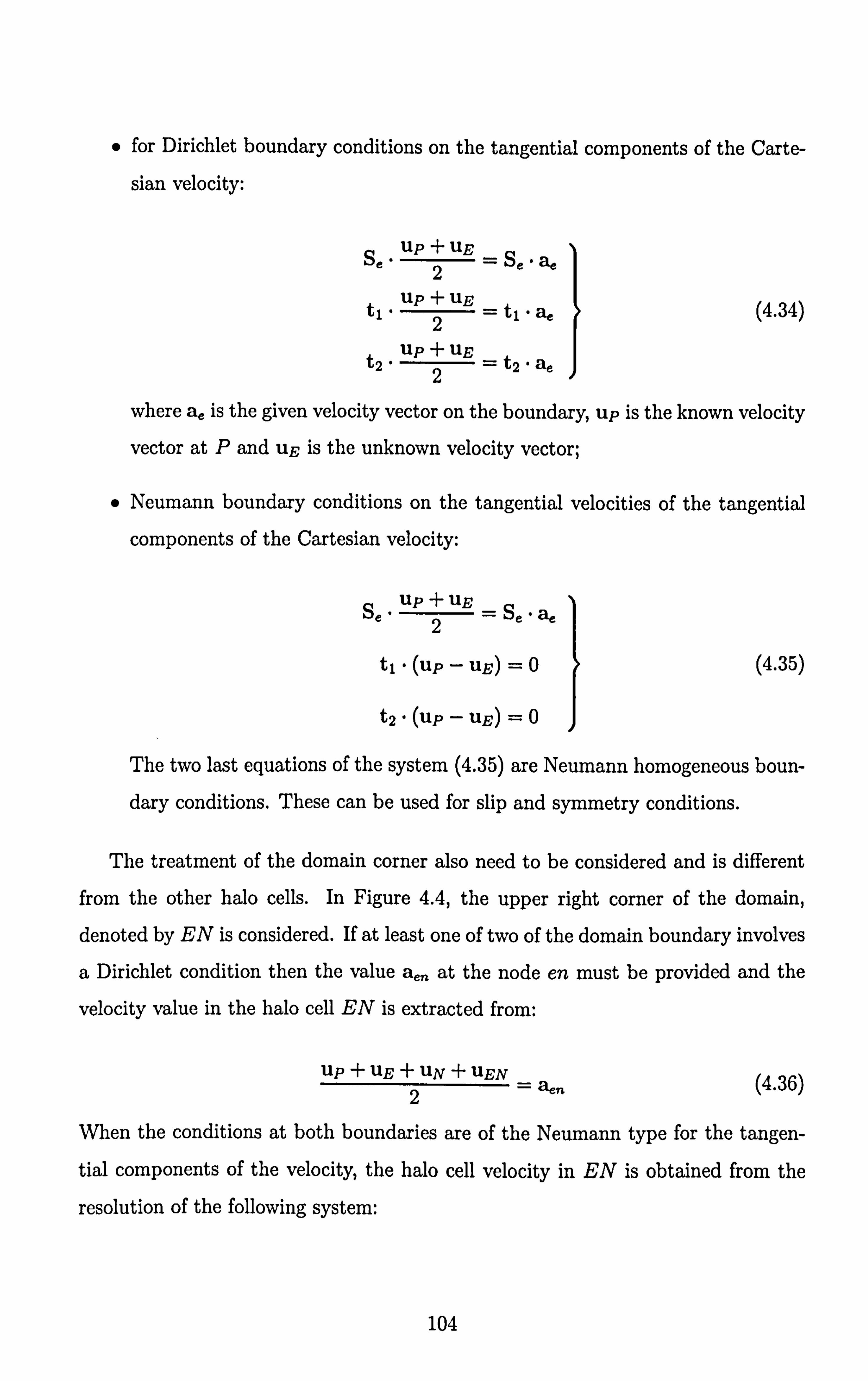
* for Dirichlet boundary conditions on the tangential components of the Carte-

sian velocity:

% ., UP + UE

- Se a. 2

tl. UP+ UE - ti a, (4.34)

2

t2 * Up + UE

" t2 a. 2

where a, is the given velocity vector on the boundary, up is the known velocity

vector at P and UE is the unknown velocity vector;

e Neumann boundary conditions on the tangential velocities of the tangential

components of the Cartesian velocity:

se - Up + UE

= Se - a,, 2

ti - (up - UE) =0 (4.35)

t2'(UP - UE) =0

The two last equations of the system (4-35) are Neumann homogeneous boun-

dary conditions. These can be used for slip and symmetry conditions.

The treatment of the domain corner also need to be considered and is different

from the other halo cells. In Figure 4.4, the upper right corner of the domain,

denoted by EN is considered. If at least one of two of the domain boundary involves

a Dirichlet condition then the value a,. at the node en must be provided and the

velocity value in the halo cell EN is extracted from:

UP + UE + UN + UEN --': aen (4.36)

2

When the conditions at both boundaries are of the Neumann type for the tangen-

tial components of the velocity, the halo cell velocity in EN is obtained from the

resolution of the following system:

104

Se - UN + UEN

=S,. ae 2

Sn - UE + UEN

= Sn -an (4.37) 2

t* (UP - UEN) =0

where t=S, x S,, -

4.8.4 Alternative wall boundary conditions

In Section 3.3, a number of alternative near-wall approximations have been de-

scribed. These wall functions return a value of the wall shear stress r,,, based on the value of the tangential velocity u, at the centre of the near-wall cell centre (see

Figure 4.9).

T,

Figure 4.9: Imposing an approximate boundary condition by replacing the momen-

tum fluxes.

Once the wall shear stress is known, any momentum flux through the cell face

coinciding with the wall is replaced by:

9 -r,,,, _-St,, t for the x-momentum equation;

9 7, w, yStot forthey-momentum equation;

9 r,,,,. St,, t for the z-momentum equation;

where St,, t -S-7 , is the surface of the cell face lying on the domain

boundary.

105

unknown

Figure 4.10: Imposing an approximate boundary condition through the halo cells.

A possible alternative route (not used here) is to introduce these boundary conditions via non-homogeneous Neumann boundary conditions for the Cartesian velocities with system (4.35) being rewritten as follows if the eastern border of the

domain is considered (see Figure 4.10):

Se - UP + UE

- Se - ae

21 tl '(UP UE) tl Tw (4.38)

t2 * (UP UE) t2 Tw rw

4.8.5 Boundary condition for the pressure

The boundary condition for the pressure on the domain is a homogeneous Neumann

condition (see system (4.13):

ap-n+l

axi (4.39)

This condition results from the requirement that the overall mass must be conserved

on the domain boundary. In this code, condition (4.39) is built in the Laplace

equation at the start of a computation when the stencils of the discrete Laplace

problem are evaluated.

106

Domain boundary

A

(trailing edge)

Figure 4.11: 'Reatment of the block interface in the aerofoil wake.

For a non-orthogonal mesh, the solver needs the nodal value of the pressure on

the boundary. This value is computed by using the content of the halo cells. The

halo cells values are determined using a lineax extrapolation from the domain inside

(as recommended by Bernard and Kapitza [16]). The linear interpolation, assuming

that the eastern face of the domain is considered (see Figure 4.1), writes:

PE : -*4 2PP - PW

4.8.6 C-grid capability

(4.40)

The present code has been designed to compute flows around airfoils with a sharp

trailing-edge and has, therefore, a C-grid capability in which the domain is folded

in such a way that one part of a boundary collapses to another part of the same

boundary. The domain being structured, special care has to be taken when updating

the halo cells of two blocks with common interfaces originating from different parts

of the same boundary. As shown in Figure 4.11, a consequence of a folded boundary

is that the cells 1 ... n of one block connect to cells n. .. 1 of the neighbouring block.

The procedure to update the halo cells is as follows. First, the halo cells axe updated

as described in Section 4.7.2. Second, the order of the halo cells is inversed so that

its content corresponds to the content of the associated cell inside the domain.

107

a Airfoil

b*

Wake .....................................

-I

Singularity point (trailing edge)

Figure 4.12: Discretisation in the trailing edge (singularity point) region.

A current requirement of the code is that the vertex located at the trailing edge

must be located on a block interface as shown in Figure 4.11. The multigrid solver

also requires that the trailing edge vertex belongs to each grid used in the multigrid

cycle.

4.8.7 Singularity point

The aerofoil considered in this work presents a sharp trailing edge on which a node is

located (see Figure 4.11). This particular point is a singulax point and the code needs the value for the pressure and the Cartesian velocities at this particular location.

For the Cartesian velocities, one is imposing that:

Unode, sing (4.41)

The nodal pressure value is computed by considering the near-wall cells next to

the trailing-edge and their corresponding halo cells (see Figure 4.12). The nodal

pressure is obtained by taking the average of the pressure at the centroid of these

four cells as follows:

Onode, ising ý1 (OA + OB + Oa + Ob) (4.42)

108

This is applied at each level of the multigrid procedure, hence the use of 0 rather

than P to represent the pressure.

4.9 Code performance on parallel platforms

4.9.1 Hardware characteristics

The code was developed and ported to four different architectures:

ea Cray T3D with 512 DEC Alpha 21064 processors having a cycle rate of 150

MHz and 64 MB of memory;

9a Cray T3E 1200E with 788 processors Alpha 21164 having a cycle rate of 600

MHz and 256 MB of memory;

ea 32 processors Intel Pentium III system (Beowulf II), each processor having

a cycle-rate of 450 MHz with 256 MB of memory and interconnected via Fast

Ethernet;

*a Compaq system (Loki) made of 16 Alpha EV67(21264A) dual-processors,

having a cycle rate of 667 MHz and 512 MB of memory with communication

achieved by the QSW high performance interconnect.

Communications-related information is given in Table 4.1.

Platform Communication software Latency Maximum bandwidth

Beowulf system LAM MPI 100ps 10 MBs

Loki system MPICH 201ts 160 MBs

Cray T3D MPI 92ps 110 MBs

Cray T3E MPI loys 220 MBs

Table 4.1: System communication chaxacteristics.

Beowulf systems are very cost-effective computing platforms. Their communi-

cations, often effected through Ethernet, is their weak point. Other interconnect

109

options offering better communications exist, but are generally too expensive for

modest systems.

4.9.2 Parallel performance for the channel flow

The first benchmark case selected is the turbulent periodic channel flow. The com-

putational domain has the dimensions 27rh x 2h x7rh (h is the channel half width)

and the Reynolds number (based on h, laminar viscosity v and bulk velocity Ub) is

equal to 10935. Each simulation started from an unitary velocity field and ran over

a period of 1000 time-steps. All computational parameters axe kept constant, while

the domain decomposition is varied. Two different grids axe employed:

ea medium size grid of 96 x 64 x4 cells;

ea large size grid of 384 x 256 x4 cells.

Figure 4.13 shows the solution time in seconds for 1000 iterations on partitions

of 4 to 32 processors for the smallest of the two problems on three of the plat-

forms described previously: the Beowulf system, the Loki system and the Cray T3E

1200E. Among these platforms, the Loki system appears to give the best overall

performance. It has the fastest processors, and its communications are also fast,

with a low-latency which is nearly as good as the Cray T3E. Fast communications

with low-latency are desirable for iterative algorithms on paxallel systems. In this

respect, the Beowulf system is clearly disadvantaged (see Table 4.1).

For the same problem, Figure 4.14 shows the scalability to be similax for all plat-

forms, with the Cray T3E performing a little better due to its better communication

network, despite the fact that its processors axe slower than those of the Beowulf

and Loki systems.

In Figure 4.15, the larger problem is considered. The speed-up curve is shown

for the Beowulf system and the Cray T3E. In this case, a virtually linear speed-up

is achieved on both machines. Indeed, a super-linear behaviour is observed for the

Cray T3E for the 32 processors case. This feature, quite common on such machines indicates an especially effective cache utilisation.

110

:i

E P

160

140- 1 T3E120QIE

120- *--x Beowulf Loki

100-

80-

60-

4U

20

0L 'L L -L If -'L A 048 12 16 20 24 28

Number of Processors

Figure 4.13: Time to solution for the channel problem. 96 x 64 x4 cells.

CD

aIIIIa

7- T3El2OO/E

6- X---X Beowulf Loki

5- 'Meoritical

4-

3-

2-

00,14 8L IL2 IL6 -2LO -2L4 '2j 8 -3L2


Figure 4.14: Speed-up curve for the channel problem. 96 x 64 x4 cells.

The relative importance of the communication to the total computational cost is

indicated in Figures 4.16 and 4.17. The communication times are identified by refe-

rence to the different variables that axe exchanged between processors, i. e. pressure,

velocities and viscosity. The first observation is that the solution of the pressure

requires the lion's share of the communications, especially for small problems with

large number of blocks. As the problem size increases, the relative contribution of

the communications to the total computational cost diminishes. The processors are

spending more time calculating than exchanging informations. This explains why

the larger problem scales much better on the Cray T3E and on the Beowulf system. For the latter, this is especially influential as the communications characteristics are

ill

I

0.

v1 9-

/+ 8- T3E12001E

Beowulf 7- Theoridcal

6-

5-

4-

3-

'L 'L LL -L -L A 48 12 16 20 24 28 32


Figure 4.15: Speed-up curve for the channel problem. 384 x 256 x4 cells.

rather poor.

.9

1

g 0

r. i

!0- Velocities X--x Viscosity

Pressure 5-

0-

5-

_____-x

J, LLLLA

-L 048 12 16 20 24 28 32


Figure 4.16: Communications time expressed as a fraction of the total execution

time for the Cray T3E and the channel problem. 96 x 64 x4 cells.

4.9.3 Parallel performance for the Aerofoil

The problem considered here is a single element high-lift aerofoil (A6rospatiale-

A [77,78]) at 13.30 angle of attack and a Reynolds number of 2x 10', based on

chord length and free-stream velocity. The spanwise extent of the aerofoil was chosen

to be 0.23% of the chord. The grid consists of 320 x 64 x 32 cells. The results were

obtained on two of the four platforms considered: the Cray T3D [114] and the Cray

112

14

12 -

10 - 8 -

Velocities 6 X---K Viscosity 1

4 ** Pressure

12 16 20 24 Number of Processors

Figure 4.17: Communications time expressed as a fraction of the total execution

time for the Cray T3E and the channel problem. 384 x 256 x4 cells.

T3E 1200E. The initial problem is decomposed into 32 blocks, and tests are carried

out for 32,64,128,256 and 512 blocks.

1

tz. =1 Ici

6- 0---o neoretical ,- T3E 1200/13

4- +---* T31) .x... x T313 (scaling using 64 CPU)

2-

0-

8-

6-

4-

2F

OL 02468 10 12 14 16

Np/32

Figure 4.18: Speed-up curve for aerofoil flow. 320 x 64 x 32 cells.

The speed-up curves obtained on both platforms are shown in Figure 4.18 for up

to 256 processors for the Cray T3D and 512 processors for the Cray T3E, respec-

tively. The scalability on both machines is good, but diminishes rapidly beyond 256

processors simply because the problem is too small for the largest partitions. For

the Cray UE, the scaling is made using 32 processors and 64 processors as referen-

ces. A substantial gain in performances was observed when increasing the number

of processors from 32 to 64 for the Cray T3E. The super-linearity, achieved by the

113

T3E indicates a poor cache utilization with 32 processors. Beyond 64 processors,

each block fits in the cache, giving a better and faster access of the data to the

processor.

114

Chapter 5

Flow analysis

5.1 Introduction

The phenomena of turbulence are very complex and their study, interpretation and

understanding require the use of a range of mathematical tools. The aim of this

chapter is to describe the tools that have been used in the present work to interpret

results and extract useful data from the simulations. Section 5.2 is concerned with basic aspects of the statistical description of tur-

bulence. Sections 5.3 and 5.4 consider, respectively, the RANS equations which

govern the mean velocity field and feature the Reynolds stress tensor and the equa-

tions dictating the transport of the Reynolds stresses. Section 5.5 introduces the

anisotropy of the Reynolds-stress tensor and some post-processing tools which re-

late to this. Two-point correlations are defined in Section 5.6, while Section 5.7 is

concerned with the study of turbulence in spectral space. Finally, Section 5.8 deals

with approaches characterising instantaneous features of the flow, with particular

emphasise on criteria for identifying vortical structures.

5.2 Statistical description

The study of the instantaneous turbulence fields offers the opportunity to extract from them certain structural features and statements on extreme events. Otherwise,

a quantitative analysis of such fields is unproductive because they are non-repetitive.

115

To undertake a quantitative analysis of turbulence, attention has thus to focus on

statistical properties. As these properties are also the focus of turbulence modelling,

or the outcome resulting from the application of models to particular flow problems,

the extraction of the statistical properties is often one of the principal objectives of a

simulation. Such data allow closure approximations to be tested and mechanisms to

be identified. This, in turn, aids model improvements. Statistical data also provide

a benchmark for model validation. The statistical analysis of turbulence is almost invariably based on time- or

ensemble-averaging, here used interchangeably:

0(X) >= lim 10

(x, t) dt (5.1) T--+oo T

10

where 0 is any property of the turbulent field, and T indicates the period over which

the average is performed. If a flow is statistically homogeneous in a certain direction,

a spatial averaging operator can be usefully defined in that direction. If z is that

direction, the averaging operator is as follow:

0 0(X, Y, t) >= lim

10 (x, t) dz (5.2) L. -oo Lz 0

where L, indicates the spatial extent of the averaging of the z-direction. Opera-

tors (5.1) and (5.2) can be combined, and this is advantageous in simulations that

contain a homogeneous direction as it helps reduce the time necessary to obtain

fully-converged statistical properties. As a simulation returns the fields at discrete

space and time locations, the averaging operators have to be written in a discrete

form such as:

<0>= 1

7E oi (5.3) i=l

where N represents the number of samples recorded. The introduction of the ave-

raging operator then allows any instantaneous flow property 0 to be separated into

two components, a mean value and an instantaneous fluctuation:

0 =< 0> +0' (5.4)

116

where <-> indicates the averaging operator. Representation (5.4) is known as

Reynolds decomposition.

In addition to the mean value of 0, it is interesting to quantify the properties of the fluctuations, in a statistical sense, axound that mean value by considering the

average of the different powers of (ý', the moments. The first moment < 0' > is, by

definition of the mean, equal to zero. The second moment, defined as a2 =< 0! 01 >'

is known as the variance, although its square root is often used, representing the

standard deviation from the mean value.

5.3 The RANS equations

The introduction of decomposition (5-4) into the governing equations of an incom-

pressible flow in the absence of body forces (described by the Navier-Stokes equations (2.1)), combined with the application of an averaging operator to these equations

lead to a new set of equations known as the Reynolds-Averaged Navier-Stokes equa-

tions (RANS):

<ui >< Ujuk >a, < ui >a< U', " +A aX2 p iUk >

(5.5) at OXk axi k

aXk

Equation (5.5) governs the mean motion and its last term, p< u'iu'k >, is the ik Reynolds-stress tensor and its components identify the primary statistical properties

of the turbulence field. The components i=k are the normal Reynolds stresses

while, for i 54 k, the Reynolds shear stresses arise. Equation (5.5) can be rewritten

in terms of the dimensionless variables (2.2) as:

1 a2<U, > a<u, I a< Ui >+a< UiUk >a+ iu k> (5.6) at OXk axi Re aX'k aXk

and this is in this form that the RANS equations will be used in what follows.

117

5.4 Turbulence transport equations

In the previous section, it is shown that the mean velocity < ui > is linked to or is

affected by < uýuý >. This stress tensor is, in fact, the only link between the mean S field and the turbulence properties. Hence, < uý, u, ' > and the processes governing

its behaviour are of principal interest. To understand the mechanisms which govern

< uý ' >, it is necessary to derive further equations which describe the evolution of zuý this tensor. As will be seen, these equations contain higher-order moments, and like

< Uý , uj' >, they too can be extracted from simulations. The higher moments provide

rich information on the constituents of the transport equations and the mechanisms driving the stresses themselves.

Equations of transport for the Reynolds stresses and the turbulence energy, de-

fined as half the sum of the normal stresses (k = 0.5 < U'kUk >), may be derived from

the Navier-Stokes equations. First, the RANS equations (5.6) are subtracted from

the Navier-Stokes equations (2.3). Equations for the turbulent velocity components

are thus obtained:

-u aui au; op, 1 a2U, 0< uiuk >' auot OUtt

k 1

-ä-+ < Uk >Z : -- - -k (5.7) t (9Xk

UX-i + -, OX2 DXk aXk aXk k

After multiplication of (5.7) by uj, and averaging, the result is:

1u1.010< ui >1 au' 1t Oui

>+< UjUk eXk >+< Uj < Uk >>+< UjUkUX > uj at k 04

(5.8) "q < ui k

.7 exi eX2 zuk

>> < U. - > +Ne- < uiý ý% >+< uj

k OXk

and with i and j reversed:

out- , aul. Ul aui, >+< Ulu, >+<U, '> -I

iki< Uk >+< UiUk > at

I 19Xk

a2 19Xk 19Xk (5.9)

1 lop '49<u- '

< Ui --< u' Ui Uk >>

ýýxj >+ Te ZFXFk >+< Ui' aXk

The sum of (5.8) and (5.9) leads to the transport equation for the Reynolds stresses:

118

D<uý > Ij Pij + Tij + Dij + rlij + cij (5.10) Dt

where

D< uiuj' >9< u'u'. >a< UU'. < Uk > Dt 19Xk

represents the substantial derivative. The group of terms

II a< ui >11 (9 < uj > Pij < UjUk > axk

< UiUk > (9Xk

(5.12)

is the production of the turbulent stress < uý, uj' >. It represents the influence of the

mean flow straining on the turbulent stresses, thus linking mean flow and turbulent

quantities. These terms are normally positive and will increase the stresses, but can

also be negative in certain unusual strain fields. The dissipation rate is:

cij 2< oulit au-17

> (5.13) We- (9Xk aXk

and expresses the transfer of turbulence energy to heat. This term always diminishes

the turbulent stresses. The term

a< UiUjUk > Tij =-

19Xk

is the turbulence transport rate and expresses the spatial redistribution of any tur-

bulent stress by the turbulence itselL Viscous diffusion is expressed by

< U', '. > iu -7 Dij 2j (5.15)

Re (9Xk

This term is usually very small, except in the viscous sublayer. Finally, the term

riii <

UILP >-< UjW > Z, Oxj exi (5.16) D<p, u, > 9<P, U,. > "gu'. ,

au' i ý) ý +<PLIL >+ axj axi axi axj

is the velocity pressure-gradient interaction term. It can be decomposed, as done

above, into two constituents: the pressure diffusion term and the pressure-strain

119

term. The latter tends to redistribute the turbulence energy among the normal

stresses, steering turbulence towaxd isotropy.

The transport equation for the turbulence energy is obtained by contracting Equation (5.10):

Dk Dt = Pk + Tk + Dk + Hk + Ck (5.17)

where

Dk Ok ak Tt- Tt +< Uk > ý- (5.18)

Xk

a< ui > Pk < UjUj > 19xj

(5.19)

III Tk = -0.5

a< Uiuiu > (5.20) 19xj

Dk -1

192 k (5.21)

Re aX j2

k a< P, Uj, > (5.22)

Oxj

Ck -` -1:: ýý Lu, Lu

-': (5.23) Re iYxj Oxj

Note that the pressure-strain term vanishes as a consequence of the mass-conser-

vation constraint (for incompressible flow, Ou'j/, 9xj = 0). This claxifies the earlier

interpretation that this term describes the redistribution of turbulence energy k

among the normal stresses and thus does not alter the level of turbulence energy.

5.5 Turbulence anisotropy and related post-pro-

cessing

The anisotropy represents the deviatoric part of the Reynolds stresses and is obtai-

ned by substraction from the Reynolds stresses the isotropic contribution (-2/3Jij

120

Ulu' >), Le.: kk

a.. =< uV. >2 Jij < U, U, > (5.24) tj 135kk

where Jjj is the Kronecker symbol*. The anisotropy tensor (5.24) is usually considered in the dimensionless form:

< U'U' > -2jij < Ulu, > bij j3kk (5.25) 2< u',, u. > k

The tensor bij is thus traceless, i. e. its first invariant is equal to zero, and this

allows the study of its properties by considering only two parameters: its second

invariant, defined as 11 = -bjjbjj12, and its third invariant, III = bijbjkbkjl3. A

consequence of this tensor being traceless is that the sum of its eigenvalues Al, A2

and A3 (the eigenvalues also represent the stresses in principal axis) is also zero, hence A3 = -Al - A2, and the eigenvalues of bij can also be used to characterise bij.

This constraints all eigenvalues to be no smaller than -1/3 (this corresponds to the

vanishing of the related component) and none can be larger than 2/3, in which case,

the two other components vanish. Hence, any physically realizable turbulent state

is constrained to lie in a zone delimited by the above extrema or the corresponding

invariant values. Table 5.1 shows the limiting values that can be attained by the

invariants and the eigenvalues, while Figure 5.1 shows graphically these limits. This

plot is known as the anisotropy inva7iant map or the Lumley tHangle (Lumley and

Newman [134], Lumley [133]). This triangle describes the various physically realistic

states that can be attained by a turbulent flow. For any turbulent flow, each point

has to lie inside or on these boundaries, for otherwise it will be unphysical (non-

realizable). The Lumley triangle is often used in RANS modelling to verify that a

turbulence model does not violate realizability constraints.

A parameter also often employed is the flatness:

1+ 9(11 + 3111) (5.26)

*Sij =1 if i=j and Jjj =0 if i ý4-j

121

0.4

-110.2

0.3

Isotropic 2DI

0.1 Axisymmetric Contracdon

L--. L--L

-Wol 0 0.01 0.02 0.03 0.04 0.05 0.06 0.07 0.08 III

Figure 5.1: Anisotropy invariant map

This parameter characterises, as best as a single scalar can do, the range of tur-

bulence states spanning from the state of isotropy to two-components turbulence

corresponding, to A=1 and A=0, respectively. This fact is often taken advantage

of in RANS modelling to secure the limiting behaviour at walls and fluid interfaces

(HanjaliC' and JakirliC' [79], Craft and Launder [42]).

122

Eigenvalues Invariant values State of turbulence

Al = A2 == A3 =0 -11 0 Isotropic turbulence

111 0

Al = A2 = 1/6 -11 = 1/12 Isotropic two-dimensional

III = -1/108 turbulence

A, = 2/3 -11 = 1/3 One-dimensional turbulence

A2 = A3 = -1/3 111 = 2/27

-1/3 < Al = A2: 5 0 111 = 2(-11/3)3/2 Axisymmetric contraction (one

large eigenvalue) straining the

flow in one direction and

contracting it in the two others

0 Al ý-- A2 :5 1/6 111 = -2(-11/3)3/2 Axisymmetric expansion (one

small eigenvalue) caused

by straining the flow equally in two orthogonal directions

and contracting it in the third

Al + A2 == 1/3 1/9 + II + 3111 =0 Two-dimensional turbulence

Table 5.1: Limits to the state of turbulence.

123

5.6 Two-point correlations

Two-point correlations are coefficients which identify the degree of correlation be-

tween the fluctuations at two different spatial or temporal locations. In what follows,

ý will represents the time or any of the three spatial coordinates x, y, z. Thus, for

0(6), the correlation coefficient relating to a separation A6 is:

R(6, Aý) <+ Aý) > (5.27) < (01(ý))2 >

If AC = 0, there is no separation in the C-direction, and, evidently, R(AC = 0) = 1.

If AC becomes sufficiently large then R(AC) drops to zero and the flow variables are

said to be uncorrelated. Note that if the flow is statistically homogeneous in the C-

direction, then R is independent of C. Two-point correlations can be used as a mean

of testing whether a computational box is large enough to contain all the turbulent

scales (even the largest) in a statistically homogeneous direction. However, Jimenez

and Moin [97] have shown, for a channel flow, that adequate first and second-order

statistics could be obtained with a box size significantly lower than a decorrelated

flow would require. This concept is known as the minimal flow unit. Nevertheless,

the application of (5.27) is useful in guiding the choice of the computational box.

5.7 Energy and velocity-spectra

In a turbulent flow, where the random signal u(ý) is periodic (ý can be the time-

variable or any of the spatial coordinates x, y, z), the two-point velocity correlation

(5-27) and its spectrum form the Fourier transform pair:

+00

Rjk 00

Eik(w)C"ý&u (5.28)

and

+00 E'k (W) Rjk(ý)e"ýdý (5.29) 3 T7r

f-00

where Rjk is the two-point correlation for the jk velocity pair and Ejk is the associate

spectrum. w represents the frequency, if ý is the time-variable, and the wave-number,

124

if ý is any of the spatial coordinates.

Velocity-spectra axe thus defined for each pair of velocities UjUk and provide in-

formations on the spectral interaction between these two variables and only them.

In most studies of turbulence, attention is restricted to the turbulence energy spec-

trum, defined as the half-sum of the velo city-spectra Ell, E22 and E33, Velocity and

energy spectra provide information on the mechanisms of energy transfer between

different wave-numbers and frequencies. In the context of numerical simulation, the

spectrum of k also provides a statement on the quality of the numerical resolution.

5.8 Identification of turbulent structures

The structure of turbulent flows is of much interest, as it provides insight into the

fundamental formation and interaction of the vortices which constitute the turbulent

motion. The presence of quasi-periodic repeating patterns of coherent motions in

the flow (Robinson [187]) has been observed for many years, and it is sought that

these coherent motions (also referred to as coherent structures) are the cause for

the maintenance of the turbulence. Most of the knowledge on these structures

comes from the study of low-Reynolds-number flows, but little of this knowledge

has so far been embedded into closure models. The main reasons for the study

of turbulence structures are the need and the wish to understand the dynamical

phenomena associated with the statistical properties. Coherent structures are usually identified from visualising iso-surfaces of certain

instantaneous flow properties. The choice of the threshold at which these iso-surfaces

are drawn is a matter of trial and error and is dictated by the ability of the observer

to see these structures within the paxticular flow property field examined. Coherent

structures are associated with vortex cores. An intuitive approach is to consider

regions where pressure minima occur. Another is based on associating a vortex core

with a region of high rotation rate and thus with regions of high enstrophy, defined

as the modulus of the vorticity (w =Vx u), or regions of high w.,,, w,, or w, '. As

noted by Jeong and Hussain [94], an inherent problem of using the vorticity is that

it assumes high values in sheared regions even in the absence of vortices. Thus, more

125

rigorous criteria are needed to identify vortical structures. One criterion, proposed by Chong et al [34], is based on the assumption that

a vortex core is a region of the flow where the eigenvalues of the velocity-gradient

tensor (Aij = 9uj1,9xj) are complex. This implies that the local streamlines are

closed. Mathematically, this can be expressed by considering the characteristic

equation of A,, -

p, \2 + QA -R=0 (5.30)

where P= auilaxi (= 0 for incompressible flows), Q= -1/2 (auj1,9xj) (, 9uj1axj)

and R= det(Aij). For an incompressible flow, all the eigenvalues are complex if the

discriminant of (5.30) is positive:

Q' +

R' : ý. 0 (5.31)

27 4

Coherent structures are thus regions of the flow where A is positive. Another proposal, made by Hunt et al [88], defines a vortex core as a region

where the second invariant Q of Aij is positive and, at the same time, where the

local pressure has a lower value than the ambient.

More recently, Jeong and Hussain [94] proposed a criterion based on the eigen-

values Of SikSkj + QikQkj. They consider that this tensor identifies local pressure

minima associated with vortical motions. They define a vortex core as a region where

two of the eigenvalues Of SikSkj + f2ikf2kj axe negative. Assuming these eigenvalues

are A, ý! A2 ýý' /\3, a vortex core is thus a region of the flow where A2 < 0-

Note that, contrary to the vorticity, the A and A2 criteria vanish at the wall

where sheax is high, but vortices are weak.

Other but less popular approaches include the kinematic vorticity number (Me-

lander and Hussain [147]) or the use of instantaneous streamlines (Lugt [132]). De-

tailed lists of criteria, with applications, can be found in Kasagi et al [104], Lesieur

et al [123] and Hanjalic' and Kenjereg [80]. In the present work, the only crite-

ria used to identify the coherent structures are: the pressure, the A-criterion, the

second-invariant criterion and the A2-criterion.

126

Chapter 6

Channel flow computations

6.1 Overview

Fully developed turbulent channel flow is the first and most studied generic configu-

ration of engineering interest in LES reseaxch (Deardorff [49], Moin and Kim [159],

Piomelli [175] among others). The simplicity of the geometry shown in Figure 6.1,

the statistical homogeneity of the flow in the strearnwise and spanwise directions

and the option of adopting periodic conditions in these two directions make this

flow an ideal test case for investigating the near-wall behaviour of LES, the performance of subgrid-scale models and the adequacy of near-wall approximations at high Reynolds numbers. Furthermore, it allows the various post-processing tools

described in the previous chapter to be examined. These tools will be applied to

analyse more complex flows.

In this chapter, channel flow at three Reynolds numbers Re,, based on the wall

shear velocity u, and the channel half width h, are considered, namely 180,590

and 1050. A summary of the test cases is given in Section 6.2. In Section 6.3, the

performance of the subgrid-scale models described in Section 3.2 will be investigated

for the case Re, = 590. Section 6.4 deals with the adequacy of the near-wall

approximations described in Section 3.3 for the cases Re, = 590 and Re, = 1050.

Section 6.5 is concerned with the study of numerical and modelling errors based on

a procedure developed by Vreman et al [228] for mixing layers, and adapted, in the

127

Lý

x

Figure 6.1: Geometry of the channel flow, with L_- and L, being periodic segments.

present work, to the case of the turbulent periodic channel flow. Mathematical tools,

used to study turbulence and presented in Chapter 5, axe tested in Section 6.6 in

order to validate the correctness of their implementation and to construct the basis

that will enable a better understanding to be gained of the phenomena studied later

in Chapters 7 and 8. Finally, Section 6.7 summarises the observations made during

the studies presented in this chapter, and draws lessons to be applied to the more

complex flows studied in the chapters to follow.

6.2 Summary of the test cases

Three different periodic channel flows at three Reynolds numbers, Re,, have been

considered. The first two cases correspond, respectively to Re, = 180 and Re, =

590, for which an extensive DNS database* is available (Moser et al [161]). The

third case, at Re, = 1050, corresponds to a high-Reynolds number LES performed

by Piomelli [175]. For each case, a range of box sizes and grids have been used, and

these are summarised in Table 6.1. *http: //www. tam. uiuc. edu/faculty/moser/

128

Ref. Re, Reb Box dimensions Discretisation Ax+ Ay+ Az+ Lx x Ly x L, N., x Ny x N,

CM1 180 2800 27rh x 2h x7rh 96 x 64 x 64 12 1.2-19.3 8.8

CM2 590 10935 27rh x 2h x 7rh 64 x 32 x 32 58 37 58

CM3 590 10935 27rh x 2h x7rh 72 x 48 x 32 51.5 10-37.1 58

CM4 590 10935 27rh x 2h x7rh 96 x 64 x 64 38.6 2-42.2 29

CM5 590 10935 27rh x 2h x 27rh

3 96 x 64 x 64 38.6 2-42.2 19.3

CM6 590 10935 27rh x 2h x7rh 96 x 64 x 96 38.6 2-42.2 19.3

CM7 1050 21351 §I-h x 2h x mh- 50 x 20 x 10 165 105 165 22

Table 6.1: Summary of the channel flow cases.

6.3 Influence of the subgrid-scale model

Simulations undertaken in this section aim to investigate the performance of the

subgrid-scale models (and some of their variants) described in Section 3.2. The task

of a subgrid-scale model is to compensate for the loss of the turbulence scales asso-

ciated with grid coarseness. If it were possible to avoid numerical errors, the perfor-

mance of subgrid-scale models could be examined unambiguously by recording the

associated LES to represent the appropriately filtered DNS solution. However, nu-

merical errors cannot be avoided, and the solution error is therefore a non-separable

amalgam of subgrid-scale model and numerical and resolution errors. Hence, in the

present investigation, the central issue is an examination of the ability of subgrid-

scale models, relative to others, to provide a solution which is close to the bench-

mark. All simulations were performed for the case Re, = 590 for which DNS data

are available (Moser et al [161]). Three different meshes, designated CM3, CM4 and

CM6, and described in Table 6.1, were used. Cases CM4 and CM6 axe wall-resolved

in the sense that Ay+(l) :ý2. Case CM3, with Ay+(l) ý- 10, is not wall-resolved

and was chosen to assess whether some models were able to compensate better than

others for the loss of near-wall resolution. In all cases, a no-slip boundary condition

was used. The ratio between the grid-filter width _, E and the cell size was chosen

equal to 1. Statistics were collected over a period of 12 flow-through times, for

129

all non-dynamic subgrid-scale models, and 24 flow-through times for the dynamic

subgrid-scale models, sufficient to ensure fully converged statistical properties. In

total, 11 modelling practices, including vaxiations of models, were examined, these

are summarised in Table 6.2. Their performance was judged by reference to mean

velocity, friction Reynolds number and Reynolds-stress components, all relative to

DNS solutions.

For the series of computations performed on the wall-resolving mesh CM4, none

of the models returns the universal velocity distribution especially well, as shown in

Figure 6.2. While the log slope is correctly reproduced in most cases, the errors in

the level of the log-law region are not insignificant and appear to be associated with

the representation of the buffer region and the predicted level of the wall shear stress

for a prescribed mean velocity, as shown in Table 6.3. Figure 6.3 demonstrates that

different models return substantially different subgrid-scale viscosity distributions.

In the core region of the flow, the maximum viscosity levels vary within the range

of one order of magnitude, between 0.1 and 1 times the fluid viscosity, with the

WALE model returning the lowest value and the localised dynamic model (LDSM)

the highest. As the subgrid-scale transport is only a small portion of the resolved

transport in the log-law region, this difference is not influential. However, the visco-

sity level in the upper part of the buffer layer, as well as the asymptotic behaviour of

the subgrid-scale viscosity, can be more important because the resolved contribution

declines rapidly as the wall is approached. The theoretical asymptotic behaviour of

the subgrid-scale viscosity is cubic in y+ and is represented by the straight line in

Figure 6.3. Only the WALE model and the dynamic variants return the asymptotic

behaviour well. The substantial variations in the subgrid-scale viscosity can be

identified to cause corresponding variations in the mean velocity. In the region

10 < y+ < 20, a high subgrid-scale viscosity tends to depress the velocity in the

buffer and log regions below the DNS variation, while the reverse occurs when the

viscosity in this region is low.

130

Model Designation Model Description

SM Smagorinsky Model (Cs 0.1)

SM + WD1 Smagorinsky Model (Cs 0.1) + Wall-Damping

Function 1 (A+ = 5)

SM + WD2 Smagorinsky Model (Cs 0.1) + Wall-Damping

Function 2 (A+ = 25)

MSM1 Mixed-Scale Model (Sagaut [192]) (Cm = 0.01 -

a=0.5) MSM2 Mixed-Scale Model (Sagaut [192]) (Cm = 0.1 -a

0.5)

GDSMT Dynamic eddy-viscosity model (Germano

et al [65]), filtering using the trapeze rule

v/'6- DSMT Dynamic eddy-viscosity model (Germano

et al [65]-Lilly [129]), filtering using the trapeze

rule V6_

DSMS Dynamic eddy-viscosity model (Germano

et al [65]-Lilly [129]), filtering using the Simpson

rule AxlAx =2 DSMTN Dynamic eddy-viscosity model (Germano

et al [65]-Lilly [129]), filtering using the trapeze

rule AxlAx = /6-

no planar averaging NSGS No subgrid-scale model WALE WALE Model (Cw = 0.1)

(Nicoud and Ducros [167])

LDSM Localised Dynamic eddy-viscosity model (Piomelli

and Liu [178])

Table 6.2: Subgrid-scale models used in channel flow computations.

131

SGS Model Re, Error U, /Ub Error

DNS 584 1.1418 sm 617 +5.6 % 1.1533 +1-00 %

msmi 565 -3.3% 1.1461 +0.04%

MSM2 605 +3.6% 1.1411 -0.06% SM + WD1 595 +1.8% 1.1444 +0.23%

SM + WD2 538 -7.8% 1.1319 -0.86% GDSMT 520 -10.8% 1.1216 -1.77% DSMT 523 -10.3% 1.1239 -1.57% DSMTN 537 -8.1 % 1.1230 -1.6% DSMS 529 -9.3% 1.1298 -1.05% WALE 542 -7.1% 1.144 +0.2%

LDSM 520 -10.8% 1.1221 -1.73% NSGS 541 -7.4% 1.1428 +0.09%

Table 6.3: Predictions of wall shear stress and centreline velocity for case CM4.

Figures 6.4 to 6.7 show, respectively, profiles of r. m. s. velocity fluctuations in

the streamwise, wall-normal and spanwise directions and of the shear stress. Away

from the wall, the streamwise intensity, shown in Figure 6.4, is correctly returned

or slightly underestimated for all cases, except MSM2 for which it is overestimated.

Near the wall, all models overestimate the peak in fluctuating velocity in the stream-

wise direction. On the other hand, Figures 6.5 and 6.6 show that the wall-normal

and spanwise intensity are too low, indicating that the energy repartition between

the three directions is not correctly resolved, thus suggesting that mesh resolution in

the spanwise extent and possibly also in the streamwise and wall-normal directions

contributes to the differences between all LES results and the DNS reference data.

This makes it difficult to judge the subgrid-scale model performance. Figure 6.7

shows the resolved shear stress to be well predicted for all cases. As the wall is ap-

proached, differences appear between the predictions given by the different models, indicating the part a model is playing in representing the subgrid scales.

Figure 6.8 shows the distributions of the subgrid-scale viscosity, highlighting

132

the variation in magnitude and shape that the models considered lead to. Overall,

the best results in this set of tests were obtained using the WALE, SM and MSM1

models, although the last two models do not present the proper near-wall asymptotic behaviour for the subgrid-scale viscosity. It is furthermore noteworthy that those

models returning the lowest subgrid-scale viscosity yield results closest to the DNS

reference solution. This might be taken to indicate that the models double-count the

effects of subgrid-scale motion, with numerical resolution errors providing another

mechanism. However, the fact that using no subgrid-scale model does not yield

a satisfactory solution indicates that a subgrid-scale model representing the scales

removed by the application of the LES filter, is necessary.

+ U

30

25- - DNS . w--wSM 20- v ... T SM + VYD I

+-. +SM+WD2 15 +

10-

5

0 I to 00 101 y.

30

25

20

15

10

5

n

-DNS A -, DSMT m DSMS

x. -. -xDSMTN

I to- ioLo Tol y

+ U-

DO

Z5 -- DNS .0... emsmi Zo - -MSM2 . -GDSMT

15 -

to -

y,

30

25

20

15

10

5

A DO

-DNS +.. +NSGS

m WALE

G-OLDSM

loo 101

y.

Figure 6.2: Streamwise velocity for channel flow for case CM4.

DO

133

--v -n. /, v

+

m

y +3

--BSM +

SM2

+ WD ... VSM+WD WD

+3

+ WD 0... OMSMI

1::: GýDSMT MSM2

y sm

m DSMT

"**"'ms 1 »*' sm

cv. >/v

,2 +3 o .Y

--, -DSMT DSMS

0-4 . x-. -. x DSMTN o--- WALE lo. --oLDSM

-61

i

1

10 10 00 101

YY

Figure 6.3: Distribution of subgrid-scale viscosity < vt > 1v in wall units for case

CM4.

U, rms

XbuI ms

/Tj b

0.2 .............. I. II. 0.2 ....... I DNS DNS

0.15 SM

0.15 0... qmsml SM + WDI --*MSM2

+-. +SM + WD2 *--oGDSMT 0.1 0.1

. ... .... ..... 0.05 0.05

............. .... ol 0... 0 0.2 0.4

y/h 0,6 .8100.2 0.4

y/h 0.6 0.8

U, rms

/U b U,

rms /TJ

b 0.2 ....... I... I... I. 0.2 11

DNS DNS 0.15 DSMT 0.15 +-+NSGS

DSMS WALE

0.1 ý x---. xDSMTN

0.1 o----oLDSM

d

0.2 0.4 y/h

0.6 0.8 1 -0 0.2 0.4 y/h

0.6 0.8 1

Figure 6-4: Distribution of r. m. s. streamwise velocity for case CM4.

134

rms

DNS *. -ESM SM + WDI

SM + WD2

V, rms

lu b

0.06r-

0.04

0.4 y/h

0.6

0.02 - DNS , DSMT

DSMS DSMTN

0,2, * '0'4 ... 0,6 ... 0,8 y/h

nns b 0.06r--

. 4ý Im 0.04-

DNS -D S 0.02

MT -*MSM2

r..

--. GDSMT

1 -0 0.2 0.4 y/h

rms b 0.06 ..........

0.04-

0.02 - DNS +--+NSGS 4-4 WALE o-. *LDSM

0.4 y/h

0.6

Figure 6.5: Distribution of r. m. s. wall-normal velocity for case CM4.

I

135

wI rml

ub

0.08,

0.06

0.04

0.02(

w9 rm/

0.08

0.06

0.041

0.02F

DNS SM SM + WDI SM + WD2

........... 0.2 0.4 y/h

0.6 0.8

- DNS ADSMT

DSMS x. -. -x DSMT

0.4 y/h

0.6 0.8

wt rm/Ub

I

0.

- DNS 0 ... emsmi

y/h

rms

0.04

- DNS +-+NSGS 4---4 WALE o---oLDSM

L ......... 0.2 0.4 YAI

0.6

Figure 6.6: Distribution of r. m. s. spanwise velocity for case CM4.

136

<u'v'

0.85akýý'

0.2

<u'v'

0.8ý ýý

0.2

- DNS W-ESM Y---vSM+WD1 +- .+ SM + WD2

<u'v'>

0.8- 9-0. -

0.6

0.4

0.2

y/h 0.6 0.8 1 -0 0.

[U

DNS 0.8 ON --,, DSMT

m DSMS 0 6 x---.. xDSMTN .

0.4

L.......

0.2

y/h 0.6 0.8 1

- DNS 0 ... OMSM1 *--*MSM2 9--*GDSMT

0.4 y/h

0.6 0.8

DNS NSGS WALE

o--. -oLDSM

y/h

Figure 6.7: Distribution of shear stress for case CM4.

137

1

<V t >/V

a--BSM -----SM+VY'Dl

SM + WD2 .v

0.6 A

0.4-

0.2,

0 .20.4 y/h 0.6 0.8 1

<v->/v

1.

0.

5 --, DSMT DSMS

----xDSMTN

5-

0.2 0.4 0.6 0.8

<vt>/v 2....

e ... OMSMI *MSM2

9---*GDSMT 0.5

......... . 0.2 0.4 y/h

0.6 0.8

<vt>/v I.

0.

", 0 14-- WALE o-oLDSMI O,

-e,

.0 0-.

-0- 0.2 0.4 -

0.6 0.8 1 Y/n y/h

Figure 6.8: Distribution of subgrid-scale viscosity < vt > 1v for case CM4.

138


DNS 584 n. a. 1.1418 n. a. GDSMT 463 -20.5% 1.1165 -2.22% DSMT 467 -19.8% 1.1231 -1.64% DSMTN 469 -19.5% 1.1232 -1.63% WALE 474 -18.6% 1.1257 -1.41% NSGS 481 -17.5% 1.1234 -1.61%

Table 6.4: Predictions of wall-shear stress and centreline velocity for case CM3.

A second set of numerical experiments was undertaken on a coarser mesh than

CM4, namely CM3 which contains 72 x 48 x 32 cells, with Ay+ (1) = 10. Simulations

were performed with 5 of the models considered previously, with the aim of investi-

gating the ability of these models to respond to the lack of near-wall resolution in

the absence of near-wall modelling. Table 6.4 shows that the wall shear stress and centreline velocity are strongly

underestimated. In fact, it appears that the best prediction is obtained when no

subgrid-scale model is used. These results are not surprising as the grid is of poor

quality for a wall-resolving LES, which requires Ay+ < 2. Figure 6.9 shows that,

with all subgrid-scale models, the log-law is misrepresented, primarily because of the

underestimation of the friction velocity. The streamwise turbulence intensity, shown

in Figure 6.10, is overestimated, with the near-wall peak being located further away

from the wall than expected. Conversely, the wall-normal intensity is consistently

underestimated, while depending upon the model the spanwise intensity is too low

(DSMT, GDSMT, DSMTN) or too high (WALE, NSGS) in the near-wall region.

For all models, the intensity is too low in the channel-centre region. The effect of the

under-resolution appears also in Figure 6.11, which shows the resolved shear stress.

Indeed, in the near-wall region, the profiles obtained from the LES significantly

depart from the DNS solution. Thus, use of the coarse near-wall grid CM3 leads

generally to poor results. Poor resolution manifests itself in excessive strearnwise

stress and too low wall-normal and spanwise stresses. Figure 6.12 show profiles of subgrid-scale viscosity for the four models tested

139

with grid CM3, both in linear and logarithmic axis. The first observation is the

increase in magnitude of the subgrid-scale viscosity when compared with the levels

produced on grid CM4 and shown in Figure 6.8. The second observation concerns

the decay of the subgrid-scale viscosity as the wall is approached. The rate of decay

is close to y +3 , as observed in the course of the simulations made on CM4, indicating

that the models axe responding as they should do to the presence of the wall. To summarise, none of the models was able to deliver accurate or close to accu-

rate predictions of the averaged quantities using the coarse mesh CM3 and no-slip

boundary condition, although they responded to the lack of resolution by an increase

in the subgrid-scale viscosity, as they should do. As in the set of computations per-

formed on CM4, a test was made without any subgrid-scale model, leading to results

very similar, this time, to those obtained with a subgrid-scale models. This points

again at the complexity of the relationship between the models and the numerics,

which will be further investigated in Section 6.5. The issue of the representation of

the wall by mean other than the no-slip condition is addressed in Section 6.4.

+ U

- VIN 3 x. -xDSMTN +---4 WALE

5

+ U

'r Jv

DNS 25- --,, DSMT 9---*GDSMT 20- +--+NSGS

15-

10-

5-

0 1,00 y

00 00 y

Figure 6.9: Streamwise velocity for case CM3.

140

U, Aj b u9

rml ub

rms 0. . IýII. ýI... 0.2 ..... .. I-, ---

-D NS 0.15 DNS

x.... -xDSMTN 0.15

]! SMT SMT DSMT

*--*GDSMT 3DSMT *---4 WALE SGS +--+', 4SGS

0.1 0.1

0.05 k 0.05-

0.2 0.4 0.6 0.8 y/h

OOL 012 . .. 0.14' 0'6

y/h V'rms'Ljb V,

Ms /U

b

0.04- 1 41 14ý

x....

0.02 DNS fx.... xDSMTN

4--, WALE

'X ""

j, -""

x**

0 0.2 0.4 0.6 0.8

y/h

w9 rms/Ub

0.04-

0.8

I-DNS 0.02 $1

. iJ., 1v11 '-. GDSMT +--1- NSGS

OF .. 0

rms

0.2 0.4 y/h

0.6 0.8

DNS DSMT GDSMT

+--+NSGS-

0.04

0.02

01 n y/h Y/ft

Figure 6.10: Distribution of r. m. s. velocities for case CM3.

I

141

<u'v'> 2T

0.8' DNS : "-- :: ý x .... xDSMTN.

0.6' WALE

0.4

0.2

0 0 0.2 0.4 -

0.6 0.8 1

<u'v'>

o. 8

0.2

0

DNS DSMT GDSMT

+--+NSGS

0.4 n-

0.6 0.8 yin Y/11

Figure 6.11: Distribution of resolved shear stress for case CM3.

<v t >/V

LD

2

<vt>/V --ADSMT

GDSMT x .... xDSMTN 0.1 x.. x *--,

WALE

X» ... X X. ý 0.01

XX. 0.001

--ADSMT

"X

: -ADSW --*GDSMT1 GDSý X.. --. xDSMTN:

w WALi +3

1-Y

10 1000 -. - y/h y

Figure 6.12: Subgrid-scale viscosity for case CM3.

142

Grid Re, Error Ulub Error

DNS 584 n. a. 1.1418 n. a. CM3 467 -19.8 % 1.1231 -1.64 %

CM4 523 -10.3 % 1.1239 -1.57 %

CM6 551 -5.6 % 1.1253 -1.45 %

Table 6.5: Predictions of wall shear stress and centreline velocity for different grids

with the dynamic model DSMT.

The foregoing set of numerical experiments presented in this section focuses

on the influence of the grid density beyond that associated with near-wall resolu-

tion. Here, a single subgrid-scale model is used, namely a version of the dynamic

Smagorinsky model (DSMT), for different grids. Table 6.5 and Figure 6.13 quantify the influence of the grid changes on global and local quantities. The switch from

CM3 to CM4 leads to a strong improvement in the predictions, primarily because of

the increase in grid density in the near-wall region. The increase in resolution, from

CM4 to CM6, is only effective in the spanwise direction, and again gives marked

improvements in the predictions. As the grid resolution increases, more small scales

are resolved, the log-law is progressively better represented, with a more accurate

value for the wall shear stress being obtained, and the turbulent intensity is getting

closer to the DNS solution. With more scales being resolved, the burden put on the

subgrid-scale model decreases, and the magnitude of the subgrid-scale viscosity de-

creases. A comparison of these results with those obtained on mesh CM4, presented

earlier in this section, tends to indicate that dynamic models require a much higher

resolution, specially in the near wall-region, than their non-dynamic counterparts in

order to achieve the same representation of the statistical properties of the flow.

143

+

25- - ViNzi sees* 9--*DSMT - CM3 a

m----DSMT - CM4 A.

20 ---DSMT-CM6

15-

10-

5-

0. I,,,, y.

rms lu

Af A-

0.04- 4 * Am

lw ,

0 02 - DNS

. --oDSMT - CM3 DSMT-CM4

--ADSMT-CM6 0.6 0.8 0.2 0.4

y/h

<u'v

0*8-

0.6

0.4

0.2

0.2 0.4 y/h

U, rms

lu b

0.2

DNS 0.15k --ODSMT - CM3

----sDSMT - CM4 --&DSMT - CM6

0.1

DO y/h

w9 rms

lu

b 0.08,

0.06 -

0.04 DNS DSMT-CM3 0.02- DSMT-CM4

-, IDSMT - CM6 OL 0 0.2 04

y/h 06 08

<vt>/v

CM3 CM4

0.

............... DSMT -C3

a ... mDSMT-CM4 DSMT - CM6

dp .......

Y/n

Figure 6.13: Effect of the variation of the grid density with the model DSMT.

144

6.4 Influence of the near-wall treatment

The performance of the wall laws, described in Section 3.3 and summarised in Ta-

ble 6.6, is examined here for two different channel flows. The first case is similar to the one considered in the previous section, at Rer = 590, but with a some-

what coarser grid, denoted CM2 in Table 6.1, while the second case, denoted CM7

in Table 6.1, is at Re, = 1050. The results of the simulations for CM7 will be

compared with the results of a LES computation performed by Piomelli [175]. All

computations presented in this section used the WALE model.

Denomination Description

LL2 Instantaneous 2-layers Log-Law

LL3 Instantaneous 3-layers Log-Law

LLK 2-layers Log-Law using k

WW Werner-Wengle

Table 6.6: Summary of wall-treatments used in the channel computations.

For case CM2, Table 6.7 gives errors in terms of friction Reynolds number and

centreline velocity relative to the DNS, while Figures 6.14 and 6.16 show velocity and turbulence intensity profiles, respectively. Despite the coarseness of the grid used, the results axe certainly not disappointing, especially in terms of the resolution of the

velocity and turbulence intensity away from the wall, over 80% of the channel width. Table 6.7 shows that the three-layers log-law formulation slightly underpredicts the

friction velocity, leading to the log-law profile lying slightly above the DNS solution

as shown in Figure 6.14, while the Werner-Wengle formulation returns the opposite behaviour, but gives results quite close to the DNS solution. A degree of uncertainty

arises here from the fact that the log-law based wall-treatments were implemented

so as to yield the wall-shear stress using, directly, the velocity ul at the wall-neaxest

node yl, while the Werner-Wengle model involved cell integration, as described in Section 3.3.3. This may have caused the offset in the wall-nearest velocity seen in Figure 6.14. The turbulence intensity, shown in Figure 6.16, is reasonably well

145


DNS 584 1.1418

WALE + LL2 558.5 -4.4% 1.12 -1.91% WALE + LL3 557.8 -4.5% 1.118 -2-08% WALE + LLK 537.6 -7.9% 1.13 -1.03% WALE + WW 598.4 2.5% 1.133 -0.08%

Table 6.7: Predictions of wall shear stress and centreline velocity for the channel flow using different wall treatments for Re, = 590 (Case CM2).

predicted, although, oscillatory features are observed in the near-wall region. This

behaviour is characteristic of a collocated finite-volume scheme when used on coarse

cells which give high local Peclet numbers. Overall, for this set of simulations, the

Werner-Wengle formulation was judged to give the best results. Further tests were then conducted with the same wall-law formulations at the

higher Reynolds number, Re, = 1050, on a much coarser grid (Case CM7). Table 6.8

gives errors in terms of friction Reynolds number and centreline velocity, relative

to a LES computation performed by Piomelli [1751. Velocity profiles are shown in

Figure 6.15, while turbulence intensity profiles axe presented in Figure 6.17. Velocity

profiles, centreline velocity and wall-shear stress axe reasonably well predicted for all

cases. In term of the turbulence intensity, shown in Figure 6.17, the predictions agree

well with the reference data, considering the differences that exist. The oscillatory

behaviour observed in Figure 6.16 is also present here and is again rooted in the use

of a co-located scheme. These observations are similar to those made for the lower

Reynolds number case CM2, although it is now difficult to judge which of the wall

laws perform best.

The above set of simulations thus demonstrate the attraction of using simple

wall treatments, which allow major flow features to be represented with a reasonable

degree of realism, while drastically reducing the computational cost. The penalty

is, however, that too coarse meshes lead to the loss of near-wall details and an

oscillatory behaviour which can contaminate the solution.

146

SGS Model Re, Error u, /Ub Error

Expected 1050 1.11

WALE + LL2 1160 +10.5% 1.10 0.9%

WALE + LL3 1090 +3.8% 1.12 0.9%

WALE +LLK 1127 +7.3% 1.11 0.0%

WALE + WW 1166 +11.0% 1.103 0.6%

Table 6.8: Predictions of wall shear stress and centreline velocity using different wall

functions for Re, = 1050 (Case CM7).

U- u-

zo -- DNS

15 ---WALE+LL3 #-WALE + LLE

10-

5

h

2

1

1

DNS WALE + LL2

-WALE + WW

5.

1+ 100 1000 1+ 100 1000 YY

Figure 6.14: Streamwise velocity for channel flow (Re, = 590), sensitivity to near-

wall modelling (Case CM2).

+u+ u 23

20- i, -. e

P

.,. i, O ea

15- wil 0

10- 0o LES

0 ---WALE + LL3 5 *--*WALE + LLK

01 0 I lu Y, I UU IUUU Y

Figure 6.15: Streamwise velocity for channel flow (Re, = 1050), sensitivity to near-


147

u9 rm!

UbUt rms

/U b

0.2 ............ 0.2 .......

DNS 0.15 DNS 0.15

... *WALE + LL2 WALE + LL3 --WALE + WW

or M. *--*WALE + LLK 0. .. 0.1 0.1

0.05- 0.05

n... 0 -00.2 0.4 y/h

0.6 0.8 0 0.2 0.4 Y/h

0.6 0.8 1

v9 rmpb

v9 rm!

Ub

0.06 - 0.06

0.04- 11"ý - 0.04-

0.02 DNS 0.02 DNS WALE + LL3 *----WALE + LL2

*--#WALE + LLK -----WALE + WW

........... ... 0 0.2 0.4 y/h

0.6 0.8 1 0.2 0.4 y/h

0.6 0.8 1

W9 rmPb W,

MIS ILJ

b

0.1 0.1 DI- Nq'S DNS

0.08: 0- -a ME

+ LL3 0.08- ... *WALE + LL2 E'*'ALE

+ LLK ALE + WW' -. WA L

0.06 0.06

0.04- 0.04-

0.02- 0.02-

... or ... ....... 0; ... 0'2 ... 0'4 ... 0-6 0.8 100.2 0.4 0.6 0.8 1 y/h y/h

Figure 6.16: Mirbulence intensity for channel flow (Re, 590), sensitivity to near-


148

uI rm/

ub

U.

0.1

O. c

o LES -WALE + LL3

L+ LL *--*WALE + LLK 000 0 0000

0 0000

0.2 0.4 0.6 0.8 Y/n

v9 rtn!

Ub

U. U

0.0

0.0

0.0

000

-0

00000 00 OlDo

00 .o000.

o LES 20 WALE + LL3

*--*WALE + LLK

10 0.2 0.4 -

0.6 0.8 1 y/n

W' nns ILJ

b 0.12.

0.1: o LES ---WALE + LL3

0.08 *--*WALE + LLK

V. VO g-r -9 00 ()0 -v-ý

0 0.045 0

0.02-

u9 rmlu b

U.. Z

O. M

0.1

OM

c

o LES ... *WALE + LL2

L WALE + WW

DO 000 0, 000 0' . ..

'ýýtrýz ý-6 ý-',

Y/11 V'rms/TJ b 0.081

0 000000

0.04-o 00, o 'ýý ýQ, - .0

o LES 0.02o ... *WALE + LL2 WALE +-WW

0 .2 0.4 0.6 0.8 1 y/h

w9 rmsUb 0.12-

0.1- o LES "W 9---oWALE + LL2'

0.08. -WALE+WW:

., 0,06 00 0 001*....... oo o

r 0 . 0 ýo

0 O.. 4 00 00

VO 0.2 0.4 y/h

0.6 0.8 1 '_10 0.2 0.4 y/h

0.6 0.8 1

Figure 6.17: Turbulence intensity for channel flow (Re, = 1050), sensitivity to

near-wall modelling (Case CM7).

149

6.5 Error analysis

As noted earlier, the differences between the LES and DNS solutions are due to

a combination of numerical and modelling errors. The relative contributions of

these are investigated in this section with the aid of a procedure first introduced

by Vreman et al [228]. The procedure involves computing the same flow with three

different levels of discretisation. The first level corresponds to a DNS, i. e. the flow is

computed on a high-density grid, so that no modelling is needed. The two others are LES computations performed on two different grids. The denser is obtained from

the initial DNS grid by removing alternate grid lines. The same procedure is applied

to obtain the coarser grid from the medium grid. Both LES computations use the

same subgrid-scale model, with the grid-filter width being kept constant. Thus,

if h is the characteristic cell size, 2K/h =1 for the coaxse-grid LES and 2K/h =2 for

the dense-grid LES.

With the above solutions obtained, discretisation error and modelling error can, following Vreman [226], be separated from each other, at least approximately. The

discretisation error is estimated by considering the difference between the two LES

computations for which it is assumed that the model, having the same filter width,

plays the same role. Thus, for any time-fluctuating quantity, Q, the discretisation

effect is represented by:

Ed " QLES-2 - QLES-1

Assuming that LES-1 does not suffer from the discretisation error, i. e. the grid density is high enough, the effect of the modelling error is obtained from:

Cm = QLES-1 - QLF-1 (6.2)

where LF-1 indicates the DNS solution filtered with the same filter width as LES-1.

The sum of (6-1) and (6-2) gives the total error:

Ct ' Cd + Em : -- QLES-2 - QLF-1 (6.3)

150

Ref. X, x N, x N. Ax+ Ay+ Az+

DNS 128 x 128 x 128 29 1-21 14.5

LES-1 64 x 64 x 64 58 2-42 29

LES-2 32 x 32 x 32 116 4-84 58

Table 6.9: Description of the different levels of discretisation for a channel flow,

error analysis.

Vreman et al [228] applied their procedure to a compressible mixing layer for

a range of spatial discretisation schemes and subgrid-scale models. In the present

work, attention will be limited to two variations of the same subgrid-scale model: the

Smagorinsky model with C, = 0.1 and denoted by SM, and the same model using

the near-wall damping function (3.6) with A+ = 25, this variant being denoted

SM + WD2. For both convective and diffusive terms, the spatial discretisation

scheme is second-order centred (see Chapter 4 for more details). The test case

is a periodic channel flow at Re, = 590. The size of the computational box is

2rh x 2h x 7rh. For this case, DNS data axe available for comparison (see Moser

et al [161]). Table 6.9 gives the description of the meshes. The filter width, for

both subgrid-scale models, is taken equal to the grid size of the coarsest mesh.

Hence, it is defined as 2K ̀ 2KLES-2 = 22KLES-1 where ýK = (AXAyAZ)1/3. All the

computations were started from an instantaneous velocity field obtained from the

DNS computation once it has reached a statistically steady state. The field was

then filtered to coincide with the filter width used in the LES computations. The

DNS and the LES computations were then restarted from these fields and ran over

a period of 24 flow-through-times before statistics and time-dependent signals were

recorded for a further 12 flow-through-times.

The relative importance of numerical and modelling errors is evaluated by con-

sidering steady and unsteady quantities in an attempt to separate the contributions

of the numerical and modelling errors to the total error in the different regions of

the flow. In addition to the statistics (mean velocity and turbulent intensity com-

ponents), the time evolution of several flow quantities is recorded. These quantities

151

Ref. SGS Model Re, Error U, /Ub Error

MKM n. a. 584 n. a. 1.1418 n. a. DNS n. a. 594.7 1.83% 1.141 -0-07%

LES-1 Sm 698.2 +19.55% 1.155 +1.16%

LES-2 Sm 658.1 +12.69% 1.155 +1.16%

LES-1 SM + WD2 545.2 -6.64% 1.107 +3.07%

LES-2 SM + WD2 515.0 -11.82% 1.117 -2.17%

Table 6.10: Predictions of wall shear stress and centreline velocity for the channel flow, error analysis.

are:

the global kinetic energy defined by E=1 2f uiui dx dy dz where x, y and z

respectively indicate the strearnwise, wall-normal and spanwise directions;

a global measure of the fluctuating velocity, defined by R=1f, (ui- < ui > 2j

)2 dx dz where yj is the jth horizontal plane (plane made of the streamwise

and spanwise directions) and <-> is the spatial averaging operator over the

plane wj.

The total kinetic energy is used to investigate the global effect of each source of

errors while R, the norm of the fluctuating velocity, can give an insight into localised

features.

The first stage of the procedure thus consists of generating the DNS data. The

results are compared with existing DNS data for the same case by Moser et al [161].

Table 6.10 shows the values of the predicted friction Reynolds number and centreline

velocity to be in very good agreement. In Figure 6.18, mean velocity, turbulence

intensity and shear stress profiles are all seen to compare well with the reference

DNS. The small differences possibly indicate that the resolution may not be high

enough in both the spanwise and streamwise directions. These data axe nevertheless

considered sufficiently accurate for the present purpose.

152

The next step consists of generating the LES data. Table 6.9 contains the predicted values of the wall shear Reynolds numbers and centreline velocities for the

LES computations. Figures 6.19 and 6.20 show, for both LES computations, the

velocity, turbulence intensity and shear stress profiles compared with the DNS data

filtered at the same filter width as the LES. Figure 6.21 shows the same results

as in Figures 6.19 and 6.20, all grouped together. Overall, the computation using SM+WD2 returns better predictions of the filtered DNS data. Figure 6.22 shows

the effect of keeping the filter width constant in the subgrid-scale model in the

LES simulations. The level of subgrid-scale viscosity does not vary if the grid is

changed, indicating the modelling contribution in LES-1 and LES-2 is essentially

the same, and that the differences between the two computations are thus rooted in

the numerics.

The next task is to quantify the two contributions to the total error. Figure 6.23

presents a global view. When the SM model is used, the largest contribution to

the total error arises from the modelling part. In agreement with the finding of Vreman et al [228], the contribution of the discretisation error is negative which, therefore, tends to reduce the total error. By introducing a damping function (model

SM+WD2), the subgrid-scale viscosity generated by the model is forced to decrease

to zero toward the wall. This results in a significant reduction of the modelling error,

which is now of the same order of magnitude as the discretisation error. Interestingly,

the discretisation error has now become positive, and this contribution increases the

magnitude of the total error. Compared to the other case where the SM model is

used, the total error has significantly decreased as a consequence of the more realistic

near-wall region modelling. Figures 6.24 to 6.26 show the evolution in time of the errors in fluctuating ve-

locity, R, at different wall-normal locations. The plots on the left-hand-side of each figure show the magnitude of the errors, while the right-hand-side plots compare their relative contribution to the total error. When SM is used, the modelling error is seen to be dominant and large in magnitude in comparison with the discretisation

error. For each location, the modelling contribution to the total error remains negative, in agreement with the observations made in Figure 6.23. When the damping

153

function (WD2) is introduced, it is observed that, near the wall, the discretisation

error is the major contributor to the total error. At the other locations considered,

modelling and discretisation errors weight similarly in their contribution to the total

error. In summary, the method developed by Vreman et al [228] to assess the impor-

tance of errors in LES has been fruitfully employed for the present case of a periodic

channel flow. Although the present results axe approximate because of the coarse-

ness of the grids used, they are qualitatively similar to those obtained by Vreman

et al [228) for the case of the mixing layer, and this inspires confidence in their

validity. Overall, it has been demonstrated that modelling and discretisation errors

can, subject to the choice of subgrid-scale models, vaxy significantly and that the

details of the subgrid-scale modelling in the near-wall region play an important role in respect of the total error in near-wall flows.

154

U/U b+ 1.2- 25

1 20 0.8-

15 0.6-

MKMI 10 O.

C4

1---DNS

25 0.2

n

rms 0.2

0.15

0.1

0.05

rms

MKM *--*DNS

0.2 0.4 y/h

0.6 0.8 1 b. 1 I

v 'rmlu b

-MKM . --. DNS

--0.

0.2 0.4 y/h

0.6 0.8

0.04

0.02

10 + 100 1000 y

-MKM --. DNS

-0,

0 0.2 0.4 y/h

0.6 0.8

<U'V'>[Lý 2

0.06 0.6,

I-MKMI'

0.04 19--*DNS I

0.4

0.02,1 MKMI I*--*DNSJ 0.2

nIfII .-I LLt 0.2 0.4 y/h

0.6 0.8 100.2 0.4 y/h

0.6 0.8 1

Figure 6.18: Comparison of the present DNS computation to that of Moser et

al [161].

155

UILJ b 12-

0.8-

0.6

0.4 4--*SM+WD2-1 -DNS - Fl

0.2

-00.2 0.4 y/h

0.6 0.8

u 'nn! ub

0.2 ......

0.15 - *--*SM+WD2-1

'I: *--*DNS - Fl 0.1

0.05f

0.2 0.4 Y/h

0.6 0.8

nns

.L

*--*SM+VýD2-1 15- o--*DNS - Fl ýf man

1 0.1

rms

0.02

I

10+ 100 1000 y

sm- 1

*--*SM+V, ID2-1 -DNS - Fl

0.2 0.4 y/h

0.6 0.8

<u'v'>/U T2

0.8- .... -SM-1 0.06- . P. -*" --*SM+WD2-1

0.6- A"O *--*DNS - F1 I. P

0.04 kv 0.4-

IB... ESM- -0-6

0.02 0.2 --*SM+WD2-1 *--*DNS - F1

0. I 0 0.2 0.4 0.6 0.8 1 0.2 0.4 0.6 0.8 1 y/h Y/h

Figure 6.19: Large eddy simulation on the medium grid using SM and SM + WD2,

comparison with filtered data.

156

U/U b 1.2r,

0.8-

0.6

0.4. *--*SM+WD2-2 *-DNS - F2

0.2

0.2 0.4 y/h

0.6 0.8

U'rm! Ub

-----SM-2 0.15-1: *--*SM+WD2-2

DNS - F2

0.1

0.05

0.2 0.4 y/h

0.6 0'. 8

W'rm! Ub

. I..

+ U

zo -e0- *--*SM+WD2-2 15- --DNS - F2

to-

I D. 1 1 10 y+ 100

v9 rml

ub

1000

0.04

S

SM-2 0.02 - SM+WD2-2 --* +WD2-2

""Osm 2

DNS - F2 I-0.2

2 <u'v'>/TJ T

0.8-

0.6 - W0,64.

04

0.2

0.04

0.02 --*SM+WD2-2 *--*DNS - F2

0.4 y/h

0.6 0.8 1

-----SM-2 --#SM+WD2-2 *--*DNS - F2

v00.2 0.4 y/h

0.6 0.8 100.2 0.4 y/h 0.6 0.8 1

Figure 6.20: Large eddy simulation on the coarsest grid using SM and SM + WD2,

comparison with filtered data.

157

U[U b 1.2 -

;

0.8 -

0.6 8 ... ESM-1 I

r

*SM+WD2-1 0.4 DNS - Fl SM-2

0.2 * SM+WD2- 2 9

0 -F2 0 DNS

0 0.2 0.4 y/h

0.6 0.8

uI rmpb

0.2

0 ... ESM-1 0.15- 4

*jrRF, SM+WD2-1 31 * 7 ? #%* .0 *---*DNS -FI 0 SM-2

S

t .0 -JI, 43 1,1

* SM+WD2-2 0.1 0

J1

00 0,0. DNS-F2

0 000 0 0 aosý 00 4-ý

0.05

'0 0.2 0.4 y/h

0.6 0.8

. L.

25

a ... ESM-1 20 - *SM+WD2-1

--*DNS - Fl SM-2

15 - SM+WD2-2 '641 0 o DNS - F2 Ji t 16 d

90* 10 -

! W,

5 Em nor.

104- 100 10

y

v9 rms

fu b

00

000 lt gio 30 a 0.04- 0 F4-1 0 4r 0 0 J.

2 --*SM+WD2-1

0

0.02 *--*DNS - Fl SM-2 SM+WD2-2

0 DNS-F2

0 0.2 0.4 y/h

0.6 0.8

w 'rms fu b ILJ

2

0.08 TIII

0.8- ... 0 SM-1

0.06- P- SM+WD2-1 000 0 sm... .4 1$ *--DNS - F1

a .10 Us, 0.6 -A oi 0*0 -

ý0_!, 10w SM-2

00_0ý_ - 00 'is.. #6 1. # SM-WD2+2 P" 0 C; DNS T2 j 0.04 2., DNS-F2

0 ... ESM-1 0.4-0 SM+WD2-1

0.02 *--*DNS - F1

0'.. 0

SM-2 0.: 2

U.

0.2 0.

SM+WD2-2 o DNS-F2

0.8 -0 0.2 0.4 0.6 0.8 1 0.2 0.4 -

0.6 0.8 1 y/h Y/h

Figure 6.21: Large eddy simulation on the coarsest grid and on the medium grid

using SM and SM + WD2, comparison with filtered data.

158

<v ý>/v

1*--*SM-2

y

<V t >/V

100+ 150 200 y

-----SM+WD2-1 *--*SM+WD2-21

50

Figure 6.22: Subgrid-scale viscosity obtained with a constant filter width for SM

and SM + WD2.

sm

0.

V. C) ........................ ................................

0.4- --- Discretisation Error F 'E ..... Modelling Error

0.2- Total Error

0- ---------------------

-0. L- .. I.. - ýDL ... 20 tub 00 60

SM + WD2

0.15

0.1- E E

0.05 . Discretisation Error

0- Modelling Error Total Error

-0.0 20 tub Ileo 60

Figure 6.23: Contributions to error in global kinetic energy.

159

SM-y 2.2 DiscrefisationDTor Modelling Error Total Error

R 0.02ý

-, --0 20 40 60 t t Ub /h

SM+WD2-y+=2.2

0.004 ..... Discrefisation Error Modelling Error

0.002- Total Error

0 .........

-0.002 R it

-0.004 #1 A IV

20 40 tUb/h

SM-y +=2.2

I

ER (%

UU:

60-

40 Discrctisaflon Error Modelling I

20

001- 20 40 60 go tub /h

SM+WD2-y+=2.2

E 'R

so

go- 60 ..... Discretisation , P) -- -Modelling Error

40-

20-

00 20 40 60 ub /h

Figure 6.24: Contributions to error in fluctuating velocity at y+ = 2.2.

160

SM-Y 67.3

E ..... Discretisatic--; ý

ý', o.

E oorl Modelling Error Total Error

0-

D. 1 - 20 40 60 8

tub Ih

SM + WD2 - Y+ = 67.3

c

0.2

..... Discretisation Error Modelling Error

0.15- Total Error

0.1- -I

f- %

0.05

20 40 60 tub III

I

ER (%

SM - y* = 67.3

uu A-14 11,

It, %, 80 60 Discrefisadon Error Modelling Error

40

20-

00L 20 40 80 tub /h

SM+WD2-Y + 67.3

Discredsadon Error 80., 1., ModellingError

60

40 % 161

1

20-

ot 0 Ub /h


161

sm-Y 584.4

0.04-

%

0.02 ...... DFiiseresaiTkýoa ýError

ER Modelling Error Total Error

-0.02-

0 20 40 60 80 tUb/h

SM + WD2 - Y+ 584.4

CR

Lp. UJ

..... Discretisation Error Modelling Error

3.02- Total Error

e-4 0.0 1L

%

%

0-t%,. II.. '. ,*.

20 40 60 81 t Ub /h

SM-Y 584.4

E (C'

% 80

t% , ý,

If I%. fI %-.,

"..:

60 - Discretisation Error Model

40 -

20 40 60 8

I

t Ub/h

SM + WD2 - y+ = 584.4

Discretisation Efforl io Modelling EiTor

to -

It I

0 20 40 60 8(

ER (CA

tub/h


162

1 6.6 Analysis of physics of the turbulent channel

flow

6.6.1 Overview

Chapter 5 described a wide range of tools used for the analysis of turbulence. The

present section sees these tools put into application on the case of the periodic tur-

bulent channel flow with two main objectives. First, the numerical implementation

of these tools has to be validated. Second, the present application provides a good basis for interpreting the information derived from the tools before they are used on

other more complex flows considered later.

In Subsection 6.6.2, the turbulence anisotropy, its invariants and realisability are

considered. Reynolds-stress and turbulence energy budgets are then examined in

Subsection 6.6.3. Two-points spatial correlations and spectra in wave-number space

are investigated in Subsection 6.6.5, while Subsection 6.6.4 deals with the spectra in the frequency domain. Finally, Subsection 6.6.6 deals with coherent-structure identification.

In Subsections 6.6.2 to 6.6.3, the case examined corresponds to CM1 in Table 6.1

for which DNS data reported by Moser et al [161] are available for comparison. As

CM1 is a LES computation, a subgrid-scale model is employed, here chosen to be

the WALE model with C,,, = 0.1. Statistics were collected over a period of 20

flow-through times.

6.6.2 Anisotropy- invariants map

Figure 6.27 shows the anisotropy-invariants map for the present channel flow case.

The map is a plot of II = -bijbij/2 vs. III = bijbjkbkjl3, as proposed by Lum-

ley [133] who shows that any turbulent state within the triangular domain is re-

alisable. In agreement with the observations made by Mansour et al [140], the

turbulence state varies from neaxly isotropic at the channel centre, II = III = 0,

to the two-component state, II = -III - 1/9, close to the wall. Up to y+ ;: tl 9, the

wall suppresses the normal component of the velocity to an extent rendering turbu-

163

lence to contain almost only fluctuations parallel to the wall. This is consistent with kinematic considerations which show that vV = O(y 4) while uV = wV =0 (y2).

Further away, the turbulence behaves in accord with a process identified as axisym-

metric expansion, until the centre of the channel where turbulence approaches an isotropic state.

0.3-

0.2-

OALý

0

y+<9.0

9.0 < Y+ < 50 50 < y+

Channel centre

0 0.02 111 0.04 0.06 0.08

Wall

Figure 6.27: Anisotropy invariants map for a channel flow (Re, = 180).

6.6.3 T`urbulence- energy and Reynolds-stress budgets

In the present subsection, the energy and Reynolds-stress budgets, described in

Section 5.4, axe assembled. Details of the precise data-recording and processing

methodology are given in Appendix C. The different terms for the budgets presented

in this subsection are scaled by U4 Iv. The results are then compaxed with DNS data

reported by Moser et al [161].

Figures 6.28 and 6.29 show the various contributions to the turbulence-energy

budget. All terms evaluated from the LES compaxe well with the corresponding

terms obtained from the DNS data. Production balances dissipation away from the

wall. At the wall, the maximum dissipation occurs because, although the turbulence

energy vanishes, the fluctuating strain does not. There, the dissipation is only balanced by the viscous diffusion, all other terms approaching zero. Mansour et

al [140] observe that, at the wall, the dissipation attains the value of 0.166.

164

Dissipation tenn

0.1 -

1 0-

-0. Ihr .... 0 0.2

-#LES - DNS M K]M

0.02

I0

0.05

y/h

Turbulent Transport term

LES DNS - MKMj

Production term

LES DNS - MKM]

D. 1 H

U. 2 0.4 U. 6 U. 8

y/h

Pressure-Strain term

o-4oLES - DNS - MKM

M&O-0--e-e- 88

0 0.2 0.4 0.6 0.8

0.1

1 01 - C. .

1 0-

-*"ý -0.05

.I. I. I. Iý.,

1

-0.1 *. .. '... ...... I ILI' 0 0.2 0.4 0.6 0.8 100.2 064 06 0.8 1 y/h y/h

Figure 6.28: Terms forming the turbulence energy budget for a channel flow at Re, = 180.

165

y/h

Pressure-Diffusion term

y/h

Viscous Diffusion term

In the present computation, this value is approximatively 0.18. At approximatively

y+ -- 12, a peak in production is reached which is only partially removed by the

dissipation, the rest being removed by turbulence transport which moves turbulence

energy towards the wall. Noteworthy is the fact that the production peak, located

at y+ ý- 12, corresponds to the point where viscous and shear stresses are equal.

Figure 6.29 shows that the balance is not completely satisfied mainly because of the

inaccurate evaluation of the dissipation, which is associated with the smallest scales.

Figure 6.30 shows the different terms contributing the budget for the streamwise

stress, while Figures 6.31 to 6.33 show the budgets for the three normal stresses. The shear stress budget is presented Figure 6.34. The data plotted in Figure 6.30

again agree well with the data of the DNS performed by Moser et al [1611. This

observation also applies to the wall-normal, spanwise and sheax stresses budgets,

and a term-by-term comparison is not therefore included.

In the streamwise-stress budget (Figures 6.30 and 6.31), the main gain term

above the viscous layer is the production which, above the buffer layer, is balanced

principally by the dissipation. There is no production in the two other normal

stresses, as shown in Figures 6.32 and 6.33, and these stresses are elevated by the

pressure-strain terms which transfer turbulence energy from the streamwise com-

ponent to the other two. For the streamwise-stress budget (Figure 6.31), it is also

observed that, towards the wall, the rise in turbulent transport is such that it be-

comes a gain term, compensating the increase in dissipation. Towards the wall, the

production decreases smoothly towards zero while the dissipation is now balanced

by viscous diffusion, which has, now, become the main gain term. The pressure- diffusion plays an insignificant role while the pressure-strain term is draining energy from the strearnwise stress. F6r the wall-normal stress budget presented in Figu-

re 6.32, the absence of production term has already been noted, and the dominant

gain term is, away from the wall, the pressure-strain, which mostly balances the

dissipation and, partially also the pressure-diffusion and the turbulent transport. In

the near-wall region, pressure-diffusion, now the gain term, is balanced by pressure-

strain, which has become a loss term. At the wall, all terms vanish. Figure 6.33

shows the spanwise-stress budget. The absence of production has been already

166

noted. The main loss term is the dissipation which, away from the wall, is balanced

by the pressure-strain term and, very close to the wall, by viscous-diffusion. Fi-

gure 6.34 shows the contributions to the shear stress (- < u'v' >) budget. Away

from the wall, the dominating term is the production, balanced by pressure-strain,

with the dissipation being minimal. Towards the wall, the dominant terms are now

pressure-strain and pressure-diffusion, and these balance each other, while the other

terms vanish.

Balance

0.2

0.1

0

-0.1

I- Balance]

.0't4, ä J. 9.. p. im m=

. 3: 9=

- .. 0 e.. 0

-0.2 ý 0 0.2 0.4

Y/11

Figure 6.29: Turbulence-energy budget for a channel flow (Re, = 180). For the

symbols meaning, see Figure 6.28

167

rA (A

J

Dissipation term 0.1 ............

*-*LES DNS MKM

0'

-0.2-

-0.4 ... 0 0.2 0.4 0.6 0.8

y/h

Pressure-Strain tenn

&A u2

J

O-OLES DNS - MKM]

0 0.2 0! 4' 0! 6' 0.8

0.0

rA (A

.9 -0.0 -0.

y/h

Turbulent Transport term

DNS-M

Production term

LES DNS - MKM,

CIS D. 1

. o. o2L 0

8 0-

-0.1 -

y/h

Pressure-Diffusion term

v- -, w LES - DNS - MKMJ

0.4 0.6 O. B y/h

Viscous Diffusion term

-*LES - DNS - MKM

I

0 0.2 0.4 0.6 0.8 1 -. -0 0.2 0.4 0.6 O. B I y/h y/h

Figure 6.30: Terms forming the streamwise-Reynolds-stress budget for a channel

flow (Re, = 180).

168

Balance

-q 0.2

0

-0.2

0.4

ý* T

pý

-0.46 0

I- Balance]

0.2 0.4 Y/11

Figure 6.31: Streamwise-Reynolds-stress budget for a channel flow (Re, = 180). For

the symbols meaning, see Figure 6.30

Balance

0.0

-0.0

Balan

!k 0-.. -

0 0.2 0.4 Y/11 -

Figure 6.32: Wall-normal Reynolds-stress budget for a channel flow (Re, = 180).

For the symbols meaning, see Figure 6.30

169

Balance U. U

0

0 G6.. Balan Of

-0.0

0 0.2 0.4

y/h

Figure 6.33: Spanwise-Reynolds-stress budget for a channel flow (Re, = 180). For

the symbols meaning, see Figure 6.30

Balance 0.1-

Balanc7ej

3. Ar * 9'.. G. 0.05

C1

-0.05. -

0 0.2

Y/11 0.4

Figure 6.34: Shear-stress budget for a channel flow (Re, = 180). For the symbols

meaning, see Figure 6.30

170

6.6.4 Spectral analysis in the frequency domain

Time-signals were recorded at various wall-normal locations over a period of 12

flow-through-times with a time-step At = 0.001 (t = hlUb). A Fourier transform

was performed on these signals and the resulting spectra axe plotted in Figure 6.35

for four locations. These spectra are expressed in terms of frequency, and can, in

principle, be related to the spatial spectra through Taylor's hypothesis. This is only

possible, however, if the local mean velocity is much larger than the corresponding fluctuating velocity. Hence, the equivalence is not valid in near-wall regions.

y+= 11.5 y+= 35.6

1

�C

�C

10,

......... . '.

I.

0-6:.

-E uu 10-9:. ..... Evv

E ww

io. t

y+ 235.5

lop

10-6 - -5/3 E u E:

Ev -12

ý

Eww 10

I

io-12

, 15 lOn

f

560.4

f

Figure 6.35: Velocity and energy spectra in the frequency space at four different

locations for the channel flow.

The maximum cut-off frequency is determined by f, = /2Aý, A short vertical line indicates the location of the cut-off for each of the spectra presented in Fig-

ure 6.35. For the spectra located at y+ = 11.5 and y+ = 35.6, the ratio /urms

are equal to 3.1 and 5.6, respectively. Hence, Taylor's hypothesis may not be ap-

171

plicable for these two cases. For the two other locations, this ratio is higher than

10.

6.6.5 Spatial two-point correlations and spectra in wave-

number space

Two-point correlations and spectra were introduced in Sections 5.6 and 5.7, res-

pectively. The two-point correlations allow an assessment of whether the size of

a computational domain is large enough to include all the resolved scales. They

also provide informations on how well the near-wall streaks are resolved. Energy

spectra help understanding the way in which the turbulence energy is distributed

and transferred among the different scales. It is also useful in judging the quality of the grid resolution.

The data presented here were generated using meshes CM4 and CM5 (see Ta-

ble 6.1) and with the Smagorinsky model (C, = 0.1). Statistics were collected over

a period of 12 flow-through-times, and results are compared with the data of Moser

et al [161]. The difference between CM4 and CM5 is the spanwise extent which, in

the case of CM5, is one third smaller than for CM4. With 64 spanwise planes used

in both cases, the resolution in CM5 is correspondingly lower.

Figures 6.36 and 6.37 show streamwise and spanwise two-points correlations for

all three components of the fluctuating velocity components at two different wall-

normal locations. As Ax and Az increase, the correlation levels rapidly decrease

towaxd zero well before the mid-box locations in both directions. As expected, R..

decreases at the lowest rate, reflecting the fact that the streamwise length scale of

the energetic eddies are considerably larger in this direction than others, especially

near the wall. The results thus demonstrate that the computational box is large

enough in both homogeneous directions, so that even the largest eddies are well-

contained within the computational domain. The fact that this is also true for

the box with a smaller spanwise extent shows this box size, used in many other

simulations discussed in the present Chapter, to be conservative. Thus, if the need

arises, the computational costs can be reduced by reducing the box size without

172

11.7 I

R.. 11 0.5

0

R.. 11

0.

uu vv ww

Ax 2

y+= 239

-R uu R vv

5-1 ww

AX

11.7

-R uu R vv

5-11 ww R.. ii

0.

AX 2

y+= 239

-R uu R vv RR

-ww .

RI,

Alk

(a) Larger box (b) Smaller box

Figure 6.36: Two-point correlations in the streamwise direction for the channel flow

(Re, = 590).

undue effect to the extent of decorrelation.

Figure 6.38 shows the two-point correlations plotted at y+ = 11.7 for both com-

putational boxes with the separation distance expressed in wall units (Az+). For

the smallest of the two boxes, R,,,,,, R,, and R,, reach a minimum at Az+ -ý 85,

Az+ ý- 35 and Az+ ý- 65, respectively. The location of the first minimum corres-

ponds to the mean distance between high and low-speed fluids. The mean spacing

between the streaks (regions of relatively slow moving fluids, with a velocity about half of the local mean) corresponds to twice this distance. This distance is larger

than Az+ e-ý 100, however, which is the usual distance separating two streaks (see

Kim et al [106]). As in the computation of Moin and Kim [1591, lack of resolution is to blame for the streaks spacing being too large. Kim et al [106] associate the

173

minimum in R,, with the presence of streamwise vortical structures, Az+ -ý 35

corresponding to the streamwise vortices averaged diameter. Again, this value is

somewhat larger than the one recorded by Kim et al [106]. The minimum in R,.,

located at Az+ ý- 65, compared to Az+ ; z_- 50 as recorded by Kim et al [106], may

indicate the presence of counter-rotating vortex pairs or may be due to the splatting

effect that can be caused by a single vortex impinging on the wall. For the larger

box, this pattern, although present, is more difficult to identify, due to the lack of

adequate spanwise resolution.

y+ 11.7

0 0.5 Az I

y+= 239

IR

11.7

uu vv ww

1.5 0 0.5 AZ

y+= 239

-R uu vv

0.5' Rww

.... ....... .....

Ruu % ..... R

% Rww

. ............

0. R..

11

0 0.5 Az 1 1.5 0 0.5 Az


Figure 6.37: Two-point correlations in the spanwise direction for the channel flow

(Re, = 590).

Figures 6.39 and 6.40 show one-dimensional spectra for the energy and its three

components in the wave-number space at two wall-normal locations. Also plotted is

174

a straight line with a -513 slope which indicates the inertial range in which energy is transfered from larger to smaller scales. The simulation clearly returns this range.

11.7

R 0.5-

.................

.......... 50 100

AZ + 150

(a) Larger box

I

0.5 R..

it

0

11.7

uu vv ww

......................

200 0 50 100 150

(b) Smaller box

200

Figure 6.38: Two-point correlations in the near-wall region in the spanwise direction

for the channel flow (Re, = 590) in wall units.

175

11.7

I -5/3

-E uu E vv E ww E

x

239

I

I

to 0

0-2- -5/3

IK Euu

0 4- ..... Evv

---E i ww -6

E 0

0.1 1

id,

10,2

E.. 11 104

10,

0

160

10-1 E..

11 10-4

10 -6

c

11.7

5/3

uu vv E ww

10 x

y+= 239

-5/3

uu E vv E ww E

0 NxKx


Figure 6.39: Velocity and turbulence-energy spectra in the streamwise direction for

the channel flow (Re, = 590).

176

11.7

lo-,

E.. 11 10-1

10-1

I

-5/3 .....................

-E uu E vv E ww E

lo z

y+ 239

-5/3 E uu

K

E vv E ww E if

lu E.. 11 10,2

10-1

10 4

11.7

. ................. :5%

4

Evq

v uu E vv E ww E

K 10 z

y+= 239 __n

lo" E..

it 10-1

10.1

, f, -4 IV 1 10 IV

E uu E vv Eww

---. E 10 &zKz


Figure 6.40: Velocity and turbulence-energy spectra in the spanwise direction for

the channel flow (Re, = 590).

177

6.6.6 Coherent structures identification

A variety of criteria designed to identify coherent structures were introduced in Sec-

tion 5.8. Their performance and characteristics are here illustrated by reference to

an instantaneous field of a DNS computation performed by CERFACSt, a contribution to the European-funded project LESFOIL [45]. Based on the friction velocity

and channel half-width, the Reynolds number of the flow is 180. The use of these

DNS data, rather than others originating from one of the LES simulations performed in this chapter, was motivated by the intention to make direct comparisons

with observations reported previously. Figure 6.41 shows near-wall structures identified by way of pressure iso-surfaces.

Contours of the discriminant criterion A, proposed by Chong et al [34], are shown

in Figure 6.42 and are seen to yield a similax result. A third criterion examined in

Section 5.8 is the second invariant Q of the tensor Aij for which coherent structures

are associated with positive Q. Contours of Q are shown in Figure 6.43. The

last criterion considered is the A2 criterion of Jeong et Hussain [94], and results of

the application of this criterion axe given in Figure 6.44. The contours shown on

Figures 6.41 to 6.44 delimit zones in which the values of the criterion considered are

smaller than the threshold value represented by the contours.

The choice of the threshold at which the contours are plotted is based on the

experience of the observer in efforts to obtain the best looking visualisation rather

than any rigorous criterion. Figures 6.41 to 6.44 show very similar pictures of

the flow. Essentially, they shows structures aligned with the streamwise direction,

parallel to the wall in the near-wall region and inclined upwards at an angle of

approximately 45*, the structures having a length of approximately 200 wall units. This is in agreement with the observations made by Blackburn et al [17], Chong et

al [35] and Jeong et al [95]. Figure 6.41 shows far fewer structures, but those picked

out are of a smoother nature and somewhat larger size than those in Figures 6.42

to 6.44. This is in agreement with the observations made by Lesieur et al [123] that

pressure fluctuations used as criterion would give smoother, bigger shapes.

tCentre Europ6en de Recherche et de Formation Avanck en Calcul Scientifique

178

x

y 100

0

Figure 6.41: Fluctuating pressure iso-contour (1)' = -0.22).

100 0

Figure 6.42: Discrin-iiiiant A iso-coiltour (A = 0.099).

179

x

y+ 100

0

Fignire 6.43: Second invariant iso-contour (Q

y+

100 0

Figure 6.44: A2 iso-contour (A,, = -0.006).

ISO


In this chapter, simulations for a number of fully-developed turbulent flows in a

channel have been performed, using the code based on the numerical methodology described in Chapter 4. The influence of subgrid-scale models, near-wall approxi-

mations, grid density and errors have been investigated. In addition, a variety of

physical aspects have been examined, and results have been compared with those in

the literature.

In Section 6.3, a variety of subgrid-scale models were tested. The model giving the best overall results were the WALE model of Nicoud and Ducros [167], the

mixed-scale model (MSM1) of Sagaut [192] and the Smagorinsky model, although the last two do not reproduce the correct decay in subgrid-scale viscosity towards the

wall. Dynamic models were observed to require higher near-wall grid densities than

non-dynamic variants to produce similar predictions. These simulations highlighted

the importance of having the subgrid-scale quantities decaying, if possible, at the

correct rate and the particular impact subgrid-scale modelling has on the buffer

region. The importance of grid resolution, especially in the near-wall region, was

shown by performing simulations with five different models and the no-slip condition

on a mesh with AY+ = 10 for the first cell. None of the models tested were able to

compensate for this loss of resolution, thus, giving rather bad results. Overall, it was

shown that the influence of the subgrid-scale model is not negligible, but difficult to

quantify as it is strongly linked to the role played by the numerics and the errors introduced through them.

The near-wall representation by other means than adequate grid resolution was investigated in Section 6.4 by performing simulations at two different Reynolds num-

bers with neax-wall approximations. Four different wall treatments, all based on

simple functions of the log-law type, were investigated. All were found to perform,

in a similar manner, although it was noted that for the lowest of the two Reynolds

number, the Werner-Wengle approach (Werner and Wengle [235]) gave slightly bet-

ter predictions than the three other vahants. The use of such approach to represent

the near-wall flow resulted in a significant reduction in the computational resources.

181

This, however, came at the price of a reduction in the accuracy of the predictions,

especially for the turbulence quantities near the walls. A second limiting factor is

the occurrence of oscillations caused by the combined use of a co-located scheme and

too coarse meshes, which leads to the solution becoming numerically contaminated.

A methodology proposed by Vreman et al [228] to distinguished between the

contributions of the numerical and modelling errors was applied to the case of the

periodic turbulent channel flow in Section 6.5.

The simulations were carried out using a second-order centred scheme in space

and two subgrid-scale models: the Smagorinsky model and the Smagorinsky model

with wall-damping. The results, while more qualitative than quantitative due to a

lack of resolution in the simulations, lead to conclusions similar to those of Vreman et

al [228] for the combination of the second-order centred scheme and the Smagorinsky

model. Thus, the numerical error was found to counteract the modelling error,

reducing the total error. The introduction of wall-damping in the Smagorinsky

model lead to a significant reduction in the modelling error, the influence of the wall being better taken into account, the result being a significant drop in the total error. The method of Vreman et al [228) gave an interesting insight into the interplay of

the errors and their influence on the results. It must be pointed, however, that the

present method is limited to low-Reynolds number flows, for which the production

of a highly-resolved simulation is feasible.

Section 6.6 considers the application of a variety of mathematical tools intended

for the analysis of turbulent flows. The results presented all reproduce well others

observed in the many studies of the periodic channel flow. This demonstrates that

the analysis tools are properly implemented and, more importantly, that the code

described in Chapter 4 correctly simulates turbulent flows. With this established, a

firm basis has been created for studying more complex flows in chapters to follow.

182

Chapter 7

Separated flow in a streamwise

periodic channel constriction

7.1 Introduction

Flows that involve separation from curved surfaces occur in numerous applications, including wings, turbine blades, car-like bodies, shaped constrictions and obstruc-

tions in pipes. Unfortunately, the satisfactory computation of flows in such geome-

tries is difficult to achieve, regardless of the computational methodology. RANS

schemes, in particular, are problematic in the sense that different turbulence models

can return very different solutions.

A particularly challenging property to determine is the mean location at which

a flow separates from any curved surface. Indeed, this location varies greatly in

space and time and the dynamics of turbulence can be expected to greatly influence

the mean separation location. However, this is invariably outside the scope of most

closure approximations used in current RANS schemes. If, as a consequence, the

separation is misrepresented, the flow is usually badly predicted further downstream.

In order to improve existing models, both in RANS and LES methods, the role

played by the physical processes in these flows requires careful analysis. There are

few extensive sets of data available, however, which cover the turbulence characteristics and flow structures in the near-wall region around the separation point, in

183

the separated shear layer, in the reattachment region and in the subsequent recove-

ry zone. While numerous experimental studies on separated flows exist, they have

yielded, in most cases, spaxse data which do not provide significant insight into the

flow mechanisms. Experimental limitations, such as the difficulty of achieving true

spanwise homogeneity and streamwise periodicity and the presence of a spanwise

confinement, often introduce non-negligible uncertainties in the data.

In principle, DNS is the ideal tool to study separated flows. However, DNS

is limited to relatively simple geometries and low Reynolds number, as the com-

putational costs become prohibitive when the complexity of the geometry and the

Reynolds number approach engineering conditions. In such circumstances, the only

reasonable approach is to perform a high-quality LES in geometries which have been

carefully designed to yield extensive data on the mechanics of a separated flow in

conditions representative of engineering conditions. Such simulations must be car-

ried out with care so that any approximations introduced into the LES do not affect

the quantities of interest. This also means that the flow must be highly-resolved.

Such data help not only to gain insight into the flow physics, but also serve to form a benchmark against which RANS calculations and less-resolved LES can be assessed.

One objective of the work presented in this chapter is to provide such data and to conduct a thorough investigation of the mechanisms of a particular separated

flow. A second objective is to investigate, by reference to the highly-resolved data

previously generated, the predictive qualities of the subgrid-scale models and wall

treatments described in Chapter 3 on the same geometry, undertaken with coarse-

grid LES.

The geometry of the flow under consideration is shown in Figure 7.1. It com-

prises a channel with periodically arranged hill-shaped constrictions on one wall.

The simulation domain extends from one hill crest to the next (or, in one case,

over two periodic segments). The spanwise direction is deliberately prescribed to be

statistically homogeneous so as to secure statistical two-dimensionality. Strearnwise

periodicity and spanwise homogeneity thus divorce the simulations from uncertain-

ties arising from boundaxy conditions, except for those at the upper and lower walls.

The inter-hill distance is chosen so that the flow reattaches well upstream of the fol-

184

lowing hill, permitting some recovery before the acccleratioll oil the wilidward side

of* that, hill. The choice of As gmnetry, was inm)il. (, (l by a 1111111ber of experillicilt'al

mid simulation studies oil related colifiguratiolls. III I he cat, cgory, il, s-crics of'

investigations by Alnicida, et al [5] was of partictilar influence. These were colicerned

with separation froin single and periodically-ansilged Nkshquil, iumdmdQ, 2D ob-

stacles oil a, wall in a large Wt. TV expTin"M were, however, affected by 31)

contamination arising florn spallwisc confillenicilt, aild, in the 111111tiple-hill collfigu-

ration, by incomplete sti-c4unwise periodicit. y. Morcover, the bre"Idt'll and re"'0111tion

of the experimental clata, are hillited and (10 not, perillit, hindaillciltal mcchallisms to

be shulied- Thus, although the data lmve Imined the basis for cxt. ciisive RANS val-

idation studies PSI, there is conAdmable ummahity abow, their reliability wheii

assessing 2D solutions.

0 () 01

Figure, 7-1: Iso-pressure and time-averaged streamlines contours obtained in highly- ýI

resolved LES.

The present chapter is orgmiised in foiir parts. In Section 7.2. the detailed argu-

185

ments justifying the choice of the geometry used in the present work and shown in

Figure 7.1, are presented. Past studies on related configurations are also reviewed in this section. Section 7.3 presents and analyses the results of the highly-resolved

LES, which serves as a foundation for judging coaxser-grid simulations. Included in

this section, are mean-flow and second-moment fields, the budgets for the turbulent

stresses and energy and spectra. Section 7.4 focuses on simulations on substantially

coarser grids, with the highly-resolved simulation serving as a benchmark. In particular, the sensitivity of the solutions to subgrid-scale modelling, grid density and

approximate near-wall treatments is investigated. Finally, conclusions are contained in Section 7.5.

7.2 The simulated configuration

This section provides arguments for the choice of the geometry shown in Figure 7.1.

A related geometry was the subject of an experimental study by Almeida et al [5].

This was previously used as a test case for the 1995 ERCOFTAC/IAHR work-

shop [188] (see also http: //f luindigo. mech. surrey. ac. uk/dat abase/). The ge-

ometry features periodic constrictions with a channel height of Ly = 6.07h, succes-

sive hills being separated by a distance of L., = 4.5h, with h being the hill height.

The Reynolds number of this flow, based on the hill height and bulk velocity above

the hill crest, was 60000.

The combination of large channel height, high Reynolds number and spanwise

confinement was concluded to imply prohibitive computing demands especially if a

sufficiently resolved LES was to be generated. It was therefore decided to modify

the configuration with the original shape of the hill being retained. The analytical

function describingthe hill shape can be found in Appendix D.

First, the Reynolds number was reduced to allow the use of a quasi-DNS resolution at the lower wall, in the sense that the SGS and near-wall modelling would have no impact on the solution. This reduction in the Reynolds number was not

seen as a major disadvantage, as the key features of a separated flow axe only weakly dependant of the Reynolds number if not too low. Based on bulk velocity Ub at the

186

hill crest and hill height h, the Reynolds number was chosen to be Reh " 10595. Second, while the shape of the hills was retained, the distance separating two succes-

sive hills was increased to L_. = 9h and the channel height, reduced to Ly = 3.035h.

Thus, based on Ly, the channel height between the hills, the Reynolds number ReL.

is 21560. These modifications in height and length of the channel, favoured stream. - wise decorrelation and permitted the reattachment to occur on a planar portion, thus, allowing a post-reattachment recovery region prior to the flow reaccelerating

on the next hill. With reattachment allowed to occur in a region unrestricted by

the geometry of the next hill, the predicted structure of the flow becomes more

sensitive to the quality of the simulation. Third, the geometry was made periodic in the spanwise direction, with the spanwise extent being L,, = 4.5h. This could ideally have been chosen larger. However, test computations with larger dimensions

(Temmerman et al [219]) demonstrated that the present choice had only a very small impact on the quality of the computed statistics. It must also be noted that this

choice is significantly less restrictive than the one implied by the minimal flow unit

of Jimenez and Moin [97).

Past simulations for geometries broadly akin to that considered here focused on flow over wavy terrain at relatively low Reynolds numbers and with coarse grids. These configurations axe chaxacterised by the lower wall having a sinusoidal shape

with wave-length A. Related DNS were performed by De Angelis et al [47] and Cherukat et al [32], matching the experimental conditions of Hudson et al [87],

namely h/A = 0.1 and a Reynolds number Re, \ = 6760 corresponding to Reh = 676.

The domain height was chosen equal to the inter-hills distance. LES for similar

configurations, again at these low Reynolds numbers, axe reported in Calhoun and Street [27], Henn and Sykes [84] and Armenio and Piomelli [6]. The statistical data

obtained from such simulations matched the experiments fairly well, as shown by

the compilation of Armenio and Piomelli [6]. Apart from the low Reynolds number,

reattachment always occurred on the up-slope of the next hill, so that there was

no post re-attachment recovery region. Hence, these simulations are substantially different from those performed in the present study.

At higher Reynolds number, DNS is no longer an option, and only LES can

187

be carried out. A simulation of the flow over a sinusoidal wall at Re, \ = 4.2.105

was conducted by Salvetti et al [195]. Although the use of a very coarse grid in

combination with a no-slip condition, as employed in this case, is a questionable

practice, the computed averaged velocity field agreed well with the experiments of Gong et al [73]. However, no information was provided on the turbulence quantities. This study also investigated the influence of wave slope and Reynolds number, but

no detailed analysis of the flow in the recirculation region and in the near-wall region

was included. LES reported by Henn and Sykes [84] and Armenio and Piomelli [6]

are concerned with the experimental situation studied by Hudson et al [87] for the

case h/A = 0.2 and Re, \ = 2.104 . The mean flow and turbulent fluctuations obtained

agreed well with the experimental data, although the mean location of the separation

was predicted to occur somewhat too far upstream, the consequence being that the

separation bubble was too long.

All the wavy terrain simulations noted above focused on the influence of the

wavy wall on -the boundary layer above the wave crests without any relaxation

of the disturbed flow between the waves. None included a detailed analysis of

the properties and structure of the separated region. This is precisely where the

emphasis of the present study is put.

7.3 Highly-resolved simulation

7.3.1 Overview

As argued in the previous section, a new taxget geometry had to be defined, ap-

propriate to the objective of studying separation from a curved surface at moderate

Reynolds number and tenable computational expenses. The main constraint is posed

by the requirement that at least one simulation can be performed on a grid dense

enough to render the results insensitive to resolution and modelling approximations.

Such a simulation would then allow the physics of the separated flow to be studied

in detail and would provide benchmark data against which to judge other compu-

tations. The present section is concerned with this highly-resolved simulation.

188

An iiiiiisual, but advantageous aspect of Ille present, configuration is that a Shim-

I (It io II perfor II led by XIcI Ic n ct, a1 [150], contein I) oranvoll", I Y, wi Ill tIIv prese III, rcscarc II

effort for the saine How conditions and inesh, allows the vAlVatimi of the vablAy

of the Imsent, computation. That Simulation was done entirely independently, 11-

Sing a different, code and a different, SGS in(AvI. 13miuse of the high gi-id density

employed, the latter difference was vxpmtml to he of' little consequence.

Case SGS \VIII

31 presellt \VA LE NS 0.22 4.72

32 INIellen et al [150] DSM NS 0.20 A. 56

Table 7.1: Comparison oftlie sinitilat ions.

The results presented here were obtained on a mcsh of' 196 x 128 x 186 ý--- -1.6 - 10';

cells. This inesh, shown in Figure 7.2 and designated Gi-id 'ý in the discussion to

follow, Is close to orthogonal and is of low aspect ratio over most of' the domain.

Near the lower Nvall, where the 110-Slip condition was applie(L the lll('Sll wils 111ade

sufficicntly fine so that a near-DNS could be attained. At the upper wall, thc Werner-

Wengle wall function [235] was applied, because the details of t he flow in that region

were not. of interest, while its gross developincia and role on the other regions of the

flow could be adequately handled with lower resolution. In the spainvise direction,

t1le cells Nvere uniformly (list ributed.

Fipuiv 7.2: Cut, In the x-y plaile throll"ll the prid (Grid 3) Ilsed 1() 1wi-fol-ill thc nn0 highly-resolved LES.

Throughout this chapter, the reference quantities for length and velocitY will he

189

h, the hill height, and Ub, the bulk velocity at the crest, respectively. The present

computation was performed using the code described in Chapter 4, in conjunction

with the WALE model for which C,, = 0.1. The CFL number was limited to 0.2.

The computation was run over 23 flow-through times (LxlUb) before statistics were

collected for a further 55 flow-through times. Averaging over the spanwise direction

was also performed. The computational effort required to assemble these statistics

amounted to 55000 CPU hours on a Cray T3E-1200E. The companion computation,

performed by Mellen et al [150], used similar computational parameters. However,

it used the dynamic Smagorinsky model to capture the SGS processes.

7.3.2 Resolution assessment

The quality of the resolution is first judged by considering the strearnwise distri-

butions of the cell dimensions in the layer closest to the wall. These distributions,

in terms of wall units, are shown in Figure 7.3. That designated Ay+/2 gives the

wall-normal distance of the nodes closest to the wall.

The centre of the first cells are located at Ay+/2 0.5 along most of the wall.

The streamwise and spanwise cell dimensions are below 25 and 10, respectively.

These values are much lower than those commonly recommended for a wall-resolved

LES: y+1 < 2, Ax+ = 50 - 150 and Az+ = 15 - 40 (Piomelli and Chasnov [176]).

Figure 7.3 also shows that, along the upward slope of the hill, the mesh size, ex-

pressed in wall units, increases, because of the steep increase in wall shear stress,

associated with acceleration. The maximum values reach Ay+/2 = 2, Ax+ = 50 and Az+ = 30, which are well within the recommended range. Neax the upper wall, the

grid is considerably coarser: Ax+ = 12 - 35, Az+ = 10 - 15 and Ay+/2 = 12 - 17.

These values are typical of wall-function computations (Fr6hlich and Rodi [61]).

In the interior of the flow, the resolution can be assessed by comparing the cell

size A to an estimate of the Kolmogorov length scale 77, which characterises the

length scale of the dissipative motion. The latter scale can be obtained from the

dissipation rate c via the relation:

190

50-

40-

30-

20-

10

0 0

Ax, Ay+ 2 Az+

-. %. * I

.,, -,.. .... %

It

I

X/11

Figure 7.3: Dimensions, in wall units, of the wall-adjacent cells near the lower wall.

77 V3 )

1/4

f The dissipation rate e was computed as paxt of the turbulence-energy budget during

the present simulation and is presented and discussed in Section 7.3.5. Figure 7.4

shows cross-flow profiles of the ratio Alq at various streamwise locations. The value

of q is a conservative estimate, as it is mostly biased toward the lowest end of the

scale range. Strictly, Equation (7.1) is a scale relation and should not be interpreted

as providing an actual eddy dimension. Considering isotropic turbulence and a

carefully devised model spectrum, Pope [180] shows that the maximum dissipation

takes place at a wave number of 0.26/77, corresponding to a length scale of about

2477. Accounting for the need to discretise an eddy by at least two grid points thus

yields a required grid spacing of 1277. With such a grid, the major part of the

dissipation is resolved. Figure 7.4 shows that this level of discretisation is achieved

with A/77 < 12 over most of the domain except near the upper wall where the

resolution is intentionally coarse. The present assessment therefore indicates that

most of the flow is highly resolved.

Another indication of the resolution is provided by the ratio of SGS and fluid

viscosity values vtlv. Figure 7.5 shows profiles of this ratio (time-averaged) at two

streamwise locations, indicating that about half of the dissipation results from the

SGS model, while the remainder is associated with the fluid viscosity. This again

191

y/h x/h = 0.0 X/h = 03 x/h = 2.0

. .......... 12 A/Tj

.0 .0

05 A/Tj 10 15 20

y/h

x/h= x/h = 6.0

12M

Ein.

.. x A/71 10 15 20

Figure 7.4: Profiles of the ratio A/71 at six strearnwise locations.

indicates a high resolution quality. The computation by Mellen et al [150] returned

a SGS viscosity which was larger than the present one. The agreement between the

two computations is nevertheless close, as will be shown in Subsection 7.3.4. This

demonstrates the low contribution of the SGS model to the present computation, in

terms of the ratio of modelled-to-resolved stresses.

x/h = 2.0 x/h = 6.0

31 - WALE 31 - WAI]E 32 - DSM 32 - DSMI

2- 2- y1h - y/h

0 00 0- 1230 <vt>/V <vt>/V

Figure 7.5: Profiles of subgrid-scale viscosity obtained with the WALE model and the

DSM model (simulation of Mellen et al [150]) at two different streamwise locations.

The above results indicate that the most critical area, in terms of resolution, is the shear layer separating from the hill and entering the region where the grid

gradually coarsens (see Figure 7.2).

Spectra can be used as a further indication of resolution. These have been

computed in characteristic regions of the flow and are reported in Subsection 7.3.6

192

and indicate the resolution to be good for the grid and method employed.

7.3.3 Extent of computational domain

In 2D separated flows, which are statistically homogeneous in the spanwise direc-

tion, structures with exceptionally large scales may exist (Zdravkovich [244]) in that

direction. A computation performed on a domain for which the spanwise extent is

smaller than these scales, would then wrongly represent them and introduce errors. The issue of the adequacy of the spanwise extent 4.5h was studied by Mellen et

al [150] on a somewhat coarser grid than the reference one, for reasons of economy, by performing two computations, one with a spanwise extent of 4.5h, and the other

with 9h, all other parameters remaining unchanged. The sensitivity of the results

to this change was minimal and far lower than that associated with the grid. Mellen

et al [150] also computed two-point correlations for the velocity fluctuations at dif-

ferent locations in their computation with a spanwise extent of 9h. The two-point

correlations give an indication of the size of the structures, this size being about

twice the distance between the origin of the correlation (the point at which the dis-

tance between the two points is zero), and the point where the correlations level off

to zero. The domain is considered large enough if all two-point correlations effec-

tively vanish at half the domain width. Mellen et al [150] showed that around the

separation point, the correlations reached zero over small distances, indicating that

the spanwise structures were also small. Downstream of the sepaxation point, they

observed a pronounced negative trough in the correlations at a two-point distance

of about 2h, which was due to the formation of strearnwise vortices discussed later.

Based on their studies, Mellen et al [150] concluded that a spanwise separation of 2.25h (half the domain size of the simulations presented here) is not quite sufficient

to ensure that the correlations vanish in all regions of the flow and that a spanwise

extent of 6- 7h would have been preferable. This introduces a modest degree of un-

certainty, as the largest scales cannot be fully represented in the simulation. Mellen

et al [150) found this error to be maxginal. The streamwise extent of the computational domain was selected to be one inter-

193

y/h x/h = 2.0

+ double segment - x/h = 2.0 double segment - x/h = 11.0 single segment

y/h x/h = 6.0

+ double segment - x/h = 6.0 x double segment - x/h = 15.0

single segment

t U/u b Ulu b

Figure 7.6: Velocity profiles at two streamwise locations for domains made of single

and double hill-periods.

hills distance (9 h), and this choice is justified by several factors. For wavy simula-

tions, Henn and Sykes [84] and Calhoun [26] demonstrated that a domain extending

to two periods of the sinusoidal wall was sufficient. In the present computation, the

inter-hills distance is substantially larger while the channel height has been reduced. In addition, the analysis of the spectra and the instantaneous flow reported in Sub-

sections 7.3.6 and 7.3.7, respectively, shows that the low-frequency contributions

result from the return time of the periodic flow rather than from the strearnwise

size of the structures. Finally, the adequacy of the choice of the strearnwise extent

was confirmed by computations performed on a grid of 112 x 64 x 56 per period

with the computational domain doubled in the streamwise direction. This is illus-

trated in Figure 7.6 which shows velocity profiles at two strearnwise locations for

two computations performed on a single and double hill-to-hill domain.

7.3.4 Comparison of solutions from highly-resolved simula-

tions

The present section intends, first, to give an overall description of the mean flow,

and, second, to compare the results of the present simulation with those of Mellen

et al [150]. Table 7.1 shows the mean locations of the separation and reattachment

points. An overall view of the mean flow is presented in Figure 7.7 in which the

194

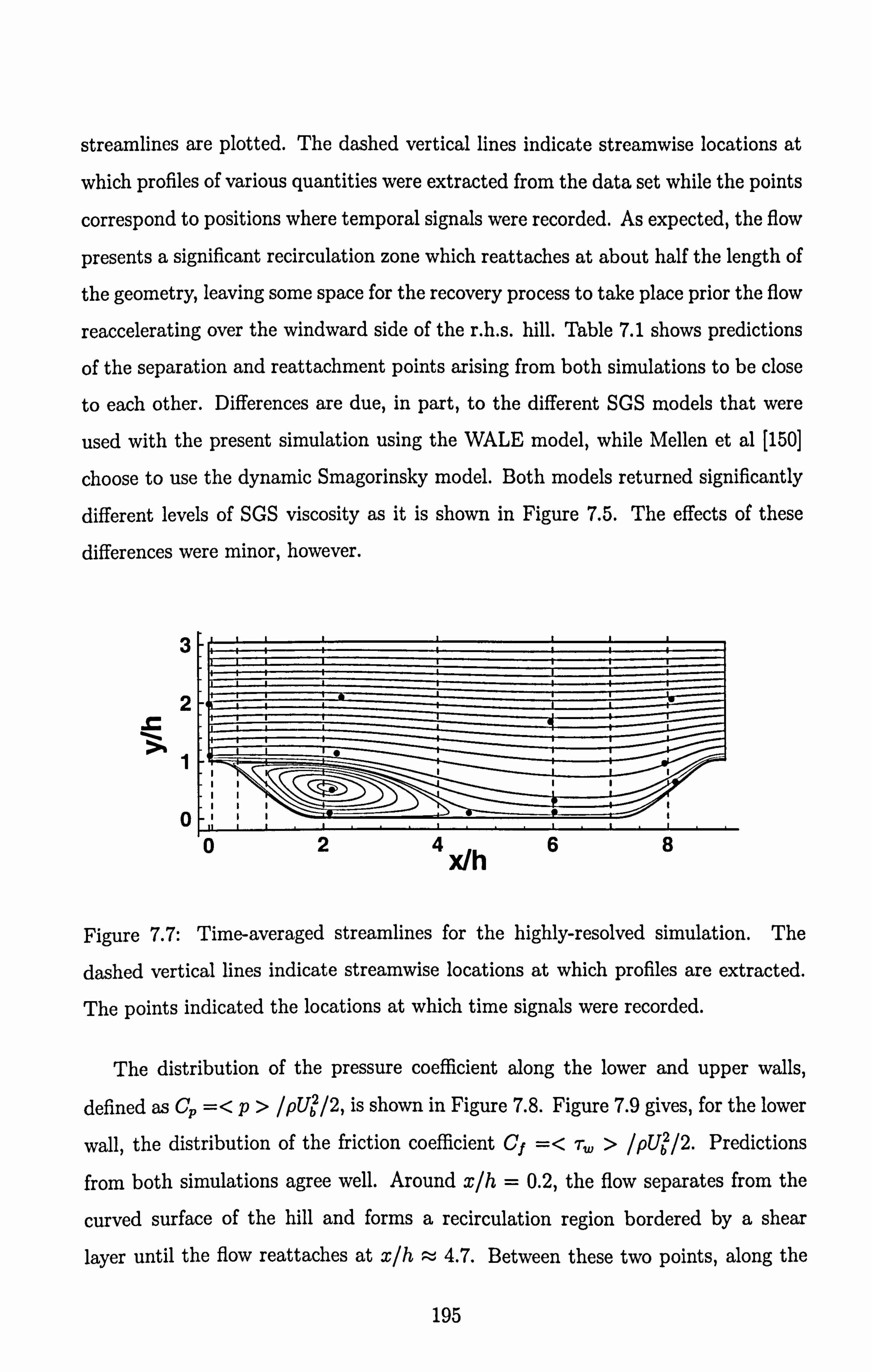
streamlines axe plotted. The dashed vertical lines indicate streamwise locations at

which profiles of various quantities were extracted from the data set while the points

correspond to positions where temporal signals were recorded. As expected, the flow

presents a significant recirculation zone which reattaches at about half the length of

the geometry, leaving some space for the recovery process to take place prior the flow

reaccelerating over the windward side of the r. h. s. hill. Table 7.1 shows predictions

of the separation and reattachment points axising from both simulations to be close

to each other. Differences are due, in part, to the different SGS models that were

used with the present simulation using the WALE model, while Mellen et al [150]

choose to use the dynamic Smagorinsky model. Both models returned significantly

different levels of SGS viscosity as it is shown in Figure 7.5. The effects of these

differences were minor, however.

3

2

0

Figure 7.7: Time-averaged streamlines for the highly-resolved simulation. The

dashed vertical lines indicate streamwise locations at which profiles are extracted.

The points indicated the locations at which time signals were recorded.

The distribution of the pressure coefficient along the lower and upper walls,

defined as Cp = /pUb2/2, is shown in Figure 7.8. Figure 7.9 gives, for the lower

wall, the distribution of the friction coefficient Cf =< -r,, > IpUb'12. Predictions

from both simulations agree well. Around x1h = 0.2, the flow separates from the

curved surface of the hill and forms a recirculation region bordered by a shear

layer until the flow reattaches at x1h ý 4-7. Between these two points, along the

195

024 x/h

lower wall, the friction coefficient CJ is negative in the reverse-flow region. In the

same region, the pressure coefficient Cp remains, first, broadly constant between the

separation point and x1h = 2.0, this position corresponds to the end of the hill slope,

then starts to rise as the outer flow expands in the channel. Along the upper wall,

at the same location, the pressure coefficient also rises, but to a lesser extent. After

reattachment, a boundary layer develops along the lower wall under the influence

of an adverse pressure gradient which extends to the next hill. The flow strongly

accelerates over this hill, resulting in a sharp rise of the friction coefficient, while

the pressure coefficient drops rapidly. In this region, the thickness of the boundary

layer also decreases from 0.2h at the end of the plane region to about 0.08h at the

hill crest. At the windward base of the hill, Mellen et al [150] noted the existence of

a small recirculation zone (the friction coefficient presents a weakly negative value

at that point), a feature not observed in the present simulation, although the dip

in friction coefficient is very similar. Above the recirculation zone, the flow velocity

remains fairly constant. Along the upper wall, the flow behaves as a flat-plate

boundary layer subject to deceleration and then, reacceleration, the latter following

reattachment.

0. c

31 - lower wal 32 - lower wall 31 - upper walill 32 - upper wall

4

x/h

Figure 7.8: Distribution of pressure coefficient Cp along the lower and upper walls

for the highly-resolved simulation.

196

0.03

0.0

cf

O. C

Case 31 Case 321

4 X/j,

Figure 7.9: Distribution of friction coefficient Cf along the lower wall for the highly-

resolved simulation.

The level of agreement between the two highly-resolved solutions is further il-

lustrated in Figures 7.10,7.11,7.14,7.17 and 7.18 which show, respectively, profiles

of mean velocity, normal and shear stresses and turbulence energy, at five diffe-

rent streamwise locations indicated by the vertical lines in Figure 7.7. Overall, the

agreement between the present simulation and the one of Mellen et al [150] is good. The velocity profiles are clearly very close, although small differences in stresses and

turbulence energy axe observed. In part, this is due to differences in the level of the

respective SGS viscosity shown in Figure 7.5. A more detailed discussion of these

results, alongside the budgets for the normal stresses, shear stress and turbulence

energy is provided in the next subsection.

The above comparisons should suffice to demonstrate the essential validity of the

claim that the highly-resolved simulation provides a secure foundation for evaluating

the accuracy of RANS model and coarse-grid LES predictions. Indeed, since the

data were generated, they have been exploited by several researchers (see Jang et

al [91], Wang et al [229] and De Langhe et al [48]). The data were also made

available to the turbulence community through the ERCOFTAC database (Case

C81 at http: //cf d. me. umist. ac. uk/ercof tac/).

197

7.3.5 Discussion of statistical properties

In what follows, profiles of mean-velocity components, turbulent stresses, turbulence

energy and budgets for the stresses and energy at the streamwise stations indicated

in Figure 7.7 are presented and discussed. The stations were chosen so as to present

the flow regions featuring particular characteristics or behavioural features. The

profiles of velocities and stresses are given over the full height of the channel from

the lower to the upper wall, while the budgets profiles are only given for the lower

portion of the flow, extending over a distance of 2h from the lower wall in which all

the physical processes of prime interest occur. To enhance clarity and facilitate the

discussion, the profiles of the stresses and contributions to the associated budgets

close to the lower wall are presented, additionally, in magnified plots. Profiles of

mean velocity, turbulent stresses and turbulence energy are included from both

simulations and, thus, compared.

The budgets arise from the various terms contributing to the transport equation for the Reynolds stresses (uý, uj) for which a complete description is given in Sec-

tion 5.4. All the terms forming Equation (5-10) were determined explicitly, except

eij which was obtained as the imbalance of the other terms. An explicit evaluation of

cij yielded approximately 50 to 70% of the value obtained from the balance, a level re-

garded as reasonable in view of the fact that the ratio of grid distance to Kolmogorov

length was of order 10. The budget for the turbulence energy (k) = 0.5(u'iu'i) (see

Equation (5.17)) follows from contracting the set of stress equations, i. e. from half

of the sum of the equations for each normal stress. In this, the pressure-strain term

should vanish, and this has been confirmed to be closely correct by summing up the

pressure-strain contributions to the normal-stress budgets.

Position x1h = 0.05

This section is located at a short distance beyond the hill crest. Profiles of velocity,

Reynolds stresses and turbulence energy at this position axe given in Figure 7.10.

Budgets, while available, are not included here because the extremely high gradients

and rates of change of the flow vaxiables very close to the wall pose uncertainties in

198

relation to the accuracy of the higher-order moments contributing to the budgets.

The boundary layer is very thin (about 0.1h) and the streamwise velocity features

a near-wall peak. Both are due to the preceding acceleration along the windward

slope of the hill. There is also a slight upward motion associated with the flow

along the steeply inclined windward hill face. The shear stress (u'v') reaches a first

minimum value in the boundary layer and then declines to virtually zero, where

the velocity component (u) reaches a maximum. Beyond this location, the velocity

gradient reverses sign, while the shear stresses does not. The lowest (ulv') value

occurs around y/h = 1.6 at a local minimum in (u), and this indicates substantial

stress-transport effects (unless 9(v)/c9x is important, which is not the case). The

velocity then rises to a second maximum toward the upper wall, and (u'v') decreases,

changing sign roughly at the location of this maximum and reaching a peak value

in the boundary layer near the upper wall. The normal stresses are remarkable primarily in so far as their respective maxima

occur at very different positions, giving rise to very high local levels of anisotropy.

(u'u') has a strong peak close to the lower wall, reflecting intense generation by

the high shear strain in the boundary layer. As expected, (wV) is lower and

(v'v'), the lowest. However, their maxima occur well outside the boundaxy layer,

suggesting a dominant history effect from upstream locations. In the boundary

layer, the anisotropy is unusually intense, with the ratio of (UV) and (v'v) reaching

a value of order 20 and indicating the approach to two-component turbulence, which

necessarily prevails close to the wall due to the wall blocking effect. The very high

near-wall level of (uV) is also due to intense streamwise fluctuations associated

with intermittently high positive and negative velocities that arise as the separation

point moves at a high rate over a substantial proportion of the surface around the

hill crest. The high level of (wV), at around y/h = 1.5, is linked, as shown in

Subsection 7.3-7, to an amplification of this component upstream of the hill crest

by the action of splatting and the subsequent transport of this component towards

the crest region. Away from the lower wall, in the weak and zero-shear regions, the

normal stresses and the turbulence energy axe maintained at fairly high levels, again

indicating intense turbulence transport from the highly disturbed upstream region.

199

3

y/h 2

I

y/h 2

1.5

1

yd

x/h = 0.05

................ L .......

31 - [U b 32 - [U b 31 - <V>/Ub

32 - <V>[Ub

Y/f 1

1

x/h = 0.05

31- /U b 32 - /Ub

31- <v>'Ub

32 - <V>/Ub

, Ll 0 / u b'<V>/Vb

x/h = 0.05 . ... ...... 1.2

0-0 31 - <u'u'>/U,, '

-- 32 - <u'u'>/U. '

31 - <v'v'>/U,, '

32 - <v'v'>/U,, ' y/h 31 - <u'v'>/U, 2

32 - <u'v'>/U. 21

/U b <v>/V b

x/h 0.05

: 31 - <u'u'>/ub 2

2 <u'u'> b

2 <V V>b

2 <V, v >b

31 - <U'V*>'Ub

32 - <u'v'>/LJ,

0- 0.05 0.1 0 0.05 0.1 . 05 0.05 ...

/Ub 2f

<V 9v' >/u b29 <U, vt>/Ej b2

<u'u' >fLjb 2'

<V'V' >lu b2 '<U'Vt >/u b2

x/h = 0.05 x/h = 0.05 1.2

y/h - 0--o 31 - k/Ub2

. ..... 32 - k/Ub2

2 31 - <w'w'>/U,, 2 rb

2 32. <W, W, >/Ij b2

-0.05 0 0.05 0.1 k/ z9 <W

9w' >/U VU ' <WS >[U Ub b bl' W' bk

Figure 7.10: Velocity, normal and sheax stresses and turbulence energy profiles at

x1h = 0.05 for the highly resolved simulation.

200

Position x1h = 2.0

This section, located in the middle of the recirculation region, is especially inter-

esting because it combines three interacting layers: a highly disturbed reverse flow,

combining a boundary layer and a mixing layer formed from the fluid originating from the separated shear layer above it, and the upper free shear layer itself, which

separates from the hill crest. Profiles pertaining to this section are included in

Figures 7.11,7.12 and 7.13, the last two figures containing the budgets.

The velocity profiles are unremarkable and show the expected reverse flow in the

lower portion, the shear layer above it and the boundary layer at the upper wall,

with the slight glitch in (u) originating from the application of the power-law-based

wall law. This is confirmed by noting that, for the (u) profiles presented in Figure 7.6

where a wall-resolved mesh was also used on the upper side of the channel, this glitch

is not present. (v) is insignificant, as this section is effectively in the streamwise

centre of the recirculation bubble. The Reynolds stresses in the shear layer conform

to expectations: (ulv') is negative, and all stresses reach a peak in the location of

maximum shear strain. Of the normal stresses, (u'u') is the highest, while both (v'v')

and (wV) axe lower and of very similar shape and magnitude, indicating that, in

the absence of significant wall influences, the pressure-strain process is unbiased in

respect of these two stresses. The anisotropy is significant, but not intense, with the

ratio (ulu)/ (v'v') of order 1.3 and the ratio (U'V')/k, about 0.3.

In the reverse-flow layer, 0< y/h < 0.5, the most interesting feature, returned by both simulations, is the distinctive rise of (wV), relative to the other two normal

stresses, leading to a virtual equality of (wV) and (u'u) close to the wall. A similar

behaviour will be shown later to occur at x1h = 6, and this is claimed to be due

to splatting effects around the reattachment region, which are then carried over

to neighbouring locations by transport. Splatting will also be seen later to be an

exceptionally influential process in the accelerating-flow portion above the windward

face of the r. h. s. hill. In contrast, (v'v') declines steadily as the wall is approached,

a behaviour anticipated due to wall blocking. A feature not foreseen is the reversal

in the streamwise-velocity gradient close to the lower wall, at y/h = 0.1, which is

201

not accompanied by a corresponding reversal in the shear stress, expected on the

basis of the eddy-viscosity concept. It follows that the turbulent shear stress cannot

support the negative wall shear stress in this region which must exist due to the

reverse motion, as seen in Figure 7.9 (note that correlation (u'v') and the shear stress (, r) have opposite signs). Hence, the viscous stress must dominate in this region. As

will be demonstrated later upon a consideration of the budgets, the processes in the

near-wall layer under consideration differ drastically from those in a conventional boundary layer. For example, although there is a sign reversal in the production of

the shear stress, in line with the sign reversal in the shear strain, other contributions

to the shear-stress balance conspire to maintain (ulv') at a positive level. Moreover,

the elevation of the turbulence energy and the wall-parallel normal stresses, due to a

combination of production, splatting-related phenomena and convective transport,

leads to very high levels of near-wall anisotropy and ratio (u'v)/k, even outside the

buffer layer, the position of which corresponds to y/h = 0.05 at x1h = 2, i. e. well

below the position of minimum reverse velocity.

The budgets of all stresses and turbulence energy are given in Figures 7.12

and 7.13. They cover only the lower region, roughly to the upper edge of the

separated shear layer, as this region is of primary interest. The shear-stress budget

shows the usual behaviour in the separated shear layer of a near-balance between

pressure-strain and production, with the remaining terms being subordinate. As the

wall is approached, but outside the viscous sublayer (y/h > 0.05), the influence of

production diminishes, the pressure-strain term becomes negative and is increasingly

balanced by the positive pressure diffusion. As the position of peak negative stream-

wise velocity is traversed, the production reverses sign, but remains low relative to

pressure diffusion, a condition that prevents the shear stress from changing sign,

as noted earlier. As the viscous sublayer is entered, the production reaches a weak

maximum, but this is insufficient to affect the rapidly declining shear stress, which

thus remains positive. Within the viscous sublayer, pressure strain rises strongly

together with a corresponding drop in pressure diffusion, with both essentially ba-

lancing each other. At the wall itself, neither is constrained to vanish, because one

constituent in both involves the correlation of pressure fluctuation and wall-normal

202

gradient of the streamwise-velocity fluctuation, neither of which asymptotes to zero

at the wall. The turbulence-energy budget shows that production is highest in the separated

shear layer, thus causing a maximum in (k). The ratio of production to dissipation

is of the order of 2 where the production reaches a maximum. Turbulent diffusion

accounts for most of this imbalance, transporting energy from the production re-

gion to the reverse-flow region and to the edge of the shear layer. This explains the elevated values of (k) in the outer region despite the low velocity gradient and hence low production therein. Convection is also significant at the edges of the

shear layer. At the outer edge, it removes energy to regions further downstream,

while, in the reverse-flow region energy, is gained through convective transport from

the reattachment region. Above the boundary layer, production is low in the re-

verse flow region, with positive convection and turbulence transport balanced by

dissipation and pressure diffusion. Hence, the characteristics of this region are very

different from those in a conventional mixing layer. As is the case with shear-stress

production, that of turbulence energy also rises to a weak maximum very close to

the wall, but its contribution to the balance is generally small. Within the viscous

sublayer, pressure diffusion and viscous diffusion become the dominant gain terms,

while dissipation becomes the dominant sink. As expected, the balance asymptotes

to viscous diffusion being cancelled by dissipation, with all other terms vanishing at

the wall. The budget for (u'u) shaxes a number of features with the budget for (k). The

productions give similar profiles, with that of (u'u') having a level about twice that

of (k), since the production of (wV) is zero, while that of (v'v') is negligible. On the

other hand, the dissipation levels of all three normal stresses in the shear layer are

similar, consistent with the concept of isotropy in the smallest scales. The imbalance

between production and dissipation is compensated mainly by the pressure-strain

term, which extracts energy from the (uV) component and transfers this to the

other normal stresses, the balance of which thus feature positive pressure-strain

contributions. In the near-wall region, outside the viscous sublayer, the budget of (w'w') is dominated by positive convection and negative dissipation and pressure

203

strain. The positive convection reflects the transport of high levels of (wV) from

the impingement zone in which splatting is an important mechanism. As shown

earlier, the consequence is a sharp increase in (wV), which reaches a level very

close to that of (uV). It is this process that causes a reversal in the pressure-strain

contribution, with both (u'u') and (wV) transferring energy to Wv'). As the wall is

approached, within the thin boundaxy layer, (v'v') has to decay rapidly, and this is

effected by a reversal in the pressure strain, which now transfers energy from (v'v')

to (u'u') and (wV). Positive convective transport remains an important contributor

to (wV), keeping this stress relatively high in the boundary layer. As the viscous

sublayer is traversed, viscous diffusion tends to balance dissipation, as is the case

with (k), while in the case of (v'v'), in which viscous diffusion is necessarily negligible

and dissipation approaches zero as turbulence, including the smallest scales, tends

toward a two-component state, the balance is dominated by pressure strain, which

has to diminish (v'v') at a rate proportional to y, and pressure diffusion.

204

x/h = 2.0

Y/11

*--o3l - [U, b

..... 32 - [Ub

---m3l - <V>[Ub,

. --. 32 - <V>/Ub,

ol 0.5

y/h 0.1

C /U b

<V>/ vb

x/h 2.0 3 *--o 31 - <u'u'>/Ub2 0.2

.... 32 - <u'u'>/U,, '

31 - <v' v'>/U 2

b . .... 32 - <v'v'>/U,

2

2 +--o 31 - <U'V'>/Ub

2 Y/11

y/h 32 - <u'v'>/U. 2 0.1

0 0.1 0

-0.05 0 0.05 <u'u'>/U

2219

b <V'V'>'Ub <U'V'

b

x/h = 2.0

9--o 31 - <U'U'>'Ub 2

.. -- 32 - <U'U'>/Ub 2

+---o 31 - <W'W'>'Ub 2

-- 32 - <w'w'>/U,, 2

y/h 0.

-0.05 0.1

Y/11

x/h = 2.0

*---* 31- [U b

..... 32 - /U b

. -, m 31- <v>[U b

-32- <V>lu b

. *-::: ýý I. D. 2 0 "ýU>lu b <V: >Nb

x/h 2.0 9---o 31 - <u'u'>/Uý

.... 32 - <u'u' >luý 31 - <v'v'>/U b 32 - <V'V'>'Ub

31 - <U'V'>/Ub

32 - <U'V'>/Ub

-0 , 05 0 0.05 0.1 129,22 lu b, <V V >/u b '<U'V' >lu b

x/h = 2.0

0-, 0 31 - <u'u'>IU, '

.... 32 - <u'u'>IU,

-31-<w'w'>/Ull 2 32 - <w'w'>IU�

.1 kfUb A, <W'W'>/Ub A k/Ub A '<W'W'>/Ub

4

Figure 7.11: Velocity, normal and shear stresses and turbulence energy profiles at


205

< U'U' > *--* Viscous diffusion < U'U' > 9-9 Viscous diffusion @--a Turbulent transport *--a Turbulent transport

0.1 1 Dissipation Dissipation Production A---& Production

-V Pressure Strain -0 Pres um Strain v--v Pressure diffusion --w Pms: um diffusion

0.05

Convection 0.01 +----+ Convection

...... .......

07 r ......

0

CA ID -0.01 (A

.9 -0.05

* 0.40 -

. 0.02 '

Ii. 200.05 0.1 0.15 0. 0 0.5 1 1.5

Y/h Y/11

< V'V' > Viscous d Iffusion < V'V' > 0---* Viscous diffusion Turbulent=po. mi-m Turbulent tramport Dissipation *. --o Dissipation Production Production

cls-0 Pressure Strain 0 -V Pressure Strain v----v Pressure diffusion 0.02 v ---v Pressure diffusion 0.02 0, Convection Convection

/0 0.01 0 0.01

Ir 00

(1) 7 . 0.01 P

i Is.

-0.02 . 0.02 /

L.... -0.03 0 0.5 1 1.5 0 0.05 0.1 0.15 0.

y/h y/h

< W'W' > Viscous diffusion < W'W' > 0-0 Viscous diffusion Turbulent transport *--a Turbulent transport Dissipation

... 9--o Dissipation &--a Production A-& Production

0.02 00 --0 Pressure Strain G-V Pressure Strain

+ -:: =diffusion r r- 0.01 w--w Pressure diffusion

on Convection

0 0.01 0% 'L-ý 0 a*IN0

. 10ý .-.

I-Zý=0.. -- 0

0 -0.01 - +

-0.01 Ot

y/h 1.5 0

y/h

Figure 7.12: Budgets of the normal stresses at x1h = 2.0 for the highly resolved

simulation. The left plots show the principal part of the channel and the right zoom

around the bottom wall.

206

C

0.05

0-4

y/h

UoV9 >0 -- * Viscous diffusion *---o Turbulent transport

Dissipation Production

a --0 Pms ure Strain --v Pms: ure diffusion

-0.05

0.5

y/h

<k>

. r. ci

,A 2

J . 0.02

0-0 Viscous diffusion E. -S Midiulent tmspon *.. -. 4 Dissipation &-a Pwduction ý-v Pmuure diffusion +--+ Convwtion

. -.. -. -- . -.. --.

. -. "-". ---. -. --. ----. 4

y/h

I(

IS -0.05

U'v' > 0-0 Viscous diffusion a.. -a Turbulent transport *---a Dissipation &---A Production 0---V Pressure Strain v -v Pressure diff-im

0.1 0.15 y/h

Figure 7.13: Budgets of the shear stress and turbulence energy at x1h = 2.0 for the

highly resolved simulation. The left plots show the principal paxt of the channel and

the right zoom around the bottom wall.

207

Position x1h = 6.0

This position is within the post-reattachment region, half way between reattachment

and the foot of the next hill. The flow here consists of a boundary layer developing

from the reattachment point with, above it, a wake originating from the separated

shear layer further upstream. It is thus characterised by flow components with

very different scales and history, which interact to form a flow recovering towaxds a fully-developed channel flow. It is well known that most statistical closures do not

represent this recovery process well. Hence, the features discussed in this section

are of particular interest to modellers.

Profiles of velocity and second moments axe shown in Figure 7.14. The boundary

layer, of thickness y ý- 0.2h, is bordered by a region of nearly constant velocity

gradient, reflecting an ongoing recovery of the reattached shear layer. As seen from

Figure 7.8, the flow develops against an adverse pressure gradient, caused by the

outer flow decelerating mildly as fluid is being transported downward to fill the

wake. The boundary layer at the upper wall is much thicker, of order y=0.6h, and

its structure is expected to conform to that of other boundary layers subjected to a

mild adverse pressure gradient.

Although the flow in this section is drastically different from that at x= 2h,

the turbulence field is characterised by qualitatively similar features, although the

intensity of turbulence is now much reduced as the strain diminishes and the flow

tends to approach a state of equilibrium. Thus, the stresses and turbulence energy

reach maxima within the high-strain region of the mixing layer, the ratio (u'v')/(k)

being close to 0.3, and (u'u') exceeding (wV) by a factor of approximately 1.4.

Some points of difference, pertaining to the flow above the boundary layer include a

more distinctive separation between (the lower) (vV) and (the higher) (wV), with

the ratio being typically 1.1 to 1.2, and the considerably broader region in which the

stresses and turbulence energy are elevated, as a consequence of the positive shear

strain and thus higher turbulence production occupying a correspondingly wider

portion of the flow. Thus, with the boundary layer at the lower wall set aside, the

distributions of second moments do not contain features not observed in other shear

208

layers. In the boundary layer, the most distinctive feature, also observed previously

at x1h = 2, is a maxked elevation of (wV), and this is again attributed to the

splatting effect around reattachment, which causes large pressure fluctuations, in

combination with convective transport from the reattachment region toward the location being considered. (u'u') is observed to develop a local maximum in the

boundaxy layer, but this is mainly due to production associated with the sheax strain in the thickening boundary layer, although splatting may here too be a contributory

process. The simultaneous elevation of (uu') and (wV) in the boundary layer

is then responsible for the high level of (k) at around y/h = 0.15. As the shear

stress remains low, for reasons clarified below by reference to the budgets, the ratio I (ulv') I/ (k) reaches very high values, of order 10, well outside the semi-viscous near-

wall region. Figures 7.15 and 7.16 show the budgets for this location. In the shear-layer re-

gion, the budget for (u'v') is similar to that at x1h = 2.0. However, the magnitude

of the terms is now considerably smaller, because the velocity gradient and thus

production axe lower. In contrast to x1h = 2.0, turbulent diffusion plays a more important role in balancing production in combination with the more dominant

pressure-strain process. The former transports shear stress away from the region

where it is produced toward the wall and the edge of the sheared layer. At this

station, production and pressure strain do not change sign, as expected for positive

and substantial shear straining across the lower flow portion. The latter develops

a near-wall minimum in a region in which pressure diffusion rises and balances the

negative turbulence transport and production. Thus, the tendency for production

to elevate the magnitude of the shear stress is counteracted by pressure-related tur-

bulence transport away from the boundary layer, keeping the sheax stress relatively low and resulting in the previously observed high levels in the ratio I (uV) I/ (k). As

the wall is approached, through the viscous sublayer, the budget is dictated by a ba-

lance between very high pressure-strain and pressure-diffusion contributions. This is

a rather surprising observation, but not an unrealistic one, as pressure fluctuations

are high in this region and evidently correlate with Ou'/Oy, which is non-zero at the

wall.

209

The budget for (k) shows a significant level of production in the broad shear-layer

region, but this is much lower than at x1h = 2.0. Also, in contrast to x1h = 2.0, it

is not much larger than dissipation, the ratio being about 1.2, so that turbulence is

here closer to local equilibrium. Alongside dissipation, turbulent transport plays an important role in this layer, transporting turbulence energy away from the region

of production toward the wall and the outer region of the sheared flow. Convection

too makes an important contribution by transporting high levels of energy from

upstream regions, (see the budget for x1h = 2.0) to the section being considered and hindering the approach toward turbulence equilibrium. In the boundary layer, the

balance is dictated by turbulent transport and dissipation, the former transporting

energy from the outer shear layer into the boundary layer. This interaction is very different from that in an ordinary boundary layer bordering a free stream, in which

the balance is mainly between production and dissipation. As the wall is approached,

pressure diffusion is the main opponent of dissipation. As will be shown below, this

gain is attained through pressure fluctuations, probably elevated by splatting at the

impingement region, correlated with v-fluctuations. At the wall itself, all terms but

viscous diffusion and dissipation tend to vanish, as required by kinematic constraints.

As in the budget for (k), the production of (uu') is now much lower than at

x1h = 2.0 and so is the pressure-strain term, which is here too the largest sink in

the sheax-layer region. Also, as in the case of (k), convection from upstream regions

increases (iýu') and turbulent diffusion decreases the stress by lateral transport

away from the central portion of the shear layer. Over most of the boundary layer,

dissipation is again balanced mainly by turbulent diffusion transporting energy from

the shear layer towards the wall. As the wall is approached, pressure-strain rises

and, aided by (relatively weak) production, balances dissipation. The presence of

positive pressure-strain reflects the need to drain energy from (v'v') as turbulence

approaches a two-component state by wall-blocking, and this energy is transferred

to both (u'u') and (wV). However, the bulk of the pressure-strain-effected transfer

will be seen to be to (wV), and this is probably associated with splatting. At

the wall, there is the usual balance between dissipation and viscous diffusion, also

observed in the budgets for (k) and (wV).

210

The budget for (v'v') in the shear-layer region is dominated by dissipation and

turbulent transport balanced mainly by a positive pressure-strain contribution,

which is derived from (u'u'). The most interesting processes pertain to the near-wall

region. Here, positive turbulence transport balances the negative pressure-strain

contribution, the latter reflecting the process that is required to diminish this com-

ponent through wall blocking. As the wall is approached, the balance is increasingly

dominated by negative pressure-strain and positive pressure diffusion. Both reflect the high level of pressure fluctuations and the interaction of these with velocity and

strain perturbations. It is the high level of pressure diffusion in the budget of (vv')

which balances the dissipation of (k). Importantly, the near-wall dissipation of (v'v')

is low and quickly diminishes as the wall is approached, reflecting the trend toward

a two-component state of the small-scale fluctuations contributing to dissipation.

Hence, the near-wall dissipation is highly anisotropic. The most noteworthy features in the budget of (wV) axe again to be found in

the near-wall region. Production is necessarily absent, and the near-wall balance is

dominated by negative dissipation and a high positive pressure-strain contribution. The strongly preferential transfer of energy from (v'v') to (wV) is important to

highlight, and this is taken to signify the contribution of splatting associated with

reattachment, a process that extends over a substantial proportion of the horizon-

tal channel wall. As a consequence of this elevation in (wV), negative turbulent

diffusion arises, transporting (W/W') away toward the wall and to the outer paxt of

the boundary layer in which all normal stresses feature positive turbulent transport

supplying the boundary layer with energy components from the outer shear layer.

211

x/h = 6.0 3

y/h

C

Y/11

y/h

.......... 31 - /U b 32 - /Ub

. --o3l - <V>[Ub

--. 32 - <v>/U b

0.2

y/h 0.1

C /U b' <v>/V b

x/h 6.0 0-0 31 - <u'u'>/U b20.2

.... 32 - <u'u' >/Ub 2

a--a 31 - <v'v' >'Ub2

2 32 - <v'v' >/Ub

ss 31 - <u'v'>/Ljb 2

y/h 32 - <u'v'>AJ,

2 0.1

-0.05 2020; 05

2 0.1

<U'U' >/u b '<V'V' >tu b '/Ub

x/h = 6.0 0-0 31 - k/U�'

32 - k/Ub2 e--* 31 - <w'w'--ý2

-- 32 - <w'w'>/U�'

Kl.

1 Ylob.

x/h = 6.0

31- /Ub

32 - /Ub

31 - <V>[Ub

32 - <v>/U bl

0.1 0.2 'Ub'<V>/Vb

x/h = 6.0

I, 1,,: - 31 - <u'u';; T,, 2 .... 32 - <u'u'>[U,, 2

31 - <v'v'>/U., 2

>, U"2 32 - <v'v'

31 - <u'v' >/U"l 32 - <U'Y' >/U"l

-0.05 0 005 0.1 222 <u'u' >/Ub '<V'V >/Ub , /ljb

x/h = 6.0

. 0.05 0 0.05 0.1 -0.05 0 0.1 k/Ub 2,

<W'W' b2 k/U b 2,

<W ,w' >/U b 20



31 - k/U, 2

32 - klUb2

31 - <w'w' >'Ub2 2

32 - <w'w'>/U b

212

< U'U' > a--* Viscous dtffusion w-at Turbulent transport *--* Dissipation s-a Production co-V Pressure Strain 0.02

002'- v--v Pressure dtfftision m1 Conwction

r. Iq 0.01

0 L

Li I....

... Z.

---; -i=- , cn

-0.01

.9 . 0.02 -0.02

0 0.5 1 1.5 2 -0.03

y/h

y/h

< W'W' > Visý d ffim Turbulent=

*---4 Dissipation &-& Prodwti a 0 --0 Pressure Strain

002 v -T Pressure diffus! +--+ Conýticn

C: - .; ý i 0

4 Z., o., e-t -00- -, 0

0.5 1 1.5

0.02

0.01

10 wl

-0.01

0.02

0

0

U'U' > 9-e Viscous diffusurn m-a Turbulent transpoi


Q, --O Pressure Stmin v --v Pressure diffusion aa Conwction

y/h

<V'V'> 0--oViscousdif @--a Turbulent t *. -*Dissipation d-L Production 4, ----0 Pressure Sti v-v Pressure dil

" ---. ---. -. --. __-�_. _____. _..

�__0-

- __0

0.02

Y/11

<W'W'> 0---, e Viscous diffusion m---a Turbulent transport

...... Dissipation Production

0- 0 Pressure Strain ý-. v Prmsum diffusion

Convmtion

I

y/h y/h


simulation. The left plots show the principal part of the channel and the right zoom


213

(A

. 0.02

0.02 cl

0

-0.02

is-is Viscous, diffusion &--e Viscous diffusion <k> is-a Turbulent traitsport <k> m--. e Turbulent trarispom

Dissipation Dissipation ---r- Production

ffusion ........... Production Pressure diffusion Pressure diffusion Convection 0.02 Convection

0.01

is-

0 ....... ....... ...

in A -0.01 -

. 0.02-

L.... L.... 4 111 ... 1 1.5 2 -0.03 - 0. 0 0.02 . 04 OM 0.08 0.1

y/h y/h

< U'V' > :. -0 Viscous diffusion < U'V' > Viscous diffusion -a Turbulent transpo, m--a Turbulent transport

Dissipation 0.2,0 ... *, -, * Dissipation Production A-L Producti n

--0 Pma um Strain O-V Pres un: Strain w-9 Pres: ure diffusion v-w Pres: ure diffusion 4--+ Convection +-+ Convection

0*0 . 040. r. 0.1 - C9

0

-0.1

L....... 51 105 -0.2 0 0.02 0.04 0.06 0.08

L

YAI YAI


highly resolved simulation. The left plots show the principal part of the channel and


214

Position x1h = 8.0

This position lies in the windward portion of the hill where the flow is subjected to strong acceleration. Profiles of mean velocity and Reynolds stress components in x, y-coordinates are given for the complete cross-section in Figure 7.17. Near

the lower wall, which is inclined at an angle of 38* at x1h =8 from the horizontal

axis, they do not lend themselves to a physically transparent interpretation and discussion, since u and v are not tangential and normal to the wall, respectively. Hence, in the near-wall region, up to a wall distance of about 0.2h, profiles of the

wall tangential (t) and normal (n) components are also provided in Figures 7.18,

albeit not along a line normal to the wall but along a vertical line.

Rom Figure 7.17, it can be seen that the overall behaviour of the u-velocity is

similar to that at x1h = 6, but due to the acceleration, the velocity is larger near the

wall and the boundary layer is thinner (only about 0.05h). Except near the lower

wall, the distribution of Reynolds stresses over the full channel height, as plotted

in Figure 7.17, is also very similar to x1h = 6. However, close to the wall, the

stresses and the corresponding budgets present some exceptional features not seen

at x1h =6 which merit closer consideration. As is seen from Figures 7.17 and 7.18,

one such feature is an extremely high level of (wV) relative to the (UV) and (vV)

in the (x, y) plane. This statement retains its validity whether made by reference to

the (x, y) or the (t, n) decomposition. The main difference between the two is that

the wall-oriented decomposition highlights the very rapid decay of v-fluctuations, as

is expected to occur due to wall blocking. While these stresses in the (x, y) plane depend on the orientation of the frame of reference, their sum does not, and it is

advantageous therefore to consider the distribution of (u'u' + vv')/2, included in

Figure 7.17, and later also the budget for this quantity rather than the budgets for

the individual components (u'u') and (v'v'). For that same reason, the budget for

the shear stress is not presented here. As seen, (wV) is also extremely high relative

to this sum. Moreover, (k) shows a distinct near-wall peak, which is evidently a

consequence of the very high near-wall level of (wV).

215

x/h = 8.0

Y/11

3-1 *'--'-- ............. 31- [U b

..... 32 - [Ub

w--w3l - <V>[Ub 2\

I- -- 32 - <v>/TJ b,

1ý

x/h 8.0

/Ub

32 - [U 0.6- b y/h -

31 - <v>[Ub -32- <V>/Ub

/U b' <V>/U b

x/h = 8.0 3- 1.,,.. 0--031-<u'u'>/Uý. 2

.... 32 - -cu'u'>/U., 2

a-im 31 - <V'V'>/Ub 2 0.

- 32 - <v'v'>/U� y/h

y/h2 4--0 31 - <u'v'>/U. - 32 - <u'v'>AJ,

31 - <u'u'+v'v'>12 32 - <u'u'+v'v'>12

0.

-0.05 0 0.05 0.1 222

<u'u'>/U, 2.

<V V, >/Ub , /Ub 0,5 <U'U'+V'V'>/Ub

xi% = 8.0

Y/h o-o 31 - k/Ub 2

.... 32 - k/Ub2

31 - <w' WWU b2 >ju b2

-0.05 -0.05 0.

yI

I

0.2 0.4 Ub <V>/Ub

x/h 8.0 31 - <u'u';

ý. '

>, Ub2 32 - <u'u' 2 31 - <v'v'>/U.

32 - ýcv'v'>/U. 2

31 - <u'v'>/U. '

32 - <u'v' >/Ub2

-005 0 0.05 0. 229'2 <U; U'>'Ub , <V, v, >/u

b, /u b

x/h = 8.0

0.6- o-o 31 - VU,

Ih 2 .... 32 - klUb

31 - <w'w'>/Ut, 2

32 - <W'W'>'Ub2i

0.5-

-0.05 - 15 0.05 0. I k'Ub"' <W'W'>/Ub& k/Ub'6"'ýW'W'>'Ub"



216

x/h = 8.0 x/h = 8.0

0.65. ,II*. -........ ;i,, ý *-* 31 - <%'u. '>/Uý

*--e3l- 'Ub" n>/Ub A"

..... 32 - /u - <VI'Vt'>/Ub2 0.6 nb0.6- 2 32 - <vt'v, '>/Ub

y/h <Vt>/Ub

Y/11 <U., Vt. >/Ub2 >/u 31 - 0.55F

32 - <v tb P 32 - <tl. 'Vt'>/Ub2

0.5

-------

0.2 0.4 -0.05 220.05 2 0.1

/U bI <v

t >/U b <Un'Un'>'Ub ' <Vt'Vt'>/Ub ' <Un'Vt'>/Tjb


x1h = 8.0 for the highly resolved simulation. These profiles are converted into the

wall normal system of coordinates at this particular location.

This extreme behaviour is not observed in other locations although, at x1h =7 (not shown here), (wV) was already found to exceed (u'u' + v'v') /2 very near the

wall, indicating that the flow is about to undergo some drastic modification further

downstream. At this location, the lower wall is still horizontal although very close

to the foot of the hill.

In order to investigate the anomalous behaviour of the w-fluctuations from a

statistical point of view, the focus is now set on the turbulence-energy budgets for

x1h =7 and x1h =8 presented in Figures 7.20 and 7.21, respectively. It must be

noted that the location x1h =7 is very close to the foot of the hill with the lower wall

still horizontal. While the budgets at both locations are qualitatively similar, they

present significant quantitative differences. In both cases, dissipation is balanced,

substantially, by viscous diffusion close to the wall. A significant difference between

the budgets lies in the substantially higher contribution of pressure diffusion to the

budget at x1h = 8, which is balanced by increased dissipation and viscous diffusion.

Figure 7.21 shows the budgets for (wV) and (u'u'+ v'v') at x1h = 8. The com-

parison leads to the conclusion that the increase in (w'w') is due to energy being

extracted from the latter components and fed to (w'w') by pressure-strain interac-

tion. This is curious as (w'w') is already higher than (u'u'+ vV). This observation,

217

thus, contradicts the established concept of pressure-strain interaction acting to

isotropize the Reynolds-normal stresses. Hence, models based on this concept must fail here. Importantly, this mode of transfer, albeit much less pronounced, is also

observed at x1h = 7. It may therefore be claimed that this process is physically

significant, unless the spanwise constraint, noted above in relation to the spanwise length scale, introduces some drastic limitations to the flow.

Reference to the budget for (wV) shows production and pressure diffusion to

be zero, as is required by physical constraints. As noted already, pressure-strain is a

major source of gain for (wV). Another is viscous diffusion, the high level of which

is consistent with the requirement that viscous turbulence-energy diffusion should

balance dissipation at the wall. Away from the wall, viscous diffusion reverses and

becomes negative, due to the reversal of the gradient of (wV). This and turbulence

transport largely balance the pressure-strain term.

The loss of (u'u' + vV) by the action of pressure-strain interaction, shown in

Figure 7.21, has already been noted. This loss is seen to be largely compensated by

pressure diffusion, except very close to the wall, where the balance is increasingly

dominated by dissipation and viscous diffusion, as it does in the case of (k). Thus,

here, more than in other sections through the flow, the message that is emerging

is that the split of the pressure-fluctuation-containing term into pressure-strain and

pressure diffusion is somewhat synthetic and not necessarily a good basis for con-

structing closures at second-moment level. A similar mode of compensation is also

observed at x1h = 7, although the magnitude of the contributions is significantly

lower. It is interesting to observe here that the budgets for (UV) and (vV), sepa-

rately, at x1h =8 display extremely large and opposite levels of pressure diffusion

and pressure-strain, rendering other contributions to the budget almost insignificant.

This is quite different to the budgets of these two stresses at x1h =6 and x1h = 7,

but this difference is due to the Caxtesian decomposition relative to the inclined wall

at this location. Hence, it is difficult to provide insightful interpretations for these

stresses individually, and this is the reason for focusing on their sum in the above discussion.

At this stage, it seems hard to provide an unambigous proof about the precise

218

mechanisms responsible for the anisotropization of the Reynolds stresses at the

bottom wall and the windward face of the hill. Apart from the present statistical

analysis, a detailed analysis of instantaneous structures has been performed and is

reported in Subsection 7.3.7. All information available points to a dominance of

a splatting effect. This is further supported by results from Perot and Moin [171]

who investigated near-wall flows with DNS. Their analysis of turbulent budgets

near a solid wall without mean flow also features an anisotropization in the budget

of the tangential Reynolds stress via the pressure-strain term. To some extent,

the present interpretation is also supported by results of simulations of reattaching backward-facing-step flows (Le and Moin [117]) which also feature large spanwise

stress levels, exceeding the streamwise stress. In the present case, the effect may have been accentuated by the high streamwise velocity in the acceleration region

along the windwaxd face of the hill.

219

< U, U, > is --, * Viscous diffusion < U, U, >9 --. * Viscous diffusion m--a Turbulent tittimport *-a Turbulent transport

0.02 Dissipation 0.02 *-. * Dissipation Production &---a Production

0 -V Pressure Strain 40-0 Pressure Strain w ---w Pressure diffusion v. ---v Pressure diffusion

Convection + Convection r. 0.01 - 0 0.01

AL

. ........... ............ .. + ....... . ... 40 :-. 0 ---+ --ýq =-. 9 ---- * -'-'* . -

.9 -0.01 -0.01-

L- L -0.02

ý.................. 002 0. 0 0.5 1.5 04 0.06 0.08 0.1

Y/h Y/h

< VY > Viscous diffusion < VY > Viscous diffusion Turbulent transport mi-e Turbulent transport

", -r- a. Dissipation 0.015 ...... Dissipation - Production Producti n 0-0 Pressure Strain 0, ---0 Pressure Strain w. -v Pressure diffusion 0.01 w -. -. v Pressure diffusion

0.01 4--+ Convection *-+Convection

0.005

I* ; *_, t.

--0 5"U. --7 - -* z

: 7: 1: 1 ,...... . ......... . In-0.005

-0.01 -0.01

-0.015 0 0.5 1 .5200.02 0.04 0.06 0.08 0.1

Y/h Y/11

< W, W, > Viacom diffusion < W, W, >a --e Viscous diffusion a Turbulent transport @. -a Turbulent tninsport

0.02 1 Dissipation 0.02 *. -* Dissipation

&--a Production A, --A Production 0 --0 Pressure Strain *--0 Pressure Strain

? Pressure diffusion w-w Pressure diffusion I+ Convection -., + Convection

0.01 '0 0 0.01-

04" 0-0 0- 40 -0- 0 00

-0-9 1

0 Cot Cn

.9 -0.01 -0.01 -

4). 020 ---- -OL ---, 'I ........ . 0.0201 1.5 0.02 0.04 0.06 0.08 0.1

Y/h Y/h


simulation. The left plots show the principal paxt of the channel and the right zoom


220

Viscous diffusion

<k> Turbulent transport Dissipation

A-6 Production T--v Pressure diffusion

0.02 +-+ Convection

0.01

. 41z:

-0.01 11

-0.02

0 0.5 1 1.5 2

0.1

0.05

10

-0.05

"01

Y/11

UY > Viscous diffusion Turbulent transpoi Dissipation Producti Pressure Stmin

T--T Pressure diffusion 4--+ Convection

0.

y/h

y/h

< U'V' >* -0 Viscous diffusion w-m Turbulent transport a. - * Dissipation A-6 Production 0-0 Pressure Strain w-w Pressure diffusion +-+ Convection

Y/11


highly resolved simulation. The left plots show the principal part of the channel and


221

u'u' + v'v' >/2

0.05

C4 0

0

. 0.05

0.02

I W0

-0.02

w. - is Viscous diffusion im--m Turbulent transport


-V Pressure Stmin -- v Pressum diffusion

i+---+, Convection

Gn

< u'u' + v'v' >2 0---* Viscous diffusion *.. -a Turbulent transpoi

Dissipation Producti n

070 Pmuum Simla v ---v Pamsum diffusion

0

y/h

W'W' > Viscous diffusion Turbulent transport Dissipation

A, --A Producti 41, -. 0 Pressure Strain

Pressure diffusion -1----+ Convection

Cd

Vj

y/h

0.04

0.02

0

. 0.02

ffmion

4---* Dtistpauon lký Production W. --v Pmuum chffuion

Y/11 0.46 0.49 0.5 0.52 034

Y/11

Figure 7.21: Budgets of the half sum of the streamwise and vertical stresses, spanwise

stress and turbulence energy at x1h = 8.0 for the highly resolved simulation. The

left plots show the principal part of the channel and the right zoom around the

bottom wall.

0.46

Y/11

Y/11

--* Viscous diffusion

<k> :

--a Turbulent transport *.. -* Disitipation

0.04 &---& Production ý-v Pressure diffusion

Con"ction

0.02

-0.02 ý

9 0.

. j

222

Anisotropy of the flow

The Lumley triangle [133], introduced in Section 5.5 and shown in Figure 7.22, is

used here to analyse the state of turbulence in chaxacteristic regions of the flow.

Fundamental considerations aside, this representation is useful to turbulence mo-

dellers attempting to construct anisotropy-resolving closures. These closures indeed

make uses of the anisotropic Reynolds stress second and third invariants, defined

in Section 5.5 and designed by II and III, respectively, and also the Flatness

parameter, defined in Equation (5.26). In Subsection 6.6.2, such a map for the

turbulent channel flow is presented and discussed.

x/h = 0.5 x/h = 2.0 Lower wa I Middle re, ion 9

0.1-

0.05 llbý

.., ,?

a0,

Hi

x/h = 6.0

0

-ii 0. (

Lower wall WOO MIg iddle region]

ý. Ol ,,, -0, --,, Hi

wir wall Middle region

0.1-

41 0.05

%k164 sR

$. 01 -0.005

x/h 8.0

0.1

0.05-

Zol -0.005 0

go

Lower w, Middle re

0.005 0.01

Figure 7.22: Invariant maps along vertical lines at four streamwise locations.

Figure 7.22 shows the loci in Lumley's triangle associated with traverses across

four streamwise locations, while Figure 7.23 gives the corresponding profiles for the

flatness parameter A. Vaxiations of II and III are not shown here but can be found

223

in Jang et al [91]. The traverses in Figure 7.22 stop short of the layer closest to

the upper wall, as the turbulence structure is not well resolved in this region. A

first observation is that all states indeed lie within the triangle, as is required by

realisability constraints. In the central region of the channel, covering 80% of the

flow and identified by the solid squares, the flow is not drastically anisotropic, as

also shown by a value of A around 0.8. Excluding the axisymmetric-expansion line,

it corresponds, broadly, to the behaviour observed in the log-region of a channel. As the region close to the lower wall is traversed, turbulence is seen to approach the two-component state in all four sections. However, the manner in which this

approach takes place varies greatly. Within the separation zone and marginally beyond the reattachment point, the approach occurs, however, at x1h = 0.5, and

this corresponds to the sharp dip in A at around y/h = 1, as seen in Figure 7.23. To

appreciate the origin of this feature, attention needs to be directed to the map for

x1h =8 where the II-III locus covering the near-wall layer shows a trend towards

that characteristic of a log-law region, reflecting the paxtial recovery of the flow

allowed by the stretch between reattachment and the following hill. The state of the

near-wall layer around x1h =0 is closely linked to that at x1h = 8. The flow then

separates slightly further downstream, and, at x1h = 0.5, it contains the separated

shear layer that is associated with the attached boundary layer just upstream of that

location. Thus, the excursion at x1h = 0.5 appears to the footprint of the attached boundary layer prior to separation.

The proximity of the II-III locus to the axisymmetric contraction line, especially

at x1h =2 and x1h = 6, is reminiscent of that seen in a developed free shear (mixing) layer (Bell and Mehta [15]). While the present near-wall flow is clearly not

" mixing layer, it is akin to a wall jet which combines a thin boundary layer with

" much thicker outer free shear layer that is only weakly affected by the wall. This

equivalence, albeit qualitative, provides an explanation for the behaviour observed in Figure 7.22. A point of difference is, however, that the anisotropy in a free shear layer is considerably lower than that in a near-wall layer, so that the former never

approaches the two-component state. In the present case, in contrast, the shear layer above the lower wall merges into a thin boundary layer, and thus the flow has

224

3 ý Qý

-"

2

y/h

#I x/h = 0.5 x/h = 2.0 ##

#4 ..

x/h = 6.0 x/h = 8.0

..................

Wo 0.2 0.4 0.6 0.8

Figure 7.23: Distribution of the flatness parameter A at different streamwise loca-

tions.

to approach the two-component limit at the wall.

Velocity behaviour in the lower near-wall region

It is often instructive to consider the velocity in terms of universal wall scaling, espe-

cially during the assessment of the performances of near-wall approximations. Five

velocity profiles, taken at different strearnwise locations, axe shown in Figure 7.24 in

comparison with the standard log-law. The profiles are seen to be remote from the

log-law, and this provides an early indication of the difficulties faced in using log-

law based wall-laws in recirculating flows. The absence of a log-law in the separated

region is, in itself, not surprising. However, Figure 7.24 also demonstrates that no

part of the reattached-flow beyond x1h = 4.7 conforms to the log-law either. Fur-

ther downstream, there is a trend toward the re-establishment of the log-law, but

this ceases when the flow accelerates strongly on the windward slope of the next

hill. The flow is, thus, clearly highly-disturbed, and the near-wall layer is not given

the opportunity to recover to a near-universal state, a condition aggravated by the

relatively low Reynolds number for which the semi-viscous sublayer is relatively

thick.

225

III 1111111 4. 'I

+ U

1'

log-Iaw x/h = 0.5 x/h = 2.0 x/h = 4.0 x/h = 6.0

-v x/h 7.01

#0 v

WO %t,

*u

luu

Figure 7.24: Near-wall velocity profiles at five strearnwise locations derived from the

highly-resolved simulation.

7.3.6 Spectral analysis

Inner flow

Time signals have been recorded at numerous locations, but only those at the points

shown in Figure 7.7 are discussed here. The duration of the sampling is 33.25

non-dimensional units (t,, f = hlUb), corresponding to 29596 time steps of At =

1.123.10-3 non-dimensional time-unit and 3.7 times the nominal flow-through period

of L. lUb.

The analysis was performed using a windowed Fourier transform with a Hanning

window and segments of length 2" samples, i. e. spanning a period of 18.4 time

units. The full signal was decomposed into four such overlapping segments over

which averaging was performed. Furthermore, signals were recorded for each (x, y)

position at 11 different z-locations and, thus, additional averaging was performed

in that direction. These parameters were selected so as to obtain a reasonable

compromise between the smoothness of the spectrum and the width of the frequency

window covered.

The first issue discussed here concerns numerical resolution, which has already

226

been considered in Subsection 7.3.2. Figure 7.25 displays the power-spectrum den-

sity at two points with different characteristics. Both spectra were recorded around

x1h = 2: one is in the centre of the recirculation region, while the other is in the

shear layer. For the former, (u) ; zý (v) ý- 0, whereas (u) = 0.73 for the latter.

These spectra exhibit several distinct ranges: low-frequencies around the inverse of

the flow-through time, at around 0.1; a central region of regular decay; and a high-

frequency region of stronger decay. Except for some near-wall spectra discussed

in what follows, it has been verified that all other spectra computed at the points

shown in Figure 7.7 have characteristics similax to the two given in Figure 7.25.

All components show the same spectrum, reflecting an isotropic distribution of the

spectral energy, except at very low frequency.

In the spectrum of Figure 7.25a, a regular decay of slope close to -5/3 is observed

over more than one decade in f. This is indicative of an inertial sub-range, a

necessary condition for the flow conform to fully-developed turbulence. At higher

frequencies, a smooth transition to a faster decay is observed. This decay is related

to the effective filter of the LES. In most circumstances, Taylor's hypothesis permits

the time and spatial spectra to be related. This is, however, only possible when the

mean velocity is significantly larger than the fluctuations.

The second spectrum, shown in Figure 7.25b, exhibits the same type of ranges discussed above. In contrast, however, a pronounced change of slope is observed

at f=4.7. This can be explained by the characteristics of the second-order cen-

tral scheme employed for the convective term in this simulation. The scheme has

a modified wave-number Ceff = sin(7rC/C,,,. _, ) in space, exhibiting a maximum at

Cm,, ý/2 = 1/(4A_, ) (Ferziger and PeriC' [59]). Any contribution with spatial wave-

number larger than this value is not adequately transported in space. Using Taylor's

hypothesis for this point is possible, subject to uncertainty arising from the rela-

tively low mean velocity: (U) / (UIUI) 1/2 ý- 3. Hence, the critical frequency in time is

fCDS = (u)/(4A.., ), which is 4.7 in the present case. fCDS is indicated by a short

vertical line in Figure 7.25b. The physically meaningful range of the spectrum there-

fore extends up to fCDS in this spectrum. These observations are similar to those of

Schmitt et al [201]. An approximate relationship to the Kolmogorov length (relation

227

(7.1)) can be established. Indeed, the maximum resolvable spatial wavelength gene-

rates the temporal frequency fA = (u)/(2A_, ) and, at the present point, A/77 P1.1 10.

The temporal frequency related to 77 would then be around 94.

The most important criterion for assessing the quality of resolution in a simu-

lation is the ratio between the energy content of the most energetic modes and the

ones with the highest physically meaningful frequency. In the present simulation,

this ratio is about two decades in the most critical area near the crest of the hill,

and this, therefore, indicates a good resolution by the grid and method employed. Attention is turned next to the low frequencies in the spectra. Two representative

time signals are displayed in Figure 7.26. They were recorded in the outer flow at a

streamwise distance of 6h on the same average streamline and at the same spanwise location. Slow undulations are visible in these signals. Animations of the whole flow field show that, at certain instances, turbulent fluctuations accumulate in some

regions before being swept away. The overall mass flux, however, is constant because

it is so prescribed by the code, so that local modifications in the streamwise velocity

are compensated for by a corresponding change in other points. On the other hand,

the two-point correlation coefficient R11 between the two u-signals is low. For

the signals displayed, R11 is only -0-085, a value very similax to those observed at

other locations. This demonstrates that the strong fluctuations are of substantially

smaller size than the distance between these points. Hence, the low frequencies, at

around 0.1, are principally due to the return time of the periodic flow, as illustrated

by the limiting case of frozen turbulence advected in a plane channel. Therefore,

the streamwise length L,,, of the domain is sufficient, because the spatial size of the

dominating vortical structures is substantially smaller than L...

Near-wall spectra

Based on the spectra shown in Figure 7.27, further insight can be gained into the

Reynolds-stress anisotropy observed at x1h =8 close to the wall. The figure displays

spectra at four near-wall locations, at about x1h = 0,4.5,6,8 and a distance of

0.09 - 0.1h from the wall. The fourth was selected to be somewhat closer to the wall

at a wall-normal distance of 0.06h, because of the reduced thickness of the boundary

228

x/h = 2.15, y/h = 0.49

loo

10,

10 4

10 -6

10-1

10-10

uu vv ww

f513

1cp

10,2

10,

10,

10 4

10-10

x/h = 2.23, y/h = 1.13

uu vv ww

r5/3

lo" 10 ff

Figure 7.25: Power spectrum densitY in the centre of the recirculation zone at x1h = 2.15, y/h = 0.49 (a) and in the centre of the shear layer at x1h = 2.23, y/h = 1.13

(b) (see Figure 7.7). The dashed line has a slope of f -5/3 . The small vertical line

in the right graph is at fCDS = 4.7 as discussed in the text.

layer at this location. The limiting frequency fCDS is relevant only for Figure 7.27a,

where (u) = 1.07. At the other locations, the streamwise velocity is substantially

smaller. Figure 7.27 shows that all temporal fluctuations with frequency larger than 1.0

feature similar, isotropic decay in their power spectrum. The most interesting range

is that of the low frequencies. At x1h = 4.5, these components axe large with equal

energy for u and w, while small for v. Further downstream, at x1h =6 and x1h = 8,

a substantial level of anisotropy gradually develops for frequencies in the decade,

f=0.06 - 0.6. The energy content in the w-fluctuations increases compared to the

other two components, reaching a ratio of up to 10 at x1h =8 for f=0.1. The

anomaly in the spectrum persists until the crest of the hill as shown in Figure 7.27a.

The frequency range and the difference in energy content have become somewhat

smaller, but are still visible to some extent. Due to the pronounced acceleration,

the energy in the u-component increases compared to that at the location on the

windward slope of the hill, while it diminishes slightly in the w- and more strongly in

the v-component. Downstream of the crest, the dominance of the w-fluctuations in

the frequency range considered vanishes, as revealed by the spectra at x1h =2 in the

229

U/U 1.6-

1.4

1.2

1

0.81

0.6-

0.4 0 10 20 30

t

Figure 7.26: Two u-signals in the outer flow at y/h =2 and the same z-location,

one at x1h = 2.2, the other at x1h = 8.0.

shear layer displayed in Figure 7.25b. The near-wall spectra at this x-position (not

included here) do not show this feature either. These observations support the earlier

discussion. Furthermore, the spectra show that the dominance of w-fluctuations is

a comparatively slow effect. It is related to temporal periods of, typically, 5 to 10

time units.

230

id,

10-1

10 -2

10,

10,

10-1

x/h = 0.0, y/h = 0.1

uu

10 -3

10 4

I n-s

x/h = 4.5, y/h = 0.1

Euu E E

ww f-5/3

10,

lop

10-1

10-1

10,

lo,

10 -5

10-1 W f

x/h = 6.0, y/h = 0.1

.............

Euu

--. Evv E

ww f, 5/3

f

10,

10-1

10,

107,

10,

10 -5

f

x/h = 8.1, y/h = 0.06

..............

uN ý-- 4...

E Elu

ww e513

vv EE ww

e

u N-*, v

e513

)I f

Figure 7.27: Power spectrum density at several near-wall locations: x1h =

0,4.5,6,8.1 at a distance of about 0.09 - O. 1h from the wall for the first three

and about 0.06 for the fourth (see Figure 7.7). The dashed line has a slope of f -1/1.

231

7.3.7 Instantaneous structural aspects of the flow

General aspects

A description of the instantaneous and structural aspects of the flow allows better

insight to be gained into some aspects of the flow behaviour observed during the

analysis of the statistical quantities reported in Subsection 7.3.5. In particular,

vortex systems are identified using a variety of criteria that are applied to several instantaneous flow realisations.

Figure 7.28 shows an instantaneous snapshot in which the flow is represented by two-dimensional streamtraces in ax-y plane. This figure, if compared with

Figure 7.7, provides a graphic illustration of the complexity introduced by the high

level of turbulence, especially the large-scale dynamics induced by separation. The

level of unsteadiness is especially evident in the lower part of the flow, with a chaotic

succession of circulating and attached feitures. The resulting high irregularity of the

flow presents a substantial challenge to its analysis and the extraction of meaningful

ordered structures. In both, the reattachment region and ahead of the upslope of

the hill, a substantial proportion of high-velocity fluid is directed toward the wall.

The strong acceleration along the upslope results in a very thin boundary layer and

the velocity overshoot near the crest shown in Figure 7.10.

3

2

0

Figure 7.28: Vertical cut showing two-dimensional instantaneous streamtraces.

The irregularity of the flow illustrates the fact that the concept of a line of

separation or reattachment, while pertinent to the average flow, is meaningless for

232

4 x/h

I'lle instantaneous flow separating from a smoot li \\, all, also poiiitcd olit hy Na and

Moin [164]. Figure 7.29 denionstnites this bY \\, a. \, of the instailtallcolis strealliNvise

velocit'. ), ill the lical-wall cells along ill(, bollom wall, while Figun, 7.30 gives, t1le

conhmrs of histantrinvous m-al-I slumir stress. The removal of ilegative vallics ill Fig-

ure 7.29 (whitc regions) slimv,; that, forward and backward flows occul. ill a lliglily

irreg"Illar fashion. Substantial backflow is observed beyond I lic avenip, lval t"IcIllucill

poilit, and ill'stalitalleolls forward flow is scon within ille 1-ccil-clilation regioll. Local

backilow (! all occul. alillost, everywhere ill illc donlaill, except, ill Ole upper lialf of'

the hill's Nvilidward face. A pronounced reattachment line calillot be ideutilied as

is illustrated ill Figure 7.30. A sintilar pictm-c to that of Figure 7.29, altliougli less-

ii-regillar, is obtained Oil grid plailes furt'hel. awaly froill Hie wall (Ilot shown licre).

Animations reveal that the locations of forward and backward flow cliallge with

corresponding inewdarilY ill time. histalitallcolis separat, ioll is confined to a 11111cli

sinaller region Own that of the real t aclinicilt, duc to t he sliape of* t ]w colist rict ion,

but the sepmutioll location still moves over a streaniNvise distance of about, 0.7h

along the leeward hill face.

5 U: 0.08 Oý 16 0.23 0.31 0.39 0.47 0.55 0.62 0 70 0.78 0 86 0 94 1,01 1.09

i sep. 1 reat.

Li

0 4

x/h

Fipurc 7.29: histantancoll's, positive stivalinvise velocity along the IONvel. Nvall of the n hill flow. The dashed lines indicate the separation and reattachment inean locations.

233

5

Figure 7.30: Iso-contours of wall shear stress at the lower wall for the highly-resolved

hill flow. The dashed lines indicate the separation and reattachment mean locations.

Identification of vortical structures

Figures 7.31 to 7.34 give structure representations obtained with the four diffe-

rent identification criteria described in Section 5.8. These were previously used in

Subsection 6.6.6 to identify coherent structures in a channel flow at Re, = 180.

In Figures 7.32 to 7.34, the structures are only plotted over one half of the channel depth. This was done for reasons of economy, in view of the very high computational

cost associated with this type of visualisation. As the structures obtained are fine,

this limitation is of little consequence. In contrast, Figure 7.31 covers the full domain

depth, as the iso-pressure-fluctuation contours tend to identify larger, smoother

structures, as observed in Lesieur et al [123] and also shown Subsection 6.6.6.

None of the criteria yields a representation which is especially revealing. To

a large degree, this is due to the streamwise periodic nature of the flow, which favours the presence of wide-spectrum, established turbulence. Figure 7.31, and

other like it but not included, suggests the formation of spanwise vortices following

separation. These vortices, which may originate from Kelvin-Helmholtz instabilities,

thus denoted KH, grow as the flow progresses downstream, and the inspection of

234

4 Xth

time-resolved visualisation movies reveal these to persist right up to the next hill.

The structures arising from Figures 7.32 to 7.34 are much more fine-grained with

all criteria yielding similar views. This type of highly fragmented structures has been observed in the shear layer of

other separated flows, such as that behind a backward-facing step (Kaltenbach [101))

or in a separated turbulent boundary layer (Chong et al [35]). As seen in Figu-

re 7.31, the coherent spanwise vortices are quickly disrupted by break-up and by

streamwise vortices swept over the hill crest. Further downstream, these vortices fragment due to secondary instabilities in a similar fashion to that behind bluff

bodies (Zdrakovich [244]) or the backward facing-step (Kaltenbach [101]). Other

vortices are occasionally found between the spanwise rollers visible in Figure 7.31,

and also in Figure 7.1. These vortices (HP) are related to the helical pairing of the

large spanwise vortices. As the flow curves upwards over the downstream hill, concave curvature might

be expected to be the source of G6rtler instabilities and of organised streamwise

vortices. Such vortices have not been observed, at least not unambiguously, in the

visualisations performed. Another interpretation can, however, be given. As already mentioned, the spanwise Kelvin- Helmholtz-type vortices in the shear

layer yield streamwise vortices through secondary instabilities. These vortices, de-

noted by S in Figure 7.31, are aligned towards the streamwise direction and are

inclined in that direction, as shown in Figure 7.35. Downstream of x1h ý- 3, these

structures evolve mostly under the influence of the mean strain aull9y. which ex-

hibits a strong vertical gradient. A consequence of this gradient is the existence of a

strong mean negative spanwise vorticity all over the domain, except neax the upper

wall. Consequently, the streamwise structures, highlighted in Figure 7.35 by the

straight lines, tend to turn in the clockwise direction. Their lower end is trapped in

the low-speed region and can even be transported upstream by the reverse flow of

the recirculation zone.

235

Figure 7.31: Iso-contour of the pressure fluctuation for the llighly-resolved hill flow.

236

Figure 7.32: Iso-contour of A,, for the highly-resolved hill flow.

237

Figure 7.33: Iso-contour of Q for the highly-resolved hill flow.

238

Figure 7.34: Iso-contour of A for the Ifighly-resolved hill flow.

W: -0.5 -0.4 -0.3 -0.2 -0.1 0 0.1 0.2 0.3 0.4 0.5

3

2 -C

1

0 4

x/h

Fi-mv 7-3,5: Iso-c0lU)"I'S Of ill, "tailtalleolis spallwise filict mitioll", III it x-y plillic f'()I' n tile Ifighly-resolved hill flow.

239

Streamwise structures

The nature of near-wall streamwise structures is illustrated in Figures 7.36 to 7.39,

which show the instantaneous velocity in spanwise cuts at four different streamwise locations. The vectors are formed from the v and w components of the velocity,

while the contours represent the streamwise velocity. At x1h =2 (Figure 7.37), in

the middle of the recirculation zone, no ordered structures can be distinguished, al-

though the pressure-fluctuation fields indicate some order. At x1h =6 (Figure 7.38),

high-speed and low-speed regions are visible, and the vectors hint at the presence of

ordered vortical structures. These are confined to the region 0< y/h < 1, however,

and extend in the spanwise direction over a distance of between 0.5h and 1h. This

can be quantified by considering the spanwise correlations at the same streamwise locations. Figure 7.40 shows the two-point correlations in the spanwise direction

for the three components of the fluctuating velocity at four different vertical loca-

tions. For the three nearest locations to the wall, up to y/h ;: ý-' 0.22, the correlation length for the v-velocity R22 is smaller than those for the two other components. The u-correlation R11 is the largest and increases with distance from the wall. The

w-correlation R33 is small at the wall, but increases away from it to become similar

to R11 beyond y/h ý- 0.22. At this location, the correlation width is about 1h.

Figure 7.35 shows the streamwise-oriented, inclined structures to extend up to

about y/h = 2.0. In fact, this behaviour even extends to the region over the hill crest. Pronounced streamwise vortices were observed over the hill crests in wavy-terrain

configurations at low Reynolds number by Calhoun and Street [27] and Zedler and Street [245], and, at higher Reynolds number, by Salvetti et al [195]. Figures 7.38

and 7.39 provide a reasonable view of these strearnwise structures away from the

wall. At x1h =2 (Figure 7.37), the highly vigourous flow activity prevents a clear

view. The spanwise correlations at x1h = 6, y/h =1 in Figure 7.40 confirms the

existence of these structures. R22declines to zero at around Az/h -ý 0.7 while R11

and R33 present the same behaviour up to Az ý- 0.7. For larger values of Az, R11

becomes negative around -0.2 while R33 levels off to zero. The u-fluctuations are

thus larger in extent than those of the two other components, while, as shown in

240

Figure 7.14, they are twice as strong. The pi-esence of' 1-(,, Iks

above thc hill crests was also reported IY in a, expci-imentid st udY bY GI-int llcl-

and von Rolir [76] for a wavy-terniiii configunition, hirther supportmg the prescilt,

filidilig-S.

3.5

3

2.5

2

1.5

1

0.5

0

X/h = 0.05

61

u 1.31 1.21 1.11 1.01 0.91 0.81 0.71 0.60 0.50 0.40 0.30 0.20 0.10 0.00

-0.10

I, IIIII,, IIIt[IIIIIIiIIIII

z/h

Figure 7.36: Instantaneous velocity iii the y-z plane at x1b = 0.05. The streamwise

velocity is indicated by the contours while the vectors shows the transverse velocity,

made from the vertical and spanwise components v and it, of the velocity vector.

Note that only every fifth vectors are plotted.

241

3.5 - Wh 2.0 u 1.27 1.14

3 - 1.01 0.88 0.75

2.5 0.62 0.49 0.35

2 0.22 0.09

A -0.04 -0.17 1.5 -0.30 -0.43 -0.56

V

0.5

0 034 5

z/h

Figure 7.37: Instantaneous velocity in the y-z plane at x1h, = 2. The streamwise


inade froin the vertical and spailwise components v and w, of the velocity vector.


242

3.5

3

2.5

2

1.5

1

0.5

0

X/h = 6.0

z/h

u 1.16 1.06 0.95 0.85 0,74 Oý64 0.53 0.43 0.33 0.22 0.12 0.01 0.09 0.20 (ý 30

Figure 7.38: Instantaneous velocity in the y-z plane at x/h = 6. The strean1wise


made from the vertical and spanwise components v and w of the velocity vector.


243

012345

3.5

3

2.5

2

1.5

1

0.5

0

X/h = 8.0

//--//-�S\--I)-

\\ __. __� - 5- S''SS SS_ 55 _____ -S\\\\\'\\�\ '5---

--�--S. S I'55__SS5\\\S5 tI \\\ i

5'

/s-Is \5'5-s

-S --------

SS- 55 55 55 \\ �5 \\I�-- ---S// __N\5-_

\ I/ / //_ -5,,

__/\5___. S, _SII/, t__,

____. SSSSS_SS5, \l, \/, 1 'I/-

I \' i\ Is___s's_\-.. / _SS___S____/_. ' '5 5\\I

l'-. - -I\

I-

-(ç\J

u 1.16 1.06 0.95 0.85 034 0.64 0.53 0.43 0.33 0.22 0.12 Mi

-0.09 -0.20 -0.30

.1, IIIIIIIIIiI[[III,, I[[IIII

z/h

Figure 7.39: Instantaneous velocity in the y-z plane at, x1h = S. The streannvise


rnade from the vertical and spanwise components v and w of the velocity vector.


244

I

0.5

C

x/h = 6, y/h = 0.00161

one ana PQ. 13-1 ,4A-

0'5 1.... 1'5 2

x/h = 6, y/h = 0.02247 A

0.5

C

Az/h

x/h = 6, y/h = 0.2179

1

0.5

0

-0.5 -o.

-

I"

) 0.5 1 1.5 2

Az/h

x/h = 6, y/h = 1.01

Az/h Az/h

Figure 7.40: Spanwise auto-correlations for the three velocity fluctuations near the

bottom wall at x1h = 6.

245

Structures near the windward face

The budgets of the Reynolds stresses at x1h = 8, shown in Figure 7.21, reveal the

dominance of spanwise velocity fluctuations which are associated with a transfer of

energy from the two other components by the pressure-strain term. A first sign

of this is already visible at x1h =6 (see Figure 7.15) where, at y1h Pzý 0.01, the

pressure-strain term dominates for (v'v) and (wV). The transfer of energy through

the pressures-strain becomes then stronger at x1h = 7, as seen in Figure 7.19 before

reaching the high level shown in Figure 7.21. The objective, here, is to explain these

observations and link them with the structural features of the flow.

It has been observed that streamwise elongated structures, such as the one in-

dicated by S in Figure 7.31, occur and collide with the windward face of the hill.

However, their cross-section being roughly circular, they are not likely to be at the

origin of the dominant w-fluctuations. On the other hand, by considering the corre-

lations and instantaneous transverses pictures of the flow, it was shown that broad

streaks interact with the windward slope of the hill. These streaks then generate

strong spanwise motions on both sides of the contact point over a large distance.

One such event is shown in Figure 7.41 by the contiguous region of positive and

negative w-fluctuations. The region of negative spanwise w-fluctuation is indicated

by S. This event is known as a splat (Perot and Moin [171]) and is defined as a local

region of stagnating flow resulting from the fluid impingement on the wall. Figu-

re 7.42 gives another view of this event by showing the horizontal components of the

instantaneous velocity vector. The region inside the circle is where such an event is

visible, with the circle centre roughly corresponding to the impingement point. Be-

cause of the presence of the wall, the impinging fluid is obliged to change direction,

so creating a lateral motion such that energy is transferred from the normal compo-

nent of the fluctuations to the wall-tangential ones. Because of continuity, so-called

anti-splats are created that transport fluid back into the core of the flow, and these

are also visible in Figure 7.39. Animations of such transversal cuts have shown these

conditions to prevail over a period of up to 0.5 flow-through-time, because of the

large strearnwise length of these streaks. Perot and Moin [171] investigated these

246

events in details for a free shear layer and a solid wall in the absence of a mean flow. Here, the circumstances are more complicated, because of the curvature of the wall and the resulting strong streamwise acceleration. This explain the strong inequality of the w-fluctuations and the u-fluctuations or, where the wall is inclined,

the streamwise tangential component of the fluctuations.

The previous observations are further supported by Figure 7.43 which shows the two-point correlations for all three components of the velocity fluctuations at

x1h = 8. The correlation R11 and R22 have very similar shapes and decay to

zero within Az/h =1 without presenting any negative values. R11 and R22 are

strongly related because u is not oriented with the streamlines and v is not normal

to them. R33 is substantially different and exhibits a large correlation distance which

varies from 0.65h to 0.95h as the distance to the wall increases. In addition, the

negative values at the large spanwise distance become more and more pronounced.

Comparing Figure 7.43 to Figure 7.40, it appears that observations made at x1h =6

are precursors to the present observations.

Beyond x1h = 8, the flow further accelerates along the hill slope. Just beyond

the hill crest, at x1h = 0.05, Figure 7.36 shows some vortical activities. Because of

the small thickness of the boundary layer at this location (about 0.05% of Ly), it is

almost impossible to distinguish the phenomena that are taking place here.

A possible source for those laxge spanwise fluctuations could have been stream-

wise G6rtler vortices, generated by the high degree of concave curvature imposed by

the hill slope to the streamlines, alongside the strong acceleration due to the adverse

pressure gradient. This however can be ruled out by qualitative arguments, as also

argued by Gong et al [73] and Phillips et al [172,173]. Because the cross-section

of G6rtler vortices is broadly circular, they would not be associated with the span-

wise fluctuations of the magnitude observed here. In addition, in the present case,

the large strearnwise structures observed appear well ahead of the hill, as shwon

in Figure 7.35, and, thus, far from the high concave curvature. Finally, a G6rtler

instability would be aligned with the flow direction and not at a significant angle. Hence, this mechanism can be ruled out as the source of these strearnwise structures in the inner flow.

247

W: -0.3 -0.24 -0.18 -0.12 -0.06 0 0.06 0.12 0.18 0.24 0.3

5

4

3 -C N2

1

0

S

Figure 7.41: Instantaneous w-fluctuating velocity along the lower wall of the hill

flow

248

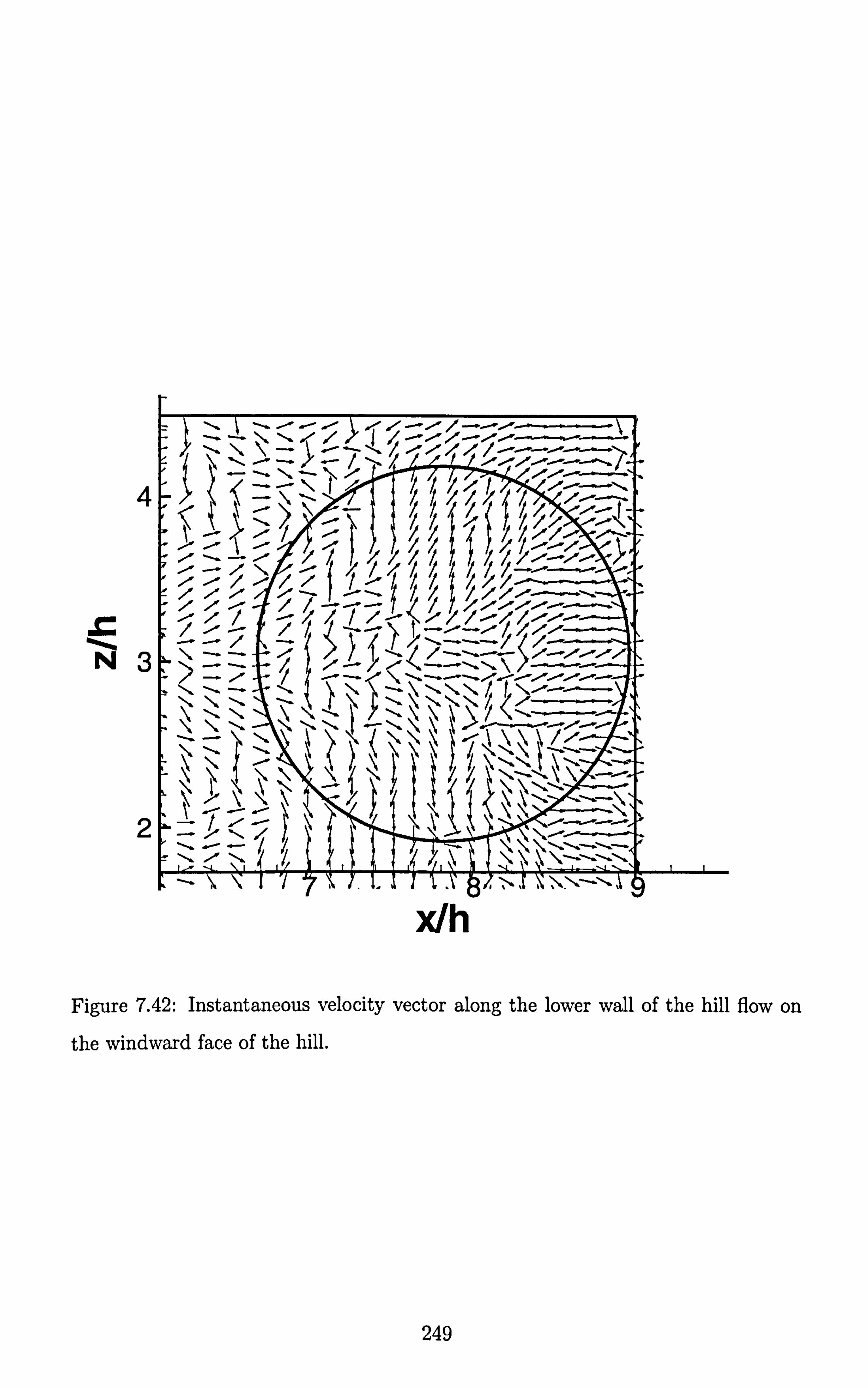
NZ, ,

1-1 Al

7,7,

JO

1\1

x/h

Figure 7.42: Instantaneous velocity vector along the lower wall of the hill flow on

the windward face of the hill.

249

x/h = 8, y/h = 0.4502

0.5

1.5 2 Az/h

x/h = 8, Y/h = 0.7169

0.

-0.

K

-140-

x/h = 8, y/h = 0.4766

0.5-

0

0 0.5 1 1.5 Az/h

x/h = 8, y/h = 1.0055

°22 R33

. 1..

1.5 2

Az/h Az/h

Figure 7.43: Spanwise auto-correlations for the three velocity fluctuations at x1h =8

and four different vertical locations.

250

7.4 Coarse-grid LES with near-wall approxinia-

tions

7.4.1 Overview

The principal purpose of the study reported in this section is to com, ey insiglit, illto

the predictive accuracy that, can be achieved by sinnilations of flow separatilig from

curved surfaces, with grids, such as those sho"m oil Figures 7.4,1 atid 7.15 mid deemed

economically tciiablc in a practical environment. Althougli t lic separat ed f1mv Illider

consideration is challenging, it's Reynolds 1111111ber is still relal ively low ill colliparisoll

to a separated wing How at a typical Heynohk nundver of IF UNd vilghmring Hows

are inuch more demandhy, and the sensitivitY Imuls rejuMed hvlow are BAY lo Q

cons i derably more severe in practice.

Figure 7.44: Cut in the xy plaile through the coni-sc. grid (Grid 1) inade of'

106 112 x 64 x 92 ; ýý 0.66 -

The range of simulations undertaken is sunimarised in Table 7.2. These simula-

tions were conducted along three parametric axes intended to allow the contribution

of resolution, SGS modelling and near-wall approximation to be separated, at least

qualitatively. Simulations I- 11 have been perforined on Grid I made of 0.66 - 106

interior cells. Of these, simulations I-7, all done with the NVALE SGS model,

are designed to convey the sensitivity of the solution to the near-wall treatment,

including the two implementation options explained in Subsection 3.3.3, while sim-

ulations 8- 11, all undertaken with the NVerner-W'611gle wall function (WW), are

intended to bring out the dependence of the solution on SGS modelling for that grid.

251

Shmdations 21 - 23 forin a selection froll, SM, I-M for the finer (, rid 2(1.0,1 - 10'

interior cells). FWAY4 came 31 MUNY thv IdWit. nmolml sil"I'lat i0l, which Was the

subject of SuctAl T3.

Fig-iii-c 7. -15: Cut in the x- 'y planc through the coarse gi-id (Grid 2) madc of

176 x 64 x 92 ýý 1.04 - 1()6 CeIIS.

x /h reat

4.4

4

3.6

3.2

2.8 L

0.25 0.3 0.35 0.4 0.45 0.5 0.55 x /h

Sep

Figure 7.46: Correlation between separation and reattachment locations, + identifies

data obtiined with Grid 1, X identifies data obtained with Grid 2. The lines indicate

the strean1wise internodal distance (nornialised by h) in the separation region. tý

In Table 7.2, the two right-most columns give the predicted time-ine. an separation

and reattachment locations, obtained upon integration over at least 55 flo,, x, -tliroiigli

times. These allow a number of interesting points to be highlighted, ahead of the de-

252

Case Grid SGS model Wall treatment (xlh)sep (x/h)reat

1 1 WALE NS 1.12 2.17

2 1 WALE ww 0.46 4.00

3 1 WALE WW-p 0.52 3.059

4 1 WALE LL2 0.54 2.95

5 1 WALE LL2-i 0.41 3.95

6 1 WALE LL3 0.53 2.98

7 1 WALE LLK 0.49 3.38

8 1 SM + WD2 ww 0.50 3.59

9 1 MSM ww 0.45 4.18

10 1 DSM ww 0.47 3.56

11 1 LDSM ww 0.47 3.56

21 2 WALE NS 0.38 3.45

22 2 WALE LL3 0.34 4.32

23 2 WALE ww 0.32 4.56

31 3 WALE NS 0.22 4.72

Table 7.2: Overview of computations discussed in the present section.

tailed discussion of field data. First, it is observed that the recirculation length varies

greatly with mesh, wall treatment and SGS model: the shortest recirculation length

is about 2 hill heights, in comparison to 4.5 - 4.7 returned by the highly-resolved

simulations. Second, the flow is evidently fairly sensitive to the implementation de-

tails of any one of the wall-laws. Thus, the simulation pairs (2,3)=(WW, WW-p) and (4,5)=(LL2, LL2-i) demonstrate a consistent difference between the integrated and

point-wise implementations, defined earlier in Section 3.3, with the former practice

yielding a significantly longer recirculation zone, in better accord with the highly-

resolved solution. Finally, as shown in Figure 7.46, there is a fairly strong correlation between the separation and reattachment locations: typically, a forward shift of the

separation point by 0.15 hill heights results in a shortening of the recirculation zone by one hill height, a causal relationship which will be revisited below. This brings

253

out an important difference between simulating a flow in which separation is fixed

by edges, relative to one in which separation occurs from a continuous surface, espe-

cially when reattachment is not enforced by a geometric feature or blockage causing

early re-acceleration.

7.4.2 Effects of resolution

Compared to the dense Grid 3, used for the highly-resolved simulation 31 in Ta-

ble 7.2, two substantially coarser grids have been used to investigate issues of resolution and modelling. The coarsest Grid 1 (0.66 . 106 cells, see Figure 7.44) has a

fairly uniform density over the domain. The medium Grid 2, shown in Figure 7.45

is moderately finer (1.04.10' cells), but the refinement was introduced preferentially

around the hill crest, and the nodes were redistributed in the y-direction so as to

achieve a better resolution at the lower wall.

Case X", Xreat Grid size

Axsep AXcrest AYcrest A2ýrest

hhhhhh (Nx x Ny x Nz)

1 1.12 2.17 112 x 64 x 92 0.065 0.08,0.032,0.049

21 0.38 3.45 176 x 64 x 92 0.039 0.04,0.02,0.049

31 0.22 4.72 196 x 128 x 186 0.032 0.032,0.0033,0.024

Table 7.3: Sensitivity of separation and reattachment locations to grid parameters

at the hill crest.

An impression of the difficulties that axe posed by using coarse grids for separated

flow is conveyed by Table 7.3 and Figures 7.46 and 7.47. Figure 7.47 shows profiles

of velocity, (resolved) streamwise normal stress and shear stress at two locations,

x1h =2 and x1h = 6, i. e. within the separation bubble and after reattachment. Re-

sults are compared for the three grids employed using the same SGS model (WALE)

and the same no-slip (NS) wall condition. This boundary condition might appear

inappropriate for the coarsest grid, although it has been used with considerably

coarser meshes in wavy-wall simulations (e. g. Salvetti et al [195]). However, as is

254

x/h = 2.0

Y/11

Comp. 31 *Grid 29 wGrid I

A .......... I.

0.5 1 /Ub [Ljb

x/h = 2.0 x/h = 6.0

Y/11

E Comp. 31 G- did 2

m-w Grid I

p

0.1

x/h = 6.0 ........... 3-

Comp. 31 2- Gni d2

G 'd I rid I

0... 0 0.2 0.4 0.6 0.8

y/h

Comp. 31 ... *Grid 2

w-Grid I 2

NIL

0 -0.02 0 0.02 0.04 0.06

-.. -, 2. -. 2

y/h

/U b

Figure 7.47: Streamwise velocity, resolved streamwise stress and resolved shear stress

at x1h =2 and x1h =6 for Grids 1,2 and 3, the WALE model and the no-slip (NS)

wall condition have been used in all cases.

evident from Figure 7.48, the time-averaged y+-values corresponding to the distance

between the lower wall and the first grid plane are mostly below 8; the peak value

of 14 arises at the crest of the hill, following the strong acceleration on the wind-

ward side. Thus, while a no-slip condition is undoubtedly a poor approximation, it might not be expected to be disastrously poor. However, when this condition is

used in combination with poor resolution axound the sepaxation point, it leads to

a serious misrepresentation of the entire flow, principally because of the substantial downstream shift in the separation point. As the wall shear strain is evaluated, in

this case, using a linear approximation to the near-wall velocity, the resulting shear

stress is underestimated relatively to both the real value and that arising from a

log-law-based wall function. Hence, following acceleration, flow-retardation by wall

255

shear is inhibited, and separation is thus delayed. Since the separation bubble is

much shorter, the (u)-profile at x1h =6 is much fuller, the substantially lower

shear strain at that location being compatible with a much lower level of turbulence

intensity and shear stress. Upstream of reattachment, at x1h = 2, the separated

shear layer returned by the coarsest grid is significantly lower and more turbulent

than the highly-resolved layer, as is reflected by the higher fluctuation intensity and

shear stress. This higher level of turbulence intensity is consistent with the smaller distance between the separation point and the profile location in question (x1h = 2),

together with the fact that the turbulence intensity reaches a maximum a short dis-

tance downstream of the separation location. Hence, it seems clear that the realism

of the solution in the vicinity of the separation location is crucially important. An

inappropriate downstream shift gives the wrong (mean) separation height and angle,

and this, coupled with strong mixing immediately following separation, encourages

rapid reattachment.

15

+ y

10 Grid 1 Grid 2 Grid 3

MEMO mmd

tt

**me

OL 0 4

x/h

Figure 7.48: Universal wall-distance along the line passing through the centre of

the wall-adjacent cells close to the lower walls; from simulations 1 and 21 using the

WALE SGS model and NS.

Evidently, the grid resolution around the hill crest, where sepaxation occurs, is

256

highly influential. Table 7.3 gives, for the 3 grids employed, the value of streamwise

cell length Ax around the time-mean separation point and the cell dimensions just

above the hill-crest (see also the horizontal line segments in Figure 7.46). Although

the position of the separation line varies in time within the wide range of -0.05h

and 0.7h, the expectation must be that the separation point cannot be determined

to a precision substantially better than the cell length, 0.08h, in the case of Grid 1.

The associated margin in the reattachment location, implied by Figure 7.46, is of

order 0.5h, and such a shift results in a substantial change to the entire flow. Thus,

subject to uncertainties arising from the crude no-slip condition used here, it may

be stated that grid resolution around the separation location is especially important

and, potentially, of major consequence to the predicted gross-flow features. As the

instantaneous position of separation shifts across a significant portion of the hill

surface, adequate grid density must be provided over the entire region in which

separation is expected to occur.

7.4.3 Sensitivity to near-wall modelling on the coarsest grid

Although the streamwise resolution around the separation point is evidently a key

factor, the near-wall treatment can also be expected to be a major contributor to

predictive accuracy, if only because the near-wall y+-value in the hill-crest region is

high and the separation point is clearly sensitive to the details of the flow conditions in this region.

An overall view of the dependence of the flow on the neax-wall approximation, on the coarsest grid, is given in Table 7.2, Cases 1-7. All simulations were performed

with the WALE model. Clearly, the separation characteristics are highly sensitive

to the near-wall approximation, and this is brought out especially well relative to

the no-slip implementation. In all cases, separation is delayed and reattachment is

early. While the latter is linked to the former (see Figure 7.46), as discussed in the

previous subsection, it is evident that the neax-wall approximation also has a direct

influence on the reattachment location. This fact is implied, albeit qualitatively, by

the scatter in Figure 7.46.

257

Profiles of velocity, streamwise normal stress and shear stress, obtained with

the various near-wall approximations, are shown in Figure 7.49. All three log-

law-based approximations, when implemented in their standard (point-wise) form,

return solutions which are better than that obtained with the no-slip condition, but which are nevertheless far from the highly-resolved simulation, especially in

the post-reattachment region. In contrast, the default (cell-integrated) Werner-

Wengle approximation (WW) returns a much better solution, which is remarkably

close to the highly-resolved simulation. As will be demonstrated below, this is

mainly the consequence of the cell-integrated implementation. Of the three log-law

approximations, that using (k) as the velocity scale in the log-law (LLK) offers a

modest advantage in terms of the separation and reattachment locations, but not in

respect of other quantities. It should be noted that this variant differs fundamentally

from the other two in its use of a time-averaged rather than instantaneous velocity

scale in the log-law. This effectively established, for any one near-wall cell, a linear

relationship between the near-wall velocity and the shear velocity, in the same sense

as that established by Schumann's wall law [200]. Moreover, a significant uncertainty

with this variant arises from the inaccuracy in determining the near-wall turbulence

energy on the coarsest grid used. This is especially problematic in the vicinity of

the separation point. As is the case with the no-slip implementation, late separation is accompanied

by higher turbulence activity in the separated shear layer (at a given x1h location),

early reattachment and lower post-reattachment turbulence activity. Although, as

argued earlier, a forward shift in the separation location is associated with an in-

crease in turbulence levels at given streamwise x1h positions, this causal relationship

is not firm, for some simulations show significant differences in maximum turbulence

levels in the shear layer together with quite similax separation locations. This sug-

gests that, at least with the coarse grid used here, separation and post-separation

behaviour is sensitive to the structure of the boundary layer as it approaches se-

paration and, arising from this, also to structural features in the separated shear

layer itself. The boundary layer is, in turn, materially influenced by the near-wall

treatment, especially in the hill-crest region where y+ values along the wall-nearest

258

x/h = 2.0

Y/11

Comp. 31 ... *LL2

--mLL3 *--*LLK

WW

f.

A

/U b

x/h = 2.0

y/h

3 - Comp. 31 ... *LL2

*--mLL3 2 *--*LLK WW

OF * O r.... ' ' .... A M00. 05 70 1

<u'v'>/U b 'L <u'u'>/TJ b,

y/h

y/h

x/h = 6.0

- Comp. 3 0 ... oLL2 --mLL3 0--OLLK -WW

ft.

[U b

x/h = 6.0

3 Comp. 31 0 ... OLL2 a--NLL3 *--*LLK

2- -WW

0ý ... ... . 0*02 0.02 0.0(

.- --20 __ý04 U-V->/U b <U-U">/U b


at x1h =2 and x1h =6 using 4 wall-treatments and the WALE model on the

coarsest grid.

grid-line are high.

Figure 7.1 demonstrates, by way of pressure contours, that the shear layer

contains a coherent motion associated with vortices associated with the Kelvin-

Helmholtz-like instability, a process identified most clearly in animations performed for this flow. This organised motion contributes directly to the turbulence level

in the shear layer, as well as interacting sensitively with the temporal variation of

the separation process. The details of the coherent component are, however, influ-

enced by the near-wall treatment, and this link is thus one potential source for the

variability in the statistical behaviour observed in Figure 7.49.

Figure 7.50 conveys the fact that the exceptional behaviour of the WW wall

259

law displayed in Figure 7.49 is not essentially due to the different velocity profile forming the basis of that wall law, but arises, primarily, from the nature of its im-

plementation. The figure compares four solutions, two obtained with the point-wise

and two with the cell-integrated implementations of the wall laws LL2 and WW.

As seen, there is fairly close correspondence between the two point-wise forms (LL2

and WW-p) and similarly close agreement between the two cell-integrated variants. The latter pair gives solutions which are significantly closer to the highly-resolved

simulation. This level of sensitivity to the implementation details is remarkable,

and is most likely linked to influential differences in the level of the wall-shear stress

returned by the two implementations. A-priori studies on plane, fully-developed

channel flow, in which DNS velocity profiles were fed into both implementations

of the LL2 and WW wall-functions, have shown that both integrated forms give

consistently higher wall-shear values than the point-wise forms, the latter return-

ing values that are closer to the DNS level when the wall-nearest node is beyond

y+ = 16. A higher wall-shear stress level (traction) just upstream of the separation

point encourages, all other conditions being unchanged, a slightly earlier separation,

apart from possibly influencing the organised behaviour in the shear layer, via the

mechanism considered earlier. The overall conclusions emerging from the above results is, therefore, that even

relatively minor variations in the near-wall treatment can have major effects on the

separation behaviour and the structural features in the separated layer, thus mate-

rially affecting gross flow features if the streamwise resolution is coarse, especially

around the separation point.

7.4.4 Sensitivity to SGS models on the coarsest grid

An overall view of the sensitivity of the solution to SGS modelling, on the coarsest

grid, is conveyed in Table 7.2, Cases 2 and 8-11. In general, the coarser the grid,

the more influential the SGS model is expected to be. Hence, it is of interest to

undertake a study of the sensitivity to SGS modelling on Grid 1, even if this grid is known to offer relatively poor resolution in the separation region. All simulations

260

x/h = 2.0

y/h

Comp. 3 ... *LL2 9 LL2-i

olf *-, *WW-p 0 mrw

*f

0.4 0.8 /Ub

x/h = 2.0

y/h

Comp. 31 0 ... OLL2 m- -m LL2-i

2- *-. +WW-p

01 ....

, 0.05 0 0.05 0.1 -. 2

- -v 2 /Ub

x/h = 6.0

y/h

Comp. 3 0 ... eLL2 --a LL2-i *-. *WW-p

ww

0., ... ****''1*'' Ti

-0.02 0 0.02 0.04 0.06

"ýU'V' >fu bl' <U'U'>[Ub 1.


at x1h =2 and x1h =6 using the point-wise and cell-integrated forms of LL2 and

WW wall-treatments and the WALE model on the coarsest grid.

were performed with the default (cell-integrated) form of the Werner-Wengle wall

law (WW), shown eaxlier to give, alongside LL2-i, the most favourable agreement

with the highly-resolved simulation.

Reference to Table 7.2 and to Figures 7.51 and 7.52, the latter showing mean-

velocity and turbulent-stress profiles, allows the overall observation that sensitivity

to SGS modelling, even on the coarsest grid, is not especially pronounced, and

this reinforces the comments made earlier about the importance of the neax-wall

approximation as the major source of variability among simulations on the coarsest

grid. The separation point is seen to be rather insensitive to the SGS model, while

261

x/h = 2.0

y/h

Y/11

Comp. 31 #--*SM+WD2 A--AMSM

0--GLDSM

£ 0

[U b

x/h = 2.0

Comp. 31 *--*SM+WD2 A-LMSM

o--oLDSM

fu 0 0.04 0.08

y/h

i

y/h

x/h = 6.0

- %-Ulllp. JI s- -* SM + WD2 A--Amsm o---oLDSM

/U b

x/h = 6.0

Comp. 31 --*SM+WD2 A-., ämsm o--oLDSM

b- 0.02 -0 0.02 - 0.04 0.06

<U'V'>[Ubý' <U'U'>/Ub' <U'V'>'Ub z <UU'>'Ub z


at x1h =2 and x1h =6 using 3 SGS models together with the WW wall function

on the coarsest grid.

the reattachment point is somewhat more sensitive. This is a consequence of the

dependence of the former primarily on the upstream near-wall flow, while the latter

responds to both the separation point and the processes in the post-separation sheax

layer which are likely to be sensitive, to a greater extent, to SGS modelling. Among

the SGS models, the WALE model and the mixed-scale model (MSM) give the

longest recirculation length, closest to the reference. The dynamic models (DSM

and LDSM), on the other hand, tend to return the shortest recirculation region.

Since the SGS model affects the simulated solution via the introduction of an

SGS viscosity, and hence SGS stresses, it is instructive to examine the level of

viscosity returned by different models. To this end, profiles of the time-averaged

262

x/h = 2.0

j

y/h

0

Comp. 31 v ... vWALE +--+DSM

0 0.4 0.8 /U b

x/h = 2.0

- Comp. 31 T ... vWALE +-+DSM

y/h

0.04 0.08

i

y/h

0

y/h

x/h = 6.0

Comp. 31 v ... v WALE

0 A S

mp L

M E.

+--+DSM v

C W D

6 0.4 0.8 /U

x/h = 6.0

Comp. 31 WALE

+-+DS 2-

1.7ý-

OT ..... ....

-0.02 0 0.02 0.04 0.06 fu >/u >/Ub <U'U" b4 "I' 'U'V' bz ""U'U' bA


at x1h =2 and x1h =6 using the WALE and the DSM model together with the

WW wall function on the coarsest grid.

SGS viscosity at the locations x1h =2 and x1h =6 axe given in Figure 7.53.

As seen, the SGS viscosity level varies between approximately 1 and 4 times the

fluid viscosity, with the mixed-scale and damped Smagorinsky models giving low

values, the dynamic model giving high levels and the WALE model being in the

middle of the range. While Table 7.2 suggests an association between low levels

of SGS viscosity and long recirculation zones, and hence improved agreement with

the reference simulation, this association is not unambiguous, as is exemplified by

the result with the damped Smagorinsky model. Broadly consistent with the above

trend is the observation, from Figures 7.51 and 7.52, that models returning relatively

low values of SGS viscosity (MSM, WALE, SM+WD2) also give rise to lower values

263

of resolved turbulent stresses and closer agreement with the reference simulation.

x/h = 2.0

y/h

Comp. 31 +--*SM+WD A-. Amsm

v ... v WALE +--+DSM

LDSM

wv :F .

y/h

x/h = 6.0 Comp. 31

--*SM+WD A--ILMSM

v ... v WALE +--+DSM

LDSM

01 <v t >/V <vt>/V

Figure 7.53: SGS viscosity at x1h =2 and x1h =6 using 5 SGS models and the

WW wall function on the coarsest grid.

This is not a behaviour that concurs with initial expectations: a high SGS vis-

cosity is expected to cause smoothing (damping) of the resolved scales close to the

wave-number cut-off, and thus to lead to a reduction in the resolved stresses. The

opposite would then be expected to occur when the SGS viscosity decreases. How-

ever, this line of reasoning is based on a consideration of isotropic turbulence, with

the cut-off located well within the inertial range, not far from the dissipative limit.

The present flow, in contrast, exhibits significant anisotropy in the resolved motion

at the cut-off, due to the coarseness of Grid 1, and hence different energy-transfer

chaxacteristics across the large-scale part of the spectrum. This applies, in particu-

lar, to the post-separation shear layer. As noted earlier, by reference to Figure 7.1,

the shear layer contains anisotropic coherent structures with relatively large span-

wise extent. Animations reveal that the vortices undergo fairly pronounced helical

pairing, whilst breaking up as they are convected downstream. Higher viscosity

slows down this process, tending to reduce the generation of spanwise fluctuation

by a dynamic redistribution of kinetic energy. This encourages the persistence of

the large-scale two-dimensional anisotropic features, which then tend to result in el-

evated levels of resolved fluctuations, as is observed in other configurations (Mellen

et al [151]).

264

7.4.5 Comparisons for the medium Grid 2

In accord with expectation, refinement of the grid results in an improvement in the

predicted flow, both in respect of the separation and the reattachment positions. At

the same time, the dependence on the near-wall approximation declines, as is seen from Figure 7.54. It is recalled, however, that the refinement is highly localised and

selective, involving mainly an increase in the streamwise grid density in the vicinity

of the hill crest. The result is a more accurate resolution of the separation process. The importance of this specific aspect of the simulation has been highlighted already by reference to the coarse-grid results. Evidently, it is this improvement which is

principally responsible for the substantial overall improvement in the predicted flow

field. Thus, the streamwise resolution, especially around the separation location, is

clearly as influential as the near-wall approximation, if not more so. Reference to

Figure 7.54 shows that, among the wall treatments, the no-slip condition remains

poor, while the Werner-Wengle approximation performs best, as it did with the

coarse grid. In fact, the departure of the WW solution from the highly-resolved

simulation is almost insignificant in respect of both the mean flow and turbulence

quantities. This simulation, Case 23 in Table 7.2, also gives separation and reat-

tachment points close to those of the highly-resolved solution.

265

x/h = 2.0

Y/11

x/h = 6.0

Comp. 31 WW

. +--+NS y/h

I

1 0.4

3- Comp. 31

A. -L

LL3 2- 4---+NS

0.5 [U b

x/h = 2.0

y/h

Comp. 31

LL3

y/h

(U -OM 0

`ýU>fu b

x/h = 6.0

comp. 31

--aLL3 --NS

0-. . L, '' -0.02 -0.01 0

<u'v'>/U b <u'v'>/U

b2

Figure 7.54: Streamwise velocity and resolved shear stress at x1h =2 and x1h =6

using 3 near-wall approximations together with the WALE model on Grid 2.

266


Large eddy simulations of a fully turbulent flow separating from a curved wall in

a periodic channel have been presented. In the first part of this chapter, a test

case was constructed for which data were generated and subjected to an in-depth

study of the turbulence phenomena taking place in the flow. The data were carefully

cross-checked by reference to another simulation performed contemporaneously on

the same grid by Mellen et al [150], enhancing the confidence in the results. In the

second part, the emphasize has been on investigating the influence of resolution, SGS modelling and near-wall modelling on the accuracy of the simulation.

The generation by LES of reliable data for a flow separating from a curved surface

was made possible by carefully selecting the characteristics of the geometry and flow

conditions, i. e. a flow which is periodic in the strearnwise and spanwise directions

with a Reynolds number and computational domain for which an highly-resolved

LES computation remained affordable. In addition, the flow was designed to present

a separation that occurred somewhere on the curved surface, while reattachment was

on the horizontal plane, sufficiently far from the downstream constriction, allowing

a significant recovery to take place. The complexity of the flow, alongside the

availability of a reliable set of data, made it an attractive test case for researchers

to develop and validate RANS and LES methods and, thus, the data were made

available to the turbulence community through the ERCOFTAC website.

The data generated included mean velocities and stress profiles, turbulence e-

nergy and Reynolds-stress budgets and a significant amount of instantaneous data.

The constrast projected by the instantaneous against the mean data highlighted the

rather chaotic behaviour of the instantaneous flow. This is very well illustrated by

the absence of clear lines of separation and reattachment. Indeed, these locations

vaxy substantially in time, and the flow is observed to be attached and detached

over most parts of the lower wall, except on the windward part of the hill where

the flow is subjected to a strong acceleration due to the raising slope and, therefore,

remains attached.

The most intriguing phenomena was the large excess of the spanwise normal

267

Reynolds stress over the other components, especially on the windward side of the

hill. The transfer of energy among these stresses was shown to occur through the

pressure-strain interaction and was linked to splatting. This process occurred due

to large streamwise-oriented structures impinging on the windward side of the hill,

generating substantial transverse motions. This splatting effect was observed to

occur at a range of locations on the wall, although its most marked manifestation

was on the windward side of the hill. In the shear layer, rollers extending over a

significant spanwise extent were observed. These originate from a Kelvin-Helmholtz

instability. Between these rollers, streamwise vortices created by helical pairing

were also found. Following the break-up of the spanwise rollers, large streamwise-

oriented inclined structures were sometimes observed and seen to transport over the

downstream hill. A representation of the velocity profiles in wall units underlined

the absence of an universal law of the wall at all locations and, in the recirculating

region, in particular. Simulations on a coarse grid have highlighted the outstanding importance of an

adequate streamwise resolution of the flow in the vicinity of the separation line. This

importance arises from the fact that the reattachment position is highly sensitive to

that of separation, and so is the entire flow. Although the separation line varies in

time over a substantial region around the mean location, the precision with which

the latter is predicted is, at best, of the order of the local mesh size. In specific

terms, a streamwise resolution of 0.08h axound the mean separation location can

be expected to produce an error margin in the reattachment position of order 0.5h.

Indeed, the present study suggests that this is a rather optimistic estimate.

The dependence of the solution on different practices of near-wall and SGS mod-

elling has been investigated on two grids and compared to the highly-resolved re-

ference simulation. The results have been found to be surprisingly sensitive to the

nature of the numerical implementation of the wall laws, rather than to the precise

assumptions of the velocity profiles underpinning them. The best performance was

obtained with cell-integrated implementations of either the log-law or the Werner-

Wengle approximation. The differences between the point-wise and cell-integrated implementations is due to the latter returning higher levels of wall-shear stress than

268

the former, all other conditions being the same. This encourages earlier separation

and hence better correspondence with the highly-resolved simulation. It must be acknowledged that the relatively low Reynolds-number of the flow

led to the wall-nearest computational point lying within the semi-viscous wall layer

over most of the lower wall bordering the separation zone. Also, a-priori studies,

exploiting the highly-resolved simulation data, have demonstrated that the near-

wall flow did not conform to the velocity profiles underpinning the wall laws. This

inevitably limits the generality of the conclusions derived in respect of near-wall

modelling. The sensitivity of the solution to SGS modelling has been found to be weaker than

to variations in resolution and near-wall treatment. Of the SGS models examined,

the WALE and the mixed-scale (MSM) models performed best, in so far as the

related coarse-grid solutions came closest to the highly-resolved simulation. Both

models returned relatively low levels of SGS viscosity, although the latter was shown

to give an incorrect wall-asymptotic viscosity variation in wall-resolved channel-flow

simulations. Further studies are clearly needed for flows at higher Reynolds numbers, but this

poses the problem of generating sufficiently detailed and accurate benchmark data

at tolerable cost. The present study at least suggests that resolution parameters

are likely to be especially critical in other flows involving separation from gently

curved surfaces, such as highly-loaded aerofoils and blades. Configurations of this

type arguably require preferential attention to identify the capabilities of LES cases

such as the one examined in the following chapter.

269

Chapter 8

Flow around a high-lift aerofoil

near stall

8.1 Introduction

Chapters 6 and 7 considered, respectively, a periodic channel flow and a separated

flow over a periodic hill. These studies demonstrated the validity of the present

method, its capabilities and characteristics, and they also helped to identify some

best practices. Issues considered included the modelling of the subgrid-scale pro-

cesses, the approximate representation of under-resolved near-wall flow, the role

played by the grid resolution and the influence of the numerical method. In the

present chapter, a final case is considered, which may be claimed to be at the very

limit of the current capabilities of LES. This case is a high-lift aerofoil at near-stall

condition at high Reynolds number. Based on the experience gathered in the pre-

vious chapters, the computation of such a flow was expected to be feasible, while

indicative of the current capabilities and limits of LES in conditions that approach

those in aeronautical practice.

The geometry under consideration is the Aerospatiale single-element aerofoil,

denoted A-aerofoil and shown in Figure 8.1. The aerofoil is just beyond stall con-

dition, at an incidence angle of 13.3' and a Reynolds number of 2.1 - 10', based on

the free stream velocity U,, and the chord length c. The present case is especially

270

challenging because of the variety of phenomena taking place at scales which differ

by orders of magnitude. These include, successively, a laminar separation bubble,

located on the suction side near the leading edge, a transitional reattachment caused by the strong acceleration of the flow, a turbulent boundary layer subjected to a

strong adverse pressure gradient, which causes separation near the trailing edge and, finally, separation extending to the wake. This test-case was selected because of the

availability of recent, well-regaxded experimental data, which have been used exten-

sively over the last 10 years for the development and validation of numerical codes

and RANS techniques, especially within two European projects EUROVAL [77]

and ECARP [78]. The conclusions of these projects indicated that very few RANS

models, mostly those based on second-moment closure, reproduced well the experi-

mental results. In addition, transition on the suction side of the aerofoil had to be

axtificially triggered.

Separation bubble with transition from laminar to turbulent

laminar b. l. Turbulent b. l.

Separated region

Wake: mixed cc= 13.3 shear layer UO

Stagnation point followed by laminar b. l.

Tripping point: transition laminar to turbulent

b. l. = boundary layer turbulent b. l.

Figure 8.1: The A-aerofoil profile and flow regions around it.

The first attempts to compute moderately detached flows around aerofoils at

high Reynolds numbers with LES are due to Kaltenbach and Choi [102] on struc-

tured meshes, and to Jansen [92,93] on an unstructured mesh. The case considered

was a NACA 4412 profile at maximum lift for a Reynolds number of 1.54.101, based

on chord length and freestream velocity. This flow is similax to the present one in

terms of the challenge it poses. Jansen [92,93] and Kaltenbach and Choi [102]

271

demonstrated that such computations were feasible, although at a very high cost because of the high mesh density and the relatively small time-steps that had to

be prescribed. Major problems encountered included the difficulty of correctly predicting the transition, aided by a triggering technique, and the presence of spurious

waves responsible for the creation of unphysical wiggles which were indistinguishable

from turbulence in some regions. The spanwise extent, limited to a few percent of

the chord length for economical reasons, was a source of substantial uncertainty in

respect of the realism of the simulations. More recently, the LESFOIL project [45] focused on the present A-aerofoll. Just

prior to this project, Weber et al [233] attempted to compute this particular flow,

but their effort was unsuccessful and hinted at the difficulties that would be encoun-

tered in trying to achieve a successful simulation of this flow. Of all contributors to

the LESFOIL project, only Mary and Sagaut [142] succeeded in matching the ex-

perimental data. However, their simulation employed a 2D/3D patching technique

with the 3D patches only covering a small portion of the domain, a very dense mesh

and a very small spanwise extent of 1.2% of chord. Some of the simulations reported

in this chapter were also performed as part of the LESFOIL project in which the

author participated. The remainder of the chapter is organised in five parts. Section 8.2 describes

in details the aerofoil and the reference data. In Section 8.3, results of computa-

tions performed on coarse grids axe presented and discussed. These attempts aimed

at identifying the role played by the subgrid-scale model, the wall treatment, the

numerical scheme, the mesh and the outflow boundary condition. Based on the

observations made in Section 8.3, further simulations were performed, and these are

presented in Section 8.4. Finally, Section 8.5 summarises the findings derived from

the simulations in this investigation and draw conclusions on the feasibility and

limitations of LES for high-Reynolds-numbers near-wall flows undergoing marginal

separation.

272

8.2 Test-case description: the A-aerofoil

Figure 8.1 gives an overall view of the phenomena encountered in the flow. On the

suction side of the aerofoil, a laminar boundary layer undergoes natural transition

in an essentially laminar separation bubble, ending by turbulent reattachment at

x1c 0.12. The boundary layer then develops and grows until it detaches at

x1c 0.83, beyond which a small recirculation zone forms. The reverse flow extends

to y/c = 0.016 from the wall. The transition on the pressure side was triggered at

x1c = 0.3 in the experiments. The experimental geometry had a blunt trailing edge

of approximatively 5% c thickness. However, for reasons of simplicity, and based on

the experience derived from the EUROVAL [77] and ECARP [78] projects, a sharp

trailing edge was prescribed in the simulations. Mary and Sagaut [142] demonstrated

this simplification to be of no consequence. The experimental data were obtained in the ONERA-F1 [86) and ONERA-

F2 [71] wind-tunnels, with respective test sections having the dimensions of 3.5m x

1.5m and 1.8m x 1.4m, where the first dimension refers to the height of the section

and the second to its width. The Mach number was 0.15 and the flow can thus

be assumed to be incompressible. Measurements of the drag, lift and skin friction

coefficients, Cd, C1 and Cf, respectively, were performed in the F1 tunnel. In the

F2 tunnel, detailed measurements of the boundaxy layer and wake were made using LDA. The drag and lift coefficients were again measured. The aerofoil tested had

a chord length of 0.6 m and was identical in the two wind-tunnels, except for

its spanwise extent which was slightly different. The F1 tunnel featured minimal blockage effect. Slight corrections of less than 1% were nevertheless applied to the lift

coefficient and incidence angle. A system designed to enhance two-dimensionality

was also used in the F1 tunnel. In the smaller F2 tunnel, blockage effects were higher

and corrections were of the order of 2- 3%. No specific measures were taken in the

F2 tunnel to maintain two-dimensionality of the flow, and this may be the source

for the slight differences in drag and lift coefficients between the two sets of data.

In addition, Cd and C1 were measured using different techniques. Nevertheless, at

the angle of incidence of 13.3', the contamination of the flow by three-dimensional

273

features remained relatively small. In what follows, predicted Cd and C, should be compared principally with the measurements originating from the F1 tunnel.

However, the data from the F2 tunnel are also included.

The exact description of the A-aerofoil profile can be found in the CD-ROM

enclosed in Haase et al [78]. The computational domain extends outwards over

10 chord lengths. The geometry being homogeneous in the spanwise direction, all

meshes presented here and in the following sections are effectively two-dimensional.

The third dimension is obtained by repeating this mesh in the spanwise direction

as many times as the discretisation chosen required it over the selected spanwise

domain size. All grids considered are of the C-type, and the code used here is able

to deal with this topology (see Subsection 4.8.6 for more details on this capability). In the present study, a total of eight different meshes are used. The first and

most used grid, referred to as Mesh 1 and shown in Figure 8.2a, is made of 320 x 64

cells with 40 cells located in the wake, 120 cells located on the suction side and 120

cells on the pressure side. Six of the remaining meshes are evolutions of this Mesh

1 and will therefore be described in the following sections as they are being used.

The last mesh, referred to as Mesh 2 and shown in Figure 8.2b, was generated by

Dahlstr6m and Davidson [45], to allow all members of the LESFOIL consortium to

perform computations on a common grid. It is made of 360 x 64 cells, 56 of them in

the wake and the remaining equally distributed on the pressure side and the suction

side, respectively. While Mesh 2 possesses a similar number of cells to Mesh 1, the

repartition and shape are slightly different, especially at the domain borders where

this mesh is highly non-orthogonal. This later characteristic has a strong negative

impact on the convergence of the pressure solver and forced the setting of the over-

relaxation coefficient to a value of 1, leading thus to an increase of the number of

multi-grid cycles needed per iteration, contributing to a significant increase in the

computational cost.

274

(a) (b)

Figure 8.2: Coarse illeslic's for the acrofoil. (a): Mesh 1; (h): Mesh 2.

8.3 Preliminary computations

8.3.1 Introducting comments

The present section contains results froin a series of computations pci, fOrnied with

the aim of gaining insight into the influence of a range of parameters and practices.

These include subgrid-scale modelling, the representation of the near-wall region,

tllc extent of the computational box in the spanwise direction, the Ofect of thc grid

resolution and the role pl, ý'vecl by the numerical scheme.

The computational domain is periodic in the spanwise direction. The spainvise

extent for the computations presented ill this section was IVO of chord, unless other-

wise stated. This was deenled to be large enough to ensure spanwise decorrelation.

All the computations were started from a potential-flow solution as the initiýil state

and then run over a period corresponding to the time taken by the flow to traverses

5 chords before statistics were collected over a further period corresponding to 5

chords.

275

8.3.2 Influence of modelling

In this first set of simulations, summarised in Table 8.1, the objective was to evaluate

the influence of the outflow boundary condition, the role played by the representation

of the near-wall layer and the choice of subgrid-scale model. All computations were

performed on Mesh 1 described in Section 8.2 with a spanwise extent of 12% of

chord covered by 32 grid planes. Table 8.2 compares the lift and drag coefficients derived from the simulations,

while Figures 8.3 to 8.7 show, respectively, the distribution of the pressure coefficient

along the aerofoil, the distribution of the friction coefficient along the suction side of

the aerofoil, and four profiles of the streamwise mean velocity, the r. m. s. streamwise

velocity fluctuations and the shear stress. Of the four positions considered, three

are located along the suction side of the aerofoil, the profiles being along lines in

the wall-normal direction. The fourth profile is taken in the wake, along a direction

normal to the free-stream velocity.

Table 8.2 shows that both the computed drag and lift coefficients are mostly

higher than the corresponding measurements. The pressure coefficient, shown in

Figure 8.3, is fairly well reproduced, except at the leading and trailing edges. Fi-

gure 8.4 conveys substantial differences among the predicted skin friction values

and also relative to the measured value. Transition, which manifests itself by the

presence of a sudden dip in the skin-friction curve, is cleaxly absent in the present

computations. Neither is the laminar separation bubble predicted. Most seriously,

the separation towards the trailing edge is missed. Consistently, none of the present

simulations returns the correct distribution of the mean streamwise velocity (Figu-

re 8.5) and r. m. s. velocity fluctuations (Figure 8.6) at any of the locations con-

sidered. The wake is predicted to be much too weak, due to the absence of the

upstream recirculation zone. In fact, all these profiles indicate that the predicted

boundary layer is fax too turbulent upstream of the experimental separation point.

Hence, the boundary layer remains attached, and the whole flow is misrepresented

at the trailing edge and beyond. An important point to highlight in Figure 8.6 is

the excessive level of the fluctuating velocity away from the wall in what should be

276

the freestream. This is caused by numerical oscillations induced by the combination

of the second-order centred scheme and large cells, which then lead to even-odd os-

cillations, a phenomenon described in Section 2.7. Figure 8.7 shows, however, that

the predicted shear stress is not affected by the presence of numerical oscillations,

signifying that the oscillations do not mimic cross-correlated fluctuations.

Overall, the simulations presented here are poor and unable to reproduce the

experimental behaviour. In addition, any changes in the parameters or practices did not bring about any evident improvement or resulted in trends that could be

interpreted as being physically meaningful.

Comp. Numerical

scheme

SGS

model

Wall treatment

Outflow boundary

1 CDS SMA+WD2 NS zero gradient

CDS SMA+WD2 NS convective 3 CDS SMA+WD2 ww convective 4 CDS WALE ww convective

Table 8.1: Description of the preliminary aerofoil computations: influence of the

modelling.

Comp. Cl Cd

Exp. - Fl 1.56 0.0204

Exp. - F2 1.515 0.0308

1 1.72 0.0348

2 1.682 0.0404

3 1.682 0.0301

4 1.646 0.0506

Table 8.2: Lift and drag coefficients predicted for the preliminary aerofoil computa-

tions (see Table 8.1 for a description of the computations).

277

-C

Experiment 4 -, - Comp. I

Comp. 2 3

.- Comp. 3 Comp. 4

2

0 ------

0 0.2 0.4 0.6 0.8 Xle

Figure 8.3: Pressure coefficient along the aerofoil for the preliminary computations

(see Table 8.1 for a description of the computations).

0.0151. - Experiment Cf - Comp. I

0.01 Comp. 2 Comp. 3 Comp. 4

0.005

0 0.2 0.4 0.6 0.8 X/C

Figure 8.4: Riction coefficient along the aerofoil suction side for the preliminary

computations (see Table 8.1 for a description of the computations).

278

x/c = 0.30 0.04 ....... I

0.03- Experiment Comp. I

Y/C - Comp. 2 0.02- Comp. 3

Comp. 4

0.01-

x/c = 0.70 0.08

0.06- - Experiment - Comp. I

Y/C Comp. 2 0.04- Comp. 3

Comp. 4

00, ,,, 0,5 -- I. 1'. 5 .... 2 0(

/UO

x/c 0.96 0.12 ...... 0

0-17 Experiment Comp. 1 -0.1 0-08-

- Comp. 2 Y/C Comp. 3 Y/C

0.06- Comp. 4 -0.2

0 0.5 1

-0.3

0.5 [U 0

x/c = 1.05

Experiment Comp. 1 Comp. 2 Comp. 3 Comp. 4

I

/Uo IUO

Figure 8.5: Profiles of mean streamwise velocity at four streamwise locations for the

preliminary computations (see Table 8.1 for a description of the computations).

279

x/c = 0.30 U. V

0.0

Y/C 0.0

O. C

3- Experiment LExpepr

eni...

C - Comp. 1 - Comp. 2

2- Comp. 3

im

Comp. 4

OOL- 0.2 0.3 0.4 0.5

U. L

O. C

Y/C O. C

O. C

x/c = 0.70

Comp. I

Comp. 2 Comp. 3 Comp. 4

u9 iuo u9 iuo

x/c 0.96 x/c 1.05

0.12: ....... ......... I. III11.1 .II

- Experi 0- C: C

.. Comp Comp

meWt rExperim

0.1, Oýp i

Comp. I Comp. I Comp. 2 Comp. 2

0.08- -0.1 . ..... Comp. 3 Comp. 3 Y/C Comp. 4 Y/C Comp. 4

0.06[

-0.2

-0.3

-0 0.05 0.1 0.15 0.2 U9

P0

Figure 8.6: Profiles of r. m. s.

locations for the preliminary

computations).

0.25 0 0.05 0.1 0.15 0.2 UP PO

streamwise turbulence intensity at four streamwise

computations (see Table 8.1 for a description of the

280

x/c = 0.30

Y/4

UAM

0.03- - Experiment c rr

c C Corr

- Comp. I

Cc

omp. 2 0.02 Comp. 3

ormrp. 4

0.01-

I............. 000.005 0.01 0.015

Y/C

0.02

0

<U'V'>/Uý

x/c 0.96

0.12

- Experiment 0.1

- comp. I Comp. 2

0.08 Comp. 3 Y/c Comp. 4 Y/C

0.06[

-C

x/c = 0.70

Experiment Comp. I Comp. 2 Comp. 3 Comp. 4

0 0.005 0,01 2 0.015 0.02 <u'v' >/UO

x/c = 1.05

Experiment Comp. 1 Comp. 2 Comp. 3 Comp. 4

0.02 [1 -0.3

ý1) 0 0.005 0.01 0 0.015 0.02 -0.02 -0.01 0 0.01 0.02

L

<U, V, ýhjO2

/TjO

Figure 8.7: Mean shear stress profiles at four streamwise locations for the preliminaxy

computations (see Table 8.1 for a description of the computations).

ý2

281

8.3.3 Effect of the spanwise extent

Previous simulations were performed with a constant spanwise extent of 12% of

chord. This was deemed to be the minimum necessary to capture the post-sepa-

ration, spanwise structures of the flow with any degree of realism. The successful

simulation of Mary and Sagaut [142] used a spanwise extent as low as 1.2% of chord. Hence, the influence of the spanwise extent on the solution needs to be examined to

determine whether the simulated flow changes drastically as the spanwise extent is

reduced. In this section, four computations, listed in Table 8.3, were performed on Mesh

1 (see Section 8.2 for more details) for spanwise domains of 12%, 6%, 3% and 1.5%

of chord, keeping the spanwise resolution invariant, i. e. the spanwise interplane dis-

tance. A detrimental consequence of this invariant resolution is that the number of

spanwise planes was reduced to four for the smallest spanwise slab. This raises seri-

ous doubts about the ability of this particular simulation to capture 3D turbulence

properly. However, maintaining the spanwise resolution invariant seems to be the

appropriate route to take in an exercise directed towards identifying the sensitivity

to spanwise box size. It may be argued that the observation of a major dependence

of the flow features on the spanwise extent provides, even at this low resolution, an

indication that this distance is too low.

As is demonstrated by the results in Figures 8.8 to 8.10, there appears to be

a substantial dependence of the predicted flow on the spanwise distance below 6%

of chord. This sensitivity must be viewed against the background of no separation being predicted. Had separation been resolved, the sensitivity might have been significantly more pronounced, as the scales of the influential structures rise rapidly with

the onset of separation and the detachment of eddies. The simulations also indicate

that the tendency towards separation grows as the spanwise extent is reduced to a

level at which the simulation becomes almost two-dimensional in nature.

282

Comp. Mesh L, Numerical SGS Wall N, scheme model treatment

5 32 12%c CDS SMA+WD2 LL3



8 4 1.5% c CDS SMA+WD2 LL3

Table 8.3: Description of the computations preformed for different spanwise extents.

-C

III. III. III.....

- Experiment 4- Comp. 5

Comp. 6 3. - Comp. 7

Comp. 8 2

0-- ----------- ...........

.11. -I. L

U. 2 U. 4 0.6 0.8 X/C

Figure 8.8: Pressure coefficient along the aerofoil for different spanwise box sizes (see Table 8.3 for a description of the computational parameters).

0.02

0.015- Experiment Cf Comp. 5

Comp. 6 0.01- Comp. 7

Comp. 8

0 0.2 0.4 0.6 0.8 X/C

Figure 8.9: Friction coefficient along the aerofoil suction side for different spanwise box sizes (see Table 8.3 for a description of the computational parameters).

283

-I- gig

Figure 8.10: Mean streamlines at the trailing edge for the four different spanwise

box sizes: Lz = 12% c (a); Lz = 6% c (b); Lz = 3% c (c); Lz = 1.5% c (d) (see

Table 8.3 for a description of the computational parameters).

284

8.3.4 Influence of the mesh density

The computations presented so far were all performed on Mesh 1, shown in Figu-

re 8.2a and containing 320 x 64. In this section, all computations but one use selective

refinements of this mesh. Table 8.4 summarises the computational details of the

simulations. The mesh used in computation 13 is Mesh 2 described in Section 8.2

and shown in Figure 8.2b. Table 8.5 gives the maximum cell sizes in all three

dimensions, expressed in wall units, while Figure 8.11 shows the variation of the

near-wall cell dimensions along the aerofoil suction side, expressed in wall units. In previous computations, it was noted that the use of central differencing gave

rise to numerical oscillations. These manifested themselves in pseudo-turbulent

normal stresses (but not shear stress) outside the boundary layer. The severity of

these oscillations greatly depends on the grid density, with the normal-to-surface density being especially influential. Figure 8.12 illustrates this by way of instanta-

neous streamwise velocity on the grids investigated and noted in Table 8.4. The

lowest level of oscillations arose from computations 10 and 12, both containing 128

wall-normal grid lines.

Results for pressure coefficient, skin-friction coefficient, velocity and the r. m. s.

of the strearnwise velocity fluctuation are given in Figures 8.13 to 8.16, respectively,

while Table 8.6 provides additional data for the lift and drag coefficients in compa-

rison with the experimental data from both wind-tunnels F1 and F2. As seen from

Figure 8.16, all five grids mimic numerical turbulence (albeit uncorrelated) outside

the boundary layer. The lowest level tends to be produced by the grids with the

highest wall-normal density, at least upstream of x1c = 0.7, and this is consistent

with the behaviour displayed in Figure 8.12. The densest grid, used in computation

12, gives the lowest r. m. s. level outside the boundaxy layer throughout the flow

domain. Moreover, only the meshes with the highest wall-normal resolution, 128

lines, show evidence of transition around x1c = 0.2-0.3. The results for computation

13 are included in Figure 8.13 to 8.16 and Table 8.6, and this did not yield better

results than the others.

It is thus evident from the above figures that none of the simulations comes close

285

to giving a satisfactory representation of either the mean flow or the turbulence

field. In particulax, Figure 8.15 shows that all simulations fail to predict separation,

although there is a gradual approach towards the experimental behaviour as the

grid is refined, especially in the wall-normal direction. The lift coefficient is rather

insensitive to the state of the boundary layer, in contrast to the drag coefficient, the

value of which depends primarily on the skin friction as well as on the structure of

the turbulent layer on the suction side. There is no sYsternaticrelationsWip between

the predicted value of this coefficient and the grid, and the fairly close agreement

achieved with computations 3 and 9, depending upon whether experiment Fl or F2

is used as the basis for compaxison, is fortuitous.

The trends displayed by the various grids provide some indications that an appro-

priate resolution might be achieved with a grid of order 1200 X 240 x 120 pý 35 x 10631

nodes. The simulations also point to the impossibility of investigating here, with

any degree of confidence, the effectiveness of alternative SGS models or near-wall

treatment, except in terms of indicating sensitivity in a qualitative sense.

Comp. Mesh

N, x Ny N, ý

L,. Numerical

scheme

SGS

model

Wall treatment

9 576 x 64 32 12%c CDS SMA+WD2 ww

10 320 x 128 32 12%c CDS SMA+WD2 ww

11 Mesh 1 64 12%c CDS SMA+WD2 ww

12 768 x 128 64 12%c CDS SMA+WD2 ww

13 Mesh 2 32 12%c CDS SMA+WD2 ww

Table 8.4: Description of the computations performed for different grid resolutions.

286

Comp. max(Ax+),, max(Ay+),,,, max(Az+),,

3 999 41.2 613

9 525 45.7 676

10 1335 27.0 803

11 1075 43.5 321

12 518 26.8 400

13 1003 42.5 619

Table 8.5: Maximum cell size (in wall units) for Comp. 3 and 9 to 13 (SS = suction

side) (see Table 8.4 for a description of the computations).

Comp. Cl Cd

Exp. - Fl 1.56 0.0204

Exp. - F2 1.515 0.0308

9 1.755

10 1.475

11 1.550

12 1.553

13 1.64

Table 8.6: Lift and drag coefficients predicte(

ble 8.4 for a description of the computations).

0.0189

0.0383

0.0646

0.0437

0.0429

1 for different gid densities (see Ta-

287

1400

1200

1000

800 AX +

600

400

200

6

5

4

Ay 3

(a)

Comp. 9 Comp. 10 Comp. II Comp. 12 Como. 13

I n-2

AZ

N +-

Comp. 9 0 Comp. 10

- ---- Comp. 11 0 Comp. 12

Comp. 13

10

0.

0L......... 0! 6 ... 018 0 Oa2 0*4

Comp. 9 Comp. 10 Comp. II Comp. 12

L---- Comp. 13

0 0.2 0.4 0.6 0.8

30 11191111. I Comp. 9 (d)

-- ----- Comp. 10 Comp. II

20 Comp. 12 Comp. 13

10-

OL ... 0 0! 2' OA 0! 6 ... 018

X/C X/C

Figure 8.11: Size of the first cell along the suction side of the aerofoil expressed in wall

units: (a) streamwise dimension; (b) spanwise dimension; (c) wall-normal dimension;

(d) location of the first cell-centre in the wall-normal direction (see Table 8.4 for a description of the computations).

288

INJ

Tim

Comp. 3

ý T. , cly

. 440 .Q

,.... ..,... 010,0 0

.. P3,1ý I 41; ý

r 10

Comp. 9

CZI-1.

Comp. 11

Comp. 10

Comp. 12

Figure 8.12: Instantaneous streamwise velocity fields for five different grids (see

Table 8.4 for a description of the computations).

289

5

4

3

Expcriment Comp. 9

--- --- Comp. 10 COMP. II Comp. 12 Comp. 13

...........................

0.2 0.4 0.6 0.8

X/C

Figure 8.13: Pressure coefficient along the aerofoil for five different grids (see Ta-

ble 8.4 for a description of the computations).

0.02

0.015 Cf

0.01

0.005

0 D

Experiment Comp. 9 Comp. 10 Comp. II Comp. 12 Comp. 13

P. 2 0! 4 ... 0'6 0.8

Experiment Comp. 9 Comp. 10 Comp. II Comp. 12 Comp. 13

X/C

Figure 8.14: Skin friction coefficient along the aerofoil suction side for five different

grids. The arrows indicate locations where transition is predicted to occur (see


290

x/c = 0.30

Y/C

0.12

0.1

0.08 Y/C

0.06

0.04

0.02

- Experiment - Comp. 9

Comp. 10 COMP. 11 Comp. 12

1. --- Comp. 13

0.5 1 1.5 2 [U 0

x/c = 0.96

Experiment Comp. 9 Comp. 10 Comp. 11 Comp. 12 Comp. 13

0 0.5 [U [U 0

Figure 8.15: Profiles of mean streamwise velocity at four different locations for five

different grids (see Table 8.4 for a description of the computations). I.

x/c 0.70 0.08

0.06- - Experiment

- Comp. 9 Y/C . ...... -- comp. 10

0.04- comp. 11 Comp. 12 Comp. 13

0.5 1 IU 0

x/c = 1.05

Y/C

.. o.

Experiment Comp. 9 Comp. 10 Comp. 11 Comp. 12 Comp. 13

291

x/c = 0.30

0.04 .......

- Experiment 0.03- - Comp. 9

Comp. 10 Y/C Comp. 11

0.02- Comp. 12 Comp. 13

0.01

0.

Y/C 0.

0.

0.

0.1 0.2 0.3 u9 iuo

x/c = 0.96

12 1.. III.

M Experiment Comp. 9



04-

02-

0 0 0.05 0.1 0.15 0.2 0.25

x/c 0.70

0.08 ....

Experime 0.06- Comp. 9

Comp. 10 Y/C Comp. 11

0.04[ Comp. 12 Comp. 13

Y/C 4

-0

0.05 0.1 0.15 0.2 u0 iuo

x/c = 1.05

Experiment Comp. 9

--- Comp. 10 Comp. 11 Comp. 12 Comp. 13

2-

0 0.05 0.1 0.15 0.2 UI P0 U,

nns /U 0

Figure 8.16: Profiles of r. m. s streamwise velocity fluctuations at four different loca-

tions for five different grids (see Table 8.4 for a description of the computations).

292

8.3.5 Influence of the numerical scheme and oscillation con-

trol

This section describes attempts made to control the numerical oscillations outside the boundary layer by blending central differencing in the near-wall region with

second-order upwinding in the irrotational outer region. This practice has also been

investigated by others for the present flow (see Dahlstr6m and Davidson [43], Mellen

et al [149], Mary and Sagaut [142]).

Blending was effected here through:

0 7--)3 X OCDS + (1 - 0) X OUPWIND (8.1)

where 0 is selected to lie between 0 and 1 and 0 represents the convected variable. Evidently, 0=1 gives the fully centred scheme (CDS), while, 8 =0 gives the upwind

scheme (UPWIND). Two alternative practices were tested:

* Blending 1: the 3 coefficient value is controlled by the local Reynolds number Re, = uAx/v:

Rej: 5 10 =0

10<Rel: 530 =#-, 8=Rej/20-0.5

Rel > 30 =*, 8 =1

(8.2)

* Blending 2: 0 is a function of the geometric coordinates, as illustrated in

Figure 8.17.

The simulations discussed here are summaxised in Table 8.7. They were all performed on Mesh 1 (see Section 8.2) for a spanwise extent of 12% of chord, discretised

by 32 cells. As illustrated by Figures 8.18 and 8.19, the two blending practices give

very different results. Reynolds-number-based blending results in massive separa-

tion due to a failure to trigger turbulence, a behaviour similar to that observed by

use of second-order upwinding throughout the domain as seen in Figure 8.20. In

contrast, geometric blending is considerably better in terms of predictive realism,

293

but fails, as is evident from Figure 8.17, to eliminate the oscillatory behaviour in

the outer irrotational region. It alleviates it, however.

Overall, the introduction of artificial damping via upwinding cannot be regarded

as a tenable practical approach, at least in the form attempted here. While it

does have a stabilising effect on the computation, detrimental effects are difficult

to avoid, and the precise details of the blending practice can strongly influence the

physical realism of the solution. In addition, oscillations in the shear layer, from

which damping is excluded, may be hidden by physical turbulence.

Mixing central and second-order upwind differencing, in a weighted-average

sense, across the whole solution domain was found to be very effective, even with a 95%/5% relative weighting, but poses uncertainty in respect of numerical damping

of turbulence in the shear layer. A more appropriate approach might be the use of

a wiggle detector, such as that implemented by Mary and Sagaut [142]. This would

remove the arbitrariness of the present approach. However, a problem is here that

the distinction between numerical wiggles and turbulent fluctuations is not clear. Whatever scheme is adopted, artificial dissipation is likely to remain a problem, and

the only realistic solution is to substantially increase the grid density.

Comp. Numerical SGS Wall scheme model treatment

14 Blending 1 SMA+WD2 ww

15 Blending 2 SMA+WD2 ww

16 Upwind SMA+WD2 ww

Table 8.7: Description of the computations performed for the different blending

practices

294

Figure 8.17: Instantaneous streamwise velocity contours around the A-aerofoil for

Blending 1 (left) and Blending 2 (right) (see Table 8.7 for a description of the

computations).

Experiment Blending I Blending 2

-C

.................

............... 0.2 0.4

X/C

Figure 8.18: Pressure coefficient obtained with two different blending practices (see


295

0.015

%%% Experiment 0.01..

....... Blending I Blending 2

Cf

ý% ------------ 01

.ý. i -, ...... ..... j. - -... .. - - -, -1* ** 0.2 0.4 0.6 0.8

X/C

Figure 8.19: Friction coefficient obtained with two different blending functions (see


\C ý

c

0

. -ý Cý! -.

Figure 8.20: Instantaneous streamwise velocity contours around the A-aerofoil for

the central scheme (left) and the upwind scheme (right) (see Table 8.7 for a descrip-

tion of the computations).

296

8.4 Final aerofoil computations

Section 8.3 described the role played by a range of numerical issues on the results for the A-aerofoil. Among these, the most influential were the grid and the ability

to control numerical oscillations. In addition, the role played by the spanwise extent

was also shown to be important. Indications were provided that a spanwise extent

of 6% of chord was sufficient to allow the 3D nature of turbulence to be properly

represented. This observation is of considerable importance in term of computational

economy if finer grids are to be used to achieve better resolution as is done in the

final part of the aerofoil study.

Three additional computations, performed on successively denser meshes over a

spanwise distance of 6% of chord, are presented in this section. Table 8.8 provides

details of the number of cells involved. The columns headed Nwake) Nss and Nps

give the number of cells which cover the length of the wake region, the suction side

and the pressure side, respectively. Figures 8.21 to 8.26 show the meshes around the

whole profile and give magnified views of the cell distributions around the leading

and trailing edges. All these meshes are evolutions of Mesh 1 described in Section 8.2.

In computation 17, the cell number has been doubled in the strearnwise and span-

wise directions, while in the wall-normal direction, the number was increased by

50%. The distribution was chosen so as to achieve a nearly wall-resolving mesh.

Computation 18 uses twice as many nodes as computation 17, the increases arising

from the addition of lines in the strearnwise direction. Essentially, each cell in com-

putation 17 is replaced by 2.5 cells. The wall-normal distribution was not modified,

however. In the wake, the cell distribution was adapted to maintain a gentle vari-

ation of the cell sizes in the trailing edge region. In the mesh used in computation

19, the number of cells in the wake has been doubled. In the wall-normal direction,

there axe 33% more nodes, distributed in a similar manner to that of computation

18. No changes were made in the spanwise direction. In the strearnwise direction,

the discretisation is organised as follows: 1904 cells are located on the suction side

of the aerofoil, nearly four times the number used in computation 18; 560 cells are

distributed along the pressure side, this distribution is very similar to that of com-

297

putation 18. The above choice is justified by two arguments. First, the successful

computation of Mary and Sagaut [142] use a similar streamwise cell distribution.

Second, the computations performed in Subsection 7.4.2 for the periodic hill on va-

rious grids indicated an especially high sensitivity to streamwise discretisation for

the prediction of separation. Last, the boundary layer on the pressure side remains laminar due to a favourable pressure gradient as demonstrated by Weber et al [233]

and Mary and Sagaut [142], so only requires moderate discretisation.

Figure 8.27 provides information on the cell dimensions, expressed in wall units, in the layer adjoining the suction side. Figure 8.27d indicates that all computations,

while not fully wall-resolving, are not very far from it with Ay+/2 ; ý-' 5 (i. e. the

first computational node is located at y+ ý- 5). In the spanwise direction, cell

sizes are of the order of 100 wall-units for all three computations. This is three to

four times larger than usually used for a wall-resolved LES in a channel flow, say. The streamwise cell dimensions are below 800 for computation 17, below 400 for

computation 18 and around 50 wall units for computation 19, the last figure being

regarded as adequate in channel-flow computations. Table 8.9 contains details of the computational parameters. All computations

started from a potential-flow solution. Computations 17 and 18 ran over a period

corresponding to 5 chords before statistics were recorded for a further 2 chords. Although some computations recorded in reference [45] used as little as 2.5 chords

prior to starting the collection of statistics, the present choice is regarded as a safer

option as it gives more time for the flow to reach a developed state. The averaging

period could have been longer, and would have resulted in smoother profiles. How-

ever, these computations were extremely costly, and economy was again the limiting

factor. The computations were run on a Origin 3000 parallel computer instead of

the previously used Cray T3E. The speed gain resulting from this switch of machines

was of the order 4 to 5.5, depending on the size of the problem considered and the

partitioning used. Estimates of the computational cost are given in Table 8.9. For

obvious reasons, the cost increases with the mesh density. Typically, 100000 itera-

tions were necessary to advance the flow in time over one chord, at CFL r-4 0.03.

The limitation in the time-step results from the use of the Adams-Bashfort time-

298

marching scheme. A switch to a Runge-Kutta schemes could have allowed the use

of significantly higher time-steps of 0(10-4), instead of 0(10-5) with a computational cost increase per step of the order of 2-3, eventually leading to a significant

reduction in the global computational cost of the simulations. The use of denser and denser meshes necessitated a reduction in the convergence

criterion for the pressure solver (see Subsection 4.6.3 for the definition of this criterion). This had to be set to values of order 10" in the present computations

compared to 10' for computation 3, i. e., individual cell residuals were close to the

zero machine. This then resulted in a significant further increase in the computational cost as the number of multigrid cycles required per iteration increased.

Control and suppression of numerical oscillations was achieved by the use of a

zonal approach. Figure 8.28 illustrates how this was implemented in computation

19. From the aerofoil surface and up to a wall-normal distance of approximately 0.5

c, central differencing was used. Further away, where the flow is essentially irrota-

tional, a second-order upwind scheme was used to introduce numerical dissipation

to prevent contamination of the solution by unphysical wiggles resulting from the

presence, in these regions, of high-aspect-ratio cells. A similar zonal approach was

previously used in computations 17 and 18.

Statistical results for the first two computations are presented in Table 8.10

and Figures 8.30 to 8.35. Statistical data for computation 19 are not included,

except in one plot, because the duration of the averaging period and the time at

which it was started were inadequate to obtain converged data. However, some

instantaneous visualisations for this computation will be shown as they permit some

useful observations to be made.

Table 8.10 compares the lift and drag coefficients. The lift coefficient predicted

by computations 17 and 18 agree broadly with the experiments, while the drag is

wrongly predicted. Figure 8.29 shows instantaneous streamlines around the trailing

edge for computation 19. While a large sepaxation bubble is clearly absent, the

flow features small recirculating bubbles along the wall. Figure 8.30 shows the

distribution of pressure coefficient distribution along the aerofoil. Computations 17

and 18 agree reasonably well with the experiment data, except, as in the previous

299

cases, at the leading and trailing edges. The distribution of the friction coefficient

along the suction side of the aerofoil is presented in Figure 8.31. Computations 17

and 18 show a dip, hinting at the presence of a laminar-to-turbulent transition.

For computation 17, this dip is located at x1c ; zý 0.16 while, for computations 18,

it is located at x1c -ý 0.12. This latter value corresponds to the location at which

transition occurs in the experiment. However, none of these minima reach negative

values that would have indicated the presence of the transitional bubble. The tails

of the profiles indicate the absence of a predicted trailing-edge separation bubble.

Figures 8.32 to 8.35 show, respectively, profiles of mean streamwise velocity, the

r. m. s. of streamwise velocity, the r. m. s. of the cross-stream velocity and the shear

stress, the last three terms consisting of the resolved components. From Figure 8.32,

it is evident that computation 18 gives the best results obtained so far in the present

research. This is confirmed when considering the other quantities in Figures 8.33

to 8.35. Interestingly, computation 19 turned out to yield the best velocity profile

at x1c = 0.3. At this location, conditions in the boundary are dictated by small-

scale activity, the resolution of which requires a relatively short integration time.

Hence, it is possible that, had this computation been pursued to its end, good

agreement with the experiment may have been obtained. Figures 8.33 and 8.34

indicate the absence of numerical oscillations in the region above the boundary layer.

This demonstrates the effectiveness of the present strategy employed to control the

numerical oscillations. This is further illustrated in Figures 8.36 to 8.38 in which

contours of instantaneous streamwise velocity are shown. The fields appear smooth,

except perhaps around the location where the switch from one numerical scheme to

the other occurs. Indeed, this switch can itself create artificial wiggles. This does

not, however, seem to have had any influence on the predictions presented here. It is

also relevant to mention that the switch from one numerical scheme to another was

used by Mellen et al [1511 to artificially trigger transition in some of their aerofoil

computations. In the course of computation 18, time-signals for the three components of the

velocity were recorded for the duration of the averaging processes at the 12 locations

shown in Figure 8.39. Points 1,3 and 5 are located inside the boundary layer, while

300

points 2,4 and 6 are at its edge. The six remaining points are located in the

wake. For each of these locations, 64 signals were recorded, each corresponding to

a spanwise location, over a period corresponding to 2.1 chords at a sampling rate At = 10-1. Each of the signals is made up of 21702 samples.

Figures 8.40 and 8.41 show the energy spectra for all 12 positions, while Figu-

res 8.42 and 8.43 present the spanwise correlations at these locations. The spectral

analysis was performed using a Hanning window with the full signal being decom-

posed into four overlapping elements over which averaging was performed. As signals

were recorded 64 different spanwise positions at each of the (x, y) locations conside-

red, additional averaging was also performed in that direction. The top four plots

shown in Figure 8.40 highlight the inadequacy of the mesh resolution in the boun-

dary layer. The energy drain from the small scales is not properly captured, and an

energy pile-up is observed neax the cut-off frequency. This pile-up is especially well

illustrated in the plot showing the spectra for point 2. The remaining two plots in

this figure indicate that as the reax, thicker portion of the boundary layer is reached,

resolution improved drastically, with the spectra assuming a shape much more simi-

lar to those observed for the other turbulent flows considered earlier in the present

efforts. Furthermore, no pile-up is observed in the spectra shown in Figure 8.41. A

point to note from this figure is the presence of peaks at low frequencies in some

of the spectra shown. This points to the presence of regularly convected structures,

possibly due to a mechanism similar to vortex shedding. Figures 8.42 and 8.43 show the spanwise two-point correlations for all three

components of velocity extracted at the locations shown in Figure 8.39. Along the

aerofoil, all correlations shown in Figure 8.42 diminish to zero. The flow is thus

decorrelated, and this indicates that the spanwise extent of 6% is, indeed, large

enough. The rate at which the correlations decrease to zero diminishes, however,

as the location considered is closer and closer to the trailing edge. As shown in

Figure 8.43, it appears that the flow in the wake is not decorrelated either. Hence,

in that region, the spanwise distance of 6% of chord is cleaxlY not large enough. This

is consistent with the expected presence of large structures in this region, which also

occupy a significant spanwise extent.

301

Figure 8.44 shows iso-contours of instantaneous spanwise velocity for compu-

tation 18, while Figure 8.45 presents the same contours for computation 19. Iso-

pressure-fluctuation contours for computation 19 are shown in Figure 8.46. The last

figure, in the aerofoil wake, features large spanwise rollers which occupies the com-

plete width of the computational domain. This explains the lack of decorrelation in

this region observed in Figure 8.43. These large spanwise rollers, also observed in

Figure 8.45, result from a Kelvin-Helmholtz instability arising from the mixing of the

lower and upper boundary layers with different speeds at the trailing edge. Careful

observations of this flow region also reveal the presence of streamwise vortices due

to helical pairing. As these rollers are convected downstream, beyond the trailing

edge, they break down in the flow and lose their structure. On the aerofoil, the

process of transition is marked by the progressive appearance of structures followed

by a build-up of a turbulent boundary layer and its progressive thickening as the

flow develops.

Comp. Mesh SGS Nx x Ny Nz Nwake NSS NPS Ntot model

17 640 x 96 64 80 240 240 3.9-106 SMA+WD2

18 1280 x 96 64 80 560 560 7.8-106 SMA+WD2

19 2836 x 128 64 176 1904 560 23.2.106 WALE

Table 8.8: Meshes used for the final aerofoil simulations ( SS = suction side; PS =

pressure side) -

Comp. Wall treatment

Ncpu Total run time

Averaging time

CPU cost Time-step (Green)

17 NS 64 7c 2c ý- 12000 h ; z: ý 8.2.10-6

18 NS 64 7c 2c ý- 23000 h i-io-, 1

19 NS 128 2.1 c 0.2 c ý- 30600 h 1.10-'

Table 8.9: Description of the computations for the final aerofoil simulations.

302

Collip.

Exp. - F1 1.56 0.020-1

Exp. - F2 1.515 (). 0: 1 () 8

17 1., 196 0.0622

18 1. G 12 0.0602

Table 8.10: Lift and drag coefficient", predicted 1,01- the fill"ll acn)foll complit'Itiolls

(see Tnbles 8.8 and 8.9 for a description of' I lic collipill at Iml, ").

Figure 8.21: Grid around the acrofoil for Conip. 17 (see Tables 8.8 and 8.9 for it

description of the computations).

303

Figure 8.22: Nlagnified views of the grid for Comp. 17 nround the lc,, iding mid

trailing c(l, ), (, s of the ael'ofoil (see Tables 8.8 and 8.9 for it description of' the compti-

tations)-

................. 111.1-1-1 .... . ...... ..... ... ..

............

Figure 8.23: Grid around the aerofoil for Comp. 18 (see Tables 8.8 and 8.9 for a


304

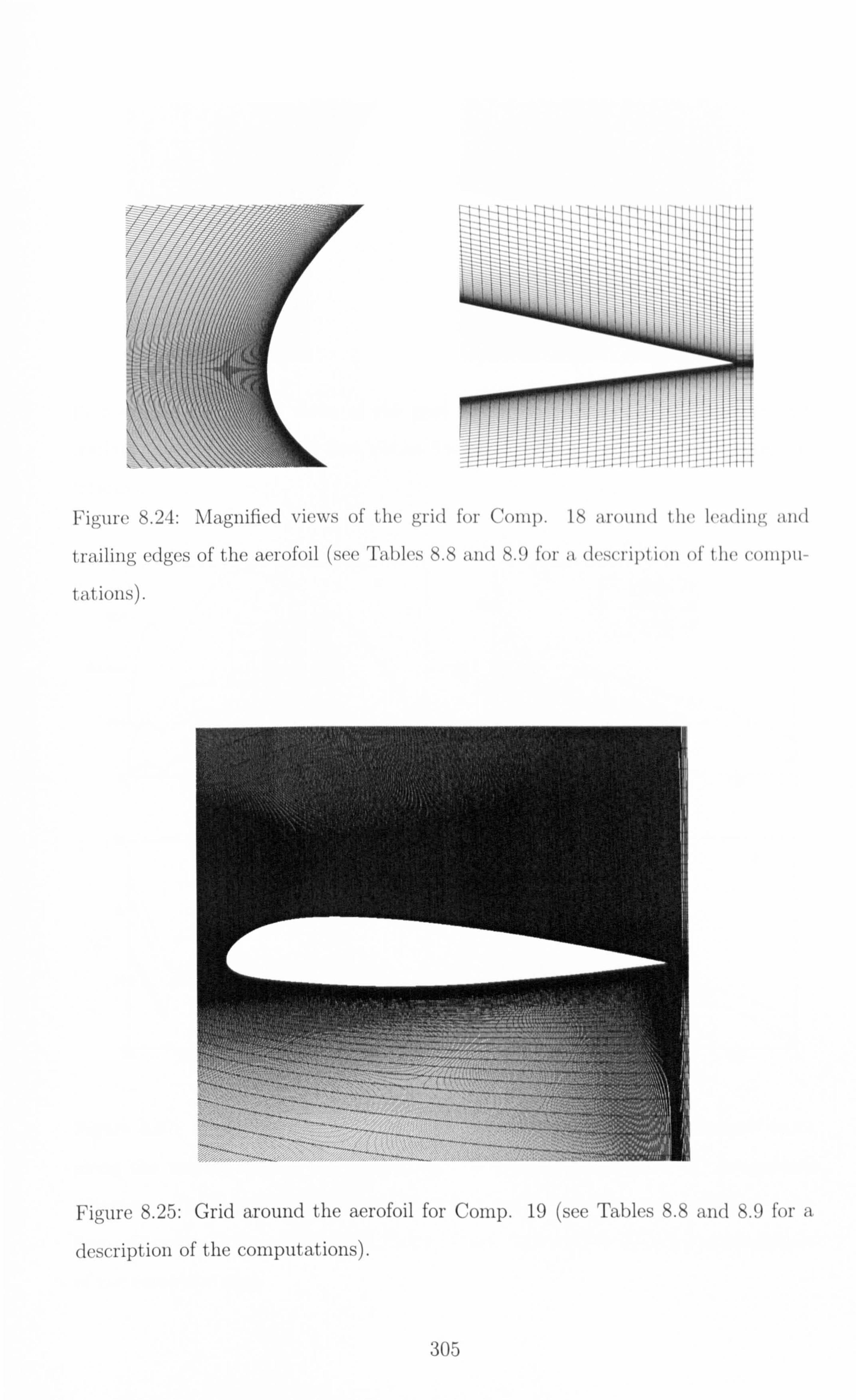
8.24: Magnified views of the grid for Comp. 18 arouild dic lcadlllý,, illid

t, railing edges of the aerofoil (see Tables 8.8 and 8-9 for a dcsci-ipl ion (d' I he c(milm-

tations') -

Figure 8.25: Grid around the aerofoil for Comp. 19 (see Tables 8.8 and 8.9 for a


305

Figure 8.26: Magnified views of' the grid for Comp. 19 around the leading ýllld

trailing edges of the aerofoil (sce Tables 8.8 and 8.9 For ýl de-wripi ion (4 t lic collipli-

tations).

Zio

60

AX 40

20

Collip. 17 Comp. 18

--- Comp. 19

...............

0.2 0.4 0.6 0.8

30

20

Ay +

10

7-conmip, 17

ýn

17 I IS Cornp. 18

------ collip 19

-- C-ý--, -: Co.,

0.2 0.4 0.6 0.8

(C) 17

200 18

Az,

10

0... 0 0! 2 0.4 0.6 0.9

Conip. 17 Comp. 18

------ comp. 19

----------

0.2 0! 4 0! 6 0.8

X/C X/C

Figure 8.27: Distribution of the near wall cell dimensions expressed in wall units

along the suction side of the acrofoil for the final computations: (a) streaniNvise

dimension; (b) spailwise dimension; (c) wall-normal dimension: (d) location of the

first, cell-centre in the wall-nornial direction (see Tables 8.8 and 8.9 for a description

of the computations).

306

Figure 8.28: Locations of the upwind and CDS regions for Comp. 19 (see Tables 8.8

and 8.9 for a description of the computations).

Figure 8.29: Instantaneous streamlines around the trailing edge for Comp. 19 af-

ter 2.1 dimensionless time-units (see Tables 8.8 and 8.9 for a description of the

computations).

307

Experiment Comp. 17

........... Comp. 18

-C

0.6

X/C

Figure 8.30: Pressure coefficient along the aerofoil for the final aerofoil computations

(see Tables 8.8 and 8.9 for a description of the computations).

0.03

62

C

Experiment Comp. 17

........... Comp. 18

0.01

X/C

Figure 8.31: Friction coefficient along the aerofoil suction side for the final aerofoil

computations (see Tables 8.8 and 8.9 for a description of the computations).

308

x/c = 0.30 0.04

0.03 - Experiment

- Comp. 17 Y/C - Comp. 18

0.02- comp. 19

0.01

0.5 1 1.5 Iuo

x/c = 0.96 0.12

0.1- - Experiment - Comp. 17

0.08 Comp. 18 Y/C -.

0.06-

0.04-

0.02

00

/Uo

x/c = 0.70 0.08

0.06 - Experiment

- Comp. 17 Y/C . -- Comp. 18

0.04[ -

0.5 /U 0

x/c = 1.05

I

Experiment Comp. 17

e. ,- .- Comp. 18

Y/C

/UO

Figure 8.32: Averaged streamwise velocity profiles at four different locations for the

final aerofoil computations (see Tables 8.8 and 8.9 for a description of the compu-

tations).

309

x/c = 0.30

0.03

Y/C 0.02

0.01

0.

Y/C 0.

0.

0.

Experiment Comp. 17 Comp. 18

0.2 u9 iuo

x/c = 0.96

12

- Experiment D. 1 - - Comp. 17 08

Comp. 18

06

04-

02-

o 0 0.05 0.1 0.15 0.2 0.25

x/c = 0.70

0,06 Expefiment Comp. 17

Y/C Comp. 18

Y/C

0 0.05 0.1 0.15 0. u9 ZUO

x/c = 1.05

0.... I.... - Experiment Comp. 17 Comp. 18

-0.1

-0.3

0 0.05 0.1 0.15 0.2 UI

. /UO U. PO

Figure 8.33: Averaged streamwise turbulence intensity profiles at four different lo-

cations for the final aerofoil computations (see Tables 8.8 and 8.9 for a description

of the computations).

310

x/c = 0.30 x/c 0.70

0.04 ....... 0.08

0.03 ' -Experiment Experiment

0.06- Comp. 17 E : Comp. 17

: Comp. 18

Y/C 0.02

Com 1 Comp. 18 Y/C - 0.04

(). 01

[ [

0.02

0.04 0.06 0.08 0.1 v9

rniPO

x/c = 0.96

Y/I YA

'(1-f) 02 0.04 0.06 0.08 0.1 0.12

0, 0 0.02 0.04 0 0.08 v9 rmiMO

x/c = 1.05

0 Experiment Comp. 17 Comp. 18

-0.1

-0.2-

-0.3-

-0.4ou .... O. Lo- -01 .....

.5 .10.15 V'nn! Uo V,

nns IU

0

Figure 8.34: Averaged vertical turbulence intensity profiles at four different locations

for the final aerofoil computations (see Tables 8.8 and 8.9 for a description of the

computations).

311

x1c = 0.30 0.04

0.03

Y/C 0.02

0.01

0

0.08

0.06

Y/C 0.04

0.02

15


5-

0 0.005 0.01

C

-0.1

Y/C -0.2

-0.3

-0.

x/c = 0.70

COmp. 17 Comp. 17 Comp. 18 Comp. 18

0.005 <u'v'>/UO"

x/c = 1.05

Experiment Comp. 17 Comp. 18_

02 -0.01 <u'v'>[Uo- /UO

Figure 8.35: Averaged shear stress profiles at four different locations for the final

aerofoil computations (see Tables 8.8 and 8.9 for a description of the computations).


312

<u'v'>/U 02

x/c = 0.96

Figure 8.36: Instantaneous strea, inwise' velocity Contours fOr Comp. 17 (sce Ta-

bles 8.8 and 8.9 for a description of the computations).

Figure 8.37: Instantaneous streamwise velocity contours for Conip. 18 (see Ta-

bles 8.8 and 8.9 for a description of the com put at ions).

313

Figure 8.38: Instantaneous strea, inwise, velocity contoill's 1,01. Collip

bles 8.8 and 8.9 for a description of the computations).

pt. 2 pt. 4 pt. 9

pl. 6 pt. 8

19 (sce Ta-

pt. 12

pt. pt. 11

pt. 10

Figure 8.39: Locations of the recording points for the time-signals extracted from

Cornp. 18 (see Tables 8.8 and 8.9 for a description of the computations).

314

ELI Point 1 Ell Point 2

le-03 1 e-04

I e-04 - le-05 ................. ................... le-05 - le-06 -

le-06 - Ell Ell

I e-07 - ....... E 22 le-07 ....... E 22 -'E 33 ---. E 33

1 e-08 - 5/3 le-08

3-f

5/3

le-091 , -L le-09L---t 10 f 100 1 10 100

EH Point 3 E, j Point 4

le-03 - le-04

le-04 - ... I e-05 -

le-05 - I e-06 -

I e-06 -E it .......

E22 le-07 - ....... E I e-07 - 22 E 33 E

33 I e-08 - 5/3,1 e-08 - 513

I e-09' I e-09' 1 10 f

100 10 100

Ell Point 5 Ell Point 6 le-03 I e-02

I e-04 -I e-03 -

I e-04 le-05 - le-05 -

I e-06 - le-06 -

Ell

I e-07 - ....... E

22 ....... E 22 E

33 le-07 -E

le-08 - 5/3 33 le-08 5/3

I e-09 0 100 oqL 11 f 10 100

Figure 8.40: Spectra at locations 1 to 6 (see Figure 8.39) for Comp. 18 (see Tables 8.8

and 8.9 for a description of the computations).

315

Eii Point 7 Eii Point 8

1 e-03 I e-02

le-03 IC-04 -

1 e-04 - le-05 -

Ell le-05 Ell le-06

22 le-06 E 22

EE 33 33 le-07 - -07 - 5/3 1e 5/3

10 -08, le-08 le 1 100 1 10 100 L

ff

Point 9 E.. Point 10 11

Ei-i le-02

le-03 - le-03 - ........... .......... -, .......

1 c-04 I e-04 -

le-05 - le-05 Ell Ell

le-06 - ....... ....... E E22 le-06 - 22 EE 33 33

I e-07 - 5/3 le-07 5/3

I e-08' L IL

I e-08 L........ 0 100 1 10

ff

Eii Point 11 Eii Point 12 1 e-02 le-02

1 03 - e- I e-03 .

..... :7

le-04 I e-04 -

le-05 le-05 E Ell

I e-06 22 I e-06 - 22 EE

33 33 le-07 - 5/3 le-07 5/3 4.

I e-08' I e-08 1 10 10 ff

Figure 8.41: Spectra at locations 7 to 12 (see Figure 8.39) for Comp. 18 (see

Tables 8.8 and 8.9 for a description of the computations).

316

RI, Point 1 Rij Point 2

R.. I'

0.

-R 0.5- ....... R

22 ---.

R

0.01 0.02 0.03 Az

Point 3

IRII t22 R ft33

33

............ . WSW

L

0.02 0.03

0.

R.. H

0.

Az

Point 4

RI, R 22 5

[2

1

R 33

0

0.01 0.02 0.03 Az

Rij Point 5 RL,

5-

0

0.01 0.02 0.03

LR

22

.......... .....

0.5

0

Az

Point 6

-R11

R33

0.0' oni AZ AZ

Figure 8.42: Spanwise two-point correlations at locations 1 to 6 (see Figure 8.39)

for Comp. 18 (see Tables 8.8 and 8.9 for a description of the computations).

317

RI, Point 7 R, j Point 8

N 0.5 . ..... ....... ................................ 0.5-

0- --------- 0

L 0 0.01 0.02 0.03 0 0.01 0.02 0.03

AZ Az

Rij Point 9 RI, Point 10

............... I ..

I. I. II. 1: Z% Rl I--- ........... .......... R 22

0.5- 0.5- 33

........................ 00

------------

0 0.01 0.02 0.03 0 0.01 0.02 0.03 Az Az

Rij Point 11 RI, Point 12

.............................. %% % ....... R 22 ..... %%

% .......

R 22

RR 33 33 0.5 0.5

% .......................................... ..........

------------- 00

L 0 0.01 0.02 0.03 0 0.01 0.02 0.0ý

Az Az

Figure 8.43: Spanwise two-point correlations at locations 7 to 12 (see Figure 8.39)

for Comp. 18 (see Tables 8.8 and 8.9 for a description of the computations).

318

Figure 8.44: Iso- contours of spanwise fluctuations (w' = -0.07) for Comp. 18 (see

Tables 8.8 and 8.9 for a description of the coniputations)-

319

Figure 8.45: Iso-contotirs of spailwise fluctuations (wl = -0.07) for Comp. 19 (sce

Tables 8.8 aild 8.9 for a description of the computations).

320

Figure 8.46: Iso-contours of pressure fluctuations (p' = -0.021) for Conip. 19 (see

Tables 8.8 and 8.9 for a description of the computations).

321


Overall, the results achieved have been disappointing. The main obstacles appear all

to be due to insufficient resolution, including the presence of numerical oscillations. Although the introduction of artificial dissipation reduces the level of oscillations,

the manner in which damping is introduced has been observed to exert a very strong influence on the predicted flow features, and the practice must, therefore, be viewed

with considerable suspicion. Despite the difficulties, it may be claimed that the results presented have shed

some light on the influence of the various parameters which exert an influence on the

quality of the results. It has been shown that a proper representation of the near-

wall region by means of an adequate grid and/or by means of an adequate treatment

of wall boundary condition is extremely important. The spanwise distance requires

considerable care, as the study has provided indications of a strong sensitivity of

the solution to this distance and the resolution within the spanwise slab. It must

be acknowledged, however, that the investigation of the influence of the spanwise

extent at a fixed resolution needs to be accompanied by additional studies in which

the influence of increasing resolution for a given spanwise distance is quantified.

Strictly, the former can only be safely identified if, for each spanwise distance, the

spanwise resolution is sufficiently high to eliminate dependence on that resolution.

Since, however, the spanwise grid density cannot be separated from the density in

other directions, this is bound to be a difficult undertaking requiring many costly

simulations. The last simulation presented in this chapter was performed on a grid of 2816 x

128 x 64 ý- 23 . 106 cells. This very laxge computation, while not executed to its

end, gives a graphic indication of the challenges that are faced when simulating

such flows. While the present x-grid probably needs very few modifications to be

completely adequate for a highly-resolved LES, the near-wall cell size in the Y-

direction need to be reduced so that y+ = 0(1). The spanwise discretisation should

be three to four times finer than the present level. This grid could not be afforded in

the present study. Even with such a fine grid, success would rely on state-of-the-art

322

numerical schemes in conjunction with advanced modelling of the subgrid scales and

of the wall regions and advanced numerical strategies such as unstructured meshes

or zonal approaches to limit the computational expense to an affordable level.

The present chapter thus demonstrates the limits of LES as an engineering tool

in aeronautical flows. At high Reynolds numbers, it will remain a research tool for

some time to come. At the industrial level, it is unlikely that it will ever become

a design tool although it may well find, and indeed it has done already, a niche for

research and development for flows in which unsteadiness is the driving force behind

the phenomena studied, for example aero-acoustics.

323

Chapter 9

0 Conclusions and outlook

The main objective of the present research was to identify the capabilities and limitations of LES as a means of predicting sepaxation from curved surfaces at high

Reynolds numbers, the ultimate practical focus being the onset of stall on high-

lift aerodynamics. The route taken was to investigate a rational sequence of flows,

starting from fully-developed-channel flow and ending in a single-element aerofoil at

high incidence and high Reynolds number. Questions needed to be answered about

the resolution level and the nature of the approximations that could be tolerated to

achieve a correct representation in applying LES to complex separated flows. These

investigations were carried out using a highly-efficient parallel LES algorithm into

which a wide range of models and numerical practices were introduced.

In the first part of the research, a range of subgrid-scale models and near-

wall approximations, based on wall functions, were investigated in fully-developed

channel flows at a range of Reynolds numbers, Re,, up to 1050. The objective

was to select practices that would be applied in the following stages of the study

in which separated flows were considered. Apart from quantifying performance by

comparisons of the solutions obtained to available benchmark data, an analysis was

undertaken to quantify the relative contributions of numerical and subgrid-scale-

modelling errors. The investigation revealed substantial differences among a variety

of subgrid-scale models, both in terms of the level of the SGS viscosity in the flow

away from the wall and the asymptotic variation of the viscosity at the wall. Of

324

the models investigated, the dynamic Smagorinsky and the WALE models were

shown to distinguish themselves by their correct asymptotic behaviour. However,

the latter tended to give viscosity levels by up to one order of magnitude lower

than the former variants. Overall, the WALE model was judged to perform best, in

terms of the accuracy it yielded and its simplicity. The error analysis, carried out for the Smagorinsky model, first in its original form and then with the addition of a damping function, provided indications that modelling and numerical errors tended

to partially cancel each other, thus reducing the overall error. The study demonstrated further that, in channel flow, near-wall approximations,

based on wall function, yielded substantial savings in computer resources and did

not degrade dramatically the ability of LES to return both the mean flow and

the second moments in the inner region of the channel flow. Similarly, the wall

functions gave credible levels of wall shear stress. However, the resolution of the flow

structure close to the wall was obviously affected. Of the near-wall approximations,

one particular form, proposed by Werner and Wengle [235], was found to give the

best results, and was judged the most promising for further application in more

complex conditions. The study clarified that, whatever model or approximation

is adopted, mesh resolution remained a critical issue. In particular, the cell-aspect

ratio must be chosen so that it allows the adequate resolution of the structures in the

near-wall region. Insufficient resolution was demonstrated to lead to a degradation

in the distribution of the turbulence energy among the normal stresses, resulting

in an excessively strong streamwise component at the expense of the other two

components. None of the subgrid-scale models tested were able to compensate for

this lack of resolution. The second part of the research focused on a massively separated flow in a channel

with periodically arranged curved constrictions on one wall. The choice of a confined

case was motivated by the wish to study the flow, especially the sepaxation process,

in great detail, but at tenable resource requirements. The absence of extensive and

reliable data which could be used as a reference to study the effectiveness of the

approximations and the response to vaxiable resolution prompted the generation of

these data as paxt of this study. The data were obtained from a highly-resolved

325

LES with a mesh containing 4.6 millions nodes, with the region at the lower wall

resolved almost to DNS level. The results of this simulation were shown to agree

closely with those of Mellen et al [150], thus inspiring confidence in their validity. Apart from providing the reference data, this simulation offered the opportunity to undertake an in-depth study of the physics of the separation and reattachment

processes. Thus, budgets for the second moments as well as much flow-structure

information were extracted. The simulation revealed substantial spatial and temporal variations in the loca-

tion of both the separation and reattachment lines. The near-wall flow, whether in the separated region or following reattachment, was found not to adhere even

remotely to the log law, pointing to the likely difficulties in using near-wall ap-

proximations based on this law. Large streamwise-oriented structures were seen to

impinge on the windward side of the hill. This effect, known as Splatting, was re-

sponsible for the energy transfer from the streamwise to the spanwise normal stress,

giving rise to very high levels of the latter. This energy transfer was shown to take

place through the pressure-strain interaction. In the shear layer bordering the upper

part of the recirculation region, a succession of large rollers, formed through Kelvin-

Helmholtz instability and separated by streamwise vortices originating from helical

pairing, were found. These structures were convected beyond the recirculation zone before breaking up. Large streamwise-oriented, inclined structures were also ob-

served beyond reattachment that tended to be transported over the downstream

hill.

A second and important part of the investigation of this separated flow was

concerned with the study of influence of the near-wall approximations, subgrid-

scale models and grid resolution by reference to the newly produced data. These

simulations, performed on coarser grids than the one used for the highly-resolved

LES, highlighted the importance of an adequate streamwise resolution, especially in the region of separation where the strearnwise cell size effectively limited the

accuracy of the prediction. The results were found equally sensitive to the details of

the numerical implementation of the wall laws, rather than to the precise shape of

the velocity profiles upon which these approximations were formulated. Overall, the

326

best performance was obtained using the Werner-Wengle formulation. The influence

of the subgrid-scale models was found to be relatively weak, with the WALE and the Mixed-Scale models giving the best results.

The third and final case considered was the flow around an aerofoil at near-stall

conditions at a Reynolds number of 2.1.10', based on chord length and freestream

velocity, at an angle of attack of 13.30. This case turned out to be extremely challenging, arguably beyond current capabilities. A wide range of phenomena occurs in this flow at disparate scales, including transition and separation. This particular

configuration was selected because it was judged to be representative of cases to

which LES would need to be applied in the context of practical aerodynamics, and because of the availability of well-regarded experimental data.

The results obtained for this flow were rather disappointing, the main obstacles being the lack of sufficient resolution and the presence of numerical oscillations

which required control by introducing artificial dissipation. Although a sequence

of extremely fine grids were used, none gave a satisfactory representation. While

transition was resolved with the finest grid, no simulation resolved the separation

on the rear suction side. Due to the difficulty of reproducing the essential features of the experimental

results, simulations in which a range of different parameters were tested could only

provide qualitative indicators of their influence. Among these parameters, the span-

wise extent was observed to be very influential. On the one hand, a spanwise box

of less than 6% of chord was found to generate solutions which were highly depen-

dent on this extent. On the other hand, a large spanwise box, coupled with the

need to maintain acceptable grid-aspect ratio, tended to push computer resources

to unacceptable heights.

With the use of wall-function-based near-wall approximations initially discoun-

ted, if only because of the importance of resolving transition, the final simulation

performed for this configuration indicated that, for a spanwise extent of 6% of chord,

a mesh of about 80 millions nodes would be required to obtain a satisfactory solution

that might match the experimental results. In addition to the fact that there is no

certainty that such a simulation would actually match the experiment, a computa-

327

tion of this magnitude, in terms of the resources needed, was unaffordable. The only hope of achieving adequate resolution at affordable expense rests on the combined

use of superior numerical schemes and approaches such as zonal and/or unstructured

meshing strategies that would permit a flexible concentration of the cells in specific

regions of interest, i. e. at the wall on the suction side of the aerofoil. This last test-case thus demonstrated the limits of LES as an engineering tool

in aerodynamics. At high Reynolds numbers, it will, for the time being, remain a

research aid, and it is unlikely that it will become a design tool for aeronautical

applications for many years, if ever. It may however find, and indeed it has already found, a niche in research and development for the study of particular aspects such

as aero-acoustics and aero-elasticity, where unsteadiness is the driving force behind

the phenomena of interests.

More generally, while it seems that LES has reached a certain degree of maturity

at low and relatively moderate Reynolds numbers, it is clearly not the case for higher

Reynolds numbers, especially in complex geometries where phenomena with a wide

range of scales occur. Several aspects still need further development before LES for

such flows become routinely feasible. A much better control of the cell distribution

across the domain is highly desirable, as this is crucial to reducing the computational

cost. Zonal strategies, unstructured grids and adaptive meshing are all techniques

that can achieve this. While these axe available in most commercial CFD software,

they are not often applied in research because the accuracy they offer is often in-

adequate for LES applied to flows which are very sensitive to near-wall processes.

More accurate, energy-conserving schemes that can easily be implemented in the

framework of complex geometries are thus needed to reduce the level of errors and

suppress the numerical oscillations similar to those seen in the aerofoil study. Another route to the reduction of computational costs is through the use of so-

phisticated wall treatments able to deal with complex neax-wall phenomena, such as

separation, through a combination of better numerical techniques, adequate hybrid

RANS/LES methods and higher computing power. Finally, there exists a need for

further reliable data sets for flows at moderately high Reynolds numbers, featuring

complex physical phenomena in relatively simple geometries that can be simulated

328

with sufficiently high resolution to yield reference data. Examples include sepa-

rated aerofoils at Reynolds numbers of order 101 and highly 3D flows around curved

obstacles, again at Reynolds number of order 104_105. Such data will allow approxi-

mations to be studied at lower resolution, as done in the case of the hill flow in the

present study, with much greater confidence that can be attained for the high-lift

A-aerofoil at the Reynolds number of 2.1.106.

329

Appendix A

Filters in large eddy simulation

In LES, three different filters are commonly used:

9 the Top-Hat Filter known also as the Box filter:

I if Ix - X, 1 :5 "' in physical space G(x - x') = 2ý 2 (A. 1) 0 otherwise

sin (k'ý') in spectral space G(k)

k'O' 2 (A. 2)

2

o the Gaussian filter:

in physical space G x-x 6

exp 6 (X

_ X#)2 (A. 3)

Vý7rA2

A2

(_ ý2A2 )

in spectral space G (k) = exp - (A. 4) 24

e the Sharp Fourier Cut-Off filter:

sin (k, (x - x')) 7r in physical space G (x

- x') = k, with k, = (A. 5) , (x - X') ýK

1 if k< ' in spectral space G (k) = (A. 6)

10

otherwise

330

2

A

Box filter

0.5

I

0.8

0.6

ROA

0.2

0

-0.2

Box filter

-0.5 0 0.5 1 -101C 0 lox X-X, kA

Figure A. 1: The Box Filter: left: in physical space; right: in spectral space.

2

1.5

n

Gaussian filter

0.5

I

0.8

: ý0.6

tý-, 00.4

0.2

a

Gaussian filter

--1 -0.5 0 0.5 1 -21t 0 2x x-X, kA

Figure A. 2: The Gaussian Filter: left: in physical space; right: in spectral space.

Fourier Cut-Off filter

-0.8 0.6

0.2

0

-0.2

2

1.75

1.5

_1.25 91

V5

0.5

0.25

n

Fourier Cut-Off filter

4 -2 024 2n -79 0R 21t x-X, kA

Figure A-3: The Fourier Cut-Off Filter: left: in physical space; right: in spectral

space.

331

Appendix B

Methods for the resolution of

numerical systems

B. 1 Eigenvalues and eigenvectors for partial di-

agonalisation

If it is assumed that the discretised Poisson problem is written as:

aixi-i + bixi + cixi+l = Si i=1n

and periodic boundary conditions are used:

XO Xn

(B. 2) Xn+l ý X1

Then, the eigenvalues associated to System (B. 1) axe:

A, =0

AN /\2i+l = -4,5in 2 '*' if n is even (B. 3)

n

An -4

where i=1---'? 2

The corresponding eigenvectors are:

332

rj1 = 0.5

Ii = Cos ati,

ri n

'+1 = sinIL-r ri, n

n (_1)j j2

The solution writes as:

1, n

j=1... n i=1... -1

j=1.. n i=1... -1

j=1... n

(B. 4)

1 n/2-1 7r zj7r

+ (-l)j Xj i+ 2i COS ýýj-

+ ! 2i+l sinL- (B. 5) nn]

which is a Fourier serie expansion whose coefficients are corresponding to the eigen-

vectors (B. 4) of System (B. 1).

B. 2 Method of Samarskii and Nikolaev

Say that the discrete system is;

ajOi-, + bi0i + coi+l = Si with i=1... n (B. 6)

If the system is periodic, then:

ai = ai+,, bi = bi+,,

Ci ---: Ci+n Si ý-- Si+n

and the solution will also be periodic:

The system writes:

(B. 7)

0, = 0. +1 (B. 8)

333

bi ci

a2 b2 C2

a1 Ol S,

02 S2

(B. 9)

... an-, bn-1 Cn-1 On-1 Sn-1

Cn ... an bn On Sn

If the system has one solution, it is a linear combination of two functions ui and

vi such that:

Oi = Ui + Olvi

where ui is the solution of:

i=1 n+l

ajui-1 + bjui + cjuj+j = Si

U, =0

U,, +l =0

and vi, the solution of:

aivi-I + bivi + civi+l

V, =0

V. +1 0

and 01 is determined from i 1:

i=2

i=2

a, (u,, + Oiv. ) + biphil + Cl (U2 + OlV2) -`

Sl

(B. 10)

(B. 11)

(B. 12)

(B. 13)

334

Appendix C

Assembling the turbulence energy

and Reynolds-stress budgets

The energy and Reynolds stress budgets presented in Section 5.4 contain a large

number of terms and, when the need to evaluate each of these terms is faced, a large number of quantities has to be recorded. The object of this appendix is to list

the quantities that require recording and highlight some simplifications that can be

taken advantage of mainly because the flows studied in this work are homogneous

in the spanwise direction z. The collection of these data and the time-averaging

procedure (denoted by <- >) are performed as the computation goes on. Once the

end of the computation is reached, the terms of the budgets axe then assembled on

a 2D plan using the quantities recorded. Spatial derivatives axe evaluated through

a second-order centred colocated finite-volume approximation. Spanwise homogeneity means that:

a(-) az

The quantities recorded in the course of the computation, are thus:

, <v>j<w>, (C. 2)

335

<uu>l <vv>l <ww>, < uv >, < uw >, < vw >, (C. 3) <UP>$ <vp>l <wp>

< uuu >, < vvv >, < www >, < uuv >, < uuw >, < Uvw >, (C. 4) < uvv >, < uww >, < vvu >, < vvw >, < wwu >, < wwv >

p au >) < POU >,

.N,, 9, z, PF < PD- >, < p? - >, (C. 5) W. 310 pa, >, P-ry >, < P-ä7Z >

>< jL- 2--- -, < 9U, 9u > *, eir, N, N-, 9, z, 9, z, >< (C. 6) W. x 9T, klw. , Oä., lza, , >< -ä 7y -ä 7y ><7>

<! L-! Lv > < L--! L- > < -9--9- > , X&. T

<> MY RZ

< 7j7 > k ft

<> (C. 7) <>

ax ax Y,; R

< U-Y- -57Y > < j.; Z7 >

336

Appendix D

Description of the hill shape

The present appendix contains the mathematical description of the shape of the hill

employed in the geometry studied in Chapter 7. This shape is identical to the one

used by Almeida et al [5], and its description of this shape can also be found in the

Ercoftac database, at http: //f luindigo. mech. surrey. ac. uk/database/.

The functions describing half the hill are given in Table D. 1 in which all dimen-

sions are quoted in mm. The hill height is equal to 28 mm while its half-basis has

a length of 54 ram. The half hill is represented in Figure D. 1.

E E 00 CM

. C-

Figure DA: Representation of an half hill.

337

Xatart x3top ao a, 0 9 2.8 - 10' 0

9 14 2.507355893131 - 101 9.754803562315 - 10-1

14 20 2.579601052357 - 101 8.206693007457-10-1

20 30 4.046435022819 - 101 -1.379581654948 30 40 1.792461334664 . 101 8.743920332081 . 10-1

40 54 5.639011190988 - 101 -2.010520359035

Xstart Xstop a2 a3 h (x)

0 9 6.775070969851 - 10-3 -2.124527775800 - 10-3 min(28, hi (x»

9 14 -1.016116352781.10-1 1.889794677828- 10-3 hi

14 20 -9.055370274339- 10-2 1.889794677828. 10-3 hi

20 30 1.945884504128 -10-2 -2.070318932190 - 10-4 hi

30 40 -5.567361123058.10-2 6.277731764683 - 10-4 hi

40 54 1.644919857549 -10-2 2.674976141766 - 10-5 max(0, hi (x»

Table D. 1: Spline describing the hill shape (h, (x) = ao + alx + a2X2 + a3X3

338

Bibliography

[1] ABBA, A., CERCIGNIANI, C., VALDETTARO, L., AND ZANINI, P. LES of

turbulent thermal convection. In Direct and Large Eddy Simulations Il (1997),

J. -P. Chollet, P. Voke, and L. Kleiser, Eds., Kluwer Academic, pp. 147-156.

[2] AKSELVOLL, K., AND MOIN, P. Large eddy simulation of a backward facing

step flow. In Engineering Turbulence Modelling and Experiments 2 (1993),

W. Rodi and F. Martelli, Eds., Elsevier Science, pp. 303-314.

[3] AKSELVOLL, K., AND MOIN, P. Large eddy simulation of turbulent confined

coannular jets and turbulent flow over a backward facing step. Tech. Rep.

TF-63, Department of Mechanical Engineering, Stanford University, 1995.

AKSELVOLL, K., AND MOIN, P. Large-eddy simulation of turbulent confined

coannular jets. J. Fluid Mech. 315 (1996), 387-411.

[51 ALMEIDA, G. P., DUR. KO, D. F. G., AND HEITOR, M. V. Wake flows

behind two-dimensional model hills. Experimental Thermal and Fluid Science

7,1 (1993), 87-101.

ARMENIO, V., AND PIOMELLI, U. A Lagrangian mixed subgrid-scale model in generalized coordinates. Flow, Turb. and Combust. 65,1 (2000), 51-81.

[7] AVITAL, E. Direct and laxge-eddy simulations of compressible open cavity flows. In Direct and Large-Eddy Simulation IV (2001), B. Geurts, R. Friedrich,

and 0. Metais, Eds., Kluwer Academic, pp. 213-220.

339

[8] BAGGET, J. I

JIMENEZ, J. I AND KRAVCHENKO, A. Resolution requirements

in large-eddy simulations of shear flows. In Annual Research Briefs (1997)s

CTR, Stanford, USA, pp. 51-66.

BALARAS, E., AND BENOCCI, C. Subgrid-scale models in finite difference

simulations of complex wall bounded flows. In Applications of Direct and Large

Eddy Simulation (1994), AGARD, pp. 2-1 - 2-6.

BALARAS, E., BENOCCI, C., AND PIOMELLI, U. Two-layer approximate

boundary conditions for large-eddy simulations. AIAA J. 34,6 (1996), 1111-

1119.

[11] BARAKOS, G., AND DRIKAKIS, D. Unsteady sepa-rated flows over manou-

vring lifting surfaces. Phil. Trans. Royal Soc. Lond. A 358 (2000), 3279-3291.

BARDINA, J., FERZIGER, J., AND REYNOLDS, W. Improved subgrid-scale

models for large-eddy simulations. AIAA Paper 80-1357,1980.

[13] BARON, F., AND LAURENCE, D. Large eddy simulation of a wall-bounded

turbulent jet flow and of a homogeneous shear flow. In Turbulent Shear Flows

(1984), D. Durst and B. Launder, Eds., Springer-Verlag, pp. 4.7-4.12.

[141 BEIIZADI, S., AND WATKINS, A. Flow and turbulence modeling in a motored

reciprocating engine using a k-e turbulence model. In Proc. 4th Int. Symp.

on Engineering Turbulence Modeling and Measurement (1999), W. Rodi and

D. Laurence, Eds., Elsevier, pp. 279-288.

[15] BELL, J., AND MEHTA, R. Development of a two-stream mixing layer from

tripped and untripped boundary. AIAA J. 28,12 (1990), 2034-2042.

[16] BERNARD, R., AND KAPITZA, H. How to discretize the pressure gradients

for curvilinear mac grids. J. Comp. Phys. 99 (1992), 288-298.

BLACKBURN, H., MANSOUR, N., AND CANTWELL, B. Topology of fine-scale

motions in turbulent channel flow. J. Fluid Mech. 310 (1998), 269-292.

340

[18] BORIS, J., GRINSTEIN, F., ORAN, E., AND KOLBE, R. New insights into

large eddy simulation. Fluid Dynamic Research 10 (1992), 199-228.

[19] BOSCH, G., AND RODII W. Simulation of vortex shedding past a square cylin-

der with different turbulence models. Int. J. Num. Meth. Fluids 28 (1998),

601-616.

[20] BRADBROOK, K., LANE, S., RICIIARDS, K., BIRON, P., AND Roy, A.

Large eddy simulation of periodic flow characteristics at river channel conflu-

ences. J. of Hydraulic Research 38 (2000), 207-215.

[21] BREUER, M. Large eddy simulation of the subcritical flow past a circular

cylinder: numerical and modeling aspects. Int. J. Numer. Meth. Fluids 28,9 (1998), 1281-1302.

[22] BREUER, M. A challenging test case for laxge eddy simulations: high reynolds

number circular cylinder flow. In Proc. of the 1st Int. Symp. Turb. Shear Flow

Phen. 1 (1999), S. Banerjee and I Eaton, Eds., Begell House, pp. 735-740.

[23] BREUER, M., AND RODI, W. Large eddy simulation of turbulent flow through

a straight squaxe duct and a 180* bend. In Direct and Large Eddy Simulation

1 (1994), P. Voke, R. Kleiser, and J. Chollet, Eds., vol. 26 of Fluid Mech. and its Appl., Kluwer Academic, pp. 273-285.

[24] BREUER, M., AND RODI, W. Large eddy simulation of complex turbulent

flows of practical interest. In Flow simulation with high performance computers II, E. Hischel, Ed., vol. 52 of Notes on numvical fluid mechanics. Vieweg,

1996, pp. 258-274.

[25] CABOT, W., AND MOIN, P. Approximate wall boundaxy conditions in the

large-eddy simulation of high reynolds number flow. Flow, Turb. and Combust.

63 (2000), 269-291.

[26] CALHOUN, R. Numerical investigations of turbulent flow over complex terrain.

PhD thesis, Stanford University, 1998.

341

[27] CALHOUN, R. , AND STREET, R. T'urbulent flow over a wavy surface: Neutral

case. Journal of Geophysical Research - Part C- Oceans 106 (2001), 9277-

9294.

[28] CARETTO, L., GOSMAN, A., PATANKAR, S., AND SPALDING, D. Two

calculation procedures for steady, three dimensional flows with recirculation. In Proc. 3rd Int. Conf. Numer. Methods Fluid. Dyn. (1972), Springer-Verlag,

pp. 60-68.

[29] CEBECI, T., AND SMITH, A. Analysis of turbulent boundary layers. Academic

Press, 1974.

[30] CHALOT, F., MARQUEZ, B., RAvAcilOL, M., AND DUCROS, F. A consistent

finite element approach to large eddy simulation. AIAA Paper 98-2652,1998.

[311 CHAMPAGNE, F., FRICHE, C., LARUE, J., AND WYNGAARD, J. Flux mea-

surements, flux estimation techniques, and fine-scale turbulence measurements in the unstable surface layer over land. J. Atmos. Sci. 34 (1977), 515-530.

[32] CHERUKAT, P., NA, Y., HANRATTY, T., AND McLAUGHLIN, J. Direct

numerical simulation of a fully developed flow over a wavy wall. Theoret.

Comput. Fluid Dynamics 11,2 (1998), 109-134.

[33] CHOI, H., AND MOIN, P. Effects of the computational time step on numerical

solutions of turbulent flow. J. Comp. Phys. 113 (1993), 1-4.

[34] CHONG, M., PERRY, A., AND CANTWELL, B. A general classification of

three-dimensional flow fields. Phys. Fluids A2,5 (1990), 765-777.

[35] CHONG, M., SORIA, J., PERRY, A., CHACIN, J., CANTWELL, B., AND

NA, Y. Turbulence structures of wall-bounded shear flows found using dns

data. J. Fluid Mech. 357 (1998), 225-247.

[36] CHORIN, A. A numerical method for solving incompressible viscous flow

problems. J. Comp. Phys. 2 (1967), 12-26.

342

[37) CHORIN, A. Numerical solution of the navier-stokes equations. Mathematical

Computations 22 (1968), 745-762.

[38] CHUNG, Y., TUCKER, P., AND Luo, K. Large-eddy simulation of complex

internal flows. In Direct and Large-Eddy Simulation IV (2001), B. Geurts,

R. Friedrich, and 0. Metais, Eds., Kluwer Academic, pp. 373-380.

[39] CLARK, R., FERZIGER, J., AND REYNOLDS, W. Evaluation of subgrid-

scale models using an accurately simulated turbulent flow. J. Fluid Mech. 91

(1979), 1-16.

[40] CONSTANTINESCU, G. ) MAIIESH, K., APTE, S., IACCARINO, G., HAM, F.,

AND MOIN, P. A new paradigm for simulation of turbulent combustion in

realistic gas turbine combustor using les. In Proc. Of ASME Turbo E: zpo 2003

Power for Land, Sea, and Air (2003), vol. 2, ASME, pp. 259-272.

[41] COOK, A., AND RILEY, J. A subgrid scale model for equilibrium chemistry

in turbulent flows. Phys. Fluids 6,8 (1994), 2868-2870.

[42] CRAFT, T., AND LAUNDER, B. A reynolds stress closure designed for comPlex

geometries. Int. J. Heat Fluid Flow 17,3 (1996), 245-254.

[43] DAHLSTR6M, D., AND DAVIDSON, L. Chalmers 30-month report, LESFOIL:

a Brite-Eurarn project. Technical report, Chalmers, G8teborg, Sweden, 2000.

[44] DAHLSTR6M, S., AND D"IDSON, L. Laxge eddy simulation of the flow

around an A6rospatiale A-aerofoil. In ECCOMAS 2000, European Congress

on Computational Methods in Applied Sciences and Engineering (2000).

[45] D"IDSON, L., COKLJAT, D., FR15HLICH, J., LESCHZINERI M., MELLEN,

C., AND RODI, W., Eds. LESFOIL: Large Eddy Simulation of Flow Around

a High Lift Airfoil. Results of the Project LESFOIL Supported by the Euro-

pean Union 1998-2001, vol. 83 of Notes on Numerical Fluid Mechanics and Multidisciplinary Design (NNFM). Springer, 2003.

343

[46] DAVIDSON, L., AND PENG, S. -H. A hybrid LES-RANS model based on

a one-equation SGS model and a two-equation k-w model. In The Sec-

ond International Symp. on Turbulence and Shear Flow Phenomena (2001),

E. Lindborg, A. Johansson, J. Eaton, J. Humphrey, N. Kasagi, M. Leschziner,

and M. Sommerfeld, Eds., vol. 2, pp. 175-180.

[47] DE ANGELIS, V., LOMBARDI, P., AND BANERJEE) S. Direct numerical

simulation of turbulent flow over a wavy wall. Phys. Fluids 9,8 (1997), 2429-

2442.

[48] DE LANGHE, C., MERCI, B., LODEFIER, K., AND DICK, E. Very-large-

eddy simulation subgrid modelling using the statistical mechanics renormal-

ization group. In 3rd International Symposium on Turbulence and Shear

Flow Phenomena (2003), N. Kasagi, J. Eaton, R. Friedrich, J. Humphrey,

M. Leschziner, and T. Miyauchi, Eds., vol. 2, pp. 657-661.

[49] DEARDORFF, J. A numerical study of three-dimensional turbulent channel

flow at large reynolds number. J. Fluid Mech. 41 (1970), 481-507.

[50] DEARDORFF, J. The use of subgrid transport equations in a three-dimensional

model of atmospheric turbulence. J. Fluids Eng. 95 (1973), 429-438.

[51] DEJOAN, A. Simulations de grandes echelles turbulentes en ecoulement de

canal plan soumis a des perturbations instationnaires. PhD thesis, Universite

de la Mediterranee, Aix-Maxseille 11,1998.

[52] DOMARADZKI, J., AND LOHý K. -C. The subgrid-scale estimation model in

the physical space representation. Phys. Fluids 11,8 (1999), 2330-2342.

[53] DUCROS, F., COMTE, P., AND LESIEUR, M. Large-eddy simulation of

transition to turbulence in a boundary layer developing spatially over a flat

plate. J. Fluid Mech. 326 (1996), 1-36.

[54] DUCROS, F., FERRAND, V., NICOUD, F., WEBER, C., DARRACQ,

D., GACHERIEU, C., AND POINSOT, T. Large-eddy simulation of the

shock/turbulence interaction. J. Comp. Phys. 152 (1999), 517-549.

344

[55] DUCROS, F., NicoUD, F., AND POINSOT, T. Wall-adapting local eddy-

viscosity models for simulations in complex geometries. In 6th ICFD Confer-

ence on numerical methods for fluid dynamic (1998), M. Baines, Ed., ICFD,

pp. 293-300.

[56] EsFAiIANI, A. Numerical study of laminar transitional and turbulent flow past

rectangular cylinders. PhD thesis, Chalmers University, G8teborg, Sweden,

1998.

[57] FAN, S., AND LAKSHMINARAYANA, B. Computation and simulation of wake-

generated unsteady pressure and boundary layers in cascades: Part 1- descrip-

tion of the approach and validation. J. Turbomachinery 118,1 (1996), 96-108.

[58] FERZIGER, J., MEHTA, U., AND REYNOLDS, W. Large eddy simulation of

homogeneous isotropic turbulence. In Symp. Turbul. Shear Flows (1977).

[59] FERZIGER, J. ý AND PERIC', M. Computational methods for fluid dynamics.

Springer Verlag, 1996.

[60] FLETCHER, R. Conjugate gradient methods for indefinite systems. In Lecture

Notes in Mathematics, vol. 506. Springer-Verlag, 1976, pp. 73-89.

[611 FR61ILICH, J., AND RODI, W. Introduction to large eddy simulation of

turbulent flows. In Closure strategies for turbulent and transitional flows,

B. Launder and N. Sandham, Eds. Cambridge University Press, 2002, pp. 267-

298.

[62] FUREBY, C., TABOR, G., WELLER, H., AND GOSMANt A. A comparative

study of subgrid scale models in homogeneous isotropic turbulence. Phys.

Fluids 9,5 (1997), 1416-1429.

[63] FUREBY, C., TABOR, C., WELLER, H., AND GOSMAN, A. Differential

subgrid stress models in large eddy simulations. Phys. Fluids 9,11 (1997),

3578-3580.

345

[64] GAO, F., AND O'BRIEN, E. A large eddy simulation scheme for turbulent

reacting flows. Phys. Fluids A 5,6 (1993), 1282-1284.

[65] GERMANO, M., PIOMELLI, U., MOIN, P., AND CABOT, W. A dynamic

subgrid-scale eddy viscosity model. Phys. Fluids A 3,7 (1991), 1760-1765.

[66] GEURTS, B., AND LEONARD, A. Is LES ready for complex flows? In Closure

strategies for turbulent and transitional flows, B. Launder and N. Sandham,

Eds. Cambridge University Press, 2002, pp. 721-739.

[67] GHOSAL, S. An analysis of numerical errors in large-eddy simulations of

turbulence. J. Comp. Phys. 125 (1996), 187-206.

[68] GHOSAL, S. Mathematical and physical constraints on large-eddy simulation.

AIAA J. 37,4 (1999), 425-433.

[69] GHOSAL, S., LUND, T., MOIN, P., AND AKSEVOLL, K. A dynamic local-

ization model for large-eddy simulation of turbulent flows. J. Fluid Mech. 286

(1995), 229-255.

[70] GHOSAL, S., AND MOIN, P. The basic equations for the large eddy simulation

of turbulent flows in complex geometry. J. Comp. Phys. 118 (1995), 24-37.

[71] GLEYZES, C. Operation decrochage - resultats de la 2eme campagne d'essais

a F2 - mesures de pression et velocimetrie laser. Tech. Rep. RT-DERAT

55/5004, ONERA, 1989.

[721 GOLUB, G., AND VAN LOAN, C. Matrix computations. John Hopkins Uni-

versity Press, 1990.

[73] GONG, W., TAYLOR, P., AND DC)RNBRACK, A. Turbulent boundary-layer

flow over fixed aerodynamically rough two-dimensional sinusoidal waves. J.

Fluid Mech. 312 (1996), 1-38.

[74] GR6TZBACH, G. Direct numerical and large eddy simulation of turbulent

channel flows. Encyclopedia of Fluid Mechanics 6 (1987), 1337-1391.

346

[75] GR6TZBACH, G., AND SCHUMANN, U. Direct numerical simulation of tur-

bulent velocity-, pressure-, and temperature-fields in channel flows. In Sym-

posium on nrbulent Shear Flow 1 (1979), F. Durst, B. Launder, F. Schmidt,

and J. Whitelaw, Eds., Springer-Verlag, pp. 370-385.

[76] GONTHER, A., AND VON ROHR, P. Laxge-scale structures in a developed

flow over wavy terrain. J. Fluid Mech. 478 (2003), 257-285.

[77] HAASE, W., BRADSMA, F., ELSIIOLZ, E., LESCIIZINER, M., AND

SCHWAMBORN, D., Eds. EUROVAL - An European Initiative on Valida-

tion of CFD Codes, vol. 43 of Notes on Nume7ical Fluid Mechanics. Vieweg

Verlag, 1993.

[78] HAASE, W., CHAPUT, E., ELSHOLZ, E., LESCIIZINER, M., AND MOLLER,

U., Eds. ECARP - European Computational Aerodynamics Research Project:

Validation of CFD Codes and Assessment of Turbulence Models, vol. 58 of Notes on Nume7ical Fluid Mechanics. Vieweg Verlag, 1997.

[79] HANJALIC', K. , AND JAKIRLIC', S. Contribution towards the second-moment

closure modelling of separating turbulent flows. Comp. & Fl. 27,2 (1998),

137-156.

[80] HANJALIC', K., AND KENJERE§, S. Reorganization of turbulence structure

in magnetic Rayleigh-Benard convection: a T-RANS study. Journal of Tur-

bulence 1 (2000), 1-22.

HANJALIC', K., AND KENJERE§, S. 'T-RANS' simulation of deterministic

eddy structure in flows driven by thermal buoyancy and lorentz force. Flow,

Turb. and Combust. 66,4 (2001), 427-451.

[82] HAwoRTH, D. , AND JANSEN, K. Large-eddy simulation on unstructured de-

forming meshes: towaxds reciprocating IC engines. Comp. & Fl. 29,5 (2000),

493-524.

347

[83] HELD, J., AND FUCHS, L. LES of shock induced separation. In Direct and

Large-Eddy Simulation 111 (1999), P. Voke, N. Sandham, and L. Kleiser, Eds.,

Kluwer Academic Publishers, pp. 111-122.

[84] HENN, D. S., AND SYKES, R. I. Large-eddy simulation of flow over wavy

surfaces. J. Fluid Mech. 383 (1999), 75-112.

[85] HIRSCH, C. Numerical computation of internal and external flows: Funda-

mental of numerical discretisation, Vol. 1. John Wiley, 1988.

[86] HUDDEVILLE, R., PICCIN, 0., AND CASSOUDESALLE, D. Operation

d6crochage - mesures de frottements sur profiles AS 239 et A240 a la souf-

fierie Fl du CFM. Tech. Rep. RT-OA 19/5025 (RT-DERAT 19/5025 DN),

ONERA, 1987.

[87] HUDSON, J., DYKHNO, L., AND HANRATTY, T. 'Mrbulence production in

flow over a wavy wall. Experiments in Fluids 20 (1996), 257-265.

[88] HUNT, J., WRAY, A., AND MOIN, P. Eddies, stream and convergence zones

in turbulent flows. Tech. Rep. CTR-S88, Center for T`urbulence Reseaxch,

Stanford, USA, 1988.

[89] HUSER, A., BIRINGEN, S., AND HATAY, F. Direct simulation of turbulent

flow in a square duct: Reynolds-stress budgets. In Applications of Direct and

Large Eddy Simulation. AGARD, 1994, pp. 12-1 - 12-12.

[90] ISSA, R. Solution of implicitly discretised fluid flow equations by operator-

splitting. J. Comp. Phys. 62 (1986), 42-65.

[91] JANG, Y., LESCHZINER, M., ABE, K., AND TEMMERMAN, L. Investigation

of anisotropy-resolving turbulence models by reference to highly-resolved LES

data for separated flow. Flow, Turb. and Combust. 69,2 (2002), 161-203.

[92] JANSEN, K. Preliminary large-eddy simulations of flow around a NACA 4412

airfoil using unstructured grids. In Annual Research Briefs (1995), CTR,

Stanford, USA, pp. 61-72.

348

[93] JANSEN, K. Large-eddy simulations of flow around a NACA 4412 airfoil using

unstructured grids. In Annual Research Briefs (1996), CTR, Stanford, USA,

pp. 225-232.

[94] JEONG, J., AND HUSSAIN, F. On the identification of a vortex. J. Fl. Mech.

285 (1995), 69-94.

[95] JEONG, J., HUSSAIN, F., SCHOPPA, W., AND Kim, J. Coherent structures

neax the wall in a turbulent channel flow. J. Fl. Mech. 332 (1997), 185-214.

[96] JIMENEZ, J. Computing high-Reynolds number channels: Will DNS ever sub-

stitute experiments? In Engineering Turbulence Modelling and Experiments

V (2002), W. Rodi and N. Fueyo, Eds., Elsevier, pp. 17-27.

[97] JIMENEZ, J., AND MOIN, P. The minimal flow unit in near-wall turbulence.

J. Fluid Mech. 225 (1991), 213-240.

[98] JONES, W., AND WILLE, M. Large eddy simulation of a plane jet in a

cross-flow. Int. J. Heat and Fluid Flow 17,3 (1996), 296-306.

[99] JONES, W., AND WILLE, M. Large eddy simulation of a round jet in a

cross-flow. In Engineering nrbulence Modelling and Experiments -4 (1996),

W. Rodi and G. Bergeles, Eds., Elsevier Science, pp. 199-208.

[100] JORDAN, S. A large-eddy simulation methodology in generalized curvilinear

coordinates. J. Comp. Phys. 148 (1999), 322-340.

KALTENBACH, H. The effect of sweep-angle variation on the turbulence struc-

ture in a separated, three-dimensional flow. Theoret. Comput. Fluid Dynamics

16 (2003), 187-210.

[102] KALTENBACH, H., AND CHOI, H. Large-eddy simulation of flow around

an aerofoil on a structured grids. In Annual Research Briefs (1995), CTR,

Stanford, USA, pp. 50-60.

349

[103] KALTENBACH, H., FATICA, M., MITTAL, R., LUND, T., AND MOINý P.

Study of flow in a planar asymmetric diffuser using large-eddy simulation. J.

Fluid Mech. 390 (1999), 151-185.

[104] KASAGI, N., SUMITANI, Y., SUZUKI, Y., AND LIDA, 0. Kinematics of

the quasi-coherent vortical structure in near-wall turbulence. Int. J. Heat and Fluid Flow 16,1 (1995), 2-10.

[105] Kim, J. The effect of rotation on turbulence structure. In Proc. 4th Symposium

on Turbulent Shear Flows (1984), F. Durst and B. Launder, Eds., Springer-

Verlag, pp. 6.14-6.19.

[106] Kim, J., MOIN, P., AND MOSER, R. Turbulence in channel flow at low

reynolds number. J. Fluid Mech. 177 (1987), 133-166.

[107] Kim, W. -W., AND MENON, S. An unsteady incompressible navier-stokes

solver for large-eddy simulation of turbulent flows. Int. J. Numer. Meth. Fluids

31,6 (1999), 983-1017.

[108] KOLMOGOROV, A. The local structure of turbulence in incompressible viscous fluid for very large reynolds number. Dokl. Akad. Navsk. SSSR 30,4 (1941),

9-13. Reprinted in Proc. R. Soc. Lond. A (434) (1991), 9-13.

[109] KosoviC', B., PULLIN, D., AND SAMTANEY, R. Subgrid-scale modeling for

laxge-eddy simulations of compressible turbulence. Phys. Fluids 14,4 (2002),

1511-1522.

[110] KRAVCHENK0, A., AND MOIN, P. On the effect of numerical errors in large

eddy simulations of turbulent flows. J. Comp. Ph. 131 (1997), 310-322.

[111] KRAVCHENKO, A., AND MOIN, P. Numerical studies of flow over a circular

cylinder at ReD = 3900. Phys. Fluids 12,2 (2000), 403-417.

[112] KRAVCHENKO, A., MOIN, P., AND MOSER, R. Zonal embedded grid for

numerical simulations of wall-bounded turbulent flows. J. Comp. Ph. 127 (1996), 421-423.

350

[113] LARDAT, R. Private communication, 1999.

[114] LARDAT, R., AND LESCHZINER, M. A Navier-Stokes solver for LES on parallel computers. Internal report, UMIST, Manchester, UK, 1998.

[115] LAUNDER, B., REECE, G., AND RODI, W. Progess in the development of

a reynolds-stress turbulence closure. J. Fl. Mech. 68 (1975), 537-566.

[116] LAUNDER, B., AND SPALDING, D. The numerical computation of turbulent

flows. Comp. Meth. in Ap. Mech. and Eng. 3 (1974), 269-289.

[117] LE, H., AND MOIN, P. An improvement of fractional step methods for the

incompressible Navier-Stokes equations. J. Comput. Phys. 92 (1991), 369-

379.

[118] LE, H., MOIN, P., AND Kim, J. Direct numerical simulation of turbulent

flow over a backward-facing step. J. Fluid Mech. 330 (1997), 349-374.

[119] LEE, S., LELE, S., AND MOIN, P. Simulation of a spatially evolving turbu-

lence and the applicability of Taylor's hypothesis in compressible flow. Phys.

Fluids A 4,7 (1997), 1521-1530.

[120] LEONARD, A. Energy cascade in laxge-eddy simulations of turbulent fluid

flows. Adv. Geophys. 18A (1974), 237-248.

[121] LEONARD, B. A stable and accurate convection modelling procedure absed

on quadratic upstream interpolation. Comput. Methods Appl. Mech. Engrg.

19 (1979), 59-98.

[122] LESCHZINER, M. Statistical turbulence modelling for the computation of

physically complex flows. In New trends in turbulence, M. Lesieur, A. Yaglow,

and F. David, Eds. Springer, 2000, pp. 187-258.

[123] LESIEUR, M., BEGOU, P., COMTE, P., AND METAIS, 0. Vortex recognition

in numerical simulations. Ercoftac Bulletin 46 (2000), 25-28.

351

[124] LESIEUR, M., AND M9TAIS, 0. New trends in large-eddy simulations of

turbulence. Ann. Rev. Fluid Mech. 28 (1996), 45-82.

[125] LESIEUR, M., AND ROGALLO, R. Large eddy simulation of passive scalar diffusion in isotropic turbulence. Phys. Fluids A 1,4 (1989), 718-722.

[126] Li, N., BALARAS, E., AND PIOMELLI, U. Inflow conditions for large-eddy

simulations of mixing layers. Phys. Fluids 12,4 (2000), 935-938.

[127] LILEK, Z., AND PERIC', M. A fourth-order finite volume method with colo-

cated variable arrangement. Comp. & Fl. 24,3 (1995), 239-252.

[128] LILLY, D. Proceedings of the IBM Scientific Computing Symposium on En-

vironmental Science. IBM Form 320-1951,1967.

[129] LILLY, D. A proposed modification of the Germano subgrid-scale closure

method. Phys. Fluids A4,3 (1992), 633-635.

[130] Liu, S., MENEVEAU, C., AND KATz, J. On the properties of similaxity

subgrid-scale models as deduced from measurements in a turbulent jet. J.

Fluid Mech. 275 (1994), 83-119.

[131] LONGATTE, E., LAURENCE, D., BARRE, F., AND LEDAC, P. Ap-

plications of large eddy simulation to a flow induced vibration problem.

In ASME-PUBLICATIONS-PVP (Pressure Vessel and Piping Conference)

(2001), M. Pettigrew, Ed., vol. 420, ASME, pp. 81-88.

[132] LUGT, H. The dilemna of identifying a vortex. In Recent developments

in theoritical and expe7imental fluid mechanics, U. Miffler, K. Roesner, and B. Schmidt, Eds. Springer, 1979, pp. 309-321.

[133] LUMLEY, J. Computational modeling of turbulent flows. Advances in Applied

Mechanics 18 (1978), 123-176.

[134] LUMLEY, J., AND NEWMAN, G. The return to isotropy of homogeneous

turbulence. J. A Mech. 82 (1977), 161-178.

352

[135] LUND, T. On the use of discrete filters for large eddy simulation. In Annual

Research Briefs (1997), CTR, Stanford, USA, pp. 83-95.

[136] LUND, T., WU, X. , AND SQUIRES, K. On the generation of turbulent inflow

conditions for boundary layer simulations. In Annual Research Briefs (1996),


[137] MAHESH, K., CONSTANTINESCU, G., AND MOIN, P. Large-eddy simulation

of gas turbine combustors. In Annual Research Briefs (2000), CTR, Stanford,

USA, pp. 219-228.

[138] MANKBADI, R., HAYER, M., AND POVINELLI, L. Structure of supersonic

jet flow and its radiated sound. AIAA J. 32,5 (1994), 897-906.

[139] MANNA, M., Ed. Introduction to the modelling of turbulence. VK1 Lecture

Series 1997-03. von Karman Institute for Fluid Dynamics, Belgium, 1997.

[140] MANSOUR, N., Kim, J., AND MOIN, P. Reynolds-stress and dissipation-rate

budgets in a turbulent channel flow. J. Fl. Mech. 194 (1988), 15-44.

[141] MARGOLIN, L., AND RIDER, W. A rationale for implicit turbulence mod-

elling. Int. J. Numer. Meth. Fluids 39,9 (2002), 821-841.

[142] MARY, I., AND SAGAUT, P. Large eddy simulation of flow around an airfoil

near stall. AIAA J. 40,6 (2001), 1139-1145.

[143] MASON, P., AND CALLEN, N. On the magnitude of the subgrid-scale eddy

coefficient in laxge-eddy simulations of turbulent channel flow. J. Fluid Mech.

162 (1986), 439-462.

[144] MCMILLAN, 0., AND FERZIGER, J. Direct testing of subgrid-scale models.

AIAA J. 17 (1979), 1340-1346.

[145] MCMILLAN, 0., FERZIGER, J., AND ROGALLO, R. Tests of subgid-scale

models in strained turbulence. AIAA Paper 80-1339,1980.

353

[146] MEINKE, M., AND KRAUSE, E. Applications of LES to jets and internal

turbulent flows. In Advanced Turbulent Flow Computations (1998), R. Peyret

and E. Krause, Eds., Springer-Verlag, pp. 155-208.

[147] MELANDER, M., AND HUSSAIN, F. Polarized vortical dynamics on a vortex

column. Phys. Fluids A5,8 (1993), 1992-2000.

[148] MELLEN, C., FRbHLICII, J., AND RODI, W. Interim LESFOIL report: 18

months. Tech. rep., Karlsruhe University, Germany, 1999.

[149] MELLEN, C., FR6HLICII, J., AND ROD12 W. Chalmers 30-month report,

LESFOIL: a Brite-Euram project. Technical report, Chalmers, G6teborg,

Sweden, 2000.

[150] MELLEN, C. P., FR6HLICH, J., AND RODI, W. Large eddy simulation of

the flow over a periodic hill. In 16th IMACS World Congress 2000 (2000).

[1511 MELLEN, C. P., FR6HLICH, J., AND RODIt W. Lessons from the EuroPean

LESFOIL project on LES of flow around an airfoil. AIAA Paper 2002-0111,

2002.

[152] MENEVEAU, C. Statistics of turbulence subgrid-scale stresses: necessary con-

ditions and experimental tests. Phys. Fluids 6,2 (1994), 815-833.

[153] MENEVEAU, C., LUND, T., AND CABOT, W. A Lagrangian dynamic

subgrid-scale model of turbulence. J. Fl. Mech. 319 (1996), 353-385.

[154] MENON, S., YEUNG, P. -K., AND Kim, W. -W. Effect of subgrid models on

the computed interscale energy transfer in isotropic turbulence. Comp. & Fl.

25 (1996), 165-180.

[155] MITTAL, R., AND BALACHANDAR, S. Direct numerical simulation of flow

past elliptic cylinders. J. Comp. Phys. 124,2 (1996), 351-367.

[156] MITTAL, R., AND MOIN, P. Suitability of upwind-biased finite-difference

schemes for large-eddy simulation of turbulent flows. AIAA J. 35,8 (1997),

1415-1417.

354

[157] MOIN, P. Towards large eddy and direct simulation of complex turbulent

flows. Comp. Meth. in App. Mech. and Eng. 87 (1991), 329-334.

[158] MOIN, P. Numerical and physical issues in large eddy simulation of turbulent

flows. JSME International Journal, Series B 41,2 (1998), 454-463.

[159] MOIN, P., AND Kim, J. Numerical investigation of turbulent channel flow.

J. Fluid Mech. 118 (1982), 341-377.

[160] MOIN, P., AND MAHESH, K. Direct numerical simulation: a tool in turbu-

lence reseaxch. Ann. Rev. Fluid Mech. 30 (1998), 539-578.

[161] MOSER, R., Kim, J., AND MANSOUR, N. Direct numerical simulation of

turbulent channel flow up to Re, = 590. Phys. Fluids 12,7 (1999), 943-945.

[162] MURAKAMI, S., MOCHIDA, A., AND HIBI, K. Three-dimensional simulation

of air flow around a cubic model by means of large-eddy simulation. J. Wind.

Eng. Ind. Aerodyn. 25 (1987), 291-305.

[163] MURAKAMI, S. I MOCHIDA, A., RODI, W. , AND SAKAMOTO, S. Large eddy

simulation of turbulent vortex shedding flow past 2D square cylinders. In

Engineering applications of large eddy simulations, S. Ragab and U. Piomelli,

Eds., vol. 162 of ASME - Publications - FED. ASME, 1993, pp. 113-120.

[164] NA, Y., AND MOIN, P. Direct numerical simulation of a separated turbulent

boundaxy layer. J. Fluid Mech. 374 (1998), 379-405.

[165] NAJJAR, F., AND TAFTI, D. Study of discrete test filters and finite difference

approximations for the dynamic subgrid-scale stress model. Phys. Fluids 8,4

(1996), 1076-1087.

[166] NEUMANN, J., AND WENGLE, H. Active control of turbulent separated flows

using large-eddy simulation. In Direct and Large-Eddy Simulation IV (2001),

B. Geurts, R. Fýriedrich, and 0. Metais, Eds., Kluwer Academic, pp. 427-434.

355

[167] NicoUD, F., AND DUCROS, F. Subgrid-scale stress modelling based on the

square of the velocity gradient tensor. Flow, Turb. and Combust. 62,3 (1999),

183-200.

[168] OLSSON, M., AND Fuciis, L. Large eddy simulations of a forced semiconfined

circular impinging jet. Phys. Fluids 10,2 (1998), 476-486.

[169] PATANKAR, S. Numerical heat transfer and fluid flow. Series in computational

methods in mechanics and thermal sciences. McGraw-Hill, 1980.

[170] PAULEY, L., MOIN, P., AND REYNOLDS, W. The structure of two-

dimensional separation. J. Fluid Mech. 220 (1990), 397-411.

[1711 PEROT, J., AND MOIN, P. Sheax-free turbulent boundary layers. Part 1.

Physical insights into near-wall turbulence. J. Fluid Mech. 295 (1995), 199-

227.

[172] PHILLIPS, W., AND WU, Z. On the instability of wave-catalysed longitudinal

vortices in strong shear. J. Fluid Mech. 272 (1994), 235-254.

[173] PHILLIPS, W., WU, Z., AND LUMLEY, J. On the formation of longitudinal

vortices in a turbulent boundary layer over wavy terrain. J. Fluid Mech. 326

(1996), 321-341.

[1741 PIERCE, C., AND MOIN, P. Large eddy simulation of a confined coaxial jet

with swirl and heat release. AIAA Paper 98-2892,1998.

[175] PIOMELLI, U. High reynolds number calculations using the dynamic subgrid-

scale stress model. Phys. Fluids A5,6 (1993), 1484-1490.

[176] PIOMELLI, U., AND CHASNOV, J. Large-eddy simulations: theory and ap-

plications. In nrbulence and Ransition Modelling, M. H. et al, Ed. Kluwer

Academic, 1996, pp. 269-331.

[177] PIOMELLI, U., FERZIGER, J., MOIN, P., AND Kim, J. New approximate

boundary conditions for large eddy simulations of wall-bounded flows. Phys.

Fluids A 1,6 (1989), 1061-1068.

356

[178) PIOMELLI, U., AND Liu, J. Large-eddy simulation of rotating channel flows

using a localized dynamic model. Phys. Fluids 7,4 (1995), 839-848.

[179] POINSOT, T., AND LELE, S. Boundary conditions for direct simulations of

compressible viscous flows. J. Comp. Phys. 101 (1992), 104-129.

[180] POPE, S. Rrbulent Flows. Cambridge University Press, 2000.

[181] PORTELA, L., AND OLIEMANS, R. Direct and large-eddy simulations of

particle-laden flows using the point-particle approach. In Dimd and Large-

Eddy Simulation IV (2001), B. Geurts, R. Riedrich, and 0. Metais, Eds.,

Kluwer Academic, pp. 453-460.

[182] PRANDTL, L. Über die ausgebildete turbulenz. ZAMM 5 (1925), 136-139.

[183) RAVERDY, B., MARY, I., SAGAUT, P., AND LIAMIS, N. Large-eddy simula-

tion of the flow around a low pressure turbine blade. In Direct and Large-Eddy

Simulation IV (2001), B. Geurts, R. Riedrich, and 0. Metais, Eds., Kluwer

Academic, pp. 381-388.

[184] REVEILLON, J., AND VERVISCH, L. Response of the dynamic LES model to

heat release induced effects. Phys. Fluids 8,9 (1996), 2248-2250.

[185] REYNOLDS, W. The potential and limitations of direct and large-eddy simu-

lations. In Whither Turbulence? Turbulence at the Crossroads, J. Lumley, Ed.

Springer-Verlag, 1990, pp. 313-342.

[186] RHIE, C., AND CHOW, W. Numerical study of the turbulent flow past an

airfoil with trailing edge separation. AIAA J. 21,11 (1983), 1525-1532.

[187] ROBINSON, S. Coherent motions in the turbulent boundary layer. Annu. rev.

Fluid Mech. 23 (1991), 601-639.

[188] RODI, W., BONNIN, J., AND BUCHAL, T., Eds. ERCOFTAC workshop on

data bases and testing of calculation methods for turbulent flows. University

of Karlsruhe, Germany, 1995.

357

[189] ROGALLO, R., AND MOIN, P. Numerical simulation of turbulent flows. Annu.

Rev. Fluid Mech. 116 (1984), 99-137.

[190] ROGERS, M., AND MOSER, R. Direct simulation of a self-similar turbulent

mixing-layer. Phys. Fluids 6,2 (1994), 903-923.

[191] ROLLET-MIET, P., LAURENCE, D., AND FERZIGER, J. LES and RANS

of turbulent flow in tube bundles. Int. J. Heat and Fluid Flow 20,3 (1999),

241-254.

[192] SAGAUT, P. Simulations of separated flows with subgrid models. La Recherche

Aerospatiale 1 (1996), 51-63.

[193] SAGAUT, P. Introduction a la simulation des grandes echelles pour

les ecoulements de fluide incompressible. Mathematiques et Applications.

Springer, 1998.

[1941 SAGAUT, P., AND GROHENS, R. Discrete filters for large eddy simulations.

Int. J. Num. Meth. in Fluids 31,8 (1999), 1195-1220.

[195] SALVETTI, M. V., DAMIANI, R, AND BEUX, F. Three-dimensional coarse

large-eddy simulations of the flow above two-dimensional sinusoidal waves.

Int. J. Num. Meth. in Fluids 35,6 (2001), 617-642.

[196] SAMARSKII, A., AND NIKOLAEV, E. Numerical methods for grid equations.

Volume L Birkhduser, 1989.

[197] SAMARSKII, A., AND NIKOLAEV, E. Numerical methods for grid equations.

Volume II. Birkhduser, 1989.

[198] SANDHAM, N. Introduction to direct numerical simulation. In Closures strate-

gies for turbulent and transitional flows, B. Launder and N. Sandham, Eds.

Cambridge University Press, 2004, pp. 248-266.

[199] SCHMITT, L., AND FRIEDRICH, R. Large-eddy simulation of turbulent back-

wa, rd facing-step flow. In Proc. of the 7th GAMM-Conference on Numvical

Methods in Fluid Mechanics (1988), Vieweg, pp. 335-362.

358

[200] SCHUMANN, U. Subgrid scale models for finite difference simulations of tur-

bulent flows in plane channels and annuli. J. Comp. Phys. 18 (1975), 376-404.

[201] SCHUMANN, U., AND FRIEDRICH, R., Eds. Large-eddy simulation of turbu-

lent boundary layer and channel flow at high Reynolds number (1986), vol. 15

of Notes on Numerical Fluid Mechanics, Vieweg.

[202] SCHUMANN, U., AND SWEET, R. Fast Fourier transforms for direct solution

of Poisson's equation with staggered boundary conditions. J. Comp. Phys. 75

(1988), 123-137.

[203] SCOTTI, A., MENEVEAU, C., AND LILLY, D. Generalised Smagorinsky

model for anisotropic grids. Phys. Fluids A 5,9 (1993), 2306-2308.

[204] SEROR, C., SAGAUT, P., BAILLY, C., AND JUVE, D. On the radiated noise

computed by large-eddy simulation. Phys. Fluids 13,2 (2001), 476-487.

[205] SHAH, K., AND FERZIGER, J. Stimulated small scale SGS model and its

application to channel flow. In 11th Symposium on Turbulent Shear Flows

(1997), pp. 16-1-16-6.

[206] SHUR, M., SPALART, P., STRELETS, M., AND TRAVIN, A. Detached-eddy

simulation of an airfoil at high angle of attack. In Engineering Turbulence

Modelling and Experiments 4 (1999), W. Rodi and D. Laurence, Eds., Elsevier

Science, pp. 669-678.

[207] SILVEIRA-NETO, A., GRAND, D., METAIS, 0., AND LESIEUR, M. A nu-

merical investigation of the coherent vortices in turbulence behind a backward-

facing step. J. Fluid Mech. 256 (1993), 1-25.

[208] SMAGORINSKY, J. General circulation experiments with the primitive equa-

tions. I. The basic experiment. Monthly Weather Review 91 (1963), 99-163.

[209] SNIR, M. ) OTTO, S., Huss-LEDERMAN, S., WALKER, D., AND DON-

GARRA, J. MPI: the complete reference. MIT Press, 1996.

359

[210] SPALART, P. Strategies for turbulence modeling and simulations. Int. J. Heat

and Fluid Flow 21,3 (2000), 252-263.

[211] SPALART, P., AND ALLMARAS, S. A one-equation turbulence model for

aerodynamic flows. La Recherche Aerospatiale 1 (1994), 5-21.

[212] SPALART, P., Joul W. -H., STRELETS, M., AND ALLMARAS, S. Comments

on the feasibility of LES for wings and on the hybrid RANS/LES approach. In Advances in DNSILES (1997), C. Liu, Z. Liu, and L. Sakell, Eds., Greden

Press, pp. 137-148.

[213] SPEZIALE, C. Galilean invariance of subgrid-scale stress models in the large-

eddy simulation of turbulence. J. Fluid Mech 156 (1985), 55-62.

[214] SPEZIALE, C., SARKAR, S., AND GATSKI, T. Modelling the pressure-strain

correlation of turbulence: an invaxiant dynamical systems approach. J. Fl.

Mech. 227 (1991), 245-272.

[215) SQUIRES, K., AND PIOMELLI, U. Dynamic modelling of rotating turbulence.

In Proc. 9th Symp. Turb. Shear Flows (1995), F. Durst, Ed., Springer-Verlag,

pp. 71-84.

[216] STOLZ, S., AND ADAMS, N. An approximate deconvolution procedure for

large-eddy simulation. Phys. Fluids 11,7 (1999), 1699-1701.

[217] STONE, H. Iterative solution of implicit approximations of multidimensional

partial differential equations. SIAM J. Numer. Anal. 5 (1968), 530-558.

[218] TEMMERMAN, L., LESCHZINER, M. , AND HANJALIC', K. A-priori studies of

a near-wall RANS model within a hybrid LES/RANS scheme. In Enginee7ing

Turbulence Modelling and Experiments V (2002), W. Rodi and N. Fueyo, Eds.,

Elsevier, pp. 317-326.

[219] TEMMERMAN, L., LESCHZINER, M., MELLEN, C. P., AND FR6HLICH,

J. Investigation of wall-function approximations and subgrid-scale models in

360

large eddy simulation of separated flow in a channel with streamwise periodic

constrictions. Int. J. Heat and Fluid Flow 24,2 (2003), 157-180.

[220] THOMPSON, K. Time dependent boundary conditions for hyperbolic systems. J. Comp. Ph. 68 (1987), 1-24.

[221] VAN DEN VORST, H. BI-CGSTAB: a fast and smoothly converging variant

of BI-CG for the solution of non-symmetric linear systems. SIAM J. Sci. Stat.

Comput. 13 (1992), 631-644.

[222] VAN DRIEST, E. On turbulent flow near a wall. Journal of the Aeronautical

Sciences 23 (1956), 1007-1011.

[223] VASILYEV, 0., LUND, T., AND MOIN, P. A general class of commutative

filters for LES in complex geometries. J. Comp. Phys. 146 (1998), 82-104.

[224] VERZICCO, R., IACCARINO, G., FATiCA, M., AND ORLANDI, P. Flow in

an impeller stirred tank using an immersed boundary method. In Annual

Research Briefs (2000), CTR, Stanford, USA, pp. 219-228.

[225] VERZICCO, R., MOHOD-YUSOF, J., ORLANDI, P., AND HAwomi, D. LES

in complex geometries using body forces. In Annual Research Briefs (1998),


[226] VREMAN, A. Direct and large-eddy simulation of the compressible mixing

layer. PhD thesis, Twente Universiteit, The Netherlands, 1995.

[227] VREMAN, B., GEURTS, B., AND KUERTEN, H. A priori tests of large eddy

simulation of the compressible mixing layer. Journal of Engineering Mathe-

matics 29 (1995), 299-327.

[228] VREMAN, B., GEURTS, B., AND KUERTEN, H. Comparison of numerical

schemes in la-rge-eddy simulation of the temporal mixing layer. Int. Joumal

for Num. Meth. in Fluids 22,4 (1996), 297-311.

[229] WANG, C., JANG, Y., AND LESCHZINER, M. Modelling 2D and 3D sep-

axation from curved surfaces with anisotropy-resolving turbulence closures.

361

In 3rd International Symposium on Turbulence and Shear Flow Phenomena

(2003), N. Kasagi, J. Eaton, R. Riedrich, J. Humphrey, M. Leschziner, and

T. Miyauchi, Eds., vol. 1, pp. 257-262.

[230] WANG, M. I AND M OIN, P. Computation of trailing-edge flow and noise using

large-eddy simulation. AIAA J. 38,12 (2000), 2201-2209.

[231] WASISTHO, B. Spatial direct numerical simulation of compressible boundary

layer flow. PhD thesis, Universiteit Twente, Enschede, The Netherlands, 1997.

[232] WEBER, C., AND DUCROS, F. Large eddy and reynolds-averaged navier-

stokes simulations of turbulent flow over an airfoil. Int. J. Comp. Fluid Dyn.

13,4 (2000), 327-356.

[233] WEBER, C., DUCROS, F., AND CORJON, A. Large eddy Simulation of

complex turbulent flows. AIAA Paper 98-2651,1998.

[234] WERNER, H., AND WENGLE, H. Large-eddy simulation of turbulent flow over

a square rib in a channel. In Advances in Turbulence 11 (1989), H. Fernholz

and H. Fiedler, Eds., Springer Verlag, pp. 418-423.

[2351 WERNER, H., AND WENGLE, H. Large-eddy simulation of turbulent flow

over and around a cube in a plate channel. In 8th Symposium on Turbulent

Shear Flows (1991), F. D. et al, Ed., Springer, pp. 155-168.

[236] WILCOX, D. Turbulence Modeling for CFD. DCW Industries, 1993.

[237] WILLE, M. Large-eddy simulation of jets in cross-flows. PhD thesis, Imperial

College London, University of London, UK, 1997.

[238] WU, X., AND SQUIRES, K. Numerical investigation of the turbulent bound-

ary layer over a bump. J. Fluid Mech. 362 (1998), 229-271.

[239] YANG, K. -S., AND FERZIGER, J. Large-eddy simulation of turbulent obstacle

flow using a dynamic subgrid-scale model. AIAA J. 31,8 (1993), 1407-1413.

362

[240] YOSHIZAWA, W. Statistical theory for compressible shear flows with the

application of subgrid modelling. Phys. Fluids 29,7 (1986), 2152-2164.

[241] ZANG, T. On the rotation and skew-sYmmetric forms for incompressible flow

simulations. Appl. Numer. Math. 7 (1991), 27-40.

[242] ZANG, Y., STREET, R., AND KoSEFF, J. A dynamic mixed subgrid-scale

model and its application to turbulent recirculating flows. Phys. Fluids A 5,

12 (1993), 3186-3196.

[243] ZANG, Y., STREET, R., AND KoSEFF, J. A non-staggered grid, frac-

tional step method for time-dependent incompressible navier-stokes equations in curvilinear coordinates. J. Comp. Phys. 114 (1994), 18-33.

[2441 ZDRAVKOVICH, M. Flow Around Circular Cylinders. Oxford University Press,

199).

[245] ZEDLER, E., AND STREET, R. Laxge-eddy simulation of sediment transport:

currents over ripples. J. Hydr. Engrg. 127,6 (2001), 444-452.

363 (Loulý

Documents

Large Eddy Simulation of separating flows from curved surfaces