doi:TBD

A Joint Analysis of BICEP2/Keck Array and Planck Data

BICEP2/Keck and Planck Collaborations: P. A. R. Ade,1 N. Aghanim,2 Z. Ahmed,3 R. W. Aikin,4

K. D. Alexander,5 M. Arnaud,6 J. Aumont,2 C. Baccigalupi,7 A. J. Banday,8, 9 D. Barkats,10 R. B. Barreiro,11

J. G. Bartlett,12, 13 N. Bartolo,14, 15 E. Battaner,16, 17 K. Benabed,18, 19 A. Benoit-Levy,20, 18, 19 S. J. Benton,21

J.-P. Bernard,8, 9 M. Bersanelli,22, 23 P. Bielewicz,8, 9, 7 C. A. Bischoff,5 J. J. Bock,13, 4 A. Bonaldi,24 L. Bonavera,11

J. R. Bond,25 J. Borrill,26, 27 F. R. Bouchet,18, 19 F. Boulanger,2 J. A. Brevik,4 M. Bucher,12 I. Buder,5 E. Bullock,28

C. Burigana,29, 30, 31 R. C. Butler,29 V. Buza,5 E. Calabrese,32 J.-F. Cardoso,33, 12, 18 A. Catalano,34, 35

A. Challinor,36, 37, 38 R.-R. Chary,39 H. C. Chiang,40, 41 P. R. Christensen,42, 43 L. P. L. Colombo,44, 13 C. Combet,34

J. Connors,5 F. Couchot,45 A. Coulais,35 B. P. Crill,13, 4 A. Curto,46, 11 F. Cuttaia,29 L. Danese,7 R. D. Davies,24

R. J. Davis,24 P. de Bernardis,47 A. de Rosa,29 G. de Zotti,48, 7 J. Delabrouille,12 J.-M. Delouis,18, 19 F.-X. Desert,49

C. Dickinson,24 J. M. Diego,11 H. Dole,2, 50 S. Donzelli,23 O. Dore,13, 4 M. Douspis,2 C. D. Dowell,13 L. Duband,51

A. Ducout,18, 52 J. Dunkley,32 X. Dupac,53 C. Dvorkin,5 G. Efstathiou,36 F. Elsner,20, 18, 19 T. A. Enßlin,54

H. K. Eriksen,55 J. P. Filippini,4, 56 F. Finelli,29, 31 S. Fliescher,57 O. Forni,8, 9 M. Frailis,58 A. A. Fraisse,40

E. Franceschi,29 A. Frejsel,42 S. Galeotta,58 S. Galli,18 K. Ganga,12 T. Ghosh,2 M. Giard,8, 9 E. Gjerløw,55

S. R. Golwala,4 J. Gonzalez-Nuevo,11, 7 K. M. Gorski,13, 59 S. Gratton,37, 36 A. Gregorio,60, 58, 61 A. Gruppuso,29

J. E. Gudmundsson,40 M. Halpern,62 F. K. Hansen,55 D. Hanson,63, 13, 25 D. L. Harrison,36, 37 M. Hasselfield,62

G. Helou,4 S. Henrot-Versille,45 D. Herranz,11 S. R. Hildebrandt,13, 4 G. C. Hilton,64 E. Hivon,18, 19 M. Hobson,46

W. A. Holmes,13 W. Hovest,54 V. V. Hristov,4 K. M. Huffenberger,65 H. Hui,4 G. Hurier,2 K. D. Irwin,3, 66, 64

A. H. Jaffe,52 T. R. Jaffe,8, 9 J. Jewell,13 W. C. Jones,40 M. Juvela,67 A. Karakci,12 K. S. Karkare,5

J. P. Kaufman,68 B. G. Keating,68 S. Kefeli,4 E. Keihanen,67 S. A. Kernasovskiy,3 R. Keskitalo,26 T. S. Kisner,69

R. Kneissl,70, 71 J. Knoche,54 L. Knox,72 J. M. Kovac,5 N. Krachmalnicoff,22 M. Kunz,73, 2, 74 C. L. Kuo,3, 66

H. Kurki-Suonio,67, 75 G. Lagache,76, 2 A. Lahteenmaki,77, 75 J.-M. Lamarre,35 A. Lasenby,46, 37 M. Lattanzi,30

C. R. Lawrence,13 E. M. Leitch,78 R. Leonardi,53 F. Levrier,35 A. Lewis,79 M. Liguori,14, 15 P. B. Lilje,55

M. Linden-Vørnle,80 M. Lopez-Caniego,53, 11 P. M. Lubin,81 M. Lueker,4 J. F. Macıas-Perez,34 B. Maffei,24

D. Maino,22, 23 N. Mandolesi,29, 82, 30 A. Mangilli,18 M. Maris,58 P. G. Martin,25 E. Martınez-Gonzalez,11

S. Masi,47 P. Mason,4 S. Matarrese,14, 15, 83 K. G. Megerian,13 P. R. Meinhold,81 A. Melchiorri,47, 84

L. Mendes,53 A. Mennella,22, 23 M. Migliaccio,36, 37 S. Mitra,85, 13 M.-A. Miville-Deschenes,2, 25 A. Moneti,18

L. Montier,8, 9 G. Morgante,29 D. Mortlock,52 A. Moss,86 D. Munshi,1 J. A. Murphy,87 P. Naselsky,42, 43

F. Nati,40 P. Natoli,30, 88, 29 C. B. Netterfield,89 H. T. Nguyen,13 H. U. Nørgaard-Nielsen,80 F. Noviello,24

D. Novikov,90 I. Novikov,42, 90 R. O’Brient,13 R. W. Ogburn IV,3, 66 A. Orlando,68 L. Pagano,47, 84 F. Pajot,2

R. Paladini,39 D. Paoletti,29, 31 B. Partridge,91 F. Pasian,58 G. Patanchon,12 T. J. Pearson,4, 39 O. Perdereau,45

L. Perotto,34 V. Pettorino,92 F. Piacentini,47 M. Piat,12 D. Pietrobon,13 S. Plaszczynski,45 E. Pointecouteau,8, 9

G. Polenta,88, 93 N. Ponthieu,2, 49 G. W. Pratt,6 S. Prunet,18, 19 C. Pryke,57, 28 J.-L. Puget,2 J. P. Rachen,94, 54

W. T. Reach,95 R. Rebolo,96, 97, 98 M. Reinecke,54 M. Remazeilles,24, 2, 12 C. Renault,34 A. Renzi,99, 100

S. Richter,5 I. Ristorcelli,8, 9 G. Rocha,13, 4 M. Rossetti,22, 23 G. Roudier,12, 35, 13 M. Rowan-Robinson,52

J. A. Rubino-Martın,96, 98 B. Rusholme,39 M. Sandri,29 D. Santos,34 M. Savelainen,67, 75 G. Savini,101 R. Schwarz,57

D. Scott,102 M. D. Seiffert,13, 4 C. D. Sheehy,57, 103 L. D. Spencer,1 Z. K. Staniszewski,4, 13 V. Stolyarov,46, 37, 104

R. Sudiwala,1 R. Sunyaev,54, 105 D. Sutton,36, 37 A.-S. Suur-Uski,67, 75 J.-F. Sygnet,18 J. A. Tauber,106 G. P. Teply,4

L. Terenzi,107, 29 K. L. Thompson,3 L. Toffolatti,108, 11, 29 J. E. Tolan,3 M. Tomasi,22, 23 M. Tristram,45 M. Tucci,73

A. D. Turner,13, 78 L. Valenziano,29 J. Valiviita,67, 75 B. Van Tent,109 L. Vibert,2 P. Vielva,11 A. G. Vieregg,103, 110

F. Villa,29 L. A. Wade,13 B. D. Wandelt,18, 19, 56 R. Watson,24 A. C. Weber,13 I. K. Wehus,13 M. White,111

S. D. M. White,54 J. Willmert,57 C. L. Wong,5 K. W. Yoon,3, 66 D. Yvon,112 A. Zacchei,58 and A. Zonca81

1School of Physics and Astronomy, Cardiff University,Queens Buildings, The Parade, Cardiff, CF24 3AA, U.K.

2Institut d’Astrophysique Spatiale, CNRS (UMR8617) Universite Paris-Sud 11, Batiment 121, Orsay, France3Department of Physics, Stanford University, Stanford, California 94305, U.S.A.

4California Institute of Technology, Pasadena, California, U.S.A.5Harvard-Smithsonian Center for Astrophysics, 60 Garden Street MS 42, Cambridge, Massachusetts 02138, U.S.A.

6Laboratoire AIM, IRFU/Service d’Astrophysique - CEA/DSM - CNRS - Universite Paris Diderot,Bat. 709, CEA-Saclay, F-91191 Gif-sur-Yvette Cedex, France

7SISSA, Astrophysics Sector, via Bonomea 265, 34136, Trieste, Italy8Universite de Toulouse, UPS-OMP, IRAP, F-31028 Toulouse cedex 4, France

arX

iv:1

502.

0061

2v1

[as

tro-

ph.C

O]

2 F

eb 2

015

2

9CNRS, IRAP, 9 Av. colonel Roche, BP 44346, F-31028 Toulouse cedex 4, France10Joint ALMA Observatory, Vitacura, Santiago, Chile

11Instituto de Fısica de Cantabria (CSIC-Universidad de Cantabria), Avda. de los Castros s/n, Santander, Spain12APC, AstroParticule et Cosmologie, Universite Paris Diderot,

CNRS/IN2P3, CEA/lrfu, Observatoire de Paris, Sorbonne Paris Cite,10, rue Alice Domon et Leonie Duquet, 75205 Paris Cedex 13, France

13Jet Propulsion Laboratory, California Institute of Technology,4800 Oak Grove Drive, Pasadena, California, U.S.A.

14Dipartimento di Fisica e Astronomia G. Galilei,Universita degli Studi di Padova, via Marzolo 8, 35131 Padova, Italy

15Istituto Nazionale di Fisica Nucleare, Sezione di Padova, via Marzolo 8, I-35131 Padova, Italy16University of Granada, Departamento de Fısica Teorica y del Cosmos, Facultad de Ciencias, Granada, Spain

17University of Granada, Instituto Carlos I de Fısica Teorica y Computacional, Granada, Spain18Institut d’Astrophysique de Paris, CNRS (UMR7095),

98 bis Boulevard Arago, F-75014, Paris, France19UPMC Univ Paris 06, UMR7095, 98 bis Boulevard Arago, F-75014, Paris, France

20Department of Physics and Astronomy, University College London, London WC1E 6BT, U.K.21Department of Physics, University of Toronto, Toronto, Ontario, M5S 1A7, Canada

22Dipartimento di Fisica, Universita degli Studi di Milano, Via Celoria, 16, Milano, Italy23INAF/IASF Milano, Via E. Bassini 15, Milano, Italy

24Jodrell Bank Centre for Astrophysics, Alan Turing Building, School of Physics and Astronomy,The University of Manchester, Oxford Road, Manchester, M13 9PL, U.K.

25CITA, University of Toronto, 60 St. George St., Toronto, ON M5S 3H8, Canada26Computational Cosmology Center, Lawrence Berkeley National Laboratory, Berkeley, California, U.S.A.

27Space Sciences Laboratory, University of California, Berkeley, California, U.S.A.28Minnesota Institute for Astrophysics, University of Minnesota, Minneapolis, Minnesota 55455, U.S.A.

29INAF/IASF Bologna, Via Gobetti 101, Bologna, Italy30Dipartimento di Fisica e Scienze della Terra, Universita di Ferrara, Via Saragat 1, 44122 Ferrara, Italy

31INFN, Sezione di Bologna, Via Irnerio 46, I-40126, Bologna, Italy32Sub-Department of Astrophysics, University of Oxford, Keble Road, Oxford OX1 3RH, U.K.

33Laboratoire Traitement et Communication de l’Information,CNRS (UMR 5141) and Telecom ParisTech, 46 rue Barrault F-75634 Paris Cedex 13, France

34Laboratoire de Physique Subatomique et Cosmologie, Universite Grenoble-Alpes,CNRS/IN2P3, 53, rue des Martyrs, 38026 Grenoble Cedex, France

35LERMA, CNRS, Observatoire de Paris, 61 Avenue de l’Observatoire, Paris, France36Institute of Astronomy, University of Cambridge, Madingley Road, Cambridge CB3 0HA, U.K.

37Kavli Institute for Cosmology Cambridge, Madingley Road, Cambridge, CB3 0HA, U.K.38Centre for Theoretical Cosmology, DAMTP, University of Cambridge, Wilberforce Road, Cambridge CB3 0WA, U.K.

39Infrared Processing and Analysis Center, California Institute of Technology, Pasadena, CA 91125, U.S.A.40Department of Physics, Princeton University, Princeton, New Jersey, U.S.A.

41Astrophysics & Cosmology Research Unit, School of Mathematics,Statistics & Computer Science, University of KwaZulu-Natal,

Westville Campus, Private Bag X54001, Durban 4000, South Africa42Niels Bohr Institute, Blegdamsvej 17, Copenhagen, Denmark

43Discovery Center, Niels Bohr Institute, Blegdamsvej 17, Copenhagen, Denmark44Department of Physics and Astronomy, Dana and David Dornsife College of Letter,Arts and Sciences, University of Southern California, Los Angeles, CA 90089, U.S.A.

45LAL, Universite Paris-Sud, CNRS/IN2P3, Orsay, France46Astrophysics Group, Cavendish Laboratory, University of Cambridge,

J J Thomson Avenue, Cambridge CB3 0HE, U.K.47Dipartimento di Fisica, Universita La Sapienza, P. le A. Moro 2, Roma, Italy

48INAF - Osservatorio Astronomico di Padova, Vicolo dell’Osservatorio 5, Padova, Italy49IPAG: Institut de Planetologie et d’Astrophysique de Grenoble,

Universite Grenoble Alpes, IPAG, F-38000 Grenoble,France, CNRS, IPAG, F-38000 Grenoble, France

50Institut Universitaire de France, 103, bd Saint-Michel, 75005, Paris, France51Service des Basses Temperatures, Commissariat a l’Energie Atomique, 38054 Grenoble, France

52Imperial College London, Astrophysics group, Blackett Laboratory, Prince Consort Road, London, SW7 2AZ, U.K.53European Space Agency, ESAC, Planck Science Office, Camino bajo del Castillo,s/n, Urbanizacion Villafranca del Castillo, Villanueva de la Canada, Madrid, Spain

54Max-Planck-Institut fur Astrophysik, Karl-Schwarzschild-Str. 1, 85741 Garching, Germany55Institute of Theoretical Astrophysics, University of Oslo, Blindern, Oslo, Norway

56Department of Physics, University of Illinois at Urbana-Champaign,1110 West Green Street, Urbana, Illinois, U.S.A.

3

57School of Physics and Astronomy, University of Minnesota, Minneapolis, Minnesota 55455, U.S.A.58INAF - Osservatorio Astronomico di Trieste, Via G.B. Tiepolo 11, Trieste, Italy59Warsaw University Observatory, Aleje Ujazdowskie 4, 00-478 Warszawa, Poland

60Dipartimento di Fisica, Universita degli Studi di Trieste, via A. Valerio 2, Trieste, Italy61INFN/National Institute for Nuclear Physics, Via Valerio 2, I-34127 Trieste, Italy

62Department of Physics and Astronomy, University of British Columbia,Vancouver, British Columbia, V6T 1Z1, Canada

63McGill Physics, Ernest Rutherford Physics Building, McGill University,3600 rue University, Montreal, QC, H3A 2T8, Canada

64National Institute of Standards and Technology, Boulder, Colorado 80305, U.S.A.65Department of Physics, Florida State University,

Keen Physics Building, 77 Chieftan Way, Tallahassee, Florida, U.S.A.66Kavli Institute for Particle Astrophysics and Cosmology, SLAC National Accelerator Laboratory,

2575 Sand Hill Rd, Menlo Park, California 94025, U.S.A.67Department of Physics, Gustaf Hallstromin katu 2a, University of Helsinki, Helsinki, Finland

68Department of Physics, University of California at San Diego, La Jolla, California 92093, U.S.A.69Lawrence Berkeley National Laboratory, Berkeley, California, U.S.A.

70European Southern Observatory, ESO Vitacura,Alonso de Cordova 3107, Vitacura, Casilla 19001, Santiago, Chile

71Atacama Large Millimeter/submillimeter Array, ALMA Santiago Central Offices,Alonso de Cordova 3107, Vitacura, Casilla 763 0355, Santiago, Chile

72Department of Physics, University of California, One Shields Avenue, Davis, California, U.S.A.73Departement de Physique Theorique, Universite de Geneve,

24, Quai E. Ansermet,1211 Geneve 4, Switzerland74African Institute for Mathematical Sciences, 6-8 Melrose Road, Muizenberg, Cape Town, South Africa

75Helsinki Institute of Physics, Gustaf Hallstromin katu 2, University of Helsinki, Helsinki, Finland76Aix Marseille Universite, CNRS, LAM (Laboratoire d’Astrophysique de Marseille) UMR 7326, 13388, Marseille, France

77Aalto University Metsahovi Radio Observatory and Dept of RadioScience and Engineering, P.O. Box 13000, FI-00076 AALTO, Finland

78University of Chicago, Chicago, Illinois 60637, U.S.A.79Department of Physics and Astronomy, University of Sussex, Brighton BN1 9QH, U.K.

80DTU Space, National Space Institute, Technical University of Denmark,Elektrovej 327, DK-2800 Kgs. Lyngby, Denmark

81Department of Physics, University of California, Santa Barbara, California, U.S.A.82Agenzia Spaziale Italiana, Viale Liegi 26, Roma, Italy

83Gran Sasso Science Institute, INFN, viale F. Crispi 7, 67100 L’Aquila, Italy84INFN, Sezione di Roma 1, Universita di Roma Sapienza, Piazzale Aldo Moro 2, 00185, Roma, Italy

85IUCAA, Post Bag 4, Ganeshkhind, Pune University Campus, Pune 411 007, India86School of Physics and Astronomy, University of Nottingham, Nottingham NG7 2RD, U.K.

87National University of Ireland, Department of Experimental Physics, Maynooth, Co. Kildare, Ireland88Agenzia Spaziale Italiana Science Data Center, Via del Politecnico snc, 00133, Roma, Italy

89Department of Astronomy and Astrophysics, University of Toronto,50 Saint George Street, Toronto, Ontario, Canada

90Lebedev Physical Institute of the Russian Academy of Sciences,Astro Space Centre, 84/32 Profsoyuznaya st., Moscow, GSP-7, 117997, Russia

91Haverford College Astronomy Department, 370 Lancaster Avenue, Haverford, Pennsylvania, U.S.A.92HGSFP and University of Heidelberg, Theoretical Physics Department, Philosophenweg 16, 69120, Heidelberg, Germany

93INAF - Osservatorio Astronomico di Roma, via di Frascati 33, Monte Porzio Catone, Italy94Department of Astrophysics/IMAPP, Radboud University Nijmegen,

P.O. Box 9010, 6500 GL Nijmegen, The Netherlands95Universities Space Research Association, Stratospheric Observatory

for Infrared Astronomy, MS 232-11, Moffett Field, CA 94035, U.S.A.96Instituto de Astrofısica de Canarias, C/Vıa Lactea s/n, La Laguna, Tenerife, Spain

97Consejo Superior de Investigaciones Cientıficas (CSIC), Madrid, Spain98Dpto. Astrofısica, Universidad de La Laguna (ULL), E-38206 La Laguna, Tenerife, Spain

99Dipartimento di Matematica, Universita di Roma Tor Vergata, Via della Ricerca Scientifica, 1, Roma, Italy100INFN, Sezione di Roma 2, Universita di Roma Tor Vergata, Via della Ricerca Scientifica, 1, Roma, Italy

101Optical Science Laboratory, University College London, Gower Street, London, U.K.102Department of Physics & Astronomy, University of British Columbia,

6224 Agricultural Road, Vancouver, British Columbia, Canada103Kavli Institute for Cosmological Physics, University of Chicago, Chicago, IL 60637, USA

104Special Astrophysical Observatory, Russian Academy of Sciences, Nizhnij Arkhyz,Zelenchukskiy region, Karachai-Cherkessian Republic, 369167, Russia

4

105Space Research Institute (IKI), Russian Academy of Sciences,Profsoyuznaya Str, 84/32, Moscow, 117997, Russia

106European Space Agency, ESTEC, Keplerlaan 1, 2201 AZ Noordwijk, The Netherlands107Facolta di Ingegneria, Universita degli Studi e-Campus, Via Isimbardi 10, Novedrate (CO), 22060, Italy

108Departamento de Fısica, Universidad de Oviedo, Avda. Calvo Sotelo s/n, Oviedo, Spain109Laboratoire de Physique Theorique, Universite Paris-Sud 11 & CNRS, Batiment 210, 91405 Orsay, France

110Department of Physics, Enrico Fermi Institute, University of Chicago, Chicago, IL 60637, USA111Department of Physics, University of California, Berkeley, California, U.S.A.

112DSM/Irfu/SPP, CEA-Saclay, F-91191 Gif-sur-Yvette Cedex, France(Draft February 3, 2015)

We report the results of a joint analysis of data from BICEP2/Keck Array and Planck. BICEP2and Keck Array have observed the same approximately 400 deg2 patch of sky centered on RA0h, Dec. −57.5◦. The combined maps reach a depth of 57 nK deg in Stokes Q and U in a bandcentered at 150 GHz. Planck has observed the full sky in polarization at seven frequencies from30 to 353 GHz, but much less deeply in any given region (1.2µK deg in Q and U at 143 GHz).We detect 150×353 cross-correlation in B-modes at high significance. We fit the single- and cross-frequency power spectra at frequencies above 150 GHz to a lensed-ΛCDM model that includes dustand a possible contribution from inflationary gravitational waves (as parameterized by the tensor-to-scalar ratio r). We probe various model variations and extensions, including adding a synchrotroncomponent in combination with lower frequency data, and find that these make little difference tothe r constraint. Finally we present an alternative analysis which is similar to a map-based cleaningof the dust contribution, and show that this gives similar constraints. The final result is expressedas a likelihood curve for r, and yields an upper limit r0.05 < 0.12 at 95% confidence. Marginalizingover dust and r, lensing B-modes are detected at 7.0σ significance.

PACS numbers: 98.70.Vc, 04.80.Nn, 95.85.Bh, 98.80.Es

I. INTRODUCTION

The cosmic microwave background (CMB) [1], is anessential source of information about all epochs of theUniverse. In the past several decades, characterizationof the temperature and polarization anisotropies of theCMB has helped to establish the standard cosmologicalmodel (ΛCDM) and to measure its parameters to highprecision (see for example Refs. [2, 3]).

An extension to the standard big bang model, inflation,postulates a short period of exponential expansion in thevery early Universe, naturally setting the initial condi-tions required by ΛCDM, as well as solving a number ofadditional problems in standard cosmology. Inflation’sbasic predictions regarding the Universes large-scale ge-ometry and structure have been borne out by cosmo-logical measurements to date (see Ref. [4] for a review).Inflation makes an additional prediction, the existenceof a background of gravitational waves, or tensor modeperturbations [5–8]. At the recombination epoch, the in-flationary gravitational waves (IGW) contribute to theanisotropy of the CMB in both total intensity and linearpolarization. The amplitude of tensors is conventionallyparameterized by r, the tensor-to-scalar ratio at a fidu-cial scale. Theoretical predictions of the value of r covera very wide range. Conversely, a measurement of r candiscriminate between models of inflation.

Tensor modes produce a small increment in the tem-perature anisotropy power spectrum over the standardΛCDM scalar perturbations at multipoles ` <∼ 60; mea-suring this increment requires the large sky coverage tra-ditionally achieved by space-based experiments, and an

understanding of the other cosmological parameters. Theeffects of tensor perturbations on B-mode polarization isless ambiguous than on temperature or E-mode polar-ization over the range ` <∼ 150. The B-mode polarizationsignal produced by scalar perturbations is very small andis dominated by the weak lensing of E-mode polarizationon small angular scales, making the detection of an IGWcontribution possible [9–12].

Planck [13] was the third generation CMB space mis-sion, which mapped the full sky in polarization in sevenbands centered at frequencies from 30 GHz to 353 GHzto a resolution of 33 to 5 arcminutes [14, 15]. The Planckcollaboration has published the best limit to date on ten-sor modes using CMB data alone [3]: r0.002 < 0.11 (at95% confidence) using a combination of Planck, SPT andACT temperature data, plus WMAP polarization, al-though the Planck r limit is model-dependent, with run-ning of the scalar spectral index or additional relativisticdegrees of freedom being well-known degeneracies whichallow larger values of r.

Interstellar dust grains produce thermal emission, thebrightness of which increases rapidly from the 100–150 GHz frequencies favored for CMB observations, be-coming dominant at ≥ 350 GHz even at high galactic lat-itude. The dust grains align with the Galactic magneticfield to produce emission with a degree of linear polariza-tion [16]. The observed degree of polarization depends onthe structure of the Galactic magnetic field along the lineof sight, as well as the properties of the dust grains (seefor example Refs. [17, 18]). This polarized dust emissionresults in both E-mode and B-mode, and acts as a poten-tial contaminant to a measurement of r. Galactic dust

5

polarization was detected by Archeops [19] at 353 GHzand by WMAP [2, 20] at 90 GHz.

BICEP2 was a specialized, low angular resolution ex-periment, which operated from the South Pole from 2010to 2012, concentrating 150 GHz sensitivity comparableto Planck on a roughly 1 % patch of sky at high Galac-tic latitude [21]. The BICEP2 Collaboration published ahighly significant detection of B-mode polarization in ex-cess of the r=0 lensed-ΛCDM expectation over the range30 < ` < 150 in Ref. [22, hereafter BK-I]. Modest evi-dence against a thermal Galactic dust component dom-inating the observed signal was presented based on thecross-spectrum against 100 GHz maps from the previousBICEP1 experiment. The detected B-mode level washigher than that projected by several existing dust mod-els [23, 24] although these did not claim any high degreeof reliability.

The Planck survey released information on the struc-ture of the dust polarization sky at intermediate lati-tudes [25], and the frequency dependence of the polar-ized dust emission at frequencies relevant to CMB stud-ies [26]. Other papers argued that the BICEP2 regionis significantly contaminated by dust [27, 28]. FinallyPlanck released information on dust polarization at highlatitude [29, hereafter PIP-XXX], and in particular ex-amined a field centered on the BICEP2 region (but some-what larger than it) finding a level of polarized dust emis-sion at 353 GHz sufficient to explain the 150 GHz excessobserved by BICEP2, although with relatively low signal-to-noise.

Keck Array is a system of BICEP2-like receivers alsolocated at the South Pole. During the 2012 and 2013seasons Keck Array observed the same field as BICEP2in the same 150 GHz frequency band [30, hereafter BK-V]. Combining the BICEP2 and Keck Array maps yieldsQ and U maps with rms noise of 57 nK in nominal 1 deg2

pixels—by far the deepest made to date.

In this paper, we take cross-spectra between the jointBICEP2/Keck maps and all the polarized bands ofPlanck. The structure is as follows. In Sec. II we describethe preparation of the input maps, the expectations fordust, and the power spectrum results. In Sec. III themain multi-frequency cross-spectrum likelihood methodis introduced and applied to the data, and a number ofvariations from the selected fiducial analysis are explored.Sec. IV describes validation tests using simulations aswell as an alternate likelihood. In Sec. V we investi-gate whether there could be decorrelation between thePlanck and BICEP2/Keck maps due to the astrophysicsof dust and/or instrumental effects. Finally we concludein Sec. VI.

II. MAPS TO POWER SPECTRA

A. Maps and preparation

We primarily use the BICEP2/Keck combined maps,as described in BK-V. We also use the BICEP2-onlyand Keck-only maps as a cross check. The Planck mapsused for cross-correlation with BICEP2/Keck are thefull-mission polarized maps from the PR2 Planck sci-ence release [31] [32], a subset of which was presentedin PIP-XXX. We compute Planck single-frequency spec-tra by taking crosses between data-split maps; we con-sider detector-set maps, yearly maps, and half-ring maps[33]. To evaluate uncertainties due to Planck instrumen-tal noise, we use 500 noise simulations of each map; theseare the standard set of time-ordered data noise simula-tions projected into sky maps (the FFP8 simulations de-fined in Ref. [34]).

While the Planck maps are filtered only by the instru-ment beam (the effective beam defined in Refs. [35] and[36]), the BICEP2/Keck maps are in addition filtered dueto the observation strategy and analysis process. In par-ticular, large angular scales are suppressed anisotropi-cally in the BICEP2/Keck mapmaking process to avoidatmospheric and ground-fixed contamination; this sup-pression is corrected in the power spectrum estimate.In order to facilitate comparison, we therefore prepare“Planck as seen by BICEP2/Keck” maps. In the firststep we use the anafast, alteralm and synfast rou-tines from the healpix [37] package [38] to resmooth thePlanck maps with the BICEP2/Keck beam profile, as-suming azimuthal symmetry of the beam. The coordi-nate rotation from Galactic to celestial coordinates ofthe T , Q, and U maps is performed using the alteralmroutine in the healpix package. The sign of the StokesU map is flipped to convert from the healpix to theIAU polarization convention. Next we pass these throughthe “observing” matrix R, described in Section VI.Bof BK-I, to produce maps that include the filtering ofmodes occuring in the data processing pipeline (includ-ing polynominal filtering and scan-synchronous templateremoval, plus deprojection of beam systematics).

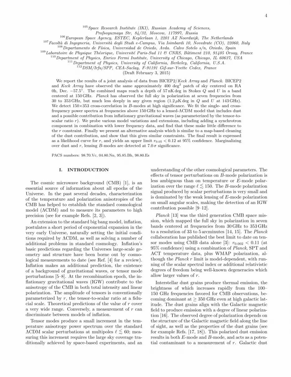
Figure 1 shows the resmoothed Planck 353 GHz T , Q,and U maps before and after filtering. In both casesthe BICEP2/Keck inverse variance apodization mask hasbeen applied. This figure emphasizes the need to ac-count for the filtering before any comparison of maps isattempted, either qualitative or quantitative.

B. Expected spatial and frequency spectra of dust

Before examining the power spectra it is useful to re-view expectations for the spatial and frequency spectraof dust. Figure 2 of PIP-XXX shows that the dust BB(and EE) angular power spectra are well fit by a sim-ple power law D` ∝ `−0.42, where D` = C`` (`+ 1) /2π,when averaging over large regions of sky. Section 5.2 of

6

T unfiltered

−70

−65

−60

−55

−50

−45T filtered

Q unfiltered

−70

−65

−60

−55

−50

−45Q filtered

Right ascension [deg.]

De

clin

atio

n [

de

g.]

U unfiltered

−50050−70

−65

−60

−55

−50

−45U filtered

−50050

−100

0

100

−40

0

40

−40

0

40

µK

µK

µK

FIG. 1. Planck 353 GHz T , Q, and U maps before (left) and after (right) the application of BICEP2/Keck filtering. Inboth cases the maps have been multiplied by the BICEP2/Keck apodization mask. The Planck maps are presmoothed tothe BICEP2/Keck beam profile and have the mean value subtracted. The filtering, in particular the third order polynominalsubtraction to suppress atmospheric pickup, removes large-angular scale signal along the BICEP2/Keck scanning direction(parallel to the right ascension direction in the maps here).

the same paper states that there is no evidence for depar-ture from this behavior for 1% sky patches, although thesignal-to-noise ratio is low for some regions. Presumablywe expect greater fluctuation from the mean behaviorthan would be expected for a Gaussian random field.

The spectral energy distribution (SED) of dust po-larization was measured in Ref. [26] for 400 patcheswith 10◦ radius at intermediate Galactic latitudes. TheSED is well fit by a modified blackbody spectrum withTd = 19.6 K and βd = 1.59±0.17, where the dust temper-ature is obtained from a fit to the SED of total intensity,and the uncertainty on the spectral index represents the1σ dispersion of the individual patch measurements. Theuncertainty is an upper limit, since some fluctuation isdue to noise rather than real variation on the sky. ThisSED is confirmed to be a good match to data when aver-aging over 24% of the cleanest high latitude sky in Fig. 6of PIP-XXX.

C. Power spectrum estimation and results

The power spectrum estimation proceeds exactly as inBK-I, including the matrix based purification operationto prevent E to B mixing. Figure 2 shows the resultsfor BICEP2/Keck and Planck 353 GHz for TT , TE, EE,and BB. In all cases the error bars are the standarddeviations of lensed-ΛCDM+noise simulations [39] andhence contain no sample variance on any other compo-nent. The results in the left column are auto-spectra,identical to those given in BK-I and BK-V—these spec-tra are consistent with lensed-ΛCDM+noise except forthe excess in BB for ` < 200.

The right column of Fig. 2 shows cross-spectra betweentwo halves of the Planck 353 GHz data set, with three dif-ferent splits shown. The Planck collaboration prefers theuse of cross-spectra even at a single frequency to gain ad-ditional immunity to systematics and to avoid the needto noise debias auto-spectra. The TT spectrum is higherthan ΛCDM around ` = 200—presumably due to a dust

7

0

2000

4000

6000

8000150x150

TT

l(l+

1)C

l/2π

[µK

2 ]

BKxBKBxBKxK

0

2000

4000

6000

8000150x353

BKxP353BxP353KxP353

0

2000

4000

6000

8000353half1x353half2

DS1xDS2Y1xY2HR1xHR2

−100

0

100

200

TE

l(l+

1)C

l/2π

[µK

2 ]

−100

0

100

200

BK

ExP353

T

BKTxP353

E

−100

0

100

200

0

2

4

6

EE

l(l+

1)C

l/2π

[µK

2 ]

χ2=19.8, χ=3.2

0

2

4

6 χ2=23.7, χ=9.7

−20

0

20

40 χ2=39.2, χ=14.8

0 50 100 150 200 250 300

−0.02

0

0.02

BB

l(l+

1)C

l/2π

[µK

2 ]

χ2=150.9, χ=31.1

0 50 100 150 200 250 300

−0.6

−0.4

−0.2

0

0.2

0.4

0.6

0.8

−0.02

0

0.02

scal

ed

χ2=76.4, χ=17.5

0 50 100 150 200 250 300

−15

−10

−5

0

5

10

15

20

Multipole

−0.02

0

0.02

scal

ed

χ2=35.6, χ=8.1

FIG. 2. Single- and cross-frequency spectra between BICEP2/Keck maps at 150 GHz and Planck maps at 353 GHz. The leftcolumn shows single-frequency spectra of the BICEP2, Keck Array and combined BICEP2/Keck maps. The BICEP2 spectraare identical to those in BK-I, while the Keck Array and combined are as given in BK-V. The center column shows cross-frequency spectra between BICEP2/Keck maps and Planck 353 GHz maps. The right column shows Planck 353 GHz data-splitcross-spectra. In all cases the error bars are the standard deviations of lensed-ΛCDM+noise simulations and hence contain nosample variance on any other component. For EE and BB the χ2 and χ (sum of deviations) versus lensed-ΛCDM for the ninebandpowers shown is marked at upper/lower left (for the combined BICEP2/Keck points and DS1×DS2). In the bottom row(for BB) the center and right panels have a scaling applied such that signal from dust with the fiducial frequency spectrumwould produce signal with the same apparent amplitude as in the 150 GHz panel on the left (as indicated by the right-sidey-axes). We see from the significant excess apparent in the bottom center panel that a substantial amount of the signal detectedat 150 GHz by BICEP2 and Keck Array indeed appears to be due to dust.

contribution. The EE and BB spectra are noisy, butboth appear to show an excess over ΛCDM for ` < 150—again presumably due to dust. We note that these spec-tra do not appear to follow the power-law expectationmentioned in Sec. II B, but we emphasize that the errorbars contain no sample variance on any dust component(Gaussian or otherwise).

The center column of Fig. 2 shows cross-spectra be-tween BICEP2/Keck and Planck maps. For TE onecan use the T -modes from BICEP2 and the E-modesfrom Planck or vice versa and both options are shown.

Since the T -modes are very similar between the two ex-periments, these TE spectra look similar to the single-experiment TE spectrum which shares the E-modes.The EE and BB cross-spectra are the most interesting—there appears to be a highly significant detection of cor-related B-mode power between 150 and 353 GHz, withthe pattern being much brighter at 353, consistent withthe expectation from dust. We also see hints of detectionin the EE spectrum—while dust E-modes are subdomi-nant to the cosmological signal at 150 GHz, the weak dustcontribution enhances the BK150×P353 cross-spectrum

8

at ` ≈ 100.The polarized dust SED model mentioned in Sec. II B

implies that dust emission is approximately 25 timesbrighter in the Planck 353 GHz band than it is in theBICEP2/Keck 150 GHz band (integrating appropriatelyover the instrumental bandpasses). The expectation for adust-dominated spectrum is thus that the BK150×P353cross-spectrum should have an amplitude 25 times thatof BK150×BK150, and P353×P353 should be 25 timeshigher again. The y-axis scaling in the bottom row ofFig. 2 has been adjusted so that a dust signal obeying thisrule will have equal apparent amplitude in each panel.We see that a substantial amount of the BK150×BK150signal indeed appears to be due to dust.

To make a rough estimate of the significance of devi-ation from lensed-ΛCDM, we calculate χ2 and χ (sumof deviations) for each of the EE and BB spectra andshow these in Fig. 2. For the nine bandpowers used theexpectation value/standard-deviation for χ2 and χ are9/4.2 and 0/3 respectively. We see that BK150×BK150and BK150×P353 are highly significant in BB, whileP353×P353 has modest significance in both EE and BB.

Figure 3 shows EE and BB cross-spectra between BI-CEP2/Keck and all of the polarized frequencies of Planck(also including the BICEP2/Keck auto-spectra). For thefive bandpowers shown the expectation value/standard-deviation for χ2 and χ are 5/3.1 and 0/2.2 respectively.As already noted, the BK150×BK150 and BK150×P353BB spectra show highly significant excesses. Addition-ally, there is evidence for excess BB in BK150×P217spectrum, and for excess EE in BK150×P353. The otherspectra in Fig. 3 show no strong evidence for excess, al-though we note that only one of the χ values is negative.There is weak evidence for excess in the BK150×P70 BBspectrum but none in BK150×P30 so this is presumablyjust a noise fluctation.

There are a large number of additional Planck-onlyspectra, which are not plotted here. The noise on these islarge and all are consistent with ΛCDM, with the possibleexception of P217×P353, where modest evidence for anexcess is seen in both EE and BB (see e.g., Figure 10 ofPIP-XXX).

D. Consistency of BICEP2 and Keck Array spectra

The BB auto-spectra for BICEP2 and Keck Array inthe lower left panel of Fig. 2 appear to differ by morethan might be expected, given that the BICEP2 andKeck maps cover almost exactly the same region of sky.However, the error bars in this figure are the standarddeviations of lensed-ΛCDM+noise simulations; while thesignal is largely common between the two experimentsthe noise is not, and the signal-noise cross terms producesubstantial additional fluctuation of the difference. Thecorrect way to quantify this is to compare the differenceof the real data to the pair-wise differences of simulations,using common input skies that have power similar to that

0

1

2

BK

150x

P30

χ2=5.0, χ=3.3

EE

BKxP

BxP

KxP

−0.1

0

0.1

χ2=5.5, χ=−5.1

BB

0

1

BK

150x

P44

χ2=3.4, χ=1.2

−0.1

0

0.1

χ2=12.5, χ=5.6

0

1

BK

150x

P70

χ2=7.7, χ=3.7

−0.1

0

0.1

χ2=12.4, χ=6.8

0

1

BK

150x

P10

0

χ2=13.0, χ=2.8

0

0.02

0.04χ2=6.9, χ=5.3

0

1

B

K15

0xP

143

χ2=6.0, χ=1.5

0

0.02

0.04χ2=2.9, χ=2.5

0

1

BK

150x

BK

150

χ2=11.5, χ=0.7

0

0.02

0.04χ2=146.9, χ=26.8

0

1

BK

150x

P21

7

χ2=11.6, χ=2.2

0

0.1

0.2

χ2=22.4, χ=8.9

0 100 2000

1

BK

150x

P35

3

χ2=20.4, χ=9.5

0 100 2000

0.1

0.2

χ2=74.6, χ=18.3

Multipole

FIG. 3. EE (left column) and BB (right column) cross-spectra between BICEP2/Keck maps and all of the polarizedfrequencies of Planck. In all cases the quantity plotted is`(` + 1)Cl/2π in units of µK2

CMB. The error bars are thestandard deviations of lensed-ΛCDM+noise simulations andhence contain no sample variance on any other component.Also note that the y-axis scales differ from panel to panel inthe right column. The χ2 and χ (sum of deviations) versuslensed-ΛCDM for the five bandpowers shown is marked atupper left. There are no additional strong detections of devi-ation from lensed-ΛCDM over those already shown in Fig. 2although BK150×P217 shows some evidence of excess.

9

0 50 100 150 200 250 300

−0.4

−0.2

0

0.2

0.4

0.6

Multipole

BB

l(l+

1)C

l/2π

[µK

2 ]

PTEs: 1−5 χ2 0.273, 1−9 χ2 0.415, 1−5 χ 0.802, 1−9 χ 0.425

B150xP353−K150xP353

FIG. 4. Differences of B150×P353 and K150×P353 BB cross-spectra. The error bars are the standard deviations of thepairwise differences of signal+noise simulations that sharecommon input skies. The probability to exceed the observedvalues of χ2 and χ statistics, as evaluated against the simula-tions, is quoted for bandpower ranges 1–5 (20 < ` < 200) and1–9 (20 < ` < 330). There is no evidence that these spectraare statistically incompatible.

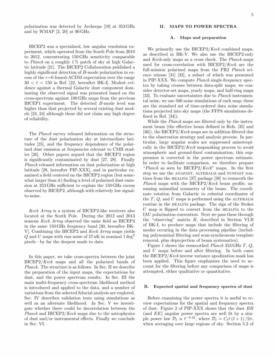
observed in the real data. This was done in Section 8 ofBK-V and the BICEP2 and Keck maps were shown to bestatistically compatible. In an analogous manner we canalso ask if the B150×P353 and K150×P353 BB cross-spectra shown in the bottom middle panel of Fig. 2 arecompatible. Figure 4 shows the results. We calculate theχ2 and χ statistics on these difference spectra and com-pare to the simulated distributions exactly as in BK-V.The probability to exceed (PTE) the observed values isgiven in the figure for bandpowers 1–5 (20 < ` < 200)and 1–9 (20 < ` < 330). There is no evidence that thesespectra are statistically incompatible.

E. Alternative power spectrum estimation

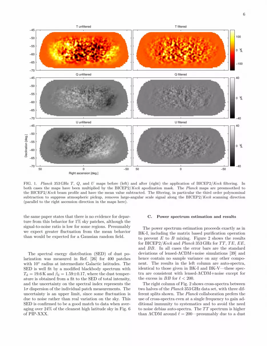
We check the reliability of the power spectrum estima-tion with an alternative pipeline. The filtered and puri-fied Planck and BICEP2 maps used to make the spectrashown in Fig. 2 are transformed back into the healpixpixelization using cubic spline interpolation. The B-mode cross-power is then computed with the Xpol [40]and PureCl [41] estimators. Figure 5 shows the differ-ence between these alternative bandpowers and the stan-dard bandpowers for the B150×P353 BB cross spectrum.As in Fig. 4 the errorbars are the standard deviations ofpairwise differences of simulations, which share commoninput skies and have power similar to that observed inthe real data. The agreement is not expected to be ex-act due to the differing bandpower window functions, butthe differences of the real bandpowers are consistent withthose of the simulations.

0 50 100 150 200 250 300

−0.4

−0.2

0

0.2

0.4

0.6

Multipole

BB

l(l+

1)C

l/2π

[µK

2 ]

Std−XPOLStd−PureCl

FIG. 5. Differences of B150×P353 BB cross-spectra from thestandard power spectrum estimator and alternate estimators.The error bars are the standard deviations of the pairwise dif-ferences of signal+noise simulations that share common inputskies. We see that the differences of the real spectra are con-sistent with the differences of the simulations.

III. LIKELIHOOD ANALYSIS

A. Algorithm

While it is conventional in plots like Fig. 2 to presentbandpowers with symmetric error bars, it is important toappreciate that this is an approximation. The likelihoodof an observed bandpower for a given model expecta-tion value is generally an asymmetric function, which canbe computed given knowledge of the noise level(s). Tocompute the joint likelihood of an ensemble of measuredbandpower values it is of course necessary to considertheir full covariance—this is especially important whenusing spectra taken at different frequencies on the samefield, where the signal covariance can be very strong.

We compute the bandpower covariance using fullsimulations of signal-cross-signal, noise-cross-noise, andsignal-cross-noise. From these, we can construct the co-variance matrix for a general model containing multiplesignal components with any desired set of SEDs. Whenwe do this we deliberately exclude terms whose expecta-tion value is zero, in order to reduce noise in the resultingmatrix due to the limited number of simulated realiza-tions.

To compute the joint likelihood of the data for anygiven proposed model we use the Hamimeche-Lewis [42]approximation (HL; see Section 9.1 of Ref. [43] for imple-mentation details). Here we extend the method to dealwith single- and cross-frequency spectra, and the covari-ances thereof, in an analogous manner to the treatmentof, for example, TT , TE, and EE in the standard HLmethod. The HL formulation requires that the band-power covariance matrix be determined for only a single“fiducial model.” We compute multi-dimensional gridsof models explicitly and/or use COSMOMC [44] to sample

10

the parameter space.

B. Fiducial analysis

As an extension of the simplest lensed-ΛCDMparadigm, we initially consider a two component modelof IGW with amplitude r, plus dust with amplitude Ad

(specified at 353 GHz and ` = 80). (Here we assumethat the spectral index of the tensor modes (nt) is zero,and a scalar pivot scale of 0.05 Mpc−1; all values of rquoted in this paper are r0.05 unless noted otherwise.)Figure 6 shows the results of fitting such a model toBB bandpowers taken between BICEP2/Keck and the217 and 353 GHz bands of Planck, using bandpowers 1–5(20 < ` < 200). For the Planck single-frequency case,the cross-spectrum of detector-sets (DS1×DS2) is used,following PIP-XXX. The dust is modeled as a power lawD` ∝ `−0.42, with free amplitude Ad and scaling withfrequency according to the modified blackbody model.

A tight Gaussian prior βd = 1.59 ± 0.11 is imposed,since this parameter is not well constrained from thesedata alone, but does appear to be stable across the sky(see Secs. II B and V A). For the frequency range of inter-est here variations in the two parameters of the modifiedblackbody are highly degenerate and the choice is madeto hold Td fixed while allowing βd to be free. The prior as-sumes that the SED of dust polarization at intermediatelatitudes [26] applies to the BICEP2/Keck field, wherethe signal-to-noise ratio of the Planck data is too low todetermine it directly. From dust astrophysics, we expectvariations of the dust SED in intensity and polarizationto be correlated [18]. We thus tested our assumption bymeasuring the spectral index of the dust total intensity inthe BICEP2/Keck field using the template fitting analy-sis described in Ref. [45], and find the same value. Theuncertainty on βd is scaled from the dispersion of spectralindices at intermediate Galactic latitudes in Ref. [26], asexplained in PIP-XXX.

In Fig. 6 we see that the BICEP2 data produce an rlikelihood that peaks higher than that for the Keck Ar-ray data. This is because for ` < 120 the auto-spectrumB150×B150 is higher than for K150×K150, while thecross-spectrum B150×P353 is lower than K150×P353(see Fig. 2). However, recall that both pairs of spectraB150×B150/K150×K150 and B150×P353/K150×P353have been shown to be consistent within noise fluctua-tion (see Sec. II D). In Sec. IV A these likelihood resultsare also found to be compatible. Given the consistencybetween the two experiments, the combined result givesthe best available measurement of the sky.

The combined curves (BK+P) in the left and cen-ter panels of Fig. 6 yield the following results: r =0.048+0.035

−0.032, r < 0.12 at 95% confidence, and Ad =

3.3+0.9−0.8. For r the zero-to-peak likelihood ratio is 0.38.

Taking 12 (1− f (−2 logL0/Lpeak)), where f is the χ2 cdf

(for one degree of freedom), we estimate that the proba-bility to get a number smaller than this is 8% if in fact

r = 0. For Ad the zero-to-peak ratio is 1.8× 10−6 corre-sponding to a smaller-than probability of 1.4×10−7, anda 5.1σ detection of dust power.

The maximum likelihood model on the grid has pa-rameters r = 0.05, Ad = 3.30µK2 (and βd = 1.6). Com-puting the bandpower covariance matrix for this model,we obtain a χ2 of 40.9. Using 28 degrees of freedom—5 bandpowers times 6 spectra, minus 2 fit parameters(since βd is not really free)—gives a PTE of 0.06. Thelargest contributions to χ2 come from the P353×P353spectrum shown in the lower right panel of Fig. 2.

C. Variations from the fiducial data set and model

We now investigate a number of variations from thefiducial analysis to see what difference these make to theconstraint on r.

• Choice of Planck single-frequency spectra:switching the Planck single-frequency spectra touse one of the alternative data splits (yearly or half-ring instead of detector-set) makes little difference(see Fig. 7).

• Using only 150 and 353 GHz: dropping thespectra involving 217 GHz from consideration alsohas little effect (see Fig. 7).

• Using only BK150×BK150 andBK150×P353: also excluding the 353 GHzsingle-frequency spectrum from considerationmakes little difference. The statistical weight ofthe BK150×BK150 and BK150×P353 spectradominate (see Fig. 7).

• Extending the bandpower range: going backto the base data set and extending the range ofbandpowers considered to 1–9 (corresponding to20 < ` < 330) makes very little difference—thedominant statistical weight is with the lower band-powers (see Fig. 7).

• Including EE spectra: we can also include inthe fits the EE spectra shown in Fig. 3. PIP-XXX(figures 5 and A.3) shows that the level of EE fromGalactic dust is on average around twice the levelof BB. However, there are substantial variationsin this ratio from sky-patch to sky-patch. SettingEE/BB = 2 we find that the constraint on Ad

narrows, while the r constraint changes little; thislatter result is also shown in Fig. 7.

• Relaxing the βd prior: relaxing the prior on thedust spectral index to βd = 1.59± 0.33 pushes thepeak of the r constraint up (see Fig. 7). However,it is not clear if this looser prior is self consistent;if the frequency spectral index varied significantlyacross the sky it would invalidate cross-spectralanalysis, but there is strong evidence against such

11

0 0.05 0.1 0.15 0.2 0.25 0.30

0.2

0.4

0.6

0.8

1

r

L/L pe

ak

BK+PB+PK+P

0 1 2 3 4 5 6 70

0.2

0.4

0.6

0.8

1

Ad @ l=80 & 353 GHz [µK2]

L/L pe

ak

r

Ad @

l=80

& 3

53 G

Hz

[µK

2 ]

0 0.05 0.1 0.15 0.2 0.25 0.30

1

2

3

4

5

6

7

FIG. 6. Likelihood results from a basic lensed-ΛCDM+r+dust model, fitting BB auto- and cross-spectra taken between mapsat 150 GHz, 217, and 353 GHz. The 217 and 353 GHz maps come from Planck. The primary results (heavy black) use the150 GHz combined maps from BICEP2/Keck. Alternate curves (light blue and red) show how the results vary when theBICEP2 and Keck Array only maps are used. In all cases a Gaussian prior is placed on the dust frequency spectrum parameterβd = 1.59 ± 0.11. In the right panel the two dimensional contours enclose 68% and 95% of the total likelihood.

variation at high latitude, as explained in Sec. V A.Nevertheless, it is important to appreciate that ther constraint curves shown in Fig. 6 shift left (right)when assuming a lower (higher) value of βd. Forβd = 1.3 ± 0.11 the peak is at r = 0.021 and forβd = 1.9± 0.11 the peak is at r = 0.073.

• Varying the dust power spectrum shape: inthe fiducial analysis the dust spatial power spec-trum is assumed to be a power law with D` ∝`−0.42. Marginalizing over spectral indices in therange −0.8 to 0 we find little change in the r con-straint (see also Sec. IV B for an alternate relax-ation of the assumptions regarding the spatial prop-erties of the dust pattern).

• Using Gaussian determinant likelihood: thefiducial analysis uses the HL likelihood approx-imation, as described in Sec. III A. An alterna-tive is to recompute the covariance matrix C ateach point in parameter space and take L =det (C)−1/2 exp (−(dTC−1d)/2), where d is the de-viation of the observed bandpowers from the modelexpectation values. This results in an r constraintwhich peaks slightly lower, as shown in Fig. 7. Run-ning both methods on the simulated realizationsdescribed in Sec. IV A, indicates that such a dif-ference is not unexpected and that there may bea small systematic downward bias in the Gaussiandeterminant method.

• Varying the HL fiducial model: as mentionedin Sec. III A the HL likelihood formulation requiresthat the expectation values and bandpower co-variance matrix be provided for a single “fiducialmodel” (not to be confused with the “fiducial anal-ysis” of Sec. III B). Normally we use the lensed-ΛCDM+dust simulations described in Sec. IV A be-low. Switching this to lensed-ΛCDM+r=0.2 pro-duces no change on average in the simulations, al-

though it does cause any given realization to shiftslightly—the change for the real data case is shownin Fig. 7.

• Adding synchrotron: BK-I took the WMAP K -band (23 GHz) map, extrapolated it to 150 GHz ac-cording to ν−3.3 (mean value within the BICEP2field of the MCMC “Model f” spectral index mapprovided by WMAP [2]), and found a negligiblepredicted contribution (rsync,150 = 0.0008±0.0041).Figure 3 does not offer strong motivation to reex-amine this finding—the only significant detectionsof correlated BB power are in the BK150×P353and, to a lesser extent, BK150×P217 spectra. How-ever, here we proceed to a fit including all thepolarized bands of Planck (as shown in Fig. 3)and adding a synchrotron component to the baselensed-ΛCDM+noise+r+dust model. We take syn-chrotron to have a power law spectrum D` ∝`−0.6 [23], with free amplitude Async, where Async isthe amplitude at ` = 80 and at 150 GHz, and scal-ing with frequency according to ν−3.3. In such ascenario we can vary the degree of correlation thatis assumed between the dust and synchrotron skypatterns. Figure 8 shows results for the uncorre-lated and fully correlated cases. Marginalizing overr and Ad we find Async < 0.0003µK2 at 95% con-fidence for the uncorrelated case, and many timessmaller for the correlated. This last is because onceone has a detection of dust it effectively becomesa template for the synchrotron. This synchrotronlimit is driven by the Planck 30 GHz band—we ob-tain almost identical results when adding only thisband, and a much softer limit when not including it.If we instead assume synchrotron scaling of ν−3.0

the limit on Async is approximately doubled for theuncorrelated case and reduced for the correlated.(Because the DS1×DS2 data-split is not availablefor the Planck LFI bands we switch to Y1×Y2 for

12

0 0.05 0.1 0.15 0.2 0.25 0.30

0.1

0.2

0.3

0.4

0.5

0.6

0.7

0.8

0.9

1

r

L/L pe

ak

Fiducial analysisY1xY2no 217GHzOnly BKxBK&BKxP3539 bandpowersInc. EE (EE/BB=2)relax β

d prior

Gauss detalt. HL fid. model

FIG. 7. Likelihood results when varying the data sets usedand the model priors—see Sec III C for details.

this variant analysis, and so we compare to thiscase in Fig. 8 rather than the usual fiducial case.)

• Varying lensing amplitude: in the fiducial anal-ysis the amplitude of the lensing effect is heldfixed at the ΛCDM expectation (AL = 1). Usingtheir own and other data, the Planck Collabora-tion quote a limit on the amplitude of the lens-ing effect versus the ΛCDM expectation of AL =0.99 ± 0.05 [3]. Allowing AL to float freely, andusing all nine bandpowers, we obtain the resultsshown in Fig. 9—there is only weak degeneracy be-tween AL and both r and Ad. Marginalizing over rand Ad we find AL = 1.13± 0.18 with a likelihoodratio between zero and peak of 3×10−11. Using theexpression given in Sec. III B this corresponds to asmaller-than probability of 2×10−12, equivalent toa 7.0σ detection of lensing in the BB spectrum.We note this is the most significant to-date directmeasurement of lensing in B-mode polarization.

IV. LIKELIHOOD VALIDATION

A. Validation with simulations

We run the algorithm used in Sec. III B on ensembles ofsimulated realizations to check its performance. We firstconsider a model where r = 0 and Ad = 3.6µK2, this lat-ter being close to the value favored by the data in a dust-only scenario [46]. We generate Gaussian random real-izations using the fiducial spatial power law D` ∝ `−0.42,scale these to the various frequency bands using the mod-ified blackbody law with Td = 19.6 K and βd = 1.59,and add to the usual realizations of lensed-ΛCDM+noise.Figure 10 shows the resulting r and Ad constraint curves,with the result for the real data from Fig. 6 overplotted.As expected, approximately 50% of the r likelihoods peak

0 0.1 0.2 0.30

0.2

0.4

0.6

0.8

1

r

No Sync+Sync uncorr.+Sync 100% corr

Async

@ l=80 & 150GHz [µK2]

Ad @

l=80

& 3

53G

Hz

[µK

2 ]

0 1 2 3 4

x 10−4

0

1

2

3

4

5

6

7

FIG. 8. Likelihood results for a fit when adding the lowerfrequency bands of Planck, and extending the model to in-clude a synchrotron component. The results for two differ-ent assumed degrees of correlation between the dust and syn-chrotron sky patterns are compared to those for the compa-rable model without synchrotron (see text for details).

0 0.1 0.2 0.30

0.2

0.4

0.6

0.8

1

1.2

1.4

1.6

r

AL

0 2 4 60

0.2

0.4

0.6

0.8

1

1.2

1.4

1.6

Ad @ l=80 & 353GHz [µK2]

AL

FIG. 9. Likelihood results for a fit allowing the lensingscale factor AL to float freely and using all nine bandpowers.Marginalizing over r and Ad, we find that AL = 1.13 ± 0.18and AL = 0 is ruled out with 7.0σ significance.

above zero. The median 95% upper limit is r < 0.075.We find that 8% of the realizations have a ratio L0/Lpeak

less than the 0.38 observed in the real data, in agreementwith the estimate in Sec. III B. Running these dust-onlyrealizations for BICEP2 only and Keck Array only, wefind that the shift in the maximum likelihood value of rseen in the real data in Fig. 6 is exceeded in about 10%of the simulations.

The above simulations assume that the dust compo-nent follows on average the fiducial D` ∝ `−0.42 spatialpower law, and fluctuates around it in a Gaussian man-ner. To obtain sample dust sky patterns that may deviatefrom this behavior in a way which better reflects reality,we take the pre-launch version of the Planck Sky Model(PSM; version 1.7.8 run in “simulation” mode) [24] eval-uated in the Planck 353 GHz band and pull out the same352 |b|> 35◦ partially overlapping regions used in PIP-XXX. We then scale these to the other bands and proceedas before. Figure 11 presents the results. Some of the re-gions have dust power orders of magnitude higher thanthe real data and we cut them out (selecting 139 regionswith peak Ad < 20µK2). The r likelihoods will broaden

13

0 0.2 0.40

0.2

0.4

0.6

0.8

1

r0 5 10 15

0

0.2

0.4

0.6

0.8

1

Ad @ l=80 & 353GHz [µK2]

FIG. 10. Likelihoods for r and Ad, using BICEP2/Keckand Planck, as plotted in Fig. 6, overplotted on constraintsobtained from realizations of a lensed-ΛCDM+noise+dustmodel with dust power similar to that favored by the realdata (Ad = 3.6µK2). Half of the r curves peak at zero asexpected.

0 0.2 0.40

0.2

0.4

0.6

0.8

1

r0 5 10 15

0

0.2

0.4

0.6

0.8

1

Ad @ l=80 & 353GHz [µK2]

FIG. 11. Constraints obtained when adding dust realizationsfrom the Planck Sky Model version 1.7.8 to the base lensed-ΛCDM+noise simulations. (Curves for 139 regions with peakAd < 20µK2 are plotted). We see that the results for rare unbiased in the presence of dust realizations which donot necessarily follow the `−0.42 power law or have Gaussianfluctuations about it.

as the level of Ad increases, and we should therefore notbe surprised if the fraction of realizations peaking at avalue higher than the real data is increased compared tothe simulations with mean Ad = 3.6µK2. However westill expect that on average 50% will peak above zero andapproximately 8% will have an L0/Lpeak ratio less thanthe 0.38 observed in the real data. In fact we find 57%and 7%, respectively, consistent with the expected val-ues. There is one realization which has a nominal (false)detection of non-zero r of 3.3σ, although this turns out toalso have one of the lowest L0/Lpeak ratios in the Gaus-sian simulations shown in Fig. 10 (with which it sharesthe CMB and noise components), so this is apparentlyjust a relatively unlikely fluctuation.

0 50 100 150 200 250 300−0.01

0

0.01

0.02

0.03

0.04

0.05

Multipole

BB

l(l+

1)C

l/2π

[µK

2 ]

BKxBK(BKxBK−αBKxP)/(1−α)

0 0.1 0.2 0.30

0.2

0.4

0.6

0.8

1

r

L/L pe

ak

Fiducial analysisCleaning analysis

FIG. 12. Upper: BB spectrum of the BICEP2/Keck mapsbefore and after subtraction of the dust contribution, esti-mated from the cross-spectrum with Planck 353 GHz. Theerror bars are the standard deviations of simulations, which,in the latter case, have been scaled and combined in the sameway. The inner error bars are from lensed-ΛCDM+noise sim-ulations as in the previous plots, while the outer error barsare from the lensed-ΛCDM+noise+dust simulations. Lower:constraint on r derived from the cleaned spectrum comparedto the fiducial analysis shown in Fig. 6.

B. Subtraction of scaled spectra

As previously mentioned, the modified blackbodymodel predicts that dust emission is 4% as bright in theBICEP2 band as it is in the Planck 353 GHz band. There-fore, taking the auto- and cross-spectra of the combinedBICEP2/Keck maps and the Planck 353 GHz maps, asshown in the bottom row of Fig. 2, and evaluating(BK×BK−αBK×P)/(1−α), at α = αfid cleans out thedust contribution (where αfid = 0.04). The upper panelof Fig. 12 shows the result.

As an alternative to the full likelihood analysis pre-sented in Sec. III B, we can instead work with the dif-ferenced spectra from above, a method we denote the“cleaning” approach. If αfid were the true value, the ex-

14

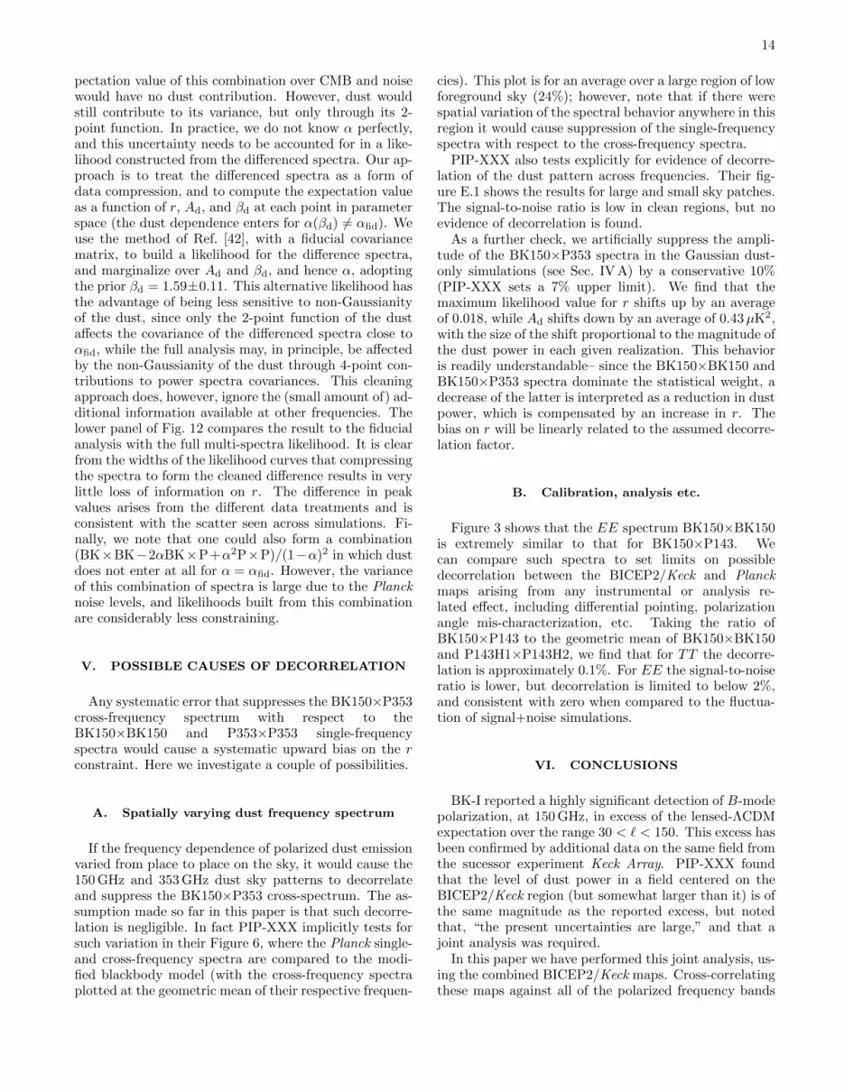
pectation value of this combination over CMB and noisewould have no dust contribution. However, dust wouldstill contribute to its variance, but only through its 2-point function. In practice, we do not know α perfectly,and this uncertainty needs to be accounted for in a like-lihood constructed from the differenced spectra. Our ap-proach is to treat the differenced spectra as a form ofdata compression, and to compute the expectation valueas a function of r, Ad, and βd at each point in parameterspace (the dust dependence enters for α(βd) 6= αfid). Weuse the method of Ref. [42], with a fiducial covariancematrix, to build a likelihood for the difference spectra,and marginalize over Ad and βd, and hence α, adoptingthe prior βd = 1.59±0.11. This alternative likelihood hasthe advantage of being less sensitive to non-Gaussianityof the dust, since only the 2-point function of the dustaffects the covariance of the differenced spectra close toαfid, while the full analysis may, in principle, be affectedby the non-Gaussianity of the dust through 4-point con-tributions to power spectra covariances. This cleaningapproach does, however, ignore the (small amount of) ad-ditional information available at other frequencies. Thelower panel of Fig. 12 compares the result to the fiducialanalysis with the full multi-spectra likelihood. It is clearfrom the widths of the likelihood curves that compressingthe spectra to form the cleaned difference results in verylittle loss of information on r. The difference in peakvalues arises from the different data treatments and isconsistent with the scatter seen across simulations. Fi-nally, we note that one could also form a combination(BK×BK−2αBK×P+α2P×P)/(1−α)2 in which dustdoes not enter at all for α = αfid. However, the varianceof this combination of spectra is large due to the Plancknoise levels, and likelihoods built from this combinationare considerably less constraining.

V. POSSIBLE CAUSES OF DECORRELATION

Any systematic error that suppresses the BK150×P353cross-frequency spectrum with respect to theBK150×BK150 and P353×P353 single-frequencyspectra would cause a systematic upward bias on the rconstraint. Here we investigate a couple of possibilities.

A. Spatially varying dust frequency spectrum

If the frequency dependence of polarized dust emissionvaried from place to place on the sky, it would cause the150 GHz and 353 GHz dust sky patterns to decorrelateand suppress the BK150×P353 cross-spectrum. The as-sumption made so far in this paper is that such decorre-lation is negligible. In fact PIP-XXX implicitly tests forsuch variation in their Figure 6, where the Planck single-and cross-frequency spectra are compared to the modi-fied blackbody model (with the cross-frequency spectraplotted at the geometric mean of their respective frequen-

cies). This plot is for an average over a large region of lowforeground sky (24%); however, note that if there werespatial variation of the spectral behavior anywhere in thisregion it would cause suppression of the single-frequencyspectra with respect to the cross-frequency spectra.

PIP-XXX also tests explicitly for evidence of decorre-lation of the dust pattern across frequencies. Their fig-ure E.1 shows the results for large and small sky patches.The signal-to-noise ratio is low in clean regions, but noevidence of decorrelation is found.

As a further check, we artificially suppress the ampli-tude of the BK150×P353 spectra in the Gaussian dust-only simulations (see Sec. IV A) by a conservative 10%(PIP-XXX sets a 7% upper limit). We find that themaximum likelihood value for r shifts up by an averageof 0.018, while Ad shifts down by an average of 0.43µK2,with the size of the shift proportional to the magnitude ofthe dust power in each given realization. This behavioris readily understandable– since the BK150×BK150 andBK150×P353 spectra dominate the statistical weight, adecrease of the latter is interpreted as a reduction in dustpower, which is compensated by an increase in r. Thebias on r will be linearly related to the assumed decorre-lation factor.

B. Calibration, analysis etc.

Figure 3 shows that the EE spectrum BK150×BK150is extremely similar to that for BK150×P143. Wecan compare such spectra to set limits on possibledecorrelation between the BICEP2/Keck and Planckmaps arising from any instrumental or analysis re-lated effect, including differential pointing, polarizationangle mis-characterization, etc. Taking the ratio ofBK150×P143 to the geometric mean of BK150×BK150and P143H1×P143H2, we find that for TT the decorre-lation is approximately 0.1%. For EE the signal-to-noiseratio is lower, but decorrelation is limited to below 2%,and consistent with zero when compared to the fluctua-tion of signal+noise simulations.

VI. CONCLUSIONS

BK-I reported a highly significant detection of B-modepolarization, at 150 GHz, in excess of the lensed-ΛCDMexpectation over the range 30 < ` < 150. This excess hasbeen confirmed by additional data on the same field fromthe sucessor experiment Keck Array. PIP-XXX foundthat the level of dust power in a field centered on theBICEP2/Keck region (but somewhat larger than it) is ofthe same magnitude as the reported excess, but notedthat, “the present uncertainties are large,” and that ajoint analysis was required.

In this paper we have performed this joint analysis, us-ing the combined BICEP2/Keck maps. Cross-correlatingthese maps against all of the polarized frequency bands

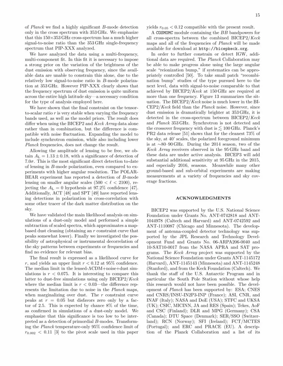
15

of Planck we find a highly significant B-mode detectiononly in the cross spectrum with 353 GHz. We emphasizethat this 150×353 GHz cross-spectrum has a much highersignal-to-noise ratio than the 353 GHz single-frequencyspectrum that PIP-XXX analyzed.

We have analyzed the data using a multi-frequency,multi-component fit. In this fit it is necessary to imposea strong prior on the variation of the brightness of thedust emission with observing frequency, since the avail-able data are unable to constrain this alone, due to therelatively low signal-to-noise ratio in B-mode polariza-tion at 353 GHz. However PIP-XXX clearly shows thatthe frequency spectrum of dust emission is quite uniformacross the entire high latitude sky—a necessary conditionfor the type of analysis employed here.

We have shown that the final constraint on the tensor-to-scalar ratio r is very stable when varying the frequencybands used, as well as the model priors. The result doesdiffer when using the BICEP2 and Keck Array data alonerather than in combination, but the difference is com-patible with noise fluctuation. Expanding the model toinclude synchrotron emission, while also including lowerPlanck frequencies, does not change the result.

Allowing the amplitude of lensing to be free, we ob-tain AL = 1.13± 0.18, with a significance of detection of7.0σ. This is the most significant direct detection to-dateof lensing in B-mode polarization, even compared to ex-periments with higher angular resolution. The POLAR-BEAR experiment has reported a detection of B-modelensing on smaller angular scales (500 < ` < 2100), re-jecting the AL = 0 hypothesis at 97.2% confidence [47].Additionally, ACT [48] and SPT [49] have reported lens-ing detections in polarization in cross-correlation withsome other tracer of the dark matter distribution on thesky.

We have validated the main likelihood analysis on sim-ulations of a dust-only model and performed a simplesubtraction of scaled spectra, which approximates a map-based dust cleaning (obtaining an r constraint curve thatpeaks somewhat lower). Finally we investigated the pos-sibility of astrophysical or instrumental decorrelation ofthe sky patterns between experiments or frequencies andfind no evidence for relevant bias.

The final result is expressed as a likelihood curve forr, and yields an upper limit r < 0.12 at 95% confidence.The median limit in the lensed-ΛCDM+noise+dust sim-ulations is r < 0.075. It is interesting to compare thislatter to dust-free simulations using only BICEP2/Keckwhere the median limit is r < 0.03—the difference rep-resents the limitation due to noise in the Planck maps,when marginalizing over dust. The r constraint curvepeaks at r = 0.05 but disfavors zero only by a fac-tor of 2.5. This is expected by chance 8% of the time,as confirmed in simulations of a dust-only model. Weemphasize that this significance is too low to be inter-preted as a detection of primordial B-modes. Transform-ing the Planck temperature-only 95% confidence limit ofr0.002 < 0.11 [3] to the pivot scale used in this paper

yields r0.05 < 0.12 compatible with the present result.A COSMOMC module containing the BB bandpowers for

all cross-spectra between the combined BICEP2/Keckmaps and all of the frequencies of Planck will be madeavailable for download at http://bicepkeck.org.

In order to further constrain or detect IGW, addi-tional data are required. The Planck Collaboration maybe able to make progress alone using the large angularscale “reionization bump,” if systematics can be appro-priately controlled [50]. To take small patch “recombi-nation bump” studies of the type pursued here to thenext level, data with signal-to-noise comparable to thatachieved by BICEP2/Keck at 150 GHz are required atmore than one frequency. Figure 13 summarizes the sit-uation. The BICEP2/Keck noise is much lower in the BI-CEP2/Keck field than the Planck noise. However, sincedust emission is dramatically brighter at 353 GHz, it isdetected in the cross-spectrum between BICEP2/Keckand Planck 353 GHz. Synchrotron is not detected andthe crossover frequency with dust is <∼ 100 GHz. Planck’sPR2 data release [51] shows that for the cleanest 73% ofthe sky, at 40’ scales, the polarized foreground minimumis at ∼80–90 GHz. During the 2014 season, two of theKeck Array receivers observed in the 95 GHz band andthese data are under active analysis. BICEP3 will addsubstantial additional sensitivity at 95 GHz in the 2015,and especially 2016, seasons. Meanwhile many otherground-based and sub-orbital experiments are makingmeasurements at a variety of frequencies and sky cov-erage fractions.

ACKNOWLEDGMENTS

BICEP2 was supported by the U.S. National ScienceFoundation under Grants No. ANT-0742818 and ANT-1044978 (Caltech and Harvard) and ANT-0742592 andANT-1110087 (Chicago and Minnesota). The develop-ment of antenna-coupled detector technology was sup-ported by the JPL Research and Technology Devel-opment Fund and Grants No. 06-ARPA206-0040 and10-SAT10-0017 from the NASA APRA and SAT pro-grams. The Keck Array project was supported by theNational Science Foundation under Grants ANT-1145172(Harvard), ANT-1145143 (Minnesota) and ANT-1145248(Stanford), and from the Keck Foundation (Caltech). Wethank the staff of the U.S. Antarctic Program and inparticular the South Pole Station without whose helpthis research would not have been possible. The devel-opment of Planck has been supported by: ESA; CNESand CNRS/INSU-IN2P3-INP (France); ASI, CNR, andINAF (Italy); NASA and DoE (USA); STFC and UKSA(UK); CSIC, MICINN, JA and RES (Spain); Tekes, AoFand CSC (Finland); DLR and MPG (Germany); CSA(Canada); DTU Space (Denmark); SER/SSO (Switzer-land); RCN (Norway); SFI (Ireland); FCT/MCTES(Portugal); and ERC and PRACE (EU). A descrip-tion of the Planck Collaboration and a list of its

16

0 50 100 150 200 250 300 35010

−4

10−3

10−2

10−1

100

101

Sync upper lim

it

Dust

BK noise uncer.

Planck noise uncer. in BK field

BKxP noise uncer.

lensed−LCDM

r=0.05

Nominal band center [GHz]

BB

in l∼

80 b

andp

ower

l(l+

1)C

l/2π

[µK

2 ]

FIG. 13. Expectation values, and uncertainties thereon,for the ` ∼ 80 BB bandpower in the BICEP2/Keck field.The green and magenta lines correspond to the expected sig-nal power of lensed-ΛCDM and r = 0.05. Since CMB unitsare used, the levels corresponding to these are flat with fre-quency. The grey band shows the best fit dust model (see Sec-tion III B) and the blue shaded region shows the allowed re-gion for synchrotron (see Sec. III C). The BICEP2/Keck noiseuncertainty is shown as a single starred point, and the noiseuncertainties of the Planck single-frequency spectra evaluatedin the BICEP2/Keck field are shown in red. The blue pointsshow the noise uncertainty of the cross-spectra taken betweenBICEP2/Keck and, from left to right, Planck 30, 44, 70, 100,143, 217 & 353 GHz, and plotted at horizontal positions suchthat they can be compared vertically with the dust and synccurves.

members, including the technical or scientific activi-ties in which they have been involved, can be foundat http://www.sciops.esa.int/index.php?project=planck&page=Planck_Collaboration.

[1] A. A. Penzias and R. W. Wilson, Astrophys. J. 142, 419(1965).

[2] C. L. Bennett, D. Larson, J. L. Weiland, N. Jarosik,G. Hinshaw, N. Odegard, K. M. Smith, R. S. Hill,B. Gold, M. Halpern, E. Komatsu, M. R. Nolta, L. Page,D. N. Spergel, E. Wollack, J. Dunkley, A. Kogut,M. Limon, S. S. Meyer, G. S. Tucker, and E. L.Wright, Astrophys. J. Suppl. Ser. 208, 20 (2013),arXiv:1212.5225.

[3] Planck Collaboration XVI, Astron. Astrophys. 571, A16(2014), arXiv:1303.5076 [astro-ph.CO].

[4] Planck Collaboration XXII, Astron. Astrophys. 571, A22(2014), arXiv:1303.5082.

[5] A. A. Starobinsky, Zh. Eksp. Teor. Fiz. Pisma Red. 30,719 (1979).

[6] V. A. Rubakov, M. V. Sazhin, and A. V. Veryaskin,Phys. Lett. B 115, 189 (1982).

[7] R. Fabbri and M. D. Pollock, Phys. Lett. B 125, 445(1983).

[8] L. F. Abbott and M. B. Wise, Nucl. Phys. B 244, 541(1984).

[9] A. G. Polnarev, Sov. Astron. 29, 607 (1985).[10] U. Seljak and M. Zaldarriaga, Phys. Rev. Lett. 78, 2054

(1997), astro-ph/9609169.

[11] U. Seljak, Astrophys. J. 482, 6 (1997), astro-ph/9608131.[12] M. Kamionkowski, A. Kosowsky, and A. Stebbins, Phys.

Rev. Lett. 78, 2058 (1997), astro-ph/9609132.[13] Planck (http://www.esa.int/planck) is a project of the

European Space Agency (ESA) with instruments pro-vided by two scientific consortia funded by ESA memberstates (in particular the lead countries, France and Italy)with contributions from NASA (USA), and telescope re-flectors provided in a collaboration between ESA and ascientific consortium led and funded by Denmark.

[14] Planck Collaboration 2011A, Astron. Astrophys. 536, A1(2011).

[15] Planck Collaboration I, Astron. Astrophys. 571, A1(2014).

[16] R. H. Hildebrand, J. L. Dotson, C. D. Dowell, D. A.Schleuning, and J. E. Vaillancourt, Astrophys. J. 516,834 (1999).

[17] B. T. Draine, in The Cold Universe, Saas-Fee AdvancedCourse 32, Springer-Verlag, 308 pages, 129 figures, Lec-ture Notes 2002 of the Swiss Society for Astronomy andAstrophysics (SSAA), Springer, 2004. Edited by A.W.Blain, F. Combes, B.T. Draine, D. Pfenniger and Y.Revaz, ISBN 354040838x, p. 213, edited by A. W. Blain,F. Combes, B. T. Draine, D. Pfenniger, and Y. Revaz

17

(2004) p. 213, astro-ph/0304488.[18] P. G. Martin, in EAS Publications Series, EAS Publica-

tions Series, Vol. 23, edited by M.-A. Miville-Deschenesand F. Boulanger (2007) pp. 165–188, astro-ph/0606430.

[19] A. Benoıt, P. Ade, A. Amblard, R. Ansari, E. Aubourg,S. Bargot, J. G. Bartlett, J.-P. Bernard, R. S. Bha-tia, A. Blanchard, J. J. Bock, A. Boscaleri, F. R.Bouchet, A. Bourrachot, P. Camus, F. Couchot, P. deBernardis, J. Delabrouille, F.-X. Desert, O. Dore,M. Douspis, L. Dumoulin, X. Dupac, P. Filliatre, P. Fos-alba, K. Ganga, F. Gannaway, B. Gautier, M. Gi-ard, Y. Giraud-Heraud, R. Gispert, L. Guglielmi, J.-C. Hamilton, S. Hanany, S. Henrot-Versille, J. Ka-plan, G. Lagache, J.-M. Lamarre, A. E. Lange, J. F.Macıas-Perez, K. Madet, B. Maffei, C. Magneville, D. P.Marrone, S. Masi, F. Mayet, A. Murphy, F. Naraghi,F. Nati, G. Patanchon, G. Perrin, M. Piat, N. Pon-thieu, S. Prunet, J.-L. Puget, C. Renault, C. Rosset,D. Santos, A. Starobinsky, I. Strukov, R. V. Sudiwala,R. Teyssier, M. Tristram, C. Tucker, J.-C. Vanel, D. Vib-ert, E. Wakui, and D. Yvon, Astron. Astrophys. 424, 571(2004), astro-ph/0306222.

[20] L. Page, G. Hinshaw, E. Komatsu, M. R. Nolta, D. N.Spergel, C. L. Bennett, C. Barnes, R. Bean, O. Dore,J. Dunkley, M. Halpern, R. S. Hill, N. Jarosik, A. Kogut,M. Limon, S. S. Meyer, N. Odegard, H. V. Peiris, G. S.Tucker, L. Verde, et al., Astrophys. J. Suppl. Ser. 170,335 (2007), astro-ph/0603450.

[21] Bicep2 Collaboration II, Astrophys. J. 792, 62 (2014).[22] Bicep2 Collaboration I, Phys. Rev. Lett. 112, 241101

(2014).[23] J. Dunkley, A. Amblard, C. Baccigalupi, M. Betoule,

D. Chuss, A. Cooray, J. Delabrouille, C. Dickinson,G. Dobler, J. Dotson, H. K. Eriksen, D. Finkbeiner,D. Fixsen, P. Fosalba, A. Fraisse, C. Hirata, A. Kogut,J. Kristiansen, C. Lawrence, A. M. Magalhaes, M. A.Miville-Deschenes, et al., AIP Conf. Proc. 1141, 222(2009), arXiv:0811.3915.

[24] J. Delabrouille, M. Betoule, J.-B. Melin, M.-A. Miville-Deschenes, J. Gonzalez-Nuevo, M. Le Jeune, G. Castex,G. de Zotti, S. Basak, M. Ashdown, J. Aumont, C. Bac-cigalupi, A. J. Banday, J.-P. Bernard, F. R. Bouchet,D. L. Clements, A. da Silva, C. Dickinson, F. Dodu,K. Dolag, et al., Astron. Astrophys. 553, A96 (2013),arXiv:1207.3675.

[25] Planck Collaboration Int. XIX, (2014),arXiv:1405.0871v1.

[26] Planck Collaboration Int. XXII, Astron. Astrophys.(2014), arXiv:1405.0874v2.

[27] R. Flauger, J. C. Hill, and D. N. Spergel, J. Cosmol.Astropart. Phys. 8, 039 (2014), arXiv:1405.7351.

[28] M. J. Mortonson and U. Seljak, J. Cosmol. Astropart.Phys. 10, 035 (2014), arXiv:1405.5857.

[29] Planck Collaboration Int. XXX, Astron. Astrophys.(2014), arXiv:1409.5738.

[30] Keck Array and Bicep2 Collaborations V, submitted toAstrophys. J..

[31] http://archives.esac.esa.int/pla2.[32] Planck Collaboration C01, in preparation (2015).[33] Planck Collaboration VIII, Astron. Astrophys. 571, A8

(2014).[34] Planck Collaboration C14, in preparation (2015).[35] Planck Collaboration IV, Astron. Astrophys. 571, A4

(2014).[36] Planck Collaboration VII, Astron. Astrophys. 571, A7

(2014).[37] http://healpix.sourceforge.net/.[38] K. M. Gorski, E. Hivon, A. J. Banday, B. D. Wandelt,

F. K. Hansen, M. Reinecke, and M. Bartelmann, Astro-phys. J. 622, 759 (2005), astro-ph/0409513.

[39] With parameters taken from Planck [3].[40] M. Tristram, J. F. Macıas-Perez, C. Renault, and

D. Santos, Mon. Not. R. Astron. Soc. 358, 833 (2005),arXiv:astro-ph/0405575.

[41] M. Preece, Analysis of Cosmic Microwave BackgroundPolarisation, Ph.D. thesis, The University of Manchester,UK (2011).

[42] S. Hamimeche and A. Lewis, Phys. Rev. D 77, 103013(2008), arXiv:0801.0554.

[43] D. Barkats, R. Aikin, C. Bischoff, I. Buder, J. P. Kauf-man, B. G. Keating, J. M. Kovac, M. Su, P. A. R. Ade,J. O. Battle, E. M. Bierman, J. J. Bock, H. C. Chiang,C. D. Dowell, L. Duband, J. Filippini, E. F. Hivon, W. L.Holzapfel, V. V. Hristov, W. C. Jones, et al., Astrophys.J. 783, 67 (2014), arXiv:1310.1422.

[44] A. Lewis and S. Bridle, Phys. Rev. D66, 103511 (2002),astro-ph/0205436.

[45] Planck Collaboration Int. XVII, Astron. Astrophys. 566,A55 (2014), arXiv:1312.5446.

[46] Note that this is the number evaluated at 353 GHzexactly—the equivalent number as integrated over thePlanck 353 GHz passband is 4.5µK2 and the mask usedin PIP-XXX is somewhat different (larger) than the BI-CEP2/Keck mask used here.

[47] Polarbear Collaboration, Astrophys. J. 794, 171(2014), arXiv:1403.2369.

[48] A. van Engelen, B. D. Sherwin, N. Sehgal, G. E. Addi-son, R. Allison, N. Battaglia, F. de Bernardis, E. Cal-abrese, K. Coughlin, D. Crichton, J. R. Bond, R. Datta,R. Dunner, J. Dunkley, E. Grace, M. Gralla, A. Ha-jian, M. Hasselfield, S. Henderson, J. C. Hill, M. Hilton,A. D. Hincks, R. Hlozek, K. M. Huffenberger, J. P.Hughes, B. Koopman, A. Kosowsky, T. Louis, M. Lungu,M. Madhavacheril, L. Maurin, J. McMahon, K. Mood-ley, C. Munson, S. Naess, F. Nati, L. Newburgh, M. D.Niemack, M. Nolta, L. A. Page, B. Partridge, C. Pappas,B. L. Schmitt, J. L. Sievers, S. Simon, D. N. Spergel, S. T.Staggs, E. R. Switzer, J. T. Ward, and E. J. Wollack,ArXiv e-prints (2014), arXiv:1412.0626.

[49] D. Hanson, S. Hoover, A. Crites, P. A. R. Ade, K. A.Aird, J. E. Austermann, J. A. Beall, A. N. Bender, B. A.Benson, L. E. Bleem, J. J. Bock, J. E. Carlstrom, C. L.Chang, H. C. Chiang, H.-M. Cho, A. Conley, T. M. Craw-ford, T. de Haan, M. A. Dobbs, W. Everett, et al., Physi-cal Review Letters 111, 141301 (2013), arXiv:1307.5830.

[50] G. Efstathiou and S. Gratton, J. Cosmol. Astropart.Phys. 6, 011 (2009), arXiv:0903.0345 [astro-ph.CO].

[51] Planck Collaboration C12, in preparation (2015).