Jackknifing the black sheep: ASJP classification performance and Austronesian

1

SENRI ETHNOLOGICAL STUDIES ●: 1–21 ©2018Let’s Talk about Trees: Genetic Relationships of Languages and Their Phylogenic RepresentationEdited by KIKUSAWA Ritsuko and Lawrence A. REID

Jackknifing the Black Sheep: ASJP Classification Performance and Austronesian

Søren WichmannLeiden University and Kazan Federal University

Taraka RamaUniversity of Oslo

AbstractThe performance of the Automated Similarity Judgment Program (ASJP) method of language classification has been tested quantitatively across the world’s language families, as well as through more detailed, qualitative inspections of ASJP trees, comparing them with classifications of individual families by experts. Different quantitative performance evaluations all point to a relatively poor overall performance in the case of Austronesian. In order to investigate why Austronesian appears to be so recalcitrant, we identify the individual Austronesian language groups that are responsible for the discrepancies between ASJP and expert classifications—the ‘black sheep’ of the family—using a simple technique called jackknifing. It turns out that many of the languages which induce a poor fit between the expert and ASJP classifications belong to subgroups of Austronesian that are problematic in various ways. Thus, inaccuracies in the experts’ classification of Austronesian must, at least partly, be responsible for the added amount of error in the ASJP classification when it comes to Austronesian.

1. Introduction1)

The Automated Similarity Judgment Program (henceforth ASJP) is a project dedicated to the diachronic analysis of the world’s linguistic diversity, including the specific task of language classification. In Holman et al. (2008a) a set of 40 highly stable lexical items was selected and subsequently a large database of wordlists with translational equivalents of these 40 items (or, minimally 70% of the items) in the majority of the world’s languages was assembled (Wichmann et al. 2012). The word lists are transcribed in a simplified ASCII representation already described in several papers (Brown et al. 2008; Wichmann et al. 2010b; Brown et al. 2013). Since 2008, the preferred approach to computing distances among languages for further input to various analyses has been a modified version of the Levenshtein or ‘edit’ distance called LDND (Holman et al. 2008b; Bakker et al. 2009; Wichmann et al. 2010a). In several papers, both papers issuing directly from the ASJP project (Wichmannet al. 2010a) and papers by other scholars (Pompei et al. 2011; Huff and Lonsdale 2011),

Søren Wichmann & Taraka Rama2

the performance of the LDND distance measure applied to ASJP word lists has been tested quantitatively on a worldwide scale. These tests show varying performance with respect to classification results across language families, from perfect to far from perfect matches with the classifications of Lewis (2009) (henceforth ETHNOLOGUE) and the scheme of Dryer (2005) (henceforth the WALS classification2)). Other tests of a more fine-grained and qualitative nature have been carried out for some individual families. Hill (2011) compares an ASJP classification of Uto-Aztecan to one exclusively based on shared phonological innovations and finds only minor differences. Walker et al. (2012) compare an ASJP classification of the Tupi language family with the literature on Tupi classification, finding that ASJP replicates the standardly assumed overall subgrouping scheme. One may wonder why it is that ASJP often works very well, but in some cases apparently fails to produce acceptable classifications, to judge from comparisons between ASJP distance matrices and ETHNOLOGUE or WALS reported in the quantitative performance studies mentioned above. To investigate this issue, we look at the specific case of Austronesian. This is a language family which the worldwide performance surveys consistently single out as being particularly problematic for the method. Moreover, Greenhill (2011) investigated the performance of the Levenshtein distance (using a simpler variant than LDND and different wordlists than in the ASJP project) across three subsets of Austronesian languages and found that for one of the subsets—one comprising languages from across the family—the performance was poor. Since Austronesian is several thousand years old and comprises more than a thousand languages there is no reason to believe that there is some inherent quality of Austronesian languages that make them especially difficult to classify. It would be strange if all these languages at all times somehow agreed to defy the assumption of the Levenshtein approach that languages are more closely related the more similar their words are. Rather, the problems should pertain to individual languages or subgroups. In order to pinpoint particular languages that seem to be recalcitrant we investigate two properties of each of the languages. The first property is inherent to the ASJP distance matrix, i.e., the property of reticulation or lack of tree-likeness. This can be measured for individual languages in ways that will be specified later on in this paper. A high degree of reticulation for an individual language shows that the ASJP method, in a manner of speaking, is in doubt about how to classify the language. Another property investigated concerns the relation between ASJP distances and distances as specified in expert classifications. We measure, for each language, how the exclusion of the language affects the fit between the entire distance matrix and relative distances specified in ETHNOLOGUE. If the fit improves when a language is removed, it means that the particular language is inaccurately classified by ASJP—at least to judge from the way it is treated in ETHNOLOGUE. This procedure is called ‘jackknifing’ in the phylogenetic literature (Felsenstein 2004: Ch. 20). The measure of reticulation will be called δ (this increases with more reticulation) and the fit with ETHNOLOGUE will be called γ’ (this decreases when the fit with the expert classification increases). These measures allow us to check the behavior of individual languages, including crucial cases where a language

3

is not very reticulate (below-average δ) and thus does not seem to pose a problem for the ASJP method, but nevertheless has a poor fit with the expert classification (above-average γ’). We finally look qualitatively at the comparative Austronesian literature on a representative sample of the apparently recalcitrant languages in order to pinpoint the responsibility for these ‘black sheep’. Are they typically misclassified by ASJP or are there reasons to believe that experts have not yet accomplished the task of accurately fitting them into the Austronesian family tree?

2. Performance of ASJP and Related Methods for AustronesianAs mentioned, the ASJP project standardly makes use of a modified version of the Levenshtein distance called LDND. Since this distance measure is evaluated in three of the papers to be discussed below we briefly describe it here. A Levenshtein distance (LD) is defined as the minimum total number of additions, deletions, and substitutions of symbols necessary to transform one word into another. This is modified in two steps. The first, leading to LDN (Levenshtein Distance Normalized), consists in dividing the LD by the length of the longer of the two strings compared. The normalization has the effect that the maximal LD for any word comparison is 1 and that longer words do not influence the overall average of the pairwise comparisons more than shorter words: all comparisons are weighted equally regardless of the lengths of the words compared. In the next step, leading to LDND (Levenshtein Distance Normalized Divided), the average LDN for all comparisons of words referring to the same concept is divided by the average LDN for words not referring to the same concept. This is intended to neutralize the effects of accidental similarities. Below we extract findings concerning the performance of the ASJP specifically with reference to LDND (and some other string similarity measures as well), and focus on how the method fares in the case of Austronesian in comparison with other language families of the world.

2.1 Wichmann et al.In Wichmann et al. (2010a) the ability of ASJP to replicate the ETHNOLOGUE and WALS classifications is measured in different ways for each of these two classifications. For the ETHNOLOGUE classification the measure of fit is called γ. To calculate γ, all sets of three languages—triples—are inspected computationally. Whenever ETHNOLOGUE classifies two languages, P and Q, in the same group and the third language, R, outside the group, this implies that the distance between P and Q is less than the distance between P and R, and also that the distance between P and Q is less than the distance between Q and R. Stated more formally, |PQ| < |PR| and |PQ| < |QR|. If the ASJP distances for the same set of languages are ordered in a similar way as one of the comparisons, it is counted as a concordant comparison, C. If not, it is counted as discordant, D. Cases of ties, such as |PQ| = |PR|, occur when the three languages are in the same subgroup or belong to distinct highest-order subgroups of a family. When a tie occurs, this is neither counted as


concordant or discordant. Now γ can be computed as (C–D)/(C+D). This can take the following values: 1 when both comparisons are concordant or when one is concordant and there is one tie; 0 when one comparison is concordant and the other discordant; –1 when both comparisons are discordant or when one is discordant and there is one tie. The measure of fit with WALS is simpler, since the WALS classification is also simpler than that of ETHNOLOGUE, having only 3 levels: two languages can belong to the same genus, to different genera within a family or to different families. These three levels are converted to numbers such as 1, 2, and 3, which are subsequently correlated with the ASJP distances using Pearson’s correlation coefficient r. For the 49 families in the study, γ ranges from 0.1974 to 1, with a mean of 0.7331. Austronesian has the next to lowest γ = 0.2535. With respect to the WALS classification there are 33 families in the study with representatives from different genera. Pearson’s r varies from 0.1589 to 0.9304, with a mean of 0.6329. The lowest r score found is for Austronesian.

2.2 Pompei et al.In their Supporting Information, Pompei et al. (2011) report generalized Robinson-Foulds (GRF) distances between phylogenetic trees from across the world’s families based on LDN and LDND, using three different phylogenetic algorithms: Neighbor-Joining (Saitou and Nei 1987), FastME (Desper and Gascuel 2002), and their own FastSBiX method. GRF is a count of nodes that differs between two trees, normalized by the theoretical maximum. Unlike the standard Robinson-Foulds distance, the GRF does not count differences arising because a resolved node in one tree corresponds to an unresolved node in the other. In other words, if one tree shows that languages P and Q are closer to one another than either is to R in one tree, whereas the other tree depicts the three languages, P, Q, and R, as descending from one and the same node, this is not counted as a difference. This is a very reasonable procedure considering the fact that trees produced by experts often contain unresolved nodes, whereas computationally derived trees will nearly always be fully binary. Whereas γ and r of the study of Wichmann et al. (2010a) increase with a better fit, GRF decreases with a better fit. For the 49 families in the study, mean GRF for the combination of LDN and LDND with the three different phylogenetic methods ranges from 0.1285 to 0.1414. The different methods consistently show poor performance for Austronesian, whose rank in terms of how well the methods work is between no. 38 and no. 44 among the 49 families. The GRF scores for Austronesian are between 0.1907 and 0.3279, consistently greater than the average.

2.3 Huff and LonsdaleSimilar to Pompei et al. (2011), Huff and Lonsdale (2011) compare the performances of different string similarity algorithms in combination with different phylogenetic algorithms. The string similarity algorithms applied are LDND and ALINE, where the latter is an algorithm that takes into account the phonetic similarity between segments when calculating the similarity between two words (Kondrak 2000). The phylogenetic

5

algorithms tested are Neighbor-Joining (mentioned earlier) and the simpler UPGMA algorithm (Sokal and Michener 1958). Also, as in Pompei et al., ETHNOLOGUE is used as a gold standard, but Huff and Lonsdale do not use a version of the Robinson-Foulds distance where node resolution is taken into account; instead the raw Robinson-Foulds (RF) distance, where all discrepancies are counted, is used. Sixty-one families are included in the study. The mean RF distances across the four combinations of methods are similar, ranging from 0.6636 to 0.6897. The ranks for Austronesian among the 61 families with respect to performances of the different combinations of methods are also similar, lying in the range from no. 48 to no. 52. The RF scores for Austronesian range from 0.85 to 0.87, well above the average.

2.4 GreenhillGiven that Austronesian consistently ranks low in the performance results reported above for three different world-wide surveys, it is not surprising that Greenhill (2011) also finds that lexically-based classifications of Austronesian languages using the Levenshtein distance apparently face problems when ETHNOLOGUE is used as the gold standard. Based on Austronesian alone, Greenhill makes the general claim that “Levenshtein distances fail to identify language relationships accurately”, to quote the title of his paper. As the other studies have clearly shown, however, the performance of string-similarity-based lexical classification methods in the specific case of Austronesian is not typical for their performance across the world’s language families. Moreover, Greenhill’s own paper shows that the performance varies considerably depending on which group of Austronesian languages is being looked at. In the following we briefly summarize the author’s findings. Greenhill uses the LDN version of the Levenshtein distance. His metric for measuring the difference between LDN-based trees and ETHNOLOGUE is related to γ described in section 1.1 above inasmuch as triples are compared. But Greenhill’s metric—which we will call μ for ‘match’—only allows for full matches (assigned 1) or non-matches (assigned 0), whereas γ allows for partial matches, in the case where there is one concordant and one discordant comparison. This difference is best illustrated with an example. Suppose that the distances among three taxa in the classification to be tested are as follows: |PQ| = 3, |QR| = 6, |PR| = 5. If the gold standard groups P and Q closer together to one another than either is to R, a situation which we can symbolize ((P, Q), R), then γ = 1 (two concordant comparisons out of two comparisons) and μ = 1. Given ((P, R), Q), then γ = 0 (a conconcordant and a disconcordant comparison) and μ = 0. Given ((Q, R), P), then γ = –1 (two disconcordant comparisons) and μ = 0. In the special case where the triplet is unresolved, i.e., where (P, Q, R) holds, μ can be set to 0 if one wants to punish the test tree for being more resolved than the gold standard, or the triplet can be ignored altogether. Greenhill reports on results of both choices. In the calculation of γ in Wichmann et al. (2010a), comparisons involving unresolved triplets were ignored. Greenhill reports different numbers for μ (which are expressed in percentages) for different samples of Austronesian languages and for the two versions of μ—the one that counts comparisons with unresolved nodes as representing failures and the one that does


not take them in account. It is the latter version which is of interest. Results for four samples of languages are reported: (1) a full set of 473 121-item word lists in the ABVD database (Greenhill et al. 2008); (2) a subset of 121 word lists from across the family compiled by Robert Blust; (3) a subset of 91 languages from Solomon Islands; (4) a subset of 45 Philippine languages. Sample (1) is problematical because orthographies vary across the sample, introducing errors that cannot be attributed to LDN. In contrast, the word lists of samples (2–4) are in standardized orthographies. The results for μ are as follows for the different samples: (1) 47.8%; (2) 44.7%; (3) 77.0%; (4) 76.8%. Greenhill writes in his conclusion that “[t]he performance of the Levenshtein distance at classifying the Austronesian languages using basic vocabulary data was poor with the correct subgroup chosen only 41.3% of the time” (a percentage which is given an extra knock down to a rounded 40% in the abstract of the paper). The 41.3% (or ≈40%) chosen by the author as representative of the entire performance study is the μ value obtained for the full sample of 473 word lists marred by orthographical inconsistencies, and it is the version of the μ that penalizes a test tree for being more resolved than the gold standard. It would be more fair to refer to the percentages for samples (2–4) just given. Here we see good, 76.8%-77.0%, fit for the regional samples and a low fit of 47.8% for the broader sample. Like the worldwide surveys, Greenhill’s results raise the question of why the performance of LDN is so variable. The author tries to address this question by looking for a correlation between the average proportion of correct triples and phylogenetic distances as measured by “the average number of ETHNOLOGUE classification nodes subtended by each language triplet.” The definition is not entirely clear, but appears to refer to the amount of nodes in the ETHNOLOGUE tree separating the two closest languages plus the number of nodes separating the ancestor of these two closest languages and the most distant one in the triple. The proportion of correct triples diminishes as the phylogenetic distance increases, but only down to about 15 nodes. Beyond that μ starts to fluctuate between values anywhere between 0 and 1. According to the author, one observes “an increase in accuracy with very large phylogenetic distances perhaps suggesting a potential role for the Levenshtein distance for discriminating between different language families” (Greenhill 2011). This is an interpretation of a rising LOESS curve of best fit. Actually, we would not invest confidence in the LOESS fitting, but would rather view the situation as one of random fluctuation around the value 0.33. When there is an equal probability of getting 0, 1 or 2 concordant comparisons the theoretical possibility of getting a fit of 1 (two concordant comparisons) is 0.33, and this appears to be the value around which μ fluctuates. Somewhat unnecessarily Greenhill samples 10,000 triples in his evaluation rather than using the full set of triples, which runs into the millions. A larger sample would mean less fluctuation around the theoretical probability of one particular event. Greenhill does not provide the kind of information that would allow us to replicate his results, but in section 2 below we look at the behavior of our own data and find a similar behavior for increased time depth of triples as Greenhill found for increased phylogenetic distance for the triples in his data. Moreover, we show that the fluctuations increase with smaller

7

samples and that the behavior for the time depth corresponding to the family age is best interpreted as random. To sum up, Greenhill’s study, as other studies before his, shows an overall poor fit between the Austronesian classification and one based on the Levenshtein distance. The fit decreases as phylogenetic distance increases. Although phylogenetic distance does not translate directly into temporal distance, the effect does seem to ultimately be an effect of age of separation. For the Solomon Islands and Philippine subset of languages the fit is very good. This suggests either that some subgroups are more ‘well behaved’ than others—possibly because some subgroups are better classified by experts than others—or that performance increases at the level of more shallow subgroups because of an age effect. Quite possibly, a combination of these factors is at work. Thus, the results are far from equivocal.

2.5 Interim SummaryThe Levenshtein distance (in its different guises) shows variable performance across different families. Austronesian is among the most recalcitrant families. But apparently some Austronesian languages are more recalcitrant than others, mirroring the variable performance situation across language families. In order to understand why a completely consistent and automated method apparently sometimes works well and sometimes not, it is necessary to go into more detail, observing the behavior of individual subgroups and languages. This will be attempted later on in this paper.

3. A Systematic Effect of AgeAs discussed in section 2.4 above, the study of Greenhill (2011) shows a decreasing fit between Levenshtein distances and ETHNOLOGUE as the phylogenetic distances for triples of languages increase. Here we are interested in seeing whether our data show a similar behavior with respect to absolute temporal separation. We sample all triples for the 1,137 Austronesian word lists (representing different doculects) in the ASJP database (Wichmann et al. 2012). In order to correctly classify three doculects relative to one another it suffices to determine which two are the closest. If there is an effect of age within the triple one should therefore look at the relationship between the distance between the two closest doculects, translated into absolute time, and γ (the fit with ETHNOLOGUE). The following example will be an aid for seeing the rationale in this approach. The languages picked for illustration are the Indo-European languages Western Punjabi (an Indic language of Pakistan), Gujarati (an Indic language of India), Persian (an Iranian language of Iran), and English (a Germanic language). We define two sets of languages: Set I {Western Punjabi, Gujarati, Persian} and Set II {Western Punjabi, Gujarati, English}. From comparative Indo-European linguistics, it is known that within these two triples Persian and English are the most distant languages, i.e., the outgroups. A greater separation of the outgroup should not make the problem of identifying which languages are the two closest more difficult. Persian is more closely related to Western Punjabi and Gujarati than English is, given that Persian, Western


Punjabi, and Gujarati all belong to the intermediate Indo-Iranian subgroup of Indo-European. But that does not make it easier to determine the relative relations within Set I than to determine the ones within Set II. Thus, when we compare the time depth of a triple and γ we should not involve the outgroup in the time depth. Following the logic of the previous paragraph we look at the distance between the two closest doculects in each triple in relation to γ. But first we translate the distance into an absolute time separation using the formula from Holman et al.(2011):

t=1000*((log10((100–LDND/100) –log10(0.92))/(2*log10(0.72)),

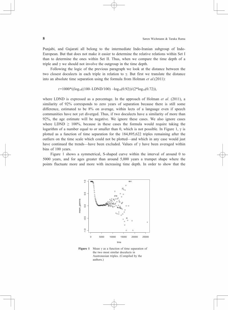
where LDND is expressed as a percentage. In the approach of Holman et al. (2011), a similarity of 92% corresponds to zero years of separation because there is still some difference, estimated to be 8% on average, within lects of a language even if speech communities have not yet diverged. Thus, if two doculects have a similarity of more than 92%, the age estimate will be negative. We ignore these cases. We also ignore cases where LDND ≥ 100%, because in these cases the formula would require taking the logarithm of a number equal to or smaller than 0, which is not possible. In Figure 1, γ is plotted as a function of time separation for the 184,895,622 triples remaining after the outliers on the time scale which could not be plotted—and which in any case would just have continued the trends—have been excluded. Values of γ have been averaged within bins of 100 years. Figure 1 shows a symmetrical, S-shaped curve within the interval of around 0 to 5000 years, and for ages greater than around 5,000 years a trumpet shape where the points fluctuate more and more with increasing time depth. In order to show that the

Figure 1 Mean γ as a function of time separation of the two most similar doculects in Austronesian triples. (Compiled by the authors.)

0 5000 10000 15000 20000 25000

-1.0

-0.5

0.0

0.5

1.0

time

mea

n_ga

mm

a

9

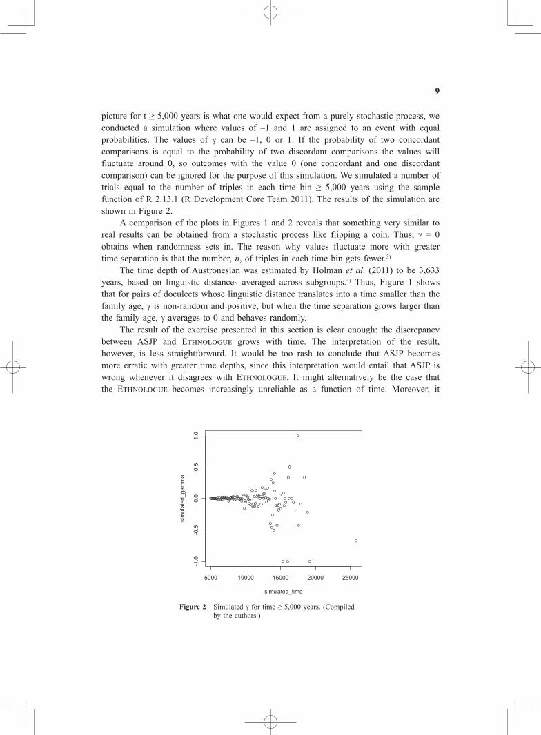
picture for t ≥ 5,000 years is what one would expect from a purely stochastic process, we conducted a simulation where values of –1 and 1 are assigned to an event with equal probabilities. The values of γ can be –1, 0 or 1. If the probability of two concordant comparisons is equal to the probability of two discordant comparisons the values will fluctuate around 0, so outcomes with the value 0 (one concordant and one discordant comparison) can be ignored for the purpose of this simulation. We simulated a number of trials equal to the number of triples in each time bin ≥ 5,000 years using the sample function of R 2.13.1 (R Development Core Team 2011). The results of the simulation are shown in Figure 2. A comparison of the plots in Figures 1 and 2 reveals that something very similar to real results can be obtained from a stochastic process like flipping a coin. Thus, γ = 0 obtains when randomness sets in. The reason why values fluctuate more with greater time separation is that the number, n, of triples in each time bin gets fewer.3)

The time depth of Austronesian was estimated by Holman et al. (2011) to be 3,633 years, based on linguistic distances averaged across subgroups.4) Thus, Figure 1 shows that for pairs of doculects whose linguistic distance translates into a time smaller than the family age, γ is non-random and positive, but when the time separation grows larger than the family age, γ averages to 0 and behaves randomly. The result of the exercise presented in this section is clear enough: the discrepancy between ASJP and ETHNOLOGUE grows with time. The interpretation of the result, however, is less straightforward. It would be too rash to conclude that ASJP becomes more erratic with greater time depths, since this interpretation would entail that ASJP is wrong whenever it disagrees with ETHNOLOGUE. It might alternatively be the case that the ETHNOLOGUE becomes increasingly unreliable as a function of time. Moreover, it

Figure 2 Simulated γ for time ≥ 5,000 years. (Compiled by the authors.)

5000 10000 15000 20000 25000

-1.0

-0.5

0.0

0.5

1.0

simulated_time

sim

ulat

ed_g

amm

a


should not be forgotten that the test has been carried out using triples whose relative distances are evaluated without reference to their relationships with any other Austronesian doculects. Given the entire set of doculects and an appropriate phylogenetic algorithm, more information would be available for the correct classification of any subset of three doculects relative to one another. Thus, even if a triple scores a γ-value of 0 or –1 it may well end up in the right place when the relationships between each of the three doculects and all other Austronesian doculects are taken into account. Thus, it is necessary to look more closely at the behavior of individual subgroups and doculects to understand the phenomena underlying the seemingly simple relation between γ and time. This is the purpose of the remainder of this paper.

4. Reticulation (δ) and Jackknife Gamma (γ’)Holland et al. (2002) define a measure of conflict in phylogenetic trees called δ. It is discussed and applied to different kinds of datasets in Gray et al. (2010), and the Splitstree software (Huson and Bryant 2006) has an implementation of it (we use our own implementation in this paper, however). Briefly, δ measures the deviation of a quartet of taxa from the so-called four-point condition on distances between the taxa. When the four-point condition holds for the six distances among the four taxa, the two sums of the two largest distances are equal and greater than the sum of the two smallest distances. Thus, δ measures the deviation from this condition. If a reticulate quartet is depicted as a box with branches issuing from each corner, as in the Neighbor-Net graphs of Splitstree, δ will correspond to the ratio between the length of the shortest side of the box and the length of the longest side. For a group of taxa (e.g., a language family) with more than 4 members, δ can be averaged over all quartets; for less than 4 members δ is not defined. Wichmann et al. (2011: 233) reported on significant correlations between δ and four different measures of fit between ASJP trees or distance matrices and expert classifications (WALS and ETHNOLOGUE), one of them being γ. The Spearman correlation between δ and γ across the language families in the ASJP database (version 14) was found to be –0.5982 (p < 0.00001). In other words, as the average reticulation across the quartets in a family increases, the fit with expert classifications tends to decrease. Normally we would trust expert classifications, and γ can then be interpreted as saying something real about how well ASJP distances fit true classifications. But if, in some individual cases, we do not trust the expert classifications, δ can be used as a proxy for the accuracy of ASJP classifications, given that it overall correlates with γ. This is a crucial insight for the present purposes, because the problem that we face with the Austronesian case is how to gauge the reliability of the classification for individual languages and subgroups when we want to leave the question of the trustworthiness of the gold standard open. In this situation, we can use δ as a proxy for the reliability of the classification of individual languages. We calculate δ for individual doculects by averaging δ over all the quartets in which a doculect participates. The proxy for the expected fit of a doculect to an accurate classification, δ, can be

11

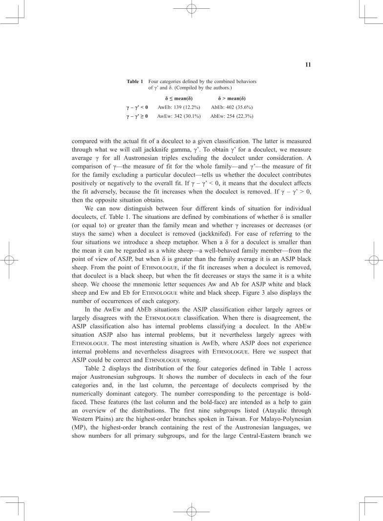
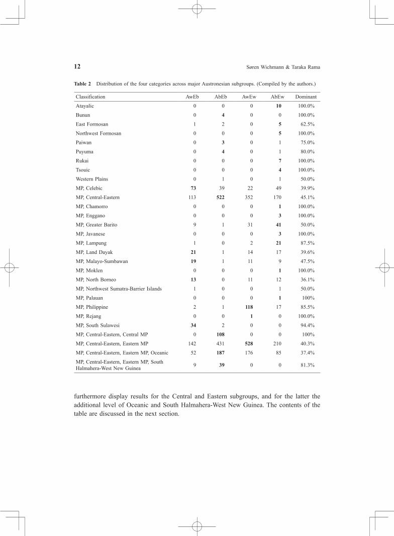
compared with the actual fit of a doculect to a given classification. The latter is measured through what we will call jackknife gamma, γ’. To obtain γ’ for a doculect, we measure average γ for all Austronesian triples excluding the doculect under consideration. A comparison of γ—the measure of fit for the whole family—and γ’—the measure of fit for the family excluding a particular doculect—tells us whether the doculect contributes positively or negatively to the overall fit. If γ – γ’ < 0, it means that the doculect affects the fit adversely, because the fit increases when the doculect is removed. If γ – γ’ > 0, then the opposite situation obtains. We can now distinguish between four different kinds of situation for individual doculects, cf. Table 1. The situations are defined by combinations of whether δ is smaller (or equal to) or greater than the family mean and whether γ increases or decreases (or stays the same) when a doculect is removed (jackknifed). For ease of referring to the four situations we introduce a sheep metaphor. When a δ for a doculect is smaller than the mean it can be regarded as a white sheep—a well-behaved family member—from the point of view of ASJP, but when δ is greater than the family average it is an ASJP black sheep. From the point of ETHNOLOGUE, if the fit increases when a doculect is removed, that doculect is a black sheep, but when the fit decreases or stays the same it is a white sheep. We choose the mnemonic letter sequences Aw and Ab for ASJP white and black sheep and Ew and Eb for ETHNOLOGUE white and black sheep. Figure 3 also displays the number of occurrences of each category. In the AwEw and AbEb situations the ASJP classification either largely agrees or largely disagrees with the ETHNOLOGUE classification. When there is disagreement, the ASJP classification also has internal problems classifying a doculect. In the AbEw situation ASJP also has internal problems, but it nevertheless largely agrees with ETHNOLOGUE. The most interesting situation is AwEb, where ASJP does not experience internal problems and nevertheless disagrees with ETHNOLOGUE. Here we suspect that ASJP could be correct and ETHNOLOGUE wrong. Table 2 displays the distribution of the four categories defined in Table 1 across major Austronesian subgroups. It shows the number of doculects in each of the four categories and, in the last column, the percentage of doculects comprised by the numerically dominant category. The number corresponding to the percentage is bold-faced. These features (the last column and the bold-face) are intended as a help to gain an overview of the distributions. The first nine subgroups listed (Atayalic through Western Plains) are the highest-order branches spoken in Taiwan. For Malayo-Polynesian (MP), the highest-order branch containing the rest of the Austronesian languages, we show numbers for all primary subgroups, and for the large Central-Eastern branch we

Table 1 Four categories defined by the combined behaviors of γ’ and δ. (Compiled by the authors.)

δ ≤ mean(δ) δ > mean(δ)

γ – γ’ < 0 AwEb: 139 (12.2%) AbEb: 402 (35.6%)

γ – γ’ ≥ 0 AwEw: 342 (30.1%) AbEw: 254 (22.3%)


furthermore display results for the Central and Eastern subgroups, and for the latter the additional level of Oceanic and South Halmahera-West New Guinea. The contents of the table are discussed in the next section.

Table 2 Distribution of the four categories across major Austronesian subgroups. (Compiled by the authors.)

Classification AwEb AbEb AwEw AbEw Dominant

Atayalic 0 0 0 10 100.0%

Bunun 0 4 0 0 100.0%

East Formosan 1 2 0 5 62.5%

Northwest Formosan 0 0 0 5 100.0%

Paiwan 0 3 0 1 75.0%

Puyuma 0 4 0 1 80.0%

Rukai 0 0 0 7 100.0%

Tsouic 0 0 0 4 100.0%

Western Plains 0 1 0 1 50.0%

MP, Celebic 73 39 22 49 39.9%

MP, Central-Eastern 113 522 352 170 45.1%

MP, Chamorro 0 0 0 1 100.0%

MP, Enggano 0 0 0 3 100.0%

MP, Greater Barito 9 1 31 41 50.0%

MP, Javanese 0 0 0 3 100.0%

MP, Lampung 1 0 2 21 87.5%

MP, Land Dayak 21 1 14 17 39.6%

MP, Malayo-Sumbawan 19 1 11 9 47.5%

MP, Moklen 0 0 0 1 100.0%

MP, North Borneo 13 0 11 12 36.1%

MP, Northwest Sumatra-Barrier Islands 1 0 0 1 50.0%

MP, Palauan 0 0 0 1 100%

MP, Philippine 2 1 118 17 85.5%

MP, Rejang 0 0 1 0 100.0%

MP, South Sulawesi 34 2 0 0 94.4%

MP, Central-Eastern, Central MP 0 108 0 0 100%

MP, Central-Eastern, Eastern MP 142 431 528 210 40.3%

MP, Central-Eastern, Eastern MP, Oceanic 52 187 176 85 37.4%

MP, Central-Eastern, Eastern MP, South Halmahera-West New Guinea 9 39 0 0 81.3%

13

5. Who’s to Blame for the Black Sheep?The classification of Austronesian languages is a hugely complicated matter and we cannot attempt to do justice either to the ASJP results (cf. the large tree in the Online Appendix 1), nor to the literature. Table 2 is offered here mainly as a guide to where ASJP and experts disagree, and here we will discuss the most salient features of the table. The results for the Formosan subgroups are unremarkable. Nearly all of the doculects are in the Ab category, indicating a high degree of reticulation. This result is in line with the finding of Wichmann et al. (2011) that within-family isolates are generally more reticulate than other languages in their family, presumably because extinction of their closest relatives have made their position in the phylogeny more indeterminate—each Formosan subgroup consists of but 1–5 languages. Among the subgroups of Malayo-Polynesian there are three that stand out because all doculects are in the Eb category. These are South Sulawesi (36 doculects), the Central MP subgroup of Central-Eastern MP (108 doculects), and the South Halmahera-West New Guinea subgroup of the Eastern subgroup of Central-Eastern MP (48 doculects). Together these subgroups, whose members are apparently all inaccurately classified by ASJP, comprise 192 doculects, or 17% of the total sample. For Greater Barito, Lampung, and Philippine the great majority of doculects are in the Ew category, showing greater-than-average fit with the ETHNOLOGUE classification. Other subgroups exhibit a more mixed picture. The goal of this paper is to understand why ASJP apparently performs so poorly in the case of Austronesian by identifying the individual culprit languages Therefore the subgroups that we are particularly interested in are the three which stand out as consistently receiving a treatment by ASJP which is in conflict with ETHNOLOGUE. While we cannot discuss all Austronesian languages, looking more closely at these three subgroups can bring us a long way towards understanding the reasons why ASJP apparently has problems with Austronesian. Thus, we devote a subsection to each.

5.1 South Sulawesi (SS)Although the measurements of differences between ASJP distances and the ETHNOLOGUE tree are made directly from the ASJP distance matrix and not by comparing two trees, the Neighbor-Joining tree for Austronesian in Online Appendix 1 can nevertheless help us to acquire an understanding of the nature of the differences. SS languages are found in two places in the tree. Budong Budong [bdx] and Panasuan [psn] are deeply embedded within a group of Celebic languages and interrupts this group which is otherwise a large and coherent one. As it turns out, their placement within SS is actually not well supported by comparative linguistic evidence. Friberg and Laskowske (1989:10) state that they assign them to the ‘Seko Family’ within SS even if the evidence is weak: “It [Budong Budong] is closely related to Panasuan at 72%. We tentatively place it in the Seko language family, though lexical similarity with Seka Tengah and Seko Padang is not so close, at 61% and 57%.” The alternative placement in


the ASJP tree may well turn out to be a more accurate classification. The remaining SS languages form a clade of their own. Different from the ETHNOLOGUE classification, where SS is a direct offspring of Malayo-Polynesian, the ASJP trees treats SS as a sister clade of various Philippine languages (Tombulu [tom], Tonsea [txs], Tondano [tdn], Tontemboan [tnt], Tonsawang [tnw], Sangil [snl], Sangil Sarangani Islands [snl], Sangir [sxn], Sangir 2 [sxn], Bantik [bnq], Ratahan [rth], Talaud [tld]). The SS + Philippine constellation is, furthermore, embedded within a large group of mostly ‘Central Malayo-Polynesian’ languages (concerning which see the following subsection). It is probably this deep embeddedness in other groups of languages supposed to be more remotely related which accounts for the poor overall fit between SS languages and the ETHNOLOGUE scheme. The fact that 34 of the 36 SS doculects are in the Aw category shows that the ASJP data has a tree-like behavior, so the position of the SS languages with a group of Philippine languages is hardly random. This placement may well turn out to be more accurate than ETHNOLOGUE’s (non-)classification of the group as a first-order offspring of Malayo-Polynesian, but it is difficult to make definitive judgments in the matter at this point.

5.2 The Central MP Subgroup of Central-Eastern MP (CMP).A summary of the evidence for CMP is given in Blust (1993). Throughout this paper the author makes it clear that the innovations that characterize many of the languages are not shared by all of them, and some are also found in other Austronesian languages. To describe the relationship among the languages, the author invokes the notion of ‘linkage’ of Ross (1988), which he (Blust) defines as “a relatively nondiscrete unit produced by differentiation in situ, in contrast with a family, defined as a product of separation” (Blust 1993: 263). A qualification such as this is of course lost when the classification of a family of languages is summarized in a family tree, but it is clear from Blust’s paper that he does not consider CMP solidly established, and other scholars concur (e.g., Adelaar 2005: 26 considers CMP “contested”). Thus, discrepancies between ASJP and ETHNOLOGUE with regard to the classification of CMP languages cannot be used as an argument of the inadequacy of ASJP.

5.3 The South Halmahera-West New Guinea Subgroup of the Eastern Subgroup of Central-Eastern MP (SHWNG).

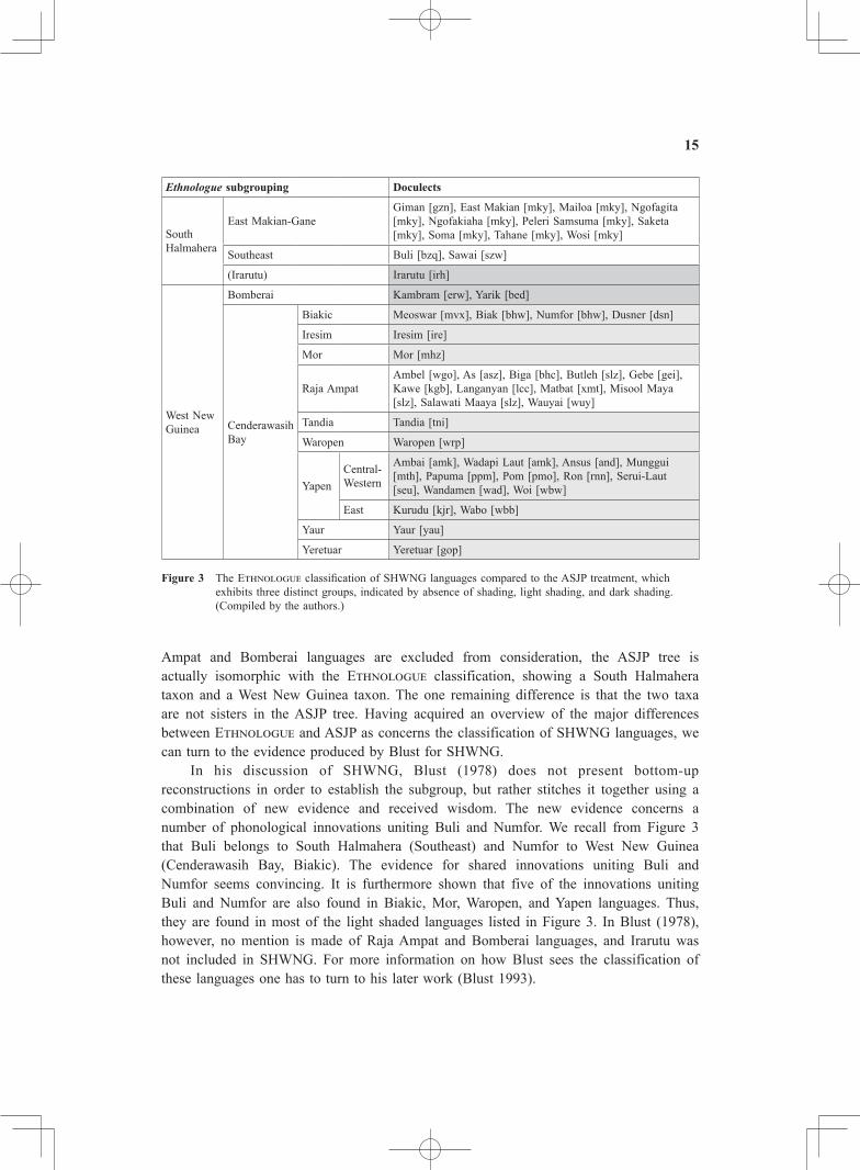
According to Blust (1978: 181), the SHWNG languages were first grouped together by Adriani and Kruijt (1914) and the name ‘South Halmahera-West New Guinea’ was bestowed upon them by Esser (1938). Blust regards previous evidence for the subgroup as insufficient but presents new evidence by way of phonological innovations and some exclusively shared lexical items in its support. As schematized in Figure 3, the SHWNG languages are found in three different segments of the ASJP Austronesian tree, suggesting a lack of support (or at least a lack of strong support) for the subgroup as a whole. One segment contains South Halmahera and Raja Ampat languages, another one Irarutu and the Bomberai languages, and a third all the Cenderawasih Bay languages minus Raja Ampat. Thus, if Irarutu and the Raja

15

Ampat and Bomberai languages are excluded from consideration, the ASJP tree is actually isomorphic with the ETHNOLOGUE classification, showing a South Halmahera taxon and a West New Guinea taxon. The one remaining difference is that the two taxa are not sisters in the ASJP tree. Having acquired an overview of the major differences between ETHNOLOGUE and ASJP as concerns the classification of SHWNG languages, we can turn to the evidence produced by Blust for SHWNG. In his discussion of SHWNG, Blust (1978) does not present bottom-up reconstructions in order to establish the subgroup, but rather stitches it together using a combination of new evidence and received wisdom. The new evidence concerns a number of phonological innovations uniting Buli and Numfor. We recall from Figure 3 that Buli belongs to South Halmahera (Southeast) and Numfor to West New Guinea (Cenderawasih Bay, Biakic). The evidence for shared innovations uniting Buli and Numfor seems convincing. It is furthermore shown that five of the innovations uniting Buli and Numfor are also found in Biakic, Mor, Waropen, and Yapen languages. Thus, they are found in most of the light shaded languages listed in Figure 3. In Blust (1978), however, no mention is made of Raja Ampat and Bomberai languages, and Irarutu was not included in SHWNG. For more information on how Blust sees the classification of these languages one has to turn to his later work (Blust 1993).

Ethnologue subgrouping Doculects

South Halmahera

East Makian-GaneGiman [gzn], East Makian [mky], Mailoa [mky], Ngofagita [mky], Ngofakiaha [mky], Peleri Samsuma [mky], Saketa [mky], Soma [mky], Tahane [mky], Wosi [mky]

Southeast Buli [bzq], Sawai [szw]

(Irarutu) Irarutu [irh]

West New Guinea

Bomberai Kambram [erw], Yarik [bed]

Cenderawasih Bay

Biakic Meoswar [mvx], Biak [bhw], Numfor [bhw], Dusner [dsn]

Iresim Iresim [ire]

Mor Mor [mhz]

Raja AmpatAmbel [wgo], As [asz], Biga [bhc], Butleh [slz], Gebe [gei], Kawe [kgb], Langanyan [lcc], Matbat [xmt], Misool Maya [slz], Salawati Maaya [slz], Wauyai [wuy]

Tandia Tandia [tni]

Waropen Waropen [wrp]

YapenCentral-Western

Ambai [amk], Wadapi Laut [amk], Ansus [and], Munggui [mth], Papuma [ppm], Pom [pmo], Ron [rnn], Serui-Laut [seu], Wandamen [wad], Woi [wbw]

East Kurudu [kjr], Wabo [wbb]

Yaur Yaur [yau]

Yeretuar Yeretuar [gop]

Figure 3 The ETHNOLOGUE classification of SHWNG languages compared to the ASJP treatment, which exhibits three distinct groups, indicated by absence of shading, light shading, and dark shading. (Compiled by the authors.)


The Raja Ampat languages are mentioned briefly by Blust (1993:271) among several other languages which “appear to belong the SHWNG group, although (…) such classificatory inferences as we dare to make are based on the presence of known SHWNG languages on either side of the speculative members of this group.” It is not clear why ETHNOLOGUE assigns them to West New Guinea. Regarding Irarutu, Blust (1993: 272) says that it is “apparently not a CMP language, and shows no known positive evidence of belonging to the SHWNG group. Its position for the present remains indeterminate.” Finally, what Blust (1993 :272) has to say concerning Yarik (a.k.a. Bedoanas) and Kambram (a.k.a. Erokwanas) is that their position “remains totally unknown.” A comparison between ETHNOLOGUE and ASJP with regard to their treatment of SHWNG languages shows discrepancies which superficially look unfavorable for ASJP if we were to judge its performance on this comparison alone. But when we dig a little deeper it turns out that the discrepancies pertain to languages whose positions within the Austronesian tree have not been firmly established by experts. An alternative conclusion to draw from the comparison is that ASJP may actually have something new to contribute to the classification of these languages. In the tree in Online Appendix 1, the relatively long branch leading to the node that unites Raja Ampat languages with the East Makian-Gane + Southeast groups indicates that the placement of Raja Ampat within South Halmahera has strong support from lexical similarities. Additional comparative linguistic work on these languages may well turn out to support this relationship. As for Irarutu and Bomberai, these are united in the ASJP tree as extreme members of a cluster containing a number of languages pertaining to the contested Central Malayo-Polynesian group (Arguni [agf], Kowiai [kwh], Uruangnirin [urn], Onin [oni], and Sekar [skz]). Again, ASJP suggests a possibly interesting hypothesis about the classification of languages which have not been conclusively dealt with from a traditional comparative linguistic perspective.

5.4 Summary of Case StudiesThe three cases studies have shown different ways in which the reliability of the ETHNOLOGUE classification is challenged by ASJP rather than the other way around. South Sulawesi is a case where the unresolved position of a subgroup as a direct daughter of Malayo-Polynesian is likely to be inaccurate and where a couple of languages are assumed to belong to the subgroup although they seem to belong elsewhere in the tree. Central Malayo-Polynesian is one of several large Austronesian subgroups where languages that do not yet have a well-defined position in Austronesian have been ‘parked’. Finally, the subgrouping of South Halmahera-West New Guinea is clearly not fully worked out by experts, and in ETHNOLOGUE it furthermore acts as a waste-basket for some languages which experts have not been able to fit into the Austronesian tree. The three cases, then, illustrate that there are problems at all levels in the ETHNOLOGUE classification of Austronesian: some larger subgroups are problematical, some individual lower-level configurations remain to be better worked out, and a number of individual languages are placed arbitrarily in the tree.

17

The three cases were selected for closer inspection because they were prominent with regard to discrepancies with ETHNOLOGUE. A full analysis of the ASJP treatment of all Austronesian languages in comparison with ETHNOLOGUE would surely reveal other cases where the trustworthiness of the latter is questionable, and surely also cases where meticulous work on phonological and other linguistic developments has allowed experts on Austronesian to more accurately classify languages than is possible for ASJP with its somewhat crude, aggregate distance measure based on 40 or, more often, even less lexical items. Such a more exhaustive study is beyond the scope of this paper. The relevance of the present study is that it shows that the ETHNOLOGUE classification cannot be taken at face value as the gold standard which will show a classificatory technique to be inadequate when it does not yield the same results.

6. CONCLUSIONThis paper should be seen as a methodological contribution to the debate about quantitative methods in historical linguistics. World-wide surveys of the performance of ASJP with respect to language classification have shown mixed results, and they all indicate that Austronesian is a particularly hard nut to crack for ASJP. As this study shows, however, the experts also have problems with aspects of Austronesian classification. So Austronesian is not a representative case for the performance of ASJP, and ASJP may well have something new to offer in the ongoing work on the classification of Austronesian. In Online Appendix 1 to this paper, we offer an ASJP-based Austronesian tree, aspects of which we hope can contribute productively to Austronesian historical linguistics. Whereas previous performance investigations have reported results of comparing ASJP distance matrices or trees with ETHNOLOGUE and other classifications for whole language families, this study has introduced tools to improve the resolution at which classifications are compared. The jackknife technique can reveal which particular languages hold the greatest responsibility for discrepancies between two classifications, and δ, the reticulation measure, can show whether a language has an inherently tree-like behavior or not. Smaller values of δ increase the amount of trust that we can allow ourselves to invest in the ASJP classification of a given language, regardless of how the language is classified by experts. In Online Appendix 2 we provide γ’ and δ values for individual doculects which may be consulted in conjunction with the ASJP tree. In order to test methods in computational quantitative historical linguistics we need real gold standards, not standards that mix gold with less noble metals. Future work concerned with methods in quantitative historical linguistics should be directed at the identification of a set of widely accepted gold standard linguistic phylogenies which may serve as stable points of reference and help towards the improvement of the quality of evaluations.


Online Appendices

Appendix 1 contains a pdf of the ASJP Austronesian tree. Appendix 2 is a tab-delimited file containing the ETHNOLOGUE classification and values of γ’ and δ for the 1137 Austronesian doculects treated in this paper. The appendices are found at https://zenodo.org/record/233000#.WHEe7H2Gfik and may be cited separately as Wichmann and Rama (2017).

Notes

1) We are grateful to Eric W. Holman for comments on this paper.2) Very many of the languages in the ASJP database are not included in WALS. For these,

judgments had to be made regarding how they would be classified according to the WALS scheme.

3) The decrease in n closely (r2 = 0.95) approximates a power-law of the shape n = 4e+35t–8.253, where 1 ≤ n ≤ 243,704.4) As Figure 1 shows, a greater time separation is obtained from many of the pairs of doculects,

but the averaging procedure protects against the aberrant behavior of individual pairs.

References

Adelaar, A. 2005 The Austronesian Languages of Asia and Madagascar: A Historical Perspective. In A.

Adelaar and N. Himmelmann (eds.) The Austronesian Languages of Asia and Madagascar, pp.1–42. London and New York: Routledge.

Adriani, N. and A. C. Kruijt 1914 De Bare’e-sprekende Toradja’s van midden-Celebes, vol. 3. VKNA 46. Batavia:

Landsdrukkerij.Bakker, D., A. Müller, V. Velupillai, S. Wichmann, C. H. Brown, P. Brown, D. Egorov, R.

Mailhammer, A. Grant., and E. W. Holman 2009 Adding Typology to Lexicostatistics: A Combined Approach to Language Classification.

Linguistic Typology 13: 167–179.Blust, R. A. 1978 Eastern Malayo-Polynesian: A Subgrouping Argument. In S. A. Wurm and L.

Carrington (eds.) Second International Conference on Austronesian Linguistics: Proceedings, Fascicle I, Western Austronesian, pp.181–234. Canberra: Pacific Linguistics.

1993 Central and Central-Eastern Malayo-Polynesian. Oceanic Linguistics 32: 241–293.Brown, C. H., E. W. Holman, S. Wichmann, and V. Velupillai 2008 Automated Classification of the World’s Languages: A Description of the Method and

Preliminary Results. STUF-Language Typology and Universals 61: 285–308.

19

Brown, C. H., E. W. Holman, and S. Wichmann 2013 Sound Correspondences in the World’s Languages. Language 89(1): 4–29. Desper, R. and O. Gascuel 2002 Fast and Accurate Phylogeny Reconstruction Algorithms Based on the Minimum-

evolution Principle. Journal of Computational Biology 9(5): 687–705.Dryer, M. S. 2005 Genealogical Language List. In M. Haspelmath, M. Dryer, D. Gil, and B. Comrie (eds.)

The World Atlas of Language Structures, pp.584–644. Oxford: Oxford University Press.

Esser, E. J. 1938 Talen. In Topografische Dienst in Nederlandsch-Indië, Nederlands Aardrijkskundig

Genootschap Atlas van tropisch Nederland, pp.9–9b. Amsterdam: Koninklijk Nederlandsch Ardrijkskundig Genootschap.

Felsenstein, J. 2004 Inferring Phylogenies. Sunderland, MA.: Sinauer Associates.Friberg, T. and T. V. Laskowske 1989 South Sulawesi Languages. In J. N. Sneddon (ed.) Studies in Sulawesi Linguistics, Part

1 (Nusa Linguistic Studies of Indonesian and Other Languages in Indonesia, 31) :pp.1–17. Jakarta: Universitas Katolik Indonesia Atma Jaya.

Gray, R. D., D. Bryant, and S. Greenhill 2010 On the Shape and Fabric of Human History. Philosophical Transactions of the Royal

Society B 365(1559): 3923–3933.Greenhill, S. J. 2011 Levenshtein Distances Fail to Identify Language Relationships Accurately.

Computational Linguistics 37: 689–698.Greenhill, S. J., R. Blust, and R. D. Gray 2008 The Austronesian Basic Vocabulary Database: From Bioinformatics to Lexomics.

Evolutionary Bioinformatics 4: 271–283.Hill, J. 2011 Subgrouping in Uto-Aztecan. Language Dynamics and Change 1: 241–278.Holland, B. R., K. T. Huber, A. Dress, and V. Moulton 2002 δ Plots: A Tool for Analyzing Phylogenetic Distance Data. Molecular Biology and

Evolution 19(12): 2051–2059. Holman, E. W., S. Wichmann, C. H. Brown, V. Velupillai, A. Müller, and D. Bakker 2008a Explorations in Automated Language Classification. Folia Linguistica 42(3–4):

331–354. 2008b Advances in Automated Language Classification. In A. Arppe, K. Sinnemäki, and U.

Nikanne (eds.) Quantitative Investigations in Theoretical Linguistics, pp.40–43. Helsinki: University of Helsinki.

Holman, E. W., C. H. Brown, S. Wichmann, A. Müller, V. Velupillai, H. Hammarström, S. Sauppe, H. Jung, D. Bakker, P. Brown, O. Belyaev, M. Urban, R. Mailhammer, J.-M. List, and D. Egorov

2011 Automated Dating of the World’s Language Families Based on Lexical Similarity.


Current Anthropology 52(6): 841–875.Huff, P. and D. Lonsdale 2011 Positing Language Relationships Using ALINE. Language Dynamics and Change 1(1):

128–162.Huson, D. H. and D. Bryant 2006 Application of Phylogenetic Networks in Evolutionary Studies. Molecular Biology and

Evolution 23(2): 254–267.Kondrak, G. 2000 A New Algorithm for the Alignment of Phonetic Sequences. Proceedings of the First

Meeting of the North American Chapter of the Association for Computational Linguistics, pp.288–295. Stroudsburg, PA.: Association for Computational Linguistics

Lewis, M. P. 2009 Ethnologue: Languages of the World, 16th ed., http://www.ethnologue.com/. (Accessed

April 1, 2014.)Pompei, S., V. Loreto, and F. Tria 2011 On the Accuracy of Language Trees. PLoS ONE 6(6): e20109. doi: 10.1371/journal.

pone.0020109. (Accessed April 1, 2014.)R Development Core Team. 2011 R: A Language and Environment for Statistical Computing. R Foundation for Statistical

Computing. Vienna, Austria. http://www.R-project.org/. (Accessed April 1, 2014.)Ross, M. D. 1988 Proto Oceanic and the Austronesian Languages of Western Melanesia. (Pacific

Linguistics C-98). Canberra: The Australian National University.Saitou, N. and M. Nei 1987 The Neighbor-joining Method: A New Method for Reconstructing Phylogenetic Trees.

Molecular Biology and Evolution 4(4): 406–425.Sokal, R. R. and C. D. Michener 1958 A Statistical Method for Evaluating Systematic Relationships. University of Kansas

Science Bulletin 38(6): 1409–1438.Walker R. S., S. Wichmann, T. Mailund, and C. J. Atkisson 2012 Cultural Phylogenetics of the Tupi Language Family in Lowland South America. PLoS

ONE 7(4): e35025. DOI:10.1371/journal.pone.0035025. (Accessed April 1, 2014.)Wichmann, S., E. W. Holman, D. Bakker, and C. H. Brown 2010a Evaluating Linguistic Distance Measures. Physica A 389: 3632–3638. 2010b Sound Symbolism in Basic Vocabulary. Entropy 12(4): 844–858.Wichmann, S., E. W. Holman, T. Rama, and R. S. Walker 2011 Correlates of Reticulation in Linguistic Phylogenies. Language Dynamics and Change 1:

205–240.Wichmann, S., A. Müller, V. Velupillai, A. Wett, C. H. Brown, Z. Molochieva, J. Bishoffberger, E.

W. Holman, S. Sauppe, P. Brown, D. Bakker, J.-M. List, D. Egorov, O. Belyaev, M. Urban, H. Hammarström, A. Carrizo, R. Mailhammer, H. Geyer, D. Beck, E. Korovina, P. Epps, P. Valenzuela, and A. Grant

2012 The ASJP Database (version 15). http://asjp.clld.org/static/lists15.zip. (Accessed April 1,

21

2014.)Wichmann, S. and T. Rama 2017 Appendices to Jackknifing the Black Sheep: ASJP Classification Performance and

Austronesian [Data set]. Zenodo. http://doi.org/10.5281/zenodo.233000. (Accessed April 1, 2014.)

Documents

Jackknifing the black sheep: ASJP classification performance and Austronesian