Embed Size (px)
Citation preview
3002 IEEE TRANSACTIONS ON INDUSTRIAL ELECTRONICS, VOL. 58, NO. 7, JULY 2011
Iterative Learning Control for Sampled-DataSystems: From Theory to Practice
Khalid Abidi and Jian-Xin Xu, Senior Member, IEEE
Abstract—This paper aims to present a framework for thedesign and performance analysis of iterative learning control(ILC) for sampled-data systems. The analysis is presented in bothtime and frequency domains. Monotonic convergence criteria arederived in both time and frequency domains and coined in ILCdesigns. In particular, the causes or conditions that lead to thepoor transient responses in the time domain are explored anddisclosed. Four ILC designs associated with different learningfunctions and filters are considered, namely, the P-type, D-type,D2-type, and general filters. The criteria for the selection of eachtype are presented. In addition, a relationship is shown betweensampling-time selection and ILC convergence. Theoretical workconcludes with a guideline for the ILC designs. Simulation resultsare shown to support the theoretical analysis in the time andfrequency domains. Furthermore, based on the frequency-domaindesign tools, a successful experimental implementation on an elec-tric piezomotor is demonstrated.
Index Terms—Iterative learning control (ILC), precision con-trol, sampled-data systems.
I. INTRODUCTION
IN THIS PAPER, iterative learning controllers are designedand analyzed for systems that perform the same operation
repeatedly and under the same operating conditions. For suchsystems, a nonlearning controller yields the same tracking erroron each repetition or iteration. Although error signals fromprevious iterations are information rich, they are not used bya nonlearning controller. The objective of iterative learningcontrol (ILC) is to improve performance by incorporating thepast control and tracking error into the control for subsequentiterations. In doing so, high performance can be achieved withlow transient tracking error despite large uncertainties andrepeating disturbances.
ILC differs from other learning-type control strategies, suchas adaptive control, neural networks, and repetitive control(RC). Adaptive control strategies modify the controller, whichis a system, whereas ILC modifies the control input, whichis a signal [5]. Additionally, adaptive controllers do not typi-cally take advantage of the information contained in repetitivecommand signals. Similarly, neural network learning involvesthe modification of controller parameters rather than a control
Manuscript received October 19, 2009; revised February 15, 2010 andJune 7, 2010; accepted August 13, 2010. Date of publication August 30, 2010;date of current version June 15, 2011.
K. Abidi is with the Department of Mechatronics, Bahcesehir University,34353 Besiktas/Istanbul, Turkey (e-mail: [email protected]).
J.-X. Xu is with the Department of Electrical and Computer Engineer-ing, National University of Singapore, Singapore 119260 (e-mail: [email protected]).
Color versions of one or more of the figures in this paper are available onlineat http://ieeexplore.ieee.org.
Digital Object Identifier 10.1109/TIE.2010.2070774
signal; in this case, large networks of nonlinear neurons aremodified. These large networks require extensive training data,and fast convergence may be difficult to guarantee [6], whereasILC usually converges adequately in just a few iterations.
ILC is perhaps most similar to RC [7], except that RC isintended for continuous operation, whereas ILC is intendedfor discontinuous operation. For example, an ILC applicationmight be to control a robot that performs a task, returns to itshome position, and comes to a rest before repeating the task.On the other hand, an RC application might be to control aconveyer system in a mass-production line moving items atperiodic intervals where the next cycle immediately followsthe current cycle. The difference between RC and ILC is thesetting of the initial conditions for each trial [8]. In ILC, theinitial conditions are set to the same value on each trial. InRC, the initial conditions are set to the final conditions ofthe previous trial. The difference in initial conditions leads todifferent analysis techniques and results [8].
Traditionally, the focus of ILC has been on improving theperformance of systems that execute a single repeated oper-ation. This focus includes many practical industrial systemsin manufacturing, robotics, and chemical processing, wheremass production on an assembly line entails repetition. ILChas been successfully applied to industrial robots [9]–[18],computer numerical control machine tools [19], wafer stagemotion systems [20], injection-molding machines [21], [22],and many more.
The basic ideas of ILC can be found in a U.S. patent [2] filedin 1967, as well as in a 1978 journal publication [1] writtenin Japanese. However, these ideas lay dormant until a series ofarticles in 1984 [9], [23]–[26] sparked widespread interests inILC. Since then, the number of publications on ILC has beengrowing rapidly, including a Special Issue [27], several books[5], [28]–[30], and three surveys [31]–[33].
It is worth highlighting the difference between this andother published works such as [34] and [35]. First, this paperfocuses on sampled-data systems, which are rather differentfrom discrete-time systems, as discussed in [34] and [35], forinstance, the reduction in relative degrees and the effect ofsampling period in relation to learning convergence perfor-mance. Second, this paper reveals the causes that yield poortransient learning performance in sampled-data systems. Third,this paper provides a number of ILC algorithms and analyzestheir effectiveness and convergence conditions in both time andfrequency domains. Fourth, using the theoretical conclusionsgiven in [35], this paper details the design procedure for theexplored ILC algorithms, namely, the choice of filter and learn-ing function, such that learning performance can be improved
0278-0046/$26.00 © 2010 IEEE

ABIDI AND XU: ITERATIVE LEARNING CONTROL FOR SAMPLED-DATA SYSTEMS 3003
drastically. Overall, this paper provides ILC design guidelinesassociated with various design factors, makes clear the scopeand suitability of the explored ILC algorithms, and presents anumber of illustrative examples on the designs of the filters andlearning functions, which are verified by a number of numer-ical and experimental case studies. From previously publishedworks like [34] and [35], this paper adopts the theoretical con-clusion from [35] on the conditions for monotonic convergence,hence facilitating the ILC design in the frequency domain. Theultimate aim of this paper is to shift from ILC theory to practicalimplementation that are sampled in nature while showing howtheoretical results can facilitate ILC designs.
Throughout this paper, ‖ · ‖ denotes the Euclidean norm.For notational convenience, in mathematical expressions, fk
represents f(k).
II. PRELIMINARIES
In this section, the problem description is presented with thehighlight on the basic differences between continuous-time andsampled-data ILC.
A. Problem Description
Consider a tracking task that ends in a finite interval [0, N ]and repeats. Let the desired trajectory be yr,k, k ∈ [0, N ].Consider the ILC law
ui+1,k = H(q) [ui,k + βL(q)ei,k+1]
ei,k = yr,k − yi,k (1)
where H(q) is a filter function, L(q) is a learning function, q isa shift operator, β > 0 is a learning gain, i denotes the iterationnumber, and yi,k is the output of the system
xi,k+1 = Φxi,k + Γui,k
yi,k =Cxi,k (2)
with the initial states xi(0). Define
xr,k+1 = Φxr,k + Γur,k
yr,k =Cxr,k (3)
where xr and yr are the desired state and output trajectoriesand ur is the required control input to achieve those trajectories.Subtracting (2) from (3) leads to
Δxi,k+1 = ΦΔxi,k + ΓΔui,k
ei,k = CΔxi,k (4)
where Δxi,k = xr,k − xi,k and Δui,k = ur,k − ui,k, and it isassumed that the identical initial condition (i.i.c.), i.e., e(0) =0, holds.
The control problem is to design L(q) and H(q) such that themaximum bound of the tracking error in an iteration converges
to zero asymptotically with respect to iteration, i.e.,
supk∈(0,N ]
|ei,k|i→∞ → 0. (5)
B. Property With Relative Degree
In the derivation of ILC, the question of the relative degree ofthe system is very important. For example, consider the n-ordersingle-input–single-input system with a relative degree of n
x(t) =Ax(t) + Bu(t)
y(t) =Cx(t). (6)
Since the system is of relative degree n, the term CAn−1Bis nonzero, which is inferred from
dn
dtny(t) = CAnx(t) + CAn−1Bu(t) (7)
while CB up to CAn−2B are zero. Now, consider that (6) issampled with time T to get
xk+1 = Φxk + Γuk
yk = Cxk. (8)
The input gain for the sampled-data system (8) is
Γ =
T∫0
(B + ABτ + · · ·
+1
(n − 1)!An−1Bτn−1 + O(Tn)
)dτ
=BT +12!
ABT 2 + · · · + 1n!
An−1BTn + O(Tn+1) (9)
and premultiplying (9) with C results in
CΓ =1n!
CAn−1BTn + O(Tn+1). (10)
This has an important implication, i.e., the relative degree ofthe system has changed from n to one upon sampling. This canbe seen from
yk+1 = CΦxk + CΓuk. (11)
This result shows that, in continuous time, ILC would requirethe nth derivative of the output signal, while it is not so insampled-data ILC. This greatly simplifies the ILC derivationfor sampled-data systems, irrespective of the order and relativedegree in continuous time. However, note that the size of theterm CΓ depends on the sampling time and order of the system.Based on this result, it is possible to proceed to the analysis ofdiscrete-time ILC.
III. TIME-DOMAIN ANALYSIS AND DESIGNS OF ILC
Consider (4) and define Δxi =[Δxi(1), . . . ,Δxi(N)]T, ei =[ei(1), . . . , ei(N)]T, and Δui = [Δui(0), . . . ,Δui(N − 1)]T.
3004 IEEE TRANSACTIONS ON INDUSTRIAL ELECTRONICS, VOL. 58, NO. 7, JULY 2011
Assuming that the i.i.c. is satisfied, (4) can be written as
Δxi =
⎡⎢⎢⎣
Γ 0 · · · 0ΦΓ Γ · · · 0
......
. . ....
ΦN−1Γ ΦN−2Γ · · · Γ
⎤⎥⎥⎦ Δui
ei =
⎡⎢⎢⎣
CΓ 0 · · · 0CΦΓ CΓ · · · 0
......
. . ....
CΦN−1Γ CΦN−2Γ · · · CΓ
⎤⎥⎥⎦
︸ ︷︷ ︸P
Δui. (12)
If the rational functions H(q) and L(q) are assumed causaland expanded as infinite series by dividing the numerator by itsdenominator, then they yield, respectively, the following:
H(q) =h0 + h1q−1 + h2q
−2 + · · ·L(q) = l0 + l1q
−1 + l2q−2 + · · · .
In the lifted form, the matrices H and L are lower triangularToeplitz matrices, as shown as follows:
H=
⎡⎢⎢⎢⎣
h0 0 · · · 0
h1. . .
. . ....
.... . .
. . . 0hN−1 · · · h1 h0
⎤⎥⎥⎥⎦ L=
⎡⎢⎢⎢⎣
l0 0 · · · 0
l1. . .
. . ....
.... . .
. . . 0lN−1 · · · l1 l0
⎤⎥⎥⎥⎦.
(13)
Subtracting (1) from ur,k and writing in lifted form yield
Δui+1 = HΔui − βHLei + (I − H)ur (14)
where ur = [ur(0), · · · , ur(N − 1)]T. Substituting (12) into(14) gives
Δui+1 = H(I − βLP)︸ ︷︷ ︸F
Δui + (I − H)ur. (15)
It can easily be shown that F has h0(1 − βl0CΓ) as arepeated eigenvalue. Stability of (15) is guaranteed if
|h0(1 − βl0CΓ)| < 1. (16)
Remark 1: Condition (16) is possible since CΓ �= 0. Thisis true for sampled-data systems, as was shown previously.However, depending on the order and degree of the continuoussystem, CΓ can be quite small requiring a large learning gain.
Remark 2: Condition (16) is sufficient for bounded-input–bounded-output (BIBO) stability but does not guarantee amonotonically decreasing ‖ei‖ [34].
A. Convergence Properties
The convergence properties of ILC can be further investi-gated by looking at the matrix F in (15). Now, considering (1)with H(q) = L(q) = 1, (15) becomes
Δui+1 = (I − βP)Δui. (17)
This form is known as the P-type ILC due to the fact that it isequivalent to a proportional controller. The expression (17) can
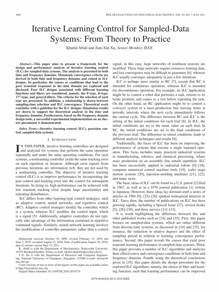
Fig. 1. Plot of mCi.
be expanded to the form of
Δui+1 =
⎡⎢⎢⎣
1 − βCΓ 0 · · · 0−βCΦΓ 1 − βCΓ
. . ....
......
. . . 0−βCΦN−1Γ −βCΦN−2Γ · · · 1 − βCΓ
⎤⎥⎥⎦
︸ ︷︷ ︸F
× Δui. (18)
The stability of (18) is now reduced to
|1 − βCΓ| < 1. (19)
Assume that
α = sup1≤k≤N−1
|βCΦkΓ| (20)
and let γ = 1 − βCΓ. Thus, the worst case matrix F can beapproximated as follows:
Fwc =
⎡⎢⎢⎣
γ 0 · · · 0−α
. . .. . .
......
. . .. . . 0
−α · · · −α γ
⎤⎥⎥⎦ . (21)
Note that a general solution of (18) is given by
Δui+1 = FiΔu0 (22)
where Δu0 is the error in control at the zeroth iteration.Approximate F in the compution of Fi to obtain
Fiwc =
⎡⎢⎢⎣
γi 0 · · · 0S(1)
. . .. . .
......
. . .. . . 0
S(N − 1) · · · S(1) γi
⎤⎥⎥⎦ (23)
where
S(m) =min(i,m)∑
p=1
(−1)p(iCp
) (m−1Cp−1
)γi−pαp. (24)
The binomial coefficient mCp is plotted for a constant m as afunction of p in Fig. 1. It can be seen that the coefficient attains

ABIDI AND XU: ITERATIVE LEARNING CONTROL FOR SAMPLED-DATA SYSTEMS 3005
a very large value before converging to unity, and if the conver-gence due to α and γ is slower than that of the initial divergenceof mCp, then S(m) would also follow the characteristic ofmCp. This kind of poor responses, which is the extremelyovershooting phenomenon, will be observed in later examples.From the aforementioned results, it is obvious that a guaranteefor monotonic convergence is necessary. Two conditions exist,which guarantee monotonic convergence. The first one is timedomain based, while the other is frequency domain based andwill be investigated later on. According to Moore et al. [31],if |1 − βCΓ| < 1, then monotonic convergence is guaranteed ifthe following condition is satisfied:
|CΓ| >
N∑j=2
|CΦj−1Γ| ∀βCΓ ∈ (0, 1)
|CΓ| <1|β| −
N∑j=2
|CΦj−1Γ| ∀βCΓ ∈ (1, 2). (25)
Later, it will be shown that, with the proper learning function,i.e., L(q), the likelihood of satisfying the aforesaid conditionis increased. Based on (24) and (25), it is worth ponderingthe effect of sampling time on ILC convergence. Note thatthe parameter N in (23) and (25) represents the number ofsamples per iteration and that the lower the value of N (thelarger the sampling time), the lower the peak of the functionmCp, as can be inferred from Fig. 1. Similarly, a lower valueof N makes (25) more likely to be satisfied. However, this istrue only for the ideal case of a stable linear time-invariantsystem with no disturbance. If the system is subjected to arepeatable disturbance, then the sampling time must be selectedsuch that the disturbance bandwidth is covered as much aspossible. Thus, a tradeoff will exist between the selection ofsampling time and how much of the disturbance bandwidth willbe covered.
B. D- and D2-Type ILC
In this section, two representative designs of the learningfunction [L(q)] will be considered, and later on, a detailedguideline will be presented from the frequency-domain per-spective for the selection of appropriate learning functions.Consider
ui+1(k) = ui,k + βL(q)ei,k+1. (26)
If the D-type ILC is considered, then L(q) represents a first-order difference, hence the name, and is given by L(q) = 1 −q−1. In the lifted form, the learning function L(q) is
L =
⎡⎢⎢⎢⎢⎢⎢⎢⎢⎣
1 0 · · · · · · 0
−1. . .
. . .. . .
...
0. . .
. . .. . .
......
. . .. . .
. . . 0
0 · · · 0 −1 1
⎤⎥⎥⎥⎥⎥⎥⎥⎥⎦
. (27)
Subtracting (26) from ur,k and writing in the lifted form yield
Δui+1 = Δui − β
⎡⎢⎢⎢⎢⎢⎢⎢⎢⎣
1 0 · · · · · · 0
−1. . .
. . .. . .
...
0. . .
. . .. . .
......
. . .. . .
. . . 0
0 · · · 0 −1 1
⎤⎥⎥⎥⎥⎥⎥⎥⎥⎦
ei. (28)
Substituting (12) into (28) results in
Δui+1 = β
⎡⎢⎢⎢⎢⎣
γβ 0 · · · 0
−C(Φ − I)Γ γβ
. . ....
.... . .
. . . 0−CΦN−2(Φ − I)Γ · · · −C(Φ − I)Γ γ
β
⎤⎥⎥⎥⎥⎦
× Δui (29)
where γ = (1 − βCΓ). A closer look at the matrix in (29) willreveal that the eigenvalues are the same as that of the matrix in(18). Thus, BIBO stability is guaranteed if
|1 − βCΓ| < 1. (30)
Another point to note is that, in (29), the term (Φ − I) ≈ ATfor small T . This indicates that, in comparison to the matrixin (18), the magnitudes of nondiagonal elements in (29) arereduced by an order O(T ). Revisiting condition (25) for theD-type ILC, it is modified to
|CΓ|>N∑
j=2
∣∣CΦj−2(I−Φ)Γ∣∣ ∀βCΓ ∈ (0, 1)
|CΓ|< 1|β| −
N∑j=2
|CΦj−2(I−Φ)Γ| ∀βCΓ ∈ (1, 2). (31)
Since (Φ − I) ≈ AT , the aforementioned conditions aremore likely to be satisfied for the D-type ILC as opposed tothe P-type one.
Proceeding further and introducing the D2-type ILC, thelearning function L(q) represents a second-order difference, asinferred by the name, given by
L(q) = 1 − 2q−1 + q−2. (32)
In the lifted form, the learning function L(q) is given by
L =
⎡⎢⎢⎢⎢⎢⎢⎢⎢⎣
1 0 · · · · · · · · · 0
−2 1. . .
. . .. . .
...
1 −2 1. . .
. . ....
0. . .
. . .. . .
. . ....
.... . .
. . .. . .
. . . 00 · · · 0 1 −2 1
⎤⎥⎥⎥⎥⎥⎥⎥⎥⎦
. (33)
3006 IEEE TRANSACTIONS ON INDUSTRIAL ELECTRONICS, VOL. 58, NO. 7, JULY 2011
Following the same procedure as that in the derivation of(29), the following is obtained:
Δui+1 = β
⎡⎢⎢⎢⎢⎢⎢⎢⎢⎣
γβ 0 · · · · · · 0
κ γβ
. . .. . .
...
−CΓφ. . .
. . .. . .
......
. . .. . .
. . . 0−CΦN−3Γφ · · · −CΓφ κ γ
β
⎤⎥⎥⎥⎥⎥⎥⎥⎥⎦
Δui
(34)
where γ = 1 − βCΓ, κ = −C(2Φ − I)Γ, and Γφ = (Φ −I)2Γ. Note that, as in the case of the D-type ILC, the eigen-values are the same as that of the P-type ILC. However, most ofthe nondiagonal elements contain the term (Φ − I)2, which issignificant since (Φ − I)2 ≈ (AT )2 ≈ O(T 2). Condition (25)for the D2-type ILC is modified to
|CΓ| >|κ|+N∑
j=3
|CΦj−3Γφ| ∀βCΓ ∈ (0, 1)
|CΓ|< 1|β| −|κ|−
N∑j=3
|CΦj−3Γφ| ∀βCΓ ∈ (1, 2). (35)
Note that, in condition (35), the term Γφ is dominat-ing. Since (Φ − I)2 ≈ O(T 2) in Γφ, it increases the like-lihood of (35) being satisfied, thus guaranteeing asymptoticconvergence.
IV. FREQUENCY-DOMAIN ANALYSIS AND DESIGNS OF ILC
It has been shown that, based on the time-domain analy-sis, it is only possible to guarantee BIBO stability. Basedon this, the system may not behave in a desirable manner.Thus, it is a must to find ways of guaranteeing monotonicconvergence.
Consider the one-sided z-transform of (4)
ΔXi(z) = (Iz − Φ)−1ΓΔUi(z)
Ei(z) =CΔXi(z) = C(Iz − Φ)−1Γ︸ ︷︷ ︸P (z)
ΔUi(z). (36)
Obtaining the z-transform of (1) and subtracting both sidesfrom Ur(z), the following is obtained:
ΔUi+1(z)=H(z)[ΔUi(z)−zβL(z)Ei(z)]+[1−H(z)] Ur(z).(37)
Substitution of (36) into (37) leads to
ΔUi+1(z)=H(z)[1−zβL(z)P (z)]︸ ︷︷ ︸F (z)
ΔUi(z)+[1−H(z)]Ur(z).
(38)
An important point to note is that if F (z) is expanded as
F (z) = f0 + f1z−1 + f2z
−2 + f3z−3 + · · ·
then the first N coefficients of the series represent the firstcolumn of the Toeplitz matrix F in (15); in other words
F =
⎡⎢⎢⎢⎣
f0 0 · · · 0
f1. . .
. . ....
.... . .
. . . 0fN−1 · · · f1 f0
⎤⎥⎥⎥⎦ .
According to Norrlof and Gunnarsson [34], if F (z) in (38) isstable and causal, then
supθ∈[−π,π]
∣∣F (ejθ)∣∣= sup
θ∈[−π,π]
∣∣H(ejθ)[1−ejθβL(ejθ)P (ejθ)
]∣∣<1 (39)
where θ = ωkT , implies that the matrix norm of F is
‖F‖ < 1.
Remark 3: Condition (39) is more conservative than (19) asit implies that the norm ‖ei‖ is monotonically decreasing andthus guarantees monotonic convergence.
Remark 4: Note that, in many cases, the plant P (z) may notbe stable; however, a stable P (z) is needed as a prerequisite tosatisfying condition (39). This can be achieved using current-cycle ILC.
A. Current-Cycle Iterative Learning
It was seen in the previous sections that, along with con-dition (39), the plant P (z) must be stable in order to guar-antee monotonic convergence of the ILC system. This canbe achieved by including an inner closed-loop feedback tostabalize the plant.
Consider the sampled-data system (2), where Φ is assumedto be unstable. The closed-loop control can be based onstate feedback or output feedback, depending on the avail-ability of the measured states. The state feedback approachis rather straightforward and will not be covered in detail.Consider
ui,k = −Kxi,k + vi,k (40)
where vi can be any of the ILC laws that have been discusseduntil now. Note that the substitution of (40) into (2) results in
xi,k+1 = (Φ − ΓK)xi,k + Γvi,k. (41)
Clearly, the gain K can be designed such that the sys-tem is stable. From here on, all the results shown earlierapply.
Now, consider if only the output measurement is avail-able. In this case, the ILC law with an output feedbackcontroller is
ui,k = G(q)ei,k + vi,k (42)
where G(q) is the controller. Considering general ILC, vi is
vi,k = H(q) [vi−1(k) + βL(q)ei−1(k + 1)] . (43)

ABIDI AND XU: ITERATIVE LEARNING CONTROL FOR SAMPLED-DATA SYSTEMS 3007
The z-transforms of (42) and (43) are, respectively [33]
Ui(z) = G(z)Ei(z) + Vi(z) (44)
Vi(z) = H(z) [Vi−1(z) + βzL(z)Ei−1(z)] . (45)
The input–output relationship of the plant in the z-domain is
Yi(z) = C(Iz − Φ)−1Γ︸ ︷︷ ︸P (z)
Ui(z). (46)
Note that the tracking error is ei,k = yr,k − yi,k. Thus
Ei(z) = Yr(z) − Yi(z) = Yr(z) − P (z)Ui(z). (47)
Substitution of (44) into (47) and simplifying the resultlead to
Ei(z) =1
1 + G(z)P (z)Yr(z) − P (z)
1 + G(z)P (z)Vi(z) (48)
which can be rewritten as
− P (z)1 + G(z)P (z)
Vi(z) = Ei(z) − 11 + G(z)P (z)
Yr(z).
(49)
If (45) is multiplied by −(P (z)/(1 + G(z)P (z))), the fol-lowing is obtained:
P (z)1 + G(z)P (z)
Vi(z) =H(z)P (z)
1 + G(z)P (z)
× (Vi−1(z) + βL(z)Ei−1(z)) . (50)
Substituting (49) into (50) and simplifying it yield
Ei(z) = H(z)(
1 − βzL(z)P (z)
1 + G(z)P (z)
)Ei−1(z)
+1 − H(z)
1 + G(z)P (z)Yr(z). (51)
Defining P ′(z) as the closed-loop transfer function
P ′(z) =P (z)
1 + G(z)P (z)(52)
(51) becomes
Ei(z) = H(z) (1 − zβL(z)P ′(z)) Ei−1(z)
+1 − H(z)
1 + G(z)P (z)Yr(z). (53)
From (53), it can be seen that monotonic convergence re-quires that P ′(z) be stable and the condition
supθ∈[−π,π]
∣∣H(ejθ)(1 − ejθβL(ejθ)P ′(ejθ)
)∣∣ < 1 (54)
be satisfied. The poles of the transfer function P ′(z) can beproperly selected by designing G(z), while condition (54)can be satisfied by the proper designs of H(z), L(z), andβ. However, note that the tracking error E(z) is effected byYr(z) through (1 − H(z))/(1 + G(z)P (z)). Thus, the designs
Fig. 2. Monotonic convergence region for βzL(z)P (z).
of G(z) and H(z) must also take into account that
supθ∈[−π,π]
∣∣∣∣ 1 − H(ejθ)1 + G(ejθ)P (ejθ)
∣∣∣∣ � 1. (55)
Remark 5: From expression (51), it can be seen that thelearning gain β affects the zero(s) of the transfer functionbetween Ei and Ei−1. Thus, in addition to satisfying (54), βmay be chosen such that the desired zero(s) are produced.
B. Considerations for L(q) and H(q) Selection
In this section, the selection criteria for L(q) and H(q)to achieve the desired monotonic convergence will bediscussed.
Consider the ILC system given by (53). Without loss ofgenerality, it will be assumed that P (z) is stable and G(z) ≡ 0.Thus, without a feedback loop, (53) becomes
Ei(z)=H(z) [1−βzL(z)P (z)] Ei−1(z)+[1−H(z)] Yr(z).(56)
If it is assumed that H(z) = 1, then, ideally, selectingL(z) = 1/zβP (z) would lead to the fastest possible conver-gence in the monotonic sense. This, however, is impracticalas it is not possible to identify P (z) exactly for real systems.Consider the term [1 − βzL(z)P (z)]. Monotonic convergencerequires that [1 − βzL(z)P (z)] be within a unit circle centeredat the origin of the complex plane. This can be restated as arequirement that βzL(z)P (z) be within a unit circle centeredat (1, 0) on the complex plane, as shown in Fig. 2. From thiscondition, it is observed that stability requires that
∠(ejθL(ejθ)P (ejθ)
)= ϕ ∈ (−π/2, π/2) ∀θ ∈ [−π, π]
supθ∈[−π,π]
∣∣∣βejθ(ϕ)L(ejθ(ϕ)
)P
(ejθ(ϕ)
)∣∣∣ < 2 cos(ϕ). (57)
An important fact to note is that zL(z) should ensure that as|∠(ejθL(ejθ)P (ejθ))| → π/2, then |βejθL(ejθ)P (ejθ)| → 0.
On the other hand, the selection of H(z) must take intoconsideration that the term [1 − H(z)] be minimized and beas close as possible to zero at steady state, thereby preventingany steady-state errors. Thus, H(z) is generally selected as
3008 IEEE TRANSACTIONS ON INDUSTRIAL ELECTRONICS, VOL. 58, NO. 7, JULY 2011
a low-pass filter. An advantage of using H(z) is that thestability region for certain frequencies can be increased ifH(z) has a gain that is less than one. This can be seenfrom (54)
∣∣1 − βejθL(ejθ)P (ejθ)∣∣ <
1|H(ejθ)| , θ ∈ [−π, π]. (58)
Later on, some examples will highlight the aforementionedpoints.
C. D- and D2-Type ILC
Consider the ILC
ui+1(k) = H(q) [ui,k + βqL(q)ei,k] (59)
substitute L(q) = 1 − q−1, and perform the z-transform of (59)after subtracting both sides from ur to obtain
ΔUi+1(z) = H(z) [ΔUi(z) − (z − 1)βEi(z)]
+ [1 − H(z)] Ur(z). (60)
Substitution of (36) into (60) leads to
ΔUi+1(z) = H(z) [1 − (z − 1)βP (z)] ΔUi(z)
+ [1 − H(z)] Ur(z). (61)
According to the results with the P-type ILC, monotonicconvergence is guaranteed if
supθ∈[−π,π]
∣∣H(ejθ)[1 − β(ejθ − 1)P (ejθ)
]∣∣ < 1. (62)
Similarly, for L(q) = 1 − 2q−1 + q−2, the condition is
supθ∈[−π,π]
∣∣H(ejθ)[1 − β(ejθ − 2 + e−jθ)P (ejθ)
]∣∣ < 1. (63)
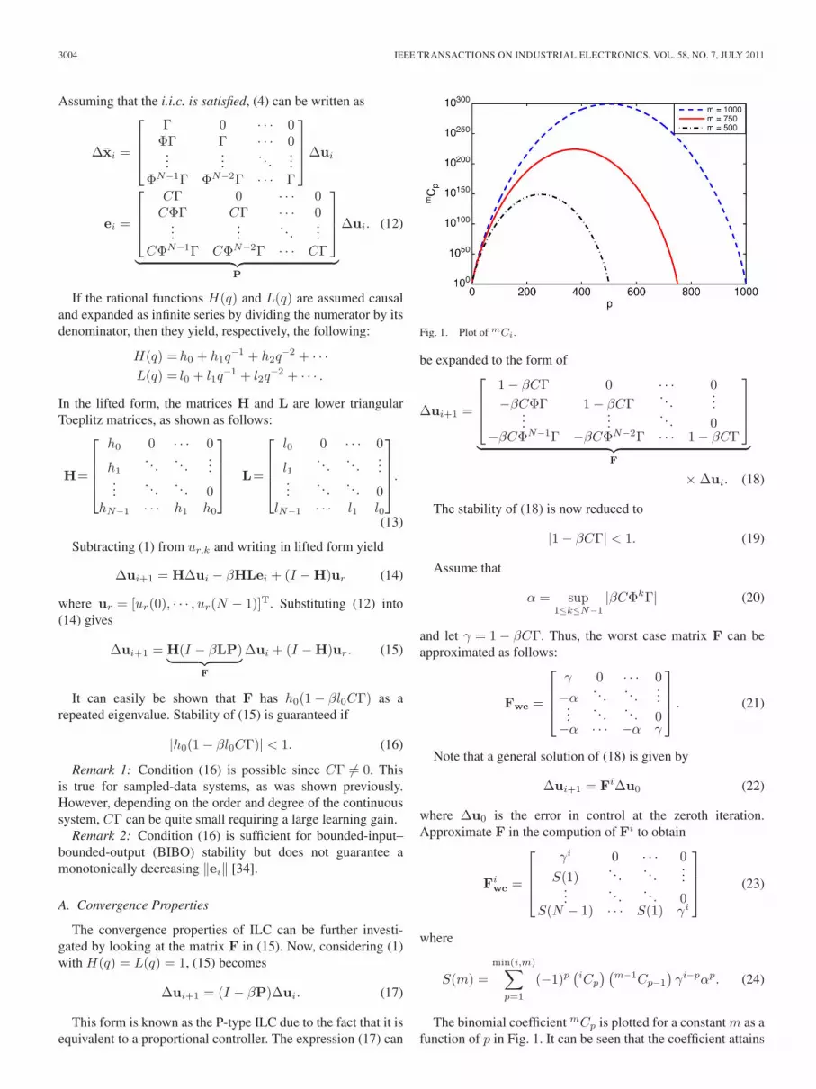
In Fig. 3, the magnitude and phase diagrams of zL(z) for theD-type ILC are plotted w.r.t. to the frequency normalized by thesampling frequency ws = 2π/T . The phase diagram indicatesthat, at low frequencies, the phase response is 90◦, which wouldviolate the stability condition (57) if P (z) has a phase that isgreater than or equal to 0◦ at low frequencies. This learningfunction would work well if it is applied to a second orderwith a single-integrator system or a third order with a single-integrator system and a cutoff frequency near ws/2. Similarly,for the D2-type ILC, the learning function would work ideallyfor a double-integrator system or a third order with a double-integrator system and a cutoff frequency near ws/2, as seenin Fig. 3.
V. NUMERICAL EXAMPLES FOR TIME-DOMAIN ILC
A. P-Type ILC
Consider the second-order system
xi(t) =Axi(t) + Bui(t)
yi(t) =Cxi(t) (64)
Fig. 3. Magnitude and phase of zL(z) for L(z) corresponding to D and D2
designs.
where the system matrices are given by
A =[
0 10 −144
]B =
[06
]
C = [1 0].
This is the nominal model of a piezomotor stage that willbe used in the experimental applications of the ILC laws. Thesampled-data system representation of (64) is given by
xi,k+1 = Φxi(t) + Γui,k
yi,k =Cxi,k. (65)
If the sampling time is set to 1 ms, the system becomes
Φ =[
1 9.313 × 10⁻⁴
0 0.8659
]Γ =
[2.861 × 10⁻⁶
0.0056
].
Note that the relative degree of the original system (64) istwo, whereas the relative degree of the sampled-data system(65) is one. Thus, the following ILC is used:
ui+1(k) = ui,k + βei,k+1
ei,k = yr,k − yi,k (66)
where the desired output trajectory is selected as yr,k =0.030 + 0.030 sin(2πkT − (π/2)) and each iteration is 0.5 sin duration. The learning gain β is selected as 2 · 105 such that1 − βCΓ = 0.4278. The maximum error for each iteration isshown in Fig. 4.
B. D- and D2-Type ILC
Now, consider the D-type ILC
ui+1(k) = ui,k + β(ei,k+1 − ei,k) (67)

ABIDI AND XU: ITERATIVE LEARNING CONTROL FOR SAMPLED-DATA SYSTEMS 3009
Fig. 4. Tracking error using P-, D-, and D2-type ILC.
where the learning gain (β) is selected as 2 · 105, which issimilar to the P-type ILC case. This is because the eigenvaluesof the system in the iteration domain are the same for bothcases. Thus, 1 − βCΓ = 0.4278 for this example. The maxi-mum error for each iteration is shown in Fig. 4. Note that theperformance with the D-type ILC is similar to that with theP-type ILC. However, in the frequency-domain analysis, it willbe shown that it is possible to select the proper learning gainto achieve monotonic ‖ei‖ and that this is not possible for theP-type ILC.
Finally, consider the D2-type ILC
ui+1(k) = ui,k + β(ei,k+1 − 2ei,k + ei,k−1) (68)
where the learning gain (β) is selected as 2 · 105, which is simi-lar to the P- and D-type ILC cases. The maximum error for eachiteration is shown in Fig. 4. Note that the performance with theD2-type ILC is much better than that with the previous cases.Monotonic convergence is achieved in this case as opposed tothe P- and D-type ILC cases with the same learning gain. Thisis because, in condition (35), the term (Φ − I)2 is rather small,and thus, the condition can be met easily.
VI. NUMERICAL EXAMPLE: FREQUENCY DOMAIN
A. P-Type ILC
In order to have more insight into the example considered inthe time-domain analysis, again, considering the system (65),the input–output relationship is given by
Y (z) = P (z)U(z). (69)
Using the same parameters as that in the time-domain exam-ple, the transfer function of the system, i.e., P (z), is
P (z) = C(Iz − Φ)−1Γ =2.861 · 10−6z + 2.727 · 10−6
z2 − 1.866z + 0.866.
(70)
The filter H(z) and learning function L(z) are set to unity.Thus, the Nyquist diagram of F (z) is shown in Fig. 5. From thefigure, it is seen that |F (ejθ)| does not lie inside the unit circle
Fig. 5. Nyquist plot of F (z) for the P-type ILC.
Fig. 6. Nyquist plot for the D-type ILC example with β = 2 · 105 and β =4.75 · 104.
for any frequencies, and as θ → 0, then |F (ejθ)| → ∞. Thus,condition (39) is not satisfied, and monotonically decreasing‖ei‖ is not guaranteed.
B. D- and D2-Type ILC
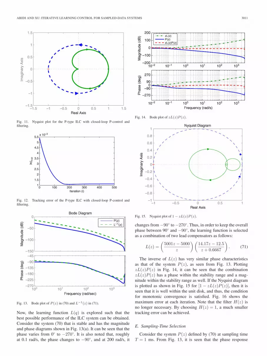
Now, construct the Nyquist diagram of H(z)[1 −βzL(z)P (z)] that has the same parameters as that of the P-typeILC example while using L(z) = 1 − z−1. From Fig. 6(a),it is seen that the Nyquist diagram of H(ejθ)[1 − β(ejθ −1)P (ejθ)] lies outside the unit disk, but there is a possibilityof selecting learning gain β that would allow it to stay insidethe unit circle. For example, choosing the value of β at around4.75 · 104 or below will lead to a Nyquist plot inside theunit circle, as shown in Fig. 6(b). Now, going back to thetime-domain analysis and using β = 4.75 · 104, the repeatedeigenvalue of (29) is 1 − βCΓ = 0.8641 < 1. The maximumtracking error for each iteration is shown in Fig. 7, which showsa monotonic convergence of the error in the iteration domain.
If the D2-type ILC or L(z) = 1 − 2z−1 + z−2 is used in-stead with the same initial learning gain for the D-type one,
3010 IEEE TRANSACTIONS ON INDUSTRIAL ELECTRONICS, VOL. 58, NO. 7, JULY 2011
Fig. 7. Tracking error using D-type ILC and β = 4.75 · 104.
Fig. 8. Nyquist plot for the D2-type ILC example with β = 2 · 105.
it is seen from Fig. 8 that the Nyquist plot of H(z)[1 −βzL(z)P (z)] is within the unit disk but takes a value that isclose to one at very low frequencies. This is because (z −1)2 → 0 as ω → 0. If the plant was a double-integrator type,then this would not be so.
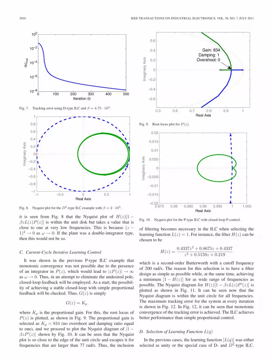
C. Current-Cycle Iterative Learning Control
It was shown in the previous P-type ILC example thatmonotonic convergence was not possible due to the presenceof an integrator in P (z), which would lead to |zP (z)| → ∞as ω → 0. Thus, in an attempt to eliminate the undesired pole,closed-loop feedback will be employed. As a start, the possibil-ity of achieving a stable closed-loop with simple proportionalfeedback will be checked. Thus, G(z) is simply
G(z) = Kp
where Kp is the proportional gain. For this, the root locus ofP (z) is plotted, as shown in Fig. 9. The proportional gain isselected as Kp = 834 (no overshoot and damping ratio equalto one), and we proceed to plot the Nyquist diagram of |1 −βzP ′(z)| shown by Fig. 10. It can be seen that the Nyquistplot is so close to the edge of the unit circle and escapes it forfrequencies that are larger than 77 rad/s. Thus, the inclusion
Fig. 9. Root locus plot for P (z).
Fig. 10. Nyquist plot for the P-type ILC with closed-loop P-control.
of filtering becomes necessary in the ILC when selecting thelearning function L(z) = 1. For instance, the filter H(z) can bechosen to be
H(z) =0.4337z2 + 0.8675z + 0.4337
z2 + 0.5159z + 0.219
which is a second-order Butterworth with a cutoff frequencyof 200 rad/s. The reason for this selection is to have a filterdesign as simple as possible while, at the same time, achievinga minimum [1 − H(z)] for as wide range of frequencies aspossible. The Nyquist diagram for H(z)[1 − βzL(z)P ′(z)] isplotted as shown in Fig. 11. It can be seen now that theNyquist diagram is within the unit circle for all frequencies.The maximum tracking error for the system at every iterationis shown in Fig. 12. In Fig. 12, it can be seen that monotonicconvergence of the tracking error is achieved. The ILC achievesbetter performance than simple proportional control.
D. Selection of Learning Function L(q)
In the previous cases, the learning function [L(q)] was eitherselected as unity or the special case of D- and D2-type ILC.
ABIDI AND XU: ITERATIVE LEARNING CONTROL FOR SAMPLED-DATA SYSTEMS 3011
Fig. 11. Nyquist plot for the P-type ILC with closed-loop P-control andfiltering.
Fig. 12. Tracking error of the P-type ILC with closed-loop P-control andfiltering.
Fig. 13. Bode plot of P (z) in (70) and L−1(z) in (71).
Now, the learning function L(q) is explored such that thebest possible performance of the ILC system can be obtained.Consider the system (70) that is stable and has the magnitudeand phase diagrams shown in Fig. 13(a). It can be seen that thephase varies from 0◦ to −270◦. It is also noted that, roughlyat 0.1 rad/s, the phase changes to −90◦, and at 200 rad/s, it
Fig. 14. Bode plot of zL(z)P (z).
Fig. 15. Nyquist plot of 1 − zL(z)P (z).
changes from −90◦ to −270◦. Thus, in order to keep the overallphase between 90◦ and −90◦, the learning function is selectedas a combination of two lead compensators as follows:
L(z) =(
5001z − 5000z
) (14.17z − 12.5z + 0.6667
). (71)
The inverse of L(z) has very similar phase characteristicsas that of the system P (z), as seen from Fig. 13. PlottingzL(z)P (z) in Fig. 14, it can be seen that the combinationzL(z)P (z) has a phase within the stability range and a mag-nitude within the stability range as well. If the Nyquist diagramis plotted as shown in Fig. 15 for [1 − zL(z)P (z)], then it isseen that it is well within the unit disk, and thus, the conditionfor monotonic convergence is satisfied. Fig. 16 shows themaximum error at each iteration. Note that the filter H(z) isno longer necessary. By choosing H(z) = 1, a much smallertracking error can be achieved.
E. Sampling-Time Selection
Consider the system P (z) defined by (70) at sampling timeT = 1 ms. From Fig. 13, it is seen that the phase response

3012 IEEE TRANSACTIONS ON INDUSTRIAL ELECTRONICS, VOL. 58, NO. 7, JULY 2011
Fig. 16. Tracking error profile of the system using P-type ILC with closed-loop P-control and filtering.
Fig. 17. Phase diagram of z.
crosses −90◦ at nearly 2π rad/s. Considering the phase diagramof z, from Fig. 17, it is linearly increasing from 0◦ to 180◦ asa function of frequency. From here, it seems obvious that if alarger sampling time is selected such that the phase responseof P (z) slightly crosses the (−90◦, 90◦) stability bound, then,combined with z, the overall phase response (ϕ) would bewithin (−90◦, 90◦). Thus, the sampling time T = 10 ms isselected, and the magnitude and phase diagrams of zP (z)are shown in Fig. 18. It can be seen from Fig. 18 that theoverall phase response of zP (z) still crosses the stability bound(−90◦, 90◦); hence, the sampling time will be increased toT = 15 ms, and the magnitude and phase diagrams of zP (z)are reshown in Fig. 18. It can be seen from Fig. 18 that, with thenew sampling time, the phase response of zP (z) is now withinthe stability bound (−90◦, 90◦), and since, for all the cases, themagnitude of zP (z) was within the stability bound, the systemcan now achieve monotonic convergence.
VII. EXPERIMENTAL INVESTIGATION
In this section, a practical implementation of the ILC laws fora linear piezoelectric motor that has many promising applica-tions in industries will be shown. Piezoelectric motors are char-acterized by low speed and high torque, which are in contrastto the high-speed and low-torque properties of conventional
Fig. 18. Bode plot of zP (z) at T = 10 ms and zP (z) at T = 15 ms.
electromagnetic motors. Moreover, piezoelectric motors arecompact and light, operates quietly, and are robust to externalmagnetic or radioactive fields. Piezoelectric motors are mainlyapplied to high-precision control problems, as they can easilyreach the precisions of micrometers and even nanometers.
Implementation was carried out on a dSPACE DS1102 con-troller card attached to a PC running on a PII CPU. Positionfeedback was available through a linear encoder with a reso-lution of 20 nm. The controller was written using C-code anddownloaded to the DS1102 via the dSPACE control desk UI.The motor and driver can be modeled approximately as
x1(t) = x2(t)
x2(t) = − kfv
Mx2(t) +
kf
Mu(t)
y(t) = x1(t) (72)
where x1 is the motion position, x2 is the motion velocity, M =1 kg is the moving mass, kfv = 144N is the velocity dampingfactor, and Kf = 6 N/V is the force constant. The system issampled at T = 0.4 ms and becomes
x1(k + 1) =x1(k)+3.8870 · 10−4x2(k)+4.7092 · 10−7u(k)x2(k + 1) = 0.9440x2(k) + 0.0023u(k)
y(k) =x1(k)366 : 1395. (73)
The simple linear model (73) does not contain any nonlinearand uncertain effects, such as the frictional force in the me-chanical part, the high-order electrical dynamics of the driver,loading condition, etc., which are hard to model in practice. Ingeneral, producing a high-precision model is more demandingthan performing a control task with the same level of precision.
Before proceeding with the ILC selection and implementa-tion, all the methods demonstrated until now shall be tabulated,and the resulting table shall act as a guideline for the implemen-tation. This can be found in Table I. The objective is to achievemotion control as precise as possible after the smallest numberof iterations. Due to the existence of uncertainties and otherunmodeled disturbances, the most suitable selection would be
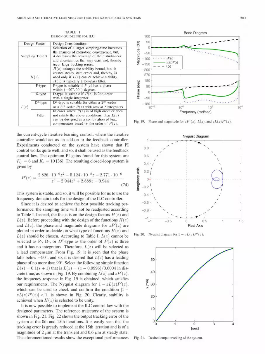
ABIDI AND XU: ITERATIVE LEARNING CONTROL FOR SAMPLED-DATA SYSTEMS 3013
TABLE IDESIGN GUIDELINE FOR ILC
the current-cycle iterative learning control, where the iterativecontroller would act as an add-on to the feedback controller.Experiments conducted on the system have shown that PIcontrol works quite well, and so, it shall be used as the feedbackcontrol law. The optimum PI gains found for this system areKp = 6 and Ki = 10 [36]. The resulting closed-loop system isgiven by
P ′(z) =2.826 · 10−6z2 − 5.124 · 10−8z − 2.771 · 10−6
z3 − 2.944z2 + 2.888z − 0.944.
(74)
This system is stable, and so, it will be possible for us to use thefrequency-domain tools for the design of the ILC controller.
Since it is desired to achieve the best possible tracking per-formance, the sampling time will not be readjusted accordingto Table I. Instead, the focus is on the design factors H(z) andL(z). Before proceeding with the design of the functions H(z)and L(z), the phase and magnitude diagrams for zP ′(z) areplotted in order to decide on what type of functions H(z) andL(z) should be chosen. According to Table I, L(z) cannot beselected as P-, D-, or D2-type as the order of P (z) is threeand it has no integrators. Therefore, L(z) will be selected asa lead compensator. From Fig. 19, it is seen that the phasefalls below −90◦, and so, it is desired that L(z) has a leadingphase of no more than 90◦. Select the following simple functionL(s) = 0.1(s + 1) that is L(z) = (z − 0.9996)/0.0004 in dis-crete time, as shown in Fig. 19. By combining L(z) and zP ′(z),the frequency response in Fig. 19 is obtained, which satisfiesour requirements. The Nyquist diagram for 1 − zL(z)P ′(z),which can be used to check and confirm the condition |1 −zL(z)P ′(z)| < 1, is shown in Fig. 20. Clearly, stability isachieved when H(z) is selected to be unity.
It is now possible to implement the ILC control law with thedesigned parameters. The reference trajectory of the system isshown in Fig. 21. Fig. 22 shows the output tracking error of thesystem at the 0th and 15th iterations. It is easily seen that thetracking error is greatly reduced at the 15th iteration and is of amagnitude of 2 μm at the transient and 0.6 μm at steady state.The aforementioned results show the exceptional performances
Fig. 19. Phase and magnitude for zP ′(z), L(z), and zL(z)P ′(z).
Fig. 20. Nyquist diagram for 1 − zL(z)P ′(z).
Fig. 21. Desired output tracking of the system.

3014 IEEE TRANSACTIONS ON INDUSTRIAL ELECTRONICS, VOL. 58, NO. 7, JULY 2011
Fig. 22. Output tracking error of the system at the 0th and 15th iterations.
of the ILC laws as add-ons to existing feedback control. Thestraightforward design also shows that the method has a lot ofpromise for practical applications.
VIII. CONCLUSION
This paper has summarized the theoretical results of ILC forsampled-data systems in the time and frequency domains. Thelarge overshooting phenomenon has been explored in the timedomain. Monotonic convergence criteria have been presentedfor both time and frequency domains. Specific cases of thelearning function have been investigated. A design guidelinehas been shown for ILC design in the frequency domain. Simu-lation results verify the theoretical analysis. In the time domain,the P-type ILC assures learning convergence, but the transientperformance in the iteration domain could be bad due to thelack of monotonic property. The reason of nonmonotonicity isfrom the off-diagonal elements in the F matrix that specifiesthe contraction mapping between consecutive iterations. Thisshortcoming can be mitigated by using D- or D2-type ILC,which can effectively scale down the magnitude of the off-diagonal elements in F. The effectiveness of D- and D2-typeILC has been further analyzed in the frequency domain. Next,the designs of the filter Q and the learning function L have beenexplored in the frequency domain. By appropriately choosingQ and L according to the time-domain characteristics, it ispossible to achieve monotonic learning convergence even withthe simple P-type ILC. ILC add-ons to closed-loop feedback,as well as the sampling effect on learning convergence, havealso been explored. Finally, the ILC has been applied to a realsystem, i.e., a piezoelectric motor, with promising results.
REFERENCES
[1] M. Uchiyama, “Formation of high-speed motion pattern of a mechanicalarm by trial,” Trans. Soc. Instrum. Control Eng., vol. 14, no. 6, pp. 706–712, 1978.
[2] M. Garden, “Learning control of actuators in control systems,” U.S. Patent3,555,252, Jan. 12, 1971.
[3] K. S. Narendra and A. M. Annaswamy, Stable Adaptive Systems, vol. 3.Upper Saddle River, NJ: Prentice-Hall, 1989.
[4] K. Kaneko and R. Horowitz, “Repetitive and adaptive control of robot ma-nipulators with velocity estimation,” IEEE Trans. Robot. Autom., vol. 13,no. 2, pp. 204–217, Apr. 1997.
[5] K. L. Moore, Iterative Learning Control for Deterministic Systems.London, U.K.: Springer-Verlag, 1993.
[6] K. J. Hunt, D. Sbarbaro, R. Zbikowski, and P. J. Gawthrop, “Neuralnetworks for control systems—A survey,” Automatica, vol. 28, no. 6,pp. 1083–112, Nov. 1992.
[7] G. Hillerstrom and K. Walgama, “Repetitive control theory andapplications—A survey,” in Proc. 13th World Congr., vol. D, ControlDesign II, Optimization, 1997, pp. 1–6.
[8] R. W. Longman, “Iterative learning control and repetitive control forengineering practice,” Int. J. Control, vol. 73, no. 10, pp. 930–954,Jul. 2000.
[9] S. Arimoto, S. Kawamura, and F. Miyazaki, “Bettering operation of robotsby learning,” J. Robot. Syst., vol. 1, no. 2, pp. 123–140, 1984.
[10] R.-E. Precup, S. Preitl, J. K. Tar, M. L. Tomescu, M. Takacs, P. Korondi,and P. Baranyi, “Fuzzy control system performance enhancement by itera-tive learning control,” IEEE Trans. Ind. Electron., vol. 55, no. 9, pp. 3461–3475, Sep. 2008.
[11] H. Deng, R. Oruganti, and D. Srinivasan, “Analysis and design of iterativelearning control strategies for UPS inverters,” IEEE Trans. Ind. Electron.,vol. 54, no. 3, pp. 1739–1751, Jun. 2007.
[12] Y. Q. Ye and D. Wang, “Learning more frequency components usingP-type ILC with negative learning gain,” IEEE Trans. Ind. Electron.,vol. 53, no. 2, pp. 712–716, Apr. 2006.
[13] K.-S. Tzeng, D. C. Tzeng, and J.-S. Chen, “An enhanced iterative learningcontrol scheme using wavelet transform,” IEEE Trans. Ind. Electron.,vol. 52, no. 3, pp. 922–924, Jun. 2005.
[14] K. Zhou and D. Wang, “Digital repetitive learning controller for three-phase CVCF PWM inverter,” IEEE Trans. Ind. Electron., vol. 48, no. 4,pp. 820–830, Aug. 2001.
[15] D. A. Bristow and A. G. Alleyne, “A manufacturing system for microscalerobotic deposition,” in Proc. Amer. Control Conf., 2003, pp. 2620–2625.
[16] H. Elci, R. W. Longman, M. Phan, J.-N. Juang, and R. Ugoletti, “Discretefrequency based learning control for precision motion control,” in Proc.IEEE Int. Conf. Syst., Man, Cybern., 1994, pp. 2767–2773.
[17] W. Messner, R. Horowitz, W.-W. Kao, and M. Boals, “A new adaptivelearning rule,” IEEE Trans. Autom. Control, vol. 36, no. 2, pp. 188–197,Feb. 1991.
[18] M. Norrlof, “An adaptive iterative learning control algorithm with experi-ments on an industrial robot,” IEEE Trans. Robot. Autom., vol. 18, no. 2,pp. 245–251, Apr. 2002.
[19] D.-I. Kim and S. Kim, “An iterative learning control method with appli-cation for CNC machine tools,” IEEE Trans. Ind. Appl., vol. 32, no. 1,pp. 66–72, Jan./Feb. 1996.
[20] D. de Roover and O. H. Bosgra, “Synthesis of robust multivariable itera-tive learning controllers with application to a wafer stage motion system,”Int. J. Control, vol. 73, no. 10, pp. 968–979, Jul. 2000.
[21] H. Havlicsek and A. Alleyne, “Nonlinear control of an electrohydraulicinjection molding machine via iterative adaptive learning,” IEEE/ASMETrans. Mechatronics, vol. 4, no. 3, pp. 312–323, Sep. 1999.
[22] F. Gao, Y. Yang, and C. Shao, “Robust iterative learning control with ap-plications to injection molding process,” Chem. Eng. Sci., vol. 56, no. 24,pp. 7025–7034, Dec. 2001.
[23] J. J. Craig, “Adaptive control of manipulators through repeated trials,” inProc. Amer. Control Conf., 1984, pp. 1566–1573.
[24] N. Amann, D. H. Owens, and E. Rogers, “Iterative learning controlfor discrete-time systems with exponential rate of convergence,” Proc.Inst. Elect. Eng.—Control Theory Appl., vol. 143, no. 2, pp. 217–224,Mar. 1996.
[25] G. Casalino and G. Bartolini, “A learning procedure for the control ofmovements of robotic manipulators,” in Proc. IASTED Symp. Robot.Autom., 1984, pp. 108–111.
[26] S. Kawamura, F. Miyazaki, and S. Arimoto, “Iterative learning control forrobotic systems,” in Proc. Int. Conf. Ind. Electron. Control Instrum., 1984,pp. 393–398.
[27] K. L. Moore and J.-X. Xu, “Editorial: Iterative learning control,” Int. J.Control, vol. 73, no. 10, pp. 819–823, Jul. 2000.
[28] Z. Bien and J.-X. Xu, Iterative Learning Control: Analysis, Design, Inte-gration and Applications. Boston, MA: Kluwer, 1998.
[29] Y. Chen and C. Wen, Iterative Learning Control: Convergence, Robust-ness, and Applications. London, U.K.: Springer-Verlag, 1999.
[30] J.-X. Xu and Y. Tan, Linear and Nonlinear Iterative Learning Control.Berlin, Germany: Springer, 2003.
[31] K. L. Moore, M. Dahleh, and S. P. Bhattacharyya, “Iterative learningcontrol: A survey and new results,” J. Robot. Syst., vol. 9, no. 5, pp. 563–594, 1992.
[32] R. Horowitz, “Learning control of robot manipulators,” Trans. ASME, J.Dyn. Syst. Meas. Control, vol. 115, no. 2B, pp. 402–411, 1993.

ABIDI AND XU: ITERATIVE LEARNING CONTROL FOR SAMPLED-DATA SYSTEMS 3015
[33] D. A. Bristow, M. Tharayil, and A. G. Alleyne, “A survey of iterativelearning control,” IEEE Control Syst. Mag., vol. 26, no. 3, pp. 96–114,Jun. 2006.
[34] M. Norrlof and S. Gunnarsson, “Time and frequency domain convergenceproperties in iterative learning control,” Int. J. Control, vol. 75, no. 14,pp. 1114–1126, Sep. 2002.
[35] M. Norrlof and S. Gunnarsson, “Disturbance aspects of iterative learningcontrol,” Eng. Appl. Artif. Intell., vol. 14, no. 1, pp. 87–94, Feb. 2001.
[36] J.-X. Xu and K. Abidi, “Discrete-time output integral sliding-mode con-trol for a piezomotor-driven linear motion stage,” IEEE Trans. Ind.Electron., vol. 55, no. 11, pp. 3917–3927, Nov. 2008.
Khalid Abidi received the B.S degree in mechanicalengineering from Middle East Technical University,Ankara, Turkey, in 2002, the M.S. degree in electri-cal engineering and computer science from SabanciUniversity, Istanbul, Turkey, in 2004, and the Ph.D.degree in electrical and computer engineering fromthe National University of Singapore, Singapore, in2009.
He was a Research Assistant with the NationalUniversity of Singapore while he was working to-ward the Ph.D. degree. He is currently an Assis-
tant Professor with the Department of Mechatronics, Bahcesehir University,Istanbul. His research interests include analysis of dynamic systems, adaptivecontrol, iterative learning control, robust control, high-precision motion control,and microsystems.
Jian-Xin Xu (M’92–SM’98) received the B.S. de-gree in electrical engineering from Zhejiang Univer-sity, Hangzhou, China, in 1982 and the M.S. andPh.D. degrees from The University of Tokyo, Tokyo,Japan, in 1986 and 1989, respectively.
He was with Hitachi Research Laboratory, Ibaraki,Japan, as a Research Engineer, with Ohio StateUniversity, Columbus, as a Visiting Scholar, andwith Yale University, New Haven, CT, as a VisitingResearch Fellow. In 1991, he joined the NationalUniversity of Singapore, Singapore, where he is cur-
rently a Professor with the Department of Electrical and Computer Engineering.He has produced 125 peer-reviewed journal papers, more than 200 peer-refereed conference papers, one monograph, and three edited books on systemmodeling and control. His research interests are in the fields of system learning,control, and applications to real-time systems.


