Integrals of polynomials associated with tableaux and the Garsia-Haiman conjecture

Math. Z. 228, 537–567 (1998)

c© Springer-Verlag 1998

Integrals of polynomials associated with tableauxand the Garsia-Haiman conjecture

Charles F. Dunkl1, Phil Hanlon2

1 Department of Mathematics, University of Virginia, Charlottesville, VA 22903-3199, USA2 Department of Mathematics, University of Michigan, Ann Arbor, MI 48109-1003, USA

(e-mail: [email protected])

Received 29 November 1994; in final form 10 December 1996

1 Introduction

In a 1983 paper [M1], I. G. Macdonald introduced his well-known “con-stant term conjectures.” These conjectures concern a certain polynomial∆ = ∆(G, k) that is indexed by a semisimple Lie algebraG and a positiveintegerk. The polynomial∆ lives in Z[Φ, q], the group ring of the root lat-ticeΦ of G over Z[q]. A basis for this ring, overZ[q], is the set of formalexponentials,ev, for v ∈ Φ that satisfy the relationsev · ew = ev+w. Theconjecture asserts that the constant term of∆, meaning the part that is inde-pendent of the formal exponentials, has a nice factorization as a polynomialin q.

Later, Macdonald [M2] generalized this work in the following way. Heshowed that there is a unique collection of polynomialsPν indexed by dom-inant weightsν, satisfying the following properties:

1) ThePν form a basis forZ[Φ, q]W , theW -invariants inZ[Φ, q], whereWis the Weyl group ofG. Moreover, the basisPν is triangular with respect tothe basiseµ of orbit sum polynomials.

2) Forν 6= µ, the constant term of

∆ · Pν · Pµ

is zero, wherePµ is obtained fromPµ by replacing eachev by e−v.

Work partially supported by the National Science Foundation.The authors are grateful to the Stieltjes Institute for its support of their visit to the Universityof Leiden during which much of this work was done.

538 C.F. Dunkl, P. Hanlon

3) The coefficient ofeν in Pν is 1.

Macdonald went on to conjecture a formula for the constant term of

∆ · Pν · Pν

for everyν. SinceP0 is the constant 1, this conjecture extended his 1983conjecture that gave a formula for the constant term of∆.

One interesting feature of the Macdonald conjectures is that the statementof the conjectures is not by itself of great interest. The constant term of∆·Pν ·Pµ has no particular significance outside of the context of these conjectures.The real motivation behind any study of the Macdonald conjectures is todiscover some deep mathematical phenomenon that has the constant termconjectures as a consequence.

Macdonald’s constant term conjectures have been proved by Chered-nik [C] using the idea of shift operators pioneered by Opdam [O] togetherwith Cherednik’s powerful affine Hecke algebra machinery. This approachdoes indeed give an interesting interpretation to the constant term conjec-tures. But there have been a number of other efforts to give mathematicalinterpretations to the constant term of∆ · Pν · Pµ. These other approacheshave succeeded in identifying interesting mathematical phenomena that haveMacdonald’s constant term conjectures as consequences. But in many ofthese cases, the deeper mathematical facts that underlie the Macdonald con-jectures have not yet been proved.

Collectively these attempts to settle the Macdonald conjectures involve aremarkable range of mathematical subjects and ideas. Different approacheslead to interesting conjectures about the homology of nilpotent Lie algebras([F] and [H]), the harmonics of a diagonal action of the symmetric groups([GH]), and the generalized traces of Lie algebras ([K]). In addition there isthe above-mentioned work of Cherednik, Opdam and Heckman that involvesshift operators, operators on polynomials that are built from elements inaffine Hecke algebras. This leads one naturally to speculate that there issome deep theory that will simultaneously explain these diverse attacks onthe Macdonald conjectures. At the very least one would like to understandhow to relate these approaches pairwise.

One motivation for this work is an effort to connect the affine Hecke alge-bra approach of Cherednik with the diagonal harmonic approach of Garsiaand Haiman. Garsia and Haiman study the module generated by partialderivative operators on an element in a polynomial ring in two sets of vari-ables (this is explained more fully in Sect. 3). They use the structure of theresulting bigraded module to generate something equivalent to Macdonald’spolynomialsPν . In this work, we replace the partial differentiation operatorsby Dunkl operators. Dunkl operatorsDi(k) are operators on a polynomialring that involve a parameterk. Moreover,Di(k) is a deformation of∂/∂xi

Integrals of polynomials 539

in the sense thatDi(0) = ∂/∂xi. The Dunkl operators are also related tothe fundamental operators that define a faithful representation of the affineHecke algebras. We hope that this work will be a starting point towardsunderstanding the connection between the shift operator proofs of the Mac-donald conjectures and the Garsia-Haiman conjectures both of which giveinteresting interpretations of the Macdonald polynomials.

Our main conjecture gives an explicit characterization of the singularpoints of this deformation. An important ingredient in this conjecture is atheorem given in Sect. 2 that gives the norms of certain special polynomials inC[x1, . . . , xn] with respect to an inner product based on the Dunkl operators.This theorem gives a significant extension of the Mehta integral.

The paper is organized as follows. The main theorem (Theorem 2.6) isproved in Sect. 2. The computational component of the proof is quite intricateand accounts for most of the section. In Sect. 3 we discuss the relevance ofthis result to the Garsia-Haiman conjecture. Section 3 contains our mainconjecture , which characterizes the singular points in our deformation ofthe Garsia-Haiman module. In Sect. 4 we describe some further conjecturesthat are based on computer evidence.

The authors are grateful to Eric Opdam for help and advice with thiswork.

2 An extension of Mehta’s integral

Fix a positive integern and letR denote the ringC[x1, . . . , xn], where thexi’s are commuting indeterminates. For eachi 6= j let (xi, xj) denote theendomorphism ofR that interchangesxi andxj .

Let p(x) be an element inR. Note that

(id− (xi, xj)) · p(x)

vanishes whenxi = xj , hence is divisible byxi − xj . So the operator

id− (xi, xj)xi − xj

mapsR toR.

Definition 2.1 Let k be an element ofC. For eachi = 1, 2, . . . , n defineXi = Xi(k) to be the map fromR toR given by

Xi =∂

∂xi+ k

∑j 6=i


.


It is clear thatXi decreases degree by 1 (“degree” means total degree inthe variablesx1, . . . , xn). A less obvious fact (see [D]) is that the operatorsX1, . . . , Xn commute pairwise. So the map fromR to C[X1, . . . , Xn] ⊆End(R) given by

p(x1, . . . , xn) −→ p(X1, . . . , Xn)

is a well-definedSn-equivariant isomorphism.

Definition 2.2 Define the inner product〈, 〉 = 〈, 〉k onR by

〈p, q〉 =

0 if deg(p) 6= deg(q)p(X1, . . . , Xn) · q(x1, . . . , xn) if deg(p) = deg(q).

(2.1)

This inner product is studied in [DDO] in connection to a certain complex.

Example 2.3Let n = 4 and letΠ ∈ R be defined by

Π =: (x1 − x2)(x3 − x4)= x1x3 − x1x4 − x2x3 + x2x4.

We will compute〈Π,Π〉.First note that the inner product〈〉 is invariant with respect to the action

of S4 onR. So

〈Π,Π〉 = 4 (X1X3 · (x1x3 − x2x3 − x1x4 + x2x4))= 4X1 ((x1 − x2) + k (2x1 − 2x2 + (x1 + x4) − (x2 + x4)))= 4(1 + 3k)X1(x1 − x2)= 4(1 + 3k)(1 + 4k).

The main result in this section will give the values of the inner products〈Πλ, Πλ〉 for certain elementsΠλ in R. We begin by defining theΠλ. Inwhat follows,∆(u1, . . . , un) denotes

∏i<j(ui − uj).

Definition 2.4 Let λ = (λ1, . . . , λ`) be a partition of n. DefineΠλ =Πλ(x1, . . . , xn) by

Πλ = ∆(x1, . . . , xλ1)∆(xλ1+1, . . . , xλ1+λ2)· · ·∆(xλ1+···+λ`−1+1, . . . , xn).

Note that〈Πλ, Πλ〉 is a polynomial ink of degree∑

i

(λi2

):= Dλ. We will

identify theDλ roots (as a polynomial ink) of 〈Πλ, Πλ〉 in terms of a certainsequence of numbers(aλ

2 , . . . , aλn).


Definition 2.5 Define the sequence(aλ2 , . . . , a

λn) according to the following

rule:n∑

i=2

aλi x

i =∑j=1

( λj−1∑u=1

(λj − u)xn−u+1

).

As an example, letλ = 431n−7. Then(aλ2 , . . . , a

λn) is determined by

n∑i=2

aλi x

i =(xn−2 + 2xn−1 + 3xn

)+(xn−1 + 2xn

)= xn−2 + 3xn−1 + 5xn

So

aλn = 5

aλn−1 = 3

aλn−2 = 1

aλi = 0 for 2 ≤ i ≤ n− 3.

Note that∑n

i=2 aλi =

∑λj=1

(∑λj−1u=1 (λj − u)

)=∑`

j=1(λj

2

). Our main

theorem in this section will be the following:

Theorem 2.6 Let λ = (λ1, . . . , λ`) be a partition ofn and letHλ denote∏`i=1(λi!). Then

〈Πλ, Πλ〉 = Hλ

n−1∏u=1

n∏i=(n+1)−aλ

n+1−u

(ik + u)

where the inside product overu is empty ifaλi = 0.

The proof of Theorem 2.6 is very complicated, and so before startingwe preview the various steps it involves. First it should be noted that wewill reduce the computation to the case whereλ is a hook. This reductionis essentially done in Theorem 2.30. Lemmas 2.28 and 2.29 are used in theproof of Theorem 2.30.

Before doing the reduction we prove Theorem 2.6 forλ a hook shapeλ = (N + 1) 1n−(N+1). Our strategy is to reduce the computation to thesame computation forλ = N1n−N and use induction. To do this reduction,it is necessary to computeXN

1 · Πλ(x), which we argue is a multiple ofΠλ(x). We need to determine what multiple. To do so, it becomes neces-sary to determineXs

1Πλ(x) for all s and most of our effort goes into thiscomputation.


The first step is to realize thatXs1 · Πλ(x) is a polynomial in the

differencesx1 − xi, i = 2, 3, . . . , n. These differences play distinct roles inthe computation depending on whether2 ≤ i ≤ N + 1 orN + 2 ≤ i ≤ n.We give them different namesβi = x1 − xi+1 for 1 ≤ i ≤ N andαi =x1 − xN+1+i for 1 ≤ i ≤ n − N − 1. We rewriteX1 as an operator onC[α, β] and compute it in terms of these new variables. These preliminarycomputations are done in Lemmas 2.7 and 2.8.

Lemma 2.7 Letu1, . . . , ud be commuting indeterminates. Then

d∑i=1

usi

∏j 6=i

uj

uj − ui=

1 if s = 00 if 1 ≤ s ≤ d− 1.

Proof. Multiply the sum on the left-hand side by∆(u1, . . . , ud). The resultis a skew-symmetric polynomial inu1, . . . , ud of degrees+

(d2

).

If s = 0 this polynomial must be a constant multiple of∆(u1, . . . , ud),i.e., the sum on the left-hand side in the statement of Lemma 2.7 must be aconstantK. To see thatK = 1 setui = i− 1.

If 1 ≤ s ≤ d− 1 the polynomial

∆(u1, . . . , ud)

(d∑

i=1

usi

∏j 6=i

uj

uj − ui

)=: Q

is clearly divisible by(∏d

i=1 ui

)=: P . Dividing Q by P yields a skew-

symmetric polynomialu1, . . . , ud of degree(d2

)− (d−s), which must be 0.SoQ = 0 and this proves Lemma 2.7. 2

For the next lemma we will assume thatα1, . . . , αm, β1, . . . , βN arecommuting indeterminates. We will leter(z1, . . . , z`) denote therth ele-mentary symmetric function inz1, . . . , z`, we will let ∂ be the differentialoperator onR = C[α1, . . . , αm, β1, . . . , βN ] given by

∂ =m∑

i=1

∂

∂αi+

N∑j=1

∂

∂βj

and we will letAi,Bj be the algebra homomorphisms onR that satisfy

Ai(z) =

−αi if z = αi

z − αi if z ∈ α1, . . . , αm, β1, . . . , βN \ αi

Bi(z) =

−βi if z = βi

z − βi if z ∈ α1, . . . , αm, β1, . . . , βN \ βi .


Defineγ1 andγ2 by

γ1 =m∑

i=1

id−Ai

αi

γ2 =N∑

i=1

1βi

[id−

N∏j=1j 6=i

βj

βj − βiBi

].

Lemma 2.8 Letp(α) be a polynomial in(α1, . . . , αm) of degree less thanor equal toI. Then

γ2(p(α) eN−I(β)

)=

(m∑

i=1

∂

∂αi+

N∑j=1

∂

∂βi

)(p(α) eN−I(β)

)+p(α) eN−I−1(β).

Proof. For eachj = 1, 2, . . . , N

Bj(p(α)) = p(α− βj) = p(α1 − βj , α2 − βj , . . . , αm − βj)

= p(α) +I∑

s=1

qs(α)βsj

whereqs(α) is a polynomial inα1, . . . , αm. Note that the sum on the righthas upper limits = I by our degree assumption onp.

γ2(p(α) eN−I(β)) =N∑

j=1

1βj

(p(α) eN−I(β) − p(α− βj)

∏` 6=j

β`

β` − βjBj(eN−I(β))

). (2.2)

ExpandeN−I(β) =∑

A βA, where the sum is over all(N − I)-subsetsAof 1, . . . , N and whereβA denotes

∏r∈A βr.

Fix A and writeγ2(p(α)βA) as a sum of two termsG1 +G2 (see (2.2))where

G1 =∑j /∈A

1βj

(p(α)βA − p(α− βj)

∏` 6=j

β`

β` − βjBj(βA)

)

G2 =∑j∈A

1βj

(p(α)βA − p(α− βj)

∏` 6=j

β`

β` − βjBj(βA)

).

(2.3)


We can writeG1 as

G1 = βA

(∑j /∈A

1βj

(p(α) −

(p(α) +

I∑s=1

qs(α)βsj

) ∏`/∈A` 6=j

β`

β` − βj

))

= βAp(α)

(∑j /∈A

1βj

(1 −

∏`/∈A` 6=j

β`

β` − βj

))

− βA

I∑s=1

(∑j /∈A

βs−1j −

∏`/∈A` 6=j

β`

β` − βj

)qs(α).

We will apply Lemma 2.7 to the second summation withu1, . . . , ud =βj : j /∈ A . Note thatd = I in this case whereas the highest exponentappearing in theβj is I − 1. Lemma 2.7 gives

G1 = βAp(α)

(∑j /∈A

1βj

(1 −

∏`/∈A` 6=j

β`

β` − βj

))− βAq1(α).

Next consider∑

j /∈A1βj

(1 −∏ `/∈A

` 6=j

β`β`−βj

):= G3 and keep the notation

u1, . . . , ud as above. Observe that

∆(u1, . . . , ud)G3 =

( ∏r<s

r,s/∈A

(βr − βs)

)∑j /∈A

(∏`/∈A` 6=j

(β` − βj))

−(∏

`/∈A`=j

β`

)βj∏

`/∈A` 6=j

(β` − βj)

,

which is a polynomial. The crucial point is thatβj divides the numerator ofthejth summand of the right-hand factor.

But this implies that∆(u1, . . . , ud)G3 is 0 since it is a skew-symmetricpolynomial of degree

(d2

)− 1 in u1, . . . , ud. So we have shown that

G1 = −βAq1(α) = −βA

∑j

∂

∂αjp(α).


Next we consider the summandG2 from (2.3). ExpandingBj(βA) accordingto the definition ofBj we obtain

G2 =∑j∈A

1βj

[p(α)βA − p(α− βj)

(∏` 6=j

β`

β` − βj

)

×(

(−βj)∏r∈Ar 6=j

(βr − βj)

)]

=∑j∈A

βA\ j

[p(α) + p(α− βj)

∏`/∈A

β`

β` − βj

]. (2.4)

LetB be a subset ofβ1, . . . , βN of sizeN−I−1. We collect together allterms inγ2(p(α) eN−I(β)) that contribute to (2.4) with leading factorβB.There is a contribution for every supersetA of B of sizeN − I (for suchAwe have j = A \B). The coefficient ofβB when we sum all such termsis

∑j /∈B

(p(α) + p(α− βj)

∏`/∈B` 6=j

β`

β` − βj

). (2.5)

As above writep(α− βj) = p(α) +∑I

s=1 qs(α)βsj . Applying Lemma 2.7

with u1, . . . , ud = β` : ` /∈ B we find that the collection of termsinvolving aqs(α) sum to 0. As a result, (2.5) is equal to

(I + 1) p(α) + p(α)

(∑j /∈B

∏`∈A` 6=j

β`

β` − βj

)= (I + 2) p(α).

Summing overB we find that the total contribution toγ2(p(α) eN−I(β))from theG2 is

(I + 2) p(α) eN−I−1(β) = p(α)

((N∑

j=1

∂

∂βj

)eN−I(β)

)

+p(α) eN−I−1(β).

Collecting together all terms of typesG1 andG2 we have the result statedin Lemma 2.8. 2

We are constructing a proof of Theorem 2.6 that will proceed by induc-tion. One crucial step in this proof will be the evaluation of

Xλ1−11 ·Πλ


whereλ is written in weakly descending orderλ1 ≥ · · · ≥ λ`. An importantingredient in our computation ofXλ1−1

1 ·Πλ will be an explicit formula for

(∂ + kγ1 + kγ2)s · eN (β1, . . . , βN )

for all values ofs. Lemma 2.8 is pertinent to the computation of thesequantities.

Let V be the vector subspace ofR spanned by allp(α) eN−I(β) suchthat the degree ofp is less than or equal toI. Lemma 2.8 implies that eachof the polynomials in (2.5) lie inV . Let γ := k/(k + 1) andα0 := x1.

Definition 2.9 The linear operatorT onV is defined by

T (p(α) ej(β)) :=m∑

i=0

∂

∂αip(α) ej(β)

+ (N − j + 1 + γ) p(α) ej−1(β) + γm∑

i=1

1 −Ai

αip(α) ej(β)

with deg(p) + j ≤ N .

Proposition 2.10 The operator∂ + kγ1 + kγ2 equalsk/(k + 1)T onV .

Proof. Combine the result of Lemma 2.8 with the fact

N∑i=1

∂

∂βieN−I(β) = (I + 1)eN−I−1(β)

2

Proposition 2.11 The set of polynomials ps(α) : s = 0, 1, 2, . . . definedby

H(ρ, α) := (1 − ρx1)−γ−1m∏

j=1

(1 − ρ(x1 − αj))−γ =∞∑

s=0

ps(α) ρs

satisfiesT (ps(α) e0) = ((m+ 1)γ + s)ps−1(α) e0

for all s (usinge0 = 1 to show this is inV ).

Proof. Apply T to the generating functionH. We will show that

TH = ρ

(ρ∂

∂ρ+ ((m+ 1)γ + 1)

)H.


Indeed

TH(ρ, α) = H(ρ, α)(ρ(γ + 1)x1

1 − ρx1

)

+γm∑

i=1

1αi

1

1 − ρx1− 1

1 − ρ(x1 − αi)

× (1 − ρx1)−γm∏

j=1

(1 − ρ(x1 − αj))−γ

= H(ρ, α) ρ

(γ + 1

1 − ρx1+ γ

m∑i=1

11 − ρ(x1 − αi)

)

while

ρ

(ρ∂

∂ρ+ ((m+ 1)γ + 1)

)H(ρ, α)

= H(ρ, α)

x1ρ

2(γ + 1)1 − ρx1

+ γρ2m∑

i=1

(x1 − αi)1 − ρ(x1 − αi)

+((m+ 1)γ + 1)ρ

= TH(ρ, α). 2

Proposition 2.12 For anyI = 0, 1, 2, . . . the set of polynomialsqI,s(α) :s = 0, 1, 2, . . . defined by

G(r, α, I) := (1 + rx1)−(m+1)γ−I−1m∏

j=1

(1 + rαj)γ =∞∑

s=0

qI,s(α) rs

satisfiesAlψj = ψj for 1 ≤ l ≤ m andTψj = 0, for j = 0, . . . , N ; whereψj :=

∑ji=0 qN−j,i(α) ej−i(β).

Proof. Fix j, let I = N − j, then

Alψ =j∑

i=0

AlqI,i(α) ej−i(β − αl)

=j∑

i=0

(AlqI,i)(α)j−i∑s=0

(s+ I + i

s

)(−αl)s ej−i−s(β))

=j∑

t=0

ej−t(β)t∑

s=0

(AlqI,t−s)(α)(I + ts

)(−αl)s


where we change the variable of summationt = i+s and we writeej−1(β−αl) for the elementary symmetric function in the variablesβ1−αl, . . . , βN −αl, which is expanded in terms ofej−i−s(β) using the generating function∑N

i=0 ei(β)ri =∏N

i=1(1 + rβi). On the other hand, the coefficient ofrt inthe expansion of

G

(r

1 + rαl, Alα, I

)(1 + rαl)−1−I

=∞∑i=0

(AlqI,i)(α) ri(1 + rαl)−1−i−I

=∞∑i=0

(AlqI,i)(α) ri∞∑

s=0

(1 + i+ I)s

s!(−αl)srs

=∞∑

t=0

rtt∑

s=0

(AlqI,t−s)(α)(I + ts

)(−αl)s

is the coefficient ofej−t(β) in Alψj . But

G

(r

1 + rαl, Alα, I

)(1 + rαl)−1−I

=(

1 +r(x1 − αl)1 + rαl

)−(m+1)γ−I−1 m∏j=1, j 6=l

(1 +

r(αj − αl)1 + rαl

)γ

×(

1 +−rαl

1 + rαl

)γ

(1 + rαl)−I−1

= (1 + rx1)−(m+1)γ−I−1(1 + rαl)(m+1)γ+I+1−mγ−I−1

×m∏

j=1, j 6=l

(1 + rαj)γ

= G(r, α, I)

and this shows thatAlψj = ψj .


To show thatTψj = 0 it suffices (because of theAl-invariance) toevaluate

j∑i=0

[∂

∂x1qN−j,i(α)

]ej−i(β)

+ (N − j + i+ 1 + γ) qN−j,i(α) ej−i−1(β)

=j∑

i=0

∂

∂x1qI,i(α) + (I + i+ γ) qI,i−1(α)

ej−i(β)

where againI = N − j. We need to show this is zero for1 ≤ i ≤ j; wheni = 0 this follows fromqI,0 = 1. For i ≥ 1 the expression in is thecoefficient ofri in

∂

∂x1G(r, α, I) + r

(I + γ + 1 + r

∂

∂r

)G(r, α, I)

= G(r, α, I)

−(r + r2x1)((m+ 1)γ + I + 1)

1 + rx1

+γm∑

j+1

r + r2αj

1 + rαj+ r(I + γ + 1)

= G(r, α, I) r −(m+ 1)γ − I − 1 +mγ + I + γ + 1 = 0. 2

Corollary 2.13 For 0 ≤ j ≤ N and for any polynomialP (α) with deg(P )≤ N − j,

T (P (α)ψj) = T (P (α))ψj .

Proof. The operatorT has differentiation and difference components. Thestandard product rule applies to the differentiation, while the differenceaction factors through multiplication byψj becauseψj is invariant undereachAl. 2

This Corollary together with the polynomials constructed in Proposi-tion 2.11 are essentially a diagonalization of the operatorT and lead to thedesired formula forTNeN (β). The reader will suspect that these construc-tions did not spontaneously jump into the authors’ minds. They are the resultof a series of various approaches to the problem that eventually led to thegenerating function method. The functionG arose from trying to set up acorrespondence betweenri in G andej−i(β) that exhibits the action of the


reflectionAl. ThusAlri should correspond to

∞∑s=0

(s+ I + i

s

)(−αl)sri+s =

∞∑s=0

(1 + I + i)s

s!(−αl)sri+s

= ri(1 + rαl)−1−I−i

=(

r

1 + rαl

)i

(1 + rαl)−1−I

(formally summing to∞ results in terms likeet(β) with negativet; these aretaken to be 0) and this explains the technique used in the proof of Proposition2.12. To finish this computation we find the expansion ofen(β) in terms of ps(α) andψj .

Theorem 2.14 eN (β) =∑N

j=0 pN−j(α)ψj .

Proof. Start with the right side of the formula:

N∑j=0

pN−j(α)ψj =N∑

j=0

j∑i=0

pN−j(α)qN−j,i(α)ej−i(β)

=N∑

t=0

eN−t(β)t∑

s=0

ps(α)qs,t−s(α),

(changing summation variablesi = t− s, j = N − s). The coefficient ofeN−t(β) in this sum equals the coefficient ofrt in the sum

∞∑s=0

ps(α)rs∞∑

j=0

qs,j(α)rj =∞∑

s=0

ps(α)rsG(r, α, s)

=∞∑

s=0

ps(α)rs(1 + rx1)−(m+1)γ−s−1m∏

j=1

(1 + rαj)γ

= H

(r

1 + rx1, α

)(1 + rx1)−(m+1)γ−1

m∏j=1

(1 + rαj)γ

=(

1 − rx1

1 + rx1

)−γ−1 m∏j=1

(1 − r(x1 − αj)

1 + rx1

)−γ

(1 + rx1)−(m+1)γ−1

×m∏

j=1

(1 + rαj)γ

= (1 + rx1)γ+1+mγ−(m+1)γ−1 = 1

and this establishes the desired formula.2


Corollary 2.15 For 0 ≤ j ≤ N the following formula holds:

T jeN (β) =N−j∑i=0

((m+ 1)γ +N − i− j + 1)jpN−j−i(α)ψi

and in particularTNeN (β) = ((m+ 1)γ + 1)N .

Proof. This is a consequence of Theorem 2.14 and Proposition 2.11 andCorollary 2.13. 2

Now we come to one of our main results.

Theorem 2.16 Letm,N be as above. Then

(∂ + kγ1 + kγ2)NeN (β) =N∏

i=1

((m+ i+ 1)k + i).

Proof. Proposition 2.10 shows that the result of evaluating the left hand sideis (k/(k + 1))N times the value specified in Corollary 2.15.

We are now ready to proceed with the proof of Theorem 2.6. We beginwith the case whereλ is a hook.

Theorem 2.17 (HOOK CASE)Letλ = (N + 1, 1n−(N+1)). Then

〈Πλ, Πλ〉 = (N + 1)!N∏

i=1

N+1−i∏u=1

((n+ 1 − i)k + u)

Proof. First note that

〈Πλ, Πλ〉 = (N + 1)!XN1 X

N−12 . . . XN · ∆(x1, . . . , xN+1).

So it is enough to show that

XN1 X

N−12 . . . XN · ∆(x1, . . . , xN+1) =

N=1∏i=1

N+1−i∏u=1

((n+ 1 − i)k + u).

(2.6)

We will prove (2.6) by induction onN . The base caseN = 1 is easy soassume thatN is greater than 1 and that (2.6) is known forN − 1.

For eachs, Xs1 · ∆(x1, . . . , xN+1) is antisymmetric inx2, . . . , xN+1,

hence divisible by∆(x2, . . . , xN+1). For eachs, definec∗ = cs(x1, . . . , xn)by

Xs1 · ∆(x1, . . . , xN+1).


Observe also thatXN1 ∆(x1, . . . , xN+1) is of degree

(N2

), hencecN must be

independent ofx1, . . . , xn. So

XN1 X

N−12 . . . XN = cNX

N−12 . . . XN∆(x2, . . . , xN+1)

= cN

(N−2∏i=1

N−i−1∏u=1

((n+ 1 − i)k + u)

)

the last equality following from our induction hypothesis.We have reduced our problem to showing that

cN =N∏

i=1

((n+ 1 − i)k + (N + 1 − i)) (2.7)

We are going to examine the functionscs.Letm = n− (N + 1). For eachi = 1, 2, . . . ,m letαi = x1 − xN+1+i

and for eachj = 1, 2, . . . , N let βj = x1 − xj+1. Note thatc0 in terms ofthis new notation iseN (β1, . . . , βN ).

Claim. Written in terms ofα1, . . . , αm, β1, . . . , βN we have

cs = (∂ + kγ1 + kγ2)s · eN (β).

Proof of Claim.By induction ons. The cases = 0 was handled above. Tocomplete the induction step we must show that

X1(cs∆(x2, . . . , xN+1)) = ((∂ + kγ1 + kγ2)cs)∆(x2, . . . , xN+1)

SupposeU(x) is a polynomial inx1, . . . , xN+1 that can be written as apolynomial in the setα1, . . . , αm, β1, . . . , βN . It is straightforward tocheck thatX1 ·U is also a polynomial inα1, . . . , αm, β1, . . . , βN givenby

(∂ + kγ1 + kγ2) · U

where

γ2 =N∑

i=1

id−Bi

βi

Also

∆(x2, . . . , xN+1) = ∆(β1, . . . , βN )


and

Bi∆(β1, . . . , βN ) =

(N∏

j=1j 6=i

βj

)( ∏u<v

u,v 6=i,j

(βu − βv)

)

=

(N∏

j=1j 6=i

βj

βj − βi

)∆(β1, . . . , βN ).

Hence,

X1(cs∆(x2, . . . , xn+1)) = X1(cs∆(β1, . . . , βN ))= (∂ + kγ1 + kγ2)(cs∆(β1, . . . , βN ))= ((∂ + kγ1)cs)∆(β1, . . . , βN )

+N∑

i=1

id−Bi

βi(cs∆(β1, . . . , βN ))

=

(((∂ + kγ1)cs) + k

N∑i=1

1βi

(id−

∏j 6=i

βj

βi − βjBi

)cs

)

·∆(β2, . . . , βN )= ((∂ + kγ1 + kγ2)cs)∆(β1, . . . , βN ),

which proves the Claim. 2

To complete the proof of (2.7) we have by the Claim above:

cN = (∂ + kγ1 + kγ2)NeN (β)

=N∏

j=1

(((n− (N + 1)) + j + 1)k + j) by Theorem 2.16

=N∏

i=1

((n+ 1 − i)k + (N + 1 − i)).

This completes the proof of Theorem 2.6 in the case thatλ is a hook. 2

We will now use a different argument to reduce to the hook case. Letλ = λ1λ2 . . . λ`1m where2 ≤ λ1 ≤ λ2 ≤ · · · ≤ λ`. As above, note that

〈Πλ, Πλ〉 = Hλ(Xλ1−11 . . . X0

λ1Xλ2−1

λ1+1Xλ2−2λ2+1 . . . )Πλ.


We must show that

(Xλ1−11 Xλ1−2

2 . . . X0λ1Xλ2−1

λ1+1Xλ2−2λ1+2 . . . ) ·Πλ

=n−1∏u=1

n∏i=(n+1)−aλ

n+1−u

(ik + u). (2.8)

We prove (2.8) by induction ondeg(Πλ). Let λ = (λ1 − 1)λ2 . . . λ`1m+1.Since

deg(Xλ1−11 Πλ) =

∑(λi

2

)

and sinceXλ1−11 Πλ is antisymmetric in the sets

x2, . . . , xλ1 xλ1+1, . . . , xλ1+λ2

...xλ1+···+λ`−1+1, . . . , xλ1+···+λ`

we have thatXλ1−1

1 Πλ is a constant multiple ofΠλ. Let that multiple bedenoted byC. Our first step is to write down what we expect this multipleto be. Forµ = µ1 . . . µ` a partition ofn, letRµ(k) be the product on theright-hand side of Theorem 2.6 (divided byHµ). More precisely, let

Rµ(k) =n−1∏u=1

n∏i=(n+1)−aλ

n+1−u

(ik + u).

Lemma 2.28 Letλ andλ be as above. Then

Rλ(k)/Rλ(k) =λ1−1∏i=1

((i`+ 1)k + i).

Proof. By the definition of theaλi (Definition 2.5) we have that

Rλ(k)/Rλ(k) =λ1−1∏i=1

(vik + i)


where

v1 = ((n+ 1) − (λ1 − 1) − (λ2 − 1) − · · · − (λ` − 1)) = `+ 1 +m,

v2 = ((n+ 1) − (λ1 − 2) − (λ2 − 2) − · · · − (λ` − 2)) = 2`+ 1 +m,

...

vλ1−1 = ((n+ 1) − (λ1 − (λ1 − 1)) − (λ2 − (λ1 − 1)) − · · ·− (λ` − (λ1 − 1)))

= (λ1 − 1)`+ 1 +m,

which proves the lemma. 2

In view of Lemma 2.28, Theorem 2.6 will follow from a proof of

Xλ1−11 Πλ =

(λ1−1∏i=1

((i`+m+ 1)k + i)

)Πλ. (2.9)

To prove (2.9) we will need one more computation.

Lemma 2.29 Suppose1 < a < b and suppose0 ≤ s ≤ (b− a). Then(b∑

j=a

id− (x1, xj)x1 − xj

)xs

1∆(xa, . . . , xb) = sxs−11 ∆(xa, . . . , xb) (2.10)

Proof. (Using Lemma 2.7) Evaluate

b∑j=a


xs1∆(xa, . . . , xb)

=b∑

j=a

1x1 − xj

[xs

1 − xsj

∏` 6=j

a≤`≤b

x1 − x`

xj − x`

]∆(xa, . . . , xb).

Now letui = x1 − xa−1+i, 1 ≤ i ≤ b− a+ 1.

It is required to find

b−a+1∑j=1

1uj

(xs

1 − (x1 − uj)s∏` 6=j

1≤`≤b−a+1

u`

u` − uj

)

The coefficient ofxs1 is

b−a+1∑j=1

1uj

(1 −

∏` 6=j

u`

u` − uj

),


a symmetric rational function, with no singularity at anyuj ; it has degree−1and becomes an alternating polynomial when multiplied by

∏i<j(ui −uj).

But then it must be zero (by a degree argument, see a similar device in theproof of formula (2.3) in Lemma 2.8). Next, the coefficient ofxs−m

1 (for1 ≤ m ≤ s) is

(−1)m+1(s

m

) b−a+1∑j=1

um−1j

∏` 6=j

u`

u` − uj,

which equalss form = 1, and equals 0 for1 ≤ m− 1 ≤ b− a (by Lemma2.7 ) that is,2 ≤ m ≤ b − a + 1, and the largest possible value form iss ≤ b− a+ 1. 2

An immediate corollary of Lemma 2.29 is the following result.

Theorem 2.30 Supposeq(x1) is any polynomial inx1 of degree less thanor equal toλ2. Then

(λ1+···+λ`∑j=λ1+1


)· q(x1)∆(xλ1+1, . . . , xλ1+λ2) . . .

∆(xλ1+···+λ`−1+1, . . . , xλ1+···+λ`)

=(

(`− 1)∂

∂x1q(x1)

)∆(xλ1+1, . . . , xλ1+λ2)

. . . ∆(xλ1+···+λ`−1+1, . . . , xλ1+···+λ`).

We are now ready to prove (2.9), which will complete the proof of Theorem2.6. We will apply Theorem 2.30 repeatedly to

qs(x1) = Osk∆(x1, . . . , xλ1)

whereOk is the operator

Ok =∂

∂x1+ k

λ1∑j=2


+ kn∑

j=(∑

λi)+1


(note that q(x1) involves the variablesx1, . . . , xλ1 as well asx(λ1+···+λ`)+1, . . . , xn). Let z denote ∆(xλ1+1, . . . , xλ1+λ2) . . .∆(xλ1+···+λ`−1+1, . . . , xλ1+···+λ`

). By Theorem 2.30 together with the ob-servation that

X1 = Ok + k

λ1+···+λ`∑j=λ1+1



we have

Xs1Πλ =

(Ok + k(`− 1)

∂

∂x1

s

∆(x1, . . . , xλ1))z

= (1 + k(`− 1))s(Os

k/(1+k(`−1))∆(x1, . . . , xλ1))z.

Note that the hook case of Theorem 2.6 (which we’ve already proved) appliesto the computation of

Osk/[1+k(`−1)]∆(x1, . . . , xλ1)

to give

Xλ1−11 Πλ = (1 + k(`− 1))λ1−1

λ1−1∏j=1

((λ1 +m) + 1 − j)

×(

k

1 + k(`− 1)

)+ (λ1 − j)

Πλ

=

λ1−1∏i=1

((m+ i+ 1)k) + i((`− 1)k + 1)

Πλ

=

λ1−1∏i=1

((i`+m+ 1)k + i)

Πλ ,

which proves (2.9) and completes the proof of Theorem 2.6. 2

It is interesting to note that the inner product computed by Theorem 2.6can be rewritten as an integral. Theorem 3.8 from Dunkl [D2] implies that

〈Πλ, Πλ〉 = ck

∫Rn

Πλ(x)2|∆(x1, . . . , xn)|2ke−|x|2/2 dx (2.11)

where

ck :=(∫

Rn

|∆(x1, . . . , xn)|2ke−|x|2/2 dx

)−1

andk ≥ 0 (orRe(k) ≥ 0) becauseΠλ(x) isk-harmonic, that is, annihilatedby∑n

i=1X2i . It is the polynomial of minimum degree with its alternating

properties. The latter integral is known as the Macdonald-Mehta-Selbergintegral. A method of evaluation that applies to all Weyl groups was found byOpdam [O]. The results of the present paper give an independent approach.Indeed

c−1k = (2π)−n/2

n∏j=2

(Γ (jk + 1)Γ (k + 1)

).


We prove this fork = 1, 2, 3, . . . ; the extension to complex values ofk withRe(k) ≥ 0 is a standard argument based on Carlson’s theorem. Applyingthe formula (2.11) with the choiceλ = (n), Theorem 2.6 shows that

c−1k+1 = c−1

k

(n!

n∏i=2

i−1∏u=1

(ik + u)

)

= c−1k

(n∏

i=2

(i∏

u=1

(ik + u)

)/(k + 1)

).

Clearlyc−10 = (2π)−n/2 and fork = 0, 1, 2, 3, . . . this formula shows

c−1k = c−1

0

n∏i=2

((ik)!k!

).

2

3 The Garsia-Haiman Conjecture

In this sectionx1, . . . , xn, y1, . . . , yn will be two sets of commutingindeterminates andR will be C[x1, . . . , xn, y1, . . . , yn].

Definition 3.1 Letkx andky be complex numbers. For eachi = 1, 2, . . . , ndefineXi = Xi(kx) andYi = Yi(ky) by

Xi =∂

∂xi+ kx

∑j 6=i


Yi =∂

∂yi+ ky

∑j 6=i

id− (yi, yj)yi − yj

The Garsia-Haiman conjecture concerns theSn-module structure of thesubspace ofR spanned by all partial derivatives of all orders applied to acertain starting vectorvλ(x, y).

Definition 3.2 Letλbe a partition ofn. Lettλ be the Young tableau obtainedby filling the Ferrer’s diagram ofλ with the numbers1, 2, . . . , n startingalong the first row from left to right, then the second row from left to right,etc. For eachi, let ri and ci be the row and column of the square intλcontainingi.

Definemλ = mλ(x, y) to be the monomial

mλ =n∏

i=1

xci−1i yri−1

i


Lastly defineuλ = uλ(x, y) by

uλ =∑σ∈Sn

sgn(σ)σ ·mλ

whereσ ·mλ is the monomial obtained frommλ by replacing eachxi withxσ−1i and eachyi with yσ−1i.

Example 3.3Let λ = 31 son = 4. Thentλ is given by

tλ = 1 2 34

A chart ofri, ci appears below:

i 1 2 3 4ri 1 1 1 2ci 1 2 3 1

So

mλ = x01y

01x

12y

02x

23y

03x

04y

14 = x2x

23y4.

The polynomialvλ is a sum of 24 distinct terms:

uλ = x2x23y4 − x1x

23y4 − x3x

22y4 − · · · .

By construction,σ · uλ = sgn(σ)uλ for σ ∈ Sn. So the one-dimensionalsubspace spanned byuλ is Sn-invariant.

Definition 3.4 Letλ be a partition ofn and letkx andky be complex num-bers. DefineVλ(kx, ky) to be the subspace ofR spanned by allXi1Xi2 . . .XirYj1Yj2 . . . Yjs · vλ for r, s non-negative andi1, . . . , ir, j1, . . . , js∈ 1, 2, . . . , n .

Note thatVλ(kx, ky) is invariant under the diagonal action ofSn onR.HenceVλ(kx, ky) has the structure of anSn-module. We begin with thefollowing conjecture due to Garsia and Haiman (see [G], [GH1]–[GH5] fora complete development of their work):

Conjecture 3.5(see [GH1]) For every partitionλ of n, Vλ(0, 0) is isomor-phic to the regular representation ofSn.

In this section we are going to discuss the deformationsVλ(kx, ky) of theSn-moduleVλ(0, 0). Straightforward arguments from linear algebra implythat theSn-module structure ofVλ(kx, ky) is the same outside a singularsetΩλ of pairs (kx, ky) that has measure 0. We will call a pair(kx, ky)singular forλ if (kx, ky) is in Ωλ. Otherwise we will say that(kx, ky) isgeneric forλ.


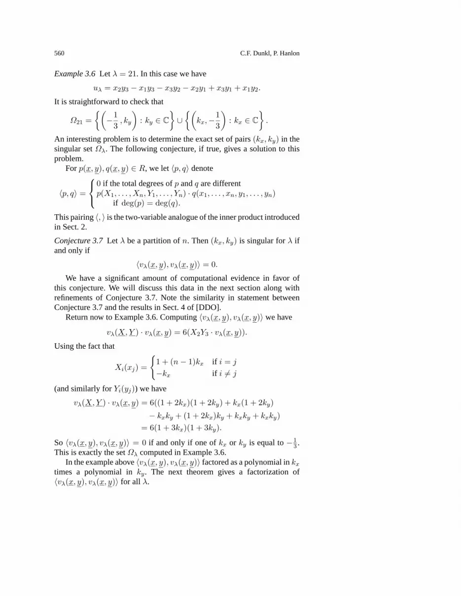
Example 3.6Let λ = 21. In this case we have

uλ = x2y3 − x1y3 − x3y2 − x2y1 + x3y1 + x1y2.

It is straightforward to check that

Ω21 =(

−13, ky

): ky ∈ C

∪(

kx,−13

): kx ∈ C

.

An interesting problem is to determine the exact set of pairs(kx, ky) in thesingular setΩλ. The following conjecture, if true, gives a solution to thisproblem.

Forp(x, y), q(x, y) ∈ R, we let〈p, q〉 denote

〈p, q〉 =

0 if the total degrees ofp andq are differentp(X1, . . . , Xn, Y1, . . . , Yn) · q(x1, . . . , xn, y1, . . . , yn)

if deg(p) = deg(q).

This pairing〈, 〉 is the two-variable analogue of the inner product introducedin Sect. 2.

Conjecture 3.7Let λ be a partition ofn. Then(kx, ky) is singular forλ ifand only if

〈vλ(x, y), vλ(x, y)〉 = 0.

We have a significant amount of computational evidence in favor ofthis conjecture. We will discuss this data in the next section along withrefinements of Conjecture 3.7. Note the similarity in statement betweenConjecture 3.7 and the results in Sect. 4 of [DDO].

Return now to Example 3.6. Computing〈vλ(x, y), vλ(x, y)〉 we have

vλ(X,Y ) · vλ(x, y) = 6(X2Y3 · vλ(x, y)).

Using the fact that

Xi(xj) =

1 + (n− 1)kx if i = j

−kx if i 6= j

(and similarly forYi(yj)) we have

vλ(X,Y ) · vλ(x, y) = 6((1 + 2kx)(1 + 2ky) + kx(1 + 2ky)

− kxky + (1 + 2kx)ky + kxky + kxky)= 6(1 + 3kx)(1 + 3ky).

So 〈vλ(x, y), vλ(x, y)〉 = 0 if and only if one ofkx or ky is equal to−13 .

This is exactly the setΩλ computed in Example 3.6.In the example above〈vλ(x, y), vλ(x, y)〉 factored as a polynomial inkx

times a polynomial inky. The next theorem gives a factorization of〈vλ(x, y), vλ(x, y)〉 for all λ.


Theorem 3.8 Let λ be a partition of n and letλ′ denote the conjugatepartition. Then

〈vλ(x, y), vλ(x, y)〉 = Λ〈Πλ(x), Πλ(x)〉〈Πλ′(y), Πλ′(y)〉whereΛ is the constant

Λ =

(HλHλ′

n∏i=2

aλi !aλ′

i !

)/n!

n∏i=1

(ri − 1)!(ci − 1)!.

and where theai are as defined in Definition 2.5.

Before proceeding with the proof it should be pointed out that〈Πλ(x), Πλ(x)〉 is a polynomial inkx whose factorization was determinedexplicitly in Theorem 2.6 and〈Πλ′(y), Πλ′(y)〉 is a corresponding polyno-mial in ky.

Proof. We begin with some general remarks. Letµ be a partition ofn andletMµ be the linear span inC[z1, . . . , zn] of thesetσ ·Πµ(z1, . . . , zn) :σ ∈ Sn . By constructionMµ is anSn-module. A theorem of Peel (see [P])asserts thatMµ is isomorphic to the irreducible representationτµ of Sn

indexed byµ.Let fµ denote the degree ofτµ, which is known to be the number of

standard Young tableaux (SYT’s) of shapeµ. For each standard Youngtableaut let σt denote the permutation inSn satisfying

σt(tµ) = t

(tµ was defined in Definition 3.2). It is known that a basis forMµ is givenby the set of

σt(Πµ) : t is an SYT of shapeµ .

Let this basis be denoted byp′1, . . . , p

′fµ

.

Suppose now that〈p, q〉 is theSn-invariant inner product onC[z1, . . . , zn]given by〈p, q〉 = p(Z1, . . . , Zn) · q(z1, . . . , zn) where

Zi =∂

∂zi+ k

∑j 6=i

id− (zi, zj)zi − zj

.

With respect to this inner product p′1, p

′2, . . . is not generally orthogonal.

By use of the Gram-Schmidt method this basis can be replaced by an orthog-onal basis p1, p2, p3, . . . such thatp′

1 = p1, and the matrix representationof the groupSn is orthogonal. This of course simultaneously implies thatthepi’s all have the same norm.


Lemma 3.9 If i 6= j then〈pi, pj〉 = 0. The value of〈pi, pi〉 is independentof i.

Proof. Forσ ∈ Sn we haveσ(pi) =∑

s(τµ(σ))s,ips and we have〈pi, pj〉 =〈σpi, σpj〉. Combining these yields,

〈pi, pj〉 =1n!

∑σ∈Sn

〈σpi, σpj〉

=∑r,s

(1n!

∑σ∈Sn

(τµ(σ))r,i(τµ(σ))s,j

)〈pr, ps〉.

It is a well-known fact from the representation theory of finite groups(see [F]) that

fµ

n!

∑σ∈Sn

(τµ(σ))r,i(τµ(σ))s,j = δr,sδij

(here we use thatτµ is real). Thus

〈pi, pj〉 =δijfµ

∑s

〈ps, ps〉. (3.1)

Let M be the subspace ofC[x1, . . . , xn] described above that affords therepresentationτλ and letM ′ be the corresponding subspace ofC[y1, . . . , yn]that affords the representationτλ′ . Let p1(x), . . . , pfµ(x) be the basis de-scribed above forM and letq1(y), . . . , qfµ(y) be the corresponding basisfor M ′ that satisfies

σ(qi(y)) =∑

s

(τλ(σ))s,isgn(σ )qs(y).

We are going to considerM⊗M ′ as a subspace ofC[x1, . . . , xn, y1, . . . , yn].TheSn action onC[x1, . . . , xn, y1, . . . , yn] will be by simultaneous permu-tation of thexi’s andyj ’s so thatM ⊗M ′, as anSn-module, is isomorphicto the internal tensor product ofτλ andτλ′ . It follows from standard factsabout the representation theory ofSn thatM ⊗ M ′ contains exactly onecopy of the sign representation. The next lemma identifies that element andcomputes its norm squared.

Lemma 3.10 In the tensor productM ⊗M ′ there is a unique polynomial(up to scalar multiple) that is skew-symmetric. This polynomial is given by

v =fλ∑i=1

pi(x) qi(y). (3.2)

Moreover〈v, v〉 = fλ〈p1, p1〉〈q1, q1〉.


Proof. Let σ ∈ Sn. Then

σv = sgn(σ)∑r,s

pr(x) qs(y)

(∑i

(τλ(σ))r,i(τλ(σ))s,i

)

= sgn(σ)∑r,s

pr(x) qs(y) δrs

here using the orthogonality relation(∑i

(τλ(σ))r,i(τλ(σ))s,i

)= δrs

(see [F]). So

σ · v = sgn(σ)v,

which shows that the linear span ofv is the unique copy of the sign repre-sentation inM ⊗M ′. Note that

〈v, v〉 =

⟨∑i

pi(x) qi(y),∑

j

pj(x) qj(y)

⟩

=∑i,j

〈pi(x), pj(x)〉〈qi(y), qj(y)〉

=∑

i

〈pi(x), pi(x)〉〈qi(y), qi(y)〉

= fλ〈p1(x), p1(x)〉〈q1(y), q1(y)〉(the last two equalities following from Lemma 3.9). This proves Lemma3.10. 2

To prove Theorem 3.8 we are going to apply this set-up tovλ(x, y). Weneed one last ingredient.

Lemma 3.11 Let notation be as above. Thenvλ(x, y) ∈ M ⊗M ′.

Proof. LetDλ andDλ′ be defined by

Dλ =∑

i

(λi

2

)

Dλ′ =∑

j

(λ′

j

2

).


Let A be the subspace ofC[x1, . . . , xn] consisting of polynomials of de-greeDλ and letB be the subspace ofC[y1, . . . , yn] consisting of polyno-mials of degreeDλ′ .

Consider the coefficient invλ(x, y) of the monomial∏

i yri−1i (this co-

efficient is a polynomial inx1, . . . , xn). It is easy to see that this coeffi-cient isΠλ(x). It follows that the coefficient invλ(x, y) of every monomialyα11 . . . yαn

n is an element ofM . This shows that

vλ(x, y) ∈ M ⊗B.

A similar argument shows that

vλ(x, y) ∈ A⊗M ′.

We can writeA = M ⊕N andB = M ′ ⊕N ′. It follows that

(M ⊗B) ∩ (A⊗M ′) = M ⊗M ′,

which proves Lemma 3.11. 2

To continue with the proof of Theorem 3.8 we note thatvλ(x, y) is in theSn-isotypic component ofM⊗M ′ corresponding to the sign representation.Sovλ(x, y) is some multiple ofv =

∑fi=1 pi(x) qi(y). By Lemma 3.10,

〈vλ(x, y), vλ(x, y)〉 = Λ〈p1, p1〉〈q1, q1〉= Λ〈Πλ(x), Πλ(x)〉〈Πλ′(y), Πλ′(y)〉

whereΛ is a constant (independent ofkx, ky).Both sides of the equation above are polynomials inkx andky. We will

evaluateΛ by computing the constant term of both sides. The constant termis obtained by applying only the partial derivative operators of eachXi

andYj . Doing so we see

CT (〈vλ(x, y), vλ(x, y)〉) = n!∏

i

(∂

∂yi

)ri−1( ∂

∂xi

)ci−1

yri−1i xci−1

i

= n!∏

i

(ri − 1)!(ci − 1)!

On the other hand,

CT (〈Πλ(x), Πλ(x)〉) = Hλ

n∏i=2

aλi !.

Theorem 3.9 follows immediately. 2


Table 1.

λ = 3a\b 3 2 1 00

λ = 21a\b 1 010 −1/3 −1/3

λ = 13

a\b 032 −1/21 −2/3 − 1/20 −1/3 − 2/3 − 1/2

A simple corollary of Theorem 3.8 is the following:

Corollary 3.12 (a) LetΩ = set −i/(j + 1): j = 1, 2, . . . , n− 1, 1 ≤ i≤ j . Then〈vλ(x, y), vλ(x, y)〉 is nonzero if bothkx, ky are fromC \Ω.

(b) (Assuming CONJECTURE 3.7): The pair(0, 0) is generic for allλ.

4 Refinements of Conjecture 3.7

TheSn-moduleVλ(kx, ky) is bigraded by homogeneous degree in thexi’s

andyj ’s. For non-negative integersa, b let V (a,b)λ (kx, ky) denote the(a, b)

piece ofVλ(kx, ky) that is homogeneous of degreea in thexi’s andb in the

yj ’s. We have computed theV (a,b)λ (kx, ky) asSn-modules for alla, b, kx,

ky and allλ with |λ| ≤ 6. For the sake of brevity we will not include all thisdata but will include certain tables that are derived from it.

The following tables are indexed by partitionsλ. Theλth table has rowsindexed bya for 0 ≤ a ≤ Dλ and columns indexed byb for 0 ≤ b ≤ Dλ′ .Thea, b entry in this table is a list of allky such that the(a, b)-graded piece

of V (a,b)λ (kx, ky) is 0 forkx generic. (See Table 1)

Note that whenV (a,b)λ (kx, ky) = 0 forky generic thenV (a,i)

λ (kx, ky) = 0for all i. This observation is consistent with all the data we have. This saysthat there is a cut-off value ofa for eachkx below whichV (a,i)

λ (kx, ky) is 0(for ky generic).

The following value ofa seems to work.


Conjecture 4.1Supposekx = −ui for u ≤ aλ

i (so in particular〈vλ(x, y),vλ(x, y)〉 = 0). Then

V(a,b)λ (kx, ky) = 0

for all b, all ky and alla ≤ u+(n−i+2

2

)− 1.

Note that the bound ona is independent ofλ. The significance of theindependence fromλ in the previous tables is that whenever−1

4 is singu-

lar for λ, V (a,b)λ

(−14 , ky

)was nonzero untila = 0. Similarly whenever(−1

4 , ky

)is singular forλ, V (a,b)

λ

(−14 , ky

)is zero iffa ≤ 1.

A weaker form of Conjecture 4.1 is the following:

Conjecture 4.2The pair (kx, ky) is singular for λ if and only if

V(0,0)λ (kx, ky) = 0.

We strongly believe Conjecture 4.2 is true but we cannot as yet prove it.The following theorem implies that Conjecture 4.2 is stronger than Conjec-ture 3.7.

Theorem 4.3 For all λ, kx andky, the following two statements are equiv-alent:

V(0,0)λ (kx, ky) 6= 0, (a)

〈vλ(x, y), vλ(x, y)〉 6= 0. (b)

Proof. It is immediate from the definition of〈 , 〉 that (b) implies (a).To prove that (a) implies (b) assume that〈vλ(x, y), vλ(x, y)〉 = 0. We

want to show thatV (0,0)λ (kx, ky) is 0.

As in the proof of Lemma 3.11 we let(Dλ, Dλ′) be the bigrading ofvλ(x, y), letAbe the subspace of polynomials of degreeDλ in C[x1, . . . , xn]and letB be the subspace of polynomials of degreeDλ′ in C[y1, . . . , yn].Let M andM ′ be theSn-modules inA andB generated byΠλ(x) andΠλ′(y) respectively. We will need the following classical result.

Lemma 4.4 The multiplicity of the irreducible representationτλ inA is one(and so the multiplicity of the irreducible representationτλ′ in B is one).

Let ∂X∂Y be a differential operator inC[X1, . . . , Xn, Y1, . . . , Yn] ofbi-degree(Dλ, Dλ′) and assume that∂X comes from theτµ-isotypic com-ponent of the differential operators of degreeDλ whereas∂Y comes fromtheτη-isotypic component of the differential operators of degreeDλ′

.By considering theSn × Sn action onA⊗B we have that

∂X∂Y |M⊗M ′ = 0


unlessµ = λ andη = λ′. By Lemma 4.4,∂X∂Y vλ(x, y)· must come fromthe copy ofM ⊗M ′ in C[X1, . . . , Xn, Y1, . . . , Yn].

Consider the diagonal action ofSn onA⊗B and on the copy ofA⊗Bin C[X1, . . . , Xn, Y1, . . . , Yn]. In order for∂X∂Y · vλ(x, y) to be nonzero,∂X∂Y must come from the sign-isotypic component of this diagonal action(sincevλ(x, y) does). So by Lemma 3.10,∂X∂Y must be a multiple ofvλ(X,Y ). But by assumption

vλ(X,Y ) · vλ(x, y) = 0,

which shows that∂X∂Y · vλ(x, y) = 0 for all operators∂X∂Y . Thus

V(0,0)λ (kx, ky) = 0. 2

References

[D1] Dunkl, C. F., Differential-Difference Operators Associated to Reflection Groups.Trans. Amer. Math. Soc.311(1989), 167–183

[D2] Dunkl, C. F., Integral Kernals with Reflection Group Invariance. Can. J. Math.43(1991), 1213–1227

[DDO] Dunkl, C. F., de Jeu, M. F. E., Opdam, E., Singular Polynomials for Finite ReflectionGroups. Trans. Amer. Math. Soc.346(1994), 237–256

[F] Feit, W., The Representation Theory of Finite Groups (1982), North-Holland Pub-lishing Company

[G] Garsia, A., Recent Progress on the Macdonaldq, t-Kostka Conjecture. Actes du4e

Colloque sur les Series Formelles et Combinatoire Algebrique, Lab. de Comb. etInformatique Mathematique, UQAM collection (1992), 249–255

[GH1] Garsia, A., Haiman, M., A GRADED Representation Model for Macdonald’s Poly-nomials. Proc. Nat. Acad. Sci. (1993), 3607–3610

[GH2] Garsia, A., Haiman, M., Orbit Harmonics and Graded Representations. Lab. deComb. et Informatique Mathematique, UQAM Collection, S. Brlek, Editor (to ap-pear)

[GH3] Garsia, A., Haiman, M., Some Natural BigradedSn-Modules and theq, t-KostkaCoefficients. Electron Combin3 (1966), #24

[GH4] Garsia, A., Haiman, M., Factorizations of Pieri Rates for Macdonald Polynomials.Proc. of 4th Colloquium on Algebraic Combinatorics. Discrete Math.139 (1995),219–256

[GH5] Garsia, A., Haiman, M., A Remarkableq, t-Catalan Sequence andq-Lagrange In-version. Journal of Algebraic Combinatorics5 (1996), 191–244

[M] Macdonald, I. G., Symmetric Functions and Hall Polynomials (1979), Oxford Uni-versity Press

[O] Opdam, E., Some Applications of Hypergeometric Shift Operators. Inv. Math.98(1989), 1–18

[P] Peel, M. H., Specht Modules and the Symmetric Groups. J. Alg.36 (1975), 88–97

Documents

Integrals of polynomials associated with tableaux and the Garsia-Haiman conjecture