arX

iv:n

lin/0

5020

47v1

[nl

in.S

I] 2

1 Fe

b 20

05

Integrable Quasiclassical

Deformations of Cubic Curves. ∗

Y. Kodama 1†, B. Konopelchenko 2,L. Martınez Alonso3 and E. Medina4

1 Department of Mathematics, Ohio State UniversityColumbus, OH 43210, USA

2 Dipartimento di Fisica, Universita di Lecce and Sezione INFN73100 Lecce, Italy

3 Departamento de Fısica Teorica II, Universidad ComplutenseE28040 Madrid, Spain

4 Departamento de Matematicas, Universidad de Cadiz

E11510 Puerto Real, Cadiz,Spain

Abstract

A general scheme for determining and studying hydrodynamic type

systems describing integrable deformations of algebraic curves is ap-

plied to cubic curves. Lagrange resolvents of the theory of cubic equa-

tions are used to derive and characterize these deformations.

Key words: Algebraic curves. Integrable systems. Lagrange resol-vents.PACS number: 02.30.Ik.

∗Partially supported by DGCYT project BFM2002-01607 and by the grant COFIN

2004 ”Sintesi”†Partially supported by NSF grant DMS0404931

1

1 Introduction

The theory of algebraic curves is a fundamental ingredient in the analysis ofintegrable nonlinear differential equations as it is shown, for example, by itsrelevance in the description of the finite-gap solutions or the formulation ofthe Whitham averaging method [1]-[8]. A particularly interesting problemis characterizing and classifying integrable deformations of algebraic curves.In [6]-[7] Krichever formulated a general theory of dispersionless hierarchiesof integrable models arising in the Whitham averaging method. It turnsout that the algebraic orbits of the genus-zero Whitham equations determineinfinite families of integrable deformations of a particular class of algebraiccurves. A different approach for determining integrable deformations of gen-eral algebraic curves C defined by monic polynomial equations

C : F (p, k) := pN −N

∑

n=1

un(k)pN−n = 0, un ∈ C[k], (1)

was proposed in [9]-[10]. It applies for finding deformations C(x, t) of C withthe deformation parameters (x, t), such that the multiple-valued functionp = p(k) determined by (1) obeys an equation of the form of conservationlaws

∂tp = ∂xQ, (2)

where the flux Q is given by an element from C[k, p]/C,

Q =

N∑

r=1

ar(k, x, t)pr−1, ar ∈ C[k].

Starting with (2), changing to the dynamical variables un and using Lenard-type relations (see [10]) one gets a scheme for finding consistent deformationsof (1). One should also note that (2) provides an infinite number of conser-vation laws, when one expands p and Q in Laurent series in z with k = zr

for some r. In this sense, we say that equation (2) is integrable.Our strategy can be applied to the generic case where the coefficients

(potentials) un of (1) are general polynomials in k

un(k) =

dn∑

i=0

un,iki,

2

with all the coefficients un,i being considered as independent dynamical vari-ables, i.e. un,i = un,i(x, t). However, with appropriate modifications, thescheme can be also applied to cases in which constraints on the potentialsare imposed. A complete description of these deformations for the genericcase of hyperelliptic curves (N = 2) was given in [10].

The present paper is devoted to the deformations of cubic curves (N = 3)

p3 − w p2 − v p − u = 0, u, v, w ∈ C[k] , (3)

and it considers not only the generic case but also the important constrainedcase w ≡ 0. Although some of the curves may be conformally equivalent(with for example the dispersionless Miura transformation), we will not dis-cuss the classification problem under this equivalence in this paper (we willdiscuss the details of the problem elsewhere). In section 2 a general approachto construct integrable deformations of algebraic curves is reported briefly.Section 3 is devoted to the analysis of the cubic case (3). We emphasize therole of Lagrange resolvents, describe the Hamiltonian structure of integrabledeformations and present several illustrative examples including Whithamtype deformations.

2 Schemes of deformations of algebraic curves

In order to describe deformations of the curve C defined by (1), one may usethe potentials un, as well as the N branches pi = pi(k) (i = 1, . . . , N) of themultiple-valued function function p = p(k) satisfying

F (p, k) =

N∏

i=1

(p − pi(k)). (4)

The potentials can be expressed as elementary symmetric polynomials sn

[11]-[13] of the branches pi

un = (−1)n−1sn(p1, p2, . . .) = (−1)n−1∑

1≤i1<...<in≤N

pi1 · · · pin . (5)

However, notice that, according to the famous Abel theorem [11], for N > 4the branches pi of the generic equation (1) cannot be written in terms of thepotentials un by means of rational operations and radicals.

3

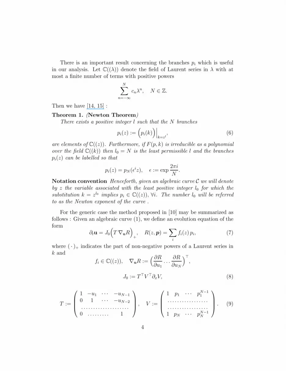
There is an important result concerning the branches pi which is usefulin our analysis. Let C((λ)) denote the field of Laurent series in λ with atmost a finite number of terms with positive powers

N∑

n=−∞

cnλn, N ∈ Z.

Then we have [14, 15] :

Theorem 1. (Newton Theorem)There exists a positive integer l such that the N branches

pi(z) :=(

pi(k))∣

∣

∣

k=zl, (6)

are elements of C((z)). Furthermore, if F (p, k) is irreducible as a polynomialover the field C((k)) then l0 = N is the least permissible l and the branchespi(z) can be labelled so that

pi(z) = pN(ǫiz), ǫ := exp2πi

N.

Notation convention Henceforth, given an algebraic curve C we will denoteby z the variable associated with the least positive integer l0 for which thesubstitution k = zl0 implies pi ∈ C((z)), ∀i. The number l0 will be referredto as the Newton exponent of the curve .

For the generic case the method proposed in [10] may be summarized asfollows : Given an algebraic curve (1), we define an evolution equation of theform

∂tu = J0

(

T ∇uR)

+, R(z, p) =

∑

i

fi(z) pi, (7)

where ( · )+ indicates the part of non-negative powers of a Laurent series ink and

fi ∈ C((z)), ∇uR :=( ∂R

∂u1

. . .∂R

∂uN

)⊤

,

J0 := T⊤V ⊤∂xV, (8)

T :=

1 −u1 · · · −uN−1

0 1 · · · −uN−2

. . . . . . . . . . . . . . . . . . . .0 . . . . . . . . . 1

, V :=

1 p1 · · · pN−11

. . . . . . . . . . . . . . . . .

. . . . . . . . . . . . . . . . .1 pN · · · pN−1

N

. (9)

4

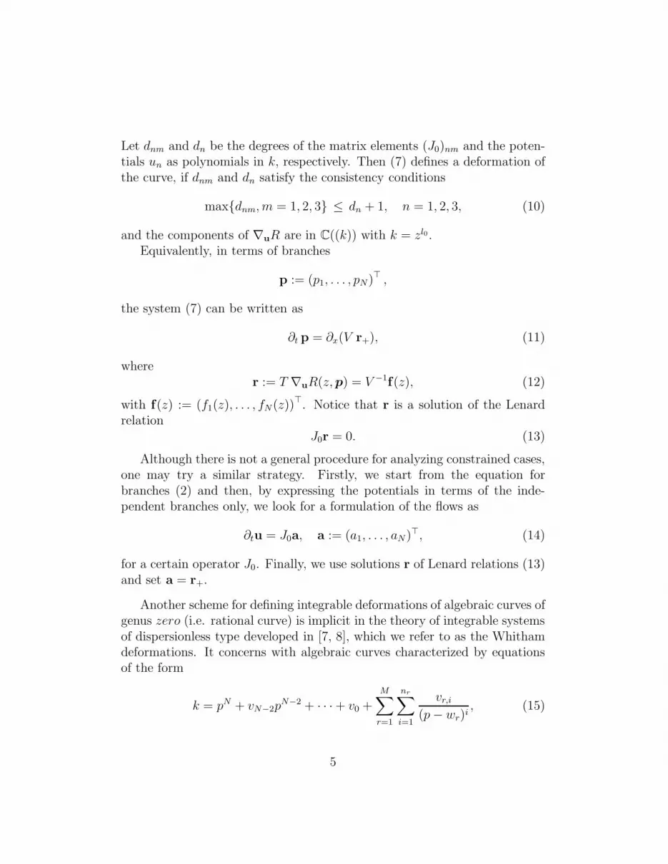
Let dnm and dn be the degrees of the matrix elements (J0)nm and the poten-tials un as polynomials in k, respectively. Then (7) defines a deformation ofthe curve, if dnm and dn satisfy the consistency conditions

max{dnm, m = 1, 2, 3} ≤ dn + 1, n = 1, 2, 3, (10)

and the components of ∇uR are in C((k)) with k = zl0 .Equivalently, in terms of branches

p := (p1, . . . , pN)⊤ ,

the system (7) can be written as

∂t p = ∂x(V r+), (11)

wherer := T ∇uR(z, p) = V −1f(z), (12)

with f(z) := (f1(z), . . . , fN(z))⊤. Notice that r is a solution of the Lenardrelation

J0r = 0. (13)

Although there is not a general procedure for analyzing constrained cases,one may try a similar strategy. Firstly, we start from the equation forbranches (2) and then, by expressing the potentials in terms of the inde-pendent branches only, we look for a formulation of the flows as

∂tu = J0a, a := (a1, . . . , aN)⊤, (14)

for a certain operator J0. Finally, we use solutions r of Lenard relations (13)and set a = r+.

Another scheme for defining integrable deformations of algebraic curves ofgenus zero (i.e. rational curve) is implicit in the theory of integrable systemsof dispersionless type developed in [7, 8], which we refer to as the Whithamdeformations. It concerns with algebraic curves characterized by equationsof the form

k = pN + vN−2pN−2 + · · · + v0 +

M∑

r=1

nr∑

i=1

vr,i

(p − wr)i, (15)

5

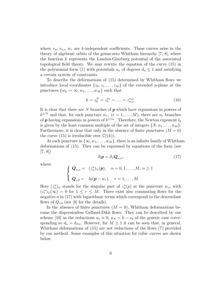
where vn, vr,i, wr are k-independent coefficients. These curves arise in thetheory of algebraic orbits of the genus-zero Whitham hierarchy [7, 8], wherethe function k represents the Landau-Ginzburg potential of the associatedtopological field theory. We may rewrite the equation of the curve (15) inthe polynomial form (1) with potentials un of degrees dn ≤ 1 and satisfyinga certain system of constraints.

To describe the deformations of (15) determined by Whitham flows weintroduce local coordinates {z0, z1, . . . , zM} of the extended p-plane at thepunctures {w0 := ∞, w1, . . . , wM} such that

k = zN0 = zn1

1 = . . . = znMnM

. (16)

It is clear that there are N branches of p which have expansions in powers ofk1/N and that, for each puncture wr, (r = 1, . . . , M), there are nr branchesof p having expansions in powers of k1/nr . Therefore, the Newton exponent l0is given by the least common multiple of the set of integers {N, n1, . . . , nM}.Furthermore, it is clear that only in the absence of finite punctures (M = 0)the curve (15) is irreducible over C((k)).

At each puncture in {∞, w1, . . . , wM}, there is an infinite family of Whithamdeformations of (15). They can be expressed by equations of the form (see[7, 8])

∂tp = ∂xQα,n, (17)

where

Qα,n = (znα)⊕(p), α = 0, 1, . . . , M, n ≥ 1

Qr,0 = ln(p − wr), r = 1, . . . , M.

Here (znα)⊕ stands for the singular part of zn

α(p) at the puncture wα, with(zn

r )⊕(∞) = 0 for 1 ≤ r ≤ M . There exist also commuting flows for thenegative n in (17) with logarithmic terms which correspond to the descendantflows of Qr,0 (see [8] for the details).

In the absence of finite punctures (M = 0), Whitham deformations be-come the dispersionless Gelfand-Dikii flows. They can be described by ourscheme [10] as the reductions u1 ≡ 0, uN = k − v0 of the generic case corre-sponding to dn = δNn. However, for M ≥ 1 it can be seen that, in general,Whitham deformations of (15) are not reductions of the flows (7) providedby our method. Some examples of this situation for cubic curves are shownbelow.

6

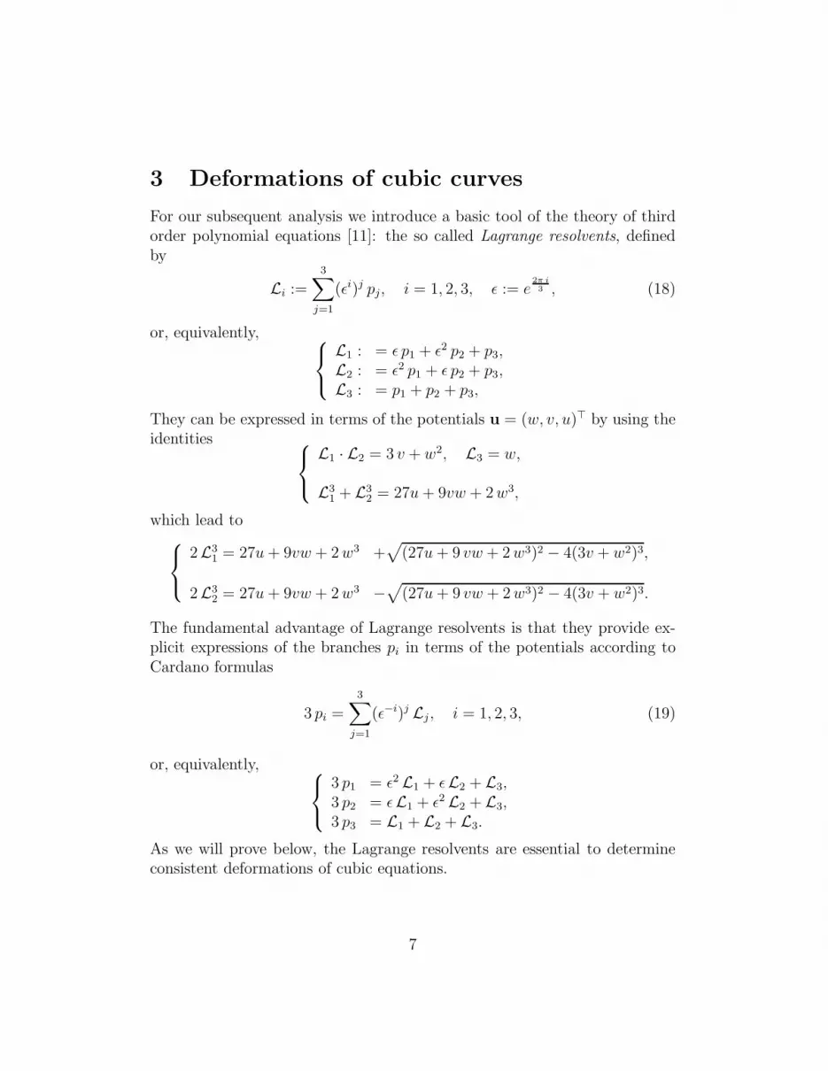
3 Deformations of cubic curves

For our subsequent analysis we introduce a basic tool of the theory of thirdorder polynomial equations [11]: the so called Lagrange resolvents, definedby

Li :=

3∑

j=1

(ǫi)j pj, i = 1, 2, 3, ǫ := e2π i3 , (18)

or, equivalently,

L1 : = ǫ p1 + ǫ2 p2 + p3,L2 : = ǫ2 p1 + ǫ p2 + p3,L3 : = p1 + p2 + p3,

They can be expressed in terms of the potentials u = (w, v, u)⊤ by using theidentities

L1 · L2 = 3 v + w2, L3 = w,

L31 + L3

2 = 27u + 9vw + 2 w3,

which lead to

2L31 = 27u + 9vw + 2 w3 +

√

(27u + 9 vw + 2 w3)2 − 4(3v + w2)3,

2L32 = 27u + 9vw + 2 w3 −

√

(27u + 9 vw + 2 w3)2 − 4(3v + w2)3.

The fundamental advantage of Lagrange resolvents is that they provide ex-plicit expressions of the branches pi in terms of the potentials according toCardano formulas

3 pi =

3∑

j=1

(ǫ−i)j Lj , i = 1, 2, 3, (19)

or, equivalently,

3 p1 = ǫ2 L1 + ǫL2 + L3,3 p2 = ǫL1 + ǫ2 L2 + L3,3 p3 = L1 + L2 + L3.

As we will prove below, the Lagrange resolvents are essential to determineconsistent deformations of cubic equations.

7

3.1 Generic case

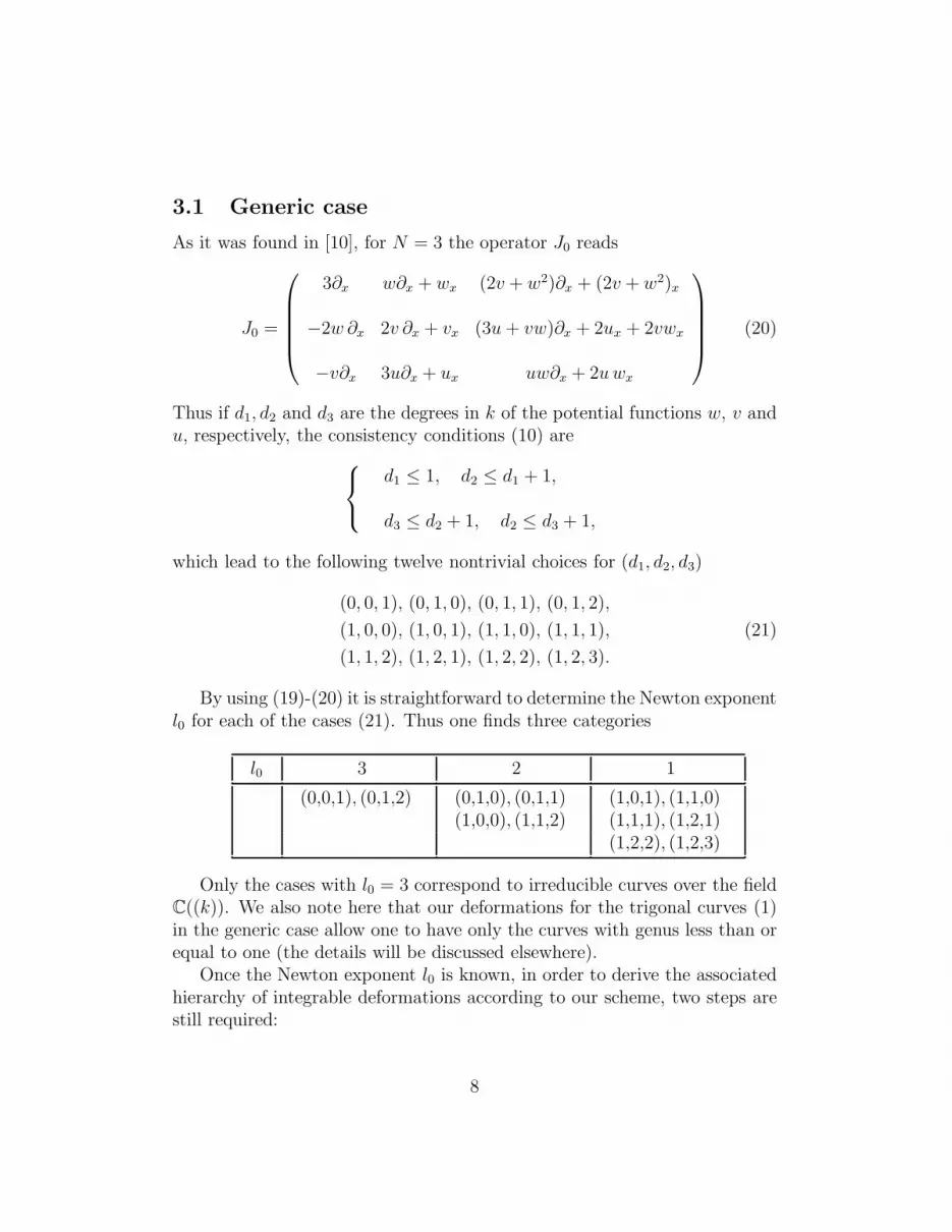
As it was found in [10], for N = 3 the operator J0 reads

J0 =

3∂x w∂x + wx (2v + w2)∂x + (2v + w2)x

−2w ∂x 2v ∂x + vx (3u + vw)∂x + 2ux + 2vwx

−v∂x 3u∂x + ux uw∂x + 2u wx

(20)

Thus if d1, d2 and d3 are the degrees in k of the potential functions w, v andu, respectively, the consistency conditions (10) are

d1 ≤ 1, d2 ≤ d1 + 1,

d3 ≤ d2 + 1, d2 ≤ d3 + 1,

which lead to the following twelve nontrivial choices for (d1, d2, d3)

(0, 0, 1), (0, 1, 0), (0, 1, 1), (0, 1, 2),

(1, 0, 0), (1, 0, 1), (1, 1, 0), (1, 1, 1), (21)

(1, 1, 2), (1, 2, 1), (1, 2, 2), (1, 2, 3).

By using (19)-(20) it is straightforward to determine the Newton exponentl0 for each of the cases (21). Thus one finds three categories

l0 3 2 1

(0,0,1), (0,1,2) (0,1,0), (0,1,1) (1,0,1), (1,1,0)(1,0,0), (1,1,2) (1,1,1), (1,2,1)

(1,2,2), (1,2,3)

Only the cases with l0 = 3 correspond to irreducible curves over the fieldC((k)). We also note here that our deformations for the trigonal curves (1)in the generic case allow one to have only the curves with genus less than orequal to one (the details will be discussed elsewhere).

Once the Newton exponent l0 is known, in order to derive the associatedhierarchy of integrable deformations according to our scheme, two steps arestill required:

8

1. To determine the functions R(z, p) =∑

i fi(z) pi such that the compo-nents of ∇uR are in C((k)) with k = zl0 .

2. To find the explicit form of the gradients ∇uR in terms of the potentials.

Both problems admit a convenient treatment in terms of Lagrange resolvents.Thus by introducing the following element σ0 of the Galois group of the curve

σ0(pi)(z) := pi(ǫ0 z), ǫ0 := e2πil0 , (22)

we see that our first problem can be fixed by determining functions R invari-ants under σ0 i.e. R(ǫ0 z, σ0 p) = R(z, p). In this way, we have the followingforms of R:

For the case l0 = 3, the element σ0 is given by the permutation

σ0 =

(

p1 p2 p3

p2 p3 p1

)

, (23)

or, in terms of Lagrange resolvents,

σ0 =

(

L1 L2 L3

ǫ2L1 ǫL2 L3

)

. (24)

Thus we get the invariant functions

R = zf1(z3)L1 + z2f2(z

3)L2 + f3(z3)L3, (25)

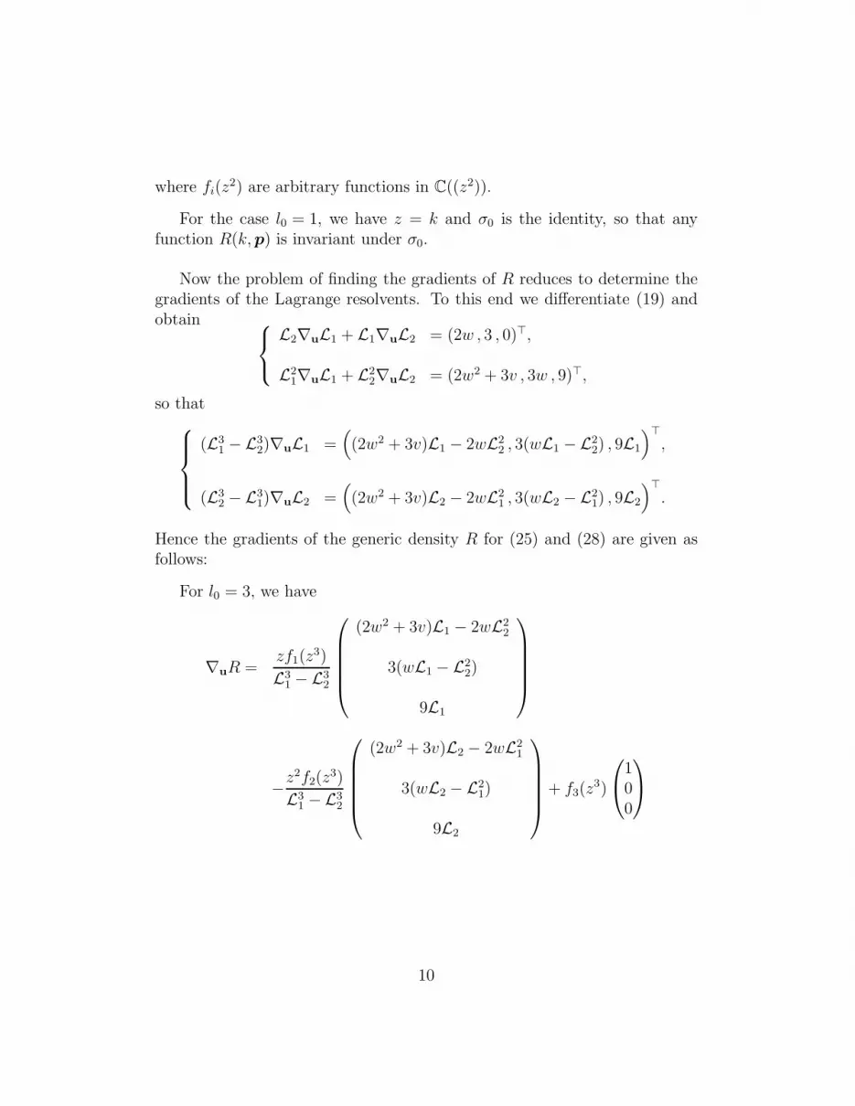
with fi(z3) being arbitrary functions in C((z3)).

For the case l0 = 2, σ20 is the identity permutation, so that under the

action of σ0 two branches are interchanged while the other remains invariant.If we label the branches in such a way that

σ0 =

(

p1 p2 p3

p2 p1 p3

)

, (26)

then

σ0 =

(

L1 L2 L3

L2 L1 L3

)

, (27)

and we obtain the invariant functions

R = f1(z2)

(

L1 + L2

)

+ zf2(z2)

(

L1 − L2

)

+ f3(z2)L3, (28)

9

where fi(z2) are arbitrary functions in C((z2)).

For the case l0 = 1, we have z = k and σ0 is the identity, so that anyfunction R(k, p) is invariant under σ0.

Now the problem of finding the gradients of R reduces to determine thegradients of the Lagrange resolvents. To this end we differentiate (19) andobtain

L2∇uL1 + L1∇uL2 = (2w , 3 , 0)⊤,

L21∇uL1 + L2

2∇uL2 = (2w2 + 3v , 3w , 9)⊤,

so that

(L31 − L3

2)∇uL1 =(

(2w2 + 3v)L1 − 2wL22 , 3(wL1 −L2

2) , 9L1

)⊤

,

(L32 − L3

1)∇uL2 =(

(2w2 + 3v)L2 − 2wL21 , 3(wL2 −L2

1) , 9L2

)⊤

.

Hence the gradients of the generic density R for (25) and (28) are given asfollows:

For l0 = 3, we have

∇uR =zf1(z

3)

L31 − L3

2

(2w2 + 3v)L1 − 2wL22

3(wL1 − L22)

9L1

−z2f2(z3)

L31 −L3

2

(2w2 + 3v)L2 − 2wL21

3(wL2 − L21)

9L2

+ f3(z3)

100

10

For l0 = 2, we get

∇uR =f1(z

2)

L31 − L3

2

(2w2 + 3v)(L1 − L2) + 2w(L21 −L2

2)

3(wL1 − L22) − 3(wL2 − L2

1)

9(L1 − L2)

+zf2(z

2)

L31 − L3

2

(2w2 + 3v)(L1 + L2) − 2w(L21 + L2

2)

3(wL1 − L22) + 3(wL2 −L2

1)

9(L1 + L2)

+ f3(z2)

100

.

From these expressions and (24) and (27) it follows that the correspondingcomponents of ∇uR are in C((k)).

Example 1: The case l0 = 3 with (d1, d2, d3) = (0, 0, 1). Taking into account(20) and (19) it is clear that there are two trivial equations corresponding tow0 and u1. Then, we take for the potentials

w = 1, v = v0(x, t), u = k + u0(x, t).

Thus, by using (25) with

f1 ≡ f3 ≡ 0, f2(z3) =

27(1 −√

3i)

4z3

we obtain

v0 t =5

3(2 + 27 u0 + 9 v0) u0x+

5

18

(

7 + 54 u0 + 36 v0 + 27 v20

)

v0 x,

u0 t =5

18

(

−1 − 54 u0 + 27 v02)

u0 x+

5

9v0 (2 + 27 u0 + 9 v0) v0 x.

11

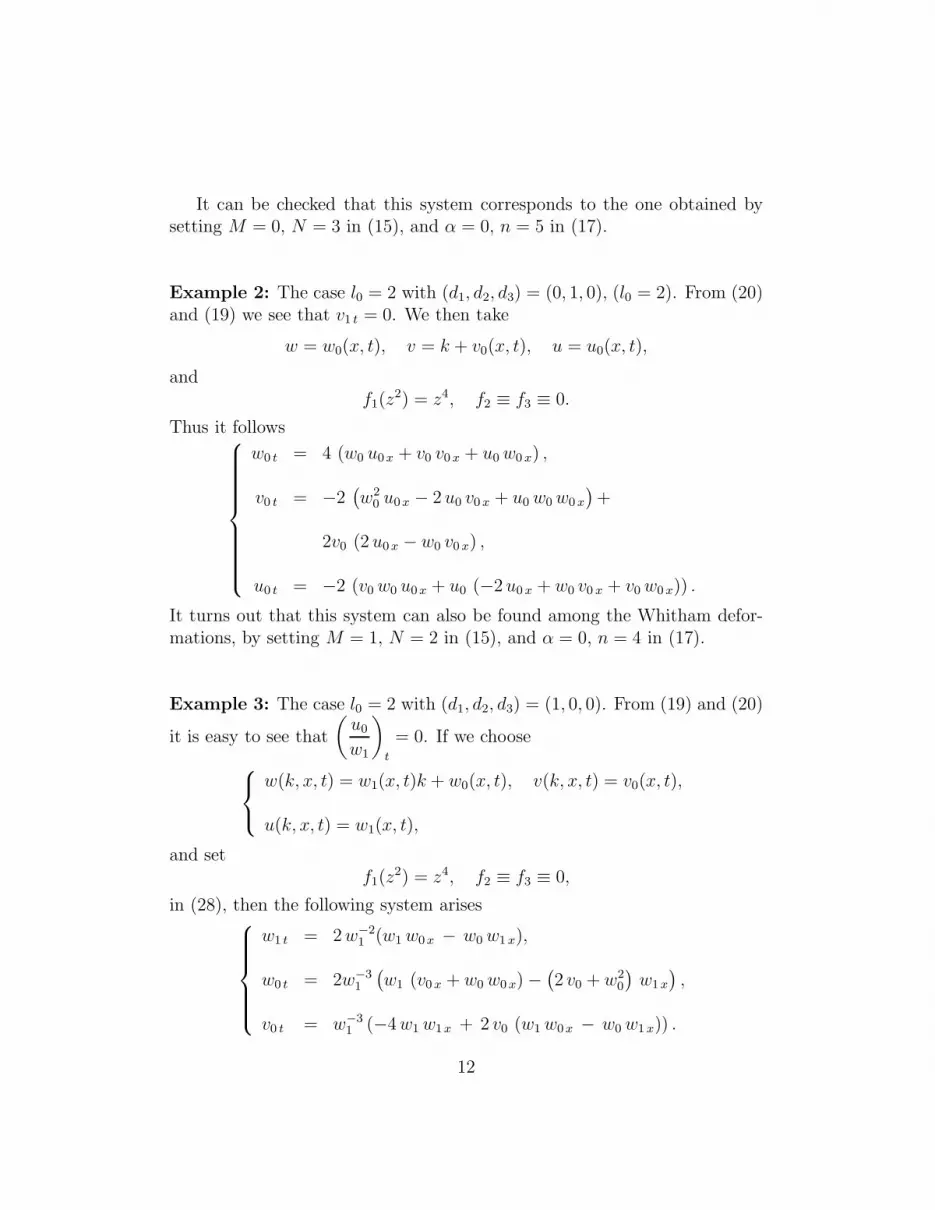
It can be checked that this system corresponds to the one obtained bysetting M = 0, N = 3 in (15), and α = 0, n = 5 in (17).

Example 2: The case l0 = 2 with (d1, d2, d3) = (0, 1, 0), (l0 = 2). From (20)and (19) we see that v1 t = 0. We then take

w = w0(x, t), v = k + v0(x, t), u = u0(x, t),

andf1(z

2) = z4, f2 ≡ f3 ≡ 0.

Thus it follows

w0 t = 4 (w0 u0x + v0 v0 x + u0 w0 x) ,

v0 t = −2(

w20 u0x − 2 u0 v0 x + u0 w0 w0 x

)

+

2v0 (2 u0x − w0 v0 x) ,

u0 t = −2 (v0 w0 u0x + u0 (−2 u0 x + w0 v0 x + v0 w0 x)) .

It turns out that this system can also be found among the Whitham defor-mations, by setting M = 1, N = 2 in (15), and α = 0, n = 4 in (17).

Example 3: The case l0 = 2 with (d1, d2, d3) = (1, 0, 0). From (19) and (20)

it is easy to see that

(

u0

w1

)

t

= 0. If we choose

w(k, x, t) = w1(x, t)k + w0(x, t), v(k, x, t) = v0(x, t),

u(k, x, t) = w1(x, t),

and setf1(z

2) = z4, f2 ≡ f3 ≡ 0,

in (28), then the following system arises

w1 t = 2 w−21 (w1 w0x − w0 w1 x),

w0 t = 2w−31

(

w1 (v0 x + w0 w0 x) −(

2 v0 + w20

)

w1x

)

,

v0 t = w−31 (−4 w1 w1x + 2 v0 (w1 w0x − w0 w1 x)) .

12

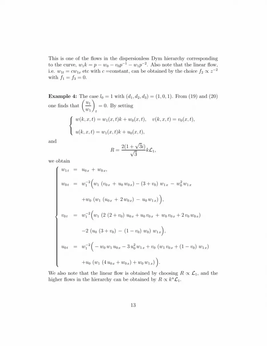
This is one of the flows in the dispersionless Dym hierarchy correspondingto the curve, w1k = p − w0 − v0p

−1 − w1p−2. Also note that the linear flow,

i.e. w1t = cw1x etc with c =constant, can be obtained by the choice f2 ∝ z−2

with f1 = f3 = 0.

Example 4: The case l0 = 1 with (d1, d2, d3) = (1, 0, 1). From (19) and (20)

one finds that

(

u1

w1

)

t

= 0. By setting

w(k, x, t) = w1(x, t)k + w0(x, t), v(k, x, t) = v0(x, t),

u(k, x, t) = w1(x, t)k + u0(x, t),

and

R =2(1 +

√3i)√

3kL1,

we obtain

w1 t = u0 x + w0 x,

w0 t = w−21

(

w1 (v0 x + u0 w0x) − (3 + v0) w1x − w20 w1 x

+w0 (w1 (u0x + 2 w0 x) − u0 w1 x))

,

v0 t = w−21

(

w1 (2 (2 + v0) u0 x + u0 v0 x + w0 v0 x + 2 v0 w0 x)

−2 (u0 (3 + v0) − (1 − v0) w0) w1x

)

,

u0 t = w−21

(

− w0 w1 u0x − 3 u20 w1 x + v0 (w1 v0 x + (1 − v0) w1x)

+u0 (w1 (4 u0x + w0 x) + w0 w1 x))

.

We also note that the linear flow is obtained by choosing R ∝ L1, and thehigher flows in the hierarchy can be obtained by R ∝ knL1.

13

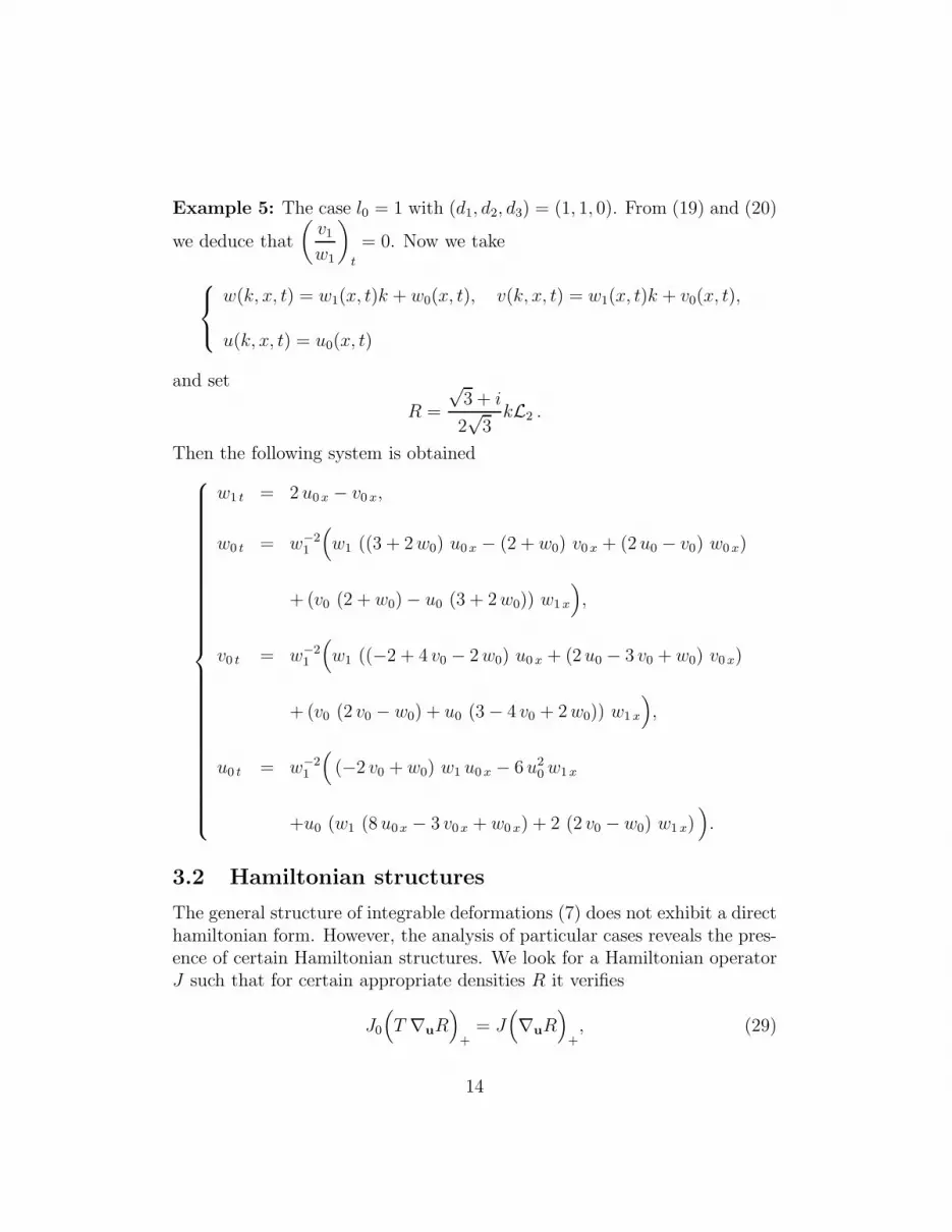
Example 5: The case l0 = 1 with (d1, d2, d3) = (1, 1, 0). From (19) and (20)

we deduce that

(

v1

w1

)

t

= 0. Now we take

w(k, x, t) = w1(x, t)k + w0(x, t), v(k, x, t) = w1(x, t)k + v0(x, t),

u(k, x, t) = u0(x, t)

and set

R =

√3 + i

2√

3kL2 .

Then the following system is obtained

w1 t = 2 u0x − v0 x,

w0 t = w−21

(

w1 ((3 + 2 w0) u0x − (2 + w0) v0 x + (2 u0 − v0) w0 x)

+ (v0 (2 + w0) − u0 (3 + 2 w0)) w1 x

)

,

v0 t = w−21

(

w1 ((−2 + 4 v0 − 2 w0) u0 x + (2 u0 − 3 v0 + w0) v0 x)

+ (v0 (2 v0 − w0) + u0 (3 − 4 v0 + 2 w0)) w1 x

)

,

u0 t = w−21

(

(−2 v0 + w0) w1 u0 x − 6 u20 w1 x

+u0 (w1 (8 u0x − 3 v0x + w0 x) + 2 (2 v0 − w0) w1 x))

.

3.2 Hamiltonian structures

The general structure of integrable deformations (7) does not exhibit a directhamiltonian form. However, the analysis of particular cases reveals the pres-ence of certain Hamiltonian structures. We look for a Hamiltonian operatorJ such that for certain appropriate densities R it verifies

J0

(

T ∇uR)

+= J

(

∇uR)

+, (29)

14

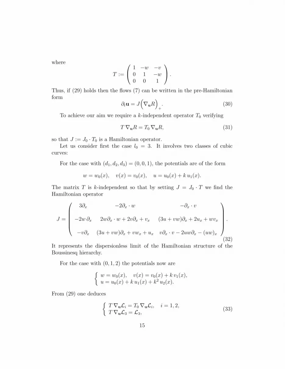
where

T :=

1 −w −v0 1 −w0 0 1

.

Thus, if (29) holds then the flows (7) can be written in the pre-Hamiltonianform

∂tu = J(

∇uR)

+. (30)

To achieve our aim we require a k-independent operator T0 verifying

T ∇uR = T0 ∇uR, (31)

so that J := J0 · T0 is a Hamiltonian operator.Let us consider first the case l0 = 3. It involves two classes of cubic

curves:

For the case with (d1, d2, d3) = (0, 0, 1), the potentials are of the form

w = w0(x), v(x) = v0(x), u = u0(x) + k u1(x).

The matrix T is k-independent so that by setting J = J0 · T we find theHamiltonian operator

J =

3∂x −2∂x · w −∂x · v

−2w ∂x 2w∂x · w + 2v∂x + vx (3u + vw)∂x + 2ux + wvx

−v∂x (3u + vw)∂x + vwx + ux v∂x · v − 2uw∂x − (uw)x

.

(32)It represents the dispersionless limit of the Hamiltonian structure of theBoussinesq hierarchy.

For the case with (0, 1, 2) the potentials now are

{

w = w0(x), v(x) = v0(x) + k v1(x),u = u0(x) + k u1(x) + k2 u2(x).

From (29) one deduces

{

T ∇uLi = T0 ∇uLi, i = 1, 2,T ∇uL3 = L3,

(33)

15

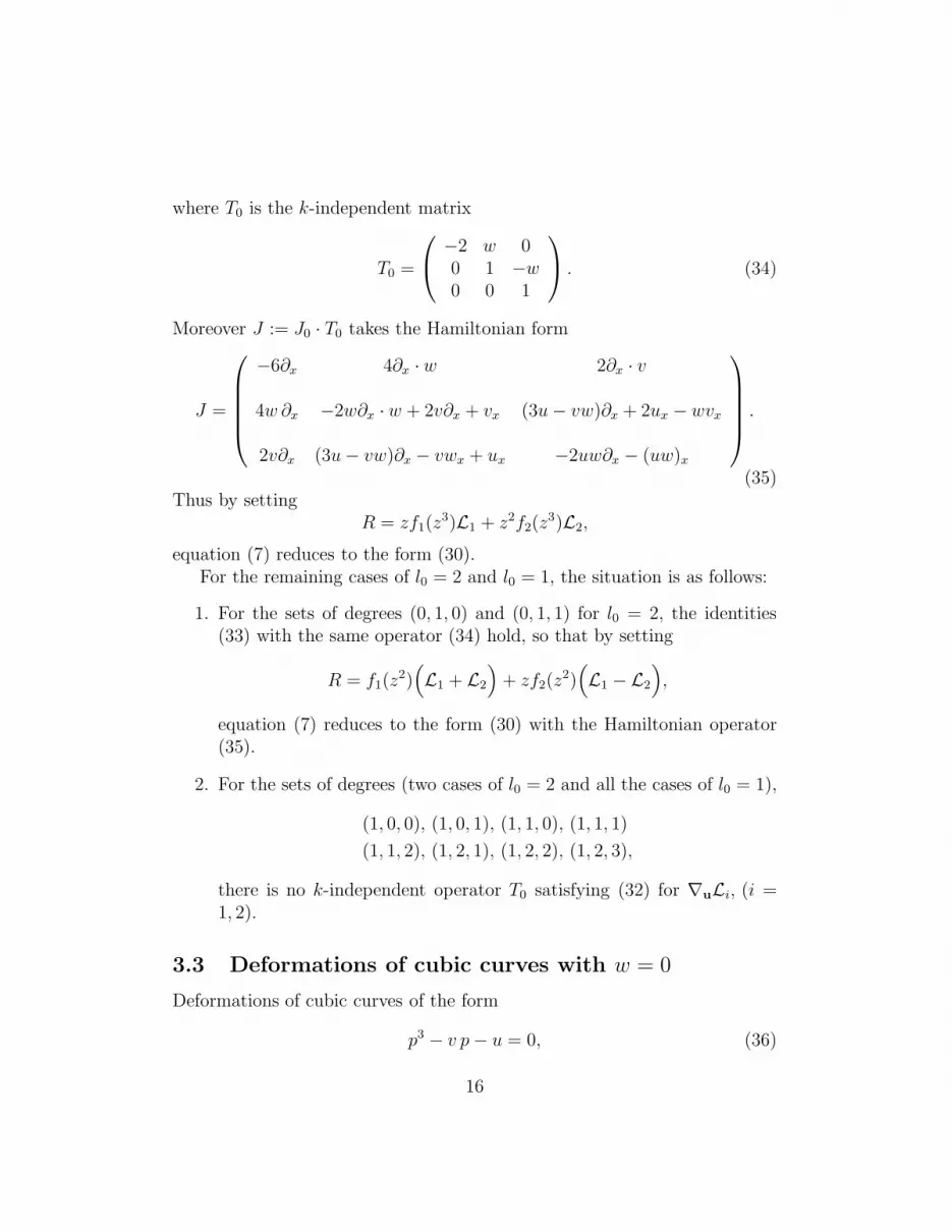
where T0 is the k-independent matrix

T0 =

−2 w 00 1 −w0 0 1

. (34)

Moreover J := J0 · T0 takes the Hamiltonian form

J =

−6∂x 4∂x · w 2∂x · v

4w ∂x −2w∂x · w + 2v∂x + vx (3u − vw)∂x + 2ux − wvx

2v∂x (3u − vw)∂x − vwx + ux −2uw∂x − (uw)x

.

(35)Thus by setting

R = zf1(z3)L1 + z2f2(z

3)L2,

equation (7) reduces to the form (30).For the remaining cases of l0 = 2 and l0 = 1, the situation is as follows:

1. For the sets of degrees (0, 1, 0) and (0, 1, 1) for l0 = 2, the identities(33) with the same operator (34) hold, so that by setting

R = f1(z2)

(

L1 + L2

)

+ zf2(z2)

(

L1 −L2

)

,

equation (7) reduces to the form (30) with the Hamiltonian operator(35).

2. For the sets of degrees (two cases of l0 = 2 and all the cases of l0 = 1),

(1, 0, 0), (1, 0, 1), (1, 1, 0), (1, 1, 1)

(1, 1, 2), (1, 2, 1), (1, 2, 2), (1, 2, 3),

there is no k-independent operator T0 satisfying (32) for ∇uLi, (i =1, 2).

3.3 Deformations of cubic curves with w = 0

Deformations of cubic curves of the form

p3 − v p − u = 0, (36)

16

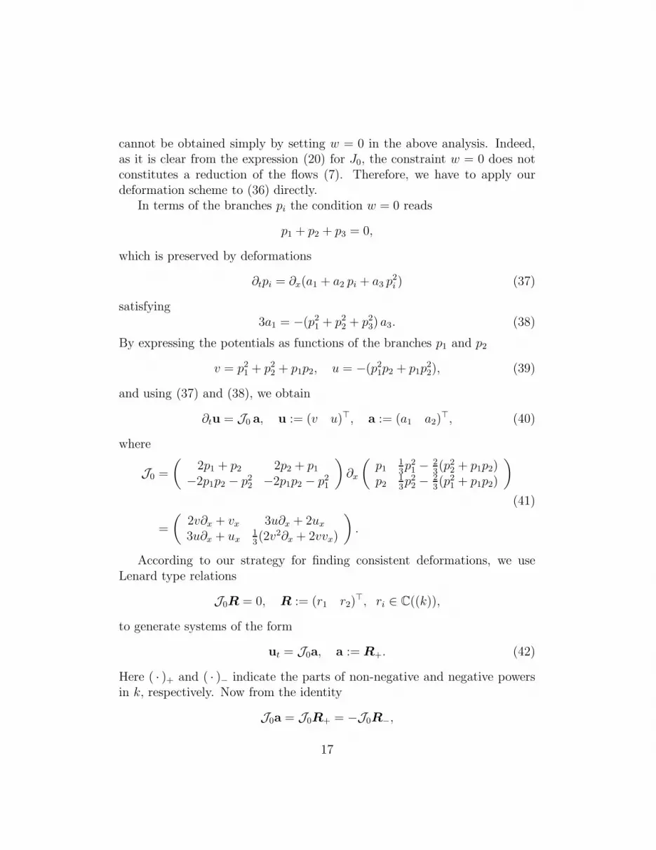
cannot be obtained simply by setting w = 0 in the above analysis. Indeed,as it is clear from the expression (20) for J0, the constraint w = 0 does notconstitutes a reduction of the flows (7). Therefore, we have to apply ourdeformation scheme to (36) directly.

In terms of the branches pi the condition w = 0 reads

p1 + p2 + p3 = 0,

which is preserved by deformations

∂tpi = ∂x(a1 + a2 pi + a3 p2i ) (37)

satisfying3a1 = −(p2

1 + p22 + p2

3) a3. (38)

By expressing the potentials as functions of the branches p1 and p2

v = p21 + p2

2 + p1p2, u = −(p21p2 + p1p

22), (39)

and using (37) and (38), we obtain

∂tu = J0 a, u := (v u)⊤, a := (a1 a2)⊤, (40)

where

J0 =

(

2p1 + p2 2p2 + p1

−2p1p2 − p22 −2p1p2 − p2

1

)

∂x

(

p113p2

1 − 23(p2

2 + p1p2)p2

13p2

2 − 23(p2

1 + p1p2)

)

(41)

=

(

2v∂x + vx 3u∂x + 2ux

3u∂x + ux13(2v2∂x + 2vvx)

)

.

According to our strategy for finding consistent deformations, we useLenard type relations

J0R = 0, R := (r1 r2)⊤, ri ∈ C((k)),

to generate systems of the form

ut = J0a, a := R+. (42)

Here ( · )+ and ( · )− indicate the parts of non-negative and negative powersin k, respectively. Now from the identity

J0a = J0R+ = −J0R−,

17

it is clear that a sufficient condition for the consistency of (42) is that thedegrees d2 and d3 of v and u as polynomials of k satisfy

d3 ≤ d2 + 1, 2d2 ≤ d3 + 1.

Hence only four nontrivial cases arise for (d2, d3)

(0, 1), (1, 1), (1, 2), (2, 3). (43)

We notice that they represent the dispersionless versions of the standardBoussinesq hierarchy and all three hidden hierarchies found by Antonowicz,Fordy and Liu for the third-order spectral problem [16].

Solutions of the Lenard relation can be generated by noticing that theoperator J0 admits the factorization

J0 = U⊤ · 1

3

(

2 −1−1 2

)

∂x · U, (44)

where

U :=

(

2p1 + p2 −2p1p2 − p22

2p2 + p1 −2p1p2 − p21

)

=

( ∂v∂p1

∂u∂p1

∂v∂p2

∂u∂p2

)

. (45)

This shows two things:

i) J0 is a Hamiltonian operator.

ii) The gradients ∇upi of the branches p1 and p2 solve the Lenard relations.

Thus our candidates to deformations are the equations of the form

∂tu = J0

(

∇uR)

+, R(z, p) = f1(z) p1 + f2(z) p2, (46)

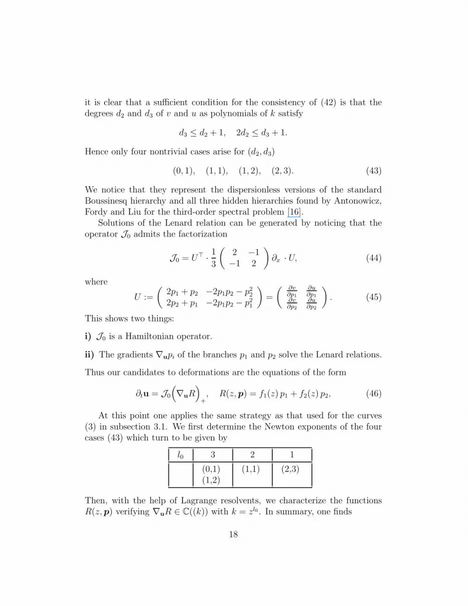
At this point one applies the same strategy as that used for the curves(3) in subsection 3.1. We first determine the Newton exponents of the fourcases (43) which turn to be given by

l0 3 2 1

(0,1) (1,1) (2,3)(1,2)

Then, with the help of Lagrange resolvents, we characterize the functionsR(z, p) verifying ∇uR ∈ C((k)) with k = zl0 . In summary, one finds

18

For the case l0 = 3,

R = zf1(z3)L1 + z2f2(z

3)L2, k = z3. (47)

For the case l0 = 2,

R = f1(z2)

(

L1 + L2

)

+ zf2(z2)

(

L1 − L2

)

, k = z2. (48)

For the case l0 = 1, we have z = k, so that any function R(k, p) =f1(k)L1 + f2(k)L2 is appropriate.

Example 1: The case l0 = 3 with (d2, d3) = (1, 2). From (40) and (41) wehave that u2 t = 0. Then if one takes

u(k, x, t) = k2 + u1(x, t)k + u0(x, t), v(k, x, t) = v1(x, t)k + v0(x, t),

and sets

f1(z3) =

1

2(1 + i

√3)z3, f2 ≡ 0,

in (47), one gets

v1 t = −2 u1x +5

9v21 v1 x,

v0 t =1

9

(

−18 u0x + v21 v0 x + 4 v0 v1 v1 x

)

,

u1 t =1

9

(

v21 u1 x − 6 v0 v1 x − 6 v1 v0 x + 6 v1 u1 v1 x

)

,

u0 t =1

9

(

v21 u0 x − 6 v0 v0 x + 6 u0 v1 v1 x

)

,

i.e., the dispersionless version of the coupled Boussinesq system (3.20b) in[16].

Example 2: The case l0 = 2 with (d2, d3) = (1, 1). Now, one can see thatv1 t = 0. By setting

u(k, x, t) = u1(x, t)k + u0(x, t), v(k, x, t) = −k + v0(x, t),

19

andf1(z

2) = −z2, f2 ≡ 0,

in (48), we find the system,

v0 t = −2 u0x − 2 v0 u1x − u1 v0 x,

u1 t = −4 u1 u1 x +2

3v0 x,

u0 t = −u1 u0 x − 3 u0 u1 x −2

3v0 v0 x .

This is the dispersionless version of the system (4.13) in [16].

3.4 Whitham deformations of cubic curves

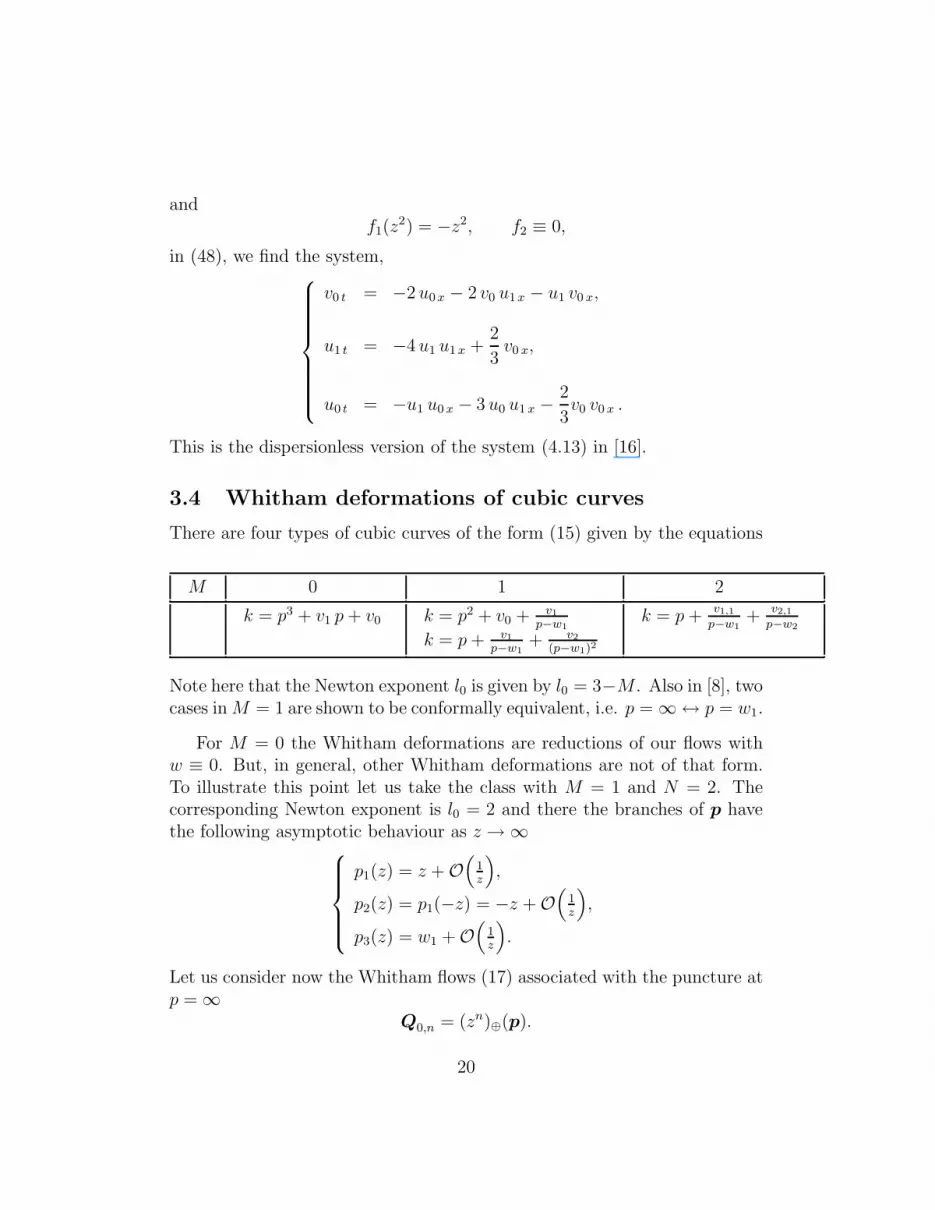
There are four types of cubic curves of the form (15) given by the equations

M 0 1 2

k = p3 + v1 p + v0 k = p2 + v0 + v1

p−w1

k = p + v1,1

p−w1

+ v2,1

p−w2

k = p + v1

p−w1

+ v2

(p−w1)2

Note here that the Newton exponent l0 is given by l0 = 3−M . Also in [8], twocases in M = 1 are shown to be conformally equivalent, i.e. p = ∞ ↔ p = w1.

For M = 0 the Whitham deformations are reductions of our flows withw ≡ 0. But, in general, other Whitham deformations are not of that form.To illustrate this point let us take the class with M = 1 and N = 2. Thecorresponding Newton exponent is l0 = 2 and there the branches of p havethe following asymptotic behaviour as z → ∞

p1(z) = z + O(

1z

)

,

p2(z) = p1(−z) = −z + O(

1z

)

,

p3(z) = w1 + O(

1z

)

.

Let us consider now the Whitham flows (17) associated with the puncture atp = ∞

Q0,n = (zn)⊕(p).

20

In terms of the potentials u = (w, v, u)⊤ they read

∂tu = J0a, (49)

where

a =

V −1

(zn)⊕(p1)(zn)⊕(p2)(zn)⊕(p3)

+

.

One easily sees that all matrix elements of V −1 are of order O(

1z

)

with the

exception of(

V −1)

13= 1 + O

(1

z

)

.

On the other hand, we have

(zn)⊕(p1) = zn + O(

1z

)

,

(zn)⊕(p2) = (−z)n + O(

1z

)

,

(zn)⊕(p3) = (zn)⊕(w1) + O(

1z

)

.

Therefore one gets

a =

znV −1

1(−1)n

0

+

+ (zn)⊕(w1) e3,

where e3 = (0, 0, 1)⊤, so that equation (49) becomes

∂tu = J0

(

T ∇u[zn(p1 + (−1)np2)])

++ J0

(

(zn)⊕(w1) e3

)

. (50)

Similar expressions can be obtained for the deformations generated by theWhitham flows (17) for α = 1 and n ≥ 1.

Acknowledgements

L. Martınez Alonso wishes to thank the members of the Physics Depart-ment of Lecce University for their warm hospitality.

21

References

[1] S. P. Novikov, S. V. Manakov, L. P. Pitaevski and V. E. ZakharovTheory of solitons. The inverse scattering method, Plenum, New York(1984).

[2] E. D. Belokolos, A. I. Bobenko , V. Z. Enolski, A. R. Its and V. B.Matveev, Algebro-Geometric approach to nonlinear integrable equations,Springer-Verlag, Berlin (1994).

[3] B. Dubrovin and S. Novikov, Russ. Math. Surv. 44(6), 35 (1989).

[4] H. Flaschka, M.G. Forest and D.W. Mclauglin , Commun. Pure Appl.Math 33, 739 (1980).

[5] B.A. Dubrovin, Commun. Math. Phys. 145, 415 (1992)

[6] I.M. Krichever, Funct. Anal. Appl. 22, 206 (1988).

[7] I.M. Krichever, Commun. Pure. Appl. Math. 47, 437 (1994).

[8] A. Aoyama and Y. Kodama, Commun. Math: Phys. 182, 185 (1996)

[9] Y. Kodama and B.G. Konopelchenko, J. Phys. A: Math. Gen. 35, L489-L500 (2002); Deformations of plane algebraic curves and integrable sys-tems of hydrodynamic type in Nonlinear Physics: Theory and Exper-iment II,edited by M.J. Ablowitz et al, World Scientific, Singapore(2003).

[10] B.G. Konopelchenko and L. Martınez Alonso, J. Phys. A: Math. Gen.37, 7859 (2004).

[11] B. L. van der Waerden,Algebra, Vol. I, Springer-Verlag, Berlin (1991).

[12] L. Redei,Introduction to algebra, Vol. I, Pergamon Press, Oxford (1967).

[13] I.G.Macdonald, Symmetric functions and Hall polynomials, ClarendomPress, Oxford (1979).

[14] R. Y. Walker, Algebraic Curves, Springer-Verlag, Berlin (1978).

[15] S. S. Abhyankar, Algebraic Geometry for Scientists and Engineers,Mathematical Surveys and Monograps vol. 35, AMS (1990).

22

[16] M. Antonowicz, A. P. Fordy and Q. P. Liu, Nonlinearity 4, 669 (1991)

23