arX

iv:c

ond-

mat

/020

4432

v2 [

cond

-mat

.str

-el]

15

Jul 2

002

Electrostatic analogy for integrable pairing force Hamiltonians

L. Amicoa, A. Di Lorenzoa, A. Mastellonea, A. Osterloha , and R. Raimondib

(a) NEST–INFM & Dipartimento di Metodologie Fisiche e Chimiche (DMFCI),Universita di Catania, viale A. Doria 6, I-95125 Catania, Italy and

(b) NEST-INFM & Dipartimento di Fisica, Universita di Roma Tre, Via della Vasca Navale 84, 00146 Roma, Italy.

For the exactly solved reduced BCS model an electrostatic analogy exists; in particular it servedto obtain the exact thermodynamic limit of the model from the Richardson Bethe ansatz equations.We present an electrostatic analogy for a wider class of integrable Hamiltonians with pairing forceinteractions. We apply it to obtain the exact thermodynamic limit of this class of models. To verifythe analytical results, we compare them with numerical solutions of the Bethe ansatz equations forfinite systems at half–filling for the ground state.

PACS numbers: 02.30.Ik , 74.20.Fg , 03.65.Fd

I. INTRODUCTION

Pairing force interactions have been successfully em-ployed to explain phenomena in different contexts suchas superconductivity1, nuclear physics2, QCD3 andastrophysics4. The original idea traces back to Bardeen,Cooper, and Schrieffer (BCS) who proposed pairing oftime-reversed electrons as the crucial mechanism forsuperconductivity5. Physical implications of the corre-sponding Hamiltonian have been extracted resorting to avariety of analytical or numerical techniques. The meanfield ground state was shown to be exact in the limitof large number of electrons where fluctuations can beneglected1,5,6. This constituted a great success of theBCS variational ansatz. However there are relevant phys-ical situations where approximations are not reliable andexact treatments are highly desirable. Fortunately, byproperly choosing the pairing couplings, the model ad-mits an exact solutions.A simplified, but still non-trivial model is the “reducedBCS model” (BCS model, for brevity) which assumesa uniform pairing g among all the electrons within theDebye shell. This model is integrable7 and was diago-nalized long ago by Richardson through Bethe Ansatz(BA)8 (see also Ref. 9). Only very recently this gener-ated a lot of interest both in nuclear and condensed mat-ter physics whose communities benefited from the simplealgorithm of Richardson’s BA solution to tackle the BCSmodel in the canonical ensemble10,11,12,13. Much workhas been done to merge the model in the schemes of theQuantum Inverse Scattering (QIS) and Conformal FieldTheory (CFT), which are modern arenas where quantumintegrability and exact solutions can be treated on equalfooting. These studies allowed significant steps forward.QIS studies identified the Richardson BA solution as thequasi classical limit of the exact solution of (twisted) dis-ordered six vertex models of the XXX-type14,15. Thispaved the way towards the exact evaluation of corre-lation functions of the BCS model16,17. The field the-oretical study of the BCS model is due to Sierra andcoworkers. The first step was to relate the RichardsonBA solution with WZNW-su(2)k models18,19. This stim-

ulated the discovery that the BA solution is the quasiclassical limit of the Babujian’s off shell BA of the (un-twisted) disordered six-vertex model15,20. The field the-oretical origin of the integrability of the BCS model hasbeen clarified definitely21 to be a twisted Chern-Simons(CS) theory on a torus. The Richardson BA solutiontogether with the underlying integrability of the theoryarises from the Knizhnik-Zamolodchikov-Bernard equa-tions (which are the Knizhnik-Zamolodchikov equationson the torus). The emergence of the CS theory is quiteinteresting and relates at a formal level the BCS the-ory of superconductivity with the Fractional QuantumHall Effect (FQHE)18 (also pointing out important dif-ferences). In fact, the exact BCS wave function admitsa “Coulomb gas” representation, which corresponds tothe “Coulomb gas” representation of the Laughlin wavefunctions (plasma analogy)18,22. Accordingly, also forthe BCS model an electrostatic analogy does exist. Itwas illustrated first by Gaudin23: the Cooper pair ener-gies are obtained as equilibrium positions of N mobilecharges in the background of Ω fixed charges and a uni-form electric field of strength 1/g. This analogy was usedby Richardson24 and Gaudin23 to obtain the thermody-namic limit of the Richardson BA equations in two dif-ferent approaches. Both reproduced the BCS mean-fieldgap equation, hence confirming the statement of Bogoli-ubov6 that at T = 0 the mean-field results become exact.Recently, Sierra and coworkers revived the attention onthe thermodynamic limit of the BCS model, comparingGaudin’s long forgotten results with the numerical solu-tion of the Richardson BA equations for a finite numberof particles25.

By generalizing the integrals of motion of the BCSmodel, the class of known integrable pairing-force Hamil-tonians could be enlarged considerably towards modelswith non-uniform interactions26,27 (for bosonic versionssee the Ref.28). Here, the term “non-uniform” indicatesthat the interactions depend on the energy levels occu-pied by the interacting electrons. As the uniform BCSmodel, also these models emerge from the quasi-classicallimit of the QIS approach for twisted disordered six ver-tex models of the XXZ-type15,29. The untwisted case,studied in the Ref.30, corresponds to large effective pair-

2

ing interaction.In the present work we generalize the 2d-electrostatic

analogy to the class of integrable Hamiltonians obtainedin Ref. 26. The thermodynamic limit of these Hamiltoni-ans is obtained. We compare the obtained analytical re-sults with numerical solutions of the BA equations. Theelectrostatic analogy of the Richardson-Sherman equa-tions is a screening condition for a total electric field pro-duced by charges distributed in two-dimensional space.Accordingly, the electric field obeys a Riccati-type differ-ential equations.

The paper is laid out as follows. In the next sectionwe review the integrability of pairing force Hamiltoni-ans that arises from the underlying infinite dimensionalGaudin algebra G[sl(2)]. In section III we present theelectrostatic analogy, review basic facts of 2d-dimensionalelectrostatics and apply them to obtain the thermody-namic limit of integrable Hamiltonians with non-uniformpairing couplings. At the end of the section, we obtainGaudin and Richardson’s results for the BCS model as alimiting case of our equations. Section IV is devoted toconclusions. In Appendix A we sketch some mathemati-cal aspects connected with the integrability of the mod-els. In Appendix B we present the connection with theRiccati equations by reviewing the work of Richardson24.In Appendix C we collect details of the calculations. InAppendix D we discuss some features of the ground stateand possible routes towards the study of the excitations.

II. EXACTLY SOLVABLE PAIRING MODELS

The Hamiltonian for N charged particles interactingthrough pairing force

H =∑

iσ

εiσniσ +∑

ij

Uij ninj −∑

ij

gij c†i↑c

†i↓cj↓cj↑, (1)

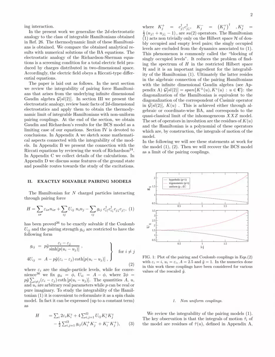
has been proved26 to be exactly solvable if the CoulombUij and the pairing strength gij are restricted to have thefollowing form

gij = pgεi − εj

sinh[p(ui − uj)],

4Uij = A− pg(εi − εj) coth[p(ui − uj)] ,

for i 6= j

(2)where εi are the single-particle levels, while for conve-nience36 we fix gii = φ, Uii = A − φ, where 2φ =pg∑

i6=j(εi − εj) coth [p(ui − uj)]. The quantities A, u,and ui are arbitrary real parameters while p can be real orpure imaginary. To study the integrability of the Hamil-tonian (1) it is convenient to reformulate it as a spin chainmodel. In fact it can be expressed (up to a constant term)as

H =∑

i 2εiKzi + 4

∑Ωi,j=1 UijK

zi K

zj

− 12

∑Ωi,j=1 gij(K

+i K

−j +K−

i K+j ), (3)

where K+j = c†j↑c

†j↓, K−

j =(

K+j

)†,Kz

j =12 (nj↑ + nj↓ − 1) , are su(2) operators. The Hamiltonian(1) acts non trivially only on the Hilbert space H of dou-bly occupied and empty level pairs; the singly occupiedlevels are excluded from the dynamics associated to (1).This phenomenon is commonly called the “blocking ofsingly occupied levels”. It reduces the problem of find-ing the spectrum of H in the restricted Hilbert spaceH and it is an important ingredient for the integrabil-ity of the Hamiltonian (1). Ultimately the latter residesin the algebraic connection of the pairing Hamiltonianswith the infinite dimensional Gaudin algebra (see Ap-pendix A) G[sl(2)] = spanK±(u),Kz(u) : u ∈ C: thediagonalization of the Hamiltonian is equivalent to thediagonalization of the correspondent of Casimir operatorin G[sl(2)], K(u) . This is achieved either through al-gebraic or coordinate-wise BA, and corresponds to thequasi-classical limit of the inhomogeneous XXZ model.The set of operators in involution are the residues ofK(u)and the Hamiltonian is a polynomial of these operatorswhich are, by construction, the integrals of motion of themodel.In the following we will see these statements at work forthe model (1), (2). Then we will recover the BCS modelas a limit of the pairing couplings.

0.5 1 1.50.5

1

1.5

2

g ij

hyperbolic (p=1)trigonometric (p=i)uniform (p→0)

0.5 1 1.5i-j

0.5

1

1.5

2

2.5

3

3.5

U i

j

FIG. 1: Plot of the pairing and Coulomb couplings in Eqs.(2)with εi = i, ui = εi, A = 2.5 and g = 1. In the numerics donein this work these couplings have been considered for variousvalues of the rescaled g.

1. Non uniform couplings.

We review the integrability of the pairing models (1).The key observation is that the integrals of motion τi ofthe model are residues of τ (u), defined in Appendix A,

3

in u = ui. In fact, H can be written as

H =

Ω∑

i

2εi τi +A

Ω∑

i,j

τi τj −∑

i

φiK2i , (4)

τi = Kzi + Ξi , (5)

Ξi := −pg∑

j 6=i

K+i K

−j +K−

i K+j

2 sinh [p(ui − uj)](6)

+Kzi K

zj coth [p(ui − uj)]

The g −→ ∞–limit of this Hamiltonian was found inRef. 30. From Eq.(4) it is evident that [H, τj ] = 0. Bythese integrals of motion, the model is connected withthe anisotropic Gaudin Hamiltonians Ξl. The property26

[τj , τl] = 0 for j, l = 1, . . . ,Ω comes from [τ(u), τ(v)] =014. The common eigenstates of H and τi are

|Ψ〉 =N∏

α=1

K+(eα) |0〉 (7)

where |0〉 is the Fock vacuum and N is the number ofpairs. The eigenvalues of the Hamiltonian H and of theconstants of the motion are

E = −pg

Ω∑

j=1

N∑

α=1

εj coth [p(eα − uj)] +AN2 (8)

τi = −g

2

N∑

α=1

p coth [p(eα − ui)]+g

4

Ω∑

j=1

j 6=i

p coth [p(uj − ui)]−1

2.

(9)The quantities eα are solutions of the following set ofequations

2

g+2

N∑

β=1

β 6=α

p coth [p(eβ − eα)]−

Ω∑

j=1

p coth [p(uj − eα)] = 0 .

(10)which are the BA equations of the model (1).

2. Uniform couplings: the BCS model

We now review the exact solution together with the in-tegrability of the pairing Hamiltonian with uniform cou-pling constants. In this case the Hamiltonian(1) reads

HBCS =

Ω∑

i=1

2εiKzi −

g

2

Ω∑

i,j=1

(

K+i K

−j +K−

i K+j

)

(11)

H can be directly diagonalized through coordinate-wise8

or algebraic31 BA. Nevertheless its diagonalization can beachieved along the lines depicted above. The integralsof motion τi of the BCS model are the residue of τ(u)in u = 2εi. By these integrals of motion, the model

becomes connected with isotropic Gaudin HamiltoniansΞl. In fact, H can be written as

HBCS =

Ω∑

i=1

2εi τi + g

Ω∑

i,j=1

τi τj + const. (12)

τi = Kzi + Ξi , (13)

Ξi := −g∑

j 6=i

~Ki · ~Kj

εi − εj(14)

where the spin vectors are: Kj := (Kxj ,K

yj ,K

zj ); K±

j =

Kxj ± iKy

j . The eigenstates of both the BCS Hamilto-

nian8,9 and its constants of motion τj14 are

|Ψ〉BCS =

N∏

α=1

K+(eα) |0〉 (15)

The eigenvalues of the Hamiltonian and of the integralsof the motion are respectively

EBCS = 2

N∑

α=1

eα , (16)

τi = −g

2

N∑

α=1

1

eα − εi+g

4

Ω∑

j=1

j 6=i

1

εj − εi−

1

2. (17)

where eα are solutions of the Richardson-Sherman (RS)equations

1

g+

Ω∑

j=1

1/2

eα − εj−

N∑

β=1

β 6=α

1

eα − eβ= 0 (18)

(the parameters eα are one half of the parameters Eα

originally defined by Richardson8). The eigenstates,eigenvalues and the RS equations can be obtained inthe p → 0 limit of the BA equations (10) with theidentification ui = εi, g = g. By the same limit theanisotropic (XXZ) Gaudin model reduces to its isotropicversion (XXX).

III. ELECTROSTATIC ANALOGY FOREXACTLY SOLVABLE PAIRING MODELS

The RS equations (18) are stating that the total forceacting on the unit charges located in eα, due to the 2delectric field37 generated by the Ω charges qfixed = −1/2fixed in εi, by the remaining N − 1 mobile unit chargesqmobile = +1 and by the external constant electric fieldof strength −1/g is zero. In other words, the solutionsof the RS equations correspond to the (unstable) equi-librium configurations of N charges in the complex planeunder the influence of a given electric field. This electro-static analogy was first pointed out by Gaudin9. It allowsthe exact access to the thermodynamic limit of the BCS

4

model23 by exploiting the formalism of complex analy-sis. The analytic structure of the ansatz electric field isprescribed by the positions of the charges.

We will now present an electrostatic analogy for thegeneralized BCS models (1), (2).

In the variables

zα :=tanh (p eα)

p, xi :=

tanh(p ui)

p, (19)

the Eqs. (10) are algebraic

−q(0)+

zα − 1/p−

q(0)−

zα + 1/p−

Ω∑

i=1

1/2

zα − xi+

N∑

β=1

α 6=β

1

zα − zβ= 0 ,

(20)

where 2q(0)± = ∓1/pg− [Ω−2(N−1)]/2. We shall assume

that the parameters ui are given by ui = f(εi) where fis a monotonic function. For the case p = i note thatdue to the π-periodicity of the transformation (19) theui can be restricted to lie in (−π/2, π/2). Hence, theBethe equations for the generalized BCS models (10) canbe recast in the same form as the original RS equationsEq. (18), except that the constant external electric fieldof strength −1/g in the homogeneous case is replaced by

the presence of two isolated charges −q(0)± fixed at points

±1/p.38 Note that for p = i the charges are complex.The interpretation of this is discussed later on.

A. Basics of 2d electrostatics

We sketch briefly the main ingredients of two-dimensional electrostatics in terms of holomorphic func-tions in C (i.e. real harmonic functions in R2).

Let the electric field E = (Ex, Ey) be associated to thecomplex number E = Ex − iEy. The Maxwell equationscan then be summarized as

∂zE =1

2(div ~E + i (curl~E)z) = π(ρ+ i (~jmag)z) (21)

with real charge density ρ and real magnetic monopolecurrent density ~jmag in z-direction; the derivatives are∂z = (∂x − i ∂y)/2, ∂z = (∂x + i ∂y)/2. Any integral overa closed curve Γ gives

1

2πi

∫

Γ

dz E(z) =1

2π

∫

Γ

(Exdy − Eydx) − i (Exdx+ Eydy)

=1

2π

∫

Γ

E · ds−i

2π

∫

Γ

E · dl

= QΓ − i IΓ ,

where QΓ and IΓ are the total electric charge and mag-netic monopole current enclosed by Γ (in the followingwe refer to QΓ − i IΓ as charge). The surface element ds

is a vector perpendicularly pointing outwards of Γ withthe same length as the line element dl.

A charge q contributes to the electric field with a simplepole with residue q. A line of charges gives a holomorphic

function on a Riemann surface with a branch cut alongthe charge line. The discontinuity of the field in cross-ing the cut gives the charge density 1

2πi (E−(z) − E+(z)),where E−(z) (E+(z)) are the limiting values of the fieldwhen z tends to the cut from the right (left) with respectto the orientation of the curve.

B. Thermodynamic limit

The thermodynamic limit of the model (1) can be ob-tained in the following way: we first divide Eq.(20) by Ωand define the (positive) charge densities

ρ(xj) :=1/2

Ω(xj+1 − xj)

σ(zα) :=1

Ω|zα+1 − zα|

To obtain a sensible thermodynamic limit, we assume i)that the pairing strength scales as g = G/Ω, with fixedG; ii) that the Debye shell defined by the end points ε1,εΩ does not depend on Ω; iii) that the number of pairsincreases with Ω according to N = νΩ, where ν is thefilling. In the limit Ω → ∞, Equations (20) then become

−Q

(0)+

z − 1/p−

Q(0)−

z + 1/p−

∫

L

dxρ(x)

z − x+

∫

Γ

|dz′|σ(z′)

z − z′= 0 .

(22)where the integrals are meant in the sense of the prin-cipal value P . After the transformations (19) the trans-formed Debye shell L is still a segment of the real axishaving end points a0 = tanh (p u1)/p, b0 = tanh (p uΩ)/p;

the isolated charges are −Q(0)± = − 1

2 (ν − 1/2± 1/(pG));the density ρ is determined by the single-particle energydensity ρε as ρ(x) = ρε(ε(x))/[f

′(ε(x))(1− p2x2)], whereε(x) = f−1(Arctanh(px)/p), and it fulfills

∫ εΩ

ε1

dερε(ε) =

∫

L

dx ρ(x) = 1/2 .

The curve Γ and the density σ have to be determined,with the constraint

∫

Γ

|dz|σ(z) = ν .

The idea of Gaudin was to construct the total elec-tric field E(z) as a function with an analytic structureprescribed by the actual charge distribution. He fur-ther assumed that eventual solutions of the equation(22) are arranged in K piece-wise differentiable arcs:

Γ = Γρ ∪⋃K

n=1 Γn, where Γρ is the common supportof ρ(x) and σ(x) which is not contained in the arcs

Γarc ≡⋃K

n=1 Γn. For example, a charge distributionalong the line [a, b] in the complex plane with total chargeq and constant charge density would lead to the totalelectric field E(z) = (q/|a− b|) ln[(z − b)/(z − a)] which

5

diverges at the end points of [a, b]. Since in the case un-der consideration the electric field has to vanish at theend points of Γ, we need the charge density to vanish“sufficiently fast” there. An example of such a functioncould be any [(z− a)(z− b)]α ln z−b

z−a with any α ∈ 12 IN or

just [(z − a)(z − b)]α2 with odd α. Both functions indeed

vanish in a and b and have a branch cut along [a, b]. Thechoice of the admissible functions is finally restricted byimposing that the free charges are distributed along a fi-

nite set Γ23,25. In fact, for α 6∈ 12 IN we either have infinite

branch cuts or divergences at the end points. We wantto stress that the run of the branch cut can be chosenin an arbitrary way as long as it joins continuously thebranch points a and b. The run is fixed requiring thatit is an equipotential curve of E(z). The ansatz functionfor the total electric field is

E(z) =S(z)

[

Q+

z − 1/p+

Q−

z + 1/p+

∫

L

dxϕ(x)

z − x

]

,

S(z) =

K∏

n=1

√

(z − an)(z − bn).

(23)

Note that the sign of the complex square root is uniquelygiven, once Γarc is fixed, by

√

(z − an)(z − bn) =√

|z − an||z − bn| exp i2 argΓn

(z − an)(z − bn). The ar-gument function argΓn

(z − an)(z − bn) is the sum of theangles between z ∈ C and the two end points of Γn, whichhas a 2π–discontinuity crossing Γn. The unknown quan-tities are the end points (an, bn) of Γarc, Q± and ϕ(x).To give a physical interpretation of such an ansatz func-tion, look at S(z)Q± and S(z)ϕ(x) as screened chargesand charge density, respectively. From the symmetry ofthe distribution of the fixed charges on L and in ±1/pit follows that if an has non-zero imaginary part, thenbn = an, and we choose the orientation of Γn from an tobn, with Im(an) < 0. If an is real, so must be bn. We ar-gue however that this occurs only for distinct “critical”values of the pairing coupling at which the imaginarypart of complex conjugate an and bn vanishes and hencean = bn. The corresponding arc is then describing aclosed curve. Therefore we consider S(z) to don’t havecuts along the transformed Debye shell L (see AppendixD). We emphasize that this does not mean that σ(z) hasno support on L. A non-zero solution charge density onL is accounted for by the screening density S(x)ϕ(x).

After having determined the an, bn, the curves Γn arefound as equipotential curves of the total electric fieldEq.(23). The density σ is then determined by the dis-continuity of E in crossing Γ.

In the following, all the unknown quantities are ob-tained following a procedure a la Gaudin on which wereport in the Appendix C. We will calculate the complexintegrals involved in this procedure by exploiting basicknowledge of electrostatics.

Since the screened charges must tend to their bare val-ues when the point z is sufficiently close to the source,

we have that

S(±1/p) Q± = −Q(0)± , (24a)

In a similar way, using σ(z) − ρ(z) = (E−(z) −E+(z))/(2πi ) , we find

S(x) ϕ(x) = σ(x) − ρ(x). (24b)

Next, imposing that the electric field asymptoticallygoes as E(z) ∼ 1/z2 (this is the leading term in themulti-pole expansion, since the total charge is zero), weobtain the following equations

∫

L

dxxnϕ(x) = −1

pn(Q+ + (−1)nQ−) , 0≤n≤K . (25)

We present a detailed derivation of these equations inAppendix C. There we also show explicitly that thecondition

∫

Γσ(z)|dz| = ν is automatically fulfilled with

Eqs.(25).

Using Eqs.(24) we can express Q± and ϕ(x) in termsof S(±1/p) and S(x) respectively. The Γn are finallyobtained as equipotential curves of the total electric fieldE(z)23,25

Re

∫ z

an

dz′E−(z′) =

∫

Exdx+ Eydy = 0 , (26)

The density σ is determined by the discontinuity of Ealong Γ, according to:

σ(z) = ρ(z) +1

π|E−(z)| . (27)

It is worth noting that Eqs.(25) are a set of K + 1 realequations for the 2K real parameters determining theend points of Γn. Gaudin stated that seemingly in anycase there is a finite number of solutions. From a phys-ical perspective, though, we expect that the K − 1 freeparameters span a family of curves corresponding to aband of excitations of the system. This conjecture willbe verified in forthcoming work35.

We summarize all the conditions found for the un-knowns an, bn, ϕ, Q

6

S(z) =K∏

n=1

√

(z − an)(z − bn) ,

E(z) = S(z)

Q+

z − 1/p+

Q−

z + 1/p+

∫

L

dxϕ(x)

z − x

,

Q± = −ν − 1/2 ± 1/pG

2S(±1/p)

ϕ(x) =σ(x) − ρ(x)

S(x)

σ(z) = ρ(z) +1

π|E−(z)|

The arcs are then determined by

∫

L

dxxn ρ(x) − σ(x)

S(x)=Q+ + (−)nQ−

pn; n = 0, . . . ,K

Γn : Re

z∫

an

dz′E−(z′) = 0 .

As we stated above, the density ρ of the transformedvariables x = tanh (pf(ε))/p is connected with the givendensity ρε of the single-particle levels via

ρ(x) = ρε(ε(x))/[f′(ε(x))(1 − p2x2)] ,

ε(x) = f−1(Arctanh(px)/p) .

The energy of the state is finally given by

E = αν2 −G

∫

L

dxρ(x)ε(x)

∫

Γ

|dz|σ(z)1 − p2xz

z − x, (28)

= αν2 + p2Gν

∫ εΩ

ε1

dε ρε(ε) ε x(ε)+

−G

∫

L

dxρε(ε(x)) ε(x)

f ′(ε(x))

∫

Γ

|dz|σ(z)

z − x, (29)

where α = AΩ.

1. Comparison with the thermodynamic limit of the BCSmodel

In the limit p → 0, the two isolated charges Q(0)± take

an infinite value and they are displaced to infinity in sucha way to give a uniform electric field 1/G. In this limit,

the charges Q± behave as

Q+ ∼ ±

[

−1

2G−

1

2

(

ν −1

2+

1

2G

K∑

n=1

(an + bn)

)

p

]

pK−1 ,

Q− ∼ ∓

[

1

2G−

1

2

(

ν −1

2+

1

2G

K∑

n=1

(an + bn)

)

p

]

(−p)K−1 ,

where we kept into account the dependence of the rela-tive determination of S(±1/p) upon the number of arcs.Thus, the ansatz field reduces to

Ep→0(z).= E0(z) = S(z)

∫

L

dxϕ(x)

z − x, (30)

Eq.(24b) still hold, while Eqs.(25) simplify to:

∫

L

dxxnϕ(x) = 0, 0≤n≤K − 2 , (31a)

∫

L

dxxK−1ϕ(x) = −1

G, (31b)

∫

L

dxxKϕ(x) = −ν +1

2−

1

2G

K∑

n=1

(an + bn) , (31c)

The last two equations come from the fact that the fieldshould go asymptotically as E0(z) ∼ −1/G + QT /z inthis limit, since the total charge is now QT = ν−1/2. Inthe approach by Gaudin the last condition was obtainedby imposing

∫

|dz|σ(z) = ν. This extracts the residueat infinity, which has to be such that the total charge iszero. In our approach, we already started from a globallyneutral system and hence this normalization condition forσ(z) was automatically fulfilled (see Appendix C)

We compare our findings for integrable pairing modelswith the results for the BCS model obtained in Refs. 23,24 and reconsidered recently by Sierra and coworkers25

7

S(z) =

K∏

n=1

√

(z − an)(z − bn) ,

E0(z) = S(z)

∫

L

dxϕ(x)

z − x,

ϕ(x) =σ(x) − ρ(x)

S(x); σ(z) = ρ(z) +

1

π|E−(z)|

The arcs are then determined by

∫

L

dxxn σ(x) − ρ(x)

S(x)= 0 , n = 0, . . . ,K − 2

∫

L

dxxK−1 ρ(x) − σ(x)

S(x)=

1

G

∫

L

dxxK ρ(x) − σ(x)

S(x)−

1

2G

K∑

n=1

(an + bn) = ν −1

2

Γn : Re

z∫

an

dz′E0−(z′) = 0 .

2. Numerics and discussion of the solutions

To solve the BA equations (10), (20) we have chosenthe parameters ui = εi at half filling Ω = 2N . The corre-sponding interactions Uij and gij are shown in Fig.1. Inthe trigonometric case the Debye shell ranges in (−1, 1);in the hyperbolic case it ranges in (0, 2) for numericalconvenience (see the caption of Fig.2). The ground stateof the system (which is the only state we consider in thenumerics) is obtained by evolving the G = 0 state

limu→0

zα = xα α ∈ (1, . . . , N). (32)

to a finite value of G. At certain value of G the equationsare singular since a couple of pairing parameters z2λ−1

and z2λ coincide with the energy level x2λ−1. Such a sin-gular behaviour can be smoothed out using the proceduredeveloped by Richardson in Ref. 33. In the following webriefly summarize it. The corresponding divergences areremoved by the following transformations

z2λ−1 = Aλ − iBλ, z2λ = Aλ + iBλ, (33)

and then

Xλ = Aλ −x2λ−1 + x2λ

2, Yλ = −

B2λ

δ2λ −X2λ

. (34)

where δλ = (x2λ−x2λ−1)/2 is half the energy spacing be-tween the corresponding energy values (with whom they

coincide if the pairing coupling strength u is zero).

0 0.5 1 1.5 2

Re z-1

-0.5

0

0.5

1

Im z

G = 0.50G = 1.00G = 1.50G = 1.75G = 1.95G = 2.00chargeL

FIG. 2: Plot of the pairing parameters z in the complex planefor the hyperbolic model corresponding to p = 1 in Eq.(2).The symbols refer to the numerical solutions of Eqs.(20) forΩ = 200, N = 100, ui = εi = 0, . . . , 2 and uniform level spac-ing. Different colors and symbols represent different values ofG, as shown in the legend box. The lines are the plots of thecurves determined by Eq.(26). If we choose the Debye shellto be (−1, 1) as in the trigonometric case, the arc for G = 2closes at infinity.

By the first transformation Eqs. (20) can be writtenin a form which is manifestly real, whereas the secondtransformation (34) removes the divergences.

Now we discuss some features of the arcs shown inFigs.2 and 3. For K = 1 (we recall that straight lineson the real axis are not counted by the index n), the endpoints are uniquely determined (if they exist) and thecurve Γ corresponds to the ground state39 of the system.In this case the end points of the arc, λ± i∆, are deter-mined by the two coupled equations (obtained as linearcombinations of Eqs. (25))

∫

L

dx(1 + px)ρ(x)

√

(x− λ)2 + ∆2= 2Q+ =

1/pG+ ν − 1/2√

(λ− 1/p)2 + ∆2

∫

L

dx(1 − px)ρ(x)

√

(x− λ)2 + ∆2= 2Q− =

−1/pG+ ν − 1/2√

(λ+ 1/p)2 + ∆2

Why this set of equation corresponds to the ground stateis discussed in some detail in Appendix D.

In the trigonometric case (p = i ), the equations areboth complex, and they are conjugate. Thus, in orderto find λ and ∆ it suffices to solve separately real andimaginary part of one of them. In the hyperbolic case(p = 1), assuming a uniform single-particle energy den-sity ρε(ε(x)) = ρ0 (i.e. ρ(x) = ρ0/(1 − x2)) and a De-bye shell spanning the interval [0, 2ωD], we have that thesystem above admits a real solution (and hence two co-

8

inciding end-points)

∆ =0

λ = sinh(2ωD)/ (cosh 2ωD − exp [(ν − 1/2)/ρ0]) ,

if 1/(ρ0G) = 2ωD. This corresponds to the external curvein Fig. (2).

-1.5 -1 -0.5 0

Re z

-1

-0.5

0

0.5

1

Im z

G = 1.5G = 2.0G = 2.5G = 3.0G = 3.5chargeL

FIG. 3: Plot of the pairing parameters z in the complexplane for the trigonometric model which correspond to p = iin Eq.(2). The symbols refer to the numerical solutions ofEqs.(20) for Ω = 200, N = 100, ui = εi = −1, . . . , 1 and uni-form level spacing. Different colors and symbols correspondto different values of G, as shown in the legend box. The linesare the plots of the curves determined by Eq.(26) .

Situations corresponding to K > 1 lead to excitedstates. We point out that the independent equations(25) are in number of K + 1 leaving undetermined K − 1parameters. This might be an evidence of “bands” ofexcitations above the ground state35.

Looking at the behaviour of the quasi–momenta solu-tions of the BA equations, we can note that the moreintense is the pairing constant G the more evident is thetendency of the quasi–energies to be complex. In Fig. 4we compare this tendency for the hyperbolic, trigonomet-ric, and uniform BCS models. We found that the pairingtendency increases from the trigonometric over the uni-form to the hyperbolic model. Looking at the explicitcouplings plotted in Fig. 1, we should conclude that thepairing and Coulomb interaction in Eqs. (2) are compet-itive couplings.

IV. SUMMARY AND CONCLUSIONS

We have discussed the electrostatic analogy for theexactly solvable pairing force Hamiltonians found inRef. 26. These models generalize the BCS model in thatthe coupling constants are not uniform (in the space ofquantum labels i, j, see Eqs. (1)). The ordinary BCS

-1 -0.8 -0.6 -0.4 -0.2 0Re e

-2

-1

0

1

2

Im e

UniformHyperbolicTrigonometric

FIG. 4: For an exemplary value of G = 2 the solutionsfor p = 1, i corresponding to hyperbolic and trigonometricmodels respectively are compared with the solutions of theBA equation for the uniform case p = 0 which are the RSequations (the Debye shell ranges in (−1, 1) for all the threecases).

model is obtainable as a limit26 p → 0 of the models(1), (2). The electrostatic analogy exists because the BAequations for the “rapidities” eα can be recast in a spe-cial algebraic form. For the class of models we deal withsuch an algebraic form is obtained by the change of vari-ables: zα = tanh(peα), xi = tanh(pεi). After this trans-formation the Bethe equations express the condition foran equilibrium alignment of mobile charges qmobile = +1in the 2d–real or complex plane in a neutralizing back-ground of qfixed = −1/2 fixed charges placed in the po-sitions xi and two further charges in the positions ±1/p.Remarkably, this analogy is very effective to obtain theexact thermodynamic limit (i.e. the large N limit) ofthe models. In this limit the mobile charges (which arethe solutions of the Bethe equations) arrange themselves

along equipotential curves Γ =⋃K

n Γn of the total elec-tric field with vanishing charge density at its extremi-ties. The electrostatic analogy presented in this workis by no means unique; the charge distribution can betransformed by the whole group of conformal Moebiustransformations. We have obtained explicitly the ther-modynamic limit for the ground state configuration athalf–filling (see Fig. (2), (3)). We note, however, thatthe approach is also valid for excited states of the sys-tem, though the explicit calculation can involve technicalsubtleties (discussed in Appendix D).The electrostatic analogy together with the construc-tive equations for the BCS model found by Gaudin andRichardson is demonstrated to be obtained from the limitp → 0 of the results presented here. A comparison be-tween the hyperbolic, trigonometric, and uniform casesis seen in Fig. (4). Since this represent an inversion ofthe behaviour one would have expected from Fig. (1) weconclude that the pairing and Coulomb interactions inEqs. (2) are competitive couplings. The exact thermody-

9

namics of integrable pairing models is one of the futuregoals.

Acknowledgments

We thank G. Sierra for helpful discussions. We furtheracknowledge constant support by G. Falci, R. Fazio, andG. Giaquinta.

APPENDIX A: THE GAUDIN ALGEBRA

The Gaudin algebra G[sl(2)] is constructed from sl(2).The sl(2) “lowest” weight module is generated by the vac-uum vector |0〉j , K

−j |0〉j = 0 , Kz

j |0〉j = kj |0〉j where

kj is the “lowest” weight (kj = −1/2 for spin 1/2 whichis the case considered for electrons). The infinite dimen-sional G[sl(2)] is generated by

K±(ξ) :=

Ω∑

j=1

φ(ξ−uj)K±j , Kz(ξ) :=

Ω∑

j=1

ψ(ξ−uj)Kzj

(A1)where ξ ∈ C and uj ∈ R. The module of G[sl(2)] is char-acterized by the vacuum |0〉 ≡ ⊗Ω

j=1|0〉j : K−(ξ)|0〉 =

0 , Kz(ξ)|0〉 = κ(ξ)|0〉 , where κ(ξ) :=∑Ω

j=1 kjψ(ξ −

uj) is the lowest weight of G[sl(2)]. The element ofG[sl(2)] corresponding to the su(2) Casimir operator isK(ξ) := Kz(ξ)Kz(ξ)+ 1

2 (K+(ξ)K−(ξ) +K−(ξ)K+(ξ)).The generating function of the integral of the motion ofthe pairing models is related to K(ξ) through

τ(ξ) = −2ΛK(ξ) +Kz(ξ) + c(ξ)1l (A2)

where c(ξ) is a C-function and Λ is a real parameter. Theproperty [τ(v), τ(w)] = 0 arises from the quasi-classicallimit of the sl(2) QIS theory; this is the ultimate reasonfor the integrability of the BCS model.

In the present paper φ and ψ are either rational ortrigonometric/hyperbolic functions.

1. Rational G[sl(2)]

In this case: φ(ξ) = ψ(ξ) := 1/ξ, κ(ξ) ≡ k0(ξ) =∑Ω

j=1 kj/(ξ − uj), and Λ ≡ g. The operators (A1) obey

[Kz(v),K±(w)] = ∓K±(v) −K±(w)

v − w,

[K−(v),K+(w)] = 2Kz(v) −Kz(w)

v − w,

where v 6= w ∈ C. The Bethe equations are theRichardson-Sherman (RS) equations

k0(eα) =1

g+

N∑

β=1

β 6=α

1

eβ − eα, α = 1, . . . , N . (A3)

We note that RS equations (A3) are intimately relatedto the algebraic structure of G[sl(2)] since they act asconstraints on the lowest weight k(Eα). The differencebetween the BCS and Gaudin model results in a differentconstraint imposed on the lowest weight vector of G[sl(2)]which leads to different sets E , E ′ of solutions of the BAequations (E ′ is spanned by the solutions of (A3) wheng → ∞). This fact has been used to extend the Sklyanintheorem for the Gaudin models to the BCS model16.

2. Hyperbolic/Trigonometric G[sl(2)]

In this case: φ(ξ) := p/ sinh[pξ], ψ(ξ) := p coth[pξ] ,

κ(ξ) ≡ k(ξ) =∑Ω

j=1 pkj coth[p(ξ − uj)]and Λ ≡ g. The

operators (A1) obey

[Kz(v),K±(w)] = ∓pK±(v) − cosh[p(v − w)]K±(w)

sinh[p(v − w)],

[K−(v),K+(w)] = 2pKz(v) −Kz(w)

sinh[p(v − w)],

where v 6= w ∈ C.The BA equations for the corresponding Hamiltonian

(1) are

k(eα) =1

g+

N∑

β=1

β 6=α

p coth[p(eβ−eα)] , α = 1, . . . , N . (A4)

Also in this case the BA equations act as constraints onthe lowest weight k(eα) of the trigonometric G[sl(2)].

APPENDIX B: THE RICHARDSON ROUTE ANDTHE RICCATI EQUATION

In this appendix we first emphasize the key role playedby the non linear differential equation of Riccati typein the electrostatic analogy of exactly solvable pairingmodels.34 Then we sketch the procedure originally em-ployed by Richardson24 to obtain the thermodynamiclimit of the BCS model.

In the non-uniform case the electric field is

E(z) :=1

2k(z) +

1

2g+p

2

N∑

β=1

β 6=α

coth[p(eβ − z)] (B1)

with k(z) as defined in the previous section. In orderto have the field obeying a Riccati-type equation, it iscrucial to map one of the isolated charges to infinity.This is done by the transformation

qi := exp (2pεi) ; ζα := exp (2peα). (B2)

In the variables qi and ζα, the Riccati equation is

dE(z)

dz+ E2(z) = τ (z) + f(z) (B3)

10

where τ0(z) := 1/g∑Ω

j=1 τj/[qj(qj − z)] is a generatingfunction of the eigenvalues of integrals of the motion ofthe model (1) (see Eqs. (9)) and

f(z) =Q0(Q0 + 1)

g2(B4)

+

Ω∑

j=1

1

qj − z

[

kj(kj + 1)

qj − z− 2

Q0

z− 2

P0

qj

]

where P0 := 2Q0 + Ω − 2N + 1/2.For the isotropic limit p → 0 the BCS rational case is

recovered. The electrostatic field is here given by (see RSEqs. (A3))

E0(z) = k0(z) +1

g−

N∑

β=1

β 6=α

1

z − eβ(B5)

=1

g+

Ω∑

j=1

1/2

z − εj−

N∑

β=1

β 6=α

1

z − eβ.

In this case the Riccati equation reads

dE0(z)

dz+ E2

0(z) = τ(z) + f(z) (B6)

where

f(z) =N2

g2+

Ω∑

j=1

kj(kj + 1)

(z − εj)2(B7)

where τ(z) is the generating function of the eigenvalues ofintegrals of the motion of the BCS model Eqs. (17). TheRichardson BA equations are the zeros of the solutionsof (B7). The role of the Riccati equations in connectionwith the Gaudin models was also investigated in Ref.34.

In both the rational or non-uniform cases it is evidentthat the Riccati equation plays an important role. Thisfact has been used by Richardson to derive the BCStheory from the expansion of the solution of the Ric-cati equation (in the rational case and kj = −1/2 ∀j)in powers of 1/N . In the following we briefly summa-rize the Richardson’s physical arguments. The Richard-son equations, via the electrostatic analogy, can be seenas a self-consistent evaluation of the field of the fixedcharges in the presence of the screening due to the mo-bile charges. The strategy followed by Richardson is toattempt to eliminate any reference to the mobile chargesin the right hand side of the above equation. In fact,using the Eqs. (A3) the Riccati equation for the field canbe recast in the following form:

dE0(z)

dz+ E2

0(z) =

Ω∑

i=1

1/2

(z − ǫi)2+

[

Ω∑

i=1

1/2

z − ǫi+

1

g

]2

−2

Ω∑

i=1

1/2

z − ǫi

N∑

β=1

1

ǫi − eβ. (B8)

In the last term on the right hand side there appears thefield due to the mobile charges at the location of the fixedcharges. The self-consistency condition, and the effectivescreening, enters here. Richardson notices that the fieldof the mobile charges may be written in the following way

1

ǫi − eβ=

1

2πi

∮

C

dzE0(z)

ǫi − z(B9)

with the curve C going around the singularities of E(z)due to the mobile charges. By using this, one gets aintegro-differential equation of the Riccati type

dE0(z)

dz+ E2

0(z) =

Ω∑

i=1

1/2

(z − ǫi)2+

[

Ω∑

i=1

1/2

z − ǫi+

1

g

]2

+1

2πi

∮

C

dz′Ω∑

i=1

E0(z′)

(z − ǫi)(z′ − ǫi). (B10)

The nice feature of the above equation is that any ref-erence to the mobile charges has disappeared. One mayobject that in the above equation there is still a referenceto the mobile charges via the curve C entering the con-tour integral. In fact, by knowing the property that thefield has to satisfy at infinity one may observe that theintegral over a closed curve may be written as the sumof two curves: the first is C enclosing the singularities ofthe mobile charges, while the second enclosing the sin-gularities of the fixed charges. Furthermore to evaluatethe contour integral along the curve extending at infinity,it is enough to know the first term in the multi-pole ex-pansion of the field. The final result is that the integralover C may be written in terms of the curve enclosingthe singularities of the fixed charges and the behavior ofthe field at infinity only. The elimination of the mobilecharges from the effective equation for the field is closelyin the spirit of the Thomas-Fermi approach to the eval-uation of the effective potential due to the combined ef-fect of fixed charges (nucleus in atoms, ions in metals)and mobile charges (electrons). The integro-differentialRiccati equation plays in this context the role of the Pois-son equation, which becomes the Thomas-Fermi equationonce the charge of the mobile electron is written in termsof the potential.

The next trick used by Richardson is to expand thecomplex electric field E0(z) near the point at infinity, inpowers of 1/z. This amounts to a multi-pole expansion.The constant electric field gives the zeroth order term.The other terms may be expanded upon using the geo-metric series. One easily gets

E(0)0 = −

1

g

E(1)0 = N −

1

2Ω (B11)

E(2)0 =

N∑

β=1

eβ −1

2

Ω∑

i=1

ǫi ≡ E −1

2

Ω∑

i=1

ǫi.

11

The monopole and dipole terms give then the numberof pairs and the energy. To perform the thermodynamiclimit, we rescale the coupling constant as g → G/Ω inorder that the energy remains an extensive quantity inthis limit (see section III B). The field is expanded asE0 = EN + E1 + E1/N + ... where the subscript indi-cated terms of order N , 1, and 1/N , respectively. Weare assuming that N and Ω keep a fixed ratio. One mayrewrite the Riccati equation order by order

E2N =

(

Ω

G+

Ω∑

i=1

1/2

z − ǫi

)2

−Ω∑

i=1

HNi

z − ǫi(B12)

2ENE1 = −dEN

dz+

Ω∑

i=1

1/2

(z − ǫi)2−

Ω∑

i=1

H1i

z − ǫi

where at each order in N

Hi =1

2πi

∮

C

dzE0(z)

ǫi − z. (B13)

Following the analogous lines presented in section III,Richardson wrote down the solution for EN as

EN = −1

2Z(z)

Ω∑

i=1

1

Z(ǫi)(z − ǫi)(B14)

with Z(z) =√

(z − a)(z − b) having a branch cut be-tween the points a and b. To see how the BCS limit isrecovered, one has to expand EN in multiple’s and insert

the E(m)N back into (B11). A direct calculation shows

that

E(0)N = −

1

2

Ω∑

i=1

1

Z(ǫi)

E(1)N = −

1

2

Ω∑

i=1

1

Z(ǫi)

(

ǫi −a+ b

2

)

(B15)

E(2)N = −

1

2

Ω∑

i=1

1

Z(ǫi)

(

ǫ2i − ǫia+ b

2−

1

8(a− b)2

)

.

By setting a = λ+ i∆ and identifying the real and imag-inary parts of a with the chemical potential and the en-ergy gap, the first two equations of (B15) reproduce thegap equation and the condition for the chemical poten-tial, while the third gives the ground state energy. Thiscompletes the evaluation of the field in the leading orderin 1/N . To proceed further, one has to solve the secondof (B12), which is complicated by the way the field E1 en-ters via the quantities H1i. Richardson showed, however,that there is an elegant way to circumvent the tacklingof the integral equation. An important point to noticeis that the singularities of EN exhaust all the charges,so that the correction E1 may have no poles at the po-sitions of the fixed charges. Inspection of the second ofEq.(B12) shows that E1 has poles at the zeros of EN .However, E1 cannot have poles because this would imply

further charges. To avoid this one has to impose that theright hand side of the second equation of (B12) has tovanish at the zeros of EN . There are Ω − 1 zeros of EN

and one gets Ω − 1 linear equations for the Ω unknownH1i. One more equation may be obtained by perform-ing a multi-pole expansion in the Riccati equation. TheRiccati equation for 1/z terms reads

2E(0)0 E

(1)0 =

Ω2

2G−

Ω∑

1=1

Hi (B16)

which may be rewritten as

N =G

Ω

Ω∑

i=1

Hi. (B17)

By expanding in powers of 1/N one gets

N =G

Ω

Ω∑

i=1

HNi

0 =

Ω∑

i=1

H1i. (B18)

The second of the above equation provides the Ωth lin-ear equation for the determination of the unknown H1i.These latter, once determined, may be inserted back intothe second of (B12) to obtain the correction E1.

APPENDIX C: ELECTRIC FIELD FROMCONTOUR INTEGRATION

In this appendix we present the derivation of Eqs.(24)and (25) exploiting standard results of complex analysis.Then we calculate the residue at infinity. Finally we dis-cuss some subtleties associated with the normalizationcondition for the charge density σ(z).

1. The contour integral

∫

dzE(z)/(z − z′)

Our first aim is to write the last term in Eq.(22) interms of the ansatz field E defined by Eq.(23). To dothis, we consider the contour C shown in Fig.(5). Fromthe generalized Cauchy theorem, we know that the sumof the contour integrations of E(z′)/(z − z′) inside C isequal to the negative residue of E(z′) at infinity (i.e. thecharge at infinity), which is zero in our case.

The contours surrounding Γ can be contracted to anintegration along the right-hand side minus an integra-tion along the left-hand side of Γ. Since the discontinuityof E(z) at z ∈ Γ equals the charge density at z times 2πi ,this gives

1

2πi

∫

CΓ

d zE(z′)

z − z′=

∫

Γ

|d z|σ(z′) − ρ(z′)

z − z′. (C1)

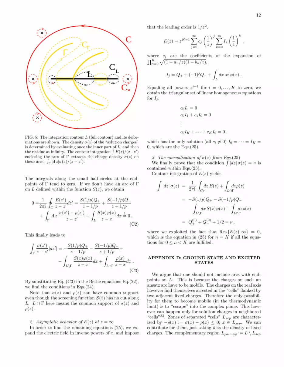
12

Γ

L

CΓ

C

C

C

L

FIG. 5: The integration contour L (full contour) and its defor-mations are shown. The density σ(z) of the “solution charges”is determined by evaluating once the inner part of L, and thenthe residue at infinity. The contour integration

∫

E(z)/(z−z′)enclosing the arcs of Γ extracts the charge density σ(z) onthese arcs:

∫

Γ|d z|σ(z)/(z − z′).

The integrals along the small half-circles at the end-points of Γ tend to zero. If we don’t have an arc of Γon L defined within the function S(z), we obtain

0 =1

2πi

∮

C

E(z′)

z − z′dz′ =

S(1/p)Q+

z − 1/p+S(−1/p)Q−

z + 1/p

+

∫

Γ

|d z|σ(z′) − ρ(z′)

z − z′+

∫

L

S(x)ϕ(x)

z − xdx

!= 0 .

(C2)

This finally leads to

∫

Γ

σ(z′)

z − z′|dz′| = −

S(1/p)Q+

z − 1/p−S(−1/p)Q−

z + 1/p+

−

∫

L\Γ

S(x)ϕ(x)

z − xdx+

∫

L∩Γ

ρ(x)

z − xdx .

(C3)

By substituting Eq. (C3) in the Bethe equations Eq.(22),we find the conditions in Eqs.(24).

Note that σ(z) and ρ(z) can have common supporteven though the screening function S(z) has no cut alongL. L ∩ Γ here means the common support of σ(z) andρ(z).

2. Asymptotic behavior of E(z) at z = ∞

In order to find the remaining equations (25), we ex-pand the electric field in inverse powers of z, and impose

that the leading order is 1/z2.

E(z) = zK−1∞∑

j=0

cj

(

1

z

)j ∞∑

k=0

Ik

(

1

z

)k

,

where cj are the coefficients of the expansion of∏K

n=0

√

(1 − an/z)(1 − bn/z).

Ij = Q+ + (−1)jQ− +

∫

L

dx xjϕ(x) .

Equaling all powers zi−1 for i = 0, . . . ,K to zero, weobtain the triangular set of linear homogeneous equationsfor Ij :

c0I0 = 0

c0I1 + c1I0 = 0

...

c0IK + · · · + cKI0 = 0 ,

which has the only solution (all ci 6= 0) I0 = · · · = IK =0, which are the Eqs.(25).

3. The normalization of σ(z) from Eqs.(25)We finally prove that the condition

∫

|dz|σ(z) = ν iscontained within Eqs.(25).

Contour integration of E(z) yields

∫

|dz|σ(z) =1

2πi

∫

CΓ

dz E(z) +

∫

L∩Γ

dzρ(z)

= −S(1/p)Q+ − S(−1/p)Q−

−

∫

L\Γ

dxS(x)ϕ(x) +

∫

L∩Γ

dzρ(z)

= Q(0)+ +Q

(0)− + 1/2 = ν ,

where we exploited the fact that Res E(z),∞ = 0,which is the equation in (25) for n = K if all the equa-tions for 0 ≤ n < K are fulfilled.

APPENDIX D: GROUND STATE AND EXCITEDSTATES

We argue that one should not include arcs with end-points on L. This is because the charges on such anansatz arc have to be mobile. The charges on the real axishowever find themselves arrested in the “cells” flanked bytwo adjacent fixed charges. Therefore the only possibil-ity for them to become mobile (in the thermodynamiclimit) is to “escape” into the complex plane. This how-ever can happen only for solution charges in neighbored“cells”33. Zones of separated “cells” Lsep are character-ized by −ρ(x) := σ(x) − ρ(x) ≤ 0; x ∈ Lsep. We cancontribute for them, just taking ρ as the density of fixedcharges. The complementary region Lpairing := L \ Lsep

13

is thus characterized by σ(x)−ρ(x) > 0 at G = 0 and welet ρ(x) := ρ(x). In the simplest case we have ρ(x) = ρ(x)everywhere and also the modulus of the total charge isρ(x) in each point. This means σ(x) = 0 for x ∈ Lsep

and distinct connected regions of neighbored “cells” withσ(x) = 2ρ(x) for x ∈ Lpairing at G = 0 (see Fig.6). Thismost simple situation applies in particular to the groundstate, which we have considered in the numerics. Thegeneral situation can be attacked replacing ρ(x) with ρ(x)and the filling ν by

ν :=

∫

Γ

|d z|σ(z)G=0=

∫

Lpairing

dxρ(x)

= ν −

∫

Lsep

dx [ρ(x) + ρ(x)] .

That the above argument applies also to the general-ized class of BCS models discussed here, follows fromthe same structure of the equation after the transforma-tion. But it can equally be seen from the electrostaticanalogy, since no two charges can penetrate each otherdue to the diverging forces when sitting upon each other,which must be zero instead due to the Richardson equa-tions. These infinite forces can only be overcome if ei-ther at least one of the external charges diverges (i.e. thecase G=0) or if two solution charges together approacha fixed charge (in the presence of a degeneracy d, morethan two solution charges are needed because the chargeratio |qmobile/qfixed| = 2/d is diminished by d). We comeback to this discussion after having presented the solu-

tion of the problem. Now we explain why the solution ofEq.(20) corresponds to the ground state of the system,which implies that up to the crossing point of Γ withthe Debye shell L all “cells” between fixed charges areoccupied. This implies that there we have σ = 2ρ andhence the total charge density is −ρ. This sign changeof the charge density below the crossing point is alreadyincluded in Eq.(20), since we apparently replaced

ρ(x)

S(x)−→

ρ(x)√

(x− λ)2 + ∆2. (D1)

Notice that the complex square root changes sign at thecrossing point xc: indeed we have

S(x) =

√

(x− λ)2 + ∆2 x > xc

for

−√

(x− λ)2 + ∆2 x < xc

.

This means that in Eq.(20) the charge density is −ρ(x)for x < xc and ρ(x) for x > xc, which correspond to theground state. For general excited states, which mightalso include more than one arc, we must furnish the realsquare roots with the proper signs as indicated in Fig.6.As long as all the arcs cross the real axis in the same in-terval of Lpairing where they are generated from, this pro-cedure can be implemented in the formalism described inthis work. Otherwise the crossing points could be deter-mined numerically.

1 M. Tinkham. Introduction to Superconductivity. McGraw-Hill, New York (1996). 2nd edition.

2 F. Iachello, Nucl. Phys. A 570, 145 (1994).3 D.H. Rischke and R.D. Pisarski, ”Fifth Workshop on

QCD””, Villefranche, nucl-th/0004016.4 H. Heiselberg and M. Hjorth-Jensen, Phys. Rep. 328, 237

(2000).5 J. Bardeen, L.N. Cooper, and J.R. Schrieffer, Phys. Rev.

108, 1175 (1957).6 N.N. Bogoliubov, Nuovo Cimento 7, 794 (1958).7 M.C. Cambiaggio, A.M.F. Rivas, and M. Saraceno, Nucl.

Phys. A 624, 157 (1997).8 R.W. R.W. Richardson, Phys. Lett. 3, 277 (1963); R.W.

Richardson and N. Sherman, Nucl. Phys. 52, 221 (1964);52, 253 (1964).

9 M. Gaudin, J. Physique 37, 1087 (1976).10 C.T. Black, D.C. Ralph, and M. Tinkham, Phys. Rev. Lett.

74, 3241 (1995); 76, 688 (1996); 78, 4087 (1997).11 A. Mastellone, G. Falci, and R. Fazio, Phys. Rev. Lett. 80,

4542 (1998); A. Di Lorenzo, R. Fazio, F.W.J. Hekking, G.Falci, A. Mastellone, and G. Giaquinta, Phys. Rev. Lett.84, 550 (2000); G. Falci, A. Fubini, and A. Mastellone,Phys. Rev. B 65, 140507R (2002).

12 J. von Delft and D.C. Ralph, Phys. Rep. 345, 61 (2001).M. Schechter, Y. Imry, Y. Levinson, and J. von Delft, Phys.Rev. B 63, 214518 (2001).

13 J. G. Hirsch, et al. nucl-th/0109036.14 E.K. Sklyanin, J. Sov. Math. 47, 2473 (1989).15 L. Amico, G. Falci, and R. Fazio, J. Phys. A 34, 6425

(2001).16 L. Amico and A. Osterloh, Phys. Rev. Lett. 88 127003

(2002).17 J. Links, H.-Q. Zhou, R.H. McKenzie, M.D. Gould Phys.

Rev. B 65, 060502R (2002).18 G. Sierra, Nucl. Phys. B 572, 517 (2000).19 G. Sierra, Proceedings of the NATO Advanced Research

Workshop on Statistical Field Theories, Como 2001, Eds.:A. Cappelli and G. Mussardo (Academic Press, Cam-bridige 2001).

20 H.M. Babujian, J. Phys. A 26, 6981 (1993); H.M. Babujianand R. Flume, Mod. Phys. Lett.9 2029 (1994).

21 M. Asorey, F. Falceto, and G. Sierra, Nucl.Phys. B 622593 (2002).

22 R.B. Laughlin, Phys. Rev. Lett. 50, 1395 (1983)23 M. Gaudin, Travaux de M. Gaudin. Modeles Exactement

resolus (Les Editions de Physique, France 1995).24 R. W. Richardson, J. Math. Phys. 18, 1802 (1977).25 J.M. Roman, G. Sierra, and J. Dukelsky, cond-

mat/0202070.26 L. Amico, A. Di Lorenzo, and A. Osterloh, Phys. Rev.

Lett. 86, 5759 (2001); Nucl. Phys. B 614, 449 (2001).27 R.W. Richardson, cond-mat 0203512.

14

Lsep

Lpairing

ρ_~ρ~ρ_~ρ_~

+

Γ

++_

+___++_

FIG. 6: Here it is indicated schematically how the signs ofthe real square roots have to be chosen in order to yield thesketched charge distribution. The function S(z) consists ofcomplex square roots and has a sign change at each crossingpoint of Γ (dash-dotted grey curve) with the Debye shell (solidlines). At the crossing point of the right-most part of Γ a signchange in the charge density (σ = 2ρ) is intended and hencethe sign change of S located there (dotted vertical line) is“shifted” to represent the desired sign change ρ → −ρ. Greyparts of the Debye shell indicate a positive total charge densityat G = 0 and hence mobile charges; the black parts insteadcorrespond to a negative total charge density at G = 0 andhence separated “cells”.

28 J. Dukelsky, C. Esebbag, P. Schuck, Phys. Rev. Lett. 87066403 (2001).

29 J. von Delft and R. Poghossian, cond-mat/0106405.30 K. Hikami, P.P. Kulish, and M. Wadati, Jou. Phys. Soc.

Jap. 61, 3071 (1992).31 F. Braun and J. von Delft, in Quantum mesoscopic

phenomena and mesoscopic devices in microelectronics,NATO, edited by I.O. Kulik and R. Ellialtioglu (Kluwer,Dortech 2000).

32 M. Lavrentiev and B. Chabat, Methodes de la theorie desfonctions d’une variable complexe, (MIR, Moscou 1972).

33 R.W. Richardson, Phys. Rev. 141, 949 (1966).34 A.G. Ushveridze, Sov. J. Nucl. 20 1185 (1989); hep-

th/9411035; hep-th/9708059.35 A. Di Lorenzo and A. Mastellone, in preparation.36 In formulas (2) instead of the single particle energies the

quantities ηj = εj − gjj/2 + 2∑

iUij enter. We fixed gjj

and Ujj such that ηj = εj37 We recall that in two dimensions the electric field generated

by a point charge q having complex coordinate z0 can berepresented by the holomorphic function E = q/(z − z0).

38 The analogy is by no means unique. In fact, a general Moe-bius transformation µ(z) = reiφ(z − ω1)/(z − ω2) ω1, ω2 ∈C preserves the algebraic structure of the Bethe equa-tions (20), varying the locations of the charges.

39 With ground state we mean that state connected with theground state for G = 0. Up to some “critical” value of Gthis is the ground state of the system.