arX

iv:c

ond-

mat

/041

2281

v1 [

cond

-mat

.sta

t-m

ech]

10

Dec

200

4

Instanton correlators and phase transitions in two- and three-dimensional logarithmic

plasmas

K. Børkje,1, ∗ S. Kragset,1, † and A. Sudbø1, ‡

1Department of Physics, Norwegian University of Science and Technology, N-7491 Trondheim, Norway

(Dated: February 2, 2008)

The existence of a discontinuity in the inverse dielectric constant of the two-dimensional Coulombgas is demonstrated on purely numerical grounds. This is done by expanding the free energy inan applied twist and performing a finite-size scaling analysis of the coefficients of higher-orderterms. The phase transition, driven by unbinding of dipoles, corresponds to the Kosterlitz-Thoulesstransition in the 2D XY model. The method developed is also used for investigating the possibilityof a Kosterlitz-Thouless phase transition in a three-dimensional system of point charges interactingwith a logarithmic pair-potential, a system related to effective theories of low-dimensional stronglycorrelated systems. We also contrast the finite-size scaling of the fluctuations of the dipole momentsof the two-dimensional Coulomb gas and the three-dimensional logarithmic system to those of thethree-dimensional Coulomb gas.

PACS numbers:

I. INTRODUCTION

Compact U(1) gauge fields in three dimensions are ofgreat interest in condensed matter theory, as they arise ineffective theories of strongly correlated two-dimensionalsystems at zero temperature.1,2,3,4 Lightly doped Mott-Hubbard insulators, such as high-Tc cuprates, are ex-amples of systems possibly described by such theories,where the compact gauge field emerges from strong lo-cal constraints on the electron dynamics.2,5,6,7 High-Tc

cuprates appear to fall outside the Landau Fermi liq-uid paradigm, and a so-called confinement-deconfinementtransition in the gauge theories may be associated withbreakdown of Fermi-liquid and quasiparticles in 2D atT = 0.6,7,8 Obliteration of electron-like quasiparticlesand spin-charge separation in the presence of interac-tions is well known to occur in one spatial dimension.However, the mechanism operative in that case, namelysingular forward scattering, is unlikely to be operative inhigher dimensions due to the much less restrictive kine-matics at the Fermi surface.9 Proliferation of instantonsof emergent gauge fields show more promise as a viablecandidate mechanism. This line of pursuit has recentlybeen reinvigorated in the context of understanding thephysics of lightly doped Mott-Hubbard insulators andunconventional insulating states.10

The compact nature of a constraining gauge field ona lattice model introduces topological defects defined bysurfaces where the field jumps by 2π, forming a gas ofinstantons (or ”monopoles”) in 2 + 1 dimensions.11 Con-sidering the gauge sector only, the interactions betweenthese instantonic defects are the same as between chargesin a 3D Coulomb gas, i.e. 1/r-interactions. Such agas is always in a metallic or plasma phase with a fi-nite screening length,11,12 and there is no phase transi-tion between a metallic regime and an insulating regime.However, in models where compact gauge fields are cou-pled to matter fields, the interaction between the mag-netic monopoles may be modified by the emergence of

an anomalous scaling dimension of the gauge field dueto critical matter-field fluctuations.13 This is the case forthe compact abelian Higgs model with matter fields inthe fundamental representation.14

In Refs. 14, it was shown that the introductionof a matter field with the fundamental charge leadsto an anomalous scaling dimension in the gauge fieldpropagator13. The effect is to alter the interaction poten-tial between the magnetic monopoles from 1/r to − ln r.The existence of a confinement-deconfinement transitionin the gauge theory is thus related to whether a phasetransition occurs in a 3D gas of point charges with log-arithmic interactions. However, one should note thatthe legitimacy of a monopole action based on just pair-wise interactions has been questioned, particularly whenviewed as an effective description of an effective gaugetheory of strongly interacting systems.15 The 3D loga-rithmic plasma is however of considerable interest in itsown right.

In two dimensions, where − ln r is the Coulomb po-tential, it is known that the logarithmic gas experiencesa phase transition from a low-temperature insulatingphase consisting of dipoles to a high-temperature metallicphase. This is nothing but the Coulomb-gas representa-tion of the Kosterlitz-Thouless transition in the 2D XYmodel. In a 3D logarithmic gas, the existence of a phasetransition is still subject to debate.14,16,17 Renormaliza-tion group arguments have been used14 to demonstratethat a transition may occur, driven by the unbinding ofdipoles. Others have claimed that the 3D logarithmic gasis always in the metallic phase.16 In a recent paper,18

large scale Monte Carlo simulations indicated that twodistinct phases of the 3D-log gas exists; a low-T regimewhere the dipole moment does not scale with system sizeand a high-T regime where the dipole moment is systemsize dependent. Those results do however not determinethe character of the phase transitions. That will be themain subject of this paper.

The Kosterlitz-Thouless transition in the 2D XY model

2

is characterized by the universal jump to zero of the helic-ity modulus.19 In the corresponding 2D Coulomb gas, itis the inverse of the macroscopic dielectric constant ǫ thatexperiences a jump to zero when going from the insulat-ing to the metallic phase. According to Ref. 14, such auniversal discontinuity should also take place for ǫ−1 inthe 3D logarithmic gas associated with the confinement-deconfinement transition. Proving that such discontinu-ities exist numerically is a subtle task. The discontinuouscharacter of the helicity modulus in the 2D XY model isvery hard to see in a convincing manner by computingthe helicity modulus, due to severe finite-size effects. Itwas only recently proven on purely numerical groundsthat such a discontinuity exists20 in a simple, but yetclever manner. By imposing a twist across the systemand expanding the free energy in this twist to the fourthorder, a stability argument was used to show that thesecond order term in the expansion, the helicity modu-lus, must be nonzero at Tc. The proof relies on the abilityto conclude that the fourth order term is negative in thethermodynamic limit, from which the discontinuity fol-lows immediately. In this paper, we will repeat this pro-cedure, but now in the language of the 2D Coulomb gas.In addition to confirming the results of Minnhagen andKim, the method which we develop here could be suit-able for proving the possibly discontinuous behaviour ofǫ−1 in the 3D logarithmic gas. This is a main motivationfor translating the procedure of Ref. 20 to the vortexlanguage, since the 3D logarithmic gas is not the dualtheory of any simple spin model. After having demon-strated the discontinuity in the 2D Coulomb gas, we goon to apply the method on the 3D logarithmic gas. Wealso compare the scaling with system size of the meansquare dipole moment for these logarithmic plasmas, andcontrast the results with those of the 3D Coulomb gas.This is important, since the mean square dipole momentdoes not scale with system size below a certain temper-ature for the logarithmic plasmas.18 This indicates thattwo phases exist, where the low-temperature regime con-sists of tightly bound pairs. However, the results for the3D Coulomb gas are qualitatively different, in accordancewith the fact that such a low-temperature phase is absentin that case.

II. MODEL

The Hamiltonian of the 2D XY model on a squarelattice modified with a twist T(x, y) is

HXY = −J∑

〈i,j〉

cos(θi − θj − 2π rij ·T), (1)

where rij is the displacement between the nearest neigh-bour pairs to be summed over. We set the coupling con-stant J to unity. The volume of the system, i.e. the num-ber of lattice points, is L2, and the angle θi is subject toperiodic boundary conditions. In the Villain approxima-tion, a duality transformation leads to the Hamiltonian

H =1

2

∑

i,j

(m + εµν∆µT ν)iVij(m + ερσ∆ρT σ)j , (2)

where mi are point charges on the dual lattice, corre-sponding to vortex excitations in the XY model. ∆µ

is a lattice derivative and εµν is the completely anti-symmetric symbol. The potential Vij is given by

V (|ri − rj |) =2π2

L2

∑

q

e−iq·(ri−rj)

2 − cos qx − cos qy, (3)

which has a logarithmic long-range behaviour. Detailsof the dualization are found in appendix A. As iswell known, eq. (2) at zero twist describes the two-dimensional Coulomb gas (2D CG). In this representa-tion, the Kosterlitz-Thouless phase transition of the 2DXY model is recognized by a discontinuous jump to zeroof the inverse macroscopic dielectric constant ǫ−1 at Tc.We note that the curl of the twist T acts as a modifica-tion of the charge field in the 2D CG.

The free energy of the system is F = −T lnZ, wherethe partition function is given by summing the Boltz-mann factor over all charge configurations:

Z =∑

{m}

e−H/T . (4)

Let us write the Hamiltonian in Fourier representation,

H =1

2L2

∑

q

(

mq + ενλQν−qT λ

q

)

Vq

(

m−q + ερσQρqT σ

−q

)

,

(5)where the discrete Fourier transform is defined as in ap-pendix B and ∆µe±iq·r ≡ e±iq·rQµ

±q.

III. STABILITY ARGUMENT

From (1), it is clear that F (T) ≥ F (0) in the low-temperature phase, i.e. the free energy is minimal forzero twist. This inequality is also valid at the criticaltemperature Tc, since the free energy must be a contin-uous function of temperature. As a consequence, theTaylor expansion

F (T) − F (0) =∑

α

∑

q1

∂F

∂T αq1

∣

∣

∣

∣

T=0

T αq1

+∑

α,β

∑

q1q2

∂2F

∂T αq1

∂T βq2

∣

∣

∣

∣

T=0

T αq1

T βq2

2+ ...

(6)

can not be negative for any T ≤ Tc. Expressions for thederivatives of the free energy with respect to a generaltwist are found in appendix B. Only terms of even orderwill contribute to the series, since mi may take equally

3

many positive and negative values. We are free to choose

the twist to be

T(x, y) =∆

Lηsin

(

2π y

L

)

x, (7)

where ∆ is an arbitrarily small constant and η = 1 forthe two-dimensional Coulomb gas. To the fourth order,this long-wavelength twist turns (6) into

F (T) − F (0) =∆2

4Ck

(

1 − Vk

L2T〈mkm−k〉

)

+∆4

32

(CkVk)2

L4T 3

(

〈mkm−k〉2 −1

2

⟨

(mkm−k)2⟩

)

,

(8)

where k = (0, 2π/L) and Ck = QykQy

−kVk. We recognizethe paranthesis in the second order term as the dielectricresponse function ǫ−1(k), where k is now the smallestnonzero wave vector in a finite system. Note that theprefactors in both terms are independent of system sizeas L → ∞. The crucial argument to use is the same asin Ref. 20. If the fourth order term approaches a finitenegative value at Tc in the limit L → ∞, the second or-der term, ǫ−1(k → 0), must be positive to satisfy theinequality F (T) ≥ F (0). Furthermore, since we knowthat the inverse dielectric constant is zero in the high-temperature phase, it necessarily experiences a disconti-nuity at Tc. As we shall see, Monte Carlo simulationsshow that the fourth order term is indeed negative at Tc

in the thermodynamic limit.The argument described above will also apply to a

three-dimensional gas of point charges interacting via apair potential of some sort, as long as the twist raisesthe free energy in the low-temperature regime. Since thecurl of the twist T is a vector in that case, one may forinstance choose the z-component of this vector as theperturbing charge in eq. (2). The two three-dimensionalsystems we will consider are the logarithmic gas and theCoulomb gas. The expansion (6) is valid for any sys-tem size L. However, to make the change in free energynondivergent as L → ∞, the twist must be chosen suchthat the terms in the expansion are independent of sys-tem size. This is obtained by choosing η = 2 for thelogarithmic gas and η = 3/2 for the Coulomb gas. η isdefined in (7). In both cases, the second order term willbe proportional to

ǫ−1(k) = 1 − Vk

L3T〈mkm−k〉 . (9)

The fourth order term will be proportional to

ǫ4(k) ≡ 1

T 3

(

〈mkm−k〉2 −1

2

⟨

(mkm−k)2⟩

)

(10)

in the logarithmic case. In the case of a 3D Coulomb gas,the interesting quantity will be ǫ4/L2, which is indepen-dent of system size since 〈mkm−k〉 ∼ L in that case.

IV. SIMULATION RESULTS

Standard Metropolis Monte Carlo simulations are car-ried out on the model (2) at zero twist. An L×L squarelattice with periodic boundary conditions is used and thesystem is kept electrically neutral at all times during thesimulations. This is achieved by inserting dipoles withprobability according to the Metropolis algorithm: Aninsertion of a negative or positive charge is attempted atrandom at a given lattice site, and an opposite chargeis placed at one of the nearest neighbour sites to makethe dipole. This is one move, accepted with probabil-ity exp(−∆E/T ) = exp[−(Hnew − Hold)/T ], and thesequence of trying this for all sites in the system onceis defined as one sweep. If a charge is placed on topof an opposite one, the effect is to annihilate the exist-ing one. All simulations are performed going from highto low temperature and after simulating one system sizeL the sampled data are postprocessed using Ferrenberg-Swendsen reweighting techniques.21

A. 2D Coulomb gas

We consider first the 2D Coulomb gas, which is knownto suffer a metal-insulator transition via a Kosterlitz-Thouless phase transition. In this case, Monte Carlo dataare obtained for L = 4 − 100 and for each L up to 200000 sweeps at each temperature is used.

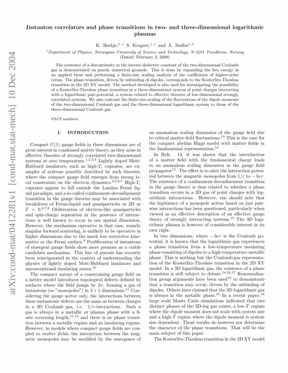
We start by taking the Hamiltonian (2) and comput-ing the mean square of the dipole moment, 〈s2〉, as afunction of system size and temperature. A mean squaredipole moment which is independent of system size in-dicates the existence of tightly bound dipoles and a di-electric or insulating phase. If the mean square dipolemoment scales with system size, this demonstrates theexistence of free unbound charges and hence a metallicphase. In other words, we expect in the low-temperaturedielectric insulating phase no finite-size scaling of 〈s2〉,whereas we should expect 〈s2〉 ∝ Lα(T ) with α(T ) ≤ 2 athigher temperatures. Using an intuitive low density ar-gument, neglecting screening effects,22 we can calculatethe behaviour of 〈s2〉 to leading order in L,

〈s2〉 ∝

Const. ; T < TKT

L(T−TKT )/T ; TKT < T < 2TKT

L2 ; 2TKT < T.

(11)

Hence, α(T ) is zero for low temperatures and a mono-tonically increasing function of temperature just aboveTKT . Including screening effects in 2D shows that thisconclusion still holds, however the temperature at whichit occurs is determined by screening.

Details of the simulations may be found in Ref. 18.The result is shown in Fig. 1 where we have the meansquare dipole moment for the 2D case both as a functionof temperature for various system sizes, and as functionof system size for various temperatures. From this we

4

may extract the scaling constant α(T ) which is shownin the center panel of Fig. 1. A related method for us-ing dipole fluctuations to measure vortex-unbinding hasrecently been used in Refs. 23.

L = 48L = 32L = 16L = 8

a)

T

〈s2〉

21.81.61.41.21

40

35

30

25

20

15

10

5

0

b)

T

α(T

)

21.81.61.41.21

0.7

0.6

0.5

0.4

0.3

0.2

0.1

0

-0.1

T = 1.00T = 1.11T = 1.20T = 1.32T = 1.35T = 1.39T = 1.43T = 1.47T = 1.52c)

L

〈s2〉

100101

10

1

FIG. 1: The mean square dipole moment 〈s2〉 as a functionof temperature (top panel), and system size (bottom panel)for the 2D Coulomb gas. The middle panel shows the scalingexponent α extracted from 〈s2〉 ∼ Lα(T ).

Below a temperature T ≈ 1.3, no scaling of 〈s2〉 is seen,consistent with a low-temperature dielectric phase. Thetemperature at which scaling stops is consistent with theknown temperature at which the 2D Coulomb gas suffersa metal-insulator transition.

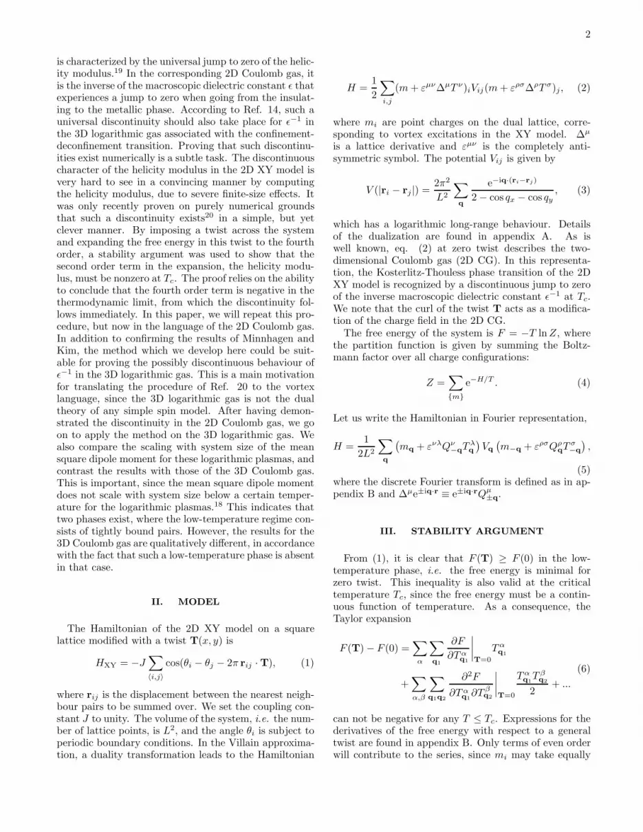
Simulation results for the inverse dielectric constant

100705030

L = 10

T

ǫ−1(k

)

1.91.81.71.61.51.41.31.2

1

0.8

0.6

0.4

0.2

0

FIG. 2: Inverse dielectric constant taken at the smallest possi-ble wave vector in a finite system, k = (0, 2π/L), and plottedagainst temperature T for system sizes L = 10, 30, 50, 70 and100, for the 2D Coulomb gas. The decrease of ǫ−1 towardszero becomes sharper with increasing L, consistent with theprediction of a discontinuous jump. Errorbars are given in thetop and bottom curves, and omitted for clarity in the others.

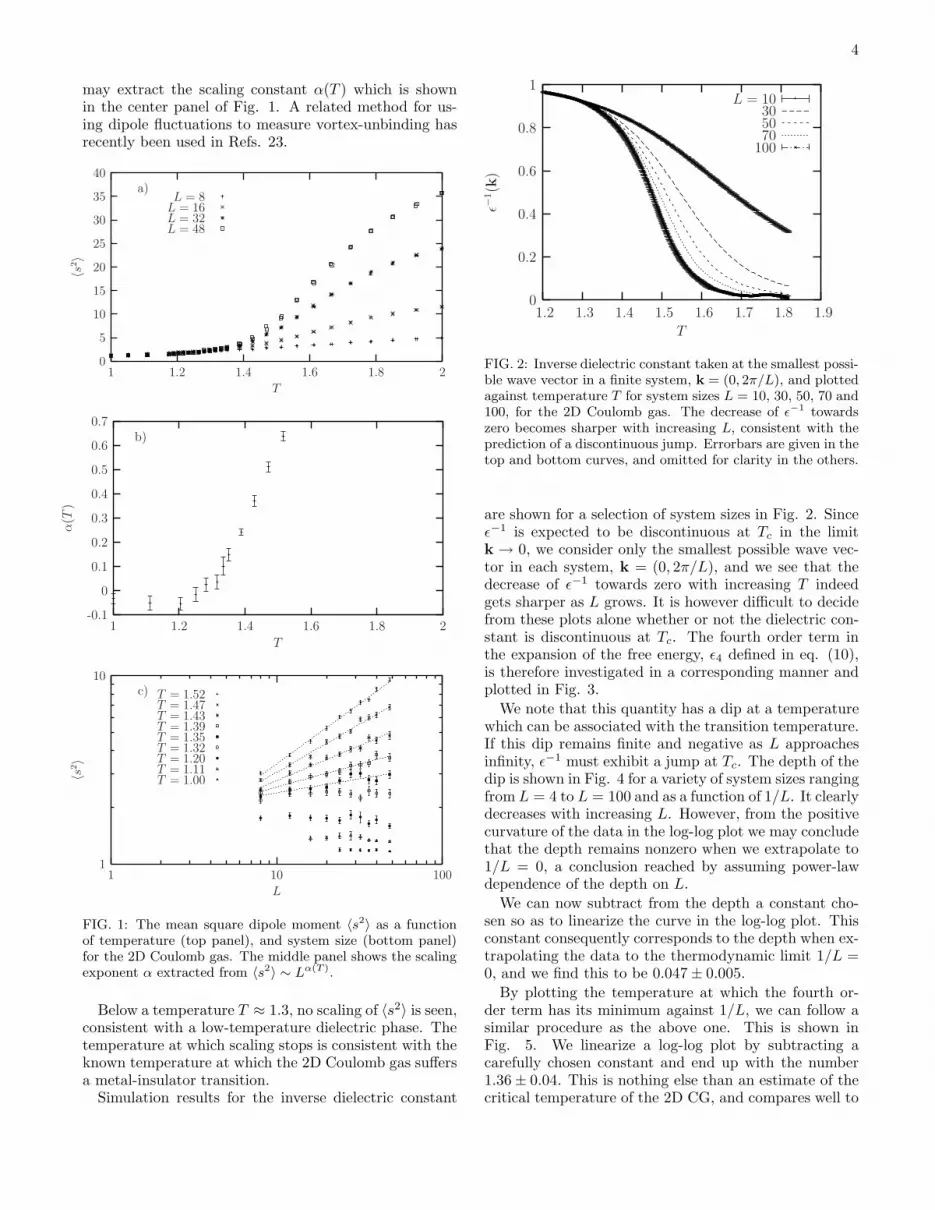
are shown for a selection of system sizes in Fig. 2. Sinceǫ−1 is expected to be discontinuous at Tc in the limitk → 0, we consider only the smallest possible wave vec-tor in each system, k = (0, 2π/L), and we see that thedecrease of ǫ−1 towards zero with increasing T indeedgets sharper as L grows. It is however difficult to decidefrom these plots alone whether or not the dielectric con-stant is discontinuous at Tc. The fourth order term inthe expansion of the free energy, ǫ4 defined in eq. (10),is therefore investigated in a corresponding manner andplotted in Fig. 3.

We note that this quantity has a dip at a temperaturewhich can be associated with the transition temperature.If this dip remains finite and negative as L approachesinfinity, ǫ−1 must exhibit a jump at Tc. The depth of thedip is shown in Fig. 4 for a variety of system sizes rangingfrom L = 4 to L = 100 and as a function of 1/L. It clearlydecreases with increasing L. However, from the positivecurvature of the data in the log-log plot we may concludethat the depth remains nonzero when we extrapolate to1/L = 0, a conclusion reached by assuming power-lawdependence of the depth on L.

We can now subtract from the depth a constant cho-sen so as to linearize the curve in the log-log plot. Thisconstant consequently corresponds to the depth when ex-trapolating the data to the thermodynamic limit 1/L =0, and we find this to be 0.047 ± 0.005.

By plotting the temperature at which the fourth or-der term has its minimum against 1/L, we can follow asimilar procedure as the above one. This is shown inFig. 5. We linearize a log-log plot by subtracting acarefully chosen constant and end up with the number1.36 ± 0.04. This is nothing else than an estimate of thecritical temperature of the 2D CG, and compares well to

5

T

ǫ 4

1.91.81.71.61.51.41.31.2

0.01

0

-0.01

-0.02

-0.03

-0.04

-0.05

-0.06

-0.07

-0.08

FIG. 3: The coefficient ǫ4 of the fourth order term of theexpansion of the free energy, for the 2D Coulomb gas. Thesame systems are used in this plot as in Figure 2, and thedepths decrease with increasing L. The important question iswhether this dip vanishes at Tc or not. Errorbars are omittedbut will be reintroduced in Figure 4. The oscillation at highT is due to noise from the reweighting.

0.20

0.1

0

1/L

Dep

thof

ǫ 4

0.30.10.01

0.1

0.05

FIG. 4: Depth of the dip in the fourth order term shown inFigure 3 for the 2D Coulomb gas. The data are obtained fromsimulations of system sizes ranging from L = 4 to L = 100 andplotted both on a linear scale (inset) and on a log-log scale.The positive curvature in the log-log plot clearly indicates anonzero value of the depth when extrapolating to the limitL → ∞.

earlier results.24 The approach towards Tc is however abit slow, making a precise determination of the criticaltemperature difficult. This drawback was also noted byMinnhagen and Kim for the corresponding computationson the 2D XY model.20

B. 3D logarithmic system

We may carry out the same type of analysis for themean square dipole moment for a system of point charges

log-log plot:

0.10.01

1.7

1.6

1.5

1.4

1/L

Tem

per

ature

min

imiz

ing

ǫ 4

0.30.250.20.150.10.050

1.8

1.6

1.4

1.2

1

0.8

0.6

0.4

0.2

0

FIG. 5: Temperature minimizing ǫ4 as a function of inversesystem size for the 2D CG. The values are plotted both on alinear scale and on a log-log scale (inset). This temperaturereaches a nonzero value at L → ∞ indicated by the positivecurvature in the log-log plot. Extrapolation gives Tc = 1.36±0.04.

interacting via a three-dimensional logarithmic bare pairpotential (3D LG). For this system, much less is known.Such a system has recently been considered in the contextof studying confinement-deconfinement phase transitionsin the (2 + 1)-dimensional abelian Higgs model.14 Theresults are shown in Fig. 6.

Qualitatively and quantitatively the results are thesame in the 3D LG as for the 2D case. This stronglysuggests that the 3D LG also has a low-temperature di-electric insulating phase separated by a phase transitionfrom a high-temperature phase. In the low-temperatureregime the charges of almost all dipoles are bound astightly as possible, the separation of the charges corre-spond to the lattice constant. In the high-temperatureregime the dipoles have started to separate, reflected bya scaling of 〈s2〉 ∼ Lα(T ) with the system size. Sinceα(T ) = 0 at low temperatures while α(T ) 6= 0 in the high-temperature regime a non-analytic behaviour of α(T ) isimplied. This necessarily corresponds to a phase tran-sition in the vicinity of T ≈ 0.3, a temperature whichagrees well with Ref. 14 where a critical value of Tc = 1/3was obtained.

Note that, although this simple type of analysis of themean square dipole moment does not by itself suffice todetermine the character of these phase transitions eitherin the case of 3D LG or 2D CG, it does suffice to shedlight on the important issue of whether a low temperatureinsulating phase exists in the 3D LG as well. This is farfrom obvious, since the screening properties of a three-dimensional system of charges interacting logarithmicallyis quite different from that of a Coulomb system (in anydimension).16 It is therefore of considerable interest torepeat the analysis carried out for the 2D Coulomb gas to,if possible, determine the character of a metal-insulatortransition in the 3D LG.

6

L = 40L = 28L = 16L = 8

a)

T

〈s2〉

0.40.380.360.340.320.30.28

30

25

20

15

10

5

0

b)

T

α(T

)

0.40.380.360.340.320.30.28

1

0.8

0.6

0.4

0.2

0

T = 0.294T = 0.303T = 0.313T = 0.323T = 0.333T = 0.345T = 0.357

c)

L

〈s2〉

100101

10

1

FIG. 6: Mean square dipole moment 〈s2〉 as a function oftemperature (top panel) and system size (bottom panel) forthe 3D system of point charges interacting with a logarithmicbare pair potential (3D LG). The middle panel shows the

scaling exponent α extracted from 〈s2〉 ∼ Lα(T ).

In Fig. 7 we show the inverse dielectric constant for the3D LG as a function of temperature for various systemsizes. It shows qualitatively the same behavior as for the2D CG in that the decrease of ǫ−1 towards zero becomessharper with increasing L. However, the downward driftin the temperature at which the inverse dielectric con-stant starts decreasing rapidly is more pronounced thanin the 2D CG case.

In Fig. 8 we have plotted the fourth order coefficientagainst temperature for the 3D LG system, and the depth

5640301610

L = 4

T

ǫ−1(k

)

0.50.450.40.350.30.25

1

0.8

0.6

0.4

0.2

0

FIG. 7: Inverse dielectric constant taken at the smallest pos-sible wave vector in a finite system, k = (0, 2π/L, 0), andplotted against temperature T for system sizes L = 4, 10, 16,30, 40 and 56, for the 3D LG system. The decrease of ǫ−1

towards zero becomes sharper with increasing L, consistentwith the prediction of a discontinuous jump. However, thedownward drift in the temperature at which the inverse di-electric constant starts decreasing rapidly is more pronouncedthan in the 2D CG case. Errorbars are given in the top andbottom curves, and omitted for clarity in the others.

6040301610

L = 4

T

ǫ 4

0.50.450.40.350.30.25

0

-1

-2

-3

-4

-5

-6

-7

-8

FIG. 8: The coefficient ǫ4 of the fourth order term of theexpansion of the free energy for the 3D LG model. The depthsdecrease with increasing L, and the important question iswhether this dip vanishes at Tc or not. Errorbars are omittedbut will be reintroduced in Figure 9.

of the dip as a function of system size is shown in Fig. 9.It would clearly have been desirable to be able to accesslarger system sizes than what we have been able to do inthe 3D LG case, to bring out a potential positive curva-ture that was observed in the 2D CG case. From theseresults, it is unfortunately not possible to tell whether thedepth of the dip remains finite and negative as L → ∞ orif it vanishes. Hence, we are presently not able to firmlyconclude that the inverse dielectric constant in the 3DLG experiences a discontinuity.

7

0.30.20.10

6

4

2

1/L

Dep

thof

ǫ 4

0.30.10.01

8

6

4

2

FIG. 9: Depth of the dip in the fourth order term shown inFigure 8 for the 3D LG. The data are obtained from simu-lations of system sizes ranging from L = 4 to L = 60 andplotted both on a linear scale (inset) and on a log-log scale.The lack of clear positive curvature in the log-log plot thatwas observed in 2D CG case makes the extrapolation to thelimit L → ∞ more difficult for the system sizes we have beenable to access in 3D.

The temperature locating the minimum in ǫ4 as a func-tion of system size is shown in Fig. 10 for the 3D LGsystem. Extrapolation gives Tc = 0.30 ± 0.04.

log-log plot:

0.10.01

0.420.4

0.380.360.340.32

1/L

Tem

per

ature

min

imiz

ing

ǫ 4

0.30.250.20.150.10.050

0.45

0.4

0.35

0.3

0.25

0.2

0.15

0.1

0.05

0

FIG. 10: Temperature minimizing ǫ4 as a function of inversesystem size for the 3D LG system. The values are plottedboth on a linear scale and on a log-log scale (inset). Thistemperature reaches a nonzero value at L → ∞. Extrapola-tion gives Tc = 0.30 ± 0.04.

C. 3D Coulomb gas

In this subsection, we contrast the results of the 2DCoulomb gas and the 3D LG to those of the 3D Coulombgas. The 3D CG is known to be in a metallic high-temperature phase for all finite temperatures and should

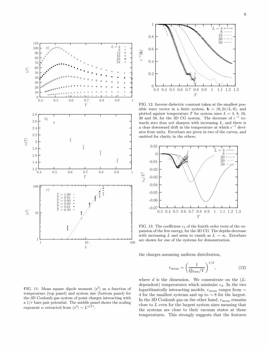
exhibit quite different finite-size scaling of 〈s2〉 comparedto the 2D CG case.11,14,25 The results are shown in Fig.11. Note that the temperature dependence of the curvesfor all different system sizes are qualitatively different inthe 3D CG compared to those in the 2D CG and the3D LG. This becomes particularly apparent upon con-sidering the L-dependence of 〈s2〉 for various tempera-tures, where the steepness of the curves increases withdecreasing temperature, resulting in a scaling exponentα(T ) (from 〈s2〉 ∼ Lα(T )) which decreases with increas-ing temperature. This is quite consistent with what isknown for the 3D CG, namely that it exhibits a metal-lic state for all finite temperatures, equivalently it cor-responds to Polyakov’s permanent confinement.11,14 It isevident that the scaling results for 〈s2〉 for the 2D CGand the 3D LG are qualitatively and quantitatively thesame, and that they are qualitatively different from thoseexhibited by the 3D CG. For low temperatures, 〈s2〉 seemto be increasing with temperature. This is only a vacuumeffect, since vacuum configurations do not contribute tothe measurement of 〈s2〉18. This means that close to vac-uum, only configurations resulting from the insertion ofone single dipole at the smallest possible distance willcontribute. See also section IVD.

The inverse dielectric constant for the 3D CG is shownas a function of temperature in Figure 12 with systemsizes ranging up to L = 50. Here also, ǫ−1 decreasesfrom unity to zero, but the downward drift in the tem-perature at which ǫ−1 deviates from unity seems to beeven stronger than for the 3D LG model. Additionally,the decrease towards zero does not sharpen significantlywith increasing L.

We find a similar minimum in the fourth order term inthe expansion of the free energy for the 3D CG, ǫ4/L2,shown in Fig. 13. However, the dip vanishes as L → ∞in the current model. This is clearly shown in Fig. 14 incontrast to the Figs. 4 and 9 of the other two models.

For completeness we have included in Fig. 15 a plot ofthe temperature locating the minimum in ǫ4 as a func-tion of system size also for the 3D CG. There is no phasetransition to which this temperature is associated, andthe stronger downward drift mentioned above is evidentwhen contrasting this plot to Fig. 10 of the 3D LG.The temperature is reduced by a factor 2 in the largestsystem considered in the 3D CG compared to the small-est whereas the variation is much smaller in the 3D LG.However, there is a weak curvature in the log-log ver-sion of Fig. 15. Performing a similar extrapolation as wedid for the other two models we end up with a “critical”temperature Tc = 0.24 ± 0.04.

D. Charge density

Finally we present in Fig. 16 the charge density forthe three models considered. In all three cases the chargedensities are independent of L and from these curves wecan approximate the average separation rmean between

8

242016128

L = 4a)

T

〈s2〉

10.90.80.70.60.50.4

110

100

90

80

70

60

50

40

30

20

10

0

b)

T

α(T

)

10.90.80.70.60.50.4

2.8

2.6

2.4

2.2

2

1.8

1.6

1.4

1.2

T = 0.50T = 0.61T = 0.69T = 0.80T = 0.91T = 1.00

c)

L

〈s2〉

100101

100

10

1

FIG. 11: Mean square dipole moment 〈s2〉 as a function oftemperature (top panel) and system size (bottom panel) forthe 3D Coulomb gas system of point charges interacting witha 1/r bare pair potential. The middle panel shows the scaling

exponent α extracted from 〈s2〉 ∼ Lα(T ).

5030168

L = 4

T

ǫ−1(k

)

1.31.21.110.90.80.70.60.50.40.3

1

0.8

0.6

0.4

0.2

0

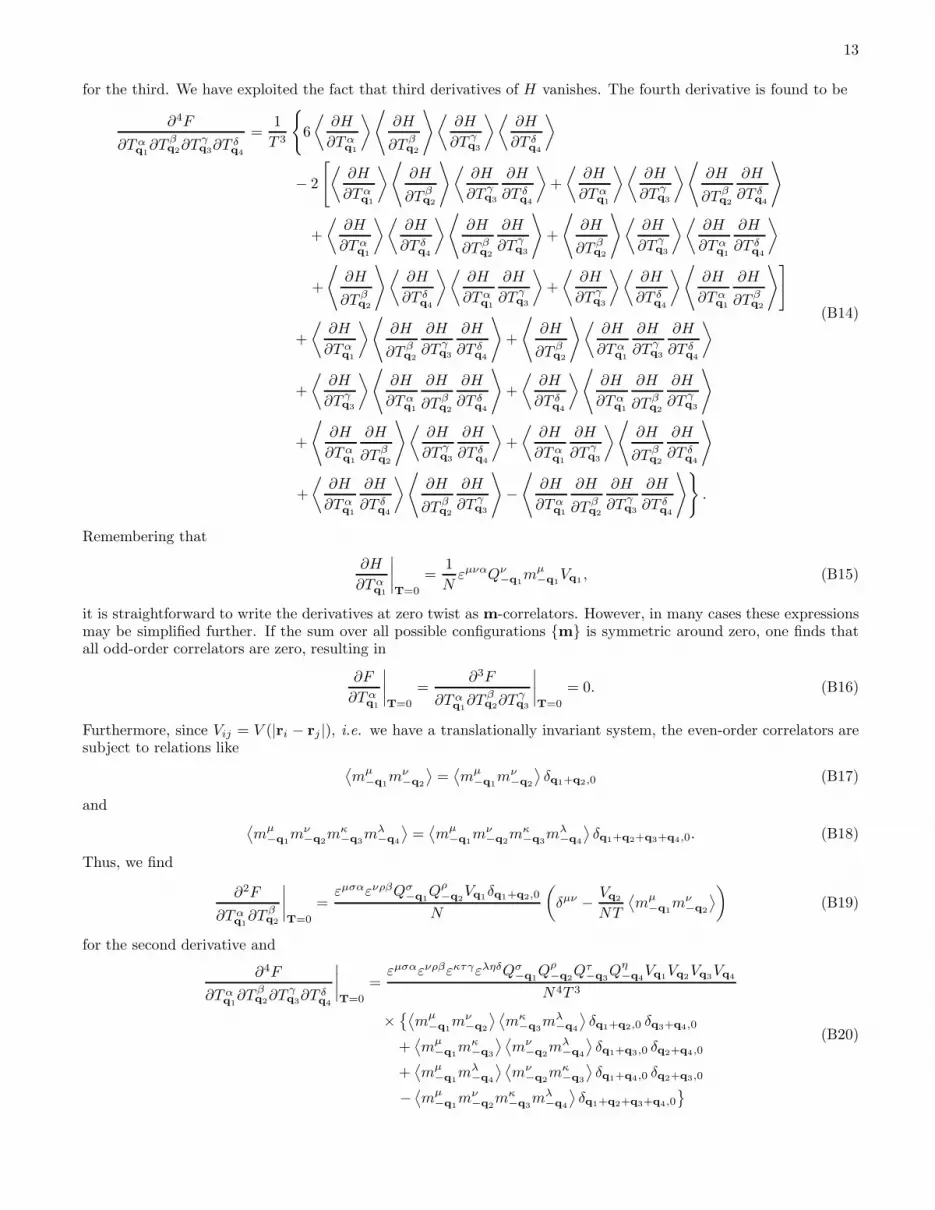
FIG. 12: Inverse dielectric constant taken at the smallest pos-sible wave vector in a finite system, k = (0, 2π/L, 0), andplotted against temperature T for system sizes L = 4, 8, 16,30 and 50, for the 3D CG system. The decrease of ǫ−1 to-wards zero does not sharpen with increasing L, and there isa clear downward drift in the temperature at which ǫ−1 devi-ates from unity. Errorbars are given in two of the curves, andomitted for clarity in the others.

5030208

L = 4

T

ǫ 4/L

2

1.31.21.110.90.80.70.60.50.40.3

0.01

0

-0.01

-0.02

-0.03

-0.04

-0.05

-0.06

-0.07

FIG. 13: The coefficient ǫ4 of the fourth order term of the ex-pansion of the free energy, for the 3D CG. The depths decreasewith increasing L and seem to vanish as L → ∞. Errorbarsare shown for one of the systems for demonstration.

the charges assuming uniform distribution,

rmean =

(

1

QSum/V

)1/d

, (12)

where d is the dimension. We consentrate on the (L-dependent) temperatures which minimize ǫ4. In the twologarithmically interacting models, rmean ranges from ∼4 for the smallest systems and up to ∼ 8 for the largest.In the 3D Coulomb gas on the other hand, rmean remainsclose to L even for the largest system sizes meaning thatthe systems are close to their vacuum states at thesetemperatures. This strongly suggests that the features

9

0.30.20.10

0.080.060.040.02

0

1/L

Dep

thof

ǫ 4/L

2

0.30.10.01

0.1

0.01

0.001

FIG. 14: Depth of the dip in the fourth order term shownin Figure 13 for the 3D CG. The data are obtained fromsimulations of system sizes ranging from L = 4 to L = 50 andplotted both on a linear scale (inset) and on a log-log scale.It is clear that the dip vanishes in the thermodynamic limit.

log-log plot:

0.10.01

0.8

0.6

0.4

1/L

Tem

per

ature

min

imiz

ing

ǫ 4

0.30.250.20.150.10.050

1

0.8

0.6

0.4

0.2

0

FIG. 15: Temperature minimizing ǫ4 as a function of inversesystem size for the 3D CG system. The values are plottedboth on a linear scale and on a log-log scale (inset).

we investigate are only extreme low-density effects in the3D CG model. Screening, which should take place atall temperatures in a system always being in a metallicstate, is not possible in this limit.

In the 2D CG and 3D LG models the situation is dif-ferent. The interesting temperature domains are smallerand the charge densities are kept close to constant whichin turn allows screening for the largest systems.

V. COMMENTS ON UNIVERSALITY

In the 2D CG, the universal jump to zero of the inversedielectric constant ǫ−1 is given by19,26

ǫ−1 =2Tc

π. (13)

100705030

L = 12

a)

QSum/V

1.91.81.71.61.51.41.31.2

0.1

0.01

0.001

6050403020106

L = 4

b)

QSum/V

0.50.40.3

0.1

0.01

0.001

0.0001

1e-05

343024168

L = 4

c)

T

QSum/V

1.10.90.70.50.3

0.1

0.01

0.001

0.0001

1e-05

1e-06

1e-07

1e-08

FIG. 16: Charge density QSum/V plotted vs. temperatureon log-log scales for the a) 2D CG, b) 3D LG and c) 3D CGmodels. The volume V corresponds to the total number ofsites Ld. Note that QSum/V is independent of system size Lin all three cases.

Using the estimate for the critical temperature found insection IVA, the value at Tc should, according to Eq.(13), be ǫ−1 = 0.86 ± 0.03. This is in agreement withFig. 2, since it is in this region the curves seem to split.

In Ref. 20, it was speculated that the finite negativevalue of the fourth order modulus 〈Υ4〉 ≈ −0.130 could

10

be associated with a universal number. In the 2D CG,Vk ∼ L2 and Qy

k ∼ 2π/L for large L, such that the

modification ∆ → ∆/(√

2π) turns (8) into

F (T) − F (0) =∆2

2ǫ−1 +

∆4

4!3ǫ4. (14)

This means that if ǫ−1 corresponds to the helicity modu-lus 〈Υ〉, it is 3ǫ4 that corresponds to the fourth ordermodulus 〈Υ4〉. It is interesting to notice that 3ǫ4 =−0.141 ± 0.015 fits nicely with the value found in Ref.20, speculated to be a universal number. One may there-fore speculate that the value of ǫ4 at Tc is a universalnumber independent of Tc. Whether this is a sign of atrue universality or a mere coincidence requires furtherinvestigation.

One should also note that with this modification of ∆,the additional twist term in the XY-Hamiltonian (1) be-

comes√

2∆ sin(2πy/L)/L. It seems natural to suggestthat the net effect of a sine twist is given by its RMS-

value, i.e.(

1/L∫ L

0sin2(2πy/L)dy

)1/2= 1/

√2. This

gives a net twist of ∆ across the system, which is thesame as in Ref. 20.

The universal jump of ǫ−1 in the 3D LG is given bythe flow equations derived in Ref. 14. In our units, thisjump is predicted to be

ǫ−1 =5Tc

2, (15)

and by using the critical temperature found in sectionIVB, this amounts to an ǫ−1 in the interval (0.65, 0.85).Since the different curves in Fig. 7 do not merge in thelow-temperature regime, as they do in the 2D CG case,it is difficult to make a precise determination of the jumpin the 3D LG based on these simulations. However, onecan not rule out that the jump lies inside the intervalmentioned.

VI. CONCLUDING REMARKS

In this paper we have considered various quantititiesrelated to a possible phase transition in systems of pointcharges interacting with bare logarithmic pair potentials,in 2D and 3D. We have also carried out comparisons withthe results obtained in the 3D Coulomb gas in some cases.The quantities we have focused on are the fluctuationsof the dipole moment, 〈s2〉, and the fourth order coeffi-cient of the free energy expanded in an appropriate twist.We have shown that the dipole moment fluctuations, as-sociated with the polarizability of the charge systems,has a scaling exponent α(T ) defined by 〈s2〉 ∼ Lα(T )

which is positive above some temperature and zero belowthis temperature for the 2D CG and the 3D LG cases,and is an increasing function of temperature. On theother hand, for the 3D CG case α(T ) is finite positive forall temperatures we have considered, and is a decreasing

function of temperature. This in itself strongly suggests

that the 3D LG has statistical physics much more akin tothe 2D CG than to the 3D CG. For the 2D CG we havedemonstrated that the inverse dielectric constant expe-riences a discontinuous jump to zero at the phase tran-sition. This has been done by investigation of a seriesexpansion of free energy using Monte Carlo simulations.The possibility of a universal value of the fourth orderterm proposed in Ref. 20 has also been commented on,and a possible agreement with this value has been ob-served. The method developed in this paper will applyto any gas of vortex loops or point charges with any in-teraction potential. We have applied it to the 3D LG.Although it would have been desirable to be able to ac-cess larger system sizes than what we have been able toin the present paper, the results we obtain for the 3DLG suggest that this model may also undergo a metal-insulator transition with a discontinuity in the inverse di-electric function at the critical point, in agreement withthe renormalization group results of Ref. 14.

Acknowledgments

This work was supported by the Research Coun-cil of Norway, Grant Nos. 158518/431, 158547/431(NANOMAT), and by the Norwegian High PerformanceComputing Consortium (NOTUR). One of us (S. K.) ac-knowledges support from the Norwegian University ofScience and Technology. We acknowledge useful discus-sions with F. S. Nogueira and Z. Tesanovic.

APPENDIX A: DUALITY TRANSFORMATION

The partition function for the XY-model with couplingconstant J = 1 is

Z = Πi

∫

dθi

2πeβ∑

rcos(∇θ−2πT), (A1)

where the sum is over all links between lattice points,∇θ ≡ θi − θj and T(r) is the twist between the twolattice points sharing the link r. We will consider threespatial dimensions and comment on any differences in2D. Applying the Villain approximation, we get

Z =

∫

Dθ∑

{n}

e−β2

∑

r(∇θ−2πT−2πn)2 . (A2)

n(r) is an integer-valued field taking care of the periodic-ity of the cosine. By a Hubbard-Stratonovich decoupling,one finds

Z =

∫

DθDv∑

{n}

e−∑

r[ 1

2βv2+iv·(∇θ−2πT−2πn)]. (A3)

The summation over n may now be evaluated using thePoisson summation formula,

∞∑

n=−∞

e2πi nv =

∞∑

l=−∞

δ(v − l), (A4)

11

at each dual lattice point, yielding

Z =

∫

Dθ∑

{l}

e∑

r2πi l·T−i l·∇θ− 1

2βl2 . (A5)

The field l(r) is integer-valued. Now, performing a par-tial summation on the second term in the exponent,the θ-integration may be carried out. This producesthe constraint that l must be divergence-free, solved bythe introduction of another integer-valued field such thatl = ∇×h. Note that h(r) is a scalar in 2D. The partitionfunction is now

Z =∑

{h}

e∑

r2πi (∇×h)·T− 1

2β(∇×h)2 , (A6)

and we observe that h → h +∇φ is a gauge transforma-tion. In two dimensions, the corresponding gauge trans-formation is h → h + c, where c is a constant. UsingPoisson’s summation formula once more, we get

Z =

∫

Dh∑

{m}

e∑

r2πi (∇×h)·T− 1

2β(∇×h)2+2πi h·m, (A7)

leaving h no longer integer-valued. The field m(r) iswhat corresponds to vortex excitations in the XY model.The gauge invariance of the theory produces the con-straint

∑

r φ (∇ · m) = 0 for all configurations of m.Choosing for instance φ = ∇ ·m, it is clear that m mustbe divergence-free, i.e. the field lines are closed loops. In2D, the corresponding constraint is

∑

r m = 0, indicat-ing an overall charge neutrality in the 2D Coulomb gasor zero total vorticity in the 2D XY model.

By another partial summation, we are now left witha Maxwell term and a coupling term between the gaugefield h and the current M(r) ≡ m + ∇× T:

Z =

∫

Dh∑

{m}

e∑

r2πih·M− 1

2β(∇×h)2 . (A8)

One may now perform a partial integration in the sec-ond term and use the gauge where ∇ · h = 0, such that∇×∇×h = −∇2h. Then, by going to Fourier space andcompleting squares, the h-integration becomes Gaussian.This leaves us with

Z = Z0

∑

{m}

e2βπ2

N

∑

qMqG−1

q M−q , (A9)

where ∇2e±iqr ≡ e±iqrGq and Z0 is a constant. Definingthe discrete Laplacian by

∆2f(r) =∑

µ

[f(r + eµ) + f(r − eµ) − 2f(r)] , (A10)

it is clear that Gq = −2(

d −∑dµ=1 cos qµ

)

, denoting

the number of space dimensions by d. Returning to real-space representation, we arrive at

Z = Z0

∑

{m}

e− β

2

∑

ri,rjM(ri) V (|ri−rj |)M(rj), (A11)

the interaction being given by

V (r) =2π2

L2

∑

q

eiq·r

d −∑dµ=1 cos qµ

. (A12)

APPENDIX B: EXPANSION OF FREE ENERGY

Consider the Hamiltonian

H0 =1

2

∑

i,j

miVijmj , (B1)

describing a 3D system of integer-valued currents m ona lattice interacting via the potential Vij = V (|ri − rj |).We impose periodic boundary conditions on the system.Perturbing the field m with a transversal twist turns (B1)into

H =1

2

∑

i,j

(m + ∇× T)iVij(m + ∇× T)j . (B2)

We let the linear system size be L and define the discreteFourier transform by

fq =∑

r

f(r) eiq·r, (B3)

where r = (nx, ny, nz) and ni = 0, ..., L − 1. The inversetransform is

f(r) =1

N

∑

q

fq e−iq·r, (B4)

where q = 2πL (kx, ky, kz) and ki = −L/2 + 1, ..., L/2. N

is the number of lattice sites. Let us also define Qν±q by

∆νe±iq·r = e±iq·rQν±q, where ∆ν is a lattice derivative.

In Fourier representation the Hamiltonian becomes

12

H =1

2N

∑

q

(

mµq + εµνλQν

−qT λq

)

Vq

(

mµ−q + εµρσQρ

qT σ−q

)

. (B5)

For later use, we calculate the derivative of H , which is

∂H

∂T αq1

=1

NεµναQν

−q1(mµ

−q1+ εµρσQρ

q1T σ−q1

)Vq1. (B6)

We also note that

∂2H

∂T αq1

∂T βq2

=1

NεµναεµρβQν

−q1Qρ

q1Vq1

δq1+q2,0 (B7)

is independent of m and that all higher order derivatives are zero.

The free energy is given by F = −T lnZ, where the partition function is

Z =∑

{m}

e−H/T , (B8)

summing over all possible configurations of m. By Taylor expansion of the free energy in the twist, we get

F (T) − F (0) =∑

α

∑

r1

∂F

∂T α(r1)

∣

∣

∣

∣

T=0

T α(r1) +∑

α,β

∑

r1,r2

∂2F

∂T α(r1)∂T β(r2)

∣

∣

∣

∣

T=0

T α(r1)Tβ(r2) + ... (B9)

Note that F (T = 0) refers to the free energy of the unperturbed system described by H0. By writing each term inthe series in Fourier representation, one finds the equivalent expansion in Fourier components of the twist, i.e.

F (T) − F (0) =∑

α

∑

q1

∂F

∂T αq1

∣

∣

∣

∣

T=0

T αq1

+∑

α,β

∑

q1q2

∂2F

∂T αq1

∂T βq2

∣

∣

∣

∣

T=0

T αq1

T βq2

2+ ... (B10)

The first derivative becomes

∂F

∂T αq1

=1

Z

∑

{m}

∂H

∂T αq1

e−H/T ≡⟨

∂H

∂T αq1

⟩

. (B11)

Proceeding, we find

∂2F

∂T αq1

∂T βq2

=1

T

⟨

∂H

∂T αq1

⟩

⟨

∂H

∂T βq2

⟩

+∂2H

∂T αq1

∂T βq2

− 1

T

⟨

∂H

∂T αq1

∂H

∂T βq2

⟩

(B12)

for the second derivative and

∂3F

∂T αq1

∂T βq2

∂T γq3

=1

T 2

[

2

⟨

∂H

∂T αq1

⟩

⟨

∂H

∂T βq2

⟩

⟨

∂H

∂T γq3

⟩

+

⟨

∂H

∂T αq1

∂H

∂T βq2

∂H

∂T γq3

⟩

−⟨

∂H

∂T αq1

⟩

⟨

∂H

∂T βq2

∂H

∂T γq3

⟩

−⟨

∂H

∂T βq2

⟩

⟨

∂H

∂T αq1

∂H

∂T γq3

⟩

−⟨

∂H

∂T γq3

⟩

⟨

∂H

∂T αq1

∂H

∂T βq2

⟩]

(B13)

13

for the third. We have exploited the fact that third derivatives of H vanishes. The fourth derivative is found to be

∂4F

∂T αq1

∂T βq2

∂T γq3

∂T δq4

=1

T 3

{

6

⟨

∂H

∂T αq1

⟩

⟨

∂H

∂T βq2

⟩

⟨

∂H

∂T γq3

⟩⟨

∂H

∂T δq4

⟩

− 2

[

⟨

∂H

∂T αq1

⟩

⟨

∂H

∂T βq2

⟩

⟨

∂H

∂T γq3

∂H

∂T δq4

⟩

+

⟨

∂H

∂T αq1

⟩⟨

∂H

∂T γq3

⟩

⟨

∂H

∂T βq2

∂H

∂T δq4

⟩

+

⟨

∂H

∂T αq1

⟩⟨

∂H

∂T δq4

⟩

⟨

∂H

∂T βq2

∂H

∂T γq3

⟩

+

⟨

∂H

∂T βq2

⟩

⟨

∂H

∂T γq3

⟩⟨

∂H

∂T αq1

∂H

∂T δq4

⟩

+

⟨

∂H

∂T βq2

⟩

⟨

∂H

∂T δq4

⟩⟨

∂H

∂T αq1

∂H

∂T γq3

⟩

+

⟨

∂H

∂T γq3

⟩⟨

∂H

∂T δq4

⟩

⟨

∂H

∂T αq1

∂H

∂T βq2

⟩]

+

⟨

∂H

∂T αq1

⟩

⟨

∂H

∂T βq2

∂H

∂T γq3

∂H

∂T δq4

⟩

+

⟨

∂H

∂T βq2

⟩

⟨

∂H

∂T αq1

∂H

∂T γq3

∂H

∂T δq4

⟩

+

⟨

∂H

∂T γq3

⟩

⟨

∂H

∂T αq1

∂H

∂T βq2

∂H

∂T δq4

⟩

+

⟨

∂H

∂T δq4

⟩

⟨

∂H

∂T αq1

∂H

∂T βq2

∂H

∂T γq3

⟩

+

⟨

∂H

∂T αq1

∂H

∂T βq2

⟩

⟨

∂H

∂T γq3

∂H

∂T δq4

⟩

+

⟨

∂H

∂T αq1

∂H

∂T γq3

⟩

⟨

∂H

∂T βq2

∂H

∂T δq4

⟩

+

⟨

∂H

∂T αq1

∂H

∂T δq4

⟩

⟨

∂H

∂T βq2

∂H

∂T γq3

⟩

−⟨

∂H

∂T αq1

∂H

∂T βq2

∂H

∂T γq3

∂H

∂T δq4

⟩}

.

(B14)

Remembering that

∂H

∂T αq1

∣

∣

∣

∣

T=0

=1

NεµναQν

−q1mµ

−q1Vq1

, (B15)

it is straightforward to write the derivatives at zero twist as m-correlators. However, in many cases these expressionsmay be simplified further. If the sum over all possible configurations {m} is symmetric around zero, one finds thatall odd-order correlators are zero, resulting in

∂F

∂T αq1

∣

∣

∣

∣

T=0

=∂3F

∂T αq1

∂T βq2

∂T γq3

∣

∣

∣

∣

T=0

= 0. (B16)

Furthermore, since Vij = V (|ri − rj |), i.e. we have a translationally invariant system, the even-order correlators aresubject to relations like

⟨

mµ−q1

mν−q2

⟩

=⟨

mµ−q1

mν−q2

⟩

δq1+q2,0 (B17)

and⟨

mµ−q1

mν−q2

mκ−q3

mλ−q4

⟩

=⟨

mµ−q1

mν−q2

mκ−q3

mλ−q4

⟩

δq1+q2+q3+q4,0. (B18)

Thus, we find

∂2F

∂T αq1

∂T βq2

∣

∣

∣

∣

T=0

=εµσαενρβQσ

−q1Qρ

−q2Vq1

δq1+q2,0

N

(

δµν − Vq2

NT

⟨

mµ−q1

mν−q2

⟩

)

(B19)

for the second derivative and

∂4F

∂T αq1

∂T βq2

∂T γq3

∂T δq4

∣

∣

∣

∣

T=0

=εµσαενρβεκτγεληδQσ

−q1Qρ

−q2Qτ

−q3Qη

−q4Vq1

Vq2Vq3

Vq4

N4T 3

×{⟨

mµ−q1

mν−q2

⟩ ⟨

mκ−q3

mλ−q4

⟩

δq1+q2,0 δq3+q4,0

+⟨

mµ−q1

mκ−q3

⟩ ⟨

mν−q2

mλ−q4

⟩

δq1+q3,0 δq2+q4,0

+⟨

mµ−q1

mλ−q4

⟩ ⟨

mν−q2

mκ−q3

⟩

δq1+q4,0 δq2+q3,0

−⟨

mµ−q1

mν−q2

mκ−q3

mλ−q4

⟩

δq1+q2+q3+q4,0

}

(B20)

14

for the fourth. These expressions may also be applied to a gas of point charges in 2D or 3D, that is when m is a scalarfield. One way to do this is by replacing ∇× T in (B2) with its z-component εzνλ∆νT λ, with the consequence thatthe greek letter summations may be taken over x and y only. For the second derivative, this results in

∂2F

∂T αq1

∂T βq2

∣

∣

∣

∣

T=0

=εzσαεzρβQσ

−q1Qρ

q1Vq1

δq1+q2,0

N

(

1 − Vq1

NT〈mq1

m−q1〉)

, (B21)

where we have applied Vq = V−q. We recognize theparanthesis as the Fourier transform of the inverse dielec-tric response function ǫ−1(q1) in the low density limit.Note that the factor

εzσαεzρβQσ−q1

Qρq1

= Qσq1

Qσ−q1

(

1 −Qα

q1Qβ

−q1

Qσq1

Qσ−q1

)

(B22)

is a projection operator times Qσq1

Qσ−q1

∼ q21x + q2

1y, re-flecting the transversality of the twist.

To arrive at eq. (8), we chose the twist (7) and com-puted the sums appearing in the expansion (B10) forboth the second and fourth order term. The sum over di-rection is trivial, since our twist points in the x-direction.The sum over momenta is also managable, since T x

q hasnonzero values only for q = (0,±2π/L). This sum givestwo contributions in the second order term, due to therestriction δq1+q2,0. The same argument results in fourcontributions for the three terms in (B20) being a prod-uct of two second order correlators. The term containinga fourth order correlator will give six contributions due

to the restriction δq1+q2+q3+q4,0.

APPENDIX C: HIGHER ORDER TERMS

Using the method described in this paper involves ex-trapolation to L → ∞ and deciding whether or not thefourth order term in the expansion (B10) goes to zero orto a finite nonzero value. This procedure could in somecases be difficult. However, if the fourth order term hadturned out to be zero in the thermodynamic limit, itwould not necessarily mean that the second order term,the inverse dielectric response function, would have to gocontinuously to zero. In fact, if one were able to provethat the fourth order term is negative or zero, one couldgo on to investigate the sixth order term instead. If itthen turned out that the value of the sixth order termwas hard to establish, one could in principle repeat theprocedure and go to higher order terms. We therefore in-clude the sixth derivative here. To simplify calculations,we work with a twist in the x-direction only.

∂6F

∂T xq1

∂T xq2

∂T xq3

∂T xq4

∂T xq5

∂T xq6

=

1

T 5

{

120

⟨

∂H

∂T xq1

⟩⟨

∂H

∂T xq2

⟩⟨

∂H

∂T xq3

⟩⟨

∂H

∂T xq4

⟩[⟨

∂H

∂T xq5

⟩⟨

∂H

∂T xq6

⟩

− 3

⟨

∂H

∂T xq5

∂H

∂T xq6

⟩]

+ 18

⟨

∂H

∂T xq1

∂H

∂T xq2

⟩[

13

⟨

∂H

∂T xq3

⟩⟨

∂H

∂T xq4

⟩⟨

∂H

∂T xq5

∂H

∂T xq6

⟩

−⟨

∂H

∂T xq3

∂H

∂T xq4

⟩⟨

∂H

∂T xq5

∂H

∂T xq6

⟩]

+ 2

⟨

∂H

∂T xq1

∂H

∂T xq2

∂H

∂T xq3

⟩[

5

⟨

∂H

∂T xq4

∂H

∂T xq5

∂H

∂T xq6

⟩

− 48

⟨

∂H

∂T xq4

⟩⟨

∂H

∂T xq5

∂H

∂T xq6

⟩

+ 60

⟨

∂H

∂T xq4

⟩⟨

∂H

∂T xq5

⟩⟨

∂H

∂T xq6

⟩]

+ 15

⟨

∂H

∂T xq1

∂H

∂T xq2

∂H

∂T xq3

∂H

∂T xq4

⟩[⟨

∂H

∂T xq5

∂H

∂T xq6

⟩

− 2

⟨

∂H

∂T xq5

⟩⟨

∂H

∂T xq6

⟩]

+6

⟨

∂H

∂T xq1

⟩⟨

∂H

∂T xq2

∂H

∂T xq3

∂H

∂T xq4

∂H

∂T xq5

∂H

∂T xq6

⟩

−⟨

∂H

∂T xq1

∂H

∂T xq2

∂H

∂T xq3

∂H

∂T xq4

∂H

∂T xq5

∂H

∂T xq6

⟩}

− 12

T 4

∂2H

∂T xq1

∂T xq2

{

2

⟨

∂H

∂T xq3

⟩⟨

∂H

∂T xq4

⟩⟨

∂H

∂T xq5

∂H

∂T xq6

⟩

+ 2

⟨

∂H

∂T xq3

∂H

∂T xq4

⟩⟨

∂H

∂T xq5

∂H

∂T xq6

⟩

+

⟨

∂H

∂T xq3

⟩⟨

∂H

∂T xq4

∂H

∂T xq5

∂H

∂T xq6

⟩}

+12

T 3

∂2H

∂T xq1

∂T xq2

∂2H

∂T xq3

∂T xq4

{⟨

∂H

∂T xq5

∂H

∂T xq6

⟩

+ 2

⟨

∂H

∂T xq5

⟩⟨

∂H

∂T xq6

⟩}

.

(C1)

15

Note that we are allowed to permute the momenta q1, ...,q6, since these are summed over in the free energy expansion.Assuming vanishing odd-order correlators and imposing that m is a scalar field gives

∂6F

∂T xq1

∂T xq2

∂T xq3

∂T xq4

∂T xq5

∂T xq6

=Qy

−q1Qy

−q2Qy

−q3Qy

−q4Qy

−q5Qy

−q6Vq1

Vq2Vq3

Vq4

N4T 3

×{

12 〈m−q1m−q2

〉[

1 − 2Vq5

NT〈m−q3

m−q4〉]

δq1+q2,0 δq3+q4,0 δq5+q6,0

− Vq5Vq6

N2T 2

[

〈m−q1m−q2

m−q3m−q4

m−q5m−q6

〉 δq1+q2+q3+q4+q5+q6,0

− 3 〈m−q1m−q2

〉 δq1+q2,0

(

5 〈m−q3m−q4

m−q5m−q6

〉 δq3+q4+q5+q6,0

−6 〈m−q3m−q4

〉 〈m−q5m−q6

〉 δq3+q4,0 δq5+q6,0

)]}

.

(C2)

∗ E-mail: kjetil.borkje(a)phys.ntnu.no† E-mail: steinar.kragset(a)phys.ntnu.no‡ E-mail: asle.sudbo(a)phys.ntnu.no1 I. Affleck and J. B. Marston, Phys. Rev. B 39, 11538

(1989).2 G. Baskaran and P. W. Anderson, Phys. Rev. B 37, 580

(1988).3 I. Affleck, Z. Zou, T. Hsu and P. W. Anderson, Phys. Rev.

B 38, 745 (1988); Z. Zou and P. W. Anderson, Phys. Rev.B 37, 627 (1988).

4 E. Dagotto, E. Fradkin and A. Moreo, Phys. Rev. B 38,2926 (1988).

5 L. B. Ioffe and A. I. Larkin, Phys. Rev. B 39, 8988 (1989).6 N. Nagaosa and P. A. Lee, Phys. Rev. B 61, 9166 (2000).7 G. Mudry and E. Fradkin, Phys. Rev. B 49, 5200 (1994);

ibid. 50, 11409 (1994).8 I. Ichinose and T. Matsui, Phys. Rev. B 51, 11860 (1995);

I. Ichinose, T. Matsui and M. Onoda, Phys. Rev. B 64,104516 (2001).

9 D. K. K. Lee and Y. Chen, J. Phys. A: Math. Gen. 21,4155 (1988).

10 T. Senthil and M. P. A. Fisher, Phys. Rev. B 62, 7850(2000).

11 A. M. Polyakov, Nucl. Phys. B 120, 429 (1977).12 J. M. Kosterlitz, J. Phys. C 1

¯0, 1046 (1977).

13 I. F. Herbut and Z. Tesanovic, Phys. Rev. Lett. 76, 4588(1996).

14 H. Kleinert, F. S. Nogueira, and A. Sudbø, Phys. Rev. Lett.

88 232001 (2002); Nucl. Phys. B 666 361-395 (2003).15 M. Hermele, T. Senthil, M. P. A. Fisher, P. A. Lee, N.

Nagaosa and X.-G. Wen, cond-mat/0404751.16 I. F. Herbut and B. H. Seradjeh, Phys. Rev. Lett. 91,

171601 (2003); I. F. Herbut, B. H. Seradjeh, S. Sachdevand G. Murthy, Phys. Rev B 68, 195110 (2003); M. J.Case, B. H. Seradjeh and I. F. Herbut, Nucl. Phys. B 676

572-586 (2004).17 M. N. Chernodub, E.-M. Ilgenfritz and A. Schiller, Phys.

Lett. B 547, 269 (2002); ibid. 555, 206 (2003).18 S. Kragset, F. S. Nogueira, and A. Sudbø, Phys. Rev. Lett.

92 186403 (2004).19 D. R. Nelson and J. M. Kosterlitz, Phys. Rev. Lett. 39,

1201 (1977); P. Minnhagen and G. G. Warren, Phys. Rev.B 24, 2526 (1981).

20 P. Minnhagen and B. J. Kim, Phys. Rev. B 67, 172509(2003).

21 A. M. Ferrenberg and R. H. Swendsen, Phys. Rev. Lett.61 2635 (1988); Phys. Rev. Lett. 63 1195 (1989).

22 J. M. Kosterlitz and D. J. Thouless, J. Phys. C 6, 1181(1973).

23 H. A. Fertig and J. P. Straley, Phys. Rev. B 66, 201402(R)2002; H. A. Fertig, Phys. Rev. Lett., 89, 035703 (2002).

24 P. Olsson, private communication.25 J. M. Kosterlitz, J. Phys. C 10, 3753 (1977).26 P. Minnhagen, Phys. Rev. B 32, 3088 (1985).