Input uncertainty propagation methods and hazard mapping of geophysical mass flows

Input uncertainty propagation methods and hazard

mapping of geophysical mass flows

K. Dalbey,1 A. K. Patra,1 E. B. Pitman,2 M. I. Bursik,3 and M. F. Sheridan3

Received 25 April 2006; revised 28 June 2007; accepted 11 December 2007; published 7 May 2008.

[1] This paper presents several standard and new methods for characterizing the effect ofinput data uncertainty on model output for hazardous geophysical mass flows. Notethat we do not attempt here to characterize the inherent randomness of such flow events.We focus here on the problem of characterizing uncertainty in model output due tolack of knowledge of such input for a particular event. Methods applied include classicalMonte Carlo and Latin hypercube sampling and more recent stochastic collocation,polynomial chaos, spectral projection and a newly developed extension thereof namedpolynomial chaos quadrature. The simple and robust samplings based Monte Carlotype methods are usually computationally intractable for reasonable physical models,while the more sophisticated and computationally efficient polynomial chaos method oftenbreaks down for complex models. The spectral projection and polynomial chaosquadrature methods discussed here produce results of quality comparable to thepolynomial chaos type methods while preserving the simplicity and robustness of theMonte Carlo-type sampling based approaches at much lower cost. The computationalefficiency, however, degrades with increasing numbers of random variables. A procedurefor converting the output uncertainty characterization into a map showing the probabilityof a hazard threshold being exceeded is also presented. The uncertainty quantificationprocedures are applied first in simple settings to illustrate the procedure and thensubsequently applied to the 1991 block-and-ash flows at Colima Volcano, Mexico.

Citation: Dalbey, K., A. K. Patra, E. B. Pitman, M. I. Bursik, and M. F. Sheridan (2008), Input uncertainty propagation methods and

hazard mapping of geophysical mass flows, J. Geophys. Res., 113, B05203, doi:10.1029/2006JB004471.

1. Introduction

[2] Determining the risk associated with hazards involvesmany factors; examining strategies for mitigation is, like-wise, a complicated problem. It is increasingly common toturn to models and computer simulation to assist in the riskassessment and mitigation process. In studying hazardousnatural flows with models and simulations, we seek answersto questions such as ‘‘Is a particular village likely to beaffected by flows in a given time frame? Should weconstruct a road along this valley or along a differentone?’’ The answer to such a question in full generalityrequires an accounting of the uncertainties in the frequencyand magnitude of likely flow events. Then, given theoccurrence of a flow of some specified size, we also requiremeasurable confidence in the prediction of the flow physicsby a computational model. However, for most models suchpredictions of flow physics are difficult to obtain in absolute

terms due to the uncertainties associated with assumedvalues of model inputs, parameters, and, oftentimes, withthe model itself (details of the parametric and modeluncertainties are included in section 2.2). In this paper, wefocus attention on this difficulty, by advocating a systematicand computationally feasible methodology especially wellsuited for mathematical models based on conservation laws,and that are expensive to evaluate. As a consequence of ourapproach, all probabilities reported in this paper are condi-tioned on the occurrence of a flow of uncertain magnitudeand character. The time period during which a flow of agiven magnitude and character might be expected to occuris obviously important in the hazard mitigation and emer-gency management process. However, the probability ofsuch an event is perhaps the least understood part of suchmass flow hazards. We believe that a careful analysis of thehazard risk conditional on the occurrence of a flow event isa necessary first step to addressing the full problem and iscrucial to developing strategies for hazard management. Abroader statistical framework to account for both of theseuncertainties, perhaps based on Bayesian methods, either afull Bayesian or the simpler Bayes linear approximation,will constitute a logical follow on to this effort (the readermay wish to see Huard and Mailhot [2006] and MacKay[2003]). Given the cost of such strategies (e.g., MarkovChain Monte Carlo), such analyses are usually built oninexpensive statistical models and/or emulators derived

JOURNAL OF GEOPHYSICAL RESEARCH, VOL. 113, B05203, doi:10.1029/2006JB004471, 2008ClickHere

for

FullArticle

1Department ofMechanical andAerospace Engineering, State Universityof New York at Buffalo, Buffalo, New York, USA.

2Department of Mathematics, State University of New York at Buffalo,Buffalo, New York, USA.

3Department of Geology, State University of New York at Buffalo,Buffalo, New York, USA.

Copyright 2008 by the American Geophysical Union.0148-0227/08/2006JB004471$09.00

B05203 1 of 16

http://dx.doi.org/10.1029/2006JB004471

from expensive simulators, topics which are themselves toodetailed to report here.[3] To disseminate information about hazards from mass

flow events, it has been found helpful to construct hazardmaps that delineate a given region into zones of high andlow risk. In areas of seismic or flood hazards this delinea-tion is usually based on the probability of a critical thresholdfor some parameter associated with the hazard beingexceeded. The probabilities are computed using a mix ofphysical principles, numerical modeling, and field data[Jibson et al., 2000; Somerville et al., 1997]. For thehazardous mass flows that are the subject of this paper,hazard maps [Macias et al., 1995; Sheridan et al., 1999;Hoblitt et al., 1998; Wolfe and Pierson, 1995] have beenobtained heuristically by practitioners using a combinationof field data and sample model results. Alternative heuristicapproaches based on statistical measures of the geometriesof areas inundated by previous flows have been advocated,for instance, by Iverson et al. [1998]. However, thesemethods are not fully based on physical principles, and,as such, may be suspect when used for prediction. Relianceon historical data biases the reliable prediction of the mostdangerous but infrequent, large events. While these mapshave been found useful on a case by case basis, they do notprovide a uniform approach to hazards mapping, exceptinsofar as they help in developing a consensus within thehazards community as to what should, or should not, beplaced in such maps. Perhaps more importantly, exceed-ances analogous to those typically calculated in seismic riskassessment cannot be obtained from such maps. We there-fore describe in this paper an alternative approach forconstruction of hazards maps for natural mass flows thatis based on (1) first principles physics based models andnumerical simulation of such flows, (2) explicit modeling ofthe input uncertainties, and (3) a strategy for propagatingthese uncertainties using statistical methodology to estimateprobabilities of a specified hazardous event. Maps con-structed on these principles provide a uniform of approachto the problem, which can thus be translated into othersettings. In addition, this approach provides the informationnecessary to calculate exceedance probabilities (the proba-bility that a flow variable, or a function of some variable,exceeds a specified threshold), once the model is coupled toinformation on the flow event and return period. Althoughthe methodology can be applied to any model that outputsinundation information about a hazardous overland flow, inthe present contribution we consider geophysical massflows that involve the flow of dry soil and rock in a complexrheological mixture, such as rock avalanches and somepyroclastic block-and-ash flows. Such flows have been therecent subject of extensive model development [Savage andHutter, 1989;Hutter et al., 1993;Hutter and Kirchner, 2003;Iverson, 1997; Iverson and Denlinger, 2001; Denlingerand Iverson, 2001, 2004; Iverson et al., 2004; Gray et al.,1999; Pudasaini et al., 2005; Pitman et al., 2003; Patraet al., 2005]. For all such models, not only are the materialproperties difficult to specify, but the terrain over which aflow occurs is not well characterized, and the size andlocation of a potentially failing mass cannot be assignedwith any certainty. There is also much that is unknownabout the exact physics activated in a mass flow. Thus,useful outputs from the model equations governing mass

flows must account for poorly characterized aspects of themodel as well as the uncertainty of the parameters used inthe equations. Furthermore, as is increasingly accepted inthe computational science literature [see, e.g., Oberkampfet al., 2002], reliable model validation for predictive sciencerequires a quantification of the effect of model and param-eter uncertainty together with measures of experimentalerror and uncertainty. Thus, the present work on quantifyingthe effect of uncertainty in model inputs on model outputs isa necessary first step toward reliable model validationprocedures as new and better models of the complex physicsof mass flows are developed. A typical scenario is that ageologist in the process of generating a hazard map hassome knowledge of the range and probability distribution ofinput variables such as the likely location of initiation of anevent, its volume, and material properties. For instance, therange of potential input volumes for a block and ash flowcomputation could be based on the historic record Oftentimes ill-constrained features within the model system areassumed to have a stochastic character, and modeled as arandom variable with an assumed distribution. We may nowrephrase the typical question posed above as somethingmore quantifiable: ‘‘Is the potential mean flow depth plusthree standard deviations at the center of this village greaterthan 1 m?’’ or alternately, given a defined range anddistribution of input data, ‘‘What is the probability that flowdepth at a point will exceed a given threshold value?’’Applying appropriate stochastic and computational methodscan provide an answer. We state explicitly that we do notattempt to characterize the probability of flow initiationduring a given time frame. Rather, in the fashion of Jibsonet al. [2000], who proposed a methodology for estimatinglandslide probability in an area if there is ground shakingconditions, we estimate the long-term probability of ahazard threshold value being exceeded at every point inan area, given initiation of a flow. (The phrase ‘‘long-term’’should be interpreted narrowly as ‘‘a sufficiently long timeduration’’ for which the distributions of different variablesthat control the output are well defined.)[4] In recent years, there have been several efforts to

quantify the uncertainty present in outputs of computermodels [Rosenblueth, 1975; Harr, 1989, 1994; Christianand Baecher, 1999, 2002; Ghanem and Spanos, 1991;Glimm and Sharp, 1991; Glimm et al., 2001; Xiu andKarniadakis, 2003, 2002; Le Maitre et al., 2001, 2002] bypropagating the uncertainty inherent in the inputs of themodel to the output. That is, an attempt is made to presentnot only the outputs of a simulation but also a measure of theuncertainty associated with this output based on inputparameter uncertainty. For all but the simplest models thesestochastic methods present significant computational chal-lenges, both in the formulation of the method and in the workrequired to solve the problem. In particular, the models ofgeophysical mass flows characterized by nonlinear hyper-bolic conservation laws pose great challenges since thesampling type methods are inhibited by cost and the func-tional approximations often break down for the nonlinearsystems. Understanding the strengths and weaknesses ofthese ideas is essential to choosing an appropriate method forpropagating input uncertainty. In particular, we review theMonte Carlo (MC) and Latin hypercube (LHS) methods ofsampling, and discuss the method of polynomial chaos (PC)

B05203 DALBEY ET AL.: INPUT UNCERTAINTY PROPAGATION

2 of 16

B05203

together with the related ideas of nonintrusive spectralprojection (NISP) and stochastic collocation (SC). We alsodescribe a method, dubbed polynomial chaos quadrature(PCQ), that can be viewed as a ‘‘smart’’ Monte Carlo methodin which sampling is informed by the PC approximation.PCQ is compared to another scheme of smart samplingcalled point estimate methods (PEM). A review of methodsis found in section 3, and a presentation of PCQ is given insection 3.3. Section 4.3 presents results of MC and PCQ asapplied to two mass flow problems. In section 4, we outlinehow the methodology can be applied to obtain the informa-tion necessary to create exceedance probability maps forhazardous natural flows over complex topography.

2. Modeling of Geophysical Mass Flows

2.1. Basic Models

[5] We adopt a model of mass flows that has its originswith the work of Savage and Hutter [1989], who showedthat for large classes of mass flows wherein the flows arerelatively long and shallow depth averaging was an appro-priate simplification. The model used here represents blockand ash or pyroclastic flows by depth averaging the motionof an incompressible granular material (for details, seeIverson and Denlinger [2001], Denlinger and Iverson[2001], Pitman et al. [2003], and Patra et al. [2005]). TheTITAN2D code developed by us in earlier work [Patra et al.,2005] employs an adaptive mesh, finite difference scheme tosolve these equations on digital representations of realtopography. In a coordinate system with the z axis normalto the basal surface, the governing equations are written as

@U

@tþ @F

@xþ @G

@yþ S ¼ 0; ð1Þ

where

U ¼ h; hVx; hVy

� �;F ¼ h; hV 2

x þ 1

2kapgzh

2; hVxVy

� �

G ¼ h; hVxVy; hV2y þ 1

2kapgzh

2

� �;

h is the height of the flow, hVx, hVy are momentums in x andy directions, g = {gx, gy, gz} are components of the gravityalong the three axes, and

kap ¼ 2 1� sgn@Vx

@xþ @Vy

@y

� ��ffiffiffiffiffiffiffiffiffiffiffiffiffiffiffiffiffiffiffiffiffiffiffiffiffiffiffiffiffiffiffiffiffiffiffiffiffiffiffiffiffiffiffiffiffiffiffiffiffiffiffiffiffiffiffiffiffiffiffi1� cos2 fintð Þ 1þ tan2 fbedð Þð Þ

q �=cos2 fintð Þ � 1:

Here fint and fbed are the internal and basal friction angles,respectively. The source term is

S ¼(0;�gxhþ hkapsgn

@Vx

@y

� �h@gz@y

þ gz@h

@y

� �sin fintð Þ:

þ VxffiffiffiffiffiffiffiffiffiffiffiffiffiffiffiffiffiV 2x þ V 2

y

q gz þV 2y

rx

!h tan fbedð Þ

� gyhþ hkapsgn@Vy

@x

� �h@gz@x

þ gz@h

@x

� �sin fintð Þ

þ VyffiffiffiffiffiffiffiffiffiffiffiffiffiffiffiffiffiV 2x þ V 2

y

q gz þV 2y

ry

!h tan fbedð Þ

):

Here rx and ry are the radii of curvature of terrain in the xand y directions. These equations are similar to the shallowwater equations of fluid dynamics, although the dissipationterms in S are more complex. Equation (1) is a hyperbolicsystem of partial differential equations (PDEs); hyperboli-city is lost as h ! 0. Computational procedures for solvingsuch systems are well documented in the literature [see, e.g.,Toro, 2001].

2.2. Parameters and Sensitivity

[6] The TITAN code constructs approximate numericalsolutions to equation (1). Inputs to the code are a digitalelevation map (DEM) of the topography, the size andlocation of the mass at initiation, and the internal and bedfriction angles. There is uncertainty in all of these inputs.The uncertainty in initiation location, initial mass size andfriction angles can be represented using field data andstandard stochastic methods [see, e.g., Saucedo et al.,2004, 2005; Sheridan and Macias, 1995]. Identification ofthese properties remains a central issue in geological studiesof these flows. More specifically, a distribution of inputsmay be elicited from earth scientists, based on severalfactors: laboratory and field measurements of friction anglesfor ostensibly similar materials, historical record of frequen-cy of flows and their magnitude, analysis of elevation datathat is used to construct DEMs. These input distributionsrepresent the best estimate of the likely environment inwhich a flow will occur. The precise method for elicitationdepends on the input being considered and the quality ofavailable data. In any event, we assume that such adistribution can be obtained from discipline experts. Thequestion we focus on in this paper is the use of thisinformation in the computer modeling process.[7] There are large uncertainties associated with the

construction of DEMs. However, efficient methods forrepresenting the uncertainty associated with spatial param-eters like terrain elevation are not well understood, due tothe high dimensionality required for a representation of suchuncertainty. The solution of (1) requires the numericalcomputation of slopes and curvatures by postprocessingelevation data, a process that can magnify the error intro-duced by incorrect elevation data. For the purposes of thisstudy we have assume DEMs are sufficiently accurate forsimulations (although the DEM can be screened for quality).We have also implemented several procedures to improvethe accuracy of the postprocessing to compute slopes andcurvatures (see Namikawa and Renschler [2004] fordetails).[8] We have found that the flow is relatively insensitive to

internal friction angle but bed friction angle and the size ofthe initial flowing mass are important. The degree ofsensitivity to initial location highly depends on the localterrain features in the neighborhood of the starting location.The combination of uncertainty and sensitivity to theseinputs dictates which ones need to represented as randomvariables.

3. Methods for Stochastic Equations

[9] As described above, the characterization of uncertaintyin computer model outputs by propagating uncertainty ininputs can be done in one of two principal ways. In the first


3 of 16

B05203

class are methods that rely on sampling the input parametersover their whole range either randomly (as in Monte Carlo orMarkov Chain Monte Carlo) or in some guided approach asin point estimate methods [Rosenblueth, 1975; Harr, 1989,1994; Christian and Baecher, 1999, 2002], and Latin hyper-cube designs. A second class of methods, with origins in thework of Wiener [Wiener, 1938], are based on a spectral(Fourier series like) approximation of the probability distri-bution functions of input parameters and model outputs[Ghanem and Spanos, 1991; Xiu and Karniadakis, 2003,2002; Le Maitre et al., 2001, 2002]. A final category ofmethods attempts to combine the advantages of both meth-odologies by sampling, with guidance provided by require-ments of estimating moments accurately or estimating termsin the spectral expansion accurately. We describe below theessential ideas of all the methods using a simple ordinarydifferential equation as the model through which we mustpropagate the uncertainty. We begin by introducing somenotation and terminology.[10] Consider the model represented by the following

equation and initial condition:

@y

@tþ ky ¼ 0

y 0ð Þ ¼ y0;

ð2Þ

where y is a field variable and k is a constant parameter.Now if k(x) is a parameter dependent on a random variable xthen the solution y depends on the random variable x inaddition to the initial condition y0 and time t. Formally, wemay then write y = Y(tjx; y0). Let a desired output of themodel be obtained by U(x) = h(Y) a functional of Y(tjx; y0).For instance, U might be the maximum flow depth at agiven location.[11] Central to most stochastic problems is computing

moments of the functional U over the stochastic space.Moments are defined by appropriate integrals:

U xð ÞND E

¼Z

U xð ÞNr xð Þdx; ð3Þ

where x is a vector random variable, and r(x) is theweighting or probability density function (PDF). From thesemoments the relevant statistics can be computed, e.g.,

mean Uð Þ ¼ Uh i

standard deviation Uð Þ ¼ffiffiffiffiffiffiffiffiffiffiffiffiffiffiffiffiffiffiffiffiffiffiffiffiffiffiffiffiffiU � Uh ið Þ2

D Er

¼ffiffiffiffiffiffiffiffiffiffiffiffiffiffiffiffiffiffiffiffiffiffiffiffiffiffiU2h i � Uh i2

q:

ð4Þ

If U(x) is significantly complex then these stochasticintegrals must be evaluated numerically using quadraturebased schemes, i.e.,

U xð Þh i ¼Xq

U xq� �

wq;

where xq, wq are suitable quadrature values and weights.

3.1. Monte Carlo and Latin Hypercube Sampling

[12] Although the idea is much older, Monte Carlo as amethod for estimating quantities of physical interest dates tovon Neumann’s and Ulam’s effort to develop the atomicbomb. MC is just random sampling of the input parameters.It is easy to implement and valid for almost all problemsregardless of complexity, since the stochastic computation ismerely an ensemble of the original deterministic computa-tion. MC carries a high computational cost, which meansthat MC became a viable method for solving complexproblems only upon the advent of digital computers andin particular supercomputers.[13] For MC, stochastic moments are computed as simple

arithmetic means

U xi¼1:NMC

� �ND E¼ 1

NMC

XNMC

i¼1

U xið ÞN ; ð5Þ

where NMC is the number of samples used in the MCsimulation by solving, for instance, (2). Thus, the meanis given as mean(U ) = hU i. By the central limittheorem [Chung, 2001] the accuracy in calculating thisexpectation is

sffiffiffiffiffiffiffiffiffiNMC

p : ð6Þ

Here s is the standard deviation of the estimate. Thus todouble the accuracy, it is necessary to quadruple the numberof sample points. Thus, to apply it to solve (2) we wouldsample the input parameter x and solve the equation for eachvalue of k(x). The ensuing ensemble of solutions can then beused in (5) and (6) for the statistics and an approximation ofthe probability distribution function U(x).[14] In applications to geophysical mass flows, a single

run of moderate accuracy might take 20 min on a singleprocessor. Thus, to obtain 3 digits of accuracy in theexpected value of a specified function NMC � 106 wouldbe necessary; one million runs of the 20 min calculationrunning non stop on 64 processors would take 217 d.Considering that TITAN runs typically take significantlymore than 20 min apiece and the limitations of resourcesavailable for simulations, MC simulations of geophysicalflows are not feasible. The high cost of random samplinghas prompted work to develop sampling methods that canreduce the computational cost.[15] We describe next Latin hypercube sampling devel-

oped by McKay et al. [1979] and nicely summarized inWikipedia (http://en.wikipedia.org/wiki/Latin_hypercube_sampling, accessed on 20 June 2007) as a means ofaccelerating the convergence of MC by constraining thesampling. Roughly speaking, LHS involves stratifying thedistribution of the random variable, and selecting randomlyinside each stratum for each dimension. Consider first theidea of a Latin square design. Such a design in twodimensions is obtained by selecting only one sample fromeach row and column of a square grid of samples. A Latinhypercube generalizes this to arbitrary numbers of dimen-sions. Thus, to sample a function of N variables we dividethe range of each variable into M equally probable intervals.M sample points are then placed to satisfy the Latin


4 of 16

B05203

hypercube requirements. These force the number of divi-sions, M, to be equal for each variable. The primaryadvantage of this scheme is that the design does not requirethe number of samples to increase with the number ofdimensions and additional samples can be added onto anexisting set to improve accuracy while preserving the designand without discarding previous ones.

3.2. Karhunen Loeve and Polynomial Chaos

[16] We now describe the second category of methods. Inthis class of methods originating in the work of Wiener[1938], the random processes that represent the inputparameters and desired model outputs are approximatedby a series of known functions

y xð Þ �XNfun

i¼1

yiyi xð Þ

where y(x) is a field variable or parameter of the partialdifferential equation dependent on the random variable x(see, e.g., equation (2)), yi(x) are known functions (e.g.,Hermite polynomials used by Wiener [1938]) and Nfun is thenumber of such functions used in the approximations. Thus,an infinite series of polynomials can approximate anysmooth function, and Nfun terms of that series canapproximate the function to specified accuracy. Note furtherthat with a proper choice of yi(x), the series will convergerapidly to y(x) [Xiu and Karniadakis, 2003; Ghanem andSpanos, 1991]. Thus, the problem of computing theuncertainty in the desired model output reduces tocomputing the coefficients of this expansion for the outputfunction. These coefficients may be computed by insertingthe expansion into the governing equation (e.g., in equation(2), y(x) and k(x) are substituted into the ODE), multiplying,the equation with each of the terms in the expansion in turnand integrating over the random variable, a process termedas Galerkin projection. Each of these operations thengenerates one equation. Thus, we obtain Nfun equationsfor the Nfun coefficients in the expansion. If we choose a setof functions {yi} that are orthogonal, then this orthogonalitycan greatly simplify the resulting, often coupled, equations.However, the reader will note that even in equation (2), theequations are coupled through the coefficients for k and y. Aparticularly elegant choice of functions is the use of theeigenfunctions of the covariance of the random process.This leads to what is termed in the literature as theKarhunen-Loeve expansion [Ghanem and Spanos, 1991].This representation has the advantage that the magnitudes ofthe eigenvalues of the covariance provide guidelines onwhen to truncate the expansion.[17] In cases where the covariance is not available, a

polynomial expansion (usually with orthogonal polyno-mials) can be used; unfortunately, determining when totruncate the expansion is left to intuition since the coef-ficients of the polynomial do not bear a predictable de-creasing behavior. Thus, this method, named PolynomialChaos (PC), is an approximate representation of the randomvariables in terms of polynomial basis functions [Xiu andKarniadakis, 2003]. The overall PC process is often calledthe stochastic Galerkin (SG) approach [Ghanem and Spanos,1991]. In the absence of orthogonality we will not obtain

independent equations for each coefficient in the expansionbut coupled systems of equations.[18] To summarize the functional approach, random pro-

cesses are expanded as a finite series of orthogonal poly-nomials of random variables. A Galerkin projection isapplied, generating a deterministic differential equation foreach coefficient in the expansion. Once this coupled systemof DEs is solved, the various statistics can be computedfrom the coefficients. SG is very efficient when the numberof random dimensions is low. However, the truncation ofthe PC expansion to a finite number of terms introduceserror, sometimes unacceptably large, when the randomvariables occur in nonpolynomial, nonlinear terms. As thereader may intuit, SG is considerably more difficult toimplement than MC.[19] To understand the application of SG, here we present

a simple example of the method. Consider a more generalversion of the model equation (2)

@y

@t¼ g y;að Þ; ð7Þ

where y is a vector of Neqn deterministic state variables, g isthe system of governing PDEs in which a, following thesemicolon, is a vector of parameters. Applying the PCexpansion (truncated to Npoly terms) to y and a we have

y xð Þ ¼ yiyi xð Þ; i ¼ 1; :;Npoly;a xð Þ ¼ aiyi xð Þ; i ¼ 1; :;Npoly;@yiyi

@t¼ g yjyj;akyk

� �:

ð8Þ

The characterization of the uncertainty in y and correspond-ing functionals U(y) thus reduces to computing thecoefficients yi in the above expansion. To obtain these, weuse the following procedure. Equations (8) are thenprojected onto each of the Npoly y to yield

@yiyi

@t;ym

� �¼ g yjyj;akyk

� �ym

D E;

@ym@t

y2m

� �¼ g yjyj;akyk

� �ym

D E;

@ym@t

¼g yjyj;akyk

� �ym

D Ey2m

� � ;

ð9Þ

where we reuse the notation introduced in equation (5) forintegrationwith respect to the random dimension. Equation (9)represents a coupled system of Neqn � Npoly deterministicPDEs for the PC coefficients. If g is a polynomial of degreegreater than Npoly, or if g is nonpolynomial, it is projectedonto a finite number y (thereby introducing a truncationerror). Standard numerical methods are then used to solve thecoefficient equations.[20] By properly pairing the probability density function

(PDF) of the random variable with its associated generatingpolynomial (which are orthogonal), rapid, even exponential,convergence may be obtained [Xiu and Karniadakis, 2002].Some examples of the pairing are shown in Table 1.[21] Now let us consider application of the methodology

above to the system described by equation (1). The standardhyperbolic system solution methodology requires the deter-


5 of 16

B05203

mination of eigenvalues and eigendirections of the Jacobianmatrices associated with F and G. Because of the complexcoupling that arises in PC equations generated from expan-sion and projection of equation (1) to the form inequation (9), bounds on eigenvalues and calculation ofsuitably limited slopes and fluxes proved prohibitivelyexpensive. For example, using a second-order expansionwith two random variables required the determination of theeigenvalues and eigenvectors of an 18 by 18 flux Jacobiansystem analytically, a task that was beyond the ability ofeven top end workstations with symbolic mathematicssoftware tools. In short, PC is not compatible with conser-vative shock capturing methods for nonlinear hyperbolicsystems. We look now at suitable extensions that will enableus to avoid this difficulty.[22] Standard methodology for solving hyperbolic PDEs

makes use of the physics of the problem to removeunphysical numerical artifacts from the solution. The coef-ficients of the PC expansions do not have easy physicalinterpretations, erasing this intuition from our solutionmethodology. As a consequence, our experience is thatnumerical solutions often tend to be unstable. In essence,the system of deterministic PDEs resulting from introducingthe PC expansion into a nonlinear hyperbolic system likeequation (1) may be intractable.

3.3. NISP, PCQ, and PEM

[23] NISP and PCQ are natural evolutions of the stochas-tic Galerkin method that remove the difficulty describedabove. Evaluation of the Galerkin projections is performedthrough quadrature: that is, via numerical rather thananalytical integration. The choice of quadrature is obvious;the same natural matching between sets of orthogonalpolynomials and their weights to probability distributionfunctions governs the selection of quadrature (see Table 1).The Gaussian quadrature points are simply the roots of theorthogonal polynomials. In other words, equation (9)becomes

@ym@t

¼

Pq wqg yjyj xq

� �;akyk xq

� �� ym xq� �

Pq wqy2

m xq� � : ð10Þ

Time integration is introduced

ym t1ð Þ � ym t0ð Þ ¼Z t1

t0

@ym@t

dt

¼Z t1

t0

Pq wqg yjyj xq

� �;akyk xq

� �� ym xq� �

Pq wqy2

m xq� � dt:

ð11Þ

Interchanging integration and the summation yields

ym t1ð Þ ¼ ym t0ð Þ þ

Pq wqym xq

� � R t1t0g yjyj xq

� �;akyk xq

� �� dtP

q wqy2m xq� � :

ð12Þ

Finally, bringing ym(t0) inside the summation gives

ym t1ð Þ ¼Xq

wqym xq� �

y t0ð Þ þZ t1

t0

g yjyj xq� �

;akyk xq� ��

dt

� �.Xq

wqy2m xq� �

:

ð13Þ

Now define G(y(t0); a) = y(t0) +R t1t0

g(y; a) dt to write

ym t1ð Þ ¼P

q wqym xq� �

G y t0; xq� �

;a xq� ��

Pq wqy2

m xq� � : ð14Þ

This is a formula for the PC coefficients obtained bydeterministic runs at points in the sample space chosenaccording to the rules of quadrature and knowledge of theinput distributions, defining a method called nonintrusivespectral projection (NISP) [Le Maitre et al., 2001, 2002].From the derivation it can easily be shown that when SG isexact, a nonintrusive PC based quadrature sampling, such asNISP, produces an identical answer. The best choice ofquadrature rule follows from the appropriate polynomial forthe distribution as shown in Table 1.[24] PCQ provides a different method for examining the

PC expansion, and leads to a more efficient way to computesolutions to the governing PDEs. Again we can write

y t1ð ÞND E

¼ ym t1ð Þym xð Þð ÞND E

; ð15Þ

y t1ð ÞND E

¼P

q wqym xq� �

G y t0; xq� �

;a xq� ��

Pq wqy2

m xq� � ym xð Þ

!N* +;

ð16Þ

y t1ð ÞND E

¼ G y t0; xð Þ;a xð Þð ÞND E

; ð17Þ

y t1ð ÞND E

¼Xq

wqG y t0; xq� �

;a xq� �� N

: ð18Þ

This formula for the Nth moment is free from the PCtruncation error that NISP produces. However, like NISP,this PCQ approach can still suffer from underintegrationerror if an insufficient number of samples are used. Inparticular, if tensor product quadrature is used to producesampling points, the number of samples is exponential inthe random dimensions (as it is for quadrature NISP).Nevertheless, for 3 random variables or fewer, the PCQapproach can still result in a substantial savings compared toMC.

Table 1. Polynomials and Distributions That They Approximate

Well From Xiu and Karniadakis [2002]

Polynomials Distributions

Hermite GaussianJacobi BetaLaguerre GammaLegendre Uniform


6 of 16

B05203

[25] We have shown that the NISP and PCQ methods arenatural extensions of the polynomial chaos methods andGalerkin type projections [Ghanem and Spanos, 1991; Xiuand Karniadakis, 2003]. These methods provide a solutionto a stochastic equation by deterministic methods thatsimply involve intelligent choices of input parameters andstandard methods for solving the governing system ofdifferential equations. An important point to note here isthat unlike the PC methods these schemes require nomodification of code. The model simply has to evaluatedat carefully chosen sample values and the outputs combinedalgebraically.[26] These methods can alternately be related to the im-

portance sampling or point estimate based (PEM) methods.The point estimate method was initially proposed byRosenblueth [1975] and then extensively developed byseveral others [Harr, 1989, 1994; Christian and Baecher,1999, 2002]. Although Rosenblueth only used 2 or 3 pointsper dimension, he prescribed a method of finding points andweights wq appropriate for a general number of points bysolving the following system of equations:

Xq

wq ¼ 1; ð19Þ

Xq

wqxq ¼ xh i; ð20Þ

Xq

wq xq � xh i� �N¼ x� xh ið ÞN

D E; N ¼ 2; 3; 4; ::;M : ð21Þ

Here x is the coordinate in the sample space. By observationwe see that this is numerical integration (exact forpolynomials) by sampling with Npts points. Because thereare an equal number of weights and points, the highestdegree of polynomial that could be integrated exactly isdetermined to be 2Npts � 1 by counting the number ofcoefficients in the polynomial. As is apparent and wasshown formally by Christian and Baecher [1999] amongothers, PEM is a form of Gaussian quadrature.[27] The difference between PEM and PCQ is that PCQ is

Gaussian quadrature chosen based on an approximation ofthe whole distribution rather than on the first M moments.Thus, while PEM is focused with controlling only the errorin the moment, PCQ can obtain trivially all the coefficientsof the PC expansion with attendant advantages of rapidconvergence. Furthermore, as we show in section 3.4applications where the entire distribution rather than justthe moments are needed cannot use PEM.

3.4. Probabilistic Maps

[28] Having obtained the values of the moments andcoefficients in the expansion we have devised a simpleprocedure to evaluate directly the hazard map, i.e., a mapindicating probability of defined hazard event occurring,given the uncertainties in the input event. For example, tocreate a map of probability of flow at a point exceeding thethreshold of a specified height hcrit we use the followingprocedure:

[29] Step 1 is to generate sample points in stochasticspace (combinations of values of input parameters beingtreated as random variables) from the quadrature schemeselected.[30] Step 2 is to perform simulations at each sample point

using the TITAN code to generate a map of maximum pileheight, hmax(x) as a function of position.[31] Step 3 is to use NISP (or PCQ) to compute the

coefficients in the representation of the stochastic distribu-tion for hmax (equation (8)) at all grid points on the map(resolution of this should be chosen to match the GISresolution).[32] Step 4 is to choose a large set of secondary sample

points (SSPs) in the stochastic space. The points must bedistributed so that these samples are uniformly spaced in thecumulative distribution function (obtained by integratingthe assumed PDF of the inputs).[33] Step 5 is that at every grid point (in the field of flow),

compute values for h from the stochastic distributioncoefficients for each SSP and find the fraction of samplepoints above the critical height value(s), hcrit. That fractionis an estimate of the probability.[34] Step 6 is to plot the probability map.[35] Note that LHS works well for generating the SSPs

since additional SSPs can be chosen in a incrementalfashion until the probability at a point in the domainconverges to within a specified tolerance. A large tensorproduct grid of SSPs is usually sufficient and has theadvantage of being simpler to implement.

4. Results and Discussion

[36] In this section, we illustrate the MC, LHS, and PCQmethodology for the granular flow equations as applied to atest case, namely, slumping flow of a cylinder of granularmaterial. Next follow two applications of the method ofchoice (PCQ); first to a flow down a piecewise inclinegeometry and second to a DEM of Colima Volcano,Mexico, using different assumptions about the probabilitydistribution of the initial volume of the geophysical flow.The Colima site is then used to illustrate the use of thismethod in hazard analysis accounting for the uncertaintiesin the inputs of the models.

4.1. Slumping Pile: Comparison of Methods

[37] The initial Titan2D test case was the flow of acylindrical pile of granular material, with a 10 cm heightand radius, resting on a horizontal surface that is suddenlyreleased (see Figure 1 for a picture of the simulation at anintermediate stage). The two material properties, the bedand internal friction angles, had random distributions,specifically

fbed ¼ 20þ 5x1ð Þ p180

fint ¼ fbed þ 5þ 3x2ð Þ p180

;

where x1 and x2 were taken from the uniform distributionranging between �1 and 1.[38] MC, LHS, and PCQ simulations were performed.

The PCQ simulations used two random variables withquadrature adequate to integrate polynomials of total order


7 of 16

B05203

6 and 9, respectively, i.e., 7 � 7 and 10 � 10 sample points.The quantities plotted in Figure 2 are the mass-averagedvelocity and maximum pile height at 0.5 s. Figure 2 showsthat both moments computed using PCQ, LHS and MCconverge in a relatively small number of runs for thisproblem. Note that the standard deviation for the massaveraged velocity was approximately 18% of the mean;this indicates that the mass averaged velocity is clearlydependent on the choice of friction angles. Although thiscase was not too difficult a test problem for MC, it shouldbe noted that PCQ and LHS still converged significantlyfaster of MC. Figure 3 illustrates the approximations of theprobability distribution function obtained using MC, LHSand PCQ. Again, PC and LHS are able to recreate the pdf ofthe output at considerably less cost.

4.2. Piecewise Incline

[39] The test case uses flow down a piecewise incline.Simple laboratory tests on variants of this geometry can beseen in the work of Pouliquen and Forterre [2002] andPatra et al. [2005] and others. Since the flow here is gravitydriven and encounters different bed slopes it is morerepresentative of natural terrain. From left to right the threesections are at angles relative to the x axis of �45�, �20�,and 0�. These spanned distances of 1, 1, and 1.5 m in the xdirection, respectively. The y extent of all three sections wasfrom �0.5 to 0.5 m (Figure 4a).[40] The pile of granular material starts from rest at the

fixed (deterministic) location (x, y) = (�1.5, 0). The radius rof the circular paraboloid shaped initial pile was stochasticand uniformly distributed such that 0.025 m � r � 0.1 m.The pile height h was set to r/2. The internal friction angleof fint = 35� was deterministic. The bed friction angle wasstochastic and was uniformly distributed such that 15� �fbed � 30�. Three seconds of time was simulated; this wasadequate for the pile to come to rest for all values of thestochastic parameters in the specified ranges. In each of the

two ‘‘directions,’’ radius and bed friction angle, 10 samplepoints were chosen via Gauss-Legendre quadrature, for atotal of 100 Titan runs. For each run the following infor-mation was recorded every 0.01 s the volume averagedspeed of the pile, the spatial maximum pile height at thatinstant, the x coordinate of the centroid (the y coordinate isalways zero due to symmetry), the spatial second momentof x, and the spatial second moment of y.[41] Also recorded was a map of maximum pile height

over time at every spatial point. The set of runs captured adistributional representation of all the above output quanti-ties. Figures 4b–4d show the mean, the standard deviation,and the mean plus three standard deviation of the maximumpile height over time at each location. To illustrate statisticson time-dependent quantities, we choose plots of mean andmean plus or minus one standard deviation of bulk quan-tities namely, the volume averaged velocity, maximum pileheight over the flow, location of X centroid and spatialsecond moment of the flow versus time (Figures 5a–5d).Note that these output distributions are not Gaussian.

4.3. Colima Volcano

[42] In this section we describe the application of thePCQ methodology to block and ash flows at ColimaVolcano, Mexico [Zobin and Taran, 2002]. Only flows withvolumes above 104 m3 are of interest, because smaller flowsare generally not recorded and do not pose a significantthreat. Flows larger than 109 m3 are presumed to bephysically infeasible. Besides this piece of information,the initial conditions are somewhat poorly characterized(aside from historical data on flow volumes), as are thevalues of the flow parameters. Inputs for starting point andflow parameters were based on the historical record, fieldmeasurements and previous modeling experience [Ruppet al., 2006]. We assume that the origin of the flow is nearthe summit of Colima Volcano and that the internal frictionangle is 40 degrees and use a DEM of the Colima Volcano

Figure 1. Simulation of the slumping of a pile of granular material on a flat surface with variable basaland internal resistance to flow.


8 of 16

B05203

area that has been tested in earlier use by Rupp et al. [2006].The DEM used for the model is one at 60 m horizontalresolution, and is one that we have used extensively in thepast.[43] The critical bed friction angle is assumed to be

uniformly distributed between 15 and 35 degrees and wassampled with 15 quadrature points. The reasoning behindthe use of a uniform distribution to model the variability ofbed friction is that there is insufficient information toassume that any value in the range for bed friction is morelikely than any other value. A choice of normal distributionis not an option because it extends infinitely in bothdirections, which means it is impossible to use it and not

represent unphysical negative bed friction angles. On thebasis of the reasoning above that flows are in the range from104 m3 to 108 m3, the first application of PCQ assumed thatthe log of potential flow volume is uniformly distributedbetween 104 and 108 m3. There were 15 quadrature pointstaken within that range. Together with the 15 sample pointsin the bed friction random dimension, this resulted in 225points in the sample space. Each point in the sample spaceresulted in one execution of the TITAN code. TITANproduced as output a map of the maximum flow depth foreach simulation at each location on the grid. The maximumflow depth is used because the value of this parameter canbe construed to reflect one characteristic of the hazard, and

Figure 2. Mean and standard deviation of the mass-averaged (a) velocity and (b) maximum pile heightof the pile after 0.5 s starting from a cylindrical pile of radius 10 cm and height 10 cm flowing over asurface with random bed and internal frictions with different methods as a function of the number ofsamples, i.e., number of model evaluations. MC corresponds to a Monte Carlo, PCQ corresponds to apolynomial chaos quadrature, and LHS corresponds to Latin hypercube sampling.


9 of 16

B05203

hence the risk of being at a certain place during an eruption.For example, flow depth could potentially be used as inputto estimate the risk of burial of either humans or buildings.Another possible parameter is maximum flow speed, as thiscould be used to estimate risk of building or tree blowdown.Using equations (4) and (18), the individual maps werecombined cell by cell to produce statistical contour maps, of(1) the mean maximum flow depth (Figure 6a), (2) thestandard deviation of the maximum flow depth, and (3) themean plus three standard deviations of the maximum flowdepth (Figure 6b).[44] All of the contours are exponentially distributed with

the smallest contour height being 0.5 m. For the uniformlog(volume) distribution, the area of which the mean of themaximum flow depth is above 0.5 m covers approximately1.8 � 107 m2, the area of which the standard deviation ofthe maximum flow depth is above 0.5 m covers approxi-mately 3.3 � 107 m2, and the area of which the mean plusthree standard deviations of the maximum flow depth isabove 0.5 m covers approximately 3.8 � 107 m2.[45] That the standard deviation is greater than the mean

indicates that the depth is sensitive to the variability in flowvolume and is dominated by the large volume end of thedistribution. Thus, the distribution chosen for the input isperhaps incorrect in some sense, as larger flows are thoughtto be less frequent than smaller flows.[46] Historical data for Colima Volcano [Sheridan and

Macias, 1995] on frequency of flows versus their vol-

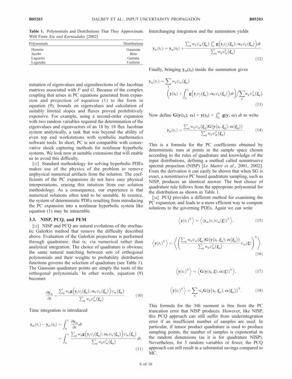
umes revealed the following relationship: log10 (numberof events) = �2.5 log10 (volume of events m3) +20.7. Thismeans that for at least one period, the PDF of log(volume)was exponential, which is a special case of the gammadistribution, and that sample points and weights should bechosen by Gauss-Laguerre quadrature. As before only flowsof which the volumes were greater than 104 m3 wereconsidered and 15 point quadrature in the log(volume)random dimension was chosen. However, those points withprobabilities less than 10�11 were excluded, the rationalebeing that even though the volume of these runs would begreater than 108 m3 the low weights mean the relative effecton the statistics would be around 108 � 10�11/104 = 10�7 orless. This resulted in using 180 rather than 225 samples. Themean and standard deviation of the maximum flow depth areplotted in Figures 7a and 7b.[47] As before, the contours are exponentially distributed

with the smallest contour height being 0.5 m. For theexponential log (volume) distribution, the area of whichthe mean of the maximum flow depth is above 0.5 m coversapproximately 1.7 � 105 m2, the area of which the standarddeviation of the maximum flow depth is above 0.5 m coversapproximately 1.6 � 105 m2, and the area of which themean plus three standard deviations of the maximum flowdepth is above 0.5 m covers approximately 7.5 � 105 m2.[48] For all the contour maps, the potential inundation

area is two orders of magnitude smaller for the exponentiallog(volume) distribution than for the uniform log(volume)

Figure 3. Approximations of the probability distribution of the mass-averaged velocity and maximumpile height of the pile after 0.5 s starting from a cylindrical pile of radius 10 cm and height 10 cm flowingover a surface with random bed and internal frictions. MC4444 indicates results based on MC samplingwith 4444 samples, LHS128 indicates Latin hypercube sampling with 128 samples, and PCQ49 andPCQ100 indicate PCQ sampling with 49 and 100 samples.


10 of 16

B05203

distribution. This is because the large volume flows hadsuch a low frequency of occurrence during the time ofsampling. Two things need to be remembered: (1) theresults represent the expected value of flow depth from allpotential future flows with volume over 104 m3, and not theexpected values over any given period of time, (2) given thestatistics of extrema, the results probably do not representthe danger from an extremal event/worst-case scenario.[49] We illustrate results of the above described procedure

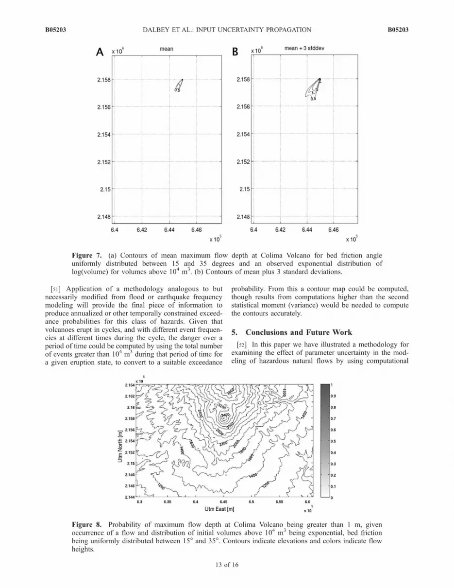
(see section 3.4) for ‘‘computing an answer’’ to the hazardmap question, i.e., given the uncertainty in the input ‘‘whatis the probability of flow at location x exceeding hcrit.’’Figure 8 is a map of probability of inundation created forColima Volcano for the log10 (volume) uniformly distribut-ed between 104 m3 and 108 m3, bed friction uniformlydistributed between 15� and 35� and an internal friction of40�, using a 100 by 100 uniform grid of secondary samplingpoints (SSP). The computed probability of flow heightexceeding 1 m is below 0.1 except for a very small zonenear the summit. The computed map differs greatly frompublished hazards maps in its portrayal of an actual long-term exceedance probability conditional to a flow event, asopposed to a qualitative hazards zone (see, e.g., Sheridanand Macias [1995] and Figure 9). Figure 9a indicates themapped flow extent for the 1913 flows at this volcano.

Figures 9b and 9c describe hazard maps delineated at thissite by using the field observations and some simple use ofmodels.[50] We hypothesize that the difference between the map

in Figures 8, 9b, and 9c is due to the fact that our currentmethodology does not adequately characterize the risk fromthe low probability ‘‘extreme event.’’ To separate out thepotential outcomes of the largest events, we estimate theprobability of a pyroclastic flow exceeding 1 m at a locationif the input volume lies in one of the three ranges 106 m3 to107 m3, 107 m3 to 108 m3 and 108 m3 to 109 m3. Resultsfrom these are plotted in Figures 10, 11, and 12. Figures 10,11, and 12 indicate that the less frequent larger flows doindeed result in large inundation areas. This ‘‘segmented’’approach, in which the volumetric range 108 m3 to 109 m3

can be taken qualitatively to correspond to ‘‘extreme andinfrequent’’ events while the other two ranges correspond to‘‘small and frequent’’ and ‘‘moderate and occasional’’events can be used as an interim, qualitative solution tocharacterize the temporal aspect of the hazard in the absenceof a suitable, long time series of flow volumes. We may nowinclude a map of the hazard based on this classification.Figure 9d includes such a map for the moderate andoccasional category for comparison to the existing maps.

Figure 4. (a) The piecewise incline geometry with three sections which are at angles relative to thex axis of �45�, �20�, and 0�. We assume uniformly distributed initial radius such that 0.025 m � r �0.1 m, and uniformly distributed bed friction such that 15� � fbed � 30�. (b) Contours of mean of themaximum flow depth over time. (c) Contours of standard deviation of the maximum flow depth overtime. (d) Contours of mean plus 3 standard deviations of maximum flow depth over time.


11 of 16

B05203

Figure 5. Plots of a bulk quantity statistics versus time plot, for the piecewise incline geometry,uniformly distributed initial radius such that 0.025 m � r � 0.1 m and uniformly distributed bed frictionsuch that 15� � fbed � 30�. (a) Volume-averaged velocity, (b) maximum pile height, (c) x coordinate offlow centroid, and (d) spatial second moment in the x direction.

Figure 6. (a) Contours of mean maximum flow depth for all realizations at Colima Volcano for bedfriction uniformly distributed between 15 and 35 degrees and uniformly distributed log(volume) forvolumes between 104 and 108 m3. (b) Contours of mean plus 3 standard deviations.


12 of 16

B05203

[51] Application of a methodology analogous to butnecessarily modified from flood or earthquake frequencymodeling will provide the final piece of information toproduce annualized or other temporally constrained exceed-ance probabilities for this class of hazards. Given thatvolcanoes erupt in cycles, and with different event frequen-cies at different times during the cycle, the danger over aperiod of time could be computed by using the total numberof events greater than 104 m3 during that period of time fora given eruption state, to convert to a suitable exceedance

probability. From this a contour map could be computed,though results from computations higher than the secondstatistical moment (variance) would be needed to computethe contours accurately.

5. Conclusions and Future Work

[52] In this paper we have illustrated a methodology forexamining the effect of parameter uncertainty in the mod-eling of hazardous natural flows by using computational

Figure 8. Probability of maximum flow depth at Colima Volcano being greater than 1 m, givenoccurrence of a flow and distribution of initial volumes above 104 m3 being exponential, bed frictionbeing uniformly distributed between 15� and 35�. Contours indicate elevations and colors indicate flowheights.

Figure 7. (a) Contours of mean maximum flow depth at Colima Volcano for bed friction angleuniformly distributed between 15 and 35 degrees and an observed exponential distribution oflog(volume) for volumes above 104 m3. (b) Contours of mean plus 3 standard deviations.


13 of 16

B05203

models. We described several standard methodologies forestimating the effect of such input parameter uncertainty onmodel outputs. We presented a new approach, dubbed PCQ,which is an efficient method of propagating uncertaintythrough a governing system of equations, using an intelli-gent sampling approach to the construction of an output

uncertainty distribution. We discussed the suitability ofthese various methods for Savage-Hutter-type models ofmass flows. Most existing stochastic methods are notsuitable to the task, either because of the nonpolynomial,nonlinear nature of the governing hyperbolic PDEs (PC),or because of their computational cost (MC). Our PCQ

Figure 9. (a) Map of the extent of the phase III pyroclastic flows from the 1913 eruption of Colima[Saucedo et al., 2005]. (b) Traditional hazard map based on field study only [Navarro and Cortez, 2003].(c) Hazard map based on deterministic calculations using the FLOW3D model [Saucedo et al., 2005].(d) Probability of flow exceeding 1 m given an event that generates a 107 to 108 m3 of flow volume.

Figure 10. Probability of maximum flow depth at Colima Volcano being greater than 1 m given theoccurrence of a flow and initial volumes exponentially distributed from 106 m3 to 107 m3 and bed frictionbeing uniformly distributed between 15� and 35�. Contours indicate elevations, and shading indicatesflow heights.


14 of 16

B05203

method, coupled with the TITAN geophysical flow solver,is suited to the equations and has comparatively reasonablecomputational cost. Furthermore, no modifications of theunderlying simulation code have to be made to implementthis procedure. A relatively simple summation procedure

can then be followed for estimating probabilities of ex-ceeding a hazard threshold in an output variable. Thisprocedure can be used for creating maps to depict theuncertainty in the model outputs. Methods of the typedescribed in this paper are crucial to the use of computermodels in hazard analysis since model parameters and eventhe models themselves are subject to much uncertainty.[53] The modeling of geophysical mass flows and in

particular incorporating the effects of fluidization is thesubject of ongoing research [see, e.g., Pitman and Le,2005]. We anticipate upgrading the representation of thephysics in the modeling framework discussed here. Impor-tantly, the question of characterizing the effect of uncertain-ty in the DEM has not been addressed in this paper and isthe subject of current work.

[54] Acknowledgments. We wish to acknowledge the financial sup-port of National Science Foundation grant ACI-0121254. We are grateful tothe reviewers and editors for their help.

ReferencesChristian, J., and G. Baecher (1999), The point estimate method as numer-ical quadrature, J. Geotech. Geoenviron. Eng., 125, 779–786.

Christian, J., and G. Baecher (2002), The point estimate method with largenumbers of variables, Int. J. Numer. Anal. Methods Geomech., 26,1515–1529.

Chung, K. L. (2001), A Course in Probability Theory, 3rd ed., Academic,San Diego, Calif.

Denlinger, R. P., and R. M. Iverson (2001), Flow of variably fluidizedgranular material across three-dimensional terrain: 2. Numerical predic-tions and experimental tests, J. Geophys. Res., 106, 553–566.

Denlinger, R. P., and R. M. Iverson (2004), Granular avalanches acrossirregular three-dimensional terrain: 1. Theory and computation,J. Geophys. Res., 109, F01014, doi:10.1029/2003JF000085.

Ghanem, R., and P. Spanos (1991), Stochastic Finite Elements: A SpectralApproach, Springer, New York.

Glimm, J., and D. Sharp (1991), Prediction and the quantification of un-certainty, Physica D, 133, 152–170.

Glimm, J., S. Hou, H. Kim, and D. Sharp (2001), A probability model forerrors in the numerical solution of a partial differential equation, Comput.Fluid Dyn. J., 9, 485–493.

Gray, J. N. M. T., M. Wieland, and K. Hutter (1999), Gravity-driven freesurface flow of granular avalanches over complex basal terrain, Proc. R.Soc. London, Ser. A, 455, 1841–1874.

Figure 11. Probability of maximum flow depth at Colima Volcano being greater than 1 m givenoccurrence of a flow and initial volumes exponentially distributed from 107 m3 to 108 m3 and bed frictionbeing uniformly distributed between 15� and 35�. Contours indicate elevations, and shading indicatesflow heights.

Figure 12. Probability of maximum flow depth at ColimaVolcano being greater than 1 m given occurrence of a flowand initial volumes exponentially distributed from 108 m3 to109 m3.


15 of 16

B05203

Harr, M. (1989), Probabilistic estimates for multivariate analyses, Appl.Math. Modell., 13, 313–318.

Harr, M. (1994), Modelling of many correlated and skewed random vari-ables, Appl. Math. Modell., 18, 635–640.

Hoblitt, R. P., J. S. Walder, C. Driedger, K. M. Scott, P. T. Pringle, and J.Vallance (1998), Volcano hazards from Mount Rainier, Washington, re-vised 1998, U.S. Geol. Surv. Open File Rep., 98-428.

Huard, D., and A. Mailhot (2006), A Bayesian perspective on input un-certainty in model calibration: Application to hydrological model ‘‘abc,’’Water Resour. Res., 42, W07416, doi:10.1029/2005WR004661.

Hutter, K., and N. Kirchner (Eds.) (2003), Dynamic Response of Granularand Porous material under large and catastrophic deformations, Lect.Notes Appl. Comput. Mech., vol. 11, Springer, New York.

Hutter, K., M. Siegel, S. B. Savage, and Y. Nohguchi (1993), Two dimen-sional spreading of a granular avalanche down an inclined plane: part 1:Theory, Acta Mech., 100, 37–68.

Iverson, R. M. (1997), The physics of debris flows, Rev. Geophys., 35,245–296.

Iverson, R. M., and R. P. Denlinger (2001), Flow of variably fluidizedgranular material across three-dimensional terrain: 1. Coulomb mixturetheory, J. Geophys. Res., 106, 537–552.

Iverson, R., S. P. Schilling, and J. Vallance (1998), Objective delineation oflahar-inundation hazard zones, Geol. Soc. Am. Bull., 110, 972–984.

Iverson, R. M., M. Logan, and R. P. Denlinger (2004), Granular ava-lanches across irregular three-dimensional terrain: 2. Experimental tests,J. Geophys. Res., 109, F01015, doi:10.1029/2003JF000084.

Jibson, R. W., E. L. Harp, and J. A. Michael (2000), A method for produ-cing digital probabilistic seismic landslide hazard maps, Eng. Geol., 58,271–289.

Le Maitre, O. P., O. M. Knio, H. N. Najm, and R. G. Ghanem (2001),A stochastic projection method for fluid flow: I. basic formulation,J. Comput. Phys., 173, 481–511.

Le Maitre, O. P., M. T. Reagan, H. N. Najm, R. G. Ghanem, and O. M.Knio (2002), A stochastic projection method for fluid flow: II. Randomprocess, J. Comput. Phys., 181, 9–44.

Macias, J. L., G. Carrasco, H. Delgado, A. L. Martin del Pozzo, R. P.Hoblitt, M. F. Sheridan, and R. I. Tilling (1995), Mapa del Peligros delVolcan Popocatepetl, informe final, 12 pp. and map, Inst. de Geofis.,Univ. Nac. Auton. de Mexico, Mexico City, Mexico.

MacKay, D. J. C. (2003), Information Theory, Inference, and LearningAlgorithms, 640 pp., Cambridge Univ. Press, Cambridge, UK.

McKay, M. D., R. J. Beckman, and W. J. Conover (1979), A comparison ofthree methods for selecting values of input variables in the analysis ofoutput from a computer code, Technometrics, 21, 239–245.

Namikawa, L. M., and C. Renschler (2004), Brazilian Symposium onGeoinformatics—GEOINFO (7:2004: Campos do Jordao: SP)/Ciranolochpe e Gilberto Camara, Inst. Nac. de Pesquisas Esp., Sao Jose doCampos, Sao Paulo, Brazil.

Navarro, C., and A. Cortez (2003), Mapa de Peligros Volcan de Fuego deColima, Univ. de Colima, Obs. Vulcanol., Colima, Mexico.

Oberkampf, W. L., T. G. Trucano, and C. Hirsch (2002), Verification,validation, and predictive capability in computational engineering andphysics, paper presented at Foundations of Verification and Validationfor the 21st Century Workshop, Johns Hopkins Univ., Laurel, Md., Oct.

Patra, A. K., A. C. Bauer, C. Nichita, E. B. Pitman, M. F. Sheridan, M.Bursik, B. Rupp, A. Webber, L. Namikawa, and C. Renschler (2005),Parallel adaptive numerical simulation of dry avalanches over naturalterrain, J. Volcanol. Geotherm. Res., 139, 1–21.

Pitman, E. B., and L. Le (2005), A two-fluid model for avalanche anddebris flow, Philos. Trans. R. Soc. London, Ser. A, 363, 1573–1601.

Pitman, E. B., A. Patra, A. Bauer, C. Nichita, M. Sheridan, and M. Bursik(2003), Computing debris flows, Phys. Fluids, 15, 3638–3646.

Pouliquen, O., and Y. Forterre (2002), Friction law for dense granularflows: Application to the motion of a mass down a rough inclined plane,J. Fluid Mech., 453, 133–151.

Pudasaini, S. P., Y. Wang, and K. Hutter (2005), Modelling debris flowsdown general channels, Nat. Hazards Earth Syst. Sci., 5, 799–819.

Rosenblueth, E. (1975), Point estimates for probability moments, Proc.Natl. Acad. Sci. U. S. A., 72, 3812–3814.

Rupp, B., M. Bursik, L. Namikawa, A. Webb, A. K. Patra, R. Saucedo, J. L.Macias, and C. Renschler (2006), Computational modeling of the 1991block and ash flows at Colima Volcano, Mexico, in Neogene-Quaternarycontinental margin volcanism: A perspective from Mexico, edited by C.Siebe, J. L. Macias, and G. J. Aguirre-Diaz, Spec. Pap. Geol. Soc. Am.,402, 237–252, doi:10.1130/2006.2402(11).

Saucedo, R., J. L. Macias, and M. Bursik (2004), Pyroclastic flow depositsof the 1991 eruption of Volcan de Colima, Mexico, Bull. Volcanol., 66,291–306.

Saucedo, R., J. L.Macias, M. F. Sheridan, M. I. Bursik, and J. C. Komorowski(2005), Modeling of pyroclastic flows of Colima Volcano, Mexico: Ap-plication to hazard assessment, J. Volcanol. Geotherm. Res., 139(1–2),103–115.

Savage, S. B., and K. Hutter (1989), The motion of a finite mass of granularmaterial down a rough incline, J. Fluid Mech., 199, 177–215.

Sheridan, M., and J. Macias (1995), Estimation of risk probability forgravity-driven pyroclastic flows at Volcan Colima, Mexico, J. Volcanol.Geotherm. Res., 66, 251–256.

Sheridan, M. F., C. Bonnard, R. Carreno, C. Siebe, W. Strauch, M. Navarro,J. C. Calero, and N. B. Trujillo (1999), 30 October 1998 rockfall/ava-lanche and breakout flow of Casita Volcano, Nicaragua. Landslide News,June, 2–4.

Somerville, P. G., N. F. Smith, R. W. Graves, and N. A. Abrahamson(1997), Modification of empirical strong ground motion attenuation rela-tions to include the amplitude and duration effects of rupture directivity,Seismol. Res. Lett., 68(1), 199–222.

Toro, E. F. (2001), Shock-Capturing Methods for Free-Surface ShallowFlows, John Wiley, San Diego, Calif.

Wiener, N. (1938), The homogeneous chaos, Am. J. Math., 60, 897–936.Wolfe, E. W., and T. C. Pierson (1995), Volcanic-Hazard Zonation forMount St. Helens, Washington, 1995, U.S. Geol. Surv. Open File Rep.,95-497.

Xiu, D., and G. Karniadakis (2002), The Wiener-Askey polynomial chaosfor stochastic differential equations, SIAM J. Sci. Comput., 24, 619–644.

Xiu, D. B., and G. E. Karniadakis (2003), Modeling uncertainty in flowsimulations via generalized polynomial chaos, J. Comput. Phys., 187,137–167.

Zobin, V. M., and Y. A. Taran (2002), Volcan de Colima, Mexico, and itsactivity in 1997–2000, J. Volcanol. Geotherm. Res., 117(1–2), 121–127.

��M. I. Bursik and M. F. Sheridan, Department of Geology, State

University of New York at Buffalo, Buffalo, NY 14260, USA.([email protected]; [email protected])K. Dalbey and A. K. Patra, Department of Mechanical and Aerospace

Engineering, State University of New York at Buffalo, Buffalo, NY 14260,USA. ([email protected]; [email protected])E. B. Pitman, Department of Mathematics, State University of New York

at Buffalo, Buffalo, NY 14260, USA. ([email protected])


16 of 16

B05203

Documents

Input uncertainty propagation methods and hazard mapping of geophysical mass flows