Inexact Uzawa Algorithms for Nonsymmetric SaddlePoint Problems�James H. Brambley, Joseph E. Pasciaky, and Apostol T. VassilevzAbstractIn this paper, we consider iterative algorithms of Uzawa type for solving lin-ear nonsymmetric block saddle point problems. Speci�cally, we consider systemswhere the upper left block is invertable nonsymmetric linear operator with pos-itive de�nite symmetric part. Such saddle point problems arise, for example, incertain �nite element and �nite di�erence discretizations of Navier{Stokes equa-tions, Oseen equations, and mixed �nite element discretization of second orderconvection-di�usion problems. We consider two algorithms which utilize an \in-complete" or \approximate" evaluation of the inverse of the operator in the upperleft block. Convergence results for the inexact algorithms are established in ap-propriate norms. The convergence of one of the algorithms is shown withoutthe assumption of a su�ciently accurate approximation to the inverse operator.The other algorithm is shown to converge provided that the approximation tothe inverse of the upper left hand block is of su�cient accuracy. Applicationsto the solution of steady-state nonlinear Navier{Stokes equations are discussedand �nally, the results of numerical experiments involving the algorithms arepresented.Key words. inde�nite systems, iterative methods, preconditioners, saddle point problems, non-symmetric saddle point systems, Navier-Stokes equations, Oseen equations, Uzawa algorithm.AMS subject classi�cations. 65N22, 65N30, 65F10.1 IntroductionThis paper provides an analysis for the inexact Uzawa method applied to the solution oflinear nonsymmetric saddle point systems. Such systems arise in certain discretizations�This manuscript has been authored under contract number DE-AC02-76CH00016 with the U.S.Department of Energy. Accordingly, the U.S. Government retains a non-exclusive, royalty-free licenseto publish or reproduce the published form of this contribution, or allow others to do so, for U.S.Government purposes. This work was also supported in part under the National Science FoundationGrant No. DMS-9626567 and by Schlumberger/GeoQuest.yDepartment of Mathematics, Texas A&M University, College Station, TX 77843.zSchlumberger/GeoQuest, 8311 N. FM 620, Austin, TX 787261

Inexact Uzawa algorithms II 2of Navier{Stokes equations, mixed discretizations of second order elliptic problems withconvective terms (cf. [11], [14], [17], [20]). The theory in this paper is an extension ofthe theory for symmetric saddle point problems developed in [4].Let H1 and H2 be �nite dimensional Hilbert spaces with inner products which weshall denote by (�; �). There is no ambiguity even though we use the same notation forthe inner products on both of these spaces since the particular inner product will beidenti�ed by the type of functions appearing. We consider the abstract saddle pointproblem: A BTB 0 ! XY ! = FG! ;(1.1)where F 2 H1 and G 2 H2 are given and X 2 H1 and Y 2 H2 are the unknowns.Here A : H1 7! H1 is assumed to be a linear, not necessarily symmetric operator.AT : H1 7! H1 is the adjoint of A with respect to the (�; �){inner product. In addition,the linear map BT : H2 7! H1 is the adjoint of B : H1 7! H2.In general, (1.1) may not even solvable unless additional conditions on the operatorsA and B, and the spaces H1 and H2 are imposed. Throughout this paper we assumethat A has a positive de�nite symmetric part. Under this assumption, (1.1) is solvableif and only if the reduced problemBA�1BTY = BA�1F �G(1.2)is solvable. In the case of a symmetric and positive de�nite operatorA, the Ladyzhenskaya{Babu�ska{Brezzi (LBB) condition (cf. [6]) is necessary and su�cient condition for solv-ability of this problem. As we shall see, the solvability of (1.1) in the nonsymmetriccase is guaranteed provided that the the LBB condition holds for the symmetric partof A.The papers [9], [18] propose solving BA�1BT by preconditioned iteration. Onecommon problem with this is that the evaluation of the action of the operator A�1 isrequired in each step of the iteration. For many applications, this operation is expen-sive and is also implemented as an iteration. The Uzawa method [1] is a particularimplementation of a linear iterative method for solving (1.2). It is an exact algorithmin the sense that the action of A�1 is required for the implementation. An alterna-tive method which solves (1.1) by preconditioned iteration was proposed in [10]. Theirpreconditioner also requires the evaluation of A�1 during each step of the iteration.The inexact Uzawa methods replace the exact inverse of A by an \incomplete" or\approximate" evaluation of A�1. Such algorithms are de�ned in Sections 3 and 4. Inthis paper we distinguish two types of inexact algorithms: (i) a linear one-step, wherethe action of the approximate inverse is provided by a linear preconditioner such as onesweep of a multigrid procedure; (ii) a multistep, where a su�ciently accurate approxima-tion to A�1 is provided by some preconditioned iterative method, e.g., preconditionedGMRES [19] or preconditioned Lancos [15].The inexact Uzawa algorithms applied to nonsymmetric problems are of interestbecause they are simple, e�cient, and have minimal computer memory requirements.

Inexact Uzawa algorithms II 3They can be applied to the solution of di�cult practical problems such as the Navier{Stokes equation. In addition, an exact Uzawa algorithm implemented as a doubleiteration can be transformed trivially into an inexact algorithm. It is not surprisingthat the inexact Uzawa methods are widely used in the engineering community.The paper is organized as follows. In Section 2 we establish su�cient conditions forsolvability of the abstract saddle point problem and analyze an exact Uzawa algorithmfor solving it. In Section 3 we de�ne and analyze a linear one-step inexact Uzawaalgorithm applied to (1.1). Next, a multistep inexact method is de�ned and analyzedin Section 4. Section 5 provides applications of the algorithms from Section 3 andSection 4 to the solution of inde�nite systems of linear equations arising from �niteelement approximations of the steady-state nonlinear Navier-Stokes equations. Finally,the results of numerical experiments involving the inexact Uzawa algorithms are givenin Section 6.2 Analysis of the exact methodIn this section we establish su�cient conditions for solvability of (1.2) and analyze theexact Uzawa algorithm applied to the solution of (1.2). Even though this algorithmis not very e�cient for reasons already mentioned, the result of Theorem 2.2 below isimportant for the analysis of the inexact algorithms de�ned in the subsequent sections.The symmetric part As of the operator A is de�ned byAs = 12(A+AT ):(2.1)In the remainder of this paper a subscript s will be used to denote the symmetric partof various operators, de�ned as in (2.1). We assume that As is positive de�nite andsatis�es (AX; Y ) � �(AsX;X)1=2(AsY; Y )1=2 for all X; Y 2 H1;(2.2)for some number �. Clearly, � � 1. Moreover, since As is positive de�nite, such an� always exists. In many applications in the numerical solution of partial di�erentialequations, the constant � can be chosen independently of the mesh parameter.In addition, the Ladyzhenskaya{Babu�ska{Brezzi condition is assumed to hold forthe the pair of spaces H1 and H2, i.e.supU2H1U 6=0 (V;BU)2(AsU; U) � c0kV k2 for all V 2 H2 ;(2.3)for some positive number c0. Here k � k denotes the norm in the space H2 (or H1)corresponding to the inner product (�; �).As is well known, the condition (2.3) is su�cient to guarantee solvability of (1.1)when A is replaced by As. We will see that it also su�ces in the case of nonsymmetric

Inexact Uzawa algorithms II 4A. To this end, we prove the following lemma which establishes that (A�1)s is positivede�nite.Lemma 2.1 Let A be an invertible linear operator with positive de�nite symmetric partAs that satis�es (2.2). Then (A�1)s is positive de�nite and satis�es((A�1)sW;W ) � ((As)�1W;W ) � �2((A�1)sW;W ) for all W 2 H1:(2.4)Proof: Clearly,((As)�1W;W ) = supU2H1U 6=0 (W;U)2(AsU; U) = supU2H1U 6=0 ((A�1)TW;AU)2(AsU; U)� �2 supU2H1U 6=0 k(A�1)TWk2AskUk2AskUk2As = �2k(A�1)TWk2As= �2((A�1)sW;W ):(2.5)Here k � k2As = (As�; �). In the above inequalities we have used the Schwarz inequality,(2.2), and the fact that (AsU; U) = (AU; U) for all U 2 H1:(2.6)On the other hand,((A�1)sU; U) = (A�1U; U) = (A1=2s A�1U; (As)�1=2U)� kA�1UkAskUk(As)�1 = (A�1U; U)kUk(As)�1 :Therefore, ((A�1)sU; U) � ((As)�1U; U):(2.7)This completes the proof of the lemma. 2It is clear now that Lemma 2.1 and (2.3) guarantee solvability of (1.2). Indeed,(BA�1BTV; V ) = ((A�1)sBTV;BTV )� ��2((As)�1BTV;BTV ) � ��2c0kV k2:Thus, we have proved the following theorem.Theorem 2.1 Let the linear operator A be invertible and let (2.3) hold. Then thereduced problem (1.2), or equivalently (1.1), is solvable.Next, we turn to the analysis of the exact Uzawa algorithm applied to the solutionof (1.2). The preconditioned variant of the exact Uzawa algorithm (cf. [1, 4]) is de�nedas follows.

Inexact Uzawa algorithms II 5Algorithm 2.1 (Preconditioned exact Uzawa) For X0 2 H1 and Y0 2 H2 given,the sequence f(Xi; Yi)g is de�ned, for i = 1; 2; : : : , byXi+1 = Xi +A�1 �F � (AXi +BTYi)� ;Yi+1 = Yi + �Q�1B (BXi+1 �G):Here the preconditioner QB : H2 7! H2 is a symmetric and positive de�nite linearoperator satisfying(1� )(QBW;W ) � (B(As)�1BTW;W )� (QBW;W ) for all W 2 H2;(2.8)for some in the interval [0; 1), and � is a positive parameter. Notice that this conditionimplies appropriate scaling of QB. In many particular applications e�ective precondi-tioners that satisfy (2.8) with bounded away from one are known.Let EXi = X �Xi(2.9a)and EYi = Y � Yi(2.9b)be the iteration errors generated by the above method. It is an easy observation thatEYi+1 = (I� �Q�1B BA�1BT )EYi :Therefore, the convergence of Algorithm 2.1 is governed by the properties of the operatorI� �Q�1B BA�1BT summarized in the following.Theorem 2.2 Let A be invertible with positive de�nite symmetric part As which satis-�es (2.2). Let also (2.3) hold. In addition, let QB be a symmetric and positive de�niteoperator satisfying (2.8). If � is a positive parameter with � � 1� �2 , thenk(I� �Q�1B BA�1BT )Uk2QB � �1� 1� �2 �� kUk2QB for all U 2 H2:(2.10)Remark 2.1 If A = AT , � can be set to one and (2.8) implies (cf. [4]) thatk(I�Q�1B BA�1BT )Uk2QB � 2kUk2QB :Hence, the result of Theorem 2.2 is not optimal in the limit when �! 1.

Inexact Uzawa algorithms II 6Proof (of Theorem 2.2): The proof is based on the result of Lemma 2.1. LetL = BA�1BT . Then, by (2.8) and Lemma 2.1,(1� )kV k2QB � ((As)�1BTV;BTV )� �2(LV; V ):(2.11)In addition,using (2.4),(A�1v; w) = ((As)1=2A�1v; (As)�1=2w)� (A�1v; v)1=2((As)�1w;w)1=2� ((As)�1v; v)1=2((As)�1w;w)1=2:(2.12)Taking v = BTV and w = BTW above gives(LV;W ) � kV kQBkWkQB :(2.13)Next, k(I� �Q�1B L)V k2QB = kV k2QB � 2�(LV; V ) + � 2(LV;Q�1B LV ):(2.14)By (2.12) and (2.11), the last term in the right hand side of (2.14) is estimated by(LV;Q�1B LV ) � kV kQBkQ�1B LV kQB= kV kQB(LV;Q�1B LV )1=2:(2.15)Using (2.11) and (2.15) in (2.14) yieldsk(I� �Q�1B L)V k2QB � 1� 2�(1� )�2 + � 2! kV k2QB :From this, the result of the theorem follows easily. 2Remark 2.2 The inequalities (2.11) and (2.13) are the basis for developing the inexactalgorithms in the subsequent sections.3 Analysis of the linear one-step inexact methodIn this section we de�ne and analyze a linear one-step inexact Uzawa algorithm appliedto (1.1). This section contains the main result of the paper. We show that, underthe minimal assumptions needed to guarantee solvability (cf. Section 2), appropriatelyscaled linear preconditioners (cf. (2.8) and (3.1) below) result in an e�cient and simplemethod for solving (1.1).To this end, the exact inverse ofA is replaced with an approximation ofA�1 in orderto improve the e�ciency of Algorithm 2.1. Let A0 : H1 7! H1 be a linear, symmetricand positive de�nite operator that satis�es(A0V; V ) � (AsV; V ) � �(A0V; V ) for all V 2 H1;(3.1)for some positive � � 1.

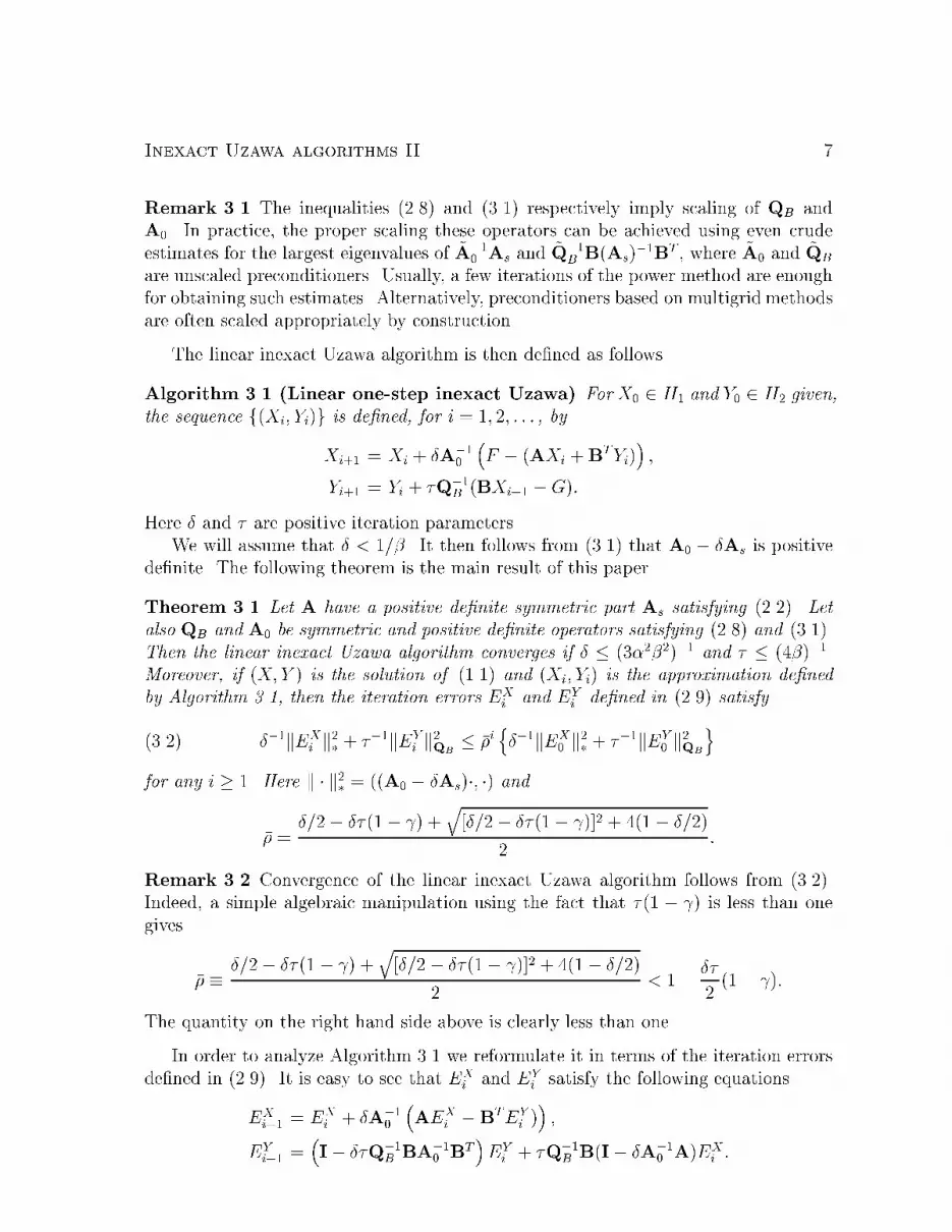
Inexact Uzawa algorithms II 7Remark 3.1 The inequalities (2.8) and (3.1) respectively imply scaling of QB andA0. In practice, the proper scaling these operators can be achieved using even crudeestimates for the largest eigenvalues of ~A�10 As and ~Q�1B B(As)�1BT , where ~A0 and ~QBare unscaled preconditioners. Usually, a few iterations of the power method are enoughfor obtaining such estimates. Alternatively, preconditioners based on multigrid methodsare often scaled appropriately by construction.The linear inexact Uzawa algorithm is then de�ned as follows.Algorithm 3.1 (Linear one-step inexact Uzawa) ForX0 2 H1 and Y0 2 H2 given,the sequence f(Xi; Yi)g is de�ned, for i = 1; 2; : : : , byXi+1 = Xi + �A�10 �F � (AXi +BTYi)� ;Yi+1 = Yi + �Q�1B (BXi+1 �G):Here � and � are positive iteration parameters.We will assume that � < 1=�. It then follows from (3.1) that A0 � �As is positivede�nite. The following theorem is the main result of this paper.Theorem 3.1 Let A have a positive de�nite symmetric part As satisfying (2.2). Letalso QB and A0 be symmetric and positive de�nite operators satisfying (2.8) and (3.1).Then the linear inexact Uzawa algorithm converges if � � (3�2�2)�1 and � � (4�)�1.Moreover, if (X; Y ) is the solution of (1.1) and (Xi; Yi) is the approximation de�nedby Algorithm 3.1, then the iteration errors EXi and EYi de�ned in (2.9) satisfy��1kEXi k2� + ��1kEYi k2QB � ��i n��1kEX0 k2� + ��1kEY0 k2QBo(3.2)for any i � 1. Here k � k2� = ((A0 � �As)�; �) and�� = �=2� ��(1� ) +q[�=2� ��(1� )]2 + 4(1� �=2)2 :Remark 3.2 Convergence of the linear inexact Uzawa algorithm follows from (3.2).Indeed, a simple algebraic manipulation using the fact that �(1 � ) is less than onegives �� � �=2� ��(1� ) +q[�=2� ��(1� )]2 + 4(1� �=2)2 < 1� ��2 (1� ):The quantity on the right hand side above is clearly less than one.In order to analyze Algorithm 3.1 we reformulate it in terms of the iteration errorsde�ned in (2.9). It is easy to see that EXi and EYi satisfy the following equations.EXi+1 = EXi + �A�10 �AEXi �BTEYi )� ;EYi+1 = �I� ��Q�1B BA�10 BT�EYi + �Q�1B B(I� �A�10 A)EXi :

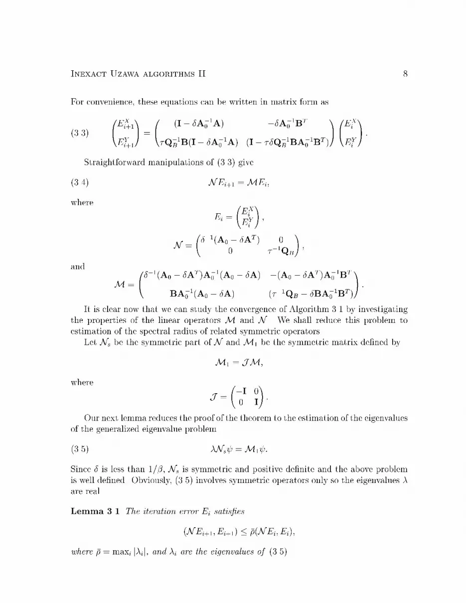
Inexact Uzawa algorithms II 8For convenience, these equations can be written in matrix form as0@EXi+1EYi+11A = 0@ (I� �A�10 A) ��A�10 BT�Q�1B B(I� �A�10 A) (I� ��Q�1B BA�10 BT )1A0@EXiEYi 1A :(3.3)Straightforward manipulations of (3.3) giveNEi+1 =MEi;(3.4)where Ei = EXiEYi ! ;N = ��1(A0 � �AT ) 00 ��1QB! ;and M = 0@��1(A0 � �AT )A�10 (A0 � �A) �(A0 � �AT )A�10 BTBA�10 (A0 � �A) (��1QB � �BA�10 BT )1A :It is clear now that we can study the convergence of Algorithm 3.1 by investigatingthe properties of the linear operators M and N . We shall reduce this problem toestimation of the spectral radius of related symmetric operators.Let Ns be the symmetric part of N and M1 be the symmetric matrix de�ned byM1 = JM;where J = �I 00 I! :Our next lemma reduces the proof of the theorem to the estimation of the eigenvaluesof the generalized eigenvalue problem�Ns =M1 :(3.5)Since � is less than 1=�, Ns is symmetric and positive de�nite and the above problemis well de�ned. Obviously, (3.5) involves symmetric operators only so the eigenvalues �are real.Lemma 3.1 The iteration error Ei satis�es(NEi+1; Ei+1) � ��(NEi; Ei);where �� = maxi j�ij, and �i are the eigenvalues of (3.5).

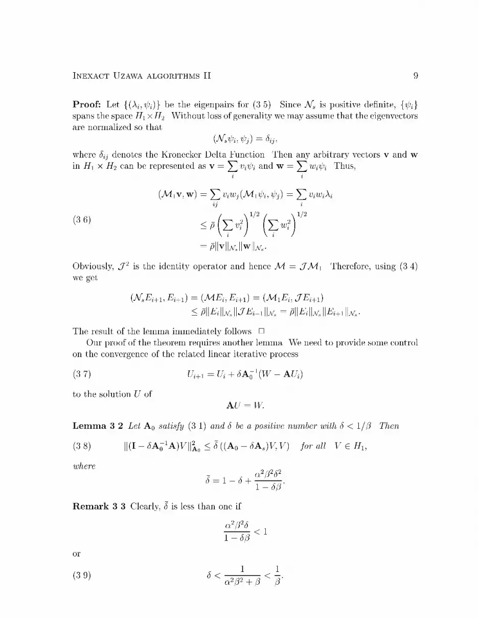
Inexact Uzawa algorithms II 9Proof: Let f(�i; i)g be the eigenpairs for (3.5). Since Ns is positive de�nite, f igspans the spaceH1�H2. Without loss of generality we may assume that the eigenvectorsare normalized so that (Ns i; j) = �ij;where �ij denotes the Kronecker Delta Function. Then any arbitrary vectors v and win H1 �H2 can be represented as v =Xi vi i and w =Xi wi i. Thus,(M1v;w) =Xij viwj(M1 i; j) =Xi viwi�i� �� Xi v2i!1=2 Xi w2i!1=2= ��kvkNskwkNs:(3.6)Obviously, J 2 is the identity operator and hence M = JM1. Therefore, using (3.4)we get (NsEi+1; Ei+1) = (MEi; Ei+1) = (M1Ei;JEi+1)� ��kEikNskJEi+1kNs = ��kEikNskEi+1kNs:The result of the lemma immediately follows. 2Our proof of the theorem requires another lemma. We need to provide some controlon the convergence of the related linear iterative processUi+1 = Ui + �A�10 (W �AUi)(3.7)to the solution U of AU = W:Lemma 3.2 Let A0 satisfy (3.1) and � be a positive number with � < 1=�. Thenk(I� �A�10 A)V k2A0 � �� ((A0 � �As)V; V ) for all V 2 H1;(3.8)where �� = 1� � + �2�2�21� �� :Remark 3.3 Clearly, �� is less than one if�2�2�1� �� < 1or � < 1�2�2 + � < 1� :(3.9)

Inexact Uzawa algorithms II 10Note in addition, that ((A0 � �As)V; V ) � (1� �)kV k2A0 :Thus, the lemma proves convergence of (3.7) provided that (3.9) holds.Proof (of Lemma 3.2): By (3.1),(1� ��)(A0V; V ) � ((A0 � �As)V; V ) for all V 2 H1:Hence, by (2.2) and (3.1),(AV;W ) � �(AsV; V )1=2(AsW;W )1=2� ��(1� ��)1=2 (A0V; V )1=2((A0 � �As)W;W )1=2:(3.10)On the other hand,k(I� �A�10 A)V k2A0 = kV k2A0 � 2�(AV; V ) + �2(A�10 AV;AV )= ((A0 � �As)V; V )� �(AV; V ) + �2(A�10 AV;AV ):(3.11)In view of (3.1), we have(AV; V ) � (A0V; V ) � ((A0 � �As)V; V ):(3.12)Also, (3.10) implies(A�10 AV;AV ) � ��(1� ��)1=2 (A�10 AV;AV )1=2((A0 � �As)V; V )1=2:Thus, (A�10 AV;AV ) � �2�21� �� ((A0 � �As)V; V ):(3.13)Using (3.12) and (3.13) in (3.11) yields (3.8). 2Proof (of Theorem 3.1): To prove the theorem, we shall bound the positive andnegative eigenvalues of (3.5) separately. We begin with the negative eigenvalues. Let(�; �) be an eigenvector (in H1�H2) with eigenvalue � < 0. Then multiplying the �rstblock equation by ��1A0(A0 � �AT )�1 gives���1A0(A0 � �AT )�1(A0 � �As)� = ���1(A0 � �A)�+BT ����1QB� = BA�10 (A0 � �A)�+ (��1QB � �BA�10 BT )�:(3.14)

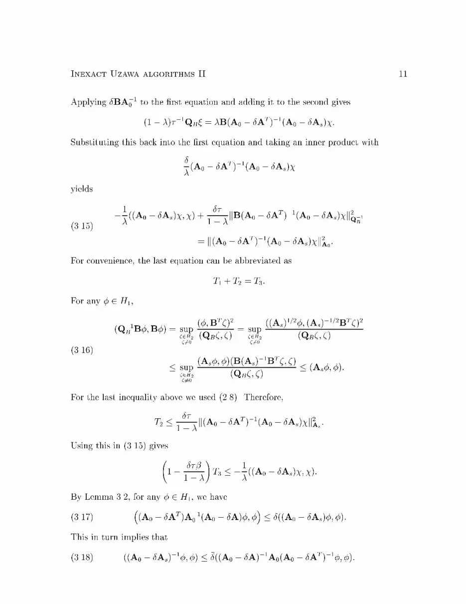
Inexact Uzawa algorithms II 11Applying �BA�10 to the �rst equation and adding it to the second gives(1� �)��1QB� = �B(A0 � �AT )�1(A0 � �As)�:Substituting this back into the �rst equation and taking an inner product with��(A0 � �AT )�1(A0 � �As)�yields �1�((A0 � �As)�; �) + ��1� �kB(A0 � �AT )�1(A0 � �As)�k2Q�1B= k(A0 � �AT )�1(A0 � �As)�k2A0 :(3.15)For convenience, the last equation can be abbreviated asT1 + T2 = T3:For any � 2 H1,(Q�1B B�;B�) = sup�2H2� 6=0 (�;BT �)2(QB�; �) = sup�2H2� 6=0 ((As)1=2�; (As)�1=2BT �)2(QB�; �)� sup�2H2� 6=0 (As�; �)(B(As)�1BT �; �)(QB�; �) � (As�; �):(3.16)For the last inequality above we used (2.8). Therefore,T2 � ��1� �k(A0 � �AT )�1(A0 � �As)�k2As :Using this in (3.15) gives 1� ���1� �!T3 � �1�((A0 � �As)�; �):By Lemma 3.2, for any � 2 H1, we have�(A0 � �AT )A�10 (A0 � �A)�; �� � ��((A0 � �As)�; �):(3.17)This in turn implies that((A0 � �As)�1�; �) � ��((A0 � �A)�1A0(A0 � �AT )�1�; �):(3.18)

Inexact Uzawa algorithms II 12Hence, T3 � 1�� ((A0 � �As)�; �):Combining and using the fact that � < 0 gives�1�((A0 � �As)�; �) � 1�� 1� ���1� �! ((A0 � �As)�; �)� 1� ����� ((A0 � �As)�; �):(3.19)Now, if � = 0 then the �rst equation in (3.14) implies that BT � = 0. Then, from thesecond equation in (3.14), we get that � = 0. Hence, we can assume that � 6= 0 in(3.19). Thus, � � � ��1� ��� :(3.20)Let � � 13�2�2 and � � 14� . Applying straightforward manipulations, we get�� = 1� � + �2�2�21� �� � 1� � 1� 1=31� 1=3! = 1� �2(3.21a)and 11� ��� � 11� �=4 :(3.21b)Using (3.21) in (3.20) gives � � � 1� �=21� �=4 � 1� �4 ;(3.22)which provides a bound for the negative part of the spectrum.Next, we bound the positive eigenvalues of (3.5). Let us factor M1 asM1 = DTM2D;where D = 0@��1=2(A0)�1=2(A0 � �A) 00 I1A ;M2 = 0@ ���1�I �1=2(A0)�1=2BT�1=2B(A0)�1=2 ��1QB � �BA�10 BT1A ;

Inexact Uzawa algorithms II 13and � = 1� �=2. By de�nition, the largest eigenvalue of (3.5) is� = supw2H1�H2w 6=0 (M1w;w)(Nsw;w) = supw2H1�H2w 6=0 (M2Dw;Dw)(Nsw;w) :We now show that for any vector ��! 2 H1 �H2, M2 ��! ; ��!! � �� h��1k�k2 + ��1k�k2QBi :(3.23)Let L = B(A0)�1=2. ThenM2 = ���1�I �1=2LT�1=2L ��1QB � �LLT! :To prove (3.23), we need to estimate the largest eigenvalue of����1�+ �1=2LT � = ���1�(3.24a) �1=2L� + (��1QB � �LLT )� = ���1QB�;(3.24b)where ��! is an eigenvector. Solving for � in (3.24a) we get� = �(�+ �)�1�1=2LT �:Substituting this in (3.24b) yields(1� �)(�+ �)QB� = ���LLT �:Taking an inner product with � in the above equation gives(1� �)(�+ �)(QB�; �) = ���(LT �;LT �):(3.25)If � = 0, then (3.24a) implies that either � = 0 or � = �� � 0. Hence, we can assumethat � 6= 0. In addition, by (3.1) and (2.8),(LT �;LT �) = (A�10 BT �;BT �) � ((As)�1BT �;BT �)� (1� )(QB�; �):Using this in (3.25) gives (1� �)(�+ �) � ���(1� )or equivalently �2 � �(1� � � ��(1� ))� � � 0:

Inexact Uzawa algorithms II 14From here we obtain that� � 1� � � ��(1� ) +q[(1� �)� ��(1� )]2 + 4�2= �=2� ��(1� ) +q[�=2� ��(1� )]2 + 4(1� �=2)2 :(3.26)Next, we observe that for ��! = D ��!the following estimate holds:��1kA�1=20 (A0 � �A)�k2 � ((A0 � �As)�; �):(3.27)Equivalently��1k�k2 + ��1k�k2QB � Ns ��! ; ��!! = ��1k�k2� + ��1k�k2QB :(3.28)Indeed, (3.27) is a direct consequence of (3.17) and (3.21a). It is clear now that (3.23),(3.28), and (3.26) provide the bound for the positive part of the spectrum.Finally, elementary inequalities imply that1� �4 � �=2� ��(1� ) +q[�=2� ��(1� )]2 + 4(1� �=2)2 ;which concludes the proof of the theorem. 24 Analysis of the multistep inexact algorithmIn this section we de�ne and analyze an inexact Uzawa algorithm with A�1 replacedwith su�ciently accurate approximation. Such an algorithm is essentially di�erentfrom the linear one-step method developed in the previous section for two main rea-sons. First, achieving certain accuracy of the approximation to A�1 typically requiresmore computational work than the evaluation of the action of a linear one-step precon-ditioner. Second, depending on the way the accurate approximate inverse is computed,the resulting inexact Uzawa algorithm may not be linear. In view of this, we shallapproach the analysis of this method di�erently.The approximate inverse is described as a map : H1 7! H1, not necessarily linear.In this section we shall assume that for any � 2 H1, (�) is \close" to the solution � ofA� = �:(4.1)

Inexact Uzawa algorithms II 15More precisely, we assume thatk(�)�A�1�kAs � �kA�1�kAs for all � 2 H1;(4.2)for some positive � with � < 1.Notice that for any � 2 (0; 1), (4.2) can be satis�ed by taking su�ciently many stepsin some iterative method for solving (4.1) which reduces the error in a norm equivalentto k � kAs. For example, we already showed in the previous section that for appropriatechoice of the corresponding iteration parameter, the linear iteration (3.7) converges (cf.Remark 3.3) to the solution of the linear system (4.1). Hence, an estimate of the type of(4.2) can be established easily for any � < 1, provided that su�ciently many iterationswith (3.7) are performed.In addition, in the case when A corresponds to a second order di�erential oper-ator, there are preconditioners B based on multigrid (cf. [5], [21], [12]) or domaindecomposition [7] which satisfyk(I�BA)�kAs � ~�k�kAs for all � 2 H1;(4.3)for some ~� < 1. Some of these preconditioners are even nonsymmetric. Typically, thesemethods require su�ciently �ne coarse grid in order to work for a given small ~�. Taking� = A�1� in (4.3) trivially implies (4.2), provided that ~� � �.Another example for is a generalized Lanczos procedure [15] applied to (4.1) whichconverges to the solution �. In this case the resulting Uzawa algorithm will be nonlinear.Among the variety of conjugate gradient-like methods for solving (4.1) proposed in theliterature, there are some for which convergence can be shown rigorously. In particular,a convergence of the following type is known to hold (cf. [19]) for the generalizedminimal residual algorithm (GMRES):k�n �A�1�kAs � �nkA�1�kAs for all � 2 H1;where �n = (�) is the approximation to the solution computed at the n-th iterationand �n ! 0 as n increases. Unlike the case when A = AT , a rate of convergence forGMRES is generally not available even though this algorithm reaches the threshold�n < � eventually. In practice, GMRES may be a more e�cient method for computingan approximation satisfying (4.2) than the linear iteration (3.7).The variant of the inexact Uzawa algorithm we investigate in this section is de�nedas follows.Algorithm 4.1 (Multistep inexact Uzawa) For X0 2 H1 and Y0 2 H2 given, thesequence f(Xi; Yi)g is de�ned, for i = 1; 2; : : : , byXi+1 = Xi + �F � �AXi +BTYi�� ;Yi+1 = Yi + �Q�1B (BXi+1 �G):

Inexact Uzawa algorithms II 16Clearly, Algorithm 4.1 reduces to Algorithm 2.1 if (�) = A�1� for all � 2 H1.The main result of this section is a bound for the rate of convergence of the multistepalgorithm in terms of the factors �, , and � introduced in (2.2), (2.8), and (4.2)respectively. The theorem below is a su�cient condition on � for convergence of thealgorithm.Theorem 4.1 Let A have a positive de�nite symmetric part As satisfying (2.2) andlet QB be symmetric and positive de�nite operator satisfying (2.8). Assume that (4.2)holds and that the iteration parameter � is chosen so that� � 1� �2 :Set � = �1� � 1� �2 �1=2 :Then the multistep inexact Uzawa algorithm converges if� � 1� �1 + 2� � � :(4.4)Moreover, if (X; Y ) is the solution of (1.1) and (Xi; Yi) is the approximation de�nedby Algorithm 4.1, then the iteration errors EXi and EYi de�ned in (2.9) satisfy��1 + �kEXi+1k2As + kEYi+1k2QB � �2(i+1) ��1 + �kEX0 k2As + kEY0 k2QB!(4.5)and kEXi+1k2As � ��1(1 + �)(1 + 2�)�2i ��1 + �kEX0 k2As + kEY0 k2QB! ;(4.6)where � = (1 + �)� + � +q((1 + �)� + �)2 + 4�(� � �)2 < 1:(4.7)Proof: We start by deriving norm inequalities involving the errors EXi and EYi . Simi-larly to the approach in the previous section, we can writeEXi+1 = EXi � �AEXi +BTEYi � ;EYi+1 = EYi + �Q�1B BEXi+1:(4.8)The �rst equation above can be rewrittenEXi+1 = (A�1 � ) �AEXi +BTEYi ��A�1BTEYi :(4.9)

Inexact Uzawa algorithms II 17It follows from the triangle inequality, (4.2), (2.4), and (2.8) thatkEXi+1kAs � �(kEXi kAs + kA�1BTEYi kAs) + kA�1BTEYi kAs= �kEXi kAs + (1 + �)kBTEYi k(A�1)s� �kEXi kAs + (1 + �)kEYi kQB :(4.10)Using (4.9) in the second equation of (4.8) givesEYi+1 = (I� �Q�1B BA�1BT )EYi + �Q�1B B(A�1 �)(AEXi +BTEYi ):Applying the k � kQB norm to both sides of the above equation and using the triangleinequality yieldskEYi+1kQB � k(I� �Q�1B BA�1BT )EYi kQB+ �kQ�1B B(A�1 � )(AEXi +BTEYi )kQB :(4.11)Since � � 1� �2 , by (2.10) we havek(I� �Q�1B BA�1BT )EYi kQB � �1� � 1� �2 �1=2 kEYi kQB = �kEYi kQB :(4.12)Because of (3.16), (4.2), the triangle inequality, and (2.8), the second term in theright-hand side of (4.11) is bounded as follows:kQ�1B B(A�1 � )(AEXi +BTEYi )kQB � �(kEXi kAs + kEYi kQB):(4.13)Using (4.12) and (4.13) in (4.11) yieldskEYi+1kQB � �kEYi kQB + ��(kEXi kAs + kEYi kQB):(4.14)Combining (4.10) and (4.14) giveskEXi+1kAs � �kEXi kAs + (1 + �)kEYi kQBkEYi+1kAs � ��kEXi kAs + (� + ��)kEYi kQB :(4.15)Let us adopt the notation x1y1! � x2y2!for vectors of nonnegative numbers x1; x2; y1; y2 if x1 � x2 and y1 � y2. Hence, from(4.15) we obtain 0@kEXi+1kAskEYi+1kQB1A � 0@ � 1 + ��� � + ��1A0@kEXi kAskEYi kQB1A :(4.16)

Inexact Uzawa algorithms II 18Repeated application of (4.16) gives0@kEXi+1kAskEYi+1kQB1A �Mi+10@kEX0 kAskEY0 kQB1A(4.17)where M is given by M = � 1 + ��� � + ��! :We consider two dimensional Euclidean space with the inner product$ x1y1! ; x2y2!% = ��1 + �x1x2 + y1y2:A trivial computation shows that M is symmetric with respect to the inner product.It follows from (4.17) that��1 + �kEXi+1k2As + kEYi+1k2QB = 66640@kEXi+1kAskEYi+1kQB1A ;0@kEXi+1kAskEYi+1kQB1A7775� 6664Mi+10@kEX0 kAskEY0 kQB1A ;Mi+10@kEX0 kAskEY0 kQB1A7775� �2(i+1) ��1 + �kEX0 k2As + kEY0 k2QB!where � is the norm of the matrix M with respect to the b�; �c-inner product. SinceM is symmetric in this inner product, its norm is bounded by its spectral radius. Theeigenvalues of M are the roots of�2 � ((1 + �)� + �)�� �(� � �) = 0:It is elementary to see that the spectral radius of M is equal to its positive eigenvaluewhich is given by (4.7).Examining the expression for � given by (4.7) we see that the square root expressionis nonnegative. Moreover, for any �xed positive � and � in the interval [0; 1], � is afunction of � only. It is straightforward to see that � < 1 if� � 1� �1 + 2� � � :Finally, we prove (4.6). Multiplying both sides of the �rst inequality in (4.15) by� 1=2 and using the fact that � < 1 we obtain� 1=2kEXi+1kAs � � 1=2�kEXi kAs + � 1=2(1 + �)kEYi kQB� � 1=2�kEXi kAs + (1 + �)kEYi kQB :

Inexact Uzawa algorithms II 19We now apply the arithmetic-geometric mean inequality to the last inequality and getthat for any positive �,�kEXi+1k2As � (1 + �)��2kEXi k2As + (1 + ��1)(1 + �)2kEYi k2QB :Inequality (4.6) follows by taking � = 1 + 1=� and applying (4.5). This completes theproof of the theorem. 2We conclude this section with the following remarks.Remark 4.1 The result of Theorem 4.1 is somewhat weaker than the result obtainedin Section 3 for the linear case due to the threshold condition (4.4) on �. In principle,it is possible to take su�ciently many iterations n so that (4.4) holds for any �xed ,�, and � . In applications involving partial di�erential equations, or � may dependon the discretization parameter h. If, however, and � can be bounded independentlyof h with also bounded away from one, then � can be bounded away from one also.Hence, a �xed number (independent of h) of iterations of (3.7) are su�cient to guaranteeconvergence of Algorithm 4.1.Remark 4.2 The result of Theorem 4.1 is similar to the result of Theorem 4.1 in [4],which considers the case of a multistep inexact Uzawa algorithm applied to a symmetricinde�nite problem. The case of a nonsymmetric A however is inherently more di�cult.Thus, in practice it is always more expensive computationally to satisfy (4.2) than itssymmetric counterpart in [4] in order to guarantee convergence of the correspondingalgorithm.5 Application to Navier-Stokes problemsHere we consider an application of the algorithms developed in the previous sections tosolving inde�nite systems of linear equations arising from �nite element approximationsof the steady-state Navier-Stokes equations.The Navier-Stokes equations provide the ow model of Newtonian uids. This is thesimplest and arguably the most useful model of viscous, incompressible uid behavior.If the forces driving the ow are time independent, the ow is stationary. We considerthe following model problem for the steady-state Navier-Stokes equations:���u + (u � r)u�rp = f in ;(5.1a) r � u = 0 in ;(5.1b) u = 0 on @;(5.1c) Z p(x) dx = 0:(5.1d)Here is a the unit square in R2 , u is a vector valued function representing the uidvelocity, and � is the kinematic viscosity of the ow. The uid pressure p is a scalar

Inexact Uzawa algorithms II 20function. The pressure of a Newtonian uid is determined only up to an additiveconstant so for uniqueness, we require (5.1d). Generalizations to more complex domainsand nonhomogenious boundary conditions are possible. For example, we shall considera problem with nonzero Dirichet boundary conditions in the next section.Let � be the set of functions in L2() with zero mean value on and H1() denotethe Sobolev space of order one on ([8, 16]). The space H10 () consists of thosefunctions in whose traces vanish on @. Also, V = (H10 ())2 will denote the productspace consisting of vector valued functions with each vector component in H10 ().In order to derive the weak formulation of (5.1) we multiply the �rst two equationsof (5.1) by functions in V and � respectively and integrate over to get�D(u;v) + b(u;u;v) + (p;r � v) = (f ;v); for all v 2 V;(5.2a) (r � u; q) = 0 ; for all q 2 �:(5.2b)Here (�; �) is the L2() inner product and D(�; �) denotes the Dirichlet form for vectorfunctions on de�ned by D(v;w) = 2Xi=1 Zrvi � rwi dx:The trilinear form b(�; �; �) for vector functions on is given byb(u;v;w) = 2Xi;j=1 Z ui(Divj)wj dx;where Di � @@xi :The existence of a solution to (5.2) has been shown (cf. [20], [11]). It is wellknown that the Navier-Stokes equations have more that one solution unless the data(the kinematic viscosity and the external forces) satisfy very stringent requirements (cf.[11], [20]). On the other hand, it has been shown that in many practical cases thesesolutions are mostly isolated, i.e. there exists a neighborhood of � and f in which eachsolution is unique. These solutions depend continuously on �. Therefore, as � variesin a given interval, each solution describes an isolated branch. This means that thebifurcation of solutions is rare and branches of solutions can be computed. We referthe reader to [11] and [20] for additional discussion of the subject.We next de�ne our �nite element approximation subspaces. The discussion here isvery closely related to the examples given in [2] and [3] where additional comments andother applications can be found. We partition into 2n� 2n square shaped elements,where n is a positive integer and de�ne h = 1=2n. Let xi = ih and yj = jh fori; j = 1; : : : ; 2n. Each of the square elements is further partitioned into two trianglesby connecting the lower left corner to the upper right corner. Let Sh be the spaceof functions that vanish on @ and are continuous and piecewise linear with respectto the triangulation just de�ned. We set Vh � Sh � Sh � V. The de�nition of the

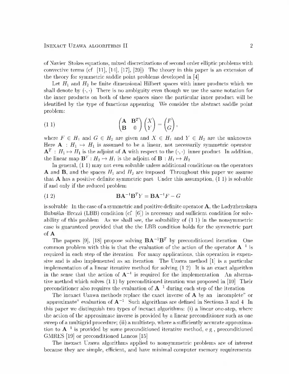
Inexact Uzawa algorithms II 211 �1�1 1

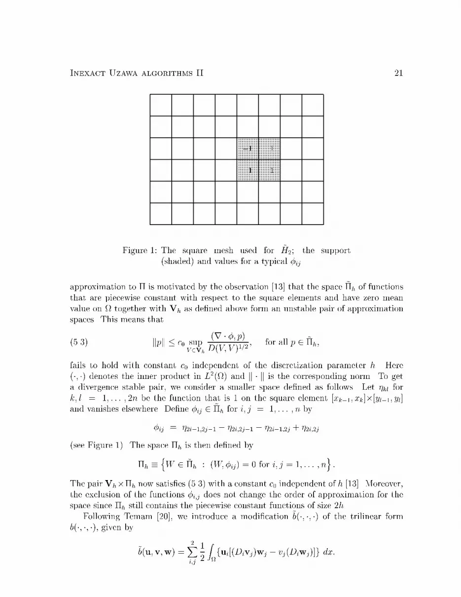
Figure 1: The square mesh used for ~H2; the support(shaded) and values for a typical �ijapproximation to � is motivated by the observation [13] that the space ~�h of functionsthat are piecewise constant with respect to the square elements and have zero meanvalue on together with Vh as de�ned above form an unstable pair of approximationspaces. This means thatkpk � c0 supV 2Vh (r � �; p)D(V; V )1=2 ; for all p 2 ~�h;(5.3)fails to hold with constant c0 independent of the discretization parameter h. Here(�; �) denotes the inner product in L2() and k � k is the corresponding norm. To geta divergence stable pair, we consider a smaller space de�ned as follows. Let �kl fork; l = 1; : : : ; 2n be the function that is 1 on the square element [xk�1; xk]�[yl�1; yl]and vanishes elsewhere. De�ne �ij 2 ~�h for i; j = 1; : : : ; n by�ij = �2i�1;2j�1 � �2i;2j�1 � �2i�1;2j + �2i;2j(see Figure 1). The space �h is then de�ned by�h � nW 2 ~�h : (W;�ij) = 0 for i; j = 1; : : : ; no :The pairVh��h now satis�es (5.3) with a constant c0 independent of h [13]. Moreover,the exclusion of the functions �i;j does not change the order of approximation for thespace since �h still contains the piecewise constant functions of size 2h.Following Temam [20], we introduce a modi�cation ~b(�; �; �) of the trilinear formb(�; �; �), given by ~b(u;v;w) = 2Xi;j 12 Zfui[(Divj)wj � vj(Diwj)]g dx:

Inexact Uzawa algorithms II 22The approximation to the solution of (5.2) is de�ned by the pair (X; Y ) 2 Vh � �hsatisfying �D(X; V ) + ~b(X;X; V ) + (Y;r � V ) = (f ; V ); for all V 2 Vh;(5.4a) (r �X;W ) = 0; for all W 2 �h:(5.4b)Note that the use of ~b(�; �; �) above is justi�ed by the observation that ~b(u; �; �) = b(u; �; �)for functions u which are divergence free. The form of ~b(�; �; �) guarantees the existenceof a solution to (5.4) (cf. [20]). The uniqueness is again subject to imposing conditionson the data � and f .To solve (5.4) we apply a Picard iteration of the following type (cf. [14]). Given aninitial approximation X0, we compute (X i; Y i), for i = 1; 2; :::, as the solution of thelinear system�D(X i; V ) + ~b(X i�1; X i; V ) + (Y i;r � V ) = (f ; V ); for all V 2 Vh;(5.5a) (r �X i;W ) = 0; for all W 2 �h:(5.5b)The convergence analysis of this algorithm is beyond the scope of the present paper.It is shown in [14] that the algorithm converges under the assumption that�2c2a > cbkfk�1;where ca and cb are the coercivity and boundedness constants of the trilinear formb(�; �; �). Such an assumption is enough to guarantee a unique solution of (5.2).The system (5.5) can be reformulated in the notation of the earlier sections. SetH1 = Vh and H2 = �h. LetB : H1 7! H2; (BU;W ) = (r � U;W ); for all U 2 H1; W 2 H2;BT : H2 7! H1; (BTW;V ) = (W;r � V ); for all V 2 H1; W 2 H2:During each iterative step, X i�1 is �xed so that we can de�neA : H1 7! H1; (AU; V ) = �D(U; V ) + ~b(X i�1; U; V ); for all U; V 2 H1:It follows that the solution (X i; Y i) of (5.5) satis�es (1.1) with F equal to the L2()projection of f into H1 and G = 0. Notice also that~b(u;v;w) = �~b(u;w;v):Therefore, As : H1 7! H1; (AsU; V ) = �D(U; V ); for all U; V 2 H1:(5.6)It is possible to show that (2.2) holds for A and As with a constant � proportionalto ��1 (cf. [20] and [11]). Moreover, it follows from (5.6) that (2.3) holds for As, B,

Inexact Uzawa algorithms II 23and BT as above with constant c0 independent of the mesh size h. This implies that(2.8) is satis�ed with QB = ��1I and bounded away from one independently of h.We still need to provide preconditioners for As. However, As consists of two copiesof the operator which results from a standard �nite element discretization of Dirichlet'sproblem. There has been an intensive e�ort focused on the development and analysisof preconditioners for such problems. For the examples in Section 6, we will use apreconditioning operator which results from a V-cycle variational multigrid algorithm.Such a preconditioner can be scaled so that (3.1) holds with � independent of the meshparameter h.Remark 5.1 It appears from the de�nition of the above operators that one has toinvert Gram matrices in order to evaluate the action of A, BT and B on vectors fromthe corresponding spaces. In practice, the H1 Gram matrix inversion is avoided bysuitable de�nition of the preconditioner QA. For the purpose of computation, theevaluation of Q�1A W forW 2 H1 is de�ned as a process which acts on the inner productdata (W; i) where f ig is the basis for H1. Moreover, from the de�nition of the Uzawa-like algorithms in the previous sections, it is clear that every occurrence of A or BT isfollowed by an evaluation of Q�1A . Thus the inversion of the Gram matrix is avoidedsince the data for the computation of Q�1A , ((BTQ; i) and (AV; i)), for any Q 2 H2and V 2 H1, can be computed by applying simple sparse matrices. In the case of thisspecial choice of H2, it is possible to compute the operator B in an economical way(see Remark 5 of [3]) and we can take QB to be ��1I. For more general spaces H2, theinversion of Gram matrices can be avoided by introducing a preconditioner QB whoseinverse is implemented acting on inner product data as in the H1 case above.Remark 5.2 By rescaling p, one can rewrite (5.1a) in the form��u +Re(u � r)u�rp = Re f ;where Re = ��1 is the Reynolds number of the ow. This results in a di�erent scaling ofthe discrete problem (5.4) which is better suited for implementation on �nite precisionmachines. We use this scaling in our examples in the next section.Remark 5.3 An alternative linearization of (5.4) can be de�ned by replacing ~b(X;X; V )with ~b(X i�1; X i�1; V ) which provides a di�erent Picard iteration. We will call this anexplicit Picard iteration because the nonlinear term is handled in an explicit fashion.This leads to a symmetric saddle point problem at each iteration. The inexact Uzawamethods analyzed in [4] can be used here. Even though the symmetric linear systemsare easier to solve, this linearization is a less robust method for computing branchesof solutions to (5.4) than the implicit linearization de�ned above, because the explicitPicard iteration breaks down for values of � where the implicit method converges. Weshall provide a comparison of these two methods in the next section.

Inexact Uzawa algorithms II 246 Numerical examplesIn this section we present the results from numerical experiments that illustrate thetheory developed in the earlier sections. Our goals here are �rst to demonstrate thee�ciency and the robustness of the new algorithms on the basis of a comparison betweenthe implicit and the explicit Picard iteration applied to a Navier-Stokes problem withknown analytic solution. Second, we show results from computations of a classical owproblem. The �nite element discretization de�ned in the previous section as well as thepressure rescaling according to Remark 5.2 are used in both cases.Our �rst experiment compares the performance of the implicit and the explicitmethods applied to the solution of (5.4) when the velocity X is given byX = x(1� x)y(1� y)x(1� x)y(1� y)! ;(6.1)and the pressure Y is given by Y = x� 12 :(6.2)Obviously, r �X 6= 0 so that the right-hand side of (5.4b) has to be adjusted appropri-ately.The implicit and explicit algorithms were tested for a set of di�erent Reynoldsnumbers (Re = 1; 10; 100; 1000), and di�erent mesh discretization parameters (h =1=8; 1=16; 1=32). Clearly, the exact solution de�ned above is very smooth in , withoutany singularities. The experiments described below show the asymptotic behavior ofthe error of the approximate solution computed by the two algorithms for the selectedset of Reynolds numbers.Four conditions were common in all experiments. First, at each Picard iteration,the corresponding linear problem was solved exactly (i.e. the L2 norm of the normal-ized residual was reduced until less than 10�15). Second, the nonlinear iteration wasconsidered to have converged when the L2 norm of the di�erence Ui � Ui�1 was lessthan 10�6. Here U consists of both velocity and pressure components. Third, the Pi-card iteration was started with zero initial guess. Fourth, we de�ned Q�1A to be theoperator which corresponds to one V{cycle sweep of variational multigrid with pointGauss-Seidel smoothing. The order of points in the Gauss-Seidel iteration was reversedin pre{ and post{smoothing. The preconditioner QB was provided by an appropriatescale of the identity operator in the pressure space (cf. Remark 5.1).In all experiments � = 0:1 was used when the nonsymmetric saddle point problem(5.4) was solved. This comes from the fact that � in (3.1) is independent of Re, becauseof the properties of the trilinear form ~b(�; �; �). The parameter � in this case was set to � =1=Re, where Re is the corresponding Reynolds number. Alternatively, � and � were setto one for the case of symmetric saddle point problem. These choices for � provided theappropriate scaling of QA according to the requirements of the corresponding algorithm

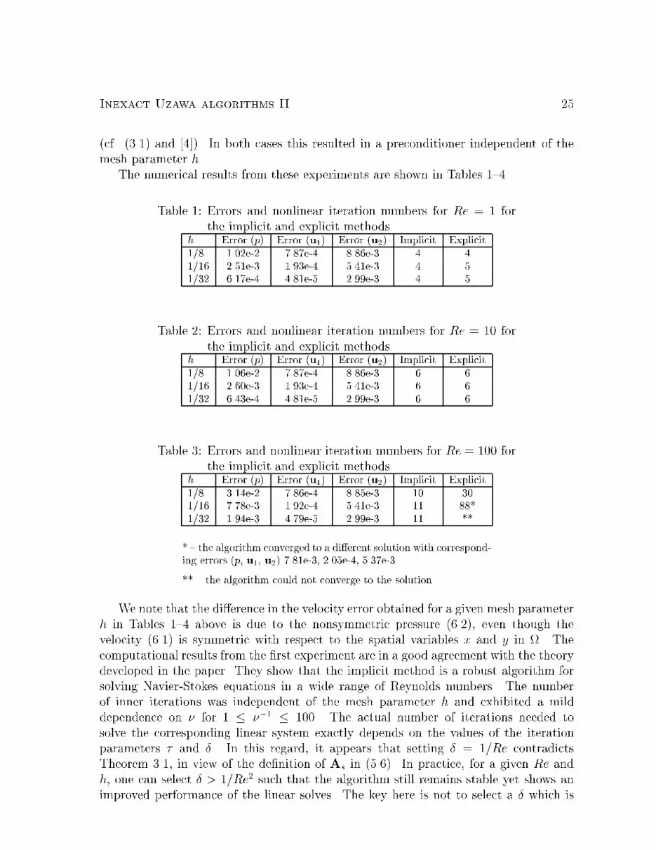
Inexact Uzawa algorithms II 25(cf. (3.1) and [4]). In both cases this resulted in a preconditioner independent of themesh parameter h.The numerical results from these experiments are shown in Tables 1{4.Table 1: Errors and nonlinear iteration numbers for Re = 1 forthe implicit and explicit methods.h Error (p) Error (u1) Error (u2) Implicit Explicit1/8 1.02e-2 7.87e-4 8.86e-3 4 41/16 2.51e-3 1.93e-4 5.41e-3 4 51/32 6.17e-4 4.81e-5 2.99e-3 4 5Table 2: Errors and nonlinear iteration numbers for Re = 10 forthe implicit and explicit methods.h Error (p) Error (u1) Error (u2) Implicit Explicit1/8 1.06e-2 7.87e-4 8.86e-3 6 61/16 2.60e-3 1.93e-4 5.41e-3 6 61/32 6.43e-4 4.81e-5 2.99e-3 6 6Table 3: Errors and nonlinear iteration numbers for Re = 100 forthe implicit and explicit methods.h Error (p) Error (u1) Error (u2) Implicit Explicit1/8 3.14e-2 7.86e-4 8.85e-3 10 301/16 7.78e-3 1.92e-4 5.41e-3 11 88*1/32 1.94e-3 4.79e-5 2.99e-3 11 *** { the algorithm converged to a di�erent solution with correspond-ing errors (p, u1, u2) 7.81e-3, 2.05e-4, 5.37e-3.** { the algorithm could not converge to the solution.We note that the di�erence in the velocity error obtained for a given mesh parameterh in Tables 1{4 above is due to the nonsymmetric pressure (6.2), even though thevelocity (6.1) is symmetric with respect to the spatial variables x and y in . Thecomputational results from the �rst experiment are in a good agreement with the theorydeveloped in the paper. They show that the implicit method is a robust algorithm forsolving Navier-Stokes equations in a wide range of Reynolds numbers. The numberof inner iterations was independent of the mesh parameter h and exhibited a milddependence on � for 1 � ��1 � 100. The actual number of iterations needed tosolve the corresponding linear system exactly depends on the values of the iterationparameters � and �. In this regard, it appears that setting � = 1=Re contradictsTheorem 3.1, in view of the de�nition of As in (5.6). In practice, for a given Re andh, one can select � > 1=Re2 such that the algorithm still remains stable yet shows animproved performance of the linear solves. The key here is not to select a � which is

Inexact Uzawa algorithms II 26Table 4: Errors and nonlinear iteration numbers for Re = 1; 000for the implicit and explicit methods.h Error (p) Error (u1) Error (u2) Implicit Explicit1/8*** 0.30 8.13e-4 8.82e-3 33 ****1/16*** 7.74e-2 3.57e-4 5.40e-3 38 ****1/32*** 1.85e-2 5.45e-5 2.99e-3 39 ******* { 50,000 inner iterations were taken for each Picard iterationin the implicit method because the inexact Uzawa algorithm couldnot reduce the residual below 1.0e-15 after 50,000 iterations whensolving the nonsymmetric saddle point problem. The norm of theresidual was on the order of 1.0e-11 after the �rst few nonlineariterations and less than 5.0e-15 towards the last Picard iterations.**** { the algorithm broke down.\too far away" from the safe zone. Indeed, setting � = q1=Re resulted in a divergentlinear solver during the Picard iteration which caused the whole solution process tobreak down. Also, as h ! 0, the method becomes more sensitive with respect todeviations from the hypothesis of Theorem 3.1. For example, the case of h = 1=128 andRe = 1; 000 in our second numerical test described below required � = 0:0001 to remainstable and broke down if � = 0:001. It is possible to tune up the parameters � and �for �xed � and h so that the number of inner iterations is minimized. We, however, didnot pursue this issue in the numerical experiments presented here.The implicit algorithm is well suited for calculations on �nite precision computers(double precision recommended). On the other hand, the explicit method is a rea-sonable approach to solving Navier-Stokes problems only for low Reynolds numbers(Re = 1; 10). It is a quite e�cient algorithm for such ow problems, outperformingthe implicit method by a factor of 10 to 1 or more. However, the stability of this al-gorithm deteriorates very fast as Re increases and the method becomes unstable forRe = 100 and Re = 1; 000. The case of Re = 1; 000 is a very di�cult computationalproblem which could only be solved by performing a large number of inner iterationsfor each Picard iteration. Clearly, the properties of A in this case are dominated byits skew-symmetric part. This in turn means that Q�1A is a poor approximation ofA�1. Nevertheless, the implicit method converged to the analytic solution branch forall values of h, showing the proper asymptotic behavior of the error. An e�cient precon-ditioned iterative method for approximating the inverse of the strongly nonsymmetricoperator A combined with the multistep algorithm from Section 4 could result in abetter method for solving the steady-state Navier-Stokes equations with high Reynoldsnumbers.Our second numerical experiment is the calculation of the ow in a cavity. Thecavity domain is the unit square and the ow is caused by a tangential velocity �eldapplied to one of the square sides in the absence of other body forces. Since all forcesare independent of time, the ow in this case limits to a steady-state which is modeled

Inexact Uzawa algorithms II 27

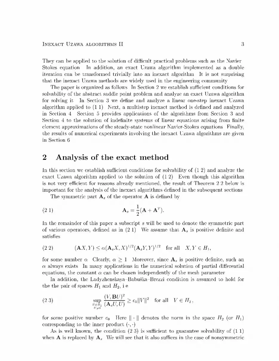
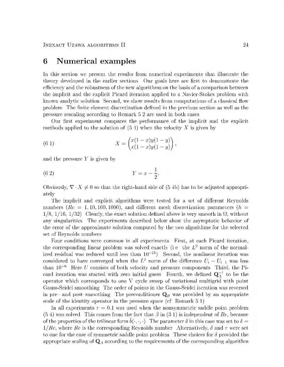
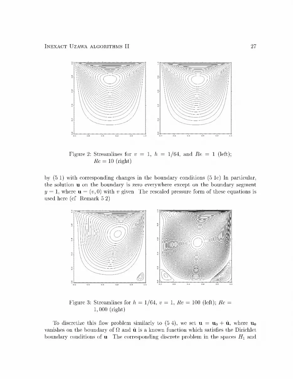
Figure 2: Streamlines for v = 1, h = 1=64, and Re = 1 (left);Re = 10 (right).by (5.1) with corresponding changes in the boundary conditions (5.1c) In particular,the solution u on the boundary is zero everywhere except on the boundary segmenty = 1, where u = (v; 0) with v given. The rescaled pressure form of these equations isused here (cf. Remark 5.2).

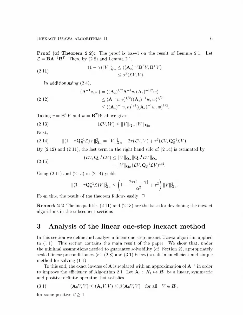
Figure 3: Streamlines for h = 1=64, v = 1, Re = 100 (left); Re =1; 000 (right).To discretize this ow problem similarly to (5.4), we set u = u0 + u, where u0vanishes on the boundary of and u is a known function which satis�es the Dirichletboundary conditions of u. The corresponding discrete problem in the spaces H1 and

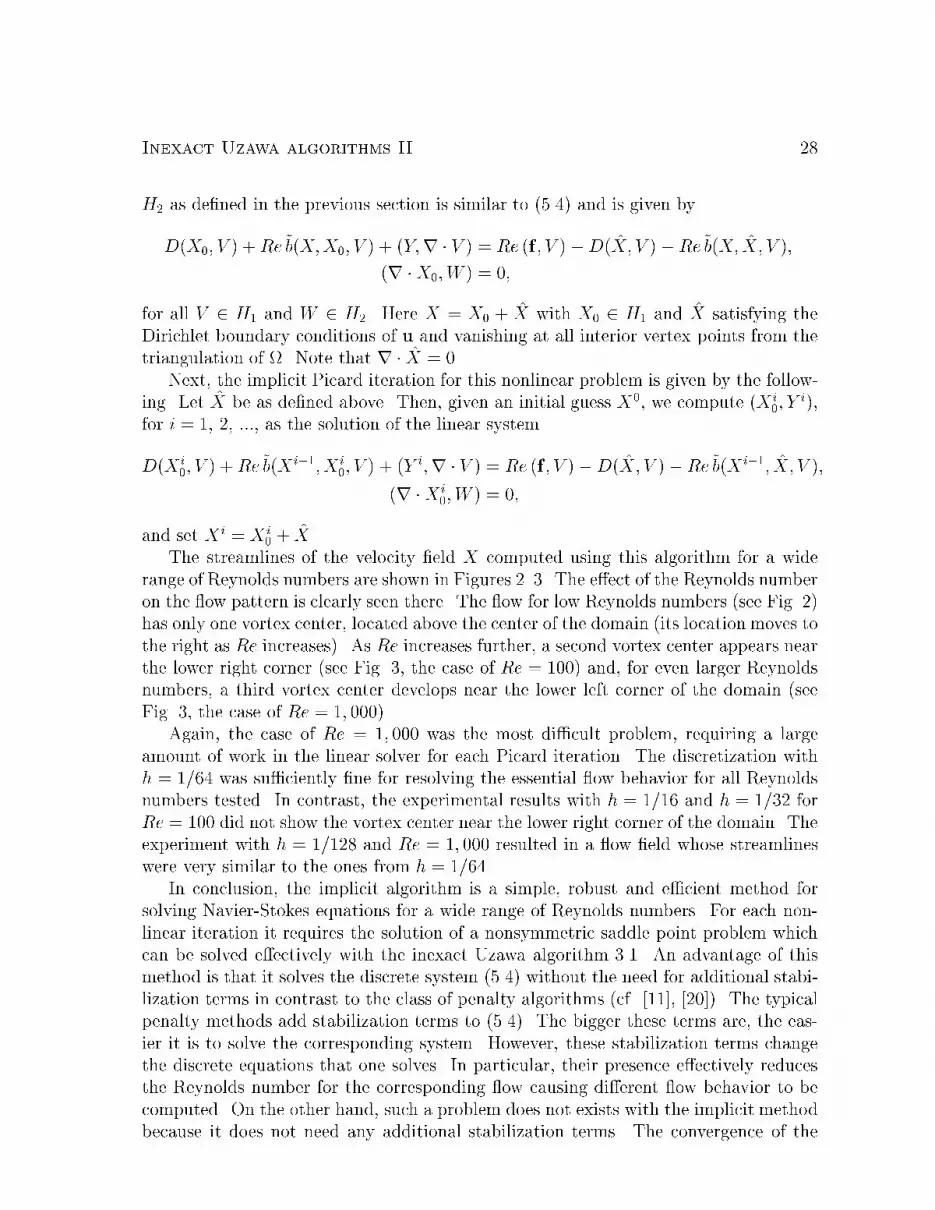
Inexact Uzawa algorithms II 28H2 as de�ned in the previous section is similar to (5.4) and is given byD(X0; V ) +Re~b(X;X0; V ) + (Y;r � V ) = Re (f ; V )�D(X; V )� Re~b(X; X; V );(r �X0;W ) = 0;for all V 2 H1 and W 2 H2. Here X = X0 + X with X0 2 H1 and X satisfying theDirichlet boundary conditions of u and vanishing at all interior vertex points from thetriangulation of . Note that r � X = 0.Next, the implicit Picard iteration for this nonlinear problem is given by the follow-ing. Let X be as de�ned above. Then, given an initial guess X0, we compute (X i0; Y i),for i = 1; 2; :::, as the solution of the linear systemD(X i0; V ) +Re~b(X i�1; X i0; V ) + (Y i;r � V ) = Re (f ; V )�D(X; V )�Re~b(X i�1; X; V );(r �X i0;W ) = 0;and set X i = X i0 + X.The streamlines of the velocity �eld X computed using this algorithm for a widerange of Reynolds numbers are shown in Figures 2{3. The e�ect of the Reynolds numberon the ow pattern is clearly seen there. The ow for low Reynolds numbers (see Fig. 2)has only one vortex center, located above the center of the domain (its location moves tothe right as Re increases). As Re increases further, a second vortex center appears nearthe lower right corner (see Fig. 3, the case of Re = 100) and, for even larger Reynoldsnumbers, a third vortex center develops near the lower left corner of the domain (seeFig. 3, the case of Re = 1; 000).Again, the case of Re = 1; 000 was the most di�cult problem, requiring a largeamount of work in the linear solver for each Picard iteration. The discretization withh = 1=64 was su�ciently �ne for resolving the essential ow behavior for all Reynoldsnumbers tested. In contrast, the experimental results with h = 1=16 and h = 1=32 forRe = 100 did not show the vortex center near the lower right corner of the domain. Theexperiment with h = 1=128 and Re = 1; 000 resulted in a ow �eld whose streamlineswere very similar to the ones from h = 1=64.In conclusion, the implicit algorithm is a simple, robust and e�cient method forsolving Navier-Stokes equations for a wide range of Reynolds numbers. For each non-linear iteration it requires the solution of a nonsymmetric saddle point problem whichcan be solved e�ectively with the inexact Uzawa algorithm 3.1. An advantage of thismethod is that it solves the discrete system (5.4) without the need for additional stabi-lization terms in contrast to the class of penalty algorithms (cf. [11], [20]). The typicalpenalty methods add stabilization terms to (5.4). The bigger these terms are, the eas-ier it is to solve the corresponding system. However, these stabilization terms changethe discrete equations that one solves. In particular, their presence e�ectively reducesthe Reynolds number for the corresponding ow causing di�erent ow behavior to becomputed. On the other hand, such a problem does not exists with the implicit methodbecause it does not need any additional stabilization terms. The convergence of the

Inexact Uzawa algorithms II 29linear iteration at each Picard iteration is guaranteed only by the appropriate scalingof QA and the appropriate choice of the parameters � and � .References[1] K. Arrow, L. Hurwicz, and H. Uzawa. Studies in Nonlinear Programming. StanfordUniversity Press, Stanford, CA, 1958.[2] J.H. Bramble and J.E. Pasciak. Iterative Techniques for Time Dependent StokesProblems. Inter. Jour. Computers and Math. with Applic. (to appear).[3] J.H. Bramble and J.E. Pasciak. A preconditioning technique for inde�nite systemsresulting from mixed approximations of elliptic problems. Math. Comp., 50:1{18,1988.[4] J.H. Bramble, J.E. Pasciak, and A.T. Vassilev. Analysis of the inexact Uzawaalgorithm for saddle point problems. SIAM J. Numer. Anal., 34:1072{1092, 1997.[5] J.H. Bramble, Z. Leyk, and J.E. Pasciak. Iterative schemes for non-symmetric andinde�nite elliptic boundary value problems. Math. Comp., 60:1{22, 1993.[6] F. Brezzi and M. Fortin. Mixed and Hybrid Finite Element Methods. Springer-Verlag, New York, 1991.[7] X.-C. Cai. An additive Schwarz algorithm for nonselfadjoint elliptic equations. InT. Chan, R. Glowinski, J. Pe�riaux, and O. Widlund, editors, Third InternationalSymposium on Domain Decomposition Methods for Partial Di�erential Equations.SIAM, Phil. PA, 1990.[8] P.G. Ciarlet. The Finite Element Method for Elliptic Problems. North-Holland,New York, 1978.[9] H. Elman. Preconditioning for the steady-state Navier-Stokes equations with lowviscosity. Technical Report CS-TR-3712, Department of Computer Science, Uni-versity of Maryland, College Park, MD 20742, 1996.[10] H. Elman and D. Silvester. Fast nonsymmetric iterations and preconditioning forNavier-Stokes equations. Technical Report CS-TR-3283, Univ. Maryland, CollegePark, June 1994.[11] V. Girault and P.A. Raviart. Finite Element Approximation of the Navier-StokesEquations. Lecture Notes in Math. # 749, Springer-Verlag, New York, 1981.[12] W. Hackbush. Multi-Grid Methods and Applications. Springer-Verlag, Berlin, 1985.

Inexact Uzawa algorithms II 30[13] C. Johnson and J. Pitk�aranta. Analysis of some mixed �nite element methodsrelated to reduced integration. Math. Comp., 38:375{400, 1982.[14] O.A. Karakashian. On a Galerkin-Lagrange multiplier method for the stationaryNavier-Stokes equations. SIAM J. Numer. Anal., 19:909{923, 1982.[15] C. Lanczos. An iteration method for the solution of the eigenvalue problem oflinear di�erential and integral operators. J. Res. National Bureau of Standards,45:255{282, 1950.[16] J.L. Lions and E. Magenes. Probl�emes aux Limites non Homog�enes et Applications,volume 1. Dunod, Paris, 1968.[17] M.M. Liu, J. Wang, and N.-N. Yan. New error estimates for approximate solutionsof convection-di�usion problems by mixed and discontinuous Galerkin methods.SIAM J. Numer. Anal. Submitted.[18] M.F. Murphy and A.J. Wathen. On preconditioning for the Oseen equations.Technical Report AM 95-07, Department of Mathematics, University of Bristol,1995.[19] Y. Saad and M.H. Schultz. Gmres: A generalized minimal residual algorithm forsolving nonsymmetric linear systems. SIAM J. Sci. Stat. Comput., 7:856 { 869,1986.[20] R. Temam. Navier-Stokes Equations. North-Holland Publishing Co., New York,1977.[21] J. Xu. Two-grid dicretization techniques. SIAM J. Numer. Anal., 33:1759{1777,1996.