Embed Size (px)
Citation preview

6Indirect estimations of land
66 Eurostat-OECD compilation guide on land estimation
Indirect estimations of land66.1. Chapter 5 described how the value of land can be
directly estimated by multiplying the area of each parcel of land by an appropriate price. However, it might be dif‑ficult to collect separate (and reliable) price information for the estimation of the land without any structures or crops. One of the challenges in estimating the value of land un‑derlying structures or crops is that often only information is available on real estate that is sold on the market (i.e. the combined value). Thus, if separate information on the price of land without structures or crops is not available then an indirect estimation method could be used.
6.2. In this chapter three indirect estimation approach‑es are discussed. Indeed, there is no ‘best’ method; which of these approaches should be used, heavily depends on the available data sources.
6.3. Because the indirect method often relies on the to‑tal real estate value as the starting point of the calculations this chapter starts by explaining how the total real estate value, that is the combined value of land and structures, can be estimated (Chapter 6.1) before discussing each of the in‑direct approaches.
6.4. Subsequently three approaches to separate land from the structures are discussed in this chapter: the re‑sidual approach (Chapter 6.2), the land‑to‑structure ratio approach (Chapter 6.3) and the hedonic approach (Chap‑ter 6.4). In this chapter the importance of service lives and depreciation for indirect estimates of land is introduced as well (Chapter 6.5).
6.1 Methods for estimating the combined value of land and structures
Introduction
6.5. The combined value of land and structures (CV) is often called the total value of a property (real estate). The CV combines the value of the structure and the value of a particular plot of land attached. It is often the only infor‑mation available from the real estate market.
6.6. The market value of a given property is most influ‑enced by its location and use. This information combined with the characteristics of the building such as size, age, maintenance (including major repairs and renovations) that best reflects the difference between new and existing buildings, helps determine the market value. Relevant data sources used for the CV estimation are one of the main is‑sues in obtaining the appropriate estimates.
6.7. There are many reasons for differences among countries in the quality of estimates of the CV: social and natural factors, such as population density and share of population in the rural areas. Climate, hydrology or topog‑raphy can also have great influence on transaction price data.
6.8. Below it is explained how the CV can be calculated by using different data sources on real estate characteristics, such as location, size of the structure, age, etc. combined with appropriate transaction price data mostly available from sales registers. This chapter discusses two methods used in many countries to obtain estimates of the CV — appraisals and ‘quantity, times, price’ approach.
Definition and characteristics
6.9. According to the balance sheets valuation require‑ments in the national accounts system, the CV should be presented at actual or at estimated current market prices. However, the vast majority of existing properties are not sold in a reference period; for the economy as a whole, mar‑ket values of the CV must be estimated. Focus shall be put on how market values can be obtained for the two differ‑ent models used for estimation of the CV as well as basic information on the construction of price indices for both methods.
6.10. The first method is a bottom‑up type of approach, where each individual unit is specified in great detail. Then the individual units can be added up to give the total val‑ue. The second method is a top‑down approach where the known quantity information at the country level is first di‑vided into regional levels. Subsequently the CV of a country is obtained by summing the regional CV values. Neverthe‑less, in practice the choice of the approach depends on the availability of data sources and the country’s compilation practice. Mixed approaches can be used as well.
6.11. This chapter starts with discussing the appraisal method, a bottom‑up approach that builds the total real estate value from individual characteristics of the real es‑tate (e.g. location, price, size, age, etc.). This information is usually provided from a well‑built property registration system in a country combining information from different administrative databases governed by law to form a nation‑wide real estate register (see Figure 6.1). Micro level charac‑teristics of a property available from the real estate register are then linked together to form larger regional systems of real estate information, sometimes on many territorial lev‑els, until a complete top level system is formed in order to obtain the appraised total real estate value in a country.
6.12. The second method, called ‘quantity, times, price’ approach, is a top‑down approach also known as stepwise
67Eurostat-OECD compilation guide on land estimation
Indirect estimations of land 6design, where, for instance, the number of dwellings in a country is broken down into regions. First, an overview of the national system is formulated, specifying but not detail‑ing any first level regions. Subsequently, each region is elab‑orated in greater detail using the local prices on a real estate market. It is important that the sum of regional estimates of the CV is consistent with the national total of the CV.
6.13. In general, depending on the available data sourc‑es, the CV concept can be mainly applied for estimating dif‑ferent types of residential and non‑residential real estates. Ideally, the data would be based on real estate transaction price data. Although the CV for a non‑residential real estate (i.e. commercial buildings, unmarketable buildings such as schools) is usually not based on actual transactions; there‑fore, various methods should be applied such as a discount‑ed cash flows method or a depreciated value of construction costs method. For more information, see the Dutch case study at the end of this chapter and further information in De Haan (2013) and Van den Bergen (2010). In addition, if transaction prices for the combined value of forest real es‑tate (or for cultivated land) are available in a country, the CV concept can be used as well. Chapter 8.1 describes how the ‘quantity, times, price’ approach could be applied for wooded land available for wood supply. Problems associated with the decomposition of the CV into the value of the tim‑ber and the value of the underlying land is also addressed in Chapter 8.1, more particularly in a Finnish case study.
Description of the methods
Appraisals
6.14. Assessed real estate values (or assessments) are re‑ferred to as appraisals (Eurostat, 2013). An appraisal takes the physical characteristics (e.g. size, age, maintenance) and loca‑tion of each real estate into account when forming a judgment about value. The value of the plot on which the building stands is as a rule included in the value of the appraised real estate.
6.15. In many countries, official government assess‑ments are available for all real estate, because such data are needed for real estate taxation. Many countries are likely to have an official property valuation office that provides peri‑odic appraisals of all taxable real estate properties (i.e. tax assessment). In other words, for these countries the entire stock of buildings (including both structures and the under‑lying land) for the period under consideration is valued.
6.16. In a typical appraisal, there are three approaches to estimate the CV: (i) the cost approach, where the ap‑praiser relies upon information about input costs for build‑ing a replacement of the structure and adds an estimated land value; (ii) the income approach, where the appraiser relies on the income from the real estate being valued and
on a capitalisation rate; (iii) and the sales comparison ap‑proach, where the appraiser relies upon comparable sales (see International Association of Assessing Officers (IAAO), 2013).
Data requirements
6.17. The derivation of the combined market value for all properties (traded and non‑traded) relies on the availability of data on a micro level. A crucial prerequisite is a real estate register in a country (see Figure 6.1) where actual transac‑tions obtained from the sales register can be related to com‑prehensive real estate information on prices that are deter‑mined by physical (and possibly other) characteristics such as size, age, maintenance, etc. and most importantly, location. These administrative sources, further explained in Chapter 4, are e.g. land cadastre, land register, sales register, etc.
6.18. The accuracy of values depends foremost on the completeness and accuracy of real estate characteristics and adequate market data. Accurate valuation of real estate by any method requires descriptions of land and building characteristics. Data on real estate characteristics should be updated regularly in response to changes brought about by new construction, new parcels, remodelling, demolition or destruction. The most efficient method involves building per‑mits and/or aerial photography identifying new or previously unrecorded construction or land use (see IAAO, 2013).
6.19. According to IAAO (2013), to determine a real es‑tate value, the appraiser must rely upon valuation equations, tables, and schedules developed through a detailed analysis of the local real estate market. Thus, the model should in‑clude all real estate characteristics that influence value in the local marketplace.
6.20. For residential properties, geographic stratification is appropriate when the value of real estate varies signifi‑cantly among areas and each area is large enough to provide adequate market data (sales).
6.21. As regards sectorisation, the real estate register or similar administrative sources used in an appraisal system usually includes information on ownership which is required for a successful allocation of the CV by sector and industry in the national accounts system. See Chapter 7 for more details.

68 Eurostat-OECD compilation guide on land estimation
Indirect estimations of land6Figure 6.1: Basic input data sources for the real estate register
Property Census(optional)
LAND REGISTERLAND CADASTRE
BUILDINGS CADASTRE
CENTRALPOPULATION
REGISTER
BUSINESSREGISTER
SALESREGISTER
REAL ESTATEREGISTER
Source: TF on Land and other non-financial assets
Numerical example
6.22. The example below illustrates how a house could be appraised (assessed) in practice, following the sales compar‑ison approach (see GURS (2011)). Nevertheless, there could be many other ways to calculate these values. A key data source for conducting the appraisal (assessment) is the sales register or a similar data source where transaction price data of similar properties have been analysed. As an output of this analysis, the reference real estate is produced, having average characteristics such as size, age, and maintenance. The reference real estate is then used as a unit of comparison as presented in the numerical example. The method is tech‑nically quite sophisticated, based on well‑developed statisti‑cal modelling to simulate the real estate market. Countries use various methods to produce such models e.g. hedonic regression methods, sometimes in combination with visual inspections (34) and local market information (IAAO, 2013).
6.23. Assessments can be more clearly presented in the form of value tables (VT) and rating tables, which take into account the quality characteristics of the real estate as well as the value zones. Value zones reflect the influence of the location on the value of the real estate.
6.24. In the valuation modelling process prior to the appraisal where VTs are created, value zones represent in‑dependent variables for different locations in a country. In other words, value zones are areas in which the same type of real estate has similar value (Pšunder and Tominc, 2013). Thus, the VT of each real estate is defined according to the value zone in which the real estate is located (Smodiš, 2011).
6.25. Before paying attention to how the valuation model works in practice, the different parts of a real estate are con‑sidered. The real estate usually combines the values of the building and the plot of land on which the building stands including yards and gardens (see Figure 6.2).
Figure 6.2: The structure of the combined value of a real estate
Value of the houseincluding plot on whichthe building stands
(VHouse)
Value of the landancillary to the housei.e. parcel includingyards and gardens aspart of the house
(VLand)
Source: The Surveying and Mapping Authority of the Republic of Slovenia
6.26. In general the combined value of the real estate (CV) can be estimated by the following valuation model:
(1) CV = (VHouse + VLand) * FDF
Where
CV Combined value of the real estate (total value)VHouse Value of the house (including the value of the
land underlying the house (35))VLand Value of the land ancillary to the house (i.e. yards
and gardens)FDF Correction factor for the distance from linear
facilities such as motorways, public highways or railways for the house
6.27. The example describes the calculation of the mar‑ket value of a house (one‑dwelling buildings (36)) — the CV from equation (1) — for which physical characteristics such as location, size of the house and the plot, and information
(34) On-site verification of real estate characteristics should be conducted at least once every 4 to 6 years (IAAO, 2013).
(35) The land underlying the house is defined as part of the area of the land on which the building stands
(36) According to the Classification of Types of Constructions (1998).
69Eurostat-OECD compilation guide on land estimation
Indirect estimations of land 6on maintenance of the house are key inputs known by the appraiser. The calculation of each of the two components of equation (1) will be elaborated separately.
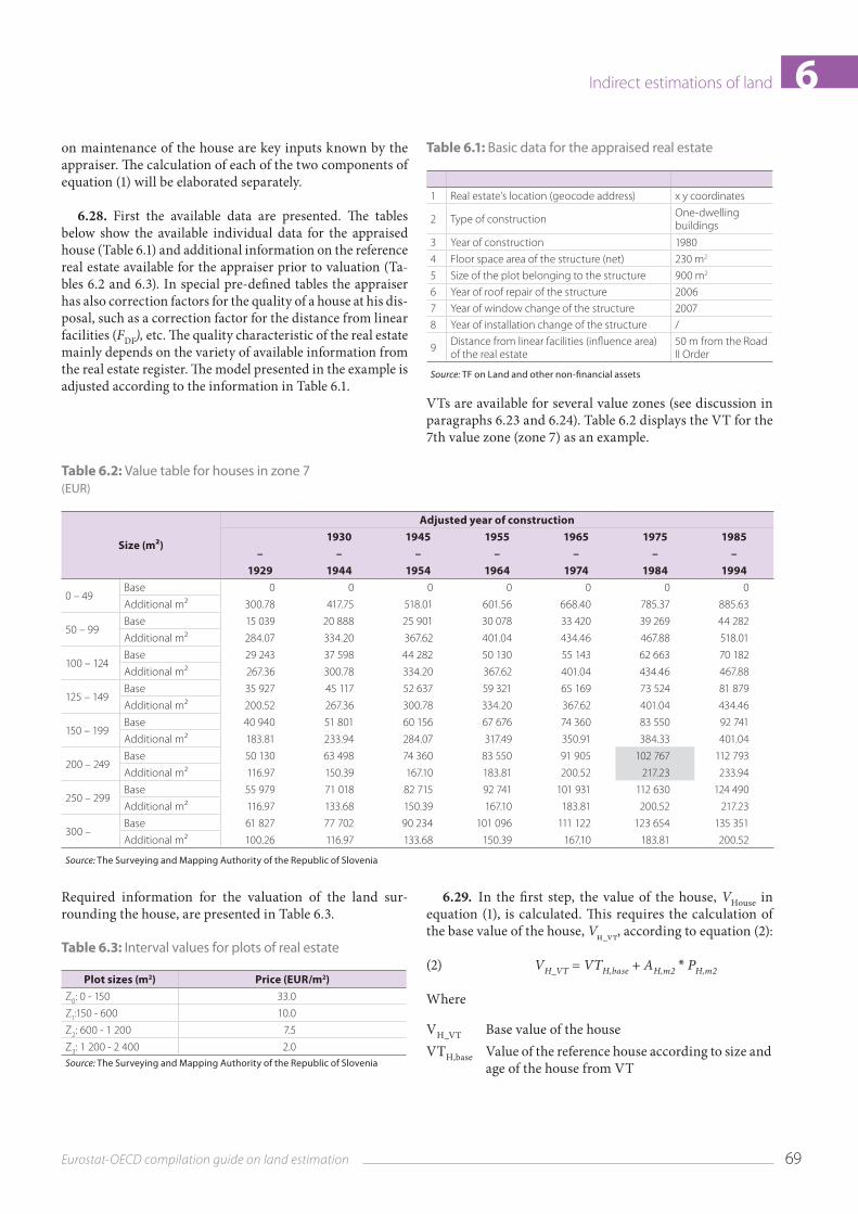
6.28. First the available data are presented. The tables below show the available individual data for the appraised house (Table 6.1) and additional information on the reference real estate available for the appraiser prior to valuation (Ta‑bles 6.2 and 6.3). In special pre‑defined tables the appraiser has also correction factors for the quality of a house at his dis‑posal, such as a correction factor for the distance from linear facilities (FDF), etc. The quality characteristic of the real estate mainly depends on the variety of available information from the real estate register. The model presented in the example is adjusted according to the information in Table 6.1.
Table 6.1: Basic data for the appraised real estate
1 Real estate’s location (geocode address) x y coordinates
2 Type of construction One-dwelling buildings
3 Year of construction 1980
4 Floor space area of the structure (net) 230 m2
5 Size of the plot belonging to the structure 900 m2
6 Year of roof repair of the structure 2006
7 Year of window change of the structure 2007
8 Year of installation change of the structure /
9 Distance from linear facilities (influence area) of the real estate
50 m from the Road II Order
Source: TF on Land and other non-financial assets
VTs are available for several value zones (see discussion in paragraphs 6.23 and 6.24). Table 6.2 displays the VT for the 7th value zone (zone 7) as an example.
Table 6.2: Value table for houses in zone 7(EUR)
Size (m²)
Adjusted year of construction1930 1945 1955 1965 1975 1985
– – – – – – –1929 1944 1954 1964 1974 1984 1994
0 – 49Base 0 0 0 0 0 0 0
Additional m² 300.78 417.75 518.01 601.56 668.40 785.37 885.63
50 – 99Base 15 039 20 888 25 901 30 078 33 420 39 269 44 282
Additional m² 284.07 334.20 367.62 401.04 434.46 467.88 518.01
100 – 124Base 29 243 37 598 44 282 50 130 55 143 62 663 70 182
Additional m² 267.36 300.78 334.20 367.62 401.04 434.46 467.88
125 – 149Base 35 927 45 117 52 637 59 321 65 169 73 524 81 879
Additional m² 200.52 267.36 300.78 334.20 367.62 401.04 434.46
150 – 199Base 40 940 51 801 60 156 67 676 74 360 83 550 92 741
Additional m² 183.81 233.94 284.07 317.49 350.91 384.33 401.04
200 – 249Base 50 130 63 498 74 360 83 550 91 905 102 767 112 793
Additional m² 116.97 150.39 167.10 183.81 200.52 217.23 233.94
250 – 299Base 55 979 71 018 82 715 92 741 101 931 112 630 124 490
Additional m² 116.97 133.68 150.39 167.10 183.81 200.52 217.23
300 –Base 61 827 77 702 90 234 101 096 111 122 123 654 135 351
Additional m² 100.26 116.97 133.68 150.39 167.10 183.81 200.52
Source: The Surveying and Mapping Authority of the Republic of Slovenia
Required information for the valuation of the land sur‑rounding the house, are presented in Table 6.3.
Table 6.3: Interval values for plots of real estate
Plot sizes (m2) Price (EUR/m2)Z0: 0 - 150 33.0
Z1:150 - 600 10.0
Z2: 600 - 1 200 7.5
Z3: 1 200 - 2 400 2.0 Source: The Surveying and Mapping Authority of the Republic of Slovenia
6.29. In the first step, the value of the house, VHouse in equation (1), is calculated. This requires the calculation of the base value of the house, Vh_vt, according to equation (2):
(2) VH_VT = VTH,base + AH,m2 * PH,m2
Where
VH_VT Base value of the house VTH,base Value of the reference house according to size and
age of the house from VT
70 Eurostat-OECD compilation guide on land estimation
Indirect estimations of land6
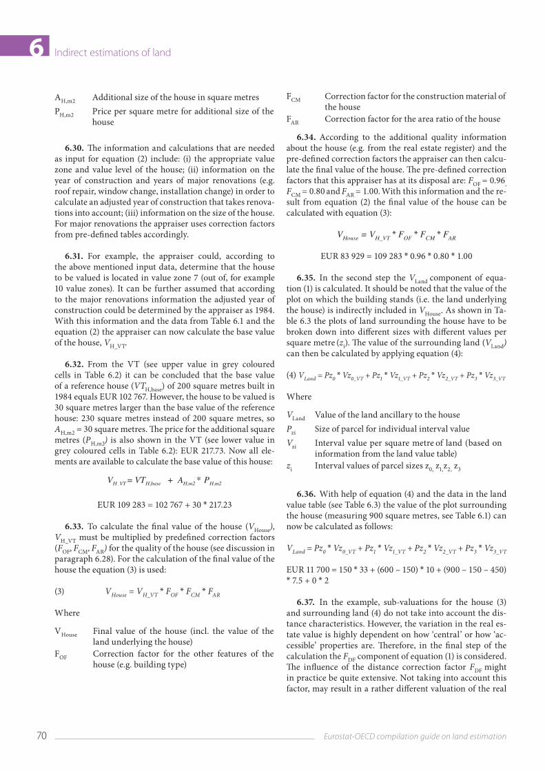
AH,m2 Additional size of the house in square metresPH,m2 Price per square metre for additional size of the
house
6.30. The information and calculations that are needed as input for equation (2) include: (i) the appropriate value zone and value level of the house; (ii) information on the year of construction and years of major renovations (e.g. roof repair, window change, installation change) in order to calculate an adjusted year of construction that takes renova‑tions into account; (iii) information on the size of the house. For major renovations the appraiser uses correction factors from pre‑defined tables accordingly.
6.31. For example, the appraiser could, according to the above mentioned input data, determine that the house to be valued is located in value zone 7 (out of, for example 10 value zones). It can be further assumed that according to the major renovations information the adjusted year of construction could be determined by the appraiser as 1984. With this information and the data from Table 6.1 and the equation (2) the appraiser can now calculate the base value of the house, VH_VT.
6.32. From the VT (see upper value in grey coloured cells in Table 6.2) it can be concluded that the base value of a reference house (VTH,base) of 200 square metres built in 1984 equals EUR 102 767. However, the house to be valued is 30 square metres larger than the base value of the reference house: 230 square metres instead of 200 square metres, so AH,m2 = 30 square metres. The price for the additional square metres (PH,m2) is also shown in the VT (see lower value in grey coloured cells in Table 6.2): EUR 217.73. Now all ele‑ments are available to calculate the base value of this house:
EUR 109 283 = 102 767 + 30 * 217.23
6.33. To calculate the final value of the house (VHouse), VH_VT must be multiplied by predefined correction factors (FOF, FCM, FAR) for the quality of the house (see discussion in paragraph 6.28). For the calculation of the final value of the house the equation (3) is used:
(3) VHouse = VH_VT * FOF * FCM * FAR
Where
VHouse Final value of the house (incl. the value of the land underlying the house)
FOF Correction factor for the other features of the house (e.g. building type)
FCM Correction factor for the construction material of the house
FAR Correction factor for the area ratio of the house
6.34. According to the additional quality information about the house (e.g. from the real estate register) and the pre‑defined correction factors the appraiser can then calcu‑late the final value of the house. The pre‑defined correction factors that this appraiser has at its disposal are: FOF = 0.96, FCM = 0.80 and FAR = 1.00. With this information and the re‑sult from equation (2) the final value of the house can be calculated with equation (3):
VHouse = VH_VT * FOF * FCM * FAR
EUR 83 929 = 109 283 * 0.96 * 0.80 * 1.00
6.35. In the second step the VLand component of equa‑tion (1) is calculated. It should be noted that the value of the plot on which the building stands (i.e. the land underlying the house) is indirectly included in VHouse. As shown in Ta‑ble 6.3 the plots of land surrounding the house have to be broken down into different sizes with different values per square metre (zi). The value of the surrounding land (VLand) can then be calculated by applying equation (4):
(4) VLand = Pz0 * Vz0_VT + Pz1 * Vz1_VT + Pz2 * Vz2_VT + Pz3 * Vz3_VT
Where
VLand Value of the land ancillary to the housePzi Size of parcel for individual interval value Vzi Interval value per square metre of land (based on
information from the land value table) zi Interval values of parcel sizes z0, z1,z2, z3
6.36. With help of equation (4) and the data in the land value table (see Table 6.3) the value of the plot surrounding the house (measuring 900 square metres, see Table 6.1) can now be calculated as follows:
VLand = Pz0 * Vz0_VT + Pz1 * Vz1_VT + Pz2 * Vz2_VT + Pz3 * Vz3_VT
EUR 11 700 = 150 * 33 + (600 – 150) * 10 + (900 – 150 – 450) * 7.5 + 0 * 2
6.37. In the example, sub‑valuations for the house (3) and surrounding land (4) do not take into account the dis‑tance characteristics. However, the variation in the real es‑tate value is highly dependent on how ‘central’ or how ‘ac‑cessible’ properties are. Therefore, in the final step of the calculation the FDF component of equation (1) is considered. The influence of the distance correction factor FDF might in practice be quite extensive. Not taking into account this factor, may result in a rather different valuation of the real
71Eurostat-OECD compilation guide on land estimation
Indirect estimations of land 6estate. With the help of a geographic information system (or other information) the distance to, for example, the central business district or the nearest commercial centre can be determined. This information can be used for the estima‑tion of the distance correction factor FDF.
6.38. In this example, it is assumed that the appraiser knows from the real estate register the distance of the real estate from facilities like motorways, etc. Based on this in‑formation the distance correction factor (FDF)for the loca‑tion of the house and surrounding land is estimated at 0.9. Now all information is available to determine the combined value (CV) of the house:
EUR 86 067 = (83 929 + 11 770) * 0.9
6.39. The example above shows how the system of ap‑praisals works and how the CV is calculated for just one individual unit. The CV for all dwellings in the total econo‑my can be obtained by repeating this exercise for all dwell‑ings in the economy and adding up the outcomes: it is the bottom‑up approach first introduced in paragraph 6.11. Information about the owner and shares of owning rights obtained from the land cadastre should be used to allocate the estimations to institutional sectors. These data should be updated on a regular basis using the information from the business register for legal persons and the central popu‑lation register for natural persons.
6.40. In most countries, data used for calculating the ap‑praised CV are not as detailed as presented in this numeri‑cal example. Nevertheless, countries should follow interna‑tional standards and recommendations such as IAAO and other standards when producing CV by appraisal methods.
Strengths and weaknesses
6.41. The major advantage of appraisals is full coverage. However, the use and interpretation of data gathered by ap‑praisals should be done with some caution. Studies show that appraisals appear to lag the true sales prices, falling sig‑nificantly below in hot markets and remaining significantly above in cold markets. Not surprisingly, the worst perfor‑mance of appraisals occurred during the 2007–2008 finan‑cial crisis (see Cannon et al., 2011 and Devaney et al., 2011).
6.42. There are several studies that have examined the reliability of commercial real estate appraisals, but accord‑ing to Cannon (ibid.), most of them are now quite dated and rely upon information from only one cycle of the commer‑cial real estate market. Cannon (ibid.) therefore proposes to measure the accuracy of an appraisal as the percentage dif‑ference between the sales price and the appraised value.
6.43. Another concern is that appraisals are not updated frequently. Consequently, they match the market value at its reference period registered in prices of a few years back (i.e. historic prices). In this case the appraisal cannot be used di‑rectly but must be taken forward in time by using appropri‑ate price indices.
6.44. In this context, the most appropriate price indices for dwellings are the residential property price indices (RP‑PIs). RPPIs are based on the market transactions for new and existing dwellings and as such they cover the land and the structure components jointly. Various methods are pos‑sible to control the changes in the quality mix of the trans‑acted dwellings from one period to the next, in order to pro‑duce constant quality RPPIs (37).
6.45. However, because of their reference to the observed market prices, RPPIs give an average price change that re‑flects weights usually based on the subset of dwellings that are transacted during the period (38). As long as the distribu‑tion of transactions by stratum is not representative for the stock distribution, the use of these RPPIs for stocks revalu‑ation gives a bias due to a compositional effect. The use of stock‑weighted RPPIs would therefore be preferable to avoid this kind of bias. However, while stock‑weighted RPPIs are also treated in the Handbook on Residential Property Pric‑es Indices (Eurostat, 2013), they are, in general, less readily available than transaction‑weighted RPPIs.
Other information
6.46. Methods that involve some controls of quality by using multiple regression models with the real estate at‑tributes as independent variables are hedonic methods. In this context the use of the ‘sale price appraisal ratio’ (SPAR) method is to be mentioned, which uses information on matched sales and appraisals to construct house price indi‑ces. This method is explained in detail for the case of house price indices in the RPPI Handbook and by Bourassa et. al. (2006). The advantage of the SPAR method as compared to the hedonic regression methods is that information on only a few property characteristics is needed: assessed values (re‑lating to a common reference period), possibly some strati‑fication variables, and addresses to merge the data files if the selling prices and appraisals come from different data sources (Eurostat, 2013). Bourassa et al. (2006) noted that the SPAR method could be applied for constructing land price indices as well but only if available information per‑mits this. This method requires a system of regularly and with sufficient frequency updated appraisals.
(37) These include for example the stratification and the hedonic approach. For an in depth review of the various methods see the RPPI Handbook referenced in footnote 21.
(38) The precise scheme for internal weights depends on the various compilation practices, which in turn are constrained by the sources available.
72 Eurostat-OECD compilation guide on land estimation
Indirect estimations of land66.47. Diewert and Shimizu (2014) discuss constructing price indices for non‑residential real estate for national ac‑counting purposes, as well as decomposing the real estate price into land and structure price indices. Their empirical analysis of commercial offices is based on the assessment of appraisal data from the Japanese Real Estate Invest‑ment Trust (REIT) market in the Tokyo area. A variant of the builder’s model (39) applied to the commercial property assessed values is presented where assessed values present a dependent variable enabling decomposition of overall val‑ue into separate land and structure components. The build‑er’s model already used for valuing a residential property is a hedonic model in which the structure price component is constrained exogenously. This model has been applied to residential property sales by de Haan and Diewert (2011), Diewert, de Haan and Hendriks (2011a) (2011b) and Diew‑ert and Shimizu (2013). In addition to the assessed value information, the age of the building, the floor space area of the structure, the area of the land plot, and the building costs per square metre and the costs of the land per square metre were used in the model as well. By using the builder’s model, which has been traditionally applied to residen‑tial property sales, Diewert and Shimizu suggest a special case of the hedonic approach and suggest that the applied method is practical and could be used by statistical agencies to improve their balance sheets estimates for commercial properties (ibid.).
6.48. If a country operates a well‑organised econo‑my‑wide public assessment system for real estate, e.g. for dwellings, this information can be used to measure the CV. Usually countries for taxation purposes assess each private‑owned individual real estate. This tax assessment value may be, as an alternative to the numerical example above, adjusted to the market price by comparing the ra‑tio of the real estate transaction price to the tax assessment value. Here, it is assumed that the ratio for traded real estate will be representative of that of untraded. If more and more real estate transaction data are obtainable during the ref‑erence period, the readjusted tax assessment value can be more closely approximated to the market price of the real estate. Meanwhile, this comparison process for each indi‑vidual real estate can be applied at the national level and enable national accountants to compute the total CV of the relevant real estate across the country.
6.49. Lastly, it should be noted that costs of ownership transfer (SNA 2008 paragraph 10.51), such as notary, real estate agent, surveyor services, transfer tax, etc., are not in‑cluded in the appraisals.
(39) See Diewert, W.E. and C. Shimizu, ‘Residential Property Price Indexes for Tokyo’, 2014. Available at http://www.unece.org/fileadmin/DAM/stats/documents/ece/ces/ge.22/2014/Diewert_and_Shimizu_Paper_01.pdf
‘Quantity times price’ approach
6.50. The ‘quantity, times, price’ approach is another option to calculate the CV of land and structures by using quantity and real estate price information. There are many ways to calculate these two variables depending on the availability of data sources. In most countries a common way is to estimate the CV for residential properties by ap‑plying average values of dwellings, derived from sales data (price), to population and housing census based estimates of the number of dwellings (quantity). Quantity estimates that do not incorporate the census data could be less reliable.
6.51. It should be noted that this approach is rarely used for estimation of the CV of non‑residential real estate. How‑ever, it can be applied in case of cultivated land.
Data requirements
6.52. The main idea that underlies this approach is the availability of plausible market values of dwellings includ‑ing land which can be observed on the real estate market. The assumption is that real estate properties sold are rep‑resentative of the population of the real estate properties including those not sold. Price information from actual transactions (sales) is then used to infer an average value of all the properties not sold during the reference period. Using actual transactions data on sales of properties is one of the better ways to estimate the price component. See the Australian case study at the end of this chapter.
6.53. By stratifying the stock according to price‑deter‑mining characteristics of properties, compositional effects can be reduced. It is desirable for sales data to only be used to infer the value of similar properties. The finer the strati‑fication, the more representative and less compositionally affected the data become.
6.54. The sales data should provide broad geographical coverage, encompassing both urban and rural areas. This is especially important in countries where regional differences have significant impact on the real estate prices.
6.55. Data sources supporting the ‘price’ part of this approach can be sales registers or similar administrative sources where information on the transfer of ownership of dwellings and land is recorded. Whenever a real estate is sold, information about the timing of the sale (date of contract), the real estate sold (e.g. information about the lo‑cation and quality characteristics of the building) and the price paid can be made available from administrative sourc‑es, possibly integrated with other sources. Similar databases have been developed by several countries for the compila‑tion of RPPIs, which measure house price movements usu‑ally on a quarterly basis. See the Australian case study for an
73Eurostat-OECD compilation guide on land estimation
Indirect estimations of land 6approach that combines sales data and RPPI information in the estimation of the ‘price’ component.
6.56. The quantity part of this approach, the number of dwellings, can be derived from a combination of census data as a starting point and additional information from con‑struction statistics on the number of completions and con‑versions that occur between two censuses. The estimated stock between two censuses should be compared with other data sources such as cadastral data.
6.57. In order to stratify the data so that an appropriate price can be matched with the ‘quantity’ information, it is useful to classify dwellings into different types, e.g. separate houses, attached dwellings (e.g. semi‑detached, row and ter‑race houses and flats, units and apartments, etc.). This infor‑mation can be derived from census data as well. Neverthe‑less, there is no single convention for classification; it can be different from country to country.
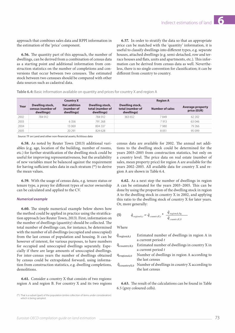
Table 6.4: Basic information available on quantity and prices for country X and region A
Year
Country X Region ADwelling stock,
census (number of dwellings)
Net addition (number of dwellings)
Dwelling stock, total (number of
dwellings)
Dwelling stock, total (number of
dwellings)Number of sales Average property
price (EUR)
2002 784 912 784 912 363 652 7 849 62 202
2003 6 356 791 268 7 913 63 046
2004 13 069 804 337 7 980 79 266
2005 20 291 824 628 8 051 95 099
Source: TF on Land and other non-financial assets; fictitious data
6.58. As noted by Reuter Town (2013) additional vari‑ables (e.g. age, location of the building, number of rooms, etc.) for further stratification of the dwelling stock could be useful for improving representativeness, but the availability of new variables must be balanced against the requirement for having sufficient sales data in each stratum (40) to derive the mean values.
6.59. With the usage of census data, e.g. tenure status or tenure type, a proxy for different types of sector ownership can be calculated and applied to the CV.
Numerical example
6.60. The simple numerical example below shows how the method could be applied in practice using the stratifica‑tion approach (see Reuter Town, 2013). First, information on the number of dwellings (quantity) should be collected. The total number of dwellings can, for instance, be determined with the number of all dwellings (occupied and unoccupied) from the last census of population and housing. It can be however of interest, for various purposes, to have numbers for occupied and unoccupied dwellings separately. Espe‑cially if there are large amounts of unoccupied dwellings. For inter‑census years the number of dwellings obtained by census could be extrapolated forward, using informa‑tion from construction statistics, e.g. dwelling completions, demolitions.
6.61. Consider a country X that consists of two regions: region A and region B. For country X and its two regions
(40) That is a subset (part) of the population (entire collection of items under consideration) which is being sampled.
census data are available for 2002. The annual net addi‑tions to the dwelling stock could be determined for the years 2003–2005 from construction statistics, but only on a country level. The price data on real estate (number of sales, mean property price) for region A are available for the years 2002–2005. All available data for country X and re‑gion A are shown in Table 6.4.
6.62. As a next step the number of dwellings in region A can be estimated for the years 2003–2005. This can be done by using the proportion of the dwelling stock in region A to the dwelling stock in country X in 2002, and applying this ratio to the dwelling stock of country X for later years. Or, more generally:
(5) q ̂ regionA,t = q ̂ countryX,t *q ̂ regionA,0q
q ̂ countryX,0
Where
Estimated number of dwellings in region A in a current period tEstimated number of dwellings in country X in a current period tNumber of dwellings in region A according to the last census Number of dwellings in country X according to the last census
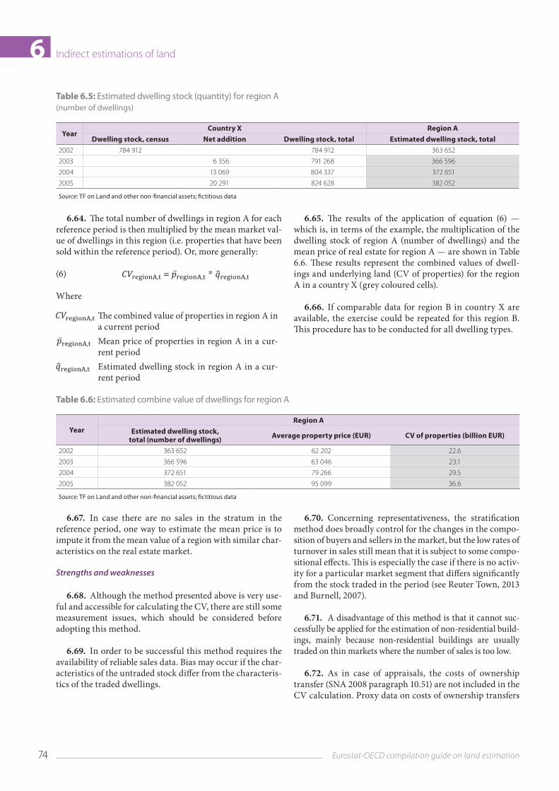
6.63. The result of the calculations can be found in Table 6.5 (grey coloured cells).
74 Eurostat-OECD compilation guide on land estimation
Indirect estimations of land6Table 6.5: Estimated dwelling stock (quantity) for region A(number of dwellings)
YearCountry X Region A
Dwelling stock, census Net addition Dwelling stock, total Estimated dwelling stock, total2002 784 912 784 912 363 652
2003 6 356 791 268 366 596
2004 13 069 804 337 372 651
2005 20 291 824 628 382 052
Source: TF on Land and other non-financial assets; fictitious data
6.64. The total number of dwellings in region A for each reference period is then multiplied by the mean market val‑ue of dwellings in this region (i.e. properties that have been sold within the reference period). Or, more generally:
(6)
Where
The combined value of properties in region A in a current periodMean price of properties in region A in a cur‑rent periodEstimated dwelling stock in region A in a cur‑rent period
6.65. The results of the application of equation (6) — which is, in terms of the example, the multiplication of the dwelling stock of region A (number of dwellings) and the mean price of real estate for region A — are shown in Table 6.6. These results represent the combined values of dwell‑ings and underlying land (CV of properties) for the region A in a country X (grey coloured cells).
6.66. If comparable data for region B in country X are available, the exercise could be repeated for this region B. This procedure has to be conducted for all dwelling types.
Table 6.6: Estimated combine value of dwellings for region A
YearRegion A
Estimated dwelling stock, total (number of dwellings) Average property price (EUR) CV of properties (billion EUR)
2002 363 652 62 202 22.6
2003 366 596 63 046 23.1
2004 372 651 79 266 29.5
2005 382 052 95 099 36.6
Source: TF on Land and other non-financial assets; fictitious data
6.67. In case there are no sales in the stratum in the reference period, one way to estimate the mean price is to impute it from the mean value of a region with similar char‑acteristics on the real estate market.
Strengths and weaknesses
6.68. Although the method presented above is very use‑ful and accessible for calculating the CV, there are still some measurement issues, which should be considered before adopting this method.
6.69. In order to be successful this method requires the availability of reliable sales data. Bias may occur if the char‑acteristics of the untraded stock differ from the characteris‑tics of the traded dwellings.
6.70. Concerning representativeness, the stratification method does broadly control for the changes in the compo‑sition of buyers and sellers in the market, but the low rates of turnover in sales still mean that it is subject to some compo‑sitional effects. This is especially the case if there is no activ‑ity for a particular market segment that differs significantly from the stock traded in the period (see Reuter Town, 2013 and Burnell, 2007).
6.71. A disadvantage of this method is that it cannot suc‑cessfully be applied for the estimation of non‑residential build‑ings, mainly because non‑residential buildings are usually traded on thin markets where the number of sales is too low.
6.72. As in case of appraisals, the costs of ownership transfer (SNA 2008 paragraph 10.51) are not included in the CV calculation. Proxy data on costs of ownership transfers
75Eurostat-OECD compilation guide on land estimation
Indirect estimations of land 6could for instance be obtained from the survey on gross fixed capital formation.
Case study estimating the combined value of land and structures: The Netherlands
Data sources
This case study presents the Dutch approach for the ap‑praisal of non‑residential buildings including the underly‑ing land, the combined value.
As explained by De Haan (2013), Van den Bergen et al. (2010), De Vries et al. (2009), in the Netherlands for tax pur‑poses the so‑called WOZ‑value of every dwelling is derived from tax registers (41). The WOZ‑value pertains to the com‑bined value of land and structure and in case of dwellings; it is based on actual prices of dwellings sold. Therefore, it provides an accurate estimate of the market price. Also for most non‑residential buildings including land, WOZ‑values are available (42). However, unlike WOZ‑values of dwell‑ings, in many cases WOZ‑values of non‑residential build‑ings cannot be directly based on selling prices. The reason for this is that often few to none comparable transactions of non‑residential buildings exist. As an alternative to transac‑tion data, tax authorities apply various methods for estimat‑ing the WOZ‑value of non‑residential buildings. In order to do so, a distinction is made between marketable buildings (commercial real estate such as office buildings and stores) and unmarketable buildings (e.g. school buildings, hos‑pitals or an energy plant). For commercial real estate the WOZ‑value is mostly determined by the net present value of future rentals. In case of unmarketable non‑residential buildings valuation is frequently based on the depreciated value of construction costs. Both methods rely on extensive guidelines.
(41) In the Netherlands, some taxes are based on the value of the dwelling or building that people own. This is laid down in the Dutch Real Estate Appraisal Act (WOZ). The value that the government subsequently assigns to each dwelling and building is called the WOZ-value.
(42) Except for tax-exempted buildings such as churches.
Methods
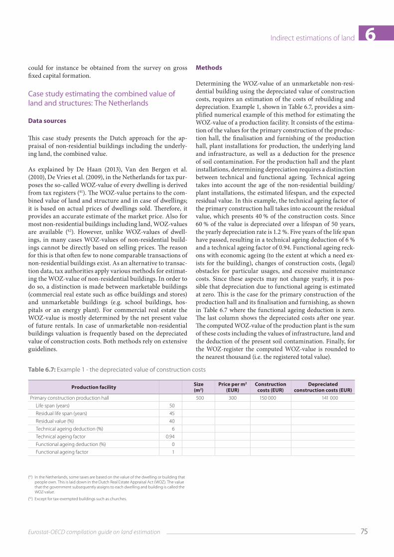
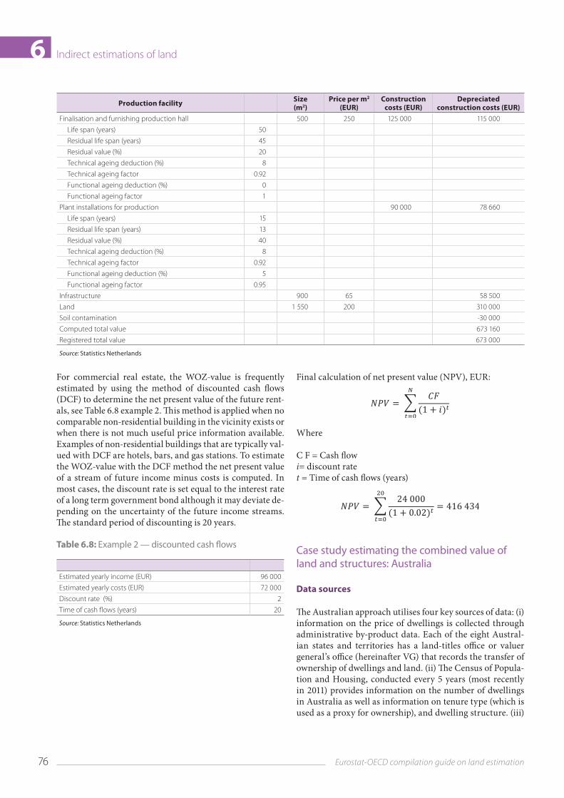
Determining the WOZ‑value of an unmarketable non‑resi‑dential building using the depreciated value of construction costs, requires an estimation of the costs of rebuilding and depreciation. Example 1, shown in Table 6.7, provides a sim‑plified numerical example of this method for estimating the WOZ‑value of a production facility. It consists of the estima‑tion of the values for the primary construction of the produc‑tion hall, the finalisation and furnishing of the production hall, plant installations for production, the underlying land and infrastructure, as well as a deduction for the presence of soil contamination. For the production hall and the plant installations, determining depreciation requires a distinction between technical and functional ageing. Technical ageing takes into account the age of the non‑residential building/plant installations, the estimated lifespan, and the expected residual value. In this example, the technical ageing factor of the primary construction hall takes into account the residual value, which presents 40 % of the construction costs. Since 60 % of the value is depreciated over a lifespan of 50 years, the yearly depreciation rate is 1.2 %. Five years of the life span have passed, resulting in a technical ageing deduction of 6 % and a technical ageing factor of 0.94. Functional ageing reck‑ons with economic ageing (to the extent at which a need ex‑ists for the building), changes of construction costs, (legal) obstacles for particular usages, and excessive maintenance costs. Since these aspects may not change yearly, it is pos‑sible that depreciation due to functional ageing is estimated at zero. This is the case for the primary construction of the production hall and its finalisation and furnishing, as shown in Table 6.7 where the functional ageing deduction is zero. The last column shows the depreciated costs after one year. The computed WOZ‑value of the production plant is the sum of these costs including the values of infrastructure, land and the deduction of the present soil contamination. Finally, for the WOZ‑register the computed WOZ‑value is rounded to the nearest thousand (i.e. the registered total value).
Table 6.7: Example 1 - the depreciated value of construction costs
Production facility Size (m2)
Price per m2 (EUR)
Construction costs (EUR)
Depreciated construction costs (EUR)
Primary construction production hall 500 300 150 000 141 000
Life span (years) 50
Residual life span (years) 45
Residual value (%) 40
Technical ageing deduction (%) 6
Technical ageing factor 0.94
Functional ageing deduction (%) 0
Functional ageing factor 1
76 Eurostat-OECD compilation guide on land estimation
Indirect estimations of land6
For commercial real estate, the WOZ‑value is frequently estimated by using the method of discounted cash flows (DCF) to determine the net present value of the future rent‑als, see Table 6.8 example 2. This method is applied when no comparable non‑residential building in the vicinity exists or when there is not much useful price information available. Examples of non‑residential buildings that are typically val‑ued with DCF are hotels, bars, and gas stations. To estimate the WOZ‑value with the DCF method the net present value of a stream of future income minus costs is computed. In most cases, the discount rate is set equal to the interest rate of a long term government bond although it may deviate de‑pending on the uncertainty of the future income streams. The standard period of discounting is 20 years.
Table 6.8: Example 2 — discounted cash flows
Estimated yearly income (EUR) 96 000
Estimated yearly costs (EUR) 72 000
Discount rate (%) 2
Time of cash flows (years) 20
Source: Statistics Netherlands
Final calculation of net present value (NPV), EUR:
Where
C F = Cash flowi= discount ratet = Time of cash flows (years)
Case study estimating the combined value of land and structures: Australia
Data sources
The Australian approach utilises four key sources of data: (i) information on the price of dwellings is collected through administrative by‑product data. Each of the eight Austral‑ian states and territories has a land‑titles office or valuer general’s office (hereinafter VG) that records the transfer of ownership of dwellings and land. (ii) The Census of Popula‑tion and Housing, conducted every 5 years (most recently in 2011) provides information on the number of dwellings in Australia as well as information on tenure type (which is used as a proxy for ownership), and dwelling structure. (iii)
Production facility Size (m2)
Price per m2 (EUR)
Construction costs (EUR)
Depreciated construction costs (EUR)
Finalisation and furnishing production hall 500 250 125 000 115 000
Life span (years) 50
Residual life span (years) 45
Residual value (%) 20
Technical ageing deduction (%) 8
Technical ageing factor 0.92
Functional ageing deduction (%) 0
Functional ageing factor 1
Plant installations for production 90 000 78 660
Life span (years) 15
Residual life span (years) 13
Residual value (%) 40
Technical ageing deduction (%) 8
Technical ageing factor 0.92
Functional ageing deduction (%) 5
Functional ageing factor 0.95
Infrastructure 900 65 58 500
Land 1 550 200 310 000
Soil contamination -30 000
Computed total value 673 160
Registered total value 673 000
Source: Statistics Netherlands
77Eurostat-OECD compilation guide on land estimation
Indirect estimations of land 6Information on additions to the dwelling stock is obtained from Australian Bureau of Statistics (ABS) survey data (the Building Activity Survey). (iv) The residential property price index (RPPI) is used to calculate mean property prices where complete VG’s coverage is not yet available. The index is primarily compiled using VG’s data. These data are sup‑plemented with mortgage loan data from banks and other mortgage lenders to provide a better estimate of residential property price change in the most recent periods.
Methods
The approach in Australia to calculate a total value of resi‑dential dwellings including land is to stratify the dwelling stock by geography and dwelling type, and calculate total values (using ‘quantity times price’) for each strata, and then aggregate up to sub‑national and national estimates. All calculations used the combined values of the structures and land and exclude any vacant land. This approach is for residential land only; it does not apply to rural and com‑mercial land.
Data from the census is used to create a point in time esti‑mate of the number of dwellings in the stock. To get quar‑terly estimates of the number of dwellings, the ABS esti‑mates the net additions to the stock since the latest census. Estimates of gross additions to the stock are available from the Building Activity Survey conducted by the ABS.
The long term realisation rate, the rate at which gross addi‑tions to the stock results in net additions to the stock, is ap‑plied to gross additions data in order to derive net additions to the stock. Net additions to the stock are added to census counts to get quarterly estimates of the number of dwellings in the stock (i.e. the quantity).
Quantity information is calculated at the state level. Strata level quantity estimates are subsequently derived from state totals by using dwelling shares (i.e. the percentage of total dwellings each strata contained at the latest census).
Once a complete set of VG’s data are available, strata level price estimates are derived by taking the arithmetic mean
price of dwellings sold in the quarter. Where insufficient data are available, the mean price is imputed from a larger geography region to which the strata belongs.
Of note, due to the way sales data are recorded in Australia (lag between the exchange and settlement dates), it takes approximately 6–9 months to get VG’s data on all transac‑tions. Direct calculation of the CV in time for publication (6 weeks after the end of the reference period) is not pos‑sible. It is necessary to use an alternative data source for the latest two quarters of data to calculate a mean price where the most recent mean price is moved in line with the move‑ments of the RPPI. This is because movements in the RPPI have been shown to correlate very well with movements in the final estimates (based on VG’s data).
For example, in the December quarter the RPPI is 104.5, then 103.4 for September and 102.1 for June (fictitious data). VG price data is only available for June, so for region A, the mean price is, for example, 532 000 Australian dollars (AUD). To calculate the mean price for September extrapo‑late June’s VG mean price by the RPPI, that is 103.4/102.1 * AUD 532 000 = AUD 538 773, and for December it is 104.5/103.4 * AUD 538 773 = AUD 544 504. When the next quarterly estimate occurs (i.e. the March quarter in this ex‑ample), the September quarter mean price is re‑calculated using the newly available VG transactions data and then the change in the RPPI is used to obtain the December and March values.
Once price and quantity level data are available for each stratum, values are calculated, and aggregated to produce state and Australia level totals.
State level estimates of the total values are then sub‑divided into sectors (households, government and non‑financial corporations) using information on Tenure Type from the latest census.
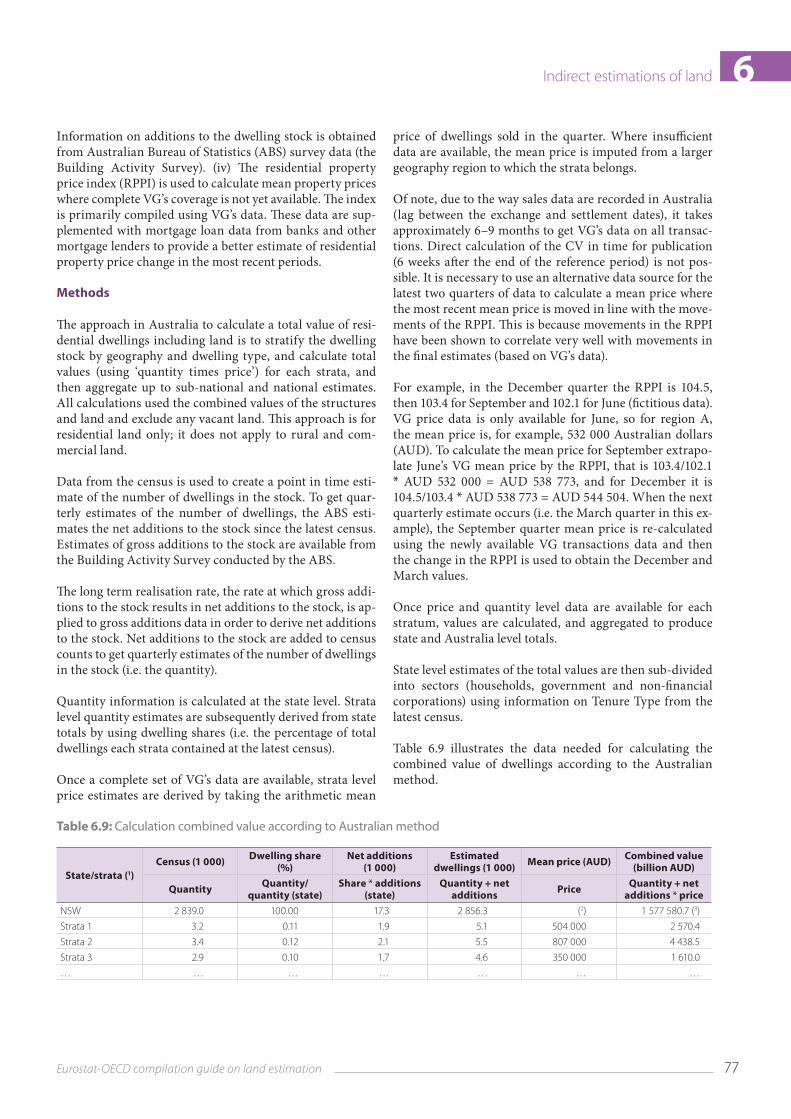
Table 6.9 illustrates the data needed for calculating the combined value of dwellings according to the Australian method.
Table 6.9: Calculation combined value according to Australian method
State/strata (1)Census (1 000) Dwelling share
(%)Net additions
(1 000)Estimated
dwellings (1 000) Mean price (AUD) Combined value (billion AUD)
Quantity Quantity/quantity (state)
Share * additions (state)
Quantity + net additions Price Quantity + net
additions * priceNSW 2 839.0 100.00 17.3 2 856.3 (2) 1 577 580.7 (3)
Strata 1 3.2 0.11 1.9 5.1 504 000 2 570.4
Strata 2 3.4 0.12 2.1 5.5 807 000 4 438.5
Strata 3 2.9 0.10 1.7 4.6 350 000 1 610.0
… … … … … … …
78 Eurostat-OECD compilation guide on land estimation
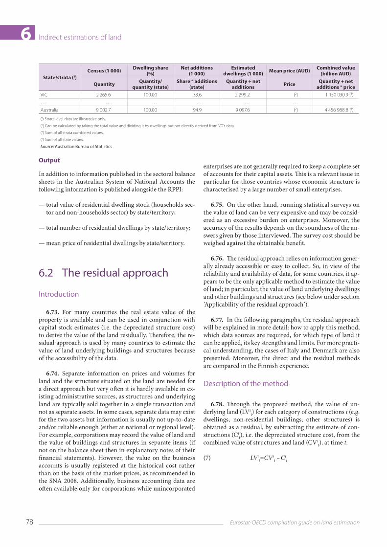
Indirect estimations of land6
State/strata (1)Census (1 000) Dwelling share
(%)Net additions
(1 000)Estimated
dwellings (1 000) Mean price (AUD) Combined value (billion AUD)
Quantity Quantity/quantity (state)
Share * additions (state)
Quantity + net additions Price Quantity + net
additions * priceVIC 2 265.6 100.00 33.6 2 299.2 (2) 1 150 030.9 (3)
… … … … … …
Australia 9 002.7 100.00 94.9 9 097.6 (2) 4 456 988.8 (4)
(1) Strata level data are illustrative only.
(2) Can be calculated by taking the total value and dividing it by dwellings but not directly derived from VG’s data.
(3) Sum of all strata combined values.
(4) Sum of all state values.
Source: Australian Bureau of Statistics
Output
In addition to information published in the sectoral balance sheets in the Australian System of National Accounts the following information is published alongside the RPPI:
— total value of residential dwelling stock (households sec‑tor and non‑households sector) by state/territory;
— total number of residential dwellings by state/territory;
— mean price of residential dwellings by state/territory.
6.2 The residual approach
Introduction
6.73. For many countries the real estate value of the property is available and can be used in conjunction with capital stock estimates (i.e. the depreciated structure cost) to derive the value of the land residually. Therefore, the re‑sidual approach is used by many countries to estimate the value of land underlying buildings and structures because of the accessibility of the data.
6.74. Separate information on prices and volumes for land and the structure situated on the land are needed for a direct approach but very often it is hardly available in ex‑isting administrative sources, as structures and underlying land are typically sold together in a single transaction and not as separate assets. In some cases, separate data may exist for the two assets but information is usually not up‑to‑date and/or reliable enough (either at national or regional level). For example, corporations may record the value of land and the value of buildings and structures in separate items (if not on the balance sheet then in explanatory notes of their financial statements). However, the value on the business accounts is usually registered at the historical cost rather than on the basis of the market prices, as recommended in the SNA 2008. Additionally, business accounting data are often available only for corporations while unincorporated
enterprises are not generally required to keep a complete set of accounts for their capital assets. This is a relevant issue in particular for those countries whose economic structure is characterised by a large number of small enterprises.
6.75. On the other hand, running statistical surveys on the value of land can be very expensive and may be consid‑ered as an excessive burden on enterprises. Moreover, the accuracy of the results depends on the soundness of the an‑swers given by those interviewed. The survey cost should be weighed against the obtainable benefit.
6.76. The residual approach relies on information gener‑ally already accessible or easy to collect. So, in view of the reliability and availability of data, for some countries, it ap‑pears to be the only applicable method to estimate the value of land; in particular, the value of land underlying dwellings and other buildings and structures (see below under section ‘Applicability of the residual approach’).
6.77. In the following paragraphs, the residual approach will be explained in more detail: how to apply this method, which data sources are required, for which type of land it can be applied, its key strengths and limits. For more practi‑cal understanding, the cases of Italy and Denmark are also presented. Moreover, the direct and the residual methods are compared in the Finnish experience.
Description of the method
6.78. Through the proposed method, the value of un‑derlying land (LVi
t) for each category of constructions i (e.g. dwellings, non‑residential buildings, other structures) is obtained as a residual, by subtracting the estimate of con‑structions (Ci
t), i.e. the depreciated structure cost, from the combined value of structures and land (CVi
t), at time t.
(7) LVit=CVi
t – Cit
79Eurostat-OECD compilation guide on land estimation
Indirect estimations of land 66.79. The total value of land underlying buildings and
structures at time t (LVt) is obtained by aggregating all the estimates LVi
t
(8) LVt= ∑ni=1LVi
t
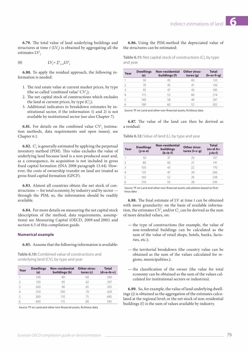
6.80. To apply the residual approach, the following in‑formation is needed:
1. The real estate value at current market prices, by type (the so called ‘combined value’ CVi
t);2. The net capital stock of constructions which excludes
the land at current prices, by type (Cit);
3. Additional indicators to breakdown estimates by in‑stitutional sector, if the information 1) and 2) is not available by institutional sector (see also Chapter 7).
6.81. For details on the combined value CVit (estima‑
tion methods, data requirements and open issues), see Chapter 6.1.
6.82. Cit is generally estimated by applying the perpetual
inventory method (PIM). This value excludes the value of underlying land because land is a non‑produced asset and, as a consequence, its acquisition is not included in gross fixed capital formation (SNA 2008 paragraph 13.44). How‑ever, the costs of ownership transfer on land are treated as gross fixed capital formation (GFCF).
6.83. Almost all countries obtain the net stock of con‑structions — for total economy, by industry and by sector — through the PIM; so, the information should be readily available.
6.84. For more details on measuring the net capital stock (description of the method, data requirements, assump‑tions) see Measuring Capital (OECD, 2009 and 2001) and section 6.5 of this compilation guide.
Numerical example
6.85. Assume that the following information is available:
Table 6.10: Combined value of constructions and underlying land (CV), by type and year
Year Dwellings (a)
Non-residential buildings (b)
Other struc-tures (c)
Total (d=a+b+c)
1 100 80 60 240
2 150 85 62 297
3 200 90 65 355
4 250 100 70 420
5 300 110 75 485
6 400 115 80 595
Source: TF on Land and other non-financial assets, fictitious data
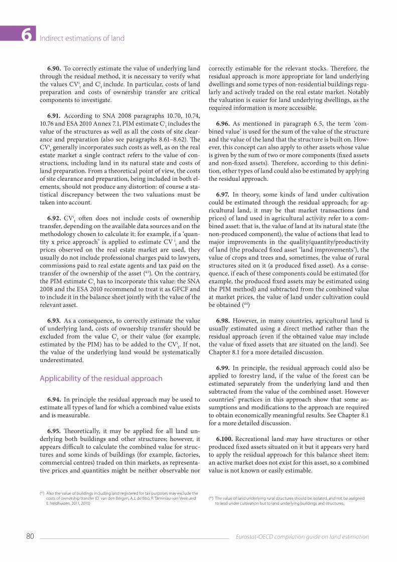
6.86. Using the PIM‑method the depreciated value of the structures can be estimated:
Table 6.11: Net capital stock of constructions (C), by type and year
Year Dwellings (e)
Non-residential buildings (f)
Other struc-tures (g)
Total (h=e+f+g)
1 50 43 40 133
2 70 45 41 156
3 95 47 43 185
4 115 53 46 214
5 140 58 49 247
6 190 60 52 302
Source: TF on Land and other non-financial assets, fictitious data
6.87. The value of the land can then be derived as a residual:
Table 6.12: Value of land (L), by type and year
Year Dwellings (j=a-e)
Non-residential buildings
(k=b-f)
Other struc-tures (l=c-g)
Total (m=d-h=
j+k+l)1 50 37 20 107
2 80 40 21 141
3 105 43 22 170
4 135 47 24 206
5 160 52 26 238
6 210 55 28 293
Source: TF on Land and other non-financial assets calculations based on ficti-tious data
6.88. The final estimate of LV at time t can be obtained with more granularity: on the basis of available informa‑tion, the estimates CVi
t and/or Cit can be derived as the sum
of more detailed values, on:
— the type of constructions (for example, the value of non‑residential buildings can be calculated as the sum of the value of retail shops, hotels, banks, facto‑ries, etc.);
— the territorial breakdown (the country value can be obtained as the sum of the values calculated for re‑gions, municipalities.);
— the classification of the owner (the value for total economy can be obtained as the sum of the values cal‑culated for institutional sectors or industries).
6.89. So, for example, the value of land underlying dwell‑ings (j) is obtained as the aggregation of the estimates calcu‑lated at the regional level; or the net stock of non‑residential buildings (f) is the sum of values available by industry.
80 Eurostat-OECD compilation guide on land estimation
Indirect estimations of land66.90. To correctly estimate the value of underlying land
through the residual method, it is necessary to verify what the values CVi
t and Cit include. In particular, costs of land
preparation and costs of ownership transfer are critical components to investigate.
6.91. According to SNA 2008 paragraphs 10.70, 10.74, 10.76 and ESA 2010 Annex 7.1, PIM estimate Ci
t includes the value of the structures as well as all the costs of site clear‑ance and preparation (also see paragraphs 8.61–8.62). The CVi
t generally incorporates such costs as well, as on the real estate market a single contract refers to the value of con‑structions, including land in its natural state and costs of land preparation. From a theoretical point of view, the costs of site clearance and preparation, being included in both el‑ements, should not produce any distortion: of course a sta‑tistical discrepancy between the two valuations must be taken into account.
6.92. CVit often does not include costs of ownership
transfer, depending on the available data sources and on the methodology chosen to calculate it: for example, if a ‘quan‑tity x price approach’ is applied to estimate CV i
t and the prices observed on the real estate market are used, they usually do not include professional charges paid to lawyers, commissions paid to real estate agents and tax paid on the transfer of the ownership of the asset (43). On the contrary, the PIM estimate Ci
t has to incorporate this value: the SNA 2008 and the ESA 2010 recommend to treat it as GFCF and to include it in the balance sheet jointly with the value of the relevant asset.
6.93. As a consequence, to correctly estimate the value of underlying land, costs of ownership transfer should be excluded from the value Ci
t or their value (for example, estimated by the PIM) has to be added to the CVi
t. If not, the value of the underlying land would be systematically underestimated.
Applicability of the residual approach
6.94. In principle the residual approach may be used to estimate all types of land for which a combined value exists and is measurable.
6.95. Theoretically, it may be applied for all land un‑derlying both buildings and other structures; however, it appears difficult to calculate the combined value for struc‑tures and some kinds of buildings (for example, factories, commercial centres) traded on thin markets, as representa‑tive prices and quantities might be neither observable nor
(43) Also the value of buildings including land registered for tax purposes may exclude the costs of ownership transfer (D. van den Bergen, A.J. de Boo, P. Taminiau-van Veen and E. Veldhuizen, 2011, 2010)
correctly estimable for the relevant stocks. Therefore, the residual approach is more appropriate for land underlying dwellings and some types of non‑residential buildings regu‑larly and actively traded on the real estate market. Notably the valuation is easier for land underlying dwellings, as the required information is more accessible.
6.96. As mentioned in paragraph 6.5, the term ‘com‑bined value’ is used for the sum of the value of the structure and the value of the land that the structure is built on. How‑ever, this concept can also apply to other assets whose value is given by the sum of two or more components (fixed assets and non‑fixed assets). Therefore, according to this defini‑tion, other types of land could also be estimated by applying the residual approach.
6.97. In theory, some kinds of land under cultivation could be estimated through the residual approach; for ag‑ricultural land, it may be that market transactions (and prices) of land used in agricultural activity refer to a com‑bined asset: that is, the value of land at its natural state (the non‑produced component), the value of actions that lead to major improvements in the quality/quantity/productivity of land (the produced fixed asset ‘land improvements’), the value of crops and trees and, sometimes, the value of rural structures sited on it (a produced fixed asset). As a conse‑quence, if each of these components could be estimated (for example, the produced fixed assets may be estimated using the PIM method) and subtracted from the combined value at market prices, the value of land under cultivation could be obtained (44).
6.98. However, in many countries, agricultural land is usually estimated using a direct method rather than the residual approach (even if the obtained value may include the value of fixed assets that are situated on the land). See Chapter 8.1 for a more detailed discussion.
6.99. In principle, the residual approach could also be applied to forestry land, if the value of the forest can be estimated separately from the underlying land and then subtracted from the value of the combined asset. However countries’ practices in this approach show that some as‑sumptions and modifications to the approach are required to obtain economically meaningful results. See Chapter 8.1 for a more detailed discussion.
6.100. Recreational land may have structures or other produced fixed assets situated on it but it appears very hard to apply the residual approach for this balance sheet item: an active market does not exist for this asset, so a combined value is not known or easily estimable.
(44) The value of land underlying rural structures should be isolated, and not be assigned to land under cultivation but to land underlying buildings and structures.
81Eurostat-OECD compilation guide on land estimation
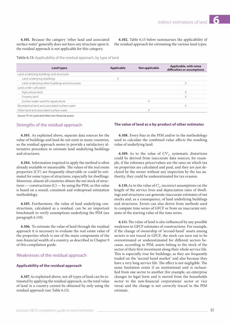
Indirect estimations of land 66.101. Because the category ‘other land and associated
surface water’ generally does not have any structure upon it, the residual approach is not applicable for this category.
6.102. Table 6.13 below summarises the applicability of the residual approach for estimating the various land types.
Table 6.13: Applicability of the residual approach, by type of land
Land types Applicable Not applicable Applicable, with some difficulties or assumptions
Land underlying buildings and structures
Land underlying dwellings X
Land underlying other buildings and structures X
Land under cultivation
Agricultural land X
Forestry land X
Surface water used for aquaculture X
Recreational land and associated surface water X
Other land and associated surface water X
Source: TF on Land and other non-financial assets
Strengths of the residual approach
6.103. As explained above, separate data sources for the value of buildings and land do not exist in many countries, so the residual approach seems to provide a satisfactory al‑ternative procedure to estimate land underlying buildings and structures.
6.104. Information required to apply the method is often already available or measurable. The values of the real estate properties (CV) are frequently observable or could be esti‑mated for some types of structures, especially for dwellings. Moreover, almost all countries obtain the net stock of struc‑tures — constructions (C) — by using the PIM, so this value is based on a sound, consistent and widespread estimation methodology.
6.105. Furthermore, the value of land underlying con‑structions, calculated as a residual, can be an important benchmark to verify assumptions underlying the PIM (see paragraph 6.110).
6.106. To estimate the value of land through the residual approach it is necessary to evaluate the real estate value of the properties which is one of the main components of the non‑financial wealth of a country, as described in Chapter 9 of this compilation guide.
Weaknesses of the residual approach
Applicability of the residual approach
6.107. As explained above, not all types of land can be es‑timated by applying the residual approach, so the total value of land in a country cannot be obtained by only using the residual approach (see Table 6.13).
The value of land as a by-product of other estimates
6.108. Every bias in the PIM and/or in the methodology used to calculate the combined value affects the resulting value of underlying land.
6.109. As to the value of CVit, systematic distortions
could be derived from inaccurate data sources; for exam‑ple, if the reference prices/values are the ones on which tax on properties are calculated and paid, and they are just de‑clared by the owner without any inspection by the tax au‑thority, they could be underestimated for tax evasion.
6.110. As to the value of Cit, incorrect assumptions on the
length of the service lives and depreciation rates of dwell‑ings and structures can generate inaccurate estimates of net stocks and, as a consequence, of land underlying buildings and structures. Errors can also derive from methods used to compute time series of GFCF or from an inaccurate esti‑mate of the starting value of the time series.
6.111. The value of land is also influenced by any possible weakness in GFCF estimates of constructions. For example, if the change of ownership of ‘second‑hand’ assets among sectors is not traced in GFCF, the stock can turn out to be overestimated or underestimated for different sectors be‑cause, according to PIM, assets belong to the stock of the sector of their first investment along their whole service life. This is especially true for buildings, as they are frequently traded on the ‘second hand market’ and also because they have a very long service life. The effect is not negligible. The same limitation exists if an institutional unit is reclassi‑fied from one sector to another (for example, an enterprise changes its legal form and is moved from the households sector to the non‑financial corporations’ sector or vice versa) and the change is not correctly traced in the PIM estimate.
82 Eurostat-OECD compilation guide on land estimation
Indirect estimations of land66.112. Inaccurate and inconsistent estimates of CVi
t and Ci
t, due to biases in the estimation method and/or in data sources, can lead to negative values of land (if the value of Ci
t is higher than CVi
t), which is not, of course, an economical‑ly meaningful result. This occurred in the United States for some components (Wasshausen, D., 2011) and in Denmark for certain years in the period 1995–2002 (see the Danish case study in Chapter 6.4) and in Finland for forestry land for some years (see the Finnish case study in Chapter 8.1).
6.113. Therefore, estimates calculated by applying the residual method need to be tested over a reasonable time span, including the ups and downs of the economic cycle, before releasing balance sheet data. Moreover, plausibility checks should be done — for example reviewing and com‑paring with another country the share of land to the total property (ratio LVi
t /CVit) and the weight of LVi
t to the total non‑financial wealth — to ensure that estimates are sensible and economically consistent. These analyses should be per‑formed within homogeneous clusters of countries to take into account the characteristics in the real estate market, territorial distribution of constructions, geographical fea‑tures of land (mountainous versus flat country), population density, propensity/restriction to land consumption, dearth of land, building permits.
Other issues related to the residual approach
6.114. Another critical issue of the residual approach is that when Ci
t is obtained through the PIM, most of the hold‑ing gains and losses for real estate properties will be allo‑cated to land. This is because the PIM‑based estimate of Ci
t only includes the change in prices driven by fluctuations in the construction costs, as the most common method of cal‑culating price indices in the PIM is through a cost approach (the change in price of the finished asset is calculated from price changes of labour and material inputs). Therefore the value LVi
t calculated as a residual will include all the other changes in prices that are not connected with the changes in the costs of construction.
6.115. Even if most holding gains and losses for the produced asset ‘building’ probably originate mainly from fluctuations in the construction costs, other kinds of re‑valuations involving the building itself may exist, but their impact may be supposed to be limited. For example, in a given period of time, buildings characterised by a specific quality feature (historical buildings versus new buildings, apartment versus detached house, apartment at the top/first floor) could be most appreciated and demanded, so that their prices increase. As a consequence, if it is not feasible to calculate and to isolate these revaluation factors, the value of land obtained by applying the residual approach could be overestimated.
6.116. Except for this possible error, imputing all the re‑valuations — other than those included in the PIM estimate of constructions — to the land underlying the construction is not to be considered a real weakness of the residual ap‑proach, if it is assumed that every change in price due to de‑mand fluctuations on the real estate market accrues more to land than to structures upon it, as land is non‑reproducible, limited and in short supply (45).
6.117. The value of real estate properties also change if the quality of the surrounding land changes. This may be the case if new amenities or infrastructures are created (for example, a school or a train station is built or a park is re‑placed by an industrial zone), generating (positive/negative) externalities. These new higher/lower values will be totally included in the value of land underlying constructions, when the residual approach is used. If it is assumed that the surrounding amenities are to be considered as quality characteristics of underlying land (see the annex to Chap‑ter 2) then this result is not necessarily a weakness of this approach. As a consequence, any increase/decrease in the value of the land — given by changes in the surrounding amenities in the vicinity — reflects changes in the quality of underlying land.
Case studies
Case study residual approach: Italy
In Italy, the value of land underlying dwellings is estimated by applying the residual approach. To estimate the com‑bined value, a ‘quantity x price approach’ is used (see Chap‑ter 6.1).
In notation:
(9) CVt = Nt * St * Pt
CVt Combined value at time tNt Number of dwellings at time tSt Average surface (square metres) of dwellings at time tPt Average price per square metre of dwellings at time t
The methodology is applied on an annual basis, at regional level (NUTS 2 (46)).
(45) In some cases and in certain economic circumstances, also depending on country specifications (mainly on how scarce is the supply of land in a certain country), the revaluations could be allocated more to structures than to the underlying land.
(46) NUTS is a three level hierarchical classification. It subdivides each Member State into a number of NUTS 1 regions, each of which is in turn subdivided into a number of NUTS 2 regions and so on. See Eurostat, Regions in the European Union — Nomenclature of territorial units for statistics, 2011. Available at http://ec.europa.eu/eurostat/documents/3859598/5916917/KS-RA-11-011-EN.PDF
.
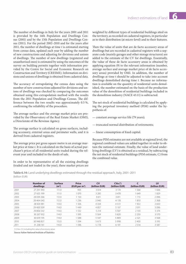
83Eurostat-OECD compilation guide on land estimation
Indirect estimations of land 6The number of dwellings in Italy for the years 2001 and 2011 is provided by the 14th Population and Dwellings Cen‑sus (2001) and by the 15th Population and Dwellings Cen‑sus (2011). For the period 2002–2010 and for the years after 2011, the number of dwellings at time t is estimated starting from census data, updated each year by adding the number of new constructions and adjusting for divisions and unions of dwellings. The number of new dwellings (registered and unauthorised ones) is estimated by using the outcomes of the survey on building permits together with information pro‑vided by the Centre for Social and Economic Research on Construction and Territory (CRESME). Information on divi‑sions and unions of dwellings is obtained from cadastral data.
The accuracy of extrapolating the census data using the number of new constructions adjusted for divisions and un‑ions of dwellings was checked by comparing the outcomes obtained using this extrapolation method with the results from the 2011 Population and Dwellings Census. The dif‑ference between the two results was approximately 0.5 %, confirming the reliability of the procedure.
The average surface and the average market price are pro‑vided by the Observatory of the Real Estate Market (OMI), a Directorate of the Revenue Agency.
The average surface is calculated on gross surfaces, includ‑ing accessory, external areas and perimeter walls, and it is derived from cadastral registers.
The average price per gross square metre is an average mar‑ket price at time t. It is calculated on the basis of actual pur‑chaser’s prices of all residential units traded during the rel‑evant year and included in the deeds of sale.
In order to be representative of all the existing dwellings (traded and not traded in the year), these market prices are
weighted by different types of residential buildings sited on the territory, as recorded on cadastral registers, in particular as to their distribution (at micro‑level) and to their features.
Then the value of units that are de facto accessory areas of dwellings but are recorded in cadastral registers with a sep‑arate code (mainly garages and other storage structures) are added to the estimate of the CV for dwellings. Essentially, the value of these de facto accessory areas is obtained by applying equation (9) to the relevant information (number, average surface and average market price of de facto acces‑sory areas) provided by OMI. In addition, the number of dwellings at time t should be adjusted to take into account dwellings demolished during time t. Because no informa‑tion is available on the quantity of residential units demol‑ished, the number estimated on the basis of the production value of the demolition of residential buildings included in the demolition industry (NACE 43.11) is subtracted.
The net stock of residential buildings is calculated by apply‑ing the perpetual inventory method (PIM) under the hy‑pothesis of:
— constant average service life (79 years);
— truncated normal distribution of retirements;
— linear consumption of fixed capital.
Because PIM estimates are not available at regional level, the regional combined values are added together in order to ob‑tain the national estimate. Finally, the value of land under‑lying dwellings (LV) is obtained as a residual, by subtracting the net stock of residential buildings (PIM estimate, C) from the combined value.
Table 6.14: Land underlying dwellings estimated through the residual approach, Italy, 2001–2011(billion EUR)
Number of dwellings
Surface (m2)
Price (EUR per m2)
CV (billion EUR)
CVa (1) (billion EUR)
C (billion EUR)
LV (billion EUR)
2001 27 291 993 111.0 995 3 014 3 174 1 568 1 606
2002 27 655 199 111.0 1 070 3 285 3 478 1 649 1 8292003 28 039 266 112.0 1 150 3 611 3 811 1 715 2 0962004 28 464 043 112.0 1 236 3 940 4 178 1 810 2 3682005 28 924 981 113.0 1 326 4 334 4 572 1 922 2 6502006 29 400 509 114.0 1 449 4 857 5 107 2 011 3 0962007 29 856 542 114.0 1 532 5 214 5 507 2 133 3 3742008 30 267 932 114.0 1 595 5 504 5 820 2 250 3 5702009 30 639 195 114.0 1 588 5 547 5 889 2 321 3 5682010 30 948 827 115.0 1 594 5 673 5 998 2 403 3 5952011 31 208 161 116.0 1 596 5 778 6 101 2 514 3 587
(1) CVa= CV including the value of accessory areas
Source: Italian National Institute of Statistics
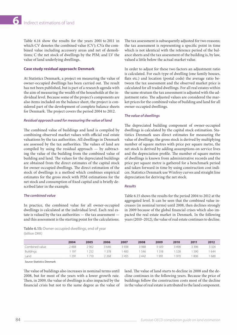
84 Eurostat-OECD compilation guide on land estimation
Indirect estimations of land6Table 6.14 show the results for the years 2001 to 2011 in which CV denotes the combined value (CV); CVa the com‑bined value including accessory areas and net of demoli‑tions; C the net stock of dwellings by the PIM; and LV the value of land underlying dwellings.
Case study residual approach: Denmark
At Statistics Denmark, a project on measuring the value of owner‑occupied dwellings has been carried out. The result has not been published, but is part of a research agenda with the aim of measuring the wealth of the households at the in‑dividual level. Because some of the project’s components are also items included on the balance sheet, the project is con‑sidered part of the development of complete balance sheets for Denmark. The project covers the period 2004 to 2012.
Residual approach used for measuring the value of land
The combined value of buildings and land is compiled by combining observed market values with official real estate valuations by the tax authorities. All dwellings in Denmark are assessed by the tax authorities. The values of land are compiled by using the residual approach — by subtract‑ing the value of the building from the combined value of building and land. The values for the depreciated buildings are obtained from the direct estimates of the capital stock for owner‑occupied dwellings. The direct estimation of the stock of dwellings is a method which combines empirical estimates for the gross stock with PIM estimations for the net stock and consumption of fixed capital and is briefly de‑scribed later in the example.
The combined value
In practice, the combined value for all owner‑occupied dwellings is calculated at the individual level. Each real es‑tate is valued by the tax authorities — the tax assessment — and this assessment is the starting point for the calculations.
The tax assessment is subsequently adjusted for two reasons; the tax assessment is representing a specific point in time which is not identical with the reference period of the bal‑ance sheets and the tax assessment of the building is, by law, valued a little below the actual market value.
In order to adjust for these two factors an adjustment ratio is calculated. For each type of dwelling (one family houses, flats etc.) and location (postal code) the average ratio be‑tween the tax assessment and the observed market price is calculated for all traded dwellings. For all real estates within the same stratum the tax assessment is adjusted with the ad‑justment ratio. The adjusted values are considered the mar‑ket prices for the combined value of building and land for all owner‑occupied dwellings.
The value of dwellings
The depreciated building component of owner‑occupied dwellings is calculated by the capital stock estimation. Sta‑tistics Denmark uses direct estimates for measuring the value of dwellings; the gross stock is derived by multiplying number of square metres with price per square metre, the net stock is derived by adding assumptions on service lives and the depreciation profile. The number of square metres of dwellings is known from administrative records and the price per square metre is gathered for a benchmark period and taken forward in time by using construction cost indi‑ces. Statistics Denmark use Winfrey curves and straight line depreciation for deriving the net stock.
Results
Table 6.15 shows the results for the period 2004 to 2012 at the aggregated level. It can be seen that the combined value in‑creases (in nominal terms) until 2008, then declines strongly in 2009 because of the global financial crises which also im‑pacted the real estate market in Denmark. In the following years (2010–2012), the value of real estate continues to decline.
Table 6.15: Owner occupied dwellings, end of year(billion DKK)
2004 2005 2006 2007 2008 2009 2010 2011 2012Combined value 2 488 2 962 3 646 3 938 3 988 3 509 3 498 3 396 3 324
Buildings 1 197 1 252 1 378 1 483 1 546 1 518 1 528 1 590 1 644
Land 1 291 1 710 2 268 2 455 2 442 1 991 1 970 1 806 1 680
Source: Statistics Denmark
The value of buildings also increases in nominal terms until 2008, but for most of the years with a lower growth rate. Then, in 2009, the value of dwellings is also impacted by the financial crisis but not to the same degree as the value of
land. The value of land starts to decline in 2008 and the de‑cline continues in the following years. Because the price of buildings follow the construction costs most of the decline in the value of real estate is attributed to the land component.
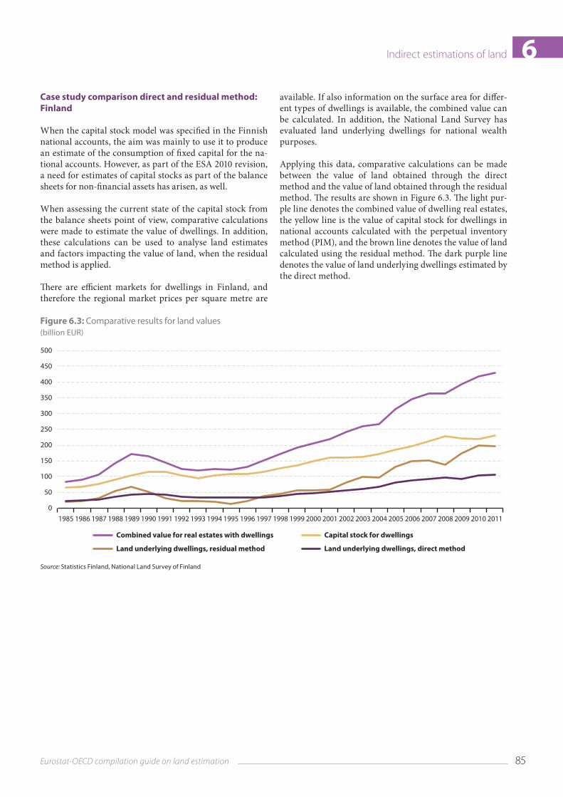
85Eurostat-OECD compilation guide on land estimation
Indirect estimations of land 6Case study comparison direct and residual method: Finland
When the capital stock model was specified in the Finnish national accounts, the aim was mainly to use it to produce an estimate of the consumption of fixed capital for the na‑tional accounts. However, as part of the ESA 2010 revision, a need for estimates of capital stocks as part of the balance sheets for non‑financial assets has arisen, as well.
When assessing the current state of the capital stock from the balance sheets point of view, comparative calculations were made to estimate the value of dwellings. In addition, these calculations can be used to analyse land estimates and factors impacting the value of land, when the residual method is applied.
There are efficient markets for dwellings in Finland, and therefore the regional market prices per square metre are
available. If also information on the surface area for differ‑ent types of dwellings is available, the combined value can be calculated. In addition, the National Land Survey has evaluated land underlying dwellings for national wealth purposes.
Applying this data, comparative calculations can be made between the value of land obtained through the direct method and the value of land obtained through the residual method. The results are shown in Figure 6.3. The light pur‑ple line denotes the combined value of dwelling real estates, the yellow line is the value of capital stock for dwellings in national accounts calculated with the perpetual inventory method (PIM), and the brown line denotes the value of land calculated using the residual method. The dark purple line denotes the value of land underlying dwellings estimated by the direct method.
Figure 6.3: Comparative results for land values(billion EUR)
Source: Statistics Finland, National Land Survey of Finland
0
50
100
150
200
250
300
350
400
450
500
1985 1986 1987 1988 1989 1990 1991 1992 1993 1994 1995 1996 1997 1998 1999 2000 2001 2002 2003 2004 2005 2006 2007 2008 2009 2010 2011
Combined value for real estates with dwellings
Land underlying dwellings, residual method
Capital stock for dwellings
Land underlying dwellings, direct method
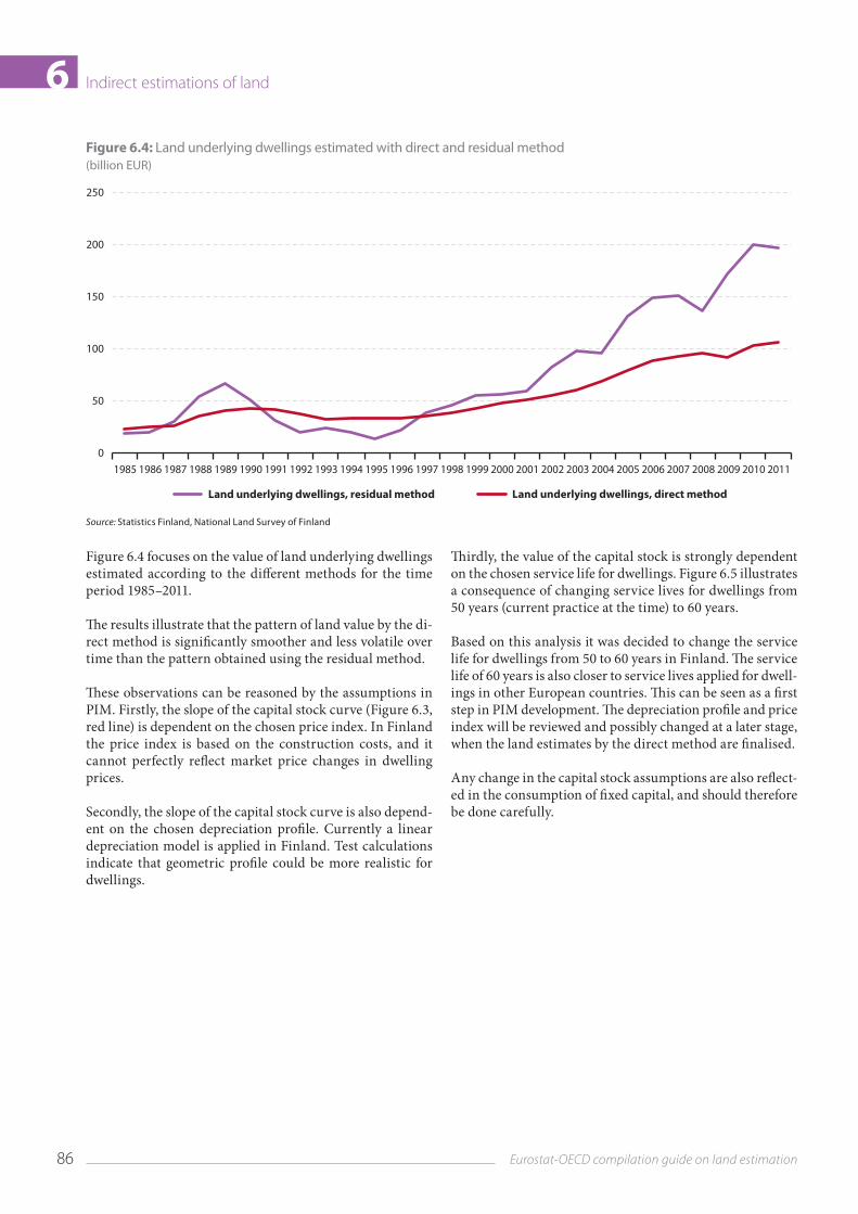
86 Eurostat-OECD compilation guide on land estimation
Indirect estimations of land6Figure 6.4: Land underlying dwellings estimated with direct and residual method(billion EUR)
Source: Statistics Finland, National Land Survey of Finland
Figure 6.4 focuses on the value of land underlying dwellings estimated according to the different methods for the time period 1985–2011.
The results illustrate that the pattern of land value by the di‑rect method is significantly smoother and less volatile over time than the pattern obtained using the residual method.
These observations can be reasoned by the assumptions in PIM. Firstly, the slope of the capital stock curve (Figure 6.3, red line) is dependent on the chosen price index. In Finland the price index is based on the construction costs, and it cannot perfectly reflect market price changes in dwelling prices.
Secondly, the slope of the capital stock curve is also depend‑ent on the chosen depreciation profile. Currently a linear depreciation model is applied in Finland. Test calculations indicate that geometric profile could be more realistic for dwellings.
Thirdly, the value of the capital stock is strongly dependent on the chosen service life for dwellings. Figure 6.5 illustrates a consequence of changing service lives for dwellings from 50 years (current practice at the time) to 60 years.
Based on this analysis it was decided to change the service life for dwellings from 50 to 60 years in Finland. The service life of 60 years is also closer to service lives applied for dwell‑ings in other European countries. This can be seen as a first step in PIM development. The depreciation profile and price index will be reviewed and possibly changed at a later stage, when the land estimates by the direct method are finalised.
Any change in the capital stock assumptions are also reflect‑ed in the consumption of fixed capital, and should therefore be done carefully.
0
50
100
150
200
250
1985 1986 1987 1988 1989 1990 1991 1992 1993 1994 1995 1996 1997 1998 1999 2000 2001 2002 2003 2004 2005 2006 2007 2008 2009 2010 2011
Land underlying dwellings, residual method Land underlying dwellings, direct method
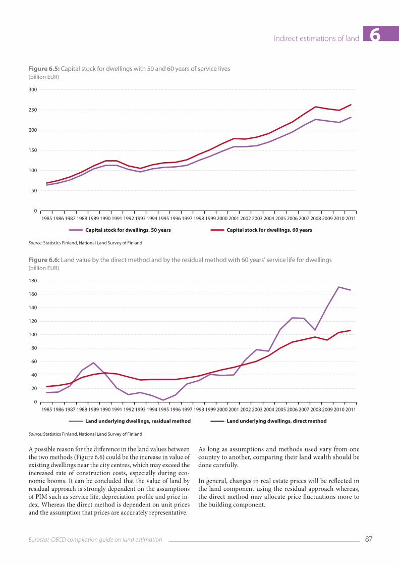
87Eurostat-OECD compilation guide on land estimation
Indirect estimations of land 6Figure 6.5: Capital stock for dwellings with 50 and 60 years of service lives(billion EUR)
Source: Statistics Finland, National Land Survey of Finland
Figure 6.6: Land value by the direct method and by the residual method with 60 years’ service life for dwellings(billion EUR)
Source: Statistics Finland, National Land Survey of Finland
A possible reason for the difference in the land values between the two methods (Figure 6.6) could be the increase in value of existing dwellings near the city centres, which may exceed the increased rate of construction costs, especially during eco‑nomic booms. It can be concluded that the value of land by residual approach is strongly dependent on the assumptions of PIM such as service life, depreciation profile and price in‑dex. Whereas the direct method is dependent on unit prices and the assumption that prices are accurately representative.
As long as assumptions and methods used vary from one country to another, comparing their land wealth should be done carefully.
In general, changes in real estate prices will be reflected in the land component using the residual approach whereas, the direct method may allocate price fluctuations more to the building component.
0
50
100
150
200
300
250
1985 1986 1987 1988 1989 1990 1991 1992 1993 1994 1995 1996 1997 1998 1999 2000 2001 2002 2003 2004 2005 2006 2007 2008 2009 2010 2011
Capital stock for dwellings, 50 years Capital stock for dwellings, 60 years
0
60
40
20
80
100
140
120
160
180
1985 1986 1987 1988 1989 1990 1991 1992 1993 1994 1995 1996 1997 1998 1999 2000 2001 2002 2003 2004 2005 2006 2007 2008 2009 2010 2011
Land underlying dwellings, residual method Land underlying dwellings, direct method
88 Eurostat-OECD compilation guide on land estimation
Indirect estimations of land6
6.3 The land-to-structure ratio approach
Introduction
6.118. The land‑to‑structure ratio (LSR) approach repre‑sents another option to indirectly derive the value of land. This method shares similarities with the residual approach discussed in Chapter 6.2, more specifically because of the reliance on a derived measure of the depreciated structure built on a given property. Therefore, this approach can be used for the estimation of land underlying dwellings and other buildings and structures.
6.119. The LSR approach is recommended when avail‑able data sources permit the derivation of a higher quality estimate for a representative LSR compared to an estimate for total property value.
6.120. In the following paragraphs, the LSR approach will be described in detail, including a description of the method, the data sources required and the strengths and weaknesses of this approach. The approach will also be il‑lustrated by means of a case study for Canada.
Description of the method
6.121. At its most basic, the LSR method uses a simple identity valid at any level of aggregation:
(10) Land‑to‑structure ratio = value of land/value of structures
6.122. Using estimates for the value of structures and the LSR, the value of land can be easily derived by reversing the previous identity:
(11) Value of land = value of structures * land‑to‑structure ratio
6.123. The accuracy of the land value estimates obtained through this approach increases with the level of detail at which these calculations are done, as the matching be‑tween structures and LSRs will more fully take into account property characteristics in terms of type, location, and geography.
Estimation of structures value
6.124. In most countries, the valuation of dwellings and other buildings and structures is based on a perpetual inven‑tory method (PIM). Given that these derivations are includ‑ed in the national accounts framework, mostly through the
balance sheet programme, the PIM approach has the major advantage of ensuring consistency across the accounts, with investment flows that are captured in the capital account fully consistent with the stock values derived through PIM.
6.125. The PIM provides a viable alternative to estimat‑ing a ‘fair’ value for dwellings and other structures in the absence of directly observable market prices. As most real estate transactions concern the total value of the property, which includes the inextricably linked values of buildings and the land on which they stand, the value of structures has to be estimated through the use of a proxy, regularly called ‘replacement value’. This valuation approach, which underlies the PIM methodology, provides, in essence, the cost of acquiring a similar produced asset that would pro‑vide the exact same level of utility to its user.
6.126. The PIM uses information about investment flows, demolitions, destructions, price indices, average service lives of capital, as well as a choice of a depreciation method. In essence, the PIM cumulates capital investment flows to obtain estimates of structures for a given time pe‑riod. For more information on the assumptions and esti‑mation methods used by countries see Chapter 6.5 in this guide. A more detailed description of the PIM can be found in Measuring Capital (OECD, 2009).
6.127. The wide use of the PIM‑based approach in the derivation of values for dwellings and other structures provides a solid basis for cross‑country comparison and consistency.
6.128. The use of the PIM methodology yields, in most countries, estimates for structures with a relatively high level of granularity, mostly dependent on data availability for investments flows. The finer the level of detail used in the derivation, the more accurate the estimates will be by type of structure and sectoral dimension.
Estimation of land-to-structure ratio
6.129. The derivation of the LSR relies on the availability of data on the value of structures and land components for a clearly defined set of properties, in other words, a sample of the total stock of properties within an economy. An es‑sential aspect of this step in the LSR methodology is the de‑gree of representativeness of the LSR sample relative to the total set of properties for which it will be used.
6.130. The accuracy of the method increases with a closer match between the type of structures and the LSR available. In most cases, PIM estimates are available for dwellings by type of dwelling as well as for non‑residential structures. In countries where regional differences are significant, the ge‑ographical detail is also very important; therefore, it should be included in the derivation of the value of structures.

89Eurostat-OECD compilation guide on land estimation
Indirect estimations of land 66.131. The next step in the methodology is the matching
of structures with the corresponding LSR, at the lowest level of detail afforded by data availability. This derives a value for land for that particular type of property with a specific geographical profile. This approach can be easily applied at a high level of aggregation, however at the expense of some loss in estimate accuracy. This impact will be more signifi‑cant the more heterogeneous the set of developed properties are in a given economy.
Data requirements
Data requirements for the estimation of the value of dwellings and other buildings and structures
6.132. The PIM data requirements are normally well un‑derstood, given the widespread use of the methodology in deriving capital stock estimates.
6.133. In brief, the PIM approach requires data on in‑vestment flows, including new construction, renovations and other fees associated with new building transactions. Price indices, service lives of structures and data on demo‑litions and destructions are also used to develop the stock time‑series. Finally, the depreciation method is the final el‑ement to consider in the accumulation of deflated capital investment flows. The typical choice is between a linear and a geometric depreciation method.
6.134. The PIM is a versatile model that can be custom‑ised to work at a level of detail afforded by data availabil‑ity. Ideally, the value of dwellings should be estimated by type — singles, multiples, condos as well as by the relevant geographic detail.
6.135. For non‑residential structures, or structures other than dwellings, it is useful to distinguish between types of structures, for building structures (such as offices, plants) and engineering structures (such as roads, bridges). This in‑formation is typically available through surveys of capital expenditures, with these data also providing the basis for the investment flows in the capital account of the national accounting framework.
Data requirements for the estimation of land-to-structure ratios
6.136. The estimation of a LSR requires complete infor‑mation on two of the three variables involved — the total combined value of the property, the value of the structure, the value of land — through research or preferably, regu‑lar observations for a representative sample. This would allow the calculation of the value of structures and the corresponding value of underlying land and thus the de‑sired ratio.
6.137. The quality and degree of representativeness of the sample are essential aspects to consider in deciding to use the LSR method. As a general observation, such samples are less of a challenge for residential properties, as many coun‑tries already have in place survey frameworks to capture current residential construction, an economic activity very relevant to a number of high‑profile statistical programmes (as well as policy making). In addition, any information on the total value of residential properties entering the real estate market is likely to be close to fair values, based on the assumption that residential real estate price dynamics would be implicitly incorporated in transaction prices.
6.138. In addition, for new residential construction, the value of structures completed in the current reporting period should be readily available through such survey frameworks, as it would rely mostly on current costs, therefore the subjectiv‑ity inherent in respondent reporting will be less of a concern.
6.139. Another alternative is asking respondents (such as major builders) to provide a value for land. Although en‑tirely feasible, this approach will introduce a fairly high level of subjectivity in the estimates, particularly because issues such as timing will play an important role. Often, build‑ers purchase large areas of vacant or undeveloped land but only develop it with some time lag that could be significant. In such cases, the transaction prices for the land purchase are unlikely to capture its current or fair value. This is of particular concern during periods when residential real es‑tate markets perform strongly, given that most of the ap‑preciation in property values is associated with the land component.
6.140. Another possible challenge presents itself for countries where the residential building construction in‑dustry is very fragmented and comprised, for the most part, of a large number of small builders. This will complicate the task of setting up and managing a successful survey.
6.141. One important aspect for the use of the LSR method is the level of detail for which data on the respective variables are available. In other words, the estimated value of land will be more accurate if LSRs are calculated by type of property, by geographic region as well as taking into ac‑count the differences between urban and suburban areas. Ideally, the resulting set of LSRs will have at least as much granularity as the PIM‑based structure value estimates to allow the estimation of the value of land at a low level of aggregation. If that is not feasible given data availability, ag‑gregate averages of LSRs represent a second best solution.
6.142. For non‑residential properties, the estimation of LSRs is likely to pose more challenges. For the most part, markets for such properties are very illiquid if observable at all. Therefore, total property values are as subjective as the associated land values. Property value assessments,

90 Eurostat-OECD compilation guide on land estimation
Indirect estimations of land6typically done by specialised assessors may provide a rea‑sonable fair value estimate for one of the two variables — combined value of the property or land value.
6.143. Maintaining a survey frame that would allow a representative coverage for non‑residential properties is inherently difficult. This is a particularly valid concern for buildings, such as offices and plants. For certain compo‑nents of engineering structures, such as bridges and roads, information that could be used to derive LSRs can poten‑tially be available in public accounts, as most of these prop‑erties would fall under government or public ownership.
6.144. For both residential and non‑residential proper‑ties, property tax assessments represent another potential data source, at the extent that the breakdown between the value of the structure and the value of the land is required and is reported reliably. One major advantage of property tax assessments is the full (or near full) coverage of proper‑ties. However, differences in assessment approaches across jurisdictions, a reality for most countries, adds an addition‑al layer of complexity to ensure full consistency.
6.145. Finally, irregular research into the valuation of real estate that could provide insight on average or aggre‑gate LSRs can constitute an alternative method to valuing land, in the absence of more accurate data sources. In such cases, given that the ratios would not be available on a regu‑lar basis, price information through real estate indices as well as indicators of real estate activity may be used as sup‑plementary inputs into the derivation of LSRs.
6.146. In addition to the sources of data and the sup‑plementary information used, the frequency at which these data are available is also critical to an accurate valuation of land. Although one‑time, infrequent valuations for land are useful, ideally, the value of land should be an integral part of the national accounts regular releases. Therefore, countries can opt for an annual or sub‑annual frequency (e.g. quarterly) for the value of land estimates, depending on their current practices for the relevant national account programmes, particularly the balance sheet accounts.
6.147. An important factor for consideration here is the potential gap between the frequency with which the source data for the LSR approach method become available and the release frequency. For example, quarterly estimates for the value of land are ideal to align with a quarterly balance sheet accounts programme. However, the survey(s) providing the source data could be annual. Property tax assessment data may also be available at lower frequencies (annual, or even once every 2–4 years). In such cases, based on the availabil‑ity of proxies and supplementary information, the gap could be bridged by using projections, however, ensuring consist‑ency in the quality of estimates in the time series could be‑come an additional challenge in the valuation of land.
Sectoral dimension
6.148. So far the estimation of the value of structures and the LSRs by type of property, location and geography has been discussed. Another relevant dimension is the sectoral allocation of the derived value of land, an integral compo‑nent to sectoral balance sheets.
6.149. Ideally, the source data would be available at a lev‑el of detail that facilitates the allocation of residential land between the households sector, the government and the cor‑porate sector. In practice, however, some assumptions and extrapolations may be necessary. The government holdings and new construction of residential properties may be avail‑able through public accounts as they mostly would relate to niche‑type housing, although this may vary greatly across countries.
6.150. Information on the corporate sector’s holdings of apartment buildings may also be available directly through surveys. The remainder (the highest proportion) would then be allocated to the households sector.
6.151. Non‑residential land will be mostly allocated to the corporate sector and the government. Assuming ad‑ditional direct data is available on government‑owned non‑residential properties, most of the residual will repre‑sent corporate sector holdings. A relatively small portion is owned by unincorporated enterprises, part of the house‑holds sector in most countries.
6.152. In the absence of such detail, however, one alter‑native is to use as a starting point the relative sector alloca‑tion of PIM‑derived structures, which, in most countries is available by sector and often by industry. However, in some cases, the assumption of equal LSRs across the various sec‑tors may be too strong. For example, government‑owned subsidised housing properties are likely to be situated in ar‑eas characterised by lower LSRs relative to households’ hold‑ings of residential properties. Such considerations though will have to rely on a subjective assessment of these differ‑ences, in the absence of additional information through di‑rect observation or research findings. A detailed discussion on sectorisation can be found in Chapter 7.
Strengths and weaknesses
6.153. The LSR approach allows the derivation of fair values for land underlying dwellings and other buildings and structures in the absence of reliable data on developed property values within an economy. The methodology is inherently versatile, and thus can be applied at the level of aggregation dictated by data availability constraints.

91Eurostat-OECD compilation guide on land estimation
Indirect estimations of land 66.154. The main data requirements for the derivation of
the ratios are likely to be met by many countries, given that the same data sets are valuable inputs in other statistical programmes within the national accounts framework. Reli‑ance on PIM estimates of structures also ensures consist‑ency across the accounts.
6.155. Moreover, this approach avoids the potential is‑sue of negative values for land, given that it builds the total property value from its two components, as opposed to the residual land methodology.
6.156. Among weaknesses, of particular mention is the actual degree of representativeness of the sample used to build the LSRs. In practice, if relying on new construction data, the sample composition could differ markedly from the composition of the existing stock of properties. There‑fore, bias represents a concern, particularly over report‑ing periods when a particular type of property is in great demand or specific geographic areas perform significantly stronger relative to others.
6.157. Countries that release higher‑frequency balance sheets (e.g. quarterly) also need to address the likely lag in the availability of data used in the calculation of LSRs. To offset the lack of information for current period(s), real es‑tate price and activity indicators can be used in projecting the ratios, using the underlying assumption that the price movement is associated with the land component.
6.158. Finally, the LSR method is applicable only to developed land, and often the data available relates only to completions. Therefore, for other types of land, such as vacant land, land under development during the respective reporting period, as well as agricultural land, other alterna‑tive methodologies will need to be used.
6.159. In conclusion, the LSR method represents a vi‑able approach to deriving land values for land underlying structures, providing countries an alternative to the direct and residual method, with data availability determining the final choice of method by type of land.
Case study land-to-structure-ratio approach: Canada
Canada produces a set of quarterly national balance sheet accounts (NBSA) which includes estimates of non‑financial assets for all relevant sectors of the economy.
For NBSA purposes, land is comprised of residential land, non‑residential land and agricultural land. Public land (such as parks) or any other type of land that is not associat‑ed with a given structure is outside the NBSA scope. (Land
under standing timber is implicitly included in the value of that natural resource).
The estimation of residential and non‑residential land is based on the land‑to‑structure ratio (LSR) approach. For agricultural land, the estimates are derived using data from the census of agriculture, conducted every five years. Given that the focus of this section is on the LSR approach, the following discussion will detail the derivation of residential and non‑residential land only.
Residential land
Residential structures
The value of residential structures is constructed using the PIM approach, based on information on investment flows, price indices, average service lives and a geometric depre‑ciation method.
The starting point is a stock estimate obtained through the 1941 Census. Investment flow data includes new construc‑tion, renovations (excluding repairs) and various fees asso‑ciated with new residential construction to reflect the value of the investment to the final buyer.
The types of structures covered comprise detached dwell‑ings, single, semi‑detached or double, row and apartment units as well as mobiles, cottages and conversions from non‑residential buildings.
Sector estimates for residential structures are derived through a number of steps. Data on government holdings of residential structures (e.g. subsidised housing, military housing) are available from public accounts, and this small amount is allocated to the government sector estimates of residential structures in the NBSA. The remaining value is then allocated between the households and the corporate sector, based on dwelling stock data by type and tenure (oc‑cupied/non‑occupied, rented/owned). This approach is con‑sistent with the sectoring of residential investment flows.
Land‑to‑structure ratios
The quarterly estimates for the LSRs are derived for new res‑idential construction, by type of dwelling — single or multi‑ples — across Canada. This information is available through a monthly survey of builders, and it covers newly completed dwellings. The survey is administered by Canada Mortgage and Housing Corporation, Canada’s national housing agen‑cy, who shares the monthly files with Statistics Canada.
For the valuation of residential land, Statistics Canada uses three key variables from this survey, by individual property:
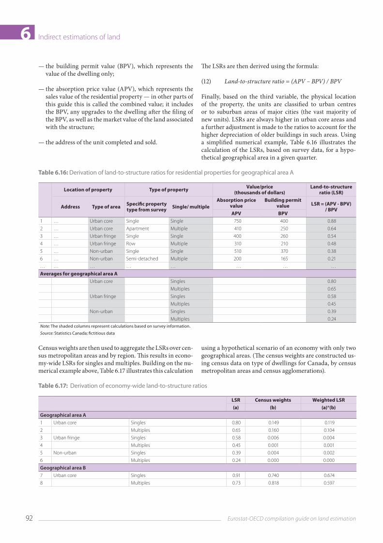
92 Eurostat-OECD compilation guide on land estimation
Indirect estimations of land6 — the building permit value (BPV), which represents the value of the dwelling only;
— the absorption price value (APV), which represents the sales value of the residential property — in other parts of this guide this is called the combined value; it includes the BPV, any upgrades to the dwelling after the filing of the BPV, as well as the market value of the land associated with the structure;
— the address of the unit completed and sold.
The LSRs are then derived using the formula:
(12) Land‑to‑structure ratio = (APV – BPV) / BPV
Finally, based on the third variable, the physical location of the property, the units are classified to urban centres or to suburban areas of major cities (the vast majority of new units). LSRs are always higher in urban core areas and a further adjustment is made to the ratios to account for the higher depreciation of older buildings in such areas. Using a simplified numerical example, Table 6.16 illustrates the calculation of the LSRs, based on survey data, for a hypo‑thetical geographical area in a given quarter.
Table 6.16: Derivation of land-to-structure ratios for residential properties for geographical area A
Location of property Type of property Value/price (thousands of dollars)
Land-to-structure ratio (LSR)
Address Type of area Specific property type from survey Single/ multiple
Absorption price value
Building permit value LSR = (APV - BPV)
/ BPVAPV BPV
1 … Urban core Single Single 750 400 0.88
2 … Urban core Apartment Multiple 410 250 0.64
3 … Urban fringe Single Single 400 260 0.54
4 … Urban fringe Row Multiple 310 210 0.48
5 … Non-urban Single Single 510 370 0.38
6 … Non-urban Semi-detached Multiple 200 165 0.21
… … … … … … … …
Averages for geographical area AUrban core Singles 0.80
Multiples 0.65
Urban fringe Singles 0.58
Multiples 0.45
Non-urban Singles 0.39
Multiples 0.24 Note: The shaded columns represent calculations based on survey information.
Source: Statistics Canada; fictitious data
Census weights are then used to aggregate the LSRs over cen‑sus metropolitan areas and by region. This results in econo‑my‑wide LSRs for singles and multiples. Building on the nu‑merical example above, Table 6.17 illustrates this calculation
using a hypothetical scenario of an economy with only two geographical areas. (The census weights are constructed us‑ing census data on type of dwellings for Canada, by census metropolitan areas and census agglomerations).
Table 6.17: Derivation of economy-wide land-to-structure ratios
LSR Census weights Weighted LSR(a) (b) (a)*(b)
Geographical area A
1 Urban core Singles 0.80 0.149 0.119
2 Multiples 0.65 0.160 0.104
3 Urban fringe Singles 0.58 0.006 0.004
4 Multiples 0.45 0.001 0.001
5 Non-urban Singles 0.39 0.004 0.002
6 Multiples 0.24 0.000 0.000
Geographical area B
7 Urban core Singles 0.91 0.740 0.674
8 Multiples 0.73 0.818 0.597
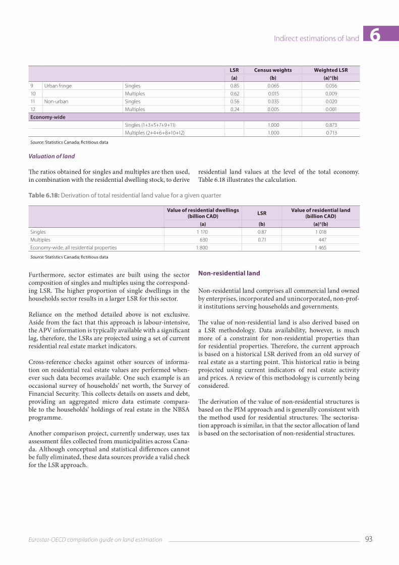
93Eurostat-OECD compilation guide on land estimation
Indirect estimations of land 6LSR Census weights Weighted LSR(a) (b) (a)*(b)
9 Urban fringe Singles 0.85 0.065 0.056
10 Multiples 0.62 0.015 0.009
11 Non-urban Singles 0.56 0.035 0.020
12 Multiples 0.24 0.005 0.001
Economy-wide
Singles (1+3+5+7+9+11) 1.000 0.873
Multiples (2+4+6+8+10+12) 1.000 0.713
Source: Statistics Canada; fictitious data
Valuation of land
The ratios obtained for singles and multiples are then used, in combination with the residential dwelling stock, to derive
residential land values at the level of the total economy. Table 6.18 illustrates the calculation.
Table 6.18: Derivation of total residential land value for a given quarter
Value of residential dwellings (billion CAD) LSR Value of residential land
(billion CAD)(a) (b) (a)*(b)
Singles 1 170 0.87 1 018
Multiples 630 0.71 447
Economy-wide, all residential properties 1 800 1 465
Source: Statistics Canada; fictitious data
Furthermore, sector estimates are built using the sector composition of singles and multiples using the correspond‑ing LSR. The higher proportion of single dwellings in the households sector results in a larger LSR for this sector.
Reliance on the method detailed above is not exclusive. Aside from the fact that this approach is labour‑intensive, the APV information is typically available with a significant lag, therefore, the LSRs are projected using a set of current residential real estate market indicators.
Cross‑reference checks against other sources of informa‑tion on residential real estate values are performed when‑ever such data becomes available. One such example is an occasional survey of households’ net worth, the Survey of Financial Security. This collects details on assets and debt, providing an aggregated micro data estimate compara‑ble to the households’ holdings of real estate in the NBSA programme.
Another comparison project, currently underway, uses tax assessment files collected from municipalities across Cana‑da. Although conceptual and statistical differences cannot be fully eliminated, these data sources provide a valid check for the LSR approach.
Non-residential land
Non‑residential land comprises all commercial land owned by enterprises, incorporated and unincorporated, non‑prof‑it institutions serving households and governments.
The value of non‑residential land is also derived based on a LSR methodology. Data availability, however, is much more of a constraint for non‑residential properties than for residential properties. Therefore, the current approach is based on a historical LSR derived from an old survey of real estate as a starting point. This historical ratio is being projected using current indicators of real estate activity and prices. A review of this methodology is currently being considered.
The derivation of the value of non‑residential structures is based on the PIM approach and is generally consistent with the method used for residential structures. The sectorisa‑tion approach is similar, in that the sector allocation of land is based on the sectorisation of non‑residential structures.
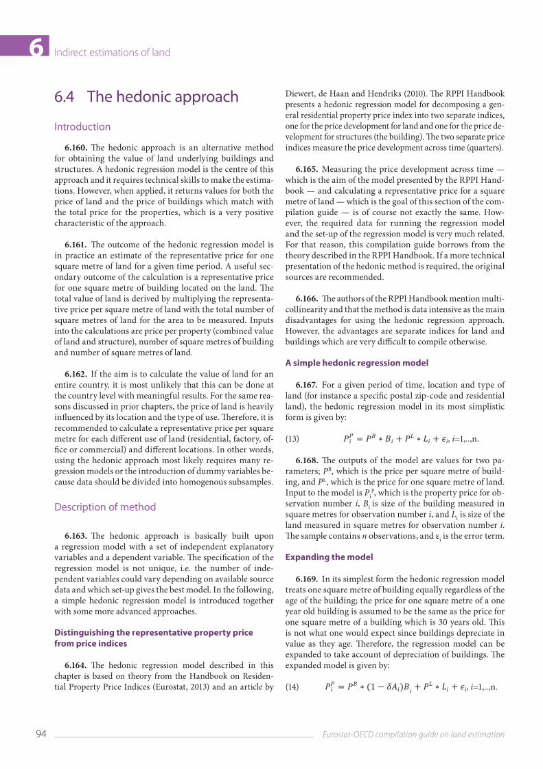
94 Eurostat-OECD compilation guide on land estimation
Indirect estimations of land6
6.4 The hedonic approach
Introduction
6.160. The hedonic approach is an alternative method for obtaining the value of land underlying buildings and structures. A hedonic regression model is the centre of this approach and it requires technical skills to make the estima‑tions. However, when applied, it returns values for both the price of land and the price of buildings which match with the total price for the properties, which is a very positive characteristic of the approach.
6.161. The outcome of the hedonic regression model is in practice an estimate of the representative price for one square metre of land for a given time period. A useful sec‑ondary outcome of the calculation is a representative price for one square metre of building located on the land. The total value of land is derived by multiplying the representa‑tive price per square metre of land with the total number of square metres of land for the area to be measured. Inputs into the calculations are price per property (combined value of land and structure), number of square metres of building and number of square metres of land.
6.162. If the aim is to calculate the value of land for an entire country, it is most unlikely that this can be done at the country level with meaningful results. For the same rea‑sons discussed in prior chapters, the price of land is heavily influenced by its location and the type of use. Therefore, it is recommended to calculate a representative price per square metre for each different use of land (residential, factory, of‑fice or commercial) and different locations. In other words, using the hedonic approach most likely requires many re‑gression models or the introduction of dummy variables be‑cause data should be divided into homogenous subsamples.
Description of method
6.163. The hedonic approach is basically built upon a regression model with a set of independent explanatory variables and a dependent variable. The specification of the regression model is not unique, i.e. the number of inde‑pendent variables could vary depending on available source data and which set‑up gives the best model. In the following, a simple hedonic regression model is introduced together with some more advanced approaches.
Distinguishing the representative property price from price indices
6.164. The hedonic regression model described in this chapter is based on theory from the Handbook on Residen‑tial Property Price Indices (Eurostat, 2013) and an article by
Diewert, de Haan and Hendriks (2010). The RPPI Handbook presents a hedonic regression model for decomposing a gen‑eral residential property price index into two separate indices, one for the price development for land and one for the price de‑velopment for structures (the building). The two separate price indices measure the price development across time (quarters).
6.165. Measuring the price development across time — which is the aim of the model presented by the RPPI Hand‑book — and calculating a representative price for a square metre of land — which is the goal of this section of the com‑pilation guide — is of course not exactly the same. How‑ever, the required data for running the regression model and the set‑up of the regression model is very much related. For that reason, this compilation guide borrows from the theory described in the RPPI Handbook. If a more technical presentation of the hedonic method is required, the original sources are recommended.
6.166. The authors of the RPPI Handbook mention multi‑collinearity and that the method is data intensive as the main disadvantages for using the hedonic regression approach. However, the advantages are separate indices for land and buildings which are very difficult to compile otherwise.
A simple hedonic regression model
6.167. For a given period of time, location and type of land (for instance a specific postal zip‑code and residential land), the hedonic regression model in its most simplistic form is given by:
(13) , i=1,..,n.
6.168. The outputs of the model are values for two pa‑rameters; PB, which is the price per square metre of build‑ing, and PL, which is the price for one square metre of land. Input to the model is Pi
P, which is the property price for ob‑servation number i, Bi is size of the building measured in square metres for observation number i, and Li is size of the land measured in square metres for observation number i. The sample contains n observations, and εi is the error term.
Expanding the model
6.169. In its simplest form the hedonic regression model treats one square metre of building equally regardless of the age of the building; the price for one square metre of a one year old building is assumed to be the same as the price for one square metre of a building which is 30 years old. This is not what one would expect since buildings depreciate in value as they age. Therefore, the regression model can be expanded to take account of depreciation of buildings. The expanded model is given by:
(14) , i=1,..,n.
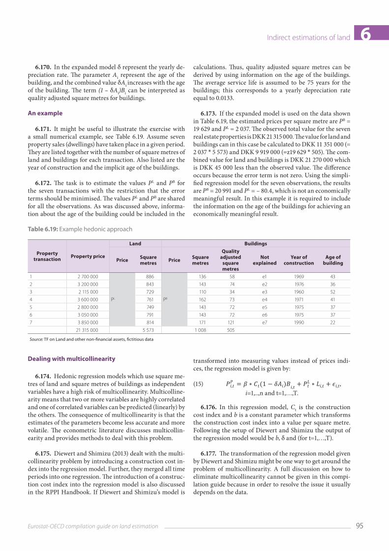
95Eurostat-OECD compilation guide on land estimation
Indirect estimations of land 66.170. In the expanded model δ represent the yearly de‑
preciation rate. The parameter Ai represent the age of the building, and the combined value δAi increases with the age of the building. The term (1 – δAi)Bi can be interpreted as quality adjusted square metres for buildings.
An example
6.171. It might be useful to illustrate the exercise with a small numerical example, see Table 6.19. Assume seven property sales (dwellings) have taken place in a given period. They are listed together with the number of square metres of land and buildings for each transaction. Also listed are the year of construction and the implicit age of the buildings.
6.172. The task is to estimate the values PL and PB for the seven transactions with the restriction that the error terms should be minimised. The values PL and PB are shared for all the observations. As was discussed above, informa‑tion about the age of the building could be included in the
calculations. Thus, quality adjusted square metres can be derived by using information on the age of the buildings. The average service life is assumed to be 75 years for the buildings; this corresponds to a yearly depreciation rate equal to 0.0133.
6.173. If the expanded model is used on the data shown in Table 6.19, the estimated prices per square metre are PB = 19 629 and PL = 2 037. The observed total value for the seven real estate properties is DKK 21 315 000. The value for land and buildings can in this case be calculated to DKK 11 351 000 (= 2 037 * 5 573) and DKK 9 919 000 (=z19 629 * 505). The com‑bined value for land and buildings is DKK 21 270 000 which is DKK 45 000 less than the observed value. The difference occurs because the error term is not zero. Using the simpli‑fied regression model for the seven observations, the results are PB = 20 991 and PL = – 80.4, which is not an economically meaningful result. In this example it is required to include the information on the age of the buildings for achieving an economically meaningful result.
Table 6.19: Example hedonic approach
Property transaction Property price
Land Buildings
Price Square metres Price Square
metres
Quality adjusted
square metres
Not explained
Year of construction
Age of building
1 2 700 000
PL
886
PB
136 58 e1 1969 43
2 3 200 000 843 143 74 e2 1976 36
3 2 115 000 729 110 34 e3 1960 52
4 3 600 000 761 162 73 e4 1971 41
5 2 800 000 749 143 72 e5 1975 37
6 3 050 000 791 143 72 e6 1975 37
7 3 850 000 814 171 121 e7 1990 22
21 315 000 5 573 1 008 505
Source: TF on Land and other non-financial assets, fictitious data
Dealing with multicollinearity
6.174. Hedonic regression models which use square me‑tres of land and square metres of buildings as independent variables have a high risk of multicollinearity. Multicolline‑arity means that two or more variables are highly correlated and one of correlated variables can be predicted (linearly) by the others. The consequence of multicollinearity is that the estimates of the parameters become less accurate and more volatile. The econometric literature discusses multicollin‑earity and provides methods to deal with this problem.
6.175. Diewert and Shimizu (2013) dealt with the multi‑collinearity problem by introducing a construction cost in‑dex into the regression model. Further, they merged all time periods into one regression. The introduction of a construc‑tion cost index into the regression model is also discussed in the RPPI Handbook. If Diewert and Shimizu’s model is
transformed into measuring values instead of prices indi‑ces, the regression model is given by:
(15) , i=1,..,n and t=1,…,T.
6.176. In this regression model, Ct is the construction cost index and b is a constant parameter which transforms the construction cost index into a value per square metre. Following the setup of Diewert and Shimizu the output of the regression model would be b, δ and (for t=1,…,T).
6.177. The transformation of the regression model given by Diewert and Shimizu might be one way to get around the problem of multicollinearity. A full discussion on how to eliminate multicollinearity cannot be given in this compi‑lation guide because in order to resolve the issue it usually depends on the data.
96 Eurostat-OECD compilation guide on land estimation
Indirect estimations of land6Data requirements
6.178. The data requirements for running the hedonic regression is a set of observations for sales of real estate properties, including number of square metres of land and number of square metres of buildings for the traded real estate properties. If the sample is non‑homogeneous with respect to location or types of buildings, it would improve the reliability of the estimations if the sample could be sub‑divided into subgroups with similar characteristics. The hedonic regression model can be compiled without infor‑mation on year of construction, but it clearly improves the quality of the results, if this information is included in the calculations. Sometimes it is a necessity.
Strengths and weaknesses
6.179. Using the hedonic approach for compiling sepa‑rate values for land and buildings and using the hedonic approach for compiling separate price indices for land and buildings is based on the same methodology. Thus some of the same weakness and benefits must be assumed for two types of calculations.
6.180. The advantages can be summarised as the following:
— Should other — and easier — methods fail, the hedon‑ic approach is probably the only method which will result in reliable figures for the value of land.
— Output of the calculations is a set of consistent figures for land, buildings and the combined value of build‑ings and land. The regression model could be used to produce stock figures for land and buildings. And the figures could be part of the balance sheets.
— Includes information on actual sales prices, number of square metres and age of buildings. The figures are used consistently.
6.181. The disadvantages can be summarised as the following:
— It is technically difficult to implement in practice. A significant amount of time may be needed to specify which regression model gives the best results.
— The calculations are data intensive. A large dataset which includes information on number of square me‑tres of building and land, age of building together with actual sales prices has to be compiled.
— There is a high risk of multicollinearity. This distorts the results and should be avoided.
— The estimated figures for buildings would most likely not be consistent with capital stock figures for build‑ings (compiled by the use of the perpetual inventory method). Some kind of balancing would probably be required if capital stock figures are used for the bal‑ance sheets.
— In practice, the hedonic approach has not yet been im‑plemented by any country in estimating the value of land. Further, the hedonic approach has not yet been applied for non‑residential buildings.
Case study hedonic approach: Denmark
The hedonic approach has not been applied by Statistics Denmark in practice, but Statistics Denmark is planning to test the hedonic approach in the future for some specific pe‑riods of time and for some specific types of buildings. If the test is successful, the results of the hedonic approach could be used in officially released figures. The reason for consid‑ering the hedonic approach is that the alternative — residual approach — does not provide reliable figures for some years.
Problematic alternative
An earlier effort at Statistics Denmark attempted to meas‑ure the value of land underlying buildings and structures for the period 1995–2002. The residual approach was used for measuring the value of land; however the residual ap‑proach proved problematic for the years 1995 and 1996 with negative values for land. The reason for the negative values for land was that a major recession hit Denmark at the end of the 1980’s and beginning of the 1990’s which also impact‑ed the real estate market. Prices for real estate decreased strongly, but construction costs did not, and because prices for buildings follow construction costs (as a consequence of the chosen perpetual inventory method/direct estimation method) whereas the price for land indirectly follows the price for real estate (which declined strongly), the value of land became negative. Therefore, the residual approach did not produce reliable figures for these years.
Statistics Denmark is planning to test the hedonic approach as an alternative to the residual approach. The plan is to test the hedonic approach for two different periods of time, one with reliable figures from the residual approach (2010–2011) and one with problematic figures (1995–1996). Since trans‑actions in owner‑occupied dwellings are the most wide‑spread, the application of the hedonic approach will be re‑stricted to this type of buildings. If the test is successful, the figures might be used for official releases.
The requirements for running the hedonic model are square metres of land, square metres of building and transaction price for all traded buildings. Statistics Denmark has access to this information together with information on the age of buildings.
97Eurostat-OECD compilation guide on land estimation
Indirect estimations of land 6
6.5 The importance of service lives and depreciation for indirect land estimates
6.182. Previous chapters have discussed the residual approach (Chapter 6.2) and the land‑to‑structure ratio approach (LSR, Chapter 6.3) for producing separate esti‑mates of national stocks of structures and underlying land. These indirect methods rely on estimates of the net stock of structures usually obtained through the perpetual inven‑tory method (PIM), in which, gross fixed capital formation (GFCF) are added to the stock, and depreciation and retire‑ments of assets subtracted from the stock. Although the PIM has many advantages, a disadvantage of the PIM is that precise information on service lives and patterns of depre‑ciation is difficult to obtain. Errors in the assumptions of the PIM, estimates of GFCF, and prices can all lead to errors in estimates of net stocks of structures, which can then lead to errors in the estimates of the value of the underlying land.
6.183. This chapter presents a summary of the responses to a 2013 OECD‑Eurostat survey of national practices in es‑timating net stocks of structures. The survey asked national accountants to provide, for a detailed list of structures, the as‑sumptions and methods used for the PIM. The goal was not to select a single ‘best’ approach for the PIM, but to promote dis‑cussions, facilitate detailed comparisons of PIM assumptions, and provide concrete options for those seeking to produce improved, internationally comparable estimates of net stocks of structures and underlying land. This chapter provides an overview of the survey and the theory of capital measure‑ment; summarises and compares reported patterns of depre‑ciation (linear, geometric, other), patterns of retirement, and other aspects of the PIM; and describes respondents’ sources of information, main concerns, and plans for the future.
Overview of the survey
6.184. The survey asked respondents to provide the methods and assumptions for their estimates of net stocks of structures. Respondents reported whether they use the PIM or other methods (census, administrative records, etc); assumed service lives, depreciation patterns, and retire‑ment patterns; sources of information used to make these assumptions; and other information.
6.185. The survey asked respondents to provide these as‑sumptions for a detailed list of structures to assist compari‑sons of similar types of structures, such as dwellings, office buildings, and schools. The list of assets conforms to widely
used classifications found in the SNA 2008, ESA 2010, and the Central Product Classification v2 (CPCv2) (47):
— For dwellings (AN.111) — one‑ and two‑dwelling resi‑dential buildings, multi‑dwelling residential buildings, major improvements, and costs of ownership transfer.
— For buildings other than dwellings (AN.1121) — ware‑houses, manufacturing or industrial buildings, office buildings, buildings for shopping and entertainment, hotels, restaurants, schools, hospitals, farm buildings, prisons, major improvements, and costs of ownership transfer.
— For other structures (AN.1122) — several types of assets including roads, railways, harbours, dams and other waterworks, mining structures, flood barriers, commu‑nication and power lines, sewage and water treatment plants, electric power plants, and natural gas structures.
6.186. The survey also asked respondents to provide information about recent ratios of net stocks to Gross Do‑mestic Product (GDP), sources of information for estimates of GFCF and prices, the treatment of transfer of ownership costs and major improvements to structures, frequency of updates of estimates, estimates of government owned land, major concerns and plans for the future.
Respondents and the use of the PIM
6.187. Responses were received from a total of 32 coun‑tries — Australia, Austria, Belgium, Canada, Chile, Cy‑prus (48) (49), Czech Republic, Denmark, Estonia, Finland, France, Germany, Hungary, Iceland, Israel (50), Italy, Japan, Korea, Latvia, Lithuania, Malta, Mexico, Netherlands, Nor‑way, Poland, Portugal, Romania, Slovakia, Slovenia, Swe‑den, the United Kingdom, and the United States.
6.188. The vast majority of respondents reported using the PIM to estimate net stocks and depreciation of struc‑tures. Most countries base these estimates on years of GFCF and price data that reflect construction spending and costs and not land values. Some countries (including Canada,
(47) See SNA 2008 paragraphs 10.68–10.78, ESA 2010 Annex 7.1, and the Central Product Classification v2 which is available at http://unstats.un.org/unsd/cr/registry/docs/CPCv2_structure.pdf
(48) The information in this document with reference to Cyprus relates to the southern part of the island. There is no single authority representing both Turkish and Greek Cypriot people on the Island. Turkey recognises the Turkish Republic of Northern Cyprus (TRNC). Until a lasting and equitable solution is found within the context of the United Nations, Turkey shall preserve its position concerning the ‘Cyprus issue’.
(49) The Republic of Cyprus is recognised by all members of the United Nations with the exception of Turkey. The information in this document relates to the area under the effective control of the government of the Republic of Cyprus.
(50) The statistical data for Israel are supplied by and under the responsibility of the relevant Israeli authorities. The use of such data by the OECD is without prejudice to the status of the Golan Heights, East Jerusalem and Israeli settlements in the West Bank under the terms of international law.
98 Eurostat-OECD compilation guide on land estimation
Indirect estimations of land6France, Hungary, Iceland, Korea, Mexico and Slovenia) ob‑tain initial or periodic benchmark‑year capital stock esti‑mates, based on a census, survey, or administrative records, and then use a PIM to extrapolate subsequent changes in the capital stock. A few countries rely on administrative re‑cords or surveys of stocks rather than a PIM to estimate the stock of fixed assets (Poland; Denmark, for dwellings and other buildings; Lithuania, for dwellings and roads; Malta and Sweden, for dwellings). However, since the majority of the respondents derive the estimates of net stock using the PIM this chapter focuses mainly on the PIM methodology and does not discuss methods for the direct estimation of the stock of fixed assets.
6.189. Only a few countries currently use the residual approach (Australia, Belgium, France, Italy and the Neth‑erlands) or the LSR approach (Canada) to estimate stocks of land with the PIM‑based estimates of net stocks of struc‑tures. Korea uses the residual method as a check on its di‑rect estimates. Some respondents expressed an interest in using the residual method in the future.
Overview of capital measurement and the PIM
6.190. Measuring Capital (OECD 2009) (51) explains the theory and methods of capital measurement, and both Measuring Capital and ESA 2010 offer recommendations as to how to measure net stocks. A brief overview of these per‑spectives is useful for understanding and interpreting the survey responses.
6.191. Measuring Capital emphasises that PIM‑based es‑timates of net stocks should be part of a broader set of capi‑tal measures that reflect capital’s dual role as both a stor‑age of wealth and a source of capital services in production. The age‑price profile of a single homogeneous asset shows how its price declines as it ages and reflects depreciation or consumption of fixed capital, defined as the loss in value of an asset due to physical deterioration (wear and tear) and normal obsolescence. The age‑efficiency profile of a single homogeneous asset summarises the change of its produc‑tive capacity over time, as measured by capital services. For a single asset, these two profiles are related: a particular age‑efficiency profile implies an age‑price profile (deprecia‑tion pattern) and vice versa, so, in theory, depreciation pat‑terns and age‑efficiency profiles should be set together.
6.192. Two common depreciation patterns are linear and geometric. With simple linear or ‘straight line’ deprecia‑tion, a homogeneous asset with a service life of T years loses
(51) Organisation for Economic Co-operation and Development, Measuring Capital: OECD Manual, Second edition, 2009. Available at http://www.oecd.org/std/productivity-stats/43734711.pdf. This section is a brief summary of a more detailed explanation of capital measurement found in Chapters 3–5 of Measuring Capital.
a constant proportion (1/T) of the initial asset value each pe‑riod, until the asset’s value becomes zero at the end of year T. With geometric depreciation, an asset stock loses value at a constant depreciation rate (say, 2 %) each year. Geometric depreciation patterns (with the value of an asset stock on the vertical axis and time on the horizontal axis) are ‘convex to the origin’ in that the amount of depreciation (in currency units) is largest at the beginning of the asset’s life and de‑clines over time. Over time, the remaining stock becomes smaller but does not disappear unless forced to do so.
6.193. When measuring net stocks of entire cohorts of assets that are similar but not quite homogenous (such as all one‑unit dwellings), national accountants may assume that not all assets in a cohort will retire at the same time. Retire‑ment refers to the removal of an asset from the capital stock because the asset is exported, sold for scrap, dismantled, or abandoned. Under the assumption of linear depreciation and a distribution of retirement ages for a cohort of assets, for example, some ‘sub‑cohorts’ will depreciate linearly with shorter service lives while other sub‑cohorts will depreciate linearly with longer service lives. With a typical bell‑shaped retirement pattern, the probability of retirement is low in the early years of an asset’s life, gradually increases to a peak near the average service life of the cohort and gradually falls in the years after the average service life.
6.194. As Measuring Capital explains, for a cohort of as‑sets, the combined age‑efficiency and retirement profiles, or the combined age‑price and retirement profiles, often tends to produce depreciation patterns for a cohort that are convex to the origin and resemble geometric deprecia‑tion. With linear depreciation for a homogeneous asset and a bell‑shaped retirement distribution for a cohort of assets, for example, the asset cohort’s value tends to decline more rapidly initially (in currency units) and less rapidly later, consistent with geometric depreciation. Measuring Capital also points out that geometric depreciation is supported by empirical studies. Accordingly, Measuring Capital ‘recom‑mends the use of geometric patterns for depreciation be‑cause they tend to be empirically supported, conceptually correct and easy to implement.’ (page 12).
6.195. ESA 2010 paragraph 3.143 recommends that ‘con‑sumption of fixed capital shall be calculated according to the “straight line” [linear] method, by which the value of a fixed asset is written off at a constant rate [of its initial value] over the whole lifetime of the good.’ ESA 2010 also recognises the advantages of geometric depreciation, stating that (ESA 2010 paragraph 3.144) ‘In some cases, the geomet‑ric depreciation method is used when the pattern of decline in the efficiency of a fixed asset requires it.’
6.196. In practice, national statistical institutes may use several ways to derive depreciation rates, service lives, and retirement patterns. Some might start with information
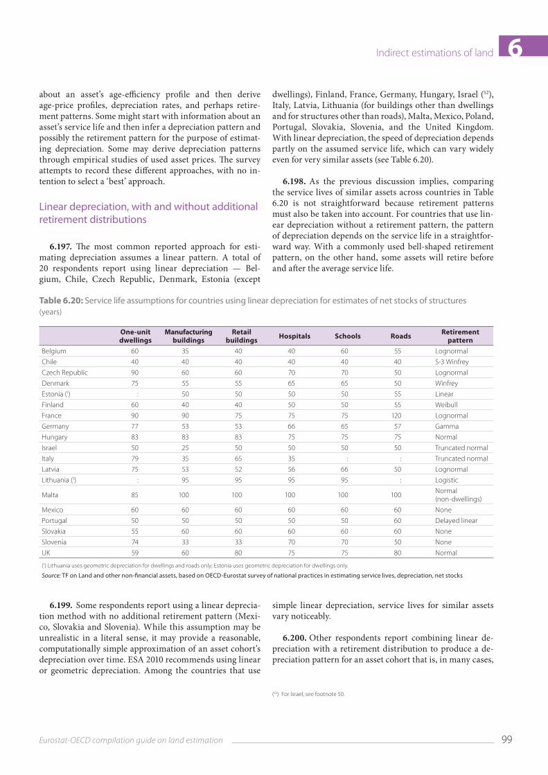
99Eurostat-OECD compilation guide on land estimation
Indirect estimations of land 6about an asset’s age‑efficiency profile and then derive age‑price profiles, depreciation rates, and perhaps retire‑ment patterns. Some might start with information about an asset’s service life and then infer a depreciation pattern and possibly the retirement pattern for the purpose of estimat‑ing depreciation. Some may derive depreciation patterns through empirical studies of used asset prices. The survey attempts to record these different approaches, with no in‑tention to select a ‘best’ approach.
Linear depreciation, with and without additional retirement distributions
6.197. The most common reported approach for esti‑mating depreciation assumes a linear pattern. A total of 20 respondents report using linear depreciation — Bel‑gium, Chile, Czech Republic, Denmark, Estonia (except
dwellings), Finland, France, Germany, Hungary, Israel (52), Italy, Latvia, Lithuania (for buildings other than dwellings and for structures other than roads), Malta, Mexico, Poland, Portugal, Slovakia, Slovenia, and the United Kingdom. With linear depreciation, the speed of depreciation depends partly on the assumed service life, which can vary widely even for very similar assets (see Table 6.20).
6.198. As the previous discussion implies, comparing the service lives of similar assets across countries in Table 6.20 is not straightforward because retirement patterns must also be taken into account. For countries that use lin‑ear depreciation without a retirement pattern, the pattern of depreciation depends on the service life in a straightfor‑ward way. With a commonly used bell‑shaped retirement pattern, on the other hand, some assets will retire before and after the average service life.
Table 6.20: Service life assumptions for countries using linear depreciation for estimates of net stocks of structures(years)
One-unit dwellings
Manufacturing buildings
Retail buildings Hospitals Schools Roads Retirement
patternBelgium 60 35 40 40 60 55 Lognormal
Chile 40 40 40 40 40 40 S-3 Winfrey
Czech Republic 90 60 60 70 70 50 Lognormal
Denmark 75 55 55 65 65 50 Winfrey
Estonia (1) : 50 50 50 50 55 Linear
Finland 60 40 40 50 50 55 Weibull
France 90 90 75 75 75 120 Lognormal
Germany 77 53 53 66 65 57 Gamma
Hungary 83 83 83 75 75 75 Normal
Israel 50 25 50 50 50 50 Truncated normal
Italy 79 35 65 35 : : Truncated normal
Latvia 75 53 52 56 66 50 Lognormal
Lithuania (1) : 95 95 95 95 : Logistic
Malta 85 100 100 100 100 100 Normal (non-dwellings)
Mexico 60 60 60 60 60 60 None
Portugal 50 50 50 50 50 60 Delayed linear
Slovakia 55 60 60 60 60 60 None
Slovenia 74 33 33 70 70 50 None
UK 59 60 80 75 75 80 Normal
(1) Lithuania uses geometric depreciation for dwellings and roads only; Estonia uses geometric depreciation for dwellings only.
Source: TF on Land and other non-financial assets, based on OECD-Eurostat survey of national practices in estimating service lives, depreciation, net stocks
6.199. Some respondents report using a linear deprecia‑tion method with no additional retirement pattern (Mexi‑co, Slovakia and Slovenia). While this assumption may be unrealistic in a literal sense, it may provide a reasonable, computationally simple approximation of an asset cohort’s depreciation over time. ESA 2010 recommends using linear or geometric depreciation. Among the countries that use
simple linear depreciation, service lives for similar assets vary noticeably.
6.200. Other respondents report combining linear de‑preciation with a retirement distribution to produce a de‑preciation pattern for an asset cohort that is, in many cases,
(52) For Israel, see footnote 50.
100 Eurostat-OECD compilation guide on land estimation
Indirect estimations of land6convex to the origin and similar to geometric depreciation, which Measuring Capital recommends. The countries that combine linear depreciation with retirement distributions employ a range of mathematical retirement functions to produce bell‑shaped or other retirement patterns, and the specific parameters of these chosen distributions vary as well. This range of assumptions further complicates com‑parisons of depreciation patterns of similar assets across countries. (See Measuring Capital, Chapter 13, for more in‑formation on these retirement distributions.)
— The normal distribution for retirements (Hungary, Malta for non‑dwellings, and the United Kingdom) is symmet‑ric, with 95 % of the probabilities lying within two stand‑ard deviations around the mean.
— The lognormal retirement distribution (Belgium, Czech Republic, France and Latvia) is a distribution whose log‑arithm is normally distributed; it is right‑skewed, with a low probability of retirement in the first years of an as‑set’s life and higher retirement probabilities later in an asset’s life.
— A truncated normal retirement distribution (Israel (53) and Italy) has a retirement period that is restricted to fall within a specified range of years before and after an as‑set’s average service life.
— Chile and Denmark combine linear depreciation with an S‑3 Winfrey retirement distribution, which is also sym‑metric and bell‑shaped.
— Germany uses the gamma distribution to calculate the distribution of retirements. The choice of this function was based on empirical data of motor vehicle registra‑tion. The parameters (and shape) of the gamma function were chosen based on empirical studies (54). The gamma distribution leads to a nearly bell‑shaped retirement dis‑tribution and an age‑price profile that is convex to the origin.
— Finland uses a Weibull retirement distribution, which is flexible, widely used, and can accommodate a range of shapes.
6.201. Respondents using linear depreciation also vary in terms of the level of asset detail at which service life as‑sumptions are made. Separate PIM‑based estimates of net stocks for detailed categories of structures enable statisti‑cians to produce estimates of values for detailed categories
(53) For Israel, see footnote 50.
(54) Schmalwasser, Oda and Michael Schidlowski, ‘Kapitalstockrechnung in Deutschland’, June 2006. Available at https://www.destatis.de/DE/Publikationen/WirtschaftStatistik/VGR/Kapitalstockrechnung.pdf?__blob=publicationFile. Slightly abridged version in English available at https://www.destatis.de/EN/Publications/Specialized/Nationalaccounts/MeasuringCapitalStockWista1106.pdf?__blob=publicationFile
of land, assuming the underlying PIM assumptions are reli‑able. Some (such as Finland, Germany and the UK) report assumptions that vary by detailed categories of types of as‑sets or industries. Others (such as Chile, Mexico, Portugal, Slovakia, or Slovenia) report assumptions for the PIM for a few broadly defined asset types (such as one assumption for all buildings that are not dwellings).
Geometric depreciation
6.202. Geometric depreciation is the second most com‑monly reported functional form. Austria, Canada, Estonia (for dwellings), Iceland, Japan, Lithuania (for dwellings and roads), Norway, Sweden, and the United States use geomet‑ric depreciation rates in their PIM estimates. Measuring Capital recommends the use of geometric depreciation; ESA 2010 recommends straight‑line or geometric depreciation. Respondents did not report separate retirement distribu‑tions with geometric depreciation; this convex pattern is already broadly consistent with the pattern of attrition pro‑duced by a number of retirement distributions.
6.203. Across countries that choose geometric deprecia‑tion pattern, the assumed annual depreciation rates vary even for very similar assets (Table 6.21). In the case of dwell‑ings, for example, annual depreciation rates range from a low of 0.011 for the USA and Sweden (which borrows the USA’s assumptions) to a high of 0.055 for wooden dwellings in Japan; other countries tend to use depreciation rates that range from 0.02 and 0.03. Across countries that choose geo‑metric depreciation patterns, the annual depreciation rates range from 0.018 to 0.081 for schools. Other assets display similar ranges of depreciation rates.
6.204. These differences in depreciation rates can lead to substantial differences in the proportion of a cohort of an asset that remains in the stock over time, especially for long‑lived assets such as structures. After 25 years, for ex‑ample, the percentage of the original value of a dwelling that is left ranges from 75 % in the United States to 30 % in Japan (for non‑wooden and wooden dwellings combined). After 50 years, the percentage of the original value of a dwelling that is left ranges from 56 % in the United States to 9 % in Japan (for non‑wooden and wooden dwellings combined). Even small differences in assumed annual depreciation rates can lead to substantial differences in estimates of the value of land, estimated through the residual method.
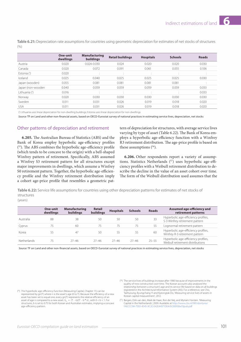
101Eurostat-OECD compilation guide on land estimation
Indirect estimations of land 6Table 6.21: Depreciation rate assumptions for countries using geometric depreciation for estimates of net stocks of structures(%)
One-unit dwellings
Manufacturing buildings Retail buildings Hospitals Schools Roads
Austria 0.020 0.024-0.030 0.024 0.020 0.020 0.030
Canada 0.020 0.072 0.091 0.061 0.055 0.106
Estonia (1) 0.020 : : : : :
Iceland 0.025 0.040 0.025 0.025 0.025 0.030
Japan (wooden) 0.055 0.081 0.081 0.081 0.081 :
Japan (non-wooden 0.040 0.059 0.059 0.059 0.059 0.033
Lithuania (1) 0.016 : : : : 0.033
Norway 0.020 0.030 0.030 0.030 0.030 0.030
Sweden 0.011 0.031 0.026 0.019 0.018 0.020
USA 0.011 0.031 0.026 0.019 0.018 0.020
(1) Lithuania uses linear depreciation for non-dwelling buildings; Estonia uses linear depreciation for non-dwellings
Source: TF on Land and other non-financial assets, based on OECD-Eurostat survey of national practices in estimating service lives, depreciation, net stocks
Other patterns of depreciation and retirement
6.205. The Australian Bureau of Statistics (ABS) and the Bank of Korea employ hyperbolic age‑efficiency profiles (55). The ABS combines the hyperbolic age‑efficiency profile (which tends to be concave to the origin) with a bell‑shaped Winfrey pattern of retirement. Specifically, ABS assumed a Winfrey S3 retirement pattern for all structures except major improvements in dwellings, which assume a Winfrey S0 retirement pattern. Together, the hyperbolic age‑efficien‑cy profile and the Winfrey retirement distribution imply a cohort age‑price profile that resembles a geometric pat‑
(55) The hyperbolic age-efficiency function (Measuring Capital, Chapter 11) can be represented by gn(T) where n is the asset’s age (0 to T). Because the efficiency of a new asset has been set to equal one, every gn(T) represents the relative efficiency of an asset of age n compared to a new asset. Gn = (T – n)/(T – b * n) , with 0 < b < 1. For structures, b is set to 0.75 for both Korean and Australian estimates, implying a concave age-efficiency pattern.
tern of depreciation for structures, with average service lives varying by type of asset (Table 6.22). The Bank of Korea em‑ploys a hyperbolic age‑efficiency function with a Winfrey R3 retirement distribution. The age‑price profile is based on these assumptions (56).
6.206. Other respondents report a variety of assump‑tions. Statistics Netherlands (57) uses hyperbolic age‑effi‑ciency profiles with a Weibull retirement distribution to de‑scribe the decline in the value of an asset cohort over time. The form of the Weibull distribution used assumes that the
(56) The service lives of buildings increase after 1980 because of improvements in the quality of new construction over time. The Korean accounts also analysed the relationship between a structure’s age and its service life based on data on all buildings registered in the Architectural Information System (AIS). For a reference, see Cho, Taehyoung, Byungchang YI and Kyeongtak Do, ‘Measuring service lives of assets in Korean capital measurement’, 2012.
(57) Bergen, Dirk van den, Mark de Haan, Ron de Heij, and Myriam Horsten. ‘Measuring Capital in the Netherlands’; 2009. Available at http://www.cbs.nl/NR/rdonlyres/FAECCC9A-75E0-4545-9C2C-E42E44371DE4/0/200936x10pub.pdf
Table 6.22: Service life assumptions for countries using other depreciation patterns for estimates of net stocks of structures(years)
One-unit dwellings
Manufacturing buildings
Retail buildings Hospitals Schools Roads Assumed age-efficiency and
retirement patterns
Australia 88 38 50 50 50 33 Hyperbolic age-efficiency profiles, S-3 Winfrey retirement pattern
Cyprus 75 60 75 75 75 55 Lognormal retirement pattern
Korea 55 47 50 55 55 60 Hyperbolic age-efficiency profiles, Winfrey R-3 retirement pattern
Netherlands 75 27–46 27–46 27–46 27–46 25–55 Hyperbolic age-efficiency profiles, Weibull retirement distributions
Source: TF on Land and other non-financial assets, based on OECD-Eurostat survey of national practices in estimating service lives, depreciation, net stocks
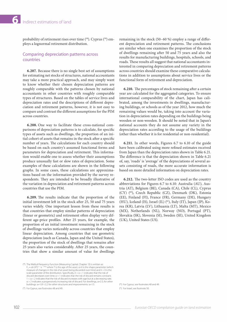
102 Eurostat-OECD compilation guide on land estimation
Indirect estimations of land6probability of retirement rises over time (58). Cyprus (59) em‑ploys a lognormal retirement distribution.
Comparing depreciation patterns across countries
6.207. Because there is no single best set of assumptions for estimating net stocks of structures, national accountants may take a more practical approach, and may simply want to know whether their chosen depreciation patterns are roughly comparable with the patterns chosen by national accountants in other countries with roughly comparable types of structures. Based on the tables of service lives and depreciation rates and the descriptions of different depre‑ciation and retirement patterns, however, it is not easy to compare and contrast the different assumptions for the PIM across countries.
6.208. One way to facilitate these cross‑national com‑parisons of depreciation patterns is to calculate, for specific types of assets such as dwellings, the proportion of an ini‑tial cohort of assets that remains in the stock after a specific number of years. The calculations for each country should be based on each country’s assumed functional forms and parameters for depreciation and retirement. This informa‑tion would enable one to assess whether their assumptions produce unusually fast or slow rates of depreciation. Some examples of these calculations are shown in the following graphs. In some cases, these calculations are approxima‑tions based on the information provided by the survey re‑spondents. They are intended to be broadly illustrative of the variation in depreciation and retirement patterns across countries that use the PIM.
6.209. The results indicate that the proportion of the initial investment left in the stock after 25, 50 and 75 years varies widely. One important lesson from these results is that countries that employ similar patterns of depreciation (linear or geometric) and retirement often display very dif‑ferent age‑price profiles. After 25 years, for example, the proportion of an initial investment remaining in the stock of dwellings varies noticeably across countries that employ linear depreciation. Among countries that use geometric depreciation (such as Canada, Japan and the United States), the proportion of the stock of dwellings that remains after 25 years also varies considerably. After 25 years, the coun‑tries that show a similar amount of value for dwellings
(58) The Weibull frequency function (Measuring Capital, Chapter 13) is written as: FT = αλ (λT)α –1 e – (λT)α where T is the age of the asset, α>0 is the shape parameter (which measure of changes in the risk of an asset being discarded over time) and λ > 0 is the scale parameter of the distribution. Specifically, 0 < α < 1 indicates that the risk of discard decreases over time; α = 1 indicates that the risk of discard remains constant; 1 < α < 2 indicates that the risk of discard increases with age but at a decreasing rate; α > 2 indicates a progressively increasing risk of discard. For dwellings, α=2.5; for other buildings: α=1.01–2.2; for other structures and improvements: α=1.5.
(59) For Cyprus, see footnotes 48 and 49.
remaining in the stock (50–60 %) employ a range of differ‑ent depreciation and retirement patterns. The conclusions are similar when one examines the proportion of the stock of dwellings remaining after 50 and 75 years and also the results for manufacturing buildings, hospitals, schools, and roads. These results all suggest that national accountants in‑terested in comparing depreciation and retirement patterns across countries should examine these comparative calcula‑tions in addition to assumptions about service lives or the functional form of retirement and depreciation.
6.210. The percentages of stock remaining after a certain year are calculated for the aggregated categories. To ensure international comparability of the chart, Japan has cali‑brated, among the investments in dwellings, manufactur‑ing buildings, or schools as of the year 2012, how much the remaining values would be, taking into account the varia‑tion in depreciation rates depending on the buildings being wooden or non‑wooden. It should be noted that in Japan’s national accounts they do not assume any variety in the depreciation rates according to the usage of the buildings (other than whether it is for residential or non‑residential).
6.211. In other words, Figures 6.7 to 6.10 of the guide have been calibrated using more refined estimates received from Japan than the depreciation rates shown in Table 6.21. The difference is that the depreciation shown in Table 6.21 of, say, ‘roads’ is ‘average’ of the depreciations of several as‑sets consisting of roads, the more accurate information is based on more detailed information on depreciation rates.
6.212. The two‑letter ISO codes are used as the country abbreviations for Figures 6.7 to 6.10: Australia (AU), Aus‑tria (AT), Belgium (BE), Canada (CA), Chile (CL), Cyprus (CY) (60), Czech Republic (CZ), Denmark (DK), Estonia (EE), Finland (FI), France (FR), Germany (DE), Hungary (HU), Iceland (IS), Israel (IL) (61), Italy (IT), Japan (JP), Ko‑rea (KR), Latvia (LV), Lithuania (LT), Malta (MT), Mexico (MX), Netherlands (NL), Norway (NO), Portugal (PT), Slovakia (SK), Slovenia (SI), Sweden (SE), United Kingdom (UK), United States (US).
(60) For Cyprus, see footnotes 48 and 49.
(61) For Israel, see footnote 50.
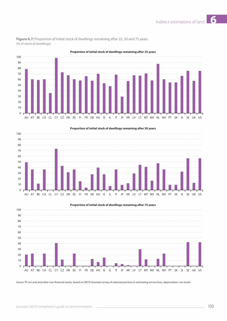
103Eurostat-OECD compilation guide on land estimation
Indirect estimations of land 6Figure 6.7: Proportion of initial stock of dwellings remaining after 25, 50 and 75 years(% of stock of dwellings)
Source: TF on Land and other non-financial assets, based on OECD-Eurostat survey of national practices in estimating service lives, depreciation, net stocks
0
40
30
20
10
50
60
80
70
90
100
Proportion of initial stock of dwellings remaining after 25 years
AU AT BE CA CL CY CZ DK EE FI FR DE HU IS IL IT JP KR LV LT MT MX NL NO PT SK SI SE UK US
Proportion of initial stock of dwellings remaining after 50 years
AU AT BE CA CL CY CZ DK EE FI FR DE HU IS IL IT JP KR LV LT MT MX NL NO PT SK SI SE UK US0
40
30
20
10
50
60
80
70
90
100
Proportion of initial stock of dwellings remaining after 75 years
AU AT BE CA CL CY CZ DK EE FI FR DE HU IS IL IT JP KR LV LT MT MX NL NO PT SK SI SE UK US0
40
30
20
10
50
60
80
70
90
100
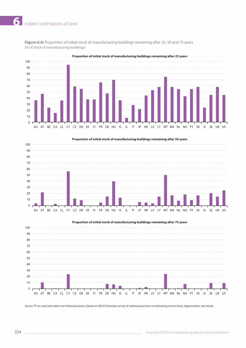
104 Eurostat-OECD compilation guide on land estimation
Indirect estimations of land6Figure 6.8: Proportion of initial stock of manufacturing buildings remaining after 25, 50 and 75 years(% of stock of manufacturing buildings)
Source: TF on Land and other non-financial assets, based on OECD-Eurostat survey of national practices in estimating service lives, depreciation, net stocks
Proportion of initial stock of manufacturing buildings remaining after 25 years
AU AT BE CA CL CY CZ DK EE FI FR DE HU IS IL IT JP KR LV LT MT MX NL NO PT SK SI SE UK US0
40
30
20
10
50
60
80
70
90
100
Proportion of initial stock of manufacturing buildings remaining after 50 years
AU AT BE CA CL CY CZ DK EE FI FR DE HU IS IL IT JP KR LV LT MT MX NL NO PT SK SI SE UK US0
40
30
20
10
50
60
80
70
90
100
Proportion of initial stock of manufacturing buildings remaining after 75 years
AU AT BE CA CL CY CZ DK EE FI FR DE HU IS IL IT JP KR LV LT MT MX NL NO PT SK SI SE UK US0
40
30
20
10
50
60
80
70
90
100
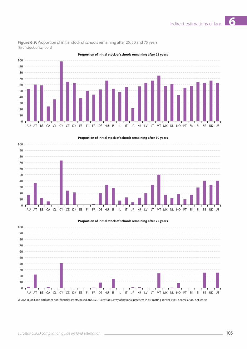
105Eurostat-OECD compilation guide on land estimation
Indirect estimations of land 6Figure 6.9: Proportion of initial stock of schools remaining after 25, 50 and 75 years(% of stock of schools)
Source: TF on Land and other non-financial assets, based on OECD-Eurostat survey of national practices in estimating service lives, depreciation, net stocks
Proportion of initial stock of schools remaining after 25 years
AU AT BE CA CL CY CZ DK EE FI FR DE HU IS IL IT JP KR LV LT MT MX NL NO PT SK SI SE UK US0
40
30
20
10
50
60
80
70
90
100
Proportion of initial stock of schools remaining after 50 years
AU AT BE CA CL CY CZ DK EE FI FR DE HU IS IL IT JP KR LV LT MT MX NL NO PT SK SI SE UK US0
40
30
20
10
50
60
80
70
90
100
Proportion of initial stock of schools remaining after 75 years
AU AT BE CA CL CY CZ DK EE FI FR DE HU IS IL IT JP KR LV LT MT MX NL NO PT SK SI SE UK US0
40
30
20
10
50
60
80
70
90
100
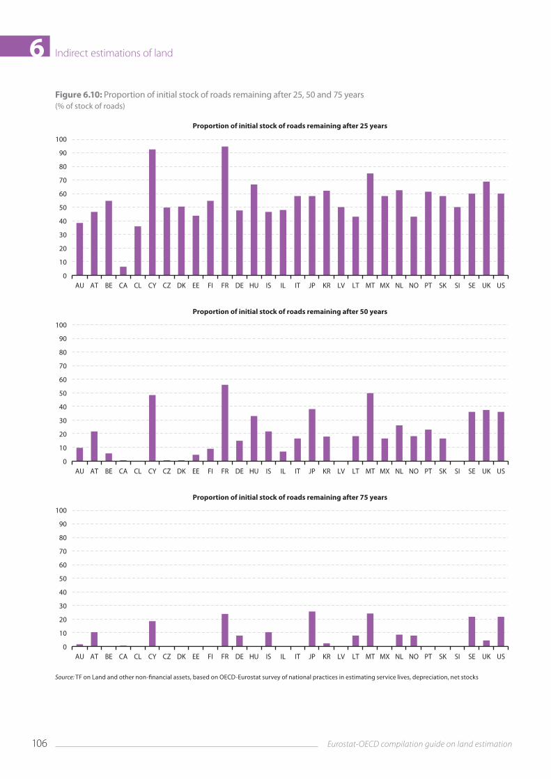
106 Eurostat-OECD compilation guide on land estimation
Indirect estimations of land6Figure 6.10: Proportion of initial stock of roads remaining after 25, 50 and 75 years(% of stock of roads)
Source: TF on Land and other non-financial assets, based on OECD-Eurostat survey of national practices in estimating service lives, depreciation, net stocks
Proportion of initial stock of roads remaining after 25 years
AU AT BE CA CL CY CZ DK EE FI FR DE HU IS IL IT JP KR LV LT MT MX NL NO PT SK SI SE UK US0
40
30
20
10
50
60
80
70
90
100
Proportion of initial stock of roads remaining after 50 years
AU AT BE CA CL CY CZ DK EE FI FR DE HU IS IL IT JP KR LV LT MT MX NL NO PT SK SI SE UK US0
40
30
20
10
50
60
80
70
90
100
Proportion of initial stock of roads remaining after 75 years
AU AT BE CA CL CY CZ DK EE FI FR DE HU IS IL IT JP KR LV LT MT MX NL NO PT SK SI SE UK US0
40
30
20
10
50
60
80
70
90
100
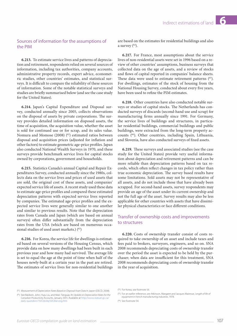
107Eurostat-OECD compilation guide on land estimation
Indirect estimations of land 6Sources of information for the assumptions of the PIM
6.213. To estimate service lives and patterns of deprecia‑tion and retirement, respondents relied on several sources of information, including tax authorities, company accounts, administrative property records, expert advice, economet‑ric studies, other countries’ estimates, and statistical sur‑veys. It is difficult to compare the reliability of these sources of information. Some of the notable statistical surveys and studies are briefly summarised below (and see the case study for the United States).
6.214. Japan’s Capital Expenditure and Disposal sur‑vey, conducted annually since 2005, collects observations on the disposal of assets by private corporations. The sur‑vey provides detailed information on disposed assets, the time of acquisition, the acquisition value, whether the asset is sold for continued use or for scrap, and its sales value. Nomura and Momose (2008) (62) estimated ratios between disposal and acquisition prices (adjusted for inflation and other factors) to estimate geometric age‑price profiles. Japan also conducted National Wealth Surveys in 1970, and these surveys provide benchmark service lives for capital stocks owned by corporations, government and households.
6.215. Statistics Canada’s annual Capital and Repair Ex‑penditures Survey, conducted annually since the 1980s, col‑lects data on the service lives and prices of used assets that are sold, the original cost of these assets, and companies’ expected service life of assets. A recent study used these data to estimate age‑price profiles and compared these estimated depreciation patterns with expected service lives reported by companies. The estimated age‑price profiles and the ex‑pected service lives were generally similar to one another and similar to previous results. Note that the depreciation rates from Canada and Japan (which are based on annual surveys) often differ substantially from the depreciation rates from the USA (which are based on numerous occa‑sional studies of used asset markets.) (63)
6.216. For Korea, the service life for dwellings is estimat‑ed based on several versions of the Housing Census, which provide data on how many dwellings had been built in each previous year and how many had survived. The average life is set to equal the age at the point of time when half of the houses newly‑built at a certain year in the past are retired. The estimates of service lives for non‑residential buildings
(62) Measurement of Depreciation Rates Based on Disposal Asset Data In Japan (OECD, 2008).
(63) See Baldwin, John, Huju Liu, and Marc Tanguay An Update on Depreciation Rates for the Canadian Productivity Accounts, January 2015. Available at http://www.statcan.gc.ca/daily-quotidien/150126/dq150126d-eng.htm
are based on the estimates for residential buildings and also a survey (64).
6.217. For France, most assumptions about the service lives of non‑residential assets were set in 1996 based on a re‑view of other countries’ assumptions, business surveys that collected data on the age of assets, and a review of stocks and flows of capital reported in companies’ balance sheets. These data were used to estimate retirement patterns (65). For dwellings, estimates of the stock of housing from the National Housing Survey, conducted about every five years, have been used to refine the PIM estimates.
6.218. Other countries have also conducted notable sur‑veys or studies of capital stocks. The Netherlands has con‑ducted surveys of discards (second‑hand use and scrap) for manufacturing firms annually since 1991. For Germany, the service lives of buildings and structures, in particu‑lar residential buildings, commercial buildings and public buildings, were extracted from the long‑term property ac‑counts (66). Other countries, including Spain, Lithuania, and Slovenia, have also conducted surveys of fixed assets.
6.219. These surveys and associated studies (see the case study for the United States) provide very useful informa‑tion about depreciation and retirement patterns and can be more reliable than depreciation patterns based on tax re‑cords, which often reflect changes in tax policy rather than true economic depreciation. The survey based results have some limitations. Sold assets may not be representative of all assets, and do not include those that have already been scrapped. For second‑hand assets, survey respondents may provide an age of the asset under its current ownership and not the full age of the asset. Survey results may also be less applicable for other countries with assets that have dissimi‑lar physical characteristics or face different conditions.
Transfer of ownership costs and improvements to structures
6.220. Costs of ownership transfer consist of costs re‑quired to take ownership of an asset and include taxes and fees paid to brokers, surveyors, engineers, and so on. SNA 2008 recommends depreciating costs of ownership transfer over the period the asset is expected to be held by the pur‑chaser; when data are insufficient for this treatment, SNA 2008 recommends depreciating costs of ownership transfer in the year of acquisition.
(64) For Korea, see footnote 56.
(65) For an earlier reference, see Atkinson, Margaret and Jacques Mairesse, Length of life of equipment in French manufacturing industries, 1978.
(66) See footnote 54.
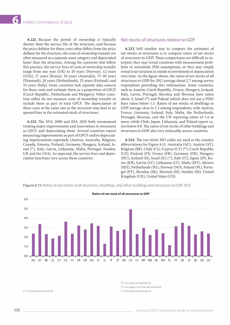
108 Eurostat-OECD compilation guide on land estimation
Indirect estimations of land66.221. Because the period of ownership is typically
shorter than the service life of the structure, and because the price deflator for these costs often differs from the price deflator for the structure, the costs of ownership transfer are often measured as a separate asset category and depreciated faster than the structure. Among the countries that follow this practice, the service lives of costs of ownership transfer range from one year (UK) to 10 years (Norway), 12 years (USA), 17 years (Korea), 18 years (Australia), 17–30 years (Denmark), 20 years (Netherlands), 25 years (Finland), and 34 years (Italy). Some countries lack separate data sources for these costs and estimate them as a proportion of GFCF (Czech Republic, Netherlands and Hungary). Other coun‑tries either do not measure costs of ownership transfer or include them as part of total GFCF. The depreciation of these costs at the same rate as the structure may lead to an upward bias in the estimated stock of structures.
6.222. The SNA 2008 and ESA 2010 both recommend treating major improvements and renovations to structures as GFCF and depreciating them. Several countries report measuring improvements as part of GFCF and/or depreciat‑ing improvements separately (Austria, Australia, Belgium, Canada, Estonia, Finland, Germany, Hungary, Iceland, Is‑rael (67), Italy, Latvia, Lithuania, Malta, Portugal, Sweden, UK and the USA). As expected, the service lives and depre‑ciation functions vary across these countries.
Net stocks of structures relative to GDP
6.223. Still another way to compare the estimates of net stocks of structures is to compare ratios of net stocks of structures to GDP. These comparisons are difficult to in‑terpret: they may reveal countries with measurement prob‑lems or unrealistic PIM assumptions, or they may simply reveal true variation in trends in investment or depreciation over time. As the figure shows, the ratios of net stocks of all structures to GDP for 2012 average about 2.7 among survey respondents providing this information. Some countries, such as Austria, Czech Republic, France, Hungary, Iceland, Italy, Latvia, Portugal, Slovakia and Slovenia have ratios above 3; Israel (68) and Poland (which does not use a PIM) have ratios below 1.3. Ratios of net stocks of dwellings to GDP average close to 1.2 among respondents, with Austria, France, Germany, Iceland, Italy, Malta, the Netherlands, Portugal, Slovenia, and the UK reporting ratios of 1.4 or more, while Chile, Japan, Lithuania, and Poland report ra‑tios below 0.8. The ratios of net stocks of other buildings and structures to GDP also vary noticeably across countries.
6.224. The two‑letter ISO codes are used as the country abbreviations for Figure 6.11: Australia (AU), Austria (AT), Belgium (BE), Chile (CL), Cyprus (CY) (69), Czech Republic (CZ), Finland (FI), France (FR), Germany (DE), Hungary (HU), Iceland (IS), Israel (IL) (70), Italy (IT), Japan (JP), Ko‑rea (KR), Latvia (LV), Lithuania (LT), Malta (MT), Mexico (MX), Netherlands (NL), Norway (NO), Poland (PL), Portu‑gal (PT), Slovakia (SK), Slovenia (SI), Sweden (SE), United Kingdom (UK), United States (US).
Figure 6.11: Ratios of net stocks of all structures, dwellings, and other buildings and structures to GDP, 2012
(67) For Israel, see footnote 50.
(68) For Israel, see footnote 50.
(69) For Cyprus, see footnotes 48 and 49.
(70) For Israel, see footnote 50.
0.0
4.0
3.0
2.0
1.0
5.0
6.0
Ratios of net stock of all structures to GDP
AU AT BE CL CY CZ FI FR DE HU IS IL IT JP KR LV LT MT MX NL NO PL PT SK SI SE UK US
109Eurostat-OECD compilation guide on land estimation
Indirect estimations of land 6
Source: TF on Land and other non-financial assets, based on OECD-Eurostat survey of national practices in estimating service lives, depreciation, net stocks
Government owned land
6.225. Chapter 8.3 notes the importance of estimates of government owned land. The survey finds that only a few countries report producing measures of the stock of gov‑ernment‑owned land, through the residual approach or any other way. The countries that report estimates of govern‑ment‑owned land are Australia, the Netherlands (although not land under roads), Czech Republic, Japan, Italy (for land under dwellings and buildings, by applying LSRs), Korea (for all government‑owned land) and Romania (for agri‑cultural land). Several countries report PIM assumptions for net stocks of typical government‑owned assets (roads, bridges, airports, waterways, and so on) but these estimates are usually not used to estimate underlying stocks of land.
Major concerns and plans for the future
6.226. Respondents were generally confident about the quality of their estimates but also expressed a range of con‑cerns. The major concerns include the reliability of assump‑tions of service lives and depreciation; the quality of GFCF data and price deflators (especially for earlier decades); price indices that do not adequately capture quality and produc‑tivity gains; inadequate measurement of costs of ownership transfer, improvements, or second‑hand sales; measures of GFCF that are on net terms (acquisitions less disposals) in‑stead of separately identifying new investment; and inaccu‑rate estimates of stocks of land through the residual or ratio approaches.
6.227. The most common plans for improving estimates in the future include the implementation of the provisions of SNA 2008 and ESA 2010 along with research to improve the estimates of nonfinancial assets for national balance sheets. Many expressed an interest in improving estimates of the total value of land and structures, improving estimates of
0.0
1.5
1.0
0.5
2.0
2.5
Ratios of net stock of dwellings to GDP
AU AT BE CL CY CZ FI FR DE HU IS IL IT JP KR LV LT MT MX NL NO PL PT SK SI SE UK US
0.0
3.0
2.5
2.0
1.5
1.0
0.5
3.5
4.0
Ratios net stock of other buildings and structures to GDP
AU AT BE CL CY CZ FI FR DE HU IS IL IT JP KR LV LT MT MX NL NO PL PT SK SI SE UK US
110 Eurostat-OECD compilation guide on land estimation
Indirect estimations of land6land through the residual approach, improving assump‑tions about service lives and depreciation, and improving price measures.
Conclusions
6.228. As the survey results indicate, national accounts across countries vary — sometimes considerably — in their assumptions and sources of information for estimates of net stocks based on a PIM. Different assumptions for the PIM can, in turn, lead to different estimates of land values ob‑tained through the residual or LSR approach. These assump‑tions may vary across countries with similar ‘true’ patterns of depreciation because of measurement errors. Even with‑out measurement error, differences in assumptions across countries may also correctly reflect real differences in fac‑tors that affect depreciation (the physical nature of struc‑tures, building materials, maintenance, climate, variation in the use of structures, etc.). Thus, disparities in estimates of land values across countries can be difficult to interpret. As this chapter notes, one way to facilitate comparisons of approaches across countries with different functional forms of depreciation and retirement is to compute the proportion of a cohort of assets left after a number of years, using each country’s assumptions for the PIM.
6.229. Despite the uncertainties in estimating net stocks of structures through the PIM, the PIM and the residual and ratio approaches for estimating stocks of land still have many advantages. For many countries, these indirect ap‑proaches may be the only credible approach for estimating stocks of land underlying structures. The residual approach gives countries a useful credibility check for estimates of the combined value of structures and land and estimates of net stocks and depreciation, which are needed for national income accounting. The presence of negative or unrealistic estimates of land values can indicate problems in one or both of these estimates. Balance sheets could arguably rely solely on estimates of the combined value of structures and land (through real estate data, for example), but these es‑timates alone provide an incomplete picture. The residual approach can help countries assess whether increases in the total value of land and structures arises mainly from land or from structures. Assuming bubbles are most likely to ap‑pear as increases in land values under the residual approach, year‑to‑year changes in the residual estimates of land values may be useful in identifying bubbles.
6.230. The results of the survey will hopefully lead to sharing of information across countries and useful discus‑sions about how best to produce reasonable, internationally comparable estimates of net stocks of structures. A more de‑tailed presentation of the responses to the survey is present‑ed in a separate report ‘Eurostat‑OECD survey of national practices in estimating net stocks of structures’.
Case study depreciation estimates: United States
The US Bureau of Economic Analysis (BEA) bases its depre‑ciation patterns on empirical evidence of used asset pric‑es in resale markets wherever possible (71). For most asset types, including all structures, geometric patterns are used because the available data suggest that they more closely ap‑proximate actual profiles of price declines than straight‑line patterns. The geometric rates for several types of fixed assets are determined by dividing the appropriate declining‑bal‑ance rate for each asset by the asset’s assumed service life. BEA’s depreciation rates for structures are not regularly up‑dated; most are based on several detailed studies conducted several years ago.
The declining‑balance rates for structures used by BEA are primarily derived by Fraumeni from estimates made by Hulten and Wykoff under the auspices of the U.S. De‑partment of the Treasury (1979–1981) (72). For some struc‑tures, extensive data were available for estimating geomet‑ric rates of depreciation: office buildings, medical buildings, commercial warehouses, other commercial buildings, multi‑merchandise shopping, food and beverage establish‑ments, mobile offices, and manufacturing buildings. For some other buildings (hospitals, special care, lodging, and amusement and recreational buildings), more limited data were available, and the depreciation rates are based on judg‑ment and the results of empirical research (73).
Depreciation rates for other structures are based on several studies. For communication, electric light and power, gas, and petroleum pipeline structures, the service lives are de‑rived by comparing book value data provided by regulatory agencies with various perpetual inventory estimates calcu‑lated using alternative service lives. The depreciation rate for wind and solar was calculated by BEA based on indus‑try trade data. For petroleum and natural gas exploration, shafts, and wells, the lives are based on data from the Cen‑sus Bureau’s annual surveys of oil and gas for 1979–1982. For farm structures, the average service life is derived from U.S. Department of Agriculture studies. For other types of non‑farm structures, service lives are based on published and unpublished data from studies conducted during the
(71) This information is primarily taken from these BEA documents: 1) BEA Depreciation Estimates, 2) Barbara M. Fraumeni, The Measurement of Depreciation in the U.S. National Income and Product Accounts, July 1997, pp. 7–23, 3) Fixed Assets and Consumer Durable Goods in the United States 1925–97,.September 2003: M-29–M-33.
(72) The information on Hulten-Wykoff methodology is taken from three sources: 1) Hulten, Charles R., and Frank C. Wykoff, The Estimation of Economic Depreciation Using Vintage Asset Prices, April 1981, pp. 367–396. 2) Hulten, Charles R., and Frank C. Wykoff, The Measurement of Economic Depreciation, 1981, pp. 81–125. 3) Wykoff, Frank C., and Charles R. Hulten, Tax and Economic Depreciation of Machinery and Equipment: A Theoretical and Empirical Appraisal, Phase II Report, Economic Depreciation of the U.S. Capital Stock: A First Step, July 26 1979.
(73) This research was conducted by BEA, Dale Jorgenson, the Bureau of Labor Statistics, and Jack Faucett Associates. See for details Fraumeni, Barbara M. The Measurement of Depreciation in the U.S. National Income and Product Accounts, July 1997, pp. 7–23. Available at http://www.bea.gov/scb/pdf/national/niparel/1997/0797fr.pdf
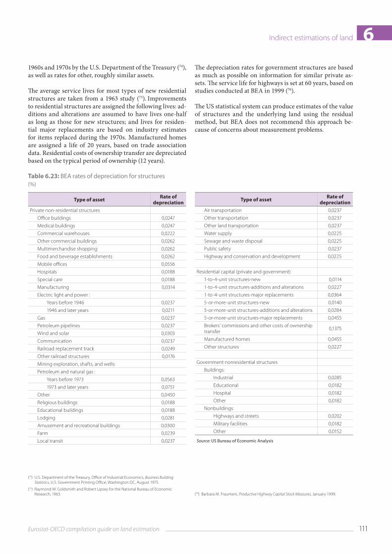
111Eurostat-OECD compilation guide on land estimation
Indirect estimations of land 61960s and 1970s by the U.S. Department of the Treasury (74), as well as rates for other, roughly similar assets.
The average service lives for most types of new residential structures are taken from a 1963 study (75). Improvements to residential structures are assigned the following lives: ad‑ditions and alterations are assumed to have lives one‑half as long as those for new structures; and lives for residen‑tial major replacements are based on industry estimates for items replaced during the 1970s. Manufactured homes are assigned a life of 20 years, based on trade association data. Residential costs of ownership transfer are depreciated based on the typical period of ownership (12 years).
(74) U.S. Department of the Treasury, Office of Industrial Economics, Business Building Statistics, U.S. Government Printing Office, Washington DC, August 1975.
(75) Raymond W. Goldsmith and Robert Lipsey for the National Bureau of Economic Research, 1963.
The depreciation rates for government structures are based as much as possible on information for similar private as‑sets. The service life for highways is set at 60 years, based on studies conducted at BEA in 1999 (76).
The US statistical system can produce estimates of the value of structures and the underlying land using the residual method, but BEA does not recommend this approach be‑cause of concerns about measurement problems.
(76) Barbara M. Fraumeni, Productive Highway Capital Stock Measures, January 1999.
Table 6.23: BEA rates of depreciation for structures(%)
Type of asset Rate of depreciation
Private non-residential structures
Office buildings 0,0247
Medical buildings 0,0247
Commercial warehouses 0,0222
Other commercial buildings 0,0262
Multimerchandise shopping 0,0262
Food and beverage establishments 0,0262
Mobile offices 0,0556
Hospitals 0,0188
Special care 0,0188
Manufacturing 0,0314
Electric light and power :
Years before 1946 0,0237
1946 and later years 0,0211
Gas 0,0237
Petroleum pipelines 0,0237
Wind and solar 0,0303
Communication 0,0237
Railroad replacement track 0,0249
Other railroad structures 0,0176
Mining exploration, shafts, and wells:
Petroleum and natural gas :
Years before 1973 0,0563
1973 and later years 0,0751
Other 0,0450
Religious buildings 0,0188
Educational buildings 0,0188
Lodging 0,0281
Amusement and recreational buildings 0,0300
Farm 0,0239
Local transit 0,0237
Type of asset Rate of depreciation
Air transportation 0,0237
Other transportation 0,0237
Other land transportation 0,0237
Water supply 0,0225
Sewage and waste disposal 0,0225
Public safety 0,0237
Highway and conservation and development 0,0225
Residential capital (private and government)
1-to-4-unit structures-new 0,0114
1-to-4-unit structures-additions and alterations 0,0227
1-to-4-unit structures-major replacements 0,0364
5-or-more-unit structures-new 0,0140
5-or-more-unit structures-additions and alterations 0,0284
5-or-more-unit structures-major replacements 0,0455
Brokers’ commissions and other costs of ownership transfer 0,1375
Manufactured homes 0,0455
Other structures 0,0227
Government nonresidential structures
Buildings:
Industrial 0,0285
Educational 0,0182
Hospital 0,0182
Other 0,0182
Nonbuildings:
Highways and streets 0,0202
Military facilities 0,0182
Other 0,0152
Source: US Bureau of Economic Analysis


From:Eurostat-OECD Compilation guide on landestimations
Access the complete publication at:https://doi.org/10.1787/9789264235175-en
Please cite this chapter as:
OECD/Eurostat (2015), “Indirect estimations of land”, in Eurostat-OECD Compilation guide on landestimations, Eurostat, Luxembourg.
DOI: https://doi.org/10.1787/9789264235175-7-en
This work is published under the responsibility of the Secretary-General of the OECD. The opinions expressed and argumentsemployed herein do not necessarily reflect the official views of OECD member countries.
This document and any map included herein are without prejudice to the status of or sovereignty over any territory, to thedelimitation of international frontiers and boundaries and to the name of any territory, city or area.
You can copy, download or print OECD content for your own use, and you can include excerpts from OECD publications,databases and multimedia products in your own documents, presentations, blogs, websites and teaching materials, providedthat suitable acknowledgment of OECD as source and copyright owner is given. All requests for public or commercial use andtranslation rights should be submitted to [email protected]. Requests for permission to photocopy portions of this material forpublic or commercial use shall be addressed directly to the Copyright Clearance Center (CCC) at [email protected] or theCentre français d’exploitation du droit de copie (CFC) at [email protected].


![STCQE=UWX[]U: - OECD iLibrary](https://img.dokumen.tips/doc/110x75/6319bb481e5d335f8d0b47fd/stcqeuwxu-oecd-ilibrary.jpg)


