Incremental Evolutionary

Methods for Automatic

Programming of Robot

Controllers

Thesis for the degree philosophiae doctor

Trondheim, November 2007

Norwegian University of Science and Technology

Faculty of Information Technology,

Mathematics and Electrical Engineering

Department of Computer and Information Science

Pavel Petrovic

I n n o v a t i o n a n d C r e a t i v i t y

NTNU

Norwegian University of Science and Technology

Thesis for the degree philosophiae doctor

Faculty of Information Technology, Mathematics and Electrical Engineering

Department of Computer and Information Science

© Pavel Petrovic

ISBN 978-82-471-5031-3 (printed version)

ISBN 978-82-471-5045-0 (electronic version)

ISSN 1503-8181

Doctoral theses at NTNU, 2007:228

Printed by NTNU-trykk

Abstract

The aim of the main work in the thesis is to investigate Incremental Evolutionmethods for designing a suitable behavior arbitration mechanism for behavior-based(BB) robot controllers for autonomous mobile robots performing tasks of higher com-plexity. The challenge of designing effective controllers for autonomous mobile robotshas been intensely studied for few decades. Control Theory studies the fundamentalcontrol principles of robotic systems. However, the technological progress allows,and the needs of advanced manufacturing, service, entertainment, educational, andmission tasks require features beyond the scope of the standard functionality andbasic control. Artificial Intelligence has traditionally looked upon the problem ofdesigning robotics systems from the high-level and top-down perspective: givena working robotic device, how can it be equipped with an intelligent controller.Later approaches advocated for better robustness, modifiability, and control dueto a bottom-up layered incremental controller and robot building (Behavior-BasedRobotics, BBR). Still, the complexity of programming such system often requiresmanual work of engineers. Automatic methods might lead to systems that performtask on demand without the need of expert robot programmer. In addition, a robotprogrammer cannot predict all the possible situations in the robotic applications.Automatic programming methods may provide flexibility and adaptability of therobotic products with respect to the task performed. One possible approach toautomatic design of robot controllers is Evolutionary Robotics (ER). Most of theexperiments performed in the field of ER have achieved successful learning oftarget task, while the tasks were of limited complexity. This work is a marriageof incremental idea from the BBR and automatic programming of controllersusing ER. Incremental Evolution allows automatic programming of robots for morecomplex tasks by providing a gentle and easy-to understand support by expert-knowledge — division of the target task into sub-tasks. We analyze different typesof incrementality, devise new controller architecture, implement an original simulatorcompatible with hardware, and test it with various incremental evolution tasks forreal robots. We build up our experimental field through studies of experimentaland educational robotics systems, evolutionary design, distributed computationthat provides the required processing power, and robotics applications. Universityresearch is tightly coupled with education. Combining the robotics research witheducational applications is both a useful consequence as well as a way of satisfyingthe necessary condition of the need of underlying application domain where theresearch work can both reflect and base itself.

Preface

When the robots will start going skiing of their own will, the age of robotswill have come.

My first meeting with programmable robots occurred as an instructor in the summercamp for talented young children in the early 90s where we were programminga simple LEGO-built scanner and greenhouse using a dialect of Logo running onMacintosh Classic.

Later on, professor Sam Thangiah introduced me to real mobile robots (B12 fromthe Real World Interfaces) that we programmed in assembly and C as the assign-ments for his Machine Learning course at Slippery Rock in Pennsylvania. He alsointroduced me to the capabilities and applications of Evolutionary Computation.

Arriving to NTNU threw me into more unavoidable hands-on LEGO experienceand hacking, where I was lucky to remain part of the increasing interest in roboticsand robotics contests at all age levels.

The studies in the field of artificial intelligence give me strong arguments tobelieve that there is a good chance for the robots being able to start sharing acommon environment with us while being at our service soon. The realizationis the job for the industry. In academia, we ought to overcome the scientificand technological barriers, develop algorithms, and methods. It is now the mostinteresting time when such technologies get born, and this work is a tiny contributioninto that area.

During my graduate studies, I happened to get involved in several differentprojects cooperating with different people and groups, while keeping work on myown lonely thesis thread at the same time. In this paper, I would like to share withyou all of that, keeping the main focus on my own original ideas, while includingall the cooperative work, which relates to it and joins into one common themeEvolutionary Robotics.

Acknowledgments

First of all, I would like to express my appreciations to the institute and the facultyfor providing me with a creative, inspiring, and friendly working environment for anextensive period of time.

Several colleagues contributed to the outcome. The most valuable feedbackand care was always received from my adviser, professor Keith Downing. Thanksto his strong principles and dedication, and due to the scientifically appreciatingenvironment created by the group and division leader professor Agnar Aamodt,the laboratory for sub-symbolic artificial intelligence existed at our departmentthroughout the whole duration of this work, and served as a wonderful place toexchange the ideas among us, the students.

I thank to Zoran Constantinescu Fulop for productive cooperation on thedistributed computation tools and projects, and for sharing a lot of valuable workand time.

A special thanks belongs to the technical group of the department. Without theirsupport, running the experiments in the student laboratories would be impossible.

I am very grateful to professor Henrik Hautop Lund from Maersk institute inOdense and his colleagues, who allowed me to spend one semester with them andwho contributed with a very useful feedback.

I am thankful to the members of Robotika.SK, namely Dusan Durina, RichardBalogh, Andrej Lucny, and Jozef Omelka, who provided a great robotics learningenvironment during my civil service year in Slovakia.

I am committed to my parents and sister, who sought for my personal happinessespecially during my visits at home, as well as for my comfort (a special thanks forall those warm hand-made wool pullovers).

And finally, big hug to all the Norwegian, Greek, Spanish, Italian, French,Dutch, German, Finish, American, African, Portuguese, Danish, and even Czechand Slovak, and other girls I met during the years, they were a great inspiration,and it was all worth just that. :)

Disclaimer

LEGO, LEGO Mindstorms, LEGO Mindstorms NXT, BlueTooth, SONY, Aibo,Khepera, and other trademarks appearing in the text are owned by the respectiveowners.

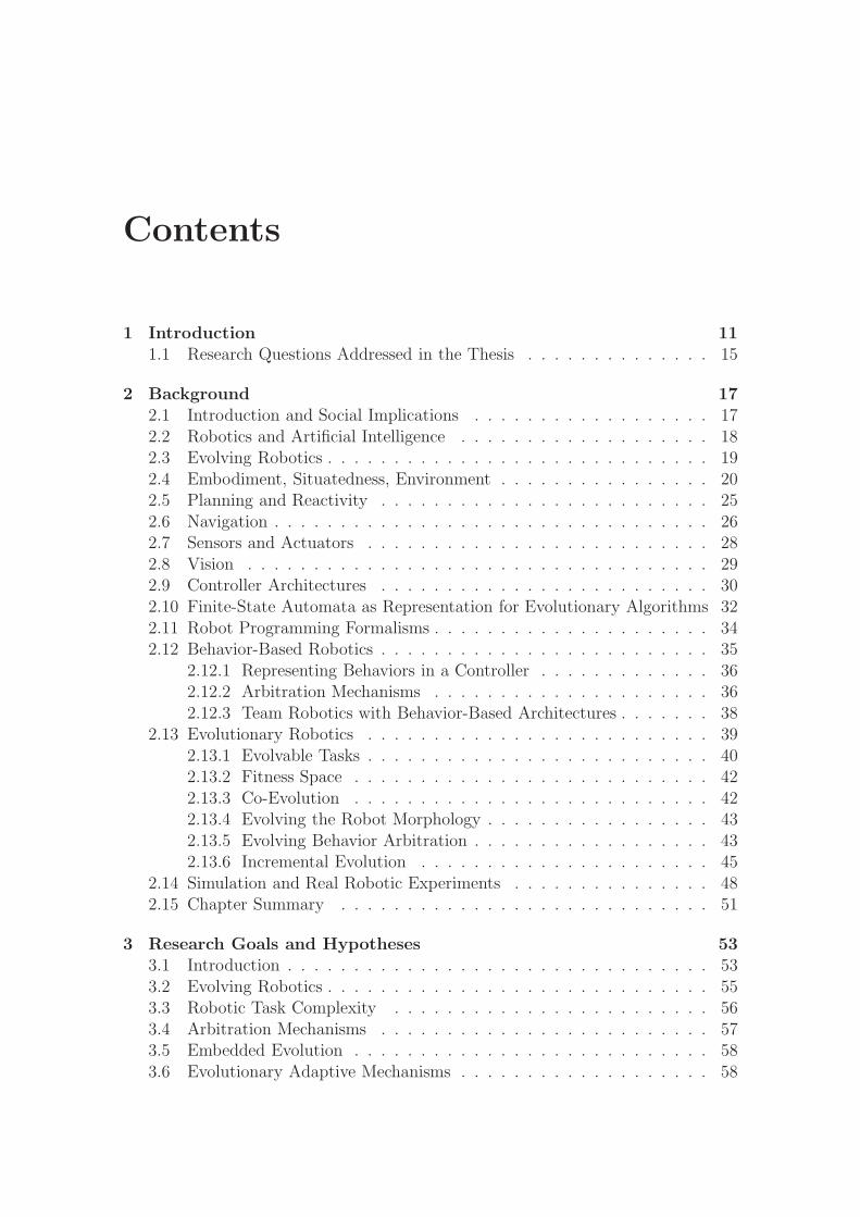
Contents

1 Introduction 111.1 Research Questions Addressed in the Thesis . . . . . . . . . . . . . . 15

2 Background 172.1 Introduction and Social Implications . . . . . . . . . . . . . . . . . . 172.2 Robotics and Artificial Intelligence . . . . . . . . . . . . . . . . . . . 182.3 Evolving Robotics . . . . . . . . . . . . . . . . . . . . . . . . . . . . . 192.4 Embodiment, Situatedness, Environment . . . . . . . . . . . . . . . . 202.5 Planning and Reactivity . . . . . . . . . . . . . . . . . . . . . . . . . 252.6 Navigation . . . . . . . . . . . . . . . . . . . . . . . . . . . . . . . . . 262.7 Sensors and Actuators . . . . . . . . . . . . . . . . . . . . . . . . . . 282.8 Vision . . . . . . . . . . . . . . . . . . . . . . . . . . . . . . . . . . . 292.9 Controller Architectures . . . . . . . . . . . . . . . . . . . . . . . . . 302.10 Finite-State Automata as Representation for Evolutionary Algorithms 322.11 Robot Programming Formalisms . . . . . . . . . . . . . . . . . . . . . 342.12 Behavior-Based Robotics . . . . . . . . . . . . . . . . . . . . . . . . . 35

2.12.1 Representing Behaviors in a Controller . . . . . . . . . . . . . 362.12.2 Arbitration Mechanisms . . . . . . . . . . . . . . . . . . . . . 362.12.3 Team Robotics with Behavior-Based Architectures . . . . . . . 38

2.13 Evolutionary Robotics . . . . . . . . . . . . . . . . . . . . . . . . . . 392.13.1 Evolvable Tasks . . . . . . . . . . . . . . . . . . . . . . . . . . 402.13.2 Fitness Space . . . . . . . . . . . . . . . . . . . . . . . . . . . 422.13.3 Co-Evolution . . . . . . . . . . . . . . . . . . . . . . . . . . . 422.13.4 Evolving the Robot Morphology . . . . . . . . . . . . . . . . . 432.13.5 Evolving Behavior Arbitration . . . . . . . . . . . . . . . . . . 432.13.6 Incremental Evolution . . . . . . . . . . . . . . . . . . . . . . 45

2.14 Simulation and Real Robotic Experiments . . . . . . . . . . . . . . . 482.15 Chapter Summary . . . . . . . . . . . . . . . . . . . . . . . . . . . . 51

3 Research Goals and Hypotheses 533.1 Introduction . . . . . . . . . . . . . . . . . . . . . . . . . . . . . . . . 533.2 Evolving Robotics . . . . . . . . . . . . . . . . . . . . . . . . . . . . . 553.3 Robotic Task Complexity . . . . . . . . . . . . . . . . . . . . . . . . 563.4 Arbitration Mechanisms . . . . . . . . . . . . . . . . . . . . . . . . . 573.5 Embedded Evolution . . . . . . . . . . . . . . . . . . . . . . . . . . . 583.6 Evolutionary Adaptive Mechanisms . . . . . . . . . . . . . . . . . . . 58

2 Contents

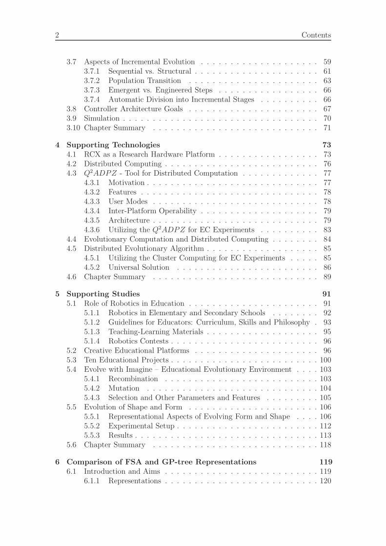
3.7 Aspects of Incremental Evolution . . . . . . . . . . . . . . . . . . . . 593.7.1 Sequential vs. Structural . . . . . . . . . . . . . . . . . . . . . 613.7.2 Population Transition . . . . . . . . . . . . . . . . . . . . . . 633.7.3 Emergent vs. Engineered Steps . . . . . . . . . . . . . . . . . 663.7.4 Automatic Division into Incremental Stages . . . . . . . . . . 66

3.8 Controller Architecture Goals . . . . . . . . . . . . . . . . . . . . . . 673.9 Simulation . . . . . . . . . . . . . . . . . . . . . . . . . . . . . . . . . 703.10 Chapter Summary . . . . . . . . . . . . . . . . . . . . . . . . . . . . 71

4 Supporting Technologies 734.1 RCX as a Research Hardware Platform . . . . . . . . . . . . . . . . . 734.2 Distributed Computing . . . . . . . . . . . . . . . . . . . . . . . . . . 764.3 Q2ADPZ - Tool for Distributed Computation . . . . . . . . . . . . . 77

4.3.1 Motivation . . . . . . . . . . . . . . . . . . . . . . . . . . . . . 774.3.2 Features . . . . . . . . . . . . . . . . . . . . . . . . . . . . . . 784.3.3 User Modes . . . . . . . . . . . . . . . . . . . . . . . . . . . . 784.3.4 Inter-Platform Operability . . . . . . . . . . . . . . . . . . . . 794.3.5 Architecture . . . . . . . . . . . . . . . . . . . . . . . . . . . . 794.3.6 Utilizing the Q2ADPZ for EC Experiments . . . . . . . . . . 83

4.4 Evolutionary Computation and Distributed Computing . . . . . . . . 844.5 Distributed Evolutionary Algorithm . . . . . . . . . . . . . . . . . . . 85

4.5.1 Utilizing the Cluster Computing for EC Experiments . . . . . 854.5.2 Universal Solution . . . . . . . . . . . . . . . . . . . . . . . . 86

4.6 Chapter Summary . . . . . . . . . . . . . . . . . . . . . . . . . . . . 89

5 Supporting Studies 915.1 Role of Robotics in Education . . . . . . . . . . . . . . . . . . . . . . 91

5.1.1 Robotics in Elementary and Secondary Schools . . . . . . . . 925.1.2 Guidelines for Educators: Curriculum, Skills and Philosophy . 935.1.3 Teaching-Learning Materials . . . . . . . . . . . . . . . . . . . 955.1.4 Robotics Contests . . . . . . . . . . . . . . . . . . . . . . . . . 96

5.2 Creative Educational Platforms . . . . . . . . . . . . . . . . . . . . . 965.3 Ten Educational Projects . . . . . . . . . . . . . . . . . . . . . . . . . 1005.4 Evolve with Imagine – Educational Evolutionary Environment . . . . 103

5.4.1 Recombination . . . . . . . . . . . . . . . . . . . . . . . . . . 1035.4.2 Mutation . . . . . . . . . . . . . . . . . . . . . . . . . . . . . 1045.4.3 Selection and Other Parameters and Features . . . . . . . . . 105

5.5 Evolution of Shape and Form . . . . . . . . . . . . . . . . . . . . . . 1065.5.1 Representational Aspects of Evolving Form and Shape . . . . 1065.5.2 Experimental Setup . . . . . . . . . . . . . . . . . . . . . . . . 1125.5.3 Results . . . . . . . . . . . . . . . . . . . . . . . . . . . . . . . 113

5.6 Chapter Summary . . . . . . . . . . . . . . . . . . . . . . . . . . . . 118

6 Comparison of FSA and GP-tree Representations 1196.1 Introduction and Aims . . . . . . . . . . . . . . . . . . . . . . . . . . 119

6.1.1 Representations . . . . . . . . . . . . . . . . . . . . . . . . . . 120

CONTENTS 3

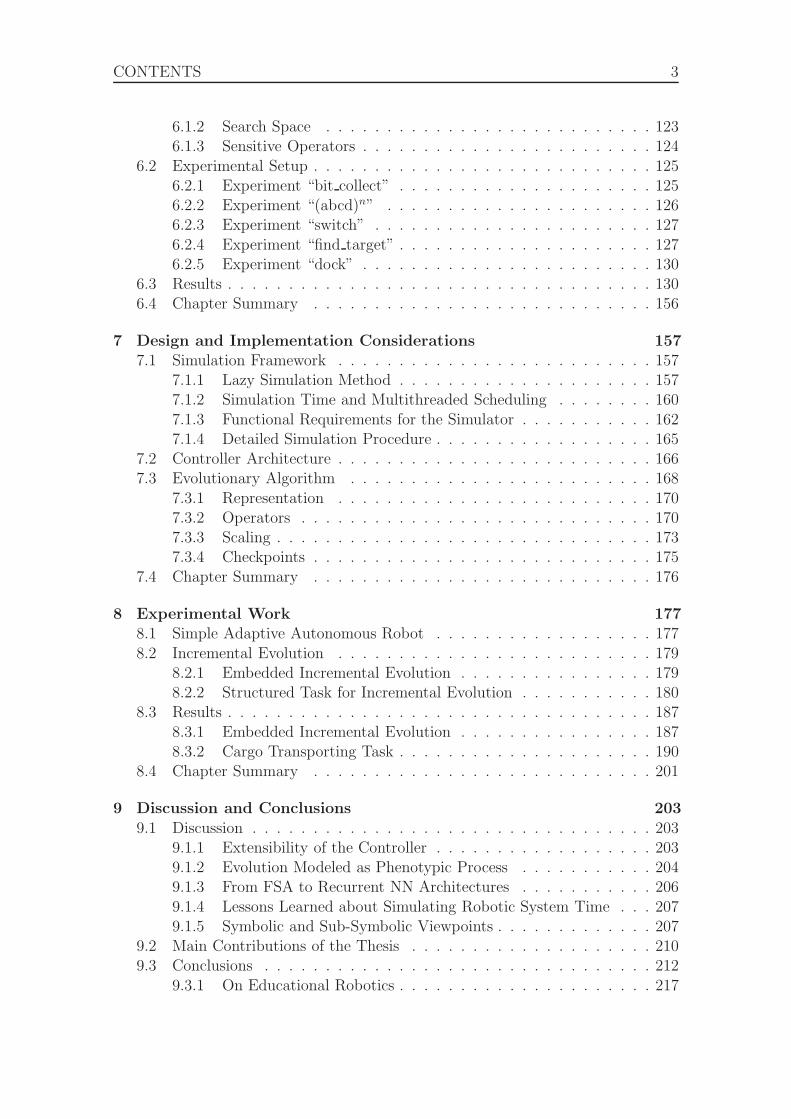
6.1.2 Search Space . . . . . . . . . . . . . . . . . . . . . . . . . . . 1236.1.3 Sensitive Operators . . . . . . . . . . . . . . . . . . . . . . . . 124

6.2 Experimental Setup . . . . . . . . . . . . . . . . . . . . . . . . . . . . 1256.2.1 Experiment “bit collect” . . . . . . . . . . . . . . . . . . . . . 1256.2.2 Experiment “(abcd)n” . . . . . . . . . . . . . . . . . . . . . . 1266.2.3 Experiment “switch” . . . . . . . . . . . . . . . . . . . . . . . 1276.2.4 Experiment “find target” . . . . . . . . . . . . . . . . . . . . . 1276.2.5 Experiment “dock” . . . . . . . . . . . . . . . . . . . . . . . . 130

6.3 Results . . . . . . . . . . . . . . . . . . . . . . . . . . . . . . . . . . . 1306.4 Chapter Summary . . . . . . . . . . . . . . . . . . . . . . . . . . . . 156

7 Design and Implementation Considerations 1577.1 Simulation Framework . . . . . . . . . . . . . . . . . . . . . . . . . . 157

7.1.1 Lazy Simulation Method . . . . . . . . . . . . . . . . . . . . . 1577.1.2 Simulation Time and Multithreaded Scheduling . . . . . . . . 1607.1.3 Functional Requirements for the Simulator . . . . . . . . . . . 1627.1.4 Detailed Simulation Procedure . . . . . . . . . . . . . . . . . . 165

7.2 Controller Architecture . . . . . . . . . . . . . . . . . . . . . . . . . . 1667.3 Evolutionary Algorithm . . . . . . . . . . . . . . . . . . . . . . . . . 168

7.3.1 Representation . . . . . . . . . . . . . . . . . . . . . . . . . . 1707.3.2 Operators . . . . . . . . . . . . . . . . . . . . . . . . . . . . . 1707.3.3 Scaling . . . . . . . . . . . . . . . . . . . . . . . . . . . . . . . 1737.3.4 Checkpoints . . . . . . . . . . . . . . . . . . . . . . . . . . . . 175

7.4 Chapter Summary . . . . . . . . . . . . . . . . . . . . . . . . . . . . 176

8 Experimental Work 1778.1 Simple Adaptive Autonomous Robot . . . . . . . . . . . . . . . . . . 1778.2 Incremental Evolution . . . . . . . . . . . . . . . . . . . . . . . . . . 179

8.2.1 Embedded Incremental Evolution . . . . . . . . . . . . . . . . 1798.2.2 Structured Task for Incremental Evolution . . . . . . . . . . . 180

8.3 Results . . . . . . . . . . . . . . . . . . . . . . . . . . . . . . . . . . . 1878.3.1 Embedded Incremental Evolution . . . . . . . . . . . . . . . . 1878.3.2 Cargo Transporting Task . . . . . . . . . . . . . . . . . . . . . 190

8.4 Chapter Summary . . . . . . . . . . . . . . . . . . . . . . . . . . . . 201

9 Discussion and Conclusions 2039.1 Discussion . . . . . . . . . . . . . . . . . . . . . . . . . . . . . . . . . 203

9.1.1 Extensibility of the Controller . . . . . . . . . . . . . . . . . . 2039.1.2 Evolution Modeled as Phenotypic Process . . . . . . . . . . . 2049.1.3 From FSA to Recurrent NN Architectures . . . . . . . . . . . 2069.1.4 Lessons Learned about Simulating Robotic System Time . . . 2079.1.5 Symbolic and Sub-Symbolic Viewpoints . . . . . . . . . . . . . 207

9.2 Main Contributions of the Thesis . . . . . . . . . . . . . . . . . . . . 2109.3 Conclusions . . . . . . . . . . . . . . . . . . . . . . . . . . . . . . . . 212

9.3.1 On Educational Robotics . . . . . . . . . . . . . . . . . . . . . 217

4 Contents

Appendix A – List of EI Parameters 220

Appendix B – Example of Specification of Environment for theSimulator 225

Appendix C – Example of Specification of Evolutionary Run 233

Bibliography 251

Index 265

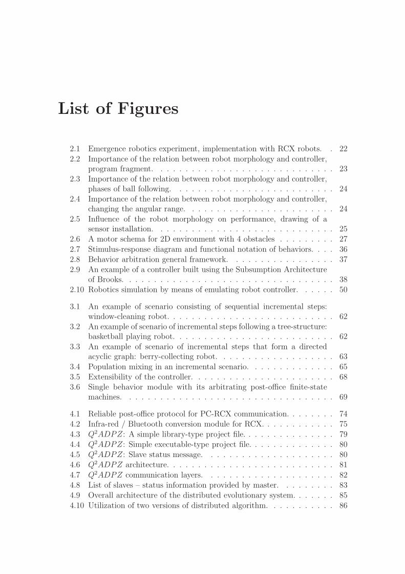
List of Figures

2.1 Emergence robotics experiment, implementation with RCX robots. . 22

2.2 Importance of the relation between robot morphology and controller,program fragment. . . . . . . . . . . . . . . . . . . . . . . . . . . . . 23

2.3 Importance of the relation between robot morphology and controller,phases of ball following. . . . . . . . . . . . . . . . . . . . . . . . . . 24

2.4 Importance of the relation between robot morphology and controller,changing the angular range. . . . . . . . . . . . . . . . . . . . . . . . 24

2.5 Influence of the robot morphology on performance, drawing of asensor installation. . . . . . . . . . . . . . . . . . . . . . . . . . . . . 25

2.6 A motor schema for 2D environment with 4 obstacles . . . . . . . . . 27

2.7 Stimulus-response diagram and functional notation of behaviors. . . . 362.8 Behavior arbitration general framework. . . . . . . . . . . . . . . . . 372.9 An example of a controller built using the Subsumption Architecture

of Brooks. . . . . . . . . . . . . . . . . . . . . . . . . . . . . . . . . . 382.10 Robotics simulation by means of emulating robot controller. . . . . . 50

3.1 An example of scenario consisting of sequential incremental steps:window-cleaning robot. . . . . . . . . . . . . . . . . . . . . . . . . . . 62

3.2 An example of scenario of incremental steps following a tree-structure:basketball playing robot. . . . . . . . . . . . . . . . . . . . . . . . . . 62

3.3 An example of scenario of incremental steps that form a directedacyclic graph: berry-collecting robot. . . . . . . . . . . . . . . . . . . 63

3.4 Population mixing in an incremental scenario. . . . . . . . . . . . . . 653.5 Extensibility of the controller. . . . . . . . . . . . . . . . . . . . . . . 683.6 Single behavior module with its arbitrating post-office finite-state

machines. . . . . . . . . . . . . . . . . . . . . . . . . . . . . . . . . . 69

4.1 Reliable post-office protocol for PC-RCX communication. . . . . . . . 744.2 Infra-red / Bluetooth conversion module for RCX. . . . . . . . . . . . 75

4.3 Q2ADPZ: A simple library-type project file. . . . . . . . . . . . . . . 794.4 Q2ADPZ: Simple executable-type project file. . . . . . . . . . . . . . 804.5 Q2ADPZ: Slave status message. . . . . . . . . . . . . . . . . . . . . 804.6 Q2ADPZ architecture. . . . . . . . . . . . . . . . . . . . . . . . . . . 81

4.7 Q2ADPZ communication layers. . . . . . . . . . . . . . . . . . . . . 824.8 List of slaves – status information provided by master. . . . . . . . . 834.9 Overall architecture of the distributed evolutionary system. . . . . . . 85

4.10 Utilization of two versions of distributed algorithm. . . . . . . . . . . 86

6 List of Figures

5.1 Students from secondary school in Trondheim preparing their robotfor the RoboCup Junior contest in Bremen, June 2006. . . . . . . . . 94

5.2 Viewing the remotely-accessible robotics laboratory in a web-browser. 985.3 Interfacing the robots in the remotely-accessible laboratory from C. . 995.4 Solution to the example 1. . . . . . . . . . . . . . . . . . . . . . . . . 1015.5 Solution to the example 2. . . . . . . . . . . . . . . . . . . . . . . . . 1015.6 View from the top-mounted camera, the same image recognized by

the image recognition plug-in for Imagine, drawing a convex hull. . . 1025.7 Voronoi representation genotype and phenotype. . . . . . . . . . . . . 1075.8 Holes representation with various geometric shapes creates more

natural shapes using less shapes than rectangular-holes representation.1085.9 Standard LEGO bricks used in layer layouts. . . . . . . . . . . . . . . 1105.10 Shapes used in the topological optimum design experiment. . . . . . . 1125.11 Comparison of the performance of the roulette-wheel selection and

steady-state GA. . . . . . . . . . . . . . . . . . . . . . . . . . . . . . 1135.12 Best individual fitness with standard deviations (random 3D models

20x20x5) for layer 4. . . . . . . . . . . . . . . . . . . . . . . . . . . . 1145.13 Example runs of 16x16 TOD shape with different genotype represen-

tations. . . . . . . . . . . . . . . . . . . . . . . . . . . . . . . . . . . . 1155.14 Best fitness (average of 20 runs) for the four different representations,

8x8 shape. . . . . . . . . . . . . . . . . . . . . . . . . . . . . . . . . . 1155.15 Best fitness (average of 20 runs) for the four different representations,

16x16 shape. . . . . . . . . . . . . . . . . . . . . . . . . . . . . . . . . 1165.16 Best fitness (average of 20 runs) for the four different representations,

32x32 shape. . . . . . . . . . . . . . . . . . . . . . . . . . . . . . . . . 1165.17 The first two layers evolved with steady-state GA. . . . . . . . . . . . 1175.18 Shapes with evolved brick layouts, from [Na, 2002]. . . . . . . . . . . 1175.19 Comparison of the performance of the improved GA that has features

of indirect representations (repetitive brick placements), [Na, 2002]. . 117

6.1 Illustration of GP-tree representation. . . . . . . . . . . . . . . . . . . 1216.2 Illustration of FSA representation. . . . . . . . . . . . . . . . . . . . . 1226.3 Environments for the find target task. . . . . . . . . . . . . . . . . . . 1286.4 Viewing the progress of simulation in a web browser using a viewer

implemented as Java applet. . . . . . . . . . . . . . . . . . . . . . . . 1296.5 Average of the fitness of the best individuals in the find target task. . 1316.6 Example trajectories of evolved individuals using the GP-tree and the

FSA representations in find target task. . . . . . . . . . . . . . . . . . 1336.7 Trajectories of the best individuals from all generations in find target

task. . . . . . . . . . . . . . . . . . . . . . . . . . . . . . . . . . . . . 1336.8 Trajectories of the best individuals from final generation in find target

task, complex environment. . . . . . . . . . . . . . . . . . . . . . . . 1346.9 Generalization of the evolved solutions when started from different

starting locations in find target task, complex environment. . . . . . . 1346.10 Performance of the FSA and GP-tree representations in find target

task, environment ten around. . . . . . . . . . . . . . . . . . . . . . . 135

LIST OF FIGURES 7

6.11 Trajectories of the best individuals from final generation in find targettask, environment ten around. . . . . . . . . . . . . . . . . . . . . . . 136

6.12 Generalization of the evolved solutions when started from differentstarting locations in find target task, ten around environment. . . . . 136

6.13 Performance of the FSA and GP-tree representations on simple ver-sion of task bit collect. . . . . . . . . . . . . . . . . . . . . . . . . . . 137

6.14 Performance of the FSA and GP-tree representations on more com-plex version of task bit collect. . . . . . . . . . . . . . . . . . . . . . . 138

6.15 Performance of the FSA and GP-tree representations on task abcdn. . 1406.16 Average of the best fitness on a switch task with four symbols for

both representations. . . . . . . . . . . . . . . . . . . . . . . . . . . . 1416.17 Average of the best fitness on a switch task with three symbols for

both representations. . . . . . . . . . . . . . . . . . . . . . . . . . . . 1426.18 The best evolved FSA in the switch task with three symbols. . . . . . 1446.19 Average of the best fitness on a 4-symbol switch task, comparison of

incremental and non-incremental runs. . . . . . . . . . . . . . . . . . 1456.20 Average of the best fitness on a 4-symbol switch task, comparison of

fully incremental and non-incremental runs. . . . . . . . . . . . . . . 1466.21 Average of the best fitness on a 4-symbol switch task, comparison of

fully incremental with freezing FSA and non-incremental runs. . . . . 1466.22 Average of the best fitness in the 4-symbol switch task, comparison

of incremental runs with restricted terminal set and non-incrementalruns. . . . . . . . . . . . . . . . . . . . . . . . . . . . . . . . . . . . . 148

6.23 Performance of the GP-tree and FSA representations on simulateddock task. . . . . . . . . . . . . . . . . . . . . . . . . . . . . . . . . . 149

6.24 A final evolved FSA in the dock task. . . . . . . . . . . . . . . . . . . 1526.25 Trajectories for the evolved individuals in typical runs, dock task. . . 1536.26 Trajectories for the evolved individuals in selected runs, dock task. . . 1546.27 Role of the crossover operator for the FSA representation in switch

task with three symbols. . . . . . . . . . . . . . . . . . . . . . . . . . 1546.28 Comparison of two selection methods in experiment find target with

environment experiment fence and the GP-tree representation. . . . . 1556.29 Comparison of two selection methods on experiment find target with

environment ten around and the GP-tree representation. . . . . . . . 1556.30 Comparison of two selection methods, difficult version of the experi-

ment bit collect and FSA representation. . . . . . . . . . . . . . . . . 156

7.1 Simulated robot topology and features. . . . . . . . . . . . . . . . . . 1597.2 Simulation implementation method. . . . . . . . . . . . . . . . . . . . 1617.3 Loading station is specified using two active areas (top view). . . . . 1647.4 Unloading station is specified using three active areas. . . . . . . . . . 1647.5 Movement types for differential drive robot used in experiments. . . . 1677.6 Example controller architecture for a mouse acquiring cheese task. . . 1677.7 Controller architecture and genotype representation . . . . . . . . . . 1697.8 Example of crossover operator functionality. . . . . . . . . . . . . . . 1717.9 Crossover operator. . . . . . . . . . . . . . . . . . . . . . . . . . . . . 175

8 List of Figures

8.1 Simple adaptive autonomous robot. . . . . . . . . . . . . . . . . . . . 1788.2 Setup for the embedded evolutionary experiment. . . . . . . . . . . . 1808.3 Environments for the embedded evolutionary experiment. . . . . . . . 1808.4 Camera setup for building the table of real-world actuator effects. . . 1818.5 Robot setup and environment for the cargo transporting task. . . . . 1828.6 Experimental environments for 6 incremental evolutionary steps of

creative incremental scenario. . . . . . . . . . . . . . . . . . . . . . . 1858.7 FSA arbitrators for modules cargo-loader, avoidance, and explore. . . 1868.8 Automatic detection of incremental step, analysis. . . . . . . . . . . . 1888.9 Automatic detection of incremental step, complex environment. . . . 1898.10 Embedded evolution task, complex environment and evolution of best

fitness. . . . . . . . . . . . . . . . . . . . . . . . . . . . . . . . . . . . 1908.11 Cargo transporting task, environment and real-robot setup. . . . . . . 1918.12 Cargo transporting task, plot of the best fitness in steps of the creative

incremental scenario. . . . . . . . . . . . . . . . . . . . . . . . . . . . 1938.13 Cargo transporting task, finite-state machines evolved in each step of

creative scenario. . . . . . . . . . . . . . . . . . . . . . . . . . . . . . 1958.14 Cargo transporting task, plot of the best fitness in steps of the

sequential scenario. . . . . . . . . . . . . . . . . . . . . . . . . . . . . 1978.15 Contribution of mutation operators to evolutionary progress. . . . . . 1988.16 Positive rate of mutation operators. . . . . . . . . . . . . . . . . . . . 1998.17 Examples of evolved misbehavior in cargo transporting task. . . . . . 200

9.1 A re-planning controller for a pick-and-place robot enabled with acamera and image recognition. . . . . . . . . . . . . . . . . . . . . . . 208

9.2 A prototype of LEGO pick-and place robot. . . . . . . . . . . . . . . 209

List of Tables

6.1 The number of binary trees of depth 1-10. . . . . . . . . . . . . . . . 1246.2 A final evolved GP-tree and FSA for the environment experiment fence.1326.3 A final evolved GP-tree and FSA for the environment ten around. . . 1366.4 A final evolved GP-tree and FSA, task abcdn. . . . . . . . . . . . . . 1396.5 The number of states in the evolved FSA and the number of states

that are reachable in the switch task with three symbols. . . . . . . . 1416.6 Evolved frozen individuals in the incremental steps 1–4, switch task

with four symbols. . . . . . . . . . . . . . . . . . . . . . . . . . . . . 1476.7 The best evolved GP-tree solution in the dock task without penalty. . 1506.8 Selected evolved individuals with the best performance for the dock

task. . . . . . . . . . . . . . . . . . . . . . . . . . . . . . . . . . . . . 151

8.1 Message interfaces for behavioral modules. . . . . . . . . . . . . . . . 1848.2 Cargo transporting task, number of evaluations in steps of the creative

scenario. . . . . . . . . . . . . . . . . . . . . . . . . . . . . . . . . . . 1928.3 Cargo transporting task, number of evaluations in steps of the se-

quential scenario. . . . . . . . . . . . . . . . . . . . . . . . . . . . . . 196

10 List of Tables

Chapter 1

Introduction

The job of a research worker is similar to the one of a concerting musi-cian. The music itself controls every single movement of the musician inorder to elude a beautiful harmony of sounds prescribed by the composer.Similarly, the nature controls every single movement of the researcher inorder to unveil the secrets of its own harmony.

In order to utilize ever advancing technological developments of materials, powersupplies, computer technology, sensors, and actuators in the field of robotics, suitablecontroller architectures at a correspondingly advanced level need to be developedfor these devices. Mobile robots could perform complicated tasks in unknown,non-deterministic, changing, noisy, and unpredictable environments, if methods fordesigning robot controllers could be developed. Successful completion of tasks willrequire the controllers to be adaptive and sometimes learning. Systematic researchefforts to study possible methods for building such controllers are to be spent.

Researchers and engineers have been designing and studying controllers for au-tonomous mobile robots since the 1950s (the famous Grey Walter’s Tortoise robot).Mainstream robotics systems are built upon the principles of the Control Theory.Artificial Intelligence traditionally approached the problem of designing roboticssystems with the philosophical motivations of building machines that can think. TheAI scientists acquired a working robotic device, and studied the problem of making itintelligent, their approach was clearly a top-down one. The naive attempt to design acomplete system in this manner, i.e. to specify the whole system from the top to thebottom layers meets various constraints that make the approach at least difficult andnot very efficient. The complexity of interactions of a mobile robotic system impliesa structured (non-monolithic) controller architecture. Traditional AI approachesbased on centralized-processing and Sense-Plan-Act cycle have difficulties dealingwith simultaneous robot activities that have different priorities. Even if a purely-planning controller would be successfully designed, its maintainability, modifiability,and performance would be compromised. Mobile agents must behave according tothe outcome of several independent threads of reasoning. This requirement is impliedby the highly parallel nature of events and processes in the real world. The controllerarchitecture can meet this requirement if it is modular, and when the modules canact simultaneously in a coordinated cooperation.

12 Introduction

A new wave of AI robotics (as a part of Nouvelle AI) was started by theproponents of behavior-based systems. In these systems, the path to an intelligentbeing starts with building simple concrete functional creatures. Their behavior iscontrolled by a set of interacting modules. On the bottom side, these modules areas simple as direct reactive connections between sensors and actuators. On the topside, these modules might perform long-term reasoning inferences running in thebackground with a low priority. These ideas are reflected well in various behavior-based and hybrid architectures, [Arkin, 1998]. Many studies focus on designinga framework, which possibly allows integration of higher-level functions and AItheories into BB architectures. We support this view, and we aim at studyingparticular aspects of the BB controller design.

A BB controller consists of a set of relatively independent modules. Each ofthese modules is responsible for making sure that the robot will successfully performcertain behavior. The behavioral modules typically have control over the robotsensors and actuators, but their activation (arbitration) and combination of theiroutputs (command fusion) is a difficult challenge. One of the main challenges ofthe BB design is how the individual modules will be coordinated. This is referredto as action selection problem or behavior arbitration, see [Pirjanian, 1999] for anoverview.

Different action selection methods were studied before. On the side of arbitra-tion, these include priority-based, state-based, and winner-take-all. On the side ofcommand fusion, these include voting, superposition, fuzzy, and multiple-objective.The coordination mechanisms can be divided into state-based and continuous, wherethe state-based can work using either competitive or temporal sequencing principles.For tasks that involve learning, the action selection problem is deeply studied byresearch in Reinforcement Learning [Sutton and Barto, 1998], one of the mostpopular methods for automatic design of robot controllers. In these cases, thebehavior arbitration or command fusion is a function to be learned based on therequirements of the task. In this thesis, we will work with BB systems without apredefined arbitration and command fusion mechanisms. On the contrary, these willbe designed using Evolutionary Algorithm (EA), with the help of simulation of therobot performing in its environment. In particular, we will study how IncrementalEvolution (IE) can be applied to the problem of the design of suitable action-selectionmechanisms in BB controllers. Since the EAs proved to be successful in creatingnovel designs in various domains, our hypothesis and planned research contributionis to demonstrate how EAs can be used in this domain.

Another strong motivation comes from the viewpoint of the field of EvolutionaryRobotics (ER) itself. Approximately 15 years of research in the field broughtsuccessful robotic systems that can perform relatively simple low-level tasks, such asobstacle avoidance, wall following, or target tracking. The controllers are often basedon arbitrarily-connected neural networks, [Beer and Gallagher, 1992]. Adaptivebehaviors on a different level could possibly be achieved by approaches [Floreanoand Urzelai, 2000] that evolve the neuron learning rules instead of the connectionweights, which are changing dynamically during the task execution. Nevertheless,it appears that evolving more complex behaviors in a single evolutionary run is not

13

plausible due to a complex search space, and becomes impossible without additionalguidance of the EA.

Few researchers addressed tasks of a higher complexity. ER uses a bottom-upapproach. The evolution typically starts at a complete bottom and has to discoverthe low-level control mechanisms. On one hand, this attributes to a very highflexibility in possibilities for the robot behavior that is formed. On the other hand,it severely limits the complexity of the task, which is to be performed. ER cannotreach beyond the low-level behaviors without a supporting framework, if it is to startat the bottom level. In the natural evolution, such framework was provided by theimmense richness of the species, niches, and the environments, and the millions ofyears of evolutionary development. When artificial evolution is to serve as a designmethod, the framework must be replaced by other means. The evolved controller isnot very likely to benefit from the structural properties of a BB-type controller, ifsuch form will not be enforced.

One way of self-guiding of an evolutionary algorithm is the use of co-evolution,[Hillis, 1990]. Co-evolution, however, applies best to that class of problems wheretwo entities are competing for the same resource, or fight. In addition, it canbe vulnerable to possible cyclic loops in the relation of strategy dominance ineffect causing stagnation of the algorithm instead of progression. Another possibleguidance, adopted also in this work, is dividing the target task into more simpleincremental steps, [Harvey, 1995]. This strategy is more general; however, it requiresa scenario of incremental evolutionary steps. How to devise such incremental steps,and how to setup such incremental EAs is the focus of this and future work.

Designing a controller for a particular task for a mobile robot requires detailedknowledge of the robot hardware and software and an experienced engineer. We areseeking an alternative: automatic design of the controller. Our aim is to minimizethe efforts and maximize the quality. The approach we promote in this thesis is touse ER with BB-type controller. We don’t put any particular constraints on howthe individual behavioral modules are designed. Typically, engineers who designedthe robot will provide the low-level control mechanisms, which will be well-tunedand efficient for the hardware the robot is equipped with. Alternately, low levelbehaviors can be learned or evolved.

Given the set of low-level behaviors, and a particular task for the robot, the goalis to complete the design of the robot’s controller using EAs. The work lays at theintersection between BB Robotics and ER. By the means of EA, the design of theBB-controller adapts to the constraints of the specific task, robot, and environment.Higher complexity of the controller, when compared to other ER approaches, isachieved by the use of a BB-type controller with a set of predefined behaviors. Weare dealing here with an adaptation at the level of the design process, where theresulting controller is adapted to the target task. Run-time adaptability of the robotitself can be achieved by learning in the individual behaviors, flexible arbitration orcommand-fusion mechanisms, and/or Embedded EC [Petrovic, 2001b], similar toAnytime Learning approach of [Grefenstette and Ramsey, 1992].

In this work, we aim at evolutionary design of behavior arbitration for a controllerof a mobile robot performing a non-trivial task, where simple reactive controller

14 Introduction

would not be sufficient. The controller has a particular BB architecture, while thearbitration is based on a set of finite-state automata. The design is the output froman incremental evolutionary algorithm.

During the work on the project, we were exposed to different projects, ideas, andenvironments. This brought us to the understanding that as advanced field as thefield of robotics is, can hardly be studied without learning and taking into accounta wider background — both from the AI-theoretical side that regards planning,optimization, evolutionary computation, machine learning, from the robot-designpoint of view that includes learning about sensors, actuators, building and low-level programming of robots, and from the educational point of view that includesbringing the world of robotics down to the schools at all levels — either topromote the computer and natural sciences among youngsters, or to provide modernmotivating learning tools and technologies for students and researchers. This report,in addition to addressing the main research questions listed at the end of this chapter,reflects the work done and lessons learned in various aspects of this broader context.

The thesis is organized into several chapters. The following chapter reviewsthe theoretical background and presents the approaches of the fields where thiswork attempts to make contributions. The third chapter analyzes and discusses thegoals and hypotheses we set to reach and verify in more details. We describe thetechnologies we employed in the fourth chapter. We add to our arguments througha series of supporting studies, which we all describe in the fifth chapter includingthe results obtained. The representation formalism of the behavior arbitrationmechanism, finite-state automata, are analyzed as a genotype representation andcompared to Genetic Programming in a preliminary study in the sixth chapter. Thefollowing two chapters lay down a more detailed specification on how we prepared ourexperiments and studies on theoretical and more practical levels. The last chapterbefore the conclusions of the thesis describes and discusses the experiments we haveperformed as well as the results obtained.

1.1 Research Questions Addressed in the Thesis 15

1.1 Research Questions Addressed in the Thesis

The main research question of the thesis asks by which ways can EvolutionaryAlgorithms provide useful solutions to the problem of automatic design of controllersfor mobile robots. Previously, EA have been successfully applied to designingrobotic controllers with simple architectures based typically on Neural Networks.These approaches were applied to relatively simple navigational or operational tasks.As indicated by previous works, Incremental Evolution can increase evolvabilitywhen designing robot controllers for mobile robots. The design methods for robotcontrollers in the traditional Artificial Intelligence usually deal with symbolic rea-soning mechanisms and make emphasis on planning, often involved in a centralizedarchitecture. Alternately, the Nouvelle AI methods rely on incremental bottom-up design of robot controllers that consist of independently executing behavioralmodules with possibly conflicting intentions, desired actions, and effects.

The particular concern of this work is whether and how the EA method could besuccessfully applied also to the controllers with architecture inspired by the NouvelleAI, the behavior-based controllers. Is Incremental Evolution a useful method inthis context, and what are the caveats of its application? The thesis will addressthe questions of which controller architectures suit the evolutionary behavioralapproach particularly well and why. The thesis will work toward providing acomplete functional solution and may include studies into related fields, building andimplementing tools that may be required to reach satisfactory solution of automaticdesign of mobile robot controllers.

16 Introduction

Chapter 2

Background

There is a noticeable difference between the national parks in Slovakiaand Norway: In Slovakia, the visitors follow the well-prepared hikingtrails and must not leave them. In Norway, the trails are often missingor very hard to find, while the tourists are free to choose any of theirways.

In this chapter, we set on a path to explore the various topics related to robotics. Themain aim of this work lies in incremental evolutionary robotics experiments. Andwe shall always keep in mind that it is there our path leads. It would be a somewhatunbalanced approach to jump right into a subject that is just a small flavor on top ofsomething that is difficult to build, understand, implement, and grasp – successfulrobotic systems. In the spirit of bottom-up approaches, our journey started in thesimplest form of robotics-experience encounters – robotics educational systems andefforts, which are explained in the fifth chapter together with supporting technologieswe used for the experimental work in our thesis explained in the fourth chapter. Thischapter touches upon the issues that are interesting and relevant for our perspective,although it is not meant to provide a comprehensive overview of the respective fields.In that spirit, we will gently cover the AI’s viewpoints on robotics and its challenges,arriving at Evolving Robotics, which is where our target lies all the long way ahead.

2.1 Introduction and Social Implications

Typical tasks, where robots can be useful, share common properties, such ashazardous or uncomfortable for humans, requiring heavy manipulation or tools,which are awkward to handle, or necessitating repetitive execution. Robots couldbe useful also in tasks, which can be carried out by humans, while performing withhigher reliability, cheaper, faster, longer or even perpetually, or more efficiently.Some opponents of technological progress could claim that robots are taking the workfrom humans. And they are right, but we must comment on it that given the aboveconditions we do not find it a negative tendency, just the opposite. There are alwaysmany more things to be done than people available, and always many challenges tobe worked on, and a long path for all of us ahead. Obviously, the enormous challenge

18 Background

will be finding and implementing a suitable economical and social model that canprovide for distribution of resources according to the new situation: the profit (orat least the value) will not anymore be generated by the human work on majority,but by the work of robots. In turn, larger amounts of financial profit will flow to theaccounts of the owners of the automatic production systems and factories. Theseowners, however, will not be generating any (or sufficient) demand for the humanwork that will be available (and indeed needed for the progress and sustaining ofmankind), but not useful for these owners. A failure of traditional market modelsmust follow, because those in demand will have no value to offer in exchange, andthose who will be producing (automatically), will have no value to demand. Today,we are already witnessing such tendencies, and intensive changes in the structure ofthe society occur. We should be prepared for more of this happening in the comingdecades. Unless we admit and alleviate the tabu put upon the correctness of themarket economy models, we will face very thin bottlenecks on the way to come, andrisk major crises. Studying, analyzing, and addressing these issues are importanttasks for economists and sociologists, and we must leave this interesting area for therest of this paper. We however forward the moral disputes regarding the progress onthe field of robotics further away to the mentioned fields, and claim that the progressin robotics is important, needed, and full of positive contributions for mankind ifattention to the above mentioned issues is paid.

Whereas some jobs are suitable for robots fixed on a factory production line,other tasks require mobility, flexibility, and adaptation to dynamic environment.To a certain extent, it is possible to use remotely controlled or human operatedrobots (tele-operation). However, the amount of information sent from sensorsand to actuators can be too large for the bandwidth of the transmission, or themission can be too distant for controlling each step of the robot in real time, andthe connection can be lost easily in certain environments. Some responses to eventsin the environment might have to be performed very quickly. In all such cases, itis inevitable and/or more cost efficient to equip the robot with its own controller,which makes it autonomous.

2.2 Robotics and Artificial Intelligence

Can there be an intelligence without a body? Some researchers argue opposite.We could claim that the study of artificial intelligence, when moved from a virtualworld inside of computers out to an embodied form, existing and operating in a realworld, ceases to be artificial. We are not anymore dealing with beings existing inartificial worlds created entirely by human engineers, but with real beings existingand performing in the same world as we humans do. If they do it with certaindegree of success, their intelligence is real, not artificial1. In each case, Robotics is

1Some may claim that the term artificial still applies to these creatures, since it comes from thefact that they were designed by engineers, however this leads to a philosophical discussion aboutwho designed the human, and on the other extreme, whether those artifacts that are designed byhuman should be called artificial, if they are part of a large image of a long-term evolution, andthus we can disregard such an argument and insist that the robots posses the real intelligence at

2.3 Evolving Robotics 19

an important testing platform, motivation, and source of inspiration for many AItheories.

In addition to standard classifications, we recognize two different flavors ofArtificial Intelligence. In the first flavor, the efforts within AI field are dedicatedtowards building systems that display certain level of intelligence while performingsome more or less specific task. In that case, the AI is confronting the taskdirectly. The intelligence can be an integrated general mechanism, or a simple hard-coded wiring. The implementation is transparent to an external observer, who onlyclassifies the observed behavior as intelligent. In the second flavor, another streamof efforts uses AI during a design process. The outcome of the design process ispossibly, but not necessarily an intelligent system. Here, AI is confronting the taskindirectly, or in other words, the output from the AI system is another system thathas to perform some task. The performance of the system can again seem to beintelligent, but this is absolutely not a requirement. In this approach, AI replacesan intelligent engineer who would otherwise be required to implement the details ofthe performing system.

Suitable labels for the two approaches could be an on-line and an off-lineintelligence. In our work, we are mainly concerned with the off-line intelligence,although the goals are to achieve a certain level of on-line intelligence as well, ifpossible. This, however, surely remains below the animal-level of intelligence, andtherefore often does not involve symbolic reasoning and planning in the outputsystem, as it is not necessary.

2.3 Evolving Robotics

The traditional approaches to robotics and AI robotics generated a broad set ofprojects, implementations, and platforms, with a more or less limited performance.These architectures are generally based on the SENSE – PLAN – ACT cycle, wherethe centralized planning unit collects information from the environment, builds amodel of the world, and performs high-level reasoning to select the next action (orconstruct a plan of atomic actions). The traditional research, however, up to dateprovides a large base that is subject to further developments and studies. Many ofthese developments grow along the traditional pillars of the established fields. Inaddition, novel, innovative, sometimes revolutionary, visionary, untested, promising,or just new and different approaches exist simultaneously, and ought to be given itsspace in order to guarantee progress. All the “alternative” approaches contribute toevolution of the Robotics research field. Let us call them here Evolving Robotics, andinterestingly enough, Evolutionary Robotics is one of them. Evolving Robotics isvery challenging to work in while it lacks the rigidity and structure of an establishedfield. However, it provides (but also demands) large amounts of inspiration, andresearch joy.

their own level.

20 Background

2.4 Embodiment, Situatedness, Environment

Some traditional definitions of the embodiment and situatedness state that a systemis embodied when it has a physical body, and that it is situated when it exists in anenvironment. See for example [Pfeifer and Scheier, 1999] for in-depth treatment. Inthis philosophical section, we discuss the aspects and limitations of such definitions.

For the first, it can make sense to talk about a body even if the system exists in acompletely simulated or artificial environment that is not part of our physical world.For the second, all systems that perform any meaningful activity do exist in someenvironment. Should then all the systems be considered embodied and situated?

Every autonomous system that performs any actions must have input andoutput. The input and output interface of the system forms its interaction withthe environment. In the cases when the system itself is part of that environment, orwhen it is recognizable (can be identified and detected) by other systems that sharethe same environment, and when the interaction with that part of the agent thatis part of the environment can have consequences on the future performance of theagent, we say that the system has a body.

Systems without bodies can take no direct action in their environments. Anexample of such a system is an oracle that can answer questions in a natural languageabout the departures and arrivals of local buses. For another example, a temperaturecontroller senses and affects the environment, and it does have a body (the heatingbody that is located in the environment) even though some would argue that it hasno intelligence. Systems without a body are passive, and as such cannot acquire theirown intelligence, which is naturally based on interactions, generating and verifyinghypotheses, world models, and constructing the knowledge based on the experience.Body-less systems are limited to imitating intelligence of existing systems, providingintelligent queries into a knowledge base that was constructed and maintained withthe help of an external intelligence.

An agent that has a body is situated in its environment as long as it takesat least one input from that environment. Robotic agents obviously have bodies,which occupy space in their environments, and allow them to take actions in thoseenvironments and to perform active sensing – focusing their sensors on relevantsource of information in the environment. An agent can possibly be situated andstill be without a body. In that case, the agent can receive direct input from theenvironment, and control which inputs it acquires and when. However, it cannotbe “seen” (detected, recognized) by other agents that share its environment, it isnot part of it and therefore cannot take actions in its environment (to prove this isstraight-forward: if the agent had any means to take actions in its environment itwould have to perform them using some actuators that would then be part of theenvironment, hence it would have a body).

The importance of the situatedness for natural intelligence have been demon-strated by the cases when an organism was disconnected from a particular sensoryinput. If this occurred in the early stages of the individual’s lifetime, the particularmental function did not develop for the rest of the life. For instance, if an eye of ayoung kitten is closed for as little as 3-4 days during the period of high susceptibility

2.4 Embodiment, Situatedness, Environment 21

in the fourth and fifth weeks, the performance of the cat’s visual system is sharplyreduced for its whole lifetime [Hubel and Wiesel, 1970].

Robots often modify their environment to communicate with each other or toease or progress their task or navigation. For example, in [Batalin and Sukhatme,2002] a robot is exploring an unknown environment. Such task is achieved withoutaccess to any global navigational information thanks to signposts that the robotdrops off in its environment.

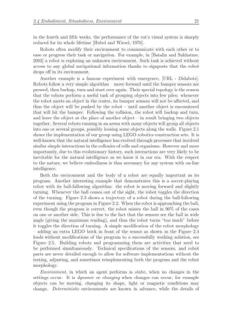
Another example is a famous experiment with emergence, [URL - Didabots].Robots follow a very simple algorithm – move forward until the bumper sensors arepressed, then backup, turn and start over again. Their special topology is the reasonthat the robots perform a useful task of grouping objects into few piles: wheneverthe robot meets an object in the center, its bumper sensors will not be affected, andthus the object will be pushed by the robot – until another object is encounteredthat will hit the bumper. Following the collision, the robot will backup and turn,and leave the object at the place of another object – in result bringing two objectstogether. Several robots running in an arena with many objects will group all objectsinto one or several groups, possibly loosing some objects along the walls. Figure 2.1shows the implementation of our group using LEGO robotics construction sets. It iswell-known that the natural intelligence has evolved through processes that involvedsimilar simple interactions in the collonies of cells and organisms. However and moreimportantly, due to this evolutionary history, such interactions are very likely to beinevitable for the natural intelligence as we know it in our era. With the respectto the nature, we believe embodiness is thus necessary for any system with on-lineintelligence.

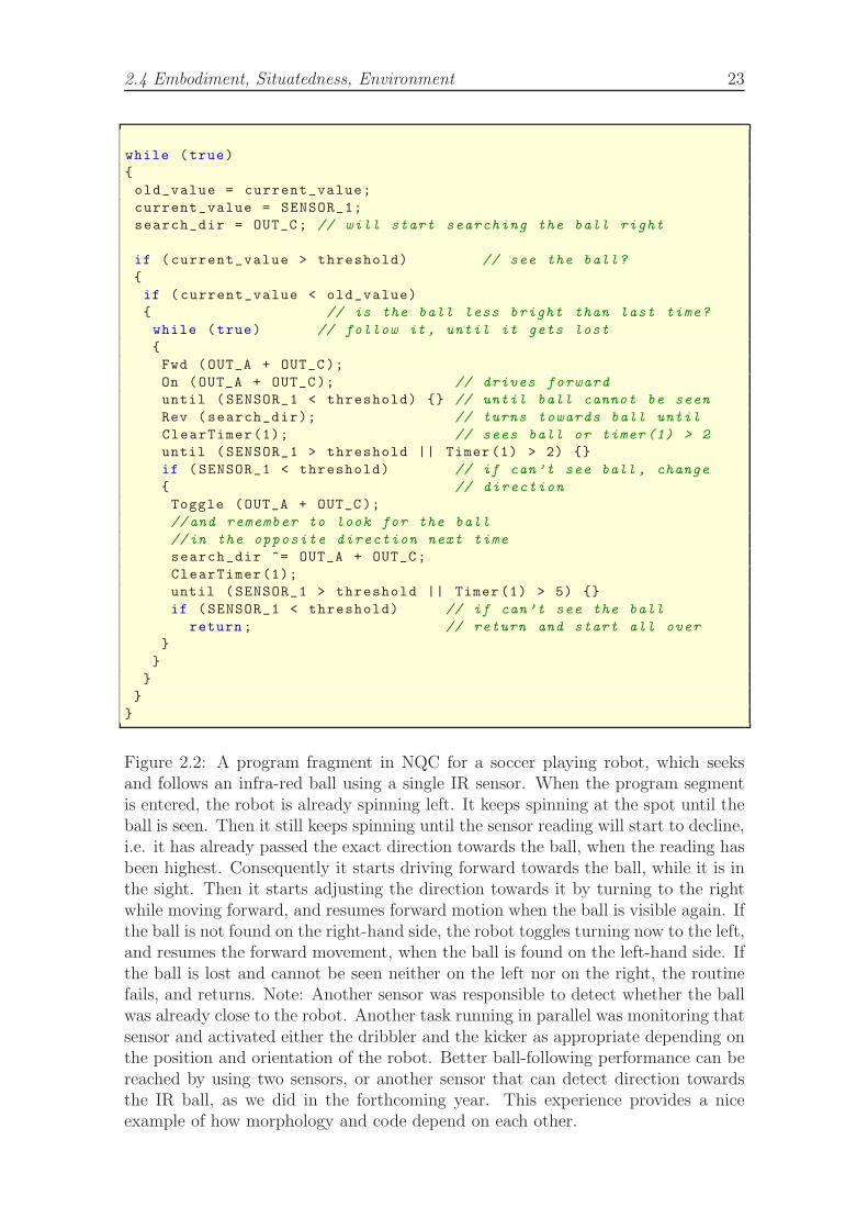
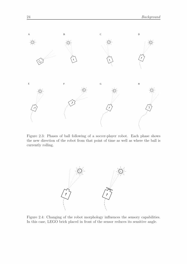
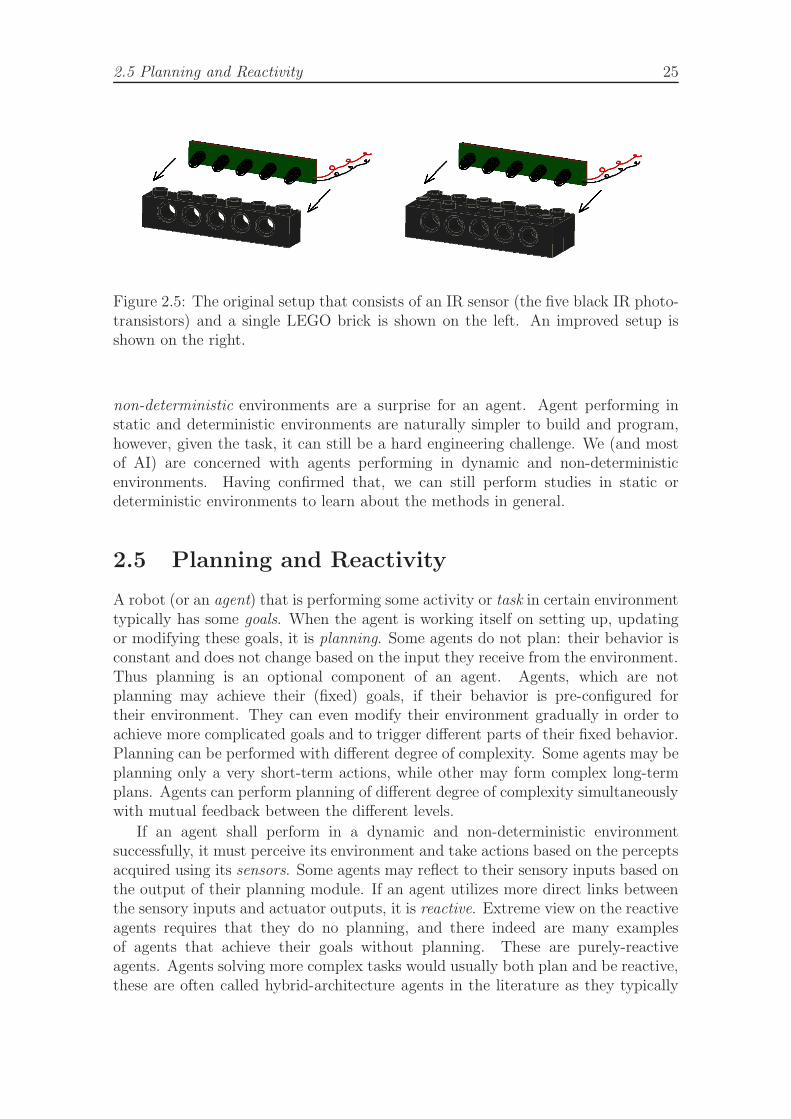
Both the environment and the body of a robot are equally important as itsprogram. Another interesting example that demonstrates this is a soccer-playingrobot with its ball-fallowing algorithm: the robot is moving forward and slightlyturning. Whenever the ball comes out of the sight, the robot toggles the directionof the turning. Figure 2.3 shows a trajectory of a robot during the ball-followingexperiment using the program in Figure 2.2. When the robot is approaching the ball,even though the program is correct, the robot misses the ball in 90% of the caseson one or another side. This is due to the fact that the sensors see the ball in wideangle (giving the maximum reading), and thus the robot turns “too much” beforeit toggles the direction of turning. A simple modification of the robot morphology– adding an extra LEGO brick in front of the sensor as shown in the Figure 2.4leads without modifications of the program to a successfully working solution, seeFigure 2.5. Building robots and programming them are activities that need tobe performed simultaneously. Technical specifications of the sensors, and robotparts are never detailed enough to allow for software implementations without thetesting, adjusting, and sometimes reimplementing both the program and the robotmorphology.

Environment, in which an agent performs is static, when no changes in thesettings occur. It is dynamic or changing when changes can occur, for exampleobjects can be moving, changing its shape, light or magnetic conditions maychange. Deterministic environments are known in advance, while the details of

22 Background

Figure 2.1: Implementation of the emergence experiment using LEGO Mindstorms.The view of the rectangular arena before and after the experiment is shown atthe top, the simple program in Robotics Invention System in the center, andLDRAW/MLCAD drawing of the robot at the bottom.

2.4 Embodiment, Situatedness, Environment 23

while (true)

{

old_value = current_value;

current_value = SENSOR_1;

search_dir = OUT_C; // will start searching the ball right

if (current_value > threshold) // see the ball?

{

if (current_value < old_value)

{ // is the ball less bright than last time?

while (true) // follow it , until it gets lost

{

Fwd (OUT_A + OUT_C);

On (OUT_A + OUT_C); // drives forward

until (SENSOR_1 < threshold) {} // until ball cannot be seen

Rev (search_dir); // turns towards ball until

ClearTimer(1); // sees ball or timer (1) > 2

until (SENSOR_1 > threshold || Timer(1) > 2) {}

if (SENSOR_1 < threshold) // if can’t see ball , change

{ // direction

Toggle (OUT_A + OUT_C);

//and remember to look for the ball

//in the opposite direction next time

search_dir ^= OUT_A + OUT_C;

ClearTimer(1);

until (SENSOR_1 > threshold || Timer (1) > 5) {}

if (SENSOR_1 < threshold) // if can’t see the ball

return; // return and start all over

}

}

}

}

}

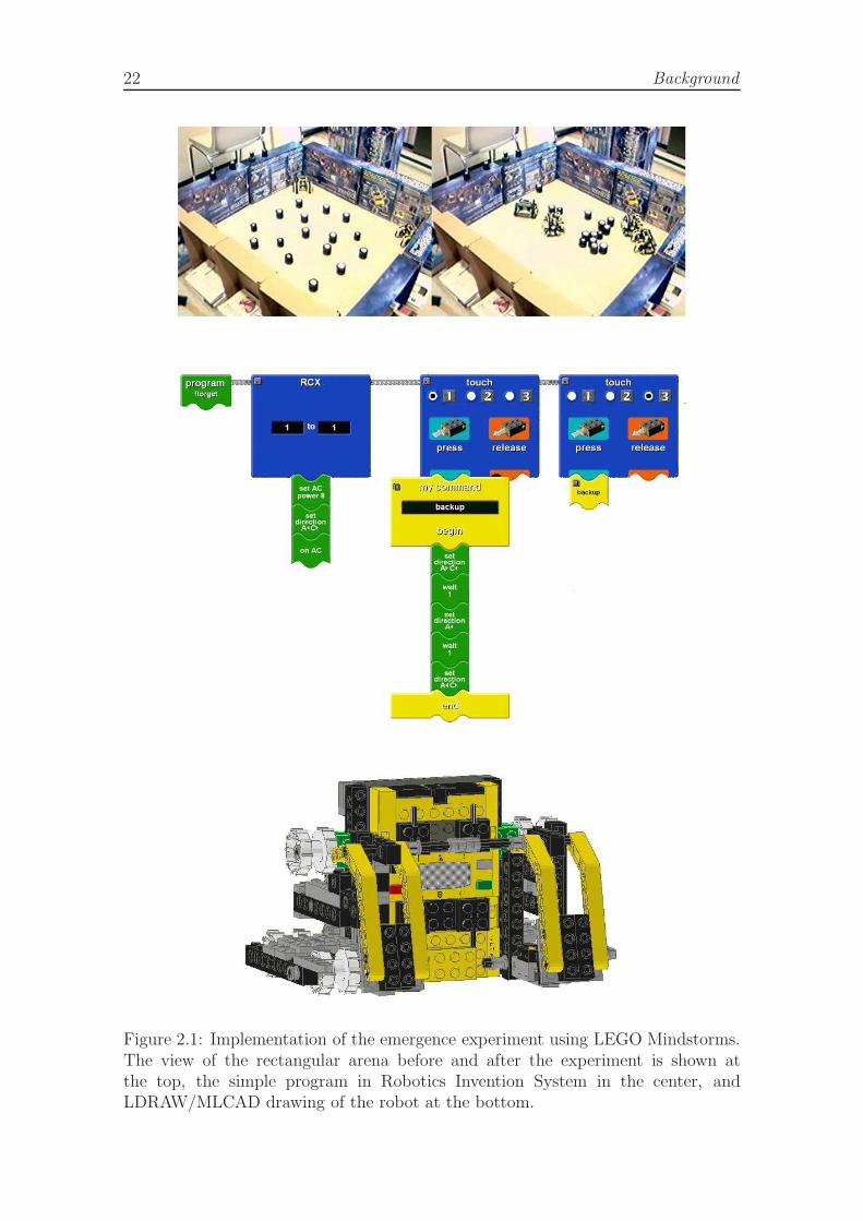
Figure 2.2: A program fragment in NQC for a soccer playing robot, which seeksand follows an infra-red ball using a single IR sensor. When the program segmentis entered, the robot is already spinning left. It keeps spinning at the spot until theball is seen. Then it still keeps spinning until the sensor reading will start to decline,i.e. it has already passed the exact direction towards the ball, when the reading hasbeen highest. Consequently it starts driving forward towards the ball, while it is inthe sight. Then it starts adjusting the direction towards it by turning to the rightwhile moving forward, and resumes forward motion when the ball is visible again. Ifthe ball is not found on the right-hand side, the robot toggles turning now to the left,and resumes the forward movement, when the ball is found on the left-hand side. Ifthe ball is lost and cannot be seen neither on the left nor on the right, the routinefails, and returns. Note: Another sensor was responsible to detect whether the ballwas already close to the robot. Another task running in parallel was monitoring thatsensor and activated either the dribbler and the kicker as appropriate depending onthe position and orientation of the robot. Better ball-following performance can bereached by using two sensors, or another sensor that can detect direction towardsthe IR ball, as we did in the forthcoming year. This experience provides a niceexample of how morphology and code depend on each other.

24 Background

A

E

B

F

D

H

C

G

Figure 2.3: Phases of ball following of a soccer-player robot. Each phase showsthe new direction of the robot from that point of time as well as where the ball iscurrently rolling.

Figure 2.4: Changing of the robot morphology influences the sensory capabilities.In this case, LEGO brick placed in front of the sensor reduces its sensitive angle.

2.5 Planning and Reactivity 25

Figure 2.5: The original setup that consists of an IR sensor (the five black IR photo-transistors) and a single LEGO brick is shown on the left. An improved setup isshown on the right.

non-deterministic environments are a surprise for an agent. Agent performing instatic and deterministic environments are naturally simpler to build and program,however, given the task, it can still be a hard engineering challenge. We (and mostof AI) are concerned with agents performing in dynamic and non-deterministicenvironments. Having confirmed that, we can still perform studies in static ordeterministic environments to learn about the methods in general.

2.5 Planning and Reactivity

A robot (or an agent) that is performing some activity or task in certain environmenttypically has some goals. When the agent is working itself on setting up, updatingor modifying these goals, it is planning. Some agents do not plan: their behavior isconstant and does not change based on the input they receive from the environment.Thus planning is an optional component of an agent. Agents, which are notplanning may achieve their (fixed) goals, if their behavior is pre-configured fortheir environment. They can even modify their environment gradually in order toachieve more complicated goals and to trigger different parts of their fixed behavior.Planning can be performed with different degree of complexity. Some agents may beplanning only a very short-term actions, while other may form complex long-termplans. Agents can perform planning of different degree of complexity simultaneouslywith mutual feedback between the different levels.

If an agent shall perform in a dynamic and non-deterministic environmentsuccessfully, it must perceive its environment and take actions based on the perceptsacquired using its sensors. Some agents may reflect to their sensory inputs based onthe output of their planning module. If an agent utilizes more direct links betweenthe sensory inputs and actuator outputs, it is reactive. Extreme view on the reactiveagents requires that they do no planning, and there indeed are many examplesof agents that achieve their goals without planning. These are purely-reactiveagents. Agents solving more complex tasks would usually both plan and be reactive,these are often called hybrid-architecture agents in the literature as they typically

26 Background

contain features of both the traditional robotics planning systems and the featuresof behavior-based controllers. For an example of an architecture that is completelybehavior-based, even though it performs higher cognitive functions (mapping), seethe work of Mataric [Mataric, 1992]. More about the robotic architectures is in thesection 2.11.

2.6 Navigation

The spatial characteristics of an agent and its environment influence the strategyfor selecting and performing actions in order to move around the environment andachieve the agent’s goals: the agent navigates in its environment. These strategies,or navigation algorithms, form a separate research subarea. From simple maze-exploration strategies such as wall-following, and left/right-hand rule, to complexstochastic strategies intertwined with map-building, localization, and explorationtasks.

The navigation strategy is deterministic, when the agent always chooses the sameaction in the same situation, and it is stochastic when the agent actions are chosenrandomly (at least include some degree of randomness).

Probably the most simple stochastic strategy is random movement used forenvironment exploration or area-cover. The robot moves for some distance alonga straight line, turning randomly, bouncing or turning randomly on the areaboundaries and obstacles. A nice example is one of the first autonomous lawn mowerrobots built by Husqvarna [Hicks II and Hall, 2000], which moves randomly on a lawnsurrounded by inductive wire dug few centimeters under the ground. Such behaviorresults in virtually all lawn of an arbitrary shape mowed without the need of specificdeterministic strategy. The cost of such a solution is a lower efficiency. However,given the robot being powered from the solar panels, this becomes a less importantissue, and (as the feedback from customers suggests) it gives some entertainmentvalue to the robot.

A simple deterministic strategy for locating a target at unknown location is thedepth-first search. If the location of target and the map of the environment is known,a simple shortest-path algorithm can be used.

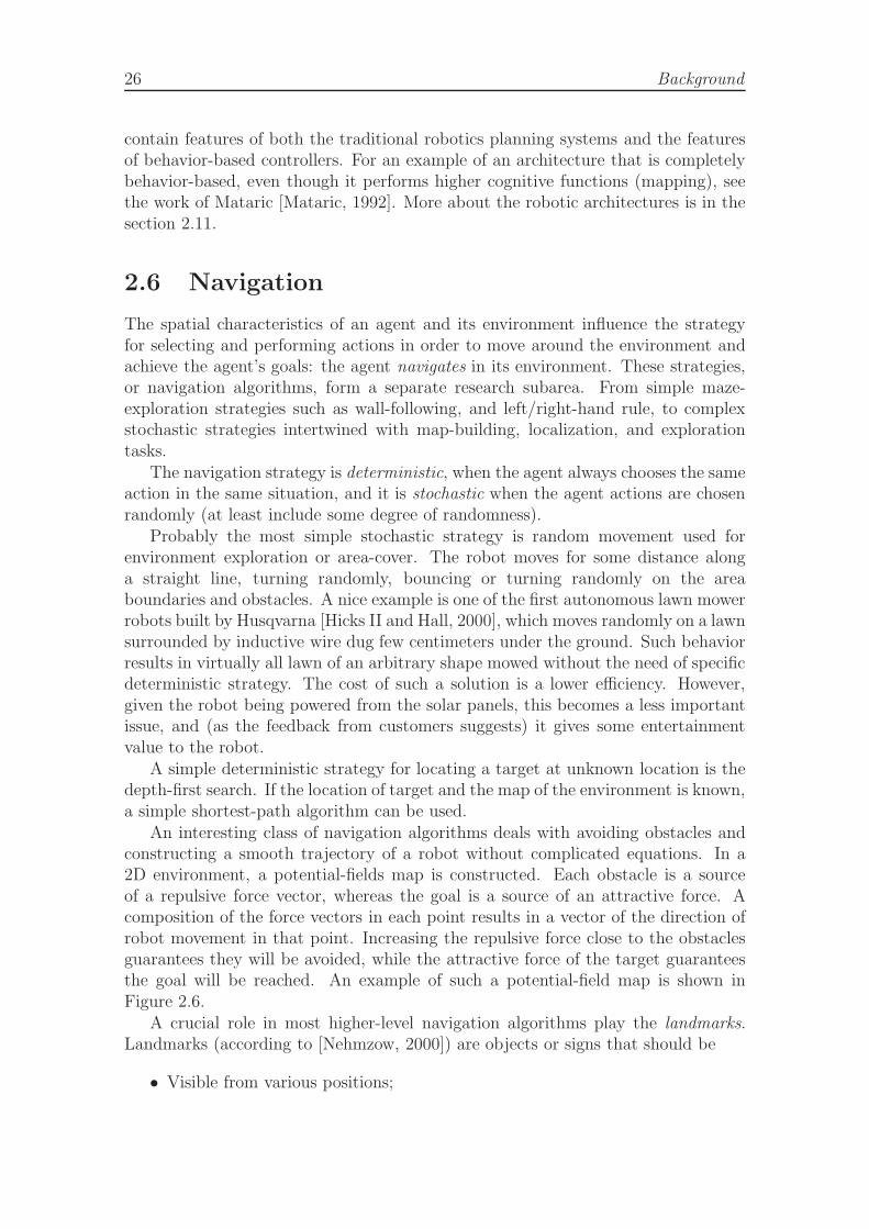
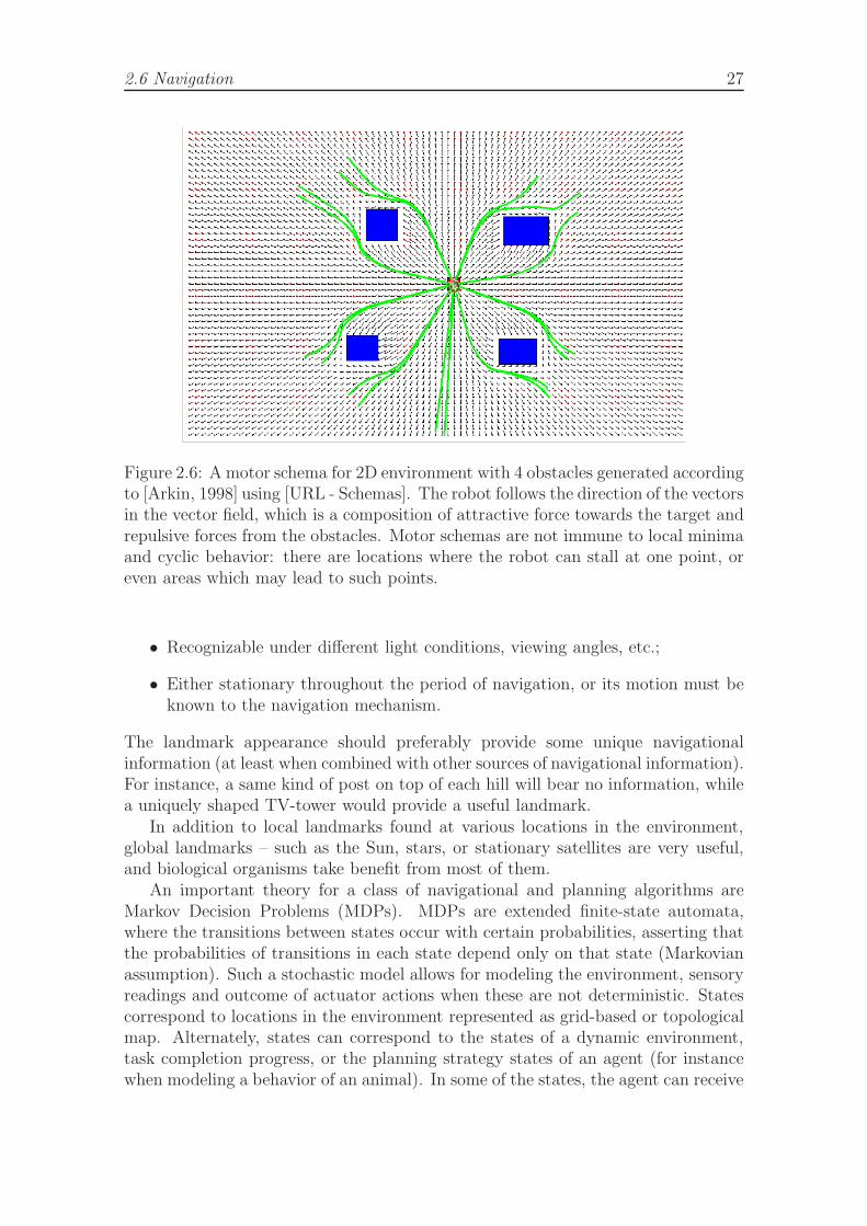
An interesting class of navigation algorithms deals with avoiding obstacles andconstructing a smooth trajectory of a robot without complicated equations. In a2D environment, a potential-fields map is constructed. Each obstacle is a sourceof a repulsive force vector, whereas the goal is a source of an attractive force. Acomposition of the force vectors in each point results in a vector of the direction ofrobot movement in that point. Increasing the repulsive force close to the obstaclesguarantees they will be avoided, while the attractive force of the target guaranteesthe goal will be reached. An example of such a potential-field map is shown inFigure 2.6.

A crucial role in most higher-level navigation algorithms play the landmarks.Landmarks (according to [Nehmzow, 2000]) are objects or signs that should be

• Visible from various positions;

2.6 Navigation 27

Figure 2.6: A motor schema for 2D environment with 4 obstacles generated accordingto [Arkin, 1998] using [URL - Schemas]. The robot follows the direction of the vectorsin the vector field, which is a composition of attractive force towards the target andrepulsive forces from the obstacles. Motor schemas are not immune to local minimaand cyclic behavior: there are locations where the robot can stall at one point, oreven areas which may lead to such points.

• Recognizable under different light conditions, viewing angles, etc.;

• Either stationary throughout the period of navigation, or its motion must beknown to the navigation mechanism.

The landmark appearance should preferably provide some unique navigationalinformation (at least when combined with other sources of navigational information).For instance, a same kind of post on top of each hill will bear no information, whilea uniquely shaped TV-tower would provide a useful landmark.

In addition to local landmarks found at various locations in the environment,global landmarks – such as the Sun, stars, or stationary satellites are very useful,and biological organisms take benefit from most of them.

An important theory for a class of navigational and planning algorithms areMarkov Decision Problems (MDPs). MDPs are extended finite-state automata,where the transitions between states occur with certain probabilities, asserting thatthe probabilities of transitions in each state depend only on that state (Markovianassumption). Such a stochastic model allows for modeling the environment, sensoryreadings and outcome of actuator actions when these are not deterministic. Statescorrespond to locations in the environment represented as grid-based or topologicalmap. Alternately, states can correspond to the states of a dynamic environment,task completion progress, or the planning strategy states of an agent (for instancewhen modeling a behavior of an animal). In some of the states, the agent can receive

28 Background

positive or negative reward. The problem is to find a good policy for traversing thestate automaton so that the reward is achieved with the highest probability. MDPsare thus closely related to the field of Reinforcement Learning, a method for learningan action-selection policy to achieve agent’s goal.

Navigational algorithms often utilize the sensors for the feedback about the robotmovements (this is referred to as local navigation in the literature). For instance,rotation sensors can provide information about the speed of spinning of the wheelsfor odometry. Using dead-reckoning, the agent estimates its location based on itsown measurements of the wheels revolutions. This information can alternately beobtained or supported also using distance sensors, compass, landmark detection, orvision.

Once the robot knows how much it travels, it can possibly try to locate itselfwithin a map of the environment or try to follow, or even construct such a map(this is referred to as global navigation in the literature). An example of a globalnavigation algorithm used by robot Xavier [Koenig and Simmons, 1998] for poseestimation in an office environment is based on the theory of Partially ObservableMarkov Decision Problem (POMDP). The environment is divided into locations(states), and at each time, the robot resides at each location with a determinedprobability. Given the sensor and motion report, and the desired directive appliedto the actuators, the probability of being at each location in the next discrete stepis computed from the prior and learned model of the environment.

In real robot implementations, navigation usually utilizes a combination ofmultiple sensory inputs (sensor fusion). For example, in [Thrun et al., 1998], theoutput from sonar sensors which detect the presence of obstacles is supported byscene analysis from stereo-vision. Thrun et al. demonstrate how the sonar sensorsalone tend to overlook objects absorbing sound, while the vision system itself missesobstacles, which are not distinguished by their optical properties – such as glassdoors, or white walls.

2.7 Sensors and Actuators

Sensors are an important source of information about non-deterministic environ-ments. Robots operating in such environments must therefore utilize the use ofsensors, which is often a difficult task given that sensory readings are usually noisyor unreliable. The robot controller thus cannot rely on a single sensory reading orit has to employ a stochastic behavior governed by stochasticity of the sensors.

The most simple sensors are tactile sensors used in combination with mechanicbumpers to avoid obstacles or other objects in the environment and avoid their orrobot’s damage. They however demand a physical contact. A feasible alternativeare infra-red (usually short-range, 2-15 cm) or ultra-sound (usually long-range, upto several meters) proximity detectors, which detect the amount of reflected signalthey emit. They are vulnerable to non-reflecting surfaces, spurious echos due to thereflections and other unexpected fluctuations in the physical properties of objects.Better precision can be achieved with laser range sensors, which can operate wellalso in outdoor environments.

2.8 Vision 29

Shaft encoders, or rotation sensors are used to determine the rotation speedof wheels, and can be applied to measure the distance traveled by a robot and itsrotation (odometry). However, this information suffers from accumulating errors andthus has to be confronted with feedback from other sensors to align the predictionwith reality. For instance, the magnetic compass sensor provides global robotorientation and thus can compensate for angular errors of robot turning. When therobot operates in large environments, GPS sensors can be used to obtain globalpositioning information. Another strategy for position estimation is to use theaccelerometers, thus determining the actual speed of the robot in all directions.

Gyroscope and tilt sensors can provide information about the robot balance,and are suitable for advanced applications, where the robot performs in three-dimensional space (flight, rough terrain).

Many other types of sensors exist providing usually task- or environment- specificinformation, such as color, temperature, humidity, atmospheric pressure, sound,radiation, altitude, etc. Of distinguished importance are visual sensor systems.

Actuators allow the robot to take physical actions in the environment, or toindicate its state. These include motors, and linear elements, such as solenoids.Sound and light actuators can be used as feedback to the user, or for communication.While the most typical role of the actuators is the source of propelling movement,various specialized actuators can perform useful actions, such as welding, drilling,sweeping, gripping, lifting, etc.

The basic types of motors that are suitable for experimental robotics includeusual DC motors that can be driven by H-Bridge drivers, stepper motors, whichallow high precision of movements, and usual modeler servomotors (often modifiedfor full-rotation operation), which include the encoders and necessary electronics sothat they can be driven by logic-level signals.

2.8 Vision

Vision is the most informative sensor system with the largest bandwidth of infor-mation. Advanced specialized algorithms have to be used to process the visioninput. In its simplest form, vision can be used to trace objects discriminated bytheir color. Usually, however, the image must be segmented into uniform areasthat form objects, their topological information together with pattern recognitionand reasoning about the overall scene may eventually result in understanding of theimage. Image itself provides only two-dimensional information, which itself is notsufficient for determining the distance of the observed objects. Stereo-vision usestwo cameras viewing the same scene from two viewpoints, and thus allowing fordistance estimation. With some drawbacks, this can be achieved by taking framesfrom different locations using a single camera that is moving. Computer visionis very difficult and computationally demanding, however a very active researchfield. Most of our experiments did not utilize any vision system as our purpose isto investigate the algorithms from their bottom application level. An up-to-dateoverview of relevant vision algorithms can be found in [Davies, 2005].

30 Background

2.9 Controller Architectures

A traditional approach of Artificial Intelligence (AI) uses the top-down designmethod, where the overall goal of the system is partitioned into sub-modules thatare developed individually. When putting such modules together, there is a certainrisk that the interfaces, although theoretically compatible, will in practice sufferfrom some unforeseen mismatch. The complexity of the robotics system is toohigh for a prototype-designer to be able to predict the behavior of all componentsaccurately. It may be found during the implementation phase that a particularmodule cannot satisfy the physical constraints of some robot parts implied by thetop-down design. Moreover, the internal architecture typically consists of a largecentralized planning module with symbolic reasoning mechanisms. This modulereceives the sensory information, and should generate next action of the robot inevery time step. However, symbolic reasoning mechanisms are generally too slowfor reactive behaviors that each mobile robot tackles, in particular in case of morecomplex systems, where the reasoning takes into account hundreds or thousands offacts and rules. In addition, a discrete symbolic model does not necessarily suitrandom physical dynamic interactions that resemble natural reflexes in animals ascontrasted to wise actions or answers produces by humans after a thorough logicalreasoning process. Even if the technological possibilities allow building a robotaccording to a top-down plan, the system is very difficult to debug and maintain.

In the literature, the traditional architectures are called the Hierarchical Paradigm.The controller is divided into three parts - SENSE, PLAN, and ACT. SENSE – theinput component is responsible for collecting the data, ACT - is a component thatdrives the actuators, and PLAN is the centralized logic, sometimes monolithic, noteven divided into further modules. A well known example is the robot Shakey[Nilsson, 1984]. The architectures that include planning components are sometimescalled deliberative.

A robot controller is responsible for selecting actions for the robot to perform,based on the current and past sensory readings and its knowledge. It is usuallya combination of specialized hardware and a software running on some embeddedmicroprocessor. In our scientific view, we are interested only in the conceptual(logical) view abstracting from the platform, implementation or other technicaldetails.

The architectures of our concern are those of bottom-up design and reactive type.Many experimental robot controllers are built as some sort of neural network. Thesimplest is perhaps a feed-forward NN, see for example [Floreano and Mondada,1994]. Direct sensory inputs are fed into the layered network, the values propagatethrough weighted connections, and the sum of inputs in each node is usuallytransformed by non-linearity before the node outputs the signal to the next layer.The output signals from the last layer are sent to the robot actuators. Since thistype of network cannot have an internal state, it is limited to tasks and environmentsthat are tractable with completely reactive behavior. The connection weights caneither be evolved or trained by a learning algorithm.

A feed-forward NN can be extended to contain an internal state by appending

2.9 FSA as Genotype Representation 31

memory units as additional input units. They contain a copy of the outputs ofnodes from previous iteration. In general, this type of architecture – recurrent NN,can achieve any type of behavior with respect to the set of computable functions.An interesting analysis of dynamics of a network that solves a simple counting task(predicting elements of sequences anbn) can be found in [Wiles and Elman, 1995].

In ER, more popular architectures are such types of recurrent NN that containarbitrary connections leading from any node to any other node. These include forexample dynamical neural networks of Gallagher and Beer [Beer and Gallagher,1992], in which the neuron excitations are updated in continuous time. Each neuronhas its memory constant that determines the speed of activation change. The groupin Sussex [Harvey, 1995] also used fully interconnected recurrent NN with binaryinhibitory connections.

NN were also used in modular architectures. One possibility is to allocate aseparate NN for each module. In another solution (an emergent modular architectureof [Nolfi, 1997]), a single NN embraces all the modules, but the outputs consist oftwo values produced by selector neurons and output neurons. The function of theselector neurons is to indicate whether the situation is appropriate for the outputneurons value to be taken into account. Modular NN architectures can be evolved thesame way as traditional NN, or the modularity description can be contained in thegenotype. A good start to the field of modular neural architectures is the overviewof [Ronco and Gawthrop, 1995]. For a criticism of the use of neural architectures asa representation for EA, see for example [Steels, 1994].

Classifier Systems (CS) compose an extensive group of controller architecturesfor adaptive robots. They typically consist of three levels. The lowest level isan immediate control of the robot actuators based on the sensory readings anda memory. The actions are usually selected by IF-THEN rules. Second level isa learning mechanism responsible for assigning the credit to those rules that leadto a successful behavior. Rules with higher credit survive, unsuccessful rules areeliminated. CS are in this way a version of reinforcement learning and use, forexample, the Bucket-brigade algorithm to propagate the credit backwards throughthe sequence of rules that result in the useful action of the robot. The third level isresponsible for finding new promising rules and is implemented using a GA. For areview of CS, see [Wilson and Goldberg, 1989].

A very popular way of automatic controller design is Genetic Programming,[Koza, 1992b]. Typically, an action of a robot is determined by an output of one ormore lisp-like S-expressions consisting of arithmetical operations and mathematicalfunctions, constants, and special operators for sensory readings. These S-expressionsare evolved by evolutionary algorithm. Special recombination operators are used,such as tree-crossover. A very first example of application of GP to robot control isin [Koza, 1992a].

Instead of S-expressions, GP techniques can be used with sequential assembler-like programs, sets of IF-THEN or fuzzy rules [Braunstingl et al., 1995] or programsin any language, for which it is possible to generate them from definition grammarrules. More on architectures is described below in section 2.11.

32 Background

2.10 Finite-State Automata as Representation for

Evolutionary Algorithms

[Fogel et al., 1995] draw a strict distinction between evolutionary approaches wherethe evolution is modeled as a genetic process and the approaches where the evolutionis modeled as a phenotypic process. The question is the one of the representationof the individuals. Strictly seen, and pertaining to a biological relevance, thegenetic processes deal with genotypes, i.e. encoding of genes that influence theshape, behavior, or other properties of the individual, whereas the phenotypicrepresentations attempt to encode directly the complete individual, its shape,behavior and other properties in their final form. See the section 9.1.2 for aphilosophical treatment of this topic.

FSA or FSMs2 have been used as genotype representation in various works,although this representation lies on the outskirts of the evolutionary algorithmsresearch and applications.

Evolutionary Programming , [Fogel, 1962, 1993, 1964, Fogel et al., 1966, 1995]is a distinguished evolutionary approach that originally used FSA as the genotyperepresentation3. EP does not utilize recombination operators4, and relies on muta-tions. The original EP works addressed the tasks of prediction, identification andcontrol.

[Chellapilla and Czarnecki, 1999] introduce modular FSMs, which are in factequivalent to non-modular FSMs, except that the topology is restricted – in par-ticular, the FSMs are partitioned into several encapsulated sub-parts (sub-FSMs),which can be entered exclusively through their starting states. The authors usemodular FSMs to evolve controllers for the artificial ant problem that was previouslysuccessfully solved by evolving binary-string encoded FSA in [Jefferson et al., 1992].They provide evidence that modular FSMs perform better on this task than non-modular FSMs, and they also provide evidence that direct encoding with structuralmutations of non-modular FSMs perform better than binary-string encoding usedin [Jefferson et al., 1992]. This idea of modular FSMs has been adopted also byAcras and Vergilio [Acras and Vergilio, 2004], who develop a universal frameworkfor modular EP experiments and demonstrate its use on two examples.

[Angeline and Pollack, 1993] are experimenting with automatic modular emer-

2The difference between FSA and FSMs in the evolutionary literature seems to be that theformer refer strictly to the formal computational model as originated sometimes in the middleof the twentieth century and intensively formalized and studied for example by [Hopcroft andUllman, 1979], while the latter usually refers to models where control actions are performed whentransitions are followed. Other computer science literature, however, often makes no distinctionin these two names, while various other names (Moore, Mealy) are used for different flavors of theformalism. The core of all representations, however, are the FSA, and we refer to the extensionsin this article as augmented FSA, or FSA for simplicity. When referring to previous work, weattempt to use the same term as the author.

3Further developments of EP moved from the FSA to real-value parameters representation,where the Gaussian mutation is applied to alter the parameters from generation to generation.

4Even though later the annual EP conferences included all works relevant for EvolutionaryAlgorithms, and later have been integrated into Congress on Evolutionary Computation – CEC.

2.10 FSA as Genotype Representation 33

gence of FSA. They suggest to freeze and release parts of the FSA so that thefrozen (or “compressed”) parts cannot be affected by the evolutionary operators.The compression occurs randomly and due to the natural selection process, it isexpected that those individuals where the compression occurs for the correctlyevolved sub-modules will perform better and thus compression process interactswith the evolutionary process in mutually beneficial manner. Indeed, the authorsdocument on the artificial ant problem that the runs with compression performedbetter than equivalent runs without compression. They reason: “An explanationfor these results is that the freezing process identifies and protects components thatare important to the viability of the offspring. Subsequent mutations are forced toalter only less crucial components in the representation.”

[Lucas, 2003] is evolving finite-state transducers (FSTs), which are FSA thatgenerate outputs, in particular, map strings in the input domain with strings in theoutput domain. FSTs for transforming 4-chain to 8-chain image chain codes wereevolved in this work, while three different fitness measures for comparing generatedstrings were used: strict equality, hamming distance and edit distance.

An interesting piece of work by [Frey and Leugering, 2001] considers FSMs ascontrollers for several 2D benchmark functions and the artificial ant problem. Intheir representation, the whole transition function is represented as a single strongly-typed GP-tree – i.e. a branching expression with conditions in the nodes that directexecution either to the left or to the right sub-tree, and finally arriving to a set ofleaves that list the legal transition pairs (old state, new state).

In his PhD thesis, [Hsiao, 1997] is using evolved FSA to generate input sequencesfor digital circuits with the purpose of their verification, and fault detection. Theauthor achieves best fault detection rate on various circuits (as compared to otherapproaches), except of those that require specific and often long sequences for faultactivation.

[Horihan and Lu, 2004] are evolving FSMs to accept words generated by a regulargrammar. They use an incremental approach, where they first evolve FSMs forsimpler grammars, and gradually progress to more complex grammars. They usethe term genetic inference to refer to their approach of generating such solution.

[Clelland and Newlands, 1994] are using EP with probabilistic FSA (PFSA) inorder to identify regularities in the input data. The PFSA is a FSA, where thetransitions are associated with probabilities as measured on input sequences. TheEP is responsible for generating the topology of the FSA – number of states andhow they are interconnected, and the transitions in PFSA are labeled according totheir “fire rate”. This combination can be applied for rapid understanding of aninternal structure of sequences.

[Ashlock et al., 2002] are evolving FSMs to classify DNA primers as good andbad in simulated DNA amplification process. They evolve machines with 64 statesin 600 generations. They used the weighted count of correct/incorrect classificationsas their fitness function. However, they sum the classifications made in each state ofFSM throughout its whole run. They argue that if only the classifications made inthe final state were taken into account, the performance was poor. In addition, thisallows the machine to produce weighted classification – how good/bad the classified

34 Background

primer is. The best of 100 resulting FSMs had success rate of classification of about70%. Hybridization, i.e. seeding 1/6th of a population of an extra evolutionary runwith the best individuals from 100 previous evolutionary runs improved the resultto about 77%. This work was continued in [Ashlock et al., 2004], where the FSMapproach was compared to more conventional Interpolated Markov Models (IMMs),which outperformed FSMs significantly.

In an inspiring study from AI Center of the Naval Research Laboratory, [Spearsand Gordon, 2000] analyze evolution of navigational strategies for the game ofcompetition for resources. The strategies are represented as FSMs. Agent moves ona 2D grid while capturing the free cells. Another agent with a fixed, but stochasticstrategy is capturing cells at the same time, and the game is over when thereare no more cells to capture. Agents cannot leave their own territory. Authorsfind that the task is vulnerable to cyclic behavior that is ubiquitous in FSMs, andtherefore implement particular run-time checking to detect and avoid cycles. Theyexperiment with the possibility to disable and again re-enable states (as contrastedto permanent and complete state deletion). They also compare evolution of machineswith fixed number of states and evolution of machines, where the number of stateschanges throughout the evolutionary run. They discover that in the case of varyingnumber, the machines utilize the lately-added states to lesser extent, as well as thatdeleting states is too dramatic for performance, and thus suggest to merge or splitstates instead of deleting and creating states. Due to the stochastic algorithm ofthe opponent agent in the game of competition for resources, the fitness functionmust evaluate each individual in many different games (G). Authors disagree withothers claiming that keeping G low can be well compensated by higher number ofgenerations and conclude that it results in unacceptable sampling error. The authorstherefore evaluate all the individuals on fewer games (500), and if the individualshould outperform the previous best individual, they re-evaluate it on many more(10000) games.

Some further FSM-relevant references can be found for example in the EPsections in the GECCO and CEC conferences.

2.11 Robot Programming Formalisms

Various formalisms were developed for programming robots. Some are based onstandard programming languages with extensions, others are trying to look atwhat is special about programming robots first, and derive a formalism from suchviewpoint.

One of the first formalisms (used also to program the famous robot Shakey)designed as early as in 1960s that dealt with robot actions similar to behaviors weretriangle tables [Nilsson, 1985]. Triangle tables are an extension of standard rule-production systems. They arrange the actions in a sequence, each having a list ofpreconditions that need to be satisfied, in order for the action to be performed. Anaction results in new facts to be inserted into the memory. A limited support forhierarchical organization is provided. Hierarchical organization is a weak side of therule production systems that tend to be flat.

2.12 Behavior-Based Robotics 35

EusLisp of [Matsui and Inaba, 1999] is an object-based extension of CommonLisp with support for solid 3D modeling, concurrences, and robot manipulators. Itcan be conveniently used also for programming mobile robots.

Task Definition Language (TDL) of [Simmons and Apfelbaum, 1998] is anextension of C++ that allows task specification and manipulation. It has been usedin numerous CMU and NASA robotics projects. A compiler translates TDL codedirectly to C++ code. TDL features very rich set of synchronization commands,which are expressed in straight-forward manner. This makes TDL unique comparedto other task-control languages. TDL is working with task trees, where nodes areassociated with actions that can succeed or fail. These are either goals or commands(leaf nodes). In addition, TDL utilizes constructs for exception handling, and taskmonitoring (actions performed repeatedly). The programs themselves manipulatethe task trees, thus the same program can generate various task trees in differentruns.

Microsoft Robotics Studio is a recent addition to the family of robotics languagesand formalisms. It is based on Microsoft Visual Programming Language (VPL) andsupports most of the currently used research architectures as well as a physics-basedsimulation.

2.12 Behavior-Based Robotics

A modern approach of the Nouvelle AI relies on building robots incrementally. Themost trivial reactive behaviors, such as obstacle avoidance, are fully implemented,tested, and debugged first, before carefully appending higher-level behaviors. Theseideas are applied in the Subsumption Architecture [Brooks, 1986]. Individualbehaviors that formed the controller communicated using a fixed network, wiresof which conducted simple signals. Fixed mechanisms of inhibition and suppression,and behavior priorities were used to resolve conflicts between the behaviors. Itsdisadvantage of hard-wiring the behaviors was addressed later in [Maes and Brooks,1990], where individual behaviors compete for robot control and the robot canlearn the conditions of applicability of each behavior in different situations. Theprecondition lists were learned by random trial-and-error method, and updated usingrelevance and reliability measures that were computed from correlation of positive(resp. negative) feedback and activity of the behavior.

The research challenge that has not been studied satisfyingly well yet is whetherthe robot controller can be designed automatically so that it would perform somenontrivial useful task, and whether the automatic method can provide some advan-tages over a human-engineered solution.

According to Miriam Webster dictionary, behavior is “anything that an organismdoes involving action and response to stimulation”. It is important that thisanything, a series of interactions of the individual with its environment, is viewedfrom the point of view of an external observer. He or she would ask the questionWhat will the agent achieve by doing this? This is in a sharp contrast with a point ofview of an engineer who would ask the questions as: What functionality is providedby the bottom light sensor? Which components of the robot form the navigational

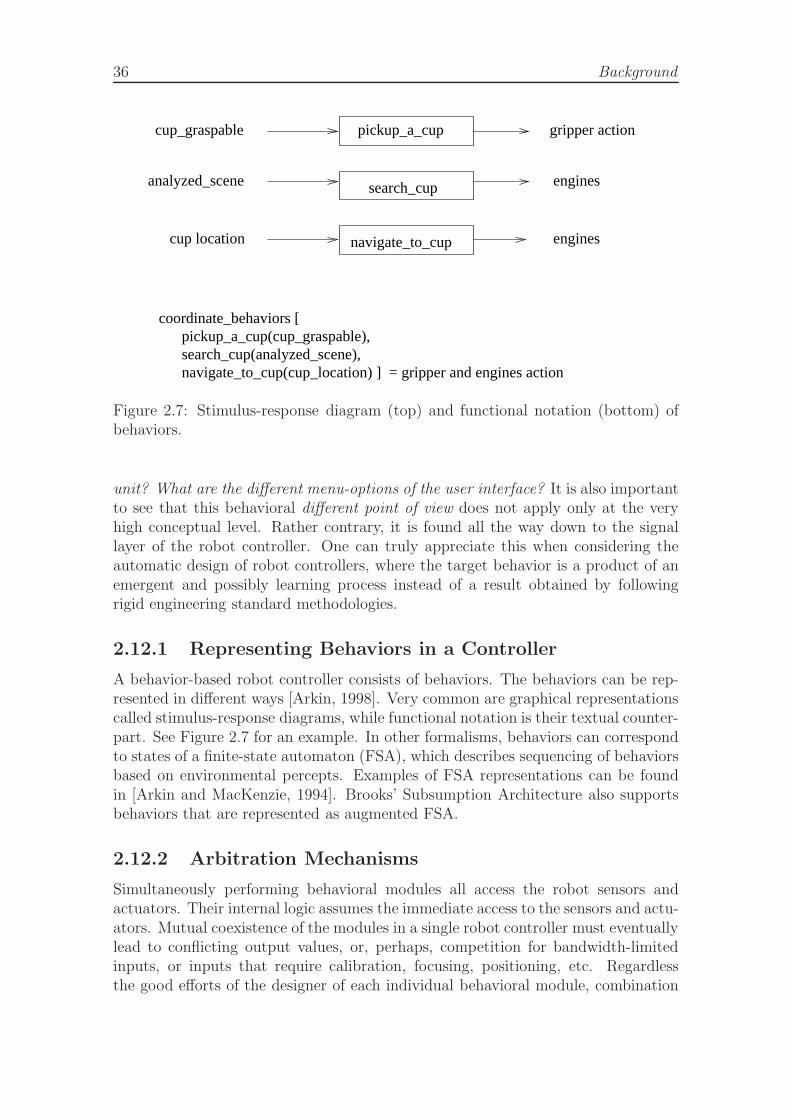
36 Background

pickup_a_cup

navigate_to_cup

search_cup

coordinate_behaviors [

search_cup(analyzed_scene), navigate_to_cup(cup_location) ] = gripper and engines action

pickup_a_cup(cup_graspable),

cup_graspable

analyzed_scene

cup location

engines

engines

gripper action

Figure 2.7: Stimulus-response diagram (top) and functional notation (bottom) ofbehaviors.

unit? What are the different menu-options of the user interface? It is also importantto see that this behavioral different point of view does not apply only at the veryhigh conceptual level. Rather contrary, it is found all the way down to the signallayer of the robot controller. One can truly appreciate this when considering theautomatic design of robot controllers, where the target behavior is a product of anemergent and possibly learning process instead of a result obtained by followingrigid engineering standard methodologies.

2.12.1 Representing Behaviors in a Controller

A behavior-based robot controller consists of behaviors. The behaviors can be rep-resented in different ways [Arkin, 1998]. Very common are graphical representationscalled stimulus-response diagrams, while functional notation is their textual counter-part. See Figure 2.7 for an example. In other formalisms, behaviors can correspondto states of a finite-state automaton (FSA), which describes sequencing of behaviorsbased on environmental percepts. Examples of FSA representations can be foundin [Arkin and MacKenzie, 1994]. Brooks’ Subsumption Architecture also supportsbehaviors that are represented as augmented FSA.

2.12.2 Arbitration Mechanisms

Simultaneously performing behavioral modules all access the robot sensors andactuators. Their internal logic assumes the immediate access to the sensors and actu-ators. Mutual coexistence of the modules in a single robot controller must eventuallylead to conflicting output values, or, perhaps, competition for bandwidth-limitedinputs, or inputs that require calibration, focusing, positioning, etc. Regardlessthe good efforts of the designer of each individual behavioral module, combination

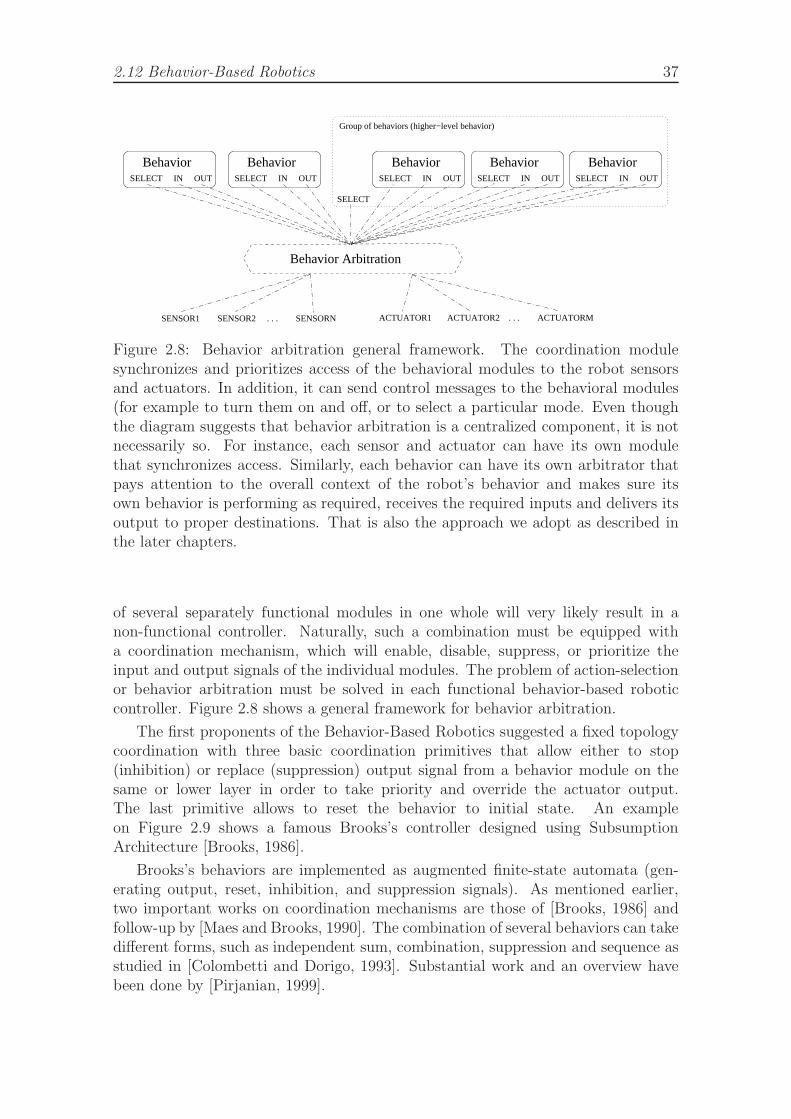
2.12 Behavior-Based Robotics 37

BehaviorSELECT IN OUT

BehaviorSELECT IN OUT

BehaviorSELECT IN OUT

BehaviorSELECT IN OUT

BehaviorSELECT IN OUT

Behavior Arbitration

Group of behaviors (higher−level behavior)

SELECT

SENSOR1 SENSOR2 . . . SENSORN ACTUATOR1 ACTUATOR2 . . . ACTUATORM

Figure 2.8: Behavior arbitration general framework. The coordination modulesynchronizes and prioritizes access of the behavioral modules to the robot sensorsand actuators. In addition, it can send control messages to the behavioral modules(for example to turn them on and off, or to select a particular mode. Even thoughthe diagram suggests that behavior arbitration is a centralized component, it is notnecessarily so. For instance, each sensor and actuator can have its own modulethat synchronizes access. Similarly, each behavior can have its own arbitrator thatpays attention to the overall context of the robot’s behavior and makes sure itsown behavior is performing as required, receives the required inputs and delivers itsoutput to proper destinations. That is also the approach we adopt as described inthe later chapters.

of several separately functional modules in one whole will very likely result in anon-functional controller. Naturally, such a combination must be equipped witha coordination mechanism, which will enable, disable, suppress, or prioritize theinput and output signals of the individual modules. The problem of action-selectionor behavior arbitration must be solved in each functional behavior-based roboticcontroller. Figure 2.8 shows a general framework for behavior arbitration.

The first proponents of the Behavior-Based Robotics suggested a fixed topologycoordination with three basic coordination primitives that allow either to stop(inhibition) or replace (suppression) output signal from a behavior module on thesame or lower layer in order to take priority and override the actuator output.The last primitive allows to reset the behavior to initial state. An exampleon Figure 2.9 shows a famous Brooks’s controller designed using SubsumptionArchitecture [Brooks, 1986].

Brooks’s behaviors are implemented as augmented finite-state automata (gen-erating output, reset, inhibition, and suppression signals). As mentioned earlier,two important works on coordination mechanisms are those of [Brooks, 1986] andfollow-up by [Maes and Brooks, 1990]. The combination of several behaviors can takedifferent forms, such as independent sum, combination, suppression and sequence asstudied in [Colombetti and Dorigo, 1993]. Substantial work and an overview havebeen done by [Pirjanian, 1999].

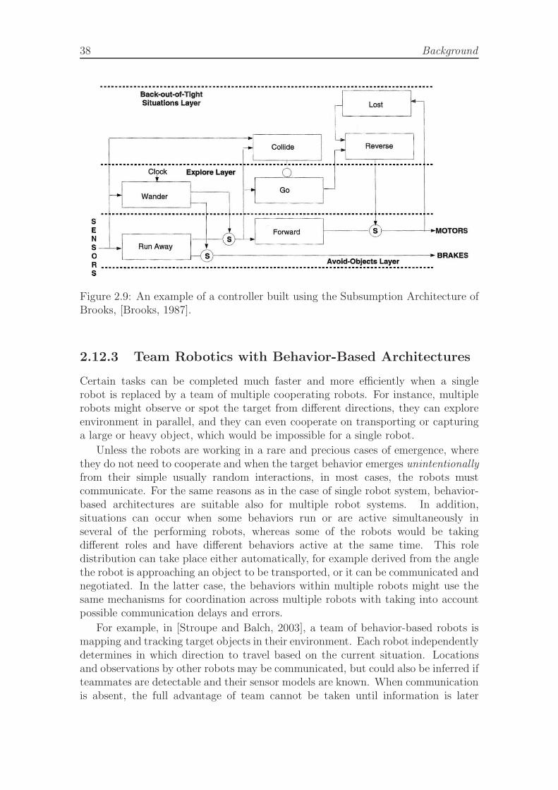
38 Background

Figure 2.9: An example of a controller built using the Subsumption Architecture ofBrooks, [Brooks, 1987].

2.12.3 Team Robotics with Behavior-Based Architectures

Certain tasks can be completed much faster and more efficiently when a singlerobot is replaced by a team of multiple cooperating robots. For instance, multiplerobots might observe or spot the target from different directions, they can exploreenvironment in parallel, and they can even cooperate on transporting or capturinga large or heavy object, which would be impossible for a single robot.

Unless the robots are working in a rare and precious cases of emergence, wherethey do not need to cooperate and when the target behavior emerges unintentionallyfrom their simple usually random interactions, in most cases, the robots mustcommunicate. For the same reasons as in the case of single robot system, behavior-based architectures are suitable also for multiple robot systems. In addition,situations can occur when some behaviors run or are active simultaneously inseveral of the performing robots, whereas some of the robots would be takingdifferent roles and have different behaviors active at the same time. This roledistribution can take place either automatically, for example derived from the anglethe robot is approaching an object to be transported, or it can be communicated andnegotiated. In the latter case, the behaviors within multiple robots might use thesame mechanisms for coordination across multiple robots with taking into accountpossible communication delays and errors.

For example, in [Stroupe and Balch, 2003], a team of behavior-based robots ismapping and tracking target objects in their environment. Each robot independentlydetermines in which direction to travel based on the current situation. Locationsand observations by other robots may be communicated, but could also be inferred ifteammates are detectable and their sensor models are known. When communicationis absent, the full advantage of team cannot be taken until information is later

2.13 Evolutionary Robotics 39

combined. Substantial amount of work on multi-robot systems can be found in thevolumes of proceedings of the International workshop on multi-robot systems.

2.13 Evolutionary Robotics

Our efforts are to combine and integrate the ideas from several independent fields.Different approaches to automatic design of robot controllers were studied. Mostknown are Reinforcement Learning [Sutton and Barto, 1998], [Humphrys, 1997],Neural Networks, Classifier Systems (CS) [Wilson and Goldberg, 1989], GeneticProgramming (GP) [Koza, 1992b], and artificial evolution used with various con-troller architectures. The latter three use some form of evolutionary technique androughly compose the sub-field of AI labeled Evolutionary Robotics, which is themain area of our interest [Beer and Gallagher, 1992], [Nolfi and Floreano, 2001],[Harvey, 1995], [Lee et al., 1998].

Most of the work in the ER field is focusing on adaptive mobile robots withneural controllers. Inspiration from biology means application of the laws of naturalDarwinian evolution and motivates towards long-term evolution of individuals thatsuccessfully perform in their artificial life environment. In these cases, the focusis not on building systems that can be directly useful today or tomorrow, ratheron the study of how the natural principles observed in the living species applyto the artificial robotic systems built by us. It is often not important what theagent will be able to do when the evolution completes, rather how the evolutionaryprocess progresses, and how it interacts with the agent learning abilities. Aim isat answering the questions of how we could imitate the clever and very effectiveanimal behavior that relies on imperfect and irregular patterns, and how to buildartificial control systems that would have similar properties of the animal brains.Naturally, researchers with such motivations study controllers based on artificialneural networks, and explore various neural architectures. The systematic researchefforts start and still progress with the early systems capable of obstacle avoidance,wall-following, target recognition and following, box pushing, simple autonomousflight, or survival of agents in artificial environment. It is important to point outthat most (if not all) of the resulting evolved controllers perform a behavior thatcan easily be achieved by a manually programmed controller of small or moderatedifficulty. However, the researchers in the field counter that argument by stressingtheir interest in adaptive and self-organizing systems, and the early stages of theresearch field.

Briefly, ER (and EC in general) relies on evolution of population (set) ofindividuals (solutions to a problem). This set is usually of a fixed size. Solutionsare not only good or bad, their quality (fitness) can be measured by the objectiveevaluation function. Objective function returns a number, which determines thequality of a solution. In the beginning of EC run, a random population is created(generation zero). Next generation is created from the previous by combining higherquality solutions and introducing few random changes into them (mutations). Thisrequires the solutions to be encoded in some uniform way (genotype). For example,bit-strings are used in Genetic Algorithm (GA) [Holland, 1975], lisp S-expressions in

40 Background

GP or sequences of machine instructions, C-language programs [Ryan et al., 1998],etc. in other methods. EC run goes on for many generations, and the result isthe best individual found during the evolution. Therefore a problem of designing arobot controller using ER method has typically the following steps (not necessarilyperformed in this order!):

• Define the target behavior(s) that the robot will have to accomplish — thetask for the robot.

• Design the physical body of the robot and its hardware, decide on the sensorsand actuators that the robot will use. Create a specification of signals comingfrom sensors and to actuators.

• Decide on the controller architecture, modularity, and software platform.

• Choose which of the modules and their parts can be easily designed manuallyand identify those which are suitable for automatic design. If there are moreparts for automatic design, choose whether they will be evolved simultaneouslyor individually.

• Find uniform encoding for automatically designed parts and define fitness(objective) functions.

• Based on experience and some experiments, set up the parameters for partic-ular evolutionary algorithm and run the evolution.

• Optimize, analyze, and test the evolved parts (ideally, prove their correctness),integrate with the other parts of the controller.

There are remaining open research questions. One problem is how to formallyspecify behaviors so that this specifications could be used automatically to generatean objective function. Another problem is how to analyze and verify the correctnessof the evolved controller based on that definition later.

Some researchers argue for simultaneous evolution of the robot physical topology(body) or hardware and its controller (brain) [Brooks, 1992], [Lund and Miglino,1998].

We are mainly concerned with application of the Evolutionary Computation tothe problem of design of robot controllers, as mentioned earlier in the section 2.2.A possible alternative, or rather extension, is using the EC for further adaptationsduring the individual’s lifetime. A systematic study of such approach can be foundin the doctoral thesis of [Walker, 2003].

2.13.1 Evolvable Tasks

Although ER has been tested on many different tasks, most of them were simple.These include the following:

2.13 Evolutionary Robotics 41

• Wall following, where the robot is placed in a closed environment and has tolearn navigation along the walls without collision. Robot is usually equippedwith laser, sonar, or infrared proximity sensors and sometimes has a vision.

• Obstacle avoidance is typically a part of some more complicated task. The goalfor the robot is to navigate in the environment without running into obstacles.The environment can be static or contain moving objects.

• Docking and recharging, where the robot has to find its docking station andsuccessfully approach it.

• Artificial ant following, a standard Artificial Life simulation problem. Robotis trained to follow a chemical trace by using its smell sensor.

• Box pushing has several variations. A robot or a group of them are given atask of pushing box(es) to the wall, corners or specified positions.

• In lawn mowing task, the robot has to move around inside of a defined arenaand cover the largest possible area. The environment may contain obstacles,irregularities and moving objects.

• Legged walking is used with 2,4,6,8-legged robot. The task is to train thecontroller to synchronize the movements of the robot.

• T-maze navigation is a standard benchmark task. The robot first reads thedirection at the entrance to a corridor. It has to follow the corridor to thecrossing and turn right or left based on the initial instruction.

• Various foraging strategies are related to Artificial Life, where the artificialenvironment contains food sources and the robot has to learn the strategiesfor finding the food.

• Trash collection, is another example of searching. The robot has to pick upthe trash objects, and carry them to an assigned area to drop them.

• In various vision discrimination and classification tasks, the controller istrained to steer the robot depending on the vision sensory inputs.

• In target tracking and navigation, the robot has to follow the target so that itremains in its vision system.

• Various aspects of pursuit-evasion behaviors were also analyzed and the co-evolution method was usually applied (see below).

• Soccer playing robots, where the robot navigates inside a closed and determin-istic environment, but interacts with other robots and the soccer ball, whichhas to be placed in the opponent’s gate.

• Navigation tasks, where the robot needs to successfully negotiate a maze,or keep navigating in an environment with environmental clues, landmarks,beacons, etc.

42 Background

2.13.2 Fitness Space

[Floreano and Urzelai, 2000] describe a classification system for ER objectivefunctions along three axes:

• functional – behavioral axis describes whether the fitness of the individual ismeasured using functional properties (for instance actuator pulse frequency,robot arm position, alignment with a line, etc.) as contrasted with behavioralproperties (for instance the distance traveled, number of objects collected,number of points scored, etc.)

• explicit – implicit axis corresponds to the number of factors taken into accountby the objective function – i.e. how much the designers tend to influence theevolutionary process towards the wished behavior (more explicit function),or leave the proper behavior to emerge naturally by keeping the number ofinvolved criteria as low as possible.

• external – internal axis refers to the types of the values utilized by the objectivefunction: if the values can be measured directly by the sensors and internalstate of the robot, the function is internal. If external observers, installations,and tools are needed, the function is external.

It is claimed and we support this observation that objective functions in the aim ofthe designers should be as behavioral, implicit, and internal as possible. Followingthat advice makes the specification of the target task more human understandable,less vulnerable to errors, the search is less prone to local optima, the functionis easier to implement and can be used in embedded (on-line) evolution withoutmodifications. In addition, it appears to correspond better in an analogy to naturalevolution. However, it may be more challenging to achieve good results.

2.13.3 Co-Evolution

Another common method used in ER for arranging the gradual increase of thetask difficulty is the co-evolution [Cliff et al., 1992, Reynolds, 1994, Smith andCribbs III, 1996, Juille and Pollack, 1996, Floreano et al., 1998]. In this approach,two simultaneous competing populations of individuals are evolved. The individualsshare the same environment during their lifetime (fitness run). The individuals mayhave opposite goals, they can compete for the same resource, they can have thesame or different roles, and optionally, they can even depend on one another incooperation. As a consequence, the environment complexity is gradually increasedover the generations as the evolution finds better individuals in both populations.

The main advantage of co-evolution is that it works automatically, without theneed to specify the incremental steps by a human (or machine) designer.

The range of tasks amenable to co-evolution is limited. In particular, there is aninherent assumption of mutual direct or indirect interactions between the individualsin the same environment. Therefore, co-evolution applies only to evolving solutionsto multi-agent problems (where the word agent is used in a broader sense, anythingthat actively changes its environment).

2.13 Evolutionary Robotics 43

Furthermore, co-evolution is vulnerable to stagnation due to strategy cycles,where a series of strategies relatively outperform each other in a loop. This is relatedto the Red Queen Effect/Hypothesis that roughly states that for an evolutionarysystem, continuing development is needed just in order to maintain its fitness relativeto the systems it is co-evolving with. It was proposed by the evolutionary biologist[Valen, 1973]. Another issue is that co-evolution tends to generate specific solutions,which are tailored for specific strategies of the competing population, and often failsto generate robust agents that are able to perform a general strategy.

2.13.4 Evolving the Robot Morphology

The natural intelligence in the natural environment resulted after many millionsof years of natural evolution. The genotype of the natural organisms influence toa large degree not only the mental and reasoning capabilities, but their physicalproperties alike. The intelligence of the living organisms is highly dependent onthe percepts from the environment, which again are completely dependent on themechanics, dynamics, and shape of the organisms.

When the ultimate goal is a design of intelligent robots performing in naturalenvironments using EA, it is obvious that these will have to be evolved includingtheir morphology. The current state of the field is not yet that far due to thephysical limitations (we are not yet capable of assembling robots with an arbitrarymorphology), however some interesting attempts and simple experiments have beenperformed. A very important tool in this respect is simulation. It is therefore partof the work of evolutionary roboticist to study the possibilities of the evolution ofshape, a field often called Evolutionary Design.

For instance [Pollack et al., 2001] evolve various LEGO structures for a givenpurpose (such as crane) using a GA, later use the 3D printing machine to generatearbitrary shapes of a robotic agent, and finally evolve 2D modular locomotionmachines with the help of generative grammatical representation based on L-systems. The most interesting, as Pollack et al. show in the latter two examples, isthe combination of evolving controllers and morphologies simultaneously (sometimesthe term co-evolution is used also for this process). Another example is [Marbachand Ijspeert, 2004], where the morphological configuration of agents that performlocommotion is evolved together with parameters of PD controllers. Yet anotherinteresting example are Framsticks, 3D life simulation project, developed by a groupin Poznan, [Komosinski, 2003].

2.13.5 Evolving Behavior Arbitration

There have been only few attempts to generate arbitration mechanisms automati-cally based on the required task or robot purpose. For example, Koza [Koza, 1992a]evolves a robot controller based on Subsumption Architecture for wall-following task.He writes: “The fact that it is possible to evolve a Subsumption Architecture to solvea particular problem suggests that this approach to decomposing problems may beuseful in building up solutions to difficult problems by aggregating task achieving

44 Background

behaviors until the problem is solved.” The usefulness of these approaches can besupported by the following reasons:

• They are inovating: Automatic method might explore unforeseen solutionsthat would otherwise be omitted by standard engineering approaches used inmanual or semi-automatic design performed by a human.

• They can provide robot controllers with higher flexibility: Mobile robots canbe built for general purpose, and the arbitration mechanism for differentachievable tasks might have to be different, either for reasons of critical limitson their efficiency, the bounds on the controller capacity, or conflicting roles indifferent tasks. In such a case, generating the arbitration mechanism based ontask description might be required. Having the option of automatic arbitrationgeneration might save extensive amounts of work needed to hand-craft eacharbitration mechanism.

• They can cope with complexity: Manual arbitration design might suffer fromthe lack of understanding of the real detailed interactions of the robot with itsenvironment. These interactions might be difficult to describe analyticallydue to their complexity. Automatic arbitration design might capture theundergoing characteristics of the robot interactions more reliably, efficientlyand precisely.

Learning action selection (term sometimes used interchangeably with behaviorarbitration) studies in his thesis Humphrys [Humphrys, 1997]. His focus is on the“communication” of agents that together form a controller; in fact, his agents are sosimple that they correspond to the nodes in a recurrent neural network, with veryfew control actions generated by output nodes. Input nodes receive discrete sensingof an artificial ant moving on a rectangular grid. The topology and connectionweights are evolved and the communication of the very few nodes in the network isstudied on a standard artificial ant seeking food in a rectangular grid problem.

The most valuable inspiration for our work stems from the work of Lee et al. [Leeet al., 1998], where the more complex, high-level task is decomposed hierarchicallyand manually into several low-level simple tasks, which can further be decomposedto lower-level tasks. The reactive controller consists of primitive behaviors at lowestlevel and behavior arbitrators at higher levels, both with the same architecture ofinterconnected logic-gate circuit networks. The evolution proceeds from the lowestlevel tasks up the hierarchy to the target complex task. We see several possibleimprovements:

• avoiding the centralized architecture,

• allowing for easier modification of task by introducing a new module withoutaffecting substantially the existing controller hierarchy, and

• removing the limitation to purely reactive tasks.

2.13 Evolutionary Robotics 45

The work has been continued on by the master thesis [Ostergaard, 2000], wherea football player has been evolved with the use of co-evolution. The qualitativechange is in the ability to work with internal state (as contrasted to purely-reactivecontrollers), and more complex architecture allowing two types of arbitration: 1) asequence of several states, and 2) selecting the module with the highest activationvalue; where the activation value is exponentially decreasing over time, and resetto maximum on request of the module. Even though extensibility has been slightlyimproved from [Lee et al., 1998] and internal state was introduced, still only a limitedsubclass of finite-state automata taking the arbitration role was supported. Reactivemodules are not general, but have to follow with the simple unifying architectureproviding only the activation level, and being based on the winner-take-all principle.Co-evolution that was used for increasing the difficulty of the evolutionary task couldbe applied due to the game character of the task, however it does not scale up tomore general classes of tasks.

2.13.6 Incremental Evolution

A challenge of evolving a robot controller for a complex task is too difficult for asimple evolutionary algorithm. However, EC can be used for automatic controllerdesign for more complex behaviors, if the task is divided into smaller sub-tasks.These sub-tasks can be either independent, for example individual modules thatcan be tested separately, or depend to some extend on other tasks – thus creating adependence hierarchy (i.e. arranged in a tree, or in a graph). In this case, one canincrementally evolve the behaviors from the bottom of the hierarchy, and later addupper layers. This is a general framework, but various researchers already executedmore concrete and specific experiments.

This section’s aim is to catch most of the current and past uses of the incrementalevolution. We believe that even though it is extensive, it will provide a goodstarting point for studying the related work about this topic. We also avoided apossible classification of the papers since there are many different viewpoints andclassification criteria.

An exercise of incrementally evolving a simple NN mapping of 4-bit binaryvectors was presented in [de Garis, 1993]. After evolving weights for a 12-nodeNN for 3 binary vector pairs, 4 nodes and 1 vector pair were added to the evolvednetworks and the evolution continued. In the incremental case (4 vector pairs and16 nodes), the resulting solutions had lower fitness than in a non-incremental case,which was also faster. The task was easy even for a standard GA and there washigh redundancy in learning after the 3 vector pairs were already learned by part ofthe network.

The behavior language BL for Brooks’ Subsumption Architecture was extendedto a version suitable for EA called GEN. [Brooks, 1992] reasons that the robotshould be initially operated with only some of its sensors, and perhaps only some ofits actuators. Once the fundamental behaviors are present, additional sensors andactuators can be made available. The fitness function can vary over the time.

Inman Harvey’s Species Adaptation Genetic Algorithm (SAGA) of [Harvey, 1992]

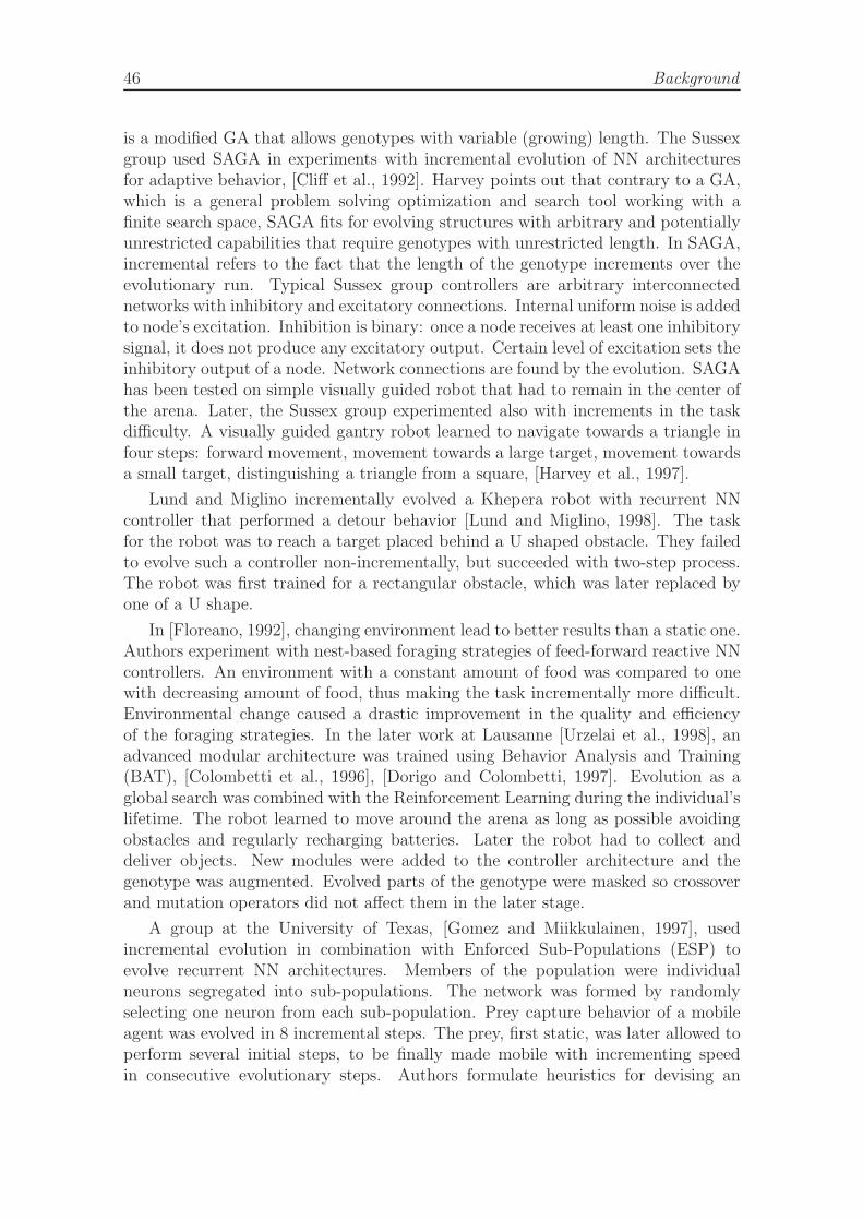
46 Background

is a modified GA that allows genotypes with variable (growing) length. The Sussexgroup used SAGA in experiments with incremental evolution of NN architecturesfor adaptive behavior, [Cliff et al., 1992]. Harvey points out that contrary to a GA,which is a general problem solving optimization and search tool working with afinite search space, SAGA fits for evolving structures with arbitrary and potentiallyunrestricted capabilities that require genotypes with unrestricted length. In SAGA,incremental refers to the fact that the length of the genotype increments over theevolutionary run. Typical Sussex group controllers are arbitrary interconnectednetworks with inhibitory and excitatory connections. Internal uniform noise is addedto node’s excitation. Inhibition is binary: once a node receives at least one inhibitorysignal, it does not produce any excitatory output. Certain level of excitation sets theinhibitory output of a node. Network connections are found by the evolution. SAGAhas been tested on simple visually guided robot that had to remain in the center ofthe arena. Later, the Sussex group experimented also with increments in the taskdifficulty. A visually guided gantry robot learned to navigate towards a triangle infour steps: forward movement, movement towards a large target, movement towardsa small target, distinguishing a triangle from a square, [Harvey et al., 1997].

Lund and Miglino incrementally evolved a Khepera robot with recurrent NNcontroller that performed a detour behavior [Lund and Miglino, 1998]. The taskfor the robot was to reach a target placed behind a U shaped obstacle. They failedto evolve such a controller non-incrementally, but succeeded with two-step process.The robot was first trained for a rectangular obstacle, which was later replaced byone of a U shape.

In [Floreano, 1992], changing environment lead to better results than a static one.Authors experiment with nest-based foraging strategies of feed-forward reactive NNcontrollers. An environment with a constant amount of food was compared to onewith decreasing amount of food, thus making the task incrementally more difficult.Environmental change caused a drastic improvement in the quality and efficiencyof the foraging strategies. In the later work at Lausanne [Urzelai et al., 1998], anadvanced modular architecture was trained using Behavior Analysis and Training(BAT), [Colombetti et al., 1996], [Dorigo and Colombetti, 1997]. Evolution as aglobal search was combined with the Reinforcement Learning during the individual’slifetime. The robot learned to move around the arena as long as possible avoidingobstacles and regularly recharging batteries. Later the robot had to collect anddeliver objects. New modules were added to the controller architecture and thegenotype was augmented. Evolved parts of the genotype were masked so crossoverand mutation operators did not affect them in the later stage.

A group at the University of Texas, [Gomez and Miikkulainen, 1997], usedincremental evolution in combination with Enforced Sub-Populations (ESP) toevolve recurrent NN architectures. Members of the population were individualneurons segregated into sub-populations. The network was formed by randomlyselecting one neuron from each sub-population. Prey capture behavior of a mobileagent was evolved in 8 incremental steps. The prey, first static, was later allowed toperform several initial steps, to be finally made mobile with incrementing speedin consecutive evolutionary steps. Authors formulate heuristics for devising an

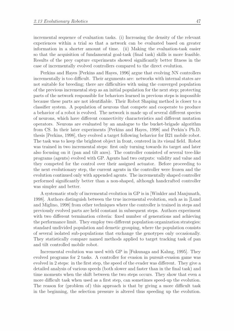
2.13 Evolutionary Robotics 47

incremental sequence of evaluation tasks. (i) Increasing the density of the relevantexperiences within a trial so that a network can be evaluated based on greaterinformation in a shorter amount of time. (ii) Making the evaluation-task easierso that the acquisition of fundamental goal-task (final task) skills is more feasible.Results of the prey capture experiments showed significantly better fitness in thecase of incrementally evolved controllers compared to the direct evolution.

Perkins and Hayes [Perkins and Hayes, 1996] argue that evolving NN controllersincrementally is too difficult. Their arguments are: networks with internal states arenot suitable for breeding; there are difficulties with using the converged populationof the previous incremental step as an initial population for the next step; protectingparts of the network responsible for behaviors learned in previous steps is impossiblebecause these parts are not identifiable. Their Robot Shaping method is closer to aclassifier system. A population of neurons that compete and cooperate to producea behavior of a robot is evolved. The network is made up of several different speciesof neurons, which have different connectivity characteristics and different mutationoperators. Neurons are evaluated by an analogue to the bucket-brigade algorithmfrom CS. In their later experiments [Perkins and Hayes, 1998] and Perkin’s Ph.D.thesis [Perkins, 1998], they evolved a target following behavior for B21 mobile robot.The task was to keep the brightest object in front, centered in its visual field. Robotwas trained in two incremental steps: first only turning towards its target and lateralso focusing on it (pan and tilt axes). The controller consisted of several tree-likeprograms (agents) evolved with GP. Agents had two outputs: validity and value andthey competed for the control over their assigned actuator. Before proceeding tothe next evolutionary step, the current agents in the controller were frozen and theevolution continued only with appended agents. The incrementally shaped controllerperformed significantly better than a non-shaped, although handcrafted controllerwas simpler and better.

A systematic study of incremental evolution in GP is in [Winkler and Manjunath,1998]. Authors distinguish between the true incremental evolution, such as in [Lundand Miglino, 1998] from other techniques where the controller is trained in steps andpreviously evolved parts are held constant in subsequent steps. Authors experimentwith two different termination criteria: fixed number of generations and achievingthe performance limit. They employ two different population organization strategies:standard undivided population and demetic grouping, where the population consistsof several isolated sub-populations that exchange the genotypes only occasionally.They statistically compare named methods applied to target tracking task of panand tilt controlled mobile robot.

Incremental evolution was used with GP in [Fukunaga and Kahng, 1995]. Theyevolved programs for 2 tasks. A controller for evasion in pursuit-evasion game wasevolved in 2 steps: in the first step, the speed of the evader was different. They give adetailed analysis of various speeds (both slower and faster than in the final task) andtime moments when the shift between the two steps occurs. They show that even amore difficult task when used as a first step, can sometimes speed-up the evolution.The reason for (problem of) this approach is that by giving a more difficult taskin the beginning, the selection pressure is altered thus speeding up the evolution.

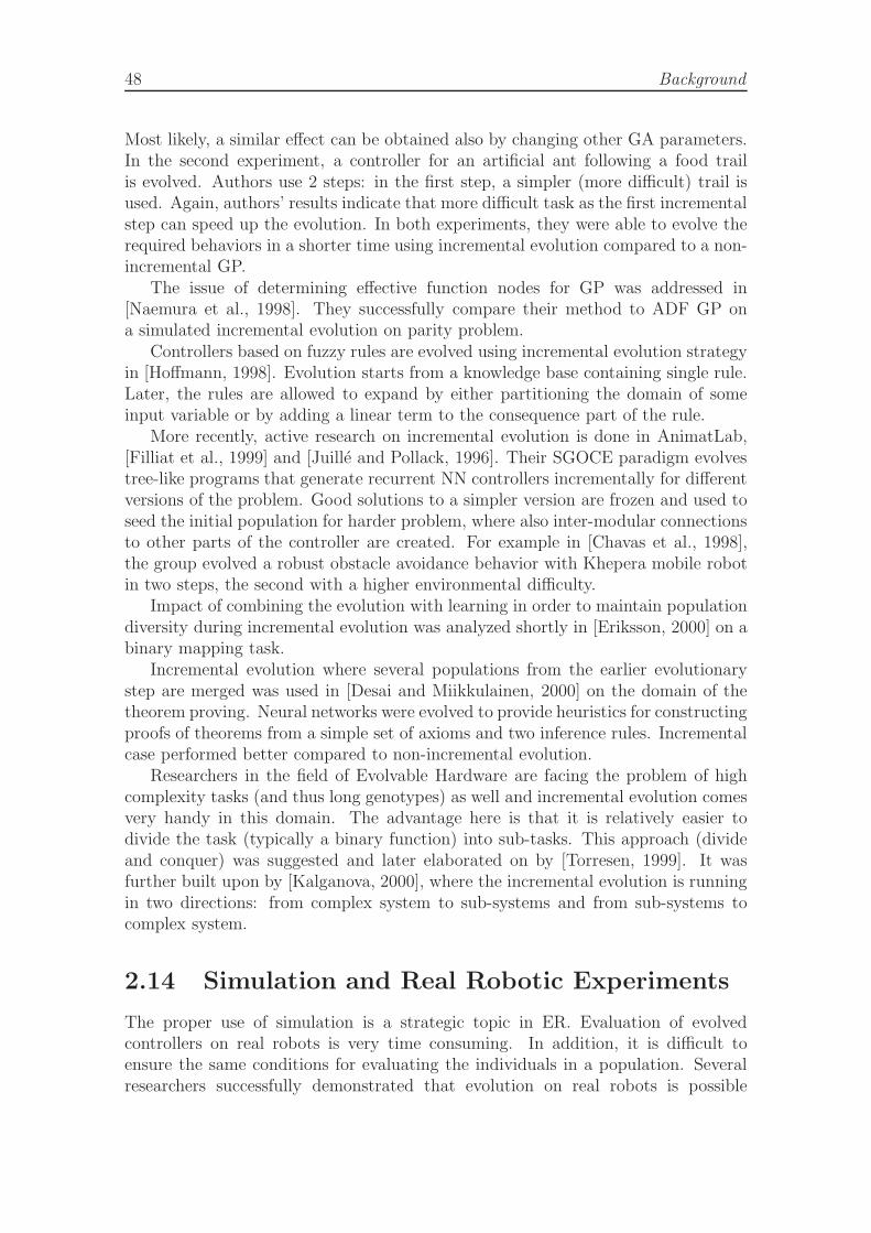
48 Background

Most likely, a similar effect can be obtained also by changing other GA parameters.In the second experiment, a controller for an artificial ant following a food trailis evolved. Authors use 2 steps: in the first step, a simpler (more difficult) trail isused. Again, authors’ results indicate that more difficult task as the first incrementalstep can speed up the evolution. In both experiments, they were able to evolve therequired behaviors in a shorter time using incremental evolution compared to a non-incremental GP.

The issue of determining effective function nodes for GP was addressed in[Naemura et al., 1998]. They successfully compare their method to ADF GP ona simulated incremental evolution on parity problem.

Controllers based on fuzzy rules are evolved using incremental evolution strategyin [Hoffmann, 1998]. Evolution starts from a knowledge base containing single rule.Later, the rules are allowed to expand by either partitioning the domain of someinput variable or by adding a linear term to the consequence part of the rule.

More recently, active research on incremental evolution is done in AnimatLab,[Filliat et al., 1999] and [Juille and Pollack, 1996]. Their SGOCE paradigm evolvestree-like programs that generate recurrent NN controllers incrementally for differentversions of the problem. Good solutions to a simpler version are frozen and used toseed the initial population for harder problem, where also inter-modular connectionsto other parts of the controller are created. For example in [Chavas et al., 1998],the group evolved a robust obstacle avoidance behavior with Khepera mobile robotin two steps, the second with a higher environmental difficulty.

Impact of combining the evolution with learning in order to maintain populationdiversity during incremental evolution was analyzed shortly in [Eriksson, 2000] on abinary mapping task.

Incremental evolution where several populations from the earlier evolutionarystep are merged was used in [Desai and Miikkulainen, 2000] on the domain of thetheorem proving. Neural networks were evolved to provide heuristics for constructingproofs of theorems from a simple set of axioms and two inference rules. Incrementalcase performed better compared to non-incremental evolution.

Researchers in the field of Evolvable Hardware are facing the problem of highcomplexity tasks (and thus long genotypes) as well and incremental evolution comesvery handy in this domain. The advantage here is that it is relatively easier todivide the task (typically a binary function) into sub-tasks. This approach (divideand conquer) was suggested and later elaborated on by [Torresen, 1999]. It wasfurther built upon by [Kalganova, 2000], where the incremental evolution is runningin two directions: from complex system to sub-systems and from sub-systems tocomplex system.

2.14 Simulation and Real Robotic Experiments

The proper use of simulation is a strategic topic in ER. Evaluation of evolvedcontrollers on real robots is very time consuming. In addition, it is difficult toensure the same conditions for evaluating the individuals in a population. Severalresearchers successfully demonstrated that evolution on real robots is possible

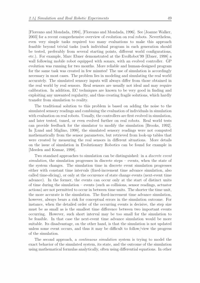
2.14 Simulation and Real Robotic Experiments 49

[Floreano and Mondada, 1994], [Floreano and Mondada, 1996]. See [Joanne Walker,2003] for a recent comprehensive overview of evolution on real robots. Nevertheless,even very simple tasks required too many evaluations to make this approachfeasible beyond trivial tasks (each individual program in each generation shouldbe tested, preferably from several starting points, different world configurations,etc.). For example, Marc Ebner demonstrated at the EvoRobot’99 [Ebner, 1998] awall following mobile robot equipped with sonars, with an evolved controller. GPevolution was running for two months. More reliable and human-designed programfor the same task was created in few minutes! The use of simulation is accordinglynecessary in most cases. The problem lies in modeling and simulating the real worldaccurately. The simulated sensory inputs will always differ from those obtained inthe real world by real sensors. Real sensors are usually not ideal and may requirecalibration. In addition, EC techniques are known to be very good in finding andexploiting any unwanted regularity, and thus creating fragile solutions, which hardlytransfer from simulation to reality.

The traditional solution to this problem is based on adding the noise to thesimulated sensory readings and combining the evaluation of individuals in simulationwith evaluation on real robots. Usually, the controllers are first evolved in simulation,and later tested, tuned, or even evolved further on real robots. Real world testscan provide feedback for the simulator to modify the simulation [Brooks, 1992].In [Lund and Miglino, 1998], the simulated sensory readings were not computedmathematically from the sensor parameters, but retrieved from look-up tables thatwere created by measuring the real sensors in different situations. More detailson the issue of simulation in Evolutionary Robotics can be found for example in[Meeden and Kumar, 1998].

Two standard approaches to simulation can be distinguished: in a discrete eventsimulation, the simulation progresses in discrete steps – events, when the state ofthe system changes. The simulation time in discrete event simulation progresseseither with constant time intervals (fixed-increment time advance simulation, alsocalled time-slicing), or only at the occurence of state change events (next-event timeadvance). In the former, the events can occur only at the start of distinct unitsof time during the simulation – events (such as collisions, sensor readings, actuatoractions) are not permitted to occur in between time units. The shorter the time unit,the more accurate is the simulation. The fixed-increment time advance simulation,however, always bears a risk for conceptual errors in the simulation outcome. Forinstance, when the detailed order of the occurring events is decisive, the step sizemust be as small as is the smallest time difference between two important eventsoccurring. However, such short interval may be too small for the simulation tobe feasible. In that case the next-event time advance simulation would be moresuitable. Its disadvantage, on the other hand, is that the simulation is not updatedunless some event occurs, and thus it may be difficult to follow/view the progressof the simulation.

The second approach, a continuous simulation system is trying to model theexact behavior of the simulated system, its state, and the outcome of the simulationusing mathematical formulas analytically, often using differential equations. In other

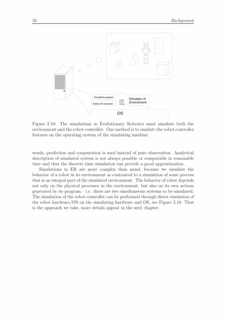
50 Background

Simulator ofEnvironment

STARTSTOPPAUSE

OS

Robot OS emulator

Emulated program

Figure 2.10: The simulations in Evolutionary Robotics must simulate both theenvironment and the robot controller. One method is to emulate the robot controllerfeatures on the operating system of the simulating machine.

words, prediction and computation is used instead of pure observation. Analyticaldescription of simulated system is not always possible or computable in reasonabletime and thus the discrete time simulation can provide a good approximation.

Simulations in ER are more complex than usual, because we simulate thebehavior of a robot in its environment as contrasted to a simulation of some processthat is an integral part of the simulated environment. The behavior of robot dependsnot only on the physical processes in the environment, but also on its own actionsgenerated by its program – i.e. there are two simultaneous systems to be simulated.The simulation of the robot controller can be performed through direct emulation ofthe robot hardware/OS on the simulating hardware and OS, see Figure 2.10. Thatis the approach we take, more details appear in the next chapter.

2.15 Chapter Summary 51

2.15 Chapter Summary

• Robotics is a multi-disciplinary field in the overlap of the sciences and tech-nologies of mechanics, electronics, and informatics.

• Robotics has a history of more than 50 years, and it reached its very advancedstage, where robots need to act autonomously in real-world environments, andfeature artificial intelligence.

• Throughout the development of the field, researchers realized that building socomplex systems as robots are must be done in incremental stages of multipleprototypes of increasing complexity.

• Robots are performing in their environments and thus they are situated, andembodied.

• A natural building block of a robotic controller is a behavior – a completeautonomous part of robot’s functionality that typically can perform on itsown, and can be built, tested and debugged independently.

• Behaviors share access to sensors and actuators and therefore do need to becoordinated. This coordination can take different forms.

• Automatic programming of robots has been attempted either using Rein-forcement Learning, or using Evolutionary Algorithms (forming the field ofEvolutionary Robotics).

• Simple robot behaviors have been successfully evolved.

• Limited amount of work has been done on evolving the behavior coordination(behavior arbitration).

• Using evolutionary algorithms to design robot controllers is very time-consuming,and therefore simulators are required. In addition, single incremental run isvery limiting with respect to the task complexity. This can be overcome usingco-evolution or incremental evolution.

52 Background

Chapter 3

Research Goals and Hypotheses

W: Fiskeboller?P: Your smell sensor is working well.

— from a conversation in the corridor of the department at 10:30 p.m.

In this chapter, in the light of the assumptions described in the previous chapter,we discuss the research agenda that we seek to contribute to in the later chapters.We start with the main goals of the thesis, in particular, issues related to evolvingrobot controllers incrementally.

3.1 Introduction

Where does Robotics meet Computer Science? Robotics is a highly engineeringand focused field with the aim to deliver compact systems capable of performing ameaningful physical activity in the real world, often with the goal to perform a usefulwork. The requirements for a physical entity imply that robotics is widely multi-disciplinary, bringing together experts from mechanical and electrical engineering, toname the two most important. As soon as the task of the robot involves processingof any information (contrasted to a simple wired circuitry), Computer Science entersthe scene. The intersections of Computer Science with Robotics thus include:

• Signal Processing and Filtering

• Data Clustering

• Numerical Algorithms, Geometric Algorithms, Algebraic Algorithms

• Pattern Recognition and Classification

• Optimization

• Data Compression, Communication Algorithms, Error-Correction

• Search Algorithms

• Planning

54 Research Goals and Hypotheses

• Simulation

• Machine Learning

• Knowledge Representation and Processing

• Human-Computer Interaction

• Image Processing and Computer Vision

• Embodied AI, and other fields.

It is important to understand the challenge that the high-level areas such asArtificial Intelligence, and Knowledge Representation come at the end of this listand imply mastering of the earlier fields – they can be successfully applied only afterthe whole thick layer of the previous sub-fields is mastered. On the other hand, theyare inevitable when working on robots performing in unpredictable, dynamic, andunknown environments. Thus the AI-robotics researchers must work tightly togetherwith the experts mastering all the areas as well with the experts in mechanical andelectrical engineering, when they wish to work or research on real products.

One possibility for the AI researchers to overcome the hurdle and difficultorganizational challenge is to use out-of-the-box solutions of robotics systems. Theoption is to take a robot – an existing working finished product, and to tweak itsbehavior on the high level.

An example of such a successful research is the work with the SONY Aibo robots.These are entertainment robots with a very advanced behavior-based controllercontaining about 2000 elementary behaviors that are coordinated in a message-passing architecture – not unlike the one used in our experiments. Fortunately,SONY made the basic architecture open for user-programming, creating a splendidresearch platform where behaviors with access to robot sensors, vision, and actuatorscan be written directly in C++ and run on the robot. An interesting work has beendone for instance on the language acquisition experiments [Steels and Kaplan, 2001].

Other successful and popular example of this kind is the Khepera robot [Mondadaet al., 1993] that is built by experts for the purpose of research experiments. Itsoverall architecture is thus modular, open and prepared for experimenting withresearch algorithms.

Our choice for a research platform, the LEGO RCX comes from the industry ofentertainment and educational robotics. Its strength is in the low-cost and high-flexibility of the robotics construction sets.

Once the Computer Science challenges in Robotics are identified, computerscientists may revert to solving them in pure simulation, or simulation combinedwith testing on real robotic platforms.

3.2 Evolving Robotics 55

3.2 Evolving Robotics

Our work clearly can be categorized as Evolving Robotics1. As contrasted to teamstrying to master some robotics system completely, we are interested in narrow andinnovative area that could possibly enhance robot use and design in the future.We take the starting assumption that a reasonable useful robotic system is alreadybuilt and programmed. We are concerned with studying particular aspects of theadaptivity of the programming and design of the controller to make the robotsuccessfully perform various non-trivial tasks according to user requirements. Usersshould be able to use our system to automatically program an existing roboticapplication. Our system aims at achieving this by the means of EvolutionaryComputation, and maintains that the controller architecture is behavior-based.

Our work classifies in the field of Evolutionary Robotics, and studies howcontrollers for mobile robots could be programmed in non-conventional way: au-tomatically using task specification in form of objective function. The advantagesof such an approach are:

• Higher flexibility. Instead of specialized one-purpose robotic systems, moreversatile systems can be produced. However, still without the requirementfor a general intelligence engine, which is difficult to produce, especially withrestricted resources that are available at embedded devices, such as robots.Instead, users could train their robots to perform various particular tasks,while the robot controllers would then be adjusted using an evolutionaryapproach.

• Extensibility. Due to the behavior-based architecture and high modularity, itshould be relatively simple to extend the functionality of the robotic systemwith additional functional modules, actuators, sensory systems, and behaviors.

• Modifiability. Once the robot controller is programmed, it should be easy toswitch back to learning mode and let the system generate a different controllerbased on the same or extended set of behaviors.

• Higher efficiency. Since the robot controller is specified for a particular task,it does not have to be equipped with a general-purpose reasoning mechanismand knowledge base. It rather consists only of relevant behavioral modules inan efficient coordination.

• Lower cost. The controllers designed automatically under the user’s supervi-sion could save the time of engineering experts who would otherwise have toproduce all the specialized controllers. Production costs also decrease when thesame system can be applied to different tasks (i.e. larger market) as contrastedto many specialized products.

• Large degree of customization. Since the users are allowed to design and traintheir robotic systems, they have better possibilities to design them in a manner

1See previous chapter

56 Research Goals and Hypotheses

that suits their particular needs. This would not be possible if fixed systemswould be produced for the whole users group.

• Open platform. The modular architecture and the possibility to add newcomponents and modules allow for excellent open-source and open-platformavailability, harnessing the potential of various contributing parts, modules,and behaviors providers. Open platforms are more likely to be robust,provide more user-friendly functionality, and have better prospects for furtherdevelopment, error discovery and correction.

While we study the design of robot controllers mainly in simulation, for a greaterrelevance, we do employ the algorithms on a real platform. This can be done onlywith a very limited accuracy, and using prototyping. We believe that testing ouralgorithms on prototypes running in the real-world can still give us valuable feedbackon their performance and the issues to be carefully considered when performing thedesign experiments in simulation.

Further sections elaborate on the flavors of Evolving Robotics in more details.

3.3 Robotic Task Complexity

Historically, the robots attached to production lines required only simple sensorsand actuators, where the direct connections between them, with simple fixed controlalgorithms were sufficient. The more realistic the environment, the more difficultit is for the robot to exist and perform in it, perceive its state, and react to theevents. Thus the complexity of the task is, for the first, influenced by the degree towhich the environment is realistic – and in consequence non-deterministic, dynamic,and unpredictable. The second aspect relates to the activity the robot is requiredto perform – does the activity require processing a lot of input information? Isit time critical? Does it require long-term planning? How many informationsources are involved? Are they conflicting or interfering? Are other agents –humans or robots involved in the activity and does the outcome depend on them?Finally, an interesting aspect of the task difficulty – especially in our context isthe difficulty to describe a task: even though the environment is simple and theactivity relatively easy, it might be difficult to describe. By the task description wemean the possibilities of its formalized transcription, which could be processed byan algorithm, for instance for the purposes of computing the fitness – a quantitativemeasure of robot performance. Another, more standard measure of task complexitycould be the Kolmogorov complexity, in our case adapted as the size of the smallestFSA arbitrators that perform the required task on a BB-controller. In this context,we should notice that for each FSA (or transducer) there exists a minimal equivalentFSA (or transducer), i.e. an automaton with the minimal number of states2.

2This can further be hyper-minimized ??, if we can give up a limited (finite) part of the FSAfunctionality. That, however, is not useful in our context. We usually do not even minimize theFSA before the final population in order not to remove a potentially useful genetic material.

3.4 Arbitration Mechanisms 57

3.4 Arbitration Mechanisms

We assume that the robot builders and designers equipped the robot with a set ofsimple primitive behaviors. However, the robot is not [yet] able to perform anycomplicated tasks, where the behaviors would need to be coordinated. This is thegoal of the behavior arbitration. A successful arbitration mechanism:

• Should allow fast reactive responses controlled by behaviors. This impliesthat the modules should have as direct as possible access to the sensors andactuators. If the arbitration must coordinate their access, there must be aprovision for a fast high-priority access for the critical behaviors.

• Should allow confidence level for generated actions (i.e. the priority of anaction will depend on how urgent it is) and this priority should provideflexibility. A behavior that may be critical in one situation may be less criticalin a different situation. Various actions initiated by the same behavior mayhave different importance. The coordination mechanism should allow for aflexible priority.

• Should be capable of taking temporal aspect into account – the actions arenot instant, but take certain time – once some behavior is started, it should befinished unless an action with a higher priority overrides it. For instance, whenan exploration behavior is about to perform a sequence of several movementsin order to scan the environment from the current robot position, it would beundesirable to preempt it by another behavior of about the same priority (forinstance a gripper positioning action, which could follow after the scanning iscompleted).

• Behaviors should receive control feedback from arbitration – i.e. whether theywere allowed to control the robot or not. The control behaviors usually dependon the feedback from their actions. This feedback can be obtained ‘cheaper’within the arbitration than from the robot sensors.

• Should allow easy modification of the existing controller by adding newfunctionality or exchanging some module for a similar alternative. This canbe useful when robot moves to other environments or gets some part changedor upgraded.

• Should ideally provide ways for easy analysis and verification. For instance,verifying that all of the parts are active and utilized during testing may excludehidden features that could activate in novel situations, which did not occurduring training and testing.

• Should be easy to represent, implement in embedded devices, and amenablefor evolution.

58 Research Goals and Hypotheses

3.5 Embedded Evolution

The nature of many tasks where robots might be useful requires adaptivity, learning,and dealing with unpredictable, changing and unstructured environments. It istherefore almost impossible to predict situations that the robot will have to handleduring the execution of its task. Robots should be able to learn new operations andskills. Particular learning algorithms for this purpose are needed.

It is becoming a real possibility to equip mobile robots with high-performancecomputers on-board. Their computational power can be used for much better visionand signal processing algorithms, better planning, reasoning, processing naturallanguage commands, etc. In addition, we propose to include a simulator of therobot itself to test robot’s planned actions without the risk of failure in the realworld. The simulator is used by an embedded evolutionary algorithm to evolve agood strategy or actual program code that performs a required operation. In thisway, the robot can learn new skills when they become needed. A similar approachby [Grefenstette and Ramsey, 1992] is called Anytime Learning. Our approach isslightly different, namely we evolve a program for the robot instead of a set ofrules; the learning component is started on demand when the novel situation isexperienced and is not running all the time in the background; we don’t requirereal-time performance of the simulator since the robot can wait before continuingthe execution of its task, although high performance of the simulator is desired asthe simulation is used to compute the fitness; our model is simpler, for example itdoesn’t require a feedback to simulation module provided by an execution module(which in turn requires the execution module to be fairly complex since it has toknow the details of the simulation module).

3.6 Evolutionary Adaptive Mechanisms

The modern AI approaches often take inspiration from or reflect upon variousprocesses that take place in the nature, in the biological world, and which displaysome similarity to the artificial problems we are attempting to solve, when an analogycan be drawn.

The Evolutionary Computation as a search method takes inspiration from thesearch for fitting genotypes of the species living in the biosphere. In this sense, wecan talk about a long-term adaptivity of species in nature, where the parallel searchmaintained by the whole population adapts to the changing conditions and modifiesthe genotype in order to improve the performance of the individuals. Most of thetime, the change of the conditions occurs continuously, or at the very least, it isperceived by the species as continuous. When adopted to Evolutionary Robotics,the parallel is somewhat skewed, as it very seldom is the case that the individualscoexist together during their lifetime in a real-world environment and interact withother species, which are also experiencing a long-term adaptation. On the contrary,in most of the cases, a single individual is being tested in some simulated world withsome fixed artificial conditions and discrete environment. The environment and theoverall conditions typically do not change throughout the course of the evolution at

3.7 Aspects of Incremental Evolution 59

all.Exposing the individuals to changing conditions throughout the evolutionary run

thus better imitates the natural processes. This suggests better performance of theincremental algorithms.

The evolved individuals in nature are adapting to the changing conditions intwo basic ways. In addition to the long-term adaptation mentioned above, theindividuals are exhibiting a short-term adaptation, or learning. This is in mostspecies supported by the neural system of the individual based on a neural networkwith high degree of plasticity of the connections. Some of the short-term adaptationcan become encoded into genotype in order to produce even more fit individuals[Baldwin, 1896]. However, it is important to notice that the long-term adaptationoccurs in discrete steps – the genes functioning like binary (or n-ary) switches arein concert with the environment shaping the individual’s phenotype (phenotypeplasticity). In this context, evolving the weights or topologies of artificial neuralnetworks has little biological plausibility. Considering the gene-copying and protein-production chemical processes and mechanisms, we argue that if a genotype encodesa set of finite-state automata that govern the behavior of the individual togetherwith the individual behavior modules that are predefined (corresponding to fixedreflexes) and may optionally contain a learning component, we are staying closer tothe ways of nature, and achieve somewhat more reasonable biological plausibility.

At the same time, it has to be pointed out that the complexity of the interactionsof all biological processes is so extremely high and difficult to grasp, describe andfully document and understand, that all inferences drawn from the similarity withthe biosphere have to be accepted with reservations and possible objections.

3.7 Aspects of Incremental Evolution

Researchers observed in the past [Harvey, 1995] that evolving robot behavior is ahard challenge for any EA. The fitness landscape tends to be rough, and evaluation ofeach individual typically takes a long time. Trying to evolve more complex behaviorsis often too difficult. Some groups, such as [Harvey, 1995, Lee et al., 1998] advocatedthe use of incremental evolution, where the complexity of the target task is decreasedby decomposing it to several simpler tasks, which are easy enough to solve by anevolutionary algorithm (see [Petrovic, 1999] for an earlier overview of incrementalevolution). We have identified five different ways, in which an evolutionary roboticalgorithm can be incremental:

Environment (where is the robot performing?): the earlier incremental stepscan be run in a simplified environment, where the frequency and characteristics ofpercepts of all kinds can be adjusted to make it easier for the robot to perform thetask. For instance, the number of obstacles or distance to the target can be reduced,the environment can be made more deterministic, the noise can be suppressed,landmarks can be made more visible, etc. An example of this type of incrementalityis [Lund and Miglino, 1998], where box-shaped obstacles were replaced by moredifficult U-shaped obstacles after the avoidance behavior for the former was evolved.

Task (what is the robot doing?): the earlier incremental steps can require only

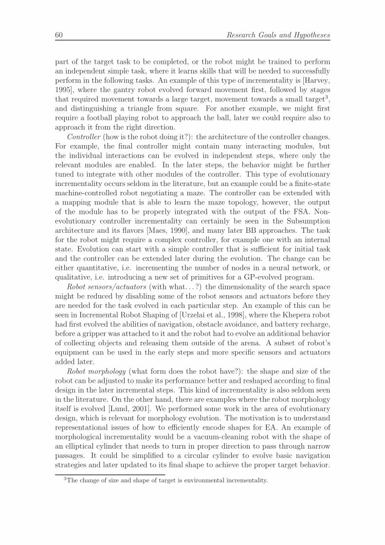
60 Research Goals and Hypotheses

part of the target task to be completed, or the robot might be trained to performan independent simple task, where it learns skills that will be needed to successfullyperform in the following tasks. An example of this type of incrementality is [Harvey,1995], where the gantry robot evolved forward movement first, followed by stagesthat required movement towards a large target, movement towards a small target3,and distinguishing a triangle from square. For another example, we might firstrequire a football playing robot to approach the ball, later we could require also toapproach it from the right direction.

Controller (how is the robot doing it?): the architecture of the controller changes.For example, the final controller might contain many interacting modules, butthe individual interactions can be evolved in independent steps, where only therelevant modules are enabled. In the later steps, the behavior might be furthertuned to integrate with other modules of the controller. This type of evolutionaryincrementality occurs seldom in the literature, but an example could be a finite-statemachine-controlled robot negotiating a maze. The controller can be extended witha mapping module that is able to learn the maze topology, however, the outputof the module has to be properly integrated with the output of the FSA. Non-evolutionary controller incrementality can certainly be seen in the Subsumptionarchitecture and its flavors [Maes, 1990], and many later BB approaches. The taskfor the robot might require a complex controller, for example one with an internalstate. Evolution can start with a simple controller that is sufficient for initial taskand the controller can be extended later during the evolution. The change can beeither quantitative, i.e. incrementing the number of nodes in a neural network, orqualitative, i.e. introducing a new set of primitives for a GP-evolved program.

Robot sensors/actuators (with what. . . ?) the dimensionality of the search spacemight be reduced by disabling some of the robot sensors and actuators before theyare needed for the task evolved in each particular step. An example of this can beseen in Incremental Robot Shaping of [Urzelai et al., 1998], where the Khepera robothad first evolved the abilities of navigation, obstacle avoidance, and battery recharge,before a gripper was attached to it and the robot had to evolve an additional behaviorof collecting objects and releasing them outside of the arena. A subset of robot’sequipment can be used in the early steps and more specific sensors and actuatorsadded later.

Robot morphology (what form does the robot have?): the shape and size of therobot can be adjusted to make its performance better and reshaped according to finaldesign in the later incremental steps. This kind of incrementality is also seldom seenin the literature. On the other hand, there are examples where the robot morphologyitself is evolved [Lund, 2001]. We performed some work in the area of evolutionarydesign, which is relevant for morphology evolution. The motivation is to understandrepresentational issues of how to efficiently encode shapes for EA. An example ofmorphological incrementality would be a vacuum-cleaning robot with the shape ofan elliptical cylinder that needs to turn in proper direction to pass through narrowpassages. It could be simplified to a circular cylinder to evolve basic navigationstrategies and later updated to its final shape to achieve the proper target behavior.

3The change of size and shape of target is environmental incrementality.

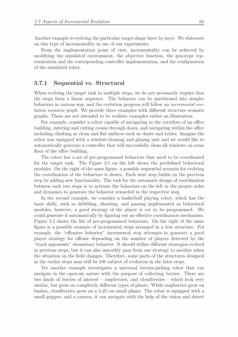
3.7 Aspects of Incremental Evolution 61

Another example is evolving the particular target shape layer by layer. We elaborateon this type of incrementality in one of our experiments.

From the implementation point of view, incrementality can be achieved bymodifying the simulated environment, the objective function, the genotype rep-resentation and the corresponding controller implementation, and the configurationof the simulated robot.

3.7.1 Sequential vs. Structural

When evolving the target task in multiple steps, we do not necessarily require thatthe steps form a linear sequence. The behavior can be partitioned into simplerbehaviors in various way, and the evolution progress will follow an incremental evo-lution scenario graph. We provide three examples with different structure scenariographs. These are not intended to be realistic examples rather an illustration.

For example, consider a robot capable of navigating in the corridors of an officebuilding, entering and exiting rooms through doors, and navigating within the officeincluding climbing at clean and flat surfaces such as chairs and tables. Imagine therobot was equipped with a window-cleaning and glazing unit and we would like toautomatically generate a controller that will successfully clean all windows on somefloor of the office building.

The robot has a set of pre-programmed behaviors that need to be coordinatedfor the target task. The Figure 3.1 on the left shows the predefined behavioralmodules. On the right of the same figure, a possible sequential scenario for evolvingthe coordination of the behaviors is shown. Each next step builds on the previousstep by adding new functionality. The task for the automatic design of coordinationbetween each two steps is to activate the behaviors on the left in the proper orderand dynamics to generate the behavior rewarded in the respective step.

In the second example, we consider a basketball playing robot, which has thebasic skills, such as dribbling, shooting, and passing implemented as behavioralmodules, however, a good strategy of the player is yet to be programmed. Wecould generate it automatically by figuring out an effective coordination mechanism.Figure 3.2 shows the list of pre-programmed behaviors. On the right of the samefigure is a possible scenario of incremental steps arranged in a tree structure. Forexample, the “offensive behavior” incremental step attempts to generate a goodplayer strategy for offense depending on the number of players detected by the“track opponents” elementary behavior. It should utilize different strategies evolvedin previous steps, but it can also smoothly pass from one strategy to another whenthe situation on the field changes. Therefore, some parts of the structures designedin the earlier steps may still be left subject of evolution in the later steps.

Yet another example investigates a universal berries-picking robot that cannavigate in the open-air nature with the purpose of collecting berries. There aretwo kinds of berries of interest – raspberries, and cloudberries – which look verysimilar, but grow on completely different types of plants. While raspberries grow onbushes, cloudberries grow on a 5-25 cm small plants. The robot is equipped with asmall gripper, and a camera, it can navigate with the help of the vision and detect

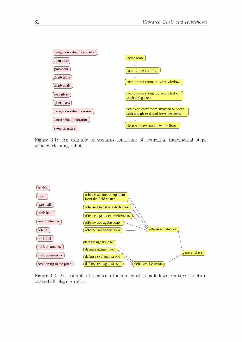
62 Research Goals and Hypotheses

avoid furniture

detect window location

navigate inside of a room

glaze glass

soap glass

climb chair

climb table

pass door

open door

navigate inside of a corridor

locate room

locate, enter room, move to window

locate and enter room

wash and glaze it, and leave the roomlocate and enter room, move to window,

wash and glaze itlocate, enter room, move to window,

clean windows on the whole floor

Figure 3.1: An example of scenario consisting of sequential incremental steps:window-cleaning robot.

dribble

shoot

pass ball

catch ball

avoid defender

defend

track ball

track opponents

track team−mate

positioning in the pitch

defense against one

defense two against one

defense two against two

offense two against two

offense two against one

offense against two deffenders

offense against one deffender

offense without an oponentfrom the field centre

defense against two

defensive behavior

offensive behavior

general player

Figure 3.2: An example of scenario of incremental steps following a tree-structure:basketball playing robot.

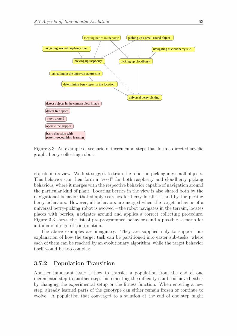
3.7 Aspects of Incremental Evolution 63

picking up cloudberry

navigating around raspberry tree navigating at cloudberry site

picking up a small round objectlocating beries in the view

picking up raspberry

navigating in the open−air nature site

determining berry types in the location

universal berry picking

detect objects in the camera view image

detect free space

move around

operate the gripper

pattern−recognition learningberry detection with

Figure 3.3: An example of scenario of incremental steps that form a directed acyclicgraph: berry-collecting robot.

objects in its view. We first suggest to train the robot on picking any small objects.This behavior can then form a “seed” for both raspberry and cloudberry pickingbehaviors, where it merges with the respective behavior capable of navigation aroundthe particular kind of plant. Locating berries in the view is also shared both by thenavigational behavior that simply searches for berry localities, and by the pickingberry behaviors. However, all behaviors are merged when the target behavior of auniversal berry-picking robot is evolved – the robot navigates in the terrain, locatesplaces with berries, navigates around and applies a correct collecting procedure.Figure 3.3 shows the list of pre-programmed behaviors and a possible scenario forautomatic design of coordination.

The above examples are imaginary. They are supplied only to support ourexplanation of how the target task can be partitioned into easier sub-tasks, whereeach of them can be reached by an evolutionary algorithm, while the target behavioritself would be too complex.

3.7.2 Population Transition

Another important issue is how to transfer a population from the end of oneincremental step to another step. Incrementing the difficulty can be achieved eitherby changing the experimental setup or the fitness function. When entering a newstep, already learned parts of the genotype can either remain frozen or continue toevolve. A population that converged to a solution at the end of one step might

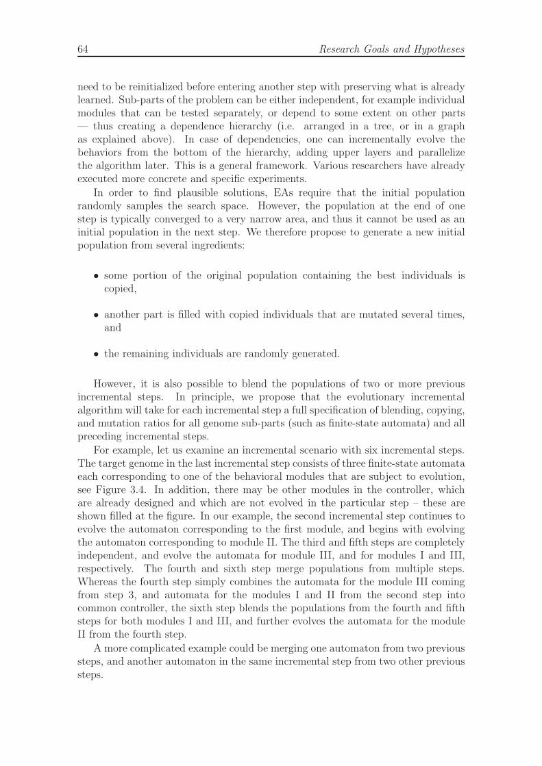
64 Research Goals and Hypotheses

need to be reinitialized before entering another step with preserving what is alreadylearned. Sub-parts of the problem can be either independent, for example individualmodules that can be tested separately, or depend to some extent on other parts— thus creating a dependence hierarchy (i.e. arranged in a tree, or in a graphas explained above). In case of dependencies, one can incrementally evolve thebehaviors from the bottom of the hierarchy, adding upper layers and parallelizethe algorithm later. This is a general framework. Various researchers have alreadyexecuted more concrete and specific experiments.

In order to find plausible solutions, EAs require that the initial populationrandomly samples the search space. However, the population at the end of onestep is typically converged to a very narrow area, and thus it cannot be used as aninitial population in the next step. We therefore propose to generate a new initialpopulation from several ingredients:

• some portion of the original population containing the best individuals iscopied,

• another part is filled with copied individuals that are mutated several times,and

• the remaining individuals are randomly generated.

However, it is also possible to blend the populations of two or more previousincremental steps. In principle, we propose that the evolutionary incrementalalgorithm will take for each incremental step a full specification of blending, copying,and mutation ratios for all genome sub-parts (such as finite-state automata) and allpreceding incremental steps.

For example, let us examine an incremental scenario with six incremental steps.The target genome in the last incremental step consists of three finite-state automataeach corresponding to one of the behavioral modules that are subject to evolution,see Figure 3.4. In addition, there may be other modules in the controller, whichare already designed and which are not evolved in the particular step – these areshown filled at the figure. In our example, the second incremental step continues toevolve the automaton corresponding to the first module, and begins with evolvingthe automaton corresponding to module II. The third and fifth steps are completelyindependent, and evolve the automata for module III, and for modules I and III,respectively. The fourth and sixth step merge populations from multiple steps.Whereas the fourth step simply combines the automata for the module III comingfrom step 3, and automata for the modules I and II from the second step intocommon controller, the sixth step blends the populations from the fourth and fifthsteps for both modules I and III, and further evolves the automata for the moduleII from the fourth step.

A more complicated example could be merging one automaton from two previoussteps, and another automaton in the same incremental step from two other previoussteps.

3.7 Aspects of Incremental Evolution 65

������������

������������

4

��������

����

3��������

��������

��������

2

1

I II

I

III

������������������������

������������

6

III III

actuatorssensors

III III

actuatorssensors

����

��������5 I III

actuatorssensors

������������

������

I (FSA for module I)

II (FSA for module II)

III (FSA for module III)

������������

sensorsactuatorssensors

actuatorssensors

actuators

Figure 3.4: Population mixing in an incremental scenario.

Formally, for each module m separately, the initial population of genome parts(automata for the module m) in the i-th step, P init

m,i , originates from three types ofsources:

P initm,i =

i−1⋃

j=1

(P init,copiedm,i,j ∪ P init,mutated

m,i,j ∪ P init,randomm,i,j )

which are generated based on three types of ratios describing the portion of theevolved population from step j to be copied (qbest

m,i,j), the portion of the initial

population in step i that the copied individuals will occupy (qcopiedm,i,j ), and the portion

of the population in step i that will be occupied by the mutated individuals fromstep j (qmutated

m,i,j ):

P init,copiedm,i,j = extract(m, scale(best(P evolved

j , Njqbestm,i,j), Niq

copiedm,i,j ))

P init,mutatedm,i,j = mutate(extract(m, scale(best(P evolved

j , min(Nj , Niqmutatedm,i,j )), Niq

mutatedm,i,j )))

P init,randomm,i,j = rnd automaton(m, Ni(1 − qcopied

m,i,j − qmutatedm,i,j ))

where Ns is the number of individuals in the population of step s, scale(S, N)enlarges or shrinks the set S to cardinality N by sampling the individuals uniformly,

66 Research Goals and Hypotheses

best(P, N) takes the N best individuals of population P , extract(m, S) takes a setof genomes and extracts the automata for the module m, mutate(S) mutates allautomata in the set S, and rnd automaton(m, N) generates N random automatafor module m.

Next, all the module-specific populations P initm,i are combined into the initial

population of step i, P initi simply by combining the automata from the corresponding

individuals (in the order of generation of the sets as defined above).That is, the whole incremental scenario is defined by:

• the number of incremental steps: s,

• the population sizes in each step: Ni, i = 1, . . . , s,

• the number of modules that are subject of evolution in each step i: ki, andtheir lists: mi,1 . . .mi,ki

, for i = 1, . . . , s,

• the ratios for copying and copying with mutation, for each pair of steps i, j,and for each module m: qbest

m,i,j, qcopiedm,i,j , qmutated

m,i,j .

In this way, one can design an evolutionary incremental process following ascenario with a topology of a complex directed acyclic graph. However, in mostof the situations, the incremental scenario does not need to be complicated and thusthe number of the parameters to specify can remain manageable.

3.7.3 Emergent vs. Engineered Steps

The above scheme for specifying the incremental steps assumes that the steps arefully described and specified. The scenario is fully engineered. However, someparts of the scenario specification may be kept open. Consider, for example, ascenario with a sequential topology of incremental steps, some assignment of tasksand controller parts that are subject to evolution for each step. The algorithmwill start the evolution at the highest level (target task), and recursively spawn theearlier steps when required. In this way, the algorithm may regulate the amountsof individuals copied and mutated from the earlier steps based on the need andmeasured learning performance of each step. In fact, the incremental steps may runin parallel, and the flow of the individuals can be perpetual as contrasted to theinitial population only as our model above assumes.

3.7.4 Automatic Division into Incremental Stages

Our aim is the automatic design of the controllers. Our discussion until now didnot question where does the incremental evolutionary scenario consisting of theincremental steps originate.

An idealistic automatic system should provide an easy to use interface and shouldnot require the user to specify many details or parameters. We would wish that thesystem would allow entering the target task in form of few sentences written ina natural language. These should be parsed and analyzed to construct a semantic

3.8 Controller Architecture Goals 67

representation referring to the robot primitive abilities, the task goals, and structure.The system should contain an extensive knowledge base that could map its conceptsagainst the parsed representation of the target task, and allow reasoning over thetarget task in the terms of

• constraints implied by the robot sensors, actuators, topology, and physicalproperties

• temporal state diagram of the target task pursue

• identifying the set of activities to be performed and the qualitative relationsbetween them (reasons and consequences)

The reasoning process should select a set of elementary competencies, which involvemultiple modules that are to be coordinated. Depending on the granularity ofthe reasoning process, higher- or lower- level competencies should be generatedthus devising a possible hierarchy of incremental steps, and the wished incrementalscenario.

Such a system would be an ultimate goal of the efforts. For the time being, wemust revert back to the manually-designed prescription described in the previoussections. However, the process shall be similar in the sense of identifying theconstraints and relations.

3.8 Controller Architecture Goals

In this section, we address the question of our choice of controller architecture.A task of an autonomous robot usually consists of many interactions occurring,

starting, or ending at various time points. Between these events, the robot remainsin some particular state. In more complex systems, this state is a juxtaposition ofstates of multiple simultaneous activities, which are started and finished at varioustimes. We consider state and event to be the crucial concepts for the controllerarchitectures of mobile robots.

Many researchers advocated the use of neural network based controllers, pri-marily for the reasons of their high degree of flexibility, plasticity, and adaptivity.Wide class of feed-forward neural networks does not have an internal state andcan only be trained for reactive behaviors, signal processing, pattern recognition,or similar. Requirement of internal state implies recurrent connections. However,the representation of states in the recurrent networks is very poorly understood.Furthermore, responsiveness of neural networks to particular events is hard to assesand analyze, and the current learning mechanisms require thousands of interactionsto learn even very simple behaviors. Controllers aiming at more complex tasks musthave modular architectures, but it is yet unclear how this modularity can efficientlybe achieved with neural networks, and what consequences it might have on theirlearning rules and algorithms, see also section 2.9. We suggest studying alternativearchitectures, which better reflect the concepts of robot state and environmentalevents.

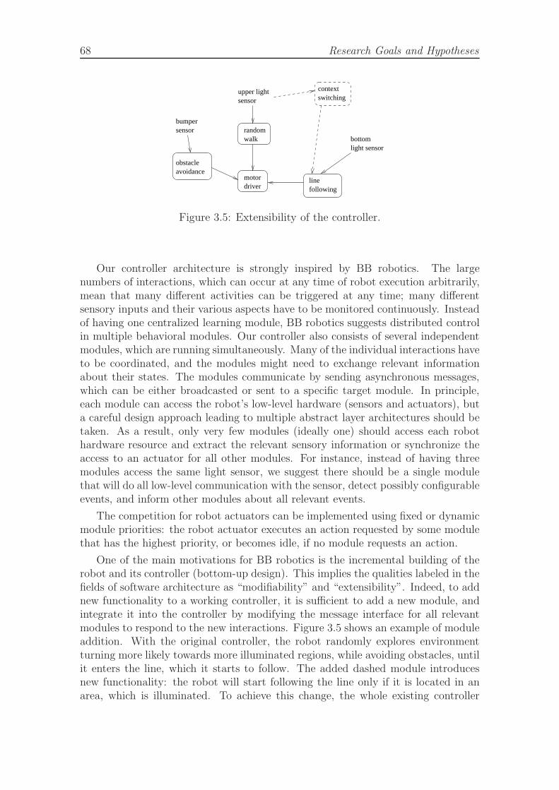
68 Research Goals and Hypotheses

bumpersensor

upper lightsensor

randomwalk

avoidanceobstacle

linefollowing

bottomlight sensor

motordriver

contextswitching

Figure 3.5: Extensibility of the controller.

Our controller architecture is strongly inspired by BB robotics. The largenumbers of interactions, which can occur at any time of robot execution arbitrarily,mean that many different activities can be triggered at any time; many differentsensory inputs and their various aspects have to be monitored continuously. Insteadof having one centralized learning module, BB robotics suggests distributed controlin multiple behavioral modules. Our controller also consists of several independentmodules, which are running simultaneously. Many of the individual interactions haveto be coordinated, and the modules might need to exchange relevant informationabout their states. The modules communicate by sending asynchronous messages,which can be either broadcasted or sent to a specific target module. In principle,each module can access the robot’s low-level hardware (sensors and actuators), buta careful design approach leading to multiple abstract layer architectures should betaken. As a result, only very few modules (ideally one) should access each robothardware resource and extract the relevant sensory information or synchronize theaccess to an actuator for all other modules. For instance, instead of having threemodules access the same light sensor, we suggest there should be a single modulethat will do all low-level communication with the sensor, detect possibly configurableevents, and inform other modules about all relevant events.

The competition for robot actuators can be implemented using fixed or dynamicmodule priorities: the robot actuator executes an action requested by some modulethat has the highest priority, or becomes idle, if no module requests an action.

One of the main motivations for BB robotics is the incremental building of therobot and its controller (bottom-up design). This implies the qualities labeled in thefields of software architecture as “modifiability” and “extensibility”. Indeed, to addnew functionality to a working controller, it is sufficient to add a new module, andintegrate it into the controller by modifying the message interface for all relevantmodules to respond to the new interactions. Figure 3.5 shows an example of moduleaddition. With the original controller, the robot randomly explores environmentturning more likely towards more illuminated regions, while avoiding obstacles, untilit enters the line, which it starts to follow. The added dashed module introducesnew functionality: the robot will start following the line only if it is located in anarea, which is illuminated. To achieve this change, the whole existing controller

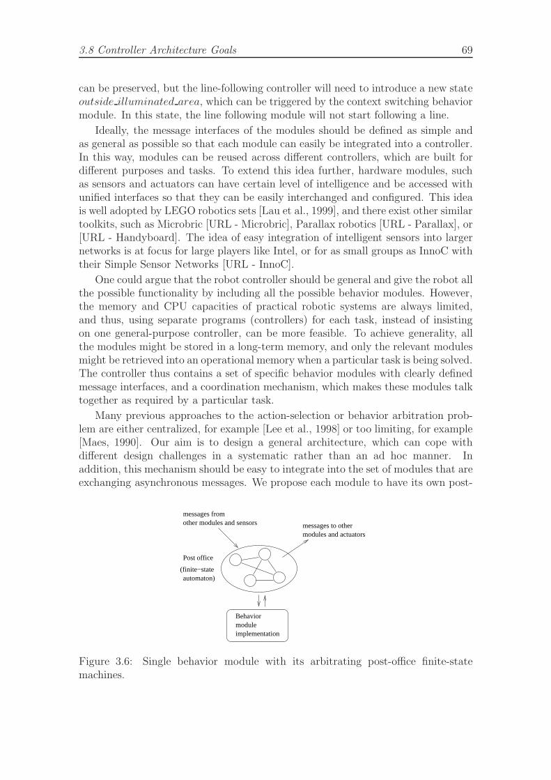
3.8 Controller Architecture Goals 69

can be preserved, but the line-following controller will need to introduce a new stateoutside illuminated area, which can be triggered by the context switching behaviormodule. In this state, the line following module will not start following a line.

Ideally, the message interfaces of the modules should be defined as simple andas general as possible so that each module can easily be integrated into a controller.In this way, modules can be reused across different controllers, which are built fordifferent purposes and tasks. To extend this idea further, hardware modules, suchas sensors and actuators can have certain level of intelligence and be accessed withunified interfaces so that they can be easily interchanged and configured. This ideais well adopted by LEGO robotics sets [Lau et al., 1999], and there exist other similartoolkits, such as Microbric [URL - Microbric], Parallax robotics [URL - Parallax], or[URL - Handyboard]. The idea of easy integration of intelligent sensors into largernetworks is at focus for large players like Intel, or for as small groups as InnoC withtheir Simple Sensor Networks [URL - InnoC].

One could argue that the robot controller should be general and give the robot allthe possible functionality by including all the possible behavior modules. However,the memory and CPU capacities of practical robotic systems are always limited,and thus, using separate programs (controllers) for each task, instead of insistingon one general-purpose controller, can be more feasible. To achieve generality, allthe modules might be stored in a long-term memory, and only the relevant modulesmight be retrieved into an operational memory when a particular task is being solved.The controller thus contains a set of specific behavior modules with clearly definedmessage interfaces, and a coordination mechanism, which makes these modules talktogether as required by a particular task.

Many previous approaches to the action-selection or behavior arbitration prob-lem are either centralized, for example [Lee et al., 1998] or too limiting, for example[Maes, 1990]. Our aim is to design a general architecture, which can cope withdifferent design challenges in a systematic rather than an ad hoc manner. Inaddition, this mechanism should be easy to integrate into the set of modules that areexchanging asynchronous messages. We propose each module to have its own post-

Behaviormoduleimplementation

messages fromother modules and sensors messages to other

modules and actuators

(finite−stateautomaton)

Post office

Figure 3.6: Single behavior module with its arbitrating post-office finite-statemachines.

70 Research Goals and Hypotheses

office module, which filters and translates the incoming messages into the messagesrecognized by the module itself, and which also monitors and possibly filters ormodifies the messages being sent by the module. Since the state is a central conceptin the controller, we chose to first study the post-offices that have the form of finite-state automata. The state transitions are triggered by messages being receivedor sent by the module owning the post-office. Each state transition can result in amessage being sent to the module or to other modules, see Figure 3.6. Please see alsoFigure 8.13 for examples of evolved FSAs and the representation of the transitions.

We design our coordination mechanism as distributed, and thus gain the standardadvantages of the distributed systems: robustness, modularity, better communica-tion throughput, better encapsulation and modifiability. In particular, adding anew module to an existing controller requires only designing a new post-office forthe added module and the minimum set of changes in post-offices of other modules,instead of inferring with all modules and modifying a centralized coordination mech-anism. This is thanks to minimalistic interfaces, one of the standard informationsystems design criteria.

3.9 Simulation

Due to the need of extensive CPU resources of the Evolutionary Robotics experi-ments, we ought to design a simulator or use an existing one. Unfortunately, noneof the existing simulators satisfied our needs, and we chose to implement our own.The following goals need to be maintained regarding simulation:

• All parts of the environment that are relevant for the simulation should beincluded.

• Simulation should be as accurate as possible.

• Simulation should be as fast as possible, in order to speed-up the evolutionaryrun.

• Simulator must provide means of quantitative feedback that can be used bythe objective function to compute fitness.

• The simulator must be configurable in order to perform experiments withdifferent:

– environments,

– robot starting locations,

– robot morphologies,

– sensory capabilities of the robots,

– active elements that are also part of the environment (such as changinglights).

Based on these requirements, we have designed a simulator as described in the laterchapters.

3.10 Chapter Summary 71

3.10 Chapter Summary

• The ultimate goal of our work is to automatically generate controllers for mo-bile robots performing in unstructured, changing, non-deterministic, dynamic,unpredictable environments.

• The method we work with are Evolutionary Algorithms, thus we work in thefield of Evolutionary Robotics.

• Instead of evolving complete robot controllers, we focus on evolving the specifictask functionality given the set of pre-designed behavioral modules.

• Evolutionary Robotics, if it should be successful, needs some guidance, becauseone evolutionary run would have to deal with too large search space.

• Our method for reducing the search space size is the Incremental Evolution.

• The use of Incremental Evolution is not straight-forward and requires carefulpreparation and investigation of issues, in particular: organization of the incre-mental scenario, understanding the different incremental fronts: environment,task, morphology, sensors/actuators, and controller.

• We attempt to evolve the arbitration mechanism for existing behaviors, idealarbitration should be: fast and reactive, provide priorities and other confidencemechanisms, take temporal aspect into account, provide feedback to behaviors,allow easy modification, be amenable to analysis and verification, easy toimplement and evolve.

• The chosen formalism for the arbitration representation are finite-state au-tomata.

• The chosen controller architecture consists of simultaneously executing behav-ioral modules that communicate with robot hardware and with each otherusing message passing.

• The method of studying the Incremental Evolution is by performing several re-alistic experiments with the chosen representation and controller architecture.These form the main focus of this thesis work.

72 Research Goals and Hypotheses

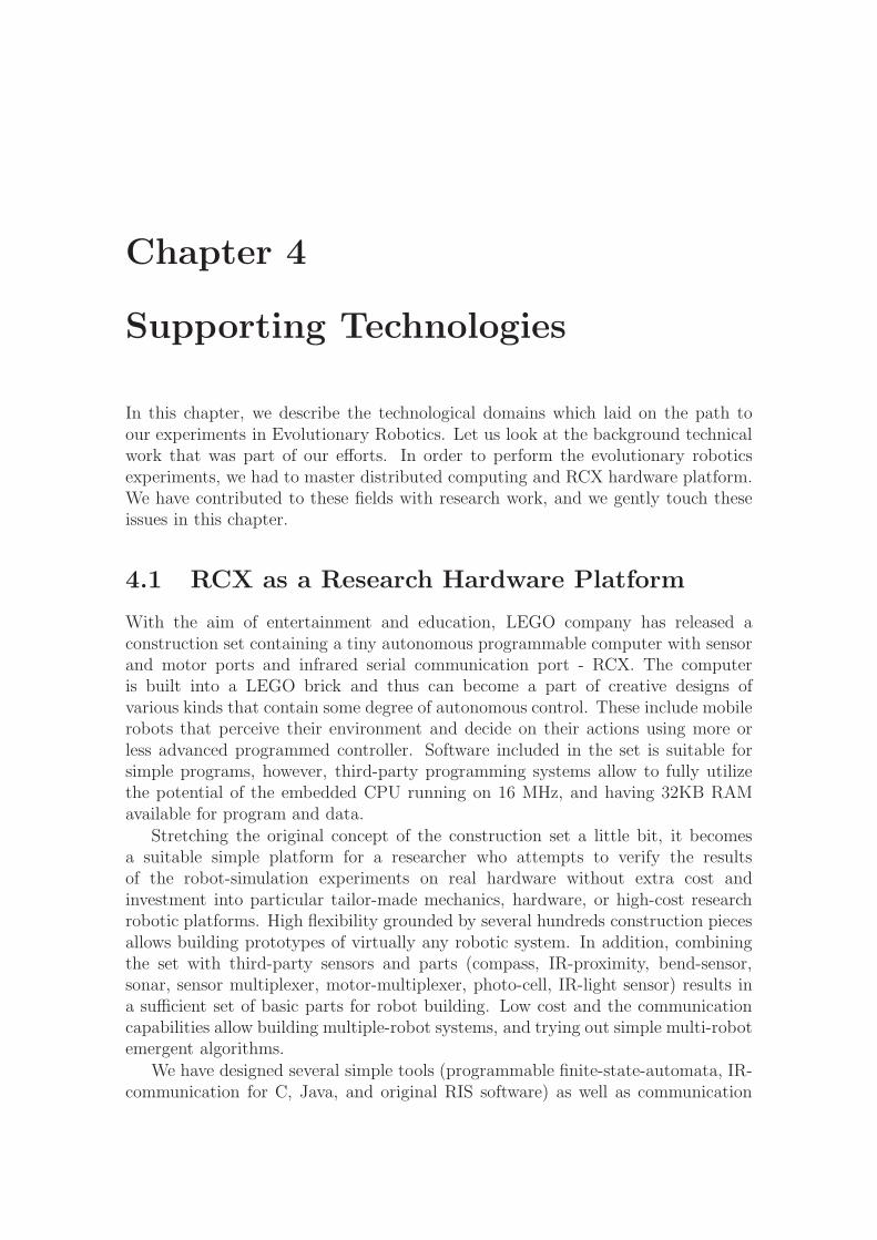
Chapter 4

Supporting Technologies

In this chapter, we describe the technological domains which laid on the path toour experiments in Evolutionary Robotics. Let us look at the background technicalwork that was part of our efforts. In order to perform the evolutionary roboticsexperiments, we had to master distributed computing and RCX hardware platform.We have contributed to these fields with research work, and we gently touch theseissues in this chapter.

4.1 RCX as a Research Hardware Platform

With the aim of entertainment and education, LEGO company has released aconstruction set containing a tiny autonomous programmable computer with sensorand motor ports and infrared serial communication port - RCX. The computeris built into a LEGO brick and thus can become a part of creative designs ofvarious kinds that contain some degree of autonomous control. These include mobilerobots that perceive their environment and decide on their actions using more orless advanced programmed controller. Software included in the set is suitable forsimple programs, however, third-party programming systems allow to fully utilizethe potential of the embedded CPU running on 16 MHz, and having 32KB RAMavailable for program and data.

Stretching the original concept of the construction set a little bit, it becomesa suitable simple platform for a researcher who attempts to verify the resultsof the robot-simulation experiments on real hardware without extra cost andinvestment into particular tailor-made mechanics, hardware, or high-cost researchrobotic platforms. High flexibility grounded by several hundreds construction piecesallows building prototypes of virtually any robotic system. In addition, combiningthe set with third-party sensors and parts (compass, IR-proximity, bend-sensor,sonar, sensor multiplexer, motor-multiplexer, photo-cell, IR-light sensor) results ina sufficient set of basic parts for robot building. Low cost and the communicationcapabilities allow building multiple-robot systems, and trying out simple multi-robotemergent algorithms.

We have designed several simple tools (programmable finite-state-automata, IR-communication for C, Java, and original RIS software) as well as communication

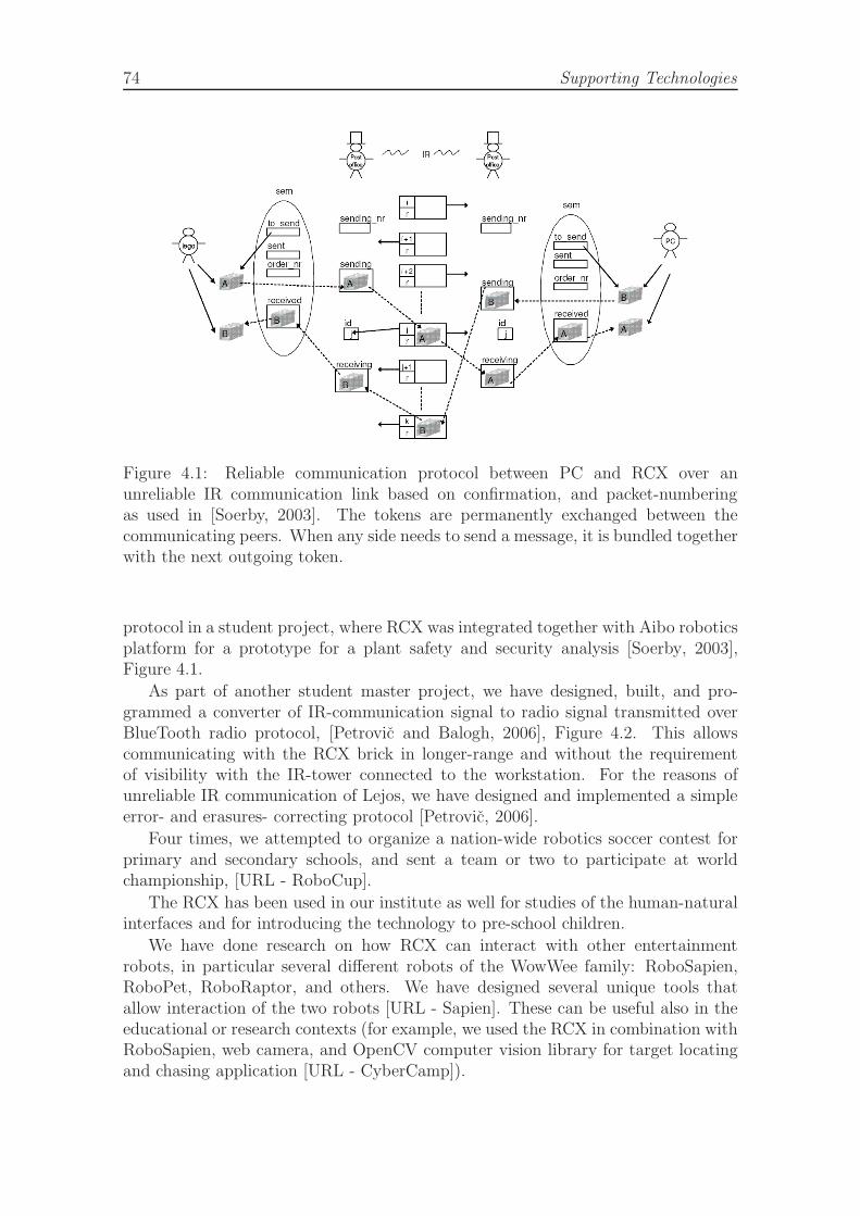
74 Supporting Technologies

Figure 4.1: Reliable communication protocol between PC and RCX over anunreliable IR communication link based on confirmation, and packet-numberingas used in [Soerby, 2003]. The tokens are permanently exchanged between thecommunicating peers. When any side needs to send a message, it is bundled togetherwith the next outgoing token.

protocol in a student project, where RCX was integrated together with Aibo roboticsplatform for a prototype for a plant safety and security analysis [Soerby, 2003],Figure 4.1.

As part of another student master project, we have designed, built, and pro-grammed a converter of IR-communication signal to radio signal transmitted overBlueTooth radio protocol, [Petrovic and Balogh, 2006], Figure 4.2. This allowscommunicating with the RCX brick in longer-range and without the requirementof visibility with the IR-tower connected to the workstation. For the reasons ofunreliable IR communication of Lejos, we have designed and implemented a simpleerror- and erasures- correcting protocol [Petrovic, 2006].

Four times, we attempted to organize a nation-wide robotics soccer contest forprimary and secondary schools, and sent a team or two to participate at worldchampionship, [URL - RoboCup].

The RCX has been used in our institute as well for studies of the human-naturalinterfaces and for introducing the technology to pre-school children.

We have done research on how RCX can interact with other entertainmentrobots, in particular several different robots of the WowWee family: RoboSapien,RoboPet, RoboRaptor, and others. We have designed several unique tools thatallow interaction of the two robots [URL - Sapien]. These can be useful also in theeducational or research contexts (for example, we used the RCX in combination withRoboSapien, web camera, and OpenCV computer vision library for target locatingand chasing application [URL - CyberCamp]).

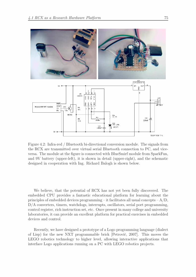
4.1 RCX as a Research Hardware Platform 75

Figure 4.2: Infra-red / Bluetooth bi-directional conversion module. The signals fromthe RCX are transmitted over virtual serial Bluetooth connection to PC, and vice-versa. The module at the figure is connected with BlueSmirf module from SparkFun,and 9V battery (upper-left), it is shown in detail (upper-right), and the schematicdesigned in cooperation with Ing. Richard Balogh is shown below.

We believe, that the potential of RCX has not yet been fully discovered. Theembedded CPU provides a fantastic educational platform for learning about theprinciples of embedded devices programming – it facilitates all usual concepts – A/D,D/A converters, timers, watchdogs, interrupts, oscillators, serial port programming,control register, rich instruction set, etc. Once present in many college and universitylaboratories, it can provide an excellent platform for practical exercises in embeddeddevices and control.

Recently, we have designed a prototype of a Logo programming language (dialectof Lisp) for the new NXT programmable brick [Petrovic, 2007]. This moves theLEGO robotics technology to higher level, allowing interactive applications thatinterface Logo applications running on a PC with LEGO robotics projects.

76 Supporting Technologies

4.2 Distributed Computing

Distributed Computing harnesses the idle processing cycles of the available work-stations on the network and makes them available for working on computationallyintensive problems that would otherwise require a supercomputer or a dedicatedcluster of computers to solve.

A distributed computing application is divided to smaller computing tasks, whichare then distributed to the workstations to process in parallel. Results are sent backto the master that has the role of a server, where the data are collected and deliveredto the client, in the cases of master-slave client-server architectures. Alternately, theresults are sent to other nodes that need them for further processing, in the casesof peer-to-peer distributed architectures. The more PCs in a network, the moreprocessors available to process applications in parallel, and the faster the results arereturned. As far as the granularity of parallelization of the application allows, anetwork of a few thousand PCs can process applications that otherwise can be runonly on fast and expensive supercomputers. This kind of computing can transforma local network of workstations into a virtual supercomputer.

Several public and popular systems for distributed computing appeared early inthe 90s [Pearson, 2007]. Most of these systems, however, are either focused on somespecific problems, they require dedicated hardware, or they are proprietary, offeringlittle flexibility to developers.

One class of distributed systems comprises large scale distributed computingbased on thousands to millions of voluntary CPU-time donators available throughoutthe Internet. The users download specialized clients for their particular softwareand hardware platforms, and let their computers work during the unused CPU timeon a particular distributed computing project, thus making their CPUs consumemaximum power possible. However, these systems are typically closed for the user,who usually has little control over the code or the data being processed on his orher machine. On one hand, this is required to guarantee validity of the submittedresults; on the other hand, it is a potential threat to the user’s security and trust.Such systems typically try to solve or prove some hard mathematics, bioinformatics,cryptographic or other search challenges. Examples include Folding@home, Find-a-Drug, or D2OL, helping to find oral drugs which could fight Anthrax, Smallpox,Ebola, SARS, deadly diseases for which there is currently no cure, and Malaria, a life-threatening disease for which 40% of the World’s population is at risk. An exampleof a multi-purpose platform of this kind is BOINC (Berkley Open Infrastructure forNetwork Computing), [Anderson, 2004]. Distributed.net [URL - Distributed.net] is avery large network of users all over the world, using their computers’ idle processingcycles to run computational challenge projects, which require a lot of computingpower. Examples of projects are RC5-64 secret-key, DES or CS-Cipher challenges.Another similar project is Seti@home, [URL - SETI], a scientific experiment thatuses Internet- connected computers in the Search for Extraterrestrial Intelligence(SETI), by analyzing radio telescope data. The focus on very specific computationalproblems, and the closed code of the client makes the above mentioned systemsdifficult to use for our research projects.

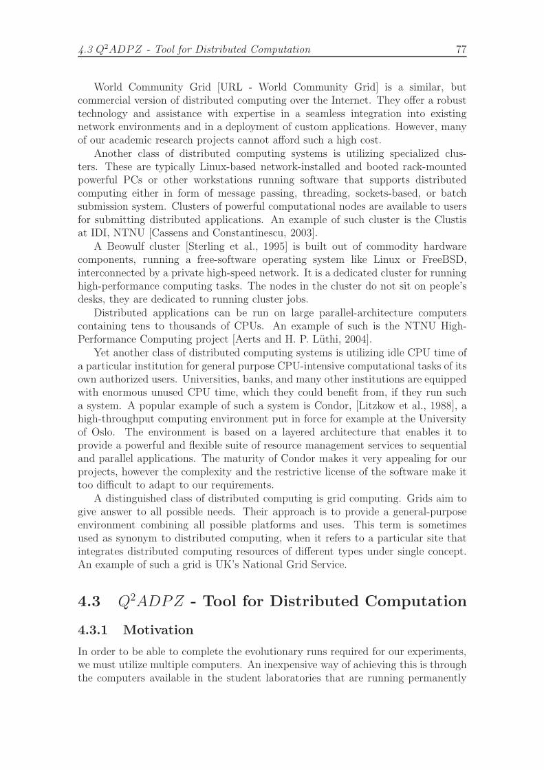
4.3 Q2ADPZ - Tool for Distributed Computation 77

World Community Grid [URL - World Community Grid] is a similar, butcommercial version of distributed computing over the Internet. They offer a robusttechnology and assistance with expertise in a seamless integration into existingnetwork environments and in a deployment of custom applications. However, manyof our academic research projects cannot afford such a high cost.

Another class of distributed computing systems is utilizing specialized clus-ters. These are typically Linux-based network-installed and booted rack-mountedpowerful PCs or other workstations running software that supports distributedcomputing either in form of message passing, threading, sockets-based, or batchsubmission system. Clusters of powerful computational nodes are available to usersfor submitting distributed applications. An example of such cluster is the Clustisat IDI, NTNU [Cassens and Constantinescu, 2003].

A Beowulf cluster [Sterling et al., 1995] is built out of commodity hardwarecomponents, running a free-software operating system like Linux or FreeBSD,interconnected by a private high-speed network. It is a dedicated cluster for runninghigh-performance computing tasks. The nodes in the cluster do not sit on people’sdesks, they are dedicated to running cluster jobs.

Distributed applications can be run on large parallel-architecture computerscontaining tens to thousands of CPUs. An example of such is the NTNU High-Performance Computing project [Aerts and H. P. Luthi, 2004].

Yet another class of distributed computing systems is utilizing idle CPU time ofa particular institution for general purpose CPU-intensive computational tasks of itsown authorized users. Universities, banks, and many other institutions are equippedwith enormous unused CPU time, which they could benefit from, if they run sucha system. A popular example of such a system is Condor, [Litzkow et al., 1988], ahigh-throughput computing environment put in force for example at the Universityof Oslo. The environment is based on a layered architecture that enables it toprovide a powerful and flexible suite of resource management services to sequentialand parallel applications. The maturity of Condor makes it very appealing for ourprojects, however the complexity and the restrictive license of the software make ittoo difficult to adapt to our requirements.

A distinguished class of distributed computing is grid computing. Grids aim togive answer to all possible needs. Their approach is to provide a general-purposeenvironment combining all possible platforms and uses. This term is sometimesused as synonym to distributed computing, when it refers to a particular site thatintegrates distributed computing resources of different types under single concept.An example of such a grid is UK’s National Grid Service.

4.3 Q2ADPZ - Tool for Distributed Computation

4.3.1 Motivation

In order to be able to complete the evolutionary runs required for our experiments,we must utilize multiple computers. An inexpensive way of achieving this is throughthe computers available in the student laboratories that are running permanently

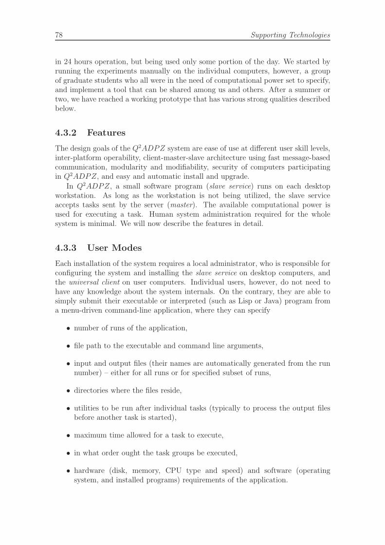
78 Supporting Technologies

in 24 hours operation, but being used only some portion of the day. We started byrunning the experiments manually on the individual computers, however, a groupof graduate students who all were in the need of computational power set to specify,and implement a tool that can be shared among us and others. After a summer ortwo, we have reached a working prototype that has various strong qualities describedbelow.

4.3.2 Features

The design goals of the Q2ADPZ system are ease of use at different user skill levels,inter-platform operability, client-master-slave architecture using fast message-basedcommunication, modularity and modifiability, security of computers participatingin Q2ADPZ, and easy and automatic install and upgrade.

In Q2ADPZ, a small software program (slave service) runs on each desktopworkstation. As long as the workstation is not being utilized, the slave serviceaccepts tasks sent by the server (master). The available computational power isused for executing a task. Human system administration required for the wholesystem is minimal. We will now describe the features in detail.

4.3.3 User Modes

Each installation of the system requires a local administrator, who is responsible forconfiguring the system and installing the slave service on desktop computers, andthe universal client on user computers. Individual users, however, do not need tohave any knowledge about the system internals. On the contrary, they are able tosimply submit their executable or interpreted (such as Lisp or Java) program froma menu-driven command-line application, where they can specify

• number of runs of the application,

• file path to the executable and command line arguments,

• input and output files (their names are automatically generated from the runnumber) – either for all runs or for specified subset of runs,

• directories where the files reside,

• utilities to be run after individual tasks (typically to process the output filesbefore another task is started),

• maximum time allowed for a task to execute,

• in what order ought the task groups be executed,

• hardware (disk, memory, CPU type and speed) and software (operatingsystem, and installed programs) requirements of the application.

4.3 Q2ADPZ - Tool for Distributed Computation 79

<Job Name="example">

<Task ID="1" Type="Library">

<RunCount>1</RunCount>

<TaskInfo>

<Memory Unit="MB">64</Memory>

<Disk Unit="MB">5</Disk>

<TimeOut>3600</TimeOut>

<OS>Linux</OS>

<CPU>i386</CPU>

<URL>http://server/lib-example.so</URL>

</TaskInfo>

</Task>

</Job>

Figure 4.3: Q2ADPZ: A simple library-type project file.

These project configuration parameters are saved into XML-structured file. Theexecutable can be taken from a local disk or downloaded from any URL-specifiedaddress. The input and output data files are automatically transferred to slavesusing a dedicated data www-server. The progress of execution can be viewed in anywww-browser, see the Figure 4.8.

Each run corresponds to a task – the smallest computational unit in Q2ADPZ.Tasks are grouped into jobs – identified by a group name and a job number.System allows control operations on the level of tasks, jobs, job groups, or users. Ifpreferred by advanced users, the project file may be edited manually or generatedautomatically, see the Figure 4.3 and the Figure 4.4 for examples.

More advanced users can write their own client application that communicatesdirectly with the master using API of the client service library. This allowssubmitting tasks with appropriate data dynamically.

Finally, advanced users can write their own slave libraries that are relativelyfaster than executable programs and very suitable for applications with many short-term small-size tasks, i.e. with a high degree of parallelism.

4.3.4 Inter-Platform Operability

Inter-platform operability is achieved by the pool of computers in a network that canrun different operating systems and have different hardware architectures. Q2ADPZhandles task submissions with platform specifications, and the appropriate libraryor executable is automatically used. At the time of writing, we have successfullytested the system on the following hardware platforms: Linux/iX86,sparc,sparc64,FreeBSD/iX86, SunOS/sun4m,sun4u, IRIX64/IP27, and Win32/iX86. Most of thecode is ANSI C++ and POSIX.1 compliant and therefore porting to a new platformdoes not require too much efforts. We use the POSIX threads API (emulated byWindows threads on WIN32 platform).

4.3.5 Architecture

The system consists of a central process called “master”, a variable (high) numberof computing processes on different computers in the network called “slaves”, and

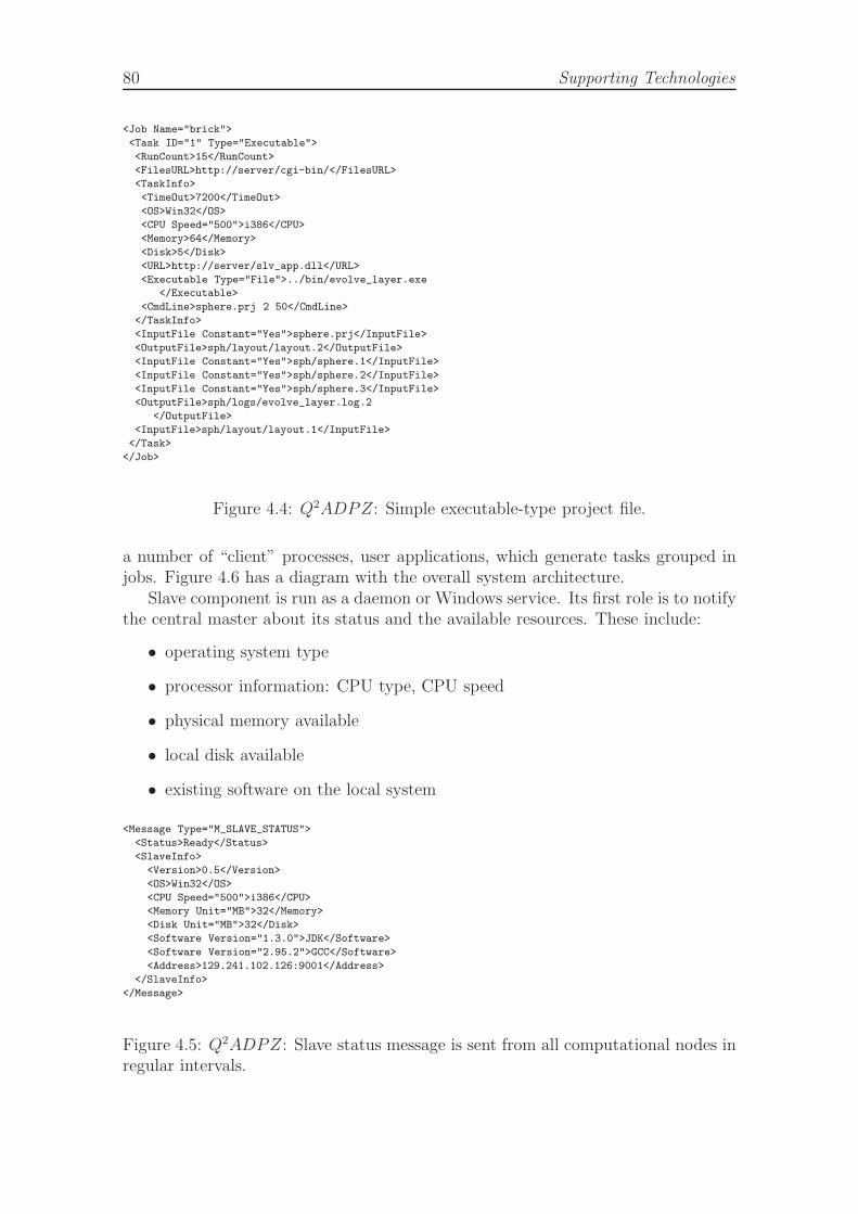
80 Supporting Technologies

<Job Name="brick">

<Task ID="1" Type="Executable">

<RunCount>15</RunCount>

<FilesURL>http://server/cgi-bin/</FilesURL>

<TaskInfo>

<TimeOut>7200</TimeOut>

<OS>Win32</OS>

<CPU Speed="500">i386</CPU>

<Memory>64</Memory>

<Disk>5</Disk>

<URL>http://server/slv_app.dll</URL>

<Executable Type="File">../bin/evolve_layer.exe

</Executable>

<CmdLine>sphere.prj 2 50</CmdLine>

</TaskInfo>

<InputFile Constant="Yes">sphere.prj</InputFile>

<OutputFile>sph/layout/layout.2</OutputFile>

<InputFile Constant="Yes">sph/sphere.1</InputFile>

<InputFile Constant="Yes">sph/sphere.2</InputFile>

<InputFile Constant="Yes">sph/sphere.3</InputFile>

<OutputFile>sph/logs/evolve_layer.log.2

</OutputFile>

<InputFile>sph/layout/layout.1</InputFile>

</Task>

</Job>

Figure 4.4: Q2ADPZ: Simple executable-type project file.

a number of “client” processes, user applications, which generate tasks grouped injobs. Figure 4.6 has a diagram with the overall system architecture.

Slave component is run as a daemon or Windows service. Its first role is to notifythe central master about its status and the available resources. These include:

• operating system type

• processor information: CPU type, CPU speed

• physical memory available

• local disk available

• existing software on the local system

<Message Type="M_SLAVE_STATUS">

<Status>Ready</Status>

<SlaveInfo>

<Version>0.5</Version>

<OS>Win32</OS>

<CPU Speed="500">i386</CPU>

<Memory Unit="MB">32</Memory>

<Disk Unit="MB">32</Disk>

<Software Version="1.3.0">JDK</Software>

<Software Version="2.95.2">GCC</Software>

<Address>129.241.102.126:9001</Address>

</SlaveInfo>

</Message>

Figure 4.5: Q2ADPZ: Slave status message is sent from all computational nodes inregular intervals.

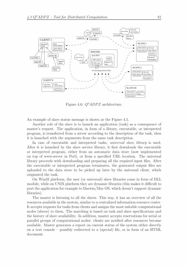
4.3 Q2ADPZ - Tool for Distributed Computation 81

www dataserver

output fileexecutable

input file

input file

www server

status

post office

slave service

slave library

universal

Executable

slave library

universal

interpreteduser program

interpreter

post office

slave service

slave library

universal

user slavelibrary

executable

www server

UDP socket

UDP confirm

usersdatabase of

crypter

post office

slave service user slavelibrary

user clientapplication

post office

clientservice library

post office

clientservice library

universalclient

project file

manualeditor

universalclient

executable

input file

output file

OS networking (Win32/UNIX)

SLAVE 2

SLAVE 1

post office

MASTER

SLAVE M

CLIENT N

CLIENT 1

Figure 4.6: Q2ADPZ architecture.

An example of slave status message is shown at the Figure 4.5.Another role of the slave is to launch an application (task) as a consequence of

master’s request. The application, in form of a library, executable, or interpretedprogram, is transferred from a server according to the description of the task, thenit is launched with the arguments from the same task description.

In case of executable and interpreted tasks, universal slave library is used.After it is launched by the slave service library, it first downloads the executableor interpreted program, either from an automatic data store (now implementedon top of www-server in Perl), or from a specified URL location. The universallibrary proceeds with downloading and preparing all the required input files. Afterthe executable or interpreted program terminates, the generated output files areuploaded to the data store to be picked up later by the universal client, whichoriginated the task.

On Win32 platform, the user (or universal) slave libraries come in form of DLLmodule, while on UNIX platform they are dynamic libraries (this makes it difficult toport the application for example to Darwin/Mac OS, which doesn’t support dynamiclibraries).

The master is listening to all the slaves. This way, it has an overview of all theresources available in the system, similar to a centralized information resource center.It accepts requests for tasks from clients and assigns the most suitable computationalnodes (slaves) to them. The matching is based on task and slave specifications andthe history of slave availability. In addition, master accepts reservations for serial orparallel groups of computational nodes: clients are notified after resources becomeavailable. Master generates a report on current status of the system either directlyon a text console – possibly redirected to a (special) file, or in form of an HTMLdocument.

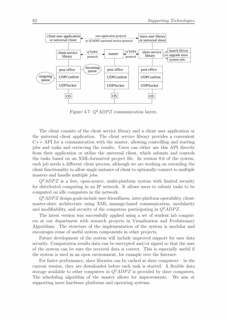
82 Supporting Technologies

queueoutgoing

client servicelibrary

slave servicelibrary

OS OS

slave user libraryor universal slave

client user applicationor universal client

post office

UDPConfirm

UDPSocket

post office

UDPConfirm

UDPSocket

post office

UDPConfirm

UDPSocket

OS

protocol

Q ADPZ2

user application protocol

or Q ADPZ universal service protocol2

Q ADPZ2

protocol

queueincoming

launch lib/exeupgrade slavesystem info

master

Figure 4.7: Q2ADPZ communication layers.

The client consists of the client service library and a client user application orthe universal client application. The client service library provides a convenientC++ API for a communication with the master, allowing controlling and startingjobs and tasks and retrieving the results. Users can either use this API directlyfrom their application or utilize the universal client, which submits and controlsthe tasks based on an XML-formatted project file. In version 0.6 of the system,each job needs a different client process, although we are working on extending theclient functionality to allow single instance of client to optionally connect to multiplemasters and handle multiple jobs.

Q2ADPZ is a free, open-source, multi-platform system with limited securityfor distributed computing in an IP network. It allows users to submit tasks to becomputed on idle computers in the network.

Q2ADPZ design goals include user-friendliness, inter-platform operability, client-master-slave architecture using XML message-based communication, modularityand modifiability, and security of the computers participating in Q2ADPZ.

The latest version was successfully applied using a set of student lab comput-ers at our department with research projects in Visualization and EvolutionaryAlgorithms. The structure of the implementation of the system is modular andencourages reuse of useful system components in other projects.

Future development of the system will include improved support for user datasecurity. Computation results data can be encrypted and/or signed so that the userof the system can be sure the received data is correct. This is especially useful ifthe system is used in an open environment, for example over the Internet.

For faster performance, slave libraries can be cached at slave computers – in thecurrent version, they are downloaded before each task is started. A flexible datastorage available to other computers in Q2ADPZ is provided by slave computers.The scheduling algorithm of the master allows for improvements. We aim atsupporting more hardware platforms and operating systems.

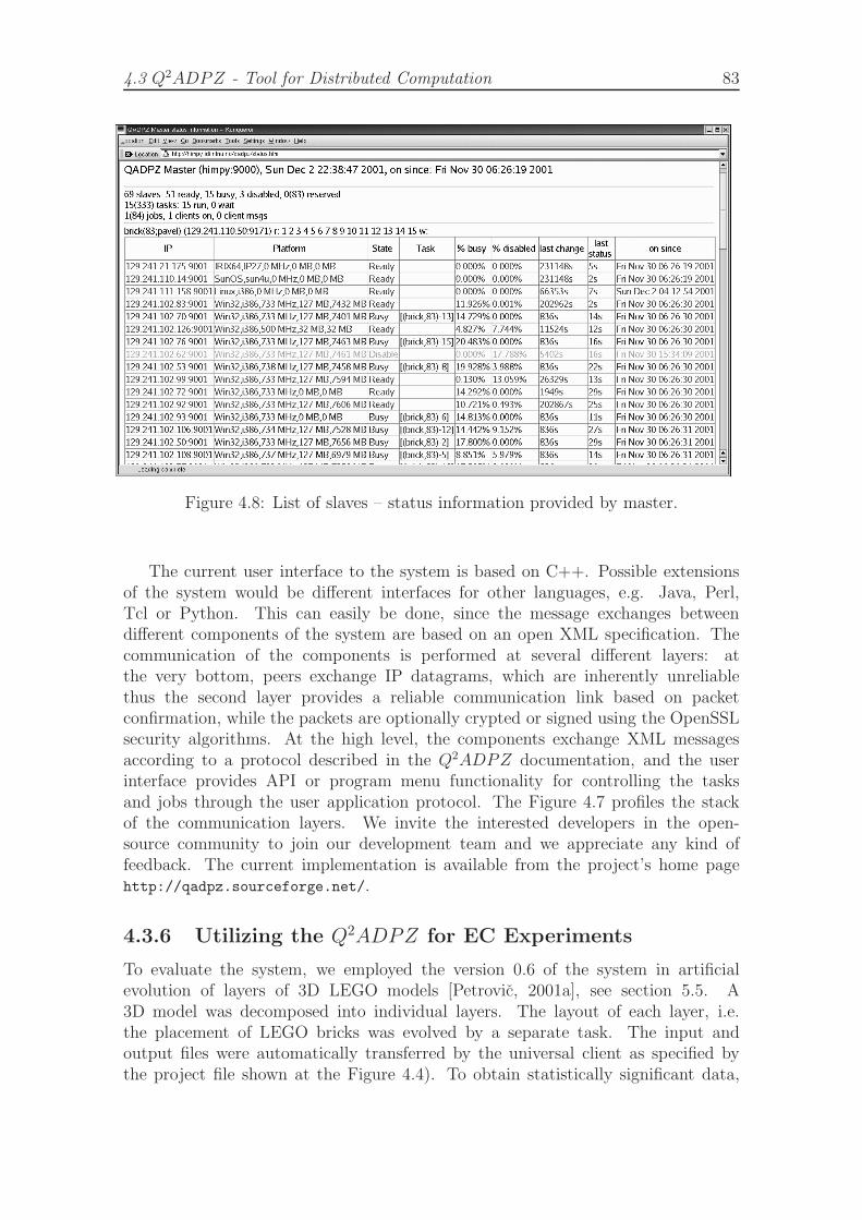
4.3 Q2ADPZ - Tool for Distributed Computation 83

Figure 4.8: List of slaves – status information provided by master.

The current user interface to the system is based on C++. Possible extensionsof the system would be different interfaces for other languages, e.g. Java, Perl,Tcl or Python. This can easily be done, since the message exchanges betweendifferent components of the system are based on an open XML specification. Thecommunication of the components is performed at several different layers: atthe very bottom, peers exchange IP datagrams, which are inherently unreliablethus the second layer provides a reliable communication link based on packetconfirmation, while the packets are optionally crypted or signed using the OpenSSLsecurity algorithms. At the high level, the components exchange XML messagesaccording to a protocol described in the Q2ADPZ documentation, and the userinterface provides API or program menu functionality for controlling the tasksand jobs through the user application protocol. The Figure 4.7 profiles the stackof the communication layers. We invite the interested developers in the open-source community to join our development team and we appreciate any kind offeedback. The current implementation is available from the project’s home pagehttp://qadpz.sourceforge.net/.

4.3.6 Utilizing the Q2ADPZ for EC Experiments

To evaluate the system, we employed the version 0.6 of the system in artificialevolution of layers of 3D LEGO models [Petrovic, 2001a], see section 5.5. A3D model was decomposed into individual layers. The layout of each layer, i.e.the placement of LEGO bricks was evolved by a separate task. The input andoutput files were automatically transferred by the universal client as specified bythe project file shown at the Figure 4.4). To obtain statistically significant data,

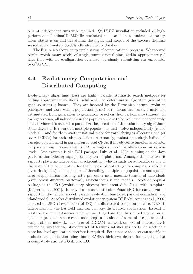
84 Supporting Technologies

tens of independent runs were required. Q2ADPZ installation included 70 high-performance PentiumIII/733MHz workstations located in a student laboratory.Their status is on and idle during the night, and except of the exercise deadlineseason approximately 30-50% idle also during the day.

The Figure 4.8 shows an example status of computational progress. We receivedresults worth many weeks of single computational time within approximately 3days time with no configuration overhead, by simply submitting our executableto Q2ADPZ.

4.4 Evolutionary Computation and

Distributed Computing

Evolutionary algorithms (EA) are highly parallel stochastic search methods forfinding approximate solutions useful when no deterministic algorithm generatinggood solutions is known. They are inspired by the Darwinian natural evolutionprinciples, and work with a population (a set) of solutions that survive, mate andget mutated from generation to generation based on their performance (fitness). Ineach generation, all individuals in the population have to be evaluated independently.That is where it is natural to parallelize the execution of the evolutionary algorithms.Some flavors of EA work on multiple populations that evolve independently (islandmodels) – and for them another natural place for parallelizing is allocating one (orseveral CPUs) for each sub-population. Alternately, evaluating a single individualcan also be performed in parallel on several CPUs, if the objective function is suitablefor parallelizing. Some existing EA packages support parallelization on variouslevels. One example is the ECJ package [Luke et al., 2005] running on the Javaplatform thus offering high portability across platforms. Among other features, itsupports platform-independent checkpointing (which stands for automatic saving ofthe state of the computation for the purpose of restarting the computation from agiven checkpoint) and logging, multithreading, multiple subpopulations and species,inter-subpopulation breeding, inter-process or inter-machine transfer of individuals(even across different platforms), asynchronous island models. Another popularpackage is the EO (evolutionary objects) implemented in C++ with templates[Keijzer et al., 2001]. It provides its own extension ParadisEO for parallelizationsupporting the cellular model, parallel evaluation functions, parallel evaluation, andisland model. Another distributed evolutionary system DREAM [Arenas et al., 2002]is based on JEO (Java brother of EO). Its distributed computation core, DRM isindependent of the EA field and can run any distributed application. Instead ofmaster-slave or client-server architecture, they base the distributed engine on anepidemic protocol, where each node keeps a database of some of the peers in thecomputational network. The user of DREAM can work on several different levelsdepending whether the standard set of features satisfies his needs, or whether amore low-level application interface is required. For instance the user can specify itsevolutionary application using simple EASEA high-level description language thatis compatible also with GaLib or EO.

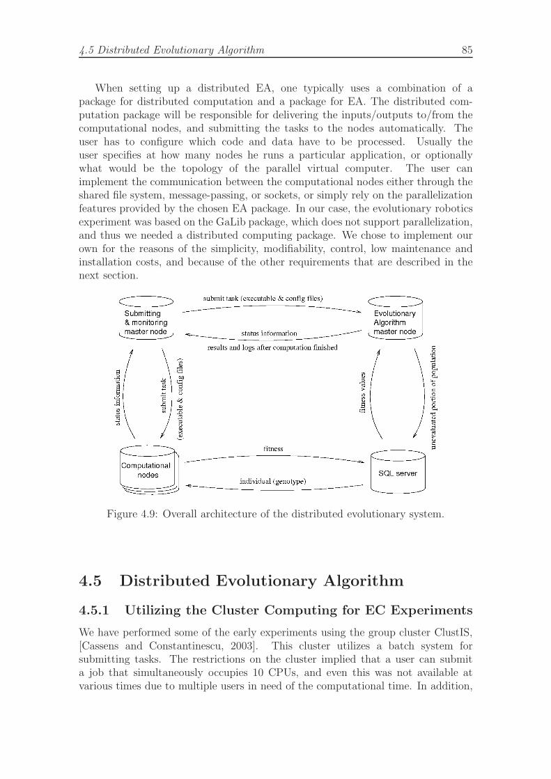
4.5 Distributed Evolutionary Algorithm 85

When setting up a distributed EA, one typically uses a combination of apackage for distributed computation and a package for EA. The distributed com-putation package will be responsible for delivering the inputs/outputs to/from thecomputational nodes, and submitting the tasks to the nodes automatically. Theuser has to configure which code and data have to be processed. Usually theuser specifies at how many nodes he runs a particular application, or optionallywhat would be the topology of the parallel virtual computer. The user canimplement the communication between the computational nodes either through theshared file system, message-passing, or sockets, or simply rely on the parallelizationfeatures provided by the chosen EA package. In our case, the evolutionary roboticsexperiment was based on the GaLib package, which does not support parallelization,and thus we needed a distributed computing package. We chose to implement ourown for the reasons of the simplicity, modifiability, control, low maintenance andinstallation costs, and because of the other requirements that are described in thenext section.

Figure 4.9: Overall architecture of the distributed evolutionary system.

4.5 Distributed Evolutionary Algorithm

4.5.1 Utilizing the Cluster Computing for EC Experiments

We have performed some of the early experiments using the group cluster ClustIS,[Cassens and Constantinescu, 2003]. This cluster utilizes a batch system forsubmitting tasks. The restrictions on the cluster implied that a user can submita job that simultaneously occupies 10 CPUs, and even this was not available atvarious times due to multiple users in need of the computational time. In addition,

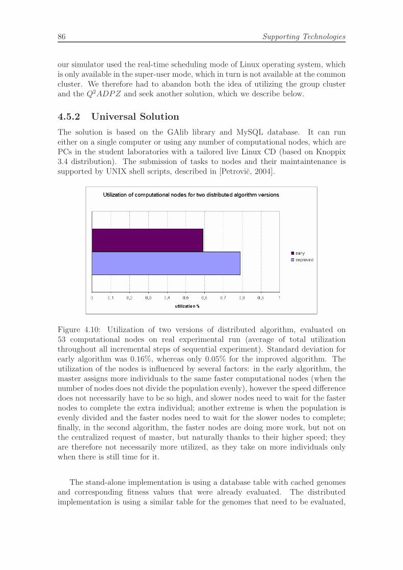
86 Supporting Technologies

our simulator used the real-time scheduling mode of Linux operating system, whichis only available in the super-user mode, which in turn is not available at the commoncluster. We therefore had to abandon both the idea of utilizing the group clusterand the Q2ADPZ and seek another solution, which we describe below.

4.5.2 Universal Solution

The solution is based on the GAlib library and MySQL database. It can runeither on a single computer or using any number of computational nodes, which arePCs in the student laboratories with a tailored live Linux CD (based on Knoppix3.4 distribution). The submission of tasks to nodes and their maintaintenance issupported by UNIX shell scripts, described in [Petrovic, 2004].

Figure 4.10: Utilization of two versions of distributed algorithm, evaluated on53 computational nodes on real experimental run (average of total utilizationthroughout all incremental steps of sequential experiment). Standard deviation forearly algorithm was 0.16%, whereas only 0.05% for the improved algorithm. Theutilization of the nodes is influenced by several factors: in the early algorithm, themaster assigns more individuals to the same faster computational nodes (when thenumber of nodes does not divide the population evenly), however the speed differencedoes not necessarily have to be so high, and slower nodes need to wait for the fasternodes to complete the extra individual; another extreme is when the population isevenly divided and the faster nodes need to wait for the slower nodes to complete;finally, in the second algorithm, the faster nodes are doing more work, but not onthe centralized request of master, but naturally thanks to their higher speed; theyare therefore not necessarily more utilized, as they take on more individuals onlywhen there is still time for it.

The stand-alone implementation is using a database table with cached genomesand corresponding fitness values that were already evaluated. The distributedimplementation is using a similar table for the genomes that need to be evaluated,

4.5 Distributed Evolutionary Algorithm 87

and possibly interacts with the cache, see Figure 4.9. In addition, a table listingthe computational nodes that are available for computation – i.e. evaluating thegenomes is used. In the distributed scenario, the evolutionary algorithm is startedat N machines, where one of them works as the master node and all other machineswork as slave nodes (multiple evolutionary algorithms can run simultaneously andindependently – they only need to have a different identifier). The master machinehas the GA object, the population, and does all the evolutionary part of work,whereas the node machines are responsible only for evaluating individuals, althoughthey are started in the same way (except of telling them to run as slaves), and readthe same configuration files. Before evaluating the population in each generation,the master machine saves all genomes to the database and marks them by ids ofthe slaves that should evaluate them. If cache is used, the genomes that alreadyhave been evaluated earlier are removed from the list first. Next, the slave nodesretrieve the genomes to be evaluated, and save the results back to the database.When there are no more genomes to evaluate, each slave marks that it has finishedits part of the work. As soon as all the slaves have finished the work, the masternode determines this and either moves all results to the cache and runs its standardfitness function, or – if cache is not used, it retrieves the newly computed fitnessvalues from the database, and removes the records. The checkpoints, which preventevaluation of non-promising individuals, are communicated to the slaves from themaster through separate CHCKPT table – it is refilled with values in the beginningof each incremental step by master. In detail, the algorithm for the master nodeis as follows: run the evolutionary algorithm as the stand-alone version, with thefollowing additions:

1. On start-up, create the slave table and TODO table

2. When the population is ready to be evaluated, it is dumped to the TODOtable, and records are marked as “temporary” since they are not yet ready forevaluation by slave nodes.

3. If cache is used, remove those records from TODO table that already exist inthe cache.

4. If at the beginning of new incremental step, save new checkpoint times andvalues to the checkpoints table

5. Retrieve list of on-line slaves and assign each slave proportional amount ofremaining genomes to be evaluated (as the future work, this can be improvedby assigning the amount of genomes proportional to the slave performance– thus allowing to use machines with different CPU power in the sameevolutionary run).

6. Set the counts of genomes to be evaluated for all slaves in the slaves table (setthe REMAINING GENOMES field)

7. Assign slave identifiers to the genome records in the table and mark them as“to do” so that the slaves start evaluating them.

88 Supporting Technologies

8. Monitor the REMAINING GENOMES values in the slaves table, as soonas they all become 0 in all records, the evaluation is finished and either allrecords are moved to the cache if it is in use, or they are retrieved to thememory and removed from the database. The retrieved values are collectedby the master’s objective function, which returns the proper value either fromthe cache or directly.

9. Maintain the average time of evaluation of genomes. If some slave reaches5-times longer time and still have not evaluated its assigned genomes, removeit from the table and assign its genomes to another slave, and continuemonitoring.

10. When the evolution is finished, all records in the slave table are marked, whichresults in the termination of the computational nodes.

11. During the run, the algorithm state values (such as the incremental stepnumber) are passed to the slaves through the records in the TODO table.

The algorithm for the slave node is more straight forward:

1. The evolutionary algorithm is not run, only the configuration files are parsedand parameters are set.

2. After start-up, the slave waits until the slave table is created, after which itputs a record to identify itself in the slaves table.

3. It monitors the value REMAINING GENOMES in the slave table, untilit becomes non-zero.

4. The slave retrieves the checkpoints from the checkpoints table.

5. The slave retrieves the genomes from the TODO table, evaluates them, andsaves the fitness value back to the table, marks the genome as done, anddecrements the REMAINING GENOMES counter in the slave table.

6. When the REMAINING GENOMES counter becomes zero again, continuewith point 3.

7. When the slave record is deleted, terminate.

Later, we have modified the distributed scenario in order to test if an improvedalgorithm would have a higher throughput. Instead of assigning the individuals toparticular computational nodes, the master only publishes all unevaluated individu-als through the database. The computational nodes individually take the individualsto be evaluated and save the fitness back to the database on the one-by-one basis.There is a little bit of communication overhead, and a little time wasted beforeeach individual is evaluated as the slaves must make short breaks while queryingthe database perpetually and waiting for new individuals. On the other hand, andmore importantly, slaves that proceed faster, and finish their package of individuals

4.6 Chapter Summary 89

early, are not utilized again in the earlier version of the algorithm until all slavesdeliver their results. However, there still may be some individuals for which theevaluation has not been started yet. Difference lies also in the handling of the faultyslave nodes – these could be simply ignored in the new version of algorithm withoutthe resource-demanding detection process, because the initiative is coming from thenodes, not from the master. If the result will not have been delivered back within afixed time constant, the individual that is being evaluated by a faulty node becomesconsidered unallocated after that time, and another computational node will allocateit, that is, starts its evaluation. We compared the utilization of CPU nodes of thetwo algorithms, as shown at the Figure 4.10.

The algorithm was adopted and further improved for the case of pool withcomputational nodes with large differences in performance by [Plavcan, 2007] in hismaster thesis that utilized distributed computing for experiments in evolutionarydesign.

4.6 Chapter Summary

• The hardware platform used in our experiments is the LEGO programmablesets. We have mastered this technology, made use of it for various purposeand contributed to the wide user community with several utilities.

• In order to perform the evolutionary experiments, we ought to utilize Dis-tributed Computing, in particular:

• We design a distributed system for harnessing the CPU power of computersin the computer labs that we use for some of our evolutionary experiments.

• For the purpose of the incremental evolution experiments, we design a special-ized distributed system based on database and Unix scripts.

90 Supporting Technologies

Chapter 5

Supporting Studies

In this chapter, we describe the scientific domains which laid the path to ourexperiments in Evolutionary Robotics. In order to better understand possibleapplications of Robotics – including Evolutionary Robotics and automatic designof controllers, we examine one of the application domains, Educational Robotics, inhigher detail. We performed, and later discuss several studies and experiments inEducational Robotics.

In our work, we are particularly interested to asses how much robotics cancontribute to educational school and after-school activities, whether it is useful at all,and what are the requirements on such systems in order to bring more positive thannegative outcome. Is robotics due to its costs and demands on high technologicalskills suitable only for the real-world applications? Can the robotics educationalsystems make the school classes more effective, and reach the educational goals?If yes, what form these activities can take and how they can be integrated intocurriculum, who can provide the necessary instruction to meet pedagogical goals?

These are serious questions that put the area into very suspicious light. Our aimin this work is to indicate several interesting ways of successful integration of therobots to curriculum and schools.

As part of the overall goal of evolving robot controllers, evolving robot morphol-ogy is an important part of the problem as explained in the previous chapters. Inorder to be able to evolve morphology, we must first understand how to representthe shapes in evolutionary algorithms. We have contributed to these fields withresearch work, and we gently touch these issues in this chapter.

5.1 Role of Robotics in Education

As modern technology advances in an ever-accelerating pace, especially in the crucialfields such as computer and automation, there is a continuous demand for skilledand highly motivated workers. To ensure that this demand could be met, technologycurriculum is needed at the school level to give students insight into engineering fieldsand attract students to technology studies. As opposed to the traditional vocationaleducation approach, technology curriculum at the school level should discard theconfined professional bias and provide an insight into engineering science [Waks,

92 Supporting Studies

1995]. Therefore, new approaches are needed to design an appropriate modernstrategy for implementing high quality technology program at school level. Robotics,being a multifaceted representation of modern science and technology, fits into thisplanning perfectly.

Realizing the potential and importance of robotics, the LEGO group has launcheda range of programmable robotics products called Mindstorms in September 1998,followed up with much more powerful version in August 2006. The Mindstormsrobotics base set consists of touch sensors, light sensors, rotational sensors, motorsand a main building block that houses a microprocessor, which is programmablevia an infrared communications port, linked to a PC. In the new version (NXT),performance and robustness have been improved, infrared communication mediumwas replaced by BlueTooth radio, new sensor types (sound, and ultrasonic distancesensors have been introduced) and motor actuators are more powerful with built-inencoders. Educational software RoboLab has been completely rewritten based onthe collected experiences. And perhaps the most important is that the platform isopen and well documented down to the low-level hardware layer.

5.1.1 Robotics in Elementary and Secondary Schools

Robotics is an engineering art combing electrical and mechanical technologies. Itis widely used nowadays and has been part of our daily life. In the industrialarea, robots are widely used to increase productivity and hence production capacity.Various robotic home appliances – such as vacuum cleaners, floor sweepers, lawnmowers are available on the market for competitive prices. However, due to thecomplexity of robotics studies, it is hard to attract and pass the knowledge tostudents. This can be overcome by developing interest in students at younger yearsby introducing the simplest robotics knowledge to them. To date, many methodshave been adopted by institutions around the world to teach and develop interestin robotics among the students.

However, a robotics program at school level should not only focus on theintroduction of engineering skills, but should also aim to bring out the best ofscientific concepts and technological principles through active, creative and mean-ingful learning. Robotics projects should also be able to stimulate critical thinking,communications and teamwork among students.

Robotics is fundamentally an applied field and its applications affect everydaylife. Focus on robotics can be an effective and exciting way for students tolearn about the problem-solving strategies used by engineers in practice. In thiscontext, the LEGO Mindstorms robotics system poses a model for creative andinnovative problem solving to the complex problems attuned to contemporaryindustrial approaches of computer system, automation, machinery and generalengineering.

The potential application of Mindstorms is unlimited, as it is open-ended. Tosuccessfully manipulate the various functions of the robotics set, users need topossess integrated skills e.g.

• Computer Acquisition – Programming the robot with modern computer soft-

5.1 Role of Robotics in Education 93

ware to achieve an assigned task, while addressing issues of object componentsinterface, addressing modes, handling events, and communications.

• Internet Usage – using the Internet to participate in on-line Mindstormsactivities

• Structuring Skill – materials, robot frames loads and stability, robot motionand collision worthiness.

• Mechanics Understanding – forces and torque, differential gear, robot motion,motor shaft loading and motor control.

• Electronics Understanding – light and touch sensors feedback, motor current,current loop and impedance.

• Other Generic Physics Theories Understanding

Mindstorms curriculum should be structured into a cooperative learning environ-ment where small groups of students work together to maximize their own and eachothers’ learning. Robotics project assigned to the students could consist of multipletasks and components, where students are given the chance for collaborationamong themselves to produce work that interface and integrate well as a wholeproject, resembling true industrial teamwork spirit. To ensure the success of thegroup project, students hold each other personally and individually accountable forassigned share of the work, and appropriately use the interpersonal and small-groupskills needed for cooperative efforts to be successful [Johnson et al., 1991, Smith,1995]. Also, as Mindstorms is highly unstructured, students are encouraged to becreative in implementing solutions to complex problems that can be easily relatedto the real life equivalent of robotics usage or even daily automation and machineryapplications.

5.1.2 Guidelines for Educators: Curriculum,Skills and Philosophy

The family of programmable LEGO products from LEGO Mindstorms and LEGOeducational division (formerly known as LEGO Dacta) provide a rich set of learningmaterials that can encompass a wide variety of curricular activities and thinkingskills. With such a wide variety of activities, students from kindergarten throughcollege are all able to learn something from an experience with these technologicaltools. All students are able to dream-up an invention that is personally meaningful tothem regardless of their background or gender. Teachers and researchers have usedprogrammable bricks and their related hardware and software tools with curriculumunits that include classroom systems engineering projects such as a recycling centeror a town [Erwin et al., 1998], designing robotic animals [Papert, 1999], kineticsculptures [Resnick, 1993], robotic competitions ([Oppliger, 2002], [Sklar et al.,2000], [URL - World Robot Olympiad]), scientific experimentation, and many more.Many activities fall outside the range of what people normally consider “robotics”,

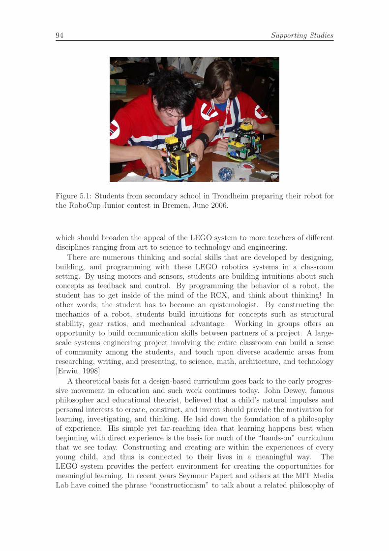
94 Supporting Studies

Figure 5.1: Students from secondary school in Trondheim preparing their robot forthe RoboCup Junior contest in Bremen, June 2006.

which should broaden the appeal of the LEGO system to more teachers of differentdisciplines ranging from art to science to technology and engineering.

There are numerous thinking and social skills that are developed by designing,building, and programming with these LEGO robotics systems in a classroomsetting. By using motors and sensors, students are building intuitions about suchconcepts as feedback and control. By programming the behavior of a robot, thestudent has to get inside of the mind of the RCX, and think about thinking! Inother words, the student has to become an epistemologist. By constructing themechanics of a robot, students build intuitions for concepts such as structuralstability, gear ratios, and mechanical advantage. Working in groups offers anopportunity to build communication skills between partners of a project. A large-scale systems engineering project involving the entire classroom can build a senseof community among the students, and touch upon diverse academic areas fromresearching, writing, and presenting, to science, math, architecture, and technology[Erwin, 1998].

A theoretical basis for a design-based curriculum goes back to the early progres-sive movement in education and such work continues today. John Dewey, famousphilosopher and educational theorist, believed that a child’s natural impulses andpersonal interests to create, construct, and invent should provide the motivation forlearning, investigating, and thinking. He laid down the foundation of a philosophyof experience. His simple yet far-reaching idea that learning happens best whenbeginning with direct experience is the basis for much of the “hands-on” curriculumthat we see today. Constructing and creating are within the experiences of everyyoung child, and thus is connected to their lives in a meaningful way. TheLEGO system provides the perfect environment for creating the opportunities formeaningful learning. In recent years Seymour Papert and others at the MIT MediaLab have coined the phrase “constructionism” to talk about a related philosophy of

5.1 Role of Robotics in Education 95

learning. Taking the idea from constructivism that knowledge in constructed insideones head (and not transmitted into the head like a pipeline), constructionism addsthat such knowledge construction inside the head is facilitated by constructionsoutside of the head, be it computer programs or physical models [Papert, 1999]. Inthis type of education, the learning takes place in the problem-solving, ”debugging”,and engineering designing and testing [Papert, 1999].

5.1.3 Teaching-Learning Materials

Throughout the recent years, many countries adopted the vision of using roboticsin schools. Robotics construction sets were purchased to thousands of primaryand secondary schools, and hundreds of teachers went through series of seminarswhere they received first-hand experience and assistance in using the sets in theclassrooms. Robotics sets are useful both at the lessons of Physics, Mathematics, andtechnology/IT/programming. In addition, they increase the students’ and pupils’motivation and learning satisfaction.

To program the intelligence into the Mindstorms robotics set, students would re-quire to use computer software to design their program to be run on the robotics set.The default standard computer software that comes with the original version of theMindstorms is RCX Code. RCX Code is a simple visual programming environmentthat caters for basic capabilities of Mindstorms. It enables user to visually plugprogramming module into each other to form a program. The educational versionof Mindstorms set comes with the software ROBOLAB. There are many otherhigh-end advanced Mindstorms programming environments developed by individualenthusiasts and groups. Most of these programming software are distributed on theInternet. Below are a few examples of these software packages:

• NQC – A text-based Mindstorms programming tool based on the popularprogramming language C.

• Bot-Kit – An interactive object oriented environment for the RCX usingSmalltalk programming language.

• TalkRCX – A programming interpreter for programming Mindstorms in Linuxenvironment

• Mind Control – A Visual Basic program that interprets user command text.

• LegOS (BrickOS) – A real C-compiler (based on GNU GCC) that providescomplete access to all RCX’s functionality and hardware, and fastest possiblecode.

• LejOS – A Java compiler and virtual machine for RCX. RCX as an embeddeddevice suffers from performance and memory limitations, and therefore is notvery suitable for Java programming that inherently implies overhead and isnot suitable for real-time performance, nevertheless, LejOS is a great tool forJava fans and programmers.

96 Supporting Studies

Educators could choose to develop their own Mindstorms software for theircurricular needs since the manufacturer made available a software development kit(SDK) that makes this possible (http://www.legomindstorms.com/sdk).

There are a few curricular materials available at the moment, from the officialmanufacturer channel and third party channel. Examples include the project ofLondon Grid for Learning and work of [Rosenblatt and Choset, 2000]. LEGO pro-vides a set of inspiration booklets on mechanics, buildings, energy, and robots, anda set of 16 activities with worksheets and supporting CD: Science and TechnologyActivity Pack. Extensive work of LDAPS team (LEGO Design and ProgrammingSystem), which was at the start of RoboLab system, produced multiple creativeproject ideas [URL - LDAPS]. These are described also in the book [Erwin, 2001].In her the recent book, Barbara Bratzel, a teacher at Shady Hill School, a preKthrough 8 independent school in Cambridge, Massachusetts, has developed a project-based course that teaches classical mechanics through engineering [Bratzel, 2005].Comprehensive set of materials is provided by CMU Robotics Academy [URL - CMURobotics Academy]. Yet, there is a large potential for more curriculum material thatwould be easy to use for teachers without extensive previous experience and technicalcompetence.

At the college and university level, Robotics can be found not only in the studydirections of automation, and robotics, but more often finds a place in other studyprograms, including Computer Science. For instance, at Indiana University, LEGORobotics sets have been used in the undergraduate computer science course, [Jadud,2000].

5.1.4 Robotics Contests

A very useful drive in the progress of robotics outside of the doors of advancedresearch laboratories has the origin in robotics contests. These exist at all levels– from simple local hobbyists’ meetings to large international events (for example,[URL - RoboCup], [URL - Fira], [URL - Eurobot]) and from simple-tasks suchas line-following (for example, [URL - Istrobot]) to complex tasks requiring intel-ligent reasoning, planning, and complex navigation (for example, AAAI roboticscompetition). A short overview can be found for example in [Balogh, 2005], andan exhaustive list is maintained at [URL - Contests]. The competitive atmosphereof the contests contributes strongly to motivation. Figure 5.1 shows a team ofNorwegian students at RoboCup Junior World championship.

5.2 Creative Educational Platforms

The importance and impact of robotics and automation systems as part of theevolution of mankind is obvious and inevitable. In order to achieve sustainableand steady progress of the technology, supply of the qualified workers is essential.In a democratic society with the freedom of choice, this can be achieved onlythrough promoting the interest of young people in technology, and maximizingtheir possibilities for hands-on experiences and small scientific and technological

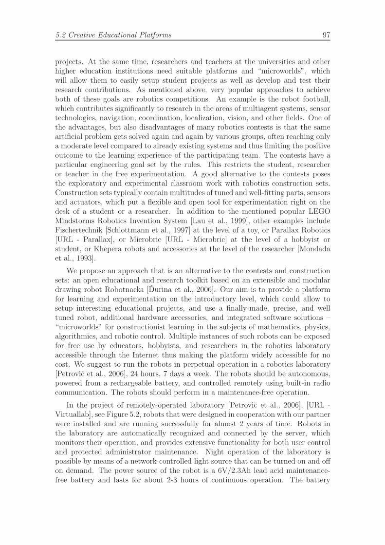
5.2 Creative Educational Platforms 97

projects. At the same time, researchers and teachers at the universities and otherhigher education institutions need suitable platforms and “microworlds”, whichwill allow them to easily setup student projects as well as develop and test theirresearch contributions. As mentioned above, very popular approaches to achieveboth of these goals are robotics competitions. An example is the robot football,which contributes significantly to research in the areas of multiagent systems, sensortechnologies, navigation, coordination, localization, vision, and other fields. One ofthe advantages, but also disadvantages of many robotics contests is that the sameartificial problem gets solved again and again by various groups, often reaching onlya moderate level compared to already existing systems and thus limiting the positiveoutcome to the learning experience of the participating team. The contests have aparticular engineering goal set by the rules. This restricts the student, researcheror teacher in the free experimentation. A good alternative to the contests posesthe exploratory and experimental classroom work with robotics construction sets.Construction sets typically contain multitudes of tuned and well-fitting parts, sensorsand actuators, which put a flexible and open tool for experimentation right on thedesk of a student or a researcher. In addition to the mentioned popular LEGOMindstorms Robotics Invention System [Lau et al., 1999], other examples includeFischertechnik [Schlottmann et al., 1997] at the level of a toy, or Parallax Robotics[URL - Parallax], or Microbric [URL - Microbric] at the level of a hobbyist orstudent, or Khepera robots and accessories at the level of the researcher [Mondadaet al., 1993].

We propose an approach that is an alternative to the contests and constructionsets: an open educational and research toolkit based on an extensible and modulardrawing robot Robotnacka [Durina et al., 2006]. Our aim is to provide a platformfor learning and experimentation on the introductory level, which could allow tosetup interesting educational projects, and use a finally-made, precise, and welltuned robot, additional hardware accessories, and integrated software solutions –“microworlds” for constructionist learning in the subjects of mathematics, physics,algorithmics, and robotic control. Multiple instances of such robots can be exposedfor free use by educators, hobbyists, and researchers in the robotics laboratoryaccessible through the Internet thus making the platform widely accessible for nocost. We suggest to run the robots in perpetual operation in a robotics laboratory[Petrovic et al., 2006], 24 hours, 7 days a week. The robots should be autonomous,powered from a rechargeable battery, and controlled remotely using built-in radiocommunication. The robots should perform in a maintenance-free operation.

In the project of remotely-operated laboratory [Petrovic et al., 2006], [URL -Virtuallab], see Figure 5.2, robots that were designed in cooperation with our partnerwere installed and are running successfully for almost 2 years of time. Robots inthe laboratory are automatically recognized and connected by the server, whichmonitors their operation, and provides extensive functionality for both user controland protected administrator maintenance. Night operation of the laboratory ispossible by means of a network-controlled light source that can be turned on and offon demand. The power source of the robot is a 6V/2.3Ah lead acid maintenance-free battery and lasts for about 2-3 hours of continuous operation. The battery

98 Supporting Studies

Figure 5.2: Viewing of the remotely-accessible robotics laboratory in a web-browser.The scene contains three robots and geometric shapes that can be detected by thecamera.

is recharged automatically. With its open architecture, the laboratory has goodpossibilities to be used both in research educational projects [Petrovic, 2005] forprimary and secondary schools, as well as research and project platform for bothundergraduate and graduate students. It can be employed in distance learning. Thelaboratory is used for several undergraduate semester and diploma projects, e.g.analysis of the power sources for mobile robots, platform for development of multi-agent architectures, as well as for experiments of graduate students with evolutionaryand BB robotics. In the educational projects, the robots in the laboratory canbe attached to the software turtle objects in the Logo programming language ofa student sitting anywhere around the world. In combination with the top-viewcamera, the laboratory can be used as an educational tool in lessons of mathematics,physics, and programming. For instance, the software is able to detect polygonshapes, and provides a creative environment for solving constructive geometry tasksin a novel and exciting way. With the ability to move objects in the arena, therobots are a perfect platform for experiments with computer vision and artificialintelligence. The robots can work as a physical instantiation and testing platformfor planning and reasoning algorithms. The exploitation of robots is also madethrough the Robotics introductory course at the Faculty of Electrical Engineeringand Information Technology STU, [Balogh, 2007].

The programming of the robots is designed to be easy to understand and learn.For an example, Figure 5.3 depicts the portion of a C/C++ program used to make

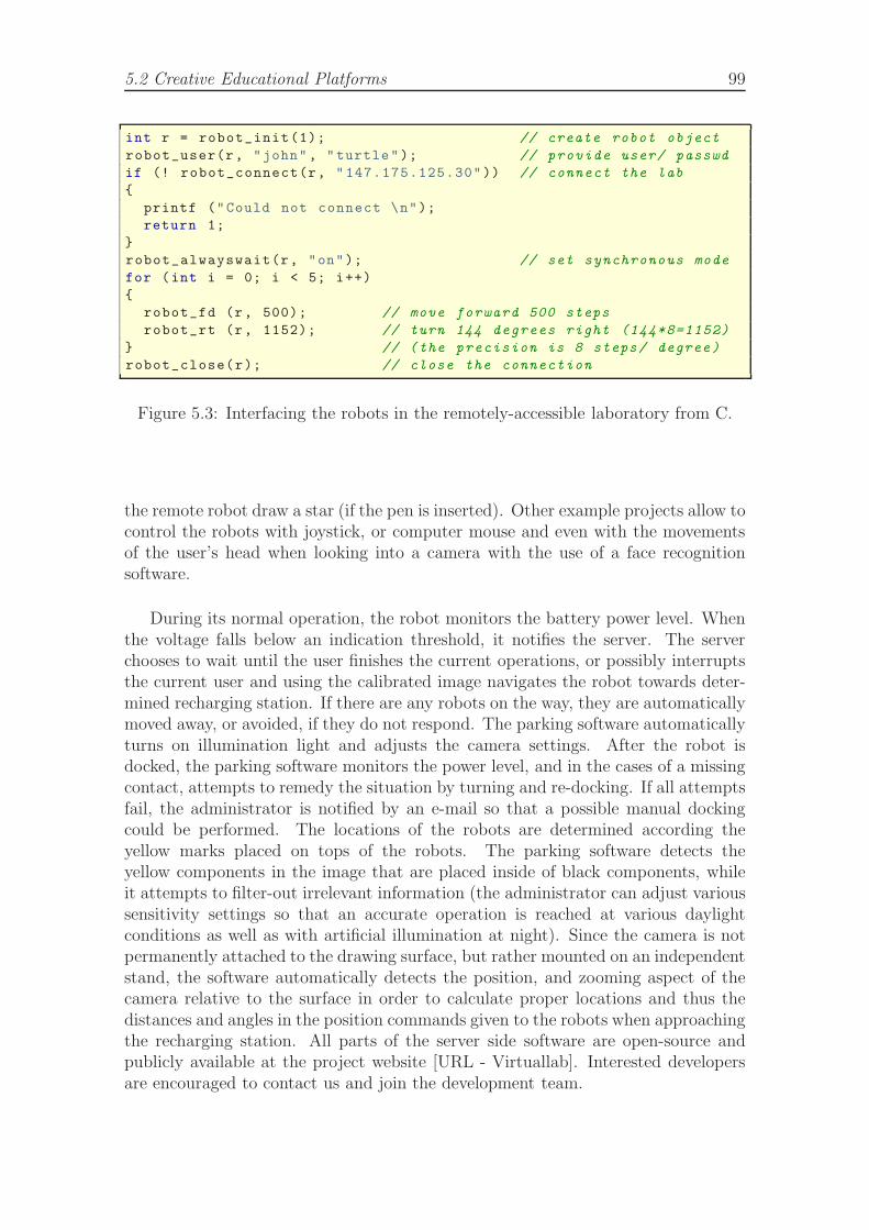
5.2 Creative Educational Platforms 99

int r = robot_init(1); // create robot object

robot_user(r, "john", "turtle"); // provide user/ passwd

if (! robot_connect(r, "147.175.125.30")) // connect the lab

{

printf ("Could not connect \n");

return 1;

}

robot_alwayswait(r, "on"); // set synchronous mode

for (int i = 0; i < 5; i++)

{

robot_fd (r, 500); // move forward 500 steps

robot_rt (r, 1152); // turn 144 degrees right (144*8=1152)

} // (the precision is 8 steps/ degree)

robot_close(r); // close the connection

Figure 5.3: Interfacing the robots in the remotely-accessible laboratory from C.

the remote robot draw a star (if the pen is inserted). Other example projects allow tocontrol the robots with joystick, or computer mouse and even with the movementsof the user’s head when looking into a camera with the use of a face recognitionsoftware.

During its normal operation, the robot monitors the battery power level. Whenthe voltage falls below an indication threshold, it notifies the server. The serverchooses to wait until the user finishes the current operations, or possibly interruptsthe current user and using the calibrated image navigates the robot towards deter-mined recharging station. If there are any robots on the way, they are automaticallymoved away, or avoided, if they do not respond. The parking software automaticallyturns on illumination light and adjusts the camera settings. After the robot isdocked, the parking software monitors the power level, and in the cases of a missingcontact, attempts to remedy the situation by turning and re-docking. If all attemptsfail, the administrator is notified by an e-mail so that a possible manual dockingcould be performed. The locations of the robots are determined according theyellow marks placed on tops of the robots. The parking software detects theyellow components in the image that are placed inside of black components, whileit attempts to filter-out irrelevant information (the administrator can adjust varioussensitivity settings so that an accurate operation is reached at various daylightconditions as well as with artificial illumination at night). Since the camera is notpermanently attached to the drawing surface, but rather mounted on an independentstand, the software automatically detects the position, and zooming aspect of thecamera relative to the surface in order to calculate proper locations and thus thedistances and angles in the position commands given to the robots when approachingthe recharging station. All parts of the server side software are open-source andpublicly available at the project website [URL - Virtuallab]. Interested developersare encouraged to contact us and join the development team.

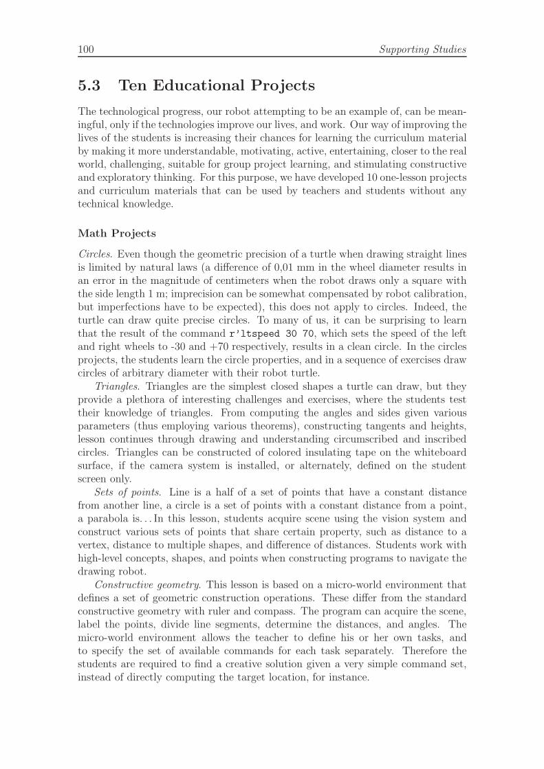
100 Supporting Studies

5.3 Ten Educational Projects

The technological progress, our robot attempting to be an example of, can be mean-ingful, only if the technologies improve our lives, and work. Our way of improving thelives of the students is increasing their chances for learning the curriculum materialby making it more understandable, motivating, active, entertaining, closer to the realworld, challenging, suitable for group project learning, and stimulating constructiveand exploratory thinking. For this purpose, we have developed 10 one-lesson projectsand curriculum materials that can be used by teachers and students without anytechnical knowledge.

Math Projects

Circles. Even though the geometric precision of a turtle when drawing straight linesis limited by natural laws (a difference of 0,01 mm in the wheel diameter results inan error in the magnitude of centimeters when the robot draws only a square withthe side length 1 m; imprecision can be somewhat compensated by robot calibration,but imperfections have to be expected), this does not apply to circles. Indeed, theturtle can draw quite precise circles. To many of us, it can be surprising to learnthat the result of the command r’ltspeed 30 70, which sets the speed of the leftand right wheels to -30 and +70 respectively, results in a clean circle. In the circlesprojects, the students learn the circle properties, and in a sequence of exercises drawcircles of arbitrary diameter with their robot turtle.

Triangles. Triangles are the simplest closed shapes a turtle can draw, but theyprovide a plethora of interesting challenges and exercises, where the students testtheir knowledge of triangles. From computing the angles and sides given variousparameters (thus employing various theorems), constructing tangents and heights,lesson continues through drawing and understanding circumscribed and inscribedcircles. Triangles can be constructed of colored insulating tape on the whiteboardsurface, if the camera system is installed, or alternately, defined on the studentscreen only.

Sets of points. Line is a half of a set of points that have a constant distancefrom another line, a circle is a set of points with a constant distance from a point,a parabola is. . . In this lesson, students acquire scene using the vision system andconstruct various sets of points that share certain property, such as distance to avertex, distance to multiple shapes, and difference of distances. Students work withhigh-level concepts, shapes, and points when constructing programs to navigate thedrawing robot.

Constructive geometry. This lesson is based on a micro-world environment thatdefines a set of geometric construction operations. These differ from the standardconstructive geometry with ruler and compass. The program can acquire the scene,label the points, divide line segments, determine the distances, and angles. Themicro-world environment allows the teacher to define his or her own tasks, andto specify the set of available commands for each task separately. Therefore thestudents are required to find a creative solution given a very simple command set,instead of directly computing the target location, for instance.

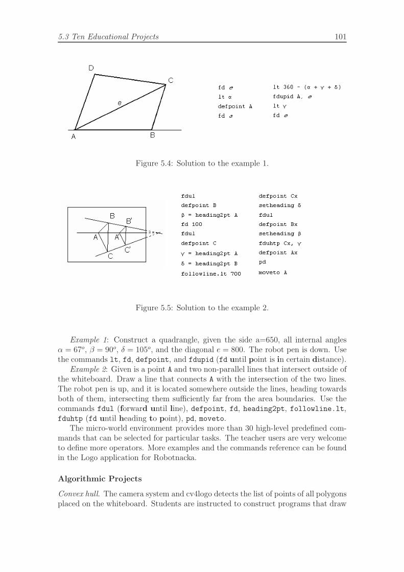
5.3 Ten Educational Projects 101

Figure 5.4: Solution to the example 1.

Figure 5.5: Solution to the example 2.

Example 1: Construct a quadrangle, given the side a=650, all internal anglesα = 67o, β = 90o, δ = 105o, and the diagonal e = 800. The robot pen is down. Usethe commands lt, fd, defpoint, and fdupid (fd until point is in certain distance).

Example 2: Given is a point A and two non-parallel lines that intersect outside ofthe whiteboard. Draw a line that connects A with the intersection of the two lines.The robot pen is up, and it is located somewhere outside the lines, heading towardsboth of them, intersecting them sufficiently far from the area boundaries. Use thecommands fdul (forward until line), defpoint, fd, heading2pt, followline.lt,fduhtp (fd until heading to point), pd, moveto.

The micro-world environment provides more than 30 high-level predefined com-mands that can be selected for particular tasks. The teacher users are very welcometo define more operators. More examples and the commands reference can be foundin the Logo application for Robotnacka.

Algorithmic Projects

Convex hull. The camera system and cv4logo detects the list of points of all polygonsplaced on the whiteboard. Students are instructed to construct programs that draw

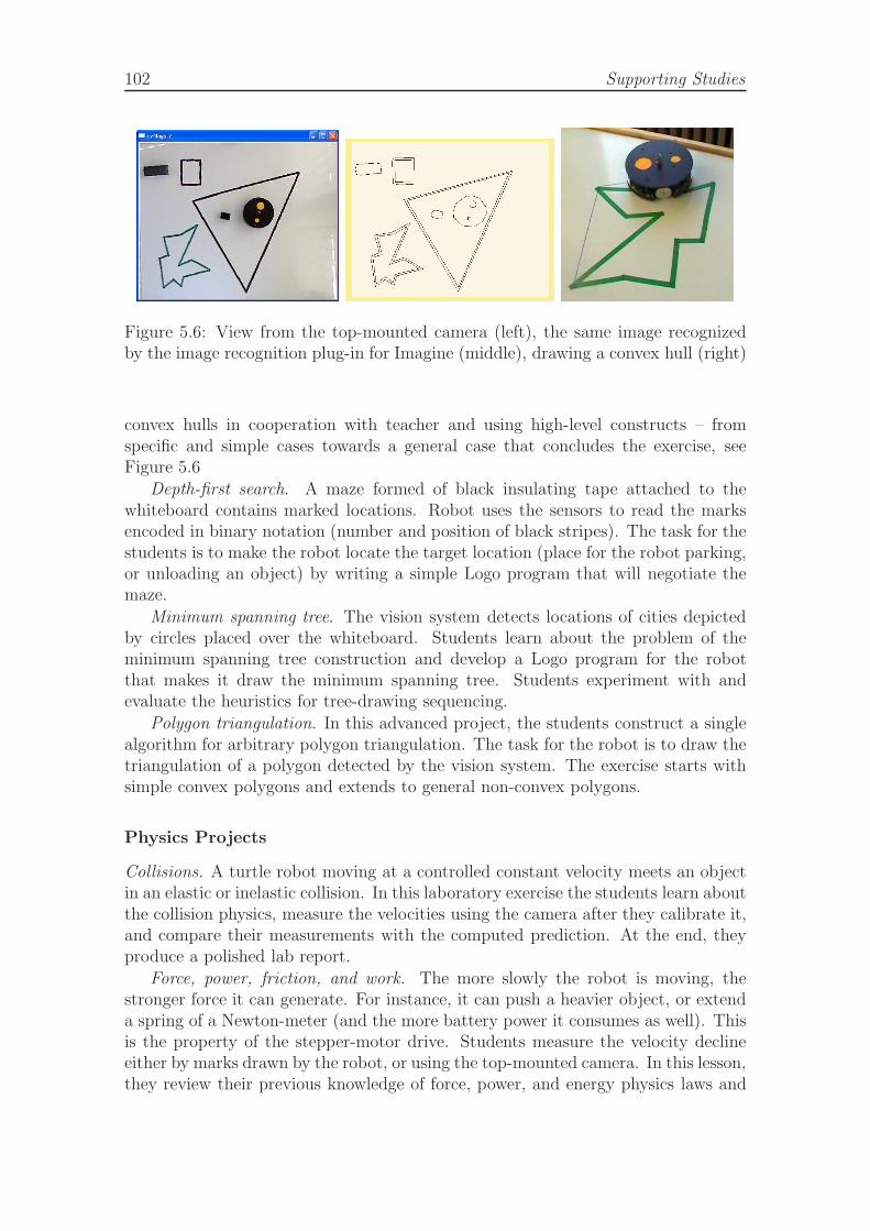
102 Supporting Studies

Figure 5.6: View from the top-mounted camera (left), the same image recognizedby the image recognition plug-in for Imagine (middle), drawing a convex hull (right)

convex hulls in cooperation with teacher and using high-level constructs – fromspecific and simple cases towards a general case that concludes the exercise, seeFigure 5.6

Depth-first search. A maze formed of black insulating tape attached to thewhiteboard contains marked locations. Robot uses the sensors to read the marksencoded in binary notation (number and position of black stripes). The task for thestudents is to make the robot locate the target location (place for the robot parking,or unloading an object) by writing a simple Logo program that will negotiate themaze.

Minimum spanning tree. The vision system detects locations of cities depictedby circles placed over the whiteboard. Students learn about the problem of theminimum spanning tree construction and develop a Logo program for the robotthat makes it draw the minimum spanning tree. Students experiment with andevaluate the heuristics for tree-drawing sequencing.

Polygon triangulation. In this advanced project, the students construct a singlealgorithm for arbitrary polygon triangulation. The task for the robot is to draw thetriangulation of a polygon detected by the vision system. The exercise starts withsimple convex polygons and extends to general non-convex polygons.

Physics Projects

Collisions. A turtle robot moving at a controlled constant velocity meets an objectin an elastic or inelastic collision. In this laboratory exercise the students learn aboutthe collision physics, measure the velocities using the camera after they calibrate it,and compare their measurements with the computed prediction. At the end, theyproduce a polished lab report.

Force, power, friction, and work. The more slowly the robot is moving, thestronger force it can generate. For instance, it can push a heavier object, or extenda spring of a Newton-meter (and the more battery power it consumes as well). Thisis the property of the stepper-motor drive. Students measure the velocity declineeither by marks drawn by the robot, or using the top-mounted camera. In this lesson,they review their previous knowledge of force, power, and energy physics laws and

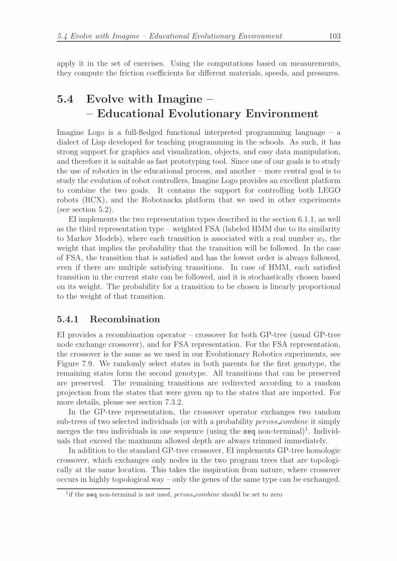
5.4 Evolve with Imagine – Educational Evolutionary Environment 103

apply it in the set of exercises. Using the computations based on measurements,they compute the friction coefficients for different materials, speeds, and pressures.

5.4 Evolve with Imagine –

– Educational Evolutionary Environment

Imagine Logo is a full-fledged functional interpreted programming language – adialect of Lisp developed for teaching programming in the schools. As such, it hasstrong support for graphics and visualization, objects, and easy data manipulation,and therefore it is suitable as fast prototyping tool. Since one of our goals is to studythe use of robotics in the educational process, and another – more central goal is tostudy the evolution of robot controllers, Imagine Logo provides an excellent platformto combine the two goals. It contains the support for controlling both LEGOrobots (RCX), and the Robotnacka platform that we used in other experiments(see section 5.2).

EI implements the two representation types described in the section 6.1.1, as wellas the third representation type – weighted FSA (labeled HMM due to its similarityto Markov Models), where each transition is associated with a real number wt, theweight that implies the probability that the transition will be followed. In the caseof FSA, the transition that is satisfied and has the lowest order is always followed,even if there are multiple satisfying transitions. In case of HMM, each satisfiedtransition in the current state can be followed, and it is stochastically chosen basedon its weight. The probability for a transition to be chosen is linearly proportionalto the weight of that transition.

5.4.1 Recombination

EI provides a recombination operator – crossover for both GP-tree (usual GP-treenode exchange crossover), and for FSA representation. For the FSA representation,the crossover is the same as we used in our Evolutionary Robotics experiments, seeFigure 7.9. We randomly select states in both parents for the first genotype, theremaining states form the second genotype. All transitions that can be preservedare preserved. The remaining transitions are redirected according to a randomprojection from the states that were given up to the states that are imported. Formore details, please see section 7.3.2.

In the GP-tree representation, the crossover operator exchanges two randomsub-trees of two selected individuals (or with a probability pcross combine it simplymerges the two individuals in one sequence (using the seq non-terminal)1. Individ-uals that exceed the maximum allowed depth are always trimmed immediately.

In addition to the standard GP-tree crossover, EI implements GP-tree homologiccrossover, which exchanges only nodes in the two program trees that are topologi-cally at the same location. This takes the inspiration from nature, where crossoveroccurs in highly topological way – only the genes of the same type can be exchanged.

1if the seq non-terminal is not used, pcross combine should be set to zero

104 Supporting Studies

It reduces the bloat (useless offspring), and smooths the fitness landscape – althoughalso slightly decreases the discovering potential of the search. The ratio of thehomologic crossover can be controlled using phomologic crossover parameter.

In both representations, EI supports brooding crossover, i.e. generating severalbroods of offspring from each selected pair of parents, and evaluating them onlyon a stochastically selected subset of testing sample (in order to avoid too highgrowth of CPU demand). Only the best two of all the generated offspring arechosen for the new generation. The parameter crossover brooding determines thenumber of offspring pairs generated, and the parameter cross brood num starts qdetermines the relative size of the subset of the training set for the brood evaluation(i.e. 1.0 means to use the whole set). Brooding increases the success rate of thecrossover, since GP-tree crossover usually generates several times more junk thanuseful genotypes. On the other hand, brooding decreases the creativity of the searchslightly, while some innovative offspring will perform worse than some other offspringof the same parents – in particular those that perform almost or exactly the sameas their parent. When they perform the same, it is often due to the fact thatthe difference in the genotypes of the parent and the offspring is irrelevant for theresulting behavior of the offspring. And while the parent already has a relativelyhigh fitness, the new useful innovative genotypes with somewhat smaller fitness thanthe parent are not accepted. Therefore the brooding crossover can either be limitedby pbrooding crossover parameter, or the user may require that the offspring withthe same fitness as the parent genotypes be discarded (parameter strict brooding),which, however, works well only for deterministic objective functions (i.e. the samegenotype always has the same fitness).

5.4.2 Mutation

For the GP-tree representation, EI utilizes the following operators:

• mut change: changes a random node (terminals → terminals, non-terminals→ non-terminals), or changes an argument of terminal/non-terminal, if any;

• mut exchange: exchanges two arbitrary nodes within the individual;

• mut insert: inserts a non-terminal node with a full random sub-tree some-where inside of the individual;

• mut remove: removes random node/sub-tree within individual;

• random node: replaces the whole individual with a completely new individual;

For the FSA representation, EI utilizes the following operators:

• mut change: changes a random transition: either by changing terminal,destination state (either randomly or by following another transition fromthe original destination state), changing relation, or splitting the transition totwo and inserting new state in the middle; alternately, it randomly reordersthe transitions in a single random state;

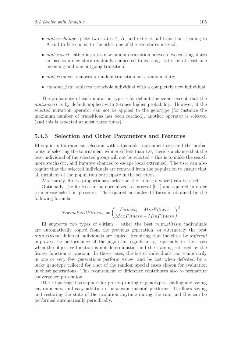
5.4 Evolve with Imagine 105

• mut exchange: picks two states A, B, and redirects all transitions leading toA and to B to point to the other one of the two states instead;

• mut insert: either inserts a new random transition between two existing statesor inserts a new state randomly connected to existing states by at least oneincoming and one outgoing transition.

• mut remove: removes a random transition or a random state;

• random fsa: replaces the whole individual with a completely new individual;

The probability of each mutation type is by default the same, except that themut insert is by default applied with 3-times higher probability. However, if theselected mutation operator can not be applied to the genotype (for instance themaximum number of transitions has been reached), another operator is selected(and this is repeated at most three times).

5.4.3 Selection and Other Parameters and Features

EI supports tournament selection with adjustable tournament size and the proba-bility of selecting the tournament winner (if less than 1.0, there is a chance that thebest individual of the selected group will not be selected – this is to make the searchmore stochastic, and improve chances to escape local extremes). The user can alsorequire that the selected individuals are removed from the population to ensure thatall members of the population participate in the selection.

Alternately, fitness-proportionate selection (i.e. roulette wheel) can be used.Optionally, the fitness can be normalized to interval [0,1] and squared in order

to increase selection pressure. The squared normalized fitness is obtained by thefollowing formula:

NormalizedF itnessi =

(

Fitnessi − MinFitness

MaxFitness − MinFitness

)2

EI supports two types of elitism – either the best num elitism individualsare automatically copied from the previous generation, or alternately the bestnum elitism different individuals are copied. Requiring that the elites be differentimproves the performance of the algorithm significantly, especially in the caseswhen the objective function is not deterministic, and the training set used by thefitness function is random. In those cases, the better individuals can temporarilyin one or very few generations perform worse, and be lost when defeated by alucky genotype tailored for a set of the random special cases chosen for evaluationin those generations. This requirement of difference contributes also to prematureconvergence prevention.

The EI package has support for pretty-printing of genotypes, loading and savingenvironments, and easy addition of new experimental platforms. It allows savingand restoring the state of the evolution anytime during the run, and this can beperformed automatically periodically.

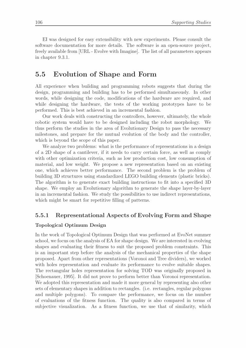
106 Supporting Studies

EI was designed for easy extensibility with new experiments. Please consult thesoftware documentation for more details. The software is an open-source project,freely available from [URL - Evolve with Imagine]. The list of all parameters appearsin chapter 9.3.1.

5.5 Evolution of Shape and Form

All experience when building and programming robots suggests that during thedesign, programming and building has to be performed simultaneously. In otherwords, while designing the code, modifications of the hardware are required, andwhile designing the hardware, the tests of the working prototypes have to beperformed. This is best achieved in an incremental fashion.

Our work deals with constructing the controllers, however, ultimately, the wholerobotic system would have to be designed including the robot morphology. Wethus perform the studies in the area of Evolutionary Design to pass the necessarymilestones, and prepare for the mutual evolution of the body and the controller,which is beyond the scope of this paper.

We analyze two problems: what is the performance of representations in a designof a 2D shape of a cantilever, if it needs to carry certain force, as well as complywith other optimization criteria, such as low production cost, low consumption ofmaterial, and low weight. We propose a new representation based on an existingone, which achieves better performance. The second problem is the problem ofbuilding 3D structures using standardized LEGO building elements (plastic bricks).The algorithm is to generate exact building instructions to fit into a specified 3Dshape. We employ an Evolutionary algorithm to generate the shape layer-by-layerin an incremental fashion. We study the possibilities to use indirect representations,which might be smart for repetitive filling of patterns.

5.5.1 Representational Aspects of Evolving Form and Shape

Topological Optimum Design

In the work of Topological Optimum Design that was performed at EvoNet summerschool, we focus on the analysis of EA for shape design. We are interested in evolvingshapes and evaluating their fitness to suit the proposed problem constraints. Thisis an important step before the analysis of the mechanical properties of the shapeproposed. Apart from other representations (Voronoi and Tree dividers), we workedwith holes representation and evaluate its performance to evolve suitable shapes.The rectangular holes representation for solving TOD was originally proposed in[Schoenauer, 1995]. It did not prove to perform better than Voronoi representation.We adopted this representation and made it more general by representing also othersets of elementary shapes in addition to rectangles. (i.e. rectangles, regular polygonsand multiple polygons). To compare the performance, we focus on the numberof evaluations of the fitness function. The quality is also compared in terms ofsubjective visualization. As a fitness function, we use that of similarity, which

5.5 Evolution of Shape and Form 107

Figure 5.7: Voronoi representation genotype and phenotype, [Schoenauer, 1995].

means that we evaluate how close is the evolved shape to the desired one. Similaritycould be defined as the number of bits matched divided between the total numbersof bits. This is a normalized fitness function between 0 and 1.

In the Voronoi representation, we consider a finite number of points V0 . . . Vn

(sites) of a given subset of Rn (the design domain). With each site Vi, we associatea set of all points of the design domain for which the closest Voronoi site is Vi,termed cell. The diagram is the partition of the design domain defined by the cells.Each cell is a polyhedral subset of the design domain, see [Preparata and Shamos,1985] for a detailed introduction.

Genotype is a variable length list of Voronoi sites, each site being labeled 0 or 1.The corresponding Voronoi diagram represents a partition of the design domain intotwo subsets, if each Voronoi cell is labeled as its associated site. The correspondingphenotype is the shape with corresponding black and white cells, see Figure 5.7.

The initial population is of size 100 for each shape. The algorithm is using anEvolutionary Strategy (N , 3N) with weak elitism, crossover ratio 0.7, and mutationratio 0.7.

In the Holes representation, the genotype consists of a set of elementary shapes.The corresponding shape is obtained from a full 2D plate of material by clippingout the shapes listed in the genotype, see Figure 5.8. In our experiments, we haveexperimented with three different kinds of holes representation: rectangles, regularpolygons, and regular polygons with repetitions. In the first, rectangles of randomreal-valued dimensions are placed at random real-valued locations. In regularpolygons representation, equilateral polygons with random real-valued lengths ofsides are placed at random real-valued coordinates and have random number ofvertices (N ≥ 3). In the last representation, regular polygons are clipped out fromthe plate several times (count) with regular horizontal or vertical spacing.

The genotype, similarly to Voronoi representation consists of a list of labeledpoints (sites). In contrast to Voronoi representation, the site labels are not simplebits determining presence or absence of a material, but they describe the particularelementary shape(s). In case of rectangles representation, the site label is simply a

108 Supporting Studies

Figure 5.8: Holes representation with various geometric shapes creates more naturalshapes using less shapes than rectangular-holes representation.

pair (width, height), dimensions of the corresponding rectangle. Labels in regularpolygons representation consist of tuples (N , r, tilted), where N is the number ofvertices of the polygon, r is the radius, i.e. the distance of the vertices from thecenter (site), and tilted is a binary flag determining the placement of the polygon.Polygons can be placed either by having one (or two, if N is even) of their verticeshorizontally aligned with the center (a), or by having the center of one (or two)of their sites aligned with the center (b). Labels in case of the regular polygonswith repetitions representation contain a triple (count, spacing, orientation) inaddition, where count is the number of times that the polygon is clipped out (real-value), spacing is the distance between the centuries of consecutive polygons, andorientation is either vertical or horizontal.

The genotype is converted to phenotype — a mesh with a particular resolution.The conversion is performed with 3 different discretization operators.

The genotype is initialized with uniformly distributed number of points (thenumber is uniformly distributed from 1 to maximum number of sites) labeled withrandom shapes. In case of rectangles, the dimensions of the shapes are randomlydistributed in the interval [0,κ · plate width], [0,κ · plate height], where κ is aparameter from [0,1].

The holes representation uses the same geometric crossover as is used in theVoronoi representation. A random line is drawn over both individuals and theoffspring is formed by combining geometric sub-parts of the crossed genotypes.The genotypes in the holes representation are altered using the following mutationoperators:

• AddSite adds a new site (rectangle, polygon, or set of polygons). The numberof sites is limited by a parameter maxsize.

• RemoveSite removes one of the existing sites

• MoveOne moves one of the sites by a random displacement (the standarddeviation for the normal distribution from which random displacement is

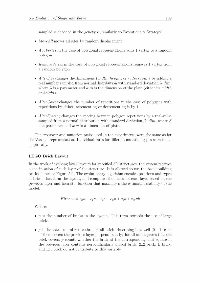
5.5 Evolution of Shape and Form 109

sampled is encoded in the genotype, similarly to Evolutionary Strategy)

• MoveAll moves all sites by random displacement

• AddVertex in the case of polygonal representations adds 1 vertex to a randompolygon

• RemoveVertex in the case of polygonal representations removes 1 vertex froma random polygon

• AlterSize changes the dimensions (width, height, or radius resp.) by adding areal number sampled from normal distribution with standard deviation λ·dim,where λ is a parameter and dim is the dimension of the plate (either its widthor height).

• AlterCount changes the number of repetitions in the case of polygons withrepetitions by either incrementing or decrementing it by 1

• AlterSpacing changes the spacing between polygon repetitions by a real-valuesampled from a normal distribution with standard deviation β · dim, where βis a parameter and dim is a dimension of plate.

The crossover and mutation ratios used in the experiments were the same as forthe Voronoi representation. Individual rates for different mutation types were tunedempirically.

LEGO Brick Layout

In the work of evolving layer layouts for specified 3D structures, the system receivesa specification of each layer of the structure. It is allowed to use the basic buildingbricks shown at Figure 5.9. The evolutionary algorithm encodes positions and typesof bricks that form the layout, and computes the fitness of each layer based on theprevious layer and heuristic function that maximizes the estimated stability of themodel:

Fitness = cnn + cpp + cee + cuu + coo + cnbnb

Where:

• n is the number of bricks in the layout. This term rewards the use of largebricks.

• p is the total sum of ratios through all bricks describing how well (0 – 1) eachof them covers the previous layer perpendicularly: for all unit squares that thebrick covers, p counts whether the brick at the corresponding unit square inthe previous layer contains perpendicularly placed brick; 2x2 brick, L brick,and 1x1 brick do not contribute to this variable.

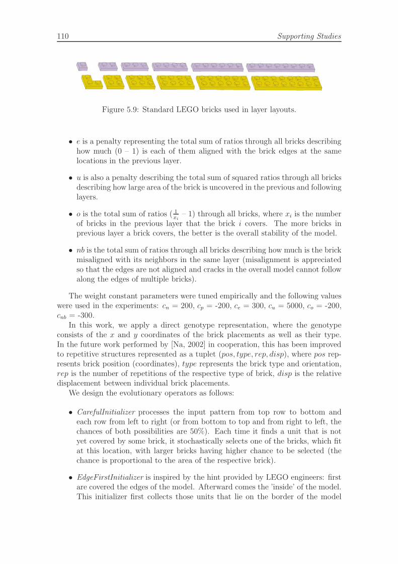
110 Supporting Studies

Figure 5.9: Standard LEGO bricks used in layer layouts.

• e is a penalty representing the total sum of ratios through all bricks describinghow much (0 – 1) is each of them aligned with the brick edges at the samelocations in the previous layer.

• u is also a penalty describing the total sum of squared ratios through all bricksdescribing how large area of the brick is uncovered in the previous and followinglayers.

• o is the total sum of ratios ( 1xi

– 1) through all bricks, where xi is the numberof bricks in the previous layer that the brick i covers. The more bricks inprevious layer a brick covers, the better is the overall stability of the model.

• nb is the total sum of ratios through all bricks describing how much is the brickmisaligned with its neighbors in the same layer (misalignment is appreciatedso that the edges are not aligned and cracks in the overall model cannot followalong the edges of multiple bricks).

The weight constant parameters were tuned empirically and the following valueswere used in the experiments: cn = 200, cp = -200, ce = 300, cu = 5000, co = -200,cnb = -300.

In this work, we apply a direct genotype representation, where the genotypeconsists of the x and y coordinates of the brick placements as well as their type.In the future work performed by [Na, 2002] in cooperation, this has been improvedto repetitive structures represented as a tuplet (pos, type, rep, disp), where pos rep-resents brick position (coordinates), type represents the brick type and orientation,rep is the number of repetitions of the respective type of brick, disp is the relativedisplacement between individual brick placements.

We design the evolutionary operators as follows:

• CarefulInitializer processes the input pattern from top row to bottom andeach row from left to right (or from bottom to top and from right to left, thechances of both possibilities are 50%). Each time it finds a unit that is notyet covered by some brick, it stochastically selects one of the bricks, which fitat this location, with larger bricks having higher chance to be selected (thechance is proportional to the area of the respective brick).

• EdgeFirstInitializer is inspired by the hint provided by LEGO engineers: firstare covered the edges of the model. Afterward comes the ’inside’ of the model.This initializer first collects those units that lie on the border of the model

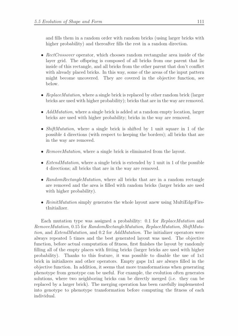
5.5 Evolution of Shape and Form 111

and fills them in a random order with random bricks (using larger bricks withhigher probability) and thereafter fills the rest in a random direction.

• RectCrossover operator, which chooses random rectangular area inside of thelayer grid. The offspring is composed of all bricks from one parent that lieinside of this rectangle, and all bricks from the other parent that don’t conflictwith already placed bricks. In this way, some of the areas of the input patternmight become uncovered. They are covered in the objective function, seebelow.

• ReplaceMutation, where a single brick is replaced by other random brick (largerbricks are used with higher probability); bricks that are in the way are removed.

• AddMutation, where a single brick is added at a random empty location, largerbricks are used with higher probability; bricks in the way are removed.

• ShiftMutation, where a single brick is shifted by 1 unit square in 1 of thepossible 4 directions (with respect to keeping the borders); all bricks that arein the way are removed.

• RemoveMutation, where a single brick is eliminated from the layout.

• ExtendMutation, where a single brick is extended by 1 unit in 1 of the possible4 directions; all bricks that are in the way are removed.

• RandomRectangleMutation, where all bricks that are in a random rectangleare removed and the area is filled with random bricks (larger bricks are usedwith higher probability).

• ReinitMutation simply generates the whole layout anew using MultiEdgeFirs-tInitializer.

Each mutation type was assigned a probability: 0.1 for ReplaceMutation andRemoveMutation, 0.15 for RandomRectangleMutation, ReplaceMutation, ShiftMuta-tion, and ExtendMutation, and 0.2 for AddMutation. The initializer operators werealways repeated 5 times and the best generated layout was used. The objectivefunction, before actual computation of fitness, first finishes the layout by randomlyfilling all of the empty places with fitting bricks (larger bricks are used with higherprobability). Thanks to this feature, it was possible to disable the use of 1x1brick in initializers and other operators. Empty gaps 1x1 are always filled in theobjective function. In addition, it seems that more transformations when generatingphenotype from genotype can be useful. For example, the evolution often generatessolutions, where two neighboring bricks can be directly merged (i.e. they can bereplaced by a larger brick). The merging operation has been carefully implementedinto genotype to phenotype transformation before computing the fitness of eachindividual.

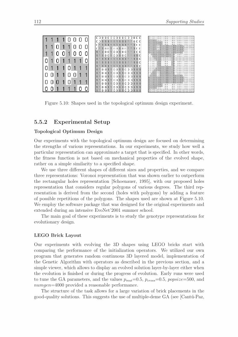
112 Supporting Studies

Figure 5.10: Shapes used in the topological optimum design experiment.

5.5.2 Experimental Setup

Topological Optimum Design

Our experiments with the topological optimum design are focused on determiningthe strengths of various representations. In our experiments, we study how well aparticular representation can approximate a target that is specified. In other words,the fitness function is not based on mechanical properties of the evolved shape,rather on a simple similarity to a specified shape.

We use three different shapes of different sizes and properties, and we comparethree representations: Voronoi representation that was shown earlier to outperformthe rectangular holes representation [Schoenauer, 1995], with our proposed holesrepresentation that considers regular polygons of various degrees. The third rep-resentation is derived from the second (holes with polygons) by adding a featureof possible repetitions of the polygons. The shapes used are shown at Figure 5.10.We employ the software package that was designed for the original experiments andextended during an intensive EvoNet’2001 summer school.

The main goal of these experiments is to study the genotype representations forevolutionary design.

LEGO Brick Layout

Our experiments with evolving the 3D shapes using LEGO bricks start withcomparing the performance of the initialization operators. We utilized our ownprogram that generates random continuous 3D layered model, implementation ofthe Genetic Algorithm with operators as described in the previous section, and asimple viewer, which allows to display an evolved solution layer-by-layer either whenthe evolution is finished or during the progress of evolution. Early runs were usedto tune the GA parameters, and the values pmut=0.5, pcross=0.5, popsize=500, andnumgen=4000 provided a reasonable performance.

The structure of the task allows for a large variation of brick placements in thegood-quality solutions. This suggests the use of multiple-deme GA (see [Cantu-Paz,

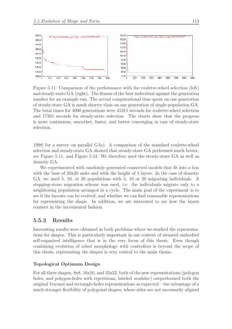
5.5 Evolution of Shape and Form 113

Figure 5.11: Comparison of the performance with the roulette-wheel selection (left)and steady-state GA (right). The fitness of the best individual against the generationnumber for an example run. The actual computational time spent on one generationof steady-state GA is much shorter than on one generation of single-population GA.The total times for 4000 generations were 41311 seconds for roulette-wheel selectionand 17391 seconds for steady-state selection. The charts show that the progressis more continuous, smoother, faster, and better converging in case of steady-stateselection.

1998] for a survey on parallel GAs). A comparison of the standard roulette-wheelselection and steady-state GA showed that steady-state GA performed much better,see Figure 5.11, and Figure 5.12. We therefore used the steady-state GA as well asdemetic GA.

We experimented with randomly-generated connected models that fit into a boxwith the base of 20x20 units and with the height of 5 layers. In the case of demeticGA, we used 5, 10, or 20 populations with 5, 10 or 20 migrating individuals. Astepping-stone migration scheme was used, i.e. the individuals migrate only to aneighboring population arranged in a cycle. The main goal of the experiment is tosee if the layouts can be evolved, and whether we can find reasonable representationsfor representing the shape. In addition, we are interested to see how the layersconnect in the incremental fashion.

5.5.3 Results

Interesting results were obtained in both problems where we studied the representa-tions for shapes. This is particularly important in our context of situated embodiedself-organized intelligence that is in the very focus of this thesis. Even thoughcombining evolution of robot morphology with controllers is beyond the scope ofthis thesis, representing the shapes is very central to the main theme.

Topological Optimum Design

For all three shapes, 8x8, 16x16, and 32x32, both of the new representations (polygonholes, and polygon-holes with repetitions, labeled modular) outperformed both theoriginal Voronoi and rectangle-holes representations as expected – the advantage of amuch stronger flexibility of polygonal shapes, where sides are not necessarily aligned

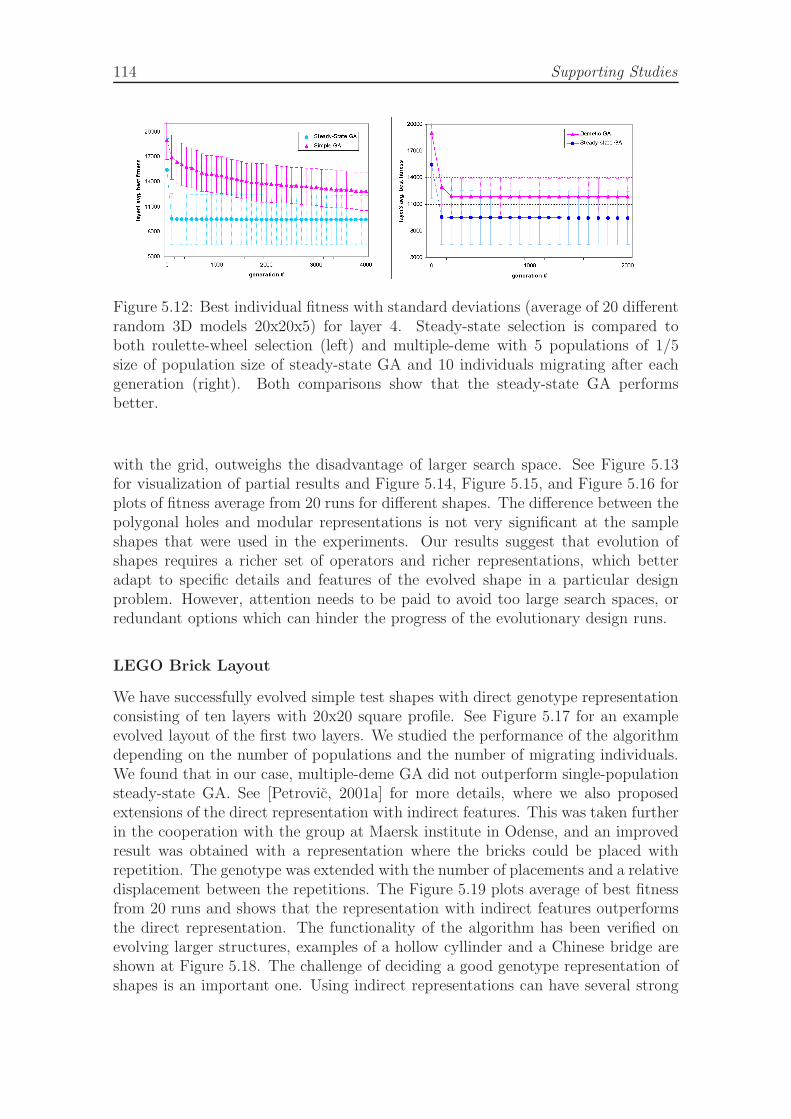
114 Supporting Studies

Figure 5.12: Best individual fitness with standard deviations (average of 20 differentrandom 3D models 20x20x5) for layer 4. Steady-state selection is compared toboth roulette-wheel selection (left) and multiple-deme with 5 populations of 1/5size of population size of steady-state GA and 10 individuals migrating after eachgeneration (right). Both comparisons show that the steady-state GA performsbetter.

with the grid, outweighs the disadvantage of larger search space. See Figure 5.13for visualization of partial results and Figure 5.14, Figure 5.15, and Figure 5.16 forplots of fitness average from 20 runs for different shapes. The difference between thepolygonal holes and modular representations is not very significant at the sampleshapes that were used in the experiments. Our results suggest that evolution ofshapes requires a richer set of operators and richer representations, which betteradapt to specific details and features of the evolved shape in a particular designproblem. However, attention needs to be paid to avoid too large search spaces, orredundant options which can hinder the progress of the evolutionary design runs.

LEGO Brick Layout

We have successfully evolved simple test shapes with direct genotype representationconsisting of ten layers with 20x20 square profile. See Figure 5.17 for an exampleevolved layout of the first two layers. We studied the performance of the algorithmdepending on the number of populations and the number of migrating individuals.We found that in our case, multiple-deme GA did not outperform single-populationsteady-state GA. See [Petrovic, 2001a] for more details, where we also proposedextensions of the direct representation with indirect features. This was taken furtherin the cooperation with the group at Maersk institute in Odense, and an improvedresult was obtained with a representation where the bricks could be placed withrepetition. The genotype was extended with the number of placements and a relativedisplacement between the repetitions. The Figure 5.19 plots average of best fitnessfrom 20 runs and shows that the representation with indirect features outperformsthe direct representation. The functionality of the algorithm has been verified onevolving larger structures, examples of a hollow cyllinder and a Chinese bridge areshown at Figure 5.18. The challenge of deciding a good genotype representation ofshapes is an important one. Using indirect representations can have several strong

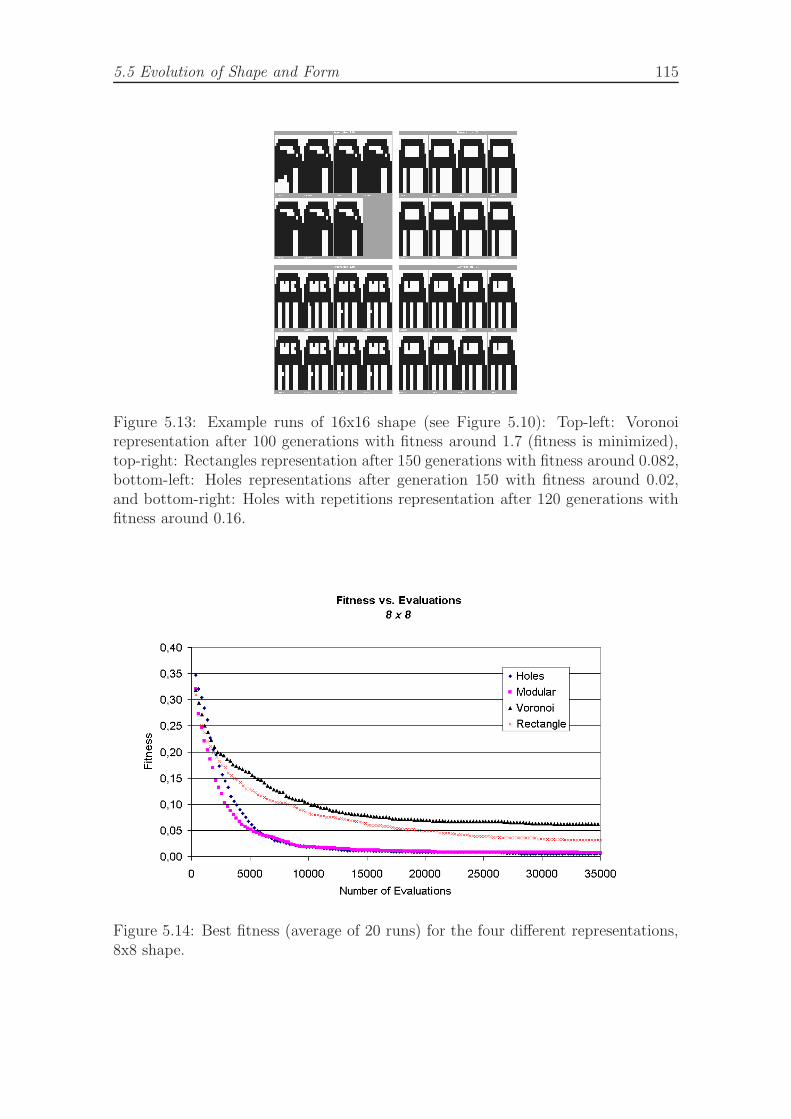
5.5 Evolution of Shape and Form 115

Figure 5.13: Example runs of 16x16 shape (see Figure 5.10): Top-left: Voronoirepresentation after 100 generations with fitness around 1.7 (fitness is minimized),top-right: Rectangles representation after 150 generations with fitness around 0.082,bottom-left: Holes representations after generation 150 with fitness around 0.02,and bottom-right: Holes with repetitions representation after 120 generations withfitness around 0.16.

Figure 5.14: Best fitness (average of 20 runs) for the four different representations,8x8 shape.

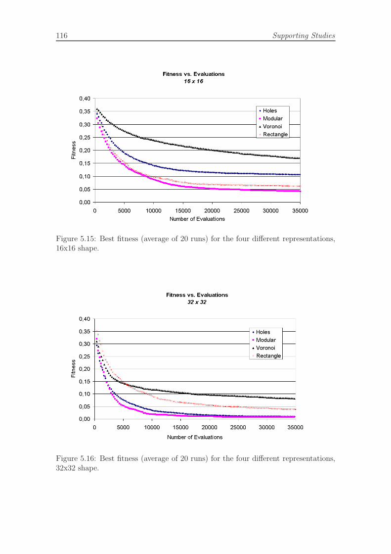
116 Supporting Studies

Figure 5.15: Best fitness (average of 20 runs) for the four different representations,16x16 shape.

Figure 5.16: Best fitness (average of 20 runs) for the four different representations,32x32 shape.

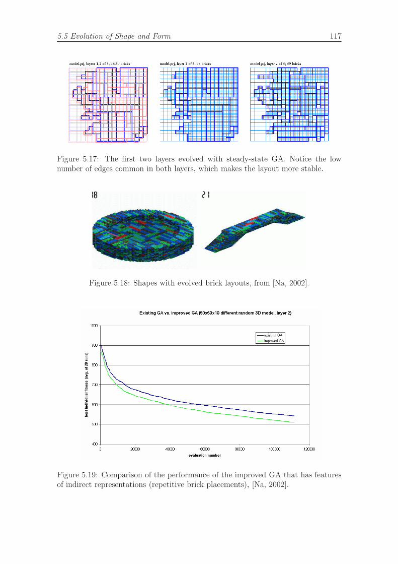
5.5 Evolution of Shape and Form 117

Figure 5.17: The first two layers evolved with steady-state GA. Notice the lownumber of edges common in both layers, which makes the layout more stable.

Figure 5.18: Shapes with evolved brick layouts, from [Na, 2002].

Figure 5.19: Comparison of the performance of the improved GA that has featuresof indirect representations (repetitive brick placements), [Na, 2002].

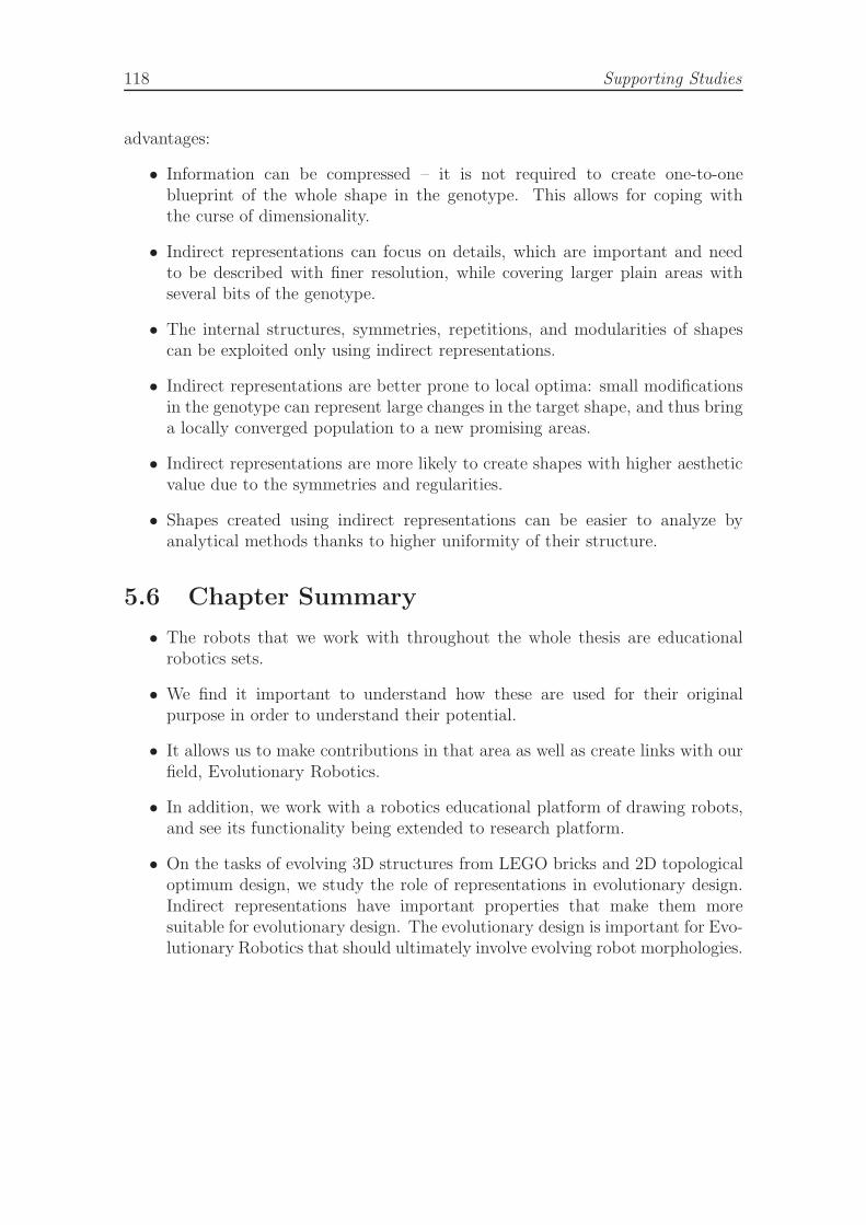
118 Supporting Studies

advantages:

• Information can be compressed – it is not required to create one-to-oneblueprint of the whole shape in the genotype. This allows for coping withthe curse of dimensionality.

• Indirect representations can focus on details, which are important and needto be described with finer resolution, while covering larger plain areas withseveral bits of the genotype.

• The internal structures, symmetries, repetitions, and modularities of shapescan be exploited only using indirect representations.

• Indirect representations are better prone to local optima: small modificationsin the genotype can represent large changes in the target shape, and thus bringa locally converged population to a new promising areas.

• Indirect representations are more likely to create shapes with higher aestheticvalue due to the symmetries and regularities.

• Shapes created using indirect representations can be easier to analyze byanalytical methods thanks to higher uniformity of their structure.

5.6 Chapter Summary

• The robots that we work with throughout the whole thesis are educationalrobotics sets.

• We find it important to understand how these are used for their originalpurpose in order to understand their potential.

• It allows us to make contributions in that area as well as create links with ourfield, Evolutionary Robotics.

• In addition, we work with a robotics educational platform of drawing robots,and see its functionality being extended to research platform.

• On the tasks of evolving 3D structures from LEGO bricks and 2D topologicaloptimum design, we study the role of representations in evolutionary design.Indirect representations have important properties that make them moresuitable for evolutionary design. The evolutionary design is important for Evo-lutionary Robotics that should ultimately involve evolving robot morphologies.

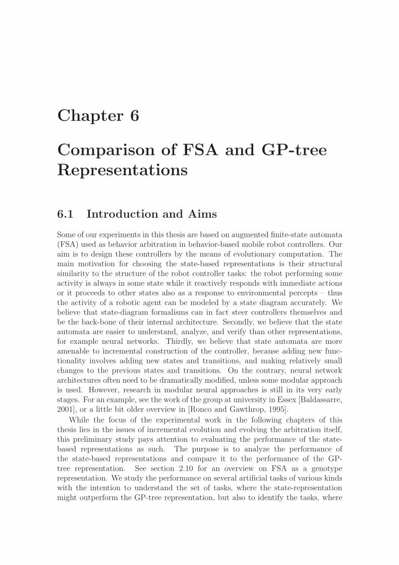
Chapter 6

Comparison of FSA and GP-treeRepresentations

6.1 Introduction and Aims

Some of our experiments in this thesis are based on augmented finite-state automata(FSA) used as behavior arbitration in behavior-based mobile robot controllers. Ouraim is to design these controllers by the means of evolutionary computation. Themain motivation for choosing the state-based representations is their structuralsimilarity to the structure of the robot controller tasks: the robot performing someactivity is always in some state while it reactively responds with immediate actionsor it proceeds to other states also as a response to environmental percepts – thusthe activity of a robotic agent can be modeled by a state diagram accurately. Webelieve that state-diagram formalisms can in fact steer controllers themselves andbe the back-bone of their internal architecture. Secondly, we believe that the stateautomata are easier to understand, analyze, and verify than other representations,for example neural networks. Thirdly, we believe that state automata are moreamenable to incremental construction of the controller, because adding new func-tionality involves adding new states and transitions, and making relatively smallchanges to the previous states and transitions. On the contrary, neural networkarchitectures often need to be dramatically modified, unless some modular approachis used. However, research in modular neural approaches is still in its very earlystages. For an example, see the work of the group at university in Essex [Baldassarre,2001], or a little bit older overview in [Ronco and Gawthrop, 1995].

While the focus of the experimental work in the following chapters of thisthesis lies in the issues of incremental evolution and evolving the arbitration itself,this preliminary study pays attention to evaluating the performance of the state-based representations as such. The purpose is to analyze the performance ofthe state-based representations and compare it to the performance of the GP-tree representation. See section 2.10 for an overview on FSA as a genotyperepresentation. We study the performance on several artificial tasks of various kindswith the intention to understand the set of tasks, where the state-representationmight outperform the GP-tree representation, but also to identify the tasks, where

120 Comparison of FSA and GP-trees

the state-representations are less efficient. For the purposes of performing theseexperiments, we have designed a package for evolutionary computation experimentsfor educational programming environment Imagine Logo [Kalas and Hrusecka, 2004]that has an interface to control both simulated and real robots [Petrovic et al., 2006],see section 5.4 on Evolve with Imagine1.

6.1.1 Representations

In the GP representation, the evolved program is a binary tree with non-terminalsin the nodes and terminals in the leaves. The growth of trees is restricted eitherby the maximum number of nodes or the maximum tree depth. Non-terminals andterminals are symbols with the semantics of a procedure (not a function as oftenis the case in GP implementations; here, the state of the computation is containedcompletely in the registers and in the state of the environment). Non-terminals havetwo sub-trees2, which themselves are binary GP-trees. Both terminals and non-terminals may contain additional arguments: constants of various ranges, registerreferences, predicates (or conditions). Each problem domain is thus defined by thesyntax and semantics of, see also Figure 6.1:

• Set of terminals T , |T | = NT .

• Set of non-terminals N , |N | = NN .

• Number of registers NR, and possibly their semantics (such as coupling tosome sensors).

• Set of binary relations Rel, for example <, >, ==, etc. that can be used bynon-terminals.

• Definition of terminals arguments, a function3 ArgT : T → ArgTypes∗,where ArgTypes is a set of possible argument types: {constant, interval,

register reference, relation}, where constant can be instantiated toany integer number given globally specified range, interval is specified as[min max] and can be instantiated to any integer from this interval, registerreference can be instantiated to any of the registers R1, . . . , RNR

, andrelation is instantiated to a member of Rel. For example, a non-terminal iftypically has arguments (register relation constant).

• Definition of non-terminals arguments, a function ArgN : N → ArgTypes∗.

1A secondary objective for producing this software package was to provide an educationalplatform for popularizing and experimenting with evolutionary computation, which is supportedby wide use of Imagine in the schools on elementary and secondary level. This objective is treatedin a separate report [Petrovic et al., 2007].

2For the reasons of better topological compatibility of all nodes with respect to evolutionaryoperators, our system currently supports only non-terminals with two sub-trees.

3With the notation M∗, we refer to the set of all the possible tuplets (m1, m2, . . .mk), k ∈ N,∀i(1 ≤ i ≤ k → mi ∈ M), including tuplets with no members.

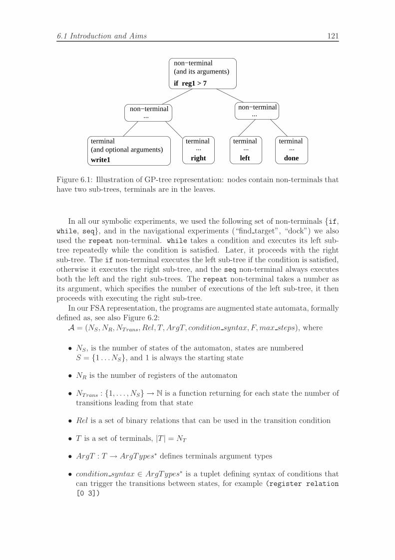
6.1 Introduction and Aims 121

(and its arguments)non−terminal

if reg1 > 7

non−terminal...

non−terminal...

terminal(and optional arguments)

write1

terminal...

right

terminal...

left

terminal...

done

Figure 6.1: Illustration of GP-tree representation: nodes contain non-terminals thathave two sub-trees, terminals are in the leaves.

In all our symbolic experiments, we used the following set of non-terminals {if,while, seq}, and in the navigational experiments (“find target”, “dock”) we alsoused the repeat non-terminal. while takes a condition and executes its left sub-tree repeatedly while the condition is satisfied. Later, it proceeds with the rightsub-tree. The if non-terminal executes the left sub-tree if the condition is satisfied,otherwise it executes the right sub-tree, and the seq non-terminal always executesboth the left and the right sub-trees. The repeat non-terminal takes a number asits argument, which specifies the number of executions of the left sub-tree, it thenproceeds with executing the right sub-tree.

In our FSA representation, the programs are augmented state automata, formallydefined as, see also Figure 6.2:

A = (NS, NR, NTrans, Rel, T, ArgT, condition syntax, F, max steps), where

• NS, is the number of states of the automaton, states are numberedS = {1 . . .NS}, and 1 is always the starting state

• NR is the number of registers of the automaton

• NTrans : {1, . . . , NS} → N is a function returning for each state the number oftransitions leading from that state

• Rel is a set of binary relations that can be used in the transition condition

• T is a set of terminals, |T | = NT

• ArgT : T → ArgTypes∗ defines terminals argument types

• condition syntax ∈ ArgTypes∗ is a tuplet defining syntax of conditions thatcan trigger the transitions between states, for example (register relation

[0 3])

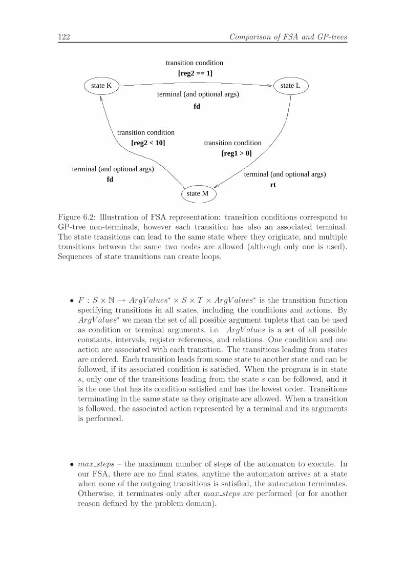
122 Comparison of FSA and GP-trees

state K

[reg2 == 1]

state L

transition condition

transition condition

state M

terminal (and optional args)

rt

terminal (and optional args)

fd

[reg1 > 0]

terminal (and optional args)

fd

transition condition

[reg2 < 10]

Figure 6.2: Illustration of FSA representation: transition conditions correspond toGP-tree non-terminals, however each transition has also an associated terminal.The state transitions can lead to the same state where they originate, and multipletransitions between the same two nodes are allowed (although only one is used).Sequences of state transitions can create loops.

• F : S × N → ArgV alues∗ × S × T × ArgV alues∗ is the transition functionspecifying transitions in all states, including the conditions and actions. ByArgV alues∗ we mean the set of all possible argument tuplets that can be usedas condition or terminal arguments, i.e. ArgV alues is a set of all possibleconstants, intervals, register references, and relations. One condition and oneaction are associated with each transition. The transitions leading from statesare ordered. Each transition leads from some state to another state and can befollowed, if its associated condition is satisfied. When the program is in states, only one of the transitions leading from the state s can be followed, and itis the one that has its condition satisfied and has the lowest order. Transitionsterminating in the same state as they originate are allowed. When a transitionis followed, the associated action represented by a terminal and its argumentsis performed.

• max steps – the maximum number of steps of the automaton to execute. Inour FSA, there are no final states, anytime the automaton arrives at a statewhen none of the outgoing transitions is satisfied, the automaton terminates.Otherwise, it terminates only after max steps are performed (or for anotherreason defined by the problem domain).

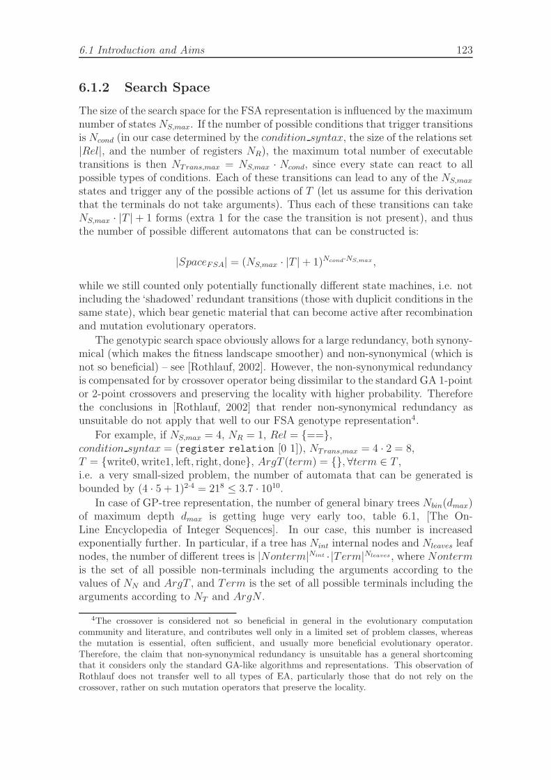
6.1 Introduction and Aims 123

6.1.2 Search Space

The size of the search space for the FSA representation is influenced by the maximumnumber of states NS,max. If the number of possible conditions that trigger transitionsis Ncond (in our case determined by the condition syntax, the size of the relations set|Rel|, and the number of registers NR), the maximum total number of executabletransitions is then NTrans,max = NS,max · Ncond, since every state can react to allpossible types of conditions. Each of these transitions can lead to any of the NS,max

states and trigger any of the possible actions of T (let us assume for this derivationthat the terminals do not take arguments). Thus each of these transitions can takeNS,max · |T | + 1 forms (extra 1 for the case the transition is not present), and thusthe number of possible different automatons that can be constructed is:

|SpaceFSA| = (NS,max · |T | + 1)Ncond·NS,max ,

while we still counted only potentially functionally different state machines, i.e. notincluding the ‘shadowed’ redundant transitions (those with duplicit conditions in thesame state), which bear genetic material that can become active after recombinationand mutation evolutionary operators.

The genotypic search space obviously allows for a large redundancy, both synony-mical (which makes the fitness landscape smoother) and non-synonymical (which isnot so beneficial) – see [Rothlauf, 2002]. However, the non-synonymical redundancyis compensated for by crossover operator being dissimilar to the standard GA 1-pointor 2-point crossovers and preserving the locality with higher probability. Thereforethe conclusions in [Rothlauf, 2002] that render non-synonymical redundancy asunsuitable do not apply that well to our FSA genotype representation4.

For example, if NS,max = 4, NR = 1, Rel = {==},condition syntax = (register relation [0 1]), NTrans,max = 4 · 2 = 8,T = {write0, write1, left, right, done}, ArgT (term) = {}, ∀term ∈ T ,i.e. a very small-sized problem, the number of automata that can be generated isbounded by (4 · 5 + 1)2·4 = 218 ≤ 3.7 · 1010.

In case of GP-tree representation, the number of general binary trees Nbin(dmax)of maximum depth dmax is getting huge very early too, table 6.1, [The On-Line Encyclopedia of Integer Sequences]. In our case, this number is increasedexponentially further. In particular, if a tree has Nint internal nodes and Nleaves leafnodes, the number of different trees is |Nonterm|Nint · |Term|Nleaves, where Nontermis the set of all possible non-terminals including the arguments according to thevalues of NN and ArgT , and Term is the set of all possible terminals including thearguments according to NT and ArgN .

4The crossover is considered not so beneficial in general in the evolutionary computationcommunity and literature, and contributes well only in a limited set of problem classes, whereasthe mutation is essential, often sufficient, and usually more beneficial evolutionary operator.Therefore, the claim that non-synonymical redundancy is unsuitable has a general shortcomingthat it considers only the standard GA-like algorithms and representations. This observation ofRothlauf does not transfer well to all types of EA, particularly those that do not rely on thecrossover, rather on such mutation operators that preserve the locality.

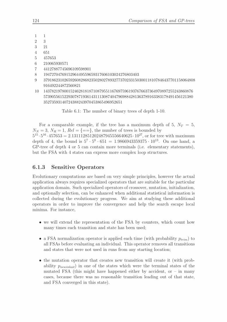
124 Comparison of FSA and GP-trees

1 1

2 3

3 21

4 651

5 457653

6 210065930571

7 44127887745696109598901

8 1947270476915296449559659317606103024276803403

9 3791862310265926082868235028027893277370233150300118107846437701158064808

916492244872560821

10 143782197800152462818187108795511676975961937676637364970897255243860876

573905561522930787193614311130874047969884281363789163383178491456121380

35273593140724388243970453865496952651

Table 6.1: The number of binary trees of depth 1-10.

For a comparable example, if the tree has a maximum depth of 5, NT = 5,NN = 3, NR = 1, Rel = {==}, the number of trees is bounded by515 ·516 ·457653 = 2.131112851202487945556640625 ·1027, or for tree with maximumdepth of 4, the bound is 57 · 58 · 651 = 1.9866943359375 · 1013. On one hand, aGP-tree of depth 4 or 5 can contain more terminals (i.e. elementary statements),but the FSA with 4 states can express more complex loop structures.

6.1.3 Sensitive Operators

Evolutionary computations are based on very simple principles, however the actualapplication always requires specialized operators that are suitable for the particularapplication domain. Such specialized operators of crossover, mutation, initialization,and optionally selection, can be enhanced when additional statistical information iscollected during the evolutionary progress. We aim at studying these additionaloperators in order to improve the convergence and help the search escape localminima. For instance,

• we will extend the representation of the FSA by counters, which count howmany times each transition and state has been used;

• a FSA normalization operator is applied each time (with probability ptrim) toall FSAs before evaluating an individual. This operator removes all transitionsand states that were not used in runs from any starting location;

• the mutation operator that creates new transition will create it (with prob-ability pnewinlast) in one of the states which were the terminal states of themutated FSA (this might have happened either by accident, or – in manycases, because there was no reasonable transition leading out of that state,and FSA converged in this state).

6.2 Experimental Setup 125

6.2 Experimental Setup

In order to asses the performance of the state representations we have designed fivetasks of different nature, falling in two categories: controlling a robotic agent ina two-dimensional environment, and processing symbolic sequences prepared on aone-dimensional bi-directional, possibly infinite tape.

6.2.1 Experiment “bit collect”

This task is designed to verify the ability of the evolutionary algorithm to encodealgorithmic structures in the chosen representation. The input to the system is aword consisting of bits (0s and 1s) printed on a tape. The start and the end of theword can optionally be marked by surrounding -1. The tape can either be infinite,or finite. In the latter case, moving outside of the tape causes the program toterminate. There is a current read/write pointer that points to one symbol on thetape. The evolved program can perform the following operations:

• left – move the current read/write pointer one symbol to the left

• right – move the current read/write pointer one symbol to the right

• write0 – write zero to the tape at the current read/write pointer

• write1 – write one to the tape at the current read/write pointer

• done – task completed, terminate

The program has at disposition the symbol of the tape at the position of thecurrent read/write pointer (register R1). The task for the program is either to fillall holes (tape positions containing zeros) with ones – in the easy version, or in adifficult version to pack – move the symbols at the tape in such a way that theremaining word will consist of a continuous sequence of ones, the same number asthe total number of ones in the input word. The program can write arbitrary numberof zeros on both sides of the output word. For example, the input:

10111001010001

would be transformed by a correct program to:

11111111111111

in the easy version, or to (for example):

11111110000000

126 Comparison of FSA and GP-trees

in the difficult version of the task. The computing platform in this task is similarto the Turing Machine. The performance of the program is measured in terms ofthe number of errors – each extra “1” as well as each missing “1” is penalized byone point. In addition, all remaining holes – symbols “0” – are penalized by onepoint each. Fitness function:

fitness = B − s · qs −nstarts∑

i=1

(ri · qr +hi

Hi

· qh +oi

Oi

· qo)

where nstarts is the number of random input words presented to the program, Hi

and Oi is the number of holes and ones in the ith input word respectively, hi is thenumber of holes remaining in the output word, oi is the difference in the number ofones expected (either too much or too little), ri is the number of execution steps, sis the size of the genotype, and qs, qr, qh, and qo are weight constants. Coefficientsqh and qo were strictly more significant than qs and qr, and in balance (we usedqo = 2qh).

6.2.2 Experiment “(abcd)n”

In this task, we test the ability of the representation to encode repetitive structures.Using the same computational model of the tape state machine as in the previoustask, the goal is to replace a continuous sequence of symbols “1” on the tape ofrandom length with a repeating sequence of symbols a, b, c, d. For instance, theinput:

11111111111111111111

would be transformed by a correct program to:

abcdabcdabcdabcdabcd

The allowed operations are the same as in the previous task, with the additionof the operations that write the symbols a, b, c, and d. In a simplified version ofthis task, we require the sequence (abc)n. Fitness function:

fitness = 1 − s · qs −nstarts∑

i=1

(ei

li

nstarts

− ri · qr)

where ei is the number of incorrect symbols in the output word (including extraplaced or missing symbols) in the ith input word, li is the number of symbols in theinput word, and the meaning of the other symbols is the same as in the previoustask.

6.2 Experimental Setup 127

6.2.3 Experiment “switch”

This is a task with a structure that shares properties with the structures of robotictasks where the robot reacts to environmental percepts depending of its currentstate, and enters other states when triggered by some input data. The computationalplatform – a tape machine – is the same as in the previous two tasks. The task forthe program is to replace all zeros on the tape with numeric symbols 1, 2, 3, and 4.The input sequence on the tape determines how the zeros are to be replaced: theinput contains random symbols 1, 2, 3, and 4 that are interleaved with sequencesof zeros, each 0-sequence containing up to 10 zeros. The program should replacethe zeros with the closest non-zero input on the left. When the program leaves thetape, it is automatically terminated. For instance, the following input:

100040300002000130040000000003000020

should be transformed to:

111144333332222133344444444443333322

The performance of the program is measured as the sum of errors from theexpected string. The allowed operations are the same as in the previous tasks,except that the program is allowed to write the symbols 0, 1, 2, 3, and 4. In asimplified version of the task, the input may contain (and the program can write)only the symbols 0, 1, 2, and 3. The fitness function is the same as in the task abcdn.We have experimented with incremental versions of this task, which are describedin the results section below.

6.2.4 Experiment “find target”

In this experiment, a robotic agent is placed in a 2D environment. It understandsthe following primitive control commands:

• fd – move forward a little bit (usually 20 steps)

• bk – move backward a little bit

• fdlong – move forward longer distance (usually 100 steps)

• bklong – move backwards longer distance

• lt – turn left a little bit (different angle values result in different behaviors:90◦ results in a square grid along which the agent can move, 60◦ results in ahexagonal grid, which is a very efficient navigational environment, other valuesthat are not divisors of 360◦ result in the ability of the agent to turn to manydifferent directions by repetitive turnings and thus exploit the environment tohigher degree – on the cost of more complex navigational sequences).

• rt – turn right a little bit

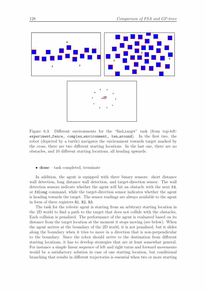
128 Comparison of FSA and GP-trees

Figure 6.3: Different environments for the “find target” task (from top-left:experiment fence, complex environment, ten around). In the first two, therobot (depicted by a turtle) navigates the environment towards target marked bythe cross, there are two different starting locations. In the last one, there are noobstacles, and 10 different starting locations, all heading upwards.

• done – task completed, terminate

In addition, the agent is equipped with three binary sensors: short distancewall detection, long distance wall detection, and target-direction sensor. The walldetection sensors indicate whether the agent will hit an obstacle with the next fd,or fdlong command, while the target-direction sensor indicates whether the agentis heading towards the target. The sensor readings are always available to the agentin form of three registers R1, R2, R3.

The task for the robotic agent is starting from an arbitrary starting location inthe 2D world to find a path to the target that does not collide with the obstacles.Each collision is penalized. The performance of the agent is evaluated based on itsdistance from the target location at the moment it stops moving (see below). Whenthe agent arrives at the boundary of the 2D world, it is not penalized, but it slidesalong the boundary when it tries to move in a direction that is non-perpendicularto the boundary. Since the robot should arrive to the destination from differentstarting locations, it has to develop strategies that are at least somewhat general.For instance a simple linear sequence of left and right turns and forward movementswould be a satisfactory solution in case of one starting location, but conditionalbranching that results in different trajectories is essential when two or more starting

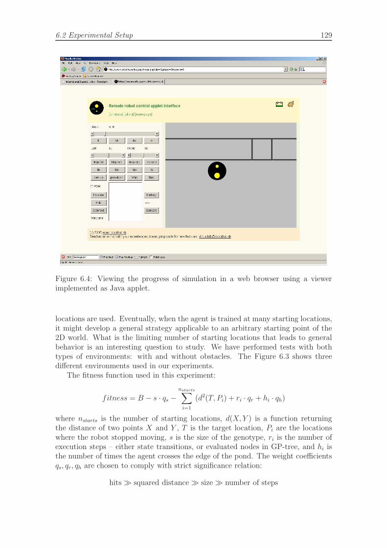
6.2 Experimental Setup 129

Figure 6.4: Viewing the progress of simulation in a web browser using a viewerimplemented as Java applet.

locations are used. Eventually, when the agent is trained at many starting locations,it might develop a general strategy applicable to an arbitrary starting point of the2D world. What is the limiting number of starting locations that leads to generalbehavior is an interesting question to study. We have performed tests with bothtypes of environments: with and without obstacles. The Figure 6.3 shows threedifferent environments used in our experiments.

The fitness function used in this experiment:

fitness = B − s · qs −nstarts∑

i=1

(d2(T, Pi) + ri · qr + hi · qh)

where nstarts is the number of starting locations, d(X, Y ) is a function returningthe distance of two points X and Y , T is the target location, Pi are the locationswhere the robot stopped moving, s is the size of the genotype, ri is the number ofexecution steps – either state transitions, or evaluated nodes in GP-tree, and hi isthe number of times the agent crosses the edge of the pond. The weight coefficientsqs, qr, qh are chosen to comply with strict significance relation:

hits ≫ squared distance ≫ size ≫ number of steps

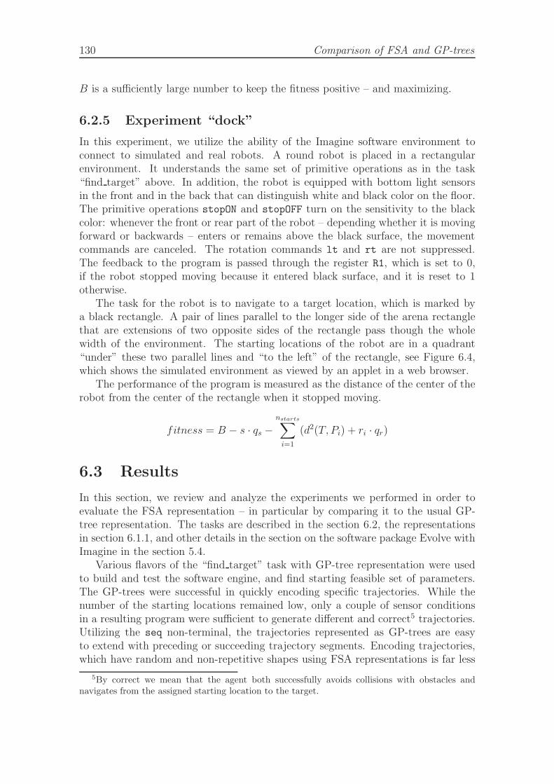
130 Comparison of FSA and GP-trees

B is a sufficiently large number to keep the fitness positive – and maximizing.

6.2.5 Experiment “dock”

In this experiment, we utilize the ability of the Imagine software environment toconnect to simulated and real robots. A round robot is placed in a rectangularenvironment. It understands the same set of primitive operations as in the task“find target” above. In addition, the robot is equipped with bottom light sensorsin the front and in the back that can distinguish white and black color on the floor.The primitive operations stopON and stopOFF turn on the sensitivity to the blackcolor: whenever the front or rear part of the robot – depending whether it is movingforward or backwards – enters or remains above the black surface, the movementcommands are canceled. The rotation commands lt and rt are not suppressed.The feedback to the program is passed through the register R1, which is set to 0,if the robot stopped moving because it entered black surface, and it is reset to 1otherwise.

The task for the robot is to navigate to a target location, which is marked bya black rectangle. A pair of lines parallel to the longer side of the arena rectanglethat are extensions of two opposite sides of the rectangle pass though the wholewidth of the environment. The starting locations of the robot are in a quadrant“under” these two parallel lines and “to the left” of the rectangle, see Figure 6.4,which shows the simulated environment as viewed by an applet in a web browser.

The performance of the program is measured as the distance of the center of therobot from the center of the rectangle when it stopped moving.

fitness = B − s · qs −nstarts∑

i=1

(d2(T, Pi) + ri · qr)

6.3 Results

In this section, we review and analyze the experiments we performed in order toevaluate the FSA representation – in particular by comparing it to the usual GP-tree representation. The tasks are described in the section 6.2, the representationsin section 6.1.1, and other details in the section on the software package Evolve withImagine in the section 5.4.

Various flavors of the “find target” task with GP-tree representation were usedto build and test the software engine, and find starting feasible set of parameters.The GP-trees were successful in quickly encoding specific trajectories. While thenumber of the starting locations remained low, only a couple of sensor conditionsin a resulting program were sufficient to generate different and correct5 trajectories.Utilizing the seq non-terminal, the trajectories represented as GP-trees are easyto extend with preceding or succeeding trajectory segments. Encoding trajectories,which have random and non-repetitive shapes using FSA representations is far less

5By correct we mean that the agent both successfully avoids collisions with obstacles andnavigates from the assigned starting location to the target.

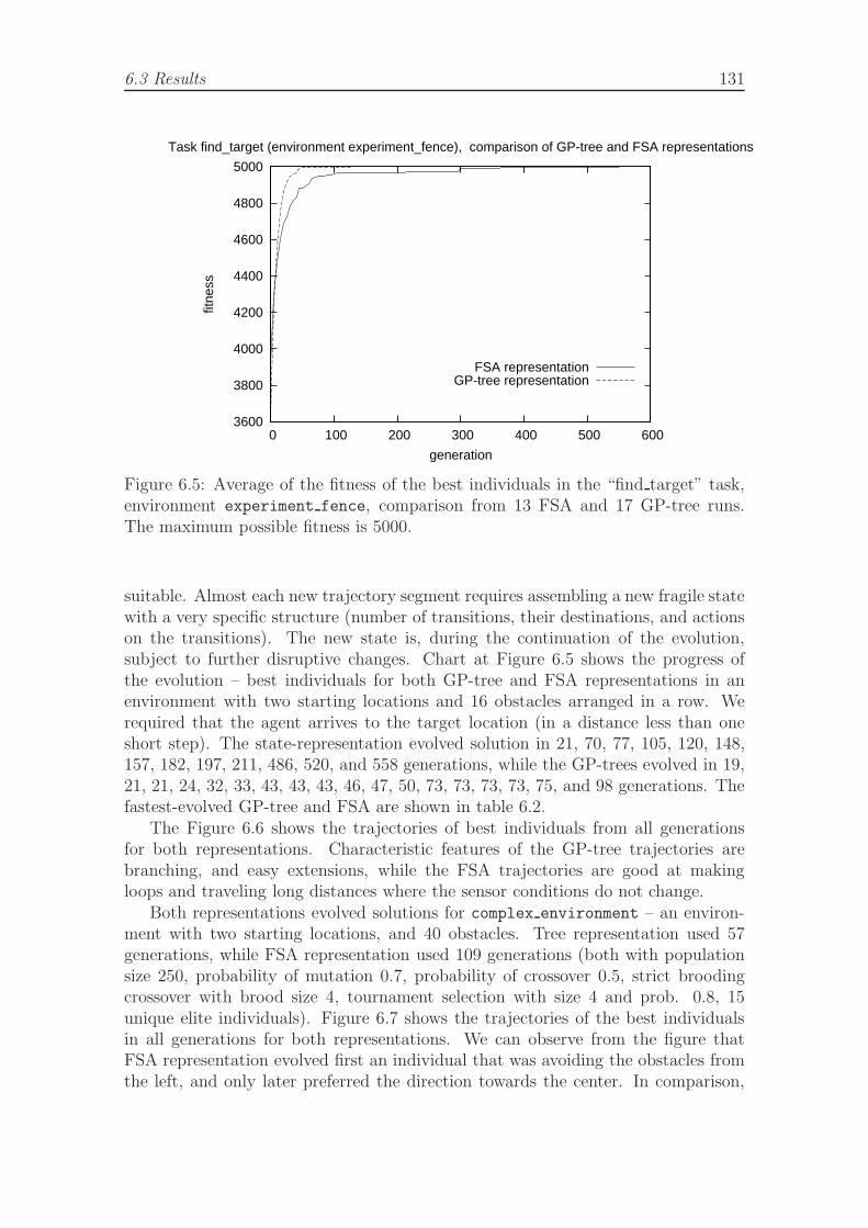
6.3 Results 131

3600

3800

4000

4200

4400

4600

4800

5000

0 100 200 300 400 500 600

fitne

ss

generation

Task find_target (environment experiment_fence), comparison of GP-tree and FSA representations

FSA representationGP-tree representation

Figure 6.5: Average of the fitness of the best individuals in the “find target” task,environment experiment fence, comparison from 13 FSA and 17 GP-tree runs.The maximum possible fitness is 5000.

suitable. Almost each new trajectory segment requires assembling a new fragile statewith a very specific structure (number of transitions, their destinations, and actionson the transitions). The new state is, during the continuation of the evolution,subject to further disruptive changes. Chart at Figure 6.5 shows the progress ofthe evolution – best individuals for both GP-tree and FSA representations in anenvironment with two starting locations and 16 obstacles arranged in a row. Werequired that the agent arrives to the target location (in a distance less than oneshort step). The state-representation evolved solution in 21, 70, 77, 105, 120, 148,157, 182, 197, 211, 486, 520, and 558 generations, while the GP-trees evolved in 19,21, 21, 24, 32, 33, 43, 43, 43, 46, 47, 50, 73, 73, 73, 73, 75, and 98 generations. Thefastest-evolved GP-tree and FSA are shown in table 6.2.

The Figure 6.6 shows the trajectories of best individuals from all generationsfor both representations. Characteristic features of the GP-tree trajectories arebranching, and easy extensions, while the FSA trajectories are good at makingloops and traveling long distances where the sensor conditions do not change.

Both representations evolved solutions for complex environment – an environ-ment with two starting locations, and 40 obstacles. Tree representation used 57generations, while FSA representation used 109 generations (both with populationsize 250, probability of mutation 0.7, probability of crossover 0.5, strict broodingcrossover with brood size 4, tournament selection with size 4 and prob. 0.8, 15unique elite individuals). Figure 6.7 shows the trajectories of the best individualsin all generations for both representations. We can observe from the figure thatFSA representation evolved first an individual that was avoiding the obstacles fromthe left, and only later preferred the direction towards the center. In comparison,

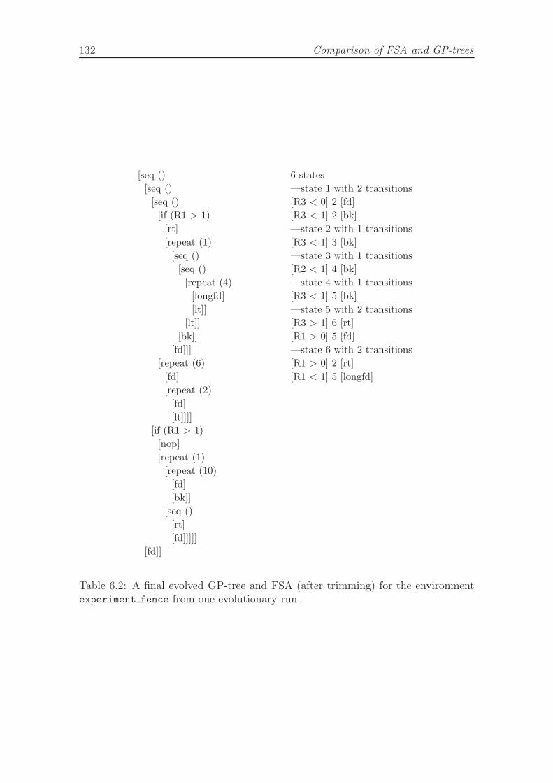
132 Comparison of FSA and GP-trees

[seq ()

[seq ()

[seq ()

[if (R1 > 1)

[rt]

[repeat (1)

[seq ()

[seq ()

[repeat (4)

[longfd]

[lt]]

[lt]]

[bk]]

[fd]]]

[repeat (6)

[fd]

[repeat (2)

[fd]

[lt]]]]

[if (R1 > 1)

[nop]

[repeat (1)

[repeat (10)

[fd]

[bk]]

[seq ()

[rt]

[fd]]]]]

[fd]]

6 states

—state 1 with 2 transitions

[R3 < 0] 2 [fd]

[R3 < 1] 2 [bk]

—state 2 with 1 transitions

[R3 < 1] 3 [bk]

—state 3 with 1 transitions

[R2 < 1] 4 [bk]

—state 4 with 1 transitions

[R3 < 1] 5 [bk]

—state 5 with 2 transitions

[R3 > 1] 6 [rt]

[R1 > 0] 5 [fd]

—state 6 with 2 transitions

[R1 > 0] 2 [rt]

[R1 < 1] 5 [longfd]

Table 6.2: A final evolved GP-tree and FSA (after trimming) for the environmentexperiment fence from one evolutionary run.

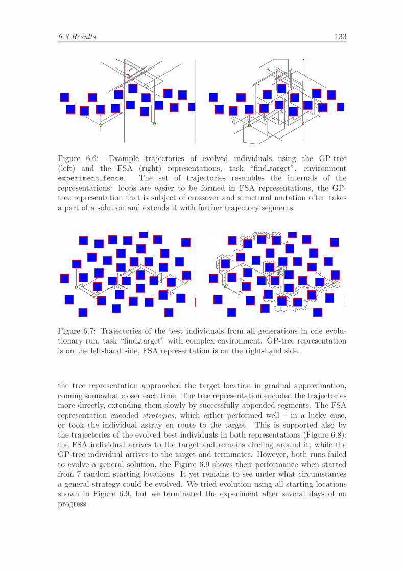
6.3 Results 133

Figure 6.6: Example trajectories of evolved individuals using the GP-tree(left) and the FSA (right) representations, task “find target”, environmentexperiment fence. The set of trajectories resembles the internals of therepresentations: loops are easier to be formed in FSA representations, the GP-tree representation that is subject of crossover and structural mutation often takesa part of a solution and extends it with further trajectory segments.

Figure 6.7: Trajectories of the best individuals from all generations in one evolu-tionary run, task “find target” with complex environment. GP-tree representationis on the left-hand side, FSA representation is on the right-hand side.

the tree representation approached the target location in gradual approximation,coming somewhat closer each time. The tree representation encoded the trajectoriesmore directly, extending them slowly by successfully appended segments. The FSArepresentation encoded strategies, which either performed well – in a lucky case,or took the individual astray en route to the target. This is supported also bythe trajectories of the evolved best individuals in both representations (Figure 6.8):the FSA individual arrives to the target and remains circling around it, while theGP-tree individual arrives to the target and terminates. However, both runs failedto evolve a general solution, the Figure 6.9 shows their performance when startedfrom 7 random starting locations. It yet remains to see under what circumstancesa general strategy could be evolved. We tried evolution using all starting locationsshown in Figure 6.9, but we terminated the experiment after several days of noprogress.

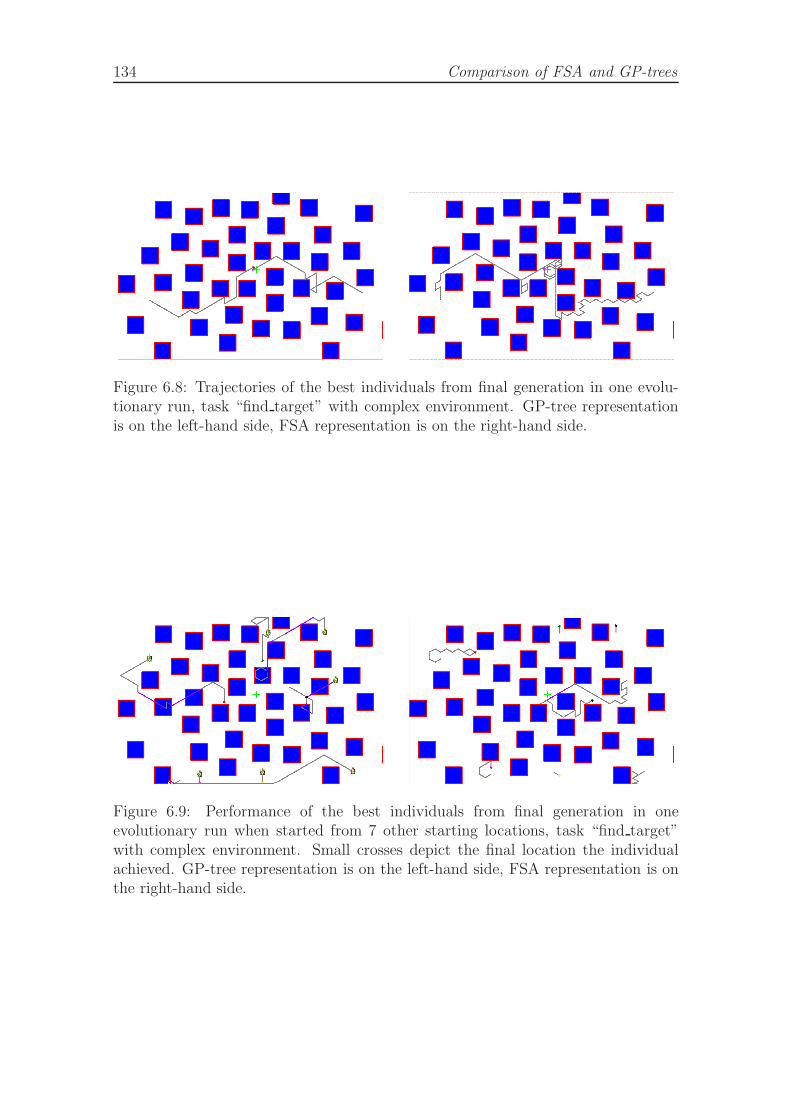
134 Comparison of FSA and GP-trees

Figure 6.8: Trajectories of the best individuals from final generation in one evolu-tionary run, task “find target” with complex environment. GP-tree representationis on the left-hand side, FSA representation is on the right-hand side.

Figure 6.9: Performance of the best individuals from final generation in oneevolutionary run when started from 7 other starting locations, task “find target”with complex environment. Small crosses depict the final location the individualachieved. GP-tree representation is on the left-hand side, FSA representation is onthe right-hand side.

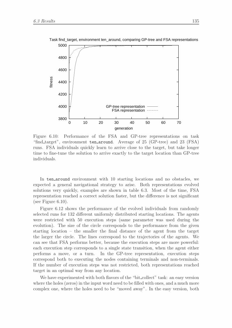
6.3 Results 135

3800

4000

4200

4400

4600

4800

5000

0 10 20 30 40 50 60 70

fitne

ss

generation

Task find_target, environment ten_around, comparing GP-tree and FSA representations

GP-tree representationFSA representation

Figure 6.10: Performance of the FSA and GP-tree representations on task“find target”, environment ten around. Average of 25 (GP-tree) and 23 (FSA)runs. FSA individuals quickly learn to arrive close to the target, but take longertime to fine-tune the solution to arrive exactly to the target location than GP-treeindividuals.

In ten around environment with 10 starting locations and no obstacles, weexpected a general navigational strategy to arise. Both representations evolvedsolutions very quickly, examples are shown in table 6.3. Most of the time, FSArepresentation reached a correct solution faster, but the difference is not significant(see Figure 6.10).

Figure 6.12 shows the performance of the evolved individuals from randomlyselected runs for 132 different uniformly distributed starting locations. The agentswere restricted with 50 execution steps (same parameter was used during theevolution). The size of the circle corresponds to the performance from the givenstarting location – the smaller the final distance of the agent from the targetthe larger the circle. The lines correspond to the trajectories of the agents. Wecan see that FSA performs better, because the execution steps are more powerful:each execution step corresponds to a single state transition, when the agent eitherperforms a move, or a turn. In the GP-tree representation, execution stepscorrespond both to executing the nodes containing terminals and non-terminals.If the number of execution steps was not restricted, both representations reachedtarget in an optimal way from any location.

We have experimented with both flavors of the “bit collect” task: an easy versionwhere the holes (zeros) in the input word need to be filled with ones, and a much morecomplex one, where the holes need to be “moved away”. In the easy version, both

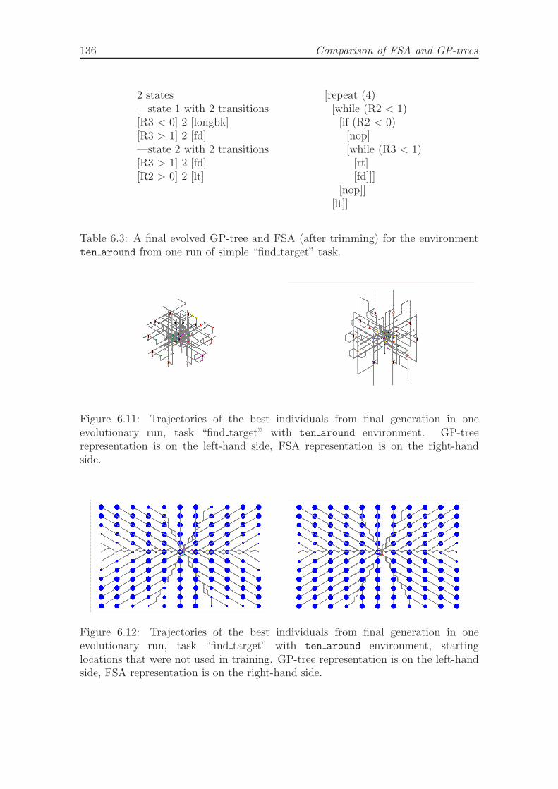
136 Comparison of FSA and GP-trees

2 states—state 1 with 2 transitions[R3 < 0] 2 [longbk][R3 > 1] 2 [fd]—state 2 with 2 transitions[R3 > 1] 2 [fd][R2 > 0] 2 [lt]

[repeat (4)[while (R2 < 1)

[if (R2 < 0)[nop][while (R3 < 1)

[rt][fd]]]

[nop]][lt]]

Table 6.3: A final evolved GP-tree and FSA (after trimming) for the environmentten around from one run of simple “find target” task.

Figure 6.11: Trajectories of the best individuals from final generation in oneevolutionary run, task “find target” with ten around environment. GP-treerepresentation is on the left-hand side, FSA representation is on the right-handside.

Figure 6.12: Trajectories of the best individuals from final generation in oneevolutionary run, task “find target” with ten around environment, startinglocations that were not used in training. GP-tree representation is on the left-handside, FSA representation is on the right-hand side.

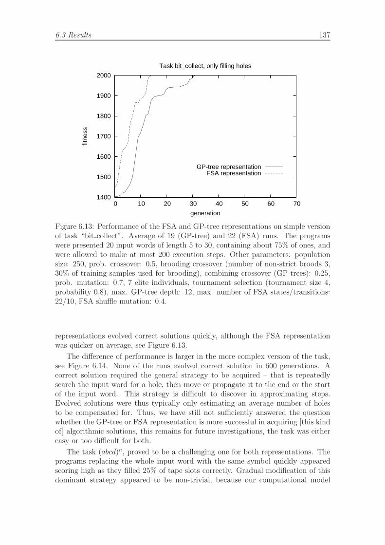
6.3 Results 137

1400

1500

1600

1700

1800

1900

2000

0 10 20 30 40 50 60 70

fitne

ss

generation

Task bit_collect, only filling holes

GP-tree representationFSA representation

Figure 6.13: Performance of the FSA and GP-tree representations on simple versionof task “bit collect”. Average of 19 (GP-tree) and 22 (FSA) runs. The programswere presented 20 input words of length 5 to 30, containing about 75% of ones, andwere allowed to make at most 200 execution steps. Other parameters: populationsize: 250, prob. crossover: 0.5, brooding crossover (number of non-strict broods 3,30% of training samples used for brooding), combining crossover (GP-trees): 0.25,prob. mutation: 0.7, 7 elite individuals, tournament selection (tournament size 4,probability 0.8), max. GP-tree depth: 12, max. number of FSA states/transitions:22/10, FSA shuffle mutation: 0.4.

representations evolved correct solutions quickly, although the FSA representationwas quicker on average, see Figure 6.13.

The difference of performance is larger in the more complex version of the task,see Figure 6.14. None of the runs evolved correct solution in 600 generations. Acorrect solution required the general strategy to be acquired – that is repeatedlysearch the input word for a hole, then move or propagate it to the end or the startof the input word. This strategy is difficult to discover in approximating steps.Evolved solutions were thus typically only estimating an average number of holesto be compensated for. Thus, we have still not sufficiently answered the questionwhether the GP-tree or FSA representation is more successful in acquiring [this kindof] algorithmic solutions, this remains for future investigations, the task was eithereasy or too difficult for both.

The task (abcd)n, proved to be a challenging one for both representations. Theprograms replacing the whole input word with the same symbol quickly appearedscoring high as they filled 25% of tape slots correctly. Gradual modification of thisdominant strategy appeared to be non-trivial, because our computational model

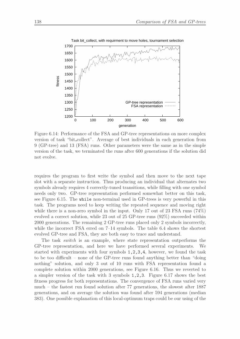
138 Comparison of FSA and GP-trees

1200

1250

1300

1350

1400

1450

1500

1550

1600

1650

1700

0 100 200 300 400 500 600

fitne

ss

generation

Task bit_collect, with requirment to move holes, tournament selection

GP-tree representationFSA representation

Figure 6.14: Performance of the FSA and GP-tree representations on more complexversion of task “bit collect”. Average of best individuals in each generation from9 (GP-tree) and 13 (FSA) runs. Other parameters were the same as in the simpleversion of the task, we terminated the runs after 600 generations if the solution didnot evolve.

requires the program to first write the symbol and then move to the next tapeslot with a separate instruction. Thus producing an individual that alternates twosymbols already requires 4 correctly-tuned transitions, while filling with one symbolneeds only two. GP-tree representation performed somewhat better on this task,see Figure 6.15. The while non-terminal used in GP-trees is very powerful in thistask. The programs need to keep writing the repeated sequence and moving rightwhile there is a non-zero symbol in the input. Only 17 out of 23 FSA runs (74%)evolved a correct solution, while 23 out of 25 GP-tree runs (92%) succeeded within2000 generations. The remaining 2 GP-tree runs placed only 2 symbols incorrectly,while the incorrect FSA erred on 7–14 symbols. The table 6.4 shows the shortestevolved GP-tree and FSA, they are both easy to trace and understand.

The task switch is an example, where state representation outperforms theGP-tree representation, and here we have performed several experiments. Westarted with experiments with four symbols 1,2,3,4, however, we found the taskto be too difficult – none of the GP-tree runs found anything better than “doingnothing” solution, and only 3 out of 10 runs with FSA representation found acomplete solution within 2000 generations, see Figure 6.16. Thus we reverted toa simpler version of the task with 3 symbols 1,2,3. Figure 6.17 shows the bestfitness progress for both representations. The convergence of FSA runs varied verymuch – the fastest run found solution after 77 generations, the slowest after 1887generations, and on average the solution was found after 594 generations (median383). One possible explanation of this local-optimum traps could be our using of the

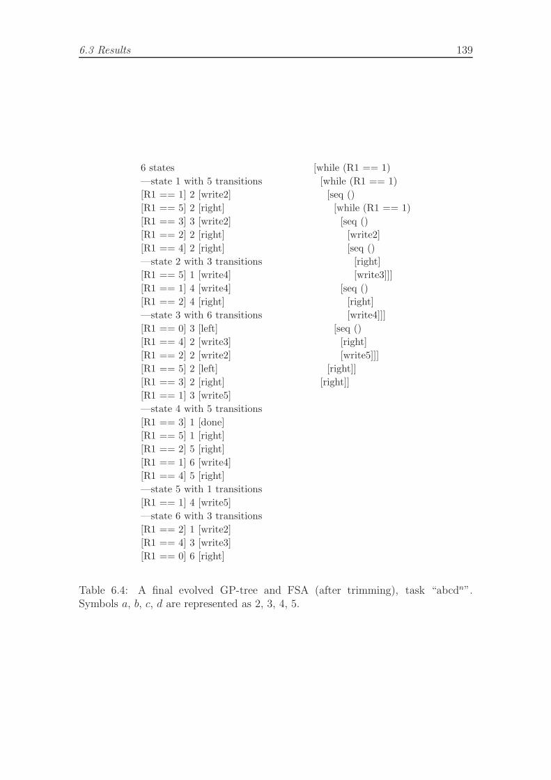
6.3 Results 139

6 states

—state 1 with 5 transitions

[R1 == 1] 2 [write2]

[R1 == 5] 2 [right]

[R1 == 3] 3 [write2]

[R1 == 2] 2 [right]

[R1 == 4] 2 [right]

—state 2 with 3 transitions

[R1 == 5] 1 [write4]

[R1 == 1] 4 [write4]

[R1 == 2] 4 [right]

—state 3 with 6 transitions

[R1 == 0] 3 [left]

[R1 == 4] 2 [write3]

[R1 == 2] 2 [write2]

[R1 == 5] 2 [left]

[R1 == 3] 2 [right]

[R1 == 1] 3 [write5]

—state 4 with 5 transitions

[R1 == 3] 1 [done]

[R1 == 5] 1 [right]

[R1 == 2] 5 [right]

[R1 == 1] 6 [write4]

[R1 == 4] 5 [right]

—state 5 with 1 transitions

[R1 == 1] 4 [write5]

—state 6 with 3 transitions

[R1 == 2] 1 [write2]

[R1 == 4] 3 [write3]

[R1 == 0] 6 [right]

[while (R1 == 1)

[while (R1 == 1)

[seq ()

[while (R1 == 1)

[seq ()

[write2]

[seq ()

[right]

[write3]]]

[seq ()

[right]

[write4]]]

[seq ()

[right]

[write5]]]

[right]]

[right]]

Table 6.4: A final evolved GP-tree and FSA (after trimming), task “abcdn”.Symbols a, b, c, d are represented as 2, 3, 4, 5.

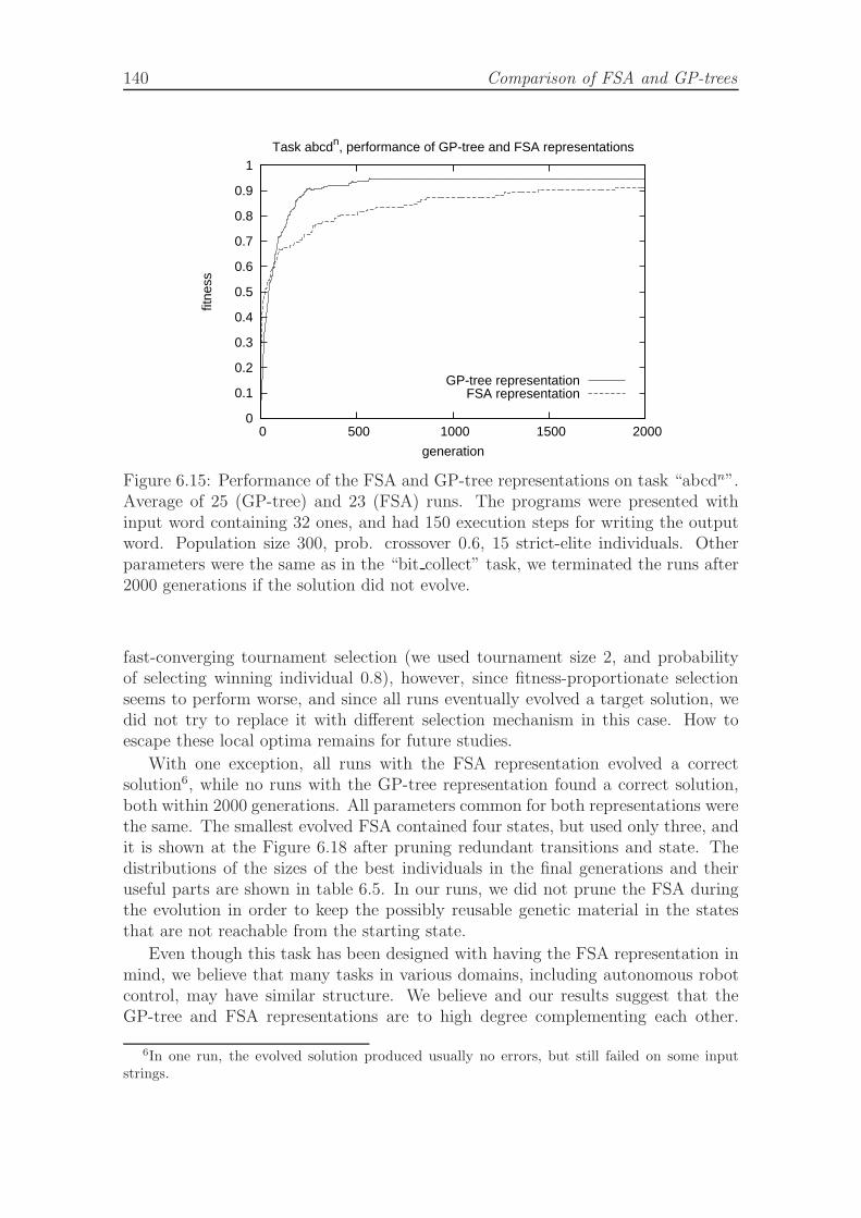
140 Comparison of FSA and GP-trees

0

0.1

0.2

0.3

0.4

0.5

0.6

0.7

0.8

0.9

1

0 500 1000 1500 2000

fitne

ss

generation

Task abcdn, performance of GP-tree and FSA representations

GP-tree representationFSA representation

Figure 6.15: Performance of the FSA and GP-tree representations on task “abcdn”.Average of 25 (GP-tree) and 23 (FSA) runs. The programs were presented withinput word containing 32 ones, and had 150 execution steps for writing the outputword. Population size 300, prob. crossover 0.6, 15 strict-elite individuals. Otherparameters were the same as in the “bit collect” task, we terminated the runs after2000 generations if the solution did not evolve.

fast-converging tournament selection (we used tournament size 2, and probabilityof selecting winning individual 0.8), however, since fitness-proportionate selectionseems to perform worse, and since all runs eventually evolved a target solution, wedid not try to replace it with different selection mechanism in this case. How toescape these local optima remains for future studies.

With one exception, all runs with the FSA representation evolved a correctsolution6, while no runs with the GP-tree representation found a correct solution,both within 2000 generations. All parameters common for both representations werethe same. The smallest evolved FSA contained four states, but used only three, andit is shown at the Figure 6.18 after pruning redundant transitions and state. Thedistributions of the sizes of the best individuals in the final generations and theiruseful parts are shown in table 6.5. In our runs, we did not prune the FSA duringthe evolution in order to keep the possibly reusable genetic material in the statesthat are not reachable from the starting state.

Even though this task has been designed with having the FSA representation inmind, we believe that many tasks in various domains, including autonomous robotcontrol, may have similar structure. We believe and our results suggest that theGP-tree and FSA representations are to high degree complementing each other.

6In one run, the evolved solution produced usually no errors, but still failed on some inputstrings.

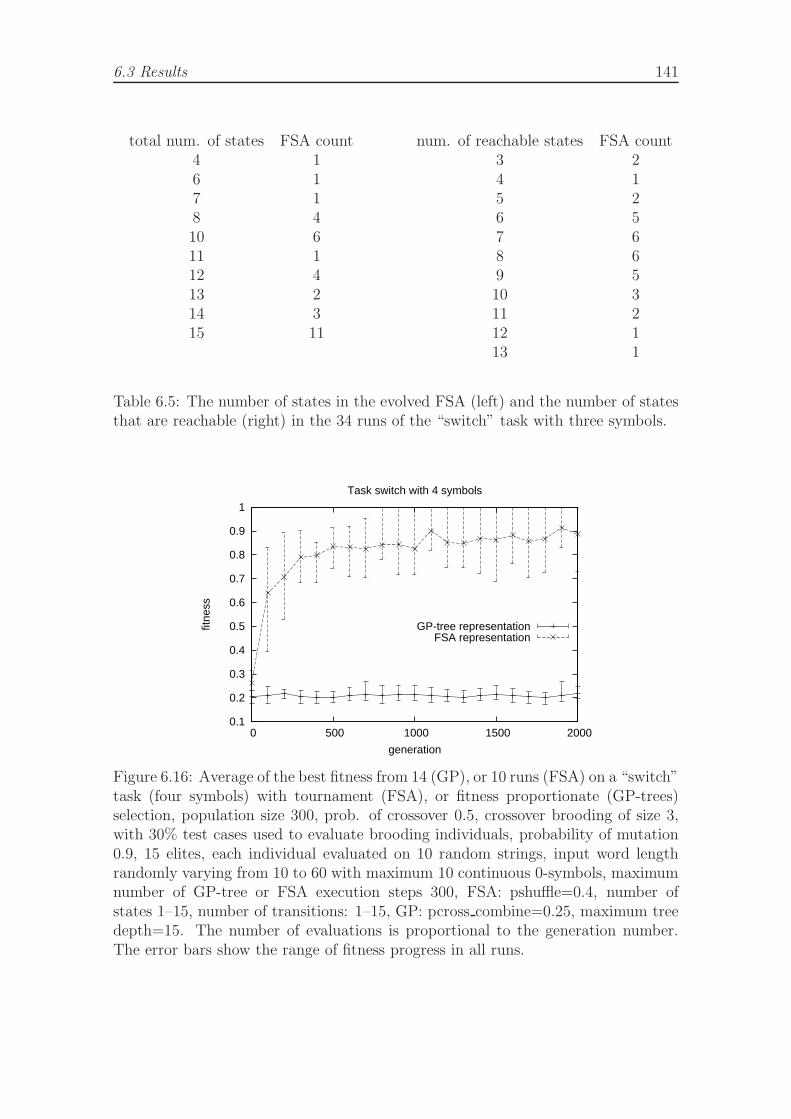
6.3 Results 141

total num. of states FSA count4 16 17 18 410 611 112 413 214 315 11

num. of reachable states FSA count3 24 15 26 57 68 69 510 311 212 113 1

Table 6.5: The number of states in the evolved FSA (left) and the number of statesthat are reachable (right) in the 34 runs of the “switch” task with three symbols.

0.1

0.2

0.3

0.4

0.5

0.6

0.7

0.8

0.9

1

0 500 1000 1500 2000

fitne

ss

generation

Task switch with 4 symbols

GP-tree representationFSA representation

Figure 6.16: Average of the best fitness from 14 (GP), or 10 runs (FSA) on a “switch”task (four symbols) with tournament (FSA), or fitness proportionate (GP-trees)selection, population size 300, prob. of crossover 0.5, crossover brooding of size 3,with 30% test cases used to evaluate brooding individuals, probability of mutation0.9, 15 elites, each individual evaluated on 10 random strings, input word lengthrandomly varying from 10 to 60 with maximum 10 continuous 0-symbols, maximumnumber of GP-tree or FSA execution steps 300, FSA: pshuffle=0.4, number ofstates 1–15, number of transitions: 1–15, GP: pcross combine=0.25, maximum treedepth=15. The number of evaluations is proportional to the generation number.The error bars show the range of fitness progress in all runs.

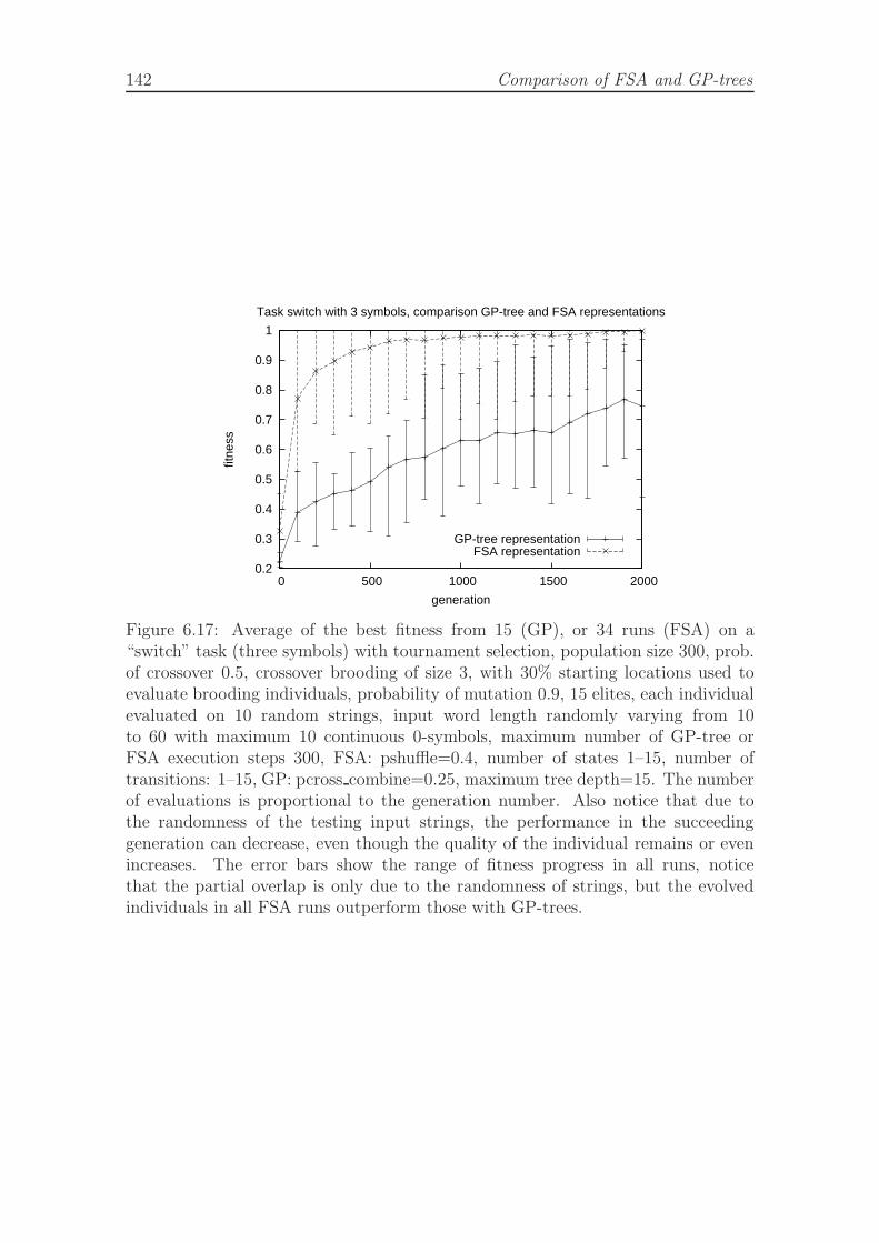
142 Comparison of FSA and GP-trees

0.2

0.3

0.4

0.5

0.6

0.7

0.8

0.9

1

0 500 1000 1500 2000

fitne

ss

generation

Task switch with 3 symbols, comparison GP-tree and FSA representations

GP-tree representationFSA representation

Figure 6.17: Average of the best fitness from 15 (GP), or 34 runs (FSA) on a“switch” task (three symbols) with tournament selection, population size 300, prob.of crossover 0.5, crossover brooding of size 3, with 30% starting locations used toevaluate brooding individuals, probability of mutation 0.9, 15 elites, each individualevaluated on 10 random strings, input word length randomly varying from 10to 60 with maximum 10 continuous 0-symbols, maximum number of GP-tree orFSA execution steps 300, FSA: pshuffle=0.4, number of states 1–15, number oftransitions: 1–15, GP: pcross combine=0.25, maximum tree depth=15. The numberof evaluations is proportional to the generation number. Also notice that due tothe randomness of the testing input strings, the performance in the succeedinggeneration can decrease, even though the quality of the individual remains or evenincreases. The error bars show the range of fitness progress in all runs, noticethat the partial overlap is only due to the randomness of strings, but the evolvedindividuals in all FSA runs outperform those with GP-trees.

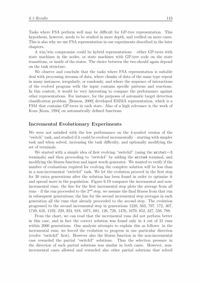
6.3 Results 143

Tasks where FSA perform well may be difficult for GP-tree representation. Thishypothesis, however, needs to be studied in more depth, and verified on more cases.This is also why we use FSA representation in our experiments described in the laterchapters.

A win/win compromise could be hybrid representations – either GP-trees withstate machines in the nodes, or state machines with GP-tree code on the statetransitions, or inside of the states. The choice between the two should again dependon the task structure.

We observe and conclude that the tasks where FSA representation is suitabledeal with processing streams of data, where chunks of data of the same type repeatin many instances, irregularly, or randomly, and where the sequence of interactionsof the evolved program with the input contains specific patterns and reactions.In this context, it would be very interesting to compare the performance againstother representations. For instance, for the purposes of automatic target detectionclassification problem, [Benson, 2000] developed EMMA representation, which is aFSM that contains GP-trees in each state. Also of a high relevance is the work ofKoza [Koza, 1994] on automatically defined functions.

Incremental Evolutionary Experiments

We were not satisfied with the low performance on the 4-symbol version of the“switch” task, and studied if it could be evolved incrementally – starting with simplertask and when solved, increasing the task difficulty, and optionally modifying theset of terminals.

We started with a simple idea of first evolving “switch3” (using the write1--3

terminals) and then proceeding to “switch4” by adding the write4 terminal, andmodifying the fitness function and input words generator. We wanted to verify if thenumber of evaluations required for evolving the complete solution will be less thanin a non-incremental “switch4” task. We let the evolution proceed in the first stepfor 30 extra generations after the solution has been found in order to optimize itand spread more in the population. Figure 6.19 compares the incremental and non-incremental runs: the line for the first incremental step plots the average from allruns – if the run proceeded to the 2nd step, we assume the final fitness from that runin subsequent generations; the line for the second incremental step averages in eachgeneration all the runs that already proceeded to the second step. The evolutionprogressed to the second incremental step in generations 1228, 563, 797, 172, 307,1749, 616, 1192, 229, 924, 918, 1071, 681, 126, 728, 1476, 1679, 852, 327, 556, 788.

From the chart, we can read that the incremental runs did not perform betterin this case, and in fact the correct solution was found only in 4 out of 21 runswithin 2000 generations. Our analysis attempts to explain this as follows: in theincremental runs, we forced the evolution to progress in one particular direction(evolve “switch3” first). However also the fitness function in the non-incrementalcase rewarded the partial “switch3” solutions. Thus the selection pressure inthe direction of such partial solutions was similar in both cases. However, non-incremental cases allowed and rewarded also other partial solutions that solved

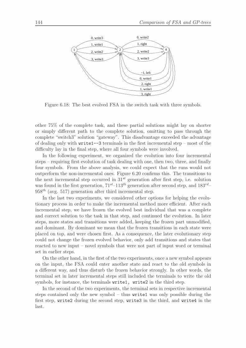
144 Comparison of FSA and GP-trees

21 4

0, write3

1, write1

2, write2

3, write3

0, write2

1, right

2, write2

3, write3

−1, left

0, write1

2, right

1, write1

3, right

Figure 6.18: The best evolved FSA in the switch task with three symbols.

other 75% of the complete task, and these partial solutions might lay on shorteror simply different path to the complete solution, omitting to pass through thecomplete “switch3” solution “gateway”. This disadvantage exceeded the advantageof dealing only with write1--3 terminals in the first incremental step – most of thedifficulty lay in the final step, where all four symbols were involved.

In the following experiment, we organized the evolution into four incrementalsteps – requiring first evolution of task dealing with one, then two, three, and finallyfour symbols. From the above analysis, we could expect that the runs would notoutperform the non-incremental ones. Figure 6.20 confirms this. The transitions tothe next incremental step occurred in 31st generation after first step, i.e. solutionwas found in the first generation, 71st–113th generation after second step, and 183rd–958th (avg. 517) generation after third incremental step.

In the last two experiments, we considered other options for helping the evolu-tionary process in order to make the incremental method more efficient. After eachincremental step, we have frozen the evolved best individual that was a completeand correct solution to the task in that step, and continued the evolution. In latersteps, more states and transitions were added, keeping the frozen part unmodified,and dominant. By dominant we mean that the frozen transitions in each state wereplaced on top, and were chosen first. As a consequence, the later evolutionary stepcould not change the frozen evolved behavior, only add transitions and states thatreacted to new input – novel symbols that were not part of input word or terminalset in earlier steps.

On the other hand, in the first of the two experiments, once a new symbol appearson the input, the FSA could enter another state and react to the old symbols ina different way, and thus disturb the frozen behavior strongly. In other words, theterminal set in later incremental steps still included the terminals to write the oldsymbols, for instance, the terminals write1, write2 in the third step.

In the second of the two experiments, the terminal sets in respective incrementalsteps contained only the new symbol – thus write1 was only possible during thefirst step, write2 during the second step, write3 in the third, and write4 in thelast.

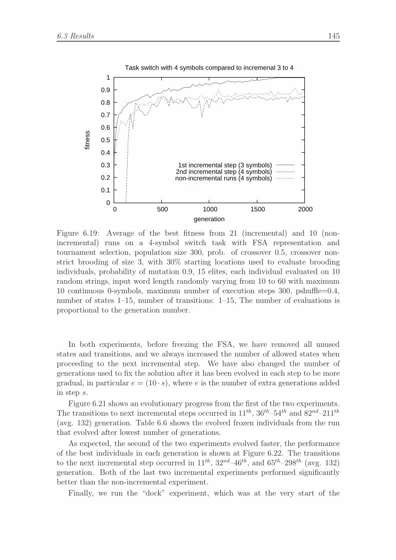
6.3 Results 145

0

0.1

0.2

0.3

0.4

0.5

0.6

0.7

0.8

0.9

1

0 500 1000 1500 2000

fitne

ss

generation

Task switch with 4 symbols compared to incremenal 3 to 4

1st incremental step (3 symbols)2nd incremental step (4 symbols)non-incremental runs (4 symbols)

Figure 6.19: Average of the best fitness from 21 (incremental) and 10 (non-incremental) runs on a 4-symbol switch task with FSA representation andtournament selection, population size 300, prob. of crossover 0.5, crossover non-strict brooding of size 3, with 30% starting locations used to evaluate broodingindividuals, probability of mutation 0.9, 15 elites, each individual evaluated on 10random strings, input word length randomly varying from 10 to 60 with maximum10 continuous 0-symbols, maximum number of execution steps 300, pshuffle=0.4,number of states 1–15, number of transitions: 1–15, The number of evaluations isproportional to the generation number.

In both experiments, before freezing the FSA, we have removed all unusedstates and transitions, and we always increased the number of allowed states whenproceeding to the next incremental step. We have also changed the number ofgenerations used to fix the solution after it has been evolved in each step to be moregradual, in particular e = (10 · s), where e is the number of extra generations addedin step s.

Figure 6.21 shows an evolutionary progress from the first of the two experiments.The transitions to next incremental steps occurred in 11th, 36th–54th and 82nd–211th

(avg. 132) generation. Table 6.6 shows the evolved frozen individuals from the runthat evolved after lowest number of generations.

As expected, the second of the two experiments evolved faster, the performanceof the best individuals in each generation is shown at Figure 6.22. The transitionsto the next incremental step occurred in 11th, 32nd–46th, and 65th–298th (avg. 132)generation. Both of the last two incremental experiments performed significantlybetter than the non-incremental experiment.

Finally, we run the “dock” experiment, which was at the very start of the

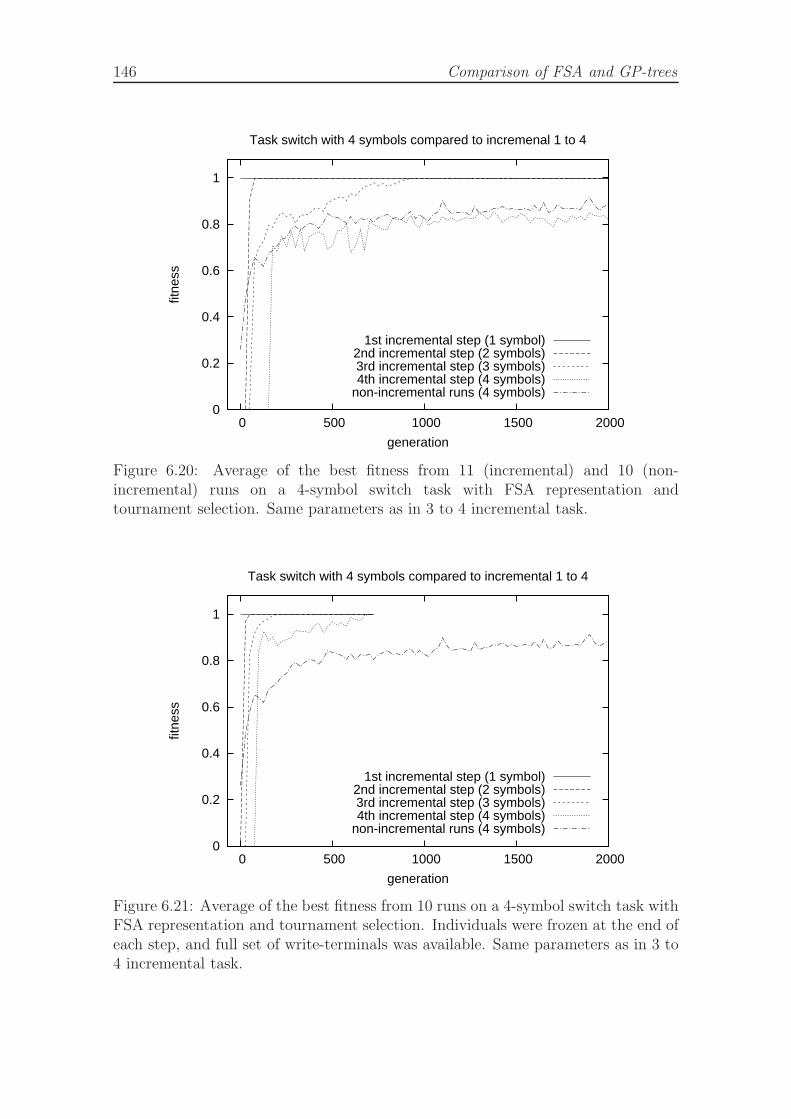
146 Comparison of FSA and GP-trees

0

0.2

0.4

0.6

0.8

1

0 500 1000 1500 2000

fitne

ss

generation

Task switch with 4 symbols compared to incremenal 1 to 4

1st incremental step (1 symbol)2nd incremental step (2 symbols)3rd incremental step (3 symbols)4th incremental step (4 symbols)

non-incremental runs (4 symbols)

Figure 6.20: Average of the best fitness from 11 (incremental) and 10 (non-incremental) runs on a 4-symbol switch task with FSA representation andtournament selection. Same parameters as in 3 to 4 incremental task.

0

0.2

0.4

0.6

0.8

1

0 500 1000 1500 2000

fitne

ss

generation

Task switch with 4 symbols compared to incremental 1 to 4

1st incremental step (1 symbol)2nd incremental step (2 symbols)3rd incremental step (3 symbols)4th incremental step (4 symbols)

non-incremental runs (4 symbols)

Figure 6.21: Average of the best fitness from 10 runs on a 4-symbol switch task withFSA representation and tournament selection. Individuals were frozen at the end ofeach step, and full set of write-terminals was available. Same parameters as in 3 to4 incremental task.

6.3 Results 147

step1: 1 states

—state 1 with 2 transit.

[R1 == 1] 1 [right]

[R1 == 0] 1 [write1]

step 2: 3 states

—state 1 with 4 transit.

[R1 == 1] 1 [right]

[R1 == 0] 1 [write1]

[R1 == 2] 2 [right]

[R1 == -1] 2 [left]

—state 2 with 4 transit.

[R1 == 1] 3 [done]

[R1 == -1] 1 [left]

[R1 == 2] 3 [write2]

[R1 == 0] 3 [write2]

—state 3 with 3 transit.

[R1 == 2] 3 [right]

[R1 == 0] 1 [left]

[R1 == 1] 3 [right]

step3: 4 states

—state 1 with 5 transit.

[R1 == 1] 1 [right]

[R1 == 0] 1 [write1]

[R1 == 2] 2 [right]

[R1 == -1] 2 [left]

[R1 == 3] 3 [right]

—state 2 with 5 transit.

[R1 == 1] 4 [done]

[R1 == -1] 1 [left]

[R1 == 2] 4 [write2]

[R1 == 0] 4 [write2]

[R1 == 3] 4 [right]

—state 3 with 4 transit.

[R1 == 2] 2 [left]

[R1 == 3] 4 [right]

[R1 == 0] 4 [write3]

[R1 == 1] 2 [write3]

—state 4 with 4 transit.

[R1 == 2] 4 [right]

[R1 == 0] 1 [left]

[R1 == 1] 4 [right]

[R1 == 3] 4 [right]

step4: 5 states

—state 1 with 6 transit.

[R1 == 1] 1 [right]

[R1 == 0] 1 [write1]

[R1 == 2] 2 [right]

[R1 == -1] 2 [left]

[R1 == 3] 3 [right]

[R1 == 4] 4 [right]

—state 2 with 5 transit.

[R1 == 1] 5 [done]

[R1 == -1] 1 [left]

[R1 == 2] 5 [write2]

[R1 == 0] 5 [write2]

[R1 == 3] 5 [right]

—state 3 with 5 transit.

[R1 == 2] 2 [left]

[R1 == 3] 5 [right]

[R1 == 0] 5 [write3]

[R1 == 1] 2 [write3]

[R1 == -1] 2 [right]

—state 4 with 5 transit.

[R1 == 4] 2 [write1]

[R1 == 1] 2 [done]

[R1 == -1] 2 [write1]

[R1 == 3] 2 [write4]

[R1 == 0] 2 [write4]

—state 5 with 5 transit.

[R1 == 2] 5 [right]

[R1 == 0] 1 [left]

[R1 == 1] 5 [right]

[R1 == 3] 5 [right]

[R1 == 4] 4 [right]

Table 6.6: Evolved frozen individuals in the incremental steps 1–4, switch task withfour symbols.

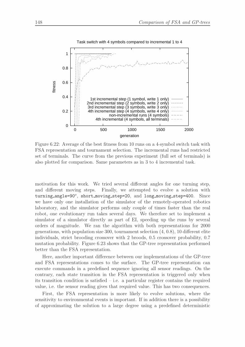
148 Comparison of FSA and GP-trees

0

0.2

0.4

0.6

0.8

1

0 500 1000 1500 2000

fitne

ss

generation

Task switch with 4 symbols compared to incremental 1 to 4

1st incremental step (1 symbol, write 1 only)2nd incremental step (2 symbols, write 2 only)3rd incremental step (3 symbols, write 3 only)4th incremental step (4 symbols, write 4 only)

non-incremental runs (4 symbols)4th incremental (4 symbols, all terminals)

Figure 6.22: Average of the best fitness from 10 runs on a 4-symbol switch task withFSA representation and tournament selection. The incremental runs had restrictedset of terminals. The curve from the previous experiment (full set of terminals) isalso plotted for comparison. Same parameters as in 3 to 4 incremental task.

motivation for this work. We tried several different angles for one turning step,and different moving steps. Finally, we attempted to evolve a solution withturning angle=90o, short moving step=20, and long moving step=400. Sincewe have only one installation of the simulator of the remotely-operated roboticslaboratory, and the simulator performs only couple of times faster than the realrobot, one evolutionary run takes several days. We therefore set to implement asimulator of a simulator directly as part of EI, speeding up the runs by severalorders of magnitude. We ran the algorithm with both representations for 2000generations, with population size 300, tournament selection (4, 0.8), 10 different eliteindividuals, strict brooding crossover with 2 broods, 0.5 crossover probability, 0.7mutation probability. Figure 6.23 shows that the GP-tree representation performedbetter than the FSA representation.

Here, another important difference between our implementations of the GP-treeand FSA representations comes to the surface. The GP-tree representation canexecute commands in a predefined sequence ignoring all sensor readings. On thecontrary, each state transition in the FSA representation is triggered only whenits transition condition is satisfied – i.e. a particular register contains the requiredvalue, i.e. the sensor reading gives that required value. This has two consequences.

First, the FSA representation is more likely to evolve solutions, where thesensitivity to environmental events is important. If in addition there is a possibilityof approximating the solution to a large degree using a predefined deterministic

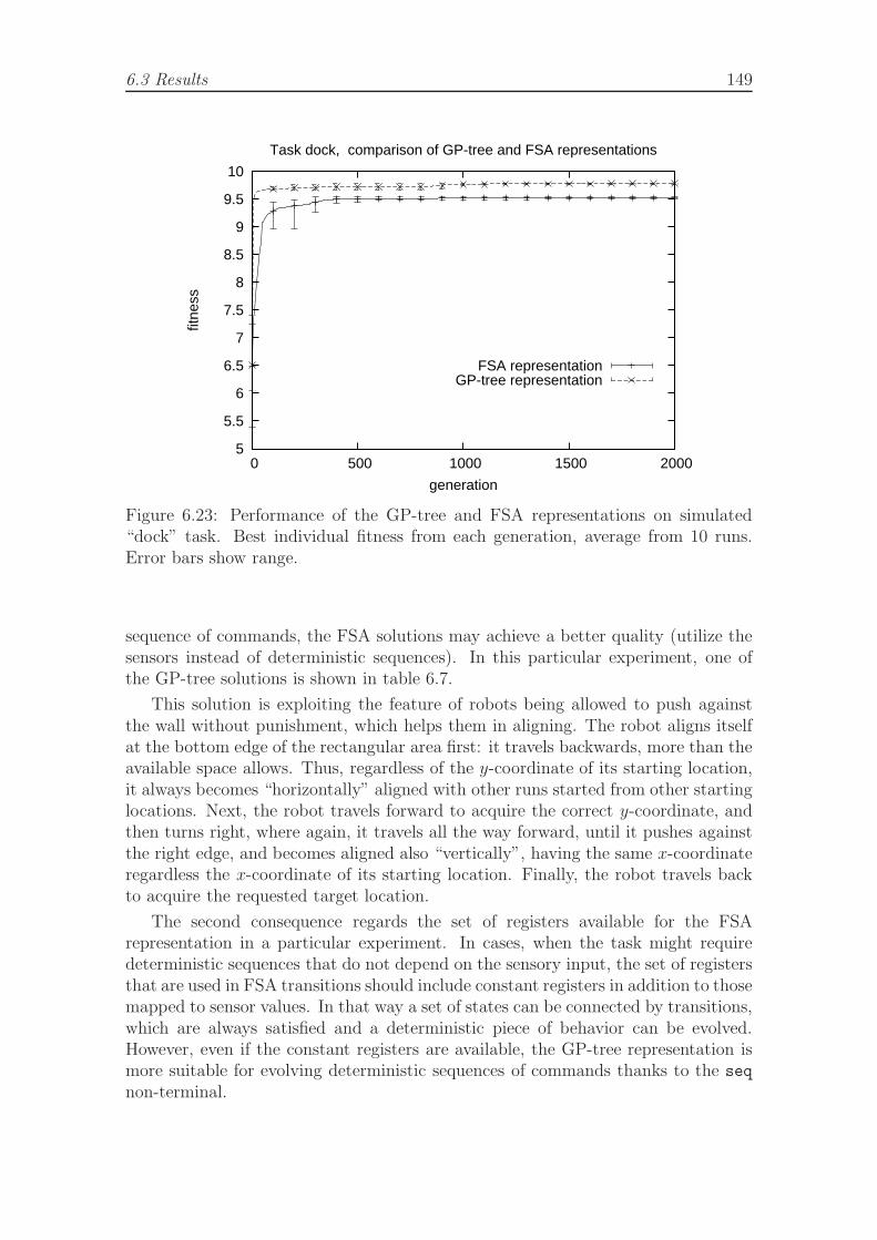
6.3 Results 149

5

5.5

6

6.5

7

7.5

8

8.5

9

9.5

10

0 500 1000 1500 2000

fitne

ss

generation

Task dock, comparison of GP-tree and FSA representations

FSA representationGP-tree representation

Figure 6.23: Performance of the GP-tree and FSA representations on simulated“dock” task. Best individual fitness from each generation, average from 10 runs.Error bars show range.

sequence of commands, the FSA solutions may achieve a better quality (utilize thesensors instead of deterministic sequences). In this particular experiment, one ofthe GP-tree solutions is shown in table 6.7.

This solution is exploiting the feature of robots being allowed to push againstthe wall without punishment, which helps them in aligning. The robot aligns itselfat the bottom edge of the rectangular area first: it travels backwards, more than theavailable space allows. Thus, regardless of the y-coordinate of its starting location,it always becomes “horizontally” aligned with other runs started from other startinglocations. Next, the robot travels forward to acquire the correct y-coordinate, andthen turns right, where again, it travels all the way forward, until it pushes againstthe right edge, and becomes aligned also “vertically”, having the same x-coordinateregardless the x-coordinate of its starting location. Finally, the robot travels backto acquire the requested target location.

The second consequence regards the set of registers available for the FSArepresentation in a particular experiment. In cases, when the task might requiredeterministic sequences that do not depend on the sensory input, the set of registersthat are used in FSA transitions should include constant registers in addition to thosemapped to sensor values. In that way a set of states can be connected by transitions,which are always satisfied and a deterministic piece of behavior can be evolved.However, even if the constant registers are available, the GP-tree representation ismore suitable for evolving deterministic sequences of commands thanks to the seq

non-terminal.

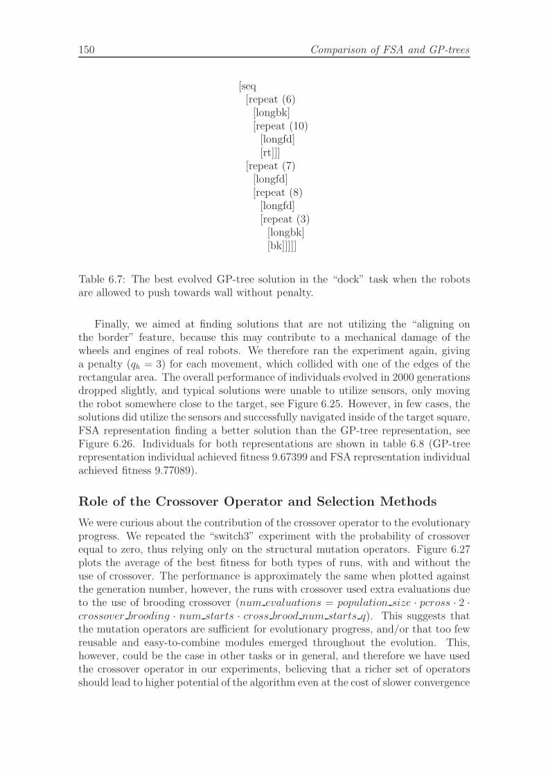
150 Comparison of FSA and GP-trees

[seq[repeat (6)

[longbk][repeat (10)

[longfd][rt]]]

[repeat (7)[longfd][repeat (8)

[longfd][repeat (3)

[longbk][bk]]]]]

Table 6.7: The best evolved GP-tree solution in the “dock” task when the robotsare allowed to push towards wall without penalty.

Finally, we aimed at finding solutions that are not utilizing the “aligning onthe border” feature, because this may contribute to a mechanical damage of thewheels and engines of real robots. We therefore ran the experiment again, givinga penalty (qh = 3) for each movement, which collided with one of the edges of therectangular area. The overall performance of individuals evolved in 2000 generationsdropped slightly, and typical solutions were unable to utilize sensors, only movingthe robot somewhere close to the target, see Figure 6.25. However, in few cases, thesolutions did utilize the sensors and successfully navigated inside of the target square,FSA representation finding a better solution than the GP-tree representation, seeFigure 6.26. Individuals for both representations are shown in table 6.8 (GP-treerepresentation individual achieved fitness 9.67399 and FSA representation individualachieved fitness 9.77089).

Role of the Crossover Operator and Selection Methods

We were curious about the contribution of the crossover operator to the evolutionaryprogress. We repeated the “switch3” experiment with the probability of crossoverequal to zero, thus relying only on the structural mutation operators. Figure 6.27plots the average of the best fitness for both types of runs, with and without theuse of crossover. The performance is approximately the same when plotted againstthe generation number, however, the runs with crossover used extra evaluations dueto the use of brooding crossover (num evaluations = population size · pcross · 2 ·crossover brooding · num starts · cross brood num starts q). This suggests thatthe mutation operators are sufficient for evolutionary progress, and/or that too fewreusable and easy-to-combine modules emerged throughout the evolution. This,however, could be the case in other tasks or in general, and therefore we have usedthe crossover operator in our experiments, believing that a richer set of operatorsshould lead to higher potential of the algorithm even at the cost of slower convergence

6.3 Results 151

15 states (unused states not shown)

—state 1 with 1 transitions

[R1 == 1] 3 [longfd]

—state 2 with 1 transitions

[R1 == 1] 11 [longfd]

—state 3 with 1 transitions

[R1 == 1] 6 [stopON]

—state 5 with 2 transitions

[R1 == 0] 2 [longfd]

[R1 == 1] 7 [longfd]

—state 6 with 1 transitions

[R1 == 1] 12 [bk]

—state 7 with 2 transitions

[R1 == 1] 8 [longbk]

[R1 == 0] 5 [stopOFF]

—state 8 with 1 transitions

[R1 == 1] 5 [longfd]

—state 10 with 1 transitions

[R1 == 1] 3 [rt]

—state 11 with 1 transitions

[R1 == 1] 10 [longfd]

—state 12 with 1 transitions

[R1 == 1] 5 [fd]

[repeat (1)

[repeat (3)

[longfd]

[seq ()

[lt]

[repeat (6)

[longbk]

[stopON]]]]

[repeat (1)

[repeat (2)

[seq ()

[rt]

[repeat (4)

[longfd]

[longfd]]]

[if (R1 == 0)

[done]

[stopOFF]]]

[seq ()

[seq ()

[lt]

[longfd]]

[longfd]]]]

Table 6.8: Selected evolved individuals with the best performance for the “dock”task. The FSA individual is also shown at the Figure 6.24.

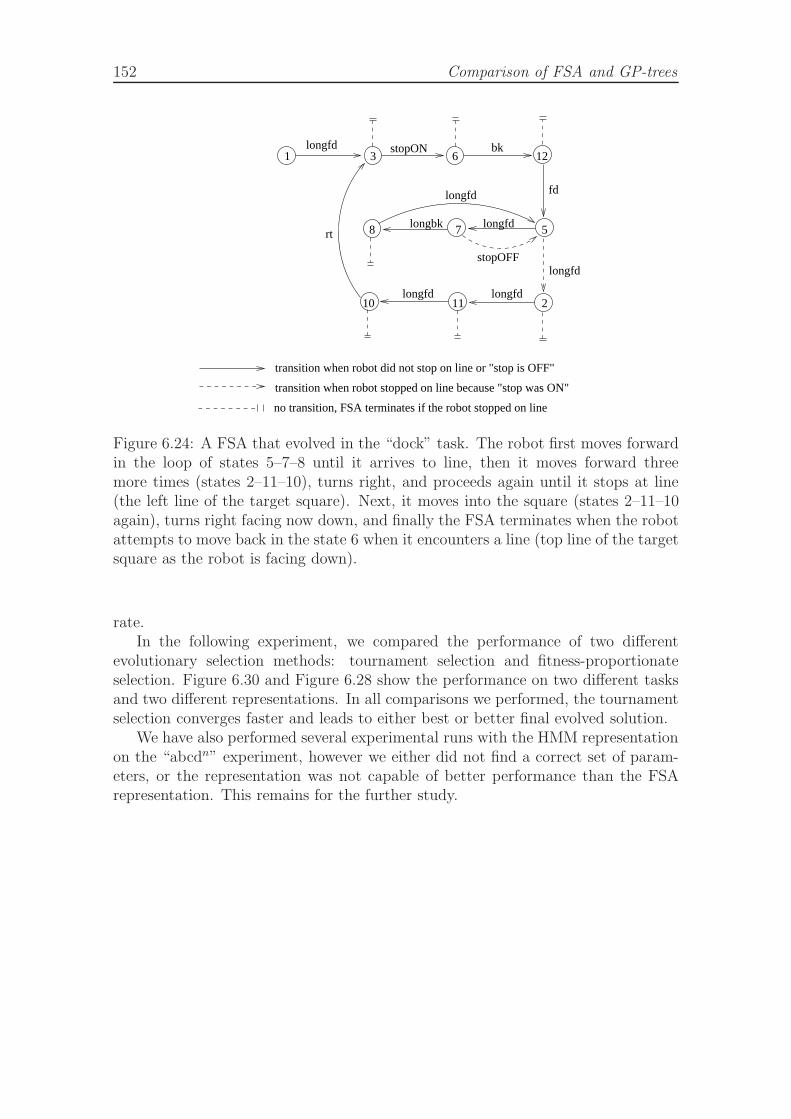
152 Comparison of FSA and GP-trees

11 210

7 58

1 6 123longfd

longfd

longfdlongfd

longfd

longfdlongbk

fd

rt

bk

stopOFF

stopON

transition when robot did not stop on line or "stop is OFF"

transition when robot stopped on line because "stop was ON"

no transition, FSA terminates if the robot stopped on line

Figure 6.24: A FSA that evolved in the “dock” task. The robot first moves forwardin the loop of states 5–7–8 until it arrives to line, then it moves forward threemore times (states 2–11–10), turns right, and proceeds again until it stops at line(the left line of the target square). Next, it moves into the square (states 2–11–10again), turns right facing now down, and finally the FSA terminates when the robotattempts to move back in the state 6 when it encounters a line (top line of the targetsquare as the robot is facing down).

rate.In the following experiment, we compared the performance of two different

evolutionary selection methods: tournament selection and fitness-proportionateselection. Figure 6.30 and Figure 6.28 show the performance on two different tasksand two different representations. In all comparisons we performed, the tournamentselection converges faster and leads to either best or better final evolved solution.

We have also performed several experimental runs with the HMM representationon the “abcdn” experiment, however we either did not find a correct set of param-eters, or the representation was not capable of better performance than the FSArepresentation. This remains for the further study.

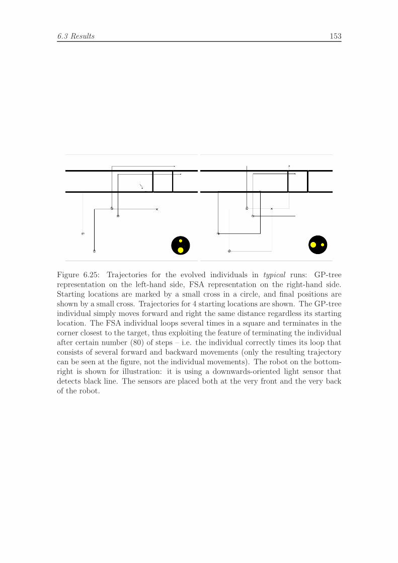
6.3 Results 153

Figure 6.25: Trajectories for the evolved individuals in typical runs: GP-treerepresentation on the left-hand side, FSA representation on the right-hand side.Starting locations are marked by a small cross in a circle, and final positions areshown by a small cross. Trajectories for 4 starting locations are shown. The GP-treeindividual simply moves forward and right the same distance regardless its startinglocation. The FSA individual loops several times in a square and terminates in thecorner closest to the target, thus exploiting the feature of terminating the individualafter certain number (80) of steps – i.e. the individual correctly times its loop thatconsists of several forward and backward movements (only the resulting trajectorycan be seen at the figure, not the individual movements). The robot on the bottom-right is shown for illustration: it is using a downwards-oriented light sensor thatdetects black line. The sensors are placed both at the very front and the very backof the robot.

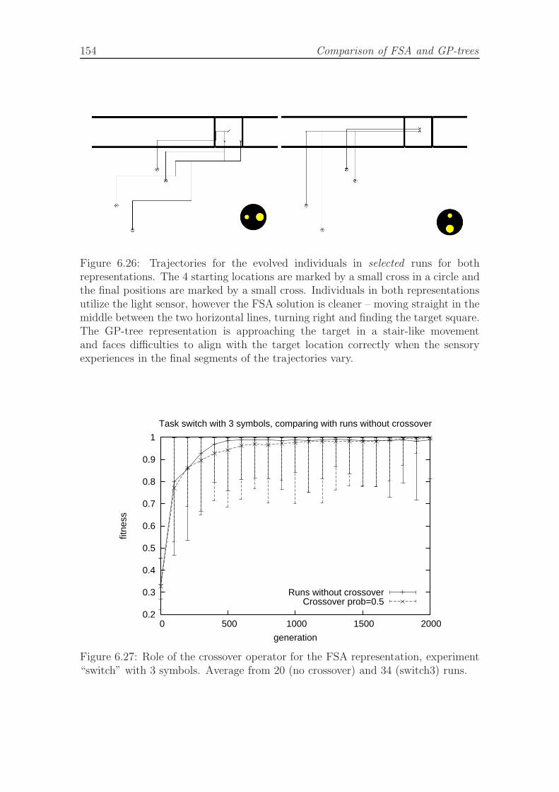
154 Comparison of FSA and GP-trees

Figure 6.26: Trajectories for the evolved individuals in selected runs for bothrepresentations. The 4 starting locations are marked by a small cross in a circle andthe final positions are marked by a small cross. Individuals in both representationsutilize the light sensor, however the FSA solution is cleaner – moving straight in themiddle between the two horizontal lines, turning right and finding the target square.The GP-tree representation is approaching the target in a stair-like movementand faces difficulties to align with the target location correctly when the sensoryexperiences in the final segments of the trajectories vary.

0.2

0.3

0.4

0.5

0.6

0.7

0.8

0.9

1

0 500 1000 1500 2000

fitne

ss

generation

Task switch with 3 symbols, comparing with runs without crossover

Runs without crossoverCrossover prob=0.5

Figure 6.27: Role of the crossover operator for the FSA representation, experiment“switch” with 3 symbols. Average from 20 (no crossover) and 34 (switch3) runs.

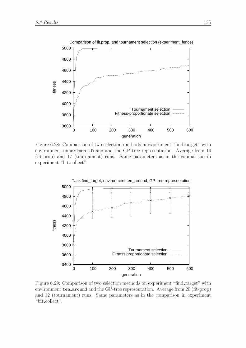
6.3 Results 155

3600

3800

4000

4200

4400

4600

4800

5000

0 100 200 300 400 500 600

fitne

ss

generation

Comparison of fit.prop. and tournament selection (experiment_fence)

Tournament selectionFitness-proportionate selection

Figure 6.28: Comparison of two selection methods in experiment “find target” withenvironment experiment fence and the GP-tree representation. Average from 14(fit-prop) and 17 (tournament) runs. Same parameters as in the comparison inexperiment “bit collect”.

3400

3600

3800

4000

4200

4400

4600

4800

5000

0 100 200 300 400 500 600

fitne

ss

generation

Task find_target, environment ten_around, GP-tree representation

Tournament selectionFitness proportionate selection

Figure 6.29: Comparison of two selection methods on experiment “find target” withenvironment ten around and the GP-tree representation. Average from 20 (fit-prop)and 12 (tournament) runs. Same parameters as in the comparison in experiment“bit collect”.

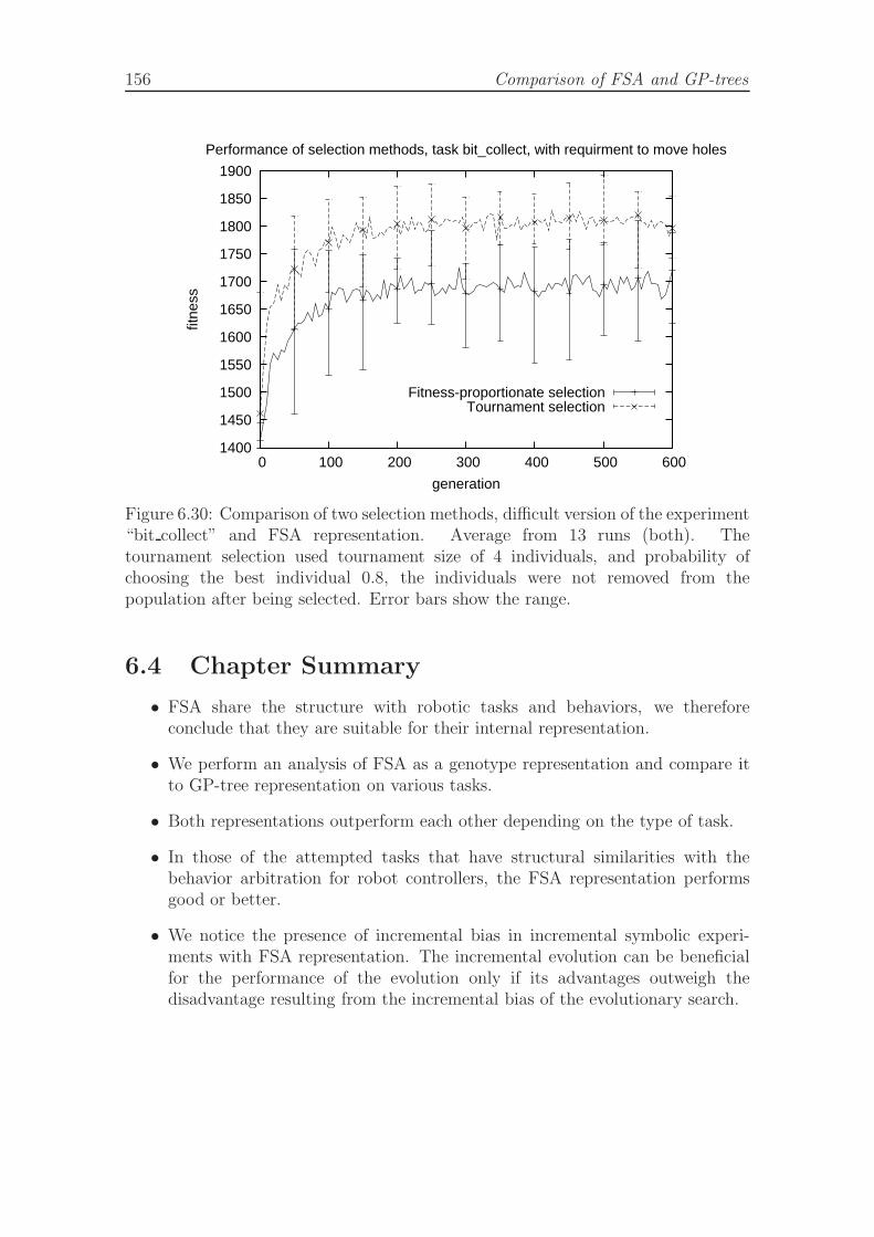
156 Comparison of FSA and GP-trees

1400

1450

1500

1550

1600

1650

1700

1750

1800

1850

1900

0 100 200 300 400 500 600

fitne

ss

generation

Performance of selection methods, task bit_collect, with requirment to move holes

Fitness-proportionate selectionTournament selection

Figure 6.30: Comparison of two selection methods, difficult version of the experiment“bit collect” and FSA representation. Average from 13 runs (both). Thetournament selection used tournament size of 4 individuals, and probability ofchoosing the best individual 0.8, the individuals were not removed from thepopulation after being selected. Error bars show the range.

6.4 Chapter Summary

• FSA share the structure with robotic tasks and behaviors, we thereforeconclude that they are suitable for their internal representation.

• We perform an analysis of FSA as a genotype representation and compare itto GP-tree representation on various tasks.

• Both representations outperform each other depending on the type of task.

• In those of the attempted tasks that have structural similarities with thebehavior arbitration for robot controllers, the FSA representation performsgood or better.

• We notice the presence of incremental bias in incremental symbolic experi-ments with FSA representation. The incremental evolution can be beneficialfor the performance of the evolution only if its advantages outweigh thedisadvantage resulting from the incremental bias of the evolutionary search.

Chapter 7

Design and ImplementationConsiderations

In this chapter, we discuss how we set to test our hypothesis described in the previoussections in several research experiments. We discuss the details of the proposedalgorithms and architectures to be investigated.

7.1 Simulation Framework

It is not the speaker who controls communication, but the listener.—proverb

The aim is to design controllers for real robots. Our current testing hardwareplatform is the LEGO Robotics RCX equipped with 32KB RAM, up to 3 sensors and3 motors, running programs built using GNU C compiler and binutils with LegOS[Noga, 1999]. Testing the performance of each individual in hardware would becompletely infeasible, and therefore a simulator is essential. The objective functionof our evolutionary algorithm evaluates individuals in simulation; each individual isstarted from several starting locations. We upload the final evolved controller onthe real hardware to verify its real-world functionality.

7.1.1 Lazy Simulation Method

Recall from the section ?? the two standard approaches to simulation: discrete eventsimulation and continuous simulation. Continuous simulations apply to variousdynamic systems. We are concerned with discrete actions and state changes occuringin the environment, thus we employ descrete event simulation. However, we makeuse a combination of next-event time advance with emulation of the controller (whichfollows the CPU clock, i.e. is a kind of fixed-increment time advance). The simulatedcontroller generates events at discrete time units on the granularity of the CPU clockfrequency of the simulating computer (for example, start the motor A, determinethe value of sensor 1), but its environment is updated “continuously”, i.e. at anytime the event occurs (an event can occur also for other reasons than due to an

158 Design and Implementation Considerations

action of the robot controller). Thus events in the environment can occur at anarbitrary time and place. Typical events include robot running against an obstacle,or over some pattern drawn on the floor, scheduled light switching, or robot enteringmonitored area of the environment.

Our lazy simulation approach (inspired by lazy evaluation in functional program-ming languages) updates the state of the simulated system only when the robotcontroller interacts with the robot hardware. At that time instant, we suspendthe emulated program, compute the current exact state of the simulated system(environment and robot) by mathematical formulas, and determine the outcomeof the interaction that triggered the update. The temporal granularity is thuslimited only by the CPU or bus frequency of the simulating machine. The emulatedprogram is not interpreted by the simulator. It runs almost independently within theoperating system of the simulating computer, see Figure 2.10. Instead of accessingthe robot hardware, it accesses the simulator that is waiting in the background. Forexample, the robot controller program might be computing without interacting withthe robot hardware for some time, during which the robot crosses several lines onthe floor, triggers switching of the light by entering an active area, passes below alight, and bounces to a wall, where it remains blocked for a while. At that point intime, the robot controller wants to read a value of its light sensor, for instance, andonly at that point in time the simulator becomes active and computes the wholesequence of the previous events that occurred, and the current location and situationof the robot and the environment. Finally, the required value of the sensor readingis determined and returned to the program, which resumes its execution. To achievebetter performance, the simulator pre-computes expected events before resuming thesimulated program. The pre-computed information helps to test quickly whether thestate of the robot or environment has changed since the last “interrupt”, withoutprocessing all the data structures of the simulator. We call this approach lazysimulation because it uses maximum possible abstraction from the environment andperforms simulation computation only when very necessary.

None of the existing robot simulators satisfied our needs. We chose to implementour own simulator in language C, now available as open-source project [URL -Eval]. The simulator is designed to cope with any program written in LegOS(later renamed to BrickOS) system, which controls an experimental robot with acompatible topology (Figure 7.1, 8.4 right). This allows us to use it both with ourcontroller architecture, and with virtually any C-program that can control the robot.Small modifications would allow simulating robots with different topologies.

There are several issues related to simulation. First of all, many researcherspointed out that simulating robotic systems accurately is almost impossible. Eachsensor and motor part has somewhat different characteristics, and the outcome ofeach sensory or motor action depends on imperfect interactions with the real world.In order to achieve a comparable performance of the simulated and real roboticsystem, noise has to be applied both to sensory readings, and motor actions. Inaddition, the outcome of the motor action is hard to compute and it appears to bemore feasible to measure it and construct a table of basic motor actions and theiroutcomes as proposed by Miglino et.al. [Miglino et al., 1995]. Figure 8.4 left shows a

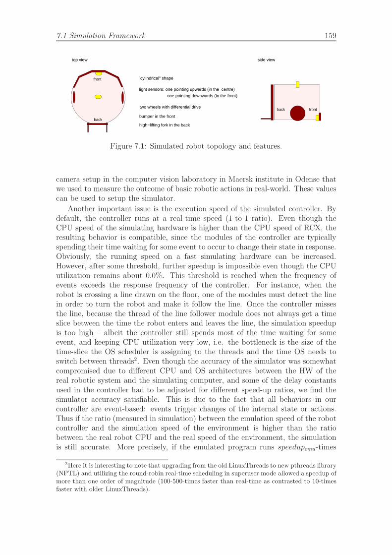
7.1 Simulation Framework 159

light sensors: one pointing upwards (in the centre)

one pointing downwards (in the front)

two wheels with differential drive

"cylindrical" shape

bumper in the front

high−lifting fork in the back

top view side view

frontback

front

back

Figure 7.1: Simulated robot topology and features.

camera setup in the computer vision laboratory in Maersk institute in Odense thatwe used to measure the outcome of basic robotic actions in real-world. These valuescan be used to setup the simulator.

Another important issue is the execution speed of the simulated controller. Bydefault, the controller runs at a real-time speed (1-to-1 ratio). Even though theCPU speed of the simulating hardware is higher than the CPU speed of RCX, theresulting behavior is compatible, since the modules of the controller are typicallyspending their time waiting for some event to occur to change their state in response.Obviously, the running speed on a fast simulating hardware can be increased.However, after some threshold, further speedup is impossible even though the CPUutilization remains about 0.0%. This threshold is reached when the frequency ofevents exceeds the response frequency of the controller. For instance, when therobot is crossing a line drawn on the floor, one of the modules must detect the linein order to turn the robot and make it follow the line. Once the controller missesthe line, because the thread of the line follower module does not always get a timeslice between the time the robot enters and leaves the line, the simulation speedupis too high – albeit the controller still spends most of the time waiting for someevent, and keeping CPU utilization very low, i.e. the bottleneck is the size of thetime-slice the OS scheduler is assigning to the threads and the time OS needs toswitch between threads2. Even though the accuracy of the simulator was somewhatcompromised due to different CPU and OS architectures between the HW of thereal robotic system and the simulating computer, and some of the delay constantsused in the controller had to be adjusted for different speed-up ratios, we find thesimulator accuracy satisfiable. This is due to the fact that all behaviors in ourcontroller are event-based: events trigger changes of the internal state or actions.Thus if the ratio (measured in simulation) between the emulation speed of the robotcontroller and the simulation speed of the environment is higher than the ratiobetween the real robot CPU and the real speed of the environment, the simulationis still accurate. More precisely, if the emulated program runs speedupemu-times

2Here it is interesting to note that upgrading from the old LinuxThreads to new pthreads library(NPTL) and utilizing the round-robin real-time scheduling in superuser mode allowed a speedup ofmore than one order of magnitude (100-500-times faster than real-time as contrasted to 10-timesfaster with older LinuxThreads).

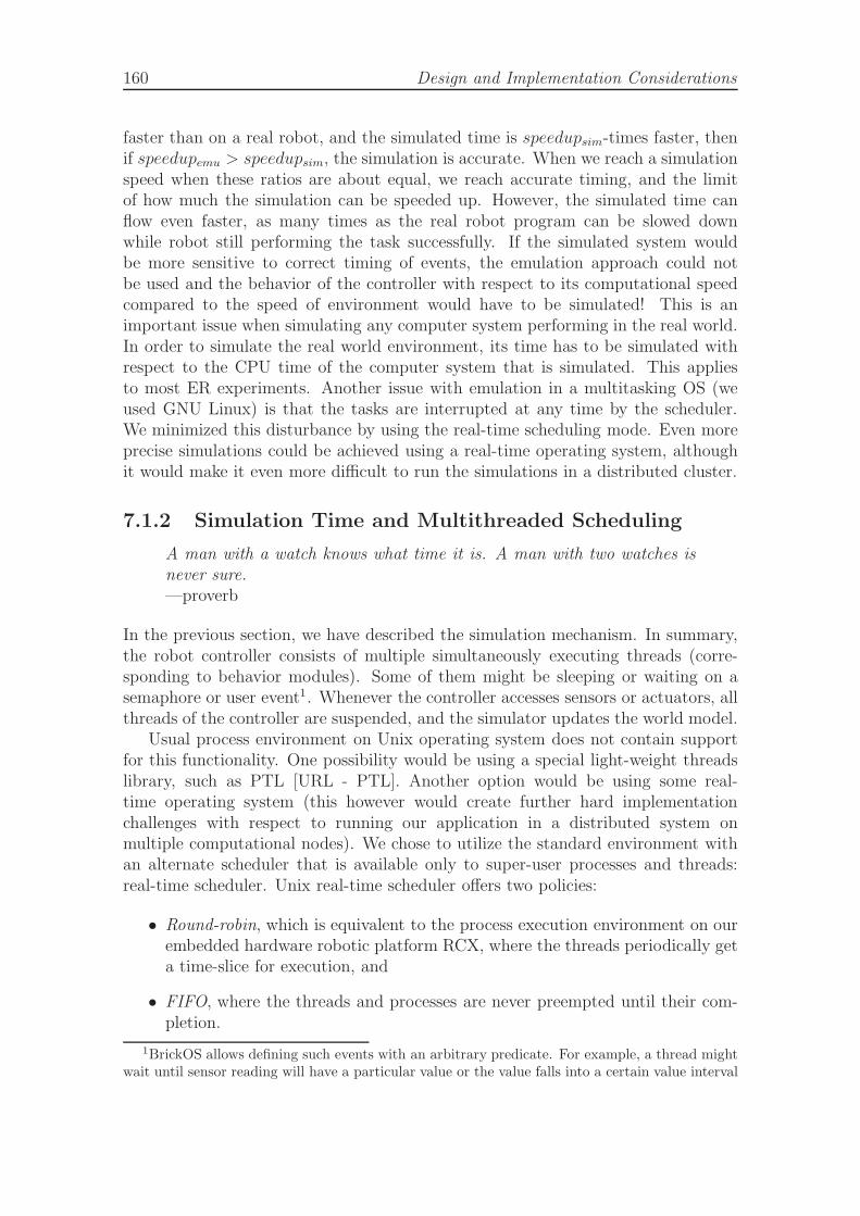
160 Design and Implementation Considerations

faster than on a real robot, and the simulated time is speedupsim-times faster, thenif speedupemu > speedupsim, the simulation is accurate. When we reach a simulationspeed when these ratios are about equal, we reach accurate timing, and the limitof how much the simulation can be speeded up. However, the simulated time canflow even faster, as many times as the real robot program can be slowed downwhile robot still performing the task successfully. If the simulated system wouldbe more sensitive to correct timing of events, the emulation approach could notbe used and the behavior of the controller with respect to its computational speedcompared to the speed of environment would have to be simulated! This is animportant issue when simulating any computer system performing in the real world.In order to simulate the real world environment, its time has to be simulated withrespect to the CPU time of the computer system that is simulated. This appliesto most ER experiments. Another issue with emulation in a multitasking OS (weused GNU Linux) is that the tasks are interrupted at any time by the scheduler.We minimized this disturbance by using the real-time scheduling mode. Even moreprecise simulations could be achieved using a real-time operating system, althoughit would make it even more difficult to run the simulations in a distributed cluster.

7.1.2 Simulation Time and Multithreaded Scheduling

A man with a watch knows what time it is. A man with two watches isnever sure.—proverb

In the previous section, we have described the simulation mechanism. In summary,the robot controller consists of multiple simultaneously executing threads (corre-sponding to behavior modules). Some of them might be sleeping or waiting on asemaphore or user event1. Whenever the controller accesses sensors or actuators, allthreads of the controller are suspended, and the simulator updates the world model.

Usual process environment on Unix operating system does not contain supportfor this functionality. One possibility would be using a special light-weight threadslibrary, such as PTL [URL - PTL]. Another option would be using some real-time operating system (this however would create further hard implementationchallenges with respect to running our application in a distributed system onmultiple computational nodes). We chose to utilize the standard environment withan alternate scheduler that is available only to super-user processes and threads:real-time scheduler. Unix real-time scheduler offers two policies:

• Round-robin, which is equivalent to the process execution environment on ourembedded hardware robotic platform RCX, where the threads periodically geta time-slice for execution, and

• FIFO, where the threads and processes are never preempted until their com-pletion.

1BrickOS allows defining such events with an arbitrary predicate. For example, a thread mightwait until sensor reading will have a particular value or the value falls into a certain value interval

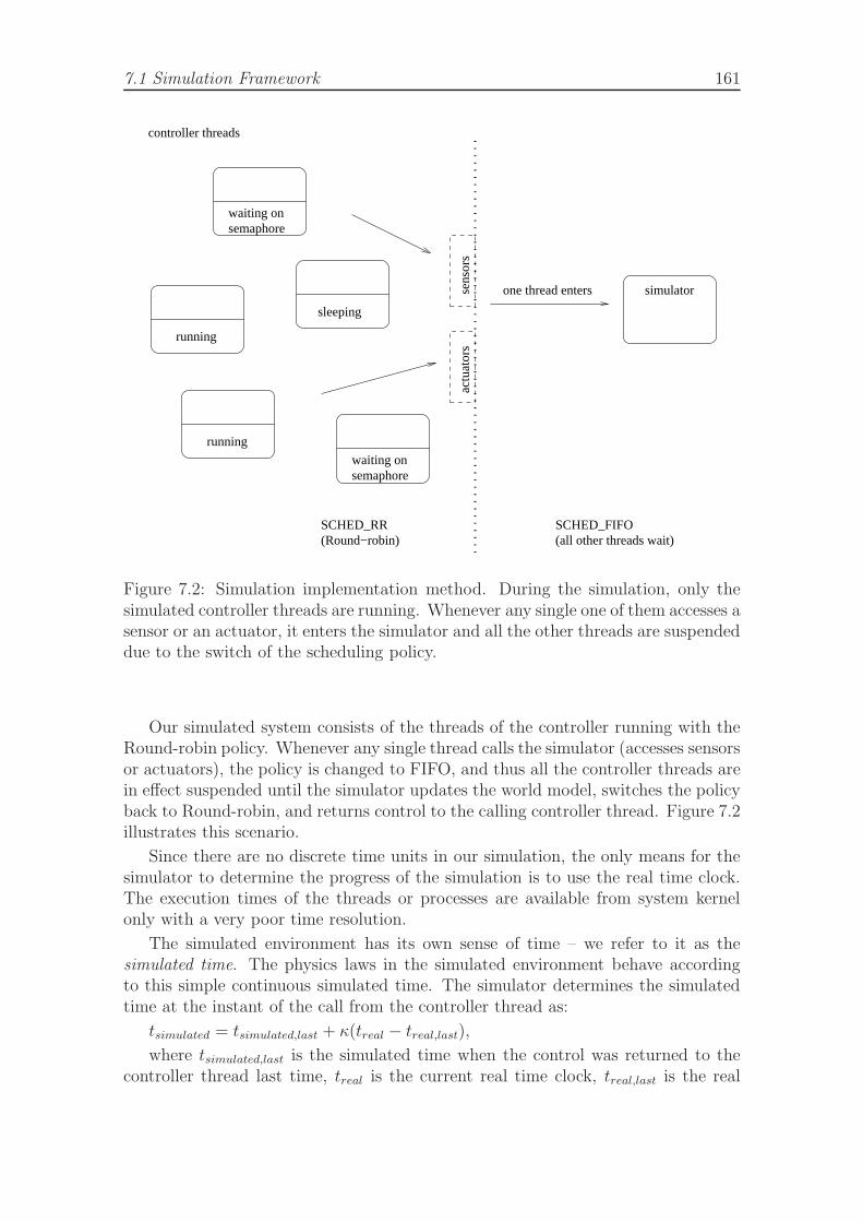
7.1 Simulation Framework 161

waiting onsemaphore

running

running

waiting onsemaphore

sleeping

SCHED_RR(Round−robin)

SCHED_FIFO(all other threads wait)

simulator

controller threads

sens

ors

actu

ator

s

one thread enters

Figure 7.2: Simulation implementation method. During the simulation, only thesimulated controller threads are running. Whenever any single one of them accesses asensor or an actuator, it enters the simulator and all the other threads are suspendeddue to the switch of the scheduling policy.

Our simulated system consists of the threads of the controller running with theRound-robin policy. Whenever any single thread calls the simulator (accesses sensorsor actuators), the policy is changed to FIFO, and thus all the controller threads arein effect suspended until the simulator updates the world model, switches the policyback to Round-robin, and returns control to the calling controller thread. Figure 7.2illustrates this scenario.

Since there are no discrete time units in our simulation, the only means for thesimulator to determine the progress of the simulation is to use the real time clock.The execution times of the threads or processes are available from system kernelonly with a very poor time resolution.

The simulated environment has its own sense of time – we refer to it as thesimulated time. The physics laws in the simulated environment behave accordingto this simple continuous simulated time. The simulator determines the simulatedtime at the instant of the call from the controller thread as:

tsimulated = tsimulated,last + κ(treal − treal,last),

where tsimulated,last is the simulated time when the control was returned to thecontroller thread last time, treal is the current real time clock, treal,last is the real

162 Design and Implementation Considerations

time clock when the control was returned to the simulator, and κ is the speed-up constant. The κ parameter describes the ratio between the simulated and realtime. For instance, κ = 1 represents a simulation, where the simulation time flowstogether with the real time (except of the interruptions by simulator, which are notseen from inside of the simulated world), and κ = 200 (a typical setting) representsa simulation speed-up by 200-times.

The described simulation procedure can handle multiple simulated controllers ina multiple-robot simulation, provided that the threshold of the critical frequency ofevents discussed above would not be exceeded.

7.1.3 Functional Requirements for the Simulator

In order to have a tool for experimenting with interesting tasks, we formulated therequirements for our simulator as follows:

• The simulator should update the location, heading and speed of one robot incompliance with the robot morphology shown in Figure 7.1. The morphologyallows for different movement types, see Figure 7.5 for details.

The robot will be navigating in a rectangular area with movable rectangularobjects (obstacles). The robot’s bumper sensor will indicate when robot pushesforward against an obstacle;

• It should be possible to define:

– marks on the floor of various shades of gray in the shape of lines of certainwidth or rectangles (or polygons), the robot’s bottom light sensor readingswill depend on the marks;

– top-mounted light sources of various intensity, the robot’s top light sensorreadings will depend on the accumulated light amount in the currentposition of the robot;

– cargo loading locations (loading stations), which are automated servicepoints, which detect the robot on arrival and notify the robot by sendingan IR message. The robot should respond with a navigation maneuverconsisting of 1) turning, 2) setting the lifting fork down, 3) approachingthe station thus moving the fork under the cargo, 4) lifting the fork withthe cargo, and 5) leaving the station. See Figure 7.3 for an illustration.Loading stations are specified with the help of scripts and active locations(see below). In real setup (as described below), the conveyer belt, theloading and unloading stations are operated by a separate RCX unitthat also sends the ‘welcome to (un)loading station’ IR messages to therobot after it has been detected by a photo cell sensor. This RCX unitis connected through the IR link also with a PC controlling the lampsthrough X10 modules.

– cargo unloading locations (unloading stations), another type of automatedservice points, which also notify the robot on arrival. The robot should

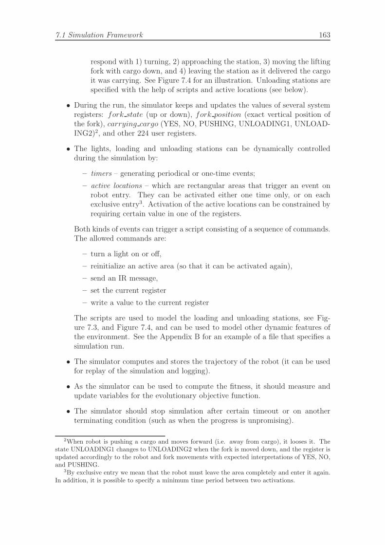
7.1 Simulation Framework 163

respond with 1) turning, 2) approaching the station, 3) moving the liftingfork with cargo down, and 4) leaving the station as it delivered the cargoit was carrying. See Figure 7.4 for an illustration. Unloading stations arespecified with the help of scripts and active locations (see below).

• During the run, the simulator keeps and updates the values of several systemregisters: fork state (up or down), fork position (exact vertical position ofthe fork), carrying cargo (YES, NO, PUSHING, UNLOADING1, UNLOAD-ING2)2, and other 224 user registers.

• The lights, loading and unloading stations can be dynamically controlledduring the simulation by:

– timers – generating periodical or one-time events;

– active locations – which are rectangular areas that trigger an event onrobot entry. They can be activated either one time only, or on eachexclusive entry3. Activation of the active locations can be constrained byrequiring certain value in one of the registers.

Both kinds of events can trigger a script consisting of a sequence of commands.The allowed commands are:

– turn a light on or off,

– reinitialize an active area (so that it can be activated again),

– send an IR message,

– set the current register

– write a value to the current register

The scripts are used to model the loading and unloading stations, see Fig-ure 7.3, and Figure 7.4, and can be used to model other dynamic features ofthe environment. See the Appendix B for an example of a file that specifies asimulation run.

• The simulator computes and stores the trajectory of the robot (it can be usedfor replay of the simulation and logging).

• As the simulator can be used to compute the fitness, it should measure andupdate variables for the evolutionary objective function.

• The simulator should stop simulation after certain timeout or on anotherterminating condition (such as when the progress is unpromising).

2When robot is pushing a cargo and moves forward (i.e. away from cargo), it looses it. Thestate UNLOADING1 changes to UNLOADING2 when the fork is moved down, and the register isupdated accordingly to the robot and fork movements with expected interpretations of YES, NO,and PUSHING.

3By exclusive entry we mean that the robot must leave the area completely and enter it again.In addition, it is possible to specify a minimum time period between two activations.

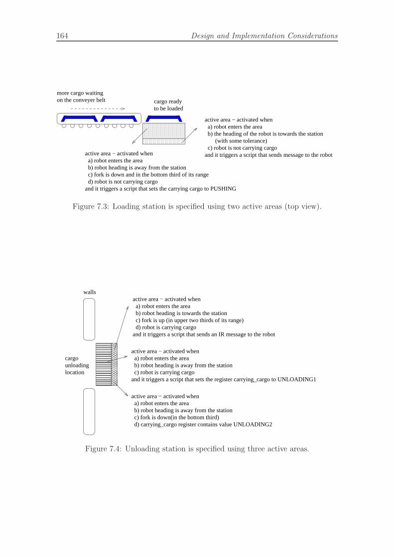
164 Design and Implementation Considerations

active area − activated when a) robot enters the area b) the heading of the robot is towards the station (with some tolerance) c) robot is not carrying cargoand it triggers a script that sends message to the robot

cargo ready to be loaded

b) robot heading is away from the station

and it triggers a script that sets the carrying cargo to PUSHING

c) fork is down and in the bottom third of its range

more cargo waitingon the conveyer belt

active area − activated when a) robot enters the area

d) robot is not carrying cargo

Figure 7.3: Loading station is specified using two active areas (top view).

cargounloadinglocation

���������������������������������������

���������������������������������������

active area − activated when a) robot enters the area b) robot heading is towards the station c) fork is up (in upper two thirds of its range) d) robot is carrying cargoand it triggers a script that sends an IR message to the robot

active area − activated when a) robot enters the area b) robot heading is away from the station c) robot is carrying cargoand it triggers a script that sets the register carrying_cargo to UNLOADING1

active area − activated when a) robot enters the area b) robot heading is away from the station c) fork is down(in the bottom third) d) carrying_cargo register contains value UNLOADING2

walls

�������������

�������������

Figure 7.4: Unloading station is specified using three active areas.

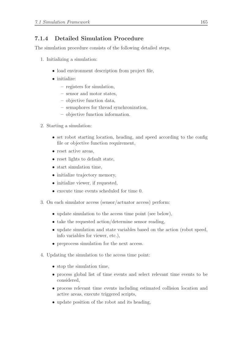
7.1 Simulation Framework 165

7.1.4 Detailed Simulation Procedure

The simulation procedure consists of the following detailed steps.

1. Initializing a simulation:

• load environment description from project file,

• initialize:

– registers for simulation,

– sensor and motor states,

– objective function data,

– semaphores for thread synchronization,

– objective function information.

2. Starting a simulation:

• set robot starting location, heading, and speed according to the configfile or objective function requirement,

• reset active areas,

• reset lights to default state,

• start simulation time,

• initialize trajectory memory,

• initialize viewer, if requested,

• execute time events scheduled for time 0.

3. On each simulator access (sensor/actuator access) perform:

• update simulation to the access time point (see below),

• take the requested action/determine sensor reading,

• update simulation and state variables based on the action (robot speed,info variables for viewer, etc.),

• preprocess simulation for the next access.

4. Updating the simulation to the access time point:

• stop the simulation time,

• process global list of time events and select relevant time events to beconsidered,

• process relevant time events including estimated collision location andactive areas, execute triggered scripts,

• update position of the robot and its heading,

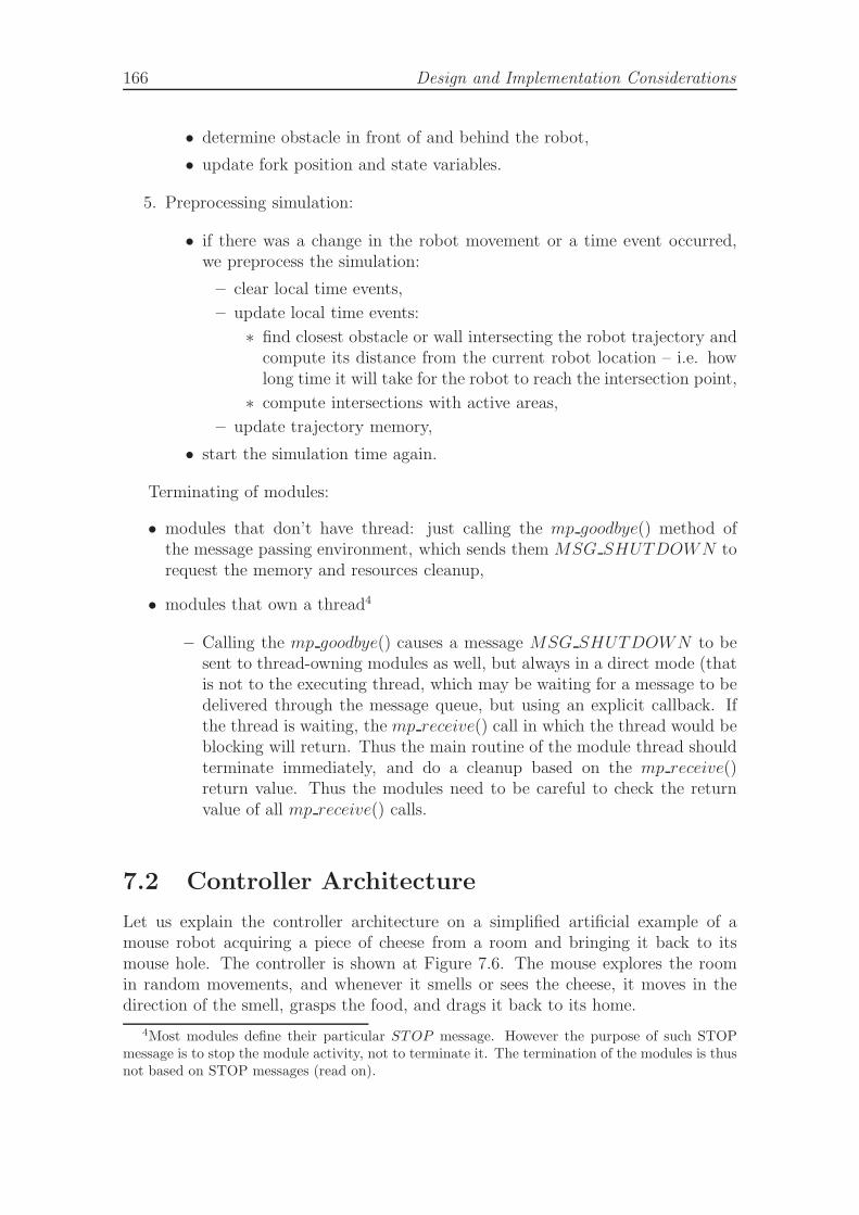
166 Design and Implementation Considerations

• determine obstacle in front of and behind the robot,

• update fork position and state variables.

5. Preprocessing simulation:

• if there was a change in the robot movement or a time event occurred,we preprocess the simulation:

– clear local time events,

– update local time events:

∗ find closest obstacle or wall intersecting the robot trajectory andcompute its distance from the current robot location – i.e. howlong time it will take for the robot to reach the intersection point,

∗ compute intersections with active areas,

– update trajectory memory,

• start the simulation time again.

Terminating of modules:

• modules that don’t have thread: just calling the mp goodbye() method ofthe message passing environment, which sends them MSG SHUTDOWN torequest the memory and resources cleanup,

• modules that own a thread4

– Calling the mp goodbye() causes a message MSG SHUTDOWN to besent to thread-owning modules as well, but always in a direct mode (thatis not to the executing thread, which may be waiting for a message to bedelivered through the message queue, but using an explicit callback. Ifthe thread is waiting, the mp receive() call in which the thread would beblocking will return. Thus the main routine of the module thread shouldterminate immediately, and do a cleanup based on the mp receive()return value. Thus the modules need to be careful to check the returnvalue of all mp receive() calls.

7.2 Controller Architecture

Let us explain the controller architecture on a simplified artificial example of amouse robot acquiring a piece of cheese from a room and bringing it back to itsmouse hole. The controller is shown at Figure 7.6. The mouse explores the roomin random movements, and whenever it smells or sees the cheese, it moves in thedirection of the smell, grasps the food, and drags it back to its home.

4Most modules define their particular STOP message. However the purpose of such STOPmessage is to stop the module activity, not to terminate it. The termination of the modules is thusnot based on STOP messages (read on).

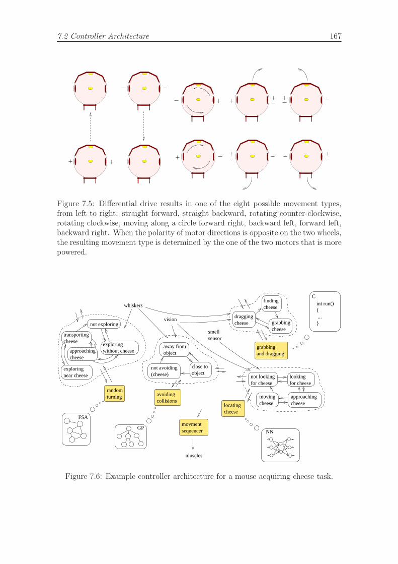
7.2 Controller Architecture 167

Figure 7.5: Differential drive results in one of the eight possible movement types,from left to right: straight forward, straight backward, rotating counter-clockwise,rotating clockwise, moving along a circle forward right, backward left, forward left,backward right. When the polarity of motor directions is opposite on the two wheels,the resulting movement type is determined by the one of the two motors that is morepowered.

close toobject

away fromobject

not avoiding(cheese)

findingcheese

draggingcheese grabbing

cheese

lookingfor cheese

approachingcheese

not lookingfor cheese

movingcheese

smellsensor

GPNN

...}

int run()C

{

FSA

exploringwithout cheese

not exploring

approachingcheese

transportingcheese

exploring near cheese

whiskers

vision

muscles

randomturning avoiding

collisions

movmentsequencer

locatingcheese

grabbingand dragging

Figure 7.6: Example controller architecture for a mouse acquiring cheese task.

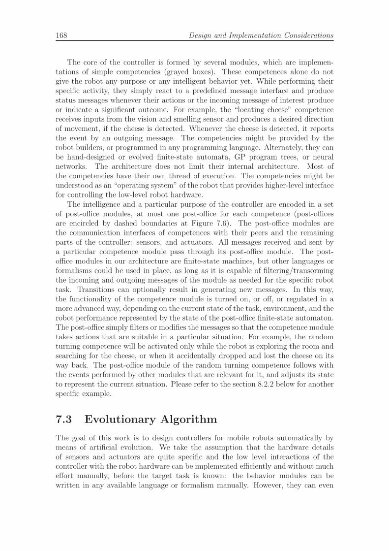
168 Design and Implementation Considerations

The core of the controller is formed by several modules, which are implemen-tations of simple competencies (grayed boxes). These competences alone do notgive the robot any purpose or any intelligent behavior yet. While performing theirspecific activity, they simply react to a predefined message interface and producestatus messages whenever their actions or the incoming message of interest produceor indicate a significant outcome. For example, the “locating cheese” competencereceives inputs from the vision and smelling sensor and produces a desired directionof movement, if the cheese is detected. Whenever the cheese is detected, it reportsthe event by an outgoing message. The competencies might be provided by therobot builders, or programmed in any programming language. Alternately, they canbe hand-designed or evolved finite-state automata, GP program trees, or neuralnetworks. The architecture does not limit their internal architecture. Most ofthe competencies have their own thread of execution. The competencies might beunderstood as an “operating system” of the robot that provides higher-level interfacefor controlling the low-level robot hardware.

The intelligence and a particular purpose of the controller are encoded in a setof post-office modules, at most one post-office for each competence (post-officesare encircled by dashed boundaries at Figure 7.6). The post-office modules arethe communication interfaces of competences with their peers and the remainingparts of the controller: sensors, and actuators. All messages received and sent bya particular competence module pass through its post-office module. The post-office modules in our architecture are finite-state machines, but other languages orformalisms could be used in place, as long as it is capable of filtering/transormingthe incoming and outgoing messages of the module as needed for the specific robottask. Transitions can optionally result in generating new messages. In this way,the functionality of the competence module is turned on, or off, or regulated in amore advanced way, depending on the current state of the task, environment, and therobot performance represented by the state of the post-office finite-state automaton.The post-office simply filters or modifies the messages so that the competence moduletakes actions that are suitable in a particular situation. For example, the randomturning competence will be activated only while the robot is exploring the room andsearching for the cheese, or when it accidentally dropped and lost the cheese on itsway back. The post-office module of the random turning competence follows withthe events performed by other modules that are relevant for it, and adjusts its stateto represent the current situation. Please refer to the section 8.2.2 below for anotherspecific example.

7.3 Evolutionary Algorithm

The goal of this work is to design controllers for mobile robots automatically bymeans of artificial evolution. We take the assumption that the hardware detailsof sensors and actuators are quite specific and the low level interactions of thecontroller with the robot hardware can be implemented efficiently and without mucheffort manually, before the target task is known: the behavior modules can bewritten in any available language or formalism manually. However, they can even

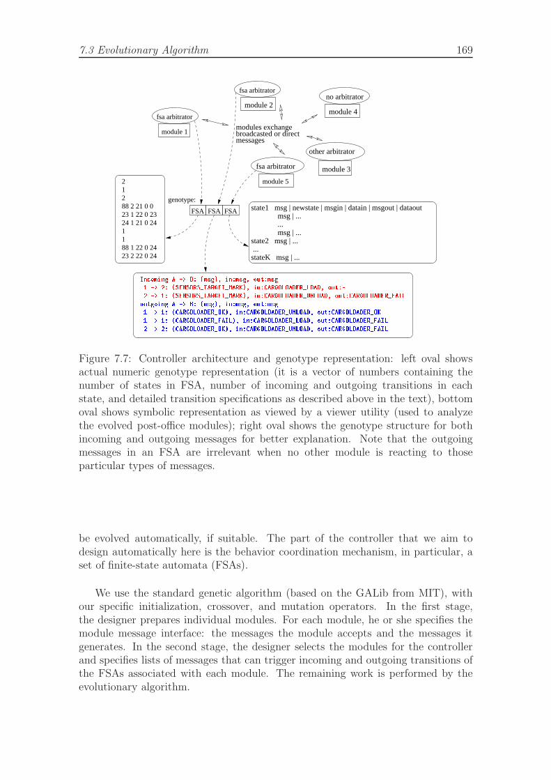
7.3 Evolutionary Algorithm 169

FSAFSAFSA msg | ...

msg | ...state2 msg | ...

stateK msg | ...

state1 msg | newstate | msgin | datain | msgout | dataout

...

...

module 1

fsa arbitrator

21288 2 21 0 023 1 22 0 2324 1 21 0 241188 1 22 0 2423 2 22 0 24

module 3

module 4

no arbitratormodule 2

fsa arbitrator

modules exchange broadcasted or directmessages

other arbitrator

genotype:

module 5

fsa arbitrator

Figure 7.7: Controller architecture and genotype representation: left oval showsactual numeric genotype representation (it is a vector of numbers containing thenumber of states in FSA, number of incoming and outgoing transitions in eachstate, and detailed transition specifications as described above in the text), bottomoval shows symbolic representation as viewed by a viewer utility (used to analyzethe evolved post-office modules); right oval shows the genotype structure for bothincoming and outgoing messages for better explanation. Note that the outgoingmessages in an FSA are irrelevant when no other module is reacting to thoseparticular types of messages.

be evolved automatically, if suitable. The part of the controller that we aim todesign automatically here is the behavior coordination mechanism, in particular, aset of finite-state automata (FSAs).

We use the standard genetic algorithm (based on the GALib from MIT), withour specific initialization, crossover, and mutation operators. In the first stage,the designer prepares individual modules. For each module, he or she specifies themodule message interface: the messages the module accepts and the messages itgenerates. In the second stage, the designer selects the modules for the controllerand specifies lists of messages that can trigger incoming and outgoing transitions ofthe FSAs associated with each module. The remaining work is performed by theevolutionary algorithm.

170 Design and Implementation Considerations

7.3.1 Representation

The genotype representation consists of blueprints of FSAs for the set of modulesfor which the FSAs are to be designed automatically (some modules might workwithout post-offices, other might use manually-designed post-offices, or some post-offices are held fixed because they are already evolved). An example of a genotypeis in Figure 7.7.

The number of states and the number of transitions in each state vary (withinspecified boundaries). Transitions are triggered by messages (incoming or outgoing)and have the following format (please see Figure 8.13 for examples, and the appendixC for example of specification of the EA parameters including the specification ofstates, and transitions):

(msg type, new state, msg to send out, [msg arguments],msg to send in, [msg arguments])

7.3.2 Operators

The GA-initialization operator generates random FSAs that comply with the sup-plied specification. The crossover operator works on a single randomly selectedFSA. It randomly divides states of the FSAs from both parents into two pairs ofsubsets, and creates two new FSAs by gluing the alternative parts together. Asimple example is shown at Figure 7.8, where two FSAs with partial functionality,each having 2 states, are combined by the crossover operator to form a new FSAthat has three states. Later, the transition in the state labeled “close to object”is mutated: the message produced by the transition is changed from steer right tobackup.

The following paragraphs describe the crossover operator in detail.Let the states of the first parent be S = (S1, . . . , SK), and the states of the

second parent be T = (T1, . . . , TL). The operator randomly picks a set of states thatwill be inherited by the first offspring from the first parent, O1fromS, and a set of apossibly different cardinality, containing states that will be inherited by the secondoffspring from the second parent, O2fromT . The first offspring will then consist ofstates O1fromS + (T − O2fromT ), and the second offspring will consist of statesO2fromT + (S − O1fromS). The state transitions cannot be always preserved,because the number of states and their numbering changes. Figure 7.9 visualizesthe crossover operator in a diagram.

The following transitions are preserved:O1fromS to O1fromS, S − O1fromS to S − O1fromS,O2fromT to O2fromT , T − O2fromT to T − O2fromT .The states are renumbered according to the new state numbers.

The transitions leading to states that are now part of the other offspring wouldpoint nowhere, therefore we randomly generate mappings between the exchangedstates of the two offspring. Since the numbers of states in these four sets are different,bijection is not possible and we need all four mappings – one in each direction forboth parts. Mapping M1 of states in S − O1fromS to states in T − O2fromT ,mapping M2 of states in T − O2fromT to S − O1fromS, mapping M3 of states in

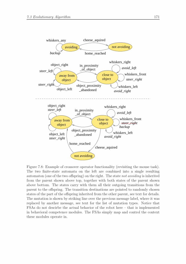
7.3 Evolutionary Algorithm 171

steer_left

object_right

object_leftsteer_right

_of_objectin_proximity

object_proximity_abandoned

whiskers_right

avoid_left

whiskers_leftavoid_right

whiskers_frontaway fromobject

close toobject steer_right

backup

whiskers_any cheese_aquired

home_reached

avoiding not avoiding

cheese_aquired

_of_objectin_proximity

object_proximity_abandoned

whiskers_right

avoid_left

whiskers_frontaway fromobject

close to

avoid_rightwhiskers_left

backup

not avoiding

object_leftsteer_right

steer_leftobject_right

home_reached

steer_rightobject

Figure 7.8: Example of crossover operator functionality (revisiting the mouse task).The two finite-state automata on the left are combined into a single resultingautomaton (one of the two offspring) on the right. The state not avoiding is inheritedfrom the parent shown above top, together with both states of the parent shownabove bottom. The states carry with them all their outgoing transitions from theparent to the offspring. The transition destinations are pointed to randomly chosenstates of the part of the offspring inherited from the other parent, see text for details.The mutation is shown by striking line over the previous message label, where it wasreplaced by another message, see text for the list of mutation types. Notice thatFSAs do not descirbe the actual behavior of the robot here – that is implementedin behavioral competence modules. The FSAs simply map and control the contextthese modules operate in.

172 Design and Implementation Considerations

O1fromS to O2fromT , and mapping M4 of states in O2fromT to O1fromS. Thenew numbers of states are taken into account when generating M1, M2, M3, andM4.

The transitions are then modified using the generated mappings, the mappingsM1 and M4 are used to generate the first offspring, the other two to generate thesecond offspring:

Transitions that lead:

• From x ∈ O1fromS to y ∈ S − O1fromS are changed to M1(y),

• From x ∈ O2fromT to y ∈ T − O2fromT are changed to M2(y),

• From x ∈ S − O1fromS to O1fromS are changed to M3(y),

• From x ∈ T − O2fromT to O2fromT are changed to M4(y).

The above transformation is attempting to maximize the genetic informationpassed from the parents to offspring by conservative approach, where the transitionsoriginally pointing to the same state will point to the same state also in the offspring.

The implementation of the crossover procedure:

1. choose the index of FSA to work on

2. randomly generate bits O1fromS[1..K] and O2fromT [1..L],

3. based on O1fromS and O2fromT , generate SRENUM [1..K]and TRENUM [1..L],

4. randomly generate M13[1..K], and M24[1..L] that represent M1, M2, M3, andM4,

5. form O1 by copying states from O1fromS and T − O2fromT , and updatingall transitions based on M1, M4, SRENUM , TRENUM ,

6. form O2 by copying states from O2fromT and S − O1fromS, and updatingall transitions based on M1, M3, SRENUM , TRENUM .

The mutation operator works upon a single FSA. One of the following opera-tions is performed (the probabilities of the mutation types are parameters of thealgorithm):

• a new random transition is created,

• random transition is deleted,

• a new state is created (with minimum incoming and outgoing random transi-tions); in addition, one new transition leading to this state from another stateis randomly generated,

• a random state is deleted as well as all its incident transitions,

7.3 Evolutionary Algorithm 173

• a random transition is modified: (one of its parts new state, msg type,msg to send out, msg to send in is replaced by an allowed random value),

• a completely random individual is produced (this operator changes all FSAs),

• a random transaction is split in two and new state is created in the middle,

• the initial state number is changed.

In our experiments, we use the roulette wheel and the tournament selectionschemes combined with steady-state or standard GA with elitism. Other parametersof the algorithm include (with these default values): pcrossover (0.3), pmutation(0.7), probabilities of all 8 mutation types that sum up to 1:pnew random transition (0.25), pdelete random transition (0.1), pnew state (0.2),prandom state deleted (0.05), prandom transition mutated (0.25), pnew random individual (0.05),psplit transition (0.05), pchange starting state (0.05); population size (100),gen number (60), ppopulation replace (0.2), number of modules in the controller (10),specification of the message interfaces and trigger messages for all modules, initialand boundary values for number of states and transitions, number of startinglocations for the robot for each evaluation, timeout for the robot evaluation run,specification of the fitness function parameters, input, output, and log file locations,details in appendix.

7.3.3 Scaling

Due to the unnatural range of fitness values produced by the objective function, theevolutionary algorithm applies a scaling method before using the particular selectionmechanism in each generation.

The GALib distinguishes two basic ways for treating the fitness values – raw andscaled fitness score and it keeps two index arrays for both viewpoints.

Various scaling schemes are supported:

• GANoScaling(), where the fitness scores are identical to the objective scores.No scaling takes place.

• GALinearScaling(linearScalingMultiplier), where the fitness scores are de-rived from the objective scores using the linear scaling method described in([Goldberg, 1989]). Negative objective scores are not allowed with this method.Objective scores are converted to fitness scores using the equation

f = a ∗ obj + b

where a and b are calculated based upon the objective scores of the individualsin the population as described in [Goldberg, 1989]. This is the scaling schemewe use in the experiments, the individuals with fitness lower than 0.001 areassigned fitness 0.001.

174 Design and Implementation Considerations

• GASigmaTruncationScaling(sigmaTruncationMultiplier).This scaling method can be used if the objective scores are negative. It scalesbased on the variation from the population average and truncates arbitrarilyat 0. The mapping from objective to fitness score for each individual is givenby

f = obj − (objavg − c ∗ objdev)

where objavg is the average and objdev is the standard deviation.

• GAPowerLawScaling(powerScalingFactor) is the power law scaling thatmaps objective scores to fitness scores using an exponential relationship definedas

f = objk

• GASharing(comparator, sharingCutoff, alpha), is a scaling method used forspeciation. The fitness score is derived from its objective score by comparingthe individual against the other individuals in the population. If there areother similar individuals then the fitness is derated. The distance functionis used to specify how similar to each other two individuals are. A distancefunction must return a value of 0 or higher, where 0 means that the twoindividuals are identical (no diversity). For a given individual,

f =obj

popsize∑

j=0

s(d(j)))

s(d(j)) =

{

1 − d(j)σ

αif d(j) < σ

0 if d(j) ≥ σ

where d(j) is a distance function with respect to individual j. The defaultsharing object uses the triangular sharing function described in [Goldberg,1989]. It is possible to specify the cutoff value (σ in [Goldberg, 1989]) usingthe sigma member function. The curvature of the sharing function is controlledby the α value. When α is 1.0 the sharing function is a straight line (triangularsharing). If a comparator is specified, that function will be used as the distancefunction for all comparisons. If comparator is not specified, the sharing objectwill use the default comparator of each genome.

The sharing scaling differs depending on whether the objective is to maximizeor minimize. If the goal is to maximize the objective score, the raw scores will bedivided by the sharing factor. If the goal is to minimize the objective score, the rawscores will be multiplied by the sharing factor. It is possible to explicitly specifythe sharing object to perform minimize- or maximize-based scaling by using the

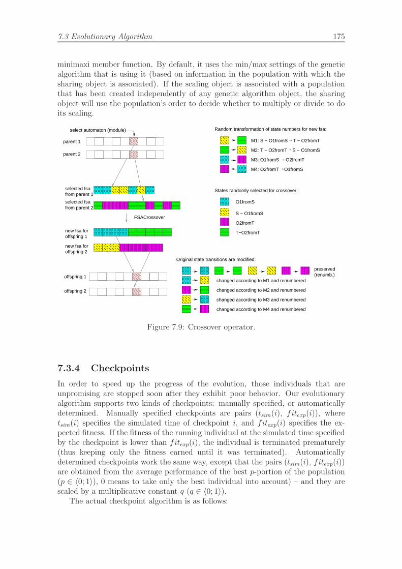
7.3 Evolutionary Algorithm 175

minimaxi member function. By default, it uses the min/max settings of the geneticalgorithm that is using it (based on information in the population with which thesharing object is associated). If the scaling object is associated with a populationthat has been created independently of any genetic algorithm object, the sharingobject will use the population’s order to decide whether to multiply or divide to doits scaling.

changed according to M1 and renumbered

changed according to M2 and renumbered

changed according to M3 and renumbered

changed according to M4 and renumbered

Original state transitions are modified:

preserved (renumb.)

M1: S − O1fromS T − O2fromT

M2: T − O2fromT S − O1fromS

M3: O1fromS O2fromT

M4: O2fromT O1fromS

Random transformation of state numbers for new fsa:

States randomly selected for crossover:

O2fromT

T−O2fromT

S − O1fromS

O1fromS

selected fsafrom parent 1

selected fsafrom parent 2

new fsa foroffspring 1

new fsa foroffspring 2

parent 2

parent 1

offspring 1

offspring 2

select automaton (module)

FSACrossover

Figure 7.9: Crossover operator.

7.3.4 Checkpoints

In order to speed up the progress of the evolution, those individuals that areunpromising are stopped soon after they exhibit poor behavior. Our evolutionaryalgorithm supports two kinds of checkpoints: manually specified, or automaticallydetermined. Manually specified checkpoints are pairs (tsim(i), fitexp(i)), wheretsim(i) specifies the simulated time of checkpoint i, and fitexp(i) specifies the ex-pected fitness. If the fitness of the running individual at the simulated time specifiedby the checkpoint is lower than fitexp(i), the individual is terminated prematurely(thus keeping only the fitness earned until it was terminated). Automaticallydetermined checkpoints work the same way, except that the pairs (tsim(i), fitexp(i))are obtained from the average performance of the best p-portion of the population(p ∈ 〈0; 1〉), 0 means to take only the best individual into account) – and they arescaled by a multiplicative constant q (q ∈ 〈0; 1〉).

The actual checkpoint algorithm is as follows:

176 Design and Implementation Considerations

1. read the checkpoints from configuration file (if manually specified), or con-struct the checkpoint times from parameters tsim(0), dt, i.e.tsim(i + 1) = tsim(i) + dt,

2. (only automatic) at the beginning of each generation, for all checkpoints,construct the fitexp(i) by averaging the measured fitness from the best p-portion of the population,

3. during the run of each individual, at the checkpoint times, compare theachieved partial fitness to the checkpoint fitness scaled by q, and stop theindividual, if the partial fitness is lower. At each checkpoint time also storethe checkpoint fitness for the case this individual will reach the best p-portionof the population. After each individual run, compare the final fitness to thelist of best p-portion fitness. If the individual reached better fitness, insert it onthe list of the best individuals fitness checkpoints, and update the best-fitnesslist.

See Appendix C for an example of a file specifying an evolutionary run.

7.4 Chapter Summary

• We design our specialized simulation method based on emulating the controlleron high-performance workstations with Linux operating system running inreal-time scheduling mode.

• We specify a specialized simulator that we use for the experiments withIncremental Evolutionary Robotics.

• Inspired by Behavior-Based Robotics, we design our own controller archi-tecture that is based on message-passing communication of independent be-havioral modules with distributed communication mechanism based on thefinite-state automata formalism.

• We design the representation for this chosen architecture as well as theevolutionary operators.

Chapter 8

Experimental Work

If you look at the rotating robot when you are tired,the robot will seem to rotate in the opposite directionafter it will have stopped.— robotika/robot/ReadMe.txt

8.1 Simple Adaptive Autonomous Robot

Our world is a very complex system with many interactions, changes, unpredictableevents, failures, and coincidences. If we ever wish to use robots for more advancedtasks than performing predefined tasks in deterministic environments (such asfactory production line robots mounting screws), the robots will have to deal withchanges, they will have to learn about their environment and they will need to adaptto it.

This project is an example of perhaps the most simple robot ever made thatcan learn. The robot can move back and forth, and it can turn left and right. Itcan also sense an obstacle in front of it – using left and right independent tactilesensors. We will use the sensors for a slightly different purpose: the left tentacle willprovide positive feedback, whereas the right tentacle will signal negative feedbackfor the robot. The robot will try various things, and each time it receives a positivereinforcement, it will retain in its memory.the most recently demonstrated sequence.Each time it receives a negative reinforcement, it will dismiss its last idea and trysomething else instead.

The behavior our robot will learn will be sequences of left and right turns. Therobot will repeat the following piece of code 10-times, for i = 1 . . . 10:

1. move forward 20 steps

2. turn left or right |Ni| steps, the direction is determined by the sign of Ni.

The robot should be started from the same initial location. The sequence ofthe moves brings the robot to some target location. Each time before the robotdemonstrates the movement represented by the sequence Ni, i = 1 . . . 10, it willalter this sequence randomly in 3 of the 10 turnings. If the user of the robot finds

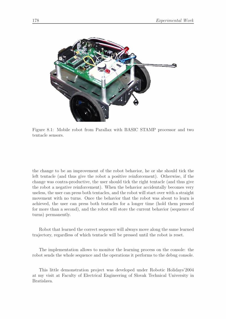
178 Experimental Work

Figure 8.1: Mobile robot from Parallax with BASIC STAMP processor and twotentacle sensors.

the change to be an improvement of the robot behavior, he or she should tick theleft tentacle (and thus give the robot a positive reinforcement). Otherwise, if thechange was contra-productive, the user should tick the right tentacle (and thus givethe robot a negative reinforcement). When the behavior accidentally becomes veryuseless, the user can press both tentacles, and the robot will start over with a straightmovement with no turns. Once the behavior that the robot was about to learn isachieved, the user can press both tentacles for a longer time (hold them pressedfor more than a second), and the robot will store the current behavior (sequence ofturns) permanently.

Robot that learned the correct sequence will always move along the same learnedtrajectory, regardless of which tentacle will be pressed until the robot is reset.

The implementation allows to monitor the learning process on the console: therobot sends the whole sequence and the operations it performs to the debug console.

This little demonstration project was developed under Robotic Holidays’2004at my visit at Faculty of Electrical Engineering of Slovak Technical University inBratislava.

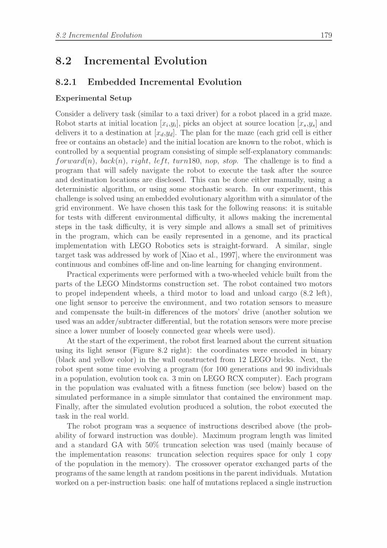
8.2 Incremental Evolution 179

8.2 Incremental Evolution

8.2.1 Embedded Incremental Evolution

Experimental Setup

Consider a delivery task (similar to a taxi driver) for a robot placed in a grid maze.Robot starts at initial location [xi,yi], picks an object at source location [xs,ys] anddelivers it to a destination at [xd,yd]. The plan for the maze (each grid cell is eitherfree or contains an obstacle) and the initial location are known to the robot, which iscontrolled by a sequential program consisting of simple self-explanatory commands:forward(n), back(n), right, left, turn180, nop, stop. The challenge is to find aprogram that will safely navigate the robot to execute the task after the sourceand destination locations are disclosed. This can be done either manually, using adeterministic algorithm, or using some stochastic search. In our experiment, thischallenge is solved using an embedded evolutionary algorithm with a simulator of thegrid environment. We have chosen this task for the following reasons: it is suitablefor tests with different environmental difficulty, it allows making the incrementalsteps in the task difficulty, it is very simple and allows a small set of primitivesin the program, which can be easily represented in a genome, and its practicalimplementation with LEGO Robotics sets is straight-forward. A similar, singletarget task was addressed by work of [Xiao et al., 1997], where the environment wascontinuous and combines off-line and on-line learning for changing environment.

Practical experiments were performed with a two-wheeled vehicle built from theparts of the LEGO Mindstorms construction set. The robot contained two motorsto propel independent wheels, a third motor to load and unload cargo (8.2 left),one light sensor to perceive the environment, and two rotation sensors to measureand compensate the built-in differences of the motors’ drive (another solution weused was an adder/subtracter differential, but the rotation sensors were more precisesince a lower number of loosely connected gear wheels were used).

At the start of the experiment, the robot first learned about the current situationusing its light sensor (Figure 8.2 right): the coordinates were encoded in binary(black and yellow color) in the wall constructed from 12 LEGO bricks. Next, therobot spent some time evolving a program (for 100 generations and 90 individualsin a population, evolution took ca. 3 min on LEGO RCX computer). Each programin the population was evaluated with a fitness function (see below) based on thesimulated performance in a simple simulator that contained the environment map.Finally, after the simulated evolution produced a solution, the robot executed thetask in the real world.

The robot program was a sequence of instructions described above (the prob-ability of forward instruction was double). Maximum program length was limitedand a standard GA with 50% truncation selection was used (mainly because ofthe implementation reasons: truncation selection requires space for only 1 copyof the population in the memory). The crossover operator exchanged parts of theprograms of the same length at random positions in the parent individuals. Mutationworked on a per-instruction basis: one half of mutations replaced a single instruction

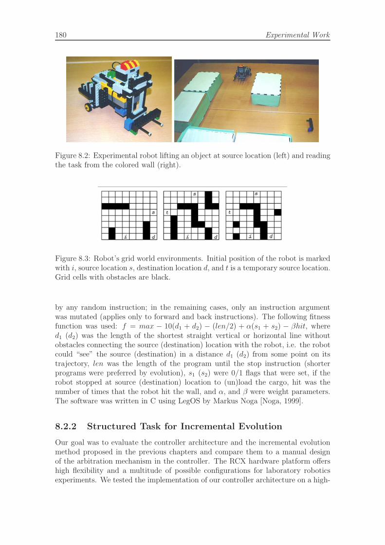
180 Experimental Work

Figure 8.2: Experimental robot lifting an object at source location (left) and readingthe task from the colored wall (right).

Figure 8.3: Robot’s grid world environments. Initial position of the robot is markedwith i, source location s, destination location d, and t is a temporary source location.Grid cells with obstacles are black.

by any random instruction; in the remaining cases, only an instruction argumentwas mutated (applies only to forward and back instructions). The following fitnessfunction was used: f = max − 10(d1 + d2) − (len/2) + α(s1 + s2) − βhit, whered1 (d2) was the length of the shortest straight vertical or horizontal line withoutobstacles connecting the source (destination) location with the robot, i.e. the robotcould “see” the source (destination) in a distance d1 (d2) from some point on itstrajectory, len was the length of the program until the stop instruction (shorterprograms were preferred by evolution), s1 (s2) were 0/1 flags that were set, if therobot stopped at source (destination) location to (un)load the cargo, hit was thenumber of times that the robot hit the wall, and α, and β were weight parameters.The software was written in C using LegOS by Markus Noga [Noga, 1999].

8.2.2 Structured Task for Incremental Evolution

Our goal was to evaluate the controller architecture and the incremental evolutionmethod proposed in the previous chapters and compare them to a manual designof the arbitration mechanism in the controller. The RCX hardware platform offershigh flexibility and a multitude of possible configurations for laboratory roboticsexperiments. We tested the implementation of our controller architecture on a high-

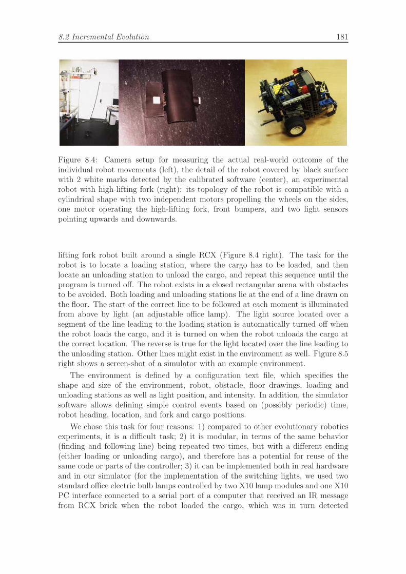
8.2 Incremental Evolution 181

Figure 8.4: Camera setup for measuring the actual real-world outcome of theindividual robot movements (left), the detail of the robot covered by black surfacewith 2 white marks detected by the calibrated software (center), an experimentalrobot with high-lifting fork (right): its topology of the robot is compatible with acylindrical shape with two independent motors propelling the wheels on the sides,one motor operating the high-lifting fork, front bumpers, and two light sensorspointing upwards and downwards.

lifting fork robot built around a single RCX (Figure 8.4 right). The task for therobot is to locate a loading station, where the cargo has to be loaded, and thenlocate an unloading station to unload the cargo, and repeat this sequence until theprogram is turned off. The robot exists in a closed rectangular arena with obstaclesto be avoided. Both loading and unloading stations lie at the end of a line drawn onthe floor. The start of the correct line to be followed at each moment is illuminatedfrom above by light (an adjustable office lamp). The light source located over asegment of the line leading to the loading station is automatically turned off whenthe robot loads the cargo, and it is turned on when the robot unloads the cargo atthe correct location. The reverse is true for the light located over the line leading tothe unloading station. Other lines might exist in the environment as well. Figure 8.5right shows a screen-shot of a simulator with an example environment.

The environment is defined by a configuration text file, which specifies theshape and size of the environment, robot, obstacle, floor drawings, loading andunloading stations as well as light position, and intensity. In addition, the simulatorsoftware allows defining simple control events based on (possibly periodic) time,robot heading, location, and fork and cargo positions.

We chose this task for four reasons: 1) compared to other evolutionary roboticsexperiments, it is a difficult task; 2) it is modular, in terms of the same behavior(finding and following line) being repeated two times, but with a different ending(either loading or unloading cargo), and therefore has a potential for reuse of thesame code or parts of the controller; 3) it can be implemented both in real hardwareand in our simulator (for the implementation of the switching lights, we used twostandard office electric bulb lamps controlled by two X10 lamp modules and one X10PC interface connected to a serial port of a computer that received an IR messagefrom RCX brick when the robot loaded the cargo, which was in turn detected

182 Experimental Work

TURN180TURN180

TURN180

TARGET_MARKLNFLWER_STOP

LNFLWER_FOLLOW

LNFLWER_STOPTARGET_MARK

TARGET_MARKLNFLWER_STOP

NAVIGATE_FINISHLINE_ENTER

outside lightoutside lineexploring (1)

LNFLWER_FOLLOW

lightsearching line (2)

start

below light (3)follow line

LIGHT_ENTER

outside light (4)follow line

LINE_LOST

line lost (5)

LINE_ENTER

after lost (6)follow line

LINE_LEAVEturning (7)

LINE_LEAVE

LINE_ENTER

LIGHT_LEAVE

LINE_ENTER

LINE_LEAVE

LINE_LOST

LINE_ENTER

LIGHT_ENTER

LINE_LOST

LIGHT_ENTER

LIGHT_LEAVE

LINE_ENTER

LINE_LEAVE

Figure 8.5: Robot executing the target task in a simulated environment (right), andan example of a manually designed FSA arbitrator for the line follower module (left).The illuminated area on the right is depicted by a large filled circle; dark squaresrepresent obstacles; thick lines are drawn on the floor and detectable by robot;loading and unloading stations are marked by rectangles at the end of line, and thethin line shows the trajectory for an example run. The transitions between stateson the left are labeled by messages that trigger them, and in cursive by messagesthey generate. The robot first travels randomly until it enters light (state 2). Thenit looks for line and follows it in states 3 and 4, with recovery in states 5, 6, and7. Whenever it reaches the loading station, it stops following the line and resetsto random walk in state 1. Module explore queries the sensor module to see if therobot is moving towards or away from light and controls the turning of the robot inorder to reach the light more quickly.

by an infrared emitter/detector from HiTechnic); 4) the task consists of multipleinteractions, and behaviors, and thus is suitable for incremental evolution.

Our robot comes with a set of preprogrammed behavioral modules. We havecoded them directly in the language C:

Sensors — translates the numeric sensory readings into events, such as robotpassed over or left a line, entered or left an illuminated area, received an IR messagefrom a cargo station, bounced into or avoided an obstacle.

Motor driver — accepts commands to power or idle the motors. The messagescome asynchronously from various modules and with various priorities. The purposeof this module is to maintain the output according to the currently highest priorityrequest, and fall back to lower priorities as needed. All motor control commands inthis controller are by convention going through the motor driver.

Navigate — is a service module, which provides higher-level navigational com-mands — such as move forward, backward, turn left, as contrasted with low-levelmotor signals that adjust wheel velocities.

Avoidance — monitors the obstacle events, and avoids the obstacles whenencountered.

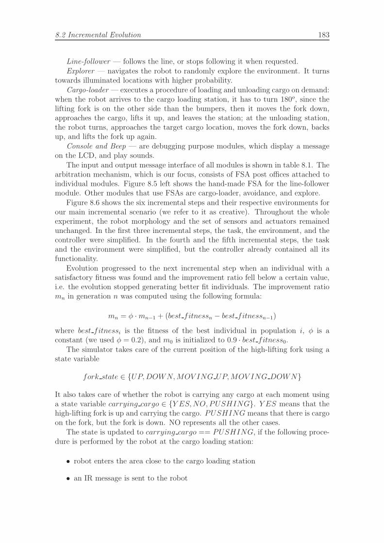
8.2 Incremental Evolution 183

Line-follower — follows the line, or stops following it when requested.Explorer — navigates the robot to randomly explore the environment. It turns

towards illuminated locations with higher probability.Cargo-loader — executes a procedure of loading and unloading cargo on demand:

when the robot arrives to the cargo loading station, it has to turn 180o, since thelifting fork is on the other side than the bumpers, then it moves the fork down,approaches the cargo, lifts it up, and leaves the station; at the unloading station,the robot turns, approaches the target cargo location, moves the fork down, backsup, and lifts the fork up again.

Console and Beep — are debugging purpose modules, which display a messageon the LCD, and play sounds.

The input and output message interface of all modules is shown in table 8.1. Thearbitration mechanism, which is our focus, consists of FSA post offices attached toindividual modules. Figure 8.5 left shows the hand-made FSA for the line-followermodule. Other modules that use FSAs are cargo-loader, avoidance, and explore.

Figure 8.6 shows the six incremental steps and their respective environments forour main incremental scenario (we refer to it as creative). Throughout the wholeexperiment, the robot morphology and the set of sensors and actuators remainedunchanged. In the first three incremental steps, the task, the environment, and thecontroller were simplified. In the fourth and the fifth incremental steps, the taskand the environment were simplified, but the controller already contained all itsfunctionality.

Evolution progressed to the next incremental step when an individual with asatisfactory fitness was found and the improvement ratio fell below a certain value,i.e. the evolution stopped generating better fit individuals. The improvement ratiomn in generation n was computed using the following formula:

mn = φ · mn−1 + (best fitnessn − best fitnessn−1)

where best fitnessi is the fitness of the best individual in population i, φ is aconstant (we used φ = 0.2), and m0 is initialized to 0.9 · best fitness0.

The simulator takes care of the current position of the high-lifting fork using astate variable

fork state ∈ {UP, DOWN, MOV ING UP, MOV ING DOWN}

It also takes care of whether the robot is carrying any cargo at each moment usinga state variable carrying cargo ∈ {Y ES, NO, PUSHING}. Y ES means that thehigh-lifting fork is up and carrying the cargo. PUSHING means that there is cargoon the fork, but the fork is down. NO represents all the other cases.

The state is updated to carrying cargo == PUSHING, if the following proce-dure is performed by the robot at the cargo loading station:

• robot enters the area close to the cargo loading station

• an IR message is sent to the robot

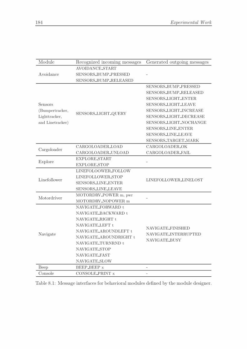
184 Experimental Work

Module Recognized incoming messages Generated outgoing messages

Avoidance

AVOIDANCE START

SENSORS BUMP PRESSED

SENSORS BUMP RELEASED

-

Sensors

(Bumpertracker,

Lighttracker,

and Linetracker)

SENSORS LIGHT QUERY

SENSORS BUMP PRESSED

SENSORS BUMP RELEASED

SENSORS LIGHT ENTER

SENSORS LIGHT LEAVE

SENSORS LIGHT INCREASE

SENSORS LIGHT DECREASE

SENSORS LIGHT NOCHANGE

SENSORS LINE ENTER

SENSORS LINE LEAVE

SENSORS TARGET MARK

CargoloaderCARGOLOADER LOAD

CARGOLOADER UNLOAD

CARGOLOADER OK

CARGOLOADER FAIL

ExploreEXPLORE START

EXPLORE STOP-

Linefollower

LINEFOLOOWER FOLLOW

LINEFOLLOWER STOP

SENSORS LINE ENTER

SENSORS LINE LEAVE

LINEFOLLOWER LINELOST

MotordriverMOTORDRV POWER m, pwr

MOTORDRV NOPOWER m-

Navigate

NAVIGATE FORWARD t

NAVIGATE BACKWARD t

NAVIGATE RIGHT t

NAVIGATE LEFT t

NAVIGATE AROUNDLEFT t

NAVIGATE AROUNDRIGHT t

NAVIGATE TURNRND t

NAVIGATE STOP

NAVIGATE FAST

NAVIGATE SLOW

NAVIGATE FINISHED

NAVIGATE INTERRUPTED

NAVIGATE BUSY

Beep BEEP BEEP x -Console CONSOLE PRINT x -

Table 8.1: Message interfaces for behavioral modules defined by the module designer.

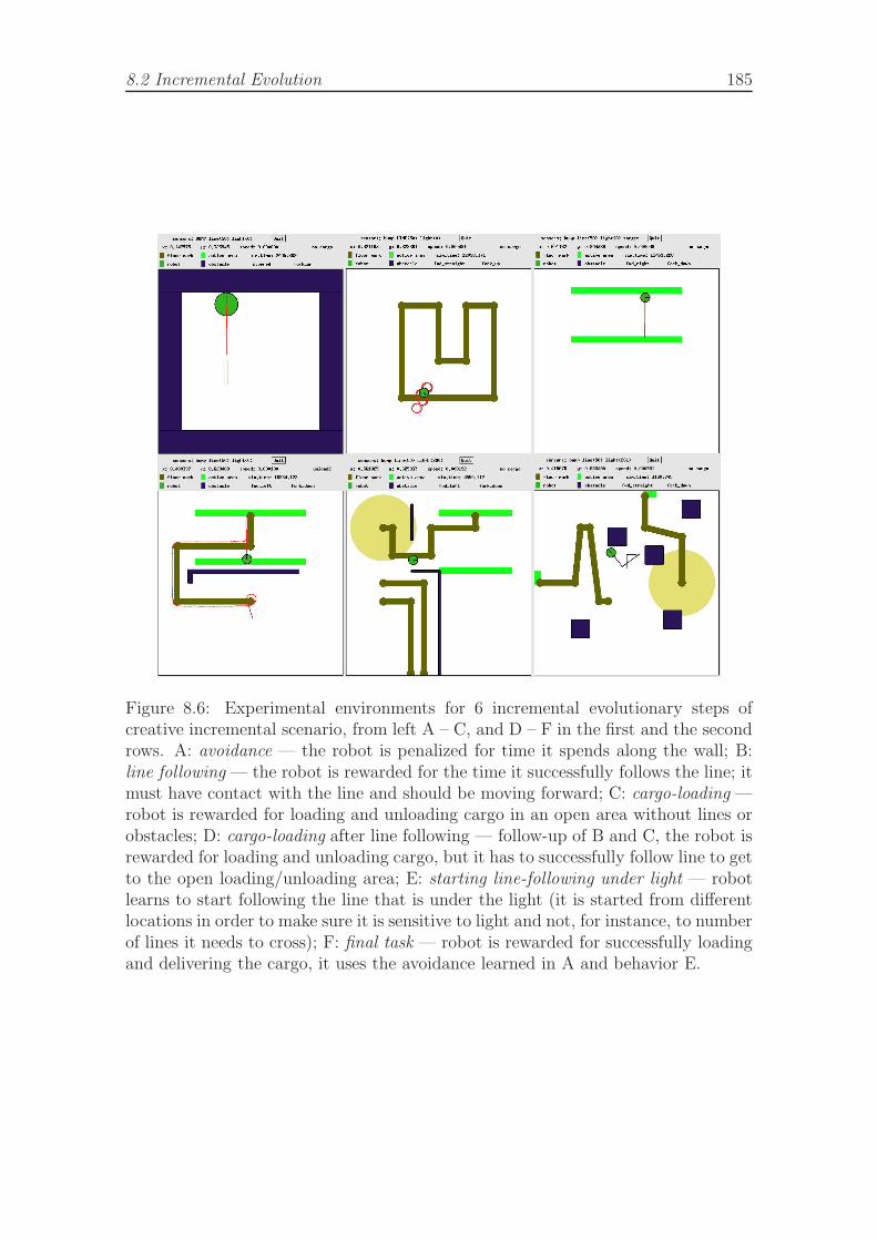
8.2 Incremental Evolution 185

Figure 8.6: Experimental environments for 6 incremental evolutionary steps ofcreative incremental scenario, from left A – C, and D – F in the first and the secondrows. A: avoidance — the robot is penalized for time it spends along the wall; B:line following — the robot is rewarded for the time it successfully follows the line; itmust have contact with the line and should be moving forward; C: cargo-loading —robot is rewarded for loading and unloading cargo in an open area without lines orobstacles; D: cargo-loading after line following — follow-up of B and C, the robot isrewarded for loading and unloading cargo, but it has to successfully follow line to getto the open loading/unloading area; E: starting line-following under light — robotlearns to start following the line that is under the light (it is started from differentlocations in order to make sure it is sensitive to light and not, for instance, to numberof lines it needs to cross); F: final task — robot is rewarded for successfully loadingand delivering the cargo, it uses the avoidance learned in A and behavior E.

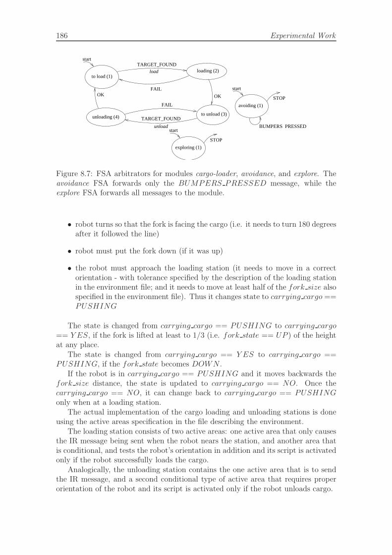
186 Experimental Work

unload

load

start

to unload (3)unloading (4)

to load (1)

TARGET_FOUND

TARGET_FOUND

FAIL

OKOKFAIL

loading (2)

BUMPERS_PRESSED

STOP

avoiding (1)

start

STOP

exploring (1)

start

Figure 8.7: FSA arbitrators for modules cargo-loader, avoidance, and explore. Theavoidance FSA forwards only the BUMPERS PRESSED message, while theexplore FSA forwards all messages to the module.

• robot turns so that the fork is facing the cargo (i.e. it needs to turn 180 degreesafter it followed the line)

• robot must put the fork down (if it was up)

• the robot must approach the loading station (it needs to move in a correctorientation - with tolerance specified by the description of the loading stationin the environment file; and it needs to move at least half of the fork size alsospecified in the environment file). Thus it changes state to carrying cargo ==PUSHING

The state is changed from carrying cargo == PUSHING to carrying cargo== Y ES, if the fork is lifted at least to 1/3 (i.e. fork state == UP ) of the heightat any place.

The state is changed from carrying cargo == Y ES to carrying cargo ==PUSHING, if the fork state becomes DOWN .

If the robot is in carrying cargo == PUSHING and it moves backwards thefork size distance, the state is updated to carrying cargo == NO. Once thecarrying cargo == NO, it can change back to carrying cargo == PUSHINGonly when at a loading station.

The actual implementation of the cargo loading and unloading stations is doneusing the active areas specification in the file describing the environment.

The loading station consists of two active areas: one active area that only causesthe IR message being sent when the robot nears the station, and another area thatis conditional, and tests the robot’s orientation in addition and its script is activatedonly if the robot successfully loads the cargo.

Analogically, the unloading station contains the one active area that is to sendthe IR message, and a second conditional type of active area that requires properorientation of the robot and its script is activated only if the robot unloads cargo.

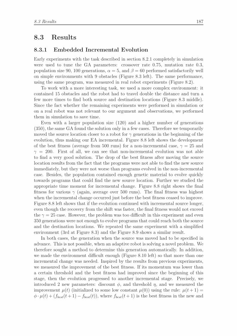
8.3 Results 187

8.3 Results

8.3.1 Embedded Incremental Evolution

Early experiments with the task described in section 8.2.1 completely in simulationwere used to tune the GA parameters: crossover rate 0.75, mutation rate 0.3,population size 90, 100 generations, α = 5, and β = 60 performed satisfactorily wellon simple environments with 9 obstacles (Figure 8.3 left). The same performance,using the same program, was measured in real robot experiments (Figure 8.2).

To work with a more interesting task, we used a more complex environment: itcontained 15 obstacles and the robot had to travel double the distance and turn afew more times to find both source and destination locations (Figure 8.3 middle).Since the fact whether the remaining experiments were performed in simulation oron a real robot was not relevant to our argument and observations, we performedthem in simulation to save time.

Even with a larger population size (120) and a higher number of generations(350), the same GA found the solution only in a few cases. Therefore we temporarilymoved the source location closer to a robot for γ generations in the beginning of theevolution, thus making our EA incremental. Figure 8.8 left shows the developmentof the best fitness (average from 500 runs) for a non-incremental case, γ = 25 andγ = 200. First of all, we can see that non-incremental evolution was not ableto find a very good solution. The drop of the best fitness after moving the sourcelocation results from the fact that the programs were not able to find the new sourceimmediately, but they were not worse than programs evolved in the non-incrementalcase. Besides, the population contained enough genetic material to evolve quicklytowards programs that could find the new source location. Further we studied theappropriate time moment for incremental change. Figure 8.8 right shows the finalfitness for various γ (again, average over 500 runs). The final fitness was highestwhen the incremental change occurred just before the best fitness ceased to improve.Figure 8.8 left shows that if the evolution continued with incremental source longer,even though the recovery from the shift was faster, the final fitness would not exceedthe γ = 25 case. However, the problem was too difficult in this experiment and even350 generations were not enough to evolve programs that could reach both the sourceand the destination locations. We repeated the same experiment with a simplifiedenvironment (3rd at Figure 8.3) and the Figure 8.9 shows a similar result.

In both cases, the generation when the source was moved had to be specified inadvance. This is not possible, when an adaptive robot is solving a novel problem. Wetherefore sought a method to determine this generation automatically. In addition,we made the environment difficult enough (Figure 8.10 left) so that more than oneincremental change was needed. Inspired by the results from previous experiments,we measured the improvement of the best fitness. If its momentum was lower thana certain threshold and the best fitness had improved since the beginning of thisstage, then the evolution progressed to another incremental stage. Precisely, weintroduced 2 new parameters: discount φ, and threshold η, and we measured theimprovement µ(t) (initialized to some low constant µ(0)) using the rule: µ(t + 1) =φ · µ(t) + (fbest(t + 1)− fbest(t)), where fbest(t + 1) is the best fitness in the new and

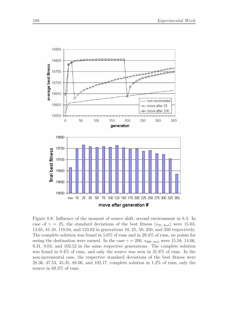
188 Experimental Work

Figure 8.8: Influence of the moment of source shift, second environment in 8.3. Incase of γ = 25, the standard deviations of the best fitness (s25−best) were 15.03,13.65, 81.10, 118.04, and 123.02 in generations 10, 25, 50, 250, and 350 respectively.The complete solution was found in 5.6% of runs and in 29.4% of runs, no points forseeing the destination were earned. In the case γ = 200, s200−best were 15.58, 14.06,9.31, 0.04, and 102.52 in the same respective generations. The complete solutionwas found in 0.4% of runs, and only the source was seen in 31.8% of runs. In thenon-incremental case, the respective standard deviations of the best fitness were28.36, 37.53, 45.35, 88.06, and 102.17, complete solution in 1.2% of runs, only thesource in 69.2% of runs.

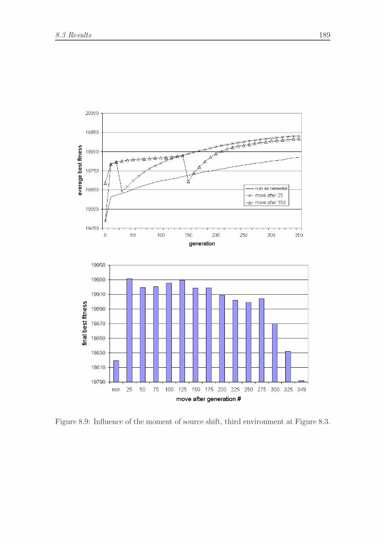
8.3 Results 189

Figure 8.9: Influence of the moment of source shift, third environment at Figure 8.3.

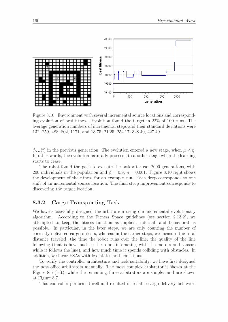
190 Experimental Work

Figure 8.10: Environment with several incremental source locations and correspond-ing evolution of best fitness. Evolution found the target in 22% of 100 runs. Theaverage generation numbers of incremental steps and their standard deviations were132, 259, 488, 802, 1171, and 13.75, 21.25, 254.17, 328.40, 427.49.

fbest(t) in the previous generation. The evolution entered a new stage, when µ < η.In other words, the evolution naturally proceeds to another stage when the learningstarts to cease.

The robot found the path to execute the task after ca. 2000 generations, with200 individuals in the population and φ = 0.9, η = 0.001. Figure 8.10 right showsthe development of the fitness for an example run. Each drop corresponds to oneshift of an incremental source location. The final steep improvement corresponds todiscovering the target location.

8.3.2 Cargo Transporting Task

We have successfully designed the arbitration using our incremental evolutionaryalgorithm. According to the Fitness Space guidelines (see section 2.13.2), weattempted to keep the fitness function as implicit, internal, and behavioral aspossible. In particular, in the later steps, we are only counting the number ofcorrectly delivered cargo objects, whereas in the earlier steps, we measure the totaldistance traveled, the time the robot runs over the line, the quality of the linefollowing (that is how much is the robot interacting with the motors and sensorswhile it follows the line), and how much time it spends colliding with obstacles. Inaddition, we favor FSAs with less states and transitions.

To verify the controller architecture and task suitability, we have first designedthe post-office arbitrators manually. The most complex arbitrator is shown at theFigure 8.5 (left), while the remaining three arbitrators are simpler and are shownat Figure 8.7.

This controller performed well and resulted in reliable cargo delivery behavior.

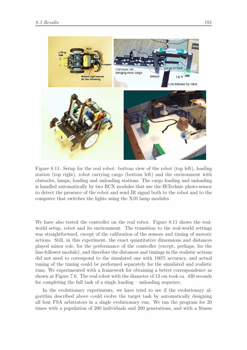
8.3 Results 191

Figure 8.11: Setup for the real robot: bottom view of the robot (top left), loadingstation (top right), robot carrying cargo (bottom left) and the environment withobstacles, lamps, loading and unloading stations. The cargo loading and unloadingis handled automatically by two RCX modules that use the HiTechnic photo-sensorto detect the presence of the robot and send IR signal both to the robot and to thecomputer that switches the lights using the X10 lamp modules.

We have also tested the controller on the real robot. Figure 8.11 shows the real-world setup, robot and its environment. The transition to the real-world settingswas straightforward, except of the calibration of the sensors and timing of motoricactions. Still, in this experiment, the exact quantitative dimensions and distancesplayed minor role, for the performance of the controller (except, perhaps, for theline-follower module), and therefore the distances and timings in the realistic actionsdid not need to correspond to the simulated one with 100% accuracy, and actualtuning of the timing could be performed separately for the simulated and realisticruns. We experimented with a framework for obtaining a better correspondence asshown at Figure 7.6. The real robot with the diameter of 12 cm took ca. 430 secondsfor completing the full task of a single loading – unloading sequence.

In the evolutionary experiments, we have tried to see if the evolutionary al-gorithm described above could evolve the target task by automatically designingall four FSA arbitrators in a single evolutionary run. We ran the program for 20times with a population of 200 individuals and 200 generations, and with a fitness

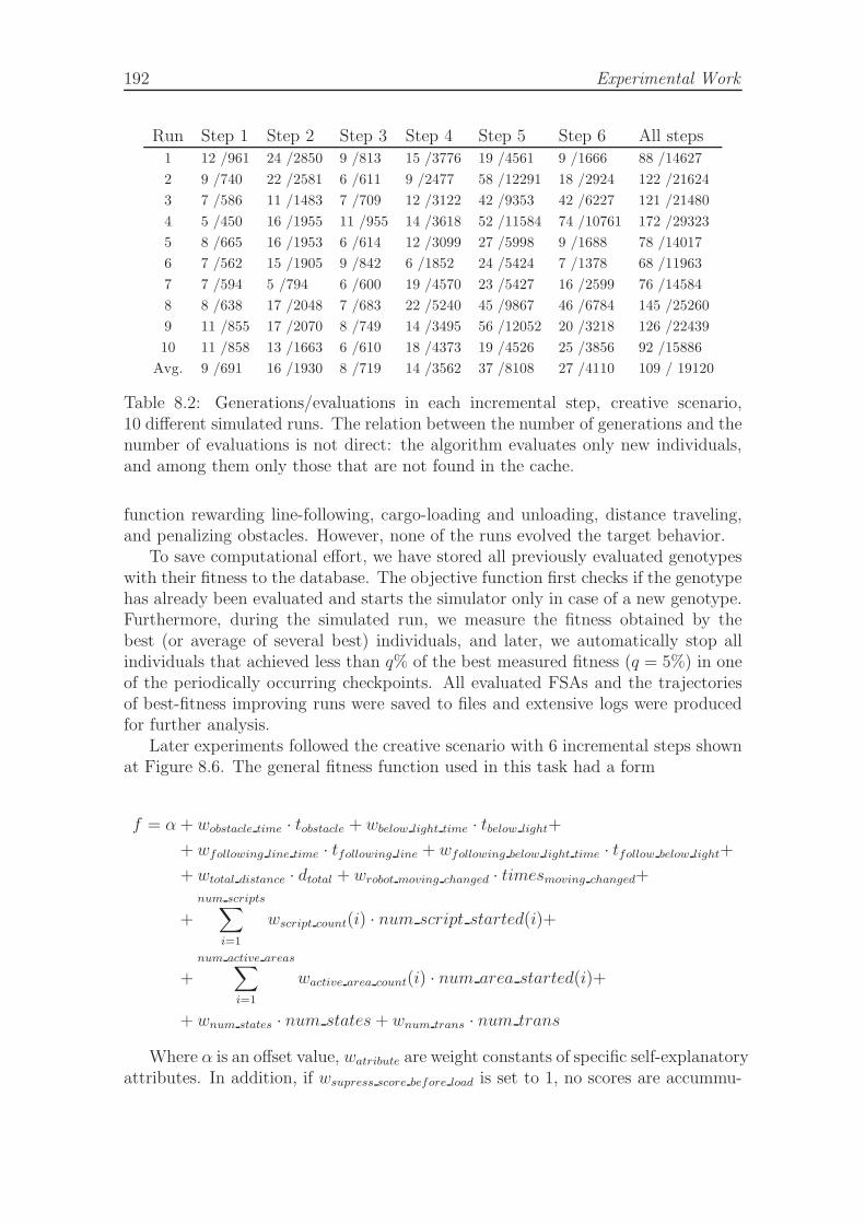
192 Experimental Work

Run Step 1 Step 2 Step 3 Step 4 Step 5 Step 6 All steps1 12 /961 24 /2850 9 /813 15 /3776 19 /4561 9 /1666 88 /14627

2 9 /740 22 /2581 6 /611 9 /2477 58 /12291 18 /2924 122 /21624

3 7 /586 11 /1483 7 /709 12 /3122 42 /9353 42 /6227 121 /21480

4 5 /450 16 /1955 11 /955 14 /3618 52 /11584 74 /10761 172 /29323

5 8 /665 16 /1953 6 /614 12 /3099 27 /5998 9 /1688 78 /14017

6 7 /562 15 /1905 9 /842 6 /1852 24 /5424 7 /1378 68 /11963

7 7 /594 5 /794 6 /600 19 /4570 23 /5427 16 /2599 76 /14584

8 8 /638 17 /2048 7 /683 22 /5240 45 /9867 46 /6784 145 /25260

9 11 /855 17 /2070 8 /749 14 /3495 56 /12052 20 /3218 126 /22439

10 11 /858 13 /1663 6 /610 18 /4373 19 /4526 25 /3856 92 /15886

Avg. 9 /691 16 /1930 8 /719 14 /3562 37 /8108 27 /4110 109 / 19120

Table 8.2: Generations/evaluations in each incremental step, creative scenario,10 different simulated runs. The relation between the number of generations and thenumber of evaluations is not direct: the algorithm evaluates only new individuals,and among them only those that are not found in the cache.

function rewarding line-following, cargo-loading and unloading, distance traveling,and penalizing obstacles. However, none of the runs evolved the target behavior.

To save computational effort, we have stored all previously evaluated genotypeswith their fitness to the database. The objective function first checks if the genotypehas already been evaluated and starts the simulator only in case of a new genotype.Furthermore, during the simulated run, we measure the fitness obtained by thebest (or average of several best) individuals, and later, we automatically stop allindividuals that achieved less than q% of the best measured fitness (q = 5%) in oneof the periodically occurring checkpoints. All evaluated FSAs and the trajectoriesof best-fitness improving runs were saved to files and extensive logs were producedfor further analysis.

Later experiments followed the creative scenario with 6 incremental steps shownat Figure 8.6. The general fitness function used in this task had a form

f = α + wobstacle time · tobstacle + wbelow light time · tbelow light+

+ wfollowing line time · tfollowing line + wfollowing below light time · tfollow below light+

+ wtotal distance · dtotal + wrobot moving changed · timesmoving changed+

+

num scripts∑

i=1

wscript count(i) · num script started(i)+

+num active areas

∑

i=1

wactive area count(i) · num area started(i)+

+ wnum states · num states + wnum trans · num trans

Where α is an offset value, watribute are weight constants of specific self-explanatoryattributes. In addition, if wsupress score before load is set to 1, no scores are accummu-

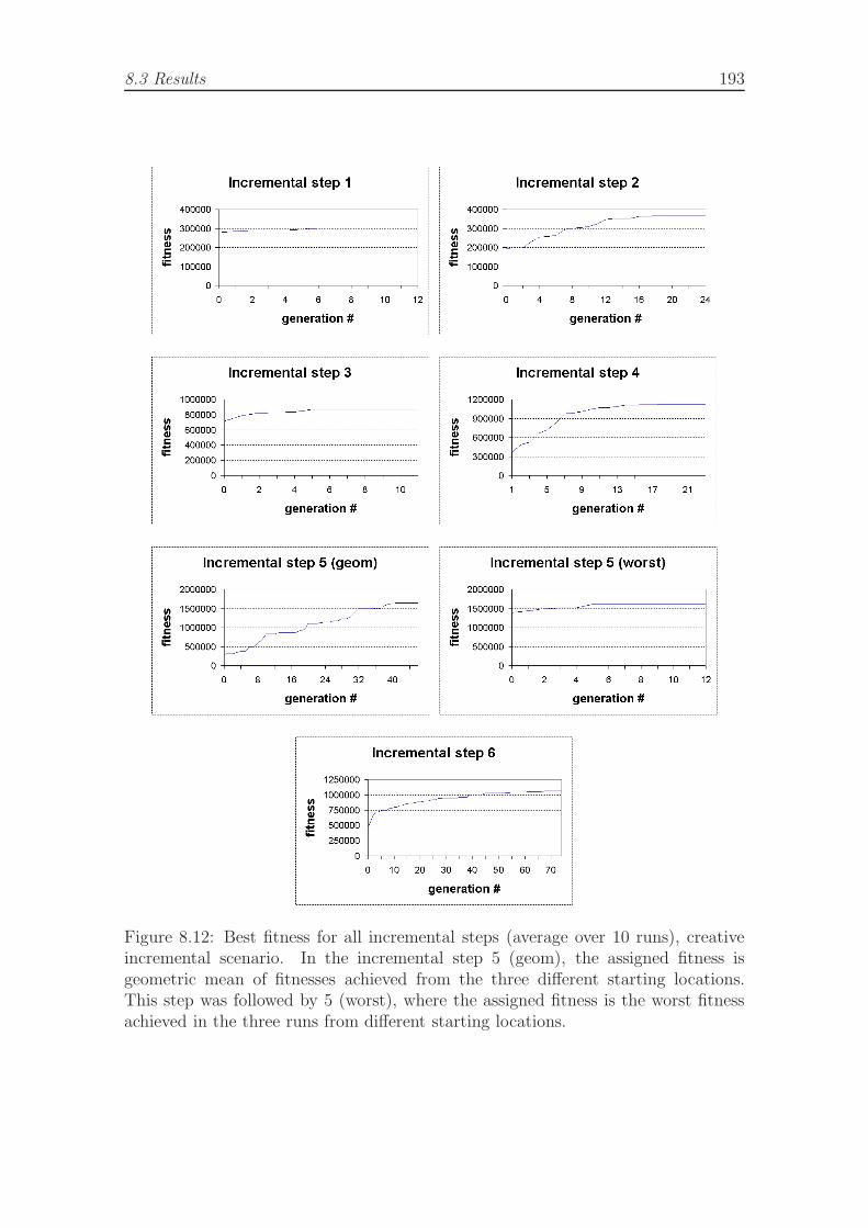
8.3 Results 193

Figure 8.12: Best fitness for all incremental steps (average over 10 runs), creativeincremental scenario. In the incremental step 5 (geom), the assigned fitness isgeometric mean of fitnesses achieved from the three different starting locations.This step was followed by 5 (worst), where the assigned fitness is the worst fitnessachieved in the three runs from different starting locations.

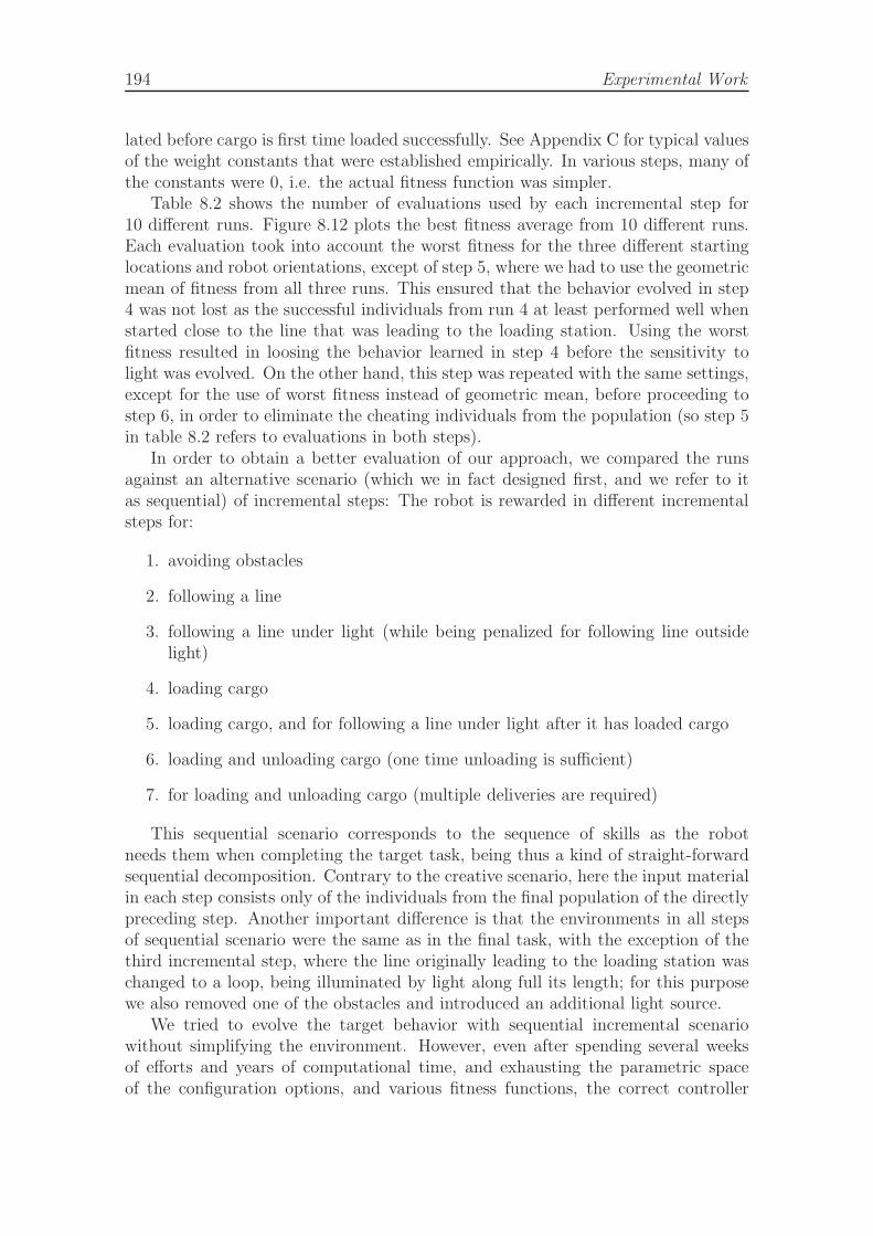
194 Experimental Work

lated before cargo is first time loaded successfully. See Appendix C for typical valuesof the weight constants that were established empirically. In various steps, many ofthe constants were 0, i.e. the actual fitness function was simpler.

Table 8.2 shows the number of evaluations used by each incremental step for10 different runs. Figure 8.12 plots the best fitness average from 10 different runs.Each evaluation took into account the worst fitness for the three different startinglocations and robot orientations, except of step 5, where we had to use the geometricmean of fitness from all three runs. This ensured that the behavior evolved in step4 was not lost as the successful individuals from run 4 at least performed well whenstarted close to the line that was leading to the loading station. Using the worstfitness resulted in loosing the behavior learned in step 4 before the sensitivity tolight was evolved. On the other hand, this step was repeated with the same settings,except for the use of worst fitness instead of geometric mean, before proceeding tostep 6, in order to eliminate the cheating individuals from the population (so step 5in table 8.2 refers to evaluations in both steps).

In order to obtain a better evaluation of our approach, we compared the runsagainst an alternative scenario (which we in fact designed first, and we refer to itas sequential) of incremental steps: The robot is rewarded in different incrementalsteps for:

1. avoiding obstacles

2. following a line

3. following a line under light (while being penalized for following line outsidelight)

4. loading cargo

5. loading cargo, and for following a line under light after it has loaded cargo

6. loading and unloading cargo (one time unloading is sufficient)

7. for loading and unloading cargo (multiple deliveries are required)

This sequential scenario corresponds to the sequence of skills as the robotneeds them when completing the target task, being thus a kind of straight-forwardsequential decomposition. Contrary to the creative scenario, here the input materialin each step consists only of the individuals from the final population of the directlypreceding step. Another important difference is that the environments in all stepsof sequential scenario were the same as in the final task, with the exception of thethird incremental step, where the line originally leading to the loading station waschanged to a loop, being illuminated by light along full its length; for this purposewe also removed one of the obstacles and introduced an additional light source.

We tried to evolve the target behavior with sequential incremental scenariowithout simplifying the environment. However, even after spending several weeksof efforts and years of computational time, and exhausting the parametric spaceof the configuration options, and various fitness functions, the correct controller

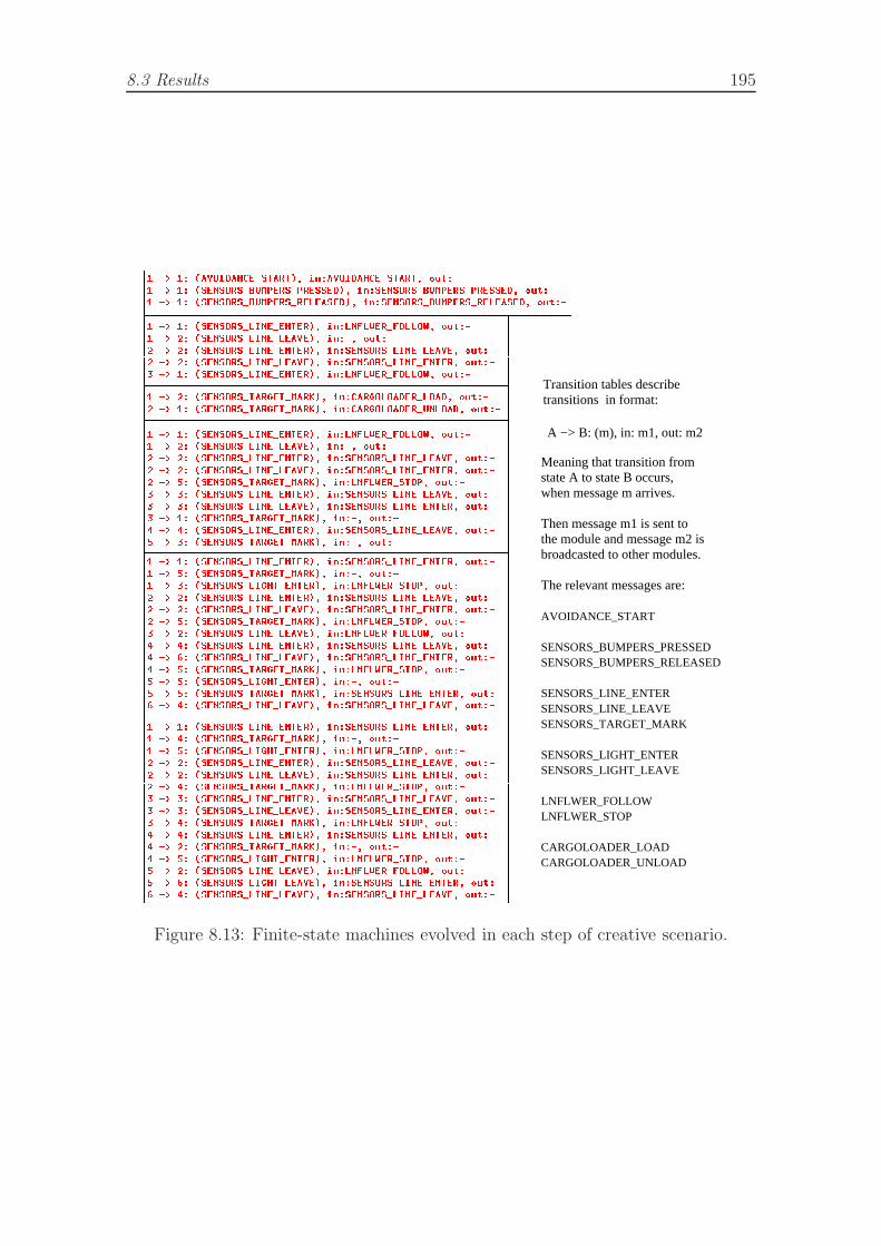
8.3 Results 195

A −> B: (m), in: m1, out: m2

Meaning that transition from state A to state B occurs,when message m arrives.

Then message m1 is sent tothe module and message m2 isbroadcasted to other modules.

The relevant messages are:

Transition tables describetransitions in format:

SENSORS_BUMPERS_PRESSEDSENSORS_BUMPERS_RELEASED

SENSORS_LINE_ENTERSENSORS_LINE_LEAVESENSORS_TARGET_MARK

SENSORS_LIGHT_ENTERSENSORS_LIGHT_LEAVE

LNFLWER_FOLLOWLNFLWER_STOP

CARGOLOADER_LOADCARGOLOADER_UNLOAD

AVOIDANCE_START

Figure 8.13: Finite-state machines evolved in each step of creative scenario.

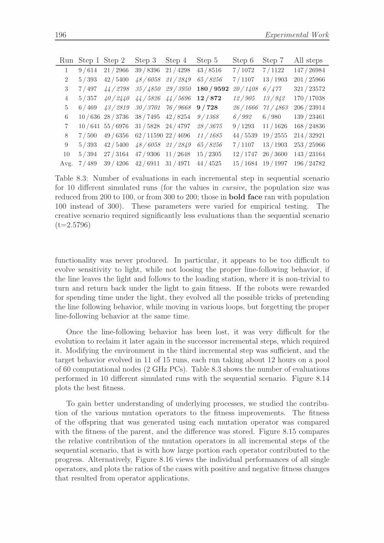
196 Experimental Work

Run Step 1 Step 2 Step 3 Step 4 Step 5 Step 6 Step 7 All steps1 9 / 614 21 / 2966 39 / 8396 21 / 4298 43 / 8516 7 / 1072 7 / 1122 147 / 26984

2 5 / 393 42 / 5400 48 / 6058 21 / 2849 65 / 8256 7 / 1107 13 / 1903 201 / 25966

3 7 / 497 44 / 2798 35 / 4850 29 / 3950 180 / 9592 20 / 1408 6 / 477 321 / 23572

4 5 / 357 40 / 2440 44 / 5826 44 / 5696 12 / 872 12 / 905 13 / 942 170 / 17038

5 6 / 469 43 / 2819 30 / 3701 76 / 9668 9 / 728 26 / 1666 71 / 4863 206 / 23914

6 10 / 636 28 / 3736 38 / 7495 42 / 8254 9 / 1368 6 / 992 6 / 980 139 / 23461

7 10 / 641 55 / 6976 31 / 5828 24 / 4797 28 / 3675 9 / 1293 11 / 1626 168 / 24836

8 7 / 500 49 / 6356 62 / 11590 22 / 4696 11 / 1685 44 / 5539 19 / 2555 214 / 32921

9 5 / 393 42 / 5400 48 / 6058 21 / 2849 65 / 8256 7 / 1107 13 / 1903 253 / 25966

10 5 / 394 27 / 3164 47 / 9306 11 / 2648 15 / 2305 12 / 1747 26 / 3600 143 / 23164

Avg. 7 / 489 39 / 4206 42 / 6911 31 / 4971 44 / 4525 15 / 1684 19 / 1997 196 / 24782

Table 8.3: Number of evaluations in each incremental step in sequential scenariofor 10 different simulated runs (for the values in cursive, the population size wasreduced from 200 to 100, or from 300 to 200; those in bold face ran with population100 instead of 300). These parameters were varied for empirical testing. Thecreative scenario required significantly less evaluations than the sequential scenario(t=2.5796)

functionality was never produced. In particular, it appears to be too difficult toevolve sensitivity to light, while not loosing the proper line-following behavior, ifthe line leaves the light and follows to the loading station, where it is non-trivial toturn and return back under the light to gain fitness. If the robots were rewardedfor spending time under the light, they evolved all the possible tricks of pretendingthe line following behavior, while moving in various loops, but forgetting the properline-following behavior at the same time.

Once the line-following behavior has been lost, it was very difficult for theevolution to reclaim it later again in the successor incremental steps, which requiredit. Modifying the environment in the third incremental step was sufficient, and thetarget behavior evolved in 11 of 15 runs, each run taking about 12 hours on a poolof 60 computational nodes (2 GHz PCs). Table 8.3 shows the number of evaluationsperformed in 10 different simulated runs with the sequential scenario. Figure 8.14plots the best fitness.

To gain better understanding of underlying processes, we studied the contribu-tion of the various mutation operators to the fitness improvements. The fitnessof the offspring that was generated using each mutation operator was comparedwith the fitness of the parent, and the difference was stored. Figure 8.15 comparesthe relative contribution of the mutation operators in all incremental steps of thesequential scenario, that is with how large portion each operator contributed to theprogress. Alternatively, Figure 8.16 views the individual performances of all singleoperators, and plots the ratios of the cases with positive and negative fitness changesthat resulted from operator applications.

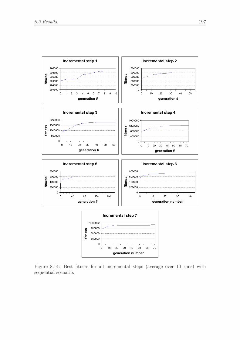
8.3 Results 197

Figure 8.14: Best fitness for all incremental steps (average over 10 runs) withsequential scenario.

198 Experimental Work

0 0,05 0,1 0,15 0,2 0,25

mut_new_trans

mut_rnd_trans

mut_del_rnd_trans

mut_new_state

mut_rnd_state_del

mut_split

mut_change_start

Relative performance of mutation operators in incremental step 1 of sequential scenario

experiment

0 0,05 0,1 0,15 0,2 0,25

mut_new_trans

mut_rnd_trans

mut_del_rnd_trans

mut_new_state

mut_rnd_state_del

mut_split

mut_change_start

Relative performance of mutation operators in incremental step 2 of sequential scenario

experiment

0 0,05 0,1 0,15 0,2 0,25

mut_new_trans

mut_rnd_trans

mut_del_rnd_trans

mut_new_state

mut_rnd_state_del

mut_split

mut_change_start

Relative performance of mutation operators in incremental step 3 of sequential scenario

experiment

0 0,05 0,1 0,15 0,2 0,25

mut_new_trans

mut_rnd_trans

mut_del_rnd_trans

mut_new_state

mut_rnd_state_del

mut_split

mut_change_start

Relative performance of mutation operators in incremental step 4 of sequential scenario

experiment

0 0,05 0,1 0,15 0,2 0,25

mut_new_trans

mut_rnd_trans

mut_del_rnd_trans

mut_new_state

mut_rnd_state_del

mut_split

mut_change_start

Relative performance of mutation operators in incremental step 5 of sequential scenario

experiment

0 0,05 0,1 0,15 0,2 0,25

mut_new_trans

mut_rnd_trans

mut_del_rnd_trans

mut_new_state

mut_rnd_state_del

mut_split

mut_change_start

Relative performance of mutation operators in incremental step 6 of sequential scenario

experiment

0 0,05 0,1 0,15 0,2 0,25

mut_new_trans

mut_rnd_trans

mut_del_rnd_trans

mut_new_state

mut_rnd_state_del

mut_split

mut_change_start

Relative performance of mutation operators in incremental step 7 of sequential scenario

experiment

Figure 8.15: Contribution of mutation operators to evolutionary progress in allincremental steps of a single run of the sequential experiment. Due to differentmutation rates, the absolute contribution of mutation operators was scaled bythe number of operator applications: in total 3970, 3321, 3951, 13329, 2974,21857, 17773 applications of mut change start, mut split, mut rnd state del,mut new state, mut del rnd trans, mut rnd trans and mut new trans operatorresp. Low success rate of mut rnd state del in earlier steps is due to the lower andupper limits on number of states. Steps introducing higher complexity in task benefitfrom mut split, when an extra state is smoothly added, extending one transition totwo steps. In total (the graph not shown to avoid direct addition of fitnesses fromdifferent incremental steps), splitting, mutating and deleting transitions are the mostsuccessful operators, however, all operators contribute significantly in more than oneincremental step.

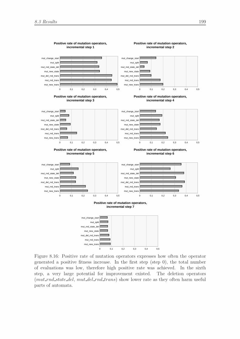
8.3 Results 199

0 0,1 0,2 0,3 0,4 0,5

mut_new_trans

mut_rnd_trans

mut_del_rnd_trans

mut_new_state

mut_rnd_state_del

mut_split

mut_change_start

Positive rate of mutation operators, incremental step 1

0 0,1 0,2 0,3 0,4 0,5

mut_new_trans

mut_rnd_trans

mut_del_rnd_trans

mut_new_state

mut_rnd_state_del

mut_split

mut_change_start

Positive rate of mutation operators, incremental step 2

0 0,1 0,2 0,3 0,4 0,5

mut_new_trans

mut_rnd_trans

mut_del_rnd_trans

mut_new_state

mut_rnd_state_del

mut_split

mut_change_start

Positive rate of mutation operators, incremental step 3

0 0,1 0,2 0,3 0,4 0,5

mut_new_trans

mut_rnd_trans

mut_del_rnd_trans

mut_new_state

mut_rnd_state_del

mut_split

mut_change_start

Positive rate of mutation operators, incremental step 4

0 0,1 0,2 0,3 0,4 0,5

mut_new_trans

mut_rnd_trans

mut_del_rnd_trans

mut_new_state

mut_rnd_state_del

mut_split

mut_change_start

Positive rate of mutation operators, incremental step 5

0 0,1 0,2 0,3 0,4 0,5

mut_new_trans

mut_rnd_trans

mut_del_rnd_trans

mut_new_state

mut_rnd_state_del

mut_split

mut_change_start

Positive rate of mutation operators, incremental step 6

0 0,1 0,2 0,3 0,4 0,5

mut_new_trans

mut_rnd_trans

mut_del_rnd_trans

mut_new_state

mut_rnd_state_del

mut_split

mut_change_start

Positive rate of mutation operators, incremental step 7

Figure 8.16: Positive rate of mutation operators expresses how often the operatorgenerated a positive fitness increase. In the first step (step 0), the total numberof evaluations was low, therefore high positive rate was achieved. In the sixthstep, a very large potential for improvement existed. The deletion operators(mut rnd state del, mut del rnd trans) show lower rate as they often harm usefulparts of automata.

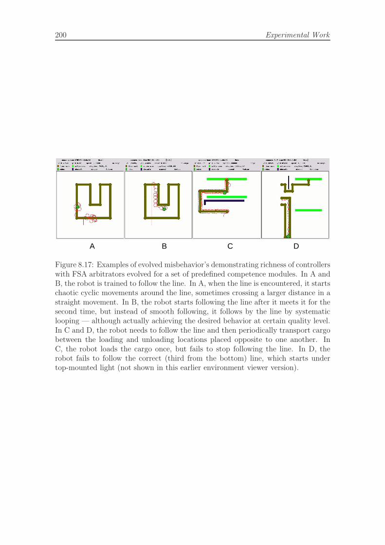
200 Experimental Work

A B C D

Figure 8.17: Examples of evolved misbehavior’s demonstrating richness of controllerswith FSA arbitrators evolved for a set of predefined competence modules. In A andB, the robot is trained to follow the line. In A, when the line is encountered, it startschaotic cyclic movements around the line, sometimes crossing a larger distance in astraight movement. In B, the robot starts following the line after it meets it for thesecond time, but instead of smooth following, it follows by the line by systematiclooping — although actually achieving the desired behavior at certain quality level.In C and D, the robot needs to follow the line and then periodically transport cargobetween the loading and unloading locations placed opposite to one another. InC, the robot loads the cargo once, but fails to stop following the line. In D, therobot fails to follow the correct (third from the bottom) line, which starts undertop-mounted light (not shown in this earlier environment viewer version).

8.4 Chapter Summary 201

8.4 Chapter Summary

• We demonstrate that the principles of evolutionary computing can make robotsadaptive on a trivial task.

• We design an experiment where an incremental evolutionary algorithm isrunning on-board of a mobile robot. The task of the robot is moving an objectbetween two specified locations. The genotype representation is a variable-length linear sequence of simple instructions.

• Finally, we design an experiment with a structural task for mobile robotevolved in simulation that can be verified in realistic environment. In thisexperiment, the robot is equipped with a behavior-based type of controllerwith distributed behavior arbitration mechanism relying on set of finite-stateautomata.

• The results from embedded incremental evolutionary task demonstrate howincremental evolution can solve the problem of designing simple controller fora navigation task.

• Evolution proceeds to later incremental steps automatically after fitness im-provement occurs and decreases.

• In a more complex robotic task that involves object localization and transport,we study different incremental scenarios of dividing the target task intomultiple sub-tasks: creative and sequential scenario.

• In the creative scenario, various skills are learned independently in modifiedenvironments and merged together in later steps.

• In the sequential scenario, the same target environment is used, and thebehavior is built in a sequential manner – from shorter sequences of actions tomore complex sequences.

• The sequential scenario fails to evolve the target behavior due to a highcomplexity, but succeeds if the environment is modified in one of the steps.

• The creative scenario succeed to evolve the target behavior in significantlyshorter time (t-test: 2.5786).

202 Experimental Work

Chapter 9

Discussion and Conclusions

9.1 Discussion

Personally, I think this is a crappy way to do things, but it’s the way thesystem works.—the head of section about this thesis review process

This section discusses various aspects we would like to attribute a point beforesummarizing the whole thesis in the conclusions that follow as a separate section.

9.1.1 Extensibility of the Controller

One of the important strengths of the incremental approach to evolution of con-trollers stems from the incremental property of the behavior-based approach tobuilding controllers.

When a functional controller is extended with a new functionality, this is typicallydone by adding one or more behavior modules. The coordination of the originalcontroller needs to be adjusted to the new task, while preserving the originalfunctionality.

In case of distributed arbitration system, this practically means modifying theprevious arbitrators to fit the new situation, and designing the new arbitrator(s) forthe new module(s). It is important to realize that this is the same kind of design stepas was repeated several times while designing the original controller that is beingextended. Thus, our methodology for design is open-ended: the controller is neverfixed-finished, rather allows for future modifications that have same characteristics,issues, and progress as the original design process.

We would like to discuss here a proposal for another interesting experiment,which demonstrates these principles. The starting point is an evolved controller forthe cargo transporting robot. Consider the following three modifications of the task:

• The environment is modified and several lines start below light. Robot isequipped with a compass sensor that allows it to recognize the correct line byremembering the orientation during its navigation along the line (a normalizedsequence of orientations). The extending module learns from experience: if the

204 Discussion and Conclusions

robot follows incorrect line and there is no cargo-loading station at the end, itwill quit following that line another time. In a slight modification, there is nocompass sensor, but the sequence of time intervals between turnings is usedto approximate the sequence of relative orientations.

The easiest integration of the new feature into the existing controller wouldbe making the line-follower arbitrator emit a message each time it starts orstops following a line, as well as reporting about whether loading or unloadingstation was present, and the new module should respond to these events bystarting a sequence measurement, and reporting its prediction, which againthe line-following arbitrator should process after the correct orientations arelearned.

• Adding a module responsible for reporting the location of obstacles. Thescenario is as follows: obstacles cannot be detected unless the robot approachesthem closely. The robot is exploring the environment and is equipped withadvanced positioning sensors based on triangulation, GPS or similar (i.e.overhead camera). Thus the location of the robot is known to it. The robotcombines the information about its location with the presence of obstacles andconstructs a map. The map is then used to avoid collisions with obstacles.

• Adding an IR sensor to the robot, and extending the task by placing anIR-emitting sphere (such as IR soccer-ball) at a random location in theenvironment. The sphere is to be avoided. A new sensor module is addedin the controller, and the Avoidance module has to be modified so that therobot will be avoiding both the obstacles and the IR ball, without hitting ortouching it.

• And finally, in another interesting experiment, consider an evolved controllerand a modification to the original cargo-transporting task. In the modifiedversion, the cargo needs to be loaded at the loading station at the end of aline and delivered below light. There is only a single line and single light. Thetask needs to be achieved by modifying the existing controller.

The importance of these modifications lies in testing the adaptivity capabilities ofthe proposed architecture and controller design method. In principle, these modifica-tions resemble the incremental steps designed in order to evolve the target behavior,and therefore there are good reasons to believe that the described transitions arepossible and likely to be successful. Yet, the actual verification of this hypothesisremains for the future work.

9.1.2 Evolution Modeled as Phenotypic Process

We return back to our remark on the distinction of evolution modeled as a geneticprocess and the approaches where the evolution is modeled as a phenotypic processfrom section 2.10. We make a point here that this biologically-inspired distinctionis not very relevant in the computational context.

9.1 Discussion 205

First, the phenotypic representation inherently implies some form of encoding,i.e. storing the usually complex patterns of interactions of the individual withthe environment or with the details of the particular task instance, where theevolved or evolving solution is applied. This encoding does not explicitly list allthese interactions, and properties, not even all the mechanisms that participate inthese interactions. They are rather implied by and contained in the whole systemthat executes the solution. Isn’t rather that whole system the phenotype? Whereis the border line between the body of the individual and its environment in thecomputational context? Consider an example from the computational world ofan evolution of an artificial agent whose behavior is controlled by a FSA, andan example from the biological world of some low-degree organism. The formeris supposed to be using a phenotype representation, while the latter is clearlyassumed to be evolved through biological genetic process. Is there really a differencebetween interpreting a FSA in order to produce a run-time behavior of the agentand interpreting a DNA of a biological organism in order to generate chemicalcompounds that are reacting to the chemicals found in the agent’s internal andexternal environment? In both cases, there is an encoding that is translated bythe “operating system” in order to obtain the actual behavior of an individual.The agent itself performs in some space, and has some spacial properties that arenot represented in the FSA. And even if the encoding would involve a directlyexecutable machine code, it would still be interpreted by the CPU to obtain theactual run-time behavior and execution of the CPU’s own microcode. Is there anyevolutionary process in the computational context that is modeled as phenotypicprocess (except of the cases of evolutionary design or evolution of robot morphology)at all? Avoiding further misunderstanding, please also notice the difference betweenthe distinction of a sexual and an asexual processes and the distinction betweenphenotypic and genetic processes. Even if the evolution of the artificial agent withFSA representation is asexual, we still can consider it to be a genetic process. Thereare many examples of asexual organisms in the biological world.

The complex interactive individual must be frozen into some sort of a staticencoding in order to be manipulated by evolutionary operators and stored in apopulation. In other words, in computational context, it is difficult and possiblymisleading to try to identify what is a phenotype. In biological terms, body of anindividual is distinguished by its spacial properties, however, those (if there could beany analogy in the computational world) are rather task-related than representation-related. The same FSA evolved for an artificial agent might perform differently whenused in different tasks, and agents with different morphologies and environments. Itis thus not the body that is encoded, but its genotype.

Does the phenotype include all the bits of the software, where the solution isbeing run? Including the operating system, and all the low-level implementation ofthe hardware of the computer, which the solution is interacting with and utilizing?Or does it include only those parts of the evolved solution that can be changed inthe evolutionary process? But isn’t that then the genotype itself?

Secondly, in many instances of the evolutionary algorithms that are renderedby [Fogel et al., 1995] as a genetic process, solutions are represented directly in the

206 Discussion and Conclusions

genotype – just recall the popular maxbit sample problem for instance. Here wecannot talk about any phenotype associated with the evolved bit-string, becausethe bit-string is the target of the search itself. The implications of our remark forthe field of evolutionary development are not dramatic, we only suggest that manyresearch questions relate to the genotype representation, and we consider the GP-trees, FSA, and virtually any evolved representation to be a genotype, rather than aphenotype evolved in a phenotypic process. In this respect, however, one has to bevery careful about any analogies drawn to the biological process of development. Inthe computational context, transformations and configurations of the genotype itselfare possible, and their usefulness has little to do with the developmental process innature, even if it might share some [but most likely forced] structural similarities.The research questions of what transformations on the genotypes and how they canbe performed, however, are still valid, interesting and worth investigation.

9.1.3 From FSA to Recurrent NN Architectures

Our chosen representation was motivated mainly by the fact that robots performingtasks as well as their behavioral modules are always in some state, which changesdepending on what situation and environmental conditions the robot is dealing with.

Other, probably more common, approach in Evolutionary Robotics experimentsis the utilization of neural network architectures. In order to explore the rich worldof the controller architectures in between, let us consider the following concepts.

Fitness landscape, neighborhood, and genetic operators. Fitness neighborhood isthe solution subspace reachable from the particular genotype with one of the geneticoperators in one step. Genotypes based on the neural networks usually operate withgradual changes to weights, or topologies by adding certain small random noise to thecurrent individual. In that way, they may suffer from the local extremes, which maybe difficult to escape by small random modifications. Larger modifications, however,may be too disruptive to the solution. In genotypes with state representation, thefitness landscape is less smooth. This may be seen as a disadvantage of the needle-in-a-haystack kind. On the other hand, it can have larger potential of avoiding localextremes, since new states and transitions may significantly improve the situation.Given the correct working solution in a state representation, we can easily makehundreds of modifications that will modify the behavior a little bit, but still leadto a working controller - therefore, we could claim that the needle to find is notnecessarily so tiny. Further experimental analysis might bring more insight.

Finite-state automata are discreet, whereas neural networks are continuous. Inparticular, the automata operate with discreet messages, the interface with thebehavior is discreet as well, they consist of discreet states, and transitions. Aninteresting experiment would be to study the evolvability change when some of theabove instances of discreetness are relaxed. This can be done in the following steps:

1. making the transitions probabilistic

2. making the states probabilistic (thus achieving a HMM-type of automaton)

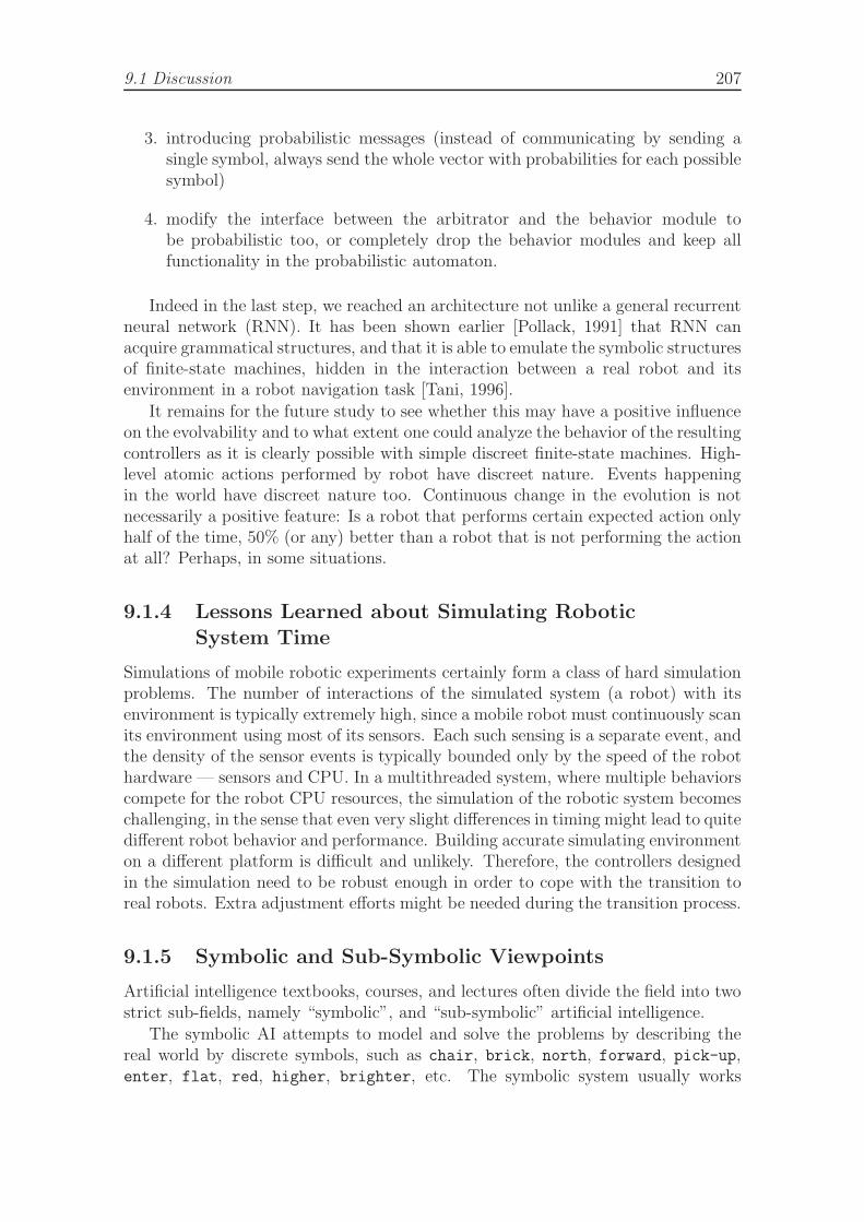
9.1 Discussion 207

3. introducing probabilistic messages (instead of communicating by sending asingle symbol, always send the whole vector with probabilities for each possiblesymbol)

4. modify the interface between the arbitrator and the behavior module tobe probabilistic too, or completely drop the behavior modules and keep allfunctionality in the probabilistic automaton.

Indeed in the last step, we reached an architecture not unlike a general recurrentneural network (RNN). It has been shown earlier [Pollack, 1991] that RNN canacquire grammatical structures, and that it is able to emulate the symbolic structuresof finite-state machines, hidden in the interaction between a real robot and itsenvironment in a robot navigation task [Tani, 1996].

It remains for the future study to see whether this may have a positive influenceon the evolvability and to what extent one could analyze the behavior of the resultingcontrollers as it is clearly possible with simple discreet finite-state machines. High-level atomic actions performed by robot have discreet nature. Events happeningin the world have discreet nature too. Continuous change in the evolution is notnecessarily a positive feature: Is a robot that performs certain expected action onlyhalf of the time, 50% (or any) better than a robot that is not performing the actionat all? Perhaps, in some situations.

9.1.4 Lessons Learned about Simulating RoboticSystem Time

Simulations of mobile robotic experiments certainly form a class of hard simulationproblems. The number of interactions of the simulated system (a robot) with itsenvironment is typically extremely high, since a mobile robot must continuously scanits environment using most of its sensors. Each such sensing is a separate event, andthe density of the sensor events is typically bounded only by the speed of the robothardware — sensors and CPU. In a multithreaded system, where multiple behaviorscompete for the robot CPU resources, the simulation of the robotic system becomeschallenging, in the sense that even very slight differences in timing might lead to quitedifferent robot behavior and performance. Building accurate simulating environmenton a different platform is difficult and unlikely. Therefore, the controllers designedin the simulation need to be robust enough in order to cope with the transition toreal robots. Extra adjustment efforts might be needed during the transition process.

9.1.5 Symbolic and Sub-Symbolic Viewpoints

Artificial intelligence textbooks, courses, and lectures often divide the field into twostrict sub-fields, namely “symbolic”, and “sub-symbolic” artificial intelligence.

The symbolic AI attempts to model and solve the problems by describing thereal world by discrete symbols, such as chair, brick, north, forward, pick-up,enter, flat, red, higher, brighter, etc. The symbolic system usually works

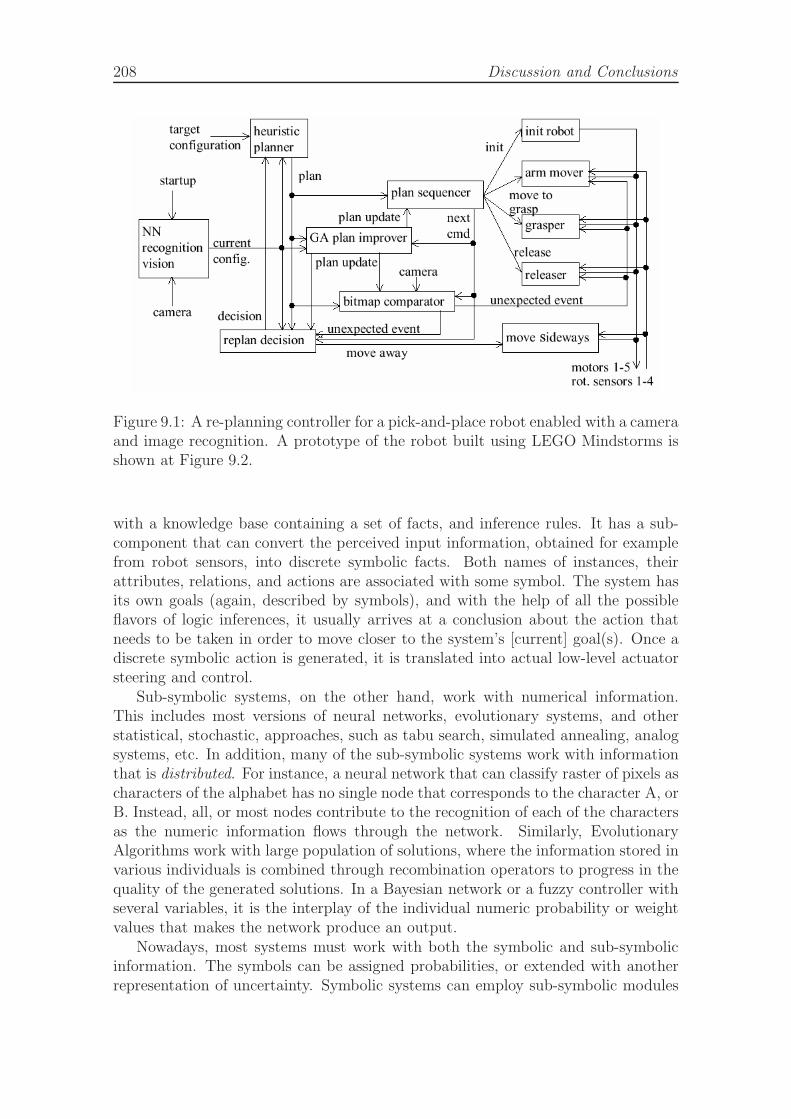
208 Discussion and Conclusions

Figure 9.1: A re-planning controller for a pick-and-place robot enabled with a cameraand image recognition. A prototype of the robot built using LEGO Mindstorms isshown at Figure 9.2.

with a knowledge base containing a set of facts, and inference rules. It has a sub-component that can convert the perceived input information, obtained for examplefrom robot sensors, into discrete symbolic facts. Both names of instances, theirattributes, relations, and actions are associated with some symbol. The system hasits own goals (again, described by symbols), and with the help of all the possibleflavors of logic inferences, it usually arrives at a conclusion about the action thatneeds to be taken in order to move closer to the system’s [current] goal(s). Once adiscrete symbolic action is generated, it is translated into actual low-level actuatorsteering and control.

Sub-symbolic systems, on the other hand, work with numerical information.This includes most versions of neural networks, evolutionary systems, and otherstatistical, stochastic, approaches, such as tabu search, simulated annealing, analogsystems, etc. In addition, many of the sub-symbolic systems work with informationthat is distributed. For instance, a neural network that can classify raster of pixels ascharacters of the alphabet has no single node that corresponds to the character A, orB. Instead, all, or most nodes contribute to the recognition of each of the charactersas the numeric information flows through the network. Similarly, EvolutionaryAlgorithms work with large population of solutions, where the information stored invarious individuals is combined through recombination operators to progress in thequality of the generated solutions. In a Bayesian network or a fuzzy controller withseveral variables, it is the interplay of the individual numeric probability or weightvalues that makes the network produce an output.

Nowadays, most systems must work with both the symbolic and sub-symbolicinformation. The symbols can be assigned probabilities, or extended with anotherrepresentation of uncertainty. Symbolic systems can employ sub-symbolic modules

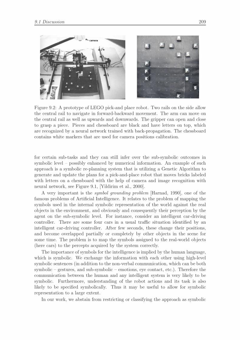
9.1 Discussion 209

Figure 9.2: A prototype of LEGO pick-and place robot. Two rails on the side allowthe central rail to navigate in forward-backward movement. The arm can move onthe central rail as well as upwards and downwards. The gripper can open and closeto grasp a piece. Pieces and chessboard are black and have letters on top, whichare recognized by a neural network trained with back-propagation. The chessboardcontains white markers that are used for camera positions calibration.

for certain sub-tasks and they can still infer over the sub-symbolic outcomes insymbolic level – possibly enhanced by numerical information. An example of suchapproach is a symbolic re-planning system that is utilizing a Genetic Algorithm togenerate and update the plans for a pick-and-place robot that moves bricks labeledwith letters on a chessboard with the help of camera and image recognition withneural network, see Figure 9.1, [Yildirim et al., 2000].

A very important is the symbol grounding problem [Harnad, 1990], one of thefamous problems of Artificial Intelligence. It relates to the problem of mapping thesymbols used in the internal symbolic representation of the world against the realobjects in the environment, and obviously and consequently their perception by theagent on the sub-symbolic level. For instance, consider an intelligent car-drivingcontroller. There are some four cars in a usual traffic situation identified by anintelligent car-driving controller. After few seconds, these change their positions,and become overlapped partially or completely by other objects in the scene forsome time. The problem is to map the symbols assigned to the real-world objects(here cars) to the percepts acquired by the system correctly.

The importance of symbols for the intelligence is implied by the human language,which is symbolic. We exchange the information with each other using high-levelsymbolic sentences (in addition to the non-verbal communication, which can be bothsymbolic – gestures, and sub-symbolic – emotions, eye contact, etc.). Therefore thecommunication between the human and any intelligent system is very likely to besymbolic. Furthermore, understanding of the robot actions and its task is alsolikely to be specified symbolically. Thus it may be useful to allow for symbolicrepresentation to a large extent.

In our work, we abstain from restricting or classifying the approach as symbolic

210 Discussion and Conclusions

or sub-symbolic. Individual modules may utilize both symbolic and sub-symbolicinformation, and the modules can exchange both kinds of information in the messagessent from one to another. The evolutionary algorithm – as inherently sub-symbolicmay find solutions, which might appear sub-symbolic, but at the same time, ourchosen representation of the finite-state automata attempts to come close to thepossibilities of symbolic treatment and explanation of the evolved arbitrators.

9.2 Main Contributions of the Thesis

The thesis studies the problem of automatic design of behavior coordination mecha-nism for behavior-based controllers of mobile robots by the means of evolutionary al-gorithms. While other researchers often investigate controller architectures inspiredby neural networks, this thesis focuses on distributed coordination mechanismsbased on finite-state automata. Plain evolutionary algorithms are not capable ofovercoming the complexity of this design problem and therefore must be supportedby additional framework. This thesis uses the method of incremental evolution,i.e. partitioning of the evolved task into a structure of simplified tasks of graduallyincreasing complexity from various viewpoints. We see the main contributions ofthis work as follows:

• We experimentally confirm that incremental evolution is a possible way ofovercoming the complexity of evolutionary task in the field of EvolutionaryRobotics, describe and experiment with various flavors of incrementality.

• We design and implement a new universal distributed coordination mechanismand controller architecture consisting of behavioral modules, message passing,and coordination modules associated with the behavior modules.

• We show how our coordination mechanism can be automatically designedusing evolutionary algorithm with the help of incremental evolution on anon-trivial mobile robot task evolved in simulation and verified on a realrobot. That means, we confirm that the behavior coordination mechanism ina behavior-based controller for a mobile robot can be automatically designedusing evolutionary computation.

• Designing the incremental scenario, i.e. dividing the task into incrementalsteps can be performed in various ways, we show that the sequential setup,where activities are always appended at the end of the previously evolved taskis not the most efficient way of task partitioning. Instead, dividing the taskinto steps based on various behavioral activities generates faster scenario.

• We show that finite-state automata, the genotype representation used inour coordination architecture, outperforms GP-tree programs on tasks withstructural similarity to behavior coordination problem.

• We experimentally confirm that embedded evolution, i.e. evolution runningon-line on the robot hardware, can generate solutions encountered by robotswhile they are performing task in real environments.

9.2 Main Contributions of the Thesis 211

• We show that incremental evolution can both improve and decrease theevolvability; the overall effect of its use can be both positive and negative andthus the use of incremental evolution requires understanding and preliminaryanalysis of the problem-specific search space.

212 Discussion and Conclusions

9.3 Conclusions

This thesis addresses the problem of designing adaptive mobile robots automatically.Similarly as the nature succeeded throughout the millions of years of naturalevolution in designing functional organisms with various degrees of intelligenceand colossal diversity of behaviors, morphologies, and functionality, we attemptto produce working robot controllers and perhaps bodies in tens of thousandsevaluations in a setup of artificial evolutionary computation.

Obviously, there is a gap between the complexities of the natural and artificialevolutions. The size of this gap is difficult to estimate even today. This gap willnever be removed by any supercomputer in the Universe as we know it. That hasa couple of consequences: First, if the natural processes of an artificial evolutionshould ever produce systems that would be at least partially comparable to anyintelligent living organisms, the conditions for the evolutionary progress in suchartificial environments would have to be enormously more favorable than they arein the nature on our planet as we know it, or, alternately, we would have to be ableto identify a very small subset of the thousands of millions of interactions betweenthe organisms, species, and their environment that are relevant for the evolutionaryprogress, if there are any such at all. Second, if we are to exploit the idea of artificialevolution for our benefit within the artificial environments that we can build withour computing power, we must restrict and guide the evolutionary process strongly.

Nevertheless, the inspiration from the natural evolution by the computer scien-tists has brought provably successful projects, particularly in the areas where thesubject of the evolution is a solution to a relatively small-size search problem, which,however, may be impossible or too hard to solve by known deterministic or otheralgorithmic methods.

We approach the design of the robots by the means of evolutionary computationby selecting those parts of the design process that are, in our opinion, most suitablefor evolution. In particular, in addition to studies into representations for evolvingmorphologies, we focus on designing a coordination mechanism of behaviors in acontroller consisting of multiple simultaneously performing behaviors in the style ofthe behavior-based robotics.

The behavior coordination in the controller used in our main experiments isbased on set of finite-state automata. One of the contributions of our work isthe analysis of the FSA representation itself. We touch several important issuesof artificial evolution with direct program representations, in particular GP-treesand FSA. While the GP-tree programs tend to have a relatively linear path ofexecution, the FSA are powerful in representing repeated and possibly irregularpatterns and behaviors that react to percepts and possibly launch different mode(or state) of operation. The internal topology of the representations corresponds1) to the topology of interactions of the evolved solution with its environment – asdemonstrated on the “switch” task and 2) to the topology of the space searched bythe evolutionary algorithm – as demonstrated by the “find target” task. On severalsample tasks, we study the performance of both representations, and confirm thatboth representations can outperform one another, depending on the structure of the

9.3 Conclusions 213

interactions the program is to perform in a particular task. We leave for the futurework comparisons against automatically defined functions of Koza [Koza, 1994], andhybrid approaches that combine both FSA and GP, for instance [Benson, 2000].

Another important difference of the GP-tree and FSA representations is that theFSA individuals require some condition to be satisfied between performing any twoactions. This is not the case in the GP-tree representation, especially when a seq

non-terminal can be used. FSA representation can be compensated by introducingtautology transition conditions, however, it still remains more sensitive to sensoryinputs (values of the registers).

Another, main contribution of this thesis relates to evolving the robot controllersincrementally. More complex tasks prove to be too difficult for an evolutionaryalgorithm, and further guidance might improve the chances for discovering a correctsolution. Incremental evolution is a possible method for such guidance. The incre-mental method is based on dividing the target task into multiple tasks of increasingcomplexity (a partial order relation). Evolved populations with individuals thatsuccessfully perform more simple tasks are transformed and combined into initialpopulations for more complex tasks thus making it possible to evolve complexbehaviors, which could not be automatically programmed otherwise. We approachthe incremental evolution from several viewpoints.

In the experiments with FSA representation, we show that using incrementalevolution requires careful preparation and understanding of the evolutionary process.Our experimental runs confirm that making the evolutionary algorithm incrementalcan both help and hinder the success rate of the evolutionary algorithm. Usually,incremental evolution introduces an extra bias, requiring the evolution to passthrough stages that could possibly be avoided in a single run. This incrementalbias must be compensated by larger benefits resulting from evolving incrementally,in favor of faster and easier progress of the evolution, otherwise the incrementalmethod performs worse.

More exploration of the abilities of FSA-based representations, and task-charac-terization guidelines that may suggest suitable genotype representation remain alsofor a possible future work. This would be especially interesting in the context ofincremental evolution. Deeper investigations into less deterministic representations,such as probabilistic state automata remain also for the future work.

In an incremental evolution experiment with an embedded evolutionary algo-rithm running on a simple robot built from flexible LEGO construction sets weshowed that the choice of the generation number for making transition to the nextincremental step has an influence on the quality of the final solution. A robot facinga novel problem to solve needs to determine this generation automatically. Weapplied a method where this choice is made based on measuring the convergence.We also demonstrated on this simple task that the incremental evolution improvesevolvability of robot controllers.

Behavior control architectures are the focus of contemporary research. Ourrobot controller architecture we proposed in the main part of the work is inspiredby the principle of independent robot competencies performed, or being ready tobe activated, in parallel. This principle is prevalent in Behavior-Based Robotics

214 Discussion and Conclusions

approaches. In our case, the behaviors communicate by sending addressed or broad-casted message signals possibly containing data. The implementation relies onshared memory locations between the individual threads of computation, and themessage-passing interface function calls achieve high efficiency (usually no data iscopied; rather the functions with arguments referring to common memory spaceare called). However, shared memory is not a requirement of this representation.Complete messages can be transmitted between the modules, if the hardwareimplementation requires.

We have designed a parallel, distributed behavior-based controller architecturewhere individual modules communicate by sending messages. Modules implementsimple behaviors and are usually hand-coded, or optionally evolved. Messages areprocessed by post-offices attached to modules in order to filter relevant messagesand adapt the behavior of the modules with independent behavioral responsibilityto the purpose of the combined controller thus achieving efficient synergy of be-havior coordination. On example task of cargo delivery, we have demonstrated asuccessful design both manually and using automatic method based on incrementalevolutionary algorithm that evaluates the individuals in simulation. The evolvedindividuals representing the arbitrators, i.e. the post-offices of all modules, take theform of finite-state automata.

Our framework for incremental evolution allows a general design of the incre-mental evolutionary scenario: the populations from several steps can be combinedtogether in different ratios for each particular FSA. In addition, it is possible tospecify a general ‘incremental’ function, which specifies a termination criterionin each incremental step, i.e. a required condition for proceeding to the nextincremental step. Incremental function can take into account various variables,such as the current generation number (globally or within this step), best fitness(globally or current generation), average fitness (globally or current), learningmomentum, which is the current learning rate with history; number of evaluations(globally or within this step), real run-time in different forms, etc. These variablescan be combined with numeric constants, binary operators and predicates. Eachincremental step has its own definition file for the environment, separate fitnessfunction, structure of the controller, and describes the robot topology. Despite thisgenerality, we concluded to several guidelines for designing the incremental scenarios:

1. Individual incremental steps ought to be as focused as possible. If a certaincompetence required for the target behavior can be learned completely in someincremental step, it should not be the subject of further learning and improve-ment in other incremental steps, as it would only increase its complexity by amultiplicative factor.

2. Each incremental step should focus on a relatively narrow and well- identifiablecompetence. Avoiding evolving of multiple competencies at the same time isessential. If some competence requires a cooperation of multiple competencies,this itself has to be identified, and formulated as a distinguished, well-definedcompetence.

9.3 Conclusions 215

3. Modifying the environment in order to create training situations for the robotis a very efficient method of devising simpler incremental steps. Modifyingthe objective function only, while keeping the same environment, is morechallenging, and often leads to multitudes of false behaviors. Evolution tendsto discover unexpected tricks due to the large number of possible interactionsin a typical target environment. Figure 8.17 shows few samples of incorrectevolved behaviors.

4. The early apparent suggestive decomposition of the task is often not necessarilythe most efficient way of task decomposition for incremental evolution. Theaverage number of evaluations was significantly lower in the case of moreelaborate task decomposition as shown in the results section of this work.

5. Special care has to be taken to prevent the individuals from gaining fitness byrandom coincidences without performing the required task. If the populationswith several hundreds individuals evolve for hundreds of generations, evenvery unlikely events do happen and if the EA uses elitism, such faulty, butlucky behavior might completely push all promising individuals out of thepopulation. Such events can, to a limited extent, be prevented by multiplestarts from all starting locations. This, however, increases the total evaluationtime for each individual. In our experiments, we used four different methodsof calculating the individual fitness from the scores gained in all startinglocations: arithmetic mean, geometric mean, worst fitness, and combination.The worst fitness has to be used, if we want to set a hard constraint andrequire that the individual performs the required behavior consistently andreliably. It should be used especially when the objective function permits avery high score in lucky situations – thus both mean and geometric meanthresholds could pass an individual that would solve only some of the runs,accidentally with a luckily high score (please note, that the geometric meanwould not suffer from this problem if the unsuccessful runs would receive zero-fitness; that is, however, not the case, because the objective function typicallyrewards multiple aspects of the task, and thus it is almost never 0). In caseof the combined option, we use the geometric mean for all runs from the samestarting location, but the worst fitness among all those means for all startinglocations. In other words, the robot has to solve each starting location, butits performance does not have to be completely stable. Using worst fitnesscan be too strict for evolution to discover any working solution as the searchtypically solves only one of the starting locations first, followed by a solutionthat can solve two, etc. We would recommended the approach we used in theexperiments: we started with geometric mean and followed with worst fitness.This allows partial solutions to have an evolutionary advantage over poor andrandom solutions and in the second stage, it eliminates individuals that donot solve all test cases reliably.

Many tasks (including ours) comprise a high degree of randomness. The sameindividual can gain fitness values that vary often more than 10%. This can lead into

216 Discussion and Conclusions

an illusory fitness improvement while the quality of the individuals does not change– or even decreases slightly, especially if elitism is in use: a small change introducedto an individual will result in a new individual, which by a lucky coincidence gainshigher fitness and replaces the old individual in the population. This makes italso more difficult for newly found individuals, which introduce changes in a gooddirection, to steer the evolution away, as there are already many individuals whohave the more lucky fitness for their real quality in the population, especially if theevolution stagnated for some time already. For this reason, it is recommended toevaluate all individuals over in each generation. Unfortunately, in our case, thiswould exceed out of practical CPU limits, but it remains for future work to studyhow much this issue hinders the evolution of arbitrators.

Sometimes, one cannot avoid transferring certain evolved features to succeedingevolutionary steps. There is a high risk that the new incremental step will quicklymove in its search away from the evolved features, which thus become easilyforgotten. A remedy for this situation would be a continuous flow of individualsfrom previous incremental step, however it remains for the future work to evaluatethis strategy.

It seems though that an insight of a human expert knowing the details ofthe robot hardware and software is still required in order to design a functionalincremental decomposition. Future work should focus on eliminating these andmaking the process of creating the controller as automatic as possible.

Two advanced evolutionary techniques were applied in order to improve theevolutionary search process:

1. The population was automatically reinitialized each time it converged prema-turely;

2. The states and transitions, which were never entered during the evaluationby the fitness function, can optionally be removed automatically. On onehand, this leads into much more readable and concise FSAs, on the otherhand, it reduces the evolvability as the overhead genetic material present inthe population becomes forbidden, and thus the population can get stuck inlocal extremes more easily. Removing unused transition also helps to win theuseful code over bloat that can prevent the evolution from progressing at anyreasonable pace.

3. Fitness cache implemented using SQL database helped to decrease the overalltime required to reach the solution.

An important observation and recommendation about the possible applicationsof evolutionary computation for designing the robot controllers is that those be-haviors are amenable to evolution that are difficult to describe by simple schemes,formalisms or clear sentences in natural language. If the target of the evolution iseasy to describe using highly-structured prescription, it is typically easier and moreefficient to use one or another kind of formalism to specify that prescription in someimplementation language and execute it directly on the robot, or provide some

9.3 Conclusions 217

interpreter for high-level natural sentences with a strongly limited domain. Theevolution can be much more useful when the target function is difficult to describe,estimate, and analyze – when the human attempts to generate formal deterministicsolutions tend to fail or are too difficult to complete. In these cases, the evolutionis able to “mechanistically” grasp the hidden interactions within the system andgenerate a solution with a suitable performance. Therefore the attempts to use theevolutionary computation in the design of robot controllers have to be thoroughlyconsidered and first undergo a sound critique.

The computational demand of the algorithm is high and requires utilization ofdistributed computational power. We have used three various systems for distributedcomputation to harness the idle CPU power of university student lab computers andcluster.

Additional further directions of this work are several. A natural languageinterface for specifying the target task would allow to program robot for complextask by giving description in human language. This would also require work onautomatic partitioning of the target task into incremental steps, and an AI systemthat could achieve that by understanding the semantic descriptions of the basicrobot capabilities. Automatic programming of multiple groups of robots is a straightextension of this work. Improvements in the simulation techniques, using real-timeoperating systems, simulating more realistic environments, as well as implementingthe robot simulator and evolutionary algorithm directly on the robot hardwareremain for further studies. Other representations in addition to FSA taking therole of behavior arbitrators should be investigated. The crispness of FSAs can bealleviated by making them more continuous: either by transitions that occur withcertain probability, or by messages that would be probability vectors for all messagetypes, or by staying in multiple states at the same time with distributed probability.This is our connection to the fields of Hidden Markov Models and neural networks,however it remains to be investigated whether such representations apply smoothlyto the crisp robotic tasks constrained by the discrete robot body, actuators, andworld interactions, which are probably modeled best by discrete states.

9.3.1 On Educational Robotics

All our evolutionary experiments have been performed with educational roboticshardware. Indeed, Evolutionary Robotics is such a highly-specialized sub-field thatper se alone does not exist and must naturally be connected to some particularrobotics domain. Our underlying domain – educational robotics deals with the useof robotics technology in schools at all levels, either as part of the curriculum, oras after-school activity. Naturally, we have performed several studies directly in thefield of educational robotics as part of this thesis, even though they are included asand considered to be the supporting studies.

Drawing robots Robotnacka are installed in the robotics laboratory and availablethrough the Internet for public use. Teachers at various levels might consider usingthe laboratory in their lessons – from mathematics, physics and programming atthe levels of primary and secondary schools, to the programming, control, hardware,

218 Discussion and Conclusions

computer vision, artificial intelligence courses at the undergraduate or graduate level.Without previous advertisement of the laboratory that is still under development,there already were hundreds of visitors who logged into the laboratory. As faras we are concerned, there are very few other perpetual robot installations in theWorld. The importance of our implementation is that the robots can be controlleddirectly from Imagine Logo – an interactive programming environment for children.However, the laboratory is available for the research and educational use from otherplatforms (including C++, Java, Agent-Space architecture, and other). Our goalis to continue and improve the operation of the remotely-controlled laboratory andserve with our best efforts to the teachers and students communities at variouseducational levels, where the use of robotics might be useful in educational process.For instance, teachers at the Faculty of Electrical Engineering use these robots inMobile Robotics course [Balogh, 2007].

Pilot set of ten projects implemented in Imagine Logo and accompanied byteachers’ and students’ instruction sheets (4 math, 4 algorithms, and 2 physics)is ready to be evaluated in the schools. All relevant materials and evaluations areavailable for review, feedback, and discussion at [URL - Robotnacka].

We achieved numerous little contributions in this area, namely finite-statemachines for RCX, computer vision package for evolutionary robotics experiments,interfacing RCX with WowWee entertainment robots, integrating RCX and Aiborobots in a model of a factory, using LEGO robots for analyzing rescue robot ap-plication, multiple participation at RoboCup Junior contests, seven years of LEGOideas in summer camps for young people interested in computers (CyberCamp), andLogo interpreter for NXT.

Using robots in schools may:

• demonstrate phenomena in novel and more ample ways,

• provide creative platforms for hands-on exploration for individual or groupstudent work,

• increase entertainment experience during the learning process,

• increase motivation for learning,

• spawn interest in technology among students.

On the other hand, using robots in education has severe drawbacks and challenges:

• high cost of robots,

• extra time, space, work and competence required from teachers and schools,

• shortage of curriculum materials and guidelines.

It remains for the enthusiastic work of proponents of robots in education to demon-strate successful examples, which then could be adopted for wider use.

219

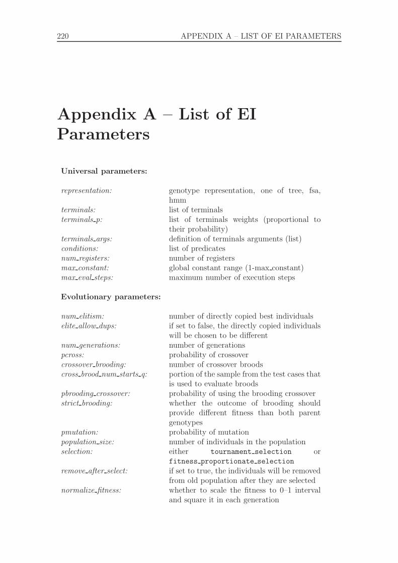
220 APPENDIX A – LIST OF EI PARAMETERS

Appendix A – List of EIParameters

Universal parameters:

representation: genotype representation, one of tree, fsa,hmm

terminals: list of terminalsterminals p: list of terminals weights (proportional to

their probability)terminals args: definition of terminals arguments (list)conditions: list of predicatesnum registers: number of registersmax constant: global constant range (1-max constant)max eval steps: maximum number of execution steps

Evolutionary parameters:

num elitism: number of directly copied best individualselite allow dups: if set to false, the directly copied individuals

will be chosen to be differentnum generations: number of generationspcross: probability of crossovercrossover brooding: number of crossover broodscross brood num starts q: portion of the sample from the test cases that

is used to evaluate broodspbrooding crossover: probability of using the brooding crossoverstrict brooding: whether the outcome of brooding should

provide different fitness than both parentgenotypes

pmutation: probability of mutationpopulation size: number of individuals in the populationselection: either tournament selection or

fitness proportionate selection

remove after select: if set to true, the individuals will be removedfrom old population after they are selected

normalize fitness: whether to scale the fitness to 0–1 intervaland square it in each generation

APPENDIX A – LIST OF EI PARAMETERS 221

tournament size: size of the tournament iftournament selection is used

tournament selection p: probability of taking the winning individualin the tournament selection

num starts: number of testing samples used by theobjective function

fitness size q: penalty for the size of the genotype (toencourage shorter genotypes)

evalsteps q: penalty for the number of execution steps (toencourage faster-running programs)

log file name: string used for naming log file (together withtime stamp)

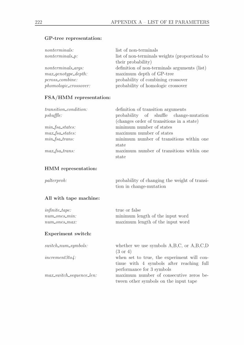
222 APPENDIX A – LIST OF EI PARAMETERS

GP-tree representation:

nonterminals: list of non-terminalsnonterminals p: list of non-terminals weights (proportional to

their probability)nonterminals args: definition of non-terminals arguments (list)max genotype depth: maximum depth of GP-treepcross combine: probability of combining crossoverphomologic crossover: probability of homologic crossover

FSA/HMM representation:

transition condition: definition of transition argumentspshuffle: probability of shuffle change-mutation

(changes order of transitions in a state)min fsa states: minimum number of statesmax fsa states: maximum number of statesmin fsa trans: minimum number of transitions within one

statemax fsa trans: maximum number of transitions within one

state

HMM representation:

palterprob: probability of changing the weight of transi-tion in change-mutation

All with tape machine:

infinite tape: true or falsenum ones min: minimum length of the input wordnum ones max: maximum length of the input word

Experiment switch:

switch num symbols: whether we use symbols A,B,C, or A,B,C,D(3 or 4)

increment3to4: when set to true, the experiment will con-tinue with 4 symbols after reaching fullperformance for 3 symbols

max switch sequence len: maximum number of consecutive zeros be-tween other symbols on the input tape

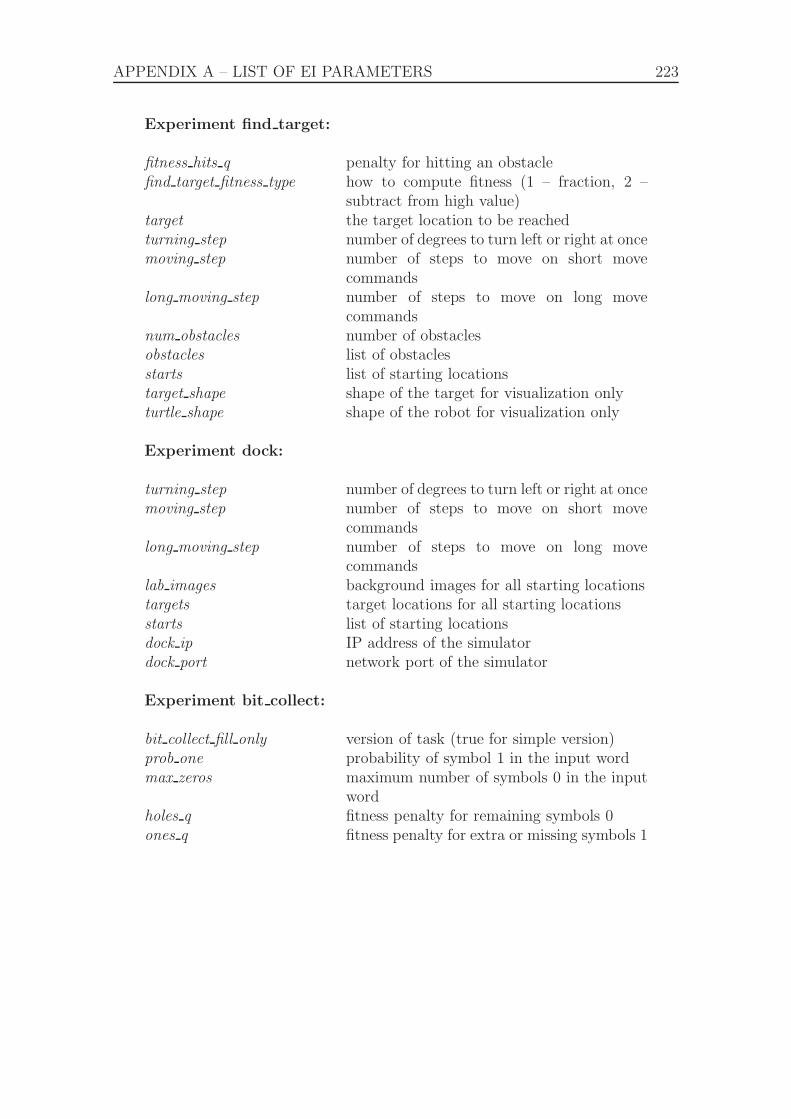
APPENDIX A – LIST OF EI PARAMETERS 223

Experiment find target:

fitness hits q penalty for hitting an obstaclefind target fitness type how to compute fitness (1 – fraction, 2 –

subtract from high value)target the target location to be reachedturning step number of degrees to turn left or right at oncemoving step number of steps to move on short move

commandslong moving step number of steps to move on long move

commandsnum obstacles number of obstaclesobstacles list of obstaclesstarts list of starting locationstarget shape shape of the target for visualization onlyturtle shape shape of the robot for visualization only

Experiment dock:

turning step number of degrees to turn left or right at oncemoving step number of steps to move on short move

commandslong moving step number of steps to move on long move

commandslab images background images for all starting locationstargets target locations for all starting locationsstarts list of starting locationsdock ip IP address of the simulatordock port network port of the simulator

Experiment bit collect:

bit collect fill only version of task (true for simple version)prob one probability of symbol 1 in the input wordmax zeros maximum number of symbols 0 in the input

wordholes q fitness penalty for remaining symbols 0ones q fitness penalty for extra or missing symbols 1

224 APPENDIX A – LIST OF EI PARAMETERS

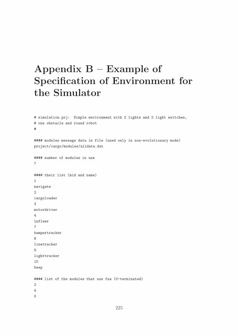
Appendix B – Example ofSpecification of Environment forthe Simulator

# simulation.prj: Simple environment with 2 lights and 2 light switches,

# one obstacle and round robot

#

#### modules message data in file (used only in non-evolutionary mode)

project/cargo/modules/alldata.dat

#### number of modules in use

7

#### their list (mid and name)

1

navigate

2

cargoloader

3

motordriver

4

lnflwer

7

bumpertracker

8

linetracker

9

lighttracker

10

beep

#### list of the modules that use fsa (0-terminated)

2

4

0

225

226 APPENDIX B – ENVIRONMENT SPECIFICATION

### version of code to start

4

#### environment type: RECTANGLE

1

#### environment dimensions: width height

1.0 1.0

#### number of obstacles

3

1 0.35 0.73 0.01 0.2

1 0.5 0.0 0.01 0.56

1 0.35 0.56 0.16 0.01

#### number of floor marks

3

#### another floor mark: type(LINE) x y width Nsegments value

#### x1 y1

#### ...

#### xN yN

#### the coordinates of vertices of this polyline are

#### in the center of the line (i.e. there’s a line around

#### these points in all directions up to a distance

#### width/2 - i.e. round corners)

#### -> this means that you should start/end the line in distance

#### width/2 from where it actually ends

2 0.2 0.8 0.05 6 30

0.25 0.8

0.25 0.65

0.46 0.65

0.46 0.8

0.7 0.8

0.7 0.865

2 0.2 0.5 0.05 2 30

0.42 0.5

0.42 0.01

2 0.2 0.4 0.05 2 30

0.35 0.4

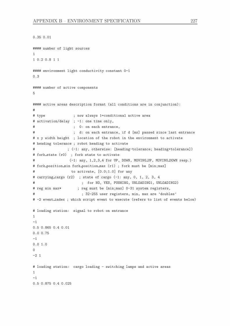
APPENDIX B – ENVIRONMENT SPECIFICATION 227

0.35 0.01

#### number of light sources

1

1 0.2 0.8 1 1

#### environment light conductivity constant 0-1

0.3

#### number of active components

5

#### active areas description format (all conditions are in conjunction):

#

# type ; now always 1=conditional active area

# activation/delay ; -1: one time only,

# ; 0: on each entrance,

# ; d: on each entrance, if d [ms] passed since last entrance

# x y width height ; location of the robot in the environment to activate

# heading tolerance ; robot heading to activate

# ; (-1: any, otherwise: [heading-tolerance; heading+tolerance])

# fork state (r0) ; fork state to activate

# (-1: any, 1,2,3,4 for UP, DOWN, MOVING UP, MOVING DOWN resp.)

# fork position min fork position max (r1) ; fork must be [min;max]

# to activate, [0.0;1.0] for any

# carrying cargo (r2) ; state of cargo (-1: any, 0, 1, 2, 3, 4

# ; for NO, YES, PUSHING, UNLOADING1, UNLOADING2)

# reg min max* ; reg must be [min;max] 0-31 system registers,

# ; 32-255 user registers, min, max are ’doubles’

# -2 event index ; which script event to execute (refers to list of events below)

# loading station: signal to robot on entrance

1

-1

0.5 0.865 0.4 0.01

0.0 0.75

-1

0.0 1.0

0

-2 1

# loading station: cargo loading - switching lamps and active areas

1

-1

0.5 0.875 0.4 0.025

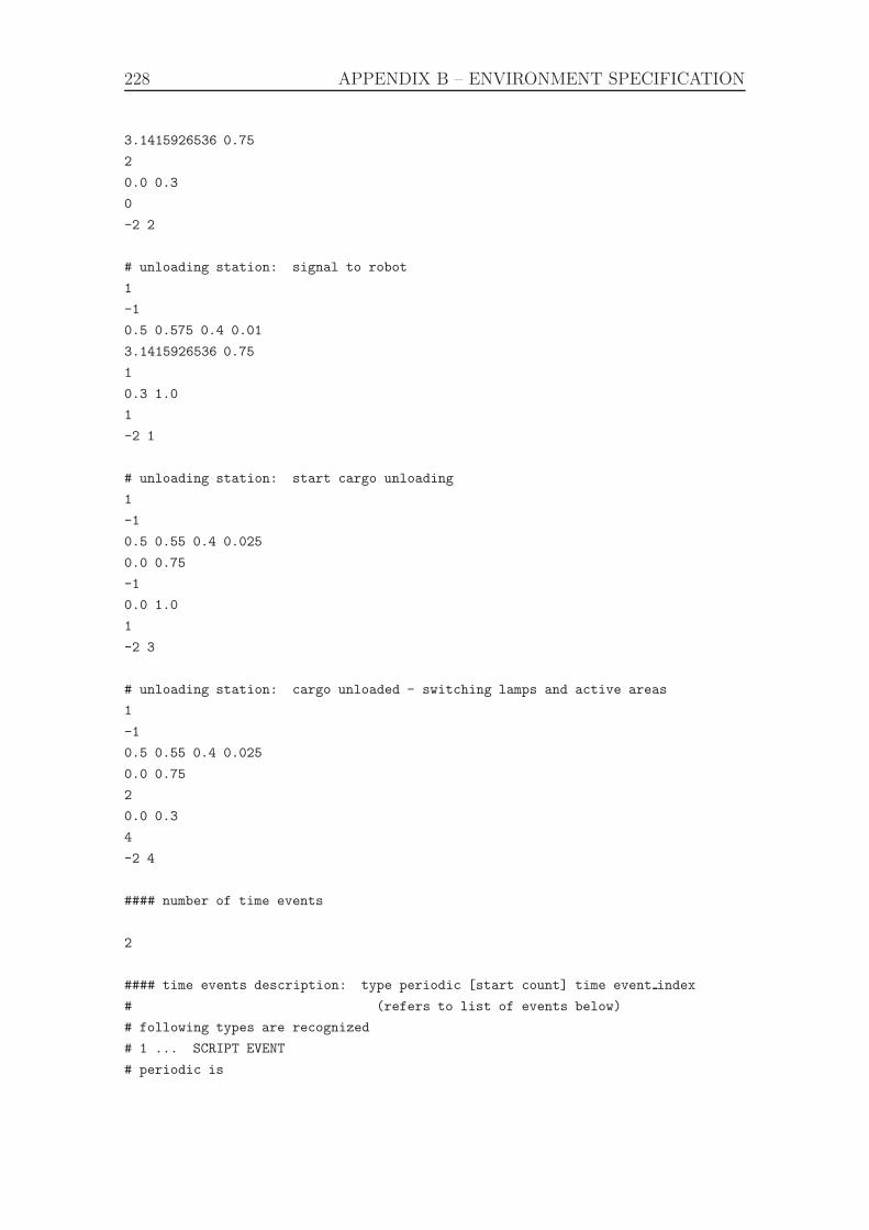
228 APPENDIX B – ENVIRONMENT SPECIFICATION

3.1415926536 0.75

2

0.0 0.3

0

-2 2

# unloading station: signal to robot

1

-1

0.5 0.575 0.4 0.01

3.1415926536 0.75

1

0.3 1.0

1

-2 1

# unloading station: start cargo unloading

1

-1

0.5 0.55 0.4 0.025

0.0 0.75

-1

0.0 1.0

1

-2 3

# unloading station: cargo unloaded - switching lamps and active areas

1

-1

0.5 0.55 0.4 0.025

0.0 0.75

2

0.0 0.3

4

-2 4

#### number of time events

2

#### time events description: type periodic [start count] time event index

# (refers to list of events below)

# following types are recognized

# 1 ... SCRIPT EVENT

# periodic is

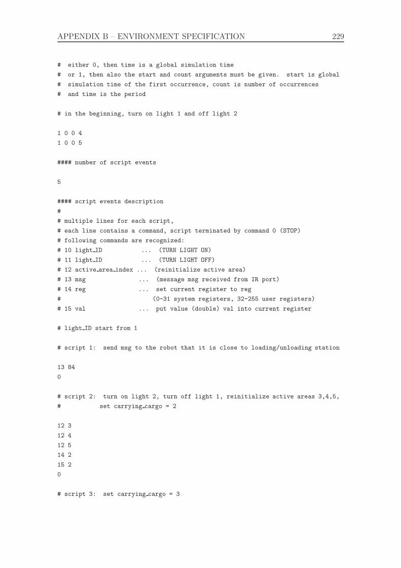
APPENDIX B – ENVIRONMENT SPECIFICATION 229

# either 0, then time is a global simulation time

# or 1, then also the start and count arguments must be given. start is global

# simulation time of the first occurrence, count is number of occurrences

# and time is the period

# in the beginning, turn on light 1 and off light 2

1 0 0 4

1 0 0 5

#### number of script events

5

#### script events description

#

# multiple lines for each script,

# each line contains a command, script terminated by command 0 (STOP)

# following commands are recognized:

# 10 light ID ... (TURN LIGHT ON)

# 11 light ID ... (TURN LIGHT OFF)

# 12 active area index ... (reinitialize active area)

# 13 msg ... (message msg received from IR port)

# 14 reg ... set current register to reg

# (0-31 system registers, 32-255 user registers)

# 15 val ... put value (double) val into current register

# light ID start from 1

# script 1: send msg to the robot that it is close to loading/unloading station

13 84

0

# script 2: turn on light 2, turn off light 1, reinitialize active areas 3,4,5,

# set carrying cargo = 2

12 3

12 4

12 5

14 2

15 2

0

# script 3: set carrying cargo = 3

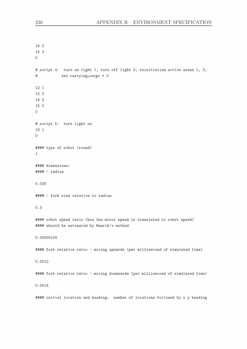
230 APPENDIX B – ENVIRONMENT SPECIFICATION

14 2

15 3

0

# script 4: turn on light 1, turn off light 2, reinitialize active areas 1, 2,

# set carrying cargo = 0

12 1

12 2

14 2

15 0

0

# script 5: turn light on

10 1

0

#### type of robot (round)

1

#### dimensions:

#### - radius

0.025

#### - fork size relative to radius

0.3

#### robot speed ratio (how the motor speed is translated to robot speed)

#### should be estimated by Henrik’s method

0.00000150

#### fork relative ratio - moving upwards (per millisecond of simulated time)

0.0012

#### fork relative ratio - moving downwards (per millisecond of simulated time)

0.0014

#### initial location and heading: number of locations followed by x y heading

APPENDIX B – ENVIRONMENT SPECIFICATION 231

3

#for evolving cargoloader

0.2 0.3 0

0.2 0.9 3.1416

0.2 0.45 0

#### time slowdown constant (how many times slower should be the simulation time

# than the system time)

200

#### trajectory file

#### (used only when run without evolution)

project/cargo/traj/five incremental/4/t

#### fsa files for all fsas (these are not used when called by objective

#### function, in that case the values specified in evolutionary config file)

#### are used, list is terminated by 0. each filename is automatically suffixed

#### with .x, where x is the number of module

2

project/cargo/fsa-handmade/fsa.dat

4

project/cargo/fsa-handmade/fsa.dat

5

project/cargo/fsa-handmade/fsa.dat

6

project/cargo/fsa-handmade/fsa.dat

0

#### how often does the viewer refresh the visual output (in ms) zero means

#### no viewer, default: 200

0

#### realtime (0/1): are we running realtime (1) or time-shared (0);

#### realtime must be run as root

1

#### save trajectory file (0/1)

0

232 APPENDIX B – ENVIRONMENT SPECIFICATION

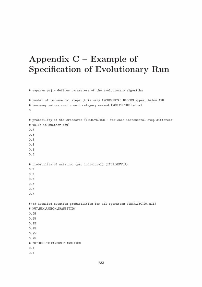
Appendix C – Example ofSpecification of Evolutionary Run

# eaparam.prj - defines parameters of the evolutionary algorithm

# number of incremental steps (this many INCREMENTAL BLOCKS appear below AND

# how many values are in each category marked INCR VECTOR below)

6

# probability of the crossover (INCR VECTOR - for each incremental step different

# value in another row)

0.3

0.3

0.3

0.3

0.3

0.3

# probability of mutation (per individual) (INCR VECTOR)

0.7

0.7

0.7

0.7

0.7

0.7

#### detailed mutation probabilities for all operators (INCR VECTOR all)

# MUT NEW RANDOM TRANSITION

0.25

0.25

0.25

0.25

0.25

0.25

# MUT DELETE RANDOM TRANSITION

0.1

0.1

233

234 APPENDIX C – EVOLUTIONARY RUN SPECIFICATION

0.1

0.1

0.1

0.1

# MUT NEW STATE

0.2

0.2

0.2

0.2

0.2

0.2

# MUT RANDOM STATE DELETED

0.05

0.05

0.05

0.05

0.05

0.05

# MUT RANDOM TRANSITION MUTATED

0.25

0.25

0.25

0.25

0.25

0.25

# MUT NEW RANDOM INDIVIDUAL

0.05

0.05

0.05

0.05

0.05

0.05

# MUT SPLIT TRANSITION

0.05

0.05

0.05

0.05

0.05

0.05

# MUT CHANGE STARTSTATE

0.05

0.05

0.05

0.05

0.05

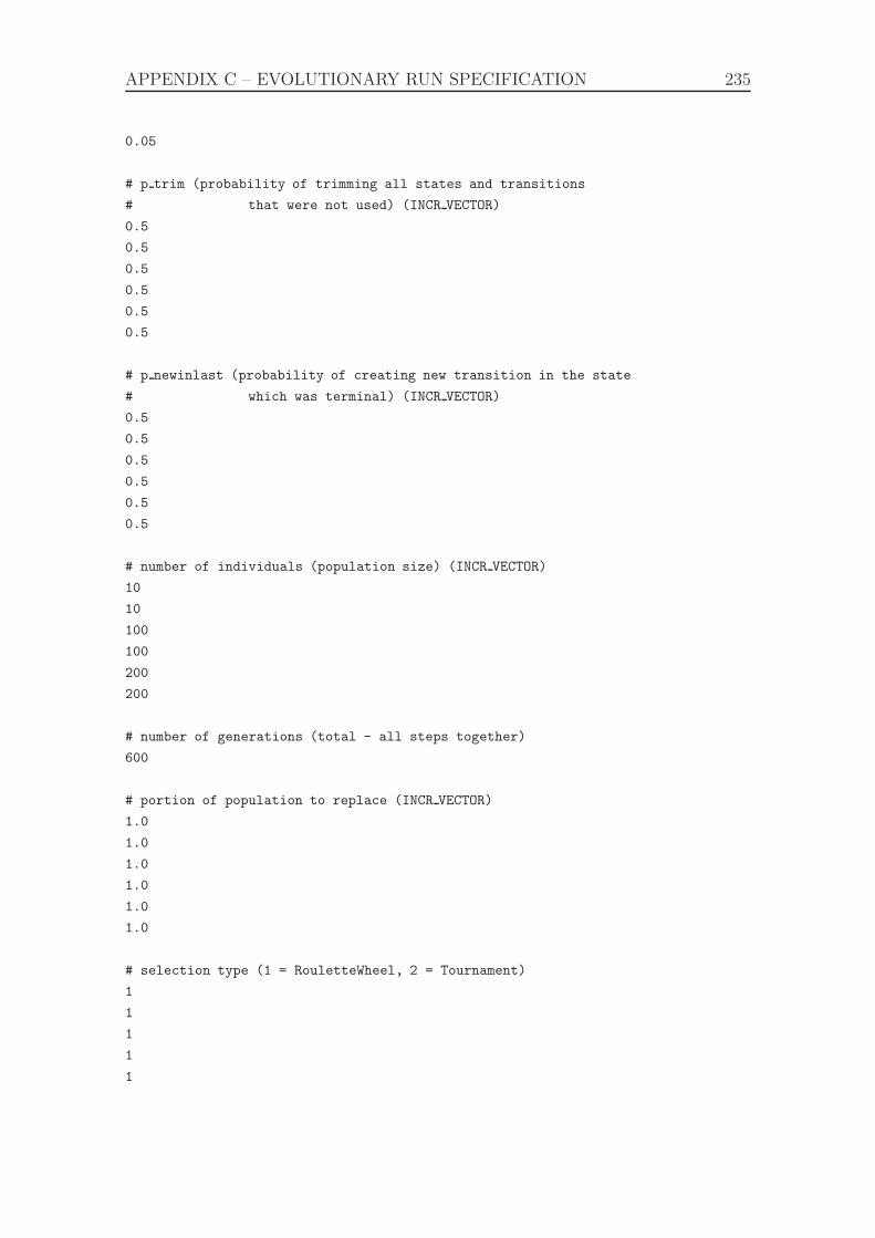
APPENDIX C – EVOLUTIONARY RUN SPECIFICATION 235

0.05

# p trim (probability of trimming all states and transitions

# that were not used) (INCR VECTOR)

0.5

0.5

0.5

0.5

0.5

0.5

# p newinlast (probability of creating new transition in the state

# which was terminal) (INCR VECTOR)

0.5

0.5

0.5

0.5

0.5

0.5

# number of individuals (population size) (INCR VECTOR)

10

10

100

100

200

200

# number of generations (total - all steps together)

600

# portion of population to replace (INCR VECTOR)

1.0

1.0

1.0

1.0

1.0

1.0

# selection type (1 = RouletteWheel, 2 = Tournament)

1

1

1

1

1

236 APPENDIX C – EVOLUTIONARY RUN SPECIFICATION

1

# total number of modules in the controller (INCR VECTOR)

10

10

10

10

10

10

# module message data in file

project/cargo/modules/alldata.dat

# module specification files for all modules - the modules must be listed

# in the order of their module ids! (INCR VECTOR)

project/cargo/modules/navigate.mod

project/cargo/modules/cargoloader.mod

project/cargo/modules/motordriver.mod

project/cargo/modules/lnflwer.mod

project/cargo/modules/avoidance.mod

project/cargo/modules/explore.mod

project/cargo/modules/bumpertracker.mod

project/cargo/modules/linetracker.mod

project/cargo/modules/lighttracker.mod

project/cargo/modules/beep.mod

#

project/cargo/modules/navigate.mod

project/cargo/modules/cargoloader.mod

project/cargo/modules/motordriver.mod

project/cargo/modules/lnflwer.mod

project/cargo/modules/avoidance.mod

project/cargo/modules/explore.mod

project/cargo/modules/bumpertracker.mod

project/cargo/modules/linetracker.mod

project/cargo/modules/lighttracker.mod

project/cargo/modules/beep.mod

#

project/cargo/modules/navigate.mod

project/cargo/modules/cargoloader.mod

project/cargo/modules/motordriver.mod

project/cargo/modules/lnflwer.mod

project/cargo/modules/avoidance.mod

project/cargo/modules/explore.mod

project/cargo/modules/bumpertracker.mod

project/cargo/modules/linetracker.mod

APPENDIX C – EVOLUTIONARY RUN SPECIFICATION 237

project/cargo/modules/lighttracker.mod

project/cargo/modules/beep.mod

#

project/cargo/modules/navigate.mod

project/cargo/modules/cargoloader.mod

project/cargo/modules/motordriver.mod

project/cargo/modules/lnflwer.mod

project/cargo/modules/avoidance.mod

project/cargo/modules/explore.mod

project/cargo/modules/bumpertracker.mod

project/cargo/modules/linetracker.mod

project/cargo/modules/lighttracker.mod

project/cargo/modules/beep.mod

#

project/cargo/modules/navigate.mod

project/cargo/modules/cargoloader.mod

project/cargo/modules/motordriver.mod

project/cargo/modules/lnflwer.mod

project/cargo/modules/avoidance.mod

project/cargo/modules/explore.mod

project/cargo/modules/bumpertracker.mod

project/cargo/modules/linetracker.mod

project/cargo/modules/lighttracker.mod

project/cargo/modules/beep.mod

#

project/cargo/modules/navigate.mod

project/cargo/modules/cargoloader.mod

project/cargo/modules/motordriver.mod

project/cargo/modules/lnflwer.mod

project/cargo/modules/avoidance.mod

project/cargo/modules/explore.mod

project/cargo/modules/bumpertracker.mod

project/cargo/modules/linetracker.mod

project/cargo/modules/lighttracker.mod

project/cargo/modules/beep.mod

# number of fsas that are part of the genome (INCR VECTOR)

# (they will be saved to project/cargo/fsa/project id/step number)

1

1

1

1

1

1

238 APPENDIX C – EVOLUTIONARY RUN SPECIFICATION

# module ids for the fsas that are evolved (each on separate line) (INCR VECTOR)

5

4

2

4

4

4

# number of fsas that are fixed and loaded from file (INCR VECTOR)

1

1

1

3

3

3

# module ids for the fsas that are fixed and loaded from file (one per line)

# followed by file name (INCR VECTOR) ; the extension .module number will

# be added to each file automatically

#---s1

6

project/cargo/fsa-handmade/fsa.dat

#---s2

6

project/cargo/fsa-handmade/fsa.dat

#---s3

6

project/cargo/fsa-handmade/fsa.dat

#---s4

2

project/cargo/fsa/five incremental/2/fsa.dat.evolved

5

project/cargo/fsa/five incremental/0/fsa.dat.evolved

6

project/cargo/fsa-handmade/fsa.dat

#---s5

2

project/cargo/fsa/five incremental/2/fsa.dat.evolved

5

project/cargo/fsa/five incremental/0/fsa.dat.evolved

6

project/cargo/fsa-handmade/fsa.dat

#---s6

2

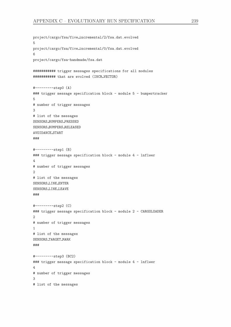
APPENDIX C – EVOLUTIONARY RUN SPECIFICATION 239

project/cargo/fsa/five incremental/2/fsa.dat.evolved

5

project/cargo/fsa/five incremental/0/fsa.dat.evolved

6

project/cargo/fsa-handmade/fsa.dat

########### trigger messages specifications for all modules

########### that are evolved (INCR VECTOR)

#---------step0 (A)

### trigger message specification block - module 5 - bumpertracker

5

# number of trigger messages

3

# list of the messages

SENSORS BUMPERS PRESSED

SENSORS BUMPERS RELEASED

AVOIDANCE START

###

#---------step1 (B)

### trigger message specification block - module 4 - lnflwer

4

# number of trigger messages

2

# list of the messages

SENSORS LINE ENTER

SENSORS LINE LEAVE

###

#---------step2 (C)

### trigger message specification block - module 2 - CARGOLOADER

2

# number of trigger messages

1

# list of the messages

SENSORS TARGET MARK

###

#---------step3 (BC2)

### trigger message specification block - module 4 - lnflwer

4

# number of trigger messages

3

# list of the messages

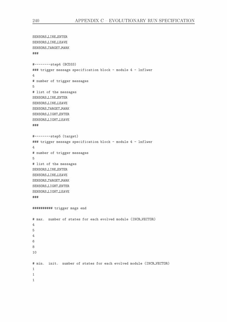
240 APPENDIX C – EVOLUTIONARY RUN SPECIFICATION

SENSORS LINE ENTER

SENSORS LINE LEAVE

SENSORS TARGET MARK

###

#--------step4 (BCD33)

### trigger message specification block - module 4 - lnflwer

4

# number of trigger messages

5

# list of the messages

SENSORS LINE ENTER

SENSORS LINE LEAVE

SENSORS TARGET MARK

SENSORS LIGHT ENTER

SENSORS LIGHT LEAVE

###

#--------step5 (target)

### trigger message specification block - module 4 - lnflwer

4

# number of trigger messages

5

# list of the messages

SENSORS LINE ENTER

SENSORS LINE LEAVE

SENSORS TARGET MARK

SENSORS LIGHT ENTER

SENSORS LIGHT LEAVE

###

########## trigger msgs end

# max. number of states for each evolved module (INCR VECTOR)

4

5

4

6

8

10

# min. init. number of states for each evolved module (INCR VECTOR)

1

1

1

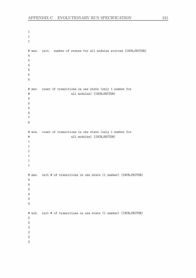
APPENDIX C – EVOLUTIONARY RUN SPECIFICATION 241

1

1

1

# max. init. number of states for all modules evolved (INCR VECTOR)

4

5

4

5

5

5

# max. count of transitions in one state (only 1 number for

# all modules) (INCR VECTOR)

5

5

5

5

7

8

# min. count of transitions in one state (only 1 number for

# all modules) (INCR VECTOR)

1

1

1

1

1

1

# max. init # of transitions in one state (1 number) (INCR VECTOR)

4

4

4

4

4

4

# min. init # of transitions in one state (1 number) (INCR VECTOR)

2

2

2

2

2

2

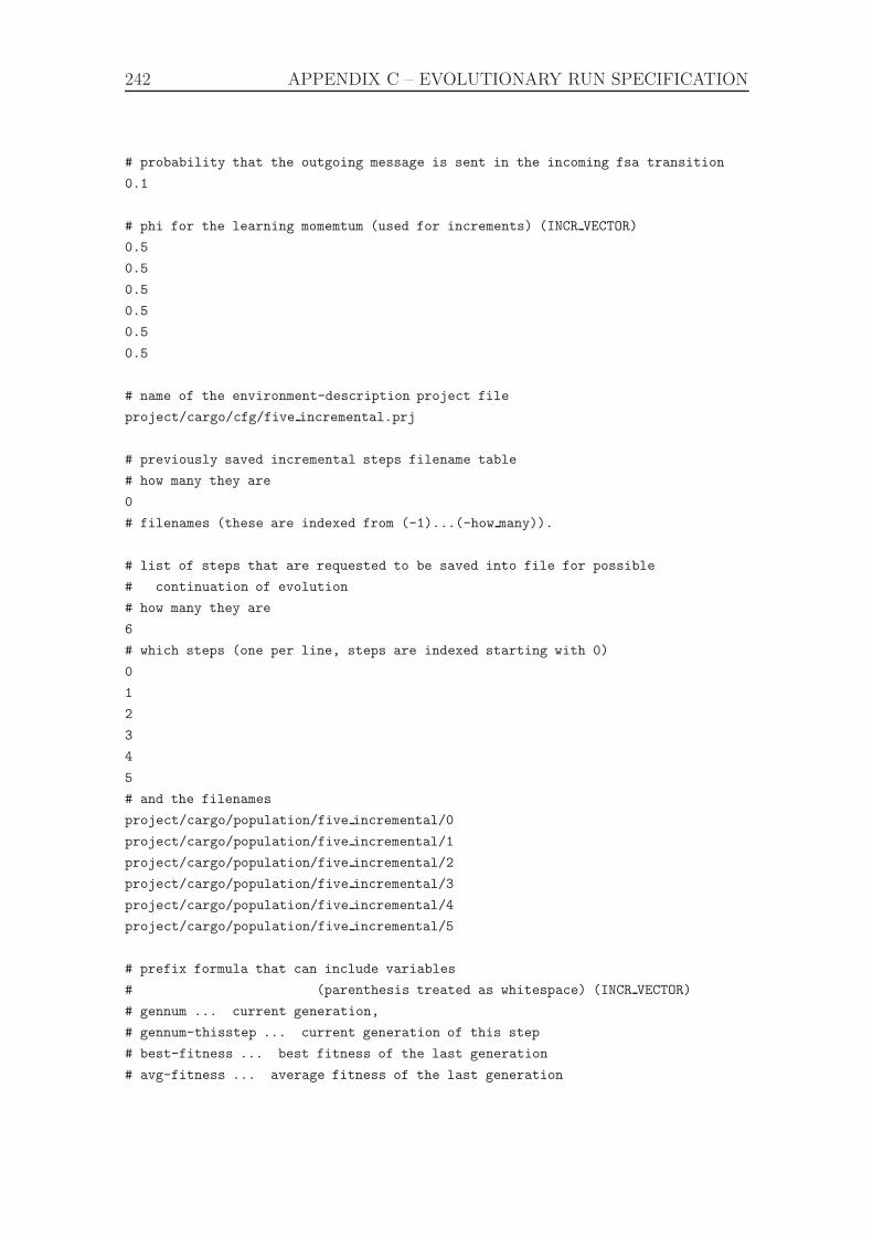
242 APPENDIX C – EVOLUTIONARY RUN SPECIFICATION

# probability that the outgoing message is sent in the incoming fsa transition

0.1

# phi for the learning momemtum (used for increments) (INCR VECTOR)

0.5

0.5

0.5

0.5

0.5

0.5

# name of the environment-description project file

project/cargo/cfg/five incremental.prj

# previously saved incremental steps filename table

# how many they are

0

# filenames (these are indexed from (-1)...(-how many)).

# list of steps that are requested to be saved into file for possible

# continuation of evolution

# how many they are

6

# which steps (one per line, steps are indexed starting with 0)

0

1

2

3

4

5

# and the filenames

project/cargo/population/five incremental/0

project/cargo/population/five incremental/1

project/cargo/population/five incremental/2

project/cargo/population/five incremental/3

project/cargo/population/five incremental/4

project/cargo/population/five incremental/5

# prefix formula that can include variables

# (parenthesis treated as whitespace) (INCR VECTOR)

# gennum ... current generation,

# gennum-thisstep ... current generation of this step

# best-fitness ... best fitness of the last generation

# avg-fitness ... average fitness of the last generation

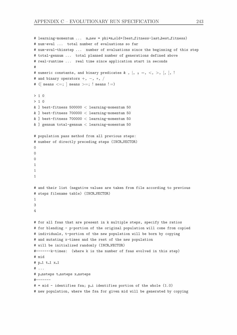
APPENDIX C – EVOLUTIONARY RUN SPECIFICATION 243

# learning-momentum ... m new = phi*m old+(best fitness-last best fitness)

# num-eval ... total number of evaluations so far

# num-eval-thisstep ... number of evaluations since the beginning of this step

# total-gennum ... total planned number of generations defined above

# real-runtime ... real time since application start in seconds

#

# numeric constants, and binary predicates & , |, , =, <, >, [, ], !

# and binary operators +, −, ∗, /

# ([ means <=; ] means >=; ! means ! =)

> 1 0

> 1 0

& ] best-fitness 500000 < learning-momentum 50

& ] best-fitness 700000 < learning-momentum 50

& ] best-fitness 700000 < learning-momentum 50

& ] gennum total-gennum < learning-momentum 50

# population pass method from all previous steps:

# number of directly preceding steps (INCR VECTOR)

0

0

0

1

1

1

# and their list (negative values are taken from file according to previous

# steps filename table) (INCR VECTOR)

1

3

4

# for all fsas that are present in k multiple steps, specify the ratios

# for blending - p-portion of the original population will come from copied

# individuals, t-portion of the new population will be born by copying

# and mutating x-times and the rest of the new population

# will be initialized randomly (INCR VECTOR)

#-------k-times: (where k is the number of fsas evolved in this step)

# mid

# p 1 t 1 x 1

# ...

# p nsteps t nsteps x nsteps

#-------

# = mid - identifies fsa; p i identifies portion of the whole (1.0)

# new population, where the fsa for given mid will be generated by copying

244 APPENDIX C – EVOLUTIONARY RUN SPECIFICATION

# individuals from i-the of the directly preceding steps listed above

# t i represents the portion which will be copied and mutated x i times,

# q identifies portion of the new pop. which will have the fsa for mid

# initialized randomly.

# copying fsas from previous steps and mutating x i times

# the sum of q and all p i for all mids together should be less than 1.

# probabilities for all preceding steps have to be listed

# (even if this fsa doesn’t occur in some of them - when the p i should be 0)

0

0

0

4

0.5 0.1 0.3 2

0

4

0.5 0.1 0.3 2

0

4

0.5 0.1 0.3 2

0

# the list is terminated by extra row with 0

# note: in the first step, or step that has no preceding step since there

# are no preceding steps, the population is generated just randomly

# and this structure should be omitted

# number of starting positions for the objective function (INCR VECTOR)

3

3

3

3

3

6

# fitness function timeout [s] (INCR VECTOR)

30

60

60

120

180

350

# fitness checkpoints (if the fitness at given time is less than specified,

# the individual is stoped, its currently gained fitness is used) (INCR VECTOR)

# format: simulation time required fitness (list should be ordered by time)

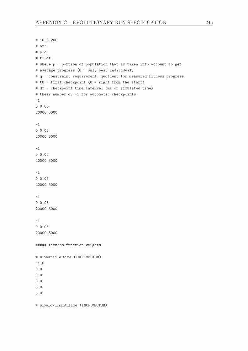
APPENDIX C – EVOLUTIONARY RUN SPECIFICATION 245

# 10.0 200

# or:

# p q

# t1 dt

# where p - portion of population that is taken into account to get

# average progress (0 - only best individual)

# q - constraint requirement, quotient for measured fitness progress

# t0 - first checkpoint (0 = right from the start)

# dt - checkpoint time interval (ms of simulated time)

# their number or -1 for automatic checkpoints

-1

0 0.05

20000 5000

-1

0 0.05

20000 5000

-1

0 0.05

20000 5000

-1

0 0.05

20000 5000

-1

0 0.05

20000 5000

-1

0 0.05

20000 5000

##### fitness function weights

# w obstacle time (INCR VECTOR)

-1.0

0.0

0.0

0.0

0.0

0.0

# w below light time (INCR VECTOR)

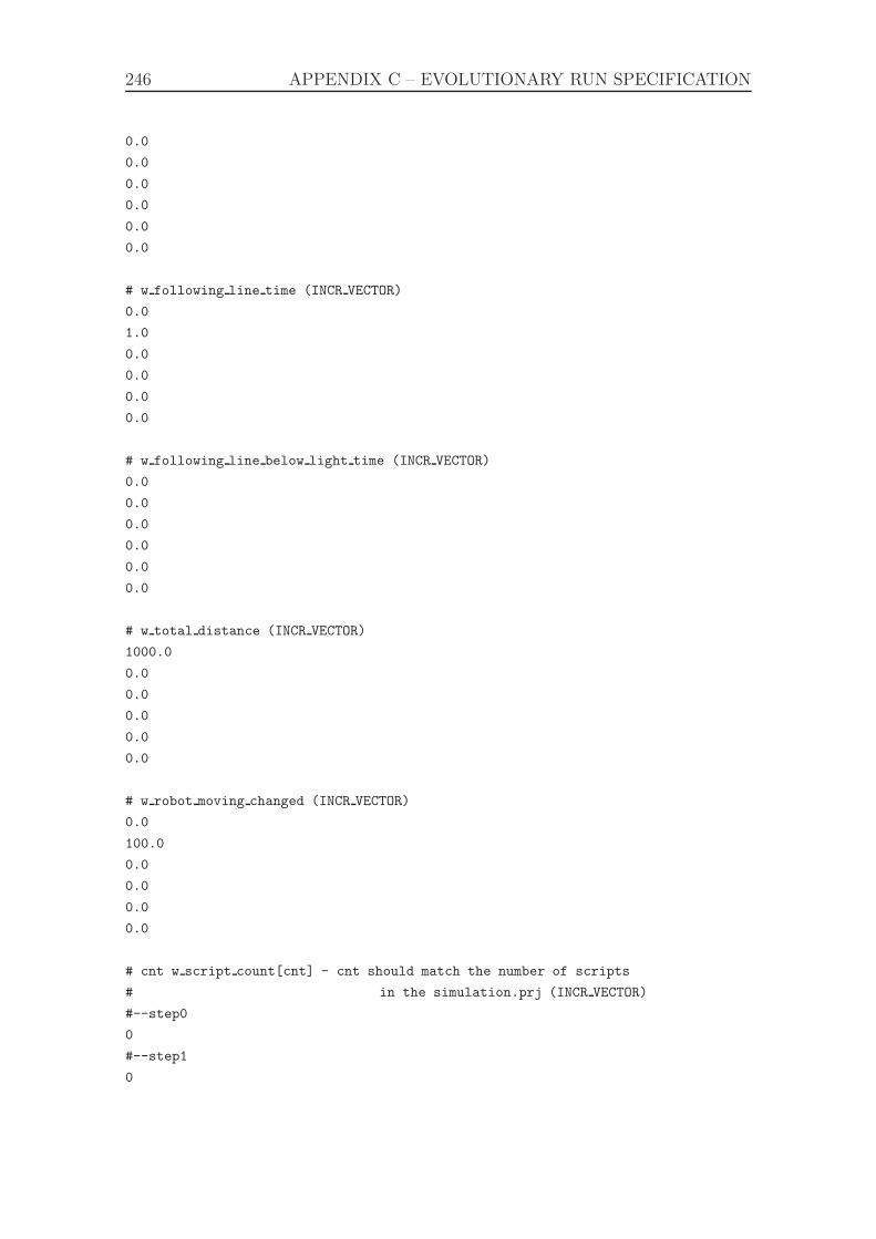
246 APPENDIX C – EVOLUTIONARY RUN SPECIFICATION

0.0

0.0

0.0

0.0

0.0

0.0

# w following line time (INCR VECTOR)

0.0

1.0

0.0

0.0

0.0

0.0

# w following line below light time (INCR VECTOR)

0.0

0.0

0.0

0.0

0.0

0.0

# w total distance (INCR VECTOR)

1000.0

0.0

0.0

0.0

0.0

0.0

# w robot moving changed (INCR VECTOR)

0.0

100.0

0.0

0.0

0.0

0.0

# cnt w script count[cnt] - cnt should match the number of scripts

# in the simulation.prj (INCR VECTOR)

#--step0

0

#--step1

0

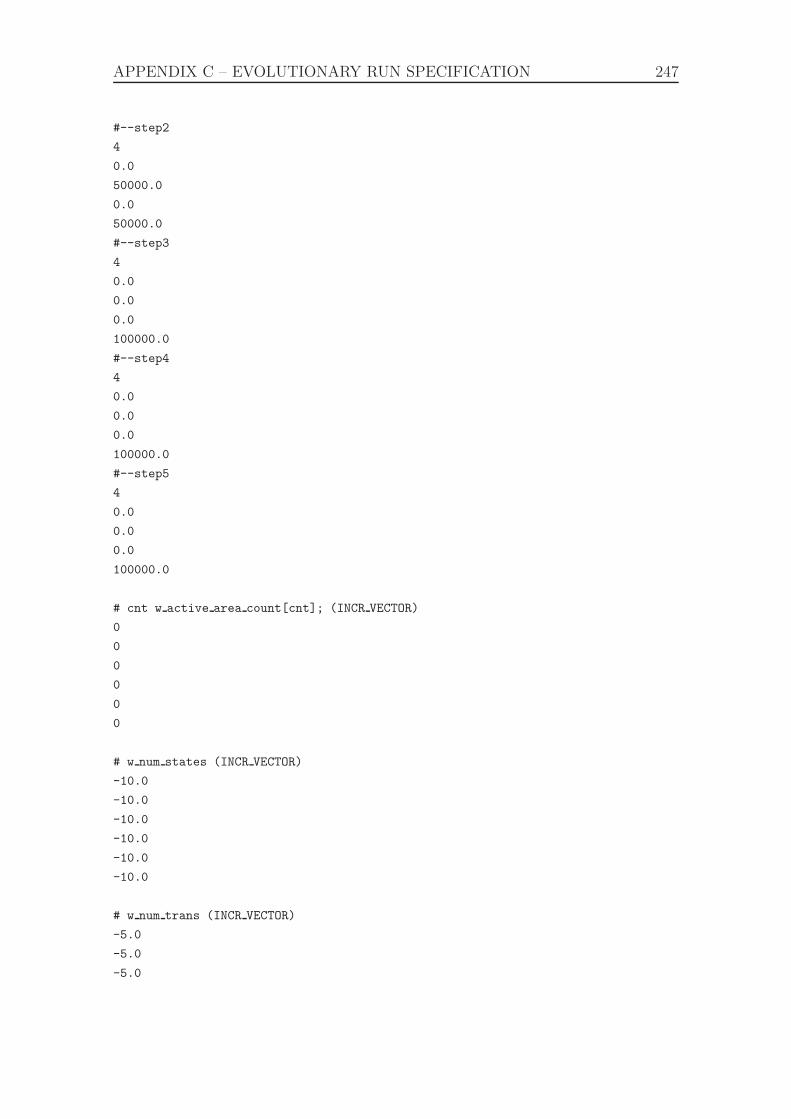
APPENDIX C – EVOLUTIONARY RUN SPECIFICATION 247

#--step2

4

0.0

50000.0

0.0

50000.0

#--step3

4

0.0

0.0

0.0

100000.0

#--step4

4

0.0

0.0

0.0

100000.0

#--step5

4

0.0

0.0

0.0

100000.0

# cnt w active area count[cnt]; (INCR VECTOR)

0

0

0

0

0

0

# w num states (INCR VECTOR)

-10.0

-10.0

-10.0

-10.0

-10.0

-10.0

# w num trans (INCR VECTOR)

-5.0

-5.0

-5.0

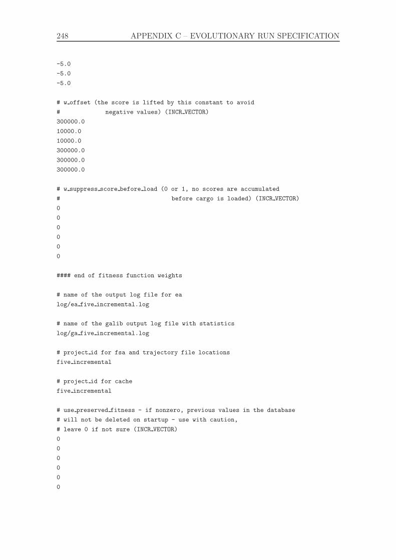
248 APPENDIX C – EVOLUTIONARY RUN SPECIFICATION

-5.0

-5.0

-5.0

# w offset (the score is lifted by this constant to avoid

# negative values) (INCR VECTOR)

300000.0

10000.0

10000.0

300000.0

300000.0

300000.0

# w suppress score before load (0 or 1, no scores are accumulated

# before cargo is loaded) (INCR VECTOR)

0

0

0

0

0

0

#### end of fitness function weights

# name of the output log file for ea

log/ea five incremental.log

# name of the galib output log file with statistics

log/ga five incremental.log

# project id for fsa and trajectory file locations

five incremental

# project id for cache

five incremental

# use preserved fitness - if nonzero, previous values in the database

# will not be deleted on startup - use with caution,

# leave 0 if not sure (INCR VECTOR)

0

0

0

0

0

0

APPENDIX C – EVOLUTIONARY RUN SPECIFICATION 249

# commands to be executed after each incremental step on the slave if running

# in distributed mode (1 line per step; ’none’ if no commands) (INCR VECTOR)

scp cargo@search:current3/project/cargo/fsa/five incremental/0/*.evolved.*

/home/current3/project/cargo/fsa/five incremental/0

scp cargo@search:current3/project/cargo/fsa/five incremental/1/*.evolved.*

/home/current3/project/cargo/fsa/five incremental/1

scp cargo@search:current3/project/cargo/fsa/five incremental/2/*.evolved.*

/home/current3/project/cargo/fsa/five incremental/2

scp cargo@search:current3/project/cargo/fsa/five incremental/3/*.evolved.*

/home/current3/project/cargo/fsa/five incremental/3

scp cargo@search:current3/project/cargo/fsa/five incremental/4/*.evolved.*

/home/current3/project/cargo/fsa/five incremental/4

scp cargo@search:current3/project/cargo/fsa/five incremental/5/*.evolved.*

/home/current3/project/cargo/fsa/five incremental/5

# commands to be executed after each incremental step on the master in

# distributed mode (INCR VECTOR)

# master command is fully executed before slave commands

scp /home/current3/project/cargo/fsa/five incremental/0/*.evolved.*

cargo@search:current3/project/cargo/fsa/five incremental/0

scp /home/current3/project/cargo/fsa/five incremental/1/*.evolved.*

cargo@search:current3/project/cargo/fsa/five incremental/1

scp /home/current3/project/cargo/fsa/five incremental/2/*.evolved.*

cargo@search:current3/project/cargo/fsa/five incremental/2

scp /home/current3/project/cargo/fsa/five incremental/3/*.evolved.*

cargo@search:current3/project/cargo/fsa/five incremental/3

scp /home/current3/project/cargo/fsa/five incremental/4/*.evolved.*

cargo@search:current3/project/cargo/fsa/five incremental/4

scp /home/current3/project/cargo/fsa/five incremental/5/*.evolved.*

cargo@search:current3/project/cargo/fsa/five incremental/5

# stop-file - when this file is detected after the generation is completed,

# the application terminates (and saves the population of the current

# incremental step, if requested)

project/cargo/true.stop computing

# skip-file - when this file is detected after the generation is completed,

# the incremental step is completed and the application proceeds with the next

# incr.step (the incr.step to skip must be added to the end of this file name!)

project/cargo/true.skip step

# save fsa file

0

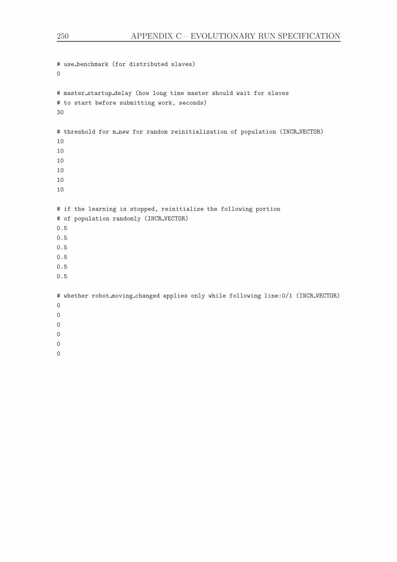
250 APPENDIX C – EVOLUTIONARY RUN SPECIFICATION

# use benchmark (for distributed slaves)

0

# master startup delay (how long time master should wait for slaves

# to start before submitting work, seconds)

30

# threshold for m new for random reinitialization of population (INCR VECTOR)

10

10

10

10

10

10

# if the learning is stopped, reinitialize the following portion

# of population randomly (INCR VECTOR)

0.5

0.5

0.5

0.5

0.5

0.5

# whether robot moving changed applies only while following line:0/1 (INCR VECTOR)

0

0

0

0

0

0

Bibliography

Ricardo Nastas Acras and Silvia Regina Vergilio. Splinter: A Generic Framework forEvolving Modular Finite State Machines. In SBIA 2004, pages 356–365. Springer-Verlag, 2004.

P. Aerts and A. Ynnerman H. P. Luthi. Evaluation of NOTUR. NOTUR– A Norwegian High Performance Computational Infrastructure. NorgesForskningsrd, 2004. ISBN 82-12-01991-8.

P. Anderson. BOINC: A System for Public-Resource Computing and Storage. InFifth IEEE/ACM International Workshop on Grid Computing, 2004.

Peter J. Angeline and Jordan Pollack. Evolutionary Module Acquisition. InProceedings of The Second Annual Conference on Evolutionary Programming,1993.

Maribel G. Arenas, Pierre Collet, A. E. Eiben, Mark Jelasity, Juan J. Merelo,Ben Peachter, Mike Preuss, and Marc Schoenauer. A Framework for DistributedEvolutionary Algorithms. In PPSN VII, volume 2439, pages 665–675. Springer-Verlag, 2002.

Ronald C. Arkin. Behavior-Based Robotics. MIT Press/Bradford Books, 1998.

Ronald C. Arkin and Douglas MacKenzie. Temporal Coordination of PerceptualAlgorithms for Mobile Robot Navigation. IEEE Transactions on Robotics andAutomation, 10(3):276–286, 1994.

Daniel Ashlock, Andrew Wittrock, and Tsui-Jung Wen. Training Finite StateMachines to Improve PCR Primer Design. In Proceedings of the Congress onEvolutionary Computation CEC ’02, pages 13–18, 2002. ISBN 0-7803-7282-4.

Daniel A. Ashlock, Scott J. Emrich, Kenneth M. Bryden, Steve M. Corns, Tsui-Jung Wen, and Patrick S. Schnable. A Comparison of Evolved Finite StateClassifiers and Interpolated Markov Models for Improving PCR Primer Design.In Proceedings of the 2004 IEEE Symposium on Computational Intelligence inBioinformatics and Computational Biology, CIBCB ’04, pages 190–197, 2004.ISBN 0-7803-8728-7.

Gianluca Baldassarre. A Modular Neural-Network Model of the Basal Ganglia’sRole in Learning and Selecting Motor Behaviours. In Proceedings of the Fourth

251

252 Bibliography

International Conference on Cognitive Modelling, pages 37–42. Lawrence ErlbaumAssociates, Mahwah NJ, 2001.

J. Mark. Baldwin. A New Factor in Evolution. American Naturalist, 30:441–451,536–554, 1896.

Richard Balogh. I Am a Robot - Competitor, A Survey of Robotic Competitions.International Journal of Advanced Robotic Systems, 2(2):144–160, 2005.

Richard Balogh. Practical Kinematics of the Differential Driven Mobile Robot. InProceedings of Robtep’07, 2007.

Maxim A. Batalin and Gaurav S. Sukhatme. Efficient Exploration withoutLocalization. In Efficient Exploration without Localization, 2002.

Randall D. Beer and John C. Gallagher. Evolving Dynamical Neural Networks forAdaptive Behavior. Adaptive Behavior, 1:91–122, 1992.

Karl A Benson. Evolving automatic target detection algorithms that logicallycombine decision spaces. In Proceedings of the 11th British Machine VisionConference, pages 685–694, Bristol, UK, 2000.

Barbara Bratzel. Physics by design. College House Enterprises, LLC, 2005.

Reinhard Braunstingl, Jokin Mujika, and Juan Pedro Uribe. A Wall FollowingRobot with a Fuzzy Logic Controller Optimized by a Genetic Algorithm. InFUZZ-IEEE/IFES’95 Fuzzy Robot Competition, Yokohama, 1995.

Rodney Allen Brooks. A Hardware Retargetable Distributed Layered Architecturefor Mobile Robot Control. In Proceedings of the IEEE International Conferenceon Robotics and Automation, pages 106–110, 1987.

Rodney Allen Brooks. Artificial Life and Real Robots. In Towards a Practice ofAutnomous Systems: Proceedings of the First European Conference on ArtificialLife, pages 3 – 10. MIT Press, 1992.

Rodney Allen Brooks. A Robust Layered Control System For a Mobile Robot. IEEEJournal of Robotics and Automation, 1986, RA-2(1, March), 1986.

Erick Cantu-Paz. A Survey of Parallel Genetic Algorithms. Calculateurs Paralleles,10(2), 1998.

Joerg Cassens and Zoran Constantinescu. It’s Magic: SourceMage GNU/Linux asa High Performance Cluster OS (abstract). In LinuxTag 2003 Conference, 2003.

J. Chavas, Christophe Corne, P. Horvai, Jerome Kodjabachian, and Jean-ArcadyMeyer. Incremental Evolution of Neural Controllers for Robust Obstacle-Avoidance in Khepera. In Phil Husbands and J. A. Meyer, editors, Proceedings ofThe First European Workshop on Evolutionary Robotics – EvoRobot’98. SpringerVerlag, 1998.

BIBLIOGRAPHY 253

Kumar Chellapilla and David Czarnecki. A Preliminary Investigation into EvolvingModular Finite State Machines. In Proceedings of the 1999 Congress onEvolutionary Computation, CEC’99, volume 2, 1999. ISBN 0-7803-5536-9.

Charlie H. Clelland and Douglas A. Newlands. PFSA Modelling of BehaviouralSequences by Evolutionary Programming. In Complex ’94 - Second AustralianConference on Complex Systems, pages 165–72. IOS Press, 1994.

Dave Cliff, Inman Harvey, and Phil Husbands. Incremental Evolution of NeuralNetwork Architectures for Adaptive Behaviour. Technical Report CSRP256,University of Sussex Technical Report, 1992.

Marco Colombetti and Marco Dorigo. Robot Shaping: Developing Situated Agentsthrough Learning. Technical Report 92-040, International Computer ScienceInstitute, 1993.

Marco Colombetti, Marco Dorigo, and Giuseppe Borghi. Behavior Analysis andTraining: A Methodology for Behavior Engineering. IEEE Transactions onSystem, Man, and Cybernetics-Part B, 26(3):365–380, 1996.

E. Roy Davies. Machine Vision : Theory, Algorithms, Practicalities. Elsevier, 2005.

Hugo de Garis. Multistrategy Learning in Neural Nets: An Incremental Approachto Genetic Programming. In Proceedings of the Second International Workshopon Multistrategy Learning, pages 138–149, 1993.

Nirav S. Desai and Risto Miikkulainen. Neuro-Evolution and Natural Deduction.In Proceedings of the First IEEE Symposium on Combinations of EvolutionaryComputation and Neural Networks, 2000.

Marco Dorigo and Marco Colombetti. Robot Shaping: An Experiment in BehaviorEngineering. MIT Press, 1997.

Marc Ebner. Evolution of a Control Architecture for a Mobile Robot. In Proceedingsof the Second International Conference on Evolvable Systems: From Biology toHardware (ICES 98), pages 303–310. Springer-Verlag, 1998.

Roger I. Eriksson. An Initial Analysis Of the Ability Of Learning To MaintainDiversity During Incremental Evolution. In GECCO Workshop On MemeticAlgorithms, 2000.

Benjamin T. Erwin. Creative Projects with LEGO MINDSTORMS. Addison-Wesley,2001.

Benjamin T. Erwin. K-12 Education and Systems Engineering: A New Perspective.In Proceedings of the American Society of Engineering Education NationalConference, 1998.

254 Bibliography

Benjamin T. Erwin, Martha Cyr, John Osborne, and Chris Rogers. Middle SchoolEngineering with LEGO and LabView. In Proceedings of National InstrumentsWeek, August 1998.

David Filliat, Jerome Kodjabachian, and Jean-Arcady Meyer. Incremental Evolutionof Neural Controllers for Navigation in a 6-legged Robot. In Sugisaka and Tanaka,editors, Proceedings of the Fourth International Symposium on Artificial Life andRobotics. Oita University Press, 1999.

Dario Floreano. Emergence of Nest-Based Foraging Strategies in Ecosystems ofNeural Networks. In From Animals to Animats 2: Proceedings of the SecondInternational Conference on Simulation of Adaptive Behavior, pages 410–416,1992.

Dario Floreano and Francesco Mondada. Evolution of Homing Navigation in a RealMobile Robot. IEEE Transactions on Systems, Man, and Cybernetics, 26:396–407, 1996.

Dario Floreano and Francesco Mondada. Automatic Creation of an AutonomousAgent: Genetic Evolution of a Neural-Network Driven Robot. In From Animalsto Animats 3: Proceedings of the Third International Conference on Simulationof Adaptive Behavior, pages 421–430. MIT Press, 1994.

Dario Floreano and Joseba Urzelai. Evolutionary Robots with On-Line Self-Organization and Behavioral Fitness. Neural Networks, 13:431–443, 2000.

Dario Floreano, Stefano Nolfi, and Francesco Mondada. Competitive CoevolutionaryRobotics: From Theory to Practice. In Proceedings of the fifth InternationalConference on Simulation of Adaptive Behavior, pages 515–524. MIT Press, 1998.

David B. Fogel. Evolving Behaviors in the Iterated Prisoners Dilemma. EvolutionaryComputation, 1(1):77–97, 1993.

Lawrence .J. Fogel. Autonomous Automata. Industrial Research, 4(2):14–19, 1962.

Lawrence J. Fogel. On the Organization of Intellect. PhD thesis, UCLA, 1964.

Lawrence J. Fogel, Alvin J. Owens, and Michael J. Walsh. Artificial IntelligenceThrough Simulated Evolution. John Wiley, 1966.

Lawrence J. Fogel, Peter J. Angeline, and David B. Fogel. An EvolutionaryProgramming Approach to Self-Adaptation on Finite State Machines. InProceedings of the 4th Annual Conference on Evolutionary Programming. MITPress, 1995.

Clemens Frey and Gnter Leugering. Evolving Strategies for Global Optimization - AFinite State Machine Approach. In Proceedings of the Genetic and EvolutionaryComputation Conference (GECCO-2001), pages 27–33. Morgan Kaufmann, 2001.ISBN 1-55860-774-9.

BIBLIOGRAPHY 255

Alex S. Fukunaga and Andrew B. Kahng. Improving the Performance ofEvolutionary Optimization by Dynamically Scaling the Evaluation Function.In Proceedings of IEEE International Conference on Evolutionary Computation,pages I–182–I–187, 1995.

David Edward Goldberg. Genetic Algorithms in Search and Optimization. Addison-Wesley, 1989.

Faustino Gomez and Risto Miikkulainen. Incremental Evolution of Complex GeneralBehavior. Adaptive Behavior, 5:317–342, 1997.

John J. Grefenstette and Connie Loggia Ramsey. An approach to Anytime Learning.In Proceedings of the Ninth International Workshop on Machine Learning, pages189–195. Morgan Kaufmann Publishers Inc., 1992.

Stevan Harnad. The Symbol Grounding Problem. Physica, D 42:335–346, 1990.

Inman Harvey. Species Adaptation Genetic Algorithms: A Basis for a ContinuingSAGA. In Proceedings of the First European Conference on Artificial Life. MITPress, 1992.

Inman Harvey. The Artificial Evolution of Adaptive Behaviours. PhD thesis,University of Sussex, 1995.

Inman Harvey, Phil Husbands, Dave Cliff, Adrian Thompson, and Nick Jakobi.Evolutionary Robotics: the Sussex Approach. Robotics and Autonomous Systems,20:205–224, 1997.

Rob Warren Hicks II and Ernest L. Hall. Survey of Robot Lawn Mowers. InProceedings of SPIE – Volume 4197, Intelligent Robots and Computer VisionXIX: Algorithms, Techniques, and Active Vision, pages 262–269, 2000.

W. Daniel Hillis. Co-evolving Parasites Improve Simulated Evolution as anOptimization Procedure. Physica, D 42:228–234, 1990.

Frank Hoffmann. Incremental Tuning of Fuzzy Controllers by Means of an EvolutionStrategy. In Proceedings of the Third Annual Conference on Genetic Programming,1998.

J. Holland. Adaptation In Natural and Artificial Systems. The University ofMichigan Press, Ann Arbor, 1975.

John E. Hopcroft and Jeffrey D. Ullman. Introduction to Automata Theory,Languages and Computation. Adison-Wesley, Reading, Mass., 1979.

Jason W. Horihan and Yung-Hsiang Lu. Improving FSM Evolution with ProgressiveFitness Functions. In GLSVLSI04, 2004.

Michael S. Hsiao. Sequential Circuit Test Generation using Genetic Techniques.PhD thesis, University of Illinois at Urbana-Champaign, 1997.

256 Bibliography

D. H. Hubel and T. N. Wiesel. The Period of Susceptibility to the PhysiologicalEffects of Unilateral Eye Closure in Kittens. The Journal of Physiology, 206(2):419–436, 1970.

Mark Humphrys. Action Selection Methods Using Reinforcement Learning. PhDthesis, University of Cambridge, 1997.

Matt C. Jadud. TeamStorms as a Theory of Instruction. In IEEE InternationalConference on Systems, Man, and Cybernetics, pages 712–717, 2000.

David Jefferson, Robert J. Collins, Claus Cooper, Michael Dyer, Margot Flowers,Richard Korf, Charles E. Taylor, and Alan Wang. Evolution as a Theme inArtificial Life: The Genesys/Tracker System. Artificial Life II, 10:549–578, 1992.

Myra Wilson Joanne Walker, Simon Garrett. Evolving Controllers for Real Robots:A Survey of the Literature. Adaptive Behavior, 11(3):179–203, 2003.

David W. Johnson, Roger T. Johnson, and Karl A. Smith. Active Learning:Cooperation in the College Classroom. Interaction Book Company, 1991.

Hugues Juille and Jordan B. Pollack. Dynamics of Co-Evolutionary Learning. InFrom Animals to Animats 4: Proceedings of the Fourth International Conferenceon Simulation of Adaptive Behavior, pages 526–534, 1996.

Ivan Kalas and Andrea Hrusecka. The Great Big Imagine Logo Project book.Logotron, 2004.

Tatiana Kalganova. Bidirectional Incremental Evolution in Evolvable Hardware. InProceedings of The Second NASA/DoD Workshop on Evolvable Hardware. IEEEPress, 2000.

Maarten Keijzer, Juan J. Merelo, Gustavo Romero, and Marc Schoenauer. EvolvingObjects: a General Purpose Evolutionary Computation Library. In P. Colletet al., editor, Proceedings of Evolution Artificielle’01. Springer Verlag, 2001.

Sven Koenig and Reid G. Simmons. Xavier: A Robot Navigation Architecture Basedon Partially Observable Markov Decision Process Models. Artificial Intelligenceand Mobile Robots, Case Studies of Successful Robot Systems, pages 91 – 122,1998.

Maciej Komosinski. The Framsticks System: Versatile Simulator of 3D Agentsand Their Evolution. Kybernetes: The International Journal of Systems &Cybernetics, 32(1/2; Special Issue on Artificial Life Software):156–173, 2003.

John R. Koza. Genetic Programming II. MIT Press, 1994.

John R. Koza. Evolution of Subsumption Using Genetic Programming. In F. J.Varela and P. Bourgine, editors, Proceedings of the First European Conference onArtificial Life. Towards a Practice of Autonomous Systems, pages 110–119. MITPress, Cambridge, MA, 1992a.

BIBLIOGRAPHY 257

John R. Koza. Genetic Programming: On the Programming of Computers by Meansof Natural Selection. Cambridge, MA: MIT Press, 1992b.

K. W. Lau, Heng Kiat Tan, Benjamin T. Erwin, and Pavel Petrovic. CreativeLearning in School with LEGO Programmable Robotics Products. In Proceedingsto Frontiers in Education’99, 1999.

Wei-Po Lee, John Hallam, and Henrik Hautop Lund. Learning Complex RobotBehaviours by Evolutionary Computing with Task Decomposition. In LectureNotes in Computer Science, volume 1545, page 155, 1998.

Michael Litzkow, Miron Livny, and Matt W. Mutka. Condor — A Hunter of IdleWorkstations. In Proceedings of the 8th International Conference of DistributedComputing Systems, pages 104–111, 1988.

Simon M. Lucas. Evolving Finite State Transducers: Some Initial Explorations.In European Conference on Genetic Programming, EuroGP’2003, pages 130–141,2003.

Sean Luke, Liviu Panait, Gabriel Balan, Sean Paus, Zbigniew Skolicki, ElenaPopovici, Joseph Harrison, Jeff Bassett, Robert Hubley, and Alexander Chircop.A Java-based Evolutionary Computation and Genetic Programming ResearchSystem, 2005. George Mason University’s ECLab Evolutionary ComputationLaboratory,http://cs.gmu.edu/∼eclab/projects/ecj/.

Henrik Hautop Lund. Co-Evolving Control and Morphology with LEGO Robots. InProceedings of Workshop on Morpho-functional Machines. Springer-Verlag, 2001.

Henrik Hautop Lund and Orazio Miglino. Evolving and Breeding Robots. InProceedings of First European Workshop on Evolutionary Robotics. Springer-Verlag, 1998.

Pattie Maes. How to Do the Right Thing. Connection Science Journal, 1, 1990.Special Issue on Hybrid Systems.

Pattie Maes and Rodney Allen Brooks. Learning to Coordinate Behaviors. In AAAI,Boston, MA, pages 796–802, 1990.

D. Marbach and A.J. Ijspeert. Co-Evolution of Configuration and Control forHomogenous Modular Robots. In Proceedings of the Eighth Conference onIntelligent Autonomous Systems (IAS8), pages 712–719. IOS Press, 2004.

Maja J Mataric. Integration of Representation into Goal-Driven Behavior-BasedRobots. IEEE Transactions on Robotics and Automation, 8(3):304–312, 1992.

Toshihiro Matsui and Masayuki Inaba. EusLisp: an Object-Based Implementationof Lisp. Journal of Information Processing, 13(3), 1999.

258 Bibliography

Lisa A. Meeden and Deepak Kumar. Trends in Evolutionary Robotics. In SoftComputing for Intelligent Robotic Systems, pages 215–233. Physica-Verlag, 1998.

Orazio Miglino, Henrik Hautop Lund, and Stefano Nolfi. Evolving Mobile Robotsin Simulated and Real Environments. Artificial Life, 2(4):417–434, 1995.

Francesco Mondada, Edoardo Franzi, and Paolo Ienne. Mobile Robot Miniaturi-sation: A Tool for Investigation in Control Algorithms. In Proceedings of the3rd International Symposium on Experimental Robotics, pages 501–513. SpringerVerlag, 1993.

Sha Na. Optimization for Layout Problem. Technical Report Master thesis,The Mrsk Mc-Kinney Moller Institute for Production Technology, University ofSouthern Denmark, 2002.

Takayoshi Naemura, Tomonori Hashiyama, and Shigeru Okuma. ModularGeneration for Genetic Programming and its Incremental Evolution. In CharlesNewton, editor, Second Asia-Pacific Conference on Simulated Evolution andLearning, 1998.

Ulrich Nehmzow. Mobile Robotics: A Practical Introduction. Springer, 2000.

Nils Nilsson. Shakey the Robot. Technical Report Technical Note 323, SRIInternational, Menlo Park, CA, 1984.

Nils J. Nilsson. Triangle Tables: a Proposal for Robot Programming Language.Technical Report technical note 347, Artificial Intelligence Center, ComputerScience and Technology Division, SRI International, 1985.

Markus L. Noga. Designing the Legos Multitasking Operating System. Dr. Dobb’sJournal, 1999.

Stefano Nolfi. Using Emergent Modularity to Develop Control System for MobileRobots. Adaptive Behavior, 5(3–4):343–364, 1997.

Stefano Nolfi and Dario Floreano. Evolutionary Robobics: The Biology, Intelligence,and Technology of Self-Organizing Machines. MIT Press/Bradford Books, 2001.

Doug Oppliger. Using FIRST Lego League to Enhance Engineering Education andto Increase the Pool of Future Engineering Students. In ASEE/IEEE Frontiersin Education Conference, 2002.

Esben H. Ostergaard. Co-Evolving Complex Robot Behaviour. Technical ReportMaster thesis, University of Aarhus, 2000.

Samuel Papert. A Critique of Technocentrism in Thinking About the School of theFuture. Epistemology and Learning Group Memo No.2, 1999.

Kirk Pearson. Internet Based Distributed Computing Projects, 2007.http://www.aspenleaf.com/distributed.

BIBLIOGRAPHY 259

Simon Perkins. Incremental Acquisition of Complex Visual Behaviour Using GeneticProgramming and Robot Shaping. PhD thesis, University of Edinburgh, 1998.

Simon Perkins and Gillian Hayes. Robot Shaping – Principles, Methods andArchitectures. In Workshop on Learning in Robots and Animals at AISB’96,University of Sussex, 1996.

Simon Perkins and Gillian Hayes. Evolving Complex Visual Behaviours UsingGenetic Programming and Shaping. In 7th European Workshop on LearningRobots, Edinburgh, 1998.

Pavel Petrovic. Distributed System for Evolutionary Robotics Experiments.Technical Report 05/04, Norwegian University of Science and Technology,Department of Computer and Information Science, 2004.

Pavel Petrovic. Solving LEGO Brick Layout Problem using EvolutionaryAlgorithms. In Proceedings to Norwegian Conference on Computer Science, 2001a.

Pavel Petrovic. Overview of Incremental Evolution Approaches to EvolutionaryRobotics. In Proceedings to Norwegian Conference on Computer Science, pages151–162, 1999.

Pavel Petrovic. Program Your NXT Robot with Imagine. In Proceedings ofEurologo’2007, 2007.

Pavel Petrovic. Simple Error-Correcting Communication Protocol for RCX.Technical Report 03/2006, IDI, NTNU, 2006.

Pavel Petrovic. Mathematics with Robotnacka and Imagine Logo. In Proceedings ofthe 10th Eurologo Conference, 2005.

Pavel Petrovic. A Step Towards Incremental On-Board Evolutionary Robotics. InProceedings to Scandinavian Conference on AI, 2001b.

Pavel Petrovic and Richard Balogh. Wireless Radio Communication with RCX.Technical Report 01/2006, IDI, NTNU, 2006.

Pavel Petrovic, Andrej Lucny, Richard Balogh, and Dusan Durina. Remotely-Accessible Robotics Laboratory. In 8th International Conference on Automationand Robotics in Theory and Practice (Robtep), Acta Mechanica Slovaca, pages389–394. SjF TU Kosice, 2006.

Pavel Petrovic, Richard Balogh, Andrej Lucny, and Ronald Weiss. Using Robotnackain Research and Education, 2007. Poster at Eurologo’2007.

Rolf Pfeifer and Christian Scheier. Understanding Intelligence. MIT Press, 1999.

Paolo Pirjanian. Behavior Coordination Mechanisms State-of-the-art. TechnicalReport IRIS-99-375, Institute of Robotics and Intelligent Systems, School ofEngineering, University of Southern California, 1999.

260 Bibliography

Juraj Plavcan. Reprezentacie v Evolucnom Dizajne. Technical report, Faculty ofMathematics, Physics and Informatics, Comenius University, Bratislava, 2007.

Jordan B. Pollack. The Induction of Dynamical Recognizers. Machine Learning, 7:227–252, 1991.

Jordan B. Pollack, Hod Lipson, Gregory Hornby, and Pablo Funes. ThreeGenerations of Automatically Designed Robots. Artificial Life, 7:215–223, 2001.

Franco P. Preparata and Michael Ian Shamos. Computational Geometry: AnIntroduction. Springer Verlag, 1985.

Mitchel Resnick. Behavior Construction Kits. Communicationsn of the ACM, 36(7):64–71, 1993.

Craig W. Reynolds. Competition, Coevolution and the Game of Tag. In Proceedingsof the Fourth Workshop on Artificial Life, pages 59–69. MIT Press, 1994.

Eric Ronco and Peter J. Gawthrop. Modular Neural Networks: State of theArt. Technical Report CSC-95026, Centre for System and Control, Universityof Glasgow, UK, 1995.

Michael Rosenblatt and Howie Choset. Designing and Implementing Hands-OnRobotics Labs. IEEE Intelligent Systems, 15(6):32–39, 2000.

Franz Rothlauf. Representations for Genetic and Evolutionary Algorithms. Physica-Verlag, 2002.

Conor Ryan, J. J. Collins, and Michael O’Neill. Grammatical Evolution: EvolvingPrograms for an Arbitrary Language. In Wolfgang Banzhaf, Riccardo Poli, MarcSchoenauer, and Terence C. Fogarty, editors, Proceedings of the First EuropeanWorkshop on Genetic Programming, pages 83–95, Paris, 1998. Springer-Verlag.

Eckart Schlottmann, Dirk Spenneberg, Michael Pauer, Thomas Christaller, andKerstin Dautenhahn. A Modular Design Approach Towards Behaviour OrientedRobotics. Technical Report GMD-Arbeitspapier 1088, GMD, Sankt Augustin,Germany, 1997.

Marc Schoenauer. Shape Representation for Evolutionary Optimization andIdentification in Structural Mechanics. In Genetic Algorithms in Engineering andComputer Science, pages 443–464, 1995.

Reid Simmons and David Apfelbaum. A Task Description Language for RobotControl. In Proceedings of Conference on Intelligent Robotics and Systems, 1998.

Elizabeth I. Sklar, Jeffrey H. Johnson, and Henrik Hautop Lund. Children LearningFrom Team Robotics: RoboCup Junior 2000. Technical Report EducationalResearch Report, Department of Design and Innovation, Faculty of Technology,The Open University, Milton Keynes, UK, 2000.

BIBLIOGRAPHY 261

Karl A. Smith. Cooperative learning: Effective teamwork for engineering classrooms.In Proceedings of the Frontiers of Education Conference, page 2b5, 1995.

Robert Elliott Smith and H. Brown Cribbs III. Cooperative Versus CompetitiveSystem Elements in Coevolutionary Systems. In From Animals to Animats 4:Proceedings of the Fourth International Conference on Simulation of AdaptiveBehavior, pages 497–505, 1996.

Karine Soerby. Relationship Between Security and Safety in a Security-SafetyCritical System: Safety Consequences of Security Threats. Technical ReportMaster thesis, IDI, NTNU, 2003.

William M. Spears and Diana F. Gordon. Evolving Finite-State Machine Strategiesfor Protecting Resources. In Proceedings of the 12th International Symposium onFoundations of Intelligent Systems, pages 166–175. Springer-Verlag, 2000. ISBN3-540-41094-5.

Luc Steels. The Artificial Life Roots of Artificial Intelligence. Artificial Life, 1:75–100, 1994.

Luc Steels and Frederic Kaplan. Aibo’s first words: The social learning of languageand meaning. Evolution of Communication, 4(1):3–32, 2001.

Thomas Sterling, Donald J. Becker, Daniel Savarese, John E. Dorband, Udaya A.Ranawake, and Charles V. Packer. BEOWULF: A Parallel Workstation forScientific Computation. In Proceedings of the 24th International Conference onParallel Processing, pages I:11–14, 1995.

Ashley Stroupe and Tucker Balch. Behavior-Based Mapping and Tracking withMulti-Robot Teams Using Probabilistic Techniques. In Proceedings of the 2003IEEE International Conference on Robotics and Automation (ICRA ’03), 2003.

Richard S. Sutton and Andrew G. Barto. Reinforcement Learning: An Introduction.MIT Press/Bradford Books, 1998.

Jun Tani. Model Based Learning for Mobile Robot Navigation from the DynamicalSystems Perspective. IEEE Trans. Syst. Man and Cybern. B, 26(3):421–436, 1996.

The On-Line Encyclopedia of Integer Sequences. The On-Line Encyclopedia ofInteger Sequences, 2007.http://www.research.att.com/∼njas/sequences.

Sebastian Thrun, Arno Bcken, Wolfram Burgard, Dieter Fox, Thorsten Frhlinghaus,Daniel Hennig, Thomas Hofmann, Michael Krell, and Timo Schmidt. MapLearning and High-Speed Navigation in RHINO. Artificial Intelligence and MobileRobots, Case Studies of Successful Robot Systems, pages 53 – 72, 1998.

Jim Torresen. Increased Complexity Evolution Applied to Evolvable Hardware. InSmart Engineering System Design, ANNIE’99, 1999.

262 Bibliography

URL - CMU Robotics Academy. CMU Robotics Academy, 2007.http://www-education.rec.ri.cmu.edu/.

URL - Contests. Robot Competition FAQ, 2007.http://robots.net/rcfaq.html .

URL - CyberCamp. CyberCamp 1999-2007, 2007.http://www.cybercamp.no/.

URL - Didabots. Didabots, 2007.http://www.robotika.sk/misc/didabots/.

URL - Distributed.net. Distributed.net, 2007.http://www.distributed.net/.

URL - Eurobot. Eurobot, 2007.http://eurobot.org/.

URL - Eval. Cargo Transporting Robot Simulator, 2007.http://www.robotika.sk/misc/cargo/.

URL - Evolve with Imagine. Evolve with Imagine CVS, 2007.http://webcvs.robotika.sk/cgi-bin/cvsweb/robotika/src/imagine/gp/.

URL - Fira. FIRA, 2007.http://fira.net/.

URL - Handyboard. Handyboard, 2007.http://handyboard.com/.

URL - InnoC. InnoC, Simple Sensor Networks, 2007.http://www.innoc.at/.

URL - Istrobot. Istrobot, 2007.http://robotika.sk/.

URL - LDAPS. LDAPS, LEGO Design and Programming System, 2007.http://www.ceeo.tufts.edu/.

URL - Microbric. Microbric Robotics Set, 2007.http://www.microbric.com/.

URL - Parallax. Parallax Robotics, 2007.http://www.parallax.com/.

URL - PTL. PTL, Portable Threads Library, 2007.http://www.media.osaka-cu.ac.jp/∼k-abe/PTL/.

URL - RoboCup. RoboCup Junior Norway, 2007.http://robocup.idi.ntnu.no/.

BIBLIOGRAPHY 263

URL - Robotnacka. Robotnacka Home, 2007.http://virtuallab.kar.elf.stuba.sk/robowiki/index.php/Robotnacka.

URL - Sapien. Controlling RoboSapien using LEGO IR-Tower, 2007.http://www.robotika.sk/projects/robsapien/index.php.

URL - Schemas. Drawing and Simulating Motor Schemas, Exercise Project, 2007.http://webcvs.robotika.sk/cgi-bin/cvsweb/robotika/src/imagine/motor schemas/.

URL - SETI. SETI at Home, 2007.http://setiathome.ssl.berkeley.edu/.

URL - Virtuallab. Remotely-Operated Robotics Laboratory Project Page, 2007.http://www.robotika.sk/projects/virtuallab/.

URL - World Community Grid. World Community Grid, 2007.http://www.worldcommunitygrid.org/.

URL - World Robot Olympiad. World Robot Olympiad, 2007.http://www.wroboto.org/.

Joseba Urzelai, Dario Floreano, Marco Dorigo, and Marco Colombetti. IncrementalRobot Shaping. Connection Science, 10:341–360, 1998.

Leigh Van Valen. A New Evolutionary Law. Evolutionary Theory, 1:1–30, 1973.

Dusan Durina, Pavel Petrovic, and Richard Balogh. Robotnacka – a DrawingRobot. In 8th International Conference on Automation and Robotics in Theoryand Practice (Robtep), Acta Mechanica Slovaca, pages 113–118. SjF TU Kosice,2006.

Shlomo Waks. Curriculum Design From an Art Towards a Science. Tempus Publ.,1995.

Joanne Walker. Experiments in Evolutionary Robotics: Investigating the Importanceof Training and Lifelong Adaptation by Evolution. PhD thesis, University of Wales,2003.

Janet Wiles and Jeff Elman. Learning to Count without a Counter: A Case Studyof Dynamics and Activation Landscapes in Recurrent Networks. In Proceedingsof the Seventeenth Annual Conference of the Cognitive Science Society, pages 482– 487. MIT Press, 1995.

Stewart W. Wilson and David E. Goldberg. A Critical Review of Classifier Systems.In Proceedings of the Third International Conference on Genetic Algorithms.Morgan Kaufman, 1989.

Jay F. Winkler and B. S. Manjunath. Incremental Evolution in GeneticProgramming. In Proceedings of the Third Annual Conference, pages 403–411,1998.

264 Bibliography

Jing Xiao, Zbigniew Michalewicz, Lixin Zhang, and Krzysztof Trojanowski.Adaptive Evolutionary Planner/Navigator for Mobile Robots. 1(1), 1997.

Sule Yildirim, Turhan Tunal, and Pavel Petrovic. A Hybrid Task PlannerArchitecture For Pick and Place Sequencing. In Proceedings of the The NinthTurkish Symposium on Artificial Intelligence and Neural Networks (TAINN 2000),2000.

Index

Acras and Vergilio [2004], 32, 251Aerts and H. P. Luthi [2004], 77, 251Anderson [2004], 76, 251Angeline and Pollack [1993], 32, 251Arenas et al. [2002], 84, 251Arkin and MacKenzie [1994], 36, 251Arkin [1998], 12, 27, 36, 251Ashlock et al. [2002], 33, 251Ashlock et al. [2004], 34, 251Baldassarre [2001], 119, 251Baldwin [1896], 59, 252Balogh [2005], 96, 252Balogh [2007], 98, 218, 252Batalin and Sukhatme [2002], 21, 252Beer and Gallagher [1992], 12, 31, 39, 252Benson [2000], 143, 213, 252Bratzel [2005], 96, 252Braunstingl et al. [1995], 31, 252Brooks [1986], 35, 37, 252Brooks [1987], 38, 252Brooks [1992], 40, 45, 49, 252Cantu-Paz [1998], 112, 252Cassens and Constantinescu [2003], 77,

85, 252Chavas et al. [1998], 48, 252Chellapilla and Czarnecki [1999], 32, 252Clelland and Newlands [1994], 33, 253Cliff et al. [1992], 42, 46, 253Colombetti and Dorigo [1993], 37, 253Colombetti et al. [1996], 46, 253Davies [2005], 29, 253Desai and Miikkulainen [2000], 48, 253Dorigo and Colombetti [1997], 46, 253Ebner [1998], 49, 253Eriksson [2000], 48, 253Erwin et al. [1998], 93, 253Erwin [1998], 94, 253Erwin [2001], 96, 253

Filliat et al. [1999], 48, 254Floreano and Mondada [1994], 30, 49,

254Floreano and Mondada [1996], 49, 254Floreano and Urzelai [2000], 12, 42, 254Floreano et al. [1998], 42, 254Floreano [1992], 46, 254Fogel et al. [1966], 32, 254Fogel et al. [1995], 32, 205, 254Fogel [1962], 32, 254Fogel [1964], 32, 254Fogel [1993], 32, 254Frey and Leugering [2001], 33, 254Fukunaga and Kahng [1995], 47, 254Goldberg [1989], 173, 174, 255Gomez and Miikkulainen [1997], 46, 255Grefenstette and Ramsey [1992], 13, 58,

255Harnad [1990], 209, 255Harvey et al. [1997], 46, 255Harvey [1992], 45, 255Harvey [1995], 13, 31, 39, 59, 60, 255Hillis [1990], 13, 255Hoffmann [1998], 48, 255Holland [1975], 39, 255Hopcroft and Ullman [1979], 32, 255Horihan and Lu [2004], 33, 255Hsiao [1997], 33, 255Hubel and Wiesel [1970], 21, 255Humphrys [1997], 39, 44, 256Jadud [2000], 96, 256Jefferson et al. [1992], 32, 256Joanne Walker [2003], 49, 256Johnson et al. [1991], 93, 256Juille and Pollack [1996], 42, 48, 256Kalas and Hrusecka [2004], 120, 256Kalganova [2000], 48, 256Keijzer et al. [2001], 84, 256

265

266 Index

Koenig and Simmons [1998], 28, 256Komosinski [2003], 43, 256Koza [1992a], 31, 43, 256Koza [1992b], 31, 39, 256Koza [1994], 143, 213, 256Lau et al. [1999], 69, 97, 257Lee et al. [1998], 39, 44, 45, 59, 69, 257Litzkow et al. [1988], 77, 257Lucas [2003], 33, 257Luke et al. [2005], 84, 257Lund and Miglino [1998], 40, 46, 47, 49,

59, 257Lund [2001], 60, 257Maes and Brooks [1990], 35, 37, 257Maes [1990], 60, 69, 257Marbach and Ijspeert [2004], 43, 257Mataric [1992], 26, 257Matsui and Inaba [1999], 35, 257Meeden and Kumar [1998], 49, 257Miglino et al. [1995], 158, 258Mondada et al. [1993], 54, 97, 258Naemura et al. [1998], 48, 258Na [2002], 6, 110, 117, 258Nehmzow [2000], 26, 258Nilsson [1984], 30, 258Nilsson [1985], 34, 258Noga [1999], 157, 180, 258Nolfi and Floreano [2001], 39, 258Nolfi [1997], 31, 258Oppliger [2002], 93, 258Ostergaard [2000], 45, 258Papert [1999], 93, 95, 258Pearson [2007], 76, 258Perkins and Hayes [1996], 47, 259Perkins and Hayes [1998], 47, 259Perkins [1998], 47, 258Petrovic and Balogh [2006], 74, 259Petrovic et al. [2006], 97, 120, 259Petrovic et al. [2007], 120, 259Petrovic [1999], 59, 259Petrovic [2001a], 83, 114, 259Petrovic [2001b], 13, 259Petrovic [2004], 86, 259Petrovic [2005], 98, 259Petrovic [2006], 74, 259

Petrovic [2007], 75, 259Pfeifer and Scheier [1999], 20, 259Pirjanian [1999], 12, 37, 259Plavcan [2007], 89, 259Pollack et al. [2001], 43, 260Pollack [1991], 207, 260Preparata and Shamos [1985], 107, 260Resnick [1993], 93, 260Reynolds [1994], 42, 260Ronco and Gawthrop [1995], 31, 119, 260Rosenblatt and Choset [2000], 96, 260Rothlauf [2002], 123, 260Ryan et al. [1998], 40, 260Schlottmann et al. [1997], 97, 260Schoenauer [1995], 106, 107, 112, 260Simmons and Apfelbaum [1998], 35, 260Sklar et al. [2000], 93, 260Smith and Cribbs III [1996], 42, 261Smith [1995], 93, 260Soerby [2003], 74, 261Spears and Gordon [2000], 34, 261Steels and Kaplan [2001], 54, 261Steels [1994], 31, 261Sterling et al. [1995], 77, 261Stroupe and Balch [2003], 38, 261Sutton and Barto [1998], 12, 39, 261Tani [1996], 207, 261The On-Line Encyclopedia of Integer Se-

quences, 123, 261Thrun et al. [1998], 28, 261Torresen [1999], 48, 261URL - CMU Robotics Academy, 96, 261URL - Contests, 96, 262URL - CyberCamp, 74, 262URL - Didabots, 21, 262URL - Distributed.net, 76, 262URL - Eurobot, 96, 262URL - Eval, 158, 262URL - Evolve with Imagine, 106, 262URL - Fira, 96, 262URL - Handyboard, 69, 262URL - InnoC, 69, 262URL - Istrobot, 96, 262URL - LDAPS, 96, 262URL - Microbric, 69, 97, 262

INDEX 267

URL - PTL, 160, 262URL - Parallax, 69, 97, 262URL - RoboCup, 74, 96, 262URL - Robotnacka, 218, 262URL - SETI, 76, 263URL - Sapien, 74, 263URL - Schemas, 27, 263URL - Virtuallab, 97, 99, 263URL - World Community Grid, 77, 263URL - World Robot Olympiad, 93, 263Urzelai et al. [1998], 46, 60, 263Valen [1973], 43, 263Waks [1995], 91, 263Walker [2003], 40, 263Wiles and Elman [1995], 31, 263Wilson and Goldberg [1989], 31, 39, 263Winkler and Manjunath [1998], 47, 263Xiao et al. [1997], 179, 263Yildirim et al. [2000], 209, 264Durina et al. [2006], 97, 263de Garis [1993], 45, 253Hicks II and Hall [2000], 26, 255

Agent goals, 25Artificial intelligence

on-line vs. off-line, 19

Behavior arbitration, 36, 43, 57, 69, 119Behavior-based controller, 54Behavior-based robotics, 35, 37Bottom-up design method, 30, 45, 68

Classifier systems, 31, 39Co-evolution, 42, 43, 45Controller

Behavior-based, 36, 67, 203extensibility, 68, 203

Controller architecture, 30, 166

Dead-reckoning, 28Digital circuits, 33

Embedded evolution, 58, 179Embodiment, 18, 20Emergence, 21, 33, 38Evolution on real robots, 48Evolutionary design, 43, 106

Evolutionary programming, 32, 33

Finite-state automata, 32, 45, 206cyclic behavior, 34, 131probabilistic, 33

Fitness space, 42FSA

and genentic programming, 33and incremental evolution, 33

Fuzzy controllers, 48

Genetic inference, 33Genetic programming, 31, 47, 49, 103,

120

Hybridization, 34

Image chain codes, 33Interpolated Markov models, 34

Landmarks, 26

Markov decision problems, 27Modular architecture, 31, 32Motor schema, 26

Navigation, 26global, 28local, 28

Neural network, 30, 39, 45–47modular, 31recurrent, 31, 46, 48, 206

Nouvelle AI, 35

Objective functionbehavioral, 42explicit, 42external, 42functional, 42implicit, 42internal, 42

Odometry, 28On-line evolution, see Embedded evolu-

tion

Phenotype, 32, 204Planning, 25Population

268 Index

demetic grouping, 47Potential-field map, see Motor schema

RCX, 21, 54, 73, 94, 95, 103, 157, 160,162, 179–181, 191, 218

Reactivity, 25Reinforcement learning, 28, 31, 39, 46Robot behavior, 35, 41, 178, 182, 200Robot football, see Robot soccerRobot morphology, 21, 43Robot soccer, 23, 45

SENSE-PLAN-ACT cycle, 19, 30Sensor fusion, 28Sensors, 28, 203Simulation, 48, 70, 157

lazy, 158time, 160, 207

Situatedness, 20SONY Aibo, 54Subsumption architecture, 37, 38, 43, 45,

60

Vision, 29, 46