ISA TRANSACTIONS®

ISA Transactions 44 (2005) 225-241

Improving immunization of programmable logic controllers using weighted median filters

Jose L. Paredes,* Dhionel Diaz Electrical Engineering Department, University of Los Andes. Merida 5/01, Venezuela

(Received 20 December 2003; accepted 3 October 2004)

Abstract

This paper addresses the problem of improving immunization of programmable logic controllers (PLC's) to electro­magnetic interference with impulsive characteristics. A filtering structure, based on weighted median filters, that does not require additional hardware and can be implemented in legacy PLC's is proposed. The filtering operation is

. implemented in the binary domain and removes the impulsive noise presented in the discrete input adding thus robustness to PLC's. By modifying the sampling clock structure, two variants of the filter are obtained. Both structures exploit the cyclic nature of the PLC to form an N-sample observation window of the discrete input, hence a status change on it is determined by the filter output taking into account all the N samples avoiding thus that a single impulse affects the PLC functionality. A comparative study, based on a statistical analysis, of the different filters' performances is presented. CD 2005 ISA-The Instrumentation, Systems, and Automation Society.

Keywords: PLC; Weighted median filters; Binary filters

1. Introduction

Programmable logic controllers (PLe's) have been widely used in many industrial applications as the brain that handles the control of an indus­trial process. The control of chemical, petrochemi­cal, food, pharmaceutical, wastewater treatment, nuclear, natural gas, and mining processes are just a few examples of industrial applications where the PLC's are used [1]. The most basic function performed by a PLC is to examine the status of a discrete input and, according to its value, perform the corresponding application program that may control some process or machines through outputs. Those discrete inputs can come from a great vari­ety of input field devices such as flow switches, temperature switches, push buttons, limit switches, motor starter contacts, and pressure

*E-mail address:paredesj@ula.ve.diazdh@ula.ve

switches, among others. They could be using as low as 0-5 V dc to indicate a logic 0 (OFF) and a logic 1 (ON), respectively.

In general, the discrete signal that is wired from the field device to the PLe across the industrial environment is exposed to heavy environment in­terferences. Furthermore, it is quite common to find several wires carrying different signals (ac, dc) and different signal levels sharing the same physical path. This closeness produces additional electromagnetic interference (EMI) due to the ca­pacitive and/or inductive coupling between wires [2,3]. These electromagnetic field interferences can be thought of as electrical noise with impul­sive characteristics, that together with thermal noise may cause unpredictable and undesirable logic status changes on a discrete input. This un­wanted change may lead the PLe to wrongly per­form the application program outputting therefore unwanted control actions.

0019-0578/2005/$ - see front matter © 2005 IS A-The Instrumentation, Systems, and Automation Society.

226 J. L Paredes, D. Diaz/ISA Transactions 44 (2005) 225-241

A first approach to address this problem is to apply techniques that reduce the influence of the EMI sources on the PLC input signals [3]. For instance, a less sensible communication channel based on shielded twisted pairs or fiber optic could be used for this purpose. This is a well-known solution that, in some situations, could have the drawback of implying a considerable cost, making it unfeasible in the short term.

In extreme situations another approach could be required for some discrete inputs. In this case ex­ternal filtering is applied to mitigate the undesired interference effects. This solution, however, im­plies to incorporate new hardware for each input signal to pre-process the field signal, filtering out the impulsive noise. Furthermore, the cost related to this solution increases with the number of input signals since the filter's electronic components should be as reliable as those used to build the PLC.

A software solution to the EMI problem is there­fore desirable as an 'alternative to the above­mentioned approaches. In this way, the large costs involved in hardware upgrading or replacement can be avoided.

In this paper, we propose to use weighted me­dian (WM) filters to remove impulsive noise [4]. Our solution need not incorporate new hardware since it implements a WM operation in the binary domain, reducing thus the filtering operation to logical AND/OR operations acting on the discrete signal. This approach exploits the cyclic nature of the PLC to form an N -sample observation window of the discrete input signal, thus a status change on it is determined by the filter output taking into account all the N samples. It is shown that by weighting only the center sample the filter re­moves all impulses of length less than or equal to (N- We)/2, where We is the weight of the center observation sample [5].

By modifying the time interval between samples, we propose two different ways to imple­ment the sampling clock leading to two different structures to add robustness to the PLC. The first structure uses a sampling period controlled by an internal timer of the PLC, whereas the second one takes a sample in each PLC operating cycle.

In order to characterize the performance of the two filtering structures developed in this paper, and to compare their relative performances to that of the nonfiltering one, PLC's output statistics for '

the various structures are derived. More precisely, the probability that impulsive noise affect the PLC functionality are found explicitly under certain as­sumptions of randomness of the interference.

To test the performance of the proposed ap­proaches they are implemented on a legacy PLC and an experimental setup is designed to show the different robustness levels of the approaches. For the purpose of this paper, it is considered that the use of a simulated interference source, that keeps the setup complexity in as manageable level, is appropriate enough to achieve the test require­ments.

The proposed approaches are simple to imple­ment and they require limited memory resources. Furthermore, they can be easily implemented in legacy PLC's where the problem of malfunction or failure caused by interference was not appropri­ately addressed during the design stage, allowing thus to continue using legacy PLC's in industrial applications avoiding expensive upgrades.

The organization of the paper is as follows. Sec­tion 2 describes briefly the weighted median filters having special attention to the Boolean represen­tation of the WM operator. In Section 3, the two filtering structures are developed. Section 4 pre­sents the statistical analysis. In Section 5, the pro­posed approaches to add robustness to the PLC are implemented and results from several tests are presented and discussed. Finally, some conclu­sions are drawn in Section 6.

2. Weighted median filters

Weighted median filters have been widely used in the field of signal and image processing as a powerful and effective nonlinear filtering opera­tion that remove noise with impulsive characteris­tics without blurring or removing important details of the input signal (see, for instance, Ref. [6], and the references therein). They are a generalization of the median filters that are the optimal ones, un­der the maximum likelihood principle, when the noise follows a Laplacian distribution. This distri­bution is commonly used to model signals with impulsive behavior like the interferences that are considered in this paper [7]. The sorting process implicit in the median filter reduces the influence of the impulsive components of the input signal on the filter's output, therefore its robustness is en-

J. L Paredes, D. DiazlISA Transactions 44 (2005) 225-241 227

hanced. Since the WM filters are also based on the median operation. they inherit its inherent robust­ness.

In their most general structures. WM filters ad­mitting real-valued weights can synthesize a fre­quency selecting filter operation [8.9]. For the ap­plication at hand. however. we focus on WM filters that synthesize a low-pass filtering opera­tion. hence the filter's weights are constrained to take on non-negative values.

Given a set of N non-negative-valued weights (W I • W 2 ••••• W N) and an observation window X(n)=[X(n-NL) ..... X(n) •...• X(n +NR)y=[X1.X2 ..... XNy where Xi=X(n-NL + i - 1). for i = 1.2 ..... N. are taken from a se-quence {X(·)} and N=NL +NR + 1 is the window size. The output of the WM filter is defined as [4]

(1)

where the <> denotes the replication operation de­fined as

W, times I ,

Wi <> X;=X; .X; •...• X;.

Thus the filtering operation in Eq. (1) consists on replicating the Xi sample Wi times. sorting the replicated samples. and taking the center of the sorted-replicated samples as the filter output. The comput~tion of the WM filter is best illustrated by means of an example. Let the window size be 5 defined by the weights (1.2.3.2.1). For the obser­vation window X(n)=[2.7.9.1.12]. the WM filter output is found as

Y(n) =MEDIAN( 1 <> 2.2 <> 7.3 <> 9.2 <> 1.1 <> 12)

= MEDIAN( 2.7.7.9.9.9.1.1.12)

=MEDIAN(1.1.2.7.7.9,9.9,12) =7, (2)

where the WM filter output is underlined. Without loss of generality, we restrict our study to two con­ditions on the weights. First Wi are integer-valued numbers and second the ~~= I Wi is an odd num­ber. The former condition reduces the computation of the WM operation to the algorithm mentioned above, although there exists a more general algo­rithm that computes the WM operation admitting positive real weights [7]. The latter condition en-

sures that WM filter output is one of the samples in the observation window.

2.1. Center weighted median filters

A subset of WM filters that has been proven to be useful in many applications is the class of me­dian based filters realized by allowing only the center observation sample to be weighted. yielding the center weighted median (CWM) filter [5]. Thus the output of the CWM filter for an observa­tion window of size N is given by

Y(n)=MEDIAN(Xl ,X2 , ... ,Xe - 1,

We <> XC'Xe+ I , ... ,XN ), (3)

where We is the weight of the center sample and c = (N + 1 )/2 is the index of the center sample. Note that if We= 1, the CWM operator reduces to the median operator. and for We~N the CWM reduces to an identity operation. In general. it can be shown that for an observation window of size N, the impUlsive noise removed by the CWM fil­ter has a width less than or equal to (N- We)12 samples. On the other hand, those pulses whose width are greater than (N - We )/2 will be accepted as a true change in the input.

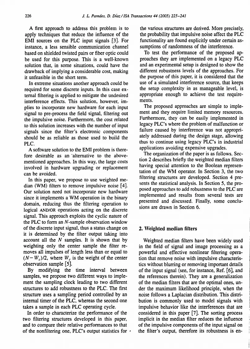
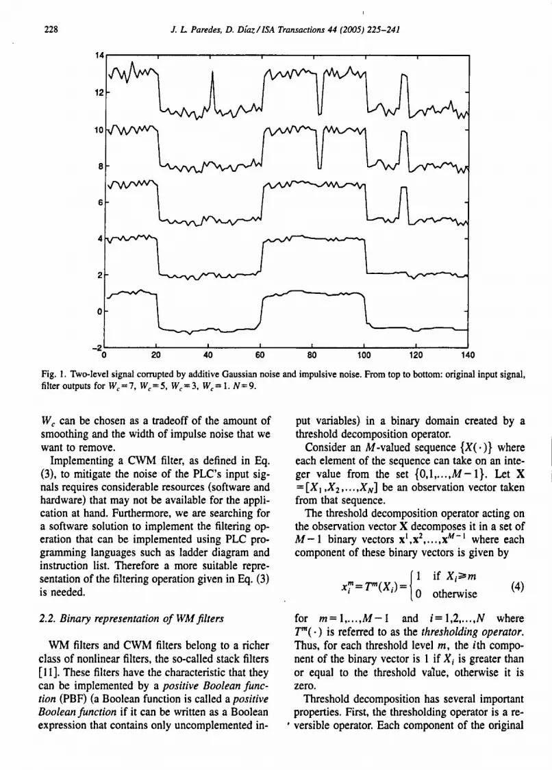
In the following example, this behavior is illus­trated. Consider the two-level signal corrupted by additive white Gaussian noise and impulse noise shown at the top of Fig. I. The two-level signal can be thought of as a discrete signal outputted by a field device. the additive impulsive noise is the electromagnetic interference coupled to the the discrete signal and the Gaussian noise is the back­ground noise. The outputs of the CWM filters as the center weight takes on different values are shown in Fig. 1. Clearly, as We is increased less smoothing occurs.

Note also that the CWM filter removes impulse noise of variable width as the center sample weight decreases. In fact, all the impulse noise of one-sample width is removed by the CWM with Wc~7. while impulse noise of two-sample width is removed by the CWM with Wc~5.

Having just one tunning parameter makes it easier to design CWM filters without the need of implementing adaptive algorithms like those pre­sented in Ref. [10]. Thus the center sample weight

228 J. L Paredes. D. DiazlISA Transactions 44 (2005) 225-241

o

-2~------~----~~----~~----~~----~~----~~----~ o 20 40 60 80 100 120 140

Fig. I. Two-level signal corrupted by additive Gaussian noise and impulsive noise. From top to bottom: original input signal. filter outputs for Wc=7. Wc=5. Wc=3. Wc= 1. N=9.

We can be chosen as a tradeoff of the amount of smoothing and the width of impulse noise that we want to remove.

Implementing a CWM filter, as defined in Eq. (3), to mitigate the noise of the PLC's input sig­nals requires considerable resources (software and hardware) that may not be available for the appli­cation at hand. Furthermore, we are searching for a software solution to implement the filtering op­eration that can be implemented using PLC pro­gramming languages such as ladder diagram and instruction list. Therefore a more suitable repre­sentation of the filtering operation given in Eq. (3) is needed.

2.2. Binary representation of WM filters

WM filters and CWM filters belong to a richer class of nonlinear filters, the so-called stack filters [11]. These filters have the characteristic that they can be implemented by a positive Boolean func­tion (PBF) (a Boolean function is called a positive Boolean function if it can be written as a Boolean expression that contains only uncomplemented in-

put variables) in a binary domain created by a threshold decomposition operator.

Consider an M-valued sequence {X(.)} where each element of the sequence can take on an inte­ger value from the set {O, 1, ... ,M - I}. Let X =[X I ,X2 ' ... ,XN] be an observation vector taken from that sequence.

The threshold decomposition operator acting on the observation vector X decomposes it in a set of M -1 binary vectors XI,X2, ... ,XM- I where each component of these binary vectors is given by

[1 if Xi~m

x'?"=rm(x·) = I I 0 otherwise

(4)

for m=I, ... ,M-l and i=1,2, ... ,N where rm( .) is referred to as the thresholding operator. Thus, for each threshold level m, the ith compo­nent of the binary vector is 1 if Xi is greater than or equal to the threshold value, otherwise it is zero.

Threshold decomposition has several important properties. First. the thresholding operator is a re­

I versible operator. Each component of the original

J. L. Paredes, D. DiazllSA Transactions 44 (2005) 225-241 229

observation vector can be reconstructed from the set of its corresponding binary values. That is,

M-)

Xi=~ x~. m=)

(5)

A second important property of threshold de­composition is the partial ordering on the set of binary vectors of fixed length. That is, for all threshold level m ~ I, it can be shown that xm os:; Xl, where the smaller than or equal to operator (os:;) holds for each component of the binary vec­tor.

Now, the class of stack filters is defined in the binary domain as the set of positive Boolean func­tionsf(·) for which it holds for any x that [11,12]

f(xm)OS:;f(xl) if m~l. (6)

The filtering operation of an M -valued observa­tion vector by a stack filter reduces to evaluate the PBF for each binary vector outputted by the thresholding operator and adding up the binary fil­ter outputs, namely ~~::lJ(xm). It is worthy to mention here that not all the Boolean functions for which Eq. (6) holds have useful filtering proper­ties. In fact, the design of stack filters is an open research area.

A more intuitive subclass of stack filters is ob­tained, however, if the positive Boolean functions are further restricted. When self-duality (a Bool­ean functipn is said to be self-dual if and only if f(x) ,X2, .. ·,XN)= 1 implies f(x) ,X2, ... ,XN)=O, and f(xl ,X2, ... ,XN)=O implies f(xl,x2, ... ,xN) = 1, where x denotes the Boolean complement of x) and linear separability are imposed, for in­stance, the equivalent stack filters reduce to the well-known class of weighted median filters [13], which in the integer domain are defined by Eq. (I).

In addition to creating the framework that leads to the definition of the family of stack filters, threshold decomposition is the particular impor­tance for analyzing median based filters (WM and CWM filters) since threshold decomposition and median are commutable operations. That is, apply­ing a median based filter on an M -valued observa­tion vector X is equivalent to decomposing the observation vector in M - 1 binary vectors, filter­ing these binary vectors independently and com­bining the results by summing up to obtain the median filter output. Namely,

M-I

= ~ MEDIAN(xr ,xi .... ,x~), (7) m=1

where the median operator acting on binary signal. right-hand side of Eq. (7), reduces to evaluate the positive Boolean function that defines it in the bi­nary domain. For instance, the median of three binary samples XI' X2, x3 is defined by the posi­tive Boolean function

f(x).x2 ,X3) =X)x2+ xlx3 + X2x3,

where we use the multiplication . and the addition + to denote the AND Boolean operator (conjunc­tion) and OR Boolean operator (disjunction), re­spectively.

The relationship in Eq. (7) establishes a weak superposition property satisfied by the nonlinear median operator, which is important from the fact that the effects of median on binary signals are much easier to analyze than those on multilevel signals.

At this point. the question that naturally arises is how to obtain the binary representation of a WM filter equivalent to its integer-valued representa­tion. By equivalent we mean that for any input signal filtering it, using the integer-valued repre­sentation of a WM filter, Eq. (1), or using its bi­nary representation, right-hand side of Eq. (7), produces the same output signal.

2.3. Finding the PBF corresponding to a weighted median filter

In this section, we focus our attention on the method to find the positive Boolean function cor­responding to a weighted median filter rather than the justification of the method itself. For a com­plete description of the ideas behind the method see Ref. [14].

Given a weighted median filter with weights (W I , W 2, ... , W N) we want to find the equivalent PBF that defines it in the binary domain. More precisely. we want to determine the minimum sum of product that describes the WM filter in the bi­nary domain.

In order to do so, let N' = ~~= I W j be the size of the extended observation window after each

230 J. L Paredes. D. D[azIISA Transactions 44 (2005) 225-241

sample has been replicated. Furthermore, let x7 be associated to the sample Xi that is weighted by Wi'

Upon closer examination of Eq. (7), it can be seen that the median operator acting on binary sig­nal outputs a value of 1 if the number of 1 's in the observation window is greater than N' /2. Further­more, note that for the median of three samples, where the weights are equal to 1, the Boolean function is formed by combining in a logical OR operation all the possible products of binary vari­ables for which the sum of their corresponding weights is greater than or equal to 3/2.

Extending these observations to the case of WM filters, it can be shown that WM operator acting on binary signal outputs a I, if the sum of the weights Wi corresponding to those binary samples Xi that take on the value of I is greater than N' /2. Thus the Boolean function equivalent to a WM filter can be formulated as a sum of product where, in each product, the sum of the weights associated to the binary variables contained in the product is greater than N' /2. This establishes a methodology to de­termine the equivalence between the integer and the binary domain representations as follows.

The problem of finding the PBF corresponding to a given WM filter with set of weights (WI' W2 , ... , W N) reduces thus to combine in a logical OR operation all the possible logical prod­ucts of the binary samples whose sum of the cor­responding weights is greater than N' /2. The re­sulting sum of products can then be minimized by using rules of Boolean algebra.

Example: Consider the five-sample center weighted median filter

Y=MEDIAN(WlOXl,W20X2,W30X3,

W40X4,WSOXS)

=MEDIAN(lOX l ,lOX2,30X3 ,

1 0 X4,1 0 Xs).

The minimum logical product and their corre­sponding sum of weights that are greater than or equal to N' /2= 3.5 are listed as follows:

"1.1 .. 1.3 "0.1 I I

.. 1.2 "1.3 I I

"1.4 "1.3 I I

"1.5 "1.3 I I

"1.1 "1.2 "1.4 "1.5 I I I I I I

Fig. 2. Ladder diagram program for a CWM filter with Wc=3, N=5.

X3X4=>W3+W4,

X3x S=> W3 + Ws

and the PBF 1(,) is then given by

I(Xl ,X2,X3 ,X4,XS) =Xlx2x4XS + X3 Xl + X3X2

3. Implementation of WM filters in a PLC

3.1. Filtering algorithm

(8)

Having defined WM filters in the binary domain as PBF's their implementation on the PLC's memory reduces to obtaining the observation win­dow by sampling multiple times the input signal and performing the binary filtering operation. In particular, if the input signal is constrained to be a discrete signal (M = 2), like the one corning from a switching device, the filtering operation reduces to evaluate the Boolean function for a single threshold value avoiding thus the summation of Eq. (7).

For instance, in Fig. 2 is shown the implemen­tation of the CWM filter of the above example using a ladder diagram, which is a well-known PLC programming language. Note that the nota­tion Ml.i denotes the ith observation sample.

To obtain an observation window of length N, the input signal is sampled and the obtained read­ings are pushed into an N -bit shift register imple­mented by software within the PLC. The PLC pro­vides us with timing resources that make it possible for us to follow at least two different ap­proaches for the generation of the sampling clock. Both approaches exploit the cyclic behavior of the

• PLC.

1. L. Paredes, D. Diaz / ISA Transactions 44 (2005) 225-241 231

~.8 loll 0.5 I 0-1

~.7 I0Il 0.11 I D-I

~o I0Il 0.7 1 D-I

loll 0.5 "0.6 A O.O I I

(a)

I TO loll 3.0 H 1----------10-1

TO TO ....

KTOO1.0 lW DE

loll 3.0

I EO.O I0Il3.1 H f-I -----D-I

I :;: :;::~ I-I---;I~ loll 3.7

I G3•

01

"3.0 f-----i/

" 3.7

loll 3.1 I G3'~

W 3.0 t---i/

W3.1

loll 3.5 loll 3.8

loll 3.6

I

A Q

loll 3.7

I

.. Q

AO.O 1-1----11 I--~--------;

(b) Fig. 3. Filtering approaches to implement a three-sample median filter. (a) A ample is taken in every operation cycle. (b) A timer is used to defi ne the sampling period.

In order to under tand these approache we have to take a clo e look at the algorithm that the PLC follows to execute the instruction programmed by the user. To do 0 , let us consider the ladder dia­gram which i widely used to design and imple­ment PLC applications. Its popularity lie in the fact that it resembles an electrical circuit made up of relays and other electromechanical elements. Unfortunately this language can give u a mi un­der tanding about the PLC operation. The behav­ior of such circuit re emble a parallel algorithm becau e aU it branches eem to work imulta­neou Iy. On a fir t look, we can end up thinking that the operation of a PLC will a1 0 follow orne

kind of para llel algorithm, but that i not true. Since the CPU of a PLC is built around either a microproce or or a microcontroller, the execution of the instructions is sequential by nature. De pite that, it i po sible to de ign the PL in a way that imulate the parallel execution, but it would be

ex pen ive and maybe unnece ary. Another detail to take into account i that the

language u ed to program a PL provide little or no upport of programming structure like condj-tional branche • jumps, and loop . Thi nsure that the u er program will b execut d in a fix d time that will only depend on it length. Furt.her­more, the operation algori thm of a PL al 0 wrap

232 J. L. Paredes. D. Diaz l ISA Transacliol1s 44 (2005) 225- 241

Personal Computer

/ DAQ Board /1 Software I

I Disk File

Fig. 4. Experimental etup.

an infinjte loop around the program in order to execute it, in truction by in truction, continuously. A side effect of thjs algorithm is that every in­struction of the user program i executed periodi­cally with a frequency tbat varies with the pro­gram length and with the speed of the PLC CPU. With these concepts in mind, we present next the two sampling approaches implemented in thi s pa­per.

A first sampling approach takes advantage of the cyclic behavior by mean of writing in the user program additional instructions that uncondition-

~ I E 0.0 AD.D ~I D-1 I T1 ... 4.0 HI D-1

Tl

~.I WO.5 I D-1

~.7 WO.S I D-1

~A WO.7 I D-1

.. 0.5 ... 0.6 AO.D I I

(a)

ally sample the input and push the reading into a shift register. In this way, the sampling period will become the time that it takes the PLC to complete an operation cycle. The second approach uses one of the timers provided by the PLC to establish the sampling period. This approach is conceptually simpler than the first but, a will be shown later, it is also the most expensive in terms of computa­tional resources.

Regarding the first approach, note that the input can be sampled repeatedly within the program in order to fill up an N-size observation window in a single cycle instead of taking N cycles to do so. This behavior leads to a nonuniform sampling of the input, in which N samples are taken with a period of a few instruction cycles between them but the following N samples wi ll be taken after a complete operation cycle. This later approach as­sumes that the input reading cou ld vary with the position of the sampling instruction within the program and this is possible if the PLC does not include a sample and hold operation on its inputs a part of its algorithm.

(b)

Fig. 5 . Ladder diagrams for the tests. (a) Program for 'filtering approach I. (b) Program for filte ring approach 2.

J. L Paredes. D. Diaz / [SA Transactions 44 (2005) 225-241 233

The first approach, hereafter denoted as filtering approach 1, is shown in Fig. 3(a). It establishes a sampling period defined by the length of the user program. This approach is simple to implement and also consumes limited resources. A drawback of this approach, however, is that the user will not have a simple control over the sampling time since the sampling period will be the same as the opera­tion cycle time. The user would be able to modify the sampling period within some limits. To achieve this, the user can insert a dummy instruc­tion into the program, in order to make it longer but equivalent to the original one.

The second approach, hereafter denoted as fil­tering approach 2, is shown in Fig. 3(b). It has the advantage of allowing the user to control the sam­pling period adjusting an internal timer. However, this approach has the drawbacks of using up more computational resources to be implemented and that the shortest sampling period allowed would normally be in the order of the tens of millisec­onds. This lower limit could be too large in appli­cations that need to reduce the propagation delay as much as possible. Recall that the delay intro­duced by the nonlinear digital filter will be always a multiple of the sampling period being that a de­sign constraint. It also has to be noted that in this approach the sampling period will not exactly be the timer delay. That is, right after the time delay ends, the PLC will read the input in the following reading stage and therefore the sampling period will be the lea~t integer multiple of the operation cycle time that is greater than or equal to the timer delay.

3.2. Implementation

To test the performance of the two approaches described above the experimental setup shown in Fig. 4 was designed. In this setup the data acqui­sition (DAQ) board provides a signal that simu­lates the interference to the input of the PLC and simultaneously acquires and stores its response.

The PLC used was a Siemens SIMATIC S5-101 U that has 20 inputs and 12 relay outputs, data memory for 512 flags, and program memory for 1024 instruction words. This PLC can execute a program of 1024 instructions in 70 ms [15]. The DAQ board is a National Instruments AT-MIO-16E-IO. It is a multifunction analog, digital, and timing I/O board for the PC-AT which features,

among other things, 16 single ended or 8 differen­tial analog input channels, 12-bit ADC resolution, sample rate of 100 ks/s, 2 24 bit up/down counters/timers, and base clocks of 20 MHz and 100 kHz [16].

The computer is a PC-AT with an Intel Pentium Processor of 200 Mhz, 32 MB of RAM memory, and a hard disk capacity of 4 GB. The software that controls the experiment was written in C+ + using the Microsoft Visual Studio IDE and the National Instruments NIDAQ 6.1 API to pro­gram the acquisition board. The interface circuit is made up with some buffers that manage the con­version between the signal levels used by the DAQ board and the PLC.

Bursts of pulses are used to simulate the inter­ference signal effect over the digital input. The DAQ board generates these bursts and keeps con­trol over the width, frequency, and number of pulses and also controls the delay between the be­ginning of the operation cycle and the beginning of the bursts. To make possible this last control, the PLC is programmed to generate a square sig­nal with a period of several operation cycles and synchronized with them. This signal is used by the DAQ board to trigger the generation of the burst and the acquisition process.

Fig. 5 shows the ladder diagrams that represent the actual programs used to obtain the results that are going to be discussed later. Dummy instruc­tions were appended to those diagrams in order to establish a program length of 256 instructions. This was done for two reasons; the first one is that a medium size user program would probably have a size similar to that number of instructions. The second reason is that it was needed to ensure that the speed of the outputs signals could be handled appropriately by the PLC used. The electrome­chanical nature of its relay outputs restricts the pulse width they are able to handle to be wider than 10 ms approximately. By updating each PLC output only once in the program and making it long enough we have ensured that the pulses gen­erated were longer than the limit mentioned above.

Fig. 5(b) shows the program that implements fil­tering approach 2. Note that the synchronization signals are generated using the output of two tim­ers. That is, timer 0 is used to generate the sam­pling clock and timer 1 is used to allow us to make the period of the synchronization signal to take time elapsed by several operation cycles. This sig-

234 J. L Paredes. D. DiazllSA Transactions 44 (2005) 225-241

nal will then be synchronized with both timers and this will ensure that the filter will take a sample at fixed delay from the rising edge of this signal. This is important since it allows us to control the relative position between the sampling moments and the burst of pulses.

Fig. 5(a) shows the program that implements fil­tering approach 1. Note that it is quite simpler than the previous one. Here, only one timer is used to allow the synchronization signal to have a period of several operation cycles. All the programs have three outputs: the detected reading at the input without filtering, that reading after the filtering stage, and the synchronization signal.

The DAQ board is programmed to acquire all the output signals together with the input signal applied to the PLC. Each signal was digitized with a sampling frequency of 20 kHz. The program that controls the experiment allows the user to indicate the pulse width, the pulse period, the number of pulses within each burst, the number of bursts de­sired, and the delay between the bursts and the rising edge of the synchronization signal.

4. Statistical analysis

In order to evaluate the robustness of the pro­posed approaches, a statistical analysis is derived next under the assumption that the contaminated discrete input signal to the various PLC structures has a random behavior. More precisely, the prob­ability that a random impUlsive noise affects the PLC functionality is derived for the PLC without filter and with the WM based filters. Closed form expressions for that probability are found, assum­ing certain random behavior for the interference.

Let us assume that the contaminated PLC input signal has a periodical behavior with a random duration, that is

where l(t) is the discrete signal outputted by a field device, p(t) is a normalized impulsive noise function, ton is the random duration of the noise, and A is a random amplitude. Although p(t) can have a wide variety of wave shapes, for instance the ones recommended to study susceptibility in equipment [17], in many cases it could be seen at the discrete input of the PLC as a pulse of width'

ton. In Eq. (9), T is the period of the interference and, for the sake of simplicity, it is assumed to be equal to the PLC reading cycle, thus only one pulse of width ton occurs within each reading cycle. Further, t d is a random time delay which can be thought of as the time between the instant at which the PLC begins a working cycle and the instant at which the next pulse occurs, or the time between the last PLC reading of the input signal and the first pulse occurs. In order to simplify the analysis, it is assumed that l(t)=O for all t (OFF level of the discrete signal). With the assumptions made p(tlton) can be defined as p(tlton ) =Ap for O<t<ton , 0 for ton<t<T beingAp the pulse am­plitude which is assumed to be greater than the value that is considered as an ON level of the dis­crete signal.

Let us define the following event

if the PLC reads a contaminated

input signal

otherwise.

The expected value of event M, denoted as E[M], is given by

where t is the instant at which the PLC reads the discrete input signal. To be more general in our statistical study. t is assumed to be a random vari­able with mean T. Thus Pr(td<t:s:;;;td+ton ) is then the probability that the PLC reading instant lies within the time interval where the unwanted inter­ference pulse is ON.

If we consider that the interference source is in­dependent of the PLC functionality, that is the im­pulsive random noise occurs at any time within the PLC cycle, and its time duration ton is inde­pendent of the instant of occurrence, then t, ton' and t d are independent random variables.

Let It(t), It (ton), and It (td) be the density on d

functions of t, ton' and t d, respectively. We are interested in computing the E[ M] = Pr(t d< t:S:;;; t d +ton ) or equivalently E[M]=Pr(O<t-td:s:;;;ton ) (at this point, we assume that the random process that generates the impulsive noise is a stationary process). Let z = t - t d, the density function of z is given by [18]

J. L Paredes, D. DiazllSA Transactions 44 (2005) 225-241 235

It is clear that the cumulative density function of Z

can be easily detennined from Eq. (10) as Fz(z) == f~J(z)dz.

Now taking conditional expectation on the val­ues that ton can take on, the computation of E[M] reduces to

E[M]=E, [E[Mlton = Ton]]. on

Pr(O<t- td::;;;ton )

=Et {Pr(O<t- td~tonlton= Ton ,Ton~ton)} on

= ft on

Pr(O<t- td~ Toni Ton)ft (Ton)dTon nn -00

(11)

(12)

Thus Eq. (12) gives a close form expression for the probability that a random impulse noise of width ton is recognized as a change in a discrete input signal affecting thus the PLC functionality.

Having defineq the probability that the event M happens, now we derive the probability that an impulse noise affects the PLC outputs.

Let us consider a PLC user program that takes the contaminated discrete input signal and outputs its value, namely the PLC reads the discrete input signal and outputs whatever its value is. We are interested in computing the probability that the PLC outputs a wrong signal due to an undesired change in the discrete input signal.

It is clear that for the user program without the proposed filtering structure the probability that the PLC outputs a wrong signal is equal to the prob­ability that the PLC reads the discrete signal at the moment that an impulsive noise occurs, that is

( PLC without filter )

Pr outputs a wrong signal

= E[M] = Pr(td<t~td+ ton)' (13)

where E[M] is given by Eq. (12).

On the other hand, the PLC user program with the proposed filtering structure (filtering approach 1) outputs a wrong signal if and only if (N + 1)/2 samples of the observation window take the values of impulse noise, where N is the obser­vation window size. That is, (N + 1)/2 out of N consecutive PLC readings have to be impulse noise. Assuming independence between samples in the observation window, the probability that the PLC with filter outputs a wrong signal is

( PLC with filter )

Pr outputs a wrong signal

(N+l)12 N) = ~ ( (E[M])N-k( 1-E[M])k.

k=O k

(14)

For the second filtering approach implemented, the probability that the PLC outputs a wrong sig­nal follows a similar expression to that of Eq. (14). In this case, however, the PLC reading period of the discrete 'input signal that has been filtered is defined by the user as

T'=mT,

where m;::=: 1 is an integer-valued tunning param­eter defined by the user. Since we are assuming that only one pulse p(t) occurs in that period the probability for filtering approach 2 follows Eq. (14) where t is a random variable with mean T'.

Example: In order to illustrate the statistical analysis for the proposed PLC filter structures and compare them with the no-filtered one, we assume certain density functions for the time delay td' time duration of the pulse ton' and for the PLC reading instance t. Let td and ton be random vari­ables uniformly distributed over (O,T). Further­more, let t be uniformly distributed over (T - TIA,T+ TIA) where A is a real number greater than 2. Note that as A goes to infinity the PLC reading instant becomes periodical and determin­istic.

It can be shown that the cumulative distribution function of z = t - t d is given by

236 J. L Paredes, D. DiazllSA Transactions 44 (2005) 225-241

0.5

~.-.-.-.-.-.-.-.-.-.-.-.-.-.-.-. 0.45

0.4

0.35

0.3

0.25

0.2

0.15 I

I

0.1 I

I I

" 0.05 I

" I

" " ,/ ,/ ". ... ... _. 0.2 0.4

I I

I I

I I

I I

I I

I

0.6

I I

" 'i , . , .' , .'

I ,

I i I .

I .' I I

I ,

I

I

I

I

I

I

I

0.8 1 1.2 1.4 1.6 1.8 2

To nIT

Fig. 6. Probability that impulsive noise affects the PLe perfonnance. (-) PLe without filter. ( approach I. (_. -) PLe with filtering approach 2. A = 10, m = 2.

) PLe with filtering

o T if z<- A

-T T if A~z<A

T T if A~z<T- A

T T if T- A~z<T+ A

T. if z~T+ A'

Replacing Eq. (15) in Eq. (12) and after some alg'ebraic manipulations yields

(I5)

J. L Paredes, D. DiazlISA Transactions 44 (2005) 225-241

E[M]=

o A 3 2

ton ton 12T3 + 4T2

2 ton ton 1 2T2 - 4AT+ 12A2

3 A 2 2 Aton ton ton tonA - 12T3 + 4 T2 + 4 T2 - 4 T

ton ton 1 1 A +2T-2AT-4+ 4A +12

1 1 2 4A

T if T- -:::::t <T A on

if ton~T.

237

(16)

Upon close examination of Eq. (16), it turns out that the probability that the event M occurs does not depend on T but on the ration ton IT which is the duty cycle of the impulsive interference and is uniformly distributed over (0, 1).

On the other hand, for the three-sample median filter implemented in Section 3.1, the probability that the output is affected by the unwanted change on the input signal is given by

5r-----r-----.-----~----~----,_----~----_r----_r----~

4

3

2

5~----r-----.-----~----~----,_----~----_r----_r----_,

4

3

2

1 O~uw~~~~~~~~~~~--~~~~~~~--~~~~

o 0.5 1.5 2 2.5 3 3.5 4 (b)

5r-----~----~----~----~----~----_r----_r----~----_,

4

3

2

o " o • •

0.5 1.5

--'"- ~I

2 2.5 3 3.5 4 (c)

Fig. 7. Results from filtering approach 2 test conditions: td=9.85 ms, T=25 ms, ton =3 ms, npu/.,= I, nbursr=50. (a) Input signal, (b) unfiltered output, (c) filtered output.

238 J. L Paredes. D. DiazllSA Transactions 44 (2005) 225-241

5 I'"" r- r- r- I'"" r- r- r- I'"" r-

4

3

2

0 "'"""= - -10.5 11 11.5 12 (a) 12.5 13 13.5 14

5 r- r- r- r- ..- r- r- r- '""" r-

4

3

2

0 10.5 11 11.5 12 (b) 12.5 13 13.5 14

5 .-- r-- r--

4

3

2

0 10.5 11 11.5 12 12.5 13 13.5 14

(c)

Fig. 8. Results from filtering approach 2 with test conditions: td=9.85 ms, T=200 ms, ton =98.5 ms, npulu= l, nbursl = 50. (a) Input signal, (b) unfiltered output, (c) filtered output.

( PLC with filter )

Pr outputs a wrong signal

=(E[M])3+3(E[M])2(I-E[M]),

(17)

where E[M] is given by Eq. (16) with T as the reading period which, for filtering approach I, is equal to the PLC cycle period whereas, for filter­ing approach 2, it is m-fold the PLC cycle period. Fig. 6 shows the probability that impulsive noise affects the PLC performance. Note that, as ex­pected, the PLC performance is more affected if the PLC user program does not filter out the dis­crete input signal. In this case, there exists a greater probability that an impulsive noise is rec­ognized as a change in the discrete input signal.

5. Results and discussion

In the following description the variable td rep­resents the time elapsed between the rising edge of '

the synchronization signal and the rising edge of the first pulse in the generated burst. The variables T and ton represent the period and width of a single pulse in the burts, respectively. The variable n pulse represents the number of pulses on each burst whereas nbursl represents the total number of burst generated.

For each filtering approach, two sets of test con- . ditions have been selected. The first one has been i

suitably adjusted to make the non filtered output have an intermediate recognize probability of the input pulse, i.e., the nonfiltered output sometimes will recognize the input pulse and some time it will not. The conditions for the second test have been adjusted to make the filtered output have an intermediate recognize probability. In both sets, in order to simplify the analy~is, only bursts contain­ing one pulse have been specified. Furthermore, for each reading cycle the tall and t d remain un­changed, namely after they have been defined for the first reading cycle they remain fixed during the all test. Note that this latter condition is not the

J. L Paredes. D. Diaz/ [SA Transactions 44 (2005) 225-241 239

5r-------~---------r--------._--------r_------~--------~

4

3

2

0.5 (a) 1.5 2 2.5 3

X 104

5r-------~---------r--------~--------r_------~------~~

4

3

2

0.5 1.5 (b)

2 2.5 3

X 10· 5r--------r--------.-------~--------~------~~----~~

4

3-

2

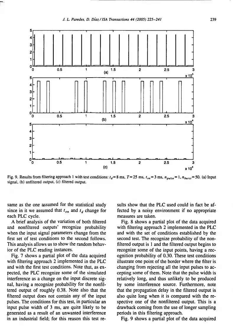
Fig. 9. Results from filtering approach 1 with test conditions: td= 8 ms, T= 25 ms, ton = 3 ms, np.I .. = I, nbm,= 50. (a) Input signal, (b) unfiltered output. (c) filtered output.

same as the one assumed for the statistical study since in it we assumed that ton and td change for each PLC cycle.

A brief analysis of the variation of both filtered and nonfiltered outputs' recognize probability when the input signal parameters change from the first set of test conditions to the second follows. This analysis allows us to show the random behav­ior of the PLC reading instances.

Fig. 7 shows a partial plot of the data acquired with filtering approach 2 implemented in the PLC and with the first test conditions. Note that, as ex­pected, the PLC recognize some of the simulated interference as a change on the input discrete sig­nal, having a recognize probability for the nonfil­tered output of roughly 0.38. Note also that the filtered output does not contain any of the input pulses. The conditions for this test, in particular an input pulse width of 3 ms, are quite likely to be generated as a result of an unwanted interference in an industrial field; for this reason this test re-

suIts show that the PLC used could in fact be af­fected by a noisy environment if no appropriate measures are taken.

Fig. 8 shows a partial plot of the data acquired with filtering approach 2 implemented in the PLC and with the set of conditions established by the second test. The recognize probability of the non­filtered output is 1 and the filtered output begins to recognize some of the input points, having a rec­ognition probability of 0.30. These test conditions illustrate one point of the border where the filter is changing from rejecting all the input pulses to ac­cepting some of them. Note that the pulse width is relatively long, and thus unlikely to be produced by some interference source. Furthermore, note that the propagation delay in the filtered output is also quite long when it is compared with the re­spective one of the nonfiltered output. This is a drawback coming from the use of longer sampling periods in this filtering approach.

Fig. 9 shows a partial plot of the data acquired

240 J. L Paredes. D. Diazl [SA Transactions 44 (2005) 225-241

5

4

3

2

0 0 2

5

4

3

2

0 0 2

5

4

3

2

0 0 2

3 (a)

3 (b)

3

(c)

4

4

4

5 6

5 6

.

5 6

Fig. 10. Results from filtering approach I with test conditions: td=8 ms, T=40 ms, ton = 19.9 ms, npu/se= I, nbu,.,=50. (a) Input signal, (b) unfiltered output, (c) filtered output.

with filtering approach 1 implemented in the PLC and with the first set of test conditions. The behav­ior is similar to the one observed with filtering approach 2 and the corresponding test conditions. In this case the recognition probability is 0.54.

Fig. 10 shows a partial plot of the data acquired with filtering approach 1 implemented in the PLC and with the second test conditions. Again the re­sults are similar to the ones obtained with filtering approach 2 but in this case the pulse width and the propagation delay are much shorter. Furthermore, the recognition probability is 0.10. These results show that this filtering approach could have a good tradeoff between computational cost and fil­tering performance, with the drawback that the only way of controlling the sampling period is by manipulating the program length by adding dummy instructions.

6. Conclusions

Two approaches for implementing weighted me­dian filters to remove impulsive interference in a '

PLC discrete input have been designed. Both ap­proaches exploit the cyclic nature of the PLC to form an N -sample observation window. For the first approach, the sampling period is directly the PLC's cycle period whereas for the second one the sampling period is a tuning parameter defined by the user. The choosing of this parameter should be a tradeoff between impulsive noise rejection and the undesired propagation delay introduced by the filtering operation.

An experimental setup based on a legacy PLC, a multifunction data acquisition board, and a per­sonal computer was used to test the performance of the design.

The interference signal was simulated by bursts of pulses whose width, period, and number are controlled by the DAQ board. Each burst is ap­plied after a controlled deiay from the beginning of the PLC operation cycle has elapsed.

The results indicate that the proposed ap­proaches work as expected. In both cases a wid­ening of the minimum pulse width recognized as a

1. L. Paredes, D. Diaz l ISA Transactions 44 (2005) 225- 241 24 1

valid one i achieved after the filtering . A stati tical analy i of the behavior of the fil­

tered output with re pect to the parameters of the simulated interference has been al 0 developed. It was shown that the propo ed filtering operations can effectively reject impul ive noise of a mini­mum pul e width which is recogrtized as a change in the discrete signal by the PLC without filtering.

Acknowledgments

This work was supported in part by the Labora­torio de In trumentacion y Automatizacion, La­bidai of The Electrical Engineering Department, ULA and by the University of Los Andes Council of Scientific, Humanistic and Technological De­velopment by means of Project No . 1-78 1-04-02-F and 1-768-04-02-B.

References

[I] Hughe , T. A. , Programmable COllfrollers. ISA Re­ources for Measurement and Control Serie (RMC),

ISA-The In trumentation, System and Automation Society. third ed .• 200 l.

[2] Howell . E. K., How switched produce electrical noise. IEEE Tran . Electromagn. Com pat. EMC·21, 162-170 (1971 ).

[3] Skibinski, G. L. . Kerkman, R. J .• and Schlegel , D., MI em is ion of modern PWM ac drives. IEEE Ind.

Appl. Mag. 5 (6), 47- 80 (1999). [4] Brownrigg, D., The weighted median filter . Commun.

ACM 27. 807- 81 (1984). [5] Ko, . and Lee, Y. H., enter weighted median filters

and their applications on image enhan emenl. IEEE Tran . ircuit y t. 38, 984 - 993 (1991 ).

[6] Yin , L. . Gabb uj , M" and euvo. Y., Weighted me· dian fi lters: A tutorial. IEEE Trans. ir uits yst. , II : Analog Digital Signal Proce s. 43 (3). 157- 192 ( 1996).

[7] Astola, J., and Kuo manen , P., undamental of on­linear Digital Fi ltering. Electronic ngineering Sy -tem Serie . R Pre s LLC, 1997.

[8] Arce, G., A general weighted median filter structure admitting negati ve weights. lEE Trans. ignal Pro­ce s. 46, 3 195- 3205 (1998).

[9] Arce, G. and Parede • J. L., Recursive weighted me­dian fi lter admitting negati ve weight. and their opti ­mization . I EE Tran . ignal Process. 43, 768 - 779 (2000).

[10] Yin , L. and Nuevo, Y. , Fa t adaptation and perfor­mance characteri sti of fir-wos hybrid filters . lEE Tran. ignal Proce . 42, 1610- 162 (1994).

[ II ] Wendt, P. D., Coyle, E. J., and Gallagher, . c., tack filter . IEEE Tran . Acousl. . peech. Signal Proce . 34,898-9 11 (1986).

[12] Parede , J. L. and Arce. G. R., Stack filter , tack moother , and milTored thre hold decompo ition.

IEEE Tran . Signal Proce . 47,2757- 2767 (1999). [ 13] Yli-Harja, 0 ., A tola, 1., and euvo, Y., Analysi of

the propertie of median and weighted median fi lter, using threshold logic and stack fi lter repre entation. IEEE Tran . Acou I. , peech. Signal Process . 39, 395- 410 (J991 ).

[14] ieweglow ki, J., Gabbouj . M. , and euvo, Y. . Weighted medians-po itive b olean fun lions conver­sion method . Signal Proce . 34. 146- 162 (1993).

[ 15] Siemens. Simantic S5-10IU. Programmable Control­ler. ser Manual , 1987.

[ 16] . I. Corporation, AT-MlO/AI E Serie er Manual. May 1996.

[ 17] I. S. Collection. Surge Protect ion. 1992 ed. [18] Pappouli , A., Probability, Random Variable. and Sto­

chastic Proce es. McGraw-Hili , ew York. 1991.

Jo e L. Paredes was born in Merida. Venezuela . He re­ceived a diploma in Electrical Engineering with the highest honors from the niven,idad de Los Ande ( LA). Merida. Venezuela. in 1995. He re­ceived the M.S. and Ph.D. de­gree in Electrical Engineering from the University of Dela­ware in 1999 and 200 I. respec­tively. Since September 2001. he has been a full time Profe~­

or in the Electrical Engineer­ing Depanment at ULA. Dr. Paredes has onsulted with indu try in the areas of digital ommunication and . ignal processing. His research interest ~ include robu t signal and image processing. nonlinear fi lter theory. adapti ve signal pro essing. and digital communicutions.

Ohionel O. 0101 Obondo was born in Merida. Vene7uela.

urrent ly he i pur uing an lectrical Engineering diploma

from the niversidad de Lo, Andes. Merida. From 1996 he has been involved in the re­search activi ties of the Grupo de Ingenieria Biomedicn of thut nivers ity. His research interests include pure ancl ap­plied to engineering mathemnt­i s. digi tal signal proces,ing. and embedded systems devet­

opment. He has pub lished several paper, in the, e areas in national and international conferen es. During hi engineering Muclies he has re­ceived a number of medals and awards for ha ving the best grades in his department.