Improved estimation of macroevolutionary rates from fossil

Article

Improved estimation of macroevolutionary rates from fossil datausing a Bayesian framework

Daniele Silvestro , Nicolas Salamin, Alexandre Antonelli, and Xavier Meyer

Abstract.—The estimation of origination and extinction rates and their temporal variation is central tounderstanding diversity patterns and the evolutionary history of clades. The fossil record provides theonly direct evidence of extinction and biodiversity changes through time and has long been used to inferthe dynamics of diversity changes in deep time. The software PyRate implements a Bayesian frameworkto analyze fossil occurrence data to estimate the rates of preservation, origination, and extinction whileincorporating several sources of uncertainty. Building upon this framework, we present a suite of methodo-logical advances includingmore complex and realistic models of preservation and the first likelihood-basedtest to compare the fit across different models. Further, we develop a new reversible jump Markov chainMonte Carlo algorithm to estimate origination and extinction rates and their temporal variation, which pro-videsmore reliable results and includes an explicit estimation of the number and temporal placement of stat-istically significant rate changes. Finally, we implement a new C++ library that speeds up the analyses byorders ofmagnitude, therefore facilitating the application of the PyRatemethods to large data sets.We dem-onstrate the new functionalities through extensive simulations and with the analysis of a large data set ofCenozoic marine mammals. We compare our analytical framework against two widely used alternativemethods to infer origination and extinction rates, revealing that PyRate decisively outperforms them acrossa range of simulated data sets. Our analyses indicate that explicit statistical model testing, which is oftenneglected in fossil-based macroevolutionary analyses, is crucial to obtain accurate and robust results.

Daniele Silvestro. Department of Biological and Environmental Sciences, University of Gothenburg,and GlobalGothenburg Biodiversity Centre, 41319 Gothenburg, Sweden; Department of Computational Biology,University of Lausanne, and Swiss Institute of Bioinformatics, Quartier Sorge, 1015 Lausanne, Switzerland.E-mail: [email protected]

Nicolas Salamin. Department of Computational Biology, University of Lausanne, and Swiss Institute ofBioinformatics, Quartier Sorge, 1015 Lausanne, Switzerland

Alexandre Antonelli. Department of Biological and Environmental Sciences, University of Gothenburg, and GlobalGothenburg Biodiversity Centre, 41319 Gothenburg, Sweden; Royal Botanic Gardens, Kew, Richmond TW93AE, United Kingdom

Xavier Meyer. Department of Computational Biology, University of Lausanne, and Swiss Institute ofBioinformatics, Quartier Sorge, 1015 Lausanne, Switzerland; Department of Integrative Biology, University ofCalifornia, Berkeley, California 94720, U.S.A.

Accepted: 27 June 2019First published online: 12 September 2019Data available from the Dryad Digital Repository: https://doi.org/10.5061/dryad.j3t420p; and Github: https://

github.com/dsilvestro/PyRate.

Introduction

The evolution of biological diversity is deter-mined by the interplay between originationand extinction processes. Estimating the paceat which lineages appear and disappear istherefore a central question in macroevolutionand paleobiology research. Inferring the pro-cesses underlying biodiversity patterns helpsus understand what drives the wax and waneof taxa (Ezard et al. 2011; Quental andMarshall

2013), the effects of competition and otherbiotic interactions on diversity changes (Liowet al. 2015; Pires et al. 2017), and the dynamicsand selectivity of mass extinctions (Peters2008). The process of taxonomic diversificationis often modeled using birth–death stochasticmodels, in which the appearance of newlineages (e.g., species or genera) and theirdemise are characterized by origination andextinction rates (Kendall 1948; Keiding 1975;

Paleobiology, 45(4), 2019, pp. 546–570DOI: 10.1017/pab.2019.23

© 2019 The Paleontological Society. All rights reserved. This is anOpenAccess article, distributed under the terms of the Cre-ative Commons Attribution-NonCommercial-ShareAlike licence (http://creativecommons.org/licenses/by-nc-sa/4.0/), whichpermits non-commercial re-use, distribution, and reproduction in any medium, provided the same Creative Commons licenceis included and the original work is properly cited. The written permission of Cambridge University Press must be obtainedfor commercial re-use. 0094-8373/19

Downloaded from http://pubs.geoscienceworld.org/paleobiol/article-pdf/45/4/546/4955909/s009483731900023xa.pdfby gueston 05 July 2022

https://orcid.org/0000-0003-0100-0961

mailto:[email protected]

https://doi.org/10.5061/dryad.j3t420p


https://github.com/dsilvestro/PyRate



Nee 2006). These parameters quantify theexpected number of origination or extinctionevents per lineage per time unit (typically1 Myr) (Foote 2000; Marshall 2017).In recent years, there have been considerable

methodological developments in the estimationof diversificationdynamics fromphylogenies ofextant taxa, in which the distribution of branch-ing times calibrated to absolute ages are used toinfer the parameters of a “reconstructed birth–death process” (e.g., Nee et al. 1994; Gernhard2008; Stadler 2009, 2013; Heath et al. 2014).These methods are appealing, because largephylogenies of extant taxa are becomingincreasingly available (e.g., Jetz et al. 2012;Zanne et al. 2014; Rolland et al. 2018; Changet al. 2019) and extend to taxawith limited fossilrecords, including hyperdiverse plant clades(e.g., Perez-Escobar et al. 2017). Despite thismethodological progress, estimating diversifi-cation dynamics from extant data remains chal-lenging, particularly in terms of estimatingrealistic extinction rates (Liow et al. 2010a;Quental and Marshall 2010; Marshall 2017;Burin et al. 2019), although recent advances inintegrating phylogenetic and paleontologicaldata have clarified part of these apparent limita-tions (Silvestro et al. 2018). Major limiting fac-tors of phylogenetic approaches to inferoriginationandextinction rates are their depend-ence on accurate phylogenetic tree estimation(Warnocket al. 2015) and the fact that extant spe-cies represent, formost clades, a small fraction ofthe total diversity that has existed since their ori-gination (Raup and Sepkoski 1984; Raup 1986).The fossil record provides the only direct evi-

dence of past biodiversity and extinction andhas therefore long been used to investigatediversification processes (Kurtén 1954; VanValen and Sloan 1966; Alroy 1996, 2008; Sep-koski 1998; Connolly and Miller 2001; Foote2001; Liow and Nichols 2010; Ezard et al.2011). However, because the paleontologicalrecord is inevitably incomplete, fossil occur-rences represent a biased representation of thepast diversity, in which the sampled longev-ities of taxa are likely to underestimate theirtrue life spans, and entire lineages (especiallythose with low preservation potential or shortlife span) may leave no trace of their existence(Foote and Raup 1996; Foote 2000; Hagen

et al. 2017). Thus, the estimation of diversifica-tion processes from fossil data involves infer-ring preservation, origination, and extinctionrates. Most available methods estimatetemporal rate variation using the presence orabsence of lineages within predefined timebins and treating the origination and extinctionrates in each bin as independent parameters(Foote 2001, 2003; Liow et al. 2008; Liow andNichols 2010; Alroy 2014). These methodshave been successfully used to distinguishbetween “background rates” and phases of sig-nificantly elevated rates (e.g., mass extinctions[Raup and Sepkoski 1982]) and to characterizegeneral diversification trends (e.g., changes inlongevity after mass extinctions [Miller andFoote 2003]). However, these methods are notdesigned to explicitly assess the degree of hetero-geneity in origination and extinction rates thatbest explains the fossil record, and while confi-dence intervals have been used to determinethe significance of rate changes between adjacenttime bins (Foote 2003; Liow and Finarelli 2014),these estimates are still based on potentiallyoverparameterized models, which limits theirrobustness (Burnham and Anderson 2002).A few years ago we presented a Bayesian

probabilistic framework to estimate preserva-tion, origination, and extinction rates fromfossil occurrence data implemented in the open-source program PyRate (Silvestro et al. 2014a,b).Unlike most other methods, PyRate does not bydefault estimate origination and extinction rateswithin fixed time bins (although that option isavailable [Silvestro et al. 2015b]). Instead, itscore functions are designed to explicitly comparemodels with different amounts of rate hetero-geneity, with the rationale that rate shifts areonly detected when statistically significant.This procedure is important to avoid overpara-meterization,which in turn can lead to inconsist-ent results and false positives. This is especiallytruewhen the amount of data is small comparedwith the number of parameters (Burnham andAnderson 2002), which is often the case forempirical fossil data sets.Since its original implementation, PyRate has

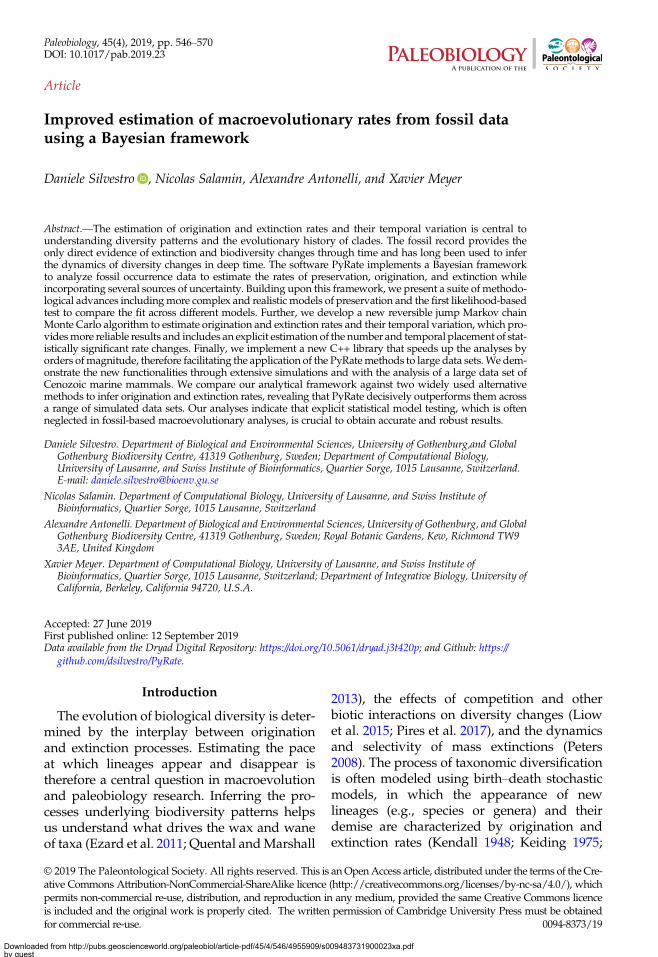
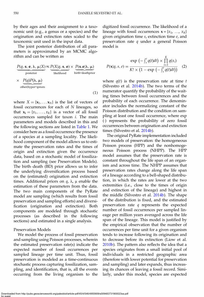
used a hierarchical Bayesian model to jointlyestimate: (1) the times of origination and extinc-tion for each sampled lineage (Fig. 1A), (2) theparameters of a Poisson process modeling

BAYESIAN ESTIMATION OF MACROEVOLUTIONARY RATES 547


fossilization and sampling (Fig. 1B), and (3) therates of origination and extinction and theirtemporal heterogeneity (Fig. 1C) (Silvestroet al. 2014a). This hierarchical structure allowsus to analyze the entire available fossil record,including all known occurrences of a lineage(i.e., not limited to first and last appearances);singletons (lineages sampled in a single occur-rence); and extant taxa, provided that theyhave at least one fossil occurrence (Fig. 1A).The analysis is conducted using MetropolisHastings Markov chain Monte Carlo (MCMC)to obtain posterior estimates of all model para-meters along with the respective 95% credibleintervals (95% CI), providing important infor-mation about the level of uncertainty surround-ing the estimates.The complexity of this Bayesian probabilistic

framework comparedwith alternativemethods(e.g., Foote 2001; Alroy 2014; Liow and Finarelli2014) means that a PyRate analysis will typic-ally require a computation time that is longerthan that required by other methods by ordersof magnitude. While recent studies have com-pared the performance of these alternativemethods using simulated data sets (Smiley2018), it remains unclear whether PyRate’sadditional computational burden does in factreturn an improved accuracy in the estimatedrates of origination and extinction.One of the main and most challenging aims

of the PyRate method is the estimation of howorigination and extinction rates vary throughtime, which is done using a birth–deathMCMC (BDMCMC) algorithm (Silvestro et al.2014b) to sample the number and temporalplacement of rate shifts in a single analysis.The power of this algorithm, however, becomeslimited with increasing levels of rate heterogen-eity through time and with large data sets(Silvestro et al. 2014b), thus making the methodpotentially unsuitable to analyze complex evo-lutionary histories. Another limitation of themethod is that model testing is focused on find-ing the best birth–death model, while thechoice between different preservation models(e.g., with homogeneous or nonhomogeneousrates) remains somewhat arbitrary (e.g., Silves-tro et al. 2015b).Here, building upon the PyRate platform, we

develop novel features that expand the scope

FIGURE 1. PyRate’s main analytical structure. The inputdata consist of dated fossil occurrences assigned to lineages,e.g., species or genera (represented by circles in A), includ-ing singletons and extant taxa. The Bayesian frameworkjointly estimates the life spans of all lineages (dashedlines), preservation rates (B), and origination and extinctionrates (C). All parameter estimates are inferred as posteriormean values (solid lines in B and C) and 95% credible inter-vals (shaded areas in B and C).

DANIELE SILVESTRO ET AL.548


and applicability of the program, providingnovel models of fossil preservation andimproved algorithms. Specifically we (1) intro-duce more realistic preservation models thatsimultaneously allow rate heterogeneity acrosslineages and through time and develop amaximum-likelihood framework to statisticallychoose the preservation model that best fits thedata. (2)We present a more powerful algorithmto infer temporal variation in origination andextinction rates using reversible jump MCMC(RJMCMC; a Bayesian algorithm that jointlyinfers the number of rate shifts best explainingthe data and the parameter values [Green 1995])and compare its performancewith the alternativeBDMCMC algorithm, demonstrating improvedresults on simulated data. (3) We compare theperformance of PyRate against two alternativeapproaches, the boundary-crossing method(Foote 2003) and the three-timer method (Alroy2014). We analyze simulated data sets generatedunder different origination and extinction

scenarios and compare the accuracy across esti-mates. (4) We demonstrate some of the novelfeatures developed here with a workedexample by analyzing a recently publisheddata set of marine mammals (Pimiento et al.2017) and provide extensive tutorials withdetailed descriptions of analysis setup and out-put processing. (5) Finally, we develop a C++library which is integrated in the PyRate pro-gram and speeds up the analyses by orders ofmagnitude, thus extending the applicability ofthe method to very large data sets.

Methods

PyRate implements a hierarchical Bayesianmodel that jointly samples the preservationrates (indicated by q), the times of originationand extinction for each sampled lineage (indi-cated by vectors s, e), and the origination andextinction rates (indicated by λ and μ). Theinput data are fossil occurrences characterized

TABLE 1. Glossary defining the main terms, acronyms, and parameters used in this study.

ModelsBD Birth–death model of origination and extinctionBDS Birth–death model with shifts in origination and/or extinction rates through timeHPP Homogeneous Poisson process—constant preservation rateNHPP Nonhomogeneous Poisson process—preservation rate changes during the life span of each lineage,

following a bell-shaped trajectoryTPP Time-variable Poisson process—preservation rates vary across time windows+G Gamma model—can be coupled with any preservation model (HPP, NHPP, TPP) to incorporate

heterogeneity in preservation rates across lineagesParametersxi = x1, . . . , xK{ } Vector of fossil occurrences for taxon iX = x1, . . . , xN{ } List of vectors of fossil occurrences across all sampled taxas Vector of times of originatione Vector of times of extinctionq Preservation rate—expected number of fossil occurrences per sampled lineage per time unitq = q1, . . . , qW

{ }Vector of preservation rates across W time windows (TPP model)

α Shape parameter of the gamma distribution modeling preservation rate heterogeneity across lineages(+G models)

Λ Origination rate—expected number of origination events per sampled lineage per time unitμ Extinction rate—expected number of extinction events per sampled lineage per time unitΛ = {λ0, …, λJ} Vector of origination rates through time delimited by J rate shifts (BDS model)

M = {μ0, …, μH} Vector of extinction rates through time delimited by H rate shifts (BDS model)

tL = tL1 , . . . , tLJ

{ }Vector times of shift in origination rates

tM = tM1 , . . . , tMH{ }

Vector times of shift in extinction rates

AlgorithmsMCMC Markov chain Monte Carlo—algorithm to jointly estimate the parameters of a given birth–death and

preservation modelBDMCMC Birth–deathMCMC to jointly estimate themodel parameters and the number and temporal placement

of rates shifts in origination and extinctionRJMCMC Reversible jump MCMC to jointly estimate the model parameters and the number and temporal

placement of rates shifts in origination and extinction



by their ages and their assignment to a taxo-nomic unit (e.g., a genus or a species) and theorigination and extinction rates scaled to thetaxonomic unit used in the input data.The joint posterior distribution of all para-

meters is approximated by an MCMC algo-rithm and can be written as

P(q, s, e, l,m|X)︸��︷︷��︸posterior

/P(X|q, s, e)︸��︷︷��︸likelihood

× P(s,e|l,m)︸��︷︷��︸birth-deathprior

× P(q)P(l,m)︸��︷︷��︸other(hyper-)priors

(1)

where X = {x1, . . . xN} is the list of vectors offossil occurrences for each of N lineages, sothat xi = {x1, . . . , xK} is a vector of all fossiloccurrences sampled for taxon i. The mainparameters and models described in this andthe following sections are listed in Table 1. Weconsider here as a fossil occurrence the presenceof a species at a sampling locality. The likeli-hood component of the model allows us to esti-mate the preservation rates and the times oforigin and extinction given the occurrencedata, based on a stochastic model of fossiliza-tion and sampling (see Preservation Models).The birth–death (BD) prior allows us to inferthe underlying diversification process basedon the (estimated) origination and extinctiontimes. Additional priors on q, λ, μ enable theestimation of these parameters from the data.The two main components of the PyRatemodel are sampling (which results from fossilpreservation and sampling efforts) and diversi-fication (origination and extinction). Bothcomponents are modeled through stochasticprocesses (as described in the followingsections) and estimated in a single analysis.

Preservation ModelsWe model the process of fossil preservation

and sampling using Poisson processes, whereinthe estimated preservation rate(s) indicate theexpected number of fossil occurrences persampled lineage per time unit. Thus, fossilpreservation is modeled as a time-continuousstochastic process capturing fossilization, sam-pling, and identification, that is, all the eventsoccurring from the living organism to the

digitized fossil occurrence. The likelihood of alineage with fossil occurrences x = {x1, …, xK}given origination time s, extinction time e, andpreservation rate q under a general Poissonmodel is

P(x|q, s, e) =exp − �e

s q(t)dt( )× ∏K

i=1q(xi)

K!× 1− exp − �es q(t)dt

( )( ) (2)

where q(t) is the preservation rate at time t(Silvestro et al. 2014b). The two terms of thenumerator quantify the probability of the wait-ing times between fossil occurrences and theprobability of each occurrence. The denomin-ator includes the normalizing constant of thePoisson distribution and the condition on sam-pling at least one fossil occurrence, where exp(·) represents the probability of zero fossiloccurrences between origination and extinctiontimes (Silvestro et al. 2014b).The original PyRate implementation included

two models of preservation: the homogeneousPoisson process (HPP) and the nonhomoge-neous Poisson process (NHPP). The HPPmodel assumes that the preservation rate isconstant throughout the life span of an organ-ism and across time. The NHPP assumes thatpreservation rates change along the life spanof a lineage according to a bell-shaped distribu-tion, in which the rates are lower at the twoextremities (i.e., close to the times of originand extinction of the lineage) and highest inthe middle (Silvestro et al. 2014b). The shapeof the distribution is fixed, and the estimatedpreservation rate q represents the expectednumber of fossil occurrences per sampled lin-eage per million years averaged across the lifespan of the lineage. This model is justified bythe empirical observation that the number ofoccurrences per time unit for a given organismtends to increase following its origination andto decrease before its extinction (Liow et al.2010b). The pattern also reflects the idea that aspecies originates from a small initial pool ofindividuals in a restricted geographic area(therefore with lower potential for preservationand sampling) and later expands, thus increas-ing its chances of leaving a fossil record. Simi-larly, under this model, species are expected



to decline in abundance and geographic rangebefore their extinction (Raia et al. 2016), result-ing in decreased preservation rates.Both HPP and NHPP models can be coupled

with a gamma model (i.e., HPP +G andNHPP +G), which allows us to incorporaterate heterogeneity across lineages. Underthese models, preservation rates are definedso that their mean equals q and their hetero-geneity is distributed according to a gammadistribution, with shape parameter α, discre-tized in a user-defined number of categories(Yang 1994; Silvestro et al. 2014b). The rate par-ameter of the gamma distribution is set equalto the shape, so the distribution has meanequal to 1. Both q and α are estimated as freeparameters by the MCMC, and small valuesof α indicate increased amounts of heterogen-eity. Gamma models do not assign individualpreservation rates to each lineage in the dataset. Instead, the likelihood of each lineage isaveraged across all rates, thus incorporatingrate heterogeneity across lineages while add-ing a single additional parameter (α) to themodel (Yang 1994).Here, we introduce a third preservation

model that implements a time-variable Poissonprocess (TPP). The TPPmodel is an extension ofthe HPP, in which the rate of preservation isconstant within predefined time windows butallowed to change between them. For instance,different preservation rates can be estimatedwithin geological epochs (Foote 2001; Liowand Nichols 2010). The likelihood of this pro-cess is the product of piecewise HPP likeli-hoods across multiple time frames, each withits specific preservation rate (q = {q1, …, qW},where W is the number of time windows in themodel). As for the HPP and NHPP models, theTPP can be coupledwith a gammamodel, there-fore allowing for rateheterogeneityboth throughtime and across lineages.The default prior specified for q is a gamma

distribution, chosen to reflect the fact that pres-ervation rates must take positive and realvalues. Defining appropriate prior distribu-tions is often a challenge in Bayesian analysis,and prior choice can strongly affect the effectiveparameter space and the complexity of a model(Gelman et al. 2013). This may become evenmore problematic under the TPP model, in

which very strict priors could artificially reducerate heterogeneity through time, whereas veryvague priors could unnecessarily expand theamount of parameter space, increasing therisk of overparameterization. To overcomethis issue, we use a hyper-prior to estimatethe prior on the preservation rates from thedata, instead of setting the prior to a fixed dis-tribution. We set a single gamma distributionas prior on the preservation rates q, with afixed shape parameter (α = 1.5) and unknownrate parameter β. The rate parameter isassigned a vague gamma hyper-prior, β∼ Γ(a= 1.01, b = 0.1), and is itself estimated by theMCMC. Estimating the rate using a hyper-priormakes the gamma prior on qmore adaptable todifferent data sets and reduces the subjectivityof prior choices. Using the properties of the con-jugate gamma prior, whereby the posterior dis-tribution of the rate parameter of a gammalikelihood with known shape and gamma-distributed prior is itself a gamma distribution(Gelman et al. 2013), we can sample the rateparameter β directly from its posterior distribu-tion, given any vector of preservation rates q,the shape parameter α, and shape and rate ofthe prior a, b:

P(b|q,a, a, b) � G a+ aW, b+∑Wi=1

(qi)( )

. (3)

A Maximum-Likelihood Test to ComparePreservation ModelsBecause the preservation process represents

a fundamental component of the PyRatemodel (Fig. 1A,B), it is important to choosethemodel that best fits the datawhen analyzinga fossil data set. To this end, we developed alikelihood-based test to assess the statistical fitof alternative preservation processes. The pres-ervation process, with constant or variablerates, is expected to leave a signature in the tem-poral distribution of fossil occurrences, whichwill tend to be roughly uniformly distributedunder an HPP model (Fig. 2A), to show higherdensity of record toward the center of a species’life span under the NHPP model (Fig. 2B) andto follow time-variable distributions underthe TPP model (Fig. 2C).



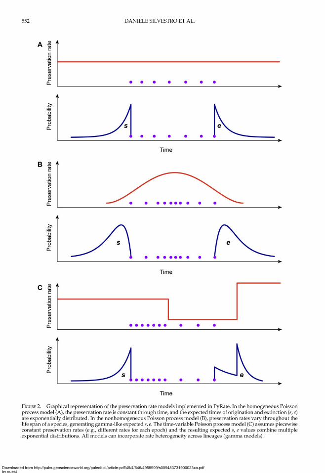
FIGURE 2. Graphical representation of the preservation rate models implemented in PyRate. In the homogeneous Poissonprocessmodel (A), the preservation rate is constant through time, and the expected times of origination and extinction (s, e)are exponentially distributed. In the nonhomogeneous Poisson process model (B), preservation rates vary throughout thelife span of a species, generating gamma-like expected s, e. The time-variable Poisson process model (C) assumes piecewiseconstant preservation rates (e.g., different rates for each epoch) and the resulting expected s, e values combine multipleexponential distributions. All models can incorporate rate heterogeneity across lineages (gamma models).



Although it is theoretically possible to inferthe marginal likelihood of a preservationmodel in a Bayesian framework (for instanceusing the thermodynamic integration availablein PyRate to test between alternative birth–death models [Lartillot and Philippe 2006;Silvestro et al. 2014b]), the task would be com-putationally extremely demanding. Indeed,the number of parameters over which thelikelihood needs to be marginalized can bevery high, including the vectors of originationand extinction times, the preservation rates,and potentially the parameters of the birth–death prior. Thus, we implemented amaximum-likelihood test for preservationmod-els that substantially reduces the computationalburden. This maximum-likelihood test isintended as a first step in the analysis of a fossildata set, inwhich the best preservationmodel isidentified. Then, the full Bayesian analysis ofpreservation, origination, and extinction ratesis performed under the selected preservationmodel (see also Analysis Protocol for MarineMammals, Supplementary Material).Let s and e be the expected times of origin-

ation and extinction of a lineage with fossiloccurrences x = {x1, . . . , xK} (sorted from oldestto most recent) for a given preservation rate q.To compare the fit of different models, wemaximize the likelihood P(x, s, e|q), where q istreated as a free parameter and estimated inthe optimization, while s and e are calculatedbased on the preservation rate and model. Inthe simplest case of an HPP of preservation,the expected times of origination and extinctionare determined by the expectation of an expo-nential distribution with rate equal q: E[Exp(q)]= 1/q. Thus, under HPP, the expected times oforigination and extinction are s = x1 + 1/q ande = xK − 1/q (Fig. 2A). Note that the expectedtimes of origination and extinction differ fromtheir maximum-likelihood estimates, whichunder HPP are sML = x1 and eML = xK.In the case of the NHPP model, neither the

expectation nor the maximum-likelihoodvalues of s and e are easily derived analytic-ally. Instead, we use a two-step approach toobtain a maximum-likelihood value that iscomparable to that obtained under HPP.First, we optimize the rate q by maximizingthe likelihood P(x|q, s, e), where q, s, and e

are treated as free parameters. This results inmaximum-likelihood estimates of the preserva-tion rate (qML) and origination and extinctiontimes (sML and eML). Second, because the likeli-hoods of different preservation models arecompared based on the expected originationand extinction times (i.e., not their maximum-likelihood values), we use MCMC samplingto infer s and e, given the estimated rate qML

(Fig. 2B). The MCMC samples from the poster-ior probability

P(s, e|qML, x)/ P(x|qML, s, e) × P(s) P(e) (4)

where P(s) � U(x1,1) and P(e) � U(0, xK) areuniform priors on origination and extinctiontimes. These priors, while unrealistic, essen-tially imply that the acceptance probability oftheMCMC is only driven by the likelihood sur-face. We sample 1000 values of s and e and usetheir mean as expected origination and extinc-tion times sq, and eq. Once we have obtainedq, sq, and eq, we can calculate the likelihood ofthe data given the model and use it for modelcomparison.Under the TPP model, the expected times

of origination and extinction are determinedby a combination of exponential expectationswith rate parameters (i.e., preservation rates)q = {q1, …, qW}, truncated at the boundariesof each of W time window (Fig. 2C). Forany given preservation rate q, we use numer-ical integration to approximate the resultingdistribution and obtain expected values forthe times of origination and extinction (s, e).We use maximum likelihood to optimize thevector of preservation rates.The likelihood of a data set encompassing

multiple taxa, under any preservation model,is the product of the individual likelihood ofeach lineage (Silvestro et al. 2014b). For the pur-pose of model testing between HPP, NHPP,and TPP models, we assume that the preserva-tion rates are constant across lineages andtherefore optimize a single parameter q (orvector of parameters q under the TPP model)to obtain the maximum likelihood of the data.We then calculate the fit of each model usingthe Akaike information criterion corrected forsample size (AICc), based on the number ofanalyzed lineages (Burnham and Anderson



2002). We consider this test as a useful tool tochoose between qualitatively different preser-vation processes (HPP, NHPP, and TPP) andadvise researchers to always couple the best-fitting Poisson process with the gamma modelin empirical analyses. The risk that thegammamodel represents an overparameteriza-tion of the preservation process is minimal,because the gamma model only adds a singleparameter to incorporate any potential amountof rate heterogeneity across clades (Silvestroet al. 2014b). Additionally, virtually all empir-ical data sets we have analyzed so far indicatedvery high levels of rate variation across clades(see also “Results”).

AICc Thresholds and Testing.—We used simu-lated data to assess the performance of our like-lihood test for preservation models. Wesimulated 1000 data sets of fossil occurrencesunder each of three models (HPP, NHPP, andTPP). Each simulation included 100 lineages,with life span determined by a randomlysampled extinction rate m � U[0.05, 0.5],reflecting a realistic range of extinction rates(Pimiento et al. 2017). Thus, for the propertiesof the birth–death process (Kendall 1948), thedistribution of life spans followed an exponen-tial distribution with mean 1/μ. Fossil occur-rences were then simulated based on eachPoisson process with a rate q randomly drawnfrom U[0.05, 3.5]. The rate q represented themean preservation rate for each lineage inNHPP simulations (Silvestro et al. 2014b).In TPP simulations, we simulated one shiftin preservation rate occurring halfwaybetween the origination time of the oldest lin-eage and the most recent extinction time. Thepreservation rate after the shift was then setto 5 × q.Although singletons (i.e., lineages repre-

sented by a single fossil occurrence) can be ana-lyzed and are usually included in PyRateanalyses, they should be removed when theaim to compare the fit of different preservationmodels. While singletons contribute to the cor-rect inference of preservation rates in an ana-lysis aimed at parameter estimation, at leastone waiting time between occurrences isneeded when testing among preservationmodels. Singletons are therefore removed auto-

matically from the data when using the model-testing function implemented in PyRate. Thus,before running the test on simulated data, weremoved all lineages with fewer than 2 occur-rences. This procedure left, depending on thesimulation settings, between 10 and 100sampled lineages, providing a range of datasizes.We used simulations to define the appropri-

ate ΔAICc thresholds necessary to confidentlychoose between preservation models. Whilethe model yielding the smallest AIC score canbe considered as best fitting (Burnham andAnderson 2002), small differences in AICcvalues might be difficult to interpret, and thethreshold for significance is often obtainedthrough simulations (e.g., Dib et al. 2014;Pennell et al. 2014). Additionally, empiricallyverifying the accuracy of model testing is espe-cially important here, because the optimizationinvolves a combination of analytical expecta-tions of origination and extinction times forHPP and numerical approximations forNHPP and TPP. Thus, we used the 3000 simu-lations (for which the true generating model isknown) as a training set and for each computedAICc score under the three preservation mod-els. Based on the resulting distributions ofAICc scores, we determined the ΔAICc thresh-olds that yielded less than 5% errors and lessthan 1% errors in model selection. We thensimulated an additional 300 data sets (100 foreach preservation model) to verify the appro-priateness of the thresholds (SupplementaryFigs. S1–S3).

Time-Variable Birth–Death ModelsThe temporal distribution of origination

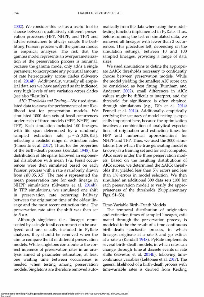
and extinction times of sampled lineages, esti-mated through the preservation process, ismodeled to be the result of a time-continuousbirth–death stochastic process, in whichlineages originate at a rate λ and go extinctat a rate μ (Kendall 1948). PyRate implementsseveral birth–death models, in which rates canchange through time at discrete events or rateshifts (Silvestro et al. 2014b), following time-continuous variables (Lehtonen et al. 2017). Thegeneral likelihood of a birth–death process withtime-variable rates is derived from Keiding



(1975):

P(s, e|l,m)/∏Ni=1

l(si)× m(ei)Ii

× exp −∫eisi

l(t) + m(t) dt( )

(5)

where N is the number of lineages, λ(t) is theorigination rate at time t, μ(t) is the extinctionrate at time t, and Ii is an indicator set to Ii = 1if species i is extinct (ei >0) and Ii = 0 if speciesi is extant (in which case the extinction time ei= 0 is not sampled as a parameter).A birth–death model with rate shifts (BDS) is

characterized by changes in rates of originationand extinction at shift times, while the rates areconstant between shifts (Silvestro et al. 2014b).TheBDSmodel isdescribedbyavectorof origin-ation ratesΛ = {λ0, λ1,…, λJ} delimitedby timesofshifts tL = {tL1 , . . . , t

LJ } and by extinction rates

M = {μ0, μ1, …, μH} delimited by times of shiftstM = {tM1 , . . . , t

MH }, where J and H represent the

number of origination and extinction rate shifts,respectively. Under this notation, originationand extinction rates are constant and equal toλ0 and μ0, respectively, when themodel includesno rate shifts. The original PyRate implementa-tion used a Bayesian algorithm, the BDMCMC(Stephens 2000), to jointly infer the number ofrate shifts ( J and H ), the rates between shifts(Λ, M ), and the times of rate shift (τΛ, τM).While we showed BDMCMC to be able to cor-rectly infer rate variation under several scen-arios, it tends to be too conservative inassessing rate heterogeneity through timewhen the true generating process involves sev-eral rate shifts (Silvestro et al. 2014b). In the fol-lowing sections we develop an alternativemethod to estimate birth–death models withrate shiftsusing themoregeneralRJMCMCalgo-rithm (Green 1995) and demonstrate throughsimulations that it outperforms BDMCMC.

Inferring Rate Variation Using RJMCMCTheRJMCMCalgorithm is amodifiedversion

of the standard Metropolis-Hastings MCMC, inwhich the model (here the number of rate shifts)is itself considered a parameter. In a maximum-likelihood framework, model testing is typically

done using AIC or similar metrics that penalizeparameter-rich models to find the best balancebetween model fit and its complexity. TheRJMCMC algorithm “jumps” across differentmodels and uses the posterior ratio to avoidunder- and overparameterization. The result ofRJMCMC is a posterior sample of parametervalues (here origination and extinction ratesthrough time) averaged over model uncertaintyand posterior probabilities associated with eachmodel, while incorporating the uncertaintiesassociated with the preservation process.In the RJMCMC framework, the number of

rate shifts is considered an unknown variableand is estimated from the data. To this endwe include two additional types of proposals:namely, the forward move and the backwardmove, which add or remove rate shifts, respect-ively, thus changing the number of parametersin the birth–death model. Given that thesemoves are identical for both speciation andextinction rates, we use the notationΦ to denoteeither the speciation (Λ) or extinction (M ) rates.We indicate the time frames identified by rateshifts with Δ = {δ0, δ1,…, δK−1}. Under this nota-tion, we set δi = τi− τi+1, where τ is the time ofrate shift for 0 < i≤K, whereas t0 = max(s) andtK+1 = min(e) represent themaximumandmin-imum ages, respectively, of the full birth–deathprocess spanned by the data. A given set oftime framesΔof lengthK is associatedwithavec-tor of rate parameters Φ = {ϕ0, ϕ1,…, ϕK}.The RJMCMC algorithm requires a modifica-

tion in the acceptance rule of a standardMCMC in order to maintain its reversibilitywhilemoving across models with different para-meterizations (Green 1995). The general form ofthe acceptance probability for a forward move(i.e., adding a rate shift) can be written as min{1, A(θ, θ′)}, where θ and θ′ are the model para-metersof the currentandnewstates, respectively,and A(θ, θ′) is the product of three main terms:

A(u, u′) = p(u′)p(u)︸�︷︷�︸

Posterior ratio

×P(M|M′)P(M′|M) ×

P(u|u′)P(u′|u)︸��︷︷��︸

Hastings ratio

× ∂(u′)∂(u, u)

∣∣∣∣∣∣∣∣︸��︷︷��︸

Jacobian

(6)



The first term is the posterior ratio, that is, theratio between unnormalized posterior probabil-ities, of the new state over the current state(where π(·) indicates the posterior as in eq. 1).The second term, often referred toas theHastingsratio (e.g., Heath et al. 2014), describes the ratiobetween the probability of going back from thenew state to the current one and the probabilityof proposing the new state given the currentone. This term includes the probability of a for-ward move, which generates a new model M′

from the current one M by adding a rate shiftand the probability of a backward move, whichremoves a rate shift. The Hastings ratio alsoincludes the probability of proposing a new par-ameter state θ′ from the current one θ and viceversa. Note that the new and current states willdiffer in the number of parameters by one add-itional time of rate shift and one additional rateshift. The third term is the Jacobian of the deter-ministic functionmapping thevalues of the para-meters of the current state into the parameters ofthe new state and corrects for the change in thedimensionality of the parameter space. Theacceptance probability of a backward move (i.e.,removing a rate shift) can be directly deducedfrom the associated forward move. The movefrom a model with parameters θ (with K rates)to amodelθ′ (withK− 1 rates) has the acceptanceprobability set to min[1, A(θ′, θ)], with

A(u′, u) = A(u, u′)−1. (7)

Probability of a Reversible Jump.—In ourimplementation, forward and backwardmoves are selected with equal probabilityP(MK+1|MK) = P(MK|MK+1) = 0.5, exceptfor the boundary cases K = 1 and K = Kmax,where Kmax is the maximum allowed numberof rate shifts. When K = 1, that is, constantrates and no rate shift, forward moves areproposed with probability 1, while only back-ward moves are proposed when K = Kmax. Toavoid numerical issues (e.g., overflows),PyRate does not allow time windows smallerthan 1 time unit (i.e., δ ≥ 1), therefore result-ing in Kmax = τK+1 − τ0.

Forward Move: Adding a New Rate Shift.—Aforward move from model MK to MK+1 isdone by splitting an existing time frame into

two time frames to which new rates areassigned. We first select a time frame δi ran-domly from Δ and split it into two time framesδx, δy by drawing a new time of rate shift τ′ fromU(ti, ti+1). Because δx + δy = δi, we can calculatethe relative weight of the two new time framesas wx = δx/δi and wy = δy/δi. We then assign therates ϕx and ϕy to the new time frames to replacethe original ϕi. Although the new rates could bedrawn from independent distributions, wechoose ϕx and ϕy, such that their weighted geo-metric mean equals the original rate ϕi, whichwas shown to be more efficient in Poisson pro-cesses with rate shifts Green (1995). Theweights arewx andwy (i.e., based on the relativesize of the new time frames) and the new ratesare chosen so that

fi = exp [wx log(fx) + wy log(fy)] (8)

We draw a random variable u from a beta dis-tribution B(a,b) that quantifies the amount ofdiscrepancy between rates ϕx and ϕy by usingthe following equation

1− uu

= fy

fx.

We therefore generate the new rates as:

fx = exp {log (fi) − wy log [(1− u)/u]} (9)

fy = exp {log(fi) + wx log [(1− u)/u]} (10)

The parameters of the beta distribution are setby default to α = β = 10, yielding an expectedE[u] = 0.5, with 95% of the values rangingfrom 0.29 to 0.71. We chose these values asthey provided good convergence in our tests,although PyRate includes commands to easilytweak this and other tuning settings.The Hastings ratio for a forward moveMk→

Mk+1 is computed as

P(M|M′)P(M′|M) ×

(K + 1)−1

(K + 1)−1 ×1

P(u|a,b)× 1

(di)−1 , (11)



where the first ratio is based on the simple rulesdescribed earlier and allows forward and back-ward moves with equal probabilities when 1< K < Kmax. The numerator and denominatorof the second ratio define the uniform probabil-ity of drawing one of the K rate shifts from thenew model MK+1 and the uniform probabilityof drawing one of the K time frames from thecurrent model MK, respectively (noting that amodel with K rate shifts includes K + 1 timeframes). The two following denominators iden-tify the probability of drawing u from its distri-bution β(α, β), where P(u|α, β) is based on theprobability density function of a beta distribu-tion and the probability of uniformly drawinga new rate shift within time frame δi. TheJacobian for the transformation of variables(ϕi, u)→ (ϕx, ϕy) (eq. 9) is equal to (Green 1995):

∂(fx,fy)

∂(fi, u)= (fx + fy)2

fi. (12)

Backward Move: Removing an Existing RateShift.—A backward move from model MK+1

to MK is done by removing an existing rateshift and merging the two adjacent time framesand their rates. The first step is to randomlyselect a rate shift J over the K− 1 existingones. The temporal placement of the rate shiftis τj, and its adjacent time frames are identifiedas δj−1 and δj. Thus, the rates ϕx and ϕy are com-bined toobtainanewrateϕibasedonequation (8).For a backward move MK+1 � MK, the

same computations are applied, but the Hast-ings ratio and the Jacobian must be invertedas defined in equation (7). The value u mustbe defined using equation (9) in order to com-pute P(u|α, β).

Priors on the Number of Shifts.—Because thenumber of origination and extinction rates(J and K, respectively) are considered unknownvariables in the RJMCMC implementation, weassign them a prior distribution to samplethem from their posterior distribution. We usea single Poisson distribution with rate param-eter r to compute the prior probability of Jand K. To reduce the subjectivity of the prior,we consider r itself an unknown parameterand estimate it from the data. We assign agamma hyper-prior, which allows us to sample

r directly from its conjugate posterior distribu-tion for any given J and K values:

P(r|J,K,a,b) � G(a+ J + K, b+ 2), (13)

where α and β are the shape and rate para-meters of the gamma hyper-prior distribution.In our simulations, we use the hyper-prior Γ(α = 2, β = 1), which sets the highest prior prob-ability to models with constant origination andextinction rates (i.e., mode = 1).

Marginal Origination and Extinction Rates.—To summarize the origination and extinctionrates sampled by RJMCMC, we marginalizethem within arbitrary small (user-defined)time bins. We emphasize that this proceduredoes not imply that the birth–death processitself is discretized in time bins, as both the ori-gination and extinction events are modeledwithin a time-continuous stochastic process.The marginal distributions of origination andextinction rates incorporate uncertainties on:(1) the true times of origination and extinctionof sampled lineages, which are themselves afunction of the preservation process; (2) thenumber of rate shifts as sampled by theRJMCMC; and (3) the temporal placement ofthe rate shifts. We summarize the marginalrates by computing their posterior mean and95% credible intervals (95% CI).

Timing of Significant Rate Shifts.—We imple-mented a function to assess the timing of sig-nificant rate changes based on the RJMCMCposterior samples. To this end, we computethe frequency of sampling a rate shift (usingarbitrarily small time bins) and plot themagainst time to assess when rate shifts aremore likely to have occurred. To assess whetherthe frequency of a rate shift significantlyexceeds the prior expectation, we run anMCMC simulation in which the number andtimes of rate shifts are purely sampled fromtheir respective priors, that is, a uniform distri-bution on the times of shift and Poisson distri-butions on the number of speciation andextinction rates with a gamma prior assignedto its hyper-parameter r (see previous para-graph). From the samples obtained from thesimulation, we compute the prior probabilityof a rate shift at any given time, based on theuser-specified size of the bins.



We then compute the posterior sampling fre-quencies corresponding to significant statisticalsupport based on the standard log Bayes fac-tors thresholds (so that 2log BF = 2 and 6, forpositive and strong support, respectively)(Kass and Raftery 1995).Given the two alternative hypotheses (pres-

ence or absence of a shift in a bin), we can definethe Bayes factor as the posterior odds dividedby the prior odds (Kass and Raftery 1995):

BF = P(t|D)1− P(t|D) /

P(t)1− P(t)

, (14)

where P(τ|D) is the posterior probability of arate shift, and P(τ) is its prior probability.After solving the equation for the posteriorterm, we obtain that the posterior probabilitycorresponding to a 2log BF = x is

P(t|D) = A1+ A

, where A

= expx2

( ) P(t)1− P(t)

. (15)

We implemented these calculations directlyinto a single function that generates plots ofmarginal origination and extinction ratesthrough time and posterior frequencies of rateshifts through time, with dashed lines indicat-ing positive and strong statistical supportbased on Bayes factors (i.e., 2 log BF = 2 and 6,respectively [Kass and Raftery 1995]).

Validation of the Method through SimulationsWe tested the new RJMCMC algorithm on

simulated data sets and compared its perform-ance with that of the BDMCMC algorithm pre-viously implemented in PyRate. We simulatedfossil data sets under three different birth–death scenarios:

1. Constant origination and extinction rates setto 0.15 and 0.07, respectively, with root ageset to 45 Ma.

2. Time-variable birth–death model with 2 rateshifts in origination and 2 rate shifts inextinction. The time of origin was set to 35,with origination rate shifts at 20 and 10 Maand extinction rate shifts at 15 and 10 Ma.Origination rates decreased across time

windows [Λ = (0.4, 0.1, 0.01)], whereasextinction rates peaked between 15 and10 Ma [M = (0.05, 0.3, 0.01)].

3. Time-variable birth–death model with 4 rateshifts in origination (at 30, 18, 15, and 7 Ma)and 4 rate shifts in extinction (at 25, 22,17, and 2). Origin time was set to 45 Ma,and the rates between shifts were: Λ = {0.3,0.07, 0.6, 0.05, 0.3} and M = {0.02, 0.6, 0.05,0.2, 0.5}.

We simulated 100 data sets under each scenario,assuming a homogeneous Poisson process ofpreservation, with rate drawn from a uniformdistribution q � U[0.5, 1.5]. To avoid extremelysmall or large data sets, we constrained thesimulations to yield between 150 and 250lineages. We analyzed each data set usingboth BDMCMC and RJMCMC, running2,000,000 MCMC iterations for each algorithmand sampling every 1000 iterations.We assessed the performance of the

BDMCMC and RJMCMC algorithms by quan-tifying their ability to infer the correct numberof rate shifts and the accuracy and precision ofthe origination and extinction rates, margina-lized within 1 Myr time bins. We computedthe posterior probability of models with differ-ent numbers of rate shifts based on their sam-pling frequencies and compared them withthe true values used to simulate the data. Toquantify the accuracy of rate estimates, weused the posterior mean of the marginal ratesat different times and calculated the relativeerror as the absolute difference between theestimated rate (rest) and the true rate (rtrue) rela-tive to their mean, that is, (|rest− rtrue|)/[(rtrue+ rest)/2]. Relative errors were then averagedacross rates and among simulations. We alsosummarized the precision of the rate estimatesin terms of size of the 95% CI relative to themean rate, again averaged across rates andamong simulations.

Comparisons with Other ApproachesWe analyzed the same simulated data sets

using two alternative methods to infer origin-ationandextinction rates, theboundary-crossingmethod (Foote 2000) and the three-timermethod(Alroy 2015) as implemented in the R package‘fbdR’ (github.com/rachelwarnock/fbdR). We



http://github.com/rachelwarnock/fbdR

binned fossil occurrences based on 20 timeintervals of equal size (bin size of 1.75–2.25 Myr depending on the simulation) andinferred origination and extinction rates withineach bin. Although there exist methods to infersome confidence intervals around rate esti-mates (Foote 2001), these are not necessarilycomparable with the 95% credible intervalsobtained from Bayesian inferences. Thus, wefocused the comparison on the accuracy of theestimates, rather than on their precision(which was only evaluated for the PyRatemethod; see Validation of the Method throughSimulations). We therefore quantified theaccuracy of the estimates by computing therelative errors averaged through time as donefor the PyRate estimates and compared relativeerrors among methods.

Empirical Case StudyWe demonstrate the new PyRate imple-

mentation by analyzing genus-level fossiloccurrences of marine mammals recentlycompiled by Pimiento et al. (2017). The dataincluded 535 genera, 73 of which are extant,and 4740 occurrences spanning from theEocene to the recent. Because the dating ofmost fossil occurrences is given as a temporalrange, we resampled the age of each occur-rence uniformly from its range and produced10 randomized input files, as in Silvestroet al. (2014b). We then repeated all analyseson each replicate and combined the resultsto incorporate dating uncertainties in ourestimates.First of all, we ran a model test to choose the

most appropriate preservation model. Wetested the HPP and NHPP models as well asa TPP model with rate shifts set at the bound-aries between epochs in the Cenozoic. Wetherefore ran the subsequent analyses usingthe best-fitting preservation model andadded the gamma option to allow for rate het-erogeneity across lineages. We assumed abirth–death process with rate shifts and usedthe RJMCMC algorithm to determine the num-ber and temporal placement of the shifts andthe origination and extinction rates throughtime. After running 50 million iterations, sam-pling every 10,000 iterations, we combinedsamples of the 10 randomized data sets to

infer the number of rate shifts and plot origin-ation and extinction rates through time. Thecomplete list of commands used for the empir-ical analyses presented here along all inputfiles are available as Supplementary Material(Dryad Repository: https://doi.org/10.5061/dryad.j3t420p).We analyzed the marine mammal data set

under the boundary-crossing and three-timermethods, for comparison. The ages of fossiloccurrences were randomized 100 times basedon the respective stratigraphic intervals, andthe rates were estimated across equal timebins of 2 Myr, using the R package ‘divDyn’(Kocsis et al. 2019).

Performance BoostBecause of the large number of parameters

estimated in a typical PyRate analysis anddue to the inherent iterative nature of MCMCalgorithms, the analyses of large fossil datasets (e.g., hundreds or thousands of lineages)can be very time-consuming. We thereforedeveloped a Python module named FastPyRa-teC to boost the performance of the analysis.This module consists of a SWIG (http://www.swig.org) wrapper to a fast C++ imple-mentation of PyRate core functions such asthe main likelihood functions (e.g., preserva-tion models and most available birth–deathmodels). This module is precompiled for themain operating systems (see Software Avail-ability), can be easily compiled using a Pythoninstallation script, and requires a single externaldependency, the C++ boost library (http://www.boost.org).We assessed the improvement in perform-

ance by running analyses on three data setsof 50, 150, and 300 lineages (with 543, 1368,and 2736 fossil occurrences, respectively). Weran 100,000 RJMCMC iterations under theHPP, NHPP, and TPP models coupled withthe gamma model of rate heterogeneityamong lineages. Analyses were run on a Mac-intosh computer with a 3.1 GHz Intel Core i7processor. We ran with and without the FAS-

TPYRATEC library to compute the speed-upachieved by the C++ library and estimate thetime necessary to run the default 10 millioniterations, which are the default number ofiterations in PyRate.





http://www.swig.org

http://www.swig.org

http://www.swig.org

http://www.boost.org



Results

Testing among Preservation ModelsThe maximum-likelihood test implemented

to distinguish among alternative preservationprocesses provides a reliable tool to infer thecorrect model. Extensive simulations showthat different δ AIC thresholds can be appliedfor different competing models. For instance,if the best model (smallest AIC) is obtainedfor NHPP, we can reject the HPP model as avalid alternative only if AICHPP-AICNHPP

>3.8 (for a 5% error tolerance) or AICHPP-

-AICNHPP >8 (for a 1% error tolerance).However, the TPP model can be confidentlyrejected simply based on AICTPP-AICNHPP

>0. The full set of thresholds derived fromour simulations is given in Table 2 and incor-porated in the model test as implemented inPyRate 2.0.Our simulations show that the ability to stat-

istically distinguish between preservationmodels (computed as δ AIC scores) generallyincreases with the size of the data set, that is,number of lineages and number of occurrences(Supplementary Figs. S1–S3). Increasing pres-ervation rates also yield stronger support forthe correct model. Additionally, there is aneffect of the extinction rate, whereby lowerextinction rates are associated with better dif-ferentiation between preservation models.This effect is likely linked with the increasedmean longevity of lineages, which thereforetend to accumulate more occurrences.

Performance of RJMCMC Compared withBDMCMCThe RJMCMC algorithm outperformed the

BDMCMC alternative in most simulations(Table 3). The RJMCMC method identifiedthe correct number of shifts in originationrates in 88% of the simulations. In compari-son, the BDMCMC method identified the cor-rect model of origination in 52% of thesimulations. This value is mostly driven by aconsistent underestimation of rate heterogen-eity in simulation scenarios 2 and 3. TheRJMCMC analyses identified the correctmodel of extinction in 67% of the simulations.We note that the correct number of shifts inextinction rates was found in 99% of the simu-lations under scenarios 1 and 2, whereasunder scenario 3 the algorithm consistentlyinferred four rates instead of five, suggestingthat one of the rate shifts did not leave a sig-nificant signature on the simulated fossil data.The BDMCMC analyses correctly identifiedthe absence of extinction rate shifts in scenario1, but were substantially less accurate thanRJMCMC analyses in finding the correctmodel in the case of rate heterogeneity(Table 3).

TABLE 2. Thresholds for change in Akaike informationcriterion (ΔAICc) estimated by simulations to test betweendifferent preservation models. Depending on the selectedbest model (i.e., the one with the lowest AICc score),different thresholds are applied to determine whether themodel is significantly better than the alternatives ( p <0.05).Values in parentheses show the thresholds estimated for p<0.01. Cases in which ΔAICc values do not exceed thethresholds provided here indicate that the evidence in thedata is not sufficient to confidently choose amongpreservation models. HPP, homogeneous Poisson process;NHPP, nonhomogeneous Poisson process; TPP,time-variable Poisson process.

Best model

ΔAICc thresholds

HPP NHPP TPP

HPP — 6.4 (17.4) 0 (0)NHPP 3.8 (8) — 0 (2.4)TPP 3.2 (6.8) 10.6 (23.3) —

TABLE 3. Model testing using the reversible jumpMarkovchain Monte Carlo (RJMCMC ) and birth–death Markovchain Monte Carlo (BDMCMC) algorithms. Thesimulations (replicated 100 times) are based on differentnumbers of origination rates (J ) and extinction rates : (1) J =1,K = 1; (2) J = 3,K = 3; and (3) J = 5,K = 5. For each value of Jand K, we estimated the how frequently it was estimated asthe best model by RJMCMC and BDMCMC across allreplicates. Values in bold represent the frequencies at whichthe correct models were identified by the algorithms.

No. of shifts

Simulation1

Simulation2

Simulation3

RJ BD RJ BD RJ BD

J = 1 0.83 0.91 0 0 0 0J = 2 0.17 0.09 0.02 0.42 0.01 0.09J = 3 0 0 0.98 0.55 0.09 0.6J = 4 0 0 0 0.03 0.06 0.22J = 5 0 0 0 0 0.83 0.09J = 6 0 0 0 0 0.01 0J = 7 0 0 0 0 0 0K = 1 0.99 1 0 0 0 0.01K = 2 0.01 0 0 0.3 0.09 0.7K = 3 0 0 0.99 0.13 0.23 0.16K = 4 0 0.01 0.56 0.65 0.13K = 5 0 0 0 0 0.03 0K = 6 0 0 0 0 0 0K = 7 0 0 0 0 0



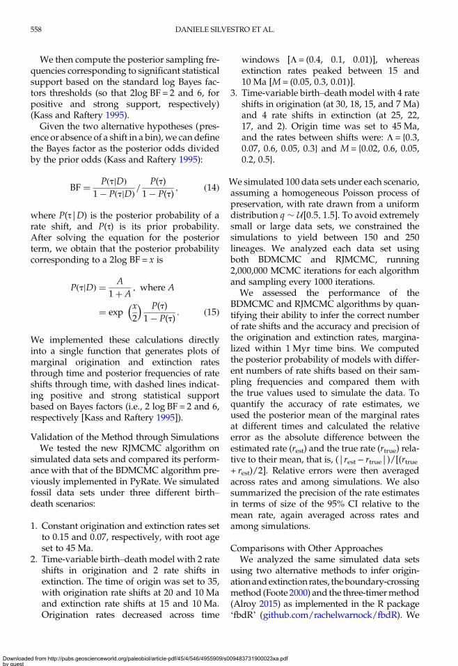
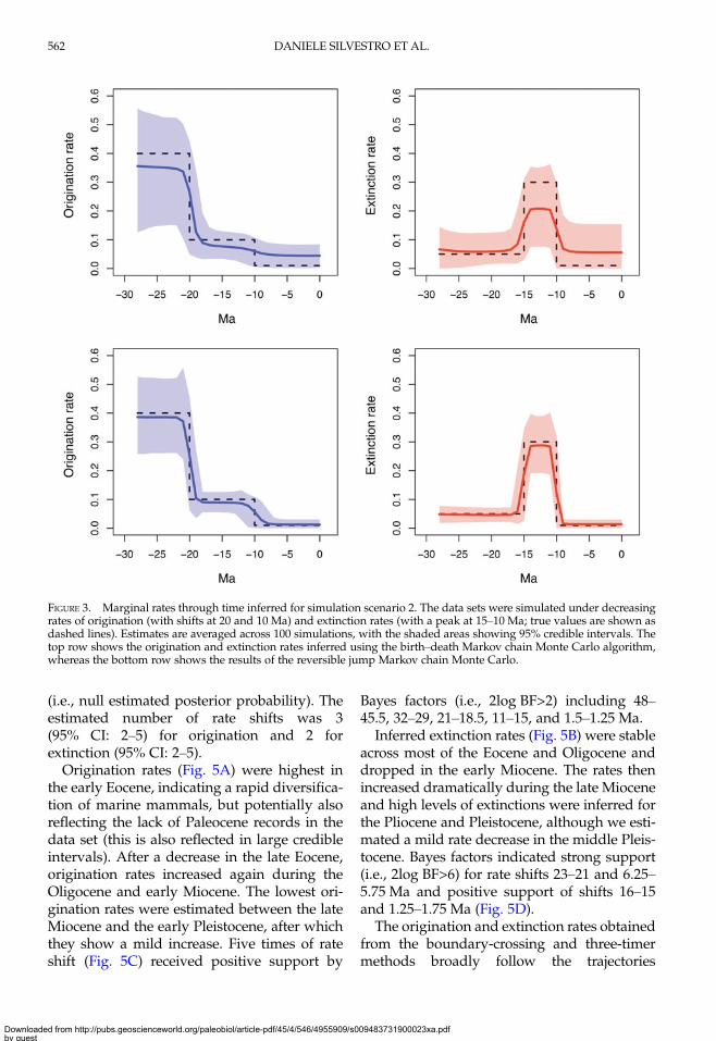
The marginal rates of origination and extinc-tion were estimated with high accuracy by bothBDMCMC and RJMCMC under scenario 1(constant rates), with relative errors between0.09 and 0.14 (Table 4, SupplementaryFig. S4). In contrast, simulations based on time-variable origination and extinction rates showthat RJMCMC estimates are substantiallymore accurate than those yielded by BDMCMC(Fig. 3; Supplementary Fig. S5). For instance,for scenario 2, RJMCMC estimates marginalrates with an average relative error around0.26, about three times more accurate than therates obtained from BDMCMC. These resultsreflect the better ability of RJMCMC to recoverthe correct birth–death model, in terms of num-ber of rate shifts (Table 3).

Performance of PyRate Compared with OtherMethodsAlthough all methods correctly picked up

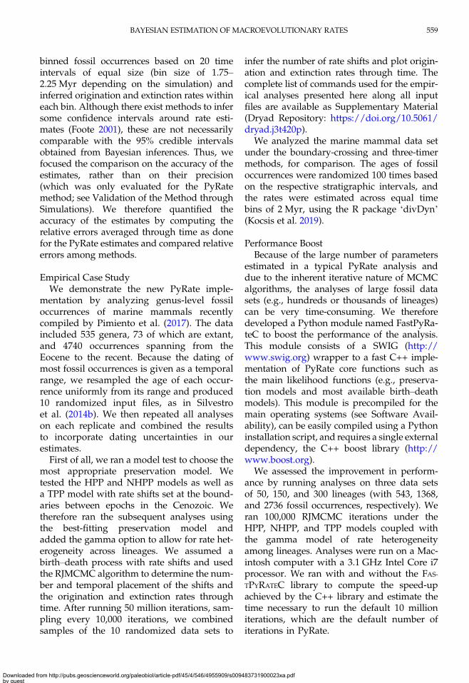
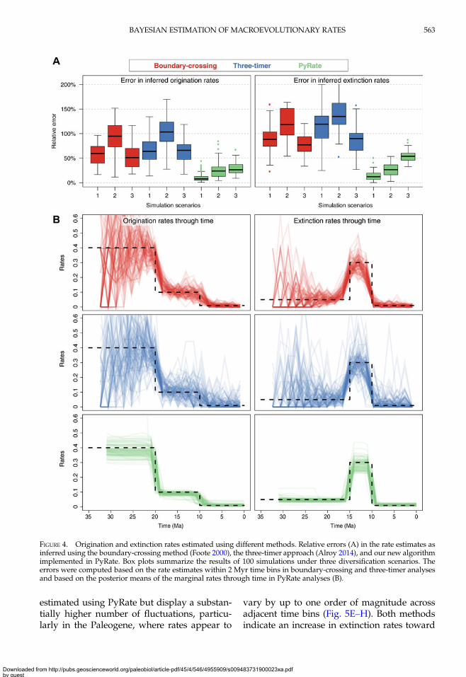
the general trends in diversification rates,PyRate estimates of both origination andextinction rates through time decisively outper-formed the results of the boundary-crossingand three-timer methods under our simulationsettings. The accuracy of the estimates wassimilar between boundary-crossing and three-timer and substantially higher in PyRate esti-mates (Fig. 4A). The relative errors generallyranged between 50 and 130% when using

boundary-crossing and three-timer methodsand ranged between 10 and 50% in PyRateestimates.The difference in accuracy between methods

does not appear to stem from any systematicbias in the estimates. Instead, it is mostly linkedto a higher volatility of the estimated ratesthrough time under the boundary-crossingand three-timer methods, which is apparentfrom the rates-through-time plots (Fig. 4B, Sup-plementary Figs. S6–S8). The volatility of therate estimates is especially high for simulationscenario 1 (constant rates; SupplementaryFig. S6) and, in general, early in the history ofthe clade (e.g., the first 10–15 Myr in simulationscenarios 1 and 2; Fig. 4B, SupplementaryFig. S6), where the size of the clade in termsof number of sampled species is lower.

Diversification Dynamics of Cenozoic MarineMammalsThe maximum-likelihood test of preserva-

tion models resulted in a very strong supportfor the TPP model against the HPP (ΔAICc =324.23) and NHPP models (ΔAICc = 799.41).The TPP model assumed independent rates ateach epoch and included 7 parameters (forEocene, Oligocene, Miocene, Pliocene, Pleisto-cene, Holocene, and the α parameter of thegammamodel).We therefore ran thePyRate ana-lyses using a TPPmodel of preservation coupledwith rate heterogeneity across lineages (gammamodel).The estimated preservation rates showed a

strong increase toward the recent. For instance,the preservation rate estimated for the Miocenewas 1.15 (95% CI: 0.89–1.40), whereas in thePliocene it was 4.06 (95% CI: 3.07–5.30), risingin the Pleistocene to 8.52 (95% CI: 6.80–10.67).Furthermore, we found evidence of strong het-erogeneity of preservation across lineages, asidentified by the estimated parameter α = 0.88(95% CI: 0.75–1.01). This indicates that, forinstance, while the average preservation ratein the Miocene was 1.15, the rate varied acrosslineages between 0.14 and 2.71 (median rate =0.88).The RJMCMC algorithm estimated a consid-

erable amount of temporal variation in the ori-gination and extinction rates. Constant-ratebirth–death models were never sampled

TABLE 4. Comparison of accuracy and precision of themarginal origination and extinction rates between the newreversible jump Markov chain Monte Carlo (RJMCMC )and birth–death Markov chain Monte Carlo (BDMCMC)algorithms. Accuracy (relative errors) and precision areaveraged across analyses of 100 simulated data sets for eachsimulation scenario. While the precision of rate estimates(here quantified by the relative size of the 95% credibleintervals) is similar between algorithms, the RJMCMCimplementation yields substantially more accurate results,especially in the presence of rate heterogeneity throughtime.

Simulation Algorithm

Originationrates Extinction rates

Rel.error Precision

Rel.error Precision

1 BD 0.088 0.477 0.134 0.517RJ 0.106 0.462 0.138 0.550

2 BD 0.729 1.393 0.840 2.058RJ 0.254 1.145 0.269 1.203

3 BD 0.496 1.317 0.696 1.085RJ 0.286 1.285 0.537 1.110



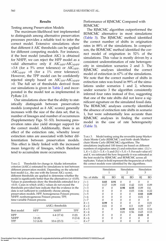
(i.e., null estimated posterior probability). Theestimated number of rate shifts was 3(95% CI: 2–5) for origination and 2 forextinction (95% CI: 2–5).Origination rates (Fig. 5A) were highest in

the early Eocene, indicating a rapid diversifica-tion of marine mammals, but potentially alsoreflecting the lack of Paleocene records in thedata set (this is also reflected in large credibleintervals). After a decrease in the late Eocene,origination rates increased again during theOligocene and early Miocene. The lowest ori-gination rates were estimated between the lateMiocene and the early Pleistocene, after whichthey show a mild increase. Five times of rateshift (Fig. 5C) received positive support by

Bayes factors (i.e., 2log BF>2) including 48–45.5, 32–29, 21–18.5, 11–15, and 1.5–1.25 Ma.Inferred extinction rates (Fig. 5B) were stable

across most of the Eocene and Oligocene anddropped in the early Miocene. The rates thenincreased dramatically during the late Mioceneand high levels of extinctions were inferred forthe Pliocene and Pleistocene, although we esti-mated a mild rate decrease in the middle Pleis-tocene. Bayes factors indicated strong support(i.e., 2log BF>6) for rate shifts 23–21 and 6.25–5.75 Ma and positive support of shifts 16–15and 1.25–1.75 Ma (Fig. 5D).The origination and extinction rates obtained

from the boundary-crossing and three-timermethods broadly follow the trajectories

FIGURE 3. Marginal rates through time inferred for simulation scenario 2. The data sets were simulated under decreasingrates of origination (with shifts at 20 and 10 Ma) and extinction rates (with a peak at 15–10 Ma; true values are shown asdashed lines). Estimates are averaged across 100 simulations, with the shaded areas showing 95% credible intervals. Thetop row shows the origination and extinction rates inferred using the birth–death Markov chain Monte Carlo algorithm,whereas the bottom row shows the results of the reversible jump Markov chain Monte Carlo.



estimated using PyRate but display a substan-tially higher number of fluctuations, particu-larly in the Paleogene, where rates appear to

vary by up to one order of magnitude acrossadjacent time bins (Fig. 5E–H). Both methodsindicate an increase in extinction rates toward

FIGURE 4. Origination and extinction rates estimated using different methods. Relative errors (A) in the rate estimates asinferred using the boundary-crossing method (Foote 2000), the three-timer approach (Alroy 2014), and our new algorithmimplemented in PyRate. Box plots summarize the results of 100 simulations under three diversification scenarios. Theerrors were computed based on the rate estimates within 2 Myr time bins in boundary-crossing and three-timer analysesand based on the posterior means of the marginal rates through time in PyRate analyses (B).



the recent, although it is difficult to pinpointwhen the extinction rates began to increase.

Performance of the FASTPYRATEC LibraryThe new C++ library dramatically boosted

the PyRate performance, with different levelsof speed-up depending on the underlyingmodel and the size of the data set. In ourtests, the C++ version was between five andeight times faster than the Python implementa-tion when using the HPP model of preservation.Under the TPP model, the speed-up reached 26times for a data set of 300 taxa (SupplementaryFig. S9). This performance improvement has avery significant impact on the feasibility of ana-lyzing large data sets. For instance, an analysisof 300 taxa with the TPP model, running 10 mil-lion RJMCMC iterations (default in PyRate) on areasonably fast CPU, takes about 3 hours usingthe FASTPYRATEC library, whereas it takes around3 days using the all-Python version. The magni-tude of this performance boost becomes crucialwhen it comes to the analysis of large empiricaldata sets. The analysis of Cenozoic marine mam-mals presented in this study (more than 500 taxa,50 millionMCMC iterations) takes about 14 h ona3.1 GHzCPU,using theC++ library. In contrast,the same analysis performed using the Pythonimplementation would need more than 19 daysto complete (i.e., more than 30 times longer).

Discussion

InferringMacroevolutionary Rates from FossilsA large proportion of macroevolutionary

research processes with the aim of understand-ing how biodiversity has evolved through timeand space and what drives the rise and demiseof clades in the tree of life (e.g., Raup and Sep-koski 1984; Raup 1986; Foote et al. 2007; Alroy2008; Quental and Marshall 2013; Benton et al.2014; Cantalapiedra et al. 2015; Ezard et al.2016). The fossil record has been used to inferdiversification and extinction processes for along time and arguably provides for manylineages (e.g., any organism with a mineralizedskeleton), the most informative available datafor understanding macroevolutionary dynam-ics (Marshall 2017).PyRate is a software designed to analyze fos-

sil data in a Bayesian framework. Its main

strengths are: (1) enabling users to analyze theentire fossil occurrence record (i.e., not onlyfirst and last appearances) and all describedlineages (including singletons and extanttaxa), (2) incorporating parameter uncertaintiesusing Bayesian algorithms, and (3) using expli-cit probabilistic model selection to adequatelyinfer the complexity of the preservation andbirth–death models based on the data. Becausefossil data are often limited in size, it is essentialto adequately quantify the uncertainty aroundeach parameter estimate to avoid interpretingthe results with a false sense of precision.Thus, the use of a Bayesian framework is wellsuited for the task, providing credible intervalsfor each parameter rather than point estimatesand simultaneously integrating the uncertain-ties associated with all parameters (Gelmanet al. 2013).

Methodological AdvancesWe presented a flexible and powerful suite of

quantitative methods to infer macroevolution-ary processes using fossil occurrence data. Pres-ervation processes are typically modeled byconstant or time-varying sampling probabil-ities (Foote 2000; Liow and Nichols 2010;Bapst and Hopkins 2016), which are, however,assumed to be constant across lineages. Here,we developed a new model in which a preser-vation process with time-variable mean ratescan be coupled with rate heterogeneity acrosslineages. Both types of rate variations areexpected to be ubiquitous, reflecting temporalenvironmental changes, which may affect sedi-mentation and fossilization processes as well aspreservation biases associatedwith each organ-ism (lifestyle, anatomy, size, and other traits,e.g., shell composition [Foote et al. 2015]). Wealso presented a novel likelihood-based testallowing a formal statistical comparisonamong alternative preservation models. Thisprocedure facilitates an objective, data-drivenselection of the most appropriate model of fos-sil preservation. As expected, our modelincorporating rate heterogeneity both throughtime and among lineages is indeed supportedby empirical data against the alternative mod-els, as shown with the marine mammals ana-lyzed here. We note that the parameterizationof the preservation process and the priors



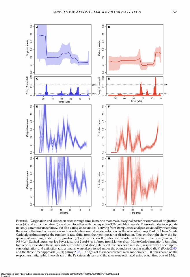
FIGURE 5. Origination and extinction rates through time in marine mammals. Marginal posterior estimates of originationrates (A) and extinction rates (B) are shown together with the respective 95% credible intervals. These estimates incorporatenot only parameter uncertainty, but also dating uncertainties (deriving from 10 replicated analyses obtained by resamplingthe ages of the fossil occurrences) and uncertainties around model selection, as the reversible jump Markov Chain MonteCarlo algorithm samples the number of rate shifts from their joint posterior distribution. Plots on the right show the fre-quency of sampling a shift in origination (C) and extinction (D) rates within arbitrarily small time bins (here set to0.5 Myr). Dashed lines show log Bayes factors of 2 and 6 (as inferred fromMarkov chainMonte Carlo simulation). Samplingfrequencies exceeding these lines indicate positive and strong statistical evidence for a rate shift, respectively. For compari-son, origination and extinction rate estimates were also inferred under the boundary-crossing method (E, F) (Foote 2000)and the three-timer approach (G, H) (Alroy 2014). The ages of fossil occurrences were randomized 100 times based on therespective stratigraphic intervals (as in the PyRate analyses), and the rates were estimated using equal time bins of 2 Myr.



used here are designed for general-purposeanalyses and do not include additional empir-ical evidence beyond the temporal distributionof fossil occurrences for each species. Thus,while the rate heterogeneity across lineagesinferred from empirical data sets may reflectpreservation potentials due to different ana-tomical and life-history traits, this informationis not provided a priori in the analysis. Simi-larly, the preservation process is affected bythe amount of available rock volume and islikely characterized by strong geographicbiases that are not explicitly accounted for byour model. Future developments shouldincorporate additional information aboutthese sampling biases, potentially buildingupon previously demonstrated analyticalmethods (Sadler et al. 2008; Wagner and Mar-cot 2013; Foote et al. 2015; Silvestro et al. 2016).We implemented a new algorithm that uses

RJMCMC to estimate birth–death processesand jointly infer (in addition to the preservationparameters) the number and temporal place-ment of rate shifts and marginal originationand extinction rates through time. We foundRJMCMC to outperform the previously imple-mented BDMCMC algorithm, providing moreaccurate rates and estimated numbers of shifts.Themain advantages of RJMCMC are that (1) itprovides marginal rates that account for uncer-tainties in the time and number of rate shifts, (2)it allows us to easily compute Bayes factors toassess statistically significant times of rateshift, and (3) its prior on the number of rateshifts is itself estimated from the data (unlikein BDMCMC, where it is fixed a priori [Silves-tro et al. 2014b]), thus making the algorithmmore versatile and able to adapt to differentdata sets.Whereas several methods have been devel-

oped to infer rate variation in origination andextinction rates through time (e.g., Foote 2001,2003; Liow and Nichols 2010; Alroy 2014,2015; Liow and Finarelli 2014; Foote et al.2015), these approaches do not explicitly assessthe minimum number of parameters requiredto accurately describe the data, that is, the best-fitting model. The suite of methods presentedhere implements probabilistic tests and algo-rithms that specifically tackle this issue. Thenumber of parameters included in preservation

models and birth–death models in PyRate isdetermined by the information intrinsic to thedata, rather than a priori. The result of thisapproach is a direct estimation of when andhow many times the pace of diversificationhas changed throughout the history of aclade. With the implementation of the newRJMCMC algorithm, the timing of rate changesis itself estimated through Bayes factors toassess its significance (Fig. 5B,C). A similarapproach had been used before in a phylogen-etic (neontological) context (May et al. 2016)but, to the best of our knowledge, was notavailable in the analysis of paleontologicaldata.Theapproachpresentedheremodelspreserva-

tion, origination, and extinction as continuous-time processes. Most other methods (e.g.,boundary-crossing and three-timer) are basedon discrete time, whereby the ages of the fossiloccurrences are translated into presence orabsence within a predefined time bin. Althoughthe true nature of natural processes such as spe-cies appearance and disappearance is obvi-ously time continuous, the choice of binneddata reflects the fact that most occurrences arenot dated directly, but instead assigned to tem-poral ranges based on their respective strati-graphic units (Foote and Miller 2007). InPyRatewe treat these temporal ranges as uncer-tainties in the dating and resample them ran-domly to incorporate such uncertainties in theanalyses (see also Analysis Protocol for MarineMammals, Supplementary Material). In adiscrete-time analysis assuming two bins forthe Pliocene or the Pleistocene, one couldassign fossil occurrences to either of the twoepochs. However, under these settings, evenan occurrence dated with higher precision(e.g., assigned to the Piacenzian) will be treatedas “Pliocene,” therefore ignoring theadditional information. In contrast, one advan-tage of our approach is that eachoccurrence (or all occurrences from each fossilassemblage) will be assigned its own uncer-tainty range.The parameterization of the PyRate model

and the algorithms implemented to carry outparameter estimation and model testing neces-sarily result in amore computationally demand-ing approach compared with alternative



methods. To alleviate this potential bottleneck,we implemented a new C++ library, whichyields considerable speed-up compared withpreviousversions of the software (orders ofmag-nitude; Supplementary Fig. S9). This and theever-increasing performance of computers andclusters make PyRate a suitable method evenfor relatively large data sets.

Importance of Model Testing in EstimatingOrigination and Extinction: Comparing PyRatewith Other MethodsUsing a robust and explicit model selection

framework is crucial to avoidoverparameteriza-tion, and this represents one of the biggest nov-elties of the methods presented here, comparedwith other approaches. Indeed, assuming ori-gination and extinction rates to be independentparameters in predefined timebins (i.e.,withoutexplicitly model testing) is common practice inpaleobiological studies of macroevolution(Foote 2003; Liow and Finarelli 2014; Alroy2015; but see Connolly and Miller 2001; Foote2007). However, this practice may generatespurious results if the amount of data is insuffi-cient to confidently estimate all the parameters(Smiley 2018), which is a general problem withoverparameterization and overfitting (Burnhamand Anderson 2002). The RJMCMC algorithmpresented here and the other algorithms imple-mented in PyRate infer the amount of rate vari-ation directly from the data. Although wefocused here on algorithms that simultaneouslyoptimize the parameters and the model(RJMCMC and BDMCMC), other methods toavoid overparameterization are available inPyRate, based on the estimation of model mar-ginal likelihoods (Silvestro et al. 2014b), Bayes-ian variable selection (Silvestro et al. 2015a),and Bayesian shrinkage (Silvestro et al. 2015b,2017). Using these methods, the complexity ofthe model adapts to the signal provided by thedata and its statistical power, so that only statis-tically significant rate changes are identified.This procedure also provides a formal approachto assess whether apparent rate variations arenot just the result of the stochastic nature of aconstant-rate birth–death process.The levels of accuracy obtained by our

RJMCMC algorithmwere up to 10 times higherthan with other methods when the true

underlying model was a time-homogeneousbirth–death process (Supplementary Fig. S6).This is clearly a case in which assuming inde-pendent rates per time bin represents an over-parameterization of the true process. Indeed,the difference in accuracy between rate esti-mates from the boundary-crossing and three-timer methods and rates inferred in PyRatetended to decrease when the true underlyingmodel included rate shifts. We interpret this asa consequence of the fact that the true speciationand extinction dynamics in these simulationsbetter conform to models with independentrates per time bin. Yet even under simulationscharacterized by a high rate heterogeneitythrough time (scenario 3), PyRate accuracywas substantially higher than with the othermethods (Supplementary Fig. S8).While a comprehensive comparison between

all available methods to infer origination andextinction rates from fossil data is beyond thescope of this study (but see Smiley [2018] fora recent and extensive simulation study), ourresults clearly indicate that there are substantialbenefits associated with the use of explicitmodel testing to prevent overparameterization.The optimization of the complexity of themodel based on the data is crucial to obtainingrealistic estimates of diversification processesfrom incomplete fossil data. Based on theseresults, we recommend always verifying thestatistical support for the number of modelparameters when inferring diversificationdynamics from fossil data.

Conclusions

PyRate is an open-source project to whichresearchers are welcome to contribute code,ideas, and feedback through its online reposi-tory. It includes many birth–death models fortaxonomic diversification as well as severalpreservation models in which rates can varythrough time and across lineages. The hierarch-ical Bayesian methods implemented in PyRateallow users to assess the statistical support ofdifferent models and to jointly infer all theparameters. We have shown that explicitmodel testing when inferring origination andextinction rates yields substantially improvedaccuracy. As a by-product of the Bayesian



algorithms used in PyRate, credible intervalsare inferred for all model parameters (e.g., pres-ervation, origination, and extinction rates) andcan be used to quantify the level of uncertain-ties surrounding the estimates.Although we focused here on diversification

processes in which origination and extinctionrates change through time, several other modelshave been implemented in PyRate enablingusers to test specific hypotheses about, forexample, diversity-dependent diversificationwith competition within and among clades(Pires et al. 2017), correlations to biotic and abi-otic factors (Lehtonen et al. 2017), and age-dependent and trait-dependent extinction rates(Hagen et al. 2017; Piras et al. 2018). The versatil-ity of a fully probabilistic Bayesian method toinfer diversification dynamics allows for thedevelopment of additional models and algo-rithms to tackle specific questions. For example,a model of pulsed turnover (Vrba 1985) mightbe better captured by an algorithm that, ratherthan looking for rate shifts, clusters time binsby the magnitude of the origination and extinc-tion rates, one example being the Dirichlet pro-cess prior method (Neal 2000) (a prototype ofwhich is already available in the current versionofPyRate). In conclusion, PyRateprovides aflex-ible, statistically sound analytical frameworkenabling researchers to analyze the growingamount of available fossil occurrence data, andwe think it can serve as a useful tool kit formany future studies in paleobiology.

Software Availability

All the models described in this study areimplemented within the open-source packagePyRate and are available at: https://github.com/dsilvestro/PyRate. The program is writ-ten in Python 2.7 and R and has been testedunder the major operating systems (MacOS,Windows, and several Linux distributions). Adetailed command list and tutorials are avail-able in the GitHub repository.Importantly, PyRate requires a minimum

number of a priori decisions from the user, andwhile each setting can be accessed through spe-cific commands, default values and settings areset to adapt to most data sets. PyRate runs as astand-alone command-line program, and

running the softwaredoesnot require anyknowl-edge of Python from the user. The program alsoincludes many utility functions that can be usedto plot and summarize the results, process mul-tiple output files, and parse large data sets toidentify potential spelling variation in taxonnamesusingabuilt-inmachine-learningclassifier(as shown in the Supplementary Material).To provide easy access to the augmented per-

formance of the FASTPYRATEC library, precom-piled modules for 64-bit versions of Windows,MacOS, and Linux are available on the PyRateGithub repository, in addition to the source code.

Acknowledgments

All analyses were run at the High-Performance Computing Center (Vital-IT) atthe Swiss Institute of Bioinformatics. D.S.received funding from the Swedish ResearchCouncil (2015-04748). N.S. received fundingfrom the University of Lausanne (Switzerland)and the Swiss National Science Foundation(CR32I3-143768). A.A. received funding fromthe Swedish Foundation for Strategic Research,the Swedish Research Council (B0569601), theFaculty of Sciences at the University of Gothen-burg, and a Wallenberg Academy Fellowship.X.M. received funding from the Swiss NationalScience Foundation (P2GEP2_178032). Weare thankful to M. Patzkowsky, P. Wagner,A. Dunhill, R. Warnock, and one anonymousreviewer for valuable feedback on this work.We thank T. Smiley, B. McHorse, M. Crotti,T. Hauffe, J. L. Cantalapiedra, O. Inostroza,T. B. Quental, M. M. Pires, and E. Gjesfjeld fordiscussion and feedback on the software. Wethank E. Orliac of the Scientific Computingand Research Support Unit, University ofLausanne (Switzerland) for support on theWindows version of FASTPYRATEC.

Literature CitedAlroy, J. 1996. Constant extinction, constrained diversification, anduncoordinated stasis in North American mammals. Palaeogeog-raphy, Palaeoclimatology, Palaeoecology 127:285–311.

Alroy, J. 2008. Dynamics of origination and extinction in themarinefossil record. Proceedings of the National Academy of SciencesUSA 105:11536–11542.

Alroy, J. 2014. Accurate and precise estimates of origination andextinction rates. Paleobiology 40:374–397.






Alroy, J. 2015. Amore precise speciation and extinction rate estima-tor. Paleobiology 41:633–639.

Bapst, D. W., and M. J. Hopkins. 2016. Comparing cal3 and other aposteriori time-scaling approaches in a case study with the pter-ocephaliid trilobites. Paleobiology 43:49–67.

Benton,M. J., J. Forth, andM. C. Langer. 2014. Models for the rise ofthe dinosaurs. Current Biology 24:R87–R95.

Burin, G., L. R. V. Alencar, J. Chang, M. E. Alfaro, and T. B. Quental.2019. How well can we estimate diversity dynamics for clades indiversity decline? Systematic Biology 68:47–62.

Burnham, K. P., and D. A. Anderson. 2002. Model selection andmultimodel inference: a practical information-theoretic approach,2nd ed. Springer, New York.

Cantalapiedra, J. L., M. H. Fernández, B. Azanza, and J. Morales.2015. Congruent phylogenetic and fossil signatures of mamma-lian diversification dynamics driven by Tertiary abiotic change.Evolution 69:2941–2953. doi:10.1111/evo.12787.

Chang, J., D. L. Rabosky, S. A. Smith, and M. E. Alfaro. 2019. An Rpackage and online resource for macroevolutionary studies usingthe ray-finned fish tree of life. Methods in Ecology and Evolution10:1118–1124. doi.org/10.1111/2041–210X.13182.

Connolly, S. R., and A. I. Miller. 2001. Joint estimation of samplingand turnover rates from fossil databases: capture-mark-recapturemethods revisited. Paleobiology 27:751–767.

Dib, L., D. Silvestro, and N. Salamin. 2014. Evolutionary footprintof coevolving positions in genes. Bioinformatics 30:1241–1249.

Ezard, T. H. G., T. Aze, P. N. Pearson, andA. Purvis. 2011. Interplaybetween changing climate and species’ ecology drives macroevo-lutionary dynamics. Science 332:349–351.

Ezard, T. H., T. B. Quental, and M. J. Benton. 2016. The challengesto inferring the regulators of biodiversity in deep time. Philosoph-ical Transactions of the Royal Society of London B 371: 20150216.doi: 10.1098/rstb.2015.0216.

Foote, M. 2000. Origination and extinction components of taxo-nomic diversity: general problems. Paleobiology 26:74–102.

Foote, M. 2001. Inferring temporal patterns of preservation, origin-ation, and extinction from taxonomic survivorship analysis.Paleobiology 27:602–630.

Foote, M. 2003. Origination and extinction through the Phanero-zoic: a new approach. Journal of Geology 111:125–148.

Foote, M. 2007. Extinction and quiescence inmarine animal genera.Paleobiology 33:261–272.

Foote, M., and A. I. Miller. 2007. Principles of paleontology.Freeman, New York.

Foote, M., and D. M. Raup. 1996. Fossil preservation and the strati-graphic ranges of taxa. Paleobiology 22:121–140.

Foote, M., J. S. Crampton, A. G. Beu, B. A. Marshall, R. A. Cooper,P. A. Maxwell, and I. Matcham. 2007. Rise and fall ofspecies occupancy in Cenozoic fossil mollusks. Science318:1131–1134.

Foote, M., J. S. Crampton, A. G. Beu, and C. S. Nelson. 2015. Ara-gonite bias, and lack of bias, in the fossil record:lithological, environmental, and ecological controls. Paleobiology41:245–265.

Gelman, A., J. B. Carlin, H. S. Stern, andD. B. Rubin. 2013. Bayesiandata analysis, 3rd ed. Chapman & Hall/CRC Texts in StatisticalScience, London.

Gernhard, T. 2008. The conditioned reconstructed process. Journalof Theoretical Biology 253:769–778.

Green, P. J. 1995. Reversible jump Markov chain Monte Carlo andBayesian model determination. Biometrika 82:711–732.

Hagen, O., T. Andermann, B. T. Quental, A. Antonelli, andD. Silvestro. 2017. Estimating age-dependent extinction: con-trasting evidence from fossil and phylogenies. Systematic Biology67:458–474. doi:10.1093/sysbio/syx082.

Heath, T. A., J. P. Hulsenbeck, and T. Stadler. 2014. The fossilizedbirth–death process for coherent calibration of divergence-time

estimates. Proceedings of the National Academy of SciencesUSA 111:2957–2966.

Jetz, W., G. H. Thomas, J. B. Joy, K. Hartmann, and A. O. Mooers.2012. The global diversity of birds in space and time. Nature491:444–448.

Kass, R. E., and A. E. Raftery. 1995. Bayes factors. Journal of theAmerican Statistical Association 90:773–795.

Keiding, N. 1975. Maximum likelihood estimation in the birth-death process. Annals of Statistics 3:363–372.

Kendall, D. G. 1948. On the generalized birth-and-death process.Annals of Mathematical Statistics 19:1–15.

Kocsis, A. T., C. J. Reddin, J. Alroy, and W. Kiessling. 2019. TheR package divdyn for quantifying diversity dynamics usingfossil sampling data. Methods in Ecology and Evolution10:735–743.

Kurtén, B. 1954. Population dynamics: a new method in paleon-tology. Journal of Paleontology 28:286–292.

Lartillot, N., and H. Philippe. 2006. Computing Bayes factors usingthermodynamic integration. Systematic Biology 55:195–207.

Lehtonen, S., D. Silvestro, D. N. Karger, C. Scotese, H. Tuomisto,M. Kessler, C. Peña, N. Wahlberg, and A. Antonelli. 2017. Envir-onmentally driven extinction and opportunistic originationexplain fern diversification patterns. Scientific Reports 7:ar4831.

Liow, L. H., and J. A. Finarelli. 2014. A dynamic global equilibriumin carnivoran diversification over 20million years. Proceedings ofthe Royal Society of London B 281:20132312.

Liow, L. H., and J. D. Nichols. 2010. Estimating rates and probabil-ities of origination and extinction using taxonomic occurrencedata: capture-recapture approaches. In G. Hunt and J. Alroy,eds. Short Courses in Paleontology 16:81–94. Yale UniversityPrinting and Publishing, New Haven, Conn.

Liow, L. H., M. Fortelius, E. Bingham, K. Lintulaakso, H. Mannila,L. Flynn, andN. C. Stenseth. 2008. Higher origination and extinc-tion rates in larger mammals. Proceedings of the National Acad-emy of Sciences USA 105:6097–6102.

Liow, L., T. Quental, and C. Marshall. 2010a. When can decreasingdiversification rates be detected with molecular phylogenies andthe fossil record? Systematic Biology 59:646–659.

Liow, L. H., H. Skaug, T. Ergon, and T. Schweder. 2010b. Globaloccurrence trajectories of microfossils: environmental volatilityand the rise and fall of individual species. Paleobiology 36:224–252.

Liow, L. H., T. Reitan, and P. G. Harnik. 2015. Ecological interac-tions on macroevolutionary time scales: clams and brachiopodsare more than ships that pass in the night. Ecology Letters18:1030–1039.

Marshall, C. R. 2017. Five paleobiological laws needed to under-stand the evolution of the living biota. Nature Ecology andEvolution 1:165.

May, M. R., S. Höhna, and B. R. Moore. 2016. A Bayesian approachfor detecting the impact of mass-extinction events on molecularphylogenies when rates of lineage diversification may vary.Methods in Ecology and Evolution 7:947–959.

Miller,A. I., andM.Foote. 2003. Increased longevitiesofpost-Paleozoicmarine genera after mass extinctions. Science 302:1030–1032.

Neal, R. M. 2000. Markov chain sampling methods for Dirichletprocess mixture models. Journal of Computational and GraphicalStatistics 9:249–265.

Nee, S. 2006. Birth-death models in macroevolution. AnnualReview of Ecology, Evolution, and Systematics 37:1–17.

Nee, S., R. M. May, and P. H. Harvey. 1994. The reconstructed evo-lutionary process. Philosophical Transactions of the Royal Societyof London B 344:305–311.

Pennell, M. W., J. M. Eastman, G. J. Slater, J. W. Brown, J. C. Uyeda,R. G. FitzJohn, M. E. Alfaro, and L. J. Harmon. 2014. geiger v2.0:an expanded suite ofmethods for fittingmacroevolutionarymod-els to phylogenetic trees. Bioinformatics 30:2216–2218.



Perez-Escobar, O. A., G. Chomicki, F. L. Condamine, A.P. Karremans, D. Bogarin, N. J. Matzke, D. Silvestro, andA. Antonelli. 2017. Recent origin and rapid speciation of neotrop-ical orchids in theworld’s richest plant biodiversity hotspot. NewPhytologist 215:891–905.

Peters, S. E. 2008. Environmental determinants of extinctionselectivity in the fossil record. Nature 454:626–638.

Pimiento, C., J. N. Griffin, C. F. Clements, D. Silvestro, S. Varela, M.D. Uhen, and C. Jaramillo. 2017. The Pliocene marine megafaunaextinction and its impact on functional diversity. Nature Ecologyand Evolution 1:1100–1106.

Piras, P., D. Silvestro, F. Carotenuto, S. Castiglione, A. Kotsakis,L. Maiorino, M. Melchionna, A. Mondanaro, G. Sansalone,C. Serio, V. A. Vero, and P. Raia. 2018. Evolution of the sabertoothmandible: a deadly ecomorphological specialization. Palaeogeog-raphy, Palaeoclimatology, Palaeoecology 496:166–174.

Pires, M. M., D. Silvestro, and T. B. Quental. 2017. Interactionswithin and between clades shaped the diversification of terres-trial carnivores. Evolution 71:1855–1864.

Quental, T., and C. R. Marshall. 2010. Diversity dynamics: Molecu-lar phylogenies need the fossil record. Trends in Ecology andEvolution 25:434–441.

Quental, T. B., and C. R. Marshall. 2013. How the RedQueen drivesterrestrial mammals to extinction. Science 341:290–292.

Raia, P., F. Carotenuto, A. Mondanaro, S. Castiglione, F. Passaro,F. Saggese, M. Melchionna, C. Serio, L. Alessio, D. Silvestro,and M. Fortelius. 2016. Progress to extinction: increased special-isation causes the demise of animal clades. Scientific Reports6:30965.

Raup, D. M. 1986. Biological extinction in earth history. Science231:1528–1533.

Raup, D.M., and J. J. Sepkoski. 1982. Mass extinctions in themarinefossil record. Science 215:1501–1503.

Raup, D. M., and J. J. Sepkoski. 1984. Periodicity of extinctions inthe geologic past. Proceedings of the National Academy ofSciences USA 81:801–805.

Rolland, J., D. Silvestro, D. Schluter, A. Guisan, O. Broennimann,and N. Salamin. 2018. The impact of endothermy on the climaticniche evolution and the distribution of vertebrate diversity.Nature Ecology and Evolution 2:459–464.

Sadler, P. M., W. G. Kemple, and M. A. Kooser. 2008. CONOP9 pro-grams for solving the stratigraphic correlation and seriation pro-blems as constrained optimization. Springer,Netherlands, 461–462.

Sepkoski, J. J. 1998. Rates of speciation in the fossil record.Philosophical Transactions of the Royal Society of London B353:315–326.

Silvestro, D., N. Salamin, and J. Schnitzler. 2014a. PyRate: a newprogram to estimate speciation and extinction rates fromincomplete fossil data. Methods in Ecology and Evolution5:1126–1131.

Silvestro, D., J. Schnitzler, L. H. Li, A. Antonelli, and N. Salamin.2014b. Bayesian estimation of speciation and extinction fromincomplete fossil occurrence data. Systematic Biology 63:349–367.

Silvestro, D., A. Antonelli, N. Salamin, and T. B. Quental. 2015a.The role of clade competition in the diversification of North

American canids. Proceedings of the National Academy ofSciences USA 112:8684–8689.

Silvestro, D., B. Cascales-Miñana, C. D. Bacon, and A. Antonelli.2015b. Revisiting the origin and diversification of vascular plantsthrough a comprehensive Bayesian analysis of the fossil record.New Phytologist 207:425–436. doi:10.1111/nph.13247.

Silvestro, D., A. Zizka, C. D. Bacon, B. Cascales-Miñana,N. Salamin,and A. Antonelli. 2016. Fossil biogeography: a new model toinfer dispersal, extinction and sampling from palaeontologicaldata. Philosophical Transactions of the Royal Society of LondonB 371:20150225.

Silvestro, D., M. M. Pires, T. B. Quental, and N. Salamin. 2017.Bayesian estimation of multiple clade competition from fossildata. Evolutionary Ecology Research 18:41–59.

Silvestro, D., R. C. M. Warnock, A. Gavryushkina, and T. Stadler.2018. Closing the gap between palaeontological and neonto-logical speciation and extinction rate estimates. Nature Commu-nications 9: 5237. doi: 10.1038/s41467–018–07622–y.

Smiley, T. M. 2018. Detecting diversification rates in relation topreservation and tectonic history from simulated fossil records.Paleobiology 44:1–24.

Stadler, T. 2009. On incomplete sampling under birth-death mod-els and connections to the sampling-based coalescent. Journalof Theoretical Biology 261:58–66.

Stadler, T. 2013. Recovering speciation and extinction dynamicsbased on phylogenies. Journal of Evolutionary Biology 26:1203–1219.

Stephens, M. 2000. Bayesian analysis of mixture models with anunknown number of components—an alternative to reversiblejump methods. Annals of Statistics 28:40–74.

Van Valen, L., and R. E. Sloan. 1966. The extinction of the multitu-berculates. Systematic Zoology 15:261–278.

Vrba, E. S. 1985. Environment and evolution: alternative causes ofthe temporal distribution of evolutionary events. South AfricanJournal of Science 81:229–236.

Wagner, P. J., and J. Marcot. 2013. Modelling distributions of fossilsampling rates over time, space and taxa: assessment and impli-cations for macroevolutionary studies. Methods in Ecology andEvolution 4:703–713.

Warnock, R. C. M., J. F. Parham, W. G. Joyce, T. R. Lyson, andP. C. J. Donoghue. 2015. Calibration uncertainty in moleculardating analyses: there is no substitute for the prior evaluation oftime priors. Proceedings of the Royal Society of London B282:20141013.

Yang, Z. 1994. Maximum likelihood phylogenetic estimation fromDNA sequences with variable rates over sites: Approximatemethods. Journal of Molecular Evolution 39:306–314.

Zanne, A. E., D. C. Tank,W. K. Cornwell, J. M. Eastman, S. A. Smith,R. G. FitzJohn, D. J. McGlinn, B. C. O’Meara, A. T. Moles, P.B. Reich, D. L. Royer, D. E. Soltis, P. F. Stevens, M. Westoby, I.J. Wright, L. Aarssen, R. I. Bertin, A. Calaminus, R. Govaerts,F. Hemmings, M. R. Leishman, J. Oleksyn, P. S. Soltis, N.G. Swenson, L. Warman, and J. M. Beaulieu. 2014. Three keysto the radiation of angiosperms into freezing environments.Nature 506:394–394.



Documents

Improved estimation of macroevolutionary rates from fossil