Impact of weights on conjunctive and disjunctive aggregation of extended possibilistic truth values

Fuzzy Sets and Systems 160 (2009) 2141–2158www.elsevier.com/locate/fss

Impact of weights on conjunctive and disjunctive aggregation ofextended possibilistic truth values

Tom Matthé∗, Guy De Tré, Axel HallezGhent University, Department of Telecommunications and Information Processing, Sint-Pietersnieuwstraat 41, B-9000 Gent, Belgium

Available online 26 February 2009

Abstract

Extended possibilistic truth values are a flexible means to model the certainty or uncertainty about the truth value of a proposition.With respect to flexible database querying, they are suited to express the extent to which a database instance satisfies a querycondition. Since a flexible query can impose several conditions, each with different importance, weighted aggregation is necessary.In this paper, weighted aggregation of extended possibilistic truth values is presented. The impact of the weights on extendedpossibilistic truth values in both conjunctive and disjunctive aggregation is handled. It is illustrated that the different aggregationtypes require a different approach. Special care is given to the case where both conjunctive and disjunctive aggregation are mixedtogether. It is shown that the weights will have to be propagated throughout the calculations, but that this can cause basic properties,like associativity, to get lost. The problems that can arise are illustrated and solutions are proposed.© 2009 Elsevier B.V. All rights reserved.

Keywords: Fuzzy connectives and aggregation operators; Flexible querying; Extended possibilistic truth values

1. Introduction

Databases are continuously growing in size, and, using traditional querying techniques, users are confronted withdifficulties to find the information they are looking for. So, more and more, users are realizing the benefits of usingflexible querying systems [1,4,5,7,14,15,17,23,24]. The main goal of flexible querying is to allow the user to expresshis/her query in a more flexible way. Preferences can be used to indicate the users wishes. Introducing these preferencescan be done at two levels: inside elementary query conditions, allowing for the user to impose flexible search criteriawhich express to what degree particular attribute values are adequate for the result, and between query conditions,allowing for the user to attach weights, expressing importance, to the individual query conditions. This paper will notdeal with the preferences inside the elementary query conditions, and hence will not discuss the evaluation of selectioncriteria. The focus of this paper lies on one aspect of flexible querying, namely on the aggregation of the results of theevaluation of the individual selection criteria (which can be flexible or not), taking into account that weights can beattached to the individual selection criteria. Primarily, these are mathematical concepts, above which there is a layer ofpractical decision making. However, discussing this decision making is not the goal of this paper.

∗Corresponding author.E-mail addresses: [email protected] (T. Matthé), [email protected] (G. De Tré), [email protected] (A. Hallez).

0165-0114/$ - see front matter © 2009 Elsevier B.V. All rights reserved.doi:10.1016/j.fss.2009.02.011

http://www.elsevier.com/locate/fss

mailto:[email protected]



2142 T. Matthé et al. / Fuzzy Sets and Systems 160 (2009) 2141–2158

In general, a flexible query will impose several different (flexible) selection criteria or (fuzzy) constraints, which canall have a different importance, indicated by the user. Weighted aggregation will combine all individual satisfactiongrades of the respective constraints, taking into account their possible importance value, to produce a global satisfactiongrade for the entire query [6]. It is assumed that the satisfaction grades of the individual selection criteria are knownor calculated in advance, and as such, no assumption needs to be made about the underlying database. As illustratedin [9,11], extended possibilistic truth values (EPTVs), which will be further described in the next section, can be usedto express the (un)certainty about query satisfaction in flexible database querying: the EPTV representing the extent towhich it is (un)certain that a given database record belongs to the result of a flexible query can be obtained by aggregatingthe calculated EPTVs that denote the extents to which it is (un)certain that the record satisfies the different criteriaimposed by the query. Although other approaches are possible [3,4,14,19,21,24], in this paper, a logical frameworkbased on EPTVs will be applied where these EPTVs will be used to model the satisfaction grades of the flexibleconstraints and as such, will also be the input (and outcome) of the aggregation. An extensive comparison betweenthe different approaches and frameworks for flexible querying and query satisfaction, lies outside the scope of thispaper.Compared to work on EPTVs that has already been published, the novelty in this paper lies in the discussion of

the impact of the weights on the EPTVs during aggregation, especially when combining conjunction and disjunction.In [12,16], some notions about this have already been given, but underlying paper gives much more detail. It will beillustrated that the impact of a weight is different according to the type of aggregation (conjunction or disjunction)and that the aggregation operators for EPTVs can be extended to incorporate the weights. It will be shown that, whencombining conjunction and disjunction, an EPTV cannot be seen separately from its attached weight and hence thatthe outcome of the weighted aggregation of two EPTVs is again an EPTV with weight attached to it.The remainder of the paper is organized as follows. In Section 2, some preliminaries of EPTVs will be presented,

together with their arithmetic rules and basic aggregation operators. Section 3 will then focus on weighted aggregation,presenting how weights have an impact on EPTVs, what problems can arise when applying the weights and how tosolve these problems. Finally, Section 4 presents some conclusions.

2. Extended possibilistic truth values

2.1. Extended truth values

In traditional Boolean logic, with truth values ‘true’ (T) and ‘false’ (F), every proposition is considered to be eithertrue or false. If I = {T, F} is the set of truth values, and P the universe of propositions, then we can define the truthvalue of a proposition by means of a function t as follows:

t : P → I : p� t(p)

t(p) equals to T if p is true, i.e. if p corresponds to reality. Otherwise t(p) equals to F.However, when evaluating propositions it is often the case that the truth value of a proposition cannot be determined

as being either true or false. For instance, consider the proposition ‘person X scored more than 810 on a math test’. If it

is known for sure that the person did not take the test, the truth value of the proposition is neither true nor false, but theproposition is inapplicable. For these kind of cases the set I will be extended to I ∗ = {T, F, ⊥}, where the additionaltruth value, ⊥, represents inapplicable or undefined. The extended truth value t∗(p) of a proposition p ∈ P can thenbe defined as follows:

t∗ : P → I ∗ : p� t∗(p)

where

• t∗(p) = T , if p corresponds to reality, i.e. if p is true;• t∗(p) = F , if p does not correspond to reality, i.e. if p is false;• t∗(p) = ⊥, if p is (partially) inapplicable, is undefined or does not exist; in these cases it is not meaningful to decidewhether or not p corresponds to reality; so, p is considered to be neither true or false, but inapplicable.

T. Matthé et al. / Fuzzy Sets and Systems 160 (2009) 2141–2158 2143

The arithmetic rules for extended truth values are based on a strong 3-valued Kleene logic [8,20] and specified asfollows:

• Negation:

∀p ∈ P : t∗(NOT p) = ¬(t∗(p))

where ¬ : I ∗ → I ∗ : x �¬(x) is defined by the truth table

x ¬xT FF T⊥ ⊥

• Conjunction:

∀p, q ∈ P : t∗(p AND q) = t∗(p) ∧ t∗(q)

where ∧ : I ∗ × I ∗ → I ∗ : (x, y)� x ∧ y is defined by the truth table

∧ T F⊥T T F⊥F F F F⊥ ⊥ F⊥

• Disjunction:

∀p, q ∈ P : t∗(p OR q) = t∗(p) ∨ t∗(q)

where ∨ : I ∗ × I ∗ → I ∗ : (x, y)� x ∨ y is defined by the truth table

∨ T F ⊥T T T TF T F ⊥⊥ T⊥ ⊥

2.2. Extended possibilistic truth values

In the real world there are a lot of situations where one cannot unambiguously say that a proposition is eithercompletely true, completely false or completely inapplicable. Often there is some form of uncertainty about the truthvalue of a proposition. Examples are ‘his/her score on the math test was high’, ‘the house is cheap’, etc. To adequatelymodel the uncertainty about the truth value of a proposition, EPTVs can be used. The concept ‘EPTV’ [9], an extensionof the concept ‘possibilistic truth value’ (PTV), which was originally introduced in [18], is defined as a (normalized)possibility distribution over the universal set I ∗ = {T, F, ⊥} of extended truth values. With the understanding that Prepresents the universe of all propositions and ℘(I ∗) denotes the set of all possible fuzzy sets that can be defined overthe set I ∗ = {T, F, ⊥}, the EPTV t∗(p) of a proposition p ∈ P can then be defined as follows:

t∗ : P → ℘(I ∗) : p� t∗(p)

which associates a fuzzy set t∗(p) with each proposition p ∈ P . The fuzzy set t∗(p) represents a possibility distribution,with possibilities in [0,1]; its membership grades are interpreted as grades of uncertainty

∀x ∈ I ∗ : �t∗(p)(x) = �t∗(p)(x) ∈ [0, 1]

or

∀p ∈ P : �t∗(p) = t∗(p)

Generally, an EPTV is a fuzzy set of the form

t∗(p) = {(T, �t∗(p)(T )), (F, �t∗(p)(F)), (⊥, �t∗(p)(⊥))} (1)


Table 1Special cases of EPTVs.

t∗(p) Interpretation

{(T, 1)} p is true{(F, 1)} p is false{(T, 1), (F, 1)} p is unknown{(⊥, 1)} p is inapplicable{(T, 1), (F, 1), (⊥, 1)} No information

where �t∗(p)(T ) (∈ [0, 1]) represents the possibility that proposition p is true, �t∗(p)(F) (∈ [0, 1]) represents thepossibility that proposition p is false and �t∗(p)(⊥) (∈ [0, 1]) represents the possibility that some parts of p are notapplicable, undefined or not supplied.In this way, EPTVs provide an epistemological representation of the truth of a proposition, which allows to reflect

the knowledge about the actual truth and additionally allow to explicitly deal with those cases where the truth value ofa proposition is (partly) inapplicable.An overview of some special values of EPTVs is given in Table 1. As an example, consider the modelling of an

unknown truth value by the possibility distribution {(T, 1), (F, 1)}, which denotes that it is completely possible thatthe proposition is true (T), or it is also completely possible that the proposition is false (F).An EPTV t∗(p) is said to be normalized if at least one of the membership grades �t∗(p)(T ), �t∗(p)(F) or �t∗(p)(⊥)

is equal to 1. With the possibilistic interpretation, normalization implies that at least one of the extended truth valuesin I ∗ should be completely possible.Remark that with EPTVs distinction can be made between ‘unknown’, ‘inapplicable’ and ‘no information’ (i.e.

‘unknown’ or ‘inapplicable’). In traditional database systems, NULL values are used to model missing information,but the above distinction cannot be made. NULL means either ‘unknown’ or ‘inapplicable’ or ‘no information’.In the context of flexible database querying, EPTVs can be used tomodel the satisfaction grade with which a database

record satisfies a flexible constraint, imposed by a user query [11]. In general, a flexible query will impose severaldifferent selection criteria, interconnected by logical operators for negation (NOT), conjunction (AND) and disjunction(OR). The logical operators for EPTVs are given in [9,10,18]. In this paper (conjunctive and disjunctive), aggregationbased on t-norms and t-conorms will be considered. With (i, u) a (t-norm, t-conorm) pair, the operators can be definedas follows:

• Negation:

∀p ∈ P : t∗(NOT p) =¬(t∗(p)) (2)

where¬ : ℘(I ∗) → ℘(I ∗) : V � ¬(V ) is calculated as follows:

�¬(V )(T )= �V (F)

�¬(V )(F)= �V (T )

�¬(V )(⊥)= �V (⊥)

• Conjunction:

∀p, q ∈ P : t∗(p AND q) = t∗(p)∧t∗(q) (3)

where ∧ : ℘(I ∗) × ℘(I ∗) → ℘(I ∗) : (U , V )� U ∧ V is calculated as follows:

�U ∧V (T ) = i(�U (T ), �V (T ))

�U ∧V (F) = u(�U (F), �V (F))

�U ∧V (⊥) = u

⎛⎜⎝ u

(i(�U (T ), �V (⊥)),

i(�U (⊥), �V (T ))

),

i(�U (⊥), �V (⊥))

⎞⎟⎠


• Disjunction:

∀p, q ∈ P : t∗(p OR q) = t∗(p)∨t∗(q) (4)

where ∨ : ℘(I ∗) × ℘(I ∗) → ℘(I ∗) : (U , V )� U ∨ V is calculated as follows:

�U ∨V (T ) = u(�U (T ), �V (T ))

�U ∨V (F) = i(�U (F), �V (F))

�U ∨V (⊥) = u

⎛⎜⎝ u

(i(�U (F), �V (⊥)),

i(�U (⊥), �V (F))

),

i(�U (⊥), �V (⊥))

⎞⎟⎠

Eqs. (3) and (4) reflect that a t-norm stands for intersection and a t-conorm for union. For a conjunction p ∧ q (seeEq. (3)) to be true, both p and qmust be true, so an intersection (t-norm) is taken. When the conjunction is false, at leastone of both (p or q) must be false, so a union (t-conorm) is taken. Finally, for a conjunction to be inapplicable, threecases are possible: either both p and q are inapplicable, or one of both is inapplicable and the other one is true (andreverse), so the union (t-conorm) is taken of the three cases, which in turn are intersections (t-norms) of the conditionson p and q. A dual explanation holds for Eq. (4).Examples of suitable t-(co)norms are:

• Zadeh t-(co)norm:

iZa(x, y) = min(x, y)

uZa(x, y) = max(x, y) (5)

• Probabilistic t-(co)norm:

iPb(x, y) = x · yuPb(x, y) = x + y − x · y (6)

Which t-(co)norm to use, can be chosen by the developer, and the best choice depends on the context of the application.Different aspects can be taken into account when deciding which t-(co)norm to use. A first one is performance. TheZadeh t-(co)norm is easier to calculate, making it a good choice in case performance is important. A second aspect is thedistinctive power, an indication of the amount of couples (x, y) that have the same image under the t-(co)norm function(the lower the amount, the higher the distinctive power). The probabilistic t-(co)norm has a higher distinctive power,making it a good choice in case the user wants to differentiate more between the several possible results [10]. Another

aspect in evaluating the t-(co)norms is idempotency (i(x, x)?= x

?= u(x, x)). The Zadeh t-(co)norm is idempotent, theprobabilistic t-(co)norm is not, so the Zadeh t-(co)norm is the better choice in case idempotency is desired, while theprobabilistic t-(co)norm is the better choice in case this is not desired (e.g. when a reinforcement effect is desired).

Other t-(co)norms can also be used.

3. Weighted aggregation of EPTVs

In flexible querying, besides introducing preferences inside query conditions, using flexible constraints and resultingin an EPTV, it is also possible to take into account preferences between query criteria, using weights to indicate thedifference in importance of the different criteria. In the approach presented here, in contrast with e.g. OWA operators[22], the importance of a criterion in the final result depends only on the criterion itself, not on the degree to which thecriterion is satisfied. So weights wi can be attached to the individual conditions Ci , with wi ∈ [0, 1]. The semanticsof the weights are as follows: wi = 1 means condition Ci is fully important, while wi = 0 means condition Ci isnot important at all and can be neglected (and hence should have no impact on the result). Criteria with intermediateweights should still be taken into account, but to a lesser extent than criteria with weight wi = 1. In order to have anappropriate scaling, it is assumed that maxi wi = 1 [13].


In what follows, a shortcut notation (�t∗(Ci )(T ); �t∗(Ci )(F); �t∗(Ci )(⊥)) will be used for an EPTV, instead of{(T, �t∗(Ci )(T )), (F, �t∗(Ci )(F)), (⊥, �t∗(Ci )(⊥))}.

3.1. Modelling weight impact

Suppose that all individual query conditions have been evaluated, resulting each in an EPTV. When aggregating theindividual EPTVs, to calculate the global satisfaction degree (also expressed by an EPTV) for the entire query, therespective weights have to be taken into account. Although other interpretations of weights are possible [2], the weights,in the presented approach, are considered to have an impact on the individual EPTVs. Therefore, before aggregatingthe individual EPTVs, the impact of the weights on these EPTVs needs to be calculated first. Let g be the operator thatrepresents this influence of the weights on the individual EPTVs

g : [0, 1] × ℘(I ∗) → ℘(I ∗) : (wi , t∗(Ci ))� g(wi , t

∗(Ci ))

Additionally, let gT , gF and g⊥ represent the functions that model the impact of a weight on the individual membershipgrades (�t∗(Ci )(T ), �t∗(Ci )(F), �t∗(Ci )(⊥), respectively) of an EPTV

gT : [0, 1] × [0, 1] → [0, 1] : (wi , �t∗(Ci )(T ))� gT (wi , �t∗(Ci )(T ))

gF : [0, 1] × [0, 1] → [0, 1] : (wi , �t∗(Ci )(F))� gF (wi , �t∗(Ci )(F))

g⊥ : [0, 1] × [0, 1] → [0, 1] : (wi , �t∗(Ci )(⊥))� g⊥(wi , �t∗(Ci )(⊥))

In order to be a suitable operator, g, gT , gF and g⊥ need to meet following requirements [12,13]:

• For a weight 1, all membership grades must remain unchanged

g(1, t∗(Ci )) = t∗(Ci )

• Because criteria with weight 0 should have no impact on the result, the EPTV needs to be mapped to the neutralelement for the aggregation (this is (1; 0; 0) in case of conjunction, but (0; 1; 0) in case of disjunction)

g(0, t∗(Ci )) = (1; 0; 0) in case of conjunctiong(0, t∗(Ci )) = (0; 1; 0) in case of disjunction

• The operators gT , gF and g⊥ need to be monotonic in the membership grades (with g• either gT , gF or g⊥ and x1, x2membership grades of T, F or ⊥, respectively)

∀w, x1, x2 ∈ [0, 1] : x1�x2 ⇒ g•(w, x1)�g•(w, x2)

• The operators gT , gF and g⊥ need to be monotonic in the weight (with g• either gT , gF or g⊥ and x the membershipgrade of T, F or ⊥, respectively)

∀ w1, w2, x ∈ [0, 1] : w1�w2 ⇒ g•(w1, x)�g•(w2, x)

or

∀ w1, w2, x ∈ [0, 1] : w1�w2 ⇒ g•(w1, x)�g•(w2, x)

depending on the kind of the aggregation and the kind of operator (for either T, F or ⊥).

Remark that because of the difference in neutral element for conjunction and disjunction, the weight impact operatorg will behave differently according to the type of aggregation. In conjunctions, weights smaller than 1 will resultin EPTVs being drawn upwards to values being ‘more true’ (toward the neutral element true or (1; 0; 0)), while indisjunctions weights smaller than 1 will result in EPTVs being drawn upwards to values being ‘more false’ (toward theneutral element false or (0; 1; 0)).Implicator functions fim and coimplicator functions f coim can be used to model the influence of weights (this idea,

although not stated so general as described below has already been introduced in [12]). fim and f coim are [0, 1]-valuedextensions of Boolean implication and coimplication functions, and hence can be rewritten as fim(x, y) = ¬x ∨ y and


f coim (x, y) = ¬ fim(¬x, ¬y) = ¬(¬(¬x) ∨ ¬y) = ¬x ∧ y. When looking at the extreme points of the first argumentx = 0 and x = 1, fim(x, y) and f coim (x, y) reduce to the following, for all y:

fim(0, y) = 1, fim(1, y) = y

f coim (0, y) = y, f coim (1, y) = 0

So, the implicator is neutral in the second argument for x = 1 and can thus be used with the weight w as first argumentand membership grade as the second argument (for weight w = 1, the membership grade should remain unchanged).Moreover, for x = 0, the result of the implicator is drawn toward 1. This makes the implicator, with the weight as firstargument and the membership grade as second argument, a good choice in cases where the membership grade shouldbe drawn upwards toward 1 for weights w < 1. This is the case for �t∗(Ci )(T ) when working with a conjunction and�t∗(Ci )(F) when working with a disjunction.The coimplicator on the other hand is neutral in the second argument for x = 0, and can thus be used with 1 − w

as first argument and the membership grade as second argument (for weight w = 1, or thus x = 0, the membershipgrade should remain unchanged). Moreover, for w = 0 (or x = 1), the result of the implicator is drawn toward 0. Thismakes the coimplicator, with 1− w as first argument and the membership grade as second argument, a good choice incases where the membership grade should be drawn downwards toward 0 for weights w < 1 (x > 0). This is the casefor �t∗(Ci )(F) and �t∗(Ci )(⊥) when working with a conjunction and for �t∗(Ci )(T ) and �t∗(Ci )(⊥) when working with adisjunction.The impact of a weight on an EPTV can then be defined as follows [12]:

• Weight operator for conjunction

g∧ : [0, 1] × ℘(I ∗) → ℘(I ∗)

(w, V ) � g∧(w, V ) (7)

where

�g∧(w,V )(T )= fim(w, �V (T ))

�g∧(w,V )(F)= f coim (1 − w, �V (F))

�g∧(w,V )(⊥)= f coim (1 − w, �V (⊥))

• Weight operator for disjunction

g∨ : [0, 1] × ℘(I ∗) → ℘(I ∗)

(w, V ) � g∨(w, V ) (8)

where

�g∨(w,V )(T )= f coim (1 − w, �V (T ))

�g∨(w,V )(F)= fim(w, �V (F))

�g∨(w,V )(⊥)= f coim (1 − w, �V (⊥))

Some interesting implicator and coimplicator functions are:

• Kleene–Dienes:

fimK D (x, y)=max(1 − x, y)

f coimK D(x, y)=min(1 − x, y) (9)

• Reichenbach implicator:

fimRb (x, y)= 1 − x + x · yf coimRb

(x, y)= (1 − x)y (10)


• Gödel implicator:

fimGo (x, y)={1 if x� y

y otherwise

f coimGo(x, y)=

{0 if x� y

y otherwise(11)

The use and semantics of the different implicator and coimplicator functions will be discussed below.

As an example consider the weight operator for conjunction based on the Kleene–Dienes implicator

g∧(w, V ) = {max(1 − w, �V (T )); min(w, �V (F)); min(w, �V (⊥))}It is easy to see that this is indeed amonotonic operator,where the result forw = 1will reduce to {�V (T ); �V (F); �V (⊥)}and for w = 0–{1; 0; 0}, as was required for a suitable conjunction weight operator.

3.1.1. Basic definition of extended operators for weighted aggregationUsing the definitions of the weight impact operators g∧ (Eq. (7)) and g∨ (Eq. (8)), and the aggregation operators ∧

(Eq. (3)) and ∨ (Eq. (4)), a basic definition of an extended operator for weighted conjunction ∧w and disjunction ∨w

of EPTVs can now be defined (this definition will be further extended below):

∧w : ([0, 1] × ℘(I ∗))2 → ℘(I ∗)

((w1, V1), (w2, V2)) � g∧(w1, V1) ∧ g∧(w2, V2) (12)

∨w : ([0, 1] × ℘(I ∗))2 → ℘(I ∗)

((w1, V1), (w2, V2)) � g∨(w1, V1) ∨ g∨(w2, V2) (13)

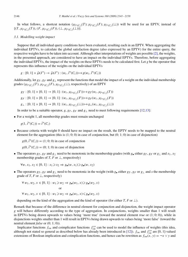
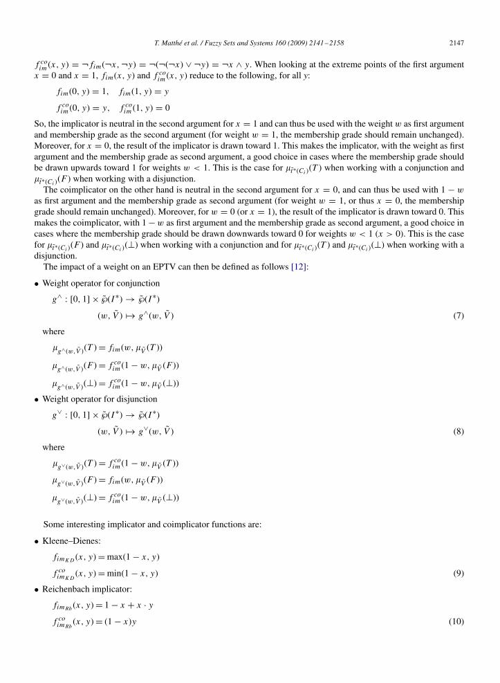
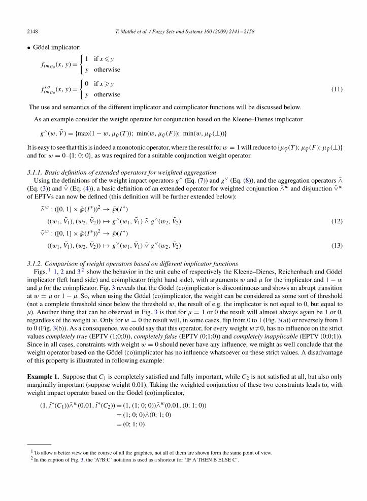
3.1.2. Comparison of weight operators based on different implicator functionsFigs. 1 1, 2 and 32 show the behavior in the unit cube of respectively the Kleene–Dienes, Reichenbach and Gödel

implicator (left hand side) and coimplicator (right hand side), with arguments w and � for the implicator and 1 − w

and � for the coimplicator. Fig. 3 reveals that the Gödel (co)implicator is discontinuous and shows an abrupt transitionat w = � or 1 − �. So, when using the Gödel (co)implicator, the weight can be considered as some sort of threshold(not a complete threshold since below the threshold w, the result of e.g. the implicator is not equal to 0, but equal to�). Another thing that can be observed in Fig. 3 is that for � = 1 or 0 the result will almost always again be 1 or 0,regardless of the weightw. Only for w = 0 the result will, in some cases, flip from 0 to 1 (Fig. 3(a)) or reversely from 1to 0 (Fig. 3(b)). As a consequence, we could say that this operator, for every weight w � 0, has no influence on the strictvalues completely true (EPTV (1;0;0)), completely false (EPTV (0;1;0)) and completely inapplicable (EPTV (0;0;1)).Since in all cases, constraints with weight w = 0 should never have any influence, we might as well conclude that theweight operator based on the Gödel (co)implicator has no influence whatsoever on these strict values. A disadvantageof this property is illustrated in following example:

Example 1. Suppose that C1 is completely satisfied and fully important, while C2 is not satisfied at all, but also onlymarginally important (suppose weight 0.01). Taking the weighted conjunction of these two constraints leads to, withweight impact operator based on the Gödel (co)implicator,

(1, t∗(C1))∧w(0.01, t∗(C2))= (1, (1; 0; 0))∧w(0.01, (0; 1; 0))= (1; 0; 0)∧(0; 1; 0)= (0; 1; 0)

1 To allow a better view on the course of all the graphics, not all of them are shown form the same point of view.2 In the caption of Fig. 3, the ‘A?B:C’ notation is used as a shortcut for ‘IF A THEN B ELSE C’.


w w

µ µ

Fig. 1. Kleene–Dienes (co)implicator: (a) fimK D (w,�) = max(1 − w,�) and (b) f coimK D(1 − w,�) = min(w,�).

w µ w µ

Fig. 2. Reichenbach (co)implicator: (a) fimRb (w,�) = 1 − w + w · � and (b) f coimRb(1 − w,�) = w · �.

W

Wµ

µ

Fig. 3. Gödel (co)implicator: (a) fimGo (w,�) = w�� ? 1 : � and (b) f coimGo(1 − w,�) = w�1 − � ? 0 : �.

This shows that an otherwise perfectly good solution is blocked completely by an unsatisfied constraint with verylow (but nonzero) weight. This is not what one would expect, because constraint C2 is considered not to be veryimportant. A similar result can be found for disjunction, where an otherwise totally unsatisfactory solution will bepresented as totally acceptable because one constraint, although with very low weight, is totally satisfied. Followingexample illustrates this:

Example 2. Suppose that C1 is completely unsatisfied and fully important, while C2 is totally satisfied, but onlymarginally important (suppose weight 0.01). Taking the weighted disjunction of these two constraints leads to, with


weight impact operator based on the Gödel (co)implicator,

(1, t∗(C1))∨w(0.01, t∗(C2))= (1, (0; 1; 0))∨w(0.01, (1; 0; 0))= (0; 1; 0)∨(1; 0; 0)= (1; 0; 0)

In contrast with the Gödel (co)implicator, the other two implicator types are continuous (see Figs. 1 and 2). Thesetwo operators also do not have the problem illustrated above of not having any influence on the strict truth values, whichis illustrated in following example, using the weight impact operator based on the Kleene–Dienes (co)implicator.

Example 3. Suppose that C1 is completely satisfied and fully important, while C2 is not satisfied at all, but also onlymarginally important (suppose weight 0.01). Taking the weighted conjunction of these two constraints leads to, withweight impact operator based on the Kleene–Dienes (co)implicator,

(1, t∗(C1))∧w(0.01, t∗(C2))= (1, (1; 0; 0))∧w(0.01, (0; 1; 0))= (max(1 − 1, 1);min(1, 0);min(1, 0))

∧(max(1 − 0.01, 0);min(0.01, 1);min(0.01, 0))

= (1; 0; 0)∧(0.99; 0.01; 0)= (0.99; 0.01; 0)

Even more, for the strict truth values, there is no difference between the weight operator based on the Kleene–Dienes(co)implicator and the one based on the Reichenbach (co)implicator, because

max(1 − w, 1) = 1 = 1 − w + w · 1max(1 − w, 0) = 1 − w = 1 − w + w · 0min(w, 1) = w = w · 1min(w, 0) = 0 = w · 0

For other than the strict truth values, there is a difference between both operators. Beside being continuous, theReichenbach (co)implicator based operator is also smooth, while the Kleene–Dienes (co)implicator based operatoris not. This last one still acts as a kind of threshold: for a fixed weight and variable membership grade (or reverse),different values are mapped to the same result (e.g. ∀� ∈ [0, 1] : ��w ⇒ min(w, �) = w). This is not the case forthe Reichenbach (co)implicator based operator. So the Reichenbach (co)implicator has greater distinguishing power,but on the downside is also harder to calculate.The final decision ofwhich operator to use depends largely on the context of the application at hand.When a threshold

interpretation of the weight is desired, the operator based on the Gödel (co)implicator is the best choice. However, mostof the time this is not the case, and then the other two operators are better choices. These two behave similarly, but, asstated above, the Kleene–Dienes (co)implicator is easier to calculate, making the operator based on it a good choicein case performance is important (as was the case for the Zadeh t-(co)norm), while the Reichenbach (co)implicatorhas a greater distinctive power, making the operator based on it a good choice in case the user wants to differentiatemore between the several possible results (as was the case for the probabilistic t-(co)norm). Opposed to the choice oft-(co)norm in the aggregation operator, idempotency is not an issue here. The reason for this is that the two componentsin the (co)implicator function are of a different nature: one is the weight (or inverse of the weight), while the other oneis a membership degree in the EPTV.

3.2. Combining different types of aggregation

The operators presented thus far are suited for the aggregation of weighted selection criteria, as long as one stayswithin one type of aggregation (either conjunctive or disjunctive). This follows from the fact that the impact of theweights can be calculated before the actual aggregation itself. So, after applying the weight operators, it is like working


with ‘regular’ EPTVs and all properties (associativity, commutativity) of the weighted aggregation are implied by theunderlying aggregation operators ∧ and ∨.

However, this is no longer the case when conjunction and disjunction operators are combined and used in one singleexpression. This is illustrated by the following straightforward examples. Hereby, (w, t∗(Ci )) is used as a shorthandnotation for the EPTV resulting from the evaluation of condition Ci , with weight w.

Example 4.

(a) [(0, t∗(C1))∧w(0, t∗(C2))]∨w(1, t∗(C3))Intuitively, this expression should reduce to t∗(C3), since constraints with weight 0 can be omitted. However, ifwe blindly apply the operators ∧w (Eq. (12)) and ∨w (Eq. (13)) given in 3.1, and taken into account that (1;0;0)is the neutral element of the conjunction, the evaluation of the expression results in [(1; 0; 0)∧(1; 0; 0)]∨t∗(C3).Further calculation leads to (1; 0; 0)∨t∗(C3) = (1; 0; 0) which is not the expected value t∗(C3).

(b) [(0, t∗(C1))∨w(0, t∗(C2))]∧w(1, t∗(C3))Intuitively, this expression should reduce to t∗(C3), since constraints with weight 0 can be omitted. However, ifwe blindly apply the operators ∧w (Eq. (12)) and ∨w (Eq. (13)) given in 3.1, and taken into account that (0;1;0)is the neutral element of the disjunction, the evaluation of the expression results in [(0; 1; 0)∨(0; 1; 0)]∧ t∗(C3).Further calculation leads to (0; 1; 0)∧ t∗(C3) = (0; 1; 0), which is not the expected value t∗(C3).

It is obvious that this is not the way to handle weights. The reason for this insufficiency is that the impact of theweights is different when using conjunction than when using disjunction. They work in a different ‘direction’, towardtheir respective neutral elements, because the neutral element of the one, is the absorbing element of the other.To solve this problem, the weights need to be propagated throughout the calculations, i.e. the weights of the inter-

mediate results need to be remembered and be taken into account when evaluating the remainder of the expression.E.g., in the first example above, the result of the conjunction (0, t∗(C1))∨w(0, t∗(C2)) should also have weight 0. Inthat case, the resulting EPTV (1; 0; 0) would, in the next step (disjunction), again be transformed to the EPTV (0; 1; 0),leading to the final (correct!) result t∗(C3). A number of rules can be imposed for the calculation of the weight of anintermediate result:

• Constraints with weight w = 0 are not allowed to have any impact at all. Therefore, both (0, t∗(C1))∧w(w, t∗(C2))and (0, t∗(C1))∨w(w, t∗(C2)) should produce an intermediate result with weight w. So for the calculations of theweights of the intermediate results, 0 will be the identity element.

• Because the aggregation itself should be associative and commutative, also the calculations of the weights of theintermediate results should be associative and commutative.

• The calculations should be monotone. If w1�w3 and w2�w4 (with w1, w2, w3 and w4 the respective weights ofconstraints C1,C2,C3 and C4) then the calculated weight for the aggregation of C1 and C2 should be less or equalto the calculated weight for the aggregation of C3 and C4.

Remark that here, opposed to the actual impact of the weights, the rules are the same for conjunction and disjunction.These are precisely the properties of a t-conorm, and thus a t-conorm can be chosen to calculate the resulting weightof an aggregation. So, both for conjunction and disjunction it holds that

wres = u(w1, w2)

where u is a t-conorm and wres represents the weight resulting from an aggregation of arguments with respectiveweights w1 and w2. Because the resulting weight is the same for conjunction and disjunction, the final aggregatedweight of (a subpart of) a query will be the same regardless whether the query has a complex conjunctive–disjunctivestructure or that it is presented in a purely conjunctive (or disjunctive) form.From the above it follows that an EPTV cannot be seen separately from its importance (indicated by a weight).

Weights are propagated and the result of a weighted aggregation of EPTVs is a new EPTVwith again a weight attachedto it. Remark also that, when using an appropriate scaling of weights (max(wi ) = 1) and a t-conorm to calculate theweight of an (intermediate) result, the weight of the final result will always be 1.So, the basic definition of the extended operators for weighted conjunction ∧w (Eq. (12)) and disjunction ∨w

(Eq. (13)) of EPTVs, presented above, must be adjusted to also calculate a weight for the result of the aggregation,


resulting finally in following operators:

∧w : ([0, 1] × ℘(I ∗))2 → [0, 1] × ℘(I ∗)

((w1, V1), (w2, V2)) � (u(w1, w2), g∧(w1, V1) ∧ g∧(w2, V2)) (14)

∨w : ([0, 1] × ℘(I ∗))2 → [0, 1] × ℘(I ∗)

((w1, V1), (w2, V2)) � (u(w1, w2), g∨(w1, V1) ∨ g∨(w2, V2)) (15)

Although not absolutely necessary and a different t-conorm could possibly be used for calculating the resulting weightsthan the one used for calculating the aggregation, a logical choice would be to use the same t-conorm used for theaggregation.Because, as stated above, an EPTV cannot be seen separately from its importance throughout the calculations, the

result of a negation should also produce a new EPTV with weight attached to it. So, also an extended operator fornegation can be defined

¬w : [0, 1] × ℘(I ∗) → [0, 1] × ℘(I ∗)(w, V )� (w, ¬(V )) (16)

where the weight of an EPTV remains unchanged under negation.When using these operators, with propagation of the weights throughout the calculations, the problems arising when

combining disjunction and conjunction, as presented above, are solved. E.g., when looking back at Examples 4(a) and(b), using these operators leads to:

Example 5.

(a)

[(0, t∗(C1))∧w(0, t∗(C2))]∨w(1, t∗(C3))= [u(0, 0), ((1; 0; 0)∧(1; 0; 0))]∨w(1, t∗(C3))

= (0, (1; 0; 0))∨w(1, t∗(C3))

= (u(0, 1), ((0; 1; 0)∨t∗(C3)))

= (1, t∗(C3))

(b)

[(0, t∗(C1))∨w(0, t∗(C2))]∧w(1, t∗(C3))= [u(0, 0), ((0; 1; 0)∨(0; 1; 0))]∧w(1, t∗(C3))

= (0, (0; 1; 0))∧w(1, t∗(C3))

= (u(0, 1), ((1; 0; 0)∧t∗(C3)))

= (1, t∗(C3))

Both Examples 5(a) and (b) result in (1, t∗(C3)), as was intuitively expected.

3.3. Associativity

The novel approach introduced above solves the problems arising when combining disjunction and conjunction.However, at the same time, it introduces new problems when working within one type of aggregation (conjunction ordisjunction). Namely, it is possible, depending on the chosen weight and aggregation operators, that the aggregation isno longer associative, i.e. (A∧wB)∧wC � A∧w(B∧wC), as illustrated in following example:

Example 6. Calculate (0.4, (1; 0.5; 0.7))∧w(0.6, (0.3; 1; 0.1))∧w(0.9, (1; 1; 0))In this example, it is not the case that max(wi ) = 1 (so, it is assumed that these are only intermediate calculations

and that somewhere in the remainder of the calculations, there is a constraint with associated weight equal to 1).


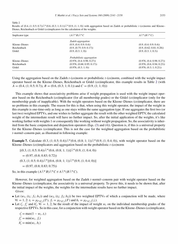
Table 2Results of (0.4, (1; 0.5; 0.7))∧w(0.6, (0.3; 1; 0.1))∧w(0.9, (1; 1; 0)) with aggregation based on Zadeh or probabilistic t-(co)norms and Kleene–Dienes, Reichenbach or Gödel (co)implicators for the calculation of the weights.

Implicator type (A∧wB)∧wC A∧w(B∧wC)

Zadeh aggregationKleene–Dienes (0.9, (0.4; 0.9; 0.4)) (0.9, (0.4; 0.9; 0.4))Reichenbach (0.9, (0.75; 0.9; 0.17)) (0.9, (0.62; 0.81; 0.28))Gödel (0.9, (0.3; 1; 0)) (0.9, (0.3; 1; 0.3))

Probabilistic aggregationKleene–Dienes (0.976, (0.4; 0.98; 0.27)) (0.976, (0.4; 0.98; 0.27))Reichenbach (0.976, (0.68; 0.95; 0.17)) (0.976, (0.6; 0.94; 0.23))Gödel (0.976, (0.3; 1; 0)) (0.976, (0.3; 1; 0.21))

Using the aggregation based on the Zadeh t-(co)norm or probabilistic t-(co)norm, combined with the weight impactoperator based on the Kleene–Dienes, Reichenbach or Gödel (co)implicator, this example results in Table 2 (withA = (0.4, (1; 0.5; 0.7)), B = (0.6, (0.3; 1; 0.1)) and C = (0.9, (1; 1; 0)))

This example shows that associativity problems arise if weight propagation is used with the weight impact oper-ator based on the Reichenbach (co)implicator (for all membership grades) or the Gödel (co)implicator (only for themembership grade of inapplicable). With the weight operators based on the Kleene–Dienes (co)implicator, there areno problems in this example. The reason for this is that, when using this weight operator, the impact of the weight inthis example is one-time-only as long as one stays within the same aggregation type. If one aggregates the first two (orlast two) weighted EPTVs, and one wishes to further aggregate the result with the other weighted EPTV, the calculatedweight of the intermediate result will have no further impact. So, after the initial application of the weights, it’s likeworking further with weights 1 or consequently like working without weight propagation. So, the associativity is inher-ited from the basic conjunction and disjunction operators (Eqs. (3) and (4)). Question is, if this is a universal propertyfor the Kleene–Dienes (co)implicator. This is not the case for the weighted aggregation based on the probabilistict-norm/t-conorm pair, as illustrated in following example:

Example 7. Calculate (0.3, (1; 0.5; 0.4))∧w(0.6, (0.8; 1; 1))∧w(0.9, (1; 0.4; 0)), with weight operator based on theKleene–Dienes (co)implicators and aggregation based on the probabilistic t-(co)norm

[(0.3, (1; 0.5; 0.4))∧w(0.6, (0.8; 1; 1))]∧w(0.9, (1; 0.4; 0))= (0.97, (0.8; 0.83; 0.72))

(0.3, (1; 0.5; 0.4))∧w[(0.6, (0.8; 1; 1))∧w(0.9, (1; 0.4; 0))]= (0.97, (0.8; 0.83; 0.75))

So, in this example (A∧wB)∧wC � A∧w(B∧wC).

However, for weighted aggregation based on the Zadeh t-norm/t-conorm pair with weight operator based on theKleene–Dienes (co)implicator, the associativity is a universal property. To prove this, it needs to be shown that, afterthe initial impact of the weights, the weights for the intermediate results have no further impact.Given:

• Let (w1, (t1; f1; b1)) and (w2, (t2; f2; b2)) be two weighted EPTVs of which a conjunction will be made, where∀i = 1, 2: ti = �t∗(Ci )(T ), fi = �t∗(Ci )(F) and bi = �t∗(Ci )(⊥).

• Let t ′i , f ′i and b′

i , ∀i = 1, 2, be the result of the impact of weight wi on the individual membership grades of therespective EPTVs. So in this case, for a conjunction with weight operator based on the Kleene–Dienes (co)implicator,

t ′i =max(1 − wi , ti )

f ′i =min(wi , fi )

b′i =min(wi , bi )


• Let C be the weighted conjunction of the two constraints C1 and C2, resulting in the weighted EPTV (w, (t; f ; b)),where t = �t∗(C)(T ), f = �t∗(C)(F) and b = �t∗(C)(⊥), then (see Eq. (14))

t = i(t ′1, t′2)

f = u( f ′1, f ′

2)

b = u[u(i(t ′1, b′2), i(b

′1, t

′2)), i(b

′1, b

′2)]

w = u(w1, w2)

• Let t ′, f ′ and b′ be the result of the impact of weightw on the individual membership grades of t∗(C) in case of furthercalculations. So in this case, for a conjunction with weight operator based on the Kleene–Dienes (co)implicator,

t ′ =max(1 − w, t)

f ′ =min(w, f )

b′ =min(w, b)

It needs to be proven that

t ′ = t

f ′ = f

b′ = b

Proof.

• For the membership grade of true, it holds that

t = i(max(1 − w1, t1),max(1 − w2, t2))

The impact of the weight w on this leads to

t ′ =max(1 − w, t)

=max(1 − u(w1, w2), i(max(1 − w1, t1),max(1 − w2, t2)))

=max(i(1 − w1, 1 − w2), i(max(1 − w1, t1),max(1 − w2, t2)))

because i and u are a De Morgan pair

= i(max(1 − w1, t1),max(1 − w2, t2))

because of the monotonicity property of a t-norm i:

max(1 − w1, t1)�1 − w1 ∧ max(1 − w2, t2)�1 − w2

⇒ i(max(1 − w1, t1),max(1 − w2, t2))� i(1 − w1, 1 − w2)

= t

So, in all cases, it holds that t ′ = t! Remark that, for the membership grade of true, no assumption needs to be madeabout the family of the t-norm/t-conorm pair.

• For the membership grade of false, it holds that

f = u(min(w1, f1),min(w2, f2))


f ′ =min(w, f )

=min(u(w1, w2), u(min(w1, f1),min(w2, f2)))

= u(min(w1, f1),min(w2, f2))


because of the monotonicity property of a t-conorm u:

min(w1, f1)�w1 ∧ min(w2, f2)�w2

⇒ u(min(w1, f1),min(w2, f2))�u(w1, w2)

= f

So, in all cases, it holds that f ′ = f ! Remark that, for the membership grade of false, no assumption needs to bemade about the family of the t-norm/t-conorm pair.

• For the membership grade of inapplicable, it holds that

b = u

⎛⎝ u

(i(max(1 − w1, t1),min(w2, b2)),i(min(w1, b1),max(1 − w2, t2))

),

i(min(w1, b1),min(w2, b2))

⎞⎠

Here, the proof cannot be given for all t-norm/t-conorm pairs, as was shown in the counterexample above (Example7). When working with the Zadeh t-(co)norm, this leads to

b =max

⎛⎜⎝max

(min(max(1 − w1, t1),min(w2, b2)),

min(min(w1, b1),max(1 − w2, t2))

),

min(min(w1, b1),min(w2, b2))

⎞⎟⎠

=max

⎛⎜⎝min(max(1 − w1, t1),min(w2, b2)),

min(min(w1, b1),max(1 − w2, t2)),


⎞⎟⎠


b′ =min(w, b)

=min

⎛⎜⎜⎜⎜⎝

max(w1, w2),

max

⎛⎜⎝min(max(1 − w1, t1),min(w2, b2)),

min(min(w1, b1),max(1 − w2, t2)),


⎞⎟⎠

⎞⎟⎟⎟⎟⎠

=max

⎛⎜⎝min(max(1 − w1, t1),min(w2, b2)),

min(min(w1, b1),max(1 − w2, t2)),


⎞⎟⎠

because:

⎧⎪⎪⎪⎪⎨⎪⎪⎪⎪⎩

max(w1, w2)�w1,max(w1, w2)�w2

w2� min(max(1 − w1, t1),min(w2, b2))

w1� min(min(w1, b1),max(1 − w2, t2))

max(w1, w2)� min(min(w1, b1),min(w2, b2))

⇒ max(w1, w2)� max

⎛⎜⎝min(max(1 − w1, t1),min(w2, b2)),

min(min(w1, b1),max(1 − w2, t2)),


⎞⎟⎠

= b

So, when working with the Zadeh t-(co)norm, it always holds that b′ = b! �

The solution of the associativity problem can be found in the reason why the Kleene–Dienes based operator withZadeh t-(co)norm does not have this problem. Namely, as long as one stays within one type of aggregation (eitherconjunction or disjunction), one should work without weight propagation. It is only when switching from aggregation


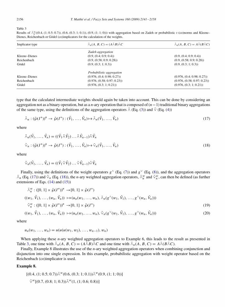
Table 3Results of ∧w

n ((0.4, (1; 0.5; 0.7)), (0.6, (0.3; 1; 0.1)), (0.9, (1; 1; 0))) with aggregation based on Zadeh or probabilistic t-(co)norms and Kleene–Dienes, Reichenbach or Gödel (co)implicators for the calculation of the weights.

Implicator type ∧n(A, B,C) = (A∧B)∧C ∧n(A, B,C) = A∧(B∧C)

Zadeh aggregationKleene–Dienes (0.9, (0.4; 0.9; 0.4)) (0.9, (0.4; 0.9; 0.4))Reichenbach (0.9, (0.58; 0.9; 0.28)) (0.9, (0.58; 0.9; 0.28))Gödel (0.9, (0.3; 1; 0.3)) (0.9, (0.3; 1; 0.3))

Probabilistic aggregationKleene–Dienes (0.976, (0.4; 0.98; 0.27)) (0.976, (0.4; 0.98; 0.27))Reichenbach (0.976, (0.58; 0.97; 0.23)) (0.976, (0.58; 0.97; 0.23))Gödel (0.976, (0.3; 1; 0.21)) (0.976, (0.3; 1; 0.21))

type that the calculated intermediate weights should again be taken into account. This can be done by considering anaggregation not as a binary operation, but as a n-ary operation that is composed of (n−1) traditional binary aggregationsof the same type, using the definitions of the aggregation operators ∧ (Eq. (3)) and ∨ (Eq. (4))

∧n : (℘(I ∗))n → ℘(I ∗) : (V1, . . . , Vn)� ∧n(V1, . . . , Vn) (17)

where

∧n(V1, . . . , Vn) = ((V1∧V2) . . . ∧Vn−1)∧Vn

∨n : (℘(I ∗))n → ℘(I ∗) : (V1, . . . , Vn)� ∨n(V1, . . . , Vn) (18)

where

∨n(V1, . . . , Vn) = ((V1∨V2) . . . ∨Vn−1)∨Vn

Finally, using the definitions of the weight operators g∧ (Eq. (7)) and g∨ (Eq. (8)), and the aggregation operators∧n (Eq. (17)) and ∨n (Eq. (18)), the n-ary weighted aggregation operators, ∧w

n and ∨wn , can then be defined (as further

extensions of Eqs. (14) and (15))

∧wn : ([0, 1] × ℘(I ∗))n →[0, 1] × ℘(I ∗)

((w1, V1), . . . , (wn, Vn)) � (un(w1, . . . , wn), ∧n(g∧(w1, V1), . . . , g

∧(wn, Vn)))

∨wn : ([0, 1] × ℘(I ∗))n →[0, 1] × ℘(I ∗) (19)

((w1, V1), . . . , (wn, Vn)) � (un(w1, . . . , wn), ∨n(g∨(w1, V1), . . . , g

∨(wn, Vn))) (20)

where

un(w1, . . . , wn) = u(u(u(w1, w2), . . . , wn−1), wn)

When applying these n-ary weighted aggregation operators to Example 6, this leads to the result as presented inTable 3, one time with ∧n(A, B,C) = (A∧B)∧C and one time with ∧n(A, B,C) = A∧(B∧C).Finally, Example 8 illustrates the use of the n-ary weighted aggregation operators when combining conjunction and

disjunction into one single expression. In this example, probabilistic aggregation with weight operator based on theReichenbach (co)implicator is used.

Example 8.

[(0.4, (1; 0.5; 0.7))∧w(0.6, (0.3; 1; 0.1))∧w(0.9, (1; 1; 0))]∨w[(0.7, (0.8; 1; 0.3))∧w(1, (1; 0.6; 0.8))]


Using the n-ary weighted aggregation operators, this leads to

∨wn

( ∧wn ((0.4, (1; 0.5; 0.7)), (0.6, (0.3; 1; 0.1)), (0.9, (1; 1; 0))),

∧wn ((0.7, (0.8; 1; 0.3)), (1, (1; 0.6; 0.8)))

)

= ∨wn

((un(0.4, 0.6, 0.9), ∧n((1; 0.2; 0.28), (0.58; 0.6; 0.06), (1; 0.9; 0))),(un(0.7, 1), ∧n((0.86; 0.7; 0.21), (1; 0.6; 0.8)))

)

= ∨wn

((0.976, (0.58; 0.97; 0.23)),(1, (0.86; 0.88; 0.79))

)

= (un(0.976, 1), ∨n((0.58; 0.97; 0.23), (0.86; 0.88; 0.79)))= (1, (0.94; 0.85; 0.85))

4. Conclusion

Inflexible queries,weights canbe attached to constraints to indicate user preferences between the different constraints.This paper showedhowweights have their impact on the satisfaction grades for the individual selection criteria,modelledby extended possibilistic truth values. The impact of the weights, modelled by means of modification functions basedon (co)implicators, is different according to the aggregation type (conjunction or disjunction). It has been shown that theweights need to be propagated throughout the calculations, and that therefore the EPTVs cannot be viewed separatelyfrom their associated weight. In addition, to eliminate associativity problems, weighted aggregation of EPTVs shouldno longer be regarded as a binary operation, but as a n-ary operation.

References

[1] G. Bordogna, G. Pasi (Eds.), Recent Issues on Fuzzy Databases, Physica-Verlag, Heidelberg, Germany, 2000.

[2] G. Bordogna, G. Pasi, A flexible approach to evaluating soft conditions with unequal preferences in fuzzy databases: research articles,International Journal of Intelligent Systems 22 (7) (2007) 665–689.

[3] P. Bosc, O. Pivert, Some approaches for relational databases flexible querying, International Journal on Intelligent Information Systems 1 (1992)323–354.

[4] P. Bosc, O. Pivert, SQLf: a relational database language for fuzzy querying, IEEE Transactions on Fuzzy Systems 3 (1995) 1–17.

[5] P. Bosc, J. Kacprzyk (Eds.), Fuzziness in Database Management Systems, Physica-Verlag, Heidelberg, Germany, 1995.

[6] P. Bosc, D.H. Kraft, F.E. Petry, Fuzzy sets in database and information systems: status and opportunities, Fuzzy Sets and Systems 156 (3)(2005) 418–426.

[7] R. de Caluwe (Ed.), Fuzzy and Uncertain Object-oriented Databases: Concepts and Models, World Scientific, Singapore, 1997.

[8] G. De Cooman, From possibilistic information to Kleene’s strong multi-valued logics, in: D. Dubois et al. (Eds.), Fuzzy Sets, Logics andReasoning about Knowledge, Kluwer Academic Publishers, Boston, USA, 1999, pp. 315–323.

[9] G. De Tré, Extended possibilistic truth values, International Journal of Intelligent Systems 17 (2002) 427–446.

[10] G. De Tré, R. De Caluwe, J.Verstraete, A. Hallez, Conjunctive aggregation of extended possibilistic truth values and flexible database querying,in: Lecture Notes in Artificial Intelligence, vol. 2522, Springer, Berlin, 2002, pp. 344–355.

[11] G. De Tré, R. De Caluwe, Modelling uncertainty in multimedia database systems: an extended possibilistic approach, International Journal ofUncertainty, Fuzziness and Knowledge-Based Systems 11 (1) (2003) 5–22.

[12] G. De Tré, B. De Baets, Aggregating constraint satisfaction degrees expressed by possibilistic truth values, IEEE Transactions on Fuzzy Systems11 (3) (2003) 361–368.

[13] D. Dubois, H. Fargier, H. Prade, Beyond min aggregation in multicriteria decision: (ordered) weighted min, discri-min and leximin, in: R.R.Yager, J. Kacprzyk (Eds.), The Ordered Weighted Averaging Operators: Theory and applications, Kluwer Academic Publishers, Boston, USA,1997, pp. 181–192.

[14] J. Galindo, J.M. Medina, O. Pons, J.C. Cubero, A server for fuzzy SQL queries, in: Lecture Notes in Computer Science, vol. 1495, Springer,Berlin, 1998, pp. 164–174.

[15] Z. Ma (Ed.), Advances in Fuzzy Object-Oriented Databases: Modeling and Applications, About Idea Group, Hershey, USA, 2005.

[16] T. Matthé, G. De Tré, Flexible querying in a relational framework supported by possibilistic logic, Fuzzy Sets and Systems 159 (12) (2008)1468–1484.


[17] F.E. Petry, Fuzzy Databases: Principles and Applications, Kluwer Academic Publishers, Boston, USA, 1996.[18] H. Prade, Possibility sets, fuzzy sets and their relation to Lukasiewicz logic, in: Proceedings of the 12th International Symposium on Multiple-

Valued Logic, Paris, France, 1982, pp. 223–227.[19] H. Prade, C. Testemale, Generalizing database relational algebra for the treatment of incomplete or uncertain information and vague queries,

Information Sciences 34 (1984) 115–143.[20] N. Rescher, Many-Valued Logic, McGraw-Hill, New York, USA, 1969.[21] A. Takaci, Handling priority within a database scenario, ETF Journal of Electrical Engineering 17 (2006) 130–134.[22] R.R. Yager, On ordered weighted averaging aggregation operators in multi-criteria decision making, IEEE Transactions on Systems, Man and

Cybernetics 18 (1988) 183–190.[23] A. Yazici, R. George, Fuzzy Database Modeling, Physica-Verlag, Heidelberg, Germany, 1999.[24] S. Zadrozny, J. Kacprzyk, FQUERY for access: towards human consistent querying user interface, in: Proceedings of the 1996ACMSymposium

on Applied Computing (SAC), Philadelphia, USA, 1996, pp. 532–536.

Documents

Impact of weights on conjunctive and disjunctive aggregation of extended possibilistic truth values