Impact of Recommender System on CompetitionBetween Personalizing and Non-Personalizing Firms

How do recommender systems affect prices and profits of firms under competition? To explore this question,

we model the strategic behavior of customers that make repeated purchases at two competing firms: one that

provides personalized recommendations and another that does not. When a customer intends to purchase

a product, she obtains recommendations from the personalizing firm and uses this recommendation to

eventually purchase from one of the firms. The personalizing firm profiles the customer (based on past

purchases) to recommend products. Hence, if a customer purchases less frequently from the personalizing

firm, the recommendations made to her become less relevant. While considering the impact on the quality of

recommendations received, a customer must balance two opposing forces: (1) the lower price charged by the

non-personalizing firm, and (2) an additional fit cost incurred when purchasing from the non-personalizing

firm and the increased cost due to recommendations of reduced quality in the future. An outcome of the

analysis is that the customers should distribute their purchases across both firms to maximize surplus over a

planning horizon. Anticipating this response, the firms simultaneously choose prices. We study the sensitivity

of the equilibrium prices and profits of the firms with respect to the effectiveness of the recommender system

and the profile deterioration rate. We also analyze some interesting variants of the base model in order

to study how its key results could be influenced. One of the key take-aways of this research is that the

recommender system can influence the price and profit of not only the personalizing firm but also of the

non-personalizing firm.

Key words : recommender systems, duopoly, pricing, dynamic optimization, Nash equilibrium.

1. Introduction

The value of commerce through online shopping increased dramatically in the past decade. In

2013, the U.S. retail e-commerce sales grew by 16.9 percent to reach $263.3 billion, and it

accounted for 5.8 percent of the total retail sales (U.S. Census Bureau 2014). Retailing firms with

an online storefront often employ recommender systems to provide personalized recommendations

to customers (hereafter referred to as personalizing firms) (Adomavicius and Tuzhilin 2005, Crum

2008, Tam and Ho 2005). Some prominent examples of personalizing firms are Amazon.com,

Target, Costco, and Home Depot. In 2007, 41 percent of electronic retailers were found to provide

personalized services, a value that is estimated to increase over time (Lovett 2007).

Fit costs are often incurred when there are a large number of items being sold and the

customer cannot evaluate all these items to purchase her ideal product. Recommender systems

1

2

help a consumer quickly learn about the products that are likely to be her ideal product (Hinz

and Eckert 2010, Murthi and Sarkar 2003, Resnick and Varian 1997). Typically, these systems

gather knowledge on customer preferences through data collected about them (such as

demographic and psychographic) and their past online transactions. Based on this knowledge,

recommender systems predict the needs of the customers to recommend items that best match

their current preferences (Cao and Li 2007, Konstan and Riedl 2012, Schafer et al. 2001). In

other words, the main goal of a recommender system is to help a customer find the item she

wishes to purchase and thereby lower the fit cost associated with the purchase. Here, the

predictive knowledge gleaned about a customer’s preferences is referred to as the customer’s

profile. The profile, for instance, consists of known characteristics of the customer as well as

several unknown characteristics that are estimated using the known characteristics and the

previous transactions of the customer. Reducing the noise associated with these estimates

corresponds to improving the quality of the profile.

Despite their recognized benefits, recommender systems are not always viable for

small-to-medium sized firms because of the high costs associated with their implementation and

use (Leavitt 2006). Hence, many less prominent electronic retailers still sell products without

providing personalization services (hereafter referred to as non-personalizing firms). For example,

the online bookseller Buybooksontheweb.com does not provide personalization services to its

customers. Similarly, while iTunes provides personalized recommendations (through their toolbar

“Genius”) for music items, another online firm iomoio.com sells music without doing so. Likewise,

movies can be purchased from Amazon (where personalized recommendations are provided) or

fullmovies.com (where recommendation is not provided).

Given that a customer has two choices (a personalizing firm and a non-personalizing firm) to

purchase products, it is always beneficial for her to first visit the personalizing firm and use the

recommendations provided to her to purchase products from one of the two firms. She can

identify a preferred product (among the recommended ones) and decide to purchase that product

from the personalizing firm or a similar product from the non-personalizing firm. Bank (1999)

3

reports such behavior in the retailing context where customers obtain recommendations from

Amazon.com, but use these recommendations to purchase similar products from another firm.

Firms that provide differentiated services often charge a price premium (Ozmen 2005, Pathak

et al. 2010, Smith and Brynjolfsson 2001). Hence, the prices at the personalizing firms are

typically higher (Moon et al. 2008).1 However, as discussed earlier, the recommendations are

based on the profile quality of the customer, which depends on the transaction history of the

customer with the personalizing firm. Hence, if the customer purchases from the

non-personalizing firm, the personalizing firm loses the opportunity to improve the customer’s

profile. As a result, the usefulness of the future recommendations for the customer may reduce.

Thus, in spite of lower prices, the customer may not always purchase from the non-personalizing

firm. Rather, she may distribute her purchases across the two firms. Several empirical studies

have provided evidence for such behavior by customers where they forgo cheaper products and

purchase from the personalizing firm to let the recommender system learn their preferences

(Ozmen 2005, Smith and Brynjolfsson 2001). Managers and analysts also confirm that today’s

customers behave in such manner (Yu 2012). Besides, the elite firms like Amazon.com educate

customers that the quality of their future recommendations improve as they purchase more from

the firm (Amazon 2013). Along these lines, researchers have also noted that the customers are

aware of this advantage (Kramer et al. 2007).

Based on the above discussion, the basic setting of our problem is as follows. The customer

first visits the personalizing firm and uses the firm’s recommendations to find her preferred

product. Then, she purchase either the preferred product from the personalizing firm or its

substitute from the non-personalizing firm. We allow for the fact that a customer may not be

able to find her ideal product at either firm (Beach 1993). Instead, the product comes with a fit

cost at both firms. Further, the product purchased from the non-personalizing firm may not be

exactly the same as her preferred product. Additionally, the customer may need to spend some

extra effort to search for a substitute at the non-personalizing firm. Hence, the customer often

1 In this study, however, we determine the prices at the two firms endogenously, and allow the price at the personalizingfirm to be higher or lower than that at the non-personalizing firm. Therefore, our model considers a general scenario.

4

incurs an additional cost while purchasing from the non-personalizing firm. Also, as discussed

earlier, when the customer purchases from the non-personalizing firm, the personalizing firm loses

the information about the preferences of the customer. This may lead to increased fit cost in the

future. Hence, while purchasing from the non-personalizing firm, the customer faces a trade-off

between increased fit costs for future purchases and the current lower price of the product (net of

additional cost). Thus, the optimal strategy for the customer is to distribute her purchases across

the two firms, rather than purchasing exclusively at one of the firms. Anticipating the purchase

behavior of customers, the two firms engage in a simultaneous move price game.

The fact that the customer may distribute her purchases across the two firms is a consequence

of the dynamic nature of the profile. When customer preferences change with time, the profile

deteriorates if the opportunity to observe the change is lost by the personalizing firm. On the

other hand, the profile improves when the customer purchases at the personalizing firm. The

analysis of the problem therefore necessitates a model that can suitably capture the dynamic

nature of the phenomenon, i.e., the profile can change (improve or deteriorate) with time

depending on the manner in which the customer chooses to allocate her purchases across the two

firms. First, we consider that the customer does not change the fraction of purchases made at the

two firms. Later, we analyze the case where the customer is able to change her purchase fractions

over time. In this case, we use optimal control theory to solve the customer’s dynamic

optimization problem (e.g., Gutierrez and He 2011, He et al. 2009, Mookerjee et al. 2011).

Further, in both cases, the solution of the customer’s problem is an input to a static price game

between the two firms.

Our analysis in this study provides insights into several questions that are of managerial interest.

With an improvement in the recommender system, customers may shift more of their purchases

toward the non-personalizing firm because they can maintain the same profile quality with fewer

purchases at the personalizing firm. Thus, the personalizing firm may lose some demand as a result

of an improved recommender system. A natural question arises then: should the personalizing

firm improve its recommender system, and if so, how will this improvement affect the prices

5

charged by the two firms? A related question is: how should the non-personalizing firm react

(with respect to its pricing decision) when the recommender system (at the personalizing firm)

improves? Also, what happens to the surplus of the customer? By improving its recommender

system, the personalizing firm may command higher prices to extract part of the customer’s

surplus. Does that reduce the surplus of the customer? Can the customer increase her surplus by

being more strategic (i.e., by changing her fractions of purchases from the two firms with time)?

Another issue of interest is the impact of changing customer preferences: if the preferences

change rapidly, how will the prices in the market be affected? A rapid change in customer

preferences can be expected to cause the customer to purchase more at the personalizing firm,

implying that the personalizing firm should always prefer changing customer preferences. Our

analysis reveals that this is not always the case.

The rest of this paper is organized as follows. The next section presents a brief review of

related literature and situates our research with respect to the past studies. In Section 3, we

discuss the model and provide solutions for both customer’s problem and firms’ problem. Next,

Section 4 presents interesting managerial insights based on the results of our model. In Section 5,

we analyze different variants of the base model and discuss how the results change under different

scenarios. Finally, Section 6 concludes the paper.

2. Literature Review

We review the literature in the following streams that are related to our study: (i) personalization

and recommender systems, (ii) loyalty rewards, and (iii) product customization. In this section,

we also differentiate our work from the past literature and highlight our contributions.

2.1. Personalization and Recommender Systems

Clearly, this stream of research is closely related to our study. Personalization has been an active

area of research for more than a decade. For detailed reviews on personalization, the readers can

refer to Adomavicius and Tuzhilin (2005) and Breese et al. (1998). The studies on personalization

mainly analyze the factors that impact the profile qualities of customers and present

methodologies for improving the recommender system. However, similar to our study, some

6

researchers have focused on the impact of recommender system on search and purchase behavior

of customers (e.g., see Bodapati 2008). In the similar direction, Fleder and Hosanagar (2009)

analyze the effect of recommender systems on diversity of sales. But, in these studies, rarely has

the question been: should an existing recommender system be improved? In the current study, we

answer this question by exploring the changes in the profits and prices of firms with improvement

in the recommender system.

A few papers in this stream analyze the interaction between the recommender system and the

price charged by the firm, a setup very similar to our research. For example, Aron et al. (2006)

explore the trade-off between better customization and better prices. In spite of some similarities,

our work is very different from that of Aron et al. (2006). First of all, unlike out work, Aron et al.

(2006) consider a monopolistic firm. Hence, the notion of learning about a preferred product at

the personalizing firm and purchasing a similar product from the non-personalizing firm is

missing in Aron et al. (2006), which is the focus of our study. Second, the customer chooses the

customization level in Aron et al. (2006), whereas the recommendation quality is endogenous in

our model.

Further, similar to our study, Ozmen (2005) and Bergemann and Ozmen (2006) consider

settings with both personalizing and non-personalizing firms. In their studies, customers are

differentiated in two dimensions – the type of product they prefer and the flexibility in terms of

their choices (i.e., are they rigid or flexible in preferences for their preferred product). The

problem they analyze is how the market is segmented between the types of customers

(differentiated in the above two dimensions) with improved recommender system. In our research,

however, we consider the impact of profile quality on customer’s decision of purchasing from the

two firms. Therefore, the basic setup and the goal of our research are different from that of

Ozmen (2005) and Bergemann and Ozmen (2006). Finally, Wattal et al. (2009) analyze under

what conditions the personalization service and the product quality are complementary when

personalizing firm competes with a non-personalizing firm.2 In contrast, we consider that the

2 They also consider many other competitions, such as between two personalizing firms and two non-personalizingfirms. We do not discuss them as these competitions are not relevant to our research.

7

customer may use the personalizing firm’s recommendation to identify her preferred product and

purchase a similar product from the non-personalizing firm.

2.2. Loyalty Rewards

At a conceptual level, loyalty programs are similar to recommendation systems: both provide

immediate value to the customer and both can grow with increased patronage. In this domain,

Biyalogorsky et al. (2001) examine how a firm should strike a balance between loyalty rewards and

attractive prices to maximize profit. Lewis (2004) provides a framework to measure the influence

of loyalty reward programs on consumer retention, while Meyer-Waarden (2008) study how

loyalty programs induce customers to continue purchasing from the firm. Unlike rewards, however,

recommendations are transferable, i.e., the customer can use the recommendations provided

by a personalizing firm to find similar products at other firms. In addition, unlike rewards,

the recommendation quality reduces if fewer purchases are made at the personalizing firm.

This happens because the preferences of a customer are usually not static and change with time.

2.3. Product Customization

The literature on product customization examines the pricing strategies of firms when

they offer products that are customized to meet the needs of individual customers. Customization

is conceptually similar to personalization in the sense that both customized and personalized

products better meet the preferences of a customer. In this domain, Dewan et al. (2003)

study competition between two customizing firms to derive equilibrium prices. Syam et al. (2005)

also investigate a duopoly in which firms decide whether to customize or not, and if so, how

much to customize. Interestingly, they find that both firms should customize on the same product

attributes and provide standard features on other attributes. Further, Syam and Kumar (2006)

find that the firms should offer both standard and customized products to maximize profit.

Mendelson and Parlakturk (2008) also consider two firms – a mass customizing firm that provides

products with some delay, and a standard firm that provides standard products without delay.

In all these studies, customization is considered in a static sense and its benefits do not depend

8

on a customer’s past purchases at a customizing firm. In addition, unlike recommendations,

customers do not have a way to transfer customization benefits from one firm to another.

3. Model and the Solution

In this section, we begin with the customer’s problem, and then study a pricing game between

the two firms.

3.1. Customer’s Optimization Problem

We consider a model where the customers purchase products from two competing firms (a

non-personalizing firm and a personalizing firm) over a period of time. The customer can either

buy the recommended product from the personalizing firm or its close substitute from the

non-personalizing firm. Thus, out of all the purchases during the planning horizon (which is

normalized to 1), the customer chooses to complete an optimal fraction (u) of purchases at the

personalizing firm and the remaining fraction (1−u) at the non-personalizing firm.

The products purchased by the customer (from either firm) are considered to belong to the

same category. Also, the price charged by each firm is considered to be same across different

products in the category. While the prices within a product category may vary slightly, we

assume that we are dealing with a product category where this variation is not substantial and

the single-price approximation is reasonable. In practice, several products (such as music items,

movies, month’s supply of cosmetics, food supplies, and pet food) belong to the category where

the prices are approximately the same (e.g., almost all songs in iTunes are sold at $0.99) and the

customers purchase the product repeatedly.

The customer maximizes her long-run surplus (i.e., the difference between her reservation price

and the cost) by distributing purchases across the two firms. We next discuss the components of

the cost.

3.1.1. Costs Incurred When Purchasing from the Personalizing Firm. As discussed

earlier, the customer typically incurs a fit cost when the product purchased (i.e., her preferred prod-

uct) is not her ideal product. The fit cost is a function of the profile at the time period of purchase

9

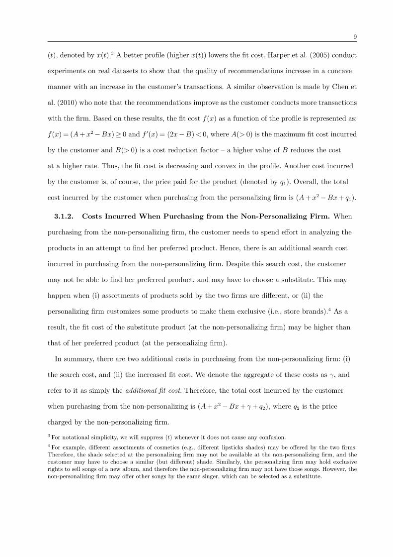
(t), denoted by x(t).3 A better profile (higher x(t)) lowers the fit cost. Harper et al. (2005) conduct

experiments on real datasets to show that the quality of recommendations increase in a concave

manner with an increase in the customer’s transactions. A similar observation is made by Chen et

al. (2010) who note that the recommendations improve as the customer conducts more transactions

with the firm. Based on these results, the fit cost f(x) as a function of the profile is represented as:

f(x) = (A+x2 −Bx)≥ 0 and f ′(x) = (2x−B)< 0, where A(> 0) is the maximum fit cost incurred

by the customer and B(> 0) is a cost reduction factor – a higher value of B reduces the cost

at a higher rate. Thus, the fit cost is decreasing and convex in the profile. Another cost incurred

by the customer is, of course, the price paid for the product (denoted by q1). Overall, the total

cost incurred by the customer when purchasing from the personalizing firm is (A+x2 −Bx+ q1).

3.1.2. Costs Incurred When Purchasing from the Non-Personalizing Firm. When

purchasing from the non-personalizing firm, the customer needs to spend effort in analyzing the

products in an attempt to find her preferred product. Hence, there is an additional search cost

incurred in purchasing from the non-personalizing firm. Despite this search cost, the customer

may not be able to find her preferred product, and may have to choose a substitute. This may

happen when (i) assortments of products sold by the two firms are different, or (ii) the

personalizing firm customizes some products to make them exclusive (i.e., store brands).4 As a

result, the fit cost of the substitute product (at the non-personalizing firm) may be higher than

that of her preferred product (at the personalizing firm).

In summary, there are two additional costs in purchasing from the non-personalizing firm: (i)

the search cost, and (ii) the increased fit cost. We denote the aggregate of these costs as γ, and

refer to it as simply the additional fit cost. Therefore, the total cost incurred by the customer

when purchasing from the non-personalizing is (A+x2 −Bx+ γ+ q2), where q2 is the price

charged by the non-personalizing firm.

3 For notational simplicity, we will suppress (t) whenever it does not cause any confusion.

4 For example, different assortments of cosmetics (e.g., different lipsticks shades) may be offered by the two firms.Therefore, the shade selected at the personalizing firm may not be available at the non-personalizing firm, and thecustomer may have to choose a similar (but different) shade. Similarly, the personalizing firm may hold exclusiverights to sell songs of a new album, and therefore the non-personalizing firm may not have those songs. However, thenon-personalizing firm may offer other songs by the same singer, which can be selected as a substitute.

10

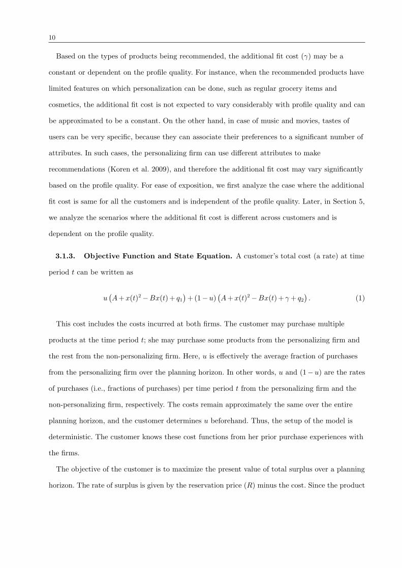
Based on the types of products being recommended, the additional fit cost (γ) may be a

constant or dependent on the profile quality. For instance, when the recommended products have

limited features on which personalization can be done, such as regular grocery items and

cosmetics, the additional fit cost is not expected to vary considerably with profile quality and can

be approximated to be a constant. On the other hand, in case of music and movies, tastes of

users can be very specific, because they can associate their preferences to a significant number of

attributes. In such cases, the personalizing firm can use different attributes to make

recommendations (Koren et al. 2009), and therefore the additional fit cost may vary significantly

based on the profile quality. For ease of exposition, we first analyze the case where the additional

fit cost is same for all the customers and is independent of the profile quality. Later, in Section 5,

we analyze the scenarios where the additional fit cost is different across customers and is

dependent on the profile quality.

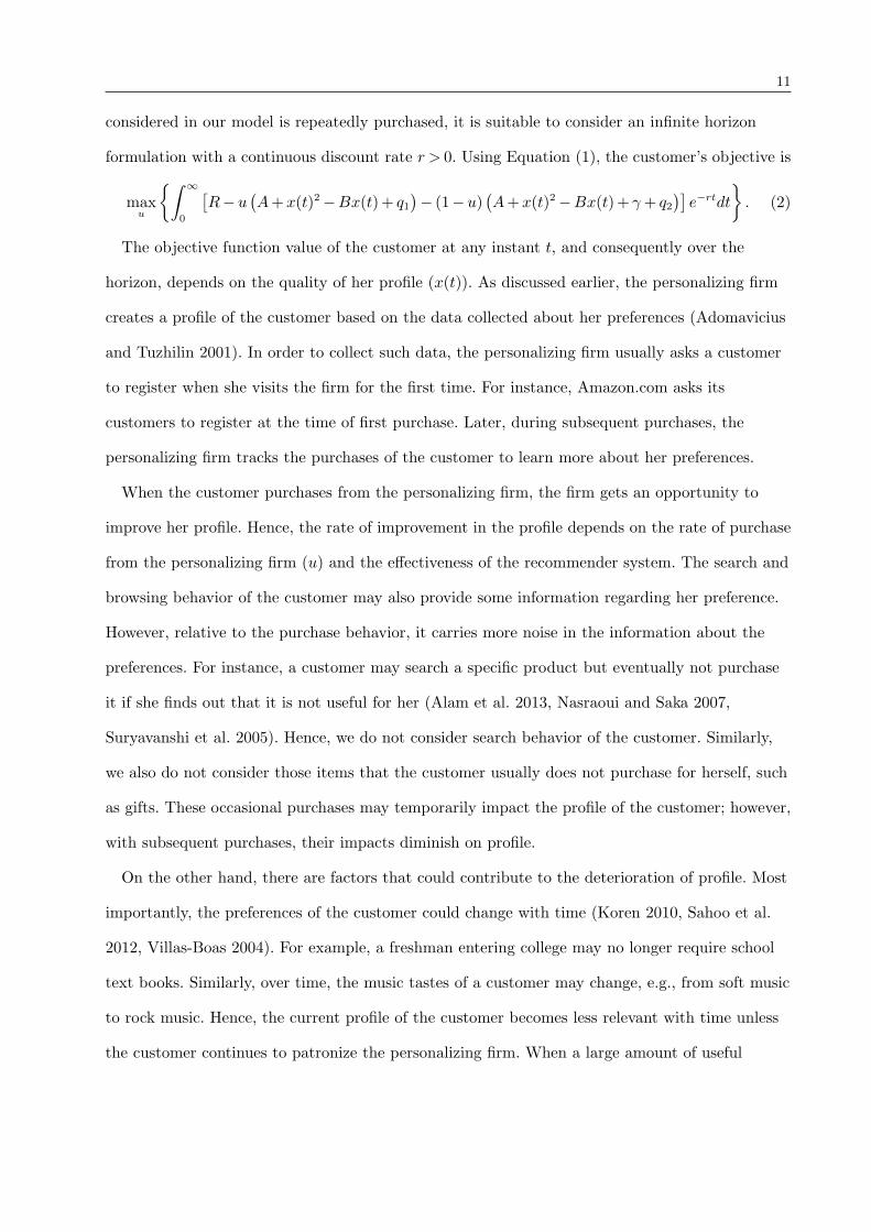
3.1.3. Objective Function and State Equation. A customer’s total cost (a rate) at time

period t can be written as

u(A+x(t)2 −Bx(t)+ q1

)+(1−u)

(A+x(t)2 −Bx(t)+ γ+ q2

). (1)

This cost includes the costs incurred at both firms. The customer may purchase multiple

products at the time period t; she may purchase some products from the personalizing firm and

the rest from the non-personalizing firm. Here, u is effectively the average fraction of purchases

from the personalizing firm over the planning horizon. In other words, u and (1−u) are the rates

of purchases (i.e., fractions of purchases) per time period t from the personalizing firm and the

non-personalizing firm, respectively. The costs remain approximately the same over the entire

planning horizon, and the customer determines u beforehand. Thus, the setup of the model is

deterministic. The customer knows these cost functions from her prior purchase experiences with

the firms.

The objective of the customer is to maximize the present value of total surplus over a planning

horizon. The rate of surplus is given by the reservation price (R) minus the cost. Since the product

11

considered in our model is repeatedly purchased, it is suitable to consider an infinite horizon

formulation with a continuous discount rate r > 0. Using Equation (1), the customer’s objective is

maxu

∫ ∞

0

[R−u

(A+x(t)2 −Bx(t)+ q1

)− (1−u)

(A+x(t)2 −Bx(t)+ γ+ q2

)]e−rtdt

. (2)

The objective function value of the customer at any instant t, and consequently over the

horizon, depends on the quality of her profile (x(t)). As discussed earlier, the personalizing firm

creates a profile of the customer based on the data collected about her preferences (Adomavicius

and Tuzhilin 2001). In order to collect such data, the personalizing firm usually asks a customer

to register when she visits the firm for the first time. For instance, Amazon.com asks its

customers to register at the time of first purchase. Later, during subsequent purchases, the

personalizing firm tracks the purchases of the customer to learn more about her preferences.

When the customer purchases from the personalizing firm, the firm gets an opportunity to

improve her profile. Hence, the rate of improvement in the profile depends on the rate of purchase

from the personalizing firm (u) and the effectiveness of the recommender system. The search and

browsing behavior of the customer may also provide some information regarding her preference.

However, relative to the purchase behavior, it carries more noise in the information about the

preferences. For instance, a customer may search a specific product but eventually not purchase

it if she finds out that it is not useful for her (Alam et al. 2013, Nasraoui and Saka 2007,

Suryavanshi et al. 2005). Hence, we do not consider search behavior of the customer. Similarly,

we also do not consider those items that the customer usually does not purchase for herself, such

as gifts. These occasional purchases may temporarily impact the profile of the customer; however,

with subsequent purchases, their impacts diminish on profile.

On the other hand, there are factors that could contribute to the deterioration of profile. Most

importantly, the preferences of the customer could change with time (Koren 2010, Sahoo et al.

2012, Villas-Boas 2004). For example, a freshman entering college may no longer require school

text books. Similarly, over time, the music tastes of a customer may change, e.g., from soft music

to rock music. Hence, the current profile of the customer becomes less relevant with time unless

the customer continues to patronize the personalizing firm. When a large amount of useful

12

information about the customer is available (i.e., the profile quality is high), pieces of information

may become obsolete with the changing preferences of the customer. Hence, the profile

deterioration rate is higher when the profile quality is higher. In contrast, when the profile quality

is low, the less amount of information is available about the customer. Hence, there is less

opportunity for the available information to be obsolete. Therefore, the profile deteriorates at a

lower rate when the profile quality is low.

Based on the above discussion, the manner in which the profile changes over time (the state

equation) can be written as

x(t) = αu−βx(t). (3)

In the above equation, the effectiveness of the recommender system is captured by the parameter

α∈ (0,1]. The effectiveness depends on two factors: (1) the quality of the algorithm used to

recommend, and (2) the data set supplied to the algorithm to learn customer preferences. The rate

at which the profile improves depends on the product α ·u, while the profile deteriorates depending

on the profile loss parameter β(> 0) times the current profile. This loss in profile is analogous

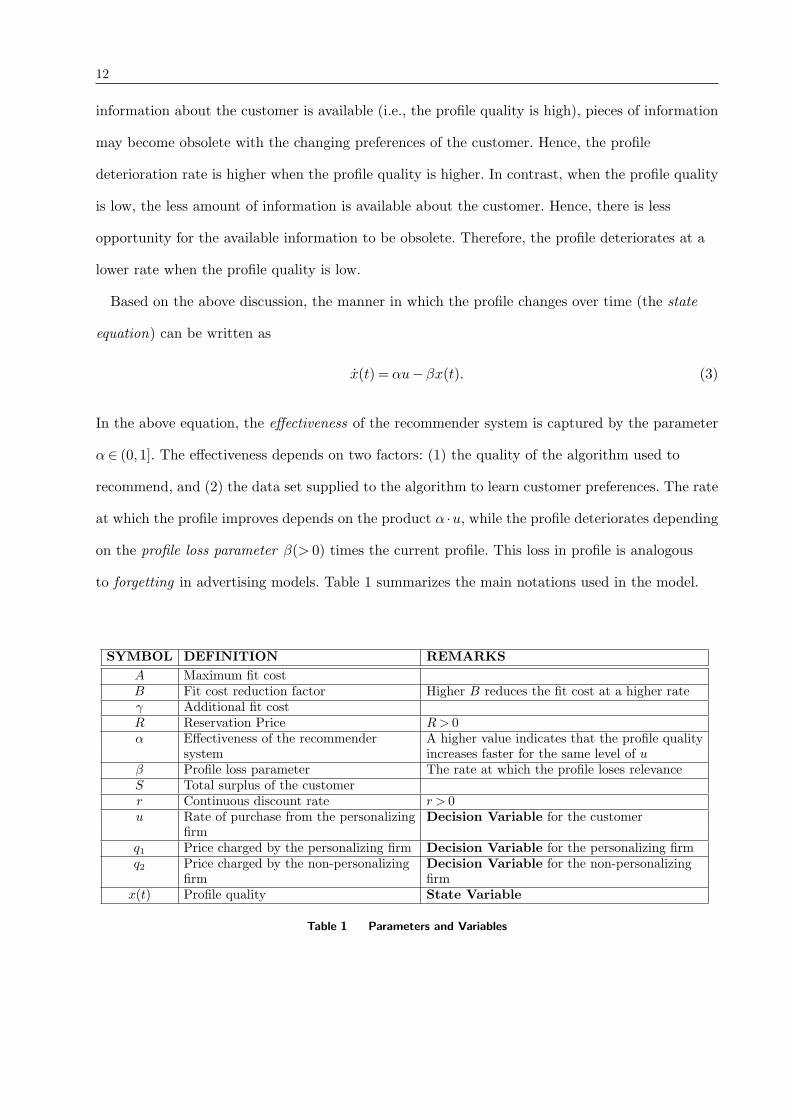
to forgetting in advertising models. Table 1 summarizes the main notations used in the model.

SYMBOL DEFINITION REMARKS

A Maximum fit costB Fit cost reduction factor Higher B reduces the fit cost at a higher rateγ Additional fit costR Reservation Price R> 0α Effectiveness of the recommender A higher value indicates that the profile quality

system increases faster for the same level of uβ Profile loss parameter The rate at which the profile loses relevanceS Total surplus of the customerr Continuous discount rate r > 0u Rate of purchase from the personalizing Decision Variable for the customer

firmq1 Price charged by the personalizing firm Decision Variable for the personalizing firmq2 Price charged by the non-personalizing Decision Variable for the non-personalizing

firm firmx(t) Profile quality State Variable

Table 1 Parameters and Variables

13

Using Equations (2) and (3), we present the surplus maximization problem of the customer as

maxu

∫ ∞

0

[R−u

(A+x(t)2 −Bx(t)+ q1

)− (1−u)

(A+x(t)2 −Bx(t)+ γ+ q2

)]e−rtdt

subject to

x(t) = αu−βx(t)

0≤ u≤ 1.

3.1.4. Solution to Customer’s Problem. We first solve Equation (3) to find the profile of

the customer at time t. Equation (3) is a differential equation of first order and the solution of

the equation is

x(t) =αu

β

(1− e−βt

). (4)

It should be clear from the above equation that x∈ [0, αβ]. The above expression for x(t) can be

substituted in Equation (2) to obtain the total (discounted) surplus for a customer that can be

optimized to find the optimal purchase rate. Therefore, implicitly u is a function of x(t).

Lemma 1. The optimal rate at which customers purchase from the personalizing firm

(0≤ u≤ 1) is

u=

(r+2β)(Bα+(q2−q1+γ)(r+β))

4α2 if 0≤ (Bα+(q2 − q1 + γ) (r+β))≤min

4α2

r+2β, 2Bαβr+2β

;

0 or 1 otherwise.(5)

The proofs are provided in the Appendix. To ensure a duopoly, we impose the condition

0≤ u≤ 1 along with 2x−B ≤ 0 (the fit cost is always decreasing in x), which provides the

condition presented in Equation (5). When this condition is not satisfied, we have a monopoly (as

shown in Lemma 1 when u is 0 or 1). Following is the interpretation of this condition. If the price

of the non-personalizing firm is very low compared to the price of the personalizing firm (i.e.,

(q1 − q2) is a large positive number), the non-personalizing firm covers the entire market. On the

other hand, when q2 is too close to q1, the entire market is covered by the personalizing firm.

As shown in Lemma 1, the optimal purchase rates from the personalizing and

non-personalizing firms (u and 1−u, respectively) are functions of the prices charged by the

firms. Therefore, we next focus on determining these prices (denoted by q1 and q2) in equilibrium.

14

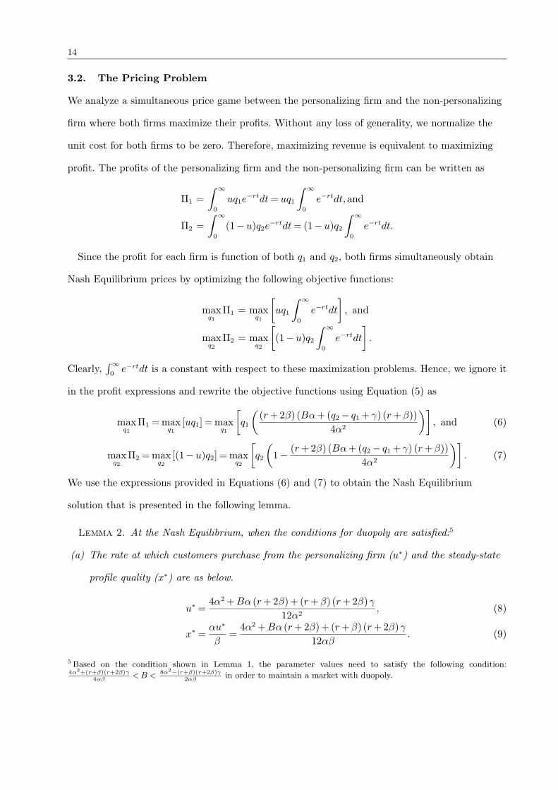
3.2. The Pricing Problem

We analyze a simultaneous price game between the personalizing firm and the non-personalizing

firm where both firms maximize their profits. Without any loss of generality, we normalize the

unit cost for both firms to be zero. Therefore, maximizing revenue is equivalent to maximizing

profit. The profits of the personalizing firm and the non-personalizing firm can be written as

Π1 =

∫ ∞

0

uq1e−rtdt= uq1

∫ ∞

0

e−rtdt,and

Π2 =

∫ ∞

0

(1−u)q2e−rtdt= (1−u)q2

∫ ∞

0

e−rtdt.

Since the profit for each firm is function of both q1 and q2, both firms simultaneously obtain

Nash Equilibrium prices by optimizing the following objective functions:

maxq1

Π1 = maxq1

[uq1

∫ ∞

0

e−rtdt

], and

maxq2

Π2 = maxq2

[(1−u)q2

∫ ∞

0

e−rtdt

].

Clearly,∫∞0

e−rtdt is a constant with respect to these maximization problems. Hence, we ignore it

in the profit expressions and rewrite the objective functions using Equation (5) as

maxq1

Π1 =maxq1

[uq1] =maxq1

[q1

((r+2β) (Bα+(q2 − q1 + γ) (r+β))

4α2

)], and (6)

maxq2

Π2 =maxq2

[(1−u)q2] =maxq2

[q2

(1− (r+2β) (Bα+(q2 − q1 + γ) (r+β))

4α2

)]. (7)

We use the expressions provided in Equations (6) and (7) to obtain the Nash Equilibrium

solution that is presented in the following lemma.

Lemma 2. At the Nash Equilibrium, when the conditions for duopoly are satisfied:5

(a) The rate at which customers purchase from the personalizing firm (u∗) and the steady-state

profile quality (x∗) are as below.

u∗ =4α2 +Bα (r+2β)+ (r+β) (r+2β)γ

12α2, (8)

x∗ =αu∗

β=

4α2 +Bα (r+2β)+ (r+β) (r+2β)γ

12αβ. (9)

5 Based on the condition shown in Lemma 1, the parameter values need to satisfy the following condition:4α2+(r+β)(r+2β)γ

4αβ<B < 8α2−(r+β)(r+2β)γ

2αβin order to maintain a market with duopoly.

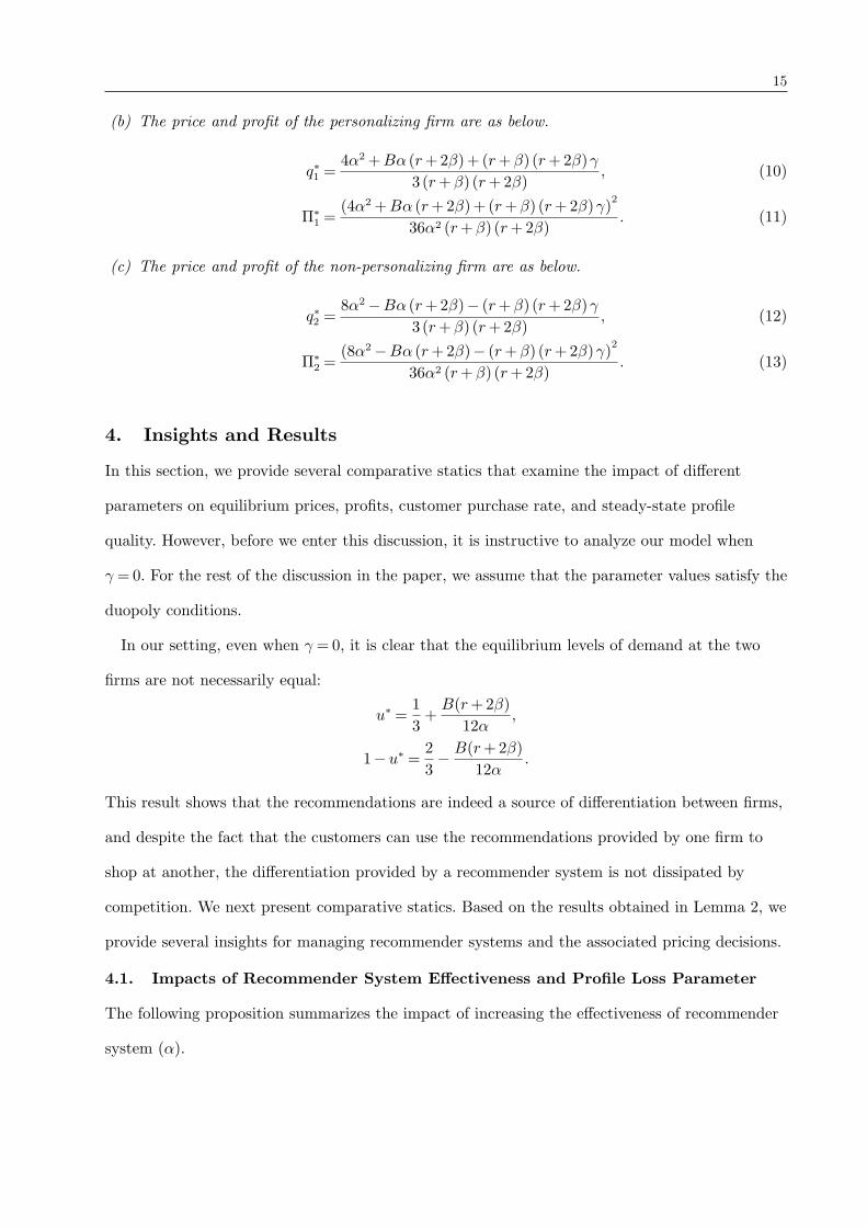
15

(b) The price and profit of the personalizing firm are as below.

q∗1 =4α2 +Bα (r+2β)+ (r+β) (r+2β)γ

3 (r+β) (r+2β), (10)

Π∗1 =

(4α2 +Bα (r+2β)+ (r+β) (r+2β)γ)2

36α2 (r+β) (r+2β). (11)

(c) The price and profit of the non-personalizing firm are as below.

q∗2 =8α2 −Bα (r+2β)− (r+β) (r+2β)γ

3 (r+β) (r+2β), (12)

Π∗2 =

(8α2 −Bα (r+2β)− (r+β) (r+2β)γ)2

36α2 (r+β) (r+2β). (13)

4. Insights and Results

In this section, we provide several comparative statics that examine the impact of different

parameters on equilibrium prices, profits, customer purchase rate, and steady-state profile

quality. However, before we enter this discussion, it is instructive to analyze our model when

γ = 0. For the rest of the discussion in the paper, we assume that the parameter values satisfy the

duopoly conditions.

In our setting, even when γ = 0, it is clear that the equilibrium levels of demand at the two

firms are not necessarily equal:

u∗ =1

3+

B(r+2β)

12α,

1−u∗ =2

3− B(r+2β)

12α.

This result shows that the recommendations are indeed a source of differentiation between firms,

and despite the fact that the customers can use the recommendations provided by one firm to

shop at another, the differentiation provided by a recommender system is not dissipated by

competition. We next present comparative statics. Based on the results obtained in Lemma 2, we

provide several insights for managing recommender systems and the associated pricing decisions.

4.1. Impacts of Recommender System Effectiveness and Profile Loss Parameter

The following proposition summarizes the impact of increasing the effectiveness of recommender

system (α).

16

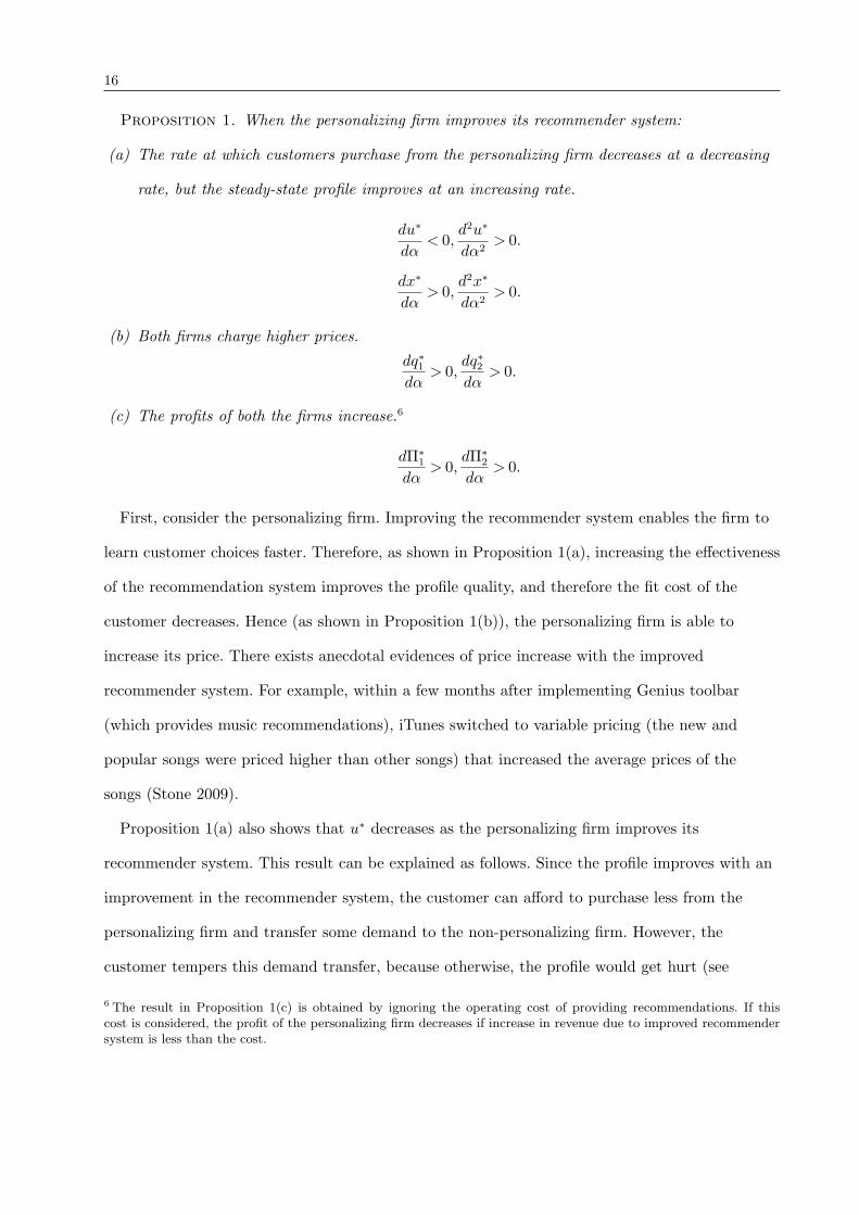
Proposition 1. When the personalizing firm improves its recommender system:

(a) The rate at which customers purchase from the personalizing firm decreases at a decreasing

rate, but the steady-state profile improves at an increasing rate.

du∗

dα< 0,

d2u∗

dα2> 0.

dx∗

dα> 0,

d2x∗

dα2> 0.

(b) Both firms charge higher prices.

dq∗1dα

> 0,dq∗2dα

> 0.

(c) The profits of both the firms increase.6

dΠ∗1

dα> 0,

dΠ∗2

dα> 0.

First, consider the personalizing firm. Improving the recommender system enables the firm to

learn customer choices faster. Therefore, as shown in Proposition 1(a), increasing the effectiveness

of the recommendation system improves the profile quality, and therefore the fit cost of the

customer decreases. Hence (as shown in Proposition 1(b)), the personalizing firm is able to

increase its price. There exists anecdotal evidences of price increase with the improved

recommender system. For example, within a few months after implementing Genius toolbar

(which provides music recommendations), iTunes switched to variable pricing (the new and

popular songs were priced higher than other songs) that increased the average prices of the

songs (Stone 2009).

Proposition 1(a) also shows that u∗ decreases as the personalizing firm improves its

recommender system. This result can be explained as follows. Since the profile improves with an

improvement in the recommender system, the customer can afford to purchase less from the

personalizing firm and transfer some demand to the non-personalizing firm. However, the

customer tempers this demand transfer, because otherwise, the profile would get hurt (see

6 The result in Proposition 1(c) is obtained by ignoring the operating cost of providing recommendations. If thiscost is considered, the profit of the personalizing firm decreases if increase in revenue due to improved recommendersystem is less than the cost.

17

Equation (3)). In equilibrium, the impact of reduced purchase on profile is dominated by the

impact of improved recommender system effectiveness. Hence, despite the reduced customer

patronage at the personalizing firm, the profile improves with the recommender system

effectiveness. For the profit of the personalizing firm, the positive impact of increased price

dominates the negative effect of decreased demand. Therefore, the profit of the personalizing firm

increases with the recommender system effectiveness (see Proposition 1(c)).

We now turn our attention to the non-personalizing firm. As shown in Proposition 1(b), the

non-personalizing firm also increases its price with an improvement in the recommender system.

Also, the customer purchases from the non-personalizing firm at a higher rate (see

Proposition 1(a)). Hence, its profit increases with an improvement in the recommender system

(as shown in Proposition 1(c)). Conceptually, an improvement in the recommender system

increases the differentiation between the two firms. Therefore, profits of both the firms increase.

Thus, the non-personalizing firm free-rides on the improved recommendations provided by the

personalizing firm. Such free-riding phenomena is also mentioned in the quality literature where

improving the quality of one product increases the profit of the competing firm due to increased

differentiation between firms (Moorthy 1988). Finally, we experimentally find that the surplus of

the customer decreases with an improvement in the recommender system: although the fit cost

reduces, both prices increase.

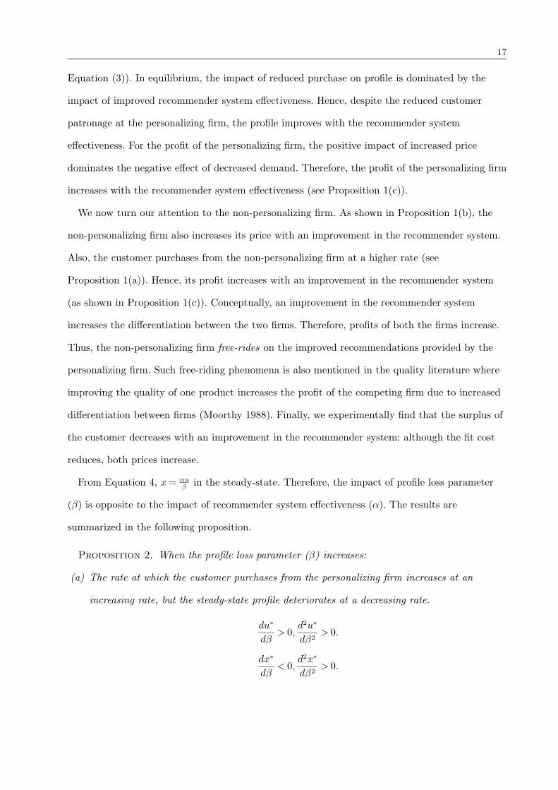
From Equation 4, x= αuβ

in the steady-state. Therefore, the impact of profile loss parameter

(β) is opposite to the impact of recommender system effectiveness (α). The results are

summarized in the following proposition.

Proposition 2. When the profile loss parameter (β) increases:

(a) The rate at which the customer purchases from the personalizing firm increases at an

increasing rate, but the steady-state profile deteriorates at a decreasing rate.

du∗

dβ> 0,

d2u∗

dβ2> 0.

dx∗

dβ< 0,

d2x∗

dβ2> 0.

18

(b) The prices and profits of both the firms decrease.

dq∗1dβ

< 0,dq∗2dβ

< 0.

dπ∗1

dβ< 0,

dπ∗2

dβ< 0.

Further, we experimentally find that the surplus of the customer increases with the profile loss

parameter. Clearly, this effect is also opposite to the effect of recommender system effectiveness.

4.2. Increase in Additional Fit Cost

An increase in additional fit cost (γ) can be considered equivalent to a situation where customers

are less able to transfer the benefit of recommendations from the personalizing firm to the other

firm. We present the impacts of additional fit cost in the following remark.

Remark 1. When the additional fit cost (γ) increases:

(a) The customer purchases more from the personalizing firm and the steady-state profile

improves.

du∗

dγ> 0,

dx∗

dγ> 0.

(b) The price charged by the personalizing firm (resp., non-personalizing firm) increases (resp.,

decreases).

dq∗1dγ

> 0,dq∗2dγ

< 0.

(c) The profit of the personalizing firm (resp., non-personalizing firm) increases (resp.,

decreases).

dΠ∗1

dγ> 0,

dΠ∗2

dγ< 0.

When γ increases, the personalizing firm increases its price to take advantage of the fact that

switching to the competing firm has become more difficult. Despite this fact, the customer

purchases more from the personalizing firm (i.e., u∗ increases) with an increase in γ. This

increase in u∗ improves the profile and reduces the fit cost incurred at both firms. On the other

hand, the non-personalizing firm has to reduce its price to make itself more attractive, i.e., to

19

compensate for the increased additional fit cost. However, the reduction in its price is less than

the increase in additional fit cost (i.e.,∣∣∣∂q∗2∂γ

∣∣∣< 1), because the non-personalizing firm realizes that

the customer benefits from the reduced fit cost. Finally, the profit of the personalizing firm

increases due to an increase in both the demand (u∗) and the price (q∗1), whereas the profit of the

non-personalizing firm decreases due to a decrease in both the demand (1−u∗) and the price

(q∗2). These results are similar to those observed in the switching cost literature. Usually, when

the switching cost increases, the firm that imposes the switching cost on the customer benefits,

and the profit of the competing firm reduces.

5. Variants of the Base Model

In this section, we extend our analysis to consider following realistic variants of the base model:

(i) customer heterogeneity in additional fit cost, (ii) additional fit cost dependent on profile, and

(iii) dynamic customer purchase rate. We begin with the case where customers are heterogeneous

in their additional fit costs.

5.1. Customers Heterogeneous in Additional Fit Cost

In our base model, the additional fit cost (γ) was same for all the customers. However, in certain

scenarios, it is possible to have different additional fit costs across customers, e.g., for certain

product categories, it may be easier for web-savvy customers to find a substitute. Hence, in this

subsection, we consider that the customers are heterogeneous in their additional fit costs. Since

we expect purchase behavior to be different across customers, this analysis may allow the firm to

devise customer segmentation and targeting strategies.

In this model, we replace γ in the objective function (i.e., Equation (2)) with kγ1 (= γ), where

0≤ γ1 ≤ 1 is the sensitivity of a customer to the substitution. A customer with no sensitivity (i.e.,

γ1 = 0) would incur zero additional fit cost for substituting a recommended product with one

from the non-personalizing firm, while a customer with the highest sensitivity (i.e., γ1 = 1) would

incur a additional fit cost k. Hence, k is the maximum additional fit cost. The surplus of a

customer with sensitivity γ1 can be written as

maxu

∫ ∞

0

(R−

[u(A+x(t)2 −Bx(t)+ q1

)+(1−u)

(A+x(t)2 −Bx(t)+ kγ1 + q2

)])e−rtdt

,

20

where

x(t) = αu−βx(t).

As shown in Section 3.1.4, we solve the customer’s surplus maximization problem and find that7

u=(r+2β) (Bα+(q2 − q1 + kγ1) (r+β))

4α2. (14)

Next, firms solve the pricing game using the customer response, u. If the sensitivities of the

customers are uniformly distributed between 0 and 1, the profits of personalizing and

non-personalizing firms can be written as

Π1 =

1∫0

uq1dγ1, and Π2 =

1∫0

(1−u)q2dγ1, respectively.

The solution to the pricing game with heterogeneous customers is presented below.

Lemma 3. At the Nash Equilibrium with heterogeneous customers:8

(a) The rate at which the customer with sensitivity γ1 purchases from the personalizing firm is

u∗ =4α2 +Bα (r+2β)+ (r+β) (r+2β)k (−1+3γ1)

12α2. (15)

(b) Price and profit of the personalizing firm are

q∗1 =8α2 +2Bα (r+2β)+ (r+β) (r+2β)k

6 (r+β) (r+2β), and

Π∗1 =

(8α2 +2Bα (r+2β)+ (r+β) (r+2β)k)2

144α2 (r+β) (r+2β), respectively.

(c) Price and profit of the non-personalizing firm are

q∗2 =16α2 − 2Bα (r+2β)− (r+β) (r+2β)k

6 (r+β) (r+2β), and

Π∗2 =

(16α2 − 2Bα (r+2β)− (r+β) (r+2β)k)2

144α2 (r+β) (r+2β), respectively.

7 Again, this expression is valid only under the following conditions that are required to maintain a duopoly:

B (α+ η)+ (q2 − q1) (r+β)> 0 and B (α+ η)+ (q2 − q1 + k) (r+β)<min(

4α2

r+2β, 2αBβr+2β

).

8 The parameters need to satisfy the following conditions in order to maintain a duopoly: (i) 4α2 +Bα (r+2β)− (r+β) (r+2β)k > 0, (ii) −8α2 +Bα (r+2β) + 2(r+β) (r+2β)k < 0, and (iii) 4α2 +Bα (r− 4β) +2k (r+β) (r+2β)< 0.

21

The key impact of introducing customer heterogeneity is that it affects the rates at which

different kinds of customers purchase from the two firms. This result is outlined in the

proposition below.

Proposition 3. When the maximum additional fit cost (k) increases, the customers with

relatively low sensitivity (γ1 <γ1t =13) purchase less from the personalizing firm, whereas other

customers (i.e., those with relatively high sensitivity) purchase more from the personalizing firm.

An increase in k increases the additional fit cost for all customers except those who have zero

sensitivity for substitution. Therefore, holding the prices constant, the customers purchase more

frequently from the personalizing firm (see Equation (14)). As a reaction, the personalizing firm

increases its price and the non-personalizing firm reduces its price. In response, less sensitive

customers (γ1 <γ1t) start purchasing more from the non-personalizing firm to take advantage of

the lower price. On the other hand, the customers with high sensitivity for the substitution

(γ1 ≥ γ1t) purchase at an increased rate from the personalizing firm to counter the increase in

additional fit costs. Thus, additional fit cost heterogeneity leads to natural segmentation in the

customer population. This segmentation is important for the firms to consider while designing

their promotions. For example, the personalizing firm may give coupons to customers that are

likely to shift purchases to the non-personalizing firm. These customers must, of course, be

identified as those that have relatively lower additional fit cost. Thus, in addition to the

conventional role of learning customer preferences, recommender systems should also aim to track

and predict the switching behavior of customers.

5.2. Heterogeneous Customers and Additional Fit Cost Dependent on Profile

So far we have considered that the additional fit cost is not dependent on the profile of the

customer. However, in certain scenarios, this cost may be a function of the profile. For example,

the substitution may be more difficult when recommendation is highly personalized (which makes

it difficult for the customer to find a similar product at the non-personalizing firm). Hence, in

this subsection, we extend our base model to introduce such dependence of additional fit cost on

profile. Moreover, like the previous subsection, we consider that the customers are heterogeneous

22

in their substitution costs. Specifically, we let, γ = kγ1 +mγ2x, where m is referred to as the

profile cost coefficient, γ2 (0≤ γ2 ≤ 1) is referred to as the sensitivity to the profile cost, and mγ2x

is referred to as the profile cost. In this case, an improvement in profile quality would increase the

additional fit cost, thus making the non-personalizing firm less attractive to the customer.

Therefore, the purchase behavior of the customers as well as the prices and profits of the firms

would be different in this scenario compared to those in the base model. Hence, it will be

interesting and useful to analyze them in detail.

Below we show the profit functions of the two firms assuming that the customers are uniformly

distributed with parameters γ1 ∈ [0,1] and γ2 ∈ [0,1].

Π1 =

∫ 1

0

∫ 1

0

uq1dγ1dγ2 and Π2 =

∫ 1

0

∫ 1

0

(1−u) q2dγ1dγ2.

Using the methods employed in Sections 3.1.4 and 3.2, we obtain the following solution.

Lemma 4. At Equilibrium:9

(a) The rate at which the customer with parameters γ1 and γ2 purchases from the personalizing

firm is

u∗ =k (r+β) (r+2β) (−1+3γ1)+α (4α+(r+2β) (B− 3mγ2))

6α (2α− (r+2β)mγ2). (16)

(b) Price and profit of the personalizing firm are

q∗1 =

k (r+β)+ 2α

(B− 2α

r+2β+ 3m

ln(α)−ln(α− 12m(r+2β))

)6 (r+β)

, and

Π∗1 =

6mα (r+2β)+(k (r+β) (r+2β)+ 2α (−2α+B (r+2β)))(

ln (α)− ln(α− 1

2m (r+2β)

))2

72mα (r+β) (r+2β)2 [ln (α)− ln

(α− 1

2m (r+2β)

)] , respectively.

(c) Price and profit of the non-personalizing firm are

9 The parameters need to satisfy the following conditions for maintaining duopoly: (i) 4α2 + Bα (r+2β) −k (r+β) (r+2β)> 0, (ii) −8α2+Bα (r+2β)+2k (r+β) (r+2β)+3α (r+2β)m< 0, (iii) 2α−mγ2 (r+2β)> 0,(iv)6αβB− 3βm (r+2β)> 2k (r+β) (r+2β) + 4α2 +Bα (r+2β)− 3mα (r+2β), and (v) 6αβB > 2k (r+β) (r+2β) +4α2 +Bα (r+2β) .

23

q∗2 =

2α

(−B+ 2α

r+2β+ 3k

ln(α)−ln(α− 12m(r+2β))

)− k (r+β)

6 (r+β), and

Π∗2 =

−6mα (r+2β)+(k (r+β) (r+2β)+ 2α (−2α+B (r+2β)))(

ln (α)− ln(α− 1

2m (r+2β)

))2

72mα (r+β) (r+2β)2 [ln (α)− ln

(α− 1

2m (r+2β)

)] , respectively.

The extensive numerical experiments show that the impacts of α, β, and k are similar to those

in Section 5.1. The numerical experiments also show that when the profile cost coefficient (m)

increases, the profits and prices of both the firms decrease, and the the customers purchase more

from the personalizing firm. Increase in m leads to an increased additional fit cost for the

customer. Therefore, the non-personalizing firm reduces its price to decrease the defection of

customers to the personalizing firm. As a reaction, the personalizing firm also reduces its price.

For the personalizing firm, increase in u∗ is not able to offset the loss due to decrease in its price.

Hence, the profit of the personalizing firm reduces with an increase in m. For the

non-personalizing firm, the profit reduces because of decrease in both demand and price.

Interestingly, increase in m tends to increase differentiation between the firms, but reduces

profits for both the firms. Situations where increased differentiation reduces the profit of a firm

have been found in other domains of marketing literature as well. For example, Syam et al.

(2005) show that in the presence of two firms who can customize products in two attributes, both

firms prefer to customize in only one attribute and in the same dimension. If a firm differentiates

by customizing in a different dimension, this leads to a price war which hurts both the firms.

5.3. Purchase Rate of Customer Varies with Time

In the base model, the customers decide on a fixed purchase fraction at each firm. However, it is

useful to investigate how the outcomes of interest change when customers are strategic in the

sense that they re-evaluate their purchase decisions to adjust the purchase fraction over time.

Because this variant of the base model is a relaxation, we would, of course, expect that customers

will benefit by being strategic. Therefore, it will be useful to study the gains achieved by

customers and the impact on the pricing strategies of the firms. In this model, since both the

24

state variable (profile x) and the control variable (fraction of purchases from the personalizing

firm, i.e., u) vary with time, we use optimal control theory to solve the customer’s problem and

derive the optimal rates at which the customers purchase from the two firms. First, we solve the

model with additional fit cost as γ = kγ1, and then we consider that the additional fit cost

depends on profile quality.

5.3.1. Additional Fit Cost Not Dependent on Profile Quality. Depending on the

initial value of the profile, the customer uses u(t) = 1 or u(t) = 0 during the initial (or transient)

phase of the solution. However, once the optimal long-run stationary equilibrium is reached, a

steady value is maintained. Hence, in infinite horizon problems, the emphasis is on finding the

optimal long-run stationary equilibrium (which is also called a turnpike solution) (Arrow and

Kurz 1970).

In the long-run stationary equilibrium, the profile and the purchase rate become independent of

time. Also, the price differential between the two firms equals the switching cost incurred by the

customer. It is important to emphasize that the long-run stationary equilibrium is not the same

as the optimal solution for a static problem since the long-run stationary equilibrium is derived

considering a trade-off between the price differential and the switching cost over the entire time

horizon (Sethi and Thompson 2000). For brevity, we will refer to the optimal run-long stationary

equilibrium as the optimal solution, and the values of the control and the profile in this solution

will be denoted by u and x, respectively. Next, we solve the static game between the two firms

using u as the rate of purchase of a customer from the personalizing firm and (1− u) as the rate

of purchase by the customer from the non-personalizing firm. The results are presented below.

Lemma 5. At the Nash Equilibrium:10

(a) The rate at which customer purchases from the personalizing firm is

u=2α2 +Bβα+ kβ (r+β) (−1+3γ1)

6α2.

10 The parameters need to satisfy the following conditions in order to maintain a duopoly: (i) 2α2+Bβα−kβ (r+β)>0, (ii) −4α2 +Bβα− 2kβ (r+β)< 0, and (iii) 2α2 − 2Bαβ+2kβ (r+β)< 0.

25

(b) Price and profit of the personalizing firm are

q∗1 =4α2 +2Bβα+ kβ (r+β)

6β (r+β), and Π∗

1 =(4α2 +2Bβα+ kβ (r+β))

2

72α2β (r+β), respectively.

(c) Price and profit of the non-personalizing firm are

q∗2 =8α2 − 2Bβα− kβ (r+β)

6β (r+β), and Π∗

2 =(8α2 − 2Bβα− kβ (r+β))

2

72α2β (r+β), respectively.

The impacts of recommender system effectiveness, profile loss parameter, and additional fit

cost coefficient (i.e., α, β, and k, respectively) on the prices and profits of the firms remain the

same as those discussed in Section 5.1. However, unlike the base case, the surplus of the customer

may increase with an increase in α based on the condition shown below.

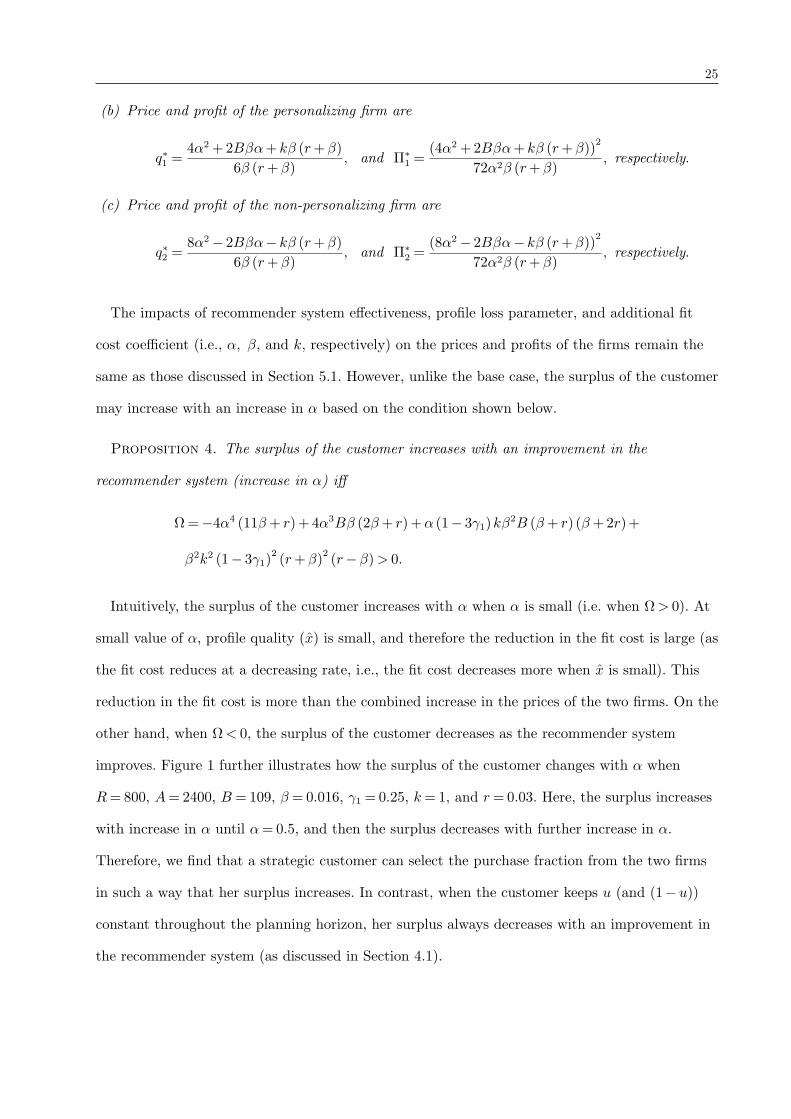
Proposition 4. The surplus of the customer increases with an improvement in the

recommender system (increase in α) iff

Ω=−4α4 (11β+ r)+ 4α3Bβ (2β+ r)+α (1− 3γ1)kβ2B (β+ r) (β+2r)+

β2k2 (1− 3γ1)2(r+β)

2(r−β)> 0.

Intuitively, the surplus of the customer increases with α when α is small (i.e. when Ω> 0). At

small value of α, profile quality (x) is small, and therefore the reduction in the fit cost is large (as

the fit cost reduces at a decreasing rate, i.e., the fit cost decreases more when x is small). This

reduction in the fit cost is more than the combined increase in the prices of the two firms. On the

other hand, when Ω< 0, the surplus of the customer decreases as the recommender system

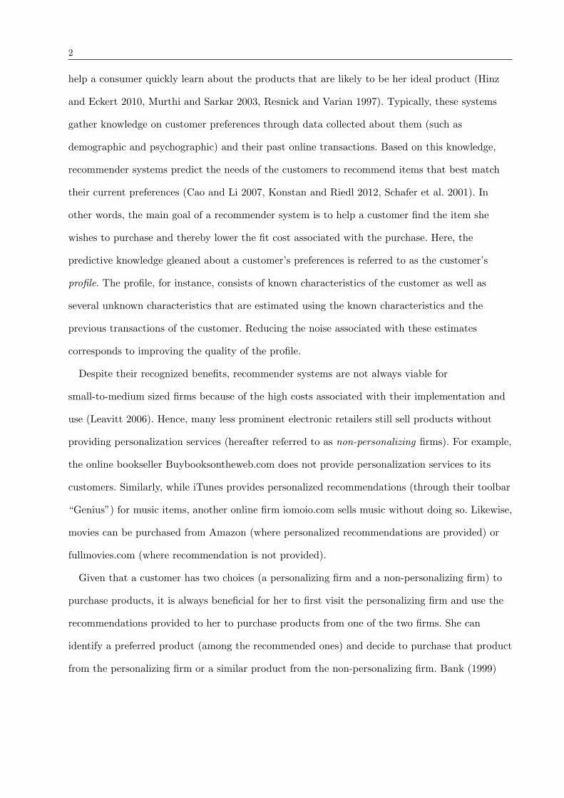
improves. Figure 1 further illustrates how the surplus of the customer changes with α when

R= 800, A= 2400, B = 109, β = 0.016, γ1 = 0.25, k= 1, and r= 0.03. Here, the surplus increases

with increase in α until α= 0.5, and then the surplus decreases with further increase in α.

Therefore, we find that a strategic customer can select the purchase fraction from the two firms

in such a way that her surplus increases. In contrast, when the customer keeps u (and (1−u))

constant throughout the planning horizon, her surplus always decreases with an improvement in

the recommender system (as discussed in Section 4.1).

26

82

84

86

88

0.45 0.5 0.55

Su

rp

lus

of

the C

ust

om

er

a

Figure 1 Impact of Recommender System Effectiveness on the Surplus of the Customer

5.3.2. Additional Fit Cost Dependent on Profile Quality. In this section, we consider

that the additional fit cost is dependent on profile (similar to that in Section 5.2). Hence, the

customers are heterogeneous in parameters γ1 and γ2. Also, they change the fractions of

purchases from the two firms over time. We obtain the equilibrium solution in a similar manner

as in the earlier scenario. The solution is presented below.

Lemma 6. At the Nash Equilibrium:11

(a) The rate at which customer purchases from the personalizing firm is

u=

β

(k (r+β) (−1+3γ1)+α

(B+ 4α

r+2β− 3mγ2 +

mr

β ln(α)−β ln(−mr2 +α−mβ)

))3α (2α−m (r+2β)γ2)

. (17)

(b) Price and profit of the personalizing firm are

q∗1 =

k (r+β)+ 2α

(B− 2α

r+2β+ m(r+3β)

β(ln(α)−ln(α− 12m(r+2β)))

)6 (r+β)

, and

11 The parameters need to satisfy the following conditions for maintaining duopoly: (i) 2k (r+β) +

α

(B+ 4α

r+2β+ mr

β ln(α)−β ln(−mr2

+α−mβ)

)> 0, (ii) 2kβ (r+β) + αβ

(B+ 4α

r+2β+ mr

β ln(α)−β ln(−mr2

+α−mβ)

)< 6α2,

(iii) 2kβ (r+β) + αβ

(B+ 4α

r+2β− 3+ mr

β ln(α)−β ln(−mr2

+α−mβ)

)< 6α2 − 3αm (r+2β), (iv)

32B (2α−m (r+2β)) > 2k (r+β) + α

(B+ 4α

r+2β− 3+ mr

β ln(α)−β ln(−mr2

+α−mβ)

), (v) 3Bα > 2k (r+β) +

α

(B+ 4α

r+2β+ mr

β ln(α)−β ln(−mr2

+α−mβ)

).

27

Π∗1 =

2mα (r+2β) (r+3β)+β

(k (r+β) (r+2β)+

2α (−2α+B (r+2β))

)(ln (α)− ln

(α− 1

2m (r+2β)

))2

36mαβ (r+β) (r+2β)3 (

ln (α)− ln(α− 1

2m (r+2β)

)) , respectively. (18)

(c) Price and profit of the non-personalizing firm are

q∗2 =

−k (r+β)+ 2α

(−B+ 2α

r+2β+ m(2r+3β)

β(ln(α)−ln(α− 12m(r+2β)))

)6 (r+β)

, and

Π∗2 =

2mα (r+2β) (2r+3β)+β

(k (r+β) (r+2β)+

2α (−2α+B (r+2β))

)(− ln (α)+ ln

(α− 1

2m (r+2β)

))2

36mαβ (r+β) (r+2β)3 (

ln (α)− ln(α− 1

2m (r+2β)

)) , respectively.

The extensive numerical experiments show that the impacts of α, β, and k are similar to those

in the previous section. Hence, in Proposition 5, we present the impacts of only the profile cost

coefficient (m).

Proposition 5. When the profile cost coefficient (m) increases:

(a) The rate of purchase from the personalizing firm (u) increases iff

(r+2β)γ2

(k (r+β) (−1+3γ1)+α

(B+ 4α

r+2β− 3mγ2+

mr

β ln(α)−β ln(−mr2 +α−mβ)

))+

(2α−m (r+2β)γ2)

−3γ2 +r(1+ 2α

mr−2α+2mβ+ ln(α)− ln

(α− 1

2m (r+2β)

))β(ln (α)− ln

(α− 1

2m (r+2β)

))2> 0.

(b) The profit of the personalizing firm (Π∗1) increases iff[

2mα (r+2β) (r+3β)+β (k (r+β) (r+2β)+ 2α (−2α+B (r+2β)))(ln (α)− ln

(α− 1

2m (r+2β)

)) ]

2m2α (r+2β)2(r+3β)−(

m (r+2β)2(4α2 +2Bαβ+ kβ (r+β)− 2mα (r+3β))+β (−2α+m (r+2β))

(k (r+β) (r+2β)+ 2α (−2α+B (r+2β)))(ln (α)− ln

(α− 1

2m (r+2β)

)) )(ln (α)− ln

(α− 1

2m (r+2β)

))

36m2αβ (r+β) (r+2β)3(−2α+m (r+2β))

(ln (α)− ln

(α− 1

2m (r+2β)

))2 > 0.

Note that the results in Proposition 5 are different from those in Section 5.2. More specifically,

when u remains constant in time (in Section 5.2), we experimentally find that with an increase in

28

m, u increases and the profit of the personalizing firm decreases. However, in the current setting,

u increases with m only when the condition in Proposition 5(a) is satisfied. Likewise, the profit of

the personalizing firm decreases with an increase in m only when the condition in

Proposition 5(b) is not satisfied.

0.8475711

0.8475714

0.8475717

0.847572

0.005 0.01

u

m

(a) γ2 = 0.10

0.8475742

0.847575

0.8475758

0.8475766

0.005 0.01

u

m

(b) γ2 = 0.15

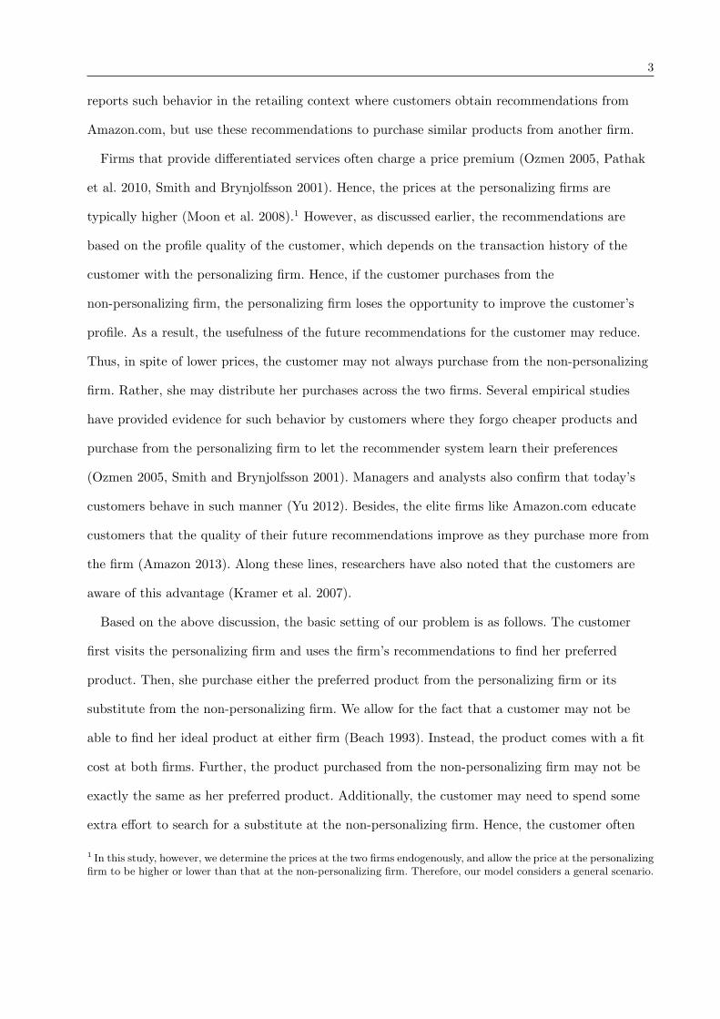
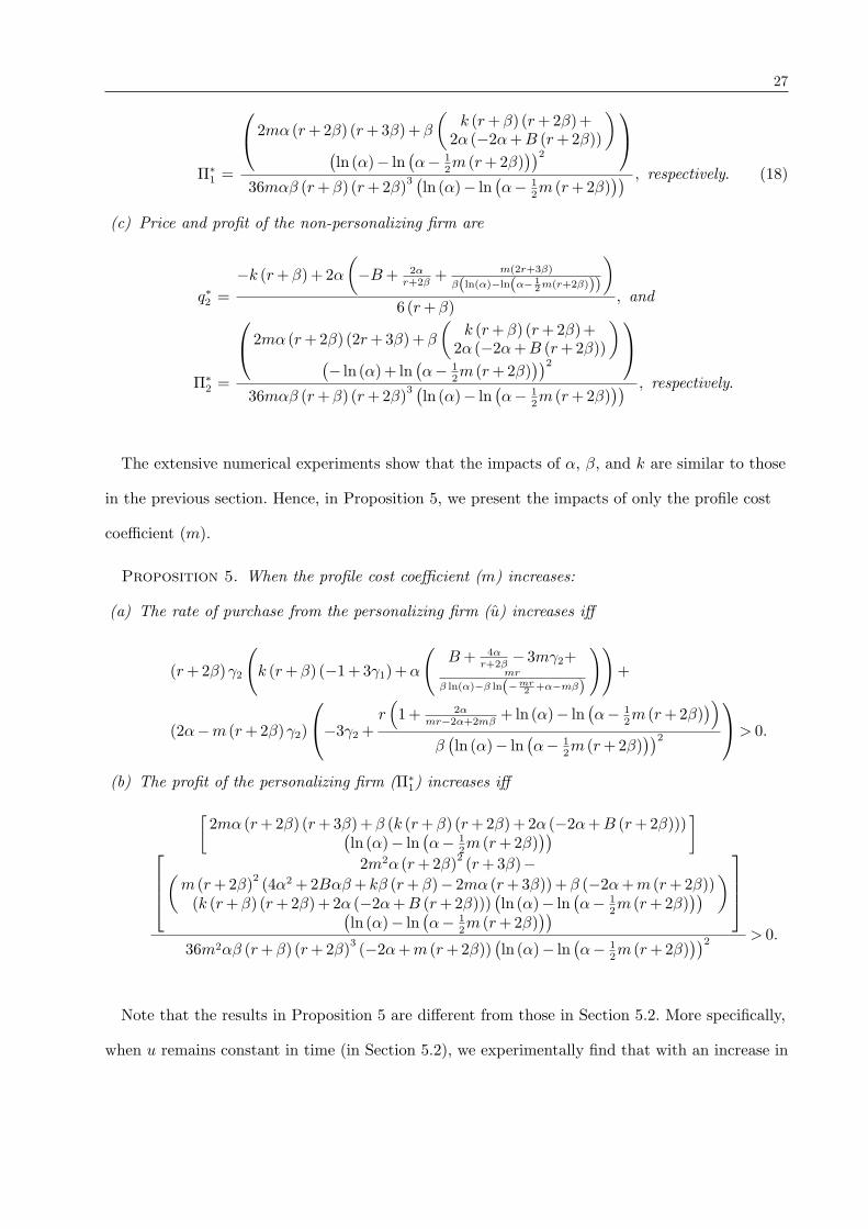
Figure 2 Impact of Profile Cost Coefficient on the Rate of Purchase from Personalizing Firm

We illustrate the impact of m on u in Figure 2 using an example where α= 0.70, β = 0.009,

r= 0.01, B = 240, and k= 0.8. In Figure 2(a), where the value of γ2 is low (γ2 = 0.10), the

customer decreases her purchases from the personalizing firm with an increase in m. These

customers have small impact of increased m on additional fit cost due to low sensitivity (γ2).

Hence, for these customers, the additional fit cost incurred in purchasing more from the

non-personalizing firm is over-compensated by lower prices at the non-personalizing firm. On the

other hand, a customer with higher γ2 (γ2 = 0.15) increases her purchases from the personalizing

firm with an increase in m (Figure 2(b)), because the additional fit cost increases substantially

with m.

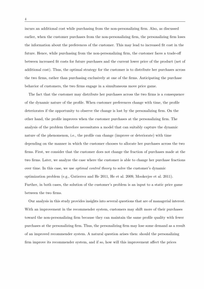
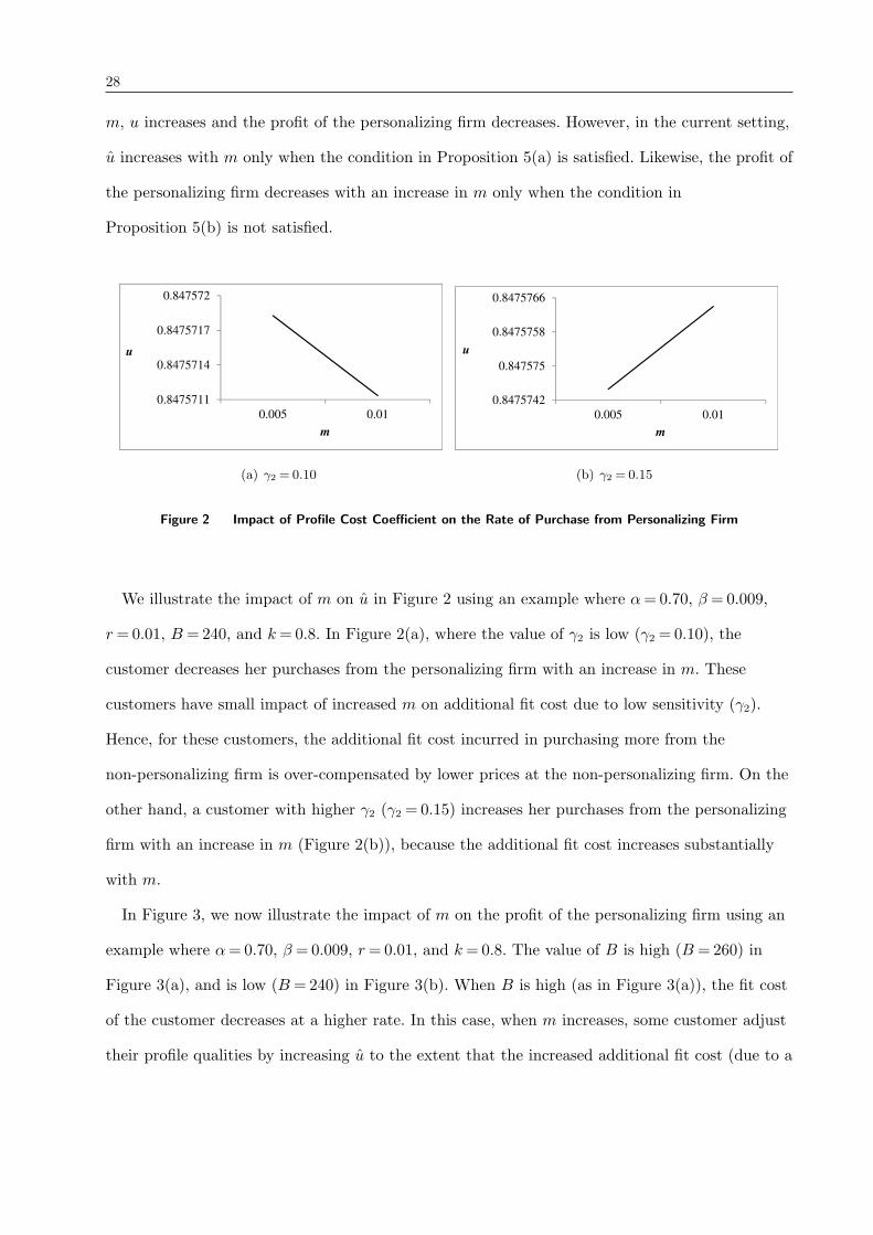
In Figure 3, we now illustrate the impact of m on the profit of the personalizing firm using an

example where α= 0.70, β = 0.009, r= 0.01, and k= 0.8. The value of B is high (B = 260) in

Figure 3(a), and is low (B = 240) in Figure 3(b). When B is high (as in Figure 3(a)), the fit cost

of the customer decreases at a higher rate. In this case, when m increases, some customer adjust

their profile qualities by increasing u to the extent that the increased additional fit cost (due to a

29

4,544.619

4,544.621

4,544.622

0.005 0.01

Pro

fit

of

the p

ers

on

ali

zin

g

firm

m

(a) B = 260

3,326.980

3,327.000

3,327.020

0.005 0.01

Pro

fit

of

the

per

son

ali

zin

g

firm

m

(b) B = 240

Figure 3 Impact of Profile Cost Coefficient on the Profit of the Personalizing Firm

higher value of m and x) is offset by the reduced fit cost (due to higher value of B). As a result,

the surplus of the customer increases significantly. Therefore, the personalizing firm does not

need to reduce its price too much. The gain due to increased u of some customers (who satisfy

the condition in Proposition 5(a)) dominates the loss due to the decreased demands of other

customers (who do not satisfy the condition) and reduced price. Hence, the profit of the

personalizing firm increases with m when B is high. On the other hand, when B is low (as in

Figure 3(b)), the profit of the personalizing firm decreases with an increase in m.

6. Discussion and Conclusions

In this research, we consider two firms that compete on price: a personalizing firm that provides

recommendations to the customer based on her profile, and a non-personalizing firm that does

not. Given a choice between these two firms, customers distribute their purchases between the

two firms to maximize surplus. In doing so, customers trade-off the quality of the

recommendations (and hence, the fit cost) with the lower price (net of additional fit cost) at the

non-personalizing firm. The customer takes advantage of recommendations not only at the

personalizing firm, but also at the non-personalizing firm. This strategic behavior of customer and

its impact on firms have never been studied in the literature, and, to the best of our knowledge,

this is the first paper that explores the economic impact of the strategic behavior of customers.

We consider the scenario in which the customer patronizes both the firms in equilibrium. When

the customers are homogeneous in their additional fit costs, they purchase less frequently at the

30

personalizing firm following an increase in the effectiveness of the recommender system. Despite

this, the personalizing firm benefits because it is able to offset the lower demand by charging a

higher price. The implication of the above result is that personalization does provide

differentiation benefits to the personalizing firm, even though the value gained from

recommendations is transferable (either perfectly or by incurring a additional fit cost). We also

find that, even in the absence of the additional fit cost, the firms do not charge the same price,

i.e., the differentiation between the firms does not dissipate. In fact, the recommender system

differentiates the two firms.

We find that the non-personalizing firm can free ride on improved recommendations provided

by the personalizing firm and increase its profits. This happens because, with improved

recommendations, the customer transacts more frequently with the non-personalizing firm.

Further, we find that the surplus of the customer decreases with an improvement in the

recommender system, despite her improved profile. This happens because the prices at both firms

increase with an improvement in the recommender system. Based on these results, we are now

able to answer the broad question: should a personalizing firm offer recommendations when the

customer is strategic? We find that the recommender system is essentially a source of

differentiation between the firms that sell similar products. Hence, improved recommender system

benefits not only the personalizing firm, but also the non-personalizing firm.

Next, we analyze the impact of change in the profile loss parameter on the profits of the firms.

We show that when the customer’s preferences change faster, prices and profits of both the firms

reduce. In this case, the customer transacts more frequently with the personalizing firm in order

to provide enough opportunities to the recommender system to help it learn her changed

preferences. In essence, the effect of increased profile loss parameter on firms is opposite to that

of increased recommender system. Thus, firms should strive to learn the trends in the changes in

preferences of customers. In general, this can be accomplished by analyzing the past transactions

of customers. Sahoo et al. (2012) describe a process of recommendation when customer

preferences change.

31

We also analyze how the changes in additional fit cost impact the purchasing behavior of the

customer and prices and profits of the firms. Our results show that both the price and the profit

of the personalizing firm (resp., non-personalizing firm) increase (resp., decrease) with the

additional fit cost. Also, as expected, the customer purchases more frequently from the

personalizing firm as the additional fit cost increases. These results are in line with those

observed in the search cost literature. Thus, the non-personalizing firm should take measures that

may help in reducing the additional fit cost. For example, the non-personalizing firm should

update its website to make it user-friendly. Also, it should track the catalog of the competitor

(i.e., personalizing firm) and attempt to offer similar products.

We also study several interesting variants of the base model. We consider a scenario where the

customers are heterogeneous in their sensitivities towards substitute products, and find that, by

and large, the results of the base case continue to hold for both firms. However, the customers

with low sensitivity to substitution decrease their purchases from the personalizing firm with an

increase in the maximum additional fit cost. This result suggests that, when the maximum

additional fit cost increases, the personalizing firm may benefit by offering coupons to those

customers that have low sensitivity to substitution in order to discourage them from migrating to

the competitor. We also consider a situation where the customers prefer purchasing from the

personalizing firm because of an extra profile cost (equal to the profile cost coefficient times the

profile quality). We find that the profits of both firms decrease with an increase in the profile cost

coefficient. Thus, the firms should try to keep the profile cost as low as possible. Firms may

accomplish this by keeping their websites user-friendly and by providing enough information so

that the customers can easily find a substitute product.

Finally, we model a situation where the customer varies (over time) the fractions of purchases

from the two firms. In this case, the profit of the personalizing firm may increase with the profile

cost coefficient under certain conditions. Further, in this case, the surplus of the customer may

increase with an improvement in the recommender system, whereas it always decreases if

customers keep the purchase fractions constant during the planning horizon. Thus, by being

32

strategic, customers can counter the advantage that firms gain through an increase in the

recommender system effectiveness.

This research is a first step in an attempt to analyze the purchase behavior of customers that

use the knowledge gained from personalization services at one firm to shop for a low price at

another firm. The model in the paper can be extended to include more than two firms as well as

to situations where two firms engage in price and recommender system competition. The key idea

of the paper can also be extended to other services (e.g., medical services) where the utility of

service has a transferable component, but because the service quality degrades with time, the

customer cannot completely switch to another service provider in the interest of maintaining

service quality.

References

Adomavicius, G. and Tuzhilin, A. 2001. Using Data Mining Methods to Build Customer Profiles. IEEE

Computer, February 2001, 74–82.

Adomavicius, G. and Tuzhilin, A. 2005. Toward the Next Generation of Recommender Systems: A Survey

of the State-of-the-Art and Possible Extensions. IEEE Transactions on Knowledge and Data

Engineering, 17(6), 734–749.

Alam, S., Dobbie, G. Riddle, P. and Koh, Y.S. 2013. Analysis of Web Usage Data for Clustering Based

Recommender System. Trends in Practical Applications of Agents and Multiagent Systems, Advances

in Intelligent Systems and Computing, 221, 171–179.

Amazon Inc. 2013.

http://www.amazon.ca/gp/help/customer/display.html?ie=UTF8&nodeId=1162208, accessed on

July 23, 2013.

Aron, R., Sundararajan, A., and Viswanathan, S. 2006. Intelligent Agents in Electronic Markets for

Information Goods: Customization, Preference Revelation and Pricing. Decision Support Systems, 41,

764–786.

Arrow, K.J. and Kurz, M. 1970. Public Investment, the Rate of Return, and Optimal Fiscal Policy. The

John Hopkins Press, Baltimore.

Bank, D. 1999. A New Model – A Site-Eat-Site World: Disappearing Profit Margins have Retailers Fretting

– and Consumers Rejoicing. Wall Street Journal, Eastern Edition, July 12.

Beach, L.R. 1993. Broadening the Definition of Decision Making: The Role of Prechoice Screening of

Options. Psychological Science, 4(4) 215-220.

33

Bergemann, D. and Ozmen, D. 2006. Optimal Pricing with Recommender Systems. Available at

http://dirkbergemann.commons.yale.edu/files/2011/01/Paper19_p1177.pdf, Accessed on

September 26, 2013.

Biyalogorsky, E., Gerstner, E., and Libai, B. 2001. Customer Referral Management: Optimal Reward

Programs. Marketing Science, 20(1), 82–95.

Bodapati, A.V. 2008. Recommendation Systems with Purchase Data. Journal of Marketing Research,

45(1), 77–93.

Breese, J., Heckerman, D., and Kadie, C. 1998. Empirical Analysis of Predictive Algorithms for

Collaborative Filtering. Proceedings of the 14th Conference on Uncertainty in AI, Morgan Kaufmann,

43–52.

Cao, Y. and Li, Y. 2007. An Intelligent Fuzzy-based Recommendation System for Consumer Electronic

Products. Expert Systems with Applications, 32, 230–240.

Chen, Y., Harper, F.M., Konstan, J., and Li, S.X. 2010. Social Comparisons and Contributions to Online

Communities: A Field Experiment on MovieLens. American Economic Review, 100, 1358–1398.

Crum, R. 2008. Personalization: Telling E-Tail Customers What They Really Want. E-Commerce Times,

June 20.

Dewan, R., Jing, B., and Seidmann, A. 2003. Product Customization and Price Competition on the

Internet. Management Science, 49(8), 1055–1070.

Fleder, D. and Hosanagar, K. 2009. Blockbuster Culture’s Next Rise or Fall: The Impact of Recommender

Systems on Sales Diversity. Management Science, 55(5), 697–712.

Gutierrez, G.J. and He, X. 2011. Life-cycle Channel Coordination Issues in Launching an Innovative

Durable Product. Production and Operations Management, 20(2), 268–279.

Harper, F.M., Li, X., Chan, Y., and Konstan, A. 2005. An Economic Model of User Rating in an Online

Recommender Systems. 10th International Conference on User Modeling, Edinburgh, UK, 307–315.

He, X., Prasad, A., and Sethi, S.P. 2009. Co-op Advertising and Pricing in a Stochastic Supply Chain:

Feedback Stackelberg Strategies. Production and Operations Management, 18(1), 78–94.

Hinz, O. and Eckert, J. 2010. The Impact of Search and Recommendation Systems on Sales in Electronic

Commerce. Business & Information Systems Engineering, 2(2), 67–77.

Konstan, J.A. and Riedl, J. 2012. Recommender Systems: From Algorithms to User Experience. User

Modeling and User-Adapted Interaction, 22(1-2), 101–123.

Koren, Y. 2010. Collaborative Filtering with Temporal Dynamics. Communications of the ACM, 53(4),

89–97.

Koren, Y., Bell, R., and Volinsky, C. 2009. Matrix Factorization Techniques for Recommender Systems.

IEEE Computer, August.

34

Kramer, T., Spolter-Weisfeld, S., and Thakkar, M. 2007. The Effect of Cultural Orientation on Consumer

Responses to Personalization, Marketing Science, 26(2), pp. 246-258.

Leavitt, N. 2006. Recommendation Technology: Will It Boost E-Commerce? IEEE Computer, May 2006,

13–16.

Lewis, M. 2004. The Influence of Loyaly Program and Short-Term Promotions on Customer Retention.

Journal of Marketing Research, 41(3), 281–292.

Lovett, J. 2007. Personalization Hat Trick: Revenue, Loyalty and Conversion. E-commerce Times, Feb. 2.

Mendelson, H. and Parlakturk, A.K. 2008. Product-Line Competition vs. Proliferation. Management

Science, 54(12), 2039–2053.

Meyer-Waarden, L. 2008. The Influence of Loyalty Programme Membership on Customer Purchase

Behaviour. European Journal of Marketing, 42(1/2), 87–114.

Mookerjee, V., Mookerjee, R., Bensoussan, A., and Yue, W.T. 2011. When Hackers Talk: Managing

Information Security Under Variable Attack Rates and Information Dissemination. Information

Systems Research, 22(3), 606–623.

Moon, J., Chadee, D., and Tikoo, S. 2008. Culture, Product Type, and Price Influences on Consumer

Purchase Intention to Buy Personalized Products Online. Journal of Business Research, 61(1), 31–41.

Moorthy, K.S. 1988. Product and Price Competition in a Duopoly. Marketing Science, 7(2), 141–168.

Murthi, B.P.S. and Sarkar, S. 2003. The Role of the Management Sciences in Research on Personalization.

Management Science, 49(10), 1344–1362.

Nasraoui, O. and Saka, E. 2007. Web Usage Mining in Noisy and Ambiguous Environments: Exploring the

Role of Concept Hierarchies, Compression, and Robust User Profiles. From Web to Social Web:

Discovering and Deploying User and Content Profiles Lecture Notes in Computer Science, 4737,

82–101.

Ozmen, D. 2005. Information Transmission and Recommender Systems. Available at

http://www.princeton.edu/~smorris/pdfs/PhD/Ozmen.pdf, accessed on September 26, 2013.

Pathak, B., Garfinkel, R., Gopal, R.D., Venkatesan, R., and Yin, F. 2010. Empirical Analysis of the Impact

of Recommender Systems on Sales. Journal of Management Information Systems, 27, 159–188.

Resnick, P. and Varian, H. 1997. Recommender Systems. Communications of the ACM, 40(3), 56–58.

Sahoo, N., Singh, P., and Mukhopadhyay, T. 2012. A Hidden Markov Model for Collaborative Filtering.

Management Information Systems Quarterly, 36(4), 1329–1356.

Schafer, J.B., Konstan, J.A., and Riedl, J. 2001. E-Commerce Recommendation Applications. Data Mining

and Knowledge Discovery, 5, 115–153.

Sethi, S.P. and Thompson, G.L. 2000. Optimal Control Theory: Applications to Management Science and

Economics. Kluwer Academic Publishers, Boston, MA.

35

Smith, M.D. and Brynjolfsson, E. 2001. Consumer Decision-making at an Internet Shopbot: Brand Still

Matters. The Journal of Industrial Economics, 49(4), 541–558.

Stone, B. 2009. Making Sense of New Prices on Apple’s iTunes. New York Times, April 7, 2009.

Suryavanshi, B.S., Shiri, N. and Mudur, S.P. 2005. Improving the Effectiveness of Model Based

Recommender Systems for Highly Sparse and Noisy Web Usage Data. Proceedings of the 2005

IEEE/WIC/ACM International Conference on Web Intelligence (WI05), 618–621.

Syam, N., Ruan, R., and Hess, J.D. 2005. Customized Products: A Competitive Analysis. Marketing

Science, 24(4), 569-584.

Syam, N. and Kumar, N. 2006. On Customized Goods, Standard Goods, and Competition. Marketing

Science, 25(5), 525-537.

Tam, K.Y. and Ho, S.Y. 2005. Web Personalization as a Persuasion Strategy: An Elaboration Likelihood

Model Perspective. Information Systems Research, 16(3), 271–291.

U.S. Census Bureau. 2014. Quarterly Retail E-commerce Sales: 4th quarter 2013. February 18. Available at

http://www.census.gov/retail/mrts/www/data/pdf/ec_current.pdf (last accessed on March 6,

2014).

Villas-Boas, J.M. 2004. Consumer Learning, Brand Loyalty, and Competition. Marketing Science, 23(1),

134–145.

Wattal, S., Telang, R., and Mukhopadhyay, T. 2009. Information Personalization in a Two Dimensional

Product Differentiation Model. Journal of Management Information Systems, 26(2), 69–95.

Yu, E. 2012. Consumer electronics retailers at risk of fading into oblivion. http://www.zdnet.com/

consumer-electronics-retailers-at-risk-of-fading-into-oblivion-2062304530/, April

2012, accessed on July 23, 2013.

36

Appendix

A. Proofs of Lemmas, Propositions and Corollaries

A.1. Proof of Lemma 1

By differentiating the solution of Equation (2) with respect to u and equating the resulting expression to 0,

we obtain the required expression in the lemma. The condition for the duopoly is derived using 0≤ u≤ 1,

2x−B < 0, and x= αuβ.

A.2. Proof of Lemma 2

From Equations (6) and (7), we get

dΠ1

dq1=

(r+2β) (Bα− 2q1 (r+β)+ (r+β) (q2 + γ))

4α2= 0, and (19)

dΠ2

dq2= 1+

(r+2β) (−Bα+(r+β) (q1 − 2q2 − γ))

4α2= 0. (20)

By solving Equations (19) and (20), we obtain the expressions for q∗1 and q∗2. Then, using Equation (5), we

obtain the optimal value of u. Next, we derive the conditions for maintaining a market with duopoly. First,

the fit cost should be decreasing and convex. Therefore, −B+2x≤ 0. At t→∞, x= αuβ. Hence 2αu

β<B,

and therefore4α2 +(r+β) (r+2β)γ

4αβ<B. (21)

Next, u< 1 provides the following condition:

B <8α2 − (r+β) (r+2β)γ

2αβ. (22)

A.3. Proof of Proposition 1

du∗

dα=− (r+2β) (Bα+2(r+β)γ)

12α3and

dx∗

dα=

4α2 − (r+β) (r+2β)γ

12α2β.

It is evident that du∗

dα< 0. Using Equations (21) and (22), we find that dx∗

dα> 0. Next, we obtain

d2u∗

dα2=

2βB+ rB

6α3+

(r+β) (r+2β)γ

2α3> 0 and

d2x∗

dα2=

(r+β) (r+2β)γ

6α3β> 0.

From Equations (10) and (11), we find that

dq∗1dα

=8α+ rB+2Bβ

3 (r+β) (r+2β), and

dΠ∗1

dα=

(4α2 − (r+β) (r+2β)γ) (4α2 +Bα (r+2β)+ (r+β) (r+2β)γ)

18α3 (r+β) (r+2β).

From Equations (21) and (22), we obtain thatdq∗1dα

> 0 anddΠ∗

1

dα> 0. Now, given that u∗ < 1, from Equations

(12) and (13), we obtaindq∗2dα

=16α−B (r+2β)

3 (r+β) (r+2β).

Since (1−u∗)> 0,dq∗2dα

> 0. Since (1−u∗) and q∗2 both increase with increase in α, Π∗2 also increases with

increase in α.

37

A.4. Proof of Proposition 2

From Equation (8),

du∗

dβ=

B

6α+

γ (3r+4β)

12α2> 0 and

d2u∗

dβ2=

γ

3α2> 0. (23)

Equation (9) gives

dx∗

dβ=

−4α2 +2β2γ

12β2α− Br

12β2− r2γ

12αβ2and

d2x∗

dβ2=

2α

3β3+

Br

6β3+

r2γ

6αβ3.

From Equations (21) and (22), we obtain that −4α2 +2β2γ < 0. Therefore, dx∗

dβ< 0. It is evident that

d2x∗

dβ2 > 0. Next, Equation (10) gives

dq∗1dβ

=−α

3 (r+β)2(r+2β)

2

[B (r+2β)

2+4α (3r+4β)

].

It is evident thatdq∗1dβ

< 0. Since both u and q∗1 decrease with increase in β, Π∗1 also decreases. From

Equations (12), (13) and (23), we obtain

dq∗2dβ

=4α2

(r+β)2(r+2β)

[− (r+β) (r+2β)

du

dβ− (1−u) (3r+4β)

]< 0, and

dΠ∗2

dβ=

− (1−u) [Brα (r+2β)+ (3r+4β) (8α2 +(r+β) (r+2β)γ)]

(r+β)2(r+2β)

2 < 0.

A.5. Proof of Remark 1

From Equations (8) and (9),

du∗

dγ=

(r+2β) (r+β)

12α2> 0 and

dx∗

dγ=

(r+2β) (r+β)

12αβ> 0.

Similarly, from Equations (10), (11), (12), and (13),

dq∗1dγ

=1

3,

dq∗2dγ

=−1

3,

dΠ∗1

dγ=

2u

3> 0, and

dΠ∗2

dγ=−2(1− u)

3< 0.

A.6. Proofs of Lemma 3 and Lemma 4

The equilibrium solution can be derived by following the steps explained in the proofs of Lemma 1 and

Lemma 2. Also, we can derive the conditions for duopoly in the similar manner.

A.7. Proof of Proposition 3

By taking the first order derivative of u∗ in Equation (15) with respect to k, we get

du∗

dk=

(r+β) (r+2β) (−1+3γ1)

12α2.

By comparing this expression with zero, we can easily derive the desired result.

38

A.8. Proof of Lemma 5

The customer solves the following surplus maximization problem:

maxu(t)

∞∫0

[R−u (t)

(A+x (t)

2 −Bx (t)+ q1

)− (1−u (t))

(A+x (t)

2 −Bx (t)+ q2 + kγ1

)]e−rtdt

subject to

x= αu (t)−βx (t) ; 0≤ u (t)≤ 1.

The Hamiltonian for this problem is

H =R−[u (t)

(A+x (t)

2 −Bx (t)+ q1

)+(1−u (t))

(A+x (t)

2 −Bx (t)+ kγ1 + q2

)]+λ(t) (αu (t)−βx (t)) ,

where λ(t) is the adjoint variable. Therefore,

Hu =−q1 + kγ1 + q2 +λα, and Hx =−2x+B−λβ. (24)

Now the adjoint equation can be written as (Sethi and Thompson 2000):

λ= λr−Hx = λ (r+β)+ 2x−B. (25)

In the long-run stationary equilibrium, all the motion ceases and the following conditions must be

satisfied (Arrow and Kurz 1970, Sethi and Thompson 2000): x= 0, λ= 0 and Hu = 0. Let the values of x,

u, and λ in the long-run stationary equilibrium be x, u and λ, respectively. Now, by setting x= 0 in

Equation (3), the optimal profile can be expressed in terms of u as

x=αu

β. (26)

Next, setting λ= 0 in Equation (25) and Hu = 0 in Equation (24) gives

u=Bβ

2α− β (β+ r)

2α2(q1 − q2 − kγ1) . (27)

Therefore, from Equation (26),

x=B

2− (β+ r)

2α(q1 − q2 − kγ1) . (28)

Now we need to check the second-order Legendre-Clebsch condition in order to ensure that the objective

function is maximized at u and x derived above (Sethi and Thompson 2000). Hence, from (24) and (25),

Hu = λα and λ= (r+β) ((r+β)λ+2x−B)+ 2(αu−βx) .

Therefore,

Hu = α [(r+β) ((r+β)λ+2x−B)+ 2(αu−βx)] .

Finally,∂

∂u

(Hu

)= 2α2 ≥ 0.

The objectives of the two firms are to maximize the following objective functions:

maxq1

Π1 =

∫ 1

0

uq1dγ1, and maxq2

Π2 =

∫ 1

0

(1− u) q2dγ1.

39

We can obtain the optimal values of q1 and q2 (i.e., q∗1 and q∗2, respectively) by taking the first-order

conditions of the objective functions and solving them simultaneously. These optimal values are

q∗1 =4α2 +2Bαβ+ kβ (r+β)

6β (r+β), and q∗2 =

8α2 − 2Bαβ− kβ (r+β)

6β (r+β). (29)

Now we check the conditions for maxima:

d2Π1

dq21=−β (r+β)

α2< 0, and

d2Π2

dq22=−β (r+β)

α2< 0.

Hence, q∗1 and q∗2 (see Equation (29)) provide equilibrium profits for the firms. These profits for

personalizing and non-personalizing firms are

Π∗1 =

(4α2 +2Bαβ+ kβ (r+β))2

72α2β (r+β), and Π∗

2 =(8α2 − 2Bαβ− kβ (r+β))

2

72α2β (r+β), respectively.

Next, we derive the conditions for maintaining a market with duopoly. First, the fit cost should be

decreasing and convex. Therefore, 2x−B < 0 for γ1 ∈ [0,1]. We know that x is increasing in γ1. Therefore,

the limiting case is 2x−B < 0 for γ1 = 1. Hence, using Equations (28) and (29), we get

2α2 − 2Bαβ+2kβ (r+β)< 0.

For γ1 = 0, u > 0. Therefore, from Equations (27) and (29),

2α2 +Bβα− kβ (r+β)> 0.

Finally, by setting u < 1 at γ1 = 1 in Equation (27) and using Equation (29), we get

−4α2 +Bβα− 2kβ (r+β)< 0.

A.9. Proof of Proposition 4

Surplus of a customer is

S =R− [u(A+ x2 −Bx+ q∗1

)+(1− u)

(A+ x2 −Bx+ q∗2 + kγ1

)].

By differentiating S with respect to α using the results in Lemma 5, we can easily derive the condition

given in the proposition.

A.10. Proof of Lemma 6

The Hamiltonian for the customer’s problem can be written as

H =R−[A+x (t)

2 −Bx (t)+ q1u (t)+ (q2 + kγ1 +mγ2x) (1−u (t))]+λ (t) (αu (t)−βx (t)) .

Using this Hamiltonian, we can obtain the equilibrium solution in the similar manner as in the earlier

scenario. Rest of the proof is similar to the proof of Lemma 5.

A.11. Proof of Proposition 5

By differentiating u in Equation (17) and and Π∗1 in Equation (18) with respect to m, we obtain the desired

conditions.